Embed Size (px)
Citation preview
Design of Tissue Leaflets for a Percutaneous Aortic Valve
by
Adriaan Nicolaas Smuts
Thesis presented at Stellenbosch University in
partial fulfilment of the requirements for the
degree of
Master of Science in Mechatronic Engineering
Department of Mechanical and Mechatronic Engineering
Stellenbosch University
South Africa
Supervisors: Prof. C Scheffer
Dr. DC Blaine
March 2009
Copyright © 2009 Stellenbosch University
All rights reserved
i
DECLARATION
I, the undersigned, hereby declare that the work contained in this thesis is my own
original work and that I have not previously in its entirety or in part submitted it at
any university for a degree.
Signed: …………………………………...
Adriaan Nicolaas Smuts
Date: …………………………………...
Copyright © 2009 Stellenbosch University
All rights reserved
ii
ABSTRACT
Design of tissue leaflets for a percutaneous aortic valve
A.N. Smuts
Department of Mechanical and Mechatronic Engineering
Stellenbosch University
Private Bag X1, 7602 Matieland, South Africa
Thesis: MScEng (Mechanical)
March 2009
In this project the shape and attachment method of tissue leaflets for a percutaneous
aortic valve is designed and tested as a first prototype. Bovine and kangaroo
pericardium was tested and compared with natural human valve tissue by using the
Fung elastic constitutive model for skin. Biaxial tests were conducted to determine
the material parameters for each material. The constitutive model was implemented
using finite element analysis (FEA) by applying a user-specified subroutine. The FEA
implementation was validated by simulating the biaxial tests and comparing it with
the experimental data. Concepts for different valve geometries were developed by
incorporating valve design and performance parameters, along with stent constraints.
Attachment techniques and tools were developed for valve manufacturing. FEA was
used to evaluate two concepts. The influence of effects such as different leaflet
material, material orientation and abnormal valve dilation on the valve function was
investigated. The stress distribution across the valve leaflet was examined to
determine the appropriate fibre direction for the leaflet. The simulated attachment
forces were compared with suture tearing tests performed on the pericardium to
evaluate suture density. In vitro tests were conducted to evaluate the valve function.
Satisfactory testing results for the prototype valves were found which indicates the
possibility for further development and refinement.
iii
UITTREKSEL
Ontwerp van weefsel klepsuile vir `n perkutane aorta klep
(“The design of tissue leaflets for a percutaneous aortic valve”)
A.N. Smuts
Departement Meganiese en Megatroniese Ingenieurswese
Universiteit van Stellenbosch
Privaatsak X1, 7602 Matieland, Suid-Afrika
Thesis: MScEng (Meganies)
Maart 2009
In hierdie projek word die vorm en hegtingsmetode van weefsel klepsuile vir „n
perkutane aortiese klep ontwerp en getoets as „n eerste prototipe. Bees en kangaroo
perikardium is getoets en vergelyk met vars menslike klepweefsel deur gebruik te
maak van die Fung elastiese konstitiewe model vir vel. Biaksiale toetse is uitgevoer
om die materiaal eienskappe van elke materiaal te bepaal. Die Fung model is
geïmplementeer in eindige element analise deur gebruik te maak van „n operateur-
gespesifiseerde subroetine. Die eindige element analise is gevalideer deur die
biaksiale toetse te simuleer en die resultate met die eksperimentele data te vergelyk.
Konsepte vir verskillende klep geometrieë is ontwikkel deur die insluiting van klep
ontwerp en werksverrigting parameters tesame met die beperkinge van die
binnespalk. Hegtingstegnieke en gereedskap is ontwikkel vir die vervaardiging van
die kleppe. Eindige element analise is gebruik om twee van die konsepte te evalueer.
Die invloed van effekte soos verskillende klepsuil materiale, materiaal oriëntasie en
abnormale klep dilatasie op die funksie van die klep is ondersoek. Die spannings-
distribusie oor die klepsuil is ondersoek om die toepaslike veselrigting vir die klep te
bepaal. Gesimuleerde vashegtingskragte is vergelyk met die skeurtoetse van steke in
die perikard om die digtheid van die steke te evalueer. In vitro toetse is gedoen om
die funksie van die klep te evalueer. Bevredigende toetsresultate vir die prototipe
kleppe is verkry wat die moontlikheid vir vêrdere ontwikkeling en verfyning aandui.
iv
ACKNOWLEDGEMENTS
I would like to express my sincere gratitude to the following people and organizations
that have contributed to this project and help make this work possible:
My promoters, Prof. Cornie Scheffer, Dr. Debbie Blaine, Dr. Hellmuth
Weich, Prof. Albert Groenwold and Mr. Kobus van der Westhuizen. Thank
you for your valuable contributions, patience and advice.
Dr. Hellmuth Weich and Prof. Anton Doubell of Tygerberg Hospital for
providing the funding for the project as well as enthusiastic support.
Mr. Anton Esterhuyse and Mr. Karl van Aswegen for making valuable
contributions to the project. I enjoyed working with you.
Prof. Leon Neethling, thank you for all your enthusiasm and valuable
contribution to the project.
Mr. Rusbeh Göcke who assisted me with my testing.
All my fellow students in the office. Thank you for all the intellectual
conversations and humor.
The staff in the workshop, thanks for all the inputs and humor.
My family who supported me all the way and provided a steady shoulder to
lean on.

v
DEDICATIONS
To my family
vi
CONTENTS
DECLARATION ........................................................................................................... i
ABSTRACT .................................................................................................................. ii
UITTREKSEL ............................................................................................................. iii
ACKNOWLEDGEMENTS ......................................................................................... iv
DEDICATIONS ............................................................................................................ v
CONTENTS ................................................................................................................. vi
LIST OF FIGURES ...................................................................................................... x
LIST OF TABLES ..................................................................................................... xiii
GLOSSARY & NOMENCLATURE ........................................................................ xiv
CHAPTER 1 ................................................................................................................. 1
1. INTRODUCTION ................................................................................................. 1
1.1 Background .................................................................................................... 1
1.2 Objectives ....................................................................................................... 1
1.3 Motivation ...................................................................................................... 1
1.4 Thesis overview ............................................................................................. 2
CHAPTER 2 ................................................................................................................. 3
2. LITERATURE REVIEW ...................................................................................... 3
2.1 The heart and heart valves .............................................................................. 3
2.2 The aortic valve .............................................................................................. 4
2.3 Aortic valve disease ....................................................................................... 4
2.3.1 Aortic stenosis ......................................................................................... 4
2.3.2 Aortic regurgitation ................................................................................. 5
2.4 Aortic valve disease treatment ....................................................................... 5
2.4.1 Conventional treatments ......................................................................... 6
2.4.2 Percutaneous aortic valve replacement (PAVR) .................................... 8
2.4.3 Current limitations in PAVR .................................................................. 9
2.4.4 PAVR technique ................................................................................... 10
2.5 Valve material and treatment ....................................................................... 11
vii
2.5.1 Conventional materials ......................................................................... 11
2.5.2 Material used for this study .................................................................. 11
2.6 Material storage and testing solutions .......................................................... 12
2.7 Valve design requirements ........................................................................... 12
2.8 Valve testing ................................................................................................. 13
2.9 Recent research ............................................................................................ 14
CHAPTER 3 ............................................................................................................... 15
3. MATERIAL PROPERTIES ................................................................................ 15
3.1 The constitutive equation of skin ................................................................. 15
3.2 Biaxial testing device ................................................................................... 16
3.2.1 Load Application and Capturing ........................................................... 17
3.2.2 Pulley System ....................................................................................... 17
3.2.3 Temperature control .............................................................................. 19
3.3 Camera calibration ....................................................................................... 20
3.3.1 The camera model ................................................................................. 20
3.3.2 Lens distortion model ........................................................................... 22
3.3.3 Calibration technique ............................................................................ 22
3.4 Strain calculation .......................................................................................... 23
3.5 Stress calculation .......................................................................................... 26
3.6 Test protocol ................................................................................................. 28
3.6.1 Sample selection and preparation ......................................................... 28
3.6.2 Placement of sample in the testing device ............................................ 29
3.6.3 Human tissue test setup ......................................................................... 30
3.6.4 Calibration ............................................................................................ 31
3.6.5 Graphical user interface (GUI) and data processing ............................. 31
3.7 Material parameters ...................................................................................... 33
3.7.1 Enforcement of convexity ..................................................................... 33
3.7.2 Condition number ................................................................................. 34
3.7.3 Nonlinear regression ............................................................................. 34
CHAPTER 4 ............................................................................................................... 36
viii
4. MATERIAL EVALUATION ............................................................................. 36
4.1 Material constants ........................................................................................ 36
4.2 Finite element analysis (FEA) implementation ............................................ 37
4.3 Finite element analysis (FEA) validation ..................................................... 38
4.4 Material comparison ..................................................................................... 40
4.4.1 Stress-strain curve comparison ............................................................. 40
4.4.2 Strain energy comparison ..................................................................... 41
CHAPTER 5 ............................................................................................................... 42
5. VALVE DESIGN ................................................................................................ 42
5.1 Native aortic valve dimensions .................................................................... 42
5.2 Native aortic valve design- and performance parameters ............................ 43
5.3 Prosthetic valve design and performance parameters .................................. 45
5.4 Implementation of valve design parameters ................................................ 46
5.5 Valve geometry design ................................................................................. 48
CHAPTER 6 ............................................................................................................... 51
6. VALVE MANUFACTURING ........................................................................... 51
6.1 Attachment material considerations ............................................................. 51
6.2 Valve sealing considerations ........................................................................ 52
6.3 Valve attachment considerations.................................................................. 53
6.4 Valve assembly tools and techniques ........................................................... 55
6.4.1 Suturing techniques ............................................................................... 55
6.4.2 Knot consideration ................................................................................ 55
6.4.3 Assembly tools developed .................................................................... 56
6.4.4 Assembly procedures ............................................................................ 57
CHAPTER 7 ............................................................................................................... 60
7. FINITE ELEMENT ANALYSIS (FEA) OF VALVE ........................................ 60
7.1 FEA implementation .................................................................................... 60
7.2 Extreme pressure simulations ...................................................................... 60
7.3 Material orientation ...................................................................................... 62
7.4 Different leaflet material .............................................................................. 63
ix
7.5 Over and under dilation of the valve ............................................................ 63
7.6 Unsymmetrical dilation of valve .................................................................. 64
7.7 Leaflet attachment forces ............................................................................. 66
7.8 Stress distribution across the valve leaflet ................................................... 67
CHAPTER 8 ............................................................................................................... 69
8. TESTING AND RESULTS ................................................................................ 69
8.1 Camera calibration testing ............................................................................ 69
8.2 Rupture tests ................................................................................................. 69
8.3 Pulse duplicator tests .................................................................................... 71
8.4 Crimping diameter ....................................................................................... 72
8.5 Deployment tests .......................................................................................... 73
CHAPTER 9 ............................................................................................................... 75
9. CONCLUSIONS AND RECOMMENDATIONS .............................................. 75
9.1 Thesis goal and outcome .............................................................................. 75
9.2 Challenges, future improvements and recommendations ............................ 75
9.3 Conclusion.................................................................................................... 76
10. REFERENCES ................................................................................................ 78
APPENDIX A ............................................................................................................. 82
EXPERIMENTAL STRESS-STRAIN RELATIONSHIPS ....................................... 82
APPENDIX B ............................................................................................................. 88
USER SUBROUTINE FOR FEA IMPLEMENTATION .......................................... 88
x
LIST OF FIGURES
Figure 2-1: Anatomy of the heart (http://encarta.msn.com) ......................................... 3
Figure 2-2: An aortic valve with calcific stenosis (http://www.pathology.vcu.edu) .... 5
Figure 2-3: Bioprosthetic and mechanical valves (Shekar et al., 2006) ....................... 6
Figure 2-4: The Edwards Lifesciences (left) (Edwards Lifesciences, 2008) and
CoreValve® (right) (CoreValve, 2008) PAVs ............................................................. 8
Figure 2-5: PAV after implantation .............................................................................. 9
Figure 2-6: PAVR implantation technique (http://www.ptca.us) ............................... 10
Figure 3-1: Biaxial testing device ............................................................................... 17
Figure 3-2: Load application setup ............................................................................. 18
Figure 3-3: Pulley system ........................................................................................... 18
Figure 3-4: SPI interface with the temperature sensor ............................................... 19
Figure 3-5: Electronic circuit for heating element ...................................................... 19
Figure 3-6: Pinhole camera model .............................................................................. 20
Figure 3-7: Four-node quadrilateral element as it appears in different coordinate
reference systems ........................................................................................................ 23
Figure 3-8: Stress calculation of test spesimen ........................................................... 26
Figure 3-9: Picture of test sample before (left) and after (right) digital alteration ..... 28
Figure 3-10: Stencil for cutting out test samples ........................................................ 29
Figure 3-11: Schematic of fibre orientation and load application .............................. 29
Figure 3-12: Placement of test sample ........................................................................ 30
Figure 3-13: Human valve tissue procurement and testing ........................................ 30
Figure 3-14: Calibration object and window .............................................................. 31
Figure 3-15: Graphical user interface (GUI) for stress-strain calculations ................ 32
Figure 3-16: Picking of markers for node location ..................................................... 32
Figure 3-17: Contour plots representing the projections of W against two strain
components with the other component set to zero with (d, e, f) and without (a, b, c)
the convexity condition imposed. ............................................................................... 35
Figure 4-1: Nonlinear regression fitting results for the normal stresses ..................... 37
Figure 4-2: Nonlinear regression fitting results for the shear stresses ........................ 37
Figure 4-3: Validation of FEA using a load ratio of 2:1 on Bovine sample # 2 ......... 38
xi
Figure 4-4: Normal stress FEA and experimental comparison ................................... 39
Figure 4-5: Shear stress FEA and experimental comparison ...................................... 39
Figure 4-6: Normal stress-strain plots of kangaroo, bovine and human for a load ratio
of 1:1 ........................................................................................................................... 40
Figure 4-7: Shear stress-strain plots of kangaroo, bovine and human for a load ratio of
1:1 ............................................................................................................................... 40
Figure 5-1: Aortic valve showing a side view of one leaflet (Thubrikar, 1990) ........ 42
Figure 5-2: The design and performance parameters of the native aortic valve
showing a side view (right) of one leaflet (Thubrikar, 1990) ..................................... 43
Figure 5-3: The design and performance parameters of the straight prosthetic valve 45
Figure 5-4: GUI for designing and evaluating a native aortic valve .......................... 47
Figure 5-5: GUI for designing and evaluating a straight aortic valve ........................ 47
Figure 5-6: The four different stent designs with measurements ............................... 48
Figure 5-7: The four different valve designs .............................................................. 49
Figure 5-8: Lines of attachment for concepts A and B ............................................... 50
Figure 6-1: Tubular fabrics ......................................................................................... 52
Figure 6-2: Valve attachment methods considered ..................................................... 54
Figure 6-3: Suture knots (Troop7, 2008) .................................................................... 55
Figure 6-4: The leaflet cut-out geometry for concepts A and B ................................. 56
Figure 6-5: Custom made tweezers for valve assembly ............................................. 56
Figure 6-6: Valve assembly procedures ...................................................................... 58
Figure 6-7: The three different manufactured valves ................................................. 59
Figure 7-1: Finite element models for concepts A and B ........................................... 61
Figure 7-2: Finite element simulations for concepts A and B under hypertensive
pressures ...................................................................................................................... 61
Figure 7-3: The effects of leaflet material orientation on valve closure ..................... 62
Figure 7-4: The effects of different leaflet material on valve closure ........................ 63
Figure 7-5: Over and under dilation of valves ............................................................ 65
Figure 7-6: Unsymmetrical dilation of the valve ........................................................ 66
Figure 7-7: Attachment forces for concepts A and B ................................................. 67
Figure 7-8: Stress distribution across the valve leaflet ............................................... 68
xii
Figure 8-1: Original and calibrated camera points ..................................................... 69
Figure 8-2: Tissue rupture tests .................................................................................. 70
Figure 8-3: Tearing loads of pericardium for various tissue thicknesses with fibre
alignment in the longitudinal and transverse directions ............................................. 71
Figure 8-4: Concept A during pulse duplicator tests showing the systole and diastole
.................................................................................................................................... 72
Figure 8-5: Pressure curves of pulse duplicator tests ................................................. 72
Figure 8-6: Crimping of concepts A and B ................................................................. 73
Figure 8-7: In vitro deployment of concept B (left) constructed out of bovine and
concept A (right) constructed out of kangaroo in a sheep heart ................................. 74
Figure 9-1: Hollow punch for cutting out valve leaflets ............................................. 76
Figure A-1: Normal stress-strain relationships for kangaroo tests for ratios of Px:Py =
1:1, 1:2 and 2:1. .......................................................................................................... 82
Figure A-2: Normal stress-strain relationships for bovine tests for ratios of Px:Py =
1:1, 1:2 and 2:1 ........................................................................................................... 83
Figure A-3: Normal stress-strain relationships for human tests for ratios of Px:Py =
1:1, 1:2 and 2:1 ........................................................................................................... 84
Figure A-4: Shear stress-strain relationships for kangaroo tests for ratios of Px:Py =
1:1, 1:2 and 2:1 ........................................................................................................... 85
Figure A-5: Shear stress-strain relationships for bovine tests for ratios of Px:Py = 1:1,
1:2 and 2:1 .................................................................................................................. 86
Figure A-6: Shear stress-strain relationships for human tests for ratios of Px:Py = 1:1,
1:2 and 2:1 .................................................................................................................. 87
xiii
LIST OF TABLES
Table 4-1: Parameters for the Fung-type elastic constitutive model .......................... 36
Table 4-2: Strain energy of kangaroo, bovine and human pericardium using the Fung
model as well as an isotropic model for comparison .................................................. 41
Table 4-3: Strain energy and von Mises stresses of kangaroo, bovine and human
pericardium with their respective thicknesses, using the Fung model and subjected to
a load ratio of 1:1 N .................................................................................................... 41
Table 5-1: The design and performance parameters for concepts A and B ................ 50
Table 6-1: Size and strength properties of Gore-Tex® sutures ................................... 52
Table 6-2: Physical properties of tubular fabrics ........................................................ 53
Table 7-1: Maximum von Mises stresses for various material properties .................. 62
Table A-1: Fung parameters for the bovine and kangaroo pericardium samples ....... 87
xiv
GLOSSARY & NOMENCLATURE
GLOSSARY
Annulus – A circular or ring-shaped structure.
Calcification – The process whereby calcium salts are
deposited in an organic matrix.
Cardiovascular – Of or pertaining to or involving the heart and
blood vessels.
Congenital – Existing at or before birth usually through
heredity, as a disorder.
Comorbid – Existing simultaneously with and usually
independently of another medical condition.
Cryopreserve – To preserve (cells or tissue, for example) by
freezing at very low temperatures.
Embolization – The process by which a blood vessel or organ
is obstructed by an embolus or other mass.
Endocarditis – Inflammation of the endocardium and
heart valves.
Haemolysis – The destruction or dissolution of red blood
cells.
Hypertensive – Characterized by or causing high blood
pressure.
Hypotensive – Having abnormally low blood pressure.
Normotensive – Having normal blood pressure.
Paravalvular leak – Backflow around the outside of the valve.
Regurgitation – Backflow of blood through the valve.
Sclerosis – Any pathological hardening or thickening of
tissue.
Sheath – An enveloping tubular structure that covers a
stent or balloon.
Stent – Expandable meshed tube used for insertion in a
blocked vessel or other part.
Systole – The contraction of the chambers of the heart
(especially the ventricles) to drive blood into
the aorta and pulmonary artery.
Thromboembolism – A clot in the blood that forms and blocks a
xv
blood vessel.
Transcatheter – Performed through the lumen of a catheter.
Includes the delivery of intravascular devices
such as balloon, coils and stents to dilate or
close cardiovascular defects.
Transluminal – Passing or occurring across a lumen, as of a
blood vessel.
Valvuloplasty – Use of an intracardiac catheter with an
inflatable balloon to dilate stenotic cardiac
valves.
Velour – A closely napped fabric resembling velvet.
Xenograft – Tissue that is transplanted from one species to
another (e.g., pigs to humans).
ABBREVIATIONS
CNC – Computer Numerically Controlled
FE – Finite Element
FEA – Finite Element Analysis
FEM – Finite Element Method
GUI – Graphical User Interface
PAV – Percutaneous Aortic Valve
PAVR – Percutaneous Aortic Valve Replacement
PIC – Peripheral Interface Controller
POM – Polyoxymethylene
PTFE – Polytetrafluoroethylene
PWM – Pulse Width Modulation
SPI – Serial Peripheral Interface
CONVERSIONS
1 mmHg = 133.32 Pa
1" (1 inch) = 25.4 mm
1 French = 0.333 mm
INTRODUCTION
1
CHAPTER 1
1. INTRODUCTION
1.1 Background
Conventional heart valve replacement surgery involves making a longitudinal
incision in the chest, stopping the heart and placing the patient on cardiopulmonary
bypass. Open heart surgery is particular invasive and requires a lengthy and difficult
recovery period which could be fatal for older or terminally ill patients. The
percutaneous transcatheter aortic valve replacement involves a minimally invasive
technique whereby the valve is placed in position inside the aorta with a catheter
through a small insertion in the femoral artery, and expanded into contact with the
host annulus by a balloon. The result is a far shorter recovery period and less risk for
the patient.
The development of a percutaneous transcatheter aortic valve (PAVR) was initiated
in 2007 in the Biomedical Engineering Research Group at Stellenbosch University,
and consisted out of three sub-projects, namely the expandable stent design
(Esterhuyse, 2008), the simulation of the flow through the aortic valve (Van
Aswegen, 2008) and the design and attachment of the tissue leaflets, (this project).
1.2 Objectives
The following objectives were set out for the project:
Test and use a newly developed processed tissue for the valve leaflets which
will be attached to an expandable stent
Investigate the valve design requirements as well as the current limitations of
percutaneous aortic valves
Develop conceptual models for leaflet geometry and attachment methods
Conduct numerical simulations in order to analyse the concepts
Manufacture and test prototypes
1.3 Motivation
Aortic valve stenosis affects up to 20% of the elderly population which accounts for
200 000 surgical aortic valve replacements annually worldwide. About 30% of
patients are denied valve replacement due to the risk factors associated with open
heart surgery and cardiac bypass which places significant physical stress on the body
(Brounstein et al., 2007). The estimated 275 000 to 370 000 annual valve
replacements benefit predominantly older patients of developed countries while
INTRODUCTION
2
developing countries with their much higher incidence of rheumatic fever often have
no access to heart surgery (Zilla et al., 2008). Cardiac surgery is only available to
8.1% of the Chinese and 6.9% of the Indian population, compared to European
service levels (Zilla et al., 2008). Given the fast growing economics of some of these
countries, along with the fact that the improved socio-economic circumstances will
only have a delayed impact on reducing the incidence of rheumatic fever, it is
predictable that they will soon develop a high demand for prosthetic heart valves that
are affordable and that address the specific needs of young patients (Zilla et al.,
2008).
Current tissue valves continue to degenerate rapidly in younger patients which make
them unsuitable for developing countries (Zilla et al., 2008). Bioprosthetic valves
have, however, been tried and tested for quite a long time in comparison to polymeric
and tissue-engineered valves. The newly developed processed tissue used in this
study has a much higher resistance to calcification and is totally biocompatible which
could possibly give rise to a solution for the large market in developing countries.
Percutaneous aortic valve replacement technology is still in an early development and
clinical trial phase with a lot of reported issues. Percutaneous aortic valve
replacement has the potential of reducing the risks associated with aortic valve
replacement and to be less expensive if the procedure is refined and enhanced. If this
technology can be improved such that it is reliable enough, it could also be applied to
younger patients. This will result in an increase in the market size for these valves.
Improvements on this technology are needed in order to reduce the risks associated
with PAVs which would improve the quality of life for many people.
1.4 Thesis overview
Chapter 2 presents the background on the aortic heart valve, its associated diseases
and conventional treatments. The PAVR technique and its limitations are discussed
which is followed by the valve materials along with the storage and testing solutions
used. The chapter ends off with the investigation into the valve design and testing
requirements. In Chapter 3 the development of a biaxial testing device is presented to
characterize the mechanical behaviour of the materials used. The test protocol and the
stress-strain calculations are presented followed by calculation of the material
parameters. In Chapter 4 the evaluation and comparison of the materials is performed
by implementing finite element analysis and comparing the simulation results with
the experimental data. Chapter 5 depicts the valve geometry design and concept
development. The manufacturing tools and techniques are demonstrated in Chapter 6.
The finite element analysis of the chosen concepts is presented in Chapter 7 whereby
various possible scenarios were tested on the two chosen concepts. The experimental
testing results are presented in Chapter 8 followed by the conclusions and
recommendations made on this study in Chapter 9.
LITERATURE REVIEW
3
CHAPTER 2
2. LITERATURE REVIEW
2.1 The heart and heart valves
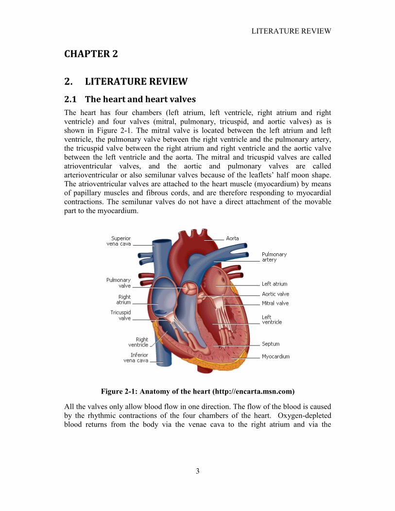
The heart has four chambers (left atrium, left ventricle, right atrium and right
ventricle) and four valves (mitral, pulmonary, tricuspid, and aortic valves) as is
shown in Figure 2-1. The mitral valve is located between the left atrium and left
ventricle, the pulmonary valve between the right ventricle and the pulmonary artery,
the tricuspid valve between the right atrium and right ventricle and the aortic valve
between the left ventricle and the aorta. The mitral and tricuspid valves are called
atrioventricular valves, and the aortic and pulmonary valves are called
arterioventricular or also semilunar valves because of the leaflets‟ half moon shape.
The atrioventricular valves are attached to the heart muscle (myocardium) by means
of papillary muscles and fibrous cords, and are therefore responding to myocardial
contractions. The semilunar valves do not have a direct attachment of the movable
part to the myocardium.
Figure 2-1: Anatomy of the heart (http://encarta.msn.com)
All the valves only allow blood flow in one direction. The flow of the blood is caused
by the rhythmic contractions of the four chambers of the heart. Oxygen-depleted
blood returns from the body via the venae cava to the right atrium and via the
LITERATURE REVIEW
4
tricuspid valve to the right ventricle. The pulmonary valve allows the blood to enter
the pulmonary artery towards the lungs. Oxygenated blood from the lungs returns via
the pulmonary veins to the left atrium and through the mitral valve to the left
ventricle. The aortic valve allows the blood to enter the aorta towards the rest of the
body.
2.2 The aortic valve
The aortic valve allows blood to flow into the aorta and prevents backflow into the
ventricle. The aortic valve opens and closes approximately 103,000 times per day and
3.7 billion times in its lifespan. Because the aortic valve is located on the high
pressure side of the blood transport through the body, it is the heart valve that must
endure the highest pressures, fatigue and strains.
2.3 Aortic valve disease
Aortic valve disease is a common clinical problem and is likely to continue to
increase with the aging of the population (Kar and Shah, 2006).
Abnormalities of the aortic valve can generally be categorized as involving
incompetence of the valve, i.e. aortic regurgitation or insufficiency and obstruction of
the valve, i.e. aortic stenosis and sclerosis.
2.3.1 Aortic stenosis
Aortic stenosis can be caused by subvalvular, valvular or supravalvular obstruction to
the left ventricular outflow. Subvalvular aortic stenosis usually occurs as a
fibromuscular membrane or a tunnel-like narrowing of the left ventricular outflow
tract. Supravalvular aortic stenosis usually occurs due to a congenital narrowing of
the ascending aorta, usually beginning just above the sinuses of Valsalva. Valvular
stenosis is the most common cause of aortic stenosis and is due to an abnormality of
the aortic valve leaflets. The causes of valvular aortic stenosis can be divided into
congenital, rheumatic and degenerative stenosis (Ward and Lang, 2006).
Congenital aortic stenosis accounts for the most cases of valvular stenosis in young
adults and may be unicuspid, bicuspid or tricuspid. A bicuspid valve is most common
in males and accounts for 1-2% of the general population. The two leaflets are
usually of unequal size with the larger leaflet generally having a raphe, which may
give the appearance of a tricuspid valve. Unicuspid valves produce severe
obstruction in infancy and thus are rarely encountered in adults (Ward and Lang,
2006).
Rheumatic aortic valve stenosis is becoming increasingly rare in developed countries,
but still has a high incidence in developing countries. Because the mitral valve is
LITERATURE REVIEW
5
preferentially affected in rheumatic heart disease, certain diagnosis of rheumatic
aortic stenosis normally requires related mitral valve stenosis (Ward and Lang, 2006).
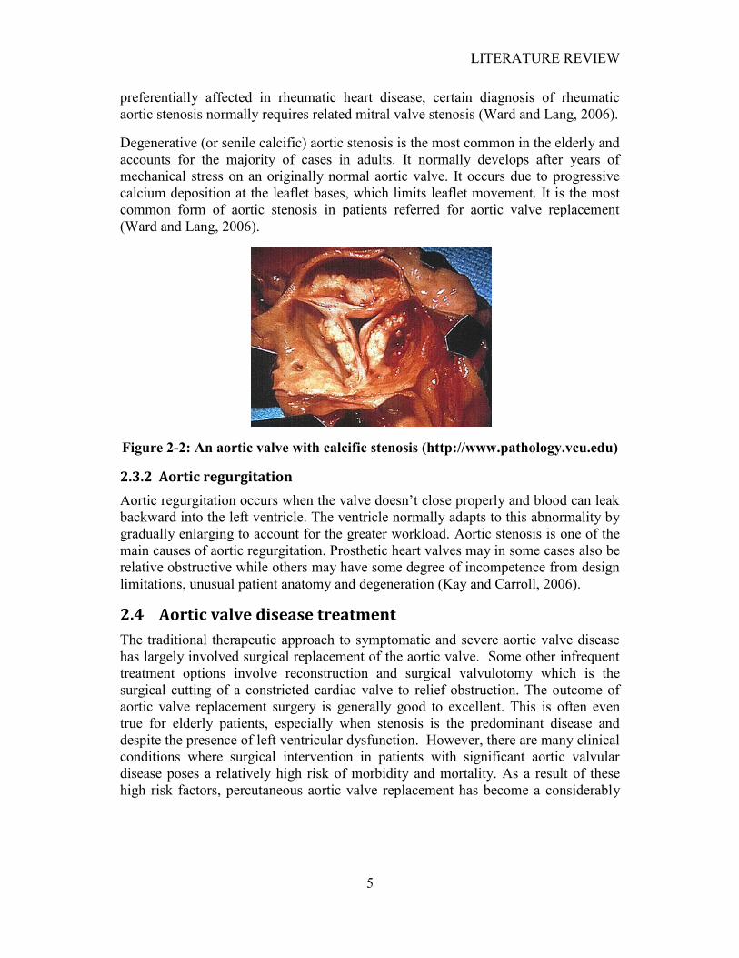
Degenerative (or senile calcific) aortic stenosis is the most common in the elderly and
accounts for the majority of cases in adults. It normally develops after years of
mechanical stress on an originally normal aortic valve. It occurs due to progressive
calcium deposition at the leaflet bases, which limits leaflet movement. It is the most
common form of aortic stenosis in patients referred for aortic valve replacement
(Ward and Lang, 2006).
Figure 2-2: An aortic valve with calcific stenosis (http://www.pathology.vcu.edu)
2.3.2 Aortic regurgitation
Aortic regurgitation occurs when the valve doesn‟t close properly and blood can leak
backward into the left ventricle. The ventricle normally adapts to this abnormality by
gradually enlarging to account for the greater workload. Aortic stenosis is one of the
main causes of aortic regurgitation. Prosthetic heart valves may in some cases also be
relative obstructive while others may have some degree of incompetence from design
limitations, unusual patient anatomy and degeneration (Kay and Carroll, 2006).
2.4 Aortic valve disease treatment
The traditional therapeutic approach to symptomatic and severe aortic valve disease
has largely involved surgical replacement of the aortic valve. Some other infrequent
treatment options involve reconstruction and surgical valvulotomy which is the
surgical cutting of a constricted cardiac valve to relief obstruction. The outcome of
aortic valve replacement surgery is generally good to excellent. This is often even
true for elderly patients, especially when stenosis is the predominant disease and
despite the presence of left ventricular dysfunction. However, there are many clinical
conditions where surgical intervention in patients with significant aortic valvular
disease poses a relatively high risk of morbidity and mortality. As a result of these
high risk factors, percutaneous aortic valve replacement has become a considerably
LITERATURE REVIEW
6
attractive solution or even an alternative for some conventional valvular interventions
(Kar and Shah, 2006).
2.4.1 Conventional treatments
Aortic valve replacement was made possible due to the cardiopulmonary bypass
system and the development of various metallic and bioprosthetic valves.
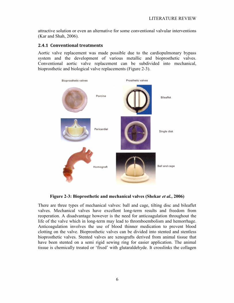
Conventional aortic valve replacement can be subdivided into mechanical,
bioprosthetic and biological valve replacements (Figure 2-3).
Figure 2-3: Bioprosthetic and mechanical valves (Shekar et al., 2006)
There are three types of mechanical valves: ball and cage, tilting disc and bileaflet
valves. Mechanical valves have excellent long-term results and freedom from
reoperation. A disadvantage however is the need for anticoagulation throughout the
life of the valve which in long-term may lead to thromboembolism and hemorrhage.
Anticoagulation involves the use of blood thinner medication to prevent blood
clotting on the valve. Bioprosthetic valves can be divided into stented and stentless
bioprosthetic valves. Stented valves are xenografts derived from animal tissue that
have been stented on a semi rigid sewing ring for easier application. The animal
tissue is chemically treated or „fixed‟ with glutaraldehyde. It crosslinks the collagen
LITERATURE REVIEW
7
fibres and reduces antigenicity. Stentless bioprosthetic valves are a newer generation
of xenograft valves which lack the semi rigid sewing ring and commonly have a layer
of Dacron® along the outside edge.
Bioprosthetic valves do not require anticoagulation, but are susceptible to
calcification and currently lasts only about 15 years, after which another surgical
intervention may be required. Stented bioprosthetic valves also have a risk of
thromboembolism. Stentless porcine valves have a lower gradient at smaller sizes and
could therefore aid in reducing load on the left ventricle and assist with ventricular
remodelling. Biological valves include homografts that are harvested from human
cadavers and cryopreserved. Although not requiring anticoagulation, homografts have
long-term problems with calcification and are relatively harder to reoperate on.
Due to years of successes and improvements, conventional treatments became the
treatment of choice. Despite all these successes, aortic valve replacement by means of
open-heart surgery still has its limitations. The 30-day mortality rate is around 3.1%
and the survival rate at five years is around 78%. Normally at follow-up, valve-
related complications, including thromboembolism, bleeding from anticoagulation,
prosthetic valve endocarditis and even reoperation may occur. Additionally most
cases of severe aortic stenosis occur in elderly patients, who often have additional
coexisting conditions that increase surgical risk. These include left ventricular failure,
coronary artery complications and patients older than 80 years. Younger patients
with aortic valve disease often outlive the bioprosthetic valve, requiring reoperations.
Although the life expectancy of patients receiving valve replacement is significantly
increased, its use in asymptomatic severe aortic valve stenosis is still controversial.
The risk of cardiac surgery often outweighs that of intense follow-up and risk
stratification of patients with asymptomatic severe aortic valve stenosis. These
limitations in surgery dictate the need for low-risk, minimally invasive surgical, or
percutaneous techniques (Kar and Shah, 2006).
The development of balloon angioplasty brought forth the use of metallic stents as a
common treatment for symptomatic coronary artery disease. Physicians later used
the same technique to dilate stenosed aortic, pulmonary, and mitral valves. Aortic
valvuloplasty is successful for children and adolescents with congenital aortic valve
stenosis, but most elderly and adult patients suffer from degenerative calcific aortic
stenosis which makes valve dilation difficult. Although initial improvement occurs,
stenosis reoccurrences is as high as 60% within 6-12 months. In most cases a
significant residual aortic stenosis still remains. Aortic valvuloplasty is also not an
option when significant regurgitation is present. Balloon aortic valvuloplasty in
elderly and adult patients is performed infrequently and often only for short-term
alleviation. It is however recently more used as part of percutaneous aortic valve
replacement.
LITERATURE REVIEW
8
2.4.2 Percutaneous aortic valve replacement (PAVR)
The refinement of balloons and the development of stents in the late 1980s led to the
percutaneous approach to aortic valve repair. In 1992, Andersen et al. (1992) reported
the first case of implementation by the transluminal catheter technique without
thoracotomy or extracorporal circulation. The valve consisted out of a porcine valve
mounted on a stent which was implanted in a pig. Percutaneous pulmonary valve
replacements using a jugular venous valve mounted in a stent, followed in humans.
In 2002, Cribier et al. (2002) reported the first successful implantation of a stent-
mounted pericardial valve in a patient with critical aortic valve stenosis. The valve
consisted out of three bovine pericardial leaflets mounted within a balloon-
expandable stent. Following this initial success, the valve underwent modifications
and several companies have developed different types of percutaneous heart valves.
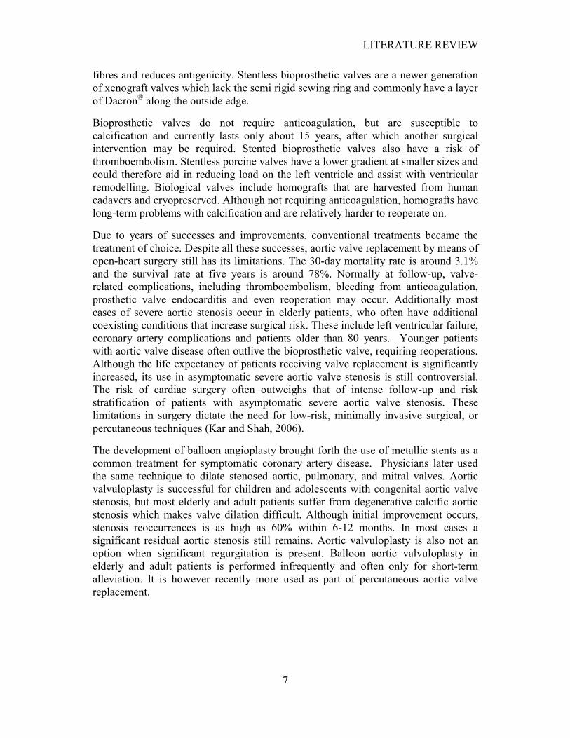
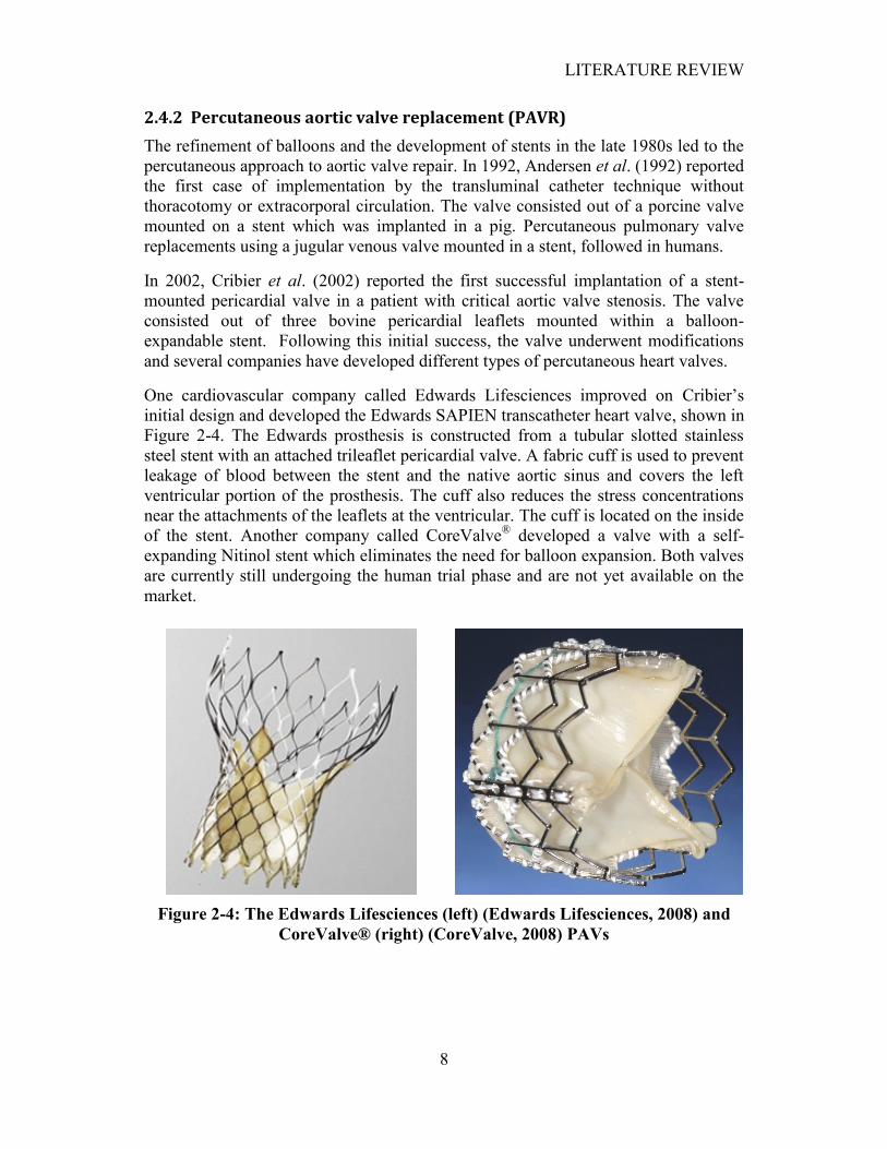
One cardiovascular company called Edwards Lifesciences improved on Cribier‟s
initial design and developed the Edwards SAPIEN transcatheter heart valve, shown in
Figure 2-4. The Edwards prosthesis is constructed from a tubular slotted stainless
steel stent with an attached trileaflet pericardial valve. A fabric cuff is used to prevent
leakage of blood between the stent and the native aortic sinus and covers the left
ventricular portion of the prosthesis. The cuff also reduces the stress concentrations
near the attachments of the leaflets at the ventricular. The cuff is located on the inside
of the stent. Another company called CoreValve® developed a valve with a self-
expanding Nitinol stent which eliminates the need for balloon expansion. Both valves
are currently still undergoing the human trial phase and are not yet available on the
market.
Figure 2-4: The Edwards Lifesciences (left) (Edwards Lifesciences, 2008) and
CoreValve® (right) (CoreValve, 2008) PAVs
LITERATURE REVIEW
9
2.4.3 Current limitations in PAVR
Current designs of percutaneous aortic valve replacements are not yet an acceptable
substitute for aortic valve surgery, mostly because of the following limitations:
The valve needs a large-diameter delivery catheter to contain the crimped
valve
Accurate and secure positioning and deployment is often a challenge
Blockage of the coronary ostia
Migration of the valve after implantation
Post-deployment paravalvular leak is common
Severe aortic regurgitation might cause interference of the coronary ostium
Temporary circulatory support might be needed to assure careful and accurate
deployment
Subsequent surgical replacement of a malfunctioning percutaneous valve
could be challenging due to the size of some valves that results in a large
section to be cut out
Calcification of the leaflets
Regurgitation due to irregular expansion
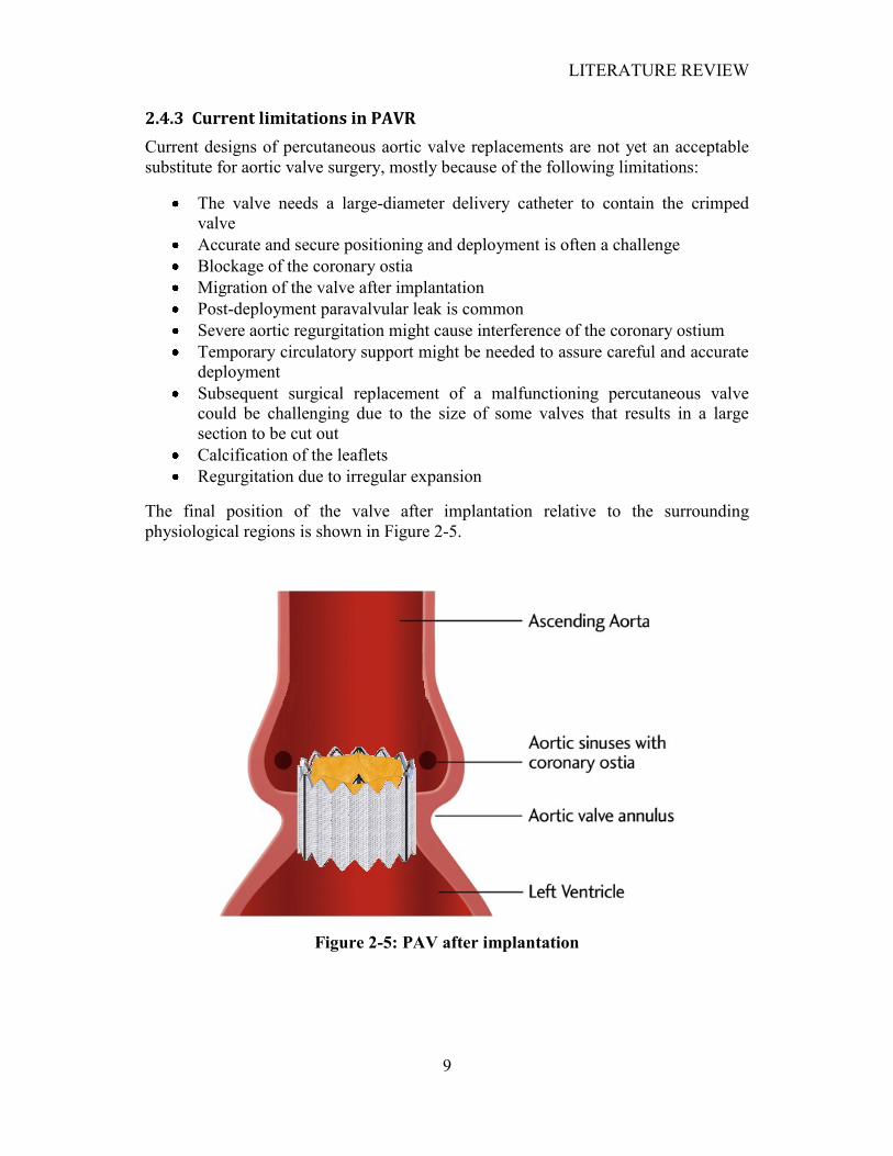
The final position of the valve after implantation relative to the surrounding
physiological regions is shown in Figure 2-5.
Figure 2-5: PAV after implantation
LITERATURE REVIEW
10
Despite these limitations, severely symptomatic patients for whom it is considered
high risk to undergo surgery because of comorbidity or poor ventricular function, are
considered potential candidates for percutaneous valve replacement. It is conceivable
that with refinements in valve design, delivery, deployment and improvement in
valve durability, the percutaneous valve replacement may well develop into a viable
alternative to surgery. This may later even include average to low-risk patients.
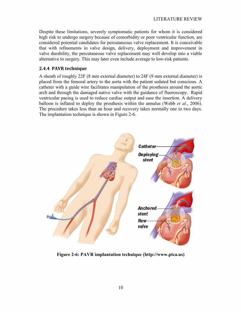
2.4.4 PAVR technique
A sheath of roughly 22F (8 mm external diameter) to 24F (9 mm external diameter) is
placed from the femoral artery to the aorta with the patient sedated but conscious. A
catheter with a guide wire facilitates manipulation of the prosthesis around the aortic
arch and through the damaged native valve with the guidance of fluoroscopy. Rapid
ventricular pacing is used to reduce cardiac output and ease the insertion. A delivery
balloon is inflated to deploy the prosthesis within the annulus (Webb et al., 2006).
The procedure takes less than an hour and recovery takes normally one to two days.
The implantation technique is shown in Figure 2-6.
Figure 2-6: PAVR implantation technique (http://www.ptca.us)
LITERATURE REVIEW
11
2.5 Valve material and treatment
2.5.1 Conventional materials
Mechanical heart valves are essentially made out of metal and other engineering
materials. The struts and occluders are made out of either pyrolytic carbon or
pyrolytic carbon coated titanium, and the sewing ring cuff is made out of Teflon®
(PTFE), polyester or Dacron®. Percutaneous heart valve stents are generally made out
of stainless steel, cobalt-chrome or Nitinol. The latter is generally used for self-
expandable stents.
Bioprosthetic aortic valves are normally constructed out of complete porcine aortic
valves or animal tissue, such as bovine pericardium, that is used to construct the
leaflets. The pericardium is the fluid-filled sac that surrounds the heart and the
proximal ends of the aorta, vena cava, and the pulmonary artery. There have been
three generations of improved bioprosthetic valve treatment processes. The first-
generation valves are high-pressure pre-fixation valves, such as the Medtronic
Hancock I. The second-generation valves are treated with low- or zero-pressure
fixation which includes the Medtronic Hancock II valve and the Carpentier-Edwards
Supra-Annular valve. The third-generation valves are subjected to an
antimineralization process, in addition to low to zero-pressure fixation like the
Medtronic Mosaic porcine valve. This process is designed to reduce material fatigue
and calcification (Shekar et al., 2006).
Percutaneous aortic valves are generally tricuspid bioprosthetic valves of which the
leaflets are made from animal tissue.
2.5.2 Material used for this study
The material used for this study is bovine and kangaroo pericardium. The material
was provided by BioMD Limited which is a medical device and surgical technology
company based in Perth, Australia. Celxcel, which is one of BioMD‟s subsidiary
companies, have developed a new anticalcific treatment called ADAPT™.
The ADAPT™ process is an antimineralization process based on a multifactorial
approach focused on synchronized synergy between enhanced crosslink stability,
removal of residual glutaraldehyde, modification of non-bifunctionally reacted
glutaraldehyde residues, reduction of the lipid content and restoration of tissue
elasticity (Neethling et al., 2004). The process prevents calcification of
glutaraldehyde treated collagen and proves to be better than conventional anticalcific
treatments.
LITERATURE REVIEW
12
In 2002, Neethling et al. (2002) reported that kangaroo pericardium has a densely
arranged collagen matrix with a higher extensibility and significantly lower
calcification potential than bovine pericardium. It can be noted that the material in
their study did not undergo the ADAPT™ treatment.
2.6 Material storage and testing solutions
As pericardium is a tissue-derived biomaterial, it is susceptible to bacterial decay and
degeneration. Chemically treated pericardium is more resistant to decay and may
remain stable for up to five days without antibiotic treatment, depending on the
surrounding environment.
Tissue prepared for experimental use is stored in 70% ethanol or 20% isopropanol.
For clinical use, the tissue is stored in propylene glycol. Before use the material must
undergo rehydration in a 0.9% NaCl (saline) solution for twenty minutes.
During fatigue tests in a pulse generator a volume-based solution of 42% glycerol and
58% water is used as the testing fluid. 0.9 wt.% NaCl is then added to the solution. If
antibiotics are added for preservation, the solution must preferably be replaced every
seven days. The preferred antibiotic is Tetracycline. Alternatively a 0.5%
glutaraldehyde buffered solution may be used as the basis solution with glycerol
added for viscosity. No antibiotics are needed for this solution (Neethling, 2008).
2.7 Valve design requirements
The valve design requirements can be split into quantifiable and non-quantifiable
requirements of which some are provided by the ISO standards for conventional heart
valve prostheses (International Organization for Standardization , 2005):
Quantifiable:
An external valve diameter of 20 mm for in vivo testing in sheep
A maximum valve height of 16 mm
A maximum valve crimping diameter of 18 French (6 mm)
Able to withstand a maximum pressure of 230 mmHg across the valve during
diastole.
Non-Quantifiable:
Allow forward flow with acceptably small mean pressure difference
Prevent retrograde flow with acceptably small regurgitation and paravalvular
leak
Resist embolization
Resist haemolysis
Resist thrombus formation
LITERATURE REVIEW
13
Is biocompatible
Is compatible with in vivo diagnostic techniques
Is deliverable and implantable in the target population
Remain fixed once placed
Has an acceptable noise level
Has reproducible function
Maintain its functionality for a reasonable lifetime
Maintain its functionality and sterility for a reasonable shelf life prior to
implantation
These design requirements were used as guidelines during the valve development and
evaluation.
2.8 Valve testing
Preclinical testing of PAVRs can be broken down into three main areas: evaluation of
device hydrodynamic function, device durability/life cycle and device
biocompatibility/host response (Lemmon, 2006).
Hydrodynamic testing is used to evaluate the function of heart valve replacements
under a range of physiologic conditions. It is typically conducted in a pulse duplicator
with typical heart rates of 45-150 beats/min and cardiac outputs of 2-10 ℓ/min.
Measurements of pressure drop, effective orifice area and regurgitant flow volume
are normally taken. Normal to hypertensive pressures across the valve are tested.
Additional measurements can be taken to assess laminar and turbulent flow regions as
well as areas with stagnant flow that could lead to thrombus formation. This flow
visualization can be performed by using a laser light sheet illuminating a test solution
seeded with small glass or plastic particles. Laboratory tests also have the benefit of
calculating the shear stresses in the flow field and thus evaluate the potential damage
to blood elements. Velocities through the valve can be measured by using Doppler
ultrasound.
Failure mode analysis is a durability analysis with the purpose of determining
whether failure is catastrophic or degenerative. Damage is caused to the valve by
increasing the cycle rate whereas overloading will reveal the weaker components that
will fail first. Biological PAVs can fail due to leaflet prolapse, leaflet abrasion, valve
dehiscence from the stent, stent migration and stent fracture. Accelerated wear testing
is in the ranges of 10-20 times the physiologic cycle rates which allow clinical cycles
of five years to be achieved in 5-6 months. This testing is performed under normal
pressures. Biological valves need to be evaluated over 200 million cycles which
represent five years of clinical implantation.
The final verification testing prior to clinical trails is to perform animal studies.
Biocompatibility testing provides data on inflammation, irritation, cytotoxicity, etc.
LITERATURE REVIEW
14
of the device. Chronic animal studies are done to test the host response at the implant
site, device histology and hemodynamic function of the valve (Lemmon, 2006).
2.9 Recent research
Many physiological, surgical, and medical device applications exist where rigorous
constitutive modelling and numerical simulations are required due to the complex
mechanical behaviour of the tissues used (Sun and Sacks, 2005). Soft tissues possess
highly nonlinear stress-strain relationships, large deformations and mechanical
anisotropy. Although finite element analysis (FEA) has been commonly used for
structural analysis of heart valves, the material models used were generally simplified
models. These models can be divided into four groups: linear anisotropic, nonlinear
isotropic, linear anisotropic and nonlinear anisotropic (Kim et al., 2006). Burriesci et
al. (1999) reported that even a small amount of anisotropy can significantly affect the
mechanical behaviour of the valve. Arcidiacono et al. (2005) suggested that leaflets
of pericardium bioprosthetic valves could be manufactured to be similar to natural
human heart valves, reproducing their well-known anisotropy. In this way it could be
possible to improve the durability and function of pericardial bioprosthetic valves. It
is therefore clear that both nonlinearity and anisotropy should be taken into
consideration for the finite element analysis of bioprosthetic heart valves. Sun et al.
(2005) employed the Fung-type elastic material model in a quasi-static analysis. They
used rigorous experimental validation and found that the utilization of actual leaflet
material properties is essential for accurate bioprosthetic heart valve simulations. Kim
et al. (2006) conducted a dynamic simulation of a pericardial bioprosthetic heart
valve during the opening phase of the valve by implementing the Fung-type elastic
material model. It is known that the highest stresses occurs during the closing phase
(diastole) of the valve, which is one of the main causes of valve failure. Currently no
literature has been found that implement the Fung-type elastic material model during
the closing phase of the valve.
The geometric modeling of the aortic leaflet and the aortic valve in general has
received considerable attention (Labrosse et al., 2006). Thubrikar (1990) explored the
design of aortic valves to ensure optimal performance whereby geometric criteria
were defined to guarantee appropriate sealing of the leaflets, minimize the dead
space, eliminate folds in the leaflets and minimize leaflet flexion. Labrosse et al.
(2006) established a method to determine by how much the dimensions of the aortic
valve components can vary while still maintaining proper function. This may aid in
the examination of “what-if” scenarios in aortic valve design and valve-sparing
operations.
MATERIAL PROPERTIES
15
CHAPTER 3
3. MATERIAL PROPERTIES
In order to perform finite element analysis (FEA) on the valve, the mechanical
behaviour of the pericardium under a generalized loading state needs to be defined.
To achieve this, rigorous experimentation involving all relevant deformations is
necessary to obtain the material constants and the strain-energy density function that
describes the material behaviour of the pericardium.
The pericardium consists partially out of collagen fibres which are integrated with
cells and intercellular substances. Sections in which the fibres are predominantly
aligned in one direction are used for testing and manufacturing the prostheses. The
fibre direction normally possesses tougher mechanical properties. In native aortic
valves these fibres are mostly aligned in the circumferential direction under pressure
(Sacks et al., 1998). Biological tissues are generally considered incompressible
(Fung, 1993), which means that planar testing allows for a two-dimensional stress-
state that can be used to fully characterize its mechanical behaviour.
3.1 The constitutive equation of skin
Accurate numerical simulations of the mechanical properties of soft biological tissues
remain a challenge due to the fact that most soft biomaterials are nonlinear
orthotropic. Consequently, tissues are assumed to be isotropic, nonlinear isotropic or
orthotropic for simulation purposes. The constitutive equation proposed by Fung
(1993) provides one of the most accurate material behaviour predictions for soft
tissues. Although this model is widely used in the literature for characterization of
experimental data, it is rarely implemented in finite element simulations (Sun and
Sacks, 2005). The main reasons are numerical instability and convergence problems.
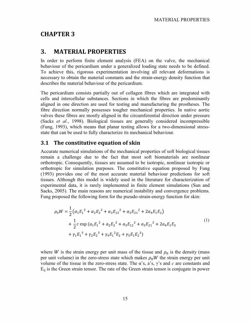
Fung proposed the following form for the pseudo-strain-energy function for skin:
(1)
where is the strain energy per unit mass of the tissue and is the density (mass
per unit volume) in the zero-stress state which makes the strain energy per unit
volume of the tissue in the zero-stress state. The α‟s, a‟s, γ‟s and c are constants and
Eij is the Green strain tensor. The rate of the Green strain tensor is conjugate in power
MATERIAL PROPERTIES
16
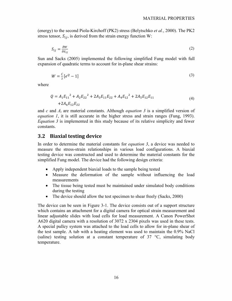
(energy) to the second Piola-Kirchoff (PK2) stress (Belytschko et al., 2000). The PK2
stress tensor, , is derived from the strain energy function W:
(2)
Sun and Sacks (2005) implemented the following simplified Fung model with full
expansion of quadratic terms to account for in-plane shear strains:
(3)
where
(4)
and c and Ai are material constants. Although equation 3 is a simplified version of
equation 1, it is still accurate in the higher stress and strain ranges (Fung, 1993).
Equation 3 is implemented in this study because of its relative simplicity and fewer
constants.
3.2 Biaxial testing device
In order to determine the material constants for equation 3, a device was needed to
measure the stress-strain relationships in various load configurations. A biaxial
testing device was constructed and used to determine the material constants for the
simplified Fung model. The device had the following design criteria:
Apply independent biaxial loads to the sample being tested
Measure the deformation of the sample without influencing the load
measurements
The tissue being tested must be maintained under simulated body conditions
during the testing
The device should allow the test specimen to shear freely (Sacks, 2000)
The device can be seen in Figure 3-1. The device consists out of a support structure
which contains an attachment for a digital camera for optical strain measurement and
linear adjustable slides with load cells for load measurement. A Canon PowerShot
A620 digital camera with a resolution of 3072 x 2304 pixels was used in these tests.
A special pulley system was attached to the load cells to allow for in-plane shear of
the test sample. A tub with a heating element was used to maintain the 0.9% NaCl
(saline) testing solution at a constant temperature of 37 °C, simulating body
temperature.
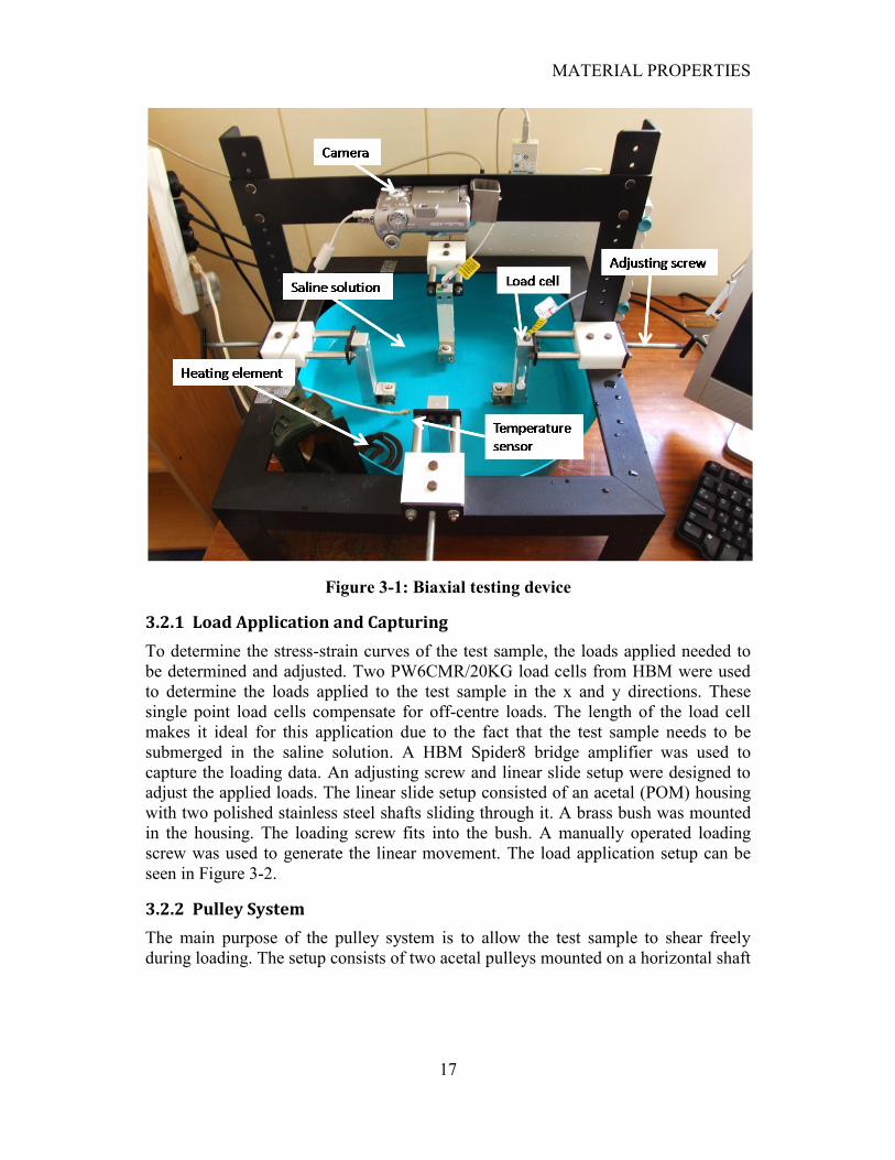
MATERIAL PROPERTIES
17
Figure 3-1: Biaxial testing device
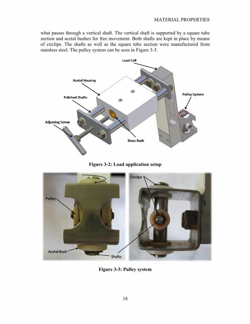
3.2.1 Load Application and Capturing
To determine the stress-strain curves of the test sample, the loads applied needed to
be determined and adjusted. Two PW6CMR/20KG load cells from HBM were used
to determine the loads applied to the test sample in the x and y directions. These
single point load cells compensate for off-centre loads. The length of the load cell
makes it ideal for this application due to the fact that the test sample needs to be
submerged in the saline solution. A HBM Spider8 bridge amplifier was used to
capture the loading data. An adjusting screw and linear slide setup were designed to
adjust the applied loads. The linear slide setup consisted of an acetal (POM) housing
with two polished stainless steel shafts sliding through it. A brass bush was mounted
in the housing. The loading screw fits into the bush. A manually operated loading
screw was used to generate the linear movement. The load application setup can be
seen in Figure 3-2.
3.2.2 Pulley System
The main purpose of the pulley system is to allow the test sample to shear freely
during loading. The setup consists of two acetal pulleys mounted on a horizontal shaft
MATERIAL PROPERTIES
18
what passes through a vertical shaft. The vertical shaft is supported by a square tube
section and acetal bushes for free movement. Both shafts are kept in place by means
of circlips. The shafts as well as the square tube section were manufactured from
stainless steel. The pulley system can be seen in Figure 3-3.
Figure 3-2: Load application setup
Figure 3-3: Pulley system
MATERIAL PROPERTIES
19
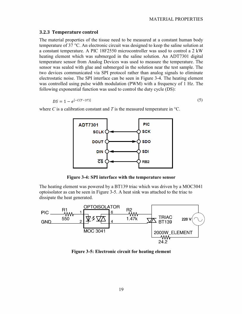
3.2.3 Temperature control
The material properties of the tissue need to be measured at a constant human body
temperature of 37 °C. An electronic circuit was designed to keep the saline solution at
a constant temperature. A PIC 18F2550 microcontroller was used to control a 2 kW
heating element which was submerged in the saline solution. An ADT7301 digital
temperature sensor from Analog Devices was used to measure the temperature. The
sensor was sealed with glue and submerged in the solution near the test sample. The
two devices communicated via SPI protocol rather than analog signals to eliminate
electrostatic noise. The SPI interface can be seen in Figure 3-4. The heating element
was controlled using pulse width modulation (PWM) with a frequency of 1 Hz. The
following exponential function was used to control the duty cycle (DS):
(5)
where C is a calibration constant and T is the measured temperature in °C.
Figure 3-4: SPI interface with the temperature sensor
The heating element was powered by a BT139 triac which was driven by a MOC3041
optoisolator as can be seen in Figure 3-5. A heat sink was attached to the triac to
dissipate the heat generated.
Figure 3-5: Electronic circuit for heating element
MATERIAL PROPERTIES
20
The temperature value was sent to the computer each second via serial port and
accessed using HyperTerminal. The calibration constant C could also be changed by
using the keyboard. A value of 0.5 for C proved to be adequate. This simple control
proved to be adequate with almost no temperature overshoot if taken into
consideration that the testing solution was kept motionless.
3.3 Camera calibration
Camera lens distortion is present in almost every camera and may contribute to
optical errors during strain measurements. The following calibration technique was
adopted from Van der Merwe, (2008).
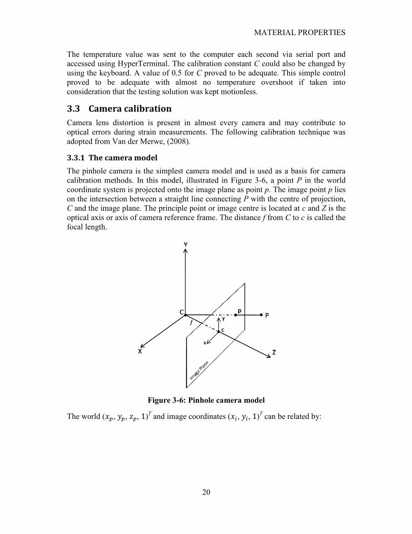
3.3.1 The camera model
The pinhole camera is the simplest camera model and is used as a basis for camera
calibration methods. In this model, illustrated in Figure 3-6, a point P in the world
coordinate system is projected onto the image plane as point p. The image point p lies
on the intersection between a straight line connecting P with the centre of projection,
C and the image plane. The principle point or image centre is located at c and Z is the
optical axis or axis of camera reference frame. The distance f from C to c is called the
focal length.
Figure 3-6: Pinhole camera model
The world ( , , , )T and image coordinates ( , , )
T can be related by:
MATERIAL PROPERTIES
21
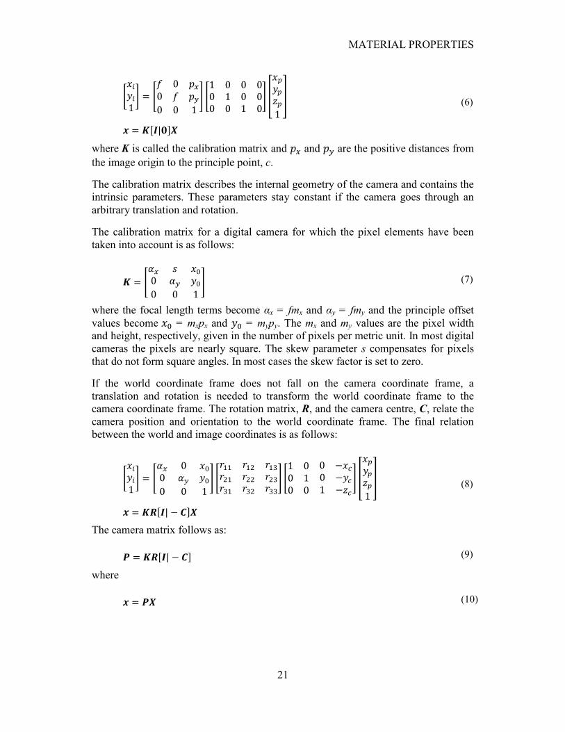
(6)
where K is called the calibration matrix and and are the positive distances from
the image origin to the principle point, c.
The calibration matrix describes the internal geometry of the camera and contains the
intrinsic parameters. These parameters stay constant if the camera goes through an
arbitrary translation and rotation.
The calibration matrix for a digital camera for which the pixel elements have been
taken into account is as follows:
(7)
where the focal length terms become αx = fmx and αy = fmy and the principle offset
values become = mxpx and = mypy. The mx and my values are the pixel width
and height, respectively, given in the number of pixels per metric unit. In most digital
cameras the pixels are nearly square. The skew parameter s compensates for pixels
that do not form square angles. In most cases the skew factor is set to zero.
If the world coordinate frame does not fall on the camera coordinate frame, a
translation and rotation is needed to transform the world coordinate frame to the
camera coordinate frame. The rotation matrix, R, and the camera centre, C, relate the
camera position and orientation to the world coordinate frame. The final relation
between the world and image coordinates is as follows:
(8)
The camera matrix follows as:
(9)
where
(10)
MATERIAL PROPERTIES
22
3.3.2 Lens distortion model
Radial distortion by camera lenses is one of the main causes of deviation from the
pinhole camera model to the digital camera model. There are mainly two types of
radial distortion, namely pincushion and barrel distortion. Pincushion distortion
causes the straight edges of an image to curve inwards and barrel distortion causes the
edges to curve away from the radial centre. The undistorted image coordinate, xu, is
computed by adding the corrected distances to the centre of radial distortion, c, as
shown in equation 11.
(11)
The correction function, f(r), is a function of the absolute Euclidean distance, r, from
the radial centre, c, to the distorted image coordinate, xd, and is calculated as follows:
(12)
where and are the distortion correction parameters to be optimized and r is
calculated by:
(13)
3.3.3 Calibration technique
Van der Merwe (2008) implemented a two-step calibration method. In the first step,
the camera matrix, P, is determined using a linear method which ignores non-linear
effects such as lens distortion. The second step introduces the non-linear effects of
lens distortion with the model described above.
In calculating the camera matrix, P, and thus the point correspondences xi ↔ xi', the
Direct Linear Transformation (DLT) method was used which calculates a matrix, H,
such that xiH = xi' for each point i. For practical implementation of the solution, the
linear system first needs to be preconditioned or by scaling and shifting both the
image and world coordinates. The DLT algorithm calculates a normalized camera
matrix, whereafter the matrix is denormalised to retrieve the final camera matrix.
In the second step the values from the camera matrix, a set of known world-
coordinates and a set of image coordinates are used to minimize the lens distortion
error. The back-projection error, or the difference between the calibration-feature
coordinates extracted from the image and the back-projection of the world
coordinates onto the image plane, needs to be minimized. The camera matrix
determined in the first step is used along with equation 11 to project a known world
coordinate onto the image plane of the camera. The projected coordinate is then
compared with the corresponding coordinate extracted directly from the image. The
Euclidean distance beween the two coordinates is used as an output to be minimized
MATERIAL PROPERTIES
23
and is called the back-projection error. Van der Merwe minimized a collection of
coordinate errors calculated by adding the mean and standard deviation of the error-
set.
A picture of a calibration object is taken each time the camera is moved or placed
onto the testing rig and a new calibration is performed. The optimized distortion
coefficients and camera matrix are then used to calibrate each image corresponding to
an applied load.
3.4 Strain calculation
When simulating hypoelastic materials large strains are common and thus need to be
taken into account. Mathematics used in finite element methods is applied to the
displacements measured optically to yield a solution for the components of plane
strain at the nodes as proposed by Hoffman and Grigg, (1984).
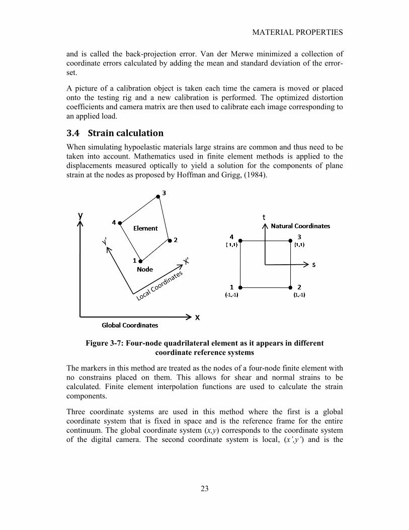
Figure 3-7: Four-node quadrilateral element as it appears in different
coordinate reference systems
The markers in this method are treated as the nodes of a four-node finite element with
no constrains placed on them. This allows for shear and normal strains to be
calculated. Finite element interpolation functions are used to calculate the strain
components.
Three coordinate systems are used in this method where the first is a global
coordinate system that is fixed in space and is the reference frame for the entire
continuum. The global coordinate system (x,y) corresponds to the coordinate system
of the digital camera. The second coordinate system is local, (x’,y’) and is the
MATERIAL PROPERTIES
24
reference frame for the element. The third coordinate system is the natural coordinate
system (t,s) and is a transformation dimensionless system in which the element
appears as a square with nodal coordinates of unity. The representation of the four-
node quadrilateral element and the different coordinate reference systems can be
observed in Figure 3-7.
The geometry of the element can be expressed as:
(14a)
(14b)
where (xi,yi) are the nodal coordinates in the global coordinate system. The horizontal
and vertical displacement components of the element can be expressed as:
(15a)
(15b)
where (ui,vi) are the nodal displacements and Ni are the interpolation functions given
in terms of s and t by:
(16)
The locations (xi,yi) and the displacements (ui,vi) of the element nodes are determined
optically. The location (x,y) and displacements (u,v) of any point within the element
(including the nodes) are calculated using the interpolation functions given by
equations 14 to 16. The same interpolation functions are used to describe the
element‟s displacement field as well as its geometry which is why it is called a four
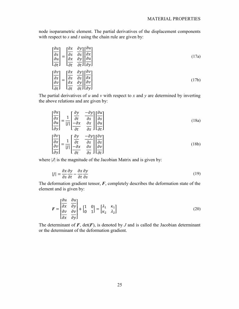
MATERIAL PROPERTIES
25
node isoparametric element. The partial derivatives of the displacement components
with respect to s and t using the chain rule are given by:
(17a)
(17b)
The partial derivatives of u and v with respect to x and y are determined by inverting
the above relations and are given by:
(18a)
(18b)
where |J| is the magnitude of the Jacobian Matrix and is given by:
(19)
The deformation gradient tensor, F, completely describes the deformation state of the
element and is given by:
(20)
The determinant of F, det(F), is denoted by J and is called the Jacobian determinant
or the determinant of the deformation gradient.
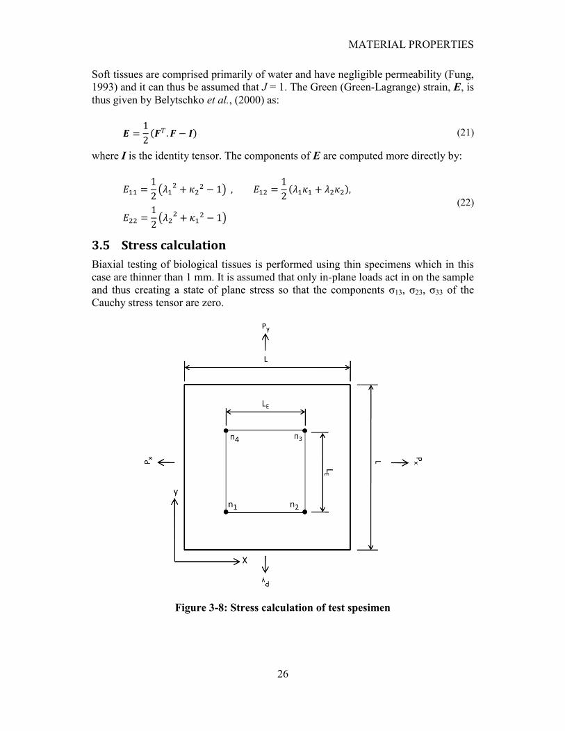
MATERIAL PROPERTIES
26
Soft tissues are comprised primarily of water and have negligible permeability (Fung,
1993) and it can thus be assumed that J = 1. The Green (Green-Lagrange) strain, E, is
thus given by Belytschko et al., (2000) as:
(21)
where I is the identity tensor. The components of E are computed more directly by:
(22)
3.5 Stress calculation
Biaxial testing of biological tissues is performed using thin specimens which in this
case are thinner than 1 mm. It is assumed that only in-plane loads act in on the sample
and thus creating a state of plane stress so that the components σ13, σ23, σ33 of the
Cauchy stress tensor are zero.
Figure 3-8: Stress calculation of test spesimen
MATERIAL PROPERTIES
27
The change in thickness of the test specimen is negligible during loading and so is
assumed to remain constant. The normal loads on the element are as follows:
(23)
where Pi is the normal distributed load applied over the length of the test sample, L,
and LE is the length of the element as can be seen in Figure 3-8.
In order to determine the Cauchy stress tensor the length ratios of the element were
determined as follows:
(24a)
(24b)
where n is an element node. The cross-sectional area of the element is thus:
(25)
where t is the average thickness of the test sample. The Cauchy stress tensor for
biaxial loading in the x and y directions follows as:
(26)
The symmetric second Piola-Kirchhoff stress tensor follows as (Belytschko et al.,
2000):
(27)
where J and F are the Jacobian determinant and the deformation gradient,
respectively, and are calculated as shown in the previous section. It should be noted
that Sacks and Sun (2000) and (2003) calculated the Lagrangian stresses (force/unit
original cross-sectional area) which does not always result in a symmetric second
Piola-Kirchhoff stress tensor. In this study the Cauchy stress tensor was used in order
to calculate a symmetric second Piola-Kirchhoff stress tensor.
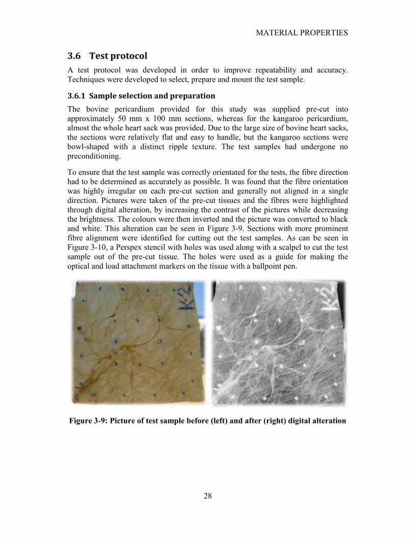
MATERIAL PROPERTIES
28
3.6 Test protocol
A test protocol was developed in order to improve repeatability and accuracy.
Techniques were developed to select, prepare and mount the test sample.
3.6.1 Sample selection and preparation
The bovine pericardium provided for this study was supplied pre-cut into
approximately 50 mm x 100 mm sections, whereas for the kangaroo pericardium,
almost the whole heart sack was provided. Due to the large size of bovine heart sacks,
the sections were relatively flat and easy to handle, but the kangaroo sections were
bowl-shaped with a distinct ripple texture. The test samples had undergone no
preconditioning.
To ensure that the test sample was correctly orientated for the tests, the fibre direction
had to be determined as accurately as possible. It was found that the fibre orientation
was highly irregular on each pre-cut section and generally not aligned in a single
direction. Pictures were taken of the pre-cut tissues and the fibres were highlighted
through digital alteration, by increasing the contrast of the pictures while decreasing
the brightness. The colours were then inverted and the picture was converted to black
and white. This alteration can be seen in Figure 3-9. Sections with more prominent
fibre alignment were identified for cutting out the test samples. As can be seen in
Figure 3-10, a Perspex stencil with holes was used along with a scalpel to cut the test
sample out of the pre-cut tissue. The holes were used as a guide for making the
optical and load attachment markers on the tissue with a ballpoint pen.
Figure 3-9: Picture of test sample before (left) and after (right) digital alteration
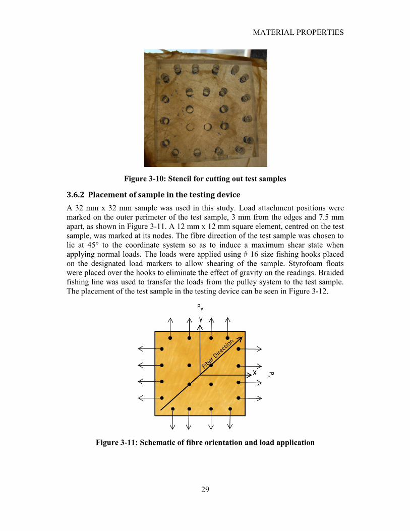
MATERIAL PROPERTIES
29
Figure 3-10: Stencil for cutting out test samples
3.6.2 Placement of sample in the testing device
A 32 mm x 32 mm sample was used in this study. Load attachment positions were
marked on the outer perimeter of the test sample, 3 mm from the edges and 7.5 mm
apart, as shown in Figure 3-11. A 12 mm x 12 mm square element, centred on the test
sample, was marked at its nodes. The fibre direction of the test sample was chosen to
lie at 45° to the coordinate system so as to induce a maximum shear state when
applying normal loads. The loads were applied using # 16 size fishing hooks placed
on the designated load markers to allow shearing of the sample. Styrofoam floats
were placed over the hooks to eliminate the effect of gravity on the readings. Braided
fishing line was used to transfer the loads from the pulley system to the test sample.
The placement of the test sample in the testing device can be seen in Figure 3-12.
Figure 3-11: Schematic of fibre orientation and load application
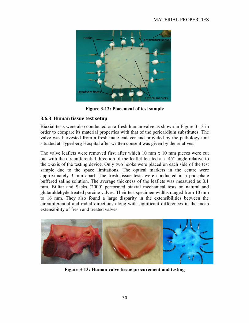
MATERIAL PROPERTIES
30
Figure 3-12: Placement of test sample
3.6.3 Human tissue test setup
Biaxial tests were also conducted on a fresh human valve as shown in Figure 3-13 in
order to compare its material properties with that of the pericardium substitutes. The
valve was harvested from a fresh male cadaver and provided by the pathology unit
situated at Tygerberg Hospital after written consent was given by the relatives.
The valve leaflets were removed first after which 10 mm x 10 mm pieces were cut
out with the circumferential direction of the leaflet located at a 45° angle relative to
the x-axis of the testing device. Only two hooks were placed on each side of the test
sample due to the space limitations. The optical markers in the centre were
approximately 3 mm apart. The fresh tissue tests were conducted in a phosphate
buffered saline solution. The average thickness of the leaflets was measured as 0.1
mm. Billiar and Sacks (2000) performed biaxial mechanical tests on natural and
glutaraldehyde treated porcine valves. Their test specimen widths ranged from 10 mm
to 16 mm. They also found a large disparity in the extensibilities between the
circumferential and radial directions along with significant differences in the mean
extensibility of fresh and treated valves.
Figure 3-13: Human valve tissue procurement and testing
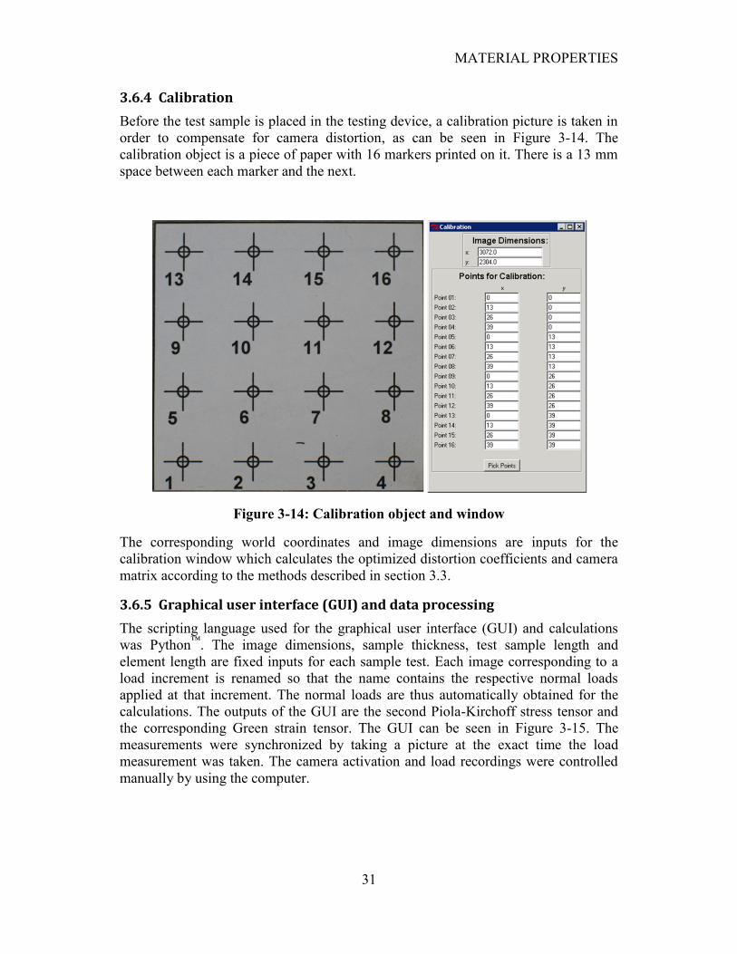
MATERIAL PROPERTIES
31
3.6.4 Calibration
Before the test sample is placed in the testing device, a calibration picture is taken in
order to compensate for camera distortion, as can be seen in Figure 3-14. The
calibration object is a piece of paper with 16 markers printed on it. There is a 13 mm
space between each marker and the next.
Figure 3-14: Calibration object and window
The corresponding world coordinates and image dimensions are inputs for the
calibration window which calculates the optimized distortion coefficients and camera
matrix according to the methods described in section 3.3.
3.6.5 Graphical user interface (GUI) and data processing
The scripting language used for the graphical user interface (GUI) and calculations
was Python™
. The image dimensions, sample thickness, test sample length and
element length are fixed inputs for each sample test. Each image corresponding to a
load increment is renamed so that the name contains the respective normal loads
applied at that increment. The normal loads are thus automatically obtained for the
calculations. The outputs of the GUI are the second Piola-Kirchoff stress tensor and
the corresponding Green strain tensor. The GUI can be seen in Figure 3-15. The
measurements were synchronized by taking a picture at the exact time the load
measurement was taken. The camera activation and load recordings were controlled
manually by using the computer.
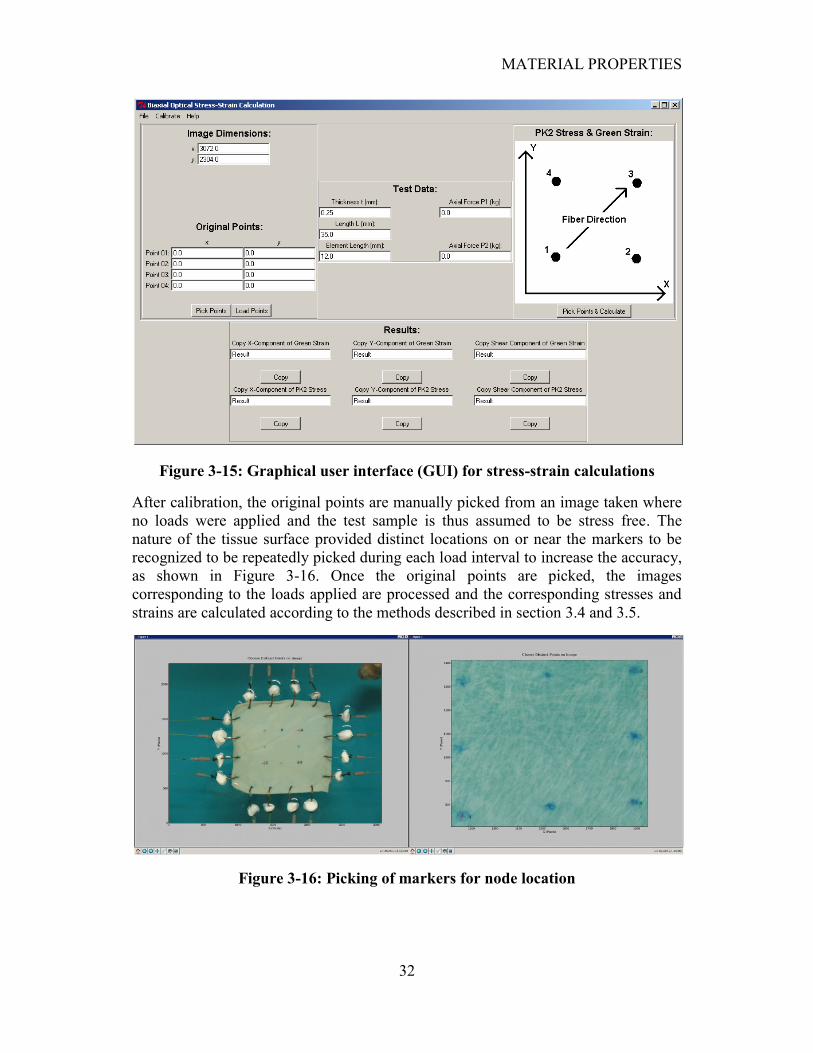
MATERIAL PROPERTIES
32
Figure 3-15: Graphical user interface (GUI) for stress-strain calculations
After calibration, the original points are manually picked from an image taken where
no loads were applied and the test sample is thus assumed to be stress free. The
nature of the tissue surface provided distinct locations on or near the markers to be
recognized to be repeatedly picked during each load interval to increase the accuracy,
as shown in Figure 3-16. Once the original points are picked, the images
corresponding to the loads applied are processed and the corresponding stresses and
strains are calculated according to the methods described in section 3.4 and 3.5.
Figure 3-16: Picking of markers for node location
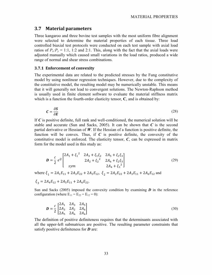
MATERIAL PROPERTIES
33
3.7 Material parameters
Three kangaroo and three bovine test samples with the most uniform fibre alignment
were selected to determine the material properties of each tissue. Three load
controlled biaxial test protocols were conducted on each test sample with axial load
ratios of Px:Py = 1:1, 1:2 and 2:1. This, along with the fact that the axial loads were
adjusted manually which caused small variations in the load ratios, produced a wide
range of normal and shear stress combinations.
3.7.1 Enforcement of convexity
The experimental data are related to the predicted stresses by the Fung constitutive
model by using nonlinear regression techniques. However, due to the complexity of
the constitutive model, the resulting model may be numerically unstable. This means
that it will generally not lead to convergent solutions. The Newton-Raphson method
is usually used in finite element software to evaluate the material stiffness matrix
which is a function the fourth-order elasticity tensor, C, and is obtained by:
(28)
If C is positive definite, full rank and well-conditioned, the numerical solution will be
stable and accurate (Sun and Sacks, 2005). It can be shown that C is the second
partial derivative or Hessian of W. If the Hessian of a function is positive definite, the
function will be convex. Thus, if C is positive definite, the convexity of the
constitutive model is enforced. The elasticity tensor, C, can be expressed in matrix
form for the model used in this study as:
(29)
where , and
.
Sun and Sacks (2005) imposed the convexity condition by examining D in the reference
configuration (where E11 = E22 = E12 = 0):
(30)
The definition of positive definiteness requires that the determinants associated with
all the upper-left submatrices are positive. The resulting parameter constraints that
satisfy positive definiteness for D are:
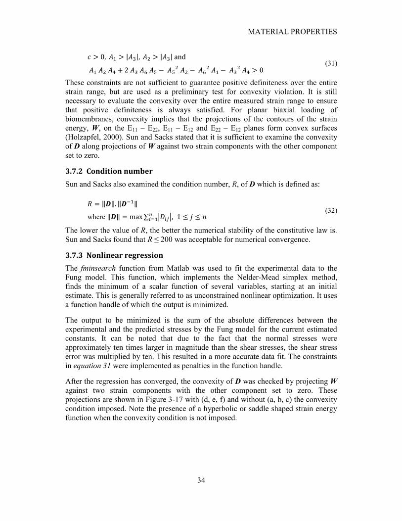
MATERIAL PROPERTIES
34
(31)
These constraints are not sufficient to guarantee positive definiteness over the entire
strain range, but are used as a preliminary test for convexity violation. It is still
necessary to evaluate the convexity over the entire measured strain range to ensure
that positive definiteness is always satisfied. For planar biaxial loading of
biomembranes, convexity implies that the projections of the contours of the strain
energy, W, on the E11 – E22, E11 – E12 and E22 – E12 planes form convex surfaces
(Holzapfel, 2000). Sun and Sacks stated that it is sufficient to examine the convexity
of D along projections of W against two strain components with the other component
set to zero.
3.7.2 Condition number
Sun and Sacks also examined the condition number, R, of D which is defined as:
where (32)
The lower the value of R, the better the numerical stability of the constitutive law is.
Sun and Sacks found that R ≤ 200 was acceptable for numerical convergence.
3.7.3 Nonlinear regression
The fminsearch function from Matlab was used to fit the experimental data to the
Fung model. This function, which implements the Nelder-Mead simplex method,
finds the minimum of a scalar function of several variables, starting at an initial
estimate. This is generally referred to as unconstrained nonlinear optimization. It uses
a function handle of which the output is minimized.
The output to be minimized is the sum of the absolute differences between the
experimental and the predicted stresses by the Fung model for the current estimated
constants. It can be noted that due to the fact that the normal stresses were
approximately ten times larger in magnitude than the shear stresses, the shear stress
error was multiplied by ten. This resulted in a more accurate data fit. The constraints
in equation 31 were implemented as penalties in the function handle.
After the regression has converged, the convexity of D was checked by projecting W
against two strain components with the other component set to zero. These
projections are shown in Figure 3-17 with (d, e, f) and without (a, b, c) the convexity
condition imposed. Note the presence of a hyperbolic or saddle shaped strain energy
function when the convexity condition is not imposed.
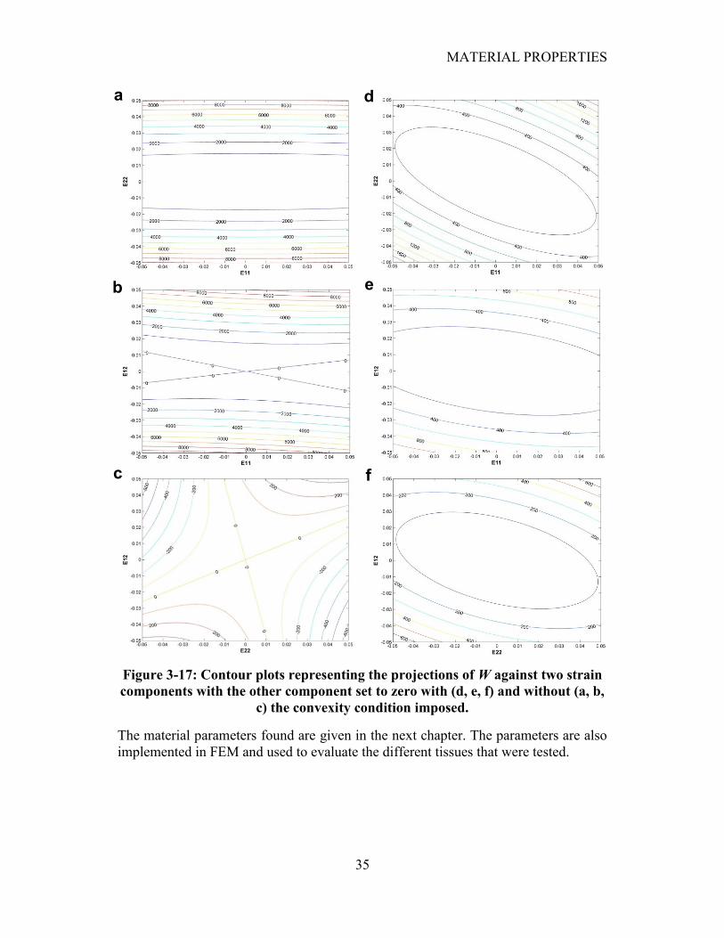
MATERIAL PROPERTIES
35
Figure 3-17: Contour plots representing the projections of W against two strain
components with the other component set to zero with (d, e, f) and without (a, b,
c) the convexity condition imposed.
The material parameters found are given in the next chapter. The parameters are also
implemented in FEM and used to evaluate the different tissues that were tested.
a d
b
c
e
f
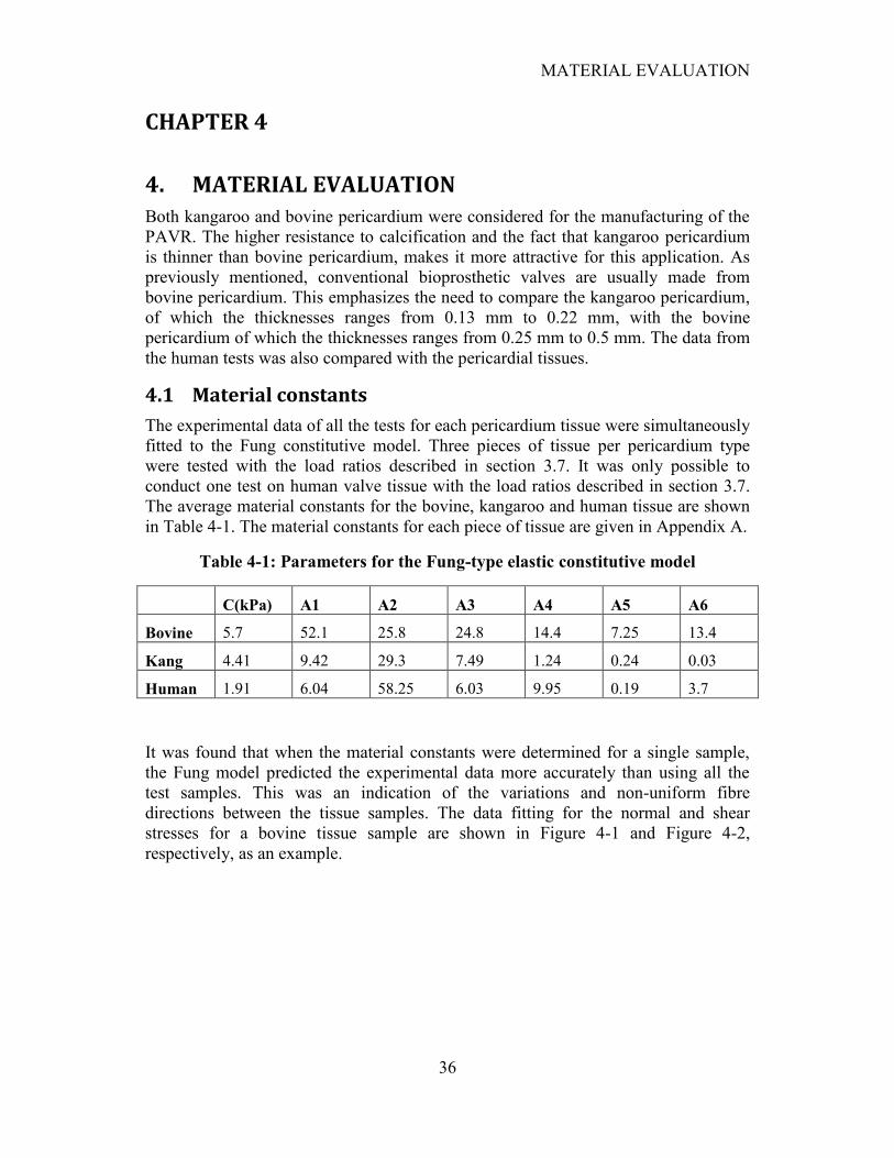
MATERIAL EVALUATION
36
CHAPTER 4
4. MATERIAL EVALUATION
Both kangaroo and bovine pericardium were considered for the manufacturing of the
PAVR. The higher resistance to calcification and the fact that kangaroo pericardium
is thinner than bovine pericardium, makes it more attractive for this application. As
previously mentioned, conventional bioprosthetic valves are usually made from
bovine pericardium. This emphasizes the need to compare the kangaroo pericardium,
of which the thicknesses ranges from 0.13 mm to 0.22 mm, with the bovine
pericardium of which the thicknesses ranges from 0.25 mm to 0.5 mm. The data from
the human tests was also compared with the pericardial tissues.
4.1 Material constants
The experimental data of all the tests for each pericardium tissue were simultaneously
fitted to the Fung constitutive model. Three pieces of tissue per pericardium type
were tested with the load ratios described in section 3.7. It was only possible to
conduct one test on human valve tissue with the load ratios described in section 3.7.
The average material constants for the bovine, kangaroo and human tissue are shown
in Table 4-1. The material constants for each piece of tissue are given in Appendix A.
Table 4-1: Parameters for the Fung-type elastic constitutive model
C(kPa) A1 A2 A3 A4 A5 A6
Bovine 5.7 52.1 25.8 24.8 14.4 7.25 13.4
Kang 4.41 9.42 29.3 7.49 1.24 0.24 0.03
Human 1.91 6.04 58.25 6.03 9.95 0.19 3.7
It was found that when the material constants were determined for a single sample,
the Fung model predicted the experimental data more accurately than using all the
test samples. This was an indication of the variations and non-uniform fibre
directions between the tissue samples. The data fitting for the normal and shear
stresses for a bovine tissue sample are shown in Figure 4-1 and Figure 4-2,
respectively, as an example.
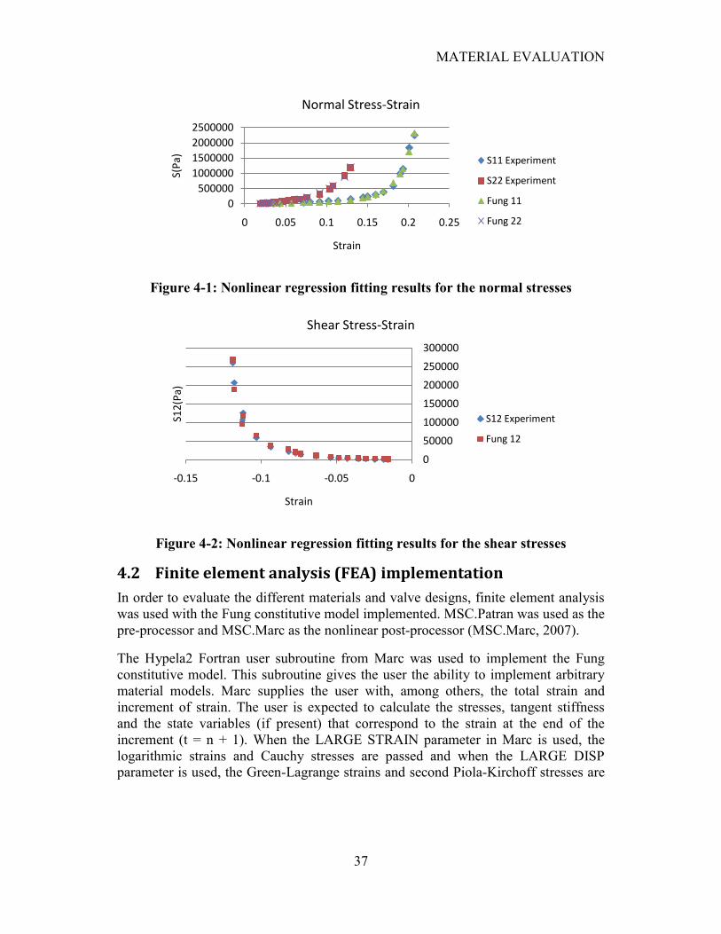
MATERIAL EVALUATION
37
Figure 4-1: Nonlinear regression fitting results for the normal stresses
Figure 4-2: Nonlinear regression fitting results for the shear stresses
4.2 Finite element analysis (FEA) implementation
In order to evaluate the different materials and valve designs, finite element analysis
was used with the Fung constitutive model implemented. MSC.Patran was used as the
pre-processor and MSC.Marc as the nonlinear post-processor (MSC.Marc, 2007).
The Hypela2 Fortran user subroutine from Marc was used to implement the Fung
constitutive model. This subroutine gives the user the ability to implement arbitrary
material models. Marc supplies the user with, among others, the total strain and
increment of strain. The user is expected to calculate the stresses, tangent stiffness
and the state variables (if present) that correspond to the strain at the end of the
increment (t = n + 1). When the LARGE STRAIN parameter in Marc is used, the
logarithmic strains and Cauchy stresses are passed and when the LARGE DISP
parameter is used, the Green-Lagrange strains and second Piola-Kirchoff stresses are
0
500000
1000000
1500000
2000000
2500000
0 0.05 0.1 0.15 0.2 0.25
S(P
a)
Strain
Normal Stress-Strain
S11 Experiment
S22 Experiment
Fung 11
Fung 22
0
50000
100000
150000
200000
250000
300000
-0.15 -0.1 -0.05 0
S12
(Pa)
Strain
Shear Stress-Strain
S12 Experiment
Fung 12
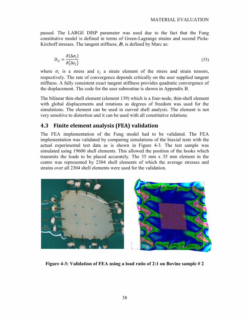
MATERIAL EVALUATION
38
passed. The LARGE DISP parameter was used due to the fact that the Fung
constitutive model is defined in terms of Green-Lagrange strains and second Piola-
Kirchoff stresses. The tangent stiffness, D, is defined by Marc as:
(33)
where is a stress and a strain element of the stress and strain tensors,
respectively. The rate of convergence depends critically on the user supplied tangent
stiffness. A fully consistent exact tangent stiffness provides quadratic convergence of
the displacement. The code for the user subroutine is shown in Appendix B.
The bilinear thin-shell element (element 139) which is a four-node, thin-shell element
with global displacements and rotations as degrees of freedom was used for the
simulations. The element can be used in curved shell analysis. The element is not
very sensitive to distortion and it can be used with all constitutive relations.
4.3 Finite element analysis (FEA) validation
The FEA implementation of the Fung model had to be validated. The FEA
implementation was validated by comparing simulations of the biaxial tests with the
actual experimental test data as is shown in Figure 4-3. The test sample was
simulated using 19600 shell elements. This allowed the position of the hooks which
transmits the loads to be placed accurately. The 35 mm x 35 mm element in the
centre was represented by 2304 shell elements of which the average stresses and
strains over all 2304 shell elements were used for the validation.
Figure 4-3: Validation of FEA using a load ratio of 2:1 on Bovine sample # 2
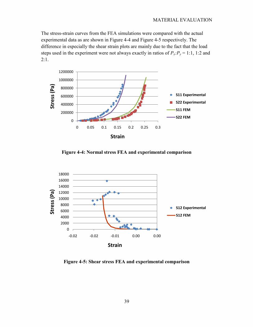
MATERIAL EVALUATION
39
The stress-strain curves from the FEA simulations were compared with the actual
experimental data as are shown in Figure 4-4 and Figure 4-5 respectively. The
difference in especially the shear strain plots are mainly due to the fact that the load
steps used in the experiment were not always exactly in ratios of Px:Py = 1:1, 1:2 and
2:1.
Figure 4-4: Normal stress FEA and experimental comparison
Figure 4-5: Shear stress FEA and experimental comparison
0
200000
400000
600000
800000
1000000
1200000
0 0.05 0.1 0.15 0.2 0.25 0.3
Stre
ss (
Pa)
Strain
S11 Experimental
S22 Experimental
S11 FEM
S22 FEM
0
2000
4000
6000
8000
10000
12000
14000
16000
18000
-0.02 -0.02 -0.01 0.00 0.00
Stre
ss (
Pa)
Strain
S12 Experimental
S12 FEM
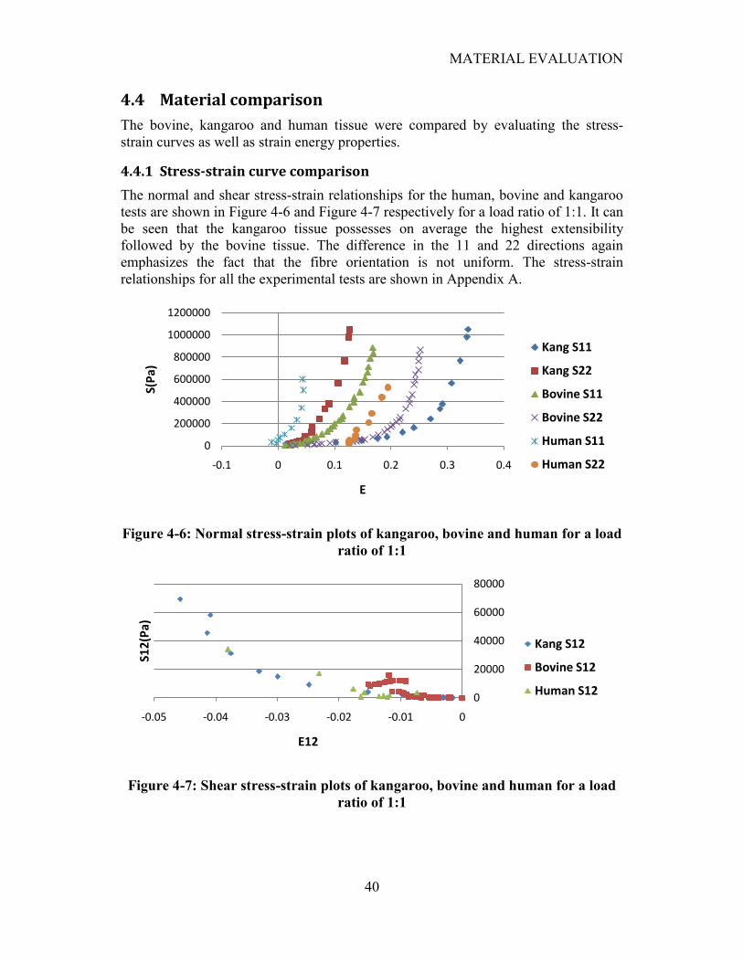
MATERIAL EVALUATION
40
4.4 Material comparison
The bovine, kangaroo and human tissue were compared by evaluating the stress-
strain curves as well as strain energy properties.
4.4.1 Stress-strain curve comparison
The normal and shear stress-strain relationships for the human, bovine and kangaroo
tests are shown in Figure 4-6 and Figure 4-7 respectively for a load ratio of 1:1. It can
be seen that the kangaroo tissue possesses on average the highest extensibility
followed by the bovine tissue. The difference in the 11 and 22 directions again
emphasizes the fact that the fibre orientation is not uniform. The stress-strain
relationships for all the experimental tests are shown in Appendix A.
Figure 4-6: Normal stress-strain plots of kangaroo, bovine and human for a load
ratio of 1:1
Figure 4-7: Shear stress-strain plots of kangaroo, bovine and human for a load
ratio of 1:1
0
200000
400000
600000
800000
1000000
1200000
-0.1 0 0.1 0.2 0.3 0.4
S(P
a)
E
Kang S11
Kang S22
Bovine S11
Bovine S22
Human S11
Human S22
0
20000
40000
60000
80000
-0.05 -0.04 -0.03 -0.02 -0.01 0
S12
(Pa)
E12
Kang S12
Bovine S12
Human S12
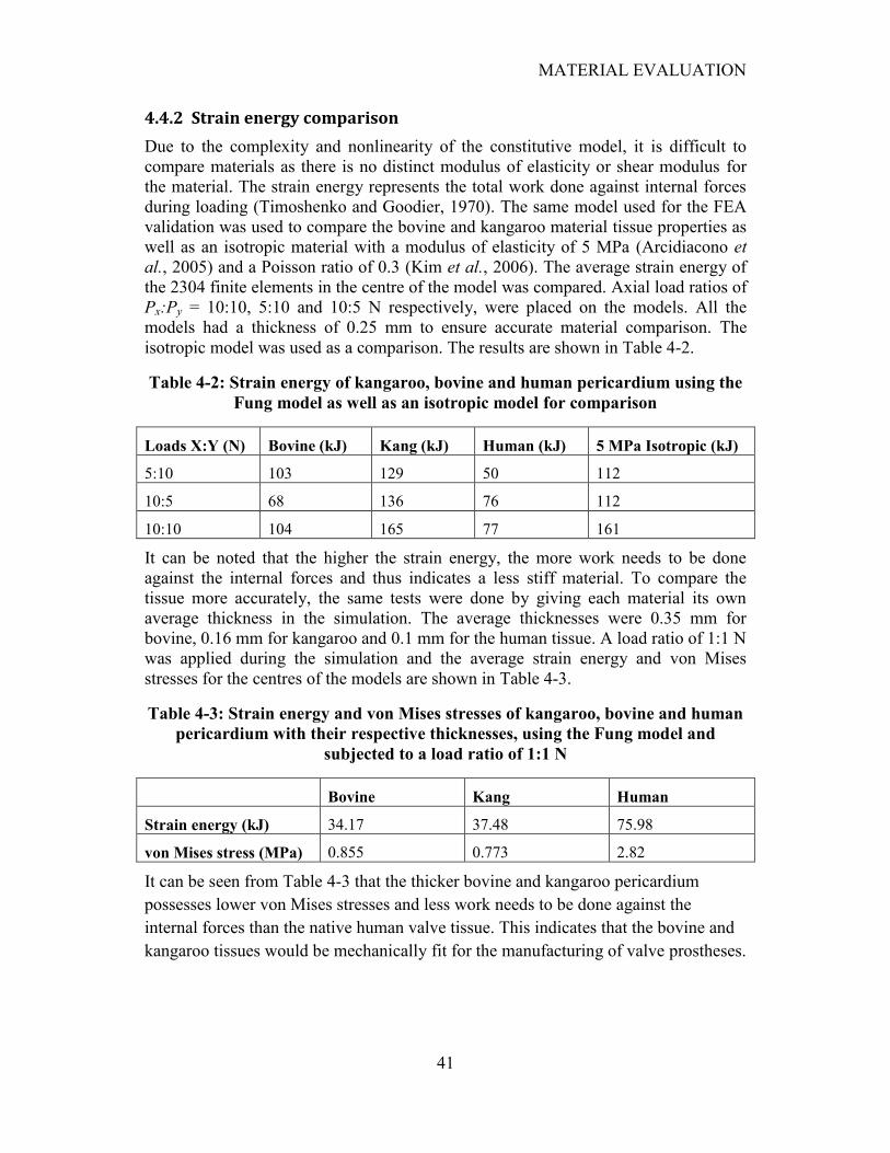
MATERIAL EVALUATION
41
4.4.2 Strain energy comparison
Due to the complexity and nonlinearity of the constitutive model, it is difficult to
compare materials as there is no distinct modulus of elasticity or shear modulus for
the material. The strain energy represents the total work done against internal forces
during loading (Timoshenko and Goodier, 1970). The same model used for the FEA
validation was used to compare the bovine and kangaroo material tissue properties as
well as an isotropic material with a modulus of elasticity of 5 MPa (Arcidiacono et
al., 2005) and a Poisson ratio of 0.3 (Kim et al., 2006). The average strain energy of
the 2304 finite elements in the centre of the model was compared. Axial load ratios of
Px:Py = 10:10, 5:10 and 10:5 N respectively, were placed on the models. All the
models had a thickness of 0.25 mm to ensure accurate material comparison. The
isotropic model was used as a comparison. The results are shown in Table 4-2.
Table 4-2: Strain energy of kangaroo, bovine and human pericardium using the
Fung model as well as an isotropic model for comparison
Loads X:Y (N) Bovine (kJ) Kang (kJ) Human (kJ) 5 MPa Isotropic (kJ)
5:10 103 129 50 112
10:5 68 136 76 112
10:10 104 165 77 161
It can be noted that the higher the strain energy, the more work needs to be done
against the internal forces and thus indicates a less stiff material. To compare the
tissue more accurately, the same tests were done by giving each material its own
average thickness in the simulation. The average thicknesses were 0.35 mm for
bovine, 0.16 mm for kangaroo and 0.1 mm for the human tissue. A load ratio of 1:1 N
was applied during the simulation and the average strain energy and von Mises
stresses for the centres of the models are shown in Table 4-3.
Table 4-3: Strain energy and von Mises stresses of kangaroo, bovine and human
pericardium with their respective thicknesses, using the Fung model and
subjected to a load ratio of 1:1 N
Bovine Kang Human
Strain energy (kJ) 34.17 37.48 75.98
von Mises stress (MPa) 0.855 0.773 2.82
It can be seen from Table 4-3 that the thicker bovine and kangaroo pericardium
possesses lower von Mises stresses and less work needs to be done against the
internal forces than the native human valve tissue. This indicates that the bovine and
kangaroo tissues would be mechanically fit for the manufacturing of valve prostheses.
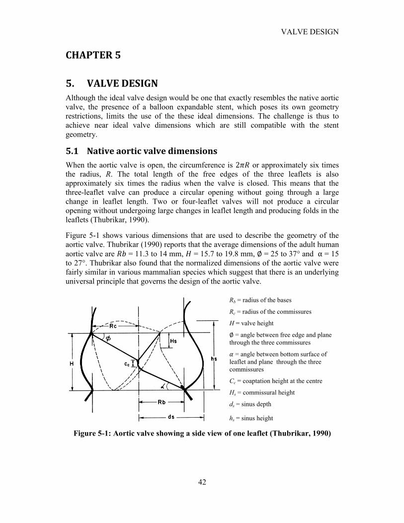
VALVE DESIGN
42
CHAPTER 5
5. VALVE DESIGN
Although the ideal valve design would be one that exactly resembles the native aortic
valve, the presence of a balloon expandable stent, which poses its own geometry
restrictions, limits the use of the these ideal dimensions. The challenge is thus to
achieve near ideal valve dimensions which are still compatible with the stent
geometry.
5.1 Native aortic valve dimensions
When the aortic valve is open, the circumference is or approximately six times
the radius, R. The total length of the free edges of the three leaflets is also
approximately six times the radius when the valve is closed. This means that the
three-leaflet valve can produce a circular opening without going through a large
change in leaflet length. Two or four-leaflet valves will not produce a circular
opening without undergoing large changes in leaflet length and producing folds in the
leaflets (Thubrikar, 1990).
Figure 5-1 shows various dimensions that are used to describe the geometry of the
aortic valve. Thubrikar (1990) reports that the average dimensions of the adult human
aortic valve are = 11.3 to 14 mm, = 15.7 to 19.8 mm, = 25 to 37° and = 15
to 27°. Thubrikar also found that the normalized dimensions of the aortic valve were
fairly similar in various mammalian species which suggest that there is an underlying
universal principle that governs the design of the aortic valve.
Rb = radius of the bases
Rc = radius of the commissures
H = valve height
= angle between free edge and plane
through the three commissures
= angle between bottom surface of
leaflet and plane through the three
commissures
Cc = coaptation height at the centre
Hs = commissural height
ds = sinus depth
hs = sinus height
Figure 5-1: Aortic valve showing a side view of one leaflet (Thubrikar, 1990)
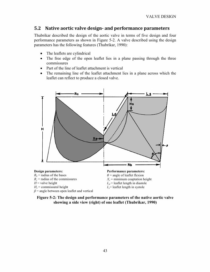
VALVE DESIGN
43
5.2 Native aortic valve design- and performance parameters
Thubrikar described the design of the aortic valve in terms of five design and four
performance parameters as shown in Figure 5-2. A valve described using the design
parameters has the following features (Thubrikar, 1990):
The leaflets are cylindrical
The free edge of the open leaflet lies in a plane passing through the three
commissures
Part of the line of leaflet attachment is vertical
The remaining line of the leaflet attachment lies in a plane across which the
leaflet can reflect to produce a closed valve.
Design parameters:
Rb = radius of the bases
Rc = radius of the commissures
H = valve height
Hs = commissural height
β = angle between open leaflet and vertical
Performance parameters:
= angle of leaflet flexion
Xs = minimum coaptation height
Ld = leaflet length in diastole
Ls= leaflet length in systole
Figure 5-2: The design and performance parameters of the native aortic valve
showing a side view (right) of one leaflet (Thubrikar, 1990)
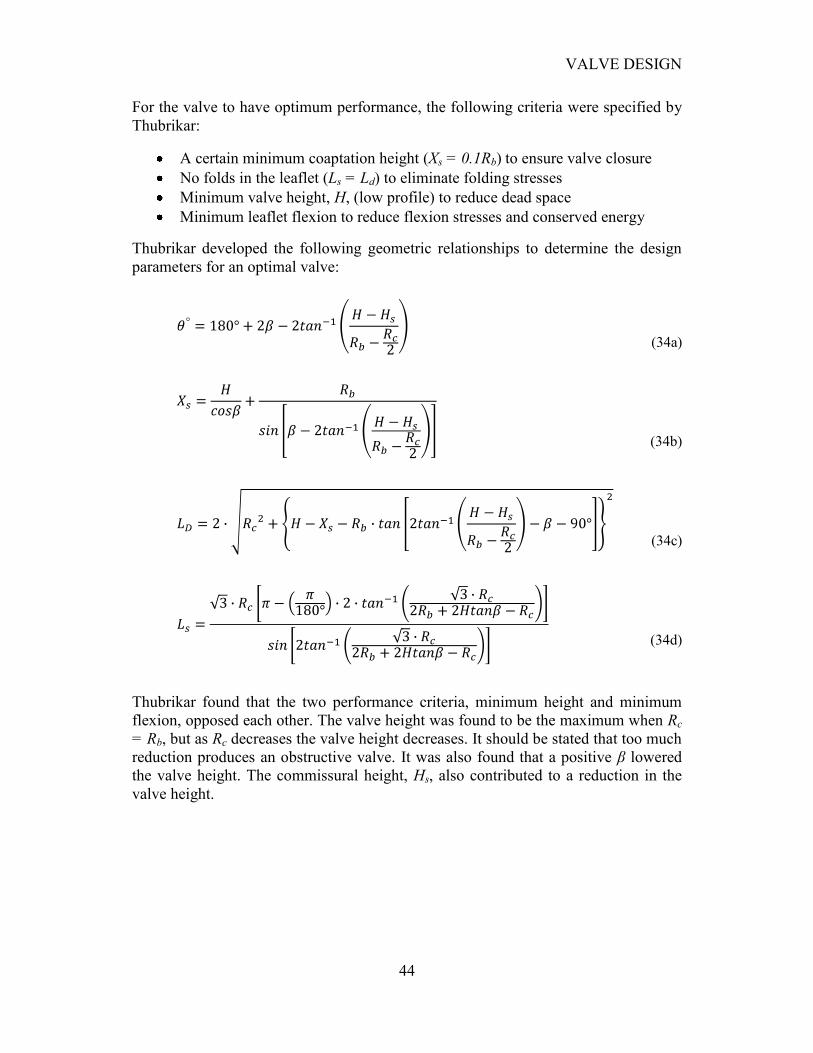
VALVE DESIGN
44
For the valve to have optimum performance, the following criteria were specified by
Thubrikar:
A certain minimum coaptation height (Xs = 0.1Rb) to ensure valve closure
No folds in the leaflet (Ls = Ld) to eliminate folding stresses
Minimum valve height, H, (low profile) to reduce dead space
Minimum leaflet flexion to reduce flexion stresses and conserved energy
Thubrikar developed the following geometric relationships to determine the design
parameters for an optimal valve:
(34a)
(34b)
(34c)
(34d)
Thubrikar found that the two performance criteria, minimum height and minimum
flexion, opposed each other. The valve height was found to be the maximum when Rc
= Rb, but as Rc decreases the valve height decreases. It should be stated that too much
reduction produces an obstructive valve. It was also found that a positive β lowered
the valve height. The commissural height, Hs, also contributed to a reduction in the
valve height.
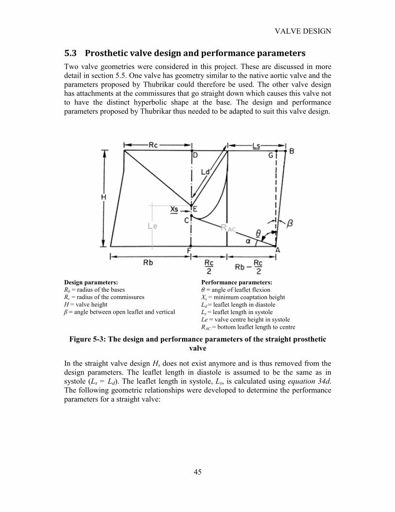
VALVE DESIGN
45
5.3 Prosthetic valve design and performance parameters
Two valve geometries were considered in this project. These are discussed in more
detail in section 5.5. One valve has geometry similar to the native aortic valve and the
parameters proposed by Thubrikar could therefore be used. The other valve design
has attachments at the commissures that go straight down which causes this valve not
to have the distinct hyperbolic shape at the base. The design and performance
parameters proposed by Thubrikar thus needed to be adapted to suit this valve design.
Design parameters:
Rb = radius of the bases
Rc = radius of the commissures
H = valve height
β = angle between open leaflet and vertical
Performance parameters:
= angle of leaflet flexion
Xs = minimum coaptation height
Ld = leaflet length in diastole
Ls = leaflet length in systole
Le = valve centre height in systole
RAC = bottom leaflet length to centre
Figure 5-3: The design and performance parameters of the straight prosthetic
valve
In the straight valve design Hs does not exist anymore and is thus removed from the
design parameters. The leaflet length in diastole is assumed to be the same as in
systole (Ls = Ld). The leaflet length in systole, Ls, is calculated using equation 34d.
The following geometric relationships were developed to determine the performance
parameters for a straight valve:
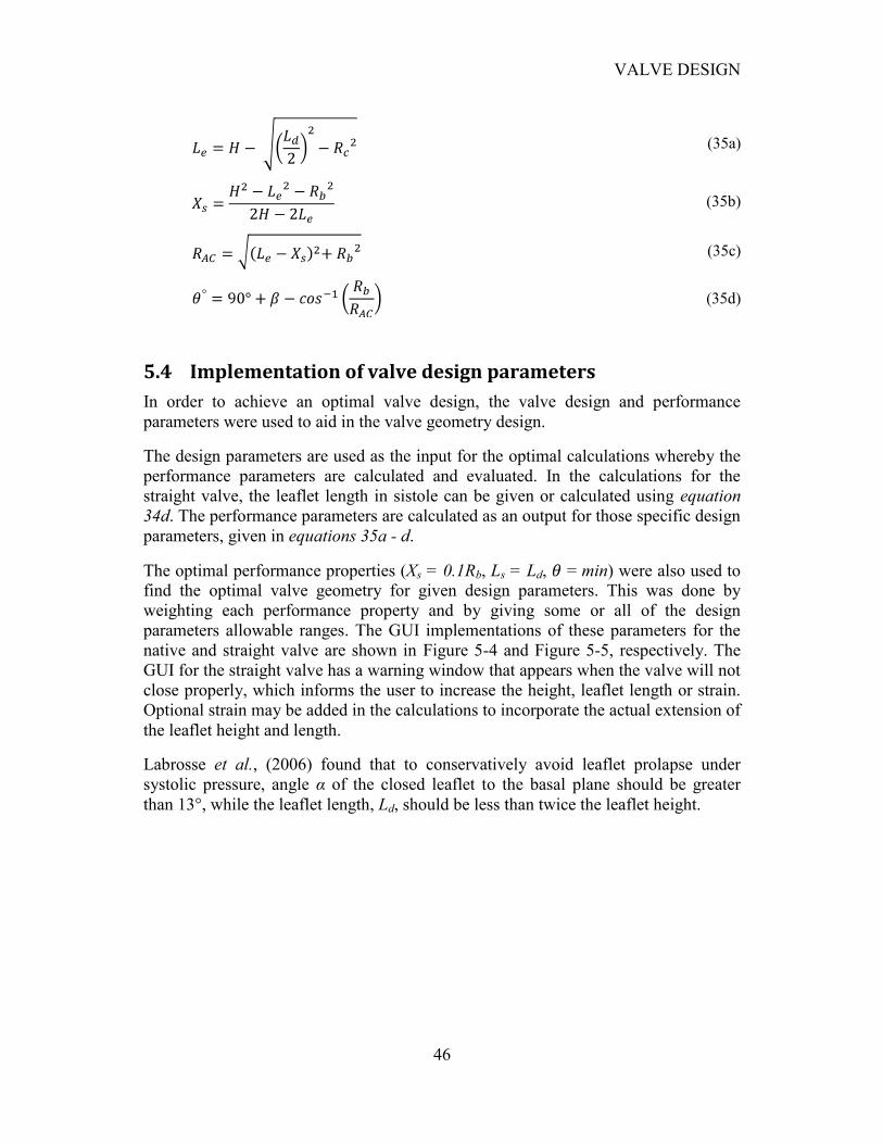
VALVE DESIGN
46
(35a)
(35b)
(35c)
(35d)
5.4 Implementation of valve design parameters
In order to achieve an optimal valve design, the valve design and performance
parameters were used to aid in the valve geometry design.
The design parameters are used as the input for the optimal calculations whereby the
performance parameters are calculated and evaluated. In the calculations for the
straight valve, the leaflet length in sistole can be given or calculated using equation
34d. The performance parameters are calculated as an output for those specific design
parameters, given in equations 35a - d.
The optimal performance properties (Xs = 0.1Rb, Ls = Ld, = min) were also used to
find the optimal valve geometry for given design parameters. This was done by
weighting each performance property and by giving some or all of the design
parameters allowable ranges. The GUI implementations of these parameters for the
native and straight valve are shown in Figure 5-4 and Figure 5-5, respectively. The
GUI for the straight valve has a warning window that appears when the valve will not
close properly, which informs the user to increase the height, leaflet length or strain.
Optional strain may be added in the calculations to incorporate the actual extension of
the leaflet height and length.
Labrosse et al., (2006) found that to conservatively avoid leaflet prolapse under
systolic pressure, angle α of the closed leaflet to the basal plane should be greater
than 13°, while the leaflet length, Ld, should be less than twice the leaflet height.
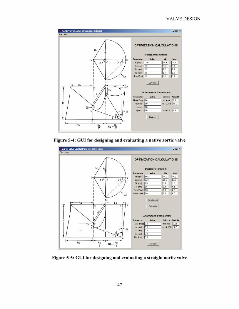
VALVE DESIGN
47
Figure 5-4: GUI for designing and evaluating a native aortic valve
Figure 5-5: GUI for designing and evaluating a straight aortic valve
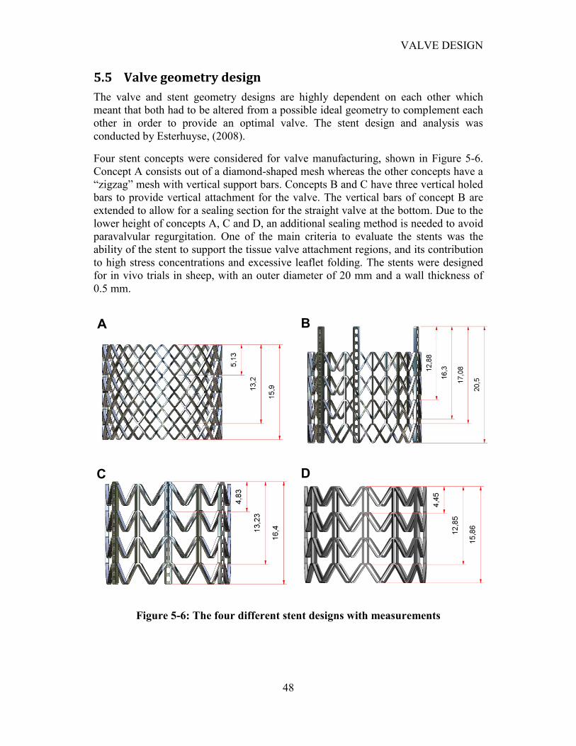
VALVE DESIGN
48
5.5 Valve geometry design
The valve and stent geometry designs are highly dependent on each other which
meant that both had to be altered from a possible ideal geometry to complement each
other in order to provide an optimal valve. The stent design and analysis was
conducted by Esterhuyse, (2008).
Four stent concepts were considered for valve manufacturing, shown in Figure 5-6.
Concept A consists out of a diamond-shaped mesh whereas the other concepts have a
“zigzag” mesh with vertical support bars. Concepts B and C have three vertical holed
bars to provide vertical attachment for the valve. The vertical bars of concept B are
extended to allow for a sealing section for the straight valve at the bottom. Due to the
lower height of concepts A, C and D, an additional sealing method is needed to avoid
paravalvular regurgitation. One of the main criteria to evaluate the stents was the
ability of the stent to support the tissue valve attachment regions, and its contribution
to high stress concentrations and excessive leaflet folding. The stents were designed
for in vivo trials in sheep, with an outer diameter of 20 mm and a wall thickness of
0.5 mm.
Figure 5-6: The four different stent designs with measurements
A B
C D
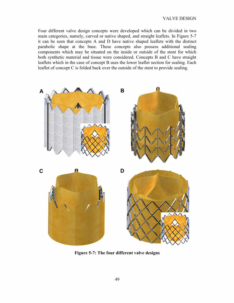
VALVE DESIGN
49
Four different valve design concepts were developed which can be divided in two
main categories, namely, curved or native shaped, and straight leaflets. In Figure 5-7
it can be seen that concepts A and D have native shaped leaflets with the distinct
parabolic shape at the base. These concepts also possess additional sealing
components which may be situated on the inside or outside of the stent for which
both synthetic material and tissue were considered. Concepts B and C have straight
leaflets which in the case of concept B uses the lower leaflet section for sealing. Each
leaflet of concept C is folded back over the outside of the stent to provide sealing.
Figure 5-7: The four different valve designs
A B
C D
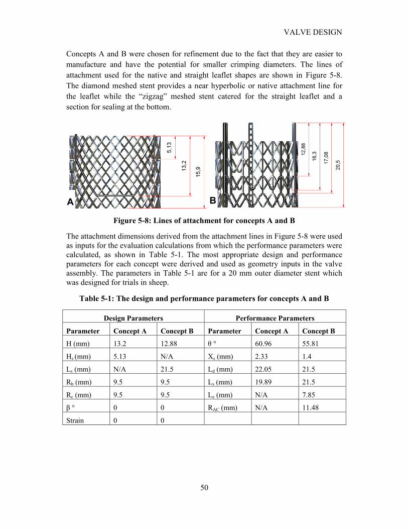
VALVE DESIGN
50
Concepts A and B were chosen for refinement due to the fact that they are easier to
manufacture and have the potential for smaller crimping diameters. The lines of
attachment used for the native and straight leaflet shapes are shown in Figure 5-8.
The diamond meshed stent provides a near hyperbolic or native attachment line for
the leaflet while the “zigzag” meshed stent catered for the straight leaflet and a
section for sealing at the bottom.
Figure 5-8: Lines of attachment for concepts A and B
The attachment dimensions derived from the attachment lines in Figure 5-8 were used
as inputs for the evaluation calculations from which the performance parameters were
calculated, as shown in Table 5-1. The most appropriate design and performance
parameters for each concept were derived and used as geometry inputs in the valve
assembly. The parameters in Table 5-1 are for a 20 mm outer diameter stent which
was designed for trials in sheep.
Table 5-1: The design and performance parameters for concepts A and B
Design Parameters Performance Parameters
Parameter Concept A Concept B Parameter Concept A Concept B
H (mm) 13.2 12.88 θ ° 60.96 55.81
Hs (mm) 5.13 N/A Xs (mm) 2.33 1.4
Ls (mm) N/A 21.5 Ld (mm) 22.05 21.5
Rb (mm) 9.5 9.5 Ls (mm) 19.89 21.5
Rc (mm) 9.5 9.5 Le (mm) N/A 7.85
β ° 0 0 RAC (mm) N/A 11.48
Strain 0 0
A B
VALVE MANUFACTURING
51
CHAPTER 6
6. VALVE MANUFACTURING
Due to the novelty of PAVR technology, there are basically no manufacturing
guidelines and techniques available to aid in the design process. Currently there are
only ISO standards for conventional heart valve prostheses (International
Organization for Standardization , 2005). The techniques and procedures used in this
study are detailed here.
6.1 Attachment material considerations
The valve attachment material is essential in the manufacturing process as it provides
the link between the tissue valve and the metal stent. It is essential that the material
should be biocompatible and durable. Another requirement for the PAV is to aid in
the low profile of the prosthesis, especially when crimped. The material is also
subjected to displacements and tension during the crimping procedure.
Surgical sutures are commonly used in conventional valve prostheses. There are two
main categories of sutures: monofilament vs. braided and permanent vs. absorbable.
Absorbable sutures are not considered as these prostheses are designed to be
permanent. Some monofilament sutures are commonly manufactured from nylon and
are usually stiff and retain their packaged shape. Braided sutures are commonly
manufactured from silk or cotton in a braided construction and are more soft and
supple.
The suture range used in this study was from Gore-Tex®. These sutures are unique,
microporous, non-absorbable monofilaments made of expanded
polytetrafluoroethylene (ePTFE). Although these are monofilament sutures, they are
also soft and supple, like braided sutures. In vivo tests have revealed that Gore-Tex
sutures caused minimal capsule formulation and limited inflammatory response
which is generally greater with multifilament or braided sutures (GORE-TEX, 2008).
These sutures have been specifically designed for cardiovascular surgery and are
swaged to needles that closely approximate the diameter of the thread which enables
the suture to fill the needle hole and reduce leakage. PTFE is one of the most inert
materials known and clinical trials have shown that it elicits minimal tissue reaction
and is also not weakened by the action of tissue enzymes or infection (GORE-TEX,
2008). The internodal spaces permit infiltration of fibroblasts and leukocytes.
Collagen also penetrates into the suture which may actually reinforce the suture
strength (GORE-TEX, 2008). The different suture sizes and their tensile strengths are
given in Table 6-1.
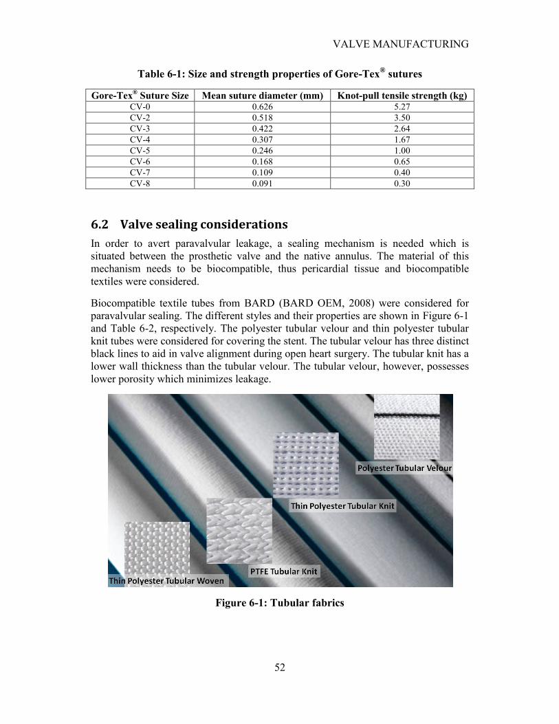
VALVE MANUFACTURING
52
Table 6-1: Size and strength properties of Gore-Tex® sutures
Gore-Tex® Suture Size Mean suture diameter (mm) Knot-pull tensile strength (kg)
CV-0 0.626 5.27
CV-2 0.518 3.50
CV-3 0.422 2.64
CV-4 0.307 1.67
CV-5 0.246 1.00
CV-6 0.168 0.65
CV-7 0.109 0.40
CV-8 0.091 0.30
6.2 Valve sealing considerations
In order to avert paravalvular leakage, a sealing mechanism is needed which is
situated between the prosthetic valve and the native annulus. The material of this
mechanism needs to be biocompatible, thus pericardial tissue and biocompatible
textiles were considered.
Biocompatible textile tubes from BARD (BARD OEM, 2008) were considered for
paravalvular sealing. The different styles and their properties are shown in Figure 6-1
and Table 6-2, respectively. The polyester tubular velour and thin polyester tubular
knit tubes were considered for covering the stent. The tubular velour has three distinct
black lines to aid in valve alignment during open heart surgery. The tubular knit has a
lower wall thickness than the tubular velour. The tubular velour, however, possesses
lower porosity which minimizes leakage.
Figure 6-1: Tubular fabrics
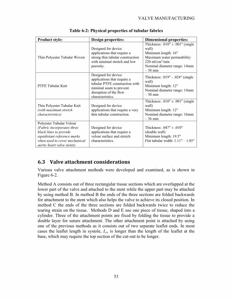
VALVE MANUFACTURING
53
Table 6-2: Physical properties of tubular fabrics
Product style: Design properties: Dimensional properties:
Thin Polyester Tubular Woven
Designed for device
applications that require a
strong thin tubular construction
with minimal stretch and low
porosity.
Thickness: .010" ± .001" (single
wall)
Minimum length: 16"
Maximum water permeability:
220 ml/cm2/min
Nominal diameter range: 14mm
– 38 mm
PTFE Tubular Knit
Designed for device
applications that require a
tubular PTFE construction with
minimal seam to prevent
disruption of the flow
characteristics.
Thickness: .019" - .024" (single
wall)
Minimum length: 12"
Nominal diameter range: 14mm
– 30 mm
Thin Polyester Tubular Knit
(with maximum stretch
characteristics)
Designed for device
applications that require a very
thin tubular construction.
Thickness: .010" ± .001" (single
wall)
Minimum length: 12"
Nominal diameter range: 16mm
– 36 mm
Polyester Tubular Velour
(Fabric incorporates three
black lines to provide
equidistant reference marks
when used to cover mechanical
aortic heart valve stents)
Designed for device
applications that require a
velour surface and stretch
characteristics.
Thickness: .047" ± .010"
(double wall)
Minimum length: 19.5"
Flat tubular width: 1.11" – 1.85"
6.3 Valve attachment considerations
Various valve attachment methods were developed and examined, as is shown in
Figure 6-2.
Method A consists out of three rectangular tissue sections which are overlapped at the
lower part of the valve and attached to the stent while the upper part may be attached
by using method B. In method B the ends of the three sections are folded backwards
for attachment to the stent which also helps the valve to achieve its closed position. In
method C the ends of the three sections are folded backwards twice to reduce the
tearing strain on the tissue. Methods D and E use one piece of tissue, shaped into a
cylinder. Three of the attachment points are fixed by folding the tissue to provide a
double layer for suture attachment. The other attachment point is attached by using
one of the previous methods as it consists out of two separate leaflet ends. In most
cases the leaflet length in systole, Ls, is longer than the length of the leaflet at the
base, which may require the top section of the cut-out to be longer.
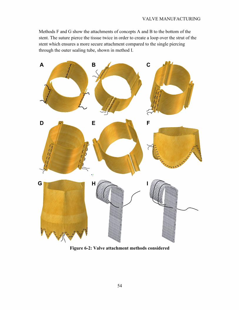
VALVE MANUFACTURING
54
Methods F and G show the attachments of concepts A and B to the bottom of the
stent. The suture pierce the tissue twice in order to create a loop over the strut of the
stent which ensures a more secure attachment compared to the single piercing
through the outer sealing tube, shown in method I.
Figure 6-2: Valve attachment methods considered
A B C
D E F
G H I
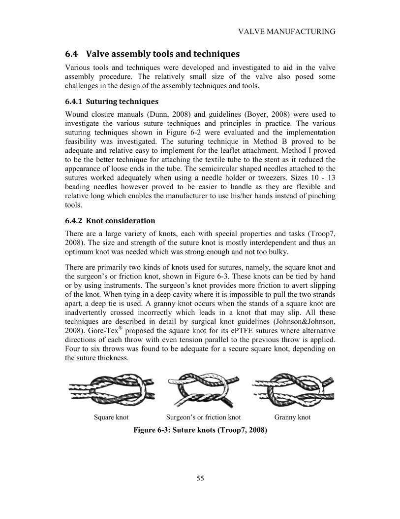
VALVE MANUFACTURING
55
6.4 Valve assembly tools and techniques
Various tools and techniques were developed and investigated to aid in the valve
assembly procedure. The relatively small size of the valve also posed some
challenges in the design of the assembly techniques and tools.
6.4.1 Suturing techniques
Wound closure manuals (Dunn, 2008) and guidelines (Boyer, 2008) were used to
investigate the various suture techniques and principles in practice. The various
suturing techniques shown in Figure 6-2 were evaluated and the implementation
feasibility was investigated. The suturing technique in Method B proved to be
adequate and relative easy to implement for the leaflet attachment. Method I proved
to be the better technique for attaching the textile tube to the stent as it reduced the
appearance of loose ends in the tube. The semicircular shaped needles attached to the
sutures worked adequately when using a needle holder or tweezers. Sizes 10 - 13
beading needles however proved to be easier to handle as they are flexible and
relative long which enables the manufacturer to use his/her hands instead of pinching
tools.
6.4.2 Knot consideration
There are a large variety of knots, each with special properties and tasks (Troop7,
2008). The size and strength of the suture knot is mostly interdependent and thus an
optimum knot was needed which was strong enough and not too bulky.
There are primarily two kinds of knots used for sutures, namely, the square knot and
the surgeon‟s or friction knot, shown in Figure 6-3. These knots can be tied by hand
or by using instruments. The surgeon‟s knot provides more friction to avert slipping
of the knot. When tying in a deep cavity where it is impossible to pull the two strands
apart, a deep tie is used. A granny knot occurs when the stands of a square knot are
inadvertently crossed incorrectly which leads in a knot that may slip. All these
techniques are described in detail by surgical knot guidelines (Johnson&Johnson,
2008). Gore-Tex® proposed the square knot for its ePTFE sutures where alternative
directions of each throw with even tension parallel to the previous throw is applied.
Four to six throws was found to be adequate for a secure square knot, depending on
the suture thickness.
Square knot Surgeon‟s or friction knot Granny knot
Figure 6-3: Suture knots (Troop7, 2008)
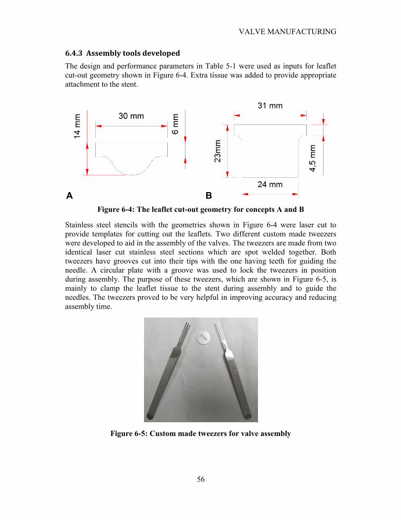
VALVE MANUFACTURING
56
6.4.3 Assembly tools developed
The design and performance parameters in Table 5-1 were used as inputs for leaflet
cut-out geometry shown in Figure 6-4. Extra tissue was added to provide appropriate
attachment to the stent.
Figure 6-4: The leaflet cut-out geometry for concepts A and B
Stainless steel stencils with the geometries shown in Figure 6-4 were laser cut to
provide templates for cutting out the leaflets. Two different custom made tweezers
were developed to aid in the assembly of the valves. The tweezers are made from two
identical laser cut stainless steel sections which are spot welded together. Both
tweezers have grooves cut into their tips with the one having teeth for guiding the
needle. A circular plate with a groove was used to lock the tweezers in position
during assembly. The purpose of these tweezers, which are shown in Figure 6-5, is
mainly to clamp the leaflet tissue to the stent during assembly and to guide the
needles. The tweezers proved to be very helpful in improving accuracy and reducing
assembly time.
Figure 6-5: Custom made tweezers for valve assembly
A B
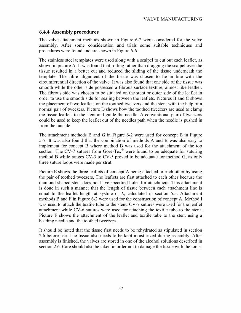
VALVE MANUFACTURING
57
6.4.4 Assembly procedures
The valve attachment methods shown in Figure 6-2 were considered for the valve
assembly. After some consideration and trials some suitable techniques and
procedures were found and are shown in Figure 6-6.
The stainless steel templates were used along with a scalpel to cut out each leaflet, as
shown in picture A. It was found that rolling rather than dragging the scalpel over the
tissue resulted in a better cut and reduced the sliding of the tissue underneath the
template. The fibre alignment of the tissue was chosen to lie in line with the
circumferential direction of the valve. It was also found that one side of the tissue was
smooth while the other side possessed a fibrous surface texture, almost like leather.
The fibrous side was chosen to be situated on the stent or outer side of the leaflet in
order to use the smooth side for sealing between the leaflets. Pictures B and C shows
the placement of two leaflets on the toothed tweezers and the stent with the help of a
normal pair of tweezers. Picture D shows how the toothed tweezers are used to clamp
the tissue leaflets to the stent and guide the needle. A conventional pair of tweezers
could be used to keep the leaflet out of the needles path when the needle is pushed in
from the outside.
The attachment methods B and G in Figure 6-2 were used for concept B in Figure
5-7. It was also found that the combination of methods A and B was also easy to
implement for concept B where method B was used for the attachment of the top
section. The CV-7 sutures from Gore-Tex® were found to be adequate for suturing
method B while ranges CV-3 to CV-5 proved to be adequate for method G, as only
three suture loops were made per strut.
Picture E shows the three leaflets of concept A being attached to each other by using
the pair of toothed tweezers. The leaflets are first attached to each other because the
diamond shaped stent does not have specified holes for attachment. This attachment
is done in such a manner that the length of tissue between each attachment line is
equal to the leaflet length at systole or Ls calculated in section 5.5. Attachment
methods B and F in Figure 6-2 were used for the construction of concept A. Method I
was used to attach the textile tube to the stent. CV-7 sutures were used for the leaflet
attachment while CV-6 sutures were used for attaching the textile tube to the stent.
Picture F shows the attachment of the leaflet and textile tube to the stent using a
beading needle and the toothed tweezers.
It should be noted that the tissue first needs to be rehydrated as stipulated in section
2.6 before use. The tissue also needs to be kept moisturized during assembly. After
assembly is finished, the valves are stored in one of the alcohol solutions described in
section 2.6. Care should also be taken in order not to damage the tissue with the tools.
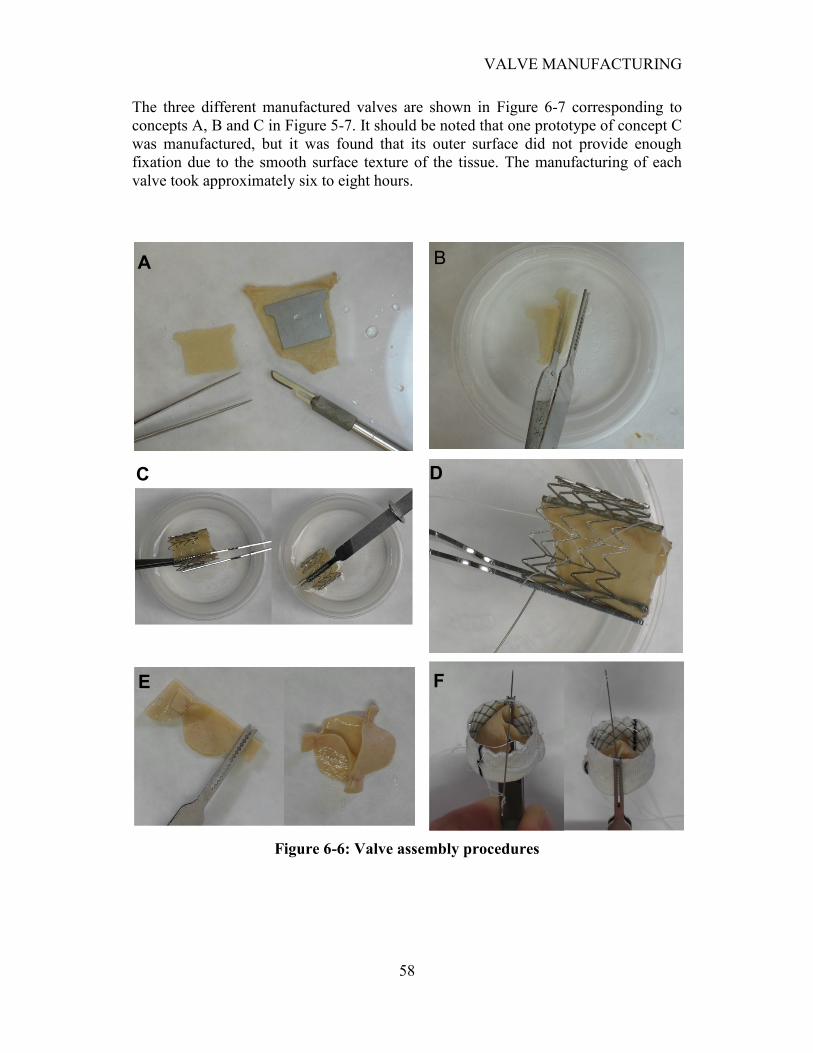
VALVE MANUFACTURING
58
The three different manufactured valves are shown in Figure 6-7 corresponding to
concepts A, B and C in Figure 5-7. It should be noted that one prototype of concept C
was manufactured, but it was found that its outer surface did not provide enough
fixation due to the smooth surface texture of the tissue. The manufacturing of each
valve took approximately six to eight hours.
Figure 6-6: Valve assembly procedures
A
C
B
D
E F
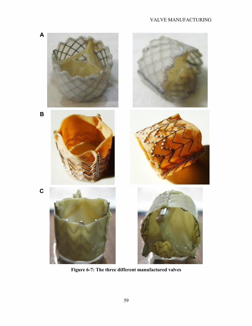
VALVE MANUFACTURING
59
Figure 6-7: The three different manufactured valves
A
B
C
FINITE ELEMENT ANALYSIS (FEA) OF VALVE
60
CHAPTER 7
7. FINITE ELEMENT ANALYSIS (FEA) OF VALVE
Finite element analysis was used to aid in the evaluation of concepts A and B. Both
normal and hypertensive pressure differences across the valve were examined by
using static analysis. This was simulated for diastole when the maximum pressure
difference across the valve occurs. The valve material orientation as well as the use of
different material properties for each leaflet was investigated to determine its
influence on the valve performance. The allowable over and under dilation, along
with unsymmetrical dilation were also investigated. The leaflet attachment forces
were determined to investigate the probability of tissue tearing. Finally the stress
distribution across the leaflet was examined.
7.1 FEA implementation
The same FEA implementation technique used in section 4.2 was used for the valve
simulations. The geometries derived in section 5.5 were used to construct the FE
models for concepts A and B, as are shown in Figure 7-1. Conventional aortic valve
simulations are performed by either using an open or closed valve geometry,
constructed according to the native aortic valve geometry. The aim in this study was
to construct the FEA geometry in such a way that it resembles the geometry of the
valve prosthesis as much as possible. This ensures a more accurate simulation,
because the initial leaflet geometry resembles the semi-relaxed state of the valve,
with minimal prestresses in the leaflet.
Contact analysis was used to accurately simulate the interaction between the leaflets.
Five integration points through the leaflet thickness were used for all the simulations.
Translation constraints were placed on lines of attachment to the stent. A uniform
pressure load was placed on the top of each leaflet. A cylindrical coordinate system
was placed in the centre of the valve to act as the material orientation system.
Concept A consisted out of 3480 elements and concept B out of 5496 elements.
7.2 Extreme pressure simulations
The ISO standards for conventional heart valve prostheses (International
Organization for Standardization , 2005) states that a heart valve substitute must be
able to withstand a single maximum cycle consisting of a pressure difference of 230
mmHg across the valve. Both concepts A and B were subjected to this pressure
during the finite element analysis. Kim et al. (2006) investigated the bioprosthetic
heart valve function using the Fung constitutive model for the opening of the valve
during systole. It is known that the highest stresses in the valve tissue occur during
diastole which is the reason why the closure of the valve was simulated in this study.
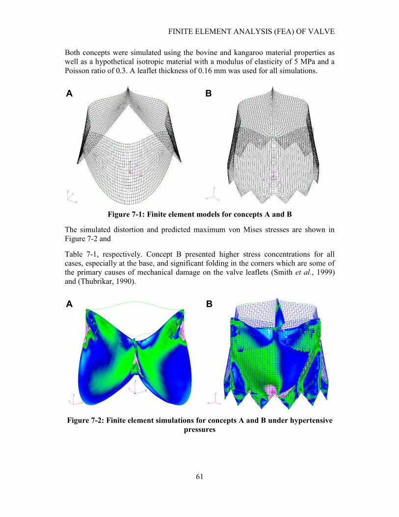
FINITE ELEMENT ANALYSIS (FEA) OF VALVE
61
Both concepts were simulated using the bovine and kangaroo material properties as
well as a hypothetical isotropic material with a modulus of elasticity of 5 MPa and a
Poisson ratio of 0.3. A leaflet thickness of 0.16 mm was used for all simulations.
Figure 7-1: Finite element models for concepts A and B
The simulated distortion and predicted maximum von Mises stresses are shown in
Figure 7-2 and
Table 7-1, respectively. Concept B presented higher stress concentrations for all
cases, especially at the base, and significant folding in the corners which are some of
the primary causes of mechanical damage on the valve leaflets (Smith et al., 1999)
and (Thubrikar, 1990).
Figure 7-2: Finite element simulations for concepts A and B under hypertensive
pressures
A B
A B
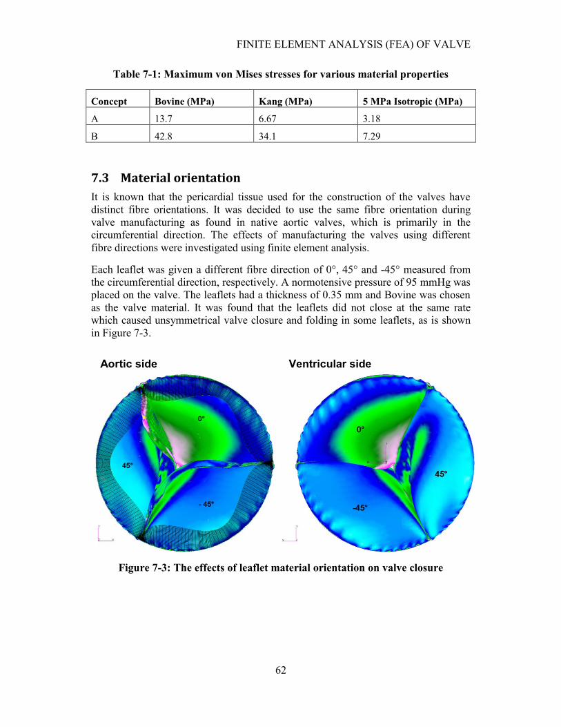
FINITE ELEMENT ANALYSIS (FEA) OF VALVE
62
Table 7-1: Maximum von Mises stresses for various material properties
Concept Bovine (MPa) Kang (MPa) 5 MPa Isotropic (MPa)
A 13.7 6.67 3.18
B 42.8 34.1 7.29
7.3 Material orientation
It is known that the pericardial tissue used for the construction of the valves have
distinct fibre orientations. It was decided to use the same fibre orientation during
valve manufacturing as found in native aortic valves, which is primarily in the
circumferential direction. The effects of manufacturing the valves using different
fibre directions were investigated using finite element analysis.
Each leaflet was given a different fibre direction of 0°, 45° and -45° measured from
the circumferential direction, respectively. A normotensive pressure of 95 mmHg was
placed on the valve. The leaflets had a thickness of 0.35 mm and Bovine was chosen
as the valve material. It was found that the leaflets did not close at the same rate
which caused unsymmetrical valve closure and folding in some leaflets, as is shown
in Figure 7-3.
Figure 7-3: The effects of leaflet material orientation on valve closure
Aortic side Ventricular side
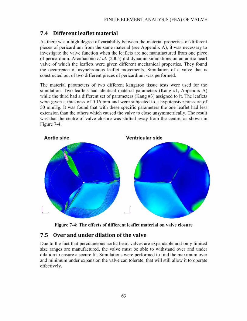
FINITE ELEMENT ANALYSIS (FEA) OF VALVE
63
7.4 Different leaflet material
As there was a high degree of variability between the material properties of different
pieces of pericardium from the same material (see Appendix A), it was necessary to
investigate the valve function when the leaflets are not manufactured from one piece
of pericardium. Arcidiacono et al. (2005) did dynamic simulations on an aortic heart
valve of which the leaflets were given different mechanical properties. They found
the occurrence of asynchronous leaflet movements. Simulation of a valve that is
constructed out of two different pieces of pericardium was performed.
The material parameters of two different kangaroo tissue tests were used for the
simulation. Two leaflets had identical material parameters (Kang #1, Appendix A)
while the third had a different set of parameters (Kang #3) assigned to it. The leaflets
were given a thickness of 0.16 mm and were subjected to a hypotensive pressure of
50 mmHg. It was found that with these specific parameters the one leaflet had less
extension than the others which caused the valve to close unsymmetrically. The result
was that the centre of valve closure was shifted away from the centre, as shown in
Figure 7-4.
Figure 7-4: The effects of different leaflet material on valve closure
7.5 Over and under dilation of the valve
Due to the fact that percutaneous aortic heart valves are expandable and only limited
size ranges are manufactured, the valve must be able to withstand over and under
dilation to ensure a secure fit. Simulations were performed to find the maximum over
and minimum under expansion the valve can tolerate, that will still allow it to operate
effectively.
Aortic side Ventricular side
FINITE ELEMENT ANALYSIS (FEA) OF VALVE
64
Valve dilation was simulated for ranges -1.0, 1.0, 2.0 and 4.0 mm relative to the valve
diameter. The simulations were performed by applying a hypotensive pressure of 50
mmHg to the valves to ensure valve closure under lower pressures. The leaflets were
given a thickness of 0.16 mm. Two load steps were used in the simulations, where the
first applied the dilation, and the second one the pressure. It was found that the gap in
the centre of the valve increased in size during over dilation and the presence of
leaflet folding occurred during under dilation, as is shown in Figure 7-5.
The simulations were compared with the normal valve simulations and it was found
that the gap in the centre was still reasonably small at an over dilation of 2.0 mm for
concept B. This is due to the extensibility of the kangaroo pericardium along with the
fact that concept B had a larger leaflet height than concept A. The gap in the centre of
concept A was larger compared to Concept B. It should be noted that both concepts
had the same leaflet length during systole. Folds were already present in the 1.0 mm
under dilation of both valves, with B possessing more distinct folding. The over and
under dilation of the valves is shown in Figure 7-5.
7.6 Unsymmetrical dilation of valve
It was found while expanding the manufactured valves with a balloon, the stent
occasionally experienced unsymmetrical expansion. The reason for this may be the
complex interaction between the folded balloon and the stent during expansion.
Another cause of unsymmetrical expansion may be the irregular geometry of a
calcified native valve annulus, as is shown in Figure 2-2.
Unsymmetrical expansion of the stent was simulated by expanding one third of the
valve using a quadratic function of the form , where is the number of stent
attachment points in one half of the section and is the stent attachment point
number starting at 1. This produced the irregular expansion of one third of the valve
with a maximum expansion of 1 mm in the centre of the section, as shown in Figure
7-6. The simulations were performed by applying a hypotensive pressure of 50
mmHg to the valves to ensure valve closure under lower pressures. The leaflets were
given a thickness of 0.225 mm and the Bovine #2 material properties given in
Appendix A was used for the simulation in Figure 7-6.
The unsymmetrical dilation caused the valve‟s centre of closure to be off-centre. The
valve still closed effectively with the 1 mm unsymmetrical expansion.
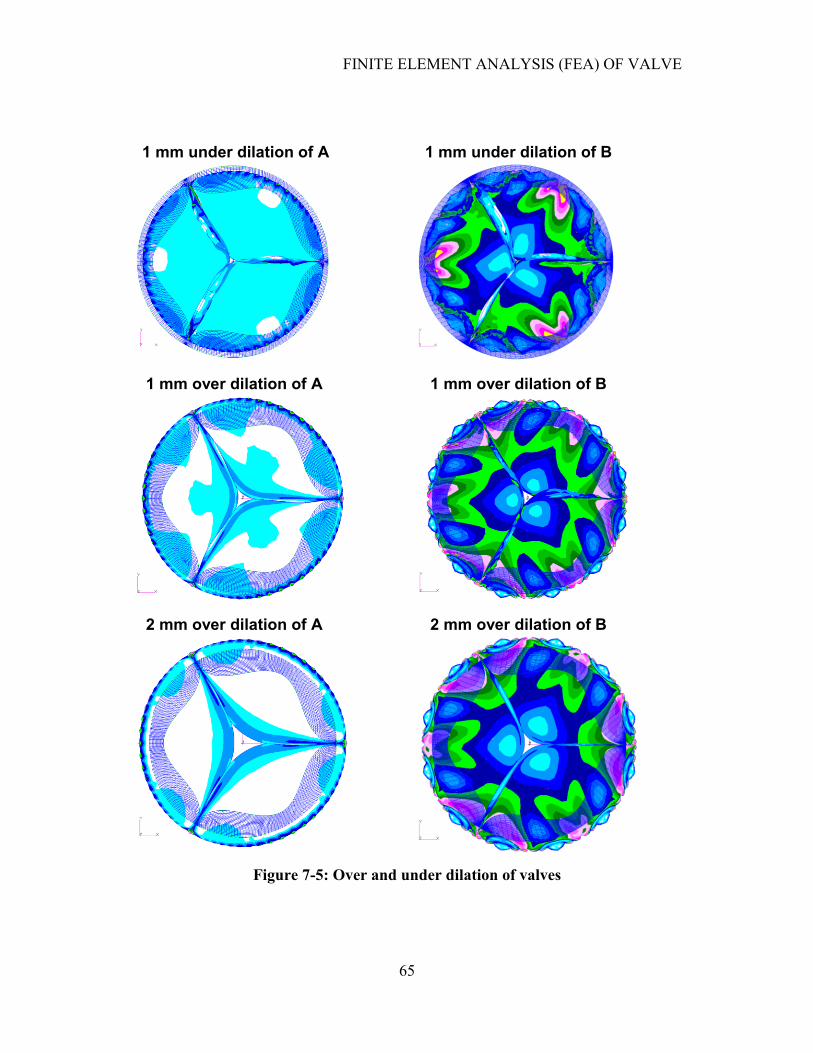
FINITE ELEMENT ANALYSIS (FEA) OF VALVE
65
Figure 7-5: Over and under dilation of valves
1 mm under dilation of A 1 mm under dilation of B
1 mm over dilation of B
2 mm over dilation of B 2 mm over dilation of A
1 mm over dilation of A
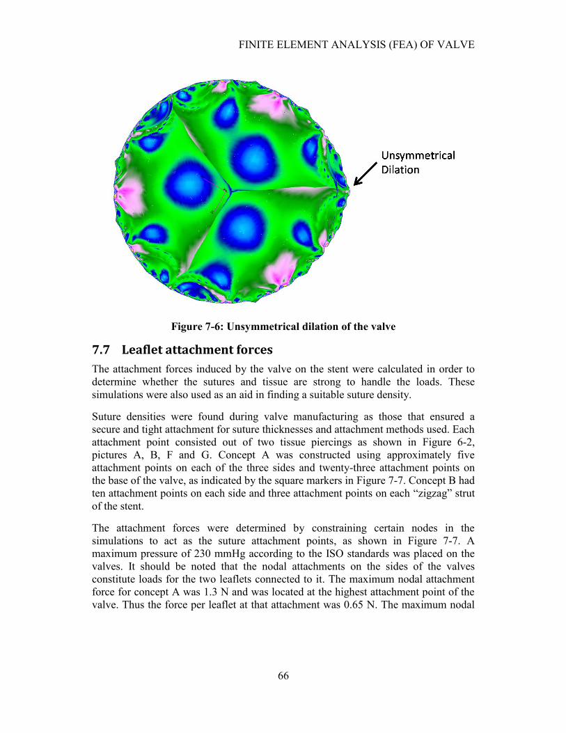
FINITE ELEMENT ANALYSIS (FEA) OF VALVE
66
Figure 7-6: Unsymmetrical dilation of the valve
7.7 Leaflet attachment forces
The attachment forces induced by the valve on the stent were calculated in order to
determine whether the sutures and tissue are strong to handle the loads. These
simulations were also used as an aid in finding a suitable suture density.
Suture densities were found during valve manufacturing as those that ensured a
secure and tight attachment for suture thicknesses and attachment methods used. Each
attachment point consisted out of two tissue piercings as shown in Figure 6-2,
pictures A, B, F and G. Concept A was constructed using approximately five
attachment points on each of the three sides and twenty-three attachment points on
the base of the valve, as indicated by the square markers in Figure 7-7. Concept B had
ten attachment points on each side and three attachment points on each “zigzag” strut
of the stent.
The attachment forces were determined by constraining certain nodes in the
simulations to act as the suture attachment points, as shown in Figure 7-7. A
maximum pressure of 230 mmHg according to the ISO standards was placed on the
valves. It should be noted that the nodal attachments on the sides of the valves
constitute loads for the two leaflets connected to it. The maximum nodal attachment
force for concept A was 1.3 N and was located at the highest attachment point of the
valve. Thus the force per leaflet at that attachment was 0.65 N. The maximum nodal
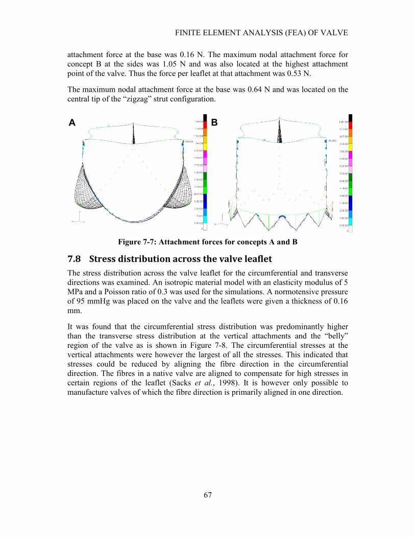
FINITE ELEMENT ANALYSIS (FEA) OF VALVE
67
attachment force at the base was 0.16 N. The maximum nodal attachment force for
concept B at the sides was 1.05 N and was also located at the highest attachment
point of the valve. Thus the force per leaflet at that attachment was 0.53 N.
The maximum nodal attachment force at the base was 0.64 N and was located on the
central tip of the “zigzag” strut configuration.
Figure 7-7: Attachment forces for concepts A and B
7.8 Stress distribution across the valve leaflet
The stress distribution across the valve leaflet for the circumferential and transverse
directions was examined. An isotropic material model with an elasticity modulus of 5
MPa and a Poisson ratio of 0.3 was used for the simulations. A normotensive pressure
of 95 mmHg was placed on the valve and the leaflets were given a thickness of 0.16
mm.
It was found that the circumferential stress distribution was predominantly higher
than the transverse stress distribution at the vertical attachments and the “belly”
region of the valve as is shown in Figure 7-8. The circumferential stresses at the
vertical attachments were however the largest of all the stresses. This indicated that
stresses could be reduced by aligning the fibre direction in the circumferential
direction. The fibres in a native valve are aligned to compensate for high stresses in
certain regions of the leaflet (Sacks et al., 1998). It is however only possible to
manufacture valves of which the fibre direction is primarily aligned in one direction.
A B
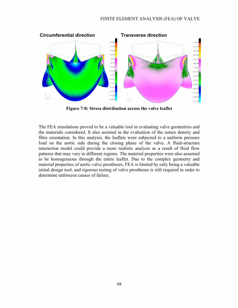
FINITE ELEMENT ANALYSIS (FEA) OF VALVE
68
Figure 7-8: Stress distribution across the valve leaflet
The FEA simulations proved to be a valuable tool in evaluating valve geometries and
the materials considered. It also assisted in the evaluation of the suture density and
fibre orientation. In this analysis, the leaflets were subjected to a uniform pressure
load on the aortic side during the closing phase of the valve. A fluid-structure
interaction model could provide a more realistic analysis as a result of fluid flow
patterns that may vary in different regions. The material properties were also assumed
to be homogeneous through the entire leaflet. Due to the complex geometry and
material properties of aortic valve prostheses, FEA is limited by only being a valuable
initial design tool, and rigorous testing of valve prostheses is still required in order to
determine unforseen causes of failure.
Circumferential direction Transverse direction
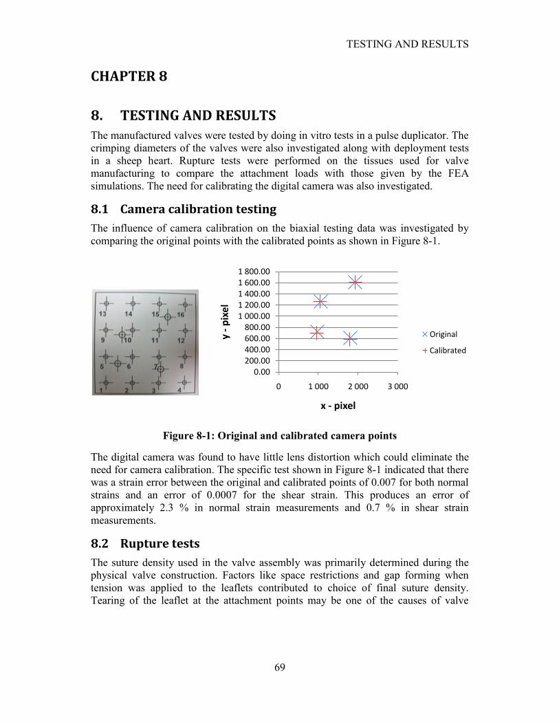
TESTING AND RESULTS
69
CHAPTER 8
8. TESTING AND RESULTS
The manufactured valves were tested by doing in vitro tests in a pulse duplicator. The
crimping diameters of the valves were also investigated along with deployment tests
in a sheep heart. Rupture tests were performed on the tissues used for valve
manufacturing to compare the attachment loads with those given by the FEA
simulations. The need for calibrating the digital camera was also investigated.
8.1 Camera calibration testing
The influence of camera calibration on the biaxial testing data was investigated by
comparing the original points with the calibrated points as shown in Figure 8-1.
Figure 8-1: Original and calibrated camera points
The digital camera was found to have little lens distortion which could eliminate the
need for camera calibration. The specific test shown in Figure 8-1 indicated that there
was a strain error between the original and calibrated points of 0.007 for both normal
strains and an error of 0.0007 for the shear strain. This produces an error of
approximately 2.3 % in normal strain measurements and 0.7 % in shear strain
measurements.
8.2 Rupture tests
The suture density used in the valve assembly was primarily determined during the
physical valve construction. Factors like space restrictions and gap forming when
tension was applied to the leaflets contributed to choice of final suture density.
Tearing of the leaflet at the attachment points may be one of the causes of valve
0.00200.00400.00600.00800.00
1 000.001 200.001 400.001 600.001 800.00
0 1 000 2 000 3 000
y -
pix
el
x - pixel
Original
Calibrated
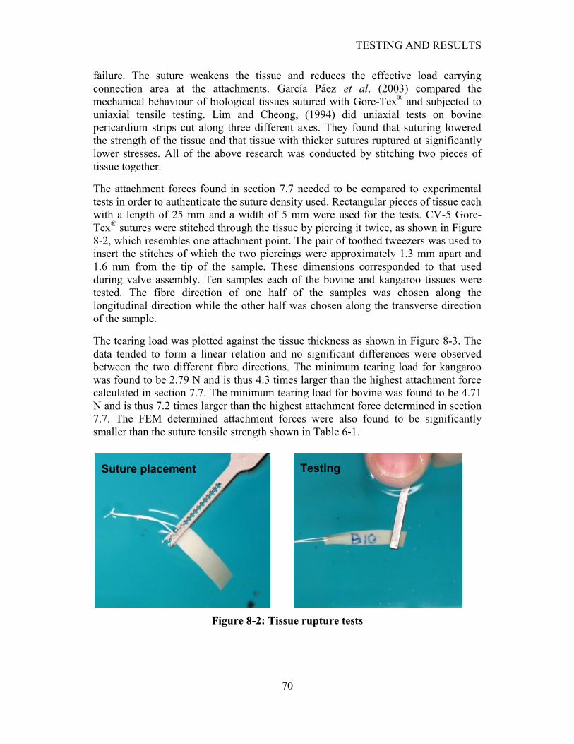
TESTING AND RESULTS
70
failure. The suture weakens the tissue and reduces the effective load carrying
connection area at the attachments. García Páez et al. (2003) compared the
mechanical behaviour of biological tissues sutured with Gore-Tex® and subjected to
uniaxial tensile testing. Lim and Cheong, (1994) did uniaxial tests on bovine
pericardium strips cut along three different axes. They found that suturing lowered
the strength of the tissue and that tissue with thicker sutures ruptured at significantly
lower stresses. All of the above research was conducted by stitching two pieces of
tissue together.
The attachment forces found in section 7.7 needed to be compared to experimental
tests in order to authenticate the suture density used. Rectangular pieces of tissue each
with a length of 25 mm and a width of 5 mm were used for the tests. CV-5 Gore-
Tex® sutures were stitched through the tissue by piercing it twice, as shown in Figure
8-2, which resembles one attachment point. The pair of toothed tweezers was used to
insert the stitches of which the two piercings were approximately 1.3 mm apart and
1.6 mm from the tip of the sample. These dimensions corresponded to that used
during valve assembly. Ten samples each of the bovine and kangaroo tissues were
tested. The fibre direction of one half of the samples was chosen along the
longitudinal direction while the other half was chosen along the transverse direction
of the sample.
The tearing load was plotted against the tissue thickness as shown in Figure 8-3. The
data tended to form a linear relation and no significant differences were observed
between the two different fibre directions. The minimum tearing load for kangaroo
was found to be 2.79 N and is thus 4.3 times larger than the highest attachment force
calculated in section 7.7. The minimum tearing load for bovine was found to be 4.71
N and is thus 7.2 times larger than the highest attachment force determined in section
7.7. The FEM determined attachment forces were also found to be significantly
smaller than the suture tensile strength shown in Table 6-1.
Figure 8-2: Tissue rupture tests
Suture placement Testing
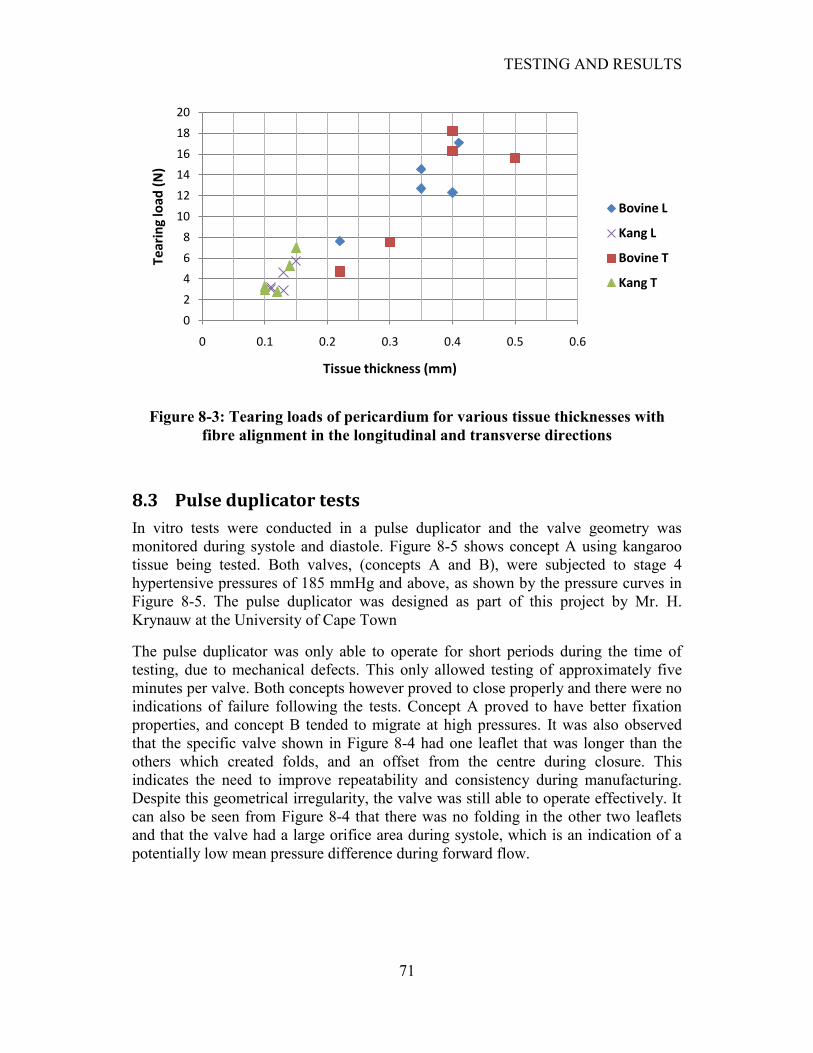
TESTING AND RESULTS
71
Figure 8-3: Tearing loads of pericardium for various tissue thicknesses with
fibre alignment in the longitudinal and transverse directions
8.3 Pulse duplicator tests
In vitro tests were conducted in a pulse duplicator and the valve geometry was
monitored during systole and diastole. Figure 8-5 shows concept A using kangaroo
tissue being tested. Both valves, (concepts A and B), were subjected to stage 4
hypertensive pressures of 185 mmHg and above, as shown by the pressure curves in
Figure 8-5. The pulse duplicator was designed as part of this project by Mr. H.
Krynauw at the University of Cape Town
The pulse duplicator was only able to operate for short periods during the time of
testing, due to mechanical defects. This only allowed testing of approximately five
minutes per valve. Both concepts however proved to close properly and there were no
indications of failure following the tests. Concept A proved to have better fixation
properties, and concept B tended to migrate at high pressures. It was also observed
that the specific valve shown in Figure 8-4 had one leaflet that was longer than the
others which created folds, and an offset from the centre during closure. This
indicates the need to improve repeatability and consistency during manufacturing.
Despite this geometrical irregularity, the valve was still able to operate effectively. It
can also be seen from Figure 8-4 that there was no folding in the other two leaflets
and that the valve had a large orifice area during systole, which is an indication of a
potentially low mean pressure difference during forward flow.
0
2
4
6
8
10
12
14
16
18
20
0 0.1 0.2 0.3 0.4 0.5 0.6
Tear
ing
load
(N
)
Tissue thickness (mm)
Bovine L
Kang L
Bovine T
Kang T
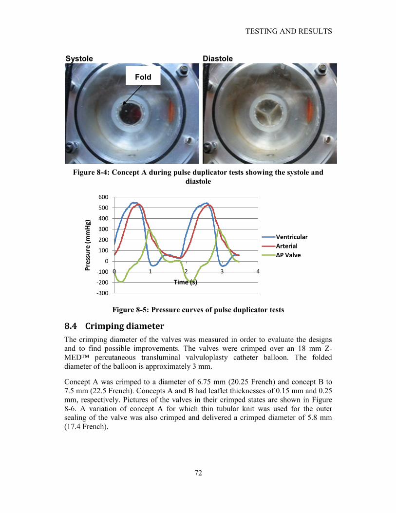
TESTING AND RESULTS
72
Figure 8-4: Concept A during pulse duplicator tests showing the systole and
diastole
Figure 8-5: Pressure curves of pulse duplicator tests
8.4 Crimping diameter
The crimping diameter of the valves was measured in order to evaluate the designs
and to find possible improvements. The valves were crimped over an 18 mm Z-
MED™ percutaneous transluminal valvuloplasty catheter balloon. The folded
diameter of the balloon is approximately 3 mm.
Concept A was crimped to a diameter of 6.75 mm (20.25 French) and concept B to
7.5 mm (22.5 French). Concepts A and B had leaflet thicknesses of 0.15 mm and 0.25
mm, respectively. Pictures of the valves in their crimped states are shown in Figure
8-6. A variation of concept A for which thin tubular knit was used for the outer
sealing of the valve was also crimped and delivered a crimped diameter of 5.8 mm
(17.4 French).
-300
-200
-100
0
100
200
300
400
500
600
0 1 2 3 4Pre
ssu
re (
mm
Hg)
Time (s)
Ventricular
Arterial
∆P Valve
Systole Diastole
Fold
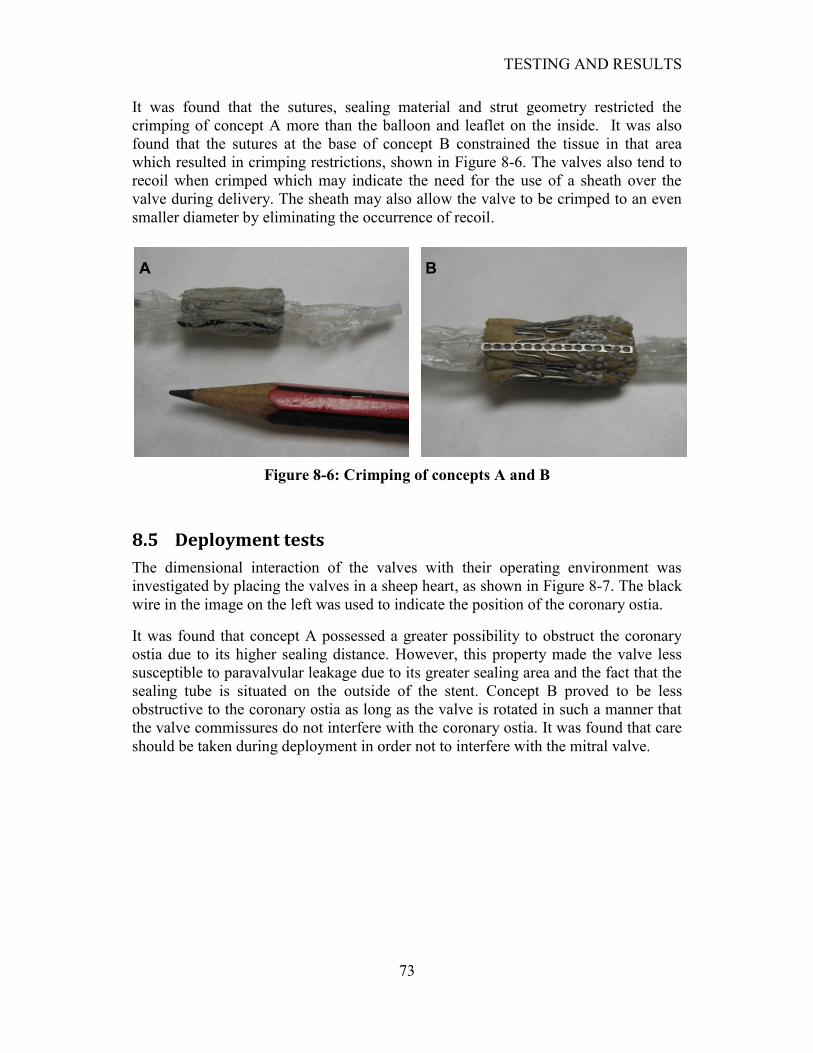
TESTING AND RESULTS
73
It was found that the sutures, sealing material and strut geometry restricted the
crimping of concept A more than the balloon and leaflet on the inside. It was also
found that the sutures at the base of concept B constrained the tissue in that area
which resulted in crimping restrictions, shown in Figure 8-6. The valves also tend to
recoil when crimped which may indicate the need for the use of a sheath over the
valve during delivery. The sheath may also allow the valve to be crimped to an even
smaller diameter by eliminating the occurrence of recoil.
Figure 8-6: Crimping of concepts A and B
8.5 Deployment tests
The dimensional interaction of the valves with their operating environment was
investigated by placing the valves in a sheep heart, as shown in Figure 8-7. The black
wire in the image on the left was used to indicate the position of the coronary ostia.
It was found that concept A possessed a greater possibility to obstruct the coronary
ostia due to its higher sealing distance. However, this property made the valve less
susceptible to paravalvular leakage due to its greater sealing area and the fact that the
sealing tube is situated on the outside of the stent. Concept B proved to be less
obstructive to the coronary ostia as long as the valve is rotated in such a manner that
the valve commissures do not interfere with the coronary ostia. It was found that care
should be taken during deployment in order not to interfere with the mitral valve.
A B
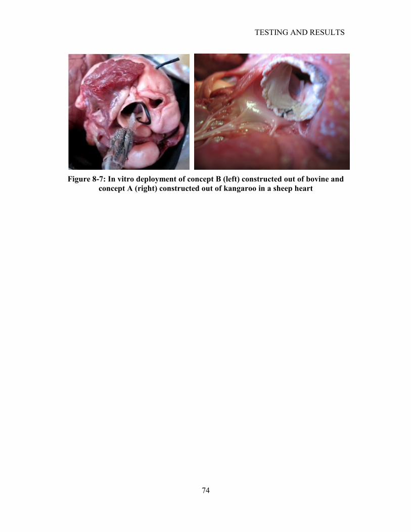
TESTING AND RESULTS
74
Figure 8-7: In vitro deployment of concept B (left) constructed out of bovine and
concept A (right) constructed out of kangaroo in a sheep heart
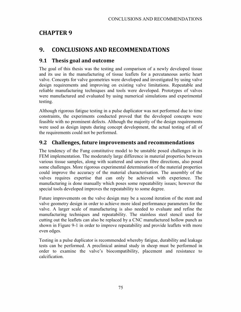
CONCLUSIONS AND RECOMMENDATIONS
75
CHAPTER 9
9. CONCLUSIONS AND RECOMMENDATIONS
9.1 Thesis goal and outcome
The goal of this thesis was the testing and comparison of a newly developed tissue
and its use in the manufacturing of tissue leaflets for a percutaneous aortic heart
valve. Concepts for valve geometries were developed and investigated by using valve
design requirements and improving on existing valve limitations. Repeatable and
reliable manufacturing techniques and tools were developed. Prototypes of valves
were manufactured and evaluated by using numerical simulations and experimental
testing.
Although rigorous fatigue testing in a pulse duplicator was not performed due to time
constraints, the experiments conducted proved that the developed concepts were
feasible with no prominent defects. Although the majority of the design requirements
were used as design inputs during concept development, the actual testing of all of
the requirements could not be performed.
9.2 Challenges, future improvements and recommendations
The tendency of the Fung constitutive model to be unstable posed challenges in its
FEM implementation. The moderately large difference in material properties between
various tissue samples, along with scattered and uneven fibre directions, also posed
some challenges. More rigorous experimental determination of the material properties
could improve the accuracy of the material characterisation. The assembly of the
valves requires expertise that can only be achieved with experience. The
manufacturing is done manually which poses some repeatability issues; however the
special tools developed improves the repeatability to some degree.
Future improvements on the valve design may be a second iteration of the stent and
valve geometry design in order to achieve more ideal performance parameters for the
valve. A larger scale of manufacturing is also needed to evaluate and refine the
manufacturing techniques and repeatability. The stainless steel stencil used for
cutting out the leaflets can also be replaced by a CNC manufactured hollow punch as
shown in Figure 9-1 in order to improve repeatability and provide leaflets with more
even edges.
Testing in a pulse duplicator is recommended whereby fatigue, durability and leakage
tests can be performed. A preclinical animal study in sheep must be performed in
order to examine the valve‟s biocompatibility, placement and resistance to
calcification.
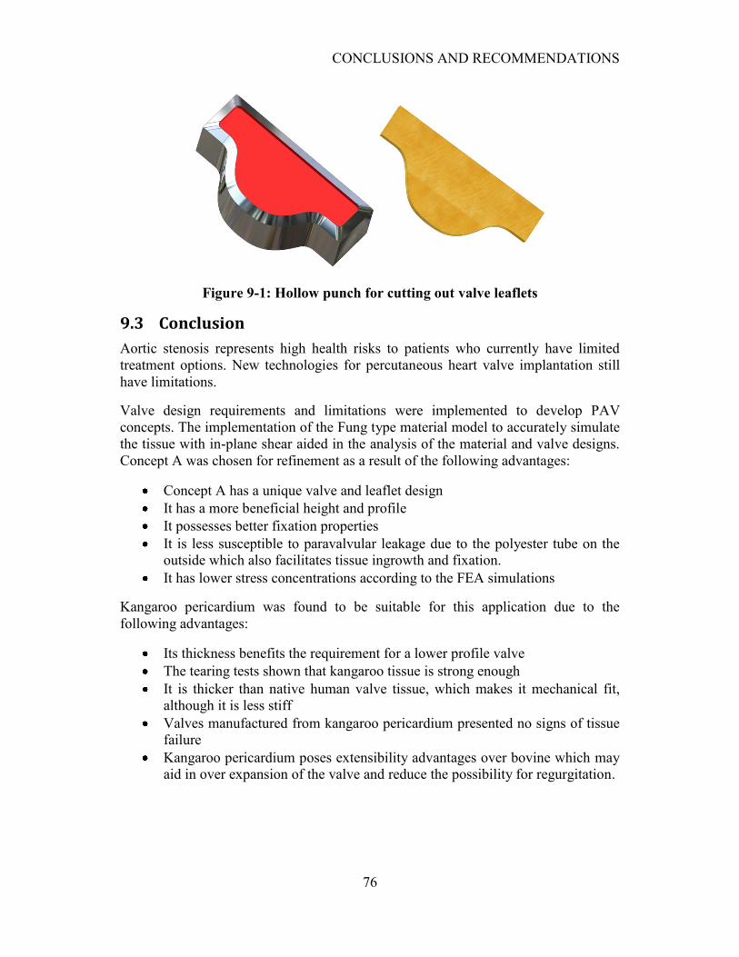
CONCLUSIONS AND RECOMMENDATIONS
76
Figure 9-1: Hollow punch for cutting out valve leaflets
9.3 Conclusion
Aortic stenosis represents high health risks to patients who currently have limited
treatment options. New technologies for percutaneous heart valve implantation still
have limitations.
Valve design requirements and limitations were implemented to develop PAV
concepts. The implementation of the Fung type material model to accurately simulate
the tissue with in-plane shear aided in the analysis of the material and valve designs.
Concept A was chosen for refinement as a result of the following advantages:
Concept A has a unique valve and leaflet design
It has a more beneficial height and profile
It possesses better fixation properties
It is less susceptible to paravalvular leakage due to the polyester tube on the
outside which also facilitates tissue ingrowth and fixation.
It has lower stress concentrations according to the FEA simulations
Kangaroo pericardium was found to be suitable for this application due to the
following advantages:
Its thickness benefits the requirement for a lower profile valve
The tearing tests shown that kangaroo tissue is strong enough
It is thicker than native human valve tissue, which makes it mechanical fit,
although it is less stiff
Valves manufactured from kangaroo pericardium presented no signs of tissue
failure
Kangaroo pericardium poses extensibility advantages over bovine which may
aid in over expansion of the valve and reduce the possibility for regurgitation.
CONCLUSIONS AND RECOMMENDATIONS
77
The preliminary pulse duplicator tests revealed no damage to the valves
manufactured from kangaroo pericardium
The numerical simulations and testing revealed the following important points:
The leaflets should preferably be cut from the same piece of tissue
The tissue fibres must be aligned in the circumferential direction of the valve
Over and under dilation of 1 mm is acceptable
A sheath may be needed to be placed over the valve during placement
Care should be taken during placement in order not to interfere with the
coronary ostia or mitral valve which again emphasizes the benefit of a lower
valve height
The developed prototypes prove to be feasible and can serve as a basis for continued
research and development.
REFERENCES
78
10. REFERENCES
Anderson, H. R., Knudsen, L. L., and Hasekam, J. M. (1992). Transluminal
implantation of artificial heart valves. Description of a new expandable aortic valve
and initial results with implantation by catheter technique in closed chest pigs.
European Heart Journal,Vol. 13(5), pp.704-708.
Arcidiacono, G., Corvi, A., and Severi, T. (2005). Functional analysis of
bioprosthetic heart valves. Journal of Biomechanics,Vol. 38, pp.1483-1490.
BARD OEM. (2008). Implantable Textiles - Tubular Fabrics. [online]. [Accessed 10
October 2008]. Available form World Wide Web:
<http://www.bardpvoem.com/pages/tubular.html>
Belytschko, T., Liu, W. K., and Moran, B. (2000). Nonlinear Finite Elements for
Continua and Structures. Chichester: Wiley.
Billiar, K. L. and Sacks, M. S. (2000). Biaxial Mechanical Properties of the Natural
and Gluteraldehyde Treated Aortic Valve Cusp - Part I: Experimental Results.
Journal of Biomechanical Engineering,Vol. 122, pp.23-30.
Billiar, K. L. and Sacks, M. S. (2000). Biaxial Mechanical Properties of the Natural
and Gluteraldehyde Treated Aortic Valve Cusp - Part II: A Structural Constitutive
Model. Journal of Biomechanical Engineering,Vol. 122, pp.327-335.
Boyer, L. (2008). Surgical Skills Laboratory. [online]. [Accessed 18 11 2008].
Available form World Wide Web: <http://www.medicine.usask.ca/surgery/surgical-
skills-lab/Suture Lab Handout>
Brounstein, K., Feygin, D., Hu, M., Koop, T., and Lee, L. (2007). Science-Based
Business Initiative Fair. [online]. [Accessed 18 11 2008]. Available form World
Wide Web: <http://www.hbs.edu/units/tom/conferences/docs/Aortic Valve Space
Station.pdf>
Burriesci, G., Howard, I. C., and Patterson, E. A. (1999). Influence of Anisotropy on
the Mechanical Behaviour of Bioprosthetic Heart Valves. Journal of Medical
Engineering,Vol. 23(6), pp.203-215.
(2008). CoreValve. [online]. [Accessed 29 September 2008]. Available form World
Wide Web: <http://www.corevalve.com/index.aspx>
Cribier, A., Eltchaninoff, H., Bash, A., Borenstein, N., Tron, C., Bauer, F.,
Derumeaux, G., Anselme, F., Laborde, F., and Leon, M. B. (2002). Percutaneous
Transcatheter Implantation of an Aortic Valve Prosthesis for Calcific Aortic Stenosis:
First Human Case Description. Circulation,Vol. 106(24), pp.3006-3008.
REFERENCES
79
Dunn, L. D. (2008). Wound Closure Manual. [online]. [Accessed 20 11 2008].
Available form World Wide Web:
<http://www.uphs.upenn.edu/surgery/dse/simulation/Wound_Closure_Manual.pdf>
(2008). Edwards Lifesciences. [online]. [Accessed 29 September 2008]. Available
form World Wide Web: <http://www.edwards.com/>
Esterhuyse, A. (2008). Structural Design and Analysis of a Stent for Implimentation
in a Percutaneous Aortic Heart Valve. Stellenbosch: University of Stellenbosch.
Fung, Y. (1993). Biomechanics: Mechanical Properties of Living Tissues. New York:
2nd ed. Springer.
García Páez, J. M., Jorge Herrero, E., Carrera Sanmartín, A., Millán, I., Cordon, A.,
Martín Maestro, M., Rocha, A., Arenaz, B., and Castillo-Olivares, J. L. (2003).
Comparison of the mechanical behaviors of biological tissues subjected to uniaxial
tensile testing: pig, calf and ostrich pericardium sutured with Gore-Tex.
Biomaterials,Vol. 24, pp.1671-1679.
GORE-TEX. (2008). GORE-TEX Suture. [online]. [Accessed 10 October 2008].
Available form World Wide Web: <http://www.goremedical.com/suture/index>
Hoffman, A. H. and Grigg, P. (1984). A method for measuring strains in soft tissue.
Journal of Biomechanics,Vol. 17(10), pp.795-800.
Holzapfel, G. A. (2000). Nonlinear solid mechanics :a continuum approach for
engineering. Chichester, West Sussex: Wiley.
International Organization for Standardization. (2005). Cardiovascular implants -
Cardiac valve prosthesis. ISO.
Johnson&Johnson. (2008). National Association of Orthopaedic Nurses (NAON).
[online]. [Accessed 20 11 2008]. Available form World Wide Web:
<http://www.orthonurse.org/portals/0/knot tying.pdf>
Kar, S. and Shah, P. K. (2006). Impact of new percutaneous techniques of aortic
valve replacement on cardiology/cardiac surgical practice. In: Transcatheter Valve
Repair, London: Taylor & Fransis, pp.139-144.
Kay, J. D. and Carroll, J. D. (2006). Hemodynamic evaluation of aortic valve disease
and indications for repair/replacement. In: Transcatheter Valve Repair, London:
Taylor & Fransis, pp.127-137.
Kim, H., Lu, J., Sacks, M. S., and Chandran, K. B. (2006). Dynamic Simulation of
Pericardial Bioprosthetic Heart Valve Function. Journal of Biomechanical
Engineering,Vol. 128, pp.717-724.
REFERENCES
80
Labrosse, M. R., Beller, C. J., Robicsek, F., and Thubrikar, M. J. (2006). Geometric
modeling of functional trileaflet aortic valves: Development and clinical applications.
Journal of Biomechanics,Vol. 39, pp.2665-2672.
Lemmon, J. D. (2006). Valve testing: Durability and beyond. In: Transcatheter Valve
Repair, London: Taylor & Fransis, pp.359-368.
Lim, K. O. and Cheong, K. C. (1994). Effect of suturing on the mechanical properties
of bovine pericardium - implications for cardiac valve bioprosthesis. Medical
engineering & physics,Vol. 16(6), pp.526-530.
MSC.Marc. (2007). Marc user manual. MSC Software.
Neethling, W. 2008. Interview with the author on 2008. E-mail correspondence.
Neethling, W., Cooper, S., van den Heever, J., Hough, J., and Hodge, A. (2002).
Evaluation of kangaroo pericardium as an alternative substitute for reconstructive
cardiac surgery. Journal of Cardiovascular Surgery,Vol. 43(3), pp.301-306.
Neethling, W. M., Glancy, R., and Hodge, A. J. (2004). ADAPT-Treated Porcine
Valve Tissue (Cusp and Wall) versus Medtronic Freestyle and Prima Plus: Crosslink
Stability and Calcification Behavior in the Subcutaneous Rat Model. The journal of
heart valve disease,Vol. 13(4).
Sacks, M. S. (2000). Biaxial Mechanical Evaluation of Planar Biological Materials.
Journal of Elasticity,Vol. 61(1-3), pp.199-246.
Sacks, M. S., Smith, D. B., and Hiester, E. D. (1998). The aortic valve
microstructure: Effects of transvalvular pressure. Journal of Biomedical Materials
Research,Vol. 41(1), pp.131-141.
Sacks, M. S. and Sun, W. (2003). Multiaxial mechanical behavior of biological
materials. Annual Review of Biomedical Engineering,Vol. 5, pp.251-284.
Shekar, P. S., Soltesz, E. G., and Cohn, L. H. (2006). Established methods of aortic
valve repair and replacement. In: Transcatheter Valve Repair, London: Taylor &
Fransis.
Smith, D. B., Sacks, M. S., Pattany, P. M., and Schroeder, R. (1999). Fatigue-induced
changes in bioprosthetic heart valve three-dimensional geometry and the relation to
tissue damage. Journal of heart valve disease,Vol. 8(1), pp.25-33.
Sun, W., Abad, A., and Sacks, M. S. (2005). Simulated Bioprosthetic Heart Valve
Deformation Under Quasi-static Loading. Journal of Biomechanical
Engineering,Vol. 127(6), pp.905-914.
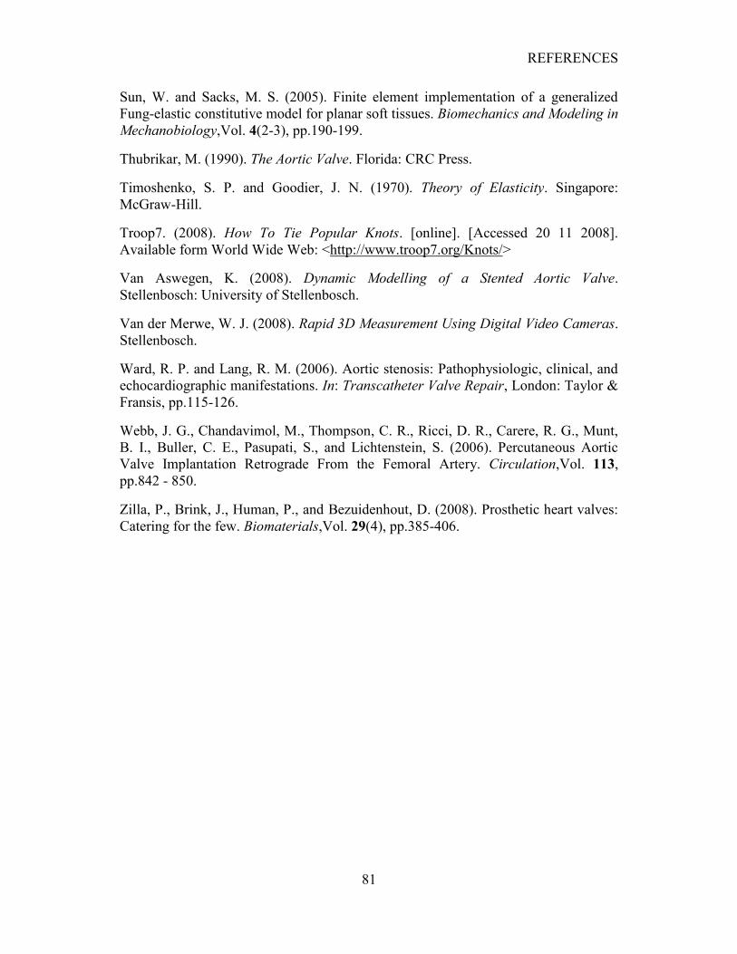
REFERENCES
81
Sun, W. and Sacks, M. S. (2005). Finite element implementation of a generalized
Fung-elastic constitutive model for planar soft tissues. Biomechanics and Modeling in
Mechanobiology,Vol. 4(2-3), pp.190-199.
Thubrikar, M. (1990). The Aortic Valve. Florida: CRC Press.
Timoshenko, S. P. and Goodier, J. N. (1970). Theory of Elasticity. Singapore:
McGraw-Hill.
Troop7. (2008). How To Tie Popular Knots. [online]. [Accessed 20 11 2008].
Available form World Wide Web: <http://www.troop7.org/Knots/>
Van Aswegen, K. (2008). Dynamic Modelling of a Stented Aortic Valve.
Stellenbosch: University of Stellenbosch.
Van der Merwe, W. J. (2008). Rapid 3D Measurement Using Digital Video Cameras.
Stellenbosch.
Ward, R. P. and Lang, R. M. (2006). Aortic stenosis: Pathophysiologic, clinical, and
echocardiographic manifestations. In: Transcatheter Valve Repair, London: Taylor &
Fransis, pp.115-126.
Webb, J. G., Chandavimol, M., Thompson, C. R., Ricci, D. R., Carere, R. G., Munt,
B. I., Buller, C. E., Pasupati, S., and Lichtenstein, S. (2006). Percutaneous Aortic
Valve Implantation Retrograde From the Femoral Artery. Circulation,Vol. 113,
pp.842 - 850.
Zilla, P., Brink, J., Human, P., and Bezuidenhout, D. (2008). Prosthetic heart valves:
Catering for the few. Biomaterials,Vol. 29(4), pp.385-406.
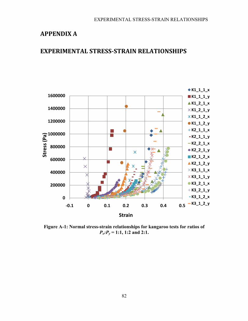
EXPERIMENTAL STRESS-STRAIN RELATIONSHIPS
82
APPENDIX A
EXPERIMENTAL STRESS-STRAIN RELATIONSHIPS
Figure A-1: Normal stress-strain relationships for kangaroo tests for ratios of
Px:Py = 1:1, 1:2 and 2:1.
0
200000
400000
600000
800000
1000000
1200000
1400000
1600000
-0.1 0 0.1 0.2 0.3 0.4 0.5
Stre
ss (
Pa)
Strain
K1_1_1_x
K1_1_1_y
K1_2_1_x
K1_2_1_y
K1_1_2_x
K1_1_2_y
K2_1_1_x
K2_1_1_y
K2_2_1_x
K2_2_1_y
K2_1_2_x
K2_1_2_y
K3_1_1_x
K3_1_1_y
K3_2_1_x
K3_2_1_y
K3_1_2_x
K3_1_2_y
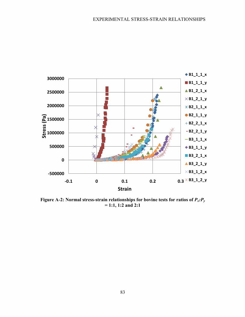
EXPERIMENTAL STRESS-STRAIN RELATIONSHIPS
83
Figure A-2: Normal stress-strain relationships for bovine tests for ratios of Px:Py
= 1:1, 1:2 and 2:1
-500000
0
500000
1000000
1500000
2000000
2500000
3000000
-0.1 0 0.1 0.2 0.3
Stre
ss (
Pa)
Strain
B1_1_1_x
B1_1_1_y
B1_2_1_x
B1_2_1_y
B2_1_1_x
B2_1_1_y
B2_2_1_x
B2_2_1_y
B3_1_1_x
B3_1_1_y
B3_2_1_x
B3_2_1_y
B3_1_2_x
B3_1_2_y
EXPERIMENTAL STRESS-STRAIN RELATIONSHIPS
84
Figure A-3: Normal stress-strain relationships for human tests for ratios of Px:Py
= 1:1, 1:2 and 2:1
0
100000
200000
300000
400000
500000
600000
700000
-0.3 -0.2 -0.1 0 0.1 0.2 0.3
Stre
ss (
Pa)
Strain
H_1_1_x
H_1_1_y
H_2_1_x
H_2_1_y
H_1_2_x
H_1_2_y
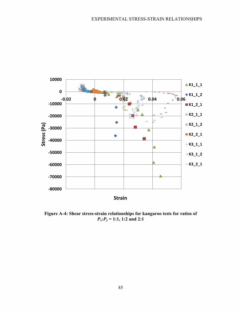
EXPERIMENTAL STRESS-STRAIN RELATIONSHIPS
85
Figure A-4: Shear stress-strain relationships for kangaroo tests for ratios of
Px:Py = 1:1, 1:2 and 2:1
-80000
-70000
-60000
-50000
-40000
-30000
-20000
-10000
0
10000
-0.02 0 0.02 0.04 0.06
Stre
ss (
Pa)
Strain
K1_1_1
K1_1_2
K1_2_1
K2_1_1
K2_1_2
K2_2_1
K3_1_1
K3_1_2
K3_2_1
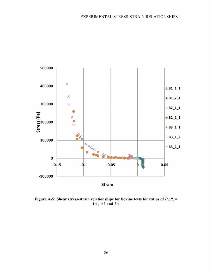
EXPERIMENTAL STRESS-STRAIN RELATIONSHIPS
86
Figure A-5: Shear stress-strain relationships for bovine tests for ratios of Px:Py =
1:1, 1:2 and 2:1
-100000
0
100000
200000
300000
400000
500000
-0.15 -0.1 -0.05 0 0.05
Stre
ss (
Pa)
Strain
B1_1_1
B1_2_1
B2_1_1
B2_2_1
B3_1_1
B3_1_2
B3_2_1
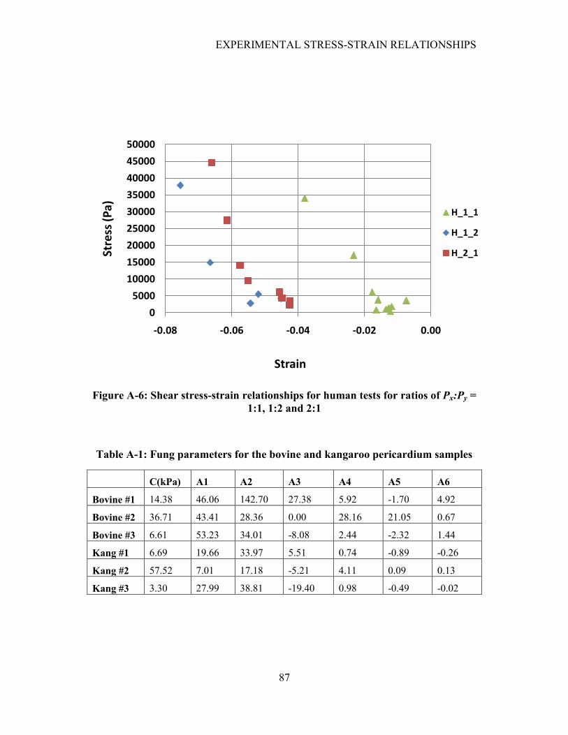
EXPERIMENTAL STRESS-STRAIN RELATIONSHIPS
87
Figure A-6: Shear stress-strain relationships for human tests for ratios of Px:Py =
1:1, 1:2 and 2:1
Table A-1: Fung parameters for the bovine and kangaroo pericardium samples
C(kPa) A1 A2 A3 A4 A5 A6
Bovine #1 14.38 46.06 142.70 27.38 5.92 -1.70 4.92
Bovine #2 36.71 43.41 28.36 0.00 28.16 21.05 0.67
Bovine #3 6.61 53.23 34.01 -8.08 2.44 -2.32 1.44
Kang #1 6.69 19.66 33.97 5.51 0.74 -0.89 -0.26
Kang #2 57.52 7.01 17.18 -5.21 4.11 0.09 0.13
Kang #3 3.30 27.99 38.81 -19.40 0.98 -0.49 -0.02
0
5000
10000
15000
20000
25000
30000
35000
40000
45000
50000
-0.08 -0.06 -0.04 -0.02 0.00
Stre
ss (
Pa)
Strain
H_1_1
H_1_2
H_2_1
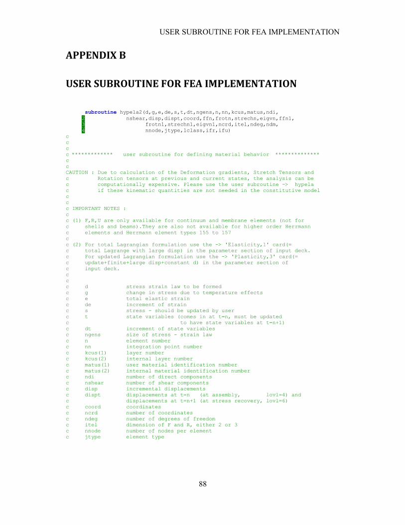
USER SUBROUTINE FOR FEA IMPLEMENTATION
88
APPENDIX B
USER SUBROUTINE FOR FEA IMPLEMENTATION
subroutine hypela2(d,g,e,de,s,t,dt,ngens,n,nn,kcus,matus,ndi,
2 nshear,disp,dispt,coord,ffn,frotn,strechn,eigvn,ffn1,
3 frotn1,strechn1,eigvn1,ncrd,itel,ndeg,ndm,
4 nnode,jtype,lclass,ifr,ifu)
c
c
c
c ************* user subroutine for defining material behavior **************
c
c
CAUTION : Due to calculation of the Deformation gradients, Stretch Tensors and
c Rotation tensors at previous and current states, the analysis can be
c computationally expensive. Please use the user subroutine -> hypela
c if these kinematic quantities are not needed in the constitutive model
c
c
c IMPORTANT NOTES :
c
c (1) F,R,U are only available for continuum and membrane elements (not for
c shells and beams).They are also not available for higher order Herrmann
c elements and Herrmann element types 155 to 157
c
c (2) For total Lagrangian formulation use the -> 'Elasticity,1' card(=
c total Lagrange with large disp) in the parameter section of input deck.
c For updated Lagrangian formulation use the -> 'Plasticity,3' card(=
c update+finite+large disp+constant d) in the parameter section of
c input deck.
c
c
c d stress strain law to be formed
c g change in stress due to temperature effects
c e total elastic strain
c de increment of strain
c s stress - should be updated by user
c t state variables (comes in at t=n, must be updated
c to have state variables at t=n+1)
c dt increment of state variables
c ngens size of stress - strain law
c n element number
c nn integration point number
c kcus(1) layer number
c kcus(2) internal layer number
c matus(1) user material identification number
c matus(2) internal material identification number
c ndi number of direct components
c nshear number of shear components
c disp incremental displacements
c dispt displacements at t=n (at assembly, lovl=4) and
c displacements at t=n+1 (at stress recovery, lovl=6)
c coord coordinates
c ncrd number of coordinates
c ndeg number of degrees of freedom
c itel dimension of F and R, either 2 or 3
c nnode number of nodes per element
c jtype element type
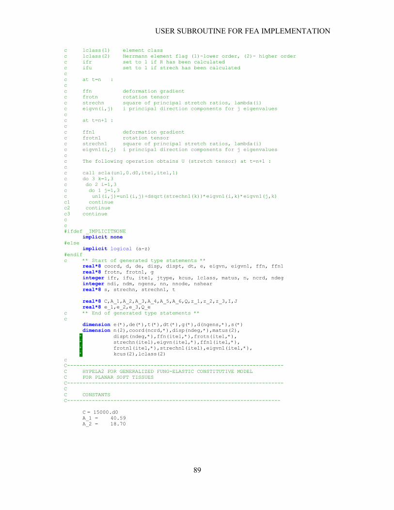
USER SUBROUTINE FOR FEA IMPLEMENTATION
89
c lclass(1) element class
c lclass(2) Herrmann element flag (1)-lower order, (2)- higher order
c ifr set to 1 if R has been calculated
c ifu set to 1 if strech has been calculated
c
c at t=n :
c
c ffn deformation gradient
c frotn rotation tensor
c strechn square of principal stretch ratios, lambda(i)
c eigvn(i,j) i principal direction components for j eigenvalues
c
c at t=n+1 :
c
c ffn1 deformation gradient
c frotn1 rotation tensor
c strechn1 square of principal stretch ratios, lambda(i)
c eigvn1(i,j) i principal direction components for j eigenvalues
c
c The following operation obtains U (stretch tensor) at t=n+1 :
c
c call scla(un1,0.d0,itel,itel,1)
c do 3 k=1,3
c do 2 i=1,3
c do 1 j=1,3
c un1(i,j)=un1(i,j)+dsqrt(strechn1(k))*eigvn1(i,k)*eigvn1(j,k)
c1 continue
c2 continue
c3 continue
c
c
#ifdef _IMPLICITNONE
implicit none
#else
implicit logical (a-z)
#endif
c ** Start of generated type statements **
real*8 coord, d, de, disp, dispt, dt, e, eigvn, eigvn1, ffn, ffn1
real*8 frotn, frotn1, g
integer ifr, ifu, itel, jtype, kcus, lclass, matus, n, ncrd, ndeg
integer ndi, ndm, ngens, nn, nnode, nshear
real*8 s, strechn, strechn1, t
real*8 C,A_1,A_2,A_3,A_4,A_5,A_6,Q,z_1,z_2,z_3,I,J
real*8 e_1,e_2,e_3,Q_e
c ** End of generated type statements **
c
dimension e(*),de(*),t(*),dt(*),g(*),d(ngens,*),s(*)
dimension n(2),coord(ncrd,*),disp(ndeg,*),matus(2),
* dispt(ndeg,*),ffn(itel,*),frotn(itel,*),
* strechn(itel),eigvn(itel,*),ffn1(itel,*),
* frotn1(itel,*),strechn1(itel),eigvn1(itel,*),
* kcus(2),lclass(2)
c
C----------------------------------------------------------------------
C HYPELA2 FOR GENERALIZED FUNG-ELASTIC CONSTITUTIVE MODEL
C FOR PLANAR SOFT TISSUES
C----------------------------------------------------------------------
C
C CONSTANTS
C---------------------------------------------------------------------
C = 15000.d0
A_1 = 40.59
A_2 = 18.70
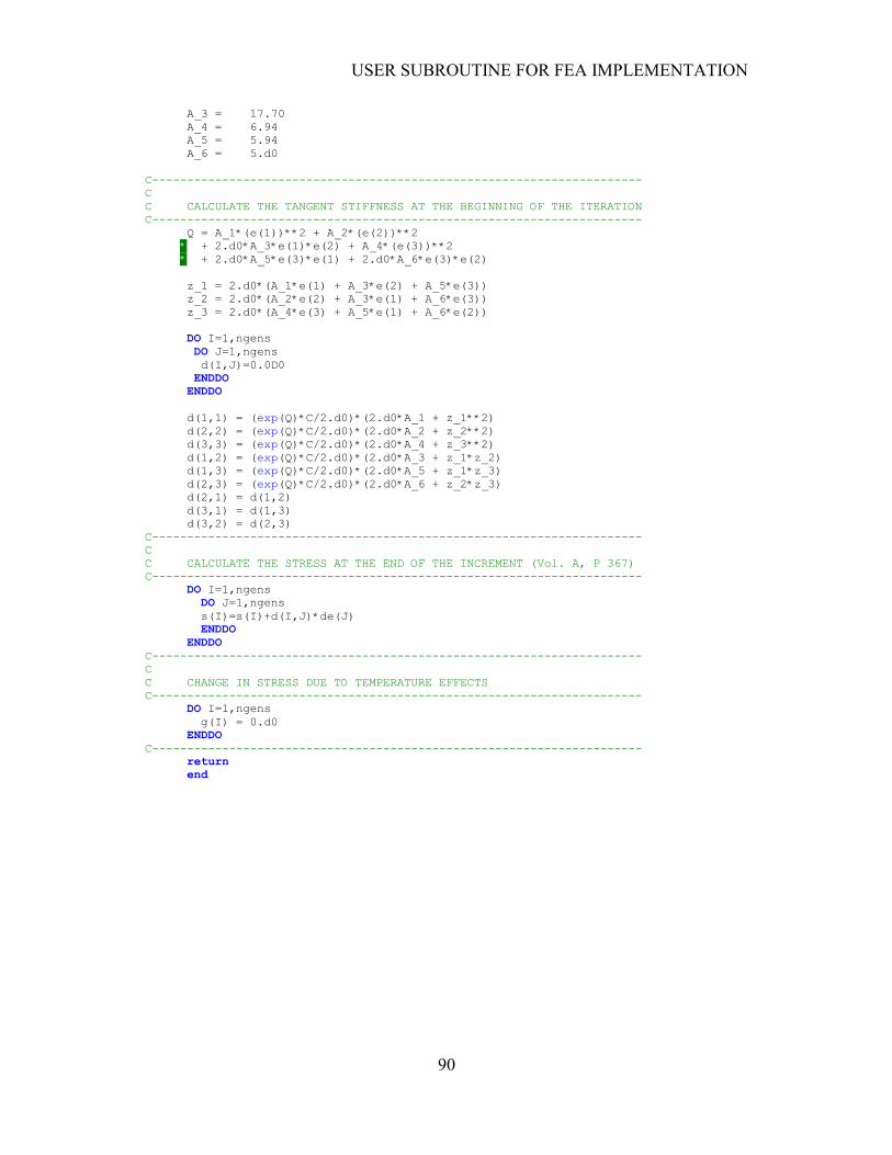
USER SUBROUTINE FOR FEA IMPLEMENTATION
90
A_3 = 17.70
A_4 = 6.94
A_5 = 5.94
A_6 = 5.d0
C----------------------------------------------------------------------
C
C CALCULATE THE TANGENT STIFFNESS AT THE BEGINNING OF THE ITERATION
C----------------------------------------------------------------------
Q = A_1*(e(1))**2 + A_2*(e(2))**2
* + 2.d0*A_3*e(1)*e(2) + A_4*(e(3))**2
* + 2.d0*A_5*e(3)*e(1) + 2.d0*A_6*e(3)*e(2)
z_1 = 2.d0*(A_1*e(1) + A_3*e(2) + A_5*e(3))
z_2 = 2.d0*(A_2*e(2) + A_3*e(1) + A_6*e(3))
z_3 = 2.d0*(A_4*e(3) + A_5*e(1) + A_6*e(2))
DO I=1,ngens
DO J=1,ngens
d(I,J)=0.0D0
ENDDO
ENDDO
d(1,1) = (exp(Q)*C/2.d0)*(2.d0*A_1 + z_1**2)
d(2,2) = (exp(Q)*C/2.d0)*(2.d0*A_2 + z_2**2)
d(3,3) = (exp(Q)*C/2.d0)*(2.d0*A_4 + z_3**2)
d(1,2) = (exp(Q)*C/2.d0)*(2.d0*A_3 + z_1*z_2)
d(1,3) = (exp(Q)*C/2.d0)*(2.d0*A_5 + z_1*z_3)
d(2,3) = (exp(Q)*C/2.d0)*(2.d0*A_6 + z_2*z_3)
d(2,1) = d(1,2)
d(3,1) = d(1,3)
d(3,2) = d(2,3)
C----------------------------------------------------------------------
C
C CALCULATE THE STRESS AT THE END OF THE INCREMENT (Vol. A, P 367)
C----------------------------------------------------------------------
DO I=1,ngens
DO J=1,ngens
s(I)=s(I)+d(I,J)*de(J)
ENDDO
ENDDO
C----------------------------------------------------------------------
C
C CHANGE IN STRESS DUE TO TEMPERATURE EFFECTS
C----------------------------------------------------------------------
DO I=1,ngens
g(I) = 0.d0
ENDDO
C----------------------------------------------------------------------
return
end