Embed Size (px)
Citation preview

Design of ultra-thin shell structures in the stochasticpost-buckling range using Bayesian machine learning and
optimization
M.A. Bessaa, S. Pellegrinoa,∗
aGraduate Aerospace Laboratories, California Institute of Technology, 1200 East CaliforniaBoulevard, Pasadena, CA 91125, USA
Abstract
A data-driven computational framework combining Bayesian machine learn-
ing for imperfection-sensitive quantities of interest, uncertainty quantification
and multi-objective optimization is developed for the analysis and design of
structures. The framework is used to design ultra-thin carbon fiber deployable
shells subjected to two bending conditions. Significant increases in the ultimate
buckling loads are shown to be possible, with potential gains on the order of
100% as compared to a previously proposed design. The key to this result is the
existence of a large load reserve capability after the initial bifurcation point and
well into the post-buckling range that can be effectively explored by the data-
driven approach. The computational strategy here presented is general and can
be applied to different problems in structural and materials design, with the
potential of finding relevant designs within high-dimensional spaces.
Keywords: ultra-thin composite structures, buckling, post-buckling, design
charts, data mining, heteroscedastic Gaussian process, evolutionary
optimization
∗Corresponding authorEmail address: [email protected] (S. Pellegrino)
Preprint submitted to Elsevier August 3, 2017

1. Introduction1
The recent resurgence of interest in buckling of slender structures (Hu and2
Burgueño, 2015; Reis, 2015) can be largely explained by the advent of new3
manufacturing techniques (Kalpakjian et al., 2014) for complex shapes, as well4
as improved modeling capabilities (Benson et al., 2010; Bai et al., 2015) that5
leverage the extensive theoretical understanding of buckling (Hutchinson and6
Koiter, 1970; Bažant and Cedolin, 2010). These developments have spawned7
a myriad of creative solutions for a wide range of applications such as energy8
harvesters (Chen et al., 2010; Wang et al., 2014), sensors (Elvin et al., 2006;9
Kiyono et al., 2012), dampers and absorbers (Dong and Lakes, 2013; Kim et al.,10
2013), actuators (Loukaides et al., 2014; Lazarus and Reis, 2015), morphing11
structures (Diaconu et al., 2008; Daynes et al., 2014), and deployable structures12
(Pellegrino, 2014; Mallikarachchi and Pellegrino, 2014), all of which exploit the13
geometrically non-linear behavior of thin shell structures.14
These structures are designed to capture the benefits of the first bifurcation15
point (initial buckling). In these cases, post-buckling is mostly viewed as a16
sudden behavior that leads to large configuration changes, often occurring as17
a form of snap-through or to a lesser extent snap-back. Hence, post-buckling18
behavior and subsequent bifurcations are not usually a design target (Hu and19
Burgueño, 2015).20
However, there are structures where the post-buckling behavior assumes21
particular importance. Thin-walled structures provide some of the most rel-22
evant examples, as can be seen in studies showing the effects of cutouts in23
composite shells (Tafreshi, 2002) or of nonuniform wall thickness in steel shells24
(Aghajari et al., 2006), as well as investigations on functionally graded carbon25
nanotube-reinforced shells undergoing thermal post-buckling (Shen, 2012) and26
functionally graded shallow plates (Woo et al., 2005). Recently, Leclerc et al.27
(2017) noted that an ultra-thin composite Triangular Rollable And Collapsible28
(TRAC) boom is able to carry significantly increased loads well into the post-29
buckling regime. The article here presented focuses on designing TRAC booms30
2

to improve their buckling and post-buckling behavior through a data-driven31
computational framework.32
In data-driven approaches (Bisagni and Lanzi, 2002; Yvonnet and He, 2007;33
Ning and Pellegrino, 2015; Bessa et al., 2017) a new model or design is found34
by collecting enough data about the response of the structure or material under35
multiple input conditions. In principle, data can be collected by experimental36
testing, analytical or computational predictions. Yet, in most engineering appli-37
cations experimental characterization of previously untested designs is too time-38
consuming to gather enough data in a timely manner, and most applications39
are too complex to be predicted by probabilistic analytical models (Elishakoff,40
2014). Hence, computational predictions are often the only viable resource to41
explore the design space and generate enough data to use machine learning42
and/or optimization.43
Multiple authors have been exploring the use of data-driven approaches for44
different scientific and engineering applications. Notable examples exist in com-45
puter science with artificial intelligence algorithms that master the game of GO46
(Silver et al., 2016), materials science with data mining of first principle calcula-47
tions leading to discoveries of new material compounds (Curtarolo et al., 2003;48
Fischer et al., 2006; Saal et al., 2013; Gautier et al., 2015), fluid mechanics in49
the characterization of flows with high Reynolds numbers (Ling and Temple-50
ton, 2015), and different solid mechanics applications (Bisagni and Lanzi, 2002;51
Yvonnet and He, 2007; Bessa et al., 2017).52
This article extends a recently developed data-driven framework for mate-53
rials and structures (Bessa et al., 2017) to the design of optimized structures54
with uncertain response. The proposed approach is illustrated for the design of55
TRAC booms, in order to increase their ultimate buckling limit, but it can be56
applied to any other structure or material. The extended framework includes57
two significant contributions: 1) machine learning for noisy observations with58
uncertainty quantification; and 2) introducing a multi-objective optimization59
step after the machine learning procedure to determine optimal designs. The60
first extension is crucial for the design and analysis of imperfection-sensitive61
3

structures (with noisy or uncertain response). The second extension is relevant62
when the goal is not just establishing the relationship between input design63
descriptors and output performance of the structure (or material), but also to64
find the set of input descriptors that leads to an optimal response within given65
constraints.66
The paper is laid out as follows. Section 2 presents the ultra-thin composite67
TRAC boom structure to which the data-driven framework is applied. Section68
3 discusses the data-driven framework for noiseless applications in 3.1, and for69
noisy applications with multi-objective optimization goals in 3.2. Concluding70
remarks are included in Section 4. Details on the structural imperfections of71
TRAC booms are provided in Appendix A, and a discussion of discontinuous72
Pareto frontiers is given in Appendix B.73
2. Behavior of ultra-thin TRAC booms74
Figure 1 shows a schematic of a TRAC boom, partially wrapped on a spool.75
This type of structure was initially developed by Murphey and Banik (2011)76
and can be viewed as two tape springs bonded along one edge and thus forming77
a flat region (web) with twice the thickness of the flanges. In the packaged78
configuration, the TRAC boom is flattened (flat cross-section) and wrapped79
around a spool of radius R. The deployed geometry is then fully characterized80
by the TRAC boom length L and its cross-section parameters: web height h81
(thickness 2t), flange radius r, angle θ, and thickness t.82
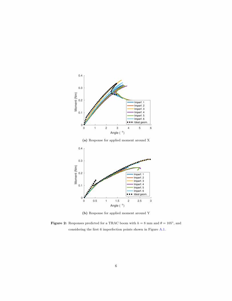
Figure 2 shows the predictions obtained from nonlinear finite element anal-83
yses using the arc length method to determine the post-buckling response of84
an ultra-thin composite TRAC boom manufactured by Leclerc et al. (2017).85
The structure was subjected to two separate boundary conditions: (a) bending86
moment around X leading to compression at the outer edge of the web; and87
(b) bending moment around Y. The same nominal geometric parameters re-88
ported by Leclerc et al. (2017) are used herein: total length L = 504 mm, and89
cross-section parameters r = 10.6 mm, θ = 105o, and h = 8 mm. The material90
4

h
t
r
𝜃𝜃
R
Y
Z X
Figure 1: Schematic of the TRAC boom architecture (modified from Murphey and
Banik (2011)).
is a composite laminate with stacking sequence [0o, 90o]S and nominal post-91
cure thickness of t = 71 µm, where the four composite plies are stacked from a92
17GSM unidirectional tape supplied by North Thin Ply Technology (T800 fibers93
and ThinPreg 120EPHTg-402 epoxy resin). The orthotropic elastic properties94
of each ply are considered as E1 = 128.0 GPa, E2 = 6.5 GPa, ν12 = 0.35,95
G12 = G13 = G23 = 7.5 GPa.96
The dashed lines in Figure 2 show the responses predicted for the idealized97
geometry, where a negligibly small imperfection based on the first buckling mode98
was seeded to numerically resolve the first bifurcation point. Details about the99
six imperfect cases shown in the figure are discussed later in Appendix A. The100
focus at this point should be on noting that due to the ultra-thin nature of101
the structure the first bifurcation point occurs prematurely for both loading102
conditions, but is followed by a further, significant increase in the applied mo-103
ment until the ultimate buckling limit of the structure is reached. Here the104
ultimate buckling limit is defined as the analytical maximum in the moment-105
angle response of the structure. Due to the complexity and stochasticity of the106
buckling and post-buckling behavior of the TRAC boom, the particular geom-107
etry considered in Figure 2 is likely not optimal for given quantities of interest,108
e.g. maximizing both buckling limits. Since closed form solutions to find such109
optimal geometries do not exist, the viable alternative is to use a data-driven110
approach applicable to stochastic responses.111
5
0 1 2 3 4 5 6
Angle (o)
0
0.1
0.2
0.3
0.4M
om
ent (N
m)
Imperf. 1
Imperf. 2
Imperf. 3
Imperf. 4
Imperf. 5
Imperf. 6
Ideal geom.
(a) Response for applied moment around X
0 0.5 1 1.5 2 2.5 3
Angle (o)
0
0.1
0.2
0.3
0.4
Mom
ent (N
m)
Imperf. 1
Imperf. 2
Imperf. 3
Imperf. 4
Imperf. 5
Imperf. 6
Ideal geom.
(b) Response for applied moment around Y
Figure 2: Responses predicted for a TRAC boom with h = 8 mm and θ = 105o, and
considering the first 6 imperfection points shown in Figure A.1.
6

3. Data-driven computational framework112
The data-driven framework conjugates the following steps: 1) Design of113
Experiments1 (DoE); 2) computational analyses; 3) machine learning; and 4)114
multi-objective optimization. The following subsections discuss the application115
of the framework to the design of TRAC booms, for two different cases. A sim-116
plified case where the machine learning process does not need to be probabilistic,117
and where the obtained design charts may be easily interpreted without an op-118
timization step. This case represents an application of the previously developed119
framework (Bessa et al., 2017) without the proposed extensions. The other case120
illustrates the need for a Bayesian machine learning process including uncer-121
tainty quantification, as well as the advantage of introducing an optimization122
step to find particular designs after machine learning. Each step is summa-123
rized in Figure 3 and explained in the following sections for each of the above124
mentioned cases.125
3.1. A design case without uncertainty nor optimization: initial buckling of ide-126
alized TRAC booms127
This first case focuses on finding the combination of cross-sectional param-128
eters h and θ that maximize the initial buckling moments of the TRAC boom129
considering idealized geometries, i.e. without imperfections. For this first ex-130
ample only the first bifurcation point occuring at the end of the linear elastic131
regime is of interest – recall Figure 2 and observe the first kink in the dashed132
line for each boundary condition applied.133
In this investigation the length L = 504mm and thickness t = 71 µm are kept134
constant, and the same composite material described previously with stacking135
sequence [0o, 90o]S is considered. The volume (mass) of the structure is also kept136
1The term “Design of Experiments” (DoE) is extensively used in the literature (Morris and
Mitchell, 1995) and refers to finding an optimal sampling of the design space without a priori
knowledge of the regions of interest. Note that “experiments” does not only refer to physical
experiments but also to “computational experiments”.
7

2. Computational Analyses Design Samples
Response Database
New Model
New DesignIxE computer simulations
Predict quantities of interest (QoI) via an appropriate analysis method
IxE sampling points
Predict QoI
Influence of design on response
Refine sampling
DoE point j
Discrete Input
point 1
Discrete Input point I
3. Machine Learning 4. Optimization
Optimum design for specific application
1. InputsI (=2) Discrete Input points Design of Experiments (DoE) with E points
Each point samples a set of continuous variables.Example:• Geometric parameters
Each point includes a set of discrete variables.Example:• Point 1: Loading condition 1• Point 2: Loading condition 2
Point E:(h=8mm, θ=20o)
Point 1:(h=6mm, θ=190o)
0.2 0.4QoI 1
0.25
0.50
0.75
1.00
QoI
2
Figure 3: Data-driven framework applied to structural modeling and design (modi-
fied from Bessa et al. (2017)).
constant for all TRAC booms, in order to establish a fair comparison between137
different geometries. This volume constraint introduces a relationship between138
the radius of the flanges r and the two independent parameters considered in139
this study, h and θ:140
r =V − 2thL
2θtL(1)
with V ≈ 1963 mm3, t = 71 µm, and L = 504 mm, while the two design141
descriptors θ (in radians, above) and h assume different values for different142
cross-sections.143
An additional constraint is introduced due to the need of flattening the boom144
8
for packaging. This causes a transverse strain εflat (Murphey et al., 2017):145
εflat =t
2r(2)
that typically needs to be below 1% to avoid failure of the composite material.146
The strain caused by wrapping the flattened structure around a spool could147
also be included as a constraint, but this strain is usually not the limiting factor148
since the radius of the spool R used to wrap the boom is large.149
The first step (DoE) in the data-driven framework is the sampling of the150
design space without a priori knowledge of the relationship between the input151
variables and the output quantities of interest. Different methods can be used152
for the DoE, with two common options being the Sobol sequence (Sobol, 1967,153
1976) and the Latin Hypercube sampling (McKay et al., 1979). According to154
previous investigations (Bessa et al., 2017), the Sobol sequence is used herein.155
For this study the bounds for the input design variables h and θ are defined as:156
h = [2, 16] mm , θ = [10o, 315o] (3)
The Sobol sequence DoE method produces a nonuniform space-filling design157
where different hyperplane projections do not lead to coincident points – prop-158
erties that have been shown to facilitate the machine learning process (Simpson159
et al., 2001). Figure 4 presents the 1, 000 DoE points obtained from a random160
Sobol sequence of the two design descriptors.161
The subsequent step in the data-driven framework after the DoE is the com-162
putational analysis of each DoE point. Note that variations in the geometry163
of the structure are expected to lead to competing effects for the two bound-164
ary conditions applied. For example adding/removing material in the web has165
significant impact on the bending stiffness and buckling of the structure for166
bending around X, but less impact for bending around Y because the web is in167
the neutral plane in this case. However, this influence is less intuitive when con-168
sidering structures with constant volume, because the material that is added169
in the web needs to be respectively removed in the flanges, which alters the170
9

50 100 150 200 250 300
θ (degree)
2
4
6
8
10
12
14
16
h (
m)
1
2
3
4
5
6
7
89
10
11
12
13
14
15
16
17
18
19
20
Figure 4: Design of Experiments to determine the influence of the TRAC boom ge-
ometries on the initial buckling behavior of the ultra-thin composite struc-
ture. The solid red circles correspond to the first 20 points of the Sobol
sequence and are labeled with the corresponding sequence number. The
black dots correspond to the remaining 880 points, and the last 100 points
are shown as blue circumferential markers.
bending stiffness and local curvature of the structure. Recall that the actual171
influence of r, θ and h is not trivial to predict analytically due to the fact that172
the structures are ultra-thin, leading to highly localized buckling modes instead173
of global modes.174
The following procedure is automated for computationally predicting the175
first bifurcation point of the structures:176
1. Linear bifurcation analysis of the undeformed configuration of the struc-177
ture. This provides an initial prediction for the first bifurcation point and178
buckling modes;179
2. Static analysis under displacement control without stabilization until the180
simulation stops or the previously determined bifurcation point is reached;181
3. Sequential linear bifurcation analyses starting from the last available in-182
crement of the static analysis until reaching an increment where the bi-183
10

furcation point can be predicted, i.e. an increment where the structure is184
not on the post-buckling regime but where it is close to the bifurcation185
point.186
The outlined procedure was implemented such that it could be performed187
automatically and in parallel for different input DoE points. The output quan-188
tities of interest obtained from the simulations, e.g. moments and angles at the189
two ends, are stored in a database that is then used for the machine learning190
process.191
The machine learning process for this subsection is simplified because the192
quantities of interest have negligible noise (no geometric imperfections). In193
this article small databases are appropriate for all the applications considered,194
favoring the use of the Gaussian process method (Krige, 1951; Matheron, 1963)195
as opposed to methods such as artificial neural networks (Rosenblatt, 1958;196
Widrow and Hoff, 1960; Hopfield, 1982; Rumelhart et al., 1986). This was197
shown in (Bessa et al., 2017) with a comparison of the data-driven framework198
for higher dimensional design spaces using both Gaussian process (also known as199
kriging) and neural networks. Gaussian process regression is discussed in detail200
in Section 3.2.1 where the less common case of noisy observations is included.201
The interested reader can consult the work of Rasmussen and Williams (2005)202
for additional details. If interested in artificial neural networks, the reader is203
referred to Demuth et al. (2014).204
Construction of design charts for the quantities of interest is then a trivial205
outcome of the machine learning process. Figure 5 shows the variation of the206
first bifurcation point of the perfect structures with different cross-sections. The207
figure also includes contour lines of the bending stiffness, radius of the flanges,208
and the transverse strain εflat caused by flattening the structure for packaging –209
see equation (2). The score based on the mean squared error of the predictions210
of the last 100 points of the Sobol sequence (see Figure 4) is evidently very211
high (above 0.99) because this is a simple regression problem (low-dimensional),212
unlike previously considered cases (Bessa et al., 2017). In fact, the score is still213
11

100 200 300
θ (o)
2
4
6
8
10
12
14
16
h (
mm
)
4
4
6
6
6
8
8
8
10
10
12
12
14
14
16
16
0.0
02
0.0
04
0.0
06
0.0080.01
0.0123
3
5
5
58
8
813
13
13
21
21
21
34
34
34
55
55
55
89
89
Buckling Moment X (Nm)Bending Stiffness X (Nm2)Flattening strain (m/m)r (mm)
0.05
0.1
0.15
0.2
0.25
0.3
(a) Initial buckling moment in X
100 200 300
θ (o)
2
4
6
8
10
12
14
16
h (
mm
)
55
5 10
10
10
15
15 20
0.0
02
0.0
04
0.0
06
0.0080.01
0.0123
3
5
5
58
8
813
13
13
21
21
21
34
34
34
55
55
55
89
89
Buckling Moment Y (Nm)Bending Stiffness Y (Nm2)Flattening strain (m/m)r (mm)
0
0.1
0.2
0.3
0.4
0.5
0.6
0.7
(b) Initial buckling moment in Y
Figure 5: Design charts obtained for the variation of the initial buckling moments in
X and Y as a function of two cross-section parameters (h and θ).
12

above 0.98 when considering 300 DoE points for the learning task instead of214
900.215
Observing Figure 5 one can identify that the maximum buckling moment216
does not occur for regions with maximum bending stiffness for both boundary217
conditions. This behavior occurs due to the presence of local buckling modes.218
From the figure it is also clear that constraining the flattening strain below 1%219
does not significantly limit the design space. Interestingly, there is a common220
region of the design space that maximizes the initial buckling moment for both221
loading conditions at large flange angles and small web heights, despite the222
bending stiffness along X being low at that region.223
Figure 6 shows the buckling modes corresponding to 4 DoE points shown224
in Figure 4. Focusing first on the modes obtained by bending the structures225
around the X axis (top row of the figure), one can see that DoE point 9 (Figure226
6b), and DoE point 14 (Figure 6c) show localized buckling modes, as opposed to227
the more global modes seen around the top of the web for the other geometries.228
The buckling behavior is improved in point 9 by localizing the deformation at229
the ends of the structure, while for point 14 it is improved by localizing it in the230
center after a more compliant behavior in this bending condition. Focusing now231
on the modes obtained by bending the structure around the Y axis (bottom row232
of the figure), one can see that only point 14 (Figure 6g) shows the localization233
of deformation at the ends of the structure, justifying the fact that only this234
geometry is in the region of the design chart with a higher buckling moment in235
Y. Therefore, DoE point 14 corresponds to the best design of the 4 geometries236
shown in Figure 6, and is within the optimal region found in the design charts.237
In general, one can conclude that designs with large flange angles and small238
web heights are the most effective when aiming to increase both initial buckling239
loads for constant mass of the structure. If the design goal is different, then the240
design charts can be used to optimize the structure for other applications, e.g.241
maximum bending stiffness achieved for a desired minimum buckling strength.242
13

(a) DoE point 1
for bending
around X
(b) DoE point 9
for bending
around X
(c) DoE point 14
for bending
around X
(d) DoE point 19
for bending
around X
(e) DoE point 1
for bending
around Y
(f) DoE point 9
for bending
around Y
(g) DoE point 14
for bending
around Y
(h) DoE point 19
for bending
around Y
Figure 6: First buckling mode observed for different geometries subjected to two
loading conditions: bending around X (top row); and bending around Y
(bottom row). From left to right the geometries shown correspond to DoE
points 1, 9, 14 and 19 shown in Figure 4. The modes are scaled such that
the maximum displacement component is 5 mm for all cases.
14

3.2. A design case with uncertainty and optimization: imperfection-sensitive243
TRAC boom ultimate buckling244
The previous approach of designing idealized structures for maximizing the245
first bifurcation point included three important simplifications: 1) each compu-246
tational analysis was relatively inexpensive, allowing the generation of a suffi-247
ciently large database; 2) the observations were noiseless, facilitating the ma-248
chine learning process; and 3) there was no need for including an optimization249
algorithm after the machine learning process due to the low-dimensionality of250
the problem and the obvious position of the optimum in the design charts.251
Nonetheless, there are problems where these simplifications are not possible.252
This subsection discusses the design of imperfect ultra-thin TRAC booms tar-253
geting improved ultimate buckling moments for the two loading conditions con-254
sidered above.255
Ultimate buckling of ultra-thin carbon fiber TRAC booms occurs after post-256
buckling, as shown in Figure 2. The computational analyses required in this257
case have a higher computational cost (each simulation requires approximately258
4 CPU-hours). This limits the exploration of the design space – see Remark 1.259
Remark 1. Data-driven approaches are limited by the generation of a suffi-260
ciently large database through efficient computational analyses – Box 2 in Figure261
3. Most engineering applications require costly computational analyses to gener-262
ate each data point. Therefore, new reduced order models (Ladevèze et al., 2010;263
Chinesta et al., 2011; Liu et al., 2016) that efficiently and accurately simulate264
such applications are one of the most critical needs in data-driven approaches265
for new designs. However, nonlinear buckling and post-buckling phenomena are266
yet to be demonstrated to be efficiently and accurately predicted by a reduced267
order model, to the authors’ knowledge.268
An additional challenge to apply the data-driven framework is in dealing269
with uncertainty, i.e. when the quantities of interest are stochastic such as270
imperfection-sensitive phenomena. Post-buckling and subsequent ultimate buck-271
ling of a structure are often strongly dependent on the presence of imperfections.272
15

This is visible in Figure 2. Furthermore, the imperfection-sensitivity is not usu-273
ally the same for different geometries of the structure. Therefore, characterizing274
the uncertainty for the entire design space involves answering a two-part ques-275
tion: what imperfections and how many imperfect samples per DoE point should276
be considered?277
In particular to the ultra-thin composite TRAC booms considered herein,278
there is currently not enough experimental evidence to devise a strategy to model279
realistic imperfections – see Remark 2. The adopted strategy is then to seed280
geometric imperfections in the form of combinations of buckling modes obtained281
from linear perturbation analysis of the first bifurcation point. This strategy282
has been successfully used by different authors, e.g. Riks (1979); Bisagni (2000);283
Ning and Pellegrino (2015).284
Remark 2. Modeling geometric imperfections can be performed with higher-285
fidelity for problems with additional experimental information. For these cases,286
imperfections can be modeled directly from three-dimensional scans of the geom-287
etry or by finding combinations of frequency and buckling modes until the local288
imperfections are statistically equivalent to the scanned geometries.289
The number of buckling modes used to seed imperfections is estimated by290
the proximity of the first eigenvalues determined from the nonlinear buckling291
analyses of the previous section. The first two eigenvalues were found to be292
similar for a large number of TRAC boom designs, hence the first two buckling293
modes were chosen to seed the imperfections. An estimation of the amplitudes294
of these modes can be extracted from a preliminary experimental investigation295
(Leclerc et al., 2017) of various specimens of a single ultra-thin TRAC boom296
design, reporting deviations from the idealized structure as large as 2 mm with297
clear localized kinks. The amplitude bounds for the first two buckling modes298
were then considered as:299
λ1 = [−30t, 30t] , λ2 = [−30t, 30t] (4)
where t = 71 µm, as previously referred.300
16

Specific details of the approach used to quantify the uncertainty of each301
TRAC boom design are included in Appendix A. Based on the initial design302
considered in Figure 2 it was determined that the first 20 imperfection sam-303
pling points highlighted in Figure A.1 would provide a reasonable estimate for304
the uncertainty of each design point. This means that the same combination of305
buckling mode amplitudes were used to generate 20 imperfect TRAC booms per306
nominal design. This does not mean that the same geometric imperfections are307
being seeded because each nominal geometry of the TRAC boom has different308
first and second buckling modes, as seen in the previous section. The statisti-309
cal distribution of the quantities of interest (ultimate buckling moments) was310
approximated as Gaussian – see Appendix A. Hence, the two metrics needed to311
approximate the distribution at each design point are the mean and standard312
deviation of the ultimate buckling moments computed from the 20 imperfect313
TRAC booms for each nominal design.314
Including uncertainty quantification for this example increases 20 times the315
number of simulations needed to subsequently perform the machine learning316
process. Also, each analysis of the post-buckling and ultimate buckling of these317
structures has a considerably higher computational cost when compared to the318
analyses used to determine the first bifurcation points, as referred previously.319
Thus, the bounds of the DoE were shrunk to:320
h = [2, 6] mm , θ = [10o, 315o] (5)
so that the number of DoE points could be reduced to 150, while keeping a321
similar density of points in the same region of the design space that led to a322
good approximation of the response in the previous example. The same method323
was used to perform the DoE as in Figure 4, so no additional figure is shown324
here.325
The database with the quantities of interest is created by conducting the326
respective computational analyses, which consist of the finite element solution327
of an arc length method using a commercial finite element software. A total328
17

of 6000 computational analyses were conducted (2 boundary conditions, and 20329
imperfect TRAC booms for each of the 150 DoE points defining the different330
nominal designs). This corresponds to approximately 3 weeks of continuous331
computations in a computer cluster using 48 CPUs on average.332
Subsequently, the machine learning process for these noisy observations is333
required to establish the relationship between the uncertain ultimate buckling334
moment and the input variables defining the nominal geometry of the TRAC335
booms. The specific method used in this article is the Gaussian process regres-336
sion, as alluded in the previous section and detailed next.337
3.2.1. Gaussian process regression with heteroscedastic noise338
Contrary to the noiseless cases discussed in previous illustrations of the data-339
driven framework – see Section 3.1 and previous materials design examples340
(Bessa et al., 2017) – the ultimate buckling moments of the TRAC booms are341
strongly imperfection-sensitive, as seen in Figure 2 and in Appendix A. More-342
over, different nominal designs of TRAC booms are expected to have different343
imperfection sensitivity, as widely reported in the buckling literature, e.g. Ning344
and Pellegrino (2015). In statistics this phenomenon is called heteroscedasticity345
(Goldberg et al., 1998), i.e. input-dependent noise (variance).346
When possible, considering noiseless cases or at least considering indepen-347
dent and identically distributed (i.i.d.) Gaussian noise with constant variance348
is attractive. In these cases the Gaussian process regression has fast implemen-349
tations because the likelihood and marginal likelihood can be integrated ana-350
lytically (Rasmussen and Williams, 2005). However, a general treatment where351
noise is allowed to be heteroscedastic (input-dependent) and/or non-Gaussian352
requires numerical integration of the likelihood and marginal likelihood.353
Gaussian process regression (GPR) with heteroscedasticity was first dis-354
cussed by Goldberg et al. (Goldberg et al., 1998), while GPR with non-Gaussian355
noise was introduced by Neal (1997). Both articles considered a fully Bayesian356
framework using Markov chain Monte Carlo to perform the integration of the357
likelihood and the marginal likelihood. Unfortunately, this approach is computa-358
18

tionally demanding, so alternative solutions have been proposed (Snelson et al.,359
2004; Kersting et al., 2007; Titsias and Lázaro-Gredilla, 2011). Snelson et al.360
(2004) proposed a warping scheme for Gaussian processes, Kersting et al. (2007)361
considered the most likely value using a maximum a posteriori (MAP) approach,362
while Titsias and Lázaro-Gredilla (2011) presented a variational approach with363
only twice the computational expense of a standard Gaussian process.364
Here the implementation provided by Pedregosa et al. (2011) is followed,365
where noise is assumed to be i.i.d. Gaussian but allowed to be heteroscedastic.366
The Gaussian assumption has implications illustrated in Figure A.3 for the367
TRAC boom design problem, since the statistical distribution for the ultimate368
buckling moment around X is not Gaussian if using the Sobol sequence to seed369
imperfections. However, considering the current lack of experimental data for370
this problem and the reported computational limitations arising from the non-371
Gaussian noise treatment, this simplifying assumption is considered henceforth.372
The previously determined database with NDoE = 150 DoE points is given373
by:374
{(x(1),q(1)), ..., (x(I),q(I)), ... , (x(NDoE),q(NDoE))} (6)
or in index notation,375
{(x(1)j , q(1)i ), ..., (x
(I)j , q
(I)i ), ... , (x
(NDoE)j , q
(NDoE)i )} for j = 1, ..., din and i = 1, ..., dout
(7)
where dout corresponds to the number of output quantities of interest q, and din376
is the number of input design variables x. In the TRAC boom design example377
there are din = 2 inputs x1 ≡ θ and x2 ≡ h, and dout = 2 outputs q1 ≡MfX and378
q2 ≡MfY corresponding to the ultimate buckling moments obtained for applied379
bending around X and Y, respectively.380
Separate Gaussian processes will be used for each output. This way, the381
notation can be simplified by dropping the index in qi because q can be sepa-382
rately associated to quantity q1 or q2. In the heteroscedastic Gaussian process383
19

considered here the noisy observations are approximated as,384
q(I) = f [x(I)] + ε(I) (8)
where f [x(I)] is the unknown function value at x(I) to be approximated by the385
Gaussian process, and ε(I) is the additive i.i.d. Gaussian noise with standard386
deviation σ(I)ε that also depends on the input point x(I).387
The Gaussian process establishes its foundations by defining a prior that388
depends on the proximity of the data points weighted by a kernel function k389
with noise added to its diagonal,390
cov[q(I), q(J)] = k[x(I),x(J)] +(σ(I)ε
)2δIJ (9)
that can be arranged as a sum of two matrices,391
cov[q] = K + R (10)
where K is called the kernel matrix or covariance matrix with element (I, J)392
as KIJ = k[x(I),x(J)], and R is the diagonal noise matrix with each term393
including the variance of the quantity of interest q at the respective input point.394
This representation of noise can be viewed as a type of Tikhonov regularization395
(Tikhonov, 1963).396
If one desires to predict the quantity of interest q(∗) at a new input point x(∗),397
then the Gaussian process is written as a multivariate Gaussian distribution:398
q
q̂(∗)
∼ N
0,
K k∗
kT∗ k[x(∗),x(∗)]
(11)
where kT = {k(x(1),x(∗)), ...,x(NDoE),x∗)} is the vector of kernel functions399
evaluated at all the pairs composed by the NDoE training points and the new400
point x(∗).401
The predicted mean and variance of the quantity of interest q(∗) at the new402
20

point is then written as:403
mean[q̂(∗)] = kT∗ (K + R)
−1q (12)
cov[q̂(∗)] = k[x(∗),x(∗)]− kT∗ (K + R)
−1k∗ (13)
In this article the kernel function k is chosen to be the squared exponential404
not just due to its ubiquitous use in the literature (Goldberg et al., 1998; Neal,405
1997; Rasmussen and Williams, 2005; Bessa et al., 2017) but also due to the406
fact that the Tikhonov regularization is directly related to the variance at the407
input values used for training. The squared exponential kernel function is then408
written as:409
k[x(I),x(J)] = η2 exp
[din∑
k=1
− 1
2λ2k(x
(I)k − x
(J)k )2
](14)
where η and λk are called hyperparameters to be determined by integration of410
the likelihood and marginal likelihood.411
Under the assumption that the prior is i.i.d Gaussian and heteroscedastic412
the likelihood and marginal likelihood can still be integrated exactly. The exact413
integration of the marginal likelihood leads to the log marginal likelihood:414
log (p[q|X,Ξ]) = −1
2qT (K + R)
−1q− 1
2log |K + R| − NDoE
2log(2π) (15)
where X is the matrix with all the input points x(I), and Ξ is the vector with415
all the hyperparameters considered in the Gaussian process.416
Finally, finding the values of the hyperparameters is achieved by maximizing417
the log marginal likelihood. In this article that maximization is performed using418
the Limited Broyden-Fletcher-Goldfarb-Shanno algorithm for Bound constraints419
(L-BFGS-B) (Zhu et al., 1997).420
The predicted mean and standard variation of the ultimate buckling mo-421
ments obtained when bending the TRAC booms around X or Y are shown in422
Figure 7. Note that even though the GPR was conducted for the bounds given423
21

50 100 150 200 250
θ [o]
2.5
3.0
3.5
4.0
4.5
5.0
5.5
h[m
m]
0.11
0.15
0.19
0.23
0.27
0.31
0.35
0.39
0.43
Mean(M
f X)[Nm]
(a) Mean ultimate buckling moment in X
50 100 150 200 250
θ [o]
2.5
3.0
3.5
4.0
4.5
5.0
5.5
h[m
m]
0.04
0.16
0.28
0.40
0.52
0.64
0.76
0.88
1.00
Mean(M
f Y)[Nm]
(b) Mean ultimate buckling moment in Y
50 100 150 200 250
θ [o]
2.5
3.0
3.5
4.0
4.5
5.0
5.5
h[m
m]
0.0045
0.0090
0.0135
0.0180
0.0225
0.0270
0.0315
0.0360
0.0405STDV(M
f X)[Nm]
(c) Standard deviation of ultimate buck-
ling moment in X
50 100 150 200 250
θ [o]
2.5
3.0
3.5
4.0
4.5
5.0
5.5
h[m
m]
0.0216
0.0234
0.0252
0.0270
0.0288
0.0306
0.0324
0.0342
0.0360
0.0378
STDV(M
f Y)[Nm]
(d) Standard deviation of ultimate buck-
ling moment in Y
Figure 7: Distribution of mean and standard deviation of the ultimate buckling mo-
ments obtained by bending the structure around X and Y.
in equation (5), the bounds of the figure were shrunk for two reasons: 1) self-424
contact was not included in the simulations, so the TRAC booms with very425
large flange angles could suffer from artificial inter-penetration of surfaces; and426
2) uncertainty typically increases close to the boundaries of the design space427
due to the decrease in point density in those regions, so by excluding the region428
close to the boundaries one is certain that there are no artificial increases of429
uncertainty. In general shrinking the bounds is not necessary, but the authors430
wanted to reinforce that the increase in uncertainty for high angles and high431
web heights seen in Figure 7d is not explained by boundary effects.432
22

3.2.2. Optimization433
Machine learning allows the creation of a non-parametric model that can434
be used for regression as shown in the previous sections. These non-parametric435
relationships between inputs and outputs can be the end goal for several ap-436
plications, such as finding the constitutive behavior of heterogeneous materials437
(Yvonnet and He, 2007; Bessa et al., 2017), or even when looking for global438
optima in low dimensional data where the maxima or minima are in obvious439
locations, as seen in Section 3.1. However, in other applications the goal is not440
creating a model relating inputs and outputs, but finding non-obvious optima441
for the quantities of interest. In these cases, optimization algorithms need to be442
considered.443
A myriad of optimization strategies is available in the literature. Typically444
they can be classified as derivative-based or derivative-free optimization meth-445
ods. Derivative-based methods usually have faster convergence, see e.g. Zhu446
et al. (1997); Gill et al. (2005). Derivative-free methods are mainly reserved for447
applications where direct access to the derivatives of the quantities of interest448
does not exist or when the derivatives are just too time-consuming to compute449
(Zitzler and Thiele, 1999; Zitzler et al., 2000; Konak et al., 2006).450
Optimization of the ultimate buckling moments of TRAC booms is an ex-451
ample where derivatives are unavailable (the derivatives are only available after452
machine learning). The TRAC boom problem also includes additional com-453
plications: each computational analysis is expensive, and the observations are454
noisy. Under these conditions direct derivative-free optimization is therefore455
prohibitively expensive, and surrogate-based modeling becomes particularly ad-456
vantageous. In the latter approach a machine learning model is developed from457
a limited number of computational analysis of the process of interest and a458
subsequent optimization step is conducted. The interested reader on surrogate-459
based analysis and optimization is referred to the following literature reviews460
and respective references (Queipo et al., 2005; Forrester and Keane, 2009).461
Including machine learning in the data-driven approach to optimization pro-462
23

vides a framework for uncertainty quantification, facilitates optimization of463
noisy observations, allows clear data visualization and sensitivity analyses, as464
well as quick evaluation of any response and respective derivatives within the465
bounded design space. One of the most important advantages is also the possi-466
bility of performing various optimizations for different applications of the same467
structure or material. For example, one may be interested in maximizing the468
TRAC boom ultimate buckling moments for a given application, but for other469
cases one may be interested in maximizing the initial and post-buckling stiff-470
nesses, or the toughness, among other possibilities. This can be achieved by471
running multiple optimization problems on the same machine learning model,472
without performing additional computational analysis.473
The challenge in this surrogate-based optimization approach is in keeping474
a balance between exploration and exploitation (Forrester and Keane, 2009).475
Exploration meaning sampling refinement (more DoE points) to improve the476
accuracy of the machine learning model, and exploitation meaning the fast eval-477
uation of the surrogate model to find its global optimum, at the expense that478
the true global optimum of the physical process may not necessarily coincide479
with the surrogate.480
Optimization applied to the the previously determined GPR model shown481
in Figure 7 can be done by a large class of optimization algorithms. For exam-482
ple, the L-BFGS-B algorithm used previously for finding the maximum of the483
log marginal likelihood function could be easily applied here. Nevertheless, in484
order to establish a fair comparison between the surrogate-based optimization485
and the results one would obtain by directly performing the optimization task486
without machine learning, derivative-free optimization algorithms are consid-487
ered instead.488
Evolutionary multi-objective optimization algorithms have been a major re-489
search area in the past two decades, as can be observed from multiple com-490
prehensive reviews (Zitzler and Thiele, 1999; Zitzler et al., 2000; Konak et al.,491
2006). Recently the topic of many-objective optimization (Ishibuchi et al., 2008)492
is gaining particular attention in the literature in an attempt to solve problems493
24
where more than four objectives are simultaneously being optimized (dealing494
with issues related to visualization of the Pareto frontier, convergence, curse of495
dimensionality, etc.).496
In this article, the authors focused on simultaneously maximizing the two497
imperfection-sensitive ultimate buckling moments of TRAC booms. Within the498
possible evolutionary algorithms adequate to perform this task, the authors se-499
lected four state-of-the-art algorithms as implemented by Izzo (2012) and initial-500
ized with the recommended default parameters: the Strength Pareto Evolution-501
ary Algorithm 2 (SPEA-2) by Zitzler et al. (2001), the Non-dominated Sorting502
Genetic Algorithm II (NSGA-II) by Deb et al. (2002), the Non-dominated Sort-503
ing Particle Swarm Optimizer for Multi-objective Optimization (NSPSO) by Li504
(2003), and the more recent S Metric Selection Evolutionary Multi-objective505
Optimization Algorithm (SMS-EMOA) by Beume et al. (2007) that is appro-506
priate for many-objective optimization problems (more than 4 objectives) due507
to improved scalability.508
The TRAC boom design problem is low-dimensional and the decision space509
is relatively small, so it is expected that all 4 algorithms should be able to510
determine the Pareto frontier without difficulties. The calculation of the Pareto511
frontier hypervolume (Beume et al., 2009) relative to a reference point located512
at MfX = 0 Nm and Mf
Y = 0 Nm was used as convergence metric. Note513
that in this application the hypervolume is in fact an area since there are only514
two objectives (area obtained from the origin of the decision space delimited515
by the Pareto frontier – see Figure 8). By definition, maximizing the Pareto516
frontier leads to its successive growth until full convergence is reached; thus, the517
hypervolume (area) tends to increase as the number of generations increases.518
As an additional note, the efficient calculation of the hypervolume for high-519
dimensional Pareto frontiers is currently still an active area of research (Bader520
and Zitzler, 2011).521
Figure 8a shows the Pareto frontier obtained from the SMS-EMOA with an522
initial population of 20 individuals after 5000 generations. This Pareto frontier523
was computed considering the mean value of the ultimate buckling moments524
25

0.2 0.3 0.4
Mean(MfX)− 2
[STDV(Mf
X)](Nm)
0.2
0.4
0.6
0.8
1.0
Mean(M
f Y)−2[ S
TDV(M
f Y)]
(Nm)
(257.1, 2.5)
(132.6, 2.5)
(77.9, 2.6)
(270.0, 2.9)
(120.1, 2.5)
(270.0, 2.5)
(87.5, 2.5)
(106.1, 2.5)
(140.8, 2.5)
(149.5, 2.5)
(128.4, 2.5)
(111.0, 2.5)
(270.0, 3.5)
(115.6, 2.5)
(270.0, 4.1)
(100.6, 2.5)
(136.7, 2.5)
(145.1, 2.5)
(124.3, 2.5)
(94.6, 2.5)
(a) Pareto frontier
0 1000 2000 3000 4000 5000
Number of generations
0.00
0.01
0.02
0.03
0.04
0.05
HypervolumeVariation
(b) Convergence metric
Figure 8: Figure (a) shows the Pareto frontier obtained from SMS-EMOA by max-
imizing the lower bound of the 95% confidence interval of the ultimate
buckling moments in X and Y. The labels refer to the input points lo-
cated in the Pareto frontier (θ, h). Figure (b) presents the hypervolume
variation with increasing number of generations. Markers in (b) represent
the hypervolume every 200 generations, and the hypervolume variation is
calculated by comparing the current value to the initial hypervolume of
0.22745 (Nm)2.
26
minus two standard deviations, in order to penalize designs sensitive to imper-525
fections. In other words, the lower bound of the 95% confidence interval of the526
ultimate buckling moments is considered for optimization – see Figure A.3.527
Figure 8b shows the variation of the hypervolume (area) as the number of528
generations increases compared to the hypervolume computed from the initial529
population of individuals. From this figure one can observe that after approxi-530
mately 1000 generations the result has converged, which corresponds to a total531
of 40, 000 function evaluations. This large number of function evaluations would532
be the approximate number of actual computational simulations of the TRAC533
booms2 required to determine the Pareto frontier if the surrogate model was not534
used. Clearly this number of simulations would be infeasable considering the535
computational expense of each simulation, so the need for the machine learning536
step is evident.537
The Pareto frontiers obtained from the other algorithms are similar, so the538
respective figures are not included in this article. The SPEA-2 showed excellent539
performance requiring only 100 generations of an initial population of 20 individ-540
uals, also leading to a uniform distribution of the objective functions values as541
in Figure 8a. This means that “only” 4, 000 function evaluations were needed,542
which is still significantly higher than the 150 DoE points used for machine543
learning. This algorithm was already expected to be more efficient than the544
SMS-EMOA for two-dimensional decision spaces, but its performance degrades545
for higher dimensional ones (Ishibuchi et al., 2008), so the authors preferred to546
focus on the most general algorithm.547
The NSGA-II algorithm showed similar convergence to the SPEA-2 but it548
required longer times to compute each generation and had the additional disad-549
vantage that the quantities of interest located in the Pareto frontier were not so550
uniformly distributed. Finally, the NSPSO showed even slower convergence than551
2In fact, since the observations are noisy the number would be higher because the esti-
mation of the standard deviation is needed at each point! Alternatively, one could use fuzzy
optimization algorithms, although they have other limitations not discussed herein.
27

the SMS-EMOA and highest nonuniformity than the NSGA-II for the Pareto552
frontier sampling. For this last algorithm a larger initial population (50) was553
needed due to the nonuniformity of the Pareto frontier sampling. Uniformity in554
sampling the Pareto frontier is desirable because it facilitates the hypervolume555
estimation and the identification of possible discontinuities as the one observed556
in Figure 8a.557
0.25 0.30 0.35 0.40
Mean(MfX) (Nm)
0.2
0.4
0.6
0.8
1.0
Mean(M
f Y)(N
m)
(134.1, 2.5)
(100.6, 2.5)
(96.0, 2.5)
(137.6, 2.5)
(140.9, 2.5)
(90.9, 2.5)
(109.0, 2.5)
(147.5, 2.5)
(123.7, 2.5)
(127.2, 2.5)
(267.6, 2.5)
(130.6, 2.5)
(112.9, 2.5)
(269.8, 2.5)
(77.0, 2.5)(85.0, 2.5)
(116.6, 2.5)
(104.9, 2.5)
(144.2, 2.5)
(120.1, 2.5)
(a) Pareto frontier of mean values
0 1000 2000 3000 4000 5000
Number of generations
0.00
0.01
0.02
0.03
0.04
0.05
0.06
HypervolumeVariation
(b) Convergence metric
Figure 9: Similar to Figure 8 but considering the mean ultimate buckling moments
as maximization objectives instead of their lower bound estimates. In
figure (b) markers are also placed every 200 generations, and the initial
hypervolume value is 0.27059 (Nm)2.
The four evolutionary algorithms above described require a large number558
of function evaluations which impairs their direct use for optimization in this559
application due to the computational cost of simulating the ultimate buckling560
moments for different TRAC booms. The Pareto frontier obtained when pe-561
nalizing imperfection-sensitive designs (Figure 8a) shows a discontinuity close562
to a 0.20 Nm for the lower bound of the ultimate buckling moment around X.563
This finding provides a reasonable argument to select the TRAC boom geome-564
try with θ = 270o and h = 4.1 mm because a small increase of the lower bound565
of the ultimate buckling moment around X would lead to an undesirably sharp566
28

decrease in the lower bound of the ultimate buckling moment around Y.567
Furthermore, different optimization objectives can be defined without addi-568
tional computational analyses, as previously mentioned. For instance, if one is569
not too concerned with imperfection-sensitivity one could simply optimize for570
the mean value of the ultimate buckling moments without taking into account571
the uncertainty of the response. Figure 9 includes the respective results ob-572
tained in this case. As can be seen the optimal values are evidently larger than573
the values in Figure 8, but interestingly the discontinuity in the Pareto frontier574
occurs earlier.575
In the exceptional circumstances provided by considering a low-dimensional576
problem and a relatively small design space, the shape of the decision space577
can be seen without performing optimization and just evaluating a large initial578
population of input points. Appendix B includes the two informative figures for579
optimization considering the lower bounds or the mean values of the ultimate580
buckling moments. Comparing Figures 8a with A.5a, and Figures 9a with A.5b,581
one can clearly understand the occurrence of the discontinuities in the Pareto582
frontiers.583
4. Conclusion584
A data-driven computational framework is proposed for the analysis and de-585
sign of a large class of structures and materials addressing complications such586
as noisy observations through machine learning with uncertainty quantification,587
and multi-objective optimization. The challenging problem of designing ultra-588
thin deployable carbon fiber composite structures for simultaneously improving589
their imperfection-sensitive ultimate buckling moments under two loading con-590
ditions is provided as an illustration of the framework.591
The combination of machine learning for imperfection-sensitivity quantities592
of interest and multi-objective optimization is shown to be critically important593
in order to reach viable solutions with a reasonable effort, due to the compu-594
tational expense involved in analyzing the ultimate buckling of structures. In595
29

particular, for TRAC booms, different designs were found by defining a Pareto596
frontier of the mean value of the ultimate buckling moments with large potential597
improvements: 1) possibility of simultaneous increases for the ultimate buckling598
moments larger than 25%; 2) separate increases above 90% and 27%, without599
decreasing the other respective ultimate buckling; and 3) an increase of above600
300% for one of the ultimate buckling moments with a respective decrease of601
28% for the other, which results from exploring the presence of a discontinuity602
in the Pareto frontier.603
Future applications of the framework to multi-physics applications of dif-604
ferent materials and structures are expected to reveal innovative solutions to605
otherwise complex problems. The main limitations of data-driven approaches606
when designing new materials or structures under untested conditions remain to607
be the computational expense of predicting the behavior for each design point,608
as well as the curse of dimensionality occurring when the input design space609
and/or the decision space are high dimensional. Advanced reduced order mod-610
els such as the “self-consistent clustering analysis” (Bessa et al., 2017; Liu et al.,611
2016) are expected to address the former challenge, while further improvements612
in machine learning and optimization algorithms will address the latter.613
Acknowledgement614
The authors acknowledge financial support from the Northrop Grumman615
Corporation.616
Appendix A. Uncertainty quantification for TRAC boom design617
Computationally generating structural imperfections as combinations of buck-618
ling modes requires the definition of a statistical distribution for the respective619
amplitudes within given bounds – see equation 4. Due to lack of experimental620
data, a statistical distribution of the amplitudes needs to be assumed. Here a621
Sobol sequence (Sobol, 1967, 1976) was used to create 300 sampling points of622
30

the imperfection amplitudes that were normalized by the thickness of the TRAC623
booms – see Figure A.1.624
-30 -20 -10 0 10 20 30
1 / t
-30
-20
-10
0
10
20
30
2 /
t1
2
3
4
5
67
8
9
10
11
12
13
14
15
16
17
18
19
20
Figure A.1: Three hundred points from a Sobol sequence used to define the ampli-
tudes of the first two buckling modes that create imperfections on the
different TRAC boom geometries. The amplitude of the first buckling
mode is λ1, while the amplitude of the second is λ2. Both amplitudes
are normalized by the flange thickness t = 71 µm. The figure highlights
the first 20 points by respective labels and solid red circles. (For inter-
pretation of the references to color in this figure legend, the reader is
referred to the web version of this article.)
Note that assuming a Sobol sequence to seed imperfection amplitudes may625
not be realistic. In fact, the quasi-uniformity of the distribution shown in Figure626
A.1 implies that higher imperfection amplitudes are increasingly more likely to627
occur than lower ones. In practice when manufacturing the TRAC booms this628
is not expected because different manufacturing processes introduce different629
systematic and random errors that can substantially skew and bias the distri-630
bution of imperfections. Nevertheless, due to the current lack of experimental631
evidence this distribution was assumed henceforth.632
Estimation of uncertainty for the quantities of interest can be achieved by633
predicting the response of each design of the structure for the various sam-634
31

pled imperfections. But how many sampling points are needed to estimate the635
uncertainty for each design point?636
0 40 80 120 160 200 240 280
Number of sampling points
0.015
0.016
0.017
0.018
0.019
0.02
0.021
ST
DV
(Mf X)
[Nm
]
0.328
0.329
0.33
0.331
0.332
0.333
Mean(M
f X)
[Nm
]
0.3315 Nm
0.0162 Nm
(a) Standard deviation (blue) and mean
(red) of the ultimate buckling mo-
ment around X
0 40 80 120 160 200 240 280
Number of sampling points
0.03
0.035
0.04
0.045
0.05
ST
DV
(Mf Y)
[Nm
]
0.245
0.25
0.255
0.26
0.265
Mean(M
f Y)
[Nm
]
0.0423 Nm
0.252 Nm
(b) Standard deviation (blue) and mean
(red) of the ultimate buckling mo-
ment around Y
Figure A.2: Mean and standard deviation of the ultimate buckling moments ob-
tained considering different amounts of imperfection sampling points.
These results are for the initial geometry of the TRAC boom with nom-
inal cross-section parameters of h = 8 mm and θ = 105o.
Figures A.2a and A.2b show the variation of the mean and standard devi-637
ation of the ultimate buckling moments of a single design of the TRAC boom638
(h = 8 mm and θ = 105o). The mean and standard deviation computed in these639
figures are obtained for an increasing number of sampling points. Note that the640
design of the TRAC boom used in this analysis coincides with the initial design641
that has the responses shown in Figure 2 for the first 6 imperfection points642
labeled in Figure A.1. Figures A.2a and A.2b demonstrate that both metrics643
(mean and standard deviation) tend to a constant value for a large enough num-644
ber of sampling points. As expected, estimating the standard deviation requires645
more sampling points than estimating the mean – see also Table A.1.646
Observing Figure A.2 and Table A.1 it may seem that there is a need for647
more than 80 sampling points to accurately estimate the standard deviation of648
a single TRAC boom design. This would be true if one were to accurately char-649
acterize only one TRAC boom design, but the data-driven framework discussed650
32

Table A.1: Error of the mean and standard deviation of the ultimate buckling mo-
ment obtained for the initial geometry of the TRAC boom (h = 8 mm
and θ = 105o) for different numbers of sampling points.
Number of sampling points
5 10 20 40 80 160
mean(M fX) error +2.3% +4.7% +2.6% −0.6% −0.7% +0.8%
STDV(M fX) error −26.7% −26.8% +0.6% +14.3% +3.6% −3.7%
mean(M fY ) error −1.0% −0.4% +0.1% +0.1% 0.0% 0.0%
STDV(M fY ) error +24.4% −6.0% +5.1% +1.9% −1.2% −0.3%
in this article is used to characterize multiple designs within a Bayesian machine651
learning framework (Gaussian process regression). Gaussian process regression652
provides a global approximation to the quantities of interest, as opposed to a653
local one, which in practice means that each design point only requires a rea-654
sonable estimate of the uncertainty. An intuitive way to understand this is by655
observing that the presence of other design points around each point improves656
the local predictions of uncertainty at every point of the domain.657
As can be seen in Figure A.2 and Table A.1, considering 20 sampling points658
provides reasonable estimates of uncertainty of the initial design. Therefore,659
this amount of sampling points is expected to be reasonable for other design660
points as well.661
An important point should be made about the statistical characterization of662
the TRAC boom ultimate buckling moments. In this article a Gaussian distri-663
bution was used to approximate their statistical distribution due to imperfec-664
tions in each design. As shown in Figure A.3 assuming a Gaussian distribution665
is more reasonable for the ultimate buckling moment obtained when bending666
around Y than around X. The choice of a Gaussian distribution simplifies the667
implementation and lowers significantly the computational cost of the Gaussian668
process regression because the likelihood function is Gaussian (Rasmussen and669
33

0.28 0.3 0.32 0.34 0.36 0.38
Collapse buckling moment (Nm)
0
10
20
30
40
50
60
Nu
mb
er
of
ob
se
rva
tio
ns
(a) Histogram and corresponding Gaus-
sian for the ultimate buckling mo-
ment around X
0.1 0.15 0.2 0.25 0.3 0.35 0.4
Collapse buckling moment (Nm)
0
10
20
30
40
50
60
70
Nu
mb
er
of
ob
se
rva
tio
ns
(b) Histogram and corresponding Gaus-
sian for the ultimate buckling mo-
ment around Y
Figure A.3: Histogram and corresponding Gaussian approximation for the distribu-
tion of the TRAC boom ultimate buckling moments. Same TRAC boom
considered in Figure A.2 and considering 280 imperfection points.
Williams, 2005). Section 3.2 further elaborates this reasoning.670
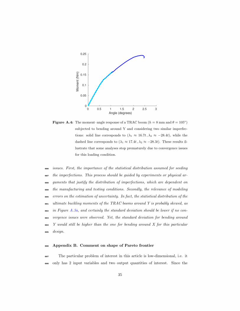
As a final comment about the statistical distributions of the ultimate buck-671
ling moments, it is noted that a small and yet non-negligible amount of com-672
putational analyses of TRAC booms subjected to bending around Y showed673
convergence issues. This was not observed for bending around X. Figure A.4674
illustrates the convergence issue by plotting the moment–angle response of the675
TRAC boom subjected to bending around Y for two very similar imperfections.676
As can be seen in the figures one of the responses is incomplete because the677
equilibrium path after a second bifurcation point is not resolved, even though678
this does not correspond to the ultimate buckling. Such small imperfection dif-679
ference is unlikely to cause the suggested premature ultimate buckling of the680
TRAC boom (see dashed line in the figure). This has implications on the distri-681
bution seen in Figure A.3b, since it is likely that the minimum ultimate buckling682
moment around Y is closer to 0.25 Nm than 0.15 Nm – see Remark 3.683
Remark 3. The detailed uncertainty analysis summarized herein for both load-684
ing conditions applied to the TRAC booms intends to demonstrate two important685
34
0 0.5 1 1.5 2 2.5 3
Angle (degrees)
0
0.05
0.1
0.15
0.2
0.25
Mom
ent (N
m)
Figure A.4: The moment–angle response of a TRAC boom (h = 8mm and θ = 105o)
subjected to bending around Y and considering two similar imperfec-
tions: solid line corresponds to (λ1 ≈ 16.7t , λ2 ≈ −28.4t), while the
dashed line corresponds to (λ1 ≈ 17.4t , λ2 ≈ −28.3t). These results il-
lustrate that some analyses stop prematurely due to convergence issues
for this loading condition.
issues. First, the importance of the statistical distribution assumed for seeding686
the imperfections. This process should be guided by experiments or physical ar-687
guments that justify the distribution of imperfections, which are dependent on688
the manufacturing and testing conditions. Secondly, the relevance of modeling689
errors on the estimation of uncertainty. In fact, the statistical distribution of the690
ultimate buckling moments of the TRAC booms around Y is probably skewed, as691
in Figure A.3a, and certainly the standard deviation should be lower if no con-692
vergence issues were observed. Yet, the standard deviation for bending around693
Y would still be higher than the one for bending around X for this particular694
design.695
Appendix B. Comment on shape of Pareto frontier696
The particular problem of interest in this article is low-dimensional, i.e. it697
only has 2 input variables and two output quantities of interest. Since the698
35

machine learning model can be evaluated for any combination of input values699
within the appropriate bounds, then there is the possibility of exhaustively700
evaluating the responses for a large number of different designs without using701
optimization strategies.702
0.1 0.2 0.3 0.4
Mean(MfX)− 2
[STDV(Mf
X)](Nm)
0.0
0.2
0.4
0.6
0.8
1.0
Mean(M
f Y)−2[ S
TDV(M
f Y)]
(Nm)
(a) Decision space considering lower
bounds of ultimate buckling mo-
ments and a large initial population.
0.2 0.3 0.4
Mean(MfX) (Nm)
0.2
0.4
0.6
0.8
1.0
Mean(M
f Y)(N
m)
(b) Decision space considering mean ul-
timate buckling moments and a large
initial population.
Figure A.5: Exhaustive exploration of a large number of possible values of the out-
put quantities of interest within the input bounds of h = [2.5, 5.5] mm,
θ = [45o, 270o]. Note that this figure is not generated with any opti-
mization algorithm. Instead, it provides the ultimate buckling moments
of 10, 000 different designs, effectively showing the entire output space
to be optimized.
Figure A.5 shows this exhaustive evaluation of a population of 10, 000 designs703
from which the entire output space can be seen as a collection of the responses704
for those points. This demonstrates why the Pareto frontier has a discontinuity705
aroundMfX = 0.20 in Figure 8a and aroundMf
X = 0.25 in Figure 9a, where there706
is no combination of points that simultaneously improves both ultimate buckling707
moments. Evidently, Figure A.5 is included here for illustrative purposes. Under708
normal circumstances the results in Figure A.5 are not available, nor necessary.709
36

References710
Aghajari, S., Abedi, K., Showkati, H., 2006. Buckling and post-buckling behav-711
ior of thin-walled cylindrical steel shells with varying thickness subjected to712
uniform external pressure. Thin-Walled Structures 44 (8), 904 – 909.713
Bader, J., Zitzler, E., 2011. Hype: An algorithm for fast hypervolume-714
based many-objective optimization. Evolutionary Computation 19 (1), 45–76,715
pMID: 20649424.716
Bai, X., Bessa, M. A., Melro, A. R., Camanho, P. P., Guo, L., Liu, W. K.,717
2015. High-fidelity micro-scale modeling of the thermo-visco-plastic behavior718
of carbon fiber polymer matrix composites. Composite Structures 134, 132 –719
141.720
Bažant, Z. P., Cedolin, L., 2010. Stability of structures: elastic, inelastic, frac-721
ture and damage theories. World Scientific.722
Benson, D., Bazilevs, Y., Hsu, M., Hughes, T., 2010. Isogeometric shell analysis:723
The reissner–mindlin shell. Computer Methods in Applied Mechanics and724
Engineering 199 (5–8), 276 – 289, computational Geometry and Analysis.725
Bessa, M., Bostanabad, R., Liu, Z., Hu, A., Apley, D. W., Brinson, C., Chen,726
W., Liu, W., 2017. A framework for data-driven analysis of materials under727
uncertainty: Countering the curse of dimensionality. Computer Methods in728
Applied Mechanics and Engineering 320, 633 – 667.729
Beume, N., Fonseca, C. M., Lopez-Ibanez, M., Paquete, L., Vahrenhold, J.,730
Oct 2009. On the complexity of computing the hypervolume indicator. IEEE731
Transactions on Evolutionary Computation 13 (5), 1075–1082.732
Beume, N., Naujoks, B., Emmerich, M., 2007. Sms-emoa: Multiobjective se-733
lection based on dominated hypervolume. European Journal of Operational734
Research 181 (3), 1653 – 1669.735
37

Bisagni, C., 2000. Numerical analysis and experimental correlation of composite736
shell buckling and post-buckling. Composites Part B: Engineering 31 (8), 655737
– 667.738
Bisagni, C., Lanzi, L., 2002. Post-buckling optimisation of composite stiffened739
panels using neural networks. Composite Structures 58 (2), 237 – 247.740
Chen, S., Gonella, S., Chen, W., Liu, W. K., 2010. A level set approach for741
optimal design of smart energy harvesters. Computer Methods in Applied742
Mechanics and Engineering 199 (37–40), 2532 – 2543.743
Chinesta, F., Ammar, A., Leygue, A., Keunings, R., 2011. An overview of the744
proper generalized decomposition with applications in computational rheol-745
ogy. Journal of Non-Newtonian Fluid Mechanics 166 (11), 578 – 592.746
Curtarolo, S., Morgan, D., Persson, K., Rodgers, J., Ceder, G., Sep 2003. Pre-747
dicting crystal structures with data mining of quantum calculations. Phys.748
Rev. Lett. 91, 135503.749
Daynes, S., Grisdale, A., Seddon, A., Trask, R., 2014. Morphing structures using750
soft polymers for active deployment. Smart Materials and Structures 23 (1),751
012001.752
Deb, K., Pratap, A., Agarwal, S., Meyarivan, T., Apr 2002. A fast and elitist753
multiobjective genetic algorithm: NSGA-II. IEEE Transactions on Evolution-754
ary Computation 6 (2), 182–197.755
Demuth, H. B., Beale, M. H., De Jess, O., Hagan, M. T., 2014. Neural Network756
Design, 2nd Edition. Martin Hagan, USA.757
Diaconu, C. G., Weaver, P. M., Mattioni, F., 2008. Concepts for morphing758
airfoil sections using bi-stable laminated composite structures. Thin-Walled759
Structures 46 (6), 689 – 701.760
Dong, L., Lakes, R., 2013. Advanced damper with high stiffness and high hys-761
teresis damping based on negative structural stiffness. International Journal762
of Solids and Structures 50 (14–15), 2416 – 2423.763
38

Elishakoff, I., 2014. Resolution of the twentieth century conundrum in Elastic764
Stability. World Scientific.765
Elvin, N. G., Lajnef, N., Elvin, A. A., 2006. Feasibility of structural monitoring766
with vibration powered sensors. Smart Materials and Structures 15 (4), 977.767
Fischer, C. C., Tibbetts, K. J., Morgan, D., Ceder, G., 2006. Predicting crystal768
structure by merging data mining with quantum mechanics. Nature Materials769
5 (8), 641–646.770
Forrester, A. I., Keane, A. J., 2009. Recent advances in surrogate-based opti-771
mization. Progress in Aerospace Sciences 45 (1), 50 – 79.772
Gautier, R., Zhang, X., Hu, L., Yu, L., Lin, Y., L., S. O., Chon, D., Poep-773
pelmeier, K. R., Zunger, A., Apr. 2015. Prediction and accelerated labora-774
tory discovery of previously unknown 18-electron abx compounds. Nat Chem775
7 (4), 308–316.776
Gill, P. E., Murray, W., Saunders, M. A., 2005. Snopt: An SQP algorithm for777
large-scale constrained optimization. SIAM Review 47 (1), 99–131.778
Goldberg, P. W., Williams, C. K., Bishop, C. M., 1998. Regression with input-779
dependent noise: A gaussian process treatment. Advances in Neural Informa-780
tion Processing Systems, 493–499.781
Hopfield, J. J., 1982. Neural networks and physical systems with emergent collec-782
tive computational abilities. Proceedings of the National Academy of Sciences783
79 (8), 2554–2558.784
Hu, N., Burgueño, R., 2015. Buckling-induced smart applications: recent ad-785
vances and trends. Smart Materials and Structures 24 (6), 063001.786
Hutchinson, J., Koiter, W., 1970. Postbuckling theory. Appl. Mech. Rev 23 (12),787
1353–1366.788
39

Ishibuchi, H., Tsukamoto, N., Nojima, Y., June 2008. Evolutionary many-789
objective optimization: A short review. In: 2008 IEEE Congress on Evolu-790
tionary Computation (IEEE World Congress on Computational Intelligence).791
pp. 2419–2426.792
Izzo, D., 2012. Pygmo and pykep: Open source tools for massively parallel op-793
timization in astrodynamics (the case of interplanetary trajectory optimiza-794
tion). In: Proceedings of the Fifth International Conference on Astrodynamics795
Tools and Techniques, ICATT.796
Kalpakjian, S., Schmid, S. R., Sekar, K. V., 2014. Manufacturing engineering797
and technology. Pearson Upper Saddle River, NJ, USA.798
Kersting, K., Plagemann, C., Pfaff, P., Burgard, W., 2007. Most likely het-799
eroscedastic gaussian process regression. In: Proceedings of the 24th Inter-800
national Conference on Machine Learning. ICML ’07. ACM, New York, NY,801
USA, pp. 393–400.802
Kim, S. Y., Mechefske, C. K., Kim, I. Y., 2013. Optimal damping layout in a803
shell structure using topology optimization. Journal of Sound and Vibration804
332 (12), 2873 – 2883.805
Kiyono, C., Silva, E., Reddy, J., 2012. Design of laminated piezocomposite shell806
transducers with arbitrary fiber orientation using topology optimization ap-807
proach. International Journal for Numerical Methods in Engineering 90 (12),808
1452–1484.809
Konak, A., Coit, D. W., Smith, A. E., 2006. Multi-objective optimization us-810
ing genetic algorithms: A tutorial. Reliability Engineering & System Safety811
91 (9), 992 – 1007, special Issue - Genetic Algorithms and ReliabilitySpecial812
Issue - Genetic Algorithms and Reliability.813
Krige, D. G., 1951. A statistical approach to some mine valuation and allied814
problems on the witwatersrand. Ph.D. thesis, Master’s thesis of the University815
of Witwatersrand.816
40

Ladevèze, P., Passieux, J.-C., Néron, D., 2010. The {LATIN} multiscale compu-817
tational method and the proper generalized decomposition. Computer Meth-818
ods in Applied Mechanics and Engineering 199 (21–22), 1287 – 1296, multi-819
scale Models and Mathematical Aspects in Solid and Fluid Mechanics.820
Lazarus, A., Reis, P. M., 2015. Soft actuation of structured cylinders through821
auxetic behavior. Advanced Engineering Materials 17 (6), 815–820.822
Leclerc, C., Wilson, L. L., Bessa, M. A., Pellegrino, S., Jan. 2017. Character-823
ization of ultra-thin composite triangular rollable and collapsible booms. In:824
AIAA SciTech Forum. American Institute of Aeronautics and Astronautics,825
AIAA-2017-0172.826
Li, X., 2003. A Non-dominated Sorting Particle Swarm Optimizer for Multi-827
objective Optimization. Springer Berlin Heidelberg, Berlin, Heidelberg, pp.828
37–48.829
Ling, J., Templeton, J., 2015. Evaluation of machine learning algorithms for830
prediction of regions of high Reynolds averaged Navier Stokes uncertainty.831
Physics of Fluids 27 (8), 085103.832
Liu, Z., Bessa, M., Liu, W. K., 2016. Self-consistent clustering analysis: An833
efficient multi-scale scheme for inelastic heterogeneous materials. Computer834
Methods in Applied Mechanics and Engineering 306, 319 – 341.835
Loukaides, E., Smoukov, S., Seffen, K., 2014. Magnetic actuation and transition836
shapes of a bistable spherical cap. International Journal of Smart and Nano837
Materials 5 (4), 270–282.838
Mallikarachchi, H. M. Y. C., Pellegrino, S., May 2014. Design of ultrathin com-839
posite self-deployable booms. Journal of Spacecraft and Rockets 51 (6), 1811–840
1821.841
Matheron, G., 1963. Principles of geostatistics. Economic geology 58 (8), 1246–842
1266.843
41

McKay, M. D., Beckman, R. J., Conover, W. J., 1979. Comparison of three844
methods for selecting values of input variables in the analysis of output from845
a computer code. Technometrics 21 (2), 239–245.846
Morris, M. D., Mitchell, T. J., 1995. Exploratory designs for computational847
experiments. Journal of Statistical Planning and Inference 43 (3), 381 – 402.848
Murphey, T. W., Banik, J., Mar. 1 2011. Triangular rollable and collapsible849
boom. US Patent 7,895,795.850
Murphey, T. W., Turse, D., Adams, L., Jan. 2017. Trac boom structural me-851
chanics. In: AIAA SciTech Forum. American Institute of Aeronautics and852
Astronautics, pp. –.853
Neal, R. M., Jan. 1997. Monte carlo implementation of gaussian process models854
for bayesian regression and classification. Technical Report 9702, Department855
of Statistics, University of Toronto.856
Ning, X., Pellegrino, S., 2015. Imperfection-insensitive axially loaded thin cylin-857
drical shells. International Journal of Solids and Structures 62, 39 – 51.858
Pedregosa, F., Varoquaux, G., Gramfort, A., Michel, V., Thirion, B., Grisel, O.,859
Blondel, M., Prettenhofer, P., Weiss, R., Dubourg, V., Vanderplas, J., Passos,860
A., Cournapeau, D., Brucher, M., Perrot, M., Duchesnay, E., 2011. Scikit-861
learn: Machine learning in Python. Journal of Machine Learning Research862
12, 2825–2830.863
Pellegrino, S., 2014. Deployable structures. Vol. 412. Springer.864
Queipo, N. V., Haftka, R. T., Shyy, W., Goel, T., Vaidyanathan, R., Tucker,865
P. K., 2005. Surrogate-based analysis and optimization. Progress in Aerospace866
Sciences 41 (1), 1 – 28.867
Rasmussen, C. E., Williams, C. K. I., 2005. Gaussian Processes for Machine868
Learning (Adaptive Computation and Machine Learning). The MIT Press.869
42

Reis, P. M., Sep. 2015. A perspective on the revival of structural (in)stability870
with novel opportunities for function: From buckliphobia to buckliphilia.871
Journal of Applied Mechanics 82 (11), 111001–111001–4.872
Riks, E., 1979. An incremental approach to the solution of snapping and buck-873
ling problems. International Journal of Solids and Structures 15 (7), 529 –874
551.875
Rosenblatt, F., 1958. The perceptron: a probabilistic model for information876
storage and organization in the brain. Psychological review 65 (6), 386.877
Rumelhart, D. E., McClelland, J. L., PDP Research Group, C. (Eds.), 1986.878
Parallel Distributed Processing: Explorations in the Microstructure of Cog-879
nition, Vol. 1: Foundations. MIT Press, Cambridge, MA, USA.880
Saal, J. E., Kirklin, S., Aykol, M., Meredig, B., Wolverton, C., 2013. Materials881
design and discovery with high-throughput density functional theory: the882
open quantum materials database (oqmd). Jom 65 (11), 1501–1509.883
Shen, H.-S., 2012. Thermal buckling and postbuckling behavior of functionally884
graded carbon nanotube-reinforced composite cylindrical shells. Composites885
Part B: Engineering 43 (3), 1030 – 1038.886
Silver, D., Huang, A., Maddison, C. J., Guez, A., Sifre, L., Van Den Driessche,887
G., Schrittwieser, J., Antonoglou, I., Panneershelvam, V., Lanctot, M., et al.,888
2016. Mastering the game of go with deep neural networks and tree search.889
Nature 529 (7587), 484–489.890
Simpson, T., Poplinski, J., Koch, N. P., Allen, J., 2001. Metamodels for891
computer-based engineering design: Survey and recommendations. Engineer-892
ing with Computers 17 (2), 129–150.893
Snelson, E., Ghahramani, Z., Rasmussen, C. E., 2004. Warped gaussian pro-894
cesses. In: Advances in Neural Information Processing Systems. pp. 337–344.895
43

Sobol, I. M., 1967. On the distribution of points in a cube and the approximate896
evaluation of integrals. Zhurnal Vychislitel’noi Matematiki i Matematicheskoi897
Fiziki 7 (4), 784–802.898
Sobol, I. M., 1976. Uniformly distributed sequences with an additional uni-899
form property. USSR Computational Mathematics and Mathematical Physics900
16 (5), 236–242.901
Tafreshi, A., 2002. Buckling and post-buckling analysis of composite cylindrical902
shells with cutouts subjected to internal pressure and axial compression loads.903
International Journal of Pressure Vessels and Piping 79 (5), 351 – 359.904
Tikhonov, A., 1963. Solution of incorrectly formulated problems and the regu-905
larization method. Soviet Meth. Dokl. 4, 1035–1038.906
Titsias, M. K., Lázaro-Gredilla, M., 2011. Variational heteroscedastic gaussian907
process regression. In: Proceedings of the 28th International Conference on908
Machine Learning (ICML-11). pp. 841–848.909
Wang, P., Casadei, F., Shan, S., Weaver, J. C., Bertoldi, K., Jul 2014. Harness-910
ing buckling to design tunable locally resonant acoustic metamaterials. Phys.911
Rev. Lett. 113, 014301.912
Widrow, B., Hoff, M. E., 1960. Adaptive switching circuits. IRE WESCON913
Convention Record 4, 96–104.914
Woo, J., Meguid, S., Stranart, J., Liew, K., 2005. Thermomechanical postbuck-915
ling analysis of moderately thick functionally graded plates and shallow shells.916
International Journal of Mechanical Sciences 47 (8), 1147 – 1171.917
Yvonnet, J., He, Q.-C., 2007. The reduced model multiscale method (r3m) for918
the non-linear homogenization of hyperelastic media at finite strains. Journal919
of Computational Physics 223 (1), 341–368.920
Zhu, C., Byrd, R. H., Lu, P., Nocedal, J., 1997. Algorithm 778: L-bfgs-b: For-921
tran subroutines for large-scale bound-constrained optimization. ACM Trans-922
actions on Mathematical Software (TOMS) 23 (4), 550–560.923
44

Zitzler, E., Deb, K., Thiele, L., 2000. Comparison of multiobjective evolutionary924
algorithms: Empirical results. Evolutionary Computation 8 (2), 173–195.925
Zitzler, E., Laumanns, M., Thiele, L., 2001. Spea2: Improving the strength926
pareto evolutionary algorithm.927
Zitzler, E., Thiele, L., Nov 1999. Multiobjective evolutionary algorithms: a928
comparative case study and the strength pareto approach. IEEE Transactions929
on Evolutionary Computation 3 (4), 257–271.930
45


![Scanned Document - University of New South Walesvm.civeng.unsw.edu.au/uniciv/R-458.pdf · Bazant and Cedolin [4] and Smitses and Hodges [5]. However, unlike column buckling analysis](https://img.pdfslide.net/doc/110x75/5c6aa09209d3f2e4178ce247/scanned-document-university-of-new-south-bazant-and-cedolin-4-and-smitses.jpg)


![[Milan Jirásek, Z. P. Bažant] Inelastic Analysis(BookZZ.org)](https://img.pdfslide.net/doc/110x75/5695d1581a28ab9b02962970/milan-jirasek-z-p-bazant-inelastic-analysisbookzzorg.jpg)