Embed Size (px)
Citation preview
DESIGN OPTIMIZATION AND EFFICIENCY MODELING OF A HOT GAS VANE MOTOR
A thesis presented to the faculty of the Graduate School
University of Missouri-Columbia
In Partial Fulfillment Of the Requirements for the Degree
Master of Science
By
GREGORY BOMMARITO
Dr. Roger Fales, Thesis Supervisor
December 2007
The undersigned, appointed by the dean of the Graduate School, have examined the
project entitled
DESIGN OPTIMIZATION AND EFFICIENCY MODELING OF A HOT GAS VANE MOTOR
Presented by Gregory Bommarito
a candidate for the degree of Masters of Science
and hereby certify that in their opinion it is worthy of acceptance.
Dr. Roger Fales, Assistant Professor, Mechanical and Aerospace Engineering
Dr. Craig Kluever, Professor, Mechanical and Aerospace Engineering
Dr. Steven Borgelt, Associate Professor, Agricultural Systems Management
ACKNOWLEDGEMENTS
Most of all I would like to thank my mentor Dr. Roger Fales for all the support he
provided me throughout this project. His motivation and passion for engineering were a
constant source of inspiration both on this project and in the classroom. I am very
grateful for the many hours of instruction that I have received from Dr. Fales. I only
hope that some day I may achieve as complete of an understanding of engineering
systems as he has.
I would like to thank the members of Vanderbilt University who collaborated on
this work with me, especially Dr. Eric Barth, Dr. Michael Goldfarb, Bo Li, and Jason
Mitchell whose support was indispensable. Their ideas helped guide me throughout this
project.
I would like to thank Dr. Craig Kluever for improving my education in both my
undergraduate and graduate courses. I admire the passion he has for his work in
education and am honored that I had the privilege of being his student.
I would like to thank Dr. Steven Borgelt for assisting in the improvement of this
work and for participating in my thesis committee.
I would like to thank my friend and colleague Adam Molitor, who was always
willing to lend a helping hand or a sympathetic ear.
Finally, I would like to thank my parents, Sam and Bonnie Bommarito, for their
support throughout my college career. They have allowed me to achieve my dreams, and
I only hope that I can some day repay them for all that they have done for me.
ii
TABLE OF CONTENTS Acknowledgements....................................................................................................... ii
List of Figures ................................................................................................................v
List of Tables ............................................................................................................... vi
Nomenclature.............................................................................................................. vii
Abstract ........................................................................................................................ ix
Chapter 1 – Introduction.............................................................................................1
1.1 –Established Research .................................................................................2
1.2 –Research Objectives...................................................................................4
1.3 –Thesis Outline ............................................................................................4
Chapter 2 –Modeling of the Hot Gas Vane Motor....................................................6
2.1 –Basic Operation..........................................................................................6
2.2 –Basic Modeling ..........................................................................................8
2.3 –Simulation Results ...................................................................................18
Chapter 3 – Friction Model.......................................................................................23
3.1 –Derivation of Friction Model ...................................................................23
3.2 –Simulation Results Including Friction Torque.........................................31
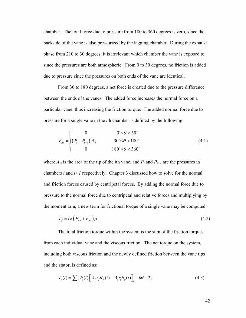
Chapter 4 – Pressure Model......................................................................................39
4.1 –Discussion of Pressure Model..................................................................39
4.2 –Straight-edged Vane Tip Pressure Calculation ........................................40
4.3 –Rounded Vane Tip Pressure Calculation .................................................43
4.4 –Results......................................................................................................44
Chapter 5 – Efficiency Modeling ..............................................................................51
iii
5.1 –Discussion of Efficiency ..........................................................................51
5.2 –Results......................................................................................................54
Chapter 6 – Conclusions............................................................................................57
6.1 –Overview..................................................................................................57
5.2 –Future Work/Recommendations ..............................................................58
References...................................................................................................................61
iv
LIST OF FIGURES
Figure 1. Vane and attached leaf spring........................................................................6
Figure 2. Cross-sectional view of the vane motor ........................................................7
Figure 3. Single chamber of the hot gas vane motor ....................................................9
Figure 4. View of a single vane in an xy coordinate frame ........................................10
Figure 5. Differential section of a chamber ................................................................12
Figure 6. Pressure in a chamber at steady state ..........................................................19
Figure 7. Volume through two rotations.....................................................................20
Figure 8. Total torque of the hot gas vane motor........................................................21
Figure 9. Angular velocity verses time for the hot gas vane motor............................22
Figure 10. Coordinate frames used to define acceleration..........................................24
Figure 11. Acceleration of a single vane throughout operation..................................26
Figure 12. Orientation of the normal force and the friction force on the vane motor.27
Figure 13. The angle β throughout a single rotation...................................................28
Figure 14. Typical Stribeck curve...............................................................................29
Figure 15. Coefficient of friction verses time.............................................................32
Figure 16. Normal force between a singular vane tip and the stator ..........................33
Figure 17. Average and actual friction torque of the hot gas vane motor ..................34
Figure 18. Net torque of the system............................................................................36
Figure 19. Angular velocity of the hot gas vane motor ..............................................37
Figure 20. Rotor and vane pressurization ports ..........................................................39
Figure 21. Orientation of a straight-edge vane ...........................................................41
Figure 22. Orientation of a rounded edge vane...........................................................43
v
Figure 23. Comparison plots of the normal forces on a single vane...........................45
Figure 24. Comparison of the coefficient of friction of a single vane........................46
Figure 25. Comparison plots of total friction torque ..................................................47
Figure 26. Comparison plot of the total torque of the system ....................................48
Figure 27. Comparison plot of angular velocities.......................................................49
Figure 28. Pressure in a single chamber .....................................................................53
Figure 29. Actual and maximum efficiencies of vane motors with various stator
radii…………………… ...........................................................................55
LIST OF TABLES
Table 1 – Vane motor parameters................................................................................17
vi
NOMENCLATURE
Symbol Description Units a Acceleration m/s2
Aa Exposed area of the aft vane m2
Aex,i Exhaust area m2
Af Exposed area of the fore vane m2
Av Area of vane tip m2
Av,in Area of the injection valve m2
bload Viscous rotational damping kgm2/s Cf Valve discharge coefficient - cp Specific heat at constant pressure J/kg/K Cr Pressure ratio at which flow becomes choked - e Offset distance between rotor and stator centers m E Energy J Ff Friction force N Fna Normal force due to acceleration of vane N Fnp Normal force including pressure forces N Jload Rotational inertia kgm2
k Lower heating value of the hot gas J/kg L Vane length m l Distance from rotor center to edge of stator m
rl Relative velocity of a vane m/s
rl Relative acceleration of a vane m/s2
m Mass of rotor kg ,in im Mass flowrate into the ith chamber kg/s
,out im Mass flowrate out of the ith chamber kg/s Ma Mach number - mv Mass of a vane kg n Number of vanes - N’ Load per unit width N/m Patm Atmospheric pressure Pa Pi Pressure in the ith chamber Pa Ps Supply Pressure Pa R Gas constant J/kg/K R Absolute acceleration of the coordinate frame m/s2
ra Moment arm of the aft vane m rf Moment arm of the fore vane m RR Radius of the rotor m RS Radius of the stator m t Vane thickness m T1 Temperature at the inlet K Tf Friction torque Nm
vii

Ti Temperature in the ith chamber K Ts Total shaft torque Nm v Velocity of the fluid m/s Vi Volume in the ith chamber m3
W Vane width m Wf Energy dissipated due to friction J α Stribeck curve coefficient - β Angle between normal direction and vane direction rad. γ Ratio of specific heats - ε Stribeck curve coefficient - η Efficiency - ηf Absolute fluid viscosity Pa s θ Vane position rad. μ Coefficient of friction - μ’ Boundary lubrication coefficient - ρl Density of liquid propellant kg/m3
cτ Time Constant s ω Angular Velocity rad./s ω Angular acceleration of the rotor rad./s2
viii
Abstract
The purpose of this research is to model and analyze the dynamics of a hot gas
vane motor for design optimization work. The pneumatic motor is a portable direct drive
actuator that is intended as an alternative to battery-powered electromagnetic motors. It
is believed that the vane motor could replace other solutions for portable power
generation. An optimal design of the motor is desirable to maximize portability and
efficiency. Modeling the device will make it possible to optimize the mechanical
efficiency by altering the geometry of the motor’s vanes and respective chambers. The
modeling of the device focuses on determining the net amount of torque that is produced
by the high pressures that drive the device. While the efficiency of the motor is affected
to a great extent by its geometry, losses from friction will also be considered. A model of
Stribeck friction was developed to account for losses from friction. For the device to
remain portable, there are limitations on the size of the final design which will restrict the
optimal efficiency of the vane motor.
ix
Chapter 1
INTRODUCTION
The purpose of this research is to analyze a unique application of a hot gas
vane motor to determine if it is a viable candidate to replace currently used
technology. The two most commonly used portable drive devices are battery-
powered electric motors and hydrocarbon-fueled internal-combustion-engines.
Battery-powered motors offer the advantage of start/stop, quiet operation, but have
the disadvantage of low mass-specific power and energy densities. Hydocarbon-
fueled combustion engines have superior mass-specific power and energy densities,
but do not allow start/stop or bidirectional operation. It is believed that a hot gas vane
motor should produce high mass-specific power and energy densities and also should
provide quiet, start/stop, bidirectional operation.
The vane motor is not a recent discovery. There is evidence of vane motors
from as early as 1868 and there are U.S. patents from 1924 [1]. Early vane motors
were typically hydraulic devices, whereas the vane motor under discussion is a
pneumatic device. Vane motors for pneumatic systems operate at free speeds up to
13,000 rpm, with rated speed approximately 50% of that level [2]. Vane motors can
come in a variety of sizes and styles. The vane motor being discussed in this research
is relatively small (< 1 kg in weight), but there are much larger versions of vane
motors. For example, the Wankel engine works in a similar fashion to a vane motor
and is used in the Mazda RX-8.
The vane motor in this work uses a monopropellant, hydrogen peroxide, as a
1
power source. Hydrogen peroxide has been used as a monopropellant for many other
applications. The Royal Aircraft Establishment of Great Britain used hydrogen
peroxide to successfully launch low cost rockets into space, including the Black
Knight and Black Arrow rockets. The German military used hydrogen peroxide as a
monopropellant in WWII to drive a turbine that powered submarines. Also hydrogen
peroxide was used to propel torpedoes from those submarines [3].
1.1 Established Research
Vane motors have been in operation in the United States for nearly a century,
and not surprisingly, much research has already been developed. However, as of yet,
there has been a limited amount of research aimed at optimizing the efficiency of the
device based on geometry. The ultimate goal of this research is to improve the
efficiency of a hot gas vane motor through variations in the geometry of the motor.
In order to accomplish this task, a viable model of the device needs to be developed.
The model constructed for this work is based primarily on the work of Barth, Fite,
Goldfarb and Li [1]. Their model of the hot gas vane motor is based on a basic torque
equation, which is derived from the relationship between the pressure in each
chamber of the device and the geometry of the device at any instant. Pressures are
solved for using the first law of thermodynamics and assuming that the ideal gas
entering the system undergoes an adiabatic process. The model for this work uses the
same assumptions from [1], however, several important features have been added to
the model in order to increase the accuracy.
The most important feature added to the system is a model for the frictional
2
torques that develop during operation. Equating the friction within any system is
typically a difficult process, due to the fact that the friction coefficient, µ, is generally
unknown and also changes throughout operation. The friction coefficient may be
solved for using experimental methods, but analytical methods for solving the friction
coefficient have also been developed. One method for approximating the friction
coefficient is to use a Stribeck Curve. The dynamic behavior of the coefficient of
friction for sliding surfaces has historically been considered using the Stribeck Curve.
Research from Manring [4], has shown that a Stribeck friction curve is a good
approximation for friction in devices similar to that of a hot gas vane motor.
The friction coefficient is not the only quantity needed to determine the
friction torques within the system. The normal forces between the moving surfaces of
the hot gas vane motor also need to be known. Research has been done to develop an
appropriate free body diagram of the forces within the motor. A detailed diagram of
the forces within the system was produced by Bertetto, Mazza, Pastorelli, and
Raparelli [5]. Their research showed that the forces on pneumatic motor vanes vary
according to the orientation of the vanes relative to the stator or housing of the device.
Vanes within the motor have a certain amount of flexibility within the motor, which
has an affect on the forces present on those vanes. Their model, however, did not
give an in depth description of how to solve for the pressures on the back and tip of
the vane.
Research from Inaguma and Hibi [6] shows an appropriate method for solving
for pressure forces on the vanes that are present throughout the operation. While their
work was for a hydraulic pump, the methodology used is completely relevant for a
3
hot gas vane motor. Much like the work from Bertetto [5], their work showed that the
orientation of the vane and the tip geometry play an important role in defining the
forces present on the vanes.
1.2 Research Objectives
The objectives of this research are to develop a detailed model of the hot gas
vane motor, and then use that model to optimize the design of the device. Models for
hot gas vane motors have been developed, but each model is partially incomplete. In
this research, a more complete model of the hot gas vane motor was developed, by
expanding on the ideas presented in existing research. Specifically, a more detailed
model of friction was developed in order to create a more viable model. The
completed model was used to optimize the design and performance of the hot gas
vane motor.
1.3 Thesis Outline
Chapter 2 focuses on establishing a basic model for the hot gas vane motor.
The research of Michael Goldfarb and Eric Barth, that is being developed at
Vanderbilt University serves as the starting point for the model development. Their
research is the fundamental basis for the model and this research. Chapter 3 works to
expand the model and increase its precision. This is accomplished by developing a
more accurate friction model, using more detailed dynamics. In addition, it is shown
that integrating the Stribeck Curve into the model gives a more accurate
approximation of friction within the system. Chapter 4 expands on Chapters 2 and 3,
4
and shows that a more detailed description of the pressure forces on the vanes is
needed in order to give an appropriate description of the friction torque. Chapter 5
shows how the fully developed model may now be used to design a more efficient hot
gas vane motor. Finally, overall conclusions and recommendations about future work
are presented in Chapter 6.
5
Chapter 2
Modeling of the Hot Gas Vane Motor
2.1 Basic Operation
A hot gas vane motor is a device that uses hot gas as a power source to
drive a shaft and produce power. The motor consists of a circular rotor that is offset
in an elliptical stator. Extendable vanes are attached to the rotor and are extended to
the inner edge of the stator. During startup, the vanes are held against the stator by a
leaf spring. Figure 1 displays a single vane with thickness, t, width, W, and length, L,
and the attached leaf spring.
t
Vane W
Leaf Spring
L
Figure 1. Vane and attached leaf spring.
The leaf spring only provides enough force to keep the vane in contact with
the stator at start up. During operation, the vanes are kept in contact with the edge of
the stator by the centrifugal force created by the rotor’s rotation. There are six vanes
6

total which create six separate chambers. It is assumed that the thickness of the vanes
is negligible so each chamber occupies 1/6th of the total volume of the device. The
device is driven by a hot gas that flows into these chambers to create a torque on the
shaft attached to the rotor. The vanes are arranged in such a way that the leading
vane is always extended further than the trailing vane. Therefore, the pressure from
the hot gas causes an increased moment arm on the leading vane, thus creating a net
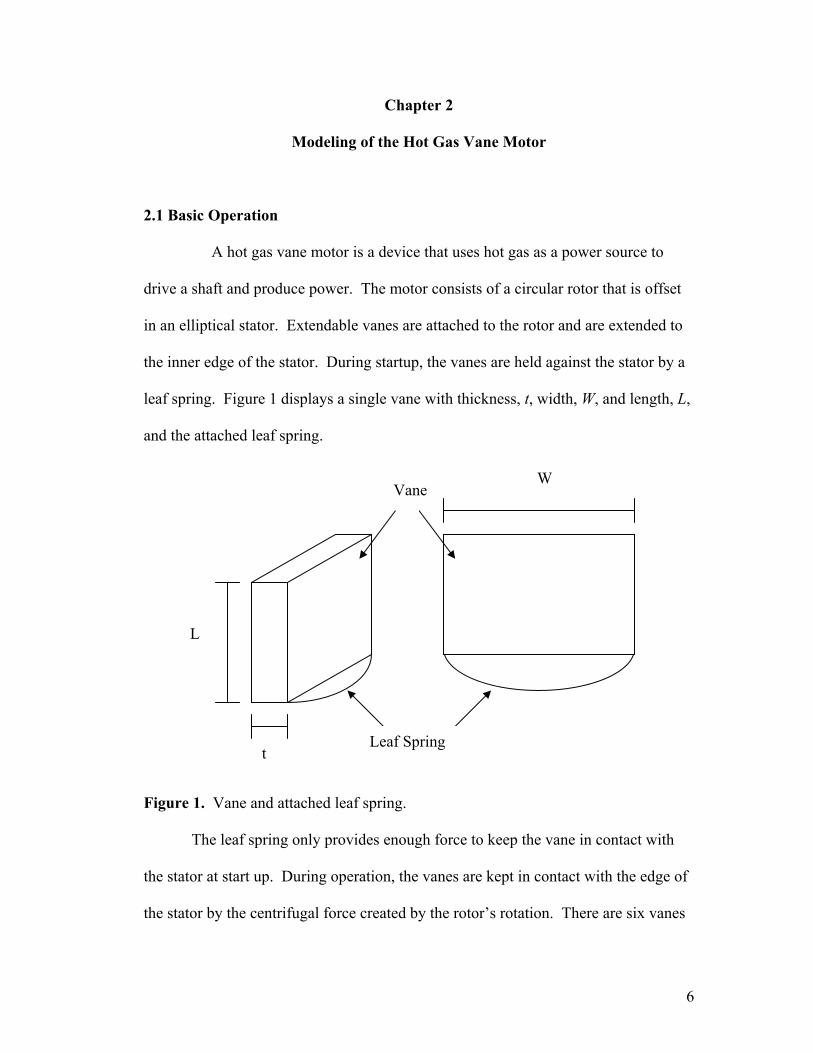
torque. A cross section of the motor is displayed in Figure 2.
Figure 2. Cross-sectional view of the vane motor.
7
Exhaust ports are present 210 degrees from the inlet port and continue for an
additional 120 degrees. Once the hot gas has rotated through 210 degrees, it is at a
much lower pressure and is cooler so it is exhausted into the atmosphere.
The leading vane of a chamber will begin to become extended less than the
trailing vane once it has rotated much past 210 degrees. If working fluid were still
trapped with no exit ports in the chamber, a negative torque would be created which
would adversely affect the performance. All working fluid should be expelled from
the motor before it has rotated a full 390 degrees. At this point hot gas is allowed to
flow into the working chamber through the injection port and the cycle repeats itself.
The hot gas is created by forcing a monopropellant, hydrogen peroxide, to flow
through a catalyst pack which causes an exothermic reaction thus creating a stream of
high pressure hot gas.
The catalyst pack is typically either a silver or platinum screen that triggers
the decomposition. The following equation from [3] shows how the hydrogen
peroxide is broken down during the reaction.
(2.1) 2 2 2 22 2H O H O O= +
Both steam and oxygen are produced in the reaction at about 232 ºC (450 ºF) and this
is what drives the device. The hot gas flows into the working chambers through the
inlet injection port seen in Figure 2.
2.2 Basic Modeling
The initial modeling of the hot gas vane motor is based off of research that is
being completed at Vanderbilt by Barth, Fite, Goldfarb and Li [1]. Specifically, the
8
equations for torque, pressure, temperature, and mass flowrate are taken from the
Vanderbilt research. The model equations are reviewed here. The entire system is
driven by torque created because the leading vane in each working chamber has a
larger area and a higher pressure than the trailing vane and therefore produces a
higher moment arm. The net torque created is defined in Eqn. (2.2) and is simply a
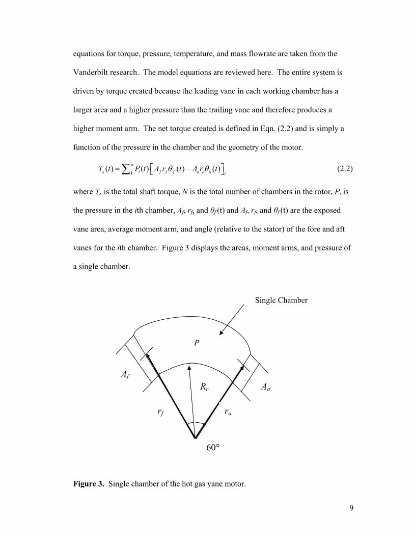
function of the pressure in the chamber and the geometry of the motor.
(2.2) 1
( ) ( ) ( ) ( )ns i f f f a a a i
T t P t A r t A r tθ θ⎡= −⎣∑ ⎤⎦
Figure 3. Single chamber of the hot gas vane motor.
where Ts is the total shaft torque, N is the total number of chambers in the rotor, Pi is
the pressure in the ith chamber, Af, rf, and θf (t) and Af, rf, and θf (t) are the exposed
vane area, average moment arm, and angle (relative to the stator) of the fore and aft
vanes for the ith chamber. Figure 3 displays the areas, moment arms, and pressure of
a single chamber.
Single Chamber
P
60°
Aa Rr
Af
rf ra
9
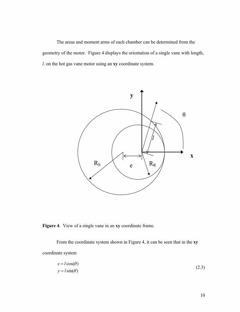
The areas and moment arms of each chamber can be determined from the
geometry of the motor. Figure 4 displays the orientation of a single vane with length,
l, on the hot gas vane motor using an xy coordinate system.
Figure 4. View of a single vane in an xy coordinate frame.
From the coordinate system shown in Figure 4, it can be seen that in the xy
coordinate system
y
cos( )sin( )
x ly l
θθ
==
(2.3)
e RR RS
θ
l
x
10
The equation for the surface of the stator may be defined as follows,
2 2( ) S2x e y R+ + = (2.4)
where e is the offset distance between the centers of the rotor and stator, and RS is the
radius of the stator. By substituting (2.3) into (2.4) the following quadratic equation
can be determined,
(2.5) 2 22 cos( ) ( ) 0Sl e l R eθ+ − − 2 =
Solving this equation for l yields the following result,
2cos( ) ( sin( ))Sl e R e 2θ θ= − + − (2.6)
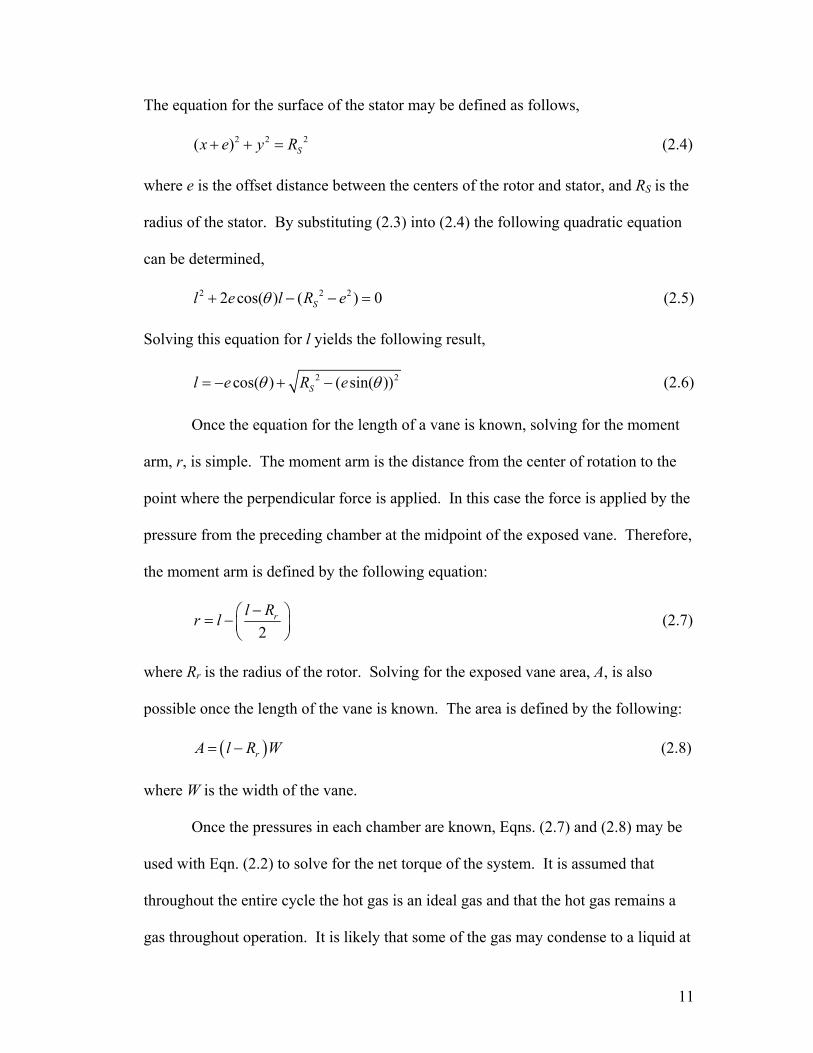
Once the equation for the length of a vane is known, solving for the moment
arm, r, is simple. The moment arm is the distance from the center of rotation to the
point where the perpendicular force is applied. In this case the force is applied by the
pressure from the preceding chamber at the midpoint of the exposed vane. Therefore,
the moment arm is defined by the following equation:
2
rl Rr l −⎛= − ⎜⎝ ⎠
⎞⎟ (2.7)
where Rr is the radius of the rotor. Solving for the exposed vane area, A, is also
possible once the length of the vane is known. The area is defined by the following:
( )rA l R W= − (2.8)
where W is the width of the vane.
Once the pressures in each chamber are known, Eqns. (2.7) and (2.8) may be
used with Eqn. (2.2) to solve for the net torque of the system. It is assumed that
throughout the entire cycle the hot gas is an ideal gas and that the hot gas remains a
gas throughout operation. It is likely that some of the gas may condense to a liquid at
11
some point which would alter the performance of the device by reducing pressure, but
for now it is assumed that the hot gas remains a gas throughout operation. By using
the first law of thermodynamics and assuming that the ideal gas undergoes an
adiabatic process, the pressure in each chamber can be defined as:
( ) ii
iout,iin,i
i
ii V
VPγmm
VRTγP −−= (2.9)
where and are the inlet and outlet mass flow rates into and out of the ith
chamber,
iinm , ioutm ,
γ is the ratio of specific heat at constant pressure to specific heat at
constant volume, Vi is the volume in the ith chamber, and Ti is the temperature in the
ith chamber.
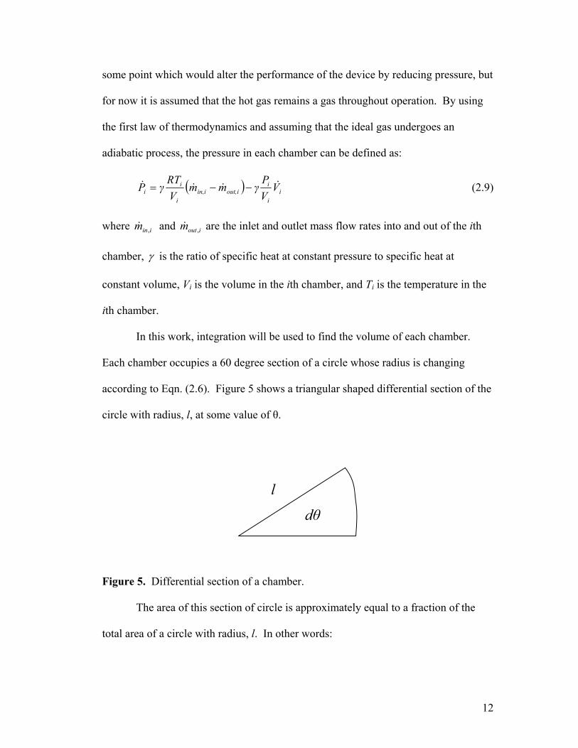
In this work, integration will be used to find the volume of each chamber.
Each chamber occupies a 60 degree section of a circle whose radius is changing
according to Eqn. (2.6). Figure 5 shows a triangular shaped differential section of the
circle with radius, l, at some value of θ.
l
dθ
Figure 5. Differential section of a chamber.
The area of this section of circle is approximately equal to a fraction of the
total area of a circle with radius, l. In other words:
12
2
2ddA l θππ
= (2.10)
In order to solve for the volume of a particular chamber, the area of a 60 degree
section is first solved for and then multiplied by the width of the vane motor.
However, each section of this circle has 1/6th of the area of the rotor present, which
needs to be subtracted off as this is not part of the chamber. In doing so, the volume
of a particular chamber may be solved for using the following equation:
22
/3 62rRlV W d
θ
θ π
πθ−
⎛ ⎞−⎜
⎝ ⎠= ∫ ⎟ (2.11)
Since l only depends on θ as seen in Eqn. (2.6), Eqn. (2.11) may be used to solve for
the volume in a chamber.
The next unknown in Eqn. (2.9) is the temperature in a chamber. Temperature
may be defined by the geometry of the hot gas vane motor. If it is assumed that the
process is adiabatic and that the working fluid is an ideal gas, the temperature may be
defined by the following:
1
2 1
1 2
T VT V
γ −⎛ ⎞
= ⎜ ⎟⎝ ⎠
(2.12)
where V2 and T2 are the volume and temperature in the ith chamber respectively and
P1 and T1 are the initial pressures and temperatures of a working chamber
respectively.
Matlab® and Simulink® models were used to integrate the preceding
equation and solve for pressure in the ith chamber using numerical differential
equation solvers. There are six separate chambers so six separate pressures were
solved for. Once pressure is known, only the inlet and outlet mass flows need to be
13
determined to solve for total torque. The mass flow rate into the motor chamber, i, is
a function of the injection valve area and is defined as follows:
1
,,, Tc
PPACkmm
p
isinvfliiniinc
−=+
ρτ (2.13)
where Cf is the valve discharge coefficient for the injection valves, Av,in is the valve
area of the injection valve, τc is the time constant of the catalyst pack reaction
dynamic, k is the lower heating value of the hot gas, ρl is the density of the liquid
propellant, T1 is the temperature at the inlet, cp is the specific heat at constant
pressure, and Ps is the upstream pressure as typically supplied in a blowdown fuel
tank. It should be noted that the mass flow rate into the system only occurs for 60
degrees of rotation. Past this point, there is no more inlet flow, because the chamber
is no longer exposed to the inlet. Again, (2.13) can be solved using Matlab
performing two integrations to solve for the mass.
The equation for the mass flow rate out of the system can be derived from
equations that are typical of pneumatic systems for isentropic flow of an ideal gas
through a converging nozzle. Mass flow rate of any system can be described by the
following:
lm Avρ= (2.14)
where lρ is the density of the fluid, A is the area of the fluid passage, and v is the
velocity of the fluid. For mass flow rate out of the chamber, the area is simply the
area at the outlet. An m-file was created to define the area of the outlet according to
the rotor angle. The density of compressible fluid undergoing isentropic flow through
a converging nozzle is defined by the following from [7]:
14
( )
11
2
11 1 / 2
l
lo Ma
γρρ γ
−⎧ ⎫⎪= ⎨+ −⎡ ⎤⎪ ⎪⎣ ⎦⎩ ⎭
⎪⎬ (2.15)
where loρ is the stagnate fluid density and Ma is the mach number which can be
solved for using the following from [7]:
( )
1
2
11 1 / 2o
PP Ma
γγ
γ
−⎧ ⎫⎪= ⎨+ −⎡ ⎤⎪ ⎪⎣ ⎦⎩ ⎭
⎪⎬ (2.16)
where Po is the stagnate fluid pressure. The velocity of the fluid can be defined by
the following equation for the definition of mach number which also comes from [7]:
v Ma RTγ= (2.17)
By substituting Eqs. (2.15) - (2.17) into (2.14) the mass flow rate out may be defined
by the following:
( )
11
atm, r
i
1
,
1
,
P2 ( ) if C 1 P
(choked)
2 11
( ) otherwise
i ex ii
atmout i
i i
atmi ex i
i
P ART
PmRT P
P P AP
γγ
γγ
γ
γ θγ
γγ
θ
⎛ ⎞+⎜ ⎟−⎝ ⎠
⎛ ⎞−⎜ ⎟⎝ ⎠
⎛ ⎞⎜ ⎟⎝ ⎠
⎛ ⎞≤⎜ ⎟+⎝ ⎠
⎛ ⎞= − ⎜ ⎟− ⎝ ⎠
⎛ ⎞×⎜ ⎟⎝ ⎠
…
…
(unchoked)
⎧⎪⎪⎪⎪⎪⎪⎪⎨⎪⎪⎪⎪⎪⎪⎪⎩
(2.18)
where Aex,I is the exhaust valve area (as a function of the rotor angle) for each
chamber, and Cr is the pressure ratio at which flow becomes choked (approximately
0.5). All equations used to derive the mass flow rate out are from [7].
15
Exhaust ports are present on the vane motor from 210 degrees through 330
degrees of rotation. Due to the fact that each chamber is 60 degrees in size, at least
some mass flow rate out of a single chamber occurs from 210 to 390 degrees of
rotation. It is desirable to have all of the working fluid removed from the system each
rotation, so that no back pressures are created that could potentially cause noise,
damage to the system or loss of efficiency.
Equations (2.9), (2.13), and (2.18) were solved simultaneously and
substituted into (2.2) to solve for the torque created by the system. The parameters
used are listed in
Table 1 and come from specifications given by Vanderbilt University for a hot gas
vane motor that is currently being constructed and also from specifications of the hot
16
gas being used from [8].
Table 1 Vane motor parameters. ymbol Name S Quantity
Av,in Valve Area 0.2047 cm2
bloaT1 d Viscous RotationalInlet Temperature Damping Width of Rotor/Stator
1.7e-4 kgm505.15 K 2/s
Cγ f Valve Discharge Ratio of Specific HeatsCoefficient Specific HeDensity of Liquid Propellant
0.78 1.344
cp at at re Constant PressuTime Constant
1005 J/kg/K
Cr Pressure Ratio 0.5 Jload Rotational Inertia 1.7e-4 kgm2 k Lower Heating Value
of the Hot Gas 800 kJ/kg
m Mass of Rotor 0.113 kg mv Mass of Vane 0.0118 kg Patm Atmospheric Pressure 101325 Pa Ps Supply Pressure 1.88 MPa R Gas Constant 287 J/kg/K
RR Radius of Rotor 0.0143 m RS Radius of Stator 0.0175 m t Vane thickness 3.175 mm
W 0.035 m
1000 kg/m3 ρl
τ 0.005 s
17
It was assumed that viscous rotational damping was present, so the torque
created by this friction needed to be subtracted from the torque created by the
working chambers. Other frictional forces are also present between the vane tips and
the stator, but the effects of that friction will be addressed in a later chapter.
Therefore, the total torque in the system may be defined as follows:
1
( )
( ) ( ) ( )
s loadN
i f f f a a a loain
T t J
P t A r t A r t b
θ
dθ θ θ=
=
⎡ ⎤= −⎣ ⎦∑
− (2.19)
where Jload is the rotational inertia, bload is the viscous rotational damping. It should
be noted that there is no load torque considered in Eqn. (2.19), so all simulations are
for no load conditions. There are six separate chambers so a total of 24 equations
need to be integrated to solve for the total torque in the system. Equations (2.13) and
(2.19) need to be integrated twice in order to be solved. The integration was
performed using Simulink software.
2.3 Simulation Results
The hot gas vane motor is driven by the forces created from pressurized hot
18
gas. Figure 6 displays the pressure in a single chamber once the device has reached a
constant velocity.
0 180 360 540 720 900 1080 1260 1440100
200
300
400
500
600
Theta (degrees)
Pre
ssur
e (K
Pa)
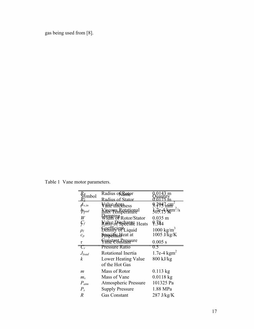
Figure 6. Pressure in a chamber at steady state.
There are pressure spikes once the device has rotated 30 degrees. This is the
point at which the chamber is first exposed to the inlet port. This is also the instant
when the chamber has its smallest volume. For a particular vane, the device is
producing a positive torque from 30 to 210 degrees. Just prior to 210 degrees, the
pressure is nearly at atmospheric pressure, and once the chamber reaches 210 degrees
the pressure drops to atmospheric pressure. This is the point at which the chamber is
exposed to the outlet ports and is no longer producing any torque. The pressure is
reduced from 30 to 210 degrees due to the fact that the volume is increasing. Figure 7
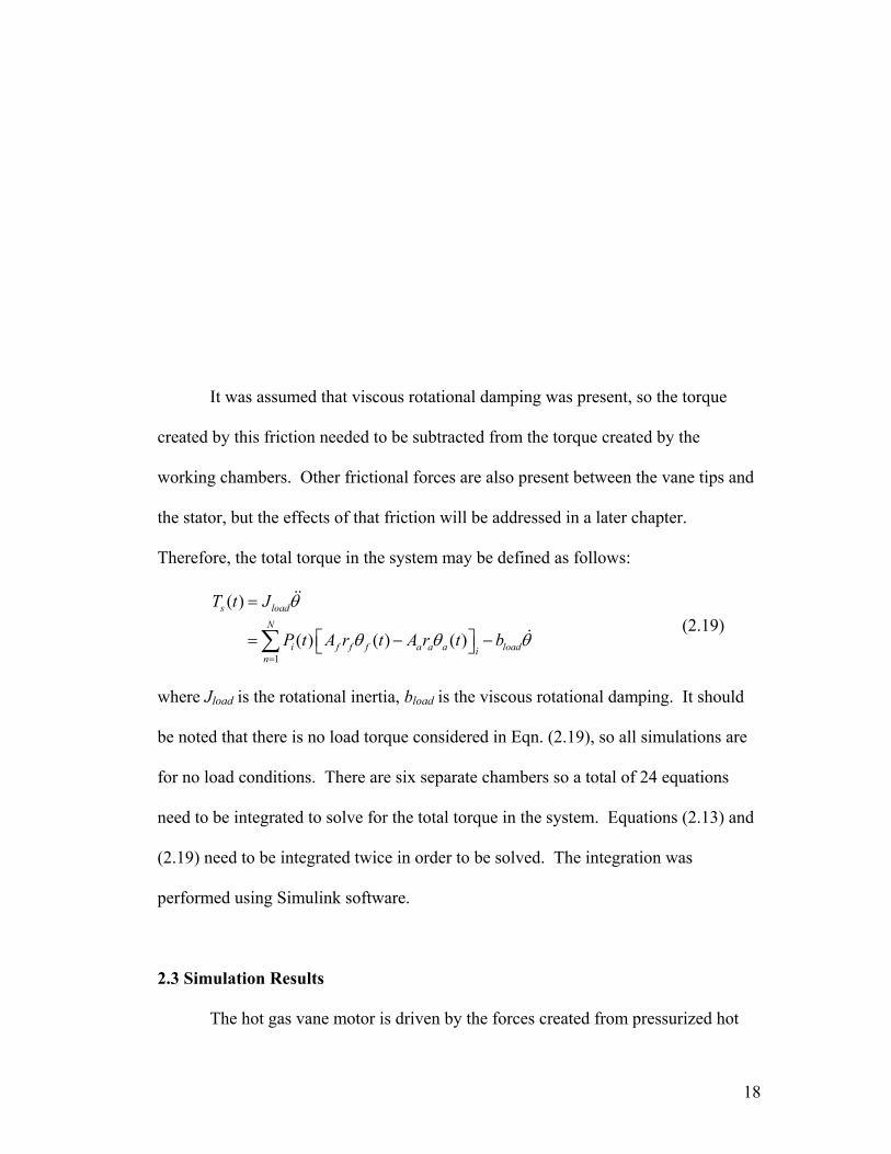
displays the volume of a single chamber through two rotations.
19
0 30 210 390 570 7200.5
1
1.5
2
2.5
3
3.5
Theta (degrees)
Vol
ume
(cm
3 )
Figure 7. Volume through two rotations.
The minimum volume occurs at 30 degrees of rotation, while the maximum
volume occurs at 210 degrees. This is why the inlet and exhaust ports are positioned
at 30 and 210 degrees respectively. In these positions the maximum amount of torque
is produced for a six chambered hot gas vane motor. Figure 8 displays the net torque
of the hot gas vane motor.
20
0 1 2 3 4 5 60.2
0.4
0.6
0.8
1
1.2
1.4
1.6
1.8
2
Time (s)
Tot
al T
orqu
e (N
-m)
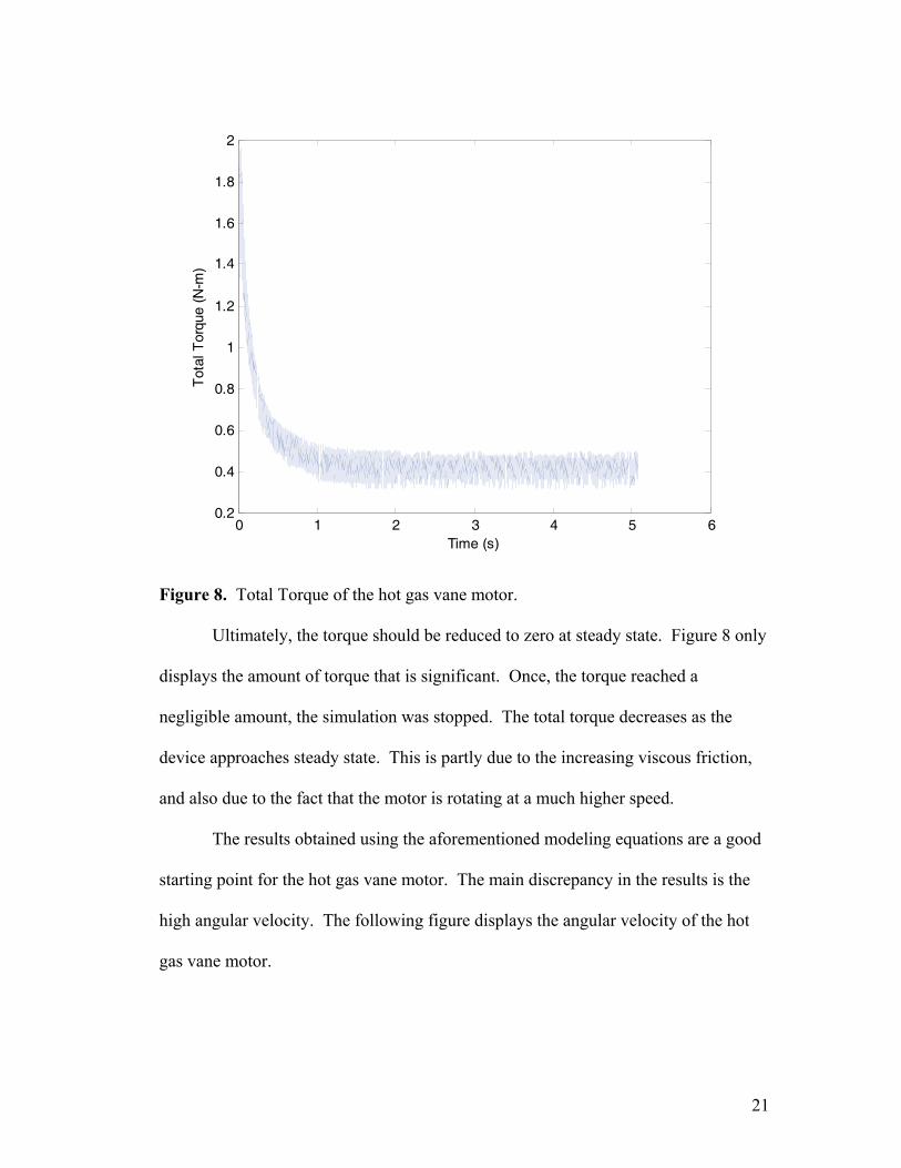
Figure 8. Total Torque of the hot gas vane motor.
Ultimately, the torque should be reduced to zero at steady state. Figure 8 only
displays the amount of torque that is significant. Once, the torque reached a
negligible amount, the simulation was stopped. The total torque decreases as the
device approaches steady state. This is partly due to the increasing viscous friction,
and also due to the fact that the motor is rotating at a much higher speed.
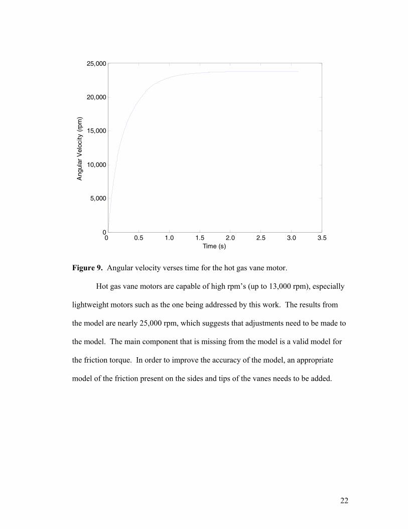
The results obtained using the aforementioned modeling equations are a good
starting point for the hot gas vane motor. The main discrepancy in the results is the
high angular velocity. The following figure displays the angular velocity of the hot
gas vane motor.
21
0 0.5 1.0 1.5 2.0 2.5 3.0 3.50
5,000
10,000
15,000
20,000
25,000
Time (s)
Ang
ular
Vel
ocity
(rp
m)
Figure 9. Angular velocity verses time for the hot gas vane motor.
Hot gas vane motors are capable of high rpm’s (up to 13,000 rpm), especially
lightweight motors such as the one being addressed by this work. The results from
the model are nearly 25,000 rpm, which suggests that adjustments need to be made to
the model. The main component that is missing from the model is a valid model for
the friction torque. In order to improve the accuracy of the model, an appropriate
model of the friction present on the sides and tips of the vanes needs to be added.
22
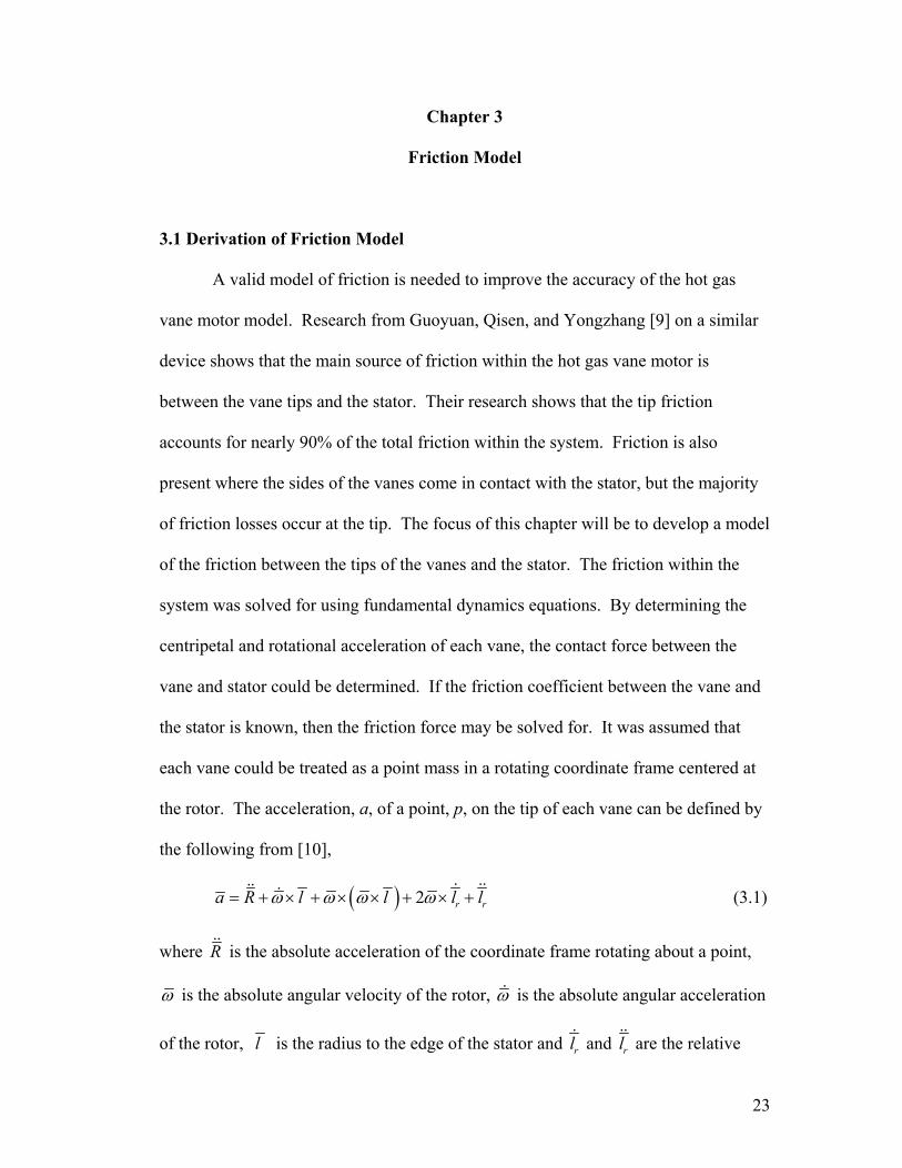
Chapter 3
Friction Model
3.1 Derivation of Friction Model
A valid model of friction is needed to improve the accuracy of the hot gas
vane motor model. Research from Guoyuan, Qisen, and Yongzhang [9] on a similar
device shows that the main source of friction within the hot gas vane motor is
between the vane tips and the stator. Their research shows that the tip friction
accounts for nearly 90% of the total friction within the system. Friction is also
present where the sides of the vanes come in contact with the stator, but the majority
of friction losses occur at the tip. The focus of this chapter will be to develop a model
of the friction between the tips of the vanes and the stator. The friction within the
system was solved for using fundamental dynamics equations. By determining the
centripetal and rotational acceleration of each vane, the contact force between the
vane and stator could be determined. If the friction coefficient between the vane and
the stator is known, then the friction force may be solved for. It was assumed that
each vane could be treated as a point mass in a rotating coordinate frame centered at
the rotor. The acceleration, a, of a point, p, on the tip of each vane can be defined by
the following from [10],
( ) 2 ra R l l l lω ω ω ω= + × + × × + × + r (3.1)
R is the absolute acceleration of the coordinate frame rotating about a point, where
ωω is the absolute angular velocity of the rotor, is the absolute angular acceleration
of the rotor, rl rll is the radius to the edge of the stator and and are the relative
23
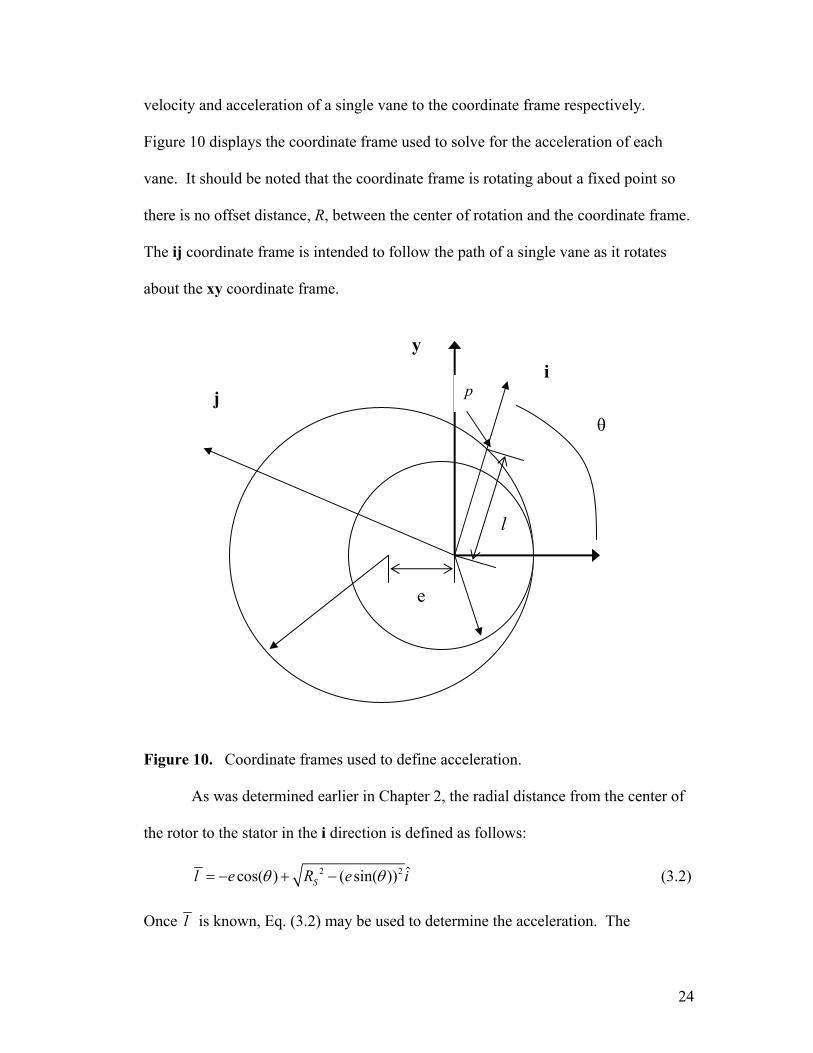
velocity and acceleration of a single vane to the coordinate frame respectively.
Figure 10 displays the coordinate frame used to solve for the acceleration of each
vane. It should be noted that the coordinate frame is rotating about a fixed point so
there is no offset distance, R, between the center of rotation and the coordinate frame.
The ij coordinate frame is intended to follow the path of a single vane as it rotates
about the xy coordinate frame.
e RR RS
x
i y
j
θ
l
e
p
Figure 10. Coordinate frames used to define acceleration. As was determined earlier in Chapter 2, the radial distance from the center of
the rotor to the stator in the i direction is defined as follows:
2 2 ˆcos( ) ( sin( ))Sl e R eθ= − + − iθ (3.2)
lOnce is known, Eq. (3.2) may be used to determine the acceleration. The
24
components of (3.1) are defined by the following,
0R = (3.3)
( ) ( )( )
2 2
2 2
ˆ ˆcos( ) ( sin( ))
ˆcos( ) ( sin( ))
S
S
l k e R e
e R e j
ω ω θ θ
ω θ θ
× = × − + −
= − + −
i (3.4)
( ) ( )( )( )( )
2 2
2 2
ˆ
ˆ
cos( ) ( sin( ))
cos( ) ( sin( ))
ˆ
ˆ
S
S
l k
k
e R e
e R e
i
i
ω ω ω
ω
θ θ
ω θ θ
× × = ×
×
− + −
= − − + −
⎛ ⎞⎜⎜⎝ ⎠
2
⎟⎟
(3.5)
( )( )( )
( )( )
2
2 2
22
2 2
ˆ 1/ 2 sin(2 ) ˆ2 2 sin( )
sin( )
1/ 2 sin(2 ) ˆ 2 sin( )sin( )
r
S
S
ke
l eR e
ee j
R e
ωω θ
ω ω θθ
θω θ
θ
× = × −−
= −−
⎛ ⎞⎜ ⎟⎜ ⎟⎝
⎛ ⎞⎜ ⎟⎜ ⎟⎝ ⎠
i
⎠ (3.6)
( )( )( ) ( )( )
( )( )
2
2
2 2
2
2 2
2 2
3/ 222
cos( ) sin( )
2 cos(2 )
sin( )ˆ 1/ 2
sin(2 )
sin( )
1/ 2 sin(2 )
sin( )
r
S S
S
e e
R ee i
l
R e
e
R e
ω θ ω θ
ω θ
θ
ω θ
θ
ω θ
θ
= +
−−
⎡ ⎤+ +⎢ ⎥
⎢ ⎥−⎢ ⎥⎢ ⎥⎢ ⎥⎢ ⎥−⎣ ⎦
(3.7)
It should be noted that only the acceleration in the i direction is needed in order to
determine the normal force. Therefore, only Eqs. (3.7) and (3.5) need to be
considered and the acceleration in the i direction is defined by the following:
( )ia lω ω= × × + rl (3.8)
25
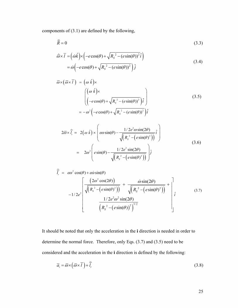
If the rotor of the vane motor was not offset from the stator then only, Eq.
(3.5) would need to be considered. However, since this is not the case, the relative
motion of the vanes moving in and out of their respective slots needs to be taken into
consideration. This motion does add a sizable amount of acceleration. The added
acceleration causes the total acceleration to oscillate more since the vanes are
accelerating in and out of their slots. A comparison of acceleration with and without
the added relative acceleration term may be seen in Figure 11.
0 0.05 0.10 0.15 0.20 0.25 0.30 0.35 0.40-12000
-10000
-8000
-6000
-4000
-2000
0
Time (s)
Acc
eler
atio
n (m
/s2 ) Centr. Ac. with Rel. Ac.
Centr. Ac.
Figure 11. Acceleration of a single vane throughout operation.
Once total acceleration is known, the normal force due to acceleration, FNa,
may be determined by using trigonometry and summing the forces in the i direction.
From Figure 12, it can be seen that the sum of the forces in the i direction is given by
the following,
26
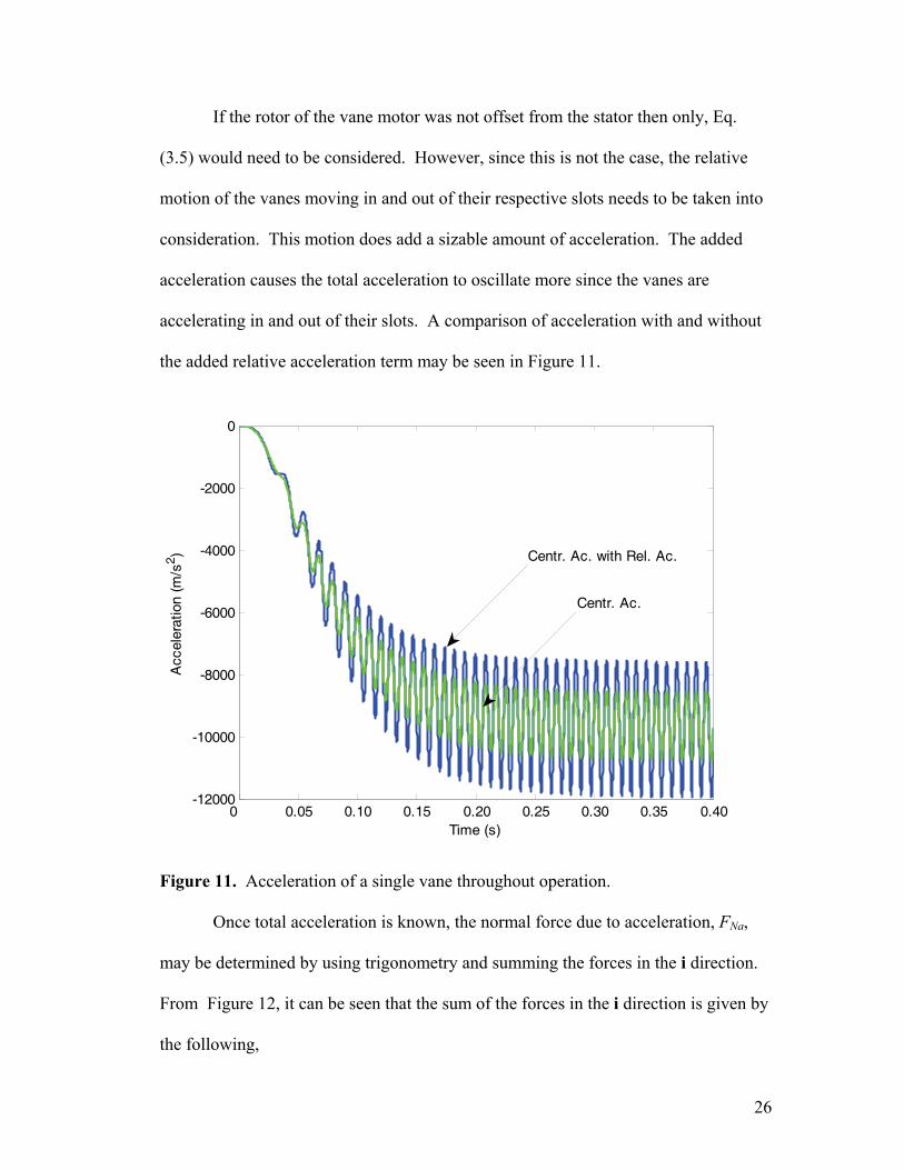
(3.9) cos( ) sin( )v i Na fiF m a F Fβ β= = −∑
where mv is the mass of the vane, ai is the i component of the vane acceleration, β is
the angle between the direction of the normal force and the i direction, and Ff is the
friction force between the rotor and stator and is defined by the following basic
equation:
f NaF Fμ= (3.10)
i FNa
j 180° - θ
β Ff
e
Rs
Figure 12. Orientation of the normal force and the friction force on the vane motor.
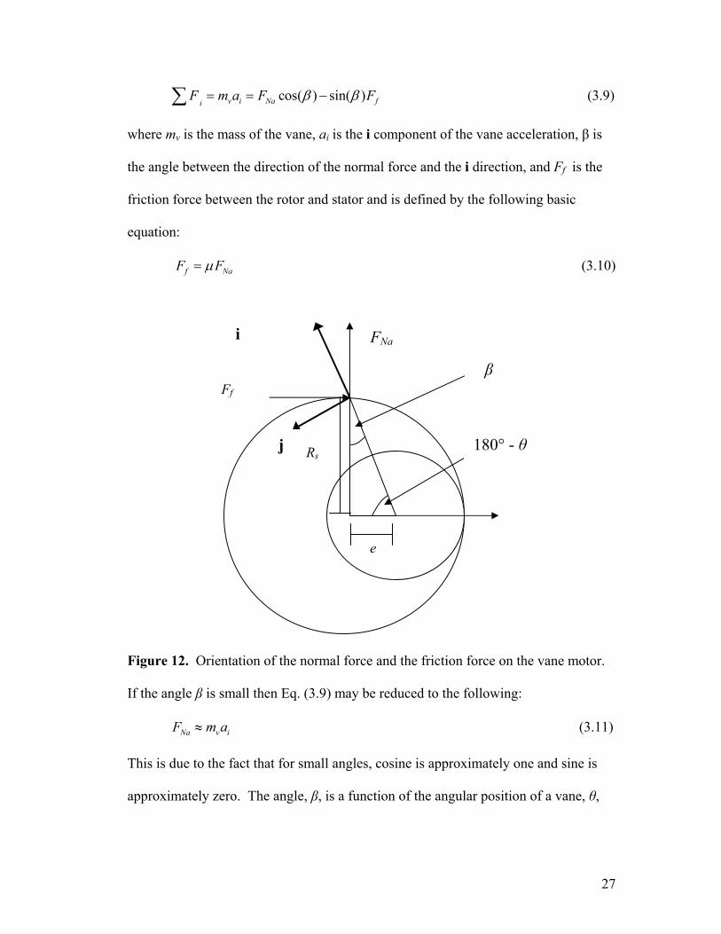
If the angle β is small then Eq. (3.9) may be reduced to the following:
(3.11) Na v iF m≈ a
This is due to the fact that for small angles, cosine is approximately one and sine is
approximately zero. The angle, β, is a function of the angular position of a vane, θ,
27
and the geometry of the hot gas vane motor. From the law of sines, it may be shown
that the equation for β is:
( )1sin 180
sins
eR
θβ
°−⎛ ⎞−⎜=⎜ ⎟⎝ ⎠
⎟ (3.12)
At maximum the angle, β, is only 10 degrees as seen in Figure 13. Therefore, the
small angle approximation used in Eqn. (3.11) will be used for the rest of this work.
0 50 100 150 200 250 300 350-15
-10
-5
0
5
10
15
Theta (degrees)
Bet
a (d
egre
es)
Figure 13. The angle β throughout a single rotation.
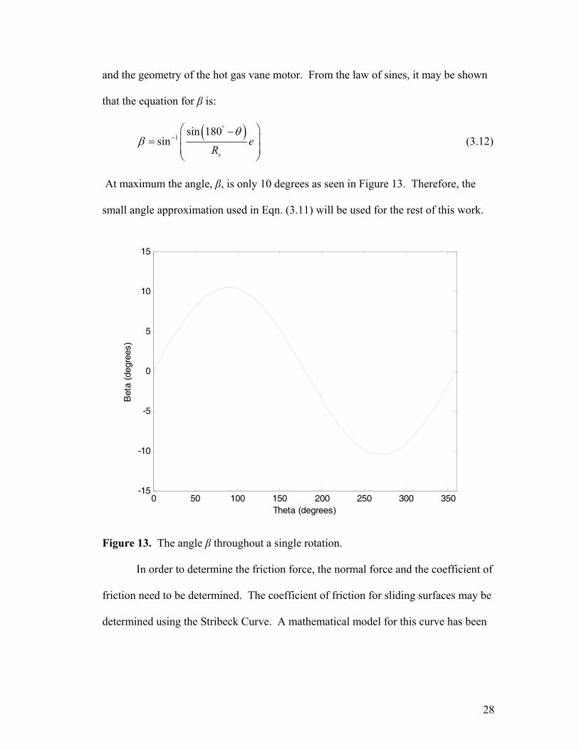
In order to determine the friction force, the normal force and the coefficient of
friction need to be determined. The coefficient of friction for sliding surfaces may be
determined using the Stribeck Curve. A mathematical model for this curve has been
28
suggested in previous work [4] and is presented here as
Exp f fl lN N
η ω η ωμ μ α ε
⎛ ⎞′= − +⎜ ⎟′⎝ ⎠ ′
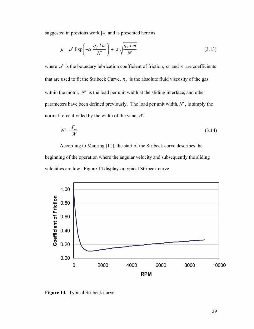
(3.13)
μ′where is the boundary lubrication coefficient of friction, α and ε are coefficients
that are used to fit the Stribeck Curve, fη is the absolute fluid viscosity of the gas
within the motor, is the load per unit width at the sliding interface, and other
parameters have been defined previously. The load per unit width, , is simply the
normal force divided by the width of the vane, W.
N ′
N ′
' naFNW
= (3.14)
According to Manring [11], the start of the Stribeck curve describes the
beginning of the operation where the angular velocity and subsequently the sliding
velocities are low. Figure 14 displays a typical Stribeck curve.
0.00
0.20
0.40
0.60
0.80
1.00
0 2000 4000 6000 8000 10000
RPM
Coef
ficie
nt o
f Fric
tion
Figure 14. Typical Stribeck curve.
29
At the beginning of the operation the vanes are fully in contact with the stator.
When the velocity is increased, mixed lubrication occurs and the vanes are only partly
in contact with the stator so the friction coefficient is reduced. The final phase of the
Stribeck curve describes the fully hydrodynamic zone of the operation where the
surfaces are fully separated by a film of fluid and friction results from shearing the
fluid itself. At this time it is unknown if there is significant liquid in the motor to
support hydrodynamic lubrication.
Now that the friction coefficient and the normal force have been defined, the
friction force may be solved for using Eq. (3.10). The goal of obtaining the friction
force between the vane tip and the stator is to determine the amount of torque that is
created by the friction. Torque is defined as the product between a force and the
perpendicular distance from the center of rotation. For the hot gas vane motor the
friction torque is defined as follows:
f fT l F= i (3.15)
where l is the distance from the center of rotation to the edge of the stator as defined
by Eq. (3.2). Since it was assumed that the angle β is small, it is also assumed that Ff
is always perpendicular to l. Therefore, a scalar multiplication is used in Eq. (3.15)
rather than a cross product multiplication.
During operation, six separate vanes are rotating, which means that six
separate torques are created. Solving for six separate friction torques greatly
increases the calculation effort of the simulation. An attempt was made to reduce the
simulation effort by computing the average friction torque during operation. It was
30
assumed that the friction torque could be approximated as the average friction torque
during one rotation which is defined by the following:
2
02f fnT T d
π
θπ
= ∫ (3.16)
where n is the number of vanes. A comparison of the results between average friction
torque and the actual calculated friction torque is presented in Section 3.2. The net
torque on the rotor, including the torque created by the pressurized chambers and both
viscous friction and the friction between the vane tips and the stator, is now defined
as:
1( ) ( ) ( ) ( )n
s i f f f a a a iT t P t A r t A r t b Tθ θ θ⎡ ⎤= −⎣ ⎦∑ f− − (3.17)
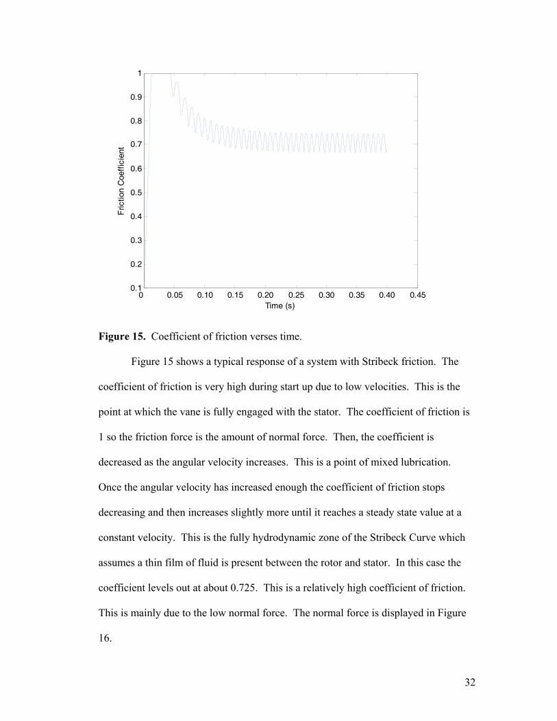
3.2 Simulation Results Including Friction Torque
The coefficient of friction between the vane tips and the stator was solved for
using a Stribeck curve. Figure 15 displays how the coefficient of friction changes
with time.
31
0 0.05 0.10 0.15 0.20 0.25 0.30 0.35 0.40 0.450.1
0.2
0.3
0.4
0.5
0.6
0.7
0.8
0.9
1
Time (s)
Fric
tion
Coe
ffic
ient
Figure 15. Coefficient of friction verses time.
Figure 15 shows a typical response of a system with Stribeck friction. The
coefficient of friction is very high during start up due to low velocities. This is the
point at which the vane is fully engaged with the stator. The coefficient of friction is
1 so the friction force is the amount of normal force. Then, the coefficient is
decreased as the angular velocity increases. This is a point of mixed lubrication.
Once the angular velocity has increased enough the coefficient of friction stops
decreasing and then increases slightly more until it reaches a steady state value at a
constant velocity. This is the fully hydrodynamic zone of the Stribeck Curve which
assumes a thin film of fluid is present between the rotor and stator. In this case the
coefficient levels out at about 0.725. This is a relatively high coefficient of friction.
This is mainly due to the low normal force. The normal force is displayed in Figure
16.
32
0 0.05 0.10 0.15 0.20 0.25 0.30 0.35 0.40 0.450
5
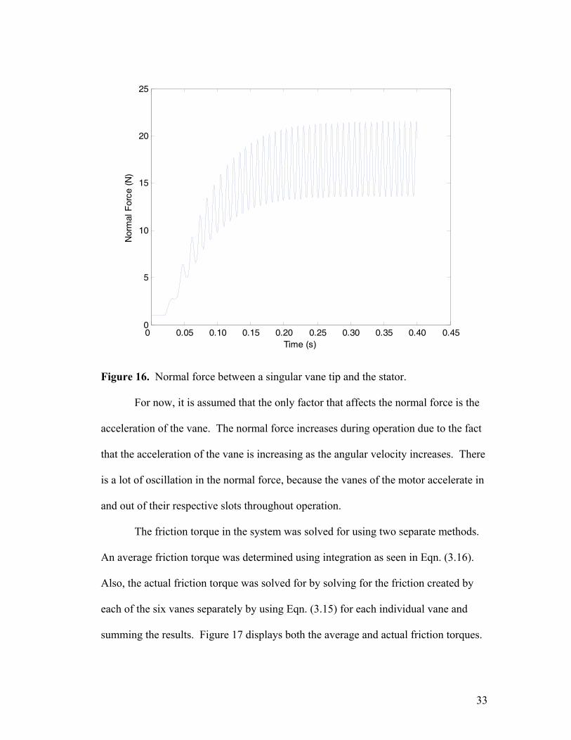
10
15
20
25
Time (s)
Nor
mal
For
ce (
N)
Figure 16. Normal force between a singular vane tip and the stator.
For now, it is assumed that the only factor that affects the normal force is the
acceleration of the vane. The normal force increases during operation due to the fact
that the acceleration of the vane is increasing as the angular velocity increases. There
is a lot of oscillation in the normal force, because the vanes of the motor accelerate in
and out of their respective slots throughout operation.
The friction torque in the system was solved for using two separate methods.
An average friction torque was determined using integration as seen in Eqn. (3.16).
Also, the actual friction torque was solved for by solving for the friction created by
each of the six vanes separately by using Eqn. (3.15) for each individual vane and
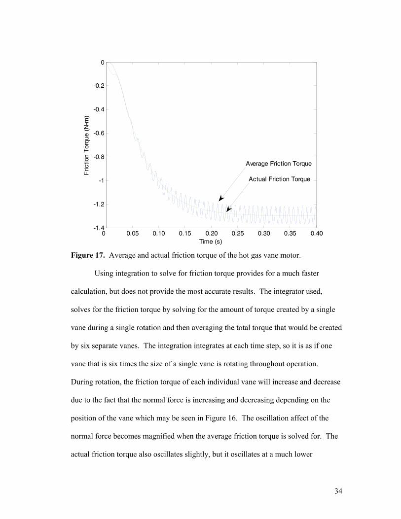
summing the results. Figure 17 displays both the average and actual friction torques.
33
0 0.05 0.10 0.15 0.20 0.25 0.30 0.35 0.40-1.4
-1.2
-1
-0.8
-0.6
-0.4
-0.2
0
Time (s)
Fric
tion
Tor
que
(N-m
)
Average Friction Torque
Actual Friction Torque
Figure 17. Average and actual friction torque of the hot gas vane motor.
Using integration to solve for friction torque provides for a much faster
calculation, but does not provide the most accurate results. The integrator used,
solves for the friction torque by solving for the amount of torque created by a single
vane during a single rotation and then averaging the total torque that would be created
by six separate vanes. The integration integrates at each time step, so it is as if one
vane that is six times the size of a single vane is rotating throughout operation.
During rotation, the friction torque of each individual vane will increase and decrease
due to the fact that the normal force is increasing and decreasing depending on the
position of the vane which may be seen in Figure 16. The oscillation affect of the
normal force becomes magnified when the average friction torque is solved for. The
actual friction torque also oscillates slightly, but it oscillates at a much lower
34
amplitude since the friction torque of each vane is solved for separately and then
summed together. The advantage to using an average friction torque is a decrease in
computational effort, but an undesirable oscillatory affect is created. For higher
accuracy, the friction torque of each vane should be solved for separately. In this
work, the friction torque was solved for by solving for the friction torque of each vane
separately for accuracy.
As was previously stated, the friction coefficient decreases during operation
while the normal force increases as speed increases. Because, the normal force
increases more than the friction coefficient decreases, the overall friction torque
increases during operation as seen in Figure 17. The friction torque works against the
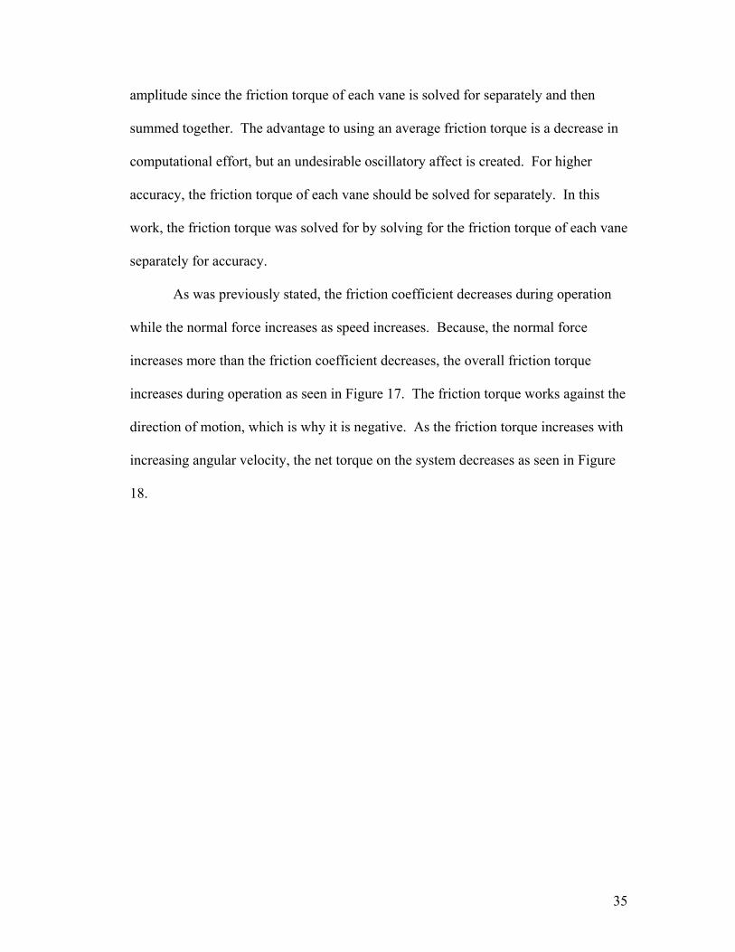
direction of motion, which is why it is negative. As the friction torque increases with
increasing angular velocity, the net torque on the system decreases as seen in Figure
18.
35
0 0.2 0.4 0.6 0.8 1.0 1.2 1.4 1.6 1.8 2.0-0.5
0
0.5
1
1.5
2
Time (s)
Tot
al T
orqu
e (N
-m) Torque with only viscous friction
Torque with viscous friction and friction at vane tip
Figure 18. Net torque of the system.
Both torques should be reduced to zero. Only the significant portion of torque
is presented in Figure 18. Once the angular velocity stopped increasing at a
significant rate the simulation was stopped. When only viscous friction was present
on the device, the net torque required more time to reach steady state. Without
friction on the vane tips the device takes almost 2 seconds to reach steady state,
whereas with friction on the vane tips, the device takes only about 0.4s. The added
friction torque from friction between the stator and the vane tips is what slows down
the device allowing a steady state to be reached at a faster rate. In both cases, the
velocity is still increasing slightly, but the rate at which it is increasing is very slow,
so it was assumed that a steady state had been reached.
36
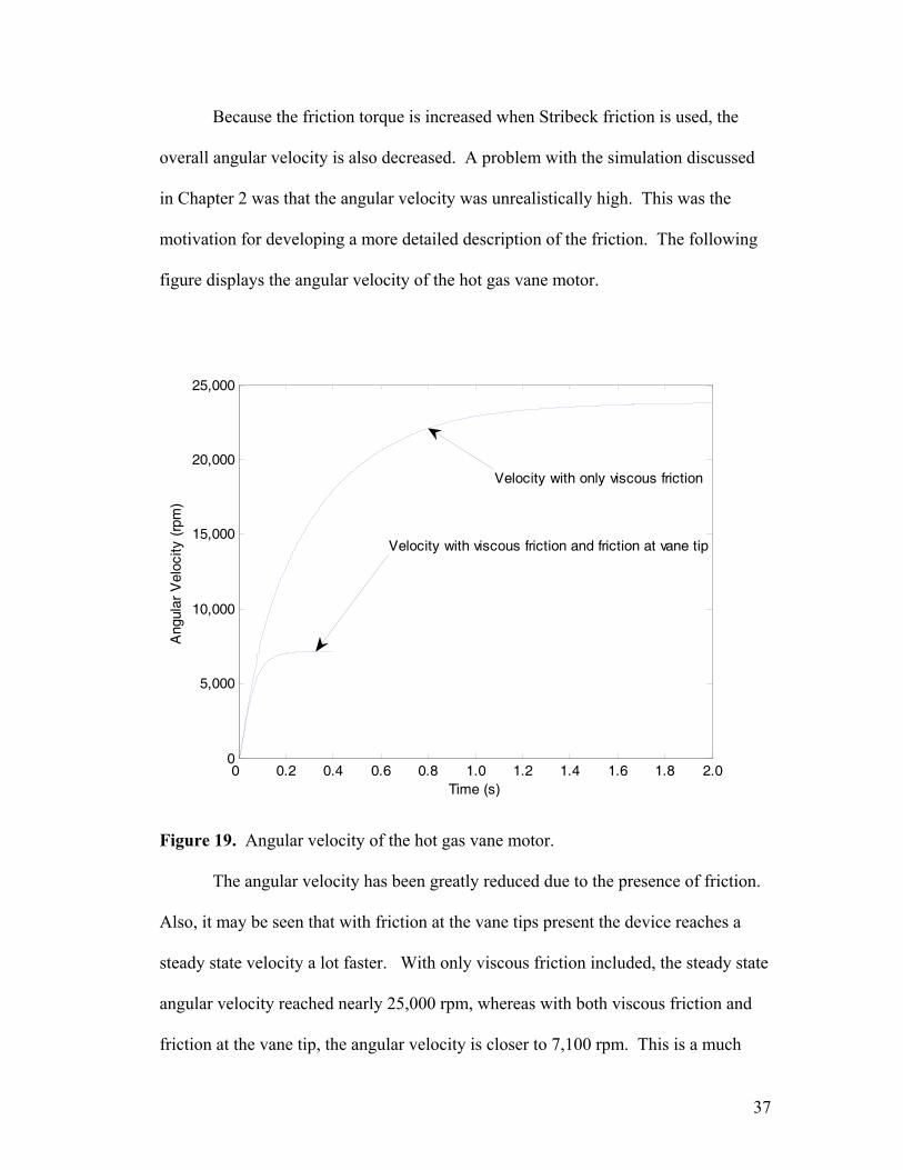
Because the friction torque is increased when Stribeck friction is used, the
overall angular velocity is also decreased. A problem with the simulation discussed
in Chapter 2 was that the angular velocity was unrealistically high. This was the
motivation for developing a more detailed description of the friction. The following
figure displays the angular velocity of the hot gas vane motor.
0 0.2 0.4 0.6 0.8 1.0 1.2 1.4 1.6 1.8 2.00
5,000
10,000
15,000
20,000
25,000
Time (s)
Ang
ular
Vel
ocity
(rp
m)
Velocity with only viscous friction
Velocity with viscous friction and friction at vane tip
Figure 19. Angular velocity of the hot gas vane motor.
The angular velocity has been greatly reduced due to the presence of friction.
Also, it may be seen that with friction at the vane tips present the device reaches a
steady state velocity a lot faster. With only viscous friction included, the steady state
angular velocity reached nearly 25,000 rpm, whereas with both viscous friction and
friction at the vane tip, the angular velocity is closer to 7,100 rpm. This is a much
37

more reasonable level of angular velocity. However, there is one factor that has yet
to be considered, and that is the pressure on the ends of the vane. Depending on how
the hot gas vane motor is designed, there may be a significant amount of pressure on
the back end of the vanes, which would in turn increase the normal force and also the
amount of friction on the tip of each vane.
38
Chapter 4
Pressure Model
4.1 Discussion of Pressure Model
It was shown in the previous chapter that the amount of friction on the end of
the vanes has a significant affect on the operation of the hot gas vane motor. The
friction force is a function of the normal force between the vane tips and the stator.
Increasing the normal force on the end of the vane increases the friction between the
vane and the stator, but it also ensures the vane stays in contact with the stator so that
minimum leakage occurs between chambers. The focus of this chapter will be to
discuss the affects of pressure on the ends of the vane.
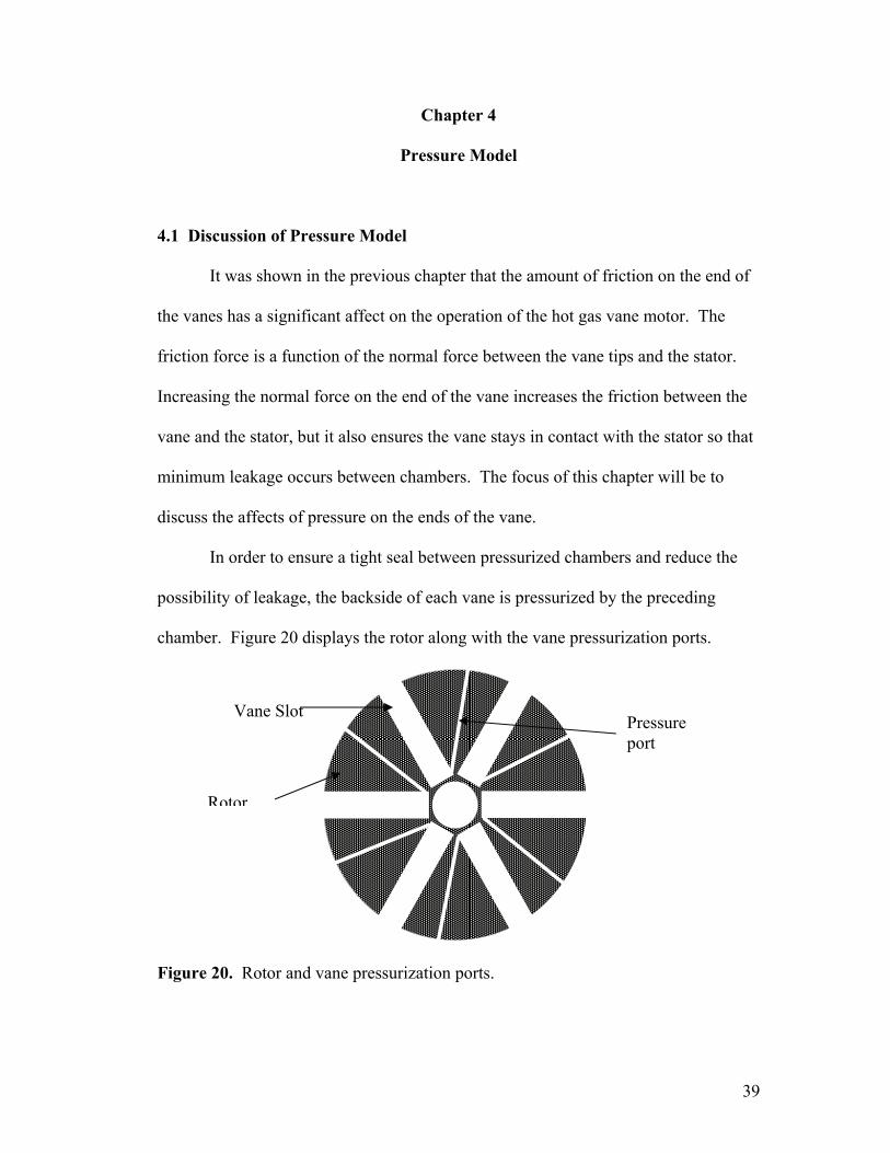
In order to ensure a tight seal between pressurized chambers and reduce the
possibility of leakage, the backside of each vane is pressurized by the preceding
chamber. Figure 20 displays the rotor along with the vane pressurization ports.
Vane Slot Pressure port
Rotor
Figure 20. Rotor and vane pressurization ports.
39
It should be noted that the vane does not need to be in contact with the stator
for the exhaust phase of operation. The chambers are not pressurized at this point and
no torque is created, so no seal is required between the vane and stator. Also, the
vane is not pressurized during the exhaust phase of the operation, between 210 and 30
degrees, since the pressure is reduced to atmospheric at this point. This means that
the pressure does not affect the amount of friction within the system during the
exhaust phase of operation since pressure forces on the ends of the vane are
equalized.
During the working phase of operation, between 30 and 210 degrees, the vane
is pressurized to counteract pressure forces on the tip of the vane so extra friction is
created. The amount of pressure on the vane tip depends on the shape of the vane.
The two most likely shapes of a vane would be either a straight-edged vane or a
rounded vane. A straight-edged vane will eventually become rounded due to wear
caused by the contact between the vane tip and the stator. This work will consider
both conditions for a vane tip.
4.2 Straight-edged Vane Tip Pressure Calculation
The straight edged vane will be considered first. The amount of pressure on
the tip of the vane is dependant on the exposed area on the tip of the vane and is
therefore dependant on the orientation of a particular vane. For a straight-edged vane,
it is assumed that the vane is either tilted forward in its slot, exposing the vane to the
pressure of the leading chamber, or else the vane is tilted back in its slot exposing the
vane to the pressure of the lagging chamber.
40
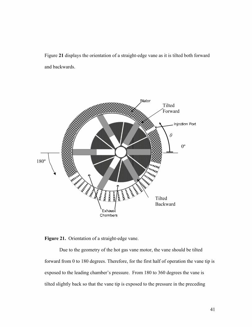
Figure 21 displays the orientation of a straight-edge vane as it is tilted both forward
and backwards.
Tilted Forward
0º
180º
Tilted Backward
Figure 21. Orientation of a straight-edge vane.
Due to the geometry of the hot gas vane motor, the vane should be tilted
forward from 0 to 180 degrees. Therefore, for the first half of operation the vane tip is
exposed to the leading chamber’s pressure. From 180 to 360 degrees the vane is
tilted slightly back so that the vane tip is exposed to the pressure in the preceding
41
chamber. The total force due to pressure from 180 to 360 degrees is zero, since the
backside of the vane is also pressurized by the lagging chamber. During the exhaust
phase from 210 to 30 degrees, it is irrelevant which chamber the vane is exposed to
since the pressures are both atmospheric. From 0 to 30 degrees, no friction is added
due to pressure since the pressures on both ends of the vane are identical.
From 30 to 180 degrees, a net force is created due to the pressure difference
between the ends of the vanes. The added force increases the normal force on a
particular vane, thus increasing the friction torque. The added normal force due to
pressure for a single vane in the ith chamber is defined by the following:
(4.1) ( )1
0 0 < 30 < 180
0 180 < 360np i i viF P P A
θ
θ
θ+
⎧ <⎪
= − <⎨⎪ <⎩
30
)
where Avi is the area of the tip of the ith vane, and Pi and Pi+1 are the pressures in
chambers i and i+1 respectively. Chapter 3 discussed how to solve for the normal
and friction forces caused by centripetal forces. By adding the normal force due to
pressure to the normal force due to centripetal and relative forces and multiplying by
the moment arm, a new term for frictional torque of a single vane may be computed.
(f na npT l F F μ= × + (4.2)
The total friction torque within the system is the sum of the friction torques
from each individual vane and the viscous friction. The net torque on the system,
including both viscous friction and the newly defined friction between the vane tips
and the stator, is defined as:
1( ) ( ) ( ) ( )n
s i f f f a a a iT t P t A r t A r t b Tθ θ θ⎡ ⎤= −⎣ ⎦∑ f− − (4.3)
42
4.3 Rounded Vane Tip Pressure Calculation
For a rounded vane tip, the total pressure on the vane is slightly different than
a straight-edged vane. For a rounded end, the actual position of the contact point
between the vane tip and the stator is slightly off center, but for simplicity it was
assumed that the center of the vane would be in contact with stator at all times.
Therefore, half of the vane tip is exposed to the leading chamber’s pressure and the
other half of the vane tip is exposed to the lagging chamber’s pressure. Figure 22
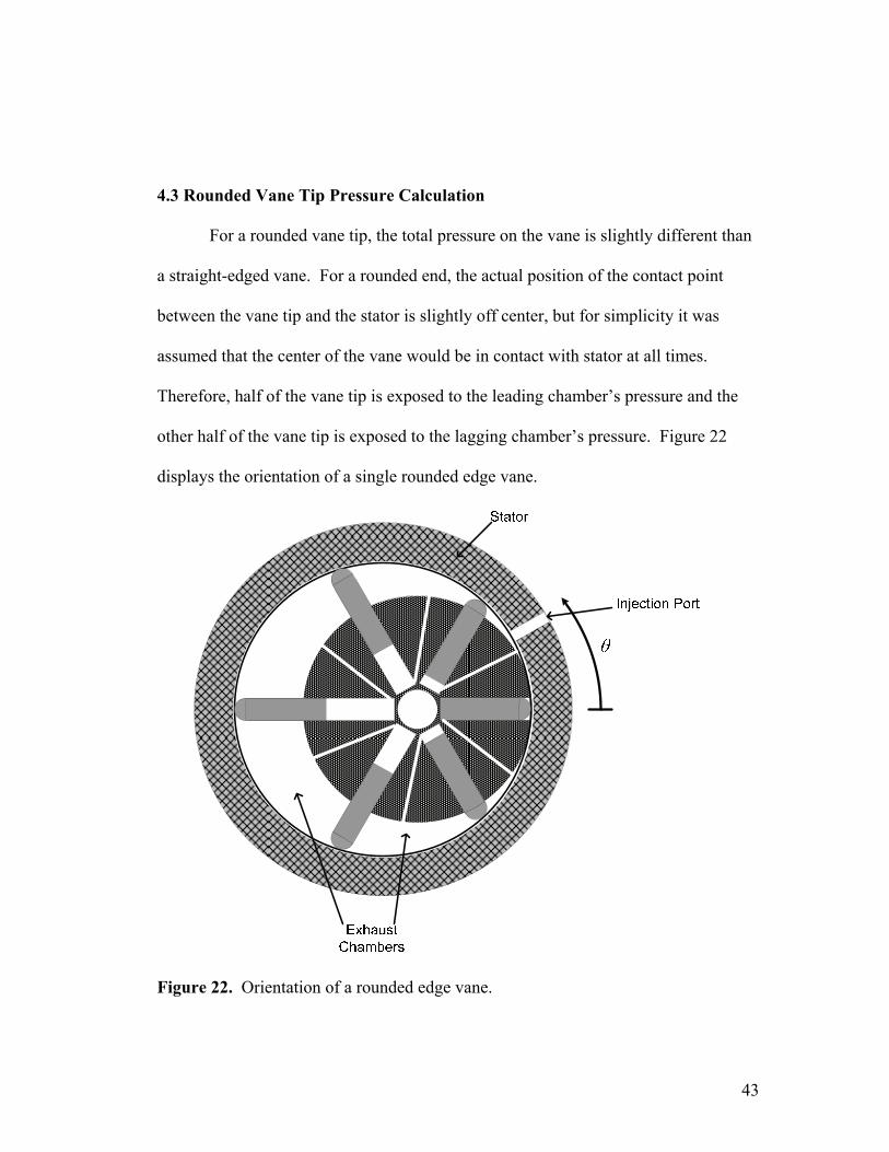
displays the orientation of a single rounded edge vane.
Figure 22. Orientation of a rounded edge vane.
43
The added normal force due to pressure for a single vane in the ith chamber is
the difference between the force on the back of the vane and force on the tip of the
vane and is defined by the following:
(4.4) ( 11/ 2 1/ 2np i vi i vi i viF P A P A P A+= − + )
where Avi is the area of the tip of the ith vane, and Pi and Pi+1 are the pressures in
chambers i and i+1 respectively. Equation (4.4) may now be substituted into Eq.
(4.2) to solve for the friction torque. The total torque may again be solved for using
Eq. (4.3).
4.4 Results
The purpose of channeling pressure to the backside of the vane is to
counteract the pressure forces on the tip of the vane. The pressure on the backside
should be larger than the pressure on the tip of the vane which means the overall
normal force between the vane tip and the stator increases. In order to operate
properly the vanes need to be pressurized to ensure the vanes never lose contact with
the stator. The simulation of a hot gas vane motor running without pressure on the
vane ends was presented to compare the affects of centripetal forces verses pressure
forces on the performance of the hot gas vane motor. A plot of normal forces for the
three cases that have been discussed, rounded-edge vane tip, straight-edge vane tip,
and an unpressurized vane, is displayed in Figure 23.
44
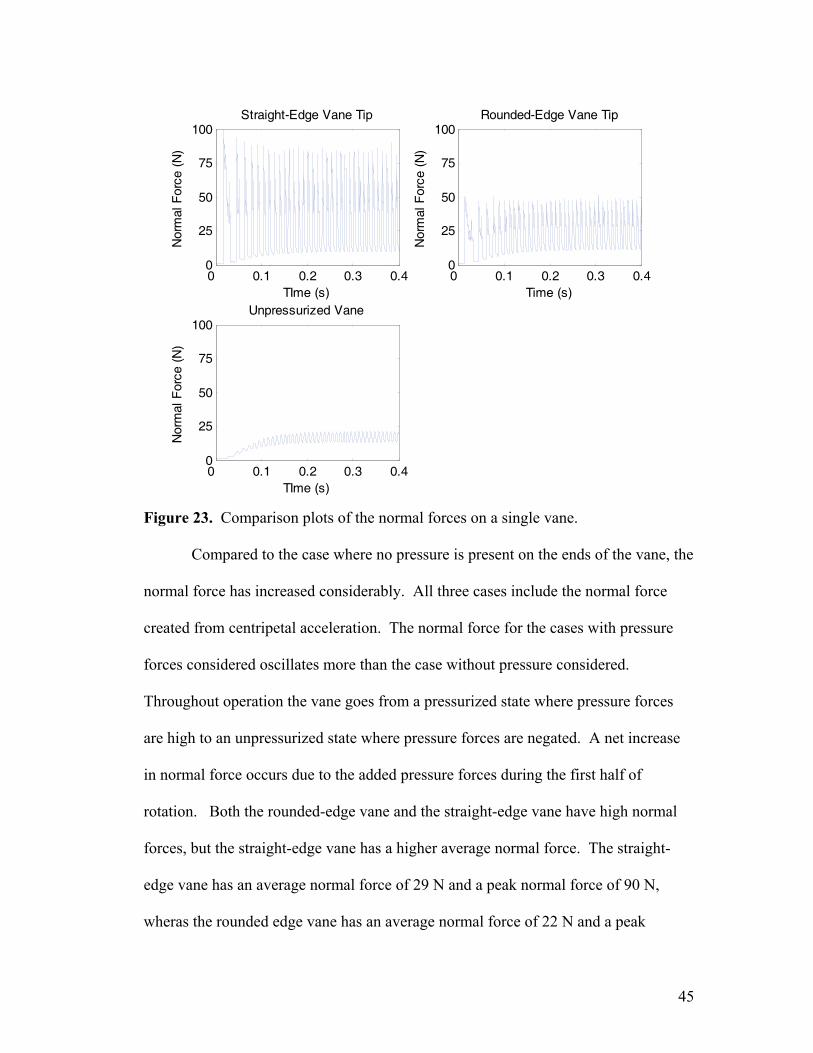
0 0.1 0.2 0.3 0.40
25
50
75
100Rounded-Edge Vane Tip
Time (s)
Nor
mal
For
ce (
N)
0 0.1 0.2 0.3 0.40
25
50
75
100Straight-Edge Vane Tip
TIme (s)
Nor
mal
For
ce (
N)
0 0.1 0.2 0.3 0.40
25
50
75
100Unpressurized Vane
TIme (s)
Nor
mal
For
ce (
N)
Figure 23. Comparison plots of the normal forces on a single vane.
Compared to the case where no pressure is present on the ends of the vane, the
normal force has increased considerably. All three cases include the normal force
created from centripetal acceleration. The normal force for the cases with pressure
forces considered oscillates more than the case without pressure considered.
Throughout operation the vane goes from a pressurized state where pressure forces
are high to an unpressurized state where pressure forces are negated. A net increase
in normal force occurs due to the added pressure forces during the first half of
rotation. Both the rounded-edge vane and the straight-edge vane have high normal
forces, but the straight-edge vane has a higher average normal force. The straight-
edge vane has an average normal force of 29 N and a peak normal force of 90 N,
wheras the rounded edge vane has an average normal force of 22 N and a peak
45
normal force of 51 N. The straight-edge vane is completely exposed to the lower
pressure leading chamber. As a result, the pressure difference between the back of
the vane and the tip of the vane should be much higher than that of the rounded edge
vane. Approximately half of the rounded edge vane is exposed to the lower pressure
leading chamber, so the pressure difference between the vane ends should be about
half that of the straight-edge case.
It was shown in the previous chapter that increasing the normal force
decreases the coefficient of friction, which is a trait of the Stribeck Curve. Figure 24
displays the coefficient of friction for the three cases under discussion.
0 0.1 0.2 0.3 0.40
0.2
0.4
0.6
0.8
1
Time (s)
Coe
ffic
ient
of
Fric
tion
Round-Edged Vane Tip
0 0.1 0.2 0.3 0.40
0.2
0.4
0.6
0.8
1
Time (s)
Coe
ffic
ient
of
Fric
tion
Straight-Edge Vane Tip
0 0.1 0.2 0.3 0.40
0.2
0.4
0.6
0.8
1
Time (s)
Coe
ffic
ient
of
Fric
tion
Unpressurized Vane
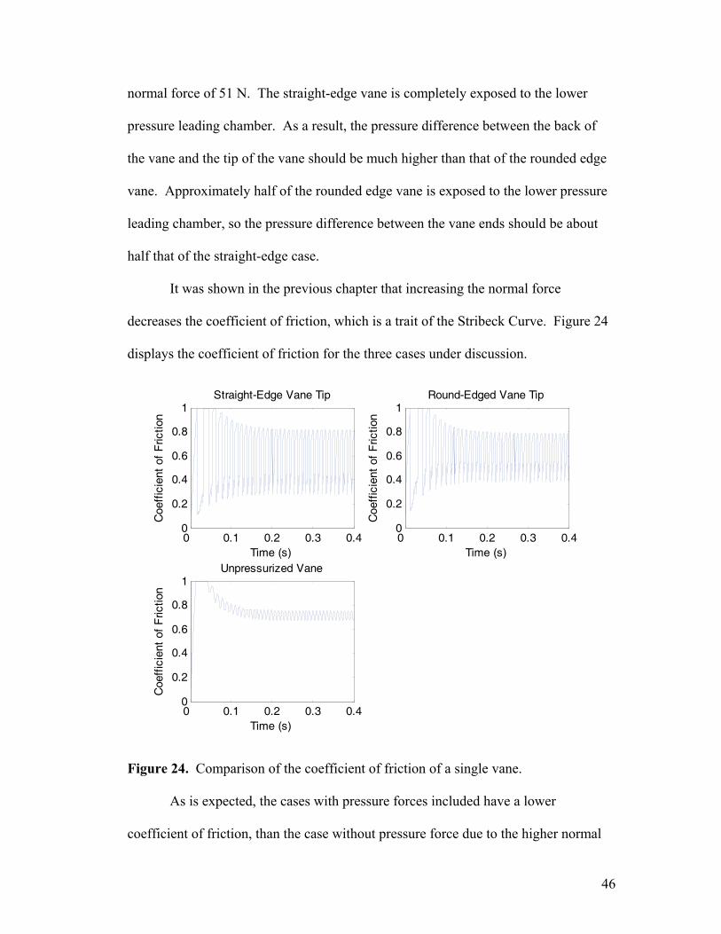
Figure 24. Comparison of the coefficient of friction of a single vane.
As is expected, the cases with pressure forces included have a lower
coefficient of friction, than the case without pressure force due to the higher normal
46
forces. The friction coefficient oscillates, because the normal force oscillates due to
the vane entering and exiting the pressurized portion of operation. When the vane is
in the exhaust phase and no pressure forces are present, the coefficient of friction is
only based on centripetal forces, and is fairly close to the results from the
unpressurized case. Without pressure, the coefficient of friction at steady state was
roughly 0.7. For a straight-edge vane tip, the coefficient of friction oscillates, but on
average the coefficient of friction is about 0.4. The rounded edge vane tip has a
slightly higher average coefficient of friction, 0.5, due to the lower normal forces.
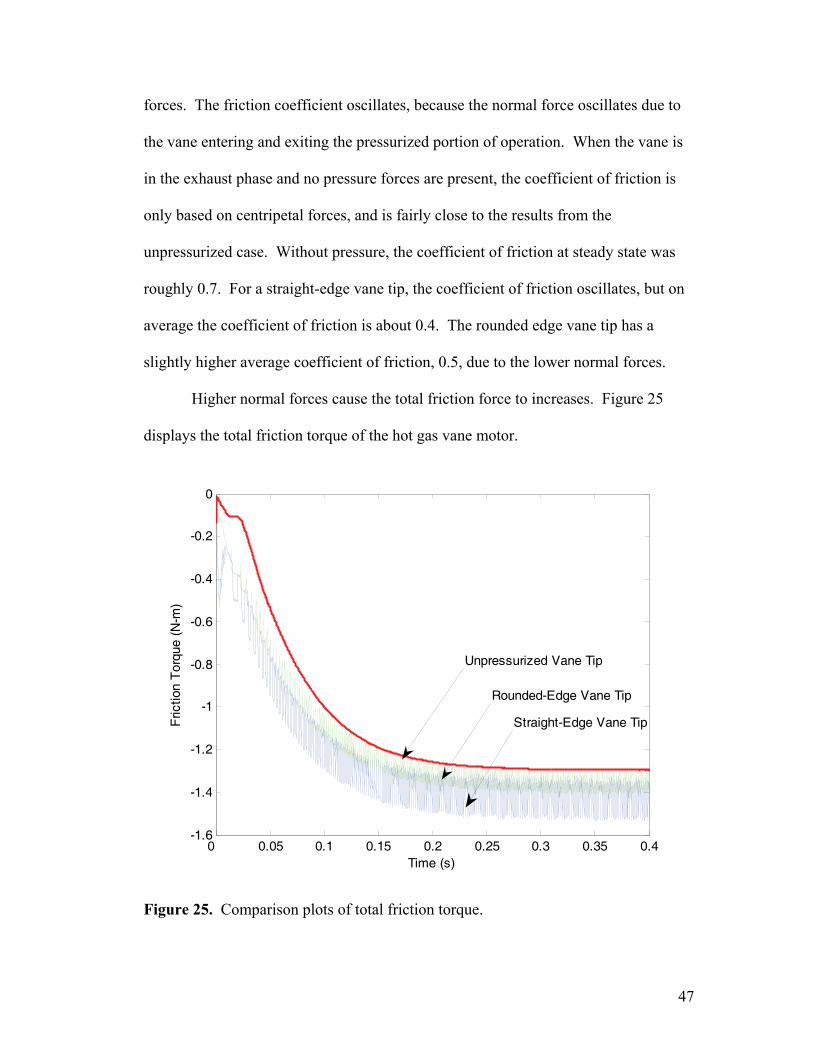
Higher normal forces cause the total friction force to increases. Figure 25
displays the total friction torque of the hot gas vane motor.
0 0.05 0.1 0.15 0.2 0.25 0.3 0.35 0.4-1.6
-1.4
-1.2
-1
-0.8
-0.6
-0.4
-0.2
0
Time (s)
Fric
tion
Tor
que
(N-m
)
Unpressurized Vane Tip
Rounded-Edge Vane Tip
Straight-Edge Vane Tip
Figure 25. Comparison plots of total friction torque.
47
The total friction in the system is the sum of the friction torques of the six
vanes. As is expected the pressurized cases have higher friction torques. Even
though the rounded edge vane tip has a higher coefficient of friction, the straight-edge
vane tip has a higher friction torque. The normal force of the straight-edge vane is
higher than the rounded edge vane which causes the overall friction torque to be
higher. Again, the pressurized cases tend to oscillate more due to the fact that vanes
are entering and exiting pressurized areas. The unpressurized case also oscillates, but
it oscillates with a much lower amplitude.
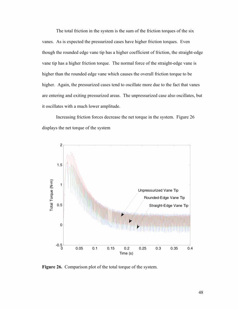
Increasing friction forces decrease the net torque in the system. Figure 26
displays the net torque of the system
0 0.05 0.1 0.15 0.2 0.25 0.3 0.35 0.4-0.5
0
0.5
1
1.5
2
Time (s)
Tot
al T
orqu
e (N
-m)
Unpressurized Vane Tip
Rounded-Edge Vane Tip
Straight-Edge Vane Tip
Figure 26. Comparison plot of the total torque of the system.
48
For all cases, the total torque should eventually decrease to zero once a steady
velocity is achieved. Due to long simulation times, only enough data to reach a
negligible amount of torque was taken. The total torque of the system decreases
slightly faster for the pressurized cases. The straight-edge vane decreases the fastest,
which means that it should give a poorer performance than a hot gas vane motor with
rounded edges due to friction losses. Also, the unpressurized case tends to oscillate
less than the pressurized cases since the friction torque oscillates more when the
vanes are pressurized. The unpressurized case’s total torque oscillated over a range
of 0.2 N-m while the rounded edge and straight-edge vane cases oscillated over a
range of 0.25 N-m and 0.5 N-m respectively.
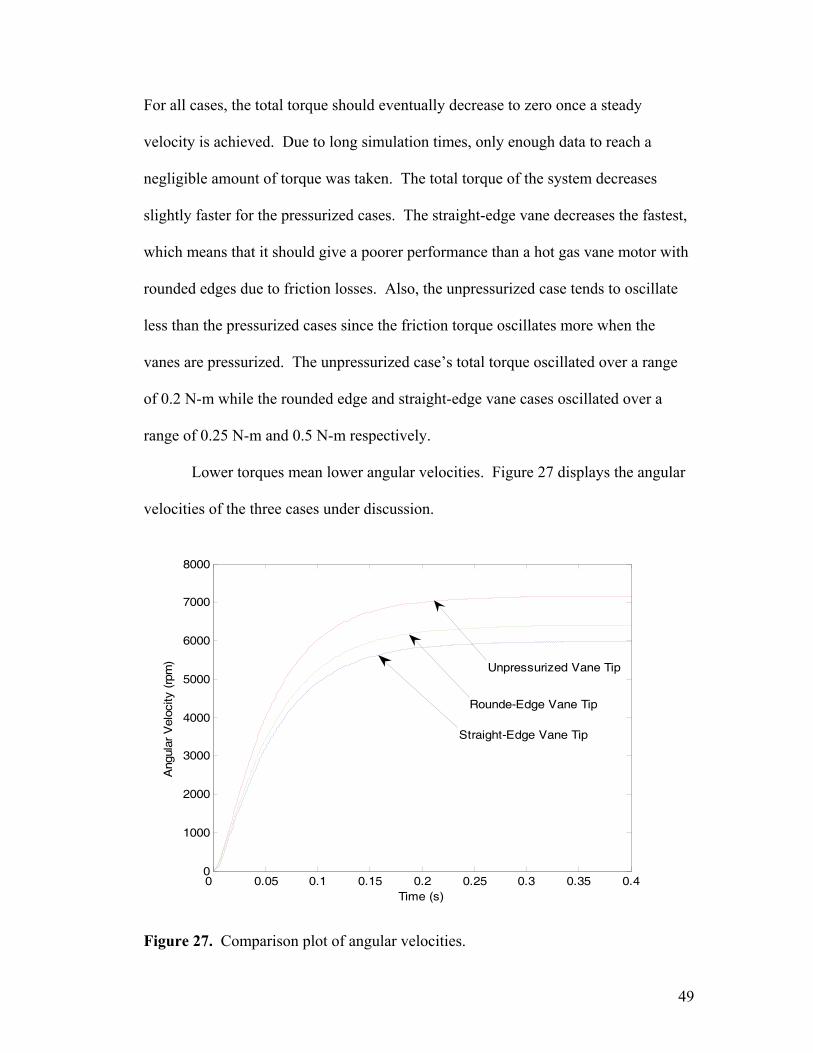
Lower torques mean lower angular velocities. Figure 27 displays the angular
velocities of the three cases under discussion.
0 0.05 0.1 0.15 0.2 0.25 0.3 0.35 0.40
1000
2000
3000
4000
5000
6000
7000
8000
Time (s)
Ang
ular
Vel
ocity
(rp
m) Unpressurized Vane Tip
Rounde-Edge Vane Tip
Straight-Edge Vane Tip
Figure 27. Comparison plot of angular velocities.
49
As is expected the unpressurized vane tip case experiences the highest angular
velocity, 7,100 rpm. The pressurized cases rotate slightly slower, 6,400 rpm and
6,000 rpm for the rounded edge and straight-edge vane tip respectively. The lower
angular velocities are due to the added pressure forces, which create friction
The unpressurized case is an unreasonable situation. Pressure needs to be
included in the design, because without pressure forces on the vane, the chambers of
the hot gas vane motor could not remain sealed. If the chambers are not sealed, then
massive amounts of leakage will occur within the device causing very poor
performance. To ensure that a minimal amount of leakage occurs between chambers,
the backside of each vane needs to be pressurized to counteract the pressure forces on
the tip. To minimize the amount of friction losses a rounded edge vane tip should be
used.
50
Chapter 5
Efficiency Modeling
5.1 Discussion of Efficiency
The first objective of this work was to model and understand the operation of
a vane motor. Then the developed model could be used to optimize the performance
of the device. The efficiency of a vane motor is based primarily on the geometry of
the device. By properly designing the dimensions of the stator and rotor relative to
each other, it is anticipated that better performance and efficiency can be observed.
In order to optimize the performance of the hot gas vane motor, a measure of
performance must first be defined. For this work, the efficiency is a comparison of
the amount of energy that is injected into the motor compared to the amount of
energy that is wasted by means of exhausting hot gas from the system. The highest
possible efficiency of the motor is defined by the following from [1]:
1
1 1 1 2 2
2 1 1
1 V PV PV Useful EnergyV PV Energy
γ
η−
⎛ ⎞ −= − = =⎜ ⎟
⎝ ⎠
in (5.1)
1
2
VV
where is the expansion ratio of the volumes, P1 is the initial pressure, P2 is the
pressure prior to exhaust, and γ is a ratio of specific heats. The initial volume, V1, is
the smallest volume of a full chamber at the beginning of the cycle which for the
model occurs at 90 degrees and is approximately 1.215e-6 m3. At 90 degrees, a
chamber is cut off from the injection port so the chamber is full of hot gas and is at its
smallest volume. The final volume, V2, is the largest volume a chamber reaches just
prior to the exhaust phase of the cycle which occurs at 210 degrees and is
51
approximately 3.11e-6 m3. From Eqn. (5.1), it can be shown that with the current
geometry the highest possible efficiency of the vane motor is approximately 27.7%.
This efficiency does not take into account heat loss, leakage, or friction effects. Also,
it is assumed that throughout the operation of the device, the propellant remains a gas,
which is not necessarily the case. The expansion ratio of the hot gas during operation
determines how much torque can be created by the device. To optimize the vane
motor, different motor geometries should be tested to see if any major changes in
performance or efficiency are observed. The total efficiency of any system is just a ratio of the energy supplied to the
system and the amount of energy that is produced as usable work. The internal
energy entering the system is defined by the following,
1 11 1
PVEγ
=−
(5.2)
where P1 is the pressure at the inlet and V1 is the inlet volume. Ideally the total
internal energy from a single chamber is 3.86 Nm. The amount of energy that is
wasted through exhaust by the system is defined by the following,
2 22 1
PVEγ
=−
(5.3)
where P2 is the pressure in the chamber just prior to exhaust and V2 is the volume in
the chamber just prior to exhaust. Equation (5.3) refers to the amount of energy that
is wasted by exhausting the hot gas. The pressure in the chambers at “steady” speed
operation may be viewed in Figure 28.
52
0 180 360 540 720 900 1080 1260 14401
2
3
4
5
6
x 105
Theta (degrees)
Pre
ssur
e (P
a)
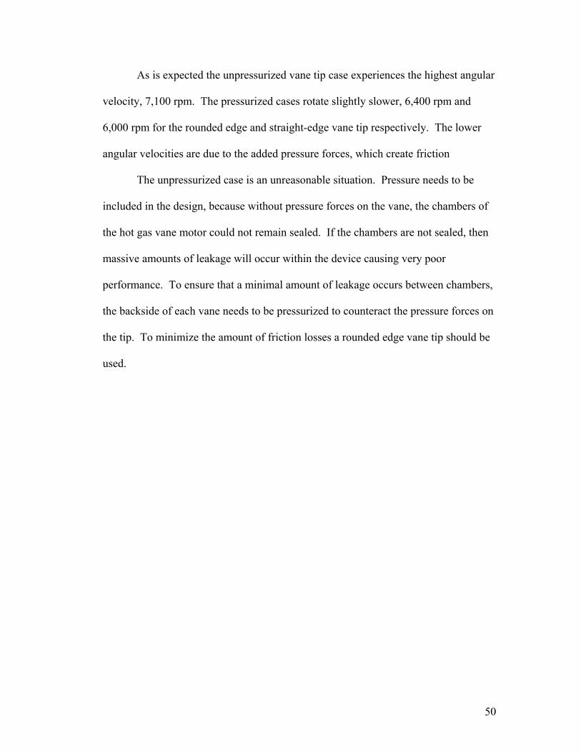
Figure 28. Pressure in a single chamber.
The pressure in the chamber just prior to exhaust is about 310,000 Pa. This means
that the amount of energy that is wasted through exhaust is 2.8 Nm.
The ideal efficiency from Eqn. (5.1) uses the assumption that E1 and E2 are the
only energies present within the system. For a more accurate description of the
efficiency of the vane motor, the energy dissipated due to friction was considered.
The actual efficiency of the vane motor is defined by the following,
1 2
1
( ) fn E E WnE
η− −
= (5.4)
where n is the number of chambers, and Wf is the energy dissipated due to friction.
The total amount of energy that is wasted as a result of friction may be determined
from dynamics by integrating the frictional force, Ff, with respect to the path of the
53
vane using the following,
(5.5) 2
0
( )f fW Fπ
θ= ∫ idr
Since the force is always parallel to the stator surface, dr is simply an arc on
the stator which may be defined as ldθ where l is the distance from the center of
rotation on the rotor to the edge of the stator as was defined by Eqn. (3.2). The
following simplified equation may be used to solve for the energy dissipated as a
result of friction,
2 2
0 0
( ) ( ) ( )f f fW F dr F l dπ π
θ θ θ θ= ∫ ∫i (5.6)
The efficiency can now be solved for using Eqn. (5.4). By including the affects of
friction the efficiency of the device is reduced from 27.7% to 8.8%.
5.2 Results
In order to optimize the design of the hot gas vane motor, the preceding
analysis was duplicated using several different vane geometries. Vane motors can be
designed in numerous sizes and shapes, and it is desirable to know how the size of the
motor will affect its performance. The following figure displays how both the ideal
efficiency and the efficiency as computed by the model vary with the radius of the
stator.
54
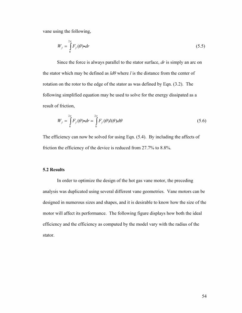
50
Figure 29. Actual and maximum efficiencies of vane motors with various stator
radii.
Both the affects of friction and the affects of pressure were considered for the
analysis. It was assumed that the ends of the vane tips were rounded. It was shown
in Chapter 4 that rounded edge vane tips tend to reduce the amount of friction as
compared with vanes with straight tips. The maximum efficiency increases with a
larger stator radius, which is expected since increasing the stator radius increases the
volume expansion ratio. The actual efficiency also increases substantially. The length
of the stator radius is limited by the distance between the rotor and stator. If the
distance is too great the vane will slip from the rotor which is obviously undesirable.
However, designing a motor with a larger stator radius does seem to produce better
0.16 0.18 0.2 0.22 0.24 0.260
5
10
15
20
25
30
35
40
Max possible Calculated
45
Radius of Stator (m)
Eff
icie
ncy
(%)
55
results. Increasing the stator size increases the efficiency of the device by increasing
the expansion ratio of the hot gas. Increasing expansion ratio ensures that less gas is
wasted through exhaust.
56
Chapter 6
Conclusions
6.1 Overview
The main objectives of this work were to first establish a working model of a
hot gas vane motor. Then, a means for measuring performance was presented by way
of efficiency. Finally, the model was used to show that by adjusting certain
parameters, the overall efficiency of the device could be improved.
The model presented is based primarily on determining the net amount of
torque produced by the device. The amount of torque in the system is dependant on
the amount of pressure in the system. By using equations for pressure based on an
isentropic process, a model of the amount of torque created may be developed. Next,
it was shown that the amount of friction within the system has a significant affect on
the performance of the device. It was shown in Chapter 3 that dynamic equations
may be used to solve for the acceleration of the vanes in the direction normal to the
stator’s surface, which may be used to solve for the friction torque between the vane
tips and the stator. Without friction, the simulations showed that the device would
rotate at nearly 25,000 rpm and that steady state velocity could be approached in 2
seconds. When friction was included, the simulation showed that the device would
rotate at a much lower speed, 7,100 rpm, and approach steady state in 0.4 seconds.
The simulation with friction is a much more reasonable result for the performance of
a hot gas vane motor. Typical vane motors do not exceed 13,000 rpm in angular
velocity.
57
A comparison of the forces created from centripetal and relative acceleration
to the forces created from pressures on the ends of the vanes was presented in Chapter
4. By including the pressure calculations, it was shown that the amount of friction
within the system was increased due to the increase in normal force. The total torque
in the system oscillated more when pressure forces were included, because the
pressure forces spiked during the working phase and were negligible during the
exhaust phase. The presence of pressure causes the torque to oscillate over a range of
0.25 N-m in the case of a rounded edge vane tip, and 0.5 N-m in the case of a
straight-edge vane tip. With no pressure present on the ends of the vanes, the total
torque oscillated over a range of only 0.2 N-m. The angular velocity of the vane
motor is reduced from 7,100 rpm to 6,300 rpm in the case of a rounded edge vane tip
or to 6,000 rpm in the case of a straight-edge vane tip. A rounded edge vane tip
reduces the amount of friction in the system by reducing the affects of pressure on
contact forces between vane and rotor.
Finally, it was shown that the geometry of the device may be adjusted to
improve the efficiency of the motor. Hot gas vane motors with larger expansion
ratios have higher efficiencies than motors with low expansion ratios. The expansion
ratio may be increased by increasing the size of the stator relative to the rotor. With a
larger expansion ratio, less usable work is wasted through exhausting gas.
6.2 Future Work/Recommendations
Future plans for this work are to improve on the existing model. The current
model accounts for the friction at the tip of the vane, but friction on the side of the
58
vanes was not considered. Research has shown that the majority of friction is present
on the vane tips, but friction is present on the side as well [6]. This friction needs to
be accounted for in order to improve the accuracy of the model.
Also, in order to improve the accuracy of the model, other losses besides
friction need to be considered. In any pneumatic or hydraulic device leakage will
occur. In the case of a hot gas vane motor, leakage is most likely present between
pressurized chambers. Leakage of the hot gases would cause the pressure in working
chambers to decrease which would cause the net torque to decrease causing the
efficiency and performance of the device to decrease as well. Other losses that may
need to be considered would be losses from heat loss. The hot gas vane motor
operates at a high temperature and is dependant on the hot gas remaining a gas
throughout operation. If any gas condensed to a liquid, then the pressure in the
chambers would be reduced causing a decrease in efficiency.
Other future work includes varying more parameters to see how efficiency is
affected. The width of the vane would not change the maximum efficiency of the
device since the expansion ratio remains constant, but the actual efficiency may be
altered due to increases in friction. Also, varying the injection pressure on the device
could alter the performance so inlet pressure should be varied to study the affects.
For this work no load torque was included on the device, so a study of the affects of
adding load torque could be added.
The best way to check the accuracy of the model created, would be to test it
against actual experimental data. Future plans of this work are to design and test an
actual vane motor, and check the modeled results against the experimental data. Then
59

the updated model may be used to optimize the efficiency of the device. The main
component of this research that is still needed is experimental results to support the
simulation results.
60
References
[1] E. Barth, K. Fite, M. Goldfarb, B. Li, “Design of a Hot Gas Vane Motor,” IMECE, November, 2004.
[2] Fluid Motors, Vane Motors, January, 2007, www.machinedesign.com. [3] E. Wernimont, M. Ventura, G. Garboden, P. Mullens, “Past and Present Uses of Rocket Grade Hydrogen Peroxide,” H202 Conference 1999. [4] N. D. Manring, Torque on the cylinder block of an axial-piston swash-plate type hydrostatic pump. Ph.D. Dissertation. Iowa State University, Ames, Iowa, 1996. [5] A. Manuello Bertetto, L. Mazza, S. Pastorelli, T. Raparelli , “A Model of Contact Forces in Pneumatic Motor Vanes,” Meccanica Vol. 36, pp. 691-700, 2001.
[6] Y. Inaguma, A. Hibi, “Vane Pump Theory for Mechanical Efficiency,” Proc. IMechE Vol. 219, Part C: J. Mechanical Engineering Science. [7] B. Munson, T. Okiishi, D. Young, Fundamentals of Fluid Mechanics, New York: John Wiley & Sons, Inc., 1994. [8] K. Fite, M. Goldfarb, “Design and Energetic Characterization of a Proportional-Injector Monopropellant-Powered Actuator,” in IEEE/ASME Transactions on Mechatronics, Vol. 11, no. 2, pp. 196-204, April 2006. [9] M. Guoyuan, Y. Qisen, Y. Yongzhang, “Dynamic Behavior of a Twin-Piece Vane Machine,” in ASME Journal of Mechanical Design Vol. 124, pp. 74-78, March 2002. [10] D. Greenwood, Principles of Dynamics, Upper Saddle River, New Jersey: Prentice Hall, 1988. [11] N. D. Manring, “Modeling of the Torque Loss Due to Vane Friction within a Hot Gas Vane Motor,” Draft, University of Missouri, Columbia, July 6, 2007.
61