Embed Size (px)
Citation preview
Proceedings of the 2016 International Conference on Industrial Engineering and Operations Management
Detroit, Michigan, USA, September 23-25, 2016
© IEOM Society International
Design optimization of a microreactor for the production of
biodiesel
Mohamed Elsholkami, Timothy Cumberland, Nathan Molyneaux, Stephen Wei, Nicolo
Zambito, Ali Elkamel, and Chandra Mouli Madhuranthakam
Department of Chemical Engineering
University of Waterloo
Waterloo, ON N2L 3G1, Canada
[email protected], [email protected], [email protected]
Abstract
The focus on climate change in recent decades has promoted an awareness of the need for renewable, clean
energy. Used as a supplement to conventional diesel, biodiesel has been shown to be a viable option to
decrease dependency on nonrenewable petroleum products while reducing air pollutants. Biodiesel
precursors can be extracted and refined from renewable resources such plants, vegetables and animal fats.
Transesterification of these natural oils and fats is the method of choice for producing biodiesel. Significant
work has been completed in carrying out the reaction in a variety of reactors however limited simulations
of the reaction have been completed due to the complexity of simulating a multiphase reacting system. This
study focuses on maximizing the yield of microfluidic biodiesel production through the use of
microreactors. The objective of the study was to build a COMSOL model of the multiphase biodiesel
reaction and to evaluate various 2D microreactor designs. Based on these results, an optimal design was to
be recommended.
Keywords
Biodiesel, COMSOL, Microreactors
1. Introduction
The focus on climate change in recent decades has promoted an awareness of the need for renewable, clean energy.
Biodiesel has been shown to be a viable option to decrease dependency on nonrenewable petroleum products while
reducing air pollutants. Biodiesel is not a new or unfamiliar source of energy. After inventing the diesel engine in
1893, Rudolph Diesel was also the first person to ever test the use of the vegetable oil in diesel engines. In 1900, he
developed the first diesel engine working on peanut oil at the World’s Exhibition in Paris. (Chalkley, 1912) Biodiesel
has always been there as an alternative to fossil fuel for diesel engines. However, biodiesel has only grown
significantly in recent decades. In the beginning of 1980, there were many discussions regarding the use of natural
oils – sourced from agriculture - as a primary fuel and that petroleum should become the alternative fuel. (Pacific
Biodiesel, 2006) However repeated experiments had shown that the direct use of vegetable oil, direct or blended with
petroleum, were found to cause many problems such as high viscosities causing engine wear, natural gums formation
would clog up filters, lines, injectors, and many other issues. There are still debates over the performance of engines
running on biodiesel fuel with regards to engine wear, viscosity and engine performance when compared to petroleum
fuel. (Monyem & Gerpen, 2001) (Schimdt, 2007)
Biodiesel precursors can be extracted and refined from renewable resources such plants, vegetables and animal
fats. Biodiesel is generally used as a supplement to conventional diesel, it is biodegradable and nontoxic. It also has
lower emission profiles compared to the conventional diesel fuel and thus is becoming an environmentally more
attractive option. (Krawczyk, 1996) Other factors such as availability, low sulfur content and low aromatic content
further increase the attractiveness of biodiesel over its counterpart. Biodiesel is a promising source of alternative fuel
to conventional fossil fuel. Thus, increased use of biodiesel in transportation and industry is very beneficial for us to
306
Proceedings of the 2016 International Conference on Industrial Engineering and Operations Management
Detroit, Michigan, USA, September 23-25, 2016
© IEOM Society International
achieve environmental and energy sustainability. Several methods were created to produce a refined biodiesel with a
lower viscosity. Of the methods available for producing biodiesel, the transesterification of natural oils and fats is
currently the method of choice. (Ma & Hanna, 1999) Animal fat, plant fat, and oils are composed of triglycerides.
Triglycerides react with an alcohol to form fatty acid esters and glycerol in the presence of a base as catalyst. Three
main steps: Sodium hydroxide (homogenous) is the widely used alkali catalyst in transesterification. In this case,
sodium hydroxide reduces the methanol into methanal, a nucleophile. Then these nucleophiles attack the carbon right
beside R1 in the triglycerides, creating the ester (biodiesel).
The largest issue with achieving 100% yield is due to phase separation (immiscibility). There are three main
regions in this reaction. (Patzek, 2009): 1) Mass transfer limited region - Initially the reaction is greatly inhibited by
the immiscibility of vegetable oils and methanol. This is observed in batch experiments by a time delay before the
reaction 'takes off‘; hence the biodiesel yield profile assumes a sigmoidal shape. (Noureddini & Zhu, 1997) This also
means that there is a large energy requirement in the form of agitation for this region. Interfacial area for mass transfer
is key in this reaction. 2) Kinetically limited region - Vegetable oil (feedstock) and biodiesel are miscible with each
other and similarly, methanol and glycerol are miscible with each other. As biodiesel is produced, the increase in
concentration of biodiesel improves the solubility of methanol in vegetable oil phase until full miscibility is achieved.
At this point the reaction rate increases greatly. (Csernica & Hsu, 2012). 3) Equilibrium limited - The glycerol by-
product forms the final phase, however, literatures observed that the formation of the glycerol phase does not have a
visible effect on the biodiesel reaction in batch reactors. The amount of glycerol formed is roughly 10% of the final
volume. (Patzek, 2009)
In the production of biodiesel, the reaction rate is limited by mass transfer. This is due to the initial immiscibility
of methanol and oil. However, the mass production of biodiesel on a macro scale (i.e. batch and continuous processes)
is limited due to several thermodynamic aspects: 1) A high residence time due to the immiscibility of the
transesterification reaction feeds (oil and methanol). Optimal mass transfer and heat transfer are very difficult to
achieve. Consequently, the system needs a lot of agitation and time to reach the equilibrium conditions. 2) High energy
requirements due to the long residence times and high agitation requirement. The high energy requirements result in
high operating costs. 3) Feedstock selectivity since the current industrial process only accepts feedstocks with a
specific compositional requirement. Certain feedstocks are outright infeasible and other feedstocks require much more
expensive and complex downstream processing.
The above mass production limitations can be reduced through the use of various reactor types. In industry, batch
reactors and CSTRs are the first choice for biodiesel production due to their simplicity. Batch reactors are generally
used in small biodiesel production plants, whereas CSTRs are used in large biodiesel production plants. CSTRs have
a few advantages over batch reactors and so they are most commonly used in industry. However, biodiesel production
in CSTRs usually requires two CSTRs in series with a separation of glycerol between the two reactors. (He & Gerpen,
2015) This setup is used to ensure a complete reaction within the CSTRs. However, this setup is quite expensive and
the residence times for CSTRs are fairly long (approximately 1 hour based on literature). Ultrasonic reactors are not
recommended for the mass production of biodiesel since many ultrasound probes would be needed to reach every area
of the reactant mixture. (He & Gerpen, 2015) Supercritical reactors are extremely effective but their high operating
costs make them infeasible for large scale production. Reactive distillation is another effective process but it is overly
complicated relative to the other reactor types. Static mixers were found to be the best performing reactor with no
significant disadvantages. Thus, based on this analysis, it is recommended that static mixers be further analyzed.
Initially, static mixers were selected to be further investigated in this report. However, static mixers were removed
from the scope of the project due to the large computational times involved with 3D simulations. Thus, microreactors
were introduced into the scope of the project. Further discussion on why microreactors were chosen can be found in
the following section. Microreactors are continuous flow reactors with channel diameters less than 1 mm.
Conventionally, industrial reactors have been known for their large sizes, some as large as 500 cubic feet. (Finlayson,
2007) However, since the 1990’s, intensive research has been conducted on the use of microreactors and chemical
engineers have found that microreactors offer many advantages over the traditional reactors. Industries like the
307
Proceedings of the 2016 International Conference on Industrial Engineering and Operations Management
Detroit, Michigan, USA, September 23-25, 2016
© IEOM Society International
medical field and pharmaceuticals have already started applying microreactors to take advantage of their small reactor
volumes, short residence times, and their ability to achieve reaction conditions which were not possible in conventional
reactors.
This study will be focusing on maximizing the yield of microfluidic biodiesel production through the use of
microreactors. Microreactors also have many other advantages (i.e. miniaturized reactors, simple scale up, etc.), but
for the purpose of the scope of this project, they will not be discussed. Since the mid to late 1990s literature has shown
that there has been an interest in producing biodiesel in a microreactor due to the advantages in mass transfer that the
system provides. There has been a significant amount of experimental work on this system but very little has been
done to contribute to simulating this system. The goals of this study are to: 1) build a COMSOL model for the
production of biodiesel, 2) apply model to evaluate 3D static mixers, 3) apply model to evaluate 2D microreactor
designs, 4) compare the performance of various 2D and 3D geometries against batch systems, 5) Apply economic
analysis to recommend an optimal reactor design.
2. Implementation in COMSOL
2.1 Linking Chemistry and TCS Modules
In order to generate the linked Chemistry and TCS modules, first a 0D time dependent Reaction Engineering
module was created where all the species (reacting and non-reacting) and reactions were defined. Next the Generate
Space-Dependent Model option was used to generate a time dependent model for a 2D geometry with the TCS module.
After the space dependent model was created, the two phase flow module was generated and coupled to the transport
module.
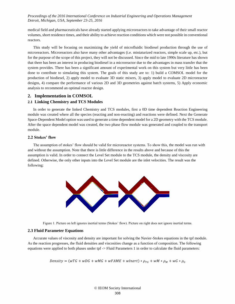
2.2 Stokes’ flow
The assumption of stokes’ flow should be valid for microreactor systems. To show this, the model was run with
and without the assumption. Note that there is little difference in the results above and because of this the
assumption is valid. In order to connect the Level Set module to the TCS module, the density and viscosity are
defined. Otherwise, the only other inputs into the Level Set module are the inlet velocities. The result was the
following:
Figure 1. Picture on left ignores inertial terms (Stokes’ flow). Picture on right does not ignore inertial terms.
2.3 Fluid Parameter Equations
Accurate values of viscosity and density are important for solving the Navier-Stokes equations in the tpf module.
As the reaction progresses, the fluid densities and viscosities change as a function of composition. The following
equations were applied to both phases under tpf -> Fluid Parameters 1 in order to calculate the fluid parameters:
𝐷𝑒𝑛𝑠𝑖𝑡𝑦 = (𝑤𝑇𝐺 + 𝑤𝐷𝐺 + 𝑤𝑀𝐺 + 𝑤𝐹𝐴𝑀𝐸 + 𝑤𝐼𝑛𝑒𝑟𝑡) ∗ 𝜌𝑇𝐺 + 𝑤𝑀 ∗ 𝜌𝑀 + 𝑤𝐺 ∗ 𝜌𝐺
308
Proceedings of the 2016 International Conference on Industrial Engineering and Operations Management
Detroit, Michigan, USA, September 23-25, 2016
© IEOM Society International
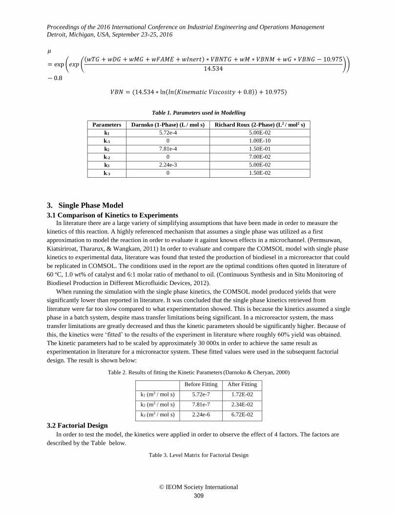
𝜇
= exp (𝑒𝑥𝑝 ((𝑤𝑇𝐺 + 𝑤𝐷𝐺 + 𝑤𝑀𝐺 + 𝑤𝐹𝐴𝑀𝐸 + 𝑤𝐼𝑛𝑒𝑟𝑡) ∗ 𝑉𝐵𝑁𝑇𝐺 + 𝑤𝑀 ∗ 𝑉𝐵𝑁𝑀 + 𝑤𝐺 ∗ 𝑉𝐵𝑁𝐺 − 10.975
14.534))
− 0.8
𝑉𝐵𝑁 = (14.534 ∗ ln(𝑙𝑛(𝐾𝑖𝑛𝑒𝑚𝑎𝑡𝑖𝑐 𝑉𝑖𝑠𝑐𝑜𝑠𝑖𝑡𝑦 + 0.8)) + 10.975)
Table 1. Parameters used in Modelling
Parameters Darnoko (1-Phase) (L / mol s) Richard Roux (2-Phase) (L2 / mol2 s)
k1 5.72e-4 5.00E-02
k-1 0 1.00E-10
k2 7.81e-4 1.50E-01
k-2 0 7.00E-02
k3 2.24e-3 5.00E-02
k-3 0 1.50E-02
3. Single Phase Model
3.1 Comparison of Kinetics to Experiments In literature there are a large variety of simplifying assumptions that have been made in order to measure the
kinetics of this reaction. A highly referenced mechanism that assumes a single phase was utilized as a first
approximation to model the reaction in order to evaluate it against known effects in a microchannel. (Permsuwan,
Kiatsiriroat, Thararux, & Wangkam, 2011) In order to evaluate and compare the COMSOL model with single phase
kinetics to experimental data, literature was found that tested the production of biodiesel in a microreactor that could
be replicated in COMSOL. The conditions used in the report are the optimal conditions often quoted in literature of
60 oC, 1.0 wt% of catalyst and 6:1 molar ratio of methanol to oil. (Continuous Synthesis and in Situ Monitoring of
Biodiesel Production in Different Microfluidic Devices, 2012).
When running the simulation with the single phase kinetics, the COMSOL model produced yields that were
significantly lower than reported in literature. It was concluded that the single phase kinetics retrieved from
literature were far too slow compared to what experimentation showed. This is because the kinetics assumed a single
phase in a batch system, despite mass transfer limitations being significant. In a microreactor system, the mass
transfer limitations are greatly decreased and thus the kinetic parameters should be significantly higher. Because of
this, the kinetics were ‘fitted’ to the results of the experiment in literature where roughly 60% yield was obtained.
The kinetic parameters had to be scaled by approximately 30 000x in order to achieve the same result as
experimentation in literature for a microreactor system. These fitted values were used in the subsequent factorial
design. The result is shown below:
Table 2. Results of fitting the Kinetic Parameters (Darnoko & Cheryan, 2000)
Before Fitting After Fitting
k1 (m3 / mol s) 5.72e-7 1.72E-02
k2 (m3 / mol s) 7.81e-7 2.34E-02
k3 (m3 / mol s) 2.24e-6 6.72E-02
3.2 Factorial Design
In order to test the model, the kinetics were applied in order to observe the effect of 4 factors. The factors are
described by the Table below.
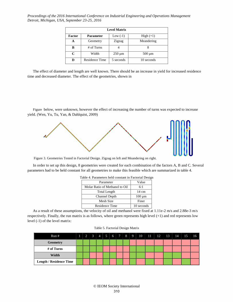
Table 3. Level Matrix for Factorial Design
309
Proceedings of the 2016 International Conference on Industrial Engineering and Operations Management
Detroit, Michigan, USA, September 23-25, 2016
© IEOM Society International
Level Matrix
Factor Parameter Low (-1) High (+1)
A Geometry Zigzag Meandering
B # of Turns 4 8
C Width 250 µm 500 µm
D Residence Time 5 seconds 10 seconds
The effect of diameter and length are well known. There should be an increase in yield for increased residence
time and decreased diameter. The effect of the geometries, shown in
Figure below, were unknown, however the effect of increasing the number of turns was expected to increase
yield. (Wen, Yu, Tu, Yan, & Dahlquist, 2009)
Figure 3. Geometries Tested in Factorial Design. Zigzag on left and Meandering on right.
In order to set up this design, 8 geometries were created for each combination of the factors A, B and C. Several
parameters had to be held constant for all geometries to make this feasible which are summarized in table 4.
Table 4. Parameters held constant in Factorial Design
Parameter Value
Molar Ratio of Methanol to Oil 6:1
Total Length 14 cm
Channel Depth 100 µm
Mesh Size Finer
Residence Time 10 seconds
As a result of these assumptions, the velocity of oil and methanol were fixed at 1.11e-2 m/s and 2.88e-3 m/s
respectively. Finally, the run matrix is as follows, where green represents high level (+1) and red represents low
level (-1) of the level matrix:
Table 5. Factorial Design Matrix
Run # 1 2 3 4 5 6 7 8 9 10 11 12 13 14 15 16
Geometry
# of Turns
Width
Length / Residence Time
310
Proceedings of the 2016 International Conference on Industrial Engineering and Operations Management
Detroit, Michigan, USA, September 23-25, 2016
© IEOM Society International
Due to the computational requirements of the model and the limitations of the server, each run took 10 to 30
hours to complete. Fortunately, results at all times are available after simulation. Thus, the yield at 5 seconds was
used for all runs that required a low level of residence time which halved the number of runs required.
3.3 Results of Factorial Design
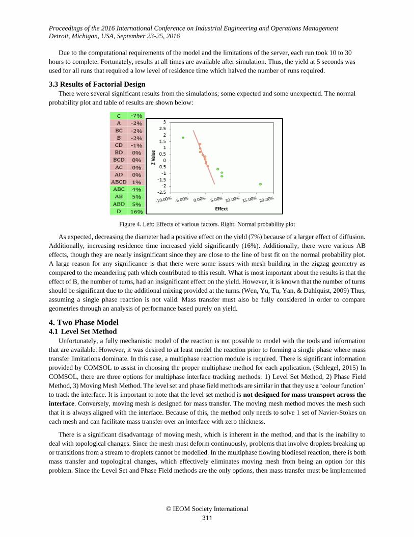
There were several significant results from the simulations; some expected and some unexpected. The normal
probability plot and table of results are shown below:
Figure 4. Left: Effects of various factors. Right: Normal probability plot
As expected, decreasing the diameter had a positive effect on the yield (7%) because of a larger effect of diffusion.
Additionally, increasing residence time increased yield significantly (16%). Additionally, there were various AB
effects, though they are nearly insignificant since they are close to the line of best fit on the normal probability plot.
A large reason for any significance is that there were some issues with mesh building in the zigzag geometry as
compared to the meandering path which contributed to this result. What is most important about the results is that the
effect of B, the number of turns, had an insignificant effect on the yield. However, it is known that the number of turns
should be significant due to the additional mixing provided at the turns. (Wen, Yu, Tu, Yan, & Dahlquist, 2009) Thus,
assuming a single phase reaction is not valid. Mass transfer must also be fully considered in order to compare
geometries through an analysis of performance based purely on yield.
4. Two Phase Model 4.1 Level Set Method
Unfortunately, a fully mechanistic model of the reaction is not possible to model with the tools and information
that are available. However, it was desired to at least model the reaction prior to forming a single phase where mass
transfer limitations dominate. In this case, a multiphase reaction module is required. There is significant information
provided by COMSOL to assist in choosing the proper multiphase method for each application. (Schlegel, 2015) In
COMSOL, there are three options for multiphase interface tracking methods: 1) Level Set Method, 2) Phase Field
Method, 3) Moving Mesh Method. The level set and phase field methods are similar in that they use a ‘colour function’
to track the interface. It is important to note that the level set method is not designed for mass transport across the
interface. Conversely, moving mesh is designed for mass transfer. The moving mesh method moves the mesh such
that it is always aligned with the interface. Because of this, the method only needs to solve 1 set of Navier-Stokes on
each mesh and can facilitate mass transfer over an interface with zero thickness.
There is a significant disadvantage of moving mesh, which is inherent in the method, and that is the inability to
deal with topological changes. Since the mesh must deform continuously, problems that involve droplets breaking up
or transitions from a stream to droplets cannot be modelled. In the multiphase flowing biodiesel reaction, there is both
mass transfer and topological changes, which effectively eliminates moving mesh from being an option for this
problem. Since the Level Set and Phase Field methods are the only options, then mass transfer must be implemented
311
Proceedings of the 2016 International Conference on Industrial Engineering and Operations Management
Detroit, Michigan, USA, September 23-25, 2016
© IEOM Society International
despite the difficulty of implementation. Since most of literature uses the Level Set method, it has been the method of
choice to calculate the two phase flow profiles.
4.2 Mass Transfer Approaches
There are few examples of attempts to implement mass transfer with the Level Set method in literature. The first
method, proposed by a commonly referenced COMSOL Support blog, involves running the Level Set method to
generate a flow profile and using this as an input into the moving mesh method to calculate the mass transfer. However,
this has limited applications since this example uses a well-defined bubble at steady state as an example and is not
general enough for this application. (Schlegel, 2015). An alternative approach is described by Ganguli and Kenig.
(Ganguli & Kenig, 2011) In this approach, the interface is assumed to be a constant range of volume fraction values
where two boundary conditions are enforced. The following assumptions are made: 1) Newtonian incompressible
fluids, 2) Laminar flow of both phases, 3) Isothermal system, 4) Absence of surface active contaminants, 5) No
chemical reaction in the system. Thus, even though there is reaction in the system, attempts to implement this method
were utilized with the knowledge that adjustments should be made to the model to accommodate the relaxation of this
assumption.
4.3 Boundary Conditions
In the mass transfer limited region, the reaction is limited by the diffusion of oil into the methanol phase, where
the reaction occurs. As biodiesel is produced, solubility is increased between the oil and methanol until enough
biodiesel is formed to allow the whole system to form a single phase. This coincides with an increase in reaction rate
commonly associated with the kinetically limited region. In order to model mass transfer with the Level Set Method,
each component is defined separately depending on whether it is in the oil or methanol phase. Then, the boundary
between the two phases is defined to have a finite thickness as a function of volume fraction with two boundary
conditions shown below.
𝐷𝑃
𝜕[𝑇𝐺]
𝜕𝑛= 𝐷𝑃𝑜
𝜕[𝑇𝐺𝑜]
𝜕𝑛
[𝑇𝐺𝑜] = [𝑇𝐺] ∙ 𝐻𝐷
The first equations represents the first boundary condition that the diffusive flux of the feed in the aqueous phase,
[TG], must equal the diffusive flux of the feed in the oil phase, [TGo], along the direction normal to the interface. The
second equation represents the second boundary condition, which facilitates the concentration jump from one phase
to the other. These two boundary conditions are added to the continuity equation for each species at the boundary,
using Heaviside functions, as follows:
𝜕[𝑇𝐺𝑜]
𝜕𝑡+ û · 𝛻[𝑇𝐺𝑜] = 𝛻(𝐷𝑃𝑜𝛻[TGo]) + 𝛼1(𝐷𝑃
𝜕[𝑇𝐺]
𝜕𝑛− 𝐷𝑃𝑜
𝜕[𝑇𝐺𝑜]
𝜕𝑛)
𝜕[𝑇𝐺]
𝜕𝑡+ û · 𝛻[𝑇𝐺 ] = 𝛻(𝐷𝑃𝑜𝛻[𝑇𝐺]) + R + 𝛼2(
[𝑇𝐺𝑜]
𝐻𝐷
− [𝑇𝐺])
Note that the reaction rate is defined for the species in the methanol phase and not the oil phase for reasons
described previously. The above equations take their new form with coefficients 𝛼1 and 𝛼2. These constants are scaled
to be arbitrarily high enough such that the boundary conditions are held to be true at all points along the interface.
According to literature, 𝛼1 = 𝛼2 = 104 is sufficient.
4.4 Implementation in COMSOL
Implementation of the boundary conditions was achieved in the TCS module under the Reactions subheading.
Here the reaction term of the continuity equation is defined. In order to achieve the boundary conditions, the rate term
was modified for all species that transfer mass between phases to include the boundary conditions as follows:
312
Proceedings of the 2016 International Conference on Industrial Engineering and Operations Management
Detroit, Michigan, USA, September 23-25, 2016
© IEOM Society International
𝑅𝑇𝐺 = 𝛼1 ∗ 𝐻(𝑉𝑓1 − 0.45) ∗ (1 − 𝐻(𝑉𝑓1 − 0.55)) ∗ (𝐴𝑜𝑇𝐺𝑀 ∗ 𝑀𝑜𝑇𝐺𝑀 − 𝐴𝑜𝑇𝐺 ∗ 𝑀𝑜𝑇𝐺)
𝑅𝑇𝐺𝑀 = 𝑅𝑇𝐺𝑀 + 𝛼2 ∗ 𝐻(𝑉𝑓1 − 0.45) ∗ (1 − 𝐻(𝑉𝑓1 − 0.55)) ∗ (𝐶𝑇𝐺 −𝐶𝑇𝐺𝑀
𝐻𝐷
)
where the following variables are defined under Definitions -> Variables:
𝐴𝑜𝑁 = atan (
𝜕𝑉𝑓1𝜕𝑦
𝜕𝑉𝑓1𝜕𝑥
+ 𝐶)
𝐴𝑜𝑇𝐺𝑀 = 1 − 𝑎𝑏𝑠(atan (𝐽𝑇𝐺𝑀𝑦
𝐽𝑇𝐺𝑀𝑥+ 𝐶
− 𝐴𝑜𝑁) ∗2
𝜋
𝑀𝑜𝑇𝐺𝑀 = √(𝐽𝑇𝐺𝑀𝑦+ 𝐶)
2
+ (𝐽𝑇𝐺𝑀𝑥+ 𝐶)
2
C is defined to be a constant that is as small as possible to remove numerical issues including divide by 0 errors
and squaring 0. The requirement for C will have an effect on the accuracy of the mass transfer as it affects both the
magnitude and direction, however, when set at 1e-11, it is an order of magnitude smaller than the diffusive flux terms.
Further, the effect of squaring the sum of the J and C greatly diminishes the negative effect that C has on the accuracy
of the implementation. The following table shows the conversion of the terms shown above into COMSOL inputs:
Table 6. Conversion of mathematical terms to COMSOL inputs
Mathematical Term COMSOL Input
𝑱𝑻𝑮𝑴𝒚 tcs2.dflux_w1TGMy
𝑱𝑻𝑮𝑴𝒙 tcs2.dflux_w1TGMx
𝝏𝑽𝒇𝟏
𝝏𝒚
d(tpf2.Vf1,y)
H(Vf1 – 0.55) flc1hs(tpf2.Vf1 – 0.55, 0.00001)
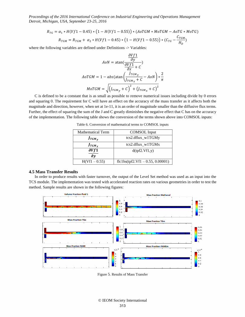
4.5 Mass Transfer Results In order to produce results with faster turnover, the output of the Level Set method was used as an input into the
TCS module. The implementation was tested with accelerated reaction rates on various geometries in order to test the
method. Sample results are shown in the following figures:
Figure 5. Results of Mass Transfer
313
Proceedings of the 2016 International Conference on Industrial Engineering and Operations Management
Detroit, Michigan, USA, September 23-25, 2016
© IEOM Society International
As shown in the figures above, the volume fraction of the phases develops as expected, as this is largely
independent of the mass transfer. As noted previously, the reaction rate is scaled up for the purposes of viewing the
behavior of the method and so the mass fraction of methanol begins high at the inlet and decreases as it reacts with
the TGm in the system. The TGo and TGm plots show the success of the method in maintaining a high mass fraction
of TGo in the oil phase and restricting TGm to the methanol phase. Due to the thickness of the interface, the TGo
appears to fill a greater volume than it should. The smaller the interface thickness is, the closer this would be to
matching the volume fraction plot. In this case the solubility limit was set such that the TGm concentration would be
5% of the TGo concentration. By looking at the scales of the plots of TGo and TGm it can be observed that this is
held true. Finally, the FAME and FAMEm are produced through the reaction of TGm and Methanol. It can be observed
that FAMEm is produced and begins to diffuse away from the methanol phase which is undesired. Conversely, FAME
remains in the methanol phase. Attempts are being made to determine which term is backwards in the model to correct
this since diffusion is occurring in the opposite direction for the product than for the reactants.
5. Interfacial Area for Design
5.1 Analytical Method To determine the degree of mixing between the two immiscible fluids, an analysis was created to quantitatively
compare the amount of interface generated within the reactor. This analysis is performed by taking a surface integral
of the following heaviside weighted function over the entire domain.
𝐻(𝑉𝑓1 − 0.4) ∗ 𝐻(0.6 − 𝑉𝑓1) = 𝐼𝑛𝑡𝑒𝑟𝑓𝑎𝑐𝑖𝑎𝑙 "𝐴𝑟𝑒𝑎"
Because the transition region between 0.4 and 0.6 does not have a zero thickness, and the thicknesses are not
consistent across all geometries, the Interfacial “Area” is corrected for the thickness by taking a line integral
perpendicular to the direction of the interface using the same function; this provides an interfacial length. The length
must also be normalized across all geometries since a longer pipe would have a longer length. The interfacial length
is divided by the total reactor area which is determined by taking the surface integral of 1 over the entire domain; this
provides an interfacial length per area. This is analogous to the “a” term in KLa which is defined as interfacial area
per volume. However, since the model is 2D instead of 3D, the interfacial length per area is achieved; this term is
denoted “l” due to this relationship. A fundamental result of this calculation is that in a straight channel with one
continuous interface, the interfacial distance per area increases as the channel diameter decreases. This is due to the
interfacial length not changing (length of the channel) while the total area decreases (length * channel diameter). This
was quickly confirmed by testing a non-straight geometry with 250 μm diameter against a geometry with 500 μm
diameter to show that it had decreased from 2388 m-1 to 1619 m-1.
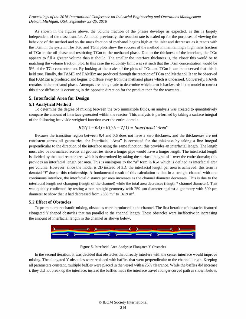
5.2 Effect of Obstacles
To promote more chaotic mixing, obstacles were introduced in the channel. The first iteration of obstacles featured
elongated Y shaped obstacles that ran parallel to the channel length. These obstacles were ineffective in increasing
the amount of interfacial length in the channel as shown below.
Figure 6. Interfacial Area Analysis: Elongated Y Obstacles
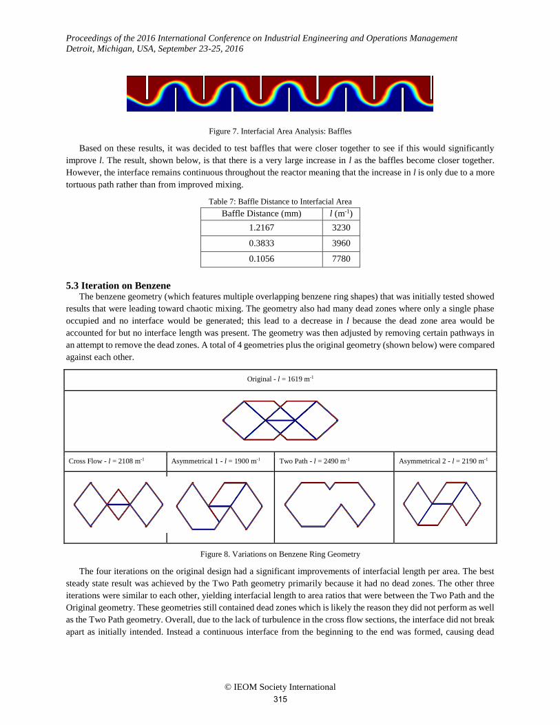
In the second iteration, it was decided that obstacles that directly interfere with the center interface would improve
mixing. The elongated Y obstacles were replaced with baffles that went perpendicular to the channel length. Keeping
all parameters constant, multiple baffles were placed in the vessel with a 25% clearance. While the baffles did increase
l, they did not break up the interface; instead the baffles made the interface travel a longer curved path as shown below.
314
Proceedings of the 2016 International Conference on Industrial Engineering and Operations Management
Detroit, Michigan, USA, September 23-25, 2016
© IEOM Society International
Figure 7. Interfacial Area Analysis: Baffles
Based on these results, it was decided to test baffles that were closer together to see if this would significantly
improve l. The result, shown below, is that there is a very large increase in l as the baffles become closer together.
However, the interface remains continuous throughout the reactor meaning that the increase in l is only due to a more
tortuous path rather than from improved mixing.
Table 7: Baffle Distance to Interfacial Area
Baffle Distance (mm) l (m-1)
1.2167 3230
0.3833 3960
0.1056 7780
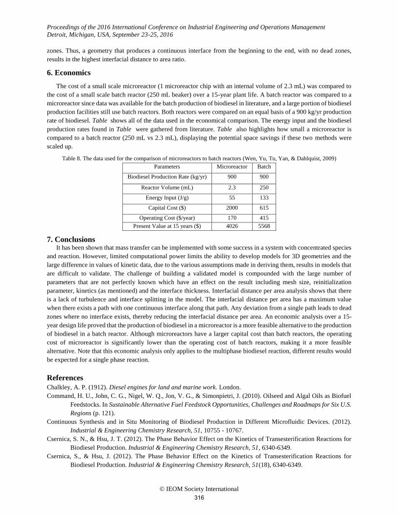
5.3 Iteration on Benzene The benzene geometry (which features multiple overlapping benzene ring shapes) that was initially tested showed
results that were leading toward chaotic mixing. The geometry also had many dead zones where only a single phase
occupied and no interface would be generated; this lead to a decrease in l because the dead zone area would be
accounted for but no interface length was present. The geometry was then adjusted by removing certain pathways in
an attempt to remove the dead zones. A total of 4 geometries plus the original geometry (shown below) were compared
against each other.
Original - l = 1619 m-1
Cross Flow - l = 2108 m-1 Asymmetrical 1 - l = 1900 m-1 Two Path - l = 2490 m-1 Asymmetrical 2 - l = 2190 m-1
Figure 8. Variations on Benzene Ring Geometry
The four iterations on the original design had a significant improvements of interfacial length per area. The best
steady state result was achieved by the Two Path geometry primarily because it had no dead zones. The other three
iterations were similar to each other, yielding interfacial length to area ratios that were between the Two Path and the
Original geometry. These geometries still contained dead zones which is likely the reason they did not perform as well
as the Two Path geometry. Overall, due to the lack of turbulence in the cross flow sections, the interface did not break
apart as initially intended. Instead a continuous interface from the beginning to the end was formed, causing dead
315
Proceedings of the 2016 International Conference on Industrial Engineering and Operations Management
Detroit, Michigan, USA, September 23-25, 2016
© IEOM Society International
zones. Thus, a geometry that produces a continuous interface from the beginning to the end, with no dead zones,
results in the highest interfacial distance to area ratio.
6. Economics
The cost of a small scale microreactor (1 microreactor chip with an internal volume of 2.3 mL) was compared to
the cost of a small scale batch reactor (250 mL beaker) over a 15-year plant life. A batch reactor was compared to a
microreactor since data was available for the batch production of biodiesel in literature, and a large portion of biodiesel
production facilities still use batch reactors. Both reactors were compared on an equal basis of a 900 kg/yr production
rate of biodiesel. Table shows all of the data used in the economical comparison. The energy input and the biodiesel
production rates found in Table were gathered from literature. Table also highlights how small a microreactor is
compared to a batch reactor (250 mL vs 2.3 mL), displaying the potential space savings if these two methods were
scaled up.
Table 8. The data used for the comparison of microreactors to batch reactors (Wen, Yu, Tu, Yan, & Dahlquist, 2009)
Parameters Microreactor Batch
Biodiesel Production Rate (kg/yr) 900 900
Reactor Volume (mL) 2.3 250
Energy Input (J/g) 55 133
Capital Cost ($) 2000 615
Operating Cost ($/year) 170 415
Present Value at 15 years ($) 4026 5568
7. Conclusions It has been shown that mass transfer can be implemented with some success in a system with concentrated species
and reaction. However, limited computational power limits the ability to develop models for 3D geometries and the
large difference in values of kinetic data, due to the various assumptions made in deriving them, results in models that
are difficult to validate. The challenge of building a validated model is compounded with the large number of
parameters that are not perfectly known which have an effect on the result including mesh size, reinitialization
parameter, kinetics (as mentioned) and the interface thickness. Interfacial distance per area analysis shows that there
is a lack of turbulence and interface splitting in the model. The interfacial distance per area has a maximum value
when there exists a path with one continuous interface along that path. Any deviation from a single path leads to dead
zones where no interface exists, thereby reducing the interfacial distance per area. An economic analysis over a 15-
year design life proved that the production of biodiesel in a microreactor is a more feasible alternative to the production
of biodiesel in a batch reactor. Although microreactors have a larger capital cost than batch reactors, the operating
cost of microreactor is significantly lower than the operating cost of batch reactors, making it a more feasible
alternative. Note that this economic analysis only applies to the multiphase biodiesel reaction, different results would
be expected for a single phase reaction.
References
Chalkley, A. P. (1912). Diesel engines for land and marine work. London.
Command, H. U., John, C. G., Nigel, W. Q., Jon, V. G., & Simonpietri, J. (2010). Oilseed and Algal Oils as Biofuel
Feedstocks. In Sustainable Alternative Fuel Feedstock Opportunities, Challenges and Roadmaps for Six U.S.
Regions (p. 121).
Continuous Synthesis and in Situ Monitoring of Biodiesel Production in Different Microfluidic Devices. (2012).
Industrial & Engineering Chemistry Research, 51, 10755 - 10767.
Csernica, S. N., & Hsu, J. T. (2012). The Phase Behavior Effect on the Kinetics of Transesterification Reactions for
Biodiesel Production. Industrial & Engineering Chemistry Research, 51, 6340-6349.
Csernica, S., & Hsu, J. (2012). The Phase Behavior Effect on the Kinetics of Transesterification Reactions for
Biodiesel Production. Industrial & Engineering Chemistry Research, 51(18), 6340-6349.
316
Proceedings of the 2016 International Conference on Industrial Engineering and Operations Management
Detroit, Michigan, USA, September 23-25, 2016
© IEOM Society International
Darnoko, D., & Cheryan, M. (2000). Kinetics of Palm Oil Transesterification in a Batch Reactor. Journal of the
American Oil Chemists' Society, 77(12), 1263-1267.
Finlayson, B. A. (2007). Microreactors (General). (Wasington State University) Retrieved Feburary 2016, from
http://faculty.washington.edu/finlayso/che475/microreactors/Group_A/whatmr1.htm
Freedman, B., Butterfield, R. O., & Pryde, E. (1986). Transesterification kinetics of soybean oil . Journal of the
American Oil Chemists’ Society, 63(10), 1375-1380.
Fukuda, H., Kondo, A., & Noda, H. (2001). Biodiesel fuel production by transesterification of oils. Journal of
Bioscience and Bioengineering, 92(5), 405-416.
He, B., & Gerpen, J. V. (2015). Reactors for Biodiesel Production. (Extension) Retrieved Feburary 2016, from
http://articles.extension.org/pages/26630/reactors-for-biodiesel-production
Hecht, K. (2013). Microreactors for Gas/Liquid Reactions: The Role of Surface Properties. Karlsruhe Institute of
Technology.
Krawczyk, T. (1996). Biodiesel-Alternative Fuel Makes Inroads but Hurdles Remain. Inform, 7(8), 801-829.
Ma, F., & Hanna, M. A. (1999). Biodiesel production: a review. Bioresource Technology, 70, 1-15.
Monisha, J., Harish, A., Sushma, R., Krishna, M. T., Blessy, B. M., & Ananda, S. (2013). Biodiesel: A Review. Int.
Journal of Engineering Research and Applications , 3(6), 902-912.
Monyem, A., & Gerpen, J. H. (2001). The effect of biodiesel oxidation on engine performance and emission. Biomass
Bioenergy. Biomass & Bioenergy, 20, 317-325.
Noureddini, H., & Zhu, D. (1997). Kinetics of transesterification of soybean oil. Journal of the American Oil Chemists'
Society, 74(11), 1457-1463.
Pacific Biodiesel. (2006). History of biodiesel fuel. (Pacific Biodiesel) Retrieved Feburary 2016, from
http://www.biodiesel.com/biodiesel/history/
Portha, J., Allain, F., Coupard, V., Girot, E., Schaer, E., & Falk, L. (2012). Simulation and kinetic study of
transesterification of triolein to biodiesel using modular reactors. Chemical Engineering Journal.
Schimdt, C. W. (2007). BIODIESEL: Cultivating Alternative Fuels. Environmental Health Perspectives, 115(2), A86-
A91.
Schlegel, F. (2015, January 27). Which Multiphase Flow Interface Should I Use? Retrieved Feburary 2016, from
https://www.comsol.com/blogs/which-multiphase-flow-interface-should-i-use/
Shay, G. E. (1993). Diesel fuel from vegetable oils: Status and opportunities. Biomass & Bioenergy, 4(4), 227-242.
U.S. Energy Information Administration. (2015). Petroleum and Other Liquids. (U.S. Energy Information
Administration) Retrieved Feburary 2016, from http://www.eia.gov/biofuels/biodiesel/production/
US Environmental Protection Agency. (2002). A Comprehensive Analysis of Biodiesel Impacts on Exhaust Emissions.
Wen, Z., Yu, X., Tu, S.-T., Yan, J., & Dahlquist, E. (2009). Intensification of biodiesel synthesis using zigzag micro-
channel reactors. Bioresource Technology, 100, 3054 - 3060.
Biography
Ali Elkamel is a professor of Chemical Engineering at the University of Waterloo, Canada. He holds a B.S. in
Chemical and Petroleum Refining Engineering and a B.S. in Mathematics from Colorado School of Mines, an M.S.
in Chemical Engineering from the University of Colorado-Boulder, and a Ph.D. in Chemical Engineering from Purdue
University. His specific research interests are in computer-aided modeling, optimization, and simulation with
applications to the petroleum and petrochemical industry. He has contributed more than 250 publications in refereed
journals and international conference proceedings and serves on the editorial board of several journals, including the
International Journal of Process Systems Engineering, Engineering Optimization, International Journal of Oil, Gas,
Coal Technology, and the Open Fuels & Energy Science Journal.
Chandra Mouli Madhuranthakam is a professor of Chemical Engineering at the University of Waterloo, Canada.
His research interests include micro Process Systems Engineering - Design and Operation of Microfluidic reactors for
efficient synthesis of biodiesel and complex copolymers, Mixed Integer Nonlinear Programming and Global
317

Proceedings of the 2016 International Conference on Industrial Engineering and Operations Management
Detroit, Michigan, USA, September 23-25, 2016
© IEOM Society International
Optimization Algorithms, Modeling and Optimal Control for Complex Biochemical Reaction Systems, Applied
Statistics- Modeling, Design of Experiments, and Parameter Estimation.
Mohamed Elsholkami is a Ph.D. student at the University of Waterloo. He earned his B.S. in Chemical Engineering
from the Petroleum Institute in Abu Dhabi, UAE. His research interests are in process systems engineering and
optimization.
T. Cumberland, N. Molyneaux, S. Wei, and N. Zambito are students at the University Of Waterloo.
318