UCRL-ID-129855

Design Process for NIF Laser Alignment and Beam Diagnostics

Andrew Grey

June 9,1998

This is an informal report intended primarily for internal or limited external distribution. The opinions and conclusions stated are those of the author

P

and may or may not be those of the Laboratory. Work performed under the auspices of the Department of Energy by the Lawrence Livermore National Laboratory under Contract W-7405Eng-48.

DISCLAIMER

This document was prcparcd as an account of work sponsored by an agency of the United States Government Neither the United States Government nor the University of California nor any of their employees, makes any warranty, express or implied, or assumes any legal liability or responsibility for the accuracy, completeness, or usefulness of any information, apparatus, product, or process disclosed, or represents that its use would not infringe privately owned rights Reference herein to any specific commercial product, process, or service by trade name, trademark, manufacturer, or otherwise, does not necessarily constitute or imply its endorsement, recommendation, ot favoring by the United States Government or the University of California. The views and opinions of authors expressed herein do not necessarily state or reflect those of the United States Government or the University of California, and shall not he used for advertising or product endorsement purposes

This report has been reproduced directly from the best available copy

Available to DOE and DOE contractors from the Office of Scientific and Technical Information

P 0 Box 62, Oak Ridge, TN 37831 Prices available from (615) 576-8401, FTS 626-8401

Available to the public from the National Technical Information Service

US Department of Commerce 5285 Port Royal Rd.,

Springfield, VA 22161

EE 3928 Final Project

UCRL- ID-129855

Andrew Grey 6/l 8198

Hartmann Spot Centroid Calculation Using Frequency Domain Analysis

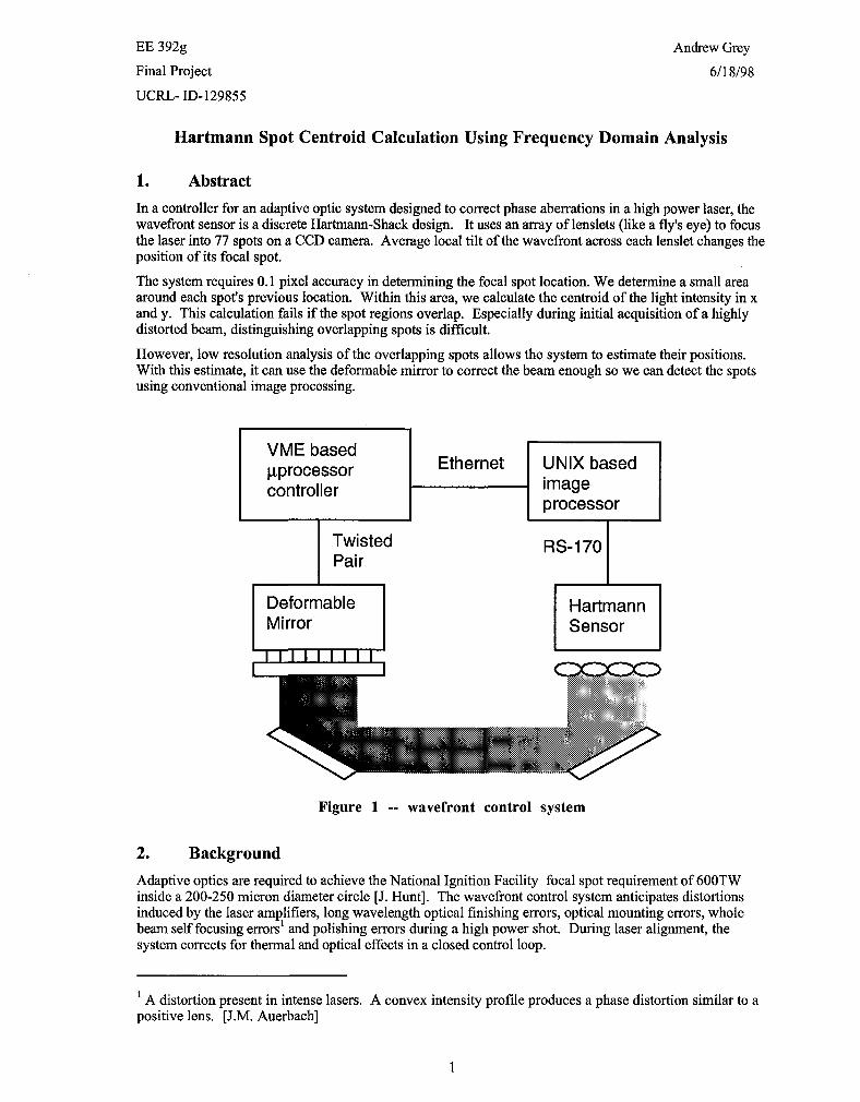
1. Abstract In a controller for an adaptive optic system designed to correct phase aberrations in a high power laser, the wavefront sensor is a discrete Hartmann-Shack design. It uses an army of lenslets (like a fly’s eye) to focus the laser into 77 spots on a CCD camera. Average local tilt of the wavefront across each lenslet changes the position of its focal spot. The system requires 0.1 pixel accuracy in determining the focal spot location. We determine a small area around each spot’s previous location. Within this area, we calculate the centroid of the light intensity in x and y. This calculation fails if the spot regions overlap. Especially during initial acquisition of a highly distorted beam, distinguishing overlapping spots is difficult. However, low resolution analysis of the overlapping spots allows the system to estimate their positions. With this estimate, it can use the deformable mirror to correct the beam enough so we can detect the spots using conventional image processing.

I I VME based pprocessor controller

Twisted Pair

RS-170

Deformable Mirror

Hartmann Sensor

I I I I I I I I ]

I 1

Figure 1 -- wavefront control system

2. Background Adaptive optics are required to achieve the National Ignition Facility focal spot requirement of 600TW inside a 200-250 micron diameter circle [J. Hunt]. The wavefront control system anticipates distortions induced by the laser amplifiers, long wavelength optical finishing errors, optical mounting errors, whole beam self focusing errors’ and polishing errors during a high power shot. During laser alignment, the system corrects for thermal and optical effects in a closed control loop.

’ A distortion present in intense lasers. A convex intensity profile produces a phase distortion similar to a positive lens. [J.M. Auerbach]

1

EE 3928 Final Project UCRL- ID-129855

Andrew Grey 6/l 8198

Wavefront control consists of three major components: a deformable mirror, wavefront sensor and digital controller (Figure 1). The mirror corrects phase errors. It uses 39 actuators to adjust zones across the face of the mirror. Sensing the wavefront, a Hartmann sensor uses 77 small lenslets focused on a CCD. Phase error across the wavefront causes the focus spot of each lenslet to move. The microprocessors analyze the Hartmamr image and move the deformable mirror actuators to correct the phase aberrations.

Image processing initially acquires the spots using their expected locations given a beam free of distortions. In closed loop operation it tracks the spots by defining a small area around each spot’s previous location. Within this area, it calculates the centroid of the light intensity in x and y. Overlapping regions around each spot produce errors in the centroid calculation. Worse, the image processor may lose track or be unable to acquire one or more spots with large distortions.

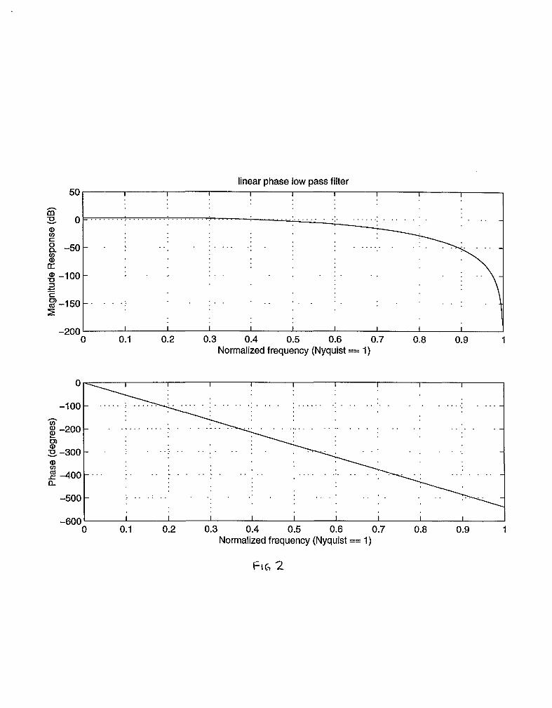
3. Solution Downsampling the Hartmamr image using a linear phase filter with four zeros at n: produces a low resolution image which reflects the concentration of spots across the image. The algorithm estimates each spot location’s offset from its reference location based on the intensity of light surrounding it. Spots move towards brighter areas and away from darker areas. Using the estimated spot locations, the mirror controller calculates the actuator movement required to compensate for the spot distortion.

3.1. Low Resolution Image

I tried various trees and filters to create the low resolution image. A linear phase filter retains the relative locations of light and dark areas. However, a simple Haar filter applied in each dimension produced poor results. Resolution low enough to produce a smooth reference image did not retain enough detail to correct problems. Requiring zeros at n helped smooth the low resolution image, creating an image which, qualitatively, seemed to better reflect the original. However, the light and dark areas failed to stay registered with various length Daubechies’ filters[M. Vetterli, table 4.31, since these filters are not linear phase. Since I use only one branch of the wavelet tree, orthogonality of the filters is not important. Additionally, perfect reconstruction of the original image is not necessary, since the algorithm works completely in the wavelet domain. Therefore, I calculated a linear phase filter with zeros at 7~. I used roots at 2 + & in addition to the four roots at 7~:

[-0.0442 0 0.3977 0.7071 0.3977 0 -0.04421

With four zeros at 7c, the filter smoothed the reference image after five iterations and retained enough detail to estimate distortions in the high resolution image. Figure 2 shows the frequency response of the filter.

Since my intuitive picture of the algorithm involves a blurry version of the original Hartmamr image, the best algorithm should use all low pass filters. I attempted a few variations using high pass filters, but none produced a good image. I chose five iterations of the low pass filter. More iterations would have mapped many of the reference focal spots to the same pixel. With two focal spots mapped to the same pixel, their estimated movement would always be identical, so the system would be unable to correct for them separately. Fewer iterations would require longer low pass filters to smooth the reference image, complicating downsampling. The spot estimation algorithm would also require a larger (in pixels) weighted average to cover the same area on the CCD with fewer downsampling iterations.

3.2. Spot Estimation

After calculating the low resolution image, I map the reference spot locations to it and subtract the reference low resolution image. Since bright areas positively indicate a concentration of spots I reduce the weight given to darker pixels by five. This significantly improves performance in large comer distortions, since otherwise the spot tends to move in the wrong direction. For each reference spot in both x and y, I weight the surrounding pixels using the following vector in the chosen direction (for the shift in x, this vector multiplies the columns):

2

linear phase low pass filter 50 I I I I I I I I I

5 z 0 -........ j . . . . . . . ..I . . . . . . . . . . . . . . . : . . . . . . . . . . . . . . .:. . . . . . . . . . . . . : . ; . . .

iz

s g-5()-.; ..I .; . . . . . ;. ; ;...

d

g -100 - r I . . . . . .

3 .e

fs a-l5O -..t.; ..I.. .._.,.:_ 5

-200 0

I 0.1

I 0.2

I I I I 0.3 0.4 0.5 0.6 0.7

Normalized frequency (Nyquist == 1) 0.8 0.9 1

-600 I -600 I I I I I I I I I I I I I I I I I I 0 0 0.1 0.1 0.2 0.2 0.3 0.3 0.4 0.4 0.5 0.5 0.6 0.6 0.7 0.7 0.8 0.8 0.9 0.9 1 1

Normalized frequency (Nyquist == 1) Normalized frequency (Nyquist == 1)

EE 392g Final Project and the following vector in the opposite direction (for x, it multiplies the rows):

111 1 iiZ?qF 1

Andrew Grey 619198

The sum of all the weighted surrounding pixels produces the estimated offset in x and y for the focal spot. With the estimated focal spot locations, the controller can calculate the phase distortion and move the actuators to correct it.

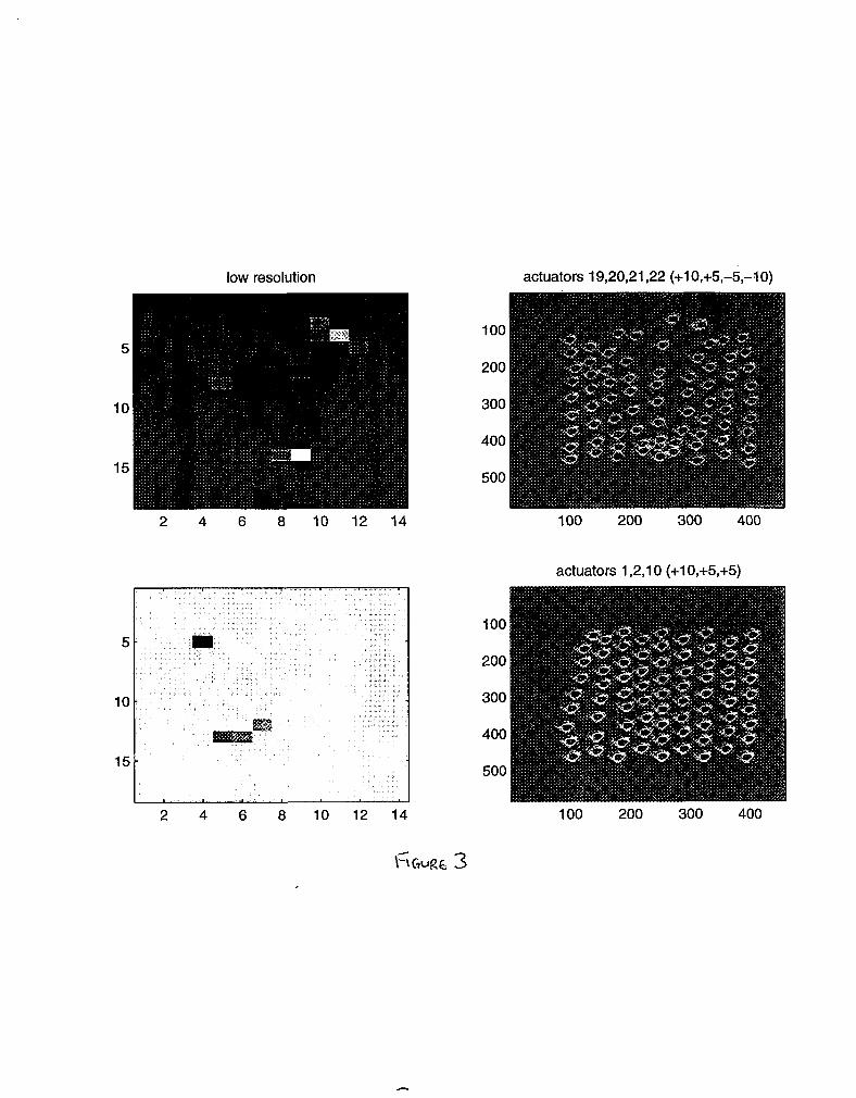
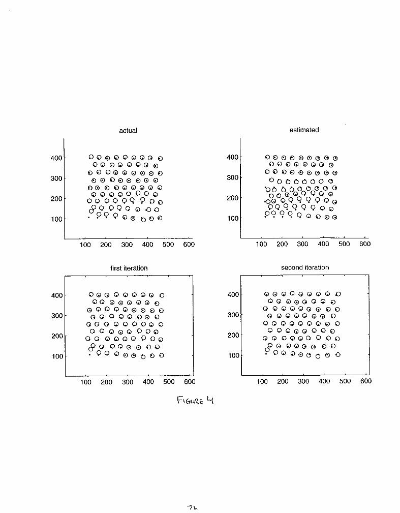
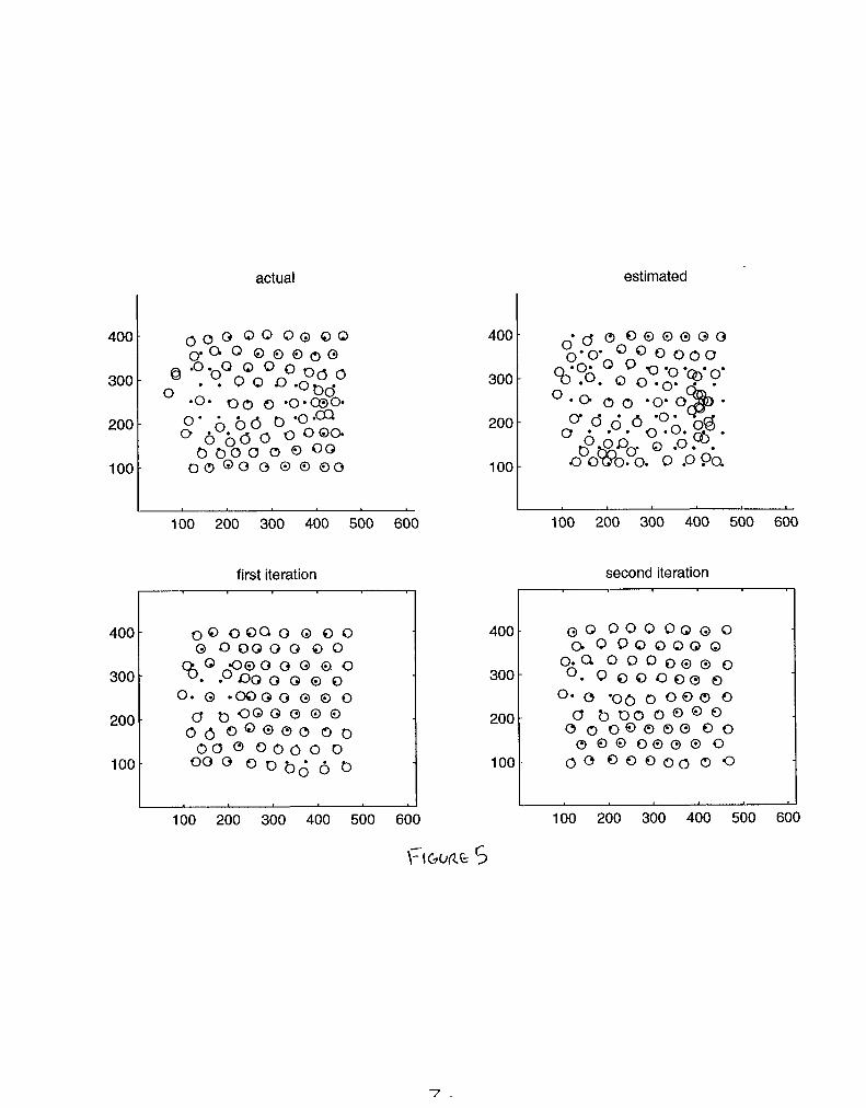
4. Performance I simulated the algorithm’s performance using Matlab. The algorithm processes distorted images simulated by calculating spot offsets produced by large actuator displacements. After processing the image and estimating the spot locations, it uses these offsets to determine corrective changes in the actuator positions. Using these new actuator positions, the simulator can determine the new focal spot positions and produce a new high resolution, simulated Hartmann image. Initially, I evaluated the low resolution images qualitatively by thresholding the resulting image and comparing it to the original, high resolution image (Figure 3 - the images were created by moving the selected actuators to the given positions). Evaluating convergence of the maximum spot offset and mean square error confirmed my qualitative assessment. Many of the nonlinear filter simply didn’t converge.

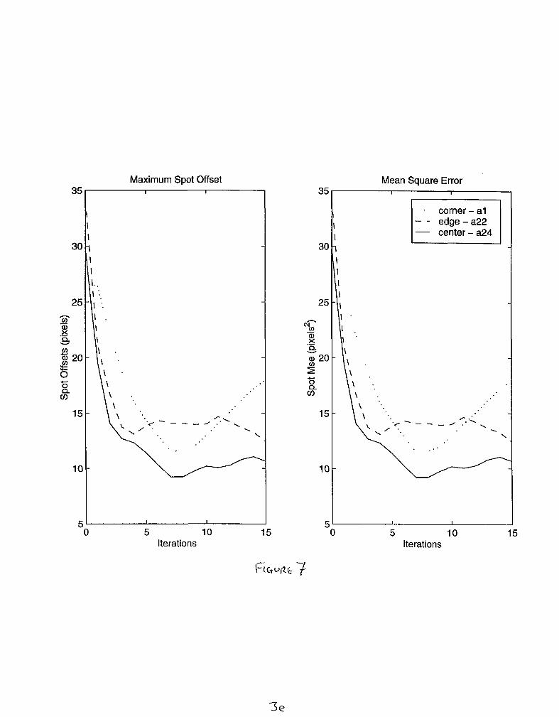
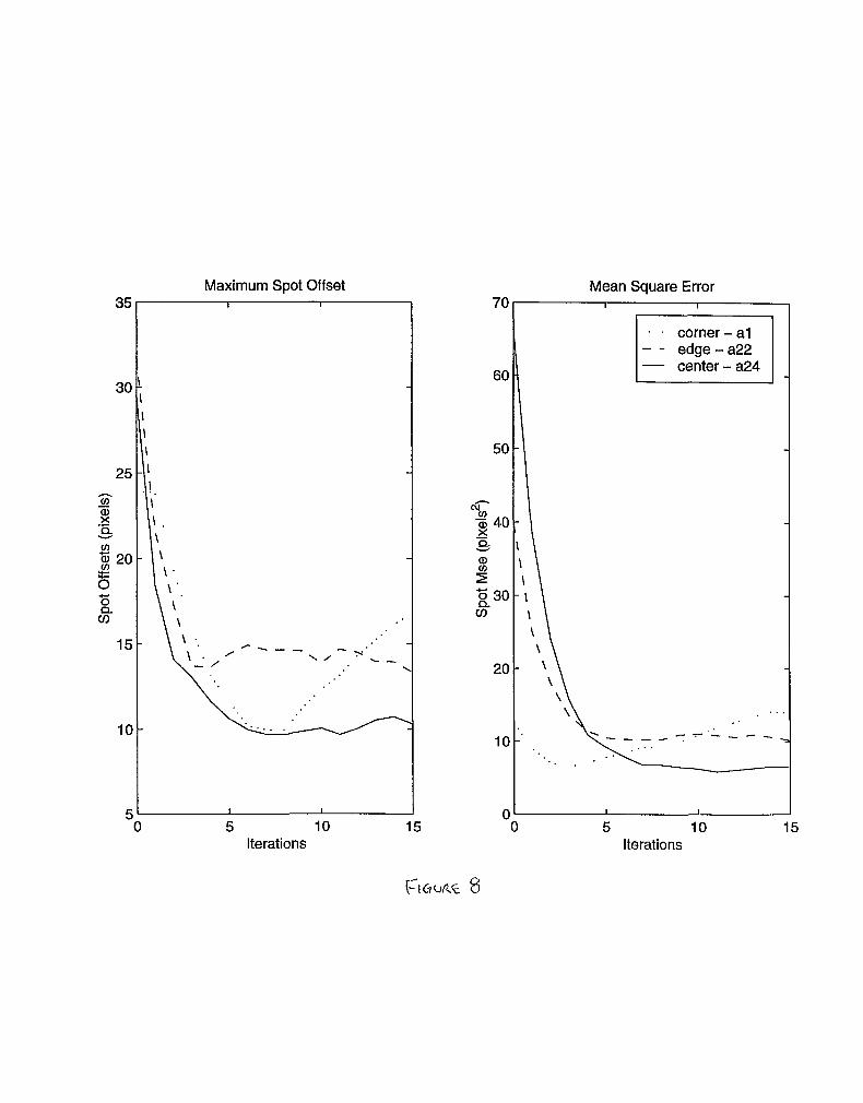
Once I produced a satisfactory low resolution image for a variety of distorted images, I developed and tested the spot estimation algorithm. Figures 4 and 5 show the system performance with the distortions shown in figure 3. [Note: the origin of Figures 4 and 5 is at the bottom left.] Figure 6 shows convergence of the spot’s mean square error and maximum spot offset. The maximum spot offset measures the ability of the normal image processing algorithm to acquire the spots. Mean square error gives a rough estimate of the beam’s quality. With actuators 1,22 and 24, a sample corner, edge and center actuator, respectively, the algorithm converges to about five pixels maximum spot offset in seven iterations. With an average reference spot distance of about fifty, about ten pixels of error on each spot may be small enough to allow spot acquisition. Certainly it’s a significant improvement over the original image. In figure 7, further iterations reduce the quality of the image. However, examination of the resulting images reveals that the system starts spreading the edge spots, aiding spot acquisition. Since the dark areas are underweighted, the simulated spots in a noisy system will receive more influence from slightly light areas than slightly dark areas. Therefore, the estimated spots will tend to move toward the center. The weighted vectors described above are a compromise between correcting edge distortions and limiting this effect. The mirror controller attempts to correct the wavefront while ignoring first order distortions. Another system controls tip and tilt so the mirror actuators save their dynamic range for higher order distortions. Figure 8 removes tip and tilt errors from the curves. Calculated with tip and tilt removed, mean square error starts larger but improves rapidly. The maximum spot offsets change only slightly, since the mean offset (the first order distortion) is only a small fraction of the maximum.

I compared results and computation speed using several techniques. With the Haar scaling function I performed convolution and downsampling five times. I tried one cascaded filter and a 32x downsample. I also computed the cascaded filter in the Fourier domain. The results were similar, but not identical. Iteration required less than 1145th the floating point operations required by the Fourier method. The large convolution required four times the calculations of the Fourier method.

5. Refinements I used relatively simple methods to construct the simulated Hartmann images. As a focal spot moves away from the reference location, it stretches along the offset axis. Test images did not simulate this effect. In addition, I constructed all the images by displacing actuators. This provided a problem with a perfect solution. Distortions produced in the optical path might have higher frequency variations than could be corrected by the mirror. Phase variation across the lenslets also blurs the focal spots. Other effects may produce intensity variations across the image. Both variations in spot shape and intensity will affect this algorithm’s ability to estimate spot locations. Perhaps a lower resolution image will help estimate the

3

low resolution

5- 5-

_, -: _, -y

lo- lo-

15- 15-

2 4 6 8 10 12 14 2 4 6 8 10 12 14

2 2 4 6 8 10 12 14 4 6 8 10 12 14

actuators 19,20,21,22 (+10,+5,-5,-IO)

100

200

300

400

500

100

200

300

400

500

100 200 300 400

actual estimated

100 200 300 400 500 600

first iteration

I I

100 200 300 400 500 600

-2L

400

300

200

100

I 100 200 300 400 500 600

second iteration

QQQ~QQQOO QQQ@QQQQ

QQQQOQQQO QQQQ~QQ 0

QQQQQQQ@Q QQQQQQQQ

QQQQQOoOQ ~QQQQ, 00

?oQQ~~o~o

100 200 300 400 500 600

actual estimated

300 *

200 -

loo-

100 200 300 400 500 600

400

300

200

00 QQ 00

0 0

100 200 300 400 500 600

first iteration

4oc

300

200

100

I

100 200 300 400 500 600

second iteration

100 200 300 400 500 600

.P

35

1C

E

Maximum Spot Offset

2 4 6 Iterations

60

i l-1

I-

)-

I-

)- 0

Mean Square Error I I

I I

. corner - al - - edge - a22 - center - a24

I I I

2 4 6 iterations

Maximum Spot Offset

35-

I 25 -

... l :

-z I .

: : : :

/- ----,: ‘\

5 I I 0 5 10

Iterations 15

35

30

10

E

3e

Mean Square Error I I

. corner - al - - edge - a22 - center - a24

I I I I I . 1 . I . \

\

\ . \ . \ . \ . .

\ . . .

5 10 Iterations

I-

\ --Y

15

Maximum Spot Offset 7(

6(

5(

Nz -$ 4( .- 4 % 2 5 &

3(

2(

l(

(

Iterations

Mean Square Error

I I

5 10 Iterations

15

EE 392g Final Project

Andrew Grey

619198

intensity variations across the image. Both the temporal and spatial frequencies of these variations will determine the best method to correct for them. Actuator failures cause many of the highly distorted images. Correction of this image may be impossible since the controller biases the actuators at high voltage and a failed actuator rests outside its normal control range. The algorithm might automatically diagnose this problem and provide a candidate list of failed actuators. Further revisions of this procedure might shift to a higher resolution image as the spots converge to their reference positions. As the working image progresses towards the initial, high resolution image, accuracy of locating the spot would increase to the 0.1 pixel precision required by the National Ignition Facility.

6. Bibliography 1. Auerbach, J.M. 1997. “The effect of full beam self-focusing on focal spot size.” Presentation to staff of

the National Ignition Facility on 24 April. 2. Hunt, J. 1997. “Review of the focal spot requirements and flowdown of requirements from the UV

focal spot to the one micron system.” Presentation to the staff of the National Ignition Facility on 24 April.

3. Salmon, J.Thaddeus, et al. 1991. “Real-time wavefront correction system using a zonal deformable mirror and a Hartmann sensor.” SPIE Vol. 1542 Active and Adaptive Optical Systems: 459-467.

4. Vetterli, Martin and Jelena Kovacevic. 1995. Wavelets and Subband Coding. New Jersey: Prentice- Hall.

7. Appendices

7.1. Close

% % FUNCTION - close % % USAGE: [new-actuators,new-image] = % close (actuators,filter,Offsets,~at,Gmat,blob,ref-image,image) % % PURPOSE: plot the original, estimated and corrected spot patterns % for two iterations of the low resolution spot estimateion % algorithm %

function [actuators,high] = close (actuators,fil,offsets,H,G,blob,low_ref,high);

% % calculate the estimated spot positions based % on either the given image (high) or actuator positions % if nargin < 8

[new-offsets,lowl = try(actuators,fil,offsets,H,blob,low_ref); else

[new-offsets,low] = estimate(fil,offsets,low_ref,high); end; % % show the original, distorted image % figure(l);

EE 392g Final Project

Andrew Grey 619198

elf; subplot (2,2,1); hold on; distorted-offsets = ceil(offsets+H*actuators); plot (distorted_offsets(l:77),distorted-offsets(78:l54),'o1); plot (offsets(l:77),offsets(78:154),'.'); axis ([l 618 1 4941); hold off; title ('actual'); % % show the estimated version % subplot (2,2,2); hold on; plot (new_offsets(l:77),new-offsets(78:154),'o'); plot (offsets(l:77),offsets(78:154),'.'); axis ([l 618 1 4941); hold off; title ('estimated'); % % calculate the actuator movement required to correct % the estimated image % find the resulting image % actuators = actuators - 0.5*(G'*(new-offsets-offsets)); subplot (2,2,3); if nargout > 1

high = mk-image (actuators,offsets,H,blob); imagesc(high);

else new-offsets = ceil (offsets+H*actuators); plot (newSoffsets(l:77),new_offsets(78:154),'o'); hold on; plot (offsets(l:77),offsets(78:154),'.'); axis ([l 618 1 4941); hold off;

end; title ('first iteration'); % % Do a second iteration % [new-offsets,low] = try(actuators,fil,offsets,H,blob,low_ref); actuators = actuators - 0.5*(G'*(new-offsets-offsets)); subplot (2,2,4); new-offsets = ceil (offsets+H*actuators); plot (newWoffsets(l:77),new_offsets(78:154),'o'); hold on; plot (offsets(l:77),offsets(78:154),'.'); axis ([l 618 1 4941); hold off; title ('second iteration');

EE 3928 Andrew Grey Final Project 619198

7.2. Iter

% % FUNCTION - iter % % USAGE: [pv,mse,new~actuators,new_image] = % iter (actuators,filter,Offsets,Hmat,Gmat,Gmat,blob,ref~image,image) % % PURPOSE: iterate the low resolution spot estimation algorithm and % compute both the mean square error and peak to valley % errors in the spots %

function [pv,mse,acts,highl = iter (acts,fil,offsets,H,G,blob,low_ref,high);

new-offsets = offsets + H*acts; xtilt = mean (new_offsets(l:77) - offsets(l:77)) * ones(1,77); ytilt = mean (new_offsets(78:154) - offsets(78:154)) * ones(1,77); mse(1) = mean( (new-offsets-offsets - [xtilt ytiltl')."2 ); pv(1) = max( abs(new-offsets-offsets - [xtilt ytilt]') ); % % calculate the estimated spot positions based % on either the given image (high) or actuator positions % if nargin < 8

[new-offsets,low] = try(acts,fil,offsets,H,blob,low_ref); else

[new-offsets,low] = estimate(fil,offsets,low_ref,high); end; % % calculate the actuator movement required to correct % the estimated image % find the resulting image % acts = acts - 0.5*(G'*(new-offsets-offsets)); high = mk-image (acts,offsets,H,blob); new-offsets = offsets + H*acts; xtilt = mean (new_offsets(l:77) - offsets(l:77)) * ones(1,77); ytilt = mean (new_offsets(78:154) - offsets(78:154)) * ones(1,77); mse(2) = mean( (new-offsets-offsets - [xtilt ytiltl').^2 ); pv(2) = max( abs(new-offsets-offsets - [xtilt ytilt]') ); % % repeat % for i = 1:6

[new-offsets,low] = try(acts,fil,offsets,H,blob, acts = acts - 0.5*(G'*(new-offsets-offsets)); high = mk-image (acts,offsets,H,blob); new-offsets = offsets + H*acts;

low-ref);

xtilt = mean (new_offsets(l:77) - offsets(l:77)) * ones(1,77); ytilt = mean (new_offsets(78:154) - offsets(78:154)) * ones(1,77); mse(2+i) = mean( (new-offsets-offsets - [xtilt ytiltl').^2 ); pv(2+i) = max( abs(new-offsets-offsets - [xtilt ytiltl') );

EE 3928 Final Project

Andrew Grey 619198

end;

7.3. Estimate

% % FUNCTION - estimate % % USAGE: [new-offsets,low-image] = % estimate (filter,Offsets,reference,image) % % PURPOSE: estimate spot locations and produce a low resolution % Hartmann image, give a high resolution image %

function [new-offsets,low] = estimate (fil,offsets,low-ref,high);

% % filter and downsample to create the low resolution image % subtract the reference image (this compensates for % darker areas around the edges). % low = high; for j = 1:5

low = conv2 (fil,fil,low, 'full'); low = down(low);

end; low = low - low-ref; % % estimate the spot positions from the low % resolution image % specifically, weight the surrounding pixels and % move the reference spots away from dark areas % and toward light areas - note: the algorithm gives % less weight to darker areas since they are, essentially, % an absence of information % offsets-low = 4 + ceil (offsets/2^5); s = size(low); direction-pattern = [-l/200 -l/70 -l/70 -l/50 0 l/50 l/70 l/70 l/200]; distance-pattern = [l/8 l/2 l/2 l/sqrt(2) 1 l/sqrt(2) l/2 l/2 l/8]; for j = l:s(l)

for k = l:s(2) if (low(j,k) < 0)

low(j,k) = low(j,k)/5; end;

end; end; % % set up vectors and perform the linear % algebra to move the spots % new-offsets = zeros(size(offsets)); for j = 1:77

EE 3928 Final Project

x = offsets-low(j); y = offsets_low(j+77); xrow = zeros(l,s(l)); xc01 = zeros(s(2),1); yrow = zeros(l,s(l)); ycol = zeros(s(2),1); xrow(x-4:x+4) = directionsattern; xcol(y-4:y+4) = distancesattern; new-offsets(j) = offsets(j) + (xrow * low * xcol); yrow(x-4:x+4) = distancesattern; ycol(y-4:y+4) = directionsattern; new_offsets(j+77) = offsets(j+77) + (yrow * low * ycol);

end; new-offsets = ceil(new-offsets);

Andrew Grey

619198

7.4. Tiy % % FUNCTION - try % % USAGE: [new-offsets,new-image] = % try (actuators,filter,Offsets,Hmat,blob,reference) % % PURPOSE: compute estimated spot locations and a low resolution '1 image, given current actuator positions %

function [offs,low] = try (actuators,fil,offs,H,blob,low_ref);

if nargin < 3 % % read the reference spot locations % 77 x coordinates, followed by 77 y's in "0" % offsets; offs = 0; clear 0;

end; if nargin < 4

% % read the influence function and convert it to a % matrix 154 x 39 % hMat; H = convertH(h); clear h;

end; if nargin < 5

% % get a sample focal spot from a real Hartmann image % i = convImag('imagel.dat'); blob = i(86:120,91:125);

EE 3928 Final Project

clear i; end: if nargin < 6

% % create the reference low resolution image from an % artificial, reference Hartmann image % filter and downsample the image % low-ref = mk_image(zeros(39,1),offs,H,blob); for j = 1:5

low-ref = conv2 (fil,fil,low-ref,'full'); low-ref = down(low-ref);

end; end;

Andrew Grey 619198

high = mk-image(actuators,offs,H,blob); [offs,low] = estimate (fil,offs,low-ref,high);

7.5. Mk-Image % % FUNCTION - mk-image % % USAGE: image = mk-image (actuators,Offsets,Hmat,blob) % % PURPOSE: Simulate a high resolution Hartmann image give % current actuator positions % This procedure assumes the mirror is the only % source of distortion %

function img = mk-image (actuators,offs,H,blob);

img = zeros([618 4941);

if nargin < 1 actuators = zeros(39,l);

end; if nargin < 2

offsets; offs = 0; clear 0;

end; if nargin < 3

hMat; H = convertH(h); clear h;

end; if nargin < 4

i = convImag('imagel.dat'); blob = i(86:120,91:125); clear i;

end;

EE 392g Final Project

Andrew Grey 619198

offs = ceil(offs + H*actuators); for j = 1:77

tmp = img(offs(j):offs(j)+34,offs(j+77):0ffs(j+77)+34); img(offs(j):offs(j)+34,offs(j+77):offs(j+77)+34) = tmp + blob;

end:

7.6. Down % % FUNCTION - down % % USAGE: new = down (old) % % PURPOSE: downsample an image % function new = down (old);

sz = size(old); new = old(sz(l):-2:l,sz(2):-2:1); SZ = size(new); new = new(sz(l):-l:l,sz(2):-1:1);

10

Technical Inform

ation Departm

ent • Lawrence Liverm

ore National Laboratory

University of C

alifornia • Livermore, C

alifornia 94551