Design space dimensionality reduction through physics-based geometry re-parameterization

Optim Eng (2013) 14:37–59DOI 10.1007/s11081-012-9189-z

Design space dimensionality reductionthrough physics-based geometry re-parameterization

András Sóbester · Stephen Powell

Received: 21 April 2010 / Accepted: 24 January 2012 / Published online: 8 February 2012© Springer Science+Business Media, LLC 2012

Abstract The effective control of the extent of the design space is the sine qua non ofsuccessful geometry-based optimization. Generous bounds run the risk of includingphysically and/or geometrically nonsensical regions, where much search time maybe wasted, while excessively strict bounds will often exclude potentially promisingregions. A related ogre is the pernicious increase in the number of design variables,driven by a desire for geometry flexibility—this can, once again, make design searcha prohibitively time-consuming exercise. Here we discuss an instance-based alterna-tive, where the design space is defined in terms of a set of representative bases (designinstances), which are then transformed, via a concise, parametric mapping into a new,generic geometry. We demonstrate this approach via the specific example of the de-sign of supercritical wing sections. We construct the mapping on the generic templateof the Kulfan class-shape function transformation and we show how patterns in thecoefficients of this transformation can be exploited to capture, within the parametricmapping, some of the physics of the design problem.

Keywords Geometry modeling · Shape description · Design optimization ·Parametric geometry · Surrogate modeling · Kriging

1 Instance-based design space definition

The recent history of design optimization is characterized by an ‘arms race’ betweenthe rapid increase in affordable computing power and a demand for increasing fidelityin the physics-based simulations such design exercises are based on. The fundamental

A. Sóbester (�) · S. PowellFaculty of Engineering and the Environment, University of Southampton, Southampton, UKe-mail: [email protected]

S. Powelle-mail: [email protected]

mailto:[email protected]

mailto:[email protected]

38 A. Sóbester, S. Powell

constraint determining the feasibility of design searches based on computer simula-tions is thus still the required number of these analysis runs, which depends chiefly onthe number of design variables. In fact, the cost of exploring a design space increasesexponentially with the number of parameters that the objective function depends on.This curse of dimensionality is particularly pressing in the context of preliminarydesign, where the desire to explore a wide range of configurations may tempt theengineer into equipping the parametric geometry with numerous degrees of freedom.These often have a drastic effect on the complexity of the design problem. Coupledwith broad ranges from which they may take values, they risk restricting any reason-able MDO (Multidisciplinary Design Optimization) process to merely scratching thesurface of an unnecessarily inflated design space. The desire for new design variableswith broad ranges driven by the need for flexibility must therefore be tempered by anunderstanding of necessary flexibility.

Simple parametric geometries sometimes permit design space size control via asimple adjustment of the ranges of their design variables. Increasing dimensionalityand the almost inevitable accompanying increase in the complexity of variable inter-actions tends, however, to preclude a truly effective implementation of this straight-forward approach. The resulting design space then is likely to either include regionspopulated by physically or even geometrically nonsensical designs (costly time wast-ing from an MDO point of view) or to be too restricted to yield significant perfor-mance gains.

Niche alternatives exist. For instance, the structural optimization community seesmuch potential in doing away with the conventional concept of design variables al-together, in favor of non-parametric, topological heuristics, typically driven by the it-erative elimination of under-utilized sub-domains within the geometry (see Rozvany2009 for a recent review of the strengths, weaknesses, future hopes and past falsepromises of this class of techniques). The area of application that this study focuseson, aerodynamic shape optimization, has non-parametric approaches too. By far themost prominent amongst these is the class of methods based on a calculus of vari-ations standpoint, where densely discretized surfaces are allowed to vary as drivenby the gradients of a chosen objective. Rooted in control theory, these so-called ad-joint methods (pioneered in an aerospace design setting by Jameson 1988) have seensuccessful applications in custom-built, local search frameworks. Nevertheless, suchmethods are, at present, confined to the realm of relatively specialized applications.The most widely adopted schemes are still those based on an explicit choice of the(often numerous) design variables and their ranges, a process strongly intertwinedwith the construction of the geometry itself.

Here we advocate a substantively different approach, aimed at tackling both thevariable number and the range problem, based on the following observation. Few en-gineers are equipped with the ability to construct the most parsimonious geometryconceivable for a given design study and to place appropriate bounds on the sets ofdesign variables that define it. However, most can readily construct specific repre-sentative instances (designs) that can be viewed as bases of a tentative design space.A generic geometry can then be built in the form of a parametric mapping betweenthese bases and the final set of coordinates representing the new shape.

In an earlier paper (Sóbester 2009a) we demonstrated this philosophy by con-structing a Non-Uniform Rational B-Spline (NURBS) geometry, whose parametric

Physics-based geometry re-parameterisation 39

mapping was determined by a set of bias variables, which simply positioned it inthe design space with respect to a set of bases. The latter had been selected for their‘representativeness’, that is, their ability to express, via the chosen mapping, otherpotential bases, which would then, of course, become redundant. Here we follow thesame basic philosophy of seeking a parametric mapping between fixed bases and anew geometry, but along an entirely different route, one that enables us to construct amapping that captures some of the physics behind the design problem too (by compar-ison to the purely geometrical reasoning employed in Sóbester 2009a). The templatewe use to construct this mapping is the class- and shape function transformation ofKulfan (2008) (the details of which we shall discuss in more detail in due course).

Perhaps the most germane format for the detailed presentation of the philosophyoutlined above is through a specific design problem. We shall consider the case ofsupercritical airfoils (i.e., transonic wing sections) for transport aircraft. We endeavorto demonstrate through this example how the Kulfan transformation can be used toexploit certain ‘family traits’ amongst our chosen set of basis shapes with the ultimategoal of constructing a low dimensionality mapping.

2 An application: parametric airfoils in preliminary design

Few would dispute that if a design brief calls for a long range airliner with a cruiseMach number of 0.8, there is little point in equipping the parametric airfoil withdegrees of freedom that will enable it to reproduce, say, highly cambered sections.There is, however, a school of thought according to which it is worth adding moreflexibility to a scheme that can produce suitable (in this example, supercritical) shapes(say, by inserting additional control points into a NURBS airfoil), because the newscheme will no doubt be capable of producing additional suitable shapes, as well asclearly inappropriate ones, which are merely seen as a byproduct of the process. Ourthesis here is two-fold. On the one hand, as we hinted earlier, this is a very expensivebyproduct: an automated optimization process will not ‘know’ that there is no pointin running the expensive numerical multidisciplinary analysis over something thatan aerodynamicist would recognize as an inappropriate, low Reynolds/Mach numbersection (or worse still, a completely nonsensical one) when looking for a Mach 0.8design—therefore many evaluations may get wasted. On the other hand, once theglobal search is complete (on the very concise airfoil), there is still scope for a localsearch in the vicinity of the optimum via a re-parameterized or even non-parametricmodel.1

Of course, the initial, parsimonious parameterization has to be flexible enough toenable a meaningful global search. Here we argue that we can achieve this by choos-ing a diverse set of existing, suitable ‘training’ geometries as bases, which will alsoserve to limit the design space to a problem-specific ‘sensible’ region. Specifically,we shall use the SC(2) series of supercritical airfoils Harris (1990) (more on the de-sign of which later).

1We reviewed some possible schemes for such local improvement in Sóbester (2009a)—one example is thealready mentioned mesh-based formulation of Jameson (1988) designed specifically for local optimizationguided by adjoint flow solutions.


The idea of exploiting the features of a well-established family of airfoils by blend-ing them into a parametric representation is not without precedent. In fact, the orthog-onal basis functions introduced by Robinson and Keane (2001) are based on the verysame class of shapes we are using here: SC(2), the second generation of NASA su-percritical airfoils.2

Here, following on from a formulation introduced in Sóbester (2009b), we de-scribe a recipe for building a very concise model by capturing the shapes of the mem-bers of the SC(2) family through a highly flexible approximation model (Kulfan’sclass-shape function transformation—see Sect. 3) and, by exploiting family-specificpatterns in the variables of these approximations (Sects. 5 and 6), establishing a para-metric mapping between these and a new, generic shape. We show how, beyond thedimensionality reduction and implicit domain size control, as an additional benefit,the parameters of the concise airfoil can be chosen such that they are linked to theknown physical properties of the members of the family. We conclude the study byreflecting on the place of these findings in the context of the overall aerodynamicdesign process (Sect. 7) and on possible future developments (Sect. 8).

3 Applying the Kulfan (class-shape function) transformation to airfoil shapes

In what follows we shall use a coordinate system whose x axis is aligned with thechord, with the leading edge point in the origin and the trailing edge point(s) at x = 1.We define a universal approximation to any airfoil in the xOz plane as a pair ofexplicit curves A = [zu(x, . . .), zl(x, . . .)], where x ∈ [0,1] and the superscripts u andl distinguish between the upper and the lower surface (here and on all the symbolsin the following discussion) and the dots indicate that the shape of the two curvesdepends on a number of parameters. A becomes the approximation to a target airfoilif we determine these parameters such that they minimize some metric of difference(say, mean squared error) between A and the target.

Here we adopt the class-shape transformation of Kulfan (2008) as the universalapproximation. The main traits that make this scheme attractive for our purposes areits ability (a) to approximate practically any airfoil (flexibility) and (b) to require arelatively small number of design variables do so with high accuracy (conciseness)—see Kulfan (2006) for the empirical and analytical underpinning of this.

Let the generic airfoil be defined as

A(V) = A[x, vu

0, vu1, . . . , vu

nuBP

, zuTE, vu

LE, vl0, v

l1, . . . , v

lnl

BP, zl

TE, vlLE

]

= [zu(x, vu

0, vu1, . . . , vu

nuBP

, zuTE, vu

LE

), zl(x, vl

0, vl1, . . . , v

lnl

BP, zl

TE, vlLE

)], (1)

where nuBP and nl

BP denote the orders of sets of Bernstein polynomials that controlthe shape of the two curves that make up the airfoil. The upper surface of the airfoilis defined as:

2See Vanderplaats (1979, 1984); Collins and Saunders (1997) for further instances of parameterisationusing basis airfoils.


zu(x, vu0, vu

1, . . . vunu

BP, zu

TE, vuLE

) = √x(1 − x)︸︷︷︸

class function

nuBP∑

r=0

vur C

rnu

BPxr(1 − x)n

uBP−r

︸︷︷︸scaled Bernstein partition of unity

+ zuTEx

︸︷︷︸trailing edge thickness term

+ x√

1 − x vuLE(1 − x)n

uBP

︸︷︷︸supplementary leading edge shaping term

, (2)

where Crnu

BP= nu

BP!r!(nu

BP−r)! . A curve built upon the same template defines the lower

surface:

zl(x, vl0, v

l1, . . . v

lnl

BP, zl

TE, vlTE

) = √x(1 − x)︸︷︷︸

class function

nlBP∑

r=0

vlrC

r

nlBP

xr(1 − x)nlBP−r


+ zlTEx


+ x√

1 − x vlLE(1 − x)n

lBP


. (3)

Approximating an arbitrary smooth airfoil with these expressions amounts to find-ing the vectors

vu = {nu

BP+2 design variables to define upper surface︷︸︸︷vu

0, vu1, . . . vu

nuBP

, vuLE

}T (4)

and

vl = {nl

BP+2 design variables to define lower surface︷︸︸︷vl

0, vl1, . . . v

lnl

BP, vl

LE

}T (5)

(note that zuTE and zl

TE are simply the trailing edge ordinates of the target airfoil sothey are known) which, as indicated earlier, minimize some metric of the differencebetween A(V) and the target airfoil.

Let us consider, say, the upper surface of a target airfoil, given as a list of nuT

coordinate pairs {(xuTi , z

uTi )|i = 1, nu

T}. We can exploit the linearity (in terms of thedesign variables) of the Kulfan approximation by re-arranging (2) in matrix form,equating each of these target points with their approximations:

Bu.vu = zu, (6)

where zu = {zuT1 − zu

TExuT1, z

uT2 − zu

TExuT2, . . . , z

uTnu

T− zu

TExuTnu

T}T and Bu is an nu

T ×(nu

BP + 2) matrix of the class-shape function transformation terms, comprising the


Bernstein polynomials

Bp,q =√

xuTp

(1 − xu

Tp

)C

q−1nu

BPxu

Tpq−1(1 − xu

Tp

)nuBP−q+1

,

p = 1, nuT, q = 1, nu

BP + 1 (7)

and the leading edge shaping terms

Bp,nBP+2 = xuTp

√(1 − xu

Tp

)(1 − xu

Tp

)nuBP , p = 1, nu

T. (8)

Computing vu = Bu+zu (where Bu+ = (BuTBu)−1BuT is the Moore-Pennrosepseudo-inverse of Bu) will now yield the set of coefficients that correspond to aleast squares fit through the points of the target airfoil. Naturally, the same procedurecan be repeated for the lower surface.

The accuracy of any such approximation can be improved by increasing the or-ders nu

BP and nlBP of the Bernstein polynomials, thus adding more shaping terms (see

Kulfan 2006 for experiments illustrating this on a range of airfoils). Generally, fewapplications require orders greater than about seven or eight and in many cases fewerterms are needed to approximate the upper surface of a cambered airfoil than thelower.

In what follows, when referring to the class-shape function approximation of anairfoil, we shall add the name of that airfoil to the previously introduced notation asa subscript, preceded by a ‘∼’ symbol to indicate the inexact nature of the approx-imation. Thus, for example, we shall refer to the class-shape approximation of thesupercritical airfoil SC(2)-0612 as

A∼SC(2)-0612 = A(V∼SC(2)-0612

)

= A[vu

0∼SC(2)-0612, vu1∼SC(2)-0612, . . . , v

lLE∼SC(2)-0612

]. (9)

Figure 1 depicts the terms of this approximation for nuBP = 2 and nl

BP = 3. As perequations (2) and (3), the total number of degrees of freedom (design variables) forthis approximation is nu

BP + 2 + nlBP + 2 = 9.

4 The SC(2) family of supercritical airfoils—origins and analysis

The SC(2) Family of Supercritical Airfoils is the result of research conducted byNASA starting in the 1960s aimed at the development of “practical airfoils with two-dimensional transonic turbulent flow and improved drag divergence Mach numberswhile retaining acceptable low-speed maximum lift and stall characteristics” Harris(1990). They trace their lineage back to the work of Whitcomb and Clark (1965), whonoted that a three quarter chord slot between the upper an lower surfaces of a NACA64A series airfoil gave it the ability to operate efficiently at Mach numbers greaterthan its original critical Mach number—hence the term ‘supercritical’, or ‘SC’ forshort. The number in brackets following the ‘SC’ designation places each of these‘family-related’ airfoils (to use the term coined by Harris 1990) into one of threedistinct phases of development through the 1970s and 1980s.


Fig. 1 The terms of equations (2) and (3) making up the class-shape approximation of the supercriticalairfoil SC(2)-0612. Note that there is a single term no. 3, because we have used fewer polynomial terms todescribe the upper surface. Somewhat counter-intuitively, the sole term present there is, in fact, a positiveone, though it participates in the approximation of the negative, lower surface

The fundamental design philosophy of the SC airfoils was to delay drag rise on thetop surface through a reduction in curvature in the middle region, in order to reduceflow acceleration and thus reduce the local Mach number. This, in turn, reduces theseverity of the adverse pressure gradient there and thus the associated shock is movedaft and is weakened. From a purely aerodynamic standpoint, the idea was to createa flat top pressure profile forward of the shock, obtained by balancing the expansionwaves emanating from the leading edge, the compression waves resulting from theirreflection off the sonic line (separating the subsonic and supersonic flow regions)back onto the surface and a second set of expansion waves associated with their re-flection. Geometrically, this was achieved through a large leading edge radius (strongexpansion waves) and a flat mid-chord region (reducing the accelerations that wouldhave needed to be overcome by the reflected compression waves) Whitcomb (1974).The well-known lower surface aft-end ‘cusp’ of the SC class of airfoils is a resultof efforts to increase circulation, which led to a relatively aggressive aft-loading onthe airfoil, as well as to the attainment of the design lift coefficients at low angles ofattack.


Of all the NASA SC airfoils the SC(2) series has shown the greatest longevity andit forms the focus of the present study. It comprises 21 airfoils of different thicknessto chord ratios and design lift coefficients. The first two digits of the encoding of eachairfoil represent the design lift coefficient (multiplied by ten), while the third and thefourth digit represent the maximum thickness to chord ratio (as a percentage). Thus,for instance, SC(2)-0714 is the 14% thick second series supercritical airfoil designedfor a lift coefficient of 0.7.

5 Exploiting shared features

Let us consider six of the 21 members of the SC(2) family, all designed for transportaircraft: SC(2)-0410, SC(2)-0610, SC(2)-0710, SC(2)-0412, SC(2)-0612 and SC(2)-0712. Following the formulation described in Sect. 3, we approximate these airfoilsusing the class-shape function transformation based on the Bernstein partitions ofunity3 of orders nu

BP = 5 and nlBP = 5. This means that we have to find the 12 poly-

nomial coefficients (6 for each surface) plus an additional leading edge shaping termfor each surface, that minimizes the difference (mean squared error) between the ap-proximation and the target. We take the trailing edge parameters zu

TE and zlTE to be

equal to the trailing edge thicknesses of the given target airfoil, so, of the total of 16approximation parameters, we are left with 14 to be determined.

Figure 2 illustrates the accuracy of the approximations we have found, indicatingthat the approximation errors are well within the typical tolerances of wind tunnelmodels (±3.5 × 10−4 units of chord within 20% of the leading edge and ±7 × 10−4

elsewhere, Kulfan and Bussoletti 2006).We thus have a 16 dimensional design space inhabited by six designs with, as yet,

no obvious connection between them. For a parameterization that is more useful froma preliminary design perspective, we now seek to construct a reduced dimensionalityspace, which we can map back into this original domain, or, more accurately, into thesub-domain delimited by the six examples. One way of achieving this is to identifycommon features the members of this family of six sections share.

5.1 Divide and conquer

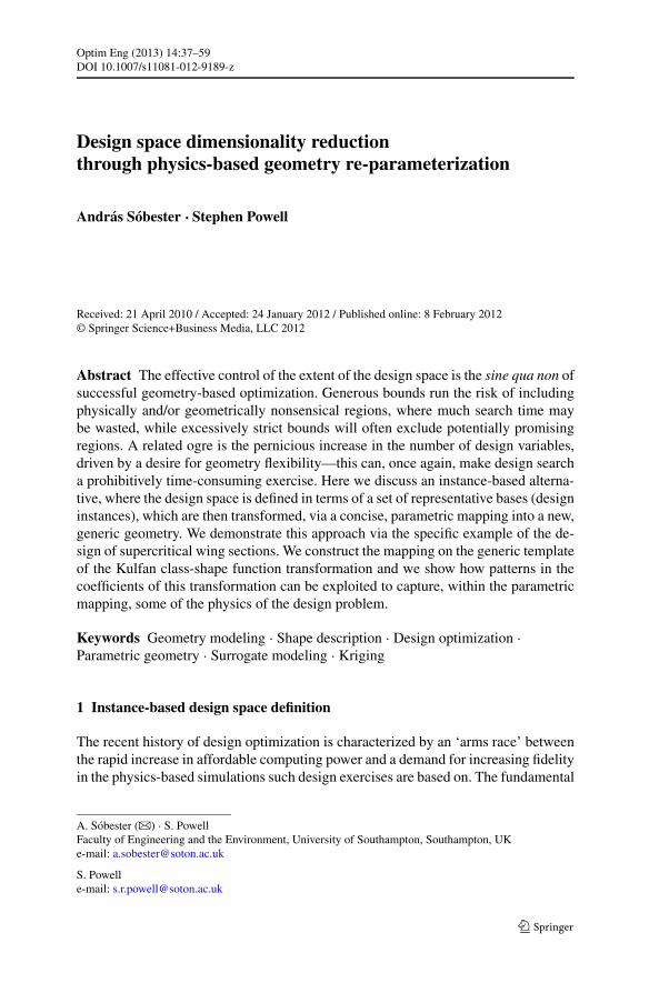
Consider the thickness distributions of our six chosen airfoils. As seen in Fig. 3, theairfoils with the same maximum thickness to chord ratios share, in fact, their entirethickness distributions. Thus, the different design lift coefficients are purely down tothe different camber curve shapes (Fig. 4) and this is good news from the perspectiveof mapping to a more concise description. We can apply the divide and conquerprinciple by separating, in terms of the transformation coefficients, the effects of thetwo features that headline each of the SC(2) airfoils, design lift coefficient (clearlydetermined by the shape of the camber curve) and maximum thickness to chord ratio(determined by the thickness distribution). It also gives us a strong indication that,of all the possible variables we could use, it makes most sense to define the new,

3So called because the terms of the series add up to one, regardless of the order nBP.


Fig. 2 Approximation errors: the differences between the six supercritical airfoils and their class-shapetransformations. The horizontal lines indicate the typical tolerances of wind tunnel models (tighter within20% chord of the leading edge)

Fig. 3 The half-thickness distributions of the six SC(2) airfoils (vertical and horizontal axes are to differ-ent scales)

concise design space in terms of maximum thickness to chord ratio and design liftcoefficient—denoted as t/c and cl respectively in what follows. The mapping weseek is therefore the first of the sequence


Fig. 4 The camber curves of the six SC(2) airfoils (axes to different scales)

(t/c, cl) �−→ (vu

0, vu1, . . . , vl

LE

) �−→ [zu(x), zl(x)

], (10)

where we already have the second step in the shape of (2) and (3).Turning now our attention to separating the airfoil into a camber line and a thick-

ness distribution, the class-shape transformation gives us a compact way of writingthese—manipulating equations (2) and (3) we get

CAMBER(x, vu

0, . . . , vuTE, vl

0, . . . , vlTE

)

= √x(1 − x)︸︷︷︸

class function

nBP∑

r=0

vur + vl

r

2Cr

nBPxr(1 − x)nBP−r


+ zuTE + zl

TE

2x


+ x√

1 − xvu

TE + vlTE

2(1 − x)nBP


, (11)

and

HT(x, vu

0, . . . , vuuTE, vl0, . . . , v

lTE

)

= √x(1 − x)︸︷︷︸

class function

nBP∑

r=0

vur − vl

r

2Cr

nBPxr(1 − x)nBP−r



+ zuTE − zl

TE

2x


+ x√

1 − xvu

TE − vlTE

2(1 − x)nBP


, (12)

respectively, where HT denotes half thickness (note that in order to simplify the equa-tions we are assuming nu

BP = nlBP = nBP). This is, in fact, a variable transformation,

which gives us the possibility of breaking up the required first mapping of (10) intotwo more easily manageable sub-problems (divide and conquer again!), the right handone of which we have just solved:

(t/c, cl) �−→(

vu0 + vl

0

2,vu

0 − vl0

2, . . . ,

vuLE − vl

LE

2

)

�−→ (vu

0, vu1, . . . , vl

LE

) �−→ [zu(x), zl(x)

]. (13)

This has not reduced the dimensionality of our design space yet, but has givenus intervening variables that are more useful in terms of exploiting the separation ofcamber and thickness distribution and have therefore taken us closer to the ultimategoal of mapping from the (t/c, cl) space. For the final remaining step we divide theproblem once more and first look at the

t/c �−→(

vu0 − vl

0

2,vu

1 − vl1

2, . . . ,

zuTE − zl

TE

2,vu

LE − vlLE

2

)(14)

subproblem. Having already established that the thickness distribution of the six ex-ample airfoils depends only on the maximum thickness to chord ratio t/c and notingthat the relationship is clearly linear, the r th half thickness term in the description ofthe parametric airfoil will be a function of t/c as follows:

vur − vl

r

2

∣∣∣∣t/c

= vur∼SC(2)−0410 − vl

r∼SC(2)−0410

2

+(

vur∼SC(2)−0412 − vl

r∼SC(2)−0412

2− vu

r∼SC(2)−0410 − vlr∼SC(2)−0410

2

)

× t/c − 10

t/c − 12, t/c ∈ [10,12]. (15)

Note that where we used coefficients from the class-shape transformation of, say,SC(2)-0412 (for example, vl

r∼SC(2)-0412), we could equally have used the relevantcoefficients of any of the 12% thick airfoils, as they only appear as part of the trans-formation coefficients of the thickness distributions, which, as we have seen, are iden-tical for airfoils of the same maximum thickness. This, as well as the above equation,are equally applicable to the calculation of the two remaining parameters, the addi-tional leading edge shaping term and the trailing edge thickness term.


We now need to find a way of constructing the coefficients of the camber curvetransformation of the parametric airfoil, that is, to find the

(t/c, cl) �−→(

vu0 + vl

0

2,vu

1 + vl1

2, . . . ,

zuTE + zl

TE

2,vu

LE + vlLE

2

)(16)

part of the mapping (13). This is a slightly more complicated proposition, as theshape of the camber curve, though chiefly influenced by the design cl , varies betweenairfoils of different thicknesses, as shown in Fig. 4. We therefore need to constructa model of each of the camber curve parameters on the right hand side of (16) as afunction of design cl and t/c, based on the six examples provided by our chosen sixSC(2) sections.

5.2 A Gaussian process model

Considering that the sets of transformation coefficients v and z (which we have identi-fied earlier) define approximations of the six ‘training’ airfoils (when inserted into (2)and (3)) and therefore the camber line coefficients are also approximations of thecamber lines of the six airfoils, we shall build a regression model of (16) (as opposedto an interpolating one) to filter out the ‘noise’ in the coefficient values.

We choose to work with a Gaussian Process modeling approach—kriging—andwe use the implementation described in Forrester et al. (2008). The interested readeris invited to consult this reference for the details of the formulation; here we limitourselves to a brief summary of the problem setup.

Let us, for each camber line class-shape transformation coefficient (the right handside of (16)), consider a 6 × 2 matrix X of the t/c ratios (column one) and designcl values (column two) of our set of supercritical airfoils and a 6 × 1 vector y of thecorresponding values of the current camber transformation coefficient. We then con-struct a matrix � of correlations between the 6 training points contained in X, whichis now a function of the correlation coefficients θ . Additionally, to account for theinexact nature of the approximations (2) and (3) constructed with the transformationvariables, we add a regression parameter λ to the leading diagonal of the correla-tion matrix—both θ and λ are estimated subsequently via a likelihood maximizationprocedure.

The kriging regression model is thus given by:

y(t/c, cl) = μ + ψT(� + λI)−1(y − 1μ), (17)

where

μ = 1T(� + λI)−1y1T(� + λI)−11

, (18)

I is a 12×12 identity matrix and ψ is a vector containing the correlations between thetraining data and the (t/c, cl) pair, where we wish to predict the current class-shapetransformation parameter.

The model (17) is an approximation of mapping (16) and thus completes the map-ping (13). We therefore now have the complete route from (t/c, cl) to the explicitdefinition of the airfoil based on (2) and (3). This, then, is a parametric airfoil de-pending on two design variables, whose ranges are defined by the six airfoil trainingset: t/c ∈ [10,12], cl ∈ [0.4,0.7].


5.3 Physical significance

While not strictly relevant from the perspective of an automated design process, it isstill natural to ask: is there a correlation between the physical properties of the newparametric airfoil we have created and the pair of design variables that control itsshape?

In order to answer this question we generated 20 pairs of (t/c, cl) values, arrangedin the [10,12] × [0.4,0.7] design space in a Latin hypercube sampling pattern (seeForrester et al. 2008 for details of the formulation and the algorithm used4). Wethen generated the corresponding airfoils using our parametric mapping and eval-uated the designs in terms of their maximum thickness to chord ratios and theirlift coefficients—the latter computed using the computational fluid dynamics solverFLUENT, with GAMBIT employed to create the unstructured mesh (∼200,000 cellsfor each mesh to obtain the required curve detail). In terms of the flow condi-tions, we kept the Reynolds number constant at 30 × 106 with the Mach numberM and the angle of attack α allowed to float until the drag divergence Mach number(dcd/dM = 0.1) was found and the pressure coefficient plot was comparable to theidealized model shown in Fig. 5 (see the report by Harris 1990 for background infor-mation). More specifically, initially we computed three flow fields, one at the Machnumbers found using the Korn equation (Mason 2009)

M + cl

10+ t

c= 0.95 (19)

and the other two at M + 0.001 and M − 0.001 respectively. We then fitted a poly-nomial to this data in the cd versus Mach number space, differentiation of whichyielded the drag divergence Mach number (where dcd/dM = 0.1). The flow fieldwas then solved at this new condition, with the result added to the existing solutionsand a polynomial fitted once more. This pattern was continued until the position ofthe drag divergence Mach number remained constant over consecutive iterations. Theresultant pressure coefficient graph at this position was compared to the ideal graphof Fig. 5, with the above heuristic repeated at a new α if the graphs were dissimilar.

Fig. 5 Typical ‘flat top’pressure distribution around anSC(2) supercritical airfoil,serving as a target for the searchfor the design conditions for agiven supercritical airfoil

4Latin hypercubes have uniform projections onto all axes and are therefore ideal for correlation studies.


Fig. 6 Actual thickness to chord ratio versus the ‘t/c’ design variable value at 20 airfoils spread evenlyacross the design space

Fig. 7 Actual cl at design M and α versus the ‘cl ’ design variable value at 20 airfoils spread evenly acrossthe design space. The corresponding R2 value is 0.9869

Figures 6 and 7 show the results of this experiment. Correlation can be observed inboth cases. In fact, the maximum thickness to chord ratio of the parametric airfoil canclearly be said to be equal, for most practical purposes, to the value of the ‘t/c’ designvariable. Once again, this has little significance in most automated design processes,but it can be seen as a useful feature, for example, if we want to restrict the design


space to, say, wings that can accommodate a certain spar depth (that is, their t/c mustbe greater than a certain threshold value).

Much of the reasoning behind the construction of the parametric mapping wasbased on the observation that we can link the design variables to easily separableelements of the airfoil shapes (crucially, we have found the thickness distributions ofthe six members of the family to be connected exclusively to the maximum thicknessto chord value that headlines each airfoil). We look at a more general case next, wheresuch simplifications are no longer possible.

6 A more diverse family

6.1 Patterns

Consider now a larger subset of SC(2) supercritical airfoils: SC(2)-0406, SC(2)-0606,SC(2)-0706, SC(2)-0410, SC(2)-0610, SC(2)-0710, SC(2)-0412, SC(2)-0612, SC(2)-0712, SC(2)-0414, SC(2)-0614 and SC(2)-0714. These 12 sections now encompassa broader range of design cl values and t/c ratios then the set we analyzed earlier.The crucial difference with respect to the previous family of six is that the pattern ofthickness distributions and camber curve variations within the family is considerablymore complicated. We shall use this broader family to illustrate a more general formof the class-shape transformation dimensionality reduction heuristic presented earlier.

Once again we begin by approximating every member of the chosen familythrough its class-shape transformation. This time, we set the orders of the Bern-stein polynomial terms to nu

BP = 2 and nlBP = 3 for the upper and lower surfaces

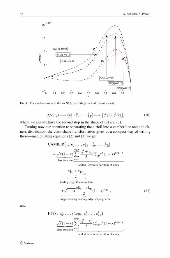
respectively. The sets of transformation coefficients of the 12 target airfoils yieldedby solving equation (6) are depicted in Fig. 8.

Also shown in the same figure are the ‘coefficient-fingerprints’ of a number ofadditional airfoils. It is clear that the SC(2) coefficient sets form a rather obvious‘wr’-shaped pattern, rather dissimilar to the shapes corresponding to the other air-foils whose coefficient patterns are depicted in the same figure (especially in thecase of the ‘w’ corresponding to the rather typical shapes of the SC(2) lower sur-faces).

If we hadn’t already studied a six airfoil subset of this family, the existence of thispattern would be our first indication that we are likely to need considerably fewerdesign variables to cover this restricted space than the 11 variables of the class-shapetransformation itself (the nine shown in Fig. 8, plus the two trailing edge thicknessparameters). Essentially, we have the opportunity to trade flexibility for conciseness.Restricting any design searches to these ‘wr’-shaped coefficient sets also has the ad-vantage of ensuring that the design space will only contain physically ‘sensible’ (and‘supercritical’) shapes.

As before, we shall aim to map the t/c, cl pair to the space of class-shape trans-formation coefficients and therefore to zu and zl , that is, we seek to build the first partof the mapping (10) ((2) and (3) form the second part).

Of course, all this reasoning on patterns is based on intuition and is the expres-sion of certain assumptions—not least that the shapes of the SC(2) airfoils are chiefly


Fig. 8 Class-shape transformation coefficients of a set of well-known airfoils. The heavy, continuous linesdenote the 12 SC(2) supercritical airfoils discussed here, while the dotted lines represent the approxima-tion coefficients of NACA5410, NLR7301, RAE5215, RAE2822 and NACA24-011. Note the distinctive‘wr’-shaped pattern of the SC(2) family

determined by design lift coefficient and thickness and that otherwise their designgenerally follows the same principles across the family (this was clear in the caseof our earlier, ‘separable’ set, but less obvious here). Additionally, we will assumeseparability, that is, that each class-shape transformation variable can be generatedfrom a (cl, t/c) pair via a mapping that is independent of the other transformationvariables. Intuitively, the similar shapes of the transformation variable patterns in-dicate that this is a reasonable assumption to make. In the case presented earlierwe made, tacitly, a weaker form of this assumption: there we could, at least, besure of the separability of the mappings between the half-thickness coefficients and‘t/c’.

The purely intuitive nature of the above, however, is of no practical significance,as long as we manage to construct a well-posed model of the mappings and the re-sulting reduced dimensionality airfoil is suitable for design studies. We shall returnshortly to the mathematical ‘checks and balances’ we can use to confirm the correct-ness of our assumptions (at least from a practical perspective)—here we merely notethat an additional bonus and further confirmation of the correctness of these assump-tions would be the existence, as in the previous study, of some degree of correlationbetween the design variable values t/c and cl and the maximum thickness and the liftcoefficient of the resulting instantiation of our parametric airfoil.

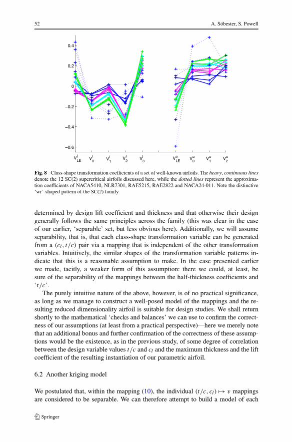
6.2 Another kriging model

We postulated that, within the mapping (10), the individual (t/c, cl) �→ v mappingsare considered to be separable. We can therefore attempt to build a model of each


Fig. 9 Gaussian Process regression model of the value of one of the class-shape transformation parameters(vl

LE), trained on the 12 values found as optimal for the set of SC(2) airfoils

class-shape transformation coefficient v in terms of cl and t/c, based on the 12 knownpairings resulting from our approximations of the 12 SC(2) airfoils.

We no longer have any of the handholds we took advantage of in the previouscase (the six airfoil family), so we have to construct 11 such models. The processemployed is much the same as before—we find the model parameters by maximizingthe likelihood of the data—except that on this occasion we do not build the mod-els in terms of the intervening camber coefficient variables, but directly in termsof the variables describing the airfoil surfaces. Figure 9 is a depiction of one suchmodel, also showing the 12 training data points, one representing each example air-foil.

If our assumption of separability was seriously wrong, this is where that wouldbecome apparent. For instance, in the absence of a clear trend (which would implythat a third variable has a significant influence over the shapes of the airfoils) thevariations within the log-likelihood landscape would be generally low and would nothave clear maxima. Recall that this is a function of the kriging model parameters (aθ per dimension and a global regression parameter λ) and the presence of significantadditional factors would lead to very different combinations of these parameters be-ing almost equally likely—clearly a sign that there are no trends in the data. Shouldthe reader opt for other methods of determining the θ ’s and λ, these are usually alsoequipped with warning devices that will indicate if the initial assumptions are wrong.For example, leave-k-out cross-validation (Forrester et al. 2008) would yield cross-


Fig. 10 Actual thickness tochord ratio versus the ‘t/c’design variable value at 20airfoils spread evenly across thedesign space

validation errors per data point comparable to the range of the responses—again, asign that other factors have a significant impact on the data.5

6.3 Physical relevance

As before, a space-filling set of designs was generated and tested from the point ofview of the accuracy of our approximation of mapping (10). Figure 10 shows that, asbefore, the t/c design variable is virtually equal to the maximum thickness to chordratio of the airfoil the mapping will generate. A weaker correlation can be observedin terms of the cl variable (Fig. 11)—here we can see a slight loss of approximationaccuracy compared to the first case.

Figure 12 is a further illustration of the physical significance of the design vari-ables: different values of the cl variable produce airfoils with variable camber (left),while the camber is maintained and the thickness changes as t/c varies (right).

7 Reflections on the design process

So what does all this mean from the perspective of the preliminary design process?6

In the previous section we described the construction of a parametric airfoil definedby two design variables—here we summarise this process as follows.

5We stress the word ‘significant’ here for a good reason—in the process of tailoring the SC(2) airfoilssmall shape alterations were necessary in some cases to obtain the desired pressure profiles (in particularshock locations) and drag rise Mach numbers, but, for practical purposes, we can assume that the twomajor factors with consistently significant impact were t/c and the desired cl .6We choose to define as ‘preliminary’ the first phase of the design process that is centered around ageometry.


Fig. 11 Actual cl versus the‘cl ’ design variable value at 20airfoils spread evenly across thedesign space. The correspondingR2 value is 0.8747

Fig. 12 Examples of instances of our two variable parametric airfoil

1. INPUTS:Axz

i = {(x, z)(i), (cl, t/c)(i)}, i = 1, . . . , nSC, that is:

– nSC airfoils Axzi given as sets of coordinate pairs

– nSC corresponding pairs of design cl and t/c values

The final goal of the algorithm is to enable the construction of new such pairsgiven (cl, t/c) values not included in this original set.

2. STEP I.—ENCODING OF THE INPUTS:for i = 1, . . . , nSC, Axz

i → AKi


We apply the Kulfan transformation to each of the nSC airfoils, that is, for each Axzi

we solve (6) to obtain the corresponding set of AKi = [vu(i)

0 , vu(i)1 , . . . , v

u(i)

nu(i)BP

, zu(i)TE ,

vu(i)LE , v

l(i)0 , v

l(i)1 , . . . , v

l(i)nl

BP(i), z

l(i)TE , v

l(i)LE ] Kulfan coefficients.

3. STEP II.—RE-PARAMETERIZATION:For each of the Kulfan parameters we build an approximation model of the formof (17) in terms of the corresponding (cl, t/c) pairs.We begin with vu

0 . For each of the (cl, t/c)(i), i = 1, . . . , nSC pairs we have a corre-

sponding vu(i)0 value from STEP I. We thus construct the kriging model vu

0(cl, t/c)

based on these nSC data.We repeat the above step for vu

1, . . . , vl0, vl

1 and the rest of the Kulfan parameters(Fig. 9 shows an example of such a bivariate model).

4. STEP III.—CONSTRUCTION OF THE NEW PARAMETRIC GEOME-TRYWe now assemble the models vu

0(cl, t/c), vu1(cl, t/c), . . . , v

l0(cl, t/c), vl

1(cl, t/c),

. . . from STEP II. into a parametric description of a complete Kulfan airfoil. Sim-ply inserting these Kulfan coefficients into (3) yields the sets of (x, z) coordinates.

The process summarised above and illustrated earlier for the family of SC(2) su-percritical airfoils can be employed to exploit patterns in the class-shape transfor-mation coefficients of other families of similar airfoils. This reduced dimensionalitymodel can then be used for global design searches, safe in the knowledge that wehave reduced the contribution of the airfoil to the overall dimensionality of the air-frame geometry and that we do not need to worry about setting sensible variablebounds.

As an illustration of the time-savings afforded by this type of approach, let usconsider the following design problem. The preliminary design process of an airlinerrequires an 11% thick airfoil with a design cl of 0.5. We have discussed the class-shape function parameterization in great detail in this paper and we could deploy itin this context too. We can apply the Kulfan transformation to the SC(2)-0412 airfoil,which is the existing supercritical airfoil that matches our requirements most closely(having a thickness-to-chord ratio of 12% and a design lift coefficient of 0.4). We canthen run a local search process starting from this airfoil (its corresponding Kulfancoefficients), which aims to minimize the drag of the airfoil, subject to the thicknessconstraint. Each objective call issued by the optimization algorithm (we employed aNelder and Mead simplex search here) involves iterating through a sequence of anglesof attack to attain the required lift coefficient. This is a relatively expensive process—we use a Navier-Stokes flow solver at the same level of fidelity as employed whengenerating the correlation plots presented earlier (e.g., Fig. 11)—we ran the Nelderand Mead search with a computational budget of 10 iterations. Table 1 shows theresults (the search history) of this exercise, featuring an ultimate drag coefficientvalue of 0.0136.

An alternative approach would be to deploy the parametric airfoil described here,using it to generate directly the target 11% thick airfoil with a design cl of 0.5. Build-ing this airfoil and running the same iterative analysis process (until we obtain the an-gle of attack that gives the required cl) yields here a drag coefficient value of 0.01298.


Table 1 Simplex optimizationhistory of the search for an 11%thick airfoil with a design cl

of 0.5. The starting point wasthe Kulfan transformation ofSC(2)-0412

Simplex iterations Function evaluations Best objective

0 1 0.0156

1 17 0.0150

2 18 0.0150771

3 19 0.0150771

4 21 0.0136

5 22 0.0136

6 23 0.0136

7 24 0.0136

8 25 0.0136

9 26 0.0136

10 27 0.0136

This is slightly better than the airfoil obtained through the rather expensive simplexoptimization process started from SC(2)-0412 (see Table 1) and it involved no designsearch at all (the computational cost of instantiating the parametric airfoil for cl = 0.5and t/c = 11% is negligible).

Once this first step of the design process is complete, we are left with an airfoilexpressed in the form of (2) and (3), i.e., as a Kulfan transformation, which can formthe starting point of a subsequent local search. This second optimization procedurecan then exploit the aerodynamic significance of some of the class-shape transforma-tion variables (e.g., the first term is related to leading edge radius, number nBP + 1controls the boattail angle), or can simply allow an automated optimizer to exploitthe current basin of attraction in terms of some design goal.

To summarise then, the preliminary designer in need of a low drag airfoil of aspecific lift coefficient and thickness to chord ratio would either have to run a globalsearch on a very flexible, generic parameterization (very expensive) or a local searchfrom the nearest existing airfoil designed for similar flow conditions (moderatelyexpensive). For the type of design scenario outlined here, the proposed alternative re-quires no optimization, indeed no analysis runs at all—a potentially significant savingat the preliminary design stage when the dimensionality of the complete airframe ge-ometry might be quite high.

8 Conclusions and future work

In the above we have shown that it is possible to build a concise parametric geometryover a design space defined purely by a set of basis shapes, regardless of how theseexample designs are represented. At a more fundamental level, the problem of build-ing such geometries as concisely as possible, translates into a more general question,which is worth further investigation and could be phrased as follows.

Let us consider a set of curves (or surfaces), which represent a diverse range offeasible (though not necessarily optimal) solutions to a design problem (the examplesor potential bases). What is the minimum dimensionality of a parametric curve (or


surface) that can reproduce all of the sample curves (or surfaces) to within a specifiedlevel of accuracy, while also creating a smooth subspace of designs defined in termsof these ‘training’ examples?

In a previous paper (Sóbester 2009a) we have approached the problem using aNURBS description. Here we have shown the Kulfan transformation to be anotherfeasible way of capturing the training cases and building the parametric mapping—atleast for the specific case of supercritical airfoils. We have constructed two parametricairfoils that distil the aerodynamic reasoning behind the designs of their respectivesubsets of basis airfoils down to two design variables. Moreover, in both cases thetwo design variables show strong correlations with physical parameters (geometricaland aerodynamic) of the parametric airfoil, whose shape they determine, a featurethat can be useful in the context of human interventions in the design process (asopposed to a purely automated search for a shape that optimizes some goal function).

Future work therefore should consider applying either strategy to broader (or dif-ferent) classes of shapes. As this initial study indicates, the method has the potentialto parameterize complex shapes very concisely, while constructing a design spacethat is relatively unlikely to include infeasible regions. Here is a summary of the keysteps to be followed in order to do this successfully for other applications.

(1) Identify the key variables. It is best to select a combination of physics- andperformance-based parameters and geometrical parameters (preferably ones withintuitive engineering appeal)—a simple example, considering a whole airframe,might be a set including wing sweep angle, cruise Mach number, maximum loadfactor, range, aspect ratio, etc.

(2) Identify the ‘basis geometries’, that is, the set of distinct designs for which theparameters chosen above are available.

(3) Apply the Kulfan transformation to these basis geometries (other shape encodingmethods could also be adapted, as indicated above).

(4) Build kriging models of each element of the encoding from (3), in terms of thevariables identified at (1).

(5) Generate instances of the new parametric geometry and test their performanceagainst what you would expect from their inputs (e.g., does the instance of theparametric airframe indeed have the range specified as the input to the parametricgeometry?).

Clearly, the success of building such a geometry will depend heavily on the choiceof variables at (1) and the choice of the parameterization scheme selected at (3), so incase (5) yields unsatisfactory results, the process will have to be repeated with differ-ent choices at (1) and/or (3). There is no hard and fast recipe for either and, indeed,for certain applications, finding the correct choices might be hard or impossible. It ishoped that the example shown here will encourage readers to explore these choicesfor their own applications.

Acknowledgements The first author’s work has been supported by the Royal Academy of Engineeringand the Engineering and Physical Sciences Research Council through their Research Fellowship scheme.


References

Collins L, Saunders D (1997) Profile: Airfoil geometry manipulation and display. Contractor Report177332, NASA

Forrester AIJ, Sóbester A, Keane AJ (2008) Engineering design via surrogate modelling. Wiley, New YorkHarris CD (1990) NASA supercritical airfoils—a matrix of family-related airfoils. Technical Paper 2969,

NASAJameson A (1988) Aerodynamic design via control theory. J Sci Comput 3(3):233–260Kulfan BM (2006) “Fundamental” parametric geometry representations for aircraft component shapes.

AIAA 2006-6948, pp 1–45Kulfan BM (2008) Universal parametric geometry representation method. J Aircr 45(1):142–158.

doi:10.2514/1.29958Kulfan BM, Bussoletti JE (2006) “Fundamental” parametric geometry representations for aircraft compo-

nent shapes. AIAA 2006-6948Mason W (2009) Configuration aerodynamics. Lecture notes, Virginia Tech UniversityRobinson GM, Keane AJ (2001) Concise orthogonal representation of supercritical airfoils. J Aircr

38:580–583Rozvany GIN (2009) A critical review of established methods of structural topology optimization. Struct

Multidiscip Optim 37:217–237Sóbester A (2009a) Concise airfoil representation via case-based knowledge capture. AIAA J 47(5):1209–

1218Sóbester A (2009b) Exploiting patterns in the Kulfan transformations of supercritical airfoils. In: 9th AIAA

aviation technology, integration, and operations conference, Hilton Head, SCVanderplaats GN (1979) Efficient algorithm for numerical optimization. J Aircr 16(12):842–847Vanderplaats GN (1984) Numerical optimization techniques for engineering design: with applications.

McGraw-Hill, New YorkWhitcomb RT (1974) Review of NASA supercritical airfoils. In: The ninth congress of the international

council of the aeronautical sciences ICAS 74-10Whitcomb RT, Clark LR (1965) An airfoil shape for efficient flight at supercritical mach numbers. Tech-

nical Report TM X-1109, NASA

http://dx.doi.org/10.2514/1.29958

Documents

Design space dimensionality reduction through physics-based geometry re-parameterization