UNIVERSITY OF MINNESOTA

ST. ANTHONY FALLS HYDRAULIC LABORATORY

LORENZ G. STRAUB, Director

Technical Paper No.9, Series B

Design Studies for a Closed-Jet Water Tunnel

by

John F. Ripken

August, 1951

Minneapolis, Minnesota

PREFACE

The design studies presented in this paper relate to the problems

and solutions encountered in formulating plans for a large hydrodynamic test­

ing facility proposed for construction by the United States Department of the

Navy at the David Taylor Model Basin, Carderock, Maryland" While a water or

cavitation tunnel of the type described herein is a rare facility in conven­

tional research or engineering work, many of the problems incident to its

design are commonly encbuntered in general practice.. However, it was apparent

at an early date that technical information adequate for the quality require­

ments of this design was not available in the literature and that extensive

tests would be necessary for proper planning.. Contract arrangements between

the st. Anthony Falls Hydraulic Laboratory and the David Taylor Model Basin

led to execution of the necessary experimental studies ..

Through the very generous cooperation of the David Taylor Model

Basin it is the privilege of the St .. Anthony Falls Hydraulic Laboratory to make

available thrbugh this paper the findings of this program.. For clarity of pur­

pose this study includes, in addition to the test analyses, prefacing abstracts

of the original design papers prepared by the author while a member of ~he

Model-Basin staff. The material presented here represents a condensation of

numerous interim reports submitted to the Model Basin by the Laboratory and,

as such" draws heavily from the discussions and analyses of these reports.

Grateful acknowledgement is therefore due Messrs. Alvin G. Anderson, James S.

Holdhusen" Owen P.. Lamb, and Edward Silberman who contributed to these re­

ports, ivith special acknowledgement due Mr. Holdhusen for his very extensive

contributions ..

The investigational program was under the general direction of Dr ..

Lorenz Go Straub, Director of the St. Anthony Falls Hydraulic Laboratory, and

was supervised by the author.. The author is indebted to Reuben S. Olson for

his technical editorial suggestions and to Loyal A" Johnson for arrangement

of the illustrations.. Preparation of the manuscript was by Leona S. Wray,

Marianne Sturtevant.9 and E. Roy Tinney ..

iii

ABSTRACT

A variable-pressure water tunnel, which is a testing facility analo­

gous to a wind tunnel, is a useful tool in the study of cavitation or hydro­

dynamic characteristics of underwater bodies. This paper includes general,

selective, hydrodynamic design studies for the construction of a large closed­

jet water tunnel, together with experimental model test data and design analysis

of a specific selection of flow components. Each flow component is critically

examined with regard to its, influence on test section flow quality, cavitation

susceptibility, and energy head loss. Included are studies of the test section,

contraction, diffuser, vaned elbows, and pumpo Presentation in chapters de­

voted to single flow components simplifies the treatment and increases adapta ...

bility of the findings to conduit design problems other than water tunnelso

iv

Preface .". . .. Abstract " " • • .. • " " . . . ..

0' ., (» (l: 0

.. . . " . • 0

Page

iii iv

List of Illustrations ".. e • . . " . . .. " o • 0 0 4) 0 vii List of Tables <> • • • , " .. • o • -0 0 e 0- i) ;0 ./) 0 (10 ix

CHAPTER I.. INTRODUCTION...... .. • • .. " • " • .. " • • • " " .. " • .. " A. The General Problem .. .. " .. • • .. • • .. • • ". " " " B.Problem at the David Taylor Model Basin .... " ...... " ...... " o·

C. Studies at the St. Anthony Falls Hydraulic Laboratory .. .. .. .. .. CHAPTER II. TEST SECTION STUDIES ." • • " • .. .. • • • .. .. .. . .. .. "

A. B ..

General Considerations ......"...................,,, "" .. 0

Design Studies ..".... .. " " .. 0 .. " • " • 0 .. .. .. . .. .. " 0

1. Size .. • .. .. .. " • " " " .. .. .. • • " " .. • " .. ao Area 6 0 • • it .fI (I. 0 0 • .0 00 • &

0... Shape.o 0 4) .,. 0 0- .0 10 0' 0 e 0 0 • 4 e 0 0 t'I 6 -0 0 0 (10 •

C 0 Length • 0- ., 6 , .. 0 ", .0 0- 0 .. .... 0 0 1) 0- 0; ., -0

Speed • 00 0 eo 0 40 0 0 0 0 .. 0 .,. ft 0 0 0 0' • ;Q. 0 0 0

Pressure 0 0 ;0 .,. • .f) 1) .. b • 0 I) 0 0 4) 0. 4 0 0 (Ii 0 9- ;0 0

a. Open~Jet Tunnels (Recirculating Type) .. " " " " .... bo Closed-Jet Tunnels "......... " .. • .. .. .. " .. .. " .. c.. Free-Jet Tunnels .."....".... .. .. .. <> .. .. " " .. ..

d.. Comparison .. " " " • ~ .. 4 .. .. .. .. .. .. .. ~ ..

40 TurbuJ..ence 0 0 0. «I 0 '$ .,. 0, 0 b '" :0 0' 0 Cj, (10 0 .(J ~ -0 (J • -0 -0

, .. Air Content " .. .. .. .. .. .. .. .. .. .. .. • .. .. .. • .. .. .. 6. Tempe;r-a ture 0- .. -Ct ., • • e • v .0 .. q '(io • 0 ~ 0. 0 0 e ~ ..

7 •. Diffuser Transition ............ " .................. .. Co Experimental Studies ".... • • .. • • .. " .. " .. .. 0

1. Apparatus and Procedures ............."................ .. 2. Velocity Distribution and Boundary Layer Thickness ..".... 3.. Energy Loss and Pressure Distribution .. " • " ............ " 4. Cavitation Indices .. " • .. 6 .. .. .. .. .. .. .. .. .. .. .. .. " .. ..

D. Conclusions .. " • .. .. .. .. " .. .0 • .0. e 0 0' 0 0.000'00

CHll.PTER III. CONTRACTION STUDIES .. . A. General Considerations 0."

Design Studies .... .. • .. .. .. • ~ 0 • • • 0 e 0 0 • 0 0 00 ~ (10 0

o -& 0 .. 0 " . 1. Selection of Area Ratio " .. .. .. • .. • .. .. .. .. .. .. .. .. .. .. .. 2. Selection of Boundary Curve .. • .. .. .. .. .. • .. .. .. .. • • • ..

a. The Plane Orifice in an Infinite Tank 0 .. .. .. " .. .. .. ..

00 The Plane Orifice Terminating a Cylindrical Conduit of Finite Diameter ....... .... ..,.. 0 • .. .. " ..

c.. The Bell-Mouth Orifice Terminating a Cylindrical Con-duit of Finite Diameter ................... "

d. The Ogee Orifice Terminating a Cylindrical Conduit of Finite Diameter ............".............. 0 0

e • Summar-y 0 (\ .. eo-. 0 0 • 0 • 0- • • • • .. e- 0 0- boO, 0

Experimental Studies ... • 0 .. 0 .. • • .. • • • 0 • • " 0 • " "

1.. Apparatus and Procedures ....... .. .. " .. " • . .. 2. Velocity Distribution Studies ........ " •• o 0 . .. 3. Pressure Distribution Studies ••• 0 0 ...... 0 0 •• 0 0

4. Energy Los6 Studies • .. .. • .. 0 • .. .. .. • • 0 0 • 0 .. .. .. 0

Conclusions 0 0 0 ~ 0 0 0 0 • 0 0 0 o. 0 0 0 ~ • 0 0 0 bOO

v

1 1 2 2 5 5 5 , , 6 6 7

10 10 11 12 13 13 14 15 15 16 16 18 21 2, 32 3, 3, 39 39 41 42

44

44

4, 4, ,2 52 54 ,6 61 63

CON TEN T S (Continued) -~------

Page

CHAPTER IV b DIFFUSER STUDIES .. .. • .. .. .. A. B.

General Considerations " .. " • .. .. " Design Studies'.... .. .. .. 1.. Di.:t'fuser Shape • .. " " .. " .. ..

.. .. .. . a. Simple Expansions ".... • " b.. Expansion by Boundary-Layer Removal c.Expansion by Boundary-Layer Acceleration. ,(L Expansion by Flow Rotation • .. .. " .. . e • Expansion by Deflectors or Vanes • .. " ..... I" Comparison".... ...." .... ..

2.. 'iJiffuser Transition Curve " ".... 3. The Pump Diffuser .. ..

c. Experimental Studies • .. .. L Apparatus and Procedures " .. 2. Velocity Distribution.. .. 3. Energy Losses "

D. Conclusions cHAPTER V" VANED ELBOw STUDIES .. ..

A. B ..

General Considerations " " .. Design Studies ..

.. .. .. ..

" . .. .. .. .

.. " . " .

.. ..

.. ..

• •

..

..

..

..

C. Experimental Studies .. .. . " .. .. .. .. .. 1" JlrJethod.... .... .. .. . .. .. ..

a. Apparatus .. "" .. b. Visual and Photographic Studies ......"..".... ..

2. Quantitative Tests in the Duct Elbow .. .. .. .. .. ., .. 3.. Quantitative Tests in the Model Tunnel Elbow ...... • .. 4. Flow Distribution _ " • .. .. .. .. " .. .. 5. Energy Loss' 0 ..... " .... .. ... G ...

6. Vane Pressure Distribution " " .. " .. .. .. .. .. .. .. .. .. 7.. Scale Effects .."".... <>......" .. '. " .. 8. Cavitation Analysis • .. .... " ........ " . . 9. Vibration and Stress Analysis .. "., ... ..

D <> Conclusions ........ .." .. .. .. CHAPTER VI. PUMP STUDIES .... ..

A. General Considerations .. .. .. .. B. Design Studies .. .. .. .. .. ,,'.

1. Discharge-Head Relations " .... 2. Type of Pump .. .. .. 3~ Pump Diameter 4. Pump Diffuser .. .. 5. PumpLocation ..

.. "

C. Experimental Studies • ..

.. . •

.. . .. 0- 0-

1.. Head and Energy " .. .. • •

" . .. .. ..

. .. .. .

.. " .. 2 • Velocity Distribution' .. .. " .. ., .. .. .. 3.. Cavitation Susceptibility • 4. Temperature Factors ........ ..

D. Conclusions .... .. APPENDICES

I. Test Apparatus . .. II. Test Instruments .. <>

III. Test Proce~ure .. " ..

" .. ..

vi

..

., ...

.. .. " •

" "

.. ..

. .. .. .. .. .. .. ..

.. ..

.. .. . ..

.. .. . .. "

• .. " " .. "

.. . " .. .. <>

.. " ..

67 67 68 68 68 68 69 70 70 70 71 71 71 71 72 75 81 83 83 86 90 90 90 97 99

101 106 107 111 i12 113 116 116 119 119 1,20 120 122 123 123 124 125 125 128 130 132 133 135 137 143 146

LIS T 0 F ILL U S T RA T ION S

Figure

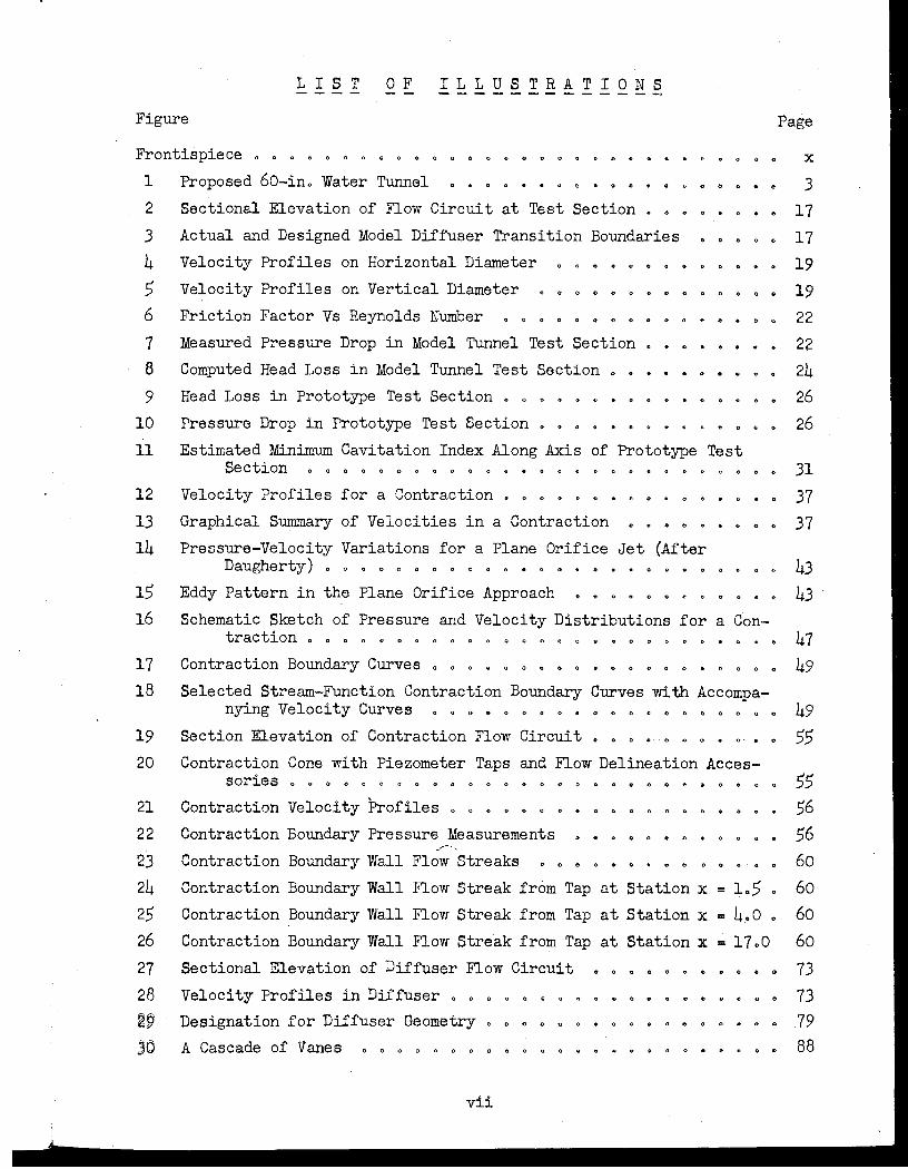
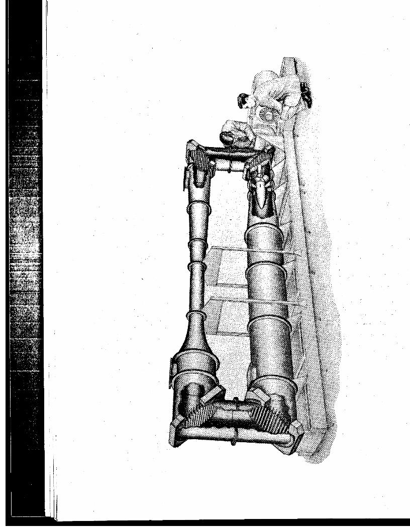
Frontispiece 0 0 0 • 0 " 0 " • " • • " • " " . 1 Proposed 60-in. Water Tunnel " • • " • • • • " " " • · " 2 Sectional Elevation of Flow Circuit at Test Section. " •

3

4 5 6

7 8

9

10

11

12

13

14

15 16

17

Actual and Designed Model Diffuser Transition Boundaries

Velocity Profiles on Horizontal Diameter

Velocity Profiles on Vertical Diameter

Friction Factor Vs Reynolds Number

. . ., () 0 C) 0 0 0

() () 0 C) 0 0 0

. . . · "

Measured Pressure Drop in Model Tunnel Test Section •

Computed Head Loss in Model Tunnel Test Section 0 •

o Goo

.. . Head Loss in Prototype Test Section • ., I) (10 0 () •

Pressure Drop in Prototype Test Section •

Estimated Minimum Cavitation Index Along Axis of Prototype Test Section () () 0 0 () I) 0 () 0 0 • ~ .e -c 0 0 0 0 0 0

Velocity Profiles for a Contraction • ., " " "

Graphical Summary of Velocities in a .Contraction . " Pressure-Velocity Variations for a Plane Orifice Jet (After

Daugherty) • • • 0 • • • " 0 • • • • • • • • 0

Eddy Pattern in the Plane Orifice Approach CioQOeOoG

Schematic Sketch of Pressure and Velocity Distributions for a Con-traction 0- 0- 0 0- (J Ct () 0 t!I 0 0 Q 0 0 0 I) 0 e (I (I 0

Contraction Boundary Curves " " • • " " • • 0 • • " " " • . . " 18 Selected Stream-Function Contraction Boundary Curves with Accompa-

Page

x

3

17 17 19

19 22

22

24

26 26

31

37 37

43 43

47 49

nying Velocity Curves • 0 0 0 0 " • " • • •• 0 • 49 19 Section Elevation of Contraction Flow Circuit • • " • • " " " • • 0 55 20 Contraction Cone with Piezometer Taps and Flow Delineation Acces-

21

22

23 24

25 26

27

28

~~

30

sories 0 0 0 0 0 0 Q 0 0 0 000 0 0 0 0 0 0

Contraction Velocity Profiles 0 0 0 0 . . . 0' 0 0 Oc

Contraction Boundary Pressure Measurements •• 0 .. • • 0- 0 0 0

.-"~-,

Contraction Boundary Wall Flow Streaks • 0 • • • ., • • " 0- '0 0

Contraction Boundary Wall Flow Streak from Tap at Station x = 1.5 . Contraction Boundary Wall Flow Streak from Tap at Station x = 4.0 • Contraction Boundary Wall Flow Streak from Tap at Station x = 17.0

Sectional Elevation of Diffuser Flow Circuit .00000000

Velocity Profiles in Diffuser • o • " o 0 -0 0 · " Designation for Diffuser Geometry ., o • o • 0- 0

A Cascade of Vanes 00Q00600800

vii

55 56 56 60

60

60

60

73 73 79 88

LIST OF r !:. :!: 12 .e. 1. !l ! 1. r Q li £ (Continued)

Figure

31 32

33

34

35

36

37

38

39 40

41

42

43

44

45

The Preliminary Vane Selection " <> " ¢ • " " .. 0 (t 0' 0 . .,

The Proposed Vane Selection <> <> <> <> 0 0 • " OOOCOOClOC)

E~ow Diversion Test Bend (Duct Elbow) • <> 0 <> "

Duct Elbow Details 0 • <> 0 0 <> 0 <> <> • <> <> o 0 (J () () <t 0- 0 • <>

Duct Elbow Assembly QUO Q 0 0 0 ()- 0 o 0 0 C 0 o • 0 " 0

Duct Elbow Vane and Trunnions o Q () 0 0 OOOOOOOOOC()OO

Upstream View of Elbow I 0 " 0 0 " 0 OOOOOOOoooo,()O

Designation of Vaned Turns and Velocity Traverse Stations

Paths of Air Bubbles at Yid~Depth of Duct Elbow Cascade " <>

<> 0 0

Duct Elbow Velocity Distribution (Series Noo 10) <> • <> 0 0 0 <>

Duct Elbow Velocity Distribution (Series Noo 15) 0 " 0 " "

Duct Elbow Velocity Distribution (Series Noo 16) " 0 <> 0 <> 0 0

Duct Elbow Velocity Distribution (Series Noo 18) 0

Wall Pressures at Mid~epth of Duct Elbow 0 " <> o 0 .,

Pressures at Mid-Depth Across 96 Degree Cascade 006QOOO

" 0

" <>

<> 0

<> <>

o 0

<) •

46 . Pressures at Mid-Depth Across 101 Degree Cascade • 0 00" o <)

·47

48

49

59 51

52

53

54

55

Pressure Variation Around Vane as a Function of Reynolds Number

o 0 0' 0 00'0 0' ()- (l 0 Duct Elbow Vane Pressure Distribution

Velocity Profiles at Station 5 0 0 0 .,

Velocity Profiles at Station 6 " 0 " •

o " 0 000(100

" " " 0000- co

Velocity Distribution at Stations 11 and 12 000000' 000

Model Tunnel Vane Pressure Distribution 00000000

Duct Elbow Energy Progressions 0 " 0 " 0 " o 0

Recommended Prototype Vane Cascade Dimensions

Discharge-Head Relations for the Prototype Pump

o 0 0- Q

o 0 -0 0

COO () 0

<> " "

" <>

" " 56 . Energy Gradients for Prototype Tunnel

57 Velocity Distribution at Station 7 0 0

00000000--0

O(l-OOOOOOOOOO o 0

58

59

60

61

62

63

Velocity Distribution at Station 8 <) <> o <> <> <> 0 <> I) 0 Q Q

Minimum Cavitation Index To Be Achieved at Centerline of Prototype Pump 00000000000000 OOOOo-OlJQo(t

Temperature Rise and Cooling Relations <> <> <> 0 0 0 0.000000

Sectional Elevation of 6-ino Model Water Tunnel 0000000

Model Pump Assembly <> 0 <> <> 00000-00.00000 <> 0

Cantilevered Pitot Cylinder and Mounting " 0 o <>

yiii

Page

88 88

91

91

93 96

96

96

98

100

100

100

100

102

103

103

103

103

104

10k

105

105

107

117

127

127

129

129

133

133

137

139 145

l

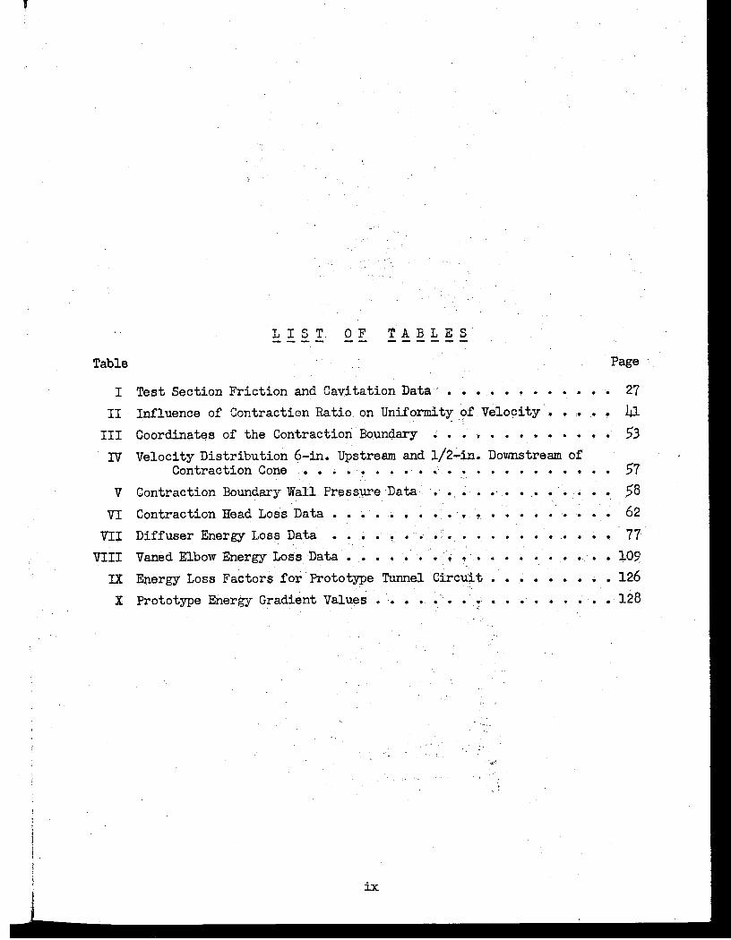
1 I ST OF TAB 1 E S' -- ...... ---Table . Page

I Test Section Friction and Cavitation Data . . . . . . . . . . . . II· Influence of Contraction Ratio, on Uniformity C?fVelocity • .. . .. - "

III Coordina~S of the Contraction Bo~ndary. • • • ~ • • • • •

IV Velocity Distribution 6-in. Upstream and 1/2-in. Downstream of Contraction Cone .• • • •• • • .'. •. •• .; • •

V Contraction Boundary Wall Pre S s'l,l!'e Data •••• • • . . . . .. • • VI Contraction Head Loss Data. • • • • • • • • •.• t. • • • · . '. . ..

VIl Diffuser Energy Loss Data •••• ~' ••••• . .. . · .

27

41 53

57 58 62

77 VIII Vaned Elbow Energy ,Loss Data • • • • ~ • .• • • •

IX Energy Loss Factors for Prototype Tunnel Circu~t ••• • • • .'. ;, 109

• " • • • • 126

X Prototype Energy Gradient Values . ". ·0 . . . . . ' .. ' . . . . · . 128

ix

C LOS E D - JET W ATE R TUNNEL ------ --- --~-- ------

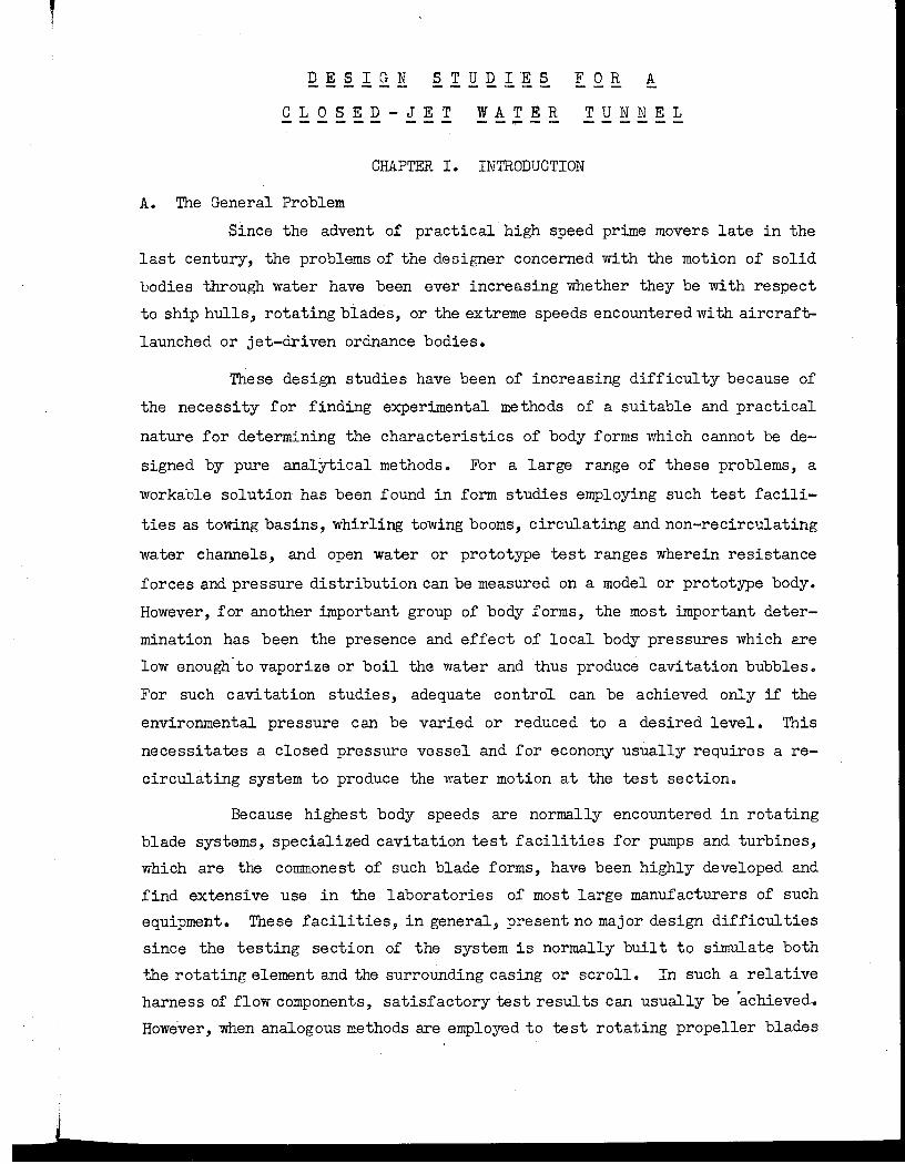
CHAPTER I. INTRODUCTION

A. The General Problem

Since the advent of practical high speed prime movers late in the

last century, the problems of the designer concerned with the motion of solid

bodies through water have been ever increasing whether they be with respect

to ship hulls, rotating blades, or the extreme speeds encountered with aircraft­

launched or jet-driven ordnance bodies.

These design studies have been of increasing difficulty because of

the necessity for finding experimental methods of a suitable and practical

nature for determining the characteristics of body forms which cannot be de­

signed by pure analytical methods. For a large range of these problems, a

workable solution has been found in form studies employing such test facili­

ties as towing basins, whirling towing booms, circulating and non-recirculating

water channels, and open water or prototype test ranges wherein resistance

forces and pressure distribution can be measured on a model or prototype body.

However, for another important group of body forms, the most important deter­

mination has been the presence and effect of local body pressures which are

low enough"to vaporize or boil the water and thus produce cavitation bubbles.

For such cavitation studies, adequate control can be achieved only if the

environmental pressure can be varied or reduced to a desired level. This

necessitates a closed pressure vessel and for economy usually requires a re­

circulating system to produce the water motion at the test section.

Because highest body speeds are normally encountered in rotating

blade systems, specialized cavitation test facilities for pumps and turbines,

which are the commonest of such blade forms, have been highly developed and

find extensive use in the laboratories of most large manufacturers of such

equipment. These facilities, in general, present no major design difficulties

since the testing section of the system is normally built to simulate both

the rotating element and the surrounding casing or scroll. In such a relative

harness of flow components, satisfactory test results can usually be 'achieved.

Howe'ver, when analogous methods are employed to test rotating propeller blades

2

or other body forms which in nature normally move in an infinite flow field,

extreme design care is necessary to prevent a material distortion of the flow

pattern around the body and a serious lack of similarity due to the presence

of the boundary walls of the recirculating pressurizing duct.

It is the purpose of this paper to discuss the problems which arise

in attempting to design a large, high speed, general purpose, variable pressure

cavitation test facilityo

B. Problem at the David Taylor Model Basin

The manifold assignrrent of research problems to the David Taylor

Model Basin during the years of World War II was such that a survey of past

and probable future assignments established a need for a large, mill tiple pur­

pose, cavitation test facility capable of producing conditions simulating a

complete range of natural, subsurface conditions.

The survey of need, which was extended to include preliminary direc­

tive specifications, was released by the tec!mical director of the Model Basin

early in 1945 and was followed by assembly of a complete bibliography relating

to similar existing test facilities and findings from visits to and inspections

of those units existing in the United Stateso As an outgrowth of this prepara­

tion, a general preliminary design was assembled as a basis for discussion and

was followed with detailed hydraulic studies of the principal components. The

proposed designs were based on the best available design data of a theoretical

and empirical nature, but finally led to the conclusion that proper plans

could be achieved only through use of experimental verification of specific

design proposals" In accord with these conclusions, experimental studies were

ini tiated at the St. Anthony Falls Hydraulic Laboratory in August, 1946, under

the terms of Contract NObs-34208.

C. Studies at the Sto Anthony Falls Hydraulic Laboratory

An early analysis of the problems incident to experimental testing

of the proposed tunnel design led to the conclusion that the best answer would

be found in tests of a complete scale model tunnel in which the mutual effects

of the various parts could be carefully studied" In a balance between the

economics of testing and the limitations of similitude, it was determined

that a one-tenth scale model would be adequate for the needs and, accordingly,

a complete unit of this size was fabricated.

, 3

While the general properties of this facility and its auxiliaries

are rather fully described in the appendix to this,paper and specific proper­

ties of the components are described in the individual chapters, it is per­

haps proper to orient the reader at this time to the salient features of the

study. This is deemed necessary because the detailed analysis seems most

effectively presented by individual studies which may at times obscure the

integrated relation of these parts.

To assist in this integration, it is well for the reader to retain

in mind that the experimental studies were conducted on a one-tenth scale

model tunnel having a. test section diameter of 6 in., a recirculating duct

loop oriented in the vertical plane, and a suitable pumping unit. The general

arrangement of flow components in the proposed prototype design is shown in

Fig. 1, while that of the model is shown in the frontispiece. The ensuing

chapters are summary treatments of the experimental studies of the various

major tunnel flow components ani are accompanied by discussions of the design

principles involved.

elbow Vaned

'b -' ~

156'-8" I

Fig,l- Proposed 60- in. Water Tunnel

h

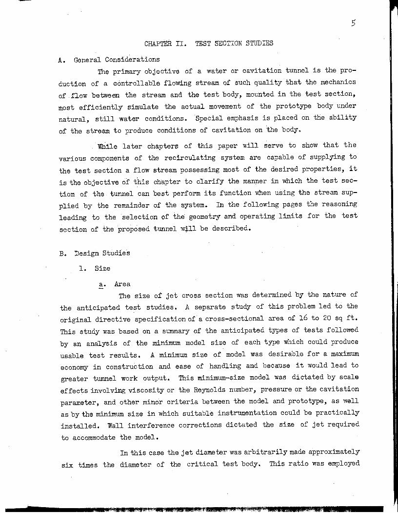
CHAPTER n. TEST SECTION STUDIES

A. General Considerations

The primary objective of a water or cavitation tu.nnel is the pro­

duction of a controllable flowing stream of such quality that the mechanics

of now between the stream and the test body, mounted in the test section,

most efficiently simulate the actual movement of the prototype body under

natural, still water conditions. Special emphasis is placed on the abiiity

of the stream to produce conditions of cavitation on the body.

While later chapters of this paper will serve to show that the

various components of the recirculating system are capable of supplying to

the test section a flow stream possessing most of the desired properties, it

is the objective of t~is chapter to clarify the manner in which the test sec­

tion of t.he. tunnel can best perform its function when using the stream sup­

plied by the remainder of the system. In the follOWing pages the reasoning

leading to the selection of the geometry and operating lim1 ts for the test

section of the proposed tunnel will be described.

B. Design Studies

1. Size

a. Area

The size of jet cross section was determined by the nature of

the anticipated test studies. A separate study of this problem led to the

original directive specification of a cross-sectional area of 16 to 20 sq ft.

This study was based on a summary of the anticipated types of tests followed

by an analysis of the minimum model size of each type which could produce

usable test results. A minimum size of model was desirable for a maximum

economy in construction and ease of handling and because it would lead to

greater tunnel work output. This minimum-size model was dictated by scale

effects involving viscosity or the Reynolds number, pressure or the cavitation

parameter, and other minor criteria between the model and prototype, as well

as by the minimum size in which sui table instrumentation could be practically

installed. Wall interference corrections dictated the size of jet required

to accommodate the model.

In this case the jet diameter was arbitrarily made approximately

six times the diameter of the critical test body. This ratio was employed

,¥1Rilxce*as E 111[2&

----:---~------_____ ~-,J __ C,,_____--- - - -- __

6

because data from aeronautical literature indicated that a cylindrical body

in a cylindrical stream of these proportions would give results in which the

wall interference effects were at a limit of acceptability_

In view of the fact that the proposed tunnel was to be an !lall

purpose" type with an undetermined future use, the area was selected generously

in conjunction with the shape determination, as treated below.

b. Shape

The external boundary form of the test section is largely de­

termined by the pressure conditions which are desired to prevail in the test

stream. As will be separately described later under the pressure discussion,

a boundary form consisting of solid parallel walls or a uclosed jetU was elec­

ted for the prototype needs.

A circular cross-sectional boundary shape was finally selected

for the following reasons:

(1) For general model testing, a circular boundary would probably afford as

little wall interference effect as any other shape.

(2) In passing from the contraction to the test section as well as from the

test section to the diffuser, area transitions could be accomplished with per­

fect lateral symmetry without shape transition, if circular transitions were

adhered to throughout. Tests indicate a smoother and less turbulent flow

could be expected in such a transition. Obse:rvati.ons on rectangular transi­

tions have shown vortex filaments in the corner regions.

(3) A circular section is inherently more efficient in the use of structural

materials for resistance to the differential pressures to be expected.

(4) Control of dimensional accuracy and surface finish could be achieved most

economically when machining circular sections.

The overall shape and size requirements are satisfied by selec­

tion of a cylindrical boundary of 60-in. inside diam.

c.Length

One of the longest models proposed for test in the tunnel is

a torpedo shaped form and its wake. The total study length of the body and

wake may be as much as 30 body diam. If the maximum body diameter is taken

as one-sixth that of the test section, as previously selected, the total test

section length should be at least 5 section diam.

•

7

7

It is recognized that the downstream: portion of the test sec­

tion jet deteriorates in flow quality as the length increases, but the fact

that this is accomplished without significant effect on the quality of the

upstream: portion of the jet permits arbitrary selection of a generous length.

From the'economic standpoint a moderate increase of test section length could

have but little effect on the total construction cost, as it represents only

a small percentage of the total tunnel length; however~ it could have an ap­

preciable effect on operating cost, as the input power is largely consumed

in the high velocity regions in and adjoining the test section. A considera­

tion of the above factors led to an arbitrary selection of a test section'

length of 30 ft.

2. Speed

The speed range anticipated as necessary in the proposed tunnel

varied from a low value of about 3 fps for certain towed body studies to the,

maximum which might be practically attained. This maximUm was considered

desirable for simulation of speeds and cavitation conditions encountered with

modern subsurface ordnance.

European practice, for purposes of operating economy, generally

leans toward cavitation simulation through operation with low pressures and

moderate speeds; however, certain deficiencies inherent to low pressures,

such as release of dissolved air, produce difficulties which can be partially

eliminated by changing to higher pressures and higher speeds. To permit maxi­

mum testing flexibility, it was considered desirable to provide the maximum

practical operating speed for the proposed facility. In determining what

constitutes the maximum practical speed, two important trends must be recog­

nized.These are the costs attending the rapidly rising power requirements,

which vary approximately as the cube of the speed, and the inherent cavitation

tendencies of the jet boundaries and model support system. Since economic

criteria are always somewhat indeterminate, the speed limit imposed by cavita­

tion conditions will,be considered approximately to frame the upper critical

speed limit ..

In view of the fact that the test model may in itself be designed

with optimum streamlining, it becomes apparent that a facility for testing

such a model cannot operate appreciably faster than the limits of the test

body without incurring serious cavitation on the tunnel boundaries or the

model supports. While relatively little data are available as to the limiting

8

values in such a case, studies conducted in the water tunnel of the California

Institute of Technology indicate that a speed of about 70 fps is a practical

maximum when used in combination with reasonable pressure values. Since the

above value is in fair agreement with the normal limits for the anticipated

tests, a speed range from 3 to 85 fps (50 knots) will be assumed as generous

coverage for subsequent design studies.

In examining the basic property of speed, it was apparent that a

facility attempting to provide a flow stream simulating a body of water at

rest must give consideration to the steadiness and uniformity of the velocity

front. 'While it is true that the natural, still water condition is not ordi­

narilya state of complete rest, it is the objective of the design to produce

a stream of maximum practical steadiness and uniformity.

The degree of perfection practically obtainable is the next consid­

eration. The original directive specification states, tiThe variation in velo­

city across any tr2nsverse plane of the test section, up to within 5 per cent

of the diameter from either boundary, shall not exceed 2 per cent. tt Calibra­

tions of existing tunnels indicated that for most modern designs·, a uniformity

of about l.,0 per cent was commonly obtainable, and in a few cases values were

about 0.5 per cento In view of this, the proposed design attempted to obtain

1.0 per cent or better. As will be seen in a later chapter, it is the inherent

function of the contraction cone preceding the test section to provide the

necessary unification of the velocity distribution.

It must be recognized, however, that the mechanics of flow within

the test section tend to reshape the uniform entrance,velocity to the hyper~

bolic velocity profile common to stable turbulent flow in pipe lines. The

reshaping of the flow takes place gradually with thickening of the retarded

wall boundary layer and acceleration of the core flow until the boundary layer

expands to a thickness equal to the duct radius. This growth results in an

increase in the mean kinetic energy of the flow, with a consequent axial re­

duction in the pressure on a gTadient greater than is u,sually evidenced by

stable wall friction alone 0 Yfuile development of a stable turbulent front

usually requires a flow distance of 20 to 40 diam from the point of inception

and may normally be computed with fair accuracy, an estimate of growth in the

6 diam of proposed test section length will have no validity since the point

of inception is unknown because of the partially developed boundary layer be­

ing delivered by the contraction.

9

Despite theinabili ty of the analysis to yield valid values of the

growth, it does show qualitatively the axial deterioration of jet quality and

warns that the quality at exit will probably be less than called for in the

directive specification. This is an unavoidable consequence of long test sec­

tions and must be accepted with their adoptiono

In addition to uniform differences in the velocity distribution, due

to the internal flow mechanics, unsteady velocity variations with time are

also evident in most tunnels" These may be short pulses, long surges, or a

continuous drift and may be due to such factors as deficiencies of the pump­

motor unit, hunting after starting, temperature variations, power variations,

etc. In addition to these bulk flow changes with time, local periodic flow

eddies may be shed from certain parts of the contraction walls or other bound­

ary components" While instrumentation obstacles have prevented evaluating

these variables in existing water tunnels, evaluations have been made in wind

tunnels with variations running as large as 10 per cent of the mean value.

In view of the possibility of using test bodies which may be sen­

sitive to eddy impact or time transients, itvdll be necessary to design all

components with a view to minimizing separation or high turbulence6

In addition to axial flow variations in velocity, it is necessary

to make provision for suppressing rotation or angularity of the flow. However,

since such variations originate almost wholly in the pumping unit, methods of

control will be discussed separately in the chapter concerning the pump uni to

In addition to the types of velocity variation just described, another form .><.

may occur when very large models are placed in the test section. Tests [1J"

with a large model in the 5-ft Royal Aircraft Establishment wind tunnel indi­

cated an image or shadow of the model was impressed on the exit flow to the

extent that the shadow was still apparent on the velocity profile entering

the test section from the contraction. This is, of course, undesirable and

must be eliminated by redistribution of the flow in the return circuit .. _ It

is anticipated that the four vaned elbows and the propeller pump of the pro­

posed circuit will give sufficient mixing; if not, a grid or honeycomb may

eventUally be found necessary in the prototype.

*Numbers in brackets refer to the corresponding numbers in the reference list at the end of the chapter.

10

Bradfield [lJ provides an interesting aspect of the shadow probl~m

in saying, ttThis forms a limit to the efficiency which it is desirable to

achieve in tunnel design, because a tunnel requiring very little power to run

it can have but little mixing and damping effect. tt

3. Pressure

Since a water tunnel differs from other types of flow-stream test

facilities principally in the controllability of pressure in the test stream,

this discussion will open with a review of the three basic ways in which test

sections have been built to effect desired control of the pressure variable.

a. Open-Jet Tunnels (Recirculating Type)

In this type of tunnel the fluid jet issues from the contrac­

tion cone, flows unconfined through· a testing chamber containing the same

fluid at rest, exits from this chamber through a pickup cone, and then returns

through a recirculating duct. This type of jet was originally evolved for

wind tunnel work wherein the testing chamber was simply the open atmosphere.

It had the advantage of providing complete vision and ready access to the

model, and, because the pressure surrounding the jet boundary was uniform,

the internal jet pressure along the axis could be assumed quite uniforme Vlhile

small non-recirculating tunnels of this type have been bull t to waste the "jet

energy, for reasons of power economy, most designs find it necessary to regain

this energy by returning the jet in a solid boundary after it leaves the test

section. This pickup is usually accomplished by a flared cone followed by a

diffuser and a return duct.

Friction between the fast moving test jet and the static fluid

surrounding it induces strong eddies at the jet periphery in the form of a

rapidly growing mixing zone and a rapidly shrinking jet core 0 As the distance

between the entering contraction and the discharging pickup cones increases,

the difficulty of smoothly squeezing the fast jet into the pickup cone rapidly

mounts and violent cavitating impact of the eddies on the cone may occur. The

net result of this is reduced speeds and short jet lengths if' vibrations or

pulses are to be avoided and a uniform core is to be attained. Such pulses

not only physically hammer the structure but introduce pressure-velocity pulses

in the flow which enters the circuit and is returned to the test section .. Al­

though numerous studies have been made of this problem, involving altering the

cone shape and other artifices, no universally successful method permitting

high speeds and long jets is yet known. As a consequence, most wind tunnels

11

of this type have a jet length less than twice the diameter.. Water tunnels,

because of the cavitation accompanying the eddies, are usually restricted to

jets of a diameter's length and are apparently restricted to speeds of about

50 ips when operating under reduced or cavitating pressures.

In addition to its other deficiencies, the eddy system accom­

panying open jets consumes considerable amounts of energy. Early wind tun­

nel measurements indicated that such types of tunnels required twice as much

driving power as a comparable closed-jet tunnel.. Measurements in more recent

tunnels indicate this ratio may now be reduced to 1.5 times or less~

In review of the foregoing, it is apparent that the limiting

length and speed of an open jet are such as to eliminate this type of test

section from consideration for the proposed tunnel, even though the internal

pressure conditions are superior to other types.

b. Closed-JetTunnels

In this type of tunnel, the fluid jet issues from the contrac­

tion cone and flows through a test se ction having a solid and continuous peri­

pheral boundary and thence into an expanding recirculating duct. This type

of tunnel is seldom employed if an open jet can be applied because the solid

boundary complicates mounting and access problems for the model and is the

source of the boundary-layer flow which destroys the desired jet uniformity.

The boundary layer is serious in that it produces an axially falling pressure

gradient as the turbulent layer thickens and the core flow accelerates. How­

ever, despite the fact that these influences are detrimental, the presence

of the fixed boundary suppresses the boundary layer to small scale eddying;

and in consequence, a much more stable and efficient flow results than in the

case of the unharnessed open jeto Accordingly, the closed jet is used where

stability and speed are necessary, and various types of corrections have been

evolved to compensate for its inherent deficiencies ..

Among these corrections to the pressure forces acting on a

test model is the compensation for the falling pressure gradient occurring

axially in the direction of flowo Because this gradient is virtually linear,

a simplified treatment of the force system considers this as a uhorizontal

buoyancy, tt and a number of papers have developed theoretical procedures for

correction" In a parallel with this analytical method of adjustment, con­

siderable work has been done on physical modifications of the test section

I--

I

II

12

to produce a natural compensation. This can be accomplished by providing a

slight downstream divergence to the test 'section boundaries.

The divergence modification has been occasionally used in wind

tunnels since the very early days but is no panacea for the pressure problem,

because the optimum correction is matched to only one speed of tunnel operation.

The Voith (Germany) propeller channel, which is a special purpose tunnel, was

tapered to suit the speed of most frequent testing, as were certain of the

early Hamburg (Germany) tunnel designs. Divergence has not been employed

with tunnels of more recent design; and it is not considered essential for a

general purpose tunnel of the proposed type, although this may be considered

debatable.

In addition to the above-described pressure problems inciden­

tal to the solid-jet boundary, other problems arise because of the inter­

ference of this boundary with normal flow lines about a mounted test model.

~ile this interference effect is sometimes appreciable, adequate theoretical

corrections for measured values are now known if the model size is not too

large in relation to the jet size.

Variations of pressure in a plane transverse to the axis of a

horizontal jet are of two types, namely, the pressure due to deficiencies of.

the contraction cone in effecting full pressure-velocity conversion and the

pressure due to the normal gravitational gradient. Proper design of the noz­

zle can eliminate the former, and in most cases the latter gradient is qUlte

consistent with the similitude of the test and should be present; therefore,

no special compensation need be made for transverse pressure variations. The

hydrostatic pressure induced by the vertical head of the chambered water does,

however, determine the lower limit of pressures which may be achieved in the

jet.

c. Free-Jet Tunnels

In this type of tunnel, the liquid jet issues from the contrac­

tion cone and flows through a test section where it is surrounded by a gaseous

medium. This gas is chambered to permit reduction of pressure to very low

values and accordingly, the pressure within the jet is everywhere reduced to

this same value, both laterally and axially, without the vertical variation

and superimposed hydrostatic heads found in the open or Closed jets.

Because the jet is not buoyed up by the surrounding fluid, it

is subject to the gravity force, and in a horizontal jet assumes a curved

)

1

t.

d.

p

13

trajectory. With moderate speeds this curvature limits the size of test models

to small lengths. Positioning the jet vertically eliminates this difficulty

but presents others.. No wholly successful tunnel of this type has as yet been

built.

The principal field for a free-jet tunnel is in the simulation

of high speed undervvater ordnance conditions where a very low cavitation pres­

sure is essential for testing.. The free jet is unique not only in the uniform,

extremely low, static pressures attainable but in the fact that these pres­

sures, being gaseous, are measurable with a high order of accuracy; for these

reasons, it is superior to other types of jets for extreme cavitation. The

jet is not, however, considered suitable to general purpose work because of

the difficulties of operating at low speed and the high energy losses occa­

sioned by trying to pick up the jet and recirculate it.

d. Comparison

In summary analysis of the foregoing tunnel types, it is appar­

ent that the closed-jet form will best answer the need for a facility of high

speed and general purpose use. In considering the value of pressure coverage

to be desired, it is apparent that the lower limit must approximate the vapor

pressure of water while the upper value should be as high as practical. Since

the upper limit is largely a matter of balancing the structural costs against

the value of the anticipated work program, a fixed selection is beyond the

scope of this paper. Position or time variations of pressure are to be avoided

and since they are generally intimately related to speed variations, their

control will be affected in the manner previously described for the velocity

variations.

4. Turbulence

The size and strength of eddy turbulence present in the flow jet of

a model testing facility has long been recognized as an important factor in

the applicability of the model data to the prototype.. To insure that proper

correlating indices be recognized, considerable work has been done using drag

and pressure studies on spheres, foils, and other devices as a standard basis·

of comparison of testing facilities ..

While the establishment of specifications for desired levels of tur­

bulence is possible from these studies, it is impossible to predict the levels

which wiJ.l be achieved from a given design. Because turbulence is more readily

I

I I

"II

>11 I 1

! 1

'I i

"':' I'

'I'

, ,

I I ,~ I I

I I ~ j

i I I

">r ....

added to than eliminated from an existing flow structure, it has been 'con­

sidered advisable to design the basic tunnel components with a minimum prac­

tical turbulence 01ltput as the objective; this concept has been pursued in

the designs treated in the later chapters.

, 'It is intended that final turbulence control be effected through

sui table honeycombs and grids placed just upstream of the contraction cone,

where adequate space should be provided" These devices are capable of reforma­

tion a.nd limited add! tion of turbulence above the minimum basic value provided

by the tunnel itself.

5" Air Content

The amount of dissolved gas present in natural waters apparently

has some influence on the inception of cavitation on bodies moving through

such water, and accordingly, a 1{ater tunnel attempting to simulate such cavi",,:

tationshould properly operat.e with a gas content approximating that in nature.

'lihile this is a desirable objective, it is difficult t.o achieve in a prac ....

tical water 'tUnnel operating under sub a tmo sphe ric pressure as this causes

gas bubbles to grow and circulate in the flow.

To eliminate the bubble trouble,mosttunneis follow a practice of

depleting and removing the gas by application of high vacuum prior to the test

run. While this procedure prevents true cavitation simulation, it was, at the

time of this original design study, the only expedient. known to cQpe, with the

problem and apparently produced no major dis~repancies.'Accordingly,no spe-. .. ~ .. . ' .

cial proviSion for air content control was ~ade in the basic flow circuit of

the proposed design except for three air collection domes to assist in' pre­

test bubble removal.

More recent efforts to improve this condition, in an existing tunnel

at the California Institute of Technology, have established that a. physical

change in cirelli t form may be made' so that the' gases released in the low pres­

sure test section may be reabsorbed in the return circlli t. This is a.ccom­

plished by physically extending a leg of the return circuit vertically down­

ward to increase the static pressure and by increaSing its diameter and length

to such an extent that the return flow is subjected to the increased press1l!'e

for sufficient time to permit substantial reabsorption. Since the California

Institute of Technology resorber ha.d not been proved at the time these tests

were initiated it was not a part of this test program.

15

6e Temperature

Temperature variations in the testing water of a variable-pressure

water tunnel are a natural result of the energy input by the pump in main­

taining recirculating flow against internal frictional resistance.. It is es­

sential consideration be given to the probable magnitude of such variations

and the controls that maybe necessaryb This is essential because temperature

is a fundamental variable in most flow problems and can produce changes of up

to 205 times in the Reynolds numbers for temperatures varying from 600 to

1500 F. While this factor may mean an important extension to the testing

range in some problems, it is an annoying variable in many cases ..

A review of the problems of heating, cooling, insulating, etc",

indicates that a rigidly controlled external thermal unit would probably cost

in excess of its worth unless the uncontrolled fluctuations appeared to be ex­

cessive.. Preliminary estimates of tunnel mass and energy added by the pump

indicate the temperature rise will be about 10 F for every 25 min of opera­

tion at maximum speed. This takes no account of heat lost through radiation,

and for an appreciable span of operation at maximum speed, the rise would

probably be less than 20 per hr or 160 in a normal 8-hr day., In view of the

apparently nominal temperature rise, the geometry of the proposed design has

no provision for temperature controls.. If subsequent tests should establish

the need, external facilities could be provided to effect the necessary con­

trol.

7.. Diffuser Transition

The purpose of the diffuser or expanding cone of the water tunnel

is to reduce the large discharge velocity of the test section efficiently ..

A later chapter will discuss the selection and tests on the diffuser proper;

but, inasmuch as the boundary-transition curve between the test section and

the diffuser is critical to the flow performance of the test section itself,

a consideration of the transition characteristics should be included here ..

The transition region is of special importance since it is the tun­

nel wall area on which cavitation first occurs.. This is true because the

static pressure is inherently lowest there, and in combination with high velo­

city and the initiation of curvilmear flow, cavitation is promoted.. Such

tunnel cavitation must be minimized since in body cavitation studies it is

desirable to impose as severe conditions as possible on the test body without

16

cavitating the water tunnel; that is, the static pressure in the test stream

should be as small as possible and the velocity on the test body as high as

possible without occurrence of cavitation in the tunnel circuit. This is

desirable for maintenance of high tunnel efficiency and elimination of boundary

pitting and because the increasing use of sonic methods of observing cavitation

on the test body makes it desirable to maintain a low ambient noise level.

An analysis of the limited amount of literature on this subject indi­

cates that a number of theories have been advanced for the mathematics of the

boundary transition curve to answer best the needs 0 These theories have been

based on such factors as providing uniform rates of retardation (dv/dt = const),

uniform velocity changes (dv/dx = canst), and uniform head loss (dhf/dx = canst) for the bulk flow. While approaches of this kind are seemingly reason­

able for the core flow of the stream, their application to the complex condi­

tions existing at the boundary wall is highly questionable since the mechanics

of combining an existing boundary layer with the unstable force influences

attending expansion of flow is analytically indeterminate. In view of these

inadequacies of the theory, there appears little justification for trying to

approximate any transition curve on the basis of rates of change; rather, the

total length of transition should be made long enough to avoid excessive rates

of curvature and short enough to avoid the friction losses accompanyi~g ex­

tended flow at high velocity.

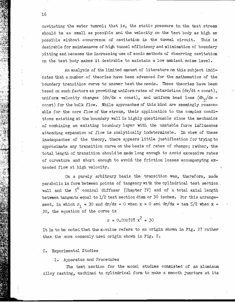
On a purely arbitrary basis the transition was, therefore, made

parabolic in form between points of' tangency with the cylindrical test section

wall and the ,0 conical dif'f'user (Chapter IV) and of a· total axial length

between tangents equal to 1/2 test section diam or 30 inches. For this arrange­

ment, in which r l = 30 and dr/dx = 0 when x = 0 and dr/dx = tan ~/2 When x =

30, the equation of the curve is

2 r = 0.000728 x + 30

It is to be noted that the x-value refers to an origin shown in Fig. 27 rather

than the more commonly used origln shown in Fig. 2.

C. Experimental Studies

1. Apparatus and Procedures

The test section for the model studies consisted of an aluminum

alloy casting, machined to cylindrical form to make a smooth juncture at its

..

17

30" 36" 7S"

Contraction Test section Diffuser 1.5~ 0.5 Traverse plane 0.5 Traverse plane

1. 0

1 . d J Flow ,..-;--. _.-_.-.-. __ . .,:r-'--. --.- r' --. -_. _.11) -.' to

10 J-po lID

T

en <P .s= u c

c

c 0 +-en c 0 ....

1--. "-IV en :::I --i5 -0

en J

"0 0

0::

3.10

3.08

3.06

3.04

3.02

Reference J Manifold (R)

Tap

R A B C D E F

·A f BCD E'F

X(in} Diam( in)

0.0 6.004 12.0 6.006 21.0 6.015 24.0 6.01S 36.0 5.999 39.0 6.015 39.S 6.062

Fig. 2 - Sectional Elevation of Flow Circuit at Test Section

End of transiti on

3.00L..--====::::O:" __ --C...-~ _ _L_ __ ___L _ __l~...L_ __ ___L __ ____.J

0.0 0.5 1.0 1.5 2.0 25 3.0 35

Distance from End of Test Section in I hc.hes

Fig. 3- Actual and Designed Model Diffuser Transition Boundaries

19

1,05 1.05

1.00

0.95

0.90

L-

( '[I%Y... '1 v.

I

1.00

0.95

0.90

L-

(( C%Y... \ v.

~

V V

Va I Vc

Y...

0.85

0,80

0.75

0.70 o

1·05

1.00 r-yo ~

0_ ii' 18;00 Fl, per secl c - Ii = 30,00 Ft, per sec A-v = 49,62 Ft. per sec

Downstream End of Test Section (t".rse plane 'If Fig,2) I

2 3 4 5 6 Distance from Wall in Inches

..."

0.85

o-v = 18.00 Ft. per sec c _ v = 30.00 Ft. per sec A- if = 49.62 ·Ft. per sec

0.80

0.75

Downstream End of Test Section

0.70 (trerse plonelf Fig2)

I 0 234 5 6

Distance from Wall in Inches

1.05

1.00

f ~

Vc 0.95 Y... 0.95

Vc

0.90

0.85 o

UpslreamEnd of Test Section (Irrverse plane 10f Fig.2) I

2 4

Distance from Wall in Inches

Fig, 4 - Velocity Profiles on Horizontal Diameter

5 6

0.90

Jo- Top of Tesi Secti"!"

0.85 o

I Upstream End of Test Section

(trorrse plane "T9.2) -.l .

2 3 4

Distance from Wall i.n Inches

Fig, 5 - Velocity Profiles on Vertical Diameter

5 6

is well within the maximum prescribed variation of 1 per cent. Only in the

boundary layer does the velocity fall below 99 per cent of .the velocity at the

axis of the test section and at the downstream end this has a measured thick­

ness value of about 0.90 in. (0.15 diam).

An analysis of the thickness of the boundary layer in the test sec­

tic;} of the prototype tunnel is made difficult because the Reynolds numbers

of proposed operations are considerably higher than those for which the best

ties between theory and data have presently been established. The problem is

further complicated by ignorance of the exact state of flow In the boundary

layer which the contraction would supply to the test section.

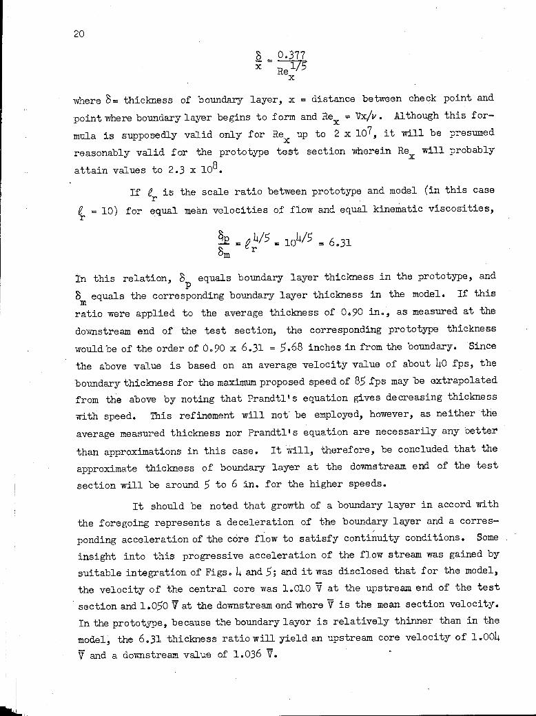
In accord with the following equation of Prandtl [2J, the prototype

boundary layer thickness at any point will be estimated from:

,

i I ! I

IIo.L

--~ ---~----

20

o 0.377 X = RellS

x

where 0= thickness of boundary layer, x = distance between check point and

point where boundary layer begins to form and Re = Vx/v. Although this for­x

mula is supposedly valid only for Re up to 2 x 107, it will be presumed x

reasonably valid for the prototype test section 'Wherein Rex will probably

attain values to 2.3 x 108•

If e is the scale ratio between prototype and model (in this case r

e = 10) for equal mean velocities of flow and equal kinematic viscosities, r

9.E = t? 4/5 = 104/ 5 6 t: .31 om r

In this relation, 0 equals boundary layer thickness in the prototype, and p -8 equals the corresponding boundary layer thickness in the model. If this m

ratio were applied to the average thickness of 0 .. 90 in", as measured at the

downstream end of the test section, the corresponding prototype thickness

would be of the order of 0.90 x 6.31 = 5.68 inches in from the boundary. Since

the- above value is based on an average velocity value of about 40 fps, the

boundary thickness for the maximum proposed speed of 85 fps may be extrapolated

from the above by noting that Prandtl's equation gives decreasing thickness

with speed. This refinement will not- be employed, however, as neither the

average measured thickness nor Prandtl's equation are necessarily any better

than approximations in this case. It Will, therefore, be concluded that the

approximate thickness of boundary layer at the downstream end of the test

section will be around 5 to 6 in. for the higher speeds.

It should be noted that growth of a boundary layer in accord with

the foregoing represents a deceleration of the boundary layer and a corres-/

ponding acceleration of the core flow to satisfy continuity conditions. Some

insight into this progressive acceleration of the flow stream was gained by

suitable integration of li'igso 4 and 5; and it was disclosed that for the model,

the velocity of the central core was 1.010 V at the upstream end of the test

section and 1.050 Vat the downstream end where V is the mean section velocity.

In the prototype, because the boundary layer is relatively thinner than in the

model, the 6,,31 thickness ratio will yield an upstream core velocity of 1.004

V and a dm¥nstream value of 1.036 V.

h

e

y

, :t , •

Le

>4

i

21

3. Energy Loss and Pressure Distribution

The prime intent of boundary pressure studies in the test section

is the evaluation of the high rate of energy loss occasioned by the local high

velocities and a determination of the lack of uniformity of test section flow

evidenced by an axial pressure gradient. Since no accepted method ·isav:.ail­

able for computation of the energy loss in the inlet length of smooth cylin­

drical pipes, recourse is made to the more illuminating laws which have been

derived for progressive skin-friction changes for flow along a flat plate

held parallel to the stream. Vfuile there are some physical discrepancies in­

volved in distorting a flat plate to a cylindrical pipe, it is a rational ap­

proximation where the boundary layer is thin relative to the pipe diameter.

The validity of the application is verified by the model data.

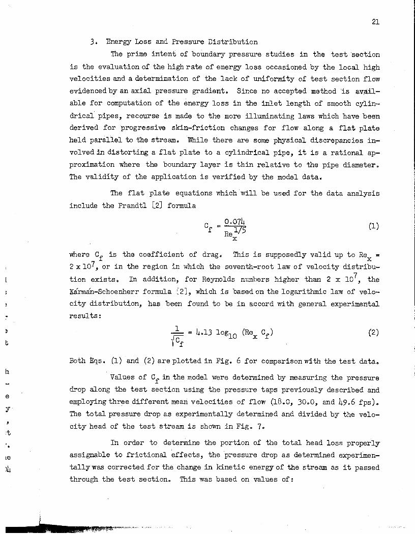
The flat plate equations which will be used for the data analysis

include the Prandtl [2J formula

0.074 Cf = 175

Re (1)

x

Where Of is the coefficient of drag. This is supposedly valid up to Rex = 2 x 107, or in the region in which the seventh-root law of velocity distribu­

tion exists.. In addition, for Reynolds numbers higher than 2 x 107, the

Karman-Schoenherr formula [2], which is based on the logarithmic law of velo­

city distribution, has been found to be in accord with general experimental

results:

(2)

Both Eqs. (1) and (2) are plotted in Fig. 6 for comparison with the test data ..

Values of Of m the model were determined by measuring the pressure

drop along the test section using the pressure taps previously described and

employing three different mean velocities of flow (18.0, 30 .. 0, and 49.6 fps) ..

The total pressure drop as experimentally determined and divided by the velo­

city head of the test stream is shown in Fig. 7.

In order to determine the portion of the total head loss properly

assignable to frictional effects, the ·pressure drop as determined experimen­

tallywas corrected for the change in kinetic energy of the stream as it passed

through the test section. This was based on values of:

___ -._ •....• ,.~ •.•...... ~ ..... :I~\!'ll!$;;~"~''''''f."< ••.••. ,

22

'i

-I<t 11

0-

~

0.0044

0.0040

0.0036

0.00~2

0.0028

0.0024

0.0020

0.0016 10·

\ Pra n d t I 0 Test secti on velocity =18.00 (ft. per sec.l

\ rCI= 0.071 [J Test section velocity =30.00 (ft. per sec.)

Rei , A Test secti on velocity =49.62 (ft. per sec.)

~ r\ 0

~ [J [\ [

l:~ A

" Range covered in model ,~ Range covered in prototype I

operation I I ~ operation

r--.-. ""-..

i'.. Kdrmdn - Schoenherr

...... r-. V ~ = 4.13xlog{Rei CI)-r--

r--.... ~

--.......... r--.. ......... ........

2 4 6 2 4 6 2 4 6

Fig. 6 - Friction Foetor Vs Reynolds Number

O.OO~----~------~------~----~-------r------~----~~----~------~

0.02~----~~~--~----~------+------+------+------4------~----~

Diffuser transition

0.04~-----+------4-~~~~~~-+~~~~------+------4--~~~~--~

~>10l ~ 0.06r-----~-------+--+---_r------~+_~~~~~--+_------r_

----~r_----~

"""-~

~13 0.08r-----~-------+--+_--~------~+_--~~----~ TopF

0.1 0 1------+-----l--t----+------l-t----4------+---~_rl~~=i#ffl:_ F+----1

I I I

Reference manifold (R) I Tap A 0.12~ ____ -L ____ L_~_-L ____ LJ ___ ~ ___ ~ ___ ~_L_~db==~~

o 5 10 15 20 25 30 35 40 45

Distance from Reference Manifold in Inches

Fig. 7 - Meosured Pressure Drop in Model Tunnel Test Section

23

integrated from theve10ci 1:.1 traverses of Figs.. 4 and S and resu1. ted iiI a ..

1.001S at the upstream end and a .. 1 .. 0160 at the d.ovrnstream end.. Values of a

at the pressure taps and reference manifold were computed by linear interpo-.

lation or extrapolation~ Since the diameter varied slightly, as shown in· Fig .. 2, correction was also made for the pressure change caused by the area

change ..

The total pressure drop was related to the frictional loss by using

Bernoulli's equation

.... 2 2 P.D v.R·. p. "':'2 V.

... a aV f xR w + it 2g .. w + .2'g + d2g

between the reference manifold and any tap where

p .. pressure at a tap (pounds per square toot),

w = specific weight ·of water (pounds per cubic foot),

V .. mean velocity of flow at a pressure tap (feet per second),

·f .. coefficient of friction,

x .. distaIfce from referenoe manifold to a pressure tap,

d = diameter of test section at piezometer tap, and.

subserlpt·R refers to the re:t'erence manifold ..

From this

.p - P R . f:; =J __ T~._ + QR-

a -2 VR 2i

Values of f (x/d) based on the experimental data applied to Eq. (3) are shown

in Fig.. 8 ..

In order to extend the energy loss data from the model to the pro­

totype through use of the flat plate extrapolation, the functional relation·

betweenf and Cf m~ be arrived at as follows .. Since Cf as used in Eqs .. (1) and (2) is defined by the drag expression:

V2 F=CfAPr...= fA ~o.

. I ! I

-..L,.

2u

0.00r-----~-----r------.-----._----_.------r_----~----_.----_,

0.02

x 1-0 Diffuser - transition 0.04

\I

~I~ II

0.06 .l:;:::' -d'I-o .......

tI

l.: tI 0.08 ~ + I ~ I

...... C> I '0: N I

I ;:;... I 1>1" 0.10 cr I I

I I I I I I

Reference manifold (R) ITapA ITape 0.12

0 5 10 15 20 25 30

Distance from Reference Manifold in Inches

Fig. 8 - Computed Head Loss in Model Tunnel Test Section

where F = frictional drag force on one side of a plate of area A,

p = density of fluid,

V = velocity of free stream, and

1'0 = average boundary shear on plate,

40 45

the relation between Cf and f can be computed because in a cylindrical pipe,

V2 f fo = P 2" (Ii')

Then Cf = f/4. Values of Cf • f/4 versus Rex = Vx/v are plotted in Fig. 6. In this plotting, values of Rex were computed assuming x to be the distance

from the manifold to a test tap. This seemed a logical assumption to make

since the extrapolated values of a were nearly unity at the manifold. It is

seen from Fig. 6 that the experimental points are in agreement with the semi­

empirical curve of Prandtl.

In extrapolating the foregoing model data to the prototype, it will \

be, necessary to use the Karman-Schoenherr equation, since the values of Rex

25

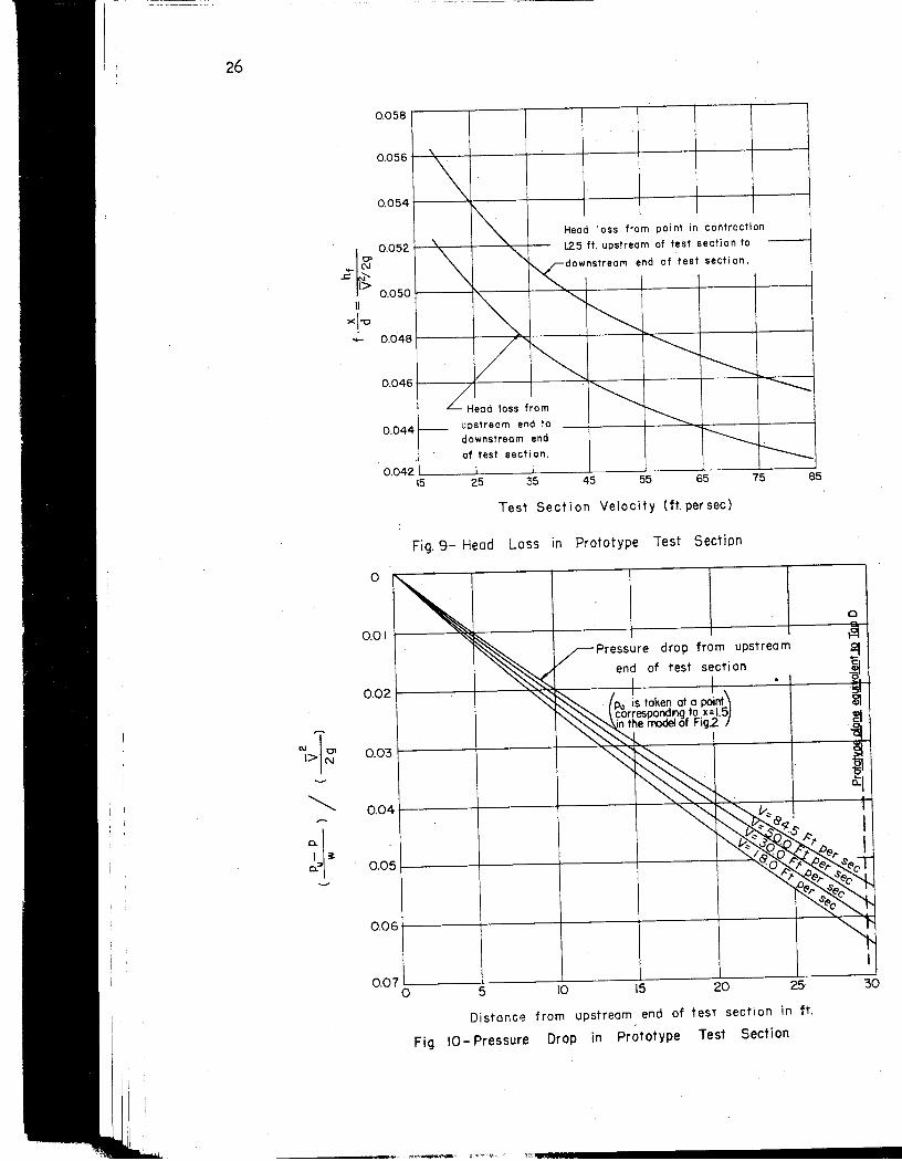
will, in general, be ten times as great as in the model and thus Will exceed

the range of Re for which the Prandtl equation is valid.. Values of Re . were x . x computed assuming a water temperature of 75° Fand a.ssuming the boundary layer

will originate at a. point 10 25 ft upstream of the test section, which is a

point corresponding to that assumed in the model (the reference man:tf'()ld) ..

Values of Re , :£'/4, and f (x/d) for the prototype test section are tabulated, x in Table I tor four test section velocities at5-ft intervals along the test

section.. The values of f (x/d) for x = )1.,25 are plotted in Fig .. 9, as is the

value of

ref !) . - (f ?E) J ~ d d . x c 31 .. 25 x = 1 .. 25

The latter is the 'expression most consistent with the losses originating in the test section proper.

In computing f,he variationin pressure along the prototype test sec­

tion, values of a were recomputed, taking into account the relatively thinner

boundary layer in the prototype" On this basis, the value of a at the upstream

end of the test section will be approximately 1.0003 and at the downstream

end 1 .. 0127" It was again assumed that the variation in a between these points

was linear and that a was 100000 at a point 1..25 ft upstream of the beginn.ing

of the test section ..

Values for the total prototype pressure gradient including the ef­

fects of both the frictional energy loss and the velocity ref,ormation are

tabulated in Table I and plotted on modified coordinates in Fig. 10 for four

velocities, the ordina.tebeing the pressure difference in teet between the

upstream end of th~' test section and any other point in the test section

divided by the velocity head of the stream ..

4. Cavitation Indices

As previously indicated under the diffuser transition deSign con­

Siderations, the pressure conditions under which cavitation will prevail in

the tunnel are of prime interest for prototype application work .. Comparative

evaluations of the test pressure conditions will, therefore, be founded on

application of the generally accepted index of cavitation,

(4)

26

~~~ ~

a. I ~ a.~

0.058

0.056

0.054

~O'I 0.052

.... C\J

.s::. '" I> 0.050

II

><1-0 '+- 0.048

0.046

0.044

0.042

_\.

\ \. ~ Head loss fram poi nt in contraction

~ '" 1.25 ft. upstream of test section to -

,,<:"downstream end of test section .

~ ~

~ V ~ ~ i"--

~ead loss from ~ ---~ r-- upstream end to

downstream end ------of test secti on. I----I I

15 25 35 45 55 65 75 85

Test Section Velocity (ft. persec)

Fig. 9- Head Loss in Prototype Test Section

o

a

001 ~----~~--------~------~------~r-------;-----~~

Pressure drop from upstream

0.02r-------~----~~~--~~~------~------_r----~~

003

0.04

0.05

006~------~--------~------~------~r_------;_--~~~

0.07~------~--------~----____ ~ ______ ~ ________ J_ ______ ~

o 5 10 15 20 25 30

Distance from upstream end of test section in ft.

Fig 10 - Pressure Drop in Prototype Test Section

-----____ V>iI!I<,' •• ....",'1'il-~"

27

TABLE I

TEST SECTION FRICTION AND CAVITATION DATA

x (:ft) V .. 18.00 fps V - 30.00 fps V .. 50.00 fps V .. 84.5 fps

Re (10-7) f fX Re (10-7) f fX Re (10-7) f fX Re (10-7) f fX x '4 a x '4 ;r x '4 d x '4 d

1.25 0.225 0.00397 0.0040 0.375 0.00357 0.0036 0.625 0.00324 0.0032 1.060 0.00292 0.0029

6.25 1.125 0.00287 0.0143 1.875 0.00265 0.0133 3.125 0.00246 0.0123 5.281 0.00228 0.0114

1l.25 2.025 0.00262 0.02,36 3.375 0.00243 0.0219 5.625 0.00226 0.0204 9.506 0.00209 0.0188

16.25 2.925 0.00249 0.0323 4.875 0.00230 0.0299 8.125 0,00214 0.0277 13.73 0.00198 0.0258

21.25 3.825 0.00239 0.0406 6.375 0.00222 0.0376 10.625 0.00206 0.0350 17.96 0.00191 0.0322 26.25 4.725 0.00232 0.0486 7.875 0.00215 0.0452 13.125 0.00200 0.0419 22.18 0.00186 0.0391

31.25 5.625 0.00226 0.0563 9.375 0.00210 0.0524 15.625 0.00195 0.0487 26.41 0.00182 0.0454

(pu - Px)jw (pu - px)/w (pu - px)/w (pu - px)/w

V~/2g O"min 'V'-/2g

O"JDin ~/2g ""min V2/2g O"JDin

1.25 0.000 0.636 0.000 0.314 0.000 0.196 0.000 0.151 6.25 0.0124 0.623 0.0118 0.302 0.01l2 0.185 0.0105 0.141

11.25 0.0237 0.612 0.0224 0.292 0.0213 0.175 0.0199 0.132 16.25 0.0345 0.601 0.0325 0.282 0.0307 0.165 0.0290 0.123 21.25 0.0449 0.591 0.0423 0.272 0.0401 0.156 0.0375 0.114 26.25 0.0550 0.581 0.0520 0.262 0.0491 0.147 0.0465 0.105 31.25 0.0647 0.571 0.0612 0.253 0.0579 0.138 0.0548 0.097

No t.e: The use of valu~s carried to the futh sl.gnificant .fl.gure is a calculating and reference expedient and is not indicative of the order of accuracy of the exper:iJnental work which, in general, can only justify the third significant figure.

This index is a relative and arbitrary evaluation of the tendency of a boundary

geometry to produce local regions of low dynamic pressure when subjected to

a liquid stream. The local pressures under consideration are those suffi-

ciently low to cause a change of state from liquid to vapor, with the atten­

dant creation of a vapor cavity or bubble.

The three terms constituting the index are:

p = the ambient absolute pressure (pounds per square foot) at a point

on a selected axis of the undisturbed flow stream before impinging

on or being influenced by the boundary geometry under consideration.

I' "':11

" I:

,

: I u

28

Obviously, this static level of pressure is important to any cavity

formation irrespective of the pressure changes created by dynamic

actions.

Pvp I: the vapor pressure (pounds per square foot) of the fluid.

V2/2g = the dynamic head represented by the relative velocity (feet) of the

undisturbed approaching flow stream. While this velocity is not the

local velocity creating a low local dynamic pressure, it is a con­

venient and usually available value for the relative measurement of

the local velocity and the local dynamic pressUre.

The combination of these three terms in the form of Eq. (4) has some­

times been described as a ratio of the net IJressure available to collapse the

vapor cavity (or the pressure necessary to maintain the stream in contact

with the body) to the pressure available to open it. The OCr value for incip­

ient cavitation is the ratio under the particular conditions when the forma­

tion of cavities i~ initially sensed. Intuitive reasoning points out that,

this critical value will be relatively high for bodies of poor flow form and

relatively low for streamlined or faired flow forms.

It should be noted that this index is not as rigidly descriptive of

the prevailing cavitation condition for tunnel studies as it is for the moving

body studies to which it is normally applied. This is true because the ab­

solute pressure of the undisturbed flow stream in infinite flow fields can

normally be treated as a constant quantity with respect to its position in a

spatial plane, whereas the pressure in a water tunnel stream varies in all

directions, including the axial direction. The data should therefore 'be pre- '

sented to show this axial variation in the tunnel.

Since operation of a prototype tunnel will usually be devoted to

cavitation studies of submerged body forms mounted on the test section axis,

the limiting or least attainable value of the cavitation index along this

axis is of prime interest. While the limiting value is desired along the

axis, the basic limitation is determined by the inception of cavitation at

the crown of the diffuser and the limiting values must be computed by referring

to the observed inception values of the model tunnel studies.

When cavi ta tion occurred at the crown of the diffuser transition,

the absolute pressure at the top of the transition at tap E was measured and

30

distribution and led to the prototype extrapolations shown in Fig.. 10. Ordi­

nate differences from this curve may be used to evaluate the second term of

Eq. (5) •.

(3) The last two terms combine to measure the influence of the diffuser tran­

sition curve on the pressure pby evaluating the local drop in pressure oc­

curring between the equivalent of tap D and the point of cavitation.. This

local pressure drop is the result of centrifugal effects incident to curvature

of the boundary.. The magnitude of the total drop is indicative of the effec­

tiveness of the curvature easement and presumably was to be approximated by

suitable measurements at the low pressure tap E. In the inception-cavitation

tests which were conducted by noting pressures at tap E, an average evaluation

of the fourth term of Eq. (5) for four tests was 0.058.. It is apparent,

however, that if tap E were really located at the point of lowest pressure,

PE should have been nearly equal to Pvp and the value of the fourth term would

accordingly be nearly zero.. Since it was found equal to 0 .. 058, it must be

inferred that tap E 'was not at the point of lowest pressure but instead re­

corded some pressure between PD and Pvp" Because the fourth term is an incom':-.

plete picture of this local pressure drop between Pn and Pvp' the third term

is introduced for completion and is evaluated at 0.013 as an average from the

model tests of Fig. 7. It is probable that this value is influenced somewhat

by boundary-layer effects but for lack of a rational basis of modifying' it

for scale, the full value (presumed conservative) will be applied i1'1 prototype

extrapolations.

(4) The analysis serves to evaluate (J. for the bare test section without mm

a mounted test body • It is apparent that. the presence of a test body would

have substantial secondary influence on this value, but it is beyond the scope

of this paper to gtve such consideration.

In determining the value of (J. the tunnel water was first deaerated nu..n to eliminate the variable and obscuring effects of gas release during the

tests. Deaeration was accomplished by lowering the tunnel pressure to approxi­

mately -30 ft of water relative while the tunnel was operated at a very slow

speed for about 1 hr, or until no more dissolved gas was withdrawn from the

water~ The instrumentation and control for the pressure and velocity were

as described in the appendix.

" ,

1

n

9

t d

e

,e

,-

0.7 ---+ 0,5

~r.'" 8 ~ ~ 3 ~I>

0.4

"0 +

~{~~'" c: cf' ~ 0.3

~ ~ I> \.L. +

g{...I~ 0.2 .c ~> o += .E (f) ~ O.

b I

f-

o o 5 10

v." J, End 01 Ie

_100_

I , per sec.

I .~

II ~I ;1 '&Ifr ~Is

V-30 1\ - . t. per sec.

'I I II

V = 50 Ft. per sec. , V = 84.5 Ft. per sec, r--

-~, 1/

I V

15 25 30

Distance from upstream end of test section in feet

1-c 0

'fi

~-

'"! e-.., c ~ 'in c

" .l:_

'6 u .3

't:I

" .. .r;

~ E "'_

35

Fig.lI- Estimated Minimum Cavitation Index Along Axis 0 f Prototype Test Section

31

After de aeration, the tunnel pressure was raised to above atmospheric

pressure and the test section velocity was set at the desired speed. The pres­

sure was again reduced until cavitation occurred quite violently in the dif­

fuser transition, as could be estimated audibly, and then the pressure was

allowed to rise slowly. During this riSing cycle, pressure was observed at

tap E (minimum pressure tap-see Fig. 1) by use of a u-tube mercury manometer

and was recorded at the instant audible cavitation ceased. Audible sensory

reactions were materially increased by placing one end of a metal rod between

the observer's teeth and the other against the wall of the tunnel in the zone

of cavitation •. The barometric pressure was obtained from an accurate aneroid

barometer, while vapor pressures were based on standard tabular values for the

measured temperature.

Values of Cl'. based on the foregoing procedure were computed for ml.n 5-ft increments along the test section. The values are listed in Table I and

plotted in Fig. 11. It should be noted that values of Cl' lower than Cl'min might

possibly be attained by increasing the speed or pressure beyond the condition

of inception in the diffuser. Such practice will, however, lead to poor flow

quality, lowered energy efficiency, and much vibration and noise.

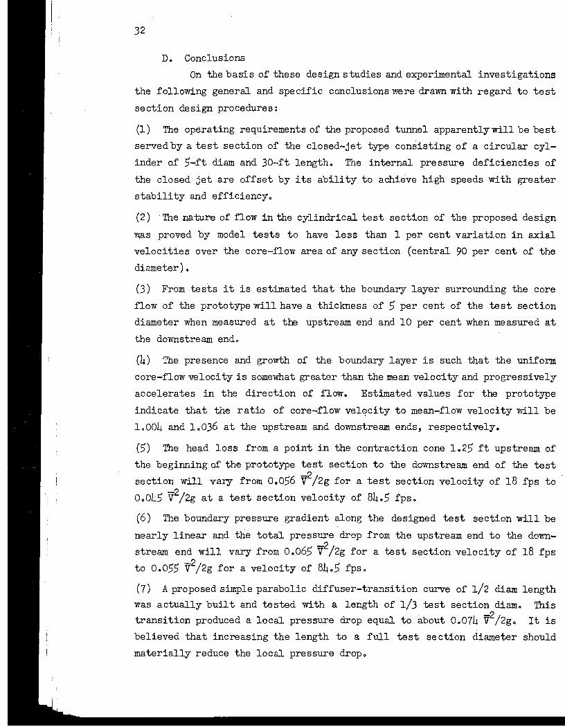
32

D. Conclusions

On the basis of these design studies and experimental investigations

the following general and specific conclusions were drawn with regard to test

section design procedures:

(1) The operating requirements of the proposed tunnel apparently will be best

served by a test section of the closed-jet type consisting of a circular cyl­

inder of 5-ft diam and 30-ft length. The internal pressure deficiencies of

the closed jet are offset by its ability to achieve high speeds with greater

stability and efficiency.

(2) . The nature of flow in the cylindrical test section of the proposed design

was proved by model tests to have less than I per cent variation in axial

velocities over the core-flow area of any section (central 90 per cent of the

diameter) •

(3) From tests it is estimated that the boundary layer surrounding the core

flow of the prototype will have a thickness of 5 per cent of the test section

diameter when measured at the upstream end and 10 per cent when measured at

the downstream end.

(4) The presence and growth of the boundary layer is such that the uniform

core-flow veloci ty is somewhat greater than the mean velocity and progressively

accelerates in the direction of now. Estimated values for the prototype

indicate that the ratio of core-flow velocity to mean-flow velocity will be

1.004 and 1.036 at the upstream and downstream ends, respectively.

(5) The head loss from a point in the contraction cone 1025 ft upstream of

the beginning of the prototype test section to the downstream end of the test

section will va~ from 0.056 V2/2g for a test section velocity of 18 fps to

0.045 V2/2g at a test section velocity of 8405 fpso

(6) The boundary pressure gradient along the designed test section will be

nearly linear and the total pressure drop from the upstream end to the down­

stream end will vary from 0.065 V2/2g for a test section velocity of 18 fps

to 0.055 V2/2g for a velocity of 8405 fps.

(?) A proposed simple parabolic diffuser-transition curve of 1/2 diam length

was actually built and tested with a length of 1/3 test section diam. This

transition produced a local pressure drop equal to about 0.074 V2/2gc It is

believed that increasing the length to a full test section diameter should

materially reduce the local pressure droPe

.~

i .~ f

33

(8) Initial cavitation of the tunnel boundary will occur at a point on the

crown of the diffuser transition where the influence of curvature produces

abnormally low local pressures. The cavitation at this point limits the mini­

mum cavitation index for all other tunnel points by reason of the intercon­

necting pressure system. The limiting centerline cavitation index is almost

linearly variable along the axis because of the existing pressure gradient

and has values ranging from 0.636 at the upstream end to 0.571 at the down­

stream end for a velocity of 18 fps and 0.151 to 0.097 at 84.5 ips.. It is

important to note that the local pressure deficiency of the diffuser transi­

tion is an important factor in establishing a minimum cavitation index for

the tunnel, but that its influence may be masked by the static pressures ac­

companying large test section diameters and by the frictional pressure losses

accompanying long test sections.. This is especially true in low speed opera­

tions, as shown in Fig. 11.

References

[1] Bradfield, F. B. The 5-foot Open Jet Wind Tunnel, Royal Aircraft Estab":' lishment. Aeronautical Research Committee Reports and Memoranda No" 1364 (British), 1930.

[2] Rouse, Hunter. Elemental Mechanics of Fluids.. New York: John Wiley & Sons, 1946, pp. 187-8. --

!

J. __ --------------~t

r

35

CHAPTER III. CONTRACTION STUDIES

A. General Considerations

A recirculating type of water tunnel is designed to produce a steady stream of fluid having uniform velocity, pressure, and turbulence character­istics in the test section comparable to those of open water prototype con­ditions. It is, however, apparent that the test stream as it leaves the test section and enters any conventional type of conduit recirculating system will progressively deteriorate in the uniformity of energy distribution, due to the growth of the boundary layer generated by the interaction of the fluid and the conduit walls. The eventual result of such boundary layer growth will be evidenced by velocity profiles possessing low values near the walls, and high values in the core of the flow, a characteristic which will require major correction before returning the flow to the test section.

In addition to the above deficiency of the recirculating system, it is apparent that the high velocities commonly employed in the test section will lead to excessive frictional energy losses and consequent pumping costs if such velocities are maintained in the recirculating system. It is, there­fore, an economic necessity to reduce this velocity as rapidly as possible and to convey the flaw at a lower and more practical value through the bulk of the circuit, following in turn with an acceleration to full value just before readmitting the stream to the test section~

Other sections of this t.reatise serve to show that the action of the diffuser, elbows, pump, and ducts fulfill their purposes in conveying the stream, but none of them operate to delay materially or to correct the est~b­lishment of the boundary layer which is so detrimental to the flow as it is discharged into the test section. It will,therefore, be necessary to provide some flow device to accelerate the velocity from the low value employed for economy in recirculation to the high values required in the test section and at the same time to provide a unifying corrective influence on the velocity profile 0 While a number of devices might conceivably be employed to provide the desired flow, experience dictates that use of a simple boundary cont:ac­tion produces natural flow phenomena which achieve both desired effects with maximum efficiency. In view of the extreme simplicity of physical form and favorable performance history, it is appropriate that the mechanics of the device be examined to permit maximum utilization of their peculiar properties.

j i

i '

36

The physical relations producing the desired condition may pe deter­

mined by applying Bernoulli's equation along a streamline of flow through the

contraction, assuming the contraction is preceded and followed by flow condi­

tions possessing static pressure distributions such that the differential

pressure drop is practically constant for all flow filaments. Such an assump­

tion is valid for established flow in straight cylindrical approach or exit

conduits and should also be valid for a tunnel if the components of the .recir­

culating conduits are properly designed.. It should be noted here that all

subsequent contraction analysis will be restricted to consideration of physical

forms having only circular cross sections.. This restriction is in accord

with the selection of the test section as it is described elsewhere.

If ; Bernoulli , s equation is written between a point "Itt at the con­

traction entrance and a point 11211 at the contraction exit, and energy losses

are assumed negligible,

where p = unit pressure,

2· [.Pl P2 J 2 V2 = - - - 2g + VI ww

V = local velocity of flow on a particular streamline,

w = unit weight, and

g = gravitation acceleration.

(6)

In addition to this, the area and velocity may be related by the equation of

continuity.as follows:

or

(7)

where A = conduit discharge area and V ::: mean velocity of flow atacross sec­

tion.

If it is assumed that there is a nonuniform distribution Of velocity

at the entrance to the contraction (VI as shown in Fig .. 12) and the pressure

r

')

:-

I Pi I

37

I . V2 ,---------

Fig. 12 - Velocity Profiles for a Contraction

drop is uniform, the graphic presen­

tation of Eq. (6) as shown in Fig. 13

indicates that the velocity distri­

bution at discharge from the contrac­

tion V 2 will be considerably improved

in uniformity over that at entrance

and that the degree of improvement

is principally dependent on the mag­

nitude of the area ratio of Eq. (7). A further analysis of the figure in­

dicates the value of V2 at various

parts of the flow section is more or

less independent of the corresponding

value of VI oecause the kinetic energy

------------

Fig. 13 - Graphical Summary of Velocities in a Contraction

represented by V 2 is largely supplied by the uniform differential pressure

energy.

In summary of the foregoing it may be said that a proper boundary

contraction will serve as a powerful corrective to the velocity variations

of a flow stream, provided that substantially uniform pressure distributions

can be achieved in the flow sections preceding and following the contraction

38

by establishment of parallelism between flow filaments at these sections.

Such parallelism in the upstream region is largely dependent on the design

quality of the recirculating system while that of the downstream or test sec­

tion region is dependent on the contraction boundary form. While this estab­

lishes the corrective possibilities of a boundary contraction with respect to

velocity, it does not serve to point out the possible influence of the con­

traction on the turbulence characteristics of the stream.. In view of the

importance of this characteristic, it is appropriate that this influence be

examined.

The turbulence characteristics of the open water conditions which

the tunnel te3t stream' attempts to 3imulate are not too well known, but ob­

servations in natural winds and in open air for aeronautical purposes indicate

that, . in general, a turbulence with equal strength in all directions (iso­

tropic) and low relative values is to be expected in the usual natural flow

field, except in boundary regions. Both theory and test for contracted air

streams [1, 2, 31 * indicate that the following' general relations apply to

turbulence changes:

(1) Turbulence is con3iderab1y reduced by the contraction, provided it· is

made isotropic in character before being admitted to the contraction.. Iso­

tropic character maybe approximately established by passing the flow through

suitable'screens or grids.

(2) While a general reduction occurs in the relative strength of turbulence,

the contraction doe3 serve to distort the initial isotropic character.

(3) The superimposed turbulent velocity component along the principal axis'

is reduced in magnitude in a ratio approximately inversely proportional to

the area ratio ~/A2.

(4) The superimposed turbulent velocity components along the two lateral

axes increased in proportion to ~Al/A2.

In view of the above, it would appear that the most natural and

satisfactory turbulence conditions will prevail in the tunnel test section

when: the recirculating system minimizes production of turbulence, particu­

larly that of large scale; space i3 provided upstream of the contraction to

*Numbers in brackets refer to the corresponding number3 in the reference list at the end of the chapter.

r

~

39

permit addition of screens or grids for turbulence control and decay, as dic­

tated by eventual tests; and the contraction ratio is a maximumb

B. Design Studies

1. Selection of Area Ratio

Having established the general influence of area reduction on velo­

city distribution, it next becomes necessary to determine the magnitude of re­

duction for a specific tunnel performanceo

Al though test stream quality is largely dependent on achieving a

maximum contraction ratio, it is obvious that economics and other factors may

limit optimum values to more practical ranges.. Fixed standards of quality

are not available; but, it would appear from previous work in water and wind

,tunnels that a velocity variation across the, test stream of less than I per

cent is a prime objective for quality work. This, of course, recognizes

that the velocity in the boundary layer must vary from zero to the velocity

of the test stream core, but assumes that models tested in such a stream have

dimensions suffiCiently small to assure that the test section boundary layer

does not influence the operation of the model mounted at the stream core.

A quantitative measure of the contraction influence on velocity

variation may be arrived at in the following manner. IfEqo (6) is written

along a streamline tla tl and a streamline tlbtl , the ratio of velocities on these

same streamlines for a section downstream of the contraction will develop thus

p - P Vb2 ::: v'b2 + ( I 2) 2g

2 1 w

Va ' 2 + (PI: P2) 2g V~ 2

Vb ::: 2 '

2 ,V~ + C\: P2) 2g

This may be translated to average conditions and established geometry by sub­

stituting the following:

__ l'l'~"t!tl.1I1 ______ I..I __ FIIIIII'IIIIIII!III!IIIM~I~""','''''

I! - 40

i

(8)

In order to gam some idea of the magnitude of ~/A2 necessary to

keep the test stream velocity Wi thin the desired limits, it Will be ass-wned

that Val. = 1.20 VI; ,Vbl = 0.2 VI; 01 = 1.07; and Q2 = 1.00. These values have

beenarbi trarily selected as representing a severe demand on the reforming

abilities of a contraction, inasmuch as they define an approach condition

typical of a fully developed turbulent pipe flow. In this case Val =1.20 VI

is, the maximum center velocity, and Vbl = 0.2 VI is an arbitrary limit such

that values above 0.2 maybe assumed to be part of the core flow -which will be

reformed, while values below 0.2 may be safely assumed ~o be contained. within

the boundary layer at section 2 and thus are not expe~ted to be Within the

prescribed limits of variation. It might also be pointed out that 02 = 1000

is an assumption on the conservative Side, since values slightly greater than

this will normally prevail. Since the above values relate to a now system

which probably will have considerably more distortion than is produced by the

recirculating system of a vvell-designed tunnel, their application should lead

to' a conservative selection of the contraction area ratio.

Values of Va2/Vb2 obtained by substituting' arbitrarY. ratios or end

areas (Ar/A2) in Eq. (8) are listed in Table II.

~I !!,,".~~~ ...... ~ ....................... _~=--____ ....... _____ ....... _________________________ _

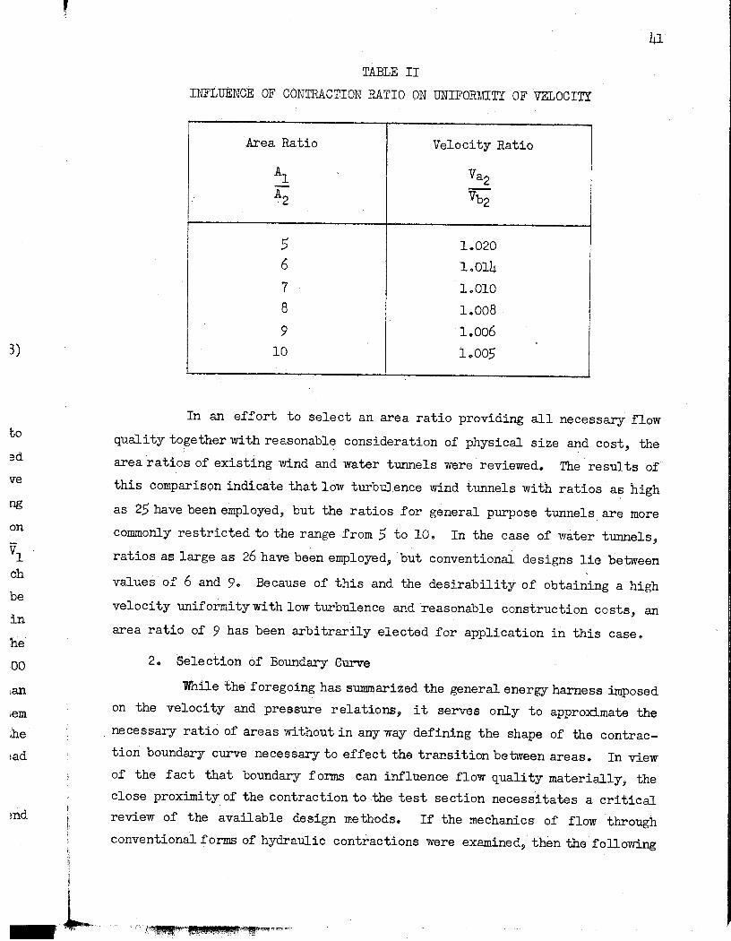
3)

to

ve

ng

on

.in

he

00

iem

;he

~ad

md

, 41

TABLE II

INFLUENCE OF CONTRACTION RATIO ON UNIFORMITY OF VELOCITY

Area Ratio Velocity Ratio

Al Va2

A2 Vb2

5 1.020

6 1..014

7 1.010

8 1..008

9 1.006

10 1.005

In an effort to select an area ratio providing all necessary flow

quality together with reasonable consideration of physical size and cost, the

area ratios of existing wind and water tunnels were reviewed. The results of

this comparison indicate that low turbulence wind tunnels with ratios as high

as 25 have been employed, but the ratios for general purpose tunnels are more

commonly restricted to the range from 5 to 10.. In the case of water tunnels,

ratios as large as 26 have been employed, but conventional deSigns lie between

values of 6 and 9.. Because of this and the desirability of obtaining a high

velocity uniformity with low turbulence and reasonable construction costs, an

area ratio of 9 has been arbitrarily elected for application in this case ..

2. Selection of Boundary Curve

While the foregoing has summarized the general energy harness imposed

on the velocity and pressure relations, it serves only to approximate the

. necessary ratio of areas without in any way defining the shape of the contrac­

tion boundary curve necessary to effect the transition between areas. In view

of the fact that boundary forms can influence flow quality materially, the

close proximity of the contraction to the test section necessitates a critical

review of the available design methods. If the mechanics of flow through

conventional forms of hydraulic contractions were examined, then the following

42

summary would approximate the order of complexity and possible benefits and

detriments which might be derived from the use of eacp form.

a. The Plane Orificd in an Infinite Tank

While this form is not particularly applicable to the case of

finite approach area, a wealth of related background : information has been

accumulated on its characteristics. For the case of the free liquid jet dis­

charging into air, the characteristics of the flow in the plane of complete

contraction (vena contracta) are a very high uniformity of velocity across

the jet, with the exception of the outer layers which have been retarded by

friction with the air and tank wall and parallel axial direction for all stream­

lines and all fluid particles at the uniform pressure of the surrounding at­

mosphere (except for a small constricting pressul:'e fl:'om the peripheral surface

tension) •

An approximation of the pressure velocity transition is indi­

cated in Fig. 14. In this it may be noted that intel:'nal pl:'essures exist in

the plane of the orifice as a result of the dynamics of the local curvilinear

flow. Such internal pressures persist until paralleliam is achieved at the

vena contracta.

Where the jet dischal:'ges free and horizontal, the quality of

flow is adversely affected, in that the lower filaments of the jet a"re sub­

jectedto a greater initial pressure than the upper fil~nts and accordingly

will have a gl:'eater final velocity. This difference is, however, small when"

the orifice diameter is small relative to the head on the orifice. In addi­

tion to the above gravitational effect, a second effect is that the free

horizontal jet will begin to show curvature of its axis as soon as the fluid

particles leave the tank wherein buoyant effects are in force.

If the jet discharges when submerged, that is, into a still

pool of the same liquid as constitutes the jet, certain important differences

result in comparison with a free discharge.. The most notable differences are:

all filaments are subjected to the same differential head and accordingly both

upper and lower filaments will have the same velocity; a horizontal jet is

buoye~ up in the still pool and ia not subject to curvature as a result of

gravity; there are no surface-tension forces effective in producing internal

pressures; the liquid surrounding the jet offers a greater viscous shear than

r

1

i

1

s

h

f

1

n

i i i fI,

"

p w

v v

At orifice At vena contracta

Fig. 14- Pressure- Velocity Variations for a Plane Orifice Jet (After Dougherty)

Pressure gradient., 1 ___ _~~_~..J..----~ W

Separati on eddy

---~ --- . . .

--~ Q

Fig. 15- Eddy Pattern in the Plane Orifice Approach

43

44

is the case with gas and, accordingly, the jet periphery is eroded at a rapid

rate due to the mixing action.

It is important to note that the dynamics of flow are such that

both analytical and experimental studies establish the position of the vena

contracta as being approximately 1/2 orifice diam downstream of the plane of

the orifice irrespective of whether the jet is free or submergedo

b" The Plane Orifice Terminating a. Cylindrical Conduit of Finite

Diameter

The action of this flow boundary is very similar to that of. the

infinite tank, except that the presence of a boundary to the appro9-ch flow

establishes a boundary layer which varies with the previous history of the

flow and accordingly impresses a variation of velocity on the discharging jet. ..

The magnitude of the discrepancy may be estimated by the method previously

described under the section on the selection of area ratio, pages 39 to 41..

In addition to inducing the above velocity discrepancy, the

flow confinement of the. boundaries of the approach conduit establishes a

streamline pattern which may be approximated by Fig .. 150 It is to be noted

that the balance of· forces establishing the streamline curvatures just up­

stream of the orifice plate is of such nature that a stagnation pressure is

approximated in the 90° boundary junction, with an increasing boundary pressure

gradient as showno The presence of such an adverse gradient in the path of

the low velocity fluid particles approaching in the conduit boundary layer

is such that an upstream motion is induced and a separation eddy begins to

grow in the dead water area.. It is the inherent nature of such eddies to grow

progressively in 3ize and .peel off into the passing flow.. This growth and

peeling is intermittent and leads to detrimental time variations in the jet

flow quality.

Co The Bell-Mouth Orifice Terminating a Cylindrical Conduit of

Finite Diameter

The addition of a solid boundary to the curvilinear surface

of the jet provides a means whereby the pressure on the outer filaments may

be increased or decreased from that which prevails at the vena contracta, and

thus provides some control over the streamline pattern. The solid boundary

increases the viscous shear and promotes the establishment of a normal boundary

layer rather than the mixing zone encountered with the submerged jeto While

the boundary layer probably consumes greater energy, it is apparent that#a

more stable flow will result from the added constraint ..

, '~

..

45

The geometry of the bell-mouthboundaryma.y consist of a simple

cone or a curve originating at either the conduit boundary (in Which case no

plane orifice would exist) or from the edge of the orifice. In ,either case,

however, a dead water area is promoted in the angular corner of the boundary

and separation eddies are to be expected.

d. The Ogee Orifice Terminating a qylindrica.l Conduit of Finite Diameter

This flowboun.dary offers the same general control as the simple

bell-mouth form, but has the advantage of providing no angular' dead water area

at the upstream end, thus reducing the possibility of separation eddies of

large size.

e •. Summary

A study of the shape of contraction curves employed in American

and European water tunnels and discussions with a number of designers indicate

that until' quite recent date, water tunnel contraction curves were largely

determined by adapting one of the foregoing forms of the plane orifice jet,

with liberal usage of the arbitrary circular arc and intui ti ve French curve

fairing as construction expedients. There is evidence that many low speed

tunnels constructed by such, methods operate successfully and wi 'lih high £1 ow

quality, but there is also evidence that such designs, when employed in high

speed tunnels, may be a source of trouble when ~ stable, low turbulence flow is

the objective. Certain of these tunnels show the higher wall velocity and

lower core velocity in the test jet apparent in the undeveloped flow of Fig ..

14. This serve'~ to indicate that such contractions are either improperly

formed or excessively foreshortened to the extent that the contraction has

not been fully accomplished wi thin the cone and is still being aompleted in

the test section.

'An attempt to find a more rational and exact approach than is

offered by intuitive fairing discloses that a number of related analytical

solutions have been offered in the aeronautical literature of recent years.

'While all of these solutions do no~ have identical design emphasis; in general,

the objectives seek a boundary form such that the boundary pressure gradient

shall not possess regions having an adverse slope leadi~ to separation of

flow .. A pressure gradient has been indicated in Fig. 15 and ~ partial solution

oftered in the form of a fairing for this dead water area. However, a more

-~,~--",,,-. --.---,----- . -----------~"-------- ----~.--- ----'---- ---------~---.-- ---- -- .. _-

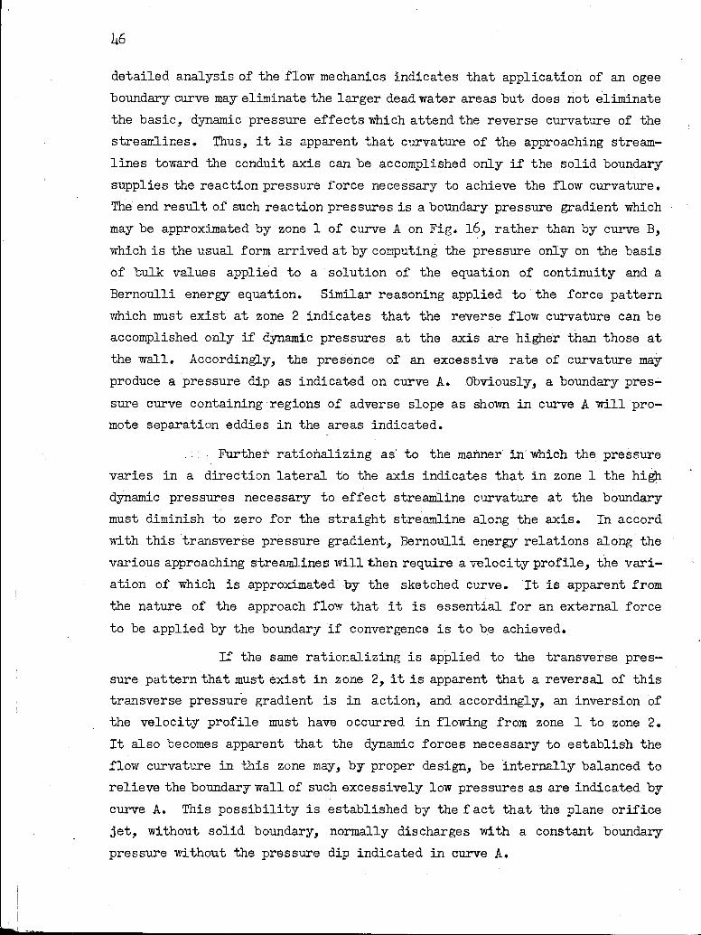
46

detailed analysis of the flow mechanics indicates that application of an ogee

boundary curve may eliminate the larger dead water areas but does not eliminate

the basic, dynamic pressure effects which attend the reverse curvature of the

streamlines. Thus, it is apparent that curvature of the approaching stream­

lines toward the conduit axis can be accomplished only if the solid boundary

supplies the reaction pressure force necessary to achieve the flow curvature.

The end result of' such reaction pressures is a boundary pressure gradient which

may be approximated by zone 1 of curve A on Fig .. 16, rather than by curve B,

which is the usual form arrived at by computing the pressure only on the basis

of bulk values applied to a solution of the equation of continuity and a

Bernoulli energy equation. Similar reasoning applied to the force pattern

which must exist at zone 2 ind.icates that the reverse flow curvature can be

accomplished only if dynamic pressures at the axis are higher than those at·

the wall. Accordingly, the presence of an excessive rate of curvature may

produce a pressure dip as indicated on curve A. Obviously, a boundary pres­

sure curve containing regions of adverse slope as shown in curve A will pro­

mote separation eddies in the areas indicated.

Further rationalizing as' to the manner in' which the: pressure

varies in a direction lateral to the axis indicates that in zone I the high

dynamic pressures necessary to effect streamline curvature at the boundary

must diminish to zero for the straight streamline along the axis. In accord

with this transverse pressure gradient, Bernoulli energy relations along the

various approaching streamlines will then require a velocity profile, the vari­

ation of which is approximated by the sketched curve. It is apparent from

the nature of the approach flow that it is essential for an external force

to be applied by the boundary 'if convergence is to be achieved.

If the same rationalizing is applied to the transverse pres­

sure pattern that must exist in zone 2, it is apparent that a reversal of this

transverse pressure gradient is in action, and accordingly, an inversion of

the velocity profile must have occurred in flowing from zone 1 to zone 2 ..

It also becomes apparent that the dynamic forces necessary to establish the

flow curvature in this zone may, by proper design, be internally balanced to

relieve the boundary wall of such excessively low pressures as are indicated by

curve A. This possibility is established by the f act that the plane orifice

jet, without solid boundary, normally discharges with a constant boundary

pressure without the pressure dip indicated in curve A.

.. b.

, s

a

n

e

,t

Y :-

'e

1e

L-

s-

is

of

2.

he

to

by

,ce

.ry

Boundary

Zone I

Boundary " pressu re

"-'\.~Curve (A)

\ \

\ \ \ \ ~

Zone

I

Boundary pressure

Curve (B)

47

Eddy,,", Vela city -1,s:~~~~~::=--

__ ~_~ _________ -~urve ____ .1 __ ' _3·~~e_b~~~tl __

L Contraction centerline

Fig. 16- Schematic Sketch of Pressure and Velocity Distributions for a Contraction

In view of the foregoing, the pertinent aeronautical literature

was reviewed am the following general reactions were applicable to this case:

The analysis of H. S. Tsien [4] is founded ·on a desire to achieve

a pressure gradient without adverse slope by deter~ning a boundary stream­

line with a constantly increasing velocity. Tsien's solution applies parti­

cularly to determination of boundary curves which will eliminate the adverse

gradient depicted in zone 2 of curve A on Fig. 16.

This analysis, based on potential flow theory, begins with a com­

bi'1.ation of the fundamental equation for irrotational flow and the equation

of continuity to give series expansions for the axial and radial velocities

that can be identified with the Laplace expression for the synnnetric potential.

These components may be combined to give the resultant velocity and the co­

ordinates of the streamline. The solution to the mathematics of the original

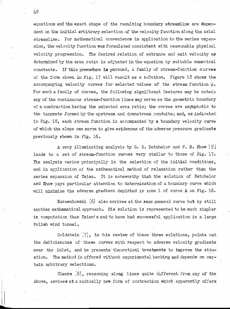
i i . I

I I

. I

I I

I , , I

i

48

equations and the exact shape of the resulting boundary streamline are depen­

dent on the initialar'bitrary selection of the velocity function along the axial

streamline. For mathematical convenience in application to the series expan­

sion, the velocity function was formulated consistent with reasonable physical

velocity progression. The desired relation of entrance and exit velocity as

determined by the area ratio is adjuste.d in the equation by suitable numerical

constants. If Wi's pl"ocedu:re is pursued, a family of stream-function rcur.ves

of the form shown in Fig, 17 will result as a solution •. Figure 18 shows the

accompanying velocity curves for selected values of the stream function 1/1 ..

For such a family of .curves, the following significant features may be noted,

any of the continuous stream-function lines may serve as the geometric boundary

ofa contraction having the selected area ratio; the curves are asymptotic to

the tangents formed by the upstream and downstream conduits; and, as indicated

in Fig. 18, each stream function. is accompanied by a boundary velocity curve

of which the slope can serve. to give evidences of the adverse pressure gradients

previously shown in Fig.. 16.

A very illuminating analysis by G .. K .. Batchelor and F. 6. Shaw [51 leads to a set of stream-function curves very similar to those of Fig.. 17.

The analysis varies principally in the selection of the initial conditions,

and in application of the mathematical method of relaxation rather than the

series expansion of Tsien. It is noteworthy that the solution of Batchelor

and Shaw pays particul·ar attention to determination of a boundary· curve which

will minimize the adverse gradient depicted in zone 1 of curve A on Fig. 16~

Szczeniowski [6] also arrives at the same general curve but by still

another mathematical approach.. His solution is represented to be much simpler

in computation than Tsien I s and to have had 5uccessful application in a large

Polish wind tunnel.

Goldstein [7], in his review of these three solutions, points out

the deficiencies of these curves with respect to adverse velocity gradients

near the inlet, and he presents theoretical treatments to improve thesi~~­

ation. The method is offered without experimental backing and depends on cer";'

tain arbitrary selections.

Cheers [8], reasoning along lines quite different from any of the

above, arrives at a radically new form of contraction which apparently offers

n-

al ,n-

as

~a1

3,ry

to

t.ed

rve

uta

[51 17.

illS,

the

~lor

lieh

16.

jill

)ler

rrge

out

ants

itu-

eer";'

the

'fers

r

Q)

0 c: c, .... tJ)

:t;

'0 "C C1 0::

.,

.. CD CD "-.!! .. ::I

v 0 It::

49

Velocity distribution showing plane of locotlon and relative val~es

0.1 0.2 0.3 0.5 0.6 0.7 0.8 0.9 1.0 0.9 1.0 2.4 I 0.0 Jil 0.2 I 0.2 9.3 0.4 07 °is 0.9 I °i9 I.p III

:Velocity relative I 10 exit velocity

I I I I I I I I I

I I Curves are based on Tsien's anOlyticol solution with a 9;J area ratio and an ,_ 2.0

PiaL af ~rafile 1 axially - symmetric flow

I I ! I I i

1.6 ';=0..15 - 1 I I I I - ~ -0.14

f-- 00.13

~ ~ ~I I I I· I 1:0.12 r-. f\. f'.... ,0.1

1.2

I-t:::: 8S: ~ ""r-.... 1\ "-1'---../ I i it r--. i /

~ t$ ~ "- I ............... I r--r--IJ 1 I ~ i""-- I

0.8

00..05 - r\- I ........ ~ ~ §:~

-...... ~ I ;::::"... r--. I I

I N r: ~ ~ ~ -1---1 f I I r-.. I;::::"... -Velocity protJle H r--i- f

-!.. M

0 -2.4

.. 7. 0

6. 0

S. 0

4 .0

0

2 .0

.0

0.

e.o

7.0

6.0

5.0

4.0

3.0

2.0

1.0.

o

--

-2

- , I I I I I I I I I

1 I 1 I I I I

-2.0 -1.6 -1.2 -0.8 -0.4 o +0.4 +0.8 .1.2 .1.6 +2.0

Axial distance· X •

F" ... 17 - Contraction Boundary Curve.

.Arbltrary tangent po\nt

'" 1 IBbundary krve

~ Velocity along boundarY-h

........ ............. ~ F=' ~V.loclty along axil -..::=

~ I--~rbit)ary tange. --- ~ poln ~

/' ~

I ...., Recommended length' 19 ft . -- -- I I I

--- -- -- co~racti~n ce~ter I!ne~ 'a) -; - 0.13

--. o

Arbitrary tongert pOInt Ie

"- _ Boun~ory ~urve "<::-

"'-........

I'--- Velocity along boundory-, ~-=velocit1 olonll axis =-r-:--- ~ f-'"' Ar itro)y tonlgent Ipointl----.,; - ~

V -----'"" Recommended len~th = 25 ft.

~ - I I -r-' -

Fig. 18 - Selected

with

Co~troct on c~nter Iline..,.,.

10 15

Axial length in Feet

Stream-Function

Accompanyrng

Contract ion

Velocity

Boundary Curves

(b)

20

Curves

'/'- 0.10

~ I

I .~

.0.20 =O.IS

-0.10

I

f

1.0

o.e

0..6

0.4

Q.2

0

I .0

0.8

0.6

0.4

0.2

o 25

,.. ·E 0 -.; > CD ,. '0 -.; 0::

~ 'u o -.; > CD ,. -" ~

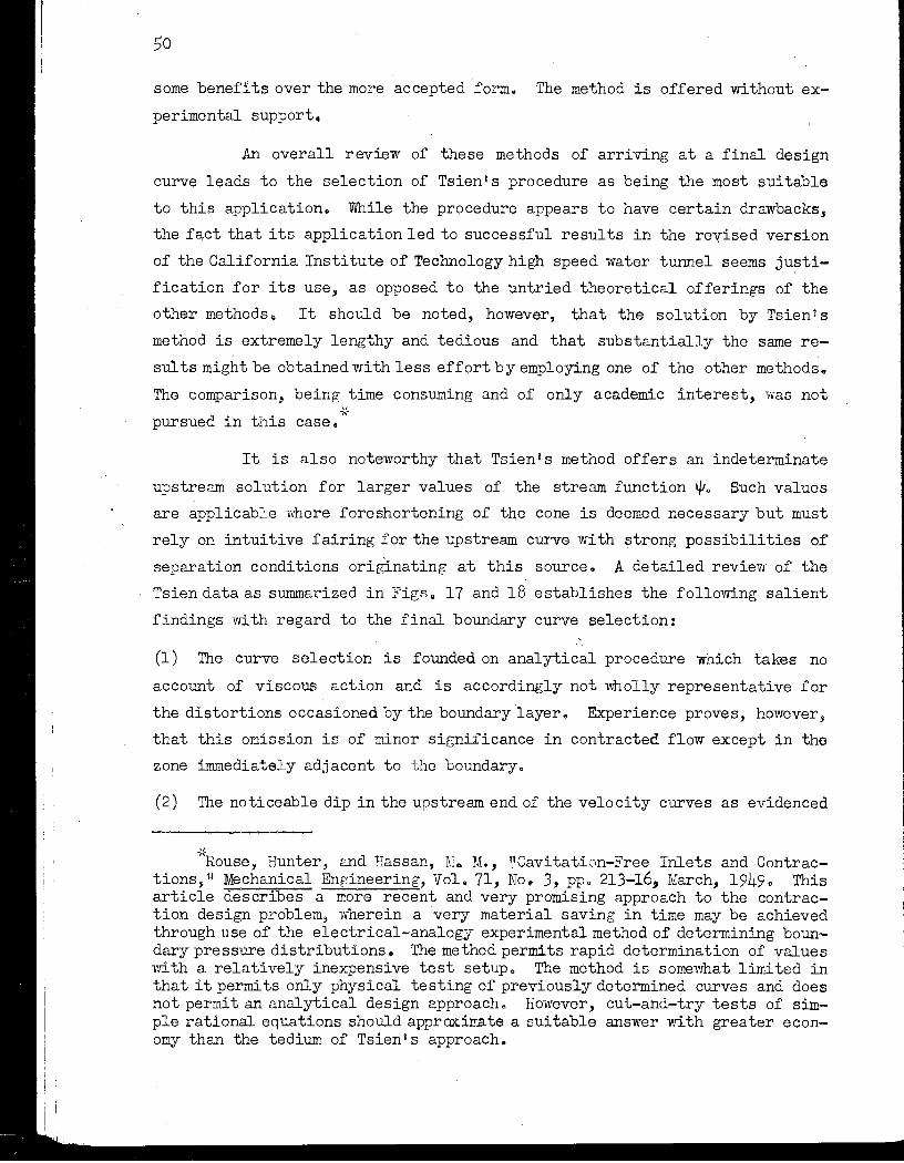
50

some benefits over the more accepted form. The method is offered without ex­

perimental support.

An overall review of these methods of arriving at a final design

curve leads to the selection of Tsien I s procedure as being the most sui table

to this application. While the procedure appears to have certain drawbacks,

the fact that its application led to successful results in the revised version

of the California Institute of Technology high speed water tunnel seems justi­

fication for its use, as opposed to the untried theoretical offerings of the

other methods.. It should be noted, however, that the solution by Tsien' S

method is extremely lengthy and tedious and that substantially the same re­

sul ts might be obtained with less effort by employing one of the other methods ..

The comparison, being time consuming and of only academic interest, was not -1f

pursued in this case.

It is also noteworthy that Tsien is method offers an indeterminate

upstream solution for larger values of the stream function to Such values

are applicable "!linere foreshortening of the cone is deemed necessary but must

rely on intuitive fairing for the upstream curve with strong possibilities of

separation conditions originating at this source. A detailed review of the

Tsien data as summarized in li'igs Q 17 and 18 establishes the following salient

findings with regard to the final boundary curve selection:

(1) The curve selection is founded on analytical procedure which takes no

account of viscous action and is accordingly not wholly representative for

the distortions occasioned by the boundary layer. Experience proves, however,

that this omission is of minor Significance in contracted flow except in the

zone immediately adjacent to the boundaryc

(2) The noticeable dip in the upstream end of the velocity curves as evidenced

-'< "Rouse, Hunter J> and Hassan, I\I. M., "Cavi ta tion-Free Inlets and Contrac-

tions, It Mechanical Engineering, VoL 71, No.3, ppo 213-16, March, 19490 This article describes a more recent and very promising approach to the contrac­tion design problem, wherein a very material saving in time may be achieved through use of the electrical-analogy experimental method of determining boun­dary pressure distributions. The method permits rapid determination of values with a relatively inexpensive test setup., The method is somewhat limited in that it permits only physical testing of previously determined curves and does not permit an analytical design approach. However, cut-and-try tests of sim­ple rational equations should approximate a suitable answer with greater econ­omy than the tedium of Tsien's approach.

-,',

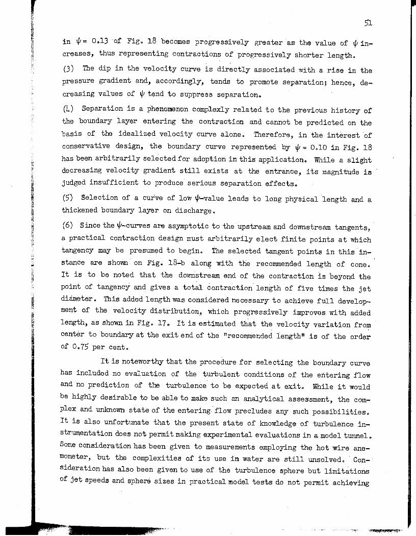
in 0/ = 0 .. 13 of Fig .. 18 becomes progressively greater as the value of t/t in­

creases, thus representing contractions of progressively shorter length.

f; (3) The dip in the velocity curve is directly associated with a rise in the

pressure gradient and, accordingly, tends to promote separation; hence, de­

creasing values of o/tend to suppress separationo

(4) Separation is a phenomenon complexly related to the previous history of

the boundary layer entering the contraction and cannot be predicted on the

basis of the idealized velocity curve alone 6 Therefore, in the interest of

conservative design, the boundary curve represented by 0/ = 0,,10 in Fig" 18

has been arbitrarily selected for adoption in this application.. While a slight

decreasing velocity gradient still exists at the entrance, its magnitUde is

judged insufficient to produce serious separation effects ..

(5) Selection of a curve of low o/-value leads to long physical length and a

thickened boundary layer on discharge.

(6) Since the o/-curves are asymptotic to the upstream and downstream tangents,

a practical contraction design must arbitrarily elect finite points at which

tangency may be presumed to begin. The selected tangent points in this in­

stance are shown on Fig. l8-b a1on~ with the recommended length of cone.

It is to be noted that the downstream end of the contraction is beyond the

point of tangency and gives a total contraction length of five times the jet

diameter. This added length was considered necessary to achieve full develop­

ment of the velocity distribution, which progre ssively improves with added

length, as shown in Fig .. 17.. It is estimated that the velocity variation fro~

center to boundary at the exit end of the "recommended length" is of the order

of 0 .. 75 per cent.

It is noteworthy that the procedure for selecting the boundary curve

has included no evaluation of the turbulent conditions of the entering flow

and no prediction of the turbulence to be expected at exi to While it would

be highly desirable to be able to make such an analytical assessment, the com­

plex and unknown state of the entering flow precludes any such possibilities.

It is also unfortunate that the present state of knowledge of turbulence in­

strumentation does not permit making experimental evaluations in a model tmmelo

Some consideration has been given to measurements employing the hot wire ane­

mometer, but the complexities of its use in water are still unsolved .. " Con­

sideration has also been given to use of the turbulence sphere but limitations

of jet speeds and sphere sizes in practicalmodel tests do not permit achieving

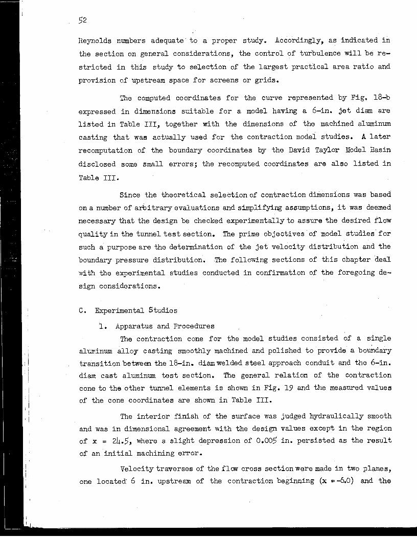
52

Reynolds numbers adequate'to a proper study. Accordingly, as 1.ndicated in

the section on general considerations, the control of turbulence will be re­

stricted in this study to selection of the largest practical area ratio and

provision of upstream space for screens or grids.

The computed coordinates for the curve represented by Fig. l8-b

expressed in dimensions suitable for a model having a 6-in. jet diam are

listed in Table III, together with the dimensions of the machined aluminum

casting that was actually used for the contraction model studies. A later

recomputation of the boundary coordinates by the David Taylor Model Basin

disclosed some small errors; the recomputed coordinates are also listed in

Table III.

Since the theoretical selection of contraction dimensions was based

on a number of arbitrary evaluations and silnplifying assumptions, it was deemed

necessary that the design be checked experimentally to assure the desired flow

quality in the tunnel test section. The prime objectives of model studies for

such a purpose are the determination of the jet velocity distribution and the

boundary pressure distribution. The following sections of this chapter deal

with the experimental studies conducted in confirmation of the foregoing de­

sign considerations.

c. Experimental Studies

1. Apparatus and Procedures

The contraction cone for the model studies consisted of a single

aluminum alloy casting smoothly machined and polished to provide a boundary

transition betweEn the l8-in. diam welded steel approach conduit and the 6-in.

diam cast aluminum test section. The general relation of the contraction

cone to the other tunnel elements is shown in Fig. 19 and the measured values

of the cone coordinates are shown in Table III.

The interior finish of the surface was judged hydraulically smooth

and was in dimensional agreement with the design values except in the region

of x = 24.5, where a slight depression of 0.005 in. persisted as the result

of an initial machining error.

Velocity traverses of the flew cross section were made in two planes,

one located" 6 in. upstream of the contraction beginning (x "" -6.0) and the

n

d

b

In

.n

.n

)w

II

Le

~y

1.

m ;1

~B ~. '~'

~: ~, ~(

t,h i )n I Lt

~

" 6,

le

53

TABLE III

COORDINATES OF THE CONTRACTION BOUNDARY*

Original Computed Values Measured Values Recomputed Values

x r x fu't-r x r (in. ) (in.) (in. ) (in. ) (in. ) (in. )

0.00 8.999 0.00 9.00 0.00 9.000 1.33 8.932 1.50 8.95 1~34 8.955 2.67 8.699 3.00 8.75 2.68 8.781 4.00 8.366 4.00 Q) 8.47 4.02 8.382 .j.l

5.33 7.699 5.00 n1 8.11 5.36 7."754 6.67 6.986 6.00

r1 7.62 6.70 7.021 ~ 8.00 6.199 7.00 $< 7.08 8.04 6.299

9.33 5.699 8.00 6.50 9.38 5.658 10.67 5.166 9.00

s::: 6.02 10.71 5.111 0

12.00 4.733 10.00 "0 5.58 12.05 4.644 Q)

13.33 4.333 11.00 S 5.21 13.39 4.286 14.67 4.000 12.00 (I) 4.88 14.73 3.994 <1! 16.00 3.746 . 13.00 :i 4.56 16.07 3.736 17.33 3.586 15.00 4.04 17.41 3.521 18.67 3.400 17.00 3.68 18.75 3.360 20.00 3.300 19.00 3.41 20.09 3.239 21.33 3.200 21.00 ~ 3".25 21.43 3.148 22.67 3.133 21.50 (I) 3.213 22.77 3.087 .j.l

24.00 3.100 22.00 s::: 3.176 24.11 3.040 25.33 3.033 22.50 ~ 3.148 25.45 3.005 Q)

26.67 3.000 23.00 S 3.126 26.79 2.984 28.00 3.000 23.50 (I) 3.110 28.13 2.969 n1 29.33 3.000 24.00 Q) 3.100 29.47 2.960 30.67 3.000 24.50

a 3.080 30.80 2.953

~< 25.00 $ 3.070 25.50 ~ 3.049 26.00 3.033

~ 26.50 C) 3.020 OM 27.00 a 3.013 27.50 Q) 3.006 "0 28.00 OM 3.003 (I)

29.00 ~ 3.002 30.00 3.002 .... '

*Values of x are measured from the upstream end of the curve (point of tangency with cylindrical approach conduit). Values of r are radii measured from the axial centerline.

**When the cone was rebored, the boundary was shifted 1/2 in. downstream. Therefore, 1/2 in. IIDlSt be added to the computed values of x before comparing the computed radii with the measured boundary radii after reboring.

54

, other 1/2 in. downstream of the contraction end (x = 30.5). These traverse

planes are designated as stations 12 and 1, respectively, in other sections

of this report. The velocity traverses were made using a 3/8-in. diam ttcanti­

levert! Pi tot cylinder in the upstream section and a '1/4-in. diam ftlong1" Pi tot

cylinder in the downstream section. The details of this instrumentation are

given separately in the appendix.

The casting was provided with 20 pressure measuring taps spaced

along an axial line at the bottom of the cone, as shown in Figs. 19 and 20.

It will be noted from Fig. 20 that three of these bottom taps were supplemented

by side and top taps to yield manifold rings utilized as a part of the velo­

city measuring instrumentation of the tUnnel. Details of this feature are

described in 'the appendix. ·The pressure taps consisted of 1/32-in. diamholes,

drilled normal to the wall and carefully deburred and chamfered at the inner

end., The taps were connected by rubber tubing to 50-in. U-tubemanometers

filled with gage fluids of specific gravity suitable to the test velocity.

Additional pressure data were obtained from a 3/8-in •. tap used for velocity

instrumeptation in the plane x = -6.0 (see Fig. 19).

In order to determine the 'possible presence of separation zones

which might not be detectable through the boundary pressure measurements, an

experimental study of flow in the boundary layer was made by utilizing a flow

streak technique [9]. This procedure consisted. of painting the questionable

boundary area with a thick mixture of white lead and t.urpentine and subjecting

this dried surface to a stream of marking fluid, introduced through one of

the pressure taps situated in the questionable area. The marking fluid ~on- <'

sisted of a saturated water solution.- of hydrogen sulfide,. which caused the

white . lead to turn to a visible black lead sulfide, in the contact areas. The solution was fed into four taps in the contraction cone: the tap at the bottom

atx = 1.5; the tap at the bottom at x = 4.0; the tap at the left side (look­

ing downstream) atx = 17; and the tap at the bottom at x = 28.5. The solution

was slOWly admitted through the. pressure tap holes with the tunnel operating

at a test section velocity of 50 fps. The flow delineation accessories are

shown in Fig. 20.

2. Velocity Distribution Studies

The upstream and downstream velocity distributions resulting from

experimental measurements at the two traverse stations previously described

18

L-

'e

ld

).

ld

)-

'e

I,

:r

S

, . iy

'S

n

,e

,-,e

,e

m

n

g

e

m

d

'J

1., ..

55

960 Vane 30.75" 30" 36"

Stagger angle ~

2.94" Chord~ 'y-,.L.-____ --.-___ __._

Test section Contraction Approach conduit

0;;1 ~~.-=~---. . __ . ______ 9_

I" Gap ~ I Ifr,

£1 I/r- { H~~U U ~ r ~ ~ggg23 la ~ ~ ~ I -- - - <.'J <.'J

1D

Values of X for Piezometer Taps

Fig. 19- Sectional Elevation of Contraction Flow Circuit

Fig, 20 - Contraction Cone with Piezometer Taps and Flow Delineation Accessories

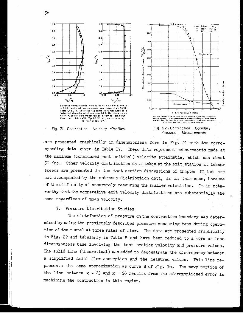
56

1.0

~ ~

1.0

0.8

0.6

0.8

0.6

0.4 0.4

0.2 0.2

OJ

",,0 N

o. 2 ~ r 4

)j e

..!? 2

4

6

o.

o.

o.

o.

o.

1 L IV ol.....r l--l

8

I",..,.d

o. o.

I. 0,4

I. 0 1.2 0.85 0.95

V02/V2

Entrance measurements were taken at x = - 6.0 in. where '1= 9.0 in,\ while exit measurements were token at x = 30.5 in. where rt::: 3.0 in. Encircled (0) points were measured on a horizontal 'diameter which was -porallel to the elbow vanes while (ca) points were measured on a vertical diameter ~ Values were taken with Vt:=49.32 fps" corresponding

to Re ' 2.48.10·.

Fig. 21- Contraction Velocity "Profiles

1.05

LOO 'l 0.90

0.80 0

0 {fiil' 0.7 ~,

}> 0.60 0

~ £ 05 0

f ~ ,(140 0

~ § .~ 0.300

E o (>2 00

0.' 00

0

~:

~ \

~ a"l'''Y "'r.-r

Symbol \Vrtmec) R, . 18,00 0,91.10: . 29.54 i:::~ :g. 0 49.32

,80UOdorypressure

\ \ \

1\ \

t--. ,

I\: -'0 - JO 15 20 25

X-axicl Distcnce in Inches

Measured pressure values ort shown for I~ree volues of 172 0nd their corresponding Reynolds numbers. The solid line represents, Q simplifie~ theoretical curve based on pure oiliol flow. The dotted line represents the theoretical curve for 'he can fraction

\Which would e~ist hod 1'19 machining error occurred.

Fig. 22 - Contraction Boundary Pressure .Measurements

•

30

are presented graphically in dimensionless form in Fig. 21 with the corre­

sponding data given in Table IV. These data represent measurements made at

the maximum (considered most critical) velocity attainable, which was about

50 fps. Other velocity distribution data taken at the exit station at lesser

speeds are presented in the test section discussions of Chapter II but are

not accompanied by the entrance distribution data, as in this case,because

of the difficulty of accurately measuring the smaller velocities. It is note­

worthy that the comparative exit velocity distributions are substantially the

same regardless of mean velocity.

3. Pressure Distribution Studies

The distribution of pressure on the contraction boundary was deter­

mined by using the previously described pressure measuring taps during opera­

tion of the tunnel at three rates of flow. The data are presented graphically

in Fig. 22 and tabularly in Table V and have been reduced to a more or less

dimen3ionless base involving the test section velocity and pressure values.

The solid line (theoretical) was added to demonstrate the discrepancy between

a simplified axial flow assumption and the measured values. This line re­

presents the same approximation as curve B of Fig. 16. The wavy portion of

the line between x = 23 and x = 26 results from the aforementioned error in

machining the contraction in this region.

"

10 "

o )

:g a:

'e-

at

lut

:er

,re

.5e

,e-

he

r-

a-

1y

55

5.

en

9-

')f

in

i v

~ ,~

" Jj!

i I ~~

57

TABLE IV VELOCITY DISTRIBUTION 6 IN. UPSTREAM AND 1/2 IN. DOWNSTREAM OF CONTRACTION CONE

Velocity Distribution 6 in. Upstream of Contraction Cone VI - 5.48 fps ReI - 0.83 x 10

6

Horizontal Diameter Vertical Diameter (Parallel to Vanes) (Perpendicular to Vanes) ~i5tance from V~ Distance from V. Distance from V

Side Wall r a1 Velocity Bottom Wall

r a1 Velocity ~ Bottom Wall r 41 Velocity ~

(in. ) r1 (fps) VI (in. ) r1 (fps) V- (in. ) r1 (fps)

VI 1 0.9 0.900 5.44 0.993 0.10 0.988 2.43 0.444 13.00 0.444 6.47 1.18 2.9 0.678 6.01 1.097 0.20 0.978 2.52 0.460 14.00 0.556 6.37 1.162 4.9 0.456 6.26 1.142 0.35 0.962 2.92 0.533 15.00 0.667 6.18 1.128 6.9 0.233 6.33 1.154 0.60 0.933 3.18 0.581 16.00 0.778 6.01 1.097 8.9 0.011 6.39 1.167. 1.00 0.888 3.68 0.672 17.00 0.889 5.75 1.045 10.9 0.211 6.27 1.143 1.50 0.833 4.46 0.815 17.40 0.933 5.70 1.04c 11.9 0.322 6.24 1.138 2.00 0.778 5.06 0.924 12.9 0.433 6.14 1.119 3.00 0.667 5.39 0.984 13.9 0.544 6.01 1.097 4.00 0.556 5,53 1.008 14.9 0.656 5.96 1.088 5.50 0,500 5.75 1.048 15.9 0.767 5.60 1.022 7.00 0.222 5.99 1.093 16.9 0.878 5.34 0.975 8.00 0.111 6.22 1.135 17.25 0.916 5.34 0.975 9.00 0.000 6.37 1.162 17.45 0.938 5.30 0.967 10.00 0.111 6.47 1.181 17.75 0.972 5.11 0.933 11.00 0.222 6.53 1.192 17.90 0.988 4.66 0.851 12.00 0.333 6.53 1.192

Velocity Distribution 1/2 in. Downstream of Contraction Cone V2 - 49.32 fps Re2 .' 2.48 x 106

Horizontal Diameter VerticaJ. Diameter (Parallel to Vanes) (Perpendicular to Vanes) Distance from V Distance from V ra2 Velocity a2 r a2 Velocity a2 Side Wall

(fps) - Bottom Wall (fps) (in.) r 2 V2 (in. ) r 2 v2

0.05 0.983 43.41 0.880 0.05 0.983 43.75 0.887 0.10 0.966 47.48 0.963 0.10 0.967 46.01 0.933 0.15 0.950 48.88 0.991 0.15 0.950 48.31 0.979 0.25 0.916 49.63 1.007 0.25 0.917 49.28 1.000 0.55 0.817 49.84 1.010 0,55 0.817 49.69 1.007 1.00 0.667 49.92 1.012 1.00 0.667 49.77 1.009 1,50 0.500 49.92 1.012 1.50 0.500 49.69 1.007 2.00 0.333 49.92 1.012 2.00 0.333 49.77 1.009 3.00 0.000 49.92 1.012 2.50 0.167 49.77 1.009 4.00 0.333 49.90 1.011 3.00 0.000 49.77 1.009 5 .. 00 0.667 49.77 1.009 3.50 0.167 49.77 1.009 5.45 0.817 49.71 1.008 4.00 0.333 49.77 1.009 5 • .75 0.917 49.36 1.001 4.50 0.500 4,9.69 1.0'07 5.85 0.950 49.02 0.994 5.00 0.667 49.69 1.007 5.90 0.967 47.69 0.96B 5.45 0.B17 49.56 1.005 5.95 0.983 44.3B 0.900 5.75 0.917 49.2B 1.000 5.B5 0.950 4B.59 0.986 5.90 0.967 47.75 0.968 5.95 0.983 44.97 0.912

Note: The use of values carried to the fourth e is a calculatin and reference signuicant .:ri ' gur g expedient and is not indicative of the order of accuracy of the experimental work which, in general, can only justify the third significant figure.

58

TABLE V

CONTRACTION BOm-mAHY WALL PRESSURE DATA

Boundary Theoretical Experimental Boundary Pressure **

Coordinates Boundary

(See Fig. 19) Pressure * For For For -*** V2 • 18.00 fps V2 • 29.54 fps V2 • 49.32 fps

x r and and and (in. ) (in. ) (1 - K) 6 6 Re '"' 2.48 x 10~ Re = 0.91 x 10 Re .1.49 x 10

1-6.00 9.00 0.988 1.012 1.0255 1.0268 0.00 9.00 0.988 1.50 8.9.5 0.987 1.012 1.0264 . 1.0284 3.00 8.75 0.986 1.012 1.0256 1.0269 4.00 8.47 0.984 1.010 1.0246 1.0262 5.00 8.11 0.981 1.009 1.023 1.024 6.00 7.62 0.976 1.006 1.019 1.020 1.00 7.08 0.968 0.997 1.011 1.012 8.00 6.50 0.955 0.981 0.995 0.998 9.00 6.02 0.93B 0.962 0.917 0.978 0.00 5.58 0.916 0.938 0.953 0.955 1.00 5.21 0.890 0.913 0·927 0.928 2.00 4.88 0.851 0.879 0.895 0.893

h3.00 4.56 0.813 0.834 0.847 0.849 5.00 4.04 0.696 0.706 0.722 0.121 7.00 3.68 0.558 0.562 0.583 0.583 9.00 3.41 0.401 0.411 0.417 0.417

21.00 3.25 0.214 0.276 0.287 0.286 23.00**** 3.13**** 0.156 0.141 0.151 0.166 25.00 3.01 0.099 0.112 0.119 0.128 21.00 3.01 0.013 0.013 0.011 0.011 28.50(2) 3.00 0.000 0.000 0.000 0.000 30.00 3.00

*Assuming pure axial flow with uniform velOCity distribution and no head loss: if

**Al1 experimental pressure differences between x and 2 are divided by the velocity head at 2:

**-v? is the average velocity at the contraction throat of 6-in. diam While Re is the Reynolds number~ased on this diameter.

****Error in machining from x = 23.5 to 25.5.

Note: The use of values carried to the -fifth significant figure is a calculating and reference expedient and is not indicative of the order of accuracy of the experimental work which, in general, can only justify the third significant figure.

.32 .fps

ld

18 x 106

268

284 269 262 24 20 l2 ~8 78 :;:5 W f3 ~9 ~1

33 L7 36 ,6 ~8 L1 )0

t;y head

3yno1ds

_ng and al work

59 It will be observed from the experimental data of Table V that a

very slight adverse pressure gradient exists at the higher velocities in the region x= -6.0 to x = 1.5 in a manner generally consistent with the rationali­zations of Fig. 16 and at a rate comparable to that expressed by the boundary velocity curve of Fig. 186

The boundary pressure data of Fig. 22 show no evidence of the low pressure values indicated in zone 2 of curve A, Fig. 16, although a marked deviation of the data is evident in the region of the machining error at x = 25.0. It is particularly unfortunate that the machining error occurred in the region it did, as this portion of the boundary might otherwise be suspected of producing separation conditions. However, the very gradual easement of the general radius of curvature at this point would indicate that a boundary with­out machining error should produce apressure curve corresponding to the dotted line faired-?-n between the points taken at taps x = 25.0 anc?_ x .. 27.0.

As a follow-up on the boundary pressure measurements, the poss:ible separation areas were subjected to the flow delineation procedure previously described and the cone was then removed from the tunnel and photographed. The significant data are shown in Figs .. 23 to' 26" In examining these figures, the following factors may be noted:

(1) Black strings representing axial traces have been taped to the boundary to define the axial flow direction. The principal flow direction may be ob­served to have a slight spiral in a counter-clockwise direction (looking downstream) but is not judged serious since it is not present to a noticeable degree in the test section. The source of a spiral in this direction is un­accountable as .. it is contrary to the slight spiral evident in the region of the pump discharge. (The pUInp would normally be considered the only source of asymmetric flow.)

(2) The flow streak originating from the tap at x = 1.5 shows definite indica­tions of upstream boundary flow but the limited extent in the upstream direc .... tion and the strong trace downstream give evidence that the separation effect is weak and confined to the immediate boundary layers. It is considered un­likely that separation eddies of any Significant strength could be generated in this region.

(3) No trace of reverse flow is evident in the streaks originating at taps x = 4.0 and x = 17.0.

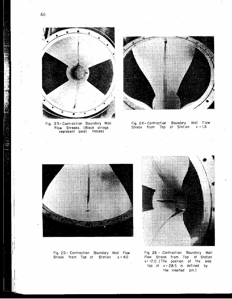
60

Fig. 23- Contraction Boundary WaU Flow Streaks. (Black strings

represent axia I traces)

Fig. 25- Contraction Boundary Wall Flow Streak from Tap at Station x = 4.0

Fig. 24- Contraction Streak from Tap

Boundary Wall Flow at Station x = 1.5

Fig. 26 - Contraction Boundary Wall Flow Streak from Tap at Station x= 17.0. (The position of the side

tap at x = 28.5 is defined by the inserted pin.)

62

Test Section Velocity

V2

fps

9.478 9.539

14.989 14.998 19.695 22.684 25.124 25.692 26.249 29.888 30.634 30.762 55.371 39.491 47.411

TABLE VI

CONTRACTION HEAD LOSS DATA

Pl- P2 -2 V2 PI ... P2 w 2g w

-2 V2

ft of water ft 2g

1.43 1.3949 1.0252 1.47 1.4129 1.0404 3.59 3.4887 1.0290 3.56 3.4929 1.0192 6.10 6.0232 1.0127 8.07 7.9901 1.0100 9.87 '9.8015 1.0070

10.33 10.2497 1.0078 10.75 10.6989 1.0048 14.00 13.8710 1.0093 14.72 14.5720 1.0101 15.02 14.6941 1.0222 19 .. 72 19.4271 1.0151 24 .. 58 24.2114 1.0150 34.96 34.9038 1.0016

hf -2 V2 2g

0.0414 0.0566 0.0452 0.0354 0.0289 0.0262 0.0232 0.0240 0.0210 0 .. 0257 0.0263 0.0384 0.0313 0.0312

. 0 .. 0178

. . . . . . Note: The use of values carr~ed to the slXth s~gIP-f;Lcant f;Lgure ~s a calculating and reference expedient and is not indicative of the order of accuracy of the experimental work which, in general, can only justify the third Significant figure.

respectively evaluated as Q 1 = 1.07 and Q 2 = 1.00, from integr.ation of the

velocity profiles shown in Fig. 21.

If the value of the head loss is mad<? dimensionless by expressing

it in ratio ~rith the test section velocity head then

Values for the expression given above are listed in the last column of Table

VI. W11ile there is evidence of appreciable scatter in the data, the general

trend indicates a decreasing percentage head loss with increasing velocity, or

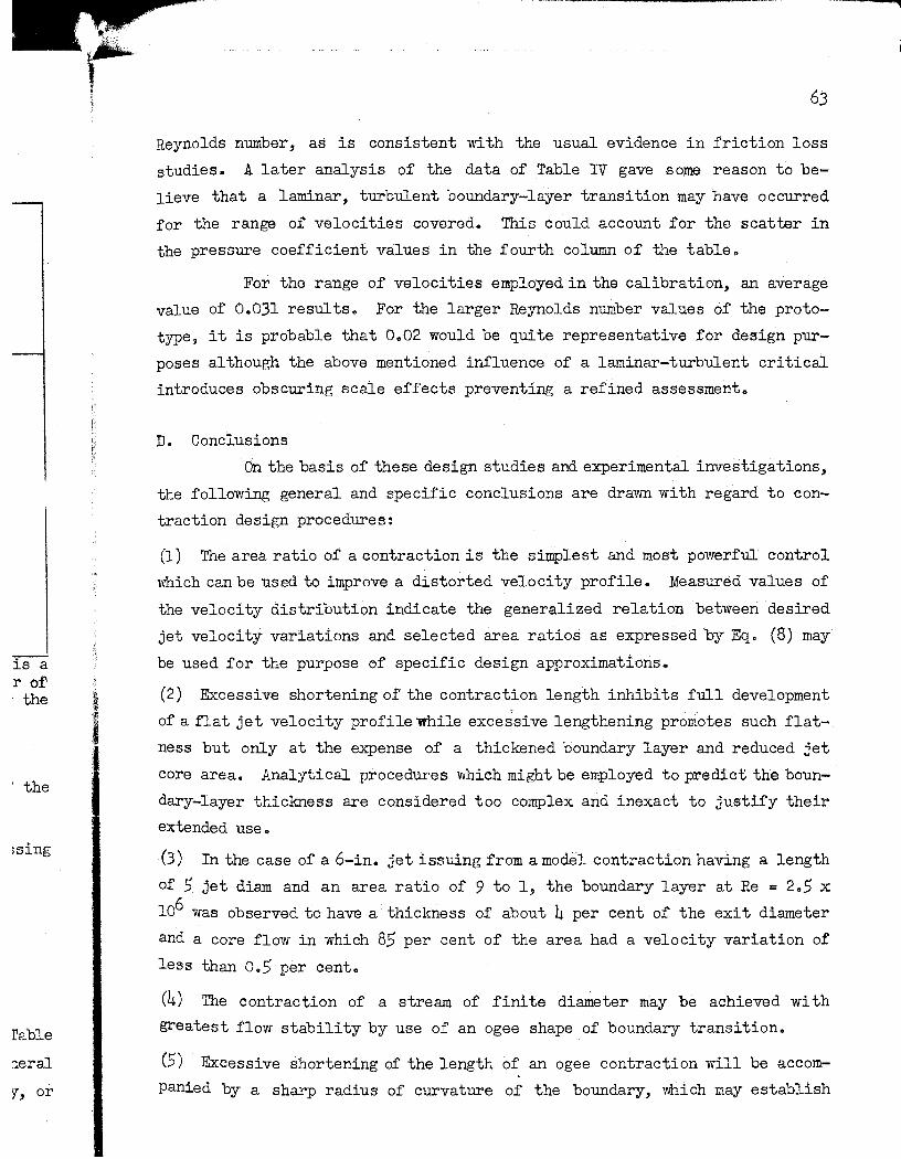
is a rof . the

. the

Ising

rable

neral

,{, or

Reynolds number, as is consistent with the usual evidence in friction loss

studies.. A later analysis of the data of Table IV gave some reason to be­

lieve that a laminar, turbulent boundary-layer transition may have occurred

for the range .of vel.ocities covered.. This could account for the scatter in

the pressure coefficient values in the fourth column of the tableo

F.or the range .of vel.ocities empl.oyed in the calibration, an average

value of 0.031 results. For the larger Reynolds number values of the proto­

type, it is probable that 0.02 would be quite representative for design pur­

poses although the above mentioned influence of a laminar-turbulent critical

introduces obscuring scale effects preventing a refined assessment&

D. Conclusions

On the basis of these design studies and experimental investigations,

the following general and specific conclusions are drawn with regard to con­

traction design procedures:

(1) The area ratio of a contraction is the simplest and most powerful control

which can be used to improve a distorted velocity profile. Measured values of

the velocity distribution indicate the generalized relation between desired

jet velocity variati.ons and selected area ratios as expressed by Eq. (8) may

be used for the purpose of specific design approximations ..

(2) Excessive shortening of the contraction length inhibits full development .

of a flat jet velocity profile While excessive lengthening promotes such flat-

ness but only at the expense of a thickened boundary layer and reduced jet

core area. Analytical procedures which might be employed to predict the boun­

dary-layer thickness are considered too complex and inexact to justify their

extended use ..

(3) In the case of a 6-in. jet issuing from a model contraction having a length

of 5 jet diam and an area ratio of 9 to 1, the boundary layer at Re = 205 x

106 was observed to have a thickness of about 4 per cent of the exit diameter

and a core flow in which 85 per cent of the area had a velocity variation of

less than 0.5 per cent.

(4) The contraction of a stream of finite diameter may be achieved with

greatest flow stability by use of an ogee shape of boundary transition.

(5) Excessive shortening of the length of an ogee contraction will be accom­

panied by a sharp radius of curvature of the boundary, which may establish

, J

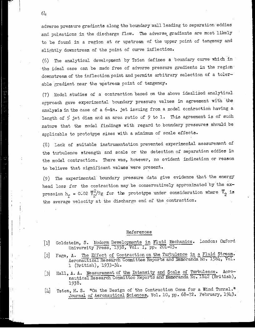
T I

64

adverse pressure gradients along the boundary wa1lleading to separation eddies

and pulsations in the discharge rlow. The advers~ gradients are most likely

to be found in a region at or upstream of the upper point of tangency and

slightly downstream of the point of curve inflection.

(6) The analytical development by Tsien defines a boundary curve which in

the ideal case can be made free of adverse pressure gradients in the region

downstream of the inflection point and permits arbitrary selection of a toler­

able gradient near the upstream point of tangency_

(7) Model studies of a contraction based on the above idealized analytical

approach gave experimental boundary pressure values in agreement with the

analysis in the case of a 6-in. jet issuing from a model contraction having a

length of 5 jet diam and an area ratio of 9 to 1. This agreement is of such

nature that the model findings with regard to boundary pressures should be

applicable to prototype sizes with a minimum of scale effects.

(8) Lack of suitable instrumentation prevented experimental measurement of

the turbulence strength and scale or the detection or separation eddieB in

the model contraction. There was, however, no evident indication or reason

to believe that significant values were present ..

(9) The experimental boundary pressure data give evidence that the energy . .

head 10s5 for the contraction may be conservatively approximated by the ex-

pression hf = 0.02 V;/2g for the prototype under consideration where V2 is

the average velocity at the discharge end of the contraction.

[4]

References

Goldstein, S. Modern Developments in Fluid Mechanics. London: Oxford University Press, 1938, Vol. I~pp. 201-03.

Fage, A. The Effect of Contraction on the Turbulence in a Fluid Stream. Aeronautical Research Committee Reports and Memoranda-No. 1584, Vol. 1 (British), 1933-34.

Hall, A. A. Measurement of the Intensity and Scale of Turbulence. Aero­nautical Research COiiiInittee Reports and Memoranda No. 1842 (British), 1938.

Tsien, H. S. \lOn the Design of' the Contraction Cone for a Wind Tunnel. t1

Journal of Aeronautical Sciences, Vol. 10, pp. 68-72. February, 1943 ..

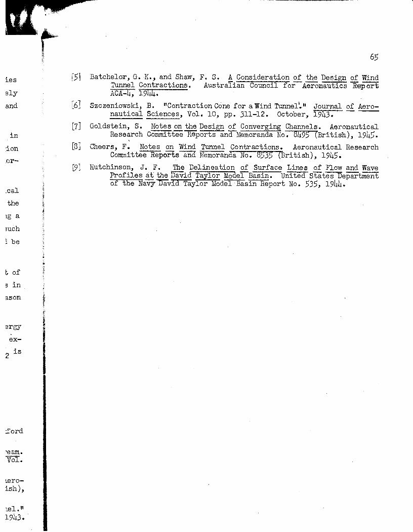
ies

ely

and

in

:ion

.eT-

.cal

the

19 a

mch

i be

~ of

5 in

9.30n

ergy

ex-

:ford

lero­ish),

leI." 1943. '

,~ .... "., I-I ~~

~ ~ ~ ~

i I I ~. i, .. i I Q,

~ ~

I

[5]

[6]

[7]

[8]

[9]

65

Batchelor, G .K., and Shaw, F. S. A Consideration of th,eDesign of Wind Tunnel Contractions • Australian Council for Aeronautics Rep ort ACA-4, 1944.

Szczeniowski, B. ttContraction Cone for a Wind Tunnell• tI Journal of Aero­nautical Sciences, Vol. 10, pp. 311-12. October, 1943. --

Goldstein, S. Notes ,on the Design of Converging Channels. Aeronautical Research Committee Reports ana-Memoranda No. 8495 (British), 1945.

, Cheers, F. Notes on Wind Tunnel Contractions. Aeronautical Research

Committee Report~ and Memoranda No. 8535 (British), 1945. Hutchinson, J. F. The Delineation of Surface Lines of Flow and Wave

Profiles at the Da'Vid Taylor Moder-Basin. United StatesDepartment of the Na;r.r~vid Taylor Model 'Basin Report No. 535, 1944.

""." --------

! I

CHAPTER IV. DIFFUSER STUDIES

A General Considerations . The purpose of the diffuser of a water tunnel is to reduce the large

discharge velocity of the test section to a value more compatible 'With the

functional requirements of the remainder of the tunnel recirculating system.

The velocity reduction or area expansion is necessary for the following reasons:

(1) It is not economically feasible to return the water stream from the diB~

charge end of the test section to the entrance without reduction of veloci ty ~

This condition prevails because such a return necessitates a 3600 directional

diversion of the flow plus a considerable straight travel distance, all of

which entails a frictional energy loss that is a function of the square of

the velocity. Obviously~ with the extremely high velocities proposed for the

test section (84 .. 5. fps), any increase in cross-sectional area of the return

eircui t will markedly reduce the energy losses and required pumping power

costs.

(2) If a constant area of cross section is used in the return duct, the in­

herent internal mechanism of fluid f'low tends to destroy any initial unifQrmi ty

of direction or velocity and returns ;to the test section a flow having defi­

nitely disturbed quality •. Numerous corrective devices and methods have been

employed but none is more simply effective than the contracting or. accelerating

cone. Accordingly, the benefits of contracting into the test section can be

available only if the return circuit has provided expansion after leaving the

test section.

(3) Among the fundamental operating specifications for the proposed tunnel

was a requirement for testing conditions having a minimum of background noise"

Operations in existing tunnels indicate that a large source of such noise is

the cavitation produced in passage through the vaned elbows and the pump of

the return circuit.. This cavitation is enhanced by an increase in velocity

and suppressed by an increase in pressure; thereforej! an increase in return

duct area can automatically contribute. dual benefits with respect to noise

abatement and the related vibration, pitting, and energy loss"

A superficial study of the diffuser problem leads to the conclusion

that a simple expansion of area should provide the desired velocity reduction;

however 9 actual tests and a more thorough analysis 'hav:e,proved. that" simple

area expansion can achieve reAsonable efficiency only under limited conditionso.

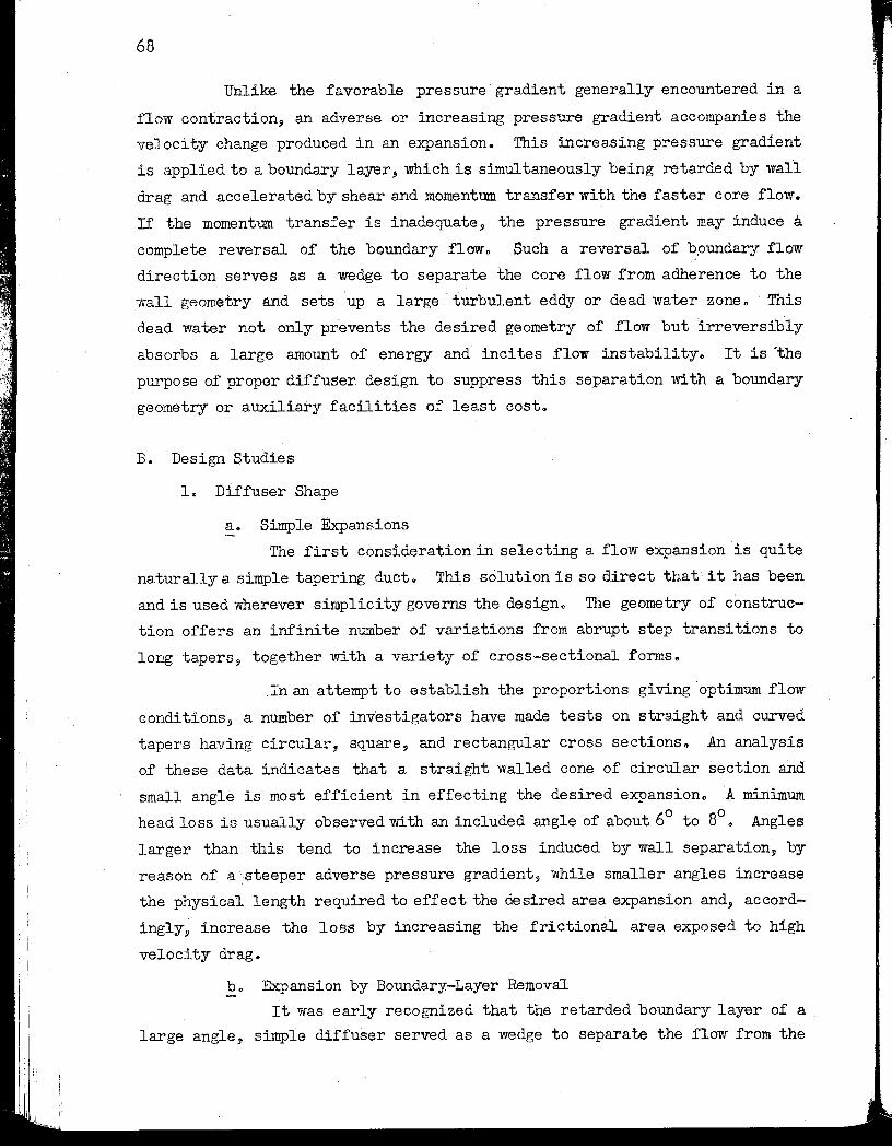
68

Unlike the favorable pressure· gradient generally encountered in a

flow contraction, an adverse or increasing pressure gradient accompanies the

velocity change produced in an expansion. This increasing pressure gradient

is applied to a boundary layer, 'Which is simultaneously being retarded by wall

drag and accelerated by shear and momentum transfer with the faster core flow.

If the momentum transfer is inadequate, the pressure gradient may induce a complete reversal of the. boundary flow 0 Such a reversal of b.oundary flow

direction serves as a wedge to separate the core flow from adherence to the

wall geometry and sets ·up a large turbulent eddy or dead water zone ... This

dead water not only prevents the desired geometry of flow but irreverSibly

absorbs a large amount of energy and incites flow instability.. It is 'the

purpose of proper diffuSer design to suppress this separation with a boundary

geometry or aUXiliary facilities of least cost.

B. Design Studies

1. Diffuser Shape

a.. Simple 1!:xpansions

Th.e first consideration in selecting a flow expansion is quite

naturally a simple tapering duct. This solution is so direct that'it has been

and is used wherever simplicity governs the design.. The geometry of construc­

tion offers an infinite number of variations from abrupt step transitions to

long tapers~ together with a variety of cross-sectional forms •

. In an attempt to establish the proportions giving optimum flow

conditions, a number of investigators have made tests on straight and curved

tapers having circular, square, and rectangular cross sectionso An analysis

of these data indicates that a straight walled cone of circular section and

small angle is most efficient in effecting the desired expansion,,! minimum

head loss is usually observed with an included angle of about 60 to So.. Angles

larger than this tend to increase the loss induced by wall separation, by

reason of a ·.steeper adverse pressure gradient, while smaller angles increase

the physical length required to effect the desired area expansion and, accord­

ingly 9 increase the loss by increasing the frictional area exposed to high

velocity drag.

b" Expansion by Boundary-Layer Removal

It was early recognized that the retarded boundary layer of a

large angle, simple diffuser served as a wedge to separate the flow from the

a

e .t

1 , •

.s

.y

om

::--

\:'0

ow

ad

is

nd

urn

es

by

se

d­gh

'a

,he

wall, thus changing the desired flow condition. Prandtl [lJ ~f-, in 1904, per­

formed elementary academic experiments serving to show that separation could

effectively be prevented by suction removal of that part of the boundary

layer which was beginning to reverse. Ackeret [2J, in 1926, made quantitative

measurements of suction removal on diffusers with rapid expansions by with­

drawing fluid through holes or slots in the boundary wall. Although his work

was not comprehensive, it did indicate that the stream could be made to follow

the diffuser shape by removing 1 or 2 per cent of the total flow at an expendi­

ture of suction energy amounting to 1 or 2 per cent of the kinetic energy of

the test jeto If these percentages are applied to the large flow and energy

of the proposed prototype, it is apparent that very substantial auxiliary

equipment would be necessary to implement flow expansion by this method.

In addition to the energy and flow handling problems oc~asioned

by this method, it would encounter additional complications in application to

a water tunnel diffuser where the suction region would be very close to that

in which minimum cavitating pressures may alreadybe in effect. The applica­

tion of suction would then promote rather than suppress harmful cavitationo

In view of these disadvantages, the suction diffuser was considered insuffi­

ciently developed to warrant use in the proposed application.

c. Expansion by Boundary-Layer Accelera'tion "While suction removal of dead water having insufficient kinetic

energy can effectively prevent separation phenomena, it is apparent that orig­

inal prevention of the dead water by energizing it to maintain its forward

motion should be equally effective. An obvious method of doing this is to jet

into the boundary flow additional fluid carrying kinetic energy from an out­

side source 0 For most effective action, this should be done at the beginning .

of the zone of energy deficiencywith the kinetic energy jet directed parallel

to the boundary. The additive energy may be supplied by external pumping

systems but it is also possible in some cases to convey fluid from high pres­

sure sources elsewhere in the parent flow system4 The latter method has met

with some success in suppressing separation on the low pressure side of air­

foils in what is known as the slotted wing. This device operates by conveying

pressurized air from the high pressure leading edge of a wing back through a

slot that jets into the boundary layer in the separation zoneo The method

also· shows some energy gains when applied to the conical draft tube diffuSers

of hydraulic tUrbines in a ·system developed by Professor Lo Fo Moody [3J 0

i~

IJ..st Numbers in brackets refer to the corresponding numbers in the reference at the end of the chapter.

70

An analysis of' the information on this general method of expan..;.

sian leads to the· conclusion that considerable physical complexity will be

encountered in its uss.. If a separate source of energy were used, it would

involve a rather substantial pumping plant and control system.. If high pres­

sure points of the return circuit were used for energy supply, a complex piping

system would be involved. In view of the complications of and the lack of

specific information on this system of expansion, it was not considered appli­

cable to the proposed design.

d. Expansion by Flow Rotation

If the flow through a diffuser has a rotation about its axis

in addition to its motion of translation, the efficiency of energy transfer

may be materially increased in some cases. The efficienC,1 increase is prob­

ably due to a complex combination of the radial pressure gradient countering

the adverse axial pressure gradient and to an increase in momentum transfer

through radial flow.

Since rotation could be· induced only by introduction of blading

systems at the diffuser entrance, it would be difficul tto induce rotation -in

a water tunnel diffuser without creating the possibility of cavitation on the'

vaning or prerotation effects in the test section flow.. Both 0.£ these effects

tend to destroy the desired flow quality and thus eliminate this method from

further design consideration.

e. Expansion by Deflectors or Vanes

As in the case of several of the other expansion systems.9 -this

one attempts to achieve diffuser efficiency through accelerating the dead

water.. This is accomplished by increasing the momentum transfer through provi­

sion of suitable deflector vanes serving to scoop the high energy core flow

into the dead water zones.. While the method offers some possibilities for

diffusers operating at nominal speeds and pressures, it must be 'dropped from

consideration in this design because of the cavitation which would occur on

the deflector vanes under low pressure conditions ..

f.. Comparison

An analysis of the diffuser types previously discussed indicates

that the small angle, simple, conical expansion is most likely to produce the

desired results. It is fully appreCiated that this system is not necessarily

71

the most economical, in view of its very large physical size and its appreciable

energy losses; but it is simple, free of maintenance and adjustment problems,

and should minimize the possibility of cavitation.

Previous investigators have found straight, tapered walls to

be just as effective as complex, curved walls for the small angle under con­

sideration except where a curved junction is judged necessary at the test

section transition.. Numerous studies indicate that 'a minimum energy loss will

occur for an included wall angle of 60 to 80 • However, because of the very

low pressures and high velocities which may exist at the entrance to the tunnel

diffuser, a conservative value of 50 was arbitrarily proposed.

2. The Diffuser Transition Curve

A parabolic transition having a length of 1/2 test section mam

was provided to avoid a sharp break in the boundary at the intersection of

the test section cylinder and the diffuser cone o Since the transition curve

is intimately associated with the test section performance, the design studies

for this element have been included With those of the test section in Chapter

II. The general arrangement of the diffuser and the transition 1m :stt0'lm in

Fig. 27 ..

3.. The Pump Diffuser

The short diffuser following the pump is not analyzed in this section

since its performance is so intima:tely dependent on the characteristics of the

pump impeller, hub fairing, and straightening vanes; these are primarily the

responsibility of the pump builder ..

For the purpose of constructing the model tunnel, the pump diffuser

was built as a simple cone with an 8° included angle.. This angle is in a

range which should provide nearly maximum efficiency yet it is of minimum

length, thus allowing the maximum length of stilling section in the lower leg

of the tunnel ..

C.Experimental Studies

1. Apparatus and Procedures

The main diffuser in the model water tunnel was made in three sections.

The upstream section was an aluminum casting bored to provide the necessary

transi tion curve between the cylindrical test section and the conical diffuser"

The two downstream sections of the diffuser were fabricated from 3/16-in" thick

sheet steel rolled to the proper shape and welded to steel flanges. Minor

-, I

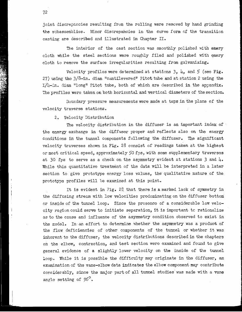
72

joint discrepancies resulting from the rolling were removed by hand grinding

the subassemblies. lunor discrepancies in the curve form of the transition

casting are described and illustrated in Chapter II.

The interior of the cast section was smoothly polished with emery

cloth while the steel sections WBre roughly filed and polished with $mery

cloth to remove the surface irregularities resulting from galvanizing.

Velocity profiles WBre determined at stations 3, 4, and 5 (see Fig.

27) using the 3/8-in. diam "cantileveredtl Pitot tube and at station 2 using the

l!L.-in. diam IIlongU Pitot tube, both of which are described in the appendix ..

The profiles were taken on both horizontal and vertical diameters of the section ..

Boundary pressure measurements were made at taps in the plane of the

velocity traverse stations4

2. Velocity Distribution

The velocity distribution in the diffuser is an important index of

the energy exchange in the diffuser proper and reflects also on the energy

conditions in the tunnel components following the diffuser. The significant

velocity traverses shown in Fig. 28 consist of readings taken at the highest

or most critical speed, approximately 50 fps, with some supplementary traverses

at 30 fps to serve as a check on the asymmetry evident at stations 3 and 4. ~bile this quantitative treatment of the data will be interpreted in a later

section to give prototype energy loss values, the qualitative nature of the

prototype profiles will be examined at this point.

It is evident in Fig.. 28, that there is a marked lack of symmetry in

the diffusing stream with low velocities predominating on the diffuser bottom

or inside of the tunnel looPe Since the presence of a considerable low velo­

city region could serve to initiate separation, it is important tc rationalize

as to the cause and influence of the asymmetry condition observed to exist in

the model. In an effort to determine whether the asymmetry was a produc~ of

the flow deficiencies of other components of the tunnel or whether it was

inherent to the diffuserp the velocity distributions described in the chapters

on the elbow, contraction, and test section were examined and found to give

general evidence of a slightly lower velocity on the inside of the tunnel

loop_ While it is possible the difficulty may originate in the diffuser, an

examination of the vane-elbow data indicates the elbow component may contribute

considerably" since the major part of all tunnel studies was made with a vane

angle setting of 96°.

7h

Rather extensive studies of the vane geometry as described in Chap""

ter V establish that flow symmetry and component performances could be, im­

proved materially by changing the vane angles to 101°. Since these diffuser

studies "Were conducted in parallel with the early vane studies, no opportunity

was presented to include diffuser tests with the optimum vane settingo How­

ever, a subsequent program of testing this tunnel when rebuilt as an open­

jet tunnel wi til an alternate closed-jet sleeve, gave evidence that the earlier

50 diffuser performance was quite abnormaL In the "rebuilt tunnel having

vanes set at 1010 , separate tests with a 6° hot and a 90 cone gave greater

symmetry and relatively higher wall velocities than evidenced i~ Fig .. 28.,

Similar tests conducted at the Ordnance Research Laboratory, Pennsylvania'

State College [h]l1 also showed satisfactory symmetry at angles of' 7,,50 and 100 "

A general study of the work of other diffuser investigators with a

view to their findings on the presence of asymmetry disclosed that Nikuradse

[5J had measured related phenomena and quantitatively determined the influence

of the cone angle e While Ni1ruradse t s numerical values' taken from 'a re ctangillar

two-dimensional diffuser are not directly appl icable to the circular cone

under consideration here, the trend of the progressive change in velocity

distribution with change in diffuser angle is judged comparable. This trend

for the diffuser tested by Nikuradse may be summarized:' (1) for small expansion

angles (So total angle) the flow profile is symmetrical and stable; (2) for

, somewhat larger angles (100 total angle) the flow becomes unsymmetrical but

without evidence of reverse boundary flow or instability; (3) for, still larger

angles (120 total angle) the unsymmetrical flow has apparent separation on

one side but is still stable; (h) for still larger angles (160 total angie)

the asymmetric flow stream switched slowly from one side to the other' in an

unstable manner"

In view of the above data~ but with full awareness of the form dis­

crepancies between the rectangular diffuser and the model tunnel and the pos­

sible deficiencies of the vane setting, it would appear that the velocity

profiles of Fig. 28 represent a flow pattern which in the worst case might t~

considered analagous in form to that of item (2) of the foregoing.. If this

is assumed to be the case9 it would then appear that a decrease in total cone

angle would tend to give a more symmetrical pattern, While only a slight in­

crease in angle would produce definite separation" It is, therefore j indicated

that use of a 5° diffuser cone in the model is definitely on the side of

1

n

e

s

e

d

f

75

conservatism, and if economic considerations dictate more radical procedures,

an angle of 60 or 70 could be employed with no great risk of adverse effects.

'While there are insufficient data in these tests to indicate any

trends in performance differences between the model and the prototype, it seems

safe to say that increasing the size by ten times and the velocity from 50 to

85 fps should serve to improve the efficiency and separation conditions b This

seems rational since the flow pattern is principally dominated by viscous

forces which for high Reynolds numbers, as in this case, normally produce

improved flow and separation suppression with increased values.

It should be noted that the discussion of flow quality applies only

to the case of flow in the unoccupied tunnel. If a test body is mounted in.

the test section, the flow may of course be profoundly influenced by the nature \

of the body. Since the nature of the body will be widely variable in a general

purpose tunnel, it will be impossible to predict the range of diffuser per­

formance. It seems reasonable to assume, however, that the simple conical

diffuser will perform as well or better than the other diffuser types sug­

gested- Which are, in general,9 rather sensitive to changes in· the design

variables. It is also worthy of note that these tests take no account of

the basic level of turbulence in either the model or the prototype tunnel"

It is probable that this has some effect on the diffuser separation conditions,

but lack of suitable instrumentation prevents evaluating the turbulence.. It

is doubtful that turbulence would produce significant scale effects because

the turbulence values in the model and the prototype are probably comparableo

3. Energy Losses

The total energy lost in a diffuser action is normally evaluated by

measuring the change in the sum of the pressure and the kinetic energy as the

flow progresses from the inflow to the outflow.. In the model tunnel studies,

this change in energy is measured by boundary pressures and velocity traverses,

as described elsewhere. The kinetic energy data as represented by the velocity

traverses of Fig .. 28 are converted to a more useful form by applying an inte­

gration of the plotted profile to the expression

Where V is the mean velocity of the section. The value of a may then be used

in the form a Tj2 /2g to express the mean velocity head of the total stream ..

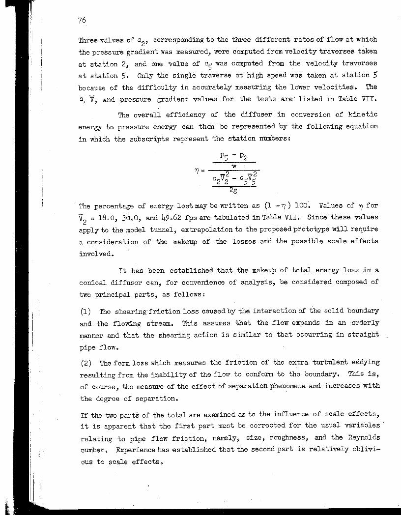
76

Three values of Q2' corresponding to the three different rates of flow at w~ich

the press'Ul'S gradient was measured, were computed from velocity traverses taken

at station 2, and. one value of a, was computed from the velocity traverses

at station ,. Only the single traverse at high speed was taken at station,

because of the difficulty in accurately measuring the lower velocities. The

Q, V, and pressure gradient values for the tests are listed in Table VII.

The overall efficiency of the diffuser "in conversion of kinetic

energy to pressure energy can then be represented by the following equation

in whi6hthe subscripts represent the station numbers:

w 7] ... ---~2:-----'2~

Q2V2 - Q,V5 2g

The percentage of energy lost may be written as (1-7]) 100. Values of 7] for

V2 = 18 .. 0, 30.0, and 49 .. 62 fps are tabulated in Table VII.. Since' these values

apply to the model tunnel,extrapola:tion to the proposed prototype will require

a consideration of the makeu,p of the losses and the possible scale effects

involved.

It has been established that the makeup of total energy loss in a

conical diffuser can, for convenience of analysis, be considered composed of

two principal parts, as follows:

(1) The shearing friction loss caused by the interaction of the solid boundary

and the flowing stream.. This assumes that the flow expands in an·.orderly

manner and that the shearing action is similar to that occurring in straight

pipe flow.

(2) The form loss which measures the friction of the extra turbulent eddying

resul ting from the inability of the flow to conform to the boundary.. This is,

of course, the measure of the effect of separation phenomena and increases with

the degree of separation ..

If the two parts of the total are examined as to the influence of scale effects,

it is apparent that the first part must be corrected for the usual variables·

relating to pipe flow friction, namely, size, roughness, and the Reynolds

number.. Experience has established that the second part is relatively oblivi­

ous to scale effects ..

i ~ .~

-~

-,i , , '-~

Velocity (fps)

a

a ('V2/2g) (ft)

Re = V (d/v)

~} f g P5/W - p!w (ft)

Pf/w (ft)

1]

~{"7~ ~ 1],* o "7 So

TABLE VII

DIFFUSER ENERGY LOSS DATA

Test Sec Vel = 18.0 fps

Station 2 Station 5

18.00

1.0185

5.12

0.9. x 106

3.72

1.812

.0.39 6 0.4 x 10

0.0198 I 0.0178

4.34

0.25

0.9164

0.9683

0.9280

0.8780

Test Sec Vel 0: 30.0 fps

Station 2 Station 5

30.00

1.0144

14.18

6.19

1.812

1.07

1.5 x 106 6 0.7 x 10

0.01981 0.0172

11.81

0.67

0.9007

0.9518

0.9280

0.8780

*With test installation in test section.

Test Sec Vel = 49.62 fps

Station 2

49.62

1.0151

38.81

2.5 x 106

Station 5

10.25

1.812

2.96

1.1 x 106

0.0195 0.0170

32.31

1.72

0.9012

0.9490

0.9280

0.8780

Note: The use of values carried to the fourth and fifth significant figure is a calculating and reference expedient and is not indicative of the order of accuracy of the experimental work which, in general, can only justify the third significant figure.

l

-oJ -oJ

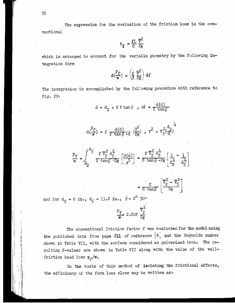
78

The exp:ression for the evaluation of the friction loss is the con-

ventional

which is arranged to account for the variable geometry 'by the following in­

tegration form

The integration is accomplished by the following procedure with reference to

Fig. 29:

f [V~ -v~J" =' 8 tang 2g

and' f~r d2 = 6 in., d5 = 1) .. 2 in., e;::. 20 )0'

-2 p£ V2 -= 2.60f -2

11" g

The conventional friction factor f was evaluated for the model using

the published data from page 211 of reference [6 J and the Reynolds number

shown in Table VII, with the surface considered as galvanized iron. The re­

sul ting f-values are sholm in Table VII along with the value of the wa.ll­

friction head loss pi/We

On the basis of this method of ,'. isolating' the frictionalef£ect~,

the efficiency of the form loss alone may be written as:

t-----t ~ I L-----I_

Fig. 29 - Designation for Diffuser Georr.etry

7] = o -2 -2 a2 V2 - as Vs 2g

79

Values of this expression for the model tunnel tests are shown in Table VII. It may be noted that these values vary somewhat, which is reasonable in view of the assumptions for the derived expressions and the accumulated experimental error. As a representative approximation, 7]0 will be assumed at 0.950 for computing the prototype extrapolation.

The total efficiency of the prototype diffuser energy conversion is then computed as follows:

I

7] = 7] -o = 7J. -o

2g

In the prototype evaluation the last term will be assulned to have a-values, t.'e same as in the model, while f = 0.008S. The latter value was chosen from measurements made by the Tennessee Valley Authority [7] on a flow conduit of approximately the same size and surface as the proposed prototype. Values I of 7] for the velocities used in the tests are shown in Table VII.

l I ~I

II \ \'

80

Comparison of the foregoing values with those of other investigators

indicates agreement but with no exactness. Peters [eJ, who carried out the

most comprehensive experiments, came to the conclusion that inherent sensiti­

vi ties made experimental determinations of efficiencies of small angle dif­

fusers vary widely. This is confirmed, since values of ~o varying from 0.89 to 0.97 have been found by various' eXperimenters for e in the region of 20

30'.. He found the nature of the inflow to the di£fuser had a powerful in­

fluence on the efficiency and losses; accordingly, it may be expected that the

previously computed "1' values will vary materially with the nature of bodies

mounted in the tunnel test section. In order to attempt some evaluation of

this influence, a conservative estimate based on Peterst work will assume that

the form loss 1 - ~o is doubled. Values of ~'* calculated on this basis fU'e

listed in Table VII ..

Peters also found that in most cases energy measurements restricted

to the diffuser cone proper did not give a true picture of the diffuser losses,

since alterations of the velocity profile and eddy decay continue for some

distance downstream of the cone length. These abnormalities in the duct fol-

10Vlring the cone produce losses which properly belong to the diffuser but which

are in many cases necessarily assigned to the following duct component. In . 1

view of this, it must be recogn,ized that the ~ values tabulated in Table VIr

are for the diffuser alone and that the abnormally high losses (see Chapter

V). occurring in the vane elbow following the diffuser are due to reformation

or normalizing of the diffuser energy discharge rather than the usual per­

formance losses of the vane. elbow itself.

While the use of "1 as an expression of the conversioneffic.lency of

the diffuser is a useful value for comparative studies of the diffuser alone,

it will be necessary to convert this value if the head loss for the diffuser

is to be compared and totaled . with the loss for other parts of' the : t~el.

In keeping with the expression for head loss of other tunnel components, the 2 .

value for ·the diffuser should then be K (V212g)~

An expression for K may baderived by writing Bernoullits equation

along the diffuser and expres sing the head 108S asK (V i/2g) .. If this· is solved

for K by using the original TJ equation' for .substi tution, the. following '&Jq1rea­

sien will result: .

-----~ ~--~~ ----81

Evaluating this by using the high velocity data of Table VII, the prototype t ... . 1*

K-value corresponding to ~ will be 00067 and that for ~ will be 0 0 1140

D. Conclusions

On the basis of these design studies and experimental investigations,

the following conclusions are drawn with regard to the proposed diffuser design

procedures:

(1) On the basis of available general dU'fuser information and the tests

herein described, a simple conical diffuser of ,0 total angle appears to offer

very conservative perfonnance characteristics for the proposed prototype"

·lVhile the tests cover only the ,0 angle, it is believed that an angle up to

70 may be used without adverse effect •

. (2) The,o cone gave evidence of conditions approaching separation along one

side. It is believed that the major portion of this asymmetry would be re­

moved by a slight change in the angular setting of the elbow vanes, as dis­

cussed in Chapter V. In view of the high energy efficiency obtained in the

tests there is reason to believe that the observed asymmetry did not produce

separation ..

(3) The energy loss in the 50 diffuser is satisfactorily low in comparison

with values of efficiency of energy conversion as determined by other inves­

tigators. It is estimated that the efficiency of the diffuser will be 0,,88

with a test body installed in the test section and 0.,93 with· no test body

installed in the test section" Corresponding total energy losses may be ex­

pressed as hf "" 0.114 vi/2g with test body and hf = 0,,067 Vi/2g without test

body, where V2 is the average velocity at the entrance to the diffuser" Sen­

sitivity to a variety of causes precludes using these values forprecise:ca.l.;;'

culations"

(4) Energy disturbances created in a diffuser persist for a considerable

distance downstream of the diffuser cone.. The evaluations of item (3) pertain

only to the energy conversions and losses wi thin the cone proper and do not

include the subsequent losses resulting from normalizing the disturbances of

the diffuser. Such losses are treated in other chapters of this paper ..

Conclusions relating to the diffuser transition characteristics are

discussed in Chapter II"

82

[1]

[2]

[3J

[4J

[5J

References

Prandtl, L .. , and Tietjens" 0" Go Applied ~~2':, and Aero ... Mechanics .. New york: McGraw-Hill Book Company, 1934,"P:31o Ackeret" J~ ltSucking of the Boundary Layer,,',·' ,ZeitschTift des Vere:bis Deutscher Ingenieure, Vol .. 35, pp .. 1153-58, 1926.. (Translated from the German in National Advisory Committee for Aeronautics Technical Memorandum No .. 395 .. ) Kerr,S .. L.. "The Moody Ejector Turbine .. " Transactions of the American Society of Mechanical Engineers, VoL 43, No" 1820, pp~ 1201-17, 1921.. -. Robertson, J .. Mo, and Ross, Do Unpublished work relating to dUfuser studies for a water tUnneL (More specifiC information concerning publication of this comprehensive and valuable work unavailable at this time .. ) Pennsylvania state College Ordnance ResearchLaboratory .. Goldstein, S.. Modern Developments in Fluid Mechanics.. London: Oxford University Press, 1938, Vol .. II, pp .. 371-76 ..

[6] Rouse, Hunter.. Elementary Fluid Mechanics.. New York: John Wiley and Sons, 1946..-[7J Hickox, GoH .. , Peterka, A .. J", and Elder, R .. A.. UFriction ,Coefficients in a Large Tunnel .. " Proceedings of the American Society of Civil Engineers, Vol .. 73, pp .. 451-70 .. April, 1947. -[8J Peters, Ho ~lConversion of Energy in Cross:..;seetional Divergerices under Different Conditions of Inflow".t Ingenieur-Archi1l", :Vol. II, pp. 92-107, 1931.. (Translated from the German in National Advisory Committee for Aeronautics Technical Memorandum Noo 737.)

8:3 CHAPTER V • VANED ELBOW STUDIES

A. General Considerations The function of the elbows in the proposed water tunnel is to assist . in recirculating the test jet from the discharge end of the test section around and back to its contracting entrance. This is to 'be. accompliShed wi th a miriim.um loss of energy and a minimum final disturbance of the uniform paral-. leI f:tow desirable in the test section.. l'Ihile a variety of physical forms might be conceived to accomplish this function, analysis of the experience available in the literature of the subject and consideration of fabrication methods pOinted the selection of the form of recirculating conduit toward a system composed of four 90° elbows joined by straight ducts.. It is the in­tent of this chapter to clarify the detailed design procedure relating to these 900 elbows ..

The first consideration in selecti~g such 900 elbows is quite nat­urally the conventional radius elbow, which seemingly offers a smooth direc­tional flow transition with standard fabricating practices and attendant economies. HOwever, a study of the internal flow in such elbows and an analysis of the quantitative values obtained from extensive tests, as given in refer­ences [1] * to [6J and summarized in [7J, indicate the following marked short­comings for the proposed application: (1) To permit the water stream to conform smoothly to the duct curvature the mean radius of sweep must be at least 2 duct diam in size and preferably 4 diam., Use of such long radii on prototype installations of large duct diameter will lead to very substantial distances between the legs or the loop; their use necessitates consideration or more compact design forms ..

(2) If a sweep radius or less than 2 duct diam is employed, the stream no longer conforms to the sweep because of the manner in 'Which the kinetic energy or the approaching core flO'flr impinges against the outer wall under the cen­trifugal force of curvature. The result is a high pressure on the center of the outer wall. and a low pressure on the inner wall.. As a consequence of this pressure differential, a flow transverse to the duct axis takes place along each side wall and produces two large, high speed vortices trailing from the elbow exit" In addition to this, an adverse boundary pressure gradient of . axial direction is created on the outer wall just upstream of the miter ~fNumbers in brackets refer to the corresponding numbers in the reference . list at the end of the chapter co

84

line and another is created on the inner wall somevmat dO"Wllstream ot'the miter.

These a.dverse gra.dients are productive of separation eddies which may be of

sufficient strength to consume appreciable en~rgy and to produce pulsations

in the exit flowo In addition to these power.f-ul .flow distortions, . another

lack of symmetry is created in the discharge flow by the tendency of the ro'"

tating fluid mass to distribute itself in accord with the energy conserving

principles of the free vortex, which produces high velocities along the path

of short radius (along the inside of the bend) and low velocities along the

path Of lmqp:r:t:diluis (along the outside of the bend).. Use of short radius plain,

elbowswill.ll accordingly, lead to energy losses and intolerable flow distortions.

A further analysis of a possible combination of the desirable flow

properties of the long radius elbow with the desirable dimensional properties

of the short radius turn leads toa compromise form which has found favor in

many applications. This solution consists of disposing the cross-sectional

duct area ins~ch fashion that the width of area (dimension perpendicular to

the plane of the bend) is increased and the dept.his decreased. The improvement

traceable to this change occurs because a.n increasing width-depth ratio (here­

after called the a.spect ratio because of its similarity to the aeronautical

term) reduces the percentage of total .now influenced by side wall vortices

and leaves a core with a curved two-dimensional flow which can be maintained

with losses oniy slightly greater than those which would be encountered in a

similar straight duct. Decreasing duct depth produces decreaSing differences

in ,!:-he centrifugal pressures on the inner and outer walls and consequent de ...

creases in transverse now. It is obvious, however, that increasing the as­

pect ratio will eventuall,. increase the total wall area and consequent friction

drag to the point where the incident losses transcend those of the normal

side wall vorticeso Test of rectangular sections with varying :aspect ,.ra.tios

established that energy losses decreased rapidlyrlth increasing aspect ratios

up to a value of about 6 [3J.

Disposing the duct area to a high aspect ratio is not as favorable

a solution for the proposed tunnel design as it is in many other duct pro­

blems. The prime objection in this case is'the:s'evere' shape tnmsition re­

quired between such a duct and the connecting circular test section. Such

transitions contribute undesirable flow irregularities a.nd are to be avoided.

In addition, tile high aspect ratio requires large plane areas in fabricating

the boundary walls; these are costly when designed for pressure loadingso

85 A digest of the foregoing indicates the large reductions in energy

105s attending larger corner radii and aspect ratios cannot be taken advantage of in direct application to the external elbow proportions" However, a further analysis of the principle shows that internal addition of splitter partitions to an elbow of low aspect ratio and short radius effectively divides the flow into separate elbows individually having increasing radii and aspect ratios as the number of partitions increases. The benefits gained by this approach are soon limited as the addition of the splitters contributes increasing area for frictional drag. Tests of these compensating effects [.3] indicate, in general, the use of two splitters yields a minimum loss i'or this type of elbow. The advantages of this type of construction led to its use in a number of early water tunnelsb

A further refinement of the principles of the previous paragraph is accomplished by redistribution of the elbow elements into a mitered elbow fitted with a large number of shortrlength formed partitions or vanes. Proper design in this direction can divide the flow into a large number of cellular units operating at most favorable ratios yet without the large friction areas occasioned by the similar use of full length splitters. The measured losses in such an elbow are only about one-half to two-thirds of those in splitter elbows and are accompanied by a more uniform velocity distribution and less turbulence. Because of their low losses and flow quality these assemblies" known as vaned elbows.\> have been extensively used in wind tunnels since the first Gottingen tunnel of 1909 and are the accepted answer in wind tunnel designs. The structure and corrosion problems attending the use of such vanes in water retarded their acceptance in general water -flow elbow applications until !IIWlr6 ::recsrlt i'lowqua..liity. :requirements necessitated such acceptance. Their use in water tunnels has become quite general since 1938 and is con­sidered the preferred approach to the proposed designo

The following summarizes the benefits attending proper use of vane type elbows in the proposed application! (1) minimum distortion of the velo­city distributi,pn, (2) minimum energy lossee (as low as 10 per cent of the local kinetic energy of translation); (3) minimum strength and scale of such turbulence as i~ created, (4) minimum external physical dimenSions; and (5) sensitive control of the velocity distribution through provision of adjus­table vanes. It is the purpose of the remainder of this chapter to describe the detailed design of the vane geometry and the experimental tests conducted thereon.

..

I

II

86

B" Design Studies

Having determined the desirability of the vane type elbow for the

application in question, the problem resolves itself into a selection of spe­

cific dimensional values which will produce an optimum flow condition cons is­

tent with practical forms for fabrication9 The first significant dimensional

value in the selection of the vanes is the spacing or number of vanes to be

employed in the given elbow" This value is determined by a combination of the

structural and hydraulic limits imposed"

Hydraulically, the only serious consideration is that the vanes shall

reduce the area of the circular duct section to a group of approximate rectan­

gles whose proportions or aspect ratio exceed a value of 6:10 Graphical di­

vision of a circular area into strips of equal width indicates that at least

six or eight vanes are required to provide this aspect ratio for the rectangles

forming the bulk of a circular section" An increase in the number of vanes

will give even greater aspect ratios and will materially improve the discharge

flow quality"

The number of vanes or spacings has! a material influence on the

structural properties of the vane when the vane is loaded as a beam since

increasing numbers result in decreasing individual vane size and greater rela­

tive span lengths" While the reduction in vane size results also in'areduc"+

tion in exposed load area, the beam strength decreases more rapidly than the

load, 'and reduction in structural rigidity carried to an extreme may lead to

deflection, vibration)) and noise under high dynamic water loads.. This can be

alleviated by tying adjacent vanes·together at points between the end supports,'

thus reducing the free span., It should be remembered, however, that such

webs, struts~ or tie plates, even though faired, introduce the same type of

disturbance as a side wall and thus necessitate that aspect ratios be computed

only on the basis of clear spans"

It therefore appears that the optimum number of vanes in an elbow

is a unique compromise between the structural and hydrauliC functions involved ..

These considerations have apparently been applied to previous water tunnel

designs as the number of vanes of existing units appear to vary from 6 to 15,

with ties being used with the larger values.. Since the selection of vane

number or spacing is :intimately associated with the vane structural properties,

nz

l. #. __ A" ;;::s;. ¥';;,H_$!£J4$-#4 - _iJ;;UC,

87 it becomes apparent that the size of the vane section is a necessary part of this selection and that certain definitions are necessary to the comparative description of vane properties. The most significant terms are defined in the following paragraphs and are sho1Vll in Fig. 30.

The vanes of a cascade are assumed to be of uniform cross section throughout so that the vanes may be replaced by their profile in a plane. The vane profile is defined by its chord length c and certain rela ti ve shape characteristics, such as maximum camber and maximum thickness" Only the chord is of importance at this time.. The chord line is defined as the line obtained by placing a straight edge against the pressure side of the vane profile; it is tangent to the leading and trailing edges. The chord length is the distance between the projections of the extreme ends of the vane on the chord line" A ;cascade of vane profiles is obtained by first selecting a straight line as a cascade axis.. To form the cascade, vane profiles are placed on the cascade axis so that corresponding points on the profile fall at regular in­tervals along the axis and so that the chords of all the profiles make the . same angle with the cascade axis. The distance between corresponding points on the B.,"'{is is then the vane spacing s and the angle between the chord and the axis is the vane stagger 8. A given cascade is defined by the profile of the vanes,the chord length, the dimensionless spacing-chord ratio sic, and the stagger angle 8. In place of the spacing-chord ratio, other investigators sometimes use the gap-chord ratio, where the gap is the projection of the spacing in the direction of approaching flow ..

A cascade of vanes is installed in an elbow so that the cascade axis falls in a plane parallel to the miter plane of the elbow, where the miter plane is that plane formed by the intersection of the elbow walls. For a 900 bend, the cascade axis is placed at 450 to the direction of the approaching flow. Iflle angle of attack between the approaching flow and the chord, desig­nated by the symbol a, is then 450 less than the stagger angle; a .. 8 - 450 •

An analysis of the limited amount of data available to justify a particular choice of dimensions disclosed that the most Significant findings are those of IUein, Tupper, and Green [8], which indicate that vane turns for minimum energy loss should possess a spacing-to-chord ratio of about one half"

..

88

1i

5 = Spacing c • Chord Length

Fig. 30 - A Cascade of Vanes

On the basis of this and a preliminary.

analysis of dynamic loads and associated

structural problems, a vane of the shape

and the spacing shown in Fig. 31 was se­

lected as a first approximation to the

proposed design. This design is founded

on arbitrary selection of a prototype vane

gap of 10 inches. This dimension requires

18 gap units in the l5-ft diam of the pro­

totype duct, a number larger than that

used in other water tunnels but still not

so large as to produce vanes of weak cross

section. The chord is of convenient fab­

ricating size, and the velocity profile

should have a fine-tooth pattern.

l~PI~ Fig. 31- The

Trunnion

Preliminary (Prototype

Vane Size)

Selection

R"2500·

--¥---- ~-Round I

Fig. 32- The Proposed Vane Selection (Model Size)

It is apparent from Fig. 31 that the selected vane is of thickened

cross section similar to wind tunnel vanes rather than the bent single plates.

used in most existing water tunnels. The thickened section was adopted be­

cause of its greater inherent structural rigidity and because it permitted a

uniform gap (constant area) for flow passage through the vane. The former

feature was important in view of the structural fan ures of single plate vanes

occurring in some water tunnel applications in this country; the latter fea­ture was desirable in reducing separation eddies and the resulting energy loss and in providing directional' stability, as evidenced by Collar I s I9J findings.

The vane was formed with a minimum number of simple, circular arcs .. For practical fabricating reasons this was considered preferable to the com~ plex theoretical curvature of Krober [lOJ or the bent airfoils of Klein, Tupper, and Green [8J even though these refined forms offered slightly less energy loss.

In reducing the first approximation of Fig .. 31 to a more practical form, Fig .. 32, 'modifications were made similar to those used by Collar [9]" These consisted of a slight displacement of the surfaces to provide a finite and arbitrary prototype edge thickness of 1/4 in., a foreshortening of the fragile trailing edge, and a rounding of the leading edge in accordance with conventional aerodynamic practice. It has been contended by some authorities that the rounded leading edge satisfactory in aeronautics is subject to low pressure zones which could produce cavitation when employed with hydraulic blading, as in pumps or turbines. Accordingly, these designs sometimes employ sharp or hatchet edged blades to minimize the low pressure areas.. This arti­fice might have been given further consideration if Collar I s [9J work had not indicated that an angular adjustability of as much as 50 'might be necessary to permit determination of the optimum vane setting. The relative insensi­tivity to cavitation and separation of the rounded edge under angular changes in vane setting therefore dictated its use for the proposed design.

A thorough analysis of all earlier vane literature available in­dicated that the foregoing vane selection might serve as a suitable general approach to the problem but clearly indicated that refined performance charac­teristics could not be fully anticipated for the proposed prototype and that experimental studies directed toward the particular .needs of this installation were imperative if the desired flow quality were to be achieved.. Therefore, it was decided that a full model study of the proposed elbow should be under­taken.

Analysis of the model problem established that the one-tenth scale model proposed for study of other tunnel components would also be adequate to produce workable values for certain overall phases of the elbow tests but that

90

certa.in other pha.ses could be more effectively examined by detailed studies

on a separate flow diversion test bend. A now diversion test bend' was assem­

bled and vaned elbows of one-tenth scale were fabricated for the" model tunnel

to accomplish these studies.. The one-tenth scale vane profiles employed in

both of these facilities were as shown in Fig .. 32 and tests were arranged to

supply these necessary design data:

(1) The angular setting of the selected vane 'Which would provide the best.

discharge flow quality and least energy loss ..

(2) The pressure distribution on the vane profile, with a view to clarifying

the probability of cavitation and the magnitUde and location of the dynamic

structural loading ..

(3) Scale relations between themode1 and the prototype~

C.. Experimental Studies

1" Method

a" Apparatus

The experim~ntal studies were conducted in two separate facili­

ties" The first setup consisted of a small square duct (900 elbow) containing

cast Cerrobendvanes; it was tested with both air and water as fluids.. . The

second setup was a model tunnel elbow containing extruded aluminum vanes; it

was tested only with water.. The elbow was installed in the test stand with

the bend in the horizontal plane" The entrance to the upstreaint tangent of the

elbow was bolted to a plate on the end of a 12-in. diam supply pipe" A 6-in.

square hole was centered in the plate to match the cross section of the Lucite

pipe" Bolts through this plate served to hold a bell-mouthed contraction and

a distributor ring in place in the 12-ino pipe.. This distributor ring was

used in conjunction with a supply of compressed air to introduce dyes or air

bubbles into the flow"

For making measurements of the velocity and pressure in the

elbow, three measuring stations (D-D~ K-K, and M-M of Fig. 34) as well as

two measuring discs and many separate piezometer taps 'Were provided.. The

discs were used to permit traversable insertion of a Pitot cylinder to obtain

.. ... ... ... ,.. .. + .. .. + ... .. .. .. ... .. ..

+ + ... ... ... ... ... ... ... .. .. + + + ... ... ...

... .... ... +

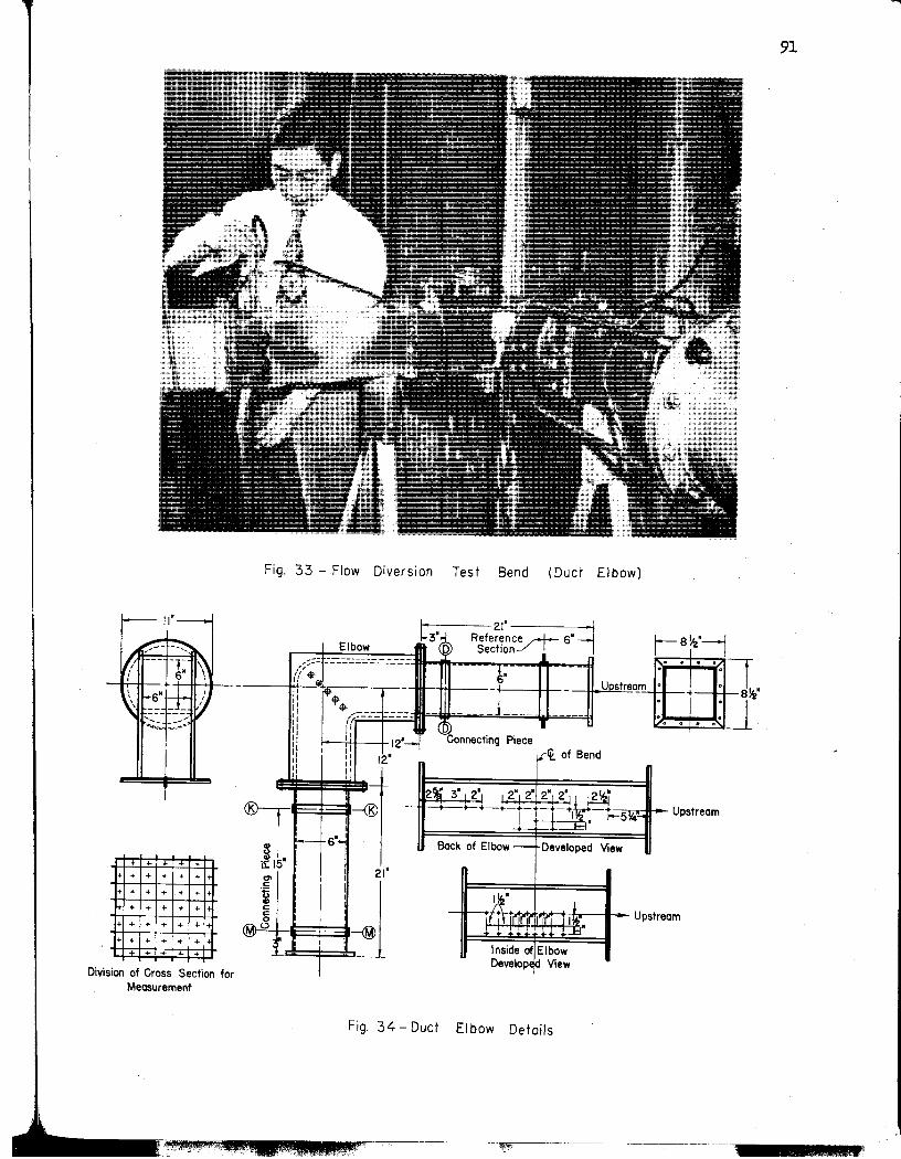
Division of Cross Section for Measurement

Fig. 33 - Flow Diversion Test Bend (Duct Elbow)

Elbow , ... -:= --- -,',:'

21" 1 Reference .r.+.- 6" SectionJ I

m if *" Upstrea ------~-J~~------r_--N~~-----r----++----~~~~ q ~ .. II .. f-~-~--~~-~-~r-~-~~-&-~~--~F-~-:-=U !i (r--- - - (D I, I ' 12. --l Connecting Piece II , II .At of Bend d :: 12" I" Ii I'

" 2~ 3"12·1 12"12" 2"1 2" ~

I . . . . · 1 · 0 · · j · · · 0 . . .

J -® - :-r-II--. Upstream f-=+--~~-"-rt-r~r.-~5~ I ..... _ I

~ 6·-: Bock of Elbow - Developed View I

~15· I

~ ,

!~r I~ ~ - hi irn ~[I j I~ • L':' .. + . .. ~

• Inside of Elbow

1 Developl Ii View

Upstream

Fig. 34 - Duct Elbow Details

91

d i I

92

velocity and energy measur~ments immediately before and after the vanes, while the separate piezometer taps were :used to obtain wall pressure measurements at many points around the bend" To remove all burrs, all 1/16";in. holes designed for wall pressure readings were carefuliy rounded at the inside edge to about 1/64-in. radius. At the measuring stations, the 1/4-'in. holes allowed entry of a Pitot cylinder into the flow. These measuring sections made pos­sibie the obtaining of wall pressure readings at 24 points and velocity and energy readings at 45 points within the section in the course of a normal traverse.

The l2-in. diam supply pipe carrying fluid to the test elbow was connected to an air blower, and alternately to the main Laboratory supply channel, drawing water directly from the Mississippi River. This arrangement is shown in Fig. 35. The regulating valves in the 12-in. line were placed about 40 ft upstream from the elbow.. .A long honeycomb in the entrance pipe rectified the flow before it entered the bell mouth of the 6-in. duct. Flow of water through the elbow up to 4.5 cfs was measured by a discharge measuring flume, while the alternate capacity of the blower limited the flow of air to 30 cfs.. The variations of the flow from either source were sufficiently small to be ~eglected entirely in the analysis and computation.

The discharge from the downstream tangent of the Luci te, duct was led through a diffuser and a short length of 12-in. round pipe into a vertical pipe.. The portion of this vertical pipe above the elevation of the Lucite,duct served as a standpipe, and the lower portion conducted the water flow to the previously calibrated measuring flume.. A valve in this lower pipe regulated the pressure in the Lucite duct while the standpipe protected the duct from an excess of pressure~ The elbow was deSigned to receive a bank of five vanes of the form of Fig. 32 at the selected spacing of 1.414 inch. The free span of the vanes was 6 in .. , the full height of the duct. Thus the spaCing-chord ratio is 0 .. 48', the gap between the. vanes is virtually I in .. , and the aspect ratio is 6 for these experiments.. The aspect ratio of 6 assured two-dimensional flow near the centers of the vanes 'where measurements were to be made.

Two sets of vanes were used in the test bend, one consisting of pieces cut from the extruded aluminum stock adopted for use in the model water tunnel construction and the other consisting of specially prepared vanes of cast Cerrobend, a low melting temperat-q.re alloy.. The Cerrobend vanes were'

Convergent Section

E.xperimental Elbow

29" I 1--------- 40'------l

1'1 Diffuser 3'

1----=E::=-+--15' ----+--

Waste

Channel

rt:+:--Stand Pipe

PLAN VIEW -12'61-r1~m ( ) L Flow Straightener

Waste Streamline Baffle Channel

Fig. 35 - Duct Elbow Assembly

Water Regulating

Valve

5'

«

93

94

used because they permitted fabrication of "cast inl' pressure taps and lines ..

The alternate set of extruded aluminum vanes was used for checking since it

was discovered that the extruded vanes could not be produced with as great

profile accuracy as could be done with the Cerrobend ..

A final check of the shape of the experimental vanes disclosed

a very close adherence of the Cerrobend vanes to all of the specified dimen­

sions but it also revealed certain signi:t;'icant discrepancies in the shape of

the extruded aluminum vanes" These differences were found to·be at the leading

edges and the region near the trailing edges of the aluminum vanes; the thicker

sections of the vanes satisfied the specifications" The leading edge appeared

to vary somewhat at different points along the spans but, in general, the nose

was slightly more pointed than the radius of 0 .. 08 in. specified., The tail of

the vane was thinner than the design called for with a small ridge at the

trailing edge 0 This thin section was bent around towards the center of curva­

ture so that the profile presented a turn of about 950 .. The overturning of

the geometrical profile and the ridge were 'corrected before the installation

of the vanes in the cascade frames 0 The verification of the performance of

the al urninum vanes in relation to the' dimensionally correct Cerrobend vanes

was substantiated in the experimental data ..

. The Cerrobend vanes were polished smooth and then waxed before

they were tested, but a slight roughness could be detected on the surface of.

the almninum vanes <> The effect of any differences in roughness between the

vanes was not apparent in the evaluation of energy loss in the cascades nor

in the observations of the flow on the surfaces of the vanes, as interpreted

in a later sectiono

Pressure lines of 1/8-ino on copper tubing were cast into all

five of the vanes and were extended out through the end trunnions to provide

a connection outside the duct for attaching the' tiubes'to: themanometerlil.. Wall

mounted, set screws bearing on the end of the vanes prevented the vanes from

turning about the vane trunnionso This arrangement provided a rigid but adjus­

table support for the vanes in the simplest manner possible without disturbing

the flowo It should be noted that the position of the trunnion as shown in

Fig" 32 was selected to approximate the force center for the gravity and

dynamic loads in order that, torsional restraint and stability about the trun­

nion might be optimum" The center of dynamic forces was approximated lby .ibite­

gration of a measured pressure diagram as obtained by Klein, Tupper, and Green

[8J on a similar vane profile"

95 The general arrangement of the Cerrobend vane and its pressure

tap system are shown in Fig 0360

The vanes used in the one-tenth scale model tunnel were all cut from bar lengths commercially extruded of alillllinillll using a special die made in accord with the profile of Fig .. 32. This method of production proved the most efficient way of making a considerable quantity of vanes of an accurate prof:Ue in :a rnonrusting material of adequate structural strength. The ends of the vane bars were carefully cut ~o fit the contour of the elliptic miter block of cast aluminum which served as the corner piece for each of the four elbows of the tunnel. The miter blocks were carefully machined with trunnion holes to accommodate the trunnion rods anchored in the vane on their inner end and clamped to the miter block with nuts on their outer end. 't"he general arrangement of the elbow, miter block, vane, and vane trunnion are shown in Fig~ 37.

. While most of the vanes in the model tunnel were not equipped for detailed measurement,Sl the central vane in elbow I (Fig .. 38) was fitted for taking comparative pressure readings at ten points on the surface.. Copper tubing was laid in grooved slots milled in the vane and then led down the in­side wall of the vertical$ circular duct to the instrument access opening in the tunnel wall at station 6 (Fig., 38).. The grooves Were filled with aluminum solder and the surface was polished,Sl then checked for dimensional accuracy" Small piezometer holes were drilled into the copper tube normal to the surface of the vane i> These holes were staggered where there might be interference but were confined to a band an inch on either side of the center of the vane span .. The manometer arrangement allowed pressure on the vane surface to be'>recorded relative to station 5,Sl a position close enoUgh to make the static pressure difference a negligible amount"

The instruments used in making velocity and energy traverses in the model tunnel consisted of the tllonglt and ('cantileveredtl Pitot cylinders described in the appendix.. The method of mounting the ncantileveredu cylinder is shown in Fig .. 370 The instruments used in the test bend traverses were df similar form but differed slightly in methods of support and reading. These instruments were connected so that pressure readings with water flowing in the

, duct were measured by a lOO-in" u-tube using air as the indicating fluidS' and a 50-inoU-tube using kerosene as the indicating fluid" An inclined manometer draft gage was used to measure the pressures for the now of air and a very

Fig. 36- Duct Elbow polished smooth but

Vane and. Trunnions is slightly discolored.

= 2.93 in.)

(Vane surface is Chord length

Fig. 37- Upstream View of Elbow I (Showing Vanes and Vane Anchorage Arrangement Together with Pitot Cylinder and Its Main

Mounting Arrangement at Station 5)

3

1------------- 15'-S" -----------~-_I

Fig. 38 - Designation of Vaned Turns and Velocity Traverse Stations.

97

large manometer bank was used as a method of obtaining s::i..multaneou,s photo':':' . graphic readings when using water.

Velocity traverses made in the model tunnelvrere taken at sta­tions 5, 6, 7, 10, 11, and 12 (Fig. 38) and employed the manometers described in the appendix.

b. Visual and Photographic Studies

Preliminary studies of the flow mechanism and certain of the final conclusions were accomplished by visual and photographic studies in the transparent walled, square elbow. These observations employed four different techniques, each of which added to or confirmed the general fund of informa­tion.. The four methods and their most significant findings follow: (1) photographs of the flow taken during a period when air bubbles were being introduced at mid-depth thro'Ugh the upstream distributor ring are typified by those shown in Fig .. 39.. The photographs indicate the existence of a more nearly axial flow immediately before and after the bend for a stagger of 1010

than is true for the 900 and 960 settings. Since the density of the air bubbles differs materially from that of the water, areas of the flow involving curved streamlines or centrifugal forces cannot be interpreted too literally from the photographso The flow streakssho~d, however, give quite reliable information on the approach-flow direction and the location of the front stag­nation pointo

(2) Analyses of the local directions of flow were obtained in many regions by cementing one· end of short filaments of fine thread to the vane surface and by stretching a fine traversable wire across the duct and attaching short threads thereto" Visual studies under a variety of flow conditions served to clarify the directional pattern and strength of turbulence both in the core flow and near the boundaries and was most helpful in pointing out the manner in which the walls produced spiral flow near the ends of the vanes. The tra­verse at mid-depth at the 960 stagger showed an extremely turbulent region from a point directly behind the trailing edge of a vane to a point about 3/8 in. from the suction side.. The same region at the 1010 stagger was very smooth except directly behind the trailirig edge, where only moderate distur­bances were noted" The flow behind the portion of the gap. closest to the pressured side of a vane was very smooth at the 960 stagger angle and exhibited a slight fluctuation at the 1010 stagger ..

,

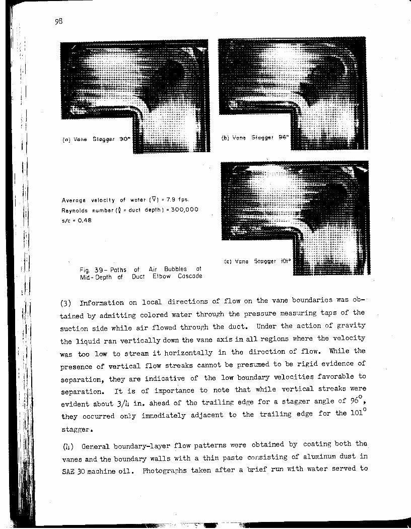
,I, ,

, I, "

I ,I, 'I

98

(a) Vane Stagger 90°

Average velocity of water (V) "' 7.9 fps.

Reynolds number (0 "' duct depth) "' 300,000

sic = 0.48

Fig. 39 - Paths of Air Bubbles at

Mid- Depth of Duct Elbow Cascode

(b) Vane Stagger 96°

(c) Vane Stagger 101 0

(3) Information on local directions of flow on the vane boundaries was ob­

tained by admitting colored water through the pressure measuring taps of the

suction side while air flowed through the duct. Under the action of gravity

the liquid ran vertically down the vane axis in all regions where the velocity

was too low to stream it horizontally in the direction of flow. While the

presence of vertical flow streaks cannot be presumed to be rigid evidence of

separation, they are indicative of the low boundary velocities favorable to

separation. It is of importance to note that while vertical streaks were

evident about 3/4 in. ahead of the trailing edge for a stagger angle of 960 ,

they occurred only immediately adjacent to the trailing edge for the 1010

stagger.

(4) General boundary-layer flow patterns were obtained by coating both the

vanes and the boundary walls with a thin paste consisting of aluminum dust in

SAE 30 machine oil. Photographs taken after a brief run with water served to

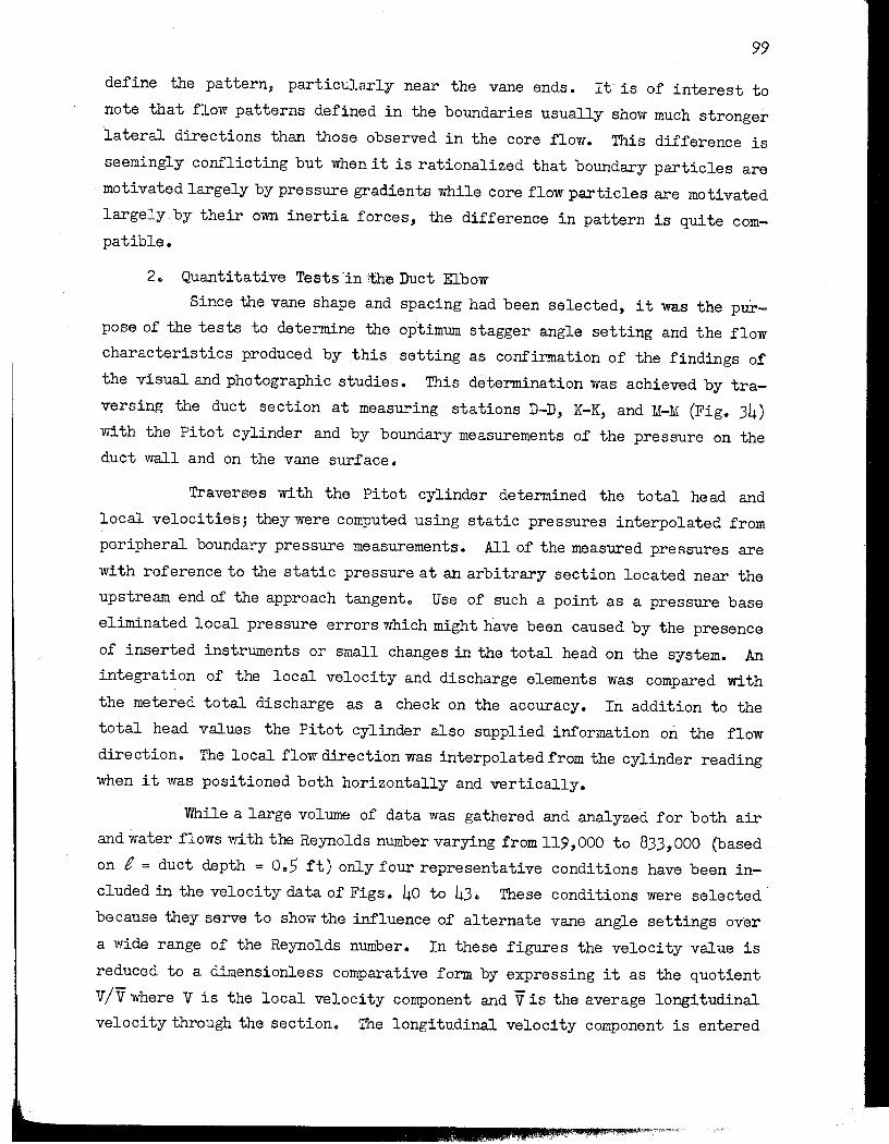
99

define the pattern, particularly near the vane ends. It' is of interest to note that flow patterns defined in the boundaries usually show much stronger

lateral directions than those observed in the core flow. This difference is

seemingly conflicting but when it is rationalized that boundary particles are

, motivated largely by pressure gradients while core flow particles are motivated

largely by their own inertia forces, the difference in pattern is quite com­

patible.

2. Quantitative Tests,"intire Duct Elbow

Since the vane shape and spacing had been selected, it was the pur­

pose of the tests to determine the optimum stagger angle setting and the flow

characteristics produced by this setting as confirmation of the findings of

the visual and photographic studies. This determination was achieved by tra­

versing the duct section at measuring stations D-D, K-K, and M-M (Fig. 34) with the Pitot cylinder and by boundary measurements of the pressure on the

duct wall and on the vane surface.

Traverses with the Pitot cylinder determined the total head and

local velocities; they were computed using static pressures interpolated from

peripheral boundary pressure measurements. All of the measured pressures are

with reference to the static pressure at an arbitrary section located near the

upstream end of the approach tangento Use of such a point as a pressure base

eliminated local pressure errors which might have been caused by the presence

of inserted instruments or small changes in the total head on the system. An

integration of the local velocity and discharge elements was compared with

the metered total discharge as a check on the accuracy. In addition to the

total head values the Pitot cylinder also supplied information on the flow

direction. The local flow direction was interpolated from the cylinder reading

when it was positioned both horizontally and vertically.

While a large volume of data was gathered and analyzed for both air

and water flows with too Reynolds number varying from 119,000 to 833,000 (based

on f = duct depth = 0.5 ft) only four representative conditions have been in­

cluded in the velocity data of Figs. 40 to 43.. These conditions were selected'

because they serve to show the influence of alternate vane angle settings over

a wide range of the Reynolds number. In these figures the velocity value is

reduced to a dimensionless comparative form by expressing it as the quotient

V/V where V is the local velocity component and Vis the average longitudinal

velocity through the section. The longitudinal velocity component is entered

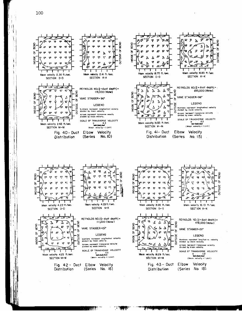
Q Z

~ U. o W Q

~

100

Mean velochy 2.36 ft.lsee. SECTION D-D

Mean velocity 2.42 ftlsee. SECTION M-M

Mean velocity 2.41 ft. /sec. SECTION K-K

REYNOLDS NO.1 0 - duct depth)-~ 119,000 (Water)

~ 15 VANE STAGGER- 96"

~ LEGEND iii Number. repr •• ent longitudinal velocity § divided by mean veloclty,

Arrow. represent 'ran,vlne velocity divided by mean velocity.

SCALE OF TRANSVERSE VELOCITY o O.S ~

(Meon velocity" I Unit)

Fig. 40 - Duct Distribution

Elbow (Series

Velocity No. 10)

Mean velochy 4.22 ft./sec. SECTION D-D

Mean velochy 425 ft./Sec. SECTION M-M

o ffi

Mean velocity 4.23 ftl sec. SECTION K-K

REYNOLDS NO.1 g - duct depth)-111,000 I Water )

~ VANE STAGGER-IOi" o

~ LEGEND (/) Number. repr ••• nt lonQitudinal velocity !:io divided by maan velocity.

Arrows repre.ent tranty"" vllocity divided by mean velocity.

SCALE OF TRANSVERSE VEL'OCITY o O.S ............

( .... on velocity. 1 Unit)

Fig. 42 - Duct Distri but ion

Elbow (Series

VeloCity No. 16)

Mean velocity 16.70 fUsee. SECTION 0-0

Mean velocity 16.83 ft.lsec. SECTION M-M

Fig. 41- Duct Distribution

Mean velocity 18.20 ftJsee. SECTION 0-0

Mean velochy 18.29 ft./sec. SECTION M-M

Fig. 43 - Duct Distri butlon

Mean velocity 16.83 ft./sec, SECTION K-K

REYNOLDS NO.1 Q - duct depth)- , ~ 833,000 (Water)

~ u. VANE STAGGER-96" o ~ LEGEND ~ Numbers repr.lln' lonQltudlnal velocity ::J divided by mean velocity.

o Arrows repr .. en' transverse nlaeity divided by mean veloci.y.

SCALE OF TRANSVERSE VELOCITY o O.S ~

(Mean velocity. I Unit)

Elbow (Series

Velocity NO. 15)

Mean velocity 18.10 fl.l sec. SECTION K-K

REYNOLDS NO.1 O· duct depth)-~ 478,000 (Water) ~ u. VANE STAGGER-IOI· o

~ LEGEND ~ Number. rapr .. en, longitudinal velocity ::) divided by maan velocity. o

Arrow. rapre.ent 'ron.ver .. velocity divided by mean velocity.

SCALE OF TRANSVERSE VELOCITY

~S (Mean v.,oclty = I Unit)

Elbow (Series

Velocity No. 18)

101

on the diagram at the point where the measurement was taken.. The velocity

components in the plane of measurement are plotted as vectors originating at

the point of measurement and are scaled as shown. The diagrams are oriented

such that the reader is looking downstream, with the inside of the bend on

his lefto

In addition to this velocity data, the relative pressure distribution

around the bend was obtained at mid-depth of the side walls and dimensionless

values of this are shown in Fig .. 44.. Pressures measured by taps on the vane

surfaces are shown in a general compara ti ve way in Figs.. 45 to 47, while a more

detailed distribution is shown in Fig .. 48 ..

30 Quantitative Tests in the Model Tunnel Elbow

'While the tests conducted in the duct elbow allowed flexibility

and detailed flow study of the vanes, the environment was essentially a two­

dimensional and somewhat idealized condition which did not wholly represent

the prototype condition.. Therefore, to assure a better understanding of pro­

totype performance, it was deemed necessary to conduct model water tunnel vane

studies in which the environment permitted the influence of other flow compo­

nents" To this end velocity profiles and contours were determined at stations

5, 6, 7, 10, 11, and 12 (Fig. 38), utilizing the 3IB-in. diam flcantilevered ll

Pitot cylinder as described in the appendix. The profiles were taken on two

diameters of the test plane, one of which lay in the plane of the tunnel loop

while the other was at 900 thereto ..

The most significant of these velocity studies were those measured

at stations 5 and 6 and at stations 11 and 12.. The former pair gives insight

into the effect of the very bad entrance condition produced by the diffuser

action, while the latter pair shows normalized approach conditions. The meas­

ured data for the former pair are shown in Figs .. 49 and 50, while typical data

for the latter pair are shown in Fig .. 51.. In examining Fig .. 51, the reader

is oriented faCing upstream.

In addition to the foregoing velocity studies of the vane, pressure

distribution studies were made on the surface of the middle vane of elbow Io Ten pressure measuring holes located around the vane periphery and disposed

in a narrow band at the center of the vane were connected to a manometer 'Which

permitted pressure measurements to be made relative to the static pressure

at station 5.. Data from these pressure taps are plotted in Fig.. 52 for three

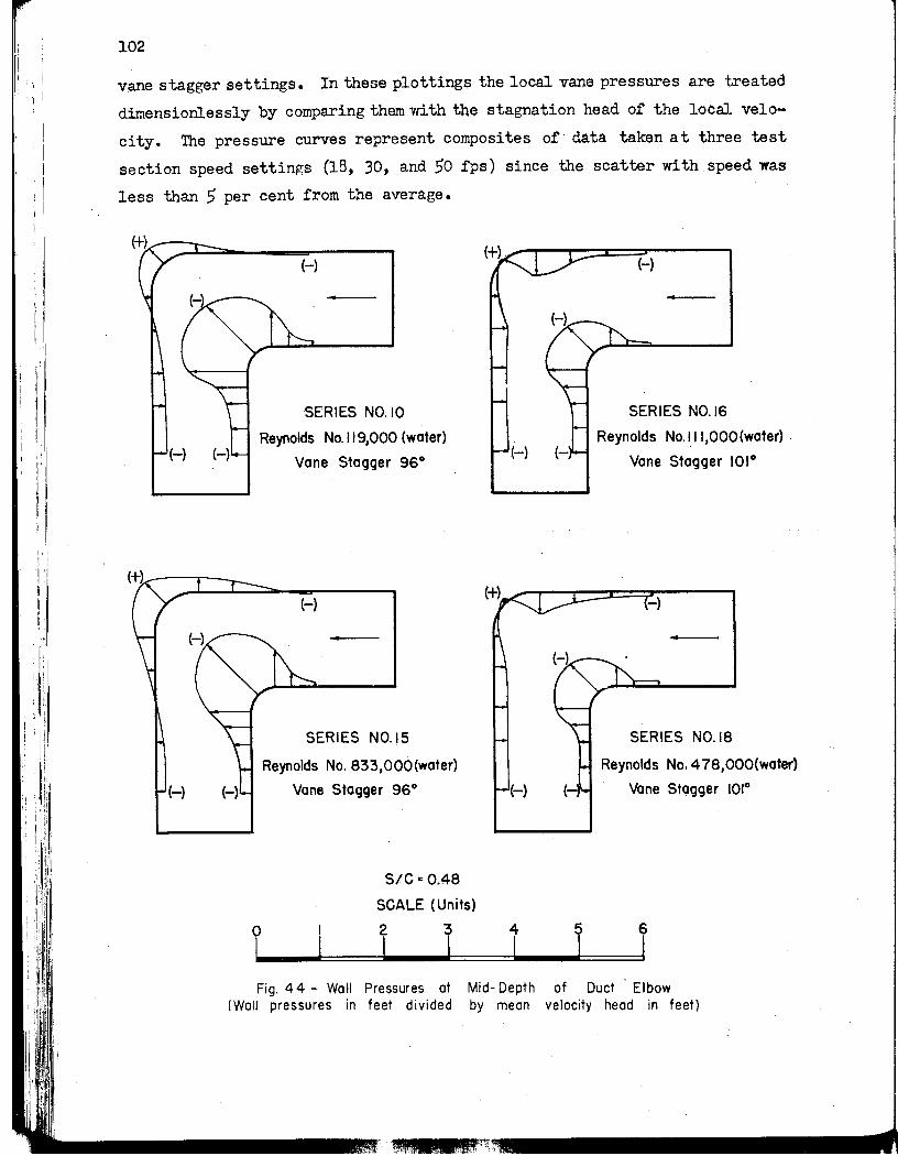
I i

I !

102

vane stagger settings. In these plottings the local vane pressures are treated

dimensionlessly by comparing them with the stagnation head of the local velo­

ci ty. The pressure curves represent composites of data taken a t three test

section speed settings (18, 30, and 50 fps) since the scatter with speed was

less than 5 per cent from the average.

(-)

H

SERIES NO. 10

Reynolds No. I 19,000 (water)

Vane Stagger 960

H

SERIES NO.15

Reynolds No. 833,000 (water)

Vane Stagger 96 0

SIC .. 0,48

SCALE (Units)

2 3 I I

o I

4 5 I I

(-)

•

SERIES NO.16

Reynolds No.I.II,OOO(water)

Vane Stagger 1010

-)

SERIES NO.18

Reynolds No.4 78,000(water)

Vane Stagger 1010

6

I Fig. 44 - Wall Pressures at Mid- Depth of Duct Elbow

(Wal] pressures in feet divided by mean velocity head in feet)

NeGative values Plotted as Broken Lines

t

Vane Stagger 96" SIC-O.48

Scale in UnHs

? i i r Fig. 45 - Pressures at Mid- Depth Across 96 Degree Cascade (Pressures in feet divided

by mean velocity head in feet)

t I ,

\ (-),

(+) Series No. 16 (+)c:) Reynolds No.III,OOO(water)

~ \

t ,

(+) Series No. 17 (+)C:) Reynolds No.302,OOO(water)

f. I

" " /// ---Series No. 18 (+) (-) Reynolds No. 478,000(~ter)

Reynolds No. based on O· Duct Depth Vane Stagger 101·

S/C-Q48

Scale in Units

L j 1

-

-----~------ ---------------~

103

Negative Values Plotted as Broken Lines

Vane Stagger 101·

r SIC- 0.48

Scale in Units 0 j 4 f , I

Fig. 46- Pressures at Mid-Depth Across 101 Degree Cascade (Pressures in feet divided

by mean velocity head in feet)

Vane Stagger-9S· __

Vone Sta9ger-~I~~_ .. / /' "

j \

~ , .'

/,;y ..... - ........ ..... ,

;::~ '- '-............ ,

::--... \ \

1/ i " , , k::: ,/ --............., I

I,; Trunniar ~ "'-V cP.... r\ V""- e-9S· ~ ~ Miter Line ~ IiIg!rOI~ e-IOI· Miter Line "-.:

SIC·

-2.25

-2.00·

-1.75

-1.50

-1.25

-1.00 ... N

-0.75~ >­.0

-0.50'i :s!

-0.25i5

f o :::I :: .. TO.25 It

to.50

to.75

TUX>

0.48

Fig. 47- Pressure variatian Around Vane as a Function of Reynolds

Number (Pressure in feet divided by

Fig. 48 - Duct Elbow Vane Pressure Distribution

mean velocit y head in feet.)

..... ------------------------~

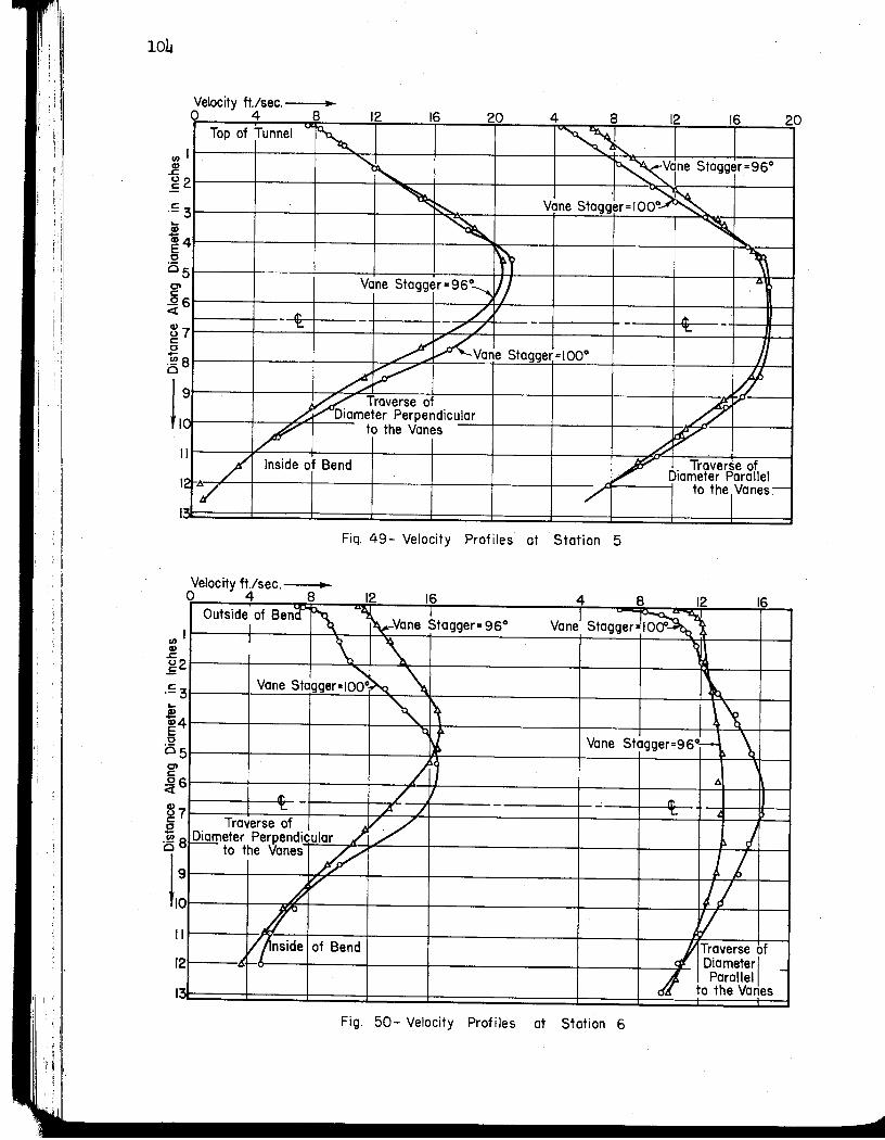
I: : I

I

:1

'I! I

104

III III ..r::. 0 E .5 ~

III 1i) E 0 0 0> t:::: .2 <1:

III III ..r::.

Velocity ft.lsec. -----~~ o 4 8 12 16 20 4 8 12 16 20

Top of Tunnel 0" ~ ~ I '-

~" ~Te Stagger=96°

2 ~ ~ Vane Stagger=IOO~

3

'" "" " 4 ty ~ 5 Vane Stagger=96~ '/

... , 6 / II- - II-

~~ -// - - 't:.. -7

8 ~ ~ Vane Stagger = I 000 A

~ V l# 9 ~ Traverse of ff ~ Diameter Perpendicular c -;7 to the Vanes ~ b II

/ Inside of Bend V . Traverse of

12/ Diameter Parallel

to the I Vanes-

I~

Fiq. 49- Velocity Profiles at Station 5

Velocity ft./sec. ~ o 4 8 12 16 4 8 12 16

Outside of Ben? , .. ~ L vane' Stagger~

I ~Vane Stagger= 960

It ~2

~ \. Vane Stagger=IO~~ ~ ,~

3

"'-~ '\ ~ ,.

Vane Stagger=96~ \ ~ 5

6 / i1

'" II' 'I:.. -

/! / - - L...

Traverse of y / 8 QiQ!!leter Perpendicular ./

9

to the Vanes # i f ~

V ,// 0

F ~V I 'I' /'nside of Bend / Traverse of

2 Diameterl 7 Parallel -

., to the Vanes

Fig. 50- Velocity Profiles at Station 6

Station II

Fig. 51- Velocity

Velocity in Te~\

Isovel Interval" le~lIon. 49.6 ftlsec Vane Stagger \ ~I~I . % = 0.48 ~i' sec.

Distribufi~

~~ ot Stations II and 12

v -------~ - 1.25 ________ ~;-_;v:::a='n~ ~~e Stagger = 1000

Vane Stag!\ ~j~gger = 98 0

~~ - 1.00 t-sso CI ---------------~~~-~~ N

Fig. 52 - Model Tunnel VQ~

,~~-.£.--------~ -0.7 5 ,~

o ! ;:, en en

:'!---==-_........:==90.--I-I-.... 1"0.25 ~

1'-------H~1--t- -to.50

1------+-¥.HI~ -to.75

---+--+WIff--t-1- 1.00

S/C-0.48

! Pressure Distribution

105

Station 12

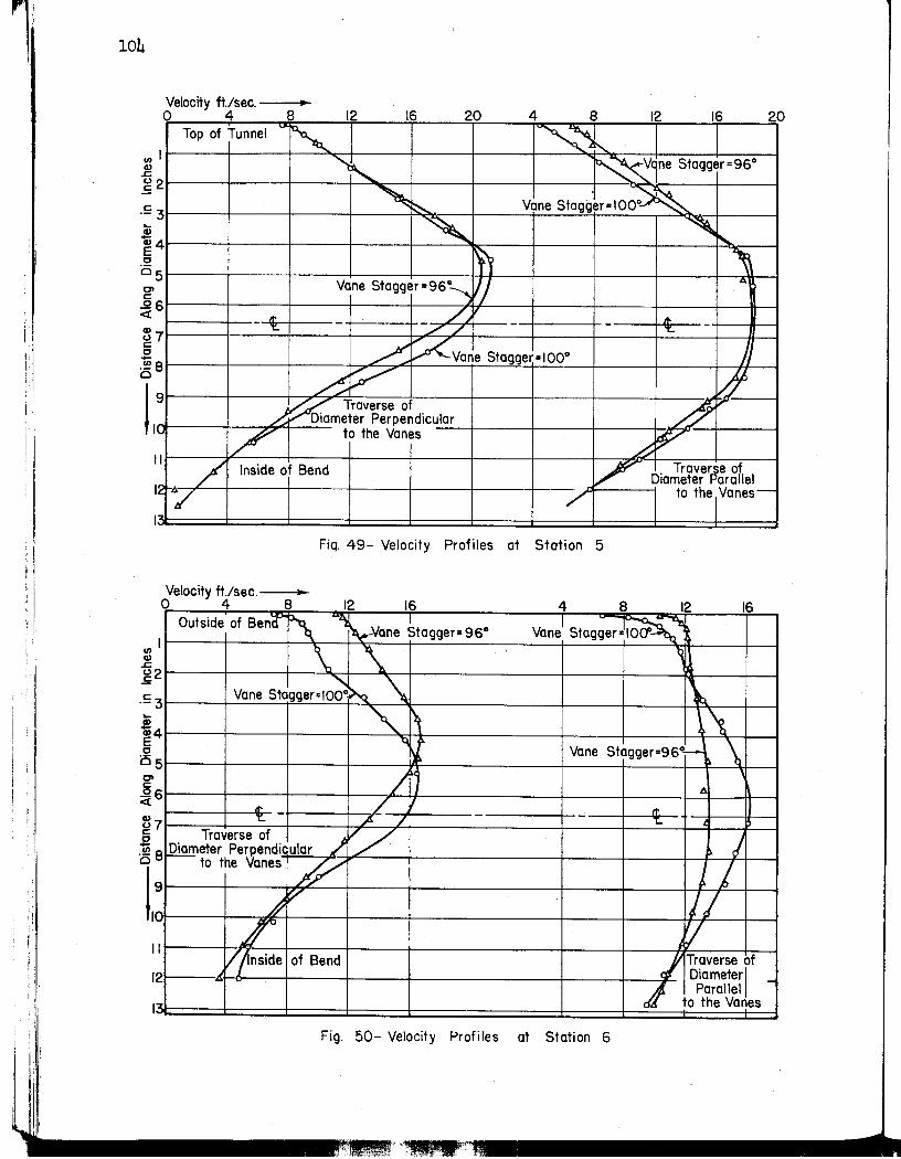
104

IJ)

~ (.)

.5

.5

Velocity ft.lsec. ----;~~ 048

Top of Tunnel UL ~ I

2

3

4

6 II' - ~

12 16 20

~,

~ ~

'" ty Vane Stagger=96°, 'l - //

-//

4 8 12 16

"'l ~I"e Stagger=9Go

Vane Stagger=IOO~

"'" ~ -" "'1

'" - - 't.. -7

8 ~ ::0<: Vane Stagger = I 00° h ~ V ~

9 ~ Traverse of 77 ....-~ Diameter Perpendicular u /' to the Vanes tp'

£-I

Inside of Bend Traverse of Diameter Parallel

20

2/ / / to the I Vanes -

FiQ. 49- Velocity Profiles at Station 5

Velocity ft./sec. .. o 4 8 12 16 4 8 12 16

Outside of Bencr' ~- ~"'. )lS ~t 960 \I J S J ~ ~ 1J)1r_----t-----~-1~~_+~~~-,a-n-e~a~g~g~e-r=~~----v-,a-ne1_-ta~g~g~e_r=~IO~)~~~~rlb----~~

~2r---+--~~\r~~+--------+---~-q~~~ c3r-____ r-va~n~e~S~tafg~g~er-=~10"~0~0~~~~~._------------_+----_+----_4~'~b~~~~ ~ ,~ ~ ~4r-----+-----_r-----+----,,~~------------~------+_----~~~4~~ E ~~ \ o Vane Stagger=96°~ o5r-----r-----+-----~----~~------------+_----+_----~~~~~ , § / ~ ~6r---r---r---r-__ ~~----------~----~----~~--~~

~----~-~II'- /~~----~7 "to 7! / - Traverse of ~V ../ ~ 8 .QiQrrIeter Perpendi!fc'u~la~r~,4/-::J""/~ __ .. -+ ______________ -+ ____ ~------+_+__j'.+___I o to the Vanes .# t: ~V Ir--~~~~· -+--~--4---~----~~--~--~~ V jtnside of Bend 2~---~-~--~----4_----+_------------+_----~~~

..; II' I - l:.. ~

I J 1

1// Xl J Traverse of

Diameter I -7 Parallel to the Vanes

."

Fig. 50-Velocity Profiles at Station 6

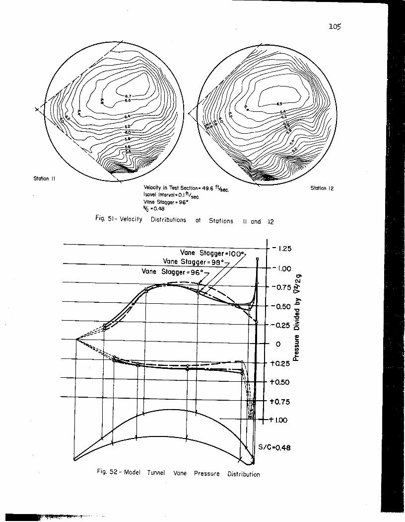
Station II

Velocity in Test Section = 49.6 ft/sec. I sovel Interval = 0.1 tt.; sec. Vane Stagger = 96° Sic =0.48

Fig. 51- Velocity Distributions at Stations II and 12

----------------------+- 1.25 Vane Stagger=IOO°

Vane Stagger = 98° -"'-----------~-~~~~~'----~ ....... - 1.00 Vane o t\I ---------::::;;?'t~IiiiiiOii~::_=~~'------_I_+ -0.75 ~

>­.Q -0.50 -0 Q)

-0 ----------~~----~----------4-----------~~~Q25 ~

--+----t--+---+--+-----+--+-----4~+_+ to.50

--+---+-+--......j-~---+-~----+-If\HI__+ to.75

-----4--j.IIJIH--+-i" 1.00

S/C-0.48

Fig. 52 - Model Tunnel Vane Pressure Distribution

105

Station 12

106

4. Flow Distribution An analysis of the physical geometry discussed on page 86 uncle):"

the section on design studies, together 'With the measured values summarized in Figs. 39 to 43, 49, and 50, discloses the ;f'oIlowingcharacter;i.stics: (1) When arranged at a 900 stagger angle, the selected vane will materially underlurn the bulk flow, according to Fig 6 39. The condition is substantially improved by increasing the ang1e to 960 but evidences of some underturning are . still apparent. An increase of angle to 1010 , however, produced a flow in 'Which the entering and discharging directions were substantially axial. This turning action, ,as shown in Fig. 39 for the duct elbow studies, ·is also confirmed by Figs .. 49 and 50 of the model tunnel studies where the poorly distributed flow coming from the diffuser is shown to be turned effectively by the 1000 elbow vanes but distinctly underturned by the 960 vanes.

(2) A more detailed probing of the velocity distribution, as evidenced in Figs. 40 to 43, shows that while all indicated settings had a quite uniform and symmetrical flow pattern in the entrance sectionD-D, the 960 blade set­tings at section K-K show a very considerable deficiency in velocity at the inside of the b end with a concentration of maximum velocities to the right or outside of center. The local velocity deficiency and lack of symmetry are evident not only at section K-K immediately adjacent to the . bend but are also apparent 5 diam downstream at section M-M. On the other hand, a study of the comparable values for the 1010 stagger angle shows orily very sli~t evidence of the same effect.

(3) The velocity vectors near the wall, as shown in Figs. 40 to 43, indicate tha t a double spiral vortex is being generated in the boundary region by the pressure differentials evident in Fig. 44. The condition is apparent for the 960 andlClo stagger angles, but it is somewhat stronger in.the case of the 960 angle.

(4) I As evidenced by the core flow vector arrows, the velocity components which are other than axial are apparently random in nature and probably reflect smaIl disturbances caused by the individual vanes.

(5) The change in velocity distribution between se ctions D-D and M-:M evidenced in Figs. 42 and 43 is consisten'\:;1rl.th the progressive changes in distribution usually found near a pipe entrance, as the boundary-layer growth changes a uniformly distributed entering now to a hyperboliC" stable, turbulent profile. Thit this change is a product of the duct boundary rather than the vane geometry

<

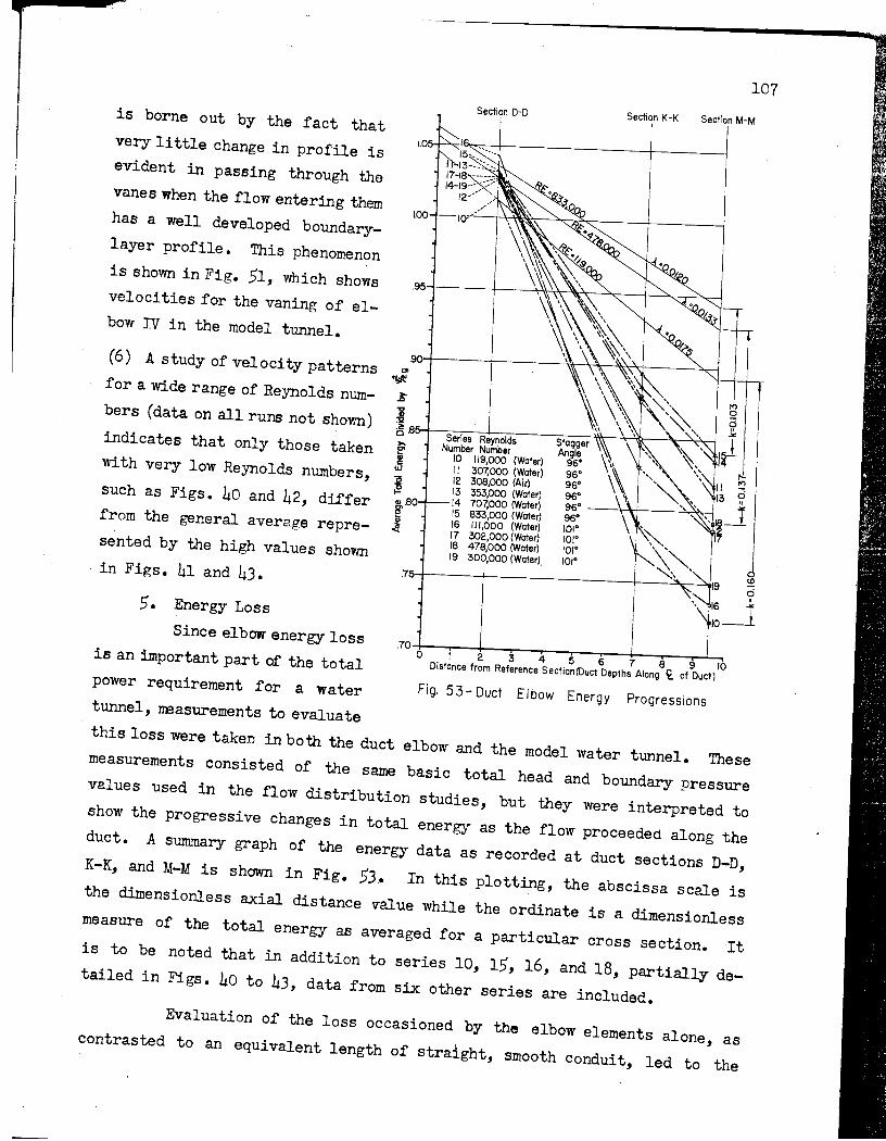
is borne out by the fact that very little change in profile is evident in passing through the vanes when the flow entering them has a well developed boundary­layer profile. This phenomenon is shown in Fig. 51, which shows velocities for the vaning of el­bow IV in the model tunnel.

1.05

1.00

107 Section D-D Section K -K Section M-M

904-----~r-------~-v~~~----~~ (6) A study of velocity patterns ""

'1-+-+-.-'t~ for a wide range of Reynolds num­bers (data on all runs not s,hown) indicates that only those taken with very low Reynolds numbers, such as Figs. 40 and 42, differ from the general average repre­sented by the high values shovm in Figs. 41 and 43.

5. Energy Loss Since elbow energy loss

is an important part of the total power requirement for a water tunnel, naasurements to evaluate

~ ~ ~ 9 ~

~ is .854--:S::-;-· --::-IR --;-;ld--:::7St-~-'r~---"~~ lSI erles eyno s agger >- Number Number Angle LIJ~ 10 119,000 (Water) 96° II 307,000 (Water) 96° 12 308,000 (Air) 96° 13 353POO (Water) 96° J4 707,000 (Water) 96° ---\--\+-----"-.2'tt-l 15 833,000 (Water) 96° 16 111,000 (Water) 101° 17 302,000 (Water) 101° 18 478,000 (Water) 101° 19 300,000 (Water) 101°

<0 .754-----!---------+--~~~

c:i 16 J:. 10~

.704--....----l,.----..---.--..,.---,--+---,--..,.-i....-., o I 2 345 6 7 8 9 ~ Distance from Reference Section(Duct Depths Along It of Duct)

Fig. 53- Duct Elbow Energy Progressions

this loss were taken in both the duct elbow and the model water tunnel. These measurements consisted of the same basic total head and boundary pressure values used in the flow distribution studies, but they were interpreted to show the progressive changes in total energy as the flow proceeded along the duct. A summary graph of the energy data as recorded at duct sections D-D, K-K, and M-M is shown in Fig. 53. In this plotting, the abscissa scale is the dimensionless axial distance value while the ordinate is a dimensionless measure of the total energy as averaged for a particular cross section. It is to be noted that in addition to series 10, 15, 16, and 18, partially de­tailed in Figs. 40 to 43, data from six other series are included. Evaluation of the loss occasioned by the elbow elements alone, as contrasted to an equivalent length of straight, smooth conduit, led to the

108

comparative plotting of the latter values at three representative levels of

the Reynolds number. The straight, smooth pipe plottings are based on compu~

tation of the formula, l/Yf = 2 log R-y'A - 0 .. 8\ where R:is the Reynolds number

and XH~ is" the dimensionless resistance coefficient. The validity of this

formula had been established previously by measurements in a straight length

of duct fabricated in the same manner as the duct elbow. The 10ss curve for

the straight pipe was arbitrarily drawn through the D-D point of the corres­

ponding Reynolds number cUrve for the duct elbow data of Fig ... 53.

From the graphical d.ata of Fig. 53, k, the coefficient of energy

loss due to the benCi,.canbe'measunad.by taking the difference of ordinate values

for the corresponding straight pipe and elbow curves at an abscissa distance

where the two ourves have become parallel. While the limited number of meas­

uring sections shown in Fig. 53 do not fully establish that complete paral ...

lelism has been achieved, it is apparently very nearly true.. On the basi;:>

of this assumption, the three representative values of k have been plotted as

shown at the right of the figure. It is to be noted that the three values

show an increase as the Reynolds number decreases.

'!'he limited evidence of Fig. 53 does not show a marked difference

in total energy loss when vane angles of 960 and 1010 are compared but the

slopes of the curves between sections D..;D and M-M consistently show that the

1010 vane series achieved most of the loss between D-D' and 'K-~, whereas the

960 vanes show substantial loss still occurring between K-K and M-M.·· Sl1ch a

loss distribution would seem consistent with the flow ' patterns of Fig .. 39.

The data taken from the model tunnel elbows were recorded in a manner

different from that summarized in Fig. 53 for the duct studies and am pre­

sented in the form shown in Table VIII. This table is based on use of the

Bernoulli energy relation integrated across the tunnel section in the following

manner:

Jfl.l P V2 . /. A.2 p V2 . Et (- + -) V dA - (-- + -) V dA - - = 0 . w 2g . w 2g w

* I I Karman-Prandtl resistance equation for turbulent flow in smooth pipes.

109

TABLE VIII VANED ELBOW ENERGY LOSS DATA

Elbow Test Section Velocity (fps) 18.00 30.00 49.62

Reynolds Number '.1-

165,000 I . . . . • · · · · · · · · · • · 90,000 370,000

V5 (fps) · · • • · · · · · · · · · · · 3.72 6.20 10.25 -2/ V5 2g (in. ) · · · · · · · · · · · · · 2.58 7.16 19.58

V6 (fps) • · · · · · • · • · · · . · · 3.72 6.20 10.25 -2/ V6 2g (in. ) · · · · · · · · · · · · · 2.58 7.16 19.58 at: • · · · · · · · · · · · · · · · · • 1.812 1.812 1.812 -'

a6 • · · · · · · · · · · · · · · · · · 1.308 1.308 1.308 P5 - P6/vr (in.) · · · · · · · · · · · +0.21 -0.41 +0.40 k · · · · · · · · · · · · · · · · · · 0.554 0.416 0.493

Reynolds Number * 165,000 II . . . . • · · · · · · · · · · • 90,000 370,000 \16 (fps) · · · • · · · · • · • · · · · 3.72 6.20 10.25 -2/ V6 2g (in. ) · · · · · · · · · · · · · 2.58 7.16 19.58 V7 (fps) · · · · · · • · · · · · · · • 3.90 6.50 10.77 V;/2g (in. ) · · · · · · · · · · · · · 2.83 7.87 21.65 a6 • · · · · • · · · · · · · · · · · · 1.308 1.308 1.308 a7 • • · · · · · · • · · · · · · · · . 1.090 1.090 1.090

P6 - pl- (in.) • • · • · · • · · • · 1.17 3.57 8.8 k · • · · · · · · · · . · . · · · · . 0.527 0.570 0.515

III and IV Reynolds Number * 46,000 75,000 138,000 • · · · · · . · · · · · V10 (fps) · • • · · · · · · · · · · · 2.0 3.33 5.51 -201 V1 2g (in. ) · · · · · · · · · · · · · 0.75 2.065 5.66 V12 (fps) · • • · · · · · · · · · · · 2.0 3.33 5.51

Vi2/2g (in.) • · • · · · · • · • • • • 0.75 2.065 .5.66

a10 · • · · · · · · · · · · • · · · • 1.050 1.050 1.050 a12 · · • · · · · · · · 0 • · · · · · 1.071 1.011 1.071

PI0 - P12/W (in.) · · 0 · · · · · '. 0 0.25 0.70 1.45 2k · · · · · · · · · · · · · · · · · • 0.244 0.250 0.166

k · · · · · · · · · · · · · · · · · • 0.122 0.125 0.083

*Reynolds number is based on chord length (2.95 in.)

110

where p = pressure,

V = axial velocity,

w ~ specific weight of fluid,

Al = area upstream of elbow, .

A2 = area downstream of elbow, and

Et = total energy loss between sections 1 and 2.

Defining a = fA (V3dA/AV3), the energy equation reduces t.o

-2 -2 -2 2 a 2V2 -alVl VI t VI

2g . = ht = k 2g + Ad 2g w

where ht is the total head loss between sections 1 and 2, k is the bend loss

coefficient, and >.. is the friction factor (assumed to be 0 .. 0170).. Therefore, .

In the tabulated computations the a-values are all based on' tra­

verses made when the test section velocity was 49.62 ips'.. This value was used

because accurately measurable velocities' could be achieved in all elbows, and

tests established that the pattern was substantially the same for the lower

velocities. '!be expressed values of the Reynolds number are bas~d on the

2 .. 95-in .. vane chord as length parameter rather than the duct depth value as

used in the other tests.. The summary represents vane angle settings of· 96°,

since a greater amount of data was available for this condi tioD.· than' for the

1000 or 101 0 angles.. It is believed that the k-values obtained by the 96°

angle setting may be applied to the 1010 setting with only minor discrepancies ..

A comparison of the k-values on Table VIII for the four elbows used ;i.n. the

model tunnel indicates that elbows I and II have a much greater loss coefficient

than elboWS III and IV ..

The reason for the high loss indicated in elbow I may be traced to

the physical nature of the flow entering this elbow from the preceding diffuser.

It may be recalled. that the inherent nature of flow in a diffuser produces a

discharge flow profile sharply peaked or indicative of a high kinetic energy

content for·.the section (a= 1..812, as measured at station 5)" Since a high

a-value of this character' is not the' usual value for balanced conditions as

found in stable, turbulent, duct now (a-values in long pipes are about. 1 .. 1)

111

a rapid and inefficient conversion to pressure eIij3rgy will follow such a velo­city distribution in a duct. In other words, considerable energy loss is to be expected for normalizing an Q"" 1.812 flow even if it is done in a straight pipe. Addition of a bend, plus large friction areas, on" the" vane surfaces, -serves to accelerate normalizing and to produce high energy loss in a very short length, as is evidenced by a measured Q = 1.)08 at station 6. On the basis of this evidence it becomes apparent that the presence of the diffuser and not the presence of the elbow causes the high energy loss evident at the elbow.

The high losses for elbow II are of a different nature and are due to the presence of the large pump shaft fairing passing through the vaning so as to cause the following secondary losses: lessening of the aspect ratio of the cascade with accompanying increase in end spiral losses; increase of flow velocity around vanes due to reduction of flow area occasioned by; shaft pres­ence; and, form loss and skin-friction loss due to flow around the shaft fairing proper.

Despite a difference in vane angle setting, the indicated losses for elbows III and IV agree quite well with thos,e obtained in the duct elbow.

6. Vane Pressure Distribution

The vane and wall pressure distributions shown in Figs. 44 to 48 and 52 serve to give considerable information on the structural loading and cavi-

o ' tation susceptibility of the selected vane geometry~ The 96 stagger angle does not lead to equal loading of each blade, as evidenced by the comparative changes in negative pressUre at corresponding points of different vanes in Fig. 45. On the other hand, relative similarity of loading for all vanes is evident in the 1010 setting shown in Figo 46~ The approximate correctness of the 1010 vane angle setting is verified by the fact that a total vane loading (determined by integrating the pressure distribution of Fig. 48) agreed closely wi th the theoretical momentum change forces required for the directional change of the flow mass. No comparable check was possible with the 960 data. The correctness of this setting is further verified by the fact that integration of the duct wall pressure at mid-depth indicated the walls carried approximately the same load as one vane, whereas the 960 integration shows the walls to be carrying much more than a single vane. Additional verification is also found in the observations discussed in paragraph (3) on page 98.

112

The integrated location of the centers of pressure, together with

the trunnion and miter line positions, is shown in Fig. 48 for both the 960

and 1010 angles.

Vane pressure distribution measurements made in elbow I of the model

tunnel (Fig. 52) agree qualitatively with those made in the duct elbow, but

do not allow an accurate quantitative comparison because of difficulties in

determining the reference pressure.

In additiqn to the quantitative pressure measurements analyzed above,

examination of the photographic and visual records of the duct elbow experiments

yields two pressure evidences: (1) Separation of the flow from the 960 vane

surface occurs locally at a point on the convex surface about 3/4 in. forward.

of the trailing edge. This was made evident by the admission of colored water

streaks into the air flow, as previously described. The flow evidently returns

to the surface a short distance downstream since it appears to have consider­

able strength and a downstream direction at the trailing edge. (2:) : Separation

with the 1010 stagger angle is confined to a very narrow region just forv{C;lrd

of the trailing edge.

7. Scale Effects

Since the intention of the foregoing tests was to determine the

adequacy of the proposed design for application to the prototype, i tis neces­

sary to examine the scale effects which may exist between the model and the

prototype. For purposes of this analysis, it would appear that the flow may

have two separate forms--the spiraling three-dimensional flow occurring near

the ends of the vanes, and the two-dimensional flow occurring over the bulk

of the central portion. A digest of the preceding tests indicates that for

the 1010 vane stagger the bulk of the flow is essentially two-dimensional and

the end effects are of negligible magnitude; this is evidenced by the satis­

factory correlation between the performance of the duct elbow and the model

tunnel elbowo From this it follows that the spiral flow cannot contribute

materially to scale errors if the 1010 stagger is employed. Use of other

stagger angles may change the energy emphasis and, accordingly, may show scale

effects.

An analysis of physicC;ll forces which might cause variations with

scale shows that neither compressibility nor gravitational effects are of

consequence and only the viscous turbulent forces should contribute to scale

variations of the two-dimensional bulk flow.

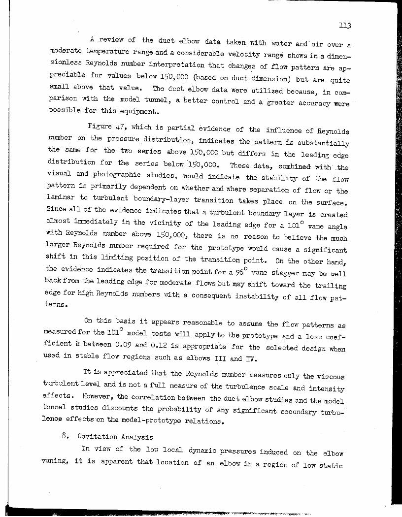
113

A review of the duct elbow data taken with water and air over a moderate temperature range and a considerable velocity range shows in a dimen­sionless Reynolds number interpretation that changes of flow pattern are ap­preciable for values below 150,000 (based on duct dimension) but are quite small above that value" The duct elbow data were utilized because, in com­parison with the model tunnel, abetter control and a greater accuracy were possible for this equipment.

Figure 47, which is partial evidence of the influence of Reynolds number on the pressure distribution, indicates the pattern is substantially the' same for the two series above 150,000 but differs in the leading edge distribution for the series below '150,000. These data, combined mth .the visual and photographic studies, would indicate the stability of the flow pattern is primarily dependent on whether and where separation of flow or the laminar to turbulent boundary-layer transition takes place on the surface. Since all of the evidence indicates that a turbulent boundary layer is created almost immediately in the vicinity of the leading edge for a 1010 vane angle with Reynolds number above 150,000, there is no reason to believe the much larger Reynolds number required for the prototype would cause a significant shift in this limiting position of the transition point~ On the other hand, the evidence indicates the transition point for a 960 vane stagger may be well back from the leading edge for moderate flows but may shift toward the trailing edge for high Reynolds numbers with a consequent instability of all flow pat­terns ..

On this basis it appears reasonable to assume the flow patterns as measured for the 1010 model tests will apply to the prototype ,and a loss coef­ficient k between 0.09 and 0012 is appropriate for the selected design when used in stable flow regions such as elbows III and IV.

It is appreciated that the Reynolds number measures only the viscous turbulent level and is not a full measure of the turbulence scale and intensity effects. However, the correlation between the duct elbow studies and the model tunnel studies discounts the probability of any significant secondary turbu­lence effectslon the model-prototype relations.

8. Cavitation Analysis

In view of the low local dynamic pressures induced on the elbow vaning, it is apparent that location of an elbow in a region of low static

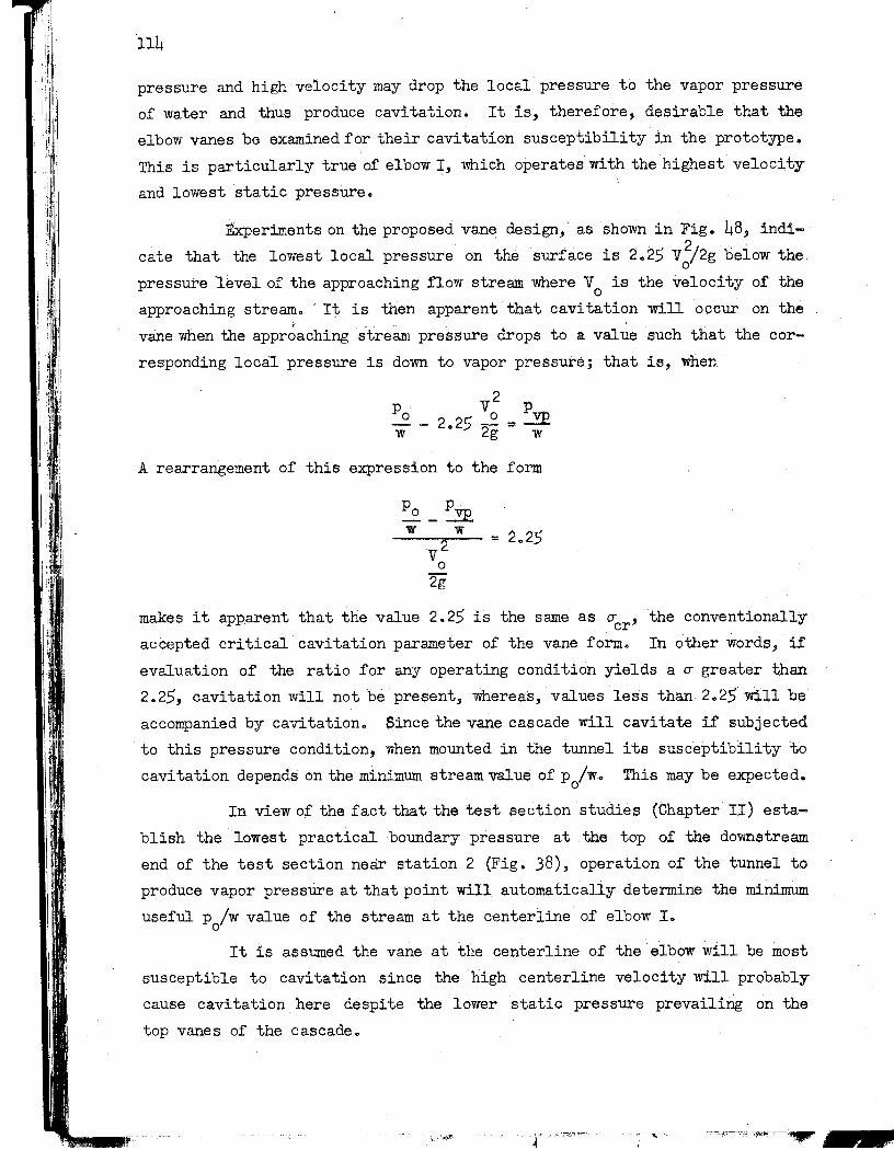
I I

114

pressure and high velocity may drop the local pressure to the vapor pressure

of water and thus produce cavitation. It is, therefore, desirable that the

elbow vanes be examined for their cavitation susceptibility in the prototype.

This is particularly true of elbow I, Which operates with the highest velocity

and lowest static pressure"

Experiments on the proposed vane design, as shown in Fig. 48, indi-'

cate that the lowest local pressure on the surface i82.25 V2/2g below the. o pressure level of the approaching flow stream where V 0 is the velocity of the

approaching stream" ' It is then apparent that cavitation will occur on the

vane when the approaching stream pressure drops to a value such that the cor­

responding local pressure is down to vapor pressure; that is, 'When

A rearrangement of this expression to the form

= 2 .. 25

makes it apparent that the value 2" 25 is the same as 0" , the conventionally cr accepted critical cavitation parameter of the vane form" In other words, if

evaluation of the ratio for any operating condition yields a 0" greater than

2,,25, cavitation will not be present9 whereas, values less than 2025 Will be

accompanied by cavitation. Since the vane cascade will cavitate if subjected

to this pressure condition, when mounted in the tunnel its susceptibility to

cavitation depends on the minimum stream value of p /w.. This may be expected .. o

In view of the fact that the test section studies (Chapter II) esta­

blish the lowest practical ·boundary pressure at . the top of the downstream

end of the test section near station 2 (Fig. 38), operation of the tunnel to

produce vapor pressure at that point will automatically determine the nrlnimum

usefulp /w value of the stream at the centerline of elbow Ie o

It is assumed the vane at the centerline of the elbow will be most

susceptible to cavitation since the high centerline velocity will probably

cause cavitation here' despite the lower static pressure prevailing on the

top vanes of the cascade.

---~------- ,---- :' '~- -- ---- - -- ---~---

115

If pressure values in t4e p18.ne of station 5 are assumed to represent

po/w for the vanes, then the minimum prototype centerline po/w value and the

local 0- may be cleared by applying the Bernoulli energy relation to the center­

line flow filament thus:

2 2 V2 P V p. -vn 0 0 2g + -!:;t + r 2 - h 1. ::: 2g + W

where V2 ::: V2 and Vo .. 2"5 (approximations from Fig .. 28),

Po .. P5~

V2 .. (r5/r2)2 V5' r5 :: radius at st)"tion 5 .. 5 .. 5 ft,

r 2 ::: radius at test section ::: 2 .. 5 ft, and

hl ::: diffuser energy loss = 06067 evi/2g), as shown in Chapter IV ..

It should be noted here that selection of a head loss factor of k = 0.067 from

the data of Chapter IV assumes a bare tunnel without a test section model

installation.. This appears to be a less conservative selection than the value

of k .. 0 .. 114 presumed to prevail in the presence of a test body" However, it

is rather reasonable to assume that if a test body is capable of producing

this loss, its wake will be suffiCiently great to necessitate considerable

reduction of the assumption of Vo = 2V5" Since these factors act to nullify

each other ~ but in a manner not wholly defined by these tests , it appears

reasonable to use the value of k = 0,,067 together with Va == 2V5, as determined

by the tests" There is also some reason to question whether the bulk value

of 0,,067 is fully applicable to energy analysis along a centerline flow fila­

ment. For lack of further evidence, the 00067 value will be presumed appli­

cable"

If the equation given above is cleared to yield the local cavitation

parameter, the follo'wing expression for the minimum cavitation index just up­

stream of elbow I will result:

It is obvious that even extremely high values of V2 will give o--values nearly

twice the critical value 0- = 2,,25 determined for the vane form.. In this case cr there is no reason to believe cavitation will exist on the vanes of the tunnel.

116

9. Vibration and Stress Analysis

In view of the fact that most American water tunnels have experienced

some difficulty with vibration noise in elbow vanes and in a few cases have

experienced structural failure, it is important tliat-,thestrength'and vibratory

characteristics of the vane design be cri ticallyexamined. A check of the

structural properties of the prototype vane was made by assuming the following~

(1) The center or longest vane of' each elbow was examined as a beam with zero

end restraint in the plane of the chord and full end restraint in the plane

normal to the chord.

(2) The vane was assumed to have a cross section of solid steel or, alterna­

tively, to be composed of solid nose and tail with 1/2-in. rolled steel sur­

faces ..

(3) The principal forces acting are the lift-drag resultant and the. de adwe iglit.

The lift-drag resultant was computed on impulse-momentum principles for the

maximum velocities determined by tunnel velocity distribution studies. The

point of application was based on integration of the measured pressure distri­

bution diagrams.

(4) There are two principal tunnel generated pulses capable of exciting vibra­

tion in the vanes.. These are the pulses from the pump blading and the separa­

tion vortices shed from the vane itself.

(5) The natural frequency of the vane can be assumed based on free beam action,

with the weight of the beam increased to include the adjoining water between

two adjacent vanes.

On the basis of these calculations, maximum tensile and compressive

stresses in the vane would be about 3000 psi with end shear values about 50 psi; maximum center deflections would be about 0,,06 in.; lowest frequency of

natural vibration would be about 15 cps; highest frequency of pump blade pulse

would be about 8 cps and would be damped to small strength before reaching

the elbows; highest frequency of vane vortice's would be 1.2 cps and such vor­

tices should be of small size. This foresees no major stresses or vibrations

and satisfactory operation should be expected of the proposed vane design.

Do Conclusions

On the basis of these experimental investigations, these conclusions

are drawn concerning the vaned turns for the 60-in. tunnel:

117

(1) The selection of vaned turns and the particular design choices of vane

shape and spacing-chord ratio (s/c = 0.48) were justified by the results of

the experiments. The original selection of location of the vanes with respect

to the miter line of the bend was changed slightly to conform more closely

with the experimental results.

(2) The proper setting of the selected cascade to insure axial flow immedi­

ately before and after the turn is a stagger of 990 to 1010 ; that is, the

angle between the chord of the vanes and the miter plane of the bend is 990

to 1010 (the angle of attack is 540 to 560 with the approaching flow).

(3) With a normal turbulent velocity distribution in the approach flow, excess

losses due to the vaned turns at the recommended setting of the cascade of

vanes should be 10 per cent of the velocity head in the approach duct ;t 2

per cent. This loss may appear to be much larger for abnormal entering velo­

ci ty distributions such as those which may occur where the elbow follows a

diffuser.

(4) When installed in the tunnel, the vanes will not be subject to cavitation.

(5) Either a solid steel or a hollow steel vane of nominal skin thickness will

be free from excessive stresses or deflections under all expected conditions

of operation and should not vibrate in resonance with either the tunnel impeller

or vortices shed from the vanes.

(6) Data obtained with the experi­

mental models should give a very close

index of the performance to be ex­

pected in the vaned turns of the large

tunnel because the Reynolds numbers

used in the models were high enough

to preclude the possibility of a loss

in similarity at the higher Reynolds

numbers of the prototype, and the on­

set of a turbulent boundary layer at

a s table point near the leading edge

of the model vanes at the stagger an­

gle of 990 to 1010 would be at a very

similar position on the larger pro­

totype vanes.

"""----~---,

... APPROACH FLOW DIRECTION

SIC = 14.14/29.5 = 0.48

Fig. 54- Recommended Prototype Vane Coscade Dimensions

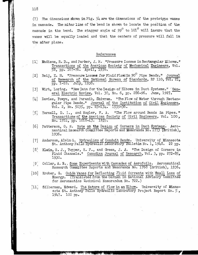
J!.

1\' i i

I: I

I

Ii

I,

118

(7) The dimensions sho-wn in Fig. 54 are the dimensions of the prototype vanes

in cascade. The miter line of the bend is shown to locate the position of the

cascade in the bendo The stagger angle of 990 to 1010 will insure that the

vanes will be equally loaded and that the centers of pressure will fall in

the miter plane.

[IJ

[ 2J

PJ

[4J

[5]

[6J

[ 7J

[ 8J

[9J

[lOJ

[11]

References

Madison, Ro Do, and Parker~ J. Ro IIPressure Losses in Rectangular Elbows .. II Transactions of the American Society of Mechanical Engineers, Vol. 58, pp. 167-707 April, 1936. -.

Beij, K. H. llPressureLosses for Fluid Flowl.oin 900 Pipe Bends. l• Journal of Research of the National Bureau of Standards, RP 110, Vol. 21, pp. 1-18. July, 1938. --

Wirt,Loring •. II New Da.ta for the Design of Elbows in Duct Systems. 1'°Geri­~ Electric Review, Vol. 30, No .. 6, pp .. 286-960 June, 1927.--

Davies, Powys, and Puranik, Shivram.. tiThe Flow of Water through Rectan­gular Pipe Bends. 1I Journal of the Institution of Civil Engineers, Vol. 2, No. 5035, pp. 83-134:- 1935-36~ -.

Yarnall, D. L., and Nagler, F.. A.. 1\ The Flow around Bends in Pipe s. 11

Transactions-of the American Society of Civil Engineers, Vol. 100, No. 1914, p;p.1018-43. 1935.. -- --

Patterson, G. No- Note on the Design of Corners in Duct Systems. Aero­- nautical Re search Committee Reports and Memoranda No .. 1773 (:Sri tish),

1936.

Anderson, Alvin G. Hydraulics of Conduit Bends. University of Minnesota. St. Anthony Falls HyaraUllcLaboratory BUlletin No.1, 1948. 22 pp.

nein, G .. J., Tupper, K. F., and Green, J" J" lIThe Design of Corners in - Fluid Channels.,u Canadian Journal of Research, Vol. 3, pp .. 272..:85,

1930. --

Collar, A. Ro, Some Experiments with Cascades of Aerofoils. Aeronautical Research Committee Reports and Memoranaa-No .. 1768 (British), 1936.

Krober, G. Guide Vanes for Deflecting Fluid Currents vdth Small Loss of Energy .. -rrranslatedfrom the German in National Advisory Committee for Aeronautics Technical MemorandUn1 No .. 722~)

Silberman, Edward. The Nature of Flow in an Elbow.. University of Minne;;" sota St. Anthony Falls Hydraulic Laboratory Project Report Noo 5 , 1947. 100 pp. -

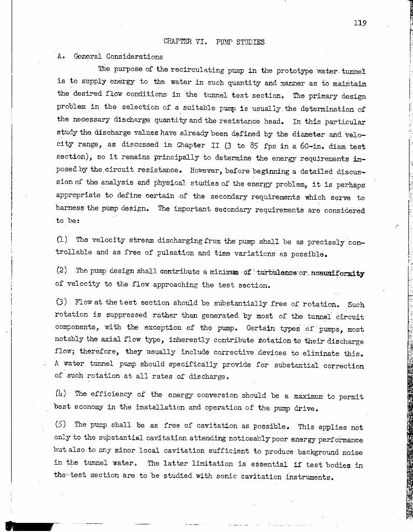
119

CHAPTER VI. PUMP STUDIES

A.. General Considerations

The purpose of the recirculating pump in the prototype water tunnel

is to supply energy to the water in such quantity and manner as to maintain

the desired flow conditions in the tunnel test section. The primary design

problem in the selection of a sui table pump is usually. the determination of

the necessary discharge quantity and the resistance head. In this particular

study the discharge values have already been defined by the diameter and velo­

city range, as discussed in Chapter II (3 to 85 fps in a 60-in. diam test

section), so it remains principally to determine the energy requirements irn­

posed by the,circuit resistance.. However, before beginning a detailed discus­

sion of the analysis and physical studies of the energy problem, it is perhaps

appropriate to define certain of the secondary requirements which serve to

harness the pump design" The important· secondary requirements are considered

to be::

(1) The velocity stream discharging from the pump shall be as precisely con­

trollable and as free of pulsation and time variations as possible.

(2) The pump design shall contribute a min1mumof'tuXbhlence'ov::'nollun:i.£ormitT

of velocity to the flow approaching the test section.

(3) Flow at the test section should be substantially free of rotation. Such

rotation is suppressed rather than generated by most of the tunnel circuit

components, with the exception of the pump.. Certain types of pumps, most

notably the axial flow type ,inherently contribute t.otation to their discharge

flow; therefore, they usually include corrective devices to eliminate this.

A water tunnel pump should specifically provide for substantial correction

of such rotation at all rates of discharge.

(4) The efficiency of the energy conversion should be a maximum to permit

best economy in the installation and operation of the pump drive ..

(5) The pump shall be as free of cavitation as possible.. This applies not

only to the su,bstantial cavitation attending noticeably poor energy performance

but also to any minor local carl tation suffiCient to produce background noise

in the tunnel water" The latter limitation is essential if test bodies in

the'test section are to be studied with sonic cavitation instruments.

!

II It }!

I;

120

In any consideration of these requirements it is important to bear

in mind that custom-built pumping machines are, in general, of such complexity

in design and physical construction that they are built by specialized manu­

facturers 'Who draw on their experience to produce a pump satisfying performance

specifications. Since detailed design information is not generall,. available

to the consumer-designer, he is confined to formulating somewhat ideal speci­

fications which the state of the manufacturer's art mayor may not permit

achieving.

The constant dissipation of the pump input energy against flow re­

sistances results in a cumulative increase in the temperature of the recir­

culated tunnel fluid. Since it is not considered advisable to permit an extreme

temperature rise to occur in a· large physical /?tructure requiring precise

axial or shaft alignments, it is highly desirable to obtain information relative

to rate and maximum temperature values to be expected in an operating tunnel.

While fluid temperature rise is not usually an inherent part of a pump design

study, the intimate energy association makes it desirable toinclude temperature·

as a part of the studies of this chapter.

B. DeSign Studies

1. Discharge-Head Relations

The head against which the pump shall operate is variable with the

discharge and is a function of the design efficiency of the various tunnel

circuit components. In an attempt to evaluate the magnitude of this total

head for original design purposes, a search was made of the literature relative

to the energy losses represented in each of the flow components of the tunnel

circuit. The major portion of this information was drawn from pipe friction

theory and related studies conducted in prototype wind tUnnels.. This informa­

tion was summarized for the proposed water tunnel in conformance with the

methods of expressing and determining the power requirements of wind tunnels

by individual components. To facilitate comparisons, all losses computed by

this method are arbitrarily expressed as a portion of the kinetic energy that

will exist in the test section jet at maximum velocity.

The test section jet energy,.eJiPressed in horsepower, is

v2 VA' (hp) o

o o. 0 w =2g~

I

~

121

'Where 'W = unit weight ot water, V 0 ;0: mean test section velocity in feet per second, and Ao = cross-sectional area ot test section.. . The component energy losses may then be expressed thus:

y2 VA (Loss) = k 20 ~ w _ n g ;J;JV

where k is the local loss coe.fficient for the component and V and A are the . n . n corresponding mean velocity and cross-sectional area. In a closed circuit VA is a constant .for all sections; there.fore V A = V A or o 0 n n

V =-2..!l=V V A [-ad:]2 n Azt 0

Where d = diameter and

(LoSs)n o 000 [d .]4 v2 V A

=k~ 2g~w

or

v 2 y A . 0 0 0 (Loss)n = kozg ~ W

Thus k = Ie (d /d )4 is the fractional' part of the total jet energy 'equal in o 0 n magnitude to the loss in the local component n.

On the basis of this method of summarizing the energy demands, an estimate table and curve were prepared for the proposed prototype and tor the scale model tunne1.o These curves were of the same general form as the curve of Fig. 55 and were the basis for selecting both the type of pump to be used in t11e proto, type and the specific pump to be used in the model. As in the case of Fig. 55, the estimated data were summarized for two alternate tunnel operations, namely, the bare tunnel without a mounted test model and the tunnel wi th a large, high, drag model in place plus a honeycomb flow straightener in the contraction approach. For purposes, of calculation, the test body was assumed to have a diameter one-sixth that of the test section and a conventional drag coefficient of 1.00. Since this method of estimating the energy losses for the several tunnel components was inexact, because of the mutual effects of the seve:r:al components 'When assembled in various combinations, the estimated energy summary could not be considered too reliable. ThiS, and the high cost of the pump installation, largely justified ~he model study.

-------

II

122

While the determination and study of the ko -values for various ele ....

ments of the tunnel leads to an inSight int9 the influence of component energy

efficiencies, it should be noted that an index: of total tunnel;energyefficiency

is available through determination of a quantity known as the 'ltenergy ra ti6.!l

In wind and water tunnel design practice, this quantity is usually defined as the ratio of the jet horsepower to the i~put horsepower necessary to sustain

the jet horsepower. The input horsepower is usually taken as the total energy

supplied to the motor, presUming for comparative purposes that. the motor and

the pump efficiency are approximately the same for most installations. (It

should be noted that Fig. 55 has been plotted with an input horsepower based

on the assumption of a pump efficiency of 80 per cent.)

2 _ Type of Pump

Modern practice in pump design and selection is founded ana firm

basis of actual experience with laboratory models and prototyPe installations;

each manufacturer has extensive records of design modifications. Most of this

is unpublished and unavailable, but in order that some measure of pump per­

formance be available to systematize comparison between various pumps, a common

denominator known as t.he Uspecific speed~l has been evolved for use in t.his

field. The specific speed of any punip may be calculated from the defining

equation

_ ygpm x rpm _21.2 ~ x rpm Ns - If/4·- H

where N is the specific speed and H the head in feet for vmi6h the pump is s designed, corresponding to its gallons per minute capacity_ Specific speed

of a pump is an index of its type. It is used when designing pumps to meet.

different conditions of head, capacity, and speed.

On the basis of published data and approximations of· the specific

speed from the estimated discharge-head data, the large discharges and small

heads involved indicate the most suitable pump geometry for tunnel use will

be found in the propeller or axial flow type. In current practice this type

of pump has two principal forms, of Which the more common is the fixed blade

propeller and the less common is the variable blade type. In t.he variable

blade type the geometry of the blade pitch angle may be mechanically varied.

For the wide .range of discharge required of the pump in the proposed

prototype tunnel, three possible applications come to mind, namely, fixed blade

1

123

with variable shaft speed, variable blade with constant shaft. speed, and :v:ari­able blade wi tb variable shaft speed. Virtuaily all existing water tunnels employ the first of these, largely because of the economy of the common vari­able speed drive systems as compared to custom-bu,l1t variable blade mechanisms. However, the narrowly peaked efficiency curve common',to. performance' character­istics of the fixed blade pump means this type of pump cannot operate at high efficiency if the resistance head of the tunnel circuit is widely variable for different modes of operation. For this reason the variable blade pump, with its high efficiency over a broad range of heads, has distinct advantages. Unfortunately, the efficiency of the variable blade, fixed speed pump is partially nullified in tunnel use by the fact that the pump is prone to cavitate under conditions of low discharge and high shaft speed. This can be improved by providing variable speed with variable blade, but it increases the expense .. Xt is the purpose of the model study to define the discharge-head character­istics of the basic tunnel to permit eventual judicious selection of the pump drive unit ..

30 Pump Diameter

The 1l-ft pump diameter tentatively selected for the prototype tun­n~l, as shown in Fig .. 1, was based· on a specific speed study of published information on the characteristics of propeller pumps and Kaplan turbines. This selection was confirmed by leading pump manufacturers as being a good

"approximation, pending more defined discharge-head conditions for the tunnel. The dimension was, therefore, fixed in this vicinity with the thought that eventualities dictating a slightly larger or smaller pump diameter could be met by a local expansion or contraction of the tunnel diameter. On this basis the dimensions of the model tunnel in the vicinity of elbows I and II of Fig. ,38 were fixed at 13 .. 2 in .. even though the model was built, for reasons of expedience described in the appendix, with a l2-in. diam pump.

4.. .Pump Diffuser The inherent tendency for the discharge from a propeller pump blade

to possess a rotational component of motion requires that some provision be made to remove this component if satisfactory axial now is to be expected in the tunnel test section. The flow straightening is usually accomplished by placing radial guide vanes in the path of the impeller discharge so that the rotational inflow is gradually converted to a nearly axial motion. This has the advantages of eliminating the undesirable rotation and recovering the

124

kinetic energy represented by the rotation, thus increasing the pump efficiency ..

The diffuser blading is also sometimes placed ahead of the pump impeller to

influence prerotation. In some cases it maybe used on both sides of the

impeller. It should be noted that the most favorable corrective action of

diffuser blading normally prevails only for a single discharge or pump speed

condition& It will be less favorable if the device is required to run under

variable conditions.. Variable diffuser blading has been proposed to remedy

this but is not yet a practical development.

In view of the intimate relation that exists between the impeller

blading and the diffuser blading, the latter is normally considered the design

responsibility of the pump builder and is, therefore, not considered a proper

part of this analysis or model study.

5. Pump Location

The disposition of the recirculating tunnel conduit in a loop lying

in a vertical plane, as shown in the frontispiece, is dictated by a design

effort to place the pumping unit at a point a maximal vertical distance below

the low pressure test section. By such disposition the cavitation suscepti­

bility of the pump is inhibited by the presence of a maximum possible gravi­

tational pressure head.. This disposition is quite different from the usual

horizontal loop employed in wind tunnels where cavitation is not a factor.

If a propeller pump is to be used the necessity of providing shaft

entry from the motor dictates that the pump be placed inboard of one of the

two lower elbowso Location of the pump just upstream of the lower elbow pre­

ceding the contraction would place a minimum distance between the eddy pro­

ducing pump and the test sectiono This is an undesirable condition which can

be remedied by placing the pump just downstream of the other elbow in the

lower leg.. Consideration was given to placing the pump in the vertical leg

just upstream of the latter elbow, but this placement reduces the gravitational

head on the impeller and complicates the motor mounting problemo

If the discharge from a propeller pump is to possess uniformity or

steadiness in the pressure and velocity distributions, it is essential that

the inflow be substantially uniform. This has been demonstrated in other

propeller pump installations where pulsing electrical demand and water dis­

charge resul ted when the inflow contained local regions of high or low kinetic .

energy causing definite force pulses on the passing blading. The strength

.....

125

of such pulses is reduced by increasing their number through an increase in

the number of blades on the impeller; but, this is not a practical way to

eliminate the pulse as about four blades appear to be the limit if a variable

blade system is to be used.

To eliminate or minimize pulsing or other undesirable conditions in

the tunnel pump, it is well to consider the nature of the inflowo The Il-ft

diam vane elbow immediately preceding the pump has been designed to include

eleven vanes dimensioned in accord with Fig.. 54 and arranged as shown in Fig ..

62 (page 141). The small dimension and the large number of spaces are believed

incapable of producing any significant pulse when imposed on a four-bladed

impeller even if a substantial shadow or wake region exists on the downstream

side of each vane 0 Evidence in the literature indicated that even if a sub­

stantial wake exists immediately downstream of the vane, its strength is largely

dissipated in a flow distance approximately four times the vane gap dimension,

or in this case, 10 inches in the prototype. Because it would be difficult

to fabricate a pump of the type shown in Fig .. 62 with the vanes closer 'bothe

impeller than four vane gap units, there seems to be no reason to make any

special effort to locate the impeller an appreciable distance from. the. elbow ..

The minimum space provided in a practical pUmp and elbow fabrication should

suffice.. To assure that velocity maldistributions are not created by other

features of the geometry preceding the pump, it was considered advisable to

make local velocity distribution studies in the model.

c.. Experimental Studies

I.. Head and Energy

Because the total energy summary necessary to a proper pump design'

is merely the summation of the energy requirements~of the tunnel components,

the data will be found in previous chapters of this paper. A tabular summary

of this information is shown in Table IX, based on the use of the previously

determined k -values plus the losses of straight cylindrical components com-o

puted from values of f for a steel surface obtained from a standard curve of

pipe friction.. For convenience in comparing all values are expressed as k o

or multiples of the test section velocity head.. As discussed in this chapter

under the section on Design Studies, the summary is prepared in alternates,

namely, the minimum resistance or bare tunnel circuit, and the maximum resis­

tance circuit presumed to contain a honeycomb straightener and a large, high

resistance test model ..

-

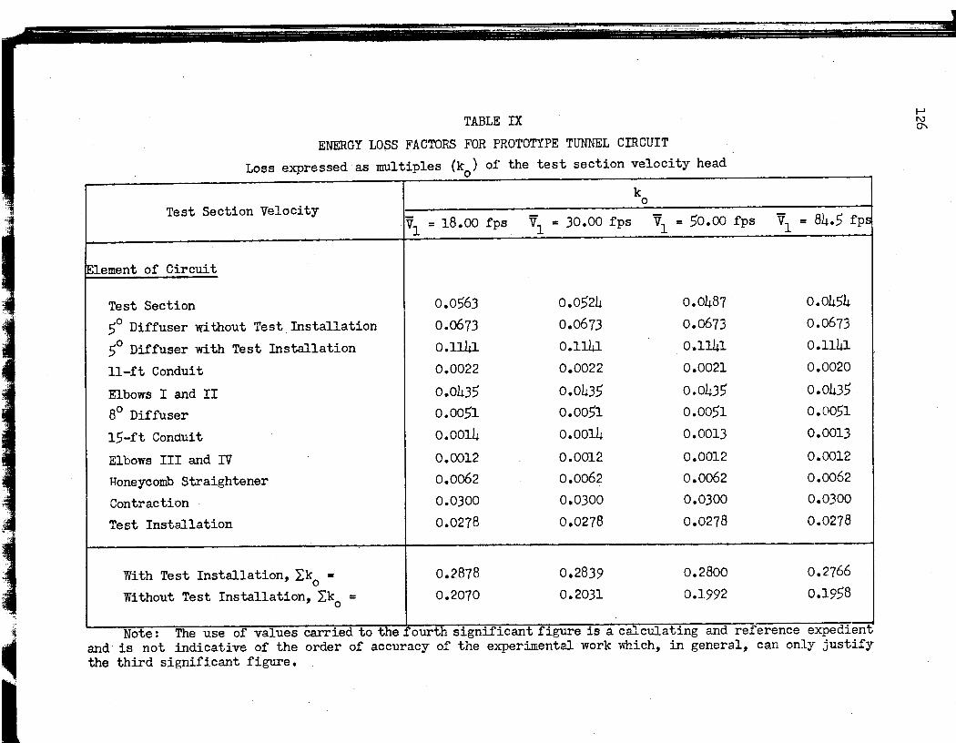
TABLE IX

ENERGY LOSS FACTORS FOR PROTOTYPE TUNNEL CIRCUIT Loss expressed as multiples (k ) of the test section velocity head o

Test Section Velocity

Element of Circuit

I Test Section

50 Diffuser without Test Installation

50 Diffuser with Test Installation

11-.1't Conduit

Elbows I and II 80 Diffuser

l5-.1't Conduit

Elbows III and IV Honeycomb Straightener

Contraction

Test Installation

With Test Installation, Lk • o

Without Test Installation, Lko •

VI = 18.00 fps

0.0563

0.0673

0.1141 0.0022

0.0435 0.0051

0.0014

0.0012 0.0062

0.0300

0.0278

0.2878

0.2070

VI • 30.00 fps

0.0524

0.0673

0.1141

0.0022

0.0435 0.0051

0.0014

0.0012

O.OOO? 0.0300

0.0278

0.2839 0.2031

k 0

VI = 50.00 fps

0.0487

0.067.3

0.1141 0.0021

0.0435 0.0051

0.0013

0.0012

0.0062

0.0300

0.0278

0.2800

0.1992

VI = 84.5 fps

0.0454

0.0673

0.1141

·0.0020

0.0435 . 0.0051

0.0013

0.0012

0.0062

0.0300

0.0278

0.2766

0.1958

Note: The use of values carried to the fo\irfll sfgn:f.1'icant figure is a calculatIng and referenc-e expeCiie-n1:' and is not indicative 0.1' the order 0.1' accuracy of the experimentaJ. work which, in general, can only justi.1'y the third signi.1'icant .1'igure.

J-I N

'"

127

'2 1000

To facilitate comparison and study, the energ,v data of Table • 1000 1/

-- WITH TEST INSTALLATION /, / IX have been plotted with varying ve­locities in Fig. 55 and supplemented in Table X and Fig. 56 by a tabular

41-0000

01-0000 ..

- - - WITHOUT ;rEST INSTALLATION

1// / " //

/ and graphical summary of the conven­tional energy gradient •. In computing g I the energy gradient, the total energy ~ at a section was computed from the local head loss data in Table IX, and

.. ~ 1/ 1/,// " 0 I ..

/ III // / 8- 4000 15

x

PUMPHEAD~ ) / t-~ " " i!! ,

/ t 5000

/ V ~; If / /~ ~INPUTHP ,/ the pressure was arbitrarily assumed

8 2000

1/ V ,-V/ ./

to be absolute zero at the beginning // ,-,-,-

of the diffuser transi tion (section C? ",' V V ",/ ",/

~ II of Fig. 56). For convenience of interpretation, the total energy and the kinetic energy at a section were divided by the velocity head of the

20 30 40 50 10 70 10 IS TEST SECTION VELOCITY (lpI)

i. Je . ! I

415 t5() TEST SECTION VELOCITY (KNOTS)

B'OO 1~1I0 II~D DISCHARGE (eft)

Fig. 55- Discharge - Head Relations for the Prototype Pump. ( Computed values based

on model findings. )

.. j ... 1>1 01

'1· Q cc LoJ %

~ U o oJ LoJ > a:: o >­Cl) a:: LoJ z LoJ

oJ cc t­o t-

~SE;;;;TlT;;;;S~;;;;N~I:;;;;:;;;a.;;;;D;;;;lff;;:U;;;SE;;;;1 ~;;;!FI;;;II';;;;C~ON=DU;;;IT;;::JI~ PIU~II~Pr* 11'~'.~~IF~.fU!IER~I~===#-15!;;;' C~O~ND~U~IT~(~ST~IL~UN~'~EN~'~TH~I===I~ITA~;~~~ ... -~.~I 1.20r I I t 4 I Ik.!.I287 I 1.1141 IR'" J 1.I!S7 vl.oea• I I I 1Aci.0857 1.0108 ~ ~0511 H 1:1 I VI" T .. " •••. l·~ I ~~ ~.0127 I ~ ~ / I Itt II ::g::1

tOO ",.. ~ ~~ ;;+/-:t-1~I--ti-+----+---+-~+--++I!I-i-:-I'-III'+::C o-OJ-+-I

I ~. I ~I II I !!. ill rl

'I 1:11' I i I I II I •~:.. I I II I 0 ~ TOTAL ENERGY. AT v.. 84.5';. I' I ~ II WITH TEST INSTALLATION.

O.tiOt-----LII -+i ~I Iii i .1 D - :~~~~U:N~=:; ~:S~~~~A~~O~~ II II I i I ; II - KINETIC ENERGY. I ~ .. \ II ~ I

OAOt--r --!-..t,L ~ - ~ \ 1m iH I ~ ~ ml ~ II 5 1\ I I II I III I 0201r---~~+-; ~~-~-~r-~--1-~-~~---+----+-~~~~1 , : ... ; \10 .. 0774 0.0·,,1,:1 I I II I I ~ ~ \.k0.onl i h-l :: 1 -y II J./ 0.0258 ~:~~~:'l\~ I o.OOok----:YnL...Lok-..L~~-~ 1~lll--..:::::!~===:;:!;:::=::;;i;::==:::£~a,l....u. . 40 80 120 160 200 240 280 320 360 3 0

0.80

Fig. 56 - Energy Gradients for Prototype Tunnel

'i 'I

128

TABLE I PROTOTYl'Ei ENERGY GRADIENT VALUES

(fer VI := 84.5 fps)

Sectien ~ Tetal Head (Vi/2g) Q~ g

(See Fig. 56) -2 VI With Test 2g Installatien

and Honeycemb

1 1.00P.3 1.0859 II 1.0121, 160127 III 0.0774 0.8986 IV 0 .. 0518 0.8531 }, 0,

V 0 .. 0731 1.1291 ' VI 0 0 0256 1.1246 VII 0,,0136 1.1221 VIII 0.0136 1.1159 I 1..o0P3 1.0859

0, ~ Total head facter represented by pumping = 002766.

/1- Total head facter represented by pumping = 0.1958.

Wi:tli~ut,:'cr~!st Installatien or Honeycomb,

1.0581 ' 1100127 0109454 0.8999,} If 1.0957 1.0906 160881 i~0881 1.0581

Nete: (a) Wumerica1 values refer to, the upstream end of the sectien. (b) The use of values carried 'to a large number ef significlil-nt

figures is a calctilatingand reference expedient and is net indicative et the erder ef accuracy ef the experimental werk which, in general, can only justify the third significant figure.

test jet to reduce the value to, a dimensionless number. The a-values used in

the kinetic energy evaluation were assumed to be the same inb6th mede1and

prete type except in the teSt section regien. In addition to the graphic sum.­

mary ef Fig. 56, the energy values of Table Umay be interpre'tedin the form ef the conventienal energy rat.ieby evaluating the reciprecal ef Ik .On this o basis the energy ratio for the pretetype tunnel will vary frem 5.1 to, 4.8 when eperating with, no test 'installation, and frem 306 to, 305 when eperating

with a test installatien~

2. Veleci ty Distributien

Fer the reasons given en pages 125 and 126 under the paragraphs en

pump loeation, velecity distribution traverses were taken at s~ations7 and 8

(see Fig. 38) arid are shewn in Figs. 57 and 58. It:i.s to, be neted that tlie inflow velocity shewn in Fig. 57 has an tmdesirable cencentration ef velocity

VELOCITY IN TEST SECTION .. 49,6 f p. ISOVEL INTE~VAL' 1.0 f p.

VANE STAGGER. 96-DIAMETER OF STATION "'13.2 IN.

DIAMETER OF IMPELLER SHAFT HOUSING· 3JN. SECTION TAKEN FACING UPSTREAM

Fig. 57 - Velocity Station

Distribution 7

at

BOTTOM OF ruNNEL

VELOCITY IN TEST SECTION' 49.6 fp. ISOVEl INTERVAL • 1.0 f p.

VANE STAGGER· 96· DIAMETER OF STATION' 18 IN.

SECTION TAKEN FACING UPSTREAM

Fig. 58 - Velocity Distribution at Station 8

129

V /"

at the bottom of the tunnel section. This evidence is consistent with the maldistribution 'Which originates in the main diffuser, as shown in Fig. 28, and 'Which is enhanced by the excessive turning action of the 960 elbow vane setting shown in Fig. 50. A later resetting of the vanes of elbow I to 1000

materially improved the velocity distribution shown in Fig. 50. It is pre­sumed, although not tested, that setting the vanes of both elbows I and II to 1000 would eliminate the bulk of the pump inflow maldistribution shown in Fig. 51.

A comparison of Figs. 51 and 58 indicates that the pump, at least in the model, was a powerful factor in regrouping the velocities and that a

. satisfactory discharge distribution in the prototype will be considerably dependent .on the design quality of the pump. Considerable protection against pump deficiencies is, however, contained in the long stilling reach existing between the pump and the test section. This cnrrective ability is evidenced in a comparison of Figs. 51 and 58.

The combined guide vane and shaft streamlining elements shown in the pump elbow of Fig. 62 (page 139) were intended to minimize the flow distur­bances inherent to this portion of the tunnel. A limited ability to make good instrument probes in this region (Pi tot studies were restricted to the four

I!

130

radial lines of Fig .. 57) leaves some question as to the detailed validity of

Fig. 57 and does not conclusively establish the worth of the vane and fairing

design. However, the design seems reasonable and the available measurements

are not seriously unfavorable.

3. Cavitation Susceptibility

The objective of this portion of the experimental studies was· to

evaluate the likelihood of vapor or cavitating pressures being achieved in

the high velocity, low pressure regions of the pump unit. Since this suscep­

tibility to cavitate is defined in pump practice by a numerical quantity known

as the cavitation index, the evaluation of this quantity for the proposed

tunnel will serve to indicate the probability of cavitation. The cavitation

index used in pump work is conventionally defined as

Ps - P vp w

(J" = ---;~--H

where p = absolute static pressure at the centerline of the pump intake s (pounds per square foot),

Pvp = vapor pressure (pounds per square foot),

w = specific weight of fluid (pounds per cubic foot), and

H = head added by pump (feet).

It is to be noted that the form of this index is not quite the ;same ,as that

previously employed in the test section and guide' vane cavitation studies

since it emphasizes the pump head rather than the flow velocity.

In applying the above index it is apparent that the least tolerable

value will occur when incipient cavitation exists at the crown of the tunnel

diffuser transition.. Using this point as a minimal pressure source, the pres­

sure at the pump intake may be computed by an application of the Bernoulli

equation as follows:

-2 ,VD PD

aD 2g + W + Zn - hi

where a = 2..6 AV3/AV3, A = area of flow (square feet),

p absolute pressure (pounds per square foot),

V = mean velocity of flow (feet per second),

I :f".,

.j ;..- -"'~~'''.'~ ......... ..-.... . ...•... ' ~~~p ~.~

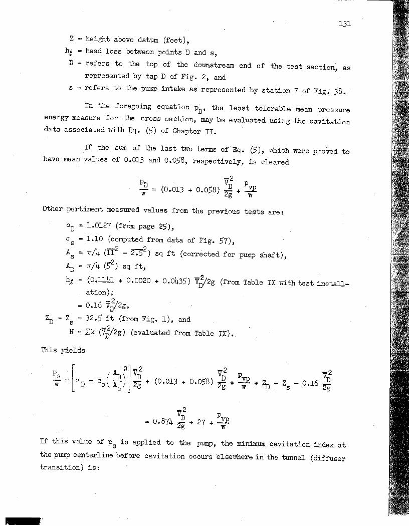
131

Z = height above datum (feet),

h~ = head loss between points D and s,

D - refers to the top of the downstream end of the test section, as

represented by tap D of Fig. 2, and

s - refers to the pump intake as represented by station 7 of Fig. 38.

In the foregoing equation PD' the least tolerable mean pressure

energy measure for the cross section, may be evaluated using the cavitation

data associated with Eq. (5) of Chapter II.

If the sum of the last two terms of Eq. (5), which were proved to

have mean values of 00013 and 0.058, respectively, is cleared

-2 PD . . VD P --. = (0.013 + 0.058) --2 + ~ w g w

Other pertinent measured values from the previous tests are:

aD =1.0127 (from page 25), a == 1.10 (computed from data of Fig. 57), s A = rr/4 (II2 - ~2) sq ft (corrected for pump shaft),

s An = rr /4 ()'2) sq ft,

ht (0.1141 ~ 0.0020 + 0.0435) V'£/2g (from Table IX with test install­

ation) ; -2/ = 0.16 VD 2g,

Zn - Zs == 32.5 ft (from Fig. 1), and

II = Ik (V;/2g) (evaluated from Table IX).

This yields

-2 VD p = 0.874 --2 + 27 + :!E g w

17. 2 D z... - Z - 0.16 -­

JJ s 2g

If this value of p is applied to the pump, the minimum cavitation index at s the pump centerline before cavitation occurs elsewhere in the tunnel (diffuser

transition) is:

132

A plotting of this equation for various test section velocities is shown in

Fig. 59. This indicates that the lowest value of [J will be approximately 4.2

at the maximum tunnel speed of 85 fps.

Evidence in the literature indicates that a [J-value of 4.2 should

be quite safe since values of 1.5 to 2 .. 0 are apparently readily obt~inable on

the basis of past designs. In fact there is a sufficient margin of safety to

justify some reduction of the vertical dimension between the horizontal legs

of the tunnel represented by the value of 32.5 ft occurring in the final ex­

pression for [Jmin-

4. Temperature Factors

The continued addition of pumping energy to a finite quantity of

water in a water tunnel will progressively raise the temperature of the water.

The rate of temperature rise will be a function of the rate of heat addition

(pump input energy), the mass concerned, and the ra.te of heat loss via the

boundaries. Vfuile the first two quantities may be calculated for the proposed

prototype design with a fair degree of accuracy, the latter item is a variable

depending on a number of unpredictable environment factors. For this reason,

it is not desirable to attempt to predict the prototype temperature until all

the environment factors are determined.. However, as a guide to such an evalu­

ation, the model tunnel was operated at top speed for an extended period. The

resulting experimental observations are shown by the plotted points in Fig. 60 ..

The tunnel is placed in a large room heated with unit heaters involving mild

air circulation; its surface is a medium gray, high gloss paint over galvanized

hot rolled steel; the equivalent heat capacity of the tunnel structure and con­

tained water is 29701b of water; and the external tunnel area is 142.5 sq i.t'.

On the basis of these observations and conditions, an attempt was made to

approximate the probable rate of temperature rise for the prototype. 'These

approximations for three different prototype speeds are also shown in Fig. 60.

In addition to the rate of rise curves, Fig. 60 contains a curve

approximating the rate of cooling of the prototype. While this curve is not

offered as an accurate index, it does serve to show certain relative values

--------- ----- -----------------------------~

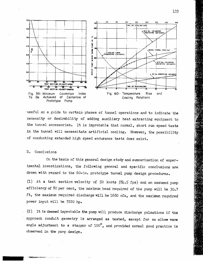
17.0

~ \ \

ISD

lao

~ \ \

11.0

9.0

'" "" 7.0

~ ---r-3.0

20 0 10 ID eo III TEST SECTION VELOCITY (FP8)

, • ~ ~ • k • ~ TEST SECTION VELOCITY IICNOTS)

Fig. 59- Minimum Cavitation Index To Be Achieved at Centerline of

Prototype Pump

133

1~°r_--~2rO----4rO--~6rO--~8rO--~r---~--~~--~

~O,r_--~----r_--~----r_--~----~--~~~

0.: • 100'r---_r----r---_r----r---_r~~~--_r--~ ! a: :II OJ

l-eoI:-----t----t-----t----t----r--' ! o ."' .. ilDr-~_r----r_--_r~~r_~~----~~_r--~ j a: :II OJ

I- ~----+_~~~~+_--~----+_--~----+_--_1 II: OJ

!C •

TIME Of RUNNING (HIll

Fig. 60 - Temperature Rise and Cooling Relations

useful as a guide to certain phases of tunnel operations and to indicate the

ne'cessity or desirability of. adding auxiliary heat extracting equipment to

the tunnel accessories. It is improbable that normal, short run speed tests

in the tunnel will necessitate artificial cooling. However, the possibility

of conducting extended high speed endurance tests does exist.

D. Conclusions

On the basis of this general design study and summarization of exper­

imental investigations, the following general and specific conclusions are

drawn with regard to the 60-in. prototype tunnel pump design procedures.

(1) At a test section velocity of 50 knots (84.5 fps) .and an assumed pump

efficiency of 80 per cent, the maximum head required of the pump will be )0.7

ft, the maximum required discharge will be 1660 cfs, and the maximum required

power input will be. 7220 hp.

(2) It is deemed improbable the pump will produce discharge pulsations if the

approach conduit geometry is arranged as tested,except for an elbow vane

angle adjustment to a stagger of 1000 , and provided normal good practice is

observed in the pump design.

i

134

(3) The pump design should attempt to correct or unify maldistribution of

velocity and to provide a discharge as free as possible of rotary components.

The proposed p~ location serves to provide considerable damping of pump

disturbances.

(4) The location of the pump in the tunnel circuit and the pressure recovery

affected by the circuit design appear to be adequate to inhibit all major

cavitation and probably most minor cavitation in a pump designed in accord with

best modern practice.

(5) An axial flow pump with either variable speed or variable blade is assumed

necessary to proper operation of the prototype tunnel.

(6.) The rate of heating, and cooling of the tunnel water may necessitate arti­

ficial cooling under test conditions calling for extended operations at high

speed.

[1]

[2J

References

Collar, A. R. Casc'ade Theory and the Design of Fan Straighteners.. Aero­nautical Research Committee Reports and Memoranda No. 1885 (British), 1940.

Silberman, Edward. The Pi tot Cylinder. Universi ty of Minnesota St. Anthony Falls HyoraulicLaooratory Circular No.1, 1947. 18 pp.

APPENDICES ~----..,...----

1 I

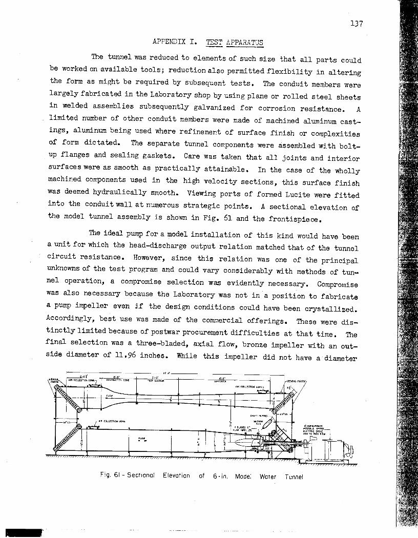
137

APPENDIX I. TEST APPARATUS

The tunnel was reduced to elements of such size that all parts could

be worked on 'available tools; reduction also permitted flexibility in altering

the form as might be required by subsequent tests. The conduit members were

largely fabricated in the Laboratory shop by using plane or rolled steel sheets

in welded assemblies subsequently galvanized for corrosion resistance. A

limited number of other conduit members were made of machined aluminum cast­

ings, aluminum being used where refinement of surface finish or complexities

of form dictated. The separate tunnel components were assembled with bol t­

up flanges and sealing gaskets. Care was taken that all joints and interior

surfaces were as smooth as practically attainable. In the case of the wholly

machined components used in the high velocity sections, this surface finish

was deemed hydraulically smooth. Viewing ports of formed Lucite were fitted

into the conduit wall at numerous strategic points. A sectional elevation of

the model tunnel assembly is shown in Fig. 61 and the frontispiece.

The ideal pump for a Illodel installation of this kind would have been

a unit for which the head-discharge output relation matched that of the tunnel

circuit resistance. However, since this relation was one of the principal

unknowns of the test program and could vary considerably with methods of tun­

nel operation, a compromise selection was evidently necessary. Compromise

was also necessary because the Laboratory was not in a position to fabricate

a pump impeller even if the design conditions could have been: crystallized.

Accordingly, best use was made of the commercial offerings. These were dis­

tinctly limited because of postwar procurement difficulties at that time. The

final selection was a three-bladed, axial flow, bronze impeller with an out­

side diameter of 11.96 inches. While this impeller did not have a diameter

1------------15'-8'-----------------4 3'_0'

TEST SECTION

Fig. 61 - SeCTIonal Elevation of 6 - in. Model Water Tunnel

138

consistent with the model scale ratio, it was deemed the best compromise on

the basis of anticipated performance requ:i.renents. Therefore, local flow

conditions at the pump l,'vere not expected to agree with prototype similitude

and the pump test program was considered primarily 'a matter of determining

correct specifications for the pump construction.

Since the Laboratory was faced with the problem of fabricating the

remainder of the pump unit without detailed design data and without facilities

for economical fabrication of the conventional warped. suction and discharge

vaning, the design was reduced to the simplest possible geometry. As can be

seen from Fig. 62, the principal features of the model pump geometry include:

(1) A housed drive shaft.

(2) A vaned approach elbow in which a streamlined splitter has been provided

to minimize the disturbance in flow created by the presence of the drive shaft.

(3) Four streamlined radial struts supporting the inboard shaft bearing.

These struts are axial vanes and make no attempt to apply selected rotary

vector components to the flow.

(4) A hub fairing piece formed to diffuse the flow as gradually as possible

consistent with practical length limitations.

(5) Seven straight diffuser vanes with dimensions based on Collar I s findings

(reference [1] of Chapter VI)~ In his design studies, Collar concluded that

radial vanes with axial alignment provide adequate straightening o:f:the rotary

impeller discharge if the vane is an airfoil section operating at less than

the stall angle and if it is of varying chord length so that the ratio of

periphel~al vane spacing to chord is unity. While a spacing ratio of 0.5 would'

have given ootterresUlt$, little':flcwqualiity",is. sacrificed arid:. the 'structure

is simplified if a ratio of 1.0 is used.

(6) A conventional packing gland placed~at the point where the drive shaft

pierced the pressure swell. Sealing against air leakage under subatmospheric

tunnel operations was accomplished by a shaft lantern ring and an external

pressure tap to the city water supplyo

The pump drive system consisted of a 15-hp electric motor integrally

connected to a variable speed, V-belt transmission. Speed changes were accom­

plished by a mechanism 'Which varied the diameters of the V-bel t pulleys to

permi t an output shaft speed continuously variable between 250 and 1500 rpm ..

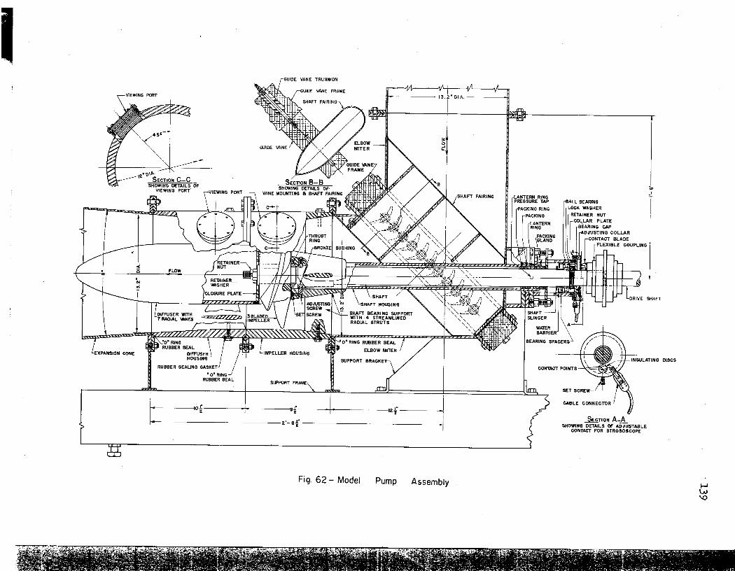
I NG PORT

GUIDE VANE

SUPPORT

VANE TRUNNION

i ~l I

1:----:1-- r -- ~'.ff ·f :1

Fig. 62 - Model Pump Assembly

CABLE r.nNN~r.TnDJ

SECTION A-A SHOWING DETAILS OF ADJUSTABLE

CONTACT FOR STROBOSCOPE

DISCS

~ '"

140

The speed change mechanism was driven by a small auxiliary electric motor,

controlled in turn by push buttons mounted on the main control panel.

A remote reading electric tachometer was connected' to the output

shaft and mounted with the indicating head at the main control panel. This

arrangement served as a ready means of establishing approximate test section

speeds. While a larger speed and power r.ange, together with elimination of

the slight vibratory characteristics inherent to a V ..... bel t drive, would have

been desirable, procurement of this unit was considered an expedient and eco­

nomical solution to the problem.

Since the ambient pressure value existing in the test section of a

water tunnel is one of the most important variables in any tunnel cavitation

study, it is essential that convenient means of varying it and accurate means

of measuring it be provided. A review of the methods used in other tUnnels

indicated that, in general, control was affe'cted by connecting the tunnel to

a regulated vacuum or pressure source while measurement was frequently accom­

plished with a modified mercury manometer.. A notable exception was the Massa­

chusetts Institute of Technology tunnel employing a tilting pipe leading from

the test section to the atmosphere. The elevation of the free liquid surface

in the atmospheric end of the pipe relative to the elevation of the test

section established the test section pressure.- Since the elevation of the

free Surface could be varied by tilting the pipe, a wide range of test section

pressures could be achieved.

In view of the large vertical space available in the St. Anthony

Falls Hydraulic Laboratory and the inherent accuracy and simplicity of a water

manometer, it was decided to employ a modified and extended version of the

Massachusetts Institute of Technology pressure system. The pressure control

portion of this system replaced the tilting pipe of the M!T system l'Vi th. a

. flexible rubber hose ending in a free surface overflow pan, with the pan being

raised and lowered vertically on an electric hoist. Separate water supply and

waste hoses served to keep·; .. the free liqu~d surface at an established position

in the overflow pan.

Measurement of the elevation of the free surface height relative to

the t'Ullnel centerline was' accomplished by affixing a surveyor' smeasuring tape

to the overflow cup with the zero set at the water sUrface. An index mark.

opposite the tape and at the elevation of the t est section centerline permitted

direct readings of the test section pressure in feet of water. Elevation of

the free surface could be varied from +16 to -31 ft of water and some addi­

tional tunnel pressure variation could be accomplished by varying the point

at which the pressure hose is attached to the tunnel boundary" The latter

technique is possible since the tunnel possesses regions (most notably the

contraction) VITi th steep· axial pressure gradient as a result of the dynamics

of the recirculating flow" Because the measuring tape was graduated to 0.01

ft, all pressure settings greater than 1000 ft could be easily and. accurately

measured with an error of less than 1 per cento

All moving body flow studies are fundamentally dependent on accurate

lmowledge of the relative velocity; therefore, it was essential that the model

tunnel be fitted with a meter capable of accurate indication of the test sec­

tion flow velocity., 'While some tunnels have employed fixed Pi tot tubes and

current meters to indicate velocity, it has been more common to employ differ­

ential pressures measured along the tunnel boundary and, particularly, the

large differentialsoc:cn:rro:fu~g :along the contraction cone boundaryo

A review of the problems led to the selection of the method of differ­

ential pressure measurement for the model tunnel studies and resulted in the

installation of three pressure manifolds located at the upstream end, midpoint,

and downstream end of the contraction. Each of the manifolds consisted of

four pressure taps, wi th two on a horizontal diameter and two on a vertical

diameter of the cross section. Each tap consisted of a 1/32-inodiam hole

carefully deburred at its inner end and expanded to a lIB-in. pipe connection

at its outer end.

To avoid locating the upstream pressure tap in a region of flow

separation, it was placed as far upstream as the casting structure permitted.,

or 1-1/2 in" from the end of the model casting" Subsequent boundary streamline

experiments in the model (Chapter III, Contraction Studies) indicated a slight

separation might exist in this region; this would make it advisable to move

even farther upstream for any similar prototype metere The middle manifold

was located 17 inc downstream of the beginning of the contraction and was

employed whenever the head between the upstream and downstream manifoldS ex­

ceeded the limits of convenient reading on the attached manometers" The down;...

stream manifold was located 1-1/2 ino upstream of the downstream end of the

contraction at a point where the minimum or test section diameter had been

reached.. This manifold, in addition to serving as a prime tap for velocity

determinations, al'so served as the usual external pressure application and

control point. The three manifolds are shown in F'ig. 20.

Pressure forces from the manifold system were originally intended

to be indicated by a water manometer reading directly to the nearest 0.01 ft;

however, mechanical difficulties with this system led to its replacement with

conventional 50-in. glass U-tubes and adjustment of gage fluid specific gravity

to match the pressure magnitude. As indicated previously the velocity was con..,

trolled by adjusting the pump speed with electric push button controls. The

measured relation between the manometer reading and the flow discharge was

determined by an experimental calibration separately described in Appendix III.

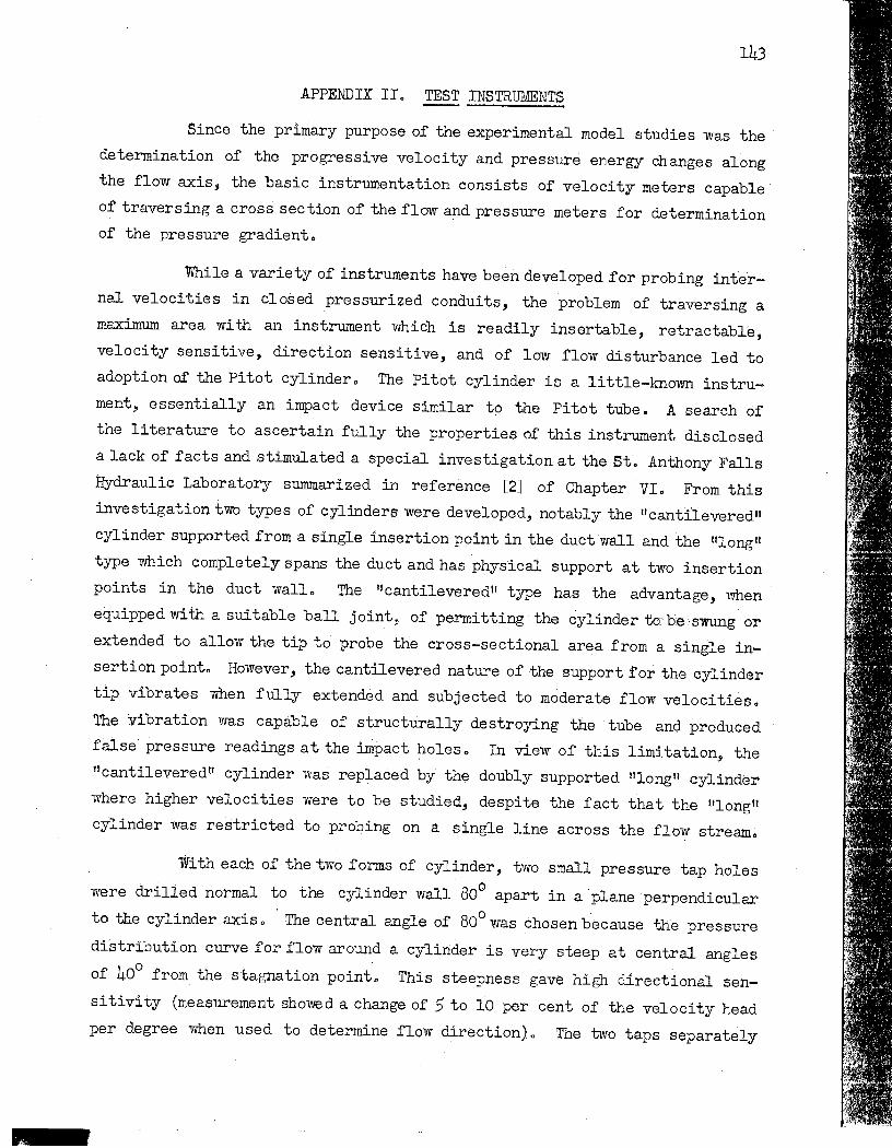
143

APPENDIX II. TEST INSTRUMENTS

Since the primary purpose of the experimental model studies was the

determination of the progressive velocity and pressure energy changes along

the flow axis, the basic instrumentation consists of velocity meters capable

of traversing a cross sec tion of the flow and pressure meters for determination

of the pressure gradient a

While a variety of instruments have been developed for probing inter­

nal velocities in closed pressurized conduits, the problem of traversing a

maximum area with an instrument which is readily insertable, retractable,

velocity sensitive, direction sensitive, and of low flow disturbance led to

adoption of the Pitot cylinder. The Pitot cylinder is a little-known instru­

ment, essentially an impact device similar to the Pitot tube. A search of

the literature to ascertain fully the properties of this instrument disclosed

a lack of facts and stimulated a special investigation at the St. Anthony Falls

Hydraulic Laboratory summarized in reference [2J of Chapter VIo From this

investigation two types of cylinders were developed, notably the ttcantlleveredll

cylinder supported from a single insertion point in the duct wall and the "long ll

type which completely spans the duct and has physical support at two insertion

points in the duct wall., The Ilcantilevered" type has the advantage, when

equipped with a suitable ball joint, of permitting the cylinder to:' he ,swung or

extended to allow the tip to probe the cross-sectional area from a single in­

sertion point. However, the cantilevered nature of the support for the cylinder

tip vibrates when fully extended and subjected to moderate flow velocities.

The Vibration was capable of structurally destroying the tube and produced

false pressure readings a t the impact holes", In view of this limitation, the

Itcantileveredlt cylinder was replaced by the doubly supported !llong!! cylinder

where higher velocities were to be studied, despite the fact that the !llongU

cylinder was restricted to probing on a single line across the flow stream.

Wi th each of the two forms of cylinder, two small pressure tap holes

were drilled normal to the cylinder wall 80° apart in a plane perpendicular

to the cylinder axis" The central angle of 800 was chosen because the pressure

distribution curve for flow around a cylinder is very steep at central angles

of 400 from the stagnation pointa This steepness gave high directional sen­

sitivity (measurement showed a change of 5 to 10 per cent of the velocity head

per degree when used to determine flow direction). The two taps separately

-

144

conveyed pressure through the cylinder interior and thence to external pressure

reading manometers" If either of the two taps 'Were oriented to face the prin­

cipal flow direction, the corresponding pressure reading would represent the

total or stagnation head and in conjunction with a static pressure tap in the

duct boundary wall would serve to give the local velocity head.. The direction

of this local velocity could then be ascertained by orienting the cylinder so

that the pressures at the twO cylinder holes were the same. The physical

position of the Pitot pressure tap in the tunnel cross section was determined

by external readings of scales tlAfI, ttE", and IICI1 shown in Fig. 6,3. A coeffi­

cient of unity was used with these tubes because the tests described in refer­

ence [2J of Chapter VI indicated such a practice introduced an error of less

than 1/2 per cent in obtaining the average energy over a cross section.

The tunnel boundary was arranged with insertion points located by .

the station numbers of Fig. ,38. At stations .3, 4, 5, 6, 8, 9, 10, 11, and

12, one ball type swinging mounting and three nonswinging mountings were spaced

at 900 around the periphery to permit insertion of a .3!8-in" diam I1cantilevered11

cylinder. The construction and mounting of this instrument are shown in Figs •

.37 and 63.. At station 7 four nonswinging mountings were provided. The non­

swinging mountings.were also suitable as static pressure taps when the cylinder

was removed.. In the high velocity regions of stations 1 and 2, the3!8-in.

IIcantileveredll cylinder was supplanted by a 1!4-in" UlongU cylinder and non­

swinging mounts located on a diameter"

Pressure measurements on the tunnelooundaxy"wall'and,th£bPitot:::taps

were generally made using 50-in.. glass U-tube manometers" Four metering

fluids--carbon tetrachloride, ethylene bromide, bromoform, and mercury--were

used selectively to give the maximum readable deflection in any particular

pressure study •. Where the readings were less than 6 in., and thus of exces­

sive error due to the coarse reading scales on the U-tubes, a micromanometer

was used.. The lI,licromanometer was an inverted U,..tube with an air loop" Reading

was accomplished with two micrometer depth gages modified to act as hook gages

measuring to the nearest 0,,001 inch.. Water levels and air pressure in the

micromanometer were controlled by a hand pump and bleed-off valve.

I

MANOMETER LINE CONNECTED HERE

A THIS SURFACE SERVES AS READING INDEX FOR SCALE A

SUPPORT

SECTION A-A

PLAN VIEW

ELEVATION

ROD

TUBE

SECTIONAL ELEVATION

Fig. 63 - Cantilevered

RING RUBBER SEAL

Pitot Cylinder and Mounting ~

146

APPENDIX III • TEST PROCEDURE

The physical measurements made in the model studies consisted of

calibrating the contraction nozzle for use as a general velocity meter, taking

velocity traverses at selected test stations on the tunnel circuit, ta1d.ng

boundary pressure gradients around the tunnel circuit, and determining critical

cavitation conditions. Since the last three of these were previously des­

cribed, only the velocity meter calibration will be described here ..

Because all instruments for measuring liquid velocities are subject

to some correction for inherent errors of indication, it was desirable that

the basic velocity measuring device be calibrated to minimize such errors ..

Therefore, in accord with accepted hydraulic practice, the velocity was deter­

mined by measuring the total discharge of the flow stream with a primar.y weight

system. The calibration of the contraction cone differential pressure drop

as an index of velocity necessitated breaching the tunnel loop and diverting

the flow at a point where the diversion would have least influence on the

meter performance.. It wa.s decided, therefore, to remove a portion of the

tunnel loop in the vicinity of elbow I (Fig" 38) and to substitute an external

water supply connection just above elbow II and a discharge connection to the

dovmstream end of the main diffuser.. The supply connection was in turn tied

into the main water supply system of the Laboratory, while the discharge con­

nection was conveyed to the main weighing tanks of the Laboratory for precise

discharge determinations.

A large number of discharge determinations were made with the mean

test section velocity varying from. 9 to 47 fpso The weighed discharge measure­

ments, together with the contraction pressure differentials, pump shaft revo­

lutions per minutes, and measured velocity distribution traverses at stations

1 and 12, served to give the basic velocity data necessary to subsequent tunnel

testing ..

I

··P".AII