Designing Power Grid Topologies for Minimizing Network Disturbances:An Exact MILP Formulation

Siddharth Bhela, Deepjyoti Deka, Harsha Nagarajan, Vassilis Kekatos

Abstract— The dynamic response of power grids to smalltransient events or persistent stochastic disturbances influencestheir stable operation. This paper studies the effect of topologyon the linear time-invariant dynamics of power networks. Fora variety of stability metrics, a unified framework based on theH2-norm of the system is presented. The proposed frameworkassesses the robustness of power grids to small disturbancesand is used to study the optimal placement of new lineson existing networks as well as the design of radial (tree)and meshed (loopy) topologies for new networks. Althoughthe design task can be posed as a mixed-integer semidefiniteprogram (MI-SDP), its performance does not scale well withnetwork size. Using McCormick relaxation, the topology designproblem can be reformulated as a mixed-integer linear program(MILP). To improve the computation time, graphical propertiesare exploited to provide tighter bounds on the continuousoptimization variables. Numerical tests on the IEEE 39-busfeeder demonstrate the efficacy of the optimal topology inminimizing disturbances.

I. INTRODUCTION

The electric power system is continually changing. Itis expected that the grid of the future will have highervariability due to renewables, changing load patterns, anddistributed energy sources [1]. This paradigm shift will posean enormous challenge for design and stable operation ofpower networks. The inherent uncertainty associated withrenewable energy sources and active loads is likely to pro-duce more frequent and higher amplitude disturbances [1].In addition, owing to the lower aggregate inertia of systemswith high penetration of renewables, the capability of powernetworks to handle such disturbances may be significantlyreduced [2].

Thus, improving the dynamic performance of the powergrid is of importance and has received greater attentionfrom academia and industry. Efforts in this direction includedevelopment of payment structures and novel markets, aswell as analysis of techniques to incentivize load-side partic-ipation [3], [4], [5], [6]. The benefits of load-side controllershas motivated a series of recent works to understand howdifferent system parameters and controller designs impactthe transient response of the network [7], [8]. Recent workin [9] has also explored the optimal placement of virtualinertia to improve stability.

Compared to the previously mentioned system parameters,the effect of network topology on transient stability is less

S. Bhela and V. Kekatos are with the Bradley Dept. of ECE, VirginiaTech, VA, USA. Emails: (sidbhela,kekatos)@vt.edu. D. Deka andH. Nagarajan are with the Theoretical Division at Los Alamos NationalLaboratory, NM, USA. Emails: (deepjyoti,harsha)@lanl.gov.The work was supported by LDRD-ER (POD) and from the Advanced GridModeling Program in the Office of Electricity in U.S. Dept. of Energy.

well understood. Without detailed simulations, it is usuallyhard to infer how a change in network topology influencesthe overall grid behavior and performance. Recent work in[8] shows that the impact of network topology on the powersystem can be quantified through the network Laplacianmatrix eigenvalues. In addition, grid robustness against lowfrequency disturbances is mostly determined by networkconnectivity [8], further motivating this study. Past studiesin the power and control systems communities have alsolooked at designing network topologies for specific goalsusing system theoretic tools. Such goals include reductionof transient line losses [1], improvement in feedback con-trol [10], [11], coherence based network design [12] andaugmentation [13]. Semidefinite programming (SDP) basedtools have also been utilized to design and augment networktopologies for dynamic control [14], [12], [15].

While the primary focus here is topology design, werecognize that there is line of related work dealing withlearning network topologies and line parameters [16], [17],[18]. Schemes that rely on passive data have been used in[18] and [16] for learning radial topologies. Different fromthem, the work in [17] actively probes the grid to recoverradial topologies and verify line statuses.

In this paper we are interested in studying the effectof topology on the power grid dynamics. For a variety ofobjective functions, such as line loss reduction, fast dampingof oscillations, and network coherence, our previous work[19] presented a unified framework to study topology designbased on the H2-norm. In [19], the focus was on topologyreconfiguration rather then topology design. Further, thework in [19] developed suboptimal algorithms, albeit withguarantees on optimality gap, to tackle the combinatorialdesign problems involved. Here, we present reformulationsof the topology design task that allow us to solve the problemto optimality.

Our contributions are as follows. First, we provide acomprehensive modeling and analysis framework for thetopology design problem to optimize a H2 norm basedperformance metric subject to budget constraints in Sec-tion II. Second, in Section III we show that although thetopology design task is inherently non-convex, it is possibleto exactly reformulate the problem in tractable form usingMcCormick relaxation (or linearization). This can then beused with off-the-shelf solvers to determine the optimalsolution. Further, we show that exploiting graph-theoreticproperties to tighten bounds on the continuous optimizationvariables yields significant improvements in computationtime. Section V discusses numerical tests based on the

IEEE 39−bus test case followed by conclusions and futuredirections in Section VI.

Notation: Column vectors (matrices) are denoted bylower- (upper-) case letters and sets by calligraphic symbols,unless noted otherwise. The cardinality of set X is denotedby |X |. Given a real-valued sequence {x1, x2, . . . , xN}, x ∈RN is the vector obtained by stacking the scalars xi anddg({xi}) is the corresponding diagonal matrix. The operator(·)> stands for transposition. The N -dimensional all onesvector is denoted by 1N ; IN is the N ×N identity matrix;and ei is the canonical vector with a 1 at the i-th entryand zero everywhere else. The notation θi denotes its timederivative δθi

δt .

II. GRID MODELING AND NETWORK COHERENCE

This section presents a linearized power system model,defines network coherence metrics, and reviews their connec-tion to studying the stability of a linear dynamical system.

A. Dynamic Power System Model

A power network having N + 1 buses can be modeledas a connected graph G = (V, E), whose nodes V :={0, 1, . . . , N} correspond to buses, and edges E ⊆ V × Vto undirected lines. Bus i = 0 is selected as the reference;all other buses constitute set Vr := V\{0}. Let bij > 0 be thesusceptance of line (i, j) ∈ E connecting nodes i and j ∈ V .Then, the susceptance Laplacian matrix L ∈ R(N+1)×(N+1)

associated with the grid graph G can be defined as

Lij :=

−bij , if (i, j) ∈ E∑

(i,j)∈E bij , if j = i

0 , otherwise.

Each node i ∈ V is associated with a phase angleθi, frequency ωi = θi, inertia constant Mi, and dampingcoefficient Di; see [20]. Since bus i may host an ensemble ofdevices such as synchronous machines, renewable or energystorage sources, frequency-dependent or actively controlledfrequency-responsive loads, the parameters Mi and Di char-acterize their aggregate behavior [9].

Focusing on small-signal stability, the quantities (θi, ωi)will henceforth refer to the deviations of nodal voltageangles and frequencies from their nominal values. The griddynamics at bus i can then be described by the linearizedswing equation [20]

Miωi +Diωi = Pmi − P ei + ui (1)

where Pmi denotes the mechanical power input; P ei is theelectric power flowing from bus i to the grid; and ui isthe power consumed at bus i. Again, the aforementionedquantities refer to the deviations from their scheduled values.Under the linearized DC model, the power flowing from busi to the grid can be approximated as [20]

P ei '∑

(i,j)∈E

bij(θi − θj). (2)

Combining (1) and (2), the state-space representation ofthe power grid is[

θω

]=

[0 IN

−M−1L −M−1D

]︸ ︷︷ ︸

A:=

[θω

]+

[0

M−1

]︸ ︷︷ ︸B:=

u (3)

where M := dg({Mi}) and D := dg({Di}) are diagonalmatrices containing the inertia and damping coefficients; thestates ω ∈ RN+1 and θ ∈ RN+1 are accordingly the stackedvectors of nodal frequencies and angles; and u ∈ RN+1 is thevector of local power disturbances. The subsequent analysisrelies on the ensuing assumption.

Assumption 1. The inertia coefficients are strictly positiveand damping coefficients are identical for all buses, that isMi > 0 and Di = d for all i ∈ V .

The non-zero inertia assumption is not necessary, butsimplifies our presentation. If Mi = 0 for a bus i ∈ V ,then a Kron-reduced network containing only nodes withinertia can be obtained. The second assumption of constantdamping has been previously used in [1], [10]. When it isnot satisfied, the stability metric defined in the next sectiondoes not enjoy a closed-form expression, and only boundscan be derived. In our future work, we plan to extend ourapproach to the case with variable D.

B. Generalized Network Coherence Metrics

Given the state-space model in (3), our goal is to designnetwork topologies or augment existing ones to minimizethe voltage angle deviations caused by load disturbances.These angle deviations are formally captured by the met-ric of network coherence [21]. The latter is defined aslimt→∞ E[fc(t)] where fc(t) is the steady-state deviation ofthe angles from their grid-average

fc(t) :=

N∑i=1

θi(t)− 1

N

N∑j=1

θj(t)

2

. (4)

In other words, network coherence quantifies how tightly busangles drift together. Larger variances in angle deviationsreflect a more disordered network [1].

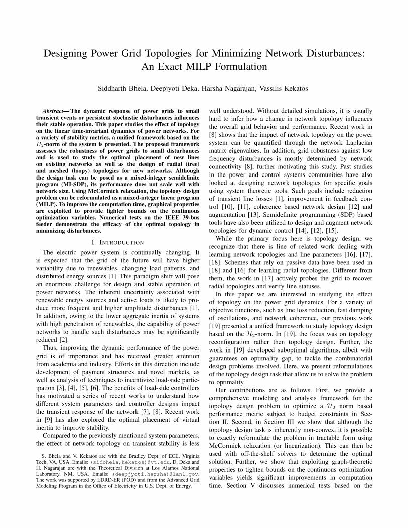
Instead of network coherence, the system operator maybe interested in minimizing the expected steady-state valueof a generalized function combining both voltage angle andfrequency excursions [19], [9]

f(t) :=∑∀i 6=j

wij(θi(t)− θj(t))2 +∑i∈V

siω2i (t) (5)

where wij and si are given non-negative scalars. The weightswij induce a connected weighted graph Gw that is notnecessarily identical to G; see Fig. 1. Let W be the Laplacianmatrix of graph Gw and S := dg({si}). Then, it is not hardto verify that f(t) = ‖y(t)‖22 where

y(t) :=

[W 1/2 0

0 S1/2

]︸ ︷︷ ︸

C:=

[θ(t)ω(t)

]. (6)

Consensus graph

Power grid

i

jwij

∼G1

∼G2

L2

L3

L4

(θi, ωi)(θj, ωj)bij

sisj

Fig. 1. Illustration of power grid and its associated coherence graph. [19]

Being a Laplacian matrix, matrix W is positive semidef-inite, and so its matrix square root W 1/2 is well-defined.The matrix S1/2 is well-defined too. The importance ofthe generalized coherence metric of (5) is that for differentchoices of (W,S), one can represent different grid perfor-mance metrics and study them in a unified manner [19]:For instance, if the system operator is only interested inminimizing frequency excursions, one can set W = 0 andS = IN+1. Similarly, if the goal is to reduce transient linelosses, one can choose W = L and S = 0. Lastly, thenetwork coherence metric of (4) corresponds to the case ofW = IN+1− 1

N+11N+11>N+1 and S = 0. Figure 1 shows thephysical power network and its associated coherence graph.Note that the choice of (W,S) for network coherence penal-izes global deviations, whereas that for line loss reductionpenalizes local deviations.

C. Relation to Stability Analysis

The expected steady-state value of f(t) can be interpretedas the squared H2-norm of the linear time-invariant (LTI)system described by (3) and (6). This system will be com-pactly denoted by H := (A,B,C). Leveraging this link, thegeneralized network coherence is amenable to a closed-formexpression [19].

The H2 norm is widely used as a stability performancemetric and has several interpretations [22]: For unit-variancestochastic white noise u(t), the H2-norm of an LTI systemequals the steady-state output variance [22, Ch. 5], [1], [9]

‖H‖2H2:= lim

t→∞E[‖y(t)‖22

]. (7)

For unit-impulse disturbances ui(t) = eiδ(t) for i =1, . . . , N , the H2-norm can be equivalently written as

‖H‖2H2:=

N∑i=1

∫ ∞0

‖yi(t)‖22dt (8)

where yi(t) is the system output corresponding to distur-bance vector ui(t). Instead of evaluating the expectationin (7) or the time integral in (8), the H2-norm for system Hcan be expressed as [22, Ch. 5]

‖H‖2H2= Tr(B>QB) (9)

where Q :=∫∞0eA>tC>CeAtdt is the observability

Gramian matrix of the LTI system H . In fact, the matrixQ can be computed as the solution to the linear Lyapunovequation [22, Ch. 5]

A>Q+QA = −C>C. (10)

Matrix Q is known to be symmetric positive semidefinite, soit can be partitioned as

Q =

[Q1 Q0

Q>0 Q2

]. (11)

Based on the reformulation in (9), we next design topologiesattaining minimum generalized network coherence.

III. OPTIMAL GRID TOPOLOGY DESIGN

Among other criteria, the topology of a grid can bedesigned to minimize the generalized network coherencemetric of (5). Given a graph G = (V, E), where E is theset of candidate lines weighted by their susceptances, thegoal is to find the subset E ⊆ E of cardinality |E| ≤ Kwith K ≥ N attaining the minimum generalized networkcoherence. Given the equivalences of the previous section,this task can be posed as the optimization problem

arg minE∈E

Tr(B>QB) (12a)

s.to |E| ≤ K (12b)Q satisfies (10) (12c)E is connected. (12d)

The constraint in (12b) reflects the budget on the numberof edges. For K = N , the problem in (12) yields a treetopology, which is important for typically radially operateddistribution grids. Interestingly, leveraging the problem struc-ture under Assumption 1, it can be shown that the objectiveof (12) simplifies as [9], [19], [1]

Tr(B>QB) =Tr(WL+) + Tr(SM−1)

2d. (13)

If Assumption 1 is not met, i.e., the damping coefficientsare not identical (D 6= dIN ), then it may not be possi-ble to find a closed-form expression for the objective in(12). If the damping coefficients are known to lie within[dmin, dmax], then the objective of (12) can be bounded asTr(WL+)+Tr(SM−1)

2dmax≤ Tr(B>QB) ≤ Tr(WL+)+Tr(SM−1)

2dmin;

see [1], [9]. Therefore, as the range [dmin, dmax] becomesnarrower, minimizing the numerator of (13) approaches theoptimal solution to (12). From Assumption 1, we considerdmin = dmax here.

The second summand in the right-hand side of (13) isindependent of the grid topology, and can thus be ignored.Problem (12) can then be reformulated as

arg minE∈E

Tr(WL+) (14)

s.to |E| ≤ Krank(L) = N

where the rank constraint ensures that the graph induced byE is connected. Problem (14) could be tackled with brute-force algorithms over all the possible topologies of budget Kand below; though that would incur exponential complexity.

The objective in (14) can be written in terms of the inverseof the reduced Laplacian matrix of G as explained next. Theclaim has appeared in [1, Lemma 3.2], albeit for the restrictedcase where W = L.

Lemma 1. If W and L are the N × N matrices obtainedafter removing the first row and column from W and L,respectively, then

Tr(WL+) = Tr(W L−1).

Proof. The Laplacian matrices can be described in terms oftheir reduced counterparts as

W = RWR> and L = RLR> (15)

where R := [1N −IN ]>. This is because a Laplacian matrixsatisfies L1N+1 = 0N+1. If we define matrix J := IN −

1N+11N1>N , then it is not hard to see that

R>R = IN + 1N1>N = J−1. (16)

Then the pseudoinverse of L can be expressed as

L+ = RJL−1JR>. (17)

The latter can be shown by simply verifying that LL+L = Land L+LL+ = L+. From (15) and (17), we get that

Tr(WL+) = Tr(RWR>RJL−1JR>

)= Tr(W L−1)

where the last equality follows from (16) and the cyclicproperty of the trace. �

To express the optimization in (14) over E in a moreconvenient form, let us introduce a binary variable zm forevery line m ∈ E . This variable is zm = 1 if line m isselected, i.e., m ∈ E ; and zm = 0, otherwise. If we stackvariables {zm}m∈E in vector z, then z has to lie in the set

Z :={z : z>1|E| ≤ K, z ∈ {0, 1}

|E|}. (18)

Based on the line selection vector z, the reduced suscep-tance Laplacian of G can be expressed as

L(z) =∑

(i,j)∈E

zijbijaija>ij (19)

where each vector aij corresponds to line (i, j) ∈ E , and itsn-th entry is defined as

[aij ]n :=

+1 , if n = i

−1 , if n = j

0 , otherwise.

Given Lemma 1 and (19), the optimization in (14) canbe equivalently written as the mixed-integer semidefiniteprogram (MI-SDP)

arg minX,z∈Z

Tr(WX) (20a)

s.to

[X ININ L(z)

]� 0. (20b)

To see this, the constraint in (20b) is equivalent to X � 0 andX � L−1(z); see [23, Sec. A.5.5]. Since W � 0, the optimalX can be shown to be X = L−1(z). In fact, constraint (20b)waives the possibility of the optimal L being singular, andthus, ensures the connectedness of the graph.

To overcome the computational complexity of the MI-SDPin (20), one may relax the binary variables to box constraintsas z ∈ [0, 1]|E| to get an ordinary SDP, which can be handledby off-the-shelf solvers for moderately-sized networks. Beinga relaxation, the SDP solution provides a lower bound on thecost of (20). If the obtained solution of the SDP turns out tobe binary, then this z minimizes the MI-SDP in (20) as well.Otherwise, (randomized) rounding heuristics can be adoptedto acquire a feasible z.

Aiming at an exact solver, we will next show how the MI-SDP of (20) can be equivalently formulated as an MILP. Tothis end, we first rewrite (20) as

(X∗, z∗) ∈ arg minX,z∈Z

Tr(WX) (21a)

s.to L(z)X = IN . (21b)

Note that for constraint (21b) to hold, L(z∗) must be non-singular and X∗ = L−1(z∗). Although its cost is linear,problem (21) is non-convex due to the bilinear constraints in(21b) and because vector z is binary. To handle the former,we adopt the McCormick relaxation technique [24], whichis briefly reviewed next.

Constraint (21b) involves the bilinear terms zmXij form ∈ E and i, j ∈ Vr. For each such term, introduce a newvariable

ymij = zmXij . (22)

Suppose that the entries X∗ij are known to lie within therange [Xij , Xij ]. Since zm ∈ [0, 1], the ensuing inequalitieshold trivially [24]

zm(Xij −Xij) ≥ 0 (23a)

(zm − 1)(Xij −Xij) ≥ 0 (23b)

zm(Xij −Xij) ≤ 0 (23c)(zm − 1)(Xij −Xij) ≤ 0. (23d)

Substituting zmXij by ymij in (23) provides

ymij ≥ zmXij (24a)

ymij ≥ Xij + zmXij −Xij (24b)

ymij ≤ zmXij (24c)ymij ≤ Xij + zmXij −Xij . (24d)

One can replace the bilinear terms in (21b) by ymij’sand enforce (22) and (24) as additional constraints for allm ∈ E and i, j ∈ Vr. In that case, the constraints (24)are apparently redundant. However, one may simplify theproblem by dropping (22) to get an MILP reformulationof (21). Interestingly, this reformulation is exact due to thebinary nature of z. To see this, if z∗m = 1 for some m,

then (24b) and (24d) imply y∗mij = X∗ij for all i, j ∈ Vr.Otherwise, if z∗m = 0, then (24a) and (24c) imply y∗mij = 0for all i, j ∈ Vr.

Through the aforementioned process, problem (21) hasbeen converted to an MILP over the variables {Xij}, {zm},and {ymij}. MILPs can be handled by state-of-the-art solverssuch as Gurobi [25], and are known to scale better than MI-SDPs. Recall that the MILP reformulation of (21) requiresthe bounds (Xij , Xij) on each (i, j)-th entry of X∗. Lackingprior information on X∗, one could select an arbitrarily widerange [Xij , Xij ]. However, this could slow down the MILPsolver significantly. In the other extreme, if X∗ is known,that is Xij = Xij for all i, j ∈ Vr, then the binary vectorz can be recovered by simply solving the linear equationsin (21b). To improve the run time of the involved MILP, wenext derive tighter, non-trivial bounds on the entries of X∗ij .

IV. BOUNDING THE CONTINUOUS VARIABLES

Depending on the problem structure, different boundscan be derived on X∗ijs. This section considers two classesof topology design tasks. In the first task, some lines arealready energized and the operator would like to augment aconnected network by additional lines to further improve itsstability. In the second task, a network topology is designedfrom scratch with the additional requirement of a radial grid.

A. Augmenting Existing Networks

Given the graph G = (V, E), this problem setup considersa pre-existing connected network described by Ge = (V, Ee),and the goal is to energize additional lines from E \ Eeto improve its stability. In essence, this corresponds to theproblem in (21) with the entries of z corresponding to thelines in Ee being set to one. Then, based on (19), the reducedLaplacian matrix of the existing network is obviously

Le :=∑

(i,j)∈Ee

bijaija>ij .

Under this setup, the entries of X∗ minimizing (21) underthe additional constraints z` = 1 for all ` ∈ Ee, can bebounded as follows.

Lemma 2. The entries of X∗ are bounded by

0 < X∗ij ≤[L−1e ]ii + [L−1e ]jj

2, ∀(i, j) ∈ Vr. (25)

Proof. Observe that Le can be written as L(z) by fixingthe entries of z corresponding to the lines in Ee to 1. Sincethe same entries will remain 1 in z∗, it readily follows thatL(z∗) � Le � 0, where Le is non-singular since the existingnetwork is already connected. Then, it follows that X∗ �L−1e and v>(X∗ − L−1e )v < 0 for any v 6= 0. Setting v =ei, the diagonal entries of X∗ can be bounded as X∗ii ≤[L−1e ]ii for all i ∈ Vr. Since X∗ � 0 by constraint (21b), wehave that (ei − ej)>X∗(ei − ej) > 0 for all i, j ∈ Vr. Thelatter provides X∗ij <

12 (X∗ii + X∗jj). Upper bounding the

diagonal entries with the bounds obtained earlier proves theupper bound in (25). The lower bound in (25) can be trivially

obtained since L(z∗) is an M-matrix, and so its inverse haspositive entries. �

The reduced Laplacian matrix Le of the existing networkGe is invertible as long as Ge is connected. If that is not thecase, one could obtain bounds on X∗ij’s by imposing a radialstructure on the sought topology as discussed next.

B. Radial Topology Design

The setup considered here designs a network afresh, butunder the requirement that it is radial. The analysis simplifiesunder the following mild assumption.

Assumption 2. There exists a node in V that is incident toexactly one edge.

To derive bounds on the entries of X∗ minimizing (21)for the special case of K = N (radial network), let us firstconstruct the graph Gr = (V, Er), where Er consists of theedges in E , but with inverse weights xij := b−1ij for all(i, j) ∈ E . Based on Gr, we define some additional propertiesthat will be useful later. If one of the nodes in V satisfyingAssumption 2 is selected as the reference node, then theweight (inverse susceptance) of its incident line is denotedby x0. Let us also define the minimum of the inverse linesusceptances

xmin := min(i,j)∈Er

xij .

Before solving (21), we find the maximum spanning treeof graph G, and denote the sum of its edge weights by f .The maximum spanning tree can be found efficiently byfinding the minimum spanning tree on G upon negating itsedge weights [26]. Lastly, for each node i ∈ Vr, we find itsshortest path to the reference node 0 in Gr. The sum of edgeweights along this shortest path will be denoted by hi.

Lemma 3. Under Assumption 2, the entries of X∗, minimiz-ing (21) for K = N , are bounded as

hi ≤ X∗ii ≤ f, ∀i ∈ Vr (26a)x0 ≤ X∗ij ≤ f − xmin, ∀i, j ∈ Vr. (26b)

Proof. The bounds rely on a fundamental property of theinverse Laplacian matrix of a radial network: If L is thereduced susceptance Laplacian of a radial network and X :=L−1, then the entry Xij equals the sum of the inversesusceptances that are common to the paths of nodes i and j tothe reference bus; see [27, Lemma 1]. Under Assumption 2,the common path of any pair of nodes (i, j) ∈ Vr mustinclude at least the line incident to the reference bus, andhence, X∗ij ≥ x0. By the definition of shortest path, the entryX∗ii is lower bounded by hi for all i ∈ Vr, thus providingthe lower bound in (26a).

Regarding the upper bound in (26a), recall that the (i, i)-th entry of X∗ equals the sum of weights on the path from ito the reference node 0. The sum of weights on the longestsuch path is still upper bounded by the sum weight f of alledges in the maximum spanning tree. Because the entry X∗ijfor i 6= j must have at least one less edge than the longestpath, the upper bound in (26b) holds as well. �

k

i j

(a)

z1 z2

z1 + z2 ≥ 1

(b)

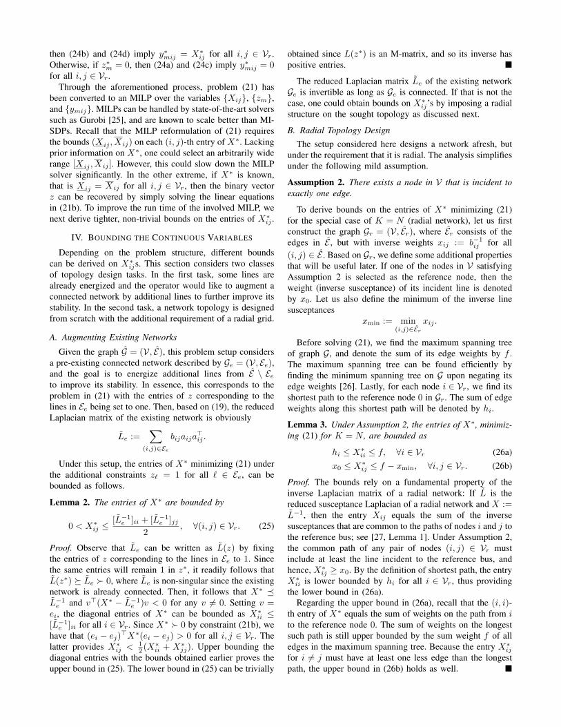
Fig. 2. Grid graph G = (V, E) with candidate location of edges. Leftpanel: The lower bounds on X∗

ki, X∗kj , and X∗

ij can be tightened usingthe shortest path weight hk due to the critical edge colored in red. Rightpanel: The size–2 cutset shown in red implies the constraint z1 + z2 ≥ 1.

Note that the upper bounds can be tight in the settingwhere the maximum spanning and optimum trees are thesame line graph.

C. Model Simplification and Bound Tightening

Exploiting the structure of G = (V, E) can provideadditional information on the bounds of X∗ matrix entries toaccelerate solving (21) for the special case of K = N (radialgrid). For example, if G gets disconnected upon removingedge ` ∈ E , this edge ` belongs to the sought tree topologyand z∗` = 1 before solving (21). To identify such edges, weresort to the notion of a graph cutset C ⊂ E , defined as asubset of edges that once removed, splits the graph G intotwo or more connected components. The edges in this cutsetwill be termed as critical edges. Now, we present a simplealgorithm to enumerate all the single critical edges (|C| = 1)by initializing the graph G’s weights to unit values.Step 1: Solve the min-cut problem on G with unit edge

weights by using the standard max-flow min-cutalgorithm [28].

Step 2: Increase the weight for the edge labelled as criticalto 1 + ε for some ε > 0.

Step 3: If |C| > 1, quit; else, go to Step 1.The second step ensures that every time we are identifying anew critical edge. Upon completing this process, the entriesof z∗ corresponding to the critical edges can be safely setto 1. This process not only reduces the binary search for z∗

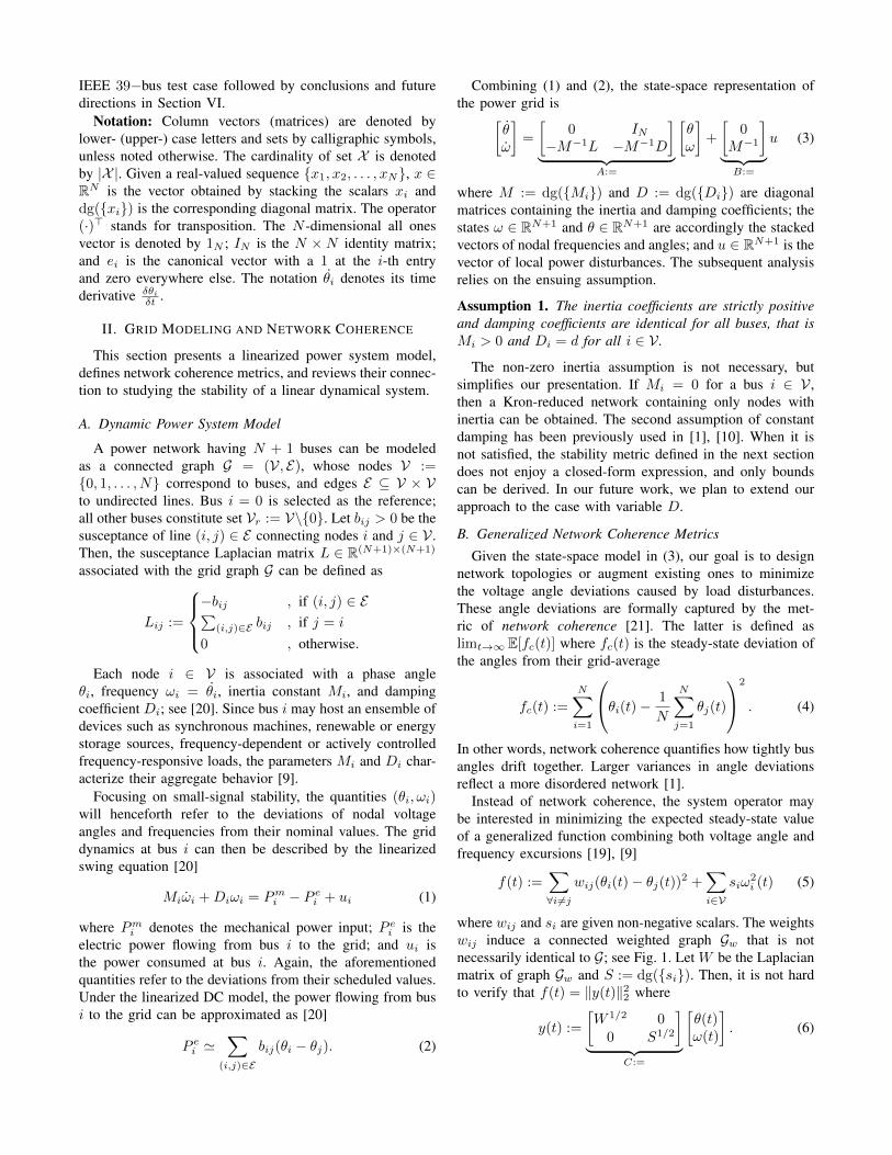
in (21), but it further tightens the lower bounds on certainX∗ij’s as discussed in Lemma 4; see also Fig. 2.

Lemma 4. Suppose a critical edge ` = (i, j) ∈ E partitionsthe nodes of G into two disjoint connected components V`and its complement V`. If V` contains node i as well as thereference bus, then (26b) can be tightened as

hj ≤ X∗kj , ∀k ∈ V`.

Proof. The edge (i, j) ∈ E is the only edge that connects thenodes in V` to the rest of the network. Hence, the commonpath to the reference bus of any two nodes in V` must includethe path of node j to the reference. It follows that the shortestpath weight hj is a valid lower bound for all nodes in V`. �

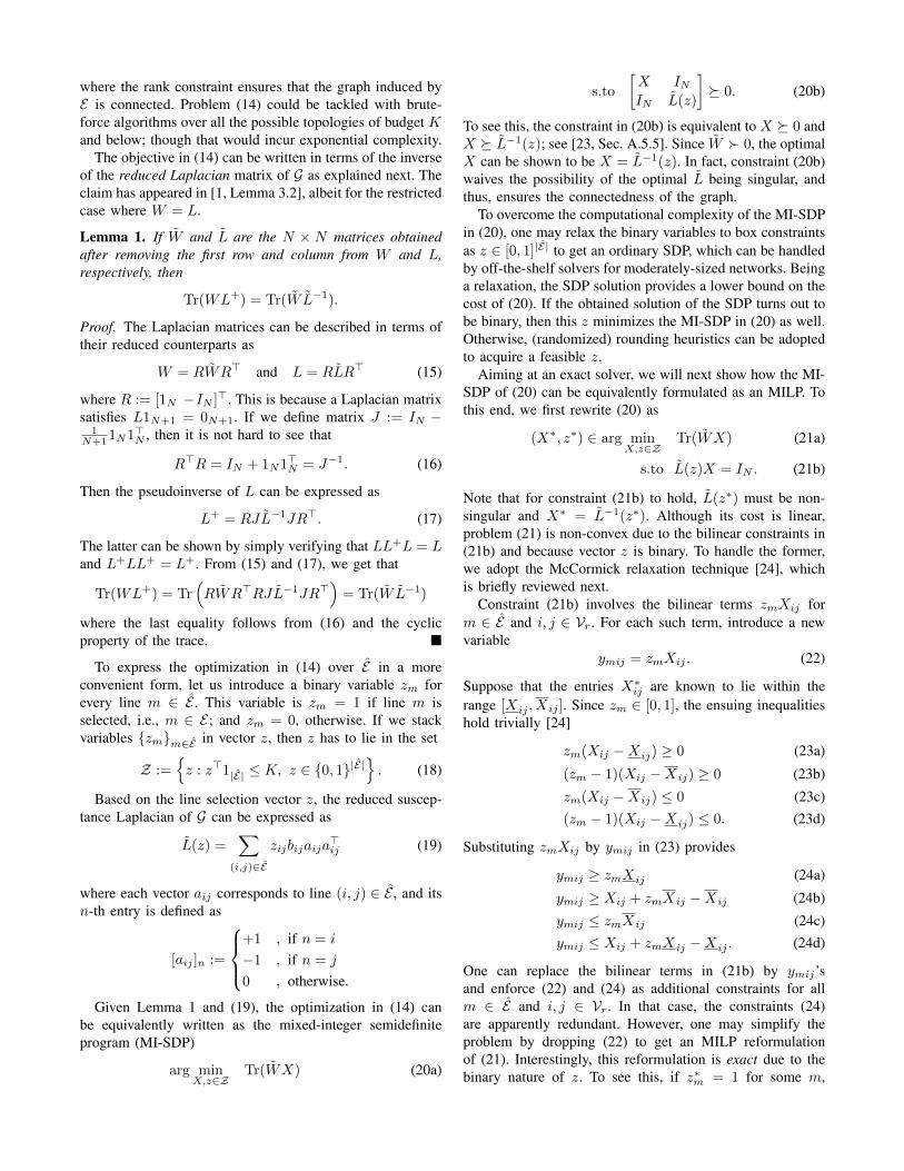
TABLE ICOST OF DESIGNED GRIDS USING THE IEEE 39-BUS NETWORK.

# of lines Optimal Topology Suboptimal Topology

2 0.570 0.5853 0.564 0.5824 0.557 0.5765 0.552 0.570

Identifying cutsets of cardinality larger than 1 offersadditional information to tighten the bounds of entries ofthe X matrix. If graph G gets disconnected upon removinglines `1, `2 ∈ E , then at least one of these lines should beactive. This logical conclusion translates to the constraintz`1 +z`2 ≥ 1, which can be augmented to (21) to tighten theMcCormick reformulation and possibly accelerate the MILPsolver. Cutsets of larger cardinality, say |C| = k, k > 1, canbe identified by iterating Steps 1 through 3 of the algorithmdescribed earlier. In this case, we assign the weights of k+εon the critical edges, where ε > 0.

V. NUMERICAL TESTS

All tests were run on a 2.7 GHz Intel Core i5 laptopwith 8GB RAM. The MILP formulations were solved usingGurobi v8.0.1 optimizer, written in Julia/JuMP [25], [31].

The performance of the MILP in (21) was tested for aug-menting an existing network as well as for designing a radialone afresh. For the augmentation setup, the IEEE 39-bussystem benchmark was used as the pre-existing connectednetwork [29]. The set E was selected by 10 randomly pickedadditional lines. From these lines, we solved the restrictedversion of (21) for K = {2, 3, 4, 5}. To satisfy Assumption 1,we assumed Mi = 10−4 on all buses that did not hostgenerators, and Di = d = 0.025 for all i ∈ V . To gradean arbitrarily constructed network, we compared its squaredH2 norm to that of the optimal network of the same edgecardinality. The results are summarized in Table I. Additionallines are useful in minimizing disturbances, and so the budgetconstraint in (21) was always met with equality. For all cases,the augmentation design problem was solved in less than 5seconds.

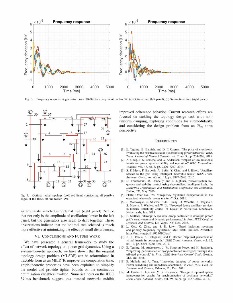
We next considered the radial topology design problemwith E composed of all edges in the IEEE 39-bus network.The optimal cost obtained after solving the MILP in this casewas 1.669, and the time required to find the optimal treewas close to 2 hours. Considering that the problem needsto be solved once off-line, this running time may not be ofconcern. Figure 4 shows the optimal radial topology that wasidentified.

Instead of using the bounds of Lemma 3 and the boundtightening procedure of Section IV-C, we attempted to solvethe same MILP with the relatively looser bounds of 0 ≤X∗ij ≤ 10 for all (i, j) ∈ V . In this case, the solver reachedthe optimality gap of 60% after running for 3 hours. Clearly,having tighter bounds improves the computation time.

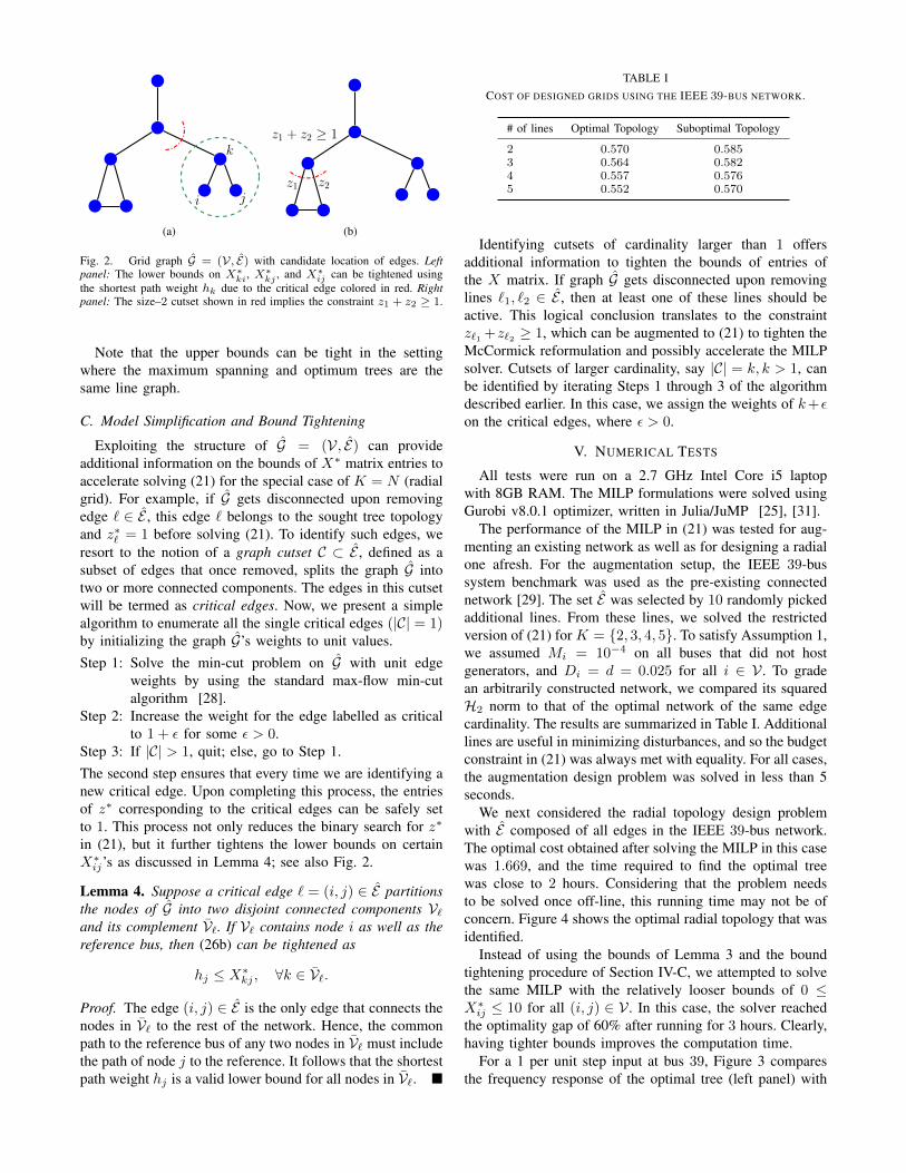
For a 1 per unit step input at bus 39, Figure 3 comparesthe frequency response of the optimal tree (left panel) with

0 1000 2000 3000 4000 5000Time [ms]

-1

0

1

2

3

4

5

6F

req

ue

ncy d

evia

tio

n [

Hz]

×10-3 Frequency response

0 1000 2000 3000 4000 5000Time [ms]

-1

0

1

2

3

4

5

6

Fre

qu

en

cy d

evia

tio

n [

Hz]

×10-3 Frequency response

Fig. 3. Frequency response at generator buses 30–39 for a step input on bus 39: (a) Optimal tree (left panel); (b) Sub-optimal tree (right panel).

Fig. 4. Optimal radial topology (bold red lines) considering all possibleedges of the IEEE 39-bus feeder [29].

an arbitrarily selected suboptimal tree (right panel). Noticethat not only is the amplitude of oscillations lower in the leftpanel, but the generators also seem to drift together. Theseobservations indicate that the optimal tree selected is muchmore effective at minimizing the effect of small disturbances.

VI. CONCLUSIONS AND FUTURE WORK

We have presented a general framework to study theeffect of network topology on power grid dynamics. Using asystem-theoretic approach, we have shown that the originaltopology design problem (MI-SDP) can be reformulated intractable form as an MILP. To improve the computation time,graph-theoretic properties have been exploited to simplifythe model and provide tighter bounds on the continuousoptimization variables involved. Numerical tests on the IEEE39-bus benchmark suggest that meshed networks exhibit

improved coherence behavior. Current research efforts arefocused on tackling the topology design task with non-uniform damping, exploring conditions for submodularity,and considering the design problem from an H∞-normperspective.

REFERENCES

[1] E. Tegling, B. Bamieh, and D. F. Gayme, “The price of synchrony:Evaluating the resistive losses in synchronizing power networks,” IEEETrans. Control of Network Systems, vol. 2, no. 3, pp. 254–266, 2015.

[2] A. Ulbig, T. S. Borsche, and G. Andersson, “Impact of low rotationalinertia on power system stability and operation,” IFAC ProceedingsVolumes, vol. 47, no. 3, pp. 7290–7297, 2014.

[3] S. P. Meyn, P. Barooah, A. Busic, Y. Chen, and J. Ehren, “Ancillaryservice to the grid using intelligent deferrable loads,” IEEE Trans.Automat. Contr., vol. 60, no. 11, pp. 2847–2862, 2015.

[4] D. Trudnowski, M. Donnelly, and E. Lightner, “Power-system fre-quency and stability control using decentralized intelligent loads,” inIEEE/PES Transmission and Distribution Conference and Exhibition,Dallas, TX, May 2006.

[5] FERC Order No. 755, “Frequency regulation compensation in theorganized wholesale power markets,” Oct. 2011.

[6] J. Matevosyan, S. Sharma, S.-H. Huang, D. Woodfin, K. Ragsdale,S. Moorty, P. Wattles, and W. Li, “Proposed future ancillary servicesin Electric Reliability Council of Texas,” in PowerTech, Eindhoven,Netherlands, Jun. 2015.

[7] E. Mallada, “iDroop: A dynamic droop controller to decouple powergrid’s steady-state and dynamic performance,” in Proc. IEEE Conf. onDecision and Control, Las Vegas, NV, Dec. 2016.

[8] L. Guo, C. Zhao, and S. H. Low, “Graph laplacian spectrumand primary frequency regulation,” Mar. 2018. [Online]. Available:https://arxiv.org/pdf/1803.03905.pdf

[9] B. K. Poolla, S. Bolognani, and F. Dorfler, “Optimal placement ofvirtual inertia in power grids,” IEEE Trans. Automat. Contr., vol. 62,no. 12, pp. 6209–6220, Dec. 2017.

[10] E. Tegling, M. Andreasson, J. W. Simpson-Porco, and H. Sandberg,“Improving performance of droop-controlled microgrids through dis-tributed pi-control,” in Proc. IEEE American Control Conf., Boston,MA, Jul. 2016.

[11] E. Mallada and A. Tang, “Improving damping of power networks:Power scheduling and impedance adaptation,” in Proc. IEEE Conf. onDecision and Control, Orlando, FL, Dec. 2011.

[12] M. Fardad, F. Lin, and M. R. Jovanovic, “Design of optimal sparseinterconnection graphs for synchronization of oscillator networks,”IEEE Trans. Automat. Contr., vol. 59, no. 9, pp. 2457–2462, 2014.

[13] T. Summers, I. Shames, J. Lygeros, and F. Dorfler, “Topology designfor optimal network coherence,” in Proc. IEEE European ControlConf., Linz, Austria, Jul. 2015.

[14] A. Ghosh, S. Boyd, and A. Saberi, “Minimizing effective resistanceof a graph,” SIAM review, vol. 50, no. 1, pp. 37–66, 2008.

[15] H. Nagarajan, P. R. Pagilla, S. Darbha, R. Bent, and P. P. Khargonekar,“Optimal configurations to minimize disturbance propagation in man-ufacturing networks,” in Proc. IEEE American Control Conf., Seattle,WA, May 2017.

[16] G. Cavraro, V. Kekatos, and S. Veeramachaneni, “Voltage analytics forpower distribution network topology verification,” IEEE Trans. SmartGrid, 2018 (early access).

[17] G. Cavraro and V. Kekatos, “Inverter Probing for Power DistributionNetwork Topology Processing,” Feb. 2018. [Online]. Available:https://arxiv.org/pdf/1802.06027.pdf

[18] D. Deka, S. Backhaus, and M. Chertkov, “Structure learning in powerdistribution networks,” IEEE Trans. Control of Network Systems,vol. 5, no. 3, pp. 1061–1074, Sep. 2018.

[19] D. Deka, H. Nagarajan, and S. Backhaus, “Optimal topology designfor disturbance minimization in power grids,” in Proc. IEEE AmericanControl Conf., Seattle, WA, May 2017.

[20] P. Kundur, Power system stability and control. New York, NY:McGraw-Hill, 1994.

[21] B. Bamieh, M. R. Jovanovic, P. Mitra, and S. Patterson, “Coherencein large-scale networks: Dimension-dependent limitations of local

feedback,” IEEE Trans. Automat. Contr., vol. 57, no. 9, pp. 2235–2249, Sep. 2012.

[22] S. P. Boyd and C. Barratt, Linear Controller Design: Limits ofPerformance. Upper Saddle River, NJ: Prentice-Hall, 1991.

[23] S. Boyd and L. Vandenberghe, Convex Optimization. New York, NY:Cambridge University Press, 2004.

[24] G. P. McCormick, “Computability of global solutions to factorablenonconvex programs: Part I- convex underestimating problems,” Math-ematical programming, vol. 10, no. 1, pp. 147–175, 1976.

[25] L. Gurobi Optimization, “Gurobi optimizer reference manual,” 2018.[Online]. Available: http://www.gurobi.com

[26] T. H. Cormen, Introduction to algorithms. MIT press, 2009.[27] D. Deka, S. Backhaus, and M. Chertkov, “Learning topology of

distribution grids using only terminal node measurements,” in Proc.IEEE Intl. Conf. on Smart Grid Commun., Nov. 2016.

[28] L. R. Ford and D. R. Fulkerson, “Maximal flow through a network,”Canadian Journal of Mathematics, vol. 8, pp. 399–404, 1956.

[29] A. Pai, Energy function analysis for power system stability. NewYork, NY: Springer Science & Business Media, 2012.

[30] J. Bezanson, A. Edelman, S. Karpinski, and V. Shah, “Julia: A freshapproach to numerical computing,” SIAM Review, vol. 59, no. 1, pp.65–98, 2017.

[31] I. Dunning, J. Huchette, and M. Lubin, “Jump: A modeling languagefor mathematical optimization,” SIAM Review, vol. 59, no. 2, pp. 295–320, 2017.