Embed Size (px)
Citation preview
Designing Sustainable Coastal Habitats
STAC Workshop Report
April 16-17, 2013
Easton, Maryland
STAC Publication 14-003

About the Scientific and Technical Advisory Committee The Scientific and Technical Advisory Committee (STAC) provides scientific and technical
guidance to the Chesapeake Bay Program (CBP) on measures to restore and protect the
Chesapeake Bay. Since its creation in December 1984, STAC has worked to enhance scientific
communication and outreach throughout the Chesapeake Bay Watershed and beyond. STAC
provides scientific and technical advice in various ways, including (1) technical reports and
papers, (2) discussion groups, (3) assistance in organizing merit reviews of CBP programs and
projects, (4) technical workshops, and (5) interaction between STAC members and the CBP.
Through professional and academic contacts and organizational networks of its members, STAC
ensures close cooperation among and between the various research institutions and management
agencies represented in the Watershed. For additional information about STAC, please visit the
STAC website at www.chesapeake.org/stac.
Publication Date: March, 2014
Publication Number: 14-003
Suggested Citation:
STAC (Chesapeake Bay Program Scientific and Technical Advisory Committee). 2014.
Designing Sustainable Coastal Habitats. STAC Publ. No. 14-003, Edgewater, MD. pp. 74.
Contributing authors: D. Bilkovic (VIMS), J. Greiner (USFWS-CBPO), J. Horan (USFWS),
Q. Stubbs (USGS-CBPO)
Cover photos courtesy of: Karen Duhring (VIMS)
Mention of trade names or commercial products does not constitute endorsement or
recommendation for use.
The enclosed material represents the professional recommendations and expert opinion of
individuals undertaking a workshop, review, forum, conference, or other activity on a topic or
theme that STAC considered an important issue to the goals of the Chesapeake Bay
Program. The content therefore reflects the views of the experts convened through the STAC-
sponsored or co-sponsored activity.
STAC Administrative Support Provided by:
Chesapeake Research Consortium, Inc.
645 Contees Wharf Road
Edgewater, MD 21037
Telephone: 410-798-1283; 301-261-4500
Fax: 410-798-0816
http://www.chesapeake.org

1
Table of Contents
Steering Committee…………………………………………………………………………..2
Executive Summary…………………………………………………………………………..2
Introduction …………………………………………………………………………………10
Ecosystem Components of Coastal Habitats………………………………………………...14
Capacity of Coastal Habitat to Support Fauna and Flora…………………………………....36
Designing Sustainable Coastal Habitats in the Face of Human Development, Climate Change,
and Sea Level Rise…………………………………………………………………………...45
Summary of Workshop Findings and Recommendations……………………………………60
References……………………………………………………………………………………65
Appendix A – Workshop Participants..………………………………………………………70
Appendix B – Additional Resources...……………………………………………………….72
Appendix C – Workshop Agenda……………………………………………………………73

2
Steering Committee:
Alicia Berlin, U.S. Geological Survey, Patuxent Wildlife Research Center
Donna Bilkovic, Virginia Institute of Marine Science
Pat Devers, U.S. Fish and Wildlife Service
Matthew Ellis, Chesapeake Research Consortium
Natalie Gardner, Chesapeake Research Consortium
Jennifer Greiner, U.S. Fish and Wildlife Service
Jeff Horan, U.S. Fish and Wildlife Service
Lee Karrh, Maryland Department of Natural Resources
Bernie Marczyk, Ducks Unlimited
Mary Ann Ottinger, University of Maryland
Walter Priest, National Oceanic and Atmospheric Administration
Quentin Stubbs, U.S. Geological Survey
Executive Summary
In response to a request from the Chesapeake Bay Program’s (CBP) Protect and Restore Vital
Habitats Goal Implementation Team (GIT 2), the CBP’s Scientific and Technical Advisory
Committee (STAC) sponsored a workshop on April 16-17, 2013 to explore approaches for
designing coastal landscapes in the Chesapeake Bay watershed through restoration and
protection of habitats that will be sustainable in the face of multiple stressors affecting coastal
ecosystems. Workshop presentations and discussions were organized around three themes:
Theme I: Ecosystem Components of Coastal Habitats; Theme II: Capacity of Coastal Habitats
to Support Fauna and Flora; and Theme III: Designing Sustainable Coastal Habitats in the Face
of Human Development, Climate Change, and Sea Level Rise (SLR). Workshop participants

3
made numerous recommendations and reached consensus on the following five key
recommendations:
1. Institute a more balanced approach to Chesapeake Bay restoration by integrating water quality,
habitat, and ecosystem-based species goals. The collective effort to restore health to the
Chesapeake Bay and its watershed must include a focus on restoration and protection of a variety
of habitat types, in addition to water quality. In recent years, substantial efforts to identify and
implement nutrient and sediment reduction measures required under the Total Maximum Daily
Load (TMDL) regulation under Section 303(d) of the Clean Water Act have resulted in a shift in
focus away from the flora and fauna of the Chesapeake, along with a multitude of ecosystem
services provided by the watershed’s many habitats including wetlands, forests, submerged
aquatic vegetation (SAV) beds, shellfish reefs, mud flats, and beaches. Currently, there is no
clear road-map for how coastal habitat restoration and protection activities should be prioritized
and implemented to meet Bay-wide restoration goals. However, the President’s Executive Order
(EO) Strategy (USEPA 2010a), combined with the evolution of state Watershed Implementation
Plans (WIPs) under the TMDL, have created significant opportunities to collaborate on efforts to
address water quality, but also to restore and protect species habitat. To capitalize on these
opportunities, messaging and focus must make a corresponding shift to clearly show how efforts
to restore specific Chesapeake Bay living resources can positively impact the lives of the people
who live and work in the watershed. Workshop participants agreed that by linking water quality
and habitat management objectives to species that are meaningful to people and representative of
key ecosystem services, the CBP can significantly enhance partnerships and advance public
understanding and support of Bay restoration goals, including water quality, habitat, and species
goals.
4
2. Expand the spatial and temporal scales used to set Bay restoration/conservation targets.
Currently, many restoration activities and shoreline management decisions occur on a parcel-by-
parcel basis, or at individual habitat patch-sized scales with limited consideration for system-
level processes or conditions such as hydrogeomorphology or ecological connectivity (Bilkovic
2013). Expanding the spatial perspective to consider landscape-scale patterns and processes is
necessary to maintain resiliency and production in the greater Bay ecosystem. Landscapes are
composed of a mosaic of habitat patches (fundamental units of landscapes, e.g., marsh) that are
surrounded by a complex terrestrial and aquatic matrix of natural and human-influenced features
with linkages between habitat patches, called corridors (Bilkovic 2013). The size of a landscape
is highly dependent on the species, taxa group, or process of interest, but generally is at an
intermediate spatial scale between local microscales, and regional or global macroscales
(Dunning et al. 1992). Conservation efforts and planning are hampered without a clear
understanding of both local and landscape-level influences on species distribution and ecosystem
resilience. For this reason a recommendation was made to conduct habitat restoration on a
tributary scale, to manage for both species and habitat diversity across a continuum of spatial
scales (ecosystem – landscape – small watershed – tributary – Bay-wide). This is consistent with
zoning and habitat recommendations from previous STAC workshops, including shale gas
development impacts (STAC 2013). For landscape-scale conservation planning and design to be
successful, both regional and local data are important. A Bay-wide synthesis of existing spatial
data relevant to habitat restoration and a prioritized list of information needs should be generated
to support efforts to design sustainable coastal landscapes. For example, there is a significant
deficiency in data on shallow water bathymetry and sediment properties, which are major
baseline data needed to identify and evaluate restoration areas in the Bay. Expanding the
5
temporal perspective will be necessary to consider impacts of climate and land use change, both
of which have the potential to greatly influence conservation or restoration actions in the Bay.
The mid-Atlantic region along the East Coast of the United States, including the Chesapeake
Bay, has been identified as a “hotspot” of accelerated SLR (Sallenger et al. 2012), which may be
due to changes in ocean dynamics, such as a weakening Gulf Stream (Ezer 2013). To effectively
assess progress and attainment of Bay habitat restoration goals, the goals should be clearly linked
to a specific planning horizon and management actions need to be carefully monitored and
evaluated to measure ecosystem change, along with habitat- and species-based outcomes.
Multiple planning windows may be used to accommodate near-term goals of sustaining existing
ecosystem services and allow for the consideration of climate or land use change over longer-
time horizons. This corresponds with CBP Management Board (MB) recommendations in the
spring of 2013 to the Principles Staff Committee (PSC) to consider climate change in the new
Bay Watershed agreement, since removed.
3. Align differing and complex objectives for management of living resources using an adaptive
management (AM) framework, such as Structured Decision Making (SDM) and Strategic Habitat
Conservation (SHC). Adaptive management is a structured, iterative process of science-based
decision making, with an aim to reduce uncertainty over time by carefully monitoring outcomes,
transparently assessing progress, and redirecting efforts when necessary. The CBP needs to
apply an AM approach to identify and manage key components of coastal ecosystems in a way
that aligns implementation and monitoring of restoration activities with living resource
objectives, such as to conserve or increase populations of black duck (and other waterbirds),
diamondback terrapin, blue crab, and anadromous fish. This will require investing in
technologies to close gaps in existing data needs, designing habitat complexes at larger scales,

6
and setting goals that consider lag-times in habitat recovery. Two specific AM approaches
should be used within the Chesapeake Bay watershed to make science-based management
decisions at multiple scales. Structured Decision Making (SDM) is an objective framework
intended to create a logical and transparent process for making informed conservation and
management decisions and for helping to evaluate processes and thresholds (Martin et al. 2009).
Strategic Habitat Conservation (SHC) is an adaptive management approach recently adopted by
the U.S. Fish and Wildlife Service (USFWS, NEAT 2006). The premise of SHC is to maximize
the conservation benefit of limited resources by allocating them to programs, areas, and activities
that have the greatest influence on our biological targets. SHC (Walters 1986) comprises 4 steps
in an iterative cycle (Fig. 1): Biological Planning, Conservation Design, Delivery of
Conservation Actions, and Monitoring and Research. The guiding principles of SHC are (NEAT
2006):
Habitat conservation is a means to attaining desired abundance and distribution of
wildlife;
Defining measurable population objectives is critical;
Biological planning is based on the best available science;
Management actions, decisions, and recommendations must be defensible and
transparent; and
Conservation strategies must by dynamic.

7
Figure 1. Conceptual framework and process of Strategic Habitat Conservation (NEAT 2006).
Surrogate species are considered a critical part of the Biological Planning phase of SHC.
Conservation biologists often use one or a small number of species to address broader
conservation needs (Caro and O’Doherty 1999). Conservationists often work in complex and
dynamic systems over large spatial areas and long temporal periods, making it impossible for
biologists to understand or plan for the requirements of all species or ecological components.
The surrogate species paradigm assumes that a subset of species can serve as surrogates for the
larger suite of species, and help inform the targeted allocation of limited conservation resources
(e.g., personnel time and money). Consequently, the selection of appropriate surrogate species is
considered an initial first step of the Biological Planning phase of SHC (NEAT 2006). When
doing conservation design and assessing ecosystems at a landscape scale, however, it is
appropriate to pair the surrogate species approach with a coarse filter approach that assesses

8
ecological integrity as applied to a suite of ecological systems. McGarigal et al. (2012) defines
“ecological integrity” as the capability of an area to sustain ecological functions over the long-
term, especially in the face of disturbance and stress (in this case, human development and
climate change). Surrogate species are used as a fine filter to evaluate the impact of climate and
other stressors on “habitat capability,” which refers to the ability of the environment to provide
local resources, such as food and cover, needed for survival and reproduction in sufficient
quantity, quality, and accessibility to meet the life history requirements of individuals and local
populations (McGarigal et al. 2012). The recommendations for implementing AM are consistent
with previous STAC workshop and review report recommendations (STAC 2011, 2012) as well
as recommendations from the National Research Council (NCR 2011).
4. Initiate a pilot study of landscape-scale restoration approaches. SDM and SHC should be used
to apply the latest science to landscape design in pilot areas in Chesapeake Bay. Workshop
participants suggested that the entire Delmarva Peninsula may be the appropriate geographic
scale for using these approaches to design and implement coastal habitat conservation efforts.
This geographic scale would allow biological planning and habitat restoration to occur at an
optimal scale to measure ecosystem, habitat, and meta-population response. SDM is well suited
for large-scale complex projects because it is a collaborative and facilitated application of
multiple-objective decision making and group deliberation methods applied to environmental
management and public policy (Gregory et al. 2012). Regional-scale models that accurately
reflect local and landscape-scale patterns and processes (e.g., relative sea level rise, sediment
accretion rates, habitat configuration and composition within a landscape), should be applied to
make predictions about a changing ecosystem and inform actions at a sub-watershed or local
scale. Such a pilot study would create the opportunity for restoration partners from a number of

9
CBP Goal Implementation Teams (GITs), with overlapping conservation goals, to collaborate
closely on restoration planning, targeting, and implementation. The CBP must also evaluate
trends in habitat suitability related to hydrogeological settings, and specifically model
environmental flow requirements that have been found to be particularly crucial in evaluating the
resiliency of aquatic systems and organisms.
5. CBP should encourage better dialogue and data/tool sharing among restoration partners by
forming a Habitat Modeling workgroup to facilitate data synthesis, coordination, and regional
model development. Rich data and powerful targeting tools exist to help identify the most
resilient and sustainable coastal habitats. These prioritization tools, and the data needed to drive
them, are important since it is not possible to protect or restore all coastal habitats. States and
communities have used these tools to purchase at-risk areas and turned them into conservation
areas where the public understands the need, supports the purchase, and helps maintain the area
for their own use, and to benefit the ecosystem. The Habitat Modeling workgroup would be
charged with:
Guiding the synthesis of available regional and local data/models to inform
targeting of sustainable coastal landscapes for restoration or protection;
Identifying information gaps and research needs;
Providing guidance to Goal Implementation Teams and Bay partners on data and
models suitable for conservation design and specific habitat restoration; and
Developing metrics and translating ecosystem service values into economic terms
that decision makers, partners, and the public can understand and act upon.
When considering conservation at this scale, the CBP’s restoration partners and the GITs that are
coordinating conservation efforts need to leverage existing resources and efforts by reaching out
10
to relatively new organizations focused on assessing the impacts of climate change, such as the
Landscape Conservation Cooperatives (LCCs) facilitated by USFWS and the climate science
centers within USGS (U.S. Geological Service), NOAA (National Oceanic and Atmospheric
Administration), and USDA (U.S. Department of Agriculture) to obtain regionally consistent data,
models, and decision support tools.
Introduction
Jeffrey Horan (USFWS) described the purpose of the Designing Sustainable Coastal Habitats
workshop and the approach the workshop steering committee used to bring together scientists,
habitat restoration partners, and policy makers to address three goals. The three workshop goals
or themes were to:
1. Assess the current status and trending condition of coastal ecosystems in the
Chesapeake Bay watershed;
2. Assess the capacity of coastal habitats to support flora and fauna; and
3. Identify and target for restoration and protection those coastal habitats that will
be sustainable under increasing human impacts and a changing climate.
These goals will elucidate where coastal habitat restoration provides the greatest return on
investment while considering habitats most vulnerable to climate change and human
development. Coastal ecosystems, because of their landscape position at the boundary of land
and sea, provide habitat for birds, mammals, reptiles, fish, shellfish, and amphibians and they
provide critical nursery areas for birds, fish, and shellfish (Fig. 2). Coastal habitats are integrated
ecological units within dynamic landscape mosaics that are structurally and functionally
connected (Bilkovic 2013). These wetland complexes serve as powerful natural filters of
nutrients and other contaminants while providing the added benefit of protecting inland areas

11
from storm surge. However, because of their landscape position they are often extremely
vulnerable to climate change (particularly sea level rise) and impacts from human development.
Figure 2. Coastal habitats of Chesapeake Bay. The location of estuarine and freshwater tidal wetlands is
based on U.S. Fish and Wildlife National Wetlands Inventory geospatial data and includes wetlands with
emergent vegetation and unvegetated intertidal areas (mudflats) in the coastal plain. “Seagrass 2012” is
the distribution of submersed aquatic vegetation (SAV) beds determined in 2012 by the Virginia Institute
of Marine Science Submerged Aquatic Vegetation program.
12
Horan suggested that integrated targeting of coastal wetland, living shoreline, and SAV
restoration and protection among CBP partners will extend limited funding and human resources
and maximize ecological benefits. This integrated approach will be necessary, since the CBP’s
current goal for wetland restoration and protection is 30,000 acres, based on current progress of
all six of the Bay watershed states and Washington, D.C. (i.e., 30,000 acres of wetland
restoration is also referenced in the federal EO strategy, USEPA 2010a). However, a recent
Environmental Protection Agency (EPA) cumulative of state Phase II WIP Best Management
Practices (BMPs) calls for a total of 83,003 acres of agricultural wetland restoration in the
watershed. This would require almost a tripling of the current program effort devoted to wetland
restoration and protection. By adding in cumulative WIP goals for urban wetland and wet pond
facilities, an additional 94,549 acres of wetlands are called for by 2025 (total 177,551 acres of
wetland restoration by 2025 in Phase II WIPs). Note: the creation of urban wetland and wet
ponds facilities provide water quality benefits, but often provide very little habitat benefit.
This additional effort in wetland restoration and protection above current program progress
presents both a serious challenge for the states and CBP partners, as well as a significant
opportunity. CBP partners need to capitalize on the opportunity to increase capacity to target
wetland creation in locations where they provide the greatest benefit for species and for water
quality. Horan previewed a number of resource ranking and targeting approaches that may be
appropriate for use by partners in coastal ecosystems. The approaches were used in the Harris
Creek watershed assessment and included Maryland Department of Natural Resources’
(MDDNR) Targeted Ecological Areas (http://www.greenprint.maryland.gov/), Coastal Atlas and
BioNet (http://www.bionet.nsw.gov.au/), along with EPA’s Watershed Resources Registry

13
(http://watershedresourcesregistry.com/overview.html). Each of these approaches, along with
others, was discussed in more detail at the workshop.
Workshop speakers delineated and discussed the various components of coastal habitats.
Workshop participants then debated whether modeling select individual species could serve as
surrogates for species groups that have similar habitat requirements and sensitivities to human
development, SLR, and climate impacts. Participants specifically looked at extensive habitat
mapping and habitat suitability work being done on black duck and diamondback terrapin to see
how modeling these species might help set benchmarks for significant ecological associations
and types. The steering committee proposed to explore how models for these species would
inform conservation design for other species that use similar habitat.
Finally, the workshop participants discussed the CBP’s ability to compile data and build broader
ecosystem-based models and targeting tools to design sustainable coastal habitats in the face of
human development and climate change. Prior to the workshop, the steering committee
developed a series of scientific questions that related to these topics, along with specific
outcomes the workshop hoped to generate. These questions and outcomes, organized by the
three workshop themes, were distributed to speakers and participants well in advance, so
speakers could incorporate these elements into their presentations and to facilitate productive
discussions around clearly defined and focused topics during the workshop. The workshop then
used the significant knowledge of its participants and the information provided by speakers to
recommend scientific approaches, targeting tools, and specific actions to protect and restore
coastal habitats.
The workshop built on work done in previous workshops including:
U.S. Fish and Wildlife Service Salt Marsh Integrity Workshop (2012)
http://www.fws.gov/fieldnotes/regmap.cfm?arskey=34100
14
Previous STAC Wetlands and SAV Workshops (2001, 2007)
http://www.chesapeake.org/pubs/wetlandsreportweb.pdf
http://www.chesapeake.org/pubs/SAVReport.pdf
STAC Climate Change Workshop (2011)
http://www.chesapeake.org/pubs/287_Pyke2012.pdf
Theme I: Ecosystem Components of Coastal Habitats
The first theme of the workshop addressed the ecosystem components and functions of
Chesapeake Bay coastal habitats with a focus on wetlands and SAV, and the current and trending
condition of those habitats placed in context of a changing system that is increasingly susceptible
to human impacts and climate change.
Coastal habitats are located within freshwater and saltwater environments of watersheds that
drain into the Atlantic, Pacific, or Gulf of Mexico and can be defined by a variety of structural
and functional characteristics. Coastal watersheds can extend many miles inland from the coast.
In the Chesapeake Bay, important coastal habitats include: oyster reefs and coastal wetlands
comprised of tidal and nontidal vegetated emergent wetlands, tidal flats, beaches, and SAV.
These habitats interact as integrated ecological units within dynamic landscape mosaics that are
structurally and functionally connected. Coastal wetlands can be classified into geomorphic
settings which have differing hydrodynamics, sediment sources, vegetative communities, and are
expected to have varying responses to pressures such as SLR (CCSP 2009).
Summary of Theme I Presentations
Donna Bilkovic (VIMS) estimated that there are currently close to 575,000 hectares (ha) of
coastal wetlands in Chesapeake Bay. Nontidal coastal wetlands make up a large percentage of
this number with ~400,000 ha. The majority of nontidal wetlands in Maryland (MD) and

15
Virginia (VA) are located in the coastal plain (MD - 90%; VA - 64%) (Brooks et al. 2013). The
highest concentrations of tidal freshwater wetlands in the United States are found in the mid-
Atlantic and southeastern regions, where numerous well-mixed estuaries occur: Chesapeake Bay
possesses a large proportion of these wetland types with ~26,000 ha in MD and VA (after Mitsch
and Gosselink 2000). Lastly, the Bay contains ~151,000 ha of brackish and salt marsh (National
Wetlands Inventory (NWI; imagery dates were from 1995-1998 for MD and 1990-2000)).
Bilkovic then discussed climate and environmental factors that influence the ability of coastal
wetlands to persist under changing conditions, and how these factors interact and act in non-
linear ways. Drivers were placed under the umbrella of two overarching threats to habitat
persistence in the near- and long-term: coastal development and climate change (i.e., SLR,
elevated temperatures, changing salinities, etc.). In terms of coastal development of the
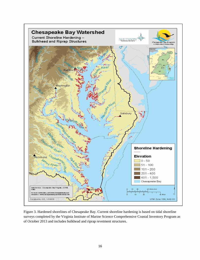
Chesapeake Bay, Bilkovic reported that 18% of the Bay’s tidal shoreline is hardened (Fig. 3)
and 32% of riparian land has been developed. Bilkovic shared examples of adverse effects of
shoreline hardening and riparian development to coastal systems including non-linear negative
responses by estuarine flora and fauna to shorelines with greater than 15-20% development
(DeLuca et al. 2004, King et al. 2007, Bilkovic and Roggero 2008, DeLuca et al. 2008).
Bilkovic emphasized the need for pro-active planning of entire communities, and their shoreline
protection needs, in advance of parcel development with considerations for functional and
structural losses, as well as the use of living shoreline alternatives. Future development and
shoreline protection is anticipated to intensify and only 7% of coastal lands have been set aside
for conservation. Almost 45% of the land is expected to be developed, thus unavailable for the
inland migration of coastal habitats (Titus et al. 2009).
16
Figure 3. Hardened shorelines of Chesapeake Bay. Current shoreline hardening is based on tidal shoreline
surveys completed by the Virginia Institute of Marine Science Comprehensive Coastal Inventory Program as
of October 2013 and includes bulkhead and riprap revetment structures.

17
To predict system-wide shifts in wetlands due to climate change, Bilkovic recommended data on
local drivers and processes controlling wetland elevation, such as sediment accretion rate across
different geomorphic settings, be integrated into broader scale regional models. Using a
geomorphic framework, Titus and others (CCSP 2009) estimated the likelihood of conversion of
tidal wetlands to open water for differing SLR scenarios. In their estimation, tidal fresh marshes
and forests are less likely to be converted to open water even under high rates of SLR, while
there is significant uncertainty for the large category of estuarine marshes because local
conditions are determining likelihood of persistence, due to rates of subsidence. Bilkovic
reviewed recent studies that examined local processes that may influence wetland vertical
development including ecogeomorphic feedbacks of climate change and nutrient enrichment.
These studies suggested that SLR in excess of 4.5 mm/yr. will cause any positive feedback effect
of increased temperature, CO2, and inundation on plant productivity to be diminished or lost and
marshes to subside (Kirwan and Mudd 2012). In addition, nutrient pollution may increase marsh
vulnerability to SLR (Deegan et al. 2012). Notably, many regions of the Bay (e.g., Southeast
Virginia) are already experiencing SLR in excess of the 4.5 mm/yr. threshold rate. Bilkovic
emphasized the need to move towards conservation of an ecologically connected network of
terrestrial, freshwater, coastal, and marine areas that are likely to be resilient to climate change.
This will entail the use of landscape-level decision support tools that integrate site or geomorphic
descriptions and a better understanding of landscape connectivity effects on wetland ecology and
associated estuarine species diversity, composition, and distribution.
Jeffrey Halka (MGS) described sediment delivery in coastal systems from both geological time-
scale and modern perspectives with consideration for current dominant anthropogenic influences.
Halka presented evidence that nearshore erosion continues even after a revetment is placed on

18
the shore, and that in some Maryland sites, erosion was similar offshore along revetment and
natural shorelines. In general, the microtidal Bay system restricts sediment movement, with
periodic drastic changes by storms. Sediment loads are affected by drought and timing of storms
can mitigate the impact from turbidity. For example, Tropical Storm Lee in 2011 generated
significant turbidity, but because the storm occurred in the fall following the growing season, the
impact to SAV was limited.
The contributing sources of sediment have changed over 10,000 years and there is a need for a
mass balance estimate of sediment. Oceanic sediment input clearly dominated in the past
(Colman et al. 1992) supplying coarser-grained material near the mouth of the Bay. More
recently, the input source is likely still significant (Hobbs et al. 1992) and may supply sediments
as far up-Bay as Tangier Sound (Newell et al. 2004). In select areas, immediately downstream
of the fall line, sand continues to be deposited in ‘deltas,’ such as the Susquehanna Flats. The
turbidity maximums in the mainstem of the Chesapeake as well as its tributaries are traps for the
majority of fine grained sediment, with the balance of fine sediments being deposited in the deep
axial mainstem and tributary channels (Byrne et al. 1982; Kerhin et al. 1988). In the low-mid
estuary, shore sediment sources dominate composed of various mixtures of sands, silts, and clays
depending on the coastal plain sediments comprising the shoreline. Sediment deposition rates on
the platforms located between the nearshore zone and the deeper axial channels approximate the
long-term rate of SLR (~1-2 mm/yr) (Colman et al. 1992). Particularly in the nearshore areas
and on the platforms, if the proximate and dominant source of sediment is lost, deposition will
generally be reduced.
In-Young Yeo (UMD) discussed the need for improvements in mapping and monitoring wetland
dynamics for improved resilience and delivery of ecosystem services in the mid-Atlantic region

19
and the Chesapeake Bay watershed. Accurate, dynamic wetland maps can improve society’s
resilience to increasing urbanization, population growth, and climate change through early
detection, improved understanding of climate change and land cover/land use change effects, and
enhanced management of wetlands to target desired ecosystem services.
The primary land cover data that are available on wetlands in the Bay are the NWI and the
following land cover data sets: the National Land Cover Dataset (NLCD), the Coastal Change
Analysis Program (CCAP), and the Chesapeake Bay Watershed Land Cover Data Series
(CBLCD). One of the challenges in conducting time series analyses of these data sets is that
each dataset covers a range of different time periods, both yearly and seasonally. Land cover
mapping classification and mapping analyses use similar quantitative methods like the
Classification and Regression Tree (CART) and cross correlation analyses. All these data sets
incorporate ancillary data like the digital elevation model for topography. One of the most
challenging land cover types to map is forested wetlands, especially at moderate to high
resolutions.
Yeo indicated that geospatial research is needed to improve data availability, the spatial and
temporal resolutions of land use and land cover data, the accuracy of land cover models, and the
integration of land cover, socioeconomic, and wetland functional models into multi-scale
vulnerability assessments. Fundamental wetland data are lacking to conduct regional-scale
vulnerability assessments of wetlands and to identify hot spots and key drivers of wetland
losses. Available wetland maps are dated or often represent mosaics of multiple maps or
imagery with variations in dates of collection. For example, forested wetlands in the Bay
continue to sustain high levels of loss, and land cover classification techniques must be improved
to accurately differentiate forest cover from forested wetland cover. Existing wetland maps also

20
tend to not accurately represent wetland process and functions (e.g., hydroperiods), more
specifically variations in water levels due to climate change and land cover change from
development. Nutrient removal function is expressed differently by different wetland types (e.g.,
constructed wetlands).
Yeo, Stubbs, and others are currently conducting a spatial-temporal analysis of wetland loss and
vulnerability. The team is also developing improved wetland mapping and change detection
tools using remote sensing data from multiple complementary sensors at various temporal and
spatial scales. New technologies and techniques include the Landsat historic record (1984-
present), the North American Forest Dynamics with the Vegetation Change Tracker
(http://daac.ornl.gov/cgi-bin/dsviewer.pl?ds_id=1077) and Wetness Change Tracker (Yeo 2013),
and DEM (digital elevation model)-based topographic wetness indices that complement optical
data like Light Detection and Ranging (LiDAR). The team will then analyze socioeconomic,
policy, and physical drivers of wetland change that affect wetland extent and function on
regional to local scales. After assessing the impacts of multiple environmental stressors, the
team will quantify the vulnerability of wetlands and wetland ecosystem services under multiple
climate and land use scenarios.
Yeo compared existing Chesapeake Bay wetland databases to illustrate their limitations and
strengths. When comparing the 2007 USFWS land cover change report with 2006 CCAP and
CBLCD calculations of wetland cover, all data sets agree that there are approximately 80,000
acres of emergent wetlands. However, CCAP and CBLCD agree on forested wetland
coverage of approximately 175,000 acres, while the USFWS report lists 225,000 acres. When
looking at the spatial agreement between land cover data sets and NWI, approximately 71% of
NWI polygons agree with the location of wetlands in CCAP and CBLCD. When looking at the
21
agreement of CCAP and NWI, there is 83%, 65%, and 38% agreement between the two for
emergent wetlands, forested wetlands, and shrub/scrub wetlands, respectively. CBLCD agrees
with most NWI polygons, i.e., 85% emergent wetlands and 61% forested wetlands.
Finally, Yeo focused on how the results of their efforts may be applied to Bay restoration
activities. Improved, consistent, recent wetland maps will improve parameterization of the Bay
model and support ecosystem markets. Near-time tracking of wetland loss will enhance
regulatory abilities, and the location of critical areas for restoration and conservation. Regional
assessments for the Bay will integrate existing data sets with land cover and hydrodynamic
models to assess the ability of wetlands to improve water quality; currently, regional water
quality models like SPARROW do not simulate natural wetland processes. Additionally, the
team will evaluate the effectiveness and accuracy of the watershed process model (Soil and
Water Assessment Tool, SWAT) to simulate natural wetland processes and its water quality
improvement benefits at the watershed scale. The team will compile literature and field data to
evaluate the range of nutrient removal efficiency of wetlands, key functional drivers affecting the
removal efficiencies, and determine if it can be applied to watersheds in the Bay like the
Choptank River Watershed.
Lee Karrh (MDDNR) gave a brief introduction to SAV and its ecological importance, and then
discussed current conditions and trends in SAV abundance in the Chesapeake Bay. In 2012,
SAV communities, including an aggregate of species, covered approximately 19,500 ha of Bay
bottom, which represents 26% of the roughly 75,000 ha goal (Fig. 4). The goal acreage is based
upon the maximum extent of SAV ever observed in the Bay, in habitats ranging from freshwater
to saltwater, and was determined by analyzing aerial photographs from as far back as 1930
through 2001.

22
Figure 4. A map showing locations of SAV beds in 2012 (in gold), relative to the GIS layer used to create
the restoration goal (in green, also known as the 'Single Best Year' SAV layer).

23
Considering only Bay-wide coverage masks subtleties in the distribution data. SAV community
composition varies based on salinity, and over time the communities in differing salinity regimes
have shown different coverage patterns. SAV communities in the polyhaline region (salinity
>18) increased in coverage from the beginning of the modern Bay-wide annual aerial survey in
1984, peaked in 1993, and declined steadily since that time, punctuated with dramatic declines in
2005 and 2010 due to heat stress in eelgrass meadows and subsequent modest recoveries. For
the mesohaline region (salinity between 5 and 18), SAV coverage trends were similar to the
polyhaline reach, with populations increasing steadily from 1984 to 1993. From 1993 to 2002,
coverage was variable, with wide annual fluctuations, but coverage peaked in 2002. For the
oligohaline (salinity 0.5 to 5) and tidal fresh (salinity < 0.5), populations were at low levels
through the 80s and into the mid-90s, when coverage began to steadily increase in both salinity
regions, peaking in the oligohaline in 2005 and the tidal fresh in 2008. Both regions maintained
high levels until the wet spring and fall tropical storms of 2011 caused massive declines.
Overall, in the last 10 years, 21 individual bay segments have surpassed their restoration goals,
mostly in the tidal fresh and oligohaline regions, with an additional 4 segments close to their
SAV acreage goals.
Karrh went on to briefly discuss the persistence of SAV communities over time, highlighting
three areas: Susquehanna Flats, upper Potomac Rivers (tidal fresh and oligohaline), and the
Lower Bay (polyhaline) identifying specific locations always vegetated (Fig. 5). The two major
points of this discussion were: 1) even when there have been dramatic challenges to SAV (heat
stress in the Lower Bay, tropical storms in the upper Bay, general water quality issues), places
have remained vegetated and 2) it is these refuges that provide the materials necessary (seeds,
tubers, plant fragments etc.) to fuel re-vegetation when the stress is relieved.
24
Figure 5. A map showing the 4 major salinity zones of the Chesapeake Bay. The tidal fresh water area of
the Bay is shown in red, the low salinity (ologohaline) area in yellow, moderate salinity (mesohaline) in
light blue, and high salinity(polyhaline) areas shown in dark blue.
25
Karrh mentioned that the best ways to preserve and enhance SAV communities are to improve
water quality, protect existing beds (particularly the refugia identified above is also extremely
important), and where possible, use direct restoration (planting) both to fuel natural recovery as
well as inform research. Planting programs need to be carefully designed so as to learn as much
as possible for adaptive management and to refine our science regarding SAV restoration. Our
existing understanding of the relationship between SAV and water quality is sufficient for
explaining persistence or declines of existing SAV populations; however, it has become apparent
that better water quality conditions are necessary to shift from an unvegetated to vegetated state.
Karrh ended by mentioning proposed work to revise existing habitat requirements through
synthesizing recent scientific results.
Renee Karrh (MDDNR) presented results of water quality status and trends analyses in
Chesapeake Bay, relative to the five parameters identified as most important for SAV growth
and survival, water clarity (Secchi depth), concentrations of chlorophyll a (CHLA), total
suspended solids (TSS), dissolved inorganic phosphorous (DIP), and dissolved inorganic
nitrogen (DIN) in the water column (Batiuk et al. 1992). Like all plants, SAV requires sufficient
light penetrating through the water column and through any fouling on the leaf surface in order
to photosynthesize. Water column clarity is assessed using Secchi depth data, where higher
values indicate clearer water. Water column light penetration is adversely affected by increasing
concentrations of CHLA (a measure of the abundance of planktonic algae in the water) and TSS
(a measure of the amount of both abiotic and biogenic particles in the water). The light reaching
the plants through the water column is further attenuated by fouling at the plant leaves’ surface.
Increased concentrations of nutrients (DIN and DIP) allow fouling algae to grow on the leaves

26
(Kemp et al. 2004). Additionally, algae (CHLA) and particles (TSS) from the water column will
settle on the SAV leaves, blocking light from reaching the leaves’ surface.
Trends were presented for the period 1999-present (2011 in VA, 2012 in MD) using seasonal
Kendal and non-linear trend analyses. Status compared the median of the most recent 3 years of
data to habitat requirement values of Batiuk et al. (1992). Special focus was placed on areas
where the trend in an individual parameter is improving but habitat requirement is not met,
suggesting that conditions may improve to the point where the habitat would be suitable for
SAV. Conversely, areas where the habitat requirement is currently met, but the trend is
degrading suggest concern for loss of suitable habitat in the future. The results of the status and
trends of each of the five habitat requirements are presented below.
Water clarity: Water clarity is degrading (Secchi depth is shallowing over time) in the upper and
lower mainstem of the Bay and some smaller rivers, while improving in some other smaller
rivers. Water clarity in the upper and middle Potomac, upper Rappahannock, upper and middle
York, James, middle mainstem, and many smaller rivers fails to meet the habitat requirement
(Table 1). In three systems (Mattawoman Creek, Manokin, and Pocomoke Sound), water clarity
fails to meet the habitat requirement but conditions are improving. In one case (Maryland’s
lower mainstem Bay), water clarity currently meets the requirement, but the trend indicates that
conditions are degrading.
Chlorophyll a (CHLA): CHLA is degrading (concentrations are increasing) in the lower
Patuxent, middle and lower Potomac, upper mainstem Bay, and many smaller rivers. CHLA is
improving in some other smaller rivers. CHLA fails to meet the habitat requirement (Table 1) in
the upper Rappahannock, upper James, middle mainstem Bay, and many of the smaller rivers.
CHLA in the upper Bay (Susquehanna Flats), C&D Canal, Elk, middle and lower Potomac,
27
Little Choptank and lower Patuxent rivers currently meets the habitat requirement, but conditions
are degrading.
Total Suspended Solids (TSS): TSS is improving (concentrations are decreasing) in many areas
including the Patuxent, lower Potomac, upper Rappahannock, upper James, lower Choptank,
lower mainstem Bay, and several smaller rivers. Many areas meet the habitat requirement (Table
1), and there are several areas where the habitat requirement is not met but the trend is improving
(upper Patuxent, upper Rappahannock, middle Chester, and Sassafras Rivers). Conversely,
while Middle River currently meets the habitat requirement, TSS conditions are degrading.
Dissolved Inorganic Phosphorus (DIP): DIP is improving (concentrations are decreasing) in the
upper Patuxent, upper and middle Potomac, upper York, upper James, and several smaller rivers.
DIP is degrading in the middle York, the upper Gunpowder, and Bush Rivers. DIP fails to meet
the habitat requirement (Table 1) in the upper and middle Patuxent, middle Potomac, middle
Choptank, middle York, lower James, and several smaller rivers and the middle mainstem Bay.
While currently failing the habitat requirement, the upper Patuxent, Piscataway Creek, upper
Potomac River, Pocomoke, and C&D Canal have improving trends.
Dissolved Inorganic Nitrogen (DIN): Many areas have improving DIN conditions
(concentrations are decreasing), including the upper Patuxent, upper and middle Potomac, upper
York, and several small rivers and the upper mainstem Bay. There are no habitat requirements
for DIN in the oligohaline or tidal fresh parts of the Bay. The middle mainstem, Patapsco River,
and Elizabeth River fail to meet the DIN habitat requirement (Table 1). In the South Elizabeth
River, DIN currently fails to meet the habitat requirement but the trend is improving.
In summary, status and trends information for parameters affecting water column light
availability (Secchi, TSS, and CHLA) suggest that there is insufficient light to support SAV in
28
almost all rivers and mesohaline Bay. Almost all of tidal fresh and oligohaline areas fail habitat
requirements for Secchi and TSS. While TSS is improving in many areas, there are degrading
trends for Secchi and CHLA, especially in oligohaline and mesohaline segments. Nutrients (DIP
and DIN) are still too high in larger rivers (e.g., Potomac River and the James River) and some
segments of the eastern shore tributaries. There are improving trends in many rivers, though
phosphorus has degraded in some.

29
Salinity
Regime
(ppt)
SAV
growing
Season
Water Column
Light Requirement
Secchi Depth (m)*
Total
Suspended
Solids (mg/l)
Plankton
Chlorophyll-
a (µg/l)
Dissolved
Inorganic
Nitrogen
(mg/l)
Dissolved
Inorganic
Phosphorus
(mg/l)
Tidal Fresh
<0.5 ppt
April-
October
0.725 m
< 15 < 15
Not
applicable
(Nitrogen
Limitation
< 0.07)
< 0.02
Oligohaline
0.5-5 ppt
April-
October
0.725 m
< 15 < 15
Not
applicable
(Nitrogen
Limitation
< 0.07)
< 0.02
Mesohaline
5-18 ppt
April-
October
0.97 m
< 15 < 15
< 0.15
(Nitrogen
Limitation
< 0.07)
< 0.01
Polyhaline
>18 ppt
March-May,
Sept.-Nov.
0.97 m
< 15 < 15
< 0.15
(Nitrogen
Limitation
< 0.07)
< 0.02
Table 1. Information from Table 1 of Chesapeake Bay Submerged Aquatic Vegetation Water Quality and
Habitat-Based Requirements and Restoration Targets: A Second Technical Synthesis
http://archive.chesapeakebay.net/pubs/sav/savreport.pdf.
* Secchi Depth Habitat Requirements are for 1 meter restoration.

30
Lewis Linker (EPA-CBP) discussed how the CBP’s watershed model (CBWM) simulates SAV
growth based on water quality inputs that ultimately attenuate light. CBWM includes 6 sub-
models to develop a eutrophication model that then provides data into the SAV model. The SAV
model computes SAV density (mass/unit area) as a function of irradiance and nutrients.
Irradiance and epiphytes are calculated separately. The model interacts with water column and
bed sediments. SAV abundance is computed on a model sub-grid independent of the
hydrodynamic grid, with those sub-grid areas based upon observed SAV beds rather than
arbitrary computational elements. Sub-grid elements permit refined (more resolved) depth
increments for computation of available light.
Linker then gave a brief description of how the water quality standards (WQS) were developed
and how they are implemented into the CBWM. Water clarity WQS were assessed by starting
with measured area of SAV in each Bay segment for the 1993–1995 critical period. On the basis
of regressions of SAV versus load, the estimated SAV area, resulting from a particular nitrogen
(N) and phosphorus (P) or sediment load reduction, was estimated (USEPA 2010). Then the
estimated water clarity acres from the Bay Water Quality (WQ) model were added after
adjustment by a factor of 2.5, to convert the water clarity acres to water clarity equivalent SAV
acres (Linker 2013). Finally, the water clarity equivalent SAV acres were added to the
regression-estimated SAV acres and compared to the Bay segment-specific SAV WQS.
A strategy was developed to achieve WQSs by first setting the nutrient allocation for achieving
all the dissolved oxygen (DO) and CHLA WQSs in all 92 bay segments, and then making any
additional sediment reductions where needed to achieve the SAV WQS. That strategy was
supported by management actions in the watershed to reduce nitrogen and phosphorus loads.

31
Just as the SAV resource is responsive to N, P, and sediment loads, many management actions in
the watershed that reduce N and P also reduce sediment loads. Examples include conservation
tillage, farm plans, riparian buffers, and other key practices. The estimated ancillary sediment
reductions resulting from implementation actions necessary to achieve the N and P reductions
needed to achieve the allocations are estimated to be about 40% less than 1985 sediment loads
and 25% less than current (2009) load estimates.
Linker discussed challenges in simulating SAV distributions in the CBWM. The linked SAV
and water clarity WQS are unique in some respects. Rather than covering the entire Bay as the
dissolved oxygen (DO) WQS does, the SAV-water clarity WQS applies in only a narrow ribbon
of shallow water habitat along the shoreline in depths of 2 meters or less. That presents certain
challenges for the CBWM simulation and monitoring systems, both of which have long been
more oriented toward the open waters of the Chesapeake Bay and its tidal tributaries and
embayments. Additional factors that complicate the simulation of SAV include:
strong dependence on temperature for some species;
strong dependence on the previous year’s distribution; and
strong effect from species shifts.
Scientific understanding of the transport, dynamics, and fate of sediment in the shallow waters of
the Chesapeake Bay, and understanding and simulating all the factors influencing SAV growth,
continues to develop.
Thomas Jordan (SERC) presented results from ongoing research on the effects of stressors on
habitat quality at the land/water interface in the Chesapeake Bay and mid-Atlantic Coastal Bays.
The research compared 34 estuarine systems in varying salinity regimes. The data suggest that
SAV adjacent to natural shorelines have higher densities, species richness and diversity, longer

32
bed length, and beds closer to shore than SAV adjacent to hardened shorelines. A temporal
analysis of SAV beds in sub-estuaries suggested that SAV recovery was inhibited when riprap
revetment covered more than 5.4% of the shoreline. Impacts to SAV may be due to wave
reflection from riprap and bulkhead structures, which appeared to be higher, at least part of the
time, than wave reflection from natural shorelines. While wave reflection has localized effects,
watershed land use appears to affect SAV at a larger scale. Watershed land uses that decrease
water quality appear to have a stronger effect on SAV than shoreline hardening. Further,
different SAV species seem to have different sensitivities in each salinity zone. For example,
milfoil was more sensitive in oligohaline waters. In general, the data suggest that sub-estuaries
may respond differently to shoreline stressors depending on their salinity and SAV community
type.
Findings and Recommendations from Theme I
The first theme of the workshop addressed the ecosystem components and functions of
Chesapeake Bay coastal habitats with a focus on wetlands and SAV, and the current and trending
condition of those habitats placed in context of a changing system that is increasingly susceptible
to human impacts and climate change.
Workshop participants were asked to consider the overarching question: What are the most
important ecological components and functions of coastal habitats? To address that question,
several outcomes were desired from the discussion:
identify the current status and trending condition for each of the targeted coastal habitats;
reach a consensus on where the system is headed in the near- and long-term and which
temporal and spatial planning window(s) is the correct one to target;

33
identify coastal ecosystem components and functions that may be sustainable under
increasing human impacts and a changing climate; and
identify priorities for restoration and protection activities.
1.1 There was consensus that restoration/conservation targets should be developed within the
context of a larger spatial scale because ecological connectivity is necessary to maintain
resiliency and production in an ecosystem. A recommendation was made to conduct habitat
restoration on a tributary scale and manage for both species and habitat diversity at a continuum
of spatial scales (ecosystem – landscape – small watershed – tributary – Bay-wide). This is
consistent with other zoning and habitat recommendations from STAC. Because of the need for
sediment sand sources for starved beaches and SAV, a suggestion was made to facilitate the
preservation of shorelines that are eroding in select reaches as ‘shoreline sanctuaries.’ In
addition, there’s a need to manage for diversity of coastal habitats or shoreline types, such as
living shorelines (created marshes), breakwater beaches, eroding cliffs, and natural marshes. The
unresolved question discussed was at what scale or continuum of scales (e.g., reach, county,
tributary, Bay-wide) should shoreline diversity be managed? It was recognized that there is a
need to move from individual property decisions to comprehensive geomorphic-based
community planned shoreline protection and restoration that truly minimizes cumulative impacts
and encourages the use of shore protection techniques that preserve and create wetlands.
Participants further discussed practical approaches for restoration targeting with consideration
for local government needs such as stormwater protection and meeting TMDL goals.
1.2 Participants recommended that there be a data synthesis at landscape levels to assist
restoration decisions. To facilitate this synthesis, workshop participants recommended that an
inventory of available data and a prioritized list of information needs be generated. For example,
34
in general, there is a lack of up-to-date shallow water bathymetry throughout the Chesapeake
Bay; most data in the shallows date to the early 1900s. Current bathymetry for shallow water
and sediment texture/properties are needed to identify and evaluate restoration areas. As a
temporary measure, a comprehensive report of where bathymetry/sediment data may have been
updated would be useful to begin to update restoration-site targeting models, such as the CBP’s
SAV model, to help identify appropriate shallow-water areas. Another data need is better
mapping of vegetation classes to support analyses of land cover effects on wetland changes.
1.3 Participants agreed that SAV resources are diminished even after restoration efforts and
there are significant uncertainties and variability in forcing functions for SAV. Restoration
successes do not translate everywhere. For example, eelgrass restoration success in VA Coastal
Bays was likely due to unique circumstances. In the 1930s, wasting disease eliminated eelgrass
beds in the area, but the environment remained ideal and primed for SAV recolonization via
local sediments, water quality, and lower extreme temperatures due to oceanic flushing.
1.4 Participants discussed the importance of a historical and future perspective when
establishing conservation goals. Historical context has been lost in some instances. Often SAV
declines have been attributed to large stochastic storm events like Hurricane Agnes in 1972,
which dumped as much as 15 inches of rain on the upper Bay watershed (Kerwin et al. 1977).
The story is actually more complex. It was observed that shifts in nitrogen loading in the 1960s
due to increased use of fertilizers led to SAV declines prior to Hurricane Agnes (Elser 1969).
Different planning horizons will likely lead to different restoration targeting goals. If planning
for longer time-periods, considerations for climate shifts are imperative. Participants discussed
the ramifications of SAV and wetland plant species shifts from climate (e.g., temperature stress)
that would likely lead to different habitat functions. Often restoration targets for coastal habitats

35
are by acreage and not species or habitat function. Additionally, the complication of lag-times
was discussed for not only restoration targeting, but also public perception. Once a water quality
restoration project is installed, there can be appreciable lag-times before water quality improves
sufficiently to allow SAV populations to reach predicted restoration levels. Lag-time in water
quality improvements from BMP improvements and SAV threshold requirements will require
continued effort and program diligence beyond 2025 to achieve SAV restoration goals. As
examples, lag-time for groundwater is 20-40 years (Sanford and Pope 2013) and rebuilding
habitats to full function can take decades (forests ~50 yrs.; marshes ~15 yrs or more (Craft et al.
2003)). These factors should be considered when selecting the planning windows for
restoration/conservation. Suggestions were made for the use of multiple planning windows to
coincide with the Bay Program timeline (e.g., 2025) and longer-time horizons that incorporate
climate change. How these issues are messaged to the public will be important in maintaining
public support for long-term and continued restoration efforts.
1.5 Currently, there is no clear road-map for how coastal habitat restoration/conservation
activities should be prioritized and implemented to meet Bay-wide restoration goals.
Participants recommended a balanced approach to habitat restoration that assures
habitat/species protection and benefits nutrient and sediment load reductions required for
meeting the local TMDL/WIP. This approach recognizes that TMDL requirements will likely
drive much of the local investments in restoration, while encouraging the placement of
restoration/conservation projects in areas that will most benefit habitat. Restoring habitats in
highly degraded systems for water quality benefits may not be the best choice for attainment of
living resource benefits. High priority coastal habitat restoration sites would ideally restore both
water quality and habitat functions. Much of the discussion in this section and throughout the

36
workshop captured strategic approaches in the near- and long-term to prioritize coastal habitat
restoration/protection irrespective of TMDL requirements. While it is expected that local
governments will be focused on meeting TMDL requirements, there are numerous federal/state
activities that are independent of local resources and do not require local zoning or planning
decisions that can be guided by other ecosystem goals. Different targeting strategies may be
developed for these activities. Finally, if resources were limited or local support was required,
defined priorities could be reshuffled to implement those most beneficial to assisting load
reductions and protecting property and citizens.
Theme II: Capacity of Coastal Habitats to Support Fauna and Flora
The second theme of the workshop was to assess the capacity of coastal habitats to support fauna
and flora. This theme explored the desire of the scientific, restoration, and management partners
to link specific habitat gains to specific species population outcomes within ecosystems. Habitat
suitability models can be developed to address an individual species’ habitat needs. However, it
is not possible to model all species, so workshop participants in theme II focused on whether
modeling select individual species could serve as surrogates for species groups that have similar
habitat requirements and sensitivities to human development and climate impacts. The
workshop specifically looked at extensive habitat mapping and habitat suitability work being
done on black duck and diamondback terrapin to see how modeling these species might help set
benchmarks for significant ecological associations and types. Speakers and participants also
investigated approaches to evaluate broader landscape level ecological integrity through data
synthesis, modeling, and cooperative conservation design.
Summary of Theme II Presentations

37
Scott Schwenk (North Atlantic Landscape Conservation Cooperative (NALCC)) presented a
NALCC initiative in designing sustainable habitats by implementing the ecological integrity and
“representative” or “surrogate” species paradigms. In 2011, the USFWS, working with partners,
selected a set of 87 terrestrial and wetland species for the North Atlantic region (New England
and eastern New York to the coastal plain of the mid-Atlantic). Of these species, 11 regularly
occur in Chesapeake coastal marshes (e.g., American black duck, diamondback terrapin, and
saltmarsh sparrow) and 6 regularly occur in Chesapeake forested wetlands (e.g., Louisiana
waterthrush and wood duck). More information is available at:
http://www.fws.gov/northeast/science/representative_species.html.
The NALCC is applying these representative species to conservation design through a project
known as Designing Sustainable Landscapes, led by Kevin McGarigal of the University of
Massachusetts-Amherst. The purpose of the project is to: a) assess the capability of current and
potential future landscapes to provide suitable habitat for representative species and integral
ecosystems, and b) provide guidance for strategic habitat conservation. In the first phase of the
project, habitat suitability for 10 species and ecosystem integrity were assessed in the Pocomoke-
Nanticoke watersheds and two other Northeastern watersheds. Currently, the project is being
expanded to the full Northeast region and the landscape design component is being developed.
SLR impacts will also be incorporated, based on work led by Robert Theiler and colleagues at
USGS-Woods Hole.
Additionally, Schwenk mentioned a new project led by the Conservation Management Institute
at Virginia Tech (http://cmi.vt.edu/), which provides an aquatic/marine counterpart to Designing
Sustainable Landscapes. This project, led by Downstream Strategies, will develop a decision
support tool to assess aquatic habitats and threats in North Atlantic watersheds and estuaries, and

38
will be utilized in conjunction with revisions to the most out-of-date coastal wetland quadrats of
the NWI.
Patrick Devers (USFWS Black Duck Joint Venture (BDJV)), John Coluccy (Ducks Unlimited),
and Timothy Jones (USFWS Atlantic Coast Joint Venture) showcased how using strategic
habitat conservation (SHC) as an adaptive management (AM) framework is presently being
implemented to manage the American black duck, which was the most abundant dabbling duck
species in eastern North America. The black duck experienced a drastic (>50%) and long-term
decline between the 1950s and1990s (Devers 2013). To inform management and improve our
understanding of black duck ecology, the BDJV is developing a decision framework that
integrates both habitat and population management (Fig. 6). The decision framework is being
developed to address the common and often repeated question, “how many hectares (ha) of
specific wetland habitat types do we need to restore black ducks?” The anticipated output will
be an optimal policy (that accounts for uncertainty about the system and partial controllability),
detailing the number of hectares to be protected and/or restored at the regional scale (e.g., Bird
Conservation Region). The decision framework will contrast support for 3 competing
hypotheses: 1) density-dependent productivity based on breeding habitat conditions, 2) density-
dependent productivity based on winter habitat conditions, and 3) density-dependent survival
based on winter habitat conditions.
To address the hypothesis that black ducks are limited by energy (i.e., food resources) on
wintering grounds, such as the Chesapeake Bay, the BDJV and its partners have conducted
research and developed systems models to estimate black duck energy balance (i.e., energy
demand minus energy availability) under the stepped down North American Waterfowl
Management Plans (NAWMP, http://www.fws.gov/birdhabitat/NAWMP/index.shtm) population

39
goal for three regions along the U.S. Atlantic coast (Long Island Sound, Southern New Jersey
and Delaware coast, and Chesapeake Bay region). Preliminary estimates suggest each region has
sufficient energy on the landscape to support the stepped down NAWMP goal during the non-
breeding season (Table 2 and Fig. 7). The Chesapeake Bay region appears to have the greatest
excess of energy supply relative to the stepped down goal, and the Long Island Sound region has
the least amount of excess supply.
Figure 6. Conceptual model describing key components of black duck population dynamics and the
influence of habitat loss and management on carrying capacity and population abundance. N is seasonal
(breeding (b), fall (f), winter (w), and spring (s)) population size in year t in each region (r), sex class(s),
and age class (a); S is seasonal survival in year t by age and sex class; H is harvest in year t by age and
sex class; and F is recruitment of young birds into the fall population in year t. This model assumes black
duck population growth is density-dependent based on changes in either F or S as a function of carrying
capacity on either the breeding or wintering grounds.

40
Table 2. Initial estimates of energy demand, supply, and balance (kcal) for black ducks wintering in three
regions along the U.S. Atlantic Coast: Long Island Sound, Southern New Jersey & Delaware Coast, and
Chesapeake Bay.
Figure 7. Initial estimates of energy balance (demand – availability) under the stepped down NAWMP
goals for American black duck across 3 regions (north [Long Island Sound], Mid [S. New Jersey and
Delaware Coast], and South [Chesapeake Bay]).
Region
Mean Demand
(kcal)
Mean Supply
(kcal)
Difference
(kcal)
Long Island Sound 10,374,127,383 11,096,229,443 722,102,060
S. NJ & DE Coast 4,835,914,468 18,953,465,266 14,117,550,798
Chesapeake Bay 8,422,801,296 42,587,737,072 34,164,935,775

41
Bruce Vogt (NOAA) showcased NOAA’s habitat blueprint initiative, a three-pronged approach
that is very similar to the adaptive management framework (Fig. 1):
establish NOAA habitat focus areas to prioritize long-term habitat science and conservation
efforts. This will direct our expertise, resources for science, and on-the-ground conservation
efforts in targeted areas to maximize any investments and the benefits to marine resources
and coastal communities;
implement a systematic and strategic approach to habitat science to inform effective
decision-making. This will prioritize science and use a more integrative approach for
planning and conducting quality habitat science; and
strengthen policy and legislation at the national level to enhance NOAA’s ability to achieve
meaningful habitat conservation. NOAA will strive to remove barriers and seize
opportunities to improve policies, regulations, and legal authorities. This will ensure that
habitat considerationsare an integral part of marine and coastal resource management and
will strengthen NOAA’s habitat conservation focus overall.
One focus area in the Chesapeake Bay where these approaches are being implemented is Harris
Creek, MD. Using restorable bottom analyses, which includes oyster metrics such as substrate
type, salinity, presence of already existing oyster sanctuary, etc., this 377 acre location was
selected as the first of 20 tributaries (Little Choptank is second) where oyster restoration efforts
are mandated to commence by the Presidential EO and the resultant federal Chesapeake Bay
Strategy. NOAA monitoring efforts on this restoration project have expanded to include habitat
metrics for other living resources, such as fish utilization, water quality changes, and
denitrification, as well as the productivity and sustainability of the oyster reef itself. Vogt stated
that there is hope the Chesapeake Bay may be selected by NOAA as a focus area for its Regional

42
Habitat Initiative. Vogt also expressed NOAA’s desire to incorporate the oyster restoration
efforts into other restoration efforts for SAV and/or living shorelines to better represent a full
ecosystem restoration approach, and leverage monitoring efforts to show the cumulative impacts
of these efforts on Chesapeake Bay living resources, such as diamondback terrapin or American
black duck.
Randall Chambers (College of William and Mary) portrayed the status of diamondback terrapin
habitats, another surrogate species noted by Schwenk, and how threats to these habitats are
altering terrapin populations. Terrapins inhabit intertidal marshes and subtidal seagrass beds in
the Chesapeake Bay estuary (mainstem and tributaries), from near freshwater to full-strength
seawater. Natural predators of juvenile and adult terrapins include bald eagles and perhaps river
otters, but the greatest threats to terrapin populations are associated with human activities. Once
considered a culinary delight, terrapins were hunted to near commercial extinction in
Chesapeake Bay around the turn of the 20th
century (Brennessel 2006). Since then, threats
include loss of wetlands and conversion of upland nesting habitat to shoreline development,
increased nest predation due to synanthropic predators (“human-adapted” species like raccoons
and crows), and drowning of terrapins in commercial style crab traps used by both watermen and
recreation crabbers. Commercial crab pots kill sufficient numbers of terrapins that population
sizes in the Bay are reduced, and sex ratios and age class distributions are altered (smaller male
terrapins drown more frequently than females). Crab pots impose an evolutionary pressure on
terrapin populations, as today’s terrapins are some 15% larger than specimens collected in
Chesapeake Bay prior to the use of commercial traps starting in the 1940s.
Researchers, including Chambers, are currently working to develop a landscape-seascape
connectivity model for the Virginia portion of Chesapeake Bay and its tributaries, an area

43
comprising an array of shoreline types and adjacent uplands, intertidal wetlands, and shallow
sub-tidal vegetated and open water zones. The faunal response of terrapins to characteristics of
the landscape-seascape interface are being determined along a disturbance gradient of human
stressors, including both terrestrial (e.g., upland development) and estuarine-based (e.g.,
commercial crabbing). A combination of field research and GIS-based modeling techniques are
used to determine how the spatial and temporal mosaic of different environmental factors and
human stressors affect ecosystem support for terrapin populations in the Bay. Preliminary results
show that terrapin habitat occupancy is positively related to proportion of marsh in the intertidal
zone (500 m scale) and negatively related to derelict crab pot density in open water (1 km scale),
proportion of agriculture in adjacent uplands (1 km scale), and presence of shoreline hardening
along the coast (270 m scale). These results demonstrate the utility of a multi-stage life history
approach that incorporates habitat connectivity and human stressor components.
Findings and Recommendations from Theme II
The second theme of the workshop addressed the capacity of coastal habitats to support fauna
and flora. Workshop participants were asked to consider how researchers and managers can use
individual species to help gauge the sustainability of coastal habitats in the face of climate
change and human development. Workshop participants were also asked to:
identify surrogate species approaches that can help identify positive and negative trends
in coastal function and habitat availability;
reach consensus on whether the characteristic black duck and/or terrapin coastal habitat is
a good surrogate for other fauna or for water quality services (i.e., are these animals good
proxies for designing sustainable coastal wetland habitats? Which coastal habitat types
do they best represent?); and

44
identify other surrogate species that stand out as particularly strong surrogates for each of
the habitat functions we wish to retain.
2.1 There was consensus that having realistic habitat and species goals tied to keystone and
recognizable species would help communities tie restoration and protection efforts back to their
environment and to people’s lives. Participants recommended that the CBP carefully consider
the benefit of choosing surrogate species that are meaningful to people so the public is willing to
engage in the restoration process. The surrogate species chosen also need to adequately
represent responses of other species into similar habitats in order to be of use in landscape level
conservation design. Species goals need to maximize habitat opportunities for an entire set of
species and should be tied to an ongoing monitoring and assessment program that analyzes
competing objectives and other system impacts. It was also noted that CBP needs to be very
careful how it weighs objectives and species priorities since it may be impacting entire coastal
systems with actions and responses tuned to just a few surrogate species.
2.2 To align the sometime conflicting objectives of the numerous stakeholder groups managing
living resources, such as American black duck and diamondback terrapin, the use of structured
decision making processes (SDM) is important. SDM is a decision analysis process for breaking
down complex decisions which often consist of multiple, and sometimes conflicting objectives,
identifying alternative actions, and evaluating trade-offs among competing objectives in order to
choose the best alternative (i.e., the alternative that best achieves each of the objectives). This is
a common decision analysis approach used in the natural resources field (Hammond et al. 1999,
Runge et al. 2011). SDM follows a common sense approach to making complex decisions and
consists of five steps:
identifying the decision to be made;

45
identifying the objectives;
identifying a manageable number of alternative actions;
evaluating the pros and cons of each alternative action; and
selecting and employing the alternative action the best meets all objectives.
The value of using an SDM approach, or decision analysis in general, is that it is a value focused,
transparent, and repeatable process. These characteristics facilitate ownership and buy-in among
partners, generate public support, and produce defensible actions.
2.3 Engage the entire CBP partnership in coordinating restoration efforts to facilitate
integration of tools, cooperation between partners, and leverage resources and efforts. It was
noted by participants and speakers that there was overlap between the habitats utilized by both
black ducks and terrapins with SAV areas. This led to a discussion about the feasibility of
coordinating oyster, SAV, and living shoreline restoration efforts to better evaluate and monitor
cumulative impacts on the ecosystem and key “outcome” and/or “surrogate” species, such as
waterbirds (i.e., black ducks, seaducks), blue crab, oysters, and terrapins. This will require
improved data and cooperative monitoring. The Little Choptank may be a perfect area to bring
this vision to fruition. However, when using data and tools to plan these restoration efforts, there
is a continual need to incorporate changes in land use, climate, and SLR as important stressors to
ecosystems that will impact restoration efforts. To showcase the success of these restoration
efforts to the public, it may be necessary to quantify monetarily the value of these living
resources more clearly.
Theme III: Designing Sustainable Coastal Habitats in the Face of Human Development,
Climate Change, and Sea Level Rise

46
Theme I delineated the various ecosystem components and functions of coastal habitats and their
current and trending conditions; Theme II examined the capacity of those coastal habitats to
support flora and fauna; Theme III addresses the biological planning and conservation design
strategies for protecting and restoring coastal habitats so they can remain resilient in the face of
human development, climate change, and SLR. Most of the case studies and projects highlighted
in this section use decision support tools and SDM processes to prioritize actions in specific
places on the landscape, to benefit species and their habitats, water quality, and ecological
function.
The central question to answer in this component of the workshop was: what data, models, and
other decision support tools are likely to be most helpful in designing coastal habitats while
managing for and adapting to a rapidly changing environment? Additionally, identifying
conditions or thresholds for each of the key coastal ecosystem components beyond which they
are no longer sustainable was desirable. Whether these factors can or cannot be managed for
under a changing system also must be considered. To do this, workshop participants recognized
it would be necessary to identify habitats that will be sustainable in a changing system and how
we might alter the habitat restoration/protection approaches used over the past 50-100 years.
Finally, Theme III attempted to explore and recommend targeting tools and methods that are
currently being used or are in development that can help identify the most resilient and
sustainable coastal habitats. This led to the consideration of specific objectives and associated
parameters that must be considered for the prioritization of restoration/protection sites.
Following this logic chain, this would also help answer where restoration and protection
opportunities exist within these coastal ecosystems that offer the greatest return on investment.
The desired goal is data, methods, and tools that will assist us in the development of realistic

47
habitat and species goals for designing sustainable coastal habitats that are likely to benefit entire
ecosystems.
Summary of Theme III Presentations:
Marcia Berman (VIMS) described the Coastal Virginia Ecological Value Assessment (VEVA,
http://www.deq.virginia.gov/Programs/CoastalZoneManagement/CoastalGEMSGeospatialData.a
spx) as a conservation planning tool for Virginia’s coastal zone. It was developed as a
collaborative effort among several state programs to synthesize and merge independently
developed landscape assessments into a single geospatial product. VEVA employs science-
based professional judgment to rank coastal landscapes based on their ecological value. VEVA
uses a series of integrated data sets, rankings, and models including:
Priority Wildlife Diversity Conservation Areas (VA Department of Game and Inland
Fisheries, http://www.landscope.org/virginia/map_layers/priorities/pwdca/22547/);
Natural Lands Network (VA Department of Conservation and Recreation-Natural
Heritage, http://www.dcr.virginia.gov/natural_heritage/vaconvisvnla.shtml);
Natural Heritage Conservation Sites Layer (VA Department of Conservation and
Recreation, DCR, - Natural Heritage,
(http://www.dcr.virginia.gov/natural_heritage/nhdeinfo.shtml);
Aquatic Resource Integrity Layer (Virginia Commonwealth University-Center for
Environmental Studies,
http://www.landscope.org/virginia/map_layers/priorities/coastal_veva/24922/);
Aquatic Priority Conservation Areas (Virginia Institute of Marine Science-Center for
Coastal Resource Management (CCRM,
48
http://ccrm.vims.edu/resources/conservation_planning/APCA_Final%20Report_FY08_T
ask11.03_Version2Revised09292010.pdf); and
Virginia’s Healthy Waters (VA Department of Conservation and Recreation (DCR)
http://www.dcr.virginia.gov/water_quality/healthy_waters/index.shtml).
The purpose of VEVA is to provide guidance on ecosystems, coastal habitats, and species to
local governments to help inform their decisions on land use and conservation planning during
the local planning process. VEVA in its current format is best used for setting near-term
priorities for conservation goals since complex issues, like SLR, can significantly influence
conservation decision making over the longer term. Additional science and data on SLR,
impacts to ecological systems, and species habitats will strengthen the efficacy of VEVA as a
long-term planning tool for resource conservation. VEVA can help local decision makers
balance habitat and species conservation needs with local desires, economic considerations, and
the concerns of private property owners.
Ralph Spagnolo (US EPA) described the multi-partner developed Watershed Resources Registry
(WRR, http://watershedresourcesregistry.com/overview.html), which is a collaborative
national/regional pilot that grew out of the Green Highways Partnership and the Maryland State
Highway Administration (MD SHA) proposal for making the Route 301 Project the first Green
Highway in Maryland. The purpose of WRR was to develop a transferable framework for
integrated watershed management to address the Federal Compensatory Mitigation Rule,
ultimately enabling creation of a “watershed banking” capability. There was also the intent to
achieve increased regulatory efficiencies through integration of Clean Water Act Sections 401,
402, and 404 (303(d), 319, etc.) in a watershed context that enables a greener, innovative, and
sustainable approach to stormwater management.
49
Spagnolo described the collaborative ongoing WRR partnership between US EPA Region 3,
several Maryland state agencies, the U.S. Army Corps of Engineers (USACE) Baltimore District,
USFWS, local governments, and others. Spurring the development of WRR was the fact that
there were very few tools available to assist regulators and others in deciding both what activity
might be most beneficial from a watershed perspective and where on the landscape that activity
would have the greatest benefit and be most cost effective. It is a comprehensive replicable
framework and GIS-based targeting tool that is intended to integrate and streamline regulatory
programs, guide resource planners, increase program efficiencies, and save time and money.
WRR screens for preferred actions and maximizes watershed benefits. Spagnolo emphasized
that more importantly the WRR facilitates multi-agency input and coordination through a web-
based GIS tool that is transparent, predictable, and reliable.
At the core of WRR lies a replicable scientific analysis framework that includes a set of eight
suitability analyses and an interactive website that provides all users, including the general
public, access to the findings. The eight suitability model layers include:
Upland Preservation;
Upland Restoration;
Wetland Preservation;
Wetland Restoration;
Riparian Zone Preservation;
Riparian Zone Restoration;
Preserve Healthy Stormwater Systems; and
Restore Degraded Stormwater Systems.

50
Spagnolo used a specific place-based example of how the WRR could be used to locate cost
effective and ecosystem-benefiting mitigation for a large linear project with projected impacts on
76 acres within the Mattawoman watershed. Portions of the Mattawoman watershed contain
valuable and highly regulated Tier II waters (e.g., applies to waters whose quality exceeds that
necessary to protect the section 101(a)(2) goals of the Act). The WRR used Maryland state
agency-developed data layers and models within the Mattawoman for the mitigation analysis
including:
Tier II waters (anti-degradation);
Wetlands of Special State Concern;
Ecological Sensitive Areas;
Targeted Ecological Areas;
MD Department of Planning’s land use/land cover;
Blue Infrastructure;
Green Infrastructure Network Identification;
Stronghold Watersheds;
Aerial Imagery;
Stream Use Classification; and
State and County Parks.
The result was an evaluation of the entire watershed that identified the most beneficial and cost
effective mitigation opportunities which provided the most significant benefit to water quality,
increased green infrastructure hubs, forest riparian buffers, and wetland restoration. Prior to the
development of WRR, a cost effective, timely, and comprehensive watershed level analysis was
not available to regulators and partners agencies. WRR’s Technical Advisory Committee (TAC)
51
is continuing to enhance and test WRR for broader applicability. The TAC held a series of
training workshops with partner agencies and targeted personnel from October - December 2012.
Additionally, a team of experts is being assembled to incorporate stormwater models appropriate
for use within the Chesapeake Bay watershed and a site registration component for tracking
mitigation within WRR. Currently the WRR TAC is soliciting feedback on this tool through its
website (www.watershedresourcesregistry.org) from participating agencies and plans for a
national roll-out strategy are being developed.
Kathleen Boomer (The Nature Conservancy (TNC)) spoke about the TNC project “Prioritizing
Wetland Restoration and Best Management Practice (BMP) Opportunities in the Pocomoke
River Watershed.” In the Pocomoke, TNC is using an AM process to target restoration in a
primarily agricultural landscape. Boomer said that when developing the agricultural targeting
approach in the Pocomoke, TNC sought the following outcomes:
improve water quality;
maximize crop yields (mitigate not eliminate stressors);
improve habitat quality; and
improve capacity to manage resources over time.
A number of BMPs were identified and evaluated including filter strips, riparian buffers,
floodplain reconnection, and targeted wetland construction or restoration.
A stepwise AM approach (from US Department of Interior (DOI) Technical Guide) was used to
guide the process that included:
clarifying the decision context;
defining objectives and evaluation criteria;
develop alternatives;
52
estimate consequences (using science-based tools and models);
evaluate trade-offs and select alternatives; and
implement and monitor.
The key thrust of the project was to provide science-based tools that can be tested and improved,
to guide BMP placement and design on the landscape. The tool’s outputs must make sense to
landowner/operators or BMPs will not be implemented. Also, BMP treatments and land use
characterizations must be consistent with Bay model parameters (Williams et al. 2009).
The conceptual approach identified opportunities for restorable ecohydrologically active areas,
then compared these opportunities based on nutrient and sediment sources, habitat quality, soil
condition, landowner cooperation, and cost. Lastly, opportunities were ranked and summed to
maximize the return on the dollars invested to install BMPs and provide services. An important
innovation used in this project was a watershed-wide assessment using high resolution
topography data derived from light detection and ranging LiDAR remote sensing data. This high
resolution LiDAR data (2 meter DEM, Digital Elevation Model) made it practical to evaluate
practices fairly precisely in the coastal plain. The previously available USGS 30-meter DEM
data would not allow the level of detail needed to compare individual practices on the landscape.
The high-resolution data also allowed for significantly improved stream mapping, which remains
a need throughout the Chesapeake Bay watershed. Importantly, the approach allowed the ability
to predict hydrologic function.
Prioritizing wetland restoration projects in the Pocomoke River watershed requires the use of
SDM to identify key decision tools and to guide monitoring and research programs. It also
requires an understanding of the linkages between wetland function and landscape position. The
decision tool evaluates different BMP practices including stream restoration, wetland restoration,
53
combinations of stream and wetland restoration, and forest buffer establishment, for their
individual nitrogen, phosphorus, and sediment removals and their practice cost per unit of
removal.
Boomer ended with recommendations to promote adaptive watershed management. In
particular, Boomer emphasized the importance of designing research to compare to the model
predictions used to guide management decisions. Additionally, Boomer suggested that STAC
and the CBP should shift their research and monitoring priorities away from before and after
control impact studies, paired watershed studies, and empirical watershed studies in favor of
coordinated field studies that provide better opportunities to test model predictions, create
credibility with local partners, and facilitate collaboration. For example, rather than basing
conclusions on stream discharge measures, monitoring ground- and surface-water interactions
and characterizing related hydrochemical patterns across a targeted field site provides an
opportunity to measure nutrient and sediment retention at a specific site, and also provides local
practitioners and decision-makers with evidence of BMP performance. Comparing results
among multiple sites can provide an opportunity to understand how wetland function varies in
relation to landscape setting. The intensity of such field studies, however, requires active
coordination among multiple researchers. In addition to providing recommendations about
monitoring, Boomer believes that evaluating the effects of climate change and human impacts on
regional water table dynamics will be increasingly important. Lastly, Boomer recommended that
the CBP integrate water quality and habitat goals, for example, by considering environmental
flow requirements (Boomer 2013).
James Uphoff (MDDNR) and Margaret McGinty (MDDNR) discussed Managing Land use, Fish
Habitat and Estuarine Fisheries in a Developing Watershed. Staff in the Fisheries Habitat and
54
Ecosystem Program within MD DNR are evaluating impacts of stressors in developing
landscapes to fish habitat and fish populations. Uphoff and McGinty developed specific goals:
Correlate assessments and management strategies to reflect land use impacts;
Provide guidance for planning agencies; and
Build public support for watershed conservation.
Fish encounter multiple development-related habitat stressors, or “Wheel of Misfortune” as
Uphoff claimed. Those stressors include: road salt, sediment deposition, contaminants, excess
nutrient loads, changes in flow, thermal pollution, and others. Impacts of stressors result in
consumption advisories related to polychlorinated biphenyls (PCBs) in fish tissue, lost habitat
due to increased hypoxia, altered food webs, less successful reproduction, and declines in egg
and larval survival. These impacts compound as a watershed develops from rural to suburban.
This reduces the options available to fisheries managers for sustainable fisheries using traditional
harvest controls and stocking.
Uphoff and McGinty used anadromous fish stream spawning survey data from 2005 through
2012 to explore specific relationships between fish spawning and urban development. Both
identified impacts of development associated with various stressors on fish habitat and fisheries.
This allowed the team to develop and apply impervious surface thresholds and management
priorities for watersheds in Maryland that promote conservation of rural watersheds for fisheries
management.
Impervious surface reference points for resident fish species and implications include:
< 5% impervious - harvest restrictions and stocking; conserve watershed;
5-10% - option to decrease harvest and stocking to compensate; conserve and
revitalize watershed;

55
10-15% - conserve and reconstruct degraded watershed; and
>15% - options limited and localized.
Uphoff and McGinty recommended targeting rural watersheds for conservation through sound
comprehensive planning. Rural watersheds should be the top priority for restoration projects.
Development of social marketing strategies will be important for promoting conservation needs
in these watersheds. New tools like Maryland’s Coastal Atlas
(http://www.dnr.state.md.us/ccs/coastalatlas/shorelines.asp), which includes the Blue
Infrastructure and Near Shore Assessment tools, allows for smaller-scale and more detailed
restoration targeting. These constantly improving new tools provide the ability to do a detailed
spatial evaluation of coastal habitat, critical natural resources, and associated human uses in the
tidal waters and near-shore area of Maryland’s coastal zone.
Uphoff and McGinty cautioned that once a suburban threshold has been exceeded, traditional
fisheries management activities have very limited impact. When development has not greatly
exceeded the threshold, conservation of remaining undeveloped portions of watershed is still
possible and strongly advised. Restoration of ecologically important habitats (wetlands and
riparian forests) may be useful, but the effective scale for these efforts is not well understood.
Stormwater BMPs are not likely to offset all multiple stressors from suburban development and
preserve local productive fish habitat in a sub-estuary, but they will provide some benefit
downstream for the Chesapeake Bay.
Bernard Marczyk (Ducks Unlimited, DU) presented an overview of DU and its conservation
efforts, specifically dealing with disappearing waterfowl habitats. In the Chesapeake Bay
watershed, DU has more than 61,000 members and nearly 600,000 members across the country.
DU was established in 1937 by sportsmen who wanted to do more to protect duck habitats. DU

56
has conserved more than 13 million acres across North America, 180,000 acres of waterfowl
habitat in the Chesapeake Bay watershed alone. DU strives to bring together diverse
partnerships to conserve waterfowl habitat that benefits other wildlife and people as well. For
the last 76 years, DU has worked with local, state, and federal agencies, especially the USFWS.
DU is guided by science and it continually works toward its vision of increasing waterfowl
population in all wetlands.
One of DU’s strengths is bringing together diverse partnerships on restoration projects with
partners such as state or local governments, non-profits, universities, foundations, and generous
donors. Marczyk hopes DU continues to be a major player in wetland restoration in the
Chesapeake Bay watershed.
According to DU, the first step to being successful is strong partnerships. Whether trying to
meet the ambitious goals of the EO, or DU’s own internal agency or organization goals, it must
pull people with similar goals together. While DU may not be as large as TNC, both do often
compete for the same federal or state fiscal resources. DU is very fortunate to be beneficiaries of
national and local funders such as National Fish and Wildlife Foundation and the Chesapeake
Bay Trust. Lastly, as competition for limited public dollars continues, DU repeatedly
emphasizes the economic impact of their work, creating local jobs, which involves local
contractors performing the land surveys, wetland design and construction, as well as provision of
construction materials and legal services, among others.
DU plans to continue work with these public and private partners while building relationships
with corporations or foundations willing to fund wetland restoration and protection. DU hopes
to continue fostering these partnerships to ensure success in reaching its organizational goal, to
57
conserved and restored millions of acres of the most critical habitat for waterfowl and other
wildlife.
Findings and Recommendations from Theme III:
Workshop participants were asked to consider the overarching question: What data, models, and
other decision support tools are likely to be particularly helpful in designing coastal habitats
while managing for and adapting to a rapidly changing environment? Workshop participants
were also asked to address some of the specific workshop outcomes desired by the steering
committee including:
Identify conditions or thresholds for each of the key coastal ecosystem components
beyond which they are no longer sustainable;
Identify resilient coastal habitats that will be sustainable in a changing system;
Recommend targeting tools and methods that help identify the most resilient and
sustainable coastal habitats;
Discuss the development of realistic habitat and species goals for designing
sustainable coastal habitats; and
Agree on some recommendations and important next steps to protect and restore
coastal ecosystems.
3.1 There was a consensus that the CBP should use an AM approach to identify and manage key
components of coastal ecosystems. Workshop participants recommended the use of SDM (an
Adaptive Management framework) and key decision support tools to guide monitoring and
research programs for protecting and restoring coastal habitats. This would include integrating
field studies, research, and monitoring. It would allow the opportunity to use scientific
hypotheses embedded within specifically tuned models like the Designing Sustainable
Landscapes model (Schwenk 2013) to make predictions about a changing landscape. It would
58
also allow the use of ecological integrity models that include landscape scale data to inform
actions at a sub-watershed or local scale. Additionally, SDM would allow the use of
complementary data at higher resolution that are often available when working locally. A further
recommendation was to evaluate trends in habitat suitability related to hydrogeologic settings
and to specifically model environmental flow requirements that have been found to be
particularly crucial in evaluating the resiliency of aquatic systems and organisms (Boomer 2013).
3.2 Participants reached a general consensus earlier under Theme I that larger spatial scales
were necessary to identify resilient coastal habitats that will be sustainable in a changing
system. Participants built onto that earlier discussion and recommended that there was a need
to link spatial scales by regional scale modeling of local processes. Another recommendation
was made that an appropriate geographic scale for conservation planning and design in the
Chesapeake Bay watershed might be the entire Delmarva peninsula. This geographic scale
would allow biological planning and habitat restoration to occur at an optimal scale to measure
both ecosystem and specific habitat response. Participants recognized that climate impacts and
SLR will greatly influence conservation or restoration actions on the Delmarva and those
management actions would need to be carefully integrated and then monitored and evaluated to
measure ecosystem, habitat, and species based outcomes.
3.3 Participants were impressed with the powerful targeting tools and methods that help identify
the most resilient and sustainable coastal habitats and they identified many opportunities to
apply these tools. Numerous targeting tools were presented such as EPA’s WRR, VEVA, Blue
Infrastructure, and the Shoreline Management Model (SMM). Participants and speakers
suggested using these powerful tools to increase understanding and to engage communities and
decision makers. Presenters gave examples of communities using these tools to help understand

59
the value of at risk habitats. Purchasing at risk areas for conservation where the public supports
the purchase and helps maintain the area for their own use, and for habitat health can be
beneficial to the local community. Participants recommended the CBP identify these high value
habitats on broad ecosystem or sub-watershed scales. Participants also recommended developing
creative and specific incentives for landowners who are losing shoreline through erosion to
encourage their implementation of living shoreline protection approaches as opposed to
traditional hardening (bulkhead, riprap). Participants believed there was still significant
misunderstanding about the term “ecosystem services” but that ecosystem services provided by
intact coastal ecosystems was a very important concept for coastal communities, decision
makers, and the general public to understand. Fishable, swimmable waters, and recreational
boating opportunities are ecosystem services provided by a healthy coastal ecosystem. It will be
important for the language and terms associated with ecosystem services to become core parts of
general concepts and language and it should be the focus of outreach to coastal communities.
3.4 Workshop participants agreed that nutrient trading programs hold promise to fund certain
restoration efforts within the Chesapeake Bay watershed; however, nutrient trading still faces
significant issues and technical hurdles that must be overcome before it can be successfully
implemented. Participants referenced the findings of the recent STAC workshop on lag-times
(STAC 2012) that pointed out that lag-times in ecosystem response would be particularly hard to
manage in certain parts of the watershed; however, the workshop recommended use of BMP
credit in headwater streams and smaller rivers that will provide more direct benefits and could be
manageable sooner. The lag-times workshop also pointed out difficult issues related to
converting annual BMP practices, common to agricultural conservation and nutrient
management, and turn them into a longer term credit. This is one example of the significant

60
issues and technical hurdles that must be overcome before nutrient trading can be successfully
implemented.
Summary of Workshop Findings and Recommendations
The overarching goal of the workshop was to explore approaches for designing coastal
landscapes in the Chesapeake Bay through restoring and protecting habitat complexes that will
be sustainable in the face of multiple stressors such as climate change and future development.
This was in response to concern regarding the lack of progress in piecemeal habitat restoration
and a desire to develop partnership and agreement toward robust prioritization approaches for
restoring and protecting coastal habitat complexes at a landscape scale. The ultimate goal is the
effective and integrated targeting of coastal ecosystem restoration and protection that will
provide not only water quality benefits, but also benefits to living resources. Currently, there is
no clear road-map for how coastal habitat restoration/conservation activities should be prioritized
and implemented to meet bay-wide restoration goals. Federal, state, and local agencies primarily
act independently with varying objectives and sometimes at cross-purposes. The workshop
served as a forum for discussion among restoration partners on how they can most effectively
work together to target and restore coastal habitats in order to strengthen coastal ecosystems and
maximize derived benefits. During workshop discussions, five major recommendations
emerged:
Institute a more balanced approach to Chesapeake Bay restoration by integrating water
quality, habitat, and ecosystem-based species goals that support "outcome" and/or
"surrogate" species;
Expand the spatial and temporal scales used to set Bay restoration/conservation targets;
61
Align differing and complex objectives for management of living resources using an AM
framework and decision matrix models, such as SDM;
Initiate a pilot study of landscape-scale restoration approaches; and
CBP should encourage better dialogue and data/tool sharing among restoration partners
by forming a Habitat Modeling group to facilitate coordination and regional model
development and potential mechanisms to integrate and coordinate local to landscape-
scale coastal habitat decisions.
In addition to the major recommendations, it was recognized that in order to meet and sustain
long-term, Bay-wide restoration goals, there has to be improved message delivery to the public.
There should be a significant effort to translate ecosystem service values into economic terms
that decision makers, partners, and the public can understand and act upon (i.e., on-water and
tourism-related jobs, edible fish, swimmable waters, recreational access, shoreline protection,
healthy communities). As part of that message, the expected lag-times for rebuilding habitats
should be conveyed to preserve public support. Going forward, the inherent linkage of the Bay’s
economy to its ecology should be at the center of messages coming from senior leaders at the
federal, state, and local levels. It should also be a priority to synthesize economic arguments and
the latest science into planning tools for local decision makers for land use decisions. A final
outcome for the workshop is to pull from the assembled knowledge of the participants and the
information presented by workshop speakers to agree on recommendations and important next
steps to protect and restore Chesapeake coastal ecosystems.
Next Steps
The dialogue and information sharing initiated during this workshop among partners should
continue. To accomplish this some immediate next steps should include:

62
Establishing a Habitat Modeling group charged with 1) guiding the synthesis of
available regional and local data/models to inform targeting of sustainable coastal
landscapes for restoration or protection; 2) identifying information gaps and research
needs; and 3) providing guidance to GITs and Bay partners on data and models
suitable for conservation design and specific habitat restoration;
Identifying pilot areas and restoration partners to pursue funding and support to
conduct a pilot study that incorporates landscape-scale conservation design and
restoration approaches. The Habitat, Sustainable Fisheries, Maintain Healthy
Watersheds, and Stewardship GITs should champion a balanced approach to
conservation design, habitat restoration, land conservation, and water quality
restoration by leveraging efforts on targeted, large, and connected natural areas that
increase resilience and achieve conservation results that people find meaningful.
Landscape level conservation design should occur at the scale of the Delmarva
Peninsula. However, habitat and species restoration should likely be implemented at
the tributary scale, by incorporating coastal habitat complexes that include wetland,
shoreline, and SAV habitats. This landscape scale approach, focusing on the entire
Eastern Shore of the Chesapeake Bay, would have the benefit of including the distinct
ecosystems on both the Bay and ocean side of the Delmarva. Additional
considerations include:
o Existing and predominant agricultural land use on the Eastern Shore
represents one of the largest sources of nutrient pollution to the adjacent Bay
and coastal waters, yet at the same time affords one of the greatest
63
opportunities for restoration (lower land costs, non-urbanized landscapes,
etc.);
o Partnership opportunities abound and offer significant leveraging potential,
including the Landscape Conservation Cooperative efforts of DOI, Habitat
Blueprint of NOAA, TNC land acquisition and nutrient reduction BMP
analysis, and investments by Ducks Unlimited, the Eastern Shore Land
Conservancy and other partners;
o The potential for cumulative fish and wildlife benefits (fish and shellfish
nursery/rearing, waterfowl and wading bird resting/feeding) is significant;
o There is great advantage to connecting our mutual efforts to conserve and
restore the Atlantic coastal habitats and Chesapeake Bay estuarine habitats
that together comprise the Delmarva Peninsula.
Address difficulties with restoration permitting particularly wetland and stream
restoration by: improving permit pre-application meeting feedback communications;
clarifying permit requirements and promote use of new (in 2013) USACE N27
(http://www.nab.usace.army.mil/Portals/63/docs/Regulatory/Pubs/NWP%2027%20ch
ecklist%20rev_21%20Mar%202013.pdf) application checklist, alternative analysis
and monitoring requirements; and improving USACE and DOE triage and speed
(including pre-application feedback) of permitting for restoration projects;
The Habitat GIT will host a STAC responsive workshop in Spring 2014 titled
"Designing Sustainable Stream Restoration Projects within the Chesapeake Bay
Watershed." Participants will develop common language and methods for designing
sustainable stream restoration projects that improve the functional elements of stream

64
health to address water quality, climatological impacts, physical and biological
components within the stream and adjacent riparian zone.
65
References
Batiuk, R A., R.J. Orth, K.A. Moore, W.C. Dennison, J.C. Stevenson, L.W. Staver, V. Carter,
N.B. Rybicki, R.E. Hickman, S. Kollar, S. Bieber, and P. Heasly. 1992. Chesapeake Bay
submerged aquatic vegetation habitat requirements and restoration targets: A
technical synthesis. Chesapeake Bay Program, Annapolis, MD., CBP/TRS 83/92,
Contract No. 68-WO-0043. 248 pp.
Bilkovic, D.M. 2013. Coastal wetland status and trends in the Chesapeake Bay Watershed.
Presentation, STAC Coastal Habitats Workshop, April 16-17, Easton, MD.
Bilkovic, D.M. and M. Roggero. 2008. Effects of coastal development on nearshore estuarine
nekton communities. Marine Ecology Progress Series 358: 27–39.
Boomer, K. 2013. Chesapeake Bay restoration: Prioritizing wetland restoration and BMP
opportunities in the Pocomoke River Watershed. Presentation, STAC Coastal Habitats
Workshop, April 16-17, Easton, MD.
Brennessel, B. 2006. Diamonds in the marsh. University Press of New England, Lebanon,
NH. 219 pp.
Brooks, R., K. Havens, D. Wardrop, and C. Hershner. 2013. Mid-Atlantic states regional
wetlands assessment. Final Report to the U.S. Environmental Protection Agency. 121 pp.
Byrne, R.S., C.H.I. Hobbs, and M.J. Carron. 1982. Baseline sediment studies to determine
distribution, physical properties, sedimentation budgets, and rates in the Virginia portion
of the Chesapeake Bay. Final Report to the U.S. Environmental Protection Agency.
Gloucester Pt., VA, Virginia Institute of Marine Sciences, 155 pp.
Caro, T.M. and G. O'Doherty. 1999. On the use of surrogate species in conservation biology.
Conservation Biology 13: 805–814. doi: 10.1046/j.1523-1739.1999.98338.x
http://onlinelibrary.wiley.com/doi/10.1046/j.1523-1739.1999.98338.x/abstract.
Climate Change Science Program (CCSP). 2009. Coastal sensitivity to sea-level rise: A focus on
the Mid-Atlantic region. A report by the U.S. Climate Change Science Program and the
Subcommittee on Global Change Research. [J.G. Titus, E..K. Anderson, D.R. Cahoon, S.
Gill, R.E.Thieler, and J.S.Williams. U.S. Environmental Protection Agency, Washington
D.C., USA. http://www.climatescience.gov/Library/sap/sap4-1/final-report/.

66
Colman, S.M., J.P. Halka, and C.H.I. Hobbs. 1992. Patterns and rates of sediment accumulation
in the Chesapeake Bay during the Holocene rise in sea level. Pages 101-111 in: C.H.
Fletcher, and J.F. Wehmiller (eds.), Quaternary coasts of the United States: Marine and
Lacustrine Systems, Volume 48: Special Publication: Tulsa, OK, (SEPM) Society for
Sedimentary Geology.
Craft, C., P. Megonigal, S.W. Broome, J. Stevenson, R. Freese, J. Cornell, and J. Sacco. 2003.
The pace of ecosystem development of constructed Spartina alterniflora marshes. Ecol.
Appl. 13: 1417–1432.
Deegan L.A., D.S. Johnson, R.S. Warren, B.J. Peterson, J.W. Fleeger, S. Fagherazzi, and W.M.
Wollheim. 2012. Coastal eutrophication as a driver of salt marsh loss. Nature 490: 388-39
DeLuca, W.V., C.E. Studds, L.L. Rockwood, and P.P. Marra. 2004. Influence of land use on the
integrity of marsh bird communities of Chesapeake Bay, USA. Wetlands 24:837-847.
DeLuca, W.V., C.E. Studds, R.S. King, and P.P. Marra. 2008. Coastal urbanization and the
integrity of estuarine waterbird communities: Threshold responses and the importance of
scale. Biological Conservation 141: 2669-2678.
Devers, P. 2013. Black duck conservation: Increasing carrying capacity. Presentation, STAC
Coastal Habitats Workshop, April 16-17, Easton, MD.
Dunning, J.B., B.J. Danielson, and H.R. Pulliam. 1992. Ecological processes that affect
populations in complex landscapes. Oikos 169-175.
Elser, H.J. 1969. Observations on the decline of the watermilfoil and other aquatic plants,
Maryland, 1962-1967. Hyacinth Control Journal 89: 52-60.
Ezer, T. 2013. Sea level rise, spatially uneven and temporally unsteady: Why the U.S. East
Coast, the global tide gauge record, and the global altimeter data show different trends.
Geophys. Res. Lett., 40, doi:10.1002/2013GL057952.
Gregory, R., L. Failing, M. Harstone, G. Long, T. McDaniels, and D. Ohlson. 2012. Structured
decision making: A practical guide to environmental management choices. Wiley-
Blackwell. 312 pp.
Hammon, J.S., R.L. Keeney, and W. Raiffa. 1999. Smart choices: A practical guide to making
better life decisions. Harvard Business School Press, Boston, Massachusetts, USA.
Hobbs, C.H. III, J.P. Halka, R.T. Kerhin, and M.J. Carron. 1992. Chesapeake Bay sediment
budget. Journal of Coastal Research, v. 8, pages 292-300.
67
Kemp W.M., R. Batiuk, R. Bartleson, P. Bergstrom, V. Carter, C. L. Gallegos, W. Hunley, L.
Karrh, E.W. Koch, J. M. Landwehr, K. A. Moore, L. Murray, M. Naylor, N. B. Rybicki,
J. C. Stevenson, and D. J. Wilcox. 2004. Habitat requirements for submerged aquatic
vegetation in Chesapeake Bay: Water quality, light regime, and physical-chemical
factors. Estuaries. 27, No. 3, pages 363–377.
Kerhin, R.T., J.P. Halka, D.V. Wells, E.L. Hennessee, P.J. Blakeslee, N. Zoltan, and R.H.
Cuthbertson. 1988. The surficial sediments of Chesapeake Bay, Maryland: Physical
characteristics and sediment budget. Report of Investigations 48, Maryland Geological
Survey. 160 pp.
Kerwin, J. A., R. E. Munro, and W.W.A. Peterson. 1977. Distribution and abundance of aquatic
vegetation in the upper Chesapeake Bay, 1971-1974. Pages 393-400 in: J. Davis
(eds.), The effects of Tropical Storm Agnes on the Chesapeake Bay estuarine system.
Chesapeake Research Consortium, Inc. Publication No. 54. The Johns Hopkins
University Press, Baltimore.
King, R.S., W.V. Deluca, D.F. Whigham, and P.P. Marra. 2007. Threshold effects of coastal
urbanization on Phragmites australis (common reed) abundance and foliar nitrogen in
Chesapeake Bay. Estuaries and Coasts 30: 469-481.
Kirwan, M.L. and S.M. Mudd. 2012. Response of salt-marsh carbon accumulation to climate
change. Nature 489: 550-553.
Martin, J., M.C. Runge, J. D. Nichols, B.C. Lubow, and W.L. Kendall. 2009. Structured
decision making as a conceptual framework to identify thresholds for conservation and
management. Ecological Applications 19(5): 1079-1090.
McGarigal, K., B. Compton, W.V. DeLuca, J. Grand, E. Plunkett, and L.L. Willey. 2012.
Assessment of landscape changes in the North Atlantic Landscape Conservation
Cooperative. Workshop. 27th Annual Landscape Ecology Symposium: Informing
decisions in a changing world. Newport Marriott, Newport, RI. 8-12 Apr. 2012.
www.usiale.org. U.S. Regional Association of the International Association for
Landscape Ecology.
http://www.usiale.org/newport2012/sites/default/files/page_attachments/USIALE2012Ab
stractBookFinal.pdf.
Mitsch, W.J., and J.G. Gosselink. 2000. Wetlands, 3rd edn. John Wiley & Sons, Inc. New
York, NY
National Ecological Assessment Team (NEAT). 2006. Strategic habitat conservation: Final
report of the National Ecological Assessment Team. U.S. Fish and Wildlife Service and
U.S. Geological Survey, Washington, D.C., USA.
68
National Research Council (NRC). 2011. Achieving nutrient and sediment reduction goals in the
Chesapeake Bay: An evaluation of program strategies and implementation. Committee on
the Evaluation of Chesapeake Bay Program Implementation for Nutrient Reduction to
Improve Water Quality, Water Science and Technology Board, National Research
Council. The National Academies Press, Washington, DC
Newell, W.L., I. Clark, and O. Bricker. 2004. Distribution of Holocene sediment in Chesapeake
Bay as interpreted from submarine geomorphology of the submerged landforms, selected
core holes, bridge borings and seismic profiles, U.S.Geologic Survey.
Runge, M.C., J.F. Cochrane, S.J. Converse, J.A. Szymanski, D.R. Smith, J.E. Lyons, M J.
Eaton, A. Matz, P. Barrett, J.D. Nichols, J.J. Parkin, K. Motivans, and D.C. Brewer.
2011. Introduction to structured decision making, 10th
edition. U.S. Fish and Wildlife
Service, National Conservation Training Center, Shepherdstown, West Virginia, USA.
Sallenger, A.H., K.S. Doran, and P.A. Howd, 2012. Hotspot of accelerated sea-level rise on the
Atlantic coast of North America. Nature Climate Change 2, 884-888.
Sanford, W. E. and Pope, J. P. 2013. Quantifying groundwater’s role in delaying improvements
to Chesapeake Bay water quality. Environmental Science and Technology 13330–13338;
U. S. Geological Survey. Reston, Virginia.
http://pubs.acs.org/doi/abs/10.1021/es401334k.
Schwenk, S. 2013. Designing sustainable landscapes in the Northeast. Presentation, STAC
Coastal Habitats Workshop, April 16-17, Easton, MD.
STAC (Chesapeake Bay Program Scientific and Technical Committee). 2011. Evaluation of the
effectiveness of SAV restoration approaches in the Chesapeake Bay. STAC Publ. #11-03,
Edgewater, MD. 31 pp.
STAC (Chesapeake Bay Program Scientific and Technical Committee). 2012. Adapting to
climate change in the Chesapeake Bay: A STAC workshop to monitor progress in
addressing climate change across the Chesapeake Bay Watershed. STAC Publ. #12-001,
Edgewater, MD. 12 pp
STAC (Chesapeake Bay Program Scientific and Technical Committee). 2013. Exploring the
environmental effects of shale gas development in the Chesapeake Bay Watershed.
STAC Publ. #13-01, Edgewater, MD. 30 pp.
Titus, J.G., D.E. Hudgens, D.L. Trescott, M. Craghan, W.H. Nuckols, C.H. Hershner, J.M.
Kassakian, C.J. Linn, P.G. Merritt, T.M. McCue, J.F. O'Connell, J. Tanski, and J. Wang.
2009. State and local government plan for development of most land vulnerable to rising
sea level along the U.S. Atlantic coast. Environmental Research Letters 4: 1–7.

69
U.S. Environmental Protection Agency (USEPA). 2010. Chesapeake Bay total maximum daily
load for nitrogen, phosphorus and sediment. Appendix P. Setting the SAV/water clarity
criteria based sediment allocations. U.S. Environmental Protection Agency. Chesapeake
Bay Program Office, Annapolis, Maryland.
http://www.epa.gov/reg3wapd/tmdl/ChesapeakeBay/tmdlexec.html.
U.S. Environmental Protection Agency (USEPA). 2010a. Presidential order 13508 protecting
and restoring the Chesapeake Bay Watershed. White House, Washington, DC
http://executiveorder.chesapeakebay.net/file.axd?file=2010%2f5%2fChesapeake+EO+Str
ategy%20.pdf.
Walters, C.J. 1986. Adaptive management of renewable resources. MacMillian, New York,
New York, USA.
Williams, B.K., R.C. Szaro, and C.C. Shapiro. 2009. Adaptive management: The U.S.
Department of the Interior technical guide. Adaptive Management Working Group, US
Department of Interior, Washington, DC.
http://www.doi.gov/initiatives/AdaptiveManagement/documents.html.
Yeo, I. 2013. A spatial-temporal analysis of wetland loss and vulnerability of the Delmarva
Peninsula: 30 years of impact from physical and anthropocentric drivers. Presentation,
STAC Coastal Habitats Workshop, April 16-17, Easton, MD.
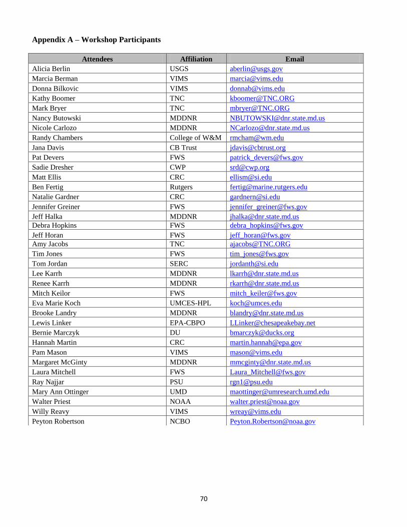
70
Appendix A – Workshop Participants
Attendees Affiliation Email
Alicia Berlin USGS [email protected]
Marcia Berman VIMS [email protected]
Donna Bilkovic VIMS [email protected]
Kathy Boomer TNC [email protected]
Mark Bryer TNC [email protected]
Nancy Butowski MDDNR [email protected]
Nicole Carlozo MDDNR [email protected]
Randy Chambers College of W&M [email protected]
Jana Davis CB Trust [email protected]
Pat Devers FWS [email protected]
Sadie Dresher CWP [email protected]
Matt Ellis CRC [email protected]
Ben Fertig Rutgers [email protected]
Natalie Gardner CRC [email protected]
Jennifer Greiner FWS [email protected]
Jeff Halka MDDNR [email protected]
Debra Hopkins FWS [email protected]
Jeff Horan FWS [email protected]
Amy Jacobs TNC [email protected]
Tim Jones FWS [email protected]
Tom Jordan SERC [email protected]
Lee Karrh MDDNR [email protected]
Renee Karrh MDDNR [email protected]
Mitch Keilor FWS [email protected]
Eva Marie Koch UMCES-HPL [email protected]
Brooke Landry MDDNR [email protected]
Lewis Linker EPA-CBPO [email protected]
Bernie Marczyk DU [email protected]
Hannah Martin CRC [email protected]
Pam Mason VIMS [email protected]
Margaret McGinty MDDNR [email protected]
Laura Mitchell FWS [email protected]
Ray Najjar PSU [email protected]
Mary Ann Ottinger UMD [email protected]
Walter Priest NOAA [email protected]
Willy Reavy VIMS [email protected]
Peyton Robertson NCBO [email protected]

71
Glynn Rountree NAHB [email protected]
Joe Scalf Lynnhaven NOW [email protected]
Amy Scaroni UMD [email protected]
Scott Schwenk FWS [email protected]
Kevin Sellner CRC [email protected]
Mike Slattery FWS [email protected]
Brittany Smith EPA
Ralph Spagnolo EPA-CBPO [email protected]
Quentin Stubbs USGS-CBPO [email protected]
Jessica Thompson CNU [email protected]
Howard Townsend NCBO [email protected]
Jim Uphoff MDDNR [email protected]
Bruce Vogt NCBO [email protected]
Julie Winters EPA-CBPO [email protected]
Matt Witbeck FWS [email protected]
Jen Wijetunga CB Trust [email protected]
In-Young Yeo UMD [email protected]

72
Appendix B - Additional Resources
Workshop participants were asked to provide additional resources that could be used as a
reference in this report. Below is a link to the STAC Designing Sustainable Coastal Habitats
workshop webpage where the resources can be found. These resources are a collection of
academic journals, articles, and supporting projects and tools that inform this workshop.
Additional Resources: http://www.chesapeake.org/stac/workshop_hab.php

73
Appendix C – Workshop Agenda
Designing Sustainable Coastal Habitats
Scientific and Technical Advisory Committee Date: April 16-17, 2013
Workshop Agenda
Location: The Tidewater Inn - Easton, MD
Workshop Goal: Design Sustainable Approaches and Initiatives for Coastal Habitat Restoration and Protection
within the Chesapeake Bay Watershed
April 16
Webinar Website: https://chesapeakeresearch.webex.com/chesapeakeresearch/j.php?ED=38425333&UID=50087038&PW=NMWQyY
2NkMzlk&RT=MiMxMQ%3D%3D
Password: tidewater
Toll-Free Number: 1-877-668-4493
Access Code: 315 308 084
12:00 pm Lunch (Provided)
12:45pm Overview of Workshop Objectives - Jeff Horan (USFWS)
Introductions
Review of Workshop Objectives
Overview of Agenda
Workshop Theme I: Ecosystem Components of Coastal Habitats
Panel Moderator: Mary Ann Ottinger (UMD)
1:00 pm Coastal Wetland Status and Trends in the Chesapeake Bay Watershed – Donna Bilkovic
(VIMS)
1:30 pm A Historic Look at Sediment Delivery and Coastal Systems - Jeff Halka (MGS)
2:00 pm A Spatial-Temporal Analysis of Wetland Loss and Vulnerability on the Delmarva Peninsula:
30 Years of Impact from Physical and Anthropocentric Drivers – Presented by: In-Young
Yeo (UMD) with contributions from: Quentin Stubbs (USGS)
2:30 pm Attaining 185,000 Acres of SAV for a Restored Chesapeake Bay - Presented by: Lee Karrh
(MD-DNR), Renee Karrh (MD-DNR), and Lewis Linker (EPA) with contributions from:
Robert Orth (VIMS)
3:30 pm Break (Provided)
3:45 pm Effects of Watershed and Shoreline Characteristics on Habitats at the Land/Water Interface
- Tom Jordan (SERC)
4:15 pm Using the Water Resources Registry to Target and Track Wetland Restoration – Ralph
Spagnolo (EPA)
4:45 pm Participants Discussion and Review of Theme I
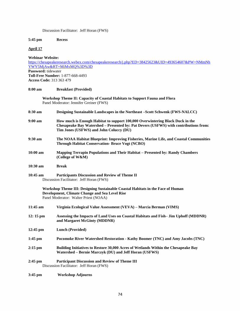
74
Discussion Facilitator: Jeff Horan (FWS)
5:45 pm Recess
April 17
Webinar Website: https://chesapeakeresearch.webex.com/chesapeakeresearch/j.php?ED=38425623&UID=493654607&PW=NMmNh
YWY5MjAw&RT=MiMxMQ%3D%3D
Password: tidewater
Toll-Free Number: 1-877-668-4493
Access Code: 313 363 479
8:00 am Breakfast (Provided)
Workshop Theme II: Capacity of Coastal Habitats to Support Fauna and Flora
Panel Moderator: Jennifer Greiner (FWS)
8:30 am Designing Sustainable Landscapes in the Northeast –Scott Schwenk (FWS-NALCC)
9:00 am How much is Enough Habitat to support 100,000 Overwintering Black Duck in the
Chesapeake Bay Watershed – Presented by: Pat Devers (USFWS) with contributions from:
Tim Jones (USFWS) and John Coluccy (DU)
9:30 am The NOAA Habitat Blueprint: Improving Fisheries, Marine Life, and Coastal Communities
Through Habitat Conservation- Bruce Vogt (NCBO)
10:00 am Mapping Terrapin Populations and Their Habitat – Presented by: Randy Chambers
(College of W&M)
10:30 am Break
10:45 am Participants Discussion and Review of Theme II
Discussion Facilitator: Jeff Horan (FWS)
Workshop Theme III: Designing Sustainable Coastal Habitats in the Face of Human
Development, Climate Change and Sea Level Rise
Panel Moderator: Walter Priest (NOAA)
11:45 am Virginia Ecological Value Assessment (VEVA) – Marcia Berman (VIMS)
12: 15 pm Assessing the Impacts of Land Uses on Coastal Habitats and Fish– Jim Uphoff (MDDNR)
and Margaret McGinty (MDDNR)
12:45 pm Lunch (Provided)
1:45 pm Pocomoke River Watershed Restoration - Kathy Boomer (TNC) and Amy Jacobs (TNC)
2:15 pm Building Initiatives to Restore 30,000 Acres of Wetlands Within the Chesapeake Bay
Watershed – Bernie Marczyk (DU) and Jeff Horan (USFWS)
2:45 pm Participant Discussion and Review of Theme III
Discussion Facilitator: Jeff Horan (FWS)
3:45 pm Workshop Adjourns