1

Destination Categories and Store Choice

Richard A. Briesch, William R. Dillon, and Edward J. Fox Cox School of Business

Southern Methodist University

May 2010

2

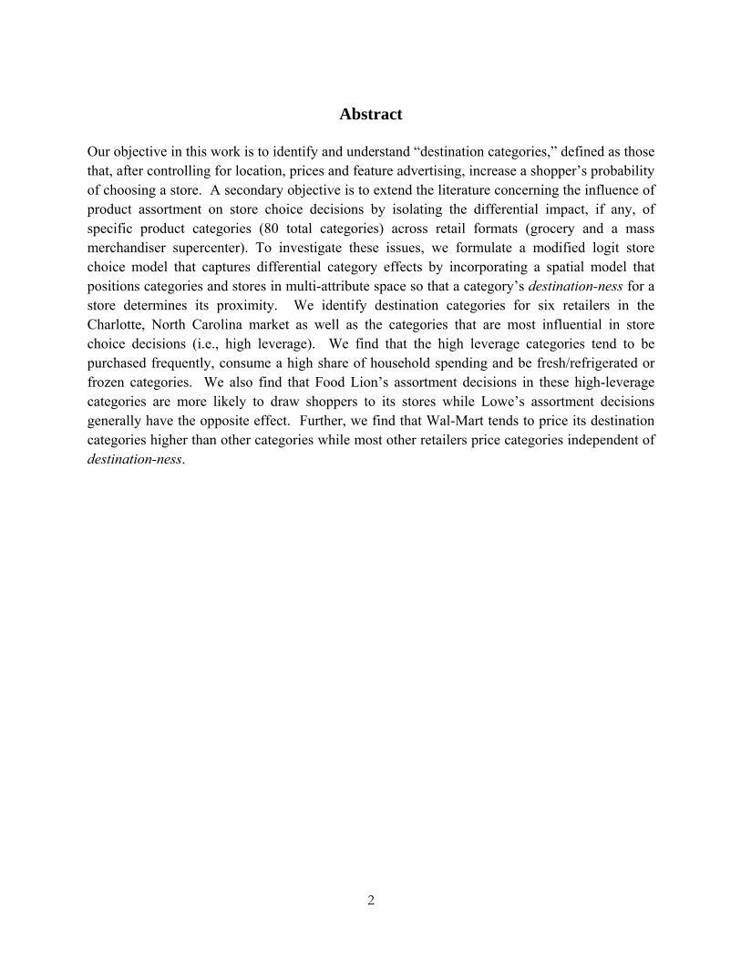
Abstract

Our objective in this work is to identify and understand “destination categories,” defined as those that, after controlling for location, prices and feature advertising, increase a shopper’s probability of choosing a store. A secondary objective is to extend the literature concerning the influence of product assortment on store choice decisions by isolating the differential impact, if any, of specific product categories (80 total categories) across retail formats (grocery and a mass merchandiser supercenter). To investigate these issues, we formulate a modified logit store choice model that captures differential category effects by incorporating a spatial model that positions categories and stores in multi-attribute space so that a category’s destination-ness for a store determines its proximity. We identify destination categories for six retailers in the Charlotte, North Carolina market as well as the categories that are most influential in store choice decisions (i.e., high leverage). We find that the high leverage categories tend to be purchased frequently, consume a high share of household spending and be fresh/refrigerated or frozen categories. We also find that Food Lion’s assortment decisions in these high-leverage categories are more likely to draw shoppers to its stores while Lowe’s assortment decisions generally have the opposite effect. Further, we find that Wal-Mart tends to price its destination categories higher than other categories while most other retailers price categories independent of destination-ness.

3

Retail practitioners have long recognized that categories play different roles (e.g.,

destination, routine, seasonal and convenience) and have differential importance to shoppers’

store choice decisions (Blattberg et al. 1995). Moreover, Dhar et al. (2001) note that retailers

develop expertise in particular categories and, once developed, category expertise becomes part

of the organization’s intellectual capital.

While there is a growing body of literature concerning the effects of category assortment

and related factors on store choice, this literature has focused almost exclusively on the store

choice decision without considering category purchase decisions. Accordingly, the influence of

specific categories on the store choice decision has not received much attention. The belief that

specific categories generate traffic by attracting shoppers to a store is widely held by retailers

though much of evidence to support the existence so called “destination categories” is anecdotal

(see, Blattberg et al. 1995, p. 23).

Objectives

Our objective in this work is to identify and understand “destination categories,” defined

as those that, after controlling for location, prices and feature advertising, increase a shopper’s

probability of choosing a particular store.1 Both retailers and manufacturers have an interest in

determining which categories have a greater or lesser influence on store choice. Retailers are

interested in this issue because it affects category merchandising, advertising and pricing

decisions; manufacturers are interested in this issue because it supports their category expertise,

hence their ability to advise retailers as a “category captain” (cf. Blattberg et al. 1995). A

secondary objective is to extend the literature concerning the influence of product assortment on

1 We will have more to say about how destination categories should be defined in a later next section.

4

store choice decisions by isolating the differential impact, if any, of specific product categories

(80 total categories) across retail formats (grocery and a mass merchandiser supercenter).

To investigate these issues, we formulate a modified logit store choice model that

captures differential category effects by incorporating a spatial model. In the spatial model,

categories and stores are positioned in multi-attribute space so that a category’s destination-ness

determines its proximity to a store.

We estimate the model using a multi-outlet scanner panel dataset containing information

about the purchases of 357 households in 80 categories across six retailers over a 104 week

period. We identify the extent to which each of the major store chains in the Charlotte, North

Carolina market area has developed specialized category expertise (i.e., destination categories).

For traditional grocery retailers, these categories primarily include perishable (fresh, refrigerated

and frozen) goods; for Wal-Mart Supercenters, these products primarily include non-grocery

products and, interestingly, candy. We further identify the categories that exert the greatest

leverage on store choice decisions across all retailers, finding that leverage is concentrated in a

few categories. Among these high-leverage categories are some of the retailers’ highest revenue

categories—milk, fresh bread & rolls, beer, carbonated beverages and cigarettes—as well as

lower revenue categories such as fresh eggs, ice cream/sherbet and frozen meat. We are also

able to determine which retailers are assorting these high leverage categories most effectively to

attract shoppers to their stores.

The rest of the paper is organized as follows. We begin by briefly reviewing the extant

literature and positioning our work relative to this literature. Next we discuss the concept of a

destination category and argue that, while it may be easy to describe, it may be far more difficult

to measure directly. In the course of that discussion, we present a number of propositions about

5

destination categories that can be subjected to empirical testing. We then formulate the general

model, discuss its rationale vis-à-vis extant models, and describe the store choice and category

incidence component models. This is followed by a discussion of how the store choice and

category incidence model intercepts are parameterized. The next section is devoted to estimation

issues, specifically parameter identification. We then describe the data and the covariates used to

estimate the model. Next, we describe our approach to testing the destination category

propositions and discuss empirical findings. Modeling results then follow. After discussing

parameter estimates, we present a policy analysis which calibrates the impact of categories on

store choice. We conclude with a discussion of our findings including which assortment-related

factors have the greatest impact on destination-ness as well how effectively each retailer has

assorted those categories shown to have the greatest impact on store choice.

Background and Contribution

Explaining store choice decisions has been of great interest to academics and

practitioners alike; however, the vast majority of research in this area has focused on what

factors influence a consumer’s decision on where to shop. With this focus in mind, researchers

have addressed a wide variety of issues such as explaining store choice behaviors in terms of

marketing activities—price promotions, feature and display, retail/price formats (HILO vs.

EDLP), shopping basket sizes and composition, travel distance, prior shopping experiences, the

need for variety, shoppers’ fixed and variable costs, cherry-picking, household characteristics

and more recently store-category loyalty and category assortments.2

2 Representative papers include: Reilly 1931; Baumol and Ide 1956; Huff 1964; Arnold, Ma and Tigert 1978; Arnold, Roth and Tigert 1981; Arnold and Tigert 1982; Arnold, Oum and Tigert 1983; Bell, Ho and Tang 1998; Bell and Lattin 1998; Rhee and Bell 2002; Fox and Hoch 2005; Briesch, Chintagunta and Fox 2009.

6

Because our focus is on the existence of and role played by destination categories, the

recent work investigating the influence of category assortments on store choice and the

phenomenon of store-category loyalty deserve some attention.

What We Know About Category Assortments

The role which category assortment plays in store choice has been the subject of some

debate. While several studies fail to find a positive relationship between assortment size and

category sales in grocery stores (Broniarczyk et al. 1998; Dreze et al. 1994; Boatwright and

Nunes 2001), others find that assortment size positively affects the probability that shoppers will

patronize a particular retailer (Fox et al. 2004). However, there is a growing body of evidence

that larger assortments are not universally preferred (Broniarczyk et al. 2006; Chernev et al.

2003; Chernev and Hamilton 2009) and that assortment preferences are heterogeneous

(Broniarczyk et al. 1998; Briesch et al. 2009). Moreover, the recent findings of Chernev and

Hamilton (2009) and Briesch et al. (2009) demonstrate that the influence of product assortment

on store choice is more nuanced than previously thought. The ability of larger assortments to

attract shoppers to a particular store varies greatly by household, is correlated with travel

distance, and depends on the attractiveness and the composition of the assortment with respect to

the brands, sizes and the number of SKUs. For example, small assortments can attract shoppers if

sufficiently attractive; increasing the number of brands offered will likely increase a shopper’s

probability of choosing a particular retailer but increasing the number of SKUs may not.

Store-Category Loyalty

Two studies have investigated the degree to which shoppers are store-category loyal; that

is, households shop at specific stores in order to make purchases in particular categories. Dhar et

al. (2001) suggest that there are categories for which consumers have strong store-category

7

preferences and shop at a specific retailer when purchasing in these categories whenever

possible. Using a controlled store experiment, they demonstrate that retailers can induce

consumers to be store-loyal for specific products through cross merchandising programs.

Zhang et al. (2010) estimate a store loyalty model at the category level with a view

toward demonstrating that store loyalty is a category-specific household trait and that it is quite

common for households to be loyal to different stores in different categories. Using a scanner

panel dataset that contains the purchases of 1321 households in 284 categories across 16 stores

over a 53 week period, they find that shopping at multiple stores is pervasive, and, of those who

shop at multiple stores, almost all are to some degree store-category loyal—they make all of their

purchases exclusively at the same store for at least one of their regularly purchased product

categories. These authors find that store-category loyalty is, among other factors, positively

influenced by category dollar share of requirements, store visit frequency, breadth, uniqueness

and relevance of SKUs in the assortment, and perceived price advantage.

Contribution

Our primary focus is not on modeling store choice per se, or, for that matter, on the role

of product assortments in store choice decisions. Rather, our objective is to assess the

destination-ness of specific categories; that is, the extent to which the attractiveness of specific

categories increases the probability of choosing a store. As such, we need to investigate factors

thought to influence store choice, including product assortments; however, our modeling

approach differs from previous store choice/loyalty studies in a number of important ways.

1. Compared to Zhang et al. (2010) we are not interested in store-category loyalty — that is,

we do not model the probability that a household makes all of its purchases in a given

category exclusively at a particular store. In addition, we adopt a model form that

8

explicitly considers category incidence and allows household and category parameters to

vary across categories. Consequently, our store choice probabilities are explicitly

informed by category purchases.

2. Compared to Bell et al. (1998) and Briesch et al. (2009) we do not adopt a shopping list

metaphor or a need-based approach to category incidence. By not conditioning on a

shopping list or on category needs, we capture all purchase incidences and therefore can

account for impulse purchases and the effects of in-store merchandising and, in addition,

can accommodate basket-splitting behaviors, i.e., when shoppers make purchases at

different stores on the same day. Because we incorporate a spatial model of household

preferences in which stores and categories are positioned in multi-attribute space, we also

are better able than either of the prior studies to assess the extent to which different

categories drive store choice across retail formats. We show how the locations of a given

store and category in multi-attribute space reflect the degree to which the category is a

destination; in other words, the closer a category is positioned to the store, the greater the

destination-ness of the category for that store. We also derive a new measure, [C]ategory

[L]everage [I]n [P]atronage [D]ecisions to determine how much leverage specific

categories exert in shoppers’ store choice decisions. Finally, we explicitly model both

store choice and category incidence and consider a much larger number of categories and

retail formats than either of the cited studies.

Substantively, we find that the categories that are most influential in store choice decisions

(i.e., highest CLIPD) tend to be fresh/refrigerated or frozen, purchased frequently and consume a

high share of household spending. We also find that Food Lion’s assortment decisions in the

most influential categories are more likely to draw shoppers to its stores while Lowe’s

9

assortment decisions generally have the opposite effect. Further, we find that Wal-Mart tends to

price its destination categories higher than other categories while most other retailers price

categories independent of destination-ness.

Destination Categories and Category Leverage

The concept of a destination category is seemingly very simple and can be defined either

from the perspective of the shopper or the retailer; for the shopper, a category is a “destination”

if it increases that shopper’s probability of choosing a store; for the retailer, a category is a

“destination” if it attracts shoppers to its stores. Although these definitional perspectives are

rather intuitive, destination categories may well be easier to describe then to measure. Consider,

for example, the following two illustrative self-reports:

“I buy all of my pasta and pasta sauce at Winn Dixie, but little else.”

“I buy almost all of my weekly household grocery needs at Winn Dixie because they stock my favorite brands of pasta and pasta sauce.”

In both instances, it is clear that the reason for shopping at Winn Dixie is the strong

preference for specific pasta and pasta sauce brands so these categories qualify as destination

categories. However, in the case of the first shopper, Winn Dixie captures only a small

percentage of this household’s grocery requirements while, for the second shopper, Winn Dixie

captures almost all of this household’s grocery requirements. Moreover, using household panel

data it is likely that even crude methods of analysis would point to pasta and pasta sauce as

destination categories for the first shopper, whereas identifying pasta and pasta sauce as

destination categories in the case of the second shopper would be more challenging.

Identifying destination categories on the basis of store scanner data may also be difficult.

Consider Table 1 which presents the Category Development Index (CDI) across 80 product

categories for six retail chains in the Charlotte, North Carolina market. These chains and product

10

categories will be the focus of the empirical analysis which follows in a later section. At an

aggregate level, CDI reflects the preference of shoppers to purchase specific categories at one

retailer (rather than at others) and is defined as the retailer’s share in a particular category

divided by its overall market share, multiplied by 100 (e.g., Dhar et al. 2001). While CDIs can

vary markedly across retail chains, as is the case for the six retail chains shown in Table 1, CDI

does not necessarily measure whether the category actually attracts shoppers to a particular store.

For example, categories in which the retailer gets more than its fair share (CDI > 100) might be

purchased coincidently with categories that actually influenced the store choice decision (see

e.g., Manchanda et al. 1999) or coincidently with other purchases that were made because of

advertised prices. More importantly, CDIs provide no diagnostic information that can explain

why certain categories have a stronger impact on a shopper’s decision to make a category

purchase at a particular store, which is the focus of this paper.

Place Table 1 about here

If a destination category increases the probability of choosing one store (i.e., draws traffic

to that store), that category must necessarily decrease the probability of choosing competing

store(s). Identifying categories that affect store choice probability, whether or not they are

destination categories, is important to retailers’ category merchandising, advertising and pricing

decisions; it is also important to manufacturers that supply those categories because they often

advise retailers on those decisions. We therefore expand our investigation of destination

categories to consider the overall effect of categories on store choice across retailers in a market,

which we call category leverage.

11

Propositions

Notwithstanding the challenge that identifying destination categories presents, there are a

number of intuitive and verifiable propositions that should be observed if destination categories

exist. The following propositions are based on the premise that, if stores do indeed develop

expertise in particular categories and if such expertise varies by store and by category, then we

should observe the following3:

Proposition 1: Households that are attracted to particular stores because of the product

offerings (i.e., assortments) in specific categories will make purchases in different

categories at different stores on the same day/week.

Proposition 2: Households that purchase at multiple stores on the same day/week will

show (non-random) patterns of store choice and category purchasing over time –

households will purchase at different stores on the same day/week with purchase

incidences reflecting the complementary nature of the stores shopped.

Proposition 3: Destination categories imply store specialization; they are not confined to

the household’s favorite store. Stated differently, store loyalty is not the driving force

behind destination categories.

In the empirical application section later in the paper, we will assess the extent to which

these propositions are observed in our sample of households. While these propositions cannot

unambiguously demonstrate category destination-ness, if these behaviors are indeed manifest in

the shopping behaviors of households in our dataset, we are in a better position to argue for the

existence of destination categories.

3 The following propositions focus on households who make category purchases at different stores. We do not mean to imply that households that make all of their purchases at one store do not exhibit category destination behaviors, but simply that, as mentioned previously, all else the same, it is more difficult to propose straight-forward empirical metrics that can provide evidence of the destination-ness of a category.

12

Model Formulation

General Model Form

Consistent with Bell et al. (1998) and Briesch et al. (2009), we assume that the decision

as to which store to visit is dependent upon store-specific characteristics (e.g., pricing, store

locations) as well as the attractiveness of all categories to the consumer:

Store Visit = f (store characteristics and attractiveness of all categories).

In this research we assume that category attractiveness is a function of merchandising activity,

consumer need for the category as well as the destination-ness of the category for the chosen

store. If we knew the attractiveness of categories a priori, then a store choice model consistent

with the specification shown above could be estimated directly. However, because we do not

know how consumers evaluate the attractiveness of categories, we use incidence models

conditional on the shopper visiting the store to estimate each category’s unobserved

attractiveness.

Denoting the probability of household h (h =1,2,...,H) purchasing a subset of the total

categories C, conditional on visiting store s (s =1,2,...,S) on trip t (t =1,2,...,T) as Pr(C | yhst =1),

the joint probability of household h purchasing the set of categories C at store s on trip t, denoted

as Pr(yhst = 1∩ C), can be expressed as:

Pr(yhst = 1∩C) = Pr(yhst = 1)Pr(C | yhst = 1). (1)

The two components of the joint probability shown in equation 1 will be referred to as the store

choice model and the category incidence model, respectively. We note that, in theory, this model

could be estimated in two steps (although less efficiently), where the category incidence model is

estimated in the first step to calculate the category attractiveness for each store, and then the

store choice model is estimated in the second step. Besides efficiency concerns, one of the many

13

problems associated with the two-step approach is that household heterogeneity is tacitly

assumed to be unrelated across the two steps. Therefore, we use a single step (i.e., simultaneous)

estimation approach.

To account for heterogeneity across household purchase incidence and store choice

decisions, we use a continuous distribution with the parameter covariance matrix . We utilize a

mixed logit model to estimate the store choice probabilities (Train 2003). Let θ denote the set of

category incidence and store choice model parameters. Now the probability that we observe

household h purchasing a subset from the set of categories C at store s on trip t can be written as

])),1|1Pr(-1(),1|1[Pr()|1Pr()|C1Pr( ∏c∈c

hcsthcst

h

y-1hsthcst

yhsthcsthsthst θ,yyθ,yyθ,yθ,y

where yhcst = 1 if household h purchases in category c at store s on trip t, and 0 otherwise.

Model Rationale

Our store choice model differs significantly from the forms used by Bell et al. (1998) and

Briesch et al. (2009). Bell et al. used a shopping list metaphor whereas Briesch et al. used a

needs-based approach to category incidence; in both cases store choice is conditional on

“intentions,” as evinced by an unobserved shopping list or by unobserved category needs. These

intentions are then used to calculate the estimated cost of visiting each store, which is part of the

indirect utility. Both of these studies take a cost minimization approach in order to calculate the

probability of choosing a particular store; our model adopts a utility maximization approach,

which, in general, is more parsimonious.4

While conditioning store choice on category purchase would at first appear to be

consistent with the notion that destination categories are those in which a household’s mere

4 Note that utility maximization is the dual problem of cost minimization.

14

intention to purchase (in the category) drives the household to a particular store, there are several

problems with this approach. In the case of the shopping list metaphor, households are presumed

to have constructed a list of planned purchases, which is not directly observable, and all items

that are purchased by the household are tacitly assumed to be on the shopping list. Moreover,

everything on the shopping list is tacitly assumed to be purchased. Adopting a needs-based

approach to category incidence, on the other hand, is also limiting because it cannot account for

impulse purchases or the effects of in-store merchandising. More limiting from a destination

category perspective is that, under either approach, it is not possible to account for category

purchases at different stores on the same day-i.e., basket-splitting. In such cases, variable costs

are difficult to assign since it is impossible, in a strict sense, to split a shopper’s total basket

across different stores if the underlying assumption is that there is one shopping list and one set

of category needs that motivated the household to shop on a given day. Further, both approaches

require an estimate of the expected quantity purchased in order to calculate the cost of visiting

each store.

In contrast, our model form does not require quantity estimates as we do not calculate

category cost, but rather category attractiveness. Category attractiveness enters the store choice

model as a covariate and is estimated at the time the store visit is made and the category

purchases are observed. We also directly account for unplanned/impulse purchases due to in-

store merchandising and promotions, behaviors which we feel must be controlled for in order to

develop a sound measure of category destination-ness. While our model form requires (via the

conditioning argument) that a household be in a store in order to make a purchase, the

conditioning is used only to estimate the attractiveness of the categories, i.e., it is not assumed to

be part of the household decision process. Finally, as demonstrated in the policy analysis which

15

follows, although we explicitly model the relationship between ex-post category purchasing and

store choice we are able to estimate the extent to which specific categories draw households to

specific stores.

Store Choice and Category Incidence Models

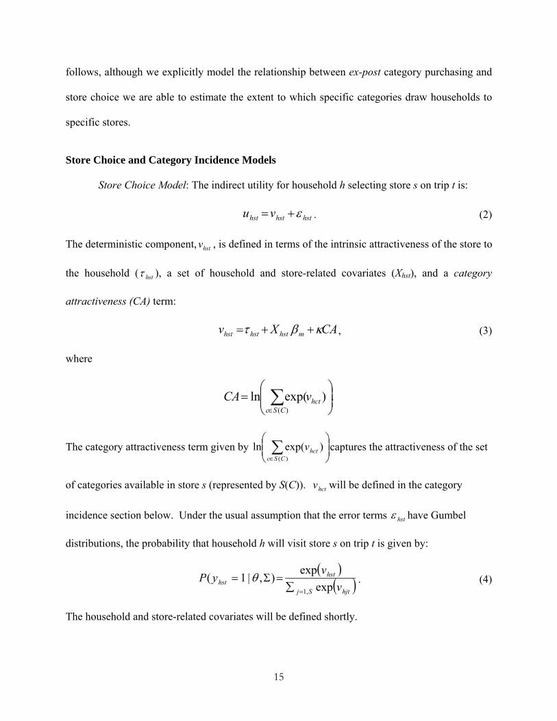
Store Choice Model: The indirect utility for household h selecting store s on trip t is:

hsthsthst vu . (2)

The deterministic component, hstv , is defined in terms of the intrinsic attractiveness of the store to

the household ( hst ), a set of household and store-related covariates (Xhst), and a category

attractiveness (CA) term:

CAXv mhsthsthst , (3)

where

.)exp(ln)(

CSchctvCA

The category attractiveness term given by

)(

)exp(lnCSc

hctv captures the attractiveness of the set

of categories available in store s (represented by S(C)). hctv will be defined in the category

incidence section below. Under the usual assumption that the error terms hst have Gumbel

distributions, the probability that household h will visit store s on trip t is given by:

hjtSj

hsthst v

vyP

exp

exp),|1(

,1 . (4)

The household and store-related covariates will be defined shortly.

16

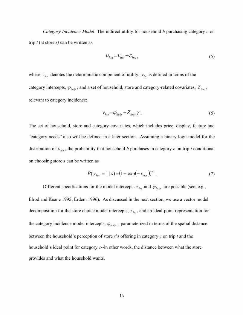
Category Incidence Model: The indirect utility for household h purchasing category c on

trip t (at store s) can be written as

hcthcthct vu , (5)

where hctv denotes the deterministic component of utility; hctv is defined in terms of the

category intercepts, shct| , and a set of household, store and category-related covariates, hsctZ ,

relevant to category incidence:

hsctshcthct Zv | . (6)

The set of household, store and category covariates, which includes price, display, feature and

“category needs” also will be defined in a later section. Assuming a binary logit model for the

distribution of hct , the probability that household h purchases in category c on trip t conditional

on choosing store s can be written as

1exp1)|1( hcthct vsyP . (7)

Different specifications for the model intercepts hst and shct| are possible (see, e.g.,

Elrod and Keane 1995; Erdem 1996). As discussed in the next section, we use a vector model

decomposition for the store choice model intercepts, hst , and an ideal-point representation for

the category incidence model intercepts, shct| , parameterized in terms of the spatial distance

between the household’s perception of store s’s offering in category c on trip t and the

household’s ideal point for category c--in other words, the distance between what the store

provides and what the household wants.

17

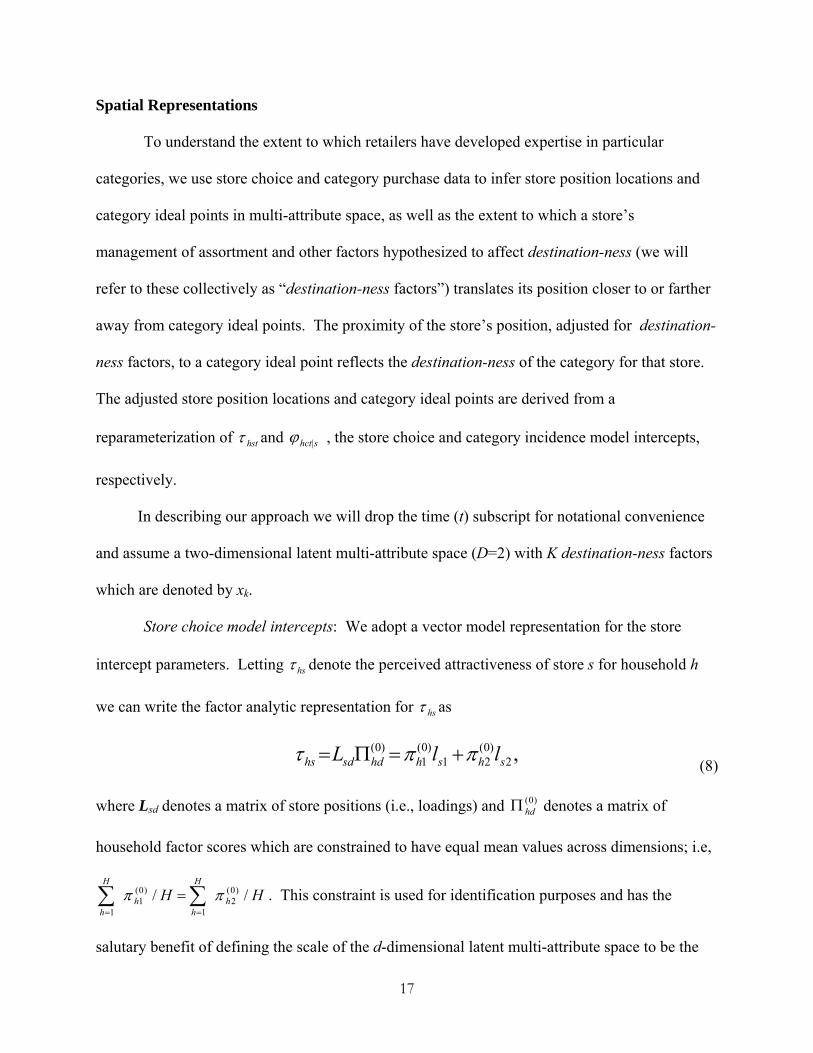
Spatial Representations

To understand the extent to which retailers have developed expertise in particular

categories, we use store choice and category purchase data to infer store position locations and

category ideal points in multi-attribute space, as well as the extent to which a store’s

management of assortment and other factors hypothesized to affect destination-ness (we will

refer to these collectively as “destination-ness factors”) translates its position closer to or farther

away from category ideal points. The proximity of the store’s position, adjusted for destination-

ness factors, to a category ideal point reflects the destination-ness of the category for that store.

The adjusted store position locations and category ideal points are derived from a

reparameterization of hst and shct| , the store choice and category incidence model intercepts,

respectively.

In describing our approach we will drop the time (t) subscript for notational convenience

and assume a two-dimensional latent multi-attribute space (D=2) with K destination-ness factors

which are denoted by xk.

Store choice model intercepts: We adopt a vector model representation for the store

intercept parameters. Letting hs denote the perceived attractiveness of store s for household h

we can write the factor analytic representation for hs as

,2

)0(21

)0(1

)0(shshhdsdhs llL

(8)

where Lsd denotes a matrix of store positions (i.e., loadings) and )0(hd denotes a matrix of

household factor scores which are constrained to have equal mean values across dimensions; i.e,

HH h

H

hh

H

h

// )0(2

1

)0(1

1

. This constraint is used for identification purposes and has the

salutary benefit of defining the scale of the d-dimensional latent multi-attribute space to be the

18

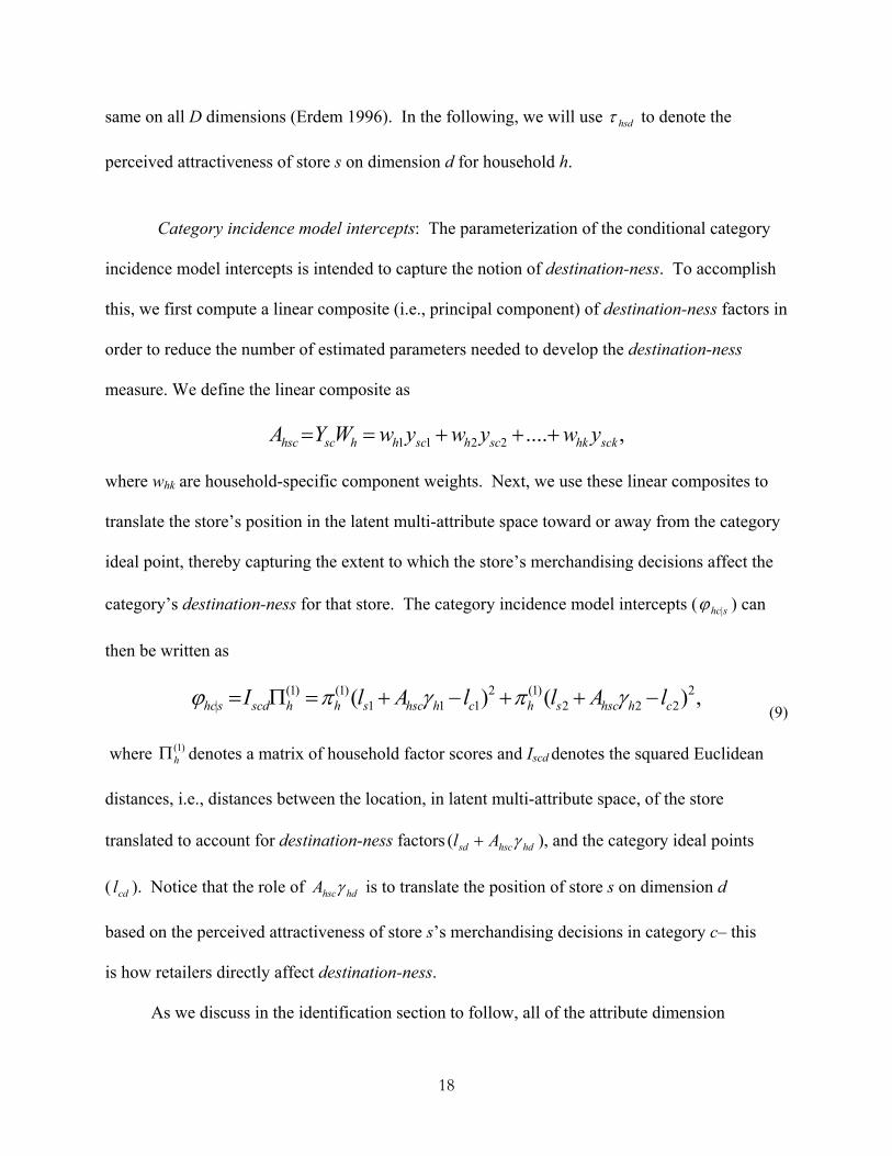
same on all D dimensions (Erdem 1996). In the following, we will use hsd to denote the

perceived attractiveness of store s on dimension d for household h.

Category incidence model intercepts: The parameterization of the conditional category

incidence model intercepts is intended to capture the notion of destination-ness. To accomplish

this, we first compute a linear composite (i.e., principal component) of destination-ness factors in

order to reduce the number of estimated parameters needed to develop the destination-ness

measure. We define the linear composite as

,....2211 sckhkschschhschsc ywywywWYA

where whk are household-specific component weights. Next, we use these linear composites to

translate the store’s position in the latent multi-attribute space toward or away from the category

ideal point, thereby capturing the extent to which the store’s merchandising decisions affect the

category’s destination-ness for that store. The category incidence model intercepts ( ) can

then be written as

,)()( 2

222)1(2

111)1()1(

| chhscshchhscshhscdshc lAllAlI (9)

where )1(h denotes a matrix of household factor scores and Iscd denotes the squared Euclidean

distances, i.e., distances between the location, in latent multi-attribute space, of the store

translated to account for destination-ness factors hdhscsd Al ( ), and the category ideal points

( cdl ). Notice that the role of hdhscA is to translate the position of store s on dimension d

based on the perceived attractiveness of store s’s merchandising decisions in category c– this

is how retailers directly affect destination-ness.

As we discuss in the identification section to follow, all of the attribute dimension

shc|

19

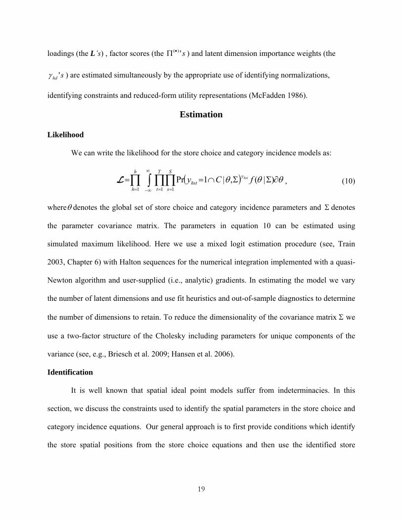
loadings (the L’s) , factor scores (the s')( ) and latent dimension importance weights (the

shd ' ) are estimated simultaneously by the appropriate use of identifying normalizations,

identifying constraints and reduced-form utility representations (McFadden 1986).

Estimation

Likelihood

We can write the likelihood for the store choice and category incidence models as:

)|(,|1Pr1 11

fCyT

t

S

s

yhst

h

h

hstL , (10)

where denotes the global set of store choice and category incidence parameters and denotes

the parameter covariance matrix. The parameters in equation 10 can be estimated using

simulated maximum likelihood. Here we use a mixed logit estimation procedure (see, Train

2003, Chapter 6) with Halton sequences for the numerical integration implemented with a quasi-

Newton algorithm and user-supplied (i.e., analytic) gradients. In estimating the model we vary

the number of latent dimensions and use fit heuristics and out-of-sample diagnostics to determine

the number of dimensions to retain. To reduce the dimensionality of the covariance matrix we

use a two-factor structure of the Cholesky including parameters for unique components of the

variance (see, e.g., Briesch et al. 2009; Hansen et al. 2006).

Identification

It is well known that spatial ideal point models suffer from indeterminacies. In this

section, we discuss the constraints used to identify the spatial parameters in the store choice and

category incidence equations. Our general approach is to first provide conditions which identify

the store spatial positions from the store choice equations and then use the identified store

20

positions to identify the category positions (and destination parameters) using the category

incidence equations.

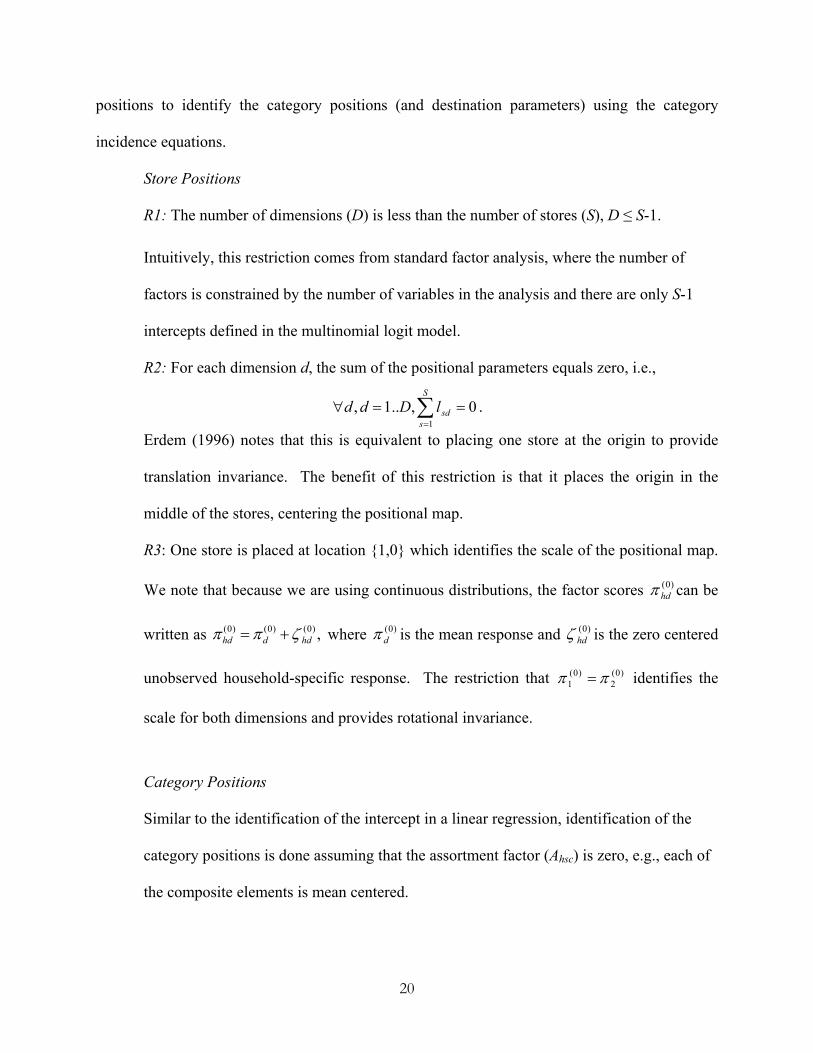
Store Positions

R1: The number of dimensions (D) is less than the number of stores (S), D ≤ S-1.

Intuitively, this restriction comes from standard factor analysis, where the number of

factors is constrained by the number of variables in the analysis and there are only S-1

intercepts defined in the multinomial logit model.

R2: For each dimension d, the sum of the positional parameters equals zero, i.e.,

0,..1,1

S

ssdlDdd .

Erdem (1996) notes that this is equivalent to placing one store at the origin to provide

translation invariance. The benefit of this restriction is that it places the origin in the

middle of the stores, centering the positional map.

R3: One store is placed at location {1,0} which identifies the scale of the positional map.

We note that because we are using continuous distributions, the factor scores )0(hd can be

written as ,)0()0()0(hddhd where )0(

d is the mean response and )0(hd is the zero centered

unobserved household-specific response. The restriction that )0(2

)0(1 identifies the

scale for both dimensions and provides rotational invariance.

Category Positions Similar to the identification of the intercept in a linear regression, identification of the

category positions is done assuming that the assortment factor (Ahsc) is zero, e.g., each of

the composite elements is mean centered.

21

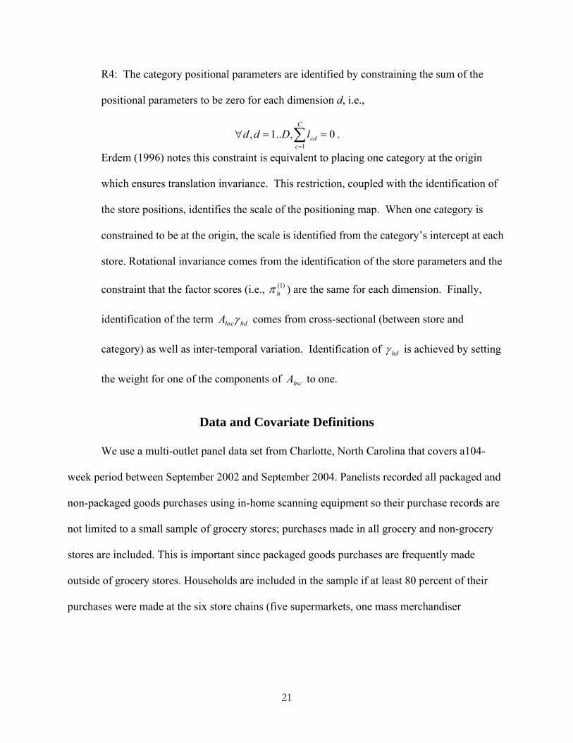
R4: The category positional parameters are identified by constraining the sum of the

positional parameters to be zero for each dimension d, i.e.,

0,..1,1

C

ccdlDdd .

Erdem (1996) notes this constraint is equivalent to placing one category at the origin

which ensures translation invariance. This restriction, coupled with the identification of

the store positions, identifies the scale of the positioning map. When one category is

constrained to be at the origin, the scale is identified from the category’s intercept at each

store. Rotational invariance comes from the identification of the store parameters and the

constraint that the factor scores (i.e., )1(h ) are the same for each dimension. Finally,

identification of the term hdhscA comes from cross-sectional (between store and

category) as well as inter-temporal variation. Identification of hd is achieved by setting

the weight for one of the components of hscA to one.

Data and Covariate Definitions

We use a multi-outlet panel data set from Charlotte, North Carolina that covers a104-

week period between September 2002 and September 2004. Panelists recorded all packaged and

non-packaged goods purchases using in-home scanning equipment so their purchase records are

not limited to a small sample of grocery stores; purchases made in all grocery and non-grocery

stores are included. This is important since packaged goods purchases are frequently made

outside of grocery stores. Households are included in the sample if at least 80 percent of their

purchases were made at the six store chains (five supermarkets, one mass merchandiser

22

supercenter) for which we have geolocation data and if they spent at least $10 every month.5

The

resulting data set included 357 families with a total of 57,755 shopping trips. Descriptive

statistics for these households are provided in Table 2. We use the first 26 weeks as an

initialization period to identify categories purchased by each household as well as to identify the

inter-temporal variables for the categories, which left 37,438 shopping trips. We used the middle

52 weeks as an estimation sample and the final 26 weeks as a validation sample.

Place Table 2 about here

We have detailed price information for 289 categories. From those categories we

selected the top 80 based upon total dollars spent in the category; this resulted in excluding only

categories which were not substantial, i.e., in which fewer than 10% of the households

purchased. The 80 categories selected together comprise more than 75% of the average market

basket (excluding products not tracked by UPC). Table 3 presents penetration rates and share-of-

wallet for each category along with the price index for each retail chain. Store statistics are

shown in Table 4; this table provides trip and spend share, travel time from home to the closest

store of the retail chain and (aggregate) category indexed measures for price and each of the

seven assortment and related variables that are hypothesized to affect destination-ness.

Place Tables 3 and 4 about here

Covariates

Table 5 provides definitions for all of the store choice, category incidence and

destination-related covariates used in estimating the model. In the table, we use x’s to denote

store choice covariates, z’s to denote category purchase incidence-related covariates, and y’s to

represent merchandising factors that affect destination-ness. Note that among the factors that are

5 The last criterion was used to ensure that panelists were faithful in recording their purchases and remained in the panel for the entire 104 week period.

23

posited to affect destination-ness are several assortment variables along with the frequency of

promotions and the average inter-purchase time. These latter two covariates have been

hypothesized to affect store traffic and the role that categories play in the store choice decisions;

i.e., merchants believe that destination categories, by definition, are those associated with short

average inter-purchase times (i.e., more frequent shopping), while frequency of promotions

provide an indicator of shoppers’ expectations concerning future promotions in a category and

thus may have longer-term consequences for store choice decisions (cf. Mela et al. 1997).

Finally, note that we have added to the set of assortment factors investigated by Briesch et al.

(2009), the proportion of unique private label items and the proportion of unique national brand

items.

Place Table 5 about here

Empirical Results: Propositions

We begin our analysis by revisiting the three propositions introduced earlier. For each

proposition, we investigate the extent to which the empirical data on household shopping

behaviors lends support to the existence of destination categories. Although we do not have the

luxury of asking our households to participate in controlled experiments, we can identify groups

of households who have exhibited specific shopping behaviors which may prove informative in

understanding the extent to which they visited a store with a specific category purchase in mind;

for example, as discussed below, shoppers who visited two or more stores on the same day and

shoppers who made a single category purchase at a store can provide some insights into category

destination-ness. We are not suggesting that the analysis and findings provided in this section

stand as strong arguments for the existence of destination categories, rather that simple analysis

24

of households’ store and category shopping behaviors may provide some preliminary insights.

As we will see, the empirical shopping behaviors of our households do indeed support the

possible existence of destination categories; however, our analysis in this section does not rule

out alternative explanations. A stronger test of the existence of destination categories will be

provided by our formal model which controls for a number of putative covariates such as price,

display, feature, etc.

Proposition 1

This proposition speculates that households shop at multiple stores on the same day/week

in order to take advantage of the category-specific expertise that retailers have developed. If this

proposition is at all tenable, then we should observe households visiting multiple stores on the

same day/week and the number of categories purchased and dollar spending levels should vary

across retailers.

Findings: Table 6, part A presents the distribution of stores shopped on the same day or

during the same week for households in our data set. As can be seen in the table, almost 16% of

the trips were made to 2 or more stores on the same day. The incidence of multiple store visits in

a given week increases to a little over 54%.6 In part B of the table, we present the same day/week

relative store spend and relative number of categories purchased reported in terms of the number

of stores visited. We see that households who made purchases at two stores on the same day

spend about four times more at one store than the other, and purchased in about four times the

number of categories.7 For households purchasing in multiple stores in one week we see a

6 In computing these incidences we excluded visits to the same store. 7 Relative spend and relative no. of categories purchased percentages were computed as follows: 1) for each household compute the dollar spend/no. of categories purchased for each pair/triplet, etc. of stores visited; 2) compute the total spend and no. of categories purchased (by summing across the appropriate set of stores); 3) compute relative quantities (step 1/step 2); 4) identify which store in the pair/triplet, etc. received the largest spend

25

similar pattern. As households shop at more stores on the same day or during the same week the

relative distribution become more skewed, reflecting even more disproportionate spending and

categories shopping behavior. Finally, we investigated whether households who visited two or

more stores on the same day/week purchased in different or the same categories. Across all 80

categories, the percentage of unique category purchases (i.e., non-overlapping) was very high (>

90%).

Comment: The incidence of visiting multiple stores on the same day or in the same week

is higher than what would be expected due to chance; perhaps more important to this proposition,

however, is the skewed relative dollar spend and number of categories shopped. If households

shop at multiple stores to take advantage of category-specific expertise then, all else the same,

we would expect households to purchase in more categories and spend greater dollar amounts at

certain stores and less at others. In addition, the data strongly suggest that when households visit

different stores on the same day or during the same week, they do purchase in different

categories.

Place Table 6 about here

Proposition 2

According to Proposition 2 households shop at different stores on the same day/week

when purchasing in specific categories because of the assortments offered and consequently will

tend to visit the same stores on a fairly consistent basis.

Findings: For stores visited on the same day/week, Table 7, part A presents the

probabilities of visiting the same pair/triplet, etc. of stores. As can be seen from the table, the

and no. of categories purchased; 5) for households who shopped at more than two stores compute average spend and no. of categories purchased across stores, excluding the store identified in step 4; and 6) compute mean relative spend and no. of categories purchased for the store identified in step 4) and for the set of remaining stores.

26

likelihoods of consistent same stores-same day/week visits (over the household’s purchase

history) are larger than what would be expected due to chance; for example for those households

visiting two stores on the same day the likelihood of visiting the same two stores over the

household’s purchase history is about .35. In the case of households who visited more than three

stores on the same day, the likelihood of consistent store choices increases to about .61 for

households who visited three stores on the same day, and to almost .82 for households who

purchased in four or more stores on the same day.8

Table 7, part B presents log odds ratios computed from the joint table of stores visited in

the same week. For a given pair of stores (e.g., Bi-Lo and Food Lion) a statistically significant

negative log-odds ratio indicates that a household is more likely to shop at both stores during the

same week as compared to making two visits to the same store (either Bi-Lo or Food Lion) in the

same week. From the table we see that five of the fifteen log-odds ratios are statistically

significant and negative, three are statistically significant and positive, and seven are statistically

non-significant.

Comment: The same stores-same day/week probabilities as well as the same week log-

odds ratios suggest that, for some households at least, the choice of which stores to visit is not

random and consequently implies that households are visiting specific set of stores for specific

reasons. Interestingly, as the number of stores visited in a day/week increases, so does the

likelihood that the household will visit the same set of stores over time, which again would

suggest distinctive patterns of store complementarities. Finally, it is also interesting to note that

three of the five statistically significant negative log-odds ratios involve across retail format

pairs, (i.e., Wal-Mart and a grocery retailer).

8 Admittedly the incidence of 4+ stores shopped on the same day is small; we present this comparison for completeness.

27

Place Table 7 about here

Proposition 3

This proposition hypothesizes that category expertise, independent of store loyalty, is a

driving force behind store choice decisions. To investigate this proposition, we limit our analysis

to trips on which the household purchased in a single category. In the case of these trips, we will

assume that the household initiated the trip for the purpose of buying in that category alone; as

such, single-purchase trips provide a sharper lens to evaluate category destination-ness.

Findings: Table 8 shows three metrics which are informative in characterizing store

choice and category purchase behaviors. The first column gives the percentage of times single

category purchase trips were consummated at the households’ favorite store; i.e., the store they

visited most frequently. The second column, CSSL, gives the percentage of times the single

category purchase was consummated at the store which had the highest category-specific store

loyalty – CSSL is the proportion of the household’s category requirements purchased at a

particular store (Bell et al. 1998). The third column, CDI, gives the percentage of times the

single category purchase was consummated at the store which had the highest category

development index—a proxy measure of category expertise. From the table, we see that shoppers

consummated a single category purchase at the households’ favorite store 38% of the time.9 We

find a higher likelihood that the household consummated the single category purchase at the

store with the highest category-specific store loyalty (41%) but a much higher likelihood that the

single category was purchased at the store with highest CDI in that category—58% of the time.

Comment: When a household makes a single category purchase at a store, we can

assume that that category drove the store visit. By comparing the favorite store/CSSL

9 Interestingly, the incidence of single purchases at the household’s favorite store is about the same as for multiple category purchases.

28

percentages and the CDI percentages, we can conclude that households are more likely to

purchase at a store which has category expertise than at the store where they purchase most often

(both in general and in that category). For trips that involve a single category purchase,

households are more likely than not to choose the store with specialized expertise in that

category.

Place Table 8 about here

Modeling Results

Model Fit

Fit statistics for three model specifications are shown in Table 9. The models differ in

the number of dimensions specified for the multi-attribute destination-ness space. The table

reports the in-sample AIC, BIC and CAIC information-theoretic statistics and the in and out-of-

sample log-likelihoods along with hit rates for each model specification. We see from the in-

sample fits that all three information criteria point to the three-dimensional solution. Although

this model does not yield the highest in-sample hit rate, all three model specifications perform

similarly on this measure. In the hold-out sample, we compare log-likelihoods and hit rates.

Out-of-sample log-likelihoods also indicate that the model with three dimensions is preferred to

both the two and four dimensional solutions. Once again, out-of-sample hit rates are high for all

three models. For these reasons, the remaining analyses will focus on the three-dimensional

model specification.

Place Table 9 about here

Parameter Estimates

Table 10 presents parameter estimates for the store choice, category incidence and

destination-ness equations. The first set of parameter estimates gives the mean parameter values,

29

whereas the second set gives the heterogeneity standard errors.

Focusing first on the store choice model, we see that all of mean parameter estimates are

statistically significant (p-value <.10). The state dependence mean parameter estimate is

negative, suggesting that on average households systematically switch between stores. The travel

time mean parameter estimate is also negative; i.e., all else the same, households prefer to shop at

stores which are closer as opposed to farther away. The mean parameter value for the CA term,

which measures the attractiveness of a store based upon the utility derived by the household from

the categories shopped, is statistically significant and positive.

With respect to heterogeneity, we see that all of the standard deviations for the store

choice covariates in the right-most panel of Table 10 are statistically significant (p < .10) except

for travel time. This suggests that households are more homogeneous when it comes to travel

time (distance) response as compared to the other covariates.

Turning next to the category incidence model, we see that all of the covariates are

statistically significant (p-value < .10), with the exception of lag quantity x lag time which

suggests, on average, the absence of significant stock pressure (cf. Assuncao and Meyer 1990).

The lag time since last purchase is positive, suggesting that the more time that has elapsed since

the last purchase in a category, the more likely the household will purchase in the category. The

lag quantity parameter mean value is negative suggesting that the greater the quantity purchased

in a category, the less likely the household is to purchase in the category on a successive trip.

The price, feature and display parameter mean values all have the appropriate algebraic signs.

The spatial mean parameter values associated with the category incidence model intercepts (the

shd ' ) are all statistically significant as is the mean value associated with the household factor

scores (the )1(h ’s) which reflect household merchandising preferences.

30

Five of the seven (estimable) mean parameter values associated with the destination-ness

composite (the whk‘s) are statistically significant; we see that in general assortment is a positive

function of favorite brand (by design), number of unique private labels, average inter-purchase

time, and number of unique national brands, and a negative function of number of UPCs/brand

and number of brands. These parameter estimates are consistent with those reported by Briesch

et al. (2009) with the exception of number of brands which has a negative algebraic sign. This

difference can be explained by the two additional covariates, namely, number of unique private

label brands and the number of unique national brands, both of which are positive and

statistically significant. These estimates suggest that the previously found positive effect from

the number of brands dissipates when controlling for unique items (brands and private labels) as

well as favorite brand. Collectively, these estimates suggest that it is the availability of favorite

brands and unique items, rather than the number of brands, that increases store choice

probability.

Turning to heterogeneity of the category incidence covariates, we see that four of the

seven standard deviations in the right-most panel of Table 10 are statistically significant (p<.10).

It appears that households are homogeneous in their response to lag time, lag quantity and

display. Interestingly, we find significant heterogeneity in lag quantity x lag time despite a non-

significant parameter mean, suggesting that stock pressure can be important in the store and

category purchase decisions of some households. It is also interesting to note that there appears

to be relatively strong heterogeneity in household’s price and feature responses – the

standardized betas for these covariates are -5.33 and 6.21, respectively. With the exception of

number of brands and number of unique national brands, all of the standard deviations

associated with the destination-ness variables are statistically significant (p<.10). In terms of

31

relative variability, it is interesting to note that there is far more heterogeneity among households

in their responses to the number of unique private labels and average inter-purchase time than in

responses to the other destination-ness covariates.

Place Table 10 about here

The reparametization of the store and category model intercepts yields a reduced-space (3

dimensional) representation of store position locations and category ideal points. Figure 1A

shows the store locations for each of the six retailers. Our interest is in the destination-ness of a

category and the degree to which the assortment decisions made by each store moves the store

closer to or farther away from the category ideal point, and in so doing increases/decreases the

probability of choosing a store. For example, in Figure 1B we have shown the translated store

positions based upon each stores’ assortment decisions in the milk category. We see that Food

Lion’s, BiLo’s and Winn Dixie’s milk-related assortment decisions (based on the average values

over time for each assortment factor) move each of these stores closer to the ideal point for milk,

whereas the assortment decisions made by Lowes and Harris Teeter move them farther away;

stated differently, the assortment decisions of Food Lion, BiLo and Winn Dixie have increased

the destination-ness of milk for their stores while Lowe’s and Harris Teeter’s assortment

decisions have reduced the destination-ness of milk for their stores. In the next section we

extend our analysis to these and other policy issues in greater detail.

Place Figure 1 about here

Policy Analysis

To assess the influence of specific categories on store choice, we use the parameter

estimates in Table 10 and the derived spatial positions of categories and stores to compute two

conditional store choice probabilities: Pr(yhst = 1|Cht = c ) and Pr(yhst = 1|Cht = c -c), where Cht

32

represents the “average” household, c is the single category of interest and c includes all

categories.10

The former probability is the “baseline” probability which conditions on every

category with the average observed purchase probability while the latter probability conditions

on all categories except the category of interest. Note that this policy simulation does not

condition on the purchase of these categories per se, but rather on the estimated attractiveness (or

absence of that attractiveness) of those categories at each store.

The change in store choice probability due to category c reported in Table 11 is computed

by taking the difference

Pr(yhst =1 | Cht = c ) − Pr(yhst =1 | Cht = c -c).

Baseline store choice probabilities are reported in the first row of the table. The remaining rows

show the percent change in expected store choice probability due to the category of interest. We

find that for 41/80 categories, the category of interest increases the expected probability of

choosing BiLo; in contrast, the probability of choosing Lowes is increased for only 27/80

categories.

Place Table 11 about here

Which categories draw shoppers to each store chain? The expected probability of

choosing BiLo is increased most by refrigerated fresh eggs (+2.8%), milk (+2.3%) or carbonated

beverages (+1.6%). The increased probability of choosing BiLo comes primarily at the expense

of Food Lion for eggs (-1.7%) or at the expense of Wal-Mart Supercenter for carbonated

10 We demonstrate the impact of a category on store choice probabilities by omitting it from a full basket, rather than adding it to an empty basket, so that our policy analysis more accurately reflects baseline store choice probabilities. There are two other salutary benefits that deserve mention. First, our approach ensures that low-share stores are not affected by each category in a way that overstates its leverage and makes comparison with higher-share stores difficult. Second, our approach takes the household’s basket as given and consequently controls for whatever cross-category basket-related correlations that may exist.

33

beverages (-2.7%) and milk (-1.5%). The expected probability of choosing Food Lion is

increased most by fresh bread & rolls (+1.4%), carbonated beverages (+1.3%) or (canned)

vegetables (+1.0%). The increased probability of choosing Food Lion comes primarily from

Wal-Mart Supercenter for fresh bread & rolls (-1.7%), carbonated beverages (-2.7%) and

vegetables (-1.8%). The expected probability of choosing Harris Teeter is increased most by

refrigerated fresh eggs (+2.7%), milk (+2.2%) or spices/seasoning (+1.3%). The increased

probability of choosing Harris Teeter comes primarily at the expense of Food Lion for eggs (-

1.7%) and spices/seasoning (-0.4%) or at the expense of Wal-Mart Supercenter for milk (-1.5%).

The expected probability of choosing Lowes is increased most by refrigerated salad/cole slaw

(+9.7%), fresh bread & rolls (+4.8%), frozen poultry (+3.2%), vegetables (+3.2%) or frozen

bread/frozen dough (+3.2%).11 For all of these categories, the gains come from Wal-Mart

Supercenter: -1.1% for refrigerated salad/cole slaw, -1.7% for fresh bread & rolls, -0.6% for

frozen poultry, -1.8% for vegetables or -0.7% for frozen bread/frozen dough. The expected

probability of choosing Winn Dixie is increased most by refrigerated salad/cole slaw (+3.1%),

milk (+3.0%) or luncheon meats (+2.2%). For all of these categories, the gains also come from

Wal-Mart Supercenter: -1.1% for refrigerated salad/cole slaw, -1.5% for milk or -1.3% for

luncheon meats. Finally, the expected probability of choosing Wal-Mart Supercenter benefits

most from total chocolate candy (+3.4%), total non-chocolate candy (+3.0%), soap (+2.2%) or

vitamins (+2.0%). Wal-Mart’s gains come primarily at the expense of Harris Teeter for chocolate

candy (-2.1%), non-chocolate candy (-1.7%) and vitamins (-1.0%) or at the expense of Lowes for

soap (-1.6%).

While the categories that most increase store choice probabilities may seem ad hoc, some

11 The relatively large magnitudes of changes in the expected probability of choosing Lowes are primarily due to the small number of stores and low baseline choice probability of the chain.

34

patterns emerge. Shoppers are more likely to choose BiLo, Harris Teeter, Lowes or Winn Dixie

due to perishable categories (i.e., fresh, refrigerated or frozen). Food Lion is more likely to be

chosen because of dry grocery (i.e., shelf stable) categories plus fresh bread & rolls. Wal-Mart

Supercenters are more likely to be chosen for non-grocery categories and candy. Overall, the

expected choice probabilities of Wal-Mart Supercenter and, to a lesser extent, Food Lion are

most negatively affected by categories that benefit the other retailers.

Discussion

The primary objective of this research is to identify categories that draw shoppers to

retailers’ stores. The preceding policy analysis shows that certain categories increase the

probability that shoppers choose some stores while decreasing the probability that they choose

others. Identifying such categories is clearly important to retailers. Manufacturers also have an

interest in whether the categories they supply affect store choice because the knowledge can

enhance their category expertise and their ability to advise retailers as “category captains;” i.e.,

making advertising, merchandising and pricing recommendations to retailers (cf. Blattberg et al.

1995). We therefore construct a new measure, [C]ategory [L]everage [I]n [P]atronage

[D]ecisions, to determine how much leverage specific categories exert in shoppers’ store choice

decisions.

Category Leverage Analysis

The impact of categories on store choice is captured by the term which is the

squared distance between category c’s ideal point and store s (translated to reflect the store’s

merchandising and assortment decisions in the category) in multi-attribute space (see equation

9). enters the store choice equation through the CA term,

)(

)exp(lnCSc

hctv , where it

shc|

shc|

35

appears as an additive component of vhct (see equation 6). Given the nature of our choice model,

the relative variation in across stores in the choice set captures the category’s differential

effect (i.e., leverage) on store choice decisions. To measure relative variation, we first determine

for each of the six stores (assuming category assortment and related variables are at average

levels for store s across time) then compute the coefficient of variation of across stores. The

coefficient of variation is reported for all 80 categories in Table 12 as the CLIPD measure of

category leverage.

Place Table 12 about here

The table shows that category leverage in store choice is highly skewed; CLIPD>1 for

two categories, CLIPD>.75 for five categories and CLIPD>.5 for only fifteen categories—(1)

milk, (2) fresh bread & rolls, (3) cigarettes, (4) beer/ale/alcoholic cider, (5) carbonated

beverages, (6) refrigerated salad/cole slaw, (7) dinner sausage, (8) frozen bread/frozen dough, (9)

refrigerated fresh eggs, (10) frozen meat, (11) ice cream/sherbet, (12) frozen poultry, (13) wine,

(14) frozen novelties and (15) [canned] vegetables. Among the highest leverage categories are

four of the five highest-ranking categories in terms of sales, yet so are the 54th, 55th, 62nd and 71st

ranking categories. Consistent with the received wisdom in grocery retail that fresh products are

important determinants of store choice, five of the fifteen high-leverage categories are fresh

and/or refrigerated (note that fresh product categories without UPCs are not tracked in our

syndicated dataset). The other categories include five frozen and three “sin” categories—

cigarettes, beer and wine.

Why do these categories have more leverage in the store choice decision? To answer this

question, we regress the category CLIPD measures on variables reflecting category (1) reach

(penetration rate), (2) frequency (average interpurchase time), and (3) monetary value (average

shc|

shc|

shc|

36

household SOW), as well as dummy variables for (4) fresh/refrigerated and (5) frozen categories.

Together, these five predictors explain a substantial amount of the variation in CLIPD across the

80 categories (R2=.55). The coefficients of all predictors are significantly different from zero.

The average household SOW coefficient is positive and significant (p-value=.007); the

penetration rate and average interpurchase time coefficients are negative and significant (p-

value=.043 and p-value=.002, respectively). Higher purchase frequency (lower interpurchase

time) and higher spending in a category would be expected to make that category more important

to the shopper and her store choice decision. Interestingly, higher penetration negatively affects

category leverage in store choice decisions, perhaps because high penetration categories receive

more merchandising support from stores without those categories being relatively more

important to individual households. The dummy variables for fresh/refrigerated and frozen

categories both have positive and significant coefficients (p-value=.001 for both coefficients).

Ceterus paribus, the CLIPD leverage measure for a fresh/refrigerated category is .155 higher

than the baseline, while CLIPD for a frozen category is .145 higher.

Assortment Decisions and Destination-ness

We now use shc| , the squared distance in multi-attribute space that reflect category

destination-ness, to investigate how retailers’ actual assortment decisions affect destination-ness.

Specifically, we compute a baseline hc|s for each store s and category c, assuming that the store

has average levels of assortment and related variables (i.e., number of brands, SKUs/brand,

sizes/brand, number of unique private labels and national brand SKUs, proportion of favorite

brands, frequency of promotion) for that category across the six stores. This baseline hc|s is

subtracted from the estimated hc|s, then the difference is divided by the baseline hc|s to capture

the percent of category destination-ness that is attributable to the retailer’s assortment decisions.

37

Negative percentages imply that the retailer’s assortment decisions reduce hc|s and so increase

category destination-ness; positive percentages imply the opposite. We compute these

percentages for the fifteen highest leverage categories and report the results in Table 13.

Place Table 13 about here

In 14/15 high leverage categories, Food Lion’s assortment decisions reducehc|s (-25%

on average) and so increase category destination-ness compared to the other stores’ assortment

decisions. In contrast, in 14/15 high leverage categories Lowes’ assortment decisions increase

hc|s (64% on average) and so reduce the destination-ness of those categories compared to other

stores’ assortment decisions. These results are consistent with the summary statistics for

assortment variables reported in Table 4, in particular Lowes’ uniformly low levels of these

variables. The other four retailers assort some categories to increase their destination-ness better

than the average retailer, but not so for other categories. Consider Wal-Mart Supercenters, whose

assortment decisions in cigarettes, refrigerated salads and wine increase the destination-ness of

these categories when compared to other retailer’s decisions but whose assortment decisions in

other categories such as ice cream/sherbet and frozen novelties do not. Harris Teeter’s

assortment decisions substantially reduce the destination-ness of milk, fresh bread & rolls and

cigarettes when compared to other retailer’s decisions but its assortment decisions in frozen

meat, ice cream/sherbet, frozen novelties, wine and beer increase the destination-ness of these

categories. Overall, we find substantial differences in the extent to which retailers’ assortment

decisions help make high-leverage categories into destination categories for their stores.

The same category cannot draw shoppers to all retailers (without drawing shoppers away

from some others); however, we did find a few cases in which the same category had a

substantial positive effect on store choice for more than one store chain. For example, fresh eggs

38

and milk substantially increase the probability of choosing BiLo but also of choosing Harris

Teeter. Thus, we find that the same category can attract customers to more than one retailer, a

finding that has implications for retailers’ selection of destination categories.

Perhaps our most surprising finding is that the categories with the most positive effect on

the choice of Wal-Mart Supercenter stores are chocolate and non-chocolate candy. This finding

belies the reputation of the supercenter format as focusing on non-grocery items and general

merchandise. Stated differently, supercenters may not be viewed as specializing in grocery

products to the same extent as supermarkets. It is clear why Wal-Mart Supercenter is preferred

by shoppers buying in this category, however. Wal-Mart has far more brands (143 index), SKUs

per brand (122 index) and sizes per brand (117 index) and carries a higher proportion of unique

SKUs (0.52) and favorite brands (0.47) compared to any other store chain. It appears that Wal-

Mart has effectively made chocolate and non-chocolate candy destination categories, in part

because of its extensive product assortment decisions.

Pricing Strategies and Destination-ness

Given our findings about how categories affect the probability of choosing stores, we

now consider how retailer prices are related to the category’s effect on store choice. To

determine the nature of the relationship we compute the correlation between the category’s effect

on store choice (from Table 11) and its average price (category price index computed from

average category price in Table 3) for each of the six store chains in our dataset. We find that

pricing strategies vis-á-vis category destination-ness vary widely among retailers. The average

correlation across categories for Wal-Mart Supercenter is +0.22, implying that it charges higher

(lower) prices in categories that customers prefer (prefer not) to buy at their stores. Wal-Mart

therefore seems to price in a way that compensates for shopper’s preference to buy particular

39

categories at its stores; stated differently, Wal-Mart appears to be “smart” about how it prices in

these categories. The average correlations for BiLo, Harris Teeter and Lowes are +0.04, +0.02

and -0.02, respectively, implying that these retailers price categories independent of shoppers

preference to purchase them at the retailer’s stores. Curiously, the average correlation is -0.37 for

Winn Dixie and -0.24 for Food Lion, implying that these retailers price lower (higher) in

categories that shoppers prefer (prefer not) to buy in their stores. Such a strategy would seem to

ignore shopper’s willingness to tradeoff price against their preference to purchase a category at

their stores, perhaps “leaving money on the table.”

CDI Revisited

Recall that CDI is an indexed measure of the retailer’s share of category sales compared

to its overall market share--a CDI above 100 indicates that shoppers buy more of the focal

category than of other categories at the retailer. Clearly, one possible reason for a high CDI is

that shoppers prefer to shop at that retailer for the category (other explanations for a higher CDI

were proffered in the introductory section). We now consider whether CDI does in fact reflect

the differential impact of a category on store choice. To address this question, we compute the

correlation between CDI (from Table 1) and changes in store choice probability due to incidence

of each of the 80 categories (from Table 11). We find that the correlation between changes in

store choice probability and CDI is 0.43. This suggests that while CDI is correlated with

category influence on store choice, it explains less than 20% of that influence.

In closing we should emphasize that our analysis of store choice is limited by the scope

and scale of the data. We used data from a single geographic market over a two-year period, with

a sample of 357 households. While this sample is sufficient for inference, generalizing our

results would require data from other markets and time periods. Notwithstanding this limitation,

40

our analysis has demonstrated how and why categories have a differential impact on store

choice.

41

References Arnold, Stephen J., Sylvia Ma and Douglas J. Tigert (1978), “A Comparative Analysis of

Determinant Attributes in Retail Store Selection,” in H. K. Hunt (ed.), Advances in Consumer Research, Vol. 5, Ann Arbor, MI: Association for Consumer Research, 663-7.

Arnold, Stephen J., Victor Roth and Douglas J. Tigert (1981), “Conditional Logit Versus MDA in the Prediction of Store Choice,” in K. B. Monroe (ed.), Advances in Consumer Research, Vol. 9, Washington: Association for Consumer Research, 665-70.

Arnold, Stephen J., Tae H. Oum and Douglas J. Tigert (1983), “Determinant Attributes in Retail Patronage: Seasonal, Temporal, Regional and International Comparisons,” Journal of Marketing Research, 20 (May) 149-57.

Arnold, Stephen J., and Douglas J. Tigert (1982), “Comparative Analysis of Determinants of Patronage,” in R. F. Lusch and W. R. Darden (eds.), Retail Patronage Theory: 1981 Workshop Proceedings, University of Oklahoma: Center for Management and Economic Research.

Assuncao, Joao and Robert J. Meyer (1990) “The Optimality of Consumer Stockpiling Strategies,” Marketing Science, 9 (1), 18-41.

Baumol, William J., and Edward A. Ide. (1956), "Variety in Retailing," Management Science 3 (1), 93-101.

Bell, David R., and James M. Lattin (1998), “Grocery Shopping Behavior and Consumer Response to Retailer Price Format: Why ‘Large Basket’ Shoppers Prefer EDLP,” Marketing Science, 17 (1), 66-88.

Bell, David R., Teck Hua Ho and Christopher S. Tang (1998), “Determining Where to Shop: Fixed and Variable Costs of Shopping,” Journal of Marketing Research, 35 (August), 352-69.

Blattberg, Robert C., Edward J Fox, and Mary E. Purk (1995): “Category Management: A Series of Implementation Guides,” FMI, Vols I-IV.

Boatwright, Peter and Joseph C. Nunes (2001), “Reducing Assortment: An Attribute-Based Approach,” Journal of Marketing, 65 (3), 50-63.

Broniarczyk, Susan M., Wayne D. Hoyer and Leigh McAlister (1998), “Consumers’ Perceptions of the Assrotment Offered in a Grocery Category: The Impact of Item Reduction,” Journal of Marketing Research, 35 (May), 166-76.

Broniarczyk, Susan M. and Wayne D. Hoyer and Leigh McAlister (2006), “Retail Assortment: More ≠ Better,” in M. Krafft and M. K. Mantrala (eds.), Retailing in the 21st Century, Springer: Berlin.

42

Briesch, Richard A., Pradeep Chintagunta, and Edward Fox (2009), “How Does Assortment Affect Grocery Store Choice?” Journal of Marketing Research, XLVI (April), 177-89.

Chernev, Alexander, David Glen Mick, and Michael D. Johnson, (2003), "When More Is Less and Less Is More: The Role of Ideal Point Availability and Assortment in Consumer Choice," Journal of Consumer Research, 30 (September), 170-83.

Chernev, Alexander and Ryan Hamilton, (2009), “Assortment Size and Option Attractiveness in Consumer Choice Among Retailers,” Journal of Marketing Research, 46 (June), 410-20.

Dhar Sanjay, Stephen J. Hoch and Nanda Kumar (2001), “Affective Category Management Depends on the Role of the Category,” Journal of Retailing, 77 (2), 165-84.

Dreze, Xavier, Stephen J. Hoch and Mary E. Purk (1994), “Shelf Management and Space Elasticity,” Journal of Retailing, 70 (4), 301-26.

Elrod, Terry and Michael P. Keane (1995), “A Factor-Analytic Probit Model for Representing the Market Structure in Panel Data,” Journal of Marketing Research, 32 (February), 1-16.

Erdem, Tulin (1996), “A Dynamic Analysis of Market Structure Based on Panel Data,” Marketing Science, 15 (4), 359-378.

Fox, Edward J. and Stephen J. Hoch (2005), “Cherry-Picking,” Journal of Marketing, 69 (January), 46-62.

Fox, Edward J., Alan L. Montgomery and Leonard M. Lodish (2004), “Consumer Shopping and Spending Across Retail Formats,” Journal of Business, 77 (2), S25-S60.

Hansen, Karsten, Vishal Singh, and Pradeep K. Chintagunta (2006), "Understanding Store-Brand Purchase Behavior Across Categories," Marketing Science, 25 (1), 75-90.

Huff, David (1964), “Redefining and Estimating a Trading Area,” Journal of Marketing, 28 (February), 34-8.

Manchanda, Puneet, Asim Ansari and Sunil Gupta (1999), “The ‘Shopping Basket”: A Model for Multicategory Purchase Incidence Decisions,” Marketing Science, 18 (2), 95-114.

Mela, Carl F., Sunil Gupta and Donald Lehmann (1997), “The Long-Term Impact of Promotion and Advertising on Consumer Choice, Journal of Marketing Research, 34 (May), 248-61.

McFadden, Daniel (1986), “The Choice Theory Approach To Market Research,” Marketing Science, 5 (4), 275-297.

Reilly, William J. (1931), The Law of Retail Gravitation, Pillsbury: New York.

Rhee, Hongjai and David Bell (2002), “The Inter-Store Mobility of Supermarket Shoppers,” Journal of Retailing, 78 (4), 225-237.

Train, Kenneth E. (2003), Discrete Choice Methods with Simulations, Cambridge University

43

Press: UK. Zhang, Qin, Manish Gangwar and PB Seetharaman (2010), “Store Loyalty as a Category-

Specific Trait: What Drives It?” Working Paper, University of Iowa

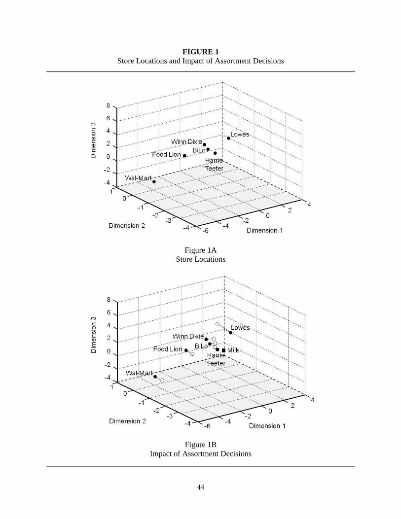
44

FIGURE 1 Store Locations and Impact of Assortment Decisions

Figure 1A Store Locations

Figure 1B Impact of Assortment Decisions

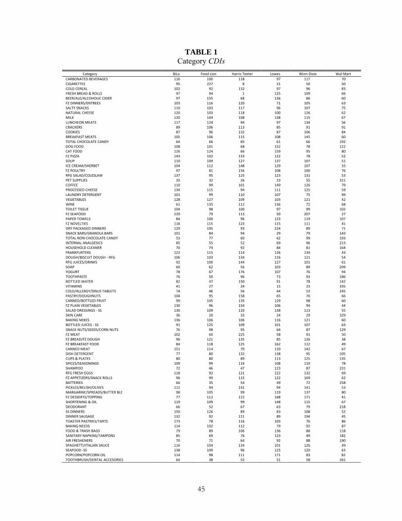
45

TABLE 1 Category CDIs

                   Category  BiLo  Food Lion  Harris Teeter  Lowes  Winn‐Dixie  Wal‐Mart 

CARBONATED BEVERAGES  116  100  118  97  117  70 CIGARETTES  95  227  8  21  50  50 COLD CEREAL  102  92  132  97  96  83 FRESH BREAD & ROLLS  97  94  1  125  109  66 BEER/ALE/ALCOHOLIC CIDER  97  155  68  136  86  60 FZ DINNERS/ENTREES  103  116  120  71  105  63 SALTY SNACKS  110  103  117  96  107  75 NATURAL CHEESE  120  103  118  100  126  62 MILK  120  104  108  138  115  67 LUNCHEON MEATS  117  124  94  97  134  56 CRACKERS  89  106  113  85  91  91 COOKIES  87  96  132  87  106  84 BREAKFAST MEATS  105  106  115  108  145  60 TOTAL CHOCOLATE CANDY  64  66  85  61  66  192 DOG FOOD  108  101  68  152  78  122 CAT FOOD  126  124  66  159  95  80 FZ PIZZA  143  102  133  122  78  52 SOUP  110  109  127  137  107  51 ICE CREAM/SHERBET  104  112  148  129  107  33 FZ POULTRY  97  81  156  108  100  76 RFG SALAD/COLESLAW  137  95  125  123  131  53 PET SUPPLIES  35  32  26  23  55  311 COFFEE  110  99  101  149  126  79 PROCESSED CHEESE  134  115  94  111  125  59 LAUNDRY DETERGENT  101  99  110  107  75  99 VEGETABLES  128  127  109  103  121  42 WINE  61  135  112  136  72  68 TOILET TISSUE  104  98  100  97  99  102 FZ SEAFOOD  220  79  113  50  207  27 PAPER TOWELS  84  100  96  123  119  107 FZ NOVELTIES  116  115  123  115  111  41 DRY PACKAGED DINNERS  129  105  93  224  89  71 SNACK BARS/GRANOLA BARS  101  84  94  29  79  143 TOTAL NON‐CHOCOLATE CANDY  53  77  60  62  99  193 INTERNAL ANALGESICS  85  55  52  69  96  213 HOUSEHOLD CLEANER  70  74  92  84  81  164 FRANKFURTERS  122  115  114  126  134  43 DOUGH/BISCUIT DOUGH ‐ RFG  106  103  134  116  121  54 RFG JUICES/DRINKS  92  100  144  127  101  61 SOAP  60  62  56  103  89  209 YOGURT  78  67  176  107  76  94 TOOTHPASTE  76  50  96  73  93  186 BOTTLED WATER  82  47  150  91  78  142 VITAMINS  41  27  24  15  23  335 COLD/ALLERGY/SINUS TABLETS  74  46  56  44  53  245 PASTRY/DOUGHNUTS  104  95  158  65  76  66 CANNED/BOTTLED FRUIT  99  105  135  129  98  60 FZ PLAIN VEGETABLES  130  96  154  106  94  44 SALAD DRESSINGS ‐ SS  130  109  110  138  113  55 SKIN CARE  36  20  33  24  29  329 BAKING MIXES  136  106  106  116  121  60 BOTTLED JUICES ‐ SS  91  125  109  101  107  63 SNACK NUTS/SEEDS/CORN NUTS  76  98  95  64  87  129 FZ MEAT  102  60  225  58  91  50 FZ BREAD/FZ DOUGH  96  121  135  85  126  38 FZ BREAKFAST FOOD  84  118  125  162  112  49 CANNED MEAT  151  114  70  110  142  67 DISH DETERGENT  77  80  132  138  95  105 CUPS & PLATES  80  80  89  113  125  135 SPICES/SEASONINGS  109  99  116  108  110  78 SHAMPOO  72  46  47  123  87  231 RFG FRESH EGGS  118  92  121  122  132  69 FZ APPETIZERS/SNACK ROLLS  96  99  115  122  169  62 BATTERIES  66  35  54  49  72  258 PICKLES/RELISH/OLIVES  112  94  141  94  141  53 MARGARINE/SPREADS/BUTTER BLE  98  105  99  119  137  80 FZ DESSERTS/TOPPING  77  112  122  168  171  41 SHORTENING & OIL  119  109  99  148  115  67 DEODORANT  66  52  67  63  79  218 SS DINNERS  150  126  89  83  108  52 DINNER SAUSAGE  132  92  121  89  194  45 TOASTER PASTRIES/TARTS  173  78  116  103  76  86 BAKING NEEDS  114  102  112  79  92  87 FOOD & TRASH BAGS  79  89  106  136  88  118 SANITARY NAPKINS/TAMPONS  85  69  76  123  49  182 AIR FRESHENERS  70  71  64  92  88  190 SPAGHETTI/ITALIAN SAUCE  116  104  134  101  126  49 SEAFOOD ‐SS  138  109  96  125  120  63 POPCORN/POPCORN OIL  114  98  111  171  83  82 TOOTHBRUSH/DENTAL ACCESORIES  64  38  52  51  58  261 

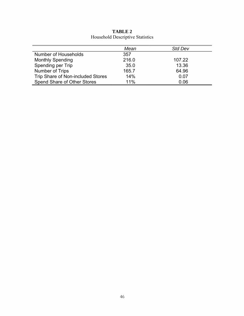
46

TABLE 2 Household Descriptive Statistics

Mean Std Dev Number of Households 357 Monthly Spending 216.0 107.22 Spending per Trip 35.0 13.36 Number of Trips 165.7 64.96 Trip Share of Non-included Stores 14% 0.07 Spend Share of Other Stores 11% 0.06

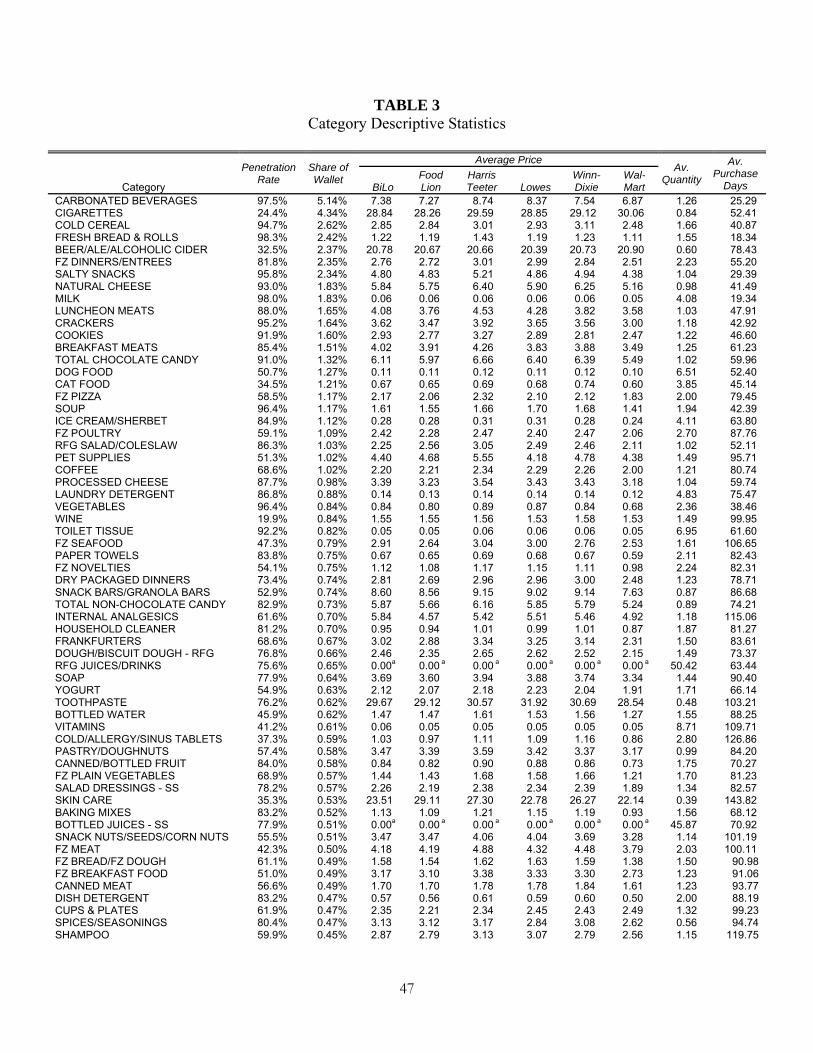
47

TABLE 3 Category Descriptive Statistics

Penetration Rate

Share of Wallet

Average Price Av.

Quantity

Av. Purchase

Days Category BiLo Food Lion

Harris Teeter Lowes

Winn-Dixie

Wal-Mart

CARBONATED BEVERAGES 97.5% 5.14% 7.38 7.27 8.74 8.37 7.54 6.87 1.26 25.29 CIGARETTES 24.4% 4.34% 28.84 28.26 29.59 28.85 29.12 30.06 0.84 52.41 COLD CEREAL 94.7% 2.62% 2.85 2.84 3.01 2.93 3.11 2.48 1.66 40.87 FRESH BREAD & ROLLS 98.3% 2.42% 1.22 1.19 1.43 1.19 1.23 1.11 1.55 18.34 BEER/ALE/ALCOHOLIC CIDER 32.5% 2.37% 20.78 20.67 20.66 20.39 20.73 20.90 0.60 78.43 FZ DINNERS/ENTREES 81.8% 2.35% 2.76 2.72 3.01 2.99 2.84 2.51 2.23 55.20 SALTY SNACKS 95.8% 2.34% 4.80 4.83 5.21 4.86 4.94 4.38 1.04 29.39 NATURAL CHEESE 93.0% 1.83% 5.84 5.75 6.40 5.90 6.25 5.16 0.98 41.49 MILK 98.0% 1.83% 0.06 0.06 0.06 0.06 0.06 0.05 4.08 19.34 LUNCHEON MEATS 88.0% 1.65% 4.08 3.76 4.53 4.28 3.82 3.58 1.03 47.91 CRACKERS 95.2% 1.64% 3.62 3.47 3.92 3.65 3.56 3.00 1.18 42.92 COOKIES 91.9% 1.60% 2.93 2.77 3.27 2.89 2.81 2.47 1.22 46.60 BREAKFAST MEATS 85.4% 1.51% 4.02 3.91 4.26 3.83 3.88 3.49 1.25 61.23 TOTAL CHOCOLATE CANDY 91.0% 1.32% 6.11 5.97 6.66 6.40 6.39 5.49 1.02 59.96 DOG FOOD 50.7% 1.27% 0.11 0.11 0.12 0.11 0.12 0.10 6.51 52.40 CAT FOOD 34.5% 1.21% 0.67 0.65 0.69 0.68 0.74 0.60 3.85 45.14 FZ PIZZA 58.5% 1.17% 2.17 2.06 2.32 2.10 2.12 1.83 2.00 79.45 SOUP 96.4% 1.17% 1.61 1.55 1.66 1.70 1.68 1.41 1.94 42.39 ICE CREAM/SHERBET 84.9% 1.12% 0.28 0.28 0.31 0.31 0.28 0.24 4.11 63.80 FZ POULTRY 59.1% 1.09% 2.42 2.28 2.47 2.40 2.47 2.06 2.70 87.76 RFG SALAD/COLESLAW 86.3% 1.03% 2.25 2.56 3.05 2.49 2.46 2.11 1.02 52.11 PET SUPPLIES 51.3% 1.02% 4.40 4.68 5.55 4.18 4.78 4.38 1.49 95.71 COFFEE 68.6% 1.02% 2.20 2.21 2.34 2.29 2.26 2.00 1.21 80.74 PROCESSED CHEESE 87.7% 0.98% 3.39 3.23 3.54 3.43 3.43 3.18 1.04 59.74 LAUNDRY DETERGENT 86.8% 0.88% 0.14 0.13 0.14 0.14 0.14 0.12 4.83 75.47 VEGETABLES 96.4% 0.84% 0.84 0.80 0.89 0.87 0.84 0.68 2.36 38.46 WINE 19.9% 0.84% 1.55 1.55 1.56 1.53 1.58 1.53 1.49 99.95 TOILET TISSUE 92.2% 0.82% 0.05 0.05 0.06 0.06 0.06 0.05 6.95 61.60 FZ SEAFOOD 47.3% 0.79% 2.91 2.64 3.04 3.00 2.76 2.53 1.61 106.65 PAPER TOWELS 83.8% 0.75% 0.67 0.65 0.69 0.68 0.67 0.59 2.11 82.43 FZ NOVELTIES 54.1% 0.75% 1.12 1.08 1.17 1.15 1.11 0.98 2.24 82.31 DRY PACKAGED DINNERS 73.4% 0.74% 2.81 2.69 2.96 2.96 3.00 2.48 1.23 78.71 SNACK BARS/GRANOLA BARS 52.9% 0.74% 8.60 8.56 9.15 9.02 9.14 7.63 0.87 86.68 TOTAL NON-CHOCOLATE CANDY 82.9% 0.73% 5.87 5.66 6.16 5.85 5.79 5.24 0.89 74.21 INTERNAL ANALGESICS 61.6% 0.70% 5.84 4.57 5.42 5.51 5.46 4.92 1.18 115.06 HOUSEHOLD CLEANER 81.2% 0.70% 0.95 0.94 1.01 0.99 1.01 0.87 1.87 81.27 FRANKFURTERS 68.6% 0.67% 3.02 2.88 3.34 3.25 3.14 2.31 1.50 83.61 DOUGH/BISCUIT DOUGH - RFG 76.8% 0.66% 2.46 2.35 2.65 2.62 2.52 2.15 1.49 73.37 RFG JUICES/DRINKS 75.6% 0.65% 0.00a 0.00 a 0.00 a 0.00 a 0.00 a 0.00 a 50.42 63.44 SOAP 77.9% 0.64% 3.69 3.60 3.94 3.88 3.74 3.34 1.44 90.40 YOGURT 54.9% 0.63% 2.12 2.07 2.18 2.23 2.04 1.91 1.71 66.14 TOOTHPASTE 76.2% 0.62% 29.67 29.12 30.57 31.92 30.69 28.54 0.48 103.21 BOTTLED WATER 45.9% 0.62% 1.47 1.47 1.61 1.53 1.56 1.27 1.55 88.25 VITAMINS 41.2% 0.61% 0.06 0.05 0.05 0.05 0.05 0.05 8.71 109.71 COLD/ALLERGY/SINUS TABLETS 37.3% 0.59% 1.03 0.97 1.11 1.09 1.16 0.86 2.80 126.86 PASTRY/DOUGHNUTS 57.4% 0.58% 3.47 3.39 3.59 3.42 3.37 3.17 0.99 84.20 CANNED/BOTTLED FRUIT 84.0% 0.58% 0.84 0.82 0.90 0.88 0.86 0.73 1.75 70.27 FZ PLAIN VEGETABLES 68.9% 0.57% 1.44 1.43 1.68 1.58 1.66 1.21 1.70 81.23 SALAD DRESSINGS - SS 78.2% 0.57% 2.26 2.19 2.38 2.34 2.39 1.89 1.34 82.57 SKIN CARE 35.3% 0.53% 23.51 29.11 27.30 22.78 26.27 22.14 0.39 143.82 BAKING MIXES 83.2% 0.52% 1.13 1.09 1.21 1.15 1.19 0.93 1.56 68.12 BOTTLED JUICES - SS 77.9% 0.51% 0.00a 0.00 a 0.00 a 0.00 a 0.00 a 0.00 a 45.87 70.92 SNACK NUTS/SEEDS/CORN NUTS 55.5% 0.51% 3.47 3.47 4.06 4.04 3.69 3.28 1.14 101.19 FZ MEAT 42.3% 0.50% 4.18 4.19 4.88 4.32 4.48 3.79 2.03 100.11 FZ BREAD/FZ DOUGH 61.1% 0.49% 1.58 1.54 1.62 1.63 1.59 1.38 1.50 90.98 FZ BREAKFAST FOOD 51.0% 0.49% 3.17 3.10 3.38 3.33 3.30 2.73 1.23 91.06 CANNED MEAT 56.6% 0.49% 1.70 1.70 1.78 1.78 1.84 1.61 1.23 93.77 DISH DETERGENT 83.2% 0.47% 0.57 0.56 0.61 0.59 0.60 0.50 2.00 88.19 CUPS & PLATES 61.9% 0.47% 2.35 2.21 2.34 2.45 2.43 2.49 1.32 99.23 SPICES/SEASONINGS 80.4% 0.47% 3.13 3.12 3.17 2.84 3.08 2.62 0.56 94.74 SHAMPOO 59.9% 0.45% 2.87 2.79 3.13 3.07 2.79 2.56 1.15 119.75

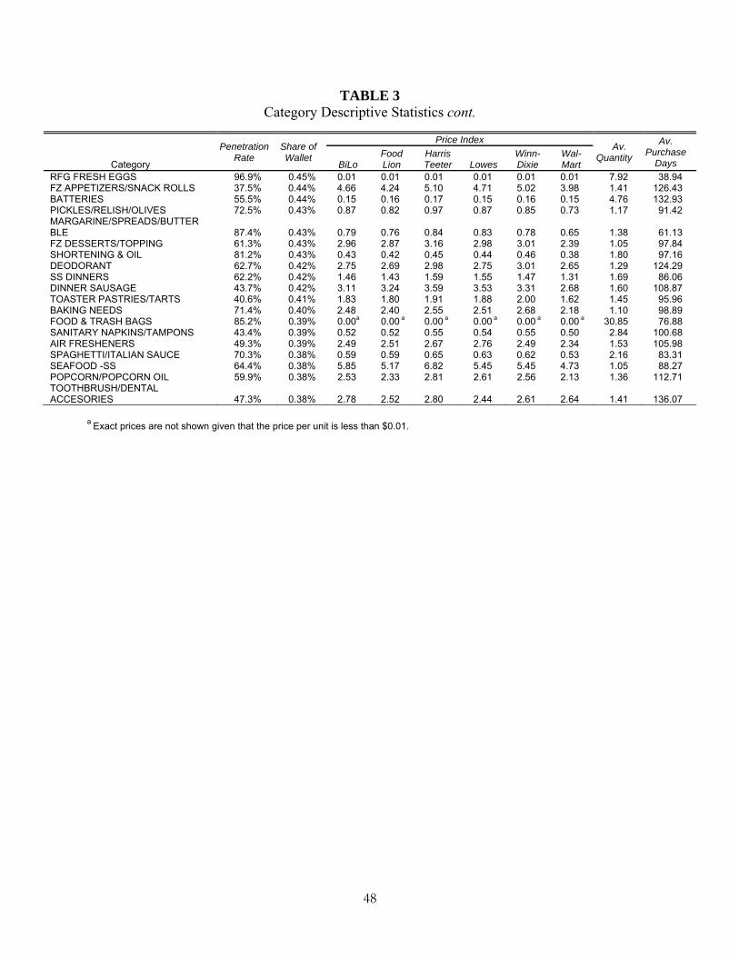
48

TABLE 3 Category Descriptive Statistics cont.

Penetration

Rate Share of Wallet

Price Index Av.

Quantity

Av. Purchase

Days Category BiLo Food Lion

Harris Teeter Lowes

Winn-Dixie

Wal-Mart

RFG FRESH EGGS 96.9% 0.45% 0.01 0.01 0.01 0.01 0.01 0.01 7.92 38.94 FZ APPETIZERS/SNACK ROLLS 37.5% 0.44% 4.66 4.24 5.10 4.71 5.02 3.98 1.41 126.43 BATTERIES 55.5% 0.44% 0.15 0.16 0.17 0.15 0.16 0.15 4.76 132.93 PICKLES/RELISH/OLIVES 72.5% 0.43% 0.87 0.82 0.97 0.87 0.85 0.73 1.17 91.42 MARGARINE/SPREADS/BUTTER BLE 87.4% 0.43% 0.79 0.76 0.84 0.83 0.78 0.65 1.38 61.13 FZ DESSERTS/TOPPING 61.3% 0.43% 2.96 2.87 3.16 2.98 3.01 2.39 1.05 97.84 SHORTENING & OIL 81.2% 0.43% 0.43 0.42 0.45 0.44 0.46 0.38 1.80 97.16 DEODORANT 62.7% 0.42% 2.75 2.69 2.98 2.75 3.01 2.65 1.29 124.29 SS DINNERS 62.2% 0.42% 1.46 1.43 1.59 1.55 1.47 1.31 1.69 86.06 DINNER SAUSAGE 43.7% 0.42% 3.11 3.24 3.59 3.53 3.31 2.68 1.60 108.87 TOASTER PASTRIES/TARTS 40.6% 0.41% 1.83 1.80 1.91 1.88 2.00 1.62 1.45 95.96 BAKING NEEDS 71.4% 0.40% 2.48 2.40 2.55 2.51 2.68 2.18 1.10 98.89 FOOD & TRASH BAGS 85.2% 0.39% 0.00a 0.00 a 0.00 a 0.00 a 0.00 a 0.00 a 30.85 76.88 SANITARY NAPKINS/TAMPONS 43.4% 0.39% 0.52 0.52 0.55 0.54 0.55 0.50 2.84 100.68 AIR FRESHENERS 49.3% 0.39% 2.49 2.51 2.67 2.76 2.49 2.34 1.53 105.98 SPAGHETTI/ITALIAN SAUCE 70.3% 0.38% 0.59 0.59 0.65 0.63 0.62 0.53 2.16 83.31 SEAFOOD -SS 64.4% 0.38% 5.85 5.17 6.82 5.45 5.45 4.73 1.05 88.27 POPCORN/POPCORN OIL 59.9% 0.38% 2.53 2.33 2.81 2.61 2.56 2.13 1.36 112.71 TOOTHBRUSH/DENTAL ACCESORIES 47.3% 0.38% 2.78 2.52 2.80 2.44 2.61 2.64 1.41 136.07

a Exact prices are not shown given that the price per unit is less than $0.01.

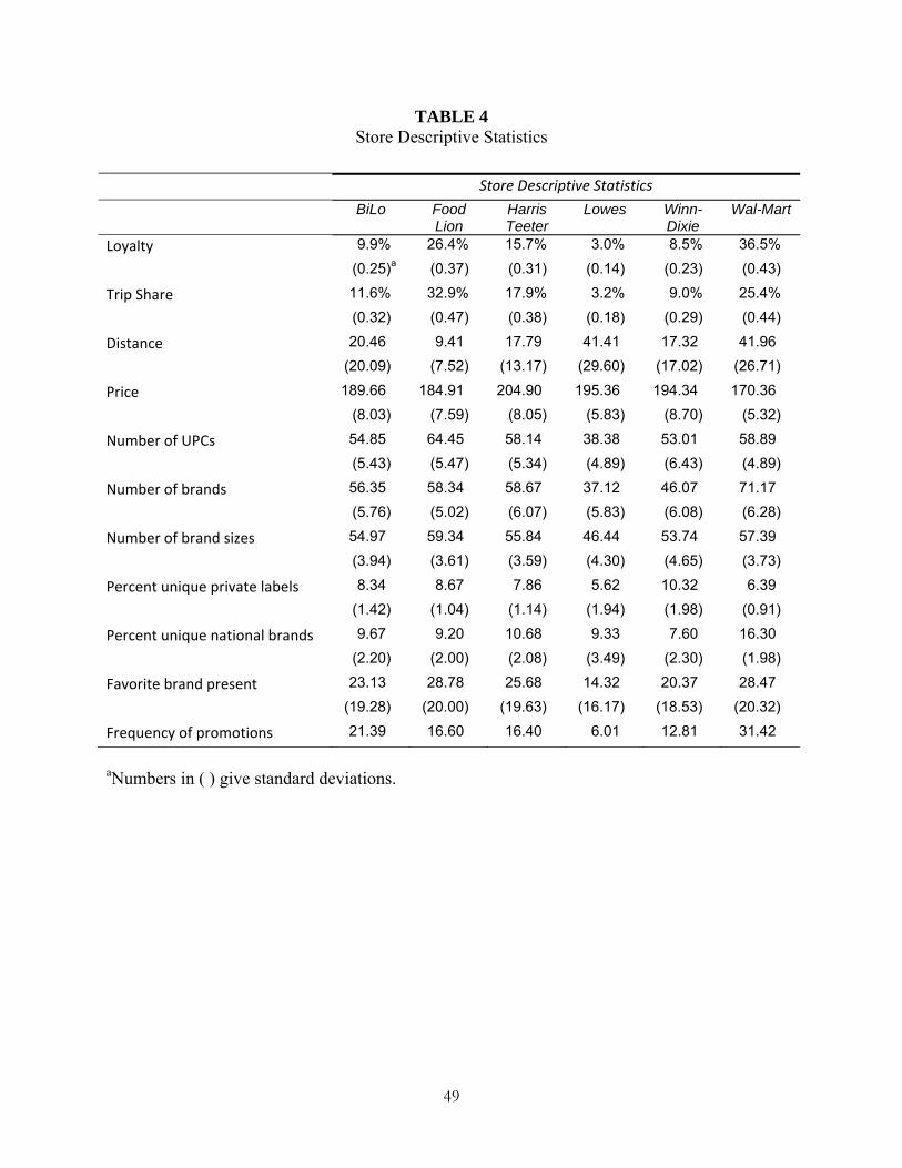
49

TABLE 4 Store Descriptive Statistics

  Store Descriptive Statistics

  BiLo Food Lion

Harris Teeter

Lowes Winn-Dixie

Wal-Mart

Loyalty  9.9% 26.4% 15.7% 3.0% 8.5% 36.5%

  (0.25)a (0.37) (0.31) (0.14) (0.23) (0.43)

Trip Share  11.6% 32.9% 17.9% 3.2% 9.0% 25.4%

  (0.32) (0.47) (0.38) (0.18) (0.29) (0.44)

Distance  20.46 9.41 17.79 41.41 17.32 41.96

  (20.09) (7.52) (13.17) (29.60) (17.02) (26.71)

Price  189.66 184.91 204.90 195.36 194.34 170.36

  (8.03) (7.59) (8.05) (5.83) (8.70) (5.32)

Number of UPCs  54.85 64.45 58.14 38.38 53.01 58.89

  (5.43) (5.47) (5.34) (4.89) (6.43) (4.89)

Number of brands  56.35 58.34 58.67 37.12 46.07 71.17

  (5.76) (5.02) (6.07) (5.83) (6.08) (6.28)

Number of brand sizes  54.97 59.34 55.84 46.44 53.74 57.39

  (3.94) (3.61) (3.59) (4.30) (4.65) (3.73)

Percent unique private labels  8.34 8.67 7.86 5.62 10.32 6.39

  (1.42) (1.04) (1.14) (1.94) (1.98) (0.91)

Percent unique national brands  9.67 9.20 10.68 9.33 7.60 16.30

  (2.20) (2.00) (2.08) (3.49) (2.30) (1.98)

Favorite brand present  23.13 28.78 25.68 14.32 20.37 28.47

  (19.28) (20.00) (19.63) (16.17) (18.53) (20.32)

Frequency of promotions  21.39 16.60 16.40 6.01 12.81 31.42

aNumbers in ( ) give standard deviations.

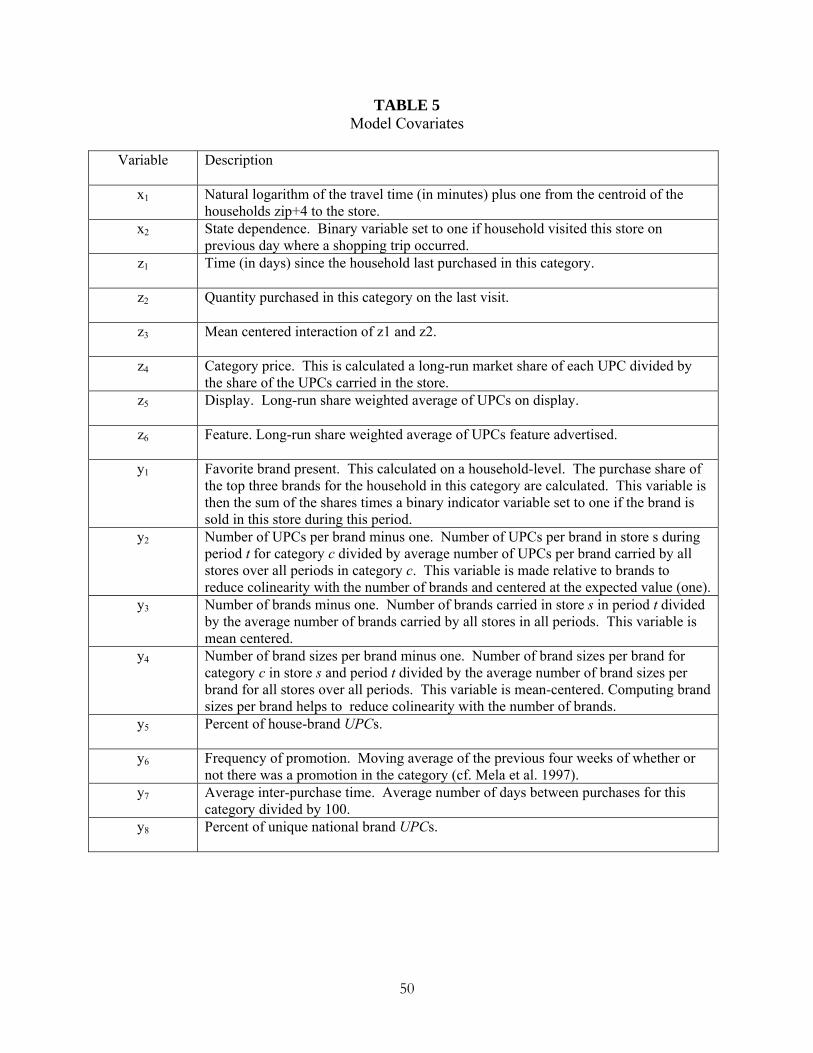
50

TABLE 5 Model Covariates

Variable Description

x1 Natural logarithm of the travel time (in minutes) plus one from the centroid of the households zip+4 to the store.

x2 State dependence. Binary variable set to one if household visited this store on previous day where a shopping trip occurred.

z1 Time (in days) since the household last purchased in this category.

z2 Quantity purchased in this category on the last visit.

z3 Mean centered interaction of z1 and z2.

z4 Category price. This is calculated a long-run market share of each UPC divided by the share of the UPCs carried in the store.

z5 Display. Long-run share weighted average of UPCs on display.

z6 Feature. Long-run share weighted average of UPCs feature advertised.

y1 Favorite brand present. This calculated on a household-level. The purchase share of the top three brands for the household in this category are calculated. This variable is then the sum of the shares times a binary indicator variable set to one if the brand is sold in this store during this period.

y2 Number of UPCs per brand minus one. Number of UPCs per brand in store s during period t for category c divided by average number of UPCs per brand carried by all stores over all periods in category c. This variable is made relative to brands to reduce colinearity with the number of brands and centered at the expected value (one).

y3 Number of brands minus one. Number of brands carried in store s in period t divided by the average number of brands carried by all stores in all periods. This variable is mean centered.

y4 Number of brand sizes per brand minus one. Number of brand sizes per brand for category c in store s and period t divided by the average number of brand sizes per brand for all stores over all periods. This variable is mean-centered. Computing brand sizes per brand helps to reduce colinearity with the number of brands.

y5 Percent of house-brand UPCs.

y6 Frequency of promotion. Moving average of the previous four weeks of whether or not there was a promotion in the category (cf. Mela et al. 1997).

y7 Average inter-purchase time. Average number of days between purchases for this category divided by 100.

y8 Percent of unique national brand UPCs.

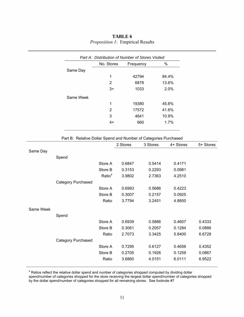
51

TABLE 6 Proposition 1: Empirical Results

Part A: Distribution of Number of Stores Visited

No. Stores Frequency %

Same Day

1 42794 84.4%

2 6878 13.6%

3+ 1033 2.0%

Same Week

1 19380 45.8%

2 17572 41.6%

3 4641 10.9%

4+ 660 1.7%

Part B: Relative Dollar Spend and Number of Categories Purchased

2 Stores 3 Stores 4+ Stores 5+ Stores

Same Day

Spend

Store A 0.6847 0.5414 0.4171

Store B 0.3153 0.2293 0.0981

Ratioa 3.9802 2.7363 4.2510

Category Purchased

Store A 0.6993 0.5686 0.4223

Store B 0.3007 0.2157 0.0925

Ratio 3.7794 3.2451 4.8850

Same Week

Spend

Store A 0.6939 0.5886 0.4607 0.4333

Store B 0.3061 0.2057 0.1284 0.0886

Ratio 2.7073 3.3425 5.8400 6.6728

Category Purchased

Store A 0.7295 0.6127 0.4656 0.4352

Store B 0.2705 0.1926 0.1259 0.0867

Ratio 3.6860 4.0151 6.0111 6.9522

a Ratios reflect the relative dollar spend and number of categories shopped computed by dividing dollar spend/number of categories shopped for the store receiving the largest dollar spend/number of categories shopped by the dollar spend/number of categories shopped for all remaining stores. See footnote #7

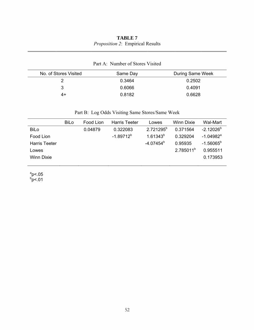
52

TABLE 7 Proposition 2: Empirical Results

Part A: Number of Stores Visited

No. of Stores Visited Same Day During Same Week

2 0.3464 0.2502

3 0.6066 0.4091

4+ 0.8182 0.6628

Part B: Log Odds Visiting Same Stores/Same Week

BiLo Food Lion Harris Teeter Lowes Winn Dixie Wal-Mart

BiLo 0.04879 0.322083 2.721295b 0.371564 -2.12026b

Food Lion -1.89712b 1.61343b 0.329204 -1.04982a

Harris Teeter -4.07454b 0.95935 -1.56065b

Lowes 2.785011b 0.955511

Winn Dixie 0.173953

ap<.05 bp<.01

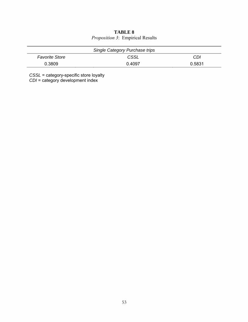
53

TABLE 8 Proposition 3: Empirical Results

Single Category Purchase trips

Favorite Store CSSL CDI

0.3809 0.4097 0.5831

CSSL = category-specific store loyalty CDI = category development index

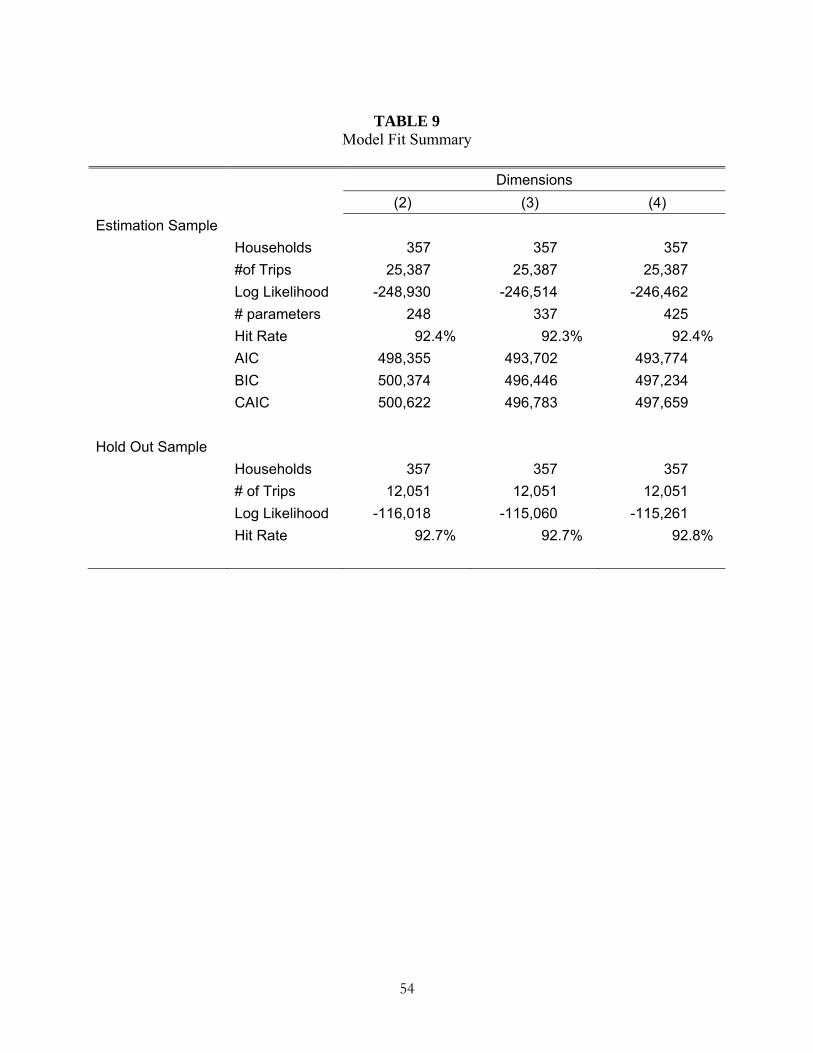
54

TABLE 9 Model Fit Summary

Dimensions

(2) (3) (4)

Estimation Sample

Households 357 357 357

#of Trips 25,387 25,387 25,387

Log Likelihood -248,930 -246,514 -246,462

# parameters 248 337 425

Hit Rate 92.4% 92.3% 92.4%

AIC 498,355 493,702 493,774

BIC 500,374 496,446 497,234

CAIC 500,622 496,783 497,659

Hold Out Sample

Households 357 357 357

# of Trips 12,051 12,051 12,051

Log Likelihood -116,018 -115,060 -115,261

Hit Rate 92.7% 92.7% 92.8%

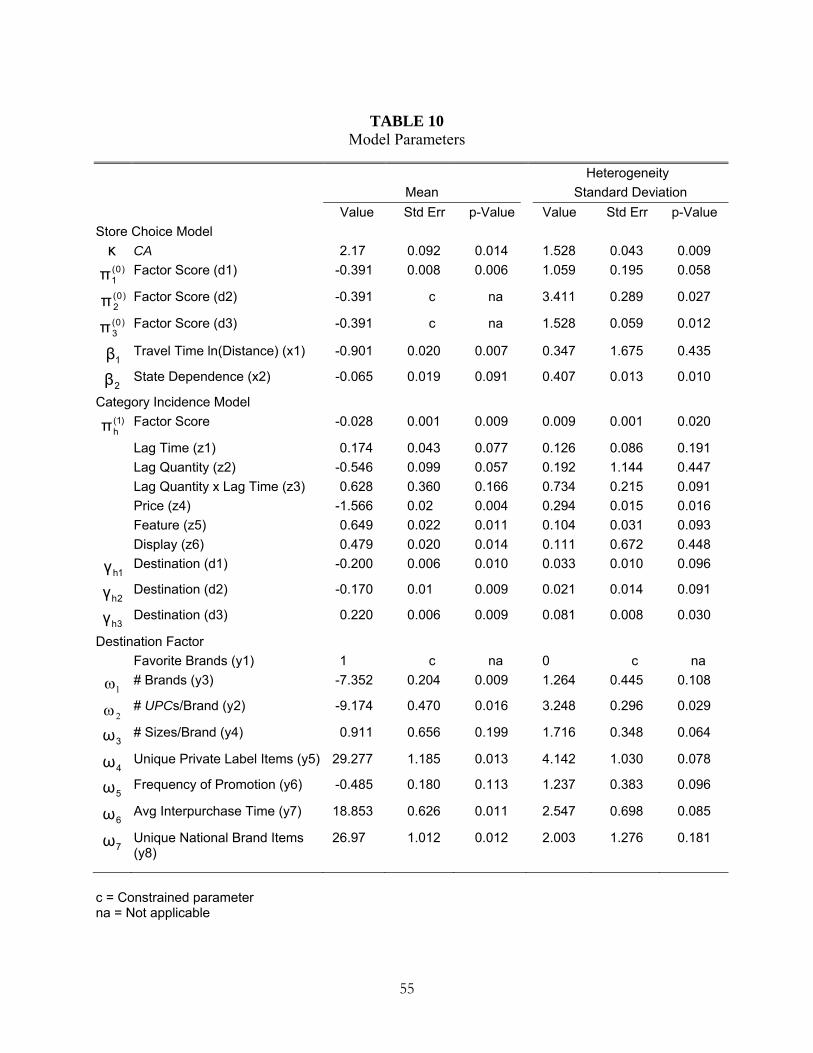
55

TABLE 10 Model Parameters

Heterogeneity

Mean Standard Deviation

Value Std Err p-Value Value Std Err p-Value

Store Choice Model

κ CA 2.17 0.092 0.014 1.528 0.043 0.009 )0(

1π Factor Score (d1) -0.391 0.008 0.006 1.059 0.195 0.058

)0(2π Factor Score (d2) -0.391 c na 3.411 0.289 0.027

)0(3π Factor Score (d3) -0.391 c na 1.528 0.059 0.012

1β Travel Time ln(Distance) (x1) -0.901 0.020 0.007 0.347 1.675 0.435

2β State Dependence (x2) -0.065 0.019 0.091 0.407 0.013 0.010

Category Incidence Model )1(

hπ Factor Score -0.028 0.001 0.009 0.009 0.001 0.020

Lag Time (z1) 0.174 0.043 0.077 0.126 0.086 0.191

Lag Quantity (z2) -0.546 0.099 0.057 0.192 1.144 0.447

Lag Quantity x Lag Time (z3) 0.628 0.360 0.166 0.734 0.215 0.091

Price (z4) -1.566 0.02 0.004 0.294 0.015 0.016

Feature (z5) 0.649 0.022 0.011 0.104 0.031 0.093

Display (z6) 0.479 0.020 0.014 0.111 0.672 0.448

1hγ Destination (d1) -0.200 0.006 0.010 0.033 0.010 0.096

2hγ Destination (d2) -0.170 0.01 0.009 0.021 0.014 0.091

3hγ Destination (d3) 0.220 0.006 0.009 0.081 0.008 0.030

Destination Factor

Favorite Brands (y1) 1 c na 0 c na

1 # Brands (y3) -7.352 0.204 0.009 1.264 0.445 0.108

2 # UPCs/Brand (y2) -9.174 0.470 0.016 3.248 0.296 0.029

3ω # Sizes/Brand (y4) 0.911 0.656 0.199 1.716 0.348 0.064

4ω Unique Private Label Items (y5) 29.277 1.185 0.013 4.142 1.030 0.078

5ω Frequency of Promotion (y6) -0.485 0.180 0.113 1.237 0.383 0.096

6ω Avg Interpurchase Time (y7) 18.853 0.626 0.011 2.547 0.698 0.085

7ω Unique National Brand Items (y8)

26.97 1.012 0.012 2.003 1.276 0.181

c = Constrained parameter na = Not applicable

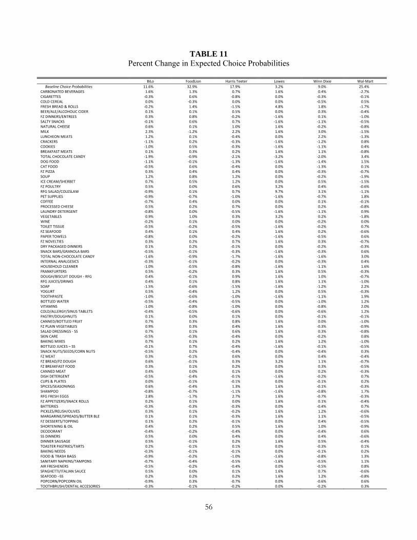
56

TABLE 11 Percent Change in Expected Choice Probabilities

   BiLo  FoodLion  Harris Teeter  Lowes  Winn Dixie  Wal‐Mart 

     Baseline Choice Probabilities  11.6%  32.9%  17.9%  3.2%  9.0%  25.4% CARBONATED BEVERAGES  1.6%  1.3%  0.7%  1.6%  0.4%  ‐2.7% CIGARETTES  ‐0.3%  0.6%  ‐0.8%  0.0%  ‐0.3%  ‐0.1% COLD CEREAL  0.0%  ‐0.3%  0.0%  0.0%  ‐0.5%  0.5% FRESH BREAD & ROLLS  ‐0.2%  1.4%  ‐1.5%  4.8%  1.8%  ‐1.7% BEER/ALE/ALCOHOLIC CIDER  0.1%  0.1%  0.5%  0.0%  0.3%  ‐0.4% FZ DINNERS/ENTREES  0.3%  0.8%  ‐0.2%  ‐1.6%  0.1%  ‐1.0% SALTY SNACKS  ‐0.1%  0.6%  0.7%  ‐1.6%  ‐1.1%  ‐0.5% NATURAL CHEESE  0.6%  0.1%  1.0%  1.6%  ‐0.2%  ‐0.8% MILK  2.3%  ‐1.2%  2.2%  1.6%  3.0%  ‐1.5% LUNCHEON MEATS  1.2%  0.1%  ‐0.4%  0.0%  2.2%  ‐1.3% CRACKERS  ‐1.1%  0.2%  ‐0.3%  ‐1.6%  ‐1.2%  0.8% COOKIES  ‐1.0%  0.5%  ‐0.3%  ‐1.6%  ‐1.1%  0.4% BREAKFAST MEATS  0.1%  0.3%  0.2%  1.6%  1.1%  ‐0.8% TOTAL CHOCOLATE CANDY  ‐1.9%  ‐0.9%  ‐2.1%  ‐3.2%  ‐2.0%  3.4% DOG FOOD  ‐1.1%  ‐0.1%  ‐1.3%  ‐1.6%  ‐1.4%  1.5% CAT FOOD  ‐0.5%  0.6%  ‐0.4%  0.0%  ‐1.3%  0.1% FZ PIZZA  0.3%  0.4%  0.4%  0.0%  ‐0.3%  ‐0.7% SOUP  1.2%  0.8%  1.2%  0.0%  ‐0.2%  ‐1.9% ICE CREAM/SHERBET  0.7%  0.5%  1.2%  0.0%  0.5%  ‐1.5% FZ POULTRY  0.5%  0.0%  0.6%  3.2%  0.4%  ‐0.6% RFG SALAD/COLESLAW  ‐0.9%  0.1%  0.7%  9.7%  3.1%  ‐1.1% PET SUPPLIES  ‐0.9%  ‐0.7%  ‐1.0%  ‐1.6%  ‐0.7%  1.8% COFFEE  ‐0.7%  0.4%  0.0%  0.0%  0.1%  ‐0.1% PROCESSED CHEESE  0.5%  0.2%  0.7%  0.0%  0.2%  ‐0.8% LAUNDRY DETERGENT  ‐0.8%  0.0%  ‐0.5%  ‐1.6%  ‐1.1%  0.9% VEGETABLES  0.9%  1.0%  0.3%  3.2%  0.2%  ‐1.8% WINE  ‐0.2%  0.1%  0.0%  0.0%  ‐0.2%  0.0% TOILET TISSUE  ‐0.5%  ‐0.2%  ‐0.5%  ‐1.6%  ‐0.2%  0.7% FZ SEAFOOD  0.4%  0.1%  0.4%  1.6%  0.2%  ‐0.6% PAPER TOWELS  ‐0.8%  0.0%  ‐0.2%  ‐1.6%  ‐0.5%  0.6% FZ NOVELTIES  0.3%  0.2%  0.7%  1.6%  0.3%  ‐0.7% DRY PACKAGED DINNERS  0.1%  0.2%  ‐0.1%  0.0%  ‐0.2%  ‐0.3% SNACK BARS/GRANOLA BARS  ‐0.5%  ‐0.1%  ‐0.3%  ‐1.6%  ‐0.3%  0.6% TOTAL NON‐CHOCOLATE CANDY  ‐1.6%  ‐0.9%  ‐1.7%  ‐1.6%  ‐1.6%  3.0% INTERNAL ANALGESICS  ‐0.3%  ‐0.1%  ‐0.2%  0.0%  ‐0.3%  0.4% HOUSEHOLD CLEANER  ‐1.0%  ‐0.5%  ‐0.8%  ‐1.6%  ‐1.1%  1.6% FRANKFURTERS  0.5%  ‐0.2%  0.3%  1.6%  0.5%  ‐0.3% DOUGH/BISCUIT DOUGH ‐ RFG  0.4%  ‐0.1%  0.9%  1.6%  1.0%  ‐0.7% RFG JUICES/DRINKS  0.4%  0.1%  0.8%  1.6%  1.1%  ‐1.0% SOAP  ‐1.5%  ‐0.6%  ‐1.5%  ‐1.6%  ‐1.2%  2.2% YOGURT  0.5%  ‐0.4%  1.2%  0.0%  0.5%  ‐0.3% TOOTHPASTE  ‐1.0%  ‐0.6%  ‐1.0%  ‐1.6%  ‐1.1%  1.9% BOTTLED WATER  ‐0.5%  ‐0.4%  ‐0.5%  0.0%  ‐1.0%  1.2% VITAMINS  ‐1.0%  ‐0.8%  ‐1.0%  0.0%  ‐0.8%  2.0% COLD/ALLERGY/SINUS TABLETS  ‐0.4%  ‐0.5%  ‐0.6%  0.0%  ‐0.6%  1.2% PASTRY/DOUGHNUTS  0.1%  0.0%  0.1%  0.0%  ‐0.1%  ‐0.1% CANNED/BOTTLED FRUIT  0.7%  0.3%  0.8%  1.6%  0.0%  ‐1.0% FZ PLAIN VEGETABLES  0.9%  0.3%  0.4%  1.6%  ‐0.3%  ‐0.9% SALAD DRESSINGS ‐ SS  0.7%  0.1%  0.6%  1.6%  0.3%  ‐0.8% SKIN CARE  ‐0.5%  ‐0.3%  ‐0.4%  0.0%  ‐0.2%  0.8% BAKING MIXES  0.7%  0.1%  0.2%  1.6%  1.2%  ‐1.0% BOTTLED JUICES – SS  ‐0.1%  0.7%  ‐0.4%  ‐1.6%  ‐0.1%  ‐0.5% SNACK NUTS/SEEDS/CORN NUTS  ‐0.5%  0.2%  ‐0.4%  0.0%  ‐0.4%  0.3% FZ MEAT  0.3%  ‐0.1%  0.6%  0.0%  0.4%  ‐0.4% FZ BREAD/FZ DOUGH  0.6%  ‐0.1%  0.3%  3.2%  1.1%  ‐0.7% FZ BREAKFAST FOOD  0.3%  0.1%  0.2%  0.0%  0.3%  ‐0.5% CANNED MEAT  0.4%  0.0%  0.1%  0.0%  0.2%  ‐0.3% DISH DETERGENT  ‐0.5%  ‐0.4%  ‐0.1%  ‐1.6%  ‐0.2%  0.7% CUPS & PLATES  0.0%  ‐0.1%  ‐0.1%  0.0%  ‐0.1%  0.2% SPICES/SEASONINGS  0.6%  ‐0.4%  1.3%  1.6%  ‐0.1%  ‐0.3% SHAMPOO  ‐0.8%  ‐0.7%  ‐1.1%  ‐1.6%  ‐0.8%  1.7% RFG FRESH EGGS  2.8%  ‐1.7%  2.7%  1.6%  ‐0.7%  ‐0.3% FZ APPETIZERS/SNACK ROLLS  0.2%  0.1%  0.0%  1.6%  0.1%  ‐0.4% BATTERIES  ‐0.3%  ‐0.3%  ‐0.3%  0.0%  ‐0.4%  0.7% PICKLES/RELISH/OLIVES  0.3%  0.1%  ‐0.2%  1.6%  1.2%  ‐0.6% MARGARINE/SPREADS/BUTTER BLE  0.1%  0.1%  ‐0.3%  1.6%  1.1%  ‐0.5% FZ DESSERTS/TOPPING  0.1%  0.2%  ‐0.1%  0.0%  0.4%  ‐0.5% SHORTENING & OIL  0.4%  0.2%  0.5%  1.6%  1.0%  ‐0.9% DEODORANT  ‐0.4%  ‐0.2%  ‐0.4%  0.0%  ‐0.4%  0.6% SS DINNERS  0.5%  0.0%  0.4%  0.0%  0.4%  ‐0.6% DINNER SAUSAGE  0.5%  ‐0.1%  0.2%  1.6%  0.5%  ‐0.4% TOASTER PASTRIES/TARTS  0.2%  ‐0.1%  0.1%  0.0%  ‐0.3%  0.1% BAKING NEEDS  ‐0.3%  ‐0.1%  ‐0.1%  0.0%  ‐0.1%  0.2% FOOD & TRASH BAGS  ‐0.9%  ‐0.2%  ‐1.0%  ‐1.6%  ‐0.8%  1.3% SANITARY NAPKINS/TAMPONS  ‐0.7%  ‐0.4%  ‐0.5%  ‐1.6%  ‐0.5%  1.1% AIR FRESHENERS  ‐0.5%  ‐0.2%  ‐0.4%  0.0%  ‐0.5%  0.8% SPAGHETTI/ITALIAN SAUCE  0.5%  0.0%  0.1%  1.6%  0.7%  ‐0.6% SEAFOOD –SS  0.2%  0.2%  0.2%  1.6%  1.2%  ‐0.8% POPCORN/POPCORN OIL  ‐0.9%  0.3%  ‐0.7%  0.0%  ‐0.6%  0.6% TOOTHBRUSH/DENTAL ACCESORIES  ‐0.3%  ‐0.1%  ‐0.2%  0.0%  ‐0.2%  0.3% 

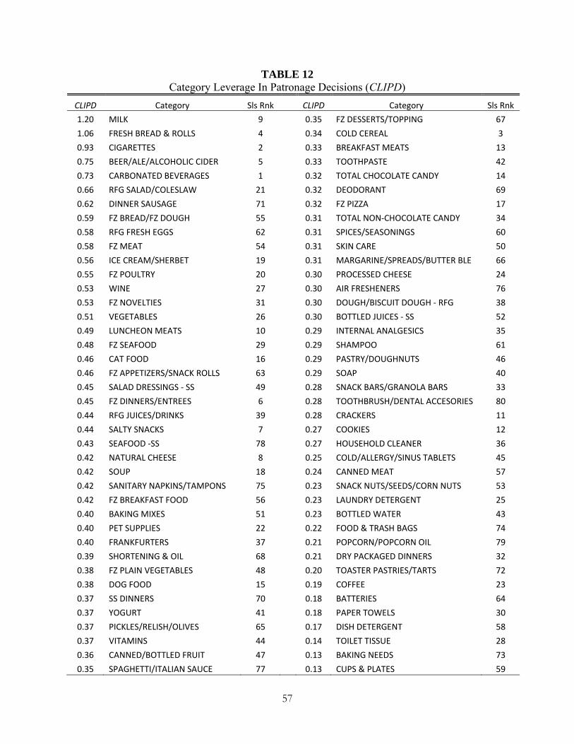
57

TABLE 12 Category Leverage In Patronage Decisions (CLIPD)

CLIPD  Category  Sls Rnk CLIPD Category  Sls Rnk

1.20  MILK  9  0.35  FZ DESSERTS/TOPPING  67 

1.06  FRESH BREAD & ROLLS  4  0.34  COLD CEREAL  3 

0.93  CIGARETTES  2  0.33  BREAKFAST MEATS  13 

0.75  BEER/ALE/ALCOHOLIC CIDER  5  0.33  TOOTHPASTE  42 

0.73  CARBONATED BEVERAGES  1  0.32  TOTAL CHOCOLATE CANDY  14 

0.66  RFG SALAD/COLESLAW  21  0.32  DEODORANT  69 

0.62  DINNER SAUSAGE  71  0.32  FZ PIZZA  17 

0.59  FZ BREAD/FZ DOUGH  55  0.31  TOTAL NON‐CHOCOLATE CANDY  34 

0.58  RFG FRESH EGGS  62  0.31  SPICES/SEASONINGS  60 

0.58  FZ MEAT  54  0.31  SKIN CARE  50 

0.56  ICE CREAM/SHERBET  19  0.31  MARGARINE/SPREADS/BUTTER BLE  66 

0.55  FZ POULTRY  20  0.30  PROCESSED CHEESE  24 

0.53  WINE  27  0.30  AIR FRESHENERS  76 

0.53  FZ NOVELTIES  31  0.30  DOUGH/BISCUIT DOUGH ‐ RFG  38 

0.51  VEGETABLES  26  0.30  BOTTLED JUICES ‐ SS  52 

0.49  LUNCHEON MEATS  10  0.29  INTERNAL ANALGESICS  35 

0.48  FZ SEAFOOD  29  0.29  SHAMPOO  61 

0.46  CAT FOOD  16  0.29  PASTRY/DOUGHNUTS  46 

0.46  FZ APPETIZERS/SNACK ROLLS  63  0.29  SOAP  40 

0.45  SALAD DRESSINGS ‐ SS  49  0.28  SNACK BARS/GRANOLA BARS  33 

0.45  FZ DINNERS/ENTREES  6  0.28  TOOTHBRUSH/DENTAL ACCESORIES  80 

0.44  RFG JUICES/DRINKS  39  0.28  CRACKERS  11 

0.44  SALTY SNACKS  7  0.27  COOKIES  12 

0.43  SEAFOOD ‐SS  78  0.27  HOUSEHOLD CLEANER  36 

0.42  NATURAL CHEESE  8  0.25  COLD/ALLERGY/SINUS TABLETS  45 

0.42  SOUP  18  0.24  CANNED MEAT  57 

0.42  SANITARY NAPKINS/TAMPONS  75  0.23  SNACK NUTS/SEEDS/CORN NUTS  53 

0.42  FZ BREAKFAST FOOD  56  0.23  LAUNDRY DETERGENT  25 

0.40  BAKING MIXES  51  0.23  BOTTLED WATER  43 

0.40  PET SUPPLIES  22  0.22  FOOD & TRASH BAGS  74 

0.40  FRANKFURTERS  37  0.21  POPCORN/POPCORN OIL  79 

0.39  SHORTENING & OIL  68  0.21  DRY PACKAGED DINNERS  32 

0.38  FZ PLAIN VEGETABLES  48  0.20  TOASTER PASTRIES/TARTS  72 

0.38  DOG FOOD  15  0.19  COFFEE  23 

0.37  SS DINNERS  70  0.18  BATTERIES  64 

0.37  YOGURT  41  0.18  PAPER TOWELS  30 

0.37  PICKLES/RELISH/OLIVES  65  0.17  DISH DETERGENT  58 

0.37  VITAMINS  44  0.14  TOILET TISSUE  28 

0.36  CANNED/BOTTLED FRUIT  47  0.13  BAKING NEEDS  73 

0.35  SPAGHETTI/ITALIAN SAUCE  77     0.13  CUPS & PLATES  59 

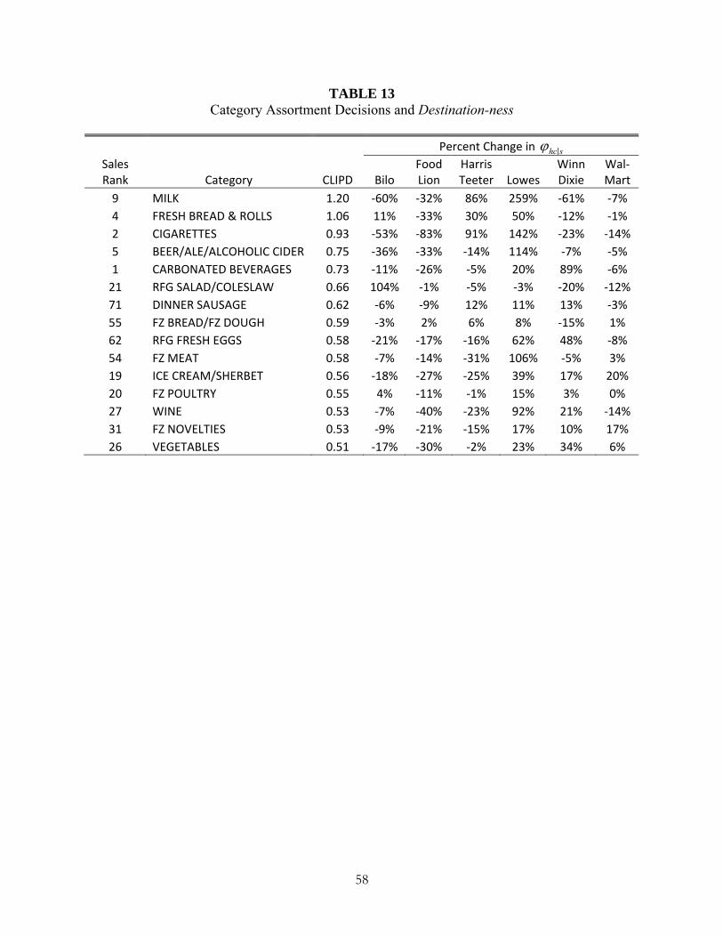
58

TABLE 13 Category Assortment Decisions and Destination-ness

         Percent Change in hc|s 

Sales Rank  Category  CLIPD  Bilo 

Food Lion 

Harris Teeter  Lowes 

Winn Dixie 

Wal‐Mart 

9  MILK  1.20  ‐60%  ‐32%  86%  259%  ‐61%  ‐7% 

4  FRESH BREAD & ROLLS  1.06  11%  ‐33%  30%  50%  ‐12%  ‐1% 

2  CIGARETTES  0.93  ‐53%  ‐83%  91%  142%  ‐23%  ‐14% 

5  BEER/ALE/ALCOHOLIC CIDER  0.75  ‐36%  ‐33%  ‐14%  114%  ‐7%  ‐5% 

1  CARBONATED BEVERAGES  0.73  ‐11%  ‐26%  ‐5%  20%  89%  ‐6% 

21  RFG SALAD/COLESLAW  0.66  104% ‐1%  ‐5%  ‐3%  ‐20%  ‐12% 

71  DINNER SAUSAGE  0.62  ‐6%  ‐9%  12%  11%  13%  ‐3% 

55  FZ BREAD/FZ DOUGH  0.59  ‐3%  2%  6%  8%  ‐15%  1% 

62  RFG FRESH EGGS  0.58  ‐21%  ‐17%  ‐16%  62%  48%  ‐8% 

54  FZ MEAT  0.58  ‐7%  ‐14%  ‐31%  106%  ‐5%  3% 

19  ICE CREAM/SHERBET  0.56  ‐18%  ‐27%  ‐25%  39%  17%  20% 

20  FZ POULTRY  0.55  4%  ‐11%  ‐1%  15%  3%  0% 

27  WINE  0.53  ‐7%  ‐40%  ‐23%  92%  21%  ‐14% 

31  FZ NOVELTIES  0.53  ‐9%  ‐21%  ‐15%  17%  10%  17% 

26  VEGETABLES  0.51  ‐17%  ‐30%  ‐2%  23%  34%  6%