NBER WORKING PAPER SERIES

DETECTING DISCRIMINATION IN AUDIT AND CORRESPONDENCE STUDIES

David Neumark

Working Paper 16448http://www.nber.org/papers/w16448

NATIONAL BUREAU OF ECONOMIC RESEARCH1050 Massachusetts Avenue

Cambridge, MA 02138October 2010

David Neumark is Professor of Economics and Director of the Center for Economics & Public Policyat UCI, a research associate of the NBER, and a research fellow at IZA. He is grateful to the UCIAcademic Senate Council on Research, Computing, and Libraries for research support, to Scott Barkowski,Marianne Bitler, Richard Blundell, Thomas Cornelißen, Ying-Ying Dong, Judith Hellerstein, JamesHeckman, an anonymous referee, and seminar participants at Baylor University, Cal State Fullerton,Cornell University, the Federal Reserve Bank of San Francisco, Hebrew University, the MelbourneInstitute, the University of Oklahoma, Tel Aviv University, the University of Sydney, and the All-CaliforniaLabor Conference for helpful comments, and to Scott Barkowski, Andrew Chang, Jennifer Graves,and Smith Williams for research assistance. He also thanks Marianne Bertrand and Sendhil Mullainathanfor supplying their data, available from the AEA website at http://www.aeaweb.org/articles.php?doi=10.1257/0002828042002561. The simulation data and the computer code used in this paper can be obtained beginning six monthsafter publication through three years hence from David Neumark, Department of Economics, 3151Social Science Plaza, UCI, Irvine, CA, 92697, dneumark@uci.edu. The views expressed herein arethose of the author and do not necessarily reflect the views of the National Bureau of Economic Research.

NBER working papers are circulated for discussion and comment purposes. They have not been peer-reviewed or been subject to the review by the NBER Board of Directors that accompanies officialNBER publications.

© 2010 by David Neumark. All rights reserved. Short sections of text, not to exceed two paragraphs,may be quoted without explicit permission provided that full credit, including © notice, is given tothe source.

Detecting Discrimination in Audit and Correspondence StudiesDavid NeumarkNBER Working Paper No. 16448October 2010, Revised September 2012JEL No. C93,J7

ABSTRACT

Audit studies testing for discrimination have been criticized because applicants from different groupsmay not appear identical to employers. Correspondence studies address this criticism by using fictitiouspaper applicants whose qualifications can be made identical across groups. However, Heckman andSiegelman (1993) show that group differences in the variance of unobservable determinants of productivitycan still generate spurious evidence of discrimination in either direction. This paper shows how torecover an unbiased estimate of discrimination when the correspondence study includes variation inapplicant characteristics that affect hiring. The method is applied to actual data and assessed usingMonte Carlo methods.

David NeumarkDepartment of EconomicsUniversity of California at Irvine3151 Social Science PlazaIrvine, CA 92697and NBERdneumark@uci.edu

1

I. Introduction

In audit or correspondence studies, fictitious individuals who are identical except for

race, sex, or ethnicity apply for jobs. Group differences in outcomes – for example, blacks

getting fewer job offers than whites – are interpreted as reflecting discrimination. Across a wide

array of countries and demographic groups, audit or correspondence studies find evidence

consistent with discrimination, including discrimination against blacks, Hispanics, and women in

the United States (Mincy 1993; Neumark 1996; Bertrand and Mullainathan [BM] 2004),

Moroccans in Belgium and the Netherlands (Smeeters and Nayer 1998; Bovenkerk, Gras, and

Ramsoedh 1995), and lower castes in India (Banerjee et al. 2008). These “field experiments” are

widely viewed as providing the most convincing evidence on discrimination (Pager 2007; Riach

and Rich 2002), and U.S. courts allow organizations that conduct audit or correspondence studies

to file claims of discrimination based on the evidence they collect (U.S. Equal Employment

Opportunity Commission 1996). Yet audit or correspondence studies have been sharply

criticized by Heckman and Siegelman [HS] (HS 1993; Heckman 1998). Perhaps the most

damaging criticism is that when the variance of unobserved productivity differs across groups –

as in the standard statistical discrimination model (Aigner and Cain 1977) – audit or

correspondence studies can generate spurious evidence of discrimination in either direction or of

its absence; equivalently, discrimination is unidentified in these studies. Although this critique

has been ignored in the literature, it clearly casts serious doubt on the validity of the evidence

from these studies. This paper addresses the unobserved variance critique of audit and

correspondence studies, proposing a method of collecting and analyzing data from these studies

that can correctly identify discrimination.

The HS criticism that has received the most attention is that audit studies – which use

“live” job applicants – fail to ensure that applicants from different groups appear identical to

2

employers. Many of these criticisms can be countered by using correspondence studies, which

use fictitious applicants on paper, or more recently the internet, whose qualifications can be

made identical across groups. However, the Heckman and Siegelman (1993) critique applies

even in the ideal case in which both observed and unobserved group averages are identical.

This paper develops and implements a method of using data from audit or

correspondence studies that accomplishes two goals. First, it provides a statistical test of

whether HS’s unobservable variance critique applies to the data from a particular study. Second,

and more important, it develops a statistical estimation procedure that identifies the effect of

discrimination. The method requires the study to have variation in applicant characteristics that

affect hiring. It is a simple matter to collect the requisite data in future correspondence studies,

and as an illustration the method is implemented using data from a correspondence study (BM

2004) that has the requisite data.

The method rests on three types of assumptions. First, it is based on an assumed binary

threshold model of hiring that asks whether the perceived productivity of a worker exceeds a

standard. Second, it imposes a parametric assumption about the distribution of unobservables

that is necessary for identification in this case. The model and parametric assumption parallel

exactly the setting used by HS to interpret data from these types of studies; but there may of

course be other contexts where this method is useful. Finally, to solve the identification problem

highlighted by HS, it relies on an additional identifying assumption that some applicant

characteristics affect the perceived productivity of workers, and hence hiring, and that the effects

of these characteristics on perceived productivity do not vary with group membership (for

example, race). This identifying assumption has testable implications in the form of

overidentifying restrictions. The estimation procedure is assessed via Monte Carlo simulations.

3

II. Background on Audit and Correspondence Studies

Earlier research on labor market discrimination focused on individual-level employment

or earnings regressions, with discrimination estimated from the race, sex, or ethnic differential

that remains unexplained after including many proxies for productivity. These analyses suffer

from the obvious criticism that the proxies do not adequately capture group differences in

productivity, in which case the “unexplained” differences cannot be interpreted as

discrimination.

Audit or correspondence studies are a response to this inherent weakness of the

regression approach to discrimination. These studies are based on comparisons of outcomes

(usually job interviews or job offers) for matched job applicants differing by race, sex, or

ethnicity (see, for example, Turner, Fix, and Struyk 1991; Neumark 1996; BM 2004). Audit or

correspondence studies directly address the problem of missing data on productivity. Rather

than trying to control for variables that might be associated with productivity differences

between groups, these studies instead create an artificial pool of job applicants, among whom

there are intended to be no average differences by group. By using either applicants coached to

act alike, with identical-quality resumes (an audit study), or simply applicants on paper who have

equal qualifications (a correspondence study), the method is largely immune to criticisms of

failure to control for important differences between, for example, black and white job applicants.

As a consequence, this strategy has come to be widely used in testing for discrimination in labor

markets (as well as housing markets). Thorough reviews are contained in Fix and Struyk (1993),

Riach and Rich (2002), and Pager (2007).

Despite the widely-held view that audit or correspondence studies are the best way to test

for labor market discrimination, critiques of these studies challenge their conclusions (HS 1993;

Heckman 1998). Many of these criticisms have been acknowledged by researchers as potentially

4

valid, and subsequent research has adapted. For example, HS noted that in the prominent audit

studies carried out by the Urban Institute (for example, Mincy 1993), white and minority testers

were told, during their training, about “the pervasive problem of discrimination in the United

States,” raising the possibility that testers subconsciously took actions in their job interviews that

led to the “expected” result (HS 1993). A constructive response to this criticism has been the

move to correspondence studies, which focus on applications on paper and whether they result in

job interviews, thus cutting out the influence of the individual job applicants used in the test.

However, a fundamental critique of audit or correspondence studies has not been

addressed by researchers. In particular, HS consider what most researchers view as the ideal

conditions for an audit or correspondence study – when not only are the observable average

differences between groups eliminated, but in addition the observable characteristics used in the

applications are sufficiently rich that it is reasonable to assume that potential employers believe

there are no average differences in unobservable characteristics across groups. HS show that,

even in this case, audit or correspondence studies can generate evidence of discrimination (in

either direction) when there is none, and can also mask evidence of discrimination when it in fact

exists. Given the pervasive use of audit and correspondence studies, the failure of any research

to address this critique is a significant gap in the social science and legal literature.

III. The Heckman-Siegelman Critique

I first set up the analytical framework that parallels the one used in HS’s critique of

evidence from audit and correspondence studies. This framework is used to illustrate the

problem of identifying discrimination when there are group differences in the variance of

unobservables. Then, in the following section, I show how discrimination can be identified in

this setting.

Suppose that productivity depends on two individual characteristics, X’ = (XI,XII). Let R

5

be a dummy for race, with R = 1 for minorities and 0 for non-minorities (which I will refer to as

“black” and “white” for short). Allow productivity also to depend on a firm-level characteristic

F, so that productivity is P(X’,F). Let the treatment of a worker depending on P and possibly R

(if there is discrimination) be denoted T(P(X’,F),R). For now, think of this treatment as

continuous, even though that is not the usual outcome for an audit or correspondence study;

suppose the treatment is, for example, the wage offered, set equal to a worker’s productivity

minus a possible discriminatory penalty for blacks as in Becker’s (1971) employer taste

discrimination model.

Define discrimination as

(1) T(P(X’,F)|R = 1) ≠ T(P(X’,F)|R = 0). Assume that P(.,.) and T(P(.,.)) are additive, so

(2) P(X’,F) = βI’XI + XII + F

(3) T(P(X’,F),R) = P + γ’R.1

Thus, discrimination against blacks implies that γ’ < 0, so that blacks are paid less than

equally-productive whites at the same firm.

In an audit or correspondence study, two testers (or applications) or multiple pairs of

testers (one with R = 1 and one with R = 0 in each pair) are sent to firms to apply for jobs. The

researcher attempts to standardize their productivity based on observable productivity-related

characteristics. Denote expected productivity for blacks and whites, based on the productivity-

related characteristics that the firm observes, as PB* and PW

*; these are not necessarily based on

both XI and XII, as we may want to treat XII as unobserved by firms. The goal of the audit or

correspondence study design is to set PB* = PW

*. Given these observables, the outcome T is

observed for each tester. So based on Equation 3, each test – thought of as the outcome of

applications to a firm by one black and one white tester – yields an observation

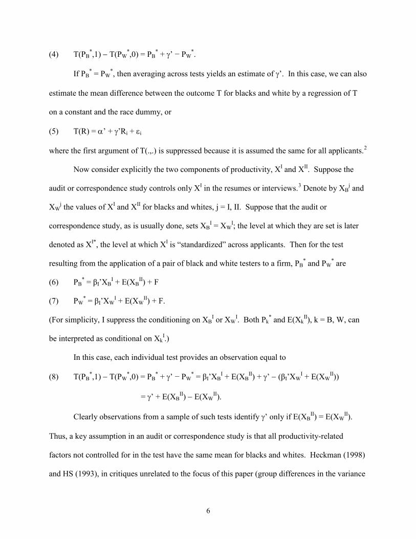
6

(4) T(PB*,1) − T(PW

*,0) = PB* + γ’ − PW

*.

If PB* = PW

*, then averaging across tests yields an estimate of γ’. In this case, we can also

estimate the mean difference between the outcome T for blacks and white by a regression of T

on a constant and the race dummy, or

(5) T(R) = α’ + γ’Ri + εi

where the first argument of T(.,.) is suppressed because it is assumed the same for all applicants.2

Now consider explicitly the two components of productivity, XI and XII. Suppose the

audit or correspondence study controls only XI in the resumes or interviews.3 Denote by XBj and

XWj the values of XI and XII for blacks and whites, j = I, II. Suppose that the audit or

correspondence study, as is usually done, sets XBI = XW

I; the level at which they are set is later

denoted as XI*, the level at which XI is “standardized” across applicants. Then for the test

resulting from the application of a pair of black and white testers to a firm, PB* and PW

* are

(6) PB* = βI’XB

I + E(XBII) + F

(7) PW* = βI’XW

I + E(XWII) + F.

(For simplicity, I suppress the conditioning on XBI or XW

I. Both Pk* and E(Xk

II), k = B, W, can

be interpreted as conditional on XkI.)

In this case, each individual test provides an observation equal to

(8) T(PB*,1) − T(PW

*,0) = PB* + γ’ − PW

* = βI’XBI + E(XB

II) + γ’ − (βI’XWI + E(XW

II))

= γ’ + E(XBII) − E(XW

II).

Clearly observations from a sample of such tests identify γ’ only if E(XBII) = E(XW

II).

Thus, a key assumption in an audit or correspondence study is that all productivity-related

factors not controlled for in the test have the same mean for blacks and whites. Heckman (1998)

and HS (1993), in critiques unrelated to the focus of this paper (group differences in the variance

7

of unobservables), offer a detailed discussion of the reasons why this assumption might be

violated in audit studies. Specifically, despite researchers’ best efforts to standardize applicants,

differences remain that may be observed by employers. And HS further show that even when

these differences are weakly related to productivity, they can lead to large biases, precisely

because the applicants are standardized on other productivity-related characteristics. Moreover,

the design of an audit study allows for experimenter effects that can – through information

conveyed to employers in the job interview – generate differences between E(XBII) and E(XW

II).

Correspondence studies are a response to these criticisms of audit studies (see, for

example, BM, p. 994). In contrast to audit studies, they do not entail face-to-face interviews that

might convey mean differences on uncontrolled variables between blacks and whites, and hence

the researcher can eliminate differences observed by employers that are not controlled in the

study. In addition, a correspondence study, by its very nature, avoids potential experimenter

effects.

Even in a correspondence study, though, differences in employer estimates of mean

unobserved characteristics for blacks and whites can affect the results, as in Equation 8. The

difference, in this case, is one of interpretation, and even when this possibility arises,

correspondence studies still have an important advantage. Regarding interpretation, because

employers are not allowed to make assumptions about race or sex differences in characteristics

not observed in the job application or interview process (U.S. Equal Employment Opportunity

Commission, n.d.), any role of assumed mean differences in characteristics in affecting the

outcomes from a correspondence study can be interpreted as statistical discrimination.

Consequently, we can interpret the estimate of the expression in Equation 8 from a

correspondence study as capturing the combined effects of taste discrimination (γ’) and statistical

discrimination (E(XBII) − E(XW

II)). But in a correspondence study, the estimate of the combined

8

effects of the two types of discrimination is still more reliable than in an audit study, because of

the absence of experimenter effects.

In other words, correspondence studies succeed, where audit studies may fail, in

providing unbiased estimates of what the law recognizes as discrimination. However, they are

not necessarily better at isolating taste discrimination. Nonetheless, when a correspondence

study includes a rich set of applicant characteristics, it becomes less likely that statistical

discrimination plays much of a role in group differences in outcomes.4

Turning to the main focus of this paper, HS show that a more troubling result emerges in

audit or correspondence studies because the relevant treatment is not linear in productivity as it

might be for a wage offer, but instead is non-linear. That is, we think that in the hiring process

firms evaluate a job applicant’s productivity relative to a standard, and offer the applicant a job

(or an interview) if the standard is met. In this case, HS show that, even when there are equal

group averages of both observed and unobserved variables, an audit or correspondence study can

generate biased estimates, with spurious evidence of discrimination in either direction, or of its

absence – or, in other words, discrimination is unidentified. Because this critique applies even to

correspondence studies, which meet higher standards of validity, the remainder of the discussion

refers exclusively to correspondence studies.

The intuitive basis of the HS critique is as follows. Consider the simplest case in which

E(XBj) = E(XW

j), j = I, II, and the only difference between blacks and whites is that the variance

of unobserved productivity is higher for whites than for blacks, for example. The

correspondence study controls for one productivity-related characteristic, XI, and standardizes on

a quite low value of XI (that is, the study makes the two groups equal on characteristic XI, but at

a low value XI*). The correspondence study does not convey any information on a second,

unobservable productivity-related characteristic, XII. Because an employer will offer a job

9

interview only if it perceives or expects the sum βI’XI + XII to be sufficiently high, when XI* is

set at a low level the employer has to believe that XII is high (or likely to be high) in order to

offer an interview. Even though the employer does not observe XII, if the employer knows that

the variance of XII is higher for whites, the employer correctly concludes that whites are more

likely than blacks to have a sufficiently high sum of βI’XI + XII, by virtue of the simple fact that

fewer blacks have very high values of XII. Employers will therefore be less likely to offer jobs to

blacks than to whites, even though the observed average of XI is the same for blacks and whites,

as is the unobserved average of XII. The opposite holds if the standardization is at a high value

of XI; in the latter case the employer only needs to avoid very low values of XII, which will be

more common for the higher-variance whites.

The idea that the variances of unobservables differ across groups has a long tradition in

research on discrimination, stemming from early models of statistical discrimination. For

example, Aigner and Cain (1977) discuss these models and suggest that a higher variance of

unobservables for blacks compared to whites is plausible, and Lundberg and Startz (1983) study

how such an assumption can lead to an equilibrium with lower investment in human capital by

blacks. On the other hand, Neumark (1999) finds no evidence that employers have better labor

market information about whites than blacks, and if anything the estimates – although imprecise

– indicate the opposite.

To see the bias formally, suppose that a job offer or interview is given if a worker’s

perceived productivity exceeds a certain threshold c’. As before, suppose that P is determined as

a linear sum of XI, XII, and F (Equation 2), with XII (and F) statistically independent of XI.5 The

hiring rules for blacks and whites (with the possibility of discrimination) are

(9) T(P(XI*,XBII)|R = 1) = 1 if βI’XI* + XB

II + γ’ + F > c’

(9’) T(P(XI*,XWII)|R = 0) = 1 if βI’XI* + XW

II + F > c’.

10

Discrimination may lead employers to “discount” the productivity of a black worker, as

captured in γ’.

To get to an econometric specification, assume that the unobservables XBII and XW

II are

normally distributed, with equal means (set to zero, without loss of generality), and standard

deviations σBII and σW

II. Finally, as long as the firm-specific productivity shifters F are normally

distributed and independent of XII, and because they have the same distribution for blacks and

whites, we can ignore them and focus solely on the unobserved variation in XII (effectively

redefining the random variable in what follows as XII + F). Under these assumptions, the

probabilities that blacks and whites get hired are

(10) Pr[T(P(XI*,XBII)|R = 1) = 1] = 1 − Φ[(c’ − βI’XI* − γ’)/σB

II] = Φ[( βI’XI* + γ’ – c’)/σBII]

(10’) Pr[T(P(XI*,XWII) |R = 0) = 1] = 1 − Φ[(c’ − βI’XI*)/σW

II] = Φ[( βI’XI* − c’)/σWII],

where Φ denotes the standard normal distribution function.

There is a potential difference between audit and correspondence studies in terms of how

we might think about what is observable to the econometrician and the firm. In an audit study,

the simplest characterization might by that both the firm and the econometrician observe XBI and

XWI, but the firm also observes XB

II and XWII. In a correspondence study, however, both the firm

and the econometrician observe only XBI and XW

I, with no variation in XBII and XW

II observed by

employers. However, the distinction between audit and correspondence studies is not quite this

sharp, because even though an employer interviews an applicant in an audit study, some (perhaps

many) determinants of productivity remain unobserved when a job offer is made.

This issue is relevant to thinking about how we arrive at a statistical model of hiring, such

as the probit specifications in Equations 10 and 10’. In an audit study, variables unobserved by

the econometrician but observed by the firm can generate variation in hiring. In a

correspondence study, however, if firms observe only XBI and XW

I, then the decision about who

11

to hire should be deterministic. Given XBI and XW

I (assumed equal), the employer hires the

higher variance group if the level of standardization is low, and vice versa, so all firms

evaluating identical job applicants should make the same decisions about hiring whites and

blacks. One way to introduce unobservables that generate random variation, with variances that

differ by race as above, is to assume that there are random productivity differences across firms

that are multiplicative in the unobserved productivity of a worker. In that case, the differences in

the variances of XBII and XW

II map directly into unobservables that vary across firms with

relative variances proportional to the relative variances of XBII and XW

II. Alternatively,

employers may make expectational errors and rather than assigning a zero expectation to the

unobservable assign a random draw based on the distribution of unobservables.

Returning to the main line of argument, the difference between Equations 10 and 10’ –

the success rates for black and white job applicants – is intended to be informative about

discrimination. However, even if γ’ = 0, so there is no discrimination, these two expressions

need not be equal because σBII and σW

II, the standard deviations of XBII and XW

II, can be unequal.

The earlier intuition about relative variance of the unobservables and the level of standardization

of XI can be made more precise. Consider the earlier case with γ’ = 0, but σWII > σB

II. Then if

XI* is set at a low level – that is, the standardization level is low – characterized by βI’XI* < c’,

σWII > σB

II implies that Φ[( βI’XI* + γ’ – c’)/σBII] < Φ[( βI’XI* − c’)/σW

II], generating spurious

evidence of discrimination against blacks. When βI’XI* > c’, we instead get spurious evidence of

discrimination in favor of blacks, and switching the relative magnitudes of σWII and σB

II reverses

these results.6

Thus, even if the means of the unobserved productivity-related variables are the same for

each group, and firms use the same hiring standard (that is, γ’ = 0), correspondence studies can

12

generate evidence consistent with discrimination against blacks (or, alternatively, in their favor).

Although demonstrated in the case of normally distributed unobservables, the argument holds for

symmetric distributions (Heckman 1998). This is the basis for HS’s claim that even under ideal

conditions correspondence (or audit) studies are uninformative about discrimination.

IV. Detecting Discrimination

With the right data from a correspondence study, the framework from the preceding

section can be used to recover an unbiased estimate of discrimination, conditional on an

identifying assumption. The intuition is as follows. The HS critique rests on differences

between blacks and whites in the variances of unobserved productivity. The fundamental

problem, as Equations 10 and 10’ show, is that we cannot separately identify the effect of race

(γ’) and a difference in the variance of the unobservables (σBII/σW

II). But a higher variance for

one group (say, whites) implies a smaller effect of observed characteristics on the probability

that a white applicant meets the standard for hiring. Thus, information from a correspondence

study on how variation in observable qualifications is related to employment outcomes can be

informative about the relative variance of the unobservables, and this, in turn, can identify the

effect of discrimination. Based on this idea, the identification problem is solved by invoking an

identifying assumption – specifically, that there is variation in some applicant characteristics in

the study that affect perceived productivity and have effects that are homogeneous across the

races.

More formally, Equations 10 and 10’ imply that the difference in outcomes between

blacks and whites is

(11) Φ[( βI’XI* + γ’ – c’)/σBII] − Φ[( βI’XI* − c’)/σW

II].

In a standard probit, we can only identify the coefficients relative to the standard

deviation of the unobservable, so we normalize by setting the variance of the unobservable to

13

equal one. In this case, impose the normalization for whites only, or σWII = 1. The parameter

σBII is then the variance of the unobservable for blacks relative to whites. To make this clear,

replace σBII with σBR

II = σBII/σW

II. The normalization σWII = 1 is equivalent to defining all of the

coefficients in Equation 11 as their ratios relative to σWII. Dropping the prime subscripts to

indicate that the coefficients are now defined in relative terms, with this normalization Equation

11 becomes

(11’) Φ[(βIXI* + γ − c)/σBRII] − Φ[βIXI* − c].

As Equation 11’ shows, without knowing σBRII we cannot tell whether the intercepts of

the two probits – and hence the hiring probabilities – differ because γ ≠ 0 or because σBRII ≠ 1.

However, if there is variation in the level of qualifications used as controls (XI*), and these

qualifications affect hiring outcomes, then we can identify βI/σBRII and βI in Equation 11’, and

the ratio of these two estimates provides an estimate of σBRII. This lets us test the hypothesis of

equal standard deviations (or variances) of the unobservables. Finally, identification of σBRII

implies identification of γ. Without meaningful variation in XI* (that is, the variation that affects

hiring) this is not possible, since in that case all we have in the model are different intercepts

with different parameters in both the numerators and the denominators ((γ − c)/σBRII and c).

The critical assumption to identify σBRII and hence γ is that βI is the same for blacks and

whites. Otherwise, the ratio of the two coefficients of XI* for blacks and whites does not identify

σBRII. As HS point out, the constancy of βI is assumed in the Urban Institute studies that they

critique, with discrimination entering through an intercept shift in the evaluation of a worker’s

productivity, depending on their race. It is not hard to come up with reasons why the coefficients

relating XI to productivity might differ by race. For example, blacks and whites on average

attend different schools, and if whites’ schools are higher quality, a given number of years of

14

schooling may do more to increase white productivity than black productivity. But in a

correspondence or audit study, it should be possible to control for these kinds of differences; for

example, in this case one can control for the area where applicants live, and hence hold school

district constant (for example, BM 2004). In other words, in these field experiments the

researcher has the capacity to generate data making it more likely that the identifying assumption

holds.

HS raise other possibilities. One is that there is discrimination in evaluating particular

attributes of a group. For example, employers may discriminate against high-education blacks

but not low-education blacks. It is not possible to rule out differences in coefficients arising for

these reasons. Finally, HS also suggest that differences in coefficients may reflect “statistical

information processing,” given incomplete information about productivity, as in statistical

discrimination models. Of course this is the idea underlying the identification strategy suggested

above, as the difference in βI for blacks and whites is assumed to reflect precisely the accuracy

with which XI signals productivity for each race. However, as discussed below, when there is

data on multiple productivity-related characteristics, there is more one can do to test whether

there is homogeneity in the coefficients that allows identification of σBRII and hence γ.

The estimation of βI/σBRII and βI, and inference on their ratio (σBR

II = σBII/σW

II), can be

done via a heteroskedastic probit model (for example, Williams 2009), which allows the variance

of the unobservable to vary with race. To do this, pool the data for blacks and whites. Similar to

Equation 5, letting i denote applicants and j firms, there is a latent variable for perceived

productivity relative to the threshold, assumed to be generated by

(12) T(Pij*) = − c + βIXij

I* + γRi + εij.

As is standard, it is assumed that E(εij) = 0. But the variance is assumed to follow

15

(13) Var(εij) = [exp(µ + ωRi)]2.

This model can be estimated via maximum likelihood. The observations should be

treated as clustered on firms to obtain a variance-covariance matrix that is robust to the

dependence of observations across firms. The normalization μ = 0 can be imposed, given that

there is an arbitrary normalization of the scale of the variance of one group (in this case whites,

with Ri = 0). Then the estimate of exp(ω) is exactly the estimate of σBRII.

In this heteroskedastic probit model, the assumption that βI is the same for blacks and

whites identifies γ.7 Observations on whites identify –c and βI, and observations on blacks

identify (–c + γ)/exp(ω) and βI/exp(ω). Thus, the ratio of βI/{βI/exp(ω)} identifies exp(ω),

which, from Equation 13, is the ratio of the standard deviation of the unobservable for blacks

relative to whites and is, as before, identified from the ratio of the effect of XI* on blacks relative

to its effect on whites. With the estimate of exp(ω) (or equivalently σBRII), along with the

estimate of c identified from whites, the expression (–c + γ)/exp(ω) identified from blacks

identifies γ as well.8

If σBRII = 1, then there is no bias from differences in the distribution of unobservables.

Alternatively, if σBRII ≠ 1, but we had some evidence on how the level of standardization XI*

compares to the relevant population of job applicants, we could determine the direction of bias.

For example, if the study points to discrimination and there is a bias against this finding – based

on the estimate of the ratio of variances and information about XI*, then the evidence of

discrimination is not spurious, because it would be even stronger absent this bias. But because

we can identify γ directly under the assumptions above, we can recover an estimate of

discrimination that is not biased by the difference in the variances of the unobservables. And we

can do this without determining whether XI* used in the study is a high or low level of

16

standardization, which may be impossible to establish.

The identification of γ and σBRII depends on the assumption that the unobservables are

distributed normally. However, the approach need not be couched solely in terms of normally

distributed unobservables and the probit specification. What is required is the separate

identification of the effect of race in the latent variable model and the relative variance of the

unobservables for blacks and whites. Although typically (for example, Maddala 1983) the logit

model is not written with the standard deviation of the error term appearing, it is possible to

rewrite it in this way, in which case the difference in coefficients would again be informative

about the ratio of the variances of the unobservables (Johnson and Kotz 1970, p. 5).

On the other hand, in the specific setting of this paper – a discrete outcome (hiring) and a

discrete treatment (race) – there is no clear way to separately identify how race affects the latent

variable and the variance without distributional assumptions. This case is covered most

explicitly in Manski (1988), who shows that when – in this context – the distribution of the

unobservable differs by race, identification of the “structural” coefficient (γ, in this case) requires

a parametric specification of the unobservable distribution unless various kinds of continuity

assumptions are imposed on the distribution of the observables (with a tradeoff between the

tightness of the restrictions on the distribution of the unobservables and on the observables); but

the latter do not hold for a discrete treatment.9 There is a budding literature on identification of

variables with dichotomous outcomes with non-parametric or semi-parametric methods. Most

prominently, perhaps, Matzkin (1992) shows how this kind of model can be identified non-

parametrically in contexts where restrictions from economic theory (concavity, homogeneity of

degree one) apply. But these types of restrictions do not apply here.

Moreover, a specific form of the hiring rule is assumed. Different hiring rules are

possible, such as one that minimizes the distance between a worker’s skill level and the required

17

skill level on the job (for example, Rothschild and Stiglitz 1982). There is no claim being made

that the identification result or the conclusions about discrimination that follow are invariant to

different assumptions about the distribution of the unobservables or the hiring rule. Rather than

deriving general results, the goal is to show that, in the specific context explored by HS in which

they showed that it was impossible to identify discrimination, an additional assumption – which

itself has testable implications that are discussed next – permits the identification of

discrimination. It remains a question for future research whether it is possible to treat the data

from a correspondence study in a less restrictive manner and still learn something about the

effects of interest.

The assumption that βI is the same for blacks and whites cannot be tested if there is only

one productivity control. With more controls, however, there is a testable restriction, because if

the effects on hiring of multiple productivity controls differ between blacks and whites only

because of the difference in the variance of the unobservables, the ratios of the estimated probit

coefficients for blacks and whites, for each variable, should be the same. Consider the case with

two observables XI and ZI, modifying Equation 11’ to be

(11’’) Φ[( βIBXI* + δI

BZI* + γ − c)/σBRII] − Φ[( βI

WXI* + δIWZI* − c)],

where the coefficients on the observables have B and W superscripts to denote possible

differences by race. Normalize the coefficients in the first expression so that β� IB = βI

B/σBRII and

δ�IB = δI

B/σBRII. If the coefficients in Equation 11’’ do not differ by race, but only the variances

of the unobservables differ, then

(14) β� IB/βI

W = δ�IB/δI

W.

In other words, the black/white ratios of the coefficients from separate probits for blacks

and whites, or from a probit with a full set of race interactions, differ from 1 only because σBRII ≠

18

1, and hence should be equal. Thus, the restrictions implied by homogeneity of effects but

unequal variances of the unobservables can be tested. Of course failure to reject the restrictions

does not decisively rule out the possibility that σBRII = 1, with the coefficients differing by race

for other reasons but Equation 14 still holding. With a larger number of control variables,

however, it seems unlikely that this alternative scenario would explain failure to reject the

restrictions in Equation 14. It is also possible to choose – as an identifying assumption – a subset

of the observable characteristics for which Equation 14 holds, and to identify σBRII only from the

coefficients of this subset of variables, or to do this and then test the restriction on the other

coefficients as overidentifying restrictions.

A final issue concerns the interpretation of the coefficients from the heteroskedastic

probit model. Consider a model with generic notation, where the latent variable depends on a

vector of variables S and coefficients ψ, and the variance depends on a vector of variables T,

which includes S, with coefficients θ. The elements of S are indexed by k. For a standard probit,

coefficient estimates are translated into estimates of the marginal effects of a variable using

(15) ∂P(hire)/∂Sk = ψkφ(Sψ),

where Sk is the variable of interest with coefficient ψk, φ(.) is the standard normal density, and

the standard deviation of the unobservable is normalized to one. Typically this is evaluated at

the means of S. When Sk is a dummy variable such as race, the difference in the cumulative

normal distribution functions is often used instead, although the difference is usually trivial.

The marginal effect is more complicated in the case of the heteroskedastic probit model,

because if the variances of the unobservable differ by race, then when race “changes” both the

variance and the level of the latent variable that determines hiring can shift. As long as we use

the continuous version of the partial derivative to compute marginal effects from the

heteroskedastic probit model, there is a natural decomposition of the effect of a change in a

19

variable Sk that also appears in T into these two components. In particular, generalize the

notation of Equation 13 to

(13’) Var(ε) = [exp(Tθ)]2,10

with the variables in T arranged such that the kth element of T is Sk. Then the overall partial

derivative of P(hire) with respect to Sk is

(16) ∂P(hire)/∂Sk = φ(Sψ/exp(Tθ))∙{(ψk – Sψ∙θk)/exp(Tθ)}.11

This expression can be broken into two pieces. First, the partial derivative with respect to

changes in Sk affecting only the level of the latent variable – corresponding to the counterfactual

of Sk changing the valuation of the worker without changing the variance of the unobservable –

is equal to

(16’) φ(Sψ/exp(Tθ)) ∙{ψk/exp(Tθ)}.

Second, the partial derivative with respect to changes via the variance of the

unobservable is equal to

(16’’) φ(Sψ/exp(Tθ))∙{(–Sψ∙θk)/exp(Tθ)}.

In the analysis below, these two separate effects are reported as well as the overall

marginal effect, and standard errors are calculated using the delta method. The effect of race via

how it shifts the latent variable – or how race shifts the employer’s valuation of worker

productivity – is of greatest interest. The point of the HS critique is that differential treatment of

blacks and whites based only on differences in variances of the unobservable should not be

interpreted as discrimination. And moreover, as argued in Section VI, the effect of race via the

latent variable captures discrimination likely to be manifested in the real economy, whereas its

effect through the variance is more of an artifact of the study.

20

V. Evidence, Implementation, and Assessment

A. Existing Evidence

As the preceding discussion shows, we need information on the effects of productivity-

related characteristics on hiring or callbacks, estimated separately for blacks and whites (or other

groups), to identify discrimination in an audit or correspondence study, or even to assess likely

biases. Reporting of such evidence is rare in the literature, because these studies typically create

one “type” of applicant for which there is only random variation in characteristics that does not

(or is not intended to) affect outcomes. However, BM’s well-known correspondence study of

race discrimination is unusual in that – for reasons unrelated to the concerns of this paper – it

uses two types of applicants.12

Part of their analysis studies callback differences by race for resumes that they

constructed to be low versus high quality, to ask whether blacks and whites have different

incentives to invest in skills, as in Lundberg and Startz (1983). White callback rates are higher

for both types of resumes. But although white callback rates increase significantly with resume

quality (from 8.5 to 10.8 percent), black callback rates increase only slightly (from 6.2 to 6.7

percent) and the change is not statistically significant. Similar qualitative conclusions are

reached based on an analysis that measures resume quality for one part of the sample based on

the predicted probability of callbacks estimated from another part of the sample. In this analysis,

both groups experience an increase in callback rates from higher-quality resumes, but the effect

is larger for whites.

Similarly, BM report probit models estimated for whites and blacks separately (their

Table 5). These estimates reveal substantially stronger effects of measured qualifications for

whites than for blacks. Among the estimated coefficients that are statistically significant for at

least one group, effects are larger for whites for experience,13 having an email address, working

21

while in school, academic honors, and other special skills (such as language). The only

exception is for computer skills, which inexplicably have a negative effect on callback rates for

whites.14

As the present paper suggests, an alternative interpretation of smaller estimated probit

coefficients or marginal effects for blacks than for whites is a difference in the variance of the

unobservables. In particular, the lower coefficients for blacks are consistent with a larger

variance for blacks, or σBRII > 1. If it is also true that BM standardized applicants at low levels

of the control variables, then the HS analysis would imply that there is a bias towards finding

discrimination in favor of blacks; that is, the evidence of discrimination against blacks would be

even stronger absent the bias from differences in the distribution of unobservables. BM

explicitly state that they tried to avoid overqualification even of the higher-quality resumes (p.

995). But it is very difficult to assess whether the characteristics of applicants were low, since

there is no way to identify the population of applicants. Hence, implementation of the estimation

procedure proposed in this paper is likely the only way even to sign the bias, let alone to recover

an unbiased estimate of discrimination.

B. Implementation Using Bertrand and Mullainathan Data

Because BM’s data include applicants with different levels of qualifications, and the

qualifications predict callbacks, their data can be used to implement the methods described

above. Table 1 begins by simply presenting probit estimates for the probability of a callback.

Marginal effects are reported for specifications with no controls except a dummy variable for

females, adding controls for the individual characteristics included on the resumes, and finally

adding also neighborhood characteristics for the applicant’s zip code; the specific variables are

listed in the footnote to the table. Estimates are shown for males and females combined, and for

females only; as the sample sizes indicate, the male sample is considerably smaller.15 Aside

22

from the estimated effects of race, estimates are shown for a few of the resume characteristics

capturing applicants’ qualifications.

Echoing BM’s conclusions, there is a sizable and statistically significant difference

between the callback rates for blacks and whites, with the rate for blacks lower by 3-3.3

percentage points (or about 33 percent relative to the white callback rate of 9.65 percent). The

estimated race differences are robust to the inclusion of the different sets of control variables,

which is what we should expect since the resume characteristics are assigned randomly.

Interestingly, in light of the results of other audit and correspondence studies, there is no

evidence of lower callback rates for females than for males. And although not reported in the

tables, this was true if the same methods used below to recover unbiased estimates of race

discrimination were applied to the estimation of sex discrimination. However, BM’s study was

to a large extent focused on jobs typically held by females, and was not designed to test for sex

discrimination.16 Table 1 also shows that a number of the resume characteristics have

statistically significant effects on the callback probability; this, of course, is an essential input for

using the methods described above to recover an unbiased estimate of discrimination.

The main analysis is reported beginning in Table 2, for the specifications with the full set

of individual resume controls, and then adding as well the full set of neighborhood controls.

Panel A simply repeats the estimated race effects from Table 1, for comparison. Panel B begins

by reporting the estimated overall marginal effects of race from the heteroskedastic probit model

(Equation 16). As the table shows, these estimates are slightly smaller (in absolute value) than

the estimates from the simple probits. They remain statistically significant and indicate callback

rates that are lower for blacks by about 2.4-2.5 percentage points (or about 25 percent).

Decomposing the marginal effect, the effect via the level of the latent variable is larger

than the marginal effect from the probit estimation, ranging from −0.054 to −0.086. The effect

23

of race via the variance of the unobservable, in contrast, is positive, ranging from 0.028 to 0.062.

(This latter effect is not statistically significant.) The implication is that race discrimination is

more severe than indicated by the analysis that ignores differences in the variances of the

unobservables. The evidence that the probit estimates understate discrimination against blacks is

consistent with a low level of standardization of XI*, coupled with a higher estimated variance of

the unobservable for blacks, as conjectured earlier based on BM’s results. And as reported in the

next row of the table, the estimated ratio of the standard deviation of the unobservable for blacks

to the standard deviation for whites always exceeds one, although the difference is not

statistically significant. The positive effect of being black via the variance is what we expect if

XI* is low, since then a larger relative variance for blacks increases the relative probability that

they are hired (called back).

The next two rows of the table report diagnostic test statistics. First, the p-values from

the test of the overidentifying restrictions (Equation 14) are shown, based on probit

specifications interacting all of the controls with race. In all four cases the restrictions are not

rejected, with p-values ranging from 0.17 to 0.62. Nonetheless, the lower end of this range of p-

values suggests that the restrictions sometimes might be fairly inconsistent with the data. As a

consequence, below some alternative estimates are discussed that use only a subset of variables,

for which Equation 14 is more consistent with the data, to identify discrimination.

Finally, the subset of control variables for which the absolute value of the estimated

coefficient for whites exceeded that for blacks – consistent with the larger standard deviation of

unobservables for blacks – was identified. Then the heteroskedastic probit model was estimated

leaving the race interactions of the other variables in the model – so that the restrictions from

Equation 14 that were less consistent with the data were not imposed – and the joint significance

of these latter variables was tested. Despite this latter subset of variables having estimated

24

coefficients less consistent with the restrictions in Equation 14, the p-values indicate that these

interactions can also be excluded from the model. This can be viewed as an overidentifying test

of the restriction that there are no differences in the effects of any of the control variables by

race, for the specifications for which the estimates are reported in the first row of Panel B.

Although technically it is only necessary to assume that there is a single variable for which the

coefficient is the same for blacks and whites, there is no obvious variable to choose for the

purposes of identification; here, instead, I let the data select a set of variables more consistent

with the identifying restriction.

Table 3 follows up on the last procedure, by instead simply dropping from the analysis

the control variables for which the absolute value of the estimated coefficient for whites was less

than for blacks. Given that the control variables are random with respect to race, dropping

controls does not introduce bias. As we would expect, the p-values for the tests of this set of

restrictions are now much closer to one, ranging from 0.68 to 0.92, compared with a range of

0.17 to 0.62 in Table 2. However, as the table shows, the estimated effects of race are similar to

those in Table 2 and do not point to any different conclusions.

C. Monte Carlo Assessment

A Monte Carlo assessment of how well the estimation procedure proposed in this paper

works in terms of removing the bias in estimates of discrimination from correspondence study

evidence was carried out. The Monte Carlo assessment uses simulated data of the type needed to

implement the estimator – namely, data with applicants at two different levels of productivity.

The analysis is described in detail in Appendix 1; here the findings are briefly summarized.

First, using simulated data either with or without discrimination, the heteroskedastic

estimation procedure eliminates the bias, and recovers an unbiased estimate of discrimination.

(And as a benchmark, the simulated data are used to replicate the HS critique, showing that a

25

simple probit analysis can generate bias in any direction.) Second, for a specific case we

consider, when the identifying assumption is violated and the coefficient on the productivity-

related characteristic in the simulated data is not equal for blacks and whites, but is treated as

equal in the estimation, there are two findings. When there is no discrimination, the

misspecification has no effect; the estimator still produces estimates of γ centered on zero. When

there is discrimination and the model is misspecified, there is bias but it is multiplicative, so the

estimator will not generate the wrong sign for the estimate of γ.

VI. The Meaning of Discrimination

The fact that a correspondence study can generate evidence of discrimination when γ = 0

raises the question of whether the evidence reflects a different kind of discrimination. In this

case, the productivity of blacks and whites are regarded equally by employers (or equivalently

there is no taste discrimination). Moreover, employers are not making any assumption about

mean differences in unobservables between blacks and whites. However, they are making

assumptions about distributional differences with regard to the variance of unobservables, and it

is these assumptions that lead them, given the level of standardization of the study applicants, to

prefer blacks or whites – which might be labeled “second-moment” statistical discrimination.

The HS critique can be recast as showing that the analysis of data from a standard audit

or correspondence study cannot distinguish between discrimination as it usually interpreted, and

discrimination based on different variances of unobservables. Indeed Manski’s (1988) paper

discussed earlier, in the context of identification, makes this same point, noting that we can

estimate the “reduced-form” effect of a binary treatment variable on a binary outcome without

strong assumptions, but not the “structural” effect. The present paper imposes an assumption to

identify the structural parameter γ, distinguishing between what is typically viewed as

discrimination (stemming from tastes or, as noted earlier, from standard statistical

26

discrimination) and different treatment stemming from differences in variances of the

unobservable.

A natural question, then, is whether the structural effect of race, captured in γ, is of

interest, or whether instead all we want to know is the reduced-form effect of race – that is, how

race affects the probability of hiring whether because employers discount black workers’

productivity (for example) or because employers treat blacks and whites differentially because of

different distributions of the unobservable. There are two reasons why the structural coefficient

γ is important. First, to the best of my knowledge, differential treatment based on assumptions

(true or not) about variances are not viewed as discriminatory in the legal literature.17 Thus,

identification of γ speaks to the discrimination that is most clearly illegal.

The second and more compelling argument is that taste discrimination or “first-moment”

statistical discrimination, captured in γ, generalizes from the correspondence study to the real

economy. In contrast, the second-moment statistical discrimination is an artifact of how a

correspondence study is done – in particular, the standardization of applicants to particular, and

similar, values of the observables, relative to the actual distribution of observables among real

applicants to these firms.

Suppose that the actual population of applicants to the employers included in a

correspondence study comes from a large range of values of XI. Then the different distributions

of the unobservables by race can have strong effects on hiring outcomes in the correspondence

study because in the study the applicants are standardized to a narrow range of XI. In that sense,

the differential treatment by race is strongly influenced by the design of the correspondence

study, rather than by behavior of real firms evaluating real applicants, and can be generated

solely from the standardization of applicants in a narrow range of XI; in that sense,

“discrimination” attributable to differences in the variance of the unobservables is an artifact of

27

the study.18 In contrast, the structural effect of race via the latent variable would generalize to

how the firms in the correspondence study, and presumably similar firms, evaluate actual job

applicants and make hiring decisions.

VII. Conclusions and Discussion

Many researchers view audit and correspondence studies as the most compelling way to

test for labor market discrimination. And research applying these methods to many different

types of groups nearly always finds evidence of discrimination. The use of audit studies to test

for labor market discrimination has been criticized on numerous grounds having to do with

whether applicants from different groups appear identical to employers. Many of these

criticisms can be countered by using correspondence studies of fictitious applicants on paper

rather than fictitious in-person applicants.

However, Heckman and Siegelman (1993) show that even in correspondence studies in

which group averages are identical conditional on the controls, group differences in the variances

of unobservable dimensions of productivity can invalidate the empirical tests, leading to spurious

evidence of discrimination in either direction, or spurious evidence of an absence of

discrimination. This is a fundamental criticism of correspondence studies, as it implies that

evidence regarding discrimination from even the best-designed correspondence study can be

misleading. Nonetheless, this criticism has been ignored in the literature.

This paper shows that if a correspondence study includes observable measures of

variation in applicants’ quality that affect hiring outcomes, an unbiased estimate of

discrimination can be recovered even when there are group differences in the variances of the

unobservable. The method is applied to Bertrand and Mullainathan’s (2004) correspondence

study, and leads to stronger evidence of race discrimination that adversely affects blacks than is

obtained when differences in the variances of the unobservable are ignored. Moreover, this

28

conclusion is bolstered by Monte Carlo simulations suggesting that the estimation procedure

performs well, eliminating the problems highlighted by Heckman and Siegelman that could

otherwise lead to badly misleading conclusions from the analysis of data from correspondence

(or audit) studies.

Finally, it should be recognized that the method proposed here can be easily implemented

in any future correspondence (or audit) study. All that is needed is for the resumes or applicants

to include some variation in characteristics that affect the probability of being hired.19 This is

different from what is often done in designing these studies, where researchers try to create a

pool of equally-qualified applicants. All that needs to be done is to intentionally create resumes

of different quality. Once a researcher confirms that a set of productivity-related characteristics

on the resumes affected hiring outcomes, it should then be possible – conditional on an

identifying assumption that has testable implications – to detect discrimination.

Appendix 1. Monte Carlo Assessment

This appendix provides Monte Carlo evidence on how well the estimation procedure

proposed in this paper works in terms of removing the bias in estimates of discrimination from

correspondence study evidence, and explores the consequences of violation of the identifying

assumption. Figure A1 replicates the basic result from Heckman (1998), showing that probit

analysis of the data from a correspondence study can generate substantial bias in either direction.

Paralleling Heckman, this is done for the case in which c = 0, βI = 1, Var(XWII)/Var(XB

II) =

(σWII)2/(σB

II)2 = 2.25,20 and there is no discrimination (γ = 0). For the Monte Carlo simulations,

the assumed data generating process is XI* ~ N(0,1), XBII ~ N(0,1), XW

II ~ N(0,2.25). Paralleling

the standardization of correspondence study applicants, the data are generated by sampling XI*

from a truncated normal distribution, in steps of 0.1 + 0.1∙SD(XI*). The simulation is done 100

times at each value of XI* shown in the graph, with samples of 2,000 blacks and 2,000 whites in

29

each simulation (roughly BM’s sample sizes), and a probit model is estimated for each simulated

data set. The panels in the figure show – for both the estimates of γ and the marginal effects –

the true values based on the assumed parameters, and the means based on the estimates.21

The upper figures clearly illustrate that, despite the absence of discrimination in the data

generating process (the true effect is constant at 0), the evidence can either point to

discrimination against blacks or discrimination in favor of blacks, depending on the level of

standardization of XI*. The marginal effects show that even though there is no discrimination in

the data generating process, quite strong evidence of discrimination in either direction can

emerge, with a marginal effect of −0.1 (0.1) for low (high) values of XI*. Finally, as we would

expect, only at XI* = 0 is the estimate of γ (and the marginal effect) unbiased. The lower panels

of Figure A1 report the same kind of evidence when γ = −0.5, consistent with discrimination. A

similar result is apparent, with substantial bias relative to the true γ or the true marginal effect.

The heteroskedastic probit estimation requires data with multiple levels of the value of

XI* at which applicants are standardized. As an intermediate step to separate the consequences

of generating the data this way, and the consequences of implementing the heteroskedastic probit

estimator, Figure A2 shows results with such generated data, but continuing to use the probit

specification. XI* is now sampled from two truncated normal distributions, one using XI*in steps

of 0.1 + 0.1∙SD(XI*), as before, and the second using instead XI* + 0.5, again in steps of 0.1 +

0.1∙SD(XI*). Figure A2 shows qualitatively similar results to Figure A1, so simply using data

with variation in productivity-related characteristics does not, in itself, eliminate the bias.

Nonetheless, the biases in both the no discrimination and discrimination cases are a bit smaller

than in Figure A1 because of the larger range covered by XI*.22

Figure A3 reports results for the heteroskedastic probit estimation, using the same data

generating process for simulating data as in Figure A2, although in this case 5,000 simulations

30

are run for each pair of values of XI* because the heteroskedastic probit estimation is less precise

than the simple probit estimation. The top panel covers the no discrimination case (γ = 0). The

left-hand graph shows the means of the true and estimated values of the marginal effects for each

value of XI*. These are largely indistinguishable in the figure, indicating no bias. The right-hand

panel provides evidence on the distribution of the estimates, showing the distance between the

25th and 75th percentiles of the estimates and between the 2.5th and 97.5th percentiles at each

value of XI*. The distribution of estimates is quite tight at levels of standardization near the

center of the distribution of XI*, but becomes wider at more extreme values, when hiring rates in

the generated data move towards zero or one. The discrimination case (γ = −0.5) similarly

demonstrates that the heteroskedastic probit estimation eliminates the bias.

The last analysis, reported in Figure A4, considers the implications of the data generating

process violating the identifying assumption that the coefficient(s) on the productivity-related

characteristics are equal for blacks and whites. Results are presented for two cases: mild

violation in which the coefficient on XI* (βI) is slightly larger for whites than for blacks (1.1

versus 1); and strong violation in which it is much larger (2 versus 1). As Figure A4 shows, in

the case of no discrimination – the left-hand panels – the results are indistinguishable from when

the identifying assumption is not violated. In contrast, in the discrimination case the estimated

marginal effects become more negative than the true effects over much of the range, only slightly

with mild violation of the identifying assumption, but more so when the violation is more

pronounced.

The implications of what happens when the identifying assumption is violated in this

specific setting make sense, thinking about how γ is identified. Using estimates of the separate

probits in Equations 10 and 10’, the ratio of the standardized white probit coefficient to the black

probit coefficient identifies σBRII (which equals σB

II/σWII). When the true value of βI is larger for

31

whites than for blacks, but it is assumed that they are equal, σBRII is overestimated. For example,

in the case in the top panel of Figure A4, the ratio of coefficients is (βI∙1.1)/(βI/σBRII) = 1.1∙σBR

II.

Recall from the earlier discussion that the probit for blacks identifies (–c + γ)/exp(ω) = (–c +

γ)/σBRII. Because c = 0 in the simulations, we identify γ by multiplying the estimate of this

expression by the estimate of σBRII; the upward bias in the estimate of σBR

II therefore implies that

the estimate of γ is biased away from zero. In the no discrimination case, when γ = 0, this is

irrelevant; multiplying an estimate that averages zero by the upward-biased estimate of σBRII has

no effect. But when the true γ is non-zero (and negative), this bias leads to an estimate of γ that

is more negative. When γ is more negative, we get exactly the “bending” of the estimated

marginal effects that the right-hand panels of Figure A4 illustrate.23 A violation of the

assumption in the opposite direction (βI larger for blacks) would lead to biases in the opposite

direction. Nonetheless, it follows from this reasoning that the bias is multiplicative, and hence

does not generate the wrong sign for the estimate of γ, or generate spurious evidence of

discrimination when there is no discrimination. However, further analysis shows that when c ≠ 0

(or, more generally, when c is not equal to the expected value of unobserved productivity), the

implications of violation of the identifying assumption are less sharp.

References Aigner, Dennis J., and Glen Cain. 1977. “Statistical Theories of Discrimination in Labor

Markets.” Industrial and Labor Relations Review 30(2):175-87.

Banerjee, Abhijit, Marianne Bertrand, Saugato Datta, and Sendhil Mullainathan. 2008.

“Labor Market Discrimination in Delhi: Evidence from a Field Experiment.” Journal of

Comparative Economics 38(1):14-27.

Becker, Gary S. 1971. The Economics of Discrimination, Second Edition. Chicago: University of

Chicago Press.

Bertrand, Marianne, and Sendhil Mullainathan. 2004. “Are Emily and Greg More Employable

than Lakisha and Jamal? A Field Experiment on Labor Market Discrimination.” American

Economic Review 94(4):991-1013.

Bovenkerk, F., M. Gras, and D. Ramsoedh. 1995. “Discrimination Against Migrant Workers and

Ethnic Minorities in Access to Employment in the Netherlands.” International Migration

Papers, No. 4. Geneva, Switzerland: International Labour Office.

Cornelißen, Thomas. 2005. “Standard Errors of Marginal Effects in the Heteroskedastic Probit

Model.” Institute of Quantitative Economic Research, Discussion Paper No. 230. Hanover,

Germany: University of Hanover.

Dickinson, David L., and Ronald L. Oaxaca. 2009. “Statistical Discrimination in Labor Markets:

An Experimental Analysis.” Southern Economic Journal 71(1):16-31.

Fix, Michael, and Raymond Struyk. 1993. Clear and Convincing Evidence: Measurement of

Discrimination in America. Washington, DC: The Urban Institute Press.

Gneezy, Uri, and John A. List. 2004. “Are the Disabled Discriminated Against in Product

Markets? Evidence from Field Experiments.” Unpublished paper. Chicago: University of

Chicago.

Goldberg, Pinelopi Koujianou. 1996. “Dealer Price Discrimination in New Car Purchases:

Evidence from the Consumer Expenditure Survey.” Journal of Political Economy

104(3):622-54.

Heckman, James J. 1998. “Detecting Discrimination.” Journal of Economic Perspectives

12(2):101-16.

Heckman, James, and Peter Siegelman. 1993. “The Urban Institute Audit Studies: Their Methods

and Findings.” In Fix and Struyk, eds., Clear and Convincing Evidence: Measurement of

Discrimination in America. Washington, D.C.: The Urban Institute Press, pp. 187-258.

Johnson, Norman L., and Samuel Kotz. 1970. Continuous Univariate Distributions – 2. New

York: John Wiley and Sons.

Lahey, Joanna N. 2008. “Age, Women, and Hiring: An Experimental Study.” Journal of Human

Resources 43(1):30-56.

Lahey, Joanna N., and Ryan A. Beasley. 2009. “Computerizing Audit Studies.” Journal of

Economic Behavior & Organization 70(3):508-14.

Lundberg, Shelly J., and Richard Startz. 1983. “Private Discrimination and Social Intervention in

Competitive Labor Markets.” American Economic Review 73(3):340-7.

Maddala, G.S. 1983. Limited-Dependent and Qualitative Variables in Econometrics. Cambridge,

U.K.: Cambridge University Press.

Manski, Charles F. 1988. “Identification of Binary Response Models.” Journal of the American

Statistical Association 83(403):729-38.

Matzkin, Rosa L. 1992. “Nonparametric and Distribution-Free Estimation of the Binary

Threshold Crossing and the Binary Choice Models.” Econometrica 60(2):239-70.

Mincy, Ronald. 1993. “The Urban Institute Audit Studies: Their Research and Policy Context.”

In Fix and Struyk, eds., Clear and Convincing Evidence: Measurement of Discrimination in

America. Washington, DC: The Urban Institute Press, pp. 165-86.

Neumark, David. 1996. “Sex Discrimination in Restaurant Hiring: An Audit Study.” Quarterly

Journal of Economics 111(3):915-41.

Neumark, David. 1999. “Wage Differentials by Race and Sex: The Roles of Taste

Discrimination and Labor Market Information.” Industrial Relations 38(3):414-45.

Pager, Devah. 2007. “The Use of Field Experiments for Studies of Employment Discrimination:

Contributions, Critiques, and Directions for the Future.” The Annals of the American

Academy of Political and Social Science 609(1):104-33.

Riach, Peter A., and Judith Rich. 2002. “Field Experiments of Discrimination in the Market

Place.” The Economic Journal 112(483):F480-518.

Riach, Peter A., and Judith Rich. 2007. “An Experimental Investigation of Age Discrimination in

the Spanish Labor Market.” IZA Discussion Paper No. 2654. Bonn, Germany: Institute for

the Study of Labor (IZA).

Rothschild, Michael, and Joseph E. Stiglitz. 1982. “A Model of Employment Outcomes

Illustrating the Effect of the Structure of Information on the Level and Distribution of

Income.” Economics Letters 10(3-4):231-6.

Smeeters, B., and A. Nayer. 1998. “La Discrimination a l’Acces a l’Emploi en Raison de

l’Origine Etrangere: le Cas de le Belgique.” International Migration Papers, No. 23.

Geneva, Switzerland: International Labour Office.

Turner, Margery, Michael Fix, and Raymond Struyk. 1991. “Opportunities Denied,

Opportunities Diminished: Racial Discrimination in Hiring.” UI Report 91-9. Washington,

DC: The Urban Institute.

U.S. Equal Employment Opportunity Commission. 1996. Notice 915.002, May 22,

http://www.eeoc.gov/policy/docs/testers.html (viewed February 28. 2010).

U.S. Equal Employment Opportunity Commission, n.d. “Facts About Race/Color

Discrimination,” http://www.eeoc.gov/facts/fs-race.pdf (viewed March 23, 2009).

Williams, Richard. 2009. “Using Heterogeneous Choice Models to Compare Logit and Probit

Coefficients Across Groups.” Unpublished manuscript. South Bend, Indiana: Notre Dame

University.

Table 1 Probit Estimates for Callbacks: Basic Results Males and females Females (1) (2) (3) (4) (5) (6) Black -.033

(.006) -.030 (.006)

-.030 (.006)

-.033 (.008)

-.030 (.007)

-.030 (.007)

Female .009 (.012)

-.001 (.011)

.001 (.011)

… … …

Selected individual resume controls

Bachelor’s degree .009 (.009)

.009 (.009)

.019 (.010)

.019 (.010)

Experience ∙10-1 .080 (.029)

.076 (.028)

.080 (.034)

.076 (.033)

Experience2 ∙10-2 -.022 (.011)

-.021 (.010)

-.019 (.013)

-.018 (.012)

Academic honors .039 (.015)

.040 (.015)

.026 (.017)

028 (.017)

Special skills .056 (.009)

.055 (.009)

.060 (.010)

.059 (.010)

Other controls: Individual resume

characteristics X X X X

Neighborhood characteristics

X X

Mean callback rate .080 .080 .080 .082 .082 .082 N 4,784 4,784 4,784 3,670 3,670 3,670 Note: Marginal effects using Equation 15 are reported. Standard errors are computed clustering on the ad to which the applicants responded, and are reported in parentheses; the delta method is used to compute standard errors for the marginal effects. Individual resume characteristics include bachelor’s degree, experience and its square, volunteer activities, military service, having an email address, gaps in employment history, work during school, academic honors, computer skills, and other special skills. Neighborhood characteristics include the fraction high school dropout, college graduate, black, and white, as well as log median household income, in the applicant’s zip code.

Table 2 Heteroskedastic Probit Estimates for Callbacks: Full Specifications Males and females Females (1) (2) (3) (4) A. Estimates from basic probit (Table 1) Black -.030

(.006) -.030 (.006)

-.030 (.007)

-.030 (.007)

B. Heteroskedastic probit model Black (unbiased estimates)

-.024 (.007)

-.026 (.007)

-.026 (.008)

-.027 (.008)

Marginal effect of race through level -.086

(.038) -.070 (.040)

-.072 (.040)

-.054 (.040)

Marginal effect of race through variance .062 (.042)

.045 (.043)

.046 (.045)

.028 (.044)

Standard deviation of unobservables,

black/white

1.37

1.26

1.26

1.15 Wald test statistic, null hypothesis that ratio

of standard deviations = 1 (p-value)

.22

.37

.37

.56 Wald test statistic, null hypothesis that ratios

of coefficients for whites relative to blacks are equal, fully interactive probit model (p-value)

.62

.42

.17

.35 Test overidentifying restrictions: include in

heteroskedastic probit model interactions for variables with |white coefficient| < |black coefficient|, Wald test for joint significance of interactions (p-value)

.83

.33

.34

.56 Number of overidentifying restrictions 3 6 2 6 Other controls: Individual resume characteristics X X X X Neighborhood characteristics X X N 4,784 4,784 3,670 3,670 Note: See notes to Table 1. In the first row of Panel B the marginal effects in Equation 16 are reported, with the decomposition in Equations 16’ and 16’’ immediately below; the marginal effects are evaluated at sample means. The standard errors for the two components of the marginal effects are computed using the delta method. Test statistics are based on the variance-covariance matrix clustering on the ad to which the applicants responded. Individual resume characteristics also include the variables listed separately in Table 1.

Table 3 Heteroskedastic Probit Estimates for Callbacks: Restricted Specifications Using only Controls with Absolute Value of Estimated Effect in Fully Interactive Probit Model Larger for Whites than Blacks Males and females Females (1) (2) (3) (4) A. Estimates from basic probit Black -.030

(.006) -.030 (.006)

-.030 (.007)

-.030 (.006)

B. Heteroskedastic probit model Black (unbiased estimates) -.024

(.007) -.025 (.007)

-.024 (.009)

-.025 (.008)

Marginal effect of race through level -.090

(.037) -.080 (.036)

-.086 (.040)

-.077 (.038)

Marginal effect of race through variance .066 (.041)

.056 (.039)

.062 (.044)

.052 (.042)

Standard deviation of unobservables,

black/white

1.41

1.33

1.37

1.30 Wald test statistic, null hypothesis that ratio

of standard deviations = 1 (p-value)

.19

.23

.25

.29 Wald test statistic, null hypothesis that ratios

of coefficients for whites relative to blacks are equal, fully interactive probit model (p-value)

.84

.92

.68

.74 Other controls: Individual resume characteristics X X X X Neighborhood characteristics X X N 4,784 4,784 3,670 3,670 Notes: See notes to Tables 1 and 2.

No discrimination (γ = 0)

Probit estimates of γ Probit estimates of marginal effect of black

Discrimination (γ = -.5)

Probit estimates of γ Probit estimates of marginal effect of black

Notes: Left-hand graphs shows true γ and mean estimated γ. Right-hand graphs show marginal effects, evaluated at sample means for simulated data. In the data generating process, XI* ~ N(0,1), XB

II ~ N(0,1), XWII ~ N(0,2.25), so Var(XW

II)/Var(XBII) =

2.25 (XWII and XB

II are unobservable); βI = 1 and c = 0 for both blacks and whites. Estimates are generated by Monte Carlo simulation, drawing 4,000 observations (2,000 white and 2,000 black) from truncated normal distribution at each value of XI* (in steps of 0.1 + 0.1∙SD(XI*)) and estimating probit model. Simulation is done 100 times at each value of XI*. Figure A1 Replication of Heckman (Figure 1, 1998), and Monte Carlo Simulations of Estimates of Marginal Effects from Simple Probit Estimation

No discrimination (γ = 0)

Probit estimates of γ Probit estimates of marginal effect of black

Discrimination (γ = -.5)

Probit estimates of γ Probit estimates of marginal effect of black

Notes: See notes to Figure A1. The only difference is as follows: Estimates are generated by Monte Carlo simulation, drawing 4,000 observations (2,000 white and 2,000 black) observations from two truncated normal distributions (one at each value of XI* (in steps of 0.1 + 0.1∙SD(XI*)), and one at each value of XI* + .5 (again in steps of 0.1) + 0.1∙SD(XI*)), and estimating probit model.

Figure A2 Monte Carlo Simulations of Probit Estimates and Marginal Effects from Simple Probit Estimation with Two Types of Applicants

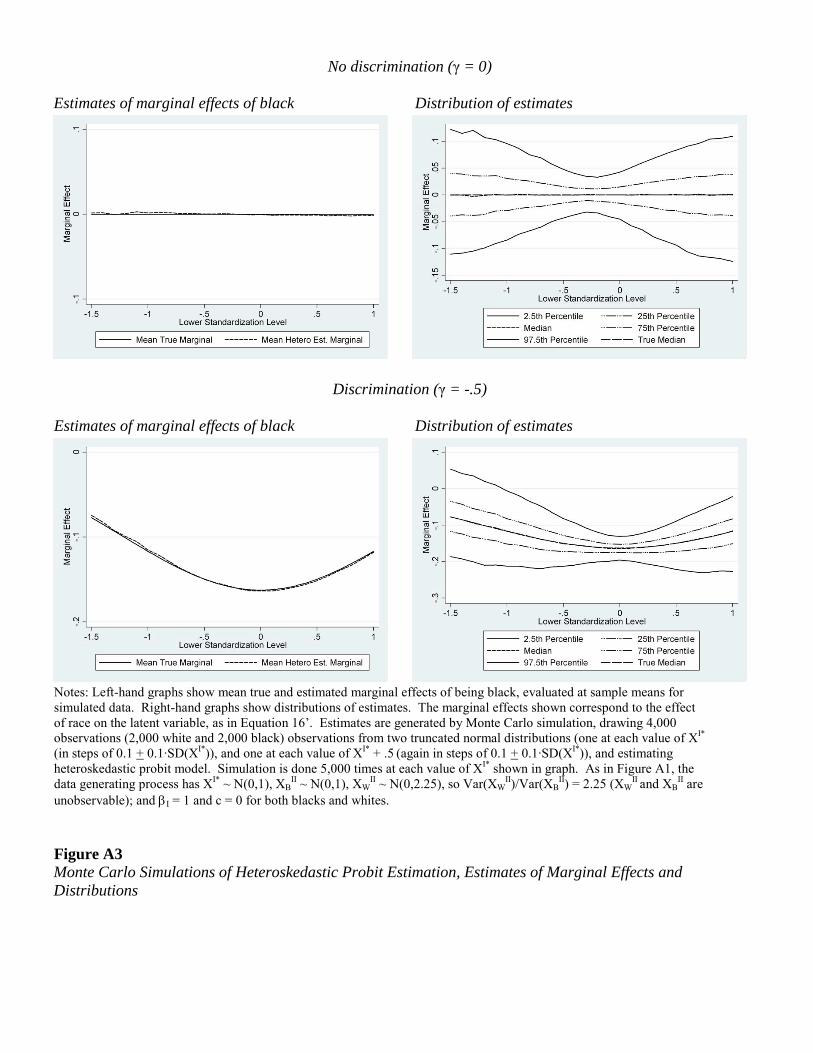
No discrimination (γ = 0)

Estimates of marginal effects of black Distribution of estimates

Discrimination (γ = -.5)

Estimates of marginal effects of black Distribution of estimates

Notes: Left-hand graphs show mean true and estimated marginal effects of being black, evaluated at sample means for simulated data. Right-hand graphs show distributions of estimates. The marginal effects shown correspond to the effect of race on the latent variable, as in Equation 16’. Estimates are generated by Monte Carlo simulation, drawing 4,000 observations (2,000 white and 2,000 black) observations from two truncated normal distributions (one at each value of XI* (in steps of 0.1 + 0.1∙SD(XI*)), and one at each value of XI* + .5 (again in steps of 0.1 + 0.1∙SD(XI*)), and estimating heteroskedastic probit model. Simulation is done 5,000 times at each value of XI* shown in graph. As in Figure A1, the data generating process has XI* ~ N(0,1), XB

II ~ N(0,1), XWII ~ N(0,2.25), so Var(XW

II)/Var(XBII) = 2.25 (XW

II and XBII are

unobservable); and βI = 1 and c = 0 for both blacks and whites. Figure A3 Monte Carlo Simulations of Heteroskedastic Probit Estimation, Estimates of Marginal Effects and Distributions

Mild violation of identifying assumption in data generating process (βI for whites = 1.1) No discrimination (γ = 0) Discrimination (γ = -.5)

Strong violation of identifying assumption in data generating process (βI for whites = 2) No discrimination (γ = 0) Discrimination (γ = -.5)

Notes: See notes to Figure A3. The only difference is that βI is unequal for blacks and whites; it is always equal to 1 for blacks, and as indicated in the graph headings for whites. Figure A4 Monte Carlo Simulations of Heteroskedastic Probit Estimation, with Model Misspecification Masking Higher Unobserved Variance for Whites, Estimates of Marginal Effects

Endnotes 1 In the ensuing discussion XI is observable and XII unobservable. I put a coefficient on XI in

Equation 2 because XI has a definable scale, whereas I treat XII as scaled such that its coefficient

equals one. Following HS, I assume that the coefficient on XI is the same for blacks and whites,

so discrimination is reflected only in an intercept difference. I return to this issue later.

2 We could include resume characteristics, which should not matter for the estimate of γ’ since

they are randomly assigned by race. The same is true of firm fixed effects, which are orthogonal

to race.

3 As discussed below, some characteristics of workers not controlled by the researcher are

observed by the employer in an audit study; but many are not.

4 This is more problematic in correspondence studies of age discrimination, because even with

many other qualifications on the resumes, if researchers give older applicants the same amount

of experience as younger applicants, employers are likely to make adverse assumptions about

older applicants whose resumes reflect limited work experience. See Lahey (2008) and Riach

and Rich (2007) for suggestions for addressing this problem in age discrimination studies.

5 We can treat F as statistically independent because resume characteristics are, or should be,

assigned randomly (for example, Lahey and Beasley 2009). And we can always think about XII

as the variation in unobserved productivity that is orthogonal to XI.

6 Heckman (1998, footnote 7) suggests that the case with a low level of standardization and

higher dispersion for whites “seems to rationalize” audit study evidence of discrimination against

blacks. It is not clear, however, that we know either the level of standardization or the relative

dispersion of unobserved productivity. Even though the first issue relates to observables, there is

no obvious way to compare the distributions of qualifications of testers in an audit study to the

population of job applicants. In fact, there are two conflicting tendencies in setting standards for

audit studies. Setting a low standard implies that call-back rates will be low, reducing the

statistical power of the evidence. But setting a standard too high raises concerns about

“overqualification” of candidates (for example, BM 2004, p. 995), which in an economic context

presumably means that the job applicant will be expected to get better job offers, deterring

employers from making offers.

7 Conversely, the following argument can be easily modified to show that if βI is not the same for

blacks and whites, then γ is unidentified. The assumption that only race shifts the variance of the

unobservable (Equation 13) is less consequential, since in a correspondence (or audit) study the

observed characteristics of applicants other than race are essentially the same.

8 Consistent with the earlier discussion of statistical discrimination, we might want to allow for

the possibility that E(XBII) – E(XW

II) ≠ 0. In this case, we can normalize by assuming E(XWII) =

0 and defining E(XBII) – E(XW

II) = μBWII. We can then replace γ in the preceding identification

argument with γ + μBWII, and it is this sum of parameters, reflecting the combination of taste

discrimination and the expected mean difference in the unobservable (statistical discrimination),

which is identified.

9 Some of the other controls on the resumes may be continuous, but they do not contribute to

identification of the effect of race on the latent variable given that they are, by construction,

orthogonal to race. By way of contrast, in audit-type studies of discrimination on a continuous

outcome – such as price quotes for cars or car repairs (Goldberg 1996; Gneezy and List 2004) –

the identification problem is simpler.

10 Recall that μ in Equation 13 is normalized to zero.

11 See Cornelißen (2005).

12 BM actually study differences in treatment between applicants with black-sounding names and

names that do not sound black. For simplicity, I discuss the results as if they capture differences

between blacks and whites, which is certainly a plausible interpretation of their findings.

13 This variable enters as a quadratic, and the effect of experience is stronger for whites up to

about 16 years of experience, more than twice the mean in their sample.

14 Also, the effect of gaps in employment is inexplicably positive, but not significant for

estimates disaggregated by race.

15 Probits estimated for males only yielded similar results for the effects of race, although the

estimated coefficients of some of the productivity-related characteristics were quite imprecise or

had unexpected signs. In estimating the heteroskedastic probit model for males, in some cases

there were computational problems, likely reflecting these other issues regarding the estimates

for males, and perhaps also the much smaller sample for males.

16 They study sales, administrative support, clerical, and customer service jobs. The male

applicants were used almost exclusively for the sales jobs, so the sex difference is identified

mainly from the sales jobs.

17 There is a small economics literature that studies discrimination based on second moments – in

particular the variance of productivity – where a group with higher variance may be penalized

because of risk aversion on the part of employers. The idea goes back to Aigner and Cain

(1977). Dickinson and Oaxaca (2009) provide an experimental study of this type of

discrimination in labor markets.

18 One could imagine more complicated scenarios in which different firms engage in strategies

that draw applicants from different parts of the distribution, in which case it is harder to

characterize how differences in the distribution of unobservables by race will impact the

treatment of whites versus blacks.

19 In principle this can be done in an audit study as well a correspondence study, although it is

much harder to generate large samples in audit studies.

20 This is the ratio of the variances of the unobservables. Note that a larger value for whites is

the opposite of the common assumption in models of statistical discrimination.

21 The true marginals are based on the heteroskedastic probit specification (Equation 16’),

because the simulated data are heteroskedastic. The true marginal effect is reported as a mean

because it is computed once using each simulated data set, holding the parameters fixed, and

then averaged.

22 In this case the unbiased estimate occurs at the value of −0.25 (for XI*) on the horizontal axis,

where the average of the upper and lower standardization levels equals zero. The reduction in

bias is a little less clear in the discrimination case. To clarify, the bias in Figures A1 and A2

should be contrasted at comparable values of XI*, given that Figure A2 shows the mean estimates

at the lower level of standardization of XI*. For example, for the discrimination case, the mean

estimate of γ at XI* = 1 in Figure A1 should be compared to the mean estimate at XI* = 0.75 in

Figure A2 (in which case this is the lower standardization level and the average is 1); the latter

estimate is in fact closer to zero.

23 In the standard marginal effect – ψkφ(Sψ), from Equation 15 – nearer the center of the

distribution the larger estimate of ψk dominates the marginal effect, whereas nearer the tails the

larger estimate of ψk lowers φ(Sψ) enough that the product ψkφ(Sψ) is closer to zero.