DETECTING PRICE LINKAGES: METHODOLOGICAL ISSUES AND ANAPPLICATION TO THE WORLD MARKET OF COTTON

JOHN BAFFES(The World Bank)

MOHAMED I. AJWAD(University of Illinois)

July 24, 1998

CORRESPONDENCE: John BaffesDevelopment Economics Research GroupThe World Bank1818 H Street, NW, MC 3-545Washington, D.C. 20433tel: (202) 458-1880fax: (202) 522-1151em: jbaffes@worldbank.org

Abstract: This paper examines the degree to which cotton prices are linked; it also tests whethersuch price linkages have been improved over the last decade. It concludes that the degree oflinkage has improved over the last decade while the main source of this improvement appears tobe a result of short-run price transmission and to a lesser extent long-run comovement.

The findings and conclusions of this paper are those of the authors and should not be attributed tothe World Bank. The authors would like to thank Alain d’Hoore and Uma Lele for valuablecomments and suggestions on an earlier draft.

1

I. INTRODUCTION

In the absence of impediments, the comparative advantage argument of trade theory dictates that

resources will be allocated in an efficient manner, in turn implying that factor and product prices

in different locations will be equalized Ä subject to transfer costs. Under certain conditions, the

existence of strong price linkages, therefore, may be viewed as a necessary requirement for

efficient allocation of resources and hence maximum welfare [Samuelson (1952); Takayama and

Judge (1964)]. This paper focuses on the degree of price linkages of the world market of cotton.

The issue of price linkages in product markets both at national and international levels has

been studied in the literature rather extensively either under the notion of the law of one price

[e.g. Protopapadakis and Stoll (1983, 1986), Ardeni (1989), Baffes (1991)] or under the notion of

market integration [e.g. Ravallion (1986), Sexton, Kling, and Carman (1991), Gardner and

Brooks (1994), Fafchamps and Gavian (1996), Baulch (1997a)]. Moreover, reflecting on the

market liberalization and structural adjustment efforts undertaken by a number of developing

countries in recent years, the degree to which markets are integrated has been used quite often as

a yardstick in assessing the success of policy reforms [e.g. Goletti and Babu (1994), Alexander

and Wyeth (1994), Gordon (1994), Dercon (1995)].

As many authors have cautioned, however, price convergence does not necessarily imply

efficient allocation of resources unless the setting in which trade takes place is competitive [e.g.

Faminow and Benson (1990), Baulch (1997b)]. For example, consider the extreme case of two

duopolists who agree to charge the same price in two segmented markets. While convergence in

prices (whenever price changes occur) would take place instantaneously, the oligopolistic setting

of the market may not necessarily allocate resources in the most efficient manner. The same

argument may be advanced for a number of developing countries where parastatals assign

panterritorial and panseasonal prices on certain commodities. In such cases the law of one price

holds by definition without necessarily implying that resources are allocated efficiently.

The present paper examines the strength of price linkages in the world market of cotton.

In pursuing this objective, the paper contributes to the literature of price linkages in two respects.

On the theoretical side, it introduces a measure of price linkage and also identifies its source (i.e.

short-run price transmission versus long-run comovement.) On the empirical side, it applies this

measure to the world market of cotton for two different time periods, thereby examining whether

improvements in price linkages have taken place over the last decade.

2

There are at least two reasons as to why one would expect that price linkages may have

improved over the last decade. First, improvements in information technology have made it much

easier for information on demand conditions to be disseminated across markets; therefore one

would expect that cotton price changes from one origin due to a demand shock would be

transmitted immediately to the price of the other origins. Second, many countries have

undertaken steps to liberalize their cotton subsectors while in other countries the role of the

government has been substantially altered. For example, under the Former Soviet Union (FSU)

structure, cotton from Central Asia shipped to other parts of the FSU was domestic trade.

Currently, cotton exports from Uzbekistan constitute the single most important component of its

foreign trade. Changes have also taken place in Africa. For example, until the early 1990s,

cotton marketing and trade in East African countries was handled in its entirety by government

parastatals. Now, Uganda, Zimbabwe, and Tanzania, operate Ä to different degrees Ä within

liberalized marketing and trade regimes. One, therefore, would expect faster long-run

convergence of cotton prices (if convergence existed) or at least some convergence (if

convergence did not exist in the first place).

The remainder of the paper proceeds as follows. In the next section the model along with

the explicit measure of the degree of market linkage is outlined. In discussing the model, we

undertake a rather extensive literature review on the subject of price linkages. The review

indicates that a number of commonly used models are, in fact, restricted versions of the same

dynamic specification. The penultimate section discusses the data and presents the empirical

findings. The data cover the periods August 1985 through December 1987 and August 1995

through January 1997 and refer to CIF prices in North European ports for US, Greek, West

African, and Central Asian types of cotton. The findings indicate that price linkages between W.

Africa and C. Asia have been much higher than between the US and the other markets. In fact, in

the first period, no comovement between the US and the other markets was detected. The last

section concludes by addressing some policy implications and subjects for further research.

II. DETECTING PRICE LINKAGES

Earlier studies examining the relationship between prices either have looked at correlation

coefficients [e.g., Lele (1967); Southworth, Jones, and Pearson (1979); Timmer, Falcon, and

Pearson (1983); Stigler and Sherwin (1985)] or have used the following type of regression [e.g.

Isard (1977), Mundlak and Larson (1992), Gardner and Brooks (1994)]:1

3

where pt1 and pt

2 denote prices from two origins of the commodity under consideration, µ and β1

are parameters to be estimated while εt denotes an IID(0, σ2) term. The hypothesis that the slope

coefficient equals unity and (possibly) the intercept term equals zero can be tested; formally, H0: µ

+ 1 = β1 = 1. Under H0 the deterministic part of (1) becomes pt1 = pt

2, in turn implying that the

price differential, pt1 - pt

2, is an IID(0, σ2) term.

Estimating (1) and testing H0, while intuitively appealing and computationally

implementable, presents two fundamental shortcomings. First, some statistical properties of the

series involved in (1), namely nonstationarity, may invalidate standard econometric tests and thus

give misleading results regarding the degree to which price signals are being transmitted from one

market to another. Second, in primary commodity markets with characteristics such as (small or

even perceived) differences in quality, high transfer costs relative to the price, etc., it is rather

unlikely that the two prices will only differ by an IID(0, σ2) term as H0 of (1) dictates. Therefore,

H0 is expected to be rejected without necessarily ruling out a relatively high degree of price

linkage. Consequently, it is deemed necessary to employ a general enough model that imposes no

a priori requirements on the stationarity properties of the series in question and at the same time

allows for some degree of flexibility.

With respect to the nonstationarity problem one can examine the order of integration of

the error term in (1) and make inferences regarding the validity of the model (Ardeni, 1989). If

prices are indeed nonstationary, the existence of a stationary error term implies comovement

between the two prices. However, if the slope coefficient is different from unity, the uniqueness

of the cointegration parameter in the bivariate case implies that the corresponding price

differential would be growing and such growth would not be accounted for, although prices may

move in a seemingly synchronous manner. Hence, stationarity of the error term of (1) (given non-

stationary prices) while establishing proportional price movement, should not be considered as a

testable form equivalent to that of the H0 of (1). Note that a number of authors have warned

against interpreting non-unity slope coefficient as a sign of market integration (e.g. Barrett

(1996)).

To account for the non-unity slope coefficient one can restrict the parameters of (1)

according to H0, in which case the problem is equivalent to testing for a unit root in the following

(1) t t tp = + p + ,11

2µ β ε

4

univariate process (Engle and Yoo, 1987):

If the price differential as defined in (2) is stationary, then one can conclude that price signals are

transmitted from one market to another, in the long run. The assumption (or finding) that the

cointegration parameter is unity is very crucial, as it ensures that there is no other nonstationary

component entering the system. As Meese (1986) and West (1987) observe, the absence of

cointegration (with unity slope coefficient in the present setting) can be attributed to omitted

nonstationary variables, in turn implying that an additional component would have to be included

in (2) in order to fully account for the variability of the price differential.

As a sidelight, it should be emphasized that if the cointegration parameter is unity, it is

immaterial for all relevant aspects of the analysis whether (1) or (2) is employed. This is the case

because as the sample size increases, regression (1) should yield β1 equal to unity. However, in

finite samples this may not be necessarily the case. For example, Ardeni (1989), using (1) in

logarithms for a number of internationally traded primary commodities, found that the

corresponding error term was not stationary, thus rejecting the law of one price. Baffes (1991),

on the other hand, by using the same data set found that in the majority of cases the price

differential was stationary, hence providing supportive evidence for the law of one price as a long

run relationship.2

From the preceding discussion, it is rather evident that cointegration tests are not very

powerful as they only make inferences about the existence of the moments of the distribution of

(pt1 - pt

2) and not about certain restrictions that may be required by economic theory [e.g. H0 of

(1)]. Therefore, (2) cannot serve as a substitute for the H0 of (1); it can only serve as an

intermediate step in establishing its validity.

With respect to the restrictive nature of (1), one can circumvent it by introducing a more

general autoregressive structure. Appending one lag to (1), gives:3

(3) t t t t tp p p p u11

22 1

23 1

1= + + + +− −µ β β β ,

where ut is IID(0, σ2) and β3<1. Despite its simplicity, (3) encompasses a wide variety of

commonly used dynamic models with different economic interpretations. For example, Hendry,

Pagan, and Sargan (1983) discuss a number of testable hypothesis, results of corresponding

(2) ( )t tp - p I(0).1 2 ~

5

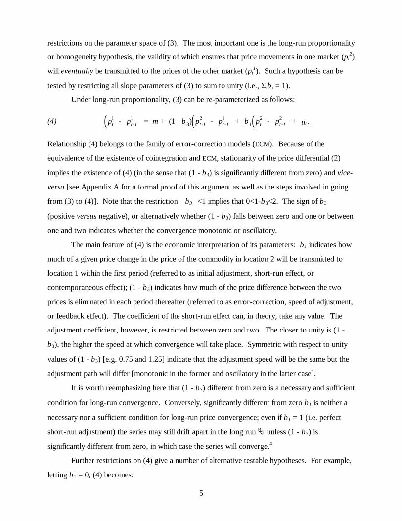
restrictions on the parameter space of (3). The most important one is the long-run proportionality

or homogeneity hypothesis, the validity of which ensures that price movements in one market (pt2)

will eventually be transmitted to the prices of the other market (pt1). Such a hypothesis can be

tested by restricting all slope parameters of (3) to sum to unity (i.e., Σiβi = 1).

Under long-run proportionality, (3) can be re-parameterized as follows:

(4) ( ) ( ) ( )t t-1 t-1 t-1 t t-1 tp - p = + p - p + p - p + u .1 13

2 11

2 21µ β β( )−

Relationship (4) belongs to the family of error-correction models (ECM). Because of the

equivalence of the existence of cointegration and ECM, stationarity of the price differential (2)

implies the existence of (4) (in the sense that (1 - β3) is significantly different from zero) and vice-

versa [see Appendix A for a formal proof of this argument as well as the steps involved in going

from (3) to (4)]. Note that the restriction β3<1 implies that 0<1-β3<2. The sign of β3

(positive versus negative), or alternatively whether (1 - β3) falls between zero and one or between

one and two indicates whether the convergence monotonic or oscillatory.

The main feature of (4) is the economic interpretation of its parameters: β1 indicates how

much of a given price change in the price of the commodity in location 2 will be transmitted to

location 1 within the first period (referred to as initial adjustment, short-run effect, or

contemporaneous effect); (1 - β3) indicates how much of the price difference between the two

prices is eliminated in each period thereafter (referred to as error-correction, speed of adjustment,

or feedback effect). The coefficient of the short-run effect can, in theory, take any value. The

adjustment coefficient, however, is restricted between zero and two. The closer to unity is (1 -

β3), the higher the speed at which convergence will take place. Symmetric with respect to unity

values of (1 - β3) [e.g. 0.75 and 1.25] indicate that the adjustment speed will be the same but the

adjustment path will differ [monotonic in the former and oscillatory in the latter case].

It is worth reemphasizing here that (1 - β3) different from zero is a necessary and sufficient

condition for long-run convergence. Conversely, significantly different from zero β1 is neither a

necessary nor a sufficient condition for long-run price convergence; even if β1 = 1 (i.e. perfect

short-run adjustment) the series may still drift apart in the long run Ä unless (1 - β3) is

significantly different from zero, in which case the series will converge.4

Further restrictions on (4) give a number of alternative testable hypotheses. For example,

letting β1 = 0, (4) becomes:

6

(5) ( ) ( )t t-1 t-1 t-1 tp - p = + p - p + u .1 13

2 11µ β( )−

The interpretation of (5) is that while no adjustment is taking place in the current period, prices

indeed converge in the long-run with speed (1 - β3).

On the other hand, letting β1 = 1, (4) is re-parameterized as follows:

(6) ( ) ( )t t t -1 t -1 tp - p = + p - p + u .2 13

2 1− µ β

(6) implies that while price changes in one market are transmitted exactly to prices in the other

market in the short-run, long-run price convergence may be achieved at a lower speed, depending

on the size of β3. Furthermore, if in addition to letting β1 = 1 one imposes β3 = 0, (6) collapses to

the H0 of (1). A number of studies examining the linkages between futures and cash prices for

commodity and asset markets have employed (5) and (6) [e.g., Garbade and Silber (1983);

Schroeder and Goodwin (1991); Wang and Yau (1994); Fortenbery and Zapata (1997)].

Alternatively, setting β3 = 1 in (4), effectively implying non-convergence, gives:

(7) ( ) ( )t t-1 t t-1 tp - p = + p - p + u .1 11

2 2µ β

Relationship (7), often termed the first difference approach, has also been used in the literature

rather extensively [e.g., Richardson (1978), Tomek (1980), Leavit, Hawkins, and Veeman (1983),

Hudson, Ethridge, and Brown (1996)].5 First differences along with detrending have been

traditionally the most widely used filters in time series analysis. It should be noted, however, that

if (pt2 - pt

1) and (pt2 - pt-1

2) are orthogonal, estimating short-run and dynamic adjustment effects

through (5) or (7) will yield the same parameter estimates as estimating them jointly through (4).6

Finally, by restricting β2 = β3 = 0, (3) reduces to (1), which as indicated earlier has been

one of the most commonly used models in the literature of price linkages. To these models one

should also add Granger-causality tests since a significantly different from zero error-correction

term implies Granger-causality with feedback from pt2 to pt

1 [Petzel and Monke (1980) used

Granger-causality for the international rice market]. Lastly, if the prices have not been adjusted

by transfer costs, one can incorporate them in either (3) or (4) Ä depending on their stationarity

properties Ä and examine their dynamic effects on prices. At this point it is straightforward to

verify that a wide variety of ‘law of one price’, market integration, or market efficiency models

can be derived by (3) (possibly with a higher lag structure) subject to the appropriate restrictions

7

on the parameters.7

From the preceding discussion is has become evident that one potential problem with

estimating (5), (6), (7), or even (4) for that matter, without ensuring that the appropriate

restrictions (or orthogonality conditions where applicable) hold, is that the estimated parameters

may be biased and hence give misleading results regarding the underlying economic behavior. For

example, β1 = 1 in (7) may erroneously lead one to conclude that there exists strong correlation

between the two prices where in fact, the prices may not even converge in the long run. On the

other hand, (5) imposes the restriction that no adjustment in the short-run takes place, which may

not necessarily be the case.

The model outlined above suggests that, given long-run proportionality exists, whether to

choose (3) or (4) to recover short- and long-run dynamic price behavior is a matter of stationarity

properties. If prices are stationary, (3) would be the preferred structure and long-run

proportionality could be tested by restricting the slope parameters to sum to unity. Under non-

stationarity, (4) would be the preferred structure and long-run proportionality can be tested by

examining the stationarity properties of the price differential (Engle and Yoo, 1987) or

equivalently by testing whether (1-β3) is different from zero (Phillips and Loretan, 1991). Then,

with appropriate tests one can determine whether any of the underlying restrictions implied by (5),

(6), or (7) can be in fact validated by the data.

Having established long-run proportionality and also having recovered the parameter

estimates of (4) the next task is to transform the information contained in the parameter space in

such a way so that a succinct interpretation of both short-run and feedback effects (and hence

price linkage) can be given. Stating the question in a simplified manner: How long does it take

for the price of cotton from origin 1 to adjust to a given price change in origin 2?

Let n be the period by which k percent of the cumulative adjustment has taken place. In

the current period, n = 0, k takes the value of β1 [also equal to 1-(1-β1)], which is the short-run

impact of (pt2 - pt-1

2) on (pt1 - pt-1

1). In the next period, n = 1, k takes the value of β1+(1-β1)β3,

which is the impact of the previous period, β1, plus the feedback effect, (1-β1)β3 [it can also be

written as 1-(1-β1)(1-β3)]. For n = 2, k takes the value of the previous period’s adjustment,

β1+(1-β1)β3 plus (1 - β3)(1-β1-(1-β1)β3) [which can be written as 1-(1-β1)(1-2β3+β32) or 1-(1-

β1)β32]. (Table 1 gives the adjustment for the first five periods, including the current one).

Hence, the cumulative adjustment at period n is given by:

8

(8) k n= − −1 1 1 3( )β β

Alternatively, solving for n in (8) gives the number of periods required to achieve a certain level

of cumulative adjustment, i.e. n = [log(1-k) - log(1-β1)]/logβ3. For values of β1 and (1 - β3) close

to unity, a small n (number of periods) is required for the adjustment to be completed (i.e. k close

to unity).8

Although most models in the literature of price linkages have based the discussion on

estimated model parameters and F-tests, there have been a number of exceptions which have

quantified the linkage in a more explicit manner.9 Ravallion (1986), for example, using an

autoregressive distributed lag model and appropriate parameter restrictions made a distinction

among market segmentation, long-run market integration, and short-run market integration and

applied it to the rice market in Bangladesh. A number of researchers have applied Ravallion’s

formulation since then [e.g. Palaskas and Harriss (1993) applied it to the food markets in West

Bengal while Gordon (1994) applied it to grain markets in Tanzania].

Timmer (1987) introduced a measure of price linkage based on the unrestricted version of

specification (3) and applied it to the corn market of Indonesia. Timmer’s Index of Market

Connection, converted to the parameters of (4) [i.e. after imposing long-run convergence] is equal

to β3/(1-β3). For values of β3 close to unity (or alternatively for values of (1 - β3) close to zero),

the index takes large values (at the limit approaching infinity), in turn indicating weak price

linkage. If β3 = 0 (or 1 - β3 = 1) the index takes the value of zero, which corresponds to error-

correction coefficient being equal to unity, consequently indicating strong price linkage Ä for

negative values of β3 the measure falls within the interval (-0.5, 0). Heytens (1986) and Alderman

(1992) used Timmer’s measure of market connection to examine the performance of food markets

in Nigeria and Ghana, respectively.

Delgado (1986) developed a variance components methodology by making a distinction

among different levels of market integration between harvest and post-harvest period and applied

it to food markets in Northern Nigeria. Goodwin and Schroeder (1991) in examining spatial price

linkages in US regional cattle markets used the magnitudes of cointegration statistics of bivariate

regressions as measures of price linkages. More recently, Lutz, van Tilburg, and van der Kamp

(1995) introduced a measure of market integration by calculating short- and intermediate-run

impact multipliers and then a measure of adjustment (similar to the one proposed in this paper);

they applied the model to wholesale and retail food markets in Benin.

9

III. DATA AND RESULTS

a. Data and Stationarity Tests

Two samples, one covering the period August 15, 1985 to December 24, 1987 (122 observations)

and a second covering the period August 3, 1995 to January 9, 1997 (73 observations) were

constructed. Thursday price quotations from the following origins were used: US (Memphis

Territory), Greece, Central Asia, and African ‘Franc Zone’ (referred to as W. Africa).10 In

addition to the four quotations, we also included the A Index, the measure of the ‘world’ price of

cotton. However, because the A Index may contain the price which it is paired with, any results

related to it should be interpreted with caution. Appendix B contains a detailed discussion of the

data. Given that the number of cotton traders in North Europe is sufficiently high to ensure that

cotton prices are determined within a competitive environment and therefore any degree of price

linkage can be attributed to market efficiency.

To determine the order of integration the augmented Dickey-Fuller (ADF) and the Phillips-

Perron (PP) procedures were utilized. The ADF is based on the following regression: (pt - pt-1) = µ

+ βpt-1 + lags(pt - pt-1) + εt, where pt denotes the series under consideration (Dickey and Fuller,

1981). A negative and significantly different from zero value of β indicates that pt is I(0). The PP

test is similar to the ADF; their difference lies on the treatment of any nuisance serial correlation

aside from that generated by the hypothesized unit root (Phillips and Perron, 1988; Phillips,

1989). To identify the presence of one unit root we test H0: pt is not I(0) against H1: pt is I(0).

Trend stationarity can be detected by appending a time trend in the relevant regression. Finally,

the significance level of the error-correction coefficient itself, (1 - β3), can serve as cointegration

test (Phillips and Loretan, 1991).

Stationarity results for both periods are reported in the upper panel of Table 2. The tests

indicate that stationarity in levels is rejected in all cases. The middle panel of Table 2 reports

results for trend stationarity tests. Here the picture changes considerably since, with the

exception C. Asia in the second period, all tests show evidence of trend stationarity.11

Because the decision on whether to use (3) or (4) ultimately depends on the stationarity

properties of the prices, we supplemented the unit root tests with a variance-ratio test (Cochrane,

1988). This test is based on the statistic defined as (1/k)Var(pt-pt-k)/Var(pt-pt-1), where pt is the

variable of interest and k denotes the lag length; it exploits the fact that the variances of

10

conditional forecasts explode for nonstationary series and converge for stationary (or trend

stationary) series as the forecast horizon grows. The idea behind Cochrane’s test goes as follows.

If pt is a random walk [i.e., pt = µ + ρpt-1 + εt, where ρ = 1], the variance of its k-differences

grows linearly with k, i.e. Var(pt-pt-k) = kσε2. If, on the other hand pt is stationary or trend

stationary, the variance of its k-differences will eventually approach zero. As a consequence, in

the former case (1/k)Var(pt-pt-k) will remain constant at σε2 as k grows Ä possibly after an initial

jump if ρ is greater than one Ä while in the latter case it will approach zero Ä slowly for values

of ρ close to but less than one. Dividing by Var(pt-pt-1) (which is independent of k) normalizes the

first period to unity.

Figures 1a through 1e provide information regarding the unit root status of the price series

under consideration in the form of the variance-ratio statistics. Undoubtedly, the pattern of all

variance-ratios is explosive in both periods, therefore pointing to the fact that we are dealing with

non-stationary price series.12 In what follows we proceed under the assumption that prices are

non-stationary Ä an assumption generally consistent with findings in the literature of the subject.

The lower panel of Table 2 reports stationarity statistics of the price differential, a measure

of the degree of comovement between pairs of cotton prices. Note that because the cointegration

parameter is assumed rather than estimated, the same critical values are used for both levels and

price differentials Ä if the parameter was to be estimated through OLS, more ‘demanding’ (i.e.

higher in absolute levels) critical values would have been used.

Consider first the A index. When compared to the US in period 1 no comovement appears

to be in place, while a high degree of comovement is present in the second period, a result

reflected in both tests. A very small improvement is detected for A Index-Greece, where the level

of significance increases from 5% and 10% in the first period to 1% and 5% in the second period.

The A Index-W. Africa price differential, while stationary in period 1, it is non-stationary in

period 2. The link between the A Index and the remaining two prices, however, appears to be

weakening in period 2. In terms of variance-ratio statistics (depicted in figures 2a and 2j), while

for the A Index-US case the pattern is explosive in both periods, it converges at a rather slow rate

for the remaining three cases, with no distinguishable pattern between the two periods.

The degree of comovement of prices increased substantially in Greece, W. Africa, and C.

Asia, when coupled with the US. In most cases, stationarity statistics more than doubled and in all

but one case they exceeded the 5% significance level. However, the variance ratio statistics for

11

US-W. Africa and US-C. Asia, indicate a non-stationary price differential in both periods (more so

in the latter than the former case). Comparing Greece with W. Africa and C. Asia, the

comovement sharply deteriorates according to stationarity statistics but the differential is

stationary in both cases as the variance-ratio statistic indicates. Finally, for W. Africa-C. Asia,

while the statistics become lower in absolute value, they are still significant at the 5 and 10% level

and in both periods stationary.

To conclude, results from the lower panel of Table 2 indicate that, excluding the A Index,

price linkages in the cotton market improved relative to the US but a deterioration was detected

among some non-US markets. Although these results are robust with respect to both stationarity

tests (PP and ADF), they are in contrast to what was expected, i.e. that improvement should have

taken place or at least no deterioration should have been observed. The variance-ratio statistics,

however, indicate that while small changes may have taken place between the first and second

period, in no case the stationarity properties have been altered for either levels or differentials, as

the ADF and PP statistics pointed in a number of cases. Therefore, the error-correction term is

expected to yield more insights on the long-run convergence issue and especially regarding the

validity of the variance-ratio versus ADF and PP stationarity tests.

b. Goodness of Fit

Model (4) was estimated for both periods and a Chow test was employed to determine whether

the parameters of period 1 were significantly different from those of period 2. The χ2 testing

procedure proposed by Hansen (1982) and White (1980) was utilized to estimate the covariance

matrix consistently. Initially we estimated (4) with four lags and subsequently we kept the

significant ones.13 With the exception of six cases, the significance of the higher order lags was

very low.

To assess the overall performance of the model, we first examine the goodness of fit

(Table 3).14 Given that (4) can be re-parameterized in terms of current and lagged price

differentials as well as one of the two (also current and lagged) price differences (Campbell and

Shiller, 1987), one can view the R2 as a measure of basis risk (i.e. the unpredictable movements in

the basis) where basis is defined as the difference between the two prices rather than its traditional

definition as the difference between cash and futures price of the same commodity. Then, the

lower the R2 the higher the basis risk and vice-versa. The R2 has been used in the literature

extensively as a measure of basis risk [e.g. Lindahl (1989) and Faruqee, Coleman, and Scott

12

(1997)].

With one exception, the R2 has improved considerably in all cases. On average, about

50% of the price variability from one origin was explained by the variability of another origin’s

price in period 1. In period 2 the average explanatory power of the model increased to 75%.

Excluding the A Index, the relative increase in the explanatory power of the model becomes even

greater (from 40% to 71%).15 Thus, with the evidence at hand, price linkages within cotton

markets appear to have improved substantially over the last decade. In what follows we examine

whether such result holds if further measures are applied and also identify and quantify the

sources of such improvement.

c. Quantifying Price Linkages

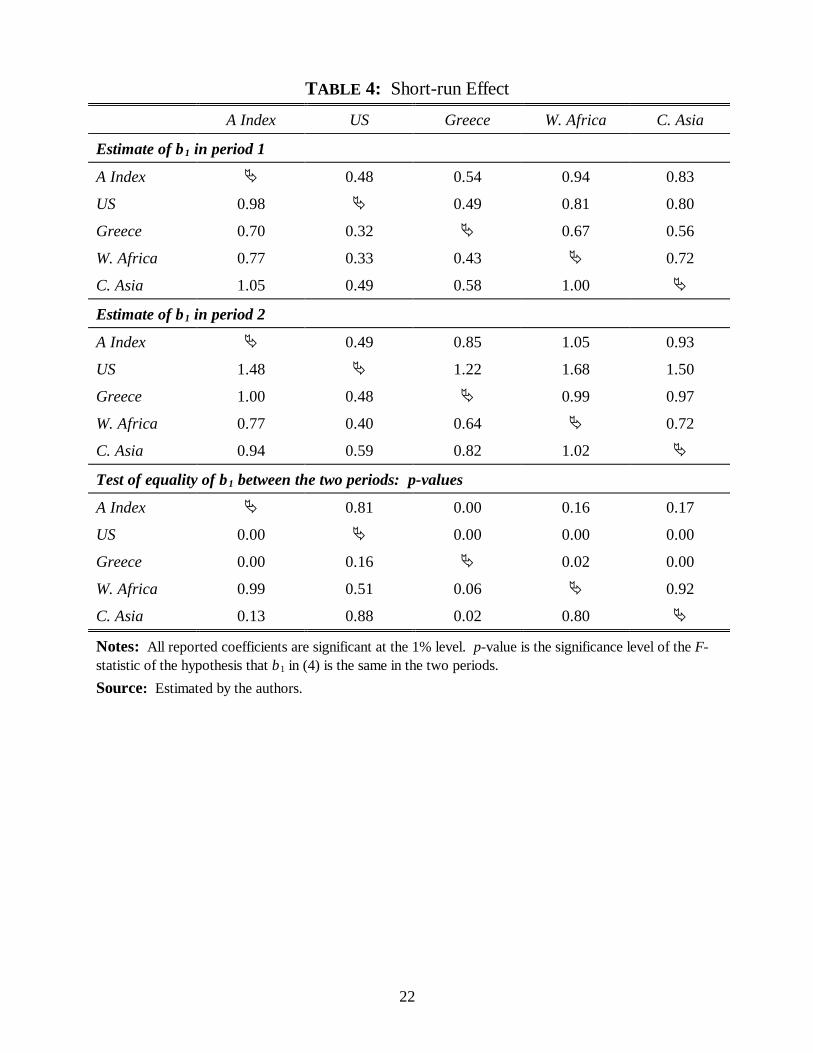
The upper and middle panels of Table 4 report the adjustment taking place within the first period.

A coefficient of one would be interpreted as a perfect transmission of price shocks, while a

coefficient of zero represents a short-run invariance to changes in prices elsewhere. Since the

short-run effect is in principle unrestricted, β1 greater than unity for example, would suggest an

over-reaction to changes in prices in the current period. The lower panel contains the p-values of

the hypothesis of equality in the β1s in the two sub-sample periods, against the two-sided

alternative.

At the 5% significance level, six of the nine overall improvements in the short-run effect

were significant, while only three of the eight remaining cases represented significant reductions in

the amount of adjustment within the first period.16 Further analysis of the nine significant changes

in the short-run effect reveals that the average deviation of the adjustment coefficient from unity

fell from 0.32 to 0.25, indicating an overall improvement in the initial adjustment. More

specifically, Greece showed the most improvement in the short-run adjustment when coupled to

the A Index, US and C. Asia. W. Africa and C. Asia revealed signs of improvement when paired

with Greece, while the opposite was true when paired with the US.

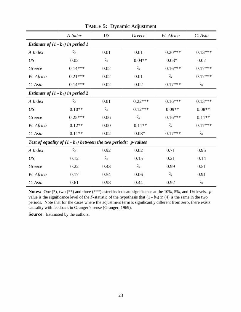
The measure of long-run comovement is presented in Table 5, with the upper and middle

panels representing period 1 and 2, respectively. In essence, the measure of long-run adjustment

captures the correction to a given price change from another origin, subsequent to the current

period. In fact, the absolute deviation from the long-run steady-state declines from period to

period (i.e., suggesting long-run convergence in prices) when this parameter is statistically

different from zero. The lower panel of Table 5 reports the p-values for the test of the hypothesis

13

that the dynamic adjustment effect remained the same against the two-sided alternative. Note that

for the cases where the error-correction parameter is not significant, specification (7) (i.e. the first

difference model) is the valid characterization of the data.

Twelve improvements were observed, while declines in the degree of comovement were

present in three cases. The remaining five cases revealed no appreciable change between periods

1 and 2. Significant improvements in the long-run effect were observed when Greece was

coupled with A Index and W. Africa at the 2% and 6% levels of significance. All other changes in

the measure of long-run comovement between the two sub-samples are not significant at

conventional levels (on average the adjustment coefficient increased from 0.08 to 0.11). This

result is congruent with the variance-ratio findings (depicted in figures 2a-2j), which do not detect

any change in the stationarity properties of the price differentials between the two periods.

Table 6 presents the number of weeks, n, required to achieve 95% of the adjustment to a

given price change. Note that n is calculated using equation (8) and, as was mentioned earlier, it

is only meaningful when long-run comovement in the Engle-Granger sense is detected. Faster

adjustment is observed in fourteen cases while a slower adjustment is observed in only two.

Except Greece-US in period 2, with the US as a reference, it is clear that none of the other origins

exhibited convergence towards the price levels in the US, a fact which becomes apparent when the

insignificant error-correction coefficient is considered.

However, Table 6 reveals that nine of fourteen changes in the number of periods required

to be within 5% of complete adjustment, were significant at the 7% level. Hence, price shocks

were transmitted at higher speed in period 2 compared with period 1. Additionally, in period 1,

nine cases of non-convergence were evident while only three cases appeared in period 2 at the

10% level of significance, indicating that prices from more origins achieved long-run convergence

in the second period.

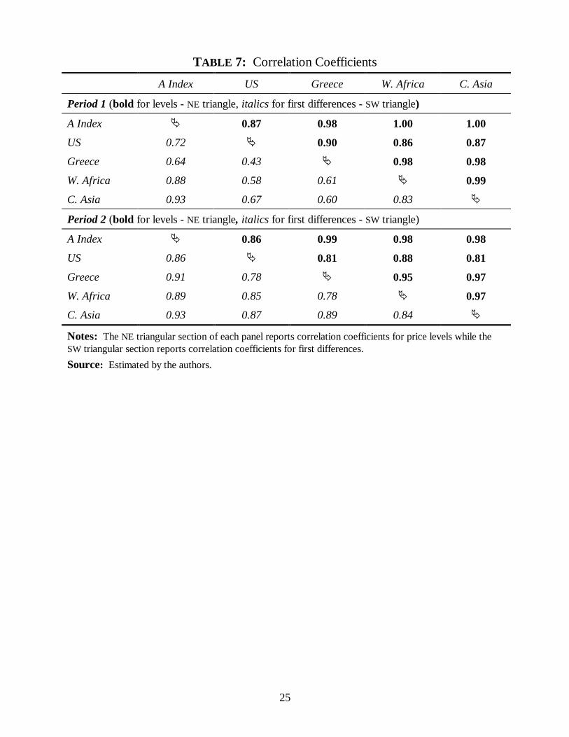
One methodological note is in order. It was argued earlier that a number of studies have

used correlation coefficients to examine price linkages. How much does one loose in terms of

informational content by using correlation coefficients? Table 6 reports correlation coefficients

for levels and first differences. The results indicate that correlation coefficients in levels are in no

way capable of detecting the improvement that has taken place. In fact, of the ten cases, eight

indicate reduction of linkages in the second period, a result contrary to a priori expectations. The

picture changes considerably when first differences are considered; with the exception of one

case, a substantial increase is detected, similar in direction to the R2 criterion reported earlier.

14

However, the magnitude of the increase is less than that of the R2; such result was expected since

R2 also captures improvements in long-run convergence. For example, the correlation coefficients

increase by an average of 25% (from 0.69 to 0.86) as opposed to the 50% improvement in R2. To

conclude, therefore, correlation coefficients, properly calculated by considering stationarity

properties, capture the short-run effect, but are incapable of capturing long-run comovement.

IV. SUMMARY AND CONCLUDING REMARKS

This paper examined the degree to which price linkages in cotton markets have improved over the

last decade. Weekly data from August 15, 1985 to December 24, 1987 (122 observations) and

August 3, 1995 to January 9, 1997 (73 observations) from US, Greece, Central Asia, and West

Africa were utilized. Price linkages between Central Asia and West Africa have been the highest

in both periods, while the linkages between the US and other markets were non-existent in the first

period.

According to the goodness of fit criterion (i.e. the R2) in almost all cases a substantial

improvement in price linkages has taken place. For example, while on average about 50% of the

variability of price from one origin was explained by the variability of another origin’s price in

period 1, the variability explained in period 2 increased to 75%. Moreover, if one excludes the A

Index, the relative increase in the explanatory power of the model is even higher (from 40% to

71%).

A number of interesting conclusions emerge from this paper, both policy related and

methodological. First, the main source of this improvement in price linkages appears to be a

result of short-run price transmission and to a very limited extent a result of long-run

comovement. To the degree that short-run price transmission reflects demand conditions while

long-run convergence reflects supply conditions, the findings of this paper suggest that over the

last decade, information on demand changes have been reflected in price changes much faster now

than a decade earlier.

A second conclusion relates to the relatively high long-run convergence between C. Asia

and W. Africa observed in both periods (with an estimated adjustment coefficient at 0.17) and the

non-existence of convergence between the US and the three other origins (especially in the first

period). Cotton produced in W. Africa and C. Asia is exported almost in its entirety, hence

making both markets subject to the same world demand conditions (prices respond only to world

demand since domestic demand is practically non-existent). On the contrary, only 40% of US

15

cotton is exported while the corresponding figure for Greece is 60% (1996/97 averages), in turn

making their respective prices subject to both domestic and world demand conditions. This

finding not only reinforces warnings cited in the literature that volume of trade may affect the

conclusions regarding the degree of price linkage, but also indicates that exports relative to the

size of the domestic market may be an important factor determining the degree of price linkage.

The third finding reflects on a methodological issue. It has been extensively argued in the

literature of time series that conventional stationarity tests exhibit low power and may give

misleading results regarding the true degree of comovement. This study confirmed this, i.e.

stationarity tests by themselves may be incapable of uncovering the comovement. Additional

measures, such as Cochrane’s variance-ratio tests or Hamilton’s advise of looking at the overall

sensibility of the results should be used to appropriately assess the presence (or absence) of price

linkage.

The results of this paper have also important implications with respect to price risk

management. Low comovement between US and non-US cotton prices implies that there is a need

for a futures contract other than the one currently traded at the New York Cotton Exchange

(NYCE) which is the only contract currently traded (apart from the São Paulo contract at the

Brazilian commodity exchange introduced in 1996, albeit with an extremely low liquidity). The

NYCE contract serves primarily domestic US needs and is not being used extensively by non-US

hedgers and speculators (Lake, 1992). This is not surprising if one considers that in December

31, 1990, the May 1991 contract closed at 76.19 cents, 8.21 cents below the A Index while it

expired on May 8, 1991 at 92.22 cents, 8.92 cents above the A Index, a results which is very

similar for the individual components of the A Index as this paper indicates.

The need for a futures exchange for non-US hedging needs, has been apparent as noted by

Cotton Outlook (December 12, 1997, p. 3) which reported: “The lack of an international trading

instrument other than the No. 2 [i.e. NYCE] contract Ä one which consistently reflects broad

world cotton market developments but is capable of being used as ‘hedge’ Ä continues to be a

shortcoming of the current pricing system.” An attempt, however, to create a ‘world’ futures

contract by NYCE in 1992 failed.

On the other hand, slow price convergence suggests that a non-US cotton contract is

unlikely to attract business from cotton merchants other than the ones that are interested in that

particular style of cotton and therefore may be expected to succeed only on national or regional

basis.

16

Finally, a note on further research. One important issue not considered here is

endogeneity. For policy related reasons, one would have to first, detect any endogeneity patterns

and correct for them through an instrumental variables model.

17

Endnotes

1 See Harriss (1980) for a comprehensive (and critical) review of the literature on market integrationstudies undertaken in the 1960s and 1970s.2 Ardeni (1989) and subsequently Baffes (1991) used quarterly averages for the following commodities:wheat, tea, beef, sugar, wool, zinc, and tin. In a more recent study, Zanias (1993) examined the degree ofspatial market integration in European Community agricultural product markets by using both unrestrictedand restricted versions [i.e. (1) and (2)], without detecting appreciable differences due to specification.3 The number of lags to be included in (3) is an empirical question. To make the exposition clear, we onlyuse one lag.4 Although the fact that the short-run effect is 1 while there may be no long-run convergence seemscounter-intuitive it should not be surprising. Consider the following thought experiment: two series aregenerated as pt

2 = (-1)trend(0.75) + εt and pt1 = pt-1

1 + (-1)trend(1.5) + 0.5 + εt, where trend denotes time (1,2, 3, ...) and εt is a white noise. pt

2 oscillates between ñ0.75 (1.5 unit swing) and pt1 rises by 2 in one

period and falls by 1 in the next period. On average, pt1 also demonstrates a swing of 1.5. Estimation of

(3) gives a short-run effect of one. However, it is clear that the two series are diverging over time. On theother hand, if pt

1 = 1 + εt, the short-run adjustment is effectively zero, i.e. changes in pt2 are completely

innocuous to changes in pt1 while the error-correction coefficient is one.

5 Relationship (7) corresponds to case (c) of Table 2.1 of Hendry, Pagan, and Sargan (1984) while (5) and(6) correspond to cases (i) and (g) of their Table 2.2.6 On this issue, Kennedy (1992) notes that (pt

2 - pt1) and (pt

2 - pt-12) are “ ...closer of being orthogonal than

the variables in the original relationship [i.e. (3)]” (p. 264).7 Baulch (1997b) discusses in detail the following four specifications: The level/cointegration version ofthe law of one price [specification (1)]; the first difference version of the law of one price [specification(7)]; the autoregressive distributed lag/error-correction [specifications (3) and (4), possibly with a higherlag structure]; and Granger-causality patterns [inferred from specifications (3) and (4)].8 Strictly speaking, (8) should read as k = (1-β1)β3 n, since as was discussed earlier, the restriction in(3) readsβ3 <1, not 0<β3<1.9 As it will be shown later, R2 and correlation coefficients can also be viewed as measures of price linkagessince both fall within the (0, 1) range, with zero corresponding to no linkage and 1 corresponding to perfectlinkage.10 The four countries/regions considered in the sample account for one third of world exports. If oneexcludes Argentina and Australia (the two dominant southern hemisphere exporters), they account for morethan 85% of world exports. With respect to the sample period, it would have been desirable to havecontinuous sample throughout the entire decade. However, these were the only large enough subperiods forwhich the price series were uninterrupted.11 The number of observations in the second period span 1.5 years as opposed to the first period whichspan 2.5 years. It is likely, therefore, that the trend stationarity result of the ADF and PP tests reflects shortsample (despite the high frequency of the data).12 Hamilton (1994) emphasizes the difficulty in distinguishing truly non-stationary processes fromprocesses that are stationary but persistent. He also suggests comparing estimates obtained underalternative specifications and choose the one that performs better according to several criteria, which is theavenue we pursue in the present case. Following Hamilton and in view of the trend stationarity evidence ofthe second period, we also estimated the model in levels (i.e. (3) with a trend variable) by testing and

18

subsequently imposing long-run proportionality. In all cases the model exhibited R2s close to unity andextremely high t-ratios. In no case we found statistically significant difference in the estimates of periods 1and 2 as the performance of the model was indistinguishable in the two periods. Cochrane (1988) alsopoints to the difficulties of parametric tests in distinguishing between true random walk models and trendstationary models with a small random walk component, which appears to be the case in the period 2.13 The lag structure of the six cases (all in the first period) was as follows: Greece-US{2,3}, W. Africa-US{0,3}, C. Asia-US{0,3}, A Index-US{0.3}, W. Africa-Greece{1,0}, and W. Africa- A Index{0,3}. Forconsistency, we retained identical lag structure in the second period.14 The complete set with estimation results is available from the authors upon request.15 Because the A Index may contain one of the prices under consideration by definition, it is expected thatthe regression on the A Index will exhibit superior performance. That explains why when the A Indexmodels are excluded, the average R2 declines in both periods.16 At this point we should clarify the fact that symmetry of the short-run coefficient with respect to unity isinterpreted as an equal departure from perfect short-run transmission. For example, the values 1.25 and0.75 are being viewed as exhibiting the same deviation from unitary short-run elasticity.

19

TABLE 1: Cumulative Adjustment

Period (n) Amount of Cumulative Adjustment (k)

0 β1 = 1 - (1 - β1)β30

1 β1 + (1 - β1)(1 - β3) = 1 - (1 - β1)β31

2 1 - (1 - β1)β3 + (1 - β3)(1 - β1)β3 = 1 - (1 - β1)β32

3 1 - (1 - β1)β32 + (1 - β3)(1 - β1)β3

2 = 1 - (1 - β1)β33

4 1 - (1 - β1)β33 + (1 - β3)(1 - β1)β3

3 = 1 - (1 - β1)β34

Notes: β1 and β3 refer to the parameters of equation (4).Source: Calculated by the authors.

20

TABLE 2: Stationarity Tests

Period 1 Period 2

ADF PP ADF PP

Levels w/o trend

A Index -1.24 -0.70 -1.18 -0.84

US -1.40 -1.10 -1.38 -1.53

Greece -1.26 -0.78 -1.18 -0.96

W. Africa -1.33 -0.72 -1.11 -0.67

C. Asia -1.30 -0.75 -1.24 -0.86

Levels w/ trend

A Index -2.42 -2.03 -3.51*** -3.44**

US -1.83 -1.55 -4.80*** -4.84***

Greece -2.55 -2.27 -2.87* -3.08**

W. Africa -2.56 -2.07 -3.71*** -3.58***

C. Asia -2.80* -2.35 -2.38 -2.59*

Price Differentials

A Index - US -1.71 -1.40 -3.11** -3.26**

A Index - Greece -2.94** -2.82* -3.58*** -3.16**

A Index - W. Africa -3.70*** -3.77*** -2.48 -2.41

A Index - C. Asia -3.39** -3.53*** -2.97** -2.65*

US - Greece -1.87 -1.71 -2.81* -3.03**

US - W. Africa -1.74 -1.46 -3.42** -3.55***

US - C. Asia -1.68 -1.28 -3.31** -3.36**

Greece - W. Africa -3.02** -2.96** -2.49 -2.35

Greece - C. Asia -2.85* -2.80* -2.26 -2.40

W. Africa - C. Asia -3.87*** -3.82*** -3.00** -2.87*

Notes: One (*), two (**) and three (***) asterisks indicate significance at the 10%, 5%, and 1% levels.Critical values are: -2.58 (10%), -2.89 (5%), and -3.51 (1%) (Fuller, 1976).Source: Estimated by the authors.

21

TABLE 3: Goodness of Fit

A Index US Greece W. Africa C. Asia

R2 in Period 1

A Index Ä 0.62 0.40 0.80 0.88

US 0.50 Ä 0.18 0.32 0.43

Greece 0.46 0.34 Ä 0.44 0.44

W. Africa 0.83 0.51 0.41 Ä 0.72

C. Asia 0.88 0.54 0.35 0.71 Ä

R2 in Period 2

A Index Ä 0.73 0.84 0.81 0.87

US 0.74 Ä 0.62 0.73 0.76

Greece 0.85 0.55 Ä 0.62 0.80

W. Africa 0.81 0.70 0.61 Ä 0.75

C. Asia 0.79 0.72 0.79 0.74 Ä

Notes: Goodness of fit is the R2 of equation (4).Source: Estimated by the authors.

22

TABLE 4: Short-run Effect

A Index US Greece W. Africa C. Asia

Estimate of β1 in period 1

A Index Ä 0.48 0.54 0.94 0.83

US 0.98 Ä 0.49 0.81 0.80

Greece 0.70 0.32 Ä 0.67 0.56

W. Africa 0.77 0.33 0.43 Ä 0.72

C. Asia 1.05 0.49 0.58 1.00 Ä

Estimate of β1 in period 2

A Index Ä 0.49 0.85 1.05 0.93

US 1.48 Ä 1.22 1.68 1.50

Greece 1.00 0.48 Ä 0.99 0.97

W. Africa 0.77 0.40 0.64 Ä 0.72

C. Asia 0.94 0.59 0.82 1.02 Ä

Test of equality of β1 between the two periods: p-values

A Index Ä 0.81 0.00 0.16 0.17

US 0.00 Ä 0.00 0.00 0.00

Greece 0.00 0.16 Ä 0.02 0.00

W. Africa 0.99 0.51 0.06 Ä 0.92

C. Asia 0.13 0.88 0.02 0.80 Ä

Notes: All reported coefficients are significant at the 1% level. p-value is the significance level of the F-statistic of the hypothesis that β1 in (4) is the same in the two periods.Source: Estimated by the authors.

23

TABLE 5: Dynamic Adjustment

A Index US Greece W. Africa C. Asia

Estimate of (1 - β3) in period 1

A Index Ä 0.01 0.01 0.20*** 0.13***

US 0.02 Ä 0.04** 0.03* 0.02

Greece 0.14*** 0.02 Ä 0.16*** 0.17***

W. Africa 0.21*** 0.02 0.01 Ä 0.17***

C. Asia 0.14*** 0.02 0.02 0.17*** Ä

Estimate of (1 - β3) in period 2

A Index Ä 0.01 0.22*** 0.16*** 0.13***

US 0.10** Ä 0.12*** 0.09** 0.08**

Greece 0.25*** 0.06 Ä 0.16*** 0.11**

W. Africa 0.12** 0.00 0.11** Ä 0.17***

C. Asia 0.11** 0.02 0.08* 0.17*** Ä

Test of equality of (1 - β3) between the two periods: p-values

A Index Ä 0.92 0.02 0.71 0.96

US 0.12 Ä 0.15 0.21 0.14

Greece 0.22 0.43 Ä 0.99 0.51

W. Africa 0.17 0.54 0.06 Ä 0.91

C. Asia 0.61 0.98 0.44 0.92 Ä

Notes: One (*), two (**) and three (***) asterisks indicate significance at the 10%, 5%, and 1% levels. p-value is the significance level of the F-statistic of the hypothesis that (1 - β3) in (4) is the same in the twoperiods. Note that for the cases where the adjustment term is significantly different from zero, there existscausality with feedback in Granger’s sense (Granger, 1969).Source: Estimated by the authors.

24

TABLE 6: Number of Periods Required to Achieve 95% of theCumulative Adjustment

A Index US Greece W. Africa C. Asia

Estimate of n in period 1

A Index Ä n.c. n.c. 0.8 8.7

US n.c. Ä 54.8 46.4 n.c.

Greece 12.3 n.c. Ä 11.2 11.4

W. Africa 4.6 n.c. n.c. Ä 9.6

C. Asia 0.4 n.c. n.c. 0.0 Ä

Estimate of n in period 2

A Index Ä n.c. 4.5 0.0 2.9

US 22.3 Ä 11.5 26.3 27.0

Greece 0.0 n.c. Ä 0.0 0.0

W. Africa 9.6 n.c. 2.6 Ä 9.0

C. Asia 1.5 n.c. 16.2 0.0 Ä

Test of equality of n between the two periods: p-values

A Index Ä n.a. 0.00 0.32 0.37

US 0.00 Ä 0.00 0.00 0.00

Greece 0.01 n.a. Ä 0.06 0.00

W. Africa 0.03 n.a. 0.01 Ä 0.99

C. Asia 0.30 n.a. 0.07 0.95 Ä

Notes: p-value is the significance level of the F-statistic of the hypothesis that (1 - β3) and β1 in (4) (andhence k and n) is the same in the two periods. n is calculated as [log(0.05) - log(1-β1)]/ logβ3 Ä a result ofsetting k = 0.95 and solving (8) for n. ‘n.c.’ indicates that long-run convergence never takes place as theerror-correction parameter is not significantly different from zero; ‘n.a.’ indicates that the test is notreported because the respective prices did not converge (for both cases 10% level of significance was thecut-off point).Source: Estimated by the authors.

25

TABLE 7: Correlation Coefficients

A Index US Greece W. Africa C. Asia

Period 1 (bold for levels - NE triangle, italics for first differences - SW triangle)

A Index Ä 0.87 0.98 1.00 1.00

US 0.72 Ä 0.90 0.86 0.87

Greece 0.64 0.43 Ä 0.98 0.98

W. Africa 0.88 0.58 0.61 Ä 0.99

C. Asia 0.93 0.67 0.60 0.83 Ä

Period 2 (bold for levels - NE triangle, italics for first differences - SW triangle)

A Index Ä 0.86 0.99 0.98 0.98

US 0.86 Ä 0.81 0.88 0.81

Greece 0.91 0.78 Ä 0.95 0.97

W. Africa 0.89 0.85 0.78 Ä 0.97

C. Asia 0.93 0.87 0.89 0.84 Ä

Notes: The NE triangular section of each panel reports correlation coefficients for price levels while theSW triangular section reports correlation coefficients for first differences.Source: Estimated by the authors.

30

ReferencesAlderman, H. “Intercommodity Price Transmittal: Analysis of Food Markets in Ghana.”

Oxford Bulletin of Economics and Statistics, 55(1993):43-64.

Alexander, C. and J. Wyeth. “Cointegration and Market Integration: An Application to theIndonesian Rice Market.” Journal of Development Studies, 30(1994):303-328.

Ardeni, P. G. “Does the Law of One Price Really Hold for Commodity Prices?” AmericanJournal of Agricultural Economics, 71(1989):661-669.

Baffes, J. “Some Further Evidence on the Law of One Price: The Law of One Price still Holds.”American Journal of Agricultural Economics, 73(1991):1264-1273.

Barrett, C. B. “Market Analysis Methods: Are Our Enriched Toolkits Well Suited to EnlivedMarkets?” American Journal of Agricultural Economics, 78(1996):825-829.

Baulch, B. “Transfer Costs, Spatial Arbitrage, and Testing for Food Market Integration.” AmericanJournal of Agricultural Economics, 79(1997a):477-487.

Baulch, B. “Testing for Food Market Integration Revisited.” Journal of Development Studies,33(1997b):512-534.

Cochrane, J. H. “How Big Is the Random Walk in GNP?” Journal of Political Economy,96(1988):893-920.

Campbell, J. Y. and R. J. Shiller. “Cointegration Tests of Present Value Models.” Journal ofPolitical Economy, 95(1987):1061-1088.

Cotton Outlook. Cotlook Limited, Liverpool: UK, various issues.

Delgado, C. “A Variance Components Approach to Food Grain Market Integration in NorthernNigeria.” American Journal of Agricultural Economics, 68(1986):970-979.

Dercon, S. “On Market Integration and Liberalization: Method and Application to Ethiopia.”Journal of Development Studies, 32(1995):112-143.

Dickey, D. and W. A. Fuller. “Distribution of the Estimators for Time Series Regressions with UnitRoots.” Journal of the American Statistical Association, 74(1979):427-431.

Engle, R. F. and C. W. Granger. “Co-Integration and Error Correction: Representation, Estimation,and Testing.” Econometrica, 55(1987):251-276.

Engle, R. F. and B. S. Yoo. “Forecasting and Testing in Co-Integrated Systems.” Journal ofEconometrics, 35(1987):143-159.

Fafchamps, M. and S. Gavian. “The Spatial Integration of Livestock Markets in Niger.” Journal ofAfrican Economies, 5(1996):366-405.

Faminow, M. and B. Benson. “Integration of Spatial Markets.” American Journal of AgriculturalEconomics, 72(1990):49-62.

Faruqee, R., J. R. Coleman, and T. Scott. “Managing Price Risk in the Pakistan Wheat Market.”World Bank Economic Review, 11(1997):263-292.

Fortenbery T. R. and H. O. Zapata. “An Evaluation of Price Linkages Between Futures and CashMarkets for Cheddar Cheese.” Journal of Futures Markets, 17(1997):279-301.

31

Fuller, W. A. Introduction to Statistical Time Series, New York: John Wiley & Sons, 1976.

Garbade, K. D. and W. L. Silber. “Price Movements and Price Discovery in Futures and CashMarkets.” Review of Economics and Statistics, 65(1983):289-297.

Gardner, B. and K. M. Brooks. “Food Prices and Market Integration in Russia: 1992-93.”American Journal of Agricultural Economics, 76(1994):641-646.

Goletti, F. and S. Babu. “Market Liberalization and Integration of Maize Markets in Malawi.”Agricultural Economics, 11(1994):311-324.

Goodwin, B. K. and T. C. Schroeder. “Co-Integration Tests and Spatial price Linkages in RegionalCattle Markets.” American Journal of Agricultural Economics, 72(1990):682-693.

Gordon, H. F. Grain Marketing Performance and Public Policy in Tanzania. Ph.D. Dissertation,Fletcher School of Law and Diplomacy, 1994.

Granger, C. W. “Investigating Causal Relations by Econometric Models and Cross-SpectralMethods.” Econometrica, 37(1969):424-438.

Hamilton, J. Time Series Analysis. New Jersey: Princeton University Press, 1994.

Hansen, L. P. “Large Sample Properties of Generalized Method of Moments Estimators.”Econometrica, 50(1982):1029-1054.

Harriss, B. “There Is Method in My Madness: Or it Is Vice Versa? Measuring Agricultural MarketPerformance.” Food Research Institute Studies, 16(1979):197-218.

Hendry, D. F., A. R. Pagan, and J. D. Sargan. “Dynamic Specification.” Handbook ofEconometrics, vol. 2, ed. Z. Griliches and M. D. Intriligator. Amsterdam: North-HollandPublishing Co., 1984.

Heytens, P. C. “Testing Market Integration.” Food Research Institute Studies, 20(1986): 25-41.

Hudson, D., D. Ethridge, and J. Brown. “Producer Prices in Cotton Markets: Evaluation ofReported Price Information Accuracy.” Agribusiness: An International Journal, 12 (1996):353-362.

Isard, P. “How Far Can We Push the ‘Law of One Price’?” American Economic Review,67(1977):942-948.

Kennedy, P. A Guide to Econometrics. Cambridge, MA: The MIT Press, 1992.

Lake, T. “A World Cotton Futures Contract.” Cotton: Review of the World Situation,International Cotton Advisory Committee. Vol. 45, no.5, May-June 1992, pp. 14-15.

Leavitt, S., M. Hawkins, and M. Veeman. “Improvements to Market Efficiency Through theOperation of the Alberta Pork Producers’ Marketing Board.” Canadian Journal ofAgricultural Economics, 31(1983):371-388.

Lele, U. “Market Integration: A Study of Sorghum Prices in Western India.” Journal of FarmEconomics, 49(1967):149-159.

Lindahl, M. “Measuring Hedging Effectiveness with R2: A Note.” Journal of Futures Markets,9(1989):469-475.

Lutz, C., A. van Tilburg, and B. van der Kamp. “The Process of Short- and Long-Term Price

32

Integration in the Benin Maize Market.” European Review of Agricultural Economics,22(1995):191-212.

Mundlak, Y. and D. F. Larson. “On the Transmission of World Agricultural Prices.” WorldBank Economic Review, 6(1992):399-422.

Meese, R. A. “Testing for Bubbles in Exchange Rates: A Case of Sparkling Rate?” Journal ofPolitical Economy, 94(1986):345-373.

Palaskas, T. B. and B. Harriss. “Testing Market Integration: New Approaches with Case Materialfrom the West Bengal Food Economy.” Journal of Development Studies, 30 (1993): 1-57.

Petzel, T. E. and E. A. Monke. “The Integration of the International Rice Market.” Food ResearchInstitute Studies, 16(1980):307-326.

Phillips, P. C. B. “Time Series Regressions with a Unit Root.” Econometrica, 55(1987):277-301.

Phillips, P. C .B. and M. Loretan. “Estimating Long-Run Economic Equilibria.” Review ofEconomic Studies, 55(1991):407-436.

Phillips, P. C. B. and P. Perron. “Testing for a Unit Root in Time Series Regression.” Biometrica,65(1988):335-346.

Protopapadakis, A. A. and H. R. Stoll. “Spot and Futures Prices and the Law of One Price.”Journal of Finance, 38(1983):1431-1455.

Protopapadakis, A. A. and H. R. Stoll. “Some Empirical Evidence on Commodity Arbitrage and theLaw of One Price.” Journal of International Money and Finance, 9(1986): 335-360.

Ravallion, M. “Testing Market Integration.” American Journal of Agricultural Economics, 68(1986):102-109.

Richardson, J. D. “Some Empirical Evidence on Commodity Arbitrage and the Law of OnePrice.” Journal of International Economics, 8(1978):341-351.

Samuelson, P. “Spatial Price Equilibrium and Linear Programming.” American EconomicReview, 42(1952):283-303.

Schroeder, T. C. and B. K. Goodwin. “Price Discovery and Cointegration of Live Hogs.” Journal ofFutures Markets, 11(1991):685-696.

Sexton, R., C. Kling, and H. Carman. “Market Integration, Efficiency of Arbitrage, andImperfect Competition: Methodology and Application to US Celery.” American Journal ofAgricultural Economics, 73(1991):568-580.

Southworth, V. R., W. O. Jones, and S. R. Pearson. “Food Crop Marketing in Atebubu District,Ghana.” Food Research Institute Studies, 16(1979):157-196.

Stigler, G. and R. A. Sherwin. “The Extent of the Market.” Journal of Law and Economics,28(1985):555-585.

Takayama, T. and G. Judge. “Spatial Equilibrium and Quadratic Programing.” Journal ofFarm Economics, 46(1964):67-93.

Timmer, C. P., W. P. Falcon, and S. R. Pearson. Food Policy Analysis. Baltimore: JohnsHopkins University Press, 1983.

Timmer, C. P. “Corn Marketing.” The Corn Economy of Indonesia, ed. C. P. Timmer. Ithaca,

33

NY: Cornell University Press, 1987.

Tommek, W. “Price Behavior on a Declining Terminal Market.” American Journal ofAgricultural Economics, 62(1980):434-444.

Wang, G. H. K. and J. Yau. “A Time Series Approach to Testing Market Linkage: Unit Rootand Cointegration Tests.” Journal of Futures Markets, 14(1994):457-474.

West, K. D. “A Standard Monetary Model and the Variability of the Deutschemark-Dollar ExchangeRate.” Journal of International Economics, 23(1987):57-76.

White, H. “A Heteroscedasticity-Consistent Covariance Matrix Estimator and Direct Tests forHeteroskedasticity.” Econometrica, 48(1980):817-838.

Zanias, G. P. “Testing for Integration in European Community Agricultural Product Markets.”Journal of Agricultural Economics, 44(1993):418-427.

34

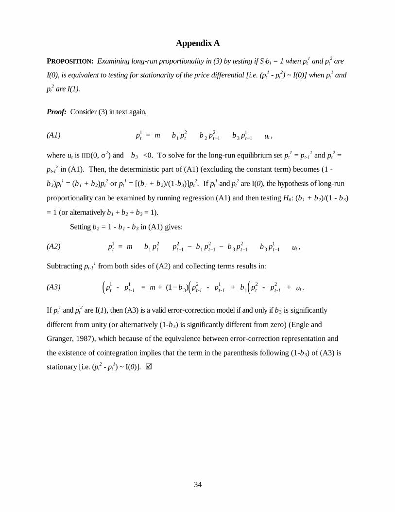
Appendix A

PROPOSITION: Examining long-run proportionality in (3) by testing if Σiβi = 1 when pt1 and pt

2 are

I(0), is equivalent to testing for stationarity of the price differential [i.e. (pt1 - pt

2) ~ I(0)] when pt1 and

pt2 are I(1).

Proof: Consider (3) in text again,

(A1) t t t t tp p p p u11

22 1

23 1

1= + + + +− −µ β β β ,

where ut is IID(0, σ2) and β3<0. To solve for the long-run equilibrium set pt1 = pt-1

1 and pt2 =

pt-12 in (A1). Then, the deterministic part of (A1) (excluding the constant term) becomes (1 -

β3)pt1 = (β1 + β2)pt

2 or pt1 = [(β1 + β2)/(1-β3)]pt

2. If pt1 and pt

2 are I(0), the hypothesis of long-run

proportionality can be examined by running regression (A1) and then testing H0: (β1 + β2)/(1 - β3)

= 1 (or alternatively β1 + β2 + β3 = 1).

Setting β2 = 1 - β1 - β3 in (A1) gives:

(A2) t t t t t t tp p p p p p u11

21

21 1

23 1

23 1

1= + + − − + +− − − −µ β β β β ,

Subtracting pt-11 from both sides of (A2) and collecting terms results in:

(A3) ( ) ( ) ( )t t-1 t-1 t-1 t t-1 tp - p = + p - p + p - p + u .1 13

2 11

2 21µ β β( )−

If pt1 and pt

2 are I(1), then (A3) is a valid error-correction model if and only if β3 is significantly

different from unity (or alternatively (1-β3) is significantly different from zero) (Engle and

Granger, 1987), which because of the equivalence between error-correction representation and

the existence of cointegration implies that the term in the parenthesis following (1-β3) of (A3) is

stationary [i.e. (pt2 - pt

1) ~ I(0)]. þ

35

Appendix B: The ‘World’ Price of Cotton and its Components

Typically, the world price of a commodity is taken to be the spot price prevailing at a certain

location where a substantial part of trade is taking place. While often this location is in a key

producing country (e.g. US for maize and Thailand for rice) this may not always be the case (e.g.

New York for coffee and London for tea). On the other hand, for several commodities there is

more than one dominant trade location (e.g. wheat in US, Canada, and Australia or wool in New

Zealand and the UK).

Cotton departs from this tradition in that its ‘world’ price is not a spot price at which

actual transactions take place in one or more locations; instead it is an index, calculated as an

average of offer quotations by cotton agents in North Europe. The index is constructed daily by

Cotlook Limited, a private information dissemination company based in Liverpool, UK and is

published in the weekly magazine Cotton Outlook.

The cotton price index (often referred to as the Cotlook A Index or simply the A Index) is

an average of the five less expensive out of 14 styles of cotton (Middling 1-3/32’’) traded in

North Europe originating from: (1) Memphis Territory (US); (2) California/Arizona (US); (3)

Mexico; (4) Paraguay; (5) Turkey; (6) Syria; (7) Greece; (8) Central Asia (until June 1997)/

Uzbekistan (since then); (9) Pakistan; (10) India; (11) China; (12) Tanzania; (13) Africa ‘Franc

Zone’; and (14) Australia (see Table B1 below for a detailed example). These are offer prices, i.e.

the price that the agent would quote for the particular type of cotton. To account for the fact that

agent’s quotation is likely to be above the price at which the actual transaction takes place (since

the buyer will probably negotiate a lower price), the index takes the five lowest priced styles.

Some styles are consistently traded with premiums or discounts compared to the A Index.

For example, cotton from the US is usually traded above the A Index, cotton from Uzbekistan is

traded below the A Index, while that from Africa ‘Franc Zone’ is traded very close to the A

Index. Since not all styles of cotton from the eligible origins are traded in North Europe all year

around, not all 14 quotations are available for the A Index at all times. Therefore, the frequency

at which a certain cotton style participates in the formation of the A Index depends on whether it

is continuously traded in North Europe and on how inexpensive it is. When less than five eligible

quotations are available, the A Index is not reported. This may happen when the Southern

Hemisphere runs out of supplies while the Northern Hemisphere is not ready to supply cotton (for

example, this was the case in June/July 1995).

36

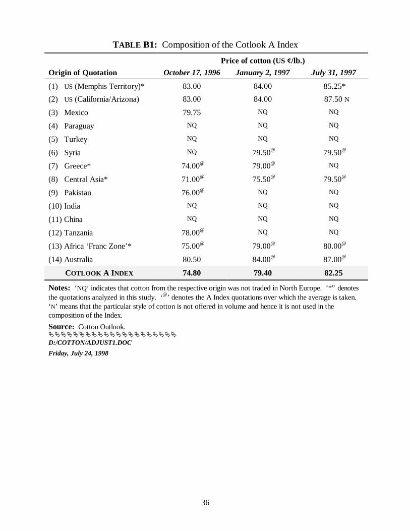
TABLE B1: Composition of the Cotlook A Index

Price of cotton (US ¢/lb.)Origin of Quotation October 17, 1996 January 2, 1997 July 31, 1997

(1) US (Memphis Territory)* 83.00 84.00 85.25*

(2) US (California/Arizona) 83.00 84.00 87.50 N

(3) Mexico 79.75 NQ NQ

(4) Paraguay NQ NQ NQ

(5) Turkey NQ NQ NQ

(6) Syria NQ 79.50@ 79.50@

(7) Greece* 74.00@ 79.00@ NQ

(8) Central Asia* 71.00@ 75.50@ 79.50@

(9) Pakistan 76.00@ NQ NQ

(10) India NQ NQ NQ

(11) China NQ NQ NQ

(12) Tanzania 78.00@ NQ NQ

(13) Africa ‘Franc Zone’* 75.00@ 79.00@ 80.00@

(14) Australia 80.50 84.00@ 87.00@

COTLOOK A INDEX 74.80 79.40 82.25

Notes: ‘NQ’ indicates that cotton from the respective origin was not traded in North Europe. ‘*” denotesthe quotations analyzed in this study. ‘@’ denotes the A Index quotations over which the average is taken.‘N’ means that the particular style of cotton is not offered in volume and hence it is not used in thecomposition of the Index.Source: Cotton Outlook.ÄÄÄÄÄÄÄÄÄÄÄÄÄÄÄÄÄÄÄÄÄD:/COTTON/ADJUST1.DOC

Friday, July 24, 1998