Embed Size (px)
Citation preview

2/7/11 Bafna
Detecting structural variations in genomes
The course so far
• Genetic variations create diversity�– Mutations, recombination �
• A population evolving neutrally under these variations might be in equilibrium conditions�– Hardy Weinberg �– Linkage�
• The evolution under neutral conditions can be modeled reasonably and efficiently by coalescent theory�
• Today: structural variations add another source of variation to the mix. Not easily captured via coalescent theory.�
2/7/11 Bafna
2/7/11 Bafna
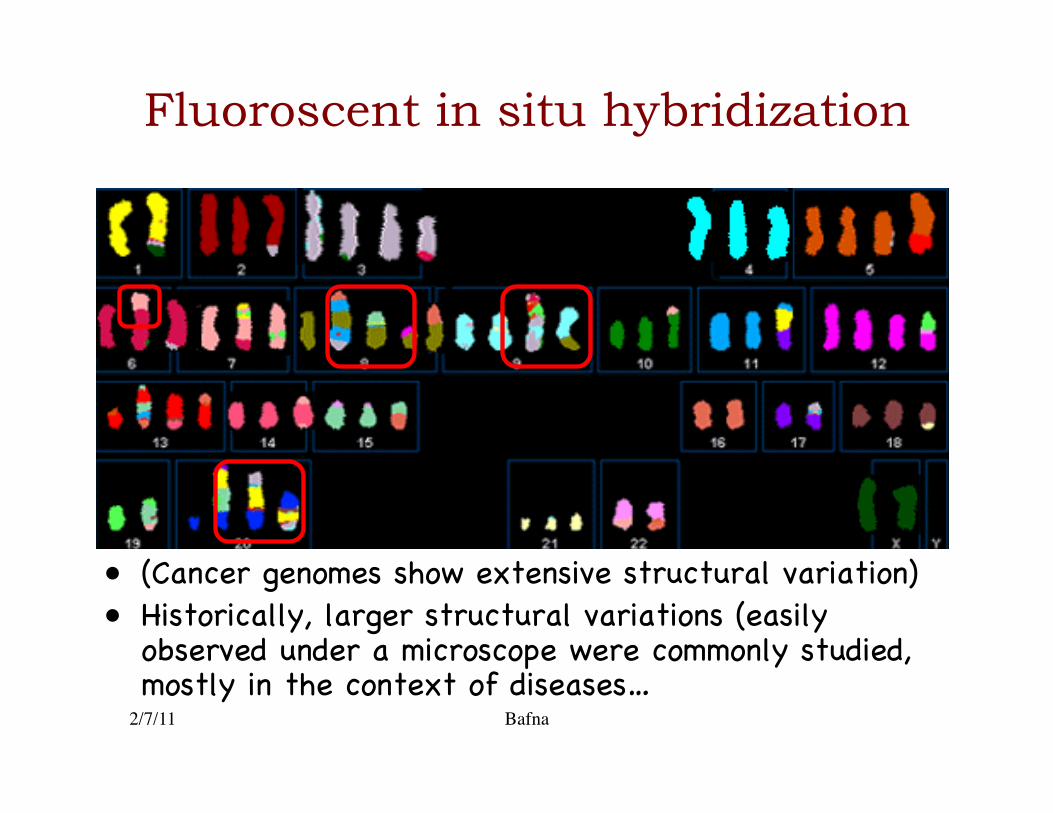
Fluoroscent in situ hybridization
• (Cancer genomes show extensive structural variation)�• Historically, larger structural variations (easily
observed under a microscope were commonly studied, mostly in the context of diseases…�
2/7/11 Bafna
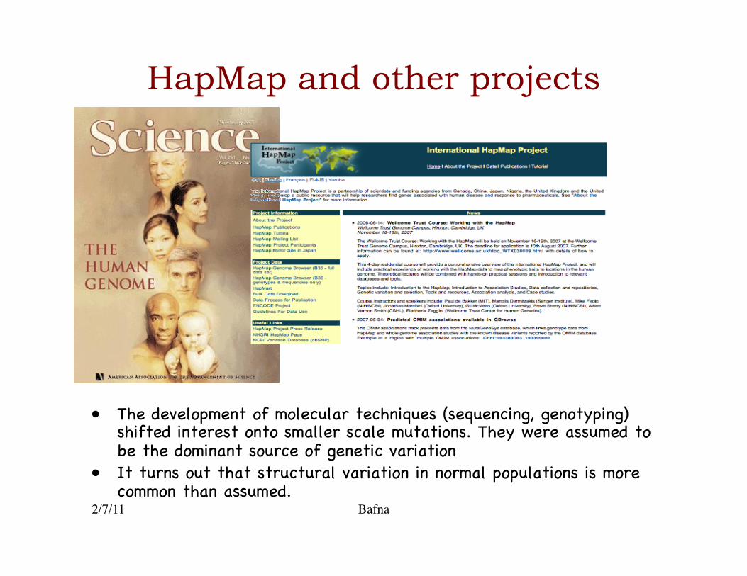
HapMap and other projects
• The development of molecular techniques (sequencing, genotyping) shifted interest onto smaller scale mutations. They were assumed to be the dominant source of genetic variation �
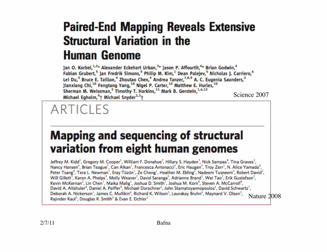
• It turns out that structural variation in normal populations is more common than assumed. �
2/7/11 Bafna
Science 2007
Nature 2008
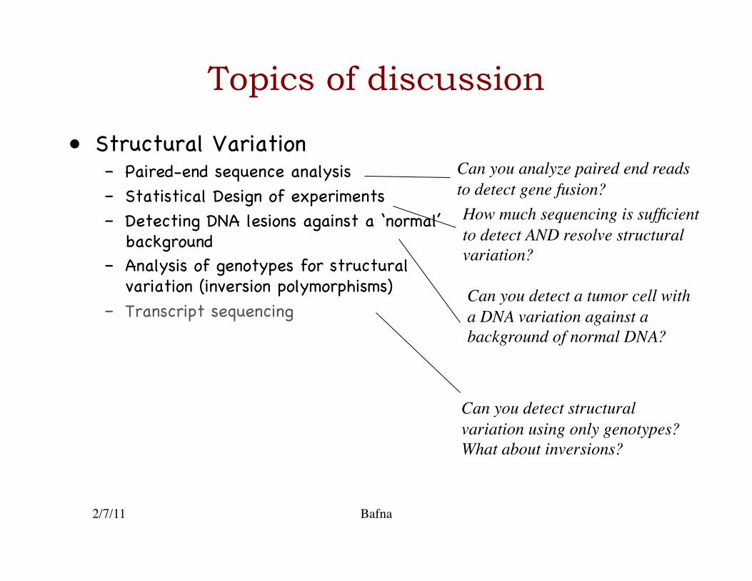
Topics of discussion
• Structural Variation �– Paired-end sequence analysis�– Statistical Design of experiments�– Detecting DNA lesions against a ‘normal’
background �– Analysis of genotypes for structural
variation (inversion polymorphisms)�– Transcript sequencing �
2/7/11 Bafna
Can you analyze paired end reads to detect gene fusion? How much sequencing is sufficient to detect AND resolve structural variation?
Can you detect a tumor cell with a DNA variation against a background of normal DNA?
Can you detect structural variation using only genotypes? What about inversions?

Mechanisms for structural variation
2/7/11 Bafna
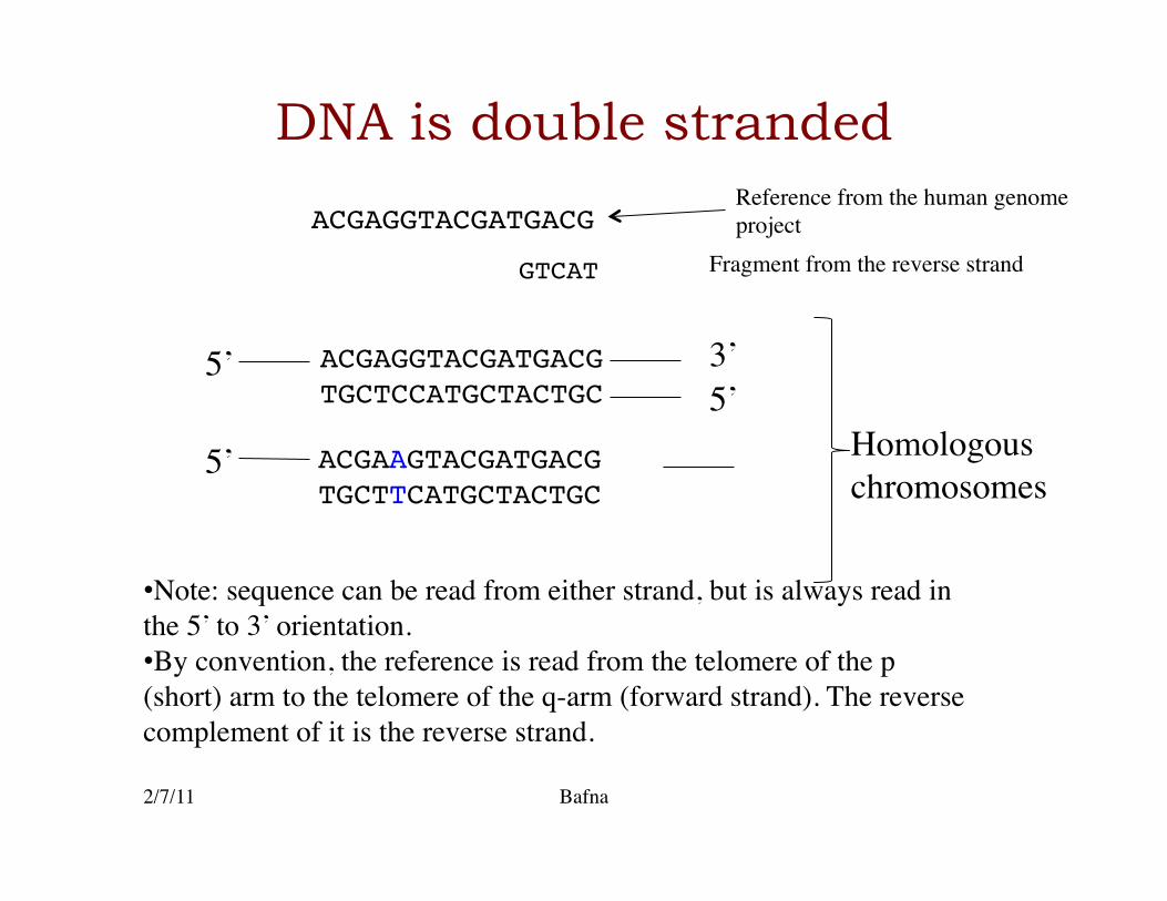
DNA is double stranded
2/7/11 Bafna
ACGAGGTACGATGACG!TGCTCCATGCTACTGC!
ACGAAGTACGATGACG!TGCTTCATGCTACTGC!
5’ 3’ 5’
Homologous chromosomes
5’
• Note: sequence can be read from either strand, but is always read in the 5’ to 3’ orientation. • By convention, the reference is read from the telomere of the p (short) arm to the telomere of the q-arm (forward strand). The reverse complement of it is the reverse strand.
ACGAGGTACGATGACG!Reference from the human genome project
GTCAT! Fragment from the reverse strand
Low Copy Repeats (LCRs)
• About 5% of the reference haploid genome is present in two or more copies (Lupski 2010) �– Also known as segmental duplications�
• LCRs can lead to Non-allelic homologous recombinations�
2/7/11 Bafna

Homologous recombination
2/7/11 Bafna
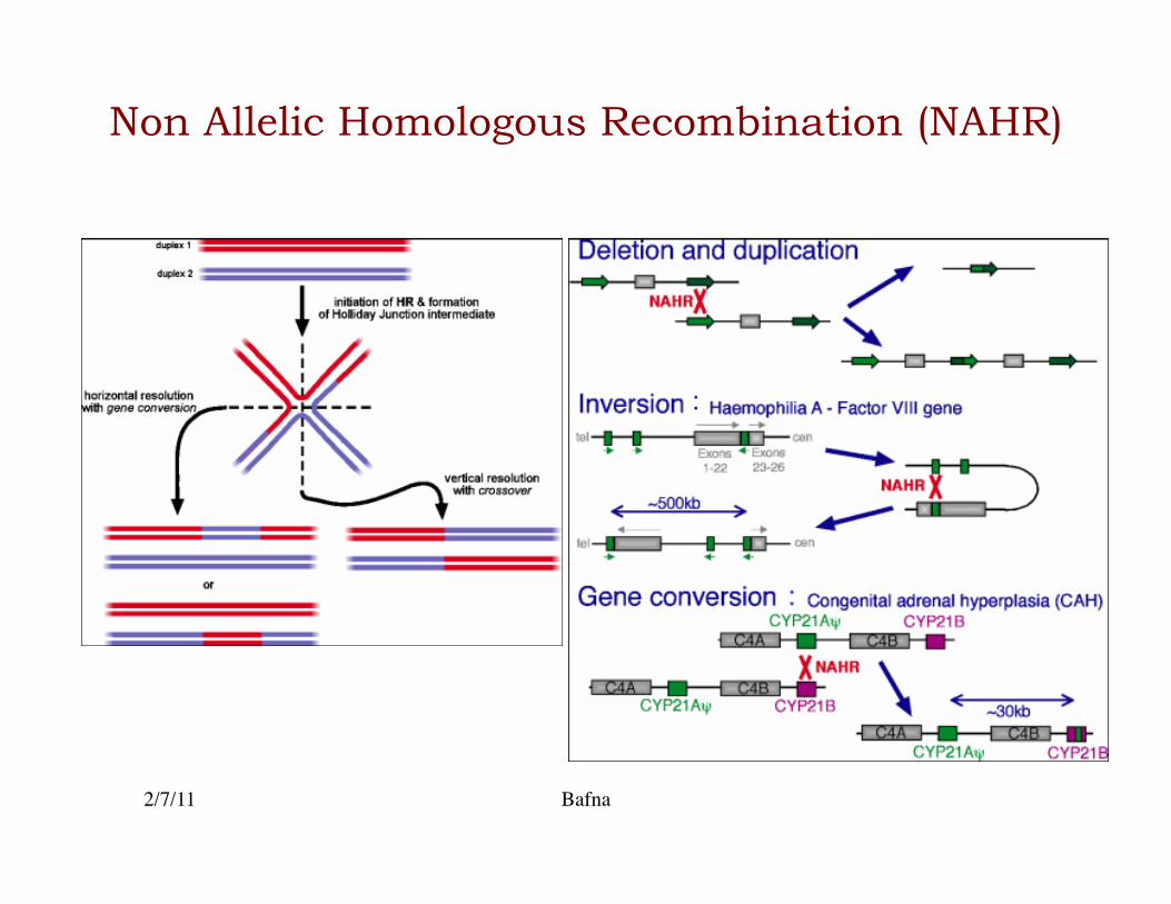
Non Allelic Homologous Recombination (NAHR)
2/7/11 Bafna

Non-homologous end joining (NHEJ)
2/7/11 Bafna

Retrotranspositions
• Reetrotransposons and DNA transposons can insert and delete themselves, leading to s.v.�
• DNA transposons work via endonuclease activity, NHEJ �
• Retrotransposons can also act as repeats for NAHR �
2/7/11 Bafna

The breakage fusion bridge cycle, and amplicon formation
2/7/11 Bafna
SV events
• Caveat: SVs are poorly understood, and none of the following is ‘textbook’ material.�
• We consider the following topics�– Sequence based signatures for SVs�– Fine-mapping of SV breakpoints�– Clustering of reads supporting a single SV �– Signatures of common events�– Design issues�– Pop. Genetic parameter changes.�
2/7/11 Bafna
Detecting ‘simple’ SVs
2/7/11 Bafna
2/7/11 Bafna
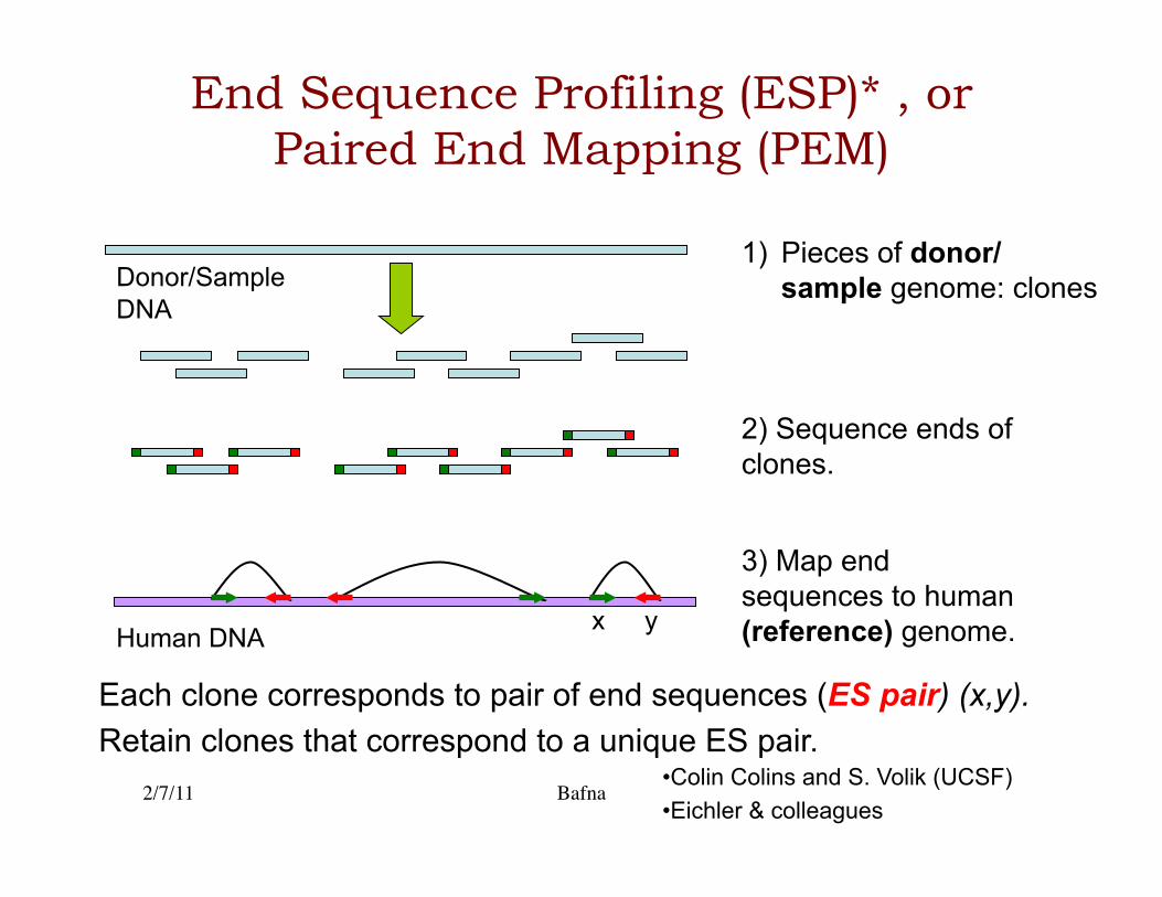
End Sequence Profiling (ESP)* , or Paired End Mapping (PEM)
1) Pieces of donor/sample genome: clones
Human DNA
2) Sequence ends of clones.
3) Map end sequences to human (reference) genome.
Donor/Sample DNA
Each clone corresponds to pair of end sequences (ES pair) (x,y). Retain clones that correspond to a unique ES pair.
y x
• Colin Colins and S. Volik (UCSF) • Eichler & colleagues

PES signatures of structural variation
2/7/11 Bafna
19 OCTOBER 2007 VOL 318 SCIENCE
PEM data
• The paired-ends of a clone help identify deformities/ structural variation in the donor genome.�
• Some SVs are copy neutral (inversions), while others are copy number variant (deletions/duplications).�
• Besides raw detection, there a re a number of problems that we might want to solve computationally.�
2/7/11 Bafna
Fine-mapping breakpoints of structural variations
2/7/11 Bafna
2/7/11 Bafna
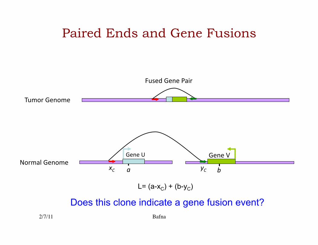
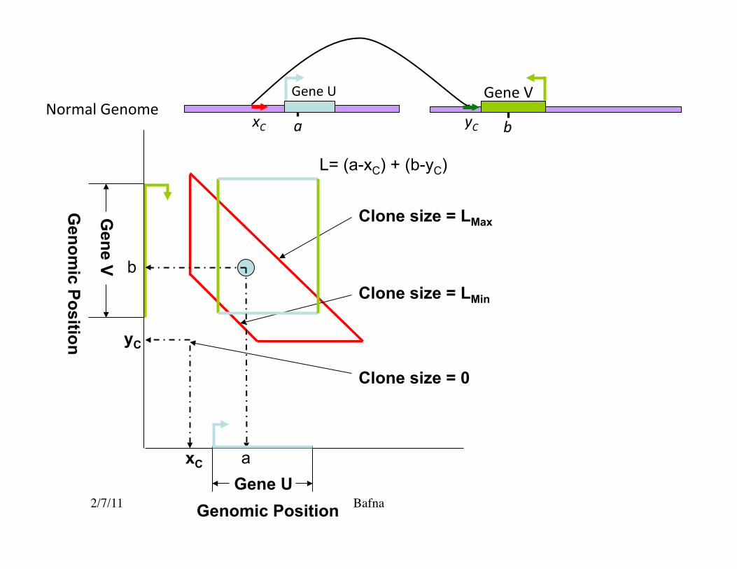
Paired Ends and Gene Fusions
Tumor Genome
L= (a-xC) + (b-yC)
yC a b xC
Gene V Gene U Normal Genome
Fused Gene Pair
Does this clone indicate a gene fusion event?
2/7/11 Bafna
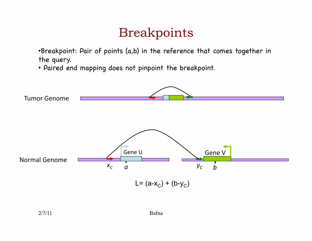
Breakpoints
Tumor Genome
L= (a-xC) + (b-yC)
yC a b xC
Gene V Gene U Normal Genome
• Breakpoint: Pair of points (a,b) in the reference that comes together in the query.�• Paired end mapping does not pinpoint the breakpoint.�
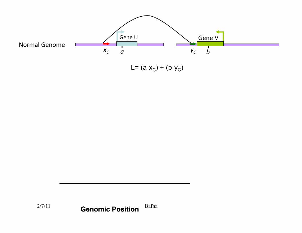
2/7/11 Bafna Genomic Position Genomic Position
L= (a-xC) + (b-yC)
yC a b xC
Gene V Gene U Normal Genome
2/7/11 Bafna Genomic Position
Genom
ic Position
Clone size = 0
Clone size = LMin
Clone size = LMax
xC
yC
a
b
Gene V
Gene U
L= (a-xC) + (b-yC)
yC a b xC
Gene V Gene U Normal Genome
2/7/11 Bafna Genomic Position
Genom
ic Position
Clone size = 0
Clone size = LMin
Clone size = LMax
xC
yC
a
b
Gene V
Gene U
L= (a-xC) + (b-yC)
yC a b xC
Gene V Gene U Normal Genome
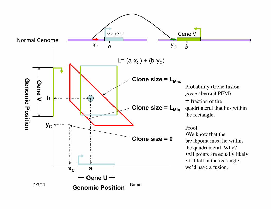
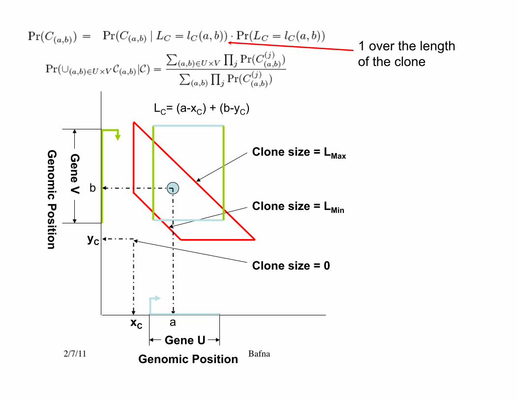
Probability (Gene fusion given aberrant PEM) = fraction of the quadrilateral that lies within the rectangle.
Proof: • We know that the breakpoint must lie within the quadrilateral. Why? • All points are equally likely. • If it fell in the rectangle, we’d have a fusion.
2/7/11 Bafna
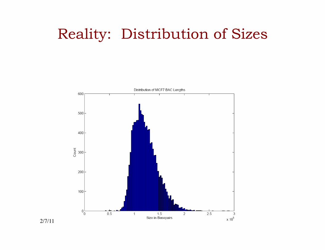
Reality: Distribution of Sizes
2/7/11 Bafna
€
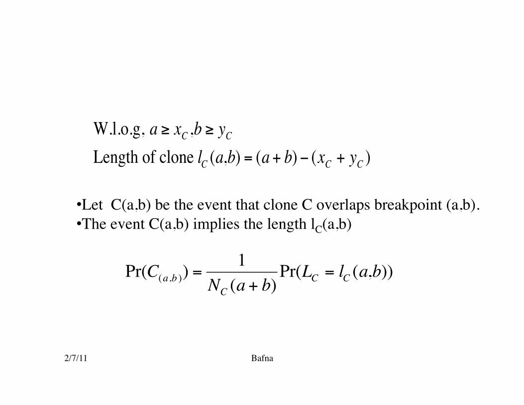
W.l.o.g, a ≥ xC ,b ≥ yCLength of clone lC (a,b) = (a + b) − (xC + yC )
• Let C(a,b) be the event that clone C overlaps breakpoint (a,b). • The event C(a,b) implies the length lC(a,b)
€
Pr(C(a,b )) =1
NC (a + b)Pr(LC = lC (a,b))
2/7/11 Bafna Genomic Position
Genom
ic Position
Clone size = 0
Clone size = LMin
Clone size = LMax
xC
yC
a
b
Gene V
Gene U
LC= (a-xC) + (b-yC)
1 over the length of the clone
2/7/11 Bafna
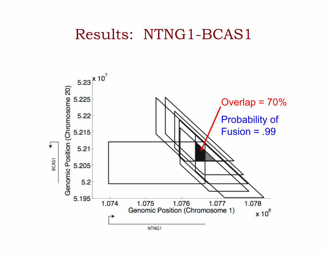
Results: NTNG1-BCAS1
Overlap = 70%
Probability of Fusion = .99
2/7/11 Bafna
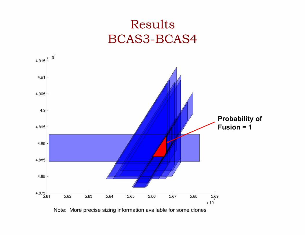
Results BCAS3-BCAS4
Probability of Fusion = 1
Note: More precise sizing information available for some clones
2/7/11 Bafna
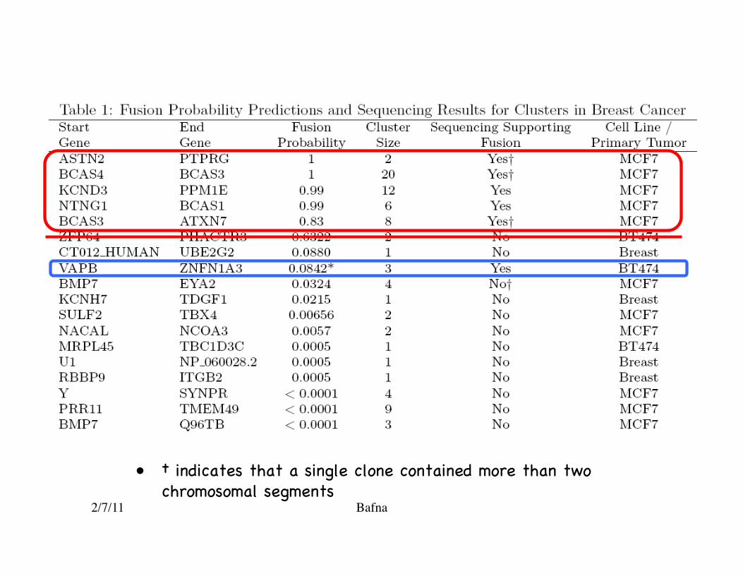
• † indicates that a single clone contained more than two chromosomal segments�
Getting CNVs out of sequence data
2/7/11 Bafna
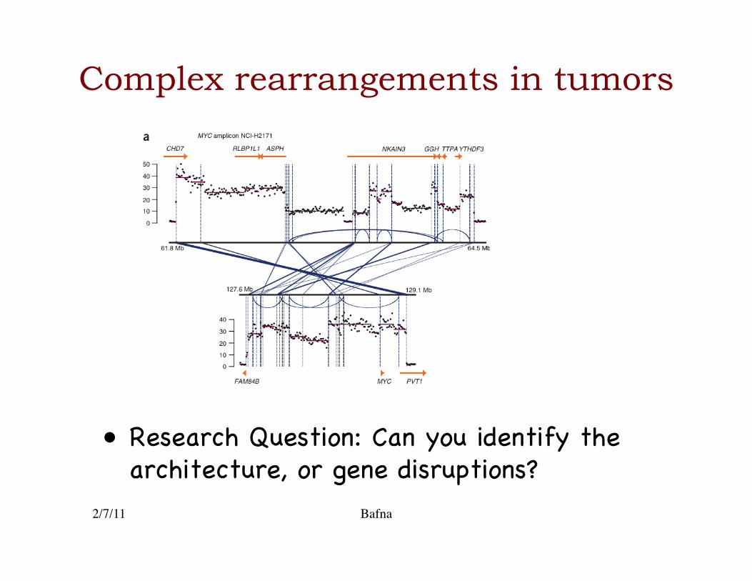
Complex rearrangements in tumors
• Research Question: Can you identify the architecture, or gene disruptions?�
2/7/11 Bafna
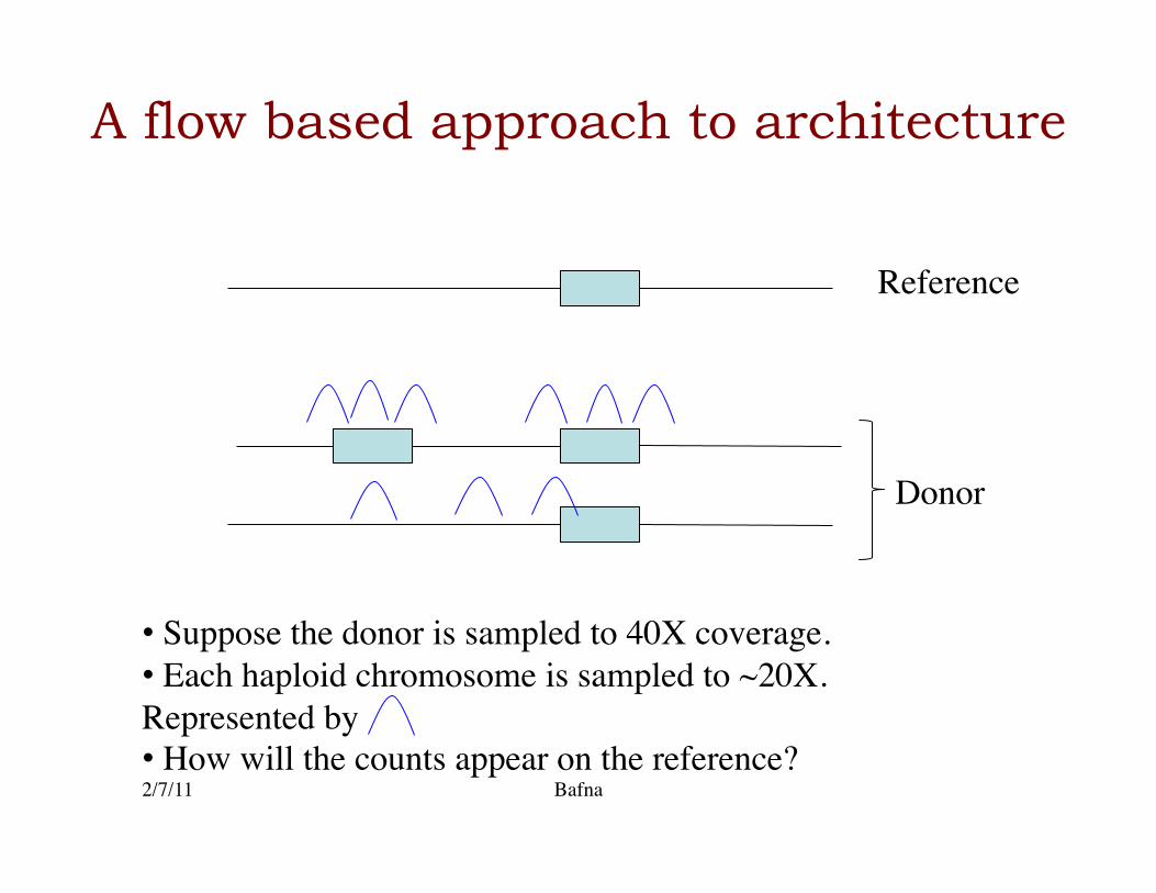
A flow based approach to architecture
2/7/11 Bafna
Donor
Reference
• Suppose the donor is sampled to 40X coverage. • Each haploid chromosome is sampled to ~20X. Represented by • How will the counts appear on the reference?
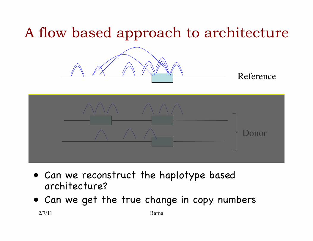
A flow based approach to architecture
• Can we reconstruct the haplotype based architecture?�
• Can we get the true change in copy numbers�2/7/11 Bafna
Donor
Reference
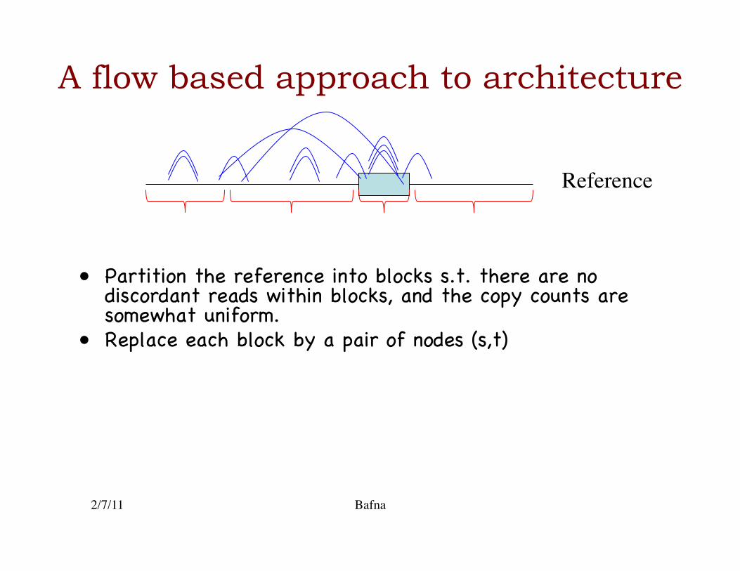
A flow based approach to architecture
• Partition the reference into blocks s.t. there are no discordant reads within blocks, and the copy counts are somewhat uniform.�
• Replace each block by a pair of nodes (s,t)�
2/7/11 Bafna
Reference
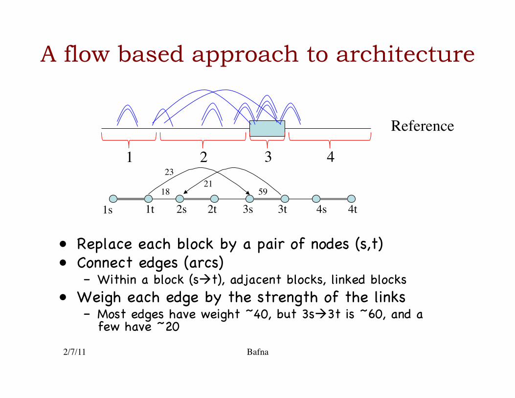
A flow based approach to architecture
• Replace each block by a pair of nodes (s,t)�• Connect edges (arcs)�
– Within a block (st), adjacent blocks, linked blocks�• Weigh each edge by the strength of the links�
– Most edges have weight ~40, but 3s3t is ~60, and a few have ~20 �
2/7/11 Bafna
Reference
1 2 3 4
1s 1t 2t 2s 3s 3t 4t 4s 18
23 21
59
A flow based approach to architecture
2/7/11 Bafna
Reference
1 2 3 4
1s 1t 2t 2s 3s 3t 4t 4s 18
23 21
59
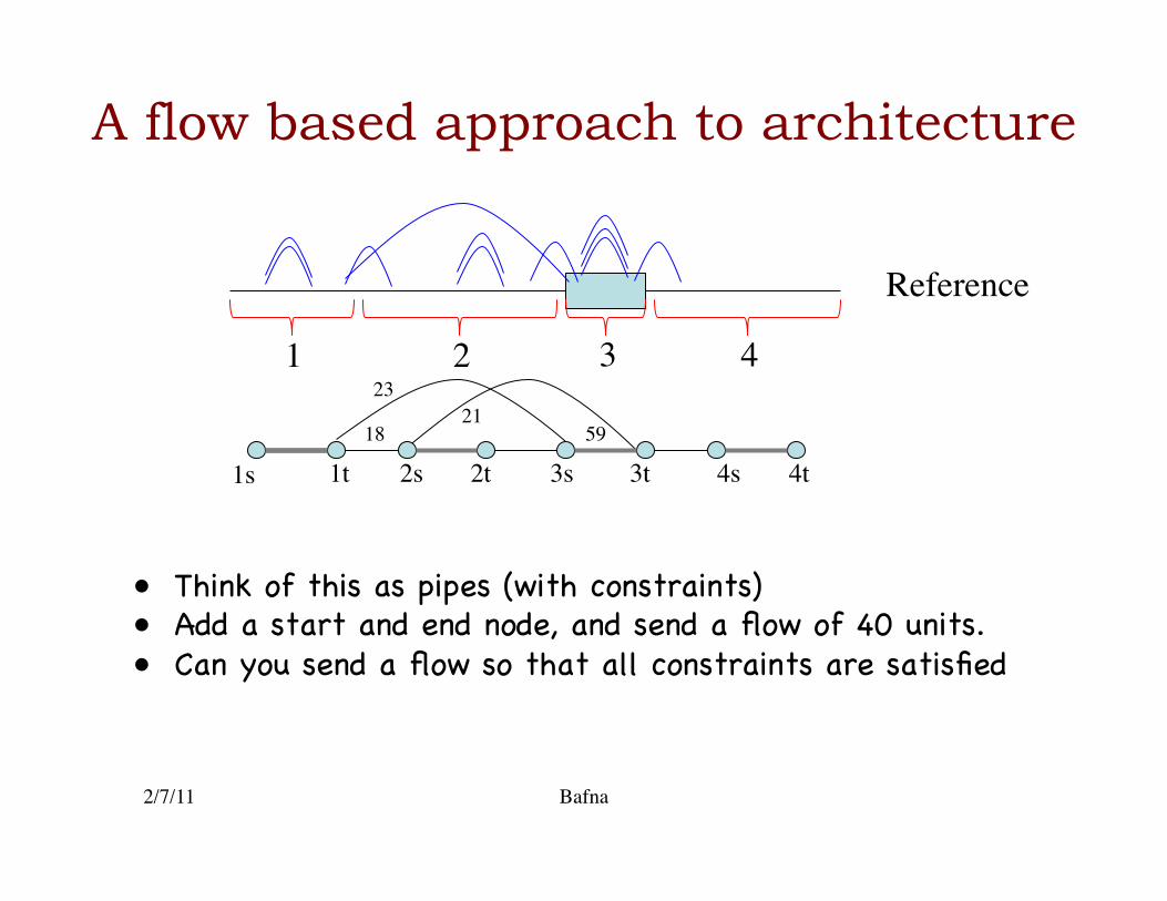
• Think of this as pipes (with constraints) �• Add a start and end node, and send a flow of 40 units.�• Can you send a flow so that all constraints are satisfied�
A flow based approach to architecture
2/7/11 Bafna
1s 1t 2t 2s 3s 3t 4t 4s 18
23 21
59
1s 1t 2t 2s 3s 3t 4t 4s
1s 1t 2t 2s 3s 3t 4t 4s 18
23 21
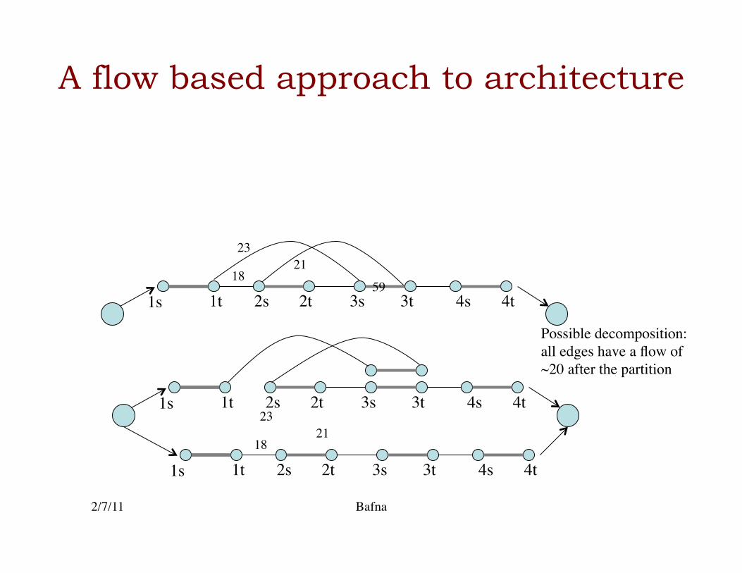
Possible decomposition: all edges have a flow of ~20 after the partition
Computing such flows is a standard problem in CS
• In this case, the flows help in correcting the CNV counts, and getting rid of noisy edges�
• They do not unambiguously reconstruct the haplotypes themselves.�
2/7/11 Bafna
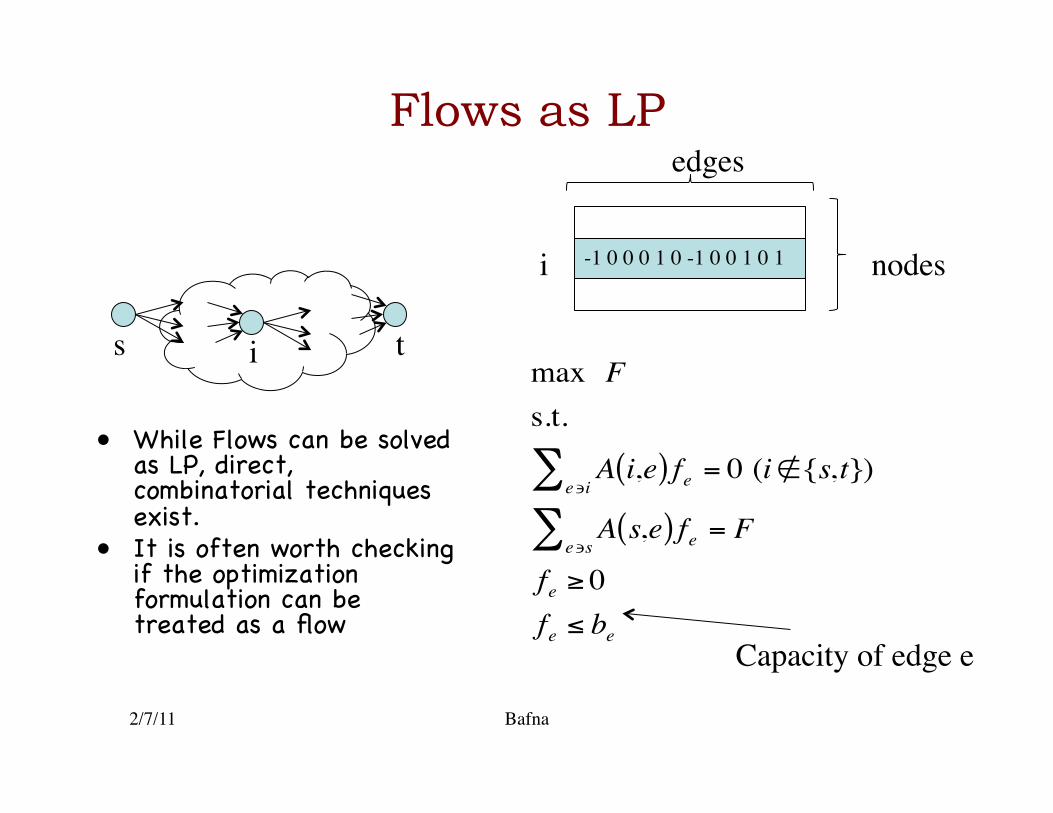
Flows as LP
• While Flows can be solved as LP, direct, combinatorial techniques exist.�
• It is often worth checking if the optimization formulation can be treated as a flow �
2/7/11 Bafna
€
max Fs.t.
A i,e( )e∍i
∑ fe = 0 (i∉{s,t})
A s,e( )e∍s
∑ fe = F
fe ≥ 0fe ≤ be
s t i
Capacity of edge e
-1 0 0 0 1 0 -1 0 0 1 0 1 i nodes
edges

A flow based approach to architecture
2/7/11 Bafna
1s 1t 2t 2s 3s 3t 4t 4s 18
23 21
59
1s 1t 2t 2s 3s 3t 4t 4s
1s 1t 2t 2s 3s 3t 4t 4s 18
23 21
Possible decomposition: all edges have a flow of ~20 after the partition
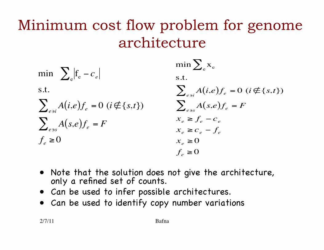
Minimum cost flow problem for genome architecture
• Note that the solution does not give the architecture, only a refined set of counts.�
• Can be used to infer possible architectures.�• Can be used to identify copy number variations�
2/7/11 Bafna
€
min fe − cee∑
s.t.
A i,e( )e∍i
∑ fe = 0 (i∉{s,t})
A s,e( )e∍s
∑ fe = F
fe ≥ 0
€
min xee∑
s.t.
A i,e( )e∍i
∑ fe = 0 (i∉{s,t})
A s,e( )e∍s
∑ fe = F
xe ≥ fe − cexe ≥ ce − fexe ≥ 0fe ≥ 0

Design issues for s.v. detection
• In the early days of sequencing, Lander and waterman came up with clean solutions to common sequencing problems�
• In spite of the idealization, their models were widely used in practice. �
• If you wanted to detect SVs, how much sequencing should you do?�
2/7/11 Bafna
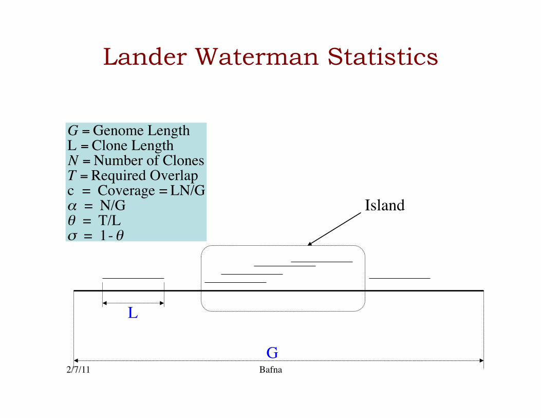
Lander Waterman Statistics
G
L €
G = Genome LengthL = Clone LengthN = Number of ClonesT = Required Overlapc = Coverage = LN/Gα = N/Gθ = T/Lσ = 1-θ
Island
2/7/11 Bafna
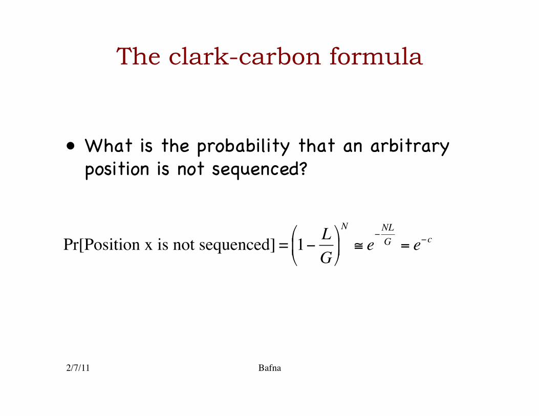
The clark-carbon formula
• What is the probability that an arbitrary position is not sequenced?�
2/7/11 Bafna
€
Pr[Position x is not sequenced] = 1− LG
⎛
⎝ ⎜
⎞
⎠ ⎟ N
≅ e−NLG = e−c
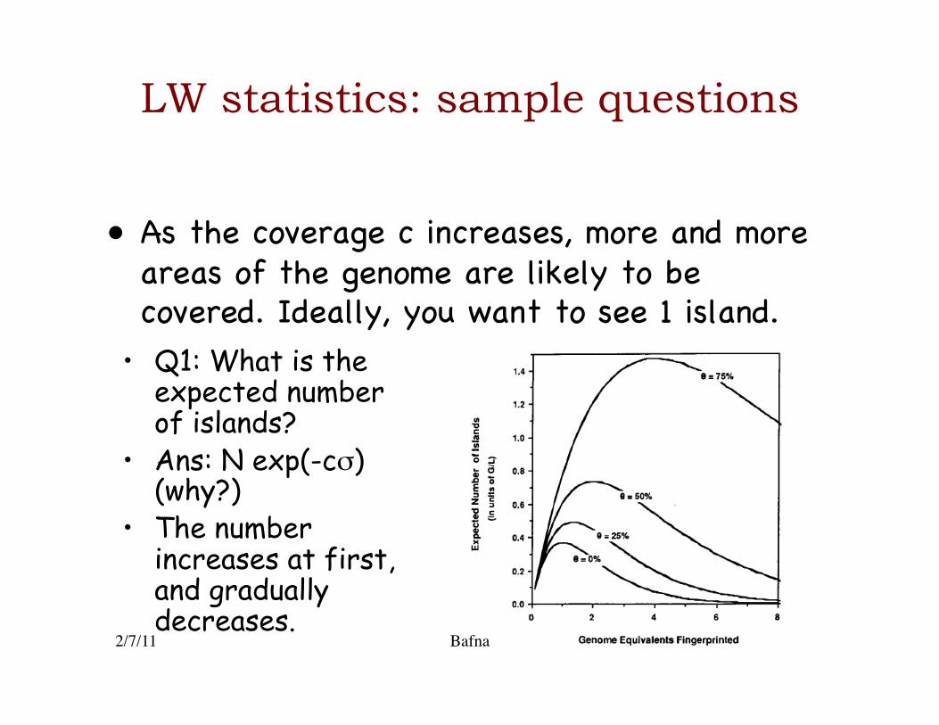
LW statistics: sample questions
• As the coverage c increases, more and more areas of the genome are likely to be covered. Ideally, you want to see 1 island.�
• Q1: What is the expected number of islands?
• Ans: N exp(-cσ) (why?)
• The number increases at first, and gradually decreases.
2/7/11 Bafna
2/7/11 Bafna
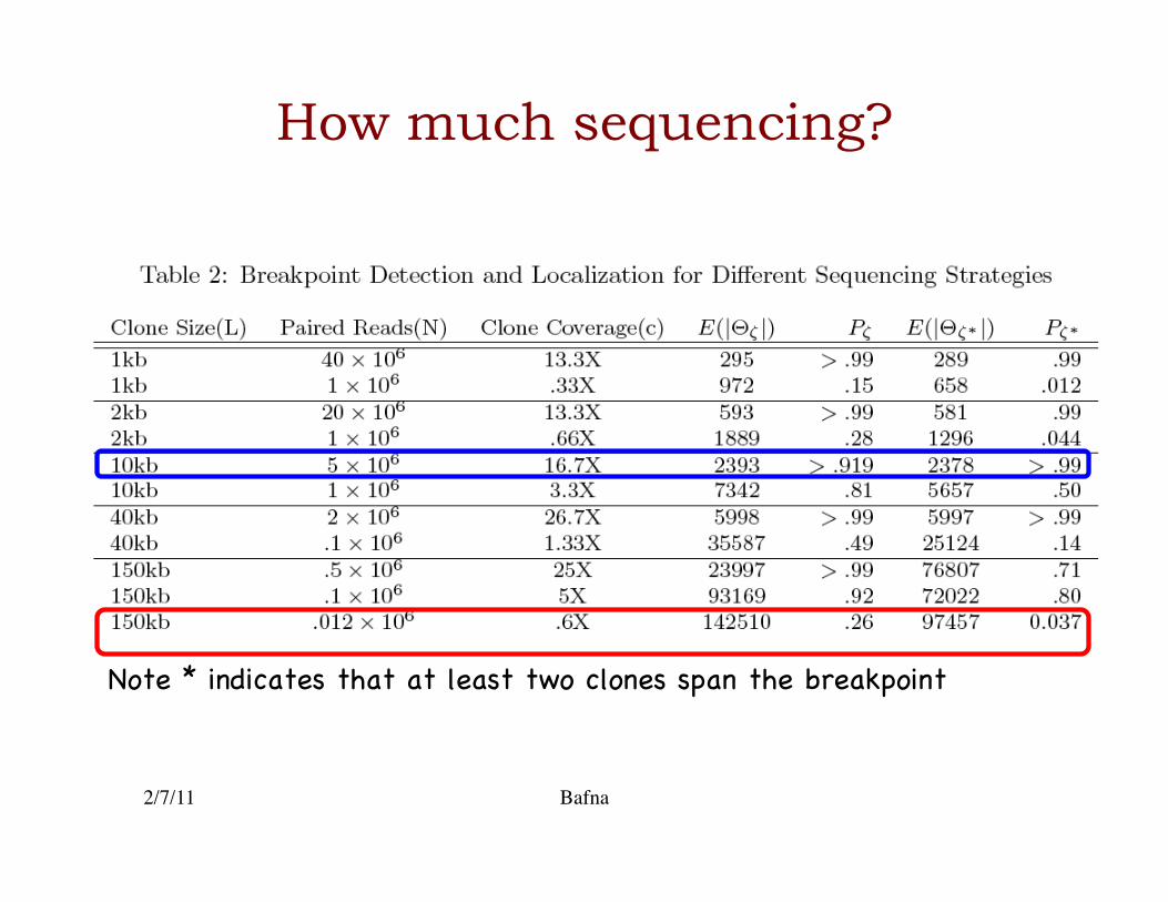
Design related questions for s.v.
• Q: How much sequencing would one need to do in order to uncover most genomic SV events?�
• If you can choose clone lengths�– What is the optimal mix of clone lengths for
detecting and resolving s.v.?�
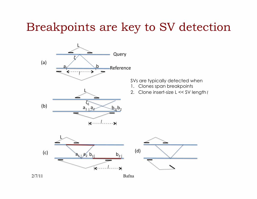
Breakpoints are key to SV detection
!"#$
%&$%'$"&$$$"'$
(&$!%#$
($
"$ %$
!)#$
*+,-.$
/,0,-,1),$$
!2#$
3$
l!
SVs are typically detected when 1.! Clones span breakpoints
2.! Clone insert-size L << SV length l!
"&$$$"'$ %&$$$$$$$$$$$$$$$$$$$%'$
l!
l!
3$
3$
2/7/11 Bafna
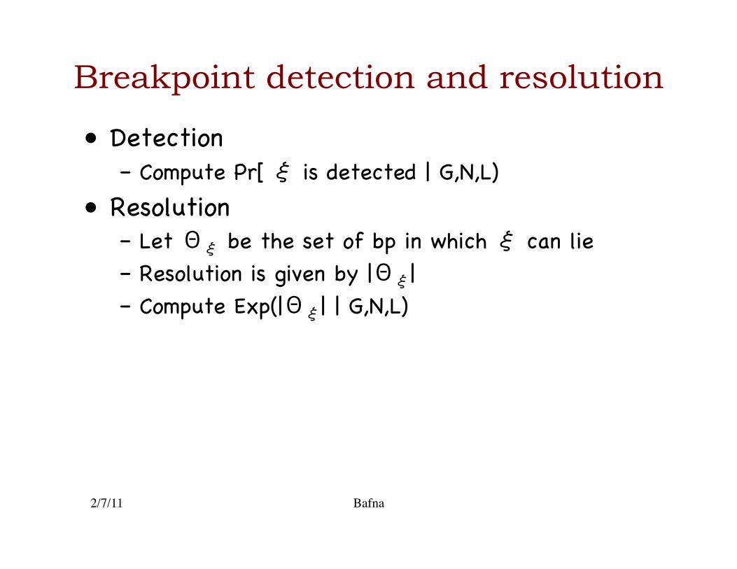
Breakpoint detection and resolution
• Detection �– Compute Pr[ ξ is detected | G,N,L)�
• Resolution �– Let Θξ be the set of bp in which ξ can lie�– Resolution is given by |Θξ|�– Compute Exp(|Θξ| | G,N,L)�
2/7/11 Bafna
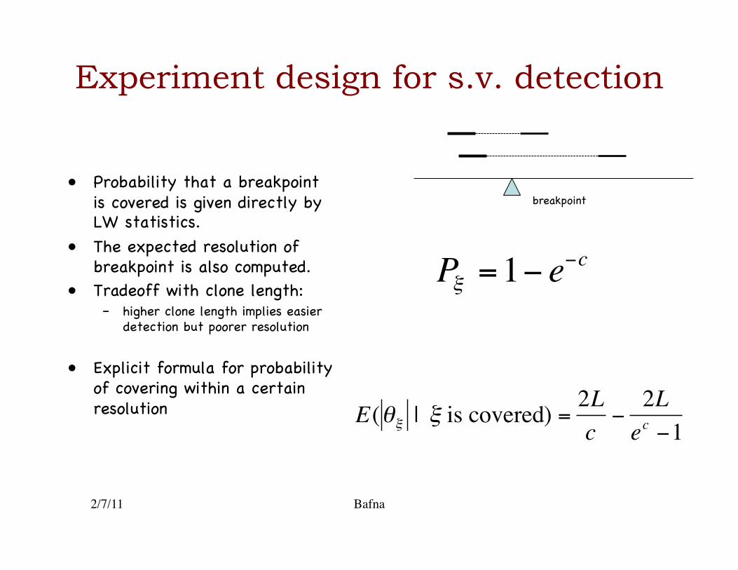
Experiment design for s.v. detection
€
Pξ =1− e−c
• Probability that a breakpoint is covered is given directly by LW statistics.�
• The expected resolution of breakpoint is also computed.�
• Tradeoff with clone length: �– higher clone length implies easier
detection but poorer resolution �
• Explicit formula for probability of covering within a certain resolution �
2/7/11 Bafna
€
E(θξ | ξ is covered) =2Lc−
2Lec −1
breakpoint �
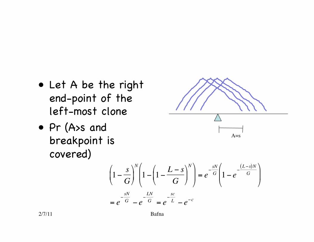
• Let A be the right end-point of the left-most clone�
• Pr (A>s and breakpoint is covered)�
2/7/11 Bafna
A=s
€
1− sG
⎛
⎝ ⎜
⎞
⎠ ⎟ N
1− 1− L − sG
⎛
⎝ ⎜
⎞
⎠ ⎟ N⎛
⎝ ⎜
⎞
⎠ ⎟ = e
−sNG 1− e
−L−s( )NG
⎛
⎝ ⎜
⎞
⎠ ⎟
= e−sNG − e
−LNG = e
−scL − e−c
2/7/11 Bafna
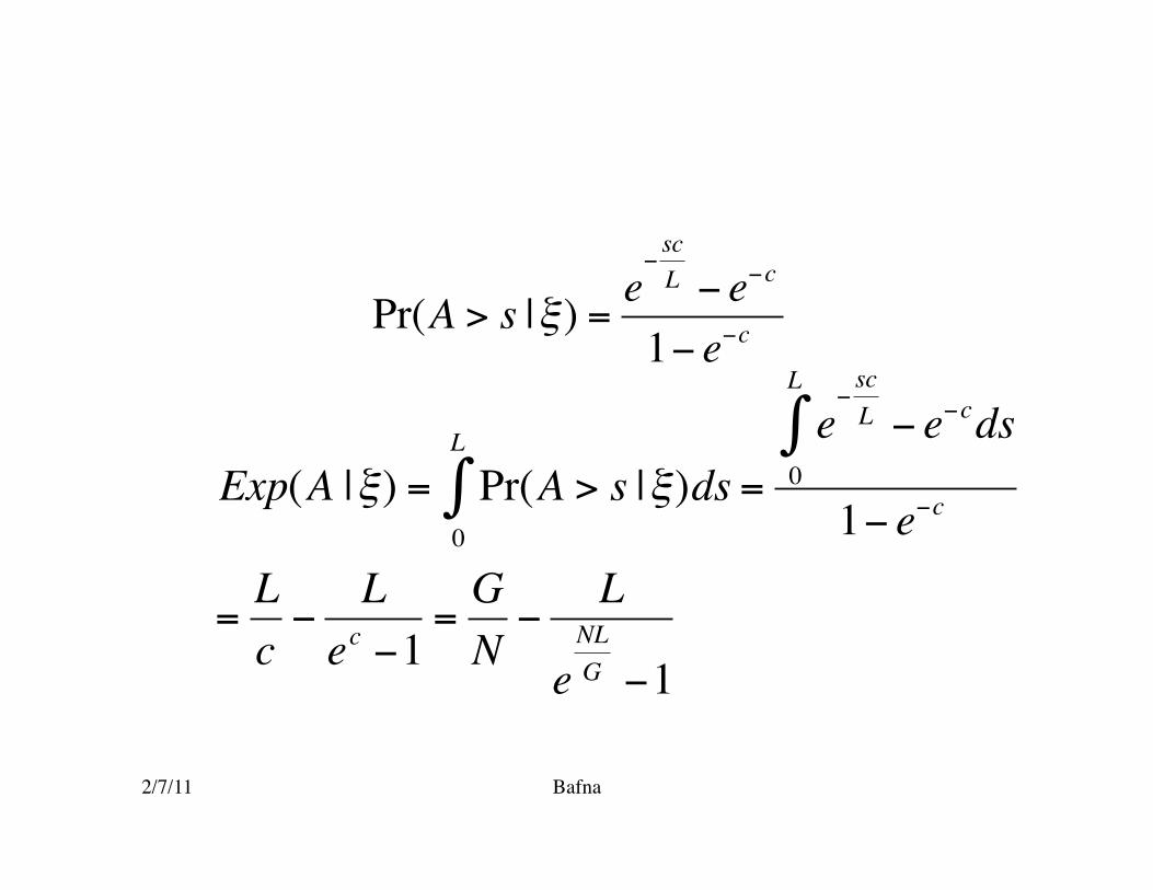
€
Pr(A > s |ξ) =e−scL − e−c
1− e−c
€
Exp(A |ξ) = Pr(A > s |ξ)ds0
L
∫ =e−scL − e−cds
0
L
∫1− e−c
=Lc−
Lec −1
=GN−
L
eNLG −1
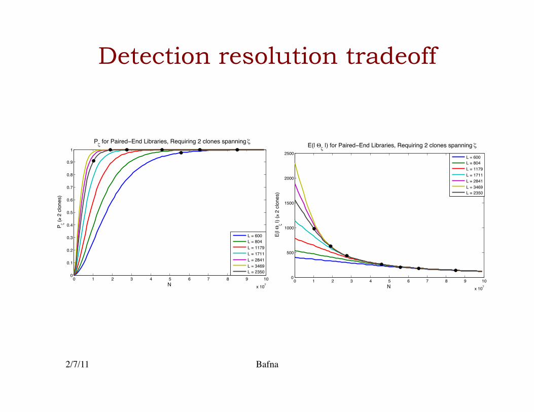
Detection resolution tradeoff
0 1 2 3 4 5 6 7 8 9 10
x 107
0
0.1
0.2
0.3
0.4
0.5
0.6
0.7
0.8
0.9
1
N
P! (" 2
clo
nes)
P! for Paired!End Libraries, Requiring 2 clones spanning !
L = 600
L = 804
L = 1179
L = 1711
L = 2841
L = 3469
L = 2350
0 1 2 3 4 5 6 7 8 9 10
x 107
0
500
1000
1500
2000
2500
N
E(|
!" |
) (#
2 c
lon
es)
E(| !" |) for Paired!End Libraries, Requiring 2 clones spanning "
L = 600
L = 804
L = 1179
L = 1711
L = 2841
L = 3469
L = 2350
2/7/11 Bafna
2/7/11 Bafna
How much sequencing?
Note * indicates that at least two clones span the breakpoint �

DETECTION OF SV UNDER
HETEROGENEITY
2/7/11 Bafna
2/7/11 Bafna
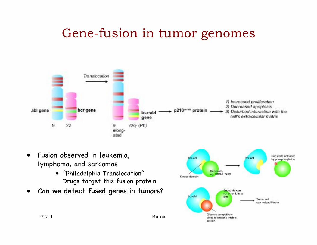
Gene-fusion in tumor genomes
• Fusion observed in leukemia, lymphoma, and sarcomas�
• “Philadelphia Translocation” Drugs target this fusion protein �
• Can we detect fused genes in tumors?�
2/7/11 Bafna
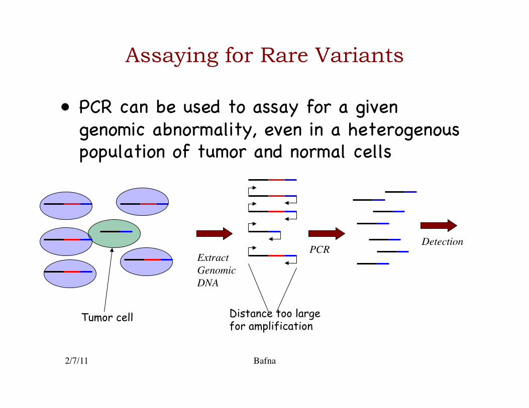
Assaying for Rare Variants
• PCR can be used to assay for a given genomic abnormality, even in a heterogenous population of tumor and normal cells�
Extract Genomic DNA
PCR
Distance too large for amplification Tumor cell
Detection
2/7/11 Bafna
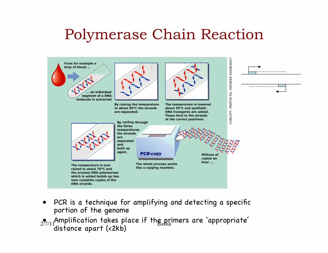
Polymerase Chain Reaction
• PCR is a technique for amplifying and detecting a specific portion of the genome�
• Amplification takes place if the primers are ‘appropriate’ distance apart (<2kb)�
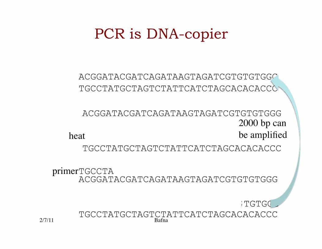
PCR is DNA-copier
2/7/11 Bafna
ACGGATACGATCAGATAAGTAGATCGTGTGTGGG TGCCTATGCTAGTCTATTCATCTAGCACACACCC
ACGGATACGATCAGATAAGTAGATCGTGTGTGGG
TGCCTATGCTAGTCTATTCATCTAGCACACACCC TGTGGG ACGGATACGATCAGATAAGTAGATCGTG
TGCTAGTCTATTCATCTAGCACACACCC
ACGGATACGATCAGATAAGTAGATCGTGTGTGGG
TGCCTATGCTAGTCTATTCATCTAGCACACACCC heat
TGCCTA primer
2000 bp can be amplified
2/7/11 Bafna
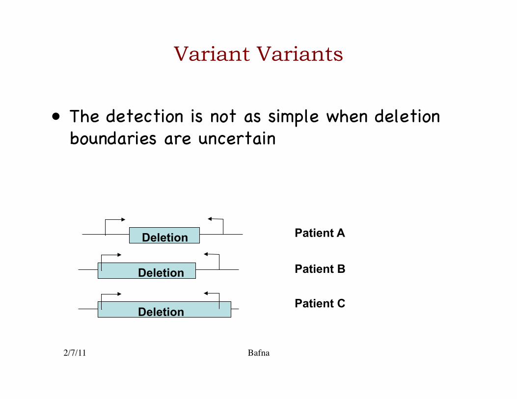
Variant Variants
• The detection is not as simple when deletion boundaries are uncertain �
Deletion
Deletion
Deletion
Patient A
Patient B
Patient C
2/7/11 Bafna
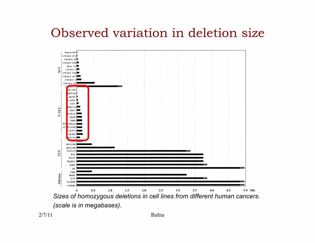
Observed variation in deletion size
Sizes of homozygous deletions in cell lines from different human cancers. (scale is in megabases).
2/7/11 Bafna
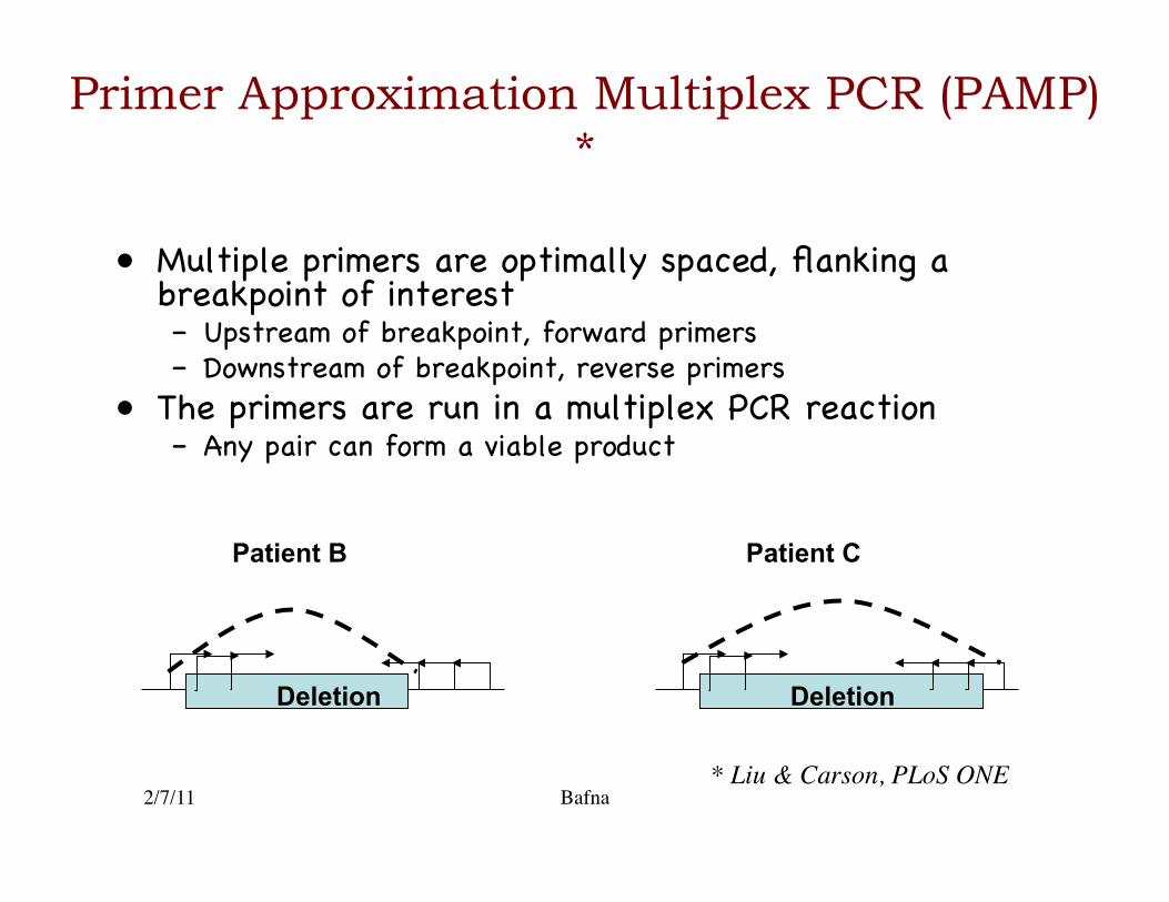
Primer Approximation Multiplex PCR (PAMP)*
• Multiple primers are optimally spaced, flanking a breakpoint of interest �– Upstream of breakpoint, forward primers�– Downstream of breakpoint, reverse primers�
• The primers are run in a multiplex PCR reaction �– Any pair can form a viable product �
Deletion Deletion
Patient B Patient C
* Liu & Carson, PLoS ONE
2/7/11 Bafna
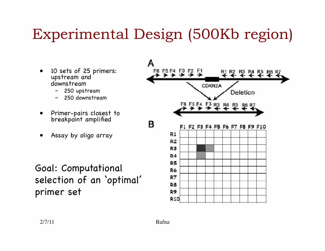
Experimental Design (500Kb region)
• 10 sets of 25 primers: upstream and downstream�– 250 upstream�– 250 downstream�
• Primer-pairs closest to breakpoint amplified�
• Assay by oligo array �
Goal: Computational selection of an ‘optimal’ primer set �
2/7/11 Bafna
The computational problem
• Recall that the primers are substrings of the genome that prime the PC Reaction.�
• A primer design refers to a selection (subset) of substrings�
• Can we design the primers so that the reaction fails in very few patients.�• False negatives are worse than false positives! �
• What are the criteria that primers must satisfy so that PAMP succeeds?�
2/7/11 Bafna
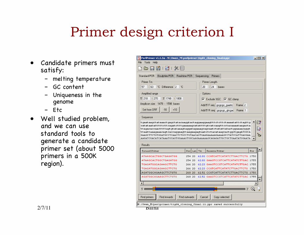
Primer design criterion I
• Candidate primers must satisfy: �– melting temperature�– GC content �– Uniqueness in the
genome�– Etc�
• Well studied problem, and we can use standard tools to generate a candidate primer set (about 5000 primers in a 500K region).�
2/7/11 Bafna
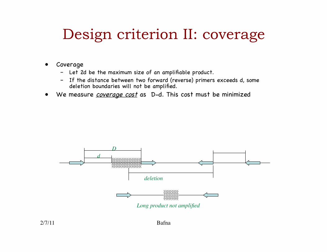
Design criterion II: coverage
• Coverage�– Let 2d be the maximum size of an amplifiable product.�– If the distance between two forward (reverse) primers exceeds d, some
deletion boundaries will not be amplified.�• We measure coverage cost as D-d. This cost must be minimized�
Long product not amplified
deletion
D d
2/7/11 Bafna
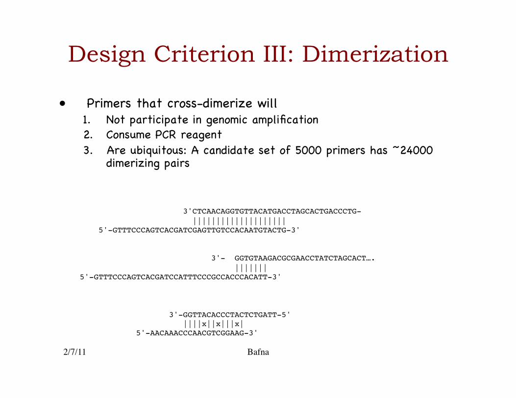
Design Criterion III: Dimerization
• Primers that cross-dimerize will�1. Not participate in genomic amplification �2. Consume PCR reagent �3. Are ubiquitous: A candidate set of 5000 primers has ~24000
dimerizing pairs�
3'CTCAACAGGTGTTACATGACCTAGCACTGACCCTG- ! ||||||||||||||||||||! 5'-GTTTCCCAGTCACGATCGAGTTGTCCACAATGTACTG-3'!
3'- GGTGTAAGACGCGAACCTATCTAGCACT….! |||||||! 5'-GTTTCCCAGTCACGATCCATTTCCCGCCACCCACATT-3'!
3'-GGTTACACCCTACTCTGATT-5'! ||||x||x|||x|! 5'-AACAAACCCAACGTCGGAAG-3'!
2/7/11 Bafna
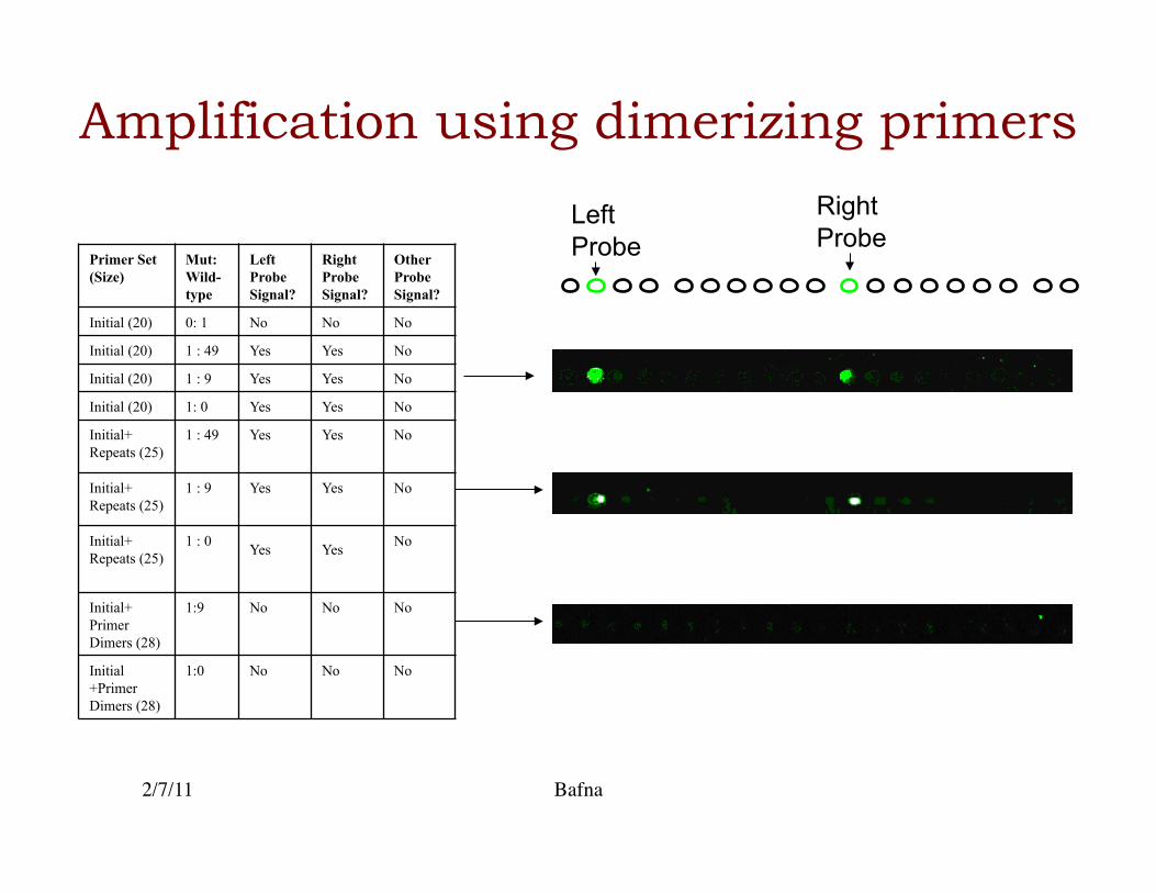
Primer Set (Size)
Mut: Wild-type
Left Probe Signal?
Right Probe Signal?
Other Probe Signal?
Initial (20) 0: 1 No No No Initial (20) 1 : 49 Yes Yes No Initial (20) 1 : 9 Yes Yes No Initial (20) 1: 0 Yes Yes No Initial+ Repeats (25)
1 : 49 Yes Yes No
Initial+ Repeats (25)
1 : 9 Yes Yes No
Initial+ Repeats (25)
1 : 0 Yes Yes No
Initial+ Primer Dimers (28)
1:9 No No No
Initial+Primer Dimers (28)
1:0 No No No
Left Probe
Right Probe
Amplification using dimerizing primers
2/7/11 Bafna
Design Criterion V: cost
• The cost is directly proportional to the number of primers.�
• Define Primer density ρ�– ρ = (# primers)/(length of region in kb)�
• As we need primers to be about 1kb apart, we must choose ρ >=1 �
• Other measures of cost exist, including protocol complexity, and efficiency of reactions. These will be included later.�
2/7/11 Bafna
Computational Goal
• Choose (compute) a low-cost, high-coverage, unique, and non-dimerizing subset from a candidate set of physiochemically appropriate primers �
Note on the problem
• In this case the optimization is very important.�– The optimization seeks to minimize the number of
breakpoints that missed�– Each missed breakpoint represents a tumor that we did
not detect �– False negatives are more important than false positives�
• We use general approaches to solving these problems�• We design algorithms based on simulated annealing (fast
convergence, but nor guaranteed optimality), and Integer Linear Programming (guaranteed optimality, but not running time) �
2/7/11 Bafna
2/7/11 Bafna
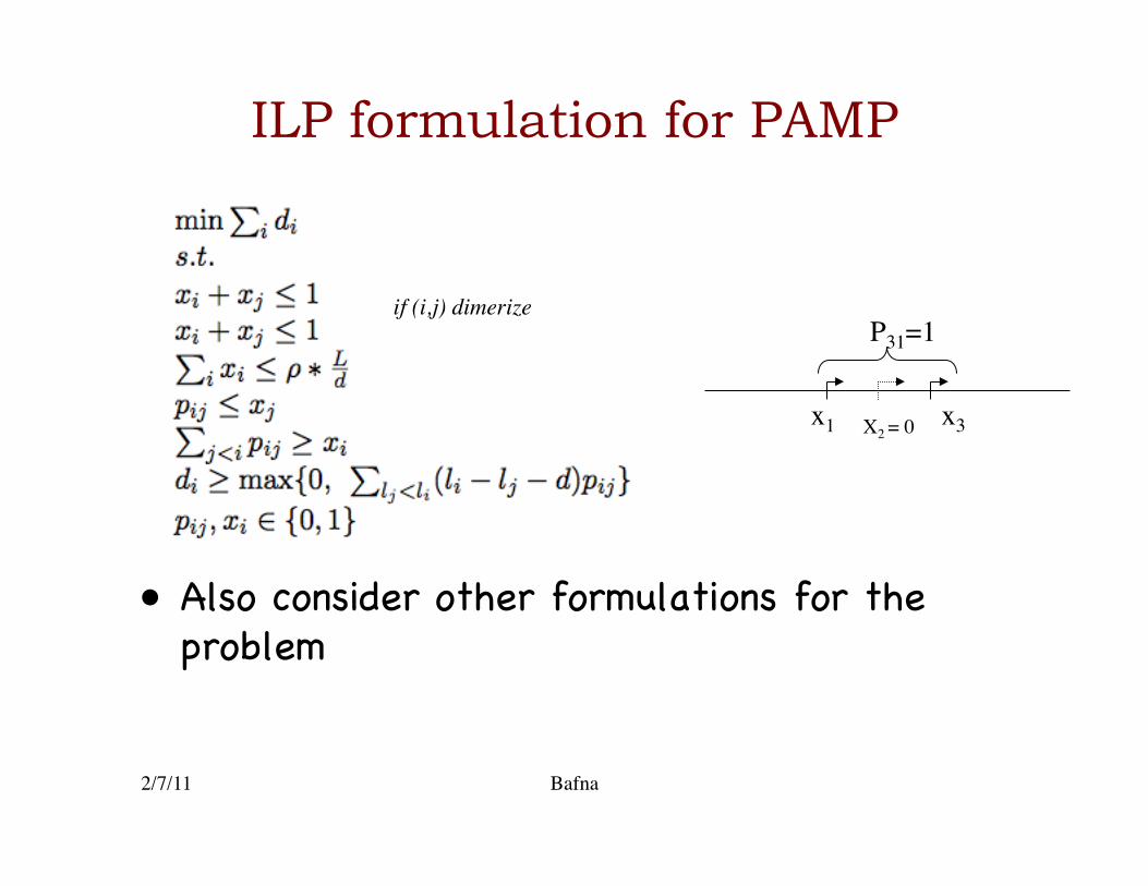
ILP formulation for PAMP
x1 X2 = 0 x3
P31=1 if (i,j) dimerize
• Also consider other formulations for the problem�
2/7/11 Bafna
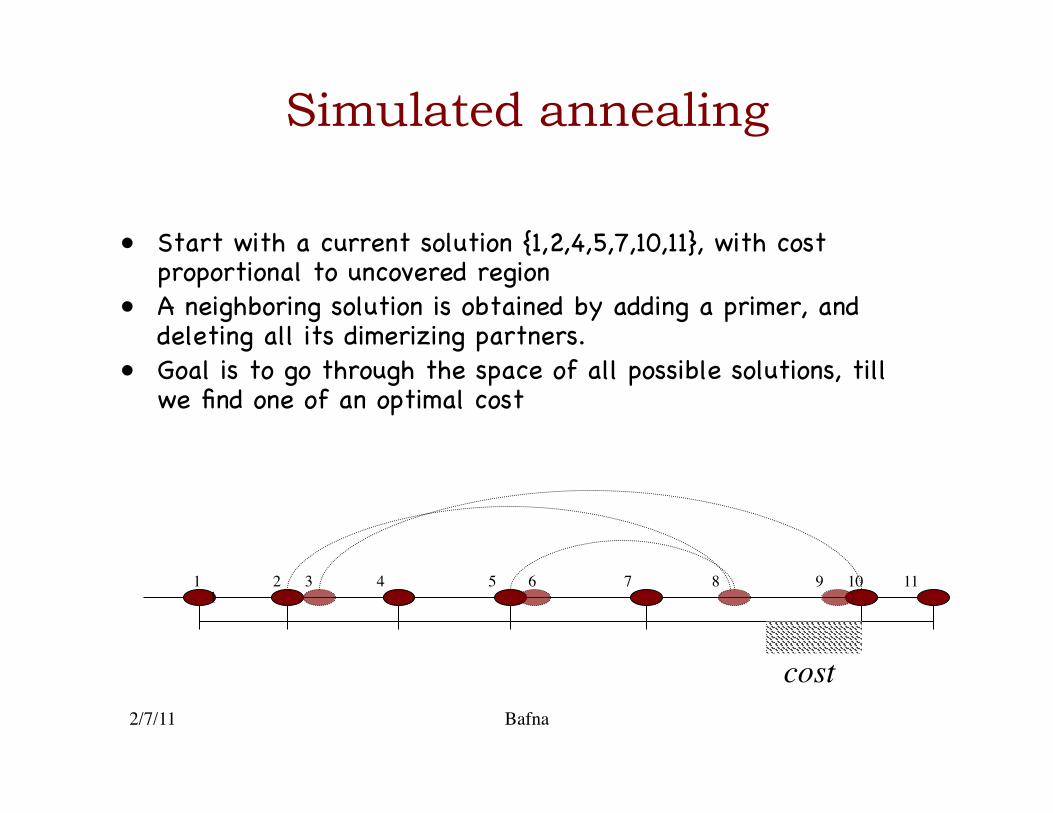
Simulated annealing
• Start with a current solution {1,2,4,5,7,10,11}, with cost proportional to uncovered region �
• A neighboring solution is obtained by adding a primer, and deleting all its dimerizing partners.�
• Goal is to go through the space of all possible solutions, till we find one of an optimal cost �
1
cost
1 2 3 5 4 7 9 8 11 10 6
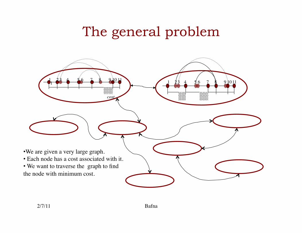
The general problem
2/7/11 Bafna
1
cost
1 2 3 5 4 7 9 8 11 10 6 1 2 3 5 4 7 9 8 11 10 6
• We are given a very large graph. • Each node has a cost associated with it. • We want to traverse the graph to find the node with minimum cost.
2/7/11 Bafna
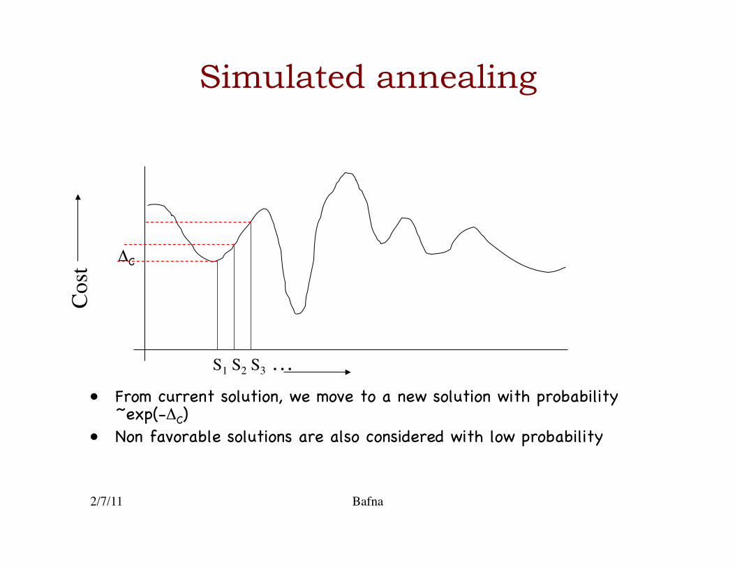
Simulated annealing
• From current solution, we move to a new solution with probability ~exp(-ΔC)�
• Non favorable solutions are also considered with low probability�
S1 S2 S3 …
Cost
ΔC�
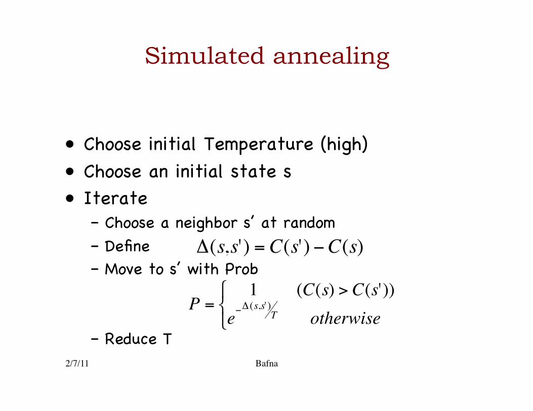
Simulated annealing
• Choose initial Temperature (high)�• Choose an initial state s�• Iterate�
– Choose a neighbor s’ at random�– Define�– Move to s’ with Prob �
– Reduce T �2/7/11 Bafna
€
Δ(s,s') = C(s') −C(s)
€
P =1 (C(s) > C(s'))
e−Δ (s,s' )
T otherwise⎧ ⎨ ⎩
2/7/11 Bafna
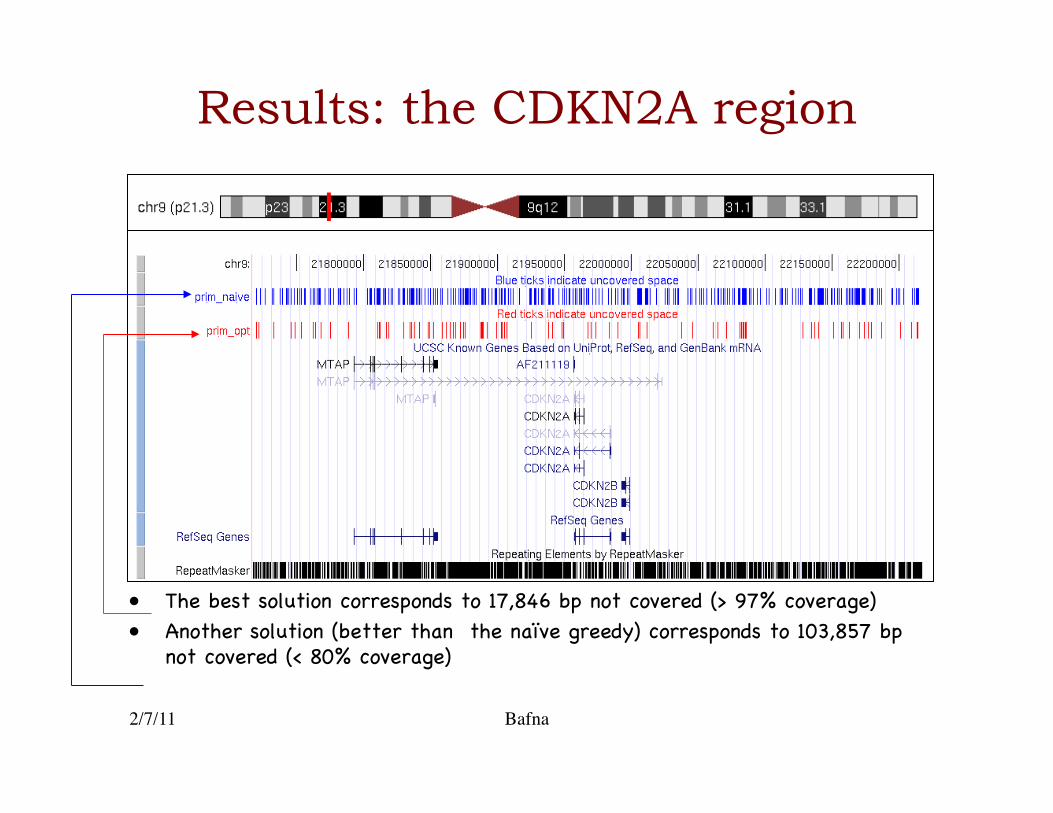
Results: the CDKN2A region
• The best solution corresponds to 17,846 bp not covered (> 97% coverage)�• Another solution (better than the naïve greedy) corresponds to 103,857 bp
not covered (< 80% coverage)�
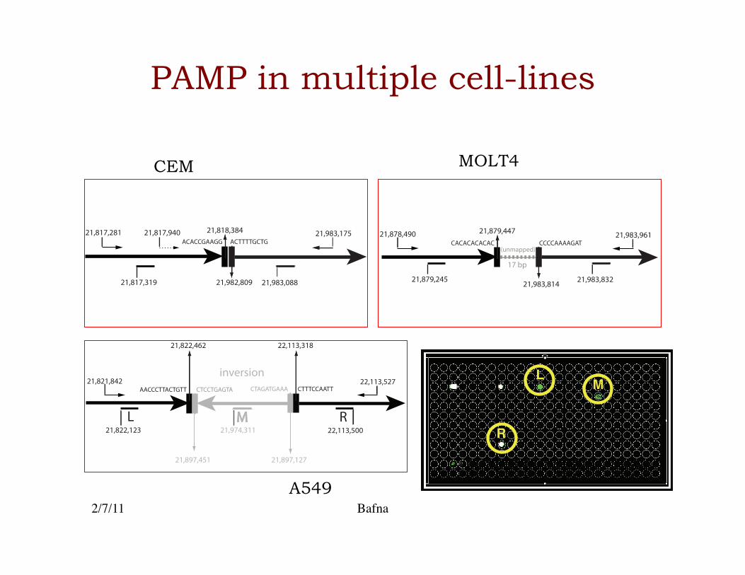
PAMP in multiple cell-lines
2/7/11 Bafna
21,879,447
21,983,814
CACACACACAC CCCCAAAAGAT
17 bp
(unmapped)
21,879,245 21,983,832
21,878,490 21,983,96121,818,384
21,982,809
ACACCGAAGG ACTTTTGCTG
21,817,319 21,983,088
21,817,281 21,983,17521,817,940
L M R
inversion
21,897,451 21,897,127
21,822,462 22,113,318
CTAGATGAAA CTTTCCAATTAACCCTTACTGTT CTCCTGAGTA21,821,842
22,113,50021,822,123 21,974,311
22,113,527 LM
R
CEM
A549
MOLT4

2/7/11 Bafna
Preliminary conclusions
• Prelim. results are very encouraging for small regions (< 1Mb). Many improvements are possible.�
• Clearly, coverage and cost are the two most important criteria.�– Higher coverage implies more patients can be sampled.�
• Cost depends upon the number of primers, protocol complexity, and miniaturization. The final design must optimize cost and protocol complexity as well.�

2/7/11 Bafna
Detecting SVs using genotypes
2/7/11 Bafna
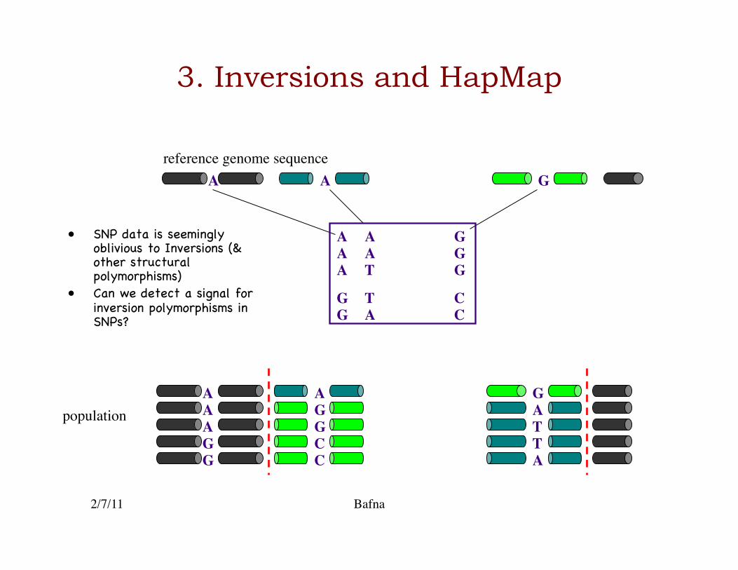
3. Inversions and HapMap
A A A
A
A
A C C
G G
G
G
T
T T
G
G G A G
A
A A
G A
A G G A
C T C A
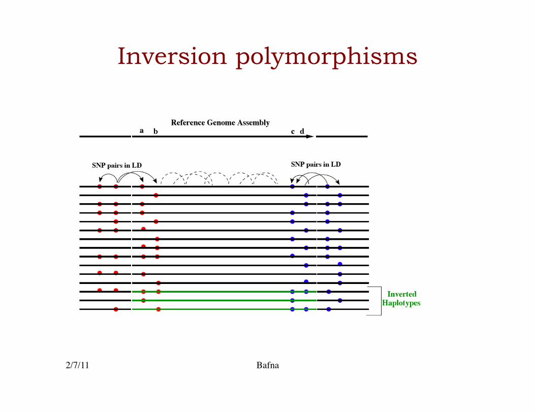
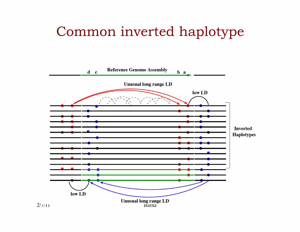
• SNP data is seemingly oblivious to Inversions (& other structural polymorphisms)�
• Can we detect a signal for inversion polymorphisms in SNPs?�
reference genome sequence
population
2/7/11 Bafna
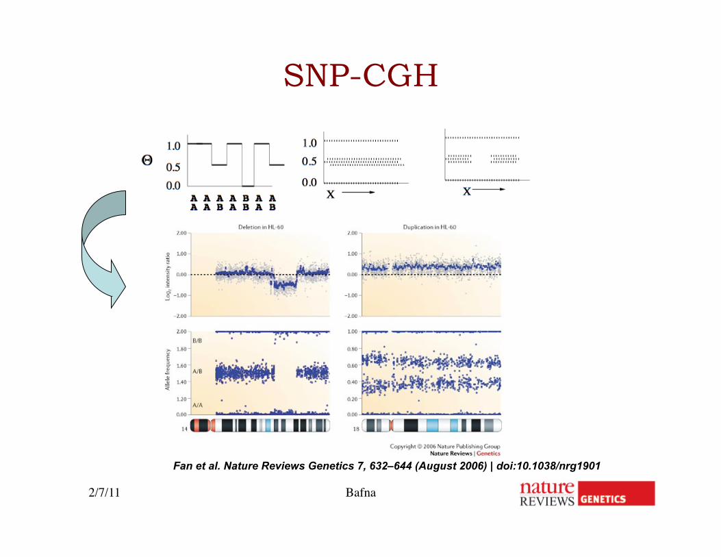
Fan et al. Nature Reviews Genetics 7, 632–644 (August 2006) | doi:10.1038/nrg1901
SNP-CGH
2/7/11 Bafna
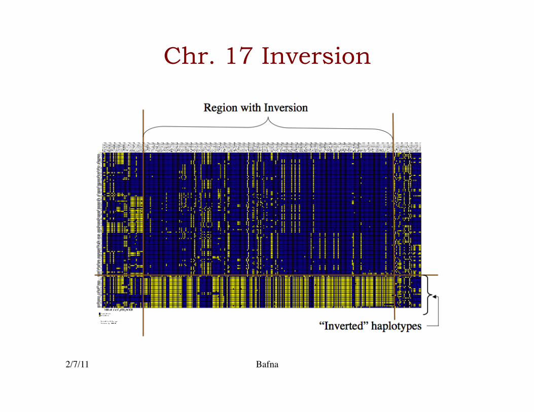
Chr. 17 Inversion
2/7/11 Bafna
Inversion polymorphisms
2/7/11 Bafna
Common inverted haplotype

2/7/11 Bafna
Conclusion
• Structural variations are prevalent in normal and disease genomes�
• A variety of techniques can be used to probe for structural variations, �
• Computation helps increase the power�
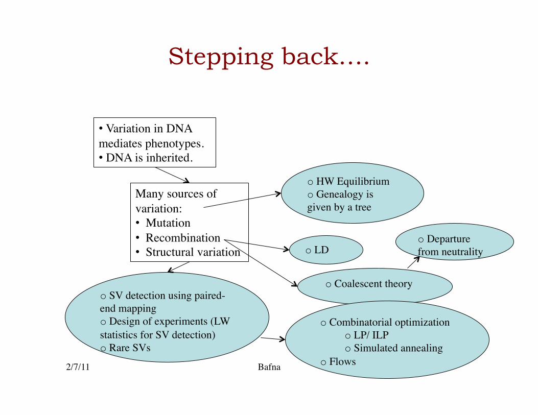
Stepping back….
2/7/11 Bafna
• Variation in DNA mediates phenotypes. • DNA is inherited.
Many sources of variation: • Mutation • Recombination • Structural variation
o HW Equilibrium o Genealogy is given by a tree
o LD
o Coalescent theory o SV detection using paired-end mapping o Design of experiments (LW statistics for SV detection) o Rare SVs
o Combinatorial optimization o LP/ ILP o Simulated annealing
o Flows
o Departure from neutrality