Embed Size (px)
Citation preview
Detection and (Linear) Data Model
Jörn WilmsRemeis-Sternwarte & ECAP
Universität Erlangen-Nürnberg
http://pulsar.sternwarte.uni-erlangen.de/wilms/

Part 1: Why is X-ray and Gamma-Ray AstronomyInteresting?


Part 2: Tools of the Trade: Satellites

Earth’s Atmosphere
CXC
Earth’s atmosphere isopaque for all types of EMradiation except for opti-cal light and radio.
Major contributer at highenergies: photoabsorption(∝ E−3), esp. from Oxygen(edge at ∼500 eV).=⇒ If one wants to look at
the sky in other wave-bands, one has to go tospace!
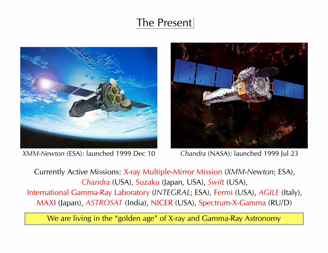
The Present
XMM-Newton (ESA): launched 1999 Dec 10 Chandra (NASA): launched 1999 Jul 23
Currently Active Missions: X-ray Multiple-Mirror Mission (XMM-Newton; ESA),Chandra (USA), Suzaku (Japan, USA), Swift (USA),
International Gamma-Ray Laboratory (INTEGRAL; ESA), Fermi (USA), AGILE (Italy),MAXI (Japan), ASTROSAT (India), NICER (USA), Spectrum-X-Gamma (RU/D)
We are living in the “golden age” of X-ray and Gamma-Ray Astronomy

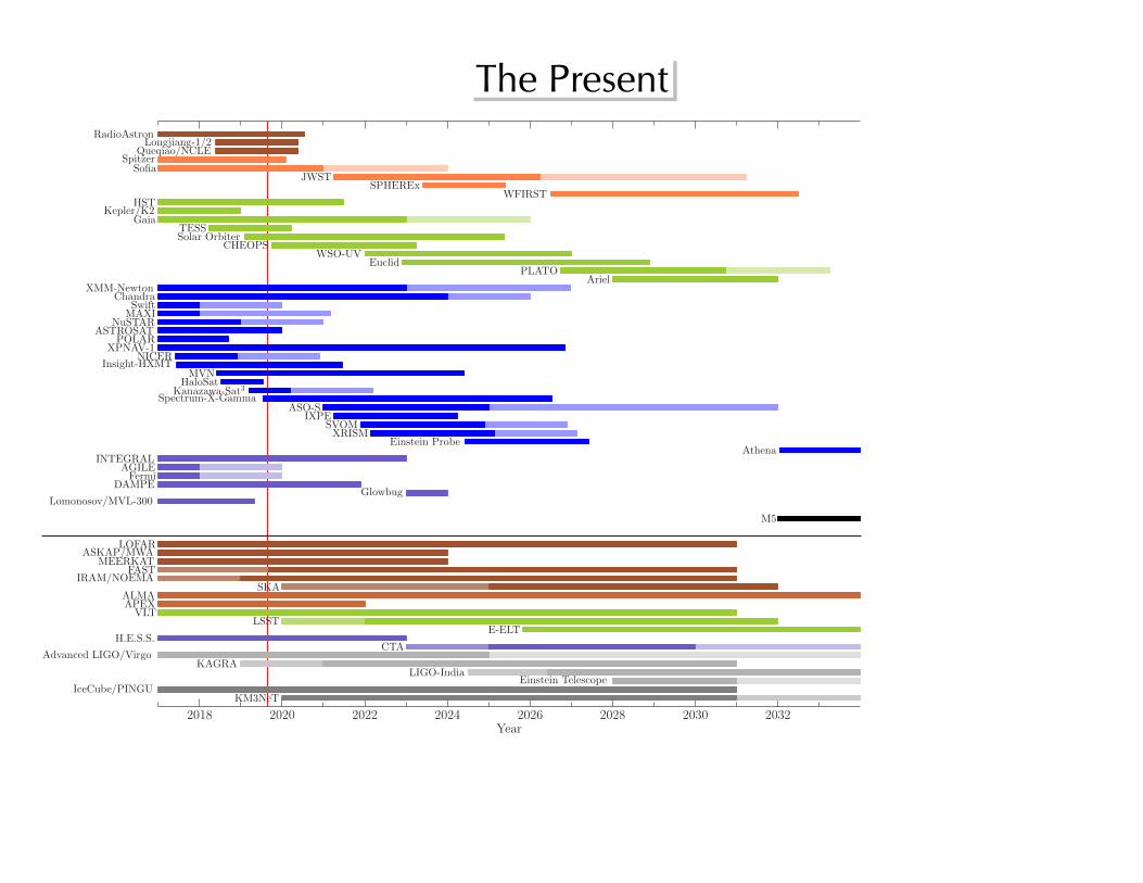
The Present
IceCube/PINGU
KAGRAAdvanced LIGO/Virgo
H.E.S.S.
VLTAPEXALMA
IRAM/NOEMAFAST
MEERKATASKAP/MWA
LOFAR
Lomonosov/MVL-300
DAMPEFermi
AGILEINTEGRAL
Spectrum-X-GammaKanazawa-Sat3HaloSatMVN
Insight-HXMTNICER
XPNAV-1POLAR
ASTROSATNuSTAR
MAXISwift
ChandraXMM-Newton
Solar OrbiterTESS
GaiaKepler/K2
HST
SofiaSpitzer
Queqiao/NCLELongjiang-1/2
RadioAstron
20322030202820262024202220202018Year
The Present
KM3NeTIceCube/PINGU
Einstein TelescopeLIGO-India
KAGRAAdvanced LIGO/Virgo
CTAH.E.S.S.
E-ELTLSST
VLTAPEXALMA
SKAIRAM/NOEMA
FASTMEERKAT
ASKAP/MWALOFAR
M5
Lomonosov/MVL-300Glowbug
DAMPEFermi
AGILEINTEGRAL
AthenaEinstein Probe
XRISMSVOM
IXPEASO-S
Spectrum-X-GammaKanazawa-Sat3HaloSatMVN
Insight-HXMTNICER
XPNAV-1POLAR
ASTROSATNuSTAR
MAXISwift
ChandraXMM-Newton
ArielPLATO
EuclidWSO-UV
CHEOPSSolar OrbiterTESS
GaiaKepler/K2
HSTWFIRST
SPHERExJWST
SofiaSpitzer
Queqiao/NCLELongjiang-1/2
RadioAstron
20322030202820262024202220202018Year

Part 3: Tools of the Trade: Mirrors and Detectors

IntroductionHow is X-ray astronomy done?
Detection process:
Imaging Detection Data reduction Data analysis
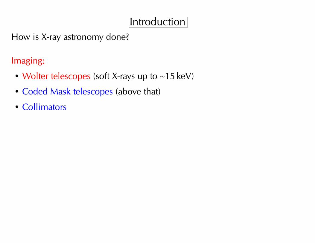
IntroductionHow is X-ray astronomy done?
Imaging:
• Wolter telescopes (soft X-rays up to ∼15 keV)
• Coded Mask telescopes (above that)
• Collimators

IntroductionHow is X-ray astronomy done?
Detectors:
• Non-imaging detectorsDetectors capable of detecting photons from a source, but without any spatial resolution
=⇒ Require, e.g., collimators to limit field of view.
Example: Proportional Counters, Scintillators
• Imaging detectorsDetectors with a spatial resolution, typically used in the IR, optical, UV or for soft X-rays.Generally behind some type of focusing optics.
Example: Charge coupled devices (CCDs), Position Sensitive Proportional Counters(PSPCs)
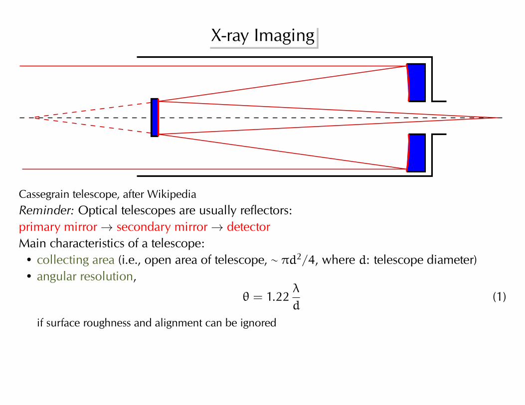
X-ray Imaging
Cassegrain telescope, after WikipediaReminder: Optical telescopes are usually reflectors:primary mirror→ secondary mirror→ detectorMain characteristics of a telescope:• collecting area (i.e., open area of telescope, ∼ πd2/4, where d: telescope diameter)• angular resolution,
θ = 1.22λ
d(1)
if surface roughness and alignment can be ignored

X-ray ImagingOptical telescopes are based on principle that reflection “just works” withmetallic surfaces. For X-rays, things are more complicated. . .
1α
2α
1θ
n2
n1
n1
<
Snell’s law of refraction:sinα1
sinα2=n2
n1= n (2)
where n index of refraction, and α1,2 angle wrt.surface normal. If n � 1: Total internal reflec-tionTotal reflection occurs for α2 = 90◦, i.e. for
sinα1,c = n ⇐⇒ cos θc = n (3)
with the critical angle θc = π/2 − α1,c.Clearly, total reflection is only possible for n <1
Light in glass at glass/air interface: n = 1/1.6 =⇒ θc ∼ 50◦ =⇒ principle behind optical fibers.

X-ray ImagingIn general, the index of refraction is given by Maxwell’s relation,
n =√εµ (4)
where ε: dielectricity constant, µ ∼ 1: permeability of the material.For free electrons (e.g., in a metal), (Jackson, 1981, eqs. 7.59, 7.60) showsthat
ε = 1 −(ωp
ω
)2with ω2
p =4πnZe2
me(5)
where ωp: plasma frequency, n: number density of atoms, Z: nuclearcharge.(i.e., nZ: number density of electrons)
With ω = 2πν = 2πc/λ, Eq. (5) becomes
ε = 1 −nZe2
πmec2λ2 = 1 −
nZre
πλ2 (6)
re = e2/mec
2 ∼ 2.8× 10⁻¹³ cm is the classical electron radius.

X-ray Imaging
n =
√1 −
nZre
πλ2 ∼ 1 −
nZre
2πλ2 = 1 −
ρ
(A/Z)mu
re
2πλ2 =: 1 − δ (7)
Z: atomic number, A: atomic weight (Z/A ∼ 0.5), ρ: density, mu = 1 amu = 1.66× 10⁻²⁴ g
Critical angle for X-ray reflection:
cos θc = n = 1 − δ (8)
Since δ� 1, Taylor (cos x ∼ 1 − x2/2):
θc =√
2δ = 5.6 ′(
ρ
1 g cm−3
)1/2λ
1 nm(9)
So for λ ∼ 1 nm: θc ∼ 1◦.

X-ray ImagingTypical parameters for selected elements
Z ρ nZ
g cm−3 e− Å−3
C 6 2.26 0.680Si 14 2.33 0.699Ag 47 10.50 2.755W 74 19.30 4.678Au 79 19.32 4.666
After Als-Nielsen & McMorrow (2004, Tab. 3.1)
To increase θc: need material with high ρ=⇒ gold (XMM-Newton) or iridium (Chandra).
For more information on mirrors etc., see, e.g., Aschenbach (1985), Als-Nielsen & McMorrow (2004),or Gorenstein (2012)

X-ray Imaging
0 5 10 15 20
Photon Energy [keV]
0.0
0.2
0.4
0.6
0.8
1.0
Reflectivity 0.5deg
0.4deg
0.2deg
1deg
Reflectivity for Gold
X-rays: Total reflec-tion only works inthe soft X-rays andonly under grazingincidence=⇒ grazing inci-dence optics.

Wolter Telescopes
Incident
paraxial
radiation
Hyperboloid
Paraboloid
HyperboloidFocus
after ESA
To obtain manageable focal lengths (∼10 m), use two reflections on aparabolic and a hyperboloidal mirror (“Wolter type I”)(Wolter 1952 for X-ray microscopes, Giacconi & Rossi 1960 for UV- and X-rays).
But: small collecting area (A ∼ πr2l/f where f: focal length)

Wolter Telescopes
−+
Ni Electroforming
Cleaning
Gold Deposition
MirrorAu
Ni
Separation
(cooled)
IntegrationProduction
Metrology
Integration
on Spider
Hole Drilling
Handling
Mandrel
Super Polished Mandrel
Recycle Mandrel
(after ESA)Recipe for making an X-ray mirror:1. Produce mirror negative (“Mandrels”): Al coated with Kanigen nickel (Ni+10% phos-
phorus), super-polished [0.4 nm roughness]).2. Deposit ∼50 nm Au onto Mandrel3. Deposit 0.2 mm–0.6 mm Ni onto mandrel (“electro-forming”, 10µm/h)4. Cool Mandrel with liquid N. Au sticks to Nickel5. Verify mirror on optical bench.
numbers for eROSITA (Arcangeli et al., 2017)

Wolter Telescopes

Wolter Telescopes
Characterization of mir-ror quality: Half EnergyWidth, i.e., circle within50% of the detected en-ergy are found. Note:energy dependent!for XMM-Newton: 20 ′′ at1.5 keV, 40 ′′ at 8 keV.for eROSITA: 16 ′′ at 1.5 keV,15.5 ′′ at 8 keV
Ground calibration, e.g., at PANTER
Detection of X-rays
Space
Ener
gy
EFermi
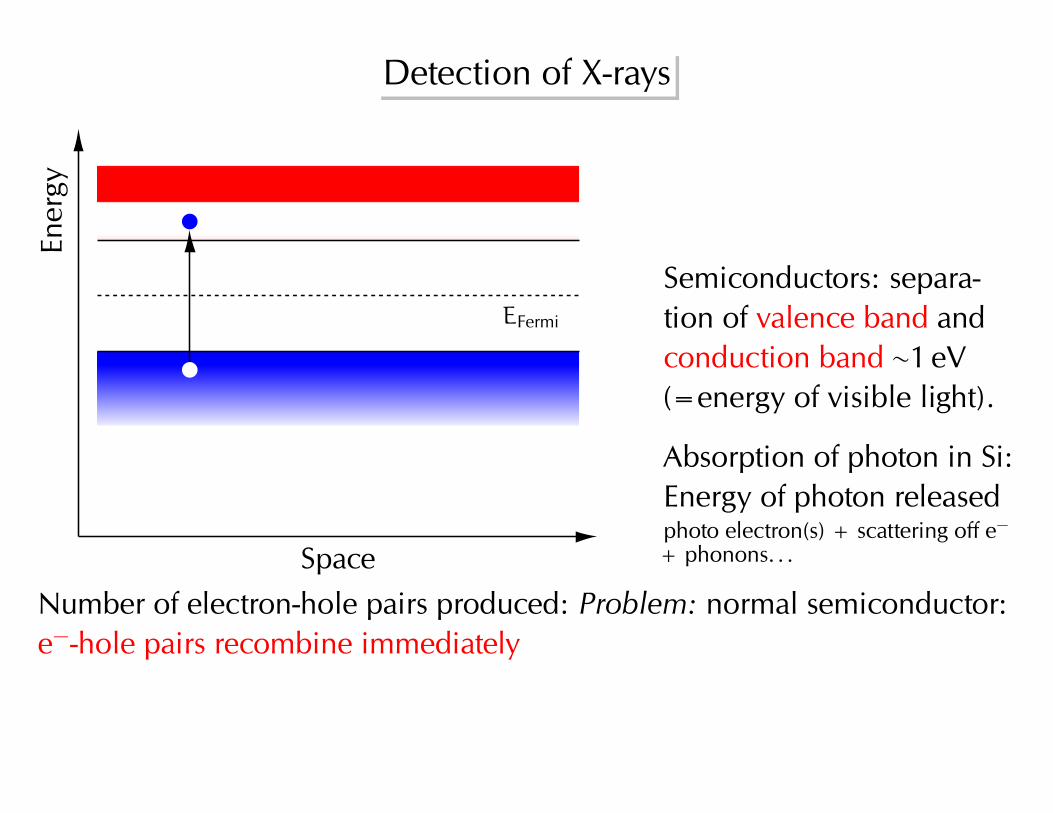
Semiconductors: separa-tion of valence band andconduction band ∼1 eV(=energy of visible light).
Absorption of photon in Si:Energy of photon releasedphoto electron(s) + scattering off e−+ phonons. . .
Number of electron-hole pairs produced: Problem: normal semiconductor:e−-hole pairs recombine immediately

Detection of X-rays
Space
Ener
gy
EFermi
Acceptors
Donors
n-type p-type
“Doping”: moves valence-and conduction bands.Connecting “n-type” anda “p-type” semiconductor:pn-junction.
In pn junction: electron-hole pairs created by ab-sorption of an X-ray areseparated by field gradient
=⇒electrons can then be collected in potential well away from the junc-tion and read out.

Detection of X-raysMaterial Z Band gap E/pair
(eV) (eV)Si 14 1.12 3.61Ge 32 0.74 2.98
CdTe 48–52 1.47 4.43HgI2 80–53 2.13 6.5GaAs 31–33 1.43 5.2
Number of electron-hole pairs produced determined by band gap + “dirteffects”(“dirt effects”: e.g., energy loss going into bulk motion of the detector crystal [“phonons”])
Npair ∼Ephoton
Epair(10)
• optical photons (E: few eV): ∼1 e−-hole-pair per absorption event• X-ray photons: ∼1000 e−-hole-pairs per photonBut: Since band gap small: thermal noise =⇒ need cooling(ground based: liquid nitrogen, −200◦C, in space: more complicated. . . )

Detection of X-rays
e_
e_
e_
e_
photoelectrons
Atom
Photoelectron
trackp−type
(undepleted)
Potential energy
for an electron
p−type (−) silicon
(depleted)
n−type (+) silicon
(depleted)
SiO insulator
0.1 m deep
Polysilicon electrodes
11
1 2 3
1 pixel
(~15 m)
~2 m
~10 m
~250 m
3 1 2 3 1 2 3 2 3
µ
µ
µµ
µ
Photon
µconductors; ~0.5 m deep
2
After Bradt
Two-Dimensional imaging is possible with more complicated semiconduc-tor structures: Charge Coupled Devices (CCDs).

CCDs
−PulseΦ
1Φ
2Φ
3Φ
− − − −−−
3Φ
2Φ
1Φ
Transfer
− − −
− − −
− − −
0V 0V 0V
0V0V
0V 0V 0V
+V
+V +V
+V
(after McLean, 1997, Fig. 6.9)
Principle of the readout of a CCD with Φ-pulses.

CCDs
Gate strips
p−
sto
ps
Read−
out e
lectro
nic
s
combine several readoutstripes gives a two dimen-sional detector.Separation of individual columnswith p-stops (highly doped Si) toprevent charge diffusion betweencolumns.
Read out:• move charge to corner• preamplify• digitize in Analog-
Digital-Converter (ADC)Fast CCDs: one read out electronics per columnExpensive, consumes more power =⇒ only done in the fastest X-ray CCDs (< µs resolution).

CCDs
+ + + + + +
+
− − − −
−
−
preamp
on−chip
n−
p p p p p p
p
285 µ
m12 µ
m
Phi−Pulses to transfer electrons
Depletion voltagePotential for electrons
Anode
Transfer direction
Schematic structure of the XMM-Newton EPIC pn CCD.
Problem: Infalling photons have to pass through structure on CCD surface =⇒ loss of lowenergy response, also danger through destruction of CCD structure by cosmic rays. . .Solution: Irradiate back side of chip. Deplete whole CCD-volume, transport electrons topixels via adequate electric field (“backside illuminated CCDs”)Note: solution works mainly for X-rays

Grades
Charge cloud in Si has roughly 2D Gaussian distribution=⇒ Distribution of clouds on adjacent pixels: “eventgrades”Total E:
∑pixels Ei
ESA: single events, double events,. . . ; US: grade 0 for singles,grade 1–4 for doubles, etc.; other grading schemes are possible.
C. Schmid

Background
M. WilleBackground in CCDs:• cosmic rays (e.g., muons), leaving long tracks on detector• low E (<MeV) protons, focused via mirrors onto CCDs. Especially during solar flares
In principle also electrons: charged “net” over mirror deflects them; this not possible for protonsdue to higher mass; back-illuminated CCDs can usually cope with this and are not damaged.
Typically background reduction on board through thresholding events, e.g., >15 keV wheremirror is non-reflective
Optical Loading
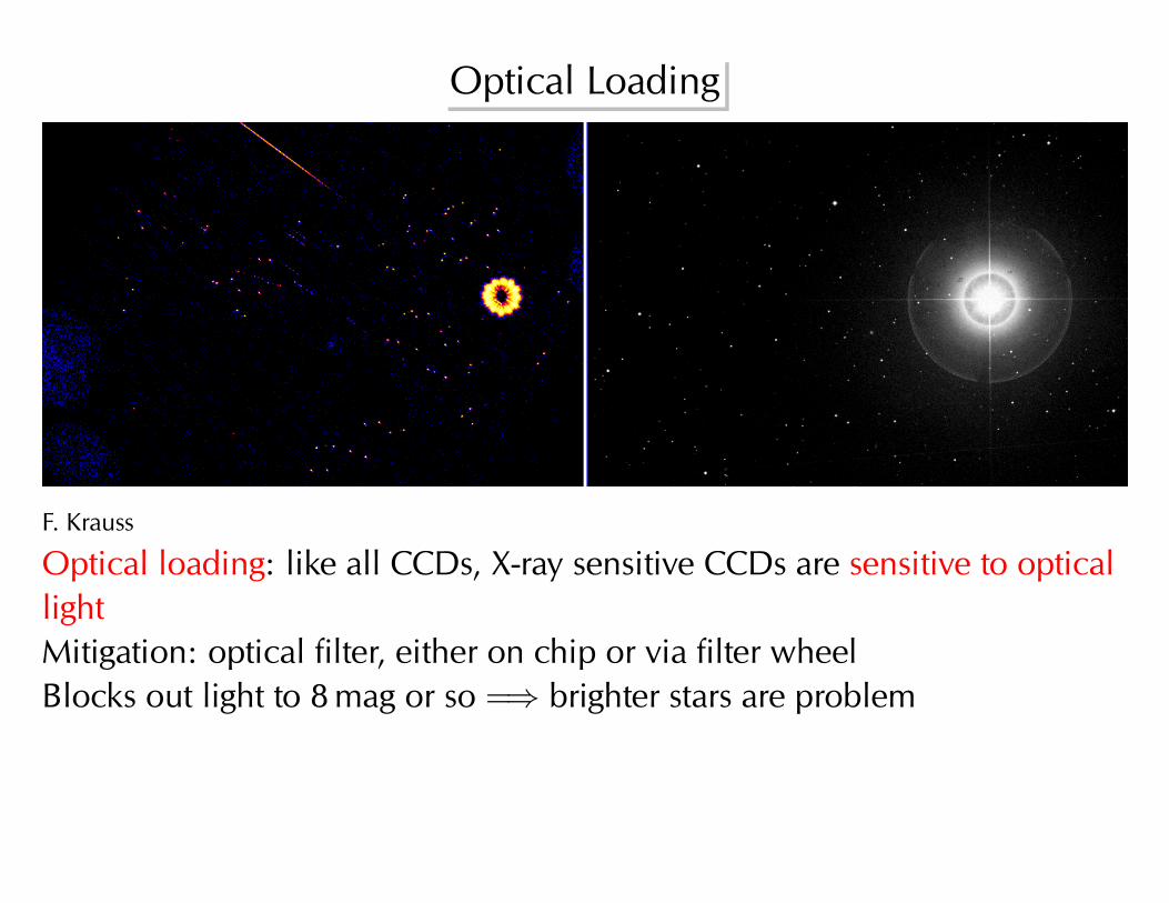
F. Krauss
Optical loading: like all CCDs, X-ray sensitive CCDs are sensitive to opticallightMitigation: optical filter, either on chip or via filter wheelBlocks out light to 8 mag or so =⇒ brighter stars are problem

Part 5: Analyzing Data – Theory

Formal Data AnalysisIn order to analyze X-ray data, we need to understand how the measuredsignal is produced:
1. Sensitivity of the detector: “how much signal do we have?”=⇒ modeled as energy-dependent collecting areaoften called the “ARF” (ancilliary response function)
2. Energy resolution of the detector: “where is the signal detected?”=⇒ modeled as convolution of signal with energy resolutionoften called the “detector response”

Linear Model
Summarizing the previous information mathematically:
nph(c) =
∫∞0R(c,E) ·A(E) · F(E)dE+ nbackground(c) (11)

Linear Model
Summarizing the previous information mathematically:
nph(c) =
∫∞0R(c,E) ·A(E) · F(E)dE+ nbackground(c) (11)
count rate inchannel c
(counts s−1)

Linear Model
Summarizing the previous information mathematically:
nph(c) =
∫∞0R(c,E) ·A(E) · F(E)dE+ nbackground(c) (11)
count rate inchannel c
(counts s−1)
photon flux density(ph cm2 s−1 keV−1),

Linear Model
Summarizing the previous information mathematically:
nph(c) =
∫∞0R(c,E) ·A(E) · F(E)dE+ nbackground(c) (11)
count rate inchannel c
(counts s−1)
photon flux density(ph cm2 s−1 keV−1),
We measure this

Linear Model
Summarizing the previous information mathematically:
nph(c) =
∫∞0R(c,E) ·A(E) · F(E)dE+ nbackground(c) (11)
count rate inchannel c
(counts s−1)
photon flux density(ph cm2 s−1 keV−1),
We measure this Astrophysics is here

Linear Model
Summarizing the previous information mathematically:
nph(c) =
∫∞0R(c,E) ·A(E) · F(E)dE+ nbackground(c) (11)
count rate inchannel c
(counts s−1)
detector response(∝ probability todetect photon of
energy E inchannel c).
effective area(cm2)
photon flux density(ph cm2 s−1 keV−1),
We measure this Astrophysics is hereCalibration
(“response” / “rsp”)

Effective Area
Mirror
IrM
4,5
IrM
3
IrM
2Ir
M1
IrL3
IrL1
1010.1
10+4
10+3
10+2
Energy [keV]
Area[cm
2]
Effective area for an Athena-like mission with a simplified Si-based detector

Effective Area
Mirror+45nm polyamide+70nm Al
AlK
OK
NK
CK
IrM
4,5
IrM
3
IrM
2Ir
M1
IrL3
IrL1
1010.1
10+4
10+3
10+2
Energy [keV]
Area[cm
2]
Effective area for an Athena-like mission with a simplified Si-based detector

Effective Area
Mirror+45nm polyamide+70nm Al
+Si QE
AlK
OK
NK
CK
SiK
IrM
4,5
IrM
3
IrM
2Ir
M1
IrL3
IrL1
1010.1
10+4
10+3
10+2
Energy [keV]
Area[cm
2]
Effective area for an Athena-like mission with a simplified Si-based detector

Effective areas of the most important currentX-ray satellites
(Hanke, 2011)

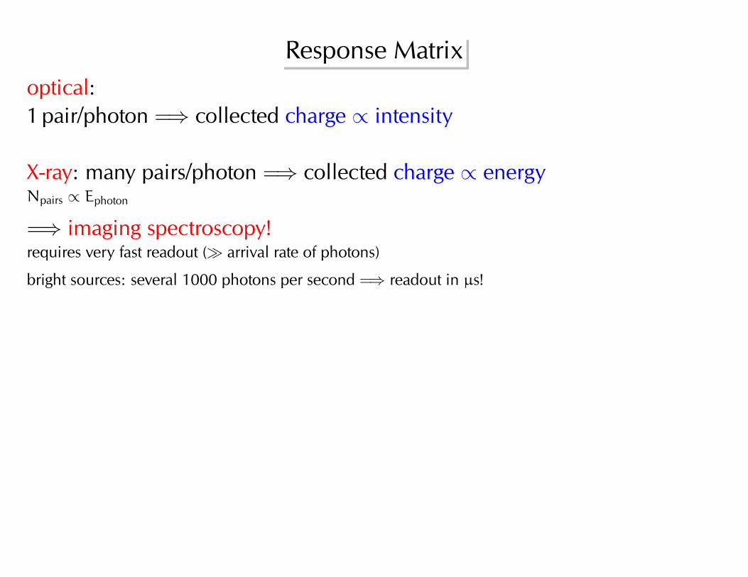
Response Matrixoptical:1 pair/photon =⇒ collected charge ∝ intensity

Response Matrixoptical:1 pair/photon =⇒ collected charge ∝ intensity
X-ray: many pairs/photon =⇒ collected charge ∝ energyNpairs ∝ Ephoton
Response Matrixoptical:1 pair/photon =⇒ collected charge ∝ intensity
X-ray: many pairs/photon =⇒ collected charge ∝ energyNpairs ∝ Ephoton
=⇒ imaging spectroscopy!requires very fast readout (� arrival rate of photons)
bright sources: several 1000 photons per second =⇒ readout in µs!
Response Matrixoptical:1 pair/photon =⇒ collected charge ∝ intensity
X-ray: many pairs/photon =⇒ collected charge ∝ energyNpairs ∝ Ephoton
=⇒ imaging spectroscopy!requires very fast readout (� arrival rate of photons)
bright sources: several 1000 photons per second =⇒ readout in µs!
Poisson statistics of relative collected charge:
∆Npair
Npair

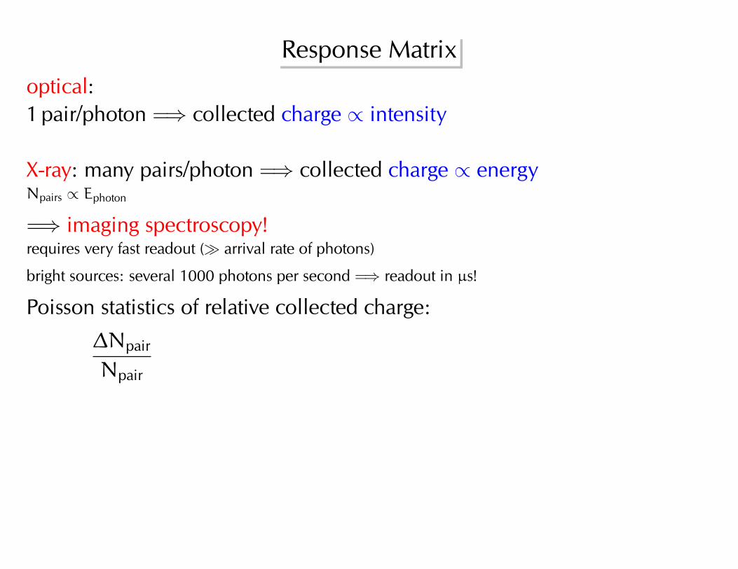
Response Matrixoptical:1 pair/photon =⇒ collected charge ∝ intensity
X-ray: many pairs/photon =⇒ collected charge ∝ energyNpairs ∝ Ephoton
=⇒ imaging spectroscopy!requires very fast readout (� arrival rate of photons)
bright sources: several 1000 photons per second =⇒ readout in µs!
Poisson statistics of relative collected charge:
∆Npair
Npair=
√Npair
Npair

Response Matrixoptical:1 pair/photon =⇒ collected charge ∝ intensity
X-ray: many pairs/photon =⇒ collected charge ∝ energyNpairs ∝ Ephoton
=⇒ imaging spectroscopy!requires very fast readout (� arrival rate of photons)
bright sources: several 1000 photons per second =⇒ readout in µs!
Poisson statistics of relative collected charge:
∆Npair
Npair=
√Npair
Npair=
1√Npair
∼∆E
E
(∆E/E ∝ E−1/2 because of Poisson!)
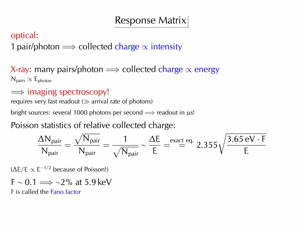
Response Matrixoptical:1 pair/photon =⇒ collected charge ∝ intensity
X-ray: many pairs/photon =⇒ collected charge ∝ energyNpairs ∝ Ephoton
=⇒ imaging spectroscopy!requires very fast readout (� arrival rate of photons)
bright sources: several 1000 photons per second =⇒ readout in µs!
Poisson statistics of relative collected charge:
∆Npair
Npair=
√Npair
Npair=
1√Npair
∼∆E
E=
exact eq.= 2.355
√3.65 eV · F
E
(∆E/E ∝ E−1/2 because of Poisson!)
F ∼ 0.1 =⇒ ∼2% at 5.9 keVF is called the Fano factor

Response Matrix
(Fürst, 2011)
Monoenergetic photons get “smeared” in energy by the detector response.Width of peak given by Eq. on previous slidenote: RMF is not required to be normalized to unity! Some missions include some quantum efficiencyterms in it.

Response Matrix
(Treis et al., 2009)
Mn Kα (5.9 keV), Mn Kβ (6.5 keV), Si escape (4.2 keV), Al fluorescence(1.5 keV) from housing [background]

Response Matrix
Response Matrix of the RXTE-PCA, log scaleSecondary “escape” peaks: response caused by Xe Kβ and Xe Lα photons escaping the de-tector.

Pile Up
some invalid patterns
Pile up: Arrival rate of photons > readouttimescale of CCD =⇒ get wrong energyassignment
• energy pileup: multiple photons insame pixel
• pattern pileup: multiple photons inadjacent pixelssome produce invalid patterns, butsome mimic normal photons
nonlinear effect!
figures by C. Schmid (PhD thesis Remeis-Observatory & ECAP, 2012)

Pile Up
Pile up: Arrival rate of photons > readouttimescale of CCD =⇒ get wrong energyassignment
• energy pileup: multiple photons insame pixel
• pattern pileup: multiple photons inadjacent pixelssome produce invalid patterns, butsome mimic normal photons
nonlinear effect!
figures by C. Schmid (PhD thesis Remeis-Observatory & ECAP, 2012)
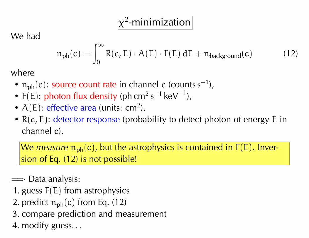
χ2-minimizationWe had
nph(c) =
∫∞0R(c,E) ·A(E) · F(E)dE+ nbackground(c) (12)
where• nph(c): source count rate in channel c (counts s−1),• F(E): photon flux density (ph cm2 s−1 keV−1),• A(E): effective area (units: cm2),• R(c,E): detector response (probability to detect photon of energy E in
channel c).
We measure nph(c), but the astrophysics is contained in F(E). Inver-sion of Eq. (12) is not possible!
=⇒ Data analysis:1. guess F(E) from astrophysics2. predict nph(c) from Eq. (12)3. compare prediction and measurement4. modify guess. . .

χ2-minimizationTo analyze data: discretize Eq. (12):
Sph(c) = ∆T ·nch∑i=0
A(Ei) · R(c, i) · F(Ei) · ∆Ei ∀c ∈ {1, 2, . . . ,nen} (13)
where Sph(c): total source counts in channel c, ∆T : exposure time (s),A(Ei): effective area in energy band i (“ancilliary response file”, ARF),R(c, i): response matrix (RMF), F(Ei): source flux in band (Ei,Ei+i), ∆Ei:width of energy band.Because of background B(c) (counts), what is measured is
Nph(c) = Sph(c) + B(c) (14)
So estimated source count rate is
S̃ph(c) = Nph(c) − B(c) (15)
with uncertainty (Poisson!)
σS̃ph(c) =√σNph(c)2 + σB(c)2 =
√Nph(c) + B(c) (16)

χ2-minimizationTo get physics out of measurement, need to find F(Ei).
Big problem: In general, Eq. (13) is not invertible.
=⇒ χ2-minimization approachUse a model for the source spectrum, F(E; x), where x vector of parameters(e.g., source flux, power law index, absorbing column,. . . ), and calculatepredicted model counts, M(c; x), using Eq. 13).Then form χ2-sum:
χ2(x) =∑c
(S̃ph(c) −M(c; x)
)2
σS̃ph(c)2(17)
Then vary x until χ2 is minimal and perform statistical test based on χ2
whether model F(E; x) describes data.
Programs used: XSPEC, ISIS, SPEX
In practice, background is not subtracted from measurement, but added on model prediction.

Part 4: Further Reading

Literature
LONGAIR, M.S., 1992, High Energy Astrophysics, Vol. 1: Particles, Photons,and their Detection, Cambridge: Cambridge Univ. Press, ∼50eGood introduction to high energy astrophysics, the 1st volume deals extensively withhigh energy procsses, the 2nd with stars and the Galaxy. The announced 3rd volume hasnever appeared. Unfortunately, everything is in SI units.
TRÜMPER, J., HASINGER, G. (eds.), 2007, The Universe in X-rays, Heidel-berg: Springer, 96.25eBook giving an overview of X-ray astronomy written by a group of experts (mainly) fromMax Planck Institut für extraterrestrische Physik, the central institute in this area in Ger-many.
BRADT, H., 2004, Astronomy Methods: A Physical Approach to Astronomi-cal Observations, Cambridge: Cambridge Univ. Press, $50Good general overview book on astronomical observations at all wavelengths.

Literature
CHARLES, P., SEWARD, F., 1995, Exploring the X-ray Universe, Cambridge:Cambridge Univ. Press, out of printSummary of X-ray astronomy, roughly presenting the state of the early 1990s.
SCHLEGEL, E.M., 2002, The restless universe, Oxford: Oxford Univ. Press,32ePopular X-ray astronomy book summarizing results from XMM-Newton and Chandra.
ASCHENBACH, B. et al., 1998, The invisible sky, New York: CopernicusPopular “table top” book summarizing the results of the ROSAT satellite, with many
beautiful pictures.
KNOLL, G.F., 2000, Radiation Detection and Measurement, 3rd edition,New York: Wiley, 126eThe bible on radiation detection. If you want one book on detectors, this is it.

WWW-Pages• http://pulsar.sternwarte.uni-erlangen.de/wilms/teach
My lectures. Including a 2 semester long course on X-ray astronomy (with exercises) anda 1 semester long course on radiation processes. Currently offline, but soon to be onlineagain, but I provide slides upon request.
• http://heasrc.gsfc.nasa.govMain www page of NASA’s satellite missions, including the data archive interface athttp://heasarc.gsfc.nasa.gov/db-perl/W3Browse/w3browse.pl
• http://cxc.harvard.edu
Chandra data center (and analysis info)
• http://xmm.esac.esa.int
XMM-Newton data center (and analysis info)
• http://ledas-www.star.le.ac.uk
Univ. Leicester data archive (many missions)
• http://www.isdc.unige.ch/heavens/
Interface to prereduced INTEGRAL and RXTE data

X-ray Data Analysis 65a
Bibliography
Als-Nielsen, J., & McMorrow, D. 2004, Elements of Modern X-ray Physics, (New York: Wiley)Arcangeli, L., Borghi, G., Bräuninger, H., et al. 2017, in Internat. Conf. on Space Optics, ed. E. Armandillo, B. Cugny, N. Karafolas, Vol. 10565, SPIE Conf. Ser.,
1056558Aschenbach, B., 1985, Rep. Prog. Phys., 48, 579Fürst, F., 2011, Ph.D. thesis, Universität Erlangen-Nürnberg, ErlangenGiacconi, R., & Rossi, B. 1960, J. Geophys. Res., 65, 773Gorenstein, P., 2012, Opt. Eng., 51, 011010Hanke, M., 2011, Ph.D. thesis, Friedrich-Alexander-Universität Erlangen-Nürnberg, ErlangenJackson, J. D., 1981, Klassische Elektrodynamik, (Berlin, New York: de Gruyter), 2 editionMcLean, I., 1997, Electronic imaging in astronomy: detectors and instrumentation, Wiley)Treis, J., Andritschke, R., Hartmann, R., et al. 2009, J. Instrumentation, 03, 03012Wolter, H., 1952, Annalen der Physik, 445, 94
0