DETECTION AND QUANTIFICATION OF ROCK … 54th annual logging symposium, june 22-26, 2013 1 detection and quantification of rock physics properties for improved hydraulic fracturing

$Page 1: DETECTION AND QUANTIFICATION OF ROCK … 54th annual logging symposium, june 22-26, 2013 1 detection and quantification of rock physics properties for improved hydraulic fracturing$
SPWLA 54th Annual Logging Symposium, June 22-26, 2013

1

DETECTION AND QUANTIFICATION OF ROCK PHYSICS PROPERTIES FOR IMPROVED HYDRAULIC FRACTURING IN

HYDROCARBON-BEARING SHALE

Antoine Montaut, Paul Sayar, and Carlos Torres-Verdín The University of Texas at Austin

ABSTRACT Horizontal drilling and hydraulic stimulation make hydrocarbon production from organic-rich shales economically viable. Identification of suitable zones to drill a horizontal well and to initiate or contain hydraulic fractures requires detection and quantification of many factors, including elastic and mechanical properties. Elastic behavior of rocks is affected by rock composition and fabric, pore pressure, confining stress, and other factors. The objective of this paper is to quantify rock fabric properties of hydrocarbon-bearing shales affecting elastic properties. Once rock fabric is validated with sonic logs, results can be used to identify suitable zones to drill a horizontal well, initiate hydraulic stimulation, and contain fracture propagation. Effective-medium theories are invoked to estimate low-frequency elastic properties of a rock for which composition has been estimated with specific fabric properties such as load-bearing matrix, anisotropic cracks, and various shape of rock components. The simulation and interpretation method is implemented in two wells in the Haynesville and in two wells in the Barnett shales. Averages of relative errors between estimated velocities and sonic logs are lower than 4% in the four wells. Simulations in the Haynesville shale indicate that rock fabric may not be the main cause of anisotropy. Rock fabric properties are constant with depth in both wells. Consequently, identification of suitable zones to drill a horizontal well or to contain fracture propagation is based on Young’s modulus rather than on rock fabric. Simulated Poisson’s ratio is shown to be more sensitive to errors in velocities than Young’s modulus (up to 6.4 times more sensitive to error measurements), and is therefore not used for interpretation. The two wells in the Barnett shale exhibit different rock fabric, indicating that the formation is laterally heterogeneous. Simulations suggest that rock fabric gives rises to mechanical anisotropy. Vertical heterogeneity is inferred from the necessary use of rock typing to adequately reproduce sonic logs in both wells. Rock types that exhibit stiff load-bearing matrices indicate suitable depths to drill horizontal wells or to contain hydraulic fractures. INTRODUCTION Designing a horizontal well and optimizing hydraulic stimulation are complex processes that require detection and quantification of many parameters such as rock composition, rock fabric, formation heterogeneity, brittleness, in-situ stress, elastic properties, pore pressure, temperature, and others (King, 2010). Affected by most of these factors, fracturability is a parameter that indicates how efficiently a fracture forms and propagates in a rock. In shale gas formations, fracturability typically correlates with mineralogy (Jarvie et al., 2007) and rock elastic properties (Britt and Schoeffler, 2009). In isotropic rocks, elastic properties are defined by Young’s modulus. Dynamic elastic properties can be calculated from sonic and density logs. Static and dynamic Young moduli tend to correlate in shale gas (Britt and Schoeffler, 2009). Therefore, Young modulus estimated from sonic logs is reliable for estimation of rock fracturability. In anisotropic rocks, an elastic tensor is defined for analysis, because elastic properties change depending on the direction of propagation. Nevertheless, only a subset of elastic tensor components is available through sonic logging in anisotropic rocks. Although sonic measurements are often incomplete in strata with a high degree of anisotropy, the widespread use of sonic logs in industry and research, including their use in shale gas formations, underlines the importance of such data for fracturability quantification and elastic properties estimation. Volumetric concentration of minerals, organic content, porosity, types of fluid, and fluid saturation can be estimated with multi-mineral nonlinear inversion of conventional well logs (Heidari et al., 2012). Although rock composition is available through such inversion methods, no information is provided on how individual components are spatially arranged—otherwise referred to as rock fabric—and how they contribute to the bulk rock mechanical properties.


2

Rocks with equal composition but different rock fabrics can exhibit different mechanical behavior, therefore different elastic properties. Due to complex solid composition, various types of porosity—from micro pores to macro fractures—, vertical variability, and other characteristics, it becomes critical to identify and quantify rock fabric parameters of shales to accurately estimate their elastic properties. Using rock composition, many theories and methods have been developed to assess elastic properties, each having different assumptions and limitations. Theoretical models have been formulated to estimate elastic properties from mixtures of grains and pores, usually referred to as effective medium elastic theories, or mixing laws (Budiansky, 1965; Wu, 1966; Kuster and Toksöz, 1974; Sheng, 1990, 1991). The majority of these effective medium theories assume isotropic rocks and do not account for presence of anisotropic cracks or inclusions. Horizontal compliant pores or vertical fractures, for example, are often encountered in shale formations and can affect elastic properties. Therefore, they should not be neglected in a rock physics model applied to anisotropic shale formations. Hudson (1980) developed a model to estimate the effects of thin, penny-shaped (ellipsoidal) cracks in isotropic media. Hudson’s theory is often used to simulate anisotropic elastic properties due to the anisotropic distribution of inclusions, either solid or fluid filled. Another limitation of previous effective medium theories is that they simulate high-frequency conditions if fluids are directly mixed with minerals. On the contrary, sonic logs—used to validate simulations—measure low-frequency velocities (from which elastic properties are derived). Gassmann’s relation (Gassmann, 1951; Biot, 1956) estimates low-frequency elastic properties of saturated rocks, either isotropic or anisotropic. Combinations of effective medium theories and fluid saturation models have been shown to reliably describe the elastic properties of complex formations, such as shales or tight gas, by accurately accounting for the combined effects of in-situ grain and pore shapes (Xu and White, 1995; Ruiz and Cheng, 2010). Assuming that rock composition is known and sonic/density logs are available, this paper’s first objective is to identify and quantify several rock fabric parameters of hydrocarbon-bearing shale formations: load-bearing matrix, shape of rock components, presence of oriented cracks (compliant pores or fractures for example), and heterogeneity. Several rock physics models are invoked to estimate elastic properties (entries of the stiffness tensor; bulk and shear moduli, Young’s modulus and Poisson’s ratio for isotropic cases) of a rock with specific fabric attributes. Velocities are calculated from estimated elastic properties and compared to field data. Rock fabric is validated when simulations accurately reproduce sonic logs. When errors arise, this indicates erroneous simulation parameters, unexpected rock fabric at a certain location, or an incorrect model. The second objective is to interpret the quantified rock fabric properties to assess suitable zones for drilling a horizontal well, initiate hydraulic stimulation, and contain fracture propagation. Brittle load-bearing matrix, high Young’s modulus (if available), limited layering, and proximity to favorable production intervals are properties that indicate suitable zones for drilling a horizontal well. Production intervals should exhibit sizeable amounts of gas and organic content. For optimal hydraulic fracturing, they should also be brittle and non-laminated. Suitable intervals for fracture containment are either very stiff (carbonate layers, for example, that do not break under fracture pressure) or very soft (clay-rich layers, for example, that absorb fracturing energy and heal/close fractures). Rock fabric properties must also contain no natural fractures (especially in stiff confining layers) so that fracturing fluids do not flow through these intervals. Herein we assume that rock elastic properties only vary with rock composition and rock fabric. Nevertheless, other parameters may affect rock elastic properties but are not studied in this paper. These other properties include in-situ stress, pore pressure, and temperature. Moreover, reproducing sonic logs with the method developed in this paper may give rise to non-unique solutions. Geology, diagenesis, core data, and as much available external information as possible should be taken into account to secure reliable, accurate, and petrophysically viable results. Shale gas formations are usually unique, and models should be carefully extrapolated from one shale to another; the same caution should be exercised to extrapolate a model from one well to another in a laterally heterogeneous formation. METHOD Inversion of petrophysical properties from well logs. Evaluation of petrophysical properties of hydrocarbon-bearing shale is challenging because of the complex composition and high spatial variability of shale properties. Shale is composed of numerous solid elements, such as quartz, calcite, clay, pyrite, and kerogen, often arranged in the form of thin layers whose size is smaller than the resolution of conventional well logs. Heidari et al. (2012) developed a


3

deterministic nonlinear inversion method from conventional well logs that is amenable to the interpretation of hydrocarbon-bearing shale. Adiguna (2012) refined the method and proposed a practical interpretation workflow to estimate rock solid composition, porosity, fluid types, and fluid saturation. The method was successfully applied to data acquired in the Haynesville and Barnett shales. Results were validated by comparison to core measurements and neutron capture spectroscopy logs. Sonic logs, elastic moduli, and stiffness tensors. Hooke’s law describes the relation between stress and strain of a solid. Its general form for an anisotropic, linear, and elastic solid is given by:

σ c ε , (1) where σ is stress, ε is strain, and c is elastic stiffness tensor. For an isotropic medium, the stiffness tensor contains only two independent entries and one can define two independent elastic moduli: bulk modulus (K) and shear modulus (μ). Young’s modulus (E) and Poisson’s ratio (ν) can be calculated from these two independent elastic moduli. In vertical transverse isotropic media, the stiffness tensor contains five independent entries. Velocities are functions of elastic properties and the bulk density of the rock. For isotropic formations, there are two velocities, compressional- (V ) and a shear-wave (V ) velocity. In transverse isotropic media, one distinguishes between one compressional- and two shear-wave velocities. Construction of the dry isotropic frame of the rock. The first step in the construction of the dry isotropic rock frame is the selection of the load-bearing phase. This selection is trivial in simple formations: in consolidated sandstones, for example, quartz grains are in contact with each other and support loads through their solid network. In horizontally laminated sequences constituted of two types of layers, the two laminated solid phases support the vertical load. However, for mixtures of different minerals and organic content, as is the case in organic shales, the concept of load-bearing matrix is more complex. There is not always a clear dominant mineral (in terms of volumetric concentration) in the rock framework. We choose two isotropic rock physics models to construct the dry isotropic frame of the rock: the self-consistent approximation (SCA) and the differential effective medium (DEM) theory. Both these effective theories estimate bulk and shear moduli of a mixture of phases. Porous space must be dry, i.e. both elastic moduli are set to zero, and saturated subsequently in order to simulate low-frequency conditions. Inclusions are assumed to exhibit idealized ellipsoidal shapes. Media are assumed to be isotropic, linear and elastic. Berryman (1980, 1995) developed a general formulation of the self-consistent approximation for a mixture of N phases, given by:

x K K∗ P∗ 0 , (2)

and

x μ μ∗ Q∗ 0 , (3)

where i refers to the i-th material, xi represents its volumetric concentration and P and Q are geometric coefficients that depend on the shape of inclusions. Superscripts *i on P and Q indicate that the factors are for the i-th inclusion in a background medium with elastic moduli K∗ and μ∗ . A penny-shaped crack is characterized by its aspect ratio, α, which is the ratio of short to long axes. An aspect ratio of 1 implies that the crack is a sphere whereas a value of 0 means that the crack is a disk of zero thickness. The self-consistent approximation estimates elastic properties of an aggregate of all rock constituents. For that reason, the self-consistent approximation is usually not suitable for estimating elastic properties of a rock in which a certain mineral, or combination of several minerals, is load-bearing (Hornby et al., 1994).


4

The differential effective medium theory estimates bulk and shear moduli of a two-phase mixture. Phase 1 is the host; it remains topologically connected regardless of concentration. Phase 2 is incrementally added to the host material until it reaches its desired concentration, x2. Berryman (1992) gives the following formulation for the DEM differential equations:

1 x∂∂x

K∗ x K K∗ P∗ x , (4) and

1 x∂∂x

μ∗ x μ μ∗ Q∗ x , (5) with initial conditions K∗ x 0 K and μ∗ x 0 μ , where subscripts or superscripts 1 and 2 refer to host and inclusion materials, respectively; K∗ and μ∗ are the bulk and shear moduli of the mixture, respectively. Geometric factors P and Q are identical to those of the self-consistent approximation, and superscript *2 indicate that coefficients P and Q are for an inclusion of material 2 in a background medium with bulk and shear moduli K∗ and μ∗ , respectively. If there is more than one secondary phase, one calculates the mixture’s effective elastic properties in several steps, adding one type of inclusion after another. The order in which inclusions are added does not necessarily reflect the true geological evolution of the rock (Mavko et al., 2009). It is found that neither the self-consistent approximation nor the differential effective medium theory are reliable to describe the behavior of rocks that exhibit several topologically connected phases. Hornby et al. (1994) emphasizes that the combination of the self-consistent approximation and the differential effective medium theory provides a solution to this problem. If two materials of concentration between 40 and 60% are mixed using the self-consistent approximation and assuming spherical shapes, the two phases are connected within the mixture. The differential effective medium model is subsequently invoked to adjust relative concentrations of the two materials. Using the differential effective medium theory, or a combination of it with the self-consistent approximation, one can estimate elastic properties of different mixtures of minerals that represent the dry isotropic frame of the rock. Simulation parameters used for this step of the simulation include load-bearing phase—composed of one or two solids—, order in which inclusions are added, and shape of inclusions.

Treatment of anisotropic cracks and inclusions. Hudson’s model (1980) is based on scattering theory and describes the effect of oriented ellipsoidal inclusions or cracks in an isotropic background medium on rock elastic properties. Before constructing the rock isotropic matrix, a percentage of certain minerals and porosity are chosen to be modeled as oriented inclusions or cracks. Hudson’s model estimates effective moduli of rocks that contain oriented penny cracks, or inclusions, by adding first- and second-order corrections to the entries of the isotropic background stiffness tensor. We use only first-order corrections because a second-order correction can lead to convergence problems (Cheng, 1993). To study the influence of the load-bearing matrix, inclusion order, and anisotropic cracks or inclusions on rock elastic properties, some tests were previously performed on synthetic cases (Montaut, 2012). Results from this exercise were then used to determine the parameters that yielded the best agreement with measurements in the Haynesville and Barnett case studies.

Treatment of fluid saturation. After adding oriented cracks and inclusions to the isotropic matrix, we simulate the effect of fluids that fill the porous space. In the field studies considered in this paper, hydrocarbon is gas. Therefore, the pore space is assumed to contain only two fluids: water and gas. In isotropic media, rocks are saturated using the isotropic formulation of Gassmann’s theory (Gassmann, 1951). Gassmann also provides a fluid-substitution formulation for the case of anisotropic rocks. Pore pressures are assumed to be equilibrated in the pore space to honor low-frequency conditions. The rock is also assumed to be fully saturated with fluids.

Rock typing. Using identical rock fabric along the entire depth interval of a formation can yield reliable estimations of elastic properties and velocities. However, in some cases the formation must be divided into segments of similar properties—otherwise referred to as rock types—that are subsequently associated with specific rock fabric properties. Rock typing is based on solid volumetric composition of the formation, more specifically on volumetric concentration of kerogen, quartz, and calcite. In the Barnett field wells, for instance, five rock types are identified for Well B1 and three for Well B2 and a specific rock fabric is associated with each rock type. Such a procedure suggests that rock fabric is vertically heterogeneous, which is commonly observed in shale formations.


5

Spatial averaging of elastic properties. Sonic tools are composed of several transmitters and an array of receivers. In field examples considered this paper, the array contains 13 receivers spaced at 0.5 ft intervals. Therefore, velocities and elastic properties calculated from sonic/density logs represent averaged in-situ rock properties. Simulated elastic properties—estimated at every 0.5 ft—must be vertically averaged so that velocities are consistently compared to sonic logs. Layers are assumed to be horizontal and linearly elastic. All beds exhibit equal thickness and effective vertical elastic moduli are averaged with Backus’ formula (Backus, 1962). It is assumed that there are no sources of intrinsic energy dissipation and layers thickness is much smaller than acoustic wavelength. Vertical compressional- and shear-wave velocities are then calculated using averaged rock density.

HAYNESVILLE CASE STUDY

Introduction. The purpose of this field case is to quantify rock fabric properties in two wells in the Haynesville shale. Results are used to identify suitable zones for drilling horizontal wells and intervals to initiate or contain hydraulic fractures. The Haynesville shale, located in east Texas and northwest Louisiana, is a major gas play in the United States. Haynesville shale is a black, organic-rich shale (Hammes et al., 2011). Its deposition occurred during Late Jurassic, about 150 million years ago. It is bounded by the Bossier shale above, and the Haynesville limestone and Smackover formation below (Hammes et al., 2011). Conventional well logs are available in both wells and are used to estimate rock solid composition, porosity, fluid types, and fluid saturation. Compressional and shear velocity logs are available and describe vertical acoustic-wave properties; both wells were drilled in the vertical direction. In the first example, velocities are simulated based on rock composition and fabric. They are compared to sonic logs in order to validate fabric properties such as load-bearing matrix, inclusion order, anisotropy, and vertical heterogeneity. Once sonic logs are accurately reproduced, a similar model is invoked in the second well; the objective of extrapolating the rock physics model from one example to the other is to study lateral continuity of this region of the Haynesville shale.

Description of the rock physics model that yields the best agreement with measured velocities. Rock fabric is assumed to be constant and isotropic throughout the entire simulation interval. The load-bearing matrix is assumed to be composed of clay and kerogen. Therefore, the first step is to invoke the SCA and DEM combination in order to model a background load-bearing matrix that comprises clay and organic matter. Although calcite exhibits a smaller volumetric concentration than quartz at most depths, carbonate inclusions are added first to the background matrix, followed by quartz. All solids are modeled as spheres. Porosity is included last, assuming an ellipsoidal shape with an aspect ratio of 0.07 in Well H1 and 0.06 in Well H2. The rock is saturated using the isotropic formulation of Gassmann’s theory.

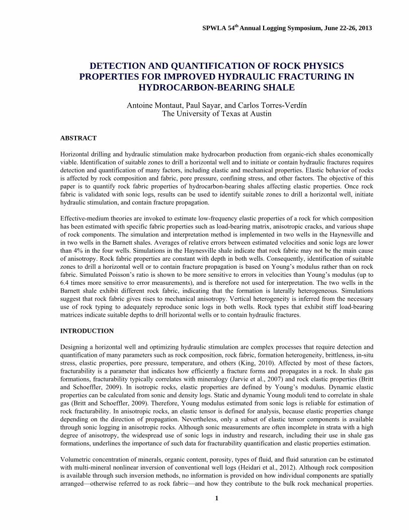
Simulation results. Figures 1 and 2 describe results obtained from velocity and elastic property estimations, showing both non-averaged and spatially averaged estimations in Wells H1 and H2, respectively. Spatially averaged estimated velocities are relevant when compared to sonic logs because sonic measurements implicitly average rock elastic properties and density. The medians of relative errors, 2.83% for V , 2.12% for V in Well H1, 3.11% for V and 2.25% for V in Well H2, indicate that estimated velocities reliably reproduce sonic logs in both wells, even if the model is isotropic. As expected, non-averaged estimated velocities are not suitable for comparison to sonic logs. They do not accurately reproduce measurements in Well H1 at depths xx728 ft and xx815ft whereas spatial averaging of estimated velocities yields a good agreement with field data. These layers are likely to be thin and stiff, and their properties are spatially averaged during sonic logging. Figures 1 and 2 also show the Young’s moduli and Poisson’s ratios calculated from logs and estimated rock elastic properties in Wells H1 and H2, respectively. Young’s modulus is reproduced accurately: the median of relative errors are 4.6% and 3.9% in Wells H1 and H2, respectively. Although the median of relative errors are not large for Poisson’s ratios, 5.7% in Well H1 and 4.5% in Well H2, the qualitative match with the field-obtained Poisson’s ratio is poor (as is the case from xx750 ft to xx790 ft in Well H1, for instance). Because of this behavior, Poisson’s ratio is not used in the interpretation. Sensitivity of Young’s modulus and Poisson’s ratio to measurement errors is addressed in a subsequent paragraph.

Interpretation of results. The rock physics model invoked to estimate rock elastic properties and velocities in both wells is isotropic. However, this choice does that imply that the mechanical properties of the formation are isotropic and it should not be assumed that horizontal and vertical velocities are equal. The fact that the rock physics model is isotropic and accurately reproduce sonic logs could indicate that rock fabric is not the main cause for anisotropy of rock mechanical properties. It could be due to other factors, such as stress, for example. In this case, given the small


6

volumetric concentration of organic matter, being that the host material is composed of clay and kerogen, clay is assumed to be the main load-bearing rock component. Carbonate material is added to the background matrix before quartz, thereby suggesting that calcite may have more influence on rock elastic properties than quartz. Therefore, calcite should be preferred to quartz in cases where identification of stiff, or compliant depth intervals is based on the volumetric concentration of these minerals.

Figure 1: Application of the isotropic rock physics method in Well H1. Track 1: relative depth. Track 2: volumetric composition of the solid part of the rock. Track 3: porosity and bulk volume (BV) of water and gas. Track 4: compressional velocity. Track 5: shear velocity. Track 6: Young’s modulus. Track 7: Poisson’s ratio. In tracks 4, 5, 6 and 7, black, red, and blue curves identify field, non-averaged estimated, and averaged estimated velocity, respectively.

When the rock physics model constructed in Well H1 is used for simulations in well H2, velocities and Young’s modulus are also accurately reproduced. Rock fabric is shown to be quasi-identical in the two wells, except for pore aspect ratio. Such variation of pore aspect ratio could indicate a larger compaction stress in Well H2 compared to Well H1 (pores are expected to flatten as stress increases). This hypothesis is supported by the fact that Haynesville shale is located in a deeper depth interval in Well H2 than in Well H1 (compaction stress usually increases with depth). All remaining rock fabric properties are identical in the two wells. Such behavior suggests that the rock fabric of the Haynesville shale is likely to be laterally homogeneous in the area where field data were acquired for analysis.

Method to identify suitable zones for drilling horizontal wells and favorable intervals to initiate or contain hydraulic fractures. Rock fabric properties are constant in both Well H1 and H2. Consequently, identification of suitable zones for drilling a horizontal well or to contain fracture propagation is not based on rock fabric. According to Sone and Zoback (2010), the higher the Young’s modulus, the less sensitive the formation becomes to creeping behavior. Creep is the tendency of a solid to deform over time under stress and is unsuitable for efficient hydraulic stimulation. Creep also correlates with fracturability (Britt and Schoeffler, 2009) and stiffness (Sone and Zoback,


7

2010). Therefore, identifying suitable zones to drill a horizontal well or to contain fracture propagation is based on Young’s modulus.

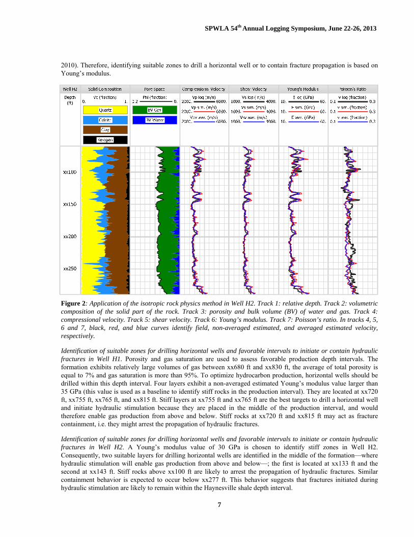
Figure 2: Application of the isotropic rock physics method in Well H2. Track 1: relative depth. Track 2: volumetric composition of the solid part of the rock. Track 3: porosity and bulk volume (BV) of water and gas. Track 4: compressional velocity. Track 5: shear velocity. Track 6: Young’s modulus. Track 7: Poisson’s ratio. In tracks 4, 5, 6 and 7, black, red, and blue curves identify field, non-averaged estimated, and averaged estimated velocity, respectively.

Identification of suitable zones for drilling horizontal wells and favorable intervals to initiate or contain hydraulic fractures in Well H1. Porosity and gas saturation are used to assess favorable production depth intervals. The formation exhibits relatively large volumes of gas between xx680 ft and xx830 ft, the average of total porosity is equal to 7% and gas saturation is more than 95%. To optimize hydrocarbon production, horizontal wells should be drilled within this depth interval. Four layers exhibit a non-averaged estimated Young’s modulus value larger than 35 GPa (this value is used as a baseline to identify stiff rocks in the production interval). They are located at xx720 ft, xx755 ft, xx765 ft, and xx815 ft. Stiff layers at xx755 ft and xx765 ft are the best targets to drill a horizontal well and initiate hydraulic stimulation because they are placed in the middle of the production interval, and would therefore enable gas production from above and below. Stiff rocks at xx720 ft and xx815 ft may act as fracture containment, i.e. they might arrest the propagation of hydraulic fractures.

Identification of suitable zones for drilling horizontal wells and favorable intervals to initiate or contain hydraulic fractures in Well H2. A Young’s modulus value of 30 GPa is chosen to identify stiff zones in Well H2. Consequently, two suitable layers for drilling horizontal wells are identified in the middle of the formation—where hydraulic stimulation will enable gas production from above and below—; the first is located at xx133 ft and the second at xx143 ft. Stiff rocks above xx100 ft are likely to arrest the propagation of hydraulic fractures. Similar containment behavior is expected to occur below xx277 ft. This behavior suggests that fractures initiated during hydraulic stimulation are likely to remain within the Haynesville shale depth interval.


8

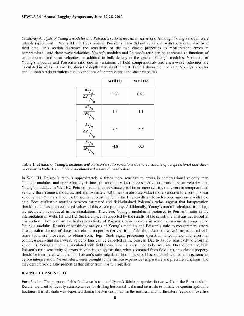
Sensitivity Analysis of Young’s modulus and Poisson’s ratio to measurement errors. Although Young’s moduli were reliably reproduced in Wells H1 and H2, simulated Poisson’s ratios did not agree well with those calculated from field data. This section discusses the sensitivity of the two elastic properties to measurement errors in compressional- and shear-wave velocities. Young’s modulus and Poisson’s ratio can be expressed as functions of compressional and shear velocities, in addition to bulk density in the case of Young’s modulus. Variations of Young’s modulus and Poisson’s ratio due to variations of field compressional- and shear-wave velocities are calculated in Wells H1 and H2, along the depth intervals of interest. Table 1 shows the median of Young’s modulus and Poisson’s ratio variations due to variations of compressional and shear velocities.

Well H1 Well H2

∆EE

∆VV

0.80 0.86

∆EE

∆VV

1.2 1.1

∆ν ν∆V

V

4.8 5.5

∆ν ν∆V

V

-4.8 -5.5

Table 1: Median of Young’s modulus and Poisson’s ratio variations due to variations of compressional and shear velocities in Wells H1 and H2. Calculated values are dimensionless.

In Well H1, Poisson’s ratio is approximately 6 times more sensitive to errors in compressional velocity than Young’s modulus, and approximately 4 times (in absolute value) more sensitive to errors in shear velocity than Young’s modulus. In Well H2, Poisson’s ratio is approximately 6.4 times more sensitive to errors in compressional velocity than Young’s modulus, and approximately 4.8 times (in absolute value) more sensitive to errors in shear velocity than Young’s modulus. Poisson’s ratio estimation in the Haynesville shale yields poor agreement with field data. Poor qualitative matches between estimated and field-obtained Poisson’s ratios suggest that interpretation should not be based on estimated values of this elastic property. Additionally, Young’s moduli calculated from logs are accurately reproduced in the simulations. Therefore, Young’s modulus is preferred to Poisson’s ratio in the interpretation in Wells H1 and H2. Such a choice is supported by the results of the sensitivity analysis developed in this section. They confirm the higher sensitivity of Poisson’s ratio to errors in sonic measurements compared to Young’s modulus. Results of sensitivity analysis of Young’s modulus and Poisson’s ratio to measurement errors also question the use of these rock elastic properties derived from field data. Acoustic waveforms acquired with sonic tools are processed to obtain sonic logs. Such signal-processing operation is complex, and errors in compressional- and shear-wave velocity logs can be expected in the process. Due to its low sensitivity to errors in velocities, Young’s modulus calculated with field measurements is assumed to be accurate. On the contrary, high Poisson’s ratio sensitivity to errors in velocities suggests that, when computed from field data, this elastic property should be interpreted with caution. Poisson’s ratio calculated from logs should be validated with core measurements before interpretation. Nevertheless, cores brought to the surface experience temperature and pressure variations, and may exhibit rock elastic properties that differ from in-situ properties.

BARNETT CASE STUDY

Introduction. The purpose of this field case is to quantify rock fabric properties in two wells in the Barnett shale. Results are used to identify suitable zones for drilling horizontal wells and intervals to initiate or contain hydraulic fractures. Barnett shale was deposited during the Mississippian. In the northern and northeastern regions, it overlies


9

the Viola/Simpson group, a stiff limestone formation that acts as a fracture barrier. Opposite to that in the southern and southwestern regions, the Barnett shale overlies the Chappel limestone or the Ellenburger dolomite/limestone (Montgomery et al., 2005). This last formation is porous and water-saturated, and is avoided during hydraulic stimulation to prevent water production and aquifer contamination. In the south/southwestern regions, where Well B1 is located, the Barnett shale consists of a single depth interval, whereas in north/northeastern regions, where Well B2 is located, it is divided into two depth intervals (Montgomery et al., 2005) referred as the upper and lower sections. Between the two sections lies the Forestburg formation, a limestone group that acts as fracture barrier. Similarly to the Haynesville shale study, vertically uniform isotropic models were used first for the Barnett. Inaccurate velocity estimations suggested that the Barnett shale rock fabric is more complex than in Haynesville. Rock typing and anisotropic rock physics models are required to accurately estimate velocities. Rock fabric is assumed to vary with rock composition. Young’s modulus and Poisson’s ratio assume isotropic elastic properties, therefore they are not suitable in the interpretation of this field case.

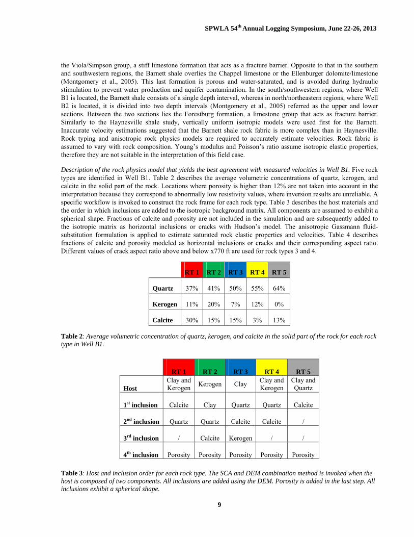
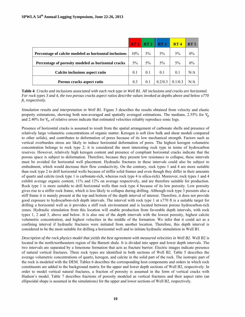
Description of the rock physics model that yields the best agreement with measured velocities in Well B1. Five rock types are identified in Well B1. Table 2 describes the average volumetric concentrations of quartz, kerogen, and calcite in the solid part of the rock. Locations where porosity is higher than 12% are not taken into account in the interpretation because they correspond to abnormally low resistivity values, where inversion results are unreliable. A specific workflow is invoked to construct the rock frame for each rock type. Table 3 describes the host materials and the order in which inclusions are added to the isotropic background matrix. All components are assumed to exhibit a spherical shape. Fractions of calcite and porosity are not included in the simulation and are subsequently added to the isotropic matrix as horizontal inclusions or cracks with Hudson’s model. The anisotropic Gassmann fluid-substitution formulation is applied to estimate saturated rock elastic properties and velocities. Table 4 describes fractions of calcite and porosity modeled as horizontal inclusions or cracks and their corresponding aspect ratio. Different values of crack aspect ratio above and below x770 ft are used for rock types 3 and 4.

Table 2: Average volumetric concentration of quartz, kerogen, and calcite in the solid part of the rock for each rock type in Well B1.

Table 3: Host and inclusion order for each rock type. The SCA and DEM combination method is invoked when the host is composed of two components. All inclusions are added using the DEM. Porosity is added in the last step. All inclusions exhibit a spherical shape.

RT 1 RT 2 RT 3 RT 4 RT 5

Quartz 37% 41% 50% 55% 64%

Kerogen 11% 20% 7% 12% 0%

Calcite 30% 15% 15% 3% 13%


Host Clay andKerogen

Kerogen Clay Clay and Kerogen

Clay and Quartz

1st inclusion Calcite Clay Quartz Quartz Calcite

2nd inclusion Quartz Quartz Calcite Calcite /

3rd inclusion / Calcite Kerogen / /

4th inclusion Porosity Porosity Porosity Porosity Porosity


10

Table 4: Cracks and inclusions associated with each rock type in Well B1. All inclusions and cracks are horizontal. For rock types 3 and 4, the two porous cracks aspect ratios describe values invoked at depths above and below x770 ft, respectively.

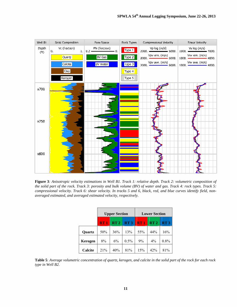
Simulation results and interpretation in Well B1. Figure 3 describes the results obtained from velocity and elastic property estimations, showing both non-averaged and spatially averaged estimations. The medians, 2.55% for V and 2.40% for V , of relative errors indicate that estimated velocities reliably reproduce sonic logs.

Presence of horizontal cracks is assumed to result from the spatial arrangement of carbonate shells and presence of relatively large volumetric concentrations of organic matter. Kerogen is soft (low bulk and shear moduli compared to other solids), and contributes to deformation of pores because of its low mechanical strength. Factors such as vertical overburden stress are likely to induce horizontal deformation of pores. The highest kerogen volumetric concentration belongs to rock type 2; it is considered the most interesting rock type in terms of hydrocarbon reserves. However, relatively high kerogen content and presence of compliant horizontal cracks indicate that the porous space is subject to deformation. Therefore, because they present low resistance to collapse, these intervals must be avoided for horizontal well placement. Hydraulic fractures in these intervals could also be subject to embedment, which would decrease their flow conductivity. On the contrary, rock types 1 and 4 are more suitable than rock type 2 to drill horizontal wells because of stiffer solid frames and even though they differ in their amounts of quartz and calcite (rock type 1 is carbonate-rich, whereas rock type 4 is silica-rich). Moreover, rock types 1 and 4 exhibit average organic content, 11% and 12% on average respectively, and are therefore suitable for production. Rock type 1 is more suitable to drill horizontal wells than rock type 4 because of its low porosity. Low porosity gives rise to a stiffer rock frame, which is less likely to collapse during drilling. Although rock type 3 presents also a stiff frame it is mainly present at the top and bottom of the depth interval of interest. Therefore, it does not provide good exposure to hydrocarbon-rich depth intervals. The interval with rock type 1 at x770 ft is a suitable target for drilling a horizontal well as it provides a stiff rock environment and is located between porous hydrocarbon-rich zones. Hydraulic stimulation from this location will enable production from favorable depth intervals, with rock types 1, 2 and 3, above and below. It is also one of the depth intervals with the lowest porosity, highest calcite volumetric concentration, and highest velocities in the middle of the formation. We infer that it could act as a confining interval if hydraulic fractures were initiated from another location. Therefore, this depth interval is considered to be the most suitable for drilling a horizontal well and to initiate hydraulic stimulation in Well B1.

Description of the rock physics model that yields the best agreement with measured velocities in Well B2. Well B2 is located in the north/northeastern region of the Barnett shale. It is divided into upper and lower depth intervals. The two intervals are separated by a limestone formation that acts as fracture barrier. Electric images indicate presence of natural vertical fractures. Three rock types are identified in both sections of Well B2. Table 5 describes the average volumetric concentrations of quartz, kerogen, and calcite in the solid part of the rock. The isotropic part of the rock is modeled with the DEM. Tables 6 describes the corresponding host components and orders in which rock constituents are added to the background matrix for the upper and lower depth sections of Well B2, respectively. In order to model vertical natural fractures, a fraction of porosity is assumed in the form of vertical cracks with Hudson’s model. Table 7 describes fractions of porosity modeled as vertical fractures and their aspect ratio (an ellipsoidal shape is assumed in the simulations) for the upper and lower sections of Well B2, respectively.


Percentage of calcite modeled as horizontal inclusions 10% 5% 5% 5% 0%

Percentage of porosity modeled as horizontal cracks 5% 5% 5% 5% 0%

Calcite inclusions aspect ratio 0.1 0.1 0.1 0.1 N/A

Porous cracks aspect ratio 0.3 0.1 0.2/0.3 0.1/0.3 N/A


11

Figure 3: Anisotropic velocity estimations in Well B1. Track 1: relative depth. Track 2: volumetric composition of the solid part of the rock. Track 3: porosity and bulk volume (BV) of water and gas. Track 4: rock types. Track 5: compressional velocity. Track 6: shear velocity. In tracks 5 and 6, black, red, and blue curves identify field, non-averaged estimated, and averaged estimated velocity, respectively.

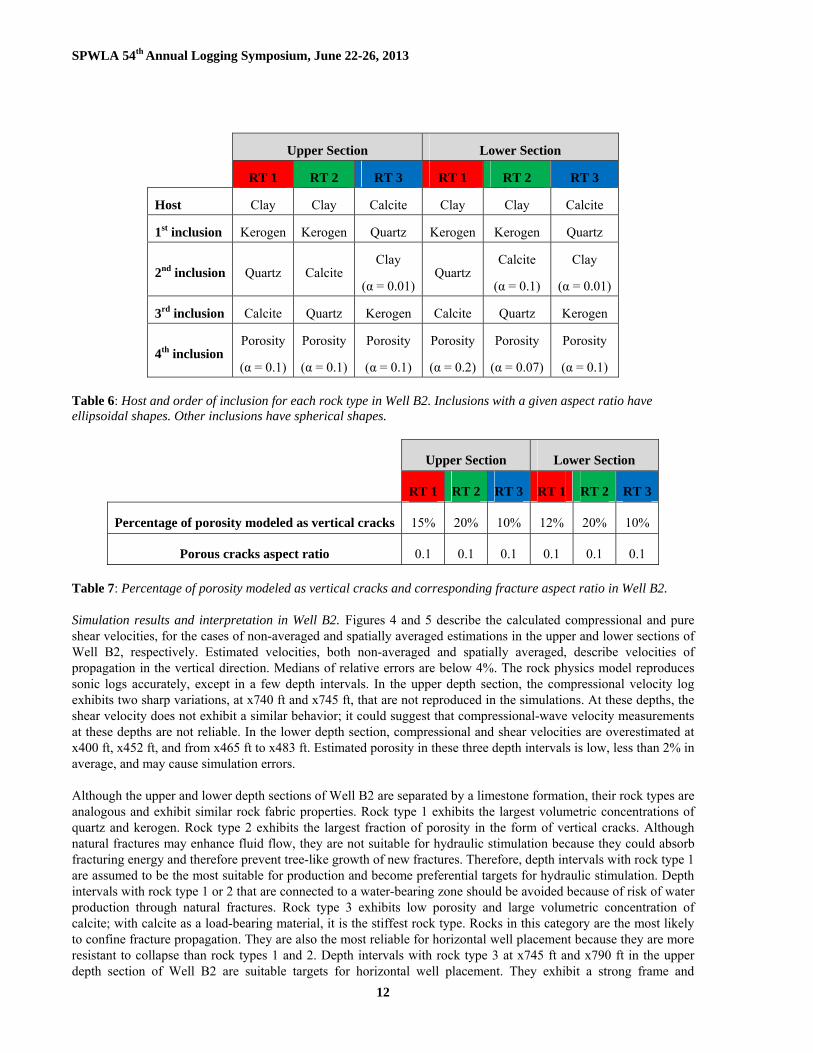
Table 5: Average volumetric concentration of quartz, kerogen, and calcite in the solid part of the rock for each rock type in Well B2.

Upper Section Lower Section

RT 1 RT 2 RT 3 RT 1 RT 2 RT 3

Quartz 50% 36% 13% 55% 44% 16%

Kerogen 8% 6% 0.5% 9% 4% 0.8%

Calcite 21% 40% 81% 15% 42% 81%


12

Table 6: Host and order of inclusion for each rock type in Well B2. Inclusions with a given aspect ratio have ellipsoidal shapes. Other inclusions have spherical shapes.



Percentage of porosity modeled as vertical cracks 15% 20% 10% 12% 20% 10%

Porous cracks aspect ratio 0.1 0.1 0.1 0.1 0.1 0.1

Table 7: Percentage of porosity modeled as vertical cracks and corresponding fracture aspect ratio in Well B2.

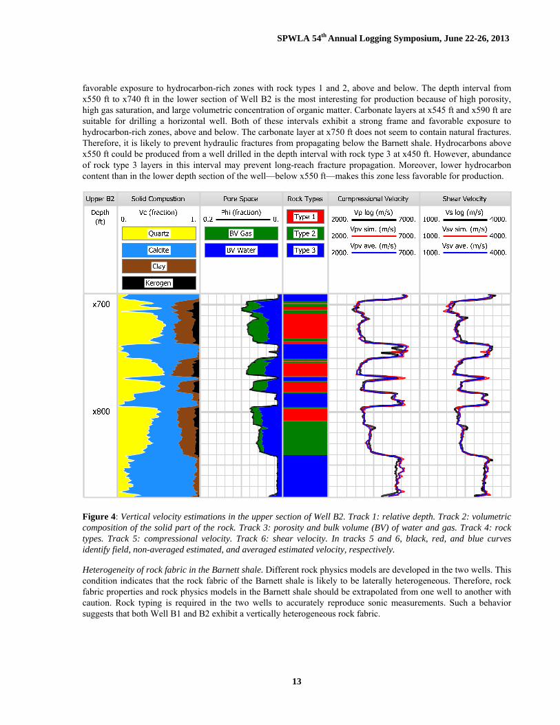
Simulation results and interpretation in Well B2. Figures 4 and 5 describe the calculated compressional and pure shear velocities, for the cases of non-averaged and spatially averaged estimations in the upper and lower sections of Well B2, respectively. Estimated velocities, both non-averaged and spatially averaged, describe velocities of propagation in the vertical direction. Medians of relative errors are below 4%. The rock physics model reproduces sonic logs accurately, except in a few depth intervals. In the upper depth section, the compressional velocity log exhibits two sharp variations, at x740 ft and x745 ft, that are not reproduced in the simulations. At these depths, the shear velocity does not exhibit a similar behavior; it could suggest that compressional-wave velocity measurements at these depths are not reliable. In the lower depth section, compressional and shear velocities are overestimated at x400 ft, x452 ft, and from x465 ft to x483 ft. Estimated porosity in these three depth intervals is low, less than 2% in average, and may cause simulation errors. Although the upper and lower depth sections of Well B2 are separated by a limestone formation, their rock types are analogous and exhibit similar rock fabric properties. Rock type 1 exhibits the largest volumetric concentrations of quartz and kerogen. Rock type 2 exhibits the largest fraction of porosity in the form of vertical cracks. Although natural fractures may enhance fluid flow, they are not suitable for hydraulic stimulation because they could absorb fracturing energy and therefore prevent tree-like growth of new fractures. Therefore, depth intervals with rock type 1 are assumed to be the most suitable for production and become preferential targets for hydraulic stimulation. Depth intervals with rock type 1 or 2 that are connected to a water-bearing zone should be avoided because of risk of water production through natural fractures. Rock type 3 exhibits low porosity and large volumetric concentration of calcite; with calcite as a load-bearing material, it is the stiffest rock type. Rocks in this category are the most likely to confine fracture propagation. They are also the most reliable for horizontal well placement because they are more resistant to collapse than rock types 1 and 2. Depth intervals with rock type 3 at x745 ft and x790 ft in the upper depth section of Well B2 are suitable targets for horizontal well placement. They exhibit a strong frame and



Host Clay Clay Calcite Clay Clay Calcite

1st inclusion Kerogen Kerogen Quartz Kerogen Kerogen Quartz

2nd inclusion Quartz Calcite Clay

(α = 0.01) Quartz

Calcite

(α = 0.1)

Clay

(α = 0.01)

3rd inclusion Calcite Quartz Kerogen Calcite Quartz Kerogen

4th inclusion Porosity

(α = 0.1)

Porosity

(α = 0.1)

Porosity

(α = 0.1)

Porosity

(α = 0.2)

Porosity

(α = 0.07)

Porosity

(α = 0.1)


13

favorable exposure to hydrocarbon-rich zones with rock types 1 and 2, above and below. The depth interval from x550 ft to x740 ft in the lower section of Well B2 is the most interesting for production because of high porosity, high gas saturation, and large volumetric concentration of organic matter. Carbonate layers at x545 ft and x590 ft are suitable for drilling a horizontal well. Both of these intervals exhibit a strong frame and favorable exposure to hydrocarbon-rich zones, above and below. The carbonate layer at x750 ft does not seem to contain natural fractures. Therefore, it is likely to prevent hydraulic fractures from propagating below the Barnett shale. Hydrocarbons above x550 ft could be produced from a well drilled in the depth interval with rock type 3 at x450 ft. However, abundance of rock type 3 layers in this interval may prevent long-reach fracture propagation. Moreover, lower hydrocarbon content than in the lower depth section of the well—below x550 ft—makes this zone less favorable for production.

Figure 4: Vertical velocity estimations in the upper section of Well B2. Track 1: relative depth. Track 2: volumetric composition of the solid part of the rock. Track 3: porosity and bulk volume (BV) of water and gas. Track 4: rock types. Track 5: compressional velocity. Track 6: shear velocity. In tracks 5 and 6, black, red, and blue curves identify field, non-averaged estimated, and averaged estimated velocity, respectively.

Heterogeneity of rock fabric in the Barnett shale. Different rock physics models are developed in the two wells. This condition indicates that the rock fabric of the Barnett shale is likely to be laterally heterogeneous. Therefore, rock fabric properties and rock physics models in the Barnett shale should be extrapolated from one well to another with caution. Rock typing is required in the two wells to accurately reproduce sonic measurements. Such a behavior suggests that both Well B1 and B2 exhibit a vertically heterogeneous rock fabric.


14

Figure 5: Vertical velocity estimations in the lower section of Well B2. Track 1: relative depth. Track 2: volumetric composition of the solid part of the rock. Track 3: porosity and bulk volume (BV) of water and gas. Track 4: rock types. Track 5: compressional velocity. Track 6: shear velocity. In tracks 5 and 6, black, red, and blue curves identify field, non-averaged estimated, and averaged estimated velocity, respectively.

CONCLUSIONS

Based on rock composition and sonic/density logs, a simulation method and corresponding interpretation technique were developed to quantify rock fabric properties in hydrocarbon-bearing organic shales. Rock physics models were invoked to model rock elastic properties of formations with specific fabric attributes: load-bearing matrix, constituent shapes, anisotropic cracks, and spatial heterogeneity. Estimated velocities were compared to measured compressional- and shear-wave velocities to validate rock fabric properties. This method was verified with well logs acquired in the Haynesville and Barnett shales. Final results showed that rock physics models are different from one formation to another and reflect differences in rock fabric.

Haynesville shale. Compressional and shear velocity logs were accurately reproduced: averages of relative errors between estimated and measured velocities were lower than 4% in the two wells. Isotropic modeling was reliable for the numerical simulation of sonic logs. Anisotropy between vertical and horizontal elastic properties could be due to other factors, such as stress, for instance. An identical rock fabric was assumed in the two wells and kept the same for their entire depth interval, from the bottom of the Bossier shale to the top of the Haynesville limestone. Measured velocities were accurately reproduced in the simulations, suggesting that rock fabric is laterally and vertically homogeneous. The only parameter that was refined was the pore aspect ratio. Well H2 exhibited a smaller pore aspect ratio and is deeper than Well H1, indicating that compaction could drive pore shape. Suitable depth


15

intervals for horizontal well placement in the two wells were identified in the middle of the Hayneville shale. These intervals exhibit high velocities, high Young’s modulus, and good exposure to hydrocarbon-rich zones above and below. The calcite-rich Haynesville limestone represents a natural fracture containment obstacle, as does the Bossier shale. Therefore, there is little risk of accidentally stimulating non-suitable intervals. Estimations of Poisson’s ratio did not accurately reproduce Poisson’s ratio calculated from sonic/density logs. Poisson’s ratio was shown to be more sensitive to measurement errors than Young’s modulus and was deemed not suitable for interpretation.

Barnett shale. Both wells were divided into layers with similar rock composition. Specific rock fabric properties were applied to each rock type, indicating that rock fabric in the Barnett shale is vertically heterogeneous. Isotropic models did not reproduce sonic logs reliably, whereby Hudson’s model was invoked to model the anisotropic distribution of some rock components. Different anisotropic properties were used in the two wells. Rock types and rock physics models are different from one well to the other. Therefore, rock fabric in the Barnett shale is expected to by laterally heterogeneous. Extrapolation of a rock physics model from one well to another in the Barnett shale should be done with caution, especially if the wells are not within the same geological demarcation zone.

Well B1. Sonic logs were reliably reproduced with an anisotropic rock physics model: averages of relative errors between estimated and measured velocities were lower than 4%. Clay is the dominant load-bearing constituent, (except for rock type 2 where kerogen was chosen as load-bearing), mixed with kerogen for rock types 1 and 4 and with quartz for rock type 5. Horizontal compliant cracks were modeled in Well B1. This type of pore shape is due to large volumetric concentration of soft organic matter. Because of the softness of the rock, pores deform under the influence of overburden stress. A rock type 3 depth interval in the middle of the formation, at x770 ft, was shown to represent the most suitable location to drill a horizontal well. It exhibited large amounts of both silica and calcite and high sonic velocities, is bounded by hydrocarbon- and organic-rich rocks, and is located far from stiff layers present at the top and bottom of this section of the Barnett shale, which could contain vertical fracture propagation.

Well B2. In Well B2, both in the upper and lower sections, the effect of presence of natural vertical fractures was accounted for when using Hudson’s model to add vertical cracks. Sonic logs were reliably reproduced with this procedure: averages of relative errors between estimated and measured velocities were lower than 4%. Rock types exhibit different numbers of natural fractures, which may indicate that the formation of such cracks could be affected by rock composition (given that rock typing was based on rock composition). Rock type 1 was preferred over rock type 2 for performing hydraulic stimulation because natural fractures tend to absorb energy from hydraulic stimulation (the fraction of porosity in the form of fractures is lower in rock type 1). Rock type 3 was identified as the most suitable rock type to place a horizontal well as the calcite load-bearing matrix is likely to provide a good resistance to collapse. Identification of suitable zones for horizontal well placement in the upper depth section of Well B2 was based on calcite volumetric concentration and velocities. Two depth intervals, at x745 ft and x790 ft, were identified as suitable for drilling a horizontal well. They exhibited large volumetric concentrations of calcite, which provide stability and resistance to collapse, and are bounded by favorable rocks for production. These suitable rocks for production exhibit high porosity and high gas saturation. The lower depth section of Well B2 is more vertically heterogeneous than the upper one. On the basis of porosity, gas saturation, and organic content, the best production interval was identified between x550 ft and x740 ft. In this interval, the carbonate layer of rock type 3 at x590 ft was identified as the most suitable location for drilling a horizontal well. It exhibited calcite load-bearing matrix, low clay volumetric concentration, low porosity, and high velocities.

ACKNOWLEDGEMENTS

The work reported in this paper was funded by The University of Texas at Austin's Research Consortium on Formation Evaluation, jointly sponsored by Afren, Anadarko, Apache, Aramco, Baker-Hughes, BG, BHP Billiton, BP, Chevron, ConocoPhillips, COSL, ENI, ExxonMobil, Halliburton, Hess, Maersk, Marathon Oil Company, Mexican Institute for Petroleum, Nexen, ONGC, OXY, Petrobras, Repsol, RWE, Schlumberger, Shell, Statoil, TOTAL, Weatherford, Wintershall, and Woodside Petroleum Limited.

REFERENCES

Adiguna, H., 2012, Comparative Study for the Interpretation of Mineral Concentrations, Total Porosity, and TOC in Hydrocarbon-Bearing Shale from Conventional Well Logs, Master’s Thesis, The University of Texas at Austin.


16

Backus, G. E., 1962, “Long-wave elastic anisotropy produced by horizontal layering,” Journal of Geophysical Research, 67, 4427-4440.

Berryman, J. G., 1980, “Long-wavelength propagation in composite elastic media,” Journal of Acoustic Society of America, 69, 1809-1831.

Berryman, J. G., 1992, Single-scattering approximations for coefficients in Biot’s equations of poroelasticity, Journal of Acoustic Society of America, 91, 551-571.

Berryman, J. G., 1995, “Mixture theories for rock properties, Rock Physics and Phase Relations: a Handbook of Physical Constants,” ed. T.J. Ahrens. Washington, DC: American Geophysical Union, pp. 205-228.

Biot, M. A., 1956, “Theory of propagation of elastic waves in a fluid saturated porous solid. I: Low frequency range, and II: Higher-frequency range,” Journal of Acoustic Society of America, 28, 168-191.

Britt, L., and Schoeffler, J., 2009, “The geomechanics of a shale play: What makes a shale prospective!,” SPE Eastern Regional Meeting, Charleston, West Virginia, September 23-25.

Budiansky, B.,1965, “On the elastic moduli of some heterogeneous materials”, Journal of the Mechanics and Physics of Solids, 13, 223-227.

Cheng, C. H., 1993, “Crack models for a transversely anisotropic medium,” Journal of Geophysical Research, 98, 675-684.

Gassmann, F., 1951, “Über die Elastizität poröser Medien,” Vierteljahrsschrift der Naturforschenden Gesellschaft in Zürich, 96, 1-23.

Hammes, U., Hamlin, H. S., and Ewing, T. E., 2011, “Geologic analysis of the upper Jurassic Haynesville shale in east Texas and west Louisiana,” AAPG Bulletin, v. 95, no. 10, pp. 1643–1666.

Heidari, Z., Torres-Verdín, C., and Preeg, W. E., 2012, “Improved estimation of mineral and fluid volumetric concentrations from well logs in thinly bedded and invaded formations”, Geophysics, v. 77, no 3, pp. WA79-WA98.

Hornby, B. E., Schwartz, L. M., and Hudson, J. A., 1994, “Anisotropic effective-medium modeling of the elastic properties of shales,” Geophysics, 59, 1570-1583.

Hudson, J. A., 1980, “Overall properties of a cracked solid, Mathematical Proceedings,” Cambridge Philosophical Society, 88, 371-384.

Jarvie, D. M., Hill, R. J., Ruble, T. E., and Pollastro, R. M., 2007, “Unconventional shale-gas systems: The Mississippian Barnett shale of north-central Texas as one model for thermogenic shale-gas assessment,” AAPG Bulletin, v. 91, no. 4, pp. 475–499.

King, G., 2010, “Thirty years of gas shale fracturing: What have we learned?,” SPE Annual Technical Conference and Exhibition, Florence, Italy, September 19-22.

Kuster, G. T., and Toksöz, M. N., 1974, “Velocity and attenuation of seismic waves in two-phase media,” Geophysics, 39, 587-618.

Montaut, A., 2012, Detection and quantification of rock physics properties for improved hydraulic fracturing in hydrocarbon-bearing shales, Master’s Thesis, The University of Texas at Austin.

Mavko, G., Mukerji, T., and Dvorkin, J., 2009, The Rock Physics Handbook, Second Edition: Tools for Seismic Analysis of Porous Media, Cambridge University Press.

Montgomery, S. L., Jarvie, D. M., Bowker, K. A., and Pollastro, R. M., 2005, “Mississippian Barnett shale, Fort Worth basin, north-central Texas: Gas-shale play with multi–trillion cubic foot potential,” AAPG Bulletin, v. 89, no. 2, pp. 155–175.

Ruiz, F., and Cheng, A., 2010, “A rock physics model for tight gas sand,” The Leading Edge, December,1484-1488. Sheng, P., 1990, “Effective-medium theory of sedimentary rocks,” Physical Review, B41, 7, 4507-4512. Sheng, P., 1991, “Consistent modeling of the electrical and elastic properties of sedimentary rocks,” Geophysics, 56,

1236-1243. Sone, H., and Zoback, M. D., 2010, “Strength, creep and frictional properties of gas shale reservoir rocks,”

American Rock Mechanics Association. Wu, T. T., 1966, “The effect of inclusion shape on the elastic moduli of a two-phase material,” International

Journal of Solids and Structure, 2, 1-8. Xu, S., and White, R. E., 1995, “A new velocity model for clay-sand mixtures,”Geophysical Prospecting, 43, 91-

118.

Documents

DETECTION AND QUANTIFICATION OF ROCK … 54th annual logging symposium, june 22-26, 2013 1 detection and quantification of rock physics properties for improved hydraulic fracturing