Embed Size (px)
Citation preview

MASTER’S THESIS
2006:39 PB
Shuvra Dev Sarker
Detection of Flow Pulsation byMicro-controller Equipped
Ultrasonic Flow Meter
Department of Computer Science and Electrical EngineeringEISLAB • Embedded Internet Systems Laboratory
M.Sc. in Computer Sciences and EngineeringCONTINUATION COURSES
2006:39 PB • ISSN: 1653 - 0187 • ISRN: LTU - PB - EX - - 06/39 - - SE

Detection of Flow Pulsation byMicro-controller Equipped Ultrasonic
Flow Meter
Shuvra Dev Sarker
Lulea University of TechnologyDept. of Computer Science and Electrical Engineering
EISLAB
August 2006
Supervisor: Jan van DeventerLuleå University of Technology


ABSTRACT
This thesis demonstrates that the small micro-controller present in ultrasonic flow meters
can detect error inducing flow pulsations. The implemented code is provided in the
appendices.
The application targets the district heating industry where the use of ultrasonic flow
meters is growing more and more common as they are accurate, non-intrusive and low
cost. District heating companies desire accurate and low cost flow measurement. An
underestimation of the flow rate leads to a loss of income and the total cost of measuring,
the reading, maintenance and installation represents a relatively large part of the total
cost.
Recently, in competitive market, micro-controllers have become inexpensive and those
are capable of doing complex computations. In this thesis, as part of self-diagnosis tech-
niques, the detection of the pulsating flow is implemented on an 8-bit ATMEL AVR
micro-controller. It saves a huge installation cost and is economically beneficial for an
industry. Serial communication and data conversion are also implemented to receive ve-
locity input data. The work shows that even with an 8-bit micro-controller flow pulsations
are detectable.
Keywords: FFT, DFT, Pulsating flow, Ultrasonic Flow Meter, Hamming window, At-
mel AVR.
iii

PREFACE
The research described in this Master’s thesis was carried out during spring 2006 at Lulea
University of Technology, under the division of EISLAB.
First and foremost, I would like to thank and express my gratitude to my Supervisor
Dr. Jan van Deventer, Head of the EISLAB, Lulea University of Technology, Sweden, for
his supervision and immense contributions in shaping this thesis. His inspiration helps
me to finish this thesis.
I would like to express my gratitude to Johan Eriksson and David Johansson for their
interesting discussions about Atmel AVR and Signal System.
A special thank also goes to David A. Carr, who has always helped me to provide
valuable feedback related to educational and administrative purposes that make possible
to complete my Master degree.
I would like to express my gratitude to Shahidul Islam Sheikh who has helped and
guided me in countless ways every day of my life in Sweden. I would like to express
my gratitude to Mr. Atanu Nath, PhD student at Division of Industrial Marketing and
e-Commerce, Lulea University of Technology, who has always guided me in numerous
ways despite having his own research workload.
My thanks go also to Sweden, and the people of Sweden, for the warm embrace, it has
given me these past years. I feel honored to have known you.
Finally, I want to express my gratitude to my parents and my brother to whom I
dedicate this thesis for their constant support. It is my greatest blessings to be their son.
v


To my loving parents,
Nirapada Sarker and Monimala Sarker
vi


CONTENTS
Chapter 1: Introduction 3
1.1 Introduction . . . . . . . . . . . . . . . . . . . . . . . . . . . . . . . . . . 3
Chapter 2: Background 5
2.1 Flow meters summary . . . . . . . . . . . . . . . . . . . . . . . . . . . . 5
2.2 Transit-Time Ultrasonic Flow Meters . . . . . . . . . . . . . . . . . . . . 7
2.3 Problems of Ultrasonic Flow Meters . . . . . . . . . . . . . . . . . . . . . 9
2.4 Carlander’s Self Diagnostics for Ultrasonic Flow Measurement . . . . . . 10
2.5 Berrebi’s Detection of Pulsating Flows in an Ultrasonic Flow Meter . . . 11
2.6 About ATMEL AVR AT90CAN128 . . . . . . . . . . . . . . . . . . . . . 12
2.7 Lab Setup . . . . . . . . . . . . . . . . . . . . . . . . . . . . . . . . . . . 15
Chapter 3: FFT Algorithm and frequency spectra 17
3.1 Fast Fourier Transform . . . . . . . . . . . . . . . . . . . . . . . . . . . . 17
3.2 FFT Algorithm . . . . . . . . . . . . . . . . . . . . . . . . . . . . . . . . 18
3.3 Frequency Spectra . . . . . . . . . . . . . . . . . . . . . . . . . . . . . . 22
Chapter 4: Implementation 25
4.1 INPUT FUNCTION . . . . . . . . . . . . . . . . . . . . . . . . . . . . . 25
4.2 EXECUTION FUNCTION . . . . . . . . . . . . . . . . . . . . . . . . . 26
4.3 OUTPUT FUNCTION . . . . . . . . . . . . . . . . . . . . . . . . . . . . 27
4.4 DETECT FREQ Function . . . . . . . . . . . . . . . . . . . . . . . . . . 27
4.5 Program to detect velocity data . . . . . . . . . . . . . . . . . . . . . . . 28
4.6 Program to convert float64 to float32 . . . . . . . . . . . . . . . . . . . . 29
Chapter 5: Results 31
Chapter 6: Future Work 35
Chapter 7: Conclusion 37
Appendix A:Code - Main function 39
Appendix B:Code - Macros 43
Appendix C:Code - Function Description and constant tables 47

Appendix D:Code - Flow Meter data filtering 55
Appendix E:Code - Covert float64 to float32 57
viii

List of Figures
2.1 A D-Flow ultrasonic flow meter with a longitudinal configuration. . . . . 8
2.2 A D-Flow ultrasonic flow meter with a diagonal configuration. . . . . . . 8
2.3 Detection of a pulsating flow by Hinich’s harmogram (simulation) . . . . 13
2.4 Detection of a pulsating flow by Hinich’s harmogram (real signal) . . . . 13
2.5 Atmel AVR AT90CAN128 Micro-controller connected with STK500, used
for this thesis. . . . . . . . . . . . . . . . . . . . . . . . . . . . . . . . . . 15
3.1 Butterfly signal flow graph . . . . . . . . . . . . . . . . . . . . . . . . . . 20
3.2 Successive steps in an 8-point FFT . . . . . . . . . . . . . . . . . . . . . 21
3.3 Successive steps in an 8-point FFT (continuation) . . . . . . . . . . . . . 22
4.1 Flow diagram of implementation for detection of pulsating flow. . . . . . 26
4.2 Packet received by serial port of micro-controller . . . . . . . . . . . . . . 28
5.1 Welch method’s output for y = 5×sin(2×π×50×t)+10×sin(2×π×200×t)
signal (Matlab simulation). . . . . . . . . . . . . . . . . . . . . . . . . . . 31
5.2 Welch method’s output for previous signal corrupted by zero-mean random
noise (Matlab simulation). . . . . . . . . . . . . . . . . . . . . . . . . . . 32
5.3 Welch method’s output for Berrebi’s data (Matlab simulation). . . . . . . 33
6.1 Future implementation for M-16 based Ultrasonic Flow Measurement. . . 35
1


CHAPTER 1
Introduction
1.1 Introduction
Accurate measurement is an important factor in District Heating Industries as annual cost
of total metering error is approximately estimated 170 Millions of Swedish Crowns for the
Swedish District Industries. These industries supply hot water in buildings and houses
through a network. The energy supplied to a customer is measured by thermometers and
by a flow meter inside the district-heating substation, which are present at the customer’s
place.
Among the flow meters, the Transit-time Ultrasonic flow meters are accepted as a
great interest as they are accurate, non-intrusive and cheap but they are very sensitive
to installation effects1 and other source of errors. Installation effects could be either
static or dynamic. A pulsating flow is a dynamic installation effect. In 2001, Carlan-
der stated in his PhD thesis that pulsating flows generate harmonic structure in the
frequency spectrum of the measured flow velocity [1] and he investigated the possibility
of self-diagnostic techniques for flow meters. Berrebi introduced and implemented the
idea of self-diagnosing technology, which can detect the pulsating flow by using Hinich’s
harmogram [2]. However, he implemented it in MATLAB and it requires powerful com-
puter, which was expensive. This was one of the drawbacks to install his implementation
industrially.
Recently, in competitive market, micro-controllers have become very cheap and they are
capable to do complex computations as they are faster and have relatively high storage
capacity. Therefore, it is of great interest to implement self-diagnosis techniques to error
1Installation effects are the performance deviations from the calibration lab due to the environmentin which the sensor or meter is installed.
3

4 Introduction
reduction for ultrasonic flow measurement in a micro-controller. It will be exceptionally
inexpensive and economically beneficial for an industry.
In this thesis, the ATMEL AVR micro-controller have used to receive the serial input
from Transit-time ultrasonic flow meter and detect pulsating flow from the flow velocity
data. Fast Fourier Transform (FFT) and absolute value of it, i.e. the frequency spectra,
have been implemented in the AVR to detect pulsating flow that Berrebi did in Matlab
and serial communication is also implemented to receive velocity input data. Experimen-
tal data have been used and results are shown which are generated by micro-controller
and perform comparison with Matlab simulations. It shows exactly the same results as
the results in Matlab calculations. Therefore, Matlab and a Laptop can be replaced by
the micro-controller already present in flow or heat meters, to detect the pulsating flow,
which fulfill the commercial use of Berrebi’s work.

CHAPTER 2
Background
2.1 Flow meters summary
Flow meters are used to measure flow rate. There are several types of flow meters with
different measuring methods. In this section, the most common industrially used flow
meters are described briefly and some of them are also commonly used in the district
heating sub-station. At close to ideal condition, accuracies of ±0.5% or slightly better
can be achieved for some types of flow meters. Rangeabilities of 1:100 and more can also
be achieved [3].
2.1.1 Differential pressure flow meters
These flow meters have been most commonly used flow rate measurement device in
industry and have about 40% of the market [4]. The orifice plate is the most excepted
and widely used among the different types of DP flow meters. All DP flow meters have
almost the same operation principles. According to Bernoulli’s equations, a change in
cross section area of flow meter causes a change in velocity and pressure. The flow rate
can be expressed as a function of the difference in pressure in larger and smaller cross
section area, by using continuity equation. The orifice flow meter uses a plate with a hole
smaller than the cross section area of the pipe for the flow restriction. The pressure of
upstream and downstream of the plate is measured by a differential pressure transmitter.
The orifice flow meter is affected by installation effect. The error will be caused by
disturbed velocity profiles and swirling flow [5].
• The advantages and disadvantages of the orifice flow meter [3].
– Simple and robust design but low range ability.
5

6 Background
– It has well established standards but sensitive to coating on the plate.
– It requires no calibration for standard design, however it is sensitive to instal-
lation effects.
2.1.2 Variable area flow meter
‘Rotameters’ are the most commonly used type of variable area flow meters. Variable
area flow meters have industrial use of more than 10% among the flow meters [4]. Its
working principle is different than the DP flow meter. In this meter, the differential
pressure remains constant and the flow is measured as a function of the reduction is area.
This area is generally displayed by the position of a freely moving float producing the
variable area. A float with a density greater than the fluid is used in the ‘Rotameters’
type. It is placed in a vertical conical tube with the wider end pointing up. The float
is lifted by the flow until the balance is reached between gravitational, buoyancy and
hydrodynamic forces. The flow rate is indicated by the position of the float and it is
sensed by a magnetic pickup and also can observed directly if the tube is transparent [3].
• The advantages and disadvantages of the ‘Rotameters’ flow meter.
– Simple design but moderate accuracy and it must be mounted vertically.
– Its price is low.
– It is insensitive to static installation effects but sensitive to pulsating flow.
2.1.3 Electromagnetic flow meters
District heating companies in Sweden, commonly use electromagnetic or magnetic induc-
tive (mag or MID) flow meters. More than 30% of the meters are of this types [6]. In
general, industrial use of MID flow meters is less than 10% [4]. MID flow meters oper-
ate on the principles of Faraday’s law of electromagnetic induction, therefore, they are
designed to measure the velocity of electrically conductive liquids. A velocity is induced
when a conductor is passed through a magnetic field. The fluid acts as a conductor in
the MID flow meters and a magnetic field is generated by magnetic coil. This coil is
mounted on the outside of a non-magnetic pipe segment. Two electrodes are used to
detect the induced voltage [7]. This flow meter is generally less sensitive to installation
effects than many other flow meter types.
• Some advantages and disadvantages of the MID flow meter are outlined below [3].
– It has good accuracy but the fluid must be conductive.
– There is no moving part but deposit inside the meter can cause errors in the
output (e.g. copper sediment from copper pipes).
– Low-pressure loss.
– Not significantly effected by moderate profile distortions.

2.2. Transit-Time Ultrasonic Flow Meters 7
2.1.4 Mass flow meter
The mass flow is directly measured by this group of flow meters, whereas other flow
meters have to measure density in order to deliver mass flow, therefore sensitive to change
in temperature and pressure. Among the Mass flow meters, Coriolis type is the most
commonly used mass flow type and industrially has more than 5% use of this flow meter
[4].
When a body is rotated about a fixed point and changes its position relative to that
fixed point, the coriolis force is generated. Forcing the pipe to vibrate, Coriolis forces
are generated in this meter. Normally, a U-bend pipe is forced to vibrate in the middle
and anchored at the ends. When a fluid passes through the pipe, Coriolis forces will
be generated in opposite directions in each half of the U-bend. This force the U-bend
to twist. The two halves of the U-bend pipe will then pass a fixed plane at different
times. This time difference is directly related to the mass flow through the pipe [8]. A
weight vector theory can apply to compensate for the velocity distribution effects inside
the pipe. This mass flow meters are known as insensitive to installation effects.
• Some advantages and disadvantages of the Coriolis flow meters are sketched below
[3].
– It has Wide rangeability but pressure drops may be high.
– High accuracy but Zero flow accuracy may be low.
– Low-pressure loss.
– Operates on virtually every fluid but the price is high.
2.2 Transit-Time Ultrasonic Flow Meters
In industrial applications, the transit-time or sing-around flow meter is widely used. This
is the most commonly used type [4]. This method was first issued by Rutten in 1931 [9].
Transit-Time ultrasonic flow meter measures the time difference for the sound to travel
between two transducers. One transducer is placed upstream and other relatively more
downstream. From both directions, the times of flight are measured. The interaction of
the fluid velocity makes the upstream time of flight longer then the downstream. The
fluid velocity is proportional to the difference between the two inverted times of flight.
The sing-around flow meter works in the frequency domain. The basic operations are
similar for the transit-time and the sing-around flow meter but instead of measuring the
time, a pulse is send continuously in a frequency and measured. Therefore, the transit-
time performs only one single sound transmission in each direction. But the sing-around
method uses multiple loops. Thus, the sing-around flow meter produces much better
time resolution. When small flow rates are measured this operation is useful as the time

8 Background
Transducer
FLOW
FLOWMETER BODY UPSTREAM DOWNSTREAM
Figure 2.1: A D-Flow ultrasonic flow meter with a longitudinal configuration. The diameter inthe metering section is 9 mm [1].
23,5 mm
48 mm
10 m
m
18,9
mm
inle
t
ou
tlet
upstreamtransducer
downstreamtransducer
ultrasonic beam
flow
Figure 2.2: The diagonal configuration. The diameter in the metering section is 10 mm [1].

2.3. Problems of Ultrasonic Flow Meters 9
difference between the up- and downstream measurements is very short. The velocity is
now proportional to the difference between the down- and upstream frequencies [10].
The flow velocity calculation algorithm does not include the speed of sound. The
flow velocity only depends on the difference between the upstream and downstream sing-
around frequencies [11]. By using the four latest determined frequencies, the performance
of the meter can be improved and calculate the flow velocity as running average [12]. The
number of loops used to determine each frequency also influences the performance [13].
There are no limits in size in ultrasonic flow meter. Measurement has also presented
using diameter of a pipe more than 5 m [14]. The ultrasonic transit-time flow meters are
sensitive for installation effect. Because the flow is measured between transducers instead
of the entire cross section area, the sensitivity to disturbed flow profiles increase as the
dimension of pipe and meter grows and ratio between the diameter of the transducer and
diameter of the pipe decreases [3]. On the previous page, two implementation of transit-
time ultrasonic flow meters are depicted in figure 2.1 and 2.2. Ultrasonic flow meter are
not widely used in Swedish district heating distribution systems. But in Denmark the
use of ultrasonic flow meter are more common. 80% of the meters are of this type in
their district heating systems [16].
• Some advantages and disadvantages are mentioned below [3].
– It is none intrusive - low pressure drop and can be used directly on the pipe.
– Good accuracy and no limit in size but sensitive to installation effects.
2.3 Problems of Ultrasonic Flow Meters
The performance of any flow meter will vary significantly between experimental results
in laboratory and real life implementation. For example, thermometers indicating the
outside temperature are usually placed close to the house in order to be readable from
the house, but the closeness of the house influences the thermometer. In winter, the
house generates heat and its neighbourhood is warmer than any other place outside.
Therefore, the indicator will show higher temperature than original outside temperature.
This is an example of installation effect. There are two types of installation effects -
Static installation effect and Dynamic installation effect.
2.3.1 Static installation effects
The effects that do not change with time are called static installation effects [3]. Some
of the static effects are:
• Single and double elbows
• Diameter reduction

10 Background
• Partially open valve
• Bluff bodies (thermometers, etc.)
These can be grouped into two categories; those that distort the flow profile but produce
little swirl and those that distort the flow profile but cause bulk swirl. Single elbow pipe
bend is the example of the first category and the second category can be exemplified by
the double elbow mounted out of plane.
2.3.2 Dynamic installation effects
Effects that arise from rapid time dependent changes in the flow field or by pulsation in
the flow are called Dynamic installation effects. It was investigated by Lindahl in 1946
[17] and by Mottram in 1992 [18]. These effects can be caused by pumps and compressor,
control valves and pressure regulators or by flow-induced oscillations. The profile of the
velocity field will be changed by the pulsations and make it time dependent [19]. Both
these effects can cause errors in the flow measurements.
2.4 Carlander’s Self Diagnostics for Ultrasonic FlowMeasurement
Carlander, in his PhD thesis Installation Effects and Self-Diagnosis for Ultrasonic Flow
Measurement, illustrates that it is possible to detect effects due to installation by analyz-
ing the measurement noise [1]. His experimental results demonstrate not only that the
installation effects tested introduce errors in the flow measurements but also that these
effects can be detected from the noise level in the data. The noise level was determined
from the standard deviation. This could be interpreted as that the disturbances amplify
the turbulence intensity. Thus, the standard deviation can be used as a measure of the
turbulence. The presence of a disturbance could be recognized by comparing the magni-
tude of the noise level in the present data with a reference level valid for the measured
flow rate. A procedure like this could possibly be performed by the meter itself in oper-
ation [15]. Therefore, a diagnostic procedure could be introduced in the flow meter and
it is called self-diagnostic techniques.
Carlander used five different test configurations i.e. a reference experiment, a single
elbow, a double elbow out of plane, a reduction in pipe diameter and a pulsating flow
experiment. He also explained different types of flow meter and comparison between
them, their advantages and disadvantages.

2.5. Berrebi’s Detection of Pulsating Flows in an Ultrasonic FlowMeter 11
2.5 Berrebi’s Detection of Pulsating Flows in an Ultra-sonic Flow Meter
Earlier it is mentioned that Ultrasonic Flow Meter is sensitive to installation effect and
installation effect can be either static or dynamic. A pulsing flow is a dynamic installation
effect and for experimental purpose it can be generated by pump. In the practical
environment, diagnostic can only be performed with the measured flow rate. In Berrebi’s
experiment he recorded flow measurement with and without pulsating flow in the flow
meter calibration facility and detect the pulsating flow using Hinich’s harmogram. It is
possible to detect harmonics that emerge from the noise by using the harmogram [2].
The description is as follows:
According to [20], a steady flow rate is the superposition of a constant flow umean and
some variation u(t) around the mean flow rate:
u(t) = umean + u(t). (2.1)
When pulsations are added to u(t), the instantaneous flow velocity can be written as:
u(t) = umean(1 + a · sin(2πfpulst)) + u(t), (2.2)
where a is the amplitude of the pulsations of the frequency fpuls. The object to be
detected is then the amplitude of the pulsations drawn in the noise. Therefore, the
constant flow umean is useless for processing the signal. We can then focus on the signal
v(t) that is the dynamic part of u(t) [2]:
v(t) = umean · a · sin(2πfpulst) + u(t). (2.3)
Therefore, pulsations generate sampling error and error due to velocity profile vari-
ations. In the experiment of Berrebi, the sampling error is neglected since the error
computed is not instantaneous, but average over 1000 samples. Instantaneously, the
sampling error Es(t) is due to the sinusoidal component of the pulsating flow:
Es(t) = umean · a · sin(2πfpulst). (2.4)
Taking the average of Es(t) over time T gives:
1
T·∫ T
0
Es(t) =umean · a · (1− cos(2πfpulst))
2πfpulst. (2.5)
The limit of the latter quantity is zero when T 1\fpuls. Therefore, the integration over
a long time interval of the flow meter error cancels the sampling error. It is then mainly
the error due to the velocity profile variations that is shown in [20].
Applying Jarque-Bera test on u(t), it is verified that u(t) is Gaussian Distributed
[21]. Let Sp(f) be the estimation of the power Spectral density (P.S.D.) of u(t) via the
periodogram on a certain time interval. Therefore,

12 Background
Sp(f) = |U(f)|2, (2.6)
where U is the Fourier transform of u. Let Sw(f) be a previous and more accurate
estimation of the P.S.D. via Welch’s method (averaged periodogram), then:
Sw(f) =1
W·
∑Wintervals
|U(f)|2, (2.7)
where W is the length of the moving average used in the P.S.D. estimation via Welch’s
method. In [22], it is describe that the gaussian assumption implies that the ratio H(f)
= Sp(f)
Sw(f)(Hinich’s harmogram for detecting the presence of one harmonic only) follows a
χ2 distribution with two degree of freedom. This quantity has then a high probability to
vary within the interval [1 - W−1/2, 1 + W−1/2]. An α−test level provides a threshold Tα
for the quantity H(f). If maximum item between H(f) and any frequency f between 0
to fs/2 is greater than Tα, i.e., max H(f), f ∈ [0, fs/2] > Tα] (where fs is the sampling
frequency), then a harmonic is detected. Pulsating flows not only generate harmonics in
the P.S.D., but also increase the noise level. The background noise of the pulsating flow
cannot be estimated alone (without harmonics). Thus a good estimation of background
noise in required to determine the value of the threshold Tα function of the noise level.
Berrebi ran the harmogram first on a mixed real-synthetic signal v(t) that is the sum of
the reference flow rate’s background noise uREF (t) from the first experiment and synthetic
sinusoid of frequency fpuls = 5 Hz whose amplitude is 0.1 times the mean flow uREFmean:
v(t) = uREFmean · 0.1 · sin(2πfpulst) + uREF (t). (2.8)
The result is shown in Figure 2.3. The maximum amplitude of the harmogram is above
the threshold at 5Hz. A pulsating flow is detected. Secondly, the harmogram is applied
to a real pulsating flow obtain during the experiments. The estimation of the background
noise is required for detecting harmonics in the signal. The results of the harmonics are
shown in Figure 2.4. A fundamental and its harmonics are above the threshold Tα around
9Hz, 18Hz and 27Hz. A Pulsating flow is then detected [2].
Therefore, It is depicted clearly that Berrebi used Matlab and described pulsating flow
in harmogram. It required implementation of FFT in Matlab. To implement his work in
micro-controller, it is also essential to implement FFT in micro-controller. The following
sections will describe this key part.
2.6 About ATMEL AVR AT90CAN128
In the Embedded Electronics project course at Lulea University of Technology, the AT-
MEL AVR AT90CAN128 micro-controller is used for the electronic part to build Formula
Student Race Car. Therefore, it is available at EISLAB and also used for this thesis. Im-

2.6. About ATMEL AVR AT90CAN128 13
Figure 2.3: Detection of a pulsating flow by Hinich’s harmogram (simulation) [2].
Figure 2.4: Detection of a pulsating flow by Hinich’s harmogram (real signal) [2].

14 Background
plementations on an 8-bit micro-controller also ensure the possibility to implement it on
a 16-bit micro-controller. Therefore, This 8-bit ATMEL AVR is used.
It is based on the AVR enhanced RISC architecture and a low-power CMOS 8-bit
micro-controller. The AT90CAN128 achieves throughput approaching 1 MIPS per MHz
and execute powerful instructions in a single clock cycle that helps the system designer
to optimize power consumption versus processing speed. Some important features are
mention below:
• 133 mostly single cycle instructions and performance 16 MIPS @ 16MHz.
• 32 general-purpose registers, all are directly connected to the Arithmetic Logic Unit
(ALU).
• 128K bytes of In-System Programmable Flash with Read-While-Write capabilities.
Endurance: 10,000 Write/Erase Cycles.
• 4K bytes EEPROM.
• 4K bytes SRAM.
• On-chip 2-cycle Multiplier. This is an essential feature for this thesis.
• 53 general-purpose I/O lines.
• Real Time Counter (RTC), four flexible Timer/Counters with compare modes and
PWM.
• Dual Programmable Serial USART.
• An 8-channel 10-bit ADC with optional differential input stage with programmable
gain.
• A programmable Watchdog Timer with Internal Oscillator.
• IEEE std. 1149.1 compliant JTAG test interface, used for accessing the On-chip
Debug system and programming.
• 5 Sleep Modes: Idle, ADC Noise Reduction, Power-save, power-down & Standby.
• Operating Voltages - 2.7 - 5.5V

2.7. Lab Setup 15
Figure 2.5: Atmel AVR AT90CAN128 Micro-controller connected with STK500, used for thisthesis.
2.7 Lab Setup
The flow meter calibration facility at Lulea University of Technology is performed with
a calibrated rig. The rig has an accuracy of ±0.1% at flow rate over 20 l/h. The
determination of flow is based on continuous weighing [15]. D-flow generates that flow
velocity values using 64-bit floating-point numbers. To use those data in Atmel AVR and
for faster calculations, it is important to convert them to 16-bit integer.

CHAPTER 3
FFT Algorithm and frequencyspectra
3.1 Fast Fourier Transform
Suppose, x(t) is a signal and X(ω) is the Fourier transform of x(t). If x(nT ) and X(rω0)
are the nth and rth samples of x(t) and X(ω), respectively, then we define new variables
xn and Xr as
xn = Tx(nT ) =T0
N0
x(nT ) (3.1)
and
Xr = X(rω0), (3.2)
where
ω0 = 2πf0 =2π
T0
(3.3)
Therefore, xn and Xr are related by the following equations [23]:
Xr =
N0−1∑n=0
xne−jrΩ0n (3.4)
xn =1
N0
N0−1∑r=0
XrejrΩ0n, (3.5)
17

18 FFT Algorithm and frequency spectra
where Ω0 = ω0T = 2πN0
and N0 is the number of samples of the signal. These equations
define the direct and the inverse discrete Fourier transforms, with Xr the direct discrete
Fourier transform (DFT) of xn, and xn the inverse discrete Fourier transform (IDFT) of
Xr. The notation
xn ⇐⇒ Xr
is also used to indicate that xn and Xr are a DFT pair [23].
Now, we can simulate 4-point FFT with the following Matlab code:
t = 0: 1/1000: 3/1000; % Sampling time
y = sin(2*pi*60*t); % Signal x(t)
N0 = 4; % Number of samples in the signal
for r = 0:3 % rth sample of X(w)
fft_y = 0;
for n = 0:3 % nth sample of x(t)
fft_y = fft_y + y(n+1)* exp(-j* r * (2*pi/N0) *n);
end
fft_y
end
The above codes execute the operation of fft function of Matlab for signal y = sin(2 ∗π ∗ 60 ∗ t) and give the output X0 = 1.9575, X1 = −0.6845 + 0.5367i, X2 = −0.5884,
X3 = −0.6845− 0.5367i. Therefore, it is clear that we need addition and multiplication
operation to implement the FFT. Now, the FFT Algorithm is described in the following
section.
3.2 FFT Algorithm
From Equation (3.4) to compute one sample Xr, it is required N0 complex multiplication
and N0 − 1 complex additions. To compute N0 such values (Xr for r = 0,1,...,N0 − 1),
it is required a total of N20 complex multiplication and N0(N0 − 1) complex addition.
Therefore, for a large N0, these computations can be prohibitively time-consuming, even
for a high-speed computer. In 1965, Cooley and Tukey developed the algorithm, known
as the Fast Fourier Transform that reduces the number of computations from something
on the order of N20 to N0logN0. The number of computations in performing the DFT
was dramatically reduced by this algorithm.
The secret is in the linearity of the Fourier transform. Because of linearity, we can
compute the Fourier transform of a signal x(t) as a sum of the Fourier transforms of

3.2. FFT Algorithm 19
segments of x(t) of shorter duration. Consider a signal of length N0 = 16 samples. As
seen earlier, DFT computation of this sequence requires N20 = 256 and N0(N0 − 1) =
240 additions. We can split this sequence in two shorter sequences, each of length 8.
To compute DFT of each of this segments, we need 64 multiplications and 56 additions.
Thus, we need a total of 128 multiplications and 112 additions. Suppose, we split the
original sequence in four segments of length 4 each. To compute DFT of each of this
segments, we require 16 multiplications and 12 additions. Thus, we need a total of 64
multiplications and 48 additions. If we split this sequence in eight segments of length 2
each, we need 4 multiplications and 2 additions for each of the segment resulting a total
of 32 multiplications and 8 additions. Therefore, we have been able to reduce the number
of multiplications from 256 to 32 and the number of addition from 240 to 8. Moreover,
some of these multiplications turn out to be multiplications by 1 or −1. Thus, we can
realize the economy of FFT without any approximation. The value obtain by the FFT
are identical to those obtained by DFT. The reduction in number of computations is
much more dramatic for higher value of N0.
The FFT algorithm is simplified if we choose N0 to be a power of 2. For convenience,
it is defined that
WN0 = e−(j2π/N0) = e−jΩ0 (3.6)
so that
Xr =
N0−1∑n=0
xnWnrN0
0 ≤ r ≤ N0 − 1 (3.7)
Although there are many variations of the Tukey-Cooley algorithm, here is described the
decimation in time algorithm.
In this algorithm we divide the N0-point data sequence xn into two (N0)/2-point se-
quence consisting of even- and odd-numbered samples, respectively, as follows:
x0, x2, x4, ...., xN0−2︸ ︷︷ ︸sequence gn
, x1, x3, x5, ...., xN0−1︸ ︷︷ ︸sequence hn
Then, from Equation (3.7),
Xr =
(N0/2)−1∑n=0
x2nW2nrN0
+
(N0/2)−1∑n=0
x2n+1W(2n+1)rN0
. (3.8)
Also, since
WN0/2 = W 2N0
, (3.9)
we have

20 FFT Algorithm and frequency spectra
Figure 3.1: Butterfly signal flow graph [23].
Xr =
(N0/2)−1∑n=0
x2nWnrN0/2 + W r
N0
(N0/2)−1∑n=0
x2n+1WnrN0/2 (3.10)
= Gr + W rN0
Hr 0 ≤ r ≤ N0 − 1 (3.11)
where Gr and Hr are the (N0/2)-point DETs of the even- and odd-numbered sequences,
gn and hn, respectively. Also, Gr and Hr, being the (N0/2)-point DETs, are (N0/2)
periodic. Hence
Gr+(N0/2) = Gr and Hr+(N0/2) = Hr. (3.12)
Moreover,
Wr+(N0/2)N0
= WN0/2N0
W rN0
= e−jπW rN0
= −W rN0
. (3.13)
From Eqs. (3.11), (3.12) and (3.13), we obtain
Xr+(N0/2) = Gr −W rN0
Hr. (3.14)
This property can be reduce the number of computations. We can computer the first
N0/2 points 0 ≤ n ≤ (N0/2)− 1 of Xr by using Eq. (3.11) and the last N0/2 points by
using Eq. (3.14) as
Xr = Gr + W rN0
Hr 0 ≤ r ≤ N0
2− 1 (3.15)
Xr+(N0/2) = Gr −W rN0
Hr 0 ≤ r ≤ N0
2− 1 (3.16)
Thus, an N0-point DFT can be computed by combining the two (N/2)-point DFTs, as
in Eqs. (3.15) and (3.16). These equations can be represented conveniently by the signal
flow graph depicted in Fig. 3.1. This structure is known as butterfly. Figure 3.2 shows
the implementation of Equs. (3.12) for the case of N0 = 8.
The next step is to compute the (N0/2)-point DFTs Gr and Hr. We can perform it by
continuing the same procedure by dividing gn and hn into two (N0/4)-point sequences

3.2. FFT Algorithm 21
Figure 3.2: Successive steps in an 8-point FFT [23].
corresponding to the even- and odd-numbered samples. Then we repeat this process until
we reach the one-point DFT. These steps for the case of N0 = 8 are shown in Fig. 3.2,
Fig. 3.3 shows that two-point DFTs require no multiplication.
To count the number of computations required in first step, assume that Gr and Hr are
known. Equations (3.15) and (3.16) clearly shows that to compute all the N0 points of the
Xr, we require N0 complex additions and N0/2 complex multiplications corresponding
to W rN0
Hr.
In the second step, to compute the (N0/2)-point DFT Gr from the (N0/4)-point DFT,
we require N0/2 complex additions and N0/4 complex multiplications. We require same
number of computations for Hr. Hence, in the second step, there are N0 complex addi-
tions and N0/2 complex multiplications. The number of computations required remains
the same in each step. Since a total of log2N0 steps is needed to arrived at a one-point
DFT, we require, conservatively, a total of N0log2N0 complex additions and (N0/2)log2N0
complex multiplications, to compute the N0-point DFT. Actually, as Fig. 3.3 shows,
many multiplications are multiplications by 1 or -1, which further reduces the number of
computations.
Another FFT algorithm, the decimation-in-frequency algorithm, is similar to that of
decimation-in-time algorithm. The only difference is that instead of dividing xn into two
sequences of odd- and ever-numbered samples, we divide xn into two sequences formed
by the first N0/2 and the last N0/2 digits, proceeding the same way until a single-point
DFT is reached in log2N0 steps. The total number of computations in this algorithm is

22 FFT Algorithm and frequency spectra
Figure 3.3: Successive steps in an 8-point FFT (continuation) [23].
the same as that in the decimation-in-time algorithm [23].
The following chapter will describe the functions input(), execution() and output() that
are written for FFT and PSD in the micro-controller.
3.3 Frequency Spectra
The frequency spectra of a continuous-time system are represented by frequency plots
of the magnitude and phase of its transfer function. Since the system transfer function
for a given frequency is a complex number, its magnitude and phase (angle) depend on
frequency; that is,
H(jω) = ReH(jω)+ jImH(jω) = |H(jω)|ej]H(jω)
|H(jω)| =√
(ReH(jω))2 + (ImH(jω))2 (3.17)

3.3. Frequency Spectra 23
]H(jω) = tan−1
(ImH(jω)ReH(jω)
)Here, H(jω) is called system transfer function. Plotting |H(jω)| and ]H(jω) in terms
of frequencies ω produces the system magnitude and phase spectra [24]. Many useful
results can be obtained by studying the shapes of the magnitude and phase spectra.
The magnitude and phase spectra are very important for communications and signal
processing.


CHAPTER 4
Implementation
In this sections, the micro-controller implementation of the FFT is described. A Mixing
of C and assembly is used to get faster output and the AVR GCC 3.4.3 compiler is used.
The main three functions are implemented in assembly to make the program faster. To
construct 16-bit operations, macros are used and those macros perform 16 bit operations
using AVR Assembler’s instructions set. addd and subd macros perform 32-bit addition
and substraction. AVR Assembler User Guide is a key data sheet for this implementation
[25]. Hyper terminal is used to display data. The flow diagram of the implementation is
depicted in Fig. 4.1 on next page.
4.1 INPUT FUNCTION
fft input() fills the complex array bfly Array with the velocity data to prepare butterfly
operations. A hamming window is applied at the same time. When fft input(flowInput,
bfly Array) is called the first parameter, flowInput is addressed by r25:r24 register and
second parameter, bfly Array is addressed by r23:r22 register. tbl window array con-
tains the data of Hamming window. Hamming window is generated using the following
equation [26] and multiply all data with 32767 value generated by that equation.
ω(n) = 0.54− 0.46 cos
(2πn
N − 1
)Some of the properties of the DFT that can lead to incorrect results can be improved
by using a windowing function on the data. These functions smoothly tail off the signal
at both ends, reducing DFT leakage. Each point in the signal is multiplied by a window
scaling factor before the FFT is calculated. The code is given in the Appendix C.
The input data for FFT that is generated by flow meter is 64-bit floating-point num-
ber. As AVR AT90CAN128 has 4K bytes SRAM, to compute 512-point FFT, it is not
25

26 Implementation
Figure 4.1: Flow diagram of implementation for detection of pulsating flow.
sufficient. Moreover, AVR does not support 64-bit floating-point number. Therefore, it
is essential to convert it in 32-bit floating-point number and for faster calculation floating
point number is converted to 16-bit integer. But flow meter data is quite lower valued
(about -40.00 to +45.00), as sampling rate is low. A lot of real values like 0.8 or 0.1 will
be 0 if they are transferred directly to integer. Therefore, before transformation, all real
values are first multiplied by 1000. That does not effect the calculation of FFT.
4.2 EXECUTION FUNCTION
The implemented algorithm can support 512, 256, 128, 64-point FFT algorithm and it
can also support complex number input. However, 512-point FFT is used for flow meter

4.3. OUTPUT FUNCTION 27
data as 512-point FFT is more accurate than the other three, however it will occupy
more program memory about 512 × 2 = 1024 bytes for input sampled data. The flow
meter samples the data in 64-bit floating-point number. Therefore, this data can handle
using integer array. It will be described later in this section.
The most important instruction in this function is FMULS16 which is 16-bit floating
point signed multiplication and generates 32-bit number. It is also possible to implement
multiplication operation using left shift operation and addition but it will take more clock
cycles in the micro-controller. Without using FMULS16, the 16× 16-bit multiplication
on a AT90CAN128 will require 4, 8-bit multiplies and then 4, 8-bit additions. Therefore,
multiplication can be done with a series of additions and shifting. The fastest way to
do this will be 8, 16-bit shifts, and 8, 16-bit adds. Thus, (8 + 8 × 2 + 8 × 2) = 40, 8
bit operations, i.e., 40 clock cycles are needed at minimum by using shifting operation,
because 8-bit add and shift operations take one cycle in AT90CAN128.
However, in section 2.6, it is described that AT90CAN128 has an advantage that can
perform on-chip 2-cycle 8-bit multiplication and generates 16-bit value. These instruc-
tions, FMUL and FMULS reduce the clock cycles and for 16 bit multiplication it will
take 19 clock cycles. The code is given in the Appendix.
In section 3.2, the FFT operation is described and following through that description,
we can find that for 512-point FFT, 256× 4 = 1024, 16-bit multiplications and 256× 2
= 512, 16-bit additions are required. Therefore, 1024×19+512×2 = 20480 clock cycles
i.e 20.48 milliseconds will take at minimum condition.
In this function, cosine and sine table are also used to make the calculation faster. This
values will be stored in program memory of the controller. The butterfly operation is
performed in this function.
4.3 OUTPUT FUNCTION
After butterfly operation using fft execute() function, it is required to find frequency
spectra to plot the data and need to verify the pulsating flow. To do this, fft output()
function performs the operation that is described in section 3.3. Execution function
constructs data in real and imaginary values. Output function squares those real and
imaginary parts and sum them together, then square-roots the resultant value. Square-
root macro receives 32-bit data and takes 526 to 542 clock cycles depending on data.
This construct the absolute values of Fourier transform and those data can be plotted to
find the pulsating flow.
4.4 DETECT FREQ Function
This function detects the pulsating frequency from the Fspectra array. Fspectra array
contains the data of frequency spectra that are generated by fft output function. This
28 Implementation
code is written in C. Simulating different data, it is found that if any pulsating frequency
exists then that can be detectable by scanning three consecutive data. If any of consecu-
tive three values are greater than the average value in the Fspectra array then a frequency
is found. The maximum value of those three data can also be found. The position of this
maximum value is multiplied with sampling frequency and divided by N-point FFT to
get the desired frequency. Max function is used to get the maximum value of three data.
4.5 Program to detect velocity data
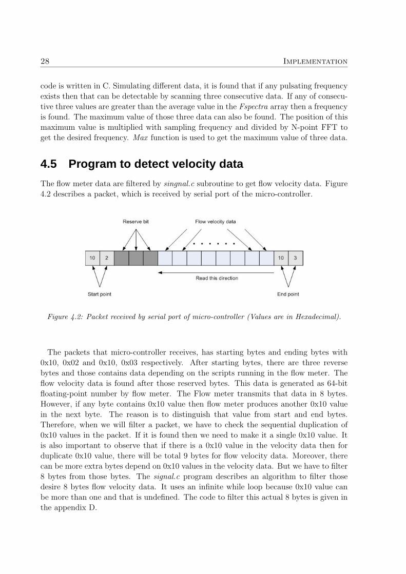
The flow meter data are filtered by singnal.c subroutine to get flow velocity data. Figure
4.2 describes a packet, which is received by serial port of the micro-controller.
Figure 4.2: Packet received by serial port of micro-controller (Values are in Hexadecimal).
The packets that micro-controller receives, has starting bytes and ending bytes with
0x10, 0x02 and 0x10, 0x03 respectively. After starting bytes, there are three reverse
bytes and those contains data depending on the scripts running in the flow meter. The
flow velocity data is found after those reserved bytes. This data is generated as 64-bit
floating-point number by flow meter. The Flow meter transmits that data in 8 bytes.
However, if any byte contains 0x10 value then flow meter produces another 0x10 value
in the next byte. The reason is to distinguish that value from start and end bytes.
Therefore, when we will filter a packet, we have to check the sequential duplication of
0x10 values in the packet. If it is found then we need to make it a single 0x10 value. It
is also important to observe that if there is a 0x10 value in the velocity data then for
duplicate 0x10 value, there will be total 9 bytes for flow velocity data. Moreover, there
can be more extra bytes depend on 0x10 values in the velocity data. But we have to filter
8 bytes from those bytes. The signal.c program describes an algorithm to filter those
desire 8 bytes flow velocity data. It uses an infinite while loop because 0x10 value can
be more than one and that is undefined. The code to filter this actual 8 bytes is given in
the appendix D.

4.6. Program to convert float64 to float32 29
The 8 bytes data that are filtered, should be read in opposite direction. Therefore, in
signal.c program data are stored from the bottom of the array so that first index contains
the starting byte of the 64-bit value.
4.6 Program to convert float64 to float32
ATMEL AVR Micro-controller does not support 64-bit float point number but it support
32-bit. Moreover, if floating-point numbers are used for calculation then it will take
double memory than an integer in data memory and that is expensive. Therefore, 64-
bit float point number is converted, first in 32-bit floating-point number where only the
integer part is used for FFT operation. Float64 to float32 program does this operation.
The 64-bit float point number is called IEEE double precision floating point standard
and 32-bit float point number is called IEEE single precision floating point standard.
The following table shows the layout for single (32-bit) and double (64-bit) precision
floating-point values. The number of bits for each field is also shown (bit ranges are in
square brackets):
Sign Exponent Fraction Bias
Single Precision 1 [31] 8 [30-23] 23 [22-00] 127
Double Precision 1 [63] 11 [62-52] 52 [51-00] 1023
Therefore, for conversion 11 bits of exponential part should be transferd in 8 bits and
52 bits fractional part should be transfer in 23 bits. In this, program left and right shift
and bias are used to perform it. First, 8 bits of 11 in exponential part and 23 bits of 52
bits in fractional part are taken and in exponential part bias 1023 is deducted and 127 is
added. This produce the 32-bit float and become almost same number that flow meter
sends. The code is shown in the appendix E.


CHAPTER 5
Results
In this section, different signals are used in Matlab and micro-controller. PWELCH
(Power Spectral Density estimate via Welch’s method) function is used to detect the
frequency in Matlab. Those signals are also used as the input of FFT in Micro-controller,
to detect the frequency then compare them with Matlab’s outputs. It shows exactly the
same result in both cases. First, y = 5× sin(2× π × 50× t) + 10× sin(2× π × 200× t)
signal’s Matlab result is shown in figure 5.1.
Figure 5.1: Welch method’s output for y = 5× sin(2× π × 50× t) + 10× sin(2× π × 200× t)signal (Matlab simulation).
31

32 Results
The Matlab code is as follows:
t = 0:0.001:300;
t = t(1:512);
y = 5 * sin(2*pi*50*t) + 10 * sin(2*pi*200*t);
y = y + abs(min(y));
y = y / max(y);
y = 1000 * y;
pwelch(y,window(@hamming,512),[],512,1000);
When this signal is used as input in Micro-controller, it detects peaks at 50.7813 Hz
and 199.2188 Hz. Therefore, an accurate performance is figured out by micro-controller.
In the next example, The same signal is used but some zero-mean random noise is used
to corrupt it. A common use of Fourier transforms is to find the frequency components
of a signal buried in a noisy time domain signal. By using Matlab’s PWELCH function,
the result is shown in figure 5.2.
Figure 5.2: Welch method’s output for previous signal corrupted by zero-mean random noise(Matlab simulation).
The Matlab code is as follows:
t = 0:0.001:0.6;
x = 5 * sin(2*pi*50*t)+ 10 * sin(2*pi*200*t);

33
y = x + 2*randn(size(t));
y = y(1:512); y = y + abs(min(y));
y = y / max(y);
y = 1000 * y;
pwelch(y, window(@hamming,512),[],512,1000);
The sampled signal is also given to the Micro-controller and it detects peaks at 50.7813
Hz and 199.2188 Hz. Therefore, the Micro-controller can detect frequencies from a signal
that is corrupted by zero-mean random noise.
In the last example, Berrebi’s data is used to detect the pulsating frequency. By using
Matlab’s PWELCH function on his data, the result is shown in figure 5.3.
Figure 5.3: Welch method’s output for Berrebi’s data (Matlab simulation).
First 512 data out of 9006 is used. Only the integer part of the data is considered. The
Matlab code for this manipulation is as follows:
t = 0:0.001:0.6;
x = 5 * sin(2*pi*50*t)+ 10 * sin(2*pi*200*t);
y = x + 2*randn(size(t));
y = y(1:512); y = y + abs(min(y));
y = y / max(y);
y = 1000 * y;
pwelch(y, window(@hamming,512),[],512,1000);

34 Results
Using those data, the Micro-controller detects peaks at 3.9437 Hz, 8.0751 Hz and
12.0188 Hz. Those are exactly similar with Matlab’s output. It shows a harmonic of
fundamental frequency 4Hz. Therefore, as in Berrebi’s implementation using a PC, a
pulsating flow is detected by the micro-controller.

CHAPTER 6
Future Work
The Inverse Fast Fourier Transform can be implemented to verify the present Fast
Fourier Transform. However, the Company, D-Flow Technology, Sweden who supplies
the flow meters, uses Mitsubishi M16 micro-controller to generate flow velocity data
from ultrasonic flow meter. From this data, pulsating flow is detected. The detection
of installation effect (both static and dynamic) can be implemented in that same micro-
controller already in the flow meter. A kernel can be designed to do both tasks (threads)
i.e. generation of flow velocity data and detection of installation effects, in parallel. It
will be more cost efficient and sophisticated then the present detection using matlab and
a laptop.
Figure 6.1: Future implementation for M-16 based Ultrasonic Flow Measurement.
35


CHAPTER 7
Conclusion
The ATMEL AVR AT90CAN128 can perform the FFT operation. The implemented
algorithm can also support some other 8-bit AVR and ATMEGA16. The detection of
pulsating flow of ultrasonic flow meter is performed accurately and satisfies the main
purpose of this thesis.
In the thesis, Floating point number conversion is implemented. The AVR does not
support 64-bit floating-point number and floating-point arithmetic is slower in AVR.
Therefore, 64-bit floating numbers are converted to 16-bit integers to support the AVR
and to make calculations faster. For computing 512-point FFT, 8-bit AVRs those have
2-cycle multiplier instruction take 371904 clock cycles i.e. about 46.49 milliseconds and
for frequency spectra, those take 155520 clock cycles i.e. about 19.44 milliseconds. It is
quite fast to synchronize with the velocity data of the ultrasonic flow meter.
This implementation enables flow meter and heat meter manufacturers to easily imple-
ment flow pulsation detection in their existing hardware, thereby improving billing and
benefits to district heating suppliers.
37


APPENDIX A
Code - Main function
This code calls main functions for FFT and display the results in Hyper Terminal.
/*------------------------------------------------*/
/* Developed by Shuvra Dev Sarker, 2006-----------*/
/* fftFlowMeter : A test program using flow meter input */
#include <avr/io.h>
#include <avr/pgmspace.h>
#include "fftHeader.h" /* Defs for using Fixed-point FFT module */
#include <inttypes.h>
#include <avr/interrupt.h>
#include <avr/signal.h>
#include <stdlib.h>
#include <stdio.h>
#include <math.h>
#define SYSCLK 8000000
#define sample_freq 96.15
/*------------------------------------------------*/
/* Global variables */
char hyper_input[16]; /* Console input buffer */
int16_t capture[FFT_N] = 512, 256, 128 or 64 sample data that will
be used as input in FFT function;
complex_t bfly_Array[FFT_N]; /* FFT buffer */
uint16_t Fspectra[FFT_N/2]; /* Spectrum output buffer */
/*------------------------------------------------*/
/* Functions */
int max(uint16_t container[],int length);
void detect_freq(uint16_t *signal);
/*:::::::::::::::::::::::::::::::::::::::::::::::::::::::::::::::*/
/*Just for test output*/
39

40 Appendix A
void USART0_Init (unsigned int baud )
/* Set baud rate */
UBRR0H = (unsigned char) (baud>>8);
UBRR0L = (unsigned char) baud;
/* Set frame format: 8data, no parity & 1 stop bits */
UCSR0C = (0<<UMSEL0) | (0<<UPM0) | (0<<USBS0) | (3<<UCSZ0);
/* Enable receiver and transmitter */
UCSR0B = (1<<RXEN0) | (1<<TXEN0);
void USART1_Init (unsigned int baud )
/* Set baud rate */
UBRR1H = (unsigned char) (baud>>8);
UBRR1L = (unsigned char) baud;
/* Set frame format: 8data, no parity & 1 stop bits */
UCSR1C = (0<<UMSEL1) | (0<<UPM1) | (0<<USBS1) | (3<<UCSZ1);
/* Enable receiver and transmitter */
UCSR1B = (1<<RXEN1) | (1<<TXEN1);
uint8_t USART0_Transmit (char data )
/* Wait for empty transmit buffer */
while ( ! ( UCSR0A & (1<<UDRE0)));
/* Put data into buffer, sends the data */
UDR0 = data;
return 0;
uint8_t USART1_Transmit (char data )
/* Wait for empty transmit buffer */
while ( ! ( UCSR1A & (1<<UDRE1)));
/* Put data into buffer, sends the data */
UDR1 = data;
return 0;
uint8_t USART0_Receive (void )
/* Wait for data to be received */
while ( ! (UCSR0A & (1<<RXC0)));
/* Get and return received data from buffer */
return UDR0;
uint8_t USART1_Receive (void )
/* Wait for data to be received */
while ( ! (UCSR1A & (1<<RXC1)));
/* Get and return received data from buffer */
return UDR1;
int main (void)
char *cp;
uint16_t n, s;
uint16_t t_input,t_execution,t_output;
int i;
DDRB = 0xFF;
USART1_Init(25); //38.4kBaud vid 16mhz
fdevopen(USART1_Transmit, USART1_Receive, 0);
TCCR1B = 3; /* clk/64 */
printf("FFT sample program\r\n");

41
for(;;)
printf("\r\n>");
scanf("%s",hyper_input);
cp = hyper_input;
switch (*cp++) /* Pick a header char (command) */
case ’\0’ : /* Blank line */
break;
case ’w’ : /* w: show flow meter data */
printf("%d\r\n ",FFT_N);
for (n = 0; n < FFT_N; n++)
s = flowInput[n];
printf("%d ",s);
break;
case ’s’ : /* s: show spectrum */
TCNT1 = 0; /* performance counter */
fft_input(flowInput, bfly_Array);
t_input = TCNT1;
printf("Input with Hamming window:");
for(i=0; i<FFT_N; i++)
printf("%d ",bfly_Array[i]);
printf("\r\n\r\n");
TCNT1 = 0;
fft_execute(bfly_Array);
t_execution = TCNT1;
printf("After Exacution of FFT:");
for(i=0; i<FFT_N; i++)
printf("%d ",bfly_Array[i]);
printf("\r\n\r\n");
printf("Fourier spectra:");
TCNT1 = 0;
fft_output(bfly_Array, Fspectra);
t_output = TCNT1;
for(i=0; i<FFT_N/2; i++)
printf("%u ",Fspectra[i]);
detect_freq(Fspectra);
printf("\r\ninput=%u, execute=%u, output=%u (x64clk)", t_input,t_execution,t_output);
break;
default : /* Unknown command */
printf("\n???");
return 0;
void detect_freq(uint16_t signal[])
uint16_t container[3];

42 Appendix A
int i,data,pos,sum, avg_signal;
double freq;
USART1_Init(25); //38.4kBaud vid 16mhz
fdevopen(USART1_Transmit, USART1_Receive, 0);
sum = 0;
for(i=0;i< FFT_N/2 ;i++)
sum= sum + signal[i];
avg_signal = ceil((double)sum/(FFT_N/2));
data = 3;
while(data < FFT_N/2 -1)
i = 0; pos = 0;
container[i]= signal[data];
container[i+1]= signal[data+1];
container[i+2]= signal[data+2];
if (avg_signal<container[i] && avg_signal<container[i+1] && avg_signal<container[i+2])
pos = max(container,3);
freq = ((double)(data+pos))*sample_freq/FFT_N;
printf("\r\nFrequency found in: %3.4f Hz",freq);
data = data + 3;
else
data = data + 1;
int max(uint16_t container[],int length)
int max = 0, i, pos = 0;
for(i = 0; i<length;i++)
if(container[i] > max)
max = container[i];
pos = i;
return pos;

APPENDIX B
Code - Macros
The following code represents all macros for FFT in Assembly language. This is the
header file of the fftSource.S, source file.
#ifndef FFT_N
#define FFT_N 512 /* Number of samples (64,128,256,512). */
#ifndef FFFT_ASM /* for c modules */
typedef struct _tag_complex_t
int16_t r;
int16_t i;
complex_t;
#ifndef INPUT_NOUSE
#ifdef INPUT_IQ
void fft_input (const complex_t *, complex_t *);
#else
void fft_input (const int16_t *, complex_t *);
#endif
#endif
void fft_execute (complex_t *);
void fft_output (complex_t *, uint16_t *);
int16_t fmuls_f (int16_t, int16_t);
extern const prog_int16_t tbl_window[];
#else /* for asm module */
#define R0L r0
#define R0H r1
#define R2L r2
#define R2H r3
#define R4L r4
#define R4H r5
#define R6L r6
#define R6H r7
#define R8L r8
#define R8H r9
#define R10L r10
43
44 Appendix B
#define R10H r11
#define R12L r12
#define R12H r13
#define R14L r14
#define R14H r15
#define AL r16
#define AH r17
#define BL r18
#define BH r19
#define CL r20
#define CH r21
#define DL r22
#define DH r23
#define EL r24
#define EH r25
#define XL r26
#define XH r27
#define YL r28
#define YH r29
#define ZL r30
#define ZH r31
.macro ldiw dh,dl, abs
ldi \dl, lo8(\abs)
ldi \dh, hi8(\abs)
.endm
.macro subiw dh,dl, abs
subi \dl, lo8(\abs)
sbci \dh, hi8(\abs)
.endm
.macro addw dh,dl, sh,sl
add \dl, \sl
adc \dh, \sh
.endm
.macro addd d3,d2,d1,d0, s3,s2,s1,s0
add \d0, \s0
adc \d1, \s1
adc \d2, \s2
adc \d3, \s3
.endm
.macro subw dh,dl, sh,sl
sub \dl, \sl
sbc \dh, \sh
.endm
.macro subd d3,d2,d1,d0, s3,s2,s1,s0
sub \d0, \s0
sbc \d1, \s1
sbc \d2, \s2
sbc \d3, \s3
.endm
.macro lddw dh,dl, src
ldd \dl, \src
ldd \dh, \src+1
.endm
.macro ldw dh,dl, src
ld \dl, \src

45
ld \dh, \src
.endm
.macro stw dst, sh,sl
st \dst, \sl
st \dst, \sh
.endm
.macro clrw dh, dl
clr \dh
clr \dl
.endm
.macro lsrw dh, dl
lsr \dh
ror \dl
.endm
.macro asrw dh, dl
asr \dh
ror \dl
.endm
.macro lslw dh, dl
lsl \dl
rol \dh
.endm
.macro pushw dh, dl
push \dh
push \dl
.endm
.macro popw dh, dl
pop \dl
pop \dh
.endm
.macro lpmw dh,dl, src
lpm \dl, \src
lpm \dh, \src
.endm
.macro rjne lbl
breq 99f
rjmp \lbl
99: .endm
// From AVR Data sheet
.macro FMULS16 d3,d2,d1,d0 ,s1h,s1l, s2h,s2l ;Fractional Multiply
(19clk)
fmuls \s1h, \s2h
movw \d2, R0L
fmul \s1l, \s2l
movw \d0, R0L
adc \d2, EH ;EH: zero reg.
fmulsu \s1h, \s2l
sbc \d3, EH
add \d1, R0L
adc \d2, R0H
adc \d3, EH
fmulsu \s2h, \s1l
46 Appendix B
sbc \d3, EH
add \d1, R0L
adc \d2, R0H
adc \d3, EH
.endm
.macro SQRT32 ; 32bit square root (526..542clk)
clr R6L
clr R6H
clr R8L
clr R8H
ldi BL, 1
ldi BH, 0
clr CL
clr CH
ldi DH, 16
90: lsl R2L
rol R2H
rol R4L
rol R4H
rol R6L
rol R6H
rol R8L
rol R8H
lsl R2L
rol R2H
rol R4L
rol R4H
rol R6L
rol R6H
rol R8L
rol R8H
brpl 91f
add R6L, BL
adc R6H, BH
adc R8L, CL
adc R8H, CH
rjmp 92f
91: sub R6L, BL
sbc R6H, BH
sbc R8L, CL
sbc R8H, CH
92: lsl BL
rol BH
rol CL
andi BL, 0b11111000
ori BL, 0b00000101
sbrc R8H, 7
subi BL, 2
dec DH
brne 90b
lsr CL
ror BH
ror BL
lsr CL
ror BH
ror BL
.endm
#endif /* FFFT_ASM */
#endif /* FFT_N */

APPENDIX C
Code - Function Descriptionand constant tables
The following code executes the fft input(), fft execute, fft output functions and the
constant tables.
; void fft_input (const int16_t *flowInput, complex_t *bfly_Array);
; void fft_execute (complex_t *bfly_Array);
; void fft_output (complex_t *bfly_Array, uint16_t *Fspectra);
;
; <flowInput>: flow meter input to be processed.
; <bfly_Array>: Complex array for butterfly operations.
; <Fspectra>: Spectrum output buffer.
;
; These functions must be called in sequence to do a DFT in FFT algorithm.
; fft_input() fills the complex array with the flow meter data to prepare butterfly
; operations. A hamming window is applied at the same time.
; fft_execute() executes the butterfly operations.
; fft_output() re-orders the results, converts the complex spectrum into
; scalar spectrum and output it in linear scale.
;
; The number of points FFT_N is defined in "fftHeader.h" and the value can be 64,
; 128, 256 or 512.
;
.nolist
#define FFFT_ASM
#include "fftHeader.h"
.list
#if FFT_N == 512
#define FFT_B 9
#elif FFT_N == 256
#define FFT_B 8
#elif FFT_N == 128
#define FFT_B 7
#elif FFT_N == 64
#define FFT_B 6
#else
47
48 Appendix C
#error FFT_N must be 64,128,256 or 512.
#endif
;----------------------------------------------------------------------------;
; Constant Tables
.global tbl_window
tbl_window: ; tbl_window[] = ... (This is a Hamming window)
#if FFT_N == 512
.dc.w 2621, 2622, 2626, 2632, 2640, 2650, 2662, 2677, 2694, 2714, 2735, 2759, 2785, 2814, 2844, 2877
.dc.w 2912, 2949, 2989, 3031, 3075, 3121, 3169, 3220, 3273, 3328, 3385, 3444, 3506, 3569, 3635, 3703
.dc.w 3773, 3845, 3919, 3996, 4074, 4155, 4237, 4321, 4408, 4496, 4587, 4680, 4774, 4870, 4969, 5069
.dc.w 5171, 5275, 5381, 5489, 5599, 5710, 5824, 5939, 6056, 6174, 6295, 6417, 6541, 6666, 6793, 6922
.dc.w 7052, 7185, 7318, 7453, 7590, 7728, 7868, 8010, 8152, 8296, 8442, 8589, 8737, 8887, 9038, 9191
.dc.w 9344, 9499, 9655, 9813, 9971, 10131, 10292, 10454, 10617, 10781, 10946, 11113, 11280, 11448, 11617, 11787
.dc.w 11958, 12130, 12303, 12476, 12650, 12825, 13001, 13178, 13355, 13533, 13711, 13890, 14070, 14250, 14431, 14612
.dc.w 14793, 14975, 15158, 15341, 15524, 15708, 15892, 16076, 16260, 16445, 16629, 16814, 16999, 17185, 17370, 17555
.dc.w 17741, 17926, 18111, 18296, 18481, 18667, 18851, 19036, 19221, 19405, 19589, 19773, 19956, 20139, 20322, 20504
.dc.w 20686, 20867, 21048, 21229, 21409, 21588, 21767, 21945, 22122, 22299, 22475, 22651, 22825, 22999, 23172, 23344
.dc.w 23516, 23686, 23856, 24025, 24192, 24359, 24525, 24689, 24853, 25016, 25177, 25337, 25496, 25654, 25811, 25967
.dc.w 26121, 26274, 26426, 26576, 26725, 26873, 27019, 27164, 27308, 27450, 27590, 27729, 27867, 28003, 28137, 28270
.dc.w 28401, 28531, 28659, 28785, 28910, 29033, 29154, 29274, 29391, 29507, 29622, 29734, 29845, 29953, 30060, 30165
.dc.w 30268, 30370, 30469, 30566, 30662, 30755, 30847, 30936, 31024, 31109, 31193, 31274, 31354, 31431, 31506, 31579
.dc.w 31650, 31719, 31786, 31851, 31913, 31974, 32032, 32088, 32142, 32194, 32243, 32291, 32336, 32379, 32419, 32458
.dc.w 32494, 32528, 32560, 32589, 32617, 32642, 32664, 32685, 32703, 32719, 32733, 32744, 32753, 32760, 32764, 32767
.dc.w 32767, 32764, 32760, 32753, 32744, 32733, 32719, 32703, 32685, 32664, 32642, 32617, 32589, 32560, 32528, 32494
.dc.w 32458, 32419, 32379, 32336, 32291, 32243, 32194, 32142, 32088, 32032, 31974, 31913, 31851, 31786, 31719, 31650
.dc.w 31579, 31506, 31431, 31354, 31274, 31193, 31109, 31024, 30936, 30847, 30755, 30662, 30566, 30469, 30370, 30268
.dc.w 30165, 30060, 29953, 29845, 29734, 29622, 29507, 29391, 29274, 29154, 29033, 28910, 28785, 28659, 28531, 28401
.dc.w 28270, 28137, 28003, 27867, 27729, 27590, 27450, 27308, 27164, 27019, 26873, 26725, 26576, 26426, 26274, 26121
.dc.w 25967, 25811, 25654, 25496, 25337, 25177, 25016, 24853, 24689, 24525, 24359, 24192, 24025, 23856, 23686, 23516
.dc.w 23344, 23172, 22999, 22825, 22651, 22475, 22299, 22122, 21945, 21767, 21588, 21409, 21229, 21048, 20867, 20686
.dc.w 20504, 20322, 20139, 19956, 19773, 19589, 19405, 19221, 19036, 18851, 18667, 18481, 18296, 18111, 17926, 17741
.dc.w 17555, 17370, 17185, 16999, 16814, 16629, 16445, 16260, 16076, 15892, 15708, 15524, 15341, 15158, 14975, 14793
.dc.w 14612, 14431, 14250, 14070, 13890, 13711, 13533, 13355, 13178, 13001, 12825, 12650, 12476, 12303, 12130, 11958
.dc.w 11787, 11617, 11448, 11280, 11113, 10946, 10781, 10617, 10454, 10292, 10131, 9971, 9813, 9655, 9499, 9344
.dc.w 9191, 9038, 8887, 8737, 8589, 8442, 8296, 8152, 8010, 7868, 7728, 7590, 7453, 7318, 7185, 7052
.dc.w 6922, 6793, 6666, 6541, 6417, 6295, 6174, 6056, 5939, 5824, 5710, 5599, 5489, 5381, 5275, 5171
.dc.w 5069, 4969, 4870, 4774, 4680, 4587, 4496, 4408, 4321, 4237, 4155, 4074, 3996, 3919, 3845, 3773
.dc.w 3703, 3635, 3569, 3506, 3444, 3385, 3328, 3273, 3220, 3169, 3121, 3075, 3031, 2989, 2949, 2912
.dc.w 2877, 2844, 2814, 2785, 2759, 2735, 2714, 2694, 2677, 2662, 2650, 2640, 2632, 2626, 2622, 2621
#elif FFT_N == 256
.dc.w 2621, 2626, 2640, 2663, 2695, 2736, 2786, 2845, 2913, 2990, 3077, 3172, 3275, 3388, 3509, 3639
.dc.w 3778, 3924, 4080, 4243, 4415, 4595, 4782, 4978, 5181, 5392, 5610, 5836, 6069, 6308, 6555, 6809
.dc.w 7069, 7336, 7608, 7888, 8173, 8463, 8760, 9061, 9368, 9681, 9998, 10319, 10645, 10976, 11310, 11648
.dc.w 11990, 12336, 12685, 13036, 13391, 13748, 14108, 14470, 14833, 15199, 15566, 15934, 16303, 16674, 17044, 17416
.dc.w 17787, 18158, 18529, 18900, 19270, 19639, 20006, 20372, 20737, 21100, 21461, 21819, 22175, 22528, 22878, 23226
.dc.w 23569, 23910, 24246, 24578, 24907, 25231, 25550, 25864, 26174, 26478, 26778, 27071, 27359, 27641, 27917, 28187
.dc.w 28450, 28707, 28957, 29201, 29437, 29666, 29888, 30103, 30310, 30509, 30701, 30885, 31060, 31228, 31387, 31538
.dc.w 31681, 31815, 31941, 32058, 32166, 32265, 32356, 32438, 32510, 32574, 32629, 32674, 32711, 32738, 32757, 32766
.dc.w 32766, 32757, 32738, 32711, 32674, 32629, 32574, 32510, 32438, 32356, 32265, 32166, 32058, 31941, 31815, 31681
.dc.w 31538, 31387, 31228, 31060, 30885, 30701, 30509, 30310, 30103, 29888, 29666, 29437, 29201, 28957, 28707, 28450
.dc.w 28187, 27917, 27641, 27359, 27071, 26778, 26478, 26174, 25864, 25550, 25231, 24907, 24578, 24246, 23910, 23569
.dc.w 23226, 22878, 22528, 22175, 21819, 21461, 21100, 20737, 20372, 20006, 19639, 19270, 18900, 18529, 18158, 17787
.dc.w 17416, 17044, 16674, 16303, 15934, 15566, 15199, 14833, 14470, 14108, 13748, 13391, 13036, 12685, 12336, 11990
.dc.w 11648, 11310, 10976, 10645, 10319, 9998, 9681, 9368, 9061, 8760, 8463, 8173, 7888, 7608, 7336, 7069
.dc.w 6809, 6555, 6308, 6069, 5836, 5610, 5392, 5181, 4978, 4782, 4595, 4415, 4243, 4080, 3924, 3778
.dc.w 3639, 3509, 3388, 3275, 3172, 3077, 2990, 2913, 2845, 2786, 2736, 2695, 2663, 2640, 2626, 2621
#elif FFT_N == 128
.dc.w 2621, 2640, 2695, 2787, 2916, 3080, 3281, 3516, 3787, 4091, 4429, 4799, 5201, 5633, 6095, 6585
.dc.w 7102, 7645, 8213, 8804, 9417, 10050, 10702, 11371, 12055, 12754, 13464, 14185, 14914, 15650, 16391, 17135
.dc.w 17881, 18626, 19369, 20107, 20840, 21565, 22281, 22985, 23677, 24354, 25014, 25657, 26280, 26882, 27462, 28018
.dc.w 28548, 29052, 29528, 29975, 30393, 30779, 31133, 31454, 31741, 31994, 32212, 32395, 32542, 32652, 32726, 32762
.dc.w 32762, 32726, 32652, 32542, 32395, 32212, 31994, 31741, 31454, 31133, 30779, 30393, 29975, 29528, 29052, 28548
.dc.w 28018, 27462, 26882, 26280, 25657, 25014, 24354, 23677, 22985, 22281, 21565, 20840, 20107, 19369, 18626, 17881
.dc.w 17135, 16391, 15650, 14914, 14185, 13464, 12754, 12055, 11371, 10702, 10050, 9417, 8804, 8213, 7645, 7102
.dc.w 6585, 6095, 5633, 5201, 4799, 4429, 4091, 3787, 3516, 3281, 3080, 2916, 2787, 2695, 2640, 2621
#elif FFT_N == 64
.dc.w 2621, 2696, 2920, 3291, 3805, 4457, 5240, 6148, 7170, 8296, 9516, 10818, 12187, 13612, 15077, 16568
.dc.w 18070, 19568, 21048, 22495, 23893, 25231, 26493, 27668, 28743, 29709, 30556, 31274, 31858, 32301, 32599, 32748
.dc.w 32748, 32599, 32301, 31858, 31274, 30556, 29709, 28743, 27668, 26493, 25231, 23893, 22495, 21048, 19568, 18070
.dc.w 16568, 15077, 13612, 12187, 10818, 9516, 8296, 7170, 6148, 5240, 4457, 3805, 3291, 2920, 2696, 2621
#endif
tbl_cos_sin: ; Table of cos(x),sin(x), (0 <= x < pi, in FFT_N/2 steps)
#if FFT_N == 512

49
.dc.w 32767, 0, 32764, 402, 32757, 804, 32744, 1206, 32727, 1607, 32705, 2009, 32678, 2410, 32646, 2811
.dc.w 32609, 3211, 32567, 3611, 32520, 4011, 32468, 4409, 32412, 4807, 32350, 5205, 32284, 5601, 32213, 5997
.dc.w 32137, 6392, 32056, 6786, 31970, 7179, 31880, 7571, 31785, 7961, 31684, 8351, 31580, 8739, 31470, 9126
.dc.w 31356, 9511, 31236, 9895, 31113, 10278, 30984, 10659, 30851, 11038, 30713, 11416, 30571, 11792, 30424, 12166
.dc.w 30272, 12539, 30116, 12909, 29955, 13278, 29790, 13645, 29621, 14009, 29446, 14372, 29268, 14732, 29085, 15090
.dc.w 28897, 15446, 28706, 15799, 28510, 16150, 28309, 16499, 28105, 16845, 27896, 17189, 27683, 17530, 27466, 17868
.dc.w 27244, 18204, 27019, 18537, 26789, 18867, 26556, 19194, 26318, 19519, 26077, 19840, 25831, 20159, 25582, 20474
.dc.w 25329, 20787, 25072, 21096, 24811, 21402, 24546, 21705, 24278, 22004, 24006, 22301, 23731, 22594, 23452, 22883
.dc.w 23169, 23169, 22883, 23452, 22594, 23731, 22301, 24006, 22004, 24278, 21705, 24546, 21402, 24811, 21096, 25072
.dc.w 20787, 25329, 20474, 25582, 20159, 25831, 19840, 26077, 19519, 26318, 19194, 26556, 18867, 26789, 18537, 27019
.dc.w 18204, 27244, 17868, 27466, 17530, 27683, 17189, 27896, 16845, 28105, 16499, 28309, 16150, 28510, 15799, 28706
.dc.w 15446, 28897, 15090, 29085, 14732, 29268, 14372, 29446, 14009, 29621, 13645, 29790, 13278, 29955, 12909, 30116
.dc.w 12539, 30272, 12166, 30424, 11792, 30571, 11416, 30713, 11038, 30851, 10659, 30984, 10278, 31113, 9895, 31236
.dc.w 9511, 31356, 9126, 31470, 8739, 31580, 8351, 31684, 7961, 31785, 7571, 31880, 7179, 31970, 6786, 32056
.dc.w 6392, 32137, 5997, 32213, 5601, 32284, 5205, 32350, 4807, 32412, 4409, 32468, 4011, 32520, 3611, 32567
.dc.w 3211, 32609, 2811, 32646, 2410, 32678, 2009, 32705, 1607, 32727, 1206, 32744, 804, 32757, 402, 32764
.dc.w 0, 32766, -402, 32764, -804, 32757, -1206, 32744, -1607, 32727, -2009, 32705, -2410, 32678, -2811, 32646
.dc.w -3211, 32609, -3611, 32567, -4010, 32520, -4409, 32468, -4807, 32412, -5205, 32350, -5601, 32284, -5997, 32213
.dc.w -6392, 32137, -6786, 32056, -7179, 31970, -7571, 31880, -7961, 31785, -8351, 31684, -8739, 31580, -9126, 31470
.dc.w -9511, 31356, -9895, 31236, -10278, 31113, -10659, 30984, -11038, 30851, -11416, 30713, -11792, 30571, -12166, 30424
.dc.w -12539, 30272, -12909, 30116, -13278, 29955, -13645, 29790, -14009, 29621, -14372, 29446, -14732, 29268, -15090, 29085
.dc.w -15446, 28897, -15799, 28706, -16150, 28510, -16499, 28309, -16845, 28105, -17189, 27896, -17530, 27683, -17868, 27466
.dc.w -18204, 27244, -18537, 27019, -18867, 26789, -19194, 26556, -19519, 26318, -19840, 26077, -20159, 25831, -20474, 25582
.dc.w -20787, 25329, -21096, 25072, -21402, 24811, -21705, 24546, -22004, 24278, -22301, 24006, -22594, 23731, -22883, 23452
.dc.w -23169, 23169, -23452, 22883, -23731, 22594, -24006, 22301, -24278, 22005, -24546, 21705, -24811, 21402, -25072, 21096
.dc.w -25329, 20787, -25582, 20474, -25831, 20159, -26077, 19840, -26318, 19519, -26556, 19194, -26789, 18867, -27019, 18537
.dc.w -27244, 18204, -27466, 17868, -27683, 17530, -27896, 17189, -28105, 16845, -28309, 16499, -28510, 16150, -28706, 15799
.dc.w -28897, 15446, -29085, 15090, -29268, 14732, -29446, 14372, -29620, 14009, -29790, 13645, -29955, 13278, -30116, 12910
.dc.w -30272, 12539, -30424, 12167, -30571, 11792, -30713, 11416, -30851, 11038, -30984, 10659, -31113, 10278, -31236, 9895
.dc.w -31356, 9511, -31470, 9126, -31580, 8739, -31684, 8351, -31784, 7961, -31880, 7571, -31970, 7179, -32056, 6786
.dc.w -32137, 6392, -32213, 5997, -32284, 5601, -32350, 5205, -32412, 4807, -32468, 4409, -32520, 4011, -32567, 3611
.dc.w -32609, 3211, -32646, 2811, -32678, 2410, -32705, 2009, -32727, 1607, -32744, 1206, -32757, 804, -32764, 402
#elif FFT_N == 256
.dc.w 32767, 0, 32757, 804, 32727, 1607, 32678, 2410, 32609, 3211, 32520, 4011, 32412, 4807, 32284, 5601
.dc.w 32137, 6392, 31970, 7179, 31785, 7961, 31580, 8739, 31356, 9511, 31113, 10278, 30851, 11038, 30571, 11792
.dc.w 30272, 12539, 29955, 13278, 29621, 14009, 29268, 14732, 28897, 15446, 28510, 16150, 28105, 16845, 27683, 17530
.dc.w 27244, 18204, 26789, 18867, 26318, 19519, 25831, 20159, 25329, 20787, 24811, 21402, 24278, 22004, 23731, 22594
.dc.w 23169, 23169, 22594, 23731, 22004, 24278, 21402, 24811, 20787, 25329, 20159, 25831, 19519, 26318, 18867, 26789
.dc.w 18204, 27244, 17530, 27683, 16845, 28105, 16150, 28510, 15446, 28897, 14732, 29268, 14009, 29621, 13278, 29955
.dc.w 12539, 30272, 11792, 30571, 11038, 30851, 10278, 31113, 9511, 31356, 8739, 31580, 7961, 31785, 7179, 31970
.dc.w 6392, 32137, 5601, 32284, 4807, 32412, 4011, 32520, 3211, 32609, 2410, 32678, 1607, 32727, 804, 32757
.dc.w 0, 32766, -804, 32757, -1607, 32727, -2410, 32678, -3211, 32609, -4010, 32520, -4807, 32412, -5601, 32284
.dc.w -6392, 32137, -7179, 31970, -7961, 31785, -8739, 31580, -9511, 31356, -10278, 31113, -11038, 30851, -11792, 30571
.dc.w -12539, 30272, -13278, 29955, -14009, 29621, -14732, 29268, -15446, 28897, -16150, 28510, -16845, 28105, -17530, 27683
.dc.w -18204, 27244, -18867, 26789, -19519, 26318, -20159, 25831, -20787, 25329, -21402, 24811, -22004, 24278, -22594, 23731
.dc.w -23169, 23169, -23731, 22594, -24278, 22005, -24811, 21402, -25329, 20787, -25831, 20159, -26318, 19519, -26789, 18867
.dc.w -27244, 18204, -27683, 17530, -28105, 16845, -28510, 16150, -28897, 15446, -29268, 14732, -29620, 14009, -29955, 13278
.dc.w -30272, 12539, -30571, 11792, -30851, 11038, -31113, 10278, -31356, 9511, -31580, 8739, -31784, 7961, -31970, 7179
.dc.w -32137, 6392, -32284, 5601, -32412, 4807, -32520, 4011, -32609, 3211, -32678, 2410, -32727, 1607, -32757, 804
#elif FFT_N == 128
.dc.w 32767, 0, 32727, 1607, 32609, 3211, 32412, 4807, 32137, 6392, 31785, 7961, 31356, 9511, 30851, 11038
.dc.w 30272, 12539, 29621, 14009, 28897, 15446, 28105, 16845, 27244, 18204, 26318, 19519, 25329, 20787, 24278, 22004
.dc.w 23169, 23169, 22004, 24278, 20787, 25329, 19519, 26318, 18204, 27244, 16845, 28105, 15446, 28897, 14009, 29621
.dc.w 12539, 30272, 11038, 30851, 9511, 31356, 7961, 31785, 6392, 32137, 4807, 32412, 3211, 32609, 1607, 32727
.dc.w 0, 32766, -1607, 32727, -3211, 32609, -4807, 32412, -6392, 32137, -7961, 31785, -9511, 31356, -11038, 30851
.dc.w -12539, 30272, -14009, 29621, -15446, 28897, -16845, 28105, -18204, 27244, -19519, 26318, -20787, 25329, -22004, 24278
.dc.w -23169, 23169, -24278, 22005, -25329, 20787, -26318, 19519, -27244, 18204, -28105, 16845, -28897, 15446, -29620, 14009
.dc.w -30272, 12539, -30851, 11038, -31356, 9511, -31784, 7961, -32137, 6392, -32412, 4807, -32609, 3211, -32727, 1607
#elif FFT_N == 64
.dc.w 32767, 0, 32609, 3211, 32137, 6392, 31356, 9511, 30272, 12539, 28897, 15446, 27244, 18204, 25329, 20787
.dc.w 23169, 23169, 20787, 25329, 18204, 27244, 15446, 28897, 12539, 30272, 9511, 31356, 6392, 32137, 3211, 32609
.dc.w 0, 32766, -3211, 32609, -6392, 32137, -9511, 31356, -12539, 30272, -15446, 28897, -18204, 27244, -20787, 25329
.dc.w -23169, 23169, -25329, 20787, -27244, 18204, -28897, 15446, -30272, 12539, -31356, 9511, -32137, 6392, -32609, 3211
#endif
tbl_bitrev: ; tbl_bitrev[] = ...
#if FFT_N == 512
#ifdef INPUT_IQ
.dc.w 1*4, 257*4, 129*4, 385*4, 65*4, 321*4, 193*4, 449*4, 33*4, 289*4, 161*4, 417*4, 97*4, 353*4, 225*4, 481*4
.dc.w 17*4, 273*4, 145*4, 401*4, 81*4, 337*4, 209*4, 465*4, 49*4, 305*4, 177*4, 433*4, 113*4, 369*4, 241*4, 497*4
.dc.w 9*4, 265*4, 137*4, 393*4, 73*4, 329*4, 201*4, 457*4, 41*4, 297*4, 169*4, 425*4, 105*4, 361*4, 233*4, 489*4
.dc.w 25*4, 281*4, 153*4, 409*4, 89*4, 345*4, 217*4, 473*4, 57*4, 313*4, 185*4, 441*4, 121*4, 377*4, 249*4, 505*4
.dc.w 5*4, 261*4, 133*4, 389*4, 69*4, 325*4, 197*4, 453*4, 37*4, 293*4, 165*4, 421*4, 101*4, 357*4, 229*4, 485*4
.dc.w 21*4, 277*4, 149*4, 405*4, 85*4, 341*4, 213*4, 469*4, 53*4, 309*4, 181*4, 437*4, 117*4, 373*4, 245*4, 501*4
.dc.w 13*4, 269*4, 141*4, 397*4, 77*4, 333*4, 205*4, 461*4, 45*4, 301*4, 173*4, 429*4, 109*4, 365*4, 237*4, 493*4
.dc.w 29*4, 285*4, 157*4, 413*4, 93*4, 349*4, 221*4, 477*4, 61*4, 317*4, 189*4, 445*4, 125*4, 381*4, 253*4, 509*4
.dc.w 3*4, 259*4, 131*4, 387*4, 67*4, 323*4, 195*4, 451*4, 35*4, 291*4, 163*4, 419*4, 99*4, 355*4, 227*4, 483*4
.dc.w 19*4, 275*4, 147*4, 403*4, 83*4, 339*4, 211*4, 467*4, 51*4, 307*4, 179*4, 435*4, 115*4, 371*4, 243*4, 499*4
.dc.w 11*4, 267*4, 139*4, 395*4, 75*4, 331*4, 203*4, 459*4, 43*4, 299*4, 171*4, 427*4, 107*4, 363*4, 235*4, 491*4

50 Appendix C
.dc.w 27*4, 283*4, 155*4, 411*4, 91*4, 347*4, 219*4, 475*4, 59*4, 315*4, 187*4, 443*4, 123*4, 379*4, 251*4, 507*4
.dc.w 7*4, 263*4, 135*4, 391*4, 71*4, 327*4, 199*4, 455*4, 39*4, 295*4, 167*4, 423*4, 103*4, 359*4, 231*4, 487*4
.dc.w 23*4, 279*4, 151*4, 407*4, 87*4, 343*4, 215*4, 471*4, 55*4, 311*4, 183*4, 439*4, 119*4, 375*4, 247*4, 503*4
.dc.w 15*4, 271*4, 143*4, 399*4, 79*4, 335*4, 207*4, 463*4, 47*4, 303*4, 175*4, 431*4, 111*4, 367*4, 239*4, 495*4
.dc.w 31*4, 287*4, 159*4, 415*4, 95*4, 351*4, 223*4, 479*4, 63*4, 319*4, 191*4, 447*4, 127*4, 383*4, 255*4, 511*4
#endif
.dc.w 0*4, 256*4, 128*4, 384*4, 64*4, 320*4, 192*4, 448*4, 32*4, 288*4, 160*4, 416*4, 96*4, 352*4, 224*4, 480*4
.dc.w 16*4, 272*4, 144*4, 400*4, 80*4, 336*4, 208*4, 464*4, 48*4, 304*4, 176*4, 432*4, 112*4, 368*4, 240*4, 496*4
.dc.w 8*4, 264*4, 136*4, 392*4, 72*4, 328*4, 200*4, 456*4, 40*4, 296*4, 168*4, 424*4, 104*4, 360*4, 232*4, 488*4
.dc.w 24*4, 280*4, 152*4, 408*4, 88*4, 344*4, 216*4, 472*4, 56*4, 312*4, 184*4, 440*4, 120*4, 376*4, 248*4, 504*4
.dc.w 4*4, 260*4, 132*4, 388*4, 68*4, 324*4, 196*4, 452*4, 36*4, 292*4, 164*4, 420*4, 100*4, 356*4, 228*4, 484*4
.dc.w 20*4, 276*4, 148*4, 404*4, 84*4, 340*4, 212*4, 468*4, 52*4, 308*4, 180*4, 436*4, 116*4, 372*4, 244*4, 500*4
.dc.w 12*4, 268*4, 140*4, 396*4, 76*4, 332*4, 204*4, 460*4, 44*4, 300*4, 172*4, 428*4, 108*4, 364*4, 236*4, 492*4
.dc.w 28*4, 284*4, 156*4, 412*4, 92*4, 348*4, 220*4, 476*4, 60*4, 316*4, 188*4, 444*4, 124*4, 380*4, 252*4, 508*4
.dc.w 2*4, 258*4, 130*4, 386*4, 66*4, 322*4, 194*4, 450*4, 34*4, 290*4, 162*4, 418*4, 98*4, 354*4, 226*4, 482*4
.dc.w 18*4, 274*4, 146*4, 402*4, 82*4, 338*4, 210*4, 466*4, 50*4, 306*4, 178*4, 434*4, 114*4, 370*4, 242*4, 498*4
.dc.w 10*4, 266*4, 138*4, 394*4, 74*4, 330*4, 202*4, 458*4, 42*4, 298*4, 170*4, 426*4, 106*4, 362*4, 234*4, 490*4
.dc.w 26*4, 282*4, 154*4, 410*4, 90*4, 346*4, 218*4, 474*4, 58*4, 314*4, 186*4, 442*4, 122*4, 378*4, 250*4, 506*4
.dc.w 6*4, 262*4, 134*4, 390*4, 70*4, 326*4, 198*4, 454*4, 38*4, 294*4, 166*4, 422*4, 102*4, 358*4, 230*4, 486*4
.dc.w 22*4, 278*4, 150*4, 406*4, 86*4, 342*4, 214*4, 470*4, 54*4, 310*4, 182*4, 438*4, 118*4, 374*4, 246*4, 502*4
.dc.w 14*4, 270*4, 142*4, 398*4, 78*4, 334*4, 206*4, 462*4, 46*4, 302*4, 174*4, 430*4, 110*4, 366*4, 238*4, 494*4
.dc.w 30*4, 286*4, 158*4, 414*4, 94*4, 350*4, 222*4, 478*4, 62*4, 318*4, 190*4, 446*4, 126*4, 382*4, 254*4, 510*4
#elif FFT_N == 256
#ifdef INPUT_IQ
.dc.w 1*4, 129*4, 65*4, 193*4, 33*4, 161*4, 97*4, 225*4, 17*4, 145*4, 81*4, 209*4, 49*4, 177*4, 113*4, 241*4
.dc.w 9*4, 137*4, 73*4, 201*4, 41*4, 169*4, 105*4, 233*4, 25*4, 153*4, 89*4, 217*4, 57*4, 185*4, 121*4, 249*4
.dc.w 5*4, 133*4, 69*4, 197*4, 37*4, 165*4, 101*4, 229*4, 21*4, 149*4, 85*4, 213*4, 53*4, 181*4, 117*4, 245*4
.dc.w 13*4, 141*4, 77*4, 205*4, 45*4, 173*4, 109*4, 237*4, 29*4, 157*4, 93*4, 221*4, 61*4, 189*4, 125*4, 253*4
.dc.w 3*4, 131*4, 67*4, 195*4, 35*4, 163*4, 99*4, 227*4, 19*4, 147*4, 83*4, 211*4, 51*4, 179*4, 115*4, 243*4
.dc.w 11*4, 139*4, 75*4, 203*4, 43*4, 171*4, 107*4, 235*4, 27*4, 155*4, 91*4, 219*4, 59*4, 187*4, 123*4, 251*4
.dc.w 7*4, 135*4, 71*4, 199*4, 39*4, 167*4, 103*4, 231*4, 23*4, 151*4, 87*4, 215*4, 55*4, 183*4, 119*4, 247*4
.dc.w 15*4, 143*4, 79*4, 207*4, 47*4, 175*4, 111*4, 239*4, 31*4, 159*4, 95*4, 223*4, 63*4, 191*4, 127*4, 255*4
#endif
.dc.w 0*4, 128*4, 64*4, 192*4, 32*4, 160*4, 96*4, 224*4, 16*4, 144*4, 80*4, 208*4, 48*4, 176*4, 112*4, 240*4
.dc.w 8*4, 136*4, 72*4, 200*4, 40*4, 168*4, 104*4, 232*4, 24*4, 152*4, 88*4, 216*4, 56*4, 184*4, 120*4, 248*4
.dc.w 4*4, 132*4, 68*4, 196*4, 36*4, 164*4, 100*4, 228*4, 20*4, 148*4, 84*4, 212*4, 52*4, 180*4, 116*4, 244*4
.dc.w 12*4, 140*4, 76*4, 204*4, 44*4, 172*4, 108*4, 236*4, 28*4, 156*4, 92*4, 220*4, 60*4, 188*4, 124*4, 252*4
.dc.w 2*4, 130*4, 66*4, 194*4, 34*4, 162*4, 98*4, 226*4, 18*4, 146*4, 82*4, 210*4, 50*4, 178*4, 114*4, 242*4
.dc.w 10*4, 138*4, 74*4, 202*4, 42*4, 170*4, 106*4, 234*4, 26*4, 154*4, 90*4, 218*4, 58*4, 186*4, 122*4, 250*4
.dc.w 6*4, 134*4, 70*4, 198*4, 38*4, 166*4, 102*4, 230*4, 22*4, 150*4, 86*4, 214*4, 54*4, 182*4, 118*4, 246*4
.dc.w 14*4, 142*4, 78*4, 206*4, 46*4, 174*4, 110*4, 238*4, 30*4, 158*4, 94*4, 222*4, 62*4, 190*4, 126*4, 254*4
#elif FFT_N == 128
#ifdef INPUT_IQ
.dc.w 1*4, 65*4, 33*4, 97*4, 17*4, 81*4, 49*4, 113*4, 9*4, 73*4, 41*4, 105*4, 25*4, 89*4, 57*4, 121*4
.dc.w 5*4, 69*4, 37*4, 101*4, 21*4, 85*4, 53*4, 117*4, 13*4, 77*4, 45*4, 109*4, 29*4, 93*4, 61*4, 125*4
.dc.w 3*4, 67*4, 35*4, 99*4, 19*4, 83*4, 51*4, 115*4, 11*4, 75*4, 43*4, 107*4, 27*4, 91*4, 59*4, 123*4
.dc.w 7*4, 71*4, 39*4, 103*4, 23*4, 87*4, 55*4, 119*4, 15*4, 79*4, 47*4, 111*4, 31*4, 95*4, 63*4, 127*4
#endif
.dc.w 0*4, 64*4, 32*4, 96*4, 16*4, 80*4, 48*4, 112*4, 8*4, 72*4, 40*4, 104*4, 24*4, 88*4, 56*4, 120*4
.dc.w 4*4, 68*4, 36*4, 100*4, 20*4, 84*4, 52*4, 116*4, 12*4, 76*4, 44*4, 108*4, 28*4, 92*4, 60*4, 124*4
.dc.w 2*4, 66*4, 34*4, 98*4, 18*4, 82*4, 50*4, 114*4, 10*4, 74*4, 42*4, 106*4, 26*4, 90*4, 58*4, 122*4
.dc.w 6*4, 70*4, 38*4, 102*4, 22*4, 86*4, 54*4, 118*4, 14*4, 78*4, 46*4, 110*4, 30*4, 94*4, 62*4, 126*4
#elif FFT_N == 64
#ifdef INPUT_IQ
.dc.w 1*4, 33*4, 17*4, 49*4, 9*4, 41*4, 25*4, 57*4, 5*4, 37*4, 21*4, 53*4, 13*4, 45*4, 29*4, 61*4
.dc.w 3*4, 35*4, 19*4, 51*4, 11*4, 43*4, 27*4, 59*4, 7*4, 39*4, 23*4, 55*4, 15*4, 47*4, 31*4, 63*4
#endif
.dc.w 0*4, 32*4, 16*4, 48*4, 8*4, 40*4, 24*4, 56*4, 4*4, 36*4, 20*4, 52*4, 12*4, 44*4, 28*4, 60*4
.dc.w 2*4, 34*4, 18*4, 50*4, 10*4, 42*4, 26*4, 58*4, 6*4, 38*4, 22*4, 54*4, 14*4, 46*4, 30*4, 62*4
#endif
;----------------------------------------------------------------------------;
#ifndef INPUT_NOUSE
.global fft_input
.func fft_input
fft_input:
pushw R2H,R2L
pushw AH,AL
pushw YH,YL
movw XL, EL ;X = hyper_input;
movw YL, DL ;Y = bfly_Array;
clr EH ;Zero
ldiw ZH,ZL, tbl_window ;Z = &tbl_window[0];
ldiw AH,AL, FFT_N ;A = FFT_N;

51
1: lpmw BH,BL, Z+ ;B = *Z++; (window)
ldw CH,CL, X+ ;C = *X++; (I-axis)
FMULS16 DH,DL,R2H,R2L, BH,BL, CH,CL ;D = B * C;
stw Y+, DH,DL ;*Y++ = D;
#ifdef INPUT_IQ
ldw CH,CL, X+ ;C = *X++; (Q-axis)
FMULS16 DH,DL,R2H,R2L, BH,BL, CH,CL ;D = B * C;
#endif
stw Y+, DH,DL ;*Y++ = D;
subiw AH,AL, 1 ;while(--A)
brne 1b ;/
popw YH,YL
popw AH,AL
popw R2H,R2L
clr r1
ret
.endfunc
#endif /* INPUT_NOUSE */
;----------------------------------------------------------------------------;
.global fft_execute
.func fft_execute
fft_execute:
pushw R2H,R2L
pushw R4H,R4L
pushw R6H,R6L
pushw R8H,R8L
pushw R10H,R10L
pushw R12H,R12L
pushw R14H,R14L
pushw AH,AL
pushw YH,YL
movw ZL, EL ;Z = bfly_Array;
ldiw EH,EL, 1 ;E = 1;
ldiw XH,XL, FFT_N/2 ;X = FFT_N/2;
1: ldi AL, 4 ;T12 = E; (angular speed)
mul EL, AL ;
movw R12L, R0L ;
mul EH, AL ;
add R12H, R0L ;/
movw R14L, EL ;T14 = E;
pushw EH,EL
movw YL, ZL ;Z = &bfly_Array[0];
mul XL, AL ;Y = &bfly_Array[X];
addw YH,YL, R0H,R0L ;
mul XH, AL ;
add YH, R0L ;/
pushw ZH,ZL
2: clrw R10H,R10L ;T10 = 0 (angle)
clr EH ;Zero reg.
3: lddw AH,AL, Z+0 ;A = *Z - *Y; *Z++ += *Y;
asrw AH,AL ;
lddw DH,DL, Y+0 ;
asrw DH,DL ;
movw CL, AL ;
subw AH,AL, DH,DL ;
addw CH,CL, DH,DL ;
stw Z+, CH,CL ;/
lddw BH,BL, Z+0 ;B = *Z - *Y; *Z++ += *Y;
asrw BH,BL ;
52 Appendix C
lddw DH,DL, Y+2 ;
asrw DH,DL ;
movw CL, BL ;
subw BH,BL, DH,DL ;
addw CH,CL, DH,DL ;
stw Z+, CH,CL ;/
movw R0L, ZL
ldiw ZH,ZL, tbl_cos_sin ;C = cos(T10); D = sin(T10);
addw ZH,ZL, R10H,R10L ;
lpmw CH,CL, Z+ ;
lpmw DH,DL, Z+ ;/
movw ZL, R0L
FMULS16 R4H,R4L,R2H,R2L, AH,AL, CH,CL ;*Y++ = A * C + B * D;
FMULS16 R8H,R8L,R6H,R6L, BH,BL, DH,DL ;
addd R4H,R4L,R2H,R2L, R8H,R8L,R6H,R6L;
stw Y+, R4H,R4L ;/
FMULS16 R4H,R4L,R2H,R2L, BH,BL, CH,CL ;*Y++ = B * C - A * D;
FMULS16 R8H,R8L,R6H,R6L, AH,AL, DH,DL ;
subd R4H,R4L,R2H,R2L, R8H,R8L,R6H,R6L;
stw Y+, R4H,R4L ;/
addw R10H,R10L, R12H,R12L ;T10 += T12; (next angle)
#if FFT_N >= 128
sbrs R10H, FFT_B - 7 ;while(T10 < pi)
#else
sbrs R10L, FFT_B + 1
#endif
rjmp 3b ;/
ldi AL, 4 ;Y += X; Z += X; (skip split segment)
mul XL, AL
addw YH,YL, R0H,R0L ;
addw ZH,ZL, R0H,R0L ;
mul XH, AL ;
add YH, R0L ;
add ZH, R0L ;/
ldi EL, 1 ;while(--T14)
subw R14H,R14L, EH,EL ;
rjne 2b ;/
popw ZH,ZL
popw EH,EL
lslw EH,EL ;E *= 2;
lsrw XH,XL ;while(X /= 2)
adiw XL, 0 ;
rjne 1b ;/
popw YH,YL
popw AH,AL
popw R14H,R14L
popw R12H,R12L
popw R10H,R10L
popw R8H,R8L
popw R6H,R6L
popw R4H,R4L
popw R2H,R2L
; clr r1
ret
.endfunc
;----------------------------------------------------------------------------;
.global fft_output
.func fft_output
fft_output:
pushw R2H,R2L
pushw R4H,R4L

53
pushw R6H,R6L
pushw R8H,R8L
pushw R10H,R10L
pushw AH,AL
pushw YH,YL
movw R10L, EL ;T10 = bfly_Array;
movw YL, DL ;Y = array_output;
ldiw ZH,ZL, tbl_bitrev ;Z = tbl_bitrev;
clr EH ;Zero
#ifdef INPUT_IQ
ldiw AH,AL, FFT_N ;A = FFT_N; (pluse/minus)
#else
ldiw AH,AL, FFT_N / 2 ;A = FFT_N / 2; (pluse only)
#endif
1: lpmw XH,XL, Z+ ;X = *Z++;
addw XH,XL, R10H,R10L ;X += bfly_Array;
ldw BH,BL, X+ ;B = *X++;
ldw CH,CL, X+ ;C = *X++;
FMULS16 R4H,R4L,R2H,R2L, BH,BL, BH,BL ;T4:T2 = B * B;
FMULS16 R8H,R8L,R6H,R6L, CH,CL, CH,CL ;T8:T6 = C * C;
addd R4H,R4L,R2H,R2L, R8H,R8L,R6H,R6L;T4:T2 += T8:T6;
SQRT32 ;B = sqrt(T4:T2);
stw Y+, BH,BL ;*Y++ = B;
subiw AH,AL, 1 ;while(--A)
rjne 1b ;/
popw YH,YL
popw AH,AL
popw R10H,R10L
popw R8H,R8L
popw R6H,R6L
popw R4H,R4L
popw R2H,R2L
clr r1
ret
.endfunc
;----------------------------------------------------------------------------;
.global fmuls_f
.func fmuls_f
fmuls_f:
movw CL, EL ;C = E;
clr EH ;Zero
FMULS16 ZH,ZL,XH,XL, CH,CL, DH,DL ;Z:X = C * D;
movw EL, ZL
clr r1
ret
.endfunc


APPENDIX D
Code - Flow Meter datafiltering
The following program filters the ultrasonic flow meter data and gets velocity data.
#include <stdio.h>
#include <avr/interrupt.h>
#include <avr/signal.h>
#include <inttypes.h>
unsigned char signal_array[11];
int main(void)
int8_t index = 10, flag = 0, i;
uint8_t c = ’\r’, old_c;
USART1_Init(25); //38.4kBaud vid 16mhz
fdevopen(USART1_Transmit, USART1_Receive, 0);
printf("\r\ntest:");
while (1)
old_c = c;
c = getchar();
if(flag == 1)
if((old_c == ’10’) && (c==’10’))// Check the 10 & 10 in string
else if(index >=0)
signal_array[index]=c;
index--;
if((old_c == ’10’) && (c==’2’)) // Check the start point of the string
flag = 1;
index = 10;
55

56 Appendix D
if((old_c == ’10’) && (c==’3’)) // Check the end point of the string
flag = 0;
break;
for(i = 0; i<11;i++)
printf("%c ",signal_array[i]);
return 0;

APPENDIX E
Code - Covert float64 tofloat32
The following program converts 64-bit floating-point number to 32-bit floating-point
number.
#include <stdio.h>
#include <avr/interrupt.h>
#include <avr/signal.h>
#include <inttypes.h>
#include <stdlib.h>
#include <string.h>
int main(void)
unsigned char ch[8] = 0x40,0x34,0xA0,0x00,0x00,0x00,0x00,0x00;
long lvalue;
double value;
long fraction= (((uint32_t)(ch[1] & 0x0f))<< 19)|
(((uint32_t)(ch[2] & 0xff))<<11)|
(((uint32_t)(ch[3] & 0xff))<<3)|
(((uint32_t)(ch[4]& 0xe0))>>5);
long mantissa=(((uint32_t)(ch[0] & 0x7f))<< 4) |((uint32_t)(ch[1] >> 4));
mantissa = mantissa - 1023 + 127;
lvalue = (((uint32_t)(ch[0] & 0x80)) << 24) | ((0xff & mantissa) << 23) | ((fraction & 0x007fffff));
memcpy(&value,&lvalue,4);
USART1_Init(25); //38.4kBaud vid 16mhz
fdevopen(USART1_Transmit, USART1_Receive, 0);
printf("Mantissa: %li\n\r", mantissa);
printf("fraction: %lx\n\r", fraction);
printf("value: %lx\n\r", value);
printf("\r\ntest:");
57

58
printf("%lf %lf", lvalue, value);
return 0;

Bibliography
[1] J. Berrebi. Self-diagnosis techniques and Their Application to Error Reduction for
Ultrasonic Flow Measurement, Doctoral Thesis 2004:23. Department of Computer
Science and Electrical Engineering, Division of EISLAB, Lulea University of Tech-
nology, 2004. ISSN 1402-1544.
[2] J. Berrebi, J. Van Deventer, J. Delsing. Lulea University of Technology. Detection
of Pulsating Flows in an Ultrasonic Flow Meter. Proc. of the 8th Int. Symposium
on District Hearting and Cooling in Trondheim, 2002.
[3] C. Carlander. Installation Effect and Self Diagnostics for Ultrasonic Flow Measure-
ment, Doctoral Thesis 2001:11. Department of Computer Science and Electrical En-
gineering, Division of Industrial Electronics, Lulea University of Technology, 2004.
ISSN 1402-1544.
[4] R. A. Furness. Fluid flow measurement, measurement and control technology series,
Edited by T. P. Flanagan. Longmann, 1989.
[5] K. J. Zanker. The development of flow straightener for use with orifice plate meters
in disturbed flows. In symposium on flow measurement in closed conduits, 1969.
Paper D-2.
[6] B. Svensson. In-situ test methods in distinct heating systems - application to heat
meters and subscriber stations. licentiate thesis 1996:46, Lulea University of Tech-
nology, 1996. ISSN 0280-8242.
[7] R. C. Jr. Mills. Magnetic flowmeters, pages 175-219 in flow measurement - practical
guides for measurement and control, Edited by D.W. Spitzer. Instrument Society of
America, 1991.
[8] L. Smith and J. R. Ruesch. Mass flowmeters, pages 221-247 in flow measurement -
practical guides for measurement and control, Edited by D. W. Spitzer, Instrument
Society of America, 1991.
[9] O. Rutten. German patent 520. filled 1928, 1931.
59

60
[10] L. C. Lynnworth. Ultrasonic Flow Meters, pages 407-525 in physical acoustic, Vol.
14, Mason and Thurston, Eds. Academic Press, New York, 1979.
[11] J. Delsing. Viscosity effects in the sing-around type flow meters. In proc. Of Int.
conf. Industrial Measurement Onshore and offshore, September, 1987.
[12] J. Delsing. A new velocity algorithm for sing-around type flow meter. IEEE Trans.
On UFFC, volumn 34, No. 4, pages 431-436, 1987.
[13] J. Delsing. The zero flow performance of sing-around type flow meter. Flow Mea-
surement and Instrumentation, volumn 2, No. 4, 1991.
[14] Z. Rui, X. Xin-hai, L. Xiang-yuan and Z. Hong-guang. Research for measuring reli-
ability of ultrasonic flow meters and dry calibration. In proc. FLOMEKO’96, 1996.
[15] C. Carlander and J. Delsing. Installation effects on an ultrasonic flow meter with
implications for self diagnostics. Flow Measurement and Instrumentation. Published
by Elsevier Science. Volumn 11, No. 2, page 109-122(14), june, 2000.
[16] J. Larsen. Ultrasonic flow metering in district heating systems - experiences in Scan-
dinavia and Switzerland. In AG-SITI. Danfoss, 1987.
[17] E. J. Lindahl. Pulsation and its effects on flow meters. Trans ASME, Volumn 68,
pages 883-894, 1946.
[18] R. C. Mottram. An overview of pulsating flow measurement. Flow measurement and
Instrumentation, volumn 3, No. 3 pages 114-117, 1992.
[19] D.C. Mizushina, T. Maruyama and Y. Shiozaki. Pulsating turbulent flow in a tube.
J. of Chemical Engineering of Japan, volumn 6, No. 2, pages 487-494, 1973.
[20] E. Hakansson, J. Delsing. Effects of Pulsating Flow on an Ultrasonic Gas Flowmeter.
Lund Institute of Technology, Lund, Sweden, 1993.
[21] R. Carter Hill, William E. Griffiths and George G. Judge. Undergraduate Economet-
rics. Second edition, John Wiley and Sons, Inc, New York, N.Y., 2001, pp 138-139.
[22] J. Hinich. Detecting a Hidden Periodic Signal When its period is Unknown. IEEE
transactions on Acoustics, Speech and Signal Processing. Vol. ASSP-30, No. 5, Oc-
tober, 1982.
[23] B. P. Lathi. Linear Systems and Signals. Oxford University Press. Second edition,
page 801, ISBN 0-19-515833-4, 2005.
[24] Z. Gajic. Linear Dynamic Systems and Signals. Prentice Hall, page 111, ISBN
0-201-61854-0, 2003.

61
[25] AVR Assembler User Guide.
Link: http://www.atmel.com/dyn/resources/prod documents/doc1022.pdf, Janu-
ary, 1998.
[26] Oppenheim, A.V., and R.W. Schafer. Discrete-Time Signal Processing. Upper Saddle
River, Prentice Hall. Second edition, page 468-471, ISBN 0-13-083443-2, 1999.