Detection of Signals by the Digital Integrate-and-Dump

TDA Progress Report 42-91 July-September 1987

Detection of Signals by the Digital Integrate-and-Dump Filter With Offset Sampling

R. Sadr and W. J. Hurd Communications Systems Research Section

The Integrate-and-Dump Filter (IDF) is used as a matched filter for the detection of signals in additive white Gaussian noise. In this article, the performance of the digital integrateanddump filter is evaluated. The case considered is when symbol times are known and the sampling clock is free running at a constant rate, i.e., the sampling clock is not phase locked to the symbol clock. Degradations in the output signal-to-noise ratio of the digital implementation due to sampling rate, sampling offset, and finite bandwidth, resulting from the anti-aliasing low-pass prefilter, are computed and compared with those of the analog counterpart. I t is shown that the digital IDF performs within 0.6 dB of the ideal analog IDF whenever the prefilter bandwidth exceeds four times the symbol rate and when sampling is performed at the Nyquist rate. The loss can be reduced to 0.3 dB by doubling the sampling rate, where 0.2 dB loss results from finite bandwidth and 0.1 dB results from the digital IDF.

1. Introduction An Integrate-and-Dump Filter (IDF) is the ideal matched

filter for coherent detection of rectangular pulse shape signals corrupted by additive white Gaussian noise (AWGN). A digital implementation of the IDF has numerous advantages over its analog counterpart, such as the ability t o dump instanta- neously with no overshoot, freedom of drift from the quies- cent operating point, and the use of advanced digital inte- grated circuits (ICs) to perform multiplication and accumula- tion with greater accuracy than the analog counterparts.

A. Current Problem

The digital implementation of the IDF requires the input waveform to be sampled. This requires that the input signal be

filtered prior t o sampling t o eliminate aliasing. Throughout this article, the anti-aliasing low-pass prefilter is also referred to simply as the filter. Filtering of the observed signal results in the transmitted signal pulses becoming band limited and also causes Inter-Symbol Interference (ISI). The finite bandwidth of the observed signal and ISJ both degrade the performance of the receiver. In order t o evaluate the performance versus the filter bandwidth and sampling frequency, the analog IDF depicted in Fig. l(a) is compared with the performance of the digital IDF shown in Fig. I(b).

In the limit, as the prefilter low-pass bandwidth W Hz and, as a consequence, the sampling rate approach infinity, the performance of the digital IDF converges t o that of the analog JDF. However, this is not practical from an implementation

I 158

point of view, since large bandwidths require higher sampling rates to satisfy the Nyquist criterion. In this article, we find the performance degradation which results from filtering the received signal and from using only a small finite number of samples.

Furthermore, we also superimpose the effect of “offset sampling” in the performance of the digital IDF. When sampling a signal of finite duration T sec with a sampling period of T, sec, the first sample of the signal may occur anywhere in the time interval 0 < f < T,. This consideration for the digital IDF has not been studied previously. In this article, in addition to analyzing the effects of prefiltering and sampling on performance, we seek to find the degradation due to this offset.

In the advanced receiver being developed for the NASA Deep Space Network, a wide range of symbol rates must be processed with the maximum available bandwidth and sampling rate. When the number of samples per symbol is large, the loss due to the offset in sampling is negligible. This loss is not negligible at high symbol rates, when the number of samples per symbol is not large.

In the digital IDF implementation, we assume that the sampling clock is free running at a constant rate, i.e., that the sampling clock is not phase locked to a multiple of the symbol clock. We also assume perfect symbol synchronization in the sense that the receiver has perfect information regarding the time that each symbol starts and ends.

For all of the results presented in this article except Section V.E, the symbol period is an integer multiple of the sampling period, and the performance is determined as a function of the relative phase offset between the sample times and the symbol times, In Section V.E, we consider the case for which the symbol period is not an integer multiple of the sampling period. We ignore quantization noise and oscillator instability in this article.

6. Previous Work

The digital IDF was studied previously by Natali [ l ] in 1969. In [ 11, a first order low-pass filter was considered and the signal-to-noise ratio (SNR) loss was analyzed for different time bandwidth products. Only a single symbol was considered. Our results match those of Natali for the case of no offset, a single symbol, and using a first order low-pass filter.

In 1969. Hartman [2] studied the degradation of SNR due to intermediate frequency (IF) filtering. He computed the SNR degradation due to bandwidth limiting of a biphase modulated signal when using an analog IDF. A lower boundary for the SNR was derived for different time-bandwidth products.

In 1976, Turin [3] analyzed the noncoherent digital matched filter matched to amplitude-modulated (AM) signals in the presence of additive white Gaussian noise and jamming. He showed that in the presence of jamming, improvement is possible over the analog matched filter by threshold biasing and dithering techniques for demodulation.

In 1978, Lim [4] analyzed the noncoherent digital matched filters with multibit quantization, matched to phase-shift- keyed signals.

In 1979, Chie [5] analyzed the digital IDF filter. The performance of the digital IDF was evaluated in relation to the number of bits used by the analog-to-digital (A/D) converter, the bandwidth of the prefilter, and the gain loading factor of the A/D converter. He also considered quantization error and the accumulator length. To study the performance of the digital IDF, he considered the symbol error probability resulting from hard quantization of the output of the digital IDF.

It is difficult to determine the exact symbol error probability in the presence of ISI, which is inherent in digital IDF systems. The IS1 is caused by the low-pass filtering of the input signal. Recently, Helstrom [6] and Levy [7] outlined general algorithms for approximation of the symbol error probability. We should note here that numerous articles and techniques address the approximation of the symbol error probability in the presence of ISI. Citing all the references on this subject is beyond the scope of this article. Furthermore, our intended application for this article is the advanced receiver for NASA’s Deep Space Network. The receiver output detected symbol values are quantized to several bits of accuracy (soft decision), as opposed to making hard decisions on the symbols. These quantized symbols are then used by the decoder for estimating the transmitted bit sequence. In our case, the SNR is therefore a more relevant parameter than the symbol error probability.

We make the fundamental assumption that the sampling clock is stable and the receiver symbol clock is synchronized. The effects of transmitter receiver clock time-base instability on coherent communication systems was analyzed by Chie [8] in 1982. The types of time-base instability modeled and analyzed are bit jitter and bit jitter rate.

C. Outline of Article

In Section 11, the IDF is formulated and the average signal response and noise variance are derived. In Section 111, the expression for the loss is formulated. In Section IV, the loss is expressed for two special cases: the first order low-pass filter and the ideal low-pass filter. In Section V, the numerical results are presented for known waveforms and for pseudo- random data patterns generated by Monte Carlo simulation.

159

Selections of bandwidth, sampling rate, and asynchronous sampling are discussed in this section. This work is summarized and conclusions are drawn in Section VI, and Section VI1 sug- gests a direction for future work.

II. System Description The received signal plus noise is denoted by r ( t ) = s ( t - r0)

+ n(t), where s ( t ) is the signal, n(t) is the noise, and ro is the delay from the transmitter to the receiver. The transmitted signal s ( t ) is a sequence of pulses expressed as

s ( t ) = ak p ( t - k T ) k

At this point we impose no restriction on the shape or duration of each pulse p ( t ) . The input alphabet U is a finite alpha- b e t w i t h a i e U = {+1,+2 , . . . , k m .

The analog IDF is shown in Fig. l(a). The analog system is an ideal matched filter when p ( t ) is a rectangular pulse from t = 0 t o t = T. It detects the k th symbol by integrating over time k T + ro t o (k + 1) T + ro . The digital IDF is depicted in Fig. l(b). In the digital implementation, an anti-aliasing low- pass prefilter is used for filtering the input signal. The filter output is sampled, with the ith sample occurring at time iT, + r l . The digital IDF detects the k t h symbol by summing

I all the samples from t = k T + ro t o t = (k + 1) T + r0.

We assume that there is perfect symbol synchronization at the receiver, so the beginning and end times of each symbol are known. For the k t h symbol, the “sampling offset” is defined by the time difference between the start of the symbol and the first sample within the symbol time, i.e., (iT, + T ~ ) - (kT + ro). The first sample within each symbol time may occur anywhere between 0 and seconds. A typical symbol waveform and the sampling points are shown in Fig. 2 . We seek t o determine the signal-to-noise ratio (SNR) for the output sample of this system.

Initially, we consider the average signal response of the digital IDF; later we consider the noise response.

A. Average Signal Response

r ( t ) is The response of the low-pass filter t o the observed signal

Using Eq. (1) for s ( t ) we have

c

This signal y ( t ) is sampled each T, sec at time 1 = iT, + T ~ . We denote y(iT, + r l ) asy;. Taking the expectation of Eq. (3) conditioned on a given data sequence a, and noting that the noise n(t) is assumed to have zero mean, the conditional expectation o f y i is

With a change of variable, Eq. (4) can be written as

E [ y ; = ‘k h(iT, - k T + 6 - x ) p(x)dx k

(5)

where 6 = r1 - ro. Let

represent the signal response of the filter a t time iTs + r1 due t o a single pulse at time k T + ro. For simplicity we denote q,(k, 6), as qi(k) . The total average signal response from Eq. (5) for a given fixed 6 may be expressed as

Let Zk be the set of all i such that the i t h sample falls in the k t h symbol time, Le.,

Ik = {i: k T < i T s + 6 < ( k + l)T} (8)

160

1

The IDF output for the k t h symbol, denoted by A , , is

The expectation of A , over the noise, conditioned on a and 6 , is

To further simplify this expression, define the event indi- cator function which is 1 if and only if idk, i.e.,

f o r k T < i T s + 6 < ( k + l)T

0 otherwise Zi(6; k) =

Thus from Eq. (10) we have

6. Noise Response

Next we consider the noise response of the IDF to compute the total SNR at the output of the IDF. Let zi denote the sampled noise response of the filter at time iT, + T ~ .

Since the IDF is a linear system, the variance of A , conditioned on _a is equal t o the variance of the response of the k t h symbol due to noise alone, i.e., it is independent of ~ ( t ) . The variance of A , is

(14) i j

Note that this variance does depend on 6 and k, because the number of samples occurring in the k t h symbol depends on 6. Using Eq. (3) and noting that E [ n ( t ) n ( ~ ) ] = N0/2 6,(t - 7 ) ,

where here &,(e) is the Dirac delta function, we have

where R, is the autocorrelation of z i .

111. Definition of Signal-to-Noise Ratio Loss The analog IDF of Fig. l a is the optimum matched when

p ( t ) = 1 for 0 < t < T and zero otherwise. The SNR is defined at the IDF output as the ratio of the square of the mean to the variance. Denoting SNR, for the analog IDF, it is well known [ 101 that

2A2T

NO SNR, = -

We assume with no loss of generality that the signal amplitude A = 1 , so SNR, = 2T/No.

The SNR at the output of the digital IDF is denoted by SNR,. We compare the performance of the digital IDF with the analog IDF by considering the ratio

. SNR- U -

SNR,

We define SNR, at the output of the IDF as the ratio of the square of the conditional mean to the conditional variance of the output, conditioned on a given sequence and offset value. From this definition of SNR.

Then we have

NO 7 = - SNR, 2T

In the remaining sections, ?dB = 10 loglo(y) (dB) is computed for various filters and data patterns. Normally y < 1, because the digital IDF has a loss with respect t o the analog IDF. The degradation or loss-in decibels is the negative of y d B ,

and minimum loss corresponds to the maximum attainable y, which typically approaches one (ydB = 0 dB). Maximum loss is unbounded. In some cases, for a given data patterng, there

161

is a gain in SNR (e.g., all-ones sequence), in which cases y > 1 and the degradation is negative in decibels.

IV. SNR Performance for Special Cases In general, the pulse shape p ( t ) may be chosen t o take

numerous shapes (e.g., raised root-cosine). In some cases, it is chosen t o extend over more than one symbol duration, e.g., for partial response signaling (sometimes referred as correlated coding or controlled intersymbol interference). For bandwidth-limited channels, the pulse shape and duration are selected to increase the bandwidth efficiency of the communication system.

We consider only non-overlapping rectangular pulses throughout the rest of this article, since this pulse shape has traditionally been used for NASA's deep space missions. It is pointed out that the results of the previous sections, namely the expressions for average signal response in Eq. (12) and the noise variance in Eq. (1 5), hold regardless of the pulse shape or its duration.

In the case of the rectangular pulse we simply have

O < t < T

otherwise P ( t ) =

then from Eq. (6)

q,(k) = h(iTs - kT t 6 - x)dx

and

It is useful t o write Eq. (1 9) as

( k + l ) T h(iT, t 6 - x) dx

We now consider two different low-pass filters, one causal and one non-causal.

A. First Order Low-Pass Filter (Causal)

The impulse response for a first order low-pass filter is h ( t ) = We-wr u ( t ) , where u ( t ) denotes the unit step response

and W is the radian cutoff frequency of the filter. The filter in this case is causal and therefore physically realizable, i.e., h ( t ) = 0 for c < 0. Using Eq. (20) t o evaluate ql(k) from Eq. (121,

) ; k T < i q t 6 < ( k t l ) T -W(ITs+6-kT)

; ( k t 1 ) T < i q + 6

To derive the equation for the noise variance, we use the expression in Eq. (1 5), resulting in

i c I k j e I k

To obtain the relative performance of the digital IDF when using a first order low-pass filter, we use the signal response expression in Eq. (21) and the noise variance in Eq. (22). Then, from Eq. (1 8), y is

where qj(kT) is defined in Eq. (21). For a known data pattern, Eq. (21) may be evaluated for different k , 6 , and time bandwidth products (WT) .

B. Ideal Low Pass Filter (Non-Causal)

width W Hz is non-causal with the impulse response The ideal low-pass filter with unit gain and low-pass band-

The expression for the signal response in Eq. (20) becomes

( k + 1 ) T sin 2n W ( i q t 6 - x ) (iq t 6 - x ) dx (25)

162

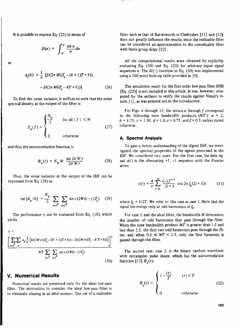
It is possible to express Eq. (25) in terms of

sinu Si(x) = Jo -du U

as

1 q,.(k) = n [ S i ( 2 ~ W(i< - (k + 1 ) T t 6))

- Si(2n W ( i 5 - kT + S))] (26)

To find the noise variance, it suffices to note that the noise spectral density at the output of the filter is

otherwise

and thus the autocorrelation function is

Thus, the noise variance at the output of the IDF can be expressed from Eq. (28) as

var[Ak16] =- No sinc(2W(i-,j)TJ (29) 2 i e I k j e r k

The performance y can be evaluated from Eq. (18), which yields

- Y =

V. Numerical Results Numerical results are presented only for the ideal low-pass

filter. The motivation to consider the ideal low-pass filter is to eliminate aliasing in an ideal manner. The use of a realizable

filter such as that of Butterworth or Chebyshev [ 111 and [12] does not greatly influence the results, since the realizable filter can be considered an approximation to the unrealizable filter with finite group delay [ 121 .

All the computational results were obtained by explicitly evaluating Eq. (30) and Eq. (23) for arbitrary input signal sequences a. The Si(.) functipn in Eq. (30) was implemented using a 500 point look-up table provided in [9].

The simulation result for the first order low-pass filter SNR [Eq. (23)] is not included in this article. It was, however, computed by the authors to verify the results against Natali’s results [ 11 , as was pointed out in the introduction.

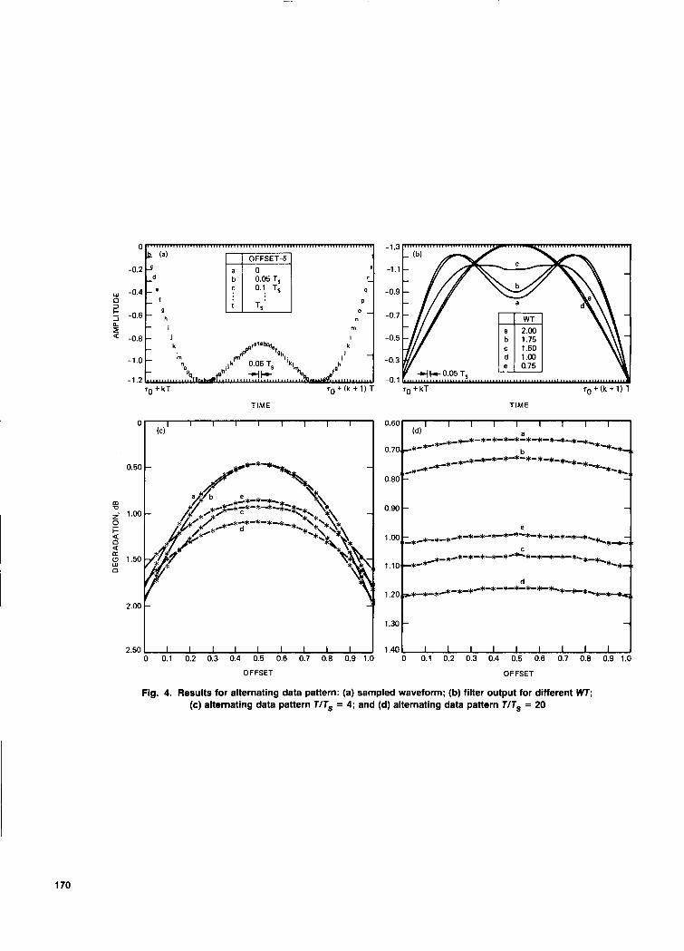
For Figs. 4 through 13, the letters a through f correspond to the following time bandwidth products (WT): a = 2, b = 1.75, c = 1.50, d = 1.0, e = 0.75, a n d f = 0.5, unless stated otherwise .

A. Spectral Analysis

To gain a better understanding of the digital IDF, we inves- tigated the spectral properties of the signals processed in the IDF. We considered two cases. For the first case, the data signal s ( r ) is the alternating t1, -1 sequence with the Fourier series

cos 2n&(2i t 1)t (3 1) n i= 0

where fo = 1/2T. We refer to this case as case 1. Note that the signal has energy only at odd harmonics of $, .

For case 1 and the ideal filter, the bandwidth W determines the number of odd harmonics that pass through the filter. When the time bandwidth product WT is greater than 1.5 and less than 2.5, the first two odd harmonics pass through the filter; and when 0.5 < WT < 1.5, only the first harmonic is passed through the filter.

The second case, case 2, is the binary random waveform with rectangular pulse shape, which has the autocorrelation function [ 131 RS(7):

( 0 otherwise

163

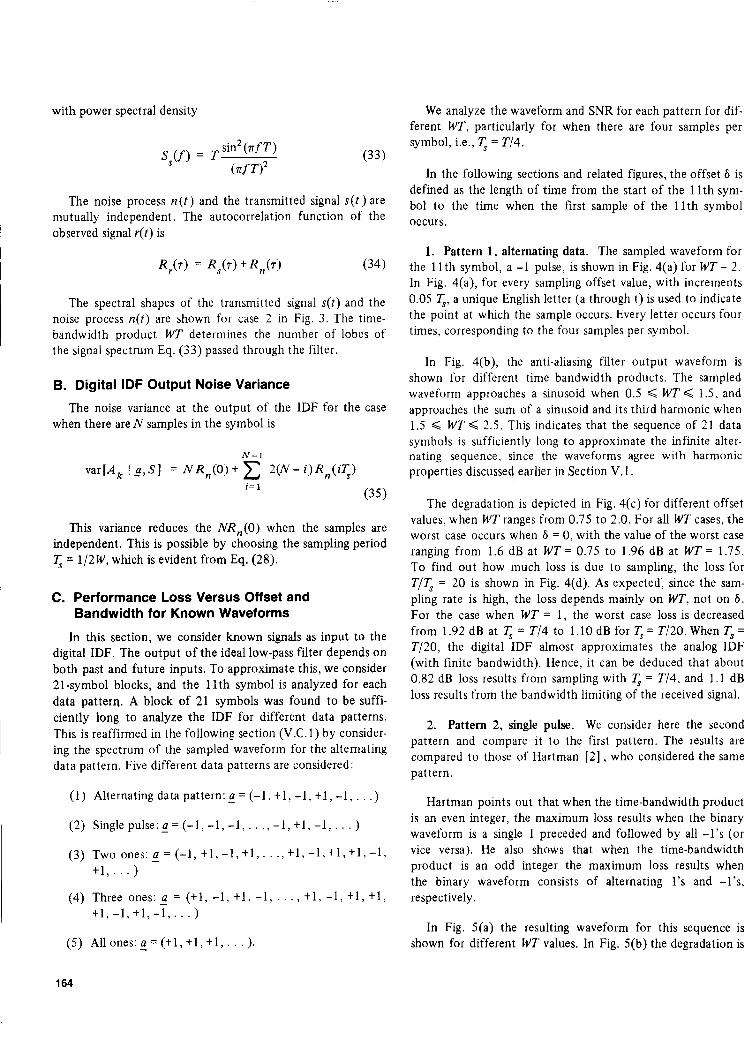
with power spectral density

(33)

The noise process n ( t ) and the transmitted signal s(t ) are mutually independent. The autocorrelation function of the observed signal r(t) is I

(34)

The spectral shapes of the transmitted signal s ( t ) and the noise process n(t) are shown for case 2 in Fig. 3. The time- bandwidth product WT determines the number of lobes of the signal spectrum Eq. (33) passed through the filter.

B. Digital IDF Output Noise Variance

when there are N samples in the symbol is The noise variance at the output of the IDF for the case

This variance reduces the NR,(O) when the samples are independent. This is possible by choosing the sampling period T, = 1/2W, which is evident from Eq. (28).

C. Performance Loss Versus Offset and Bandwidth for Known Waveforms

In this section, we consider known signals as input t o the digital IDF. The output of the ideal low-pass filter depends o n both past and future inputs. To approximate this, we consider 21 -symbol blocks, and the 1 lth symbol is analyzed for each data pattern. A block of 21 symbols was found t o be sufficiently long t o analyze the IDF for different data patterns. This is reaffirmed in the following section (V.C.l) by considering the spectrum of the sampled waveform for the alternating data pattern. Five different data patterns are considered:

(1) Alternat ingdatapat tern:g=(-1.+1,-1, t 1 , - 1 , . . .)

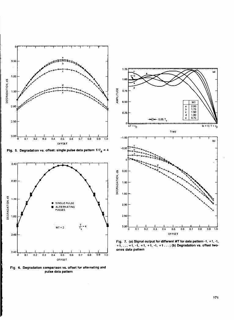
(2) Single pulse: g = (-1, -1, -1, . . . , -1, t 1 , -1, . . . )

(3) Two ones: - a = ( - l , + 1 , - 1 , + 1 , . . . , + 1 , - 1 , t 1 , t 1 , - 1 , t 1 , . . . )

t 1 , -1, t 1 , - 1 , . . . ) (4) Three ones: - a = ( t l , -1, +1, - 1 . . . . , +I . -1, + I , + I ,

(5) All ones: - a = ( + I , + I , + I , . . . ).

We analyze the waveform and SNR for each pattern for different WT, particularly for when there are four samples per symbol, Le., = T/4.

In the following sections and related figures, the offset 6 is defined as the length of time from the start of the 1 1 t h symbol t o the time when the first sample of the 11th symbol occurs.

1. Pattern 1, alternating data. The sampled waveform for the 11 t h symbol, a -1 pulse, is shown in Fig. 4(a) for WT = 2. In Fig. 4(a), for every sampling offset value, with increments 0.05 T,, a unique English letter (a through t) is used to indicate the point at which the sample occurs. Every letter occurs four times, corresponding to the four samples per symbol.

In Fig. 4(b), the anti-aliasing filter output waveform is shown for different time bandwidth products. The sampled waveform approaches a sinusoid when 0.5 < WT < 1.5, and approaches the sum of a sinusoid and its third harmonic when 1.5 < WT < 2.5. This indicates that the sequence of 21 data symbols is sufficiently long t o approximate the infinite alternating sequence. since the waveforms agree with harmonic properties discussed earlier in Section V.1.

The degradation is depicted in Fig. 4(c) for different offset values, when WT ranges from 0.75 to 2.0. For all WT cases, the worst case occurs when 6 = 0, with the value of the worst case ranging from 1.6 dB at WT = 0.75 to 1.96 dB at WT = 1.75. To find out how much loss is due t o sampling, the loss for T/T, = 20 is shown in Fig. 4(d). As expected; since the sampling rate is high, the loss depends mainly on WT, not on 6 . For the case when WT = 1, the worst case loss is decreased from 1.92 dB at T, = T/4 to 1.10 dB for = T/20. When T, = T/20, the digital IDF almost approximates the analog IDF (with finite bandwidth). Hence, it can be deduced that about 0.82 dB loss results from sampling with = T/4, and 1.1 dB loss results from the bandwidth limiting of the received signal.

2. Pattern 2, single pulse. We consider here the second pattern and compare it t o the first pattern. The results are compared t o those of Hartman [2] , who considered the same pattern.

Hartman points out that when the time-bandwidth product is an even integer, the maximum loss results when the binary waveform is a single 1 preceded and followed by all -1’s (or vice versa). He also shows that when the time-bandwidth product is an odd integer the maximum loss results when the binary waveform consists of alternating 1’s and -l’s, respectively.

In Fig. 5(a) the resulting waveform for this sequence is shown for different WT values. In Fig. 5(b) the degradation is

164

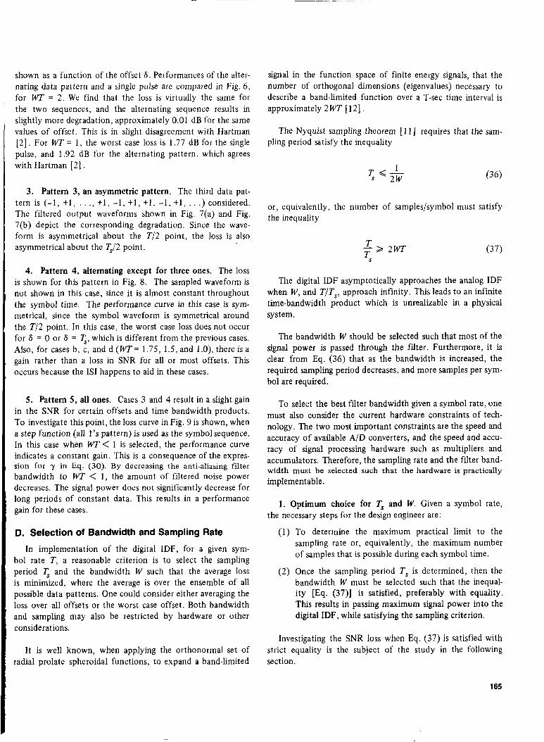
shown as a function of the offset 6. Performances of the alternating data pattern and a single pulse are compared in Fig. 6, for WT = 2. We find that the loss is virtually the same for the two sequences, and the alternating sequence results in slightly more degradation, approximately 0.01 dB for the same values of offset. This is in slight disagreement with Hartman [2]. For WT = 1, the worst case loss is 1.77 dB for the single pulse, and 1.92 dB for the alternating pattern, which agrees with Hartman [2].

3. Pattern 3, an asymmetric pattern. The third data pattern is (-1, t 1 , . . ., t 1 , -1, t 1 , t 1 , -1, t 1 , . . .) considered. The filtered output waveforms shown in Fig. 7(a) and Fig. 7(b) depict the corresponding degradation. Since the waveform is asymmetrical about the T/2 point, the loss is also asymmetrical abaut the T,/2 point.

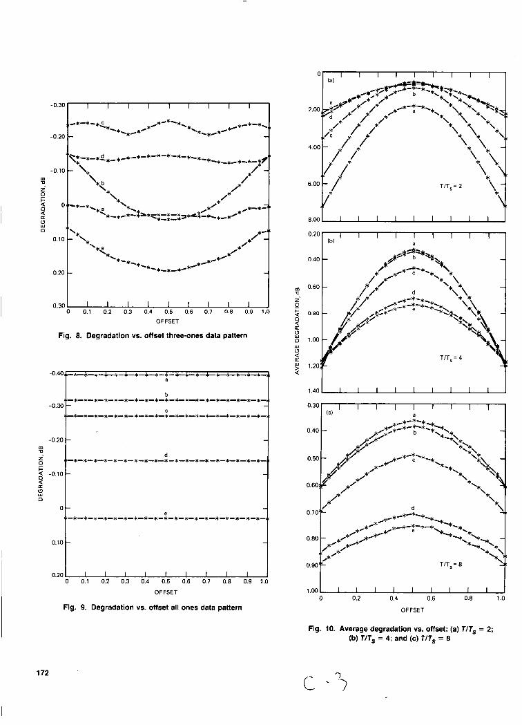
4. Pattern 4, alternating except for three ones. The loss is shown for this pattern in Fig. 8. The sampled waveform is not shown in this case, since it is almost constant throughout the symbol time. The performance curve in this case is symmetrical, since the symbol waveform is symmetrical around the T/2 point. In this case, the worst case loss does not occur for 6 = 0 or 6 = q, which is different from the previous cases. Also, for cases b, c, and d (WT= 1.75, 1.5, and 1 .O), there is a gain rather than a loss in SNR for all or most offsets. This occurs because the IS1 happens to aid in these cases.

5. Pattern 5, all ones. Cases 3 and 4 result in a slight gain in the SNR for certain offsets and time bandwidth products. To investigate this point, the loss curve in Fig. 9 is shown, when a step function (all 1’s pattern) is used as the symbol sequence. In this case when WT < 1 is selected, the performance curve indicates a constant gain. This is a consequence of the expression for y in Eq. (30). By decreasing the anti-aliasing filter bandwidth to WT < 1, the amount of filtered noise power decreases. The signal power does not significantly decrease for long periods of constant data. This results in a performance gain for these cases.

D. Selection of Bandwidth and Sampling Rate

In implementation of the digital IDF, for a given symbol rate T, a reasonable criterion is to select the sampling period T, and the bandwidth W such that the average loss is minimized, where the average is over the ensemble of all possible data patterns. One could consider either averaging the loss over all offsets or the worst case offset. Both bandwidth and sampling may also be restricted by hardware or other considerations.

It is well known, when applying the orthonormal set of radial prolate spheroidal functions, to expand a band-limited

signal in the function space of finite energy signals, that the number of orthogonal dimensions (eigenvalues) necessary to describe a band-limited function over a T-sec time interval is approximately 2 WT [ 121 .

The Nyquist sampling theorem [l 11 requires that the sampling period satisfy the inequality

1 2 w

T , <-

or, equivalently, the number of samples/symbol must satisfy the inequality

(37) T j ~ 2 2WT S

The digital IDF asymptotically approaches the analog IDF when W , and T/T,, approach infinity. This leads to an infinite time-bandwidth product which is unrealizable in a physical system.

The bandwidth W should be selected such that most of the signal power is passed through the filter. Furthermore, it is clear from Eq. (36) that as the bandwidth is increased, the required sampling period decreases, and more samples per symbol are required.

To select the best filter bandwidth given a symbol rate, one must also consider the current hardware constraints of tech- nology. The two most important constraints are the speed and accuracy of available A/D converters, and the speed and accuracy of signal processing hardware such as multipliers and accumulators. Therefore, the sampling rate and the filter bandwidth must be selected such that the hardware is practically implementable.

1. Optimum choice for T, and W. Given a symbol rate,

(1) To determine the maximum practical limit to the sampling rate or, equivalently, the maximum number of samples that is possible during each symbol time.

( 2 ) Once the sampling period T, is determined, then the bandwidth W must be selected such that the inequality [Eq. (37)] is satisfied, preferably with equality. This results in passing maximum signal power into the digital IDF, while satisfying the sampling criterion.

the necessary steps for the design engineer are:

Investigating the SNR loss when Eq. (37) is satisfied with strict equality is the subject of the study in the following section.

165

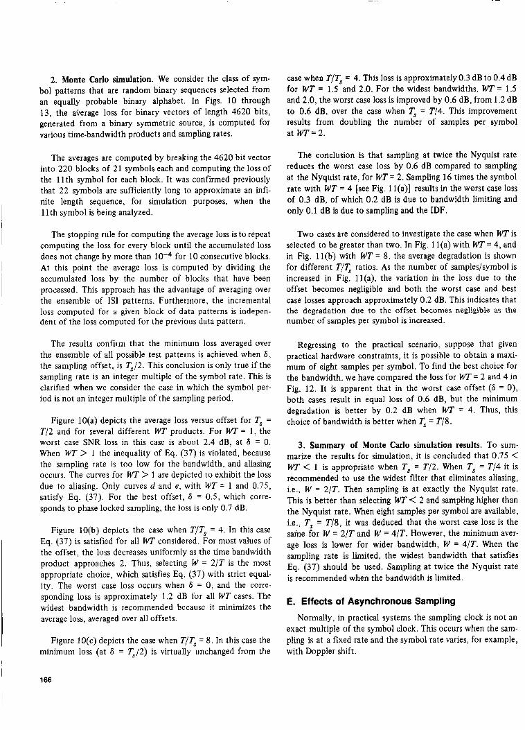
2. Monte Carlo simulation. We consider the class of symbol patterns that are random binary sequences selected from an equally probable binary alphabet. In Figs. 10 through 13, the airerage loss for binary vectors of length 4620 bits, generated from a binary symmetric source, is computed for various time-bandwidth products and sampling rates.

The averages are computed by breaking the 4620 bit vector into 220 blocks of 21 symbols each and computing the loss of the 11th symbol for each block. It was confirmed previously that 22 symbols are sufficiently long to approximate an infinite length sequence, for simulation purposes, when the 11 th symbol is being analyzed.

The stopping rule for computing the average loss is to repeat computing the loss for every block until the accumulated loss does not change by more than for 10 consecutive blocks. At this point the average loss is computed by dividing the accumulated loss by the number of blocks that have been processed. This approach has the advantage of averaging over the ensemble of IS1 patterns. Furthermore, the incremental loss computed for a given block of data patterns is independent of the loss computed for the previous data pattern.

The results confirm that the minimum loss averaged over the ensemble of all possible test patterns is achieved when 6 , the sampling offset, is T,/2. This conclusion is only true if the sampling rate is an integer multiple of the symbol rate. This is clarified when we consider the case in which the symbol period is not an integer multiple of the sampling period.

Figure lO(a) depicts the average loss versus offset for T, = T/2 and for several different WT products. For WT = 1, the worst case SNR loss in this case is about 2.4 dB, at 6 = 0. When WT > 1 the inequality of Eq. (37) is violated, because the sampling rate is too low for the bandwidth, and aliasing occurs. The curves for WT > 1 are depicted to exhibit the loss due to aliasing. Only curves d and e, with WT = 1 and 0.75, satisfy Eq. (37). For the best offset, 6 = 0.5, which corresponds to phase locked sampling, the loss is only 0.7 dB.

Figure 10(b) depicts the case when TIT, = 4. In this case Eq. (37) is satisfied for all WT considered. For most values of the offset, the loss decreases uniformly as the time bandwidth product approaches 2. Thus, selecting W = 2/T is the most appropriate choice, which satisfies Eq. (37) with strict equality. The worst case loss occurs when 6 = 0, and the corresponding loss is approximately 1.2 dB for all WT cases. The widest bandwidth is recommended because it minimizes the average loss, averaged over all offsets.

Figure 1O(c) depicts the case when T/T, = 8. In this case the minimum loss (at 6 = T,/2) is virtually unchanged from the

case when TIT, = 4. This loss is approximately 0.3 dB to 0.4 dB for WT = 1.5 and 2.0. For the widest bandwidths, WT = 1.5 and 2.0, the worst case loss is improved by 0.6 dB, from 1.2 dB to 0.6 dB, over the case when T, = T/4. This improvement results from doubling the number of samples per symbol at WT=2.

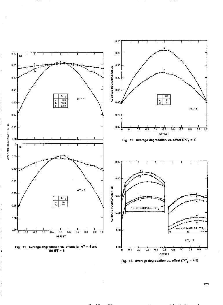
The conclusion is that sampling at twice the Nyquist rate reduces the worst case loss by 0.6 dB compared to sampling at the Nyquist rate, for WT= 2. Sampling 16 times the symbol rate with WT = 4 [see Fig. 1 l(a)] results in the worst case loss of 0.3 dB, of which 0.2 dB is due to bandwidth limiting and only 0.1 dB is due to sampling and the IDF.

Two cases are considered to investigate the case when WT is selected to be greater than two. In Fig. 1 l(a) with WT = 4, and in Fig. 1 l(b) with WT = 8. the average degradation is shown for different T/T, ratios. As the number of samples/symbol is increased in Fig. ll(a), the variation in the loss due to the offset becomes negligible and both the worst case and best case losses approach approximately 0.2 dB. This indicates that the degradation due to the offset becomes negligible as the number of samples per symbol is increased.

Regressing to the practical scenario, suppose that given practical hardware constraints, it is possible to obtain a maximum of eight samples per symbol. To find the best choice for the bandwidth. we have compared the loss for WT = 2 and 4 in Fig. 12. It is apparent that in the worst case offset (6 = 0), both cases result in equal loss of 0.6 dB, but the minimum degradation is better by 0.2 dB when WT = 4. Thus, this choice of bandwidth is better when T, = T/8.

3. Summary of Monte Carlo simulation results. To sum- marize the results for simulation, it is concluded that 0.75 < WT < 1 is appropriate when T, = T/2. When T, = T/4 it is recommended to use the widest filter that eliminates aliasing, i.e., W = 2/T. Then sampling is at exactly the Nyquist rate. This is better than selecting WT < 2 and sampling higher than the Nyquist rate. When eight samples per symbol are available, i.e., T, = T/8, it was deduced that the worst case loss is the same for W = 2/T and W = 4/T. However, the minimum average loss is lower for wider bandwidth, W = 4/T. When the sampling rate is limited, the widest bandwidth that satisfies Eq. (37) should be used. Sampling at twice the Nyquist rate is recommended when the bandwidth is limited.

E. Effects of Asynchronous Sampling

Normally, in practical systems the sampling clock is not an exact multiple of the symbol clock. This occurs when the sampling is at a fixed rate and the symbol rate varies, for example, with Doppler shift.

166

Figure 13 depicts the average loss for a random data pattern when T/T, = 4.5. Some symbols have four samples, and some have five. When the number of samples is four (or when the offset S < T,/2), the degradation is approximately 0.3 dB less than when the number of samples is five. This is true for all WT considered. The average loss for five samples per symbol is due to additional noise power in the last sample, since the last sample occurs near the transition point of the filtered symbol waveform. Despite this variation in loss with the number of samples, the worst case loss for T/T, = 4.5 is only 0.7 dB for WT = 1.5 and 2.0, which is less than the worst case loss of 1.2 dB when TIT, = 4. Even though there is a variation in loss with number of samples per symbol, a higher sampling helps performance rather than hurting it.

VI. Summary and Conclusions The performance of the digital IDF was studied in this

article, with special attention to the effect of offset in sampling. We derived the expressions for the signal response, noise variance, and IDF output SNR for general pulse shapes and anti-aliasing filters. These results were then specialized to the rectangular pulse shape and the ideal low-pass filter. Perfor- mance was evaluated in terms of loss in SNR compared to an analog IDF with infinite bandwidth.

Performance was evaluated for five different known data sequences, and for random sequences. Observations regarding the worst case degradation and the effects of the offset in the sample time were made. It was concluded that when the system is bandlimited, i.e., the time bandwidth product WT is finite, a sampling rate in excess of the Nyquist rate (2W) should be chosen. For example, when the bandwidth is only twice the symbol rate, sampling at twice the Nyquist rate results in a 0.6 dB improvement over sampling at the Nyquist

rate, when the worst case loss is the performance criterion. When the sampling rate is limited, i.e., TIT, is f s e d the bandwidth W should be selected such that W = 1/2T,.

The above results are for the case when the sampling rate is not phase locked to the symbol rate. For an integer number of ymples per symbol, it was shown that the degradation due to offset in sampling is minimized when the offset is half the sampling period, i.e., 6 = TJ2. For four samples per symbol, the worst case loss is 0.9 dB greater than the best case. This means that phase locked sampling is 0.9 dB better than the worst case for the non-phase-locked sampling, when the ratio of symbol rate to the sampling rate is small (G4).

The loss due to the offset becomes negligible when the number of samples/symbol becomes sufficiently large. With WT > 4, T, < 1/2W, the digital IDF always performs within 0.6 dB of the analog IDF, for the random data pattern and the worst case sampling offset.

The effect of a non-integer ratio of sampling rate to symbol rate was also studied, for the case when T/T, = 4.5. For a given time bandwidth product, the worst case loss is lower than the case when T/T, = 4. Thus letting the sampling rate be a non- integer rate relative to symbol rate did not degrade the performance.

VII. Direction for Future Research For the Deep Space Network receiver, the losses incurred

for the digital IDF at high symbol rates are undesirable. To reduce the loss, it is possible to weight each sample in the IDF such that the loss is minimized. That is, instead of performing a simple summation, a weighted summation is performed. This will be considered in a later article.

167

Glossary of Terms

T, - Sampling time in seconds s ( t ) - The transmitted signal

T - Symbol time in seconds

W - Filter bandwidth in hertz

- Transmitted symbol ai

n(t) - Additive white Gaussian noise with flat spectral density No/2

r ( t ) - The received signal

y ( t ) - The output of the low-pass prefilter

p ( t ) - Pulse shaping waveform h(t) - The transfer function of the low-pass prefilter

- The sampled output of the Integrate-and-Dump Fil- ter at time k

- The sampled output of the pre-filter

- Transport lag from transmitter to receiver in seconds

- Sampling delay in seconds r 1

A ,

yi Rx(7) - Autocorrelation function of signal x ( t )

Ref e ren ces

[ 11 F. D. Natali, “Comparison of Analog and Digital Integrate-and-Dump Filters,” Proc. IEEE, vol. 57. pp. 1766-1768, October 1969.

H. P. Hartman. “Degradation of Signal-to-Noise-Ratio due to IF Filtering,” IEEE Trans. Aero. and Elect. Sys., vol. AES-5. no. 1, pp. 22-32, January 1969.

G. L. Turin, “An Introduction to Digital Matched Filters,” Proc. IEEE, vol. 64,

[2]

[3] pp. 1092-1 112. July 1976.

[4] T. L. Lim, “Non-Coherent Digital Matched Filters: Multibit Quantization,” IEEE Trans. Comm., vol. COM-26, pp. 409-419, April 1978.

C. M . Chie, “Performance Analysis of Digital Integrate-and-Dump Filters,” IEEE Trans. Comm., vol. COM-30, no. 8, pp. 1979-1983. August 1982.

C. W. Helstrom, “Calculating Error Probabilities for Intersymbol and Cochannel Interference,” IEEE Trans. Comm., vol. COM-34. no. 5, pp. 430-435, May 1986.

A. J. Levy, “Fast Error Rate Evaluation in the Presence of Intersymbol Interfer- ence,” IEEE Trans. Comm.. vol. COM-33, no. 5, pp. 479-481, May 1985.

C. M. Chie, “The Effects of Transmitter/Receiver Clock Time-Base Instability on Coherent Communication System Performance,” IEEE Trans. Comm., vol. COM-30, no. 3, pp. 510-516, March 1982.

M. Abramowitz and A. I. Stegun (eds.), Handbook of Mathematical Functions, Washington, D.C.: National Bureau of Standards; 1964.

D. A. Whalen, Detection ofsignals in Noise, New York: Academic Press, 1971.

A. V. Oppenheim and R. W. Schafer, Digital Signal Processing, New York: Prentice- Hall, 1975.

A. Papoulis, SignalAnalysis, New York: McGraw-Hill, 1977.

A. Papoulis. Probability, Random Variables and Stochastic Processes, New York: McGraw-Hill. 1965.

[SI

[6]

[7]

[8]

[9]

[ lo ]

[ 111

[12]

[13]

I 168

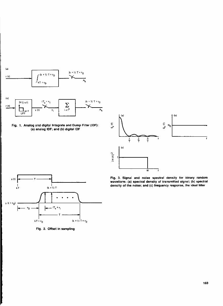
Fig. 1. Analog and digital Integrate and Dump Filter (IDF): (a) analog IDF; and (b) digital IDF

Fig. 2. Offset in sampling

Fig. 3. Signal and noise spectral density for binary random waveform: (a) spectral density of transmitted signal; (b) spectral density of the noise; and (c) frequency response, the ideal filter

169

O C OFFSET4

0.1. T,

i T ~ ' 0

"

m -1.0 n

-1.2

0

0.50

m =- 1.00 0 I- 4 n 4

w 1.50 n

U

[r

w

2.00

2.50

ro t ( k t 1 ) T

TIME

I I I I I I l l I (C)

I I I I I 1 1 1 I 0.1 0.2 0.3 0.4 0.5 0.6 0.7 0.8 0.9

OFFSET

-1.3

-1.1

-0.9

-0.7

-0.5

-0.3

-0.1

TIME

I I I I I I I I

_*,***-*-*-*-*-* h

e

1.30 t 1.401 1 I I I I I l l 1

0 0.1 0.2 0.3 0.4 0.5 0.6 0.7 0.8 0.9 1.0

OFFSET

Fig. 4. Results for alternating data pattern: (a) sampled waveform; (b) filter output for different WT; (c) alternating data pattern TITs = 4; and (d) alternating data pattern T/Ts = 20

170

0

0.50

1 .oo m 0

i 0 + 2 1.50 4 a: s n

2.00

2.50

3.00

I I I I I I I I I

I I I I I I 1 I I

OFFSET

0.1 0.2 0.3 0.4 0.5 0.6 0.7 0.8 0.9 1.

Fig. 5. Degradation vs. offset: single pulse data pattern T/Ts = 4

0 SINGLEPULSE W ALTERNATING

PULSES

W T = 2

2.00

2.40 I I I 1 I I I I 1 0 0.1 0.2 0.3 0.4 0.5 0.6 0.7 0.8 0.9 1

OFFSET

-1.00

-0.50

0

gg 0.50

i 0 I-

4 2 1.00

s n 1.50

a:

2.00

2.50

3.00

kT + ro (k + 1) T + r o

TIME

I 1 1 1 1 I I 1 I (b)

I I I I I I I I I I 0.1 0.2 0.3 0.4 0.5 0.6 0.7 0.8 0.9 1.0

OFFSET

Fig. 7. (a) Signal output for different WTfor data pattern -1, +1, -1, +1,. . . +1, -1, +1, +1, -1, +1 . . . ; (b) Degradation vs. offset two- ones data pattern

Fig. 6. Degradation comparison vs. offset for alternating and pulse data pattern

171

-0.30 ~

0 20

*-*-*-I \*-*,*#*/ .* *e*-* *:* -*.*,* .*’ r*-*- t -0.20

I I 1 I 1 1 (bl

I I I a

0.30 I I I I 1 1 I I I I J 0 0.1 0.2 0.3 0.4 0.5 0.6 0.7 0.8 0.9 1.0

1.40

OFFSET

Fig. 8. Degradation vs. offset three-ones data pattern

I I I I I I I I I a

0.30

-0.20 1 1 1 1 I I 1

( C ) 1 1 I

a

d U

*-*-*-*-*-*-*-*-*-*-*-*-~-~-*-*-*-~-*- P 2 -0.10 a s n (r

OC e

-*-*-*-*-*-*-*-L-*-*-*-*-*-*-*-*-*-*-*-

O.1° t 0.20 I I I I I I I I I I

0 0.1 0.2 0.3 0.4 0.5 0.6 0.7 0.8 0.9 1

OFFSET

Fig. 9. Degradation vs. offset all ones data pattern

m U

i 0 n I- Q

< a: 0 w

w n

a (3

(r w > U

1.ooL I I I I I I I I 1 1 0 0.2 0.4 0.6 0.8 1 .o

OFFSET

Fig. 10. Average degradation vs. offset: (a) TITs = 2; (b) TITs = 4; and (c) TITs = 8

172 c -3

0.10 1 I 1 1 1 I I 1 I

0.70

0.10 (a)

I I I I I 1 I I I

.

0.20

0.30 t

I 1 I I I I I I I

1 1.20

0.35 I 1 I I I I I I I I 0 0.1 0.2 0.3 0.4 0.5 0.6 0.7 0.8 0.9 1.0

OFFSET

TIT, = 5

I I I I I I I I I Fig. 11. Average degradation vs. offset: (a) WT = 4 and (b) WT = 8

0.80 0 0.1 0.2 0.3 0.4 0.5 0.6 0.7 0.8 0.9 1.0

OFFSET

Fig. 12. Average degradation vs. offset (TITs = 8)

*' m

i

n

u

0.60 4

d l3 W

W n

2 0.80 a W

2

l.O0 t -*-*-*-*\

*.*/ *-*4y*-ik

/* NO. OF SAMPLES: TIT,

OFFSET

Fig. 13. Average degradation vs. offset (TITs = 4.5)

173

Documents

Detection of Signals by the Digital Integrate-and-Dump