Detection of Snapshot Isolation Anomalies in SoftwareTransactional Memory: A Static Analysis Approach

Ricardo J. Dias, Joao M. Lourenco and Joao Costa Seco∗

CITI and Departamento de InformaticaUniversidade Nova de Lisboa, Portugal

{rjfd, joao.lourenco, joao.seco}@di.fct.unl.pt

Technical Report: UNL-DI-5-2011

May 2011

Abstract

Some performance issues of software transactional mem-ory are caused by unnecessary abort situations wherenon serializable and yet non conflicting transactions arescheduled to execute concurrently. By smartly relaxingthe isolation properties of transactions, transactional sys-tems may overcome these performance issues and attainconsiderable gains. However, it is known that relax-ing isolation restrictions may lead to execution anoma-lies causing programs to yield unexpected results. Somedatabase management systems make that compromiseand allow the option to operate with relaxed isolationmechanisms. In this cases, developers must accept thefact that they must explicitly deal with anomalies. Insoftware transactional memory systems, where transac-tions protect the volatile state of programs, executionanomalies may have severe and unforeseen semanticconsequences. In this setting, the balance between a re-laxed isolation level and the ability to enforce the neces-sary correctness in general purpose language programs isharder to achieve.

The solution we devise in this paper is to statically an-alyze programs to detect the kind of execution anoma-lies that emerge under snapshot isolation. We proposea semantic approach to the challenging scenario of ana-lyzing programs with dynamic allocated data structures.Although limited to acyclic data structures, our analy-

∗This research was partially supported by the EU COST ActionIC1001 (Euro-TM) and the Portuguese Fundacao para a Cienciae Tecnologia in the research projects PTDC/EIA/74325/2006(Byzantium), PTDC/EIA-CCO/104583/2008 (StreamLine), andPTDC/EIA-EIA/113613/2009 (Synergy-VM), and the research grantSFRH/BD/41765/2007.

sis is able to detect anomalies in well know examples ofanomalous code. Our approach allows a compiler to ei-ther warn the developer about the possible snapshot iso-lation anomalies in a given program, or to possibly in-form automatic correctness strategies to ensure executionunder full serializability.

1 IntroductionUsing relaxed isolation levels, such as Snapshot Isola-tion (SI) [2], is a well known and long used strategy indatabase transactional systems to increase performance.Software Transactional Memory [11, 5] (STM) usuallyrequires full serializability but, in principle, can also useSI, although with different semantic guaranties.

Unlike full-fledged STM systems that provide strictisolation between transactions, STM systems providingrelaxed isolation levels allow for transactions to inter-fere, and generate non-serializable execution schedules.Such interferences are commonly known as serializabil-ity anomalies [2]. One of these anomalies, the write-skew, occurs when two transactions are writing on dis-joint memory locations and are entangled in reading datathat is being modified by the other. For instance, con-sider the implementation of an ordered linked list thatis being accessed in the context of a transactional mem-ory program. The insert operation has a footprint ofread(R)/write(W) operations (on the next field of listnodes) that can be depicted as follows:

insert : R −→ . . . −→ R −→ R/W

The invariant here is that the insert operation does notread beyond the node it writes into. If transactionA reads

1

a node that is being modified by transaction B, from theinvariant above we can infer that either transaction A iswriting on the same node as transaction B (and one ofthem will necessarily abort), or transaction A will mod-ify some other node ahead of the one modified by trans-action B. Hence, if two transactions A and B are set toinsert a value in the list then no anomaly can occur.

If one considers the remove operation which reads thefield next of the node being removed, its footprint is:

remove : R −→ . . . −→ R −→ R/W −→ R

When a remove operation is set to run concurrently withother remove or insert operations, then a write-skewanomaly may be observed. There is a crossed read/writesituation when one transaction removes a node while theother is removing or inserting a new node just ahead ofit. By introducing a minor correction in the code, an ad-ditional (dummy) write in the node to be removed, thefootprint for a new remove’ operation becomes

remove’ : R −→ . . . −→ R −→ R/W −→ R/W

and insert and remove’ operations can now be executedconcurrently under SI with no anomalies ever occurring.

In this paper we introduce a static analysis techniqueand corresponding algorithm that mechanically assertsthat a given transactional memory application executingunder Snapshot Isolation behaves as if executed underfull serializability. More precisely, we detect the kindof anomalies of Snapshot Isolation that are known tolead to non-serializable histories [2]. We build on re-lated work directed to database transactions [4, 6] andextend it to the very different domain of transactionalmemory. Our technique allows for the automatic iden-tification of anomalous code patterns which were previ-ously detected only by ad-hoc code inspection. To thebest of our knowledge, SI has only been applied to STMin semantically harmless situations [9], where anomaliesdo not occur. Our technique allows SI to be used as thedefault isolation level for STM applications by signalingconflicting programs and allowing for explicit code cor-rections.

We take a standard approach to define our analysis,and use a simple core imperative language with limiteduse of pointer indirection and support for heap allocateddata. Applications written in main stream programminglanguages are translated to the core language and thenanalyzed. For each transaction in the original applica-tion we create a separate program in the core language.We assume that all transactions in the application canbe run concurrently, and define an intra-procedural data-flow analysis that extracts the information necessary todetect SI anomalies.

The analysis starts by extracting compact read/writesets and defining static dependencies between programs,thus creating a static dependency graph. We then applyan algorithm to that graph to determine if the concurrentexecution of such transactional programs is serializableunder SI.

The analysis of heap allocated data follows a modi-fied shape analysis technique [10], that combines shapegraphs with sets of read and written data items. We de-fine a set of new properties for shape graphs in order toavoid the state explosion that would result from the ap-plication of the original definition to our setting. Unlikein standard shape analysis procedures, termination in ourapproach does not depend on the comparison of shapegraphs but rather on the collected read/write-sets, whosecomputation converges faster. A drawback of our defi-nition is that it can only be applied to acyclic data struc-tures, but we foresee that the model can be extended withbackward pointers to support more general cases.

Like in any other static analysis procedure, we allowfor some kind of false positive results. Nevertheless, weguarantee that if the analysis procedure does not detectany serializability anomaly, then all possible executionswill be anomaly-free and correspond to a possible inter-leaving of the transactions. On the other hand, if someanomalies are found, they should be considered as po-tentially harmful. At this stage, analysis results can befurther refined and code can be modified to avoid unde-sired interferences. The application of our approach toreal programs is more adequate if allied the aggregationof memory transactions in independent modules.

In summary, we introduce

• a shape graph definition that supports acyclic datastructures and limits the explosion of the statespace;

• an intra-procedural data-flow analysis that extractsfine grained read and write set information fromtransactional programs;

• a procedure to identify static program dependenciesfrom the results of the data-flow analysis phase;

• an enhanced algorithm to detect SI anomalies basedon the graph of the static program dependencies.

We now proceed by introducing the background workin Section 2, namely the properties of snapshot isola-tion and the detection of snapshot isolation anomalies us-ing dependencies between programs. We follow in Sec-tion 3 with the description of an intra-procedural data-flow analysis for a simple imperative language using ex-tended shape graphs. Given the results of the data-flow

2

void Withdraw ( boolean b , i n t value ) {i f ( x + y > value )

i f ( b ) x = x − value ;else y = y − value ;

}

Figure 1: Withdraw program.

analysis, in Section 4 we describe the construction of agraph of program dependencies, which is used by the al-gorithm described in Section 5 for detecting SI anoma-lies. We proceed by presenting the results obtained whenapplying the technique to a known benchmark in Sec-tion 6, and relating with the work of others in Section 7.We end with the concluding remarks and some refer-ences to future work.

2 Background

2.1 Snapshot Isolation

Snapshot Isolation [2] is a relaxed isolation level whereeach transaction executes with relation to a private copyof the system state, taken in the beginning of the transac-tion and stored in a local buffer. All write operations arekept pending in the local buffer until they are commit-ted in the global state. Reading modified items alwaysrefers to the pending values in the local buffer. In allcases, committing transactions obey the general First-Commiter-Wins rule. This rule states that a transactionA can only commit if no other concurrent transaction Bhas committed modifications to data items pending to becommitted by transaction A. Hence, for any two concur-rent transactions modifying the same data item, only thefirst one to commit will succeed.

Although appealing for performance reasons, the ap-plication of SI may lead to non-serializable executions,resulting in two kinds of consistency anomalies: write-skew and SI read-only anomaly [4]. Consider the follow-ing example that suffers from the write-skew anomaly. Abank client can withdraw money from two possible ac-counts represented by two shared variables, x and y. Theprogram listed in Figure 1 can be used in several transac-tions to perform bank operations customized by its inputvalues. The behavior is based on a parameter b and onthe sum of the two accounts. Let the initial value of x be20 and the initial value of y be 80. If two transactionsexecute concurrently, one calling the Withdraw(true, 30)(T1) and the other calling the Withdraw(false, 90) (T2),

then one possible execution history of the two transac-tions under SI is:

H = R1(x, 20) R2(x, 20) R1(y, 80) R2(y, 80) R1(x, 20)W1(x,−10) C1 R2(y, 80) W2(y,−10) C2

After the execution of these two transactions the finalsum of the two accounts will be−20, which is a negativevalue. Such execution would never be possible under Se-rializable isolation level, as the last transaction to commitwould abort because it read a value that was written bythe first transaction.

2.2 Program Dependencies and AnomaliesSerialization graphs are the most common formal tool todefine serializable anomalies. In a serialization graph,nodes correspond to transactions and edges correspondto data dependencies between transactions. These graphsare build upon dynamic information collected during ex-ecution of programs. Three types of transaction depen-dencies can de defined [4]:write-read (wr), write-write(ww) and read-write (rw).

The static counter-part of the (dynamic) serializationgraphs is the static dependency graph (SDG ). In a SDG,nodes are programs instead of transactions and edges aredata dependencies between programs. If executed morethan once, a single program P may define the behaviorof multiple transactions.

There is a static dependency between programsPn andPm, written Pn

x−ρ−−−→ Pm, where x is a state variable andρ is a dependency type (ρ ∈ {wr,ww, rw}) if, for anytwo transactions Tn and Tm resulting from the executionof Pn and Pm respectively, there is a transactional de-pendency Tn

x−ρ−−−→ Tm on any variable x.A static dependency between programs Pn and Pm

is said to be vulnerable if it is of type rw and the cor-responding transactions Tn and Tm may execute con-currently. A vulnerable static dependency on a vari-able x between programs Pn and Pm is represented asPn

x−rw===⇒ Pm. Note that a single program P may gen-

erate multiple transactions, hence in a SDG the pro-gram may have dependencies to itself. In summary, theSDG(A) of an application A is a graph with programsP1, . . . , Pk of A as nodes, and with edges labeled asPn

x−ρ−−−→ Pm (non-vulnerable) or Pnx−rw===⇒ Pm (vul-

nerable) representing static dependencies.Serializable anomalies can be signaled by the presence

of certain kinds of dangerous structures in the SDG ofan application. Fekete et al. [4] define the concept ofdangerous structure in a static dependency graph. TheSDG(A) of an application A has a dangerous structure

3

ww wr rwP1

Figure 2: Static dependency graph of the Withdraw pro-gram.

if it contains three nodes P , Q and R (not necessarilydistinct) such that there are vulnerable edges from R toP and from P to Q, and there is a path from Q to R.Node P is called the pivot node. If the SDG(A) of anapplication A has a dangerous structure, then some exe-cutions of A may be non-serializable. In the opposite, isthe SDG(A) has no dangerous structures, then all exe-cutions of A are serializable.

From the Withdraw program depicted in Figure 1 wecan generate the static dependency graph in Figure 2.There is one node in the graph representing programWithdraw (P1) and there are three edges1: non-vulnerableP1

ww−−→ P1 and P1wr−−→ P1, and vulnerable P1

rw=⇒ P1.

The vulnerable edge is represented by a dashed arrowin the diagram. Intuitively the three edges represent thefollowing situations: the dependency P1

ww−−→ P1 re-sults from sequentially calling the program P1 twice withthe same value for parameter b, thus generating non-concurrent transactions; dependency P1

wr−−→ P1 resultsfrom sequentially calling P1 twice with different valuesfor parameter b; and dependency P1

rw=⇒ P1 results from

calling P1 twice with different values for parameter b,and the two corresponding transactions are concurrent.

According to the definition, the SDG in Figure 2 hasa dangerous structure. Note that this does not imply thatthe corresponding application will necessarily have a SIanomaly, but only that it may have one.

We next show how to build a SDG by analyzing thesource code of an application, and how to detect danger-ous structures that point to possible SI anomalies.

3 Static AnalysisWe now define a data-flow analysis based on a small im-perative language with heap allocated memory [7] andthen describe how to build a SDG from the results ofthe analysis. The abstract syntax of the language is thefollowing:

R ::= x | x.selE ::= R | n | E op E | true | false | not E | nullS ::= R := E | skip | S ;S | new R| if E then S else S | while E do S

1The variable identifiers are omitted for the sake of simplicity.

//x points to the head of a list//v is the value to be insertedp := x;n := p.next;tv := n.value;while(tv < v) {

p := n;n := p.next;tv := n.value;

}if (tv != vv) {

new y;y.value := v;y.next := n;p.next := y;

}

Figure 3: Example of an insertion of a value into a linkedlist.

Where a program is a statement S. The values of the lan-guage are integer values (n), boolean values, pointers toheap cells or the special value null. Arithmetic operatorsare only defined for integer values. Boolean expressionsare extended to support equality of pointers and to sup-port the comparison of pointers with the special valuenull. The statement newR assigns the pointer of a newheap cell to R.

Figure 3 describes a program that implements an insertfunction in an ordered singly linked list. By convention,the value to be inserted is given in variable v and thepointer for the head of the list is given by variable x.The program uses local variables n, tv and vv, and thenodes in this list implementation are heap cells with twoselectors value and next.

We follow a general model of a heap cell where itscontents are only accessible through a finite number ofselectors (cf. fields in structures). For instance, one mayinstantiate a cell and assign the resulting pointer to a vari-able x by using the statement new x. The contents of thecell may be changed by assigning to a selector val, as instatement x.val := 1. Note that statement y := x re-sults in a state where x and y point to the same heap cell,and that statement x := 1 changes the value of variablex from a pointer to an integer value. Selectors work likea dereferencing operator and also provide language sup-port for dynamically allocated structure-like values.

As expected, the semantics of our language is definedwith relation to a state and a heap. The state is a map-ping of variables to values, and the heap is a mappingfrom heap cells to values. The size of a program state

4

is bounded by the number of variables that occur in thesource code of the program, and the heap is unlimited insize and structure. In order to analyze the executions ofa program we use a compact and bounded representationof the state and heap, similar to the standard notion ofShape Graph [10].

In the remaining of this document, we present the def-inition of shape graphs that will be used to identify heapaccesses during the data-flow analysis. We then define adata-flow analysis that generates, for each analyzed pro-gram, a set of read/write states for variables and heapaccesses. The information retrieved from the analysisis used to generate a static dependency graph which istraversed by an algorithm to search for dangerous struc-tures.

3.1 Shape Graphs

A shape graph is an abstract representation of the stateand heap of a program, defined from the notion of ab-stract location, which is the representative for one (ormore) heap cells in the program heap. A shape graphis composed by an abstract state S, which is a mappingfrom variable names to abstract locations, and an abstractheap H, which is a mapping from abstract locations toabstract locations by means of selectors. We write n

Xto

denote an abstract location, where X ⊆ Var is the setof state variables pointing to that location. In the generalcase, abstract locations are associated to one (and onlyone) heap cell. When X = ∅ we call n∅ the summary lo-cation. In this particular case, n∅ is the representative ofmore than one heap cell, more precisely, of all the heapcells that are not directly pointed by a state variable. Forinstance, n{x,y} is the abstract location that represents aheap cell pointed by the state variables x and y. This alsomeans that variables x and y are aliases of the same heapcell.

The original definition of a shape graph by Sagiv etal. [10] also includes information about sharing of ab-stract locations, signaling those that are reachable bymore than one abstract location. On the one hand, weadopt a simpler version, dropping this kind of informa-tion, and hence we only represent acyclic memory datastructures. On the other hand, we extend the notion ofsummary node. Instead of using a single summary noden∅, we use a set of summary nodes indexed by an inte-ger number ni∅ (i ∈ N0). Summary node n0∅ plays theusual role of aggregating a set of heap cells. We usuallyomit the index if it is 0 and write only n∅. Summarynodes with positive indexes, ni∅ with i > 0, represent ab-stract locations occurring in the middle of a path of an

acyclic data structure which are not directly pointed bystate variables.

We define an abstract state of a program S , Var ×ALoc , mapping from variables to abstract locations, andan abstract heap H , ALoc × Sel × ALoc , mappingfrom abstract locations to abstract locations via selectors.Here, ALoc is the infinite set of all abstract locations andSel is the finite set of all selectors. We use Locs(S) andLocs(H) to signify the set of abstract locations used ina abstract state or abstract heap. The set of all ShapeGraphs is thus SG , S ×H, and a shape graph SG is apair (S,H) with S ∈ S andH ∈ H. We refine the notionof shape graph and define an Acyclic Shape Graph as ashape graph that satisfies some conditions to cope withacyclic data structures.

Definition 1 (Acyclic Shape Graph). For all programstates S ∈ S and heaps H ∈ H

1. A state variable can only point to an abstract loca-tion:

∀nV, n

W∈ Locs(S)∪Locs(H) : (V = W )∨(V ∩

W = ∅)

2. State variables pointing to an AL are referred in itsvariable set.

∀(x, nX) ∈ S : x ∈ X

3. A selector of an AL points at most to one AL.

∀(nV, s, n

W), (n

V, s, n

W ′ ) ∈ H : (W = W ′)

4. No AL is pointed by any two ALs (the heap isacyclic).

∀(nV, s, n

X), (n

W, s′, n

X) ∈ H : V 6= W ⇒ X =

∅

5. The summary node only points to itself.

∀(n0∅, s, nV) ∈ H : V = ∅

Since we only generate acyclic shape graphs and forthe sake of simplicity, in the remaining of this paper, andunless stated otherwise, we will refer to acyclic shapegraphs simply as shape graphs.

Figure 4 depicts a shape graph representing a heapcontaining a singly linked list. Circles represent statevariables and rectangles represent abstract locations.Edges between abstract locations are labelled with thecorresponding selector. This shape graph is defined asfollows:

SG , ({(x, n{x}), (y, n{y}), (z, n{z,w}), (w, n{z,w})},{(n{x}, next, n{y}), (n{y}, next, n{z,w}),(n{z,w}, next, n∅), (n∅, next, n∅)})

5

nextnext nextnext

n{x} n{z,w} n∅

wyx z

n{y}

Figure 4: Shape Graph representing a singly linked list.

nextnext nextnext

n{z,w}

z

n1∅ n∅

wyx

n{x,y}

Figure 5: Result of the assignment y := x.

A shape graph SG is modified by the evaluation ofassignments and by the cell creation statement (new x).We will now illustrate the effect of these statements start-ing with SG of Figure 4 and divide the assignments infour different fundamental forms: from variable to vari-able (x := y), from selector to variable (x := y.sel),from variable to selector (x.sel := y) and from selectorto selector (x.sel1 := y.sel2).

Variable to variable: [x := y] If x is a pointer, thefirst effect of this type of assignments is that the vari-able x must be removed from the set of variables of theabstract location pointed by x. In the case where theabstract location is only referred by variable x, writtenn{x}, removing the reference results on replacing it bya summary location. We replace it by a new summarylocation ni+1

∅ where i is the maximum index currentlyfound in the abstract heap.

The second visible effect of the assignment is the cre-ation of new bindings. This only occurs when the valuebeing assigned to variable x is a pointer. In this case, theabstract location pointed by y, nY is updated to nY ∪{x}.

Take the example of the shape graph of Figure 4. Theeffect of the assignment y := x is the removal of thebinding of state variable y to the abstract location n{y}.This results in the shape graph of Figure 5 where n{y}is replaced by n1∅, and the update of the bindings of bothvariables x and y result in replacing the abstract locationn{x} with n{x,y}.

Selector to Variable [x := y.sel] As before, the bind-ings of x must first be removed, and if y.sel is not apointer this is the only effect of the assignment.

nextnextnextnextnext

n{x} n{z} n{w} n∅

wyx z

n{y}

Figure 6: Result of the assignment w := z.next.

When y.sel is a pointer, it either points to an abstractlocation n

Vwith V 6= ∅, to an intermediate summary

location ni∅ with i > 0, or to the summary location n∅.In the first case, the bindings described in the abstract

location nV

are updated to nV ∪{x}, and the connectionsin the new graph are such that the state variable x nowpoints to nV ∪{x}.

In the second case, when y.sel = ni∅ with i > 0, wehave that the abstract location is replaced by n{x}, whichis pointed by the state variable x in the resulting graph.

In the third case, when y.sel = n∅, we must mate-rialize a new abstract location n{x} from the summarylocation. All links from n∅ to itself must now be created(with the same selectors) from n{x} to n∅. Also, y.selmust be updated to point to n{x}.

Figure 6 illustrates the effect of assignment w :=z.next in a heap represented by the shape graph of Fig-ure 4. There is a new abstract location in the graph,n{w} pointed byw, and the abstract location pointed by zchanged to n{z}. The cyclic reference that the summarynode n∅ has to itself in Figure 4, through selector next,causes a reference from the new abstract location n{w}to n∅ to appear in Figure 6. The reference from n{z} ton∅ in Figure 4 is modified in Figure 6 to a reference fromn{z} to n{w}, again, through selector next.

Variable to selector [x.sel := y] When the value de-noted by y is an abstract location, the resulting graph af-ter this assignment has an updated edge from n

X, where

x ∈ X , to the abstract location pointed by y, throughselector sel.

Selector to selector [x.sel1 := y.sel2] The effect ofthis assignment statement can be understood by compo-sition of a sequence of previous assignment forms. It canbe re-written by the sequence: t := y.sel2; x.sel1 :=t; t := null, where variable t is temporary.

Cell creation [new x] In the shape graph resultingfrom evaluating a cell creation statement, the old bind-ing of variable x is removed as in all other cases, and anew abstract location n{x} pointed by x is added to theshape graph. In the case of the statement new x.sel,

6

it can be explained by the sequence: new t; x.sel :=t; t := null, where variable t is temporary.

We use shape graphs in the data-flow analysis to modelthe heap cells used by a transaction. We model the usageof a heap cell by a triple with a variable name, an inte-ger number, and a selector. The pair composed by thevariable name x and the integer value n refers to the setof abstract locations that are reachable from the variablex in n number of hops. All abstract locations identifiedby the same variable and distance measure are indistin-guishable from now on, which is a conservative approachin terms of the analysis. So, when modeling the usage ofone particular heap cell we are really referring to a setof abstract locations. The usage of an abstract locationis completed with a selector. This distance measure ofan abstract location corresponds to the length of the pathfrom a state variable in the heap, its root variable, and theabstract location.

The distance of an abstract location to the programstate is calculated by the maximum number of edges inthe path that lead from one to the other, ignoring thenumber of edges pointing to summary nodes ni∅ withi > 0. Given a shape graph SG and an abstract locationn

X, function dist(SG, n

X) computes a pair with the root

variable x for nX

, the farthest variable in the programstate, and the distance between them. For example, in theshape graph of Figure 5, the result of dist(SG, n{x,y}) is(x, 1) and the result of dist(SG, n{z,w}) is (x, 2). Whenmore than one state variable can be root variable wechoose the lexicographically smaller one.

In the subsequent analysis, we use function id that re-trieves the root variable and corresponding distance foran expression accessing an abstract location. Functionid is defined as follows id : SG×V ar×Sel −→ V ar×N × Sel where id(SG, x, sel) , (dist(SG, n

X), sel)

where nX

is such that SG = (S,H) and (x, nX

) ∈ S.For example, when analyzing the expression z.next :=null with relation to the shape graph of Figure 5,our algorithm computes id(SG, z, next) and obtains(x, 2, next).

3.2 Read-Write Analysis

In our language, transactional applications consist of sev-eral programs, each one representing a separate transac-tion. In order to define static dependencies between theseprograms we need to know which data items they writeor read. We start with a finite set of shared variables thatall programs can read and write. We then use a standarddata-flow analysis to obtain the set of variables and heapaccesses that each program performs. We hereafter refer

�

? M

m

Figure 6: Lattice Γ order relation diagram.

Lemma 1. The partial order relation � defined over the set Γ is reflexive.

Proof. We defined the elements of � as {(x, y) ∈ Γ2 : x = y} ∪ {(x,�) : x ∈ Γ} ∪ {(m, M), (m, ?)}. The subsetof � , {(x, y) ∈ Γ2 : x = y}, is the set of all elements (x, y) ∈ Γ2 where x = y which implies that the relation �contains all the pairs (x, y) belonging to Γ2 where x = y.

Lemma 2. The partial order relation � defined over the set Γ is transitive.

Proof. The relation � is transitive if ∀x,y,z : (x, y) ∈� ∧ (y, z) ∈� ⇒ (x, z) ∈� . In � the only pair ofelements (x, y) and (z, t) such that x �= t and y = z are those that x = m and t = �, and the pair (x, t) = (m,�)belongs to � which proves the transitive implication.

Lemma 3. The partial order relation � defined over the set Γ is anti-symmetric.

Proof. The relation � is anti-symmetric if ∀x,y : (x, y) ∈� ∧ (y, x) ∈� ⇒ x = y. In � does not exist any pairof elements (x, y) and (z, t) such that x = t and y = z. Therefore the left side of the anti-symmetric implicationis false and the overall implication is true meaning that the relation � is anti-symmetric.

With the above proved claims we can state that the set Γ with the partial order relation � is a latticerepresented by the diagram depicted in Figure 6.

Now we define a set Υ = Γ×Γ×V ar where V ar is the set of all variables present in a program. An elementof set Υ of the form (M,m)x means that variable x is read in every possible execution of the program and iswritten at least in one possible execution of the program.

We also define a partial order relation � over the set Υ as:

Definition 3 (Partial order relation � ). � =��

(x, y, z), (t, u, v)�

: (x, t) ∈� ∧ (y, u) ∈� ∧ z = v�

Lemma 4. The partial order relation � defined over the set Υ is reflexive.

Proof. By the definition of the relation � , the set of � contains all elements satisfying the reflexive property.

Lemma 5. The partial order relation � defined over the set Υ is transitive.

Proof. Our hypothesis are:�(x, y, z), (t, u, v)

�∈� and

�(t, u, v), (q, r, s)

�∈� , and we want to prove that�

(x, y, z), (q, r, s)�∈� . If

�(x, y, z), (q, r, s)

�∈� then by Definition 3 x � q, y � r and z = s.

• Case [x � q]: Using our hypothesis if�(x, y, z), (t, u, v)

�∈� then x � t and if

�(t, u, v), (q, r, s)

�∈� then

t � q, therefore x � q.

• Case [y � r]: Using our hypothesis if�(x, y, z), (t, u, v)

�∈� then y � u and if

�(t, u, v), (q, r, s)

�∈� then

u � r, therefore y � r.

• Case [z = s]: Using our hypothesis if�(x, y, z), (t, u, v)

�∈� then by Definition 3 z = v and if�

(t, u, v), (q, r, s)�∈� then by Definition 3 v = s, therefore z = s.

Lemma 6. The partial order relation � defined over the set Υ is anti-symmetric.

10

Figure 7: Order relation v diagram in Γ.

to both shared variables and heap accesses as data items.Our data-flow analysis associates data items to a read-

/write state. A read/write state of a data item is a pair ofvalues from the set Γ = {?,M,m,>}. The first compo-nent of the pair indicates the read state of the data item,and the second component indicates its write state. A ?value in the read/write state for a data access x meansthat x is not read/written by the program. A M value inthe read/write state for a data access x means that x isindeed read/written by the program. A m value in theread/write state for a data access x means that x may beread/written by the program (at least by one possible ex-ecution path). Looking at a pair of the form (M,m)x,it means that data item x is read in all possible execu-tions of the program and that it is written at least in ofthe possible executions of the program.

We now define the data-flow transfer functions over alattice defined from the set Υ = Γ× Γ× (Cell ∪Var ),and the order relation v depicted in Figure 7 on Γ. Re-member that Var is the set of all state variable andconsider Cell as the set of all heap accesses defined asCell = Var ×N×Sel. Notice that a heap access refersto all abstract locations at a certain depth from a root statevariable in the data structure. In spite of a precision loss,the usage of heap accesses is conservative with relationto singular abstract locations and is still highly informa-tive.

Besides the read/write states for data items, the trans-fer functions of our analysis also compute a set of shapegraphs on each node of the control-flow graph. Shapegraphs are used to identify the abstract locations beingread or written by the statements. We need to manu-ally make the bootstrap of the shape graph by choos-ing the shape graph that better describes the invariant ofthe heap, and associating it to the starting node of thecontrol-flow graph. For instance, to analyze the code ofa program based on a singly linked list we need to use ashape graph as depicted in Figure 8. The automatic gen-eration of bootstrap shape graphs is out of the scope ofthis work.

We define our analysis in a lattice over the set Λ ,Υ × P(SG) with the order relation applied to the set Υ

7

next

next

n∅n{head}head

Figure 8: A bootstrap shape graph of a singly linked list.

and the transfer functions Ren, which computes the en-try point of a node of the control flow graph, and Rexthat computes the exit point of a node of the control flowgraph. We define the functions such that the analysis pro-ceeds forward in the graph.

A key point for the convergence of the data-flow analy-sis is that only the set Υ is taken into account in the orderrelation, thus making the functions monotonic. Shapegraphs in the node annotations are only used to identifythe used heap cells.

Each transfer function works over an ordered pairwhere the first entry is the lattice Υ and the second en-try is the set of shape graphs that represent the state andthe heap. Below, we use the notation 1p to denote thefirst component of a given pair p, and 2p to denote thesecond component. The entry functionRen is defined asfollows:

Definition 2 (Entry function).

Ren(l)

=

(∅, {SG }

)if l = init(P )(d

{1Rex(l′) | (l′, l) ∈ flow(P )},⊕

{2Rex(l′) | (l′, l) ∈ flow(P )}

)otherwise

The case for the initial node of the CFG, the entry funci-ton defines that the read/write state set is empty, and thatthe set of shape graphs contains only the bootstrap shapegraph SG . In the case for the other nodes, the resultsof the exit functions of the predecessors of the currentnode (which are pairs) are merged by means of the great-est lower bound (

d) for the set of elements on the first

component (of the resulting pairs), and using a choiceoperator

⊕to combine the shape graphs in the second

component of the pairs. The choice operator⊕

mergesshape graphs according to the relation K whose descrip-tion follows. We use flow(P ) to denote the set of alledges in the control-flow graph.

Two shape graphsA andB are in the relationK in oneof three cases. In the first case, we consider strict equiv-alence of graphs. In the second case, two shape graphsare in the relation K if both have the same state vari-ables, and if all abstract (non-summary) locations havethe same distance to the state of the program on bothgraphs. Recall the dist(SG ,ALoc) function defined ear-lier on this section. In the third scenario, we consider that

SG / Vars x y z

A 1 2 3B 1 1 2

A(d = 1) 1 1 2

Table 1: Variable distances for shape graphs A and B.

two shape graphs are equivalent if by decreasing once thedistance of a well determined set of abstract locations tothe program state, we obtain an equivalent shape graphby one of the other two cases.

To explain how we build the set of abstract locationsto be decreased we use the example depicted in Figure 9.Shape graph A is equivalent to shape graph B by thethird case since the merging of the two abstract locationsn{x} and n{y} in shape graph A results in a shape graphequivalent to B.

Pick a number d ∈ N to use as threshold, we saythat A is equivalent to B if for all non-summary abstractlocations in A, whose distance is less or equal than d,their corresponding distances in B are the same, and forall non-summary abstract locations in A, with distancegreater than d, their distances in A are greater by onethan the corresponding distances inB. Table 1 shows thedistance of all non-summary abstract locations for shapegraphs A and B in Figure 9. By choosing d = 1 as athreshold, and decreasing all the distances greater thand, shape graph A becomes equivalent to shape graph B.In this case, it is visible that shape graph A subsumesshape graph B. We use this to define the choice operatorto return shape graph A and discard shape graph B.

Before we define the exit function Rex we need todefine some auxiliary functions: sameDist, write andread. Function sameDist asserts if an abstract locationpointed by a state variable is at the same distance in allelements of a given set of shape graphs. Function writecomputes the write state of an expression, if the expres-sion denotes a pointer, then it makes use of the shapegraph to retrieve an identifier. Function read is dual tofunctionwrite for read states. Functions read andwriteuse a binary operator C, which takes a complete read-/write state and a new state for a particular variable, andreturns a state with that variable replaced by the givenstate.

8

Definition 3 (Record a Read Operation).

read(U, SG,E)

=

U C {(M, σx(U))x} if E = x

U C {(M, σi(U))i | sg ∈ SG ∧ i = id(sg, x, sel)}if E = x.sel ∧ sameDist(SG, x)

U C {(m, σi(U))i | sg ∈ SG ∧ i = id(sg, x, sel)}if E = x.sel ∧ ¬sameDist(SG, x)

We write σ to denote the previous write state of a dataitem.

If the expression is a variable access then the read stateis updated to value M and the write value in the state iskept as it was (σx(U)). In the case of a selector access, xmust be a pointer and if the distance to the program stateof that abstract location is the same in all possible heapconfigurations (shape graphs), then the value is updatedto M since we are certain this abstract location is goingto be read. If we cannot establish a single distance for allshape graphs, then the value is updated to m. Definitionof function write is very similar to the definition abovebut it updates the write state part and keeps the read stateuntouched.

We also use function eval(SG, S) to obtain the ef-fect of executing a statement in a heap modeled by agiven shape graph according. We omit a formal defi-nition of this function (that can be found in a technicalreport [omitted for review purposes]) since its intuitivesemantics is given in Section 3.1. Function blocks(P )denotes the set of all elementary blocks in the control-flow graph.

We can now define the exit function Rex that com-putes the read/write states of all data items:

A

nextnextnextnext

n{x} n{z} n∅

yx z

n{y}

B

nextnextnext

n{z}n{x,y} n∅

yx z

Figure 9: Example of two equivalent shape graphs.

Definition 4 (Exit Function).

Rex(l)

=

(write(U, SG,R), {sg′ | sg ∈ SG∧ sg′ = eval(sg, [R := E])})

if Bl = [R := E], where Bl ∈blocks(P ) and E 6= (y|y.sel′),andRen(l) = (U, SG)

(write(U, SG,R)C read(U, SG,E), {sg′ | sg ∈ SG∧ sg′ = eval(sg, [R := E])})

if Bl = [R := E], where Bl ∈blocks(P ) and E = (y|y.sel′),andRen(l) = (U, SG)

(read(U, SG,E), SG)

if Bl = [E], where Bl ∈ blocks(P )and E = (x|x.sel), and Ren(l) =(U, SG)

(write(U, SG,R), {sg′ | sg ∈ SG∧ sg′ = eval(sg, [newR])})

if Bl = [newR], where Bl ∈blocks(P ) and R = (x|x.sel), andRen(l) = (U, SG)

Ren(l) otherwise

On all cases of the exit function, we compute a new shapegraph based on the effect of the statement in the currentnode, and record the effect of writing or reading a dataitem in the resulting set.

The first case records the effect of an assignment of aliteral value to a state variable or heap cell, it records awriting on the abstract location denoted by the left handside of the assignment. The second case defines the ef-fect of assigning a pointer to a state variable or heap cell,it records a writing on the abstract location on the lefthand side and reading the abstract location on the righthand side. The third case is of an expression reading adata item. The forth case is a creation of a heap cell and

9

records a writing on the given state variable (x) or ab-stract location (x.sel). In all other cases, the effect isvoid and the set is the same as it is in the entry of thenode.

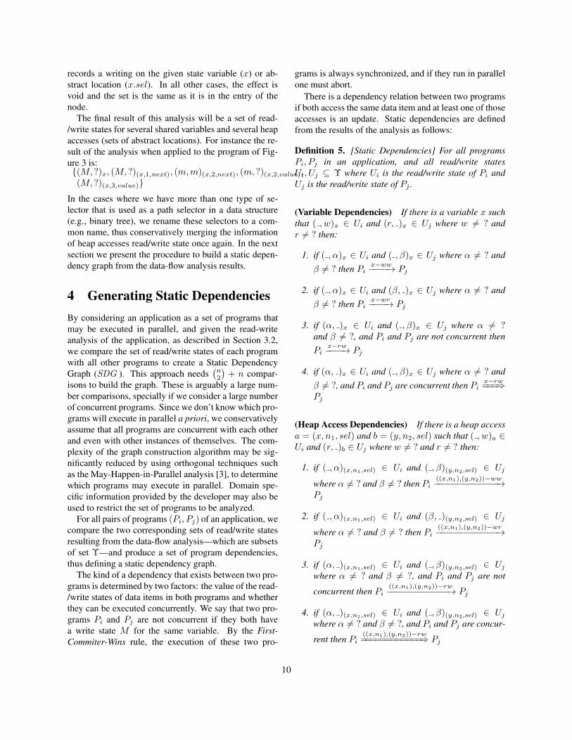
The final result of this analysis will be a set of read-/write states for several shared variables and several heapaccesses (sets of abstract locations). For instance the re-sult of the analysis when applied to the program of Fig-ure 3 is:{(M, ?)x, (M, ?)(x,1,next), (m,m)(x,2,next), (m, ?)(x,2,value),(M, ?)(x,3,value)}

In the cases where we have more than one type of se-lector that is used as a path selector in a data structure(e.g., binary tree), we rename these selectors to a com-mon name, thus conservatively merging the informationof heap accesses read/write state once again. In the nextsection we present the procedure to build a static depen-dency graph from the data-flow analysis results.

4 Generating Static DependenciesBy considering an application as a set of programs thatmay be executed in parallel, and given the read-writeanalysis of the application, as described in Section 3.2,we compare the set of read/write states of each programwith all other programs to create a Static DependencyGraph (SDG ). This approach needs

(n2

)+ n compar-

isons to build the graph. These is arguably a large num-ber comparisons, specially if we consider a large numberof concurrent programs. Since we don’t know which pro-grams will execute in parallel a priori, we conservativelyassume that all programs are concurrent with each otherand even with other instances of themselves. The com-plexity of the graph construction algorithm may be sig-nificantly reduced by using orthogonal techniques suchas the May-Happen-in-Parallel analysis [3], to determinewhich programs may execute in parallel. Domain spe-cific information provided by the developer may also beused to restrict the set of programs to be analyzed.

For all pairs of programs (Pi, Pj) of an application, wecompare the two corresponding sets of read/write statesresulting from the data-flow analysis—which are subsetsof set Υ—and produce a set of program dependencies,thus defining a static dependency graph.

The kind of a dependency that exists between two pro-grams is determined by two factors: the value of the read-/write states of data items in both programs and whetherthey can be executed concurrently. We say that two pro-grams Pi and Pj are not concurrent if they both havea write state M for the same variable. By the First-Commiter-Wins rule, the execution of these two pro-

grams is always synchronized, and if they run in parallelone must abort.

There is a dependency relation between two programsif both access the same data item and at least one of thoseaccesses is an update. Static dependencies are definedfrom the results of the analysis as follows:

Definition 5. [Static Dependencies] For all programsPi, Pj in an application, and all read/write statesUi, Uj ⊆ Υ where Ui is the read/write state of Pi andUj is the read/write state of Pj .

(Variable Dependencies) If there is a variable x suchthat ( , w)x ∈ Ui and (r, )x ∈ Uj where w 6= ? andr 6= ? then:

1. if ( , α)x ∈ Ui and ( , β)x ∈ Uj where α 6= ? andβ 6= ? then Pi

x−ww−−−−→ Pj

2. if ( , α)x ∈ Ui and (β, )x ∈ Uj where α 6= ? andβ 6= ? then Pi

x−wr−−−−→ Pj

3. if (α, )x ∈ Ui and ( , β)x ∈ Uj where α 6= ?and β 6= ?, and Pi and Pj are not concurrent thenPi

x−rw−−−−→ Pj

4. if (α, )x ∈ Ui and ( , β)x ∈ Uj where α 6= ? andβ 6= ?, and Pi and Pj are concurrent then Pi

x−rw===⇒

Pj

(Heap Access Dependencies) If there is a heap accessa = (x, n1, sel) and b = (y, n2, sel) such that ( , w)a ∈Ui and (r, )b ∈ Uj where w 6= ? and r 6= ? then:

1. if ( , α)(x,n1,sel) ∈ Ui and ( , β)(y,n2,sel) ∈ Uj

where α 6= ? and β 6= ? then Pi((x,n1),(y,n2))−ww−−−−−−−−−−−−−→

Pj

2. if ( , α)(x,n1,sel) ∈ Ui and (β, )(y,n2,sel) ∈ Uj

where α 6= ? and β 6= ? then Pi((x,n1),(y,n2))−wr−−−−−−−−−−−−→

Pj

3. if (α, )(x,n1,sel) ∈ Ui and ( , β)(y,n2,sel) ∈ Ujwhere α 6= ? and β 6= ?, and Pi and Pj are not

concurrent then Pi((x,n1),(y,n2))−rw−−−−−−−−−−−−→ Pj

4. if (α, )(x,n1,sel) ∈ Ui and ( , β)(y,n2,sel) ∈ Ujwhere α 6= ? and β 6= ?, and Pi and Pj are concur-

rent then Pi((x,n1),(y,n2))−rw============⇒ Pj

10

x − rw

x − rwP2P1

Figure 10: A SDG with a cycle of read-write dependen-cies for the same variable.

It is important to note that the comparison between pro-grams P1 and P2 is a two-way procedure. Most of thetimes this comparison generates dependencies in bothways. For instance, if we consider programs P1 with theanalysis yieldingR1 = {(M,m)x} and P2 with the anal-ysis yielding R2 = {(m,M)x}, comparing them gener-ates two dependencies: P1

wr−−→ P2 since P1 may writevariable x that is being read by P2; and P2

wr−−→ P1 be-cause P2 writes variable x which may being read by P1.

If we know that programs Pi and Pj are not concur-rent, we generate non-vulnerable read-write dependen-cies.

4.1 Incompatible Variable Static Depen-dencies

Definition 5 generates pairs of static dependencies thatcannot co-exist in a real execution, and although they areharmless, they will be detected as dangerous structures.For instance, consider the two programsP1 andP2 whereP1 = P2 and where the analysis yields {(m,m)x}. Weobtain the simplified SDG of Figure 10.

According to definition of dangerous structures, theSDG for programs P1 and P2 contains a dangerousstructure. However, no execution of these programs willtrigger a SI anomaly. This is due to the existence of somepairs of edges that are incompatible with each other, thuswe cannot blindly apply the algorithm to detect danger-ous structures, as presented in Section 2.2, as we wouldfind too many false positives.

When traversing the edges in the SDG depicted inFigure 10, one can observe that P1 has an incoming vul-nerable edge from P2, has an outgoing vulnerable edgeto P2, and there is cyclic path from P2 to itself. Now,consider a history with two committed transactions T1and T2, resulting from the execution of P1 and P2 respec-tively. We claim that is not possible to define such historyunder Snapshot Isolation if there is a transactional de-pendency T1

x−rw−−−−→ T2 and a transactional dependencyT2

x−rw−−−−→ T1. Consider that T1 is executing concurrentlywith T2, and there are dependencies T1

x−rw−−−−→ T2 andT2

x−rw−−−−→ T1. These dependencies mean that T1 readsvariable x and T2 writes variable x, and that T2 readsvariable x and T1 writes variable x. From the above one

((x, 1), (y, 2)) − rw

((y, 1), (y, 2)) − rw

((x, 2), (y, 2)) − rw

((y, 1), (x, 3)) − rw

P2P1

Figure 11: A SDG with a cycle of read-write dependen-cies for heap accesses.

can infer that T1 and T2 are necessarily concurrent, thatboth write to variable x, and that both commit. How-ever, by the First-Committer-Wins rule, one of the twotransactions should have aborted, hence it is not possibleto define such a history. This incompatibility betweenedges also applies to the other types of dependencies.

Given these observations, if we apply the definition ofdangerous structures to the SDG of Figure 10 and followthe edge P1

x−rw===⇒ P2, we can ignore the same type of

edge for the same variable in the opposite direction, i.e.,the edge P2

x−rw===⇒ P1.

4.2 Incompatible Heap Access Static De-pendencies

The processing of static dependencies for heap ac-cesses must also be enhanced, as there are pairsof heap access static dependencies that can notexist in a real execution. Consider an exam-ple with two programs P1 = {(M, ?)(x,1,sel),(M, ?)(x,2,sel), (?,M)(x,3,sel), (M, ?)(y,1,sel)} andP2 = {(M, ?)(y,1,sel), (M,M)(y,2,sel)}. Figure 11depicts the simplified SDG for these two programs,which resulted from their static dependencies. Lookingat this SDG is easy to identify a dangerous structurebetween P1 and P2, but this is actually a false positive.

In this example the dependency P2((y,1),(x,3))−rw==========⇒

P1 is incompatible with the other three opposite depen-dencies. When we say that there is a static dependency

P1((x,1),(y,2))−rw==========⇒ P2, it means that we are assuming

that the heap cell accessed by P1 with base variable xand distance 1, is the same heap cell accessed by P2 withbase variable y and distance 2. If the heap cell (x, 1) inP1, that from now on we will represent as P1(x, 1), isthe same as P2(y, 2) than it is impossible that the heapcell P1(x, 3) be the same as the P2(y, 1), as cell P1(x, 3)comes after cell P1(x, 1) and cell P2(y, 1) comes before

11

P2(y, 2), and we are assuming only acyclic data struc-tures. This can be illustrated in the following diagram:

P1 : x 1 → 2 → 3P2 : y 1 → 2

Also, if we assume P1(x, 2) to be the same as P2(y, 2),then we have the following diagram:

P1 : x 1 → 2 → 3P2 : y 1 → 2

In the case of the dependency P1((y,1),(y,2))−rw==========⇒ P2, we

are assuming that variable y in P1 is the same as variabley in P2, but the opposite dependency assume that vari-able y in P2 is the same as variable x in P1, and thereforethey are incompatible.

If the dependency P2((y,1),(x,3))−rw==========⇒ P1 is incompat-

ible with the other three opposite dependencies, then theSDG depicted in Figure 11 has no dangerous structures.

5 Dependency Detection Algorithm

The algorithm for detecting dangerous structures, de-scribed in Section 2.2, must be extended to ignore incom-patible dependencies as defined in Sections 4.1 and 4.2.The pseudo-code in Algorithm 1 defines the new proce-dure for detecting dangerous structures in an SDG . Itlooks for cyclic paths in the graph with at least two con-secutive vulnerable edges. This pattern identifies a dan-gerous structure in the SDG and signals the correspond-ing anomaly. The application of this algorithm to theSDG finalizes our static analysis procedure. The overaloutput is a set of possible SI anomalies and the corre-sponding set of anomalous programs.

The main difference between our algorithm and thealgorithm described in Section 2.2 is that we keep thehistory of visited dependencies and check for their com-patibility in the rest of the graph. Function compatibletests whether an edge e is compatible with the trailof edges already visited. The pseudo-code in Algo-rithm 2 defines function compatible, where functionisHeapAccess asserts that an edge is a dependency ona heap access. Functions varF , distF , varS, and distSextract components from heap access tuples of the form((x, d1), (y, d2)), their results are respectively x, d1, y,and d2. Function var denotes the variable of a givenvariable dependency in the graph, and function type de-notes the type of a given dependency.

Algorithm 1: Detection of Dangerous StructuresInput: nodes[], edges[], visited[]Result: true or falseinitialization;foreach Node n : nodes do

foreach Edge in : incoming(n, edges) doif vulnerable(in) then

add(visited, in);foreach Edge out : outgoing(n, edges) do

if vulnerable(out) ∧ compatible(out,visited) then

add(visited, out);if existsPath(target(out),source(in), visited) then

return true;end

endend

endendclear(visited);

endreturn false;

6 ValidationIn order to validate our approach, we developed a pro-totype using Polyglot [8] to analyze Java programs ex-tended with software transactional memory. In ourlanguage, transactional methods are identified by an@Atomic annotation accepting two parameters. Oneparameter establishes the initial state of the heap, andthe other associates a group name to that transactionalmethod. All transactional methods annotated with thesame group name are considered, by the developer, asconcurrent and are analyzed together in the same staticdependency graph.

We apply our analysis to an implementation of theSmallBank benchmark [1], originally used to evaluate SIdatabase systems crafted to dynamically avoid anoma-lies. Along with the description of the benchmark,the authors also provide its SDG , identify a dangerousstructure in the graph and corresponding anomaly. Ourgoal is to mechanically obtain the same results.

The benchmark contains five banking proce-dures [1]: Balance, Deposit Check, Transaction Saving,Amalgamate and Write Check. These proce-dures operate over three relations: Account(Name,CustomerId), Saving(CustomerId, Balance), andChecking(CustomerId, Balance). The Account relation

12

Algorithm 2: compatible functionInput: edge, visited[]Result: true or falseforeach Edge v : visited do

if source(edge) = target(v) ∧ target(edge) =source(v) then

if isHeapAccess(edge) ∧ isHeapAccess(v)then

if varF(edge) = varS(v) ∧ varS(edge) =varF(v) then

if distF(edge) = distS(v) ∧distS(edge) = distF(v) ∧ type(edge) =type(v) then

return false;else if

(distF(edge) ≥ distS(v) ∧

distS(edge) ≤ distF(v))∨(

distF(edge) ≤ distS(v) ∧ distS(edge)≥ distF(v)

)then

return false;end

else if varF(edge) = varS(e) ∧ varS(edge)6= varF(e) then

return false;else if varF(edge) 6= varS(e) ∧varS(edge) = varF(e) then

return false;end

else if not (isHeapAccess(edge) ∨isHeapAccess(v)) then

if var(edge) = var(v) ∧ type(edge) =type(v) then

return false;end

elsereturn false;

endend

endreturn true;

identifies the customers of the bank. The Balance at-tribute in both Saving and Checking relations quantifiesthe amount in each kind of account for each customer.In our implementation of the benchmark, we representthe three relations using an ordered singly linked list oftriples, containing a name and a balance for each kindof account. Each banking procedure is implemented asa Java method, tagged with the @Atomic annotation,and operating over the triples in the list. We dividethe transactional methods in two groups, one for the

add ={(M, ?)h, (M, ?)(h,1,next), (m,m)(h,2,next)},remove ={(M, ?)h, (M, ?)(h,1,next), (m,m)(h,2,next),

(m, ?)(h,3,next)}get ={(M, ?)h, (M, ?)(h,1,next), (m, ?)(h,2,next)}

Table 2: Analysis on the list group.

addrw=⇒ remove

rw=⇒ add (write-skew)

removerw=⇒ remove

rw=⇒ remove (write-skew)

getrw=⇒ add

rw=⇒ remove (False Positive)

getrw=⇒ remove

rw=⇒ add (False Positive)

Table 3: Anomalies

list operations and another for the five SmallBankbenchmark operations.

The list group contains three transactional methods:add, remove and get. The list nodes are stored in heapcells with selector next pointing to the next node in thelist, and selector val storing the node’s value. The re-sult of the data-flow analysis on this group, focused onthe selector next, is presented in Table 2. The selec-tor val is irrelevant for detecting anomalies. The SDGgenerated from the result of the data-flow analysis is de-picted in Figure 12, where we can identify the dangerousstructures described in Table 3. Two of the dangerousstructures, involving the get method, are false positives.

The write-skew anomalies detected by our analysis,involving the transactions add and remove, correspondto the example introduced in Section 1. These anoma-lies can be corrected by forcing full serializability on theexecution of add and remove methods, or by adding adummy write operation on the node to be removed bythe remove method.

The results of the analysis of the five transactionalmethods in the benchmark group are presented in Ta-ble 4. The SDG generated from the result of the data-flow analysis is depicted in Figure 13. The only danger-ous structure identified is Bal rw

=⇒ WCrw=⇒ TS, where

WC is the pivot. This dangerous structure is the oneoriginally referred in the benchmark [1].

Our prototype is able to mechanically identify all theexpected anomalies in this sample code, but for the firsttime through a semantic analysis, and targeting the chal-lenging setting of transactional memory programs writ-ten in a general purpose language.

13

add remove

get

Figure 12: SDG of an ordered linked list.

Bal ={(M, ?)(a,1,chec), (M, ?)(a,1,savi)}DC ={(M,M)(a,1,chec)}TS ={(M,M)(a,1,savi)}

Amg ={(M,M)(a1,1,chec), (M,M)(a1,1,savi), (M,M)(a2,1,chec)}WC ={(M,M)(a,1,chec), (M, ?)(a,1,savi)}

Table 4: Analysis on the benchmark group.

7 Related WorkSoftware Transactional Memory (STM) [11, 5] systemscommonly implement full serializability to ensure thecorrect execution of transactional memory programs. Tothe best of our knowledge, SI-STM [9] is the only im-plementation of a STM using Snapshot Isolation. Theirwork focuses on the improvement of transactional pro-cessing throughput by using a snapshot isolation algo-rithm. They also propose a SI safe variant of the algo-rithm where anomalies are automatic and dynamicallyavoided by enforcing validation of read/write conflicts.In our work, we aim at providing the serializability se-mantics under snapshot isolation STM systems. This isachieved by performing a static analysis to assert that noSI anomalies will occur when executing a transactionalapplication.

The use of Snapshot Isolation in databases is a com-mon place, and there is some previous works on the de-tection of SI anomalies in this domain. Our work isclearly inspired in [4], which presents the theory of SIanomaly detection and a syntactic analysis to detect SIanomalies for the database setting. They assume appli-cations are described in some form of pseudo-code, with-out conditional (if-then-else) and cyclic structures. Theproposed analysis is informally described and applied tothe database benchmark TPC-C [12]. A sequel of thatwork [6], describes a prototype which is able to auto-matically analyze database applications. Their syntacticanalysis is based on the names of the columns accessedin the SQL statements that occur within the transaction.They also discuss some solutions to reduce the number offalse positives produced by their analysis. Although tar-geting similar results, our work deals with significantly

Bal

WC

DC

Amg

TS

Figure 13: SDG of the SmallBank benchmark.

different problems. The more significant one is relatedto the full power of general purpose languages and theuse of dynamically allocated heap data structures. Be-sides that, we treat the full control-flow of imperativeprograms. Our work strives for reducing the state explo-sion during the analysis by conservatively merging somekinds of information.

8 Concluding RemarksIn this paper we define a new static analysis techniqueand present the corresponding algorithm to mechanicallyassert that a given transactional memory application ex-ecuting under Snapshot Isolation will not suffer from SIanomalies. Our work allows for the automatic identifica-tion of anomalous transactional code, by signaling con-flicting programs and allowing for explicit code correc-tions. Thus, we enable the use of SI as the default isola-tion level for STM applications.

A major difference of our analysis to existing relatedwork [4, 6] is that, instead of targeting languages withlimited expressiveness like SQL, we target a general pur-pose imperative language with support for dynamicallyallocated data structures. We define a data-flow analysisthat extracts fine grained read/write state information foreach state variable and heap cell manipulated by trans-actional programs. We adapt a standard shape analysistechnique [10] to track heap cell manipulation during theanalysis.

The results of our data-flow analysis are then usedto build dependency graphs on programs from whichwe can detect connection patterns that correspond to SIanomalies. Our algorithm may be used in the future asinput for manual or automatic procedures of anomalouscode correction.

To validate our approach, we implemented a proto-type of the analysis framework capable of identifyingthe same anomalies in complete Java programs as re-lated benchmarks detect in SQL procedures [1]. We

14

also show that our analysis identifies known anomalies(write-skew) in simple acyclic dynamic data structuresand illustrate the procedure on an ordered singly linkedlist implementation. We also propose an enhancement tothe algorithm that uses a compatibility relation betweendependencies to reduce the number of false positives in-troduced by the static analysis. We foresee that othertechniques, such as using information from the type sys-tem, can also be used to further reduce the presence offalse-positives.

Looking at the short term evolution of our framework,we plan to extend the shape graph model to include datastructures with backward pointers, and enable the auto-matic correction of SI anomalies by source code trans-formation. In the long term, we aim at extending thecorrectness guarantees provided by our analysis to sup-port further studies of SI in the STM setting, such as withdistributed transactional memory.

References

[1] M. Alomari, M. Cahill, A. Fekete, and U. Rohm.The cost of serializability on platforms that usesnapshot isolation. In ICDE ’08: Proceedingsof the 2008 IEEE 24th International Conferenceon Data Engineering, pages 576–585, Washington,DC, USA, 2008. IEEE Computer Society.

[2] H. Berenson, P. Bernstein, J. N. Gray, J. Melton,E. O’Neil, and P. O’Neil. A critique of ANSI SQLisolation levels. In SIGMOD ’95: Proceedings ofthe 1995 ACM SIGMOD international conferenceon Management of data, pages 1–10, New York,NY, USA, 1995. ACM.

[3] E. Duesterwald and M. L. Soffa. Concurrency anal-ysis in the presence of procedures using a data-flowframework. In TAV4: Proceedings of the sympo-sium on testing, analysis, and verification, pages36–48, New York, NY, USA, 1991. ACM.

[4] A. Fekete, D. Liarokapis, E. O’Neil, P. O’Neil, andD. Shasha. Making snapshot isolation serializable.ACM Trans. Database Syst., 30(2):492–528, 2005.

[5] M. Herlihy, V. Luchangco, M. Moir, and I. WilliamN. Scherer. Software transactional memory fordynamic-sized data structures. In PODC ’03: Pro-ceedings of the twenty-second annual symposiumon Principles of distributed computing, pages 92–101, New York, NY, USA, 2003. ACM.

[6] S. Jorwekar, A. Fekete, K. Ramamritham, andS. Sudarshan. Automating the detection of snap-shot isolation anomalies. In VLDB ’07: Proceed-ings of the 33rd international conference on Verylarge data bases, pages 1263–1274, Vienna, Aus-tria, 2007. VLDB Endowment.

[7] F. Nielson, H. Nielson, and C. Hankin. Principlesof Program Analysis. Springer, 1999.

[8] N. Nystrom, M. R. Clarkson, and A. C. Myers.Polyglot: An extensible compiler framework forJava. Technical Report TR2002-1883, Cornell Uni-versity, Nov. 2002.

[9] T. Riegel, C. Fetzer, and P. Felber. Snapshotisolation for software transactional memory. InTRANSACT’06: First ACM SIGPLAN Workshop onLanguages, Compilers, and Hardware Support forTransactional Computing, Ottawa, Canada, June2006.

[10] M. Sagiv, T. Reps, and R. Wilhelm. Solving shape-analysis problems in languages with destructive up-dating. ACM Trans. Program. Lang. Syst., 20(1):1–50, 1998.

[11] N. Shavit and D. Touitou. Software transactionalmemory. In PODC ’95: Proceedings of the four-teenth annual ACM symposium on Principles ofdistributed computing, pages 204–213, New York,NY, USA, 1995. ACM.

[12] Transaction Processing Performance Council.TPC-C Benchmark, Standard Specification,Revision 5.11. Feb. 2010.

15