Detection of Thin Boundaries between Different Types of Anomalies in

Outlier Detection using Enhanced Neural Networks

Rasoul Kiania, Amin Keshavarzia,* and Mahdi Bohloulib,c,d

a Department of Computer Engineering, Marvdasht Branch, Islamic Azad University,

Marvdasht, Iran.

b Department of Computer Science and Information Technology, Institute for advanced

Studies in Basic Sciences, Zanjan Iran.

cResearch Center for Basic Sciences and Modern Technologies, Institute for Advanced

Studies in Basic Sciences, Zanjan, Iran.

dResearch and Innovation Department, Petanux GmbH, Bonn, Germany.

*Corresponding author: keshavarzi@miau.ac.ir

Detection of Thin Boundaries between Different Types of Anomalies in

Outlier Detection using Enhanced Neural Networks

Outlier detection has received special attention in various fields, mainly for those

dealing with machine learning and artificial intelligence. As strong outliers,

anomalies are divided into point, contextual and collective outliers. The most

important challenges in outlier detection include the thin boundary between the

remote points and natural area, the tendency of new data and noise to mimic the

real data, unlabelled datasets and different definitions for outliers in different

applications. Considering stated challenges, we defined new types of anomalies

called Collective Normal Anomaly and Collective Point Anomaly in order to

improve a much better detection of the thin boundary between different types of

anomalies. Basic domain-independent methods are introduced to detect these

defined anomalies in both unsupervised and supervised datasets. The Multi-Layer

Perceptron Neural Network is enhanced using the Genetic Algorithm to detect new

defined anomalies with a higher precision so as to ensure a test error less than that

calculated for the conventional Multi-Layer Perceptron Neural Network.

Experimental results on benchmark datasets indicated reduced error of anomaly

detection process in comparison to baselines.

Keywords: outlier detection; anomaly detection; neural network; genetic

algorithm

Introduction

Data extraction (Keshavarzi et al., 2008) and pre-processing operations lead to a refined

explorable dataset in different machine learning applications such as cloud computing

(Keshavarzi et al, 2019; Keshavarzi et al., 2017), big data (Bohlouli et al., 2013), and

sensor networks (Jafarizadeh et al., 2017). Pre-processing aims at identification and

removing outliers to improve the quality of cleansing process (Agarwal, 2013; Kiani et

al.,2015). Outliers show a higher deviation and are not in line with the behaviour of

general dataset, which could cause unexpected results in analytics. Outliers probably

created due to measurement error, the inherent variability of data or faulty sensors

(Chandola et al., 2009; Agarwal, 2015; Chandarana and Dhamecha, 2015). Noises are

weak outliers but anomalies are strong outliers. The boundary between the noises and

anomalies is not clear but can be determined through different analytical methods

(Agarwal, 2015). Anomalies are divided into three categories of point, contextual and

collective anomalies (Chandola et al., 2009; Agarwal, 2015; Song et al., 2007; Malik et

al., 2014).

Point Anomalies (PA) are located at a considerable distance from normal data and

diverged from the usual pattern of data. According to conditions, contextual anomalies

can be (or not to be) outlier relative to normal data. Collective anomalies are a set of

related outliers relative to normal data. Such anomalies may be free of deviations alone

(Chandola et al., 2009; Malik et al., 2014; Gupta et al., 2014 ). In fact, point and collective

anomalies are two subsets of contextual anomalies (Chandola et al., 2009; Agarwal,

2015). Based on the use of labelled data, outlier detection approaches are divided into

supervised, semi-supervised and unsupervised methods (Vijayarani and Nithya, 2011;

Theiler and Cai, 2003; Steinwart et al., 2005; Fujimaki et al., 2005; Bolton et al., 2001).

Also outlier detection methods are divided into distribution-based, clustering-based,

distance-based and density-based methods (Hodge and Austin, 2004; Kou et al., 2007;

Zhang, 2008; Chllalagalla et al., 2010). The key components of anomaly detection

methods are research area, anomaly detection technique, problem characteristic and

application domain (Chandola, 2009).

The most important challenges in outlier detection include the thin boundary between

the remote points and natural area, the tendency of new data and noise to mimic the real

data, unlabelled datasets and different definitions for outliers in different application areas

(Chandola, 2009; Agarwal, 2015). In this paper, the thin boundary between normal data

and various types of anomalies is examined. Furthermore, other types of anomalies called

Collective Normal Anomaly (CNA) and Collective Point Anomaly (CPA) are

investigated.

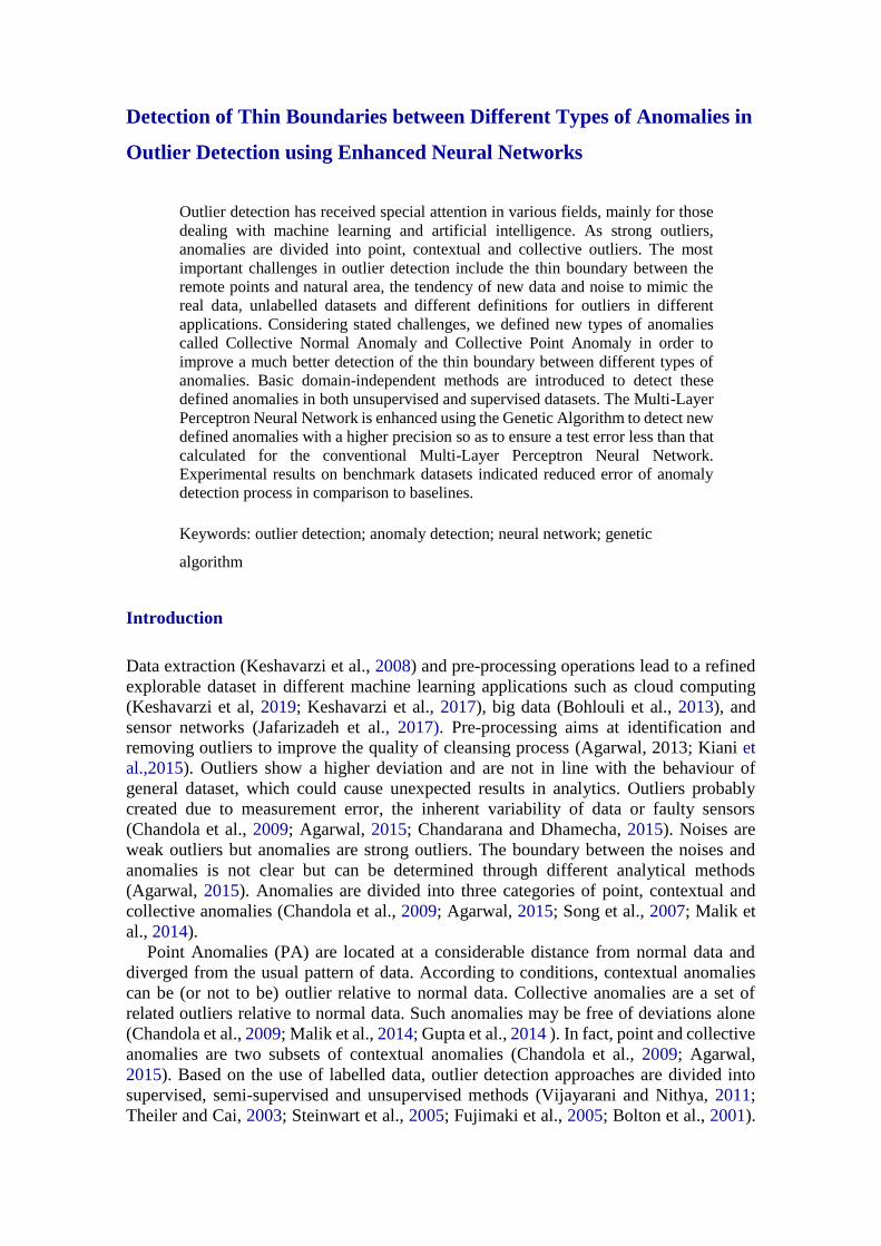
CNA: There is a thin boundary between Normal Data (ND) and CNA. Due to the

characteristics of ND, it is assumed that CNA can be clustered. CNA is a cluster

that its standard deviation density is greater than or equal to the threshold for

standard deviation of all clusters.

CPA: CPA is a subset of Point Anomaly (PA) and there is a thin boundary

between PA and CPA. Due to the characteristics of PA, it is assumed that CPA

cannot be clustered.

Figure 1 shows ND, CNA, PA and CPA in a schematic plot and the thin boundary

between various types of anomalies is visible.

Figure 1. A schematic plot of thin boundary between normal data and various types of anomalies.

For this purpose, unsupervised and supervised datasets are first studied. Using proposed

framework in this paper, the supervised dataset is divided into subsets based on the

number of classes. The Multi-Layer Perceptron Neural Network (MLP-NN) is also

improved using the Genetic Algorithm (GA) to detect the thin boundary between different

types of anomalies. Because of the fact that neural network learning which is based on

neurons weight and detection accuracy is variable in each epoch, using GA seems

possible to solve this problem which is improved both better detection of new defined

anomalies and reducing the test error.

The rest of this paper is organized as fallows. Section 2 reviews related work in outlier

detection. The proposed method is discussed in detail in Section 3. The results are

analyzed in Section 4. Finally, conclusions are presented.

Literature Review

As a supervised or semi-supervised method, the neural networks have been used to detect

outliers and anomalies in various fields such as host based intrusion detection (Ghosh et

al., 1998), network intrusion detection (Ramadas et al., 2003; Smith et al., 2002; Zhang

et al., 2001), credit card fraud detection (Zhang et al., 2001; Aleskerov et al., 1997),

mobile fraud detection (Barson et al.,1996; Taniguchi et al., 1998), medical and public

health domain (Campbell, 2001), fault detection in mechanical units (Diaz and Hollmen,

2002; Li et al., 2002), structural damage detection (Shon et al., 2001), image processing

(Singh et al., 2004; Augusteijn and Folkert, 2002) and anomalous topic detection in text

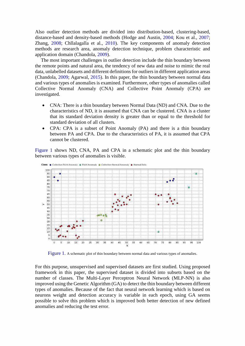
data (Manevitz and Yousef, 2001). Figure 2 shows the variation of efficiency with

dimensions for all methods. Moreover, Figure 3 shows the variation of scalability with

the dimensions respectively for all methods (Malik et al., 2014). As can be seen in Figures

2 and 3, both efficiency and scalability are considered based on dimensionality

respectively for all the methods. It seems likely the methods based on NN and clustering

benefit greatly from the best efficiency and scalability. For example, when dimensionality

is 80, the scalability of NN, clustering and density methods are approximately equal

therefore NN seems a much better choice owing to the fact that its efficiency is better.

Figure 2. Efficiency of various outlier detection methods in scale up (Malik et al., 2014).

Figure 3. . Scalability of various outlier detection methods in scale up (Malik et al., 2014).

A 3-step process has been proposed to detect false alarms and outliers (Hachmi et al.,

2015). In the first step, preliminary alerts are clustered to create a set of meta-alerts. In

the second step, outliers are removed from the meta-alerts. In the third step, a binary

classification algorithm is used to classify meta-alerts into attacks and false alarms. An

extended statistical unsupervised method has been used to detect outliers in object-

relational data (Riahi et al., 2015). For this purpose, a metric was introduced based on the

likelihood ratio of vectors of population association and individual association. To detect

outliers in large matrices, a two-stage adaptive approach has been suggested that its

performance is guaranteed using an inference met (Li et al., 2015). Song et al., (2007)

proposed a general-purpose method called conditional anomaly detection. They used

three different learning algorithms for their proposed model. A distributed outlier detector

with a reasonable speed and efficiency has been proposed to detect so-called global

outliers in a distributed database (Zhang et al., 2012). Wang and Davidson (2009)

detected contextual outliers by using the random walks graph. The most important feature

of this approach is to consider scores for outliers. A data driven approach has been

proposed to detect anomalies in the patient management actions (Hauskrecht et al., 2010).

This method is based on past patient records in the electronic patient health record system.

A semi-supervised framework based on fixed-background mixture has been proposed to

detect anomalies (Vatanen et al., 2012). This framework is robust enough to detect

patterns of anomaly model. To detect collective anomalies and DoS attacks in network

traffic analysis, a framework has been suggested based on X-means clustering algorithm

(Ahmed and Mahmood, 2014). Noble and Cook (2003) used anomalous infrastructure

detection and anomalous sub graph detection to provide a graph-based approach for

anomaly detection. Yang and Liu (2011) detected anomalies in collective moving patterns

using the hidden Markov model. Abnormal detection research preprocessing the data and

sets the normal sample set has been presented. This method based on outlier mining

calculated the outlier score of each sample in the normal sample set (Zhang et al., 2018).

Taylor et al. proposed the outlier detection method using the super efficiency which

removal of one outlier little effect in estimation since the neighbor outlier serves as a

proxy benchmark. In other words, they developed an alternative method based on the

stochastic DEA model of Banker (Boyd et al., 2016). Ko et al., (2017) suggested the

model based on data integration and machine learning-based anomaly detection so as to

the overcome the conventional methods for estimating the level of quality. Also, the

method for segmentation and indexing multi-dimensional time series data is introduced.

Maheshwari and Singh (2016) proposed an algorithm to output clusters and outliers in a

divide and conquer manner. The method following outliers in each cluster identified core

objects outliers. Guo et al. (2018) proposed a new distance-based method on which

depends the data structure to detects such points. In the proposed method, firstly, a global

binary tree is used and then the local distance score of point is calculated for evaluating

to what degree the observations in an outlier. Zhao and Hryniewicki (2018) proposed an

algorithm called XGBOD which was a new semi-supervised method. XCBOD described

and demonstrated for enhanced detection of outliers from normal data. This framework

combined the strengths of both supervised and unsupervised methods by a hybrid

approach. Kutsuna and Yamamoto (2017) suggested a novel method for outlier detection

using binary decision diagram which is used a new measure for detecting outliers. Lin et

al., (2018) proposed a method has employed a spatial-feature-temporal tensor model

analyzed latent mobility patterns through unsupervised learning and LOF algorithm is

used to localize anomaly in a given time interval. Macha and Akoglu (2018) proposed a

new approach called x-PACS which are used reverse engineering to detect anomalies

based on both the groups and characterizing subcase and features rules.

The Proposed Method

Assumptions

It is assumed that there are two types of datasets: (1) datasets containing labeled data and

(2) those containing unlabeled data. The main assumption of our proposed method is that

data has been previously labeled using common techniques such as clustering algorithm,

decision tree, hidden Markov Model, etc. Equation (1) shows the relationship between

different types of anomalies and normal data (Chandola et al., 2009):

PA: If an individual data instance can be considered as anomalous with respect to

the rest of data, then the instance is termed as a PA.

Collective Anomalies (CA): If a collection of related data instances is anomalous

with respect to the entire data set, it is termed as a CA. The individual data

instances in a collective anomaly may not be anomalies by themselves, but their

occurrence together as a collection is anomalous.

ND: ND instances occur in dense neighborhoods, while anomalies occur far from

their closest neighbors.

The relationship between the PA and CPA is shown in Equation (2). Based on Equation

(2) CPA is a subset of PA and there is a thin boundary between PA and CPA. Equation

(3) defines CPA that the neighborhood radius of CPA is less than average neighborhood

radius of PA.

PA∪ CA∪ ND =Dataset (1)

CPA⊂ PA (2)

CPA= {Pi∈ CPA|Pi∈ PA and Out_RadPi

< Out_RadPA} (3)

where Out_RadPi is the neighborhood radius of Pi as well as its average distance to PA

and Out_RadPA is the neighborhood radius of PA.

Equations (4)-(6) show the calculation of neighborhood radius.

Out_RadPi = ∑ MDistOi

ki=1

k

(4)

MDistOi= {

∑ Dist(Oi,Oj)kj=1

k-1|i≠j , i={1,…,k}} (5)

Dist(Oi,Oj)= {√(xOi-xOj

)2+(y

Oi-y

Oj)2| i,j={1,…,k}} (6)

where Out_RadPi is the outlier radius of CPA, MDist is the mean distances table from

point anomalies, Oi and Oj are PA, and k is the number of point anomalies.

Equation (7) shows the relationship between the ND and CNA. Based on Equation (7)

CNA is a subset of ND and there is a thin boundary between ND and CNA. Due to the

characteristics of ND means that their neighborhood radius is less than the mean distances

from points, is assumed that CNA can be clustered in order to use in supervised data. The

definition of CNA is given in Equation (8). CNA is a cluster that its standard deviation

density is greater than or equal to the threshold for standard deviation of all clusters.

CNA⊂ ND (7)

CNA= {Ci∈C|Ci∈ND and σ_DenCi≥Th_σ

DenC} (8)

where Ci is one of detected clusters, C is the set of all clusters, σ_DenCi is standard

deviation of cluster density Ci, and Th_σDenC

is the threshold for standard deviation of all

clusters.

In this paper the research area is data mining as well as this the application range is

independent of domain and the problem characteristic is the type of anomaly .The

proposed method to detect different types of anomalies is described and a new framework

is proposed for labeling supervised datasets in the proposed framework section. After

that, MLP-NN is enhanced using the GA to increase the precision of anomaly detection.

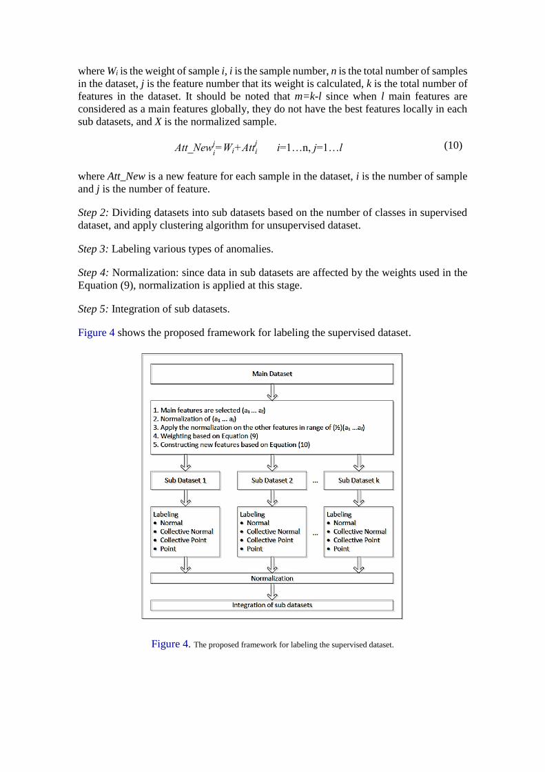
The Proposed Framework

One of the important points considered in this paper is adaptability of the proposed

algorithm with both supervised and unsupervised datasets. As previously mentioned

anomalies have been labeled using common techniques and are ready to be used in the

neural network. In the first step, the supervised dataset is divided into sub datasets to

detect local anomalies.

Step 1: Various types of anomalies should be investigated in all classes in the supervised

dataset. Thus, among k features in the reference dataset, l features with a higher separation

capability should be analytically selected as the main features. In other words, based on

three criteria including the type of dataset, functional domain and its features, the most

distinguishing features should be selected. Although l features have been selected to suit

all classes means that supervised dataset, they may be not the best if they are evaluated

locally (in each sub dataset). Thus, aggregation technique is used here. That is to say,

aggregation is a type of data smoothing. Therefore, two aggregation techniques are used

to reduce the number of features from k to l. As a first technique, normalization is used

to improve the accuracy of data mining algorithms. The second technique is to weight for

valuation of all features. The range of numbers has a direct effect on the weight obtained

for each feature in the weighting process. If normalization techniques are not used,

weights will be unbalanced leading to unsmoothed features. Accordingly, normalization

technique is used to solve this problem to put all the numbers for all features in a constant

range.

Equation (9) shows the weighting formula and Equation (10) shows the formula for

constructing new features.

Wi=Xi

1+Xi2+…+Xi

j

j 𝑖 = 1. . . 𝑛 , 𝑗 = 1. . . 𝑚 𝑎𝑛𝑑 𝑚 = 𝑘 − 𝑙 (9)

where Wi is the weight of sample i, i is the sample number, n is the total number of samples

in the dataset, j is the feature number that its weight is calculated, k is the total number of

features in the dataset. It should be noted that m=k-l since when l main features are

considered as a main features globally, they do not have the best features locally in each

sub datasets, and X is the normalized sample.

Att_Newi

j=Wi+Atti

j i=1…n, j=1…l (10)

where Att_New is a new feature for each sample in the dataset, i is the number of sample

and j is the number of feature.

Step 2: Dividing datasets into sub datasets based on the number of classes in supervised

dataset, and apply clustering algorithm for unsupervised dataset.

Step 3: Labeling various types of anomalies.

Step 4: Normalization: since data in sub datasets are affected by the weights used in the

Equation (9), normalization is applied at this stage.

Step 5: Integration of sub datasets.

Figure 4 shows the proposed framework for labeling the supervised dataset.

Figure 4. The proposed framework for labeling the supervised dataset.

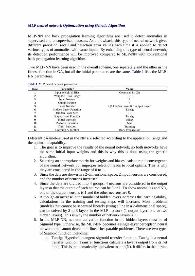
MLP neural network Optimization using Genetic Algorithm

MLP-NN and back propagation learning algorithms are used to detect anomalies in

supervised and unsupervised datasets. As a drawback, this type of neural network gives

different precision, recall and detection error values each time it is applied to detect

various types of anomalies with same inputs. By enhancing this type of neural network,

its detection performance will be improved compared to MLP-NN with conventional

back propagation learning algorithm.

Two MLP-NN have been used in the overall scheme, one separately and the other as the

fitness function in GA, but all the initial parameters are the same. Table 1 lists the MLP-

NN parameters.

Table 1. MLP neural network parameters.

Row Parameter Value

1 Input Weight & Bias Generated by GA

2 Weight & Bias Range [0-1]

3 Input Neuron 2

4 Output Neuron 4

5 Layer Number 2 (1 Hidden Layer & 1 output Layer)

6 Hidden Layer Function Tansig

7 Hidden Layer Size 10

8 Output Layer Function Tansig

9 Initial Function Initlay

10 Perform Function Mse

11 Train Function Trainscg

12 Learning Algorithm Back Propagation

Different parameters used in the NN are selected according to the application range and

the optimal adaptability.

1. The goal is to improve the results of the neural network, so both networks have

the same initial input weights and this is why this is done using the genetic

algorithm.

2. Selecting an appropriate matrix for weights and biases leads to rapid convergence

of the neural network but improper selection leads to local optima. This is why

they are considered in the range of 0 to 1.

3. Since the data are shown in a 2-dimensional space, 2 input neurons are considered,

and the number of neurons increased.

4. Since the data are divided into 4 groups, 4 neurons are considered in the output

layer so that the output of each neuron can be 0 or 1. To show anomalies and ND,

one of the output neurons is 1 and the other neurons are 0.

5. Although an increase in the number of hidden layers increases the learning ability,

calculations in the training and testing steps will increase. Most problems

(models) that cannot be separated linearly (using a line in a 2-dimensional space),

can be solved by 2 to 3 layers in the MLP network (1 output layer, one or two

hidden layers). This is why the number of network layers is 2.

6. In the MLP-NN, neurons activation function in the hidden layers must be of

Sigmoid type. Otherwise, the MLP-NN becomes a single-layer perceptron neural

network and cannot detect non-linear inseparable problems. There are two types

of Sigmoid function including:

a. Tansig: Hyperbolic tangent sigmoid transfer function. Tansig is a neural

transfer function. Transfer functions calculate a layer's output from its net

input. This is mathematically equivalent to tanh(N). It differs in that it runs

faster than the MATLAB implementation of tanh, but the results can have

very small numerical differences. This function is a good tradeoff for

neural networks, where speed important and the exact shape of the transfer

function is not.

b. Logsig: Log-sigmoid transfer function. Logsig is a transfer function.

Therefore, Tansig is used.

7. The small number of neurons in the hidden layer causes inadaptability while the

large number of neurons in the hidden layer leads to over fitting. Therefore, 10

neurons were considered in the hidden layer by trial and error.

8. The use of Sigmoid function in the output layer limits the network output to a

small range. As previously stated, Tansig function is more appropriate for this

purpose.

9. Since the weights and biases are injected to the neural networks, Initlay (Layer-

by-layer network initialization) function is used. Initlay is a network initialization

function that initializes each layer i according to its own initialization function net

and returns the network with each layer updated. Initlay does not have any

initialization parameters.

10. MSE (Mean squared normalized error performance function) is used as the

performance function. MSE is a network performance function which measures

the network's performance according to the mean of squared errors and returns

the mean squared error. Note that MSE can be called with only one argument

because the other arguments are ignored. MSE supports those ignored arguments

to conform to the standard performance function argument list.

11. To select training algorithm for the MLP-NN, different parameters such as

problem complexity, the number of data in the dataset, the number of weights and

biases, the error and so on should be considered. According to the parameters

listed above, Trainscg (Scaled conjugate gradient back propagation) function is

used which is a network training function that updates weight and bias values

according to the scaled conjugate gradient method. Trainscg can train any network

as long as its weight, net input, and transfer functions have derivative functions.

Back propagation is used to calculate derivatives of performance with respect to

the weight and bias variables. One of the main reasons for selecting trainscg

function is to improve network generalization as well as this one of the ways to

improve the network generalization is early stopping where the dataset is divided

into training, evaluation and testing data and the trainscg function shows a better

performance with early stopping.

This section outlines the GA steps to enhance the results of MLP-NN.

Step 1: the initial population is generated by the GA. The number of genes in individuals

equals the number of weights and biases required for the MLP-NN. The purpose is to

apply the same input weights to the MLP-NN outside the GA and the evaluation function

(the MLP-NN inside the GA). The extracted weights are generated as an initial population

in the form of a matrix where the number of rows equals the population in each generation

and the number of columns is equal to the total number of weights and biases. In the

future generations, GA will produce the next generation.

Step 2: Applying the crossover operator according to Equation (11).

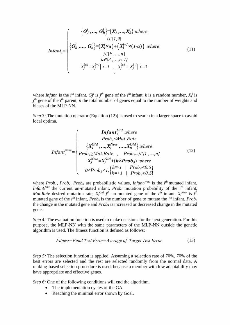
Infanti=

{

{G1

i ,…, Gk

i}={X1

i ,…,Xk

i } where

i∈{1,2}

{Gki ,…, Gn

i}=(Xj

i×α)+ (Xj

i±1×(1-α)) where

j∈{k ,…,n}

k∈{2 ,…,n-1}

Xji±1

=Xji+1| i=1 , Xj

i±1= Xj

i-1| i=2

,

(11)

where Infanti is the ith infant, Gji is jth gene of the ith infant, k is a random number, Xji is

jth gene of the ith parent, n the total number of genes equal to the number of weights and

biases of the MLP-NN.

Step 3: The mutation operator (Equation (12)) is used to search in a larger space to avoid

local optima.

Infanti

New=

{

Infant

i

Old where

Prob1<Mut.Rate

{X1Old

,…,XjNew

,…,XnOld} where

Prob1≥Mut.Rate , Prob2=j∈{1 ,…,n}

XjNew

=XjOld

+(k×Prob3) where

0<Prob3<1, {k=-1 | Prob4<0.5

k=+1 | Prob4≥0.5}

(12)

where Prob1, Prob2, Prob3 are probabilistic values, InfantiNew is the ith mutated infant,

InfantiOld the current un-mutated infant, Probi mutation probability of the ith infant,

Mut.Rate desired mutation rate, XjOld jth un-mutated gene of the ith infant, Xj

New is jth

mutated gene of the ith infant, Prob2 is the number of gene to mutate the ith infant, Prob3

the change in the mutated gene and Prob4 is increased or decreased change in the mutated

gene.

Step 4: The evaluation function is used to make decisions for the next generation. For this

purpose, the MLP-NN with the same parameters of the MLP-NN outside the genetic

algorithm is used. The fitness function is defined as follows:

Fitness=Final Test Error=Average of Target Test Error (13)

Step 5: The selection function is applied. Assuming a selection rate of 70%, 70% of the

best errors are selected and the rest are selected randomly from the normal data. A

ranking-based selection procedure is used, because a member with low adaptability may

have appropriate and effective genes.

Step 6: One of the following conditions will end the algorithm.

The implementation cycles of the GA.

Reaching the minimal error shown by Goal.

Step 7: At the end, the test errors obtained from the enhanced and conventional MLP-NN

are compared.

Table 2 lists the initial parameters of the GA.

Table 2. The initial parameters of the genetic algorithm.

Value Parameter Row

20 Cycle 1

15 Population Size 2

0.3 Crossover α 3

0.1 Mutation Rate 4

0.7 Selection Rate 5

0 Goal 6

Test Error Fitness Function 7

The reasons for selecting the initial parameters of the GA are discussed.

1. The cycle is selected by trial and error.

2. Initial population is selected by trial and error.

3. The use of crossover operator generates members with adaptability higher than

the average and this avoids dispersion. For this purpose, a single point is used. An

increase in the number of points in the crossover operator will result in higher

variation in the search space and a lower reliability (the answers will considerably

change in different generations).

4. Mutation leads to search in the space that has not been previously investigated.

Mutation rate should not be high, because the GA becomes a completely random

search algorithm and thus convergence is delayed.

5. One of the problems with small population in the GA is local optima. To

overcome this problem, Rank Scaling selection function is used. The default

fitness scaling option, Rank, scales the raw scores based on the rank of each

individual instead of its score. The rank of an individual is its position in the sorted

scores: the rank of the fit individual is 1, the next most fit is 2, and so on. The rank

scaling function assigns scaled values so that. Rank fitness scaling removes the

effect of the spread of the raw scores.

6. The target error of the fitting function is 0. When an error of 0 is achieved, the

algorithm is stopped.

7. The fitness function in the GA is defined using MLP-NN to minimize the test

error. Figure 5 shows the proposed scheme to enhance MLP-NN using the GA. It

should be noted that the MLP-NN is enhanced using the GA to detect new defined

anomalies with a higher precision so as to ensure a test error less than that

calculated for the conventional MLP-NN.

Results and Discussion

The proposed techniques have applied on 2 parts (Part A and B). Firstly, three datasets

were selected based on an idea which is showed the evaluation parameters include

precession, recall, test error and ROC curve. Secondly, the ability of proposed framework

so as to detect the thin boundary challenge between new anomalies based on 8 UCI

datasets has considered. Additionally, we have used a few benchmark datasets based on

the repository which proposed in (Campos et al., 2016) to calculate both true positive rate

and false positive rate. It should be noted that datasets have picked in various fields.

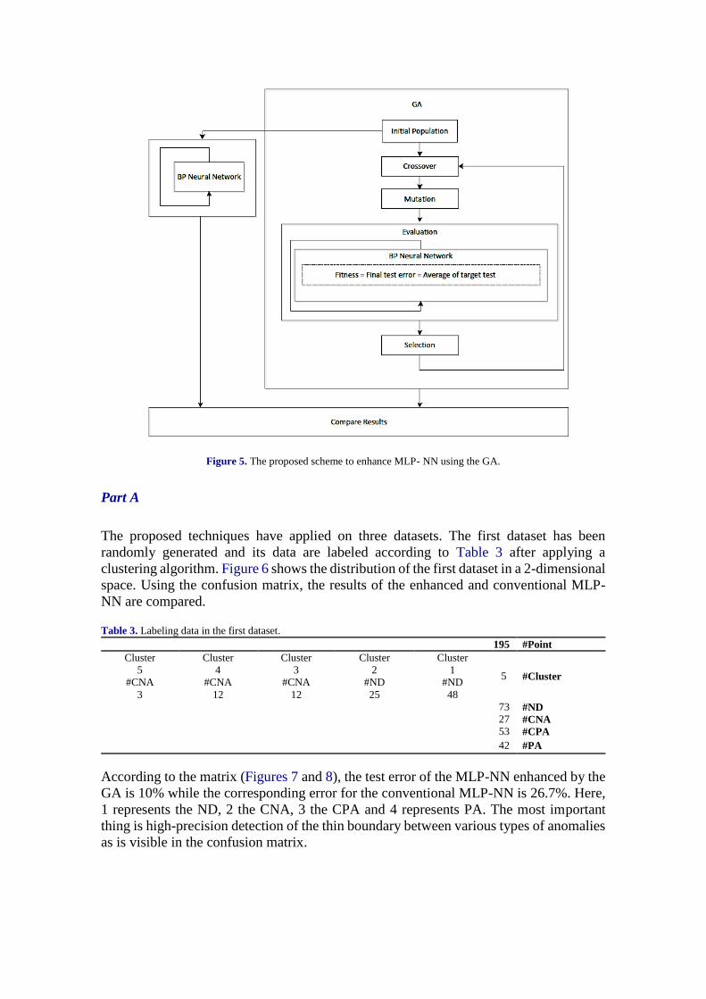
Figure 5. The proposed scheme to enhance MLP- NN using the GA.

Part A

The proposed techniques have applied on three datasets. The first dataset has been

randomly generated and its data are labeled according to Table 3 after applying a

clustering algorithm. Figure 6 shows the distribution of the first dataset in a 2-dimensional

space. Using the confusion matrix, the results of the enhanced and conventional MLP-

NN are compared.

Table 3. Labeling data in the first dataset.

#Point 195

#Cluster 5

Cluster

1

Cluster

2

Cluster

3

Cluster

4

Cluster

5

#ND #ND #CNA #CNA #CNA

48 25 12 12 3

#ND 73

#CNA 27

#CPA 53

#PA 42

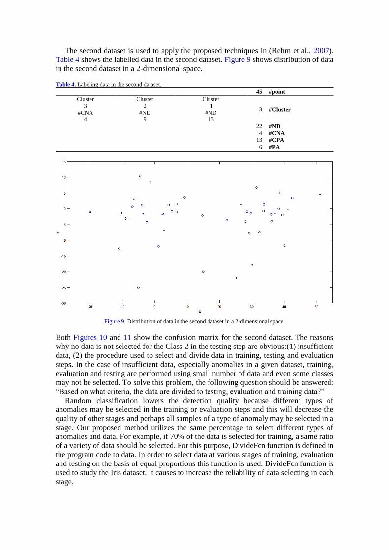
According to the matrix (Figures 7 and 8), the test error of the MLP-NN enhanced by the

GA is 10% while the corresponding error for the conventional MLP-NN is 26.7%. Here,

1 represents the ND, 2 the CNA, 3 the CPA and 4 represents PA. The most important

thing is high-precision detection of the thin boundary between various types of anomalies

as is visible in the confusion matrix.

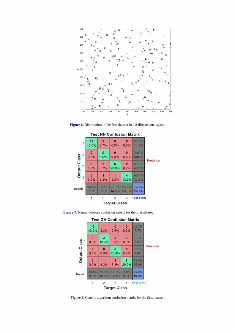
Figure 6. Distribution of the first dataset in a 2-dimensional space.

Figure 7. Neural network confusion matrix for the first dataset.

Figure 8. Genetic algorithm confusion matrix for the first dataset.

The second dataset is used to apply the proposed techniques in (Rehm et al., 2007).

Table 4 shows the labelled data in the second dataset. Figure 9 shows distribution of data

in the second dataset in a 2-dimensional space.

Table 4. Labeling data in the second dataset.

#point 45

#Cluster 3

Cluster

1

Cluster

2

Cluster

3

#ND #ND #CNA

13 9 4

#ND 22

#CNA 4

#CPA 13

#PA 6

Figure 9. Distribution of data in the second dataset in a 2-dimensional space.

Both Figures 10 and 11 show the confusion matrix for the second dataset. The reasons

why no data is not selected for the Class 2 in the testing step are obvious:(1) insufficient

data, (2) the procedure used to select and divide data in training, testing and evaluation

steps. In the case of insufficient data, especially anomalies in a given dataset, training,

evaluation and testing are performed using small number of data and even some classes

may not be selected. To solve this problem, the following question should be answered:

“Based on what criteria, the data are divided to testing, evaluation and training data?”

Random classification lowers the detection quality because different types of

anomalies may be selected in the training or evaluation steps and this will decrease the

quality of other stages and perhaps all samples of a type of anomaly may be selected in a

stage. Our proposed method utilizes the same percentage to select different types of

anomalies and data. For example, if 70% of the data is selected for training, a same ratio

of a variety of data should be selected. For this purpose, DivideFcn function is defined in

the program code to data. In order to select data at various stages of training, evaluation

and testing on the basis of equal proportions this function is used. DivideFcn function is

used to study the Iris dataset. It causes to increase the reliability of data selecting in each

stage.

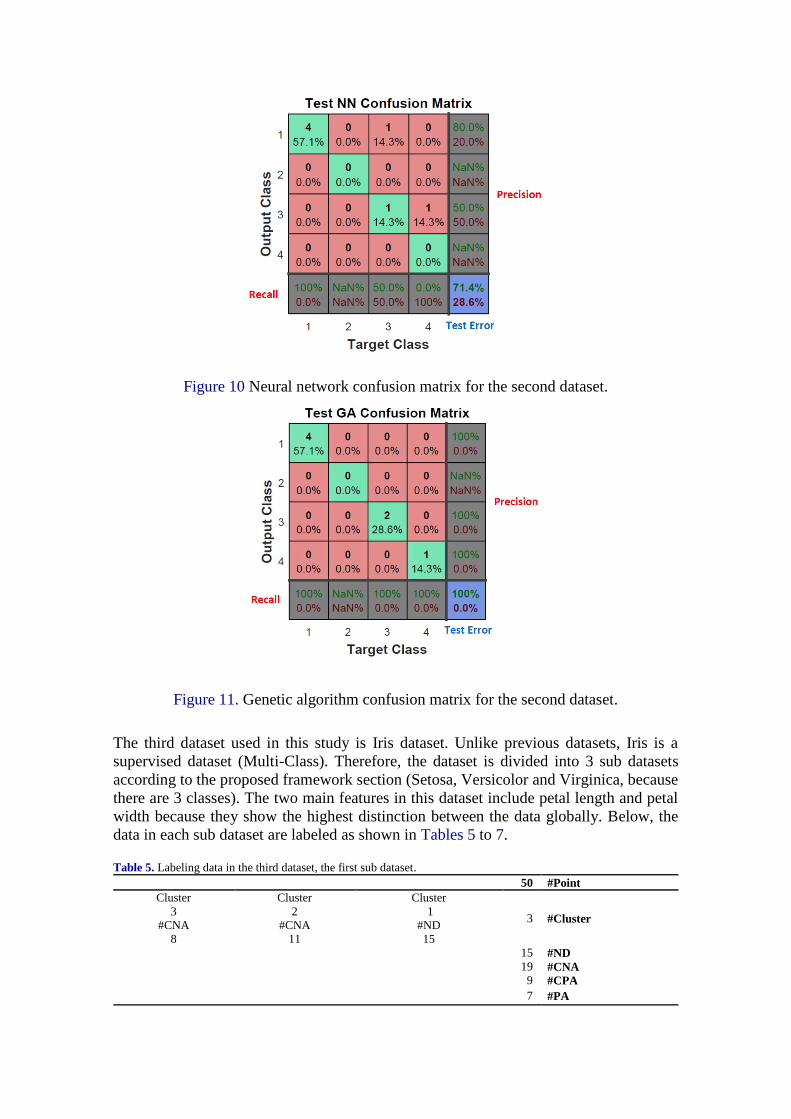
Figure 10 Neural network confusion matrix for the second dataset.

Figure 11. Genetic algorithm confusion matrix for the second dataset.

The third dataset used in this study is Iris dataset. Unlike previous datasets, Iris is a

supervised dataset (Multi-Class). Therefore, the dataset is divided into 3 sub datasets

according to the proposed framework section (Setosa, Versicolor and Virginica, because

there are 3 classes). The two main features in this dataset include petal length and petal

width because they show the highest distinction between the data globally. Below, the

data in each sub dataset are labeled as shown in Tables 5 to 7.

Table 5. Labeling data in the third dataset, the first sub dataset.

#Point 50

#Cluster 3

Cluster

1

Cluster

2

Cluster

3

#ND #CNA #CNA

15 11 8

#ND 15

#CNA 19

#CPA 9

#PA 7

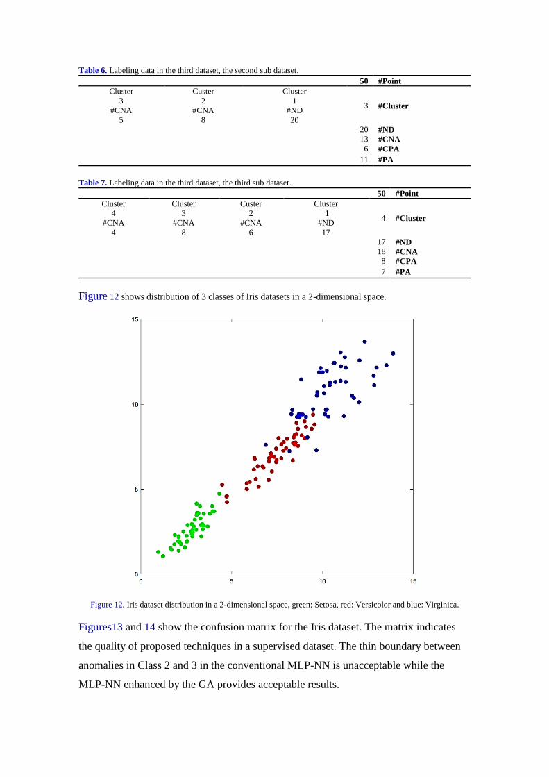
Table 6. Labeling data in the third dataset, the second sub dataset.

#Point 50

#Cluster 3

Cluster

1

Custer

2

Cluster

3

#ND #CNA #CNA

20 8 5

#ND 20

#CNA 13

#CPA 6

#PA 11

Table 7. Labeling data in the third dataset, the third sub dataset.

#Point 50

#Cluster 4

Cluster

1

Custer

2

Cluster

3

Cluster

4

#ND #CNA #CNA #CNA

17 6 8 4

#ND 17

#CNA 18

#CPA 8

#PA 7

Figure 12 shows distribution of 3 classes of Iris datasets in a 2-dimensional space.

Figure 12. Iris dataset distribution in a 2-dimensional space, green: Setosa, red: Versicolor and blue: Virginica.

Figures13 and 14 show the confusion matrix for the Iris dataset. The matrix indicates

the quality of proposed techniques in a supervised dataset. The thin boundary between

anomalies in Class 2 and 3 in the conventional MLP-NN is unacceptable while the

MLP-NN enhanced by the GA provides acceptable results.

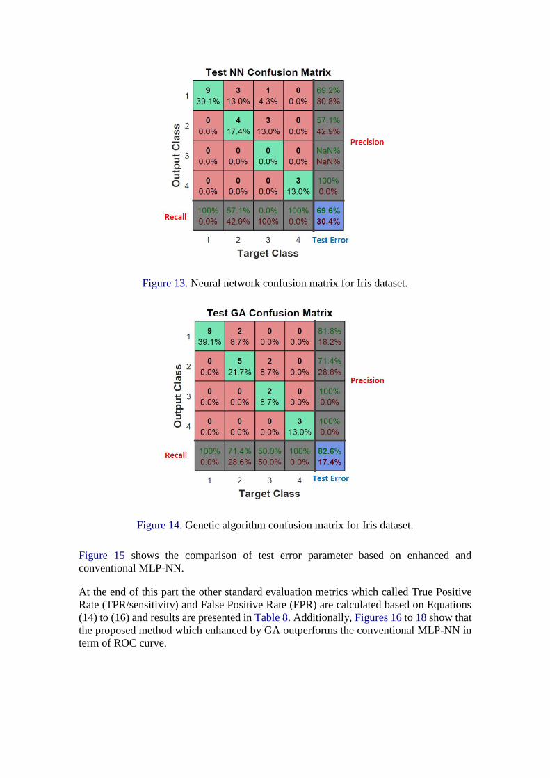
Figure 13. Neural network confusion matrix for Iris dataset.

Figure 14. Genetic algorithm confusion matrix for Iris dataset.

Figure 15 shows the comparison of test error parameter based on enhanced and

conventional MLP-NN.

At the end of this part the other standard evaluation metrics which called True Positive

Rate (TPR/sensitivity) and False Positive Rate (FPR) are calculated based on Equations

(14) to (16) and results are presented in Table 8. Additionally, Figures 16 to 18 show that

the proposed method which enhanced by GA outperforms the conventional MLP-NN in

term of ROC curve.

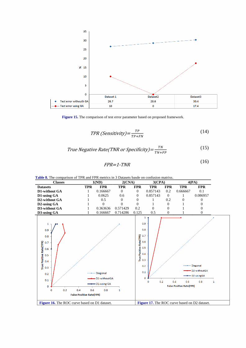
Figure 15. The comparison of test error parameter based on proposed framework.

TPR (Sensitivity)= 𝑇𝑃

𝑇𝑃+𝐹𝑁 (14)

True Negative Rate(TNR or Specificity)= 𝑇𝑁

𝑇𝑁+𝐹𝑃 (15)

FPR=1-TNR (16)

Table 8. The comparison of TPR and FPR metrics in 3 Datasets basde on confusion matrixs.

Classes 1(ND) 2(CNA) 3(CPA) 4(PA)

Datasets TPR FPR TPR FPR TPR FPR TPR FPR

D1-without GA 1 0.166667 0 0 0.857143 0.2 0.666667 0.1

D1-using GA 1 0.0625 0.6 0 0.857143 0 1 0.086957

D2-without GA 1 0.5 0 0 1 0.2 0 0

D2-using GA 1 0 0 0 1 0 1 0

D3-without GA 1 0.363636 0.571429 0.2 0 0 1 0

D3-using GA 1 0.166667 0.714286 0.125 0.5 0 1 0

Figure 16. The ROC curve based on D1 dataset. Figure 17. The ROC curve based on D2 dataset.

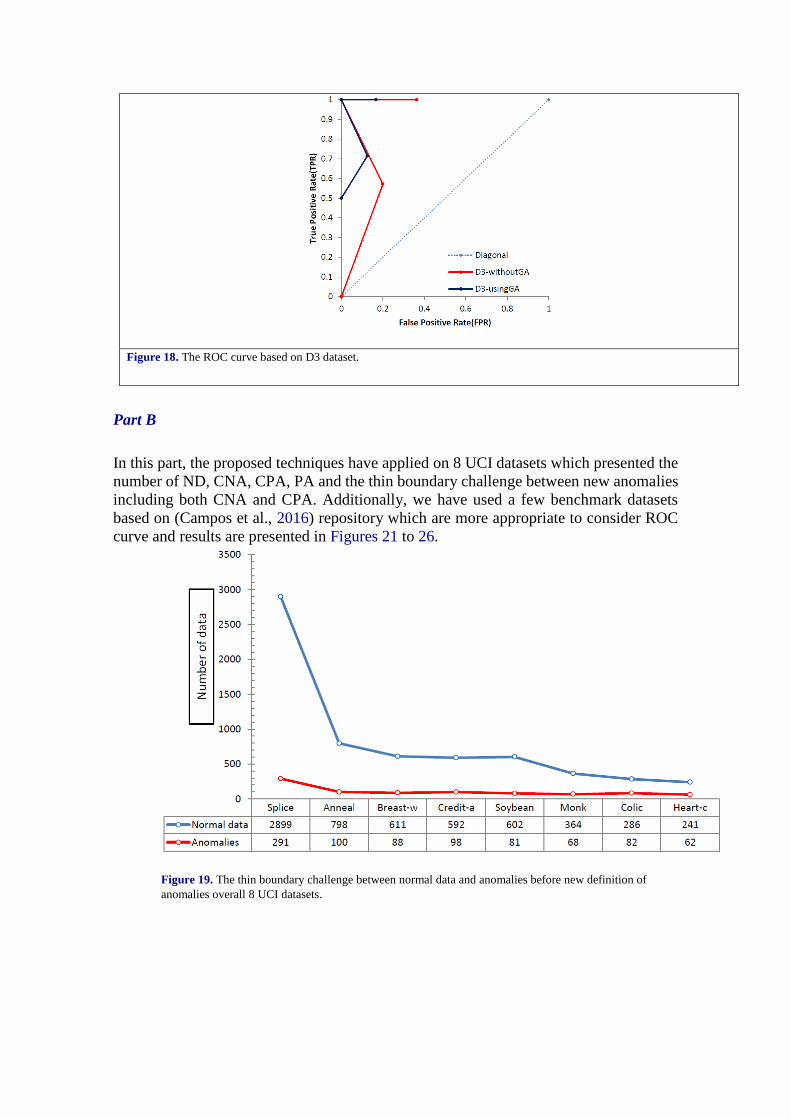
Figure 18. The ROC curve based on D3 dataset.

Part B

In this part, the proposed techniques have applied on 8 UCI datasets which presented the

number of ND, CNA, CPA, PA and the thin boundary challenge between new anomalies

including both CNA and CPA. Additionally, we have used a few benchmark datasets

based on (Campos et al., 2016) repository which are more appropriate to consider ROC

curve and results are presented in Figures 21 to 26.

Figure 19. The thin boundary challenge between normal data and anomalies before new definition of

anomalies overall 8 UCI datasets.

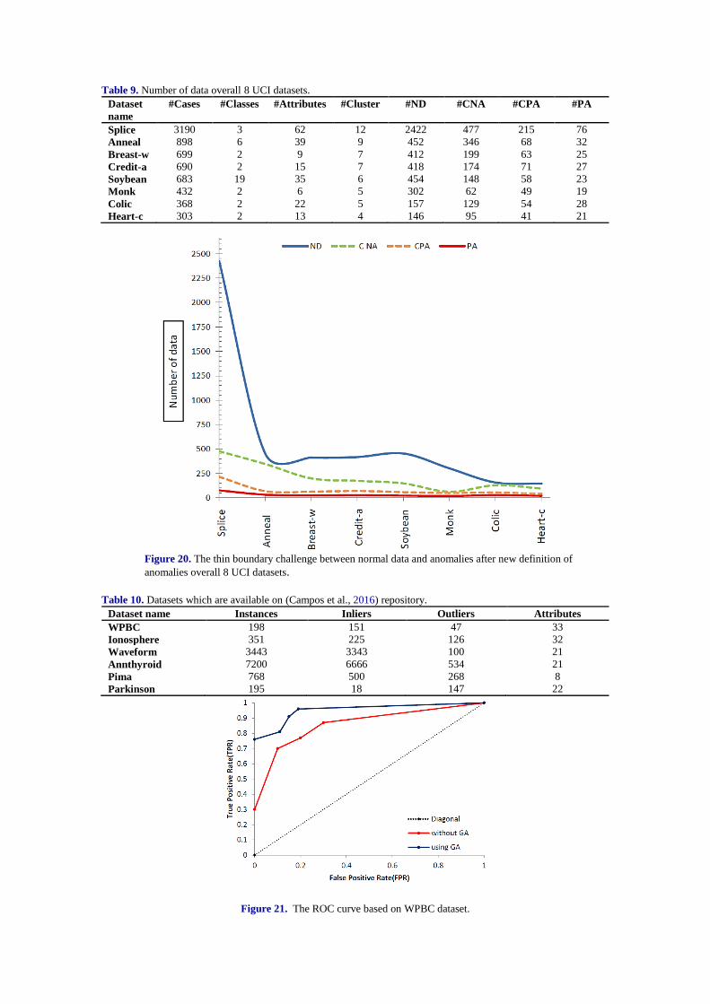
Table 9. Number of data overall 8 UCI datasets.

Dataset

name

#Cases #Classes #Attributes #Cluster #ND #CNA #CPA #PA

Splice 3190 3 62 12 2422 477 215 76

Anneal 898 6 39 9 452 346 68 32

Breast-w 699 2 9 7 412 199 63 25

Credit-a 690 2 15 7 418 174 71 27

Soybean 683 19 35 6 454 148 58 23

Monk 432 2 6 5 302 62 49 19

Colic 368 2 22 5 157 129 54 28

Heart-c 303 2 13 4 146 95 41 21

Figure 20. The thin boundary challenge between normal data and anomalies after new definition of

anomalies overall 8 UCI datasets.

Table 10. Datasets which are available on (Campos et al., 2016) repository.

Dataset name Instances Inliers Outliers Attributes

WPBC 198 151 47 33

Ionosphere 351 225 126 32

Waveform 3443 3343 100 21

Annthyroid 7200 6666 534 21

Pima 768 500 268 8

Parkinson 195 18 147 22

Figure 21. The ROC curve based on WPBC dataset.

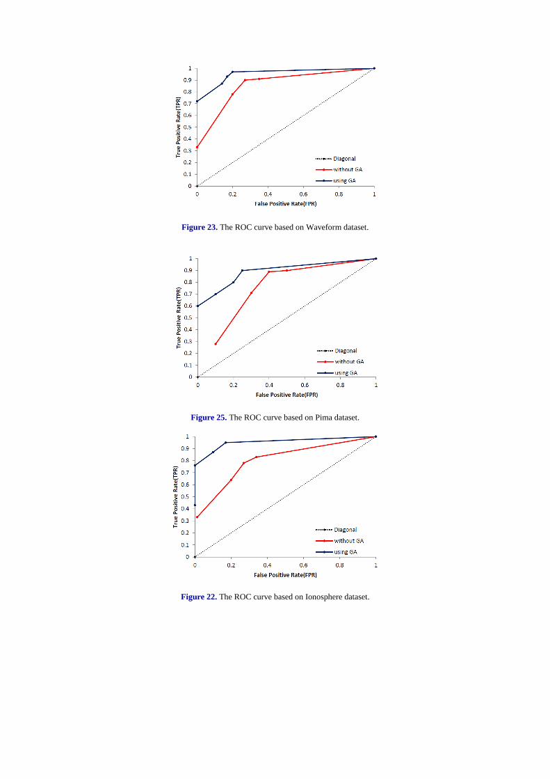
Figure 23. The ROC curve based on Waveform dataset.

Figure 25. The ROC curve based on Pima dataset.

Figure 22. The ROC curve based on Ionosphere dataset.

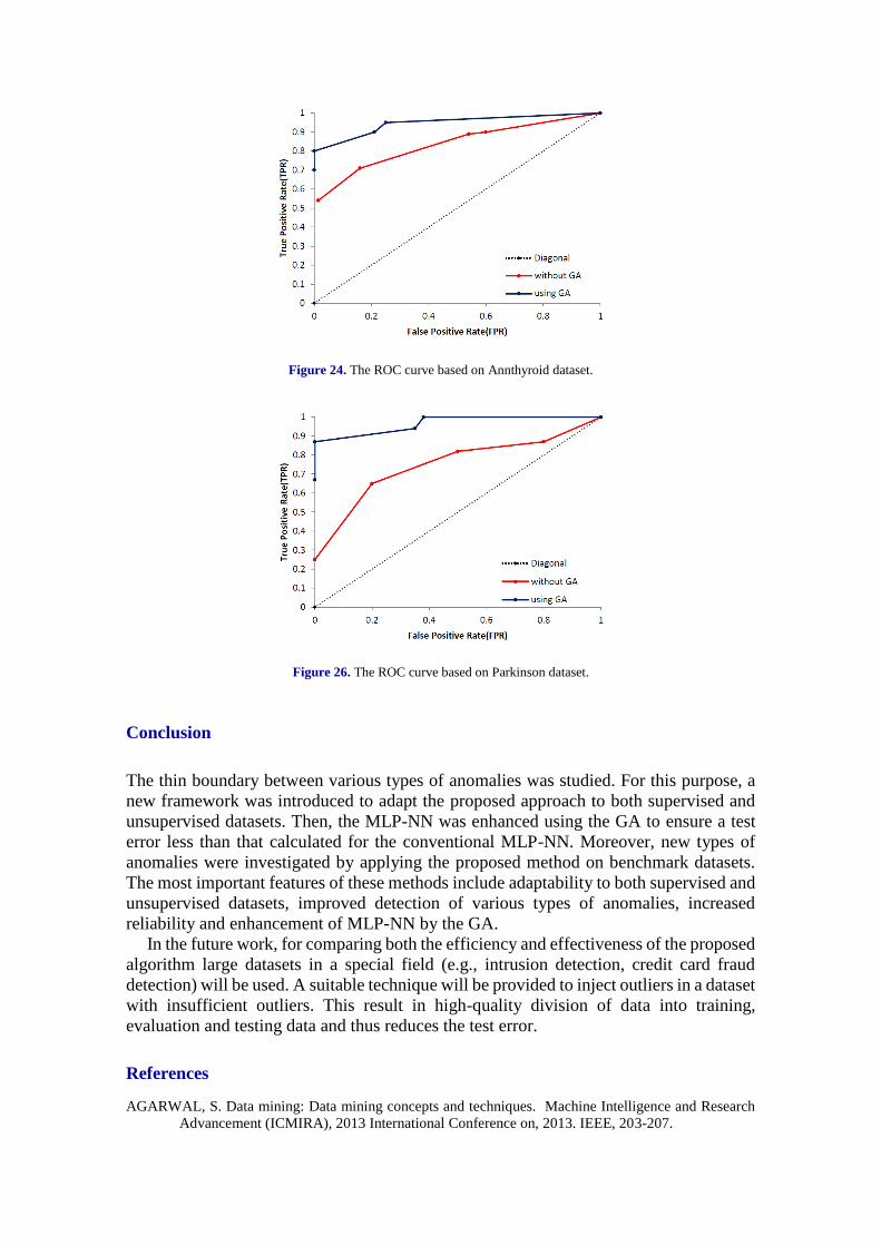
Figure 24. The ROC curve based on Annthyroid dataset.

Figure 26. The ROC curve based on Parkinson dataset.

Conclusion

The thin boundary between various types of anomalies was studied. For this purpose, a

new framework was introduced to adapt the proposed approach to both supervised and

unsupervised datasets. Then, the MLP-NN was enhanced using the GA to ensure a test

error less than that calculated for the conventional MLP-NN. Moreover, new types of

anomalies were investigated by applying the proposed method on benchmark datasets.

The most important features of these methods include adaptability to both supervised and

unsupervised datasets, improved detection of various types of anomalies, increased

reliability and enhancement of MLP-NN by the GA.

In the future work, for comparing both the efficiency and effectiveness of the proposed

algorithm large datasets in a special field (e.g., intrusion detection, credit card fraud

detection) will be used. A suitable technique will be provided to inject outliers in a dataset

with insufficient outliers. This result in high-quality division of data into training,

evaluation and testing data and thus reduces the test error.

References

AGARWAL, S. Data mining: Data mining concepts and techniques. Machine Intelligence and Research

Advancement (ICMIRA), 2013 International Conference on, 2013. IEEE, 203-207.

AGGARWAL, C. C. Outlier analysis. Data mining, 2015. Springer, 237-263.

AHMED, M. & MAHMOOD, A. N. Network traffic analysis based on collective anomaly detection.

Industrial electronics and applications (ICIEA), 2014 IEEE 9th Conference on, 2014. IEEE, 1141-

1146.

ALESKEROV, E., FREISLEBEN, B. & RAO, B. Cardwatch: A neural network based database mining

system for credit card fraud detection. Computational Intelligence for Financial Engineering

(CIFEr), 1997., Proceedings of the IEEE/IAFE 1997, 1997. IEEE, 220-226.

AUGUSTEIJN, M. & FOLKERT, B. J. I. J. O. R. S. 2002. Neural network classification and novelty

detection. 23, 2891-2902.

BARSON, P., FIELD, S., DAVEY, N., MCASKIE, G. & FRANK, R. J. N. N. W. 1996. The detection of

fraud in mobile phone networks. 6, 477-484.

BOHLOULI, M., SCHULZ, F., ANGELIS, L., PAHOR, D., BRANDIC, I., ATLAN, D., & TATE, R.

2013. Towards an integrated platform for big data analysis. In Integration of practice-oriented

knowledge technology: Trends and prospectives (pp. 47-56). Springer, Berlin, Heidelberg.

BOLTON, R. J., HAND, D. J. J. C. S. & VII, C. C. 2001. Unsupervised profiling methods for fraud

detection. 235-255.

BOYD, T., DOCKEN, G. & RUGGIERO, J. J. J. O. C. C. 2016. Outliers in data envelopment analysis. 9,

168-183.

CAMPBELL, C. & BENNETT, K. P. A linear programming approach to novelty detection. Advances in

neural information processing systems, 2001. 395-401.

Campos, G.O., Zimek, A., Sander, J., Campello, R.J., Micenková, B., Schubert, E., Assent, I. and Houle,

M.E., 2016. On the evaluation of unsupervised outlier detection: measures, datasets, and an

empirical study. Data Mining and Knowledge Discovery, 30(4), pp.891-927.

CHALLAGALLA, A., DHIRAJ, S. S., SOMAYAJULU, D. V., MATHEW, T. S., TIWARI, S. &

AHMAD, S. S. Privacy preserving outlier detection using hierarchical clustering methods.

Computer Software and Applications Conference Workshops (COMPSACW), 2010 IEEE 34th

Annual, 2010. IEEE, 152-157.

CHANDARANA, D. R. & DHAMECHA, M. V. A survey for different approaches of Outlier Detection in

data mining. International Conference on Electrical, Electronics, Signals, Communication and

Optimization (EESCO), 2015.

CHANDOLA, V., BANERJEE, A. & KUMAR, V. J. A. C. S. 2009. Anomaly detection: A survey. 41, 15.

DIAZ, I. & HOLLMEN, J. Residual generation and visualization for understanding novel process

conditions. Neural Networks, 2002. IJCNN'02. Proceedings of the 2002 International Joint

Conference on, 2002. IEEE, 2070-2075.

FUJIMAKI, R., YAIRI, T. & MACHIDA, K. An approach to spacecraft anomaly detection problem using

kernel feature space. Proceedings of the eleventh ACM SIGKDD international conference on

Knowledge discovery in data mining, 2005. ACM, 401-410.

GHOSH, A. K., WANKEN, J. & CHARRON, F. Detecting anomalous and unknown intrusions against

programs. Computer Security Applications Conference, 1998. Proceedings. 14th Annual, 1998.

IEEE, 259-267.

GHOSH, S. & REILLY, D. L. Credit card fraud detection with a neural-network. System Sciences, 1994.

Proceedings of the Twenty-Seventh Hawaii International Conference on, 1994. IEEE, 621-630.

GUO, F., SHI, C., LI, X., HE, J. & XI, W. Outlier Detection Based on the Data Structure. 2018 International

Joint Conference on Neural Networks (IJCNN), 2018. IEEE, 1-6.

GUPTA, M., GAO, J., AGGARWAL, C., HAN, J. J. S. L. O. D. M. & DISCOVERY, K. 2014. Outlier

detection for temporal data. 5, 1-129.

HACHMI, F., BOUJENFA, K. & LIMAM, M. A three-stage process to detect outliers and false positives

generated by intrusion detection systems. Computer and Information Technology; Ubiquitous

Computing and Communications; Dependable, Autonomic and Secure Computing; Pervasive

Intelligence and Computing (CIT/IUCC/DASC/PICOM), 2015 IEEE International Conference on,

2015. IEEE, 1749-1755.

HAUSKRECHT, M., VALKO, M., BATAL, I., CLERMONT, G., VISWESWARAN, S. & COOPER, G.

F. Conditional outlier detection for clinical alerting. AMIA annual symposium proceedings, 2010.

American Medical Informatics Association, 286.

HODGE, V. & AUSTIN, J. J. A. I. R. 2004. A survey of outlier detection methodologies. 22, 85-126.

JAFARIZADEH, V., KESHAVARZI, A., & DERIKVAND, T. (2017). Efficient cluster head selection

using Naïve Bayes classifier for wireless sensor networks. Wireless Networks, 23(3), 779-785.

KESHAVARZI, A., HAGHIGHAT, A. T., & BOHLOULI, M. 2019. Enhanced time-aware QoS prediction

in multi-cloud: a hybrid k-medoids and lazy learning approach (QoPC). Computing, 1-27.

KESHAVARZI, A., HAGHIGHAT, A. T., & BOHLOULI, M. 2017. Adaptive Resource Management and

Provisioning in the Cloud Computing: A Survey of Definitions, Standards and Research

Roadmaps. KSII Transactions on Internet & Information Systems, 11(9).

KESHAVARZI, A., RAHMANI A.M., MOHSENZADEH M., KESHAVARZI R. 2008 Recognition of

Data Records inSemi-structured Web-Pages Using Ontology and χ2 Statistical Distribution. In:

Tang C., Ling C.X., Zhou X., Cercone N.J., Li X. (eds) Advanced Data Mining and Applications.

ADMA 2008. Lecture Notes in Computer Science, vol 5139. Springer, Berlin, Heidelberg.

KIANI. R., MAHDAVI, S., & KESHAVARZI, A. 2015. Analysis and prediction of crimes by clustering

and classification. International Journal of Advanced Research in Artificial Intelligence, 4(8), 11-

17.

KO, T., LEE, J. H., CHO, H., CHO, S., LEE, W., LEE, M. J. I. M. & SYSTEMS, D. 2017. Machine

learning-based anomaly detection via integration of manufacturing, inspection and after-sales

service data. 117, 927-945.

KOU, Y., LU, C.-T. & DOS SANTOS, R. F. Spatial outlier detection: a graph-based approach. ictai, 2007.

IEEE, 281-288.

Kutsuna, T. and Yamamoto, A., 2017. Outlier detection using binary decision diagrams. Data mining and

knowledge discovery, 31(2), pp.548-572. LI, X. & HAUPT, J. D. J. I. T. S. P. 2015. Identifying outliers in large matrices via randomized adaptive

compressive sampling. 63, 1792-1807.

LI, Y., PONT, M. J. & JONES, N. B. J. P. R. L. 2002. Improving the performance of radial basis function

classifiers in condition monitoring and fault diagnosis applications whereunknown'faults may

occur. 23, 569-577.

Lin, C., Zhu, Q., Guo, S., Jin, Z., Lin, Y.R. and Cao, N., 2018. Anomaly detection in spatiotemporal data

via regularized non-negative tensor analysis. Data Mining and Knowledge Discovery, 32(4),

pp.1056-1073.

Macha, M. and Akoglu, L., 2018. Explaining anomalies in groups with characterizing subspace rules. Data

Mining and Knowledge Discovery, 32(5), pp.1444-1480.

MAHESHWARI, K. & SINGH, M. Outlier detection using divide-and-conquer strategy in density based

clustering. Recent Advances and Innovations in Engineering (ICRAIE), 2016 International

Conference on, 2016. IEEE, 1-5.

MALIK, K., SADAWARTI, H. & G S, K. J. I. J. O. C. A. 2014. Comparative analysis of outlier detection

techniques. 97, 12-21.

MANEVITZ, L. M. & YOUSEF, M. J. J. O. M. L. R. 2001. One-class SVMs for document classification.

2, 139-154.

NOBLE, C. C. & COOK, D. J. Graph-based anomaly detection. Proceedings of the ninth ACM SIGKDD

international conference on Knowledge discovery and data mining, 2003. ACM, 631-636.

RAMADAS, M., OSTERMANN, S. & TJADEN, B. Detecting anomalous network traffic with self-

organizing maps. International Workshop on Recent Advances in Intrusion Detection, 2003.

Springer, 36-54.

REHM, F., KLAWONN, F. & KRUSE, R. J. S. C. 2007. A novel approach to noise clustering for outlier

detection. 11, 489-494.

RIAHI, F. & SCHULTE, O. Model-based outlier detection for object-relational data. Computational

Intelligence, 2015 IEEE Symposium Series on, 2015. IEEE, 1590-1598.

SINGH, S., MARKOU, M. J. I. T. O. K. & ENGINEERING, D. 2004. An approach to novelty detection

applied to the classification of image regions. 16, 396-407.

SMITH, R., BIVENS, A., EMBRECHTS, M., PALAGIRI, C. & SZYMANSKI, B. J. P. O. I. E. S. T. A.

N. N. 2002. Clustering approaches for anomaly based intrusion detection. 579-584.

SOHN, H., WORDEN, K. & FARRAR, C. R. Novelty detection under changing environmental conditions.

Smart Structures and Materials 2001: Smart Systems for Bridges, Structures, and Highways, 2001.

International Society for Optics and Photonics, 108-119.

SONG, X., WU, M., JERMAINE, C., RANKA, S. J. I. T. O. K. & ENGINEERING, D. 2007. Conditional

anomaly detection. 19, 631-645.

STEINWART, I., HUSH, D. & SCOVEL, C. J. J. O. M. L. R. 2005. A classification framework for anomaly

detection. 6, 211-232.

TANIGUCHI, M., HAFT, M., HOLLMEN, J. & TRESP, V. Fraud detection in communication networks

using neural and probabilistic methods. Acoustics, Speech and Signal Processing, 1998.

Proceedings of the 1998 IEEE International Conference on, 1998. IEEE, 1241-1244.

THEILER, J. P. & CAI, D. M. Resampling approach for anomaly detection in multispectral images.

Algorithms and Technologies for Multispectral, Hyperspectral, and Ultraspectral Imagery IX,

2003. International Society for Optics and Photonics, 230-241.

VATANEN, T., KUUSELA, M., MALMI, E., RAIKO, T., AALTONEN, T. & NAGAI, Y. Semi-

supervised detection of collective anomalies with an application in high energy particle physics.

IJCNN, 2012. 1-8.

VIJAYARANI, S. & NITHYA, S. J. I. J. O. C. A. 2011. An efficient clustering algorithm for outlier

detection. 32, 22-27.

WANG, X. & DAVIDSON, I. Discovering contexts and contextual outliers using random walks in graphs.

Data Mining, 2009. ICDM'09. Ninth IEEE International Conference on, 2009. IEEE, 1034-1039.

YANG, S. & LIU, W. Anomaly detection on collective moving patterns: A hidden markov model based

solution. 2011 IEEE International Conferences on Internet of Things, and Cyber, Physical and

Social Computing, 2011. IEEE, 291-296.

ZHANG, J. 2008. Towards outlier detection for high-dimensional data streams using projected outlier

analysis strategy. Dalhousie University, Canada.

ZHANG, J., CAO, J. & ZHU, X. Detecting global outliers from large distributed databases. Proceedings

of the 9th International Conference on Fuzzy Systems and Knowledge Discovery (FSKD 2012),

2012. IEEE, 1632-1636.

ZHANG, L., LIU, C., CHEN, Y. & LAO, S. Abnormal Detection Research Based on Outlier Mining. 2018

11th International Conference on Intelligent Computation Technology and Automation (ICICTA),

2018. IEEE, 5-7.

ZHANG, Z., LI, J., MANIKOPOULOS, C., JORGENSON, J. & UCLES, J. HIDE: a hierarchical network

intrusion detection system using statistical preprocessing and neural network classification. Proc.

IEEE Workshop on Information Assurance and Security, 2001. 85-90.

ZHAO, Y. & HRYNIEWICKI, M. K. Xgbod: improving supervised outlier detection with unsupervised

representation learning. 2018 International Joint Conference on Neural Networks (IJCNN), 2018.

IEEE, 1-8.