Embed Size (px)
Citation preview
Journal of Physics Conference Series
OPEN ACCESS
Detection of time of arrival of ultrasonic pulsesTo cite this article Carl D Latino PhD et al 2006 J Phys Conf Ser 52 002
View the article online for updates and enhancements
You may also likeComparison of active-set methoddeconvolution and matched-filtering forderivation of an ultrasound transit timespectrumM-L Wille M Zapf N V Ruiter et al
-
A method of RCS Sequence extractionbased on CAC + EMDNanping Mao Yan Su Gaofeng Pan et al
-
On the distortion of a wave packetpropagating in an amplifying mediumN S Bukhman
-
This content was downloaded from IP address 2112292416 on 23112021 at 0117
Detection of time of arrival of ultrasonic pulses
Carl D Latino PhD1
Associate Professor ECEN Oklahoma State University Stillwater OK 74078 USA Niels Lervad Andersen 2
Associate Professor University of Southern Denmark Grundtvigs Alleacute 150 DK 6400 Soenderborg Denmark Frands Voss 3
Director MCI University of Southern Denmark Grundtvigs Alleacute 150 DK 6400 Soenderborg Denmark
1 Latinookstateedu 2 NLAingsdbsdudk 3 Vossmcisdudk
Abstract Applications exist that employ transit-time measurements to determine distances to scattering objects These include blood-flow measurements fluid-level detection non-destructive testing of materials image processing of geometrical bodies etc Many of these require extreme accuracy in measuring transit time through a medium The system typically consists of a transmitter a medium and a receiver The signal sent must operate within the limitations imposed by this overall system Under ideal conditions a finite duration pulse consisting of a sinusoidal signal is sent and received If the transmitted signal contains an integer number of complete cycles of a single frequency performing a correlation between transmitted and received signals can accurately recover the transit time information The method has difficulties especially in the presence of noise The problem is compounded if the desired accuracy is a small fraction of a single sinusoid period Noise could cause the correlation results to be off by a complete cycle For a one MHz signal one cycle error corresponds to a one microsecond error For applications requiring nanosecond accuracy this is not acceptable Varying the frequency content of the signal reduces the error but requires that the transmitter receiver and medium all have a broader band spectrum The improvements we propose here work within a narrow band while enhancing the chance of recovering the signal accurately
Keywords time of arrival ultrasonic pulse correlation frequency sweep Piezoelectrics Signal Coding Arrival Time Detection Vibroseis PACS 4360 Acoustic Signal Processing 4385 Acoustical Measurements and Instrumentation 4388 Transduction Acoustical Devices for the Generation and Reproduction of Sound Mathematics Subject Classification 60Gxx60G35 Applications (signal detection filteringetc) 91Axx91A28 Signaling communication 94Axx94A12 Signal theory (characterization reconstruction etc)
Institute of Physics Publishing Journal of Physics Conference Series 52 (2006) 14ndash26doi1010881742-6596521002 Mathematics for Industry in Denmark
14copy 2006 IOP Publishing Ltd
1 Introduction When transmitting a pulse through a medium the received signal is attenuated time shifted and distorted We define a pulse to be any signal of finite amplitude and temporal duration composed of one or a combination of frequencies Even if the pulse is designed to be of a single frequency the mere act of turning a signal on and then off introduces many unwanted frequencies These frequencies make the problem of receiving the signal more complex but not intractable Maximizing the energy transmitted in the form of higher amplitude or longer pulse duration improves the signal to noise ratio making signal reception more manageable However the system parameters and time constraints limit the pulse duration and maximum energy possible Receiving a signal imbedded in noise is a task that can be handled effectively by correlation Correlation is a commonly used mathematical operation where two signals are multiplied together and the result integrated over all time If the signals are time shifted relative to each other the integration results in a function of time shift The function has a maximum point corresponding to the time shift of best alignment For a given amount of energy performing a correlation between transmitted and received pulse (cross correlation) gives an accurate measure of the delay time between the signals The correlation plot of the transmitted and received pulses generally has multiple peaks but the maximum absolute value occurs when the pulses align perfectly For correlation we used C=XCORR(AB) which is one of the many Matlabreg functions This function takes two vectors A and B each of length N and returns a vector C of length 2N-1 Where C is a cross correlation sequence In the case of A=B then the result is called the autocorrelation This is the function we used to get many of our plots If the signal is transmitted without distortion doing a cross correlation between the transmitted and received signals gives an accurate means of measuring time delay This is accomplished by locating the absolute highest point of the cross correlation function The time shift required to accomplish this maximum represents the transit time Unfortunately in the presence of noise and with bandwidth limitations of the system the highest peak in the cross correlation may be difficult to distinguish from its nearest neighbors It is desirable to increase the difference between the maximum peak and the secondary peaks in order to more reliably determine the true maximum peak and thus the true time delay Working within the fixed limitations of the system we propose a method of improving the discrimination between the correlation peaks to improve the chance of identifying the true maximum An application requiring very accurate measurement is the measure of speed of sound through a liquid Typical velocities are in the order of Mach 1 This method may be used to study the effects of pressure and other parameters on the speed of sound through the liquid in question It may also be used to measure flow rates of the liquid The restrictions imposed by the system are critical when it is necessary to measure transit times accurate in the nanosecond range For example if the driving frequency of the sinusoidal signal is 1 MHz one period corresponds to one microsecond If the speed in question is of the order of 300 meters per second a nanosecond represents about 3 millimeters If the desired accuracy is in the nanosecond range it must be possible to measure accurately within a small portion of a single cycle of the 1 MHz signal This is approximately three orders of magnitude smaller time than a single period of the transmitted frequency By appropriate selection of frequency and pulse duration a cross correlation of the transmitted and received signals can very accurately recover the transit time In practical applications the medium introduces not only a time delay but also a distortion The transmitter and receiver also have characteristics which operate
15
as filters further introducing noise The transmitter and receiver also often resonate at these frequencies All these conditions complicate the problem and limit the effectiveness of the cross correlation 2 System Limitations Assuming the system is fixed and cannot be modified improvement of the correlation can be accomplished by carefully crafting the transmitted pulse A coded pulse technique of this type has been used by the oil exploration industry since the 1960rsquos and is called Vibroseis [1] Vibroseis uses large trucks to shake the ground with swept frequency signals and detect the reflected signals with seismometers The choice of frequency sweep was dependent on many factors A typical sweep duration was in the order of five to twenty seconds with frequencies from 5 to 100 Hz Their application was therefore less restrictive than the one we are addressing Unlike the Vibroseis[1] application the system we are addressing uses low energy and narrow band transducers which actually resonate at their natural frequency If the application refers to measuring velocity through a medium this velocity is affected by various parameters including flow direction and rate For example in flow measuring applications the transducer is used for both receiving and transmitting the signal This means that the pulse must travel with and against the flow and have a relatively short duration A short pulse limits the amount of energy injected in the system and thus making it more susceptible to noise Working within these constraints we propose some solutions
Figure 1 ldquo1 MHz 10 Cycle Pulserdquo
16
Figure 2 ldquo1 MHz Autocorr RectEnvrdquo
3 Limitations of Single Frequency Pulses A single frequency sinusoid of finite duration has an autocorrelation whose value is a function of the number of complete cycles N We used Matlabreg to do all our models and simulations for this paper A single frequency example is illustrated in Figure 1 This figure illustrates a 1 MHz pulse of 10 microsecond duration The value of the signal outside this range is zero This particular 10 microsecond pulse was modeled using 200 sample points The Autocorrelation is shown in Figure 2 The x axis corresponds to shift in sample points Each sample point therefore corresponds to 50 nanoseconds Thus the 600 point on the x axis corresponds to a zero time shift and maximum overlap whereas 400 or less or 800 or more are the points where the transmitted and received pulses have no overlap The larger we make N the larger the maximum correlation value Making N too large however introduces the unwanted result that the secondary peaks of the autocorrelation are close in magnitude to the maximum For example if the maximum peak of the autocorrelation is KN the next peak has a magnitude K(N-1) For large values of N the two adjacent peaks are close in magnitude relatively measured and it is difficult to tell which one is the true maximum Another problem with large N is that for a given frequency it makes for a long pulse The applications often limit the pulse duration If N is too small however there may be insufficient energy that makes it to the receiver Selecting N in the range of 10 to 20 and the frequency of about 1 MHz may be a good compromise We will work under this assumption and use these numbers in our paper Actual numbers selected must conform to the actual system parameters With these numbers in mind there are other practical problems to be addressed If the transducers used in the system are very narrow band they may resonate and oscillate even when no longer energized To reduce the introduction of unwanted frequencies the pulse should be amplitude modulated with a suitable envelope Although the envelope reduces the amount of total
17
energy it is advantageous because it reduces the amount of unwanted frequency components being transmitted Quantitative analysis of the effects of envelopes or windows on the signal can be found in fundamental textbooks on signal analysis such as [5] [6] [7] and are beyond the scope of this paper 4 Proposed Pulse Designs An improvement to the single frequency method is the use of a swept frequency pulse that operates within the bandwidth of the transducers in question A swept frequency has a very unique shape and is easier to recognize at the receiver than a fixed frequency Figure 3 illustrates such a pulse The sudden start and stop of a frequency pulse due to a rectangular envelope has the additional disadvantage of generating unwanted frequencies To reduce these unwanted frequencies the pulse must not only consist of the desired frequencies but also be combined with an appropriate envelope in order to transmit a more suitably shaped pulse The envelope causes the overall pulse amplitude to smoothly grow from zero to peak value and descend smoothly at the end of the pulse An unwanted result of the inclusion of the amplitude modulating envelope is that the total amount of energy transmitted is reduced
Figure 3 ldquoLinear Sweep (09 MHz to 11 MHz)rdquo
18
Figure 4 ldquoSwept Sine RectEnv AutoCorrrdquo
Figure 5 ldquoTwo Frequencyrdquo Pulse
19
Figure 6 ldquo2 Frequency With SinEnv Autocorrrdquo
Another possible improvement is to generate a pulse consisting of two distinct frequencies close to the resonant frequencies of the transducers and added together The two frequencies are carefully selected such that they consist of integer number of cycles each and correspond to the resonance points of the transducers For example if the pulse duration is 10 microseconds and the two frequencies are to have nine and eleven complete cycles each the calculation is as follows T = N1T1 = N2T2 where T is the 10 microseconds T1 = 1f1 and T2 = 1f2 are the periods of the two frequencies in question and N1 and N2 are the number of cycles that are to occur in the given time T Arbitrarily choosing N1 to be 9 and N2 to be 11 it can be found that the corresponding frequencies are f1 = 09 MHz and f2 = 11111 MHz The frequencies selected will depend on the actual application Figure 5 illustrates this pulse and Figure 6 the autocorrelation By combining the frequencies this way the correlation has a ldquobeatingrdquo effect which improves the results by accentuating the difference in the amplitudes of the primary and secondary peaks in the cross correlation 5 System Models To evaluate the effectiveness of our proposed improvements and to compare with the single frequency methods used we modeled the system and the pulses using Matlabreg The system we modeled consisted of two narrow band transducers that could each operate as both a receiver or a transmitter and a medium such as water to transmit the signal The transducers were modeled after units actually in use [2] These transducers had a tendency to oscillate at their resonant frequency even after they were no longer energized The model for the transducer created in Matlabreg is an approximation of the real system and may not fully incorporate all of the complexities associated with an actual transducer [3] Although the transducers are not modeled in their full complexity they clearly illustrate the advantages of the multi frequency pulses over the single
20
frequency ones Our intent here is to show that by carefully designing the pulse tangible improvement over the single frequency method can be realized A block diagram of the Matlabreg model used (which includes the pulse generator the transmitter the medium and the receiver) is illustrated in Figure 7
Figure 7 ldquoSystem Block Diagramrdquo
6 Testing the Pulses In order to evaluate the efficacy of our proposed solution we generated a series of pulses with different frequency contents envelopes and durations We will illustrate only a small sampling of these in this paper To obtain a baseline we generated pulses of 10 cycles of a 1 MHz frequency of amplitude 1 This frequency was selected to match the narrow frequency bandwidth of the transducers To illustrate a comparison of the results we did an autocorrelation of each of three types of pulses Each was investigated both with a rectangular (no amplitude modulation) envelope and with a sinusoidal envelope The latter envelope e(t) which we will call Sinusoidal has the form of Equation (1)
e(t) = 1- cos(xt) For 0 lt t lt 2πx (1)
This envelope rises and descends smoothly from a zero amplitude to a maximum value of two and returns to zero We arbitrarily selected this envelope to match the duration of the pulse Other envelope shapes are also possible (such as Gaussian) but the main objective here is to demonstrate the advantages of certain pulse designs based on their frequency content We used Matlabreg [4] to do the modeling and mathematical operations To get a baseline we started with a pulse consisting of 10 cycles of a pure 1 MHz sinusoidal signal with a rectangular envelope (that is to say the signal abruptly
21
starts and abruptly stops) as shown in Figure 1 The time function CP(t) is depicted in Equation (2)
CP(t) = Asin((2π10^6)t ) for 0 lt t lt 1010^(-6) (2) Doing an autocorrelation on this 10 microsecond 1 MHz pulse reveals a ldquodiamondrdquo shaped waveform as shown in Figure 2 This waveform exhibits secondary peaks that have an amplitude approximately 93 of the main peak Multiplying the pulse with the Sinusoidal envelope and repeating the autocorrelation gave similar results That is the secondary peaks were also around 93 however the tertiary and other peaks were considerably lower than the corresponding peaks with the rectangular envelope In the presence of noise it becomes more difficult to identify the maximum peak of the correlation The second pulse design that we are considering here is also 10 microseconds in duration but consists of a linearly swept frequency ranging from 09 MHz to 11 MHz Equation (3) and Figure 3 illustrate the waveform SP(t)= Asin(2π(0910^6+(0210^6)t(1010^(-6)))t) 0 ltt lt 1010^(-6) (3) The autocorrelation of this pulse with the rectangular envelope shown in Figure 4 illustrated a dramatic improvement over the single frequency pulse CP(t) The secondary peaks of the autocorrelation of the swept pulse were less than 77 of the primary peak This greatly improves the ability to discriminate the primary from secondary peaks The swept pulse was then multiplied by the envelope and again autocorrelated As expected the main peak was lowered and a small degradation in performance was noticed This resulted in secondary peaks approximately 81 of the main peak This however is still a great improvement over the single frequency case The third pulse design we considered TF(t) given by Equation (4) and shown in Figure 5 was also 10 microseconds in duration and consisted of the sum of the two distinct frequencies 09 MHz and 11 MHz TF(t)= A(sin((2π0910^6)t)+sin((2π1110^6)t)) 0lttlt 1010^(-6) (4) With a rectangular envelope this pulse exhibited the best results with secondary peaks 64 of the primary peak When the Sinusoidal envelope was incorporated the secondary peaks increased to 78 as depicted in Figure 6 This proved to be the best performing of the three pulses considered It was then a question to see how well these pulses performed in the simulated ldquorealrdquo system The three pulses with Sinusoidal envelopes and injected noise were each applied to the input of the system and correlated with the output The particular characteristics of the system and the noise may further degrade the performance of the pulses but the overall performance of the multi-frequency pulses was far superior to that of the single frequency pulse Figure 8 Figure 9 and Figure 10 illustrate these results Figure 11 illustrates the relatively small effect that 25 noise had on the correlation
22
Figure 8 ldquo1 MHz RectEnv System Output and Cross Correlationrdquo
Figure 9 ldquo1 MHz SinEnv System Output and Cross Correlationrdquo
23
Figure 10 ldquoTwo Freqency SinEnv System Output and Cross Correlationrdquo
Figure 11 ldquoFigure 10 with 25 Noise on Outputrdquo
7 Conclusions Accurately measuring the arrival time of an ultrasonic pulse in a ldquorealrdquo system with nanosecond accuracy is a difficult problem This necessitates the use of carefully
24
crafted signals and sophisticated signal processing techniques To maximize the accuracy of time of arrival measurement the pulse should be customized to best operate within the system parameters To make the transit from transmitter and be accurately recognized at the receiver the pulse should be made as unique as possible This is necessary because the pulse will be distorted in transit and also by the transducer characteristics In this paper we briefly discussed the advantages of multiple frequency pulses over the currently used single frequency versions The swept frequency pulse is fashioned after a technique used in the seismic exploration field The application considered here however had the additional limitations of short time duration and high frequencies making the pulse design even more critical One advantage of a narrow band system is that the injection of white noise in the system has little effect on the received signal as evidenced by Figure 11 In this paper we compared the performance of the single frequency pulse with our proposed swept frequency and two-frequency pulses Table 1 below summarizes the findings The pulses were all 10 microsecond duration and the two envelopes used were Rectangular and Sinusoidal An autocorrelation of each pulse was performed and a measure taken of the relative amplitudes of the primary and secondary peaks The primary peak was considered 100 Table 1 ldquoRelationship of Primary and Secondary Peaksrdquo
10 Microsecond Pulse Autocorr Secondary Envelope Peak Peak Amp 1 MHz 100 93 Rectangular 09 MHz to 11 MHz Linear Sweep 100 77 Rectangular 09 MHz to 11 MHz Linear Sweep 100 81 Sinusoidal 09 MHz and 11 MHz Frequencies 100 64 Rectangular 09 MHz and 11 MHz Frequencies 100 78 Sinusoidal
If system parameters could be modified ie if the transmitter and receiver can be made to have slightly different frequencies or if the transducer bandwidth broadened the pulse frequencies should be selected to take advantage of these facts Methods to take advantage of different transducer designs such as broadening the bandwidth or using different resonant frequencies in the transmitter and receiver are being studied It should be noted that white noise had relatively little effect on a system with such tight frequency constraints This is so because most of the noise energy is filtered out In summary and based on our findings multi frequency pulses outperformed their single frequency counterpart operating under similar conditions Of the two pulse designs we proposed the swept frequency pulse showed great improvement over the single frequency pulse but the two frequency pulse was the one that performed the best
25
Acknowledgements
The authors gratefully acknowledge the contributions provided by Roderick Melnik for his encouragement and Morten Willatzen for providing the problem and his help in developing some of the solutions discussed in this paper Jonathan McAfeersquos editorial suggestions were greatly appreciated We are also grateful to all involved in making EMCI47 a most educational and productive experience
References [1] Baeten G and Ziolkowski A The Vibroseis Source Elsevier Science Ltd 1990 [2] M Willatzen ldquoUltrasound Transducer Modelling General Theory and Applications to Ultrasound Reciprocal Systemsrdquo IEEE Trans Ultras Ferroelectrics and Freq Control 48 100-112 Jan 2001 [3] M Willatzen et al rdquoArrival-Time Detection and Ultrasonic Flow-Meter Applicationsrdquo (This Journal) [4] Matlab The Mathworks Inc MA USA [5] Defatta D Lucas J and Hodgkiss W Digital Signal Processing A System Design Approach John Wiley and Sons Inc 1988 [6] Phillips C and Parr J Signals Systems and Transforms Second Edition Prentice-Hall Inc 1995 [7] Ziemer R Tranter W and Fannin D Signals amp Systems Continuous and Discrete Prentice-Hall Inc 1998
26
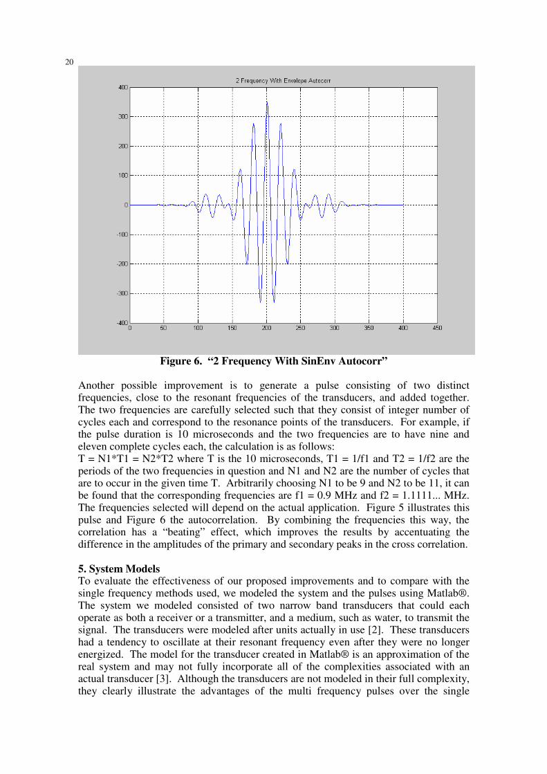
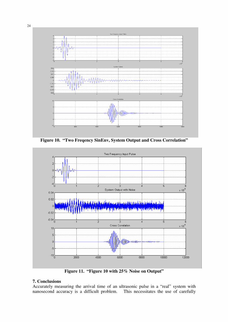


![A Doppler-Tolerant Ultrasonic Multiple Access Localization ...clinics and in unrestrained environments [1]. In [1], single tone pulses were used for localizing a single mobile node](https://img.pdfslide.net/doc/110x75/5fae610a744f8544937bce1c/a-doppler-tolerant-ultrasonic-multiple-access-localization-clinics-and-in-unrestrained.jpg)