Embed Size (px)
Citation preview
CERN Program Library Long Writeup W5013
GEANTGEANTGEANTGEANTGEANTGEANTGEANTGEANTGEANTGEANTGEANTGEANTGEANTGEANTGEANTGEANTGEANTGEANTGEANTGEANTDetector Description and
Simulation Tool
Application Software Group
Computing and Networks Division
CERN Geneva, Switzerland
Copyright Notice
GEANT – Detector Description and Simulation Tool
c© Copyright CERN, Geneva 1993
Copyright and any other appropriate legal protection of these computer programs and associated docu-mentation reserved in all countries of the world.
These programs or documentation may not be reproduced by any method without prior written consentof the Director-General of CERN or his delegate.
Permission for the usage of any programs described herein is granted apriori to those scientific insti-tutes associated with the CERN experimental program or with whom CERN has concluded a scientificcollaboration agreement.
CERN welcomes comments concerning the Geant code but undertakes no obligation for the main-tenance of the programs, nor responsibility for their correctness, and accepts no liability whatsoeverresulting from the use of its programs.
Requests for information should be addressed to:
CERN Program Library Office
CERN-IT Division
CH-1211 Geneva 23
Switzerland
Tel. +41 22 767 4951
Fax. +41 22 767 7155
Email: [email protected]
WWW: http://wwwinfo.cern.ch/asd/index.html
Trademark notice: All trademarks appearing in this guide are acknowledged as such.
Contact Persons: IT/ASD/SImulation section ([email protected])
Documentation Consultant: Michel Goossens /IT ([email protected])
Edition – March 1994

Chapter 1: Catalog of Geant sections
AAAA001 Foreword
AAAA002 Introduction to the manual
BASE001 Introduction to GEANT
BASE010 Simplified Program Flow Chart
BASE020 The data structures and their relationship
BASE040 Summary of Data Records
BASE090 The reference systems and physical units
BASE100 Examples of GEANT application
BASE110 The system initialisation routines
BASE200 Steering routines for event processing
BASE280 Storing and retrieving JRUNG and JHEAD information
BASE299 The banks JRUNG and JHEAD
BASE300 Example of user termination routine
BASE400 Debugging facilities
BASE410 Utility Routines
BASE420 The random number generator
CONS001 Introduction to the section CONS
CONS100 Material definition
CONS101 Retrieve material cross-sections and stopping power
CONS110 Mixtures and Compounds
CONS199 The Material data structure JMATE
CONS200 Tracking medium parameters
CONS210 Special Tracking Parameters
CONS300 Particle definition
CONS310 Branching Ratios and Particle Decay Modes
DRAW001 Introduction to the Drawing package
DRAW010 The Ray-tracing package
DRAW110 Drawing a Volume – Case 1
DRAW115 Drawing a Volume Projection view – Case 2
DRAW120 Draw a volume cut view
DRAW130 Draw Particle Trajectories
DRAW140 Drawing Track Hits in Sensitive Detectors
DRAW210 Drawing the geometrical tree
DRAW220 Drawing volume specifications
DRAW300 Handling View banks
DRAW399 The data structure JDRAW
DRAW400 Utility routines of the drawing package
GEOM001 The geometry package
1 Catalog – 1
GEOM010 Tracking inside volumes and optimisation
GEOM020 “MANY” Volumes and boolean operations on volumes
GEOM050 The GEANT shapes
GEOM100 Creation of a volume
GEOM110 Positioning a volume inside its mother
GEOM120 Positioning a volume inside its mother with parameters
GEOM130 Division of a volume into a given number of cells
GEOM140 Division of a Volume into cells of a given size
GEOM150 Division of a volume - general case
GEOM199 The volume data structure – JVOLUM
GEOM200 Rotation matrices
GEOM299 The rotation matrix data structure JROTM
GEOM300 Finding in which volume a point is
GEOM310 Finding distance to next boundary
GEOM320 Reference system transformations
GEOM400 Pseudo-division of a volume
GEOM410 Ordering the contents of a volume
GEOM500 Volume attributes
GEOM600 User initialisation of the common block /GCVOLU/
GEOM700 Medium search statistics
GEOM900 End of geometry definition
GEOM910 The CADINT Interface
HITS001 The detector response package
HITS100 Sensitive DETector definition
HITS105 Detector aliases
HITS110 DETector hit parameters
HITS120 DETector Digitisation parameters
HITS130 User detector parameters
HITS199 The SET data structure JSET
HITS200 Routines to store and retrieve HITS
HITS299 The JHITS data structure
HITS300 Routines to store and retrieve DIGItisations
HITS399 The JDIGI data structure
HITS400 Intersection of a track with a cylinder or a plane
HITS500 Digitisation for drift- or MWP- Chambers
HITS510 Digitisation for drift chambers
IOPA001 The I/O routines
IOPA200 ZEBRA sequential files handling
IOPA300 Data structure I/O with sequential files
IOPA400 ZEBRA direct access files handling
Catalog – 2 2

IOPA500 Data structure I/O with direct access files
KINE001 Section KINE
KINE100 Storing and retrieving vertex and track parameters
KINE199 The data structures JVERTX and JKINE
KINE200 Interface to the Lund Monte Carlo
KINE210 τ± generation and decay
PHYS001 Introduction to the section PHYS
PHYS010 Compute the occurrence of a process
PHYS100 Steering routine for physics initialisation
PHYS210 Total cross-section for e+e- pair production by photons
PHYS211 Simulation of e-e+ pair production by photons
PHYS220 Total cross-section for Compton scattering
PHYS221 Simulation of Compton scattering
PHYS230 Total cross-section for photoelectric effect
PHYS231 Simulation of photoelectric Effect
PHYS240 Photon-induced fission on heavy materials
PHYS250 Total cross-section for Rayleigh scattering
PHYS251 Simulation of Rayleigh scattering
PHYS260 Cerenkov photons
PHYS320 Gaussian multiple scattering
PHYS325 Moliere scattering
PHYS328 Plural scattering
PHYS330 Ionisation processes induced by e+/e-
PHYS331 Simulation of the delta-ray production
PHYS332 Simulation of energy loss straggling
PHYS333 Information about energy loss fluctuations
PHYS334 Models for energy loss fluctuations in thin layers
PHYS337 Birks’ saturation law
PHYS340 Total cross-section and energy loss for bremsstrahlung by e-e+
PHYS341 Simulation of discrete bremsstrahlung by electrons
PHYS350 Total cross-section for e+e- annihilation
PHYS351 Simulation of e+e- annihilation
PHYS360 Synchrotron radiation
PHYS400 Simulation of particle decays in flight
PHYS410 Rotations and Lorentz transformation
PHYS430 Ionisation processes for muons and protons
PHYS431 Ionisation processes for heavy ions
PHYS440 Total cross-section and energy loss for bremsstrahlung by Muons
PHYS441 Simulation of discrete bremsstrahlung by muons
PHYS450 Total cross-section and energy loss for e-e+ pair production by muons
3 Catalog – 3
PHYS451 Simulation of e+e- pair production by muons
PHYS460 Muon-nucleus interactions
PHYS510 The GEANT/GHEISHA Interface
PHYS520 The GEANT/FLUKA Interface
PHYS530 The GEANT/MICAP interface
TRAK001 The tracking package
TRAK110 Steering routine to track one event
TRAK120 Steering routine to track one particle
TRAK130 Tracking one particle through a volume
TRAK200 The tracking routines block diagrams
TRAK300 Storing secondary tracks in the stack
TRAK310 Altering the order of tracking secondary particles
TRAK399 The temporary stack data structure JSTAK
TRAK400 Handling of track space points
TRAK499 The space point data structure JXYZ
TRAK500 Tracking routines in magnetic field
XINT001 The interactive version of GEANT
XINT002 Introduction to the Interactive version of GEANT
XINT010 Screen views of GEANT++
ZZZZ010 List of COMMON Blocks
ZZZZ999 Index of Documented GEANT routines
Catalog – 4 4

Geant 3.21 GEANT User’s Guide AAAA001
Origin : Submitted: 01.10.84Revision : Revised:20.04.94Documentation :
Foreword
As the scale and complexity of High Energy Physics experiments increase, simulation studies require moreand more care and become essential to
• design and optimise the detectors,
• develop and test the reconstruction and analysis programs, and
• interpret the experimental data.
GEANT is a system of detector description and simulation tools that help physicists in such studies. TheGEANT system can be obtained from CERN as six Patchy [8]/CMZ [9] files: GEANT, GEANG, GEANH, GEANF,GEANE and GEANX. The program runs everywhere the CERN Program Library has been installed 1.
The GEANT and GEANG files contain most of the basic code. The GEANH file contains the code for the hadronicshowers simulation from the program GHEISHA [1]. The GEANF file contains the source of the routines forhadronic showers development from the FLUKA [2, 3, 4, 5, 6, 101, 102] program which is interfaced withGEANT as an alternative to GHEISHA to simulate hadronic cascades. The GEANE [11] file contains a trackingpackage to be used, in the context of event reconstruction, for trajectory estimation and error propagation.The GEANX file contains the main program for the interactive version of GEANT (GXINT) and a few examplesof application programs which may help users to get started with GEANT.
General information concerning GEANT, for example access to the source code, the list of problems andtheir proposed corrections, the context of utilisation on the CERN machines, the status of some applicationprograms, the acquisition of documentation, etc., are kept up to date through CERN news and InterNetnews group (cern.lgeant) and an electronic mailing list which is installed on the CERN IBM mainframe(BITnet/EARN node CERNVM). The name of the list is LGEANT (see below how to subscribe).
The first version of GEANT was written in 1974 as a bare framework which initially emphasised trackingof a few particles per event through relatively simple detectors. The system has been developed with somecontinuity over the years [12]
New versions may differ from the previous ones. Some of the modifications may lead to backward incom-patibilities. The user is therefore invited to read carefully the Patch HISTORY of the current GEANT file whereall changes are described in detail.
The development and the maintenance of GEANT are possible only thanks to the devoted and continuouscollaboration of physicists around the world who use the program and contribute their feedback to theauthors and maintainers at CERN. It is of course impossible to mention all of them, and new names areadded frequently to the list of the contributors. The GEANT team wish to thank them all and expresses itshope that they will continue to help us.
GEANT version 3 originated from an idea of Rene Brun and Andy McPherson in 1982 during the developmentof the OPAL simulation program. GEANT3 was based on the skeleton of GEANT version 2 code [12].
In close collaboration with Rene and Andy, Pietro Zanarini developed the first versions of the graphicssystem as well as the early versions of the interactive package initially based on ZCEDEX, then upgraded toKUIP.
1At the moment of writing these are the systems on which the CERN Program Library is maintained: VM/CMS-HPO-XA-ESA, SUN, Silicon Graphics, CRAY Y-XMP, Apollo 3000 series, Apollo 10000, HP 400 series, HP 700 series, IBM RS/6000,IBM AIX/370, VAX/VMS, Alliant, Dec Ultrix, NeXT, IBM MVS-HPO-XA-ESA, Convex, MAC/MPW (partial implementation),PC-DOS, PC-Linux, PC-Windows/NT.
5 AAAA001 – 1
Glenn Patrick (RAL) implemented a first version of the electromagnetic processes. Tony Baroncelli (Roma)helped in interfacing GEANT to his hadronic shower package TATINA. Federico Carminati contributed to theinterface with GHEISHA, an hadronic shower package developed by Harn Fesefeldt (Aachen).
Francis Bruyant and Michel Maire (LAPP) made substantial contributions to the geometry, tracking andphysics parts of GEANT while adapting the system to the L3 environment. Francis has been, for many years,an essential collaborator, testing new ideas for the geometry and hits packages. Michel, together with ElemerNagy and Vincenzo Innocente, developed the GEANE system.
A very important contribution to GEANT has been made by Laszlo Urban (KFKI Budapest) who has contin-uously improved the electromagnetic physics package. Lazlo has spent a considerable amount of time inreading the relevant papers in the literature and in making comparisons with experimental results.
Rene Brun has coordinated the development and the maintenance of GEANT from 1982 until 1991 (versions3.00 up to 3.14). Federico Carminati coordinated the development of the versions 3.15 and 3.16 between1991 and 1993. Since January 1994, the responsability for GEANT is in the hands of Simone Giani. Beforeassuming this responsability, Simone made substantial improvements in the graphics and interactive pack-ages. After he has enhanced the power of the geometry package and the performance of the tracking fora new version of GEANT: in March 1994 the version 3.21 has been released and is the current version ofGEANT.
Many people contributed their work or their experience. We have tried to acknowledge their names in themanual pages and we apologise for any omissions.
Special mention should be made here of the following contributions:
S.Banerjee (contribution to the tracking package), R.Jones (contribution to the simulation of electromag-netic processes), K.Lassila-Perini (interface with FLUKA and MICAP), G.Lynch (contribution to the mul-tiple scattering algorithms), E.Tchernyaev (original code for hidden-line removal graphics), J.Salt (originalinterface to the GC package).
S. Ravndal did a complete revision and update of the full documentation for the release of GEANT version3.21.
Special thanks should go to the authors of the packages interfaced with GEANT, and in particular to HarnFesefeldt (GHEISHA) and Alfredo Ferrari (FLUKA see later). Their patience in explaining the internals oftheir code, their experience and their collaborative and open attitude have been instrumental.
Another special thanks goes to Mike Metcalf, who helped to improve the English and the structure of themanual.
Any reader who is not familiar with GEANT should first have a glance at the notes numbered 001 to 009 ineach section of this manual.
Despite our efforts, the documentation is still incomplete and far from perfect. We accept full responsibilityfor its present status.
Finally, we express our thanks to Michel Goossens for translating the SCRIPT/SGML source of the originalGEANT manual into LATEX.
1 The GEANT-FLUKA interface
Since version 3.15, GEANT includes an interface with some FLUKA [2, 3, 4, 5, 6, 101, 102] routines. Thispart has been updated and extended in subsequent releases.
FLUKA is a standalone code with its own life. Only a few parts have been included into GEANT, namely theones dealing with hadronic elastic and inelastic interactions.
The implementation of FLUKA routines in GEANT does not include any change, apart from interface ones andthose agreed by the FLUKA authors. Whenever different options are available in FLUKA, the one suggested bythe authors have been retained. Nevertheless the results obtained with FLUKA routines inside GEANT couldnot be representative of the full FLUKA performances, since they generally depend on other parts which areGEANT specific.
AAAA001 – 2 6
The routines made available for GEANT have been extensively tested and are reasonably robust. They usuallydo not represent the latest FLUKA developments, since the policy is to supply for GEANT well tested andreliable code rather than very recent developments with possibly better physics but also still undetectederrors.
It is important that GEANT users are aware of the conditions at which this code has been kindly made avail-able:
• relevant authorship and references about FLUKA [2, 3, 4, 5, 6, 101, 102] should be clearly indicatedin any publication reporting results obtained with this code;
• the FLUKA authors reserve the right of publishing about the physical models they developed and im-plemented inside FLUKA, GEANT users are not supposed to extract from the GEANT-FLUKA code therelevant routines running them standalone for benchmarks;
• more generally, FLUKA routines contained in the GEANF file are supposed to be included and used withGEANT only: any other use must be authorised by the FLUKA authors.
2 Documentation
The main source of documentation on GEANT is this manual. Users are invited to notify any correction orsuggestion to the authors.
A detailed description of the history of modifications to the GEANT code is contained in the $VERSION Patchin the GEANT file.
GEANT is part of the CERN Program Library, and problems or questions about GEANT should be directed tothe Program Library Office (see next section).
GEANT problems can be submitted to an InterNet discussion group cern.lgeant.
A mailing list is maintained on CERN’s central IBM machine (BITnet node CERNVM) via the LISTSERVmechanism. LISTSERV acts as a rudimentary conferencing system, which forwards the mail received to allsubscribed users and to the InterNet group cern.lgeant. The list is accessible to all users who have ane-mail connection to CERNVM. To subscribe to the list from a BITnet node a user has to send the followingmessage to LISTSERV at CERNVM using the local BITnet message facility:
SUBSCRIBE LGEANT
From a non-BITnet node, the user can send an ordinary mail message to the user LISTSERV at CERNVMcontaining that single line.
Together with the GEANT library comes a correction cradle(see section on maintenance policy) which con-tains the history of the modifications to the current version of the GEANT program. This file is accessible toall users in the PRO area and can be found in:
GCORRxxx.CAR
where xxx is the version number.
Documentation on the elements of the CERN Program Library used by the GEANT program is available fromthe CERN Program Library Office.
3 Update policy
The GEANT program is constantly updated to reflect corrections, most of the time originating from users’feed-back, and improvements to the code. This constant evolution, which is one of the reasons for thesuccess of GEANT, poses the serious problem of managing change without disrupting stability, which is veryimportant for physicists doing long production runs.
7 AAAA001 – 3
In the CERN Program Library maintenance scheme, three versions of any product are present at the sametime on the central systems, in the OLD, PRO and NEW areas with those same names. This scheme does notapply to GEANT because every new release usually contains modifications in the physics which can produce,we hope, better but often different results with respect to the previous version. It is therefore appropriate tooffer to the users an extra level of protection against running inadvertedly the wrong version by appendingthe version number to all the files of GEANT. In this way the users will have to change their procedure tochange the version of GEANT.
On the other hand, the new user should not bother about version numbers and correction files, and so analias is installed on all systems without any version number, always pointing to the latest released version.
As said before, users’ feed-back is of paramount importance in detecting problems or areas for improvementin the system, so the new version is made available in the NEW area well before the official release. If, onthe one hand, those who use this version do so at their own risk, on the other hand users are encouraged toperform as much testing as possible, in order to detect the maximum number of problems before the finalrelease. Modifications in the pre-release version are made directly in the source code.
When problems are discovered, which may seriously affect the validity of the results of the simulation,they are corrected and the library recompiled in the /new area. To minimise network transfer for remoteusers and in the interest of the stability of the system, the source code of the released version in PRO isnot touched, but rather the correction is applied via a so-called correction cradlewhich is a file containingthe differences between the original and the corrected version in a format required by PATCHY/CMZ. Boththese programs can read the original source and the correction cradle and produce the corrected source. Thecorrected car/cmz source and the corrected binary library are made then available in /pro at the followingCERNLIB release (when /new becomes /pro).
The cmz source files contain the full history of the corrections applied with proper versioning, so that everyintermediate version can be rebuild. Users at CERN should not need to use the correction cradle other thanfor documentation purposes. Remote users may want to obtain the cradle and apply the corrections. Atevery CERNLIB release the correction cradle is obviously reset to be empty, as all the corrections have beenapplied in the code directly. The correction cradle for the OLD version is available but has to be consideredfrozen. No correction is ever applied to an old version.
New versions of GEANT are moved into the PRO area synchronously with releases of the CERN ProgramLibrary. If no new version of GEANT is available at the time of the release of the Program Library, the GEANTfiles do not change their location and the production version remains the same.
4 Availability of the documentation
This document has been produced using LATEX2 with the cernman and cerngeant style options, devel-oped at CERN. A printable version of each of the sections described in this manual can be obtained asa compressed PostScript file from CERN by anonymous ftp. You can look in the directory described inthe procedure below for more details. For instance, if you want to transfer the description of the physics
2Leslie Lamport, LATEX – A Document Preparation System. Addison–Wesley, 1985
AAAA001 – 4 8

routines, then you can type the following (commands that you have to type are underlined):3
ftp asis01.cern.ch
Trying 128.141.201.136...
Connected to asis01.cern.ch.
220 asis01 FTP server (SunOS 4.1) ready.
Name (asis01:username): anonymous
Password: your_mailaddress
ftp> binary
ftp> cd cernlib/doc/ps.dir/geant
ftp> get phys.ps.Z
ftp> quit
3You can of course issue multiple get commands in one run.
9 AAAA001 – 5
Geant 3.21 GEANT User’s Guide AAAA002
Origin : Submitted: 01.10.84Revision : Revised:10.03.94Documentation :
Introduction to the manual
The present documentation is divided into sections which follow the structure of GEANT and its major func-tions. Each section is identified by a keywordwhich indicates its content. Sections are in alphabetical order:
AAAA introduction to the system;
BASE GEANT framework and user interfaces to be read first;
CONS particles, materials and tracking medium parameters;
DRAW the drawing package, interfaced to HIGZ;
GEOM the geometry package;
HITS the detector response package;
IOPA the I/O package;
KINE event generators and kinematic structures;
PHYS physics processes;
TRAK the tracking package;
XINT interactive user interface;
ZZZZ appendix.
Within each section, the principal system functions or the details of subroutines are described in a seriesof papersnumbered from 001 to 999. In the upper left corner it is indicated in which Geant release thesubroutines were introduced and left unchanged. The authors of the conceptual ideas or/and of the earlyversions of the code are acknowledged under the item Origin , while Revisioncontains the contributors toany important upgrade. Documentation is essential, but sometime implies a not negligeable amount ofwork. When relevant these contributions are acknowledged here. In addition all reported bugs, acceptedsuggestions...etc...are mentioned in the history part of the source code and correction cradle.
Subroutines which are not necessary for an understanding of the program flow and which are not intendedto be called directly by the user have been omitted.
The notation [<KEYW>nnn] is used whenever additional information can be found in the quoted section. Inthe description of subroutine calling sequences, the arguments used both on input and on output are precededby a * and the output arguments are followed by a * .
For convenience, two more sections have been added: the section AAAA, for general introductory informationat the beginning, and the section ZZZZ, for various appendices and indexed lists, at the end.
A table of contents is available in AAAA000. To ease access to this documentation an index appears inZZZZ999. It gives in alphabetic order the names of all documented GEANT subroutines with references tothe appropriate write up(s).
A short write up of GEANT can be obtained by collecting the papers numbered 001 to 009 in each section.
10 AAAA002 – 1
AAAA Bibliography
[1] H.J. Klein and J. Zoll. PATCHY Reference Manual,Program Library L400. CERN, 1988.
[2] M. Brun, R. Brun, and F. Rademakers. CMZ - A Source Code Management System. CodeME S.A.R.L.,1991.
[3] H.C.Fesefeldt. Simulation of hadronic showers, physics and applications. Technical Report PITHA85-02, III Physikalisches Institut, RWTH Aachen Physikzentrum, 5100 Aachen, Germany, September1985.
[4] P.A.Aarnio et al. Fluka user’s guide. Technical Report TIS-RP-190, CERN, 1987, 1990.
[5] A.Fasso A.Ferrari J.Ranft P.R.Sala G.R.Stevenson and J.M.Zazula. FLUKA92. In Proceedings of theWorkshop on Simulating Accelerator Radiation Environments, Santa Fe, USA, 11-15 January 1993.
[6] A.Fasso A.Ferrari J.Ranft P.R.Sala G.R.Stevenson and J.M.Zazula. A Comparison of FLUKA Sim-ulations with measurements of Fluence and Dose in Calorimeter Structures. Nuclear Instruments &Methods A, 332:459, 1993.
[7] C.Birattari E.DePonti A.Esposito A.Ferrari M.Pelliccioni and M.Silari. Measurements and character-ization of high energy neutron fields. approved for pubblication in Nuclear Instruments & MethodsA.
[8] P.A.Aarnio, A.Fasso, A.Ferrari, J.-H.Moehring, J.Ranft, P.R.Sala, G.R.Stevenson and J.M.Zazula.FLUKA: hadronic benchmarks and applications. In MC93 Int. Conf. on Monte-Carlo Simulation inHigh-Energy and Nuclear Physics, Tallahassee, Florida, 22-26 February 1993. Proceedings in press.
[9] P.A.Aarnio, A.Fasso, A.Ferrari, J.-H.Moehring, J.Ranft, P.R.Sala, G.R.Stevenson and J.M.Zazula.Electron-photon transport: always so good as we think? Experience with FLUKA. In MC93 Int.Conf. on Monte-Carlo Simulation in High-Energy and Nuclear Physics, Tallahassee, Florida, 22-26February 1993. Proceedings in press.
[10] A.Ferrari and P.R.Sala. A New Model for hadronic interactions at intermediate energies for the FLUKAcode. In MC93 Int. Conf. on Monte-Carlo Simulation in High-Energy and Nuclear Physics, Tallahas-see, Florida, 22-26 February 1993. Proceedings in press.
[11] V.Innocente, M.Maire, and E.Nagy. GEANE: Average Tracking and Error Propagation Package, July1991.
[12] R.Brun, M.Hansroul, and J.C.Lassalle. GEANT User’s Guide, DD/EE/82 edition, 1982.
AAAA002 – 2 11
Geant 3.16 GEANT User’s Guide BASE001
Origin : GEANT Submitted: 01.10.84Revision : Revised:08.11.93Documentation : F.Bruyant
Introduction to GEANT
1 GEANT applications
The GEANT program simulates the passage of elementary particles through the matter. Originally designedfor the High Energy Physics experiments, it has today found applications also outside this domain in areassuch as medical and biological sciences, radio-protection and astronautics.
The principal applications of GEANT in High Energy Physics are:
• the transportof particles (tracking in this manual) through an experimental setup for the simulationof detector response;
• the graphical representation of the setup and of the particle trajectories.
The two functions are combined in the interactive version of GEANT. This is very useful, since the directobservation of what happens to a particle inside the detector makes the debugging easier and may revealpossible weakness of the setup (also sometimes of the program!).
In view of these applications, the GEANT system allows you to:
• describe an experimental setup by a structure of geometrical volumes. A MEDIUM number is assignedto each volume by the user ([GEOM]). Different volumes may have the same medium number. Amedium is defined by the so-called TRACKING MEDIUM parameters, which include reference to theMATERIAL filling the volume [CONS];
• accept events simulated by Monte Carlo generators [KINE];
• transport particles through the various regions of the setup, taking into account geometrical volumeboundaries and physical effects according to the nature of the particles themselves, their interactionswith matter and the magnetic field [TRAK], [PHYS];
• record particle trajectories and the response of the sensitive detectors [TRAK], [HITS];
• visualise the detectors and the particle trajectories [DRAW], [XINT].
The program contains dummyand defaultuser subroutines called whenever application-dependent actionsare expected.
It is the responsibility of the user to:
• code the relevant user subroutines providing the data describing the experimental environment;
• assemble the appropriate program segments and utilities into an executable program;
• compose the appropriate data records which control the execution of the program.
The section [BASE] of this manual gives more information on the above.
Note: the names of the dummy or default user subroutines have GU or UG as their first two letters.
12 BASE001 – 1
2 Event simulation framework
The framework offered by GEANT for event simulation is described in the following paragraphs, in order tofamiliarise the reader with the areas where user interventions are expected. For each item we will indicatein brackets the relevant section where more information can be found.
At the same time, the GEANT data structures are introduced. This is important as the coding to be provided bythe user most often consists of storing and retrieving information from data structures, or reading or writingdata structures. For simple applications user routines are provided as an interface to the data structurespartially hiding them from the users. For advanced users of GEANT, some idea of the layout of the data inmemory is helpful. GEANT data structures are logically related set of data which are physically stored inthe /GCBANK/ common block. The position of each structure is contained in an INTEGER variable which isconstantly kept up-to-date by ZEBRA. By convention the names of these variable, called pointersbegin withJ, and they are used in this manual to designate the structure they point to.
A main program has to be provided by the user ([BASE100]) for batch type operation. For interactiveoperation a main program is provided, both binary and source, in the library directory both at CERN and inthe standard distribution tape of the CERN Program Library. The file is called gxint<ver>.<ext>, where<ver> is the version of GEANT to which this file belongs and <ext> is the system-dependent file-nameextension to denote a FORTRAN source or an object file. This file should be loaded in front of all otherfiles when assembling a GEANT application. The source is provided in case the user wants to modify it, inparticular changing the size of the commons /GCBANK/ or /PAWC/.
The main program allocates the dynamic memory for ZEBRA and HBOOK and passes control to the threephases of the run:
1. initialisation
2. event processing
3. termination
where in each of the three phases the user can implement his own code in the appropriate routines.
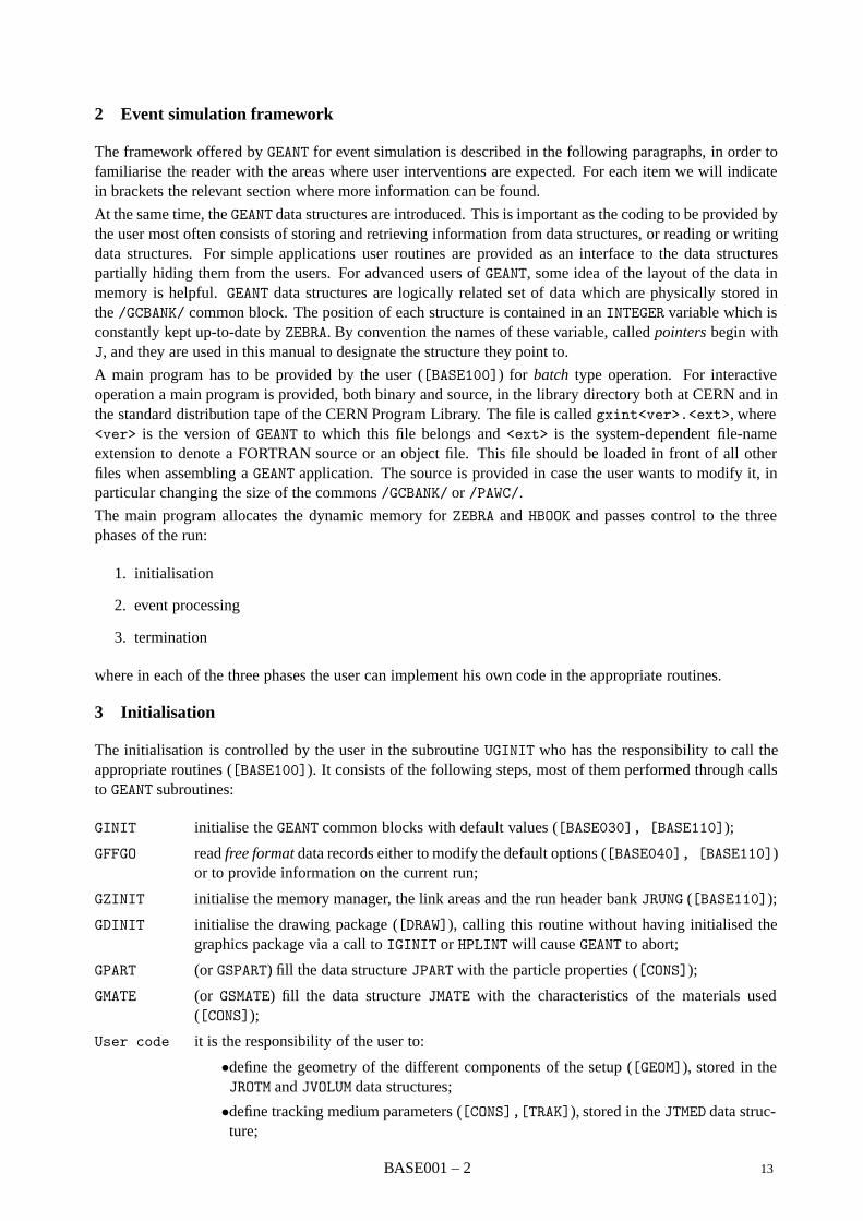
3 Initialisation
The initialisation is controlled by the user in the subroutine UGINIT who has the responsibility to call theappropriate routines ([BASE100]). It consists of the following steps, most of them performed through callsto GEANT subroutines:
GINIT initialise the GEANT common blocks with default values ([BASE030], [BASE110]);
GFFGO read free formatdata records either to modify the default options ([BASE040], [BASE110])or to provide information on the current run;
GZINIT initialise the memory manager, the link areas and the run header bank JRUNG ([BASE110]);
GDINIT initialise the drawing package ([DRAW]), calling this routine without having initialised thegraphics package via a call to IGINIT or HPLINT will cause GEANT to abort;
GPART (or GSPART) fill the data structure JPART with the particle properties ([CONS]);
GMATE (or GSMATE) fill the data structure JMATE with the characteristics of the materials used([CONS]);
User code it is the responsibility of the user to:
•define the geometry of the different components of the setup ([GEOM]), stored in theJROTM and JVOLUM data structures;
•define tracking medium parameters ([CONS],[TRAK]), stored in the JTMED data struc-ture;
BASE001 – 2 13
•specify which elements of the geometrical setup should be considered as sensitivedetectors, giving a responsewhen hit by a particle ([HITS]);
•usually all done in a user routine called UGEOM;
GGCLOS process all the geometrical information provided by the user and prepare for particle trans-port;
GBHSTA book standard GEANT histograms if required by the user with the data record HSTA ([BASE040],[BASE110]);
GPHYSI compute energy loss and cross-section tables and store them in the data structure JMATE([CONS], [PHYS]).
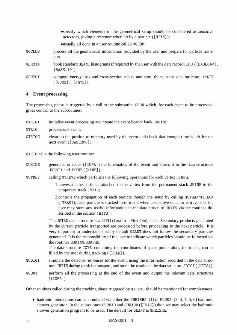
4 Event processing
The processing phase is triggered by a call to the subroutine GRUN which, for each event to be processed,gives control to the subroutines:
GTRIGI initialise event processing and create the event header bank JHEAD;
GTRIG process one event;
GTRIGC clean up the portion of memory used by the event and check that enough time is left for thenext event ([BASE200]).
GTRIG calls the following user routines:
GUKINE generates or reads ([IOPA]) the kinematics of the event and stores it in the data structuresJVERTX and JKINE ([KINE]);
GUTREV calling GTREVE which performs the following operations for each vertex in turn:
1.moves all the particles attached to the vertex from the permanent stack JKINE to thetemporary stack JSTAK;
2.controls the propagation of each particle though the setup by calling GUTRAK/GTRACK([TRAK]); each particle is tracked in turn and when a sensitive detector is traversed, theuser may store any useful information in the data structure JHITS via the routines de-scribed in the section [HITS];
The JSTAK data structure is a LIFO (Last In – First Out) stack. Secondary products generatedby the current particle transported are processed before proceeding to the next particle. It isvery important to understand that by default GEANT does not follow the secondary particlesgenerated. It is the responsibility of the user to indicate which particles should be followed viathe routines GSKING/GSKPHO.The data structure JXYZ, containing the coordinates of space points along the tracks, can befilled by the user during tracking ([TRAK]).
GUDIGI simulate the detector responses for the event, using the information recorded in the data struc-ture JHITS during particle transport, and store the results in the data structure JDIGI ([HITS]);
GUOUT perform all the processing at the end of the event and output the relevant data structures([IOPA]).
Other routines called during the tracking phase triggered by GTREVE should be mentioned for completeness:
• hadronic interactions can be simulated via either the GHEISHA [1] or FLUKA [2, 3, 4, 5, 6] hadronicshower generator. In the subroutines GUPHAD and GUHADR ([TRAK]) the user may select the hadronicshower generation program to be used. The default for GEANT is GHEISHA;
14 BASE001 – 3

• after each tracking step along the track, control is given to the subroutine GUSTEP. From the infor-mation available in labelled common blocks the user is able to take the appropriate action, such asstoring a hit or transferring a secondary product either in the stack JSTAK or in the event structureJVERTX/JKINE via the subroutine GSKING. In the subroutine GSSTAK, called by GSKING, a user rou-tine GUSKIP is called which permits skipping any unwanted track before entering it in the stack forsubsequent transport;
• the subroutine GUSWIM is called by the the routines which transport charged particles when in a mag-netic field; it selects and calls the appropriate routine to transport the particle. Although formally auser routine, the default version provided by GEANT is usually appropriate for most situations. Themagnetic field, unless it is constant along the Z axis, has to be described via the subroutine GUFLD.
5 Termination
The termination phase is under the control of the user ([BASE300]) via the routine GULAST. In simple casesit may consist of a call to the subroutine GLAST which computes and prints some statistical information(time per event, use of dynamic memory, etc.).
BASE001 – 4 15
Geant 3.16 GEANT User’s Guide BASE010
Origin : Submitted: 01.10.84Revision : Revised:19.10.94Documentation : F.Bruyant, S.Ravndal
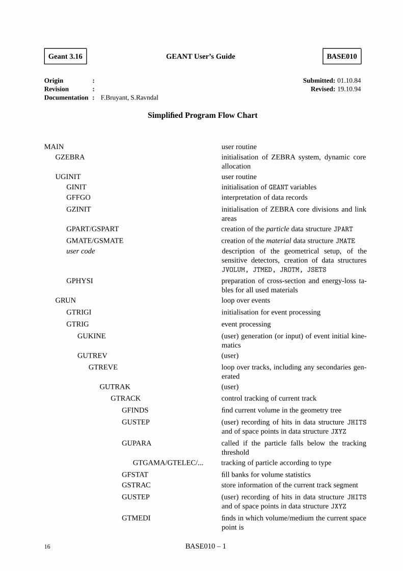
Simplified Program Flow Chart
MAIN user routine
GZEBRA initialisation of ZEBRA system, dynamic coreallocation
UGINIT user routine
GINIT initialisation of GEANT variables
GFFGO interpretation of data records
GZINIT initialisation of ZEBRA core divisions and linkareas
GPART/GSPART creation of the particle data structure JPART
GMATE/GSMATE creation of the materialdata structure JMATE
user code description of the geometrical setup, of thesensitive detectors, creation of data structuresJVOLUM, JTMED, JROTM, JSETS
GPHYSI preparation of cross-section and energy-loss ta-bles for all used materials
GRUN loop over events
GTRIGI initialisation for event processing
GTRIG event processing
GUKINE (user) generation (or input) of event initial kine-matics
GUTREV (user)
GTREVE loop over tracks, including any secondaries gen-erated
GUTRAK (user)
GTRACK control tracking of current track
GFINDS find current volume in the geometry tree
GUSTEP (user) recording of hits in data structure JHITSand of space points in data structure JXYZ
GUPARA called if the particle falls below the trackingthreshold
GTGAMA/GTELEC/... tracking of particle according to type
GFSTAT fill banks for volume statistics
GSTRAC store information of the current track segment
GUSTEP (user) recording of hits in data structure JHITSand of space points in data structure JXYZ
GTMEDI finds in which volume/medium the current spacepoint is
16 BASE010 – 1

GUSTEP (user) recording of hits in data structure JHITSand of space points in data structure JXYZ
GUDIGI computation of digitisations and recording indata structure JDIGI
GUOUT output of current event
GTRIGC clearing of memory for next event
UGLAST (user)
GLAST standard GEANT termination
BASE010 – 2 17
Geant 3.11 GEANT User’s Guide BASE020
Origin : Submitted: 01.10.84Revision : Revised:20.03.94Documentation : M.Maire
The data structures and their relationship
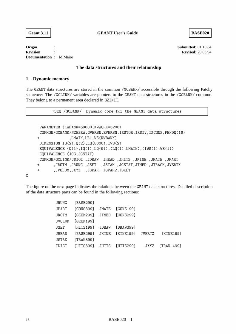
1 Dynamic memory
The GEANT data structures are stored in the common /GCBANK/ accessible through the following Patchysequence: The /GCLINK/ variables are pointers to the GEANT data structures in the /GCBANK/ common.They belong to a permanent area declared in GZINIT.
+SEQ /GCBANK/ Dynamic core for the GEANT data structures
PARAMETER (KWBANK=69000,KWWORK=5200)COMMON/GCBANK/NZEBRA,GVERSN,ZVERSN,IXSTOR,IXDIV,IXCONS,FENDQ(16)
+ ,LMAIN,LR1,WS(KWBANK)DIMENSION IQ(2),Q(2),LQ(8000),IWS(2)EQUIVALENCE (Q(1),IQ(1),LQ(9)),(LQ(1),LMAIN),(IWS(1),WS(1))EQUIVALENCE (JCG,JGSTAT)COMMON/GCLINK/JDIGI ,JDRAW ,JHEAD ,JHITS ,JKINE ,JMATE ,JPART
+ ,JROTM ,JRUNG ,JSET ,JSTAK ,JGSTAT,JTMED ,JTRACK,JVERTX+ ,JVOLUM,JXYZ ,JGPAR ,JGPAR2,JSKLT
C
The figure on the next page indicates the ralations between the GEANT data structures. Detailed descriptionof the data structure parts can be found in the following sections:
JRUNG [BASE299]
JPART [CONS399] JMATE [CONS199]
JROTM [GEOM299] JTMED [CONS299]
JVOLUM [GEOM199]
JSET [HITS199] JDRAW [DRAW399]
JHEAD [BASE299] JKINE [KINE199] JVERTX [KINE199]
JSTAK [TRAK399]
IDIGI [HITS399] JHITS [HITS299] JXYZ [TRAK 499]
18 BASE020 – 1
Particles
JPART
Materials
JMATE/JTMED
Geometry
JVOLUM/JROTM
Drawing
JDRAW
JSET
Tracking
GUSTEP
JSTAK
PHYSICS
Event processing
History
JVERTX/JKINE
Simulated
Raw DataJHITS/JDIGI
Initializationof
Kinematics
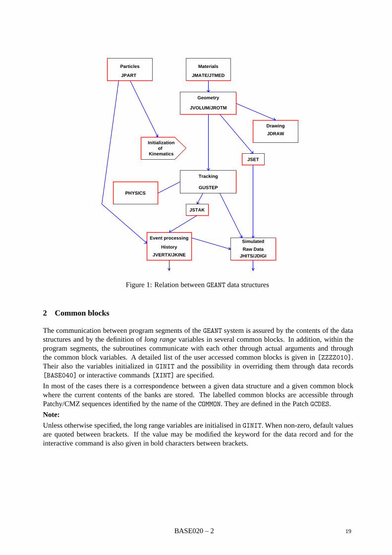
Figure 1: Relation between GEANT data structures
2 Common blocks
The communication between program segments of the GEANT system is assured by the contents of the datastructures and by the definition of long range variables in several common blocks. In addition, within theprogram segments, the subroutines communicate with each other through actual arguments and throughthe common block variables. A detailed list of the user accessed common blocks is given in [ZZZZ010].Their also the variables initialized in GINIT and the possibility in overriding them through data records[BASE040] or interactive commands [XINT] are specified.
In most of the cases there is a correspondence between a given data structure and a given common blockwhere the current contents of the banks are stored. The labelled common blocks are accessible throughPatchy/CMZ sequences identified by the name of the COMMON. They are defined in the Patch GCDES.
Note:
Unless otherwise specified, the long range variables are initialised in GINIT. When non-zero, default valuesare quoted between brackets. If the value may be modified the keyword for the data record and for theinteractive command is also given in bold characters between brackets.
BASE020 – 2 19
Geant 3.16 GEANT User’s Guide BASE040
Origin : Submitted: 01.10.84Revision : Revised: 16.12.93Documentation : F.Bruyant, M.Maire
Summary of Data Records
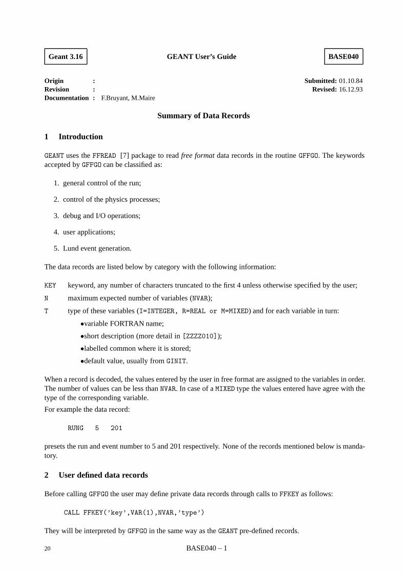
1 Introduction
GEANT uses the FFREAD [7] package to read free format data records in the routine GFFGO. The keywordsaccepted by GFFGO can be classified as:
1. general control of the run;
2. control of the physics processes;
3. debug and I/O operations;
4. user applications;
5. Lund event generation.
The data records are listed below by category with the following information:
KEY keyword, any number of characters truncated to the first 4 unless otherwise specified by the user;
N maximum expected number of variables (NVAR);
T type of these variables (I=INTEGER, R=REAL or M=MIXED) and for each variable in turn:
•variable FORTRAN name;
•short description (more detail in [ZZZZ010]);
•labelled common where it is stored;
•default value, usually from GINIT.
When a record is decoded, the values entered by the user in free format are assigned to the variables in order.The number of values can be less than NVAR. In case of a MIXED type the values entered have agree with thetype of the corresponding variable.
For example the data record:
RUNG 5 201
presets the run and event number to 5 and 201 respectively. None of the records mentioned below is manda-tory.
2 User defined data records
Before calling GFFGO the user may define private data records through calls to FFKEY as follows:
CALL FFKEY(’key’,VAR(1),NVAR,’type’)
They will be interpreted by GFFGO in the same way as the GEANT pre-defined records.
20 BASE040 – 1
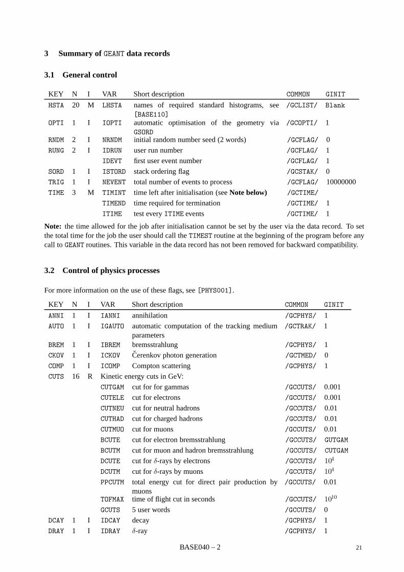
3 Summary of GEANT data records
3.1 General control
KEY N I VAR Short description COMMON GINIT
HSTA 20 M LHSTA names of required standard histograms, see[BASE110]
/GCLIST/ Blank
OPTI 1 I IOPTI automatic optimisation of the geometry viaGSORD
/GCOPTI/ 1
RNDM 2 I NRNDM initial random number seed (2 words) /GCFLAG/ 0
RUNG 2 I IDRUN user run number /GCFLAG/ 1
IDEVT first user event number /GCFLAG/ 1
SORD 1 I ISTORD stack ordering flag /GCSTAK/ 0
TRIG 1 I NEVENT total number of events to process /GCFLAG/ 10000000
TIME 3 M TIMINT time left after initialisation (see Note below) /GCTIME/
TIMEND time required for termination /GCTIME/ 1
ITIME test every ITIME events /GCTIME/ 1
Note: the time allowed for the job after initialisation cannot be set by the user via the data record. To setthe total time for the job the user should call the TIMEST routine at the beginning of the program before anycall to GEANT routines. This variable in the data record has not been removed for backward compatibility.
3.2 Control of physics processes
For more information on the use of these flags, see [PHYS001].
KEY N I VAR Short description COMMON GINIT
ANNI 1 I IANNI annihilation /GCPHYS/ 1
AUTO 1 I IGAUTO automatic computation of the tracking mediumparameters
/GCTRAK/ 1
BREM 1 I IBREM bremsstrahlung /GCPHYS/ 1
CKOV 1 I ICKOV Cerenkov photon generation /GCTMED/ 0
COMP 1 I ICOMP Compton scattering /GCPHYS/ 1
CUTS 16 R Kinetic energy cuts in GeV:
CUTGAM cut for for gammas /GCCUTS/ 0.001
CUTELE cut for electrons /GCCUTS/ 0.001
CUTNEU cut for neutral hadrons /GCCUTS/ 0.01
CUTHAD cut for charged hadrons /GCCUTS/ 0.01
CUTMUO cut for muons /GCCUTS/ 0.01
BCUTE cut for electron bremsstrahlung /GCCUTS/ GUTGAM
BCUTM cut for muon and hadron bremsstrahlung /GCCUTS/ CUTGAM
DCUTE cut for δ-rays by electrons /GCCUTS/ 104
DCUTM cut for δ-rays by muons /GCCUTS/ 104
PPCUTM total energy cut for direct pair production bymuons
/GCCUTS/ 0.01
TOFMAX time of flight cut in seconds /GCCUTS/ 1010
GCUTS 5 user words /GCCUTS/ 0
DCAY 1 I IDCAY decay /GCPHYS/ 1
DRAY 1 I IDRAY δ-ray /GCPHYS/ 1
BASE040 – 2 21
KEY N I VAR Short description COMMON GINIT
ERAN 3 M cross-section tables structure:
R EKMIN minimum energy for the cross-section tables /GCMULO/ 10−5
R EKMAX maximum energy for the cross-section tables /GCMULO/ 104
I NEKBIN number of logarithmic bins for cross-section ta-bles
/GCMULO/ 90
HADR 1 I IHADR hadronic process /GCPHYS/ 1
LABS 1 I ILABS Cerenkov light absorbtion /GCPHYS/ 0
LOSS 1 I ILOSS energy loss /GCPHYS/ 2
MULS 1 I IMULS multiple scattering /GCPHYS/ 1
MUNU 1 I IMUNU muon nuclear interaction /GCPHYS/ 1
PAIR 1 I IPAIR pair production /GCPHYS/ 1
PFIS 1 I IPFIS photofission /GCPHYS/ 0
PHOT 1 I IPHOT photo electric effect /GCPHYS/ 1
RAYL 1 I IRAYL Rayleigh scattering /GCPHYS/ 0
STRA 1 I ISTRA energy fluctuation model /GCPHYS/ 0
SYNC 1 I ISYNC synchrotron radiation generation /GCPHYS/ 0
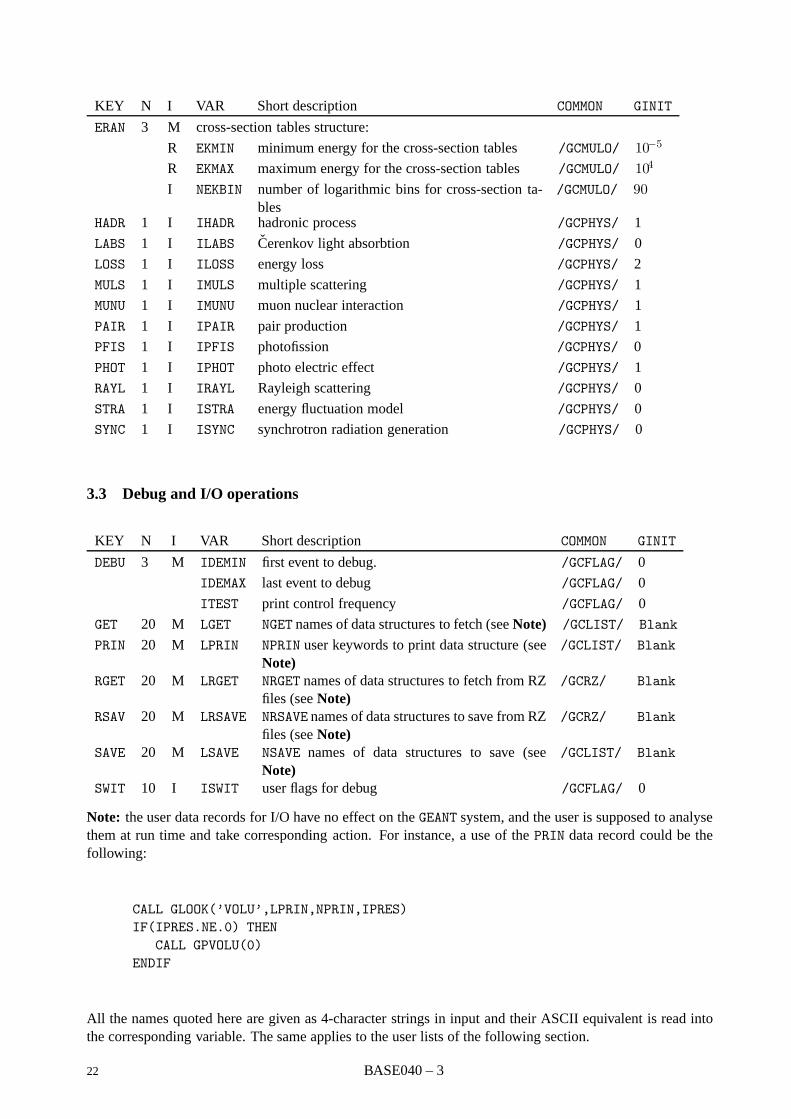
3.3 Debug and I/O operations
KEY N I VAR Short description COMMON GINIT
DEBU 3 M IDEMIN first event to debug. /GCFLAG/ 0
IDEMAX last event to debug /GCFLAG/ 0
ITEST print control frequency /GCFLAG/ 0
GET 20 M LGET NGET names of data structures to fetch (see Note) /GCLIST/ Blank
PRIN 20 M LPRIN NPRIN user keywords to print data structure (seeNote)
/GCLIST/ Blank
RGET 20 M LRGET NRGET names of data structures to fetch from RZfiles (see Note)
/GCRZ/ Blank
RSAV 20 M LRSAVE NRSAVE names of data structures to save from RZfiles (see Note)
/GCRZ/ Blank
SAVE 20 M LSAVE NSAVE names of data structures to save (seeNote)
/GCLIST/ Blank
SWIT 10 I ISWIT user flags for debug /GCFLAG/ 0
Note: the user data records for I/O have no effect on the GEANT system, and the user is supposed to analysethem at run time and take corresponding action. For instance, a use of the PRIN data record could be thefollowing:
CALL GLOOK(’VOLU’,LPRIN,NPRIN,IPRES)IF(IPRES.NE.0) THEN
CALL GPVOLU(0)ENDIF
All the names quoted here are given as 4-character strings in input and their ASCII equivalent is read intothe corresponding variable. The same applies to the user lists of the following section.
22 BASE040 – 3
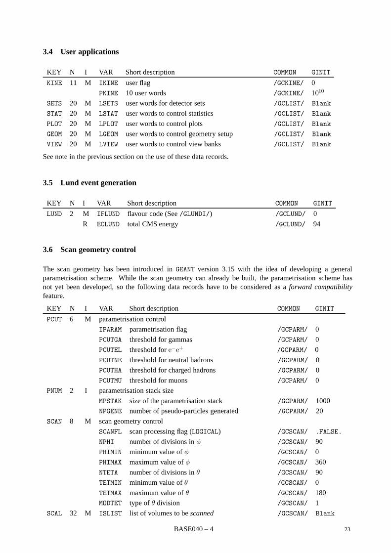
3.4 User applications
KEY N I VAR Short description COMMON GINIT
KINE 11 M IKINE user flag /GCKINE/ 0
PKINE 10 user words /GCKINE/ 1010
SETS 20 M LSETS user words for detector sets /GCLIST/ Blank
STAT 20 M LSTAT user words to control statistics /GCLIST/ Blank
PLOT 20 M LPLOT user words to control plots /GCLIST/ Blank
GEOM 20 M LGEOM user words to control geometry setup /GCLIST/ Blank
VIEW 20 M LVIEW user words to control view banks /GCLIST/ Blank
See note in the previous section on the use of these data records.
3.5 Lund event generation
KEY N I VAR Short description COMMON GINIT
LUND 2 M IFLUND flavour code (See /GLUNDI/) /GCLUND/ 0
R ECLUND total CMS energy /GCLUND/ 94
3.6 Scan geometry control
The scan geometry has been introduced in GEANT version 3.15 with the idea of developing a generalparametrisation scheme. While the scan geometry can already be built, the parametrisation scheme hasnot yet been developed, so the following data records have to be considered as a forward compatibilityfeature.
KEY N I VAR Short description COMMON GINIT
PCUT 6 M parametrisation control
IPARAM parametrisation flag /GCPARM/ 0
PCUTGA threshold for gammas /GCPARM/ 0
PCUTEL threshold for e−e+ /GCPARM/ 0
PCUTNE threshold for neutral hadrons /GCPARM/ 0
PCUTHA threshold for charged hadrons /GCPARM/ 0
PCUTMU threshold for muons /GCPARM/ 0
PNUM 2 I parametrisation stack size
MPSTAK size of the parametrisation stack /GCPARM/ 1000
NPGENE number of pseudo-particles generated /GCPARM/ 20
SCAN 8 M scan geometry control
SCANFL scan processing flag (LOGICAL) /GCSCAN/ .FALSE.
NPHI number of divisions in φ /GCSCAN/ 90
PHIMIN minimum value of φ /GCSCAN/ 0
PHIMAX maximum value of φ /GCSCAN/ 360
NTETA number of divisions in θ /GCSCAN/ 90
TETMIN minimum value of θ /GCSCAN/ 0
TETMAX maximum value of θ /GCSCAN/ 180
MODTET type of θ division /GCSCAN/ 1
SCAL 32 M ISLIST list of volumes to be scanned /GCSCAN/ Blank
BASE040 – 4 23

KEY N I VAR Short description COMMON GINIT
SCAP 6 R scan parameters
VX scan vertex X coordinate /GCSCAN/ 0
VY scan vertex Y coordinate /GCSCAN/ 0
VZ scan vertex Z coordinate /GCSCAN/ 0
FACTX0 scale factor for SX0 /GCSCAN/ 100
FACTL scale factor for SL /GCSCAN/ 1000
FACTR scale factor for R /GCSCAN/ 100
3.7 Landau fluctuations versus δ-rays
In order to avoid double counting between energy loss fluctuations (ILOSS=2) and generation of δ-raysIDRAY=1, if ILOSS = 2 the default value for δ-ray generation is set to 0 and it cannot be changed. Thedifferent cases are summarised in the table below.
Full fluctuations Restricted fluctuations No fluctuations
ILOSS = 2 (D) ILOSS = 1 or 3 ILOSS = 4
IDRAY 0 1 1
DCUTE 10 TeV CUTELE CUTELE
DCUTM 10 TeV CUTELE CUTELE
24 BASE040 – 5
Geant 3.16 GEANT User’s Guide BASE090
Origin : Submitted: 01.10.84Revision : Revised: 26.10.93Documentation : R.Brun, F.Bruyant
The reference systems and physical units
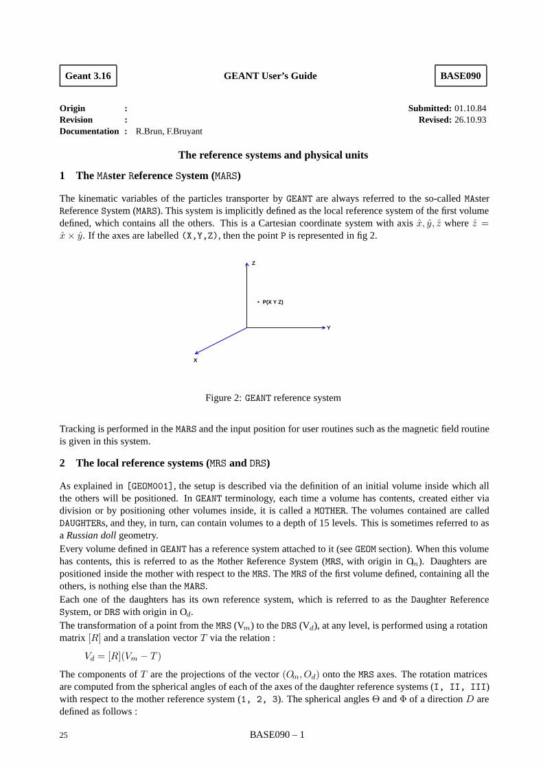
1 The MAster Reference System (MARS)
The kinematic variables of the particles transporter by GEANT are always referred to the so-called MAsterReference System (MARS). This system is implicitly defined as the local reference system of the first volumedefined, which contains all the others. This is a Cartesian coordinate system with axis x, y, z where z =x× y. If the axes are labelled (X,Y,Z), then the point P is represented in fig 2.
Z
Y
X
P(X Y Z)•
Figure 2: GEANT reference system
Tracking is performed in the MARS and the input position for user routines such as the magnetic field routineis given in this system.
2 The local reference systems (MRS and DRS)
As explained in [GEOM001], the setup is described via the definition of an initial volume inside which allthe others will be positioned. In GEANT terminology, each time a volume has contents, created either viadivision or by positioning other volumes inside, it is called a MOTHER. The volumes contained are calledDAUGHTERs, and they, in turn, can contain volumes to a depth of 15 levels. This is sometimes referred to asa Russian doll geometry.Every volume defined in GEANT has a reference system attached to it (see GEOM section). When this volumehas contents, this is referred to as the Mother Reference System (MRS, with origin in Om). Daughters arepositioned inside the mother with respect to the MRS. The MRS of the first volume defined, containing all theothers, is nothing else than the MARS.Each one of the daughters has its own reference system, which is referred to as the Daughter ReferenceSystem, or DRS with origin in Od.The transformation of a point from the MRS (Vm) to the DRS (Vd), at any level, is performed using a rotationmatrix [R] and a translation vector T via the relation :
Vd = [R](Vm − T )
The components of T are the projections of the vector (Om, Od) onto the MRS axes. The rotation matricesare computed from the spherical angles of each of the axes of the daughter reference systems (I, II, III)with respect to the mother reference system (1, 2, 3). The spherical angles Θ and Φ of a direction D aredefined as follows :
25 BASE090 – 1

Θ is the angle formed by the axis 3 and D (0 < Θ < 180).
Φ is the angle formed by the axis 1 and the projection of D onto the plane defined by the axes 1 and2 (0 < Φ < 360).
Examples are given in [GEOM200]. The various rotation matrices required for a given setup must be definedby the user during the initialisation stage. A number is assigned to each matrix [GEOM200]. The translationvector and the number of the rotation matrix are specified by the user when the volumes are positionedinside their mother [GEOM110].
3 Physical units
Unless otherwise specified, the following units are used throughout the program: centimeter, second, kilo-gauss, GeV, GeV c−1 (momentum), GeV c−2 (mass) and degree.
BASE090 – 2 26
Geant 3.21 GEANT User’s Guide BASE100
Origin : Submitted: 01.10.84Revision : Revised: 10.03.94Documentation : R.Brun, S.Ravndal
Examples of GEANT application
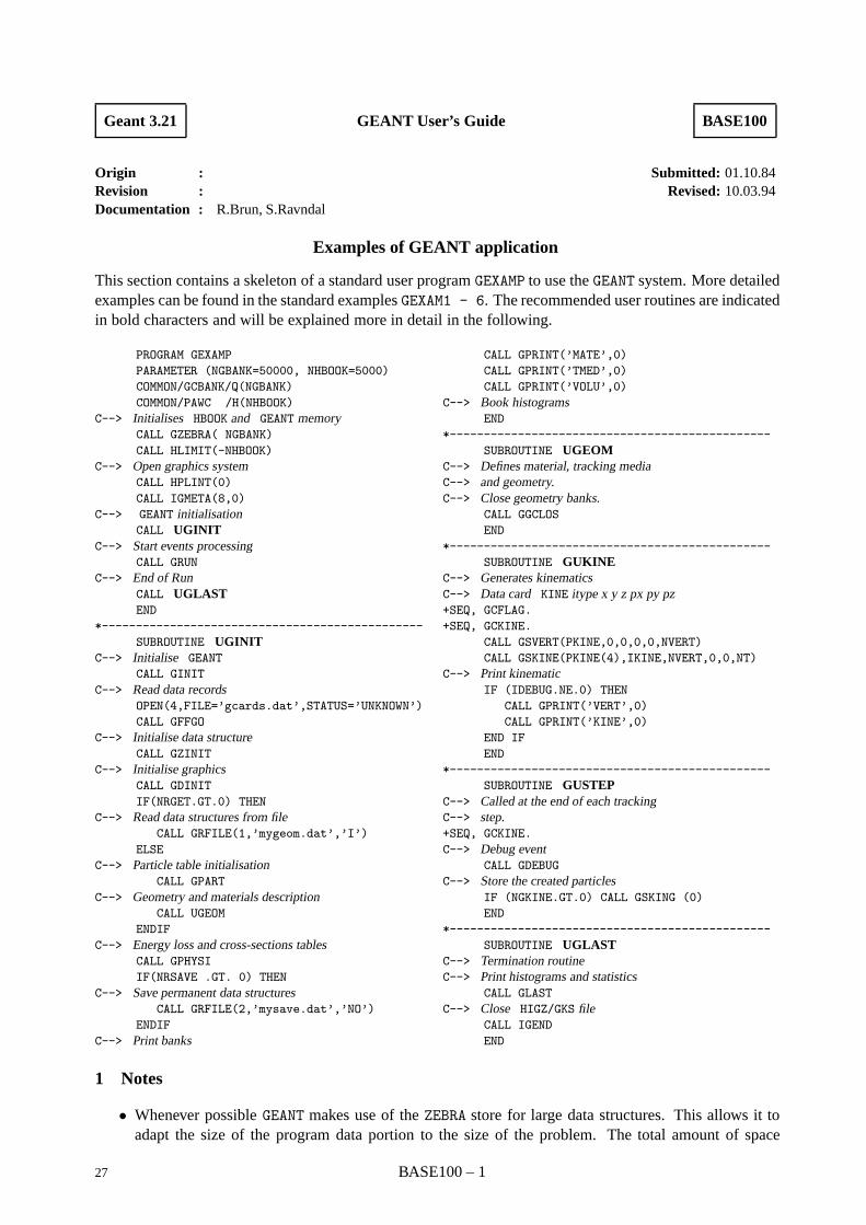
This section contains a skeleton of a standard user program GEXAMP to use the GEANT system. More detailedexamples can be found in the standard examples GEXAM1 - 6. The recommended user routines are indicatedin bold characters and will be explained more in detail in the following.
PROGRAM GEXAMP
PARAMETER (NGBANK=50000, NHBOOK=5000)
COMMON/GCBANK/Q(NGBANK)
COMMON/PAWC /H(NHBOOK)
C--> Initialises HBOOK and GEANT memoryCALL GZEBRA( NGBANK)
CALL HLIMIT(-NHBOOK)
C--> Open graphics systemCALL HPLINT(0)
CALL IGMETA(8,0)
C--> GEANT initialisationCALL UGINIT
C--> Start events processingCALL GRUN
C--> End of RunCALL UGLASTEND
*-----------------------------------------------
SUBROUTINE UGINITC--> Initialise GEANT
CALL GINIT
C--> Read data recordsOPEN(4,FILE=’gcards.dat’,STATUS=’UNKNOWN’)
CALL GFFGO
C--> Initialise data structureCALL GZINIT
C--> Initialise graphicsCALL GDINIT
IF(NRGET.GT.0) THEN
C--> Read data structures from fileCALL GRFILE(1,’mygeom.dat’,’I’)
ELSE
C--> Particle table initialisationCALL GPART
C--> Geometry and materials descriptionCALL UGEOM
ENDIF
C--> Energy loss and cross-sections tablesCALL GPHYSI
IF(NRSAVE .GT. 0) THEN
C--> Save permanent data structuresCALL GRFILE(2,’mysave.dat’,’NO’)
ENDIF
C--> Print banks
CALL GPRINT(’MATE’,0)
CALL GPRINT(’TMED’,0)
CALL GPRINT(’VOLU’,0)
C--> Book histogramsEND
*-----------------------------------------------
SUBROUTINE UGEOMC--> Defines material, tracking mediaC--> and geometry.C--> Close geometry banks.
CALL GGCLOS
END
*-----------------------------------------------
SUBROUTINE GUKINEC--> Generates kinematicsC--> Data card KINE itype x y z px py pz+SEQ, GCFLAG.
+SEQ, GCKINE.
CALL GSVERT(PKINE,0,0,0,0,NVERT)
CALL GSKINE(PKINE(4),IKINE,NVERT,0,0,NT)
C--> Print kinematicIF (IDEBUG.NE.0) THEN
CALL GPRINT(’VERT’,0)
CALL GPRINT(’KINE’,0)
END IF
END
*-----------------------------------------------
SUBROUTINE GUSTEPC--> Called at the end of each trackingC--> step.+SEQ, GCKINE.
C--> Debug eventCALL GDEBUG
C--> Store the created particlesIF (NGKINE.GT.0) CALL GSKING (0)
END
*-----------------------------------------------
SUBROUTINE UGLASTC--> Termination routineC--> Print histograms and statistics
CALL GLAST
C--> Close HIGZ/GKS fileCALL IGEND
END
1 Notes
• Whenever possible GEANT makes use of the ZEBRA store for large data structures. This allows it toadapt the size of the program data portion to the size of the problem. The total amount of space
27 BASE100 – 1
required depends on the application. GEANT can run with as little as 50,000 words or less, but for largedetectors it is not uncommon to declare stores of several million words. The call to GZEBRA initialisesthe common /GCBANK/ to receive the GEANT data structures. This call is necessary before any otherroutine of the GEANT system is called.
• The call to HLIMIT initialises the ZEBRA system to use the /PAWC/ common block for the HBOOKhistogram package. The size of the common depends on the number and size of the plot requested.The ZEBRA system must be initialised only once, and the negative argument to HLIMIT prevents asecond initialisation of the system. The HLIMIT call has to be placed after the call to GZEBRA and theargument has to be the dimension of the /PAWC/ common block with a negative sign in front.
• The main program is intended for batch applications, while to run the simulation interactively, theinteractive main program called GXINT should be linked in front of the user code.
• The program shown will require the graphic libraries in the link sequence. Often, for batch productionor for small tests, graphics is not needed, and not loading the graphics code makes the programsmaller. To avoid loading graphic routines the calls to IGINIT, IGMETA, IGEND, GDINIT and GDEBUGshould be removed.
If, on the other hand, the user is interested in including the routine GDEBUG and in excluding graphicsat the same time, then the following routine should be included in the code:
SUBROUTINE GDCXYZENTRY IGSAENTRY GDTRAKEND
which will avoid every reference to the graphics routines from GDEBUG.
• The user code to define the tracking media and the geometry of the setup should be inside the routineUGEOM. The pre-initialised data structured can be read from disk, but it is recommended to call GPHYSIin any case, to initialise the cross-section tables. An example of a full material, geometry and detectordesign is given below and has been extracted from the example GEXAM3. Here only major calls areshown, the redundant parts can be found in the source code of UGEOM in GEXAM3.
The example shows the basic concept in GEANT. First material parameters are defining the properitiesof a detector material calling the subroutine GSMATE. Here in addition to the 16 predefined materi-als, the material definition of Calcium is examplary shown. More information towards the prede-fined materials and further use of material definition routines can be found in the section CONS001- CONS101. Then tracking parameters are associated to the materials, defining a so called trackingmedium. Each GEANT volume must be associated to an existing tracking medium. Here in the examplethe tracking medium ’TARGET’ is defined to exist of Calcium.
In the example shown below several detector volumes are defined using the subroutine GSVOLU.The defined volume have associated parameters of name, shape, tracking medium and shape pa-rameters. In this example the volume ’TGT ’ consists of the previously defined tracking medium’TARGET’.The volumes (and if necessary identical copies of them) are then positioned according tothe detector geometry. The volumes are positioned on the same level, or inside each other. By settingthe parameter ONLY or MANY in the call of GSPOS the user has the opportunity to tell either GEANT thelogical volume structure and to apply boolean operations (cutting, joining and intersection) betweentwo positioned volumes. More information about the concept in defining volumes and positioning canbe retrieved from the section GEOM.
Finally the user is required to classify into sets all sensitive detectors (defined as those volume definedas detector via GSDET and other related routines, for which he wants to store hits in the hit datastructure JHITS.
BASE100 – 2 28
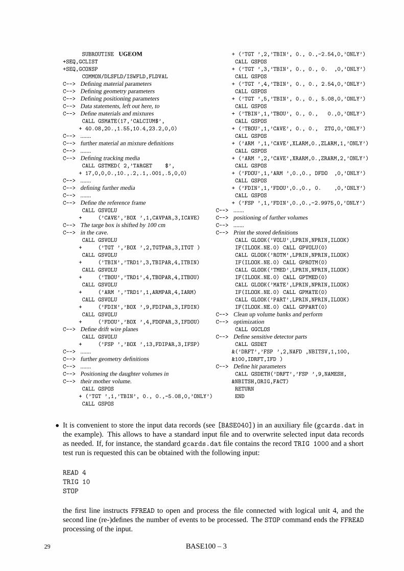
SUBROUTINE UGEOM+SEQ,GCLIST
+SEQ,GCONSP
COMMON/DLSFLD/ISWFLD,FLDVAL
C--> Defining material parametersC--> Defining geometry parametersC--> Defining positioning parametersC--> Data statements, left out here, toC--> Define materials and mixtures
CALL GSMATE(17,’CALCIUM$’,
+ 40.08,20.,1.55,10.4,23.2,0,0)
C--> .......C--> further material an mixture definitionsC--> .......C--> Defining tracking media
CALL GSTMED( 2,’TARGET $’,
+ 17,0,0,0.,10.,.2,.1,.001,.5,0,0)
C--> .......C--> defining further mediaC--> .......C--> Define the reference frame
CALL GSVOLU
+ (’CAVE’,’BOX ’,1,CAVPAR,3,ICAVE)
C--> The targe box is shifted by 100 cmC--> in the cave.
CALL GSVOLU
+ (’TGT ’,’BOX ’,2,TGTPAR,3,ITGT )
CALL GSVOLU
+ (’TBIN’,’TRD1’,3,TBIPAR,4,ITBIN)
CALL GSVOLU
+ (’TBOU’,’TRD1’,4,TBOPAR,4,ITBOU)
CALL GSVOLU
+ (’ARM ’,’TRD1’,1,ARMPAR,4,IARM)
CALL GSVOLU
+ (’FDIN’,’BOX ’,9,FDIPAR,3,IFDIN)
CALL GSVOLU
+ (’FDOU’,’BOX ’,4,FDOPAR,3,IFDOU)
C--> Define drift wire planesCALL GSVOLU
+ (’FSP ’,’BOX ’,13,FDIPAR,3,IFSP)
C--> .......C--> further geometry definitionsC--> .......C--> Positioning the daughter volumes inC--> their mother volume.
CALL GSPOS
+ (’TGT ’,1,’TBIN’, 0., 0.,-5.08,0,’ONLY’)
CALL GSPOS
+ (’TGT ’,2,’TBIN’, 0., 0.,-2.54,0,’ONLY’)
CALL GSPOS
+ (’TGT ’,3,’TBIN’, 0., 0., 0. ,0,’ONLY’)
CALL GSPOS
+ (’TGT ’,4,’TBIN’, 0., 0., 2.54,0,’ONLY’)
CALL GSPOS
+ (’TGT ’,5,’TBIN’, 0., 0., 5.08,0,’ONLY’)
CALL GSPOS
+ (’TBIN’,1,’TBOU’, 0., 0., 0.,0,’ONLY’)
CALL GSPOS
+ (’TBOU’,1,’CAVE’, 0., 0., ZTG,0,’ONLY’)
CALL GSPOS
+ (’ARM ’,1,’CAVE’,XLARM,0.,ZLARM,1,’ONLY’)
CALL GSPOS
+ (’ARM ’,2,’CAVE’,XRARM,0.,ZRARM,2,’ONLY’)
CALL GSPOS
+ (’FDOU’,1,’ARM ’,0.,0., DFDO ,0,’ONLY’)
CALL GSPOS
+ (’FDIN’,1,’FDOU’,0.,0., 0. ,0,’ONLY’)
CALL GSPOS
+ (’FSP ’,1,’FDIN’,0.,0.,-2.9975,0,’ONLY’)
C--> .......C--> positioning of further volumesC--> .......C--> Print the stored definitions
CALL GLOOK(’VOLU’,LPRIN,NPRIN,ILOOK)
IF(ILOOK.NE.0) CALL GPVOLU(0)
CALL GLOOK(’ROTM’,LPRIN,NPRIN,ILOOK)
IF(ILOOK.NE.0) CALL GPROTM(0)
CALL GLOOK(’TMED’,LPRIN,NPRIN,ILOOK)
IF(ILOOK.NE.0) CALL GPTMED(0)
CALL GLOOK(’MATE’,LPRIN,NPRIN,ILOOK)
IF(ILOOK.NE.0) CALL GPMATE(0)
CALL GLOOK(’PART’,LPRIN,NPRIN,ILOOK)
IF(ILOOK.NE.0) CALL GPPART(0)
C--> Clean up volume banks and performC--> optimization
CALL GGCLOS
C--> Define sensitive detector partsCALL GSDET
&(’DRFT’,’FSP ’,2,NAFD ,NBITSV,1,100,
&100,IDRFT,IFD )
C--> Define hit parametersCALL GSDETH(’DRFT’,’FSP ’,9,NAMESH,
&NBITSH,ORIG,FACT)
RETURN
END
• It is convenient to store the input data records (see [BASE040]) in an auxiliary file (gcards.dat inthe example). This allows to have a standard input file and to overwrite selected input data recordsas needed. If, for instance, the standard gcards.dat file contains the record TRIG 1000 and a shorttest run is requested this can be obtained with the following input:
READ 4TRIG 10STOP
the first line instructs FFREAD to open and process the file connected with logical unit 4, and thesecond line (re-)defines the number of events to be processed. The STOP command ends the FFREADprocessing of the input.
29 BASE100 – 3

• In the above example the common blocks have not been expanded in the code. The notation used isthe one of the PATCHY/CMZ [8, 9] code management systems. These products, among other things, canrun as pre-processors, replacing the +SEQ,... instructions with the corresponding code fragments.Users are strongly recommended to use these systems to include GEANT common blocks in their code.
Long experience in supporting GEANT users has shown that, as the user program grows, typing errorsin the insertion of the common blocks by hand become very common, but difficult to find. Theinvestment needed to learn a code management system at the user level is usually negligible comparedwith the time and energy needed in hunting a problem introduced by a mistyped common.
BASE100 – 4 30
Geant 3.16 GEANT User’s Guide BASE110
Origin : R.Brun Submitted: 01.06.83Revision : Revised: 16.12.93Documentation :
The system initialisation routines
CALL GZEBRA (NZ)
Initialises the ZEBRA memory manager to use the common /GCBANK/ to store the GEANT data structures.
NZ (INTEGER) size of the /GCBANK/ common as it is dimensioned in the main program.
The size of the dynamic memory is set to NZ-30. The common /GCBANK/ must be dimensioned in the mainprogram. ZEBRA [8] must be initialised only once. The call to the HBOOK initialisation routine HLIMITtries to initialise ZEBRA as well, and this will cause a program abort. To avoid this, HLIMIT must be calledafter GZEBRA and its argument must be a negative number whose absolute value is the size of the /PAWC/common containing the histograms. This is shown in the example of main program given in [BASE100].
CALL GINIT
Presets labelled common block variables to default values. See [BASE030] for more information.
CALL GFFGO
Reads a set of data records via the FFREAD package. See [BASE040] for more information on the possibledata records. GFFGO must be called after GINIT.
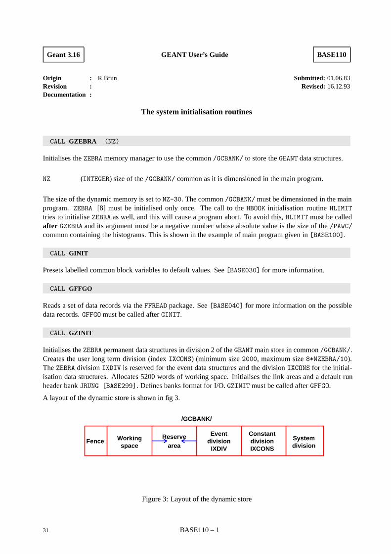
CALL GZINIT
Initialises the ZEBRA permanent data structures in division 2 of the GEANT main store in common /GCBANK/.Creates the user long term division (index IXCONS) (minimum size 2000, maximum size 8*NZEBRA/10).The ZEBRA division IXDIV is reserved for the event data structures and the division IXCONS for the initial-isation data structures. Allocates 5200 words of working space. Initialises the link areas and a default runheader bank JRUNG [BASE299]. Defines banks format for I/O. GZINIT must be called after GFFGO.
A layout of the dynamic store is shown in fig 3.
Fence Workingspace
Reservearea
Eventdivision
IXDIV
ConstantdivisionIXCONS
Systemdivision
/GCBANK/
Figure 3: Layout of the dynamic store
31 BASE110 – 1
CALL GDINIT
This routine initialises the GEANT drawing package [DRAW001] and it has to be called before any othergraphic routine. GEANT uses the CERN-developed HIGZ [1] graphic library, and this has to be initialisedbefore the call to GDINIT. In the example given in [BASE100] the routines IGINIT and IGMETA are used.Alternatively, the routine HPLINT from HPLOT [7] can be used. This routine calls the appropriate proce-dures from HIGZ to initialise the underlaying graphics system. At the moment HIGZ can use several flavoursof GKS [2, 3, 4] and X11 and it is available on all machines where the CERN Program Library has beeninstalled.
CALL GPHYSI
Completes the data structure JMATE, (see [PHYS100]) calculating the cross-section and stopping powertables.
CALL GBHSTA
Initialises the standard histograms requested by the user via the data record HSTA. The following histogramkeywords may be used :
TIME time per event;
SIZE size of division IXDIV per event;
MULT total number of tracks per event;
NTRA number of long life tracks per event;
STAK maximum stack size per event.
GBHSTA should be called after GFFGO.
CALL GGCLOS
This routine has to be called at the end of the definition of the geometry by the user, after thal all volumeshave been defined and positioned and all detectors defined. Failure to call this routine will prevent the GEANTsystem from working correctly. Main tasks of this routine are:
• close the geometry package;
• complete the JVOLUM data structure;
• process the detector definition provided by the user;
• prepare the tables for the tracking speed optimisation requested by the user via the GSORD routine orthe OPTI data record.
BASE110 – 2 32
Geant 3.16 GEANT User’s Guide BASE200
Origin : R.Brun Submitted: 01.06.83Revision : Revised: 26.10.93Documentation :
Steering routines for event processing
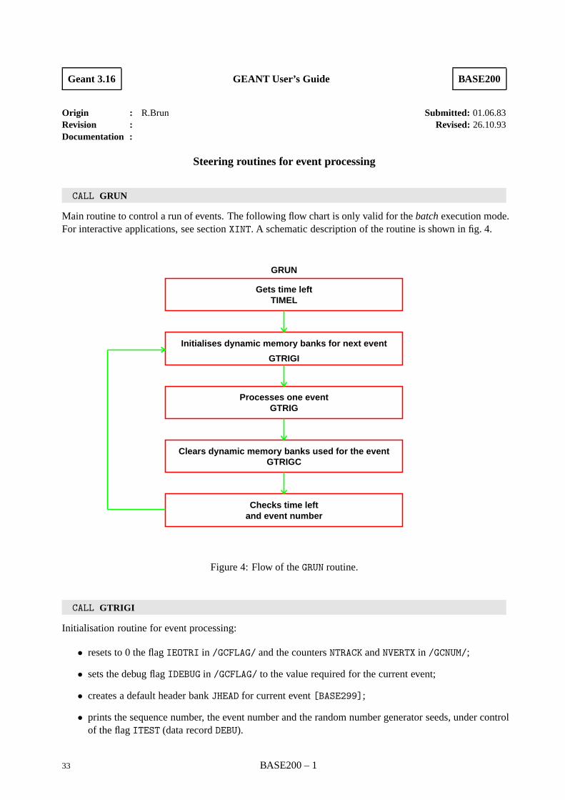
CALL GRUN
Main routine to control a run of events. The following flow chart is only valid for the batch execution mode.For interactive applications, see section XINT. A schematic description of the routine is shown in fig. 4.
Gets time leftTIMEL
Initialises dynamic memory banks for next event
GTRIGI
Processes one eventGTRIG
Clears dynamic memory banks used for the eventGTRIGC
Checks time leftand event number
GRUN
Figure 4: Flow of the GRUN routine.
CALL GTRIGI
Initialisation routine for event processing:
• resets to 0 the flag IEOTRI in /GCFLAG/ and the counters NTRACK and NVERTX in /GCNUM/;
• sets the debug flag IDEBUG in /GCFLAG/ to the value required for the current event;
• creates a default header bank JHEAD for current event [BASE299];
• prints the sequence number, the event number and the random number generator seeds, under controlof the flag ITEST (data record DEBU).
33 BASE200 – 1
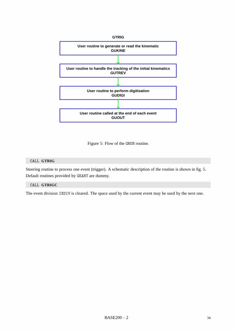
User routine to generate or read the kinematicGUKINE
User routine to handle the tracking of the initial kinematicsGUTREV
User routine to perform digitisationGUDIGI
User routine called at the end of each eventGUOUT
GTRIG
Figure 5: Flow of the GRUN routine.
CALL GTRIG
Steering routine to process one event (trigger). A schematic description of the routine is shown in fig. 5.
Default routines provided by GEANT are dummy.
CALL GTRIGC
The event division IXDIV is cleared. The space used by the current event may be used by the next one.
BASE200 – 2 34
Geant 3.16 GEANT User’s Guide BASE280
Origin : M.Maire Submitted: 14.12.93Revision : Revised: 14.12.93Documentation :
Storing and retrieving JRUNG and JHEAD information
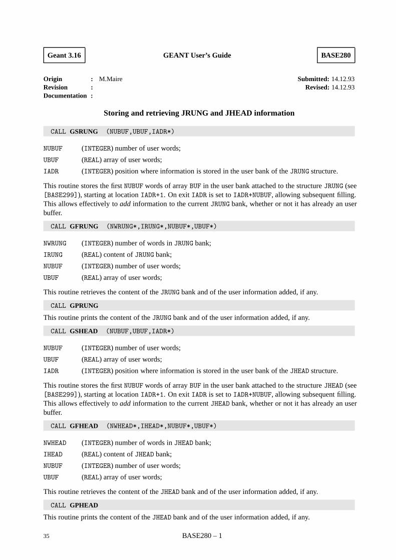
CALL GSRUNG (NUBUF,UBUF,IADR*)
NUBUF (INTEGER) number of user words;
UBUF (REAL) array of user words;
IADR (INTEGER) position where information is stored in the user bank of the JRUNG structure.
This routine stores the first NUBUF words of array BUF in the user bank attached to the structure JRUNG (see[BASE299]), starting at location IADR+1. On exit IADR is set to IADR+NUBUF, allowing subsequent filling.This allows effectively to add information to the current JRUNG bank, whether or not it has already an userbuffer.
CALL GFRUNG (NWRUNG*,IRUNG*,NUBUF*,UBUF*)
NWRUNG (INTEGER) number of words in JRUNG bank;
IRUNG (REAL) content of JRUNG bank;
NUBUF (INTEGER) number of user words;
UBUF (REAL) array of user words;
This routine retrieves the content of the JRUNG bank and of the user information added, if any.
CALL GPRUNG
This routine prints the content of the JRUNG bank and of the user information added, if any.
CALL GSHEAD (NUBUF,UBUF,IADR*)
NUBUF (INTEGER) number of user words;
UBUF (REAL) array of user words;
IADR (INTEGER) position where information is stored in the user bank of the JHEAD structure.
This routine stores the first NUBUF words of array BUF in the user bank attached to the structure JHEAD (see[BASE299]), starting at location IADR+1. On exit IADR is set to IADR+NUBUF, allowing subsequent filling.This allows effectively to add information to the current JHEAD bank, whether or not it has already an userbuffer.
CALL GFHEAD (NWHEAD*,IHEAD*,NUBUF*,UBUF*)
NWHEAD (INTEGER) number of words in JHEAD bank;
IHEAD (REAL) content of JHEAD bank;
NUBUF (INTEGER) number of user words;
UBUF (REAL) array of user words;
This routine retrieves the content of the JHEAD bank and of the user information added, if any.
CALL GPHEAD
This routine prints the content of the JHEAD bank and of the user information added, if any.
35 BASE280 – 1
Geant 3.16 GEANT User’s Guide BASE299
Origin : R.Brun, F.Bruyant Submitted: 01.10.84Revision : Revised: 14.12.93Documentation :
The banks JRUNG and JHEAD
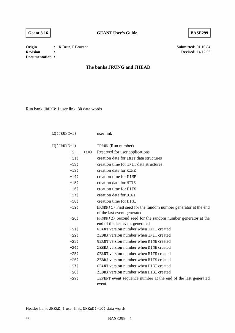
Run bank JRUNG: 1 user link, 30 data words
LQ(JRUNG-1) user link
IQ(JRUNG+1) IDRUN (Run number)
+2 ...+10) Reserved for user applications
+11) creation date for INIT data structures
+12) creation time for INIT data structures
+13) creation date for KINE
+14) creation time for KINE
+15) creation date for HITS
+16) creation time for HITS
+17) creation date for DIGI
+18) creation time for DIGI
+19) NRNDM(1) First seed for the random number generator at the endof the last event generated
+20) NRNDM(2) Second seed for the random number generator at theend of the last event generated
+21) GEANT version number when INIT created
+22) ZEBRA version number when INIT created
+23) GEANT version number when KINE created
+24) ZEBRA version number when KINE created
+25) GEANT version number when HITS created
+26) ZEBRA version number when HITS created
+27) GEANT version number when DIGI created
+28) ZEBRA version number when DIGI created
+29) IEVENT event sequence number at the end of the last generatedevent
Header bank JHEAD: 1 user link, NHEAD(=10) data words
36 BASE299 – 1

LQ(JHEAD-1) user link
IQ(JHEAD+1) IDRUN Run number
+2) IDEVT Event number
+3) NRNDM(1) Value of random number generator first seed at thebeginning of the event
+4) NRNDM(2) Value of random number generator second seed at thebeginning of the event
+5 ...10) Reserved for user applications
BASE299 – 2 37
Geant 3.16 GEANT User’s Guide BASE300
Origin : Submitted: 01.10.84Revision : Revised: 08.11.93Documentation : R.Brun
Example of user termination routine
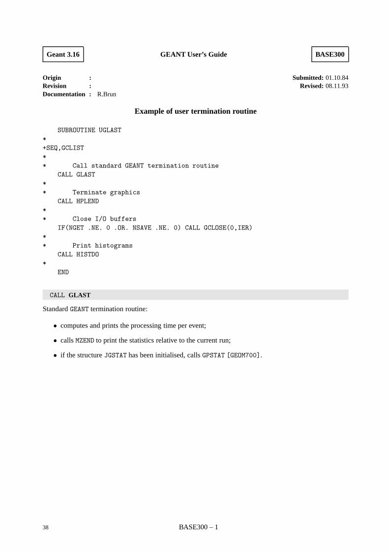
SUBROUTINE UGLAST*+SEQ,GCLIST** Call standard GEANT termination routine
CALL GLAST** Terminate graphics
CALL HPLEND** Close I/O buffers
IF(NGET .NE. 0 .OR. NSAVE .NE. 0) CALL GCLOSE(0,IER)** Print histograms
CALL HISTDO*
END
CALL GLAST
Standard GEANT termination routine:
• computes and prints the processing time per event;
• calls MZEND to print the statistics relative to the current run;
• if the structure JGSTAT has been initialised, calls GPSTAT [GEOM700].
38 BASE300 – 1
Geant 3.16 GEANT User’s Guide BASE400
Origin : R.Brun, F.Carena Submitted: 01.10.84Revision : Revised: 16.12.93Documentation :
Debugging facilities
The flags IDEBUG, ITEST and ISWIT(1-10) are available to in the common /GCFLAG/ for debug control[BASE030]. The array ISWIT is filled through the data record SWIT. Some flags are used by GHEISHA[PHYS510] and by the routine GDEBUG.
The flag IDEBUG is set to 1 in GTRIGI for the events with sequence number from IDEMIN to IDEMAX,as specified by the user on the data record DEBU. If IDEMIN is negative, debug is activated also in theinitialisation phase.
The flag ITEST, set by the user via the data record DEBU, is also used by GTRIGI. The sequence number, theevent number and the random numbers seeds are printed at the beginning of each event every ITEST fromIDEMIN to IDEMAX.
1 Debug of data structures
The contents of the data structures can be dumped by the routine
CALL GPRINT (CHNAME,NUMB)
CHNAME (CHARACTER*4) name of a top level data structure;
NUMB (INTEGER) number of the substructure to be printed, 0 for all.
Examples
• CALL GPRINT(’KINE’,0) prints all banks JKINE;
• CALL GPRINT(’KINE’,8) prints JKINE bank for track 8;
• CALL GPRINT(’VOLU’,0) prints all existing volumes.
The following names are recognised:
DIGI,HITS,KINE,MATE,VOLU,ROTM,SETS,TMED,PART,VERT,JXYZ
GPRINT calls selectively the routines:
GPDIGI(’*’,’*’) GPHITS(’*’,’*’) GPKINE(NUMB) GPMATE(NUMB)
GPVOLU(NUMB) GPROTM(NUMB) GPSETS(’*’,’*’) GPTMED(NUMB)
GPPART(NUMB) GPVERT(NUMB) GPJXYZ(NUMB)
These routines can be called directly by the user. In case of SETS, HITS and DIGI the content of all detectorsof all sets will be printed, so NUMB is irrelevant.
39 BASE400 – 1
2 Debug of events
The development of an event can be followed via the routine:
CALL GDEBUG
which operates under the control of the ISWIT array. It is the user responsibility to call this routine fromGUSTEP. If the DEBUG flag is active, the routine will perform as follows:
ISWIT(1)
2 the content of the temporary stack for secondaries in the common /GCKING/ is printed;
ISWIT(2)
1 the current point of the track is stored in the JDXYZ bank via the routine GSXYZ;
2 the current information on the track is printed via the routine GPCXYZ;
3 the current step is drawn via the routine GDCXYZ;
4 the current point of the track is stored in the JDXYZ bank via the routine GSXYZ. When theparticle stops the track is drawn via the routine GDTRAK and the space occupied by the trackin the structure JDXYZ released;
ISWIT(3)
1 the current point of the track is stored in the JDXYZ bank via the routine GSXYZ.
BASE400 – 2 40
Geant 3.16 GEANT User’s Guide BASE410
Origin : R.Brun Submitted: 08.08.87Revision : Revised: 08.11.93Documentation :
Utility Routines
CALL GLOOK (CHNAME,IVECT,N,ILOOK*)
CHNAME (CHARACTER*4) variable containing the name to be searched for in IVECT;
IVECT (INTEGER) array containing the ASCII code of the names among which NAME is searched. Thenames are stored 4 characters per word;
N (INTEGER) number of items in IVECT;
ILOOK (INTEGER) position in IVECT where NAME has been found, 0 if not found.
This routine is very useful when searching for a string stored in a ZEBRA bank. For instance to find theposition of the ’CRYS’ volume in the volume bank, the following piece of code could be written:
+SEQ,GCBANK.+SEQ,GCNUM.
.
.
.CALL GLOOK(’CRYS’,IQ(JVOLUM+1),NVOLUM,IVO)IF(IVO.GT.0) THEN
JVO = LQ(JVOLUM-IVO)ELSE
JVO = 0ENDIF
JVO, if different from 0, is the pointer to the data bank containing the information relative to the volume’CRYS’.
CALL GEVKEV (EGEV,ENERU*,CHUNIT*)
EGEV (REAL) input, energy in GeV;
ENERU (REAL) output, energy in the new unit;
CHUNIT (CHARACTER*4) unit in which the energy has been converted.
This subroutine converts the input energy in GeV to a unit in which 1 ≤ E ≤ 999. CHUNIT contains thenew unit. The following piece of code illustrates the use of GEVKEV:
+SEQ,GCTRAK.CHARACTER*4 CHUNIT...CALL GEVKEV(DESTEP, DE, CHUNIT)WRITE(6,10000) DE, CHUNIT
10000 FORMAT(’ The energy loss in this step is ’,F7.2,A)
41 BASE410 – 1
Geant 3.16 GEANT User’s Guide BASE420
Origin : R.Brun, F.Carminati Submitted: 27.07.93Revision : Revised: 14.12.93Documentation :
The random number generator
CALL GRNDM (VEC*,LEN)
VEC (REAL) vector containing the generated random number;
LEN (INTEGER) number of random numbers to generate.
GRNDM generates a sequence of uniformly distributed random numbers in the interval (0,1). The numbersare returned in a vector. The code is a copy of the CERN Program Library routine RANECU [16, 17] (entryV114).
Several independent sequences can be defined and used. Each sequence must be initialised by the user,otherwise the result is unpredictable. Two integer seeds are used to initialise a sequence. Not all pairs ofintegers define a good random sequence or one which is independent from others. Sections of the samerandom sequence can be defined as independent sequences. The period of the generator is 260 ≈ 1018. Ageneration has been performed in order to provide the seeds to start any of the generated sections. There are215 possible seed pairs and they are all 109 numbers apart. Thus a sequence started from one of the seedpairs, after 109 numbers will start generating the next one.
CALL GRNDMQ (ISEED1,ISEED2,ISEQ,CHOPT)
ISEED1 (INTEGER) first seed of the sequence;
ISEED2 (INTEGER) second seed of the sequence;
ISEQ (INTEGER) number of the independent sequence of random numbers referred to by this call. IfISEQ≤0, then the last valid sequence used will be addressed either for a save or a store. In casethe option ’G’ is specified, on output the variable will contain the sequence actually used;
CHOPT (CHARACTER*(*)) the action to be taken:
’ ’ if 1≤ISEQ≤215, sequence number ISEQ will be initialised with the seeds of the pre-computed independent sequence ISEQ.If ISEQ≤0 or ISEQ>215, sequence number 1 will be initialised with the default seeds.ISEED1 and ISEED2 are ignored;
’G’ get the present status of the generator: the two integer seeds ISEED1 and ISEED2 willbe returned for sequence ISEQ;
’S’ set the status of the generator. The two integer seeds ISEED1 and ISEED2 will be usedto restart the generator for sequence ISEQ.
’SH’ the same action as for ’S’ and store the two integer seeds ISEED1 and ISEED2 in theevent header bank.
’Q’ Get the pre-generated seeds for ISEQ (1≤ISEQ≤215). There are 215 pre-generatedsequences each one will generate 109 numbers before reproducing the following one.
Initialises the random number generator.
42 BASE420 – 1
VALUE = GARNDM (DUMMY)
DUMMY (REAL) dummy parameter, ignored;
Returns a random number r distributed as e−x. r = − ln(η) where η is a random number extracted byGRNDM.
CALL GPOISS (AMVEC,NPVEC*,LEN)
AMVEC (REAL) array of length LEN containing the average values of the Poisson distributions requested;
NPVEC (INTEGER) array of length LEN containing the random numbers: NPVEC(I) is a random numberwith a Poisson distribution of average AMVEC(I);
LEN (INTEGER) number of random numbers requested.
This routine extracts integer random numbers according to the Poisson distribution. Given a Poisson distri-bution of average λ ≤ 16 and r uniformly distributed between 0 and 1, the method used is the following:
1. let P = exp(−λ), N = 0 and S = P ;
2. if r ≤ S accept N ;
3. let N = N + 1, P = Pλ/N , S = S + P and go back to 2;
If λ > 16, a gaussian distribution with average λ and σ =√λ is generated.
BASE420 – 2 43

BASE Bibliography
[1] H.C.Fesefeldt. Simulation of hadronic showers, physics and applications. Technical Report PITHA85-02, III Physikalisches Institut, RWTH Aachen Physikzentrum, 5100 Aachen, Germany, September1985.
[2] P.A.Aarnio et al. Fluka user’s guide. Technical Report TIS-RP-190, CERN, 1987, 1990.
[3] A.Fasso A.Ferrari J.Ranft P.R.Sala G.R.Stevenson and J.M.Zazula. FLUKA92. In Proceedings of theWorkshop on Simulating Accelerator Radiation Environments, Santa Fe, USA, 11-15 January 1993.
[4] A.Fasso A.Ferrari J.Ranft P.R.Sala G.R.Stevenson and J.M.Zazula. A Comparison of FLUKA Sim-ulations with measurements of Fluence and Dose in Calorimeter Structures. Nuclear Instruments &Methods A, 332:459, 1993.
[5] C.Birattari E.DePonti A.Esposito A.Ferrari M.Pelliccioni and M.Silari. Measurements and character-ization of high energy neutron fields. approved for pubblication in Nuclear Instruments & MethodsA.
[6] P.A.Aarnio, A.Fasso, A.Ferrari, J.-H.Moehring, J.Ranft, P.R.Sala, G.R.Stevenson and J.M.Zazula.FLUKA: hadronic benchmarks and applications. In MC93 Int. Conf. on Monte-Carlo Simulation inHigh-Energy and Nuclear Physics, Tallahassee, Florida, 22-26 February 1993. Proceedings in press.
[7] R.Brun et al. FFREAD User Guide and Reference Manual, dd/us/71 edition, February 1987.
[8] H.J. Klein and J. Zoll. PATCHY Reference Manual, Program Library L400. CERN, 1988.
[9] M. Brun, R. Brun, and F. Rademakers. CMZ - A Source Code Management System. CodeME S.A.R.L.,1991.
[10] R.Brun, M.Goossens, and J.Zoll. ZEBRA Users Guide, Program Library Q100. CERN, 1991.
[11] R.Bock et al. HIGZ Users Guide, Program Library Q120. CERN, 1991.
[12] R.Brun and H.Renshall. HPLOT users guide, Program Library Y251. CERN, 1990.
[13] ISO. The graphical kernel system (gks). Technical Report ISO 7942, ISO Geneva, 1985.
[14] ISO. The graphical kernel system for three dimensions (gks-3d). Technical Report ISO 8805, ISOGeneva, 1987.
[15] D.R.Myers. GKS/GKS-3D Primer, DD/US/110. CERN, 1987.
[16] P.L’Ecuyer. Efficient and portable random number generators. Comm. ACM, 31:742, 1988.
[17] F.James. A review of pseudorandom number generators. Computer Phys. Comm., 60:329–344, 1990.
44 BASE420 – 3
Geant 3.16 GEANT User’s Guide CONS001
Origin : Submitted: 01.10.84Revision : Revised: 17.12.93Documentation : F.Bruyant
Introduction to the section CONS
1 Introduction
The setup where the particles are transported is represented by a structure of geometrical volumes. Eachvolume is filled with matter (which can have the properties of the vacuum in case of it contains no matter).
The matter composing the volumes is described via two sets of attributes. The first set is relative to thenature of the material composing the volume, and contains information such as the atomic number, theatomic weight, the density and so on (see the description of the routine GSMATE in this section for moreinformation).
The second set of attributes is relevant to the process of particle transport and they define a so-called trackingmedium. These are parameters such as the material composing the volume, the magnetic field, the requiredtracking precision, the maximum energy that can be lost in one step and so on (see the description of theroutine GSTMED in this section for more information).
Each tracking medium refers to a material via a material number which is assigned by the user. Differenttracking media can, with some limitation, refer to the same material.
Each volume is filled by a tracking medium identified by a medium number. Different volumes may havethe same medium number (see [GEOM]).
The transport of particles through a setup ([TRAK]) requires access to data which describe:
• the geometry of the setup;
• the material and tracking medium parameters;
• the particle properties.
The section [CONS] contains the routines for the storage and retrieval of information related to materials,tracking media and the particles.
Important note: many entities in GEANT are user-defined via a subroutine call. One of the arguments of thissubroutine is a integer number which identifies the entity. Examples are materials, tracking media, particlesand so on. It can be tempting, for booking purposes, to use very large numbers. For instance, in a largedetector, the number of all the materials in the hadronic calorimeter could be 1001 ≤ I ≤ 2000. Even ifthese conventions are very handy, they can introduce a performance penalty.
For reasons of speed, the number provided by the user is used directly as the number of the link in theZEBRA data structure indicating where to store the pointer to the bank containing the information on theentity. ZEBRA pointers are contiguous. Defining an object with a user number of 1000 forces ZEBRA to allowspace for 1000 links. This entails a loss of space (999 words), but much worse than that, induces ZEBRA tobelieve that there are in fact 999 more banks. At every operation which causes a relocation of banks, ZEBRAwill check all the possible links, which can be very time consuming.
So values of user-defined entities must be kept as small as possible and contiguous. In large applicationsone could write a routine which returns the next free number to be allocated, which can then be stored in avariable and always referenced symbolically, freeing the user from the need to define ranges. As an examplewe give here a function performing this operation for the material number:
45 CONS001 – 1
FUNCTION NEXTMA()+SEQ, GCBANK
IF(JMATE.LE.0) THENNEXTMA = 1
ELSEDO 10 IMAT = 1, IQ(JMATE-2)
IF(LQ(JMATE-IMAT).EQ.0) GOTO 2010 CONTINUE20 NEXTMA = IMAT
ENDIFEND
2 Materials
The material constants are stored in the data structure JMATE via the routine GSMATE and can be retrievedvia the routine GFMATE and printed via the routine GPMATE. The routine GMATE calls repeatedly the routineGSMATE to define a standard set of materials, but its use is not mandatory. Mixtures of basic materials, com-pounds or molecules with atoms from different basic materials, may also be defined and their characteristicsare stored in the structure JMATE, through calls to the routine GSMIXT. Mixtures of compounds are allowed.
Quantities such as energy loss and cross-section tables (see [PHYS]), computed during the initialisationof the program are stored in the structure JMATE. These can be accessed through the routine GFTMAT andplotted or printed through the routines GPLMAT and GPRMAT respectively.
3 Tracking media
The tracking medium parameters are stored in the data structure JTMED by the routine GSTMED. Details aboutthese parameters are given in [TRAK]. They can be accessed with the routine GFTMED and printed with theroutine GPTMED.
The correctness of the transport process and thus the reliability of the results obtained with GEANT dependcritically on the values of the tracking medium parameters. To help the user, most of the parameters arerecalculated by default by GEANT irrespective of the value assigned by the user. Advanced users can controlthe value of the parameters thus bypassing the automatic computation. See the description of the routineGSTMED for more information.
The tracking thresholds, and other parameters and flags that control the physics processes, defined in GINITand possibly modified through the relevant data records, are also stored in the structure JTMED. These pa-rameters can be redefined for each tracking medium via the routine GSTPAR.
4 Particles
The parameters of the particles transported by GEANT are stored in the data structure JPART via the routineGSPART. The decay properties of particles are defined via the routine GSDK. The particle constants can beaccessed with the routine GFPART and printed with the routine GPPART.
The routine GPART defines the standard table of particles, branching ratios and decay modes. This routineneeds to be called for the GEANT system to work properly. GPART calls the routine GSPART for the particleproperties and GSDK for the decays for each particle in the standard GEANT table. The user may call GSPARTand GSDK to extend or modify the table defined by GPART.
CONS001 – 2 46
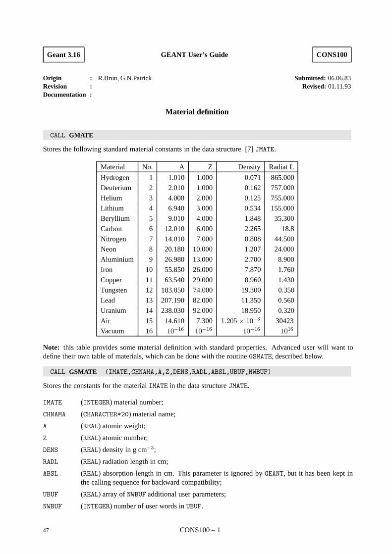
Geant 3.16 GEANT User’s Guide CONS100
Origin : R.Brun, G.N.Patrick Submitted: 06.06.83Revision : Revised: 01.11.93Documentation :
Material definition
CALL GMATE
Stores the following standard material constants in the data structure [7] JMATE.
Material No. A Z Density Radiat L
Hydrogen 1 1.010 1.000 0.071 865.000
Deuterium 2 2.010 1.000 0.162 757.000
Helium 3 4.000 2.000 0.125 755.000
Lithium 4 6.940 3.000 0.534 155.000
Beryllium 5 9.010 4.000 1.848 35.300
Carbon 6 12.010 6.000 2.265 18.8
Nitrogen 7 14.010 7.000 0.808 44.500
Neon 8 20.180 10.000 1.207 24.000
Aluminium 9 26.980 13.000 2.700 8.900
Iron 10 55.850 26.000 7.870 1.760
Copper 11 63.540 29.000 8.960 1.430
Tungsten 12 183.850 74.000 19.300 0.350
Lead 13 207.190 82.000 11.350 0.560
Uranium 14 238.030 92.000 18.950 0.320
Air 15 14.610 7.300 1.205 × 10⁻³ 30423
Vacuum 16 10−16 10−16 10−16 1016
Note: this table provides some material definition with standard properties. Advanced user will want todefine their own table of materials, which can be done with the routine GSMATE, described below.
CALL GSMATE (IMATE,CHNAMA,A,Z,DENS,RADL,ABSL,UBUF,NWBUF)
Stores the constants for the material IMATE in the data structure JMATE.
IMATE (INTEGER) material number;
CHNAMA (CHARACTER*20) material name;
A (REAL) atomic weight;
Z (REAL) atomic number;
DENS (REAL) density in g cm−3;
RADL (REAL) radiation length in cm;
ABSL (REAL) absorption length in cm. This parameter is ignored by GEANT, but it has been kept inthe calling sequence for backward compatibility;
UBUF (REAL) array of NWBUF additional user parameters;
NWBUF (INTEGER) number of user words in UBUF.
47 CONS100 – 1

CALL GFMATE (IMATE,CHNAMA*,A*,Z*,DENS*,RADL*,ABSL*,UBUF*,NWBUF*)
Retrieves the constants of material IMATE from the data structure JMATE. The parameters are the same asfor GSMATE.
CALL GPMATE (IMATE)
Prints the material constants:
IMATE (INTEGER) material number. If IMATE=0 then all materials will be printed. If IMATE<0 thematerial number -IMATE will be printed without the header describing the value of the variousfields.
CONS100 – 2 48
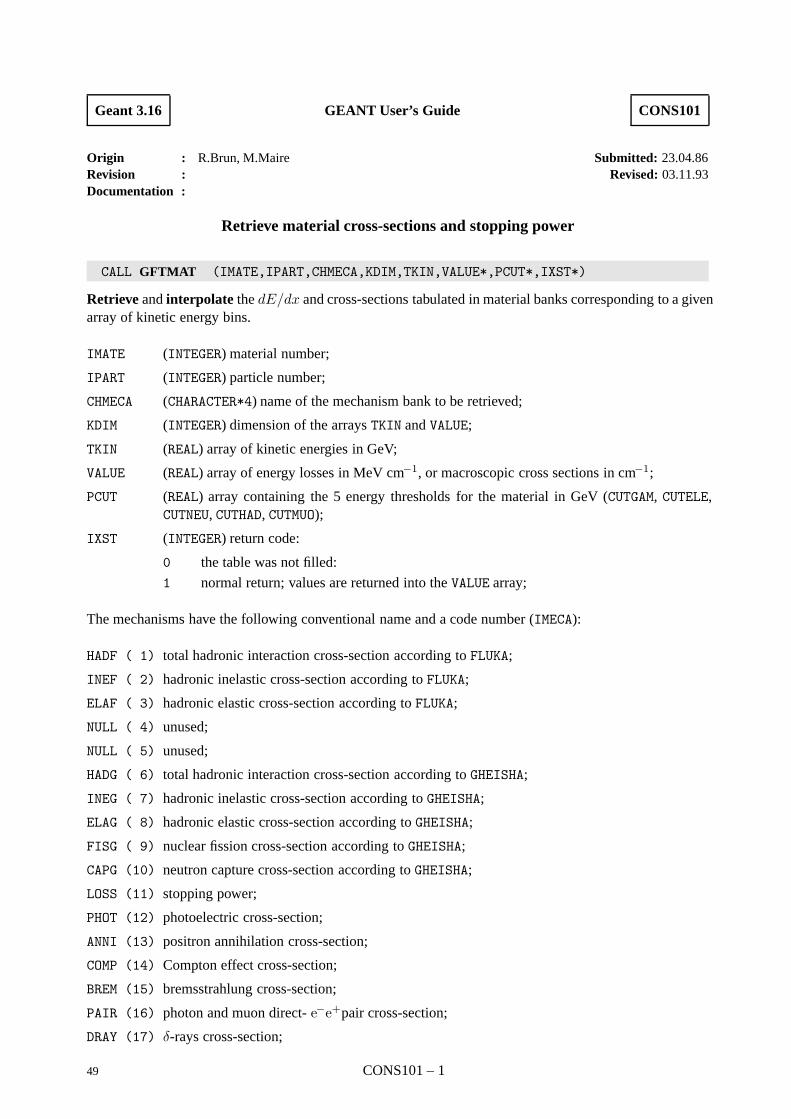
Geant 3.16 GEANT User’s Guide CONS101
Origin : R.Brun, M.Maire Submitted: 23.04.86Revision : Revised: 03.11.93Documentation :
Retrieve material cross-sections and stopping power
CALL GFTMAT (IMATE,IPART,CHMECA,KDIM,TKIN,VALUE*,PCUT*,IXST*)
Retrieve and interpolate the dE/dx and cross-sections tabulated in material banks corresponding to a givenarray of kinetic energy bins.
IMATE (INTEGER) material number;
IPART (INTEGER) particle number;
CHMECA (CHARACTER*4) name of the mechanism bank to be retrieved;
KDIM (INTEGER) dimension of the arrays TKIN and VALUE;
TKIN (REAL) array of kinetic energies in GeV;
VALUE (REAL) array of energy losses in MeV cm−1, or macroscopic cross sections in cm−1;
PCUT (REAL) array containing the 5 energy thresholds for the material in GeV (CUTGAM, CUTELE,CUTNEU, CUTHAD, CUTMUO);
IXST (INTEGER) return code:
0 the table was not filled:
1 normal return; values are returned into the VALUE array;
The mechanisms have the following conventional name and a code number (IMECA):
HADF ( 1) total hadronic interaction cross-section according to FLUKA;
INEF ( 2) hadronic inelastic cross-section according to FLUKA;
ELAF ( 3) hadronic elastic cross-section according to FLUKA;
NULL ( 4) unused;
NULL ( 5) unused;
HADG ( 6) total hadronic interaction cross-section according to GHEISHA;
INEG ( 7) hadronic inelastic cross-section according to GHEISHA;
ELAG ( 8) hadronic elastic cross-section according to GHEISHA;
FISG ( 9) nuclear fission cross-section according to GHEISHA;
CAPG (10) neutron capture cross-section according to GHEISHA;
LOSS (11) stopping power;
PHOT (12) photoelectric cross-section;
ANNI (13) positron annihilation cross-section;
COMP (14) Compton effect cross-section;
BREM (15) bremsstrahlung cross-section;
PAIR (16) photon and muon direct- e−e+pair cross-section;
DRAY (17) δ-rays cross-section;
49 CONS101 – 1
PFIS (18) photo-fission cross-section;
RAYL (19) Rayleigh scattering cross-section;
MUNU (20) muon-nuclear interaction cross-section;
RANG (21) range in cm;
STEP (22) maximum step in cm.
Note: Common /GCMULO/ contains an array ELOW(200) (see [CONS199]) with NEK1 kinetic energy valuesranging from EKMIN to EKMAX. GPHYSI initialises by default the first 91 locations of ELOW with values ofenergy from 10−5 GeV (10 keV) to 104 GeV (10 TeV) equally spaced on logarithmic scale. This can becontrolled by the user via the data record or the interactive command ERAN ([BASE040]). ELOW can be usedas the input argument TKIN, e.g.:
CALL GFTMAT (10, 1,’PHOT’,NEK1, ELOW ,VALUE, PCUT, IXST)
will return in array VALUE the photoelectric cross-section in material number 10.
CALL GPLMAT (IMATE,IPART,CHMECA,KDIM,TKIN,IDM)
Plot and interpolate the dE/dx and cross-sections tabulated in material banks corresponding to a givenarray of kinetic energy bins. The mechanisms are the same as the previous routine. If the mechanism nameis ’ALL’, then all the mechanisms will be plotted.
The first five parameters have the same meaning as in the previous routine and:
IDM (INTEGER) treatment of the created histogram(s):
> 0 fill, print, keep histogram(s);
= 0 fill, print, delete histogram(s);
< 0 fill, noprint, keep histogram(s).
The result is not returned to the user as is the case in the previous routine but it is put in an HBOOK histogram.The HBOOK package needs to be initialised by the user via the routine HLIMIT, see [BASE100] for moreinformation. The histogram identifier is calculated as: 10000*IMATE+100*IPART+IMECA where IMECA isthe mechanism code listed above.
CALL GPRMAT (IMATE,IPART,CHMECA,KDIM,TKIN)
Print and interpolate the dE/dx and cross-sections tabulated in material banks corresponding to a givenarray of kinetic energy bins. The mechanisms are the same as the previous routine. If the mechanism nameis ’ALL’, then all the mechanisms will be printed.
The result is printed in the form of a table.
The five parameters have the same meaning as in the previous routine.
CONS101 – 2 50
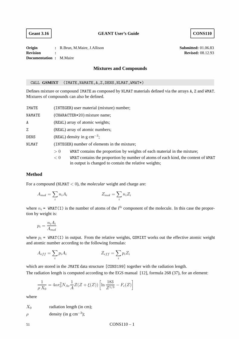
Geant 3.16 GEANT User’s Guide CONS110
Origin : R.Brun, M.Maire, J.Allison Submitted: 01.06.83Revision : Revised: 08.12.93Documentation : M.Maire
Mixtures and Compounds
CALL GSMIXT (IMATE,NAMATE,A,Z,DENS,NLMAT,WMAT*)
Defines mixture or compound IMATE as composed by NLMAT materials defined via the arrays A, Z and WMAT.Mixtures of compounds can also be defined.
IMATE (INTEGER) user material (mixture) number;
NAMATE (CHARACTER*20) mixture name;
A (REAL) array of atomic weights;
Z (REAL) array of atomic numbers;
DENS (REAL) density in g cm−3;
NLMAT (INTEGER) number of elements in the mixture;
> 0 WMAT contains the proportion by weights of each material in the mixture;
< 0 WMAT contains the proportion by number of atoms of each kind, the content of WMATin output is changed to contain the relative weights;
Method
For a compound (NLMAT < 0), the molecular weight and charge are:
Amol =∑i
niAi Zmol =∑i
niZi
where ni = WMAT(I) is the number of atoms of the ith component of the molecule. In this case the propor-tion by weight is:
pi =niAi
Amol
where pi = WMAT(I) in output. From the relative weights, GSMIXT works out the effective atomic weightand atomic number according to the following formulas:
Aeff =∑i
piAi Zeff =∑i
piZi
which are stored in the JMATE data structure [CONS199] together with the radiation length.
The radiation length is computed according to the EGS manual [12], formula 268 (37), for an element:
1ρ X0
= 4αr20NAv1AZ(Z + ξ(Z))
[ln183Z1/3
− Fc(Z)]
where
X0 radiation length (in cm);
ρ density (in g cm−3);
51 CONS110 – 1
α fine structure constant;
r classical electron radius (in cm);
NAv Avogadro’s number;
A atomic weight;
Z atomic number;
Fc(Z) Coulomb correction function.
Fc(Z) = (αZ)2[
11 + (αZ)2
+ 0.20206 − 0.0369(αZ)2 + 0.0083(αZ)4 − 0.0020(αZ)6]
ξ(Z) =ln 1440
Z2/3
ln 183Z1/3 − Fc(Z)
for a compound or mixture:
1ρX0
=∑i
piρiX0i
where pi is the proportion by weight of the ith element. For more information on the organisation of thedata in memory see [CONS199].
The effective absorption length λ is defined as the interaction length of a 5GeV pion in the material:
1λ=∑i
piλi
1λi=
σπi (5GeV )NAv
Aig−1 cm2
Once this value has been determined, an effective hadronic atomic weight (Ah−eff ) is calculated by theroutine GHMIX [3] and stored in the data structure.
CONS110 – 2 52
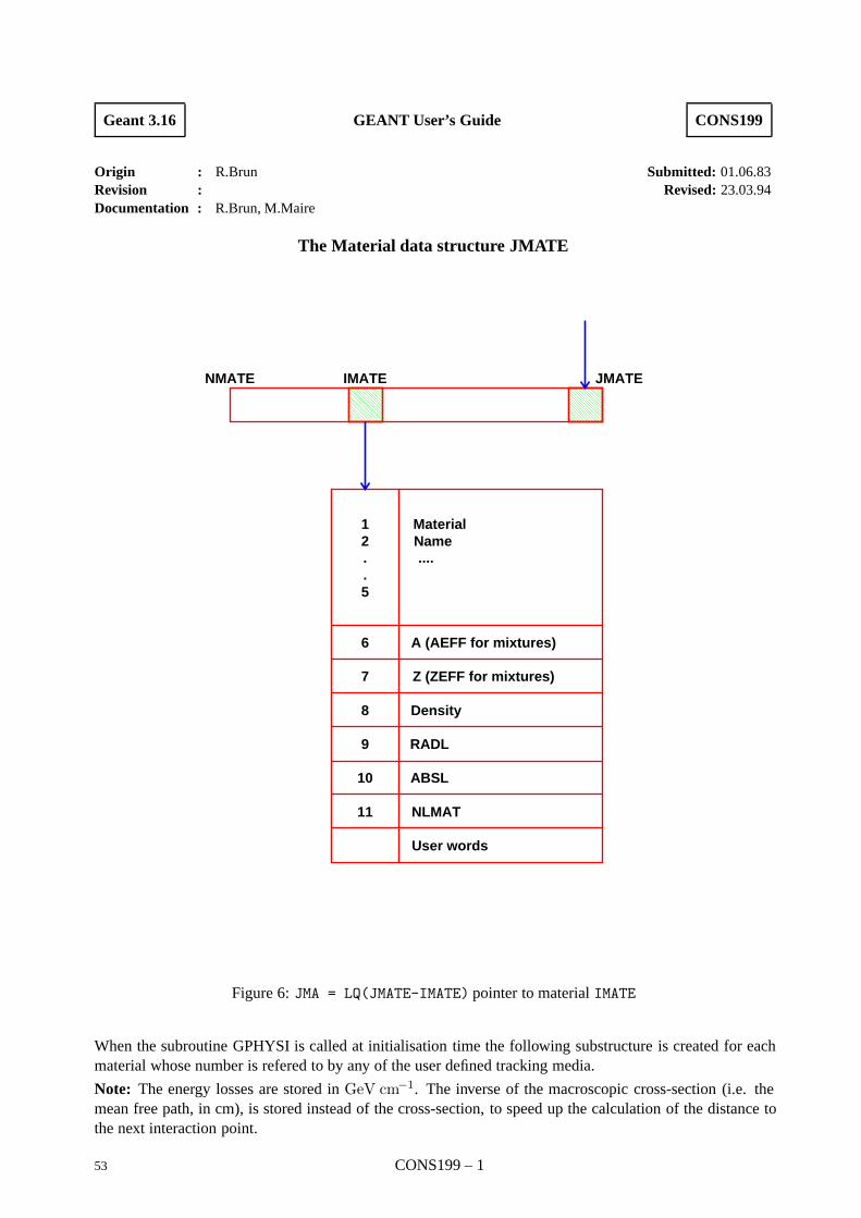
Geant 3.16 GEANT User’s Guide CONS199
Origin : R.Brun Submitted: 01.06.83Revision : Revised: 23.03.94Documentation : R.Brun, M.Maire
The Material data structure JMATE
NMATE IMATE JMATE
12..5
6
7
8
9
10
11
A (AEFF for mixtures)
Z (ZEFF for mixtures)
Density
RADL
ABSL
NLMAT
User words
MaterialName....
Figure 6: JMA = LQ(JMATE-IMATE) pointer to material IMATE
When the subroutine GPHYSI is called at initialisation time the following substructure is created for eachmaterial whose number is refered to by any of the user defined tracking media.
Note: The energy losses are stored in GeV cm−1. The inverse of the macroscopic cross-section (i.e. themean free path, in cm), is stored instead of the cross-section, to speed up the calculation of the distance tothe next interaction point.
53 CONS199 – 1
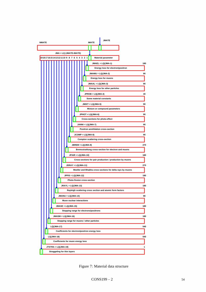
IMATEJMATE
NMATE
JMAEL = LQ(JMA-1)
JMAMU = LQ(JMA-2)
JMAAL = LQ(JMA-3)
JPROB = LQ(JMA-4)
JMIXT = LQ(JMA-5)
JPHOT = LQ(JMA-6)
JANNI = LQ(JMA-7)
JCOMP = LQ(JMA-8)
JBREM = LQ(JMA-9)
JPAIR = LQ(JMA-10)
JDRAY = LQ(JMA-11)
JPFIS = LQ(JMA-12)
JRAYL = LQ(JMA-13)
JMUNU = LQ(JMA-14)
JMASE = LQ(JMA-15)
JMASM = LQ(JMA-16)
LQ(JMA-17)
LQ(JMA-18)
JTSTRA = LQ(JMA-19)
JMA = LQ (JMATE-IMATE)
180
90
90
40
90
90
90
90
270
180
270
180
180
90
180
180
540
540
1
12345678910111213141516171819 Material parameter
Energy loss for electron/positron
Energy loss for muons
Energy loss for other particles
Some material constants
Mixture or compound parameters
Cross-sections for photo-effect
Positron annihilation cross-section
Compton scattering cross-section
Bremsstrahlung cross-section for electron and muons
Cross-sections for pair production / production by muons
Moeller and Bhabha cross-sections for delta rays by muons
Photo-fission cross-section
Rayleigh scattering cross section and atomic form factors
Muon nuclear interactions
Stopping range for electrons/positrons
Stopping range for muons / other particles
Coefficients for electron/positron energy loss
Coefficients for muon energy loss
Straggeling for thin layers
Figure 7: Material data structure
CONS199 – 2 54
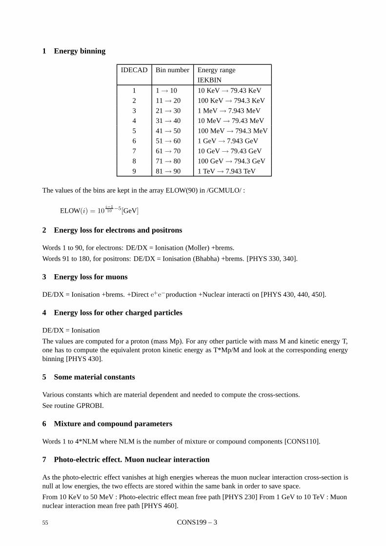
1 Energy binning
IDECAD Bin number Energy range
IEKBIN
1 1 → 10 10 KeV → 79.43 KeV
2 11 → 20 100 KeV → 794.3 KeV
3 21 → 30 1 MeV → 7.943 MeV
4 31 → 40 10 MeV → 79.43 MeV
5 41 → 50 100 MeV → 794.3 MeV
6 51 → 60 1 GeV → 7.943 GeV
7 61 → 70 10 GeV → 79.43 GeV
8 71 → 80 100 GeV → 794.3 GeV
9 81 → 90 1 TeV → 7.943 TeV
The values of the bins are kept in the array ELOW(90) in /GCMULO/ :
ELOW(i) = 10i−110
−5[GeV]
2 Energy loss for electrons and positrons
Words 1 to 90, for electrons: DE/DX = Ionisation (Moller) +brems.
Words 91 to 180, for positrons: DE/DX = Ionisation (Bhabha) +brems. [PHYS 330, 340].
3 Energy loss for muons
DE/DX = Ionisation +brems. +Direct e+e−production +Nuclear interacti on [PHYS 430, 440, 450].
4 Energy loss for other charged particles
DE/DX = Ionisation
The values are computed for a proton (mass Mp). For any other particle with mass M and kinetic energy T,one has to compute the equivalent proton kinetic energy as T*Mp/M and look at the corresponding energybinning [PHYS 430].
5 Some material constants
Various constants which are material dependent and needed to compute the cross-sections.
See routine GPROBI.
6 Mixture and compound parameters
Words 1 to 4*NLM where NLM is the number of mixture or compound components [CONS110].
7 Photo-electric effect. Muon nuclear interaction
As the photo-electric effect vanishes at high energies whereas the muon nuclear interaction cross-section isnull at low energies, the two effects are stored within the same bank in order to save space.
From 10 KeV to 50 MeV : Photo-electric effect mean free path [PHYS 230] From 1 GeV to 10 TeV : Muonnuclear interaction mean free path [PHYS 460].
55 CONS199 – 3
8 Positron annihilation
[PHYS 350].
9 Compton scattering
[PHYS 220].
10 Bremsstrahlung for electrons and muons
Words 1 to 90, mean free path for electrons [PHYS 340] Words 91 to 180, mean free path for muons [PHYS440].
11 Pair production by gammas and muons
Words 1 to 90, for gammas [PHYS 210]. Words 91 to 180, for muons [PHYS 450].
12 Delta ray production by electrons and muons
Words 1 to 90, for e−e−→ e−e−[PHYS 330].
Words 91 to 180, for e+e−→ e+e−[PHYS 330]
Words 181 to 270, for e−→ e−[PHYS 430].
13 Photo-fission
Only for material with atomic number A¿200 [PHYS 240].
CONS199 – 4 56
Geant 3.16 GEANT User’s Guide CONS200
Origin : R.Brun Submitted: 01.06.83Revision : F.Carminati, M.Maire Revised: 08.12.93Documentation :
Tracking medium parameters
Description of the routines
CALL GSTMED (ITMED,NATMED,NMAT,ISVOL,IFIELD,FIELDM,TMAXFD,STEMAX,DEEMAX,EPSIL,STMIN,UBUF,NWBUF)
This routine associates a set of tracking parameters to a material, defining a so-called tracking medium.Every GEANT volume must be associated to an existing tracking medium. The routine stores the parametersof the tracking medium ITMED in the data structure JTMED.
ITMED (INTEGER) tracking medium number;
NATMED (CHARACTER*20) tracking medium name;
NMAT (INTEGER) material number corresponding to ITMED;
ISVOL (INTEGER) sensitivity flag (see later):
≤0 not a sensitive volume;
>0 sensitive volume;
IFIELD (INTEGER) magnetic field flag:
=0 no magnetic field;
=1 strongly inhomogeneous magnetic field (returned by the user function GUFLD): trackingperformed with the Runge-Kutta method by the routine GRKUTA;
=2 inhomogeneous magnetic field (returned by the user function GUFLD), tracking along ahelix performed by the routine GHELIX;
=3 uniform magnetic field along the z axis of strength FIELDM, tracking performed alonga helix by the routine GHELX3;
FIELDM (REAL) maximum field value (in Kilogauss);
TMAXFD (REAL) maximum angular deviation due to the magnetic field permitted in one step (in degrees);
STEMAX (REAL) maximum step permitted (cm);
DEEMAX (REAL) maximum fractional energy loss in one step (0 < DEEMAX ≤ 1);
EPSIL (REAL) boundary crossing precision (cm);
STMIN (REAL) minimum value for the maximum step imposed by energy loss, multiple scattering,Cerenkov or magnetic field effects (cm);
UBUF (REAL) array of NWBUF additional user parameters;
NWBUF (INTEGER) number of additional user parameters.
Note: the tracking medium number can in principle be any positive integer from 1 to 65,535. However thisnumber is used directly by GEANT as the number of the pointer to the data structure where the information isstored. When a pointer is defined, all pointers from 1 to the one allocated are created, if not already existing.Every time data structures are moved in memory, all the links are potentially scanned for update. This canbe time consuming and it can seriously affect performances. So a continuous range of numbers should beused for tracking media.
57 CONS200 – 1
CALL GFTMED (ITMED,NATMED*,NMAT*,ISVOL*,IFIELD*,FIELDM*,TMAXFD*,STEMAX*,DEEMAX*,EPSIL*,STMIN*,UBUF*,NWBUF*)
Extracts the parameters of the tracking medium ITMED from the data structure JTMED.
CALL GPTMED (ITMED)
Prints the tracking medium parameters for the given medium.
ITMED (INTEGER) tracking medium to be printed, all tracking media if ITMED=0.
Automatic calculation of the tracking parameters
The results of the simulation depend critically on the choice of the tracking medium parameters. To makeof GEANT a reliable and consistent predictive tool, the calculation of these parameters has been automated.In a normal GEANT run, the variable IGAUTO in common /GCTRAK/ is set to 1. In this case the followingparameters are calculated by the program:
TMAXFD =
20 if TMAXFD ≤ 0 or TMAXFD > 20input value if 0 < TMAXFD ≤ 20
STEMAX = BIG(= 1010)
DEEMAX =
0.25 if ISVOL= 0 and X0 ≤ 2cm, where X0 is the radiation length of
the material0.25 − 0.2√
X0otherwise
STMIN =
2R√X0
if ISVOL = 0
5R√X0
if ISVOL = 0
where R is the range in cm of an electron of energy CUTELE+200keV.If the IGAUTO variable is set to 0 via the AUTO data record, then value given by the user for the aboveparameters is accepted as the true parameter value if > 0, while automatic calculation still takes place incase the input value is negative.Users are strongly recommended to begin their simulation with the parameters as calculated by GEANT.Users who want to modify any of the above parameters must be sure they understand their function in theprogram and the implications of a change.The EPSIL parameter represents the absolute precision with which the tracking is performed. It has adouble meaning. When tracking in magnetic field, EPSIL is the minimum distance for which boundariesare checked. A particle nearer than EPSIL to the boundary is considered as exiting the current volume. Ifthe end point of the step of a particle in magnetic field is distant less than EPSIL along each axis from whatwould be the end point in absence of magnetic field, then no boundary checking is performed.In all cases, when a particle is going to reach the boundary of the current volume with the current step, thestep length is increased by a quantity (PREC, common /GCTMED/) which is set to the minimum between0.1 × EPSIL and 10 micron at the beginning of the tracking. This quantity is recalculated at every stepaccording to the formula:
PREC = max[min
(EPSIL
10, 10µ
),max [|x|, |y|, |z|, S) × ε
](1)
Where x, y, z are the current coordinates of the particle, S is the length of the track, and ε is the assumedmachine precision. ε (called EPSMAC in the program) is initially set to 10−6 for 32 bits machines and 10−11
for 64 bits machines. During the tracking, every fifth time that a particle tries unsuccessfully to exit fromthe same volume, the machine precision is multiplied by the number of trials. This accounts for additionallosses of precision due to transformation of coordinates and region of the floating point range where thereal machine precision is different from the above (this happens in particular on IBM mainframes with 370floating point number representation).
CONS200 – 2 58
Geant 3.16 GEANT User’s Guide CONS210
Origin : R.Brun,F.Bruyant Submitted: 11.02.86Revision : Revised: 08.12.93Documentation : same
Special Tracking Parameters
CALL GSTPAR (ITMED,CHPAR,PARVAL)
ITMED (INTEGER) tracking medium number;
CHPAR (CHARACTER*4) character string, name of the variable to be modified;
PARVAL (REAL) new value (must be given as a floating point).
Default parameters Parameter name Default value
Q(JTMN +1) = CUTGAM CUTGAM 0.001GeV
Q(JTMN +2) = CUTELE CUTELE 0.001GeV
Q(JTMN +3) = CUTNEU CUTNEU 0.01GeV
Q(JTMN +4) = CUTHAD CUTHAD 0.01GeV
Q(JTMN +5) = CUTMUO CUTMUO 0.01GeV
Q(JTMN +6) = BCUTE BCUTE CUTGAM
Q(JTMN +7) = BCUTM BCUTM CUTGAM
Q(JTMN +8) = DCUTE DCUTE 10.TeV
Q(JTMN +9) = DCUTM DCUTM 10.TeV
Q(JTMN+10) = PPCUTM PPCUTM 0.01GeV
Q(JTMN+11) = IPAIR PAIR 1
Q(JTMN+12) = ICOMP COMP 1
Q(JTMN+13) = IPHOT PHOT 1
Q(JTMN+14) = IPFIS PFIS 0
Q(JTMN+15) = IDRAY DRAY 2
Q(JTMN+16) = IANNI ANNI 1
Q(JTMN+17) = IBREM BREM 1
Q(JTMN+18) = IHADR HADR 1
Q(JTMN+19) = IMUNU MUNU 0
Q(JTMN+20) = IDCAY DCAY 1
Q(JTMN+21) = ILOSS LOSS 2
Q(JTMN+22) = IMULS MULS 1
Q(JTMN+26) = GHEISHA GHCOR1 see [PHYS700]
Q(JTMN+27) = MODEL BIRK1 see [PHYS337]
Q(JTMN+28) = RKB BIRK2 see [PHYS337]
Q(JTMN+29) = C BIRK3 see [PHYS337]
Q(JTMN+31) = ILABS LABS see [PHYS260]
Q(JTMN+32) = ISYNC SYNC see [PHYS360]
Q(JTMN+33) = ISTRA STRA see [PHYS333]
The data structure JTMED contains the standard tracking parameters (CUTS and flags to control the physicsprocesses) which are used by default for all tracking media. It is possible to redefine individually with
59 CONS210 – 1
GSTPAR any of these parameters for a given tracking medium. For example to change CUTGAM to 0.0001 fortracking medium ITMED:
CALL GSTPAR(ITMED,’CUTGAM’,0.0001)
For more information on default values for IDRAY and ILOSS see [BASE040].
The default tracking medium parameters are stored in the bank whose pointer is stored in the JTMED variable.In this case in the above table JTMN = JTMED. In the case one or more of the above parameters has beenmodified for a specific tracking medium, the whole parameter set is stored in the next bank of the giventrackin medium. In this case JTMN = LQ(JTM) in the above table, where JTM is the pointer to the bank of thetracking medium, i.e. JTM = LQ(JTMED-ITMED).
Note
At tracking time the parameters above are copied from JTMN into the common blocks /GCCUTS/ and/GCPHYS/. GSTPAR must be called before GPHYSI.
CONS210 – 2 60
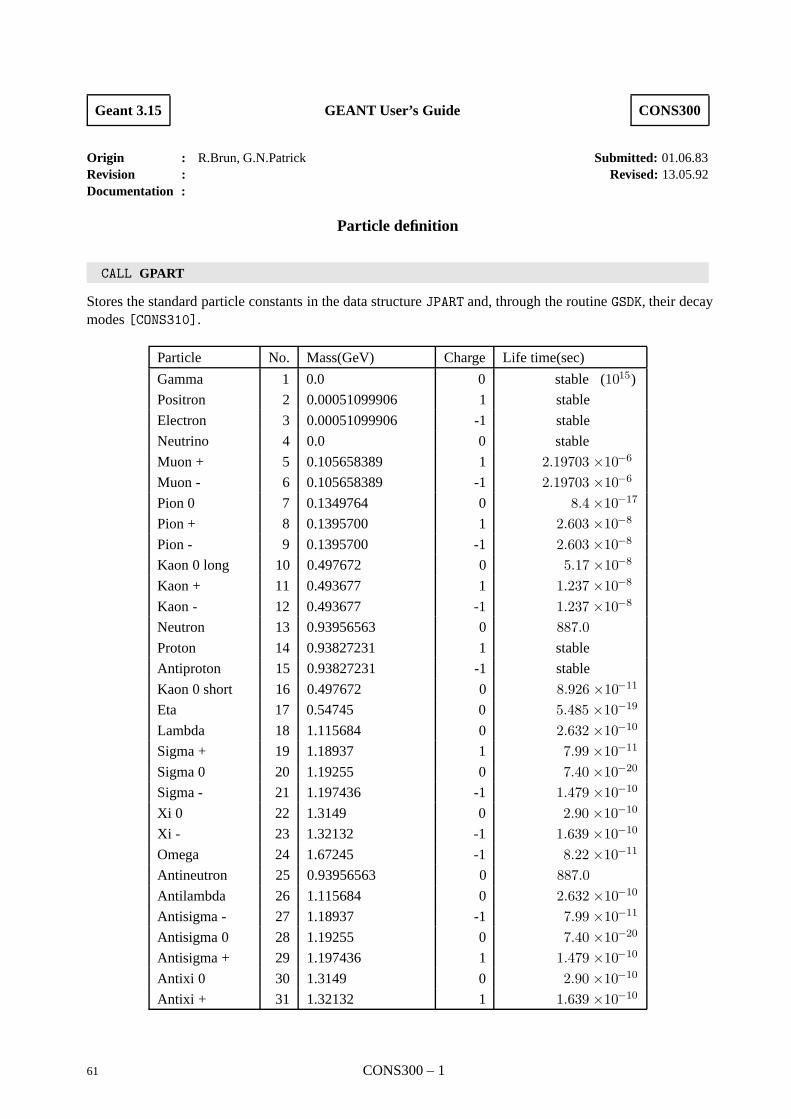
Geant 3.15 GEANT User’s Guide CONS300
Origin : R.Brun, G.N.Patrick Submitted: 01.06.83Revision : Revised: 13.05.92Documentation :
Particle definition
CALL GPART
Stores the standard particle constants in the data structure JPART and, through the routine GSDK, their decaymodes [CONS310].
Particle No. Mass(GeV) Charge Life time(sec)
Gamma 1 0.0 0 stable (1015)Positron 2 0.00051099906 1 stable
Electron 3 0.00051099906 -1 stable
Neutrino 4 0.0 0 stable
Muon + 5 0.105658389 1 2.19703 ×10⁻⁶Muon - 6 0.105658389 -1 2.19703 ×10⁻⁶Pion 0 7 0.1349764 0 8.4×10⁻¹⁷Pion + 8 0.1395700 1 2.603 ×10⁻⁸Pion - 9 0.1395700 -1 2.603 ×10⁻⁸Kaon 0 long 10 0.497672 0 5.17 ×10⁻⁸Kaon + 11 0.493677 1 1.237 ×10⁻⁸Kaon - 12 0.493677 -1 1.237 ×10⁻⁸Neutron 13 0.93956563 0 887.0Proton 14 0.93827231 1 stable
Antiproton 15 0.93827231 -1 stable
Kaon 0 short 16 0.497672 0 8.926 ×10⁻¹¹Eta 17 0.54745 0 5.485 ×10⁻¹⁹Lambda 18 1.115684 0 2.632 ×10⁻¹⁰Sigma + 19 1.18937 1 7.99 ×10⁻¹¹Sigma 0 20 1.19255 0 7.40 ×10⁻²⁰Sigma - 21 1.197436 -1 1.479 ×10⁻¹⁰Xi 0 22 1.3149 0 2.90 ×10⁻¹⁰Xi - 23 1.32132 -1 1.639 ×10⁻¹⁰Omega 24 1.67245 -1 8.22 ×10⁻¹¹Antineutron 25 0.93956563 0 887.0Antilambda 26 1.115684 0 2.632 ×10⁻¹⁰Antisigma - 27 1.18937 -1 7.99 ×10⁻¹¹Antisigma 0 28 1.19255 0 7.40 ×10⁻²⁰Antisigma + 29 1.197436 1 1.479 ×10⁻¹⁰Antixi 0 30 1.3149 0 2.90 ×10⁻¹⁰Antixi + 31 1.32132 1 1.639 ×10⁻¹⁰
61 CONS300 – 1
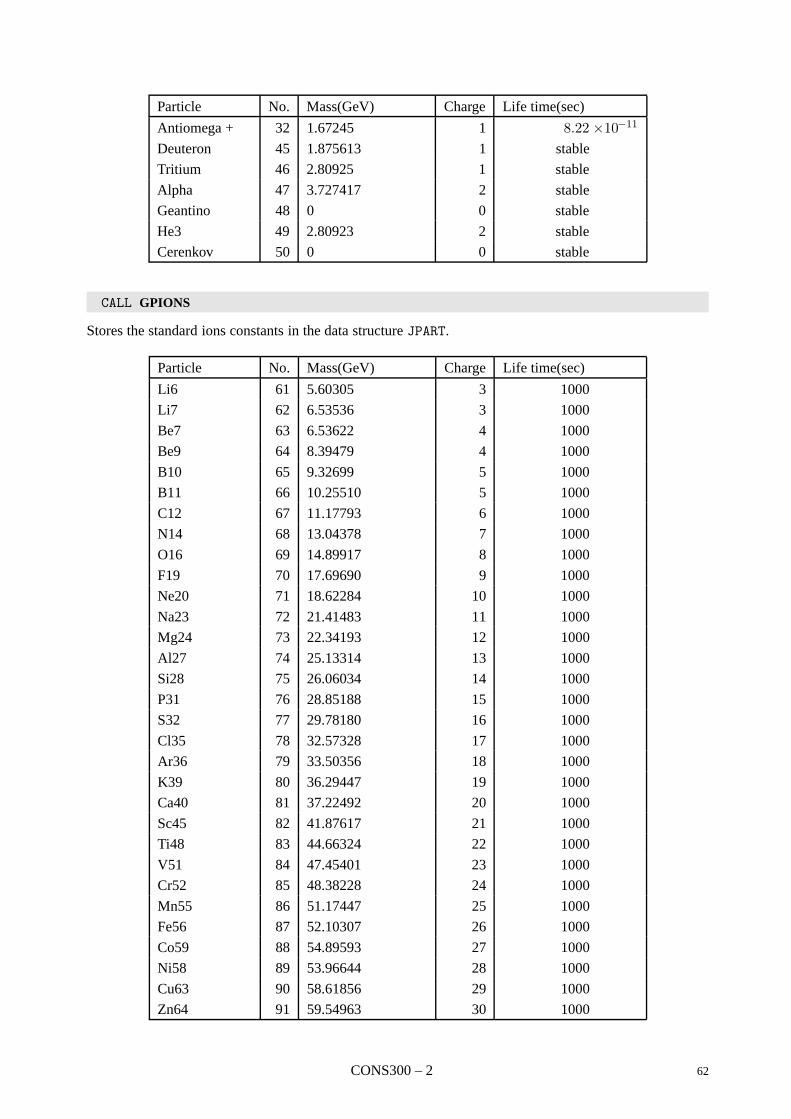
Particle No. Mass(GeV) Charge Life time(sec)
Antiomega + 32 1.67245 1 8.22 ×10⁻¹¹Deuteron 45 1.875613 1 stable
Tritium 46 2.80925 1 stable
Alpha 47 3.727417 2 stable
Geantino 48 0 0 stable
He3 49 2.80923 2 stable
Cerenkov 50 0 0 stable
CALL GPIONS
Stores the standard ions constants in the data structure JPART.
Particle No. Mass(GeV) Charge Life time(sec)
Li6 61 5.60305 3 1000
Li7 62 6.53536 3 1000
Be7 63 6.53622 4 1000
Be9 64 8.39479 4 1000
B10 65 9.32699 5 1000
B11 66 10.25510 5 1000
C12 67 11.17793 6 1000
N14 68 13.04378 7 1000
O16 69 14.89917 8 1000
F19 70 17.69690 9 1000
Ne20 71 18.62284 10 1000
Na23 72 21.41483 11 1000
Mg24 73 22.34193 12 1000
Al27 74 25.13314 13 1000
Si28 75 26.06034 14 1000
P31 76 28.85188 15 1000
S32 77 29.78180 16 1000
Cl35 78 32.57328 17 1000
Ar36 79 33.50356 18 1000
K39 80 36.29447 19 1000
Ca40 81 37.22492 20 1000
Sc45 82 41.87617 21 1000
Ti48 83 44.66324 22 1000
V51 84 47.45401 23 1000
Cr52 85 48.38228 24 1000
Mn55 86 51.17447 25 1000
Fe56 87 52.10307 26 1000
Co59 88 54.89593 27 1000
Ni58 89 53.96644 28 1000
Cu63 90 58.61856 29 1000
Zn64 91 59.54963 30 1000
CONS300 – 2 62
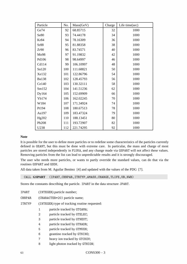
Particle No. Mass(GeV) Charge Life time(sec)
Ge74 92 68.85715 32 1000
Se80 93 74.44178 34 1000
Kr84 94 78.16309 36 1000
Sr88 95 81.88358 38 1000
Zr90 96 83.74571 40 1000
Mo98 97 91.19832 42 1000
Pd106 98 98.64997 46 1000
Cd114 99 106.10997 48 1000
Sn120 100 111.68821 50 1000
Xe132 101 122.86796 54 1000
Ba138 102 128.45793 56 1000
Ce140 103 130.32111 58 1000
Sm152 104 141.51236 62 1000
Dy164 105 152.69909 66 1000
Yb174 106 162.02245 70 1000
W184 107 171.34924 74 1000
Pt194 108 180.67513 78 1000
Au197 109 183.47324 79 1000
Hg202 110 188.13451 80 1000
Pb208 111 193.72907 82 1000
U238 112 221.74295 92 1000
Note
It is possible for the user to define more particles or to redefine some characteristics of the particles currentlydefined in GEANT, but this must be done with extreme care. In particular, the mass and charge of mostparticles are stored independently in FLUKA, and any change made via GSPART will not affect these values.Removing particles from the list can lead to unpredictable results and it is strongly discouraged.
The user who needs more particles, or wants to partly override the standard values, can do that via theroutines GSPART and GSDK.
All data taken from M. Aguilar Benitez [4] and updated with the values of the PDG [7].
CALL GSPART (IPART,CHNPAR,ITRTYP,AMASS,CHARGE,TLIFE,UB,NWB)
Stores the constants describing the particle. IPART in the data structure JPART.
IPART (INTEGER) particle number;
CHNPAR (CHARACTER*20) particle name;
ITRTYP (INTEGER) type of tracking routine requested:
1 particle tracked by GTGAMA;
2 particle tracked by GTELEC;
3 particle tracked by GTNEUT;
4 particle tracked by GTHADR;
5 particle tracked by GTMUON;
6 geantino tracked by GTNINO;
7 heavy ion tracked by GTCKOV;
8 light photon tracked by GTHION;
63 CONS300 – 3

AMASS (REAL) particle mass in GeV;
CHARGE (REAL) particle charge;
TLIFE (REAL) particle life time (in seconds);
UB (REAL) array of NWB user additional parameters;
NWB (INTEGER).
CALL GFPART (IPART,CHNPAR*,ITRTYP*,AMASS*,CHARGE*,TLIFE*,UB*,NWB*)
Extracts the constants describing the particle IPART from the data structure JPART.
CALL GPPART (IPART)
Prints the particle constants for particle IPART (for all particles if IPART=0).
CONS300 – 4 64
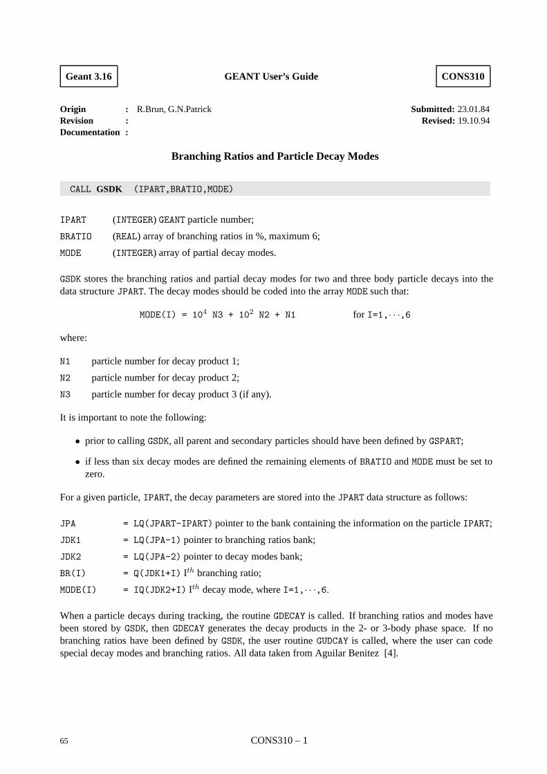
Geant 3.16 GEANT User’s Guide CONS310
Origin : R.Brun, G.N.Patrick Submitted: 23.01.84Revision : Revised: 19.10.94Documentation :
Branching Ratios and Particle Decay Modes
CALL GSDK (IPART,BRATIO,MODE)
IPART (INTEGER) GEANT particle number;
BRATIO (REAL) array of branching ratios in %, maximum 6;
MODE (INTEGER) array of partial decay modes.
GSDK stores the branching ratios and partial decay modes for two and three body particle decays into thedata structure JPART. The decay modes should be coded into the array MODE such that:
MODE(I) = 104 N3 + 102 N2 + N1 for I=1,· · ·,6
where:
N1 particle number for decay product 1;
N2 particle number for decay product 2;
N3 particle number for decay product 3 (if any).
It is important to note the following:
• prior to calling GSDK, all parent and secondary particles should have been defined by GSPART;
• if less than six decay modes are defined the remaining elements of BRATIO and MODE must be set tozero.
For a given particle, IPART, the decay parameters are stored into the JPART data structure as follows:
JPA = LQ(JPART-IPART) pointer to the bank containing the information on the particle IPART;
JDK1 = LQ(JPA-1) pointer to branching ratios bank;
JDK2 = LQ(JPA-2) pointer to decay modes bank;
BR(I) = Q(JDK1+I) Ith branching ratio;
MODE(I) = IQ(JDK2+I) Ith decay mode, where I=1,· · ·,6.
When a particle decays during tracking, the routine GDECAY is called. If branching ratios and modes havebeen stored by GSDK, then GDECAY generates the decay products in the 2- or 3-body phase space. If nobranching ratios have been defined by GSDK, the user routine GUDCAY is called, where the user can codespecial decay modes and branching ratios. All data taken from Aguilar Benitez [4].
65 CONS310 – 1
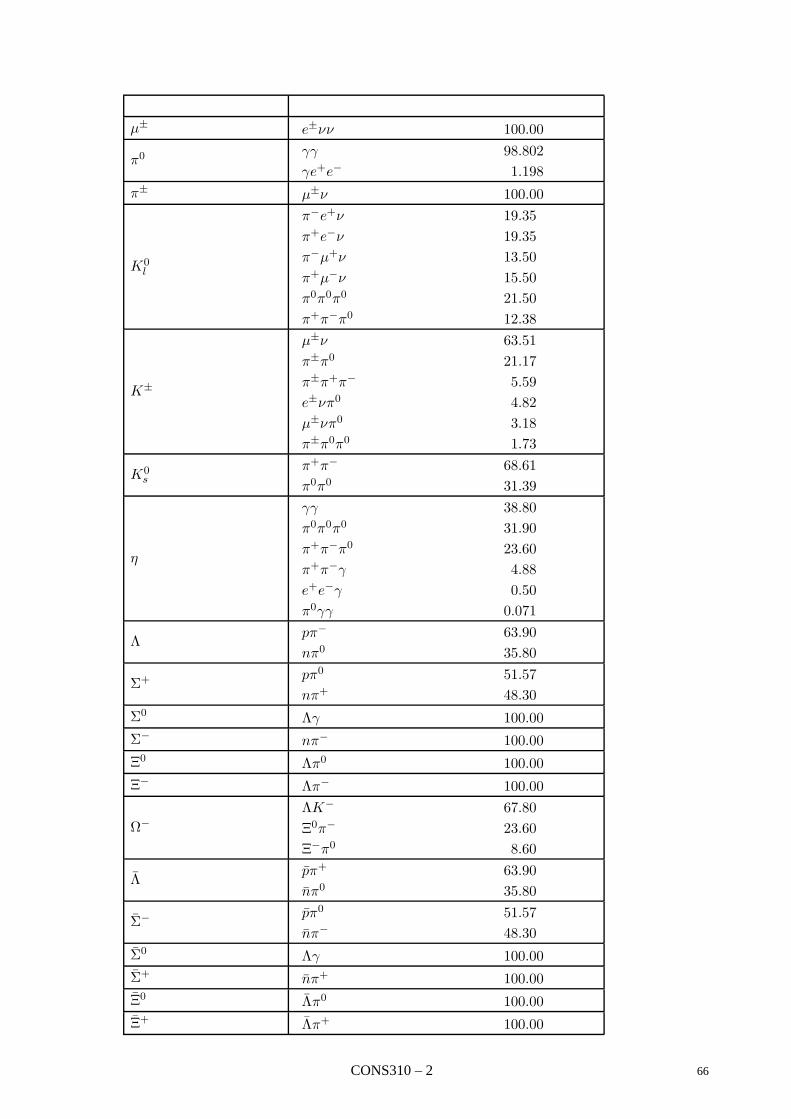
µ± e±νν 100.00
π0γγ 98.802γe+e− 1.198
π± µ±ν 100.00
K0l
π−e+ν 19.35π+e−ν 19.35π−µ+ν 13.50π+µ−ν 15.50π0π0π0 21.50π+π−π0 12.38
K±
µ±ν 63.51π±π0 21.17π±π+π− 5.59e±νπ0 4.82µ±νπ0 3.18π±π0π0 1.73
K0s
π+π− 68.61π0π0 31.39
η
γγ 38.80π0π0π0 31.90π+π−π0 23.60π+π−γ 4.88e+e−γ 0.50π0γγ 0.071
Λpπ− 63.90nπ0 35.80
Σ+pπ0 51.57nπ+ 48.30
Σ0 Λγ 100.00Σ− nπ− 100.00Ξ0 Λπ0 100.00Ξ− Λπ− 100.00
Ω−ΛK− 67.80Ξ0π− 23.60Ξ−π0 8.60
Λpπ+ 63.90nπ0 35.80
Σ− pπ0 51.57nπ− 48.30
Σ0 Λγ 100.00Σ+ nπ+ 100.00Ξ0 Λπ0 100.00Ξ+ Λπ+ 100.00
CONS310 – 2 66

Ω+ΛK+ 67.80Ξ0π+ 23.60Ξ+π0 8.60
67 CONS310 – 3

CONS Bibliography
[1] R.M. Barbett et al. Review of particle properties. Physical Review D, 54(1), July 1996.
[2] R.Ford and W.Nelson. SLAC 210, UC 32. SLAC, June 1978.
[3] J.Allison. Calculation of hadronic interaction lengths for mixtures. Technical ReportOPAL/0037N/JA/md, CERN, Hadron Milestone 84/003 1984.
[4] Aguillar Benitez et al. Review of particle properties. Rev. Mod. Phys., 56(198), 1984.
CONS310 – 4 68
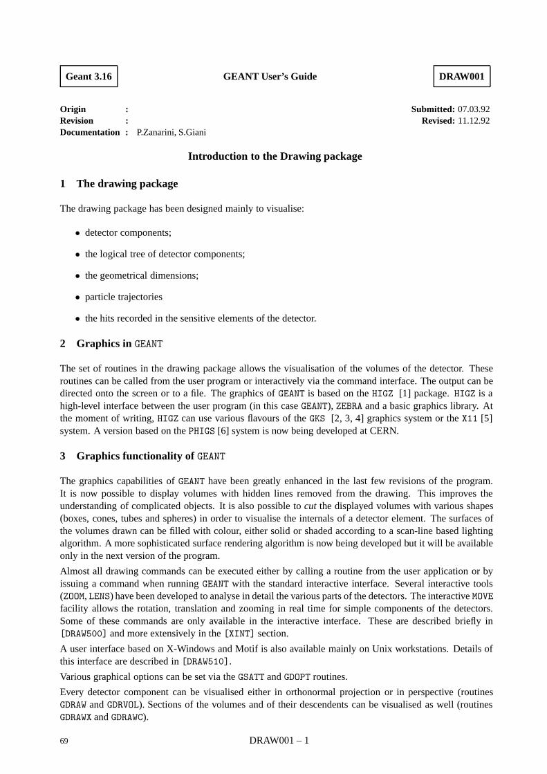
Geant 3.16 GEANT User’s Guide DRAW001
Origin : Submitted: 07.03.92Revision : Revised: 11.12.92Documentation : P.Zanarini, S.Giani
Introduction to the Drawing package
1 The drawing package
The drawing package has been designed mainly to visualise:
• detector components;
• the logical tree of detector components;
• the geometrical dimensions;
• particle trajectories
• the hits recorded in the sensitive elements of the detector.
2 Graphics in GEANT
The set of routines in the drawing package allows the visualisation of the volumes of the detector. Theseroutines can be called from the user program or interactively via the command interface. The output can bedirected onto the screen or to a file. The graphics of GEANT is based on the HIGZ [1] package. HIGZ is ahigh-level interface between the user program (in this case GEANT), ZEBRA and a basic graphics library. Atthe moment of writing, HIGZ can use various flavours of the GKS [2, 3, 4] graphics system or the X11 [5]system. A version based on the PHIGS [6] system is now being developed at CERN.
3 Graphics functionality of GEANT
The graphics capabilities of GEANT have been greatly enhanced in the last few revisions of the program.It is now possible to display volumes with hidden lines removed from the drawing. This improves theunderstanding of complicated objects. It is also possible to cut the displayed volumes with various shapes(boxes, cones, tubes and spheres) in order to visualise the internals of a detector element. The surfaces ofthe volumes drawn can be filled with colour, either solid or shaded according to a scan-line based lightingalgorithm. A more sophisticated surface rendering algorithm is now being developed but it will be availableonly in the next version of the program.
Almost all drawing commands can be executed either by calling a routine from the user application or byissuing a command when running GEANT with the standard interactive interface. Several interactive tools(ZOOM, LENS) have been developed to analyse in detail the various parts of the detectors. The interactive MOVEfacility allows the rotation, translation and zooming in real time for simple components of the detectors.Some of these commands are only available in the interactive interface. These are described briefly in[DRAW500] and more extensively in the [XINT] section.
A user interface based on X-Windows and Motif is also available mainly on Unix workstations. Details ofthis interface are described in [DRAW510].
Various graphical options can be set via the GSATT and GDOPT routines.
Every detector component can be visualised either in orthonormal projection or in perspective (routinesGDRAW and GDRVOL). Sections of the volumes and of their descendents can be visualised as well (routinesGDRAWX and GDRAWC).
69 DRAW001 – 1
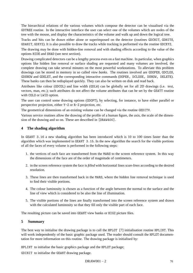
The hierarchical relations of the various volumes which compose the detector can be visualised via theGDTREE routine. In the interactive interface the user can select one of the volumes which are nodes of thetree with the mouse, and display the characteristics of the volume and walk up and down the logical tree.
Tracks and hits can be drawn either alone or superimposed on the detector (routines GDCHIT, GDHITS,GDAHIT, GDXYZ). It is also possible to draw the tracks while tracking is performed via the routine GDCXYZ.
The drawing may be done with hidden-line removal and with shading effects according to the value of theoptions HIDE and SHAD (see next section).
Drawing complicated detectors can be a lengthy process even on a fast machine. In particular, when graphicsoptions like hidden line removal or surface shading are requested and many volumes are involved, thecomplete drawing can take several minutes on the most powerful workstations. To alleviate this problemdrawings can be stored in memory in so called view banks. The routines involved are GDOPEN, GDCLOS,GDSHOW and GDELET, and the corresponding interactive commands (DOPEN, DCLOSE, DSHOW, DELETE).These banks can then be redisplayed quickly. They can also be written on disk and read back.
Attributes like colour (GDCOL) and line width (GDLW) can be globally set for all 2D drawings (i.e. text,vectors, man, etc.); such attributes do not affect the volume attributes that can be set by the GSATT routinewith COLO or LWID option.
The user can control some drawing options (GDOPT), by selecting, for instance, to have either parallel orperspective projection, either Y-Z or R-Z projection, etc.
The geometrical dimensions of an existing volume can be changed via the routine GEDITV.
Various service routines allow the drawing of the profile of a human figure, the axis, the scale of the dimen-sion of the drawing and so on. These are described in [DRAW400].
4 The shading algorithm
In GEANT 3.16 a new shading algorithm has been introduced which is 10 to 100 times faster than thealgorithm which was implemented in GEANT 3.15. In the new algorithm the search for the visible portionsof all the faces of every volume is performed in the following steps:
1. the vertices of each face are transformed from the MARS to the screen reference system. In this waythe dimensions of the face are of the order of magnitude of centimeters.
2. in the screen reference system the face is filled with horizontal lines scan-lines according to the desiredresolution.
3. These lines are then transformed back in the MARS, where the hidden line removal technique is usedto find their visible portions.
4. The colour luminosity is chosen as a function of the angle between the normal to the surface and theline of view which is considered to be also the line of illumination.
5. The visible portions of the lines are finally transformed into the screen reference system and drawnwith the calculated luminosity so that they fill only the visible part of each face.
The resulting picture can be saved into GEANT view banks or HIGZ picture files.
5 Summary
The best way to initialise the drawing package is to call the HPLOT [7] initialisation routine HPLINT. Thiswill work independently of the basic graphic package used. The reader should consult the HPLOT documen-tation for more information on this routine. The drawing package is initialised by:
HPLINT to initialise the basic graphics package and the HPLOT package;
GDINIT to initialise the GEANT drawing package.
DRAW001 – 2 70
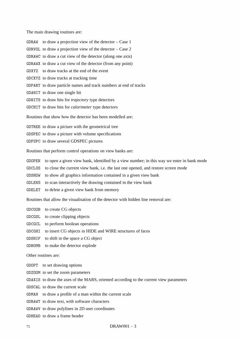
The main drawing routines are:
GDRAW to draw a projection view of the detector – Case 1
GDRVOL to draw a projection view of the detector – Case 2
GDRAWC to draw a cut view of the detector (along one axis)
GDRAWX to draw a cut view of the detector (from any point)
GDXYZ to draw tracks at the end of the event
GDCXYZ to draw tracks at tracking time
GDPART to draw particle names and track numbers at end of tracks
GDAHIT to draw one single hit
GDHITS to draw hits for trajectory type detectors
GDCHIT to draw hits for calorimeter type detectors
Routines that show how the detector has been modelled are:
GDTREE to draw a picture with the geometrical tree
GDSPEC to draw a picture with volume specifications
GDFSPC to draw several GDSPEC pictures
Routines that perform control operations on view banks are:
GDOPEN to open a given view bank, identified by a view number; in this way we enter in bank mode
GDCLOS to close the current view bank, i.e. the last one opened, and restore screen mode
GDSHOW to show all graphics information contained in a given view bank
GDLENS to scan interactively the drawing contained in the view bank
GDELET to delete a given view bank from memory
Routines that allow the visualisation of the detector with hidden line removal are:
GDCGOB to create CG objects
GDCGSL to create clipping objects
GDCGCL to perform boolean operations
GDCGHI to insert CG objects in HIDE and WIRE structures of faces
GDSHIF to shift in the space a CG object
GDBOMB to make the detector explode
Other routines are:
GDOPT to set drawing options
GDZOOM to set the zoom parameters
GDAXIS to draw the axes of the MARS, oriented according to the current view parameters
GDSCAL to draw the current scale
GDMAN to draw a profile of a man within the current scale
GDRAWT to draw text, with software characters
GDRAWV to draw polylines in 2D user coordinates
GDHEAD to draw a frame header
71 DRAW001 – 3

GDCOL to set colour code
GDLW to set line width
GDCURS to have an input from the graphics cursor
GDFR3D to convert from 3D coordinates (either in MARS or DRS) to 2D user coordinates
GD3D3D to convert from 3D MARS coordinates to 3D Projection Reference System coordinates.
DRAW001 – 4 72
Geant 3.21 GEANT User’s Guide DRAW010
Origin : S.Giani Submitted: 10.03.94Revision : Revised: 10.03.1994Documentation : S.Giani, S.Ravndal
The Ray-tracing package
Running interactively under X11, a new visualization tool is provided in GEANT 3.21: the ray-tracing pack-age. Based on the new GEANT tracking (see GEOM and TRACK), a set of routines doing light processing isprovided to visualize the detectors (useful also to visualize the results of boolean operations). Basically,visible light particles are tracked throughout the detector until when they do not hit the surface of a vol-ume declared not transparent; then, the intersection point is transformed to the screen coordinates and thecorresponding pixel is drawn with a computed hue and luminosity.
In case the command (DOPT RAYT ON) is executed, the drawings are performed by the GEANT ray-tracing;automatically, the color is assigned according to the tracking medium of each volume and the volumes witha density lower/equal than the air are considered transparent; if the option (USER) is set (ON) (again via thecommand (DOPT)), the user can set color and visibility for the desired volumes via the command (SATT), asusual, relatively to the attributes (COLO) and (SEEN). The resolution can be set via the command (SATT *FILL VALUE), where (VALUE) is the ratio between the number of pixels drawn and 20 (user coordinates).Parallel view and perspective view are possible (DOPT PROJ PARA/PERS).
In the first case, we assume that the first mother volume of the tree is a box with dimensions 10000 X10000 X 10000 cm and the view point (infinetely far) is 5000 cm far from the origin along the Z axis ofthe user coordinates; in the second case, the distance between the observer and the origin of the worldreference system is set in cm by the command (PERSP NAME VALUE). Grand-angle or telescopic effects canbe achieved changing the scale factors in the command (DRAW). (Please, note that in case of perspectiveviews, fixed the distance of the viewer, the zooming factors for the raytracing option must be 8.25 timesbigger than the ones used for the HIDE options in order to get the same picture). When the final picturedoes not occupy the full window, mapping the space before tracing can speed up the drawing, but canalso produce less precise results; values from 1 to 4 are allowed in the command (DOPT MAPP VALUE), themapping being more precise for increasing (VALUE). For (VALUE = 0) no mapping is performed (thereforemax precision and lowest speed).
The command (VALCUT) allows the cutting of the detector by three planes ortogonal to the x,y,z axis. Theattribute (LSTY) can be set by the command SATT for any desired volume and can assume values from 0 to7. It determines the different light processing to be performed for different materials: 0 = dark-matt, 1 =bright-matt, 2 = plastic, 3 = ceramic, 4 = rough-metals, 5 = shiny-metals, 6 = glass, 7 = mirror.
The detector is assumed to be in the dark, the ambient light luminosity is 0.2 for each basic hue (the satu-ration is 0.9) and the observer is assumed to have a light source (therefore he will produce parallel light inthe case of parallel view and point-like-source light in the case of perspective view). Finally, a second lightsource can be positioned in the space (with a desired intensity) via the command (SPOT).
73 DRAW010 – 1
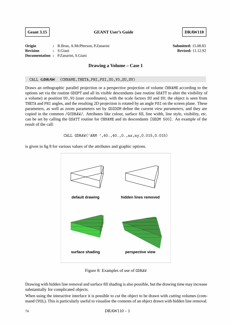
Geant 3.15 GEANT User’s Guide DRAW110
Origin : R.Brun, A.McPherson, P.Zanarini Submitted: 15.08.83Revision : S.Giani Revised: 11.12.92Documentation : P.Zanarini, S.Giani
Drawing a Volume – Case 1
CALL GDRAW (CHNAME,THETA,PHI,PSI,U0,V0,SU,SV)
Draws an orthographic parallel projection or a perspective projection of volume CHNAME according to theoptions set via the routine GDOPT and all its visible descendants (see routine GSATT to alter the visibility ofa volume) at position U0,V0 (user coordinates), with the scale factors SU and SV; the object is seen fromTHETA and PHI angles, and the resulting 2D projection is rotated by an angle PSI on the screen plane. Theseparameters, as well as zoom parameters set by GDZOOM define the current view parameters, and they arecopied in the common /GCDRAW/. Attributes like colour, surface fill, line width, line style, visibility, etc.can be set by calling the GSATT routine for CHNAME and its descendants [GEOM 500]. An example of theresult of the call:
CALL GDRAW(’ARM ’,40.,40.,0.,nx,ny,0.015,0.015)
is given in fig 8 for various values of the attributes and graphic options.
default drawing hidden lines removed
surface shading perspective view
Figure 8: Examples of use of GDRAW
Drawing with hidden line removal and surface fill shading is also possible, but the drawing time may increasesubstantially for complicated objects.
When using the interactive interface it is possible to cut the object to be drawn with cutting volumes (com-mand CVOL). This is particularly useful to visualise the contents of an object drawn with hidden line removal.
74 DRAW110 – 1

Another feature which is available only interactively is the possibility to draw each decendant of a volumeshifted along the axis which goes from the centre of the local coordinate system to the centre of gravityof the descendant itself. This again is useful to improve the visibility of the details of a complicated setup(command BOMB). Please see the interactive interface description for more information on this part.
CHNAME (CHARACTER*4) volume name.
THETA (REAL) theta angle between the line of sight and the Z axis of MAster Reference System (MARS).
PHI (REAL) phi angle between the projection of the line of sight on plane X Y and the X axis of MARS.
PSI (REAL) psi angle by which the projected image will be rotated on the screen plane.
U0 (REAL) u coordinate on the screen of the volume origin.
V0 (REAL) v coordinate on the screen of the volume origin.
SU (REAL) scale factor for u coordinates.
SV (REAL) scale factor for v coordinates.
DRAW110 – 2 75
Geant 3.15 GEANT User’s Guide DRAW115
Origin : P.Zanarini Submitted: 01.01.86Revision : Revised: 11.12.92Documentation : P.Zanarini, F.Carminati
Drawing a Volume Projection view – Case 2
CALL GDRVOL (NNAMS,CHNAMS,LNUMBS,NRS,THETA,PHI,PSI,U0,V0,SU,SV)
Draws an orthographic parallel projection or a perspective projection (depending on the option chosen viaGDOPT) of the volume CHNAMS(N),LNUMBS(N)with all its descendants, at the position U0,V0 (user coordi-nates), with the scale factors SU and SV. The object is seen from THETA and PHI angles, and the resulting 2Dprojection is also rotated by an angle PSI on the screen plane. These parameters, as well as zoom parametersset by GDZOOM, define the current view parameters, and they are copied in /GCDRAW/. Attributes like colour,fill area, line width, line style, visibility, etc. can be set by the GSATT routine for CHNAMS(N) and or itsdescendants [GEOM 500]. This routine differs from GDRAW in the following aspects:
• The object to be drawn is identified by a full path. This gives the possibility of drawing a particularcopy or division of a volume, or even a volume that has more than one mother in the geometrytree. CHNAMS(1),...,CHNAMS(N) contain the volume names and LNUMBS(1),...,LNUMBS(N), thevolume numbers defining the path to go from the top volume to the one to be drawn.
• The object can be drawn either with respect to the MAster Reference System (NRS=0) or with respectto its Daugther Reference System (i.e. the Local R.S.); in the first case it is drawn in its position in thereal world, while in the second one it is drawn like GDRAW would do.
• In this latter case, track and hit points will be drawn with respect to the DRS of the volume last drawnby this routine, and not with respect to the MARS as is done normally (to reset to the normal case a callwith NRS=0 or NNAMS=0 is required).
NNAMS (INTEGER) number of elements levels in the arrays CHNAMS, LNUMBS. The bottom volume ofthis path is also the one that is actually drawn;
CHNAMS (CHARACTER*4) array of volume name (dimensioned at least to NNAMS);
LNUMBS array of volume numbers (dimensioned at least to NNAMS);
NRS reference system used:
NRS=0 to have the volume(s) drawn with respect to the MARS
NRS =0 to have the volume(s) drawn with respect to the DRS
THETA θ angle between the line of sight and the Z axis of MARS;
PHI φ angle between the projection of the line of sight on plane X Y and the X axis of MARS
PSI ψ angle by which the projected image will be rotated on the screen plane
U0 u coordinate on the screen of the volume origin
V0 v coordinate on the screen of the volume origin
SU scale factor for u coordinates
SV scale factor for v coordinates
Two examples of use of GDRVOL are shown in fig 9 and 10.
76 DRAW115 – 1
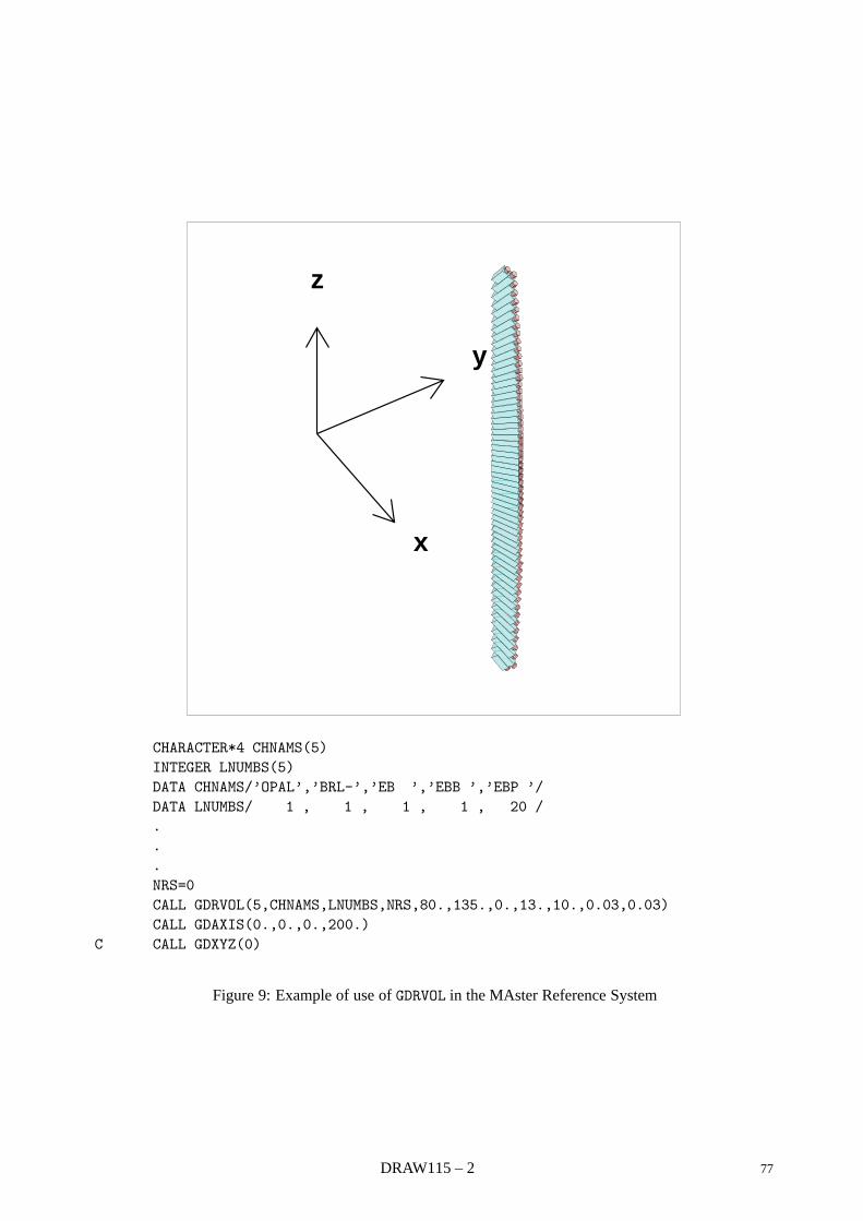
x
y
z
CHARACTER*4 CHNAMS(5)INTEGER LNUMBS(5)DATA CHNAMS/’OPAL’,’BRL-’,’EB ’,’EBB ’,’EBP ’/DATA LNUMBS/ 1 , 1 , 1 , 1 , 20 /...NRS=0CALL GDRVOL(5,CHNAMS,LNUMBS,NRS,80.,135.,0.,13.,10.,0.03,0.03)CALL GDAXIS(0.,0.,0.,200.)
C CALL GDXYZ(0)
Figure 9: Example of use of GDRVOL in the MAster Reference System
DRAW115 – 2 77
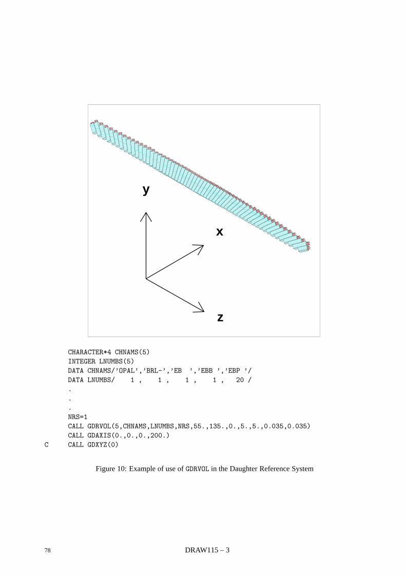
x
y
z
CHARACTER*4 CHNAMS(5)INTEGER LNUMBS(5)DATA CHNAMS/’OPAL’,’BRL-’,’EB ’,’EBB ’,’EBP ’/DATA LNUMBS/ 1 , 1 , 1 , 1 , 20 /...NRS=1CALL GDRVOL(5,CHNAMS,LNUMBS,NRS,55.,135.,0.,5.,5.,0.035,0.035)CALL GDAXIS(0.,0.,0.,200.)
C CALL GDXYZ(0)
Figure 10: Example of use of GDRVOL in the Daughter Reference System
78 DRAW115 – 3
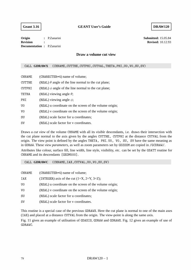
Geant 3.16 GEANT User’s Guide DRAW120
Origin : P.Zanarini Submitted: 15.05.84Revision : Revised: 10.12.93Documentation : P.Zanarini
Draw a volume cut view
CALL GDRAWX (CHNAME,CUTTHE,CUTPHI,CUTVAL,THETA,PHI,U0,V0,SU,SV)
CHNAME (CHARECTER*4) name of volume;
CUTTHE (REAL) θ angle of the line normal to the cut plane;
CUTPHI (REAL) φ angle of the line normal to the cut plane;
TETHA (REAL) viewing angle θ;
PHI (REAL) viewing angle φ;
U0 (REAL) u coordinate on the screen of the volume origin;
V0 (REAL) v coordinate on the screen of the volume origin;
SU (REAL) scale factor for u coordinates;
SV (REAL) scale factor for v coordinates.
Draws a cut view of the volume CHNAME with all its visible descendants, i.e. draws their intersection withthe cut plane normal to the axis given by the angles CUTTHE, CUTPHI at the distance CUTVAL from theorigin. The view point is defined by the angles THETA, PHI. U0, V0, SU, SV have the same meaning asin GDRAW. These view parameters, as well as zoom parameters set by GDZOOM are copied in /GCDRAW/.
Attributes like colour, surface fill, line width, line style, visibility, etc. can be set by the GSATT routine forCHNAME and its descendants [GEOM500].
CALL GDRAWC (CHNAME,IAX,CUTVAL,U0,V0,SU,SV)
CHNAME (CHARECTER*4) name of volume;
IAX (INTEGER) axis of the cut (1=X, 2=Y, 3=Z);
U0 (REAL) u coordinate on the screen of the volume origin;
V0 (REAL) v coordinate on the screen of the volume origin;
SU (REAL) scale factor for u coordinates;
SV (REAL) scale factor for v coordinates.
This routine is a special case of the previous GDRAWX. Here the cut plane is normal to one of the main axes(IAX) and placed at a distance CUTVAL from the origin. The view-point is along the same axis.
Fig. 11 gives an example of utilisation of GDAXIS, GDRAW and GDRAWX. Fig. 12 gives an example of use ofGDRAWC.
79 DRAW120 – 1
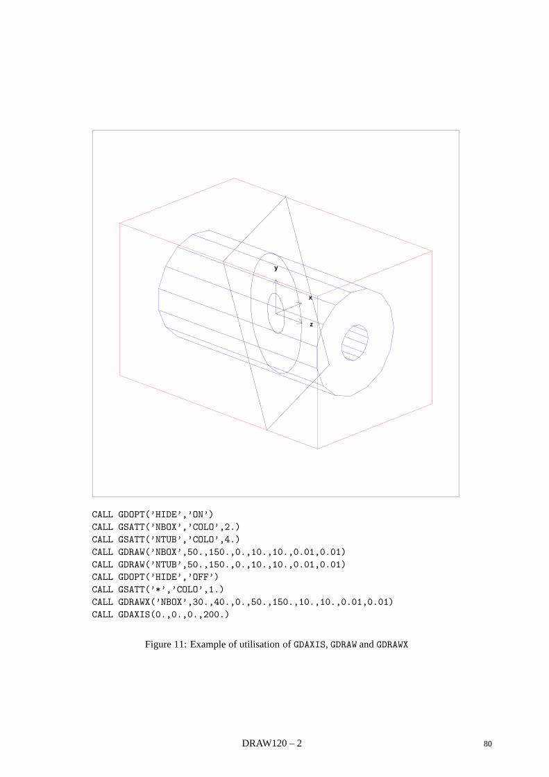
x
y
z
CALL GDOPT(’HIDE’,’ON’)CALL GSATT(’NBOX’,’COLO’,2.)CALL GSATT(’NTUB’,’COLO’,4.)CALL GDRAW(’NBOX’,50.,150.,0.,10.,10.,0.01,0.01)CALL GDRAW(’NTUB’,50.,150.,0.,10.,10.,0.01,0.01)CALL GDOPT(’HIDE’,’OFF’)CALL GSATT(’*’,’COLO’,1.)CALL GDRAWX(’NBOX’,30.,40.,0.,50.,150.,10.,10.,0.01,0.01)CALL GDAXIS(0.,0.,0.,200.)
Figure 11: Example of utilisation of GDAXIS, GDRAW and GDRAWX
DRAW120 – 2 80
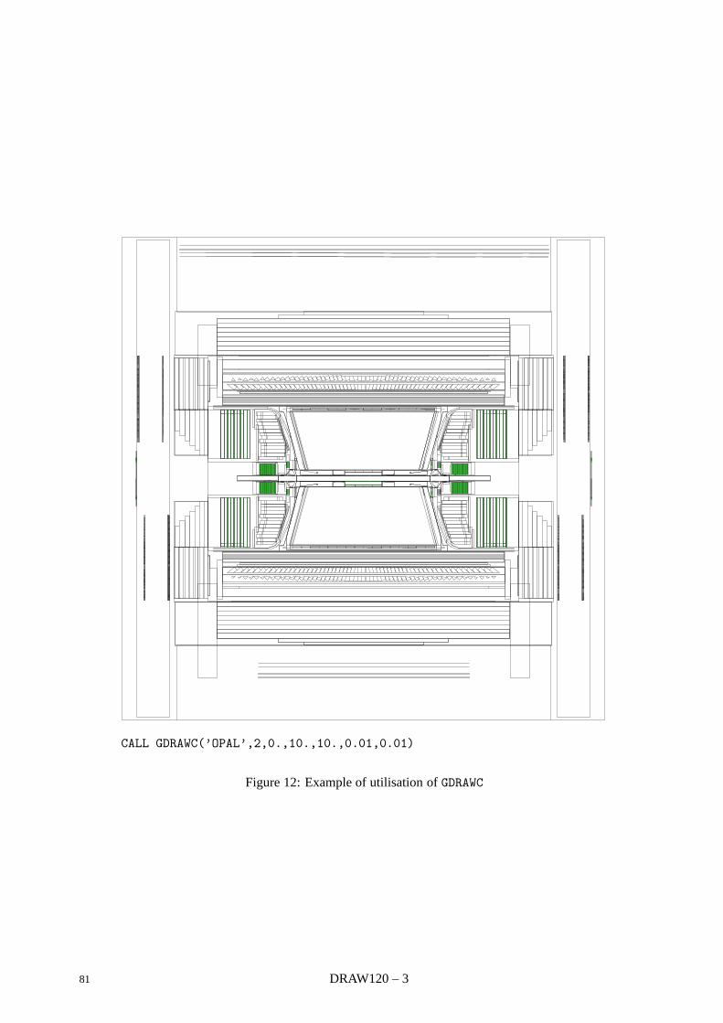
CALL GDRAWC(’OPAL’,2,0.,10.,10.,0.01,0.01)
Figure 12: Example of utilisation of GDRAWC
81 DRAW120 – 3

Geant 3.16 GEANT User’s Guide DRAW130
Origin : R.Brun, P.Zanarini Submitted: 15.05.84Revision : Revised: 11.12.92Documentation : P.Zanarini
Draw Particle Trajectories
1 Visualisation of particle trajectories
The tracks generated by the tracking package, and optionally stored in the data structure JXYZ, can bedisplayed by the routine GDXYZ (corresponding to the interactive command DXYZ).
The names of the particles and or the track numbers can be added by the routine GDPART (corresponding tothe interactive command DPART).
A special routine has been provided to visualise the tracks during the transport process (GDCXYZ), that couldbe called for instance by GUSTEP. That routine shows the tracks while they are transported by the trackingpackage of GEANT, providing a useful interactive debugging tool.
CALL GDXYZ (ITRA)
Draws track number ITRA for which space points have been stored in bank JXYZ via calls to the routineGSXYZ. The view parameters are taken from /GCDRAW/.
ITRA (INTEGER) track number (if 0 all tracks are taken)
The colour and line style corresponds to the track type :
(blue) dotted line for gammas . . . . . . . . . . . . . . . . .
(red) solid line for charged particles (except muons)
(black) blank/dotted line for neutral hadrons or neutrinos . . . . . .
(green) dashed line for muons - - - - - -
(yellow) dotted line for Cerenkov photons . . . . . . . . . . . . . . . . .
CALL GDPART (ITRA,ISEL,SIZE)
Draws the particle names and/or the track numbers of track ITRA, supposing that its space points had beenstored in the bank JXYZ via the routine GSXYZ. At present only primary tracks are displayed by GDPARTand their name or number is written at the end the track trajectory. The view parameters are taken from/GCDRAW/.
ITRA (INTEGER) Track number (if 0 all tracks are taken)
ISEL (INTEGER)ISEL=x1 draws the track number,ISEL=1x draws the particle name,ISEL=11 draws both.
SIZE (REAL) Character size in cm.
CALL GDCXYZ
If GDCXYZ is called at tracking time (for instance by GUSTEP), it draws the tracks while tracking is performed,at the same time as they are generated by the tracking package of GEANT. This is a very useful interactivedebugging tool. The line style is the same as for GDXYZ. The view parameters are taken from /GCDRAW/.
Here we give an example of the use of GDPART:
82 DRAW130 – 1

CALL GSATT(’HB’,’FILL’,3)CALL GSATT(’HE’,’FILL’,1)- - - - -- - - - -
CALL GDRAWC(’OPAL’,2,5.,10.,10.,0.013,0.013)CALL GDXYZ(0)CALL GDPART(0,11,0.25)
DRAW130 – 2 83
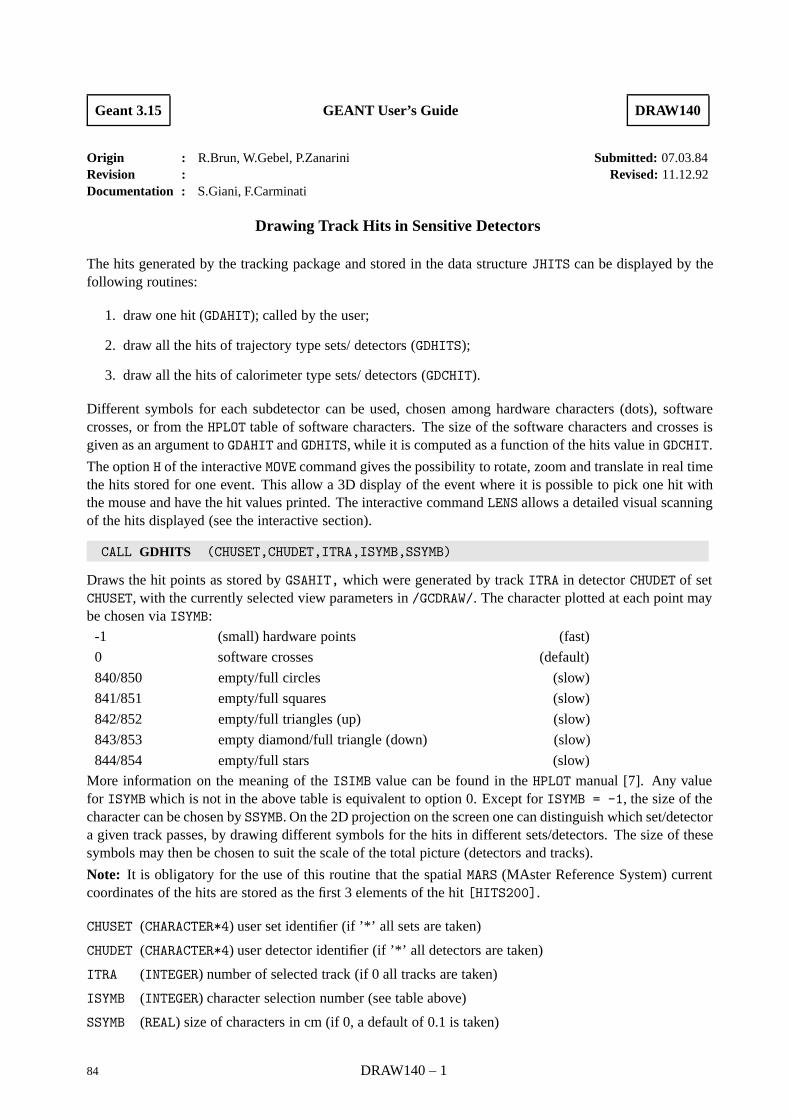
Geant 3.15 GEANT User’s Guide DRAW140
Origin : R.Brun, W.Gebel, P.Zanarini Submitted: 07.03.84Revision : Revised: 11.12.92Documentation : S.Giani, F.Carminati
Drawing Track Hits in Sensitive Detectors
The hits generated by the tracking package and stored in the data structure JHITS can be displayed by thefollowing routines:
1. draw one hit (GDAHIT); called by the user;
2. draw all the hits of trajectory type sets/ detectors (GDHITS);
3. draw all the hits of calorimeter type sets/ detectors (GDCHIT).
Different symbols for each subdetector can be used, chosen among hardware characters (dots), softwarecrosses, or from the HPLOT table of software characters. The size of the software characters and crosses isgiven as an argument to GDAHIT and GDHITS, while it is computed as a function of the hits value in GDCHIT.
The option H of the interactive MOVE command gives the possibility to rotate, zoom and translate in real timethe hits stored for one event. This allow a 3D display of the event where it is possible to pick one hit withthe mouse and have the hit values printed. The interactive command LENS allows a detailed visual scanningof the hits displayed (see the interactive section).
CALL GDHITS (CHUSET,CHUDET,ITRA,ISYMB,SSYMB)
Draws the hit points as stored by GSAHIT, which were generated by track ITRA in detector CHUDET of setCHUSET, with the currently selected view parameters in /GCDRAW/. The character plotted at each point maybe chosen via ISYMB:
-1 (small) hardware points (fast)
0 software crosses (default)
840/850 empty/full circles (slow)
841/851 empty/full squares (slow)
842/852 empty/full triangles (up) (slow)
843/853 empty diamond/full triangle (down) (slow)
844/854 empty/full stars (slow)
More information on the meaning of the ISIMB value can be found in the HPLOT manual [7]. Any valuefor ISYMB which is not in the above table is equivalent to option 0. Except for ISYMB = -1, the size of thecharacter can be chosen by SSYMB. On the 2D projection on the screen one can distinguish which set/detectora given track passes, by drawing different symbols for the hits in different sets/detectors. The size of thesesymbols may then be chosen to suit the scale of the total picture (detectors and tracks).
Note: It is obligatory for the use of this routine that the spatial MARS (MAster Reference System) currentcoordinates of the hits are stored as the first 3 elements of the hit [HITS200].
CHUSET (CHARACTER*4) user set identifier (if ’*’ all sets are taken)
CHUDET (CHARACTER*4) user detector identifier (if ’*’ all detectors are taken)
ITRA (INTEGER) number of selected track (if 0 all tracks are taken)
ISYMB (INTEGER) character selection number (see table above)
SSYMB (REAL) size of characters in cm (if 0, a default of 0.1 is taken)
84 DRAW140 – 1
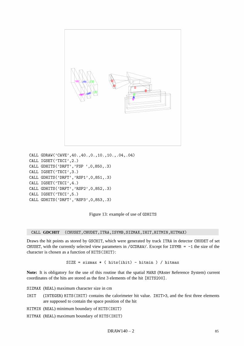
CALL GDRAW(’CAVE’,40.,40.,0.,10.,10.,.04,.04)CALL IGSET(’TXCI’,2.)CALL GDHITS(’DRFT’,’FSP ’,0,850,.3)CALL IGSET(’TXCI’,3.)CALL GDHITS(’DRFT’,’RSP1’,0,851,.3)CALL IGSET(’TXCI’,4.)CALL GDHITS(’DRFT’,’RSP2’,0,852,.3)CALL IGSET(’TXCI’,5.)CALL GDHITS(’DRFT’,’RSP3’,0,853,.3)
Figure 13: example of use of GDHITS
CALL GDCHIT (CHUSET,CHUDET,ITRA,ISYMB,SIZMAX,IHIT,HITMIN,HITMAX)
Draws the hit points as stored by GSCHIT, which were generated by track ITRA in detector CHUDET of setCHUSET, with the currently selected view parameters in /GCDRAW/. Except for ISYMB = -1 the size of thecharacter is chosen as a function of HITS(IHIT):
SIZE = sizmax * ( hits(ihit) - hitmin ) / hitmax
Note: It is obligatory for the use of this routine that the spatial MARS (MAster Reference System) currentcoordinates of the hits are stored as the first 3 elements of the hit [HITS200].
SIZMAX (REAL) maximum character size in cm
IHIT (INTEGER) HITS(IHIT) contains the calorimeter hit value. IHIT>3, and the first three elementsare supposed to contain the space position of the hit
HITMIN (REAL) minimum boundary of HITS(IHIT)
HITMAX (REAL) maximum boundary of HITS(IHIT)
DRAW140 – 2 85

CALL GDAHIT (X,Y,Z,ISYMB,SSYMB)
Draws one hit point at coordinates X, Y, Z. This routine is useful when the user wants only to displaybut not to store the hits. The first three arguments are the position of the hit in the MARS, and the last twoarguments have the same meaning as the similar arguments in GDHITS.
X (REAL) x coordinate in MARS of the hit point
Y (REAL) y coordinate in MARS of the hit point
X (REAL) z coordinate in MARS of the hit point
An example of use of the hits drawing routines is given in fig 13.
86 DRAW140 – 3
Geant 3.16 GEANT User’s Guide DRAW210
Origin : P.Zanarini Submitted: 15.01.84Revision : S.Giani Revised: 10.12.93Documentation : P.Zanarini, S.Giani
Drawing the geometrical tree
The geometrical tree is a hierarchical representation of the structure of the detector, based on the mother-daughter relationship among the various volumes composing it. The GDTREE routine (corresponding to theDTREE interactive command) allows the drawing of the logical tree, displaying name, multiplicity and otherinformation about the volumes.
CALL GDTREE (CHNAME,LEVMAX,ISEL)
CHNAME (CHARACTER*4) volume name;
LEVMAX (INTEGER) depth levels (if 0 all levels are taken) default is 3;
ISEL (INTEGER) used to select options in the picture of the tree:
0 only the node name is drawn;
xxxx1 multiplicity is added:
•each node that has been positioned several times (by GSPOS or GSPOSP) has amultiplicity number preceded by the symbol ’*’;
•each node that has been obtained by division mechanism (by GSDVN, GSDVT,etc.) has a multiplicity number preceded by the symbol #;
xxx1x ONLY information is added. volumes that are MANY will be drawn as three squarenodes, one overlapping the others but slightly shifted;Note: if CHNAME itself is MANY it will not be recognised as such, because this infor-mation is stored in its mother which is unknown;
xx1xx DET information is added; if a volumes is a detector it is drawn as a square node withanother one slightly larger around it;
x1xxx SEEN information is added; if a volume is not seen (either because of its SEEN at-tribute or because of its ancestors SEEN attributes affecting the whole tree path) itssquare node is drawn by using dashed lines;
1xxxx a little picture of the volume is added above each node.
GDTREE draws the tree of the volume data structure starting from the volume CHNAME, for LEVMAX depthlevels; a continuation link line is drawn for those elements at the last level on the picture but having descen-dants. An example of use of GDTREE can be found in Fig. 14. For every node, as many red arrows as thenumber of existing levels below it are plotted on the link; vice versa, as many green arrows as the numberof existing levels before it are also plotted. When running GEANT interactively, if the ISEL argument is notspecified, control is given to the mouse after issuing the DTREE command. This allows the display of variousvolume parameters and the navigation of the geometrical tree by clicking the mouse buttons. The size of thepicture and the dimensions of each element and arrows are computed automatically.
Interactive use
In an interactive session, control can be given to the mouse:
• clicking on the left button when the cursor is inside a volume pave will generate a DSPEC commandfor that volume;
87 DRAW210 – 1
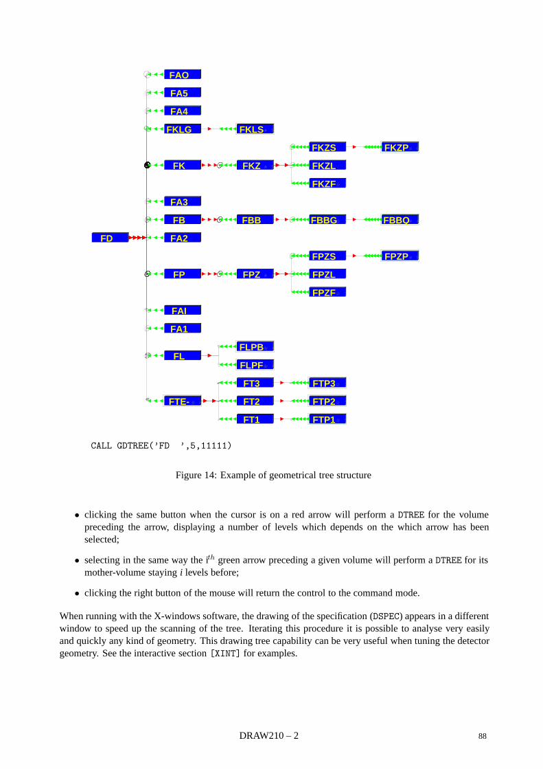
FD
FTE-
FL
FA1
FAI
FP
FA2
FB
FA3
FK
FKLG
FA4
FA5
FAO
FT1
FT2
FT3
FLPF
FLPB
FPZ
FBB
FKZ
FKLS
FTP1
FTP2
FTP3
FPZF
FPZL
FPZS
FBBG
FKZF
FKZL
FKZS
FPZP
FBBQ
FKZP
CALL GDTREE(’FD ’,5,11111)
Figure 14: Example of geometrical tree structure
• clicking the same button when the cursor is on a red arrow will perform a DTREE for the volumepreceding the arrow, displaying a number of levels which depends on the which arrow has beenselected;
• selecting in the same way the ith green arrow preceding a given volume will perform a DTREE for itsmother-volume staying i levels before;
• clicking the right button of the mouse will return the control to the command mode.
When running with the X-windows software, the drawing of the specification (DSPEC) appears in a differentwindow to speed up the scanning of the tree. Iterating this procedure it is possible to analyse very easilyand quickly any kind of geometry. This drawing tree capability can be very useful when tuning the detectorgeometry. See the interactive section [XINT] for examples.
DRAW210 – 2 88
Geant 3.16 GEANT User’s Guide DRAW220
Origin : P.Zanarini Submitted: 01.11.83Revision : Revised: 13.12.93Documentation : P.Zanarini, S.Giani, F.Carminati
Drawing volume specifications
The geometrical parameters of the volumes can be displayed via the GDSPEC routine (corresponding to theDSPEC interactive command). This facility provides a detailed picture of a particular piece of the detector.The set of geometrical specifications of all the descendants of a given node on the tree, can be obtained eachon a separate picture with the routine GDFSPC (DFSPC interactive command).
CALL GDSPEC (CHNAME)
CHNAME (CHARACTER*4) volume name;
Draws a picture showing all specifications for a given volume. An example of use of GDSPEC can be foundin Fig. 15.The following information on the volume are presented in a single frame:
• the volume daughters (one level down in the geometrical tree);
• a space view of the volume (with θ=45 and φ=135);
• a front view cut;
• a side view cut;
• the axes of the local coordinate system;
• a human figure;
• the scale;
• the shape type;
• all the numerical parameters that define the volume.
In drawing the volumes GDSPEC turns on the sets visibility (’SEEN’) attribute for the volume CHNAME itselfand its direct descendents. The setting of drawing options (HIDE, CVOL, FILL . . .) will be respected, allowingto customise the drawing. An example is shown in Fig. 16.
CALL GDFSPC (CHNAME,ISORT,INTER)
Draws on separate pictures the full set of GDSPEC for the geometrical tree starting from CHNAME, i.e. callsGDSPEC for the volume CHNAME and for all its descendants.
CHNAME (CHARACTER*4) volume name;
ISORT (INTEGER) alphabetic sorting flag;
= 1 all the volumes will be drawn in ascending alphabetic order according to their name;= 1 the volumes will be drawn in the order in which they have been created;
INTER (INTEGER) interactive/batch version flag;
= 1 the routine will prompt the user at each plot before doing a clear screen;= 0 the routine will clear automatically the screen before starting a new frame.
Note: INTER should be set to 1 when using the interactive version of GEANT and to any othervalue when using a batch version.
89 DRAW220 – 1
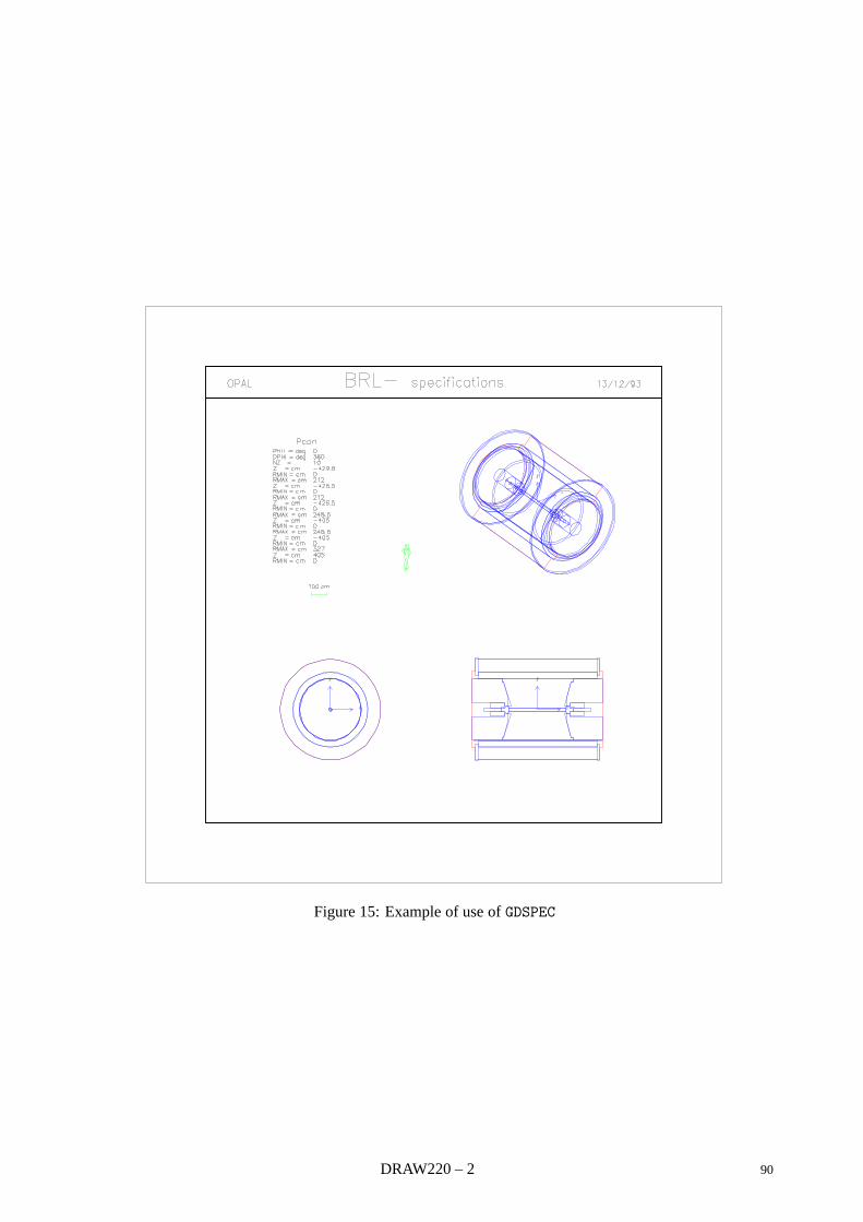
Figure 15: Example of use of GDSPEC
DRAW220 – 2 90
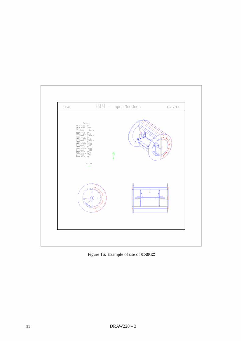
Figure 16: Example of use of GDSPEC
91 DRAW220 – 3
Geant 3.16 GEANT User’s Guide DRAW300
Origin : R.Brun, P.Zanarini Submitted: 01.10.83Revision : S.Giani Revised: 13.12.93Documentation : P.Zanarini, S.Giani, F.Carminati
Handling View banks
1 The view banks
The basic detector drawing routines (GDRAW, GDRAWC, GDRAWX) scan the data structure JVOLUM repeatedly toextract position and dimension information on the volumes. This can be a rather lengthy process even on fastcomputer. Hidden line removal drawing requires an auxiliary data structure and the relative visibility of allthe volumes has to be analysed. With complicated detectors the time spent in this process can be substantial,depending on the drawing options chosen and on the speed of the machine on which the program is run. Inorder to alleviate this problem the graphic banks and the associated routines have been developed.
The interpretation of the structure (for instance scanning of the volumes’ data structure to convert the 3Dgeometry structure into a set of 2D lines, visibility analysis, surface creation or light processing) is thusseparate from the drawing itself. In this way, the interpretation is performed only once and all the 2Dinformation is stored in view banks (data structure JDRAW [DRAW399]). These views can then be displayedquickly, having only to draw the 2D vectors or the fill areas previously stored.
For a detector with more than 100 different volumes, for example, this costs only a few thousand words ofmemory for each drawing stored.
If the drawing routines are called while a view bank, identified by a positive integer, is open (GDOPEN) onlyinterpretation will be made, no output will be generated until the bank is closed (GDCLOS). When a viewbank has been closed it cannot be modified, but it can be displayed as many times as wanted (GDSHOW) ordeleted (GDELET).
Once a drawing (detectors, tracks or hits) is in a view bank, it is possible to scan it in detail via the LENS orZOOM interactive commands (only available with X11). For more information see the [XINT] section.
CALL GDOPEN (IVIEW)
IVIEW (INTEGER) view bank number (IVIEW>0).
Opens a view bank, used to store 2D graphics information coming from the interpretation of 3D structures(but also 2D annotation). All subsequent calls to the drawing routines will fill the view bank IVIEW, withoutgenerating any output.
CALL GDCLOS
Closes the current opened view bank. Once a view bank has been closed no more drawing can be added toit. A call to GDCLOS also restores the screen.
CALL GDSHOW (IVIEW)
IVIEW (INTEGER) view bank number (IVIEW>0).
Displays view bank IVIEW. GDSHOW can be called either before or after a view bank has been closed. If aview bank is currently open, the content of bank IVIEW will be added to it.
92 DRAW300 – 1
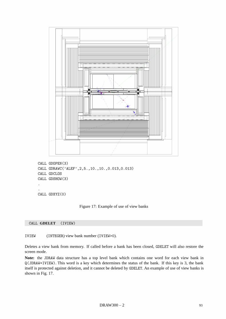
CALL GDOPEN(3)CALL GDRAWC(’ALEF’,2,5.,10.,10.,0.013,0.013)CALL GDCLOSCALL GDSHOW(3)..CALL GDXYZ(0)
Figure 17: Example of use of view banks
CALL GDELET (IVIEW)
IVIEW (INTEGER) view bank number (IVIEW>0).
Deletes a view bank from memory. If called before a bank has been closed, GDELET will also restore thescreen mode.
Note: the JDRAW data structure has a top level bank which contains one word for each view bank inQ(JDRAW+IVIEW). This word is a key which determines the status of the bank. If this key is 3, the bankitself is protected against deletion, and it cannot be deleted by GDELET. An example of use of view banks isshown in Fig. 17.
DRAW300 – 2 93

Geant 3.16 GEANT User’s Guide DRAW399
Origin : R.Brun, P.Zanarini Submitted: 15.11 83Revision : Revised: 13.12.93Documentation :
The data structure JDRAW
This data structure contains the so-called view banks. The layout of the data structure can be found inFig. 18. The meaning of the variables is the following:
NKVIEW number of views stored in the structure;
IVIEW current view selected;
IGU current graphic unit pointer;
MAXGU number of units in graphic unit bank;
MORGU number of words to push the graphic unit bank;
IGS current graphic segment pointer;
MAXGS number of segments in graphic segment bank;
MORGS number of words to push the graphic segment bank;
ITU current text unit pointer;
MAXTU number of units in text unit bank;
MORTU number of words to push the text unit bank;
ITS current text segment pointer;
MAXTS number of segments in text segment bank;
MORTS number of words to push in text segment bank
LENGU array of lengths for each graphic unit and of line attributes (LINATT);
ADDGU array of addresses for each graphic unit;
ADDTU array of addresses for each text unit;
X array of u coordinates of graphic segments;
Y array v coordinates of graphic segments;
ICUT cut axis (1, 2, 3 or 0 if no cut) of the view;
LINWID text line width and text attributes (ITXATT);
GTHETA, GPHI, GPSI, GU0, GV0, GSCU, GSCV, are the viewing parameters stored in /GCDRAW/.
U0, V0, SIZE, ANGLE, IOPT, ITEXT have the same meaning of those given as arguments to GDRAWT(or HPLSOF [7]).
A control word is stored in Q(JDRAW+IVIEW), with the following meaning:
1 empty bank (created by internal routines to avoid gaps) or for deleted banks;
2 bank created by the user;
3 protected bank reserved for internal use: it cannot be deleted by the user.
94 DRAW399 – 1
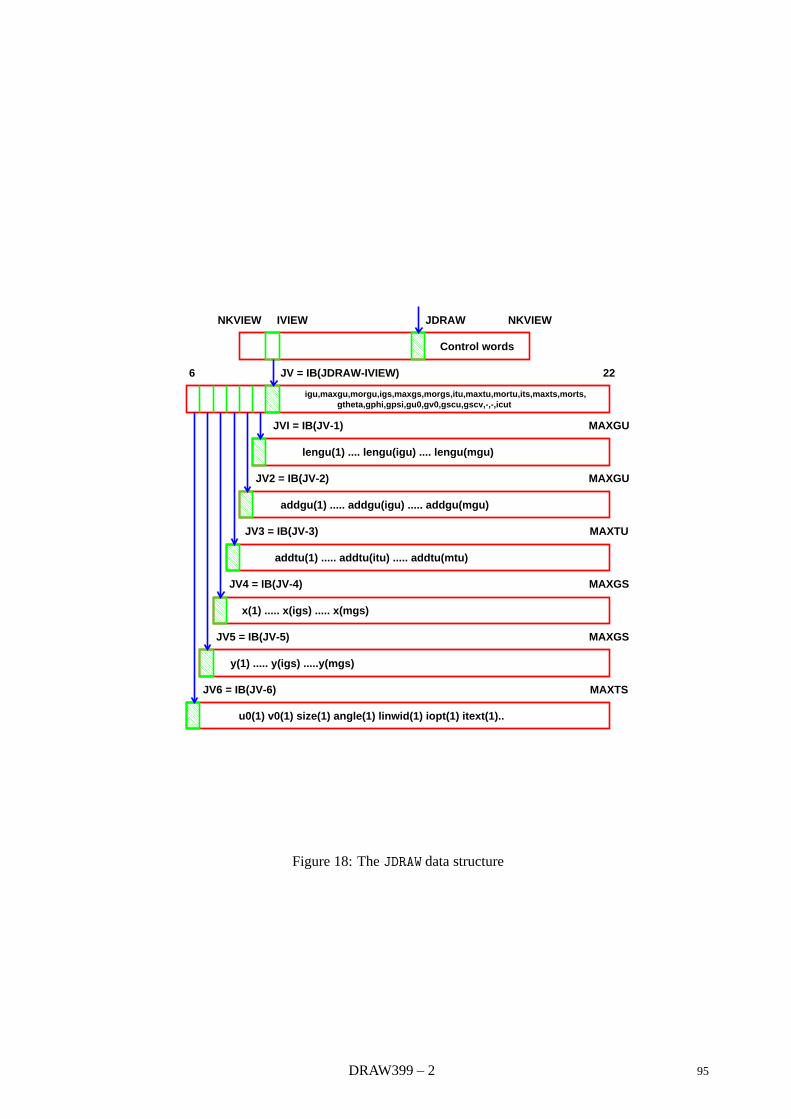
NKVIEW IVIEW JDRAW NKVIEW
Control words
JV = IB(JDRAW-IVIEW)
igu,maxgu,morgu,igs,maxgs,morgs,itu,maxtu,mortu,its,maxts,morts,gtheta,gphi,gpsi,gu0,gv0,gscu,gscv,-,-,icut
JVI = IB(JV-1)
lengu(1) .... lengu(igu) .... lengu(mgu)
JV2 = IB(JV-2)
addgu(1) ..... addgu(igu) ..... addgu(mgu)
JV3 = IB(JV-3)
addtu(1) ..... addtu(itu) ..... addtu(mtu)
JV4 = IB(JV-4)
x(1) ..... x(igs) ..... x(mgs)
JV5 = IB(JV-5)
y(1) ..... y(igs) .....y(mgs)
JV6 = IB(JV-6)
u0(1) v0(1) size(1) angle(1) linwid(1) iopt(1) itext(1)..
22
MAXGU
MAXGU
MAXTU
MAXGS
MAXGS
MAXTS
6
Figure 18: The JDRAW data structure
DRAW399 – 2 95
Geant 3.16 GEANT User’s Guide DRAW400
Origin : P.Zanarini Submitted: 15.08.83Revision : S.Giani Revised: 16.12.93Documentation : P.Zanarini, S.Giani, F. Carminati
Utility routines of the drawing package
CALL GDOPT (CHOPT,CHVAL)
CHOPT (CHARACTER*4) option to be set;
CHVAL (CHARACTER*4) value to be assigned to the option.
Drawing options can be set via the routine GDOPT (corresponding to the DOPT interactive command). Thepossible value of CHOPT and of CHVAL are the following:
PROJ selects the type of projection, it can have the following values:
PARA orthographic parallel projection (the default);PERS perspective projection.
THRZ acronym for Tracks and Hits in a Radius versus Z projection, where R is the vertical axis of thedrawing and Z the horizontal one. If a cut view has been drawn with the following parameters:
X-Z cut CUTTHE=90 and CUTPHI=90 in GDRAWX or icut=2 in GDRAWC;
Y-Z cut CUTTHE=90 and CUTPHI=180 in GDRAWX or icut=1 in GDRAWC.
the different values of the option THRZ have the following effect on the drawing of hits andtracks:
360 hits and tracks will be rotated around Z onto the Z-R, R>0 half plane;180 (equivalent to ON) hits and tracks will be rotated around Z onto the Z-R plane by the
smaller φ angle, so to conserve the sign of their R-ordinate (where R is either X or Y;OFF (the default) tracks and hits will be projected from their position in space onto the
plane R-Z.
Note: when the THRZ option is set to ON or 180, particles originating in one half space andcrossing the horizontal axis will be reflected back into the original half space. If the option 360can be chosen, all tracks and hits are on the top (positive) half space.
TRAK selects the way tracks are drawn. Possible values:
LINE (the default) the lines joining track points are drawn by GDXYZ;POIN only the track points are drawn.
HIDE selects the hidden line removal technique for the drawings. Possible values are:
OFF (the default) hidden lines are not removed from the drawing: the drawing is usuallyrather fast, but the result can be quite messy if a large number of volumes is visible;
ON hidden lines are not drawn: if this value is selected, the detector can be exploded(interactive command BOMB), cut with different shapes (interactive command menuCVOL), and some parts can be shifted from their original position (interactive com-mand SHIFT). Drawing with hidden line removal can be demanding in terms of CPUtime and memory. At the end of each drawing the program displays the memory usedand the statistics on the volume visibility. When the drawing requires more memorythan available, the program will evaluate and display the number of missing words,so that the user can increase accordingly the size of the ZEBRA store in the common/GCBANK/.
96 DRAW400 – 1
SHAD when HIDE is ON, selects the shading and filling option for the detector’s surfaces that aredrawn:
OFF (the default) no shading of the surfaces will be performed;ON the volume surfaces will be filled according to the value of their FILL and LWID
attribute, set via GSATT:FILL=1 the surfaces are filled with the current colour assigned to the volume via
GSATT, 166 different colours are available;FILL>1 the surfaces are filled with a shade of the basic colour assigned to the
volume according to their angle with respect to the line of illumination,the resolution increases with the value of FILL (1< FILL ≤ 7);
LWID>0 just as the number of scan-lines used to fill a surface depends on the valueof FILL, their width depends on the value of LWID: increasing the valueof LWID will result in thicker lines.
EDGE control drawing of the volume edges in HIDE=ON, FILL=ON mode:
ON the edges of the faces are not drawn, so that they will be visible only as intersectionsof filled faces with different luminosity;
OFF the edges of the faces are drawn. For the volumes which are not filled, the normaledges will be drawn irrespective of the value of this option.
CALL GDZOOM (ZFU,ZFV,UZ0,VZ0,U0,V0)
ZFU (REAL) zoom factor for U coordinate;
ZFV (REAL) zoom factor for V coordinate;
UZ0 (REAL) U coordinate of centre of zoom;
VZ0 (REAL) V coordinate of centre of zoom;
U0 (REAL) U coordinate of centre of zoom in the resulting picture;
V0 (REAL) V coordinate of centre of zoom in the resulting picture.
This routine sets the zoom parameters (part of the viewing parameters in common /GCDRAW/) that definehow objects will be displayed by the subsequent drawing operations. The zoom is computed around UZ0,VZ0 (user coordinates). This point will be moved to U0, V0 in the resulting picture. ZFU, ZFV are the zoomfactors (positive). If ZFU or ZFV are zero, the zoom parameters are reset, and the original viewing is restored.
CALL GDAXIS (X0,Y0,Z0,AXSIZ)
X0 (REAL) X coordinate of origin;
Y0 (REAL) Y coordinate of origin;
Z0 (REAL) Z coordinate of origin;
AXSIZ (REAL) axis size in centimeters.
Draws the axes of the MAster Reference System, corresponding to the current viewing parameters. All thearguments refer to the MARS.
CALL GDSCAL (U0,V0)
U0 (REAL) U coordinate of the centre of the scale;
V0 (REAL) V coordinate of the centre of the scale.
Draws a scale corresponding to the current viewing parameters. Seven kinds of units are available, from 1micron to 100 cm. The best unit is automatically selected.
DRAW400 – 2 97
CALL GDMAN (U0,V0)
CALL GWOMA1 (U0,V0)
CALL GDWMN2 (U0,V0)
CALL GDWMN3 (U0,V0)
U0 (REAL) U coordinate of the centre of the figure;
V0 (REAL) V coordinate of the centre of the figure.
Draws the profile of a man, or three different female figures in 2D user coordinates, with the current scalefactors. The figure is approximately 160 cm high.
CALL GDRAWT (U,V,CHTEXT,SIZE,ANGLE,LWIDTH,IOPT)
U (REAL) U position of text string;
V (REAL) V position of text string;
CHTEXT (CHARACTER*(*)) text string;
SIZE (REAL) character size (cm);
ANGLE (REAL) rotation angle (degrees);
LWIRTH (INTEGER) line width (1,2,3,4,5);
IOPT (INTEGER) centering option for the text:
-1 left adjusted;
0 centered;
1 right adjusted.
Draws text with software characters. It has the same arguments of the HPLOT [7] routine HPLSOF (a call toHPLSOF is actually performed).
CALL GDRAWV (U,V,NP)
U (REAL) array of U coordinates;
DT (REAL) array of V coordinates;
NP (INTEGER) number of points.
Draws 2D polylines in user coordinates. The routine GDFR3D can be called to transform 3D points in 2Duser coordinates.
CALL GDHEAD (ISEL,CHNAME,CHRSIZ)
ISEL (INTEGER) option to be selected for the title name (decimal integer):
0 only the header lines;
xxxxx1 add the text CHNAME centered on top of header;
xxxx1x add global detector name (first volume) on left;
xxx1xx add date on right;
xx1xxx select thick characters for text in top of head (i.e. with larger line width);
98 DRAW400 – 3
x1xxxx add the text EVENT NR x on top of header;
1xxxxx add the text RUN NR x on top of header.
Note: ISEL=x1xxx1 or ISEL=1xxxx1 are illegal choices, i.e. they generate overwritten text.
CHNAME (CHARACTER*4) title string;
CHRSIZ (REAL) character size (cm) of text CHNAME.
This routine draws a frame header.
CALL GDCOL (ICOL)
This routine has been kept for backward compatibility. The appropriate HIGZ routines should becalled instead.
ICOL (INTEGER) colour code (1,2,. . . ,8), it can be positive, negative, or zero:
>0 to set the colour permanently;
<0 to set the colour temporarily;
=0 to restore the permanent colour value.
This routine sets the colour code. For example we can set ICOL=-1 to start with colour 1, then change toICOL=3 to set colour 3, and at the end restore the original colour by setting ICOL=0 that takes colour 1 again.
CALL GDLW (LW)
This routine has been kept for backward compatibility. The appropriate HIGZ routines should becalled instead.
LW (INTEGER) line width code (1,2,. . . ,5), it can be positive, negative, or zero:
>0 to set the line width permanently;
<0 to set the line width temporarily;
=0 to restore the permanent line width value.
This routine sets the line width. For example we can set LW=-1 to start with line width 1, then change toLW=3 to set line width 3, and at the end restore the original line width by setting LW=0 that takes line width1 again.
CALL GDCURS (U0*,V0*,ICHAR*)
U0 (REAL) U coordinate of the graphics cursor;
V0 (REAL) V coordinate of the graphics cursor;
ICHAR (INTEGER) ASCII value of the key pressed.
A graphics input is provided by this routine to fetch the 2D user coordinates of the graphics cursor on thescreen. Interactive commands to zoom, measure, or pick tracks or hits make use of this routine. When theroutine is called in the interactive version of GEANT, the present position of the graphics cursor on the screenbecomes visible and it can be moved with the mouse. The user then positions the cursor and presses the leftbutton. The routine returns then in U0, V0 the user coordinates of the graphics cursor. On terminals whichdo not have the mouse, the graphic cursor is moved with the arrows, and the point is acquired when anykey, except carriage return, is pressed. In this case the routine returns in ICHAR the ASCII value of the keypressed. If the user types the carriage return, the previous value is retained.
DRAW400 – 4 99

CALL GDFR3D (X,NPOINT,U*,V*)
X (REAL) array X(3,NPOINT) of space points;
NPOINT (INTEGER) number of points:
>0 X is in the current DRS;
<0 X is in MARS;
U (REAL) array of NPOINT U coordinates;
V (REAL) array of NPOINT V coordinates.
Converts from 3D space coordinates (either in MAster or Daughter Reference System) to the corresponding2D user coordinates.
This routine maps a space point (X, Y, Z in a right-handed reference system) onto a plane perpendicularto the observer’s line of sight, defined by the spherical angles θ, φ:
θ the angle between the line of sight and the Z axis (0 ≤ θ ≤ 180);
φ the angle between the X axis and the projection onto the X-Y plane of the line of sight (0 ≤ φ ≤ 360).
The plane onto which the point is mapped is actually the X-Y plane of the Projection Reference System, andthe observer’s line of sight is the Z axis of PRS. The vertical axis on this plane (Y axis on PRS) is obtained byintersecting this plane with the one of MARS or DRS containing the line of sight and the Y axis.
CALL GD3D3D (XIN,NPOINT,XOUT*)
XIN (REAL) array XIN(3,NPOINT) of input points in MARS;
NPOINT (INTEGER) number of points;
XOUT (REAL) array XOUT(3,NPOINT) of output points in PRS.
Converts from 3D space coordinates in MARS to 3D coordinates in Projection Reference System (whose Zaxis is along the line of sight given by θ and φ angles).
100 DRAW400 – 5

DRAW Bibliography
[1] R.Bock et al. HIGZ Users Guide, Program Library Q120. CERN, 1991.
[2] ISO. The graphical kernel system (gks). Technical Report ISO 7942, ISO Geneva, 1985.
[3] ISO. The graphical kernel system for three dimensions (gks-3d). Technical Report ISO 8805, ISOGeneva, 1987.
[4] D.R.Myers. GKS/GKS-3D Primer, DD/US/110. CERN, 1987.
[5] J.Gettys, R.W.Scheiffer, and R.Newman. 1989.
[6] ISO. Programmer’s hierarchichal interactive graphics system (phigs), – part 1: Functional description.Technical Report ISO 9592-1, ISO Geneva, 1989.
[7] R.Brun and H.Renshall. HPLOT users guide, Program Library Y251. CERN, 1990.
DRAW400 – 6 101
Geant 3.21 GEANT User’s Guide GEOM001
Origin : Submitted: 01.10.84Revision : Revised: 10.03.94Documentation : F.Bruyant
The geometry package
The geometry package has two main functions:
1. define, during the initialisation of the program, the geometry in which the particles will be tracked;
2. communicate, during the event processing phase, to the tracking routines the information for thetransport of the particles in the geometry which has been defined.
The present section reviews the concepts of the geometry package and explains how the geometrical in-formation should be provided by the user. It is important to point out that, once the geometry has beendefined, the tracking of particles through the different volumes proceeds without any intervention from theuser [TRAK].The connection between the geometry and tracking packages is established by the subroutines GMEDIA/GTMEDI,GTNEXT/GNEXT and GINVOL which answer respectively the questions:
• In which volume is a given point ?
• What is the distance to the nearest volume along the trajectory of the particle ?
• What is the distance to the nearest volume ?
• Is a given point still in the current volume ?
The routines GTMEDI, GTNEXT are used in a dynamic context, at tracking time, when the knowledge of thetrack direction can be used to save time.
1 The volume definition
Experimental setups, as complex as the LEP1 detectors, can be described rather accurately through thedefinition of a set of volumes. Each volume is given a name and is characterised by:
• a shape identifier, specifying one of the basic geometrical shapes available [GEOM050];
• the shape parameters, giving the dimensions of the volume;
• a local reference system, with origin and axes defined for the each shape;
• the physical properties, given by a set of constants describing the homogeneous material which fillsthe volume ([CONS]);
• additional properties, known as tracking medium parameters, which depend on the characteristics ofthe volume itself (the material identifier is one of the constants) and on its geometrical and physicalenvironment (properties of the neighbouring volumes, magnetic field, etc.) [CONS, TRAK];
• a set of attributes, in connection with the drawing package and the detector response package [DRAW,HITS].
Until it is positioned in a given reference frame, a volume is an entity which has no spatial relation with theother volumes. By convention, a unique initial volume has to be defined first which will contain all the othervolumes. The reference frame intrinsic to this volume is considered to be the master reference frame.There are sixteen basic shapes in GEANT, which are described in [GEOM050].
1The Large Electron Positron collider in operation at CERN.
102 GEOM001 – 1
2 Volumes with contents
A volume can be declared to have contents and as such it becomes a mother volume. The contents areeither predefined volumes which are explicitly positioned inside the mother, or new volumes which areimplicitly defined by a division mechanism applied to the mother. Positioning a volume with given shapeand dimensions inside a mother volume is obtained by specifying its translation and rotation with respect tothe mother reference frame. The user should make sure that no volume extends beyond the boundaries ofits mother.
When a volume is positioned, the user gives it a number. Multiple copies of the same volume can bepositioned inside the same or different mothers as long as their copy numbers differ. The contents of thepositioned volume are reproduced in all copies.
Mother volumes can be divided by planes along the three axes (x, y, z), radially along Rxy, or along thespherical coordinates of a polar system: R, θ and φ. The axis along which it is possible to perform adivision depend on the shape to be divided. The general rule is that the result of the division be still a GEANTshape.
A volume can be partially or totally divided. The division process generates a number of cells, which areconsidered as new volumes. The cell dimensions are computed according to the number of divisions orthe step size. A cell, as any other volume, can again be divided, or have other volumes positioned into it.Any operation of positioning or division performed on one cell is repeated to all the cells resulting from thedivision. A volume can be either divided or have contents, but not the two things together.
These operations define a physical tree with several levels. The material and properties of the contentsreplace the ones of the mother within the space region they occupy. A volume is therefore defined notonly by its intrinsic characteristics but also by those of its descendants, namely its contents (by division orpositioning), the contents of its contents, etc.
3 Overlapping volumes, see also [GEOM020]
The user may define volumes which have no relation with the real objects. It is sometimes convenient tomake use of such volumes, to artificially delimit regions with simple shapes. Doing this, it may happen thatvolumes partially overlap each other. (A volume positioned inside a mother is obviously not regarded asoverlapping the mother).
It is possible in GEANT to handle partially overlapping volumes, but there are some implications that the usershould be aware of. A flag ’ONLY’/’MANY’ is assigned to each copy of a given volume at the moment thisis positioned. The ’MANY’ option indicates that a point found in this volume could also be in other volumeswhich are not its direct descendants. If one of the overlapping volumes where the point is found is declaredas ’ONLY’, the geometry subroutines will give priority to this volume, and the search stops. If a point isinside several ’MANY’ volumes and outside all ’ONLY’ ones, priority will be given to the volume found atthe deepest level, or to the first found, if there are many valid ’MANY’ candidates at the same level. In orderto avoid ambiguities, two overlapping ’MANY’ volumes should in general have the same tracking medium.
4 The physical tree
An example of a 4 level physical tree with embedded volumes and the corresponding geometrical configu-ration are shown in fig 19.
where A and B are BOXes, C a TRAPezoid, and D and E TUBEs (see [GEOM050] for more detail). Noticethat the same physical configuration could be described as well though a 3 level tree if D were defined as ahollow TUBE, with inner radius non-zero and E directly positioned into B. The package accepts a maximumof 15 levels, which should be enough to represent the fine details of a complex structure.
GEOM001 – 2 103
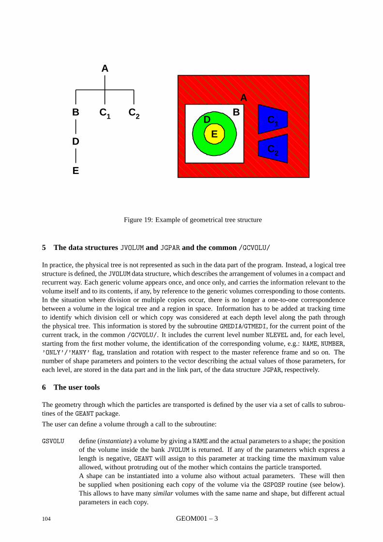
C1
C2
BA
DE
A
B
D
E
C1 C2
Figure 19: Example of geometrical tree structure
5 The data structures JVOLUM and JGPAR and the common /GCVOLU/
In practice, the physical tree is not represented as such in the data part of the program. Instead, a logical treestructure is defined, the JVOLUM data structure, which describes the arrangement of volumes in a compact andrecurrent way. Each generic volume appears once, and once only, and carries the information relevant to thevolume itself and to its contents, if any, by reference to the generic volumes corresponding to those contents.In the situation where division or multiple copies occur, there is no longer a one-to-one correspondencebetween a volume in the logical tree and a region in space. Information has to be added at tracking timeto identify which division cell or which copy was considered at each depth level along the path throughthe physical tree. This information is stored by the subroutine GMEDIA/GTMEDI, for the current point of thecurrent track, in the common /GCVOLU/. It includes the current level number NLEVEL and, for each level,starting from the first mother volume, the identification of the corresponding volume, e.g.: NAME, NUMBER,’ONLY’/’MANY’ flag, translation and rotation with respect to the master reference frame and so on. Thenumber of shape parameters and pointers to the vector describing the actual values of those parameters, foreach level, are stored in the data part and in the link part, of the data structure JGPAR, respectively.
6 The user tools
The geometry through which the particles are transported is defined by the user via a set of calls to subrou-tines of the GEANT package.
The user can define a volume through a call to the subroutine:
GSVOLU define (instantiate) a volume by giving a NAME and the actual parameters to a shape; the positionof the volume inside the bank JVOLUM is returned. If any of the parameters which express alength is negative, GEANT will assign to this parameter at tracking time the maximum valueallowed, without protruding out of the mother which contains the particle transported.A shape can be instantiated into a volume also without actual parameters. These will thenbe supplied when positioning each copy of the volume via the GSPOSP routine (see below).This allows to have many similar volumes with the same name and shape, but different actualparameters in each copy.
104 GEOM001 – 3
The user can position a volume through a call to either one of the following subroutines:
GSPOS position a copy of a volume inside its mother with respect to the mother’s reference system.A a point in space, a rotation matrix index, a copy number and the ’ONLY’/’MANY’ flag aresupplied;
GSPOSP position a copy of a volume which has been instantiated without actual parameters inside itsmother with respect to the mother reference system. The parameters of the copy being posi-tioned are supplied as well. The volumes will be identified by name and copy number as formultiple copies of the same volume.
The user can divide a volume through a call to either one of the following subroutines:
GSDVN divide a volume in a given number of cells completely filling the mother. In this case the celltracking medium is assumed to be the same as for the mother. See also GSDVN2.
GSDVT divide a volume with slices of a given step. The cell tracking medium can be different from theone of the mother. See also GSDVT2.
GSDVX divide a volume starting from a given offset. In addition to STEP and NDIV (with at least one ofthem positive to be effectively useful), the origin of the first cell, the cell tracking medium andeventually the computed (maximum) number of divisions must be specified.
7 Geometrical information retrieval
The parameters of a volume may depend on the physical tree which leads to this volume. The dimensions ofone of the slices of a cone divided along Z depends on which slice we consider. So a volume is completelydefined only if we specify the path in the tree. This is composed by the name and copy number of thevolumes containing the one we are interested in, from the first mother.
Given this information, the routine GLVOLU is capable to fill the common /GCVOLU/, and the structure JGPARwith the actual parameters of the instance chosen.
GEOM001 – 4 105
Geant 3.21 GEANT User’s Guide GEOM010
Origin : Submitted: 10.03.94Revision : Revised: 10.03.94Documentation : S.Giani, S.Ravndal
Tracking inside volumes and optimisation
The tracking of particles through the geometrical data structure is the key functionality of GEANT. At everyparticle’s step, the program must find the volume where the particle is (GTMEDI) and the next boundary itwill cross (GTNEXT). This can take about 60% of the total simulation time (even for detectors described inan optimized way); therefore, a new logic has been introduced to minimize the time spent for the search inthe geometrical tree.
1 Virtual divisions
Instead of a linear or binary search (time spent proportional or logarithmic with the number of volumes,respectively), a ‘direct access’ technique has been developed to make the time basically independent fromthe number of volumes. Every volume containing other volumes is ‘virtually’ divided in equal slices atinitialization time via the call to GGCLOS (the best axis is computed automatically). For each slice, a datastructure is filled with a list of the volumes identifiers intersecting such slice. Slices with identical listsare pointing to the same contents and are collected. At tracking time it is immediate to find in which slicethe particle is and only its contents have to be checked. The same is true to find the next boundary to becrossed: only if the intersection point with a content lies outside the current collection of slices, the nextone will be checked. The algorithm gives in average about a factor 2 in speed for the overall simulation inthe large detectors. It also minimizes the dependency of the performance on the skill and experience of theprogrammer and allows a fast tracking even in geometrical structures received from CAD systems.
2 Other optimisation tools
The following facilities are kept for backward compatibility reasons. If called by the user, these optimisationtools are called at initialisation time, but not used at tracking time. Instead, the new optimisation using’virtual divisions’ is performed. If the user wants to use the older optimisation tools, he can recompileGEANT 3.21 using the PATCHY flag +OLD.
1. GSORD/GGORD
From the position of the contents inside a given volume, the subroutine GSORD computes fictitiousboundaries along the specified coordinate, simulating a division with irregular step size. A binarysearch technique is used to identify within which pseudo-cell the current point is. The slow processof computing whether the point is inside or outside the contents is therefore limited to the few (if any)volumes overlapping with that pseudo-cell, as sketched in fig 20.
The coordinate selected for the pseudo division can be any of X, Y, Z, Rxy, R, φ or θ;. For agiven volume, the call to GSORD has to come after all its first level contents have been positioned.
2. GSNEXT/GSNEAR
when a particle exits from a daugther of a mother volume, the contents are scanned initially in theorder in which they have been positioned, and the user should take care over the best sequence ofGSPOS calls. However, when the particle comes back inside the mother from any one of the contents,it is usually possible to limit the search to the neighbour contents. The subroutines GSNEXT/GSNEARpermit the user to inject, at initialisation time, for each content in turn, the list of neighbours to searchfor. GSNEAR is recommended, GSNEXT is kept for backward, compatibility and has a different defaultoption. A proper use of this facility can reduce the search time significantly.
106 GEOM010 – 1

1 2 3 4 5 6 7
0 1 2 1 0 1 0
Figure 20: Example of pseudo-cells created by GSORD
3. GSUNEA/GUNEAR
The volumes to be checked when exiting from one daughter can depend on the direction and positionof the exiting particles. To optimise tracking taking into account these dynamic features, the user cancode the GUNEAR routine, and inform GEANT that it has to use it at tracking time by calling the GSUNEAroutine.
GEOM010 – 2 107
Geant 3.21 GEANT User’s Guide GEOM020
Origin : Submitted: 22.03.94Revision : Revised: 22.03.94Documentation : S.Giani, S.Ravndal
“ MANY” Volumes and boolean operations on volumes
The topology of GEANT is given by 16 general shapes which are used to represent solids in the design ofdetectors. These shapes are bounded by 2-nd order surfaces for reasons of speed at tracking time. Newtools have been introduced to extend the power of the GEANT geometry: boolean operations (union, inter-section and subtraction) between such shapes are now allowed, so that an infinity of new shapes can bebuilt; divisions along arbitrary axis are now possible, allowing to exploit any simmetry in the design. Thetracking is now able to handle overlapping volumes in the most general sense: the concept of MANY volumeshas been extended to automatic clipping for protuding objects. Thanks to this MANY technique, any 3D or2D geometrical pattern can be reduced to a single dimensional structure, basically cancelling the need forGUNEAR at tracking time. Finally, more than one order of magnitude in speed has been gained compared tothe old step search algorithm used to track in MANY volumes.
• Topological extensions via boolean operations.
• Divisions along arbitrary axis.
• Reduction of 2D structure to 1D structure.
• Logic and algorithm.
1 Topological extensions via boolean operations
Boolean operations between a given set of shapes allow the creation of an infinite number of shapes. Addinga single new primitive (for ex. a toroid) to the basic set of shapes, all the possible combinations with all theold shapes become moreover possible.
• UNION: the union of two volumes B and C is obtained positioning two overlapping ‘MANY’ daughtersB and C inside the same mother A. To identify the result of the union as a single volume is enough tocreate a SET associated to the volumes B and C.
• SUBTRACTION: the subtraction of a volume B from a volume C is obtained positioning B as ‘ONLY’and C as a ‘MANY’ overlapping B. The result of the subtraction is automatically what the trackingsees as the C volume, so GSPOS is the only user interface needed. The volume B can have the samematerial as the mother A or not. The normal positioning technique used for ‘ONLYs’ is a particularcase of boolean subtraction (a volume is contained inside the other).
• INTERSECTION: the intersection of two volumes B and C is obtained positioning a protuding ‘MANY’object C in a ‘MANY’ object B which is normally placed in a ‘ONLY’ mother A. A and B must have thesame material, while C has the material asked for the intersection. The intersection is given by thepart of C which is not protuding from B, therefore by what the new tracking sees as the volume C:again the only needed user interface is GSPOS. If not interacting with other daughters of A, B couldalso be ‘ONLY’. Without any ambiguity, even further ‘MANY’ daughters of A can overlap the protudingpart of C outside B, because it is really invisible to the new tracking.
108 GEOM020 – 1
2 Divisions along arbitrary axis
As protuding MANY daughters are automatically clipped by their mother, it is possible to divide objects alongarbitrary directions. Suppose for example that we want to divide a PCON into planar slices parallel to theplane X + Y = 0; it is enough to position a MANY BOX embedding completely the PCON ‘inside’ the PCONitself; the BOX must be rotated of 45 degrees in X and Y and then divided along one of its natural axis.Another example can be the following: suppose we want to divide 24 times in PHI a PGON with only 6natural segmentations in PHI; then we have to position a MANY TUBE, completely embedding the PGON,‘inside’ the PGON itself; again, we can now divide the tube in 24 slices in PHI and the tracking will seeonly the PGON divided 24 times in PHI.
Reduction of 2D structure to 1D structure.
Sometimes there are complicated multidimensional geometrical structures (like honeycombs, spaghetti, etc.)which can be reduced to the overlap of several one-dimensional patterns (for which divisions can be usedor virtual divisions are particularly efficient). The MANY option allows to superimpose such 1D structures toreproduce the multi-dimensional ones in a very effective way, instead of positioning the volumes one by onein the 2D or 3D pattern. The following picture will explain better this concept.
3 Logic and algorithm
In GTMEDI, all the ’MANY’ volumes for which the point is found inside (and not in any of its daughters) isput in a stack saving also its branch of the tree. The point is considered to be in the deepest level ’MANY’.Each time the point is also found in an intermediate ’ONLY’ volume the stack is cleared (to insure booleansubtraction). In GTNEXT, if stepping inside a ’MANY’ volume, not ONLY its daughters and its own boundariesare checked, but also the daughters and the boundaries of all the others ’MANY’ in the list have to be checked.This is not yet enough: the logic requires that the boundaries of all the possible overlapping volumes arechecked, so it is also necessary for each ‘MANY’ volume of the list to go up to the first ’ONLY’ mother inthe tree repeating the same procedure. This allows also boolean intersection. Obviously, volumes alreadychecked are not checked again.
GEOM020 – 2 109
Geant 3.16 GEANT User’s Guide GEOM050
Origin : R.Brun, A.McPherson Submitted: 15.08.83Revision : Revised: 08.11.93Documentation :
The GEANT shapes
The GEANT geometry package offers sixteen basic shapes with which to describe the setups where particlesare transported. In this section we will describe these shapes. For each shape figs (21), (22), (23), (24) showa simple drawing illustrating the meaning of the parameters and the position and orientation of the referenceframe proper of that shape. A description of the shapes and of their parameters follows. Angles are alwaysin degrees. With every shape is given the code which is used internally by GEANT to identify it.
1 BOX box with faces perpendicular to the axes. It has 3 parameters:
1.DX half-length of the box along the x-axis;
2.DY half-length of the box along the y-axis;
3.DZ half-length of the box along the z-axis;
2 TRD1 trapezoid with the x dimension varying along z. It has 4 parameters:
1.DX1 half-length along x at the z surface positioned at -DZ;
2.DX2 half-length along x at the z surface positioned at +DZ;
3.DY half-length along the y-axis;
4.DZ half-length along the z-axis;
3 TRD2 trapezoid with both x and y dimensions varying along z. It has 5 parameters:
1.DX1 half-length along x at the z surface positioned at -DZ;
2.DX2 half-length along x at the z surface positioned at +DZ;
3.DY1 half-length along y at the z surface positioned at -DZ;
4.DY2 half-length along y at the z surface positioned at +DZ;
5.DZ half-length along the z-axis;
4 TRAP general trapezoid: the faces perpendicular to z are trapezia and their centres are not necessarilyon a line parallel to the z axis. This shape has 11 parameters, but only considering that thefaces should be planar, only 9 are really independent. A check is performed on the user param-eters and a message is printed in case of non-planar faces. Ignoring this warning may causeunpredictable effect at tracking time.
1.DZ half-length along the z axis;
2.THET polar angle of the line joining the centre of the face at -DZ to the centre of the oneat +DZ;
3.PHI azimuthal angle of the line joining the centre of the face at -DZ to the centre of theone at +DZ;
4.H1 half-length along y of the face at -DZ;
5.BL1 half-length along x of the side at -H1 in y of the face at -DZ in z;
6.TL1 half-length along x of the side at +H1 in y of the face at -DZ in z;
7.ALP1 angle with respect to the y axis from the centre of the side at -H1 in y to the centreof the side at +H1 in y of the face at -DZ in z;
8.H2 half-length along y of the face at +DZ;
110 GEOM050 – 1

9.BL2 half-length along x of the side at -H2 in y of the face at +DZ in z;
10.TL2 half-length along x of the side at +H2 in y of the face at +DZ in z;
11.ALP2 angle with respect to the y axis from the centre of the side at -H2 in y to the centreof the side at +H2 in y of the face at +DZ in z;
5 TUBE tube. It has 3 parameters:
1.RMIN inside radius;
2.RMAX outside radius;
3.DZ half length in z;
6 TUBS φ segment of a tube. It has 5 parameters:
1.RMIN inside radius;
2.RMAX outside radius;
3.DZ half length in z;
4.PHI1 starting angle of the segment;
5.PHI2 ending angle of the segment;
PHI1 should be smaller than PHI2. If this is not the case, the system adds 360 degrees to PHI2.
7 CONE conical tube. It has 5 parameters:
1.DZ half-length in z;
2.RMN1 inside radius at -DZ in z;
3.RMX1 outside radius at -DZ in z;
4.RMN2 inside radius at +DZ in z;
5.RMX2 outside radius at +DZ in z;
8 CONS φ segment of a conical tube. It has 7 parameters:
1.DZ half-length in z;
2.RMN1 inside radius at -DZ in z;
3.RMX1 outside radius at -DZ in z;
4.RMN2 inside radius at +DZ in z;
5.RMX2 outside radius at +DZ in z;
6.PHI1 starting angle of the segment;
7.PHI2 ending angle of the segment;
PHI1 should be smaller than PHI2. If this is not the case, the system adds 360 degrees to PHI2.
9 SPHE segment of spherical shell. It has 6 parameters:
1.RMIN inside radius of the shell;
2.RMAX outside radius of the shell;
3.THE1 starting polar angle of the shell;
4.THE2 ending polar angle of the shell;
5.PHI1 starting azimuthal angle of the shell;
6.PHI2 ending azimuthal angle of the shell;
10 PARA parallelepiped. It has 6 parameters:
1.DX half-length in x;
2.DY half-length in y;
3.DZ half-length in z;
GEOM050 – 2 111
4.ALPH angle formed by the y axis and by the plane joining the centre of the faces parallelto the z-x plane at -DY and +DY;
5.THET polar angle of the line joining the centres of the faces at -DZ and +DZ in z;
6.PHI azimuthal angle of the line joining the centres of the faces at -DZ and +DZ in z;
11 PGON polygon. It has at least 10 parameters:
1.PHI1 the azimuthal angle φ at which the volume begins (angles are counted counterclock-wise);
2.DPHI opening angle of the volume, which extends from PHI1 to PHI1+DPHI;
3.NPDV number of sides of the cross section between the given φ limits;
4.NZ number of planes perpendicular to the z axis where the dimension of the section isgiven – this number should be at least 2 and NP triplets of numbers must follow;
5.Z z coordinate of the section;
6.RMIN radius of the circle tangent to the sides of the inner polygon in the cross-section;
7.RMAX radius of the circle tangent to the sides of the outer polygon in the cross-section;
12 PCON polycone. It has at least 9 parameters:
1.PHI1 the azimuthal angle φ at which the volume begins (angles are counted counterclock-wise);
2.DPHI opening angle of the volume, which extends from PHI1 to PHI1+DPHI;
3.NZ number of planes perpendicular to the z axis where the dimension of the section isgiven – this number should be at least 2 and NP triplets of numbers must follow;
4.Z z coordinate of the section;
5.RMIN radius of the inner circle in the cross-section;
6.RMAX radius of the outer circle in the cross-section;
13 ELTU elliptical cross-section tube. It has three parameters:
1.P1 semi-axis of the ellipse along x;
2.P2 semi-axis of the ellipse along y;
3.DZ half-length in z;
The equation of the surface is x2P1−2 + y2P2−2 = 1.
14 HYPE hyperbolic tube, i.e. the inner and outer surfaces are hyperboloids, as would be formed by asystem of cylindrical wires which were then rotated tangentially about their centres. It has 4parameters:
1.RMIN inner radius at z=0, where tube is narrowest;
2.RMAX outer radius at z=0, where tube is narrowest;
3.DZ half-length in z;
4.THET stereo angle of rotation of the two faces;
The hyperbolic surfaces are given by: r2 = (z tan θ)2 + r2z=0
28 GTRA general twisted trapezoid: the faces perpendicular to z are trapezia and their centres are notnecessarily on a line parallel to the z axis as the TRAP; additionally, the faces may be twistedso that none of their edges are parallel. It is a TRAP shape, except that it is twisted in the x-yplane as a function of z. The parallel sides perpendicular to the z axis are rotated with respectto the x axis by an angle TWIST, which is one of the parameters. The shape is defined by theeight corners and is assumed to be constructed of straight lines joining points on the boundaryof the trapezoidal face at z=-DZ to the corresponding points on the face at z=DZ. Divisions arenot allowed. It has 12 parameters:
112 GEOM050 – 3
1.DZ half-length along the z axis;
2.THET polar angle of the line joining the centre of the face at -DZ to the centre of the oneat +DZ;
3.PHI azimuthal angle of the line joining the centre of the face at -DZ to the centre of theone at +DZ;
4.TWIST twist angle of the faces parallel to the x-y plane at z = ±DZ around an axis parallelto z passing through their centre;
5.H1 half-length along y of the face at -DZ;
6.BL1 half-length along x of the side at -H1 in y of the face at -DZ in z;
7.TL1 half-length along x of the side at +H1 in y of the face at -DZ in z;
8.ALP1 angle with respect to the y axis from the centre of the side at -H1 in y to the centreof the side at +H1 in y of the face at -DZ in z;
9.H2 half-length along y of the face at +DZ;
10.BL2 half-length along x of the side at -H2 in y of the face at +DZ in z;
11.TL2 half-length along x of the side at +H2 in y of the face at +DZ in z;
12.ALP2 angle with respect to the y axis from the centre of the side at -H2 in y to the centreof the side at +H2 in y of the face at +DZ in z;
Note: this shape suffers from the same limitations than the TRAP: the tracking routines assumethat the faces are planar, but this constraint is not easily expressed in terms of the 12 parameters.Additionally, no check on the faces is performed in this case. Users should avoid to use thisshape as much as possible, and if they have to do so, they should make sure that the faces arereally planes. If this is not the case, the result of the transport is unpredictable.To accelerate the computations necessary for transport, 18 additional parameters are calculatedfor this shape:
1.DX0DZ dx/dz of the line joining the centres of the faces at z=±DZ;
2.DY0DZ dy/dz of the line joining the centres of the faces at z=±DZ;
3.X01 x at z=0 for line joining the + on parallel side, perpendicular corners at z=±DZ;
4.Y01 y at z=0 for line joining the + on parallel side, + on perpendicular corners at z=±DZ;
5.DXDZ1 dx/dz for line joining the + on parallel side, + on perpendicular corners at z=±DZ;
6.DYDZ1 dy/dz for line joining the + on parallel side, + on perpendicular corners at z=±DZ;
7.X02 x at z=0 for line joining the - on parallel side, + on perpendicular corners at z=±DZ;
8.Y02 y at z=0 for line joining the - on parallel side, + on perpendicular corners at z=±DZ;
9.DXDZ2 dx/dz for line joining the - on parallel side, + on perpendicular corners at z=±DZ;
10.DYDZ2 dy/dz for line joining the - on parallel side, + on perpendicular corners at z=±DZ;
11.X03 x at z=0 for line joining the - on parallel side, - on perpendicular corners at z=±DZ;
12.Y03 y at z=0 for line joining the - on parallel side, - on perpendicular corners at z=±DZ;
13.DXDZ3 dx/dz for line joining the - on parallel side, - on perpendicular corners at z=±DZ;
14.DYDZ3 dy/dz for line joining the - on parallel side, - on perpendicular corners at z=±DZ;
15.X04 x at z=0 for line joining the + on parallel side, - on perpendicular corners at z=±DZ;
16.Y04 y at z=0 for line joining the + on parallel side, - on perpendicular corners at z=±DZ;
17.DXDZ4 dx/dz for line joining the + on parallel side, - on perpendicular corners at z=±DZ;
18.DYDZ4 dy/dz for line joining the + on parallel side, - on perpendicular corners at z=±DZ;
29 CTUB cut tube, a tube cut at the extremities with planes not necessarily perpendicular to the z axis. Ithas 11 parameters:
GEOM050 – 4 113

1.RMIN inside radius;
2.RMAX outside radius;
3.DZ half length in z;
4.PHI1 starting angle of the segment;
5.PHI2 ending angle of the segment;
6.LX x component of a unit vector perpendicular to the face at -DZ;
7.LY y component of a unit vector perpendicular to the face at -DZ;
8.LZ z component of a unit vector perpendicular to the face at -DZ;
9.HX x component of a unit vector perpendicular to the face at +DZ;
10.HY y component of a unit vector perpendicular to the face at +DZ;
11.HZ z component of a unit vector perpendicular to the face at +DZ;
PHI1 should be smaller than PHI2. If this is not the case, the system adds 360 degrees to PHI2.
114 GEOM050 – 5
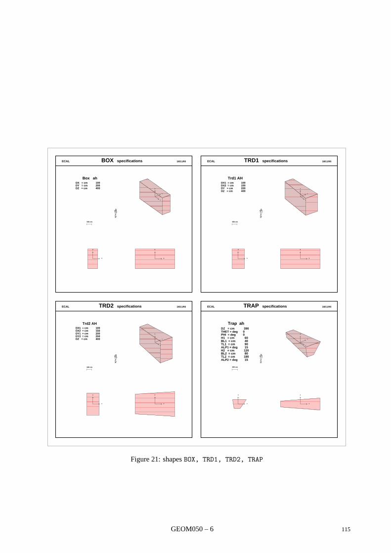
ECAL BOX specifications 18/11/93
Box ahDX = cm 100 DY = cm 200 DZ = cm 400
100 cm
x
y
z
x
y y
z
ECAL TRD1 specifications 18/11/93
Trd1 AHDX1 = cm 100 DX2 = cm 150 DY = cm 200 DZ = cm 400
100 cm
x
y
z
x
y y
z
ECAL TRD2 specifications 18/11/93
Trd2 AHDX1 = cm 100 DX2 = cm 150 DY1 = cm 200 DY2 = cm 250 DZ = cm 400
100 cm
x
y
z
x
y y
z
ECAL TRAP specifications 18/11/93
Trap ahDZ = cm 390 THET = deg 0 PHI = deg 0 H1 = cm 60 BL1 = cm 40 TL1 = cm 90 ALP1 = deg 15 H2 = cm 120 BL2 = cm 80 TL2 = cm 180 ALP2 = deg 15
100 cm
x
y
z
x
y y
z
Figure 21: shapes BOX, TRD1, TRD2, TRAP
GEOM050 – 6 115
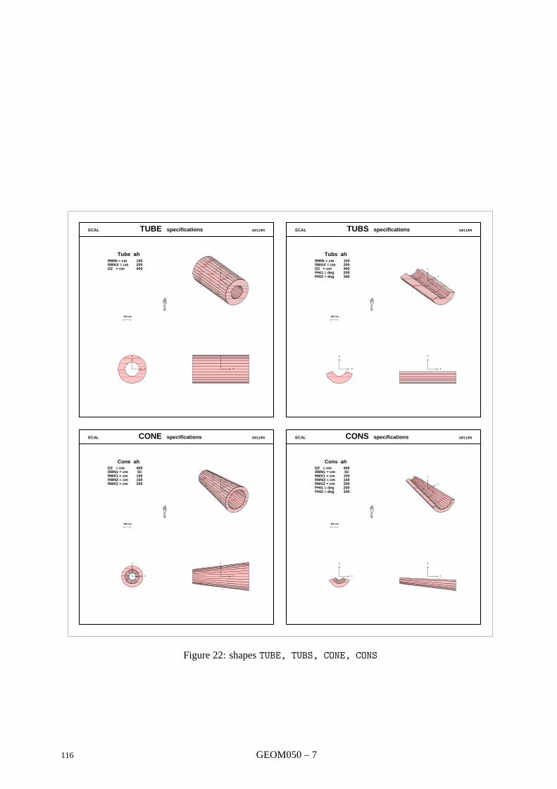
ECAL TUBE specifications 18/11/93
Tube ahRMIN = cm 100 RMAX = cm 200 DZ = cm 400
100 cm
x
y
z
x
y y
z
ECAL TUBS specifications 18/11/93
Tubs ahRMIN = cm 100 RMAX = cm 200 DZ = cm 400 PHI1 = deg 200 PHI2 = deg 340
100 cm
x
y
z
x
y y
z
ECAL CONE specifications 18/11/93
Cone ahDZ = cm 400 RMN1 = cm 50 RMX1 = cm 100 RMN2 = cm 150 RMX2 = cm 200
100 cm
x
y
z
x
y y
z
ECAL CONS specifications 18/11/93
Cons ahDZ = cm 400 RMN1 = cm 50 RMX1 = cm 100 RMN2 = cm 150 RMX2 = cm 200 PHI1 = deg 200 PHI2 = deg 340
100 cm
x
y
z
x
y y
z
Figure 22: shapes TUBE, TUBS, CONE, CONS
116 GEOM050 – 7
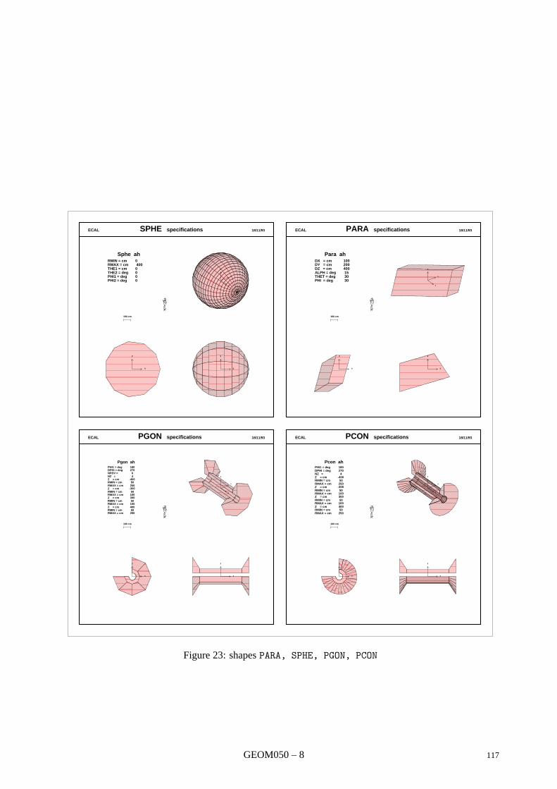
ECAL SPHE specifications 18/11/93
Sphe ahRMIN = cm 0 RMAX = cm 400 THE1 = cm 0 THE2 = deg 0 PHI1 = deg 0 PHI2 = deg 0
100 cm
x
y
z
x
y y
z
ECAL PARA specifications 18/11/93
Para ahDX = cm 100 DY = cm 200 DZ = cm 400 ALPH = deg 15 THET = deg 30 PHI = deg 30
100 cm
x
y
z
x
y y
z
ECAL PGON specifications 18/11/93
Pgon ahPHI1 = deg 180 DPHI = deg 270 NPDV = 6 NZ = 4 Z = cm -400 RMIN = cm 50 RMAX = cm 250 Z = cm -300 RMIN = cm 50 RMAX = cm 100 Z = cm 300 RMIN = cm 50 RMAX = cm 100 Z = cm 400 RMIN = cm 50 RMAX = cm 250
100 cm
x
y
z
x
y y
z
ECAL PCON specifications 18/11/93
Pcon ahPHI1 = deg 180 DPHI = deg 270 NZ = 4 Z = cm -400 RMIN = cm 50 RMAX = cm 250 Z = cm -300 RMIN = cm 50 RMAX = cm 100 Z = cm 300 RMIN = cm 50 RMAX = cm 100 Z = cm 400 RMIN = cm 50 RMAX = cm 250
100 cm
x
y
z
x
y y
z
Figure 23: shapes PARA, SPHE, PGON, PCON
GEOM050 – 8 117
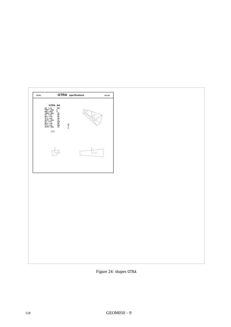
ECAL GTRA specifications 18/11/93
GTRA AHDZ = cm 390 THET = deg 0 PHI = deg 0 TWIS = deg 20 H1 = cm 60 BL1 = cm 40 TL1 = cm 90 ALP1 = deg 15 H2 = cm 120 BL2 = cm 80 TL2 = cm 180 ALP2 = deg 15
100 cm
x
y
z
x
y y
z
Figure 24: shapes GTRA
118 GEOM050 – 9
Geant 3.16 GEANT User’s Guide GEOM100
Origin : R.Brun,A.McPherson Submitted: 15.08.83Revision : Revised: 16.11.93Documentation :
Creation of a volume
CALL GSVOLU (CHNAME,CHSHAP,NMED,PAR,NPAR,IVOLU*)
Defines a volume with a given name, shape, tracking medium number and shape parameters.
CHNAME (CHARACTER*4) volume name – it must be unique;
CHSHAP (CHARACTER*4) name of one of the GEANT shapes;
NMED (INTEGER) tracking medium number for the volume – if other volumes are positioned withinthis one, their tracking medium replaces the one of the mother;
PAR (REAL) array containing the shape parameters;
NPAR (INTEGER) number of parameters – if zero, then the volume must be positioned via the routineGSPOSP indicating the parameters for each copy (see [GEOM120]);
IVOLU (INTEGER) internal volume number – if ≤ 0 an error condition has happened.
If one of the parameters expressing a length is negative, GEANT will try to maximise its value in each copy,without extending beyond the limits of the mother. This facility can be used in conjunction with the divisionof volumes using GSDVN, GSDVT, and GSDVX. Restriction apply to this facility:
• the daughter should be positioned without a rotation matrix;
• all shapes can be positioned within a similar shape with negative parameters, but only in the centre ofthe mother;
• boxes with negative parameters can be positioned in: box, TRD1, TRD2 and TRAP with θ = φ = 0;
• HYPE, ELTU and CTUB cannot have negative parameters;
• PCON and PGON can only have 2 z planes.
Examples
DIMENSION PECAL(3)DATA PECAL/1.71,4.,0.2/
CALL GSVOLU(’ECAL’,’BOX ’,1,PECAL,3,IVOLU)
CALL GPVOLU (IVOLU)
Prints the volume parameters:
IVOLU (INTEGER) GEANT number of the volume to print – if IVOLU ≤ 0, all volumes will be printed;
119 GEOM100 – 1
Geant 3.16 GEANT User’s Guide GEOM110
Origin : R.Brun, A.McPherson Submitted: 15.08.83Revision : Revised: 16.11.93Documentation :
Positioning a volume inside its mother
CALL GSPOS (CHNAME,NR,CHMOTH,X,Y,Z,IROT,CHONLY)
Places a copy of a volume previously defined by a call to GSVOLU inside its mother volume CHMOTH.
CHNAME (CHARACTER*4) name of the volume being positioned;
NR (INTEGER) copy number of the volume CHNAME being positioned;
CHMOTH (CHARACTER*4) name of the volume in which copy NR of CHNAME is positioned;
X (REAL) x position of the volume in the mother reference system;
Y (REAL) y position of the volume in the mother reference system;
Z (REAL) z position of the volume in the mother reference system;
IROT (INTEGER) rotation matrix number describing the orientation of the volume relative to thecoordinate system of the mother;
CHONLY (CHARACTER*4) flag to indicate whether a point found to be in this volume may also be inother volumes which are not direct descendants of it – possible values are ONLY and MANY.
The following points are important for a correct use of GSPOS:
• the position and rotation with which a volume is positioned are relative to the mother reference system,that is to the reference system of the volume which contains the copy being positioned. To see howthe reference system is defined for the GEANT shapes, see [GEOM050];
• GSPOS can be called several times with the same name, to place multiple copies of the same volumeeither in the same mother volume or in different ones. The copy number parameter NR is user defined,and it allows the different copies of the same volume to be distinguished. The user is free to assignany valid integer to this parameter. If two volumes are positioned with the same copy number, it willbe impossible to decide in which one a particle is during tracking. If the same volume is positionedtwice inside the same mother with the same copy number, the parameters of the second call to GSPOSwill override the first ones for that copy;
• all the copies of a volume are identical: in particular they contain all the same daughters recursively –conversely, positioning a volume inside a mother will insert it in all the copies of that mother;
• the volumes mentioned in the call must be already defined by a call to GSVOLU;
• no volume can be positioned in a divided mother;
• in case of positioning without rotation, IROT should be set to 0 – note that this is faster than defininga unit matrix;
• the first volume, containing all the apparatus, cannot be positioned;
• if the CHONLY flag is equal to ONLY, the volume being positioned should not overlap with any othervolume except his mother and his daughters and should not extend beyond the limits of its mother.In this case the search routines assume that, when a point is found in this volume, the only furthersearching required is in its contents. Other volumes at the same or higher levels or in separate brancheswill not be looked at. The first volume must be ONLY;
120 GEOM110 – 1
• if the CHONLY flag is set to MANY, a point found in this volume can also be in another volume at thesame or higher level or in a different branch of the tree. To decide where a point is the followingalgorithm is applied:
1. the tree is scanned upward until an ONLY mother with positioned contents (i.e. non-divided) isfound;
2. all the branches of the tree descending from this volume are scanned to find other volumes wherethe point may be;
3. a winner is selected among the candidates according to the following rules:
– if one of the candidates is ONLY, the point is declared in this volume. If more than onecandidate is ONLY there is an error in the geometry definition;
– amongst several MANY candidates, the one at the deepest level is chosen;
– amongst several MANY candidates at the same level, the first one found is chosen;
Although a considerable effort has been put in making sure that the MANY option works properly andcaters for all the possible cases, still it introduces a considerable complication in the tracking andperformance can be rather poor.
Users should resort to this only when it is not possible to describe the experimental setup with ONLYvolumes.
The data structure is so designed that, in any case, the parameters of a volume and the information aboutthe number and position of its daughters are stored only once. This allows the creation of very complexgeometries without correspondingly large storage requirements.
GEOM110 – 2 121
Geant 3.16 GEANT User’s Guide GEOM120
Origin : R.Brun, F.Bruyant, M.Maire, A.McPherson Submitted: 15.08.83Revision : Revised: 18.11.93Documentation :
Positioning a volume inside its mother with parameters
CALL GSPOSP (CHNAME,NR,CHMOTH,X,Y,Z,IROT,CHONLY,PAR,NPAR)
Position a copy of volume CHNAME inside its mother CHMOTH assigning its parameters.
CHNAME (CHARACTER*4) name of the volume being positioned;
NR (INTEGER) copy number of the volume CHNAME being positioned;
CHMOTH (CHARACTER*4) name of the volume in which copy NR of CHNAME is positioned;
X (REAL) x position of the volume in the mother reference system;
Y (REAL) y position of the volume in the mother reference system;
Z (REAL) z position of the volume in the mother reference system;
IROT (INTEGER) rotation matrix number describing the orientation of the volume relative to thecoordinate system of the mother;
CHONLY (CHARACTER*4) flag to indicate whether a point found to be in this volume may also be inother volumes which are not direct descendants of it – possible values are ONLY and MANY;
PAR (REAL) array of parameters for the volume being positioned;
NPAR (INTEGER) number of parameters.
It is often the case in a detector to have a family of similar objects, differing only by their dimensions. Atypical example are the crystals of an electromagnetic calorimeter. In this case it is convenient and logicallyconsistent to give them all the same name, but assign to each copy a different set of parameters.
This can be done defining the volume with 0 parameters through the routine GSVOLU and then assigning theparameters to each copy via the routine GSPOSP.
GSPOSP is similar in all other aspects to GSPOS and the user is referred to the description of this routine formore information. An obvious limitation is that a volume defined with 0 parameters can only be positionedvia GSPOSP, because otherwise its dimensions will be undefined.
122 GEOM120 – 1
Geant 3.16 GEANT User’s Guide GEOM130
Origin : R.Brun, A.McPherson Submitted: 29.09.83Revision : Revised: 18.11.93Documentation :
Division of a volume into a given number of cells
CALL GSDVN (CHNAME,CHMOTH,NDIV,IAXIS)
Divide a volume in a given number of parts along a direction.
CHNAME (CHARACTER*4) a unique name for the volume to be generated by subdivision of the mothervolume;
CHMOTH (CHARACTER*4) volume that has to be subdivided;
NDIV (INTEGER) number of divisions into which the mother volume is to be divided;
IAXIS (INTEGER) axis of the division.
The volumes resulting from a division are true volumes in the GEANT sense, with the only limitation thatthey cannot be positioned. They can have daughters and they can still be divided in turn. Different divisionsare distinguished by a different division number, much the same as different copy of the same volume by thecopy number. Every operation performed on a division cell (positioning or further division), is automaticallypropagated to all divisions cells of the same mother.
The kind of the division is indicated by the IAXIS argument. The allowed values of IAXIS and the resultingdivisions are shown in figs. 25, 26, 27, 28, where the pictures in the first column correspond to an IAXISvalue equal to 1, the second column to IAXIS = 2, and the third column to IAXIS = 3 respectivly. The basicconstraint imposed by the GEANT geometry is that the result of a division is a volume which can be describedin terms of the basic shapes.
The local coordinate system of the divisions is parallel to the system of the mother in case of divisionsobtained by parallel planes or concentric divisions. In the case of parallel axes the coordinate system isshifted so that it is in the centre of the division. In case of φ divisions produced by planes passing throughthe axis of a volume with axial symmetry (TUBE, TUBS, CONE, CONS, PGON, PCON, SPHE), the localcoordinate systems will be rotated so that the x axis passes through the centre of the division.
This routine allows the user to generate a large number of identical volumes filling a defined volume. Thematerial of the slices is inherited from the mother.
It may happen that the different divisions of a volume have different dimensions. In this case, if a volumehas to be positioned in each division, its dimensions must be different according to the division number.This can be obtained in some special cases giving to the dimension of the volume which has to vary in orderto fit into the different mothers, the value of -1 in the call to GSVOLU which defines it. As explained in[GEOM050], GEANT will take care to assign to this dimension the maximum value in order to fill the currentmother.
What can be done with division can be done also, in most cases, explicitly positioning all the copies. Usersmust be aware, however, that divisions offer the best performance in tracking of all GEANT geometricalconstructs, and they should be used instead of positioning whenever possible in the definition of objects.
123 GEOM130 – 1
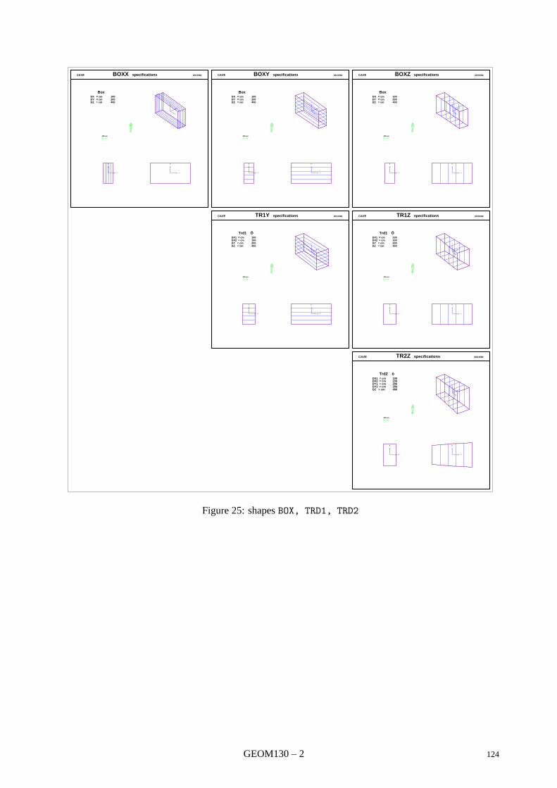
CAVE BOXX specifications 20/10/94
Box DX = cm 100 DY = cm 200 DZ = cm 400
100 cm
x
y
z
x
y y
z
CAVE BOXY specifications 20/10/94
Box DX = cm 100 DY = cm 200 DZ = cm 400
100 cm
x
y
z
x
y y
z
CAVE BOXZ specifications 20/10/94
Box DX = cm 100 DY = cm 200 DZ = cm 400
100 cm
x
y
z
x
y y
z
CAVE TR1Y specifications 20/10/94
Trd1 ÔDX1 = cm 100 DX2 = cm 150 DY = cm 200 DZ = cm 400
100 cm
x
y
z
x
y y
z
CAVE TR1Z specifications 20/10/94
Trd1 ÔDX1 = cm 100 DX2 = cm 150 DY = cm 200 DZ = cm 400
100 cm
x
y
z
x
y y
z
CAVE TR2Z specifications 20/10/94
Trd2 öDX1 = cm 100 DX2 = cm 150 DY1 = cm 200 DY2 = cm 250 DZ = cm 400
100 cm
x
y
z
x
y y
z
Figure 25: shapes BOX, TRD1, TRD2
GEOM130 – 2 124
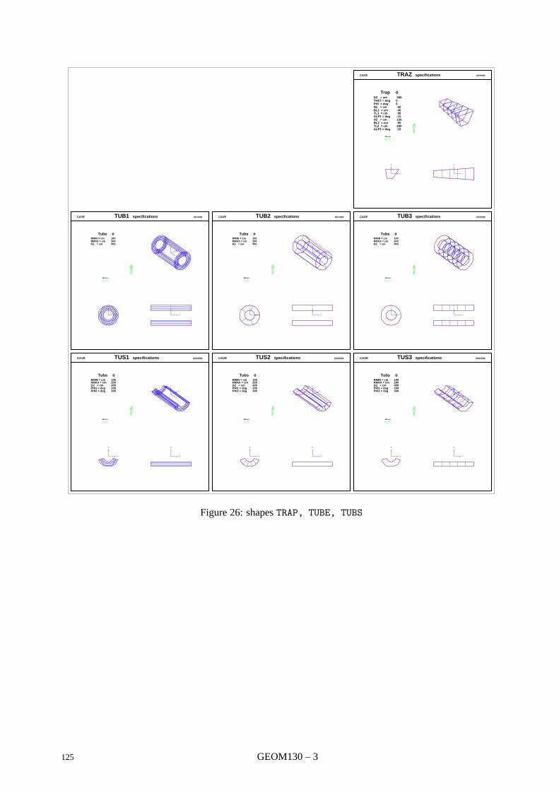
CAVE TRAZ specifications 20/10/94
Trap öDZ = cm 390 THET = deg 0 PHI = deg 0 H1 = cm 60 BL1 = cm 40 TL1 = cm 90 ALP1 = deg 15 H2 = cm 120 BL2 = cm 80 TL2 = cm 180 ALP2 = deg 15
100 cm
x
y
z
x
y y
z
CAVE TUB1 specifications 20/10/94
Tube öRMIN = cm 100 RMAX = cm 200 DZ = cm 400
100 cm
x
y
z
x
y y
z
CAVE TUB2 specifications 20/10/94
Tube öRMIN = cm 100 RMAX = cm 200 DZ = cm 400
100 cm
x
y
z
x
y y
z
CAVE TUB3 specifications 20/10/94
Tube öRMIN = cm 100 RMAX = cm 200 DZ = cm 400
100 cm
x
y
z
x
y y
z
CAVE TUS1 specifications 20/10/94
Tubs öRMIN = cm 100 RMAX = cm 200 DZ = cm 400 PHI1 = deg 200 PHI2 = deg 340
100 cm
x
y
z
x
y y
z
CAVE TUS2 specifications 20/10/94
Tubs öRMIN = cm 100 RMAX = cm 200 DZ = cm 400 PHI1 = deg 200 PHI2 = deg 340
100 cm
x
y
z
x
y y
z
CAVE TUS3 specifications 20/10/94
Tubs öRMIN = cm 100 RMAX = cm 200 DZ = cm 400 PHI1 = deg 200 PHI2 = deg 340
100 cm
x
y
z
x
y y
z
Figure 26: shapes TRAP, TUBE, TUBS
125 GEOM130 – 3
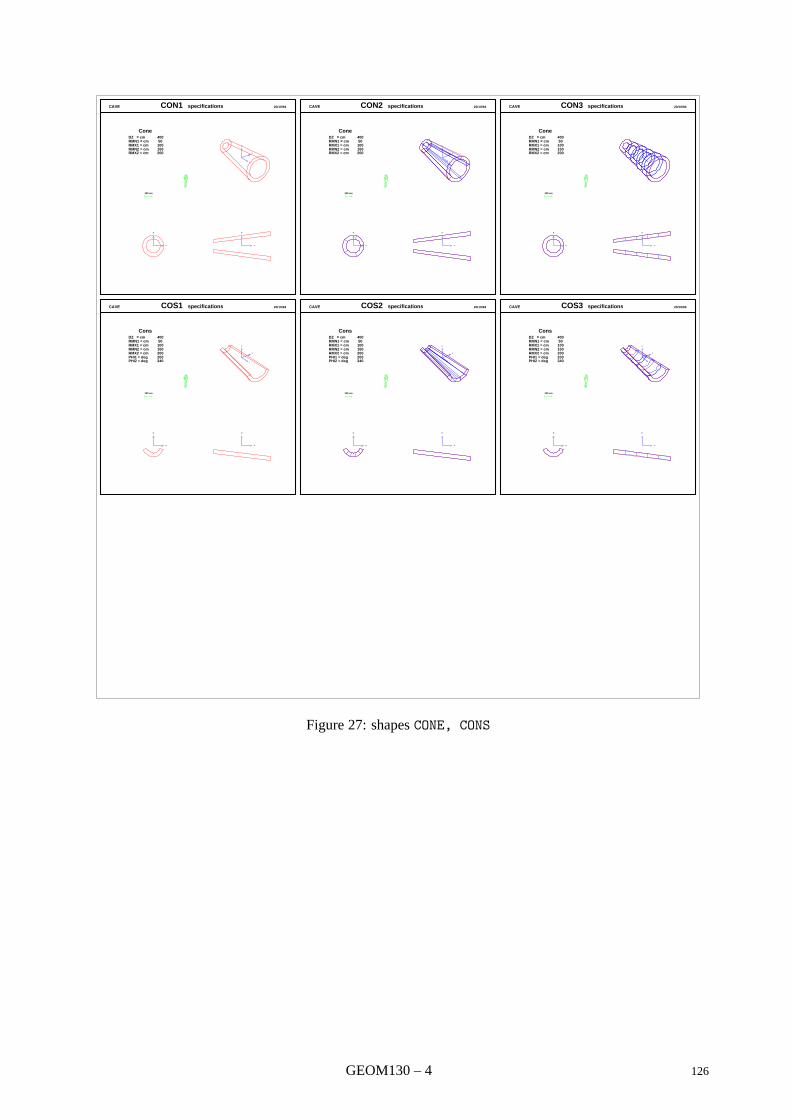
CAVE CON1 specifications 20/10/94
Cone DZ = cm 400 RMN1 = cm 50 RMX1 = cm 100 RMN2 = cm 150 RMX2 = cm 200
100 cm
x
y
z
x
y y
z
CAVE CON2 specifications 20/10/94
Cone DZ = cm 400 RMN1 = cm 50 RMX1 = cm 100 RMN2 = cm 150 RMX2 = cm 200
100 cm
x
y
z
x
y y
z
CAVE CON3 specifications 20/10/94
Cone DZ = cm 400 RMN1 = cm 50 RMX1 = cm 100 RMN2 = cm 150 RMX2 = cm 200
100 cm
x
y
z
x
y y
z
CAVE COS1 specifications 20/10/94
Cons DZ = cm 400 RMN1 = cm 50 RMX1 = cm 100 RMN2 = cm 150 RMX2 = cm 200 PHI1 = deg 200 PHI2 = deg 340
100 cm
x
y
z
x
y y
z
CAVE COS2 specifications 20/10/94
Cons DZ = cm 400 RMN1 = cm 50 RMX1 = cm 100 RMN2 = cm 150 RMX2 = cm 200 PHI1 = deg 200 PHI2 = deg 340
100 cm
x
y
z
x
y y
z
CAVE COS3 specifications 20/10/94
Cons DZ = cm 400 RMN1 = cm 50 RMX1 = cm 100 RMN2 = cm 150 RMX2 = cm 200 PHI1 = deg 200 PHI2 = deg 340
100 cm
x
y
z
x
y y
z
Figure 27: shapes CONE, CONS
GEOM130 – 4 126
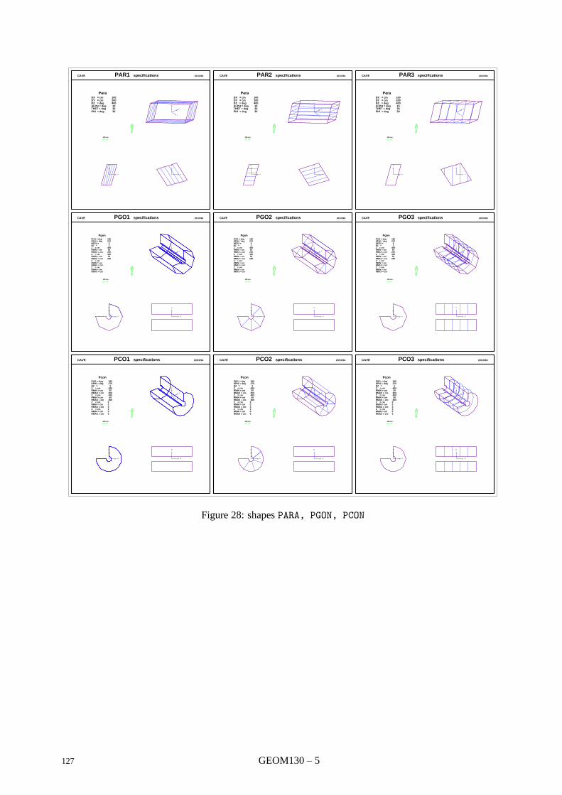
CAVE PAR1 specifications 20/10/94
Para DX = cm 100 DY = cm 200 DZ = deg 400 ALPH = deg 15 THET = deg 30 PHI = deg 30
100 cm
x
y
z
x
y y
z
CAVE PAR2 specifications 20/10/94
Para DX = cm 100 DY = cm 200 DZ = deg 400 ALPH = deg 15 THET = deg 30 PHI = deg 30
100 cm
x
y
z
x
y y
z
CAVE PAR3 specifications 20/10/94
Para DX = cm 100 DY = cm 200 DZ = deg 400 ALPH = deg 15 THET = deg 30 PHI = deg 30
100 cm
x
y
z
x
y y
z
CAVE PGO1 specifications 20/10/94
Pgon PHI1 = deg 180 DPHI = deg 270 NPDV = 6 NZ = 2 Z = cm -400 RMIN = cm 50 RMAX = cm 250 Z = cm 400 RMIN = cm 50 RMAX = cm 250 Z = cm RMIN = cm RMAX = cm Z = cm RMIN = cm RMAX = cm
100 cm
x
y
z
x
y y
z
CAVE PGO2 specifications 20/10/94
Pgon PHI1 = deg 180 DPHI = deg 270 NPDV = 6 NZ = 2 Z = cm -400 RMIN = cm 50 RMAX = cm 250 Z = cm 400 RMIN = cm 50 RMAX = cm 250 Z = cm RMIN = cm RMAX = cm Z = cm RMIN = cm RMAX = cm
100 cm
x
y
z
x
y y
z
CAVE PGO3 specifications 20/10/94
Pgon PHI1 = deg 180 DPHI = deg 270 NPDV = 6 NZ = 2 Z = cm -400 RMIN = cm 50 RMAX = cm 250 Z = cm 400 RMIN = cm 50 RMAX = cm 250 Z = cm RMIN = cm RMAX = cm Z = cm RMIN = cm RMAX = cm
100 cm
x
y
z
x
y y
z
CAVE PCO1 specifications 20/10/94
Pcon PHI1 = deg 180 DPHI = deg 270 NZ = 2 Z = cm -400 RMIN = cm 50 RMAX = cm 250 Z = cm 400 RMIN = cm 50 RMAX = cm 250 Z = cm 0 RMIN = cm 0 RMAX = cm 0 Z = cm 0 RMIN = cm 0 RMAX = cm 0
100 cm
x
y
z
x
y y
z
CAVE PCO2 specifications 20/10/94
Pcon PHI1 = deg 180 DPHI = deg 270 NZ = 2 Z = cm -400 RMIN = cm 50 RMAX = cm 250 Z = cm 400 RMIN = cm 50 RMAX = cm 250 Z = cm 0 RMIN = cm 0 RMAX = cm 0 Z = cm 0 RMIN = cm 0 RMAX = cm 0
100 cm
x
y
z
x
y y
z
CAVE PCO3 specifications 20/10/94
Pcon PHI1 = deg 180 DPHI = deg 270 NZ = 2 Z = cm -400 RMIN = cm 50 RMAX = cm 250 Z = cm 400 RMIN = cm 50 RMAX = cm 250 Z = cm 0 RMIN = cm 0 RMAX = cm 0 Z = cm 0 RMIN = cm 0 RMAX = cm 0
100 cm
x
y
z
x
y y
z
Figure 28: shapes PARA, PGON, PCON
127 GEOM130 – 5
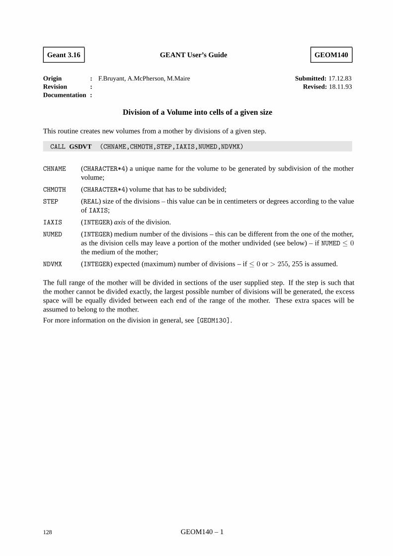
Geant 3.16 GEANT User’s Guide GEOM140
Origin : F.Bruyant, A.McPherson, M.Maire Submitted: 17.12.83Revision : Revised: 18.11.93Documentation :
Division of a Volume into cells of a given size
This routine creates new volumes from a mother by divisions of a given step.
CALL GSDVT (CHNAME,CHMOTH,STEP,IAXIS,NUMED,NDVMX)
CHNAME (CHARACTER*4) a unique name for the volume to be generated by subdivision of the mothervolume;
CHMOTH (CHARACTER*4) volume that has to be subdivided;
STEP (REAL) size of the divisions – this value can be in centimeters or degrees according to the valueof IAXIS;
IAXIS (INTEGER) axis of the division.
NUMED (INTEGER) medium number of the divisions – this can be different from the one of the mother,as the division cells may leave a portion of the mother undivided (see below) – if NUMED ≤ 0the medium of the mother;
NDVMX (INTEGER) expected (maximum) number of divisions – if ≤ 0 or > 255, 255 is assumed.
The full range of the mother will be divided in sections of the user supplied step. If the step is such thatthe mother cannot be divided exactly, the largest possible number of divisions will be generated, the excessspace will be equally divided between each end of the range of the mother. These extra spaces will beassumed to belong to the mother.
For more information on the division in general, see [GEOM130].
128 GEOM140 – 1
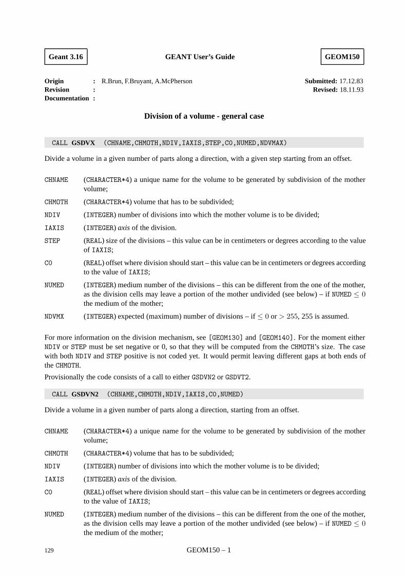
Geant 3.16 GEANT User’s Guide GEOM150
Origin : R.Brun, F.Bruyant, A.McPherson Submitted: 17.12.83Revision : Revised: 18.11.93Documentation :
Division of a volume - general case
CALL GSDVX (CHNAME,CHMOTH,NDIV,IAXIS,STEP,C0,NUMED,NDVMAX)
Divide a volume in a given number of parts along a direction, with a given step starting from an offset.
CHNAME (CHARACTER*4) a unique name for the volume to be generated by subdivision of the mothervolume;
CHMOTH (CHARACTER*4) volume that has to be subdivided;
NDIV (INTEGER) number of divisions into which the mother volume is to be divided;
IAXIS (INTEGER) axis of the division.
STEP (REAL) size of the divisions – this value can be in centimeters or degrees according to the valueof IAXIS;
C0 (REAL) offset where division should start – this value can be in centimeters or degrees accordingto the value of IAXIS;
NUMED (INTEGER) medium number of the divisions – this can be different from the one of the mother,as the division cells may leave a portion of the mother undivided (see below) – if NUMED ≤ 0the medium of the mother;
NDVMX (INTEGER) expected (maximum) number of divisions – if ≤ 0 or > 255, 255 is assumed.
For more information on the division mechanism, see [GEOM130] and [GEOM140]. For the moment eitherNDIV or STEP must be set negative or 0, so that they will be computed from the CHMOTH’s size. The casewith both NDIV and STEP positive is not coded yet. It would permit leaving different gaps at both ends ofthe CHMOTH.
Provisionally the code consists of a call to either GSDVN2 or GSDVT2.
CALL GSDVN2 (CHNAME,CHMOTH,NDIV,IAXIS,C0,NUMED)
Divide a volume in a given number of parts along a direction, starting from an offset.
CHNAME (CHARACTER*4) a unique name for the volume to be generated by subdivision of the mothervolume;
CHMOTH (CHARACTER*4) volume that has to be subdivided;
NDIV (INTEGER) number of divisions into which the mother volume is to be divided;
IAXIS (INTEGER) axis of the division.
C0 (REAL) offset where division should start – this value can be in centimeters or degrees accordingto the value of IAXIS;
NUMED (INTEGER) medium number of the divisions – this can be different from the one of the mother,as the division cells may leave a portion of the mother undivided (see below) – if NUMED ≤ 0the medium of the mother;
129 GEOM150 – 1
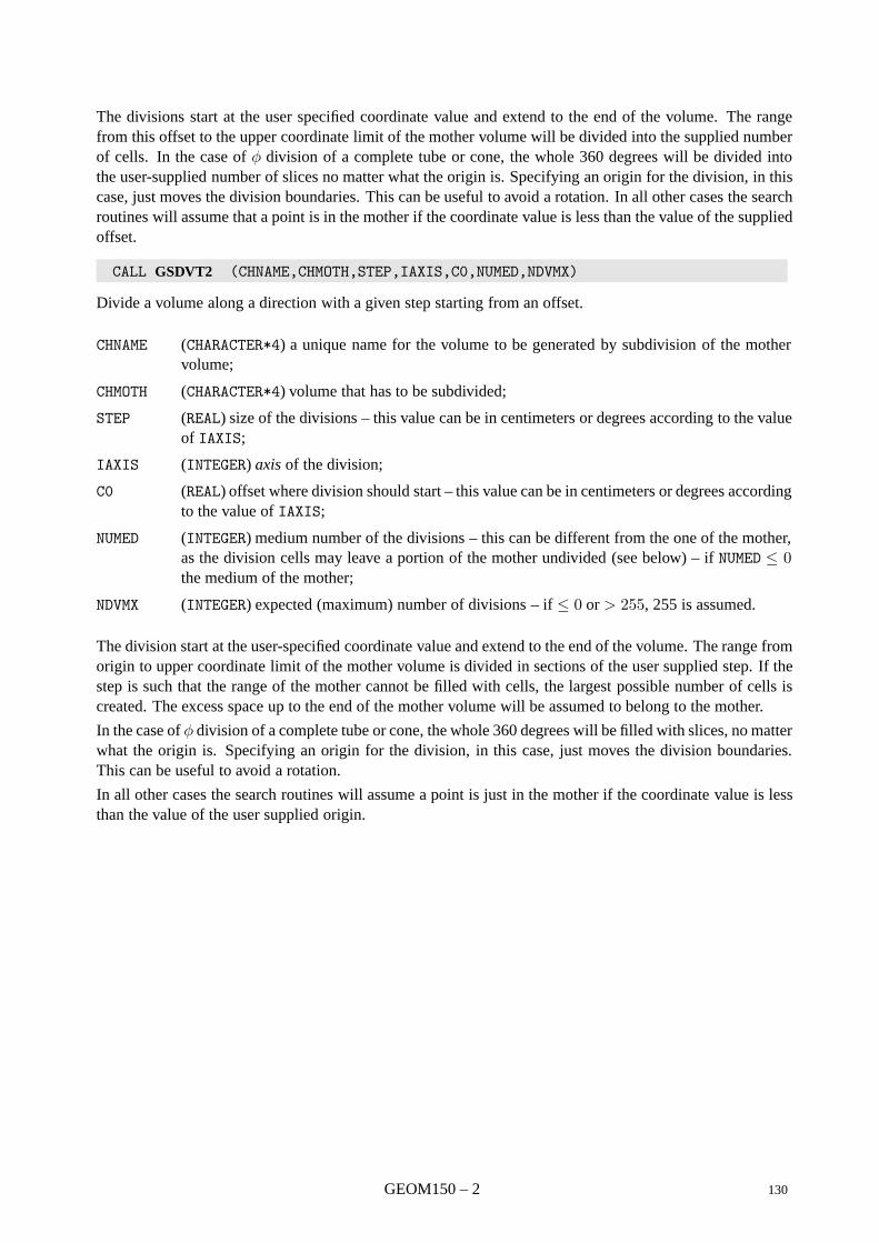
The divisions start at the user specified coordinate value and extend to the end of the volume. The rangefrom this offset to the upper coordinate limit of the mother volume will be divided into the supplied numberof cells. In the case of φ division of a complete tube or cone, the whole 360 degrees will be divided intothe user-supplied number of slices no matter what the origin is. Specifying an origin for the division, in thiscase, just moves the division boundaries. This can be useful to avoid a rotation. In all other cases the searchroutines will assume that a point is in the mother if the coordinate value is less than the value of the suppliedoffset.
CALL GSDVT2 (CHNAME,CHMOTH,STEP,IAXIS,C0,NUMED,NDVMX)
Divide a volume along a direction with a given step starting from an offset.
CHNAME (CHARACTER*4) a unique name for the volume to be generated by subdivision of the mothervolume;
CHMOTH (CHARACTER*4) volume that has to be subdivided;
STEP (REAL) size of the divisions – this value can be in centimeters or degrees according to the valueof IAXIS;
IAXIS (INTEGER) axis of the division;
C0 (REAL) offset where division should start – this value can be in centimeters or degrees accordingto the value of IAXIS;
NUMED (INTEGER) medium number of the divisions – this can be different from the one of the mother,as the division cells may leave a portion of the mother undivided (see below) – if NUMED ≤ 0the medium of the mother;
NDVMX (INTEGER) expected (maximum) number of divisions – if ≤ 0 or > 255, 255 is assumed.
The division start at the user-specified coordinate value and extend to the end of the volume. The range fromorigin to upper coordinate limit of the mother volume is divided in sections of the user supplied step. If thestep is such that the range of the mother cannot be filled with cells, the largest possible number of cells iscreated. The excess space up to the end of the mother volume will be assumed to belong to the mother.
In the case of φ division of a complete tube or cone, the whole 360 degrees will be filled with slices, no matterwhat the origin is. Specifying an origin for the division, in this case, just moves the division boundaries.This can be useful to avoid a rotation.
In all other cases the search routines will assume a point is just in the mother if the coordinate value is lessthan the value of the user supplied origin.
GEOM150 – 2 130
Geant 3.16 GEANT User’s Guide GEOM199
Origin : R.Brun,F.Bruyant,A.McPherson Submitted: 01.11.83Revision : Revised: 18.11.93Documentation :
The volume data structure – JVOLUM
1 The data structure JVOLUM and JGPAR
The meaning of the variables in the data structure JVOLUM shown in fig. 29 is the following:
ISEARC search flag [GEOM400], [GEOM410]:
=0 volume positioning order or ordering by GSNEXT/GSNEAR;
<0 binary search as defined by GSORD;
>0 user ordering GSUNEA/GUNEAR;
ISHAPE system shape number (see [GEOM050];
NIN number of volumes contained in the mother volume – if negative the volume is divided;
NMED medium number for the volume;
NPAR number of shape parameters;
NATT number of attributes;
PAR array of shape parameters;
IAT array of attributes;
IAXIS direction of the division (see [GEOM130]);
IVO system volume number;
NDIV number of divisions (-NDVMX, if computed dynamically, see [GEOM140]);
C0 coordinate value at which the division starts;
STEP coordinate step for the division;
NR user copy number;
IROT rotation matrix number defining the orientation of the volume with respect to the mother refer-ence system;
X,Y,Z position of the volume with respect to the mother reference system;
KONLY ONLY/MANY flag, see [GEOM110] for more information;
131 GEOM199 – 1
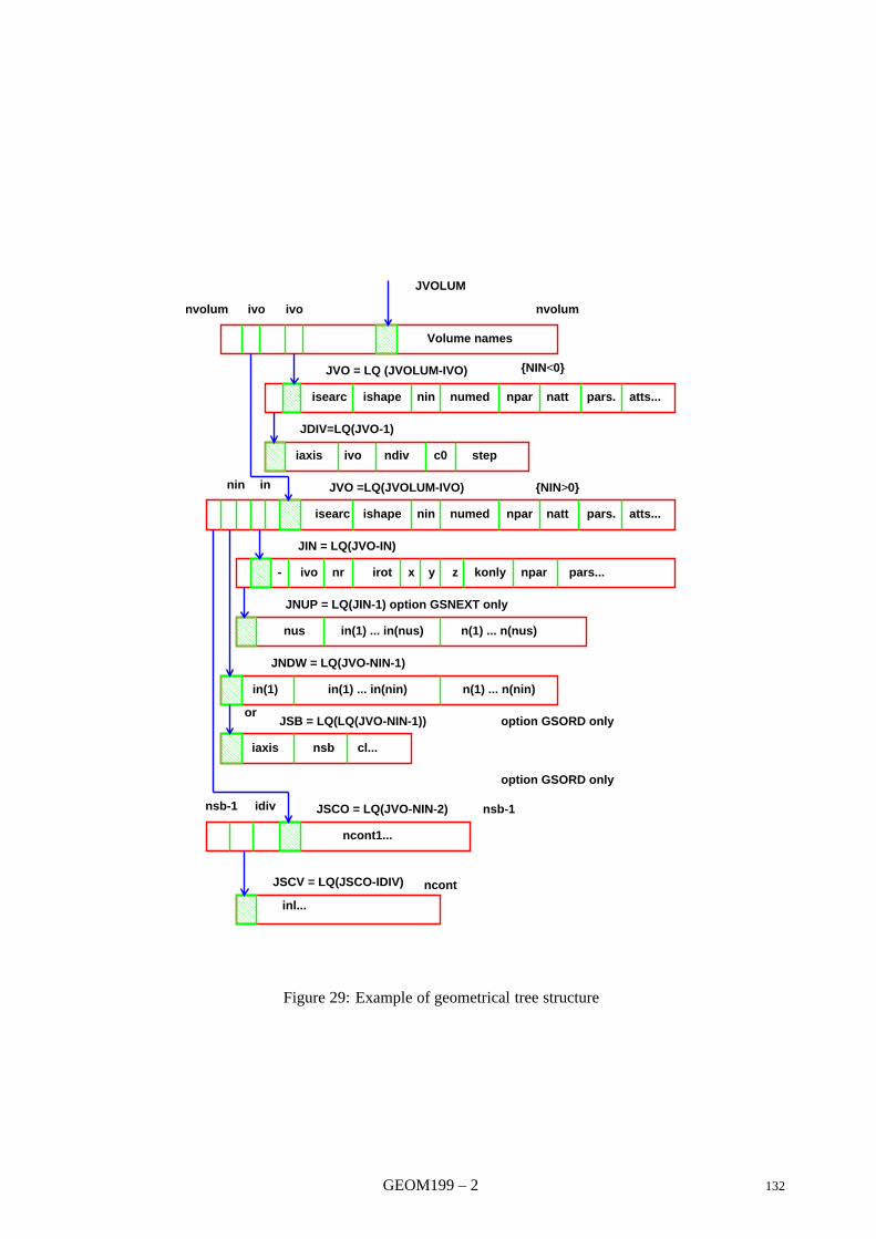
nvolum ivo ivo
JVOLUM
nvolum
Volume names
JVO = LQ (JVOLUM-IVO) NIN<0
isearc ishape nin numed npar natt pars. atts...
JDIV=LQ(JVO-1)
iaxis ivo ndiv c0 step
nin in JVO =LQ(JVOLUM-IVO) NIN>0
isearc ishape nin numed npar natt pars. atts...
JIN = LQ(JVO-IN)
- ivo nr irot x y z konly npar pars...
JNUP = LQ(JIN-1) option GSNEXT only
nus in(1) ... in(nus) n(1) ... n(nus)
JNDW = LQ(JVO-NIN-1)
in(1) in(1) ... in(nin) n(1) ... n(nin)
orJSB = LQ(LQ(JVO-NIN-1)) option GSORD only
iaxis nsb cl...
JSCO = LQ(JVO-NIN-2)
option GSORD only
nsb-1 idiv nsb-1
ncont1...
JSCV = LQ(JSCO-IDIV) ncont
inl...
Figure 29: Example of geometrical tree structure
GEOM199 – 2 132
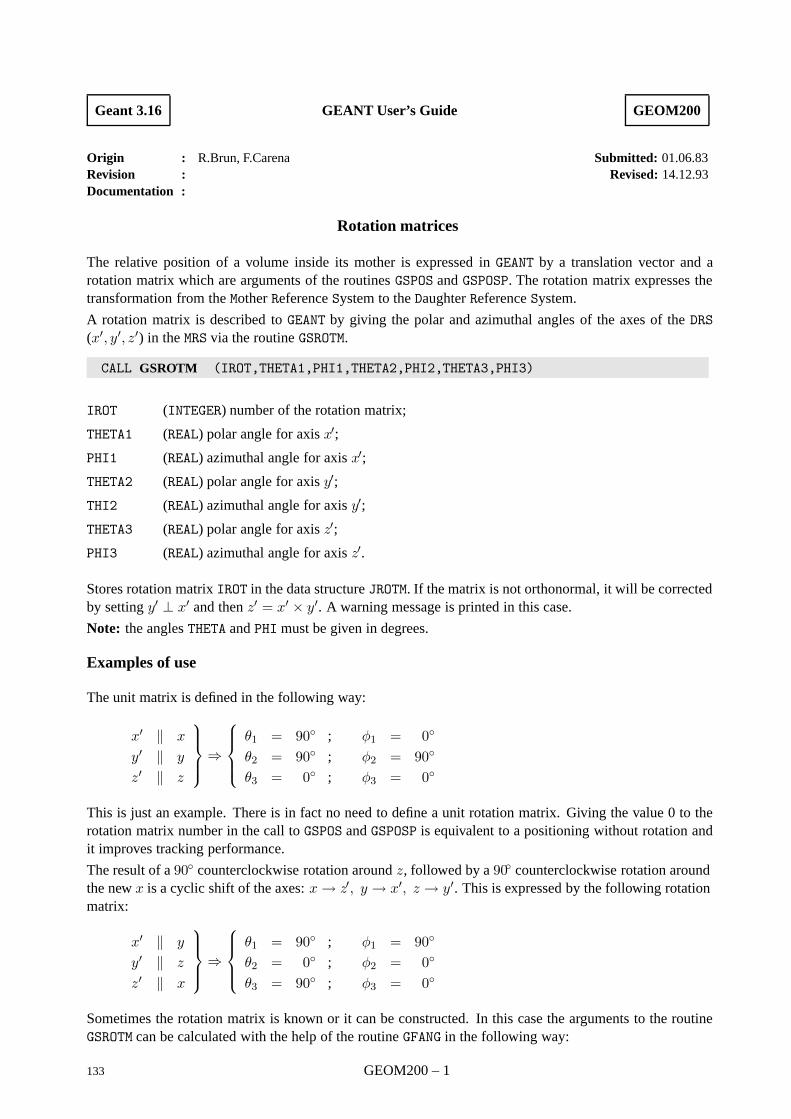
Geant 3.16 GEANT User’s Guide GEOM200
Origin : R.Brun, F.Carena Submitted: 01.06.83Revision : Revised: 14.12.93Documentation :
Rotation matrices
The relative position of a volume inside its mother is expressed in GEANT by a translation vector and arotation matrix which are arguments of the routines GSPOS and GSPOSP. The rotation matrix expresses thetransformation from the Mother Reference System to the Daughter Reference System.
A rotation matrix is described to GEANT by giving the polar and azimuthal angles of the axes of the DRS(x′, y′, z′) in the MRS via the routine GSROTM.
CALL GSROTM (IROT,THETA1,PHI1,THETA2,PHI2,THETA3,PHI3)
IROT (INTEGER) number of the rotation matrix;
THETA1 (REAL) polar angle for axis x′;
PHI1 (REAL) azimuthal angle for axis x′;
THETA2 (REAL) polar angle for axis y′;
THI2 (REAL) azimuthal angle for axis y′;
THETA3 (REAL) polar angle for axis z′;
PHI3 (REAL) azimuthal angle for axis z′.
Stores rotation matrix IROT in the data structure JROTM. If the matrix is not orthonormal, it will be correctedby setting y′ ⊥ x′ and then z′ = x′ × y′. A warning message is printed in this case.
Note: the angles THETA and PHI must be given in degrees.
Examples of use
The unit matrix is defined in the following way:
x′ ‖ x
y′ ‖ y
z′ ‖ z
⇒
θ1 = 90 ; φ1 = 0
θ2 = 90 ; φ2 = 90
θ3 = 0 ; φ3 = 0
This is just an example. There is in fact no need to define a unit rotation matrix. Giving the value 0 to therotation matrix number in the call to GSPOS and GSPOSP is equivalent to a positioning without rotation andit improves tracking performance.
The result of a 90 counterclockwise rotation around z, followed by a 90 counterclockwise rotation aroundthe new x is a cyclic shift of the axes: x → z′, y → x′, z → y′. This is expressed by the following rotationmatrix:
x′ ‖ y
y′ ‖ z
z′ ‖ x
⇒
θ1 = 90 ; φ1 = 90
θ2 = 0 ; φ2 = 0
θ3 = 90 ; φ3 = 0
Sometimes the rotation matrix is known or it can be constructed. In this case the arguments to the routineGSROTM can be calculated with the help of the routine GFANG in the following way:
133 GEOM200 – 1
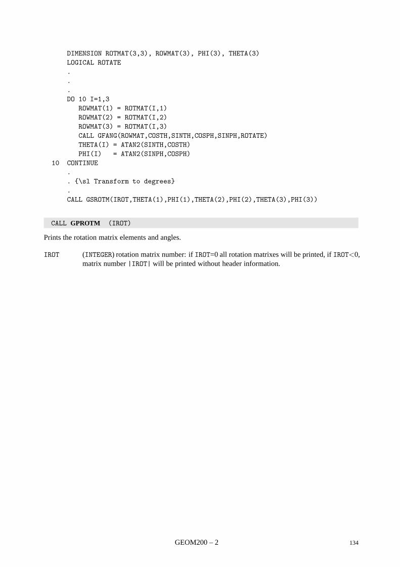
DIMENSION ROTMAT(3,3), ROWMAT(3), PHI(3), THETA(3)LOGICAL ROTATE...DO 10 I=1,3
ROWMAT(1) = ROTMAT(I,1)ROWMAT(2) = ROTMAT(I,2)ROWMAT(3) = ROTMAT(I,3)CALL GFANG(ROWMAT,COSTH,SINTH,COSPH,SINPH,ROTATE)THETA(I) = ATAN2(SINTH,COSTH)PHI(I) = ATAN2(SINPH,COSPH)
10 CONTINUE.. \sl Transform to degrees.CALL GSROTM(IROT,THETA(1),PHI(1),THETA(2),PHI(2),THETA(3),PHI(3))
CALL GPROTM (IROT)
Prints the rotation matrix elements and angles.
IROT (INTEGER) rotation matrix number: if IROT=0 all rotation matrixes will be printed, if IROT<0,matrix number |IROT| will be printed without header information.
GEOM200 – 2 134
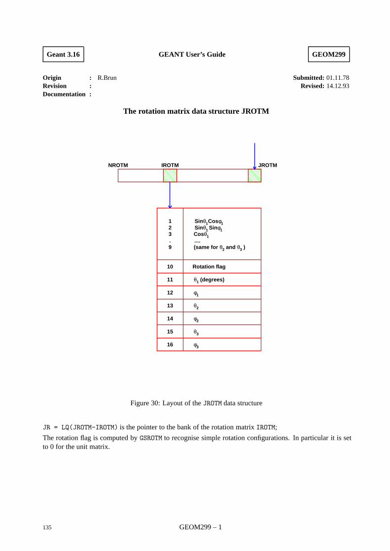
Geant 3.16 GEANT User’s Guide GEOM299
Origin : R.Brun Submitted: 01.11.78Revision : Revised: 14.12.93Documentation :
The rotation matrix data structure JROTM
NROTM IROTM JROTM
123.9
10
11
12
13
14
15
16
Rotation flag
θ1 (degrees)
φ1
θ2
φ2
θ3
φ3
Sinθ1Cosφ1Sinθ1 Sinφ1Cosθ1....(same for θ2 and θ3 )
Figure 30: Layout of the JROTM data structure
JR = LQ(JROTM-IROTM) is the pointer to the bank of the rotation matrix IROTM;
The rotation flag is computed by GSROTM to recognise simple rotation configurations. In particular it is setto 0 for the unit matrix.
135 GEOM299 – 1
Geant 3.16 GEANT User’s Guide GEOM300
Origin : R.Brun, A.C.McPherson, F.Bruyant Submitted: 18.12.83Revision : S.Giani Revised: 14.12.93Documentation :
Finding in which volume a point is
CALL GMEDIA (X,NUMED*)
X (REAL) array of dimension 3 with the coordinates in the MRS;
NUMED (INTEGER) medium number, if this is zero the point is outside the detector.
Searches the geometrical tree structure to find in which volume the point X is. The tracking medium isreturned in NUMED, and the common /GCVOLU/ is updated.GMEDIA uses the geometry data structure to conduct its search starting its search from the last volume wherea point was found. If no previous search has been conducted, the first volume is used as a starting point.If the point is not inside the current volume, GMEDIA looks in its mother and so on, until it finds a volumewhich contains the point. It then looks at the contents of this object and so on until the point is in a volumebut in none of its contents (if any).If this downward search terminates in a ’MANY’ object, GMEDIA looks for another candidate. See [GEOM110]for a description of the ‘MANY’ volumes tratment.The physical geometrical tree from the first volume to the current one is stored in the common block GCVOLU(see [BASE030]) and in the structure JGPAR (see [GEOM199]).
CALL GTMEDI (X,NUMED*)
X (REAL) array of dimension 3 with the coordinates in the MRS;
NUMED (INTEGER) medium number, if this is zero the point is outside the detector.
This routine performs the same function than GMEDIA, but it uses the dynamical information of the particlehistory to speed-up the search:
• when INWVOL=2 (common /GCTRAK/) the particle just came out of a volume. In this case, if INFROM(common /GCVOLU/) is positive, it is interpreted by GTMEDI as the number IN of the content just left,inside the mother volume where the point X is assumed to be. This content will not be searched again.
• the daughter of the current volume which limits the geometrical step of the particle (i.e. where the par-ticle would be heading moving along a straight line) is searched first. INGOTO (common /GCVOLU/)is set by GTNEXT, to transmit the information on this one volume which has limited the geometricalstep SNEXT as follows:
>0 INth content;=0 current volume;<0 -NLONLY, with NLONLY defined as the lowest ’ONLY’ level up in the tree which is an ancestor
of the ’MANY’ volume where the point X is.
CALL GINVOL (X,ISAME*)
X (REAL) array of dimension 3 with the coordinates in the MRS;
ISAME (INTEGER) return flag.
Checks if particle at point X has left current volume. If so, returns ISAME = 0 and prepares informationuseful to identify the new volume entered, otherwise, returns ISAME = 1.
136 GEOM300 – 1
Geant 3.21 GEANT User’s Guide GEOM310
Origin : R.Brun, A.C.McPherson Submitted: 01.06.83Revision : S.Giani Revised: 15.12.93Documentation :
Finding distance to next boundary
CALL GNEXT (X,SNEXT*,SAFETY*)
CALL GTNEXT (X,SNEXT*,SAFETY*)
Finds distance to the next boundary. It takes explicit account of shape content and uniqueness.
X (REAL) array of 6 of coordinates and direction cosines;
SNEXT (REAL) distance to the nearest volume boundary along the particle direction;
SAFETY (REAL) safety distance, that is smaller distance to any boundary;
This routine evaluates the two distances which are needed by the GEANT tracking routines. GTNEXT andGNEXT perform the same function, but GNEXT is a static routine which can be called by the user, whileGTNEXT is the routines used internally by GEANT during tracking, and it should not be called by the user.
If INFROM (common /GCVOLU/) is different from 0, GTNEXT interprets it as the daughter out of which the par-ticle just came, and uses the list of daughters stored with that volume, possibly modified by GSNEXT/GSNEARto calculate the distance to the next boundary.
The first action of GTNEXT is to calculate the SAFETY distance. If this is larger than the current step candidate,no other calculation is performed and the IGNEXT flag (common /GCTRAK/) is set to 0, indicating that nochange of volume is occurring at the end of the current step. If the step is smaller than safety, then SNEXT iscomputed. If the step is smaller than SNEXT, again there will not be any change of volume during the stepand IGNEXT is set to 0. If on the contrary the candidate step is larger than SNEXT, a change of volume willoccur at the end of the step, and IGNEXT is set to 1 and INGOTO (common /GCTRAK/) is set to the numberof the daughter where the particle is entering, if any.
Charged particles in magnetic field are transported with a similar logic. However, even if the candidate stepis smaller than SNEXT, the particle can still cross into another volume due to its bent path. When trackingin magnetic field, after every step greater than SAFETY it is checked whether the particle is still in the samevolume. If this is not the case, the step is divided by two and transport is tried again. Conversely a chargedparticle in magnetic field may still be in the current volume even after having travelled the distance to thenearest boundary along a straight line. So boundary crossing is declared only when IGNEXT is differentfrom 0 and the difference between the real trajectory and the bent one is smaller than EPSIL (common/GCTMED/).
137 GEOM310 – 1
Geant 3.16 GEANT User’s Guide GEOM320
Origin : R. Brun Submitted: 18.08.87Revision : Revised: 15.12.93Documentation :
Reference system transformations
CALL GMTOD (XM,XD*,IFLAG)
XM (REAL) array of 3 containing the input position (IFLAG=1) or direction cosines (IFLAG=2) inthe Master Reference System;
XD (REAL) array of 3 containing the output position (IFLAG=1) or direction cosines (IFLAG=2) inthe (current) Daughter Reference System;
IFLAG (INTEGER) transformation flag:
1 input is a position, it must be translated and rotated;
2 input is a direction, it must be rotated.
This routine transform coordinates or directions from the MRS to the reference system of the current volume.The /GCVOLU/ must be properly filled, either by the tracking routines, by GMEDIA or by GLVOLU.
CALL GDTOM (XD,XM*,IFLAG)
Performs the inverse operation to GMTOD.
138 GEOM320 – 1
Geant 3.16 GEANT User’s Guide GEOM400
Origin : R.Brun,F.Bruyant,A.C.McPherson Submitted: 16.12.83Revision : S.Egli Revised: 15.12.93Documentation :
Pseudo-division of a volume
CALL GSORD (CHNAME,ICORD)
CHNAME (CHARACTER*4) name of the volume;
ICORD (INTEGER) direction of the pseudo-divisions:
1 x;
2 y;
3 z;
4 cylindrical R (√x2 + y2);
5 spherical ρ (√x2 + y2 + z2);
6 φ, azimuthal angle;
7 θ, polar angle with respect to the z axis.
This routine sets the search flag (Q(JVO+1)) of volume CHNAME to -ICORD. When the definition of thegeometry is complete and GGCLOS is called, this flag is interpreted as a request to order the content ofCHNAME along axis ICORD. This operation is performed by the routine GGORD. GGORD computes the limitsof each of the contents along the given coordinate axis (see [GEOM001]), and prepares the lists of contentsin each of the sections defined by the neighbouring coordinate. The JVOLUM structure is extended, for themother volume, with banks which contains the list of boundaries and the lists of contents, so as to permita binary search to access the contents of interest. The coordinates are in the local system of the mothervolume. The routine GGORD will not be called if the number of contents exceeds 500.
The actual effect of this routine depends on the setting of the IOPTIM variable in the common /GCOPTI/.IOPTIM is controlled by the data record OPTI or the interactive command with the same name. The meaningof the different values of IOPTIM is the following:
<0 no call to GGORD will be made, irrespective of the value of ISEARCH;
0 GGORD will be called for those volumes for which GSORD has been called;
1 for all volumes with contents for which neither GUSEAR nor GSORD has been called, the routineGGORDQ will be called;
2 GGORDQ is called for all volumes with contents for which GUSEAR has not been called.
GGORDQ orders the contents along all the possible axes and choses the ordering which provides the lowestnumber of volumes per division.
139 GEOM400 – 1
Geant 3.16 GEANT User’s Guide GEOM410
Origin : F.Bruyant, A.C.McPherson Submitted: 16.12.83Revision : Revised: 14.12.93Documentation : F.Carminati, M.Lefebvre
Ordering the contents of a volume
In the case of a mother volume containing a large number of daughters, tracking can be rather slow. This isdue to the fact that each time GEANT requires to know in which daughter it is or will be tracking, it searchthrough the whole list of daughter volumes. This is done by GEANT creating for every daughter volume a listwhich contain pointers to all the daughters of the same mother.
Clearly this may be avoided, because at any step of tracking, the coordinates and direction cosines of thecurrent step are known. From this and the knowledge of the geometry, a restricted list of daughter volumesto be searched can be built. This can be accomplished in GEANT in two ways, which are described in thischapter.
Note: the user must be aware that the following routines alter the default search list of daughters of agiven mother. A user mistake can cause wrong transport because GEANT does not make any check on thecorrectness of the list of neighbours provided by the user.
Static ordering
CALL GSNEXT (CHMOTH,IN,NLIST,LIST)
CHMOTH (CHARACTER*4) name of the mother volume to be ordered;
IN (INTEGER) number of the content for which a list is established;
NLIST (INTEGER) number of neighbours to be considered during tracking;
LIST (INTEGER) list of neighbours to volume IN.
This routine stores a given ordered LIST of NLIST daughter volumes to search when leaving the INth
daughter of the mother volume CHMOTH.
If IN=0, for each content, GSNEXT builds a list limited to the contents IN+1 (if it exists), IN-1 (if it exists)and IN itself.
CALL GSNEAR (CHMOTH,IN,NLIST,LIST)
CHMOTH (CHARACTER*4) name of the mother volume to be ordered;
IN (INTEGER) number of the content for which a list is established;
NLIST (INTEGER) number of neighbours to be considered during tracking;
LIST (INTEGER) list of neighbours to volume IN.
This routine stores a given ordered LIST of NLIST daughter volumes to search when leaving the INth
daughter of the mother volume CHMOTH.
If LIST(1)=0 the particle is back into the mother when leaving the INth daughter. This means that the INth
is not contiguous to any other daughter or to the boundary of the mother.
If IN=-1, the mother does not have contents contiguous to its boundaries (status bit 4 set in mother volumebank for action in GGCLOS).
If IN=0 for each content GSNEAR sets LIST(1)=0.
GSNEAR must be called after all contents have been position ( except when IN=-1)
140 GEOM410 – 1
Dynamic ordering
The list of neighbours to search when exiting from the INth content may depend also on the directionand position of the particle. In case where it is necessary, for performance reasons, to exploit also thisinformation, GEANT offers the possibility to the user to build a dynamic search list.
CALL GSUNEA (CHNAME,ISEARC)
CHNAME (CHARACTER*4) name of the volume where the user search has to be activated;
ISEARCH (INTEGER) specifies the kind of search list to be used: a positive value must be specified withthis routine to activate user search lists.
This routine should be called once for every volume where user volume search is activated.
CALL GUNEAR (ISEARC,ICALL,XC,JNEAR)
ISEARCH (INTEGER) number associated to the volume in which the user search is used, it is the samenumber set by the user with GSUNEA;
ICALL (INTEGER) type of question that the list of volumes must answer:
1 GMEDIA-like call, where am I?
2 GTNEXT-like call, where can I go?
XC (REAL) array of 6 containing the position and the direction cosines of the particle (x, y, z, px/p,py/p, px/p);
JNEAR (INTEGER) pointer to the volume list bank which has to be filled by the user;
The list of volumes where GEANT has to search to answer the question specified by ICALL is returned by theuser starting at Q(JNEAR+1. GEANT will only look at the volumes specified by the user and in the order inwhich they appear in the list. Daughters are numbered from 1 to N according to the order with which theyhave been positioned in the mother. The list should be filled in the following way:
IQ(JNEAR+1) = N, number of volumes in the list
IQ(JNEAR+1+1) = number of the first daughter to search
IQ(JNEAR+1+2) = number of the second daughter to search
.
.
.
IQ(JNEAR+1+N) = number of the Nth daughter to search
The user should be aware that this routine is called very often, almost at every tracking step, so it should becoded with the maximum efficiency in mind. An example of GUNEAR could be the following:
SUBROUTINE GUNEAR(ISEARC,ICALL,XC,JNEAR)*--- Make sure to add GEANT main store+SEQ, GCBANK.
DIMENSION XC(6), MYLIST(100)*--- Executable code
IF(ISEARC.EQ.1) THEN*--- Build a list using XC and ISEARC for a GMEDIA type call*--- Put all the daughters where the particle may be in
MYLIST(1) = .....
GEOM410 – 2 141
.
.MYLIST(N) = ....
ELSE*--- Build a list using XC and ISEARC for a GTNEXT type call*--- Put all the daughters where the particle may be going
MYLIST(1) = .......MYLIST(N) = ....
ENDIF*--- Return the information to GEANT
DO 10 I=1,NIQ(JNEAR+1+I) = MYLIST(I)
10 CONTINUEIQ(JNEAR+1) = N
*--- End of GUNEAREND
142 GEOM410 – 3
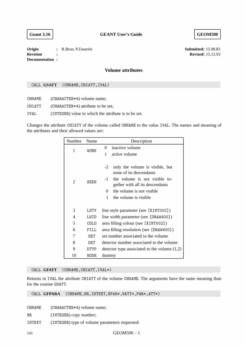
Geant 3.16 GEANT User’s Guide GEOM500
Origin : R.Brun, P.Zanarini Submitted: 15.08.83Revision : Revised: 15.12.93Documentation :
Volume attributes
CALL GSATT (CHNAME,CHIATT,IVAL)
CHNAME (CHARACTER*4) volume name;
CHIATT (CHARACTER*4) attribute to be set;
IVAL (INTEGER) value to which the attribute is to be set.
Changes the attribute CHIATT of the volume called CHNAME to the value IVAL. The names and meaning ofthe attributes and their allowed values are:
Number Name Description
1 WORK0 inactive volume
1 active volume
2 SEEN
-2 only the volume is visible, butnone of its descendants
-1 the volume is not visible to-gether with all its descendants
0 the volume is not visible
1 the volume is visible
3 LSTY line style parameter (see [XINT002])
4 LWID line width parameter (see [DRAW400])
5 COLO area filling colour (see [XINT002])
6 FILL area filling resolution (see [DRAW400])
7 SET set number associated to the volume
8 DET detector number associated to the volume
9 DTYP detector type associated to the volume (1,2)
10 NODE dummy
CALL GFATT (CHNAME,CHIATT,IVAL*)
Returns in IVAL the attribute CHIATT of the volume CHNAME. The arguments have the same meaning thanfor the routine GSATT.
CALL GFPARA (CHNAME,NR,INTEXT,NPAR*,NATT*,PAR*,ATT*)
CHNAME (CHARACTER*4) volume name;
NR (INTEGER) copy number;
INTEXT (INTEGER) type of volume parameters requested:
143 GEOM500 – 1

0 user parameters;
1 internal parameters;
NPAR (INTEGER) number of parameters returned;
NATT (INTEGER) number of attributes returned;
PAR (REAL) array of parameters;
ATT (REAL) array of attributes.
Returns parameters PAR(1...NPAR) and attributes ATT(1...NATT) for the volume CHNAME with copynumber NR.
GEOM500 – 2 144
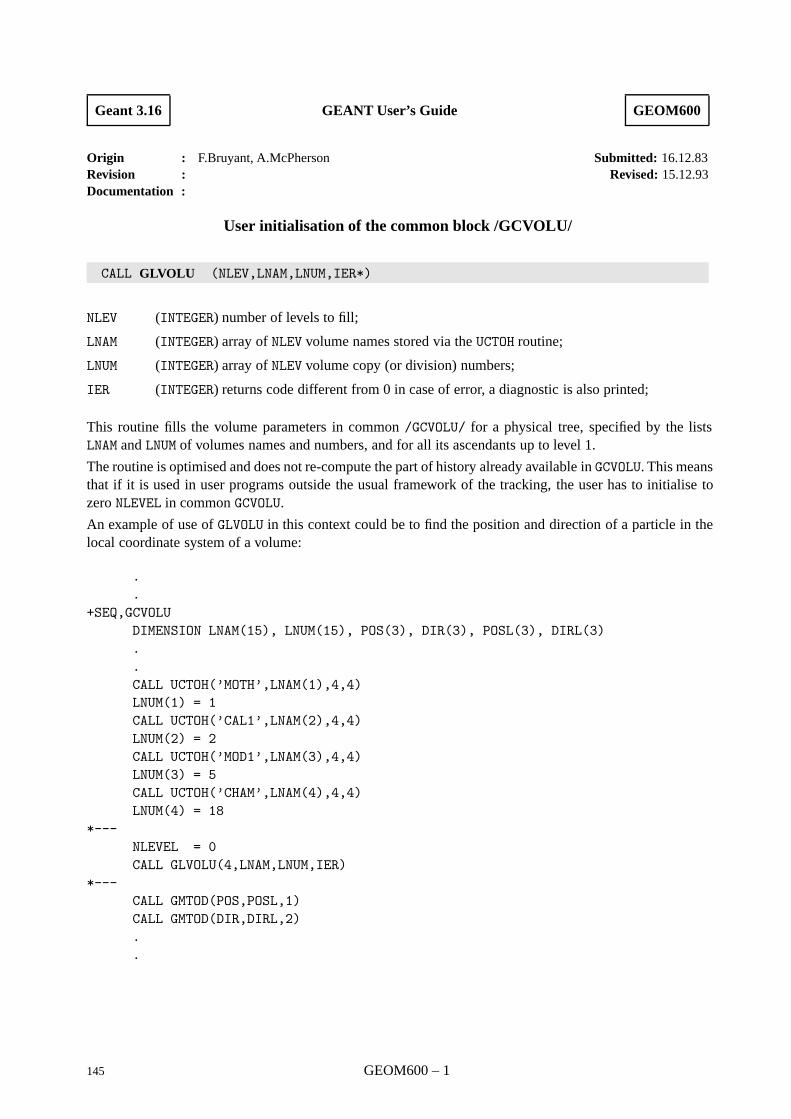
Geant 3.16 GEANT User’s Guide GEOM600
Origin : F.Bruyant, A.McPherson Submitted: 16.12.83Revision : Revised: 15.12.93Documentation :
User initialisation of the common block /GCVOLU/
CALL GLVOLU (NLEV,LNAM,LNUM,IER*)
NLEV (INTEGER) number of levels to fill;
LNAM (INTEGER) array of NLEV volume names stored via the UCTOH routine;
LNUM (INTEGER) array of NLEV volume copy (or division) numbers;
IER (INTEGER) returns code different from 0 in case of error, a diagnostic is also printed;
This routine fills the volume parameters in common /GCVOLU/ for a physical tree, specified by the listsLNAM and LNUM of volumes names and numbers, and for all its ascendants up to level 1.
The routine is optimised and does not re-compute the part of history already available in GCVOLU. This meansthat if it is used in user programs outside the usual framework of the tracking, the user has to initialise tozero NLEVEL in common GCVOLU.
An example of use of GLVOLU in this context could be to find the position and direction of a particle in thelocal coordinate system of a volume:
.
.+SEQ,GCVOLU
DIMENSION LNAM(15), LNUM(15), POS(3), DIR(3), POSL(3), DIRL(3)..CALL UCTOH(’MOTH’,LNAM(1),4,4)LNUM(1) = 1CALL UCTOH(’CAL1’,LNAM(2),4,4)LNUM(2) = 2CALL UCTOH(’MOD1’,LNAM(3),4,4)LNUM(3) = 5CALL UCTOH(’CHAM’,LNAM(4),4,4)LNUM(4) = 18
*---NLEVEL = 0CALL GLVOLU(4,LNAM,LNUM,IER)
*---CALL GMTOD(POS,POSL,1)CALL GMTOD(DIR,DIRL,2)..
145 GEOM600 – 1
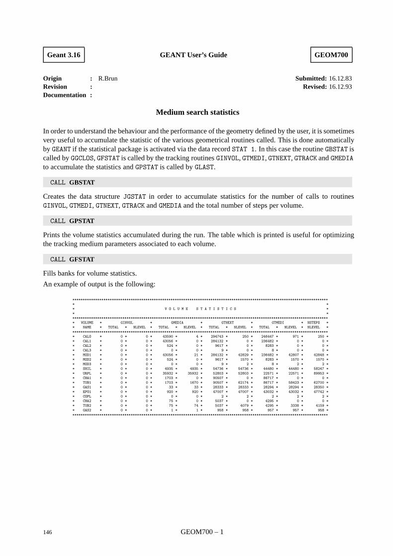
Geant 3.16 GEANT User’s Guide GEOM700
Origin : R.Brun Submitted: 16.12.83Revision : Revised: 16.12.93Documentation :
Medium search statistics
In order to understand the behaviour and the performance of the geometry defined by the user, it is sometimesvery useful to accumulate the statistic of the various geometrical routines called. This is done automaticallyby GEANT if the statistical package is activated via the data record STAT 1. In this case the routine GBSTAT iscalled by GGCLOS, GFSTAT is called by the tracking routines GINVOL, GTMEDI, GTNEXT, GTRACK and GMEDIAto accumulate the statistics and GPSTAT is called by GLAST.
CALL GBSTAT
Creates the data structure JGSTAT in order to accumulate statistics for the number of calls to routinesGINVOL, GTMEDI, GTNEXT, GTRACK and GMEDIA and the total number of steps per volume.
CALL GPSTAT
Prints the volume statistics accumulated during the run. The table which is printed is useful for optimizingthe tracking medium parameters associated to each volume.
CALL GFSTAT
Fills banks for volume statistics.
An example of output is the following:
**************************************************************************************************************************
* *
* V O L U M E S T A T I S T I C S *
* *
**************************************************************************************************************************
* VOLUME * GINVOL * GMEDIA * GTNEXT * GTMEDI * NSTEPS *
* NAME * TOTAL * NLEVEL * TOTAL * NLEVEL * TOTAL * NLEVEL * TOTAL * NLEVEL * NLEVEL *
**************************************************************************************************************************
* CALO * 0 * 0 * 43590 * 4 * 294743 * 250 * 246447 * 971 * 250 *
* CAL1 * 0 * 0 * 43056 * 0 * 284132 * 0 * 236482 * 0 * 0 *
* CAL2 * 0 * 0 * 524 * 0 * 9617 * 0 * 8283 * 0 * 0 *
* CAL3 * 0 * 0 * 0 * 0 * 9 * 0 * 8 * 0 * 0 *
* MOD1 * 0 * 0 * 43056 * 21 * 284132 * 42829 * 236482 * 42807 * 42848 *
* MOD2 * 0 * 0 * 524 * 0 * 9617 * 1570 * 8283 * 1570 * 1570 *
* MOD3 * 0 * 0 * 0 * 0 * 9 * 2 * 8 * 2 * 2 *
* SHIL * 0 * 0 * 4935 * 4935 * 54736 * 54736 * 44480 * 44480 * 58247 *
* URPL * 0 * 0 * 35932 * 35932 * 52803 * 52803 * 22571 * 22571 * 89953 *
* CHA1 * 0 * 0 * 1703 * 0 * 90507 * 0 * 86717 * 0 * 0 *
* TUB1 * 0 * 0 * 1703 * 1670 * 90507 * 62174 * 86717 * 58423 * 62700 *
* GAS1 * 0 * 0 * 33 * 33 * 28333 * 28333 * 28294 * 28294 * 28350 *
* EPO1 * 0 * 0 * 920 * 920 * 47007 * 47007 * 43032 * 43032 * 47742 *
* COPL * 0 * 0 * 0 * 0 * 2 * 2 * 2 * 2 * 2 *
* CHA2 * 0 * 0 * 75 * 0 * 5037 * 0 * 4295 * 0 * 0 *
* TUB2 * 0 * 0 * 75 * 74 * 5037 * 4079 * 4295 * 3338 * 4159 *
* GAS2 * 0 * 0 * 1 * 1 * 958 * 958 * 957 * 957 * 958 *
**************************************************************************************************************************
146 GEOM700 – 1
Geant 3.16 GEANT User’s Guide GEOM900
Origin : A.C.McPherson Submitted: 16.12.83Revision : F.Bruyant, R.Brun Revised: 16.12.93Documentation :
End of geometry definition
CALL GGCLOS
This routine should be called after all volumes, positions, hits and digits have been defined. Its action isconfined to clean up the volume banks and to take any action required by the ordering techniques.
GGCLOS performs all the requested geometry optimisation, included the creation of pseudo-divisions involumes flagged by GSORD. It performs the local development of tha last leaves of the geometrical tree,where applicable.
It also calls the routine GGDETV which prepares the prototype lists of volume names and maximum mul-tiplicities which permit to identify uniquely any sensitive detector whose generic name has been declaredthrough the routine GSDETV (and not GSDET) [HITS001].
GGCLOS must be called also after reading a geometry data structure from disk.
147 GEOM900 – 1
Geant 3.21 GEANT User’s Guide GEOM910
Origin : J.Vuoskoski, N. Høimyr Submitted: 22.03.94Revision : Revised: 23.09.94Documentation :
The CADINT Interface
1 Introduction
The engineering work in HEP for design, analysis and manufacturing of detectors requires Computer AidedEngineering (CAE) tools. To ensure coherent design the same detector descriptions should be used byphysicists, engineers and, eventually, manufacturers. Efficient exchange of data between CAE tools andGEANT becomes crucial.
The CADINT interface allows to export detector models from GEANT to Computer Aided Design (CAD)systems. CADINT outputs detector models in the SET (Standard d’Echange et de Transfert) [1] neutral fileformat. A detector model is written as an assembly of solid volumes, with respect to a global coordinatesystem. The geometric representation used is Constructed Solid Geometry (CSG) [2].
A GEANT detector geometry exported through CADINT into a CAD system can be used to check the coher-ence of the model used in simulation. The CADDFAS service at CERN can be used to convert SET filesinto IGES (Initial Graphics Exchange Specification, an American standard for exchange of CAD data) [3]format, which is readable by most CAD systems. For more information about the CADDFAS service, sendan e-mail to [email protected] with subject: info
2 SET File Format
SET is a French standard to exchange and archive CAD data. It was developed as a neutral file formatfor exchanging data between different CAD systems at Aerospatiale in 1983. The aim was to develop amore reliable alternative to IGES. It became an official French standard, Afnor Z68-300, SET, in 1985.SET was revised and extended in 1989. The version (89-06) used in CADINT, supports wireframe, surfaceand solid entities. Entities for drafting and connectivity applications, as well as scientific data and FEM(Finite Element Method) modelling are also included. The philosophy behind the standard is that it shouldbe able to handle the complete information that may occur. It is also considered to be important to havean unambiguously defined format, that is compact in size, and is flexible enough to handle future demandsfrom the CAD/CAM industry.
The structure of SET is based upon a three level hierarchical structure, which consists of data assemblies,data blocks, and data sub-blocks. Information that is common to several blocks or assemblies, is stored in aso-called dictionary.
• Assembly: A SET data assembly is a collection of data defining a certain piece of information, suchas a mechanical part. A SET file can contain one or more data assemblies;
• Block: In the nomenclature of the SET files, the blocks are identified by an @, followed by thenumber of the block identifying its type. This number is followed by the block’s reference numberin the file. (i.e. in a file with n blocks, the block sequence numbers will be from 0 to n.) After this,sub-blocks and dictionary entries used in the block follows. A SET data block is an elementary entity,which consists of definition or control data that are used in different applications. Such entities couldbe geometric objects as points or lines, or other entities like matrices, drawings and views or SET fileidentifiers;
• Sub-block: A sub-block consists of an identifier, and a list of data that contributes to the description ofthe entity defined by the data block. The different parameters inside a sub-block, such as coordinates,
148 GEOM910 – 1
are represented by their values. A sub-block has the identifier “#”, followed by its type number,possible references to the dictionary, and parameters applicable in the sub-block;
• Dictionary: The dictionary is a set of predefined parameters in the specifications of the standard.They are accessible as dictionary entries which are assigned an identifier (a colon “:” and the dictio-nary number), and a precise meaning given by authorised and/or default values.
References among entities in a SET file are made by using pointers, either directly from the blocks, orvia sub-blocks or dictionary entries. Pointers to other blocks are identified by an “!”, followed by thesequence numbers of the blocks. SET has no unique mapping of sub-block types and dictionary entries intoblocks. Several combinations are allowed for each different block. Definitions of possible combinations andguidelines for implementation are given in the SET standard [1].
3 Implementation
In the CADINT interface, a user can indicate a subtree of a detector by giving the name of a volume. All thecontents of this volume will be written into a SET file. A user can also choose the contents by setting thedaughter volumes visible or invisible using the visibility attribute. Only the visible volumes will be writteninto the SET file. In order to avoid repeated volumes, a number of divisions can be chosen. The rest of thedivisions can be reproduced in a CAD system, if needed. The colors of volumes defined by the GEANT colorattribute are also transmitted into SET files.The CADINT interface writes the geometry of a GEANT detector model in the SET file format in two basicphases:
1. write the volume information;2. write the position information.
The interface writes volumes into the SET format as CSG solids i.e. the volumes are created using extru-sions, revolutions, ruled solids, rectangular parallelepipeds, etc. Divisions are written as normal volumes.Every division of a divided volume is a distinct volume in a SET file. An index is attached to the end ofthe name of each of the divisions in order to distinguish each division instance. The indexing of instancesis reset in each division. An index is attached to the end of the volume name of multiple copies of normalvolumes as well.In SET format, a volume must be first written, after that it can be positioned. All volumes are positionedwith respect to the global coordinate system. Thus, the tree structure in the SET file is flat. There will beoverlaps between volumes, since no Boolean operations are used to define the tree structure. However, thetree structure is written into a separate file. The material information is written into this same text file.The interface decodes the JVOLUM data structure and computes the necessary parameters if needed (negativeparameters, dimensions of divisions, etc.). These computations are based on the GEANT drawing routines.The interface decodes a detector model starting from the global mother volume. After that it decodes thefirst daughter volume in the left side of the tree. The daughter volume can be a normal volume or a division.It continues decoding daughter volumes until it is at the bottom of the tree. After that the interface returnsone level and decodes the next daughter of the current volume if any exists. In a case of a divided volume,the divisions are treated in the same way as the daughter volumes. The creation of the SET file is performedsimultaneously.
3.1 Volume Information
The tree decoding routine transfers the volume information during decoding to the relevant shape routinewhich writes the volumes into the SET file. Every different shape has its own routine. For example, thesimplest shape, BOX, is written in the SET format as follows:@50,N1,:5,2#60,X,Y,Z@302,N2#317,-DX,-DY,-DZ@100,N3,:5,2,:9,’Name’#101,!N1,!N2
GEOM910 – 2 149

Where
• @50 is the block number which defines a primitive solid;
• N1,N2,N3 are the sequence numbers of each block;
• :5,2 is the dictionary entry number which gives a total subordination to one block;
• #60 is the sub-block number which defines the geometric parameters of a solid rectangular paral-lelepiped;
• X,Y,Z are the dimensions of the rectangular parallelepiped;
• @302 is the block number for geometric transformation;
• #317 is the sub-block number for translation;
• DX,DY,DZ are the coefficients of the translation;
• @100 is the block number which defines a constructed solid;
• :9 is the dictionary entry number for a name associated with the block;
• Name is the name of the volume;
• #101 is the sub-block number for transformation operation.
The rectangular parallelepiped is first defined with the given parameters. Then the translation of coordinatesis defined. The translation is necessary since GEANT and SET use origins in different places. Finally,the transformation operation is defined for a constructed solid which in this case is the translation of thecoordinates of a primitive solid. The GEANT shapes are converted to SET as follows:
SHAPE DEFINITION IN SET
BOX rectangular parallelepiped
TRD1 ruled solid between 2 faces
TRD2 ruled solid between 2 faces
TRAP ruled solid between 2 faces
TUBE solid of revolution of a face
TUBS solid of revolution of a face
CONE solid of revolution of a face
CONS solid of revolution of a face
SPHE sphere
PARA ruled solid between 2 faces
PGON first segment ruled solid, other segments copied and ro-tated, finally boolean union for all the segments
PCON solid of revolution of a face
ELTU solid of linear extrusion of a face
HYPE not implemented
GTRA ruled solid between 2 faces
CTUB solid of revolution and boolean subtraction by 2 half-spaces
3.2 Position Information
The position information of a volume is handled by a routine, which writes the coordinates and the rotationmatrix. The tree decoding routine transforms the coordinates and the rotation matrix of a volume to theglobal coordinate system, and then transfers the data to the routine which writes the translation and rotationof a volume into the SET format as follows:
@302,N1#301,M1,M2,M3,M4,M5,M6,M7,M8,M9,XC,YC,ZC@100,N2,:9,’Name’#101,!N1(of the shape),!N1
150 GEOM910 – 3
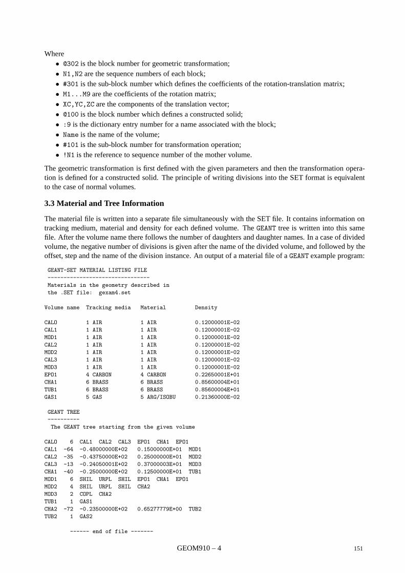
Where• @302 is the block number for geometric transformation;• N1,N2 are the sequence numbers of each block;• #301 is the sub-block number which defines the coefficients of the rotation-translation matrix;• M1...M9 are the coefficients of the rotation matrix;• XC,YC,ZC are the components of the translation vector;• @100 is the block number which defines a constructed solid;• :9 is the dictionary entry number for a name associated with the block;• Name is the name of the volume;• #101 is the sub-block number for transformation operation;• !N1 is the reference to sequence number of the mother volume.
The geometric transformation is first defined with the given parameters and then the transformation opera-tion is defined for a constructed solid. The principle of writing divisions into the SET format is equivalentto the case of normal volumes.
3.3 Material and Tree Information
The material file is written into a separate file simultaneously with the SET file. It contains information ontracking medium, material and density for each defined volume. The GEANT tree is written into this samefile. After the volume name there follows the number of daughters and daughter names. In a case of dividedvolume, the negative number of divisions is given after the name of the divided volume, and followed by theoffset, step and the name of the division instance. An output of a material file of a GEANT example program:
GEANT-SET MATERIAL LISTING FILE
--------------------------------
Materials in the geometry described in
the .SET file: gexam4.set
Volume name Tracking media Material Density
CALO 1 AIR 1 AIR 0.12000001E-02
CAL1 1 AIR 1 AIR 0.12000001E-02
MOD1 1 AIR 1 AIR 0.12000001E-02
CAL2 1 AIR 1 AIR 0.12000001E-02
MOD2 1 AIR 1 AIR 0.12000001E-02
CAL3 1 AIR 1 AIR 0.12000001E-02
MOD3 1 AIR 1 AIR 0.12000001E-02
EPO1 4 CARBON 4 CARBON 0.22650001E+01
CHA1 6 BRASS 6 BRASS 0.85600004E+01
TUB1 6 BRASS 6 BRASS 0.85600004E+01
GAS1 5 GAS 5 ARG/ISOBU 0.21360000E-02
GEANT TREE
----------
The GEANT tree starting from the given volume
CALO 6 CAL1 CAL2 CAL3 EPO1 CHA1 EPO1
CAL1 -64 -0.48000000E+02 0.15000000E+01 MOD1
CAL2 -35 -0.43750000E+02 0.25000000E+01 MOD2
CAL3 -13 -0.24050001E+02 0.37000003E+01 MOD3
CHA1 -40 -0.25000000E+02 0.12500000E+01 TUB1
MOD1 6 SHIL URPL SHIL EPO1 CHA1 EPO1
MOD2 4 SHIL URPL SHIL CHA2
MOD3 2 COPL CHA2
TUB1 1 GAS1
CHA2 -72 -0.23500000E+02 0.65277779E+00 TUB2
TUB2 1 GAS2
------ end of file -------
GEOM910 – 4 151
4 Usage
In order to carry out a successful transfer of a detector model, a user needs to be aware of certain limitationsof the interface. The user is recommended to communicate with the engineers using CAD systems toestablish a proper transfer methodology. If a CAD system is not capable of receiving the whole detectorgeometry in a single SET file, a user can transfer a detector model in smaller parts. These parts can then bejoined together in the CAD system. Normally it is a good idea to just export one instance of each divisionin order to limit the number of exported volumes. The divisions can be reproduced in CAD systems. It isimpossible to give an exact size-limit for a detector model which can be transferred in one file, because thelimitation depends on the structure of the detector model.
The GEANT graphics package provides excellent capabilities for viewing parts of a detector model which isto be exported. Using the visibility attribute and the number of division instances, a user will be able tosee what is to be exported. A user can use different colors in order to help to distinguish different volumes(eg division instances, etc.) in a CAD system. Dummy volumes, such as mothers made of air or vacuumshould be suppressed using the visibility attribute, since the interface is currently not able to discard suchinformation. A user must remember to specify the drawing parameters again if he wants to draw the detectormodel after using the interface. This is because the interface uses modified drawing routines.
A plot of the GEANT tree can be useful for engineers to understand the structure of the GEANT detector model.GEANT volume names are useful references regarding the material and tree information. The tree informationis also provided in the material file, but a graphical presentation is often useful.
152 GEOM910 – 5

GEOM Bibliography
[1] French Standardization, Data exchange and transfer standard specification, Afnor 1989.
[2] Michael E. Mortenson, Geometric Modeling, John Wiley & Sons, Inc., 1985.
[3] US department of Commerce, Initial Graphics Exchange Specification, 1988.
GEOM910 – 6 153

GEOM Bibliography
154 GEOM910 – 7
Geant 3.16 GEANT User’s Guide HITS001
Origin : Submitted: 15.08.84Revision : Revised: 17.12.93Documentation : F.Bruyant
The detector response package
1 Introduction
In the context of GEANT:
• hit is the user-defined information recorded at tracking time to keep track of the interaction betweenone particle and a given detector, and necessary to compute the digitisations later.
• digitisation (digit) is the user-defined information simulating the response of a given detector ele-ment, usually estimated after tracking a complete event.
The detector response package consists of tools to store, retrieve or print the information relevant to hits anddigitisation which is in the data structures JSET, JHITS and JDIGI. A few subroutines which may help theuser to solve some of the usual digitisation problems in simple detectors have been added to the package,e.g. the intersection of a track with a plane or a cylinder and the digitisation of conventional drift and MWPchambers.
For complex setups with different types of detectors the user has normally to define several types of hits anddigitisations. In addition to the hits generated by all particles of the current event, computing the digitisationsrequires usually some information about the intrinsic characteristics and performance of the detectors. Theinformation to be recorded for the hits and digitisations is highly experiment dependent, therefore only aframework can be proposed to store it.
Two remarks can be made:
• during the life of an experiment, the stability of the format and content of the information to be storedis usually reached much earlier for the hits than for the digitisations. Therefore the user may savecomputing time by designing an intermediate event output at the hits level.
• the scheme proposed for storing the digitisations should in any case be considered as an intermediatestage, a further processing of the data being necessary if the user wants to simulate more closely thespecific format of the real data-acquisition system.
2 SETs and DETectors
The reader is assumed to be familiar with the way the geometrical setup is described ([GEOM]), in particularwith the concepts of logical and physical volume tree structure.
The user is required to classify into sets all sensitive detectors (defined as those volume defined as detectorvia GSDET/GSDETV) for which he wants to store hits in the data structure JHITS. The 4-character nameswhich identify the sets are user defined, and the list of sets which the user wants to activate for a given runcan be entered through the data record SETS. The user can group together in one or in several sets detectorsof the same or different types. For convenience, it is recommended to have at least one set for each maincomponent of the setup, e.g. hadronic calorimeters, electromagnetic calorimeters, vertex chamber, etc.
A volume can be declared as a sensitive detector through the tracking medium parameter ISVOL, and allo-cated to a set through the subroutine GSDET or GSDETV. Each (logical) sensitive detector is identified by the4-character name of the corresponding volume. As a given volume may describe several similar detectors inthe physical setup, some additional information is needed for associating correctly the hits with the physicaldetectors.
155 HITS001 – 1
When using GSDET the user has to enter the (shortest) list of volume names (the vector CHNMSV), whichpermits unambiguous identification of the path through the physical tree, even in the presence of multiplecopies. This identification is obtained by specifying a list of volume numbers (the vector NUMBV), in a oneto one correspondence with the list of volume names. This list, after packing, will constitute the identifierof the physical detector.
If GSDETV is used instead of GSDET then the routine GGDETV (called by GGCLOS) constructs the lists CHNMSVautomatically and stores them in the structure JSET.
3 The user tools
The data structure JSET is built through calls to the routine GSDET or GSDETV which assign detectors to setsand define their parameters. After this, the following routines can be called, for each detector, to completethe structure:
GSDETH provides the parameters required for the storage of the hit elements in the data structure JHITS,such as the packing and scaling conventions;
GSDETD provides the parameters required for the storage of the digitisations in the structure JDIGI,such as the packing conventions;
GSDETU adds the user parameters, which may consist, for instance, of the intrinsic detector characteris-tics needed for computing the digitisations.
To permit storage of more than one type of hit for a given sensitive detector, or to provide additional detectorentries, detector aliases can be defined through calls to the routine GSDETA. They are entered in the JSETstructure as new detectors, with the same geometrical characteristics as the original one. The user has thepossibility to call appropriate routines GSDETH, GSDETD and GSDETU for this new detector.
During the tracking, for each step inside the sensitive detectors, under control of the subroutine GUSTEP, thehits can be stored in the data structure JHITS through the subroutine GSAHIT (or GSCHIT, more appropriatefor calorimetry). For each hit the information consists of:
• the reference to the track in the structure JKINE;
• the packed identifier of the physical detector;
• the packed data for the different elements of the hit.
When the tracking has been completed for the whole event the digitisations can be computed in the usersubroutine GUDIGI which may extract the hits with the subroutine GFHITS and store the digitisations inthe data structure JDIGI, with the subroutine GSDIGI. For each digitisation the information should at leastconsist of:
• the reference to the track(s);
• the packed identifier of the physical detector;
• the packed data for the digitisation itself.
4 Retrieval of geometrical information
The packed identifier of a physical detector, stored as part of the hit (or digitisation) information, is returnedunpacked by the routine GFHITS (or GFDIGI) which extracts the information from the JHITS or JDIGIstructures, and may be used to retrieve the geometrical characteristics of the given detector.
If the detectors have been defined by the routine GSDETV, the geometrical information can be retrieved by theroutines GFPATH and GLVOLU. GFPATH prepares the lists CHNAM and LNUM required by GLVOLU ([GEOM001]),from the information preprocessed at initialisation time by the routine GGDETV and stored in the structureJSET
HITS001 – 2 156
Geant 3.16 GEANT User’s Guide HITS100
Origin : R.Brun,F.Bruyant Submitted: 01.11.83Revision : Revised: 17.12.93Documentation :
Sensitive DETector definition
CALL GSDET (CHSET,CHDET,NV,CHNMSV,NBITSV,IDTYP,NWHI,NWDI,ISET*,IDET*)
CHSET (CHARACTER*4) set identifier, user defined;
CHDET (CHARACTER*4) detector identifier, has to be the name of an existing volume;
NV (INTEGER) number of volume descriptors;
CHNMSV (CHARACTER*4) array of NV volume descriptors;
NBITSV (INTEGER) array of NV, NBITSV(I) (I=1,...,NV) is the number of bits in which to pack thecopy number of volume CHNMSV(I);
IDTYP (INTEGER) detector type, user defined;
NWHI (INTEGER) initial size of HITS banks;
NWDI (INTEGER) initial size of DIGI banks;
ISET (INTEGER) position of set in bank JSET;
IDET (INTEGER) position of detector in bank JS=LQ(JSET-ISET).
Assigns detector CHDET to the set CHSET and defines its basic parameters.
Note: The vector CHNMSV (length NV) contains the list of volume names which permit unambiguous iden-tification of all copies of volume CHDET [see example in [HITS110]. Each element of the vector NBITSV(length NV) is the number of bits used for packing the number of the corresponding volume, when buildingthe packed identifier of a given physical detector.
For more details see the example given in [HITS110]. The detector type IDTYP is not used internally byGEANT and can be used to distinguish quickly between various kinds of detectors, in the routine GUSTEP forexample.
CALL GSDETV (CHSET,CHDET,IDTYP,NWHI,NWDI,ISET*,IDET*)
The arguments of this routine are the same than the previous one, but NAMES, NBITSV will be computed byGGDETV called by GGCLOS) (see [HITS001]).
CALL GFDET (CHSET,CHDET,NV*,CHNMSV*,NBITSV*,IDTYP*,NWHI*,NWDI*,ISET*,IDET*)
Returns the parameters for detector CHDET of set CHSET, the arguments have the same meaning than forroutine GSDET.
CALL GPSETS (CHSET,CHDET)
Prints SET and DETector parameters.
CHSET (CHARACTER*4) set to be printed, if * prints all detectors of all sets;
CHDET (CHARACTER*4) detector to be printed, if * prints all detectors of set CHSET.
157 HITS100 – 1
Geant 3.16 GEANT User’s Guide HITS105
Origin : F.Bruyant Submitted: 13.06. 85Revision : Revised: 16.12.93Documentation :
Detector aliases
Detector aliases can be specified for any sensitive detector for which the user either needs to store morethan one type of hit or wants to define additional detector entries.
CALL GSDETA (CHSET,CHDET,CHALI,NWHI,NWDI,IALI*)
CHSET (CHARACTER*4) set name;
CHDET (CHARACTER*4) name of the detector for which an alias is being defined;
CHALI (CHARACTER*4) alias name;
NWHI (INTEGER) initial number of words of HITS banks;
NWDI (INTEGER) initial number of words of DIGI banks;
IALI (INTEGER) position of alias in bank JS=LQ(JSET-ISET).
Defines an alias CHALI for detector CHDET of set CHSET and enters it in the JSET structure as an additionaldetector in the corresponding set, at the position IALI. The new detector will be a copy at position IALI ofthe original detector CHDET, with empty links to the GSDETH, GSDETD and GSDETU parameter banks. Theuser can therefore call these three routines again with the arguments appropriate to the detector CHALI.Several aliases can be defined for the same detector through calls to GSDETA.
158 HITS105 – 1
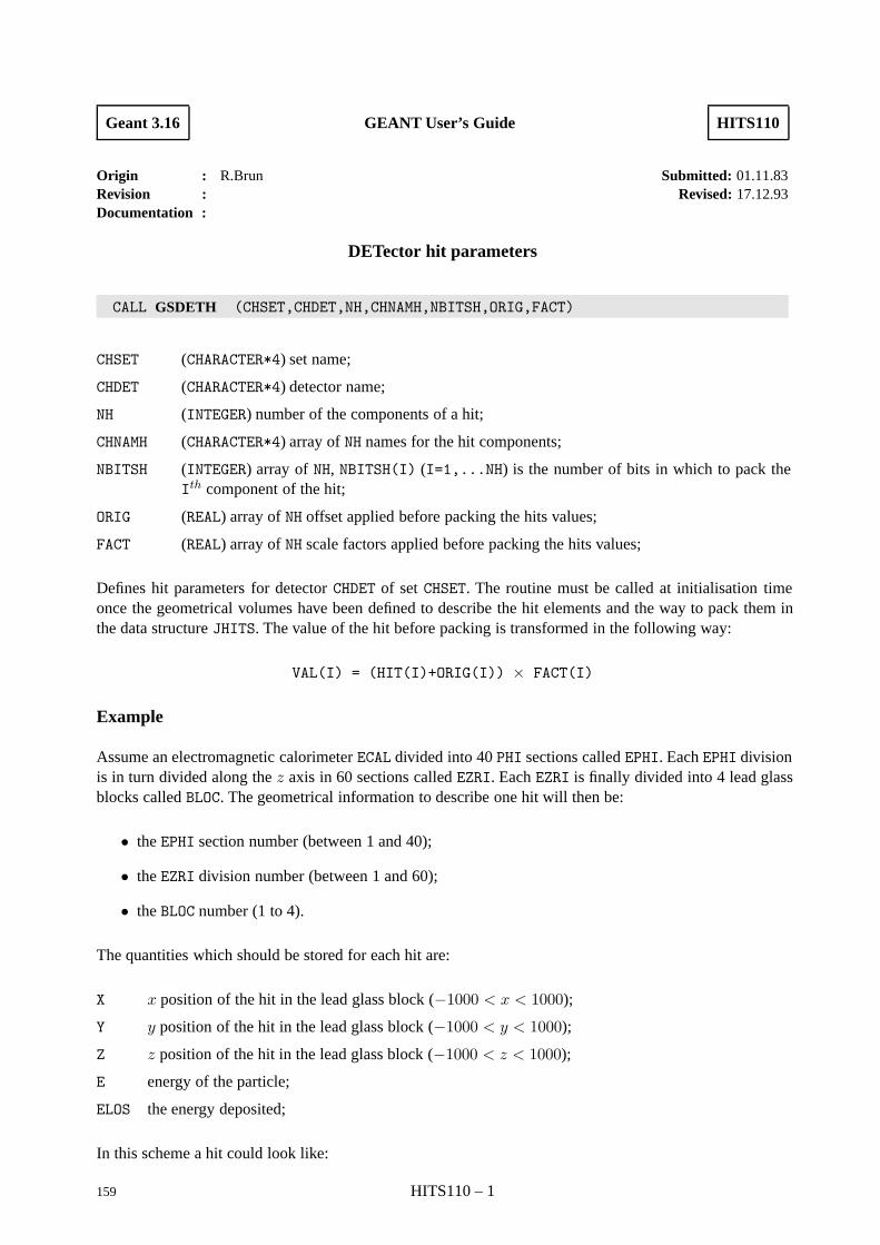
Geant 3.16 GEANT User’s Guide HITS110
Origin : R.Brun Submitted: 01.11.83Revision : Revised: 17.12.93Documentation :
DETector hit parameters
CALL GSDETH (CHSET,CHDET,NH,CHNAMH,NBITSH,ORIG,FACT)
CHSET (CHARACTER*4) set name;
CHDET (CHARACTER*4) detector name;
NH (INTEGER) number of the components of a hit;
CHNAMH (CHARACTER*4) array of NH names for the hit components;
NBITSH (INTEGER) array of NH, NBITSH(I) (I=1,...NH) is the number of bits in which to pack theIth component of the hit;
ORIG (REAL) array of NH offset applied before packing the hits values;
FACT (REAL) array of NH scale factors applied before packing the hits values;
Defines hit parameters for detector CHDET of set CHSET. The routine must be called at initialisation timeonce the geometrical volumes have been defined to describe the hit elements and the way to pack them inthe data structure JHITS. The value of the hit before packing is transformed in the following way:
VAL(I) = (HIT(I)+ORIG(I)) × FACT(I)
Example
Assume an electromagnetic calorimeter ECAL divided into 40 PHI sections called EPHI. Each EPHI divisionis in turn divided along the z axis in 60 sections called EZRI. Each EZRI is finally divided into 4 lead glassblocks called BLOC. The geometrical information to describe one hit will then be:
• the EPHI section number (between 1 and 40);
• the EZRI division number (between 1 and 60);
• the BLOC number (1 to 4).
The quantities which should be stored for each hit are:
X x position of the hit in the lead glass block (−1000 < x < 1000);
Y y position of the hit in the lead glass block (−1000 < y < 1000);
Z z position of the hit in the lead glass block (−1000 < z < 1000);
E energy of the particle;
ELOS the energy deposited;
In this scheme a hit could look like:
159 HITS110 – 1
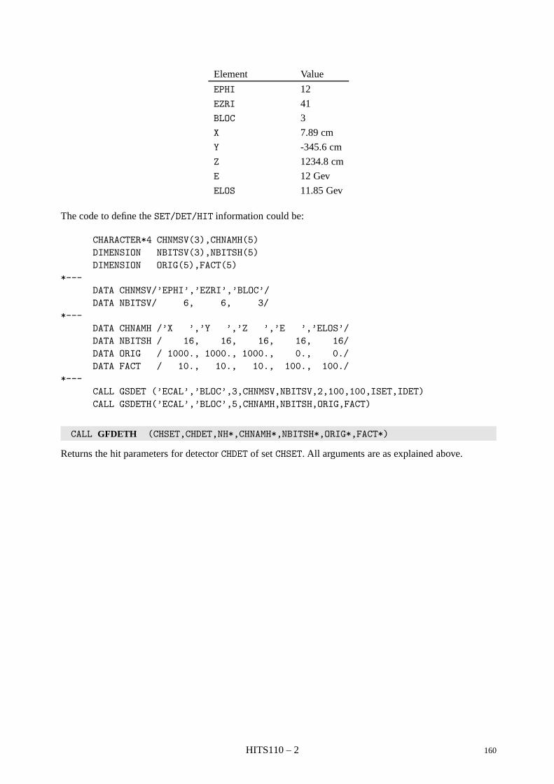
Element Value
EPHI 12
EZRI 41
BLOC 3
X 7.89 cm
Y -345.6 cm
Z 1234.8 cm
E 12 Gev
ELOS 11.85 Gev
The code to define the SET/DET/HIT information could be:
CHARACTER*4 CHNMSV(3),CHNAMH(5)DIMENSION NBITSV(3),NBITSH(5)DIMENSION ORIG(5),FACT(5)
*---DATA CHNMSV/’EPHI’,’EZRI’,’BLOC’/DATA NBITSV/ 6, 6, 3/
*---DATA CHNAMH /’X ’,’Y ’,’Z ’,’E ’,’ELOS’/DATA NBITSH / 16, 16, 16, 16, 16/DATA ORIG / 1000., 1000., 1000., 0., 0./DATA FACT / 10., 10., 10., 100., 100./
*---CALL GSDET (’ECAL’,’BLOC’,3,CHNMSV,NBITSV,2,100,100,ISET,IDET)CALL GSDETH(’ECAL’,’BLOC’,5,CHNAMH,NBITSH,ORIG,FACT)
CALL GFDETH (CHSET,CHDET,NH*,CHNAMH*,NBITSH*,ORIG*,FACT*)
Returns the hit parameters for detector CHDET of set CHSET. All arguments are as explained above.
HITS110 – 2 160
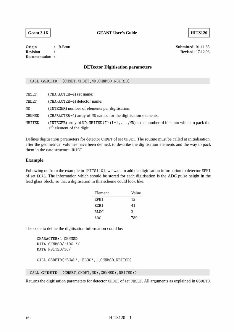
Geant 3.16 GEANT User’s Guide HITS120
Origin : R.Brun Submitted: 01.11.83Revision : Revised: 17.12.93Documentation :
DETector Digitisation parameters
CALL GSDETD (CHSET,CHDET,ND,CHNMSD,NBITSD)
CHSET (CHARACTER*4) set name;
CHDET (CHARACTER*4) detector name;
ND (INTEGER) number of elements per digitisation;
CHNMSD (CHARACTER*4) array of ND names for the digitisation elements;
NBITSD (INTEGER) array of ND, NBITSD(I) (I=1,...,ND) is the number of bits into which to pack theIth element of the digit.
Defines digitisation parameters for detector CHDET of set CHSET. The routine must be called at initialisation,after the geometrical volumes have been defined, to describe the digitisation elements and the way to packthem in the data structure JDIGI.
Example
Following on from the example in [HITS110], we want to add the digitisation information to detector EPHIof set ECAL. The information which should be stored for each digitisation is the ADC pulse height in thelead glass block, so that a digitisation in this scheme could look like:
Element Value
EPHI 12
EZRI 41
BLOC 3
ADC 789
The code to define the digitisation information could be:
CHARACTER*4 CHNMSDDATA CHNMSD/’ADC ’/DATA NBITSD/16/
CALL GSDETD(’ECAL’,’BLOC’,1,CHNMSD,NBITSD)
CALL GFDETD (CHSET,CHDET,ND*,CHNMSD*,NBITSD*)
Returns the digitisation parameters for detector CHDET of set CHSET. All arguments as explained in GSDETD.
161 HITS120 – 1
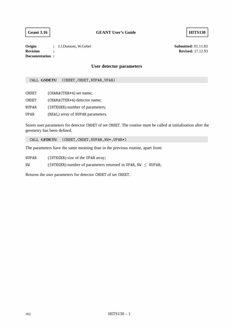
Geant 3.16 GEANT User’s Guide HITS130
Origin : J.J.Dumont, W.Gebel Submitted: 01.11.83Revision : Revised: 17.12.93Documentation :
User detector parameters
CALL GSDETU (CHSET,CHDET,NUPAR,UPAR)
CHSET (CHARACTER*4) set name;
CHDET (CHARACTER*4) detector name;
NUPAR (INTEGER) number of parameters;
UPAR (REAL) array of NUPAR parameters.
Stores user parameters for detector CHDET of set CHSET. The routine must be called at initialisation after thegeometry has been defined.
CALL GFDETU (CHSET,CHDET,NUPAR,NW*,UPAR*)
The parameters have the same meaning than in the previous routine, apart from:
NUPAR (INTEGER) size of the UPAR array;
NW (INTEGER) number of parameters returned in UPAR, NW ≤ NUPAR;
Returns the user parameters for detector CHDET of set CHSET.
162 HITS130 – 1
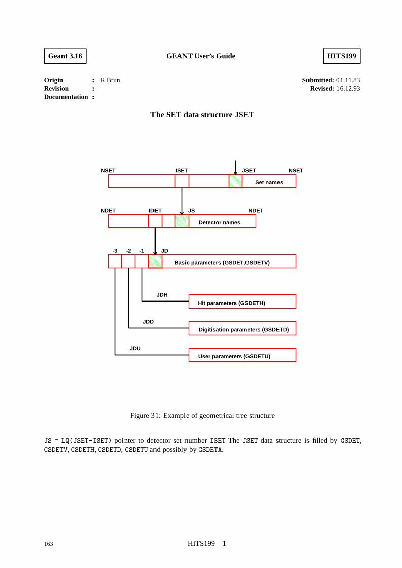
Geant 3.16 GEANT User’s Guide HITS199
Origin : R.Brun Submitted: 01.11.83Revision : Revised: 16.12.93Documentation :
The SET data structure JSET
NSET ISET JSET NSET
NDET IDET
Set names
JS NDET
Detector names
-3 -2 -1 JD
Basic parameters (GSDET,GSDETV)
Hit parameters (GSDETH)
Digitisation parameters (GSDETD)
User parameters (GSDETU)
JDH
JDD
JDU
Figure 31: Example of geometrical tree structure
JS = LQ(JSET-ISET) pointer to detector set number ISET The JSET data structure is filled by GSDET,GSDETV, GSDETH, GSDETD, GSDETU and possibly by GSDETA.
163 HITS199 – 1
Geant 3.16 GEANT User’s Guide HITS200
Origin : R.Brun, F.Bruyant, W.Gebel, M.Maire Submitted: 01.11.83Revision : Revised: 17.12.93Documentation :
Routines to store and retrieve HITS
CALL GSAHIT (ISET,IDET,ITRA,NUMBV,HITS,IHIT*)
ISET (INTEGER) set number (see below);
IDET (INTEGER) detector number;
ITRA (INTEGER) number of the track producing this hit
NUMBV (INTEGER) array of volume numbers corresponding to list NAMESV of GSDET;
HITS (REAL) array of values for current hit elements;
IHIT (INTEGER) current hit number, if 0 the hit has not been stored.
Stores element values for current hit into the data structure JHITS. The values ISET, IDET and NUMBV canbe found in the corresponding variables of common /GCSETS/. These values are set by the routine GFINDSevery time that a particle is in a defined detector.
CALL GSCHIT (ISET,IDET,ITRA,NUMBV,HITS,NHSUM,IHIT*)
Same action as GSAHIT, but in case the detector identified by ISET, IDET and NUMBV contains already a hitfor the same track, the routine will make a cummulative sum for the latest NHSUM elements of JHITS. Theother previous elements of JHITS are replaced. That facility is particularly interesting in the case of hitsgenerated into a calorimeter. No packing (i.e. 32 bits per hit element) should be requested for the last NHSUMhits in GSDETH and for these hits ORIG should be set to 0.
CALL GPHITS (CHSET,CHDET)
CHSET (CHARACTER*4) set name, if ’*’ prints all JHITS banks of all sets;
CHDET (CHARACTER*4) detector name, if ’*’ prints hits in all detectors of set CHSET.
Prints JHITS banks for detector CHDET of set CHSET.
CALL GFHITS (CHSET,CHDET,NVDIM,NHDIM,NHMAX,ITRS,NUMVS,ITRA*,NUMBV*,HITS*,NHITS*)
CHSET (CHARACTER*4) set name;
CHDET (CHARACTER*4) detector name;
NVDIM (INTEGER) 1st dimension of arrays NUMBV and NUMVS: 1≤NVDIM≤NV argument of GSDET;
NHDIM (INTEGER) 1st dimension of array HITS: 1≤NHDIM≤NH argument of GSDETH;
NHMAX (INTEGER) maximum number of hits to be returned, this should be not larger than the seconddimension of array NUMBV and HITS;
ITRS (INTEGER) number of the selected track, if ITRS=0, all tracks are taken;
NUMVS (INTEGER) is a 1-dimension array of NVDIM elements that contains the list of volume numberswhich identify the selected detector, 0 is interpreted as ’all valid numbers’;
164 HITS200 – 1
ITRA (INTEGER) is a 1-dim array of dimension NHMAX that contains on output for each hit the numberof the track which has produced it;
NUMBV (INTEGER) 2-dim array (NVDIM,NHMAX) that containis on output for each hit the list of volumenumbers which identify the detector, all values set to 0 means that no more volumes are stored;
HITS (REAL) 2-dim array (NHDIM,NHMAX) that containis NHITS hits;
NHITS (INTEGER) number of hits returned, in case the total number of hits is greater than NHMAX,NHITS is set to NHMAX+1 and NHMAX hits are returned.
This rotine returns the hits produced by track ITRS (or by any track) in the detector CHDET identified by thelist NUMVS belonging to set CHSET.
HITS(1,I) is element 1 of hit number I;
NUMBV(1,I) is volume number 1 of hit number I;
ITRA(I) is the track number corresponding to hit number I;
The arrays NUMVS, NUMBV, HITS and ITRA must be dimensioned to:
NUMVS(NVDIM)NUMBV(NVDIM,NHMAX)HITS(NHDIM,NHMAX)ITRA(NHMAX)
CALL GFPATH (ISET,IDET,NUMBV,NLEV*,LNAM*,LNUM*)
ISET (INTEGER) set number;
IDET (INTEGER) detector number;
NUMBV (INTEGER) array of numbers which identify uniquely detector number IDET;
NLEV (INTEGER) number of elements filled of arrays LNAM and LNUM;
LNAM (INTEGER) array of NLEV volume names stored in ASCII code in integers;
LNUM (INTEGER) array of NLEV copy numbers.
This routine returns the list of volume names and numbers which identify the complete ancestry in theJVOLUM data structure of the volume corresponding to the detector number IDET in set number ISET andwhich is identified by the volume numbers NUMBV (see GFHITS).
GFPATH assumes that the detectors have been declared via GSDETV and not GSDET. The main use of GFPATHis to prepare the lists LNAM and LNUM required by the routine GLVOLU to fill the common /GCVOLU/. Once/GCVOLU/ is properly filled, it is possible to use the GEANT routines to transform from the local to the masterreference system and so on.
HITS200 – 2 165
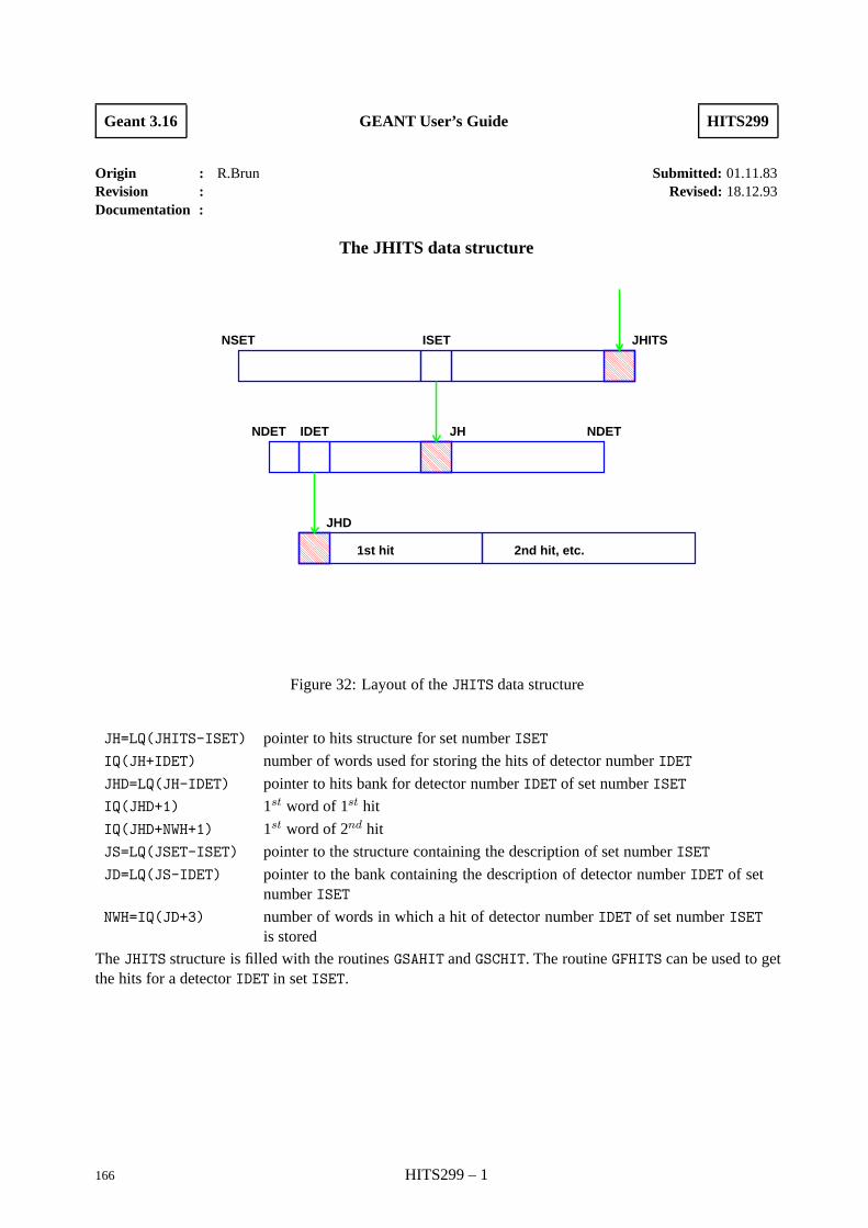
Geant 3.16 GEANT User’s Guide HITS299
Origin : R.Brun Submitted: 01.11.83Revision : Revised: 18.12.93Documentation :
The JHITS data structure
NSET ISET JHITS
NDET IDET JH NDET
JHD
1st hit 2nd hit, etc.
Figure 32: Layout of the JHITS data structure
JH=LQ(JHITS-ISET) pointer to hits structure for set number ISET
IQ(JH+IDET) number of words used for storing the hits of detector number IDET
JHD=LQ(JH-IDET) pointer to hits bank for detector number IDET of set number ISET
IQ(JHD+1) 1st word of 1st hit
IQ(JHD+NWH+1) 1st word of 2nd hit
JS=LQ(JSET-ISET) pointer to the structure containing the description of set number ISET
JD=LQ(JS-IDET) pointer to the bank containing the description of detector number IDET of setnumber ISET
NWH=IQ(JD+3) number of words in which a hit of detector number IDET of set number ISETis stored
The JHITS structure is filled with the routines GSAHIT and GSCHIT. The routine GFHITS can be used to getthe hits for a detector IDET in set ISET.
166 HITS299 – 1
Geant 3.16 GEANT User’s Guide HITS300
Origin : R.Brun, W.Gebel Submitted: 10.08.84Revision : Revised: 18.12.93Documentation :
Routines to store and retrieve DIGItisations
CALL GSDIGI (ISET,IDET,LTRA,NTRA,NUMBV,KDIGI,IDIG*)
ISET (INTEGER) set number;
IDET (INTEGER) detector number;
LTRA (INTEGER) array of NTRA track numbers producing this digitisation;
NUMBV (INTEGER) volume numbers corresponding to list NAMESV of GSDET;
KDIGI (INTEGER) array of current digisation elements;
IDIG (INTEGER) stored digitisation number, if 0, digitisation has not been stored.
Stores element values for current digitisation into the data structure JDIGI.
CALL GPDIGI (CHSET,CHDET)
CHSET (CHARACTER*4) set name, if ’*’ prints all JDIGI banks of all sets;
CHDET (CHARACTER*4) detector name, if ’*’ prints digitisations in all detectors of set; CHSET
Prints JDIGI banks for detector CHDET of set CHSET.
CALL GFDIGI (CHSET,CHDET,NTDIM,NVDIM,NDDIM,NDMAX,NUMVS,LTRA*,NTRA*,NUMBV*,KDIGI*,NDIGI*)
CHSET (INTEGER) set name;
CHDET (INTEGER) detector name;
NTDIM (INTEGER) 1st dimension of LTRA, maxmum number of tracks contributing to each hit to bereturned;
NVDIM (INTEGER) 1st dimension of arrays NUMVS, NUMBV, same as argument NV of GSDET;
NDDIM (INTEGER) 1st dimension of KDIGI, same as argument ND of GSDETD;
NDMAX (INTEGER) maximum number of digitisations to be returned, second dimension of arrays NTDIM,NUMBV and KDIGI;
NUMVS (INTEGER) is a 1-dim array of length NVDIM that contains the copy numbers identifying thedetector to be selected, all 0 is interpreted as all copies of detector CHDET;
LTRA (INTEGER) is a 2-dim array NTDIM,NDMAX that contains for each digitisation the numbers ofthe tracks which have produced it;
NTRA (INTEGER) is a 1-dim array of length NDMAX that contains, for each digitisation, the number oftracks contributing, in case this number is greater than NTDIM, only the first NTDIM correspond-ing tracks are returned on LTRA;
NUMBV (INTEGER) is a 2-dim array NVDIM,NDMAX that contains, for each digitisation, the list of volumenumbers which identify each detector;
167 HITS300 – 1
KDIGI (INTEGER) is a 2-Dim array NDDIM,NDMAX that contains the NDIGI digitisations returned;
NDIGI (INTEGER) is the total number of digitisations in this detector, in case the total number ofdigitisations is greater than NDMAX, NDIGI is set to NDMAX+1 and only NDMAX digitisations arereturned.
Returns the digitisations for the detector CHDET identified by the list of copy numbers NUMVS belonging toset CHSET. The maning of the variables is the following:
KDIGI(1,I) digitisation element 1 for digitisation number I
NUMBV(1,I) first volume number for digitisation number I
LTRA (1,I) number of the first track contributing to digitisation number I
In the calling routine, the arrays LTRA, NTRA, NUMVS, NUMBV, KDIGI must be dimensioned to:
LTRA (NTDIM,NDMAX)NTRA (NDMAX)NUMVS(NVDIM)NUMBV(NVDIM,NDMAX)KDIGI(NDDIM,NDMAX)
HITS300 – 2 168
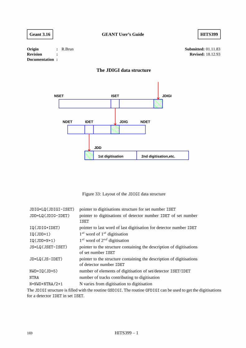
Geant 3.16 GEANT User’s Guide HITS399
Origin : R.Brun Submitted: 01.11.83Revision : Revised: 18.12.93Documentation :
The JDIGI data structure
NSET ISET JDIGI
NDET IDET JDIG NDET
JDD
1st digitisation 2nd digitisation,etc.
Figure 33: Layout of the JDIGI data structure
JDIG=LQ(JDIGI-ISET) pointer to digitisations structure for set number ISET
JDD=LQ(JDIG-IDET) pointer to digitisations of detector number IDET of set numberISET
IQ(JDIG+IDET) pointer to last word of last digitisation for detector number IDET
IQ(JDD+1) 1st word of 1st digitisation
IQ(JDD+N+1) 1st word of 2nd digitisation
JS=LQ(JSET-ISET) pointer to the structure containing the description of digitisationsof set number ISET
JD=LQ(JS-IDET) pointer to the structure containing the description of digitisationsof detector number IDET
NWD=IQ(JD+5) number of elements of digitisation of set/detector ISET/IDET
NTRA number of tracks contributing to digitisation
N=NWD+NTRA/2+1 N varies from digitisation to digitisation
The JDIGI structure is filled with the routine GSDIGI. The routine GFDIGI can be used to get the digitisationsfor a detector IDET in set ISET.
169 HITS399 – 1
Geant 3.10 GEANT User’s Guide HITS400
Origin : R.Brun,H. Boerner Submitted: 01.10.81Revision : Revised: 18.12.93Documentation :
Intersection of a track with a cylinder or a plane
CALL GICYL (R,X1,X2,S1,S2,IC,XINT*,SINT*,PZINT*,IFLAG*)
R (REAL) radius of cylinder in cm;
X1 (REAL) array of 6, (x, y, z, dx/ds, dy/ds, dz/ds) of 1st point;
X2 (REAL) array of 6, (x, y, z, dx/ds, dy/ds, dz/ds) of 2nd point;
S1 (REAL) track length s at 1st point;
S2 (REAL) track length s at 2nd point;
IC (INTEGER) type of interpolation:
1 straight line defined as (Xi(1),Xi(2),Xi(3)) + s (Xi(4),Xi(5),Xi(6)), where iis 1 or 2 according to which of the two points is inside the cylinder;
2 straight line going from (X1(1),X1(2),X1(3)) to (X2(1),X2(2),X2(3));
3 third degree curve with:
3P (s) = 3a s3 +3b s2 + 3c s+ 3d Xi =
(3P (Si),
d 3P
ds
∣∣∣∣∣s=Si
)i = 1, 2
XINT (REAL) array of 6 x, y, z, dx/ds, dy/ds, dz/ds at intersection point;
SINT (REAL) S at intersection point;
PZINT (REAL) φ, z, dφ/dr, dz/dr in cylindrical coordinates at intersection point;
IFLAG (INTEGER) return flag:
0 track does not intersect cylinder;
1 track intersects cylinder.
Calculates intersection of track with a cylinder of radius R. The track is approximated by a cubic in the tracklength. To improve stability, the coordinate system is shifted.
CALL GIPLAN (YC,X1,X2,S1,S2,IC,XINT*,SINT*,PZINT*,IFLAG*)
The arguments have the same meaning than in the previous routine, apart from:
YC (REAL) y coordinate of plane;
Calculates intersection of track with a plane parallel to x − z. The track is approximated by a cubic in thetrack length. To improve stability, the coordinate system is shifted.
Note: the default accuracy is 10 microns. The value of EPSI (internal variable) must be changed for a betterprecision.
170 HITS400 – 1
Geant 3.16 GEANT User’s Guide HITS500
Origin : GEANT2 Submitted: 01.10.81Revision : Revised: 19.12.93Documentation :
Digitisation for drift- or MWP- Chambers
CALL GPDRIF (DETREP,HITREP,IOUT*)
DETREP (REAL) array of 6 with detector description:
1 number of wires;2 wire spacing in cm;3 sin(α);4 cos(α);5 distance of wire 1 from the origin in cm;6 drift velocity (cm/nsec)
HITREP (REAL) array of 2 with track description:
1 x coordinate of intersection;2 y coordinate of intersection;
IOUT (INTEGER) result of digitisation:
1 wire number;2 drift time (signed to avoid left/right ambiguity).
Digitisation routine for a plane drift chamber. The drift chamber is supposed to be in the x− y plane. Thenormal to the wires in the x− y plane and the z axis form an angle α.
CALL GCMWPC (DETREP,HITREP,IOUT*)
DETREP (REAL) array of 6 with detector description:
1 number of wires;2 wire spacing (radians);3 dθ/dz along the wires;4 θ of a point on wire 1;5 z of a point on wire 1 corresponding to θ=DETREP(4);6 gap width;
HITREP (REAL) array of 4 with track description:
1 θ coordinate of intersection;2 z coordinate;3 dθ/dr;4 dz/dr;
IOUT (INTEGER) array of 4 with result of digitisation:
1 wire number (-1 if missing);2 cluster size;3 wire number of second cluster if any;4 cluster size;
Routine to compute one or two digitisations produced by a hit on a cylindrical MWPC. The chamber is acylinder of thickness DETREP(6) which should be small compared with the radius.
171 HITS500 – 1
CALL GPMWPC (DETREP,HITREP,IOUT*)
DETREP (REAL) array of 6 with detector description:
1 number of wires;
2 wire spacing (radians);
3 sin(α);4 cos(α);5 distance of wire 1 from the origin in cm;
6 gap width;
HITREP (REAL) array of 4 with track description:
1 x coordinate of intersection;
2 y coordinate of intersection;
3 dx/dz;
4 dy/dz;
IOUT (INTEGER) array of 2 with result of digitisation:
1 wire number (-1 if missing);
2 cluster size;
Digitisation routine for a plane MWPC.
HITS500 – 2 172
Geant 3.16 GEANT User’s Guide HITS510
Origin : W.Mitaroff Submitted: 21.02.85Revision : Revised: 19.12.93Documentation :
Digitisation for drift chambers
CALL GCDRIF (RADD,ZMIN,ZMAX,DETREP,HITREP,IOUT*)
RADD (REAL) radius of cylindrical chamber in cm;
ZMIN (REAL) z of lower end of cylindrical chamber;
ZMAX (REAL) z of upper end of cylindrical chamber;
DETREP (REAL) array of 8 with detector description:
1 number of wires;
2 wire spacing in φ (radians);
3 cosine of wire angle with respect to the z axis;
4 sine of wire angle with respect to the z axis (signed like dφ/dz);
5 dφ/dz along wire;
6 φ of point with z = 0 on wire 1;
7 drift velocity (cm nsec−1);
8 if > 0 user routine GUDTIM will be called to calculate drift time;
HITREP (REAL) array of 4 describing the track:
1 φ coordinate of intersection;
2 z coordinate of intersection;
3 dφ/dr;
4 dz/dr;
IOUT (INTEGER) array of 4 with digitisation information:
1 wire number (1...NWI with increasing phi), -1 if DETREP parameters are inconsistent;
2 drift time in nsec, > 0 if φ(hit) > φ(wire);3 digitised current division information (relative position of charge along wire, per mille);
4 amount of charge deposited onto wire.
Digitisation routine for a cylindrical drift chamber.
Knowing the position Z of the deposit of charge we can calculate
ICD = LZ − Zl
Zu − Zl
where L = 1000 in the program. This is the information stored into IOUT(3).
CALL GCDERR (ICD*,ERP,ERS)
ICD (INTEGER) digitised current division information (≤ ICD ≤ 1000), overwritten on output withthe modified value taking into account the errors;
ERP (REAL) variance of Gaussian pedestal errors on the measured pulse heights relative to the sumof the pulse heights;
173 HITS510 – 1
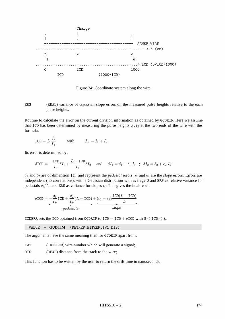
Charge. | .| . |========================================= SENSE WIRE
...................................................> Z (cm)Z Z Zl u
...............................................> ICD (0<ICD<1000)0 ICD 1000
ICD (1000-ICD)
Figure 34: Coordinate system along the wire
ERS (REAL) variance of Gaussian slope errors on the measured pulse heights relative to the eachpulse heights.
Routine to calculate the error on the current division information as obtained by GCDRIF. Here we assumethat ICD has been determined by measuring the pulse heights I1, I2 at the two ends of the wire with theformula:
ICD = LI2I+
with I+ = I1 + I2
Its error is determined by:
δICD = −ICD
I+δI1 +
L− ICD
I+δI2 and δI1 = δ1 + ε1 I1 ; δI2 = δ2 + ε2 I2
δ1 and δ2 are of dimension [I] and represent the pedestal errors. ε1 and ε2 are the slope errors. Errors areindependent (no correlations), with a Gaussian distribution with average 0 and ERP as relative variance forpedestals δi/I+ and ERS as variance for slopes εi. This gives the final result
δICD = − δ1I+
ICD+δ2I+(L− ICD)︸ ︷︷ ︸
pedestals
+(ε2 − ε1)ICD(L− ICD)
L︸ ︷︷ ︸slope
GCDERR sets the ICD obtained from GCDRIF to ICD = ICD+ δICD with 0 ≤ ICD ≤ L.
VALUE = GUDTIM (DETREP,HITREP,IW1,DIS)
The arguments have the same meaning than for GCDRIF apart from:
IW1 (INTEGER) wire number which will generate a signal;
DIS (REAL) distance from the track to the wire;
This function has to be written by the user to return the drift time in nanoseconds.
HITS510 – 2 174

HITS Bibliography
175 HITS510 – 3

Geant 3.16 GEANT User’s Guide IOPA001
Origin : Submitted: 15.08.84Revision : Revised: 16.12.93Documentation : R.Brun
The I/O routines
The I/O routines allow one to read, write or print the GEANT data structures. All GEANT I/O is handled thoughthe ZEBRA system, which provides the following facilities:
• native and machine independent I/O to and from disk and tape devices;
• sequential and direct access I/O (from disk);
This allows, for example, to generate events on one machine, dump the data structures to a mass storagedevice, and then read them back for further processing on a different machine.
This section describes the various routines for I/O in GEANT. For a complete reference on the ZEBRA I/Osystem the user is referred to the ZEBRA documentation [1, 8].
176 IOPA001 – 1
Geant 3.16 GEANT User’s Guide IOPA200
Origin : R.Brun Submitted: 01.06.83Revision : Revised: 16.12.93Documentation :
ZEBRA sequential files handling
CALL GOPEN (LUN,CHOPT,LEN,IER*)
LUN (INTEGER) logical unit number, 1≤LUN<100;
CHOPT (CHARACTER*(*)) any valid combination of FZFILE options (see [1, 8]), the most commonbeing:
I input file;
O output file;
X exchange mode file;
LEN (INTEGER) maximum record length, for more details see routine FZFILE in the ZEBRA manual;
IER (INTEGER) error flag:
0 legal open request;
1 attempt to open more than 5 ZEBRA sequential files;
Opens a ZEBRA FZ file for sequential I/O of GEANT data structures. No more than 5 files can be open at anyone time.
CALL GCLOSE (LUN,IER*)
LUN (INTEGER) logical unit to be closed, if 0 all ZEBRA FZ streams will be closed;
IER (INTEGER) error flag:
0 legal close request;
1 no unit was found open;
This routine closes one or all ZEBRA FZ file(s). This is a mandatory routines for all open ZEBRA files beforethe end of the program. Failure to call this routine may cause files to be incompletely written to the storagemedia.
177 IOPA200 – 1

Geant 3.16 GEANT User’s Guide IOPA300
Origin : R. Brun Submitted: 01.06.83Revision : Revised: 17.12.93Documentation :
Data structure I/O with sequential files
CALL GFIN (LUN,CHOBJ,NKEYS,IDVERS*,CHOPT,IER*)
LUN (INTEGER) logical unit;
CHOBJ (CHARACTER*4) array with the data structures to be read:
MATE material;
TMED tracking medium;
VOLU volumes;
ROTM rotation matrix;
SETS detector set;
PART particle;
SCAN scan geometry;
DRAW drawing;
INIT all of the above;
KINE this keyword will trigger the read of KINE and VERT unless the flag S is set;
DIGI digitisation;
HEAD event header;
HITS hits;
RUNG run;
STAK particle temporary stack;
STAT volume statistic;
VERT vertex;
JXYZ track points;
TRIG this keyword will trigger the read of DIGI, HEAD, HITS, KINE, VERT and JXYZ unlessthe S flag is set;
NKEYS (INTEGER) number of keys in array CHOBJ;
IDVERS (INTEGER) version of the data structure to be read in, if 0 it will read any version, on output itcontains the version of the data structure read in;
CHOPT (CHARACTER*(*)) option:
I among the data structures specified in CHOBJ read only the initialisation ones;
K among the data structures specified in CHOBJ read only KINE and TRIG, if present;
T among the data structures specified in CHOBJ read only DIGI, HEAD, HITS, KINE, VERTand JXYZ, if present;
S interpret KINE to mean only the KINE data structure and ignore TRIG and INIT;
Q quiet option, no message is printed;
IER (INTEGER) error flag:
<0 ZEBRA error flag as returned in IQUEST(1);
0 read completed successfully;
178 IOPA300 – 1
>0 if only IER] structures read in out of the NKEYS requested;
Routine to read GEANT object(s) from a ZEBRA/FZ file. The data structures from disk are read in memory.The FZ data base must have been been created via GOPEN/GFOUT. Example:
CALL GOPEN(1,’I’,1024,IER)IDVOLU = 0IDMATE = 0IDTMED = 0IDROTM = 0IDPART = 0IDSCAN = 0IDSETS = 0CALL GFIN (1,’VOLU’,1,IDVOLU,’ ’,IER)CALL GFIN (1,’MATE’,1,IDMATE,’ ’,IER)CALL GFIN (1,’TMED’,1,IDTMED,’ ’,IER)CALL GFIN (1,’ROTM’,1,IDROTM,’ ’,IER)CALL GFIN (1,’PART’,1,IDPART,’ ’,IER)CALL GFIN (1,’SCAN’,1,IDSCAN,’ ’,IER)CALL GFIN (1,’SETS’,1,IDSETS,’ ’,IER)
CALL GFOUT (LUN,CHOBJ,NKEYS,IDVERS,CHOPT,IER*)
The arguments have the same meaning than for GFIN with the following differences:
IDVERS (INTEGER) version identifier of the data structures to be written out;
Routine to write GEANT object(s) into a ZEBRA/FZ file. The data structures from memory are written on thefile. The FZ data base must have been been created via GOPEN/GFOUT. Example:
CALL GOPEN(1,’O’,1024,IER)CALL GFOUT (1,’VOLU’,1,IDVOLU,’ ’,IER)CALL GFOUT (1,’MATE’,1,IDMATE,’ ’,IER)CALL GFOUT (1,’TMED’,1,IDTMED,’ ’,IER)CALL GFOUT (1,’ROTM’,1,IDROTM,’ ’,IER)CALL GFOUT (1,’PART’,1,IDPART,’ ’,IER)CALL GFOUT (1,’SCAN’,1,IDSCAN,’ ’,IER)CALL GFOUT (1,’SETS’,1,IDSETS,’ ’,IER)
Note: the routines GGET and GSAVE are obsolete and should not be used.
IOPA300 – 2 179
Geant 3.16 GEANT User’s Guide IOPA400
Origin : R.Brun Submitted: 20.08.87Revision : Revised: 17.12.93Documentation :
ZEBRA direct access files handling
I/O with direct access files is the most efficient way to use direct access devices. All the routines describedin this section and in ([IOPA500]) are based on the ZEBRA-RZ package and the user is referred to the relateddocumentation [8] for an understanding of the basic principles.
CALL GRFILE (LUN,CHFILE,CHOPT)
LUN (INTEGER) logical unit number;
CHFILE (CHARACTER*(*)) file name;
CHOPT (CHARACTER*(*)) any valid option for RZOPEN, RZMAKE and RZFILE and in particular:
N create a new file;U open an existing file for update;Q the initial allocation (default 1000 records) is in IQUEST(10);I read all initialisation data structures (see description of GRIN/GROUT) from file to mem-
ory;O write all initialisation data structures from memory to file;
This routine opens a file for direct access I/O of ZEBRA data structures. By default the file is opened inexchange mode and the option W is added, which creates an RZ top level directory with the name //LUNnnwhere nn is the logical unit number.The default allocation of an RZ directory is enough for 1000 records, which allows for a 4Mb file with thestandard record length of 1024 words. If a larger file is needed, the size of the directory should be changedwhen creating the file. This can be done by assigning to the variable IQUEST(10) in the common /QUEST/the requested number of records, and calling GRFILE with the option Q as shown in the following example:
COMMON / QUEST / IQUEST(100)...IQUEST(10) = 5000CALL GRFILE(1,’mygeom.geom’,’Q’)
CALL GRMDIR (CHDIR,CHOPT)
CHDIR (CHARACTER*(*)) subdirectory name to create;
CHOPT option string:
’ ’ create a subdirectory;S create a subdirectory and set the current directory to it;
This routine creates an RZ subdirectory.
CALL GREND (LUN)
LUN (INTEGER) logical unit number (see RZEND in the ZEBRA manual [8]);
Routine to close an RZ file. It is very important to call this routine for all RZ files open in write mode. Failureto do may result in the files being incompletely written or corrupted.
180 IOPA400 – 1
Geant 3.16 GEANT User’s Guide IOPA500
Origin : R.Brun Submitted: 20.08.87Revision : Revised: 17.12.93Documentation :
Data structure I/O with direct access files
CALL GRIN (CHOBJ,IDVERS*,CHOPT)
CHOBJ (CHARACTER*(4)) name of the data structure to read in, see [IOPA300] for more informationon this;
IDVERS (INTEGER) version of the data structure to be read in, if 0 it will read any version, on output itcontains the version of the data structure read in;
CHOPT (CHARACTER*(*)) option:
I perform read only if CHOBJ is an initialisation data structure;
K perform read only if CHOBJ is KINE or TRIG;
T perform read only if CHOBJ is DIGI, HEAD, HITS, KINE, VERT or JXYZ;
Q quiet option, no message is printed;
This routine reads GEANT data structures from the current working directory of an RZ file (see the ZEBRAdocumentation for a clarification of this concept). Example:
CALL GRFILE(1,’Geometry.dat’,’ ’)CALL GRIN (’VOLU’,1,’ ’)CALL GRIN (’MATE’,1,’ ’)CALL GRIN (’TMED’,1,’ ’)CALL GRIN (’ROTM’,1,’ ’)CALL GRIN (’PART’,1,’ ’)CALL GRIN (’SCAN’,1,’ ’)CALL GRIN (’SETS’,1,’ ’)
The same result can be achieved by:
CALL GRFILE(1,’Geometry.dat’,’I’)
CALL GROUT (CHOBJ,IDVERS,CHOPT)
The meaning of the arguments is the same than in the previous routine GRIN, but for writing instead than forreading.
This routine writes GEANT data structures into the current working directory of an RZ file (see the ZEBRAdocumentation for a clarification of this concept). Note that if the cross-sections and energy loss tables areavailable in the data structure JMATE, then they are saved on the data base. The data structures saved by thisroutine can be retrieved with the routine GRIN. Before calling this routine att RZ data base must have been created using GRFILE. The data base must be closed with RZEND. Example:
181 IOPA500 – 1
CALL GRFILE(1,’Geometry.dat’,’N’)CALL GROUT (’VOLU’,1,’ ’)CALL GROUT (’MATE’,1,’ ’)CALL GROUT (’TMED’,1,’ ’)CALL GROUT (’ROTM’,1,’ ’)CALL GROUT (’PART’,1,’ ’)CALL GROUT (’SCAN’,1,’ ’)CALL GROUT (’SETS’,1,’ ’)
The same result can be achieved by:
CALL GRFILE(1,’Geometry.dat’,’NO’)
The interactive version of tt GEANT provides facilities to interactively update, create and display objects.
The routines GRGET and GRSAVE are obsolete and should not be used.
IOPA500 – 2 182

IOPA Bibliography
[1] J.Zoll. ZEBRA - Reference Manual - FZ Sequential I/O, Program Library Q100. CERN, 1991.
[2] R.Brun, M.Goossens, and J.Zoll. ZEBRA Users Guide, Program Library Q100. CERN, 1991.
183 IOPA500 – 3

Geant 3.16 GEANT User’s Guide KINE001
Origin : Submitted: 28.04.86Revision : Revised: 15.12.93Documentation :
Section KINE
This section describes the GEANT kinematics structures JVERTX and JKINE and the routines which permitone to store and retrieve the information. It also contains a short description of the GEANT interface to theJETSET generator and related routines.
184 KINE001 – 1
Geant 3.16 GEANT User’s Guide KINE100
Origin : R.Brun Submitted: 01.06.83Revision : M.Maire Revised: 14.12.93Documentation : R.Brun
Storing and retrieving vertex and track parameters
CALL GSVERT (VERT,NTBEAM,NTTARG,UBUF,NUBUF,NVTX*)
VERT (REAL) array of 3 containing the position of the vertex in the MRS;
NTBEAM (INTEGER) beam track number origin of the vertex (0 if none exists);
NTTARG (INTEGER) target track number origin of the vertex (0 if none exists);
UBUF (REAL) user array of NUBUF user words to be stored in the data structure together with thevertex;
NWBUF (INTEGER) number of user words;
NVTX (INTEGER) number of the vertex stored (0 in case of error).
This routine stores the parameters of a vertex to which tracks should be attached via calls to GSKINE. Verticesare stored in the JVERTX data structure (see [KINE199]) and they are preserved for the whole duration ofthe event.
GEANT tracks one vertex at a time: all the particles of one vertex, and all the secondaries generated thereofmust be transported before the particles of the next vertex are considered.
This routine should be called only from GUKINE when the initial kinematics of the event is defined. Duringtracking it is possible to add vertices to the JVERTX data structure, but this should be done via the GSKINGroutine and the appropriate variables in the /GCKING/ common block. Please see [TRAK300] for moreinformation.
CALL GSVERU (NVTX,NUBUF,UBUF,IADR*)
NVTX (INTEGER) vertex number;
NUBUF (INTEGER) number of user words;
UBUF (REAL) array of user words;
IADR (INTEGER) position where information is stored in the user bank of the vertex.
This routine stores the first NUBUF words of array BUF in the user bank attached to vertex NVTX, starting atlocation IADR+1. On exit IADR is set to IADR+NUBUF, allowing subsequent filling. This allows effectivelyto add information to an existing vertex, whether or not it has already an user buffer. This is the only wayto add user information to a vertex which has been created at tracking time by the routine GSKING via anappropriate setting of parameters in the common /GCKING/.
CALL GFVERT (NVTX,VERT*,NTBEAM*,NTTARG*,TOFG*,UBUF*,NUBUF*)
Retrieves vertex parameters. The parameters have the same meaning than the ones of GSVERT.
TOFG (REAL) time of flight when the vertex was created;
185 KINE100 – 1
CALL GPVERT (IVTX)
Prints vertex parameters.
IVTX (INTEGER) vertex number to be printed, all vertices if IVTX=0;
CALL GSKINE (PLAB,IPART,NV,UBUF,NUBUF,NT*)
PLAB (REAL) array of 3 containing the components of the momentum of the particle in GeV c−1;
IPART (INTEGER) particle code (see [CONS300]);
NV (INTEGER) number of the vertex origin of track;
UBUF (REAL) array of NUBUF user words to be stored with the track;
NUBUF (INTEGER) number of user words;
NT (INTEGER) number of the stored track (0 in case of error).
This routine stores the parameters of a track in the JKINE data structure (see [KINE199]). This data structuresurvives for the whole event, and it is wiped out by GTRIGI at the beginning of each new event. There aretwo reasons to store tracks in the JKINE data structure:
• at the beginning of an event, from within GUKINE, to define the initial kinematics of the event, i.e. theparticles which GEANT will transport. This must be done through GSKINE after that the vertices fromwhich the particles originate have been defined through GSVERT;
• during tracking, to preserve the kinematic information of a particular track till the end of the currentevent. In this case the user should not call GSKINE directly, but rather set the appropriate flags in the/GCKING/ common block and call GSKING. This is explained in detail in [TRAK300].
CALL GSKINU (NT,NUBUF,UBUF,IADR*)
NT (INTEGER) track number;
NUBUF (INTEGER) number of user words;
UBUF (REAL) array of user words;
IADR (INTEGER) position where information is stored in the user bank of the track.
This routine stores the first NUBUF words of array BUF in the user bank attached to track NT, starting atlocation IADR+1. On exit IADR is set to IADR+NUBUF, allowing subsequent filling. This allows effectively toadd information to an existing track, whether or not it has already an user buffer. This is the only way to adduser information to a track which has been created at tracking time by the routine GSKING via an appropriatesetting of parameters in the common /GCKING/.
CALL GFKINE (ITRA,VERT*,PVERT*,IPART*,NVERT*,UBUF*,NUBUF*)
Retrieves long-life track parameters. The parameters have the same meaning than the ones of GSKINE.
CALL GPKINE (ITRA)
Prints initial track parameters.
ITRA (INTEGER) track to be printed, all tracks if IVTX=0;
KINE100 – 2 186
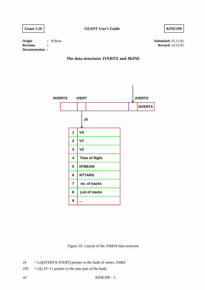
Geant 3.16 GEANT User’s Guide KINE199
Origin : R.Brun Submitted: 01.11.83Revision : Revised: 14.12.93Documentation :
The data structures JVERTX and JKINE
NVERTX IVERT JVERTX
NVERTX
JV
1
2
3
4
5
6
7
8
9
VX
VY
VZ
Time of flight
NTBEAM
NTTARG
no. of tracks
List of tracks
...
Figure 35: Layout of the JVERTX data structure
JV = LQ(JVERTX-IVERT) pointer to the bank of vertex IVERT.
JVU = LQ(JV-1) pointer to the user part of the bank.
187 KINE199 – 1

The JVERTX banks are filled by the routine GSVERT and GSVERU. Vertex parameters can be retrieved by theroutine GFVERT and printed by the routine GPVERT.
KINE199 – 2 188
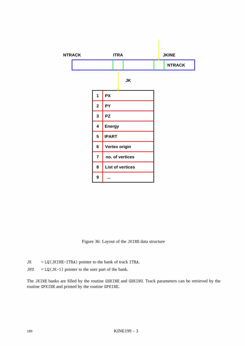
NTRACK ITRA JKINE
NTRACK
JK
1
2
3
4
5
6
7
8
9
PX
PY
PZ
Energy
IPART
Vertex origin
no. of vertices
List of vertices
...
Figure 36: Layout of the JKINE data structure
JK = LQ(JKINE-ITRA) pointer to the bank of track ITRA.
JKU = LQ(JK-1) pointer to the user part of the bank.
The JKINE banks are filled by the routine GSKINE and GSKINU. Track parameters can be retrieved by theroutine GFKINE and printed by the routine GPKINE.
189 KINE199 – 3
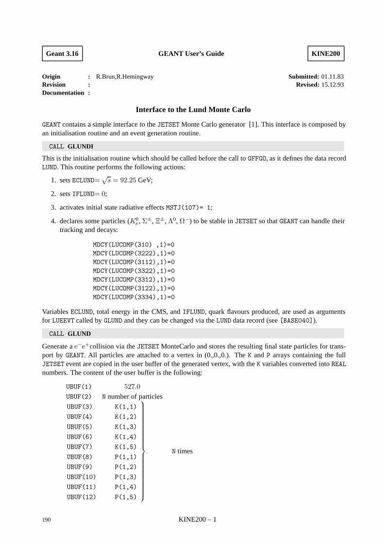
Geant 3.16 GEANT User’s Guide KINE200
Origin : R.Brun,R.Hemingway Submitted: 01.11.83Revision : Revised: 15.12.93Documentation :
Interface to the Lund Monte Carlo
GEANT contains a simple interface to the JETSET Monte Carlo generator [1]. This interface is composed byan initialisation routine and an event generation routine.
CALL GLUNDI
This is the initialisation routine which should be called before the call to GFFGO, as it defines the data recordLUND. This routine performs the following actions:
1. sets ECLUND=√s = 92.25 GeV;
2. sets IFLUND= 0;
3. activates initial state radiative effects MSTJ(107)= 1;
4. declares some particles (K0s , Σ±, Ξ±, Λ0, Ω−) to be stable in JETSET so that GEANT can handle theirtracking and decays:
MDCY(LUCOMP(310) ,1)=0MDCY(LUCOMP(3222),1)=0MDCY(LUCOMP(3112),1)=0MDCY(LUCOMP(3322),1)=0MDCY(LUCOMP(3312),1)=0MDCY(LUCOMP(3122),1)=0MDCY(LUCOMP(3334),1)=0
Variables ECLUND, total energy in the CMS, and IFLUND, quark flavours produced, are used as argumentsfor LUEEVT called by GLUND and they can be changed via the LUND data record (see [BASE040]).
CALL GLUND
Generate a e−e+collision via the JETSET MonteCarlo and stores the resulting final state particles for trans-port by GEANT. All particles are attached to a vertex in (0.,0.,0.). The K and P arrays containing the fullJETSET event are copied in the user buffer of the generated vertex, with the K variables converted into REALnumbers. The content of the user buffer is the following:
UBUF(1) 527.0UBUF(2) N number of particles
UBUF(3) K(1,1)
UBUF(4) K(1,2)
UBUF(5) K(1,3)
UBUF(6) K(1,4)
UBUF(7) K(1,5)
UBUF(8) P(1,1)
UBUF(9) P(1,2)
UBUF(10) P(1,3)
UBUF(11) P(1,4)
UBUF(12) P(1,5)
N times
190 KINE200 – 1

Geant 3.16 GEANT User’s Guide KINE210
Origin : R.Hemingway Submitted: 01.11.83Revision : Revised: 15.12.93Documentation :
τ± generation and decay
CALL GALL GTAU
This routine is now dummy and it will only print an error message. The appropriate routines from a generatorMonte Carlo (for instance the JETSET [1] package) should be used to handle τ± production and decay.
191 KINE210 – 1

KINE Bibliography
[1] T.Sjostrand et al. The LUND MonteCarlo Programs, CERN Program Library Pool Writeup W5035 /W5045 / W5046 / W5047 / W5048 edition, November 1989.
KINE210 – 2 192

Geant 3.16 GEANT User’s Guide PHYS001
Origin : Submitted: 24.09.84Revision : Revised: 26.07.93Documentation : M. Maire, F.Carminati
Introduction to the section PHYS
1 Summary of the physics processes
The computer simulation of particles traversing an experimental setup has to take into account the interac-tions of those particles with the material of the detector. GEANT is able to simulate the dominant processeswhich can occur in the energy range from 10 keV to 10 TeV for electromagnetic interactions. As far ashadronic interactions are concerned, the range of validity is the one of the hadronic packages used, whichusually does not extend below a few tens of MeV. For more information the user is invited to consult therelevant documentation [1, 2, 3, 4, 5, 6].
Simulating a given process means:
– Evaluating the probability of occurrence of the process, by sampling the total cross-section of theprocess.
– Generating the final state after interaction, by sampling the differential cross-section of the process.
– In case of (quasi-)continuous processes, e.g. CSDA (Continuous Slowing Down Approximation),energy losses or multiple scattering, computing the mean values of some characteristic quantities.
In Table 1 below we summarise all the processes currently implemented in GEANT, with a reference to thecorresponding sections.
1.1 Simulated Processes
Hadronic Interactions
To simulate the interactions of hadrons with the nuclei of the matter traversed, two alternatives are provided:
1. The generator of the FLUKA [2, 3] hadron shower MonteCarlo and the interface routines to GEANT.See [PHYS520] for more information.
2. The generator of the GHEISHA [1] hadron shower MonteCarlo and the interface routines to GEANT.See [PHYS510] for more information.
The code both of the GHEISHA and of the FLUKA generators is contained in the GEANT library. Users shouldbe aware that the routines of these packages do not follow the GEANT naming conventions and therefore theycan clash with the names of user procedures.
Electromagnetic Processes
By means of systematic fits to the existing data, the cross-sections of the electromagnetic processes arewell reproduced (within a few percent) from 10 keV up to 100 GeV, both for light (low Z) and for heavymaterials.
This feature, together with the use of the interface with one of the hadronic shower generators available,makes GEANT useful also for shower simulation in gases.
Muonic interactions
Muonic interactions are simulated up to 10 TeV, making GEANT useful for cosmic rays studies.
193 PHYS001 – 1
Ionisation by charged particles
The following alternatives are provided to simulate this process:
• Sampling from the appropriate distribution around the mean value of the energy loss ([PHYS332]).
• Explicit generation of δ-rays (see [PHYS330/331/430]) and restricted fluctuations below the energythreshold for the production of δ-rays.
• Sampling the contribution of single collisions from statistical distributions. This can be used as analternative to the first one when simulating energy losses in very thin layers (small value of g cm−2)(see [PHYS334]).
Full Landau fluctuations and generation of δ-rays cannot be used together in order to avoid double countingof the fluctuations. An automatic protection has been introduced in GEANT to this effect. See [PHYS333/332]and [BASE040] for further information.
Multiple Scattering
Two methods are provided:
1. Moliere distribution or plural scattering ([PHYS325], [PHYS328]).
2. Gaussian approximation ([PHYS320]).
The JMATE data structure
In order to save time during the transport of the particles, relevant energy-dependent quantities are tabulatedat the beginning of the run, for all materials, as functions of the kinetic energy of the particle. In particular,the inverse of the total cross-sections of all processes involving photons, electrons and muons and the dE/dxand range tables for electrons, muons and protons are calculated. The actual value of, say, the interactionlength for a given process (i.e. the inverse of the macroscopic cross section) is then obtained via a linearinterpolation in the tables. The data structure which contains all this information in memory is supported bythe link JMATE in the /GCLINK/ common block. See [PHYS100] and [CONS199] for a more informationon these tables.
Probability of Interaction
The total cross-section of each process is used at tracking time to evaluate the probability of occurrence ofthe process. See [PHYS010] for an explanation of the method used.
Note: The section PHYS is closely related to the section CONS. Users wishing to have a complete overviewof the physics processes included in GEANT should read both sections.
1.2 Control of the physical processes
For most of the individual processes the default option (indicated below) can be changed via data records[BASE040]. The processes are controlled via a control variable which is in the common /GCKING/. If nototherwise noted, the meaning of the control variable is the following:
= 0 The process is completely ignored.
= 1 The process is considered and possible secondary particles generating from the interaction are putinto the /GCKING/ common. If the interacting particle disappears in the interaction, then it is stoppedwith ISTOP=1 (common /GCTRAK/)
= 2 The process is considered. If secondary particles result from the interaction, they are not generatedand their energy is simply added in the variable DESTEP (common /GCTRAK/. If the interactingparticle disappears in the interaction, the variable ISTOP is set to 2.
PHYS001 – 2 194
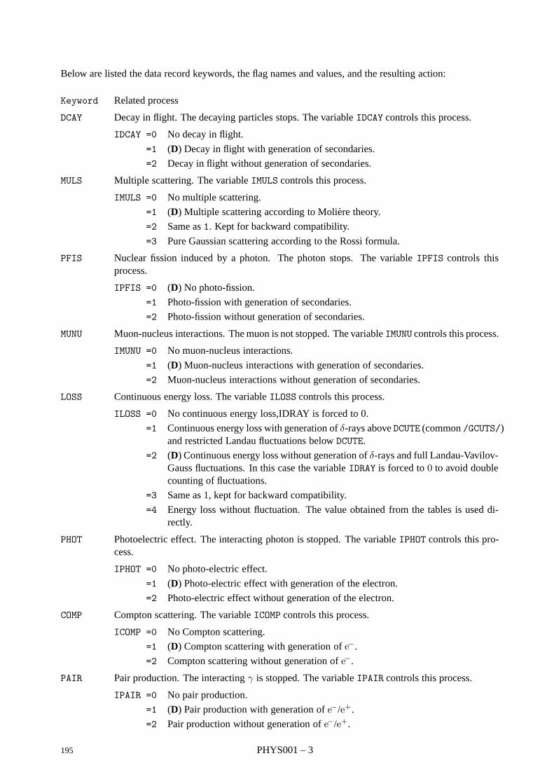
Below are listed the data record keywords, the flag names and values, and the resulting action:
Keyword Related process
DCAY Decay in flight. The decaying particles stops. The variable IDCAY controls this process.
IDCAY =0 No decay in flight.
=1 (D) Decay in flight with generation of secondaries.
=2 Decay in flight without generation of secondaries.
MULS Multiple scattering. The variable IMULS controls this process.
IMULS =0 No multiple scattering.
=1 (D) Multiple scattering according to Moliere theory.
=2 Same as 1. Kept for backward compatibility.
=3 Pure Gaussian scattering according to the Rossi formula.
PFIS Nuclear fission induced by a photon. The photon stops. The variable IPFIS controls thisprocess.
IPFIS =0 (D) No photo-fission.
=1 Photo-fission with generation of secondaries.
=2 Photo-fission without generation of secondaries.
MUNU Muon-nucleus interactions. The muon is not stopped. The variable IMUNU controls this process.
IMUNU =0 No muon-nucleus interactions.
=1 (D) Muon-nucleus interactions with generation of secondaries.
=2 Muon-nucleus interactions without generation of secondaries.
LOSS Continuous energy loss. The variable ILOSS controls this process.
ILOSS =0 No continuous energy loss,IDRAY is forced to 0.
=1 Continuous energy loss with generation of δ-rays above DCUTE (common /GCUTS/)and restricted Landau fluctuations below DCUTE.
=2 (D) Continuous energy loss without generation of δ-rays and full Landau-Vavilov-Gauss fluctuations. In this case the variable IDRAY is forced to 0 to avoid doublecounting of fluctuations.
=3 Same as 1, kept for backward compatibility.
=4 Energy loss without fluctuation. The value obtained from the tables is used di-rectly.
PHOT Photoelectric effect. The interacting photon is stopped. The variable IPHOT controls this pro-cess.
IPHOT =0 No photo-electric effect.
=1 (D) Photo-electric effect with generation of the electron.
=2 Photo-electric effect without generation of the electron.
COMP Compton scattering. The variable ICOMP controls this process.
ICOMP =0 No Compton scattering.
=1 (D) Compton scattering with generation of e−.
=2 Compton scattering without generation of e−.
PAIR Pair production. The interacting γ is stopped. The variable IPAIR controls this process.
IPAIR =0 No pair production.
=1 (D) Pair production with generation of e−/e+.
=2 Pair production without generation of e−/e+.
195 PHYS001 – 3
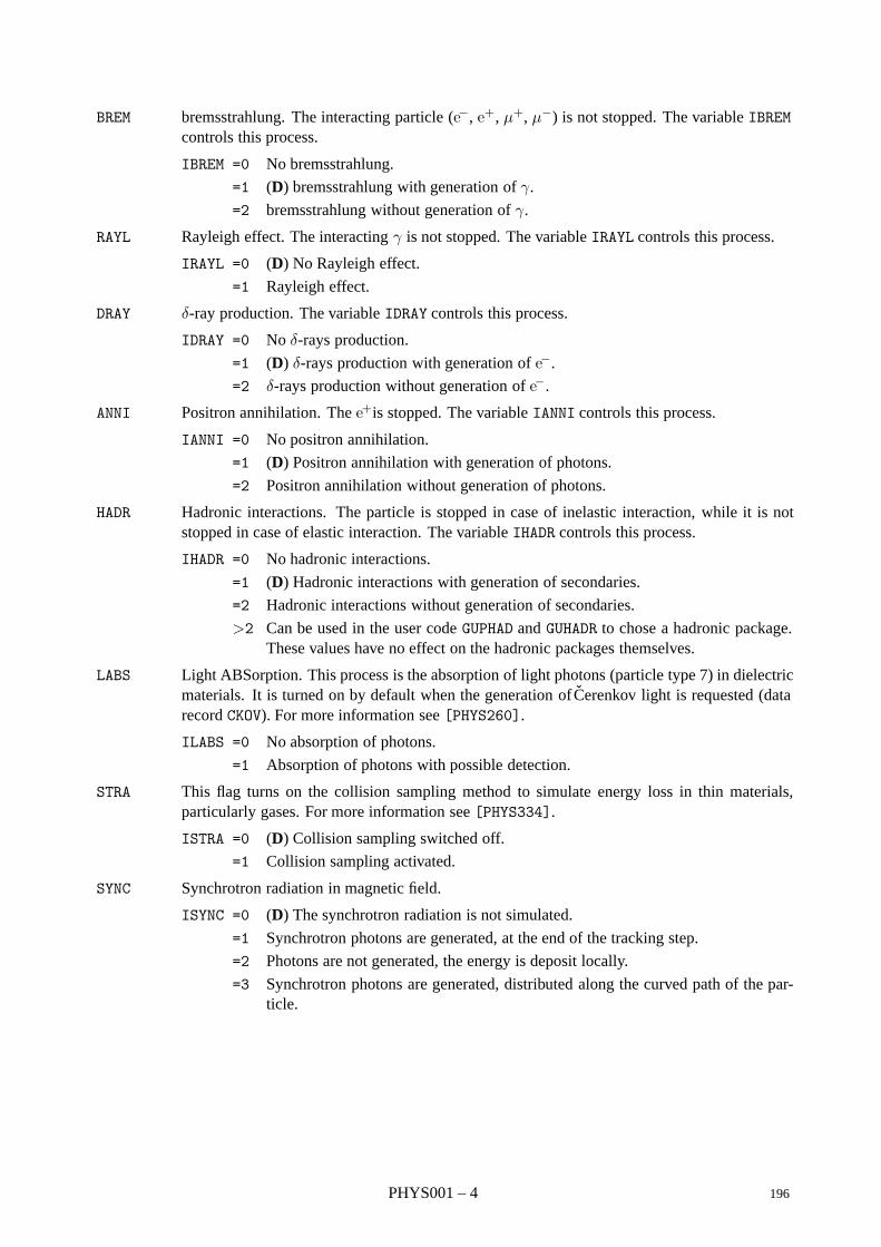
BREM bremsstrahlung. The interacting particle (e−, e+, µ+, µ−) is not stopped. The variable IBREMcontrols this process.
IBREM =0 No bremsstrahlung.
=1 (D) bremsstrahlung with generation of γ.
=2 bremsstrahlung without generation of γ.
RAYL Rayleigh effect. The interacting γ is not stopped. The variable IRAYL controls this process.
IRAYL =0 (D) No Rayleigh effect.
=1 Rayleigh effect.
DRAY δ-ray production. The variable IDRAY controls this process.
IDRAY =0 No δ-rays production.
=1 (D) δ-rays production with generation of e−.
=2 δ-rays production without generation of e−.
ANNI Positron annihilation. The e+is stopped. The variable IANNI controls this process.
IANNI =0 No positron annihilation.
=1 (D) Positron annihilation with generation of photons.
=2 Positron annihilation without generation of photons.
HADR Hadronic interactions. The particle is stopped in case of inelastic interaction, while it is notstopped in case of elastic interaction. The variable IHADR controls this process.
IHADR =0 No hadronic interactions.
=1 (D) Hadronic interactions with generation of secondaries.
=2 Hadronic interactions without generation of secondaries.
>2 Can be used in the user code GUPHAD and GUHADR to chose a hadronic package.These values have no effect on the hadronic packages themselves.
LABS Light ABSorption. This process is the absorption of light photons (particle type 7) in dielectricmaterials. It is turned on by default when the generation of Cerenkov light is requested (datarecord CKOV). For more information see [PHYS260].
ILABS =0 No absorption of photons.
=1 Absorption of photons with possible detection.
STRA This flag turns on the collision sampling method to simulate energy loss in thin materials,particularly gases. For more information see [PHYS334].
ISTRA =0 (D) Collision sampling switched off.
=1 Collision sampling activated.
SYNC Synchrotron radiation in magnetic field.
ISYNC =0 (D) The synchrotron radiation is not simulated.
=1 Synchrotron photons are generated, at the end of the tracking step.
=2 Photons are not generated, the energy is deposit locally.
=3 Synchrotron photons are generated, distributed along the curved path of the par-ticle.
PHYS001 – 4 196
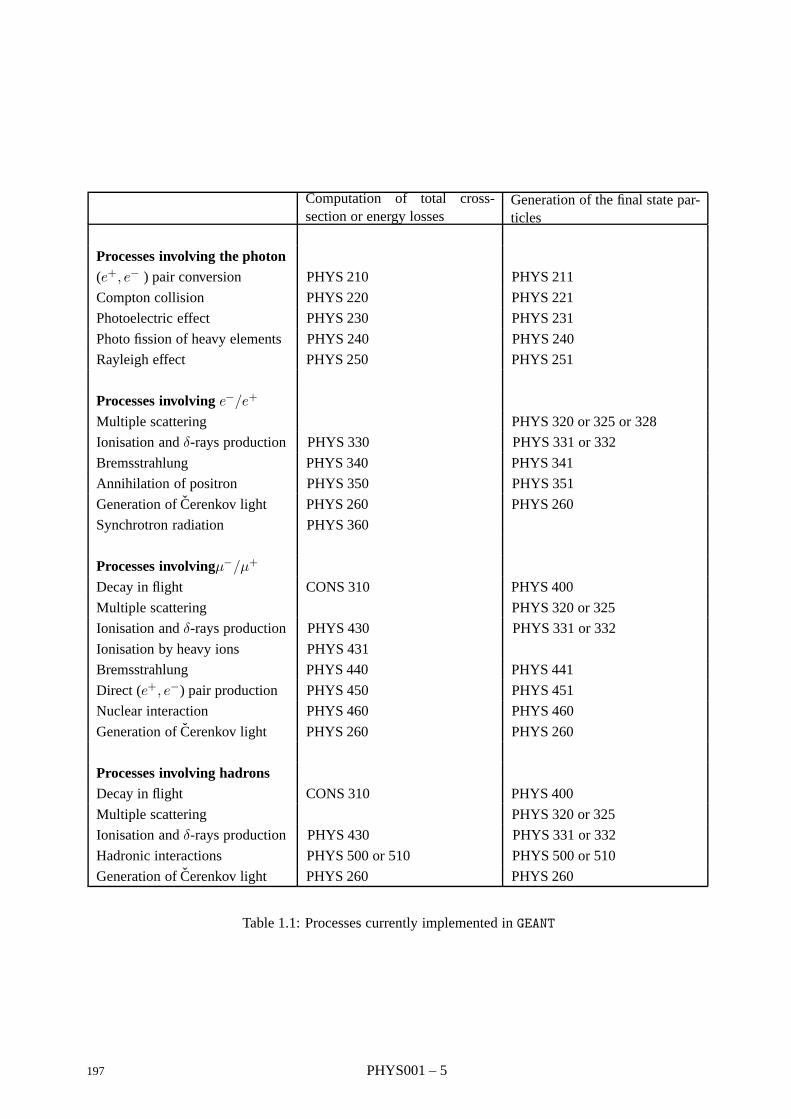
Computation of total cross-section or energy losses
Generation of the final state par-ticles
Processes involving the photon(e+, e− ) pair conversion PHYS 210 PHYS 211
Compton collision PHYS 220 PHYS 221
Photoelectric effect PHYS 230 PHYS 231
Photo fission of heavy elements PHYS 240 PHYS 240
Rayleigh effect PHYS 250 PHYS 251
Processes involving e−/e+
Multiple scattering PHYS 320 or 325 or 328
Ionisation and δ-rays production PHYS 330 PHYS 331 or 332
Bremsstrahlung PHYS 340 PHYS 341
Annihilation of positron PHYS 350 PHYS 351
Generation of Cerenkov light PHYS 260 PHYS 260
Synchrotron radiation PHYS 360
Processes involvingµ−/µ+
Decay in flight CONS 310 PHYS 400
Multiple scattering PHYS 320 or 325
Ionisation and δ-rays production PHYS 430 PHYS 331 or 332
Ionisation by heavy ions PHYS 431
Bremsstrahlung PHYS 440 PHYS 441
Direct (e+, e−) pair production PHYS 450 PHYS 451
Nuclear interaction PHYS 460 PHYS 460
Generation of Cerenkov light PHYS 260 PHYS 260
Processes involving hadronsDecay in flight CONS 310 PHYS 400
Multiple scattering PHYS 320 or 325
Ionisation and δ-rays production PHYS 430 PHYS 331 or 332
Hadronic interactions PHYS 500 or 510 PHYS 500 or 510
Generation of Cerenkov light PHYS 260 PHYS 260
Table 1.1: Processes currently implemented in GEANT
197 PHYS001 – 5

Geant 3.16 GEANT User’s Guide PHYS010
Origin : Submitted: 20.12.84Revision : Revised: 26.07.93Documentation : M. Maire, F.Carminati
Compute the occurrence of a process
1 Principle
The simulation of the processes which accompany the propagation of a particle through the material of thedetector (e.g. bremsstrahlung, δ-rays production, Compton scattering and so on) is performed by GEANT inthe following steps:
1. Fetch a new particle to be tracked (often called track or history) from the stack supported by thelink JSTAK (see [TRAK399]). This is done once at the beginning of each new track. The numberof interaction lengths that the particle is going to travel, before undergoing each one of the possiblediscrete processes, is sampled at this point. These operations are done in the routine GLTRAC.
2. Evaluate the distance to the interaction point. This is done by the individual tracking routines (GTGAMA,GTNEUT, GTHADR, GTNINO, GTMUON, GTHION and GTCKOV) which control the tracking of particularparticles. The number of interaction lengths remaining to travel before each of the possible processes(often called tracking mechanisms or simply mechanisms) is multiplied by the inverse of the macro-scopic cross-section for that process in the current material (i.e. the interaction length). This gives thedistances that the particle has to travel before each of the processes occurs in the current medium. Theminimum among these numbers is the step over which the particle will be transported. In additionto the physics mechanisms, four pseudo-interactions are taken into account in the calculation of thestep:
(a) boundary crossing. The crossing of a volume boundary is treated like a discrete process. Aparticle never crosses a boundary during a step but rather stops there (NEXT mechanism);
(b) maximum step limit. For each tracking medium a value for the maximum step can be specifiedby the user. Process SMAX;
(c) maximum fraction of continuum energy loss, maximum angular deviation in magnetic field ormaximum step for which the Moliere formula, to simulate multiple scattering is valid. These arecontinuous processes, which introduce a limitation on the tracking step expressed by a singlevariable (see section [PHYS325] on GMULOF).
(d) energy and time cut. Charged particles in matter are stopped when their energy falls below theirenergy threshold or when their time of flight exceeds the time cut;
More information is given in the individual sections explaining the implementation of the physicalprocesses.
3. Transport the particle either along a straight line (if no magnetic field or for a neutral particle) or alonga helicoidal path (for charged particles in magnetic field).
4. Update the energy of the particle if continuous energy loss was in effect (charged particles in matter).
5. If a physical discrete process has been selected, generate the final state of the interaction.
6. If the incident particle survives the interaction (Compton, δ-rays production, bremsstrahlung, directpair production by µ and µ-nucleus interaction, hadronic elastic scattering), sample again the numberof interaction lengths to travel before the next event of the same kind. This is generally done byspecialised routines: GMUNU, GCOMP, GBREM, etc.
198 PHYS010 – 1
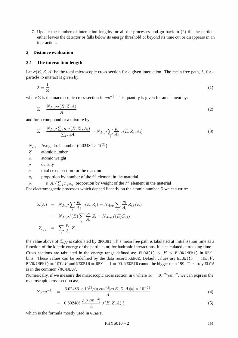
7. Update the number of interaction lengths for all the processes and go back to (2) till the particleeither leaves the detector or falls below its energy threshold or beyond its time cut or disappears in aninteraction.
2 Distance evaluation
2.1 The interaction length
Let σ(E,Z,A) be the total microscopic cross section for a given interaction. The mean free path, λ, for aparticle to interact is given by:
λ =1Σ
(1)
where Σ is the macroscopic cross-section in cm−1. This quantity is given for an element by:
Σ =NAvρσ(E,Z,A)
A(2)
and for a compound or a mixture by:
Σ =NAvρ
∑i niσ(E,Zi, Ai)∑
i niAi= NAvρ
∑i
piAi
σ(E,Zi, Ai) (3)
NAv Avogadro’s number (6.02486 × 10²³)Z atomic number
A atomic weight
ρ density
σ total cross-section for the reaction
ni proportion by number of the ith element in the material
pi = niAi/∑
j njAj , proportion by weight of the ith element in the materialFor electromagnetic processes which depend linearly on the atomic number Z we can write:
Σ(E) = NAvρ∑i
piAi
σ(E,Zi) = NAvρ∑i
piAi
Zif(E)
= NAvρf(E)∑i
piAi
Zi = NAvρf(E)Zeff
Zeff =∑i
piAi
Zi
the value above of Zeff is calculated by GPROBI. This mean free path is tabulated at initialisation time as afunction of the kinetic energy of the particle, or, for hadronic interactions, it is calculated at tracking time.Cross sections are tabulated in the energy range defined as: ELOW(1) ≤ E ≤ ELOW(NEK1) in NEK1bins. These values can be redefined by the data record RANGE. Default values are ELOW(1) = 10keV ,ELOW(NEK1) = 10TeV and NEKBIN = NEK1−1 = 90. NEKBIN cannot be bigger than 199. The array ELOWis in the common /GCMULO/.Numerically, if we measure the microscopic cross section in b where 1b = 10−24cm−2, we can express themacroscopic cross section as:
Σ[cm−1] =6.02486 × 10²³ρ[g cm−3]σ(E,Z,A)[b] × 10−24
A(4)
= 0.602486ρ[g cm−3]
Aσ(E,Z,A)[b] (5)
which is the formula mostly used in GEANT.
PHYS010 – 2 199

2.2 Determination of the interaction point
The mean free path of a particle for a given process, λ, depends on the medium and cannot be used directlyto sample the probability of an interaction in a heterogeneous detector. The number of mean free pathswhich a particle travels is:
Nλ =∫
dx
λ(x)
and it is independent of the material traversed. If NR is a random variable denoting the number of mean freepaths from a given point until the point of interaction, it can be shown that NR has the distribution function
P (NR < Nλ) = 1− e−Nλ
The total number of mean free paths the particle travels before the interaction point, Nλ, is sampled at thebeginning of the trajectory as:
Nλ = − log (η)
where η is a random number uniformly distributed in the range (0, 1). Nλ is updated after each step ∆xaccording the formula:
N ′λ = Nλ − ∆x
λ(x)
until the step originating from s(x) = Nλλ(x) is the shortest and this triggers the specific process.
3 Common /GCPHYS/
The variables described above are stored in the common /GCPHYS/, one process per line:
COMMON/GCPHYS/IPAIR,SPAIR,SLPAIR,ZINTPA,STEPPA+ ,ICOMP,SCOMP,SLCOMP,ZINTCO,STEPCO+ ,IPHOT,SPHOT,SLPHOT,ZINTPH,STEPPH+ ,IPFIS,SPFIS,SLPFIS,ZINTPF,STEPPF+ ,IDRAY,SDRAY,SLDRAY,ZINTDR,STEPDR+ ,IANNI,SANNI,SLANNI,ZINTAN,STEPAN+ ,IBREM,SBREM,SLBREM,ZINTBR,STEPBR+ ,IHADR,SHADR,SLHADR,ZINTHA,STEPHA+ ,IMUNU,SMUNU,SLMUNU,ZINTMU,STEPMU+ ,IDCAY,SDCAY,SLIFE ,SUMLIF,DPHYS1+ ,ILOSS,SLOSS,SOLOSS,STLOSS,DPHYS2+ ,IMULS,SMULS,SOMULS,STMULS,DPHYS3+ ,IRAYL,SRAYL,SLRAYL,ZINTRA,STEPRACOMMON/GCPHLT/ILABS,SLABS,SLLABS,ZINTLA,STEPLA
+ ,ISYNC+ ,ISTRA
*
The first 9 processes (from PAIR production up to MUon NUclear interaction) and the RAYLeigh scattering andLight ABSorbtion have the same scheme. Let’s take as an example the first one (for a complete descriptionof the common see [BASE030]):
IPAIR flag for secondaries:
0= the process is turned off;
200 PHYS010 – 3

1= generation of secondaries enabled;
2= no generation of secondaries.
SPAIR Nλλ(x) = remaining track-length before interaction, evaluated at the last point where the mech-anism was active, i.e. IPAIR = 0.
SLPAIR track length at the time when the interaction last happened for the current particle. Only SLPAIR(direct pair production by µ), SLDRAY (δ-ray production), SLBREM (bremsstrahlung for µ), SLHADR(hadronic interactions), SLMUNU (muon-nucleus interactions) and SLRAYL (Rayleigh effect) areused. The variables SOLOSS, STLOSS, SOMULS, STMULS are obsolete. They have been kept forbackward compatibility, but their value is undefined and should not be used.
ZINTPA Nλ = remaining number of interaction lengths (mean free paths) evaluated at the last point wherethe mechanism was active, i.e. IPAIR = 0.
STEPPA λ(x) = value of the interaction length at the last point where the mechanism was active, i.e.IPAIR = 0;
The evaluation and update of the quantities like STEPPA, SPAIR and ZINTPA are turned off in the mediawhere the mechanism is not active (IPAIR = 0). Turning off a mechanism in one tracking medium may giveincorrect physics results because not only will the mechanism not be active, but the interaction probabilitieswill not be updated, as if that medium had not been traversed at all. This feature of the tracking routines isused mainly in the vacuum, (defined as a medium with atomic number Z < 1), where all the mechanismsbut DECAy (and SYNChrotron radiation, if activated) are inactive.
The DECAy in flight is simpler since the mean life time of the particle, τ , is not material dependent and canbe sampled directly.
SLIFE not used.
SUMLIF proper time left before the decay. At the beginning of the track SUMLIF = −cτ log (η).
SDCAY distance left to decay point evaluated at the last point where the mechanism was active, i.e. IDECA =0.
4 Cross-section, energy loss and range tables
Cross-sections, energy loss dE/dx and range R(Ekin) are tabulated for all materials which enter in thedefinition of a tracking medium by the routine GPHYSI. The values of the energy for which the tabulatedquantities are calculated are stored in the common /GCMULO/ (see [BASE030]). To evaluate one of thetabulated quantities for a particle of kinetic energy E0, a linear interpolation is used. Let i be such that:
Ei < E0 ≤ Ei+1
The integer variable IEKBIN in common /GCTRACK/ is equal to i during tracking and its value is recomputedby the routine GEKBIN when the energy of the particle changes. If the quantity Y has been tabulated so thatYi = Y (Ei) then the value Y0 = Y (E0) is calculated as:
Y0 = Yi +E0 − Ei
Ei+1 − Ei(Yi+1 − Yi) = Yi
(1− E0 − Ei
Ei+1 −Ei
)+ Yi+1
E0 − Ei
Ei+1 − Ei(6)
Inside the code the following quantities are used:
GEKRAT =E0 − Ei
Ei+1 − EiGEKRT1 =
(1− E0 − Ei
Ei+1 − Ei
)
where GEKRAT is in common /GCTRAK/ and GEKRT1 is a local variable recomputed when needed.
PHYS010 – 4 201
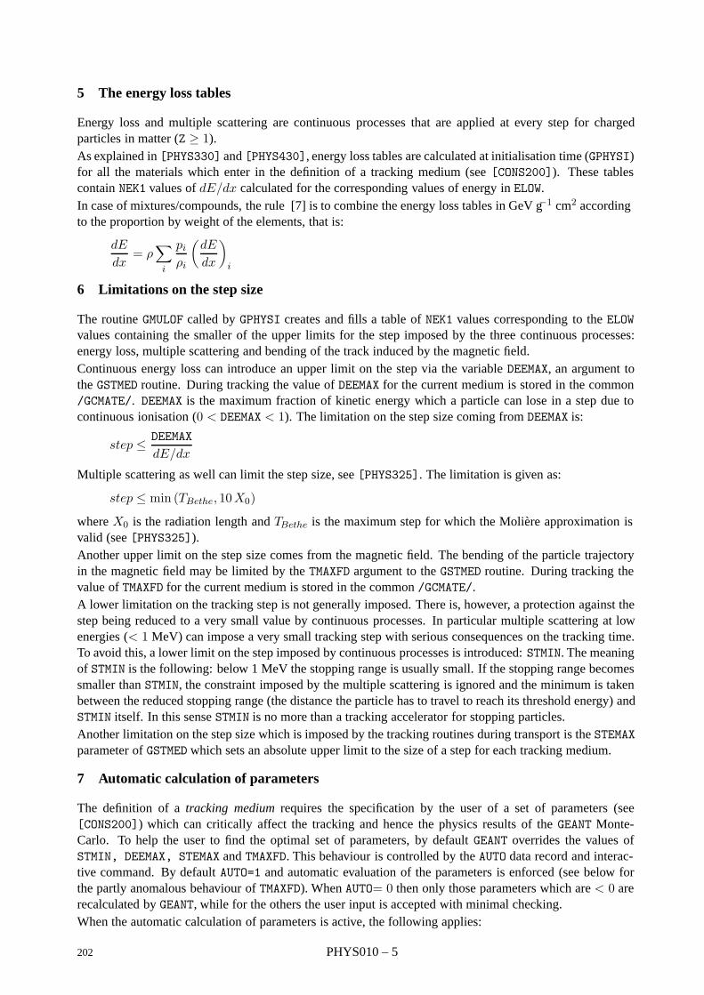
5 The energy loss tables
Energy loss and multiple scattering are continuous processes that are applied at every step for chargedparticles in matter (Z ≥ 1).As explained in [PHYS330] and [PHYS430], energy loss tables are calculated at initialisation time (GPHYSI)for all the materials which enter in the definition of a tracking medium (see [CONS200]). These tablescontain NEK1 values of dE/dx calculated for the corresponding values of energy in ELOW.In case of mixtures/compounds, the rule [7] is to combine the energy loss tables in GeV g−1 cm2 accordingto the proportion by weight of the elements, that is:
dE
dx= ρ
∑i
piρi
(dE
dx
)i
6 Limitations on the step size
The routine GMULOF called by GPHYSI creates and fills a table of NEK1 values corresponding to the ELOWvalues containing the smaller of the upper limits for the step imposed by the three continuous processes:energy loss, multiple scattering and bending of the track induced by the magnetic field.Continuous energy loss can introduce an upper limit on the step via the variable DEEMAX, an argument tothe GSTMED routine. During tracking the value of DEEMAX for the current medium is stored in the common/GCMATE/. DEEMAX is the maximum fraction of kinetic energy which a particle can lose in a step due tocontinuous ionisation (0 < DEEMAX < 1). The limitation on the step size coming from DEEMAX is:
step ≤ DEEMAX
dE/dx
Multiple scattering as well can limit the step size, see [PHYS325]. The limitation is given as:
step ≤ min (TBethe, 10X0)
where X0 is the radiation length and TBethe is the maximum step for which the Moliere approximation isvalid (see [PHYS325]).Another upper limit on the step size comes from the magnetic field. The bending of the particle trajectoryin the magnetic field may be limited by the TMAXFD argument to the GSTMED routine. During tracking thevalue of TMAXFD for the current medium is stored in the common /GCMATE/.A lower limitation on the tracking step is not generally imposed. There is, however, a protection against thestep being reduced to a very small value by continuous processes. In particular multiple scattering at lowenergies (< 1 MeV) can impose a very small tracking step with serious consequences on the tracking time.To avoid this, a lower limit on the step imposed by continuous processes is introduced: STMIN. The meaningof STMIN is the following: below 1 MeV the stopping range is usually small. If the stopping range becomessmaller than STMIN, the constraint imposed by the multiple scattering is ignored and the minimum is takenbetween the reduced stopping range (the distance the particle has to travel to reach its threshold energy) andSTMIN itself. In this sense STMIN is no more than a tracking accelerator for stopping particles.Another limitation on the step size which is imposed by the tracking routines during transport is the STEMAXparameter of GSTMED which sets an absolute upper limit to the size of a step for each tracking medium.
7 Automatic calculation of parameters
The definition of a tracking medium requires the specification by the user of a set of parameters (see[CONS200]) which can critically affect the tracking and hence the physics results of the GEANT Monte-Carlo. To help the user to find the optimal set of parameters, by default GEANT overrides the values ofSTMIN, DEEMAX, STEMAX and TMAXFD. This behaviour is controlled by the AUTO data record and interac-tive command. By default AUTO=1 and automatic evaluation of the parameters is enforced (see below forthe partly anomalous behaviour of TMAXFD). When AUTO= 0 then only those parameters which are < 0 arerecalculated by GEANT, while for the others the user input is accepted with minimal checking.When the automatic calculation of parameters is active, the following applies:
202 PHYS010 – 5
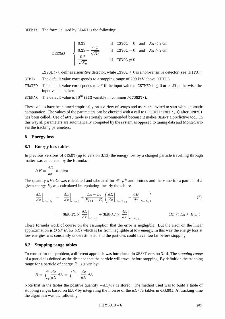
DEEMAX The formula used by GEANT is the following:
DEEMAX =
0.25 if ISVOL = 0 and X0 < 2 cm
0.25− 0.2√X0
if ISVOL = 0 and X0 ≥ 2 cm
0.2√X0
if ISVOL = 0
ISVOL > 0 defines a sensitive detector, while ISVOL ≤ 0 is a non-sensitive detector (see [HITS]).
STMIN The default value corresponds to a stopping range of 200 keV above CUTELE.
TMAXFD The default value corresponds to 20 if the input value to GSTMED is ≤ 0 or > 20, otherwise theinput value is taken.
STEMAX The default value is 1010 (BIG variable in common /GCONST/).
These values have been tuned empirically on a variety of setups and users are invited to start with automaticcomputation. The values of the parameters can be checked with a call to GPRINT(’TMED’,0) after GPHYSIhas been called. Use of AUTO mode is strongly recommended because it makes GEANT a predictive tool. Inthis way all parameters are automatically computed by the system as opposed to tuning data and MonteCarlovia the tracking parameters.
8 Energy loss
8.1 Energy loss tables
In previous versions of GEANT (up to version 3.13) the energy lost by a charged particle travelling throughmatter was calculated by the formula:
∆E =dE
dx× step
The quantity dE/dx was calculated and tabulated for e±, µ± and protons and the value for a particle of agiven energy E0 was calculated interpolating linearly the tables:
dE
dx
∣∣∣∣E=E0
=dE
dx
∣∣∣∣E=Ei
+E0 − Ei
Ei+1 − Ei
(dE
dx
∣∣∣∣E=Ei+1
− dE
dx
∣∣∣∣E=Ei
)(7)
= GEKRT1× dE
dx
∣∣∣∣E=Ei
+ GEKRAT× dE
dx
∣∣∣∣E=Ei+1
(Ei < E0 ≤ Ei+1)
These formula work of course on the assumption that the error is negligible. But the error on the linearapproximation is O
(∂2E/∂x ∂E
)which is far from negligible at low energy. In this way the energy loss at
low energies was constantly underestimated and the particles could travel too far before stopping.
8.2 Stopping range tables
To correct for this problem, a different approach was introduced in GEANT version 3.14. The stopping rangeof a particle is defined as the distance that the particle will travel before stopping. By definition the stoppingrange for a particle of energy E0 is given by:
R =∫ 0
E0
dx
dEdE =
∫ E0
0− dx
dEdE
Note that in the tables the positive quantity −dE/dx is stored. The method used was to build a table ofstopping ranges based on ELOW by integrating the inverse of the dE/dx tables in GRANGI. At tracking timethe algorithm was the following:
PHYS010 – 6 203

1. Evaluate the stopping range for the threshold energy (STOPC). This was done only once at the begin-ning of each new track.
2. From the energy of the particle derive the stopping range by a linear interpolation of the range table:
R0 = GEKRT1×Ri + GEKRAT×Ri+1
where Ei < E0 ≤ Ei+1.
3. Evaluate the stopping range for the particle after the step: R′0 = R0 − step. If this is less than thestopping range of a particle with threshold energy, the particle is terminated as a stopping particlebelow the energy cut. Otherwise the following quantities are evaluated:
Rj < R′0 ≤ Rj+1 GEK =
R′0 −Rj
Rj+1 −RjGEK1 = 1− GEK
and the final energy is computed as:
E′0 = GEK1× ELOW(j) + GEK× ELOW(j+1)
4. the energy loss is computed as:
∆E = E0 − E′0
This value is then corrected to take into account the energy loss fluctuations (see [PHYS332]).
This method has two main disadvantages. The first is due to the finite precision of computers. As the energyloss in a step is calculated as the difference of two numbers, it is subject to large relative errors. The effectcan be particularly serious in the case of light materials, particles near the minimum ionisation point or withvery short steps, where ∆E = DESTEP can even result in a negative quantity. As the relative precision of a32-bit computer is around 10−6, the error on the energy loss of a 100 GeV track can be as large as 100 keV.
The second problem connected with this method can be easily shown if we compute dE/dx as:
dE
dx=
d
dx
(E0 −E′
0
)=
d
dx(E0 − GEK1× ELOW(j)− GEK× ELOW(j+1))
=d
dx
(E0 − Ej −
R′0 −Rj
Rj+1 −Rj(Ej+1 − Ej)
)= − d
dx
∆Ej
∆Rj
(R′0 −Rj
)
= −∆Ej
∆Rj
dR′0
dx=∆Ej
∆Rj
step
dx=∆Ej
∆Rj
As we can see, the reconstructed dE/dx curve due to continuous energy loss is a step function and constantin each energy bin. Thus, although the results obtained with GEANT 3.14 were very satisfactory, this wasfelt to be an undesirable feature.
8.3 Energy loss in GEANT
The two problems mentioned above have been solved in GEANT 3.15. As far as the precision is concerned,the solution was to revert to the algorithm of GEANT 3.13 every time the relative energy loss in the step(DESTEP/GEKIN) is smaller than five times the machine precision. This has given good results withoutloosing the substantial improvements obtained in GEANT 3.14 with the introduction of the stopping rangealgorithm. As a matter of fact, the above condition happens only the in the case of very small steps orwhen the dE/dx curve is very flat, and in both cases the algorithm based on the dE/dx tables is a goodapproximation.
204 PHYS010 – 7
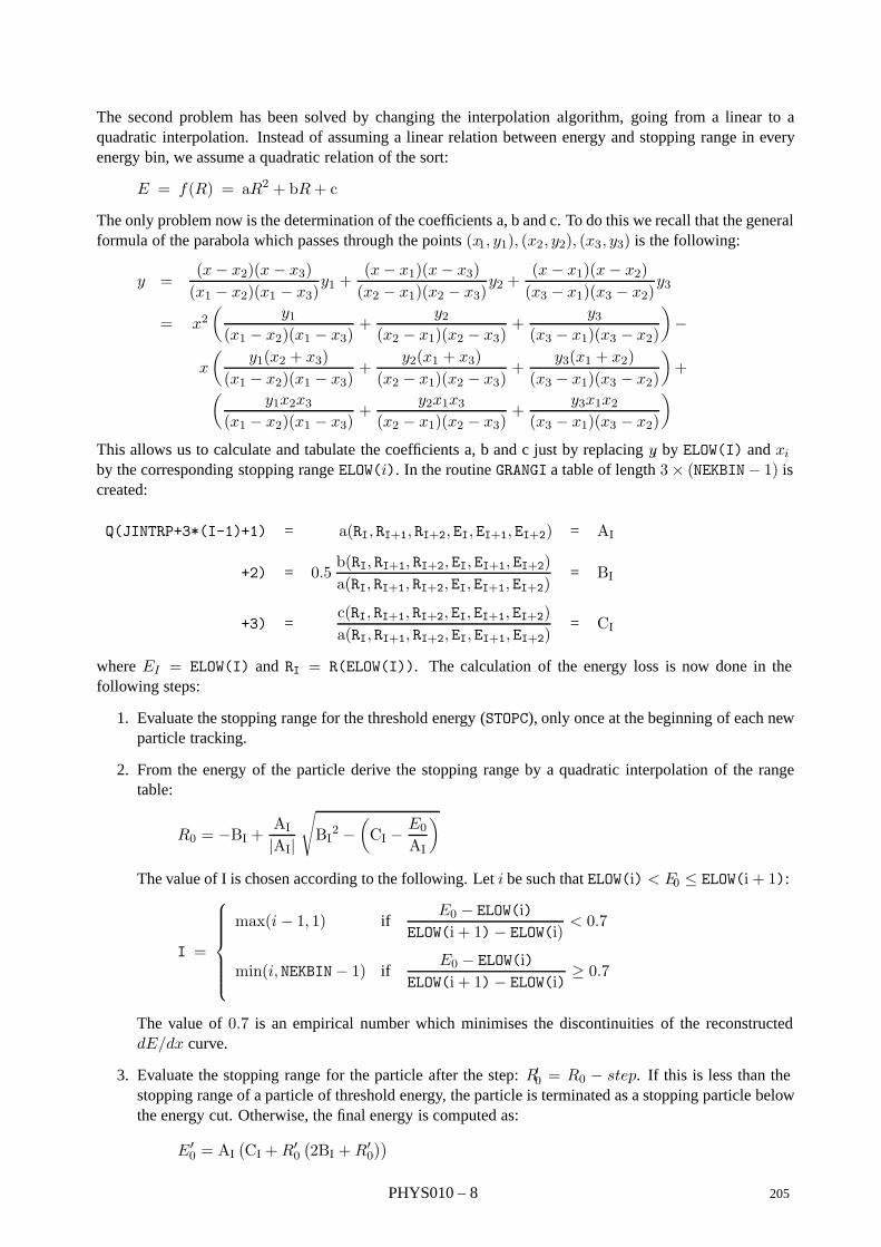
The second problem has been solved by changing the interpolation algorithm, going from a linear to aquadratic interpolation. Instead of assuming a linear relation between energy and stopping range in everyenergy bin, we assume a quadratic relation of the sort:
E = f(R) = aR2 + bR+ c
The only problem now is the determination of the coefficients a, b and c. To do this we recall that the generalformula of the parabola which passes through the points (x1, y1), (x2, y2), (x3, y3) is the following:
y =(x− x2)(x− x3)(x1 − x2)(x1 − x3)
y1 +(x− x1)(x− x3)(x2 − x1)(x2 − x3)
y2 +(x− x1)(x− x2)(x3 − x1)(x3 − x2)
y3
= x2(
y1(x1 − x2)(x1 − x3)
+y2
(x2 − x1)(x2 − x3)+
y3(x3 − x1)(x3 − x2)
)−
x
(y1(x2 + x3)
(x1 − x2)(x1 − x3)+
y2(x1 + x3)(x2 − x1)(x2 − x3)
+y3(x1 + x2)
(x3 − x1)(x3 − x2)
)+(
y1x2x3(x1 − x2)(x1 − x3)
+y2x1x3
(x2 − x1)(x2 − x3)+
y3x1x2(x3 − x1)(x3 − x2)
)This allows us to calculate and tabulate the coefficients a, b and c just by replacing yi by ELOW(I) and xi
by the corresponding stopping range ELOW(i). In the routine GRANGI a table of length 3× (NEKBIN− 1) iscreated:
Q(JINTRP+3*(I-1)+1) = a(RI, RI+1, RI+2, EI, EI+1, EI+2) = AI
+2) = 0.5b(RI, RI+1, RI+2, EI, EI+1, EI+2)a(RI, RI+1, RI+2, EI, EI+1, EI+2)
= BI
+3) =c(RI, RI+1, RI+2, EI, EI+1, EI+2)a(RI, RI+1, RI+2, EI, EI+1, EI+2)
= CI
where EI = ELOW(I) and RI = R(ELOW(I)). The calculation of the energy loss is now done in thefollowing steps:
1. Evaluate the stopping range for the threshold energy (STOPC), only once at the beginning of each newparticle tracking.
2. From the energy of the particle derive the stopping range by a quadratic interpolation of the rangetable:
R0 = −BI +AI|AI|
√BI2 −
(CI −
E0AI
)
The value of I is chosen according to the following. Let i be such that ELOW(i) < E0 ≤ ELOW(i + 1):
I =
max(i− 1, 1) ifE0 − ELOW(i)
ELOW(i + 1)− ELOW(i)< 0.7
min(i, NEKBIN− 1) ifE0 − ELOW(i)
ELOW(i + 1)− ELOW(i)≥ 0.7
The value of 0.7 is an empirical number which minimises the discontinuities of the reconstructeddE/dx curve.
3. Evaluate the stopping range for the particle after the step: R′0 = R0 − step. If this is less than thestopping range of a particle of threshold energy, the particle is terminated as a stopping particle belowthe energy cut. Otherwise, the final energy is computed as:
E′0 = AI
(CI +R′
0
(2BI +R′
0
))PHYS010 – 8 205

4. the energy loss is computed as:
∆E = E0 − E′0
This value is then corrected to take into account the energy loss fluctuations (see [PHYS332]).
This method results in a dE/dx curve which is a set of connected straight lines and not a step function.
206 PHYS010 – 9
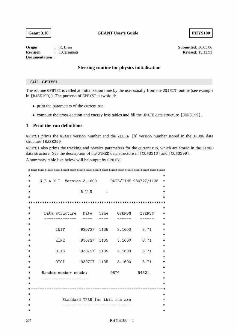
Geant 3.16 GEANT User’s Guide PHYS100
Origin : R. Brun Submitted: 30.05.86Revision : F.Carminati Revised: 15.12.93Documentation :
Steering routine for physics initialisation
CALL GPHYSI
The routine GPHYSI is called at initialisation time by the user usually from the UGINIT routine (see examplein [BASE100]). The purpose of GPHYSI is twofold:
• print the parameters of the current run
• compute the cross-section and energy loss tables and fill the JMATE data structure [CONS199].
1 Print the run definitions
GPHYSI prints the GEANT version number and the ZEBRA [8] version number stored in the JRUNG datastructure [BASE299]
GPHYSI also prints the tracking and physics parameters for the current run, which are stored in the JTMEDdata structure. See the description of the JTMED data structure in [CONS210] and [CONS299].
A summary table like below will be output by GPHYSI
************************************************************* ** G E A N T Version 3.1600 DATE/TIME 930727/1135 ** ** R U N 1 ** ************************************************************** ** Data structure Date Time GVERSN ZVERSN ** -------------- ---- ---- ------ ------ ** ** INIT 930727 1135 3.1600 3.71 ** ** KINE 930727 1135 3.1600 3.71 ** ** HITS 930727 1135 3.1600 3.71 ** ** DIGI 930727 1135 3.1600 3.71 ** ** Random number seeds: 9876 54321 ** -------------------- ** **----------------------------------------------------------** ** Standard TPAR for this run are ** ------------------------------ ** *
207 PHYS100 – 1
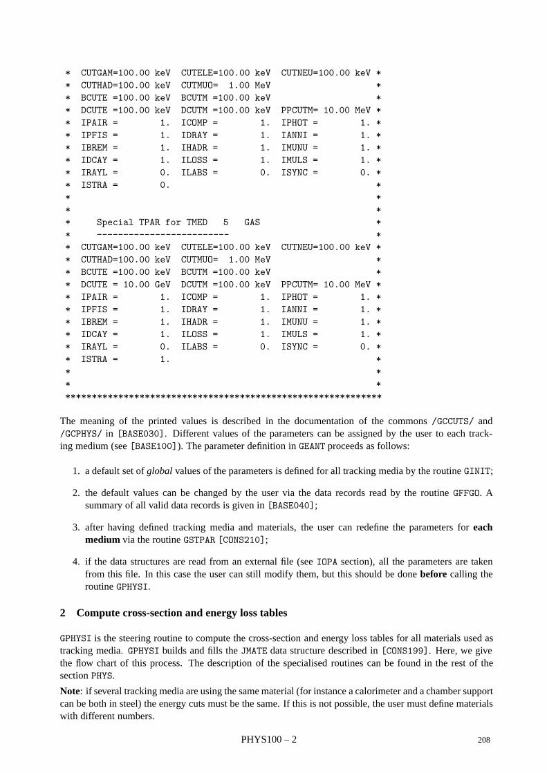
* CUTGAM=100.00 keV CUTELE=100.00 keV CUTNEU=100.00 keV ** CUTHAD=100.00 keV CUTMUO= 1.00 MeV ** BCUTE =100.00 keV BCUTM =100.00 keV ** DCUTE =100.00 keV DCUTM =100.00 keV PPCUTM= 10.00 MeV ** IPAIR = 1. ICOMP = 1. IPHOT = 1. ** IPFIS = 1. IDRAY = 1. IANNI = 1. ** IBREM = 1. IHADR = 1. IMUNU = 1. ** IDCAY = 1. ILOSS = 1. IMULS = 1. ** IRAYL = 0. ILABS = 0. ISYNC = 0. ** ISTRA = 0. ** ** ** Special TPAR for TMED 5 GAS ** ------------------------- ** CUTGAM=100.00 keV CUTELE=100.00 keV CUTNEU=100.00 keV ** CUTHAD=100.00 keV CUTMUO= 1.00 MeV ** BCUTE =100.00 keV BCUTM =100.00 keV ** DCUTE = 10.00 GeV DCUTM =100.00 keV PPCUTM= 10.00 MeV ** IPAIR = 1. ICOMP = 1. IPHOT = 1. ** IPFIS = 1. IDRAY = 1. IANNI = 1. ** IBREM = 1. IHADR = 1. IMUNU = 1. ** IDCAY = 1. ILOSS = 1. IMULS = 1. ** IRAYL = 0. ILABS = 0. ISYNC = 0. ** ISTRA = 1. ** ** *************************************************************
The meaning of the printed values is described in the documentation of the commons /GCCUTS/ and/GCPHYS/ in [BASE030]. Different values of the parameters can be assigned by the user to each track-ing medium (see [BASE100]). The parameter definition in GEANT proceeds as follows:
1. a default set of global values of the parameters is defined for all tracking media by the routine GINIT;
2. the default values can be changed by the user via the data records read by the routine GFFGO. Asummary of all valid data records is given in [BASE040];
3. after having defined tracking media and materials, the user can redefine the parameters for eachmedium via the routine GSTPAR [CONS210];
4. if the data structures are read from an external file (see IOPA section), all the parameters are takenfrom this file. In this case the user can still modify them, but this should be done before calling theroutine GPHYSI.
2 Compute cross-section and energy loss tables
GPHYSI is the steering routine to compute the cross-section and energy loss tables for all materials used astracking media. GPHYSI builds and fills the JMATE data structure described in [CONS199]. Here, we givethe flow chart of this process. The description of the specialised routines can be found in the rest of thesection PHYS.
Note: if several tracking media are using the same material (for instance a calorimeter and a chamber supportcan be both in steel) the energy cuts must be the same. If this is not possible, the user must define materialswith different numbers.
PHYS100 – 2 208
GPHYSI Initialisation of physics processes. This routine should be calledby the user before the tracking starts, but after all the material,mechanism flags and energy cuts have been defined. GPHYSIshould also be called whenever a new initialisation data structureis read from disk.
GRNDMQ Initialises the value of the seeds of the random number generator.See [BASE420] for more information
GEVKEV Routine to format energy values for printout. See [BASE410] formore details.
GPHINI Initialisation of the constants for photoelectric effect (see[PHYS230]).
Loop on tracking media
GPHXSI Initialisation of the cross section coefficients for the photoelectriceffect in a tracking medium, see [PHYS230].
GPROBI Initialisation of constants for various physical effects.
GMOLI Initialises constants for Moliere scattering, see [PHYS325].
Loop on energy bins
GDRELA Initialises the ionisation energy loss tables dE/dx for protons, µand e+, e−, see [PHYS430].
GDRELP Calculates ionisation energy loss for protons, see [PHYS430].
GDRELM Calculates ionisation energy loss for µ, see [PHYS430].
GDRELE Calculates ionisation energy loss for e−/e+, see [PHYS330].
GBRELA Adds the contribution of bremsstrahlung to continuous energyloss tables for protons, µ and e−/e+, see [PHYS440].
GPRELA Adds the contribution of direct pair production and µ-nucleus in-teractions to the µ continuous energy loss tables, see [PHYS450].
GPHOTI Calculates the cross section for photoelectric effect, see[PHYS230].
GRAYLI Initialises the tables of cross sections for the Rayleigh effect, see[PHYS250].
GANNII Initialises the cross section for positron annihilation, see[PHYS350].
GCOMPI Initialises the cross section tables for Compton effect, see[PHYS220].
GBRSGA Initialises the cross section tables for discrete bremsstrahlung ofe−/e+and µ, see [PHYS340], [PHYS440].
GPRSGA Initialises cross section tables for pair production by photons anddirect pair production by muons, see [PHYS210], [PHYS450].
GDRSGA Initialises the cross section tables for delta rays production by µand electrons, see [PHYS330], [PHYS430].
GMUNUI Initialises the cross section tables for µ-nucleus interactions, see[PHYS460].
GPFISI Initialises the cross section tables for photo-fission and photo-absorption, see [PHYS240].
End of loop on energy bins
GRANGI Calculates the stopping range integrating the dE/dx tables, see[PHYS010].
GCOEFF Calculation of the coefficients of the interpolating parabolas forthe range tables, see [PHYS010].
209 PHYS100 – 3
GSTINI Initialisation of the energy loss tables for the thin layers, see[PHYS334].
GFCNRM Calculation of mean ionisation potentials and normalisation fac-tors for oscillator functions.
GSREE0 Calculation of the real part of the refractive index.
GSDNDX Calculation of number of collisions for a given value of β.
GMULOF Calculation of the STMIN tables, see [PHYS325].
GMOLIO Calculation of the constants of Moliere scattering to estimatethe step limitation due to multiple scattering simulation, see[PHYS325].End of loop on tracking media
Notes:
1. The µ-nucleus interactions are treated either as a continuous energy loss by the muon (IMUNU= 0) oras a discrete process (IMUNU≥1), in an exclusive way i.e.:
• If IMUNU= 0, the dE/dx due to the interactions is added to that coming from direct (e+/e−)pair production in the routine GPRELA.
• If IMUNU≥ 1, the total cross section is computed in GMUNUI.
2. The total cross sections for hadronic interactions cannot be tabulated at initialisation time, as they aredependent on the nature of the incident particle. They are computed at tracking time by the functionFLDIST in case of FLUKA [PHYS520], GHESIG in case of GHEISHA [PHYS510] or FMDIST in case ofMICAP [PHYS530].
PHYS100 – 4 210
Geant 3.16 GEANT User’s Guide PHYS210
Origin : L. Urban Submitted: 10.11.84Revision : Revised: 16.12.93Documentation :
Total cross-section for e+e- pair production by photons
1 Subroutines
CALL GPRSGA
GPRSGA calculates the total cross-section for the pair production of photons and the direct pair productionof muons in all materials. It tabulates the mean free path, λ = 1/Σ (in cm), as a function of the medium andthe energy. For the pair production by photons, it calls the function GPRSGG. The energy bins are the one ofthe array ELOW in common /CGMULO/ initialised in the routine GPHYSI. The following pointers are used:
JMA = LQ(JMATE-I) pointer to the Ith material
JPAIR = LQ(JMA-10) pointer to pair production cross-sections
GPRSGA is called at initialisation time by GPHYSI.
VALUE = GPRSGG (Z,E)
GPRSGG calculates the total cross-section for the pair production of a photon with energy E in material withatomic number Z. It is called by GPRSGA.
2 Method
We have parameterised the total cross-section of e+e−-pair production by photon as:
σ(Z,Eγ) = Z(Z + 1) (F1(X) + F2(X)Z + F3(X)/Z) (barn/atom) (1)
where
X = ln(Eγ/m),m = electron mass,
Eγ = photon energy
and
Fi(X) =5∑
n=0
cnXn
The parameters cn were taken from a least-square fit to the data [9] and can be found in the DATA statementin the function GPRSGG(Z,E) which computes the formula (1) (in barn/atom).
This parameterisation gives a good description of the data in the range:
1 ≤ Z ≤ 1001.5 MeV ≤ Eγ ≤ 100 GeV
∆ σ
σ≤ 5% with a mean value of ≈ 2.2% (2)
This mean free path is tabulated at initialisation as a function of the medium and of the energy by the routineGPRSGA.
211 PHYS210 – 1
Geant 3.16 GEANT User’s Guide PHYS211
Origin : G.N.Patrick, L.Urban Submitted: 12.12.84Revision : Revised: 16.12.93Documentation :
Simulation of e-e+ pair production by photons
1 Subroutines
CALL GPAIRG
GPAIRG generates e−e+-pair production by photons. It uses a modified version of the random number tech-niques of Butcher and Messel [10] to sample the secondary electron/positron energies from the Coulombcorrected Bethe-Heitler differential cross-section. For the angular distribution of the pair, it calls the functionGBTETH.
Input: via COMMON /GCTRAK/
Output: via COMMON /GCKING/
GPAIRG is called from GTGAMA, when the photon reaches its pair production point.
VALUE = GBTETH (ENER,PARTM,EFRAC)
GBTETH calculates the angular distribution of the e−e+-pair for pair production and of the photon for bre-msstrahlung. In case of e−e+-pair production by photons, it gives the scaled angle for an electron (massPARTM) of energy ENER which is EFRAC times the initial energy of the photon. GBTETH is called by GPAIRG.
2 Method
2.1 MonteCarlo technique
We give a very short summary of the random number technique used here [10, 11]. The method is acombination of the composition and rejection Monte Carlo methods. Suppose we wish to sample x fromthe distribution f(x) and the (normalised) probability density function can be written as
f(x) =n∑
i=1
αifi(x)gi(x) (1)
where fi(x) are normalised density functions, αi > 0 and 0 ≤ gi(x) ≤ 1.
According to this method, x can sampled in the following way:
1. select a random integer i such that (1 ≤ i ≤ n) with probability proportional to αi
2. select a value x′ from the distribution fi(x)
3. calculate gi(x′) and accept x = x′ with probability gi(x′);
4. if x′ is rejected restart from step 1.
It can be shown that this scheme is correct and the mean number of tries to accept a value is∑
i αi.
In practice we have a good method of sampling from the distribution f(x), if
• all the subdistributions fi(x) can be sampled easily;
• the rejection functions gi(x) can be evaluated easily/quickly;
212 PHYS211 – 1
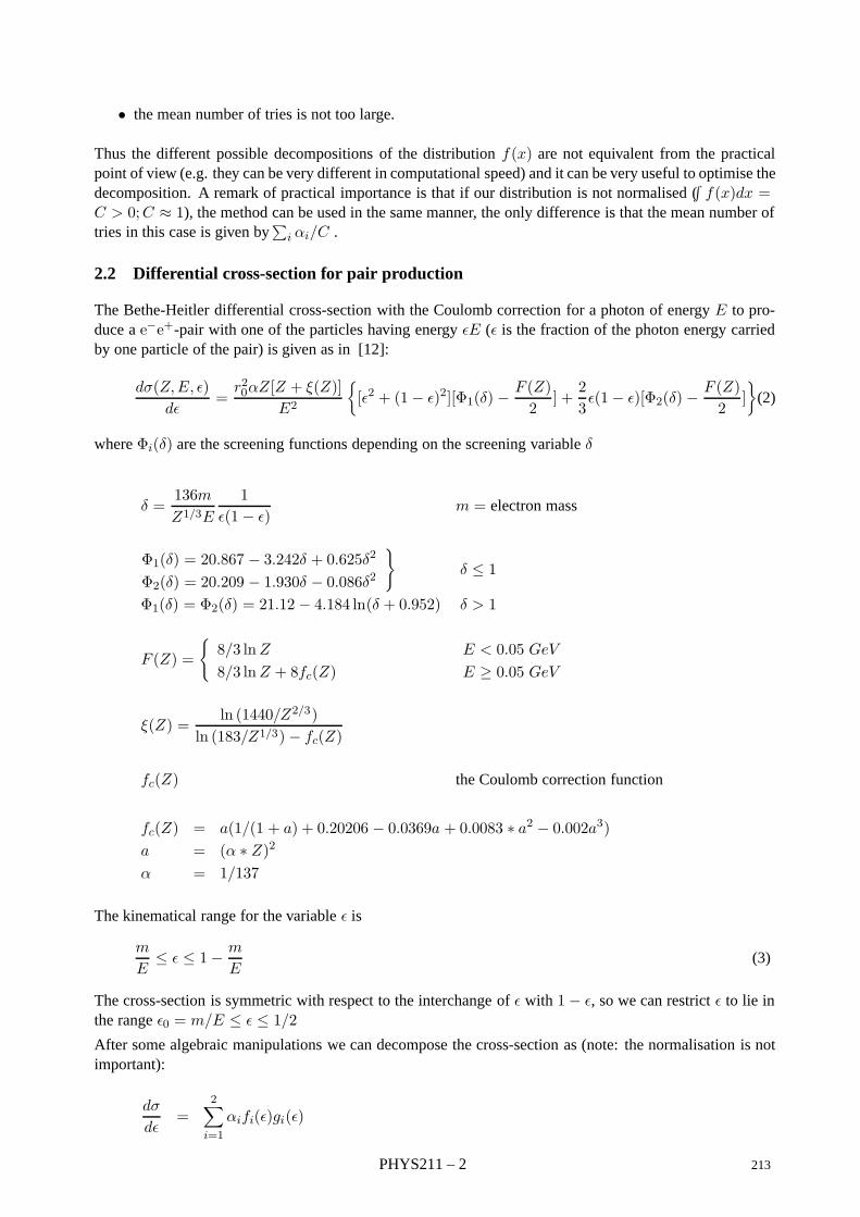
• the mean number of tries is not too large.
Thus the different possible decompositions of the distribution f(x) are not equivalent from the practicalpoint of view (e.g. they can be very different in computational speed) and it can be very useful to optimise thedecomposition. A remark of practical importance is that if our distribution is not normalised (
∫f(x)dx =
C > 0;C ≈ 1), the method can be used in the same manner, the only difference is that the mean number oftries in this case is given by
∑i αi/C .
2.2 Differential cross-section for pair production
The Bethe-Heitler differential cross-section with the Coulomb correction for a photon of energy E to pro-duce a e−e+-pair with one of the particles having energy εE (ε is the fraction of the photon energy carriedby one particle of the pair) is given as in [12]:
dσ(Z,E, ε)dε
=r20αZ[Z + ξ(Z)]
E2
[ε2 + (1− ε)2][Φ1(δ) −
F (Z)2
] +23ε(1− ε)[Φ2(δ) −
F (Z)2
]
(2)
where Φi(δ) are the screening functions depending on the screening variable δ
δ =136mZ1/3E
1ε(1− ε)
m = electron mass
Φ1(δ) = 20.867 − 3.242δ + 0.625δ2
Φ2(δ) = 20.209 − 1.930δ − 0.086δ2
δ ≤ 1
Φ1(δ) = Φ2(δ) = 21.12 − 4.184 ln(δ + 0.952) δ > 1
F (Z) =
8/3 lnZ8/3 lnZ + 8fc(Z)
E < 0.05 GeV
E ≥ 0.05 GeV
ξ(Z) =ln (1440/Z2/3)
ln (183/Z1/3)− fc(Z)
fc(Z) the Coulomb correction function
fc(Z) = a(1/(1 + a) + 0.20206 − 0.0369a + 0.0083 ∗ a2 − 0.002a3)a = (α ∗ Z)2
α = 1/137
The kinematical range for the variable ε is
m
E≤ ε ≤ 1− m
E(3)
The cross-section is symmetric with respect to the interchange of ε with 1− ε, so we can restrict ε to lie inthe range ε0 = m/E ≤ ε ≤ 1/2
After some algebraic manipulations we can decompose the cross-section as (note: the normalisation is notimportant):
dσ
dε=
2∑i=1
αifi(ε)gi(ε)
PHYS211 – 2 213
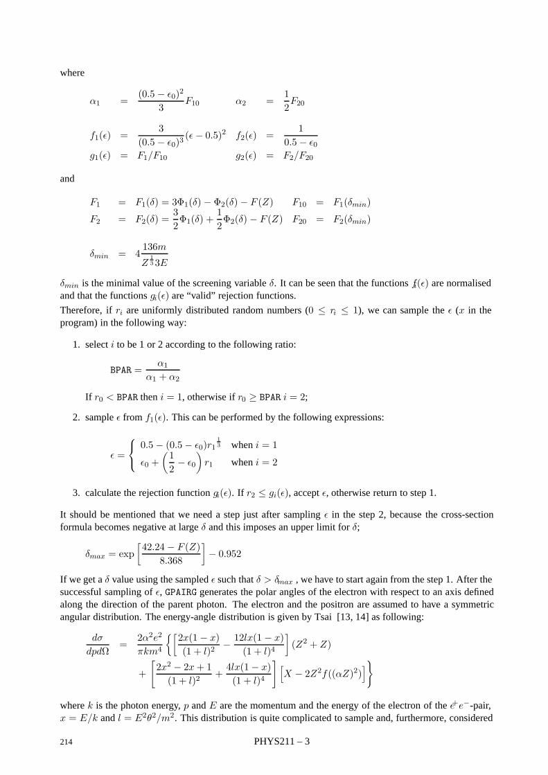
where
α1 =(0.5 − ε0)2
3F10 α2 =
12F20
f1(ε) =3
(0.5 − ε0)3(ε− 0.5)2 f2(ε) =
10.5− ε0
g1(ε) = F1/F10 g2(ε) = F2/F20
and
F1 = F1(δ) = 3Φ1(δ) − Φ2(δ)− F (Z) F10 = F1(δmin)
F2 = F2(δ) =32Φ1(δ) +
12Φ2(δ) − F (Z) F20 = F2(δmin)
δmin = 4136m
Z133E
δmin is the minimal value of the screening variable δ. It can be seen that the functions fi(ε) are normalisedand that the functions gi(ε) are “valid” rejection functions.
Therefore, if ri are uniformly distributed random numbers (0 ≤ ri ≤ 1), we can sample the ε (x in theprogram) in the following way:
1. select i to be 1 or 2 according to the following ratio:
BPAR =α1
α1 + α2
If r0 < BPAR then i = 1, otherwise if r0 ≥ BPAR i = 2;
2. sample ε from f1(ε). This can be performed by the following expressions:
ε =
0.5 − (0.5− ε0)r1
13 when i = 1
ε0 +(12− ε0
)r1 when i = 2
3. calculate the rejection function gi(ε). If r2 ≤ gi(ε), accept ε, otherwise return to step 1.
It should be mentioned that we need a step just after sampling ε in the step 2, because the cross-sectionformula becomes negative at large δ and this imposes an upper limit for δ;
δmax = exp[42.24 − F (Z)
8.368
]− 0.952
If we get a δ value using the sampled ε such that δ > δmax , we have to start again from the step 1. After thesuccessful sampling of ε, GPAIRG generates the polar angles of the electron with respect to an axis definedalong the direction of the parent photon. The electron and the positron are assumed to have a symmetricangular distribution. The energy-angle distribution is given by Tsai [13, 14] as following:
dσ
dpdΩ=
2α2e2
πkm4
[2x(1− x)(1 + l)2
− 12lx(1 − x)(1 + l)4
](Z2 + Z)
+
[2x2 − 2x+ 1(1 + l)2
+4lx(1− x)(1 + l)4
] [X − 2Z2f((αZ)2)
]
where k is the photon energy, p and E are the momentum and the energy of the electron of the e+e−-pair,x = E/k and l = E2θ2/m2. This distribution is quite complicated to sample and, furthermore, considered
214 PHYS211 – 3
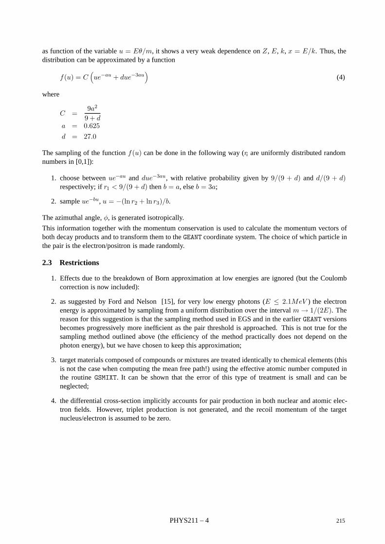
as function of the variable u = Eθ/m, it shows a very weak dependence on Z , E, k, x = E/k. Thus, thedistribution can be approximated by a function
f(u) = C(ue−au + due−3au
)(4)
where
C =9a2
9 + da = 0.625d = 27.0
The sampling of the function f(u) can be done in the following way (ri are uniformly distributed randomnumbers in [0,1]):
1. choose between ue−au and due−3au, with relative probability given by 9/(9 + d) and d/(9 + d)respectively; if r1 < 9/(9 + d) then b = a, else b = 3a;
2. sample ue−bu, u = −(ln r2 + ln r3)/b.
The azimuthal angle, φ, is generated isotropically.
This information together with the momentum conservation is used to calculate the momentum vectors ofboth decay products and to transform them to the GEANT coordinate system. The choice of which particle inthe pair is the electron/positron is made randomly.
2.3 Restrictions
1. Effects due to the breakdown of Born approximation at low energies are ignored (but the Coulombcorrection is now included):
2. as suggested by Ford and Nelson [15], for very low energy photons (E ≤ 2.1MeV ) the electronenergy is approximated by sampling from a uniform distribution over the interval m → 1/(2E). Thereason for this suggestion is that the sampling method used in EGS and in the earlier GEANT versionsbecomes progressively more inefficient as the pair threshold is approached. This is not true for thesampling method outlined above (the efficiency of the method practically does not depend on thephoton energy), but we have chosen to keep this approximation;
3. target materials composed of compounds or mixtures are treated identically to chemical elements (thisis not the case when computing the mean free path!) using the effective atomic number computed inthe routine GSMIXT. It can be shown that the error of this type of treatment is small and can beneglected;
4. the differential cross-section implicitly accounts for pair production in both nuclear and atomic elec-tron fields. However, triplet production is not generated, and the recoil momentum of the targetnucleus/electron is assumed to be zero.
PHYS211 – 4 215
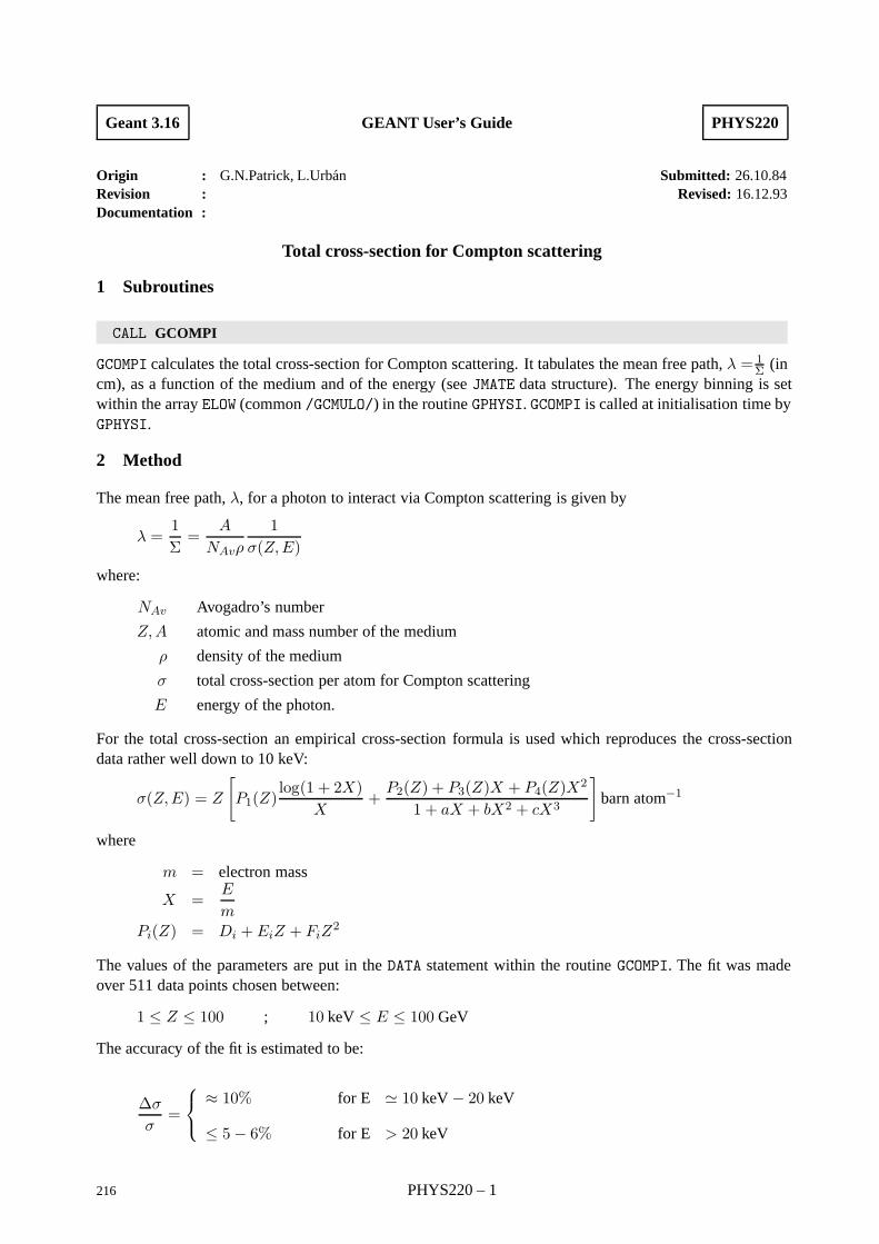
Geant 3.16 GEANT User’s Guide PHYS220
Origin : G.N.Patrick, L.Urban Submitted: 26.10.84Revision : Revised: 16.12.93Documentation :
Total cross-section for Compton scattering
1 Subroutines
CALL GCOMPI
GCOMPI calculates the total cross-section for Compton scattering. It tabulates the mean free path, λ = 1Σ (in
cm), as a function of the medium and of the energy (see JMATE data structure). The energy binning is setwithin the array ELOW (common /GCMULO/) in the routine GPHYSI. GCOMPI is called at initialisation time byGPHYSI.
2 Method
The mean free path, λ, for a photon to interact via Compton scattering is given by
λ =1Σ=
A
NAvρ
1σ(Z,E)
where:
NAv Avogadro’s number
Z,A atomic and mass number of the medium
ρ density of the medium
σ total cross-section per atom for Compton scattering
E energy of the photon.
For the total cross-section an empirical cross-section formula is used which reproduces the cross-sectiondata rather well down to 10 keV:
σ(Z,E) = Z
[P1(Z)
log(1 + 2X)X
+P2(Z) + P3(Z)X + P4(Z)X2
1 + aX + bX2 + cX3
]barn atom−1
where
m = electron mass
X =E
mPi(Z) = Di + EiZ + FiZ
2
The values of the parameters are put in the DATA statement within the routine GCOMPI. The fit was madeover 511 data points chosen between:
1 ≤ Z ≤ 100 ; 10 keV ≤ E ≤ 100 GeV
The accuracy of the fit is estimated to be:
∆σ
σ=
≈ 10% for E 10 keV − 20 keV
≤ 5− 6% for E > 20 keV
216 PHYS220 – 1
Geant 3.16 GEANT User’s Guide PHYS221
Origin : G.N.Patrick, L.Urban Submitted: 26.09.83Revision : Revised: 16.12.93Documentation :
Simulation of Compton scattering
1 Subroutines
CALL GCOMP
GCOMP generates the Compton scattering of a photon on an atomic electron. It uses the random numbertechniques of Butcher and Messell [10] to sample the scattered photon energy according to the Klein-Nishina formula [16].
The interaction produces one electron, which is put in the /GCKING/ common block for further tracking.Tracking of the scattered photon will continue, with direction and energy changed by the interaction. Allinput/output information is through GEANT common blocks.
Input: via COMMON /GCTRACK/
Output: via COMMONs /GCTRAK/ and /GCKING/
Compton scattering is selected in GEANT by the input data record COMP. When Compton scattering is se-lected, GCOMP is called automatically from the GEANT photon tracking routine GTGAMA.
2 Method
For a complete account of the Monte Carlo methods used the interested user is referred to the publications ofButcher and Messel [10], Messel and Crawford [17] and Ford and Nelson [12]. Only the basic formalismis outlined here.
The quantum mechanical Klein-Nishina differential cross-section is:
Φ(E,E′) =X0nπr
20me
E2
[1ε+ ε
] [1− ε sin2 θ
1 + ε2
]
where, E = energy of the incident photon
E′ = energy of the scattered photon
ε = E′/E
me = electron mass
n = electron density
r0 = classical electron radius
X0 = radiation length
Assuming an elastic collision, the scattering angle θ is defined by the Compton formula:
E′ = Eme
me + E(1 − cos θ)
Using the combined “composition and rejection” Monte Carlo methods described in chapter PHYS211, we
217 PHYS221 – 1
may set:
f(ε) =[1ε+ ε
]=
2∑i=1
αifi(E) for ε0 > ε > 1
g(ε) =
[1− ε sin2 θ
1 + ε2
]rejection function
α1 =1
ln(1/ε0)α2 =
12(1− ε20)
f1(ε) =1
ε ln(1/ε0)f2(ε) =
2ε1− ε2
The value of ε corresponding to the minimum photon energy (backward scattering) is given by:
ε0 =1
1 + 2E/me
Given a set of random numbers ri uniformly distributed in [0,1], the sampling procedure for ε is the follow-ing:
1. decide which element of the f(ε) distribution to sample from. Let αT = (α1 + α2)r0. If α1 ≥ αT
select f1(ε), otherwise select f2(ε);
2. sample ε from the distributions corresponding to f1 or f2. For f1 this is simply achieved by:
ε = ε0eα1 r1
For f2, we change variables and use:
ε′ =
max(r2, r3) for E/m ≥ (E/m + 1)r4r5 for all other cases
Then, ε = ε0 + (1− ε0)ε′;
3. calculate sin2 θ = max(0, t(2 − t)) where t = me(1− ε)/E′
4. test the rejection function, if r6 ≤ g(ε) accept ε, otherwise return to step 1.
After the successful sampling of ε, GCOMP generates the polar angles of the scattered photon with respectto the direction of the parent photon. The azimuthal angle, φ, is generated isotropically and θ is as definedabove. The momentum vector of the scattered photon is then calculated according to kinematic considera-tions. Both vectors are then transformed into the GEANT coordinate system.
3 Restriction
The differential cross-section is only valid for those collisions in which the energy of the recoil electron islarge compared with its binding energy (which is ignored). However, as pointed out by Rossi [18], this hasa negligible effect because of the small number of recoil electrons produced at very low energies.
PHYS221 – 2 218
GEANT 3.16 GEANT User’s Guide PHYS230
Origin : L.Urban Submitted: 26.10.84Revision : J. Chwastowski Revised: 16.12.93Documentation :
Total cross-section for photoelectric effect
1 Subroutines
CALL GPHINI
GPHINI steers initialisation of the constants. It calls GHPRIN for initialisation of the atom decay rates,GHSLIN to initialise atomic shell potentials and ionisation energies and GPHXIN for the initialisation of thecross-section constants. It is called by GPHOTI.
CALL GPHRIN
Initialisation of the atom decay rates. The routine is called by GPHINI.
CALL GSHLIN
Initialisation of the atomic shell potentials and ionisation energies. GSHLIN is called by GPHINI.
CALL GPHXIN
Initialisation of the cross-section constants for elements with Z ≤ 100. It is called by GPHINI.
CALL GPHXSI
GPHXSI is called by GPHYSI for every tracking medium. It calculates the cross-section coefficients. Theresults of the calculations are stored in the photoelectric effect constants bank created by this routine.
CALL GFSHDC
GFSHDC calls GFRDT, GNRDT and GFSDPR for the probabilities of atomic state transitions and the transitionenergies and stores them in the ZEBRA bank. It is called by GPHXSI.
CALL GFSHLS
GFSHLS returns the shell potentials in eV for an atom. It is called by GFSHDC.
CALL GFRDT
GFRDT returns probability distribution and energies of the atomic radiative transitions. It is called by GFSHDC.
CALL GNFRDT
GNFRDT returns probability distribution and energies of the non-radiative atomic transitions. It is called byGFSHDC.
CALL GFSDPR
GFSDPR returns probability of the shell radiative decay. It is called by GFSHDC.
CALL GPHOTI
GPHOTI calculates the total cross-section for the photoelectric effect. It tabulates the mean free path, λ =1/Σ (in cm), as a function of the medium and the energy. If Z ≤ 100 then it calls the function GPHSG1for the total cross-section. Otherwise GPHSIG function is used. GPHOTI is called at initialisation time byGPHYSI.
219 PHYS230 – 1
VALUE = GPHSG1 (EGAM)
GPHSG1 calculates the total cross-section for photoelectric effect. It is called by GPHOTI for Z ≤ 100.
VALUE = GPHSIG (Z,EGAM)
GPHSIG calculates the total cross-section for the photoelectric effect of a photon with energy EGAM in mate-rial with atomic number Z > 100. It is called by GPHOTI.
2 Method
2.1 Materials with Z ≤ 100
For media with Z ≤ 100 we use SANDIA parametrisation [19]. The cross-section for elements wasfitted with a linear combination of reciprocal powers of the photon energy Eγ (Eγ in keV). The fits wereperformed in different intervals j of the photon energy. In such an interval the cross-section reads as:
µij =C1,ijEγ
+C2,ijE2γ
+C3,ijE3γ
+C4,ijE4γ
(cm2g−1) (1)
with j changing from 1 to mi, where mi is the number of fitting intervals used for element i.
For the composites or mixtures of N elements the cross-section for jth interval is calculated as:
µj =N∑
k=1
fkµj,k (2)
where fk is the fraction by mass of kth element in the material. Substituting (1) into (2) one finds that thecross-section coefficients can be calculated as:
Ci,total =N∑
k=1
fkCi,jk (3)
for i from 1 to 4. The macroscopic cross-section is calculated as follows:
Σ = ρµ (cm−1) (4)
where ρ is the medium density.
As follows from (3) each compound is decomposed to its components which should coincide with chemicalelements. If this is not the case i.e. a component has a non-integer atomic number Zx and is created by acall to GSMATE then the cross-section constants are calculated using two elements with Z1 = integer(Zx)and Z2 = Z1 + 1 applying the weights w1 = Z2 − Zx and w2 = Zx − Z1 respectively.
2.2 Materials with Z > 100
Originally the parametrisation described below was developed for the elements with the atomic number Zbetween 5 and 100. Lacking more accurate data and assuming that there are no dramatic changes of thecross-section behaviour this method (i.e. GPHSIG function) is used for Z > 100.
The macroscopic cross-section for an element is given by
Σ =Nρσ(Z,Eγ)
A(cm−1) (5)
and for a compound or a mixture
Σ =Nρ
∑i σ(Zi, Eγ)∑i niAi
= Nρ∑i
piAi
σ(Zi, Eγ) (cm−1) (6)
PHYS230 – 2 220

where
N Avogadro’s number
Z(Zi) atomic number (of ith component) of the medium
A(Ai) atomic mass (of ith component) of the medium
ρ density
σ cross-section
ni proportion by number of the ith element in the material (ni = Wpi/Ai
where pi is the corresponding proportion by weight and W is the molecularweight).
The binding energy of the inner shells has been parameterised as:
Ei(Z) = Z2(Ai +BiZ + CiZ2 +DiZ
3) MeV (7)
where, i = K,LI , LII and the constants Ai, Bi, Ci and Di are tabulated below.
A B C D
K 0.66644·10−5 0.22077·10−6 -0.32552·10−8 0.18199·10−10LI -0.29179·10−6 0.87983·10−7 -0.12589·10−8 0.69602·10−11LII -0.68606·10−6 0.10078·10−6 -0.14496·10−8 0.78809·10−11
The photoelectric effect total cross-section has been parameterised as:
σ(Z,E) = ZαXβ
p1/Z + p2X + p3 + p4Z + p5/X + p6Z2
+ p7Z/X + p8/X2 + p9Z
3
+ p10Z2/X + p11Z/X
2 + p12/X3
if E > Ek(Z)
p13/Z + p14X + p15 if ELI< E ≤ Ek(Z)
p16/Z + p17X + p18 if ELII< E ≤ ELI
p19 if 10 keV ≤ E ≤ ELII
(8)
where X is the ratio of the electron mass to the incident photon energy and σ is expressed in barns/atom.The fit was made over 301 data points chosen between 5 ≤ Z ≤ 100 and 10 keV ≤ E ≤ 50 MeV .The values of the parameters are put in a DATA statement within the function GPHSIG which computes theformula (8). The accuracy of the fit is estimated to be
∆σ
≤25% near to the peaks
10% elsewhere.
3 Photoelectric effect Bank
The banks connected to the photoelectric effect are created during initialisation for each tracking medium.PHXS bank (data area) The total cross-section values are stored in PHOT bank in energy bins set within thearray ELOW (common CGMULO). This bank is pointed by JPHOT link. The first structural link of PHOT supportsthe PHXS bank. For each energy interval of the cross-section we store the upper limit of the interval and fourconstants of equation (3). For each chemical element used to build the medium a PHFN bank is created. Thisbank, pointed by a structural link of the PHXS bank, contains the data needed for the photoelectric effectfinal state simulation. All data word are of the Fortran REAL type. The descriptions of the PHXS and PHFNbanks are given below.
221 PHYS230 – 3
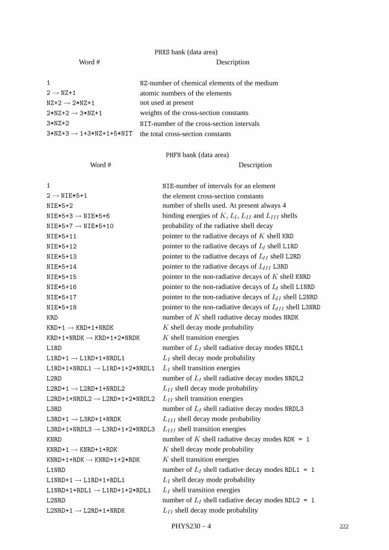
PHXS bank (data area)
Word # Description
1 NZ-number of chemical elements of the medium2→ NZ+1 atomic numbers of the elementsNZ+2→ 2*NZ+1 not used at present
2*NZ+2→ 3*NZ+1 weights of the cross-section constants
3*NZ+2 NIT-number of the cross-section intervals3*NZ+3→ 1+3*NZ+1+5*NIT the total cross-section constants
PHFN bank (data area)
Word # Description
1 NIE-number of intervals for an element2→ NIE*5+1 the element cross-section constantsNIE*5+2 number of shells used. At present always 4
NIE*5+3→ NIE*5+6 binding energies of K, LI , LII and LIII shells
NIE*5+7→ NIE*5+10 probability of the radiative shell decay
NIE*5+11 pointer to the radiative decays of K shell KRD
NIE*5+12 pointer to the radiative decays of LI shell L1RD
NIE*5+13 pointer to the radiative decays of LII shell L2RD
NIE*5+14 pointer to the radiative decays of LIII L3RD
NIE*5+15 pointer to the non-radiative decays of K shell KNRD
NIE*5+16 pointer to the non-radiative decays of LI shell L1NRD
NIE*5+17 pointer to the non-radiative decays of LII shell L2NRD
NIE*5+18 pointer to the non-radiative decays of LIII shell L3NRD
KRD number of K shell radiative decay modes NRDK
KRD+1→ KRD+1+NRDK K shell decay mode probability
KRD+1+NRDK→ KRD+1+2*NRDK K shell transition energies
L1RD number of LI shell radiative decay modes NRDL1
L1RD+1→ L1RD+1+NRDL1 LI shell decay mode probability
L1RD+1+NRDL1→ L1RD+1+2*NRDL1 LI shell transition energies
L2RD number of LI shell radiative decay modes NRDL2
L2RD+1→ L2RD+1+NRDL2 LII shell decay mode probability
L2RD+1+NRDL2→ L2RD+1+2*NRDL2 LII shell transition energies
L3RD number of LI shell radiative decay modes NRDL3
L3RD+1→ L3RD+1+NRDK LIII shell decay mode probability
L3RD+1+NRDL3→ L3RD+1+2*NRDL3 LIII shell transition energies
KNRD number of K shell radiative decay modes RDK = 1
KNRD+1→ KNRD+1+RDK K shell decay mode probability
KNRD+1+RDK→ KNRD+1+2*RDK K shell transition energies
L1NRD number of LI shell radiative decay modes RDL1 = 1
L1NRD+1→ L1RD+1+RDL1 LI shell decay mode probability
L1NRD+1+RDL1→ L1RD+1+2*RDL1 LI shell transition energies
L2NRD number of LI shell radiative decay modes RDL2 = 1
L2NRD+1→ L2RD+1+NRDK LII shell decay mode probability
PHYS230 – 4 222

PHFN bank (data area, continued)
Word # Description
L2NRD+1+RDL2→ L2RD+1+2*RDL2 LII shell transition energies
L3NRD number of LI shell radiative decay modes RDL3 = 1
L3NRD+1→ L3RD+1+RDL3 LIII shell decay mode probability
L3NRD+1+RDL3→ L3RD+1+2*NRDL3 LIII shell transition energies
223 PHYS230 – 5
GEANT 3.16 GEANT User’s Guide PHYS231
Origin : L.Urban Submitted: 26.10.84Revision : J. Chwastowski Revised: 16.12.93Documentation :
Simulation of photoelectric Effect
1 Subroutines
CALL GPHOT GPHOT
simulates the photoelectric effect. It uses the following input and output:
Input via common GCTRAK
Output via common GCKING
It calls the functions GPHSG1, GPHSGP, GAVRL2 and GAVRL3 for the cross-section and the functions GHPHAK,GHPHAL1, GHPHAL2, GPHAL3 for the cosine distribution of the photoelectron. GPHOT is called by the trackingroutine GTGAMA, if, and when, the photon reaches its interaction point.
VALUE = GAVRL2 (GAMAL2,BETAL2,X)
GAVRL2 calculates approximation of the cross-section for the photoelectric effect from LII shell. GAMAL2,BETAL2 are the Lorentz gamma and beta factors of the emitted photoelectron and X = me/Eγ where me isthe electron mass and Eγ is the incident radiation energy. GAVRL2 is called by GHPOT.
VALUE = GAVRL3 (GAMAL3,BETAL3,X)
GAVRL3 calculates approximation of the cross-section for the photoelectric effect from LIII shell. GAMAL3,BETAL3 are the Lorentz gamma and beta factors of the emitted photoelectron and X = me/Eγ where me isthe electron mass and Eγ is the incident radiation energy. GAVRL3 is called by GPHOT.
VALUE = GPHAK (BETAK)
VALUE = GPHAL1 (BETAL1)
GPHAK and its entry point GPHAL1 poll the cosine distribution (w.r.t. the incident photon direction) of thephotoelectron emitted from K or LI shell, respectively. They are called by GPHOT.
VALUE = GPHAL2 (BETAL2)
GPHAL2 polls the cosine distribution (w.r.t. the incident photon direction) of the photoelectron emitted fromLII shell.
VALUE = GPHAL3 (BETAL3)
GPHAL3 polls the cosine distribution (w.r.t. the incident photon direction) of the photoelectron emitted fromLIII shell. It is called by GPHOT.
VALUE = GPHSGP (EGAM)
GPHSGP calculates the photoelectric effect total cross-section for a particular atom of a mixture taking intoaccount weights. It is called by GPHOT for Z ≤ 100.
224 PHYS231 – 1
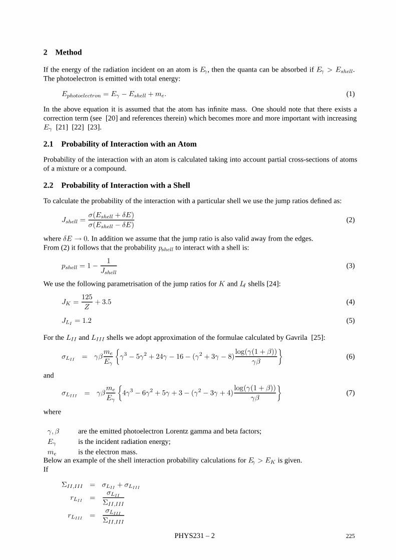
2 Method
If the energy of the radiation incident on an atom is Eγ , then the quanta can be absorbed if Eγ > Eshell.The photoelectron is emitted with total energy:
Ephotoelectron = Eγ − Eshell +me. (1)
In the above equation it is assumed that the atom has infinite mass. One should note that there exists acorrection term (see [20] and references therein) which becomes more and more important with increasingEγ [21] [22] [23].
2.1 Probability of Interaction with an Atom
Probability of the interaction with an atom is calculated taking into account partial cross-sections of atomsof a mixture or a compound.
2.2 Probability of Interaction with a Shell
To calculate the probability of the interaction with a particular shell we use the jump ratios defined as:
Jshell =σ(Eshell + δE)σ(Eshell − δE)
(2)
where δE → 0. In addition we assume that the jump ratio is also valid away from the edges.From (2) it follows that the probability pshell to interact with a shell is:
pshell = 1−1
Jshell(3)
We use the following parametrisation of the jump ratios for K and LI shells [24]:
JK =125Z
+ 3.5 (4)
JLI= 1.2 (5)
For the LII and LIII shells we adopt approximation of the formulae calculated by Gavrila [25]:
σLII= γβ
me
Eγ
γ3 − 5γ2 + 24γ − 16− (γ2 + 3γ − 8)log(γ(1 + β))
γβ
(6)
and
σLIII= γβ
me
Eγ
4γ3 − 6γ2 + 5γ + 3− (γ2 − 3γ + 4)log(γ(1 + β))
γβ
(7)
where
γ, β are the emitted photoelectron Lorentz gamma and beta factors;
Eγ is the incident radiation energy;
me is the electron mass.Below an example of the shell interaction probability calculations for Eγ > EK is given.If
ΣII,III = σLII+ σLIII
rLII=
σLII
ΣII,III
rLIII=
σLIII
ΣII,III
PHYS231 – 2 225
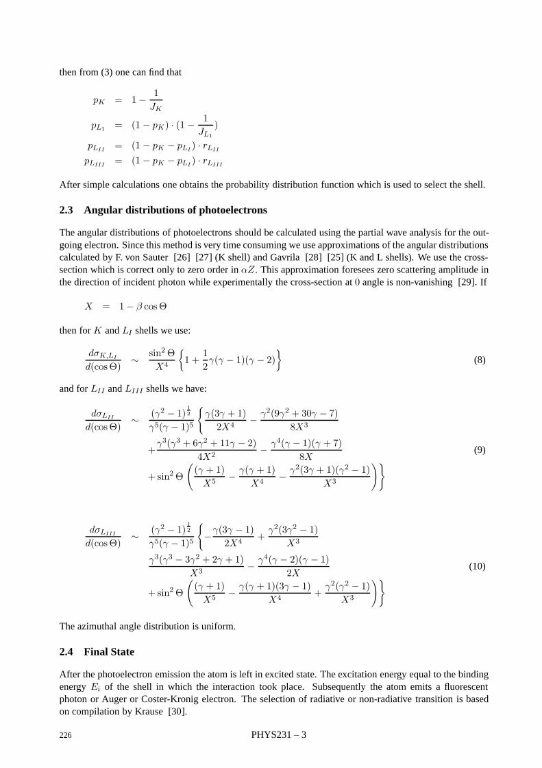
then from (3) one can find that
pK = 1− 1JK
pL1 = (1− pK) · (1−1
JL1
)
pLII= (1− pK − pLI
) · rLII
pLIII= (1− pK − pLI
) · rLIII
After simple calculations one obtains the probability distribution function which is used to select the shell.
2.3 Angular distributions of photoelectrons
The angular distributions of photoelectrons should be calculated using the partial wave analysis for the out-going electron. Since this method is very time consuming we use approximations of the angular distributionscalculated by F. von Sauter [26] [27] (K shell) and Gavrila [28] [25] (K and L shells). We use the cross-section which is correct only to zero order in αZ . This approximation foresees zero scattering amplitude inthe direction of incident photon while experimentally the cross-section at 0 angle is non-vanishing [29]. If
X = 1− β cosΘ
then for K and LI shells we use:
dσK,LI
d(cosΘ)∼ sin2Θ
X4
1 +
12γ(γ − 1)(γ − 2)
(8)
and for LII and LIII shells we have:
dσLII
d(cosΘ)∼ (γ2 − 1) 1
2
γ5(γ − 1)5
γ(3γ + 1)2X4
− γ2(9γ2 + 30γ − 7)8X3
+γ3(γ3 + 6γ2 + 11γ − 2)
4X2− γ4(γ − 1)(γ + 7)
8X(9)
+sin2Θ
((γ + 1)X5
− γ(γ + 1)X4
− γ2(3γ + 1)(γ2 − 1)X3
)
dσLIII
d(cosΘ)∼ (γ2 − 1) 1
2
γ5(γ − 1)5
−γ(3γ − 1)
2X4+
γ2(3γ2 − 1)X3
γ3(γ3 − 3γ2 + 2γ + 1)X3
− γ4(γ − 2)(γ − 1)2X
(10)
+sin2Θ
((γ + 1)X5
− γ(γ + 1)(3γ − 1)X4
+γ2(γ2 − 1)
X3
)
The azimuthal angle distribution is uniform.
2.4 Final State
After the photoelectron emission the atom is left in excited state. The excitation energy equal to the bindingenergy Ei of the shell in which the interaction took place. Subsequently the atom emits a fluorescentphoton or Auger or Coster-Kronig electron. The selection of radiative or non-radiative transition is basedon compilation by Krause [30].
226 PHYS231 – 3
The Auger or Coster-Kronig transitions are represented by the most probable line for a given vacancy [31].The emitted electron energy Ee is
Ee = Ei − (Ej + Ek) (11)
where Ei, Ej , Ek are the subshell binding energies and Ej > Ek.In case of fluorescence we use transition rates of Scofield [32]. We use only those transitions for which theoccurrence probability is not less than 1%. The fluorescent photon is emitted with energy Eγ
Eγ = Ei − Ej (12)
for transition between the subshells i and j.In addition to the above, to fulfill the energy conservation law, emission of an additional photon is simulated.For non-radiative transitions its energy is Ek (see formula 11). In case of fluorescent transition this photonhas energy Ej (see equation 12). The angular distribution of the emitted particle is isotropic.
PHYS231 – 4 227
Geant 3.16 GEANT User’s Guide PHYS240
Origin : H.C.Fesefeldt, F.Carminati Submitted: 20.12.85Revision : Revised: 16.12.93Documentation :
Photon-induced fission on heavy materials
1 Subroutines
CALL GPFISI
GPFISI computes and stores in the appropriate bank (see JMATE data structure) the value of the photo-fissioncross sections as a function of the energy for all the material for which this process is activated and with230 ≤ A ≤ 240. It is called during initialisation by GPHYSI.
CALL GPFIS
GPFIS is called by the tracking routine GTGAMA to generate the final state of a photon-induced fission.
2 Method
This set of routines generates the photon-induced fission in the nuclei of heavy materials. The code is astraight translation into the GEANT style of the corresponding code from the GHEISHA Monte Carlo program.
The information contained in this chapter is mainly taken from the GHEISHA manual to which the user isreferred [1]. In fissionable elements the inelastic reaction of photons may be accompanied by the fissionof the nucleus. This channel is taken into account only when the nuclear mass is between 230 and 240.The fission cross-section for uranium is tabulated, and for other elements the parameterisation of the A-dependence at 3 MeV neutron energy is used:
σf (3MeV ) = −67.0 + 38.7 Z4/3A
which implies that the fission may occur only for Z ≥ 90. The fission products are generated in an ap-proximate way. The giant resonance effect is included here as nuclear photoabsorbtion. The photo-fissionis activated by the data record PFIS. Secondaries coming from the interaction of the virtual photon withthe nucleus will be in the GEANT temporary stack. If IPFIS=2 the secondary particles will not be generatedand the energy of the photon will be summed to DESTEP. A table with the photo-fission cross-sections as afunction of the energy is put in a bank at initialization time for all the materials with A bigger than 230. Seematerial bank structure for details.
228 PHYS240 – 1
Geant 3.16 GEANT User’s Guide PHYS250
Origin : G.Tromba, P.Bregant Submitted: 10.10.89Revision : Revised: 16.12.93Documentation :
Total cross-section for Rayleigh scattering
1 Subroutines
CALL GRAYLI
GRAYLI computes the mean free path, λ, for Rayleigh scattering as a function of the medium and of the en-ergy. It evaluates also an integral of atomic form factors which is used in the routine GRAYL (see [PHYS251])to sample the scattering angles. GRAYLI is called during initialization by GPHYSI.
2 Method
2.1 Total cross-section
An empirical cross-section is used to produce the total cross-section data [12, 33]:
σc (Z,E) = aE3 + bE2 + cE + d barn/atom (1)
The values of the coefficients are stored in the DATA statement within the routine GRAYLI. For each elementthe fit was obtained over 27 experimental values of the total coherent cross-section. The accuracy of the fitis estimated to be about ∆σ/σ ≈ 10%, but it is better for most of the elements.
2.2 The atomic form factors
Different empirical formulae are used to produce the atomic form factor F(Z,E) data [34]. For Z = 1 −3, 91 − 99 the empirical expression is:
F (Z,E) = a1E7 + b1E
6 + c1E5 + d1E
4 + e1E3 + f1E
2 + g1E + h1 (2)
for Z=100 the formula used is:
F (Z,E) = a2E5 + b2E
4 + c2E3 + d2E
2 + e2E + f2 (3)
for the other elements F is calculated as:
F (Z,E) =
a3E
3 + b3E2 + c3E + d3 if E ≤ Ec
a4E3 + b4E
2 + c4E + d4 if E > Ec
(4)
The value of the energy Ec depends on Z and it is set in the array ELIM. The values of the coefficientsare stored in the DATA statement in the routine GRAYLI. For each element the fits were performed over 97tabulated values of the form factors. The accuracy of the fit is estimated to about ∆σ/σ = 10% for E ≤ 1MeV for most of the elements. The integral over the atomic form factors A (Ei) is defined as follows:
A (Ei) = 2∫ Ei
0|FT (E)|2EdE =
∫ Ei
0|FT (E)|2dE2 (5)
where FT (E) is the total atomic form factor which is function of the energy E.
229 PHYS250 – 1
Geant 3.16 GEANT User’s Guide PHYS251
Origin : G.Tromba, P.Bregant Submitted: 10.10.89Revision : Revised: 16.12.93Documentation :
Simulation of Rayleigh scattering
CALL GRAYL
GRAYL generates Rayleigh scattering of a photon using the random-number composition and rejection tech-nique to sample the momentum of the scattered photon and the scattering angle, according to the form-factordistribution. In this reaction no new particles are generated and the kinematical quantities of the scatteredphoton replace the original ones in the /GCTRAK/ common block.
Activation of the Rayleigh scattering is done via the FFREAD data record RAYL. If this process is activated,GRAYL is called by GTGAMA when a Rayleigh scattering occurs.
1 Method
The Rayleigh differential cross section as a function of q2 is given by [35]:
dσR(q2)
dΩ=
πr20k2
(1 + µ2
2
)|FT (q)|2 (1)
where:
r0 electron radius
k incident wave vector
q = 2ksinθ
2momentum of scattered photon (θ is the scattering angle)
µ = cosθ = 1− q2
2k2FT (q) molecular form factor
Under the assumption that the atoms of a molecule are completely independent, |FT (q)|2 is given by:
|FT (q)|2 =N∑i=1
Wi
Ai|Fi (qi, Zi)|2 σci (Zi, E) (2)
where the index i runs on the N atoms in the molecule and:
Wi proportion by weight
Zi, Ai atomic number and weight
Fi form factor
σci total atomic cross section for coherent scattering
Using the combined composition and rejection sampling method described in GPAIRG ([PHYS211]) we mayset:
f (q) =N∑i=1
αifi (q) gi (q) =N∑i=1
A(q2i
) |FT (q)|2
A (q2n)
(1 + µ2
2
)(3)
230 PHYS251 – 1
where:
n number of energy bins
qi momentum of the photon with energy Ei of the ith bin
qn upper limit for the momentum of the scattered photon
αi A(q2i
)fi (q)
|FT (q)|2
A (q2n)
gi (q) =1 + µ2
2rejection function.
Therefore, for given values of the random numbers r1 and r2, GRAYL samples the momentum of the scatteredphoton and the scattering angle θ via the following steps:
1. sample A(q2)= r1A
(q2n)
2. find the (qi−1, qi] interval which gives A(q2i−1
)≤ A
(q2)≤ A
(q2i)
3. calculate the linear extrapolation:
q = qi−1 +(A(q2)−A
(q2i−1
)) qi − qi−1
A(q2i)−A
(q2i−1
) (4)
4. calculate µ = cosθ = 1− q2/(2k2)
5. calculate gi (q) = (1 + µ2)/2
6. if gi (q) > r2 the event is accepted, otherwise go back to 1.
PHYS251 – 2 231
Geant 3.16 GEANT User’s Guide PHYS260
Origin : F.Carminati, R.Jones Submitted: 03.02.93Revision : Revised: 16.12.93Documentation : F. Carminati
Cerenkov photons
Cerenkov photons are produced when a charged particle traverses a dielectric material.
1 Physics processes for optical photons
A photon is called optical when its wavelength is much greater than the typical atomic spacing, for instancewhen λ ≥ 10nm which corresponds to an energy E ≤ 100eV . Production of an optical photon in a HEPdetector is primarily due to:
1. Cerenkov effect;
2. Scintillation;
3. Fluorescence.
Fluorescence is taken into account in GEANT in the context of the photoelectric effect ([PHYS230], [PHYS231]),but only above the energy cut CUTGAM. Scintillation is not yet simulated by GEANT.
Optical photons undergo three kinds of interactions:
1. Elastic (Rayleigh) scattering;
2. Absorption;
3. Medium boundary interactions.
1.1 Elastic scattering
For optical photons elastic scattering is usually unimportant. For λ = .200µm we have σRayleigh ≈ .2b forN2 or O2 which gives a mean free path of ≈ 1.7 km in air and ≈ 1 m in quartz. An important exception tothis is found in aerogel, which is used as a Cerenkov radiator for some special applications. Because of thespectral properties of this material, Rayleigh scattering is extremely strong and this limits its usefulness asa RICH radiator. At present, elastic scattering of optical photons is not simulated in GEANT.
1.2 Absorption
Absorption is important for optical photons because it determines the lower λ limit in the window of trans-parency of the radiator. Absorption competes with photo-ionisation in producing the signal in the detector,so it must be treated properly in the tracking of optical photons.
1.3 Medium boundary effects
When a photon arrives at the boundary of a dielectric medium, its behaviour depends on the nature of thetwo materials which join at that boundary:
• Case dielectric → dielectric.The photon can be transmitted (refracted ray) or reflected (reflected ray). In case where the photoncan only be reflected, total internal reflection takes place.
232 PHYS260 – 1
• Case dielectric → metal.The photon can be absorbed by the metal or reflected back into the dielectric. If the photon is absorbedit can be detected according to the photoelectron efficiency of the metal.
• Case dielectric → black material.A black material is a tracking medium for which the user has not defined any optical property. In thiscase the photon is immediately absorbed undetected.
2 Photon polarisation
The photon polarisation is defined as a two component vector normal to the direction of the photon:(a1e
iφ1
a2eiφ2
)= eφo
(a1e
iφc
a2e−iφc
)
where φc = (φ1 − φ2)/2 is called circularity and φo = (φ1 + φ2)/2 is called overall phase. Circularitygives the left- or right-polarisation characteristic of the photon. RICH materials usually do not distinguishbetween the two polarisations and photons produced by the Cerenkov effect are linearly polarised, that isφc = 0. The circularity of the photon is ignored by GEANT.
The overall phase is important in determining interference effects between coherent waves. These are im-portant only in layers of thickness comparable with the wavelength, such as interference filters on mirrors.The effects of such coatings can be accounted for by the empirical reflectivity factor for the surface, and donot require a microscopic simulation. GEANT does not keep track of the overall phase.
Vector polarisation is described by the polarisation angle tanψ = a2/a1. Reflection/transmission proba-bilities are sensitive to the state of linear polarisation, so this has to be taken into account. One parameteris sufficient to describe vector polarisation, but to avoid too many trigonometrical transformations, a unitvector perpendicular to the direction of the photon is used in GEANT.
The polarisation vectors are stored in a special track structure which is lifted at the link LQ(JSTACK-1)when the first Cerenkov photon is stored in the stack.
3 Method
3.1 Generation of the photons
For the formulas contained in this chapter, please see [36]. Let n be the refractive index of the dielectricmaterial acting as a radiator (n = c/c′ where c′ is the group velocity of light in the material: it follows that1 ≤ n). In a dispersive material n is an increasing function of the photon momentum pγ , dn/dp ≥ 0. Aparticle travelling with speed β = v/c will emit photons at an angle θ with respect to its direction, where θis given by the relation:
cos θ =1βn
from which follows the limitation for the momentum of the emitted photons:
n(pminγ ) =
1β
Additionally, the photons must be within the window of transparency of the radiator. All the photons willbe contained in a cone of opening cos θmax = 1/(βn(pmax
γ )).The average number of photons produced is given by the relations (Gaussian units):
dN =2πz2e2
hcsin2 θ
dν
cdx =
2πz2e2
hc
(1− cos2 θ
) dν
cdx =
2πz2e2
hc
(1− 1
n2β2
)dν
cdx =
PHYS260 – 2 233
=z2e2
h2c2
(1− 1
n2β2
)dpγ dx ≈ 370z2
photonscm eV
(1− 1
n2β2
)dpγ dx
and
dN
dx≈ 370z2
∫ pmaxγ
pminγ
dpγ
(1− 1
n2β2
)= 370z2
(pmaxγ − pmin
γ − 1β2
∫ pmaxγ
pminγ
dpγ1
n(pγ)2
)
The number of photons produced is calculated from a Poissonian distribution with average value n =STEP dN/dx. The momentum distribution of the photon is then sampled from the density function:
f(pγ) =
(1− 1
n2(pγ)β2
)
3.2 Tracking of the photons
Cerenkov photons are tracked in the routine GTCKOV. These particles are subject to in flight absorption (pro-cess LABS, number 101) and boundary action (process LREF, number 102, see above). As explained above,the status of the photon is defined by 2 vectors, the photon momentum (3p = h3k) and photon polarisation(3e). By convention the direction of the polarisation vector is that of the electric field. Let also 3u be thenormal to the material boundary at the point of intersection, pointing out of the material which the photon isleaving and toward the one which the photon is entering. The behaviour of a photon at the surface boundaryis determined by three quantities:
1. refraction or reflection angle, this represents the kinematics of the effect;
2. amplitude of the reflected and refracted waves, this is the dynamics of the effect;
3. probability of the photon to be refracted or reflected, this is the quantum mechanical effect which wehave to take into account if we want to describe the photon as a particle and not as a wave;
As said above, we distinguish three kinds of boundary action, dielectric → black material, dielectric →metal, dielectric → dielectric. The first case is trivial, in the sense that the photon is immediately absorbedand it goes undetected.
To determine the behaviour of the photon at the boundary, we will at first treat it as an homogeneousmonochromatic plane wave:
3E = 3E0ei+k·+x−iωt
3B =√µε
3k × 3E
k
Case dielectric → dielectric
In the classical description the incoming wave splits into a reflected wave (quantities with a double prime)and a refracted wave (quantities with a single prime). Our problem is solved if we find the followingquantities:
3E′ = 3E′0e
i+k′·+x−iωt
3E′′ = 3E′′0e
i +k′′·+x−iωt
For the wave numbers the following relations hold:
234 PHYS260 – 3
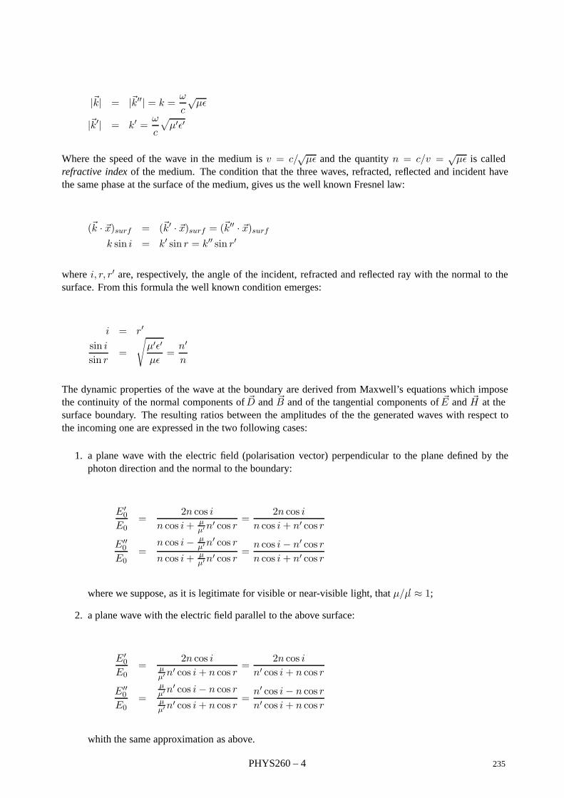
|3k| = |3k′′| = k =ω
c
√µε
|3k′| = k′ =ω
c
√µ′ε′
Where the speed of the wave in the medium is v = c/√µε and the quantity n = c/v =
√µε is called
refractive index of the medium. The condition that the three waves, refracted, reflected and incident havethe same phase at the surface of the medium, gives us the well known Fresnel law:
(3k · 3x)surf = (3k′ · 3x)surf = (3k′′ · 3x)surfk sin i = k′ sin r = k′′ sin r′
where i, r, r′ are, respectively, the angle of the incident, refracted and reflected ray with the normal to thesurface. From this formula the well known condition emerges:
i = r′
sin isin r
=
√µ′ε′
µε=
n′
n
The dynamic properties of the wave at the boundary are derived from Maxwell’s equations which imposethe continuity of the normal components of 3D and 3B and of the tangential components of 3E and 3H at thesurface boundary. The resulting ratios between the amplitudes of the the generated waves with respect tothe incoming one are expressed in the two following cases:
1. a plane wave with the electric field (polarisation vector) perpendicular to the plane defined by thephoton direction and the normal to the boundary:
E′0
E0=
2n cos in cos i+ µ
µ′n′ cos r=
2n cos in cos i+ n′ cos r
E′′0
E0=
n cos i− µµ′n′ cos r
n cos i+ µµ′n′ cos r
=n cos i− n′ cos rn cos i+ n′ cos r
where we suppose, as it is legitimate for visible or near-visible light, that µ/µ′ ≈ 1;
2. a plane wave with the electric field parallel to the above surface:
E′0
E0=
2n cos iµµ′n′ cos i+ n cos r
=2n cos i
n′ cos i+ n cos r
E′′0
E0=
µµ′n′ cos i− n cos rµµ′n′ cos i+ n cos r
=n′ cos i− n cos rn′ cos i+ n cos r
whith the same approximation as above.
PHYS260 – 4 235
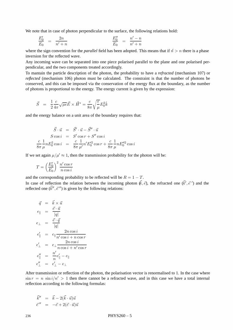
We note that in case of photon perpendicular to the surface, the following relations hold:
E′0
E0=
2nn′ + n
E′′0
E0=
n′ − n
n′ + n
where the sign convention for the parallel field has been adopted. This means that if n′ > n there is a phaseinversion for the reflected wave.Any incoming wave can be separated into one piece polarised parallel to the plane and one polarised per-pendicular, and the two components treated accordingly.To mantain the particle description of the photon, the probability to have a refracted (mechanism 107) orreflected (mechanism 106) photon must be calculated. The constraint is that the number of photons beconserved, and this can be imposed via the conservation of the energy flux at the boundary, as the numberof photons is proportional to the energy. The energy current is given by the expression:
3S =12
c
4π√µε 3E × 3H∗ =
c
8π
√ε
µE20 k
and the energy balance on a unit area of the boundary requires that:
3S · 3u = 3S′ · 3u− 3S′′ · 3uS cos i = S′ cos r + S′′ cos i
c
8π1µnE20 cos i =
c
8π1µ′n
′E′20 cos r +
c
8π1µnE′′2
0 cos i
If we set again µ/µ′ ≈ 1, then the transmission probability for the photon will be:
T =(E′0
E0
)2 n′ cos rn cos i
and the corresponding probability to be reflected will be R = 1− T .In case of reflection the relation between the incoming photon (3k,3e), the refracted one (3k′, 3e ′) and thereflected one (3k′′, 3e ′′) is given by the following relations:
3q = 3k × 3u
e‖ =3e · 3u|q|
e⊥ =3e · 3q|q|
e′‖ = e‖2n cos i
n′ cos i+ n cos r
e′⊥ = e⊥2n cos i
n cos i+ n′ cos r
e′′‖ =n′
ne′‖ − e‖
e′′⊥ = e′⊥ − e⊥
After transmission or reflection of the photon, the polarisation vector is renormalised to 1. In the case wheresin r = n sin i/n′ > 1 then there cannot be a refracted wave, and in this case we have a total internalreflection according to the following formulas:
3k′′ = 3k − 2(3k · 3u)3u3e ′′ = −3e+ 2(3e · 3u)3u
236 PHYS260 – 5
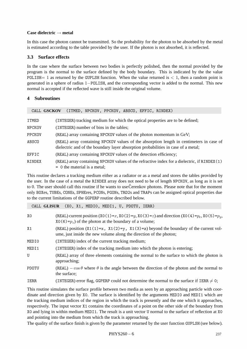
Case dielectric → metal
In this case the photon cannot be transmitted. So the probability for the photon to be absorbed by the metalis estimated according to the table provided by the user. If the photon is not absorbed, it is reflected.
3.3 Surface effects
In the case where the surface between two bodies is perfectly polished, then the normal provided by theprogram is the normal to the surface defined by the body boundary. This is indicated by the the valuePOLISH= 1 as returned by the GUPLSH function. When the value returned is < 1, then a random point isgenerated in a sphere of radius 1−POLISH, and the corresponding vector is added to the normal. This newnormal is accepted if the reflected wave is still inside the original volume.
4 Subroutines
CALL GSCKOV (ITMED, NPCKOV, PPCKOV, ABSCO, EFFIC, RINDEX)
ITMED (INTEGER) tracking medium for which the optical properties are to be defined;
NPCKOV (INTEGER) number of bins in the tables;
PPCKOV (REAL) array containing NPCKOV values of the photon momentum in GeV;
ABSCO (REAL) array containing NPCKOV values of the absorption length in centimeters in case ofdielectric and of the boundary layer absorption probabilities in case of a metal;
EFFIC (REAL) array containing NPCKOV values of the detection efficiency;
RINDEX (REAL) array containing NPCKOV values of the refractive index for a dielectric, if RINDEX(1)= 0 the material is a metal;
This routine declares a tracking medium either as a radiator or as a metal and stores the tables provided bythe user. In the case of a metal the RINDEX array does not need to be of length NPCKOV, as long as it is setto 0. The user should call this routine if he wants to useCerenkov photons. Please note that for the momentonly BOXes, TUBEs, CONEs, SPHEres, PCONs, PGONs, TRD2s and TRAPs can be assigned optical properties dueto the current limitations of the GGPERP routine described below.
CALL GLISUR (X0, X1, MEDI0, MEDI1, U, PDOTU, IERR)
X0 (REAL) current position (X0(1)=x, X0(2)=y, X0(3)=z) and direction (X0(4)=px, X0(5)=py,X0(6)=pz) of the photon at the boundary of a volume;
X1 (REAL) position (X1(1)=x, X1(2)=y, X1(3)=z) beyond the boundary of the current vol-ume, just inside the new volume along the direction of the photon;
MEDI0 (INTEGER) index of the current tracking medium;
MEDI1 (INTEGER) index of the tracking medium into which the photon is entering;
U (REAL) array of three elements containing the normal to the surface to which the photon isapproaching;
PDOTU (REAL) − cos θ where θ is the angle between the direction of the photon and the normal tothe surface;
IERR (INTEGER) error flag, GGPERP could not determine the normal to the surface if IERR = 0;
This routine simulates the surface profile between two media as seen by an approaching particle with coor-dinate and direction given by X0. The surface is identified by the arguments MEDI0 and MEDI1 which arethe tracking medium indices of the region in which the track is presently and the one which it approaches,respectively. The input vector X1 contains the coordinates of a point on the other side of the boundary fromX0 and lying in within medium MEDI1. The result is a unit vector U normal to the surface of reflection at X0and pointing into the medium from which the track is approaching.The quality of the surface finish is given by the parameter returned by the user function GUPLSH (see below).
PHYS260 – 6 237
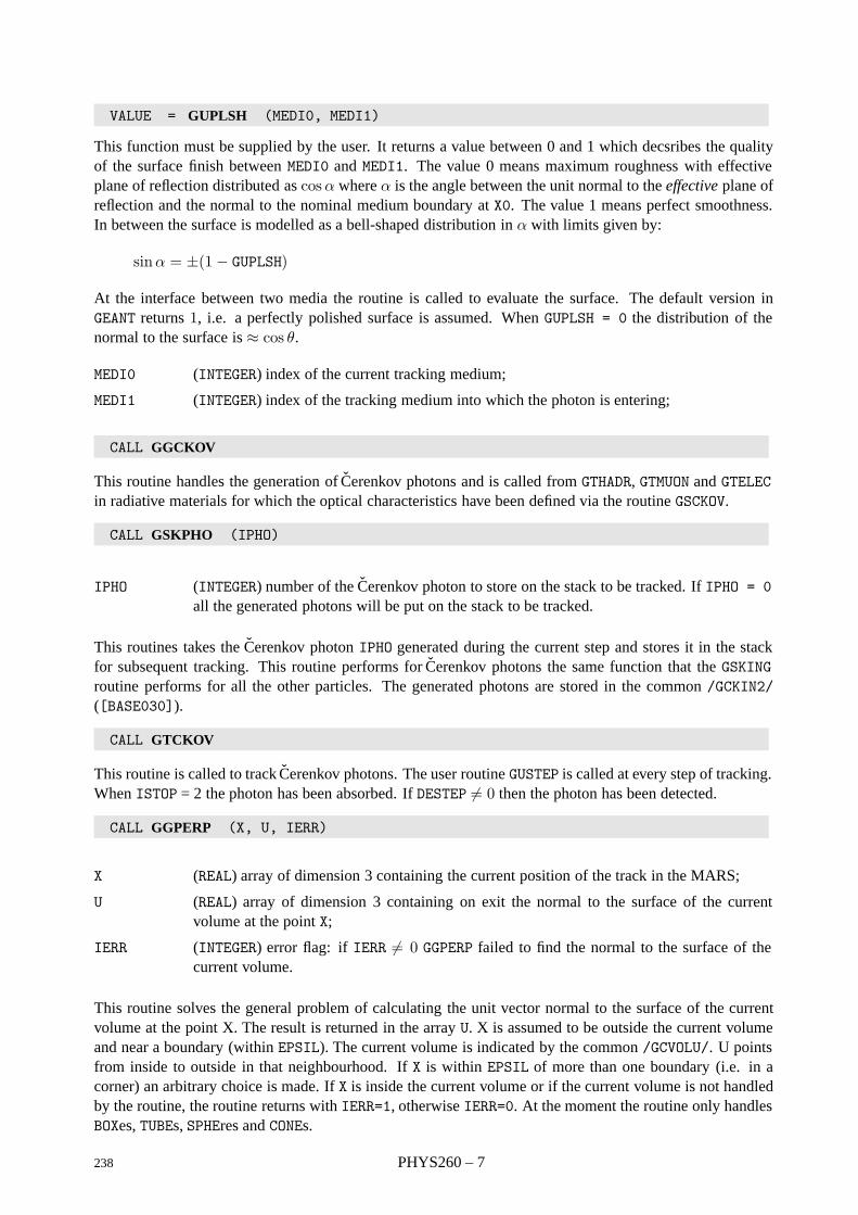
VALUE = GUPLSH (MEDI0, MEDI1)
This function must be supplied by the user. It returns a value between 0 and 1 which decsribes the qualityof the surface finish between MEDI0 and MEDI1. The value 0 means maximum roughness with effectiveplane of reflection distributed as cosα where α is the angle between the unit normal to the effective plane ofreflection and the normal to the nominal medium boundary at X0. The value 1 means perfect smoothness.In between the surface is modelled as a bell-shaped distribution in α with limits given by:
sinα = ±(1− GUPLSH)
At the interface between two media the routine is called to evaluate the surface. The default version inGEANT returns 1, i.e. a perfectly polished surface is assumed. When GUPLSH = 0 the distribution of thenormal to the surface is ≈ cos θ.
MEDI0 (INTEGER) index of the current tracking medium;
MEDI1 (INTEGER) index of the tracking medium into which the photon is entering;
CALL GGCKOV
This routine handles the generation of Cerenkov photons and is called from GTHADR, GTMUON and GTELECin radiative materials for which the optical characteristics have been defined via the routine GSCKOV.
CALL GSKPHO (IPHO)
IPHO (INTEGER) number of the Cerenkov photon to store on the stack to be tracked. If IPHO = 0all the generated photons will be put on the stack to be tracked.
This routines takes the Cerenkov photon IPHO generated during the current step and stores it in the stackfor subsequent tracking. This routine performs for Cerenkov photons the same function that the GSKINGroutine performs for all the other particles. The generated photons are stored in the common /GCKIN2/([BASE030]).
CALL GTCKOV
This routine is called to track Cerenkov photons. The user routine GUSTEP is called at every step of tracking.When ISTOP = 2 the photon has been absorbed. If DESTEP = 0 then the photon has been detected.
CALL GGPERP (X, U, IERR)
X (REAL) array of dimension 3 containing the current position of the track in the MARS;
U (REAL) array of dimension 3 containing on exit the normal to the surface of the currentvolume at the point X;
IERR (INTEGER) error flag: if IERR = 0 GGPERP failed to find the normal to the surface of thecurrent volume.
This routine solves the general problem of calculating the unit vector normal to the surface of the currentvolume at the point X. The result is returned in the array U. X is assumed to be outside the current volumeand near a boundary (within EPSIL). The current volume is indicated by the common /GCVOLU/. U pointsfrom inside to outside in that neighbourhood. If X is within EPSIL of more than one boundary (i.e. in acorner) an arbitrary choice is made. If X is inside the current volume or if the current volume is not handledby the routine, the routine returns with IERR=1, otherwise IERR=0. At the moment the routine only handlesBOXes, TUBEs, SPHEres and CONEs.
238 PHYS260 – 7

5 Processes involving Cerenkov photons
The process of generating a Cerenkov photon is called CKOV and corresponds to the process value 105(variable LMEC in common /GCTRAK/). This process is activated only in a radiator defined via the routineGSCKOV.
The process of photon absorption (name LABS, code 101) is controlled by the LABS FFREAD data record. Bydefault the process is activated for all the materials for which optical properties have been defined.
The action taken at the boundary is identified by the process name LREF, code 102.
At a boundary a photon can be either reflected (name REFL, code 106) or refracted (name REFR, code 107).
PHYS260 – 8 239
Geant 3.16 GEANT User’s Guide PHYS320
Origin : R.Brun, M.Hansroul Submitted: 17.06.85Revision : F.Carminati, G.R.Lynch Revised: 16.12.93Documentation : M.Hansroul, G.R.Lynch
Gaussian multiple scattering
1 Subroutines
CALL GMGAUS (BETA2,DIN*)
BETA2 (REAL) β2;
DIN (REAL) array of 3 containing the direction of the scattered particle with respect to theincoming direction.
This routine is called by GTELEC, GTHADR, GTMUON and GTHION via GMULTS when the variable IMULS,controlled by the data record MULS is equal to 3.
2 Method
2.1 Approximations in use
A charged particle traversing a medium is deflected by many scatters, mostly at small angle. These scattersare due to the interaction with the Coulomb field of the nuclei, and to a lesser degree, to the electron field,hence the name of Coulomb scattering. For hadronic projectiles, however, the strong interaction contributesto multiple scattering. Multiple scattering is well described by Moliere theory [37]. Moliere multiplescattering theory is used by default in GEANT (see [PHYS325]). We define θ0 = θrms
plane = θrmsspace/
√2 as
the r.m.s. of the angle between the directions projected on a plane of a particle before and after traversinga thickness t of absorber. In this case a simple form for the multiple Coulomb scattering of singly chargedparticles which is widely used is:
θ0 ≈15MeV
Eβ2
√t
X0
where X0 is the radiation length of the absorber. This form was proposed by [38], [39]. It can introducelarge errors because it ignores significant dependences from pathlength and Z . To compensate for this, asimilar formula was proposed [40], [41]:
θ0 ≈14.1MeV
Eβ2
√t
X0
[1 + 0.038 log
(t
X0
)](1)
A form taking into account the β and z dependence of the particle has been proposed by [42]:
θ0 =S2Eβ2
√t
X0
[1 + ε log10
(tZ2incX0β2
)](2)
The problem with the formulae (1) and (2) is that if the distance t in the absorber is travelled in two steps
t = t1 + t2, the r.m.s. angle θ0(t) = θ0(t1 + t2) =√θ20(t1) + θ20(t2), limiting their use in a MonteCarlo
like GEANT.
240 PHYS320 – 1
Much of the difficulty in approximating multiple Coulomb scattering in terms of the radiation length is thatthe number of radiation lengths is a poor measure of the scattering. A better expression, which is used inGEANT has been proposed by [42]:
θ20 =χ2c
1 + F 2
[1 + ν
νlog(1 + ν)− 1
](3)
where
ν =Ω0
2(1 − F )F = fraction of the tracks in the sample
Ω0 =χ2c
1.167χ2αis the mean number of scatters
χ2c and χ2α are parameters of the Moliere theory, for which the reader is invited to see [PHYS325], and1.167 ≈ exp(2γ − 1) where γ is the Euler’s constant = 0.57721 . . .. This form, which is the result ofempirical fits, is derived from the screened Rutherford cross section, which has the form 2χ2α/(χ2α + θ20).For F anywhere from 0.9 to 0.995 this expression represents Moliere scattering to better than 2% for 10 <Ω0 < 108, which covers singly charged relativistic particles (β ≈ 1) in the range 10−3 < t/X0 < 100.
In GEANT we have adopted the values of F = 0.98 and Ω0 = 40, 000 scatters, obtaining the followingformula:
θ0 = 2.557χcc
√t
Eβ2
where χcc is another parameter of the Moliere theory for which the reader is referred to [PHYS325]. Thisalgorithm is implemented by the routine GMGAUS.
PHYS320 – 2 241
Geant 3.16 GEANT User’s Guide PHYS325
Origin : M.S. Dixit Submitted: 17.06.85Revision : G.Lynch Revised: 16.12.93Documentation : F.Carminati
Moliere scattering
1 Subroutines
1.1 Initialisation
CALL GMULOF
GMULOF calculates the table of maximum steps corresponding to the energies in the array ELOW for electronsand muons. It is called during initialisation by GPHYSI. For hadrons and ions the computation is performedduring tracking in the routines GTHADR and GTHION.
CALL GMOLI (AC,ZC,WMAT,NLM,DENS,OMC*,CHC*)
AC REAL array of dimenstion NLM containing the mass numbers;
ZC REAL array of dimenstion NLM containing the atomic numbers;
WMAT REAL array containing the proportions by weight of the component of a mixture/compound. 1in case of a single component;
NLM INTEGER number of the elements in the mixture/compound;
DENS REAL density in g cm−3;
OMC REAL bc constant of Moliere theory;
CHC REAL χcc constant of Moliere theory.
GMOLI calculates the two material-dependent constants (OMC and CHC). These are needed during initialisationby GMULOF and during tracking to sample the scattering angle, as explained below. It is called at initialisationtime by the routine GPROBI which initialises some material constants and computes the probabilities forvarious processes.
1.2 Sampling of the multiple scattering angle
CALL GMULTS
GMULTS is the steering routine for the sampling of the multiple scattering angle when the variable IMULTS incommon /GCPHYS/ is 1 or 2. This variable can be controlled by the MULT data record. The routine decidesif the material-dependent constant OMC computed by GMOLI during initialisation has to be corrected due toits dependence on β and Zinc, and selects Moliere theory (GMOLIE) or single Coulomb scattering (GMCOUL).It updates the direction of the particle in the array VECT (COMMON GCTRAK). It is called by the trackingroutines GTELEC, GTHADR, GTHION and GTMUON.
CALL GMOLIO (AC,ZC,WMAT,NLM,DENS,BETA2,CHARG2,OMC*)
BETA2 REAL β2 of the particle;
CHARG2 REAL charge squared of the particle in electron charge unit (Z2inc in the following).
All the other arguments are routine GMOLI. GMOLIO re-evaluates the material-dependent constant OMC. It iscalled by GMULTS, if needed.
242 PHYS325 – 1
CALL GMOLIE (OMEGA,BETA2,DIN*)
OMEGA REAL Ω0 of the Moliere theory;
BETA2 REAL β2 of the particle;
DIN REAL array of dimension 3 containing the new direction cosines with respect to the originaldirection of the particle.
GMOLIE samples the multiple scattering angle according to Moliere theory, as explained in the next section.It is called by the multiple scattering steering routine GMULTS,
CALL GMOL4 (Y*,X,VAL,ARG,EPS,IER*)
Y REAL value of the interpolated function;
X REAL value at which the function should be interpolated;
VAL REAL array of four values of the function to interpolate;
ARG REAL array of four values of the argument of the function to which the values contained in VALcorrespond;
EPS REAL required precision for the interpolation;
IER INTEGER error flag;
GMOL4 inverts the integral of Moliere distribution function using four-points continued-fraction interpola-tion. It is called by GMOLIE.
2 Method
2.1 Introduction
When traversing ordinary matter, elementary particles undergo deflection from their originary trajectory dueto the interaction with the atoms. This effect is rather large for charged particles, which are deflected by theelectric field of nuclei and electrons via a large number of small elastic collisions. To simulate precisely thetransport of particles in matter, it is important to provide a precise description of this effect. Considerableeffort has gone over the years into the formulation of a theory of Coulomb multiple scattering. In GEANT wefollow the theory originally formulated by Moliere [43] [44] and then elaborated by Bethe [37]. A reviewof this theory can be found in [45].
It should be noted that this is not the only theory which describes multiple Coulomb scattering, and athorough analysis of the problem has been performed by Goudsmit and Saunderson [46] [47].
A complete account of the Moliere theory is outside the scope of this manual. For more information theinterested reader could refer to the works cited above and to the EGS4 manual [15], from which the notationused in the present chapter has been derived.
The principal limitations of Moliere theory are the following:
1. the angular deflection is small. Effectively this constraint provides the upper limit for the step-size;
2. the theory is a multiple scattering theory; that is, many atomic collisions participate in causing theincident particle to be deflected. In some implementations, this constraints provides a lower limit onthe step size. In GEANT, when the number of scatters is below the limit of applicability of Molieresingle Coulomb scatterings are simulated, so that there is no effective minimum step size below whichmultiple scattering is switched off;
3. the theory applies only in semi-infinite homogeneous media. This constraint calls for a very carefulhandling of particles near to a medium’s boundary;
PHYS325 – 2 243
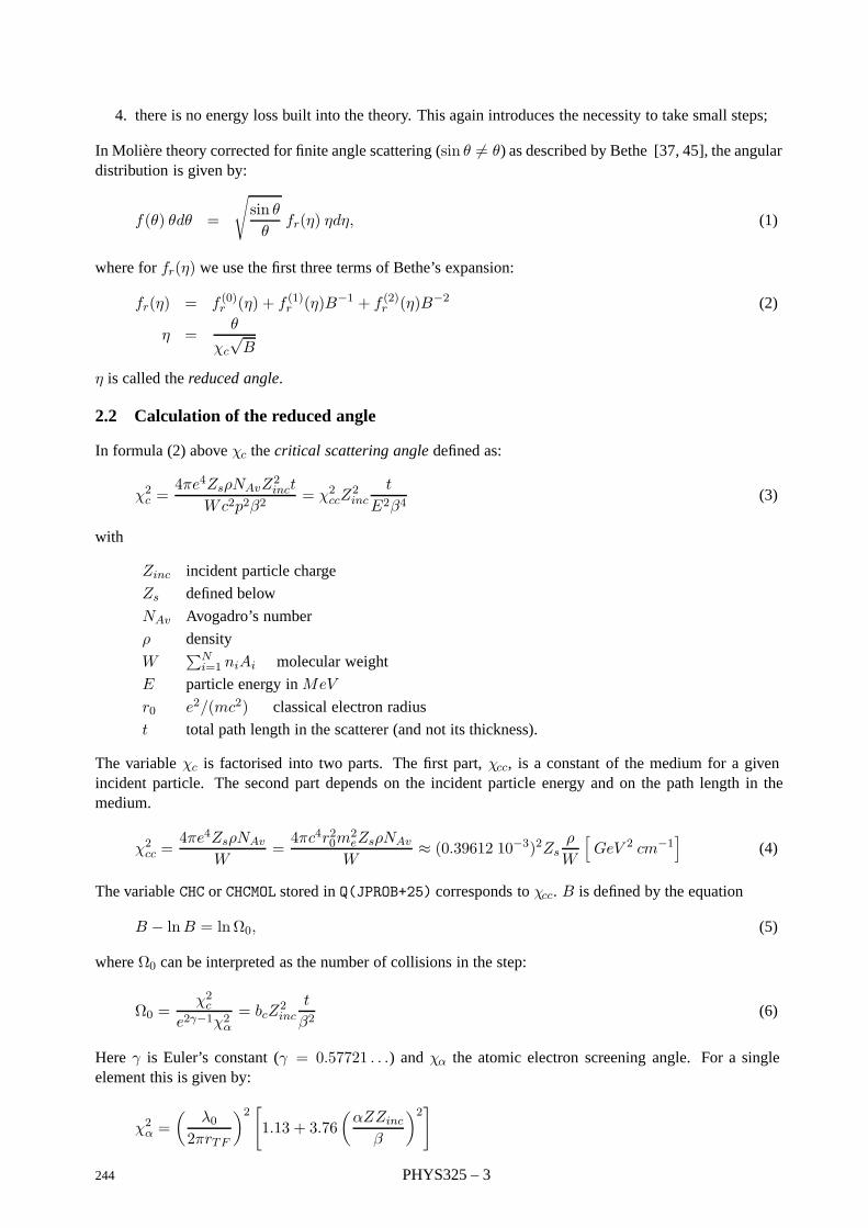
4. there is no energy loss built into the theory. This again introduces the necessity to take small steps;
In Moliere theory corrected for finite angle scattering (sin θ = θ) as described by Bethe [37, 45], the angulardistribution is given by:
f(θ) θdθ =
√sin θθ
fr(η) ηdη, (1)
where for fr(η) we use the first three terms of Bethe’s expansion:
fr(η) = f (0)r (η) + f (1)r (η)B−1 + f (2)r (η)B−2 (2)
η =θ
χc
√B
η is called the reduced angle.
2.2 Calculation of the reduced angle
In formula (2) above χc the critical scattering angle defined as:
χ2c =4πe4ZsρNAvZ
2inct
Wc2p2β2= χ2ccZ
2inc
t
E2β4(3)
with
Zinc incident particle charge
Zs defined below
NAv Avogadro’s number
ρ density
W∑N
i=1 niAi molecular weight
E particle energy in MeV
r0 e2/(mc2) classical electron radius
t total path length in the scatterer (and not its thickness).
The variable χc is factorised into two parts. The first part, χcc, is a constant of the medium for a givenincident particle. The second part depends on the incident particle energy and on the path length in themedium.
χ2cc =4πe4ZsρNAv
W=4πc4r20m
2eZsρNAv
W≈ (0.39612 10−3)2Zs
ρ
W
[GeV 2 cm−1
](4)
The variable CHC or CHCMOL stored in Q(JPROB+25) corresponds to χcc. B is defined by the equation
B − lnB = lnΩ0, (5)
where Ω0 can be interpreted as the number of collisions in the step:
Ω0 =χ2c
e2γ−1χ2α= bcZ
2inc
t
β2(6)
Here γ is Euler’s constant (γ = 0.57721 . . .) and χα the atomic electron screening angle. For a singleelement this is given by:
χ2α =(
λ02πrTF
)2 [1.13 + 3.76
(αZZinc
β
)2]
244 PHYS325 – 3
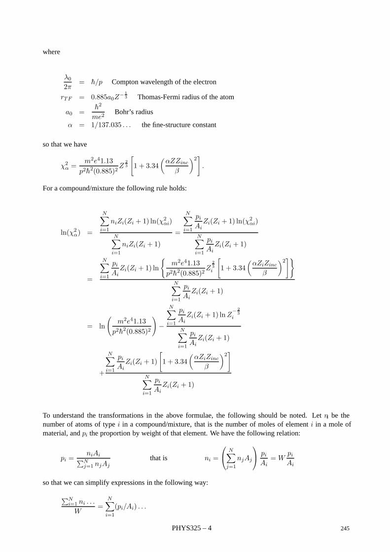
where
λ02π
= h/p Compton wavelength of the electron
rTF = 0.885a0Z− 13 Thomas-Fermi radius of the atom
a0 =h2
me2Bohr’s radius
α = 1/137.035 . . . the fine-structure constant
so that we have
χ2α =m2e41.13
p2h2(0.885)2Z
23
[1 + 3.34
(αZZinc
β
)2].
For a compound/mixture the following rule holds:
ln(χ2α) =
N∑i=1
niZi(Zi + 1) ln(χ2αi)
N∑i=1
niZi(Zi + 1)
=
N∑i=1
piAi
Zi(Zi + 1) ln(χ2αi)
N∑i=1
piAi
Zi(Zi + 1)
=
N∑i=1
piAi
Zi(Zi + 1) ln
m2e41.13
p2h2(0.885)2Z
23i
[1 + 3.34
(αZiZinc
β
)2]N∑i=1
piAi
Zi(Zi + 1)
= ln
(m2e41.13
p2h2(0.885)2
)−
N∑i=1
piAi
Zi(Zi + 1) lnZ− 2
3i
N∑i=1
piAi
Zi(Zi + 1)
+
N∑i=1
piAi
Zi(Zi + 1)
[1 + 3.34
(αZiZinc
β
)2]N∑i=1
piAi
Zi(Zi + 1)
To understand the transformations in the above formulae, the following should be noted. Let ni be thenumber of atoms of type i in a compound/mixture, that is the number of moles of element i in a mole ofmaterial, and pi the proportion by weight of that element. We have the following relation:
pi =niAi∑N
j=1 njAj
that is ni =
N∑
j=1
njAj
pi
Ai=W
piAi
so that we can simplify expressions in the following way:
∑Ni=1 ni . . .
W=
N∑i=1
(pi/Ai) . . .
PHYS325 – 4 245

If now we set
Zs =N∑i=1
niZi(Zi + 1) =WN∑i=1
piAi
Zi(Zi + 1) =WZ ′s
ZE=N∑i=1
niZi(Zi + 1) lnZ−2/3i =W
∑ piAi
Zi(Zi + 1) lnZ−2/3i =WZ ′
E
Zx=N∑i=1
niZi(Zi + 1) ln
[1 + 3.34
(αZiZinc
β
)2]
=WN∑i=1
piAi
Zi(Zi + 1) ln
[1 + 3.34
(αZiZinc
β
)2]=WZ ′
x
we can write:
ln(χ2α) = ln
(m2e41.13
p2h2(0.885)2
)+
Zx − ZE
Zs
χ2α =m2e41.13
p2h2(0.885)2e(Zx−ZE)/Zs =
m2e41.13p2h2(0.885)2
e(Z′x−Z′
E)/Z′s
and finally:
Ω0 =χ2c
e2γ−1χ2α
=1
1.1674πe4ZsρNAvZ
2inct
Wc2p2β2p2h2(0.885)2
1.13m2e4e−(Z
′x−Z′
E)/Z′s
= bcZ2inc
t
β2
bc =4πNAvh
2
m2c2(0.885)2
1.13 × 1.167ρZ′se(Z′
E−Z′x)/Z
′s ≈ 6702.33ρZ ′
se(Z′
E−Z′x)/Z
′s
The quantity bc is calculated during initialisation by the routine GMOLI setting β = 1 and Zinc = 1. Thisvariable is called OMC or OMCMOL and it is stored in Q(JPROB+21). It has, via the atomic electron screeningangle χ2α, a small dependence on β and Zinc in the term Zx. The quantity bcρZ
′s is re-evaluated during
tracking by the routine GMOLIO, called by GMULTS, only when necessary.
The dependence of Zx on β and Zinc is via a term of the form: 1+3.34(αZZincβ
−1)2, so it is not necessary
to recalculate it as long as 1 + 3.34(αZZincβ
−1)2 ≈ 1 + 3.34 (αZ)2 that is:
3.34(Zα)2[(
Zinc
β
)2− 1
] 1 ⇒ Z2
Z2inc − β2
β2 3.34α−2 ≈ 5500
Z2(Z2inc − β2) ≤ 50β2
For mixtures/compounds this condition should be checked for every component and this would be unaccept-able from the point of view of computer time. So we simply make the condition more restrictive multiplyingthe first term by the number of elements in the mixture/compound.
246 PHYS325 – 5
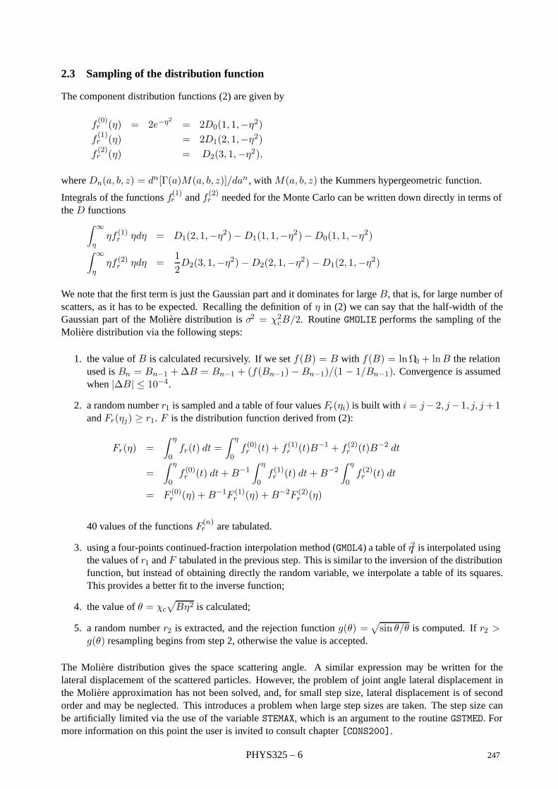
2.3 Sampling of the distribution function
The component distribution functions (2) are given by
f(0)r (η) = 2e−η2
= 2D0(1, 1,−η2)f(1)r (η) = 2D1(2, 1,−η2)f(2)r (η) = D2(3, 1,−η2),
where Dn(a, b, z) = dn[Γ(a)M(a, b, z)]/dan , with M(a, b, z) the Kummers hypergeometric function.
Integrals of the functions f(1)r and f(2)r needed for the Monte Carlo can be written down directly in terms of
the D functions∫ ∞
ηηf (1)r ηdη = D1(2, 1,−η2)−D1(1, 1,−η2)−D0(1, 1,−η2)∫ ∞
ηηf (2)r ηdη =
12D2(3, 1,−η2)−D2(2, 1,−η2)−D1(2, 1,−η2)
We note that the first term is just the Gaussian part and it dominates for large B, that is, for large number ofscatters, as it has to be expected. Recalling the definition of η in (2) we can say that the half-width of theGaussian part of the Moliere distribution is σ2 = χ2cB/2. Routine GMOLIE performs the sampling of theMoliere distribution via the following steps:
1. the value of B is calculated recursively. If we set f(B) = B with f(B) = lnΩ0 + lnB the relationused is Bn = Bn−1 +∆B = Bn−1 + (f(Bn−1)− Bn−1)/(1 − 1/Bn−1). Convergence is assumedwhen |∆B| ≤ 10−4.
2. a random number r1 is sampled and a table of four values Fr(ηi) is built with i = j−2, j−1, j, j+1and Fr(ηj) ≥ r1. F is the distribution function derived from (2):
Fr(η) =∫ η
0fr(t) dt =
∫ η
0f (0)r (t) + f (1)r (t)B−1 + f (2)r (t)B−2 dt
=∫ η
0f (0)r (t) dt+B−1
∫ η
0f (1)r (t) dt +B−2
∫ η
0f (2)r (t) dt
= F (0)r (η) +B−1F (1)r (η) +B−2F (2)r (η)
40 values of the functions F(n)r are tabulated.
3. using a four-points continued-fraction interpolation method (GMOL4) a table of η2i is interpolated usingthe values of r1 and F tabulated in the previous step. This is similar to the inversion of the distributionfunction, but instead of obtaining directly the random variable, we interpolate a table of its squares.This provides a better fit to the inverse function;
4. the value of θ = χc
√Bη2 is calculated;
5. a random number r2 is extracted, and the rejection function g(θ) =√sin θ/θ is computed. If r2 >
g(θ) resampling begins from step 2, otherwise the value is accepted.
The Moliere distribution gives the space scattering angle. A similar expression may be written for thelateral displacement of the scattered particles. However, the problem of joint angle lateral displacement inthe Moliere approximation has not been solved, and, for small step size, lateral displacement is of secondorder and may be neglected. This introduces a problem when large step sizes are taken. The step size canbe artificially limited via the use of the variable STEMAX, which is an argument to the routine GSTMED. Formore information on this point the user is invited to consult chapter [CONS200].
PHYS325 – 6 247
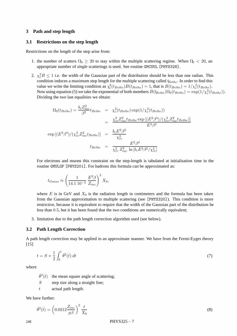
3 Path and step length
3.1 Restrictions on the step length
Restrictions on the length of the step arise from:
1. the number of scatters Ω0 ≥ 20 to stay within the multiple scattering regime. When Ω0 < 20, anappropriate number of single scatterings is used. See routine GMCOUL [PHYS328].
2. χ2cB ≤ 1 i.e. the width of the Gaussian part of the distribution should be less than one radian. Thiscondition induces a maximum step length for the multiple scattering called tBethe. In order to find thisvalue we write the limiting condition as χ2c(tBethe)B(tBethe) = 1, that is B(tBethe) = 1/χ2c(tBethe).Now using equation (5) we take the exponential of both members B(tBethe)Ω0(tBethe) = exp(1/χ2c(tBethe)).Dividing the two last equalities we obtain:
Ω0(tBethe) =bcZ
2inc
β2tBethe = χ2c(tBethe) exp(1/χ2c(tBethe))
=χ2ccZ
2inctBethe exp [(E2β4)/(χ2ccZ
2inctBethe)]
E2β4
exp [(E2β4)/(χ2ccZ2inctBethe)] =
bcE2β2
χ2cc
tBethe =E2β4
χ2cc Z2inc ln [bcE2β2/χ2cc]
For electrons and muons this constraint on the step-length is tabulated at initialisation time in theroutine GMULOF [PHYS201]. For hadrons this formula can be approximated as:
tGauss ≈(
114.1 10−3
E2β
Zinc
)2X0,
where E is in GeV and X0 is the radiation length in centimeters and the formula has been takenfrom the Gaussian approximation to multiple scattering (see [PHYS320]). This condition is morerestrictive, because it is equivalent to require that the width of the Gaussian part of the distribution beless than 0.5, but it has been found that the two conditions are numerically equivalent;
3. limitation due to the path length correction algorithm used (see below).
3.2 Path Length Correction
A path length correction may be applied in an approximate manner. We have from the Fermi-Eyges theory[15]
t = S +12
∫ t
0θ2(t) dt (7)
where
θ2(t) the mean square angle of scattering;
S step size along a straight line;
t actual path length.
We have further:
θ2(t) =(0.0212
Zinc
pβ
)2 t
X0(8)
248 PHYS325 – 7
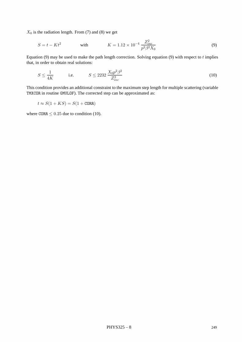
X0 is the radiation length. From (7) and (8) we get
S = t−Kt2 with K = 1.12 × 10⁻⁴ Z2incp2β2X0
(9)
Equation (9) may be used to make the path length correction. Solving equation (9) with respect to t impliesthat, in order to obtain real solutions:
S ≤ 14K
i.e. S ≤ 2232X0p
2β2
Z2inc(10)
This condition provides an additional constraint to the maximum step length for multiple scattering (variableTMXCOR in routine GMULOF). The corrected step can be approximated as:
t ≈ S(1 +KS) = S(1 + CORR)
where CORR ≤ 0.25 due to condition (10).
PHYS325 – 8 249
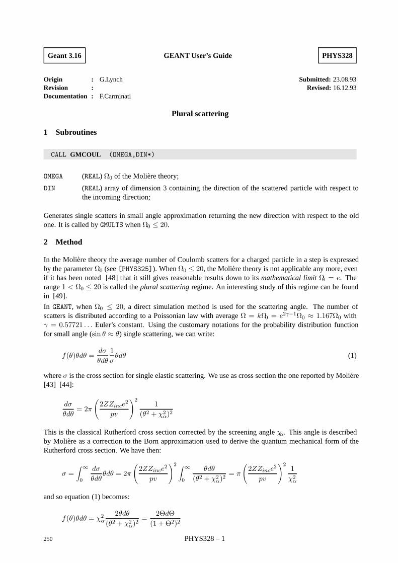
Geant 3.16 GEANT User’s Guide PHYS328
Origin : G.Lynch Submitted: 23.08.93Revision : Revised: 16.12.93Documentation : F.Carminati
Plural scattering
1 Subroutines
CALL GMCOUL (OMEGA,DIN*)
OMEGA (REAL) Ω0 of the Moliere theory;
DIN (REAL) array of dimension 3 containing the direction of the scattered particle with respect tothe incoming direction;
Generates single scatters in small angle approximation returning the new direction with respect to the oldone. It is called by GMULTS when Ω0 ≤ 20.
2 Method
In the Moliere theory the average number of Coulomb scatters for a charged particle in a step is expressedby the parameter Ω0 (see [PHYS325]). When Ω0 ≤ 20, the Moliere theory is not applicable any more, evenif it has been noted [48] that it still gives reasonable results down to its mathematical limit Ω0 = e. Therange 1 < Ω0 ≤ 20 is called the plural scattering regime. An interesting study of this regime can be foundin [49].
In GEANT, when Ω0 ≤ 20, a direct simulation method is used for the scattering angle. The number ofscatters is distributed according to a Poissonian law with average Ω = kΩ0 = e2γ−1Ω0 ≈ 1.167Ω0 withγ = 0.57721 . . . Euler’s constant. Using the customary notations for the probability distribution functionfor small angle (sin θ ≈ θ) single scattering, we can write:
f(θ)θdθ =dσ
θdθ
1σθdθ (1)
where σ is the cross section for single elastic scattering. We use as cross section the one reported by Moliere[43] [44]:
dσ
θdθ= 2π
(2ZZince
2
pv
)21
(θ2 + χ2α)2
This is the classical Rutherford cross section corrected by the screening angle χα. This angle is describedby Moliere as a correction to the Born approximation used to derive the quantum mechanical form of theRutherford cross section. We have then:
σ =∫ ∞
0
dσ
θdθθdθ = 2π
(2ZZince
2
pv
)2 ∫ ∞
0
θdθ
(θ2 + χ2α)2= π
(2ZZince
2
pv
)21χ2α
and so equation (1) becomes:
f(θ)θdθ = χ2α2θdθ
(θ2 + χ2α)2=
2ΘdΘ(1 + Θ2)2
250 PHYS328 – 1
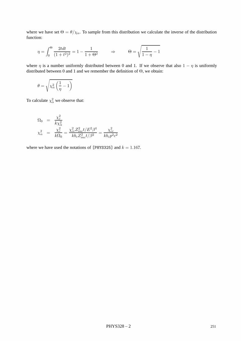
where we have set Θ = θ/χα. To sample from this distribution we calculate the inverse of the distributionfunction:
η =∫ Θ
0
2tdt(1 + t2)2
= 1− 11 + Θ2
⇒ Θ =
√1
1− η− 1
where η is a number uniformly distributed between 0 and 1. If we observe that also 1 − η is uniformlydistributed between 0 and 1 and we remember the definition of Θ, we obtain:
θ =
√χ2α
(1η− 1
)
To calculate χ2α we observe that:
Ω0 =χ2ckχ2α
χ2α =χ2ckΩ0
=χ2ccZ
2inct/E
2β4
kbcZ2inct/β2=
χ2cckbcp2c2
where we have used the notations of [PHYS325] and k = 1.167.
PHYS328 – 2 251

Geant 3.16 GEANT User’s Guide PHYS330
Origin : L.Urban Submitted: 26.10.84Revision : Revised: 16.12.93Documentation :
Ionisation processes induced by e+/e-
1 Subroutines
CALL GDRELA
GDRELA initialises the ionisation energy loss tables for different materials for muons, electrons and positronsand other particles. The energy binning is set within the array ELOW (common /GCMULO/) in the routineGPHYSI. The tables are filled with the quantity dE/dx in GeV/cm (formula (4) below) which is valid for anelement as well as a mixture or a compound. In the tables the dE/dx due to ionisation is summed with theenergy loss coming from bremsstrahlung. For energy loss of electrons and positrons, it calls GDRELE usingthe following pointers:
JMA = LQ(JMATE-I) pointer to the Ith material
JEL1 = LQ(JMA-1) pointer for dE/dx for electrons
JEL1+90 pointer for dE/dx for positron
GDRELA is called at initialisation time by GPHYSI.
CALL GDRELE (EEL,CHARGE,JMA,DEDX)
GDRELE computes the ionisation energy loss (DEDX) for electrons (CHARGE = -1) and positrons (CHARGE= +1) with kinetic energy EEL in the material indicated by I in JMA = LQ(JMATE-I). It is called by theroutine GDRELA.
CALL GDRSGA
CDRSGA calculates the total cross-section in all materials for delta rays for Moller (e−e−) and Bhabha (e−e+)scattering and for muons. It tabulates the mean free path, λ = 1/Σ (in cm) as a function of the medium andthe energy. The energy binning is set within the array ELOW (common /GCMULO/) in the routine GPHYSI.The following pointers are used (see JMATE data structure):
JMA = LQ(JMATE-I) pointer to the Ith material
JDRAY = LQ(JMA-11) pointer to δ-ray cross-sections
JDRAY pointer for electrons
JDRAY+90 pointer for positrons
JDRAY+180 pointer for µ+/µ−.
The routine is called during initialisation by GPHYSI.
2 Method
Let:
dσ(E,T )dT
be the differential cross-section for the ejection of an electron with kinetic energy T by an incident e± oftotal energy E moving in a medium of density ρ.
252 PHYS330 – 1
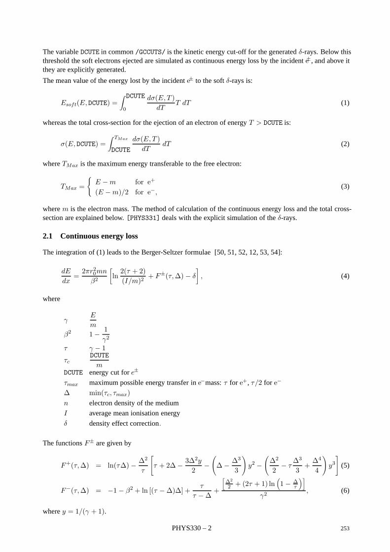
The variable DCUTE in common /GCCUTS/ is the kinetic energy cut-off for the generated δ-rays. Below thisthreshold the soft electrons ejected are simulated as continuous energy loss by the incident e±, and above itthey are explicitly generated.
The mean value of the energy lost by the incident e± to the soft δ-rays is:
Esoft(E, DCUTE) =∫ DCUTE
0
dσ(E,T )dT
T dT (1)
whereas the total cross-section for the ejection of an electron of energy T > DCUTE is:
σ(E, DCUTE) =∫ TMax
DCUTE
dσ(E,T )dT
dT (2)
where TMax is the maximum energy transferable to the free electron:
TMax =
E −m for e+
(E −m)/2 for e−,(3)
where m is the electron mass. The method of calculation of the continuous energy loss and the total cross-section are explained below. [PHYS331] deals with the explicit simulation of the δ-rays.
2.1 Continuous energy loss
The integration of (1) leads to the Berger-Seltzer formulae [50, 51, 52, 12, 53, 54]:
dE
dx=2πr20mn
β2
[ln2(τ + 2)(I/m)2
+ F±(τ,∆)− δ
], (4)
where
γE
m
β2 1− 1γ2
τ γ − 1τc
DCUTE
mDCUTE energy cut for e±
τmax maximum possible energy transfer in e−mass: τ for e+, τ/2 for e−
∆ min(τc, τmax)n electron density of the medium
I average mean ionisation energy
δ density effect correction.
The functions F± are given by
F+(τ,∆) = ln(τ∆)− ∆2
τ
[τ + 2∆− 3∆2y
2−(∆− ∆3
3
)y2 −
(∆2
2− τ
∆3
3+∆4
4
)y3]
(5)
F−(τ,∆) = −1− β2 + ln [(τ −∆)∆] + τ
τ −∆ +
[∆2
2 + (2τ + 1) ln(1− ∆
τ
)]γ2
, (6)
where y = 1/(γ + 1).
PHYS330 – 2 253
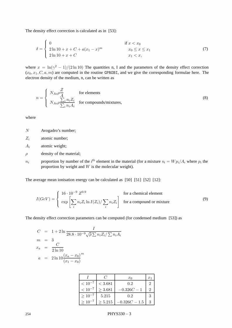
The density effect correction is calculated as in [53]:
δ =
0 if x < x0
2 ln 10 + x+ C + a(x1 − x)m x0 ≤ x ≤ x1
2 ln 10 + x+ C x1 < x,
(7)
where x = ln(γ2 − 1)/(2 ln 10) The quantities n, I and the parameters of the density effect correction(x0, x1, C, a,m) are computed in the routine GPROBI, and we give the corresponding formulae here. Theelectron density of the medium, n, can be written as
n =
NAvρZ
Afor elements
NAvρ
∑i niZi∑i niAi
for compounds/mixtures,(8)
where
N Avogadro’s number;
Zi atomic number;
Ai atomic weight;
ρ density of the material;
ni proportion by number of the ith element in the material (for a mixture ni = Wpi/Ai where pi theproportion by weight and W is the molecular weight).
The average mean ionisation energy can be calculated as [50] [51] [52] [12]:
I(GeV ) =
16 · 10−9 Z0.9 for a chemical element
exp
[∑i
niZi ln I(Zi)/∑i
niZi
]for a compound or mixture
(9)
The density effect correction parameters can be computed (for condensed medium [53]) as
C = 1 + 2 lnI
28.8 · 10−9√ρ∑
niZi/∑
niAi
m = 3
xa =C
2 ln 10
a = 2 ln 10(xa − x0)(x1 − x0)
m
I C x0 x1
< 10−7 < 3.681 0.2 2< 10−7 ≥ 3.681 −0.326C − 1 2≥ 10−7 5.215 0.2 3≥ 10−7 ≥ 5.215 −0.326C − 1.5 3
254 PHYS330 – 3

2.2 Total cross-sections
The integration of formula (2) gives the total cross-section [15], [17] for Moller scattering (e−e−):
σ(Z,E, DCUTE) =2πr20mZ
β2(E −m)
[(γ − 1)
γ2
(1x− 1
)+1x− 11− x
− 2γ − 1γ2
ln1− x
x
](10)
and for Bhabha scattering (e+e−):
σ(Z,E, DCUTE) =2πr20mZ
(E −m)
[1β2
(1x− 1
)+B1x+B2(1− x)− B3
2(1− x2) +
B43(1− x3)
](11)
where
γ =E
mβ2 = 1− 1
γ2
x =DCUTE
E −mγ =
1γ + 1
B1 = 2− y2 B2 = (1− 2y)(3 + y2)
B3 = (1− 2y)2 + (1− 2y)3 B4 = (1− 2y)3
The formulae [10] and [11] give the total cross-section of the scattering above the threshold energies
T thrMoller = 2DCUTE and T thrBhabha = DCUTE (12)
The interaction length for the production of δ-rays is calculated during initialisation by routine GDRSGA.
PHYS330 – 4 255
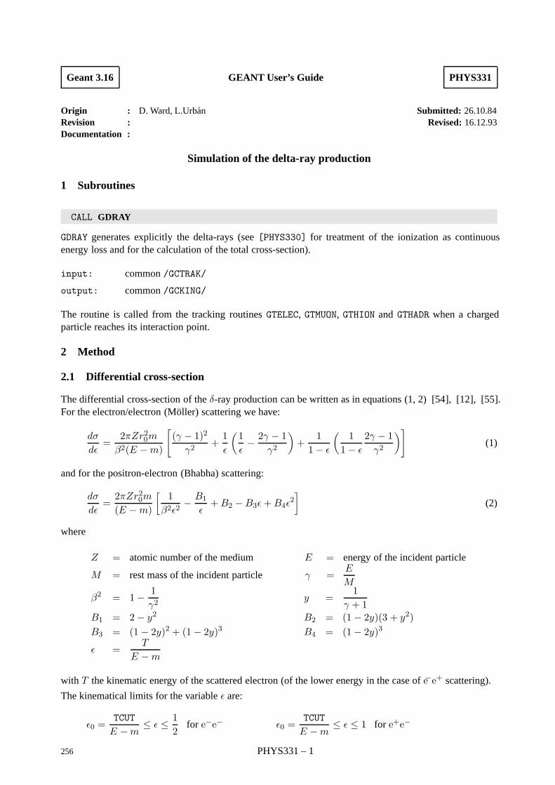
Geant 3.16 GEANT User’s Guide PHYS331
Origin : D. Ward, L.Urban Submitted: 26.10.84Revision : Revised: 16.12.93Documentation :
Simulation of the delta-ray production
1 Subroutines
CALL GDRAY
GDRAY generates explicitly the delta-rays (see [PHYS330] for treatment of the ionization as continuousenergy loss and for the calculation of the total cross-section).
input: common /GCTRAK/
output: common /GCKING/
The routine is called from the tracking routines GTELEC, GTMUON, GTHION and GTHADR when a chargedparticle reaches its interaction point.
2 Method
2.1 Differential cross-section
The differential cross-section of the δ-ray production can be written as in equations (1, 2) [54], [12], [55].For the electron/electron (Moller) scattering we have:
dσ
dε=
2πZr20m
β2(E −m)
[(γ − 1)2
γ2+1ε
(1ε− 2γ − 1
γ2
)+
11− ε
(1
1− ε
2γ − 1γ2
)](1)
and for the positron-electron (Bhabha) scattering:
dσ
dε=2πZr20m
(E −m)
[1
β2ε2− B1
ε+B2 −B3ε+B4ε
2]
(2)
where
Z = atomic number of the medium E = energy of the incident particle
M = rest mass of the incident particle γ =E
M
β2 = 1− 1γ2
y =1
γ + 1B1 = 2− y2 B2 = (1− 2y)(3 + y2)B3 = (1− 2y)2 + (1− 2y)3 B4 = (1− 2y)3
ε =T
E −m
with T the kinematic energy of the scattered electron (of the lower energy in the case of e−e+ scattering).
The kinematical limits for the variable ε are:
ε0 =TCUT
E −m≤ ε ≤ 1
2for e−e− ε0 =
TCUT
E −m≤ ε ≤ 1 for e+e−
256 PHYS331 – 1
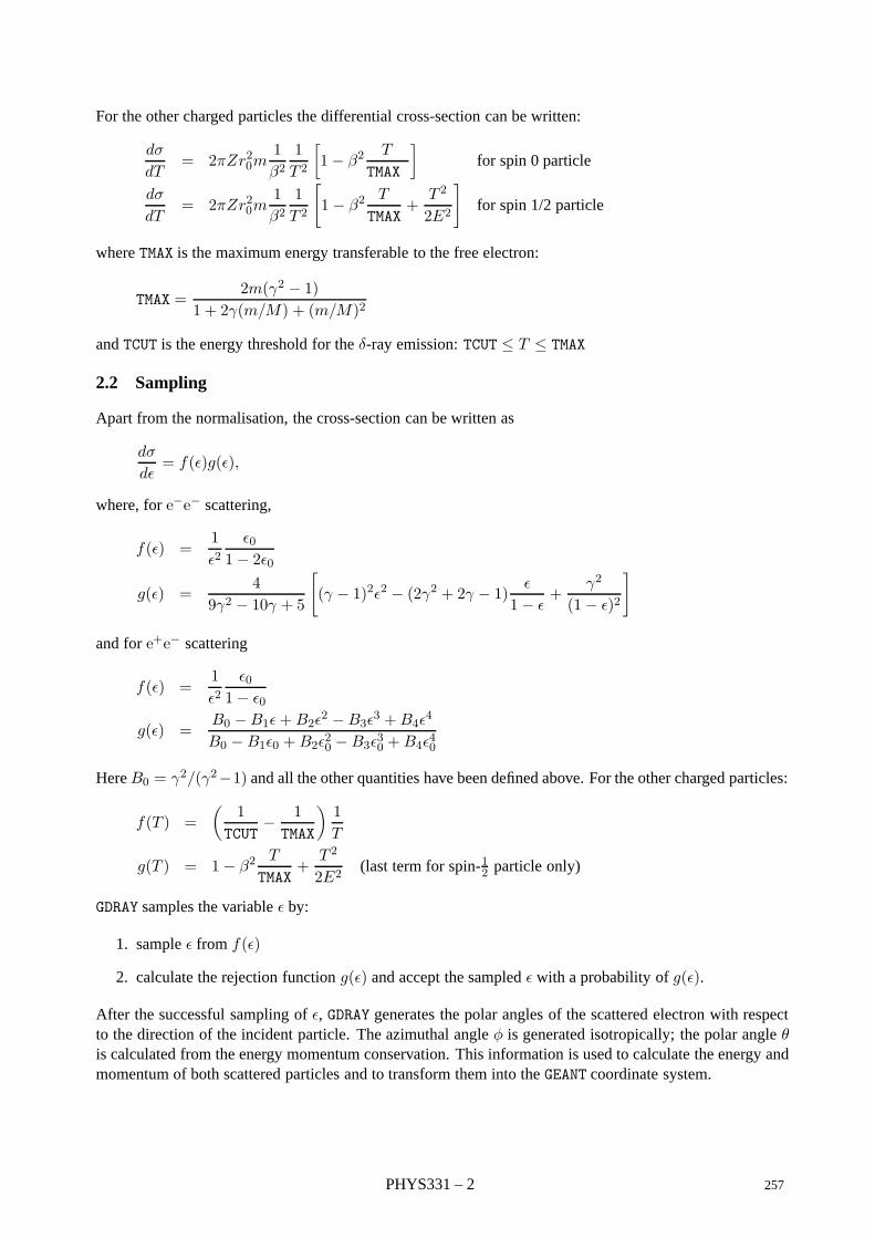
For the other charged particles the differential cross-section can be written:
dσ
dT= 2πZr20m
1β2
1T 2
[1− β2
T
TMAX
]for spin 0 particle
dσ
dT= 2πZr20m
1β2
1T 2
[1− β2
T
TMAX+
T 2
2E2
]for spin 1/2 particle
where TMAX is the maximum energy transferable to the free electron:
TMAX =2m(γ2 − 1)
1 + 2γ(m/M) + (m/M)2
and TCUT is the energy threshold for the δ-ray emission: TCUT ≤ T ≤ TMAX
2.2 Sampling
Apart from the normalisation, the cross-section can be written as
dσ
dε= f(ε)g(ε),
where, for e−e− scattering,
f(ε) =1ε2
ε01− 2ε0
g(ε) =4
9γ2 − 10γ + 5
[(γ − 1)2ε2 − (2γ2 + 2γ − 1) ε
1− ε+
γ2
(1− ε)2
]
and for e+e− scattering
f(ε) =1ε2
ε01− ε0
g(ε) =B0 −B1ε+B2ε
2 −B3ε3 +B4ε
4
B0 −B1ε0 +B2ε20 −B3ε30 +B4ε40
Here B0 = γ2/(γ2−1) and all the other quantities have been defined above. For the other charged particles:
f(T ) =(
1TCUT
− 1TMAX
)1T
g(T ) = 1− β2T
TMAX+
T 2
2E2(last term for spin-12 particle only)
GDRAY samples the variable ε by:
1. sample ε from f(ε)
2. calculate the rejection function g(ε) and accept the sampled ε with a probability of g(ε).
After the successful sampling of ε, GDRAY generates the polar angles of the scattered electron with respectto the direction of the incident particle. The azimuthal angle φ is generated isotropically; the polar angle θis calculated from the energy momentum conservation. This information is used to calculate the energy andmomentum of both scattered particles and to transform them into the GEANT coordinate system.
PHYS331 – 2 257
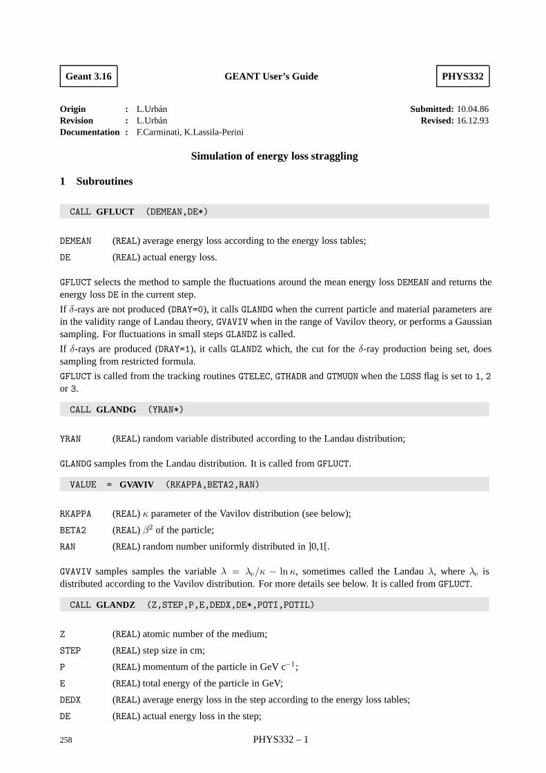
Geant 3.16 GEANT User’s Guide PHYS332
Origin : L.Urban Submitted: 10.04.86Revision : L.Urban Revised: 16.12.93Documentation : F.Carminati, K.Lassila-Perini
Simulation of energy loss straggling
1 Subroutines
CALL GFLUCT (DEMEAN,DE*)
DEMEAN (REAL) average energy loss according to the energy loss tables;
DE (REAL) actual energy loss.
GFLUCT selects the method to sample the fluctuations around the mean energy loss DEMEAN and returns theenergy loss DE in the current step.
If δ-rays are not produced (DRAY=0), it calls GLANDG when the current particle and material parameters arein the validity range of Landau theory, GVAVIV when in the range of Vavilov theory, or performs a Gaussiansampling. For fluctuations in small steps GLANDZ is called.
If δ-rays are produced (DRAY=1), it calls GLANDZ which, the cut for the δ-ray production being set, doessampling from restricted formula.
GFLUCT is called from the tracking routines GTELEC, GTHADR and GTMUON when the LOSS flag is set to 1, 2or 3.
CALL GLANDG (YRAN*)
YRAN (REAL) random variable distributed according to the Landau distribution;
GLANDG samples from the Landau distribution. It is called from GFLUCT.
VALUE = GVAVIV (RKAPPA,BETA2,RAN)
RKAPPA (REAL) κ parameter of the Vavilov distribution (see below);
BETA2 (REAL) β2 of the particle;
RAN (REAL) random number uniformly distributed in ]0,1[.
GVAVIV samples samples the variable λ = λv/κ − lnκ, sometimes called the Landau λ, where λv isdistributed according to the Vavilov distribution. For more details see below. It is called from GFLUCT.
CALL GLANDZ (Z,STEP,P,E,DEDX,DE*,POTI,POTIL)
Z (REAL) atomic number of the medium;
STEP (REAL) step size in cm;
P (REAL) momentum of the particle in GeV c−1;
E (REAL) total energy of the particle in GeV;
DEDX (REAL) average energy loss in the step according to the energy loss tables;
DE (REAL) actual energy loss in the step;
258 PHYS332 – 1

POTI (REAL) average ionisation potential for the medium;
POTIL (REAL) logarithm of the average ionisation potential.
GLANDZ gives the energy loss DE for the current particle with energy E and momentum P in a material ofatomic number Z where the average energy loss is DEDX and the current step length STEP. It is called fromGFLUCT for restricted Landau fluctuations when δ-rays are produced or to sample the fluctuations in thinlayers (with or without δ-ray production).
2 Method
Due to the statistical nature of ionisation energy loss, large fluctuations can occur in the amount of energydeposited by a particle traversing an absorber element. As recently reviewed [56], continuous processessuch as multiple scattering and energy loss play a relevant role in the longitudinal and lateral development ofelectromagnetic and hadronic showers, and in the case of sampling calorimeters the measured resolution canbe significantly affected by such fluctuations in their active layers. The description of ionisation fluctuationsis characterised by the significance parameter κ, which is proportional to the ratio of mean energy loss tothe maximum allowed energy transfer in a single collision with an atomic electron
κ =ξ
Emax
Emax is the maximum transferable energy in a single collision with an atomic electron.
Emax =2meβ
2γ2
1 + 2γme/mx + (me/mx)2 ,
where γ = E/mx, E is energy and mx the mass of the incident particle, β2 = 1 − 1/γ2 and me is theelectron mass. ξ comes from the Rutherford scattering cross section and is defined as:
ξ =2πz2e4NAvZρδx
meβ2c2A= 153.4
z2
β2Z
Aρδx keV,
wherez charge of the incident particle
NAv Avogadro’s number
Z atomic number of the material
A atomic weight of the material
ρ density
δx thickness of the materialκ measures the contribution of the collisions with energy transfer close to Emax. For a given absorber, κtends towards large values if δx is large and/or if β is small. Likewise, κ tends towards zero if δx is smalland/or if β approaches 1.
The value of κ distinguishes two regimes which occur in the description of ionisation fluctuations :
1. A large number of collisions involving the loss of all or most of the incident particle energy duringthe traversal of an absorber.
As the total energy transfer is composed of a multitude of small energy losses, we can apply thecentral limit theorem and describe the fluctuations by a Gaussian distribution. This case is applicableto non-relativistic particles and is described by the inequality κ > 10 (i.e. when the mean energy lossin the absorber is greater than the maximum energy transfer in a single collision).
2. Particles traversing thin counters and incident electrons under any conditions.
The relevant inequalities and distributions are 0.01 < κ < 10, Vavilov distribution, and κ < 0.01,Landau distribution.
PHYS332 – 2 259
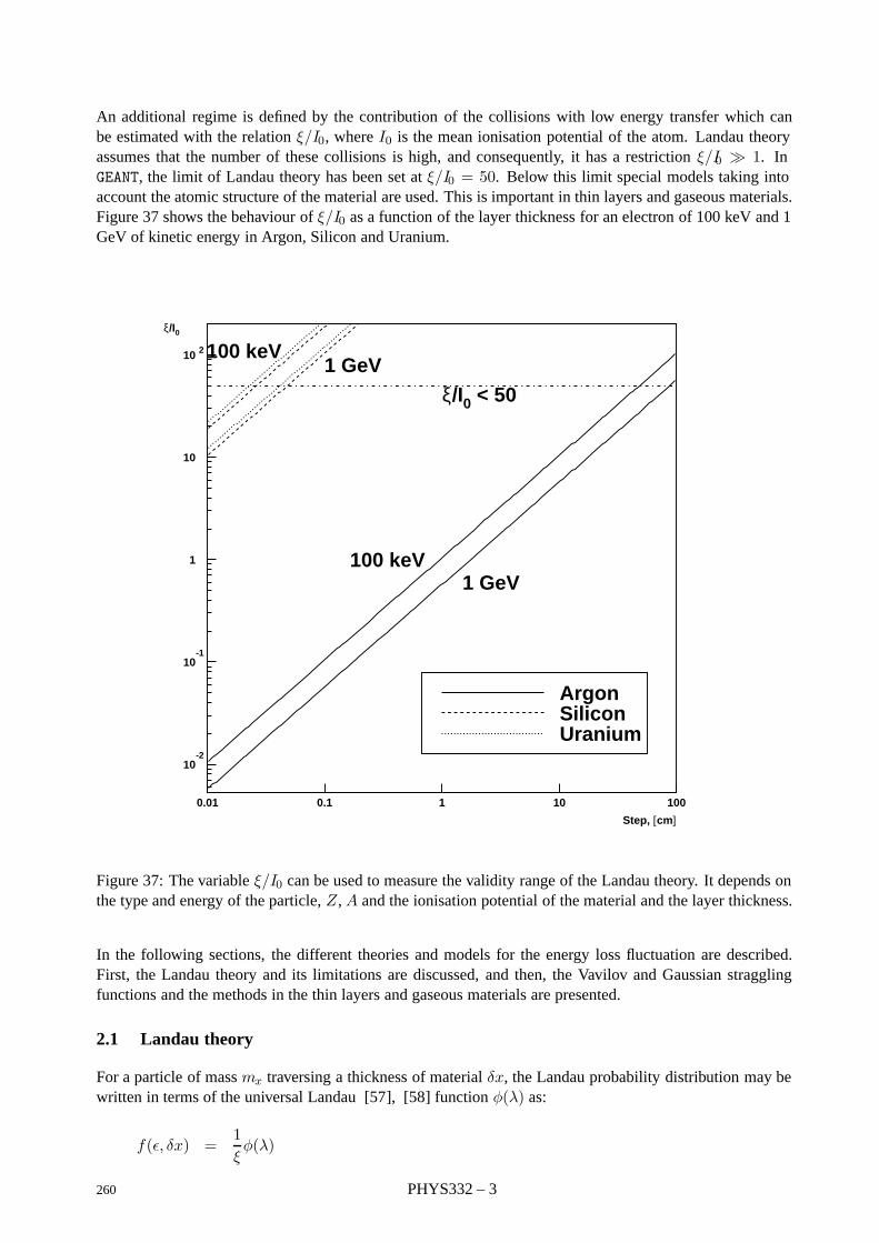
An additional regime is defined by the contribution of the collisions with low energy transfer which canbe estimated with the relation ξ/I0, where I0 is the mean ionisation potential of the atom. Landau theoryassumes that the number of these collisions is high, and consequently, it has a restriction ξ/I0 1. InGEANT, the limit of Landau theory has been set at ξ/I0 = 50. Below this limit special models taking intoaccount the atomic structure of the material are used. This is important in thin layers and gaseous materials.Figure 37 shows the behaviour of ξ/I0 as a function of the layer thickness for an electron of 100 keV and 1GeV of kinetic energy in Argon, Silicon and Uranium.
10-2
10-1
1
10
10 2
0.01 0.1 1 10 100
ξ/I0 < 50
ArgonSiliconUranium
1 GeV100 keV
1 GeV100 keV
Step, [cm]
ξ/I0
Figure 37: The variable ξ/I0 can be used to measure the validity range of the Landau theory. It depends onthe type and energy of the particle, Z , A and the ionisation potential of the material and the layer thickness.
In the following sections, the different theories and models for the energy loss fluctuation are described.First, the Landau theory and its limitations are discussed, and then, the Vavilov and Gaussian stragglingfunctions and the methods in the thin layers and gaseous materials are presented.
2.1 Landau theory
For a particle of mass mx traversing a thickness of material δx, the Landau probability distribution may bewritten in terms of the universal Landau [57], [58] function φ(λ) as:
f(ε, δx) =1ξφ(λ)
260 PHYS332 – 3
where
φ(λ) =12πi
∫ c+i∞
c−i∞exp (u lnu+ λu) du c ≥ 0
λ =ε− ε
ξ− γ′ − β2 − ln ξ
Emaxγ′ = 0.422784 . . . = 1− γ
γ = 0.577215 . . . (Euler’s constant)
ε = average energy loss
ε = actual energy loss
Restrictions
The Landau formalism makes two restrictive assumptions :
1. The typical energy loss is small compared to the maximum energy loss in a single collision. Thisrestriction is removed in the Vavilov theory (see section 2.2).
2. The typical energy loss in the absorber should be large compared to the binding energy of the mosttightly bound electron. For gaseous detectors, typical energy losses are a few keV which is comparableto the binding energies of the inner electrons. In such cases a more sophisticated approach whichaccounts for atomic energy levels (see for instance Talman [59]) is necessary to accurately simulatedata distributions. In GEANT, a parameterised model by L. Urban is used (see section 2.4).
In addition, the average value of the Landau distribution is infinite. Summing the Landau fluctuation ob-tained to the average energy from the dE/dx tables, we obtain a value which is larger than the one comingfrom the table. The probability to sample a large value is small, so it takes a large number of steps (extrac-tions) for the average fluctuation to be significantly larger than zero. This introduces a dependence of theenergy loss on the step size which can affect calculations.
A solution to this has been to introduce a limit on the value of the variable sampled by the Landau distribution[60], in order to keep the average fluctuation to 0. The value obtained from the GLANDO routine is:
δdE/dx = ε− ε = ξ(λ− γ′ + β2 + lnξ
Emax)
In order for this to have average 0, we must impose that:
λ = −γ′ − β2 − ln ξ
Emax
This is realised introducing a λmax(λ) such that if only values of λ ≤ λmax are accepted, the average valueof the distribution is λ.
A parametric fit to the universal Landau distribution has been performed, with following result:
λmax = 0.60715 + 1.1934λ + (0.67794 + 0.052382λ) exp(0.94753 + 0.74442λ)
only values smaller than λmax are accepted, otherwise the distribution is resampled.
PHYS332 – 4 261
2.2 Vavilov theory
Vavilov [61] derived a more accurate straggling distribution by introducing the kinematic limit on themaximum transferable energy in a single collision, rather than using Emax = ∞. Using the notations of[62] we can write:
f (ε, δs) =1ξφv
(λv, κ, β
2)
where
φv
(λv, κ, β
2)
=12πi
∫ c+i∞
c−i∞φ (s) eλsds c ≥ 0
φ (s) = exp[κ(1 + β2γ)
]exp [ψ (s)] ,
ψ (s) = s lnκ+ (s+ β2κ) [ln(s/κ) + E1(s/κ)] − κe−s/κ,
and
E1(z) =∫ ∞
zt−1e−tdt (the exponential integral)
λv = κ
[ε− ε
ξ− γ′ − β2
]
The Vavilov parameters are simply related to the Landau parameter by λL = λv/κ − lnκ. It can beshown that as κ → 0, the distribution of the variable λL approaches that of Landau. For κ ≤ 0.01 thetwo distributions are already practically identical. Contrary to what many textbooks report, the Vavilovdistribution does not approximate the Landau distribution for small κ, but rather the distribution of λLdefined above tends to the distribution of the true λ from the Landau density function. Thus the routineGVAVIV samples the variable λL rather than λv. For κ ≥ 10 the Vavilov distribution tends to a Gaussiandistribution (see next section).
2.3 Gaussian Theory
Various conflicting forms have been proposed for Gaussian straggling functions, but most of these appear tohave little theoretical or experimental basis. However, as noted by Schorr [62] it has been demonstrated bySeltzer and Berger [63] that for κ ≥ 10 the Vavilov distribution can be replaced by a Gaussian of the form :
f(ε, δs) ≈ 1
ξ√2πκ (1− β2/2)
exp
[(ε− ε)2
2κ
ξ2(1− β2/2)
]
thus implying
mean = ε
σ2 =ξ2
κ(1− β2/2) = ξEmax(1− β2/2)
2.4 Urban model
The method for computing restricted energy losses with δ-ray production above given threshold energy inGEANT is a Monte Carlo method that can be used for thin layers. It is fast and it can be used for any thicknessof a medium. Approaching the limit of the validity of Landau’s theory, the loss distribution approachessmoothly the Landau form as shown in figure 38.
262 PHYS332 – 5
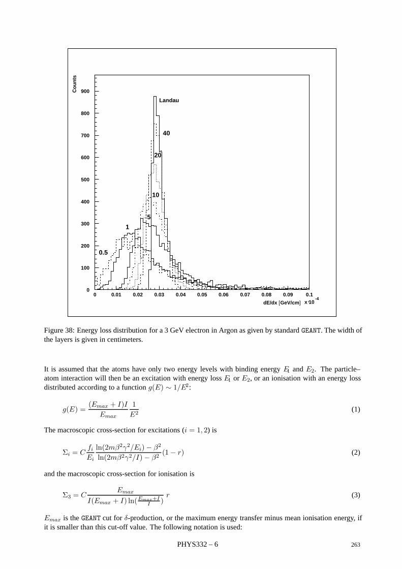
Landau
40
20
10
5
1
0.5
dE/dx [GeV/cm] ‘
Co
un
ts
0
100
200
300
400
500
600
700
800
900
0 0.01 0.02 0.03 0.04 0.05 0.06 0.07 0.08 0.09 0.1x 10
-4
Figure 38: Energy loss distribution for a 3 GeV electron in Argon as given by standard GEANT. The width ofthe layers is given in centimeters.
It is assumed that the atoms have only two energy levels with binding energy E1 and E2. The particle–atom interaction will then be an excitation with energy loss E1 or E2, or an ionisation with an energy lossdistributed according to a function g(E) ∼ 1/E2:
g(E) =(Emax + I)I
Emax
1E2
(1)
The macroscopic cross-section for excitations (i = 1, 2) is
Σi = CfiEi
ln(2mβ2γ2/Ei)− β2
ln(2mβ2γ2/I)− β2(1− r) (2)
and the macroscopic cross-section for ionisation is
Σ3 = CEmax
I(Emax + I) ln(Emax+II )
r (3)
Emax is the GEANT cut for δ-production, or the maximum energy transfer minus mean ionisation energy, ifit is smaller than this cut-off value. The following notation is used:
PHYS332 – 6 263
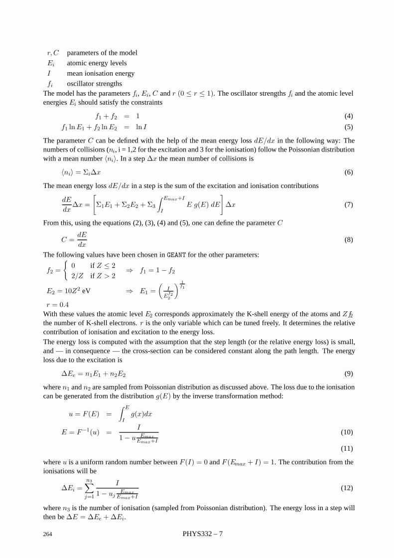
r, C parameters of the model
Ei atomic energy levels
I mean ionisation energy
fi oscillator strengthsThe model has the parameters fi, Ei, C and r (0 ≤ r ≤ 1). The oscillator strengths fi and the atomic levelenergies Ei should satisfy the constraints
f1 + f2 = 1 (4)
f1 lnE1 + f2 lnE2 = ln I (5)
The parameter C can be defined with the help of the mean energy loss dE/dx in the following way: Thenumbers of collisions (ni, i = 1,2 for the excitation and 3 for the ionisation) follow the Poissonian distributionwith a mean number 〈ni〉. In a step ∆x the mean number of collisions is
〈ni〉 = Σi∆x (6)
The mean energy loss dE/dx in a step is the sum of the excitation and ionisation contributions
dE
dx∆x =
[Σ1E1 +Σ2E2 +Σ3
∫ Emax+I
IE g(E) dE
]∆x (7)
From this, using the equations (2), (3), (4) and (5), one can define the parameter C
C =dE
dx(8)
The following values have been chosen in GEANT for the other parameters:
f2 =
0 if Z ≤ 22/Z if Z > 2
⇒ f1 = 1− f2
E2 = 10Z2 eV ⇒ E1 =(
I
Ef22
) 1f1
r = 0.4With these values the atomic level E2 corresponds approximately the K-shell energy of the atoms and Zf2the number of K-shell electrons. r is the only variable which can be tuned freely. It determines the relativecontribution of ionisation and excitation to the energy loss.The energy loss is computed with the assumption that the step length (or the relative energy loss) is small,and — in consequence — the cross-section can be considered constant along the path length. The energyloss due to the excitation is
∆Ee = n1E1 + n2E2 (9)
where n1 and n2 are sampled from Poissonian distribution as discussed above. The loss due to the ionisationcan be generated from the distribution g(E) by the inverse transformation method:
u = F (E) =∫ E
Ig(x)dx
E = F−1(u) =I
1− u EmaxEmax+I
(10)
(11)
where u is a uniform random number between F (I) = 0 and F (Emax + I) = 1. The contribution from theionisations will be
∆Ei =n3∑j=1
I
1− ujEmax
Emax+I
(12)
where n3 is the number of ionisation (sampled from Poissonian distribution). The energy loss in a step willthen be ∆E = ∆Ee +∆Ei.
264 PHYS332 – 7
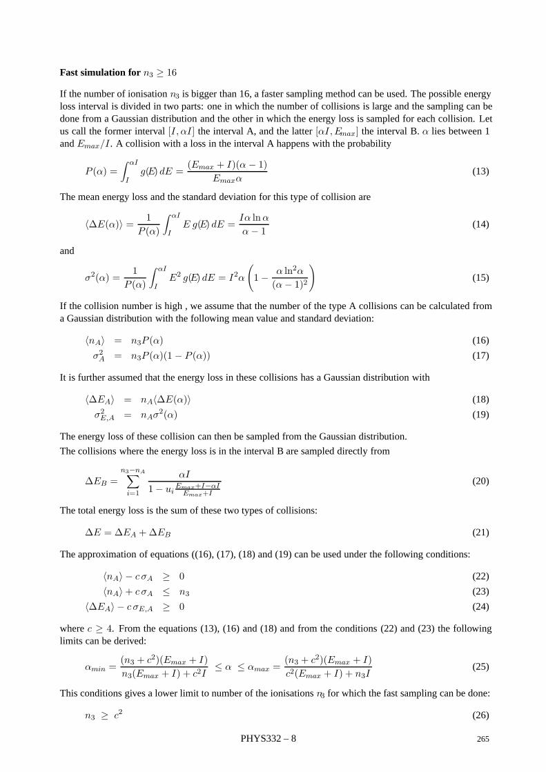
Fast simulation for n3 ≥ 16
If the number of ionisation n3 is bigger than 16, a faster sampling method can be used. The possible energyloss interval is divided in two parts: one in which the number of collisions is large and the sampling can bedone from a Gaussian distribution and the other in which the energy loss is sampled for each collision. Letus call the former interval [I, αI] the interval A, and the latter [αI,Emax] the interval B. α lies between 1and Emax/I . A collision with a loss in the interval A happens with the probability
P (α) =∫ αI
Ig(E) dE =
(Emax + I)(α − 1)Emaxα
(13)
The mean energy loss and the standard deviation for this type of collision are
〈∆E(α)〉 = 1P (α)
∫ αI
IE g(E) dE =
Iα lnαα− 1 (14)
and
σ2(α) =1
P (α)
∫ αI
IE2 g(E) dE = I2α
(1− α ln2α
(α− 1)2
)(15)
If the collision number is high , we assume that the number of the type A collisions can be calculated froma Gaussian distribution with the following mean value and standard deviation:
〈nA〉 = n3P (α) (16)
σ2A = n3P (α)(1 − P (α)) (17)
It is further assumed that the energy loss in these collisions has a Gaussian distribution with
〈∆EA〉 = nA〈∆E(α)〉 (18)
σ2E,A = nAσ2(α) (19)
The energy loss of these collision can then be sampled from the Gaussian distribution.
The collisions where the energy loss is in the interval B are sampled directly from
∆EB =n3−nA∑i=1
αI
1− uiEmax+I−αI
Emax+I
(20)
The total energy loss is the sum of these two types of collisions:
∆E = ∆EA +∆EB (21)
The approximation of equations ((16), (17), (18) and (19) can be used under the following conditions:
〈nA〉 − c σA ≥ 0 (22)
〈nA〉+ c σA ≤ n3 (23)
〈∆EA〉 − c σE,A ≥ 0 (24)
where c ≥ 4. From the equations (13), (16) and (18) and from the conditions (22) and (23) the followinglimits can be derived:
αmin =(n3 + c2)(Emax + I)n3(Emax + I) + c2I
≤ α ≤ αmax =(n3 + c2)(Emax + I)c2(Emax + I) + n3I
(25)
This conditions gives a lower limit to number of the ionisations n3 for which the fast sampling can be done:
n3 ≥ c2 (26)
PHYS332 – 8 265
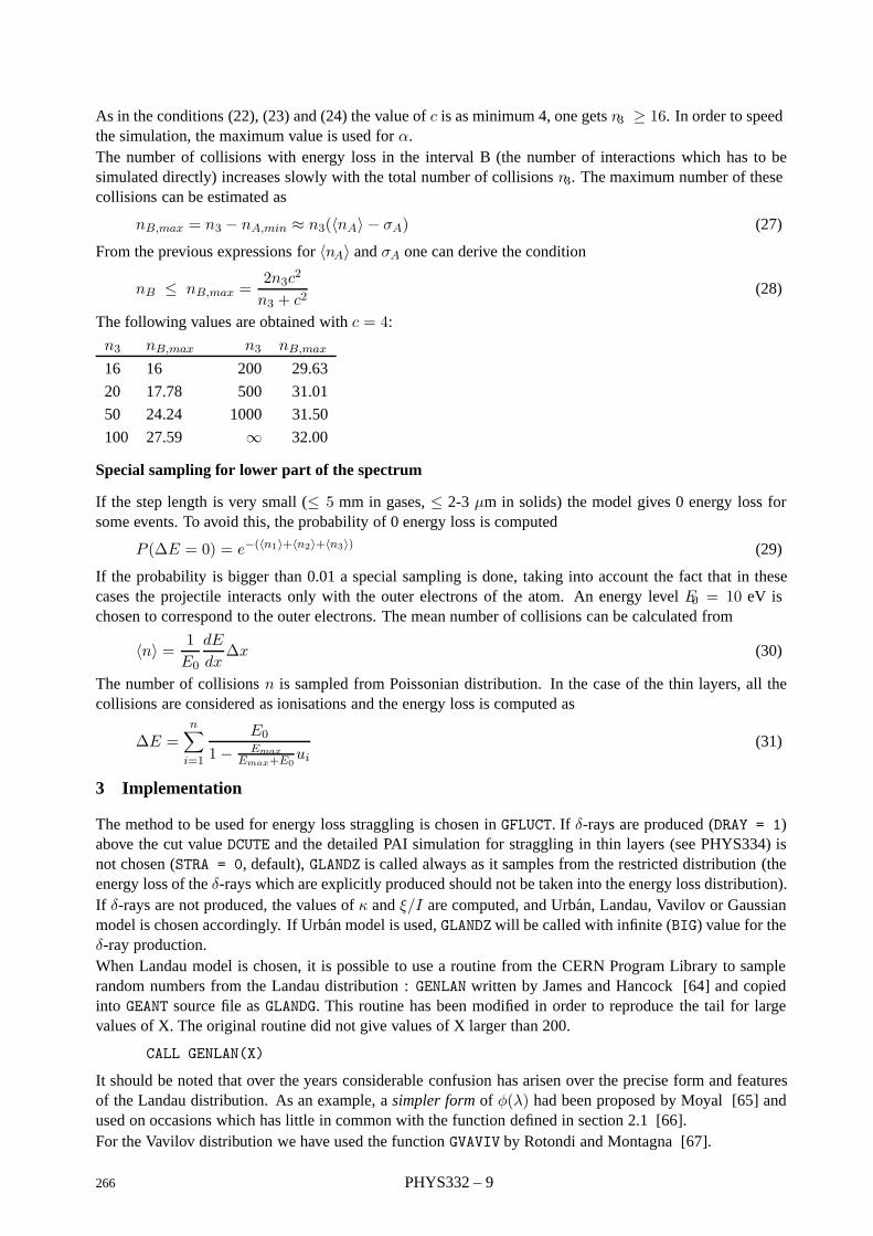
As in the conditions (22), (23) and (24) the value of c is as minimum 4, one gets n3 ≥ 16. In order to speedthe simulation, the maximum value is used for α.The number of collisions with energy loss in the interval B (the number of interactions which has to besimulated directly) increases slowly with the total number of collisions n3. The maximum number of thesecollisions can be estimated as
nB,max = n3 − nA,min ≈ n3(〈nA〉 − σA) (27)
From the previous expressions for 〈nA〉 and σA one can derive the condition
nB ≤ nB,max =2n3c2
n3 + c2(28)
The following values are obtained with c = 4:
n3 nB,max n3 nB,max
16 16 200 29.63
20 17.78 500 31.01
50 24.24 1000 31.50
100 27.59 ∞ 32.00
Special sampling for lower part of the spectrum
If the step length is very small (≤ 5 mm in gases, ≤ 2-3 µm in solids) the model gives 0 energy loss forsome events. To avoid this, the probability of 0 energy loss is computed
P (∆E = 0) = e−(〈n1〉+〈n2〉+〈n3〉) (29)
If the probability is bigger than 0.01 a special sampling is done, taking into account the fact that in thesecases the projectile interacts only with the outer electrons of the atom. An energy level E0 = 10 eV ischosen to correspond to the outer electrons. The mean number of collisions can be calculated from
〈n〉 = 1E0
dE
dx∆x (30)
The number of collisions n is sampled from Poissonian distribution. In the case of the thin layers, all thecollisions are considered as ionisations and the energy loss is computed as
∆E =n∑
i=1
E0
1− EmaxEmax+E0
ui
(31)
3 Implementation
The method to be used for energy loss straggling is chosen in GFLUCT. If δ-rays are produced (DRAY = 1)above the cut value DCUTE and the detailed PAI simulation for straggling in thin layers (see PHYS334) isnot chosen (STRA = 0, default), GLANDZ is called always as it samples from the restricted distribution (theenergy loss of the δ-rays which are explicitly produced should not be taken into the energy loss distribution).If δ-rays are not produced, the values of κ and ξ/I are computed, and Urban, Landau, Vavilov or Gaussianmodel is chosen accordingly. If Urban model is used, GLANDZ will be called with infinite (BIG) value for theδ-ray production.When Landau model is chosen, it is possible to use a routine from the CERN Program Library to samplerandom numbers from the Landau distribution : GENLAN written by James and Hancock [64] and copiedinto GEANT source file as GLANDG. This routine has been modified in order to reproduce the tail for largevalues of X. The original routine did not give values of X larger than 200.
CALL GENLAN(X)
It should be noted that over the years considerable confusion has arisen over the precise form and featuresof the Landau distribution. As an example, a simpler form of φ(λ) had been proposed by Moyal [65] andused on occasions which has little in common with the function defined in section 2.1 [66].For the Vavilov distribution we have used the function GVAVIV by Rotondi and Montagna [67].
266 PHYS332 – 9
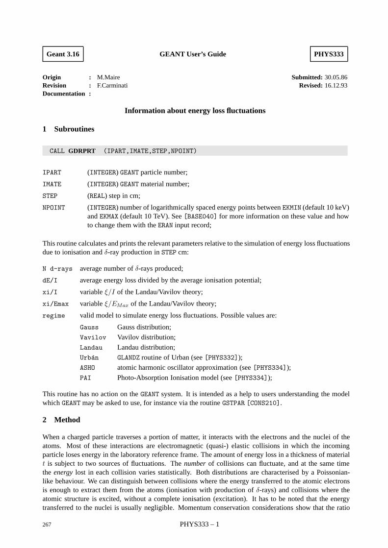
Geant 3.16 GEANT User’s Guide PHYS333
Origin : M.Maire Submitted: 30.05.86Revision : F.Carminati Revised: 16.12.93Documentation :
Information about energy loss fluctuations
1 Subroutines
CALL GDRPRT (IPART,IMATE,STEP,NPOINT)
IPART (INTEGER) GEANT particle number;
IMATE (INTEGER) GEANT material number;
STEP (REAL) step in cm;
NPOINT (INTEGER) number of logarithmically spaced energy points between EKMIN (default 10 keV)and EKMAX (default 10 TeV). See [BASE040] for more information on these value and howto change them with the ERAN input record;
This routine calculates and prints the relevant parameters relative to the simulation of energy loss fluctuationsdue to ionisation and δ-ray production in STEP cm:
N d-rays average number of δ-rays produced;
dE/I average energy loss divided by the average ionisation potential;
xi/I variable ξ/I of the Landau/Vavilov theory;
xi/Emax variable ξ/EMax of the Landau/Vavilov theory;
regime valid model to simulate energy loss fluctuations. Possible values are:
Gauss Gauss distribution;
Vavilov Vavilov distribution;
Landau Landau distribution;
Urban GLANDZ routine of Urban (see [PHYS332]);
ASHO atomic harmonic oscillator approximation (see [PHYS334]);
PAI Photo-Absorption Ionisation model (see [PHYS334]);
This routine has no action on the GEANT system. It is intended as a help to users understanding the modelwhich GEANT may be asked to use, for instance via the routine GSTPAR [CONS210].
2 Method
When a charged particle traverses a portion of matter, it interacts with the electrons and the nuclei of theatoms. Most of these interactions are electromagnetic (quasi-) elastic collisions in which the incomingparticle loses energy in the laboratory reference frame. The amount of energy loss in a thickness of materialt is subject to two sources of fluctuations. The number of collisions can fluctuate, and at the same timethe energy lost in each collision varies statistically. Both distributions are characterised by a Poissonian-like behaviour. We can distinguish between collisions where the energy transferred to the atomic electronsis enough to extract them from the atoms (ionisation with production of δ-rays) and collisions where theatomic structure is excited, without a complete ionisation (excitation). It has to be noted that the energytransferred to the nuclei is usually negligible. Momentum conservation considerations show that the ratio
267 PHYS333 – 1
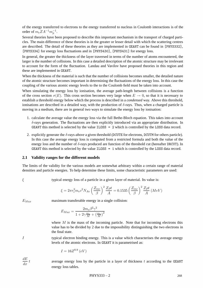
of the energy transferred to electrons to the energy transferred to nucleus in Coulomb interactions is of theorder of meZA−1m−1
p .
Several theories have been proposed to describe this important mechanism in the transport of charged parti-cles. The main difference of these theories is in the greater or lesser detail with which the scattering centresare described. The detail of these theories as they are implemented in GEANT can be found in [PHYS332],[PHYS334] for energy loss fluctuations and in [PHYS430], [PHYS431] for energy loss.
In general, the greater the thickness of the layer traversed in terms of the number of atoms encountered, thelarger is the number of collisions. In this case a detailed description of the atomic structure may be irrelevantto account for the form of the fluctuation. Landau and Vavilov have proposed theories in this region andthese are implemented in GEANT.
When the thickness of the material is such that the number of collisions becomes smaller, the detailed natureof the atomic structure becomes important in determining the fluctuations of the energy loss. In this case thecoupling of the various atomic energy levels to the to the Coulomb field must be taken into account.
When simulating the energy loss by ionisation, the average path-length between collisions is a functionof the cross section σ(E). This cross section becomes very large when E → 0, so that it is necessary toestablish a threshold energy below which the process is described in a condensed way. Above this threshold,ionisations are described in a detailed way, with the production of δ-rays. Thus, when a charged particle ismoving in a medium, there are in general two ways to simulate the energy loss by ionisation:
1. calculate the average value the energy loss via the full Bethe-Bloch equation. This takes into accountδ-rays generation. The fluctuations are then explicitly introduced via an appropriate distribution. InGEANT this method is selected by the value ILOSS = 2 which is controlled by the LOSS data record.
2. explicitly generate the δ-rays above a given threshold (DCUTE for electrons, DCUTM for others particle).In this case the average energy loss is computed from a restricted formula and both the value of theenergy loss and the number of δ-rays produced are function of the threshold cut (hereafter DRCUT). InGEANT this method is selected by the value ILOSS = 1 which is controlled by the LOSS data record.
2.1 Validity ranges for the different models
The limits of the validity for the various models are somewhat arbitrary within a certain range of materialdensities and particle energies. To help determine these limits, some characteristic parameters are used:
ξ typical energy loss of a particle in a given layer of material. Its value is:
ξ = 2πr2emec2NAv
(Zinc
β
)2 Zρt
A= 0.1535
(Zinc
β
)2 Zρt
A(MeV )
EMax maximum transferable energy in a single collision:
EMax =2meβ
2γ2
1 + 2γmeM +
(meM
)2where M is the mass of the incoming particle. Note that for incoming electrons thisvalue has to be divided by 2 due to the impossibility distinguishing the two electrons inthe final state.
I typical electron binding energy. This is a value which characterises the average energylevels of the atomic electrons. In GEANT it is parametrised as:
I = 16Z0.9 (eV )
dE
dxt average energy loss by the particle in a layer of thickness t according to the GEANT
energy loss tables.
PHYS333 – 2 268

ξ/EMax (hereafter κ) relative importance of high energy transfer collisions in the ionisation pro-cess
min(dEdx t, ξ
)/I (hereafter ∆) estimation of the number of collisions with energy close to the ionisation
energy.
In GEANT two variables control the model used to describe the energy loss fluctuations:
ILOSS fluctuation model:
0 no energy loss;
1 δ-rays are produced above the threshold, reduced fluctuations from δ-rays belowthe threshold are added to the energy loss;
2 no δ-rays are produced, complete fluctuations are calculated;
3 same as 1;
4 no fluctuations;
ISTRA energy loss model for thin layer (see below):
0 Urban model;
1 PAI model;
2 ASHO model for 1 < ∆ ≤ 30,(not yet available) PAI model otherwise;
The validity limits of the different models are estimated as follows:
1. large number of low-energy collisions: ∆ ≥ 50
if δ-rays generation is requested (ILOSS = 1 or 3 and IDRAY = 1) the Urban model is used. If δ-raysare not produced (ILOSS = 2 and IDRAY = 0) we distinguish three regions:
(a) very few energy transfers close to the maximum: κ ≤ 10−2
the Landau distribution is used;
(b) few energy transfers close to the maximum: 10−2 < κ ≤ 10the Vavilov distribution is used;
(c) many energy transfers close to the maximum: κ > 10the Gauss distribution is used;
2. small number of low-energy collisions: ∆ < 50
in this region the same model is used for 1 ≤ ILOSS ≤ 3 irrespective of the value of IDRAY. Themodel used depends on the value of ISTRA.
(a) 30 < ∆ ≤ 50Urban model if ISTRA = 0, PAI model otherwise.
(b) 1 < ∆ ≤ 30Urban model if ISTRA = 0, PAI model if ISTRA = 1 and ASHO model if ISTRA = 2.
(c) 0.01 < ∆ ≤ 1Urban model if ISTRA = 0, PAI model otherwise.
(d) ∆ ≤ 0.01Urban model if ISTRA = 0, PAI model otherwise.
269 PHYS333 – 3
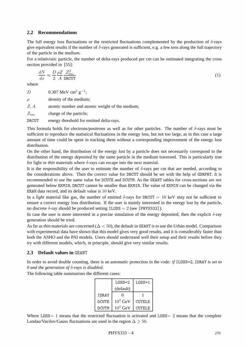
2.2 Recommendations
The full energy loss fluctuations or the restricted fluctuations complemented by the production of δ-raysgive equivalent results if the number of δ-rays generated is sufficient, e.g. a few tens along the full trajectoryof the particle in the medium.For a relativistic particle, the number of delta-rays produced per cm can be estimated integrating the crosssection provided in [55]:
dN
dx≈ D
2ρZ
A
Z2incDRCUT
(1)
where
D 0.307 MeV cm2 g−1;
ρ density of the medium;
Z,A atomic number and atomic weight of the medium;
Zinc charge of the particle;
DRCUT energy threshold for emitted delta-rays.
This formula holds for electrons/positrons as well as for other particles. The number of δ-rays must besufficient to reproduce the statistical fluctuations in the energy loss, but not too large, as in this case a largeamount of time could be spent in tracking them without a corresponding improvement of the energy lossdistribution.On the other hand, the distribution of the energy lost by a particle does not necessarily correspond to thedistribution of the energy deposited by the same particle in the medium traversed. This is particularly truefor light or thin materials where δ-rays can escape into the next material.It is the responsibility of the user to estimate the number of δ-rays per cm that are needed, according tothe considerations above. Then the correct value for DRCUT should be set with the help of GDRPRT. It isrecommended to use the same value for DCUTE and DCUTM. As the GEANT tables for cross-sections are notgenerated below EKMIN, DRCUT cannot be smaller than EKMIN. The value of EKMIN can be changed via theERAN data record, and its default value is 10 keV.In a light material like gas, the number of emitted δ-rays for DRCUT = 10 keV may not be sufficient toensure a correct energy loss distribution. If the user is mainly interested in the energy lost by the particle,no discrete δ-ray should be produced setting ILOSS = 2 (see [PHYS332]).In case the user is more interested in a precise simulation of the energy deposited, then the explicit δ-raygeneration should be tried.As far as thin materials are concerned (∆ < 50), the default in GEANT is to use the Urban model. Comparisonwith experimental data have shown that this model gives very good results, and it is considerably faster thanboth the ASHO and the PAI models. Users should understand well their setup and their results before theytry with different models, which, in principle, should give very similar results.
2.3 Default values in GEANT
In order to avoid double counting, there is an automatic protection in the code: if ILOSS=2, IDRAY is set to0 and the generation of δ-rays is disabled.The following table summarises the different cases:
LOSS=2 LOSS=1
(default)
IDRAY 0 1
DCUTE 104 GeV CUTELE
DCUTM 104 GeV CUTELE
Where LOSS= 1 means that the restricted fluctuation is activated and LOSS= 2 means that the completeLandau/Vavilov/Gauss fluctuations are used in the region ∆ ≥ 50.
PHYS333 – 4 270
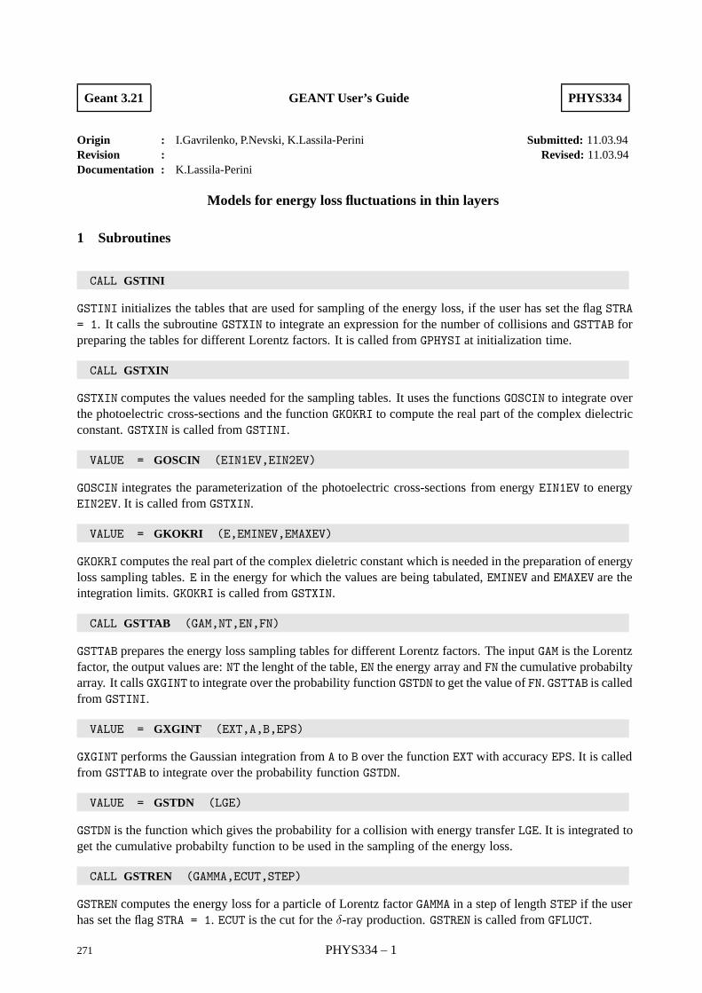
Geant 3.21 GEANT User’s Guide PHYS334
Origin : I.Gavrilenko, P.Nevski, K.Lassila-Perini Submitted: 11.03.94Revision : Revised: 11.03.94Documentation : K.Lassila-Perini
Models for energy loss fluctuations in thin layers
1 Subroutines
CALL GSTINI
GSTINI initializes the tables that are used for sampling of the energy loss, if the user has set the flag STRA= 1. It calls the subroutine GSTXIN to integrate an expression for the number of collisions and GSTTAB forpreparing the tables for different Lorentz factors. It is called from GPHYSI at initialization time.
CALL GSTXIN
GSTXIN computes the values needed for the sampling tables. It uses the functions GOSCIN to integrate overthe photoelectric cross-sections and the function GKOKRI to compute the real part of the complex dielectricconstant. GSTXIN is called from GSTINI.
VALUE = GOSCIN (EIN1EV,EIN2EV)
GOSCIN integrates the parameterization of the photoelectric cross-sections from energy EIN1EV to energyEIN2EV. It is called from GSTXIN.
VALUE = GKOKRI (E,EMINEV,EMAXEV)
GKOKRI computes the real part of the complex dieletric constant which is needed in the preparation of energyloss sampling tables. E in the energy for which the values are being tabulated, EMINEV and EMAXEV are theintegration limits. GKOKRI is called from GSTXIN.
CALL GSTTAB (GAM,NT,EN,FN)
GSTTAB prepares the energy loss sampling tables for different Lorentz factors. The input GAM is the Lorentzfactor, the output values are: NT the lenght of the table, EN the energy array and FN the cumulative probabiltyarray. It calls GXGINT to integrate over the probability function GSTDN to get the value of FN. GSTTAB is calledfrom GSTINI.
VALUE = GXGINT (EXT,A,B,EPS)
GXGINT performs the Gaussian integration from A to B over the function EXT with accuracy EPS. It is calledfrom GSTTAB to integrate over the probability function GSTDN.
VALUE = GSTDN (LGE)
GSTDN is the function which gives the probability for a collision with energy transfer LGE. It is integrated toget the cumulative probabilty function to be used in the sampling of the energy loss.
CALL GSTREN (GAMMA,ECUT,STEP)
GSTREN computes the energy loss for a particle of Lorentz factor GAMMA in a step of length STEP if the userhas set the flag STRA = 1. ECUT is the cut for the δ-ray production. GSTREN is called from GFLUCT.
271 PHYS334 – 1
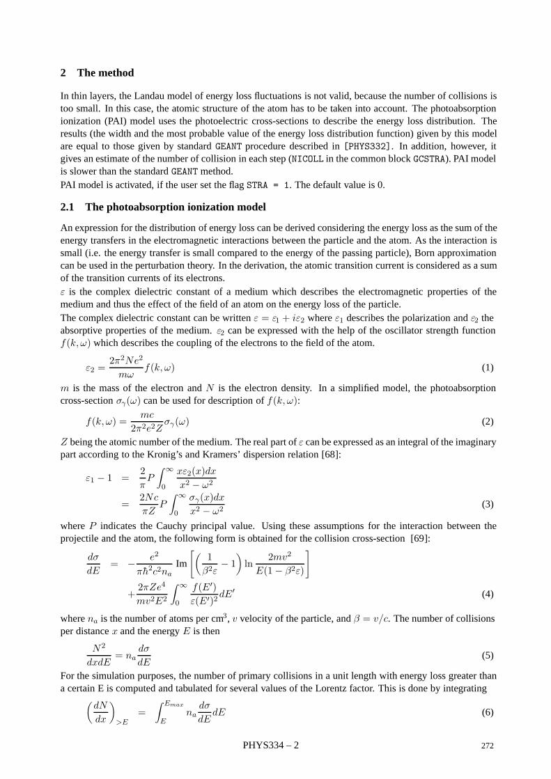
2 The method
In thin layers, the Landau model of energy loss fluctuations is not valid, because the number of collisions istoo small. In this case, the atomic structure of the atom has to be taken into account. The photoabsorptionionization (PAI) model uses the photoelectric cross-sections to describe the energy loss distribution. Theresults (the width and the most probable value of the energy loss distribution function) given by this modelare equal to those given by standard GEANT procedure described in [PHYS332]. In addition, however, itgives an estimate of the number of collision in each step (NICOLL in the common block GCSTRA). PAI modelis slower than the standard GEANT method.PAI model is activated, if the user set the flag STRA = 1. The default value is 0.
2.1 The photoabsorption ionization model
An expression for the distribution of energy loss can be derived considering the energy loss as the sum of theenergy transfers in the electromagnetic interactions between the particle and the atom. As the interaction issmall (i.e. the energy transfer is small compared to the energy of the passing particle), Born approximationcan be used in the perturbation theory. In the derivation, the atomic transition current is considered as a sumof the transition currents of its electrons.ε is the complex dielectric constant of a medium which describes the electromagnetic properties of themedium and thus the effect of the field of an atom on the energy loss of the particle.The complex dielectric constant can be written ε = ε1 + iε2 where ε1 describes the polarization and ε2 theabsorptive properties of the medium. ε2 can be expressed with the help of the oscillator strength functionf(k, ω) which describes the coupling of the electrons to the field of the atom.
ε2 =2π2Ne2
mωf(k, ω) (1)
m is the mass of the electron and N is the electron density. In a simplified model, the photoabsorptioncross-section σγ(ω) can be used for description of f(k, ω):
f(k, ω) =mc
2π2e2Zσγ(ω) (2)
Z being the atomic number of the medium. The real part of ε can be expressed as an integral of the imaginarypart according to the Kronig’s and Kramers’ dispersion relation [68]:
ε1 − 1 =2πP
∫ ∞
0
xε2(x)dxx2 − ω2
=2Nc
πZP
∫ ∞
0
σγ(x)dxx2 − ω2
(3)
where P indicates the Cauchy principal value. Using these assumptions for the interaction between theprojectile and the atom, the following form is obtained for the collision cross-section [69]:
dσ
dE= − e2
πh2c2naIm
[(1
β2ε− 1
)ln
2mv2
E(1− β2ε)
]
+2πZe4
mv2E2
∫ ∞
0
f(E′)ε(E′)2
dE′ (4)
where na is the number of atoms per cm3, v velocity of the particle, and β = v/c. The number of collisionsper distance x and the energy E is then
N2
dxdE= na
dσ
dE(5)
For the simulation purposes, the number of primary collisions in a unit length with energy loss greater thana certain E is computed and tabulated for several values of the Lorentz factor. This is done by integrating(
dN
dx
)>E
=∫ Emax
Ena
dσ
dEdE (6)
PHYS334 – 2 272
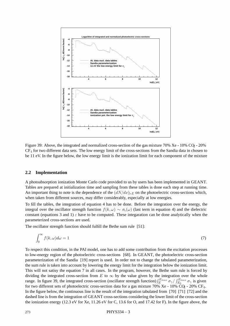
Logarithm of integrated and normalized photoelectric cross-sections
ln(E), [eV]
ln(∫
σ γ dE
/no
rm.f
acto
r)At. data nucl. data tablesSandia parameterization11 eV the low energy limit for σγ
ln(E), [eV]
ln(∫
σ γ dE
/no
rm.f
acto
r)
At. data nucl. data tablesSandia parameterizationionization pot. the low energy limit for σγ
-18
-16
-14
-12
-10
-8
-6
-4
4 6 8 10 12
-18
-16
-14
-12
-10
-8
-6
-4
4 6 8 10 12
Figure 39: Above, the integrated and normalized cross-section of the gas mixture 70% Xe - 10% CO2 - 20%CF4 for two different data sets. The low energy limit of the cross-sections from the Sandia data in chosen tobe 11 eV. In the figure below, the low energy limit is the ionization limit for each component of the mixture
2.2 Implementation
A photoabsorption ionization Monte Carlo code provided to us by users has been implemented in GEANT.Tables are prepared at initialization time and sampling from these tables is done each step at running time.An important thing to note is the dependence of the (dN/dx)>E on the photoelectric cross-sections which,when taken from different sources, may differ considerably, especially at low energies.
To fill the tables, the integration of equation 4 has to be done. Before the integration over the energy, theintegral over the oscillator strength function f(k, ω) ∼ σγ(ω) (last term in equation 4) and the dielectricconstant (equations 3 and 1) ε have to be computed. These integaration can be done analytically when theparameterized cross-sections are used.
The oscillator strength function should fulfill the Bethe sum rule [51]:∫ ∞
0f(k, ω)dω = 1 (7)
To respect this condition, in the PAI model, one has to add some contribution from the excitation processesto low-energy region of the photoelectric cross-sections [68]. In GEANT, the photoelectric cross-sectionparameterization of the Sandia [19] report is used. In order not to change the tabulated parameterization,the sum rule is taken into account by lowering the energy limit for the integration below the ionization limit.This will not satisy the equation 7 in all cases. In the program, however, the Bethe sum rule is forced bydividing the integrated cross-section from E to ∞ by the value given by the integration over the wholerange. In figure 39, the integrated cross-section (oscillator strength function)
∫ EmaxE σγ/
∫ EmaxE0
σγ is givenfor two different sets of photoelectric cross-section data for a gas mixture 70% Xe - 10% CO2 - 20% CF4.In the figure below, the continuous line is the result of the integration tabulated from [70] [71] [72] and thedashed line is from the integration of GEANT cross-sections considering the lower limit of the cross-sectionthe ionization energy (12.3 eV for Xe, 11.26 eV for C, 13.6 for O, and 17.42 for F). In the figure above, the
273 PHYS334 – 3
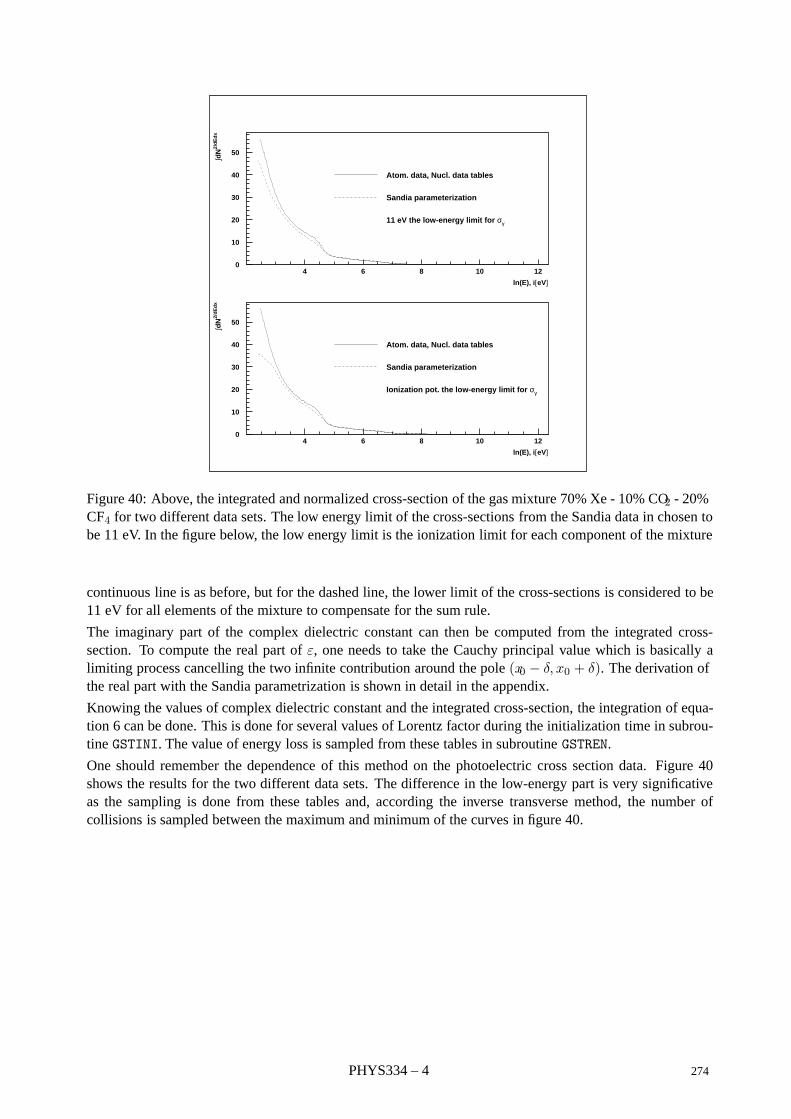
ln(E), i[eV]
∫dN
2/d
Ed
x
Atom. data, Nucl. data tables
Sandia parameterization
11 eV the low-energy limit for σγ
ln(E), i[eV]
∫dN
2/d
Ed
x
Atom. data, Nucl. data tables
Sandia parameterization
Ionization pot. the low-energy limit for σγ
0
10
20
30
40
50
4 6 8 10 12
0
10
20
30
40
50
4 6 8 10 12
Figure 40: Above, the integrated and normalized cross-section of the gas mixture 70% Xe - 10% CO2 - 20%CF4 for two different data sets. The low energy limit of the cross-sections from the Sandia data in chosen tobe 11 eV. In the figure below, the low energy limit is the ionization limit for each component of the mixture
continuous line is as before, but for the dashed line, the lower limit of the cross-sections is considered to be11 eV for all elements of the mixture to compensate for the sum rule.
The imaginary part of the complex dielectric constant can then be computed from the integrated cross-section. To compute the real part of ε, one needs to take the Cauchy principal value which is basically alimiting process cancelling the two infinite contribution around the pole (x0 − δ, x0 + δ). The derivation ofthe real part with the Sandia parametrization is shown in detail in the appendix.
Knowing the values of complex dielectric constant and the integrated cross-section, the integration of equa-tion 6 can be done. This is done for several values of Lorentz factor during the initialization time in subrou-tine GSTINI. The value of energy loss is sampled from these tables in subroutine GSTREN.
One should remember the dependence of this method on the photoelectric cross section data. Figure 40shows the results for the two different data sets. The difference in the low-energy part is very significativeas the sampling is done from these tables and, according the inverse transverse method, the number ofcollisions is sampled between the maximum and minimum of the curves in figure 40.
PHYS334 – 4 274
Geant 3.16 GEANT User’s Guide PHYS337
Origin : N.Van Eijndhoven Submitted: 26.07.93Revision : Revised: 16.12.93Documentation :
Birks’ saturation law
1 Subroutines
CALL GBIRK (EDEP)
EDEP (REAL) and on output the energy equivalent to the calorimeter response in the current step.
Organic scintillators are usually calibrated with particles whose energy is near the minimum ionisation(γβ ≈ 4). However, the energy response of such scintillators for large local energy deposit is attenuated.GBIRK returns the energy detected by the scintillator in the current step.
2 Method
The phenomenological description of the response attenuation of organic scintillators [73] is known asBirks’ law:
R =∆E
1 + C1δ +C2δ2δ =
1ρ
dE
dxMeV g−1 cm2 (1)
The values quoted in [74] for the parameters C1, C2 are:
C1 = 0.013 g MeV−1 cm−2 and C2 = 9.6× 10⁻⁶ g2 MeV−2 cm−4
These values have been measured for various scintillators. If the charge of the particle is greater than one, abetter description can be obtained by correcting C1:
C ′1 =
7.212.6
C1 ≈ 0.5714C1 (2)
The values of the parameters of Birks’ formula (if defined) are in the ZEBRA bank next to the material bank:
JTM = LQ(JMATE-NTMED) pointer to the current tracking medium bank;
JTMN = LQ(JTM) pointer to the next bank to the current material one, where the specific trackingmedium parameters are stored;
MODEL = Q(JTMN+27) flag controlling the correction (2) for multiply charged particles:
=1 correction is not applied;=1 correction is applied;
C1 = Q(JTMN+28) first parameter of the Birks’ formula;
C2 = Q(JTMN+29) second parameter of the Birks’ formula.
These parameters are set via the GSTPAR routine, with names BIRK1, BIRK2 and BIRK3, respectively. Forinstance, to define the standard Birks’ parameters for tracking medium ITM with correction for multiplycharged particles, one would have to insert the following piece of code, after the definition of trackingmedia but before the call to GPHYSI
CALL GSTPAR(ITM,’BIRK1’,1.)CALL GSTPAR(ITM,’BIRK2’,0.013)CALL GSTPAR(ITM,’BIRK3’,9.6E-6)
275 PHYS337 – 1

Geant 3.16 GEANT User’s Guide PHYS340
Origin : L. Urban Submitted: 28.05.86Revision : Revised: 16.12.93Documentation :
Total cross-section and energy loss for bremsstrahlung by e-e+
1 Subroutines
CALL GBRELA
GBRELA fills the tables for the energy loss of electrons, positrons and muons due to bremsstrahlung at initial-isation time for different materials. The energy binning is set within the array ELOW (common /CGMULO/) inthe routine GPHYSI. In the tables, the dE/dx due to bremsstrahlung is summed with that due to the ionisation.For energy loss of electrons and positrons, GBRELA calls the function GBRELE. Following pointers are used:
JMA = LQ(JMATE-I) pointer to the Ith material;
JEL1 = LQ(JMA-1) pointer to dE/dx for e−;
JEL1+NEK1 pointer to dE/dx for e+.
GBRELA is called at initialisation time by GPHYSI.
VALUE = GBRELE (ZZ,T,BCUT)
GBRELE calculates the energy loss due to bremsstrahlung of an electron with kinetic energy T in materialwith atomic number ZZ. It is called by GBRELA and for energies below the cut BCUT it adds the contributionof bremsstrahlung to. Above this cut, the bremsstrahlung process is simulated explicitly (see [PHYS341])and tabulation of these continuous losses is not needed. GBRELE is called by GBRELA.
VALUE = GBFLOS (T,C)
GBFLOS calculates a weight factor for the positron continuous bremsstrahlung energy loss. T is the kineticenergy in GeV of the positron and C is the energy cut for bremsstrahlung (BCUTE). The value is the ratioof the energy loss due to bremsstrahlung of the positron to that of the electron so that: <positron loss> =GBFLOS × <electron loss>. GBFLOS is called by GBRELA.
CALL GBRSGA
GBRSGA calculates the total cross-section for bremsstrahlung in all materials. It tabulates the mean freepath, λ = 1
Σ (in cm) as a function of medium and energy. The energy binning is set within the array ELOW(common /CGMULO/) in the routine GPHYSI. The following pointers are used:
JMA = LQ(JMATE-I) pointer to the Ith material
JBREM = LQ(JMA-9) pointer to bremsstrahlung cross-sections
JBREM pointer for e−
JBREM+NEK1 pointer for e+
JBREM+2*NEK1 pointer for µ+/µ−
GBRSGA is called at initialisation time by GPHYSI.
VALUE = GBRSGE (ZZ,T,BCUT)
GBRSGE calculates the total cross-section of bremsstrahlung of an electron with kinetic energy T in materialwith atomic number ZZ. It is called by GBRSGA. For kinetic energies which are below the cut BCUT or forwhich bremsstrahlung process is not simulated explicitly (see [PHYS341]) it returns 0.
276 PHYS340 – 1

VALUE = GBFSIG (T,C)
GBFSIG calculates a weight factor for the positron discrete (hard) bremsstrahlung cross section. T is thekinetic energy in GeV of the positron and C is the energy cut for bremsstrahlung (BCUTE). The value returnedis the ratio of the positron bremsstrahlung cross-section to that of the electron so that: ¡positron cross-section¿ = GBFSIG × ¡electron cross-section¿. GBFSIG is called by GBRSGA.
2 Method
Let’s call dσ(Z, T, k)/dk the differential cross-section for production of a photon of energy k by an electronof kinetic energy T in the field of an atom of charge Z , and kc the energy cut-off below which the softphotons are treated as continuous energy loss (BCUTE in the program). Then the mean value of the energylost by the electron due to soft photons is
EbremLoss (Z, T, kc) =
∫ kc
0kdσ(Z, T, k)
dkdk (1)
whereas the total cross-section for the emission of a photon of energy larger than kc is
σbrem(Z, T, kc) =∫ T
kc
dσ(Z, T, k)dk
dk (2)
Many theories of the bremsstrahlung process exist, each with its own limitations and regions of applicability.Perhaps the best synthesis of these theories can be found in the paper of S.M. Seltzer and M.J. Berger [75].The authors give a tabulation of the bremsstrahlung cross-section dσ/dk differential in the photon energy k,for electrons with kinetic energies T from 1 keV to 10 GeV. For electron energies above 10 GeV the screenedBethe-Heitler differential cross-section can be used [12, 35] together with the Midgal corrections [54, 76].The first of the two Migdal corrections is important for very high electron energies only (T ≥ 1 TeV) andhas the effect of reducing the cross-section. The second Migdal correction is effective even at “ordinary”energies (100 MeV – 1 GeV) and it decreases the differential cross-section at photon energies below acertain fraction of the incident electron energy (dσ/dk decreases significantly if k/T ≤ 10−4.)
2.1 Parameterisation of energy loss and total cross-section
Using the tabulated cross-section values of Seltzer and Berger together with the Migdal corrected Bethe-Heitler formula we have computed σ(Z, T, kc) and we have used these computed values as “data points” inthe fitting procedure. Calculating the “low energy” (T ≤ 10 GeV) data we have applied the second Midgalcorrection to the results of Seltzer and Berger. We have chosen the parameterisations:
σ(Z, T, kc) =Z(Z + ξσ)(T +m)2
T (T + 2m)[ln(T/kc)]αFσ(Z,X, Y ) (barn) (3)
and
EbremLoss (Z, T, kc) =
Z(Z + ξl)(T +m)2
(T + 2m)
[kcCM
T
]βFl(Z,X, Y ) (GeV barn) (4)
where m is the mass of the electron,
X = ln(E/m), Y = ln(vσE/kc) for the total cross-section σ
X = ln(T/m), Y = ln(kc/vlE) for the energy loss EbremLoss
with E = T +m. The constants ξσ, ξl, α, β, vσ, vl are parameters to be fitted.
CM =1
1 + nr0λ−2(T +m)2
πk2c
is the Midgal correction factor, with
PHYS340 – 2 277
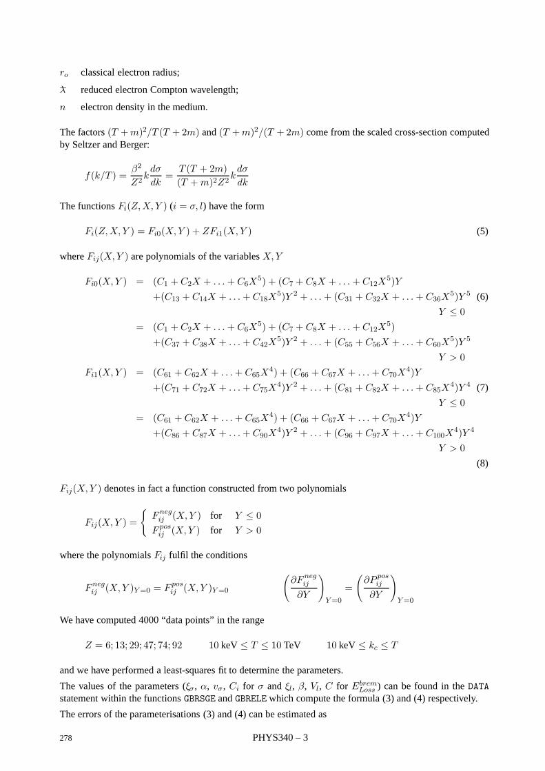
ro classical electron radius;
λ− reduced electron Compton wavelength;
n electron density in the medium.
The factors (T +m)2/T (T +2m) and (T +m)2/(T +2m) come from the scaled cross-section computedby Seltzer and Berger:
f(k/T ) =β2
Z2kdσ
dk=
T (T + 2m)(T +m)2Z2
kdσ
dk
The functions Fi(Z,X, Y ) (i = σ, l) have the form
Fi(Z,X, Y ) = Fi0(X,Y ) + ZFi1(X,Y ) (5)
where Fij(X,Y ) are polynomials of the variables X,Y
Fi0(X,Y ) = (C1 + C2X + . . .+ C6X5) + (C7 + C8X + . . . + C12X
5)Y+(C13 + C14X + . . .+ C18X
5)Y 2 + . . . + (C31 + C32X + . . .+ C36X5)Y 5 (6)
Y ≤ 0= (C1 + C2X + . . .+ C6X
5) + (C7 + C8X + . . . + C12X5)
+(C37 + C38X + . . .+ C42X5)Y 2 + . . . + (C55 + C56X + . . .+ C60X
5)Y 5
Y > 0Fi1(X,Y ) = (C61 + C62X + . . .+ C65X
4) + (C66 + C67X + . . .+ C70X4)Y
+(C71 + C72X + . . .+ C75X4)Y 2 + . . . + (C81 + C82X + . . .+ C85X
4)Y 4 (7)
Y ≤ 0= (C61 + C62X + . . .+ C65X
4) + (C66 + C67X + . . .+ C70X4)Y
+(C86 + C87X + . . .+ C90X4)Y 2 + . . . + (C96 + C97X + . . .+ C100X
4)Y 4
Y > 0(8)
Fij(X,Y ) denotes in fact a function constructed from two polynomials
Fij(X,Y ) =
Fnegij (X,Y ) for Y ≤ 0
F posij (X,Y ) for Y > 0
where the polynomials Fij fulfil the conditions
Fnegij (X,Y )Y=0 = F pos
ij (X,Y )Y=0
(∂Fneg
ij
∂Y
)Y=0
=
(∂P pos
ij
∂Y
)Y=0
We have computed 4000 “data points” in the range
Z = 6; 13; 29; 47; 74; 92 10 keV ≤ T ≤ 10 TeV 10 keV ≤ kc ≤ T
and we have performed a least-squares fit to determine the parameters.
The values of the parameters (ξσ, α, vσ, Ci for σ and ξl, β, Vl, C for EbremLoss ) can be found in the DATA
statement within the functions GBRSGE and GBRELE which compute the formula (3) and (4) respectively.
The errors of the parameterisations (3) and (4) can be estimated as
278 PHYS340 – 3
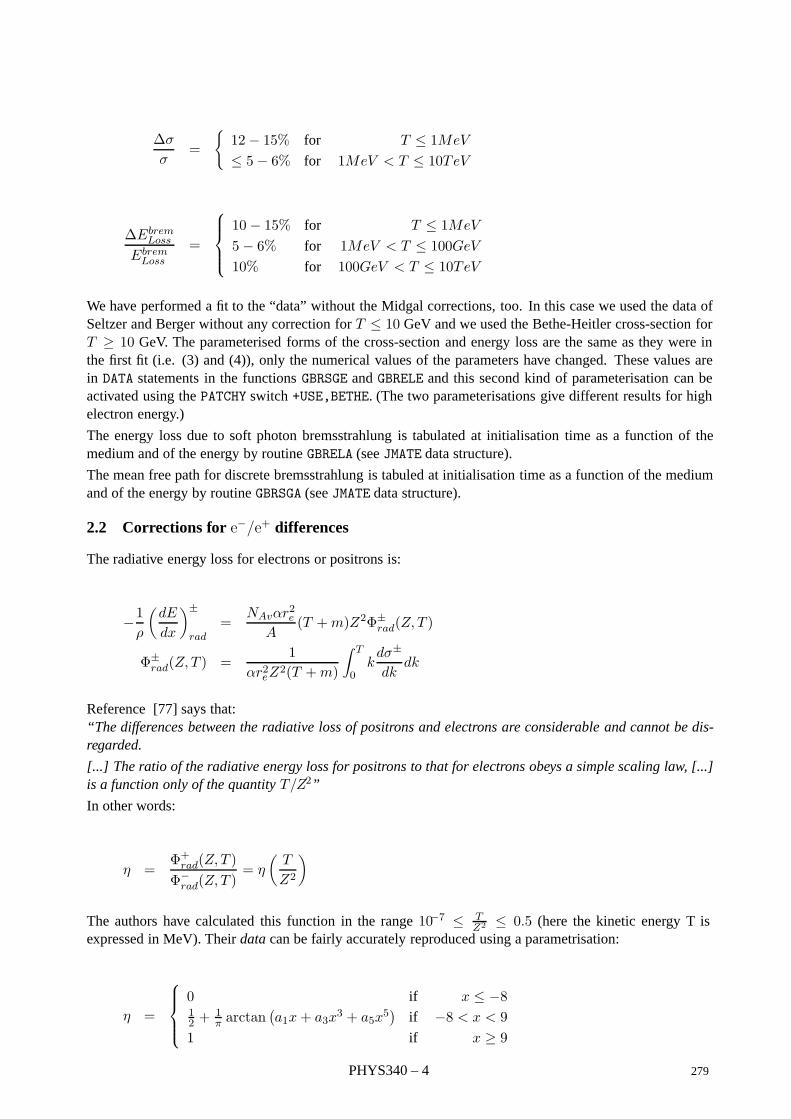
∆σ
σ=
12− 15% for T ≤ 1MeV
≤ 5− 6% for 1MeV < T ≤ 10TeV
∆EbremLoss
EbremLoss
=
10− 15% for T ≤ 1MeV
5− 6% for 1MeV < T ≤ 100GeV
10% for 100GeV < T ≤ 10TeV
We have performed a fit to the “data” without the Midgal corrections, too. In this case we used the data ofSeltzer and Berger without any correction for T ≤ 10 GeV and we used the Bethe-Heitler cross-section forT ≥ 10 GeV. The parameterised forms of the cross-section and energy loss are the same as they were inthe first fit (i.e. (3) and (4)), only the numerical values of the parameters have changed. These values arein DATA statements in the functions GBRSGE and GBRELE and this second kind of parameterisation can beactivated using the PATCHY switch +USE,BETHE. (The two parameterisations give different results for highelectron energy.)
The energy loss due to soft photon bremsstrahlung is tabulated at initialisation time as a function of themedium and of the energy by routine GBRELA (see JMATE data structure).
The mean free path for discrete bremsstrahlung is tabuled at initialisation time as a function of the mediumand of the energy by routine GBRSGA (see JMATE data structure).
2.2 Corrections for e−/e+ differences
The radiative energy loss for electrons or positrons is:
−1ρ
(dE
dx
)±
rad=
NAvαr2e
A(T +m)Z2Φ±
rad(Z, T )
Φ±rad(Z, T ) =
1αr2eZ
2(T +m)
∫ T
0kdσ±
dkdk
Reference [77] says that:“ The differences between the radiative loss of positrons and electrons are considerable and cannot be dis-regarded.
[...] The ratio of the radiative energy loss for positrons to that for electrons obeys a simple scaling law, [...]is a function only of the quantity T/Z2”
In other words:
η =Φ+rad(Z, T )Φ−
rad(Z, T )= η
(T
Z2
)
The authors have calculated this function in the range 10−7 ≤ TZ2 ≤ 0.5 (here the kinetic energy T is
expressed in MeV). Their data can be fairly accurately reproduced using a parametrisation:
η =
0 if x ≤ −812 +
1π arctan
(a1x+ a3x
3 + a5x5)
if −8 < x < 91 if x ≥ 9
PHYS340 – 4 279
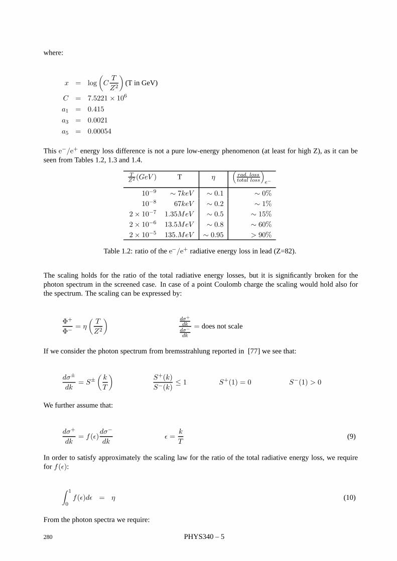
where:
x = log(C
T
Z2
)(T in GeV)
C = 7.5221 × 10⁶
a1 = 0.415a3 = 0.0021a5 = 0.00054
This e−/e+ energy loss difference is not a pure low-energy phenomenon (at least for high Z), as it can beseen from Tables 1.2, 1.3 and 1.4.
TZ2 (GeV ) T η
(rad. losstotal loss
)e−
10−9 ∼ 7keV ∼ 0.1 ∼ 0%10−8 67keV ∼ 0.2 ∼ 1%
2× 10⁻⁷ 1.35MeV ∼ 0.5 ∼ 15%2× 10⁻⁶ 13.5MeV ∼ 0.8 ∼ 60%2× 10⁻⁵ 135.MeV ∼ 0.95 > 90%
Table 1.2: ratio of the e−/e+ radiative energy loss in lead (Z=82).
The scaling holds for the ratio of the total radiative energy losses, but it is significantly broken for thephoton spectrum in the screened case. In case of a point Coulomb charge the scaling would hold also forthe spectrum. The scaling can be expressed by:
Φ+
Φ− = η
(T
Z2
) dσ+
dkdσ−dk
= does not scale
If we consider the photon spectrum from bremsstrahlung reported in [77] we see that:
dσ±
dk= S±
(k
T
)S+(k)S−(k)
≤ 1 S+(1) = 0 S−(1) > 0
We further assume that:
dσ+
dk= f(ε)
dσ−
dkε =
k
T(9)
In order to satisfy approximately the scaling law for the ratio of the total radiative energy loss, we requirefor f(ε):
∫ 1
0f(ε)dε = η (10)
From the photon spectra we require:
280 PHYS340 – 5
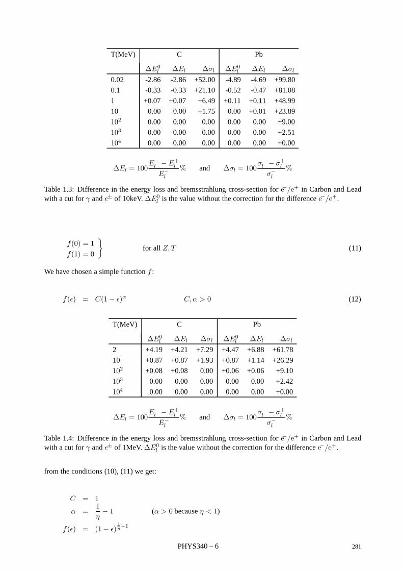
T(MeV) C Pb
∆E0l ∆El ∆σl ∆E0l ∆El ∆σl
0.02 -2.86 -2.86 +52.00 -4.89 -4.69 +99.80
0.1 -0.33 -0.33 +21.10 -0.52 -0.47 +81.08
1 +0.07 +0.07 +6.49 +0.11 +0.11 +48.99
10 0.00 0.00 +1.75 0.00 +0.01 +23.89
102 0.00 0.00 0.00 0.00 0.00 +9.00
103 0.00 0.00 0.00 0.00 0.00 +2.51
104 0.00 0.00 0.00 0.00 0.00 +0.00
∆El = 100E−
l − E+lE−
l
% and ∆σl = 100σ−l − σ+lσ−l
%
Table 1.3: Difference in the energy loss and bremsstrahlung cross-section for e−/e+ in Carbon and Leadwith a cut for γ and e± of 10keV. ∆E0l is the value without the correction for the difference e−/e+.
f(0) = 1f(1) = 0
for all Z, T (11)
We have chosen a simple function f :
f(ε) = C(1− ε)α C,α > 0 (12)
T(MeV) C Pb
∆E0l ∆El ∆σl ∆E0l ∆El ∆σl
2 +4.19 +4.21 +7.29 +4.47 +6.88 +61.78
10 +0.87 +0.87 +1.93 +0.87 +1.14 +26.29
102 +0.08 +0.08 0.00 +0.06 +0.06 +9.10
103 0.00 0.00 0.00 0.00 0.00 +2.42
104 0.00 0.00 0.00 0.00 0.00 +0.00
∆El = 100E−
l − E+lE−
l
% and ∆σl = 100σ−l − σ+lσ−l
%
Table 1.4: Difference in the energy loss and bremsstrahlung cross-section for e−/e+ in Carbon and Leadwith a cut for γ and e± of 1MeV. ∆E0l is the value without the correction for the difference e−/e+.
from the conditions (10), (11) we get:
C = 1
α =1η− 1 (α > 0 because η < 1)
f(ε) = (1− ε)1η−1
PHYS340 – 6 281
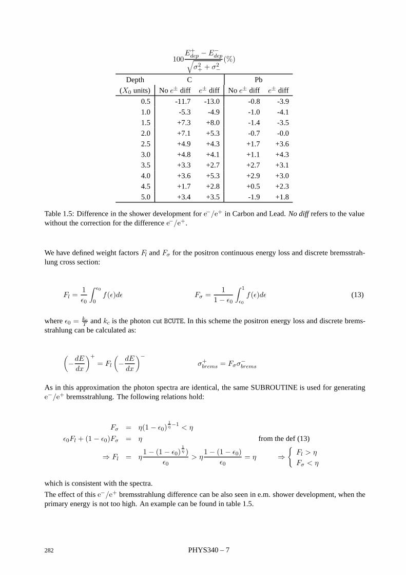
100E+dep − E−
dep√σ2+ + σ2−
(%)
Depth C Pb
(X0 units) No e± diff e± diff No e± diff e± diff
0.5 -11.7 -13.0 -0.8 -3.9
1.0 -5.3 -4.9 -1.0 -4.1
1.5 +7.3 +8.0 -1.4 -3.5
2.0 +7.1 +5.3 -0.7 -0.0
2.5 +4.9 +4.3 +1.7 +3.6
3.0 +4.8 +4.1 +1.1 +4.3
3.5 +3.3 +2.7 +2.7 +3.1
4.0 +3.6 +5.3 +2.9 +3.0
4.5 +1.7 +2.8 +0.5 +2.3
5.0 +3.4 +3.5 -1.9 +1.8
Table 1.5: Difference in the shower development for e−/e+ in Carbon and Lead. No diff refers to the valuewithout the correction for the difference e−/e+.
We have defined weight factors Fl and Fσ for the positron continuous energy loss and discrete bremsstrah-lung cross section:
Fl =1ε0
∫ ε0
0f(ε)dε Fσ =
11− ε0
∫ 1
ε0f(ε)dε (13)
where ε0 = kcT and kc is the photon cut BCUTE. In this scheme the positron energy loss and discrete brems-
strahlung can be calculated as:
(−dE
dx
)+= Fl
(−dE
dx
)−σ+brems = Fσσ
−brems
As in this approximation the photon spectra are identical, the same SUBROUTINE is used for generatinge−/e+ bremsstrahlung. The following relations hold:
Fσ = η(1 − ε0)1η−1 < η
ε0Fl + (1− ε0)Fσ = η from the def (13)
⇒ Fl = η1− (1− ε0)
1η )
ε0> η
1− (1− ε0)ε0
= η ⇒
Fl > η
Fσ < η
which is consistent with the spectra.
The effect of this e−/e+ bremsstrahlung difference can be also seen in e.m. shower development, when theprimary energy is not too high. An example can be found in table 1.5.
282 PHYS340 – 7
Geant 3.16 GEANT User’s Guide PHYS341
Origin : G.N. Patrick, L.Urban Submitted: 26.10.84Revision : Revised: 16.12.93Documentation :
Simulation of discrete bremsstrahlung by electrons
1 Subroutines
CALL GBREME
GBREME generates a bremsstrahlung photon from an electron as a discrete process. The photon energyis sampled from a parameterisation of the bremsstrahlung cross-section of Seltzer and Berger [75] forelectron energies below 10 GeV, and from the screened Bethe-Heitler cross-section above 10 GeV. Midgalcorrections are applied in both cases. The angular distribution of the photon is calculated by the functionGBTETH.
Input : via common block /GCTRAK/
Output: via common block /GCKING/.GBREME is called from the tracking routine GTELEC when the parent electron reaches a radiation point duringtracking.
THETA = GBTETH (ENER,PARTM,EFRAC)
THETA (REAL) angle of the radiated photon or e± pair;
ENER (REAL) energy of the particle;
PARTM (REAL) mass of the particle;
EFRAC (REAL) ratio between the energy of the photon and the energy of the particle.
GBTETH calculates the angular distribution of the e+e−-pair in photon pair production and of the emittedphoton in µ and e± bremsstrahlung. GBTETH is called by GBREME.
2 Method
The photon energy is sampled according to the Seltzer and Berger bremsstrahlung spectrum [75]. Seltzerand Berger have calculated the spectra for materials with atomic numbers Z = 6,13,29,47,74,92 in theelectron (kinetic) energy range 1 keV - 10 GeV. Their tabulated results have been used as input in aparametrising-fitting procedure. The functional form of the parameterisation for the quantity:
S(x) = Ckdσ
dk
can be written as
S(x) =
(1− ahε)F1(δ) + bhε
2F2(δ) T ≥ 1MeV
1 + alx+ blx2 T < 1MeV
(1)
where:
C normalisation constant k photon energy
T,E kinetic and total energy of the primary electron x =k
T
ε =k
E= x
T
E
283 PHYS341 – 1
The Fi(δ) screening functions depend on the screening variable:
δ =136me
Z1/3E
ε
1− εF1(δ) = F0(42.392 − 7.796δ + 1.961δ2 − F ) δ ≤ 1F2(δ) = F0(41.734 − 6.484δ + 1.250δ2 − F ) δ ≤ 1F1(δ) = F2(δ) = F0(42.24 − 8.368 ln(δ + 0.952) − F ) δ > 1
F0 =1
42.392 − FF = 4 lnZ − 0.55(lnZ)2
ah,l and bh,l are parameters to be fitted.
The ‘high energy’ (T > 1 MeV) formula comes from the Coulomb-corrected, sceened Bethe-Heitler formula(see e.g. [78, 10, 12]). However, there are two things in eq. (1) which make a difference:
1. ah, bh depend on T and on the atomic number Z ( in the case of the Bethe-Heitler spectrum ah = 1,bh = 0.75);
2. the function F is not the same than that in the Bethe-Heitler cross-section, this function gives a betterbehaviour in the high frequency limit, i.e. when k → T (x → 1).
The T and Z dependence of the parameters are described by the equations:
ah = 1 +ah1u+
ah2u2
+ah3u3
bh = 0.75 +bh1u+
bh2u2
+bh3u3
al = al0 + al1u+ al2u2
bl = bl0 + bl1u+ bl2u2
with
u = ln(
T
me
)
the ahi, bhi, ali, bli parameters are polynomials of second order in the variable:
v = [Z(Z + 1)]1/3
It can be seen relatively easily that for the limiting case T → ∞, ah → 1, bh → 0.75, so eq. (1) gives theBethe-Heitler cross section.
There are altogether 36 linear parameter in the formulae , their values are given in GBREME. The parameter-isation reproduces the Seltzer-Berger tables within a few % (2-3 % on average, the maximum error beingless than 10-12 %), the tables, on the other hand, agree well with the experimental data and theoretical (low-and high-energy) results (less than 10 % below 50 MeV, less than 5 % above 50 MeV).
Apart from the normalisation the cross section differential in photon energy can be written as:
dσ
dk=
1ln 1
xc
1xg(x) =
1ln 1
xc
1x
S(x)Smax
where xc = kc/T , kc is the photon cut-off energy below which the bremsstrahlung is treated as a continuousenergy loss (this cut is BCUTE in the program). Using this decomposition of the cross section and two randomnumbers r1, r2 uniformly distributed in ]0, 1[, the sampling of x is done as follows:
PHYS341 – 2 284
1. sample x from
1ln 1
xc
1x
setting x = er1 lnxc
2. calculate the rejection function g(x) and:
• if r2 > g(x) reject x and go back to 1;
• if r2 ≤ g(x) accept x.
To apply the Migdal correction [76] all it has to be done is to multiply the rejection function by the Migdalcorrection factor:
CM (ε) =1 + C0/ε
2c
1 + C0/ε2
where
C0 =nr0λ−
2
π, εc =
kcE
n electron density in the medium
r0 classical electron radius
λ− reduced Compton wavelength of the electron.
This correction decreases the cross-section for low photon energy.
After the successful sampling of ε, GBREME generates the polar angles of the radiated photon with respectto the parent electron’s momentum. It is difficult to find in the literature simple formulas for this angle. Forexample the double differential cross section reported by Tsai [13, 14] is the following:
dσ
dkdΩ=
2α2e2
πkm4
[2ε− 2(1 + u2)2
+12u2(1− ε)(1 + u2)4
]Z(Z + 1)
+
[2− 2ε− ε2
(1 + u2)2− 4u2(1− ε)(1 + u2)4
] [X − 2Z2fc((αZ)2)
]
u =Eθ
m
X =∫ m2(1+u2)2
tmin
[Gel
Z (t) +GinZ (t)
] t− tmin
t2dt
Gel,inZ (t) atomic form factors
tmin =
[km2(1 + u2)2E(E − k)
]2=
[εm2(1 + u2)2E(1 − ε)
]2
This distribution is complicated to sample, and it is anyway only an approximation to within few percent,if nothing else, due to the presence of the atomic form-factors. The angular dependence is contained in thevariable u = Eθm−1. For a given value of u the dependence of the shape of the function on Z , E, ε = k/Eis very weak. Thus, the distribution can be approximated by a function
f(u) = C(ue−au + due−3au
)(2)
where
C =9a2
9 + da = 0.625 d = 0.13
(0.8 +
1.3Z
)(100 +
1E
)(1 + ε)
285 PHYS341 – 3
P =∫ ∞
umax
f(u) du
E (MeV) P(%)
0.511 3.4
0.6 2.2
0.8 1.2
1.0 0.7
2.0 < 0.1
Table 1.6: Angular sampling efficiency
where E is in GeV. While this approximation is good at high energies, it becomes less accurate around fewMeV. However in that region the ionisation losses dominate over the radiative losses.
The sampling of the function f(u) can be done in the following way (ri, i = 1, 2, 3 are uniformly distributedrandom numbers in [0,1]):
1. Choose between ue−au and due−3au:
b =
a if r1 < 9/(9 + d)3a if r1 ≥ 9/(9 + d)
2. Sample ue−bu:
u = − log(r2r3)b
3. check that:
u ≤ umax =Eπ
m
otherwise go back to 1.
The probability of failing in the last test is reported in table 1.6.
The function f(u) can be used also to describe the angular distribution of the photon in µ bremsstrahlungand to describe the angular distribution in photon pair production.
The azimuthal angle, Φ, is generated isotropically. This information is used to calculate the momentumvector of the radiated photon, to transform it to the GEANT coordinate system and to store the result intocommon block /GCKING/. Also, the momentum of the parent electron is updated.
2.1 Restrictions
1. Target materials composed of compounds or mixtures are treated identically to elements using theeffective atomic number Z calculated in GSMIXT (this is not correct when computing the mean freepath!).
PHYS341 – 4 286
Geant 3.16 GEANT User’s Guide PHYS350
Origin : L.Urban Submitted: 26.10.84Revision : G.Azuelos Revised: 16.12.93Documentation :
Total cross-section for e+e- annihilation
1 Subroutines
CALL GANNII
GANNII tabulates the mean free path at initialisation as a function of the medium and of the energy (seeJMATE data structure). The energy binning is set within the array ELOW (common block /GCMULO/) in theroutine GPHYSI. GANNII is called from GPHYSI.
2 Method
For the annihilation into two photons the cross-section formula of Heitler is used. The total cross-section isgiven by [12, 79]
σ2γ(Z,E) =Zπr20γ + 1
[γ2 + 4γ + 1
γ2 − 1 ln(γ +
√γ2 − 1
)− γ + 3√
γ2 − 1
](1)
r0 = classical electron radius
For compounds, the cross-section is calculated using an effective atomic number as explained in [PHYS010].
Positrons can annihilate in a single photon if the electron with which it interacts is bound to a nucleus. Thetotal cross-section for such a process is
σ1γ(Z,E) = 4πr20α4 Z5
γβ(γ + 1)2
[γ2 +
23γ +
43+
γ + 2γβ
ln(γ + γβ)]
(2)
α = fine structure constant
In the derivation of this formula, only the interactions with the K-shell electrons are taken into account. Asthe cross-section depends on Z5, a special value of Zeff is computed in GPROBI:
Zeff =∑i
piAi
Z5 (3)
The notation of [PHYS010] is used.
The total cross-section for the positron annihilation is σ = σ2γ + σ1γ . The value of σ1γ is at it largest forheavy materials, for example, it is ∼ 20 % of σ for a positron of 440 keV of kinetic energy in lead. Forlower and higher energies the probability is lower.
287 PHYS350 – 1
Geant 3.16 GEANT User’s Guide PHYS351
Origin : L.Urban Submitted: 26.10.84Revision : G.Azuelos Revised: 16.12.93Documentation :
Simulation of e+e- annihilation
1 Subroutines
CALL GANNI
GANNI generates the annihilation of a positron into either one or two photons. It uses the following inputand output:
input: via common /GCTRAK/
output: via common /GCKING/
The routine is called automatically from the tracking routine GTELEC, when the positron reaches its interac-tion point during the tracking.
CALL GANNIR
GANNIR generates the positron annihilation at rest. It is called from the tracking routine GTELEC, if thepositron energy is below the cut-off energy CUTELE in common block /GCCUTS/.
2 Method
The type of annihilation is sampled from the total cross-sections for the annihilation into two photons andinto one photon (see section [PHYS350]).
Annihilation into two photons
The differential cross-section of the two-photon positron-electron annihilation can be written as [79, 12]:
dσ(Z, ε)dε
= m a[S(aε) + S(a(1− ε))] (1)
where m is the electron mass Z is the atomic number of the material. If we indicate with E the initialenergy of the positron, with r0 the classical electron radius and with k the energy of the less energeticphoton generated, we have:
γ =E
ma = γ + 1
ε =k
E +mS(x) = C1
[−1 + C2
x− 1
x2
]C1 =
Zπr20a(E −m)
C2 = a+eγ
a
The kinematical limits for the variable ε are:
ε0 =1
a+√γ2 − 1
≤ ε ≤ 12
288 PHYS351 – 1
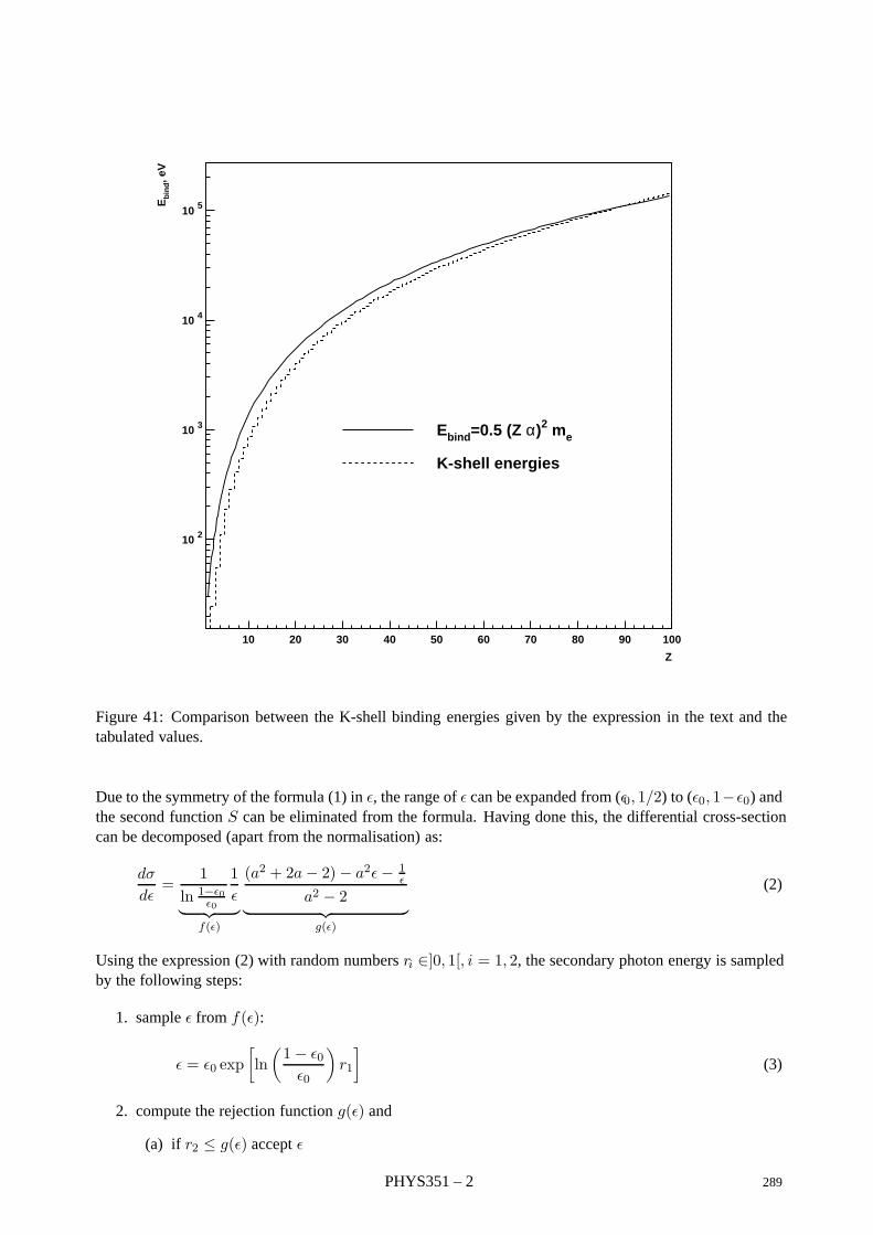
10 2
10 3
10 4
10 5
10 20 30 40 50 60 70 80 90 100
Ebind=0.5 (Z α)2 me
K-shell energies
Z
Eb
ind, e
V
Figure 41: Comparison between the K-shell binding energies given by the expression in the text and thetabulated values.
Due to the symmetry of the formula (1) in ε, the range of ε can be expanded from (ε0, 1/2) to (ε0, 1−ε0) andthe second function S can be eliminated from the formula. Having done this, the differential cross-sectioncan be decomposed (apart from the normalisation) as:
dσ
dε=
1ln 1−ε0
ε0
1ε︸ ︷︷ ︸
f(ε)
(a2 + 2a− 2)− a2ε− 1ε
a2 − 2︸ ︷︷ ︸g(ε)
(2)
Using the expression (2) with random numbers ri ∈]0, 1[, i = 1, 2, the secondary photon energy is sampledby the following steps:
1. sample ε from f(ε):
ε = ε0 exp[ln(1− ε0ε0
)r1
](3)
2. compute the rejection function g(ε) and
(a) if r2 ≤ g(ε) accept ε
PHYS351 – 2 289
(b) if r1 > g(ε) go back to 1.
After the successful sampling of ε, the photon energy is computed as
k = (E +m)ε (4)
and then GANNI generates the polar angles of the photon with respect to an axis defined by the momentumof the positron. The azimuthal angle Φ is generated isotropically and Θ is computed from the energy-momentum conservation. With this information, the momentum vector of both photons can be calculatedand transformed into the GEANT coordinate system.
The routine GANNIR treates the special case when a positron falls below the cut-off energy (CUTELE in com-mon block /GCCUTS/) before annihilating. In this case, it is assumed that the positron comes to rest beforeannihilating. GANNIR generates two photons with energy k = m. The angular distribution is isotropic.
Annihilation into one photon
The generated photon is assumed to be collinear with the positron. Its energy will be
k = E +me − Ebind (5)
where Ebind is the binding energy of the K-shell electron. It can be estimated as follows
Ebind = 0.5(Z α)2me (6)
where α is the fine stucture constant. The comparison of this expression with the experimental data from[80] is shown in figure 41.
3 Restrictions
1. The annihilation processes producing three or more photons are ignored, because these processes arenegligible compared to the annihilation into two photons [12, 54];
2. In calculating the process it is assumed that the atomic electron initially is free and at rest. This is theusual assumption used in shower programs [12];
290 PHYS351 – 3
Geant 3.16 GEANT User’s Guide PHYS360
Origin : I.Gavrilenko Submitted: 17.11.93Revision : Revised: 16.12.93Documentation : K.Lassila-Perini, I.Gavrilenko
Synchrotron radiation
1 Subroutines
CALL GSYNC
GSYNC is called for electron and positrons when the flag ISYNC is set > 0. It computes the magnetic fieldand calls GSYNGE for the generation of the synchrotron radiation photons. It reads them in the GEANT stack.GSYNC is called from GTELEC.
CALL GSYNGE (GAMMA,AMASS,FLDT,STEP,NTR,ETR,STR)
GSYNGE generates the synchrotron radiation for an e− or e+ with the Lorentz factor GAMMA in the magneticfield FLDT and when the step length is STEP. The number of the secondary photons is NTR, their energy isin the array ETR and their position along the step is in STR. GSYNGE is called by GSYNC.
2 Method
A charged particle in a magnetic field emits radiation. The number of photons emitted in a second is
d2N
dεdt=15√3
8P
εc(1)
where εc is the critical photon energy (the median of the energy spectrum) and P the total radiated power:
εc =32hc
γ3
ρ(2)
P =23e2c
ρ2β4γ4 (3)
γ is the e−/e+ Lorentz factor Etot/me and β = 1 − 1/γ2. ρ is the curvature caused by the magnetic field.For more detailed derivation of these equations, see [81]. The velocity of the particle being βc, the numberof photons per meter is
d2N
dεdx=
d2N
dεdt
1βc
=5√36
e2
hcβ3γ
1ρ
=52√3αγ
ρ≈ 0.01053
γ
ρ(4)
The fine structure constant α = e2/(hc) and it is assumed that β3 ≈ 1.
The curvature in a magnetic field B which has a component B⊥ transversal to the particle velocity can becomputed [55]
ρ =p
0.3B⊥(5)
291 PHYS360 – 1
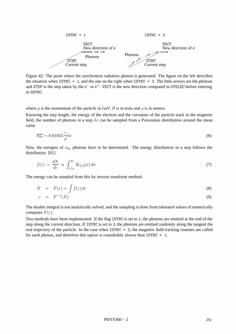
ISYNC = 1
STEPCurrent step
VECTNew direction of e
Photons
ISYNC = 3
STEPCurrent step
VECTNew direction of e
Photons
Figure 42: The point where the synchrotron radiation photon is generated. The figure on the left describesthe situation when ISYNC = 1, and the one on the right when ISYNC = 3. The little arrows are the photonsand STEP is the step taken by the e− or e+. VECT is the new direction computed in GTELEC before enteringin GSYNC.
where p is the momentum of the particle in GeV. B is in tesla and ρ is in meters.
Knowing the step length, the energy of the electron and the curvature of the particle track in the magneticfield, the number of photons in a step δx can be sampled from a Poissonian distribution around the meanvalue
nδx = 0.01053γ
ρδx (6)
Now, the energies of nδx photons have to be determined. The energy distribution in a step follows thedistribution [81]
f(ε) =dN
dε∝
∫ ∞
ε/εc
K5/3(x) dx (7)
The energy can be sampled from this by inverse transform method:
N = F (ε) =∫
f(ε) dε (8)
ε = F−1(N) (9)
The double integral is not analytically solved, and the sampling is done from tabulated values of numericallycomputes F (ε).Two methods have been implemented. If the flag ISYNC is set to 1, the photons are emitted at the end of thestep along the current direction. If ISYNC is set to 3, the photons are emitted randomly along the tangent thereal trajectory of the particle. In the case when ISYNC = 3, the magnetic field tracking routines are calledfor each photon, and therefore this option is considrably slower than ISYNC = 1.
PHYS360 – 2 292

Geant 3.16 GEANT User’s Guide PHYS400
Origin : G.N.Patrick Submitted: 30.03.82Revision : Revised: 16.12.93Documentation :
Simulation of particle decays in flight
1 Subroutines
CALL GDECAY
GDECAY is the control routine for the simulation of particle decays in flight. For a given parent particle itselects from a list a two- or three-body decay mode using the known branching ratios and calls the routinesneeded to generate the vertex and secondary tracks. It used the following input and output:
input: via common blocks /GCTRAK/ and /GCKINE/
output: via common block /GCKING/
GDECAY is called by the tracking routines. It calls the subroutines GDECA2 for two-body decay, GDECA3 forthree-body decay, GLOREN for Lorentz transformation and GDROT for rotation. For the documentation ofGLOREN and GDROT, see [PHYS410].
CALL GDECA2 (XM0,XM1,XM2,PCM)
XM0 (REAL) mass of the parent particle
XM1 (REAL) mass of the first decay product
XM2 (REAL) mass of the second decay product
PCM(3,4) (REAL) array containing the four-vectors of the decay products
GDECA2 simulates the two-body decay with isotropic angular distribution in the center-of-mass system. It iscalled from GDECAY.
CALL GDECA3 (XM0,XM1,XM2,XM3,PCM)
XM0 (REAL) mass of the parent particle
XM1 (REAL) mass of the first decay product
XM2 (REAL) mass of the second decay product
XM3 (REAL) mass of the third decay product
PCM(3,4) (REAL) array containing the four-vectors of the decay products
GDECA3 simulates the three-body decay with isotropic angular distribution in the center-of-mass system. Itis called from GDECAY.
293 PHYS400 – 1
2 Method
• Upon entry to GDECAY a binary search is made in a list of parent particles. This list is stored inthe JPART structure and currently contains the particles defined in GPART [CONS300]. If the currentparticle cannot be found in the list, control is returned without any decay generation. Up to six decaymodes and their corresponding branching ratios are then extracted from the JPART data banks (see[CONS310]).
• A decay channel is selected according to the branching ratios. If the sum of the branching ratios for aparticle is not equal 100%, it is possible that no decay is selected.
• Depending on whether the two- or three-body decay is selected, either GDECA2 or GDECA3 is called togenerate the four-momenta of the decay products with isotropic angular distribution in the center-of-mass system.
• The momentum vectors of the decay products are transformed into the laboratory system and rotatedback into the GEANT coordinate frame. The kinematics of the products is stored in the common/GCKING/.
• When a particle decays and no branching ratio is defined, then GDECAY calls the user routine GUDCAY.
PHYS400 – 2 294
Geant 3.16 GEANT User’s Guide PHYS410
Origin : M. Hansroul Submitted: 01.09.76Revision : Revised: 16.12.93Documentation :
Rotations and Lorentz transformation
1 Subroutines
CALL GLOREN (BETA,PA,PB*)
GLOREN transforms the momentum and the energy from one Lorentz frame (A) to another (B). It uses thefollowing input and output:
BETA(4) (REAL) velocity components in light units of frame B in frame A, BETA(1. . .3) = 3β, BETA(4)=(1− β2)−1/2 = γ;
PA(4) (REAL) momentum components in the frame (A);
PB(4) (REAL) momentum components in the frame (B).
GLOREN is called from the routine GDECAY. The momentum 3pA and energy EA in reference frame A aretransformed into the momentum 3pB and energy EB in reference frame B which translates with velocity 3βwith respect to A:
EB = γ(EA − 3β · 3pA)
3pB = 3pA + γ3β
(γ3β · 3pAγ + 1
− EA
)
CALL GDROT (P*,COSTH,SINTH,COSPH,SINPH)
GDROT rotates a vector from one reference system to another.
P(3) (REAL) vector to rotate, overwritten on output;
COSTH (REAL) cosine of the polar angle;
SINTH (REAL) sine of the polar angle;
COSPH (REAL) cosine of the azimuthal angle;
SINPH (REAL) sine of the azimuthal angle;
GDROT is called from several routines to rotate a particle from in the center-of-mass system to the GEANT(laboratory) system. The following rotation matrix is used:
cos θ cosφ − sinφ sin θ cosφcos θ sinφ cosφ sin θ sinφ− sin θ 0 cos θ
=
cosφ − sinφ 0sinφ cosφ 00 0 1
︸ ︷︷ ︸Rφ
cos θ 0 sin θ0 1 0
− sin θ 0 cos θ
︸ ︷︷ ︸Rθ
Rθ is a counterclockwise rotation around axis y by an angle θ, and Rφ is a counterclockwise rotation aroundaxis z′ (rotated by an angle θ from the initial position) by an angle φ.
295 PHYS410 – 1
CALL GFANG (P,COSTH*,SINTH*,COSPH*,SINPH*,ROTATE*)
P(3) (REAL) input direction;
COSTH (REAL) cosine of the polar angle;
SINTH (REAL) sine of the polar angle;
COSPH (REAL) cosine of the azimuthal angle;
SINPH (REAL) sine of the azimuthal angle;
ROTATE (LOGICAL) rotation flag, the rotation matrix is the unit matrix if ROTATE=.FALSE., i.e. norotation is needed;
Find the sine and cosine of the polar and azimuthal angle of the direction defined by the vector P. If P isalong the z axis, ROTATE=.FALSE..
CALL GVROT (DCOSIN,PART*)
PART(3) (REAL) direction to be rotated, overwritten on output;
DCOSIN(3) (REAL) direction of the new z axis;
Given the direction PART in a system of reference O, it returns the same direction in the system of referencewhere the z axis of O is along DCOSIN. This routine is very useful when the θ angle of a secondary particleis sampled in a reference frame where the parent particle moves along the z axis. Then the direction of thesecondary product in the MRS is returned by GVROT if DCOSIN is the direction of the parent particle.
A call to GVROT is equivalent to the following code:
DIMENSION PART(3), DCOSIN(3)LOGICAL ROTATE...CALL GFANG(DCOSIN,COSTH,SINTH,COSPH,SINPH,ROTATE)IF(ROTATE) CALL GDROT(PART,COSTH,SINTH,COSPH,SINPH)
with the advantage that inside GVROT all calculations are performed in double precision.
PHYS410 – 2 296
Geant 3.16 GEANT User’s Guide PHYS430
Origin : G.N.Patrick, L.Urban, D.Ward Submitted: 12.03.82Revision : Revised: 16.12.93Documentation :
Ionisation processes for muons and protons
1 Subroutines
CALL GDRELA
GDRELA initialises the ionisation energy-loss tables for different materials and particles. The energy binningis in the array ELOW (/GCMULO/) initialised in the routine GPHYSI. The tables are filled with the quantitydE/dx in GeV cm−1, for elements, mixtures and compounds. A temporary table is also filled, containingadditional points for integration, to obtain the range-energy table (see [PHYS010]).
GDRELP computes the ionisation energy loss for protons, and the values are stored in the energy loss table.This value is used for other charged hadrons with scaled energy bin.
GDRELM computes the ionisation energy loss for muons, and sums it in the muon table with the energy lossdue to the other processes (bremsstrahlung, pair production and nuclear interactions).
The following pointers are used:
JMA = LQ(JMATE-I) Ith material bank;
JEL1 = LQ(JMA-1) dE/dx for e+/e−(see [PHYS330]);
JEL2 = LQ(JMA-2) dE/dx for µ+/µ−;
JEL3 = LQ(JMA-3) dE/dx for protons (used also for other charged particles).
GDRELA is called during initialisation by GPHYSI.
CALL GDRELP (A,Z,DENS,T,DEDX*)
GDRELP computes the ionisation energy loss for protons. It is called by the routine GDRELA. See GDRELXbelow for the meaning of the parameters.
CALL GDRELM (A,Z,DENS,T,DEDX*)
GDRELM computes the energy loss due to ionisation for muons. It is called by the routine GDRELA. SeeGDRELX below for the meaning of the parameters.
CALL GDRELX (A,Z,DENS,T,HMASS,DEDX*)
A (REAL) mass number of the material;
Z (REAL) atomic number of the material;
DENS (REAL) density of the material in g cm−3; it is only used to calculate the density correction incase of high values of T;
T (REAL) kinetic energy of the particle in GeV;
HMASS (REAL) mass of the particle;
DEDX (REAL) energy loss of the particle in GeV cm2 g−1.
This routine calculates the ionisation energy loss for a muon or a proton. It is called by GDRELM and GDRELP.
297 PHYS430 – 1
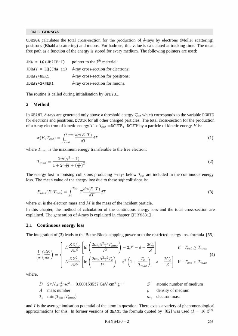
CALL GDRSGA
CDRSGA calculates the total cross-section for the production of δ-rays by electrons (Moller scattering),positrons (Bhabha scattering) and muons. For hadrons, this value is calculated at tracking time. The meanfree path as a function of the energy is stored for every medium. The following pointers are used:
JMA = LQ(JMATE-I) pointer to the Ith material;
JDRAY = LQ(JMA-11) δ-ray cross-section for electrons;
JDRAY+NEK1 δ-ray cross-section for positrons;
JDRAY+2*NEK1 δ-ray cross-section for muons.
The routine is called during initialisation by GPHYSI.
2 Method
In GEANT, δ-rays are generated only above a threshold energy Tcut which corresponds to the variable DCUTEfor electrons and positrons, DCUTM for all other charged particles. The total cross-section for the productionof a δ-ray electron of kinetic energy T > Tcut =DCUTE, DCUTM by a particle of kinetic energy E is:
σ(E,Tcut) =∫ Tmax
Tcut
dσ(E,T )dT
dT (1)
where Tmax is the maximum energy transferable to the free electron:
Tmax =2m(γ2 − 1)
1 + 2γ mM +
(mM
)2 (2)
The energy lost in ionising collisions producing δ-rays below Tcut are included in the continuous energyloss. The mean value of the energy lost due to these soft collisions is:
Eloss(E,Tcut) =∫ Tcut
0Tdσ(E,T )
dTdT (3)
where m is the electron mass and M is the mass of the incident particle.
In this chapter, the method of calculation of the continuous energy loss and the total cross-section areexplained. The generation of δ-rays is explained in chapter [PHYS331].
2.1 Continuous energy loss
The integration of (3) leads to the Bethe-Block stopping power or to the restricted energy loss formula [55]:
1ρ
(dE
dx
)=
DZZ2incAβ2
[ln
(2meβ
2γ2Tmax
I2
)− 2β2 − δ − 2Ce
Z
]if Tcut ≥ Tmax
DZZ2incAβ2
[ln
(2meβ
2γ2Tc
I2
)− β2
(1 +
Tc
Tmax
)− δ − 2Ce
Z
]if Tcut < Tmax
(4)
where,
D 2πNAr2emc2 = 0.000153537 GeV cm2 g−1 Z atomic number of medium
A mass number ρ density of medium
Tc min(Tcut, Tmax) me electron mass
and I is the average ionisation potential of the atom in question. There exists a variety of phenomenologicalapproximations for this. In former versions of GEANT the formula quoted by [82] was used (I = 16 Z0.9
PHYS430 – 2 298
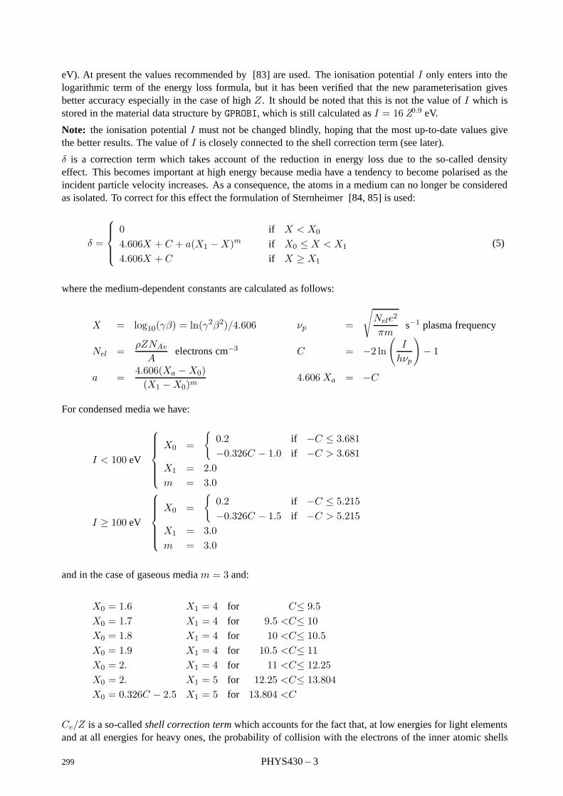
eV). At present the values recommended by [83] are used. The ionisation potential I only enters into thelogarithmic term of the energy loss formula, but it has been verified that the new parameterisation givesbetter accuracy especially in the case of high Z . It should be noted that this is not the value of I which isstored in the material data structure by GPROBI, which is still calculated as I = 16 Z0.9 eV.
Note: the ionisation potential I must not be changed blindly, hoping that the most up-to-date values givethe better results. The value of I is closely connected to the shell correction term (see later).
δ is a correction term which takes account of the reduction in energy loss due to the so-called densityeffect. This becomes important at high energy because media have a tendency to become polarised as theincident particle velocity increases. As a consequence, the atoms in a medium can no longer be consideredas isolated. To correct for this effect the formulation of Sternheimer [84, 85] is used:
δ =
0 if X < X0
4.606X + C + a(X1 −X)m if X0 ≤ X < X1
4.606X + C if X ≥ X1
(5)
where the medium-dependent constants are calculated as follows:
X = log10(γβ) = ln(γ2β2)/4.606 νp =
√Nele2
πms−1 plasma frequency
Nel =ρZNAv
Aelectrons cm−3 C = −2 ln
(I
hνp
)− 1
a =4.606(Xa −X0)(X1 −X0)m
4.606Xa = −C
For condensed media we have:
I < 100 eV
X0 =
0.2 if −C ≤ 3.681−0.326C − 1.0 if −C > 3.681
X1 = 2.0m = 3.0
I ≥ 100 eV
X0 =
0.2 if −C ≤ 5.215−0.326C − 1.5 if −C > 5.215
X1 = 3.0m = 3.0
and in the case of gaseous media m = 3 and:
X0 = 1.6 X1 = 4 for C≤ 9.5X0 = 1.7 X1 = 4 for 9.5 <C≤ 10X0 = 1.8 X1 = 4 for 10 <C≤ 10.5X0 = 1.9 X1 = 4 for 10.5 <C≤ 11X0 = 2. X1 = 4 for 11 <C≤ 12.25X0 = 2. X1 = 5 for 12.25 <C≤ 13.804X0 = 0.326C − 2.5 X1 = 5 for 13.804 <C
Ce/Z is a so-called shell correction term which accounts for the fact that, at low energies for light elementsand at all energies for heavy ones, the probability of collision with the electrons of the inner atomic shells
299 PHYS430 – 3
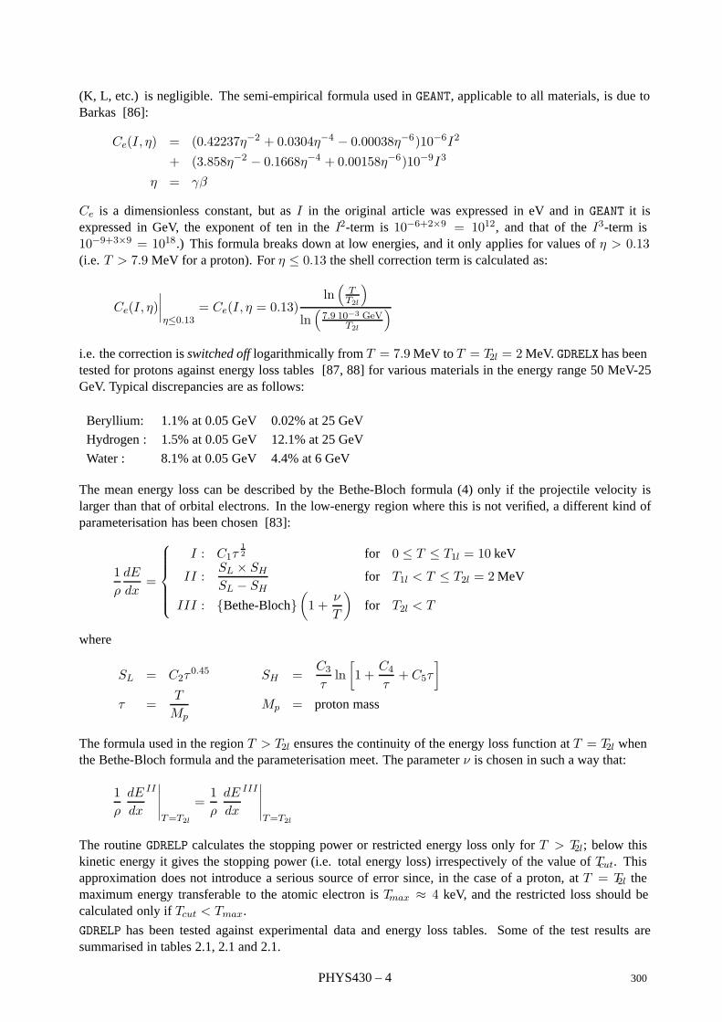
(K, L, etc.) is negligible. The semi-empirical formula used in GEANT, applicable to all materials, is due toBarkas [86]:
Ce(I, η) = (0.42237η−2 + 0.0304η−4 − 0.00038η−6)10−6I2
+ (3.858η−2 − 0.1668η−4 + 0.00158η−6)10−9I3
η = γβ
Ce is a dimensionless constant, but as I in the original article was expressed in eV and in GEANT it isexpressed in GeV, the exponent of ten in the I2-term is 10−6+2×9 = 1012, and that of the I3-term is10−9+3×9 = 1018.) This formula breaks down at low energies, and it only applies for values of η > 0.13(i.e. T > 7.9 MeV for a proton). For η ≤ 0.13 the shell correction term is calculated as:
Ce(I, η)∣∣∣∣η≤0.13
= Ce(I, η = 0.13)ln(
TT2l
)ln(7.9 10−3 GeV
T2l
)i.e. the correction is switched off logarithmically from T = 7.9MeV to T = T2l = 2MeV. GDRELX has beentested for protons against energy loss tables [87, 88] for various materials in the energy range 50 MeV-25GeV. Typical discrepancies are as follows:
Beryllium: 1.1% at 0.05 GeV 0.02% at 25 GeV
Hydrogen : 1.5% at 0.05 GeV 12.1% at 25 GeV
Water : 8.1% at 0.05 GeV 4.4% at 6 GeV
The mean energy loss can be described by the Bethe-Bloch formula (4) only if the projectile velocity islarger than that of orbital electrons. In the low-energy region where this is not verified, a different kind ofparameterisation has been chosen [83]:
1ρ
dE
dx=
I : C1τ12 for 0 ≤ T ≤ T1l = 10 keV
II :SL × SH
SL − SHfor T1l < T ≤ T2l = 2MeV
III : Bethe-Bloch(1 +
ν
T
)for T2l < T
where
SL = C2τ0.45 SH =
C3τln[1 +
C4τ+ C5τ
]τ =
T
MpMp = proton mass
The formula used in the region T > T2l ensures the continuity of the energy loss function at T = T2l whenthe Bethe-Bloch formula and the parameterisation meet. The parameter ν is chosen in such a way that:
1ρ
dE
dx
II∣∣∣∣∣T=T2l
=1ρ
dE
dx
III∣∣∣∣∣T=T2l
The routine GDRELP calculates the stopping power or restricted energy loss only for T > T2l; below thiskinetic energy it gives the stopping power (i.e. total energy loss) irrespectively of the value of Tcut. Thisapproximation does not introduce a serious source of error since, in the case of a proton, at T = T2l themaximum energy transferable to the atomic electron is Tmax ≈ 4 keV, and the restricted loss should becalculated only if Tcut < Tmax.
GDRELP has been tested against experimental data and energy loss tables. Some of the test results aresummarised in tables 2.1, 2.1 and 2.1.
PHYS430 – 4 300
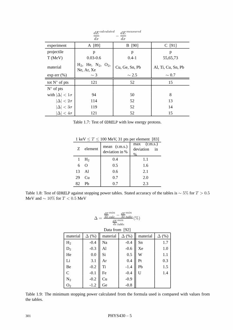
dE
dx
calculated
− dE
dx
measured
experiment A [89] B [90] C [91]
projectile p p p
T (MeV) 0.03-0.6 0.4-1 55,65,73
materialH2, He, N2, O2,Ne, Ar, Xe
Cu, Ge, Sn, Pb Al, Ti, Cu, Sn, Pb
exp err (%) ∼ 3 ∼ 2.5 ∼ 0.7
tot N of pts 121 52 15
N of pts
with |∆| < 1σ 94 50 8
|∆| < 2σ 114 52 13
|∆| < 3σ 119 52 14
|∆| < 4σ 121 52 15
Table 1.7: Test of GDRELP with low energy protons.
1 keV ≤ T ≤ 100 MeV, 31 pts per element [83]
Z element mean (r.m.s.)deviation in %
max (r.m.s.)deviation in%
1 H2 0.4 1.1
6 O 0.5 1.6
13 Al 0.6 2.1
29 Cu 0.7 2.0
82 Pb 0.7 2.3
Table 1.8: Test of GDRELP against stopping power tables. Stated accuracy of the tables is ∼ 5% for T > 0.5MeV and ∼ 10% for T < 0.5 MeV
∆ =dEdx
min
calc− dE
dx
min
table
dEdx
min
table
(%)
Data from [92]
material ∆ (%) material ∆ (%) material ∆ (%)
H2 -0.4 Na -0.4 Sn 1.7
D2 -0.3 Al -0.6 Xe 1.0
He 0.0 Si 0.5 W 1.1
Li 3.1 Ar 0.4 Pt 0.3
Be -0.2 Ti -1.4 Pb 1.5
C -0.1 Fe -0.4 U 1.4
N2 -0.2 Cu -0.9
O2 -1.2 Ge -0.8
Table 1.9: The minimum stopping power calculated from the formula used is compared with values fromthe tables.
301 PHYS430 – 5
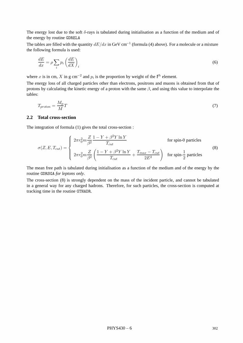
The energy lost due to the soft δ-rays is tabulated during initialisation as a function of the medium and ofthe energy by routine GDRELA
The tables are filled with the quantity dE/dx in GeV cm−1 (formula (4) above). For a molecule or a mixturethe following formula is used:
dE
dx= ρ
∑i
pi
(dE
dX
)i
(6)
where x is in cm, X in g cm−2 and pi is the proportion by weight of the Ith element.
The energy loss of all charged particles other than electrons, positrons and muons is obtained from that ofprotons by calculating the kinetic energy of a proton with the same β, and using this value to interpolate thetables:
Tproton =Mp
MT (7)
2.2 Total cross-section
The integration of formula (1) gives the total cross-section :
σ(Z,E, Tcut) =
2πr20m
Z
β21− Y + β2Y lnY
Tcutfor spin-0 particles
2πr20mZ
β2
(1− Y + β2Y lnY
Tcut+
Tmax − Tcut
2E2
)for spin-
12
particles
(8)
The mean free path is tabulated during initialisation as a function of the medium and of the energy by theroutine GDRSGA for leptons only.
The cross-section (8) is strongly dependent on the mass of the incident particle, and cannot be tabulatedin a general way for any charged hadrons. Therefore, for such particles, the cross-section is computed attracking time in the routine GTHADR.
PHYS430 – 6 302
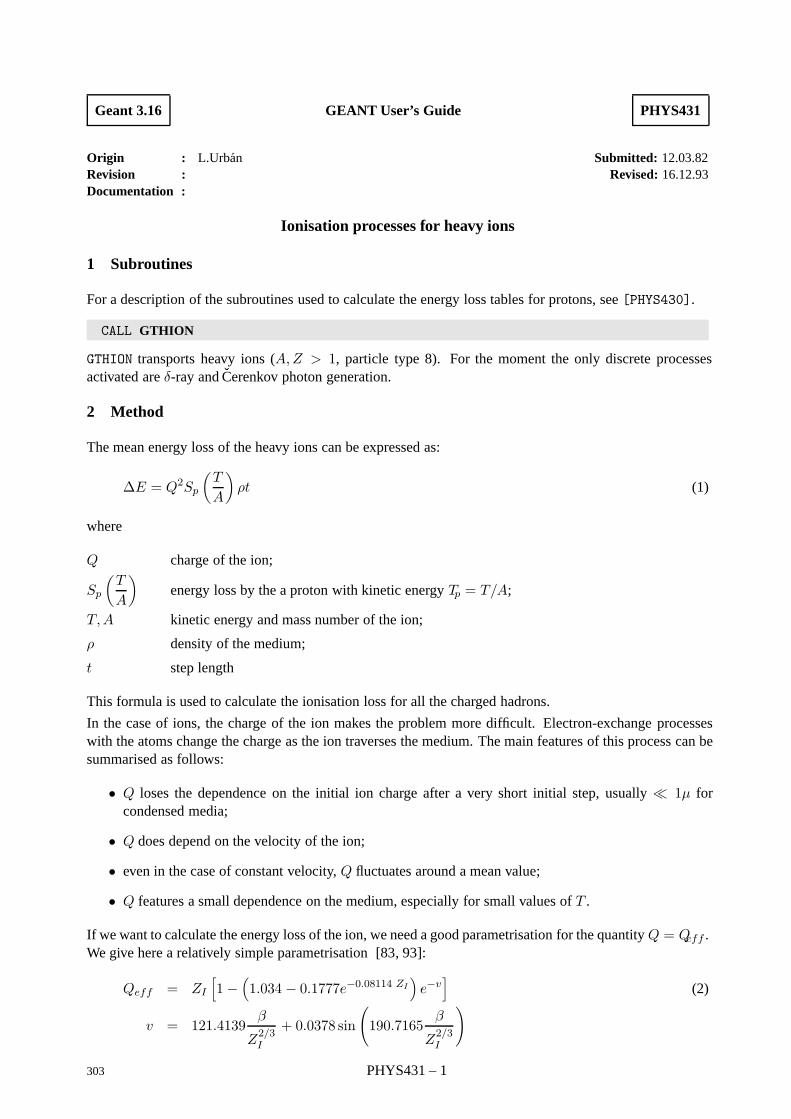
Geant 3.16 GEANT User’s Guide PHYS431
Origin : L.Urban Submitted: 12.03.82Revision : Revised: 16.12.93Documentation :
Ionisation processes for heavy ions
1 Subroutines
For a description of the subroutines used to calculate the energy loss tables for protons, see [PHYS430].
CALL GTHION
GTHION transports heavy ions (A,Z > 1, particle type 8). For the moment the only discrete processesactivated are δ-ray and Cerenkov photon generation.
2 Method
The mean energy loss of the heavy ions can be expressed as:
∆E = Q2Sp
(T
A
)ρt (1)
where
Q charge of the ion;
Sp
(T
A
)energy loss by the a proton with kinetic energy Tp = T/A;
T,A kinetic energy and mass number of the ion;
ρ density of the medium;
t step length
This formula is used to calculate the ionisation loss for all the charged hadrons.
In the case of ions, the charge of the ion makes the problem more difficult. Electron-exchange processeswith the atoms change the charge as the ion traverses the medium. The main features of this process can besummarised as follows:
• Q loses the dependence on the initial ion charge after a very short initial step, usually 1µ forcondensed media;
• Q does depend on the velocity of the ion;
• even in the case of constant velocity, Q fluctuates around a mean value;
• Q features a small dependence on the medium, especially for small values of T .
If we want to calculate the energy loss of the ion, we need a good parametrisation for the quantity Q = Qeff .We give here a relatively simple parametrisation [83, 93]:
Qeff = ZI
[1−
(1.034 − 0.1777e−0.08114 ZI
)e−v
](2)
v = 121.4139β
Z2/3I
+ 0.0378 sin
(190.7165
β
Z2/3I
)
303 PHYS431 – 1
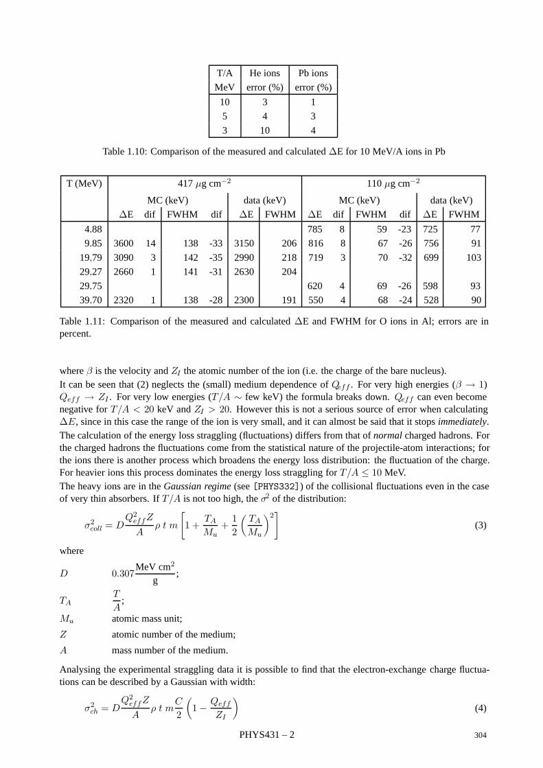
T/A He ions Pb ions
MeV error (%) error (%)
10 3 1
5 4 3
3 10 4
Table 1.10: Comparison of the measured and calculated ∆E for 10 MeV/A ions in Pb
T (MeV) 417 µg cm−2 110 µg cm−2
MC (keV) data (keV) MC (keV) data (keV)
∆E dif FWHM dif ∆E FWHM ∆E dif FWHM dif ∆E FWHM
4.88 785 8 59 -23 725 77
9.85 3600 14 138 -33 3150 206 816 8 67 -26 756 91
19.79 3090 3 142 -35 2990 218 719 3 70 -32 699 103
29.27 2660 1 141 -31 2630 204
29.75 620 4 69 -26 598 93
39.70 2320 1 138 -28 2300 191 550 4 68 -24 528 90
Table 1.11: Comparison of the measured and calculated ∆E and FWHM for O ions in Al; errors are inpercent.
where β is the velocity and ZI the atomic number of the ion (i.e. the charge of the bare nucleus).It can be seen that (2) neglects the (small) medium dependence of Qeff . For very high energies (β → 1)Qeff → ZI . For very low energies (T/A ∼ few keV) the formula breaks down. Qeff can even becomenegative for T/A < 20 keV and ZI > 20. However this is not a serious source of error when calculating∆E, since in this case the range of the ion is very small, and it can almost be said that it stops immediately.The calculation of the energy loss straggling (fluctuations) differs from that of normal charged hadrons. Forthe charged hadrons the fluctuations come from the statistical nature of the projectile-atom interactions; forthe ions there is another process which broadens the energy loss distribution: the fluctuation of the charge.For heavier ions this process dominates the energy loss straggling for T/A ≤ 10 MeV.The heavy ions are in the Gaussian regime (see [PHYS332]) of the collisional fluctuations even in the caseof very thin absorbers. If T/A is not too high, the σ2 of the distribution:
σ2coll = DQ2effZ
Aρ t m
[1 +
TA
Mu+12
(TA
Mu
)2](3)
where
D 0.307MeV cm2
g;
TAT
A;
Mu atomic mass unit;
Z atomic number of the medium;
A mass number of the medium.
Analysing the experimental straggling data it is possible to find that the electron-exchange charge fluctua-tions can be described by a Gaussian with width:
σ2ch = DQ2effZ
Aρ t m
C
2
(1− Qeff
ZI
)(4)
PHYS431 – 2 304
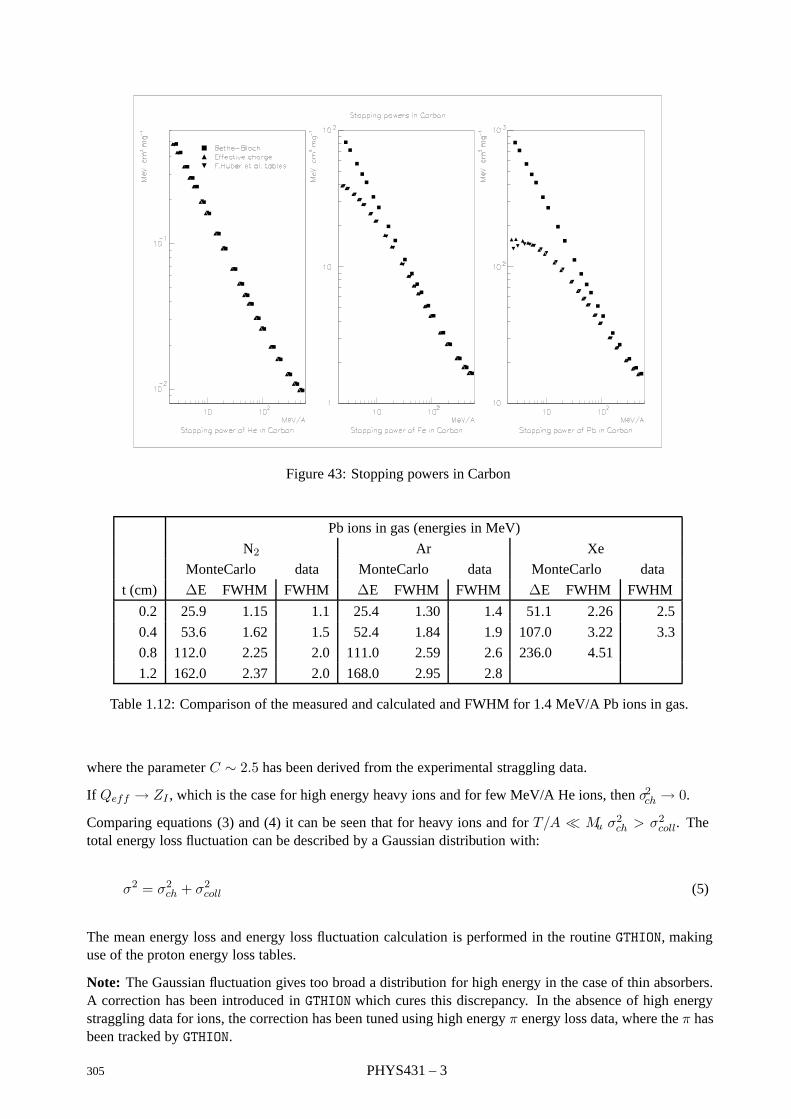
Figure 43: Stopping powers in Carbon
Pb ions in gas (energies in MeV)
N2 Ar Xe
MonteCarlo data MonteCarlo data MonteCarlo data
t (cm) ∆E FWHM FWHM ∆E FWHM FWHM ∆E FWHM FWHM
0.2 25.9 1.15 1.1 25.4 1.30 1.4 51.1 2.26 2.5
0.4 53.6 1.62 1.5 52.4 1.84 1.9 107.0 3.22 3.3
0.8 112.0 2.25 2.0 111.0 2.59 2.6 236.0 4.51
1.2 162.0 2.37 2.0 168.0 2.95 2.8
Table 1.12: Comparison of the measured and calculated and FWHM for 1.4 MeV/A Pb ions in gas.
where the parameter C ∼ 2.5 has been derived from the experimental straggling data.
If Qeff → ZI , which is the case for high energy heavy ions and for few MeV/A He ions, then σ2ch → 0.
Comparing equations (3) and (4) it can be seen that for heavy ions and for T/A Mu σ2ch > σ2coll. Thetotal energy loss fluctuation can be described by a Gaussian distribution with:
σ2 = σ2ch + σ2coll (5)
The mean energy loss and energy loss fluctuation calculation is performed in the routine GTHION, makinguse of the proton energy loss tables.
Note: The Gaussian fluctuation gives too broad a distribution for high energy in the case of thin absorbers.A correction has been introduced in GTHION which cures this discrepancy. In the absence of high energystraggling data for ions, the correction has been tuned using high energy π energy loss data, where the π hasbeen tracked by GTHION.
305 PHYS431 – 3
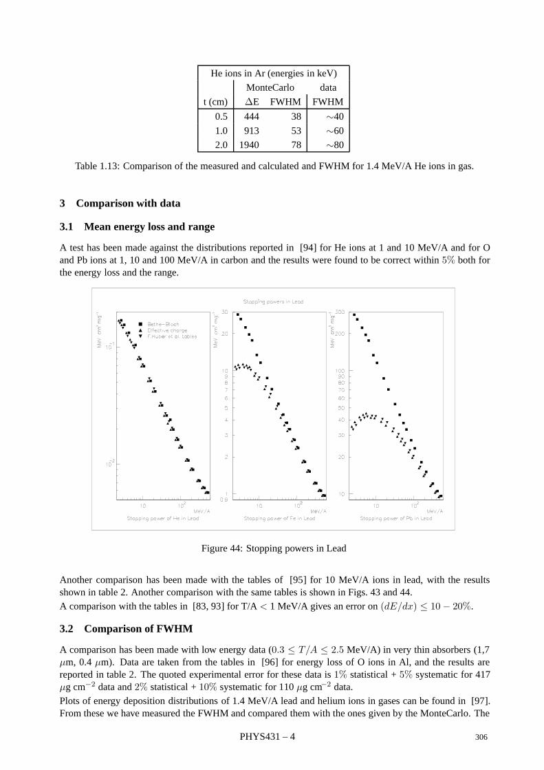
He ions in Ar (energies in keV)
MonteCarlo data
t (cm) ∆E FWHM FWHM
0.5 444 38 ∼40
1.0 913 53 ∼60
2.0 1940 78 ∼80
Table 1.13: Comparison of the measured and calculated and FWHM for 1.4 MeV/A He ions in gas.
3 Comparison with data
3.1 Mean energy loss and range
A test has been made against the distributions reported in [94] for He ions at 1 and 10 MeV/A and for Oand Pb ions at 1, 10 and 100 MeV/A in carbon and the results were found to be correct within 5% both forthe energy loss and the range.
Figure 44: Stopping powers in Lead
Another comparison has been made with the tables of [95] for 10 MeV/A ions in lead, with the resultsshown in table 2. Another comparison with the same tables is shown in Figs. 43 and 44.
A comparison with the tables in [83, 93] for T/A < 1 MeV/A gives an error on (dE/dx) ≤ 10− 20%.
3.2 Comparison of FWHM
A comparison has been made with low energy data (0.3 ≤ T/A ≤ 2.5 MeV/A) in very thin absorbers (1,7µm, 0.4 µm). Data are taken from the tables in [96] for energy loss of O ions in Al, and the results arereported in table 2. The quoted experimental error for these data is 1% statistical + 5% systematic for 417µg cm−2 data and 2% statistical + 10% systematic for 110 µg cm−2 data.
Plots of energy deposition distributions of 1.4 MeV/A lead and helium ions in gases can be found in [97].From these we have measured the FWHM and compared them with the ones given by the MonteCarlo. The
PHYS431 – 4 306

results can be seen in table 2 and 3.1. It should be noted that the absorber thickness of, for example, Arcompares with that of the preceding case (0.2 cm Ar = 356 µg cm−2 and 1.2 cm Ar = 2136 µg cm−2).
Similar comparison has been made for C ions of energies 17.1 and 39.4 MeV in isobuthane [98] and theagreement between data and GEANT for FWHM is within 30%.
307 PHYS431 – 5
Geant 3.16 GEANT User’s Guide PHYS440
Origin : L.Urban Submitted: 26.10.84Revision : Revised: 16.12.93Documentation :
Total cross-section and energy loss for bremsstrahlung by Muons
1 Subroutines
CALL GBRELA
GBRELA fills the tables for continuous energy loss of electrons, positrons and muons due to bremsstrahlungduring initialisation time. The energy binning is determined by the array ELOW (common /CGMULO/) in theroutine GPHYSI. In the tables, the dE/dx due to bremsstrahlung is summed with that due to the ionisation.For energy loss of muons, GBRELA calls the function GDRELM. The following pointers are used:
JMA = LQ(JMATE-I) pointer to the Ith material;
JEL1 = LQ(JMA-1) pointer to dE/dx for electrons;
JEL1+NEK1 pointer to dE/dx for positrons;
JEL2 = LQ(JMA-2) pointer to dE/dx for electrons.
GBRELA is called by GPHYSI.
VALUE = GBRELM (Z,T,BCUT)
Z (REAL) atomic number of the material;
T (REAL) kinetic energy of the muon;
BCUT (REAL) soft bremsstrahlung cut.
GBRELM calculates the muon energy loss due to bremsstrahlung of photons with energy below BCUT, (variableBCUTM in the common /GCCUTS/). Above this value, the bremsstrahlung process is simulated explicitly (see[PHYS441]) and the energy lost by the muons is not included in the tables. In the tables, the dE/dx dueto bremsstrahlung is summed with the energy lost coming from ionisation, pair production and nuclearinteraction. GBRELM is called by GBRELA.
CALL GBRSGA
GBRSGA calculates the total cross-section for bremsstrahlung. It tabulates the mean free path in cm as afunction of the medium and the energy. The energy binning is determined by the array ELOW (common/CGMULO/). The following pointers are used:
JMA = LQ(JMATE-I) pointer to the Ith material;
JBREM = LQ(JMA-9) pointer to bremsstrahlung cross-sections;
JBREM pointer for e−;
JBREM+NEK1 pointer for e+;
JBREM+2*NEK1 pointer for µ+/µ−.
GBRSGA is called during initialisation by GPHYSI.
308 PHYS440 – 1
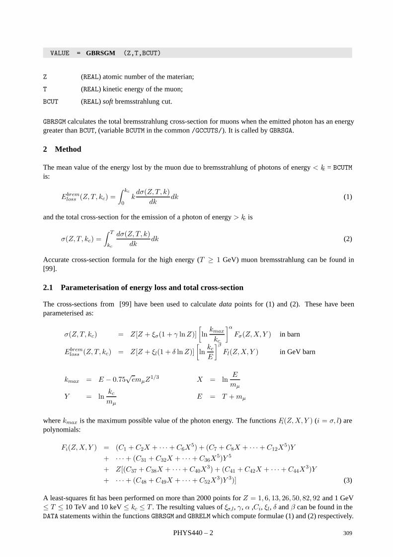
VALUE = GBRSGM (Z,T,BCUT)
Z (REAL) atomic number of the materian;
T (REAL) kinetic energy of the muon;
BCUT (REAL) soft bremsstrahlung cut.
GBRSGM calculates the total bremsstrahlung cross-section for muons when the emitted photon has an energygreater than BCUT, (variable BCUTM in the common /GCCUTS/). It is called by GBRSGA.
2 Method
The mean value of the energy lost by the muon due to bremsstrahlung of photons of energy < kc = BCUTMis:
Ebremloss (Z, T, kc) =
∫ kc
0kdσ(Z, T, k)
dkdk (1)
and the total cross-section for the emission of a photon of energy > kc is
σ(Z, T, kc) =∫ T
kc
dσ(Z, T, k)dk
dk (2)
Accurate cross-section formula for the high energy (T ≥ 1 GeV) muon bremsstrahlung can be found in[99].
2.1 Parameterisation of energy loss and total cross-section
The cross-sections from [99] have been used to calculate data points for (1) and (2). These have beenparameterised as:
σ(Z, T, kc) = Z[Z + ξσ(1 + γ lnZ)][ln
kmax
kc
]αFσ(Z,X, Y ) in barn
Ebremloss (Z, T, kc) = Z[Z + ξl(1 + δ lnZ)]
[ln
kcE
]βFl(Z,X, Y ) in GeV barn
kmax = E − 0.75√emµZ
1/3 X = lnE
mµ
Y = lnkcmµ
E = T +mµ
where kmax is the maximum possible value of the photon energy. The functions Fi(Z,X, Y ) (i = σ, l) arepolynomials:
Fi(Z,X, Y ) = (C1 + C2X + · · ·+ C6X5) + (C7 + C8X + · · ·+ C12X
5)Y+ · · · + (C31 + C32X + · · ·+ C36X
5)Y 5
+ Z[(C37 + C38X + · · ·+ C40X3) + (C41 + C42X + · · ·+ C44X
3)Y+ · · · + (C48 + C49X + · · ·+ C52X
3)Y 3)] (3)
A least-squares fit has been performed on more than 2000 points for Z = 1, 6, 13, 26, 50, 82, 92 and 1 GeV≤ T ≤ 10 TeV and 10 keV ≤ kc ≤ T . The resulting values of ξσ,l, γ, α ,Ci, ξl, δ and β can be found in theDATA statements within the functions GBRSGM and GBRELM which compute formulae (1) and (2) respectively.
PHYS440 – 2 309
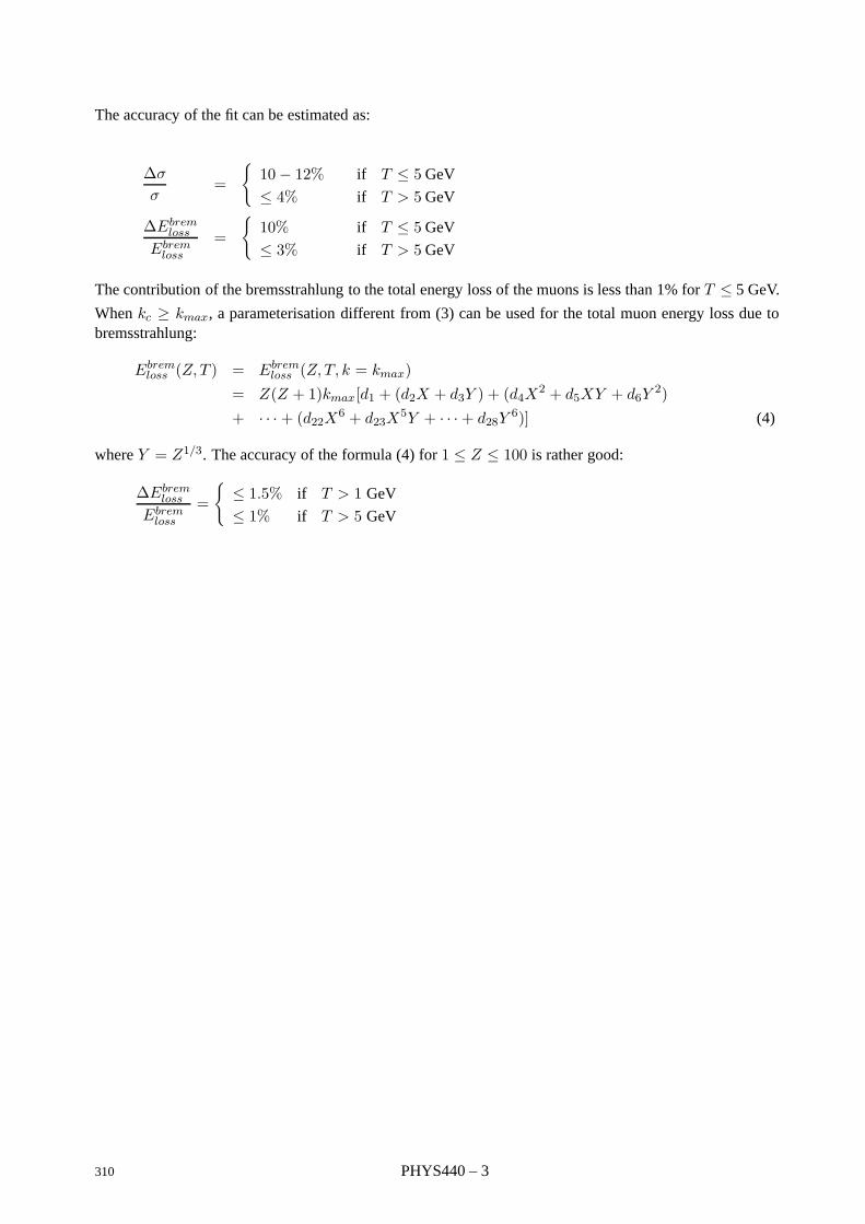
The accuracy of the fit can be estimated as:
∆σ
σ=
10− 12% if T ≤ 5GeV
≤ 4% if T > 5GeV
∆Ebremloss
Ebremloss
=
10% if T ≤ 5GeV
≤ 3% if T > 5GeV
The contribution of the bremsstrahlung to the total energy loss of the muons is less than 1% for T ≤ 5 GeV.
When kc ≥ kmax, a parameterisation different from (3) can be used for the total muon energy loss due tobremsstrahlung:
Ebremloss (Z, T ) = Ebrem
loss (Z, T, k = kmax)= Z(Z + 1)kmax[d1 + (d2X + d3Y ) + (d4X2 + d5XY + d6Y
2)+ · · · + (d22X6 + d23X
5Y + · · ·+ d28Y6)] (4)
where Y = Z1/3. The accuracy of the formula (4) for 1 ≤ Z ≤ 100 is rather good:
∆Ebremloss
Ebremloss
=
≤ 1.5% if T > 1 GeV
≤ 1% if T > 5 GeV
310 PHYS440 – 3
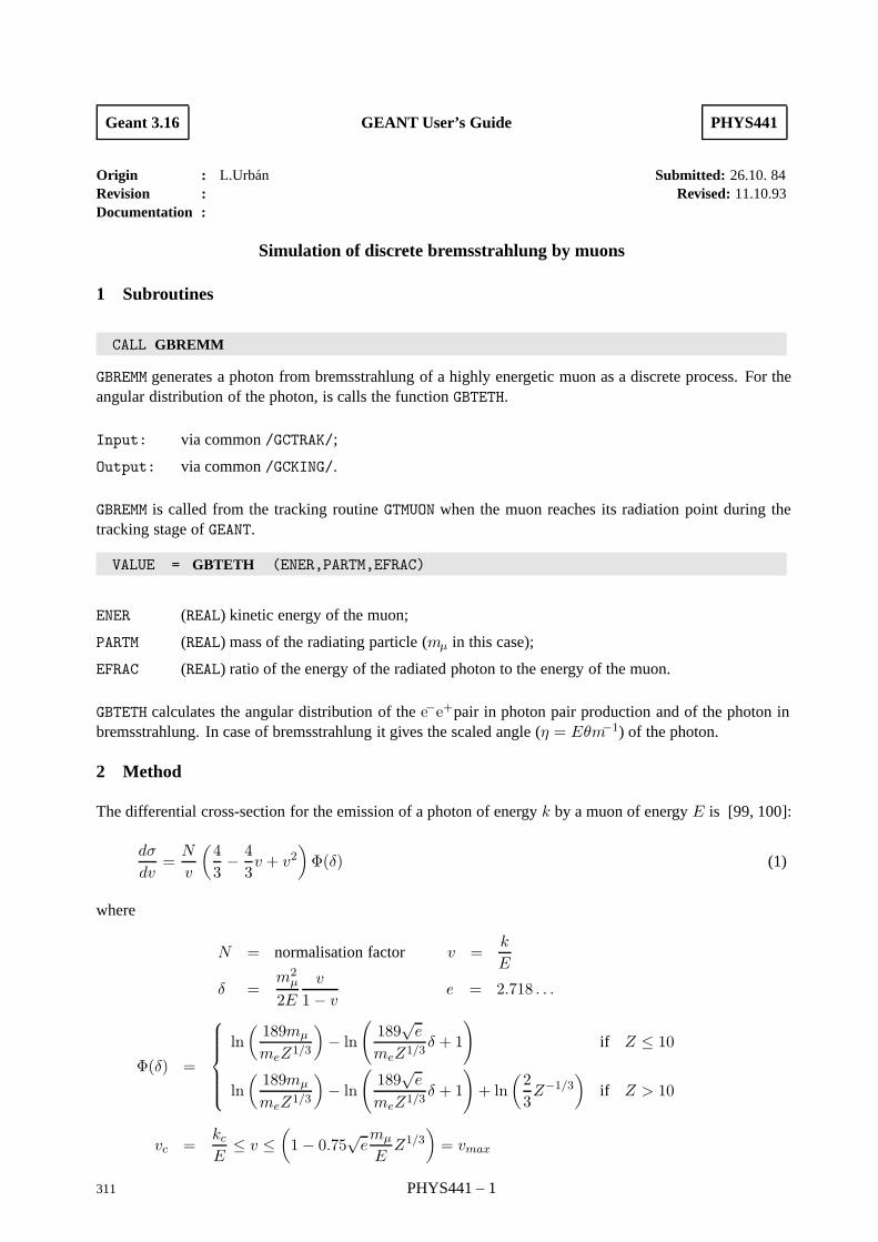
Geant 3.16 GEANT User’s Guide PHYS441
Origin : L.Urban Submitted: 26.10. 84Revision : Revised: 11.10.93Documentation :
Simulation of discrete bremsstrahlung by muons
1 Subroutines
CALL GBREMM
GBREMM generates a photon from bremsstrahlung of a highly energetic muon as a discrete process. For theangular distribution of the photon, is calls the function GBTETH.
Input: via common /GCTRAK/;
Output: via common /GCKING/.
GBREMM is called from the tracking routine GTMUON when the muon reaches its radiation point during thetracking stage of GEANT.
VALUE = GBTETH (ENER,PARTM,EFRAC)
ENER (REAL) kinetic energy of the muon;
PARTM (REAL) mass of the radiating particle (mµ in this case);
EFRAC (REAL) ratio of the energy of the radiated photon to the energy of the muon.
GBTETH calculates the angular distribution of the e−e+pair in photon pair production and of the photon inbremsstrahlung. In case of bremsstrahlung it gives the scaled angle (η = Eθm−1) of the photon.
2 Method
The differential cross-section for the emission of a photon of energy k by a muon of energy E is [99, 100]:
dσ
dv=
N
v
(43− 43v + v2
)Φ(δ) (1)
where
N = normalisation factor v =k
E
δ =m2µ2E
v
1− ve = 2.718 . . .
Φ(δ) =
ln(189mµ
meZ1/3
)− ln
(189
√e
meZ1/3δ + 1
)if Z ≤ 10
ln(189mµ
meZ1/3
)− ln
(189
√e
meZ1/3δ + 1
)+ ln
(23Z−1/3
)if Z > 10
vc =kcE
≤ v ≤(1− 0.75
√emµ
EZ1/3
)= vmax
311 PHYS441 – 1
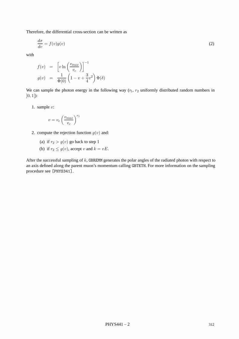
Therefore, the differential cross-section can be written as
dσ
dv= f(v)g(v) (2)
with
f(v) =[v ln
(vmax
vc
)]−1g(v) =
1Φ(0)
(1− v +
34v2)Φ(δ)
We can sample the photon energy in the following way (r1, r2 uniformly distributed random numbers in]0, 1[):
1. sample v:
v = vc
(vmax
vc
)r1
2. compute the rejection function g(v) and:
(a) if r2 > g(v) go back to step 1
(b) if r2 ≤ g(v), accept v and k = vE.
After the successful sampling of k, GBREMM generates the polar angles of the radiated photon with respect toan axis defined along the parent muon’s momentum calling GBTETH. For more information on the samplingprocedure see [PHYS341].
PHYS441 – 2 312
Geant 3.16 GEANT User’s Guide PHYS450
Origin : L.Urban Submitted: 24.03.86Revision : Revised: 16.12.93Documentation :
Total cross-section and energy loss for e-e+ pair production by muons
1 Subroutines
CALL GPRELA
GPRELA adds to the muon energy loss tables the contribution due to µ-nucleus interactions and e+e−-pairproduction in which the energy of the pair is below threshold (see later). For the contribution of pairproduction, it calls the function GPRELM. The energy binning is in the array ELOW (common /CGMULO/). Thefollowing pointers are used:
JMA = LQ(JMATE-I) pointer to the Ith material;
JEL2 = LQ(JMA-2) pointer to dE/dx for µ+µ−.
GPRELA is called during initialisation by GPHYSI.
VALUE = GPRELM (Z,T,CUT)
Z (REAL) atomic number of the material;
T (REAL) kinetic energy of the muon;
CUT (REAL) maximum energy for the pair considered by the routine.
GPRELM calculates the energy loss due to the direct production by muons of e−e+pairs with energy belowCUT (PPCUTM in common /GCCUTS/). Above this cut, the direct pairs are produced as discrete processes(see [PHYS451]). GPRELM is called by GPRELA.
CALL GPRSGA
GPRSGA calculates the total cross-section for the pair production by photons and the direct pair productionby muons. It tabulates the mean free path in cm as a function of medium and energy. For the directpair production of muons, it calls the function GPRSGM. The energy binning is in the array ELOW (common/CGMULO/). The following pointers are used:
JMA = LQ(JMATE-I) pointer to the Ith material;
JPAIR = LQ(JMA-10) pointer to photon pair production cross-sections;
JPAIR+NEK1 pointer to muon pair production.
GPRSGA is called during initialisation by GPHYSI.
VALUE = GPRSGM (Z,T,CUT)
Z (REAL) atomic number of the medium;
T (REAL) kinetic energy of the muon;
CUT (REAL) minimum energy for the e−e+pair.
GPRSGM calculates the total cross-section for muon direct pair production where the energy of the pair isgreater than CUT (PPCUTM in common /GCCUTS/). It is called by GPRSGA (see [PHYS451]).
313 PHYS450 – 1
2 Method
When a muon of energy E moves in the field of an atom of charge Z , it can radiate a e+e−-pair (4th orderQED process) with differential cross-section [99]:
∂2σ
∂ν ∂ρ= α4
23π(Zλ−)2 1− v
v
φe +
(me
mµ
)2φµ
(1)
where
ν =E+ + E−
Eand ρ =
E+ − E−
E+ + E−
and
α 1/137, fine structure constant;
λ− 3.8616 × 10⁻¹¹ cm, electron Compton wavelength;
v k/E fraction of energy transferred to the pair;
T E −M kinetic energy of the muon.
E± the energy of the e±.
The explicit form of the terms φe and φµ can be found in [99]. The kinematic ranges of ν and ρ are:
4me
E= νmin ≤ ν ≤ νmax = 1− 0.75
√emµ
EZ1/3
0 = ρmin ≤ |ρ(ν)| ≤ ρmax(ν) =
[1−
6m2µE2(1− ν)
]√1− 4me
νE
(2)
where e = 2.718 . . ..Ec (PPCUTM in the program) is the energy cut-off; below this energy e+e−-pair are treated as continuousenergy loss, and above they are explicitly generated and vc = Ec/E. The mean value of the energy lost bythe incident muon due to e+e−-pair with energy below Ec is:
Epairloss (Z, T,Ec) = 2E
∫ νc
νmin
dν ν
∫ ρmax(ν)
0dρ
∂2σ
∂ν ∂ρGeV barn/atom (3)
whereas the total cross-section for the emission of a hard e+e−-pair is:
σ(Z, T,Ec) = 2∫ νmax
νc
dν
∫ ρmax(ν)
0dρ
∂2σ
∂ν ∂ρbarn/atom (4)
2.1 Parameterisation of energy loss and total cross-section
Instead of using the explicit formula (3) and (4), we have chosen to parameterise directly Epairloss (Z, T,Ec)and σ(Z, T,Ec) as:
σ(Z, T,Ec) = Z[Z + ξσ(1 + γ lnZ)][ln
Emax
E
]αFσ(Z,X, Y ) (5)
Epairloss (Z, T,Ec) = Z[Z + ξl(1 + δ lnZ)]E
[Ec − Emin
c
E
]βFl(Z,X, Y ) (6)
where ξσ,l, α, β, γ and δ are parameters obtained by a fitting procedure and Eminc = E vmin = 4me and
Emax = E vmax
PHYS450 – 2 314
The functions Fi (Z,X,Y) (i = σ, l) have the form:
Fi(Z,X, Y ) = Fi0(X,Y ) + ZFi1(X,Y ) (7)
where Fij(X,Y ) denotes a function constructed from two polynomials
Fij(X,Y ) =
Pnegij (X,Y ) if Y ≤ 0
P posij (X,Y ) if Y > 0
(8)
and Pnegij , P pos
ij fulfil the conditions:
Pnegij (X,Y )Y=0 = P pos
ij (X,Y )Y=0∂Pneg
ij
∂Y
∣∣∣∣∣Y=0
=∂P pos
ij
∂Y
∣∣∣∣∣Y=0
The detailed form of the Pij polynomials is:
Pnegi0 (X,Y ) = (C1 + C2X + · · · +C6X
5) + (C7 + C8X + · · ·+ C12X5)Y
+ (C13 + C14X + · · ·+ C18X5)Y 2 + · · ·+ (C31 + · · ·+ C36X
5)Y 5
P posi0 (X,Y ) = (C1 + C2X + · · · +C6X
5) + (C7 + C8X + · · ·+ C12X5)Y
+ (C37 + C38X + · · ·+ C42X5)Y 2 + · · ·+ (C55 + · · ·+ C60X
5)Y 5 (9)
Pnegi1 (X,Y ) = (C61 + C62X + · · ·+ C65X
4) + (C66 + C67X + · · ·+ C70X4)Y
+ (C71 + C72X + · · ·+ C75X4)Y 2 + · · ·+ (C81 + · · ·+ C85X
4)Y 4
P posi1 (X,Y ) = (C61 + C62X + · · ·+ C65X
4) + (C66 + C67X + · · ·+ C70X4)Y
+ (C86 + C87X + · · ·+ C90X4)Y 2 + · · ·+ (C96 + · · ·+ C100X
4)Y 4
with
X = lnE
mµY = ln
Ec
vjEj = σ, l
where vσ,l are additional parameters of the fit. By a numerical (twofold) integration of the formulae (5)and (6) above, we have calculated 1800 data points in the range Z = 1, 6, 13, 26, 50, 82, 92 and the energyranges 1GeV ≤ T ≤ 10 TeV and 4m ≤ Ec ≤ T and performed a least-squares fit to determine theparameters. The fitted values of the parameters are in the DATA statements in the functions GPRSGM andGPRELM, which compute the formulae (5) and (6) respectively. The accuracy of the fit is:
∆σ
σ≤10% if T ≤ 5 GeV
5% if T > 5 GeV
∆Epairloss
Epairloss
≤10% if T ≤ 5 GeV
4% if T > 5 GeV
The function GPRELM contains a second formula to calculate the total energy lost by the muon due to directe+e−-production used when Ec ≥ Emax = E − 0.75√emµZ
1/3. This formula describes the total energyloss with an error less than 1%:
Epairloss (Z, T ) = Epair
loss (Z, T,Ec = Emax) (10)
= Z(Z + 1)Emax[d1 + (d2X + d3Y ) + (d4X2 + d5XY + d6Y2) +
+ · · ·+ (d22X6 + d23X5Y + · · ·+ d28Y
6)]
where X = ln(E/mµ) and Y = Z1/3. The fitted parameters di can be found in the DATA statement in thefunction GPRELM.
315 PHYS450 – 3
Geant 3.10 GEANT User’s Guide PHYS451
Origin : L.Urban Submitted: 26.10.84Revision : Revised: 16.12.93Documentation :
Simulation of e+e- pair production by muons
1 Subroutines
CALL GPAIRM
GPAIRM generates the e+e−-pair radiated by a high energetic muon. It uses the following input and output:
input: via common block /GCTRAK/
output: via common block /GCKING/
GPAIRM is called automatically from the tracking routine GTMUON if, and when, the parent muon reaches itsradiation point during the tracking.
2 Method
The double differential cross-section for the process can be written [99]:
d2σ
dνdρ= α4
23π(Zλ)2 · 1− ν
ν
[φe + (m/M)2φµ
](1)
All the quantities in the expression above are defined in [PHYS450]. By computing this cross-section fordifferent (ν, ρ) points, it can be seen that:
1. the shape of the functions d2σdνdρ and dσ
dν
∫dρ d2σ
dνdρ practically does not depend on Z
2. the dominant contribution comes from the low ν region:
νmin = (4m/E) ≤ ν ≤ 100 ∗ νmin (2)
3. in this low region (d2σ/dνdρ) is flat as a function of ρ
Therefore, we propose the following sampling method as a rough approximation:
1. In the low ν region the differential cross-section
dσ
dν=∫
dρd2σK
dνdσ
can be approximated as:
dσ
dν≈[1− νmin
ν
]1/2 1va
with: a = 2− lnE10
(E in GeV) (3)
We can write:
dσ
dν≈ f(ν)g(ν) (4)
316 PHYS451 – 1
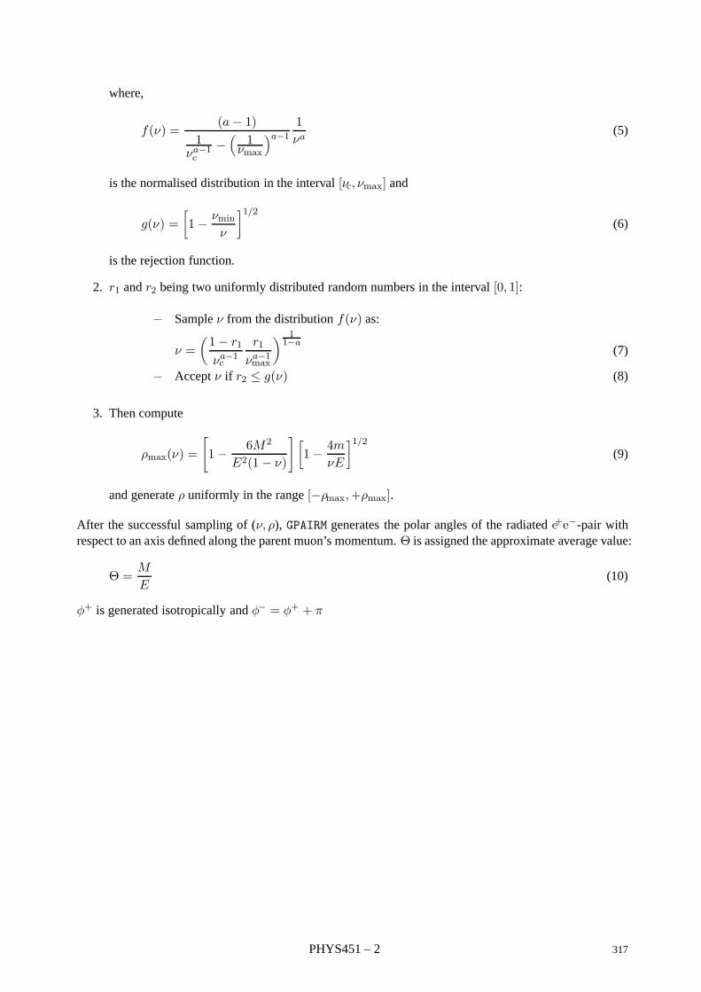
where,
f(ν) =(a− 1)
1νa−1c
−(1
νmax
)a−11νa
(5)
is the normalised distribution in the interval [νc, νmax] and
g(ν) =[1− νmin
ν
]1/2(6)
is the rejection function.
2. r1 and r2 being two uniformly distributed random numbers in the interval [0, 1]:
− Sample ν from the distribution f(ν) as:
ν =(1− r1
νa−1c
r1
νa−1max
) 11−a
(7)
− Accept ν if r2 ≤ g(ν) (8)
3. Then compute
ρmax(ν) =
[1− 6M2
E2(1− ν)
] [1− 4m
νE
]1/2(9)
and generate ρ uniformly in the range [−ρmax,+ρmax].
After the successful sampling of (ν, ρ), GPAIRM generates the polar angles of the radiated e+e−-pair withrespect to an axis defined along the parent muon’s momentum. Θ is assigned the approximate average value:
Θ =M
E(10)
φ+ is generated isotropically and φ− = φ+ + π
PHYS451 – 2 317
Geant 3.10 GEANT User’s Guide PHYS460
Origin : H.C.Fesefeldt, F.Carminati Submitted: 20.12. 85Revision : Revised: 16.12.93Documentation : F. Carminati
Muon-nucleus interactions
1 Subroutines
CALL GMUNUI
GMUNUI computes and stores in the appropriate bank the value of the muon-nucleus cross-section for a givenmaterial. It is called at initialisation time by GPHYSI.
CALL GMUNU
GMUNU is called by GTMUON every time a muon-nucleus interaction has to happen. It generates the final stateparticles as well as the outgoing muon. A call to GUHADR is performed if IMUNU (which is the variable set bythe MUNU data record) is equal to 1. An inelastic interaction is forced (which could also be a fission in caseof heavy materials). The secondaries from the π-nucleus interaction are always generated if IMUNU is equalto 1, irrespectively of the value of IHADR.
Note: IMUNU should be set to 1 only when using the GHEISHA hadronic interactions package. Setting it to 1when using FLUKA can give unpredictable results.
VALUE = GMUSIG (E,E1,COSTET)
E (REAL) initial µ energy;
E1 (REAL) final µ energy;
COSTET (REAL) µ scattering angle.
This function returns the value of the differential cross-section in millibarns for a muon of energy E togenerate a nuclear interaction recoil with energy E1 at an angle the cosine of which is COSTET.
2 Method
This set of routines generates the interactions of muons with the nuclei of the tracking material. The codeis a straight translation into the GEANT style of the corresponding code from the GHEISHA Monte CarloProgram. The GHEISHA routines CASMU and CALIM have been used [1].
The information contained in this chapter is mainly taken from the GHEISHA manual to which the user isreferred. The muon-nucleus inelastic cross-section is taken as 0.0003 mb for a nucleon when the energy ofthe incoming muon is E < 30 GeV, and slowly increases for E > 30 GeV according to the law:
σ = 0.3 ∗ (E/30)0.25 [µb]
The energy and angle of final state muon is generated according to the “free quark parton model”. If E is theenergy of the incoming muon and Ω and W the angle and the energy of the outgoing muon, the differentialcross-section can be written as:
dσ
dΩdW= γ(σT + εσS)
318 PHYS460 – 1
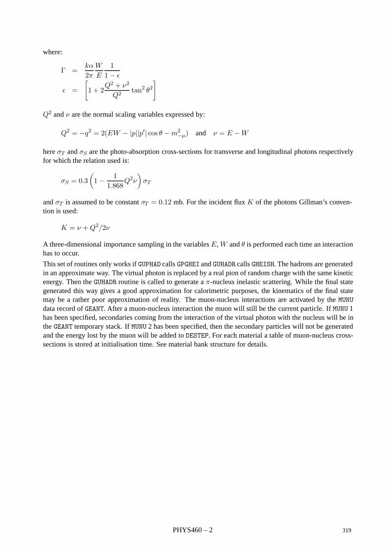
where:
Γ =kα
2πW
E
11− ε
ε =
[1 + 2
Q2 + ν2
Q2tan2 θ2
]
Q2 and ν are the normal scaling variables expressed by:
Q2 = −q2 = 2(EW − |p||p′| cos θ −m2−µ) and ν = E −W
here σT and σS are the photo-absorption cross-sections for transverse and longitudinal photons respectivelyfor which the relation used is:
σS = 0.3(1− 1
1.868Q2ν
)σT
and σT is assumed to be constant σT = 0.12 mb. For the incident flux K of the photons Gillman’s conven-tion is used:
K = ν +Q2/2ν
A three-dimensional importance sampling in the variables E, W and θ is performed each time an interactionhas to occur.
This set of routines only works if GUPHAD calls GPGHEI and GUHADR calls GHEISH. The hadrons are generatedin an approximate way. The virtual photon is replaced by a real pion of random charge with the same kineticenergy. Then the GUHADR routine is called to generate a π-nucleus inelastic scattering. While the final stategenerated this way gives a good approximation for calorimetric purposes, the kinematics of the final statemay be a rather poor approximation of reality. The muon-nucleus interactions are activated by the MUNUdata record of GEANT. After a muon-nucleus interaction the muon will still be the current particle. If MUNU 1has been specified, secondaries coming from the interaction of the virtual photon with the nucleus will be inthe GEANT temporary stack. If MUNU 2 has been specified, then the secondary particles will not be generatedand the energy lost by the muon will be added to DESTEP. For each material a table of muon-nucleus cross-sections is stored at initialisation time. See material bank structure for details.
PHYS460 – 2 319
Geant 3.16 GEANT User’s Guide PHYS510
Origin : H.C. Fesefeldt, F.Carminati Submitted: 24.02.86Revision : Revised: 11.10.93Documentation : F. Carminati
The GEANT/GHEISHA Interface
1 Introduction
There are two packages to describe the hadronic showers in matter which are available to the users of GEANT:GHEISHA [1] and FLUKA (see [PHYS520]).
The GHEISHA code generates hadronic interactions with the nuclei of the current tracking medium, evaluat-ing cross-sections and sampling the final state multiplicity and kinematics, while the GEANT philosophy ispreserved for the tracking. The GHEISHA code is stored in the GEANH car file.
The GHEISHA printing flags can be set via the GEANT SWIT data record: each switch greater than 100 butsmaller that 111 sets the corresponding printing flag of GHEISHA modulo 100, so that SWIT 105 will setthe printing flag 5 of GHEISHA. Setting the printing flags of GHEISHA the following information will bedisplayed:
NPRT(1) one header for each track in the shower;
NPRT(2) all tracking information;
NPRT(3) kinematic of decays (not effective);
NPRT(4) kinematic of nuclear interactions;
NPRT(5) kinematic of electromagnetic interactions (not effective);
NPRT(6) material constants, dE/dX and absorbed energies (not effective);
NPRT(7) event summary;
NPRT(8) history of all interactions/decays;
NPRT(9) free;
NPRT(10) tables of the geometry, cross-sections, etc.;
NPRT(1), NPRT(2) and NPRT(6) should be used only in case of suspected errors. NPRT(8) produces themost illustrative output. Those flags work in conjunction with the DEBUG data record of GEANT.
1.1 Description of the routines
CALL GHESIG (P,EK,AVER,A,Z,W,NLM,DENS,CORR,IPART)
P (REAL) momentum of the particle (in GeV/c);
EK (REAL) kinetic energy of the particle (in GeV);
AVER (REAL) average mass number of the material;
A(NLM) (REAL) vector containing the mass numbers of the components of the mixture, the same asAVER in case of an element;
Z(NLM) (REAL) vector containing the atomic numbers of the components of the mixture, or theatomic number in case of an element;
W(NLM) (REAL) vector of length NLM containing the relative weights of the components of the mix-ture (normalised to one), one in case of an element;
320 PHYS510 – 1
NLM (INTEGER) number of components of the mixture, 1 in case of an element;
DENS (REAL) density of the material;
CORR (REAL) if this parameters is > 0, then corrections are applied to the cross-section; should beused in case of inorganic scintillators;
IPART (INTEGER) GEANT particle code.
This routine returns the total macroscopic cross-section in cm−1. The correction flag is taken from the 26th
word of the next bank in the tracking medium linear structure pointed at by LQ(JTMED-NUMED).The cross-sections on nucleus are known only for pions and protons. The general law:
σ(A) = 1.25 ∗ σProtontot Aα
is used but it is valid only for momenta > 2 GeV. The parametrisation done gives only a behaviour averagedover momenta and particle types. For H, Al, Cu and Pb the measured cross-sections are stored in DATAstatements.The stored cross-sections are the pre-calculated GHEISHA ones. As a starting point the measured cross-sections of pions, kaons, protons, antiprotons and neutrons on protons are used. The cross-sections tabulatedare measured values taken from the CERN HERA compilations. The values for K0s/K0l are updated as ofJuly 1980. Strange baryon cross-section are calculated using a parametrisation in terms of quark-quarkforward scattering amplitudes and optical theorem. The additive quark quark scattering model is used. Allthe cross-sections are contained in data statements so no external file is needed for GHEISHA.
CALL GPGHEI
This routine returns the distance to the next hadronic interaction according to the GHEISHA cross-sections.It calls GHESIG and is called by GUPHAD. The default copy provided in the GEANT library uses the GHEISHAshower code:
SUBROUTINE GUPHAD******************************************************************* ** GEANT user routine called at each step to evaluate ** the remaining distance to the hadronic interaction point ** *******************************************************************
CALL GPGHEI*
END
SUBROUTINE GUHADR*.***************************************************************** ** GEANT user routine called when a hadronic process ** has been selected in the current step, in order to ** generate the final particle’s state ** ******************************************************************
CALL GHEISH*
END
PHYS510 – 2 321
CALL GHEISH
This is the main steering routine for the hadronic interactions and is a fan-out to the various cascade routinesof GHEISHA which treat the particular hadronic interaction. Here the kind of interaction is stored in the INTflag, with the following meaning:
INT=0 no interaction (NONE);
INT=1 elastic scattering occurs (ECOH);
INT=2 inelastic incoherent interaction occurs (INHE), 1 and 2 include also nuclear reaction processesat very low energies;
INT=3 nuclear fission with inelastic scattering occurs (FISS);
INT=4 neutron nuclear capture occurs (CAPT).
After the interaction has been selected, the appropriate cascade routine is called. Upon exit from this there isa check whether the interaction has generated new particles or not. If yes, the new particles are copied in theGEANT temporary stack (GKING). If the particle is a heavy fragment or a proton and it is below the energycut specified via the CUTS data record, it is not stored in the stack but the kinetic energy is collected. Thesize of the GHEISHA stack is parametrised, and its limit is currently set to 100 in sequence GCKMAX. The useris left to decide in GUSTEP what to do with the new tracks. This routine is called also in case of a stoppinghadron, i.e. with kinetic energy below the GEANT cuts. In this case the routine GHSTOP (see later) is calledto handle the stopping hadron. The printing flags for GHEISHA are also set in this routine according to thecurrent value of IDEBUG.
This routine must be called by the user routine GUHADR (see above).
As explained above, for inorganic scintillators such as the BGO, it is possible to activate a correction to thehadronic cross-section. This is done via the routine GSTPAR in the following way:
CALL GSTPAR(ITMED,’GHCOR1’,1.0)
The parameter is actually a flag which, if different from 0, triggers the calculation of the cross-sectioncorrection, but in view of future developments it is good practice set it to 1.0 when those corrections arerequired. ITMED is the tracking medium number as used in GSTMED for which corrections are requested.This routine has to be called before GPHYSI.
CALL GHSTOP
This is an internal routine used to handle stopping particles, called by GHEISH. Here again we have a switchto the various routines handling stopping particles. In particular this routine can lead to nuclear absorptionfor negative pions and negative kaons (ABSO) and to annihilation for antineutrons, and antiprotons (ANNH).The kinetic energy is completely absorbed, and in the case of an unstable particle, the particle is decayed atrest via the standard GEANT decay routine GDECAY.
322 PHYS510 – 3
Geant 3.16 GEANT User’s Guide PHYS520
Origin : A.Ferrari, K.Lassila-Perini Submitted: 25.10.91Revision : Revised: 17.12.93Documentation : K.Lassila-Perini
The GEANT/FLUKA Interface
1 Subroutines
CALL FLINIT
FLINIT initialises the FLUKA variables and reads data from a file (flukaaf.dat) which is automatically opened.FLINIT is called from FLDIST when a hadron enters there first time in the run.
CALL FLDIST
FLDIST computes the distance to the next interaction point. It calls the FLUKA routines to compute the cross-sections for all particles except neutrons with kinetic energy below 20 MeV for which GHEISHA routines arecalled. FLDIST is called from the user routine GUPHAD where the hadronic package can be chosen.
CALL FLUFIN
FLUFIN calls the FLUKA routines to generate the hadronic interaction. It passes the particle to FLUKA inter-action routines and puts the eventual secondary particles to the GEANT stack. FLUFIN is called from the userroutine GUHADR.
2 Method
FLUKA [2, 3, 4, 5, 6, 101, 102] is a simulation program which as a standalone code contains transport andthe physical processes for hadrons and leptons and tools for geometrical description. In GEANT, only thehadronic interaction part is included.
The total cross-section of the hadronic processes is computed by FLUKA routines called from FLDIST (thecross-section for neutrons below 20 MeV is computed in GHEISHA). If hadronic intercation is chosen inGEANT tracking routine, the particle is passed to FLUFIN.
If particles are stopping (i.e. their energy is below the cut-off energy), their kinetic energy is deposited.However, if the particle can decay (π+, K±) it is forced to decay, or if it is an annihilating particle (π−, n,p), it is sent to FLUKA routines for annihilation. The neutrons with kinetic energy below 20 MeV are passedto GHEISHA.
If the particle is not stopping, a sampling is done between elastic and inelastic processes. The cross-sectionshave been computed in FLDIST in the same time as the total cross-section. The particle is sent correspond-ingly to the elastic or inelastic interaction routines. After the interaction, the eventual secondary particlesare written to GEANT stack. The program flow is shown in figures 46 and 45.
When the tracking media is a mixture or a compound material (defined by GSMIXT, see [CONS110]), theatom with which the interaction is taking place is chosen by sampling on the basis of the cross-sections.This is important especially in hydrogenous materials.
323 PHYS520 – 1
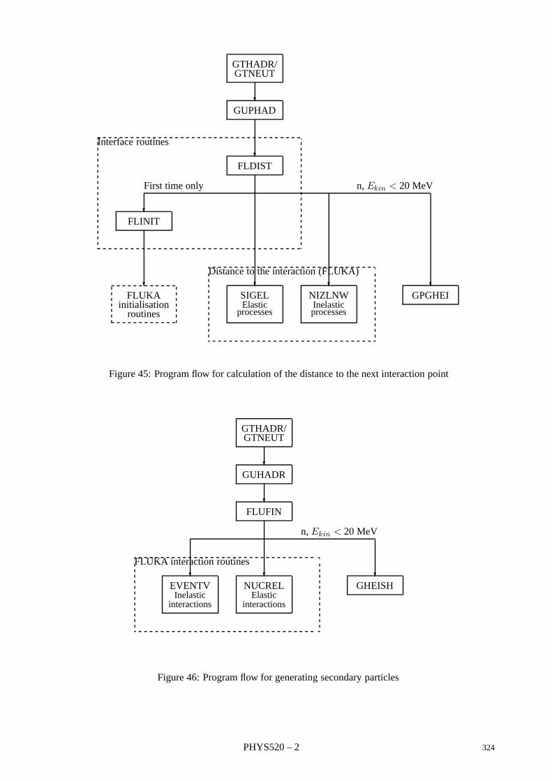
GTHADR/GTNEUT
GUPHAD
Interface routines
FLDIST
First time only n, Ekin < 20 MeV
FLINIT
Distance to the interaction (FLUKA)
SIGELElastic
processes
NIZLNWInelasticprocesses
GPGHEI
FLUKA
initialisationroutines
Figure 45: Program flow for calculation of the distance to the next interaction point
GTHADR/GTNEUT
GUHADR
FLUFIN
FLUKA interaction routines
NUCRELElastic
interactions
EVENTVInelastic
interactions
n, Ekin < 20 MeV
GHEISH
Figure 46: Program flow for generating secondary particles
PHYS520 – 2 324
Geant 3.16 GEANT User’s Guide PHYS530
Origin : T.Gabriel, C.Zeitnitz, K.Lassila-Perini Submitted: 17.12.93Revision : Revised: 17.12.93Documentation : K.Lassila-Perini
The GEANT/MICAP interface
1 Subroutines
CALL GMORIN
GMORIN initialises the MICAP variables and reads the cross-section file for the materials that have beendefined. It is called from GFMDIS when a neutron with kinetic energy below 20 MeV enters there first time.
CALL GFMDIS
GFMDIS computes the distance to the next interaction points. It calls the FLUKA routines to compute thecross-sections for all particles except neutrons with kinetic energy below 20 MeV for which MICAP functionSIGMOR is called. GFMDIS is called from the user routine GUPHADwhere the hadronic package can be chosen.The only difference between GFLDIS (see [PHYS520]) and GFMDIS is that for the former, GHEISHA hadronicpackage is called for the neutrons below 20 MeV, and for the latter, the low-energy neutrons are handled byMICAP.
CALL GFMFIN
GFMFIN calls the FLUKA routines to generate the hadronic interaction. For the neutrons with kinetic energybelow 20 MeV GMICAP is called. The only difference between GFLFIN (see [PHYS520]) and GFMFIN is thatfor the former, GHEISHA hadronic package is called for the neutrons below 20 MeV, and for the latter, thelow-energy neutrons are handled by MICAP. GFMFIN is called from the user routine GUHADR.
CALL GMICAP
GMICAP calls the MICAP routines to handle the low-energy interaction of neutrons. It writes the eventualsecondaries to the GEANT stack. GMICAP is called from GFMFIN.
2 Method
MICAP (A Monte Carlo Ionization Chamber Analysis Package) [103], [104] is a Monte Carlo system toanalyze ionisation chamber responses. As a standalone program it contains the code for formatting thecross-section files, neutron and photon transport, the geometry definitions and the code for the chamberresponse. In GEANT, only the sampling of the neutron interactions from the already prepared cross-sectionfile is included. The interface between GEANT and MICAP has been extracted from GCALOR package [105] byC.Zeitnitz and T. Gabriel.
When using GEANT-MICAP interface the low-energy neutrons are handled in MICAP routines. Other hadronsand high-energy neutrons are passed to FLUKA interaction routines. For low-energy neutrons, the total cross-section is given by MICAP and if the neutron interaction is chosen by GEANT tracking routine, GMICAP readsthe cross-section for neutron interactions processes, samples and generates the interaction and the returnsthe secondary particles (nucleons, heavy fragments, or photons) to GEANT. Information on the recoil nucleus(atomic number AMED, charge ZMED and kinetic energy ERMED) can be found in MCRECO common block. Theprogram flow is shown in figures 48 and 47.
MICAP uses pointwise cross-section data (as a difference to so called group cross-sections where the data areaveraged over certain energy intervals). This method has the advantage that the resonances are not smoothedby averaging the data. The neutron cross-section are available for the following isotopes:
325 PHYS530 – 1
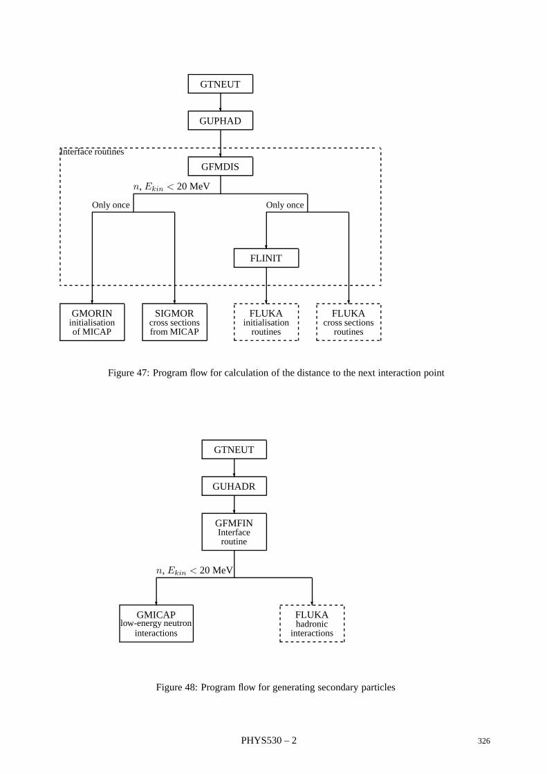
GTNEUT
GUPHAD
Interface routines
GFMDIS
n, Ekin < 20 MeV
Only once
GMORIN
initialisationof MICAP
SIGMOR
cross sectionsfrom MICAP
Only once
FLINIT
FLUKA
initialisationroutines
FLUKA
cross sectionsroutines
Figure 47: Program flow for calculation of the distance to the next interaction point
GTNEUT
GUHADR
GFMFINInterfaceroutine
n, Ekin < 20 MeV
GMICAP
low-energy neutroninteractions
FLUKAhadronic
interactions
Figure 48: Program flow for generating secondary particles
PHYS530 – 2 326

Hydrogen (bound) Sodium Copper
Hydrogen (free) Magnesium Molybdenum
Lithium (5) Aluminium Barium
Lithium (6) Silicon Tantalum
Boron (10) Chlorine Tungsten
Boron (11) Argon Lead
Carbon Calcium Uranium (235)
Nitrogen Chromium Uranium (238)
Oxygen Iron
Fluorine Nickel
If the cross-sections are not found for some of the defined materials, a warning is printed first at the ini-tialisation time telling which cross-section are used (the closest Z available) instead. Then, an additionalwarning is printed each tracking step.
327 PHYS530 – 3
PHYS Bibliography
[1] H.C.Fesefeldt. Simulation of hadronic showers, physics and applications. Technical Report PITHA85-02, III Physikalisches Institut, RWTH Aachen Physikzentrum, 5100 Aachen, Germany, September1985.
[2] P.A.Aarnio et al. Fluka user’s guide. Technical Report TIS-RP-190, CERN, 1987, 1990.
[3] A.Fasso A.Ferrari J.Ranft P.R.Sala G.R.Stevenson and J.M.Zazula. FLUKA92. In Proceedings of theWorkshop on Simulating Accelerator Radiation Environments, Santa Fe, USA, 11-15 January 1993.
[4] A.Fasso A.Ferrari J.Ranft P.R.Sala G.R.Stevenson and J.M.Zazula. A Comparison of FLUKA Sim-ulations with measurements of Fluence and Dose in Calorimeter Structures. Nuclear Instruments &Methods A, 332:459, 1993.
[5] C.Birattari E.DePonti A.Esposito A.Ferrari M.Pelliccioni and M.Silari. Measurements and character-ization of high energy neutron fields. approved for pubblication in Nuclear Instruments & MethodsA.
[6] P.A.Aarnio, A.Fasso, A.Ferrari, J.-H.Moehring, J.Ranft, P.R.Sala, G.R.Stevenson and J.M.Zazula.FLUKA: hadronic benchmarks and applications. In MC93 Int. Conf. on Monte-Carlo Simulation inHigh-Energy and Nuclear Physics, Tallahassee, Florida, 22-26 February 1993. Proceedings in press.
[7] Particle Data Group. Review of particle properties. Physical Review D, 45(11), June 1992.
[8] R.Brun, M.Goossens, and J.Zoll. ZEBRA Users Guide, Program Library Q100. CERN, 1991.
[9] J.H.Hubbell, H.A.Gimm, and I.Overbo. Jou. Phys. Chem. Ref. Data, 9:1023, 1980.
[10] J.C.Butcher and H.Messel. Nucl. Phys, 20:15, 1960.
[11] J.M.Hammersley and D.S.Handscomb. Monte Carlo methods. J.Wiley et Sons Inc, New York, 1964.
[12] R.Ford and W.Nelson. SLAC 210, UC 32. SLAC, June 1978.
[13] Y-S.Tsai. Rev. Mod. Phys., 46:815, 1974.
[14] Y-S.Tsai. Rev. Mod. Phys., 49:421, 1977.
[15] W.R.Nelson et al. The EGS4 code system. Technical Report 265, SLAC, 1985.
[16] O.Klein and Y.Nishina. Z. f. Physik, 52:853, 1929.
[17] H.Messel and D.F.Crawford. volume 3. Pergamon Press, 1970.
[18] B.Rossi. Prentice-Hall, 1952.
[19] F. Biggs and R. Lighthill. Analitycal approximations for x-ray cross sections 3. Sandia NationalLab., SAND87-0070 UC-34, 1987.
[20] H. Bethe and E. Salpeter. Encyclopedia of Physics, volume XXXV. Springer-Verlag, Berlin, 1957.
[21] H. Hall. The theory of photoelectric absorbtion for x-rays and γ-rays. Rev. Mod. Phys., 8:358, 1936.
[22] R. H. Pratt. Atomic photoelectric effect at high energies. Phys. Rev., 117:1017, 1960.
[23] R. H. Pratt. Photoeffect form the l shell. Phys. Rev., 119:1619, 1960.
[24] WM. J. Veigele. Photon cross sections from 0.1 kev to 1 mev for elements z = 1 to z = 94. AtomicData Tables, 5:51, 1973.
PHYS530 – 4 328
[25] M. Gavrila. Relativistic l-shell photoeffect. Phys. Rev., 124:1132, 1961.
[26] F. Sauter. Ann. Physik, 9:217, 1931.
[27] F. Sauter. Ann. Physik, 11:454, 1931.
[28] M. Gavrila. Relativistic k-shell photoeffect. Phys. Rev., 113:514, 1959.
[29] B. C. H. Nagel and P. O. M. Olsson. Arkiv f. Fysik, 18:1, 1960.
[30] M. O. Krause. Atomic radiative and radiationless yields for k and l shells. J. Phys. Chem. Ref. Data,8:307, 1979.
[31] S.T. Perkins et al. UCRL-50400, 30, 1991.
[32] J. H. Scofield. Relativistic hatree-slater values for k and l x-ray emission rates. Atomic Data andNuclear Data Tables, 14:121, 1974.
[33] J.H.Hubbell and I.Overbo. J. Phys. Chem. Ref. Data, 1/8, 1979.
[34] H.Storm and H.I.Israel. Nucl. data tables. A7:565, 1970.
[35] W.R.Nelson, H.Hirayama, and D.W.O.Rogers. Technical Report 265, SLAC, 1985.
[36] J.D.Jackson. Classical Electrodynamics. J.Wiley et Sons, Inc, New York, 1975.
[37] H.A.Bethe. Phys. Rev., 89:1256, 1953.
[38] B.Rossi. Prentice-Hall, Englewood Cliffs, 1961.
[39] B.Rossi and K.Greisen. Rev. Mod. Physics, 13:240, 1941.
[40] V.L.Highland. Nucl. Inst. and Meth., 129:497, 1975.
[41] V.L.Highland. Nucl. Inst. and Meth., 161:171, 1979.
[42] G.R.Lynch and O.I.Dahl. Approximation to multiple coulomb scattering. Technical Report LBL-28165, Physics Division, Laurence Berkeley Laboratory, University of California, Berkeley, CA94720, February 1990.
[43] G.Z.Moliere. Theorie der Streuung schneller geladener Teilchen I: Einzelstreuung am abgerschmittenCoulomb-Feld. Z. Naturforsch., 2a:133, 1947.
[44] G.Z.Moliere. Theorie der Streuung schneller geladener Teilchen II: Merfach- und Vielfachstreuung.Z. Naturforsch., 3a:78, 1948.
[45] W.T.Scott. Rev. Mod. Phys., 35:231, 1963.
[46] S.Goudsmit and J.L.Saunderson. Multiple scattering of electrons. Phys. Rev., 57:24, 1940.
[47] S.Goudsmit and J.L.Saunderson. Multiple scattering of electrons II. Phys. Rev., 36:36, 1940.
[48] T.M.Jenkins, W.R.Nelson, and A.Rindi. MonteCarlo transport of electrons and photons. PlenumPress, New York, 1988.
[49] E.Keil, E.Zeitler, and W.Zinn. Zur Einfach- und Mehrfachstreuung geladener Teilchen.Z.Naturforsch., 15a:1031, 1960.
[50] S.M. Selzer M.J. Berger. Technical Report SP 3012, NASA, 1964.
[51] H.A.Bethe. Ann. Phys., 5:325, 1930.
329 PHYS530 – 5
[52] F.Bloch. Z. fur Phys., 81:363, 1933.
[53] R.M.Sternheimer. Phys. Rev. B, 3:3681, 1971.
[54] H.Messel and D.F. Crawford. Pergamon Press, Oxford, 1970.
[55] Particle Data Group. Lawrence Berkeley Laboratory and CERN, 1992.
[56] G.N.Patrick. Physical processes in the simulation of electromagetic cascades. In Workshop on ShowerSimulation for LEP Experiments, January 1985.
[57] L. Landau. On the Energy Loss of Fast Particles by Ionisation J. Phys. 8:201, 1944. In D.ter Haar,editor, L.D.Landau, Collected papers, page 417. Pergamon Press, Oxford, 1965.
[58] K.S.Kolbig and B.Schorr. Asymptotic expansion for the Landau density and distribution functions.Comp. Phys. Comm., 32:121, 1984.
[59] R.Talman. On the statistics of particle identification using ionization. Nucl. Inst. Meth., 159:189,1979.
[60] R.Jones. Private communication to a GEANT monthly meeting.
[61] P.V.Vavilov. Ionisation losses of high energy heavy particles. Soviet Physics JETP, 5:749, 1957.
[62] B.Schorr. Programs for the Landau and the Vavilov distributions and the corresponding randomnumbers. Comp. Phys. Comm., 7:216, 1974.
[63] S.M.Seltzer and M.J.Berger. Energy loss straggling of protons and mesons. In Studies in Penetrationof Charged Particles in Matter. Nuclear Science Series 39, Nat. Academy of Sciences, WashingtonDC, 1964.
[64] F.James. Program formerly in the CERN Program Library, but now replaced by G110, entry RAN-LAN.
[65] J.E.Moyal. Theory of ionisation fluctuations. Phil. Mag., 46:263, 1955.
[66] K.S.Kolbig and B.Schorr. A program package for the Landau distribution. Comp. Phys. Comm.,31:97, 1984.
[67] A. Rotondi and P. Montagna. Fast calculation of Vavilov distribution. Nucl. Inst. Meth., B47:215,1990.
[68] W. W. M. Allison and J. H. Cobb. Ann. Rev. Nucl. Part. Sci., 30:253, 1980.
[69] S. K. Kotelnikov V. M. Grishin, V. K. Ermilova. Nucl. Instr. Meth., A307:273, 1991.
[70] At. data Nucl. data tables, 20:1, 1978.
[71] At. data Nucl. data tables, 27:2, 1982.
[72] At. data Nucl. data tables, 32:1, 1985.
[73] J.B.Birks. The theory and practice of Scintillation Counting. Pergamon Press, 1964.
[74] R.L.Craun and D.L.Smith. Nucl. Inst. and Meth., 80:239–244, 1970.
[75] S.M. Seltzer and M.J. Berger. Nucl. Inst. Meth., B12:95, 1985.
[76] A.B.Migdal. Phys. Rev., 103:1811, 1956.
[77] L.Kim, R.H.Pratt, S.M.Seltzer, and M.J.Berger. Phys. Rev., A33:3002, 1986.
PHYS530 – 6 330
[78] R.W.Williams. Fundamental Formulas of Physics, volume 2. Dover Pubs. Inc, 1960.
[79] W.Heitler. The Quantum Theory of radiation. Clarendon Press, Oxford, 1954.
[80] D. Vaughan. X-Ray Data Booklet. Center for X-Ray Optics, 1986.
[81] R.Maier. In CERN Accelerator School. CERN, 17-28 September 1990. CERN 91-04.
[82] C.Bricman et al. Rev. Mod. Phys., 52, 1980.
[83] H.H.Andersen and J.F.Ziegler. Hidrogen stopping powers and ranges in all elements. PergamonPress, 1977.
[84] R.M.Sternheimer. Phys. Rev., 88:851, 1952.
[85] R.M. Sternheimer. Phys. Rev., 183:511, 1956.
[86] W.H.Barkas. Technical Report 10292, UCRL, August 1962.
[87] C.R.Serre. Technical Report 67 5, CERN, March 1967.
[88] C.R.Serre. Technical Report 71 18, CERN, September 1971.
[89] H.K.Reynold et al. Phys. Rev., 92:742, 1953.
[90] D.W.Green et al. Phys. Rev., 98:466, 1955.
[91] N.Sakamoto et al. Rad. Effects and Defects in Solids, 117:193, 1991.
[92] W.H.Barkas and M.J. Berger. Technical Report SP 3013, NASA, 1964.
[93] H.H.Andersen and J.F.Ziegler. Helium stopping powers and ranges in all elements. Pergamon Press,1977.
[94] W.Heinrich et al. Technical Report GSI-91-30, GSI, Darmstad, June 1991.
[95] F.Hubert et al. At. Data Nucle. Data Tables, 46:1, 1990.
[96] C.Tschalar and H.D.Maccabee. Phys. Rev. B, 1:2863, 1970.
[97] H.Geisel et al. NIM, 194:21, 1982.
[98] H.Schmidt-Boring and H.Harnung. Z.f.Phys., A286:253, 1978.
[99] W. Lohmann and R. Voss. Yellow Report 85 03, CERN, 1985.
[100] P.Marmier and E.Sheldon. volume 1. Academic Press, 1969.
[101] P.A.Aarnio, A.Fasso, A.Ferrari, J.-H.Moehring, J.Ranft, P.R.Sala, G.R.Stevenson and J.M.Zazula.Electron-photon transport: always so good as we think? Experience with FLUKA. In MC93 Int.Conf. on Monte-Carlo Simulation in High-Energy and Nuclear Physics, Tallahassee, Florida, 22-26February 1993. Proceedings in press.
[102] A.Ferrari and P.R.Sala. A New Model for hadronic interactions at intermediate energies for theFLUKA code. In MC93 Int. Conf. on Monte-Carlo Simulation in High-Energy and Nuclear Physics,Tallahassee, Florida, 22-26 February 1993. Proceedings in press.
[103] J.O. Johnson and T.A. Gabriel. A User’s Guide to MICAP: A Monte Carlo Ionization ChamberAnalysis Package. Technical Report TM-10340, ORNL, 1988.
[104] J.O. Johnson and T.A. Gabriel. Development and Evaluation of a Monte Carlo System for Analysisof Ionization Chamber Responses. Technical Report TM-10196, ORNL, 1987.
[105] C.Zeitnitz T.Gabriel. In Proc. of International Conference on Calorimetry in High Energy Physics,Tallahasse, FL, USA, February 1993.
331 PHYS530 – 7
Geant 3.16 GEANT User’s Guide TRAK001
Origin : Submitted: 15.08.84Revision : Revised: 16.12.93Documentation : F.Bruyant
The tracking package
1 Introduction
In GEANT tracking a particle through a geometry of objects consists in calculating a set of points in a seven-dimensional space (x, y, z, t, px, py, pz) which is called the trajectory of the particle. This is achieved byintegrating the equations of motion over successive steps from one trajectory point to the next and applyingcorrections to account for the presence of matter.
To have a detailed description of the kinematic of the particle it would be necessary to calculate a trajectorypoint every time the component of the momentum change. This is not possible because it would mean calcu-lating an enormously large number of points. Processes like the deviation of a charged particle in a magneticfield, the loss of energy due to bremsstrahlung and ionisation or the deviation due to elastic electromagneticscatterings are essentially continuous. An arbitrary distinction is thus made between discrete and continuousprocesses, controlled by a set of thresholds which can be set by the user. A particle trajectory is thus a setof points at which a discrete process has happened.
The tracking package contains a subprogram which performs the tracking for all particles in the current eventand for the secondary products which they generate, plus some tools for storing the space point coordinatescomputed along the corresponding trajectories.
2 The step size
When tracking particles through a complex structure one of the critical tasks is the estimation a priori ofthe step size. This is performed automatically by the program. For a particle with a given energy thestep size depends primarily on the intrinsic properties of the particle (mass, charge, lifetime, etc.) and on thecharacteristics of the current medium. The dependence may be due either to the (quasi)continuous processeswhich usually impose a limit to the interval of integration (energy loss, multiple scattering ...) or to theoccurrence of a discrete process which introduces a discontinuity in the trajectory (decay, electromagnetic orhadronic interaction). The modification of the kinematic parameters (position and energy) due to continuousprocesses between two discrete ones is taken into account and the necessary modifications are applied at theend of the step.
In addition to the physical effects there are constraints of a geometrical nature, the step being limited by thepath length to the medium boundary. In practice, the step size depends ultimately on a set of tolerances andcuts, which the program will set automatically, but which may be also optimised by the user, such as:
• the maximum turning angle due to magnetic field permitted in one step;
• the maximum fractional energy loss in one step;
• the maximum geometrical step allowed;
• the accuracy for crossing medium boundaries;
• the minimum step size due to either energy loss or multiple scattering.
These quantities are part of the so-called tracking medium parameters. They can either be calculated by theprogram or provided by the user and are stored in the data structure JTMED, through the routine GSTMED (see
332 TRAK001 – 1
[CONS]). Usually, this is done together with the initialisation of the geometrical setup. The optimisation isby no means trivial as the economy of computing time should not lead to an unacceptable loss of accuracy.
Other information required for the computation of the step size is found in the data structures JPART andJMATE, for the properties of the particles and of the materials, and in the data structure JVOLUM, for thecurrent medium and its geometrical boundaries. The communication between the tracking package andthe structure JVOLUM is achieved through the basic subroutines of the geometry package GMEDIA, GTMEDI,GTNEXT and GINVOL (see [GEOM]). Some information is computed at tracking time such as the probabilityof occurrence of an interaction.
For convenience every particle is assigned a tracking type:
1. γ (GTGAMA);
2. e± (GTELEC);
3. neutral hadrons and neutrinos (GTNEUT);
4. charged hadrons (GTHADR);
5. muons (GTMUON);
6. geantinos, particles only sensitive to geometry used for debugging (GTNINO);
7. Cerenkov photons (GTCKOV);
8. heavy ions (GTHION).
Which processes have to be considered for a given particle depends on its tracking type. For the hadronsit depends also, through the subroutine GUPHAD, on which hadronic processes from GHEISHA, FLUKA havebeen selected (see [PHYS001]).
3 Transport subroutines
At the event level the tracking is controlled by the subroutine GTREVE called by the subroutine GUTREVwherethe user can perform additional actions. GTREVE loops over all vertices and for every vertex in turn storesall tracks in the stack JSTAK. Then tracking begins: particles are fetched from JSTAK by GLTRAC whichprepares the commons for tracking. GUTRAK is then called, which calls GTRACK. The subroutine GTRACKtransports the particle up to the its end: stop, decay, interaction or escape. During this phase it may happenthat secondary products have been generated and stored by the user, as explained below, in the JSTAK stack,and possibly in the permanent structure JKINE.
The subroutine GTRACK transports the track through the geometrical volumes identifying, through the sub-routine GTMEDI, every new volume which the particle has reached, and storing the corresponding materialand tracking medium constants in the common blocks /GCMATE/ and /GCTMED/. The actual transport isperformed by a different routine for each tracking type, as indicated in the previous section. These computethe physical step size according to the activated physics processes, and compute the geometrical limit forthe step, only when necessary, through GTNEXT, and propagate the particle over the computed step.
4 Magnetic field transport routines
Once the step size has been decided, transport proceeds along a straight lines for all neutral particles andfor charged particle in absence of magnetic field. When magnetic field is present, the direction of chargedparticles will change along the step. The routine GUSWIM calculates the deviation in magnetic field over agiven step. Depending on the tracking medium parameter IFIELD the GUSWIM routine calls:
• GRKUTA for inhomogeneous fields, IFIELD=1;
• GHELIX for quasi-homogeneous fields, IFIELD=2;
TRAK001 – 2 333

• GHELX3 for uniform fields along the z axis, IFIELD=3).
GRKUTA and GHELIX call the user subroutine GUFLD to obtain the components of the field in a given point.GHELX3 takes the value of the field from the tracking medium parameter FIELDM.
5 The subroutine GUSTEP
The current track parameters are available in the common /GCTRAK/ together with all variables necessaryto the tracking routines for the control of the step size. In addition, a few flags and variables are stored inthe common block /GCTRAK/ to record the history of the current step:
• The flag INWVOL informs on the boundary crossing:
0 transport inside a volume;
1 entering a new volume or beginning of new track;2 exiting a volume;
3 exiting the first mother;
• The flag ISTOP informs on the particle status:
0 normal transport;
1 particle has disappeared (decay, interaction...);2 particle has crossed a threshold (time, energy...).
• The array LMEC informs on the mechanisms active in the current step. The mechanism names arestored in ASCII equivalent in LMEC(1...NMEC).
• The total energy loss in the current step is stored in the variable DESTEP.
This information is necessary for the user to take the proper actions in the subroutine GUSTEP which is calledby GTRACK at the end of every step and when entering a new volume.
The variable NGKINE in common /GCKING/ contains the number of secondary particles generated at everystep, and which are stored in the same common. Depending on the application and on the particle type theuser may then take the appropriate action in GUSTEP:
• ignore the particle;
• store the secondary produced in the JSTAK stack for further tracking;
• store the secondary also in the JKINE/JVERTX structure where it will be kept till the end of the event.
6 Connection with the detector response package
The detector response package ([HITS]) allows to establish a correspondence between the volumes seenby the particle and the active components of the detectors. When entering a new volume in GTRACK thesubroutine GFINDS is called. If the volume has been declared by the user as a sensitive detector throughappropriate calls to GSDET and if the corresponding tracking medium constant ISVOL is non zero, GFINDSfills the common block /GCSETS/ with the information to identify uniquely the detector component. Thisenables the user, in GUSTEP, to record the hits in the proper JHITS substructure [HITS].
7 Connection with the drawing package
The coordinates of the space points generated during the tracking are available at each step in the commonblock/GCTRAK/. In GUSTEP the user can store them in the structure JXYZ with the help of the subroutineGSXYZ. This information can be used later for debugging (subroutine GPJXYZ) or for the graphical represen-tation of the particle trajectories [DRAW].
334 TRAK001 – 3
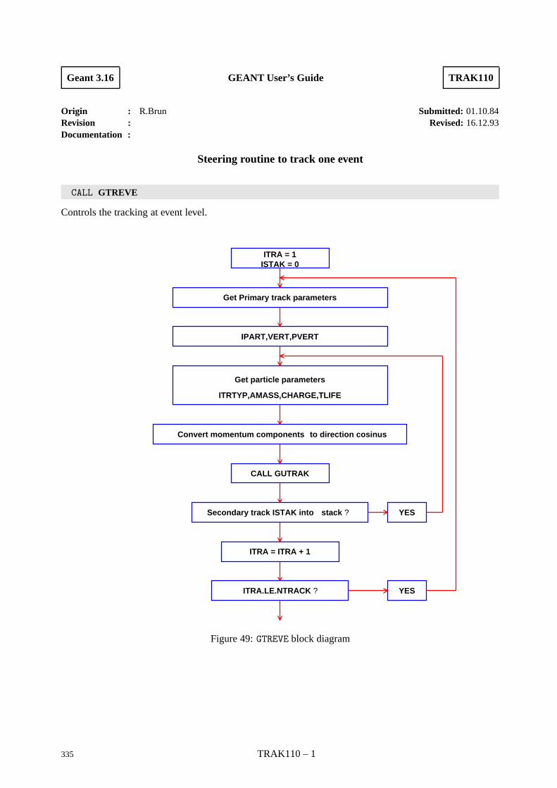
Geant 3.16 GEANT User’s Guide TRAK110
Origin : R.Brun Submitted: 01.10.84Revision : Revised: 16.12.93Documentation :
Steering routine to track one event
CALL GTREVE
Controls the tracking at event level.
ITRA = 1ISTAK = 0
Get Primary track parameters
IPART,VERT,PVERT
Get particle parameters
ITRTYP,AMASS,CHARGE,TLIFE
Convert momentum components to direction cosinus
CALL GUTRAK
Secondary track ISTAK into stack ? YES
ITRA = ITRA + 1
ITRA.LE.NTRACK ? YES
Figure 49: GTREVE block diagram
335 TRAK110 – 1
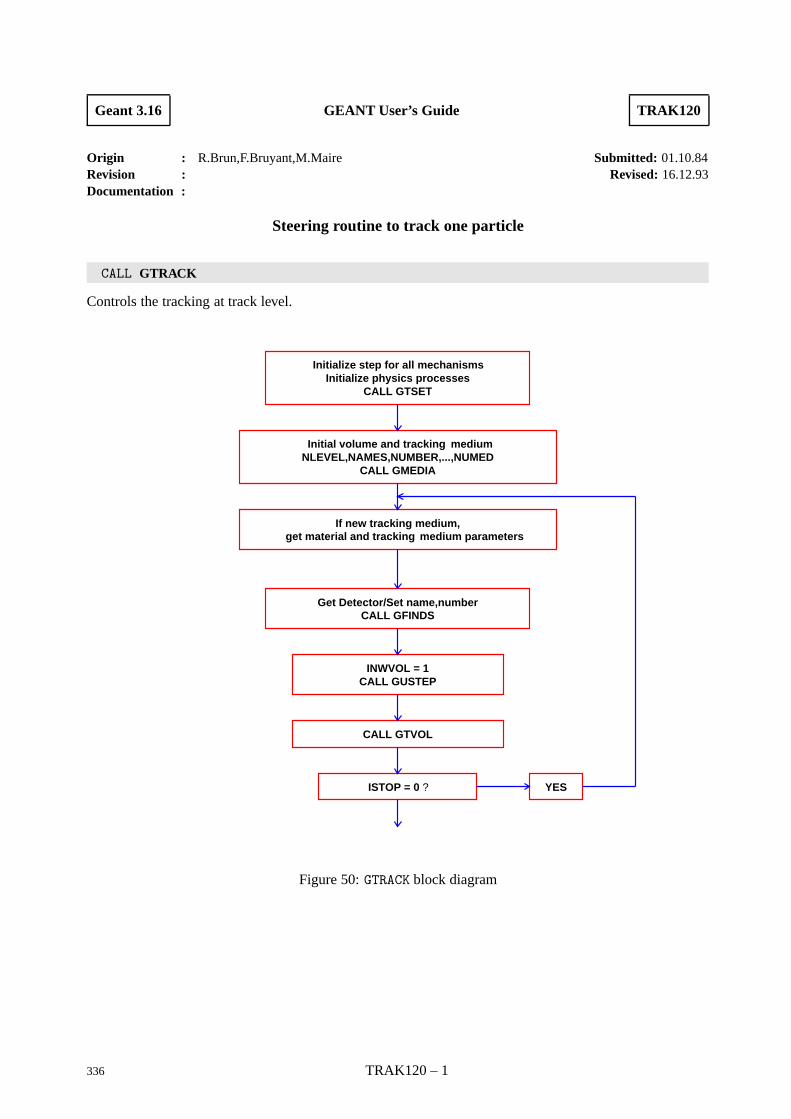
Geant 3.16 GEANT User’s Guide TRAK120
Origin : R.Brun,F.Bruyant,M.Maire Submitted: 01.10.84Revision : Revised: 16.12.93Documentation :
Steering routine to track one particle
CALL GTRACK
Controls the tracking at track level.
Initialize step for all mechanismsInitialize physics processes
CALL GTSET
Initial volume and tracking mediumNLEVEL,NAMES,NUMBER,...,NUMED
CALL GMEDIA
If new tracking medium,get material and tracking medium parameters
Get Detector/Set name,numberCALL GFINDS
INWVOL = 1CALL GUSTEP
CALL GTVOL
ISTOP = 0 ? YES
Figure 50: GTRACK block diagram
336 TRAK120 – 1
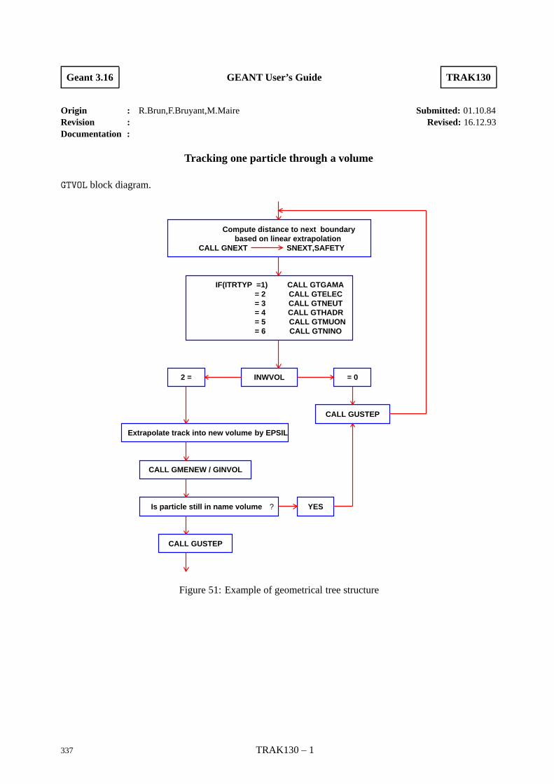
Geant 3.16 GEANT User’s Guide TRAK130
Origin : R.Brun,F.Bruyant,M.Maire Submitted: 01.10.84Revision : Revised: 16.12.93Documentation :
Tracking one particle through a volume
GTVOL block diagram.
Compute distance to next boundarybased on linear extrapolation
CALL GNEXT SNEXT,SAFETY
IF(ITRTYP =1) CALL GTGAMA= 2 CALL GTELEC= 3 CALL GTNEUT= 4 CALL GTHADR= 5 CALL GTMUON= 6 CALL GTNINO
2 = INWVOL = 0
CALL GUSTEP
Extrapolate track into new volume by EPSIL
CALL GMENEW / GINVOL
Is particle still in name volume ? YES
CALL GUSTEP
Figure 51: Example of geometrical tree structure
337 TRAK130 – 1
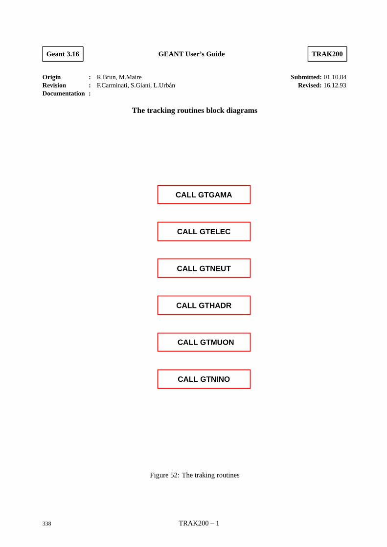
Geant 3.16 GEANT User’s Guide TRAK200
Origin : R.Brun, M.Maire Submitted: 01.10.84Revision : F.Carminati, S.Giani, L.Urban Revised: 16.12.93Documentation :
The tracking routines block diagrams
CALL GTGAMA
CALL GTELEC
CALL GTNEUT
CALL GTHADR
CALL GTMUON
CALL GTNINO
Figure 52: The traking routines
338 TRAK200 – 1
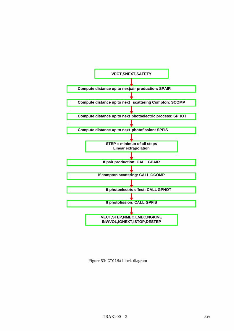
VECT,SNEXT,SAFETY
Compute distance up to nextpair production: SPAIR
Compute distance up to next scattering Compton: SCOMP
Compute distance up to next photoelectric process: SPHOT
Compute distance up to next photofission: SPFIS
STEP = minimun of all stepsLinear extrapolation
If pair production: CALL GPAIR
If compton scattering: CALL GCOMP
If photoelectric effect: CALL GPHOT
If photofission: CALL GPFIS
VECT,STEP,NMEC,LMEC,NGKINEINWVOL,IGNEXT,ISTOP,DESTEP
Figure 53: GTGAMA block diagram
TRAK200 – 2 339
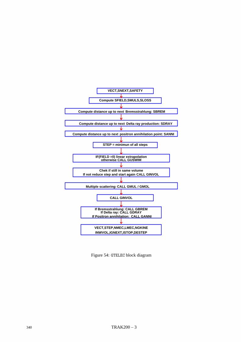
VECT,SNEXT,SAFETY
Compute SFIELD,SMULS,SLOSS
Compute distance up to next Bremsstrahlung: SBREM
Compute distance up to next Delta ray production: SDRAY
Compute distance up to next positron annihilation point: SANNI
STEP = minimun of all steps
IF(FIELD =0) linear extrapolationotherwise CALL GUSWIM
Chek if still in same volumeIf not reduce step and start again CALL GINVOL
Multiple scattering: CALL GMUL / GMOL
CALL GINVOL
If Bremsstrahlung: CALL GBREMIf Delta ray: CALL GDRAY
If Positron annihilation: CALL GANNI
VECT,STEP,NMEC,LMEC,NGKINEINWVOL,IGNEXT,ISTOP,DESTEP
Figure 54: GTELEC block diagram
340 TRAK200 – 3
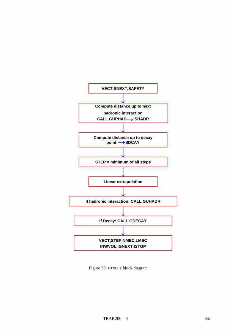
VECT,SNEXT,SAFETY
Compute distance up to next
hadronic interactionCALL GUPHAD SHADR
Compute distance up to decaypoint SDCAY
STEP = minimum of all steps
Linear extrapolation
If hadronic interaction: CALL GUHADR
If Decay: CALL GDECAY
VECT,STEP,NMEC,LMECINWVOL,IGNEXT,ISTOP
Figure 55: GTNEUT block diagram
TRAK200 – 4 341
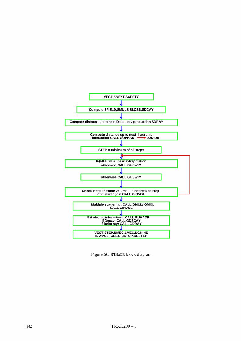
VECT,SNEXT,SAFETY
Compute SFIELD,SMULS,SLOSS,SDCAY
Compute distance up to next Delta ray production SDRAY
Compute distance up to next hadronicinteraction CALL GUPHAD SHADR
STEP = minimum of all steps
IF(FIELD=0) linear extrapolationotherwise CALL GUSWIM
otherwise CALL GUSWIM
Check if still in same volume. If not reduce stepand start again CALL GINVOL
Multiple scattering: CALL GMUL/ GMOLCALL GINVOL
If Hadronic interaction: CALL GUHADRIf Decay: CALL GDECAY
If Delta ray: CALL GDRAY
VECT,STEP,NMEC,LMEC,NGKINEINWVOL,IGNEXT,ISTOP,DESTEP
Figure 56: GTHADR block diagram
342 TRAK200 – 5
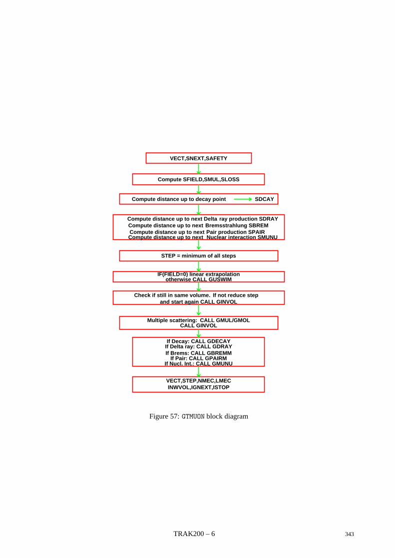
VECT,SNEXT,SAFETY
Compute SFIELD,SMUL,SLOSS
Compute distance up to decay point SDCAY
Compute distance up to next Delta ray production SDRAYCompute distance up to next Bremsstrahlung SBREMCompute distance up to next Pair production SPAIRCompute distance up to next Nuclear interaction SMUNU
STEP = minimum of all steps
IF(FIELD=0) linear extrapolationotherwise CALL GUSWIM
Check if still in same volume. If not reduce stepand start again CALL GINVOL
Multiple scattering: CALL GMUL/GMOLCALL GINVOL
If Decay: CALL GDECAYIf Delta ray: CALL GDRAYIf Brems: CALL GBREMM
If Pair: CALL GPAIRMIf Nucl. Int.: CALL GMUNU
VECT,STEP,NMEC,LMECINWVOL,IGNEXT,ISTOP
Figure 57: GTMUON block diagram
TRAK200 – 6 343
Geant 3.16 GEANT User’s Guide TRAK300
Origin : R.Brun Submitted: 01.06.83Revision : Revised: 14.12.93Documentation :
Storing secondary tracks in the stack
CALL GSKING (IT)
IT (INTEGER) number of the track to be stored for subsequent tracking, if IT=0 all secondarytracks generated in the current step are stored for tracking.
During transport, particles can generate new particles, called secondary. In GEANT these particles are storedin the common /GCKING/ (see [BASE030] for an explanation of the variables in this common). The numberof particles generated in the current step is NGKINE (common /GCKING/). If no user action is taken, thevariable NGKINE is reset to 0 at the beginning of the subsequent step and these particles are not transported.
To be transported by GEANT, these particles need to be stored in the data structure JSTAK (see [TRACK399])which normally is a LIFO stack: the last particle generated is the first one to be tracked when the currentone stops. The order of tracking can be changed by the user, plase see [TRAK310] for more information onthis subject.
The routine GSKING moves particles from the /GCKING/ common to the JSTAK structure, where GEANTlooks for particles to transport.
When a particle is fetched from the JSTAK data structure, its place is freed for a new one, so the informa-tion on the initial kinematics of this track is lost. It may be useful in some occasion to record the initialkinematic of a track and save it till the end of the event. This is accomplished by storing the particle in-formation both in the JSTAK data structure and in the JVERTX/JKINE one, which is permanent throughoutthe life of the event. As already said in [KINE100], this should not be done by the user calling directly theGSVERT/GSKINE routines during tracking, but rather controlling the action of GSKING via the array IFLGKin common /GCKING/. If the particle number IG generated in the current step (1 ≤ IG ≤ NGKINE) is beingmoved to the JSTAK stack, either singularly or together with all the other particles generated in the currentstep (setting the argument of GSKING to 0), the action performed depends on IFLGK(IG):
IFLGK(IG)<0 the particle is ignored;
=0 the particle is stored on the temporary stack JSTAK to be transported;
=1 the particle is stored on the temporary stack JSTAK to be transported and in the JKINEdata structure attaching it to a vertex created in the current position (array VECT(I),I=1,3 in the /GCTRAK/ common);
>1 the particle is stored on the temporary stack JSTAK to be transported and in the JKINEdata structure attaching it to vertex number IFLGK(IG), which must exist.
If IFLGK(IG)>0, after the call to GSKING, IFLGK(IG) is set to the newly created track number in JKINE.The number of the vertex used is returned in IFLGK(NGKINE+1). This feature allows the user to identifythe created vertex and tracks via the routines GSVERU and GSKINU (see [KINE100]).
Example
In case of a hadronic interaction, discard the neutrinos, store the protons in the permanent data structureJVERTX/JKINE, and store all the other particles produced in the temporary stack.
Add to the protons in the JKINE bank the JVOLUM and copy number of the volume and the number of thetracking medium where they have been produced by an interaction.
344 TRAK300 – 1
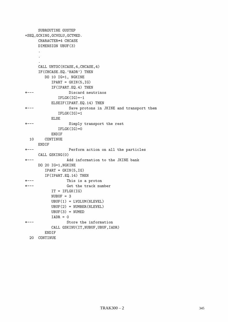
SUBROUTINE GUSTEP+SEQ,GCKING,GCVOLU,GCTMED.
CHARACTER*4 CHCASEDIMENSION UBUF(3)...CALL UHTOC(KCASE,4,CHCASE,4)IF(CHCASE.EQ.’HADR’) THEN
DO 10 IG=1, NGKINEIPART = GKIN(5,IG)IF(IPART.EQ.4) THEN
*--- Discard neutrinosIFLGK(IG)=-1
ELSEIF(IPART.EQ.14) THEN*--- Save protons in JKINE and transport them
IFLGK(IG)=1ELSE
*--- Simply transport the restIFLGK(IG)=0
ENDIF10 CONTINUE
ENDIF*--- Perform action on all the particles
CALL GSKING(0)*--- Add information to the JKINE bank
DO 20 IG=1,NGKINEIPART = GKIN(5,IG)IF(IPART.EQ.14) THEN
*--- This is a proton*--- Get the track number
IT = IFLGK(IG)NUBUF = 3UBUF(1) = LVOLUM(NLEVEL)UBUF(2) = NUMBER(NLEVEL)UBUF(3) = NUMEDIADR = 0
*--- Store the informationCALL GSKINU(IT,NUBUF,UBUF,IADR)
ENDIF20 CONTINUE
TRAK300 – 2 345
Geant 3.16 GEANT User’s Guide TRAK310
Origin : F.Carminati Submitted: 14.12.93Revision : Revised: 14.12.93Documentation :
Altering the order of tracking secondary particles
When secondary particles are produced during particle transport, if the user wants to transport them inturn, they must be stored by a call to GSKING or GSKPHO onto the temporary stack JSTAK. As explainedin [TRAK310], this is a LIFO structure, where the last particle introduced is the first to be extracted to betransported. It may be sometimes interesting to alter the order of tracking, for instance to decide whetherthe current event is worth completing or whether it should be skipped to go to next one.
It is possible in GEANT to alter the behaviour of the JSTAK structure using one of the words of the stack,normally reserved for the user. Stack ordering is activated via the data record SORD 1. This will set to 1 thevariable ISTORD in common /GCSTAK/, which is by default initialised to 0.
When stack ordering is activated, the routine GLTRAC, which fetches the next particle to be tracked fromJSTAK, instead of the last one, will select the one with the maximum value of the user word. This user wordmust be set by the user in the variable UPWGHT in the common /GCTRAK/ prior to the call to GSKING to storeeach secondary.
If, for instance, all the protons must be tracked first, in order of production, and all the other particles after,again according to their time of production, the following code should appear in GUSTEP:
SUBROUTINE GUSTEP+SEQ,GCTRAK,GCKING
.
.
.DO 10 IG=1,NGKINE
*--- Younger particles tracked first*--- Add to the current time of flight the time delay of*--- the secondary
UPWGHT = -TOFG-TOFD(IG)IPART = GKIN(5,IG)IF(IPART.EQ.14) THEN
*--- This is a proton, add a 100 microseconds to have it*--- tracked first
UPWGHT = UPWGHT+1E-4ENDIF
*--- Now store the particle in the GEANT stackCALL GSKING(IG)
10 CONTINUE
Users should be aware of the fact that ordering the stack will change the results, because transport dependson random numbers which will be different for the same particle in the two cases.
346 TRAK310 – 1
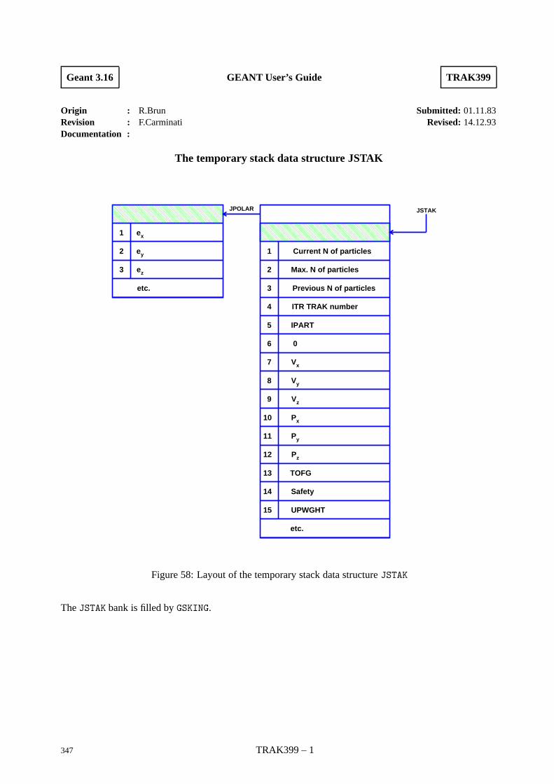
Geant 3.16 GEANT User’s Guide TRAK399
Origin : R.Brun Submitted: 01.11.83Revision : F.Carminati Revised: 14.12.93Documentation :
The temporary stack data structure JSTAK
1
2
3
ex
ey
ez
etc.
1
2
3
4
5
6
7
8
9
10
11
12
13
14
15
Current N of particles
Max. N of particles
Previous N of particles
ITR TRAK number
IPART
0
Vx
Vy
Vz
Px
Py
Pz
TOFG
Safety
UPWGHT
etc.
JSTAKJPOLAR
Figure 58: Layout of the temporary stack data structure JSTAK
The JSTAK bank is filled by GSKING.
347 TRAK399 – 1

Geant 3.10 GEANT User’s Guide TRAK400
Origin : R.Brun Submitted: 01.06.83Revision : Revised: 15.12.93Documentation :
Handling of track space points
CALL GSXYZ
Stores the position of the current particle from common /GCTRAK/ into the data structure JXYZ.
CALL GPJXYZ (NUMB)
NUMB (INTEGER) track number, all tracks if =0;
Prints space points stored in the data structure JXYZ for track number NUMB.
CALL GPCXYZ
Prints tracking and physics parameters after the current step. This routine can be called from GUSTEP.
Some of these routines are called by GDEBUG, see [BASE400] for more information.
348 TRAK400 – 1
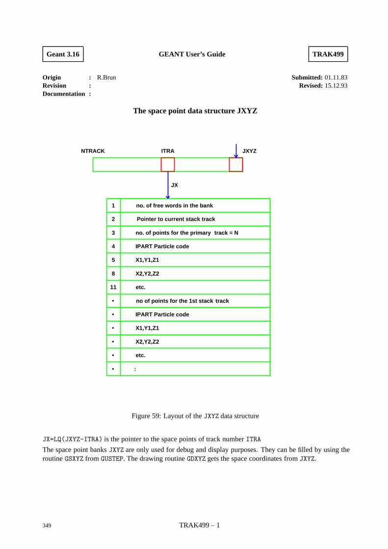
Geant 3.16 GEANT User’s Guide TRAK499
Origin : R.Brun Submitted: 01.11.83Revision : Revised: 15.12.93Documentation :
The space point data structure JXYZ
NTRACK ITRA JXYZ
JX
1
2
3
4
5
8
11
no. of free words in the bank
Pointer to current stack track
no. of points for the primary track = N
IPART Particle code
X1,Y1,Z1
X2,Y2,Z2
etc.
no of points for the 1st stack track
IPART Particle code
X1,Y1,Z1
X2,Y2,Z2
etc.
:
•
•
•
•
•
•
Figure 59: Layout of the JXYZ data structure
JX=LQ(JXYZ-ITRA) is the pointer to the space points of track number ITRA
The space point banks JXYZ are only used for debug and display purposes. They can be filled by using theroutine GSXYZ from GUSTEP. The drawing routine GDXYZ gets the space coordinates from JXYZ.
349 TRAK499 – 1
Geant 3.16 GEANT User’s Guide TRAK500
Origin : R.Brun, M.Hansroul Submitted: 01.10.81Revision : Revised: 16.12.93Documentation :
Tracking routines in magnetic field
CALL GUSWIM (CHARGE,STEP,VECT,VOUT*)
CHARGE (REAL) particle charge in e unit;
STEP (REAL) step size in cm;
VECT (REAL) array of 7 with the initial coordinates, direction cosines and momentum (x, y, z, px/p,py/p, pz/p, p);
VOUT (REAL) array of 7 with the final coordinates, direction cosines and momentum after the step.
This is the steering routine for calculating the deviation of a charged particle in magnetic field. It is calledby the GEANT tracking routines: GTELEC, GTHADR, GTMUON and GTHION. Even if this routine follows thenaming conventions of the user routines, the version provided in the GEANT library is quite adequate formost situation, and users should have a very good reason to modify it.
It calls GRKUTA, GHELIX, GHELX3 according to the value 1, 2 or 3 of IFIELD in common /GCTMED/. IFIELDcorrespond to the argument to the GSTMED routine (see [CONS200]). IFIELD = -1 is reserved for userdecision in case GUSWIM is modified by the user.
CALL GHELX3 (FIELD,STEP,VECT,VOUT*)
FIELD (REAL) field value in kilo-Gauss multiplied by the charge of the particle in e units;
STEP (REAL) step size in cm;
VECT (REAL) array of 7, same as for GUSWIM;
VOUT (REAL) array of 7, same as for GUSWIM;
Transport the particle by a length STEP in a magnetic field. The field is assumed to be uniform and parallelto the z axis. The value of the field is the FIELDM argument to the GSTMED routine (see [CONS200]). Theparticle is transported along an helix. The call to this routine is selected by GUSWIM when IFIELD=3 in thecall to GSTMED.
CALL GHELIX (CHARGE,STEP,VECT,VOUT*)
CHARGE (REAL) particle charge in e units;
STEP (REAL) step size in cm;
VECT (REAL) array of 7, same as for GUSWIM;
VOUT (REAL) array of 7, same as for GUSWIM;
Transport the particle by a length STEP in a magnetic field. The magnetic field is calculated in the middle ofthe step (along a straight line) and it is supposed to be constant along the step and the particle is transportedalong an helix. The call to this routine is selected by GUSWIM when IFIELD=2 in the call to GSTMED. Thisroutine is intended for magnetic fields with a small gradient. The value of the field is obtained from theroutine GUFLD which must be coded by the user.
350 TRAK500 – 1

CALL GRKUTA (CHARGE,STEP,VECT,VOUT*)
The arguments have the same meaning than those of GHELIX. Transport a particle in magnetic field usingRunge-Kutta method for solving the kinematic equations (Nystroem algorithm [1], procedure 25.5.20). Thecall to this routine is selected by GUSWIM when IFIELD=1 in the call to GSTMED. This method is the slowerof the three and it must be used for magnetic fields with strong gradient. Again the magnetic field is obtainedfrom the GUFLD routine which the user has to code.
CALL GUFLD ((VECT,F*)
VECT (REAL) array of 3 with the position in space where the field has to be returned;
F (REAL) array of 3 with the magnetic field in VECT, in kilo-Gauss units.
User routine to return the three components of the magnetic field at point VECT expressed in kilo-Gauss.This routine must be provided by the user for all tracking media where IFIELD is 1 or 2. This routine willbe called very often, at least three times at each step, so all the care must be put in its optimisation.
TRAK500 – 2 351

TRAK Bibliography
[1] Handbook. Technical report, National Bureau of Standards.
352 TRAK500 – 3
Geant 3.16 GEANT User’s Guide XINT001
Origin : Submitted: 15.06.84Revision : Revised: 19.12.93Documentation : R.Brun
The interactive version of GEANT
The interactive version is an essential tool for users who are in charge of the design of a detector. In additionto all the batch tools which are also available, the interactive user can call one by one and in any order allthe basic functions of GEANT to:
• design or modify the geometry of the setup;
• exploit the drawing package in a more efficient way;
• change the running conditions on a event by event basis.
The system is based on the KUIP [1] command processor. The user has to know a minimum about KUIPand should read at least the first chapter of the manual.
A set of encapsulated Postscript files have been collected in a new section XINT010. They illustrate thevisualization possibilities of the interactive version of GEANT.
1 Invoking the interactive version
Instead of writing a MAIN program to initialize the Geant batch version, it is possible to use the MAINinteractive program (GXINT321.F) provided in /cern/pro/lib exactly as the library LIBGEANT321.A. Theuser has simply to insert in his link file the file GXINT321.F as the main program, followed by the userobject code and by the library LIBGEANT321.A.
Example:PROGRAM GXINT** GEANT main program. To link with the MOTIF user interface* the routine GPAWPP(NWGEAN,NWPAW) should be called, whereas* the routine GPAW(NWGEAN,NWPAW) gives access to the basic* graphics version.*PARAMETER (NWGEAN=3000000,NWPAW=1000000)COMMON/GCBANK/GEANT(NWGEAN)COMMON/PAWC/PAW(NWPAW)*CALL GPAWPP(NWGEAN,NWPAW)*END
The user has to set the desired value of NWGEAN and NWPAW for the GEANT and PAW Zebra stores,and to call the desired initialization routine:
• GPAW to initialize, besides GEANT, also HIGZ and to include the full functionality of PAW;
• GPAWPP to initialize, besides GEANT and HIGZ, also the Motif version and to include the fullfunctionality of Paw++;
353 XINT001 – 1
• USER initialization routine, to do anything else (for example a UGINIT- like routine or a gxint315.f–like routine).
The interactive version, after the initialization, gives the control to the user at the prompt GEANT > ; thenit is possible to type and execute commands (corresponding to batch routines) to edit the geometry, the ma-terials or the tracking media at run time. It is also possible to execute commands to visualize the detectors,to set the kinematics and to run events. Again interactively, one can spy the histograms, change the kine-matics, and run more events (visualizing the tracks and the hits, for example). The GXINT chapter containsin the following pages a full description of the available GEANT commands. See the PAW, KUIP, DZDOC,HIGZ manuals for a description of the relative commands executable from GEANT. All the commands arealso documented by an on-line help. (Try to type HELP at the first GEANT > prompt). In the interactiveversion, a COMIS interface is also available: COMIS is a FORTRAN interpreter which allows:
• to edit at run time important routines like UGEOM, GUSTEP, GUKINE, etc.
• to ‘execute’ them from the interactive session, without having to recompile and relink, by typingcommands like CALL UGEOM.F.
Of course the interpreter is slower than the compiled object code, then, since GEANT321, it is also possibleto invoke the native compiler and to link dinamically to the executable the compiled routine (see the COMISmanual for further details).
The following write ups describe individual commands which can be typed one by one at the terminal, orgrouped into macros which can be edited and saved in the KUIP environment.
The commands are listed in subsection 1 - 13:
1. General GEANT
2. Clipping commands GEANT/CVOL
3. Drawing commands GEANT/DRAWING
4. Graphics control commands GEANT/DRAWING
5. Geometry commands GEANT/GEOMETRY
6. Volume creation commands GEANT/CREATE
7. Control commands GEANT/CONTROL
8. ZEBRA/RZ commands GEANT/RZ
9. ZEBRA/FZ commands GEANT/FZ
10. Data structure commands GEANT/DZ
11. Scanning commands GEANT/SCAN
12. Physics parameter commands GEANT/PHYSICS
13. List commands GEANT/LISTS
2 The Motif Interface
The interactive version 3.21 contains an object oriented Motif-based user interface. It can be accessed spec-ifying ‘m’ as workstation type. The full functionality of the X11 version remains available, while newMotif-specific features have been added.
3 The main ideas
The GEANT data structures are considered as KUIP browsable classes and their contents as ‘objects’ onwhich one can perform actions (the GEANT commands). According to the Motif conventions, an object canbe selected clicking the left button of the mouse (when the cursor is on the icon representing that object).
XINT001 – 2 354
Clicking then on the right button of the mouse, a menu of possible commands will appear (double clickingon the left button the first action of this list will be executed); the selected command will perform the relativeactions on the selected object. Such actions (like drawing, for example) can be executed either directly orvia the use of an automatically opened Motif panel. Objects drawn in the graphics window can be ‘picked’as well (for example, volumes, tracks, hits); clicking the right button when the cursor is on the selected ob-ject, a menu of possible actions on that object is displayed. Users can finally define Motif panels containingbuttons corresponding to the most frequently used commands. An on-line help is available for any specificsubject.
4 The Geant++ Executive Window
It replaces the normal dialog window; it contains a Transcript Pad, where the text output of the executedcommands is displayed, and an Input Pad, where the user can still type the desired commands in the oldstyle.
The Geant++ Main File Browser
On the left side it displays a list of the GEANT data structures, of the available commands, file, macros andZebra divisions used. Selecting one of them, the full list of icons representing the objects of that class isshown in the main area of the browser. Proceeding as described before, it is possible to perform actions onthe classes (like create a new object) or on the objects belonging to them. It is possible to create menus ofcommands just clicking on the string ‘commands’ at the top line of the browser.
The Geant++ Graphics Window
Any object to be drawn in the graphics window can be stored in the current picture file (automaticallyopened after each NEXT command) via a call to IGPID (see Higz manual). It can be afterwards ‘picked’as described before. In the case of commands executed via the use of Motif panels, some input values canbe set with a slider ranging in the specifed range for the relative variable; moving the slider (after havingclicked on the right-hand ‘activating box’) the relative action is performed in the graphics window whenreleasing the button of the mouse; when in ‘drag mode’, the action is performed while moving the slider(keeping the left button pressed): especially when double buffering has been selected, this can be useful forreal time manipulations.
5 An Example
Start your GEANT321 executable module (linked with GXINT321 and Motif1.2);
type ‘m’ as workstation type;
click the left button of the mouse after positioning the cursor on the string VOLU in the browser;
click the left button of the mouse after positioning the cursor on any icon in the main area of the browser;
click now the right button of the mouse and keep it pressed;
move the mouse to select the action ‘Tree’ and release the button;
the drawing of the logical tree will be displayed in the graphics window;
position the cursor on the drawing of a box (containing a volume name) in the graphics window, click theright button and keep it pressed;
release the button selecting the action ‘Dspec’;
355 XINT001 – 3

the command DSPEC for that volume will be executed in a separate window;
repeat the exercise selecting this time the action ‘Dspe3d’;
the DSPEC will be executed in the first window, the volume specifications will be printed in a separatewindow and a Motif panel will appear;
click the left button of the mouse positioning the cursor in the Motif panel on the ‘Value changed’ button,and select the DRAG option;
click now the left button on the ‘activating box’ on the right of the ‘Theta’ slider;
click on the ‘Theta’ slider and, keeping pressed the left button of the mouse, move it right-wards;
the drawing in the graphics window will rotate;
release the button and type ‘igset 2buf 1’ in the executive window;
restart moving the slider as before.
XINT001 – 4 356
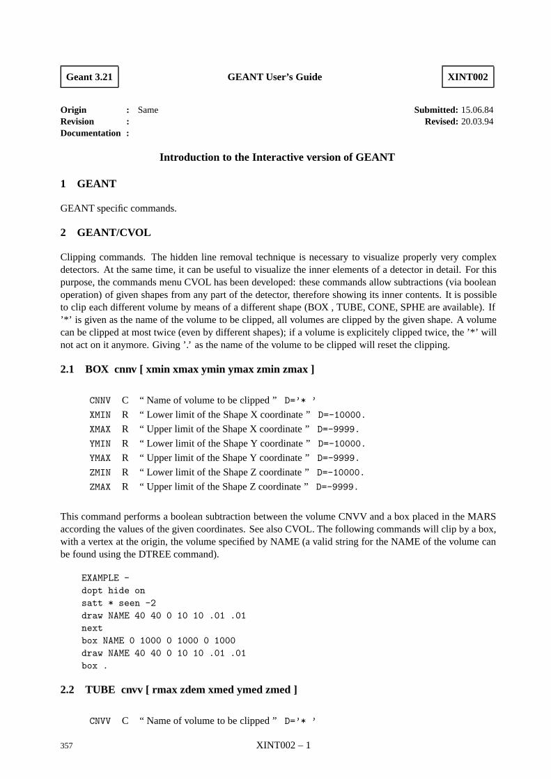
Geant 3.21 GEANT User’s Guide XINT002
Origin : Same Submitted: 15.06.84Revision : Revised: 20.03.94Documentation :
Introduction to the Interactive version of GEANT
1 GEANT
GEANT specific commands.
2 GEANT/CVOL
Clipping commands. The hidden line removal technique is necessary to visualize properly very complexdetectors. At the same time, it can be useful to visualize the inner elements of a detector in detail. For thispurpose, the commands menu CVOL has been developed: these commands allow subtractions (via booleanoperation) of given shapes from any part of the detector, therefore showing its inner contents. It is possibleto clip each different volume by means of a different shape (BOX , TUBE, CONE, SPHE are available). If’*’ is given as the name of the volume to be clipped, all volumes are clipped by the given shape. A volumecan be clipped at most twice (even by different shapes); if a volume is explicitely clipped twice, the ’*’ willnot act on it anymore. Giving ’.’ as the name of the volume to be clipped will reset the clipping.
2.1 BOX cnnv [ xmin xmax ymin ymax zmin zmax ]
CNNV C “ Name of volume to be clipped ” D=’* ’
XMIN R “ Lower limit of the Shape X coordinate ” D=-10000.
XMAX R “ Upper limit of the Shape X coordinate ” D=-9999.
YMIN R “ Lower limit of the Shape Y coordinate ” D=-10000.
YMAX R “ Upper limit of the Shape Y coordinate ” D=-9999.
ZMIN R “ Lower limit of the Shape Z coordinate ” D=-10000.
ZMAX R “ Upper limit of the Shape Z coordinate ” D=-9999.
This command performs a boolean subtraction between the volume CNVV and a box placed in the MARSaccording the values of the given coordinates. See also CVOL. The following commands will clip by a box,with a vertex at the origin, the volume specified by NAME (a valid string for the NAME of the volume canbe found using the DTREE command).
EXAMPLE -dopt hide onsatt * seen -2draw NAME 40 40 0 10 10 .01 .01nextbox NAME 0 1000 0 1000 0 1000draw NAME 40 40 0 10 10 .01 .01box .
2.2 TUBE cnvv [ rmax zdem xmed ymed zmed ]
CNVV C “ Name of volume to be clipped ” D=’* ’
357 XINT002 – 1
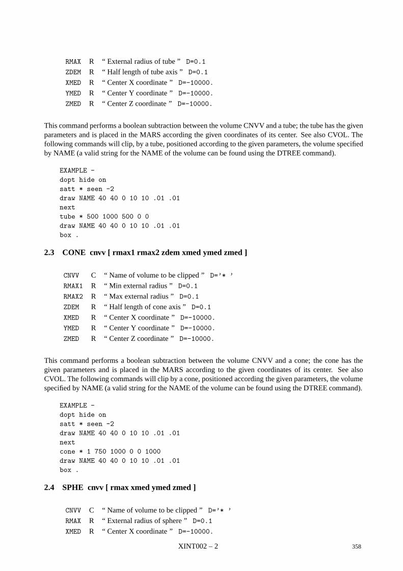
RMAX R “ External radius of tube ” D=0.1
ZDEM R “ Half length of tube axis ” D=0.1
XMED R “ Center X coordinate ” D=-10000.
YMED R “ Center Y coordinate ” D=-10000.
ZMED R “ Center Z coordinate ” D=-10000.
This command performs a boolean subtraction between the volume CNVV and a tube; the tube has the givenparameters and is placed in the MARS according the given coordinates of its center. See also CVOL. Thefollowing commands will clip, by a tube, positioned according to the given parameters, the volume specifiedby NAME (a valid string for the NAME of the volume can be found using the DTREE command).
EXAMPLE -dopt hide onsatt * seen -2draw NAME 40 40 0 10 10 .01 .01nexttube * 500 1000 500 0 0draw NAME 40 40 0 10 10 .01 .01box .
2.3 CONE cnvv [ rmax1 rmax2 zdem xmed ymed zmed ]
CNVV C “ Name of volume to be clipped ” D=’* ’
RMAX1 R “ Min external radius ” D=0.1
RMAX2 R “ Max external radius ” D=0.1
ZDEM R “ Half length of cone axis ” D=0.1
XMED R “ Center X coordinate ” D=-10000.
YMED R “ Center Y coordinate ” D=-10000.
ZMED R “ Center Z coordinate ” D=-10000.
This command performs a boolean subtraction between the volume CNVV and a cone; the cone has thegiven parameters and is placed in the MARS according to the given coordinates of its center. See alsoCVOL. The following commands will clip by a cone, positioned according the given parameters, the volumespecified by NAME (a valid string for the NAME of the volume can be found using the DTREE command).
EXAMPLE -dopt hide onsatt * seen -2draw NAME 40 40 0 10 10 .01 .01nextcone * 1 750 1000 0 0 1000draw NAME 40 40 0 10 10 .01 .01box .
2.4 SPHE cnvv [ rmax xmed ymed zmed ]
CNVV C “ Name of volume to be clipped ” D=’* ’
RMAX R “ External radius of sphere ” D=0.1
XMED R “ Center X coordinate ” D=-10000.
XINT002 – 2 358
YMED R “ Center Y coordinate ” D=-10000.
ZMED R “ Center Z coordinate ” D=-10000.
This command performs a boolean subtraction between the volume CNVV and a sphere; the sphere hasthe given parameters and is placed in the MARS according to the given coordinates of its center. See alsoCVOL. The following commands clip by a sphere, positioned according to the given parameters, the volumespecified by NAME (a valid string for the NAME of the volume can be found using the DTREE command).EXAMPLE -
dopt hide onsatt * seen -2draw NAME 40 40 0 10 10 .01 .01nextsphe * 500 0 0 500draw NAME 40 40 0 10 10 .01 .01box .
2.5 VALCUT xcut ycut zcut
XCUT R “x coordinate of cutted value” D=0.
YCUT R “y coordinate of cutted value” D=0.
ZCUT R “z coordinate of cutted value” D=0.
It allows the cutting in the ray-tracing. All the volumes are cutted from XCUT to +BIG along the x axis,from YCUT to +BIG along the y axis and from ZCUT to +BIG along the z axis.
359 XINT002 – 3
3 GEANT/DRAWING
Drawing commands. These commands allow the visualization in several ways of the volumes defined inthe geometrical data structure. It is possible to draw the logical tree of volumes belonging to the detec-tor (DTREE), to show their geometrical specification (DSPEC,DFSPC), to draw them and their cut views(DRAW, DCUT). Moreover, it is possible to execute these commands when the hidden line removal op-tion is activated; in this case, the volumes can be also either translated in the space (SHIFT), or clipped byboolean operation (CVOL). In addition, it is possible to fill the surfaces of the volumes with solid colourswhen the shading option (SHAD) is activated. Several tools (ZOOM, LENS) have been developed to zoomdetailed parts of the detectors or to scan physical events as well. Finally, the command MOVE will allow therotation, translation and zooming on real time parts of the detectors or tracks and hits of a simulated event.Ray-tracing commands. In case the command (DOPT RAYT ON) is executed, the drawing is performed bythe Geant ray-tracing; automatically, the color is assigned according to the tracking medium of each volumeand the volumes with a density lower/equal than the air are considered transparent; if the option (USER) isset (ON) (again via the command (DOPT)), the user can set color and visibility for the desired volumes viathe command (SATT), as usual, relatively to the attributes (COLO) and (SEEN). The resolution can be setvia the command (SATT * FILL VALUE), where (VALUE) is the ratio between the number of pixels drawnand 20 (user coordinates). Parallel view and perspective view are possible (DOPT PROJ PARA/PERS); inthe first case, we assume that the first mother volume of the tree is a box with dimensions 10000 X 10000X 10000 cm and the view point (infinetely far) is 5000 cm far from the origin along the Z axis of the usercoordinates; in the second case, the distance between the observer and the origin of the world referencesystem is set in cm by the command (PERSP NAME VALUE); grand-angle or telescopic effects can beachieved changing the scale factors in the command (DRAW). When the final picture does not occupy thefull window, mapping the space before tracing can speed up the drawing, but can also produce less preciseresults; values from 1 to 4 are allowed in the command (DOPT MAPP VALUE), the mapping being moreprecise for increasing (VALUE); for (VALUE = 0) no mapping is performed (therefore max precision andlowest speed). The command (VALCUT) allows the cutting of the detector by three planes ortogonal to thex,y,z axis. The attribute (LSTY) can be set by the command SATT for any desired volume and can assumevalues from 0 to 7; it determines the different light processing to be performed for different materials: 0= dark-matt, 1 = bright-matt, 2 = plastic, 3 = ceramic, 4 = rough-metals, 5 = shiny-metals, 6 = glass, 7 =mirror. The detector is assumed to be in the dark, the ambient light luminosity is 0.2 for each basic hue (thesaturation is 0.9) and the observer is assumed to have a light source (therefore he will produce parallel lightin the case of parallel view and point-like-source light in the case of perspective view).
3.1 DRAW name [ theta phi psi u0 v0 su sv ]
NAME C “Volume name”
THETA R “Viewing angle theta (for 3D projection)” R=0.:180.
PHI R “Viewing angle phi (for 3D projection)” R=0.:360.
PSI R “Viewing angle psi (for 2D rotation)” R=0.:360.
U0 R “U-coord. (horizontal) of volume origin”
V0 R “V-coord. (vertical) of volume origin”
SU R “Scale factor for U-coord.”
SV R “Scale factor for V-coord.”
CALL GDRAW(name,theta,phi,psi,u0,v0,su,sv)
If optional parameters are missing, the corresponding values are taken from the common /GCDRAW/. Thiscommand will draw the volumes, selected with their graphical attributes, set by the SATT facility. Thedrawing may be performed with hidden line removal and with shading effects according to the value of theoptions HIDE and SHAD; if the option SHAD is ON, the contour’s edges can be drawn or not. If the option
XINT002 – 4 360

HIDE is ON, the detector can be exploded (BOMB), clipped with different shapes (CVOL), and some ofits parts can be shifted from their original position (SHIFT). When HIDE is ON, if the drawing requiresmore than the available memory, the program will evaluate and display the number of missing words (sothat the user can increase the size of its ZEBRA store). Finally, at the end of each drawing (with HIDEon), the program will print messages about the memory used and statistics on the volumes’ visibility. Thefollowing commands will produce the drawing of a green volume, specified by NAME, without using thehidden line removal technique, using the hidden line removal technique, with different linewidth and colour(red), with solid colour, with shading of surfaces, and without edges. Finally, some examples are given forthe ray-tracing. (A possible string for the NAME of the volume can be found using the command DTREE).
EXAMPLE -satt * seen -2satt NAME colo 3draw NAME 40 40 0 10 10 .01 .01nextdopt hide ondraw NAME 40 40 0 10 10 .01 .01nextsatt NAME colo 2satt NAME lwid 4draw NAME 40 40 0 10 10 .01 .01nextdopt shad onsatt * lwid 1satt NAME fill 1draw NAME 40 40 0 10 10 .01 .01nextsatt NAME fill 3draw NAME 40 40 0 10 10 .01 .01nextdopt edge offdraw NAME 40 40 0 10 10 .01 .01dopt rayt onsatt * fill 20dopt mapp 1draw NAME 40 40 0 10 10 .01 .01dopt proj perspersp NAME 500draw NAME 40 40 0 10 10 1 1valcut 100 100 100dopt mapp 0dopt user onsatt NAM1 seen 0satt NAM2 colo 2draw NAME 40 40 0 10 10 5 5
3.2 SPOT xlpos ylpos zlpos inten
XLPOS R “x coordinate of light source”
YLPOS R “y coordinate of light source”
ZLPOS R “z coordinate of light source”
INTEN I “intensity of light source”
361 XINT002 – 5
This point-like light source can be moved in the space and its intensity can be changed (INTEN going from0 to 10) relatively to the ambience light.
3.3 VAR5D tseqto nproc nmptot totmby tseq tlat tnet
TSEQTO R “total sequential time”
NPROC I “number of processors”
NMPTOT I “number of message passing”
TOTMBY R “total megabytes transfert”
TSEQ R “not parallelized code”
TLAT R “latency time”
TNET R “network speed in Mbytes/sec”
It sets the values of the parameters expressed in the formula and specify which variables must be assumedas x,y,z (setting their value to 1001,1002,1003, respectively).
3.4 RANG5D x1min x1max y1min y1max z1min z1max
X1MIN R “x coordinate min”
X1MAX R “x coordinate max”
Y1MIN R “y coordinate min”
Y1MAX R “y coordinate max”
Z1MIN R “z coordinate min”
Z1MAX R “z coordinate max”
It sets the range for the x,y,z variables.
3.5 DVOLUME n namnum chnrs [ theta phi psi u0 v0 su sv ]
N I “Number of elements in arrays LNAMES and LNUMBS” D=1
NAMNUM C “Volume names and numbers (ex. "NAME1,NR1,NAME2,NR2")”
CHNRS C “Reference system used” D=’MARS’
THETA R “Viewing angle theta (for 3D projection)” R=0.:360.
PHI R “Viewing angle phi (for 3D projection)” R=0.:360.
PSI R “Viewing angle psi (for 2D rotation)” R=0.:180.
U0 R “U-coord. (horizontal) of volume origin”
V0 R “V-coord. (vertical) of volume origin”
SU R “Scale factor for U-coord.”
SV R “Scale factor for V-coord.”
Possible CHNRS values are:MARS
DRS
CALL GDRVOL(n,lnames,lnumbs,nrs,theta,phi,psi,u0,v0,su,sv)
N is the number of levels from the top of the geometry structure to the volume lnames(n),lnumbs(n) to
XINT002 – 6 362

be drawn. NAMNUM contain the arrays lnames and lnumbs, identifying the path, in pairs and separatedby commas; for example (with n=2) : ’lname(1),lnumbs(1),lname(2),lnumbs(2) ’ CHNRS is the name ofthe reference system used: MARS for MAster Reference System or DRS for Daughter Reference System.NRS=0 for MARS or NRS〈〉0 for DRS If optional parameters are missing, the current values in /GCDRAW/are taken.
3.6 DCUT name caxis cutval [ u0 v0 su sv ]
NAME C “Volume name”
CAXIS C “Axis value”
CUTVAL R “Cut plane distance from the origin along the axis”
U0 R “U-coord. (horizontal) of volume origin”
V0 R “V-coord. (vertical) of volume origin”
SU R “Scale factor for U-coord.”
SV R “Scale factor for V-coord.”
Possible CAXIS values are:
X
Y
Z
CALL GDRAWC(name,iaxis,cutval,u0,v0,su,sv)
The cut plane is normal to caxis (X,Y,Z), corresponding to iaxis (1,2,3), and placed at the distance cutvalfrom the origin. The resulting picture is seen from the the same axis. If optional parameters are missing, thecurrent values in /GCDRAW/ are taken. When HIDE Mode is ON, it is possible to get the same effect withthe CVOL/BOX command.
3.7 DXCUT name cutthe cutphi cutval [ theta phi u0 v0 su sv ]
NAME C “Volume name”
CUTTHE R “Theta angle of the line normal to cut plane” R=0.:360.
CUTPHI R “Phi angle of the line normal to cut plane” R=0.:360.
CUTVAL R “Cut plane distance from the origin along the axis”
THETA R “Viewing angle theta (for 3D projection)” R=0.:360.
PHI R “Viewing angle phi (for 3D projection)” R=0.:360.
U0 R “U-coord. (horizontal) of volume origin”
V0 R “V-coord. (vertical) of volume origin”
SU R “Scale factor for U-coord.”
SV R “Scale factor for V-coord.”
CALL GDRAWX(name,cutthe,cutphi,cutval,theta,phi,u0,v0,su,sv)
The cut plane is normal to the line given by the cut angles cutthe and cutphi and placed at the distance cutvalfrom the origin. The resulting picture is seen from the viewing angles theta,phi. If optional parameters aremissing, the current values in /GCDRAW/ are taken.
363 XINT002 – 7
3.8 SHIFT cnvn xxxx yyyy zzzz
CNVN C “ Name of volume to be shifted ” D=’*’
XXXX R “ Shift along X axis ” D=0.
YYYY R “ Shift along Y axis ” D=0.
ZZZZ R “ Shift along Z axis ” D=0.
To draw a volume shifted from its initial position when hidden line removal is ON. It can be useful if youwant to extract a volume or some volumes from the detector to show them more clearly. The last requestedSHIFT for each volume NAME is performed. Moreover, the SHIFT of each volume will be performedstarting from where its mother has been shifted, so that it’s easier to SHIFT nicely sets of volumes usingthe mother-daughter relationships. If ’.’ is given as the name of the volume to be shifted, the shifts forall volumes will be reset. The following commands will produce the translation along the Z-axis of thepreviously drawn volume:
EXAMPLE -dopt hide onsatt * seen -2draw NAME 40 40 0 10 10 .01 .01shift NAME 0 0 10
3.9 BOMB boom
BOOM R “ Exploding factor for volumes position ” D=0. R=-10.:10.
To ’explode’ the detector. If BOOM is positive (values smaller than 1. are suggested, but any value ispossible) all the volumes are shifted by a distance proportional to BOOM along the direction between theircentre and the origin of the MARS; the volumes which are symmetric with respect to this origin are simplynot shown. BOOM equal to 0 resets the normal mode. A negative (greater than -1.) value of BOOM willcause an ’implosion’; for even lower values of BOOM the volumes’ positions will be reflected respect tothe origin. This command can be useful to improve the 3D effect for very complex detectors. The followingcommands will make explode the detector:
EXAMPLE -dopt hide onsatt * seen 1draw NAME 40 40 0 10 10 .01 .01bomb 1nextdraw NAME 40 40 0 10 10 .01 .01
3.10 DTREE [ name levmax iselt ]
NAME C “Volume name” D=’[’
LEVMAX I “Depth level” D=3 R=-15:15
ISELT I “Options ” D=111
This command allows the drawing of the logical tree, displaying the name, the multiplicity and other in-formation about the volumes, via a call to GDTREE(name,levmax,isel): if the third parameter is not given(default), the command will produce the drawing of the tree displaying, for each volume, the number of the
XINT002 – 8 364
following levels (red arrows) and of the preceeding levels (green arrows); then the control is automaticallygiven to the mouse: clicking on the left button when the cursor is inside a volume’s pave will perform aDSPEC for that volume; doing the same when the cursor is on a red arrow, will perform a DTREE for therelative volume (the number of levels displayed depending on the clicked arrow); doing the same for the’i-th’ green arrow of a given volume, will perform a DTREE for its mother-volume staying ’i’ levels before.If running with X-windows, the drawing of the specification (DSPEC) is performed in a different windowto speed up the scanning of the tree. Iterating this procedure it is possible to analyse very easily and quicklyany kind of tree. Clicking the right button of the mouse will return the control to the command mode. Ifthe ISELT parameter is given, then the TREE will work as in the previous version, with ISELT up to 10001.The following command will perform a drawing of the tree and give the control to the user via the mouse:
EXAMPLE -dtree NAME 3
3.11 DSPEC name
NAME C “Volume name”
Trough a call to GDSPEC(name), this command allows one to show three views of the volume (two cut-views and a 3D view), together with its geometrical specifications. The 3D drawing will be performedaccording the current values of the options HIDE and SHAD and according the current CVOL clippingparameters for that volume.
3.12 D3DSPEC name [ teta3 phi3 psi3 u03 v03 zm3 ]
NAME C “Volume name”
TETA3 R “Theta angle” D=40. R=0.:180.
PHI3 R “Phi angle” D=40. R=0.:360.
PSI3 R “Psi angle” D=0. R=0.:360.
U03 R “U-coord. (horizontal) of volume origin” D=10. R=-40.:40.
V03 R “V-coord. (vertical) of volume origin” D=10. R=-40.:40.
ZM3 R “Zoom factor for current size factors” D=1. R=0.00001:10.
Trough a call to GSPE3D, this command allows one to show the volume (3D views in real time), togetherwith its geometrical specifications (if using MOTIF). The 3D drawing will be performed according thecurrent values of the options HIDE and SHAD and according the current CVOL clipping parameters forthat volume.
3.13 DFSPC name [ csort cinter ]
NAME C “Volume name”
CSORT C “Alphabetic sorting flag” D=’N’
CINTER C “Interactive/Batch version” D=’I’
Possible CSORT values are:
365 XINT002 – 9
Y
N
0
1
Possible CINTER values are:
I
B
0
1
CALL GDFSPC(name,isort,inter)
Same as DSPEC, but it will draw the specifications for all the volumes. If the alphabetic sorting flag is YES,all pictures will be drawn in ascending alphabetic order; isort is set to 1. If INTERACTIVE, (inter=1), theroutine will prompt the user at each plot before doing a clear screen, otherwise it will clear automaticallythe screen before starting a new frame.
3.14 DTEXT x0 y0 text size angle lwid cent
X0 R “X-coord. (horizontal) of text string” D=10. R=0.:20.
Y0 R “Y-coord. (vertical) of text string” D=10. R=0.:20.
TEXT C “Text string” D=’GEANT’
SIZE R “Character size (cm)” D=.5
ANGLE R “Rotation angle (deg)” D=0. R=0.:360.
LWID I “Line width” D=4
CENT C “Centering option” D=’CENT’
Possible CENT values are:
CENT
LEFT
RIGH
CALL GDRAWT(x0,y0,text,size,angle,lwid,opt)
It allows one to draw some text in the current picture. Now more than 160 colours are available. The textcolour must be set via the command IGSET. The size of the text will follow the zooming factors in the viewbanks.
3.15 DVECTOR xvect yvect npoint
XVECT C “Vector containing X-coord. (horizontal)”
YVECT C “Vector containing Y-coord. (vertical)”
NPOINT I “Number of coord.”
XINT002 – 10 366
Draw a polyline of ’npoint’ point via a call to GDRAWV(xvect,yvect,npoint) where xvect and yvect are twoKUIP vectors
3.16 DSCALE u v
U R “U-coord. (horizontal) of the centre of scale”
V R “V-coord. (vertical) of the centre of scale”
CALL GDSCAL(u,v)
It draws a scale centered in U,V.
3.17 DAXIS x0 y0 z0 dx
X0 R “X-coord. of axis origin”
Y0 R “Y-coord. of axis origin”
Z0 R “Z-coord. of axis origin”
DX R “Axis size”
CALL GDAXIS(x0,y0,z0,dx)
This commmand superimposes the axis of the MARS on the current picture. It is useful for finding imme-diately the orientation of the current drawing of the detector in the space.
3.18 DMAN u v type
U R “U-coord. (horizontal) of the centre of man”
V R “V-coord. (vertical) of the centre of man”
TYPE C “Man, Wm1, Wm2, Wm3” D=’MAN’
Possible TYPE values are:
MAN
WM1
WM2
WM3
CALL GDMAN(u,v),CALL GDWMN1(u,v),CALL GDWMN2(u,v),CALL GDWMN2(u,v)
It superimposes the picure of a man or of a woman, chosen among three different ones, with the same scalefactors as the detector in the current drawing.
3.19 DHEAD [ isel name chrsiz ]
ISEL I “Option flag” D=111110
NAME C “Title” D=’[’
CHRSIZ R “Character size (cm) of title NAME” D=0.6
367 XINT002 – 11

CALL GDHEAD(isel,name,chrsiz)
ISEL =
0 to have only the header linesxxxxx1 to add the text name centered on top of headerxxxx1x to add global detector name (first volume) on leftxxx1xx to add date on rightxx1xxx to select thick characters for text on top of headerx1xxxx to add the text ’EVENT NR x’ on top of header1xxxxx to add the text ’RUN NR x’ on top of header
NOTE that ISEL=x1xxx1 or ISEL=1xxxx1 are illegal choices, i.e. they generate overwritten text. NAME isthe title and CHRSIZ the character size in cm of text name.
3.20 MEASURE
Position the cursor on the first point (u1,v1) and hit the space bar(GKS). Position the cursor on the secondpoint (u2,v2) and hit the space bar(GKS). Clicking the left button of the mouse (X11) will have the sameeffect as hiting the space bar (GKS). The command will compute and print the distance in space separatingthe two points on the projection view. It can be useful to measure distances either between volumes orbetween tracks or hits.
3.21 PICK
Activates graphic input to identify detector elements in a cut view. Clicking on the left button of the mousewhen the cursor is in a given point of the drawing and clicking again (outside the detector) will producethe following effect: a line joininig the two points will be drawn together with the name and the mediumnumber of the volume picked with the first clicking close to the second point.
3.22 MOVE name [ nopt ]
NAME C “Volume name” D=’ ’
NOPT C “S=sample mode,T=tracks,H=hits” D=’ ’
Positioning some daughter volumes inside a ’mother’, it can be important to check if overlaps between suchvolumes have occurred. Instead of putting the drawing in a view bank, zooming, and iterating the process fordifferent viewing angles of the same detector, the MOVE facility has been developed (for machines runningwith X11): it is sufficient to draw a view of the volumes to be analysed (after setting the proper SEEN,COLO, etc. attributes) and then to enter ’MOVE’ followed by the same ’NAME’ used for the last commandDRAW. The detector will appear in a panel with five buttons at the bottom: THETA, PHI, TRASL, ZOOM,OFF. Clicking on the left button of the mouse, when the cursor is inside the THETA area, will rotate thedetector along the polar angle theta according to the backward-to-forward movement of the mouse (clickingup and down the left button if not in sample mode); clicking on the right button of the mouse will stop therotation; clicking now on the left button of the mouse when inside the PHI area will activate a rotation alongthe polar angle phi. In the same way, activating the TRASL button, the detector can be translated in theu,v plane of the screen according to the 2D-movement of the mouse. Finally, activating the ZOOM button,the detector will be zoomed (or unzoomed) according to the backward-to-forward movement of the mouse.Clicking on the OFF button will return the control to the ’command mode’. The MOVE command willwork also with hidden line removal and shading options (when SHAD is on the background will be black);moreover, if the volumes are clipped, exploded, shifted, etc., they will be ’MOVED’ with these features aswell. Tracks and hits of a previously stored physical event can be moved together with the detector, allowing
XINT002 – 12 368

a dynamical 3-D analysis of the simulated events. Clicking the central button of the mouse when a goodview of the event is found, will stop any movement and the mouse will allow the normal picking capabilitiesfirst for the tracks and then for the hits. After clicking of the right button, the normal movement will restartto find another interesting view of the event and to iterate the process. The MOVE is also available in samplemode. The following commands will produce a drawing of a volume and then will give the control to theMOVE panel; try the following possibilities:
EXAMPLE 1 -dopt hide offsatt * seen -2draw NAME 40 40 0 10 10 .01 .01move NAMEEXAMPLE 2 -dopt hide onsatt * seen -2draw NAME 40 40 0 10 10 .01 .01move NAMEEXAMPLE 3 -dopt shad onsatt * colo 3satt * fill 2dopt edge offdraw NAME 40 40 0 10 10 .01 .01move NAME
3.23 MOVE3D name [ theta phi psi u0 v0 su sv sz nopt ]
NAME C “Volume name” D=’ ’
THETA R “Viewing angle theta (for 3D projection)” D=40. R=0.:180.
PHI R “Viewing angle phi (for 3D projection)” D=40. R=0.:360.
PSI R “Viewing angle psi (for 2D rotation)” D=0. R=0.:180.
U0 R “U-coord. (horizontal) of volume origin” D=10. R=0.:20.
V0 R “V-coord. (vertical) of volume origin” D=10. R=0.:20.
SU R “Scale factor for U-coord.” D=0.01
SV R “Scale factor for V-coord.” D=0.01
SZ R “Scale zoom factor” D=1. R=0.1:10.
NOPT C “T=tracks,H=hits” D=’ ’
Possible NOPT values are:
T
H
Same functionality of the command MOVE interfaced with MOTIF.
3.24 PERSP name distt [ samp ]
NAME C “Volume name” D=’ ’
DISTT R “Volume distance from observer” D=1000.
SAMP C “Control to the mouse” D=’OFF ’
369 XINT002 – 13
To control the perspective according to the variation of the distance between the observer and the object (ifPROJ has the value PERS). If SAMP is ON the control of the distance is given via the mouse.
3.25 LENS knum [ ksam ]
KNUM I “View bank identifier” D=1
KSAM C “Sample mode ” D=’OFF ’
Interactive zooming for detectors and events when running with X-windows. Using this command, whenshowing the contents of a view bank, it is possible to click (left button) in two points of the drawing (whichwill represent the left upper corner and the right bottom corner of the part to be zoomed). After the secondclick a new ’window’ will appear to fit the frame defined by the two clicks and it will show a zoomed viewas seen from a lens with those dimensions. Clicking now the central button will translate the lens over thedrawing, while clicking the right button will stop it. Moreover, clicking the left button of the mouse, thelens will increase (or decrease) its magnification power according to the backward-to-forward movementof the mouse. A click on the right button will stop this action and it is possible to restart the translationof the lens or, clicking on the right button again, to make the lens disappear. It is then possible to openanother ’window-lens’ with different dimensions. Thus, this command can be useful to scan detailed partsof a detector or to scan hits and showers for events. Clicking the right button when no lens is displayedwill return the control to the ’command mode’. The LENS is also available in sample mode when KSAMis ’ON’. The following commands will fill a view bank and will allow to scan the detector and an eventpreviously stored via the use of LENS (when running with X-windows):
EXAMPLE -satt * seen 1dopen 1draw NAME 40 40 0 10 10 .01 .01dxyz 0dhits * * 0 0 .2dclosedsh 1lens 1 on
3.26 ZOOM [ zfu zfv isel uz0 vz0 u0 v0 ]
ZFU R “Zoom factor for U-coord. (horizontal)” D=2.
ZFV R “Zoom factor for V-coord. (vertical)” D=2.
ISEL I “Options” D=1
UZ0 R “U-coord. of the centre of zoom rectangle” D=10. R=0.:20.
VZ0 R “V-coord. of the centre of zoom rectangle” D=10. R=0.:20.
U0 R “U-coord. of the centre of resulting zoomed rectangle” D=10. R=0.:20.
V0 R “V-coord. of the centre of resulting zoomed rectangle” D=10. R=0.:20.
CALL GDZOOM(zfu,zfv,uz0,vz0,u0,v0)
This command sets the zoom parameters that will be used by subsequent calls to the drawing routines. Eachzoom operation is always relative to the status of the current zoom parameters. The scale factors in u,v arerespectively zfu,zfv. zfu=0 (or zfv=0) will act as a reset (i.e. unzoomed viewing). The zoom is computedaround uz0,vz0 (user coordinates), and the resulting picture will be centered at u0,v0. The use of the spacebar is replaced by the left button of the mouse running with X11: If isel=0 :
XINT002 – 14 370
1. position the cursor at (uz0,vz0)2. type the space bar (GKS)
(u0,v0 are chosen at centre of screen) If isel=1 :
1. position the cursor at first corner of zoom rectangle2. type the space bar (GKS)3. position the cursor at second corner of zoom rectangle4. type the space bar (GKS)
(zfu,zfv are chosen according to the zoom rectangle; uz0,vz0 are chosen at the centre of the zoom rectangle;u0,v0 are chosen at centre of screen) If isel=2 :
1. position the cursor at (uz0,vz0)2. type the space bar (GKS)3. position the cursor at (u0,v0)4. type the space bar (GKS)
If isel=1000+n and running with X-windows:
1. n must be the identifier of an active view bank2. clicking on the left button of the mouse will display
a zoomed view (computed around the cursor position) ofthe previous drawing in a new window
3. it is now possible to iterate the zooming from the new window4. clicking on the right button will return the control to the
main window5. clicking on the left button it is possible to open new windows
zooming in other points of the detector6. clicking on the right button when the main window is active
will return the control to the ’command mode’.
3.27 DXYZ [ itra ]
ITRA I “Track number” D=0
CALL GDXYZ(itra)
Draw tracks previously stored via GSXYZ.
3.28 KXYZ [ epsilo ]
EPSILO R “Delta angle” D=0.25
CALL GKXYZ(epsilo)
The picking of track points requires the JXYZ data structure and is repeated until the character typed is ’Q’or ’q’ (GKS) or the right button of the mouse is clicked (X11). EPSILO is the delta angle used for picking;if EPSILO=0 there is no optimization performed and over all the track points the one nearest to the pickpoint is taken.
3.29 DPART [ itra isel size ]
371 XINT002 – 15
ITRA I “Track number” D=0
ISEL I “Option flag” D=11
SIZE R “Character size (cm) for particle names” D=0.25
CALL GDPART(itra,isel,size)isel=x1 to draw the track numberisel=1x to draw the particle name
3.30 DHITS [ chuset chudet itra isymb ssymb ]
CHUSET C “User set identifier” D=’*’
CHUDET C “User detector identifier” D=’*’
ITRA I “Number of the selected track” D=0
ISYMB I “Character selection number” D=0
SSYMB R “Size of characters (cm)” D=0.1
CALL GDHITS(chuset,chudet,itra,isymb,ssymb). The character plotted at each hit point may be chosen byisymb :
-1 (small) hardware points (fast)0 software crosses (default)
840,850 empty/full circles (slow)841,851 empty/full squares (slow)842,852 empty/full triangles (up) (slow)843,853 empty diamond/full triangle (down) (slow)844,854 empty/full stars (slow)
Except for isymb=-1, the size of the character on the screen can be chosen by SSYMB cm. The hitcolour will follow the value of TXCI (text colour) for isymb〉0, the value of PMCI (polymarkers colour)for isymb〈0, the value of PLCI (polyline colour) for isymb=0.
3.31 KHITS [ chuset chudet epsilo ]
CHUSET C “User set identifier” D=’*’
CHUDET C “User detector identifier” D=’*’
EPSILO R “Pick aperture” D=0.1
CALL GKHITS(chuset,chudet,epsilo)
The picking of hit points requires the appropriate JSET data structure have been filled and is repeated untilthe character typed is ’Q’ or ’q’ (GKS) or the right button of the mouse is clicked (X11). If the charactertyped to pick is ’K’ or ’k’ then the kinematics of the corresponding track is also printed. The search is madeof all the hits of all tracks in detector CHUDET of set CHUSET. EPSILO is the pick aperture; if EPSILO〈0its absolute value is taken and in addition the pick aperture is drawn; if EPSILO=0 there is an infinite pickaperture and over all the hits the one nearest to the pick point is taken.
3.32 DCHIT [ chuset chudet itra isymb sizmax ihit hitmin hitmax ]
XINT002 – 16 372
CHUSET C “User set identifier” D=’*’
CHUDET C “User detector identifier” D=’*’
ITRA I “Number of the selected track” D=0
ISYMB I “Character selection number” D=0
SIZMAX R “Maximum character size (cm)” D=1
IHIT I “Index of array HITS” D=4
HITMIN R “Lower boundary of HITS(IHIT)” D=0
HITMAX R “Upper boundary of HITS(IHIT)” D=0
CALL GDCHIT(chuset,chudet,itra,isymb,sizmax,ihit,hitmin,hitmax)
The character plotted at each hit point may be chosen via CSYMB; isymb is composed as:
-1 (small) hardware points (fast)0 software crosses (default)
840,850 empty/full circles (slow)841,851 empty/full squares (slow)842,852 empty/full triangles (up) (slow)843,853 empty diamond/full triangle (down) (slow)844,854 empty/full stars (slow)
Except for isymb=-1 the SIZE of the character on the screen is a function of HITS(IHIT), the array contain-ing the calorimeter quantity, with HITMIN and HITMAX defining its range. The maximum character size(used in overflow) is SIZMAX.
SIZE = SIZMAX * ( HITS(IHIT) - HITMIN ) / HITMAX
3.33 DUVIEW name type cpxtyp [ iview ]
NAME C “Detector name”
TYPE C “View name”
CPXTYP C “Complexity name”
IVIEW I “View number where picture is stored” D=0
CALL GUVIEW(name,type,cpxtyp,iview)
373 XINT002 – 17
4 GEANT/GRAPHICS˙CONTROL
Graphics control commands.
4.1 DOPEN iview
IVIEW I “View number”
CALL GDOPEN(iview)
When a drawing is very complex and requires a long time to be executed, it can be useful to store it in aview bank: after a call to DOPEN and the execution of the drawing (nothing will appear on the screen), andafter a necessary call to DCLOSE, the contents of the bank can be displayed in a very fast way through acall to DSHOW; therefore, the detector can be easily zoomed many times in different ways. Please note thatthe pictures with solid colours can now be stored in a view bank or in ’PICTURE FILES’.
4.2 DSHOW [ iview ]
IVIEW I “View number”
CALL GDSHOW(iview)
It shows on the screen the contents of a view bank. It can be called after a view bank has been closed.
4.3 DELETE iview
IVIEW I “View number”
CALL GDELET(iview)
It deletes a view bank from memory.
4.4 DCLOSE
CALL GDCLOS
It closes the currently open view bank; it must be called after the end of the drawing to be stored.
4.5 CHANGEWK
CALL GCHNWK It open a new workstation (if not already opened) and activate it (deactivating the defaultone).
4.6 RESETWK
CALL GRESWK It deactivate the previosly activated workstation and reactivate the default one.
4.7 SSETAT iopt
IOPT C “Attribute name”
XINT002 – 18 374
Set current attribute.
4.8 SSETVA [ rval ]
RVAL R “Attribute value” D=1. R=-10.:10.
Set current attribute value.
4.9 SATT [ name iopt ival ]
NAME C “Volume name” D=’* ’
IOPT C “Name of the attribute to be set” D=’DEFA’
IVAL I “Value to which the attribute is to be set” D=10000
CALL GSATT(name,iopt,ival)
name=’*’ stands for all the volumes. iopt can be chosen among the following :
’WORK’ 0=volume name is inactive for the tracking1=volume name is active for the tracking (default)
’SEEN’ 0=volume name is invisible1=volume name is visible (default)
-1=volume invisible with all its descendants in the tree-2=volume visible but not its descendants in the tree
’LSTY’ line style 1,2,3,... (default=1)LSTY=7 will produce a very precise approximation forrevolution bodies.
’LWID’ line width -7,...,1,2,3,..7 (default=1)LWID<0 will act as abs(LWID) was set for the volumeand for all the levels below it. When SHAD is ’ON’, LWIDrepresent the linewidth of the scan lines filling the surfaces(whereas the FILL value represent their number). Thereforetuning this parameter will help to obtain the desiredquality/performance ratio.
’COLO’ colour code -166,...,1,2,..166 (default=1)n=1=blackn=2=red; n=17+m, m=0,25, increasing luminosity according to
’m’;n=3=green; n=67+m, m=0,25, increasing luminosity according to
’m’;n=4=blue; n=117+m, m=0,25, increasing luminosity according to
’m’;n=5=yellow; n=42+m, m=0,25, increasing luminosity according to
’m’;n=6=violet; n=142+m, m=0,25, increasing luminosity according to
’m’;n=7=lightblue; n=92+m, m=0,25, increasing luminosity according to
’m’;colour=n*10+m, m=1,2,...9, will produce the same colouras ’n’, but with increasing luminosity according to ’m’;COLO<0 will act as if abs(COLO) was set for the volume
375 XINT002 – 19
and for all the levels below it.When for a volume the attribute FILL is > 1 (and theoption SHAD is on), the ABS of its colour code must be < 8because an automatic shading of its faces will beperformed.
’FILL’ (1992) fill area -7,...,0,1,...7 (default=0)when option SHAD is ’on’ the FILL attribute of anyvolume can be set different from 0 (normal drawing);if it is set to 1, the faces of such volume will be filledwith solid colours; if ABS(FILL) is > 1, then a lightsource is placed along the observer line, and the faces ofsuch volumes will be painted by colours whose luminositywill depend on the amount of light reflected;if ABS(FILL) = 1, then it is possible to use all the 166colours of the colour table, becouse the automatic shadingis not performed;for increasing values of FILL the drawing will be performedwith higher and higher resolution improving the quality (thenumber of scan lines used to fill the faces increases with FILL);it is possible to set different values of FILLfor different volumes, in order to optimize at the same timethe performance and the quality of the picture;FILL<0 will act as if abs(FILL) was set for the volumeand for all the levels below it.This kind of drawing can be saved in ’picture files’or in view banks.0=drawing without fill area1=faces filled with solid colours and resolution = 62=lowest resolution (very fast)3=default resolution4=.................5=.................6=.................7=max resolutionFinally, if a coloured background is desired, the FILLattribute for the first volume of the tree must be setequal to -abs(colo), colo being >0 and <166.
’SET ’ set number associated to volume name’DET ’ detector number associated to volume name’DTYP’ detector type (1,2)
4.10 SCALE gscu gscv
GSCU R “Scale factor for U-coord.”
GSCV R “Scale factor for V-coord.”
Change the scale factors GSCU and GSCV in /GCDRAW/.
4.11 COLOR icol
ICOL I “Colour code” D=1
XINT002 – 20 376
CALL GDCOL(-abs(icol))
4.12 LWID lwidth
LWIDTH I “Line width code” D=1
CALL GDLW(-abs(lwidth))
4.13 NEXT
Clear screen (start a new picture on graphics file, if opened).
4.14 DOPT [ iopt ival ]
IOPT C “Option name” D=’*’
IVAL C “Option value” D=’*’
CALL GDOPT(iopt,ival)
To set/modify the drawing options.
IOPT IVAL ActionTHRZ ON Draw tracks in R vs Z
OFF (D) Draw tracks in X,Y,Z180360
PROJ PARA (D) Parallel projectionPERS Perspective
TRAK LINE (D) Trajectory drawn with linesPOIN " " with markers
HIDE ON Hidden line removal using the CG packageOFF (D) No hidden line removal
SHAD ON Fill area and shading of surfaces.OFF (D) Normal hidden line removal.
RAYT ON Ray-tracing on.OFF (D) Ray-tracing off.
EDGE OFF Does not draw contours when shad is on.ON (D) Normal shading.
MAPP 1,2,3,4 Mapping before ray-tracing.0 (D) No mapping.
USER ON User graphics options in the raytracing.OFF (D) Automatic graphics options.
4.15 SIZE [ xsize ysize ]
XSIZE R “Size along X” D=20.
YSIZE R “Size along Y” D=20.
Set the size of the picture. On the terminal, the pictures will have the ratio YSIZE/XSIZE, and, if a metafileis produced, pictures will be YSIZE by XSIZE cm. This command sets the parameters for the normalisation
377 XINT002 – 21

transformation number 1 to [0-XSIZE], [0-YSIZE].
4.16 SPERS dpers
DPERS R “Distance from the origin”
Set the variable dpers in /GCDRAW/, representing the distance from the origin when using option PER-Spective.
4.17 MAP˙COLOR [ icadd icval ]
ICADD I “Colour table index” D=0
ICVAL I “Colour table value” D=0
Sets the color table LOOKTB(ICADD)=ICVAL. If ICADD=0 then LOOKTB(1:16) is taken. If ICVAL isomitted the current value of LOOKTB(ICADD) is shown.
XINT002 – 22 378

5 GEANT/GEOMETRY
Geometry commands.
5.1 OPTI iopti
IOPTI C “GSORD optimisation level” D=’0’ Minus
Possible IOPTI values are:
-1
2
This flag controls the tracking optimisation performed via the GSORD routine:
1 no optimisation at all; GSORD calls disabled;0 no optimisation; only user calls to GSORD kept;1 all non-GSORDered volumes are ordered along the best axis;2 all volumes are ordered along the best axis.
5.2 SVOLU name shape numed npar par
NAME C “Volume name”
SHAPE C “Volume type”
NUMED I “Tracking medium number”
NPAR I “Number of shape parameters”
PAR C “Vector containing shape parameters”
CALL GSVOLU(name,shape,numed,par,npar,ivolu)
where par is a KUIP vector. It creates a new volume in the JVOLUM data structure.
5.3 SPOS name number mother x0 y0 z0 irot only
NAME C “Volume name”
NUMBER I “Copy number of the volume”
MOTHER C “Mother volume name”
X0 R “X coord. of the volume in mother ref. sys.”
Y0 R “Y coord. of the volume in mother ref. sys.”
Z0 R “Z coord. of the volume in mother ref. sys.”
IROT I “Rotation matrix number w.r.t. mother ref. sys.”
ONLY C “ONLY/MANY flag”
CALL GSPOS(name,number,mother,x0,y0,z0,irot,only)
It positions a previously defined volume in the mother.
5.4 SDVN name mother ndiv caxis
379 XINT002 – 23
NAME C “Volume name”
MOTHER C “Mother volume name”
NDIV I “Number of divisions”
CAXIS C “Axis value”
Possible CAXIS values are:
X
Y
Z
1
2
3
CALL GSDVN(name,mother,ndiv,iaxis)
X,Y,Z of CAXIS will be translated to 1,2,3 for IAXIS. It divides a previously defined volume.
5.5 PVOLU numb
NUMB I “Volume ID”
CALL GPVOLU(numb)
Prints volumes’ specifications.
5.6 SROTM irot theta1 phi1 theta2 phi2 theta3 phi3
IROT I “Rotation matrix number”
THETA1 R “Polar angle for axis I” D=0. R=0.:180.
PHI1 R “Azimuthal angle for axis I” D=0. R=0.:360.
THETA2 R “Polar angle for axis II” D=0. R=0.:180.
PHI2 R “Azimuthal angle for axis II” D=0. R=0.:360.
THETA3 R “Polar angle for axis III” D=0. R=0.:180.
PHI3 R “Azimuthal angle for axis III” D=0. R=0.:360.
CALL GSROTM(irot,theta1,phi1,theta2,phi2,theta3,phi3)
It defines the rotation matrix number IROT.
5.7 PROTM numb
NUMB I “Matrix ID”
CALL GPROTM(numb)
XINT002 – 24 380
Print matrixes’ specifications.
5.8 STMED ntmed name nmat isvol ifield fieldm tmaxfd stemax deemax epsil stmin
NTMED I “Tracking medium number” D=1
NAME C “Tracking medium name”
NMAT I “Material number” D=1
ISVOL I “Sensitive volume flag” D=0
IFIELD I “Magnetic field” D=0
FIELDM R “Max. field value (Kilogauss)” D=0
TMAXFD R “Max. angle due to field (deg/step)” D=0.01
STEMAX R “Max. step allowed” D=1.E+10
DEEMAX R “Max. fraction of energy lost in a step” D=0.01
EPSIL R “Tracking precision (cm)” D=0.01
STMIN R “Min. step due to continuos processes (cm)” D=0.1
CALL GSTMED(ntmed,name,nmat,isvol,ifield,fieldm,tmaxfd,+ stemax,deemax,epsil,stmin,0,0)
IFIELD = 0 if no magnetic field; IFIELD = -1 if user decision in GUSWIM; IFIELD = 1 if tracking per-formed with GRKUTA; IFIELD = 2 if tracking performed with GHELIX; IFIELD = 3 if tracking performedwith GHELX3.
5.9 PTMED numb
NUMB I “Medium ID”
CALL GPTMED(numb)
Print tracking media’s specifications.
5.10 EDITV [ isel name ]
ISEL I “Options” D=0
NAME C “Volume name” D=’ ’
CALL GEDITV(isel,name)
When the routine prompts for input parameters that do not need to be changed, type return. ISEL is used toselect the editing operation to be performed:
ISEL=0, CALL GGCLOSISEL=1, to modify shape parameters PAR given by GSVOLUISEL=2, to modify NAME given by GSVOLUISEL=3, to delete NAME given by GSVOLUISEL=4, to unlink NAME,NR given by GSPOS/GSDVN/GSDV..ISEL=5, to modify X0,Y0,Z0 of NAME,NR given by GSPOSISEL=6, to modify IROT of NAME,NR given by GSPOSISEL=7, to modify NDIV given by GSDVNISEL=8, to modify IAXIS given by GSDVN
381 XINT002 – 25
5.11 CADINT fname aname nbins lunit lunit2 inst site dept resp
FNAME C “Name of the SET file” D=’example.set’
ANAME C “Name of the volume”
NBINS I “Number of the instances” D=1
LUNIT I “Logical unit number for SET file” D=66
LUNIT2 I “Logical unit number for material file” D=67
INST C “Name of your institute” D=’CERN’
SITE C “Name of site” D=’MEYRIN’
DEPT C “Name of departement” D=’CN’
RESP C “Name of sender” D=’god_knows_who’
CALL GTXSET(fname,aname,nbins,lunit,lunit2,inst,site,dept,resp)
This command produces a SET file describing the given volume with the contents currently set visible. (Usethe visibility attribute, see SATT SEEN.) The description is given as a flat assembly related to the globalcoordinate system. The ouput can be read into CAD systems (EUCLID-IS) trough a SET interface. A listof materials of the volumes in the SET file and the GEANT tree is written into a file with the same filenameas the SET file, but with extension .mat.
5.12 REUCLID lun fname
LUN I “Logical unit of the file to be read” R=1:100
FNAME C “Name of the EUCLID file to be read”
CALL GREUCL(LUN,FNAME)
Calls the routine to read into GEANT a geometry from an ASCII file written by the EUCLID-GEANTinterface.
5.13 WEUCLID lun fname topvol [ number nlevel ]
LUN I “Logical unit of the file to be written” R=1:100
FNAME C “Name of the EUCLID file to be written”
TOPVOL C “Volume name of the starting node”
NUMBER I “Copy number of TOPVOL (relevant for GSPOSP)” D=1
NLEVEL I “Number of levels in the tree structure” D=15
CALL GWEUCL(LUN,FNAME)
Calls the routine to write the current GEANT geometry into an ASCII file in EUCLID compatible format.
XINT002 – 26 382
6 GEANT/CREATE
It creates volumes of the given shape interactively. CALL GSVOLU(name,shape,numed,par,npar,ivolu)where par is a KUIP vector
6.1 SBOX name numed halfx halfy halfz [ yesno ]
NAME C “Volume name”
NUMED I “Tracking medium number”
HALFX R “Half X length”
HALFY R “Half Y length”
HALFZ R “Half Z length”
YESNO C “GSPOSP option” D=’NO’
Possible YESNO values are:
YES
NO
6.2 STRD1 name numed hlfdwx hlfupx halfy halfz [ yesno ]
NAME C “Volume name”
NUMED I “Tracking medium number”
HLFDWX R “Half X length in Lower Z Surface”
HLFUPX R “Half X length in Upper Z Surface”
HALFY R “Half Y length”
HALFZ R “Half Z length”
YESNO C “GSPOSP option” D=’NO’
Possible YESNO values are:
YES
NO
6.3 STRD2 name numed hlfdwx hlfupx hlfdwy hlfupy halfz [ yesno ]
NAME C “Volume name”
NUMED I “Tracking medium number”
HLFDWX R “Half X length in Lower Z Surface”
HLFUPX R “Half X length in Upper Z Surface”
HLFDWY R “Half Y length in Lower Z Surface”
HLFUPY R “Half Y length in Upper Z Surface”
HALFZ R “Half Z length”
YESNO C “GSPOSP option” D=’NO’
Possible YESNO values are:
383 XINT002 – 27

YES
NO
6.4 STUBE name numed inrad outrad halfz [ yesno ]
NAME C “Volume name”
NUMED I “Tracking medium number”
INRAD R “Inside Radius”
OUTRAD R “Outside Radius”
HALFZ R “Half Z length”
YESNO C “GSPOSP option” D=’NO’
Possible YESNO values are:
YES
NO
6.5 STUBS name numed inrad outrad halfz sphi ephi [ yesno ]
NAME C “Volume name”
NUMED I “Tracking medium number”
INRAD R “Inside Radius”
OUTRAD R “Outside Radius”
HALFZ R “Half Z length”
SPHI R “Start of section PHI” R=0.:360.
EPHI R “End of section PHI” R=0.:360.
YESNO C “GSPOSP option” D=’NO’
Possible YESNO values are:
YES
NO
6.6 SCONE name numed inrdw outrdw inrup outrup halfz [ yesno ]
NAME C “Volume name”
NUMED I “Tracking medium number”
INRDW R “Inside Radius in Lower Z Surface”
OUTRDW R “Outside Radius in Lower Z Surface”
INRUP R “Inside Radius in Upper Z Surface”
OUTRUP R “Outside Radius in Upper Z Surface”
HALFZ R “Half Z length”
YESNO C “GSPOSP option” D=’NO’
Possible YESNO values are:
XINT002 – 28 384

YES
NO
6.7 SCONS name numed inrdw outrdw inrup outrup halfz sphi ephi [ yesno ]
NAME C “Volume name”
NUMED I “Tracking medium number”
INRDW R “Inside Radius in Lower Z Surface”
OUTRDW R “Outside Radius in Lower Z Surface”
INRUP R “Inside Radius in Upper Z Surface”
OUTRUP R “Outside Radius in Upper Z Surface”
HALFZ R “Half Z length”
SPHI R “Start of section PHI” R=0.:360.
EPHI R “End of section PHI” R=0.:360.
YESNO C “GSPOSP option” D=’NO’
Possible YESNO values are:
YES
NO
6.8 SSPHE name numed inrad outrad sphi ephi stheta etheta [ yesno ]
NAME C “Volume name”
NUMED I “Tracking medium number”
INRAD R “Inside Radius”
OUTRAD R “Outside Radius”
SPHI R “Start of section PHI” R=0.:360.
EPHI R “End of section PHI” R=0.:360.
STHETA R “Start of section THETA”
ETHETA R “End of section THETA”
YESNO C “GSPOSP option” D=’NO’
Possible YESNO values are:
YES
NO
6.9 SPARA name numed halfx halfy halfz axis phi theta [ yesno ]
NAME C “Volume name”
NUMED I “Tracking medium number”
HALFX R “Half X length”
HALFY R “Half Y length”
HALFZ R “Half Z length”
AXIS R “Angle of Y mid-faces segment to Y axis” R=0.:360.
PHI R “PHI angle of Low Z mid-face to High Z mid-face segment” R=0.:360.
385 XINT002 – 29

THETA R “THETA angle of mid-low-Z-face to mid-high-Z-face segment” R=0.:360.
YESNO C “GSPOSP option” D=’NO’
Possible YESNO values are:
YES
NO
XINT002 – 30 386

7 GEANT/CONTROL
Control commands.
7.1 KINE ikine [ pkine1 pkine2 pkine3 pkine4 pkine5 pkine6 pkine7 pkine8 pkine9 pkine10]
IKINE I “IKINE” D=1
PKINE1 R “PKINE(1)”
PKINE2 R “PKINE(2)”
PKINE3 R “PKINE(3)”
PKINE4 R “PKINE(4)”
PKINE5 R “PKINE(5)”
PKINE6 R “PKINE(6)”
PKINE7 R “PKINE(7)”
PKINE8 R “PKINE(8)”
PKINE9 R “PKINE(9)”
PKINE10 R “PKINE(10)”
Set the variables in /GCFLAG/ IKINE, PKINE(10)
7.2 RUNG idrun idevt
IDRUN I “User run number”
IDEVT I “User starting event number”
Set the run number and the starting value for the user event number.
7.3 SORD istord
ISTORD C “Flag to control user ordering of the stack” D=’1’
Possible ISTORD values are:
1
0
If ISTORD is set to 1, the particle with the highest value of the user weight UPWGHT will be selected to betracked next.
7.4 GTIME timint timend itime
TIMINT R “Total time after initialisation”
TIMEND R “Time reserved for the termination phase”
ITIME I “Frequency of control printing”
These commands have limited use in the interactive version. In particular the value of TIMINT is disre-garded by GEANT.
387 XINT002 – 31
7.5 TRACK
Restart tracking, clearing the track and hit banks, but keeping the kinematics.
7.6 TRIGGER [ n ]
N I “Number of events” D=1
Start one or more new events.
7.7 RNDM [ iseed1 iseed2 ]
ISEED1 I “First seed for the random number generator”
ISEED2 I “Second seed for the random number generator”
Set the seeds for the random number generator. If no numbers are given, the currents seeds are printed.
7.8 SWITCH iswi ival
ISWI I “Switch number”
IVAL I “New switch value”
Change one element of array ISWIT(10) in /GCFLAG/
7.9 MZLOGL level
LEVEL I “MZ log level” D=0
Set the log level for the MZ package of ZEBRA: CALL MZLOGL(0,level)
LEVEL = -3 no messages at all-2 error messages only-1 terse logging0 normal
+1 log rare events+2 log calls to MZ routines
7.10 PRINT name number
NAME C “Name”
NUMBER I “Number” D=0
CALL GPRINT(name,number)
7.11 OUTPUT˙LP lout
LOUT I “New output unit”
XINT002 – 32 388

To change lout in /GCUNIT/ Note: unit numbers 5,11,12,13,14,15 are reserved and cannot be used.
7.12 PHITS [ chuset chudet numhi ]
CHUSET C “User set” D=’*’
CHUDET C “User detector” D=’*’
NUMHI I “Hit number” D=0
CALL GPHITS(chuset,chudet)
7.13 PDIGI [ chuset chudet ]
CHUSET C “User set” D=’*’
CHUDET C “User detector” D=’*’
CALL GPDIGI(chuset,chudet)
7.14 SMATE imat namate a z dens radl absl ubuf nwbuf
IMAT I “Material number”
NAMATE C “Material name”
A R “Atomic weight”
Z R “Atomic number”
DENS R “Density”
RADL R “Radiation lenght”
ABSL R “Absorption lenght”
UBUF R “ ”
NWBUF I “ ”
CALL GSMATE(imat,namate,a,z,dens,radl,absl,ubuf,nwbuf)
7.15 SMIXT imat namate a z dens nlmat wmat
IMAT I “Material number”
NAMATE C “Material name”
A R “Atomic weight”
Z R “Atomic number”
DENS R “Density”
NLMAT I “Flag for WMAT”
WMAT R “Relative weights or n. of atoms in molecule”
CALL GSMIXT(imat,namate,a,z,dens,nlmat,wmat)
7.16 PMATE numb
NUMB I “Material number”
389 XINT002 – 33

CALL GPMATE(numb)
7.17 PRMAT imate ipart mecan
IMATE I “Material number”
IPART I “Particle number”
MECAN C “Mechanism”
CALL GPRMAT(imate,ipart,mecan,nekbin,elow)
7.18 PLMAT imate ipart mecan [ idm ]
IMATE I “Material number”
IPART I “Particle number”
MECAN C “Mechanism”
IDM I “ID mode option” D=0
CALL GPLMAT(imate,ipart,mecan,nekbin,elow,idm)
IDM convention for histogramming mode :IDM.gt.0 fill, print, keep histogram(s)IDM.eq.0 fill, print, delete histogram(s)IDM.lt.0 fill, noprint, keep histogram(s)
If MECAN = ’ALL’ all the mechanisms are histogrammed. If the material number is negative, the crosssections relative to material ABS(IMATE) will be histogrammed in barns rather than in 1/cm.
7.19 DRMAT imate ipart [ mecan ]
IMATE I “Material number”
IPART I “Particle number”
MECAN C “List of mechanism” D=’ALL’
CALL GDRMAT(imate,ipart,mecan,nmec) If MECAN = ’ALL’ all the mechanisms are plotted. If thematerial number is negative, the cross sections relative to material ABS(IMATE) will be plotted in barnsrather than in 1/cm. Note that it is not possible to plot anything if GSTMED has not been called for thematerial number IMATE.
7.20 STPAR itmed chpar parval
ITMED I “Medium number”
CHPAR C “Cut or mechanism”
PARVAL R “Value”
CALL GSTPAR(itmed,chpar,parval)
7.21 SPART ipart napart itrtyp amass charge tlife ubuf nwbuf bratio mode
XINT002 – 34 390
IPART I “Particle number”
NAPART C “Particle name”
ITRTYP I “ ”
AMASS R “Mass”
CHARGE R “Charge”
TLIFE R “Lifetime”
UBUF R “ ”
NWBUF I “ ”
BRATIO R “Branching ratios”
MODE I “Decay mode”
CALL GSPART(ipart,napart,itrtyp,amass,charge,tlife,ubuf,nwbuf); CALL GSDK(ipart,bratio,mode)
7.22 PPART numb
NUMB I “Particle number”
CALL GPPART(numb)
7.23 PRKINE numb
NUMB I “Track number”
CALL GPKINE(numb)
7.24 DEBUG [ ideb ]
IDEB C “Debug option” D=’ON’
Possible IDEB values are:
ON
OFF
If ideb=’ON ’ then :
idebug=1, idemin=1, idemax=1000000, itime=1
else :
idebug=0, idemin=0, idemax=0
391 XINT002 – 35
8 GEANT/RZ
ZEBRA/RZ commands.
8.1 PQUEST [ iq1 iq2 ]
IQ1 I “Lower limit for IQ index” D=1
IQ2 I “Upper limit for IQ index” D=20
Print the array IQUEST in /QUEST/.
8.2 FILE lun fname [ chopt ]
LUN I “Logical unit number”
FNAME C “File name”
CHOPT C “Options” D=’[’
Possible CHOPT values are:
’[’
A
N
U
Open a GRZ file.
CHOPT=’ ’ readonly modeCHOPT=’U’ update modeCHOPT=’N’ create new fileCHOPT=’I’ Read all structures from existing fileCHOPT=’O’ Write all structures on file
8.3 REND lunrz
LUNRZ I “Logical unit number”
Close an RZ file opened by GRFILE on logical unit LUNRZ.
CALL GREND(LUNRZ)
8.4 MDIR chdir [ chopt ]
CHDIR C “Directory name”
CHOPT C “Options” D=’[’
To create a new RZ directory below the current directory. with
RZTAGS(1)=’Object’RZTAGS(2)=’Idvers-NR ’
XINT002 – 36 392
8.5 CDIR [ chpath chopt ]
CHPATH C “Path name” D=’[’
CHOPT C “CHOPT” D=’[’
Change or print the current directory.
Ex. CD dir1 ; make DIR1 the new CWDCD //file1/dir2 ; make //FILE1/DIR2 the new CWDCD ; print the name of the CWD
8.6 IN object [ idvers chopt ]
OBJECT C “Structure name”
IDVERS I “Version number” D=1
CHOPT C “Option” D=’[’
Read data structure identified by OBJECT,IDVERS into memory.
MATE read JMATE structureTMED read JTMED structureVOLU read JVOLUM structureROTM read JROTM structureSETS read JSET structurePART read JPART structureSCAN read LSCAN structureINIT read all above data structures
8.7 OUT object [ idvers chopt ]
OBJECT C “Structure name”
IDVERS I “Version number” D=1
CHOPT C “Option” D=’[’
Write data structure identified by OBJECT,IDVERS to RZ file.
MATE write JMATE structureTMED write JTMED structureVOLU write JVOLUM structureROTM write JROTM structureSETS write JSET structurePART write JPART structureSCAN write LSCAN structureINIT write all above data structures
8.8 LDIR [ chpath chopt ]
CHPATH C “Path name” D=’[’
CHOPT C “CHOPT” D=’[’
393 XINT002 – 37
List the contents of a directory (memory or disk). To list all RZ files currently open, type ’LD //’.
8.9 PURGE [ nkeep ]
NKEEP I “Number of cycles to keep” D=1
Purge an RZ directory.
8.10 SCR object [ idvers ]
OBJECT C “Structure name”
IDVERS I “Version number” D=1
Delete entry identified by OBJECT,IDVERS on RZ file. OBJECT may be : MATE,TMED,VOLU,ROTM,SETS,PART,SCA* If OBJECT= * delete all entries with IDVERS.
8.11 LOCK chdir
CHDIR C “Lock identifier” D=’RZFILE’
Lock an RZ directory.
8.12 FREE chdir
CHDIR C “Lock identifier” D=’RZFILE’
Free an RZ directory.
XINT002 – 38 394
9 GEANT/FZ
ZEBRA/FZ commands
9.1 FZIN lun keysu [ ident ]
LUN I “Fortran unit of the FZ file”
KEYSU C “Name of the data structure to be retrieved”
IDENT I “Version of the data structure to be retrieved” D=0
Equivalent to a call to:
CALL GFIN(LUN,KEYSU,1,IDENT,’ ’,IER)
9.2 FZOPEN lun file luntyp len [ chopt ]
LUN I “Fortran unit with which to open the file”
FILE C “Name of the file to be opened”
LUNTYP C “Type of FZ file to be opened by GOPEN” D=’XI’
LEN I “Recordlenght of the file” D=0
CHOPT C “Optional parameter to specify the action” D=’[’
Equivalent to a call to:
CALL GOPEN(LUN,FILE,LUNTYP,LEN,IER)
If CHOPT = I then a call to GFIN or GFOUT will be performed in addition according to the value ofLUNTYP, with the key INIT to save or retrieve the whole initialization data structure.
9.3 FZOUT lun keysu [ ident ]
LUN I “Fortran unit of the FZ file”
KEYSU C “Name of the data structure to be saved”
IDENT I “Version of the data structure to be saved” D=1
Equivalent to a call to:
CALL GFOUT(LUN,KEYSU,1,IDENT,’ ’,IER)
9.4 FZCLOSE lun
LUN I “Fortran unit of the FZ to close”
Equivalent to a call to:
CALL GCLOSE(LUN,IER)
395 XINT002 – 39
10 GEANT/DZ
10.1 SURV name [ number ]
NAME C “Bank name”
NUMBER I “Bank number” D=1
Print a survey of the structure identified by NAME, NUMBER.
10.2 SHOW name [ number chopt ]
NAME C “Bank name”
NUMBER I “Bank number” D=1
CHOPT C “Options” D=’BSV’
Display the contents of a bank or a data structure identified by its NAME and NUMBER. The output formatof the data part is controlled by the internal or external I/O characteristic.
CHOPT=’B’ Print the bank.CHOPT=’S’ Print the bank contents from left to right Sideways
with up to ten elements per line.CHOPT=’V’ Print the vertical (down) structure.CHOPT=’D’ Print the bank contents from top to bottom Downwards
with five elements per line.CHOPT=’L’ Print the linear structure.CHOPT=’Z’ Print the data part of each bank in hexadecimal format
10.3 SNAP [ idiv chopt ]
IDIV I “Division number ” D=2 R=0:24
CHOPT C “Options” D=’M’
Snap of one or more divisions. Provides a snapshot of one or more divisions in a ZEBRA store. The kindof information provided is controlled by CHOPT.
CHOPT=’M’ Print Map entry for each bankCHOPT=’E’ Extend map entry to dump all links of each bank
(otherwise only as many links as will fit on a line)CHOPT=’F’ Full. Dump all active banks, links and dataCHOPT=’K’ Kill. Dropped banks to be treated as active
(dropped banks are not normally dumped under D or F option)CHOPT=’L’ Dump all Link areas associated with the storeCHOPT=’W’ Dump the Working space, links and dataCHOPT=’Z’ Dump the information in hexadecimal.
10.4 VERIFY [ idiv chopt ]
IDIV I “Division number ” D=0 R=0:24
CHOPT C “Options” D=’CLSU’
XINT002 – 40 396
Check the structure of one or more ZEBRA divisions. The verification detail depends on the settings inCHOPT.
CHOPT=’C’ Check chaining of banks onlyCHOPT=’L’ Check validity of the structural links (implies ’C’)CHOPT=’S’ Check the store parametersCHOPT=’U’ Check the validity of the up and origin (implies ’C’)CHOPT=’F’ Errors are considered fatal and generate a call to ZFATAL
10.5 STORE [ ixstor ]
IXSTOR I “Store number” D=0 R=0:24
Display the structure of the ZEBRA store IXSTOR. Output the parameters characterizing the store, followedby a list of all divisions and all link areas associated with the store in question.
10.6 DDIV [ idiv path ]
IDIV I “Division number” D=2
PATH C “Name of the doc file” D=’[’
Facility to display the layout of stores and divisions.
CALL DZDDIV(idiv,LDUMMY,path,’IN’,1,0,1,IWTYPE)
10.7 DISP bank [ path number ]
BANK C “Name of the bank”
PATH C “Name of the doc file” D=’[’
NUMBER I “Number of the bank” D=1
Interactive bank display tool.
CALL DZDISP(IXSTOR,LBANK,path,’N’,1,0,1,IWTYPE)
10.8 DIRZ [ path ]
PATH C “Name of the RZ directory to analyse”
Facility to display RZ directory trees.
CALL DZDIRZ(0,LDUMMY,0,path,’N’,1,0,1)
397 XINT002 – 41
11 GEANT/SCAN
To define parameters for the SCAN geometry. If the routine GUSTEP and GUKINE are properly instru-mented (see examples in GEANX), when the TRI command is entered NTETA Geantinos will be trackedthrough the real detector starting at the vertex position defined by the command vertex. A simplified ver-sion of the geometry is automatically generated in (ETA,PHI) or (THETA,PHI) following the option givenin the command TETA. The data structure LSCAN generated may be saved on an RZ file for subsequentprocessing. This data structure may be used for fast parametrization techniques.
11.1 PHI nphi [ phimin phimax ]
NPHI I “Number of PHI divisions” D=90
PHIMIN R “Minimum PHI in degrees” D=0. R=0.:360.
PHIMAX R “Maximum PHI in degrees” D=360. R=0.:360.
To specify number of divisions along PHI. If no parameter is given, the current values of the parameters aredisplayed.
11.2 TETA nteta [ tetmin tetmax divtyp ]
NTETA I “Number of TETA divisions” D=90
TETMIN R “Minimum value of TETA”
TETMAX R “Maximum value of TETA”
DIVTYP I “Type of TETA division” R=1:3
To specify number of divisions along TETA. If DIVTYP=1 divisions in pseudo-rapidity ETA. If DIVTYP=2divisions in degrees following the THETA angle. If DIVTYP=3 divisions in cos(TETA). If no parameter isgiven, the current values of the parameters are displayed.
11.3 SLIST list
LIST C “List of master volumes”
Only boundary crossings of volumes given in LIST will be seen in the SCAN geometry. If no parametersare given, the current SCAN volumes will be listed. If a full stop (.) is given, the list of scan volumes willbe erased.
11.4 VERTEX vx vy vz
VX R “Scan X-origin” D=0.
VY R “Scan Y-origin” D=0.
VZ R “Scan Z-origin” D=0.
All Geantinos tracked will start from position VX,VY,VZ.
11.5 SFACTORS factx0 factl factr
FACTX0 R “Scale factor for SX0” D=100.
XINT002 – 42 398
FACTL R “Scale factor for SL” D=1000.
FACTR R “Scale factor for R” D=100.
Set scale factors for SX0,SL and R. The given scale factors must be such that:
SX0*FACTX0 < 2**15-1 (32767)SL*FACTL < 2**10-1 (1023)SR*FACTR < 2**17-1 (131071)
11.6 STURN chopt
CHOPT C “SCAN mode setting”
Possible CHOPT values are:
ON
OFF
INIT
Switch on/off SCAN mode. If SCAN mode is on, SCAN geantinos are generated and tracked to fill (orcomplete) the current scan data structure. If SCAN mode is off, normal kinematics generation and trackingwill take place. If INIT is given, the current SCAN data structure (if any) will be dropped and SCAN modewill be turned on.
11.7 PCUTS [ iparam pcutga pcutel pcutha pcutne pcutmu ]
IPARAM I “Parametrization Flag” R=0:1
PCUTGA R “Parametrization Cut for gammas”
PCUTEL R “Parametrization Cut for electrons”
PCUTHA R “Parametrization Cut for charged hadrons”
PCUTNE R “Parametrization Cut for neutral hadrons”
PCUTMU R “Parametrization Cut for muons”
Control parametrization at tracking time.
IPARAM=0 No parametrization is performedIPARAM=1 Parametrization is performed
If parametrization is active and a particle falls below its parametrization cut, then the particle will be replacedby a parametrized shower which will be tracked in the SCAN geometry.
11.8 LSCAN id [ volume chopt ]
ID I “Lego plot identifier” D=2000
VOLUME C “Volume name” D=’XXXX’
CHOPT C “List of options” D=’OPX’
Possible CHOPT values are:
399 XINT002 – 43
’[’
O
P
I
X
L
Generates and plot a table of physics quantities such as the total number of radiation lengths or interactionlengths in function of the SCAN parameters TETA,PHI.
CHOPT=’O’ table is generated at Exit of VOLUME.CHOPT=’I’ table is generated at Entry of VOLUME.CHOPT=’X’ radiation lengthsCHOPT=’L’ Interaction lengthsCHOPT=’P’ Plot the table
If VOLUME=’XXXX’ Mother volume is used.
11.9 HSCAN idphi [ volume chopt ]
IDPHI I “Histogram/phi identifier” D=1000
VOLUME C “Volume name” D=’XXXX’
CHOPT C “List of options” D=’OPX’
Possible CHOPT values are:
’[’
O
P
I
X
L
Generates and plots an histogram of physics quantities such as the total number of radiation lengths orinteraction lengths as a function of the SCAN parameter TETA for a given value of PHI.
CHOPT=’O’ histogram is generated at Exit of VOLUME.CHOPT=’I’ histogram is generated at Entry of VOLUME.CHOPT=’X’ radiation lengthsCHOPT=’L’ Interaction lengthsCHOPT=’P’ Plot the histogram
If VOLUME=’XXXX’ Mother volume is used. The histogram identifier IDPHI is used to also identifywhich PHI division to plot: IPHI=MOD(IDPHI,1000). If IPHI=0, then all PHI divisions are generated (notplotted) with histogram identifiers IDPHI+PHI division number.
XINT002 – 44 400
12 GEANT/PHYSICS
Commands to set physics parameters.
12.1 ANNI [ ianni ]
IANNI C “Flag IANNI” D=’1’
Possible IANNI values are:
0
1
2
To control positron annihilation.
IANNI=0 no annihilation=1 annihilation. Decays processed.=2 annihilation. No decay products stored.
12.2 AUTO [ iauto ]
IAUTO C “Flag IAUTO” D=’1’
Possible IAUTO values are:
0
1
To control automatic calculation of tracking medium parameters:
IAUTO=0 no automatic calculation;=1 automati calculation.
12.3 BREM [ ibrem ]
IBREM C “Flag IBREM” D=’1’
Possible IBREM values are:
0
1
2
To control bremstrahlung.
IBREM=0 no bremstrahlung=1 bremstrahlung. Photon processed.=2 bremstrahlung. No photon stored.
12.4 CKOV [ ickov ]
401 XINT002 – 45
ICKOV C “Flag ICKOV” D=’0’
Possible ICKOV values are:
0
1
2
To control Cerenkov production
ICOMP=0 no Cerenkov;=1 Cerenkov;=2 Cerenkov with primary stopped at each step.
12.5 COMP [ icomp ]
ICOMP C “Flag ICOMP” D=’1’
Possible ICOMP values are:
0
1
2
To control Compton scattering
ICOMP=0 no Compton=1 Compton. Electron processed.=2 Compton. No electron stored.
12.6 DCAY [ idcay ]
IDCAY C “Flag IDCAY” D=’1’
Possible IDCAY values are:
0
1
2
To control Decay mechanism.
IDCAY=0 no decays.=1 Decays. secondaries processed.=2 Decays. No secondaries stored.
12.7 DRAY [ idray ]
IDRAY C “Flag IDRAY” D=’1’
XINT002 – 46 402
Possible IDRAY values are:
0
1
2
To control delta rays mechanism.
IDRAY=0 no delta rays.=1 Delta rays. secondaries processed.=2 Delta rays. No secondaries stored.
12.8 ERAN [ ekmin ekmax nekbin ]
EKMIN R “Minimum energy of the tables” D=1E-5
EKMAX R “Maximum energy of the tables” D=1E+4
NEKBIN I “Number of bins in the tables” D=90 R=1:200
To define the range and binning of internal tables.
12.9 HADR [ ihadr ]
IHADR I “Flag IHADR” D=1
To control hadronic interactions.
IHADR=0 no hadronic interactions.=1 Hadronic interactions. secondaries processed.=2 Hadronic interactions. No secondaries stored.
12.10 LABS [ labs ]
LABS I “Flag LABS” D=0
To control absorbtion of Cerenkov photons:
LABS=0 no absorbtion of photons;LABS=1 absorbtion of photons;
12.11 LOSS [ iloss ]
ILOSS C “Flag ILOSS” D=’2’
Possible ILOSS values are:
403 XINT002 – 47
0
1
2
3
4
To control energy loss.
ILOSS=0 no energy loss;=1 restricted energy loss fluctuations;=2 complete energy loss fluctuations;=3 same as 1;=4 no energy loss fluctuations.
If the value ILOSS is changed, then cross-sections and energy loss tables must be recomputed via thecommand ’PHYSI’.
12.12 MULS [ imuls ]
IMULS C “Flag IMULS” D=’1’
Possible IMULS values are:
0
1
2
3
To control multiple scattering.
IMULS=0 no multiple scattering.=1 Moliere or Coulomb scattering.=2 Moliere or Coulomb scattering.=3 Gaussian scattering.
12.13 MUNU [ imunu ]
IMUNU C “Flag IMUNU” D=’1’
Possible IMUNU values are:
0
1
2
To control muon nuclear interactions.
IMUNU=0 no muon-nuclear interactions.=1 Nuclear interactions. Secondaries processed.=2 Nuclear interactions. Secondaries not processed.
XINT002 – 48 404
12.14 PAIR [ ipair ]
IPAIR C “Flag IPAIR” D=’1’
Possible IPAIR values are:
0
1
2
To control pair production mechanism.
IPAIR=0 no pair production.=1 Pair production. secondaries processed.=2 Pair production. No secondaries stored.
12.15 PFIS [ ipfis ]
IPFIS C “Flag IPFIS” D=’1’
Possible IPFIS values are:
0
1
2
To control photo fission mechanism.
IPFIS=0 no photo fission.=1 Photo fission. secondaries processed.=2 Photo fission. No secondaries stored.
12.16 PHOT [ iphot ]
IPHOT C “Flag IPHOT” D=’1’
Possible IPHOT values are:
0
1
2
To control Photo effect.
IPHOT=0 no photo electric effect.=1 Photo effect. Electron processed.=2 Photo effect. No electron stored.
12.17 RAYL [ irayl ]
IRAYL C “Flag IRAYL” D=’1’
405 XINT002 – 49
Possible IRAYL values are:
0
1
To control Rayleigh scattering.
IRAYL=0 no Rayleigh scattering.=1 Rayleigh.
12.18 STRA [ istra ]
ISTRA C “Flag ISTRA” D=’0’
Possible ISTRA values are:
0
1
2
To control energy loss fluctuation model:
ISTRA=0 Urban model;=1 PAI model;=2 PAI+ASHO model (not active at the moment).
12.19 SYNC [ isync ]
ISYNC C “Flag ISYNC” D=’1’
Possible ISYNC values are:
0
1
To control synchrotron radiation:
ISYNC=0 no synchrotron radiation;=1 synchrotron radiation.
12.20 CUTS [ cutgam cutele cuthad cutneu cutmuo bcute bcutm dcute dcutm ppcutmtofmax gcuts ]
CUTGAM R “Cut for gammas” D=0.001
CUTELE R “Cut for electrons” D=0.001
CUTHAD R “Cut for charged hadrons” D=0.01
CUTNEU R “Cut for neutral hadrons” D=0.01
CUTMUO R “Cut for muons” D=0.01
BCUTE R “Cut for electron brems.” D=-1.
BCUTM R “Cut for muon brems.” D=-1.
DCUTE R “Cut for electron delta-rays” D=-1.
DCUTM R “Cut for muon delta-rays” D=-1.
XINT002 – 50 406
PPCUTM R “Cut for e+e- pairs by muons” D=0.01
TOFMAX R “Time of flight cut” D=1.E+10
GCUTS R “5 user words” D=0.
To change physics cuts. If no parameter is given, the list of the current cuts is printed.
If the default values (-1.) for BCUTE ,BCUTM ,DCUTE ,DCUTMare not modified, they will be set to CUTGAM,CUTGAM,CUTELE,CUTELErespectively.
If one of the parameters from CUTGAM to PPCUTM included is modified, cross-sections and energy losstables must be recomputed via the command ’PHYSI’.
12.21 DRPRT ipart imate step [ npoint ]
IPART I “GEANT particle number”
IMATE I “GEANT material number”
STEP R “step length in centimeters”
NPOINT I “number of logarithmically spaced energy points” D=10 R=2:100
This routine prints the relevant parameters linked with the energy loss fluctuation.
12.22 PHYSI
Call the GEANT initialisation routine GPHYSI to recompute the tables of cross-sections and energy loss.This command must be invoked after CUTS, LOSS or ERAN commands.
407 XINT002 – 51
13 GEANT/LISTS
13.1 HSTA [ lhsta˙1 lhsta˙2 lhsta˙3 lhsta˙4 lhsta˙5 lhsta˙6 lhsta˙7 lhsta˙8 lhsta˙9 lhsta˙10lhsta˙11 lhsta˙12 lhsta˙13 lhsta˙14 lhsta˙15 lhsta˙16 lhsta˙17 lhsta˙18 lhsta˙19 lhsta˙20]
LHSTA_1 C “user word”
LHSTA_2 C “user word”
LHSTA_3 C “user word”
LHSTA_4 C “user word”
LHSTA_5 C “user word”
LHSTA_6 C “user word”
LHSTA_7 C “user word”
LHSTA_8 C “user word”
LHSTA_9 C “user word”
LHSTA_10 C “user word”
LHSTA_11 C “user word”
LHSTA_12 C “user word”
LHSTA_13 C “user word”
LHSTA_14 C “user word”
LHSTA_15 C “user word”
LHSTA_16 C “user word”
LHSTA_17 C “user word”
LHSTA_18 C “user word”
LHSTA_19 C “user word”
LHSTA_20 C “user word”
The command HSTA is similar to the HSTA data records. It can accept up to 20 4-character words. If thefirst argument is ’.’, the number of words is reset to 0 and all the words to four blanks.
13.2 GET [ lget˙1 lget˙2 lget˙3 lget˙4 lget˙5 lget˙6 lget˙7 lget˙8 lget˙9 lget˙10 lget˙11 lget˙12lget˙13 lget˙14 lget˙15 lget˙16 lget˙17 lget˙18 lget˙19 lget˙20 ]
LGET_1 C “user word”
LGET_2 C “user word”
LGET_3 C “user word”
LGET_4 C “user word”
LGET_5 C “user word”
LGET_6 C “user word”
LGET_7 C “user word”
LGET_8 C “user word”
LGET_9 C “user word”
LGET_10 C “user word”
LGET_11 C “user word”
LGET_12 C “user word”
LGET_13 C “user word”
LGET_14 C “user word”
XINT002 – 52 408
LGET_15 C “user word”
LGET_16 C “user word”
LGET_17 C “user word”
LGET_18 C “user word”
LGET_19 C “user word”
LGET_20 C “user word”
The command GET is similar to the GET data records. It can accept up to 20 4-character words. If the firstargument is ’.’, the number of words is reset to 0 and all the words to four blanks.
13.3 SAVE [ lsave˙1 lsave˙2 lsave˙3 lsave˙4 lsave˙5 lsave˙6 lsave˙7 lsave˙8 lsave˙9 lsave˙10lsave˙11 lsave˙12 lsave˙13 lsave˙14 lsave˙15 lsave˙16 lsave˙17 lsave˙18 lsave˙19 lsave˙20]
LSAVE_1 C “user word”
LSAVE_2 C “user word”
LSAVE_3 C “user word”
LSAVE_4 C “user word”
LSAVE_5 C “user word”
LSAVE_6 C “user word”
LSAVE_7 C “user word”
LSAVE_8 C “user word”
LSAVE_9 C “user word”
LSAVE_10 C “user word”
LSAVE_11 C “user word”
LSAVE_12 C “user word”
LSAVE_13 C “user word”
LSAVE_14 C “user word”
LSAVE_15 C “user word”
LSAVE_16 C “user word”
LSAVE_17 C “user word”
LSAVE_18 C “user word”
LSAVE_19 C “user word”
LSAVE_20 C “user word”
The command SAVE is similar to the SAVE data records. It can accept up to 20 4-character words. If thefirst argument is ’.’, the number of words is reset to 0 and all the words to four blanks.
13.4 SETS [ lsets˙1 lsets˙2 lsets˙3 lsets˙4 lsets˙5 lsets˙6 lsets˙7 lsets˙8 lsets˙9 lsets˙10 lsets˙11lsets˙12 lsets˙13 lsets˙14 lsets˙15 lsets˙16 lsets˙17 lsets˙18 lsets˙19 lsets˙20 ]
LSETS_1 C “user word”
LSETS_2 C “user word”
LSETS_3 C “user word”
LSETS_4 C “user word”
LSETS_5 C “user word”
409 XINT002 – 53
LSETS_6 C “user word”
LSETS_7 C “user word”
LSETS_8 C “user word”
LSETS_9 C “user word”
LSETS_10 C “user word”
LSETS_11 C “user word”
LSETS_12 C “user word”
LSETS_13 C “user word”
LSETS_14 C “user word”
LSETS_15 C “user word”
LSETS_16 C “user word”
LSETS_17 C “user word”
LSETS_18 C “user word”
LSETS_19 C “user word”
LSETS_20 C “user word”
The command SETS is similar to the SETS data records. It can accept up to 20 4-character words. If thefirst argument is ’.’, the number of words is reset to 0 and all the words to four blanks.
13.5 LPRIN [ lprin˙1 lprin˙2 lprin˙3 lprin˙4 lprin˙5 lprin˙6 lprin˙7 lprin˙8 lprin˙9 lprin˙10lprin˙11 lprin˙12 lprin˙13 lprin˙14 lprin˙15 lprin˙16 lprin˙17 lprin˙18 lprin˙19 lprin˙20]
LPRIN_1 C “user word”
LPRIN_2 C “user word”
LPRIN_3 C “user word”
LPRIN_4 C “user word”
LPRIN_5 C “user word”
LPRIN_6 C “user word”
LPRIN_7 C “user word”
LPRIN_8 C “user word”
LPRIN_9 C “user word”
LPRIN_10 C “user word”
LPRIN_11 C “user word”
LPRIN_12 C “user word”
LPRIN_13 C “user word”
LPRIN_14 C “user word”
LPRIN_15 C “user word”
LPRIN_16 C “user word”
LPRIN_17 C “user word”
LPRIN_18 C “user word”
LPRIN_19 C “user word”
LPRIN_20 C “user word”
The command PRIN is similar to the PRIN data records. It can accept up to 20 4-character words. If thefirst argument is ’.’, the number of words is reset to 0 and all the words to four blanks.
XINT002 – 54 410

13.6 GEOM [ lgeom˙1 lgeom˙2 lgeom˙3 lgeom˙4 lgeom˙5 lgeom˙6 lgeom˙7 lgeom˙8 lgeom˙9lgeom˙10 lgeom˙11 lgeom˙12 lgeom˙13 lgeom˙14 lgeom˙15 lgeom˙16 lgeom˙17 lgeom˙18lgeom˙19 lgeom˙20 ]
LGEOM_1 C “user word”
LGEOM_2 C “user word”
LGEOM_3 C “user word”
LGEOM_4 C “user word”
LGEOM_5 C “user word”
LGEOM_6 C “user word”
LGEOM_7 C “user word”
LGEOM_8 C “user word”
LGEOM_9 C “user word”
LGEOM_10 C “user word”
LGEOM_11 C “user word”
LGEOM_12 C “user word”
LGEOM_13 C “user word”
LGEOM_14 C “user word”
LGEOM_15 C “user word”
LGEOM_16 C “user word”
LGEOM_17 C “user word”
LGEOM_18 C “user word”
LGEOM_19 C “user word”
LGEOM_20 C “user word”
The command GEOM is similar to the GEOM data records. It can accept up to 20 4-character words. If thefirst argument is ’.’, the number of words is reset to 0 and all the words to four blanks.
13.7 VIEW [ lview˙1 lview˙2 lview˙3 lview˙4 lview˙5 lview˙6 lview˙7 lview˙8 lview˙9 lview˙10lview˙11 lview˙12 lview˙13 lview˙14 lview˙15 lview˙16 lview˙17 lview˙18 lview˙19 lview˙20]
LVIEW_1 C “user word”
LVIEW_2 C “user word”
LVIEW_3 C “user word”
LVIEW_4 C “user word”
LVIEW_5 C “user word”
LVIEW_6 C “user word”
LVIEW_7 C “user word”
LVIEW_8 C “user word”
LVIEW_9 C “user word”
LVIEW_10 C “user word”
LVIEW_11 C “user word”
LVIEW_12 C “user word”
LVIEW_13 C “user word”
LVIEW_14 C “user word”
LVIEW_15 C “user word”
411 XINT002 – 55
LVIEW_16 C “user word”
LVIEW_17 C “user word”
LVIEW_18 C “user word”
LVIEW_19 C “user word”
LVIEW_20 C “user word”
The command VIEW is similar to the VIEW data records. It can accept up to 20 4-character words. If thefirst argument is ’.’, the number of words is reset to 0 and all the words to four blanks.
13.8 PLOT [ lplot˙1 lplot˙2 lplot˙3 lplot˙4 lplot˙5 lplot˙6 lplot˙7 lplot˙8 lplot˙9 lplot˙10lplot˙11 lplot˙12 lplot˙13 lplot˙14 lplot˙15 lplot˙16 lplot˙17 lplot˙18 lplot˙19 lplot˙20 ]
LPLOT_1 C “user word”
LPLOT_2 C “user word”
LPLOT_3 C “user word”
LPLOT_4 C “user word”
LPLOT_5 C “user word”
LPLOT_6 C “user word”
LPLOT_7 C “user word”
LPLOT_8 C “user word”
LPLOT_9 C “user word”
LPLOT_10 C “user word”
LPLOT_11 C “user word”
LPLOT_12 C “user word”
LPLOT_13 C “user word”
LPLOT_14 C “user word”
LPLOT_15 C “user word”
LPLOT_16 C “user word”
LPLOT_17 C “user word”
LPLOT_18 C “user word”
LPLOT_19 C “user word”
LPLOT_20 C “user word”
The command PLOT is similar to the PLOT data records. It can accept up to 20 4-character words. If thefirst argument is ’.’, the number of words is reset to 0 and all the words to four blanks.
13.9 STAT [ lstat˙1 lstat˙2 lstat˙3 lstat˙4 lstat˙5 lstat˙6 lstat˙7 lstat˙8 lstat˙9 lstat˙10 lstat˙11lstat˙12 lstat˙13 lstat˙14 lstat˙15 lstat˙16 lstat˙17 lstat˙18 lstat˙19 lstat˙20 ]
LSTAT_1 C “user word”
LSTAT_2 C “user word”
LSTAT_3 C “user word”
LSTAT_4 C “user word”
LSTAT_5 C “user word”
LSTAT_6 C “user word”
XINT002 – 56 412
LSTAT_7 C “user word”
LSTAT_8 C “user word”
LSTAT_9 C “user word”
LSTAT_10 C “user word”
LSTAT_11 C “user word”
LSTAT_12 C “user word”
LSTAT_13 C “user word”
LSTAT_14 C “user word”
LSTAT_15 C “user word”
LSTAT_16 C “user word”
LSTAT_17 C “user word”
LSTAT_18 C “user word”
LSTAT_19 C “user word”
LSTAT_20 C “user word”
The command STAT is similar to the STAT data records. It can accept up to 20 4-character words. If thefirst argument is ’.’, the number of words is reset to 0 and all the words to four blanks.
13.10 RGET [ lrget˙1 lrget˙2 lrget˙3 lrget˙4 lrget˙5 lrget˙6 lrget˙7 lrget˙8 lrget˙9 lrget˙10lrget˙11 lrget˙12 lrget˙13 lrget˙14 lrget˙15 lrget˙16 lrget˙17 lrget˙18 lrget˙19 lrget˙20 ]
LRGET_1 C “user word”
LRGET_2 C “user word”
LRGET_3 C “user word”
LRGET_4 C “user word”
LRGET_5 C “user word”
LRGET_6 C “user word”
LRGET_7 C “user word”
LRGET_8 C “user word”
LRGET_9 C “user word”
LRGET_10 C “user word”
LRGET_11 C “user word”
LRGET_12 C “user word”
LRGET_13 C “user word”
LRGET_14 C “user word”
LRGET_15 C “user word”
LRGET_16 C “user word”
LRGET_17 C “user word”
LRGET_18 C “user word”
LRGET_19 C “user word”
LRGET_20 C “user word”
The command RGET is similar to the RGET data records. It can accept up to 20 4-character words. If thefirst argument is ’.’, the number of words is reset to 0 and all the words to four blanks.
413 XINT002 – 57

13.11 RSAV [ lrsave˙1 lrsave˙2 lrsave˙3 lrsave˙4 lrsave˙5 lrsave˙6 lrsave˙7 lrsave˙8 lrsave˙9lrsave˙10 lrsave˙11 lrsave˙12 lrsave˙13 lrsave˙14 lrsave˙15 lrsave˙16 lrsave˙17 lrsave˙18lrsave˙19 lrsave˙20 ]
LRSAVE_1 C “user word”
LRSAVE_2 C “user word”
LRSAVE_3 C “user word”
LRSAVE_4 C “user word”
LRSAVE_5 C “user word”
LRSAVE_6 C “user word”
LRSAVE_7 C “user word”
LRSAVE_8 C “user word”
LRSAVE_9 C “user word”
LRSAVE_10 C “user word”
LRSAVE_11 C “user word”
LRSAVE_12 C “user word”
LRSAVE_13 C “user word”
LRSAVE_14 C “user word”
LRSAVE_15 C “user word”
LRSAVE_16 C “user word”
LRSAVE_17 C “user word”
LRSAVE_18 C “user word”
LRSAVE_19 C “user word”
LRSAVE_20 C “user word”
The command RSAV is similar to the RSAV data records. It can accept up to 20 4-character words. If thefirst argument is ’.’, the number of words is reset to 0 and all the words to four blanks.
XINT002 – 58 414
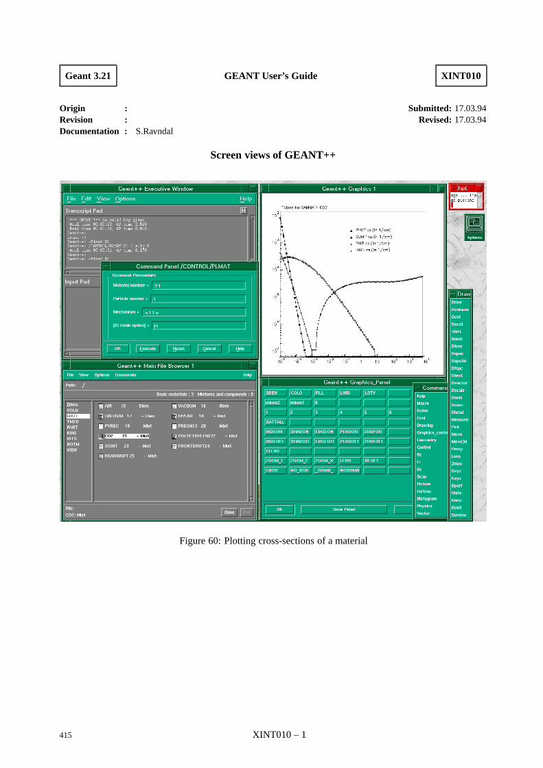
Geant 3.21 GEANT User’s Guide XINT010
Origin : Submitted: 17.03.94Revision : Revised: 17.03.94Documentation : S.Ravndal
Screen views of GEANT++
Figure 60: Plotting cross-sections of a material
415 XINT010 – 1
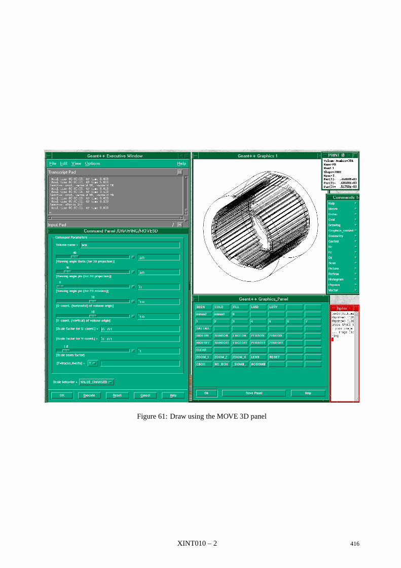
Figure 61: Draw using the MOVE 3D panel
XINT010 – 2 416

XINT Bibliography
[1] R.Brun and P.Zanarini. KUIP – Kit for a User Interface Package, Program library I202. CERN, 1988.
417 XINT010 – 3

Geant 3.16 GEANT User’s Guide ZZZZ010
Origin : GEANT Submitted: 01.10.84Revision : Revised: 08.11.93Documentation :
List of COMMON Blocks
1 Introduction
Here, the main features of the common blocks used in GEANT are summarised, with special mention of thevariables initialised in GINIT and of the possibility of overriding them through data records [BASE040] orinteractive commands [XINT]. In most of the cases there is a correspondence between a given data structureand a given common block where the current contents of the banks are stored. The labelled common blocksare accessible through Patchy/CMZ sequences identified by the name of the COMMON. They are defined inthe Patch GCDES.
Note:
Unless otherwise specified, the long range variables are initialised in GINIT. When non-zero, default valuesare quoted between brackets. If the value may be modified the keyword for the data record and for theinteractive command is also given in bold characters between brackets.
1.1 Dynamic memory
The GEANT data structures are stored in the common /GCBANK/ accessible through the following Patchysequence:
The /GCLINK/ variables are pointers to the GEANT data structures in the /GCBANK/ common. They belongto a permanent area declared in GZINIT.
+SEQ /GCBANK/ Dynamic core for the GEANT data structures
PARAMETER (KWBANK=69000,KWWORK=5200)COMMON/GCBANK/NZEBRA,GVERSN,ZVERSN,IXSTOR,IXDIV,IXCONS,FENDQ(16)
+ ,LMAIN,LR1,WS(KWBANK)DIMENSION IQ(2),Q(2),LQ(8000),IWS(2)EQUIVALENCE (Q(1),IQ(1),LQ(9)),(LQ(1),LMAIN),(IWS(1),WS(1))EQUIVALENCE (JCG,JGSTAT)COMMON/GCLINK/JDIGI ,JDRAW ,JHEAD ,JHITS ,JKINE ,JMATE ,JPART
+ ,JROTM ,JRUNG ,JSET ,JSTAK ,JGSTAT,JTMED ,JTRACK,JVERTX+ ,JVOLUM,JXYZ ,JGPAR ,JGPAR2,JSKLT
C
1.2 Other user accessed common blocks
+SEQ /GCCUTS/ Tracking thresholds
COMMON/GCCUTS/CUTGAM,CUTELE,CUTNEU,CUTHAD,CUTMUO,BCUTE,BCUTM+ ,DCUTE ,DCUTM ,PPCUTM,TOFMAX,GCUTS(5)
C
418 ZZZZ010 – 1

This common contains the threshold for various processes and particles. The energy values are the kineticenergy in GeV:
CUTGAM threshold for gamma transport (0.001, CUTS);
CUTELE threshold for electron and positron transport (0.001, CUTS);
CUTNEU threshold for neutral hadron transport (0.01, CUTS);
CUTHAD threshold for charged hadron and ion transport (0.01, CUTS);
CUTMUO threshold for muon transport (0.01, CUTS);
BCUTE threshold for photons produced by electron bremsstrahlung (CUTGAM, CUTS);
BCUTM threshold for photons produced by muon bremsstrahlung (CUTGAM, CUTS);
DCUTE threshold for electrons produced by electron δ-rays (CUTELE, CUTS);
DCUTM threshold for electrons produced by muon or hadron δ-rays (CUTELE, CUTS);
PPCUTM threshold for e+e−direct pair production by muon (0.002, CUTS);
TOFMAX threshold on time of flight counted from primary interaction time (1010, CUTS);
GCUTS free for user applications (CUTS).
Note: The cuts BCUTE, BCUTM and DCUTE, DCUTM are given the respective default values CUTGAM andCUTELE. Experienced users can make use of the facility offered (command CUTS) to change BCUTE, DCUTE,BCUTM and DCUTM.
+SEQ /GCDRAW/ Variables used by the drawing package
COMMON/GCDRAW/NUMNOD,MAXNOD,NUMND1,LEVVER,LEVHOR,MAXV,IPICK,+ MLEVV,MLEVH,NWCUT,JNAM,JMOT,JXON,JBRO,JDUP,JSCA,JDVM,JPSM,+ JNAM1,JMOT1,JXON1,JBRO1,JDUP1,JSCA1,JULEV,JVLEV,+ LOOKTB(16),+ GRMAT0(10),GTRAN0(3),IDRNUM,GSIN(41),GCOS(41),SINPSI,COSPSI,+ GTHETA,GPHI,GPSI,GU0,GV0,GSCU,GSCV,NGVIEW,+ ICUTFL,ICUT,CTHETA,CPHI,DCUT,NSURF,ISURF,+ GZUA,GZVA,GZUB,GZVB,GZUC,GZVC,PLTRNX,PLTRNY,+ LINATT,LINATP,ITXATT,ITHRZ,IPRJ,DPERS,ITR3D,IPKHIT,IOBJ,LINBUF,+ MAXGU,MORGU,MAXGS,MORGS,MAXTU,MORTU,MAXTS,MORTS,+ IGU,IGS,ITU,ITS,NKVIEW,IDVIEW,+ NOPEN,IGMR,IPIONS,ITRKOP,IHIDEN,+ ZZFU,ZZFV,MYISEL,+ DDUMMY(15)
C
NUMNOD number of nodes in non-optimized tree;
MAXNOD max. number of nodes of non-optimized tree (MIN(NLEFT, 16,000));
NUMND1 number of nodes in optimized tree;
LEVVER vertical level in the tree currently scanned by tree routines;
LEVHOR horizontal node in the tree currently scanned by tree routines;
MAXV max vertical levels in the tree to be scanned by tree routines;
IPICK node selected by GDTREE;
MLEVV number of vertical levels in the last tree scanned;
ZZZZ010 – 2 419
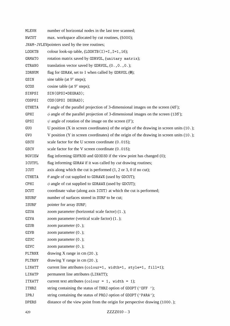
MLEVH number of horizontal nodes in the last tree scanned;
NWCUT max. workspace allocated by cut routines, (5000);
JNAM-JVLEVpointers used by the tree routines;
LOOKTB colour look-up table, (LOOKTB(I)=I,I=1,16);
GRMAT0 rotation matrix saved by GDRVOL, (unitary matrix);
GTRAN0 translation vector saved by GDRVOL, (0.,0.,0.);
IDRNUM flag for GDRAW, set to 1 when called by GDRVOL (0);
GSIN sine table (at 9 steps);
GCOS cosine table (at 9 steps);
SINPSI SIN(GPSI*DEGRAD);
COSPSI COS(GPSI DEGRAD);
GTHETA θ angle of the parallel projection of 3-dimensional images on the screen (45);
GPHI φ angle of the parallel projection of 3-dimensional images on the screen (135);
GPSI ψ angle of rotation of the image on the screen (0);
GU0 U position (X in screen coordinates) of the origin of the drawing in screen units (10.);
GV0 V position (Y in screen coordinates) of the origin of the drawing in screen units (10.);
GSCU scale factor for the U screen coordinate (0.015);
GSCV scale factor for the V screen coordinate (0.015);
NGVIEW flag informing GDFR3D and GD3D3D if the view point has changed (0);
ICUTFL flag informing GDRAW if it was called by cut drawing routines;
ICUT axis along which the cut is performed (1, 2 or 3, 0 if no cut);
CTHETA θ angle of cut supplied to GDRAWX (used by GDCUT);
CPHI φ angle of cut supplied to GDRAWX (used by GDCUT);
DCUT coordinate value (along axis ICUT) at which the cut is performed;
NSURF number of surfaces stored in SURF to be cut;
ISURF pointer for array SURF;
GZUA zoom parameter (horizontal scale factor) (1.);
GZVA zoom parameter (vertical scale factor) (1.);
GZUB zoom parameter (0.);
GZVB zoom parameter (0.);
GZUC zoom parameter (0.);
GZVC zoom parameter (0.);
PLTRNX drawing X range in cm (20.);
PLTRNY drawing Y range in cm (20.);
LINATT current line attributes (colour=1, width=1, style=1, fill=1);
LINATP permanent line attributes (LINATT);
ITXATT current text attributes (colour = 1, width = 1);
ITHRZ string containing the status of THRZ option of GDOPT (’OFF ’);
IPRJ string containing the status of PROJ option of GDOPT (’PARA’);
DPERS distance of the view point from the origin for perspective drawing (1000.);
420 ZZZZ010 – 3
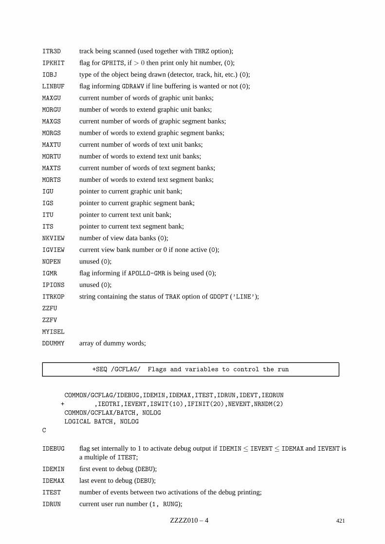
ITR3D track being scanned (used together with THRZ option);
IPKHIT flag for GPHITS, if > 0 then print only hit number, (0);
IOBJ type of the object being drawn (detector, track, hit, etc.) (0);
LINBUF flag informing GDRAWV if line buffering is wanted or not (0);
MAXGU current number of words of graphic unit banks;
MORGU number of words to extend graphic unit banks;
MAXGS current number of words of graphic segment banks;
MORGS number of words to extend graphic segment banks;
MAXTU current number of words of text unit banks;
MORTU number of words to extend text unit banks;
MAXTS current number of words of text segment banks;
MORTS number of words to extend text segment banks;
IGU pointer to current graphic unit bank;
IGS pointer to current graphic segment bank;
ITU pointer to current text unit bank;
ITS pointer to current text segment bank;
NKVIEW number of view data banks (0);
IGVIEW current view bank number or 0 if none active (0);
NOPEN unused (0);
IGMR flag informing if APOLLO-GMR is being used (0);
IPIONS unused (0);
ITRKOP string containing the status of TRAK option of GDOPT (’LINE’);
ZZFU
ZZFV
MYISEL
DDUMMY array of dummy words;
+SEQ /GCFLAG/ Flags and variables to control the run
COMMON/GCFLAG/IDEBUG,IDEMIN,IDEMAX,ITEST,IDRUN,IDEVT,IEORUN+ ,IEOTRI,IEVENT,ISWIT(10),IFINIT(20),NEVENT,NRNDM(2)COMMON/GCFLAX/BATCH, NOLOGLOGICAL BATCH, NOLOG
C
IDEBUG flag set internally to 1 to activate debug output if IDEMIN ≤ IEVENT ≤ IDEMAX and IEVENT isa multiple of ITEST;
IDEMIN first event to debug (DEBU);
IDEMAX last event to debug (DEBU);
ITEST number of events between two activations of the debug printing;
IDRUN current user run number (1, RUNG);
ZZZZ010 – 4 421
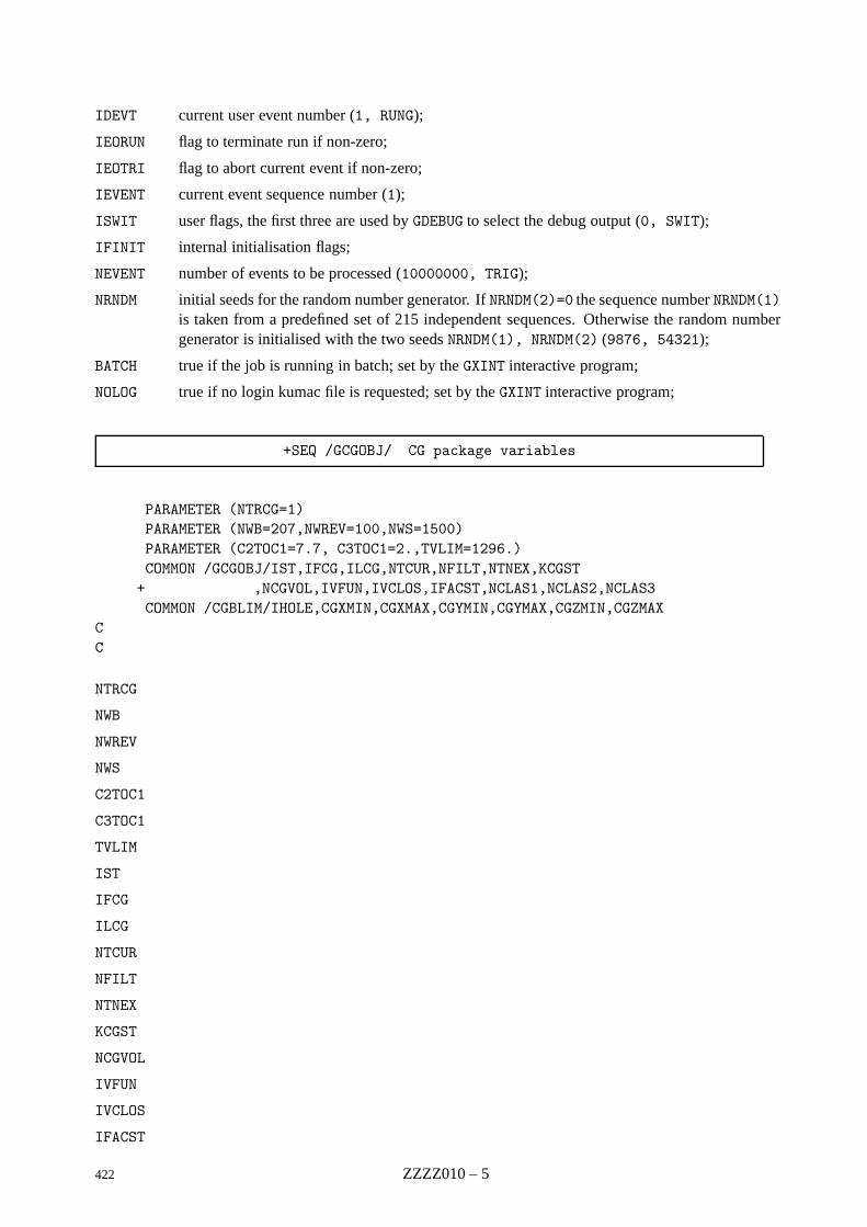
IDEVT current user event number (1, RUNG);
IEORUN flag to terminate run if non-zero;
IEOTRI flag to abort current event if non-zero;
IEVENT current event sequence number (1);
ISWIT user flags, the first three are used by GDEBUG to select the debug output (0, SWIT);
IFINIT internal initialisation flags;
NEVENT number of events to be processed (10000000, TRIG);
NRNDM initial seeds for the random number generator. If NRNDM(2)=0 the sequence number NRNDM(1)is taken from a predefined set of 215 independent sequences. Otherwise the random numbergenerator is initialised with the two seeds NRNDM(1), NRNDM(2) (9876, 54321);
BATCH true if the job is running in batch; set by the GXINT interactive program;
NOLOG true if no login kumac file is requested; set by the GXINT interactive program;
+SEQ /GCGOBJ/ CG package variables
PARAMETER (NTRCG=1)PARAMETER (NWB=207,NWREV=100,NWS=1500)PARAMETER (C2TOC1=7.7, C3TOC1=2.,TVLIM=1296.)COMMON /GCGOBJ/IST,IFCG,ILCG,NTCUR,NFILT,NTNEX,KCGST
+ ,NCGVOL,IVFUN,IVCLOS,IFACST,NCLAS1,NCLAS2,NCLAS3COMMON /CGBLIM/IHOLE,CGXMIN,CGXMAX,CGYMIN,CGYMAX,CGZMIN,CGZMAX
CC
NTRCG
NWB
NWREV
NWS
C2TOC1
C3TOC1
TVLIM
IST
IFCG
ILCG
NTCUR
NFILT
NTNEX
KCGST
NCGVOL
IVFUN
IVCLOS
IFACST
422 ZZZZ010 – 5
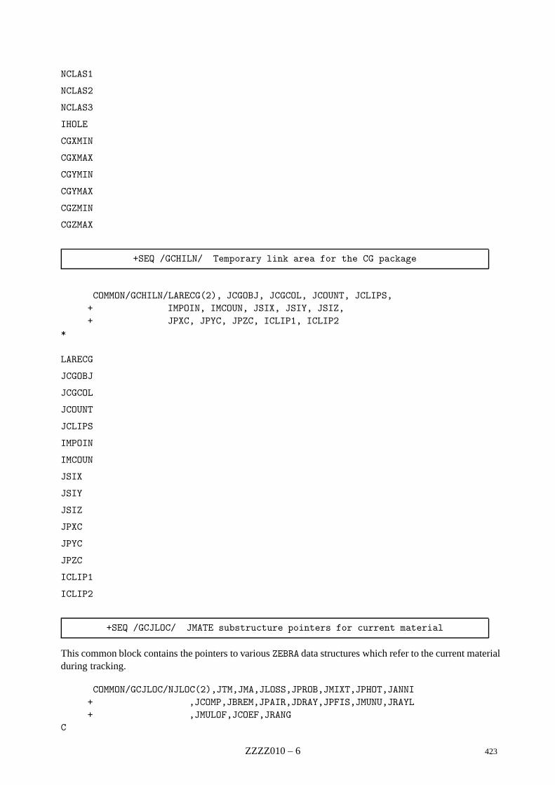
NCLAS1
NCLAS2
NCLAS3
IHOLE
CGXMIN
CGXMAX
CGYMIN
CGYMAX
CGZMIN
CGZMAX
+SEQ /GCHILN/ Temporary link area for the CG package
COMMON/GCHILN/LARECG(2), JCGOBJ, JCGCOL, JCOUNT, JCLIPS,+ IMPOIN, IMCOUN, JSIX, JSIY, JSIZ,+ JPXC, JPYC, JPZC, ICLIP1, ICLIP2
*
LARECG
JCGOBJ
JCGCOL
JCOUNT
JCLIPS
IMPOIN
IMCOUN
JSIX
JSIY
JSIZ
JPXC
JPYC
JPZC
ICLIP1
ICLIP2
+SEQ /GCJLOC/ JMATE substructure pointers for current material
This common block contains the pointers to various ZEBRA data structures which refer to the current materialduring tracking.
COMMON/GCJLOC/NJLOC(2),JTM,JMA,JLOSS,JPROB,JMIXT,JPHOT,JANNI+ ,JCOMP,JBREM,JPAIR,JDRAY,JPFIS,JMUNU,JRAYL+ ,JMULOF,JCOEF,JRANG
C
ZZZZ010 – 6 423
COMMON/GCJLCK/NJLCK(2),JTCKOV,JABSCO,JEFFIC,JINDEX,JCURIN+ ,JPOLAR,JTSTRA,JTSTCO,JTSTEN,JTASHO
CEQUIVALENCE (JLASTV,JTSTEN)
C
NJLOC ZEBRA link area control variables;
JTM tracking medium;
JMA material;
JLOSS energy loss table;
JPROB bank containing some physic constants of the material;
JMIXT mixture parameters;
JPHOT photoelectric effect cross-section;
JANNI positron annihilation cross-section;
JCOMP Compton effect cross-section;
JBREM bremsstrahlung cross-section;
JPAIR photon pair production and muon direct pair production cross-section;
JDRAY δ-ray production cross-section;
JPFIS photo-fission cross-section;
JMUNU muon-nucleus interaction cross-section;
JRAYL Rayleigh effect cross-section;
JMULOF STMIN, see [PHYS010];
JCOEF bank containing the coefficients of the parabolic range-energy fit;
JRANG range;
NJLCK ZEBRA link area control variables;
JTCKOV Cerenkov photons energy binning;
JABSCO absorption coefficient;
JEFFIC quantum efficiency;
JINDEX refraction index;
JCURIN Cerenkov angle integral;
JPOLAR polarisation information;
JTSTRA top level bank for PAI energy loss fluctuations model;
JTSTCO coefficients for PAI energy loss fluctuations model;
JTSTEN energy binning for PAI energy loss fluctuations model;
JTASHO coefficients for ASHO energy loss fluctuations model;
For more information see [CONS199].
+SEQ /GCJUMP/ Pointers for the jump package
Variable JU. . . contains the address of the routine GU. . ..
424 ZZZZ010 – 7
PARAMETER (MAXJMP=30)COMMON/GCJUMP/JUDCAY, JUDIGI, JUDTIM, JUFLD , JUHADR, JUIGET,
+ JUINME, JUINTI, JUKINE, JUNEAR, JUOUT , JUPHAD,+ JUSKIP, JUSTEP, JUSWIM, JUTRAK, JUTREV, JUVIEW,+ JUPARADIMENSION JMPADR(MAXJMP)EQUIVALENCE (JMPADR(1), JUDCAY)
*
+SEQ /GCKINE/ Kinematics of current track
COMMON/GCKINE/IKINE,PKINE(10),ITRA,ISTAK,IVERT,IPART,ITRTYP+ ,NAPART(5),AMASS,CHARGE,TLIFE,VERT(3),PVERT(4),IPAOLD
C
IKINE user integer word (0, KINE);
PKINE user array of real (0, KINE);
ITRA track number;
ISTAK stack track number;
IVERT vertex number;
IPART particle number;
ITRTYP particle tracking type;
NAPART name of current particle (ASCII codes stored in an integer array, 4 characthers per word);
AMASS mass of current particle in GeV c−2;
CHARGE charge of current particle in electron charge unit;
TLIFE average life time of current particle in seconds;
VERT coordinates of origin vertex for current track;
PVERT track kinematics at origin vertex (PVERT(4) not used);
IPAOLD particle number of the previous track.
+SEQ /GCKMAX/ Size of the /GCKING/ stack
INTEGER MXGKINPARAMETER (MXGKIN=100)
+SEQ /GCMUTR/ Auxiliary variables for the CG package
*PARAMETER (MULTRA=50)CHARACTER*4 GNASH, GNNVV, GNVNVCOMMON/GCMUTR/NCVOLS,KSHIFT,NSHIFT,ICUBE,NAIN,JJJ,
+ NIET,IOLDSU,IVOOLD,IWPOIN,IHPOIN,IVECVO(100),+ PORGX,PORGY,PORGZ,POX(15),POY(15),POZ(15),GBOOM,+ PORMIR(18),PORMAR(18),IPORNT,
ZZZZ010 – 8 425
+ ICGP,CLIPMI(6),CLIPMA(6),+ ABCD(4),BMIN(6),BMAX(6),CGB(16000),CGB1(16000),+ GXMIN(MULTRA),GXMAX(MULTRA),GYMIN(MULTRA),+ GYMAX(MULTRA),GZMIN(MULTRA),GZMAX(MULTRA),+ GXXXX(MULTRA),GYYYY(MULTRA),GZZZZ(MULTRA)
*COMMON/GCMUTC/ GNASH(MULTRA),GNNVV(MULTRA),GNVNV(MULTRA)
*
NCVOLS
KSHIFT
NSHIFT
ICUBE
NAIN
JJJ
NIET
IOLDSU
IVOOLD
IWPOIN
IHPOIN
IVECVO
PORGX
PORGY
PORGZ
POX
POY
POZ
GBOOM
PORMIR
PORMAR
IPORNT
ICGP
CLIPMI
CLIPMA
ABCD
BMIN
BMAX
CGB
CGB1
GXMIN
GXMAX
GYMIN
426 ZZZZ010 – 9
GYMAX
GZMIN
GZMAX
GXXXX
GYYYY
GZZZZ
GNASH
GNNVV
GNVNV
+SEQ /GCKING/ Kinematics of generated secondaries
+SEQ, GCKMAXCOMMON/GCKING/KCASE,NGKINE,GKIN(5,MXGKIN),
+ TOFD(MXGKIN),IFLGK(MXGKIN)INTEGER KCASE,NGKINE ,IFLGK,MXPHOT,NGPHOTREAL GKIN,TOFD,XPHOT
CPARAMETER (MXPHOT=800)COMMON/GCKIN2/NGPHOT,XPHOT(11,MXPHOT)
CCOMMON/GCKIN3/GPOS(3,MXGKIN)REAL GPOS
C
KCASE Mechanism which has generated the secondary particles;
NGKINE Number of generated secondaries;
GKIN(1,I) x component of momentum of Ith particle;
GKIN(2,I) y component of momentum;
GKIN(3,I) z component of momentum;
GKIN(4,I) total energy;
GKIN(5,I) particle code (see [CONS300]);
TOFD(I) time offset with respect to current time of flight;
IFLGK(I) Flag controlling the handling of track by GSKING, GSSTAK;
<0 particle is discarded;
0 (D) particle is stored in the temporary stack JSTAK for further tracking;
1 like 0 but particle is stored in JVERTX/JKINE structure as well;
>1 particle is attached to vertex IFLGK(I).
GPOS(1,I) x position of Ith particle;
GPOS(2,I) y position;
GPOS(3,I) z position;
NGPHOT number of Cerenkov photons generated in the current step;
XPHOT(1,I) x position of the Ith photon;
ZZZZ010 – 10 427
XPHOT(2,I) y position;
XPHOT(3,I) z position;
XPHOT(4,I) x component of momentum;
XPHOT(5,I) y component of momentum;
XPHOT(6,I) z component of momentum;
XPHOT(7,I) momentum of the photon;
XPHOT(8,I) x component of the polarisation vector;
XPHOT(9,I) y component of the polarisation vector;
XPHOT(10,I) z component of the polarisation vector;
XPHOT(11,I) time of flight in seconds of the photon.
+SEQ /GCLINK/ See /GCBANK/ above
+SEQ /GCLIST/ Various system and user lists
COMMON/GCLIST/NHSTA,NGET ,NSAVE,NSETS,NPRIN,NGEOM,NVIEW,NPLOT+ ,NSTAT,LHSTA(20),LGET (20),LSAVE(20),LSETS(20),LPRIN(20)+ ,LGEOM(20),LVIEW(20),LPLOT(20),LSTAT(20)
C
NHSTA number of histograms on data record HSTA;
NGET number of data structures on data record GET;
NSAVE number of data structures on data record SAVE;
NSETS number of items on data record SETS;
NPRIN number of items on data record PRIN;
NGEOM number of items on data record GEOM;
NVIEW number of items on data record VIEW;
NPLOT number of items on data record PLOT;
NSTAT number of items on data record STAT (obsolete);
LHSTA ...LSTAT lists of items set via the input records (HSTA ...,STAT).
LSTAT(1) is reserved by the system for volume statistics.
+SEQ /GCMATE/ Parameters of current material
COMMON/GCMATE/NMAT,NAMATE(5),A,Z,DENS,RADL,ABSLC
NMAT current material number;
NAMATE name of current material (ASCII codes stored in an integer array, 4 characthers per word);
A atomic weight of current material;
Z atomic number of current material;
428 ZZZZ010 – 11
DENS density of current material in g cm−3;
RADL radiation length of current material;
ABSL absorption length of current material.
+SEQ /GCMULO/ Energy binning and multiple scattering
Precomputed quantities for multiple scattering and energy binning for JMATE banks. See also [CONS199]for the energy binning and [PHYS325] for a description of the variables OMCMOL and CHCMOL.
COMMON/GCMULO/SINMUL(101),COSMUL(101),SQRMUL(101),OMCMOL,CHCMOL+ ,EKMIN,EKMAX,NEKBIN,NEK1,EKINV,GEKA,GEKB,EKBIN(200),ELOW(200)
C
SINMUL not used any more;
COSMUL not used any more;
SQRMUL not used any more;
OMCMOL constant Ω0 of the Moliere theory;
CHCMOL χcc constant of the Moliere theory;
EKMIN lower edge of the energy range of the tabulated cross sections (10−5, ERAN);
EKMAX upper edge of the energy range of the tabulated cross sections (104, ERAN);
NEKBIN number of energy bins to be used (90, ERAN);
NEK1 NEKBIN+1;
EKINV 1/ (log10(EKMAX)− log10(EKMIN));GEKA NEKBIN*EKINV;
GEKB 1-GEKA*EKBIN(1);
EKBIN log (ELOW);
ELOW low edges of the energy bins.
+SEQ /GCMZFO/ I/O descriptors of GEANT banks
COMMON/GCMZFO/IOMATE,IOPART,IOTMED,IOSEJD,IOSJDD,IOSJDH,IOSTAK+ ,IOMZFO(13)
C
IOMATE I/O descriptor for the JMATE bank;
IOPART I/O descriptor for the JPART bank;
IOTMED I/O descriptor for the JTMED bank;
IOSEJD I/O descriptor for the detector banks;
IOSJDD I/O descriptor for the second dependent bank of the detector banks;
IOSJDH I/O descriptor for the first dependent bank of the detector banks;
IOSTAK I/O descriptor for the JSTAK bank;
IOMZFO free I/O descriptors.
ZZZZ010 – 12 429
+SEQ /GCNUM/ Current number for various items
COMMON/GCNUM/NMATE ,NVOLUM,NROTM,NTMED,NTMULT,NTRACK,NPART+ ,NSTMAX,NVERTX,NHEAD,NBITCOMMON /GCNUMX/ NALIVE,NTMSTO
C
NMATE number of material banks;
NVOLUM number of volume banks;
NROTM number of rotation matrix banks;
NTMED number of tracking media banks;
NTMULT total number of tracks processed in current event (including secondaries);
NTRACK number of tracks in the JKINE bank for current event;
NPART maximum particle code;
NSTMAX maximum number of tracks (high-water mark) in stack JSTAK for current event;
NVERTX number of vertices in JVERTX bank for current event;
NHEAD number of data words in the JHEAD bank (10);
NBIT number of bits per word (initialised in GINIT via ZEBRA);
NALIVE number of particles to be tracked in the parallel tracking stack (this mode of tracking is disabledin the current GEANT version);
NTMSTO total number of tracks tracked in the current event so far. Same as NTMULT in /GCTRAK/;
+SEQ /GCOMIS/ Variables for the COMIS package
Variable JU... contains the COMIS address of routine GU....
COMMON/GCOMIS/ICOMIS,JUINIT,JUGEOM,JUKINE,JUSTEP,JUOUT,JULAST*
ICOMIS flag to avoid a double initialisation of COMIS;
+SEQ /GCONST/ Basic constants
See next section for the value of these parameters.
COMMON/GCONST/PI,TWOPI,PIBY2,DEGRAD,RADDEG,CLIGHT,BIG,EMASSCOMMON/GCONSX/EMMU,PMASS,AVO
C
PI π;
TWOPI 2π;
PIBY2 π/2;
DEGRAD degrees to radiants conversion factor (π/180);
430 ZZZZ010 – 13
RADDEG radiants to degrees conversion factor (180/π);
CLIGHT light velocity in cm s−1;
BIG arbitrary large number;
EMASS electron mass in GeV c−2;
EMMU muon mass in GeV c−2;
PMASS proton mass in GeV c−2;
AVO Avogadro’s number ×10−24.
+SEQ /GCONSP/ Basic constants
These parameters are in SINGLE PRECISION on 64 bits machines.
DOUBLE PRECISION PI,TWOPI,PIBY2,DEGRAD,RADDEG,CLIGHT,BIG,EMASSDOUBLE PRECISION EMMU,PMASS,AVO
*PARAMETER (PI=3.14159265358979324D0)PARAMETER (TWOPI=6.28318530717958648D0)PARAMETER (PIBY2=1.57079632679489662D0)PARAMETER (DEGRAD=0.0174532925199432958D0)PARAMETER (RADDEG=57.2957795130823209D0)PARAMETER (CLIGHT=29979245800.D0)PARAMETER (BIG=10000000000.D0)PARAMETER (EMASS=0.0005109990615D0)PARAMETER (EMMU=0.105658387D0)PARAMETER (PMASS=0.9382723128D0)PARAMETER (AVO=0.60221367D0)
*
+SEQ /GCOPTI/ Control of geometry optimisation
COMMON/GCOPTI/ IOPTIMC
IOPTIM Optimisation flag
-1 no optimisation at all; GSORD calls disabled;
0 no optimisation; only user calls to GSORD kept;
1 all non-GSORDered volumes are ordered along the best axis;
2 all volumes are ordered along the best axis.
+SEQ /GCPARA/ Control of parametrized energy deposition
INTEGER BITPHI, BITTET, BITPOTLOGICAL SYMPHI, SYMTEU, SYMTEDPARAMETER (LSTACK = 5000)
C BITPOT is for Phi.Or.TetC
ZZZZ010 – 14 431
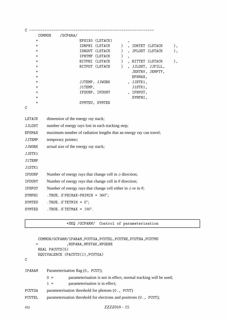
C ---------------------------------------------------------COMMON /GCPARA/
+ EPSIX0 (LSTACK) ,+ IDRPHI (LSTACK ) , IDRTET (LSTACK ),+ IDROUT (LSTACK ) , JPLOST (LSTACK ),+ IPHTMP (LSTACK ) ,+ BITPHI (LSTACK ) , BITTET (LSTACK ),+ BITPOT (LSTACK ) , JJLOST, JJFILL,+ JENTRY, JEMPTY,+ EPSMAX,+ JJTEMP, JJWORK , JJSTK1,+ J1TEMP, J1STK1,+ IFOUNP, IFOUNT , IFNPOT,+ SYMPHI,+ SYMTEU, SYMTED
C
LSTACK dimension of the energy ray stack;
JJLOST number of energy rays lost in each tracking step;
EPSMAX maximum number of radiation lengths that an energy ray can travel;
JJTEMP temporary pointer;
JJWORK actual size of the energy ray stack;
JJSTK1
J1TEMP
J1STK1
IFOUNP Number of energy rays that change cell in φ direction;
IFOUNT Number of energy rays that change cell in θ direction;
IFNPOT Number of energy rays that change cell either in φ or in θ;
SYMPHI .TRUE. if PHIMAX-PHIMIN = 360;
SYMTEU .TRUE. if TETMIN = 0;
SYMTED .TRUE. if TETMAX = 180.
+SEQ /GCPARM/ Control of parameterisation
COMMON/GCPARM/IPARAM,PCUTGA,PCUTEL,PCUTNE,PCUTHA,PCUTMU+ ,NSPARA,MPSTAK,NPGENEREAL PACUTS(5)EQUIVALENCE (PACUTS(1),PCUTGA)
C
IPARAM Parameterisation flag (0, PCUT);
0 = parameterisation is not in effect, normal tracking will be used;
1 = parameterisation is in effect;
PCUTGA parameterisation threshold for photons (0., PCUT)
PCUTEL parameterisation threshold for electrons and positrons (0., PCUT);
432 ZZZZ010 – 15
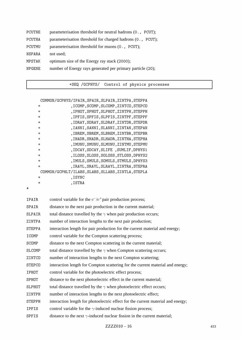
PCUTNE parameterisation threshold for neutral hadrons (0., PCUT);
PCUTHA parameterisation threshold for charged hadrons (0., PCUT);
PCUTMU parameterisation threshold for muons (0., PCUT);
NSPARA not used;
MPSTAK optimum size of the Energy ray stack (2000);
NPGENE number of Energy rays generated per primary particle (20);
+SEQ /GCPHYS/ Control of physics processes
COMMON/GCPHYS/IPAIR,SPAIR,SLPAIR,ZINTPA,STEPPA+ ,ICOMP,SCOMP,SLCOMP,ZINTCO,STEPCO+ ,IPHOT,SPHOT,SLPHOT,ZINTPH,STEPPH+ ,IPFIS,SPFIS,SLPFIS,ZINTPF,STEPPF+ ,IDRAY,SDRAY,SLDRAY,ZINTDR,STEPDR+ ,IANNI,SANNI,SLANNI,ZINTAN,STEPAN+ ,IBREM,SBREM,SLBREM,ZINTBR,STEPBR+ ,IHADR,SHADR,SLHADR,ZINTHA,STEPHA+ ,IMUNU,SMUNU,SLMUNU,ZINTMU,STEPMU+ ,IDCAY,SDCAY,SLIFE ,SUMLIF,DPHYS1+ ,ILOSS,SLOSS,SOLOSS,STLOSS,DPHYS2+ ,IMULS,SMULS,SOMULS,STMULS,DPHYS3+ ,IRAYL,SRAYL,SLRAYL,ZINTRA,STEPRACOMMON/GCPHLT/ILABS,SLABS,SLLABS,ZINTLA,STEPLA
+ ,ISYNC+ ,ISTRA
*
IPAIR control variable for the e−/e+pair production process;
SPAIR distance to the next pair production in the current material;
SLPAIR total distance travelled by the γ when pair production occurs;
ZINTPA number of interaction lengths to the next pair production;
STEPPA interaction length for pair production for the current material and energy;
ICOMP control variable for the Compton scattering process;
SCOMP distance to the next Compton scattering in the current material;
SLCOMP total distance travelled by the γ when Compton scattering occurs;
ZINTCO number of interaction lengths to the next Compton scattering;
STEPCO interaction length for Compton scattering for the current material and energy;
IPHOT control variable for the photoelectric effect process;
SPHOT distance to the next photoelectric effect in the current material;
SLPHOT total distance travelled by the γ when photoelectric effect occurs;
ZINTPH number of interaction lengths to the next photoelectric effect;
STEPPH interaction length for photoelectric effect for the current material and energy;
IPFIS control variable for the γ-induced nuclear fission process;
SPFIS distance to the next γ-induced nuclear fission in the current material;
ZZZZ010 – 16 433

SLPFIS total distance travelled by the γ when γ-induced nuclear fission occurs;
ZINTPF number of interaction lengths to the next γ-induced nuclear fission;
STEPPF interaction length for γ-induced nuclear fission for the current material and energy;
IDRAY control variable for the δ-ray production process;
SDRAY distance to the next δ-ray production in the current material;
SLDRAY total distance travelled by the particle when δ-ray production occurs;
ZINTDR number of interaction lengths to the next δ-ray production;
STEPDR interaction length for δ-ray production for the current material and energy;
IANNI control variable for the positron annichilation process;
SANNI distance to the next positron annichilation in the current material;
SLANNI total distance travelled by the positron when positron annichilation occurs;
ZINTAN number of interaction lengths to the next positron annichilation;
STEPAN interaction length for positron annichilation for the current material and energy;
IBREM control variable for the bremsstrahlung process;
SBREM distance to the next bremsstrahlung in the current material;
SLBREM total distance travelled by the particle when bremsstrahlung occurs;
ZINTBR number of interaction lengths to the next bremsstrahlung;
STEPBR interaction length for bremsstrahlung for the current material and energy;
IHADR control variable for the hadronic interaction process;
SHADR distance to the next hadronic interaction in the current material;
SLHADR total distance travelled by the particle when hadronic interaction occurs;
ZINTHA number of interaction lengths to the next hadronic interaction;
STEPHA interaction length for hadronic interaction for the current material and energy;
IMUNU control variable for the µ nuclear interaction process;
SMUNU distance to the next µ nuclear interaction in the current material;
SLMUNU total distance travelled by the µ when µ nuclear interaction occurs;
ZINTMU number of interaction lengths to the next µ nuclear interaction;
STEPMU interaction length for µ nuclear interaction for the current material and energy;
IDCAY control variable for the decay in flight process;
SDCAY distance to the next decay in flight in the current material;
SLIFE total distance travelled by the particle when decay in flight occurs;
SUMLIF time to the next interaction point in ct units;
DPHYS1 not used;
ILOSS control variable for the energy loss process;
SLOSS step limitation due to continuous processes: energy loss, bending in magnetic field,Cerenkovphoton generation and multiple scattering;
SOLOSS not used;
STLOSS not used; set equal to STEP for backward compatibility;
DPHYS2 not used;
IMULS control variable for the energy loss process;
434 ZZZZ010 – 17
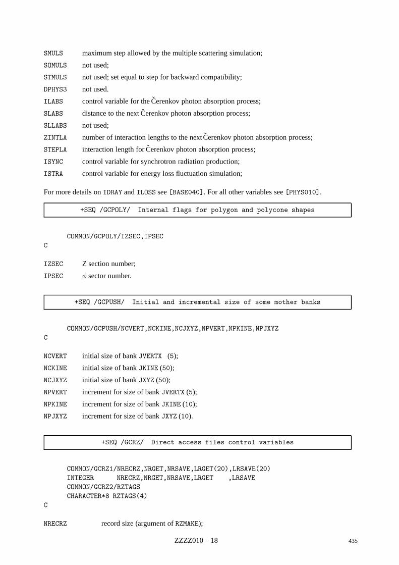
SMULS maximum step allowed by the multiple scattering simulation;
SOMULS not used;
STMULS not used; set equal to step for backward compatibility;
DPHYS3 not used.
ILABS control variable for the Cerenkov photon absorption process;
SLABS distance to the next Cerenkov photon absorption process;
SLLABS not used;
ZINTLA number of interaction lengths to the next Cerenkov photon absorption process;
STEPLA interaction length for Cerenkov photon absorption process;
ISYNC control variable for synchrotron radiation production;
ISTRA control variable for energy loss fluctuation simulation;
For more details on IDRAY and ILOSS see [BASE040]. For all other variables see [PHYS010].
+SEQ /GCPOLY/ Internal flags for polygon and polycone shapes
COMMON/GCPOLY/IZSEC,IPSECC
IZSEC Z section number;
IPSEC φ sector number.
+SEQ /GCPUSH/ Initial and incremental size of some mother banks
COMMON/GCPUSH/NCVERT,NCKINE,NCJXYZ,NPVERT,NPKINE,NPJXYZC
NCVERT initial size of bank JVERTX (5);
NCKINE initial size of bank JKINE (50);
NCJXYZ initial size of bank JXYZ (50);
NPVERT increment for size of bank JVERTX (5);
NPKINE increment for size of bank JKINE (10);
NPJXYZ increment for size of bank JXYZ (10).
+SEQ /GCRZ/ Direct access files control variables
COMMON/GCRZ1/NRECRZ,NRGET,NRSAVE,LRGET(20),LRSAVE(20)INTEGER NRECRZ,NRGET,NRSAVE,LRGET ,LRSAVECOMMON/GCRZ2/RZTAGSCHARACTER*8 RZTAGS(4)
C
NRECRZ record size (argument of RZMAKE);
ZZZZ010 – 18 435
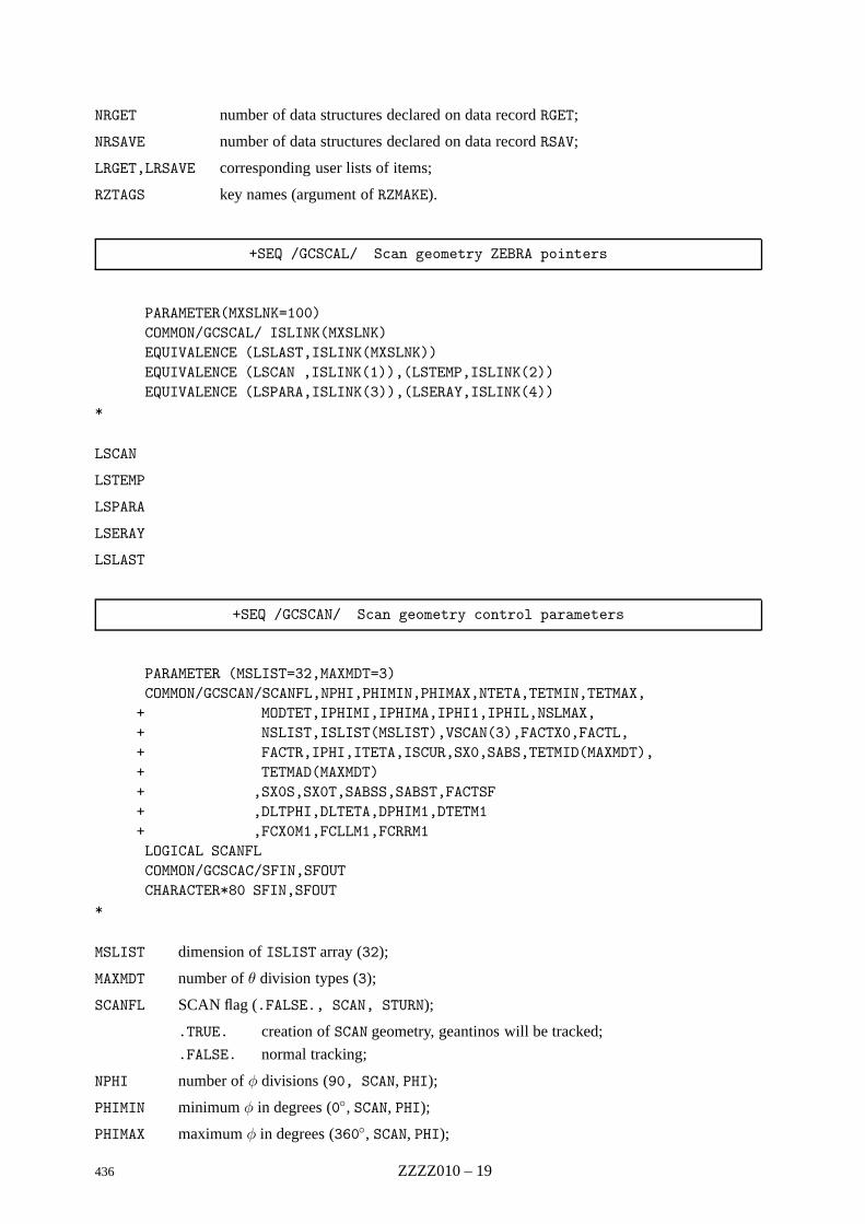
NRGET number of data structures declared on data record RGET;
NRSAVE number of data structures declared on data record RSAV;
LRGET,LRSAVE corresponding user lists of items;
RZTAGS key names (argument of RZMAKE).
+SEQ /GCSCAL/ Scan geometry ZEBRA pointers
PARAMETER(MXSLNK=100)COMMON/GCSCAL/ ISLINK(MXSLNK)EQUIVALENCE (LSLAST,ISLINK(MXSLNK))EQUIVALENCE (LSCAN ,ISLINK(1)),(LSTEMP,ISLINK(2))EQUIVALENCE (LSPARA,ISLINK(3)),(LSERAY,ISLINK(4))
*
LSCAN
LSTEMP
LSPARA
LSERAY
LSLAST
+SEQ /GCSCAN/ Scan geometry control parameters
PARAMETER (MSLIST=32,MAXMDT=3)COMMON/GCSCAN/SCANFL,NPHI,PHIMIN,PHIMAX,NTETA,TETMIN,TETMAX,
+ MODTET,IPHIMI,IPHIMA,IPHI1,IPHIL,NSLMAX,+ NSLIST,ISLIST(MSLIST),VSCAN(3),FACTX0,FACTL,+ FACTR,IPHI,ITETA,ISCUR,SX0,SABS,TETMID(MAXMDT),+ TETMAD(MAXMDT)+ ,SX0S,SX0T,SABSS,SABST,FACTSF+ ,DLTPHI,DLTETA,DPHIM1,DTETM1+ ,FCX0M1,FCLLM1,FCRRM1LOGICAL SCANFLCOMMON/GCSCAC/SFIN,SFOUTCHARACTER*80 SFIN,SFOUT
*
MSLIST dimension of ISLIST array (32);
MAXMDT number of θ division types (3);
SCANFL SCAN flag (.FALSE., SCAN, STURN);
.TRUE. creation of SCAN geometry, geantinos will be tracked;
.FALSE. normal tracking;
NPHI number of φ divisions (90, SCAN, PHI);
PHIMIN minimum φ in degrees (0, SCAN, PHI);
PHIMAX maximum φ in degrees (360, SCAN, PHI);
436 ZZZZ010 – 19
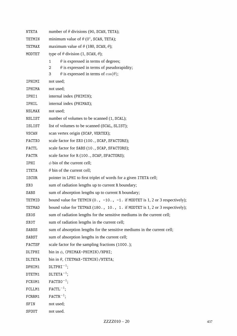
NTETA number of θ divisions (90, SCAN, TETA);
TETMIN minimum value of θ (0, SCAN, TETA);
TETMAX maximum value of θ (180, SCAN, θ);
MODTET type of θ division (1, SCAN, θ);
1 θ is expressed in terms of degrees;
2 θ is expressed in terms of pseudorapidity;
3 θ is expressed in terms of cos(θ);
IPHIMI not used;
IPHIMA not used;
IPHI1 internal index (PHIMIN);
IPHIL internal index (PHIMAX);
NSLMAX not used;
NSLIST number of volumes to be scanned (1, SCAL);
ISLIST list of volumes to be scanned (SCAL, SLIST);
VSCAN scan vertex origin (SCAP, VERTEX);
FACTX0 scale factor for SX0 (100., SCAP, SFACTORS);
FACTL scale factor for SABS (10., SCAP, SFACTORS);
FACTR scale factor for R (100., SCAP, SFACTORS);
IPHI φ bin of the current cell;
ITETA θ bin of the current cell;
ISCUR pointer in LPHI to first triplet of words for a given ITETA cell;
SX0 sum of radiation lengths up to current R boundary;
SABS sum of absorption lengths up to current R boundary;
TETMID bound value for TETMIN (0., -10., -1. if MODTET is 1, 2 or 3 respectively);
TETMAD bound value for TETMAX (180., 10., 1. if MODTET is 1, 2 or 3 respectively);
SX0S sum of radiation lengths for the sensitive mediums in the current cell;
SX0T sum of radiation lengths in the current cell;
SABSS sum of absorption lengths for the sensitive mediums in the current cell;
SABST sum of absorption lengths in the current cell;
FACTSF scale factor for the sampling fractions (1000.);
DLTPHI bin in φ, (PHIMAX-PHIMIN)/NPHI;
DLTETA bin in θ, (TETMAX-TETMIN)/NTETA;
DPHIM1 DLTPHI−1;
DTETM1 DLTETA−1;
FCX0M1 FACTX0−1;
FCLLM1 FACTL−1;
FCRRM1 FACTR−1;
SFIN not used;
SFOUT not used.
ZZZZ010 – 20 437
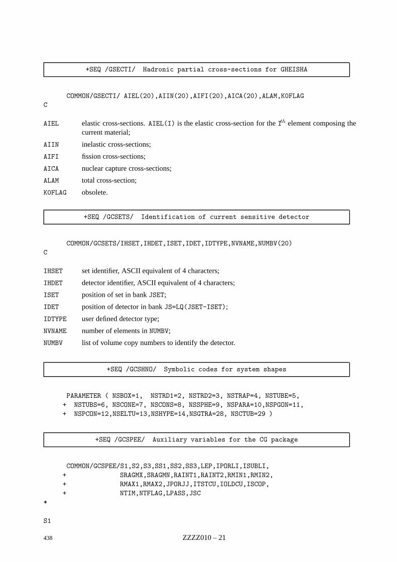
+SEQ /GSECTI/ Hadronic partial cross-sections for GHEISHA
COMMON/GSECTI/ AIEL(20),AIIN(20),AIFI(20),AICA(20),ALAM,K0FLAGC
AIEL elastic cross-sections. AIEL(I) is the elastic cross-section for the Ith element composing thecurrent material;
AIIN inelastic cross-sections;
AIFI fission cross-sections;
AICA nuclear capture cross-sections;
ALAM total cross-section;
K0FLAG obsolete.
+SEQ /GCSETS/ Identification of current sensitive detector
COMMON/GCSETS/IHSET,IHDET,ISET,IDET,IDTYPE,NVNAME,NUMBV(20)C
IHSET set identifier, ASCII equivalent of 4 characters;
IHDET detector identifier, ASCII equivalent of 4 characters;
ISET position of set in bank JSET;
IDET position of detector in bank JS=LQ(JSET-ISET);
IDTYPE user defined detector type;
NVNAME number of elements in NUMBV;
NUMBV list of volume copy numbers to identify the detector.
+SEQ /GCSHNO/ Symbolic codes for system shapes
PARAMETER ( NSBOX=1, NSTRD1=2, NSTRD2=3, NSTRAP=4, NSTUBE=5,+ NSTUBS=6, NSCONE=7, NSCONS=8, NSSPHE=9, NSPARA=10,NSPGON=11,+ NSPCON=12,NSELTU=13,NSHYPE=14,NSGTRA=28, NSCTUB=29 )
+SEQ /GCSPEE/ Auxiliary variables for the CG package
COMMON/GCSPEE/S1,S2,S3,SS1,SS2,SS3,LEP,IPORLI,ISUBLI,+ SRAGMX,SRAGMN,RAINT1,RAINT2,RMIN1,RMIN2,+ RMAX1,RMAX2,JPORJJ,ITSTCU,IOLDCU,ISCOP,+ NTIM,NTFLAG,LPASS,JSC
*
S1
438 ZZZZ010 – 21
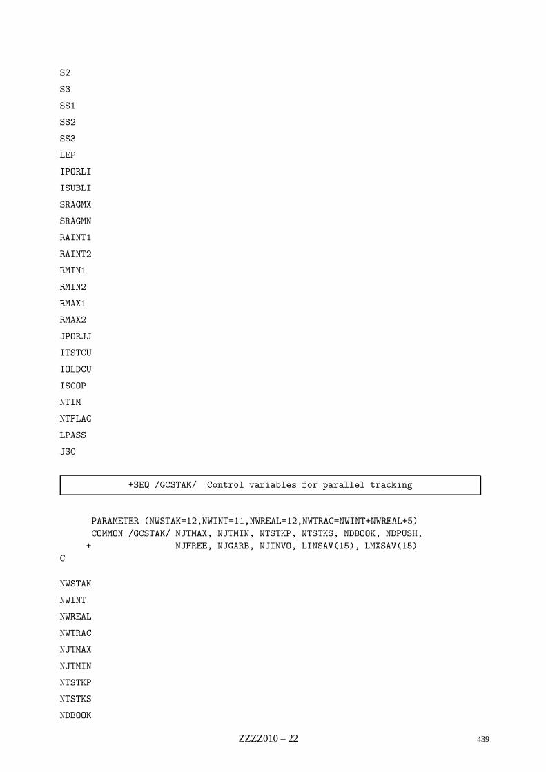
S2
S3
SS1
SS2
SS3
LEP
IPORLI
ISUBLI
SRAGMX
SRAGMN
RAINT1
RAINT2
RMIN1
RMIN2
RMAX1
RMAX2
JPORJJ
ITSTCU
IOLDCU
ISCOP
NTIM
NTFLAG
LPASS
JSC
+SEQ /GCSTAK/ Control variables for parallel tracking
PARAMETER (NWSTAK=12,NWINT=11,NWREAL=12,NWTRAC=NWINT+NWREAL+5)COMMON /GCSTAK/ NJTMAX, NJTMIN, NTSTKP, NTSTKS, NDBOOK, NDPUSH,
+ NJFREE, NJGARB, NJINVO, LINSAV(15), LMXSAV(15)C
NWSTAK
NWINT
NWREAL
NWTRAC
NJTMAX
NJTMIN
NTSTKP
NTSTKS
NDBOOK
ZZZZ010 – 22 439
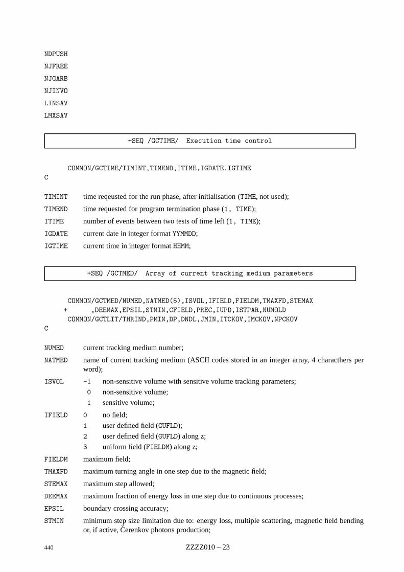
NDPUSH
NJFREE
NJGARB
NJINVO
LINSAV
LMXSAV
+SEQ /GCTIME/ Execution time control
COMMON/GCTIME/TIMINT,TIMEND,ITIME,IGDATE,IGTIMEC
TIMINT time reqeusted for the run phase, after initialisation (TIME, not used);
TIMEND time requested for program termination phase (1, TIME);
ITIME number of events between two tests of time left (1, TIME);
IGDATE current date in integer format YYMMDD;
IGTIME current time in integer format HHMM;
+SEQ /GCTMED/ Array of current tracking medium parameters
COMMON/GCTMED/NUMED,NATMED(5),ISVOL,IFIELD,FIELDM,TMAXFD,STEMAX+ ,DEEMAX,EPSIL,STMIN,CFIELD,PREC,IUPD,ISTPAR,NUMOLDCOMMON/GCTLIT/THRIND,PMIN,DP,DNDL,JMIN,ITCKOV,IMCKOV,NPCKOV
C
NUMED current tracking medium number;
NATMED name of current tracking medium (ASCII codes stored in an integer array, 4 characthers perword);
ISVOL -1 non-sensitive volume with sensitive volume tracking parameters;
0 non-sensitive volume;
1 sensitive volume;
IFIELD 0 no field;
1 user defined field (GUFLD);
2 user defined field (GUFLD) along z;
3 uniform field (FIELDM) along z;
FIELDM maximum field;
TMAXFD maximum turning angle in one step due to the magnetic field;
STEMAX maximum step allowed;
DEEMAX maximum fraction of energy loss in one step due to continuous processes;
EPSIL boundary crossing accuracy;
STMIN minimum step size limitation due to: energy loss, multiple scattering, magnetic field bendingor, if active, Cerenkov photons production;
440 ZZZZ010 – 23
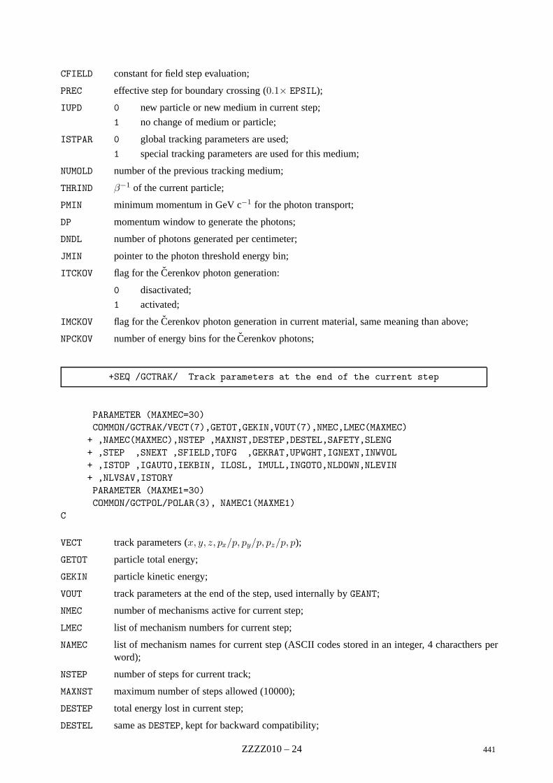
CFIELD constant for field step evaluation;
PREC effective step for boundary crossing (0.1× EPSIL);
IUPD 0 new particle or new medium in current step;
1 no change of medium or particle;
ISTPAR 0 global tracking parameters are used;
1 special tracking parameters are used for this medium;
NUMOLD number of the previous tracking medium;
THRIND β−1 of the current particle;
PMIN minimum momentum in GeV c−1 for the photon transport;
DP momentum window to generate the photons;
DNDL number of photons generated per centimeter;
JMIN pointer to the photon threshold energy bin;
ITCKOV flag for the Cerenkov photon generation:
0 disactivated;
1 activated;
IMCKOV flag for the Cerenkov photon generation in current material, same meaning than above;
NPCKOV number of energy bins for the Cerenkov photons;
+SEQ /GCTRAK/ Track parameters at the end of the current step
PARAMETER (MAXMEC=30)COMMON/GCTRAK/VECT(7),GETOT,GEKIN,VOUT(7),NMEC,LMEC(MAXMEC)
+ ,NAMEC(MAXMEC),NSTEP ,MAXNST,DESTEP,DESTEL,SAFETY,SLENG+ ,STEP ,SNEXT ,SFIELD,TOFG ,GEKRAT,UPWGHT,IGNEXT,INWVOL+ ,ISTOP ,IGAUTO,IEKBIN, ILOSL, IMULL,INGOTO,NLDOWN,NLEVIN+ ,NLVSAV,ISTORYPARAMETER (MAXME1=30)COMMON/GCTPOL/POLAR(3), NAMEC1(MAXME1)
C
VECT track parameters (x, y, z, px/p, py/p, pz/p, p);
GETOT particle total energy;
GEKIN particle kinetic energy;
VOUT track parameters at the end of the step, used internally by GEANT;
NMEC number of mechanisms active for current step;
LMEC list of mechanism numbers for current step;
NAMEC list of mechanism names for current step (ASCII codes stored in an integer, 4 characthers perword);
NSTEP number of steps for current track;
MAXNST maximum number of steps allowed (10000);
DESTEP total energy lost in current step;
DESTEL same as DESTEP, kept for backward compatibility;
ZZZZ010 – 24 441
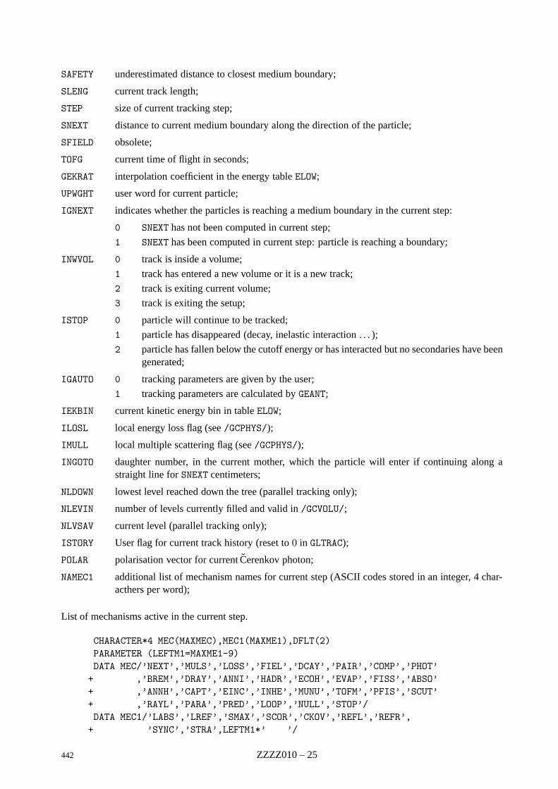
SAFETY underestimated distance to closest medium boundary;
SLENG current track length;
STEP size of current tracking step;
SNEXT distance to current medium boundary along the direction of the particle;
SFIELD obsolete;
TOFG current time of flight in seconds;
GEKRAT interpolation coefficient in the energy table ELOW;
UPWGHT user word for current particle;
IGNEXT indicates whether the particles is reaching a medium boundary in the current step:
0 SNEXT has not been computed in current step;
1 SNEXT has been computed in current step: particle is reaching a boundary;
INWVOL 0 track is inside a volume;
1 track has entered a new volume or it is a new track;
2 track is exiting current volume;
3 track is exiting the setup;
ISTOP 0 particle will continue to be tracked;
1 particle has disappeared (decay, inelastic interaction . . . );
2 particle has fallen below the cutoff energy or has interacted but no secondaries have beengenerated;
IGAUTO 0 tracking parameters are given by the user;
1 tracking parameters are calculated by GEANT;
IEKBIN current kinetic energy bin in table ELOW;
ILOSL local energy loss flag (see /GCPHYS/);
IMULL local multiple scattering flag (see /GCPHYS/);
INGOTO daughter number, in the current mother, which the particle will enter if continuing along astraight line for SNEXT centimeters;
NLDOWN lowest level reached down the tree (parallel tracking only);
NLEVIN number of levels currently filled and valid in /GCVOLU/;
NLVSAV current level (parallel tracking only);
ISTORY User flag for current track history (reset to 0 in GLTRAC);
POLAR polarisation vector for current Cerenkov photon;
NAMEC1 additional list of mechanism names for current step (ASCII codes stored in an integer, 4 char-acthers per word);
List of mechanisms active in the current step.
CHARACTER*4 MEC(MAXMEC),MEC1(MAXME1),DFLT(2)PARAMETER (LEFTM1=MAXME1-9)DATA MEC/’NEXT’,’MULS’,’LOSS’,’FIEL’,’DCAY’,’PAIR’,’COMP’,’PHOT’
+ ,’BREM’,’DRAY’,’ANNI’,’HADR’,’ECOH’,’EVAP’,’FISS’,’ABSO’+ ,’ANNH’,’CAPT’,’EINC’,’INHE’,’MUNU’,’TOFM’,’PFIS’,’SCUT’+ ,’RAYL’,’PARA’,’PRED’,’LOOP’,’NULL’,’STOP’/DATA MEC1/’LABS’,’LREF’,’SMAX’,’SCOR’,’CKOV’,’REFL’,’REFR’,
+ ’SYNC’,’STRA’,LEFTM1*’ ’/
442 ZZZZ010 – 25
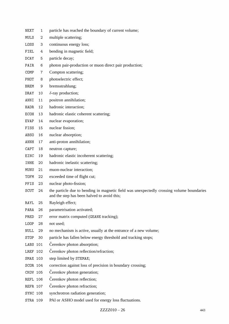
NEXT 1 particle has reached the boundary of current volume;
MULS 2 multiple scattering;
LOSS 3 continuous energy loss;
FIEL 4 bending in magnetic field;
DCAY 5 particle decay;
PAIR 6 photon pair-production or muon direct pair production;
COMP 7 Compton scattering;
PHOT 8 photoelectric effect;
BREM 9 bremsstrahlung;
DRAY 10 δ-ray production;
ANNI 11 positron annihilation;
HADR 12 hadronic interaction;
ECOH 13 hadronic elastic coherent scattering;
EVAP 14 nuclear evaporation;
FISS 15 nuclear fission;
ABSO 16 nuclear absorption;
ANNH 17 anti-proton annihilation;
CAPT 18 neutron capture;
EINC 19 hadronic elastic incoherent scattering;
INHE 20 hadronic inelastic scattering;
MUNU 21 muon-nuclear interaction;
TOFM 22 exceeded time of flight cut;
PFIS 23 nuclear photo-fission;
SCUT 24 the particle due to bending in magnetic field was unexpectedly crossing volume boundariesand the step has been halved to avoid this;
RAYL 25 Rayleigh effect;
PARA 26 parametrisation activated;
PRED 27 error matrix computed (GEANE tracking);
LOOP 28 not used;
NULL 29 no mechanism is active, usually at the entrance of a new volume;
STOP 30 particle has fallen below energy threshold and tracking stops;
LABS 101 Cerenkov photon absorption;
LREF 102 Cerenkov photon reflection/refraction;
SMAX 103 step limited by STEMAX;
SCOR 104 correction against loss of precision in boundary crossing;
CKOV 105 Cerenkov photon generation;
REFL 106 Cerenkov photon reflection;
REFR 107 Cerenkov photon refraction;
SYNC 108 synchrotron radiation generation;
STRA 109 PAI or ASHO model used for energy loss fluctuations.
ZZZZ010 – 26 443
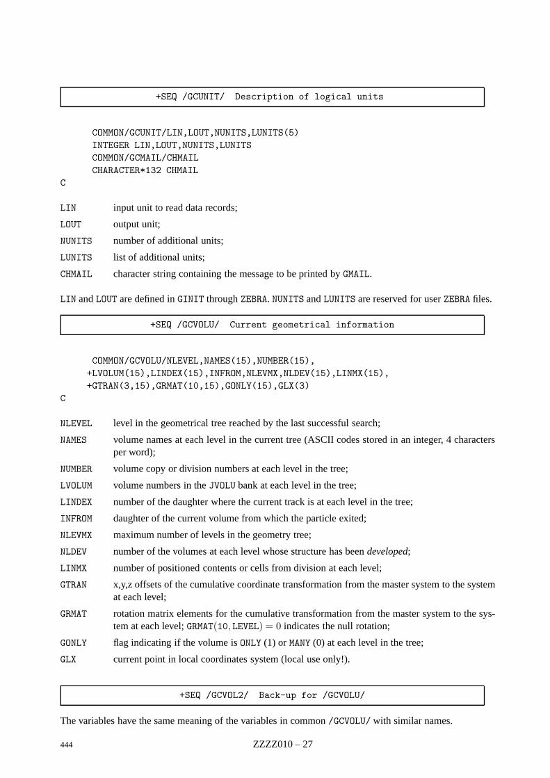
+SEQ /GCUNIT/ Description of logical units
COMMON/GCUNIT/LIN,LOUT,NUNITS,LUNITS(5)INTEGER LIN,LOUT,NUNITS,LUNITSCOMMON/GCMAIL/CHMAILCHARACTER*132 CHMAIL
C
LIN input unit to read data records;
LOUT output unit;
NUNITS number of additional units;
LUNITS list of additional units;
CHMAIL character string containing the message to be printed by GMAIL.
LIN and LOUT are defined in GINIT through ZEBRA. NUNITS and LUNITS are reserved for user ZEBRA files.
+SEQ /GCVOLU/ Current geometrical information
COMMON/GCVOLU/NLEVEL,NAMES(15),NUMBER(15),+LVOLUM(15),LINDEX(15),INFROM,NLEVMX,NLDEV(15),LINMX(15),+GTRAN(3,15),GRMAT(10,15),GONLY(15),GLX(3)
C
NLEVEL level in the geometrical tree reached by the last successful search;
NAMES volume names at each level in the current tree (ASCII codes stored in an integer, 4 charactersper word);
NUMBER volume copy or division numbers at each level in the tree;
LVOLUM volume numbers in the JVOLU bank at each level in the tree;
LINDEX number of the daughter where the current track is at each level in the tree;
INFROM daughter of the current volume from which the particle exited;
NLEVMX maximum number of levels in the geometry tree;
NLDEV number of the volumes at each level whose structure has been developed;
LINMX number of positioned contents or cells from division at each level;
GTRAN x,y,z offsets of the cumulative coordinate transformation from the master system to the systemat each level;
GRMAT rotation matrix elements for the cumulative transformation from the master system to the sys-tem at each level; GRMAT(10, LEVEL) = 0 indicates the null rotation;
GONLY flag indicating if the volume is ONLY (1) or MANY (0) at each level in the tree;
GLX current point in local coordinates system (local use only!).
+SEQ /GCVOL2/ Back-up for /GCVOLU/
The variables have the same meaning of the variables in common /GCVOLU/ with similar names.
444 ZZZZ010 – 27
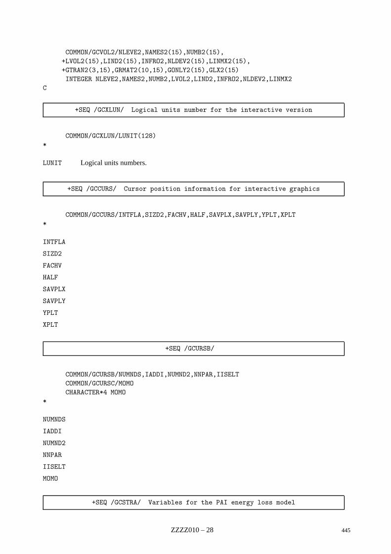
COMMON/GCVOL2/NLEVE2,NAMES2(15),NUMB2(15),+LVOL2(15),LIND2(15),INFRO2,NLDEV2(15),LINMX2(15),+GTRAN2(3,15),GRMAT2(10,15),GONLY2(15),GLX2(15)INTEGER NLEVE2,NAMES2,NUMB2,LVOL2,LIND2,INFRO2,NLDEV2,LINMX2
C
+SEQ /GCXLUN/ Logical units number for the interactive version
COMMON/GCXLUN/LUNIT(128)*
LUNIT Logical units numbers.
+SEQ /GCCURS/ Cursor position information for interactive graphics
COMMON/GCCURS/INTFLA,SIZD2,FACHV,HALF,SAVPLX,SAVPLY,YPLT,XPLT*
INTFLA
SIZD2
FACHV
HALF
SAVPLX
SAVPLY
YPLT
XPLT
+SEQ /GCURSB/
COMMON/GCURSB/NUMNDS,IADDI,NUMND2,NNPAR,IISELTCOMMON/GCURSC/MOMOCHARACTER*4 MOMO
*
NUMNDS
IADDI
NUMND2
NNPAR
IISELT
MOMO
+SEQ /GCSTRA/ Variables for the PAI energy loss model
ZZZZ010 – 28 445
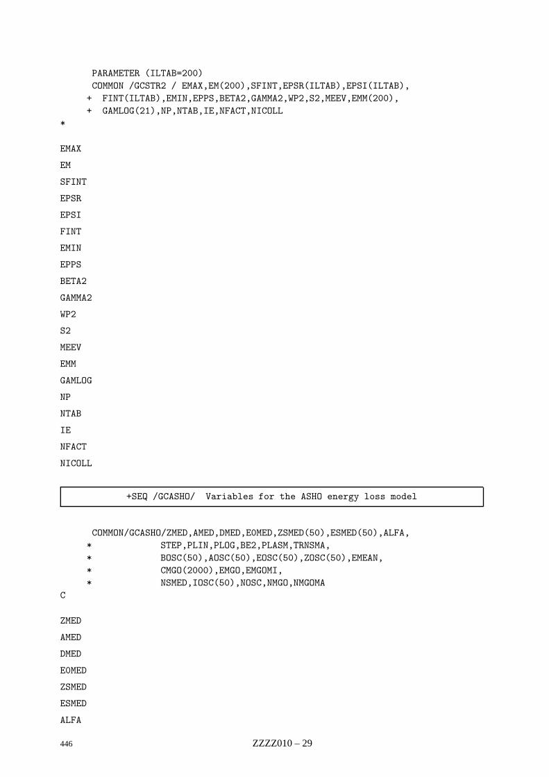
PARAMETER (ILTAB=200)COMMON /GCSTR2 / EMAX,EM(200),SFINT,EPSR(ILTAB),EPSI(ILTAB),
+ FINT(ILTAB),EMIN,EPPS,BETA2,GAMMA2,WP2,S2,MEEV,EMM(200),+ GAMLOG(21),NP,NTAB,IE,NFACT,NICOLL
*
EMAX
EM
SFINT
EPSR
EPSI
FINT
EMIN
EPPS
BETA2
GAMMA2
WP2
S2
MEEV
EMM
GAMLOG
NP
NTAB
IE
NFACT
NICOLL
+SEQ /GCASHO/ Variables for the ASHO energy loss model
COMMON/GCASHO/ZMED,AMED,DMED,E0MED,ZSMED(50),ESMED(50),ALFA,* STEP,PLIN,PLOG,BE2,PLASM,TRNSMA,* BOSC(50),AOSC(50),EOSC(50),ZOSC(50),EMEAN,* CMGO(2000),EMGO,EMGOMI,* NSMED,IOSC(50),NOSC,NMGO,NMGOMA
C
ZMED
AMED
DMED
E0MED
ZSMED
ESMED
ALFA
446 ZZZZ010 – 29
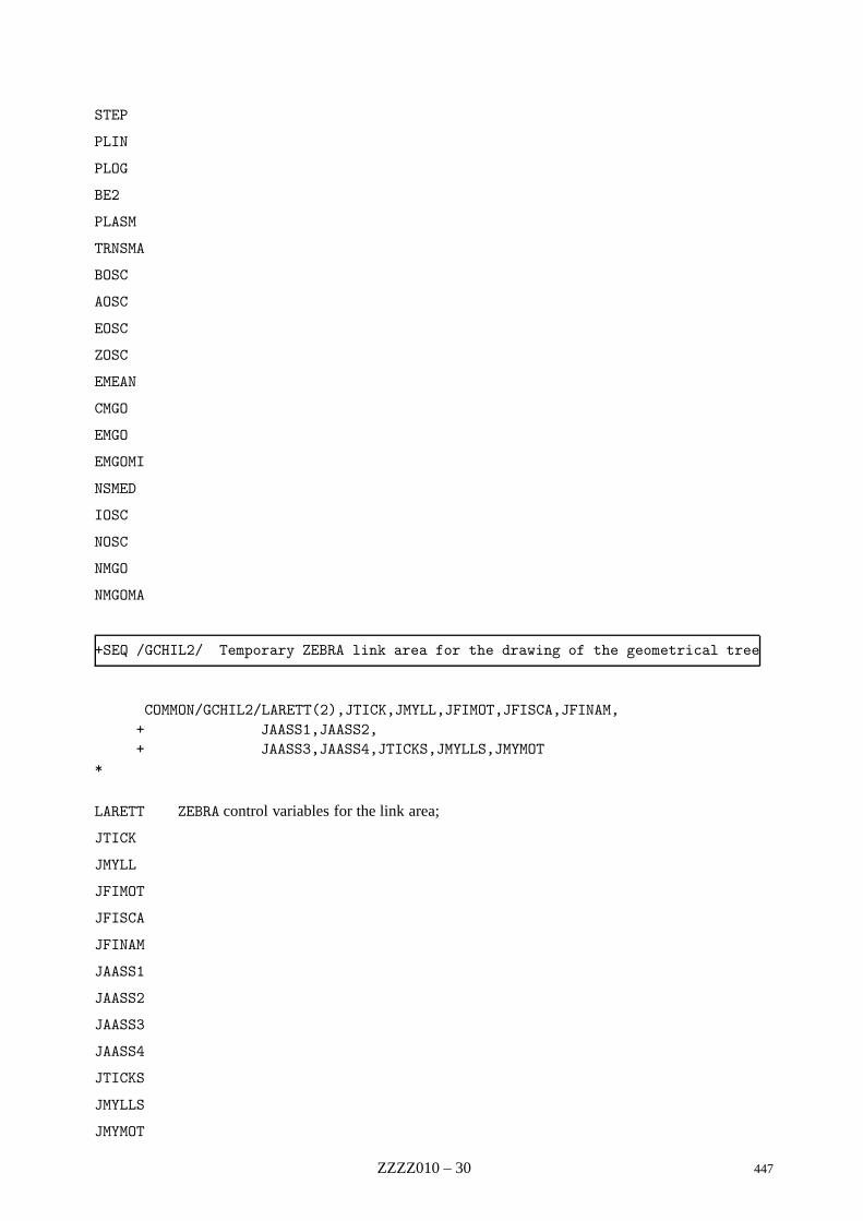
STEP
PLIN
PLOG
BE2
PLASM
TRNSMA
BOSC
AOSC
EOSC
ZOSC
EMEAN
CMGO
EMGO
EMGOMI
NSMED
IOSC
NOSC
NMGO
NMGOMA
+SEQ /GCHIL2/ Temporary ZEBRA link area for the drawing of the geometrical tree
COMMON/GCHIL2/LARETT(2),JTICK,JMYLL,JFIMOT,JFISCA,JFINAM,+ JAASS1,JAASS2,+ JAASS3,JAASS4,JTICKS,JMYLLS,JMYMOT
*
LARETT ZEBRA control variables for the link area;
JTICK
JMYLL
JFIMOT
JFISCA
JFINAM
JAASS1
JAASS2
JAASS3
JAASS4
JTICKS
JMYLLS
JMYMOT
ZZZZ010 – 30 447
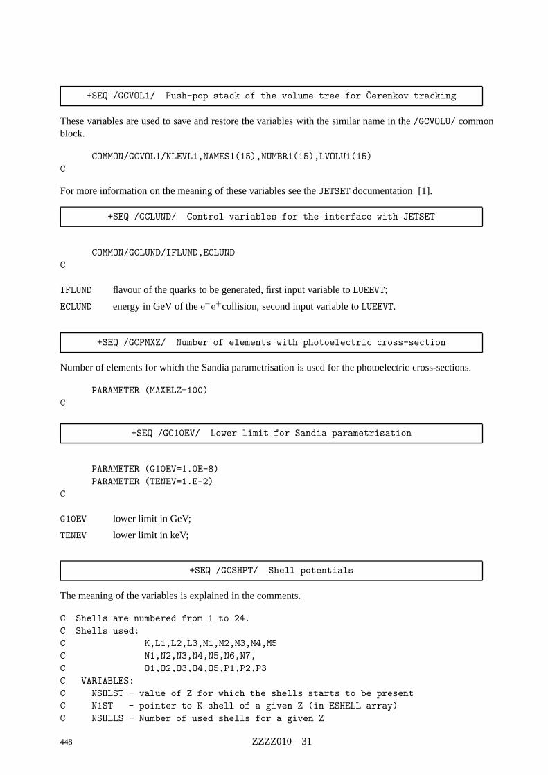
+SEQ /GCVOL1/ Push-pop stack of the volume tree for Cerenkov tracking
These variables are used to save and restore the variables with the similar name in the /GCVOLU/ commonblock.
COMMON/GCVOL1/NLEVL1,NAMES1(15),NUMBR1(15),LVOLU1(15)C
For more information on the meaning of these variables see the JETSET documentation [1].
+SEQ /GCLUND/ Control variables for the interface with JETSET
COMMON/GCLUND/IFLUND,ECLUNDC
IFLUND flavour of the quarks to be generated, first input variable to LUEEVT;
ECLUND energy in GeV of the e−e+collision, second input variable to LUEEVT.
+SEQ /GCPMXZ/ Number of elements with photoelectric cross-section
Number of elements for which the Sandia parametrisation is used for the photoelectric cross-sections.
PARAMETER (MAXELZ=100)C
+SEQ /GC10EV/ Lower limit for Sandia parametrisation
PARAMETER (G10EV=1.0E-8)PARAMETER (TENEV=1.E-2)
C
G10EV lower limit in GeV;
TENEV lower limit in keV;
+SEQ /GCSHPT/ Shell potentials
The meaning of the variables is explained in the comments.
C Shells are numbered from 1 to 24.C Shells used:C K,L1,L2,L3,M1,M2,M3,M4,M5C N1,N2,N3,N4,N5,N6,N7,C O1,O2,O3,O4,O5,P1,P2,P3C VARIABLES:C NSHLST - value of Z for which the shells starts to be presentC N1ST - pointer to K shell of a given Z (in ESHELL array)C NSHLLS - Number of used shells for a given Z
448 ZZZZ010 – 31
C ESHELL - Shells potentials in eV !!!INTEGER LENGTH,MAXSHLPARAMETER (LENGTH= 1409)PARAMETER (MAXSHL=24)INTEGER NSHLST,N1ST,NSHLLSREAL ESHELLDIMENSION NSHLST(MAXSHL),N1ST(MAXELZ),NSHLLS(MAXELZ)DIMENSION ESHELL(LENGTH)COMMON /GCSHPT/NSHLST,N1ST,NSHLLS,ESHELL
C
+SEQ /GCPHPR/ Probability of radiative decay mode
C Probability of radiative decay mode.COMMON /GCPHPR/ GFLUPR(4,MAXELZ)
C
+SEQ /GCPHNR/ Nonradiative decay mode for photoelectric effect
C INRFIN - nonradiative decay modeCOMMON /GCPHNR/ IGNRFN(8,MAXELZ)
C
+SEQ /GCPHRD/ Radiative rates for photoelectric effect
C GRATE - radiative modes’ ratesPARAMETER (KSHLS=6)PARAMETER (L1SHLS=8)PARAMETER (L2SHLS=7)PARAMETER (L3SHLS=8)PARAMETER (ISHLS=29)COMMON / GCPHRD / GPHRAT(ISHLS,MAXELZ),ISHLUS(24,4),ISHLTR(ISHLS)
C
+SEQ /GCPHXS/ Sandia parametrisation coefficients
+KEEP,GCPHXS.PARAMETER (MAXPOW=4)PARAMETER (MAXINT=13)CHARACTER*6 CRNGUPCOMMON /GCPXRN/ CRNGUP(MAXINT,MAXELZ)COMMON /GCPXCF/ COFS(MAXPOW,MAXINT,MAXELZ),GPOMIN(MAXELZ)
C
MAXPOW maximum power of the variable E−1 in the parametrisation;
MAXINT maximum number of parametrisation intervals;
ZZZZ010 – 32 449

MAXELZ maximum number of elements included in the parametrisation;
CRNGUP limits of the energy intervals for the parametrisation;
COFS coefficients of the parametrisation;
GPOMIN minimum value of the parametrisation;
450 ZZZZ010 – 33

Geant 3.11 GEANT User’s Guide ZZZZ999
Origin : GEANT Submitted: 01.10.84Revision : Revised: 09.09.87Documentation :
Index of Documented GEANT routines
GANNI PHYS351, TRAK200
GANNII PHYS100, PHYS350
GANNIR PHYS351
GBHSTA BASE001, BASE110
GBRELA PHYS100, PHYS340, PHYS440
GBRELE PHYS100, PHYS340
GBRELM PHYS100, PHYS440
GBREM TRAK200
GBREME PHYS341
GBREMM PHYS441, TRAK200
GBRSGA PHYS100, PHYS340, PHYS440
GBRSGE PHYS100, PHYS340
GBRSGM PHYS100, PHYS440
GBSTAT GEOM700
GCDERR HITS510
GCDRIF HITS510, IOPA001
GCLOSE IOPA200
GCMWPC HITS500
GCOMP PHYS221, TRAK200
GCOMPI PHYS100, PHYS220
GDAHIT DRAW001, DRAW140
GDAXIS DRAW001, DRAW120, DRAW300, DRAW400
GDCHIT DRAW001, DRAW140, DRAW300
GDCLOS DRAW001, DRAW300
GDCOL DRAW001, DRAW400
GDCURS DRAW001, DRAW400
GDCXYZ DRAW001, DRAW130
GDDVS GEOM140
GDECAY CONS310, PHYS400, TRAK200
GDECA2 PHYS400
GDECA3 PHYS400
GDELET DRAW001, DRAW300
GDFR3D DRAW001, DRAW400
451 ZZZZ999 – 1

GDFSPC DRAW001, DRAW220
GDHEAD DRAW001, DRAW400
GDHITS DRAW001, DRAW140, DRAW300
GDINIT BASE001, BASE110, DRAW001
GDLW DRAW001, DRAW400
GDMAN DRAW001, DRAW300, DRAW400
GDOPEN DRAW001, DRAW300
GDOPT DRAW001, DRAW110, DRAW115, DRAW140, DRAW400
GDPART DRAW001, DRAW130, DRAW300
GDRAW DRAW001, DRAW110, DRAW115, DRAW120
GDRAWC DRAW001, DRAW120, DRAW130, DRAW140, DRAW300, DRAW400
GDRAWT DRAW001, DRAW300, DRAW399, DRAW400
GDRAWV DRAW001, DRAW400
GDRAWX DRAW001, DRAW120, DRAW400
GDRAY PHYS331, TRAK200
GDRPRT PHYS333
GDRELA PHYS100, PHYS330, PHYS430
GDRELE PHYS100, PHYS330
GDRELP PHYS100, PHYS430
GDRSGA PHYS100, PHYS430
GDRVOL DRAW001, DRAW115
GDSCAL DRAW001, DRAW300, DRAW400
GDSHOW DRAW001, DRAW300
GDSPEC DRAW001, DRAW220
GDTOM GEOM320
GDTREE DRAW001, DRAW210
GDXYZ DRAW001, DRAW115, DRAW130, DRAW300, DRAW400, TRAK499
GDZOOM DRAW001, DRAW110, DRAW115, DRAW120, DRAW400
GD3D3D DRAW001, DRAW400
GEDITV DRAW001
GFATT GEOM500
GFDET HITS100
GFDETA HITS105
GFDETD HITS120
GFDETH HITS110
GFDETU HITS130
GFDIGI HITS300, HITS399
GFFGO BASE001, BASE040, BASE110, PHYS100
GFHITS HITS001, HITS200
GFINDS HITS200, TRAK001
ZZZZ999 – 2 452
GFKINE KINE001, KINE100, KINE199
GFMATE CONS001, CONS100
GFPARA GEOM500
GFPART CONS001, CONS300
GFPATH HITS001, HITS200
GFSTAT GEOM700
GFTMAT CONS001, CONS101
GFTMED CONS001, CONS200
GGCLOS GEOM900, HITS001
GGDETV GEOM900, HITS001
GGET IOPA300, KINE001
GHEISH PHYS510
GHELIX CONS200, TRAK001, TRAK500
GHELX3 CONS200, TRAK001, TRAK500, XINT001, XINT110, XINT120,XINT130, XINT140, ZZZZ001, ZZZZ002, ZZZZ999
GHESIG PHYS510, TRAK001
GHMIX CONS110
GHSTOP PHYS510
GICYL HITS400
GINIT BASE040, BASE110, CONS001, PHYS100
GINVOL GEOM001, GEOM300, GEOM700, TRAK001, TRAK130, TRAK200
GIPLAN HITS400
GLANDG PHYS332
GLANDO PHYS332
GLANDR PHYS332
GLAST BASE001, BASE300, GEOM700
GLOREN PHYS410
GLOOK BASE410
GLUDKY KINE210
GLUND KINE200
GLUNDI BASE040, KINE200
GLVOLU GEOM001, GEOM300, GEOM600, HITS001
GMATE BASE001, CONS001, CONS100
GMEDIA GEOM001, GEOM300, GEOM310, GEOM410, GEOM700, TRAK001
GMENEW GEOM001, GEOM300, GEOM410, TRAK130
GMOL PHYS325, TRAK200
GMOLI PHYS325
GMOLS PHYS325
GMOL4 PHYS325
GMTOD GEOM320
453 ZZZZ999 – 3

GMUNU PHYS460, TRAK200
GMUNUI PHYS100, PHYS460
GMUSIG PHYS460
GNEXT GEOM001, GEOM310, GEOM700, TRAK001, TRAK130
GNEXTS GEOM310
GNSOUT GEOM310
GOPEN IOPA200
GOSEAR GEOM001, GEOM300, GEOM410
GPAIR TRAK200
GPAIRG PHYS211
GPAIRM PHYS451, TRAK200
GPART BASE001, CONS001, CONS300
GPCXYZ TRAK400
GPDIGI HITS300
GPDRIF HITS500
GPFIS PHYS240, TRAK200
GPFISI PHYS100, PHYS240
GPGHEI PHYS510
GPHADR PHYS500
GPHITS HITS200
GPHOT PHYS231, PHYS240, TRAK200
GPHOTI PHYS100, PHYS230
GPHSIG PHYS230
GPHYSI BASE001, BASE110, CONS199, PHYS100
GPJXYZ TRAK001, TRAK400
GPKINE KINE001, KINE100
GPLMAT CONS001, CONS102
GPMATE CONS001, CONS100
GPMWPC HITS500
GPPART CONS001, CONS300
GPRELA PHYS100, PHYS450
GPRELM PHYS100, PHYS450
GPRINT BASE400, CONS001
GPRMAT CONS001, CONS103
GPROBI CONS199
GPROTM GEOM200
GPRSGA PHYS100, PHYS210, PHYS450
GPRSGG PHYS100, PHYS210
GPRSGM PHYS100, PHYS450
GPSETS HITS100
ZZZZ999 – 4 454
GPSTAT GEOM700
GPTMED CONS001, CONS200
GPVERT KINE001, KINE100
GPVOLU GEOM100
GRDSGA PHYS330
GREND IOPA400
GRFILE IOPA400
GRKUTA CONS200, TRAK001, TRAK500
GRUN BASE001, BASE200, BASE299
GSAHIT DRAW140, HITS001, HITS200, HITS299
GSATT DRAW110, DRAW115, DRAW120, DRAW130, DRAW210, DRAW220,DRAW500, DRAW510, GEOM500
GRGET IOPA500
GRSAVE IOPA500
GSAVE IOPA300
GSCHIT HITS001, HITS200, HITS299
GSCMED GEOM600
GSDET HITS001, HITS100, HITS105, HITS110, HITS199, HITS200, HITS300, TRAK
GSDETA HITS001, HITS105, HITS199
GSDETD HITS001, HITS105, HITS120, HITS199, HITS300
GSDETH HITS001, HITS100, HITS105, HITS110, HITS120, HITS199, HITS200
GSDETU HITS001, HITS105, HITS130, HITS199
GSDETV GEOM900, HITS001, HITS100, HITS199
GSDIGI HITS001, HITS300, HITS399
GSDK CONS001, CONS300, CONS310, CONS399, DRAW001, DRAW110,DRAW115, DRAW120, DRAW130, DRAW140, DRAW210, DRAW220,DRAW300, DRAW399, DRAW400, DRAW500, DRAW510, GEOM001, GEOM050
GSDVN DRAW210, GEOM001, GEOM100, GEOM130, GEOM140
GSDVN2 GEOM001, GEOM150
GSDVT DRAW210, GEOM001, GEOM100, GEOM140, GEOM199
GSDVT2 GEOM001, GEOM150
GSDVX GEOM001, GEOM100, GEOM150, GEOM199
GSEAR GEOM300, GEOM410
GSKINE KINE001, KINE100, KINE199
GSKING TRAK300, TRAK399
GSMATE CONS001, CONS100
GSMIXT CONS001, CONS110, CONS199
GSNEXT GEOM001, GEOM199, GEOM300, GEOM410
GSORD GEOM001, GEOM199, GEOM300, GEOM400, GEOM900
GSPART CONS001, CONS300, CONS310, KINE100
455 ZZZZ999 – 5

GSPOS DRAW210, GEOM001, GEOM110, GEOM130, GEOM199
GSPOSP DRAW210, GEOM001, GEOM100, GEOM120
GSROTM GEOM110, GEOM120, GEOM200, GEOM299
GSSEAR GEOM001, GEOM199, GEOM300, GEOM410
GSSTAK TRAK300
GSTMED CONS001, CONS200, TRAK001
GSTPAR CONS001, CONS210, CONS299, PHYS100
GSUSEA GEOM410
GSVERT KINE001, KINE100, KINE199, KINE200
GSVOLU GEOM001, GEOM100, GEOM110, GEOM120
GSXYZ TRAK001, TRAK400, TRAK499
GTAU KINE210, PHYS001, PHYS010
GTELEC CONS300, PHYS010, TRAK001, TRAK130, TRAK200
GTGAMA CONS300, PHYS010, TRAK001, TRAK130, TRAK200
GTHADR CONS300, PHYS010, TRAK001, TRAK130, TRAK200
GTMUON CONS300, PHYS010, TRAK001, TRAK130, TRAK200
GTNEUT CONS300, PHYS010, TRAK001, TRAK130, TRAK200
GTNINO CONS300, TRAK001, TRAK130, TRAK200
GTRACK TRAK001, TRAK120
GTREVE BASE001, DRAW140, TRAK001, TRAK110
GTRIG BASE001, BASE200
GTRIGC BASE001, BASE200
GTRIGI BASE001, BASE200, BASE400
GTSET PHYS010
GTVOL TRAK001, TRAK130, TRAK200
GUDCAY CONS310, KINE210, PHYS400
GUDIGI BASE001, HITS001
GUFLD BASE001, TRAK001, TRAK500
GUHADR BASE001, TRAK200
GUKINE BASE001, KINE200, KINE210
GUOUT BASE001
GUPHAD BASE001, TRAK001, TRAK200
GUSEAR GEOM410
GUSTEP BASE001, DRAW140, HITS001, HITS100, TRAK001, TRAK130,TRAK300, TRAK400, TRAK499
GUSWIM BASE001, CONS200, TRAK001, TRAK200, TRAK500
GUTRAK TRAK001, TRAK110
GUTREV BASE001, TRAK001, TRAK110
GZEBRA BASE110
GZINIT BASE001, BASE110
ZZZZ999 – 6 456

ZZZZ Bibliography
[1] T.Sjostrand et al. The LUND MonteCarlo Programs, CERN Program Library Pool Writeup W5035 /W5045 / W5046 / W5047 / W5048 edition, November 1989.
457 Index – 1
Index
/CGMULO/, 211, 276, 308, 313/GC10EV/, 448/GCASHO/, 446/GCBANK/, 12, 13, 18, 27, 31, 96, 418, 428/GCBANK/, 18, 418/GCCURS/, 445/GCCUTS/, 21, 60, 208, 252, 288, 290, 308, 313/GCCUTS/, 418/GCDRAW/, 74, 76, 79, 82, 84, 94, 97/GCDRAW/, 419/GCFLAG/, 20, 22, 33, 39/GCFLAG/, 421/GCGOBJ/, 422/GCHIL2/, 447/GCHILN/, 423/GCJLOC/, 423/GCJUMP/, 424/GCKIN2/, 238/GCKINE/, 22, 293/GCKINE/, 425/GCKING/, 39, 185, 186, 194, 212, 217, 256, 283,
286, 288, 293, 294, 311, 316, 334, 344,425
/GCKING/, 427/GCKMAX/, 425/GCLINK/, 18, 194, 418/GCLINK/, 428/GCLIST/, 20, 22/GCLIST/, 428/GCLUND/, 23/GCLUND/, 448/GCMATE/, 202, 333/GCMATE/, 428/GCMULO/, 21, 50, 199, 201, 216, 252, 287, 297/GCMULO/, 428/GCMUTR/, 425/GCMZFO/, 429/GCNUM/, 33/GCNUM/, 429/GCOMIS/, 430/GCONSP/, 431/GCONST/, 203/GCONST/, 430/GCOPTI/, 20, 139/GCOPTI/, 431/GCPARA/, 431/GCPARM/, 23/GCPARM/, 432/GCPHNR/, 449/GCPHPR/, 449/GCPHRD/, 449
/GCPHXS/, 449/GCPHYS/, 21, 60, 200, 208, 242, 442/GCPHYS/, 433/GCPMXZ/, 448/GCPOLY/, 435/GCPUSH/, 435/GCRZ/, 22/GCRZ/, 435/GCSCAL/, 435/GCSCAN/, 23/GCSCAN/, 436/GCSETS/, 164, 334/GCSETS/, 438/GCSHNO/, 438/GCSHPT/, 448/GCSPEE/, 438/GCSTAK/, 20, 346/GCSTAK/, 439/GCSTRA/, 445/GCTIME/, 20/GCTIME/, 440/GCTMED/, 21, 58, 137, 333, 350/GCTMED/, 440/GCTRACK/, 201, 217/GCTRAK/, 21, 58, 136, 137, 194, 201, 212, 217,
230, 238, 256, 283, 288, 293, 311, 316,334, 344, 346, 348, 430
/GCTRAK/, 441/GCUNIT/, 443/GCURSB/, 445/GCUTS/, 195/GCVOL1/, 447/GCVOL2/, 444/GCVOLU/, 103, 105, 136–138, 145, 165, 238,
442, 444, 447/GCVOLU/, 444/GCXLUN/, 445/GLUNDI/, 23/GSECTI/, 437/PAWC/, 13, 28, 31/QUEST/, 180GCOMP, 217
ANNI, 401AUTO, 401
BOMB, 364BOX, 357BREM, 401
CADINT, 381CDIR, 392
Index – 2 458
CDRSGA, 297CGMULO, 221CHANGEWK, 374CKOV, 401COLOR, 376COMP, 402CONE, 358CUTS, 406
D3DSPEC, 365DAXIS, 367DCAY, 402DCHIT, 372DCLOSE, 374DCUT, 363DDIV, 397DE, 258DEBUG, 391DELETE, 374DEMEAN, 258DFSPC, 365DHEAD, 367DHITS, 372DIRZ, 397DISP, 397DMAN, 367DOPEN, 374DOPT, 377DPART, 371DRAW, 360DRAY, 402DRMAT, 390DRPRT, 407DSCALE, 367DSHOW, 374DSPEC, 365DSPEC, 87, 88DTEXT, 366DTREE, 364DTREE, 87DUVIEW, 373DVECTOR, 366DVOLUME, 362DXCUT, 363DXYZ, 371
EDITV, 381ERAN, 403
FFKEY, 20FILE, 392FLDIST, 210, 323, 323FLINIT, 323, 323
FLUFIN, 323, 323FLUKA, 193FMDIST, 210FREE, 394FZCLOSE, 395FZFILE, 177FZIN, 395FZOPEN, 395FZOUT, 395
GALL GTAU, 191GANNI, 288, 288, 290GANNII, 209, 287, 287GANNIR, 288, 288, 290GARNDM, 42GAVRL2, 224, 224GAVRL3, 224, 224GBFLOS, 276, 276GBFSIG, 276, 276GBHSTA, 14, 32, 32GBIRK, 275, 275GBRELA, 209, 276, 276, 279, 308, 308GBRELE, 276, 276, 278GBRELM, 308, 308, 309GBREM, 198GBREME, 283, 283, 284, 285GBREMM, 311, 311, 312GBRSGA, 209, 276, 276, 279, 308, 308GBRSGE, 276, 276, 278GBRSGM, 308, 308, 309GBSTAT, 146, 146GBTETH, 212, 212, 283, 283, 311, 311, 312GCDERR, 173, 174GCDES, 19, 418GCDRIF, 173, 173, 174GCKING, 224GCLOSE, 177GCMWPC, 171GCOEFF, 209GCOMP, 198, 217, 217, 218GCOMPI, 209, 216, 216GCTRAK, 224, 242GCVOLU, 136, 145GD3D3D, 71, 100, 420GDAHIT, 69, 71, 84, 85GDAXIS, 71, 79, 97GDBOMB, 71GDCGCL, 71GDCGHI, 71GDCGOB, 71GDCGSL, 71GDCHIT, 69, 71, 84, 84GDCLOS, 70, 71, 92, 92
459 Index – 3
GDCOL, 70, 71, 99GDCURS, 71, 99GDCUT, 420GDCXYZ, 40, 69, 71, 82, 82GDEBUG, 28, 39, 39, 348, 422GDECA2, 293, 293GDECA3, 293, 293GDECAY, 65, 293, 293, 294, 322GDELET, 70, 71, 92, 92GDFR3D, 71, 98, 99, 420GDFSPC, 71, 89, 89GDHEAD, 71, 98GDHITS, 69, 71, 84, 84GDINIT, 13, 28, 31, 31, 70GDLENS, 71GDLW, 70, 71, 99GDMAN, 71, 97GDOPEN, 70, 71, 92, 92GDOPT, 69–71, 74, 76, 96, 96, 420, 421GDPART, 71, 82, 82GDRAW, 69, 70, 74, 76, 79, 92, 420GDRAWC, 69, 71, 79, 79, 92, 96GDRAWT, 71, 94, 98GDRAWV, 71, 98, 421GDRAWX, 69, 71, 79, 79, 92, 96, 420GDRAY, 256, 256, 257GDRELA, 209, 252, 252, 297, 297, 300GDRELE, 209, 252, 252GDRELM, 209, 297, 297, 308GDRELP, 209, 297, 297GDRELX, 297, 297, 300GDROT, 293, 295GDRPRT, 267, 270GDRSGA, 209, 252, 255, 297, 302GDRVOL, 69, 70, 76, 76, 420GDSCAL, 71, 97GDSHIF, 71GDSHOW, 70, 71, 92, 92GDSPEC, 71, 89, 89GDTOM, 138GDTRAK, 40GDTREE, 69, 71, 87, 87, 419GDWMN2, 98GDWMN3, 98GDXYZ, 69, 71, 82, 82, 349GDZOOM, 71, 74, 76, 79, 97GEANT/CONTROL/DEBUG, 391GEANT/CONTROL/DRMAT, 390GEANT/CONTROL/GTIME, 387GEANT/CONTROL/KINE, 387GEANT/CONTROL/MZLOGL, 388GEANT/CONTROL/OUTPUT_LP, 388
GEANT/CONTROL/PDIGI, 389GEANT/CONTROL/PHITS, 389GEANT/CONTROL/PLMAT, 390GEANT/CONTROL/PMATE, 389GEANT/CONTROL/PPART, 391GEANT/CONTROL/PRINT, 388GEANT/CONTROL/PRKINE, 391GEANT/CONTROL/PRMAT, 390GEANT/CONTROL/RNDM, 388GEANT/CONTROL/RUNG, 387GEANT/CONTROL/SMATE, 389GEANT/CONTROL/SMIXT, 389GEANT/CONTROL/SORD, 387GEANT/CONTROL/SPART, 390GEANT/CONTROL/STPAR, 390GEANT/CONTROL/SWITCH, 388GEANT/CONTROL/TRACK, 387GEANT/CONTROL/TRIGGER, 388GEANT/CREATE/SBOX, 383GEANT/CREATE/SCONE, 384GEANT/CREATE/SCONS, 385GEANT/CREATE/SPARA, 385GEANT/CREATE/SSPHE, 385GEANT/CREATE/STRD1, 383GEANT/CREATE/STRD2, 383GEANT/CREATE/STUBE, 384GEANT/CREATE/STUBS, 384GEANT/CVOL/BOX, 357GEANT/CVOL/CONE, 358GEANT/CVOL/SPHE, 358GEANT/CVOL/TUBE, 357GEANT/CVOL/VALCUT, 359GEANT/DRAWING/BOMB, 364GEANT/DRAWING/D3DSPEC, 365GEANT/DRAWING/DAXIS, 367GEANT/DRAWING/DCHIT, 372GEANT/DRAWING/DCUT, 363GEANT/DRAWING/DFSPC, 365GEANT/DRAWING/DHEAD, 367GEANT/DRAWING/DHITS, 372GEANT/DRAWING/DMAN, 367GEANT/DRAWING/DPART, 371GEANT/DRAWING/DRAW, 360GEANT/DRAWING/DSCALE, 367GEANT/DRAWING/DSPEC, 365GEANT/DRAWING/DTEXT, 366GEANT/DRAWING/DTREE, 364GEANT/DRAWING/DUVIEW, 373GEANT/DRAWING/DVECTOR, 366GEANT/DRAWING/DVOLUME, 362GEANT/DRAWING/DXCUT, 363GEANT/DRAWING/DXYZ, 371
Index – 4 460
GEANT/DRAWING/KHITS, 372GEANT/DRAWING/KXYZ, 371GEANT/DRAWING/LENS, 370GEANT/DRAWING/MEASURE, 368GEANT/DRAWING/MOVE, 368GEANT/DRAWING/MOVE3D, 369GEANT/DRAWING/PERSP, 369GEANT/DRAWING/PICK, 368GEANT/DRAWING/RANG5D, 362GEANT/DRAWING/SHIFT, 363GEANT/DRAWING/SPOT, 361GEANT/DRAWING/VAR5D, 362GEANT/DRAWING/ZOOM, 370GEANT/DZ/DDIV, 397GEANT/DZ/DIRZ, 397GEANT/DZ/DISP, 397GEANT/DZ/SHOW, 396GEANT/DZ/SNAP, 396GEANT/DZ/STORE, 397GEANT/DZ/SURV, 396GEANT/DZ/VERIFY, 396GEANT/FZ/FZCLOSE, 395GEANT/FZ/FZIN, 395GEANT/FZ/FZOPEN, 395GEANT/FZ/FZOUT, 395GEANT/GEOMETRY/CADINT, 381GEANT/GEOMETRY/EDITV, 381GEANT/GEOMETRY/OPTI, 379GEANT/GEOMETRY/PROTM, 380GEANT/GEOMETRY/PTMED, 381GEANT/GEOMETRY/PVOLU, 380GEANT/GEOMETRY/REUCLID, 382GEANT/GEOMETRY/SDVN, 379GEANT/GEOMETRY/SPOS, 379GEANT/GEOMETRY/SROTM, 380GEANT/GEOMETRY/STMED, 381GEANT/GEOMETRY/SVOLU, 379GEANT/GEOMETRY/WEUCLID, 382GEANT/GRAPHICS_CONTROL/CHANGEWK, 374GEANT/GRAPHICS_CONTROL/COLOR, 376GEANT/GRAPHICS_CONTROL/DCLOSE, 374GEANT/GRAPHICS_CONTROL/DELETE, 374GEANT/GRAPHICS_CONTROL/DOPEN, 374GEANT/GRAPHICS_CONTROL/DOPT, 377GEANT/GRAPHICS_CONTROL/DSHOW, 374GEANT/GRAPHICS_CONTROL/LWID, 377GEANT/GRAPHICS_CONTROL/MAP_COLOR, 378GEANT/GRAPHICS_CONTROL/NEXT, 377GEANT/GRAPHICS_CONTROL/RESETWK, 374GEANT/GRAPHICS_CONTROL/SATT, 375GEANT/GRAPHICS_CONTROL/SCALE, 376GEANT/GRAPHICS_CONTROL/SIZE, 377
GEANT/GRAPHICS_CONTROL/SPERS, 378GEANT/GRAPHICS_CONTROL/SSETAT, 374GEANT/GRAPHICS_CONTROL/SSETVA, 375GEANT/LISTS/GEOM, 410GEANT/LISTS/GET, 408GEANT/LISTS/HSTA, 408GEANT/LISTS/LPRIN, 410GEANT/LISTS/PLOT, 412GEANT/LISTS/RGET, 413GEANT/LISTS/RSAV, 413GEANT/LISTS/SAVE, 409GEANT/LISTS/SETS, 409GEANT/LISTS/STAT, 412GEANT/LISTS/VIEW, 411GEANT/PHYSICS/ANNI, 401GEANT/PHYSICS/AUTO, 401GEANT/PHYSICS/BREM, 401GEANT/PHYSICS/CKOV, 401GEANT/PHYSICS/COMP, 402GEANT/PHYSICS/CUTS, 406GEANT/PHYSICS/DCAY, 402GEANT/PHYSICS/DRAY, 402GEANT/PHYSICS/DRPRT, 407GEANT/PHYSICS/ERAN, 403GEANT/PHYSICS/HADR, 403GEANT/PHYSICS/LABS, 403GEANT/PHYSICS/LOSS, 403GEANT/PHYSICS/MULS, 404GEANT/PHYSICS/MUNU, 404GEANT/PHYSICS/PAIR, 404GEANT/PHYSICS/PFIS, 405GEANT/PHYSICS/PHOT, 405GEANT/PHYSICS/PHYSI, 407GEANT/PHYSICS/RAYL, 405GEANT/PHYSICS/STRA, 406GEANT/PHYSICS/SYNC, 406GEANT/RZ/CDIR, 392GEANT/RZ/FILE, 392GEANT/RZ/FREE, 394GEANT/RZ/IN, 393GEANT/RZ/LDIR, 393GEANT/RZ/LOCK, 394GEANT/RZ/MDIR, 392GEANT/RZ/OUT, 393GEANT/RZ/PQUEST, 392GEANT/RZ/PURGE, 394GEANT/RZ/REND, 392GEANT/RZ/SCR, 394GEANT/SCAN/HSCAN, 400GEANT/SCAN/LSCAN, 399GEANT/SCAN/PCUTS, 399GEANT/SCAN/PHI, 398
461 Index – 5
GEANT/SCAN/SFACTORS, 398GEANT/SCAN/SLIST, 398GEANT/SCAN/STURN, 399GEANT/SCAN/TETA, 398GEANT/SCAN/VERTEX, 398GEDITV, 70GEKBIN, 201GENLAN, 266GEOM, 410GET, 408GEVKEV, 41, 41, 209GFANG, 133, 295GFATT, 143GFCNRM, 209GFDET, 157GFDETD, 161GFDETH, 160GFDETU, 162GFDIGI, 156, 167, 169GFFGO, 13, 20, 31, 31, 32, 190, 208GFHEAD, 35GFHITS, 156, 164, 165, 166GFIN, 178, 179GFINDS, 164, 334GFKINE, 186, 189GFLDIS, 325GFLFIN, 325GFLUCT, 258, 258, 271GFMATE, 46, 47GFMDIS, 325, 325GFMFIN, 325, 325GFOUT, 178, 179, 179GFPARA, 143GFPART, 46, 64GFPATH, 156, 165, 165GFRDT, 219, 219GFRUNG, 35GFSDPR, 219, 219GFSHDC, 219, 219GFSHLS, 219, 219GFSTAT, 146, 146GFTMAT, 46, 49GFTMED, 46, 57GFVERT, 185, 187GGCKOV, 238GGCLOS, 14, 32, 139, 140, 146, 147, 147, 156, 157GGDETV, 147, 156, 157GGET, 179GGORD, 106, 139GGORDQ, 139GGPERP, 237, 238, 238GHEISH, 319, 321, 322
GHEISHA, 39, 193, 322GHELIX, 57, 333, 350, 350GHELX3, 57, 333, 350, 350GHESIG, 210, 320, 321GHMIX, 52GHPHAK, 224GHPHAL1, 224GHPHAL2, 224GHPOT, 224GHPRIN, 219GHSLIN, 219GHSTOP, 322, 322GICYL, 170GINIT, 13, 19–23, 31, 31, 46, 418, 430, 444GINVOL, 102, 136, 146, 332GIPLAN, 170GKOKRI, 271, 271GLANDG, 258, 258, 266GLANDO, 261GLANDZ, 258, 258, 267GLAST, 15, 38, 146GLISUR, 237GLOOK, 41GLOREN, 293, 295GLTRAC, 198, 333, 346, 442GLUND, 190, 190GLUNDI, 190GLVOLU, 105, 138, 145, 145, 156, 165GMAIL, 444GMATE, 13, 46, 47GMCOUL, 242, 247, 250GMEDIA, 102, 103, 136, 136, 138, 141, 146, 332GMGAUS, 240, 241GMICAP, 325, 325GMOL4, 243, 243, 247GMOLI, 209, 242, 242, 246GMOLIE, 242, 242, 243, 247GMOLIO, 210, 242, 242, 246GMORIN, 325, 325GMTOD, 138, 138GMULOF, 198, 202, 210, 242, 242, 248, 249GMULTS, 240, 242, 242, 243, 246, 250GMUNU, 198, 318, 318GMUNUI, 209, 210, 318, 318GMUSIG, 318GNEXT, 102, 137, 137GNFRDT, 219, 219GNRDT, 219GOPEN, 177, 178, 179GOSCIN, 271, 271GPAIRG, 212, 212, 214, 230GPAIRM, 316, 316, 317
Index – 6 462
GPART, 13, 46, 61, 293GPCXYZ, 40, 348GPDIGI, 39, 167GPDRIF, 171GPFIS, 228, 228GPFISI, 209, 228, 228GPGHEI, 319, 321GPHAK, 224GPHAL1, 224GPHAL2, 224, 224GPHAL3, 224, 224GPHEAD, 35GPHINI, 209, 219, 219GPHITS, 39, 164, 420GPHOT, 224, 224GPHOTI, 209, 219, 219GPHRIN, 219GPHSG1, 219, 219, 224GPHSGP, 224, 224GPHSIG, 219, 219, 220, 221GPHXIN, 219, 219GPHXSI, 209, 219, 219GPHYSI, 14, 28, 32, 50, 60, 201–203, 207, 207,
208, 211, 216, 219, 228, 229, 242, 252,271, 275, 276, 287, 297, 308, 313, 318,322
GPIONS, 62GPJXYZ, 39, 334, 348GPKINE, 39, 186, 189GPLMAT, 46, 50GPMATE, 39, 46, 47GPMWPC, 171GPOISS, 42GPPART, 39, 46, 64GPRELA, 209, 210, 313, 313GPRELM, 313, 313, 315GPRINT, 39, 39GPRMAT, 46, 50GPROBI, 199, 209, 242, 253, 298GPROTM, 39, 134GPRSGA, 209, 211, 211, 313, 313GPRSGG, 211, 211GPRSGG(Z,E), 211GPRSGM, 313, 313, 315GPRUNG, 35GPSETS, 39, 157GPSTAT, 38, 146, 146GPTMED, 39, 46, 58GPVERT, 39, 185, 187GPVOLU, 39, 119GRANGI, 203, 205, 209GRAYL, 229, 230, 230, 231
GRAYLI, 209, 229, 229GREND, 180GRFILE, 180, 180, 181GRGET, 182GRIN, 180, 181, 181GRKUTA, 57, 333, 350, 350GRMDIR, 180GRNDM, 42, 42GRNDMQ, 42, 208GROUT, 180, 181GRSAVE, 182GRUN, 14, 33GSAHIT, 156, 164, 164, 166GSAHIT,, 84GSATT, 69, 70, 74, 76, 79, 97, 143, 143GSAVE, 179GSCHIT, 84, 156, 164, 166GSCKOV, 237, 238GSDET, 28, 147, 155–157, 157, 163–165, 167, 334GSDETA, 156, 158, 158, 163GSDETD, 156, 158, 161, 161, 163, 167GSDETH, 156, 158, 159, 163, 164GSDETU, 156, 158, 162, 163GSDETV, 147, 155, 156, 157, 163, 165GSDIGI, 156, 167, 169GSDK, 46, 61, 63, 65, 65GSDNDX, 210GSDVN, 87, 105, 119, 123GSDVN2, 105, 129, 129GSDVT, 87, 105, 119, 128GSDVT2, 105, 129, 130GSDVX, 105, 119, 129GSHEAD, 35GSHLIN, 219, 219GSKINE, 185, 185, 186, 189, 344GSKING, 14, 185, 186, 238, 344, 344, 346, 347,
427GSKINU, 186, 189, 344GSKPHO, 14, 238, 346GSMATE, 13, 28, 45–47, 47, 220GSMIXT, 46, 51, 51, 215, 286, 323GSNEAR, 106, 131, 137, 140, 140GSNEXT, 106, 131, 137, 140, 140GSORD, 20, 32, 106, 131, 139, 139, 147, 431GSPART, 13, 46, 63, 63, 65GSPOS, 28, 87, 104, 106, 120, 120, 122, 133GSPOSP, 87, 104, 105, 119, 122, 122, 133GSREE0, 210GSROTM, 133, 133, 135GSRUNG, 35GSSTAK, 14, 427GSTDN, 271, 271
463 Index – 7
GSTINI, 209, 271, 271GSTMED, 45, 46, 57, 202, 203, 247, 322, 332, 350GSTPAR, 46, 59, 59, 60, 208, 267, 275, 322GSTREN, 271, 271GSTTAB, 271, 271GSTXIN, 271, 271GSUNEA, 106, 131, 141, 141GSVERT, 185, 185, 186, 187, 344GSVERU, 185, 187, 344GSVOLU, 28, 104, 119, 120, 122, 123GSXYZ, 40, 82, 334, 349GSXYZ , 348GSYNC, 291, 291GSYNGE, 291, 291GTCKOV, 63, 198, 234, 238, 333GTELEC, 63, 238, 240, 242, 256, 258, 283, 288,
291, 333, 350GTGAMA, 63, 198, 212, 217, 224, 228, 230, 333GTHADR, 63, 198, 238, 240, 242, 256, 258, 302,
333, 350GTHION, 63, 198, 240, 242, 256, 303, 303, 305,
333, 350GTIME, 387GTMEDI, 102, 103, 136, 136, 146, 332, 333GTMUON, 63, 198, 238, 240, 242, 256, 258, 311,
316, 318, 333, 350GTNEUT, 63, 198, 333GTNEXT, 102, 136, 137, 137, 141, 146, 332, 333GTNINO, 63, 198, 333GTRACK, 14, 146, 333, 334, 336GTREVE, 14, 333, 335GTRIG, 14, 33GTRIGC, 14, 34GTRIGI, 14, 33, 39, 186GTVOL, 337GUDCAY, 65, 294GUDIGI, 14, 156GUDTIM, 173, 174GUFLD, 15, 57, 333, 350, 351, 440GUHADR, 14, 196, 318, 319, 322, 323GUKINE, 14, 185, 186GULAST, 15GUNEAR, 106, 131, 141, 141GUOUT, 14GUPHAD, 14, 196, 319, 321, 323, 333GUPLSH, 237, 237GUSEAR, 139GUSKIP, 14GUSTEP, 14, 39, 82, 156, 157, 238, 322, 334, 346,
348, 349GUSWIM, 15, 333, 350, 350GUTRAK, 14, 333
GUTREV, 14, 333GVAVIV, 258, 258, 262, 266GVROT, 296, 296GWOMA1, 97GXGINT, 271, 271GXINT, 28GZEBRA, 27, 28, 31, 31GZINIT, 13, 18, 31, 31, 418
HADR, 403HIGZ, 69HLIMIT, 28, 31, 50HPLINT, 13, 31, 70HPLSOF, 94, 98HSCAN, 400HSTA, 408
IGEND, 28IGINIT, 13, 28, 31IGMETA, 28, 31IN, 393
KHITS, 372KINE, 387KXYZ, 371
LABS, 403LDIR, 393LENS, 370LENS, 84LOCK, 394LOSS, 403LPRIN, 410LSCAN, 399LUEEVT, 190, 448LWID, 377
MAP_COLOR, 378MDIR, 392MEASURE, 368MOVE, 368MOVE, 84MOVE3D, 369MULS, 404MUNU, 404MZEND, 38MZLOGL, 388
NEXT, 377
OPTI, 379OUT, 393OUTPUT_LP, 388
PAIR, 404
Index – 8 464
PATCHY, 278PCUTS, 399PDIGI, 389PERSP, 369PFIS, 405PFIS, 228PHI, 398PHITS, 389PHOT, 405PHYSI, 407PICK, 368PLMAT, 390PLOT, 412PMATE, 389PPART, 391PQUEST, 392PRINT, 388PRKINE, 391PRMAT, 390PROTM, 380PTMED, 381PURGE, 394PVOLU, 380
RANECU, 42RANG5D, 362RAYL, 405REND, 392RESETWK, 374REUCLID, 382RGET, 413RNDM, 388RSAV, 413RUNG, 387RZEND, 180, 181RZFILE, 180RZMAKE, 180RZOPEN, 180
SATT, 375SAVE, 409SBOX, 383SCALE, 376SCONE, 384SCONS, 385SCR, 394SDVN, 379SETS, 409SFACTORS, 398SHIFT, 363SHOW, 396SIGMOR, 325SIZE, 377
SLIST, 398SMATE, 389SMIXT, 389SNAP, 396SORD, 387SPARA, 385SPART, 390SPERS, 378SPHE, 358SPOS, 379SPOT, 361SROTM, 380SSETAT, 374SSETVA, 375SSPHE, 385STAT, 412STMED, 381STORE, 397STPAR, 390STRA, 406STRD1, 383STRD2, 383STUBE, 384STUBS, 384STURN, 399SURV, 396SVOLU, 379SWITCH, 388SYNC, 406
TETA, 398TIMEST, 21TRACK, 387TRIGGER, 388TUBE, 357
UCTOH, 145UGEOM, 13, 28UGINIT, 207
VALCUT, 359VAR5D, 362VERIFY, 396VERTEX, 398VIEW, 411
WEUCLID, 382
ZEBRA, 96ZOOM, 370
465 Index – 9