Embed Size (px)
Citation preview
Advances in Applied Mathematics 29 (2002) 137–151
www.academicpress.com
Determinant formulas for multidimensionalhypergeometric period matrices
Donald Richardsa,b,∗,1 and Qifu Zhengc,2
a School of Mathematics, Institute for Advanced Study, Princeton, NJ 08540, USAb Department of Statistics, University of Virginia, Charlottesville, VA 22904, USA
c Department of Mathematics and Statistics, The College of New Jersey, Ewing, NJ 08628, USA
Received 27 June 2001; accepted 5 August 2001
Abstract
In this article we derive closed-form determinant formulas for certain period matriceswhose entries are multidimensional integrals of hypergeometric type with integrands basedon power functions. Our results are motivated by the work of Varchenko [Izv. Akad. NaukSSSR Ser. Mat. 53 (1989) 1206–1235; Izv. Akad. NaukSSSR Ser. Mat. 54 (1990) 146–158] and Richards and Zheng [Adv. Appl. Math. 28 (2002) 602–633] who derived closed-form expressions for determinants of matrices with entries as multidimensional integralsof rational functions. 2002 Elsevier Science (USA). All rights reserved.
Keywords:Aomoto’s integral; Basic composition formula; Binet–Cauchy formula; Hypergeometricperiod matrix; Selberg’s integral; Vandermonde-type determinant
1. Introduction
In a recent paper [8], we derived new proofs of determinant formulas ofVarchenko [10,11] for certain hypergeometric period matrices whose entries areone-dimensional Euler-type integrals. In this article we continue our earlier work,
* Corresponding author.E-mail address:[email protected] (D. Richards).
1 This research was supported by a grant from the Bell Fund to the Institute for Advanced Study.2 This research was supported by a grant from the SOSA Fund of the College of New Jersey.
0196-8858/02/$ – see front matter 2002 Elsevier Science (USA). All rights reserved.PII: S0196-8858(02)00013-1

138 D. Richards, Q. Zheng / Advances in Applied Mathematics 29 (2002) 137–151
deriving closed-form expressions for the determinants of some matrices whoseentries are multidimensional integrals of hypergeometric type with integrandscontaining symmetrized power functions.
As a consequence of the new closed-form determinant formulas given here, wediscover some multidimensional integral formulas. The simplest example of theseintegral formulas is given in the following result. Supposeλj ∈ R, j = 1,2,3,with λ1 < λ2 < λ3. Define the region
D(λ1, λ2, λ3) := {(s1, t1, s2, t2, s3, t3) ∈ R
6: s1, t1, s2 ∈ (λ1, λ2);t2, s3, t3 ∈ (λ2, λ3)
}. (1.1)
Letα1, α2, α3, γ ∈ C with Re(αj ) > 0,j = 1,2, and Re(γ ) > −min{1/2,Re(α1),
Re(α2),Re(α3)}. As a consequence of our general theory, we shall derive the six-dimensional integral formula∫
D(λ1,λ2,λ3)
[(t3 − t2)(s3 − t1)(s2 − s1) + (s3 − s2)(t3 − s1)(t2 − t1)
]
×3∏
i=1
[|si − ti |2γ
3∏p=1
∣∣(si − λp)(ti − λp)∣∣αp−1
]dsi dti
=[
Γ (2γ + 1)∏3
p=1 Γ (αp)
Γ (γ + 1)Γ(2γ +∑3
p=1αp
)]2∏3
p=1 Γ (γ + αp)
Γ(γ +∑3
p=1αp
)×
∏1�i<j�3
(λj − λi)3(αi+αj−1)+2γ . (1.2)
It is interesting to observe that this integral is the sum of two six-dimensionalintegrals, each of which is of the type considered by Kaneko [4], Macdonald [6],and other authors. Neither of these two integrals can generally be evaluated inclosed form; indeed, the results of Kaneko [4] indicate that each integral can beevaluated only as an infinite series of Jack polynomials. Nevertheless, the sum ofthe two integrals reduces to the closed-form expression given in (1.2).
A pictorial representation of the domainD(λ1, λ2, λ3) shows that the range ofthe pairs(s1, t1), (s2, t2), and(s3, t3) is given by the diagram
λ1
(s2, t2) (s3, t3)
(s1, t1)
λ1 λ2 λ3
λ2
λ3

D. Richards, Q. Zheng / Advances in Applied Mathematics 29 (2002) 137–151 139
In our general higher-dimensional extensions of (1.2), similar diagrams are validfor the domains of integration generalizing (1.1).
It is also noticeable that the integrand in (1.2) contains a sum of two terms,e.g.,(t3 − t2)(s3 − t1)(s2 − s1), each of which is reminiscent of a Vandermonde-type determinant. We will see that similar Vandermonde-type products of mixedvariables appear in the general context.
Let us examine some special cases of (1.2). Substitutingλ1 = 0, λ2 = λ, andλ3 = 1,λ ∈ (0,1), then, (1.2) reduces to∫
D(0,λ,1)
[(t3 − t2)(s3 − t1)(s2 − s1) + (s3 − s2)(t3 − s1)(t2 − t1)
]
×3∏
i=1
|si − ti |2γ (si ti )αi−1∣∣(si − λ)(ti − λ)
∣∣α2−1
× ((1− si)(1− ti)
)α3−1 dsi dti
=[
Γ (2γ + 1)∏3
p=1Γ (αp)
Γ (γ + 1)Γ(2γ +∑3
p=1αp
)]2∏3
p=1Γ (γ + αp)
Γ(γ +∑3
p=1 αp
)× λ3(α1+α2−1)+2γ (1− λ)3(α2+α3−1)+2γ . (1.3)
If we next apply to (1.3) the change of variables(s1, t1, s2) → λ(s1, t1, s2) and(t2, s3, t3) → λ(1,1,1) + (1 − λ)(t2, s3, t3), we obtain the formidable-lookingresult ∫
(0,1)6
[λ(1− λ)(t3 − t2)
((1− λ)s3 + λ(1− t1)(s2 − s1)
)+ (
(1− λ)s3 + λ(1− s2))(
(1− λ)t3 + λ(1− s1))
× ((1− λ)t2 + λ(1 − t1)
)]× |s1 − t1|2γ
∣∣λ(s2 − 1) − (1− λ)t2∣∣2γ |s3 − t3|2γ
× [s1s2
(λ + (1− λ)s3
)t1(λ + (1− λ)t2
)(λ + (1− λ)t3
)]α1−1
× [(1− s1)(1− s2)s3(1− t1)t2t3
]α2−1
× [(1− λs1)(1− λs2)(1− s3)(1− λt1)(1− t2)(1− t3)
]α3−1
×3∏
i=1
dsi dti
=[
Γ (2γ + 1)∏3
p=1Γ (αp)
Γ (γ + 1)Γ(2γ +∑3
p=1αp
)]2∏3
p=1Γ (γ + αp)
Γ(γ +∑3
p=1 αp
) . (1.4)
It is also remarkable that the left-hand side of (1.4) depends onλ, but the right-hand side does not.
140 D. Richards, Q. Zheng / Advances in Applied Mathematics 29 (2002) 137–151
Forλ = 0 or 1, the formula (1.4) reduces to a product of three double integrals,one of which is a product of classical beta integrals, and the remaining two doubleintegrals are two-dimensional beta integrals of the type evaluated by Selberg [9].
Turning to the general case, let us now provide a description of the resultsto follow. In Section 2 we derive a closed-form evaluation of a determinantwhose entries aren-dimensional hypergeometric-type integrals. These integralsare generalizations of some integrals considered by Varchenko [10,11], Richardsand Zheng [8], and other authors (cf. Markov et al. [7]), and the evaluation of theresulting determinant extends a formula of Varchenko [10,11].
In Section 3 we apply a multidimensional variation on the Binet–Cauchy for-mula [5, p. 17] to express the determinant evaluation as an iterated multidimen-sional integral. Then we deduce (1.2) as the simplest special case of these inte-grals. We remark that the derivation of integrals such as (1.2) from the determinantevaluation formula is related to results developed in our earlier paper [8, Sec-tion 3] in which we utilized the Binet–Cauchy formula to obtain a new proof ofsome well-known multidimensional beta integrals of Selberg [9] and Aomoto [1].
2. Determinant formulas
The preceding observation is only a small part of the connection between(1.2)–(1.4) and the integral formulas of Selberg and Aomoto. Indeed, the generalresults underlying these special cases are obtained, in part, by application ofSelberg’s formula, and we now develop this connection.
For positive integersn andN , define the index set
In,N := {I = (i1, . . . , in) ∈ N
n: 1 � i1 � · · · � in � N}.
Let α1, . . . , αN+1, γ ∈ C with positive real parts, andλ1, . . . , λN+1 ∈ R. Usingthe notationα = (α1, . . . , αN+1), λ = (λ1, . . . , λN+1), andx = (x1, . . . , xn) ∈Rn, we define
Φ(x;λ) :=N+1∏p=1
n∏i=1
(xi − λp)αp−1
∏1�i<j�n
(xj − xi)2γ .
Here, the principal branch ofxαp−1 (p = 1, . . . ,N + 1) or xγ is fixed by−π/2< argx < 3π/2. It is well known that functions of this form arise in randommatrix theory (cf. [2,3]) and in evaluation of the determinants of period matrices(cf. [12] and [8]).
ForJ = (j1, . . . , jn) ∈ In,N andx ∈ Rn, define
ωJ (x) := 1
n!∑
σ∈Sn
n∏k=1
xjk−1σ(k) .

D. Richards, Q. Zheng / Advances in Applied Mathematics 29 (2002) 137–151 141
This function is a monomial symmetric function inx1, . . . , xn. Alternatively,n!ωJ (x) can be viewed as thepermanentof then × n matrix with (i, j)th entryxjk−1i . Also, the functionωJ (x) is related to the concept of aλ-mean(cf. [6,
p. 32]).For I = (i1, . . . , in) andJ = (j1, . . . , jn) in In,N , define
aI,J :=λi1+1∫λi1
· · ·λin+1∫λin
Φ(x;λ)ωJ (x)dx. (2.1)
Form the|In,N | × |In,N | matrix with entriesaI,J , where rows and columns arelisted in increasing order according to the natural lexicographic ordering on theindex setIn,N . A variation on this matrix, treated by Varchenko [12], replaced theterms
∏nk=1x
jk−1k with certain rational functions ofx1, . . . , xn (cf. [8, Eq. (5.3)]).
Next we define the determinant
Dn,N+1(λ;α) := det(aI,J ). (2.2)
We now proceed to obtain a closed-form expression for the value of thedeterminant (2.2). This result is analogous to a result of Varchenko [12] whichevaluated in closed form the determinant of a matrix whose entries all aremultidimensional integrals of Selberg-type (cf. [8, Theorem 5.1]). The followingis the main result of the paper.
Theorem 2.1. For n,N ∈ N, supposeλ ∈ RN+1, α ∈ CN+1 with Re(αj ) > 0,j = 1, . . . ,N + 1, and let γ ∈ C with Re(γ ) > −min{1/n,Re(αj )/(n − 1):1 � j � N + 1}. Then
Dn,N+1(λ;α) = Cn,N+1(α)∏
1�i<j�N+1
(λj − λi)(N+n−1
N )+2(N+n−1N+1 )γ
×∏
1�i �=j�N+1
(λj − λi)(N+n−1
N )(αi−1), (2.3)
where
Cn,N+1(α)
=n−1∏k=1
[(n
k
)−(N+k−1k+1 ) k−1∏
s=1
(k
s
)−(N+n+s−k−2N−3 )
]
×n∏
i=1
[[Γ (iγ + 1)]N[Γ (γ + 1)]N
∏N+1j=1 Γ (αj + (i − 1)γ )
Γ((2n − i − 1)γ +∑N+1
j=1 αj
)](N+n−i−1
N−1 )
. (2.4)

142 D. Richards, Q. Zheng / Advances in Applied Mathematics 29 (2002) 137–151
Proof. As in our previous article, it suffices to assume thatα1, . . . , αN+1 arepositive integers. Once the proof of the integer case is complete, the extensionto complexα1, . . . , αN+1 follows immediately by analytic continuation throughan application of Carlson’s theorem.
By making a change of variables in (2.1), we find thataI,J is a polynomialin λ1, . . . , λN+1 and is homogeneous of degreen
∑N+1p=1 (αp − 1) + n(n − 1)γ +
j1 + · · · + jn. Therefore the determinantDn,N+1(λ;α) is also a polynomial inλ1, . . . , λN+1 and is homogeneous of degree
∑1�j1�···�jn�N
[n
N+1∑p=1
(αp − 1) + n(n − 1)γ + j1 + · · · + jn
]
=[n
N+1∑p=1
αp + n(n − 1)γ − 1
2n(N + 1)
](N + n − 1
n
).
Consider the row(1, . . . ,1) in the determinant and make the change ofvariablesxi → (λ2 − λ1)xi + λ1, i = 1, . . . , n, in the integral defininga(1, . . . ,1;j1, . . . , jn). Then the integral is transformed into an integral over(0,1)n, andΦ(x;λ)dx is transformed into
N+1∏p=1
n∏i=1
((λ2 − λ1)xi + λ1 − λp
)αp−1
×∏
1�i<j�n
((λ2 − λ1)xj − (λ2 − λ1)xi
)2γ · (λ2 − λ1)n dx
= (λ2 − λ1)n(n−1)γ+nα1(λ1 − λ2)
n(α2−1)
×N+1∏p=3
n∏i=1
((λ2 − λ1)xi + λ1 − λp
)αp−1 ∏1�i<j�n
(xj − xi)2γ
×n∏
i=1
xα1−1i (1− xi)
α2−1 dxi.
This shows that the polynomial(λ2 − λ1)n(n−1)γ+nα1(λ1 − λ2)
n(α2−1) divides therow (1, . . . ,1).
Proceeding similarly, we deduce that(λ2 − λ1)(n−1)(n−2)γ+(n−1)α1 ×
(λ1 − λ2)(n−1)(α2−1) divides the row(1, . . . ,1, i) for eachi = 2, . . . ,N . Further,
for eachk = 0, . . . , n, (λ2−λ1)(n−k)(n−k−1)γ+(n−k)α1(λ1−λ2)
(n−k)(α2−1) dividesthe row(1, . . . ,1, in−k+1, . . . , in) wherein−k+1 � 2. Multiplying together thesefactors, it follows that
(λ2 − λ1)∑n
k=0(n−k)[(n−k−1)γ+α1](N+k−2k )(λ1 − λ2)
∑nk=0(n−k)(α2−1)(N+k−2
k )
≡ (λ2 − λ1)2(N+n−1
N+1 )γ+(N+n−1N )α1(λ1 − λ2)
(N+n−1N )(α2−1) (2.5)
D. Richards, Q. Zheng / Advances in Applied Mathematics 29 (2002) 137–151 143
divides the determinantDn,N+1(λ;α).We now consider the effect on the determinantDn,N+1(λ;α) of permuting
the pairs(λp,αp), p = 1, . . . ,N + 1. Let us call a permutationτ ∈ SN+1 an“adjacent transposition” ifτ transposes a pair(λm,αm) and (λm+1, αm+1) forsomem ∈ {1, . . . ,N}. We claim that under the action ofτ , the determinantDn,N+1(λ;α) changes only by a constant multiple which does not dependent onλ or α.
For (i1, . . . , in) ∈ In,N we write (i1, . . . , in) = (1r12r2 · · ·NrN ) if, for all k =1, . . . ,N , the numberk appears exactlyrk times in the set{i1, . . . , in}; i.e.,
{i1, . . . , in} = {1, . . . ,1︸ ︷︷ ︸r1
, 2, . . . ,2︸ ︷︷ ︸r2
, . . . , N, . . . ,N︸ ︷︷ ︸rN
}. (2.6)
By (2.6) and the invariance ofΦ(x;λ), we find thatτ transforms the integral (2.1)for aI,J into∫
(λ1,λ2)r1
· · ·∫
(λm−1,λm+1)rm−1
∫(λm+1,λm)rm
∫(λm,λm+2)
rm+1
· · ·
×∫
(λN ,λN+1)rN
Φ(x;λ)ωJ (x)dx. (2.7)
Concerning the integrals affected by the permutationτ , we rewrite these in theform
λm+1∫λm−1
=λm∫
λm−1
+λm+1∫λm
,
λm∫λm+1
= −λm+1∫λm
, and
λm+2∫λm
=λm+1∫λm
+λm+2∫
λm+1
.
Now we substitute these into (2.7) and multiply out the resulting expression. Thenwe obtain a sum of multidimensional integrals, each of which is either of the formaI ′,J for someI ′ or can be changed to anaI ′,J by a change of variables consistingof a permutation ofx1, . . . , xn; in the latter case, we then use the invarianceof Φ(x;λ) under permutation of thex1, . . . , xn to transform those terms intoan aI ′,J . Then we find that the effect ofτ has been to changeaI,J into a linearcombination∑
I ′cI ′aI ′,J ,
for some set of constantscI ′ which are independent ofλ andα. It follows thatwhen τ is applied to the determinant, we obtain a new determinant in whicheach row is a linear combination of rows of the old determinant. Thereforethe determinant changes in value by a constant multiple, and this constant isindependent ofλ andα.

144 D. Richards, Q. Zheng / Advances in Applied Mathematics 29 (2002) 137–151
Since every element ofSN+1 can be expressed as a product of adjacenttranspositions, it follows that under permutation of any pair(λk,αk) and(λl, αl),1 � k < l � N + 1, the determinantDn,N+1(λ;α) changes by at most a constantmultiple. By repeatedly applying adjacent transpositions and noting that thesymmetric group can be generated by the set of adjacent transpositions, it followsfrom (2.5) that, for allk < l, the polynomial
(λl − λk)2(N+n−1
N+1 )γ+(N+n−1N )αk (λk − λl)
(N+n−1N )(αl−1)
divides the determinantDn,N+1(λ;α).Then it follows that the product∏
1�i<j�N+1
(λj − λi)(N+n−1
N )+2(N+n−1N+1 )γ
∏1�i �=j�N+1
(λj − λi)(N+n−1
N )(αi−1)
also divides the determinant. However, this polynomial is homogeneous and is ofthe same degree asDn,N+1(λ;α). Therefore the two differ by at most a constantterm.
To calculate the constant termCn,N+1(α), we will proceed similarly to theprevious paper and use column operations on the determinant. The basic idea isto:
(i) use column operations to extract powers ofλ2 − λ1 and(ii) divide the determinant by appropriate powers ofλ2 − λ1 and take limits as
λ1 → λ2.
This leads to a recurrence relation, which we then solve to obtain an explicitformula, forCn,N+1.
Now let us carry out the column operations on the determinant. We shallactually haven series of column operations. At the end of thekth set of operations,we will denote the(I, J )th entry of the resulting determinant bya(k)
I,J . For the restof the proof, we denote byκ(j1, . . . , jn) the(j1, . . . , jn)th column of the currentdeterminant.
The first set of column operations.Here, there are no changes toκ(1, . . . ,1),the first column. Next, forjn � 2, we replaceκ(j1, . . . , jn), with κ(j1, . . . , jn) −λ2κ(j1, . . . , jn−1, jn − 1), where (j1, . . . , jn−1, jn − 1) is to be reordered, ifnecessary, into nondecreasing order. Then a direct calculation shows thata
(0)I,J
is transformed to
a(1)I,J =
λi1+1∫λi1
· · ·λin+1∫λin
Φ(x;λ)ω(1)J (x)dx,

D. Richards, Q. Zheng / Advances in Applied Mathematics 29 (2002) 137–151 145
where
ω(1)J (x) = 1
n!∑
σ∈Sn
xj1−1σ(1) · · ·xjn−1−1
σ(n−1)xjn−2σ(n) (xσ(n) − λ2).
This completes the first of then series of column operations.
The second set of column operations.There are no changes to allκ(j1, . . . , jn)
with jn−1 = 1. For jn−1 � 2, we replaceκ(j1, . . . , jn) with κ(j1, . . . , jn) −λ2κ(j1, . . . , jn−2, jn−1 − 1, jn), where the index(j1, . . . , jn−2, jn−1 − 1, jn) isto be reordered, if necessary, into nondecreasing order. Thena
(1)I,J is transformed
to
a(2)I,J =
λi1+1∫λi1
· · ·λin+1∫λin
Φ(x;λ)ω(2)J (x)dx,
where
ω(2)J (x) = 1
n!∑
σ∈Sn
xj1−1σ(1) · · ·xjn−2−1
σ(n−2)xjn−1−2σ(n−1)x
jn−2σ(n) (xσ(n−1) − λ2)
× (xσ(n) − λ2).
This completes the second of then series of column operations.
The kth series of column operations,1 � k � n. There are no changesto any columnκ(j1, . . . , jn) with jn−k+1 = 1. For jn−k+1 � 2, we replaceκ(j1, . . . , jn) with κ(j1, . . . , jn)−λ2κ(j1, . . . , jn−k, jn−k+1−1, jn−k+2, . . . , jn),where(j1, . . . , jn−k, jn−k+1 − 1, jn−k+2, . . . , jn) is to be reordered, if necessary,into nondecreasing order. Thena(k−1)
I,J is transformed to
a(k)I,J =
λi1+1∫λi1
· · ·λin+1∫λin
Φ(x;λ)ω(k)J (x)dx,
where
ω(k)J (x) = 1
n!∑
σ∈Sn
n−k∏l=1
xjl−1σ(l)
n∏l=n−k+1
xjl−2σ(l) (xσ(l) − λ2).
This completes thekth of then sets of column operations,k = 1, . . . , n.Then, forj1 � 2 we find that
a(n)I,J =
λi1+1∫λi1
· · ·λin+1∫λin
Φ(x;λ)ω(n)J (x)dx,
146 D. Richards, Q. Zheng / Advances in Applied Mathematics 29 (2002) 137–151
where
ω(n)J (x) = 1
n!∑
σ∈Sn
n∏l=1
xjl−2σ(l) (xσ(l) − λ2).
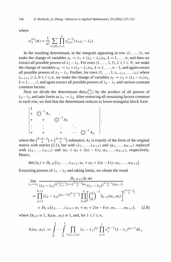
In the resulting determinant, in the integrals appearing in row(1, . . . ,1), wemake the change of variablesxk → λ1 + (λ2 − λ1)xk, k = 1, . . . , n, and then weextract all possible powers ofλ2 −λ1. For rows(1, . . . ,1, l), 2� l � N , we makethe change of variablesxk → λ1+(λ2−λ1)xk , k = 1, . . . , n−1, and again extractall possible powers ofλ2 − λ1. Further, for rows(1, . . . ,1, in−l+1, . . . , in) wherein−l+1 � 2, 0� l � n, we make the change of variablesxk → λ1 + (λ2 − λ1)xk,k = 1, . . . , l, and again extract all possible powers ofλ2 −λ1 and various constantcommon factors.
Next we divide the determinant det(a(n)I,J ) by the product of all powers of
λ2−λ1 and take limits asλ1 → λ2. After removing all remaining factors commonto each row, we find that the determinant reduces to lower-triangular block form∣∣∣∣∣∣∣∣∣∣∣
1∗ (
n1
)−1A1
∗ ∗ (n2
)−1A2
......
.... . .
∗ ∗ ∗ · · · (nn
)−1An
∣∣∣∣∣∣∣∣∣∣∣,
where the(N+k−2
k
)× (N+k−2
k
)submatrixAk is exactly of the form of the original
matrix with entries (2.1), but with(λ1, . . . , λN+1) and(α1, . . . , αN+1) replacedwith (λ2, . . . , λN+1) and (α1 + α2 + 2(n − k)γ,α3, . . . , αN+1), respectively.Hence,
det(Ak) = Dk,N
(λ2, . . . , λN+1;α1 + α2 + 2(n − k)γ,α3, . . . , αN+1
).
Extracting powers ofλ1 − λ2 and taking limits, we obtain the result
limλ1→λ2
Dn,N+1(λ;α)
(λ2 − λ1)2(N+n−1
N+1 )γ+(N+n−1N )α1(λ1 − λ2)
(N+n−1N )(α2−1)
=N+1∏p=3
(λ2 − λp)(αp−1)(N+n−1
N )n∏
k=0
[(n
k
)−1
Sn−k(α1, α2)
](N+k−2k )
× Dk,N
(λ2, . . . , λN+1;α1 + α2 + 2(n− k)γ,α3, . . . , αN+1
), (2.8)
whereD0,N ≡ 1, S0(α1, α2) ≡ 1, and, for 1� l � n,
Sl(α1, α2) :=1∫
0
· · ·1∫
0
∏1�i<j�l
|λi − λj |2γl∏
j=1
λα1−1j (1− λj )
α2−1 dλj
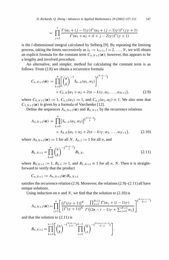
D. Richards, Q. Zheng / Advances in Applied Mathematics 29 (2002) 137–151 147
=l∏
j=1
Γ (α1 + (j − 1)γ )Γ (α2 + (j − 1)γ )Γ (jγ + 1)
Γ (α1 + α2 + (l + j − 2)γ )Γ (γ + 1)
is thel-dimensional integral calculated by Selberg [9]. By repeating the limitingprocess, taking the limits successively asλl → λl+1, l = 2, . . . ,N , we will obtainan explicit formula for the constant termCn,N+1(α); however, this appears to bea lengthy and involved procedure.
An alternative, and simpler, method for calculating the constant term is asfollows. From (2.8) we obtain a recurrence formula
Cn,N+1(α) =n∏
k=0
[(n
k
)−1
Sn−k(α1, α2)
](N+k−2k )
× Ck,N
(α1 + α2 + 2(n− k)γ,α3, . . . , αN+1
), (2.9)
whereC0,N+1(α) := 1, Cn,1(α1) := 1, andCn,2(α1, α2) ≡ 1. We also note thatC1,N+1(α) is given by a formula of Varchenko [12].
Define the sequencesAn,N+1(α) andBn,N+1 by the recurrence relations
An,N+1(α) =n∏
k=0
[Sn−k(α1, α2)
](N+k−2k )
× Ak,N
(α1 + α2 + 2(n − k)γ,α3, . . . , αN+1
), (2.10)
whereA0,N+1(α) := 1 for all N , An,1 := 1 for all n, and
Bn,N+1 =n∏
k=0
(n
k
)−(N+k−2k )
Bk,N , (2.11)
whereB0,N+1 := 1, Bn,1 := 1, andB1,N+1 ≡ 1 for all n, N . Then it is straight-forward to verify that the product
Cn,N+1 := An,N+1(α)Bn,N+1
satisfies the recurrence relation (2.9). Moreover, the relations (2.9)–(2.11) all haveunique solutions.
Using induction onn andN , we find that the solution to (2.10) is
An,N+1(α) =n∏
i=1
[[Γ (iγ + 1)]N[Γ (γ + 1)]N
∏N+1j=1 Γ (αj + (i − 1)γ )
Γ((2n − i − 1)γ +∑N+1
j=1 αj
)](N+n−i−1
N−1 )
and that the solution to (2.11) is
Bn,N+1 =n−1∏k=1
[(n
k
)−(N+k−1k+1 ) k−1∏
s=1
(k
s
)−(N+n+s−k−2N−3 )
].

148 D. Richards, Q. Zheng / Advances in Applied Mathematics 29 (2002) 137–151
Multiplying these two results together we obtain (2.4), and now the proof of (2.3)is complete. ✷
We remark that both (2.10) and (2.11) are multiplicative analogs of linearpartial recurrence relations, for which a general theory is provided by Zeilberger[13]. By solving the corresponding linear relations using Zeilberger’s theoryand then converting the results to the multiplicative formulation, we obtain analternative method for solving (2.10) and (2.11).
We can also generalize Example 2.3 of Richards and Zheng [8]. SubstitutingαN+1 = aλN+1, a > 0, into Theorem 2.1 and lettingλN+1 → ∞, we obtain thefollowing result.
Corollary 2.2. For n,N ∈ N, letλ1, . . . , λN ∈ R, α1, . . . , αN ∈ C with Re(αj ) > 0,j = 1, . . . ,N , and γ ∈ C with Re(γ ) > −min{1/n,Re(αj )/(n − 1): j =1, . . . ,N}. Let
Φ(x;λ1, . . . , λN)
:= exp
(−a
n∑i=1
xi
)N∏
p=1
n∏i=1
(xi − λp)αp−1
∏1�i<j�n
(xj − xi)2γ ,
x ∈ Rn, a > 0. For I = (i1, . . . , in) and J = (j1, . . . , jn) in In,N , define the
|In,N | × |In,N | matrix whose(I, J )th entry is
aI,J :=λi1+1∫λi1
· · ·λin+1∫λin
Φ(x;λ1, . . . , λN)ωJ (x)dx,
whereλN+1 ≡ ∞. Then
det(aI,J ) = C′n,N (α1, . . . , αN)
∏1�i<j�N
(λj − λi)(N+n−1
N )+2(N+n−1N+1 )γ
×∏
1�i �=j�N
(λj − λi)(N+n−1
N )(αi−1),
where
C′n,N (α1, . . . , αN)
= e−a(N+n−1N )
∑Np=1 λpa
−(N+n−1N )
∑Np=1 αp−2N(N+n−1
N+1 )γ
×n−1∏k=1
[(n
k
)−(N+k−1k+1 ) k−1∏
s=1
(k
s
)−(N+n+s−k−2N−3 )
]
×n∏
i=1
[(Γ (1+ iγ )
Γ (1+ γ )
)N N∏p=1
Γ(αp + (i − 1)γ
)](N+n−i−1N−1 )
.

D. Richards, Q. Zheng / Advances in Applied Mathematics 29 (2002) 137–151 149
3. Application of the Binet–Cauchy formula
Throughout this section we assume thatλ1 < · · · < λN+1. For
x = (x1, . . . , xn) ∈ Rn
we define
Ψ (x;λ) :=N+1∏p=1
n∏i=1
|xi − λp|αp−1∏
1�i<j�n
|xj − xi |2γ ,
whereα ∈ CN+1 andγ ∈ C. For I = (i1, . . . , in) andJ = (j1, . . . , jn) in In,N ,we define the Cartesian product of open intervalsRI (λ) := (λi1, λi1+1) × · · · ×(λin , λin+1) and
aI,J =∫
RI (λ)
ωJ (x)Ψ (x;λ)dx. (3.1)
From Theorem 2.1 we deduce the formula
det(aI,J ) = Cn,N+1(α)
×∏
1�i<j�N+1
(λj − λi)(N+n−1
N )(αi+αj−1)+2(N+n−1N+1 )γ , (3.2)
whereCn,N+1(α) is the constant in (2.4). Now we can derive the following result.
Corollary 3.1. Suppose thatλ1 < · · · < λN+1 and let α and γ satisfy thesame hypotheses as in Theorem2.1. For I = (i1, . . . , in) ∈ In,N , let xI :=(x1,I , . . . , xn,I ) ∈ Rn and define the domainD(λ) := {xI ∈ RI (λ) for all I ∈In,N } ⊂ R
n × · · · × Rn (|In,N | copies). Then∫
· · ·∫
D(λ)
det(ωI (xJ )
) ∏J∈In,N
Ψ (xJ ;λ)dxJ
= Cn,N+1(α)∏
1�i<j�N+1
(λj − λi)(N+n−1
N )(αi+αj−1)+2(N+n−1N+1 )γ . (3.3)
Proof. Let us write (3.1) in the form
aI,J :=∫Rn
fI (x)ωJ (x)Ψ (x;λ)dx, wherefI (x) ={
1, if x ∈ RI ,
0, otherwise,
I ∈ In,N . Observe that the index setIn,N is totally ordered under the usuallexicographic ordering and that the functionΨ (x;λ) is symmetric inx1, . . . , xn.Proceeding as in the proof of the classical Basic Composition Formula (cf. [5,p. 17]) and starting with (3.2), we obtain the result

150 D. Richards, Q. Zheng / Advances in Applied Mathematics 29 (2002) 137–151
Cn,N+1(α)∏
1�i<j�N+1
(λj − λi)(N+n−1
N )(αi+αj−1)+2(N+n−1N+1 )γ
= det(aI,J ) = det
( ∫Rn
fI (x)ωJ (x)Ψ (x;λ)dx
)
=∫
· · ·∫
D(λ)
det(fI (xJ )
)det(ωI (xJ )
) ∏J∈In,N
Ψ (xJ ;λ)dxJ . (3.4)
Sinceλ1 < · · · < λN+1 then, by a straightforward extension of a well knownformula on the determinant of a matrix of indicator functions (cf. [5, p. 16]),we deduce that
det(fI (xJ )
)={
1, if xI ∈ RI for all I ∈ In,N ,
0, otherwise.
Substituting this result into (3.4), then, the proof of (3.3) is complete.✷Example 3.2. Consider the case in whichn = 2 and N = 2. Then I2,2 ={(1,1), (1,2), (2,2)}, and we setx(1,1) := (s1, t1), x(1,2) := (s2, t2), andx(2,2) :=(s3, t3). Next we verify that the region of integration,D(λ1, λ2, λ3), is exactly thedomain (1.1). Moreover,
det(ωI (xJ )
) =∣∣∣∣∣
1 1 112(s1 + t1)
12(s2 + t2)
12(s3 + t3)
s1t1 s2t2 s3t3
∣∣∣∣∣= 1
2
[(t3 − t2)(s3 − t1)(s2 − s1) + (s3 − s2)(t3 − s1)(t2 − t1)
].
Substituting this determinant formula into the right-hand side of (3.3), we obtain(1.2).
Note also that the expression of the determinant as a sum of Vandermonde-type products is not unique. For we can interchangesj andtj for anyj = 1,2,3without changing the value of the determinant.
For generaln andN , it appears difficult to evaluate the determinant det(ωI (xJ ))
using the theory of symmetric functions. Prior to now, these determinants appar-ently have not appeared in the literature and even for smalln andN they are notwell-understood.
Example 3.3. Let n = 3 andN = 2. ThenI3,2 = {(1,1,1), (1,1,2), (1,2,2),(2,2,2)}, and set x(1,1,1) := (s1, t1, u1), x(1,1,2) := (s2, t2, u2), x(1,2,2) :=(s3, t3, u3), andx(2,2,2) := (s4, t4, u4). Then
9 det(ωI (xJ )
)=∣∣∣∣∣∣
1 1 1 1s1 + t1 + u1 s2 + t2 + u2 s3 + t3 + u3 s4 + t4 + u4
s1t1 + s1u1 + t1u1 s2t2 + s2u2 + t2u2 s3t3 + s3u3 + t3u3 s4t4 + s4u4 + t4u4s1t1u1 s2t2u2 s3t3u3 s4t4u4
∣∣∣∣∣∣

D. Richards, Q. Zheng / Advances in Applied Mathematics 29 (2002) 137–151 151
≡ det(ei(sj , tj , uj )
),
whereej denotes thej th elementary symmetric function. Symbolic calculationssuggest that this determinant can be written as a sum of Vandermonde-type products of mixed variables, e.g.,(s4 − s3)(t4 − s2)(u4 − s1)(t3 − t2)×(u3 − t1)(u2 − u1). However, the number of such terms can be large, and suchdecompositions are not unique.
References
[1] K. Aomoto, Jacobi polynomials associated with Selberg integrals, SIAM J. Math. Anal. 18 (1987)545–549.
[2] P.J. Forrester, Selberg correlation integrals and the 1/r2 quantum many body system, Nucl.Phys. B 388 (1992) 671–699.
[3] P.J. Forrester, Addendum to Selberg correlation integrals and the 1/r2 quantum many bodysystem, Nucl. Phys. B 416 (1994) 377–385.
[4] J. Kaneko, Selberg integrals and hypergeometric functions associated with Jack polynomials,SIAM J. Math. Anal. 24 (1993) 1086–1110.
[5] S. Karlin, in: Total Positivity, Vol. I, Stanford University Press, Stanford, CA, 1968.[6] I.G. Macdonald, Symmetric Functions and Hall Polynomials, 2nd ed., Oxford University Press,
New York, 1995.[7] Y. Markov, T. Tarasov, A. Varchenko, The determinant of a hypergeometric period matrix,
Houston J. Math. 24 (1998) 197–219.[8] D. Richards, Q. Zheng, Determinants of period matrices, and an application to Selberg’s
multidimensional beta integral, Adv. Appl. Math. 28 (2002) 602–633.[9] A. Selberg, Bemerkninger om et multipelt integral, Norsk. Mat. Tidsskr. 26 (1944) 71–78.
[10] A. Varchenko, The Euler beta-function, the Vandermonde determinant, the Legendre equation,and critical values of linear functions on a configuration of hyperplanes, I, Izv. Akad. Nauk SSSRSer. Mat. 53 (1989) 1206–1235; Math. USSR-Izv. 35 (1990) 543–571.
[11] A. Varchenko, The Euler beta-function, the Vandermonde determinant, the Legendre equation,and critical values of linear functions on a configuration of hyperplanes. II, Izv. Akad. NaukSSSR Ser. Mat. 54 (1990) 146–158 [Math. USSR-Izv. 36 (1991) 155–167].
[12] A.N. Varchenko, A determinant formula for Selberg integrals, Funct. Anal. Appl. 25 (1991) 304–305.
[13] D. Zeilberger, The algebra of linear partial difference operators and its applications, SIAM J.Math. Anal. 11 (1980) 919–932.