Embed Size (px)
Citation preview
Yale UniversityEliScholar – A Digital Platform for Scholarly Publishing at Yale
Public Health Theses School of Public Health
January 2012
Determinants Of Dengue Transmission DuringEpidemic And Inter-Epidemic Periods In TwoColombian CitiesYao FuYale University, [email protected]
Follow this and additional works at: http://elischolar.library.yale.edu/ysphtdl
This Open Access Thesis is brought to you for free and open access by the School of Public Health at EliScholar – A Digital Platform for ScholarlyPublishing at Yale. It has been accepted for inclusion in Public Health Theses by an authorized administrator of EliScholar – A Digital Platform forScholarly Publishing at Yale. For more information, please contact [email protected].
Recommended CitationFu, Yao, "Determinants Of Dengue Transmission During Epidemic And Inter-Epidemic Periods In Two Colombian Cities" (2012).Public Health Theses. 1095.http://elischolar.library.yale.edu/ysphtdl/1095
Yao Fu | MPH Thesis | Yale School of Public Health
DETERMINANTS OF DENGUE TRANSMISSION DURING
EPIDEMIC AND INTER-EPIDEMIC PERIODS IN TWO
COLOMBIAN CITIES
By Yao Fu
Thesis in Candidacy for the Degree of Master of Public Health
Yale School of Public Health
Yale University
Epidemiology of Microbial Diseases Division
Format: Investigative Thesis
May 1, 2012
Yao Fu | MPH Thesis | Yale School of Public Health
Table of Contents ABSTRACT .................................................................................................................................................. 3
ACKNOWLEDGMENTS ............................................................................................................................ 4
INTRODUCTION ........................................................................................................................................ 5
Objectives ..................................................................................................................................................... 5
Statement of General Problem under Investigation .................................................................................. 5
Relevant Studies........................................................................................................................................ 7
METHODS ................................................................................................................................................. 10
Locations under Study ............................................................................................................................ 10
Armenia, Quindio Department, Colombia .......................................................................................... 10
Barranquilla, Atlántico Department, Colombia .................................................................................. 10
Sources of Data ....................................................................................................................................... 10
Spatial data .......................................................................................................................................... 11
Other sources of data........................................................................................................................... 11
Analysis .................................................................................................................................................. 12
Defining Epidemic and Inter-epidemic Periods .................................................................................. 12
Determinants of Dengue Transmission during Epidemic and Inter-epidemic Periods ....................... 15
RESULTS ................................................................................................................................................... 16
Epidemiology Trends .............................................................................................................................. 16
Regression Tree Results .......................................................................................................................... 17
DISCUSSION ............................................................................................................................................. 20
LIMITATIONS ........................................................................................................................................... 22
CONCLUSIONS......................................................................................................................................... 22
REFERENCES ........................................................................................................................................... 24
APPENDIX ................................................................................................................................................. 27
Yao Fu | MPH Thesis | Yale School of Public Health
— 3 —
ABSTRACT
Dengue fever is an urban disease that has a complex epidemiology consisting of alternating
periods of intense epidemics and persistence in endemic locations. No studies have compared the patterns
of geographic variation and determinants of dengue transmission in neighborhoods during epidemic and
non-epidemic periods. Colombia’s individual-based epidemiological surveillance system provides a
unique opportunity to study this topic. The goal of this study was to better understand dengue
epidemiology in two of the highest dengue fever reporting Colombian cities that vary in climate, Armenia
(elevation 1320-1580 m, 21-23°C) and Barranquilla (elevation 5-134m . 27-30°C). We used a novel
ecological approach, Levin’s niche breadth, to define epidemic and inter-epidemic periods in each city.
Regression tree models were built with the following outcome variables for each neighborhood: total
number of dengue cases reported during the study period and proportion of dengue cases that occur
during inter-epidemic periods. The explanatory variables used were elevation, house count (in lieu of
population), housing density, and the Colombian socioeconomic class (SEC) indicator. House count was
consistently found to be the main determinant of the total number of reported dengue cases in
neighborhoods in both cities. The proportion models identified different determinants of persistent dengue
virus transmission in the two cities. Lower elevation was the main driver of persistence in Armenia while
lower SEC was the main driver in Barranquilla. These findings suggest that although the overall number
of dengue cases depend on the impact of population (as represented by house count) on viral introduction,
factors that influence the reproductive rate have a larger influence on transmission during inter-epidemic
periods. The persistence determinants identified in this study could potentially help vector control
programs to identify key areas to focus disease control efforts.

Yao Fu | MPH Thesis | Yale School of Public Health
— 4 —
ACKNOWLEDGMENTS
I would like to thank my academic and thesis advisor, Dr. Maria Diuk-Wasser (Yale University),
for her guidance and support, as well as my thesis reader and project preceptor, Dr. Harish Padmanabha
(Yale University and University Del Norte), for his valuable teachings and insight. Support for this
project also came from Instituto Nacional de Salud of Colombia, especially from Dr. Salua Osorio and Mr.
Camilo Rubio. This study was funded by the World Bank – Integrated National Adaptation Pilot to
Climate Change in Colombia and the Yale Climate and Energy Institute. In addition, I would also like to
thank the Wilbur G. Downs International Health Student Travel Fellowship and the Office of Student
Research at the Yale School of Medicine for providing funding for my travels to Colombia in the summer
of 2011 in preparation of this study.
Yao Fu | MPH Thesis | Yale School of Public Health
— 5 —
INTRODUCTION
Objectives
This investigative study was motivated by the need to better understand the dynamics of dengue
transmission during epidemic versus inter-epidemic periods in an urban setting. The objectives were two-
fold and were met through a study of two cities in Colombia that have variable patterns of endemic
dengue transmission—Armenia and Barranquilla. The first objective was to explore the geographic
patterns of dengue cases during dengue epidemics and inter-epidemic periods. The second objective was
to determine whether different socio-ecological determinants drive dengue transmission in neighborhoods
during epidemic compared to inter-epidemic periods.
Statement of General Problem under Investigation
Dengue is a febrile illness caused by a flavivirus and is principally transmitted by the Aedes
aegypti mosquito. This is an urban disease that has a complex epidemiological cycle consisting of
alternating epidemic and inter-epidemic periods. The pattern of dengue epidemic cycle is highly variable
in different locations due to its dependence on natural and built environmental conditions, vectorial
capacity, human biology and behavior, viral serotypes, and susceptibility of the population1–3
. Dengue
was first detected in Colombia in 1971 and its incidence and prevalence has since grown exponentially4.
Colombia now experiences about 40-50,000 cases of dengue annually and has one of the highest severe
dengue to dengue fever ratio in all of Latin America5. Currently, all four dengue serotypes are circulating
in the country and almost all departments (states) experience periodic epidemics4. The National Institute
of Health of Colombia (Instituto Nacional de Salud, INS) operates a national dengue surveillance system
that collects weekly reports of individual, probable dengue cases for each neighborhood in each city. This
study utilized Colombia’s unique dengue surveillance system and georeferencable neighborhood
descriptive data to identify the determinants of dengue transmission during epidemic and inter-epidemic
periods in two Colombian cities over multiple year time span.
Yao Fu | MPH Thesis | Yale School of Public Health
— 6 —
Dengue epidemics occur in multi-year cycles and are characterized by marked increases in the
number of dengue cases above expected levels2,6
. When epidemics occur in the city, there are high levels
of viral introductions occurring in the neighborhoods. Inter-epidemic periods, on the other hand, are
characterized by persistent transmission of dengue at low or undetectable levels and are influenced by
seasonal cycles1,2,7–11
. Persistent transmission is initially started by viral introduction, but its continuation
depends on dengue’s effective reproductive number (R). While the highly visible epidemics often
overshadow the inter-epidemic periods, recent studies have elucidated the importance of dengue
persistence through inter-epidemic periods. First, separate studies in Australia, Puerto Rico, Brazil,
Argentina, Venezuela, and Cuba concurred that the spatial patterns of dengue persistence is stable over
time, thereby resulting in clustering of dengue in a few key areas during inter-epidemic periods1,12–15
.
Secondly, these key areas are also responsible for producing a significant portion of the total dengue cases
in a city1,12–15
. Third, persistent pockets can also act as virus reservoirs and cause outbreaks in other
locations1,16,17
. Given the evidence, it is logical to conclude that neighborhoods that have continuous
transmission even during inter-epidemic periods must have the ideal conditions for the proliferation of the
dengue virus. These neighborhoods are likely to be the first places where new viral introductions take
hold and subsequently spread to neighboring communities.
While the dengue vaccine is still under development, dengue prevention and control is heavily
based on combating the mosquito vector. However, the outcomes of vector control programs have not
been very effective or long lasting1,15,17,18
. Studies in Singapore determined that the cause of dengue
reemergence was due to the adaptation of a case-reactive approach to vector control in combination with
other factors including increased global travel and urbanization17
. Case-reactive vector control programs
cannot identify subclinical infections or viral persistence, thereby allowing dengue to reemerge when herd
immunity wanes17
. In addition, conditions that favor proliferation of mosquitos such as uncontrolled
urban development and sprawl, reintroduction of vectors, and climate change may also hinder vector
Yao Fu | MPH Thesis | Yale School of Public Health
— 7 —
control programs17,19,20
. Since most vector control programs have limited resources, strategic allocation of
these resources to combat A. aegypti may lead to better and more sustainable outcomes1.
Given the studies on inter-epidemic periods described above, factors that drive persistent viral
transmission need to be better understood. Vector control programs should focus its resources to stop
dengue transmission at its weakest during the inter-epidemic periods in these key neighborhoods7.
Furthermore, identification of persistent areas can help direct immunization campaigns once dengue
vaccines are approved for general use7. Lastly, disease persistence in a neighborhood lowers the overall
quality of life of its residents and it is important for public health interventions to focus on these areas to
decrease health disparity across a city.
Relevant Studies
To our knowledge, no studies have compared geographic variation and determinants of dengue
transmission during epidemic and inter-epidemic periods. In order to fulfill this knowledge gap, we need
to first address several challenges in studying this topic. The first challenge is in establishing a definition
to differentiate between epidemic and inter-epidemic periods. The transition between the two periods is a
gradual process and not readily apparent. In addition, definitions used in past studies are based on total
cases within a certain time period, which was useful for areas being studied but lacked the capability to be
used in comparative investigations between cities because case thresholds are relative to each location’s
dengue burdens1,3,8
. For example, the estimated overall dengue prevalence (in cases per 10,000 inhabitants)
is 339 in Brazil, 116.5 in Colombia, but only 36.7 in Peru, therefore a cases-based definition can represent
different epidemic extents in each of these places21
.
A study on dengue persistence by Barrera et al. showed that there is a statistical significant
correlation between the number of cases and the total area that report cases—meaning that as the number
of dengue cases increase over time, the geographical areas that experience dengue transmission also
expands13
. Since epidemics are initiated by introductions, this observation suggests that epidemics (city
Yao Fu | MPH Thesis | Yale School of Public Health
— 8 —
level events) are perpetuated by multiple local introductions (neighborhood level events). This
phenomenon underlines the importance of studying epidemic cycles from the perspectives of both the city
and local areas such as neighborhoods. Therefore, in order to encompass conditions of both the city and
neighborhoods, we used a novel ecological approach based on the correlation of geographic dengue
distribution with number of cases to define epidemic and inter-epidemic periods.
After defining epidemic and inter-epidemic periods, the second challenge lies in finding outcome
measurements for regression analysis that can distinguish between transmissions occurring during these
two periods. If the determinants of these two periods are different, then disease control would benefit
greatly from this knowledge and could adapt their programs accordingly. The main ecological difference
between epidemic and inter-epidemic periods is that inter-epidemic periods experience lower rates of
viral introductions among neighborhoods. Modeling studies have shown that it is important to distinguish
between introduced cases and local transmissions, in other words, transmission among groups and
transmission within groups, respectively22
. Furthermore, strictly local transmission that do not have new
introductions are maintained based on the R of the system, which can be influenced by social,
environmental, herd immunity, and vectorial capacity factors9,22
.
The term persistence had also been interpreted inconsistently in relation to inter-epidemic periods
in literature. For example, Barrera et al. stratified neighborhoods in a city into three-levels of persistence,
where persistence was defined as having a certain number of consecutive months reporting dengue13
.
Barrera et al.’s definition of persistence captured dengue transmission only with respect to conditions
within the neighborhood. Our study is the first to specifically focus on dengue persistence in
neighborhoods during a time when a majority of neighborhoods in the city does not have dengue (inter-
epidemic periods). This second definition of persistence is more selective and depends on conditions in
both the neighborhoods and the remainder of the city. Past studies have found evidence that supports
differential transmission dynamics when examining the drivers of local and global dengue transmission
patterns6,10,11,23
. Preliminary studies at our study sites found that these two definitions result in
Yao Fu | MPH Thesis | Yale School of Public Health
— 9 —
identification of different key neighborhoods, thereby also suggesting that different mechanisms may
underline transmission at the local level than transmission at the city level. Therefore, we hypothesized
that the determinants of total dengue cases in each neighborhood would be different from the number of
cases that occur during inter-epidemic periods (standardized by the total cases in each respective
neighborhoods) in those neighborhoods.
Research on dengue epidemiology is often limited by the lack of vector or seroprevalence data.
Vector data is not available for every neighborhood in a city simply because it is a time and resource-
consuming process. In addition, both modeling and seroprevalence evidence found that fluctuations in
vector abundance are not associated with fluctuations in epidemic size and often moderated by other
factors such as socioeconomic status (SEC)3,24
. Seroprevalence data would be useful to determine the
source of infection (introductory versus autochthonous), but it is expensive to obtain and impractical for
city-wide studies. In terms of operability of the model, however, surveillance data is superior to
seroprevalence data because surveillance data is likely to reflect the temporal dynamics of epidemic and
persistent cycles, unlike cross-sectional seroprevalence data.
Alternative mechanisms by which dengue virus persists during inter-epidemic periods include
vertical transmission of virus to new mosquito generations and virus replication in alternative vectors25,26
.
Vertical transmission alone is the least probable cause of virus persistence since mosquito life cycles are
short and the virus will be diluted quickly25
. In addition, the strength of association of vertical
transmission is most likely very small when other factors are present. In Colombia, virus replication in
alternative vectors is also not likely since A. aegypti has been the sole Aedes mosquito found in vector
surveillance in the two study cities. Therefore, these mechanisms were not examined in this study.
This study focused on drivers of dengue transmission at the neighborhood level for practical,
scientific, and political reasons. Neighborhood level analysis is practical because dengue surveillance and
prevention programs are often conducted at the neighborhood level7,27
. Neighborhoods are good units of
measurements scientifically because characteristics such as SEC are generally homogenous within
Yao Fu | MPH Thesis | Yale School of Public Health
— 10 —
neighborhoods and movement patterns generally revolve around neighborhoods28,29
. Finally, study results
based on neighborhood-level analysis can be directly applied to policies targeting community
improvement and health projects. Studies have found that policies and programs targeting health
disparities can be especially effective if it engages the community at the neighborhood level30
.
METHODS
Locations under Study
Armenia, Quindio Department, Colombia
Armenia is located on the Cordillera Central within the mountainous regions of Western
Colombia. The city has a large altitude range that varies from 1320 – 1580 m and has an annual average
ambient temperature ranges between 20 - 20.3˚C31,32
. According to the 2005 census, the city has an
estimated population of 272,574 people33
.
Barranquilla, Atlántico Department, Colombia
Barranquilla is located on the Caribbean coast of Colombia. The city is located at approximately
sea level has an altitude range between 5 - 134 m and has average ambient temperature range between
26.8 - 28.3˚C31,32
. The population of the city is approximately 1,112,889 people33
.
Sources of Data
Epidemiological data
Dengue surveillance data consisting of weekly, individual-based probable cases were obtained
from each city. The data was originally collected as part of the national dengue surveillance system of the
Colombian National Institute of Health. Probable dengue cases from 2001 - 2011 were obtained for
Armenia. Laboratory confirmed dengue cases from 2004 - 2006 and probably dengue cases from 2007 -
Yao Fu | MPH Thesis | Yale School of Public Health
— 11 —
2011 were obtained for Barranquilla. The surveillance data reported diagnosis date, doctor notification
date, patient’s age, and patient’s neighborhood of residence. Prior to analysis, the weekly surveillance
data were organized into three-week periods based on doctor-visit-dates to account for the time lag
between initial infection and doctor visit date. In instances where the doctor-visit-date was not available,
dengue-case-notification-date was used in lieu of doctor-visit-date. Based on the 2010-2011 Armenia
dengue surveillance reports, the average time lag between doctor-visit date and notification date was 0.53
days for 99.9% of the data. Neighborhoods were included in the analysis if they reported greater than 5
cases during the study period in order to account for neighborhood identification errors that may have
occurred during surveillance reporting.
Spatial data
Geographically projected shapefiles of the cities were obtained from municipal governments
(projection-Transverse Mercator, datum-Bogota). The shapefiles contained digitalized polygons of
neighborhoods and houses in each city.
Other sources of data
Orthorectified digital elevation data (90 m resolution, datum-WGS_1984) for the study areas
were downloaded from The CGIAR Consortium for Spatial Information in raster format
(http://srtm.csi.cgiar.org/). The elevation data was projected to the same coordinates of the city shapefiles
using the Project Raster Tool of the Data Management Tools in ArcMap Software v.10.0 (ESRI,
Redlands, CA). Mean elevation of each neighborhood was calculated using the Zonal Statistics function
in ArcMap10. SEC ratings of the neighborhoods and house count of the neighborhoods were obtained
from municipal governments. The SEC ratings were based on a scale of 1-6 (from less to more affluent)
and measures socioeconomic status relative to each municipality (not comparable between cities). House
counts were used as a proxy for population because population data was not available. Interpretation of
this proxy is limited because house count does not take into account possible differences in household
Yao Fu | MPH Thesis | Yale School of Public Health
— 12 —
size. The estimated area in hectare of each neighborhood was calculated from the neighborhood
shapefiles using Zonal Statistics function in ArcMap10. Housing density of each neighborhood in houses
per hectare was calculated using its corresponding house count and area.
Analysis
Defining Epidemic and Inter-epidemic Periods
We observed a statistically significant correlation between the total number of dengue cases
reported in each 3-week period and the number of neighborhoods reporting five or more cases of dengue
in the same 3-week period in both cities (Armenia, Pearson Correlation Coefficient 0.91605, p<0.0001;
Barranquilla, Pearson Correlation Coefficient 0.94476, p<0.0001). When the total dengue cases increased,
the area that experience dengue cases expanded and vice versa. This geographic variation between
epidemic and inter-epidemic periods was the rational for using an ecological approach, specifically
Levin’s standardized niche breadth index (Bn), to define and standardize dengue epidemic and inter-
epidemic periods.
Niche breadth measures the extent of utilization of a single type of resource by a species within
an environment at a given time34
. The concept of niche breadth was applied to the dengue system as
follows: dengue was considered the species, the city was the species environment, each neighborhood in
the city was a unique resource, and each dengue case reported in a neighborhood was interpreted as a
single utilization of the resource34
. In summary, the extent of resource utilization as measured by the
niche breadth corresponded to the geographical distribution of dengue cases within a city. The niche
breadth was then standardized by the total number of neighborhoods in each city. The standardization step
in the formula ensured that Bn from different surveillance data sources could be integrated. It also allowed
comparative analysis between cities that have different underlying transmission dynamics.
Yao Fu | MPH Thesis | Yale School of Public Health
— 13 —
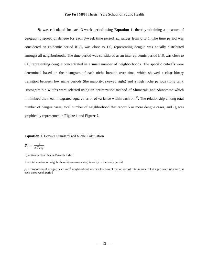
Bn was calculated for each 3-week period using Equation 1, thereby obtaining a measure of
geographic spread of dengue for each 3-week time period. Bn ranges from 0 to 1. The time period was
considered an epidemic period if Bn was close to 1.0, representing dengue was equally distributed
amongst all neighborhoods. The time period was considered as an inter-epidemic period if Bn was close to
0.0, representing dengue concentrated in a small number of neighborhoods. The specific cut-offs were
determined based on the histogram of each niche breadth over time, which showed a clear binary
transition between low niche periods (the majority, skewed right) and a high niche periods (long tail).
Histogram bin widths were selected using an optimization method of Shimazaki and Shinomoto which
minimized the mean integrated squared error of variance within each bin35
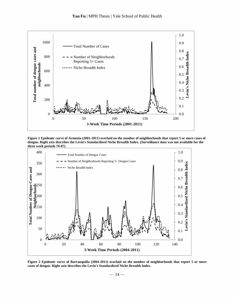
. The relationship among total
number of dengue cases, total number of neighborhood that report 5 or more dengue cases, and Bn was
graphically represented in Figure 1 and Figure 2.
Equation 1. Levin’s Standardized Niche Calculation
∑
Bn = Standardized Niche Breadth Index
R = total number of neighborhoods (resource states) in a city in the study period
pi = proportion of dengue cases in ith neighborhood in each three-week period out of total number of dengue cases observed in
each three-week period
Yao Fu | MPH Thesis | Yale School of Public Health
— 14 —
Figure 1 Epidemic curve of Armenia (2001-2011) overlaid on the number of neighborhoods that report 5 or more cases of
dengue. Right axis describes the Levin's Standardized Niche Breadth Index. (Surveillance data was not available for the
three week periods 78-87)
Figure 2 Epidemic curve of Barranquilla (2004-2011) overlaid on the number of neighborhoods that report 5 or more
cases of dengue. Right axis describes the Levin's Standardized Niche Breadth Index.
0.0
0.1
0.2
0.3
0.4
0.5
0.6
0.7
0.8
0.9
1.0
0
200
400
600
800
1000
0 50 100 150 200
Lev
in's
Nic
he
Bre
ad
th I
nd
ex
To
tal
nu
mb
er o
f d
eng
ue
case
s a
nd
nei
gh
bo
rho
od
s
3-Week Time Periods (2001-2011)
Total Number of Cases
Number of Neighborhoods
Reporting 5+ Cases
Niche Breadth Index
0.0
0.1
0.2
0.3
0.4
0.5
0.6
0.7
0.8
0.9
1.0
0
50
100
150
200
250
300
350
400
0 20 40 60 80 100 120 140
Lev
in's
Sta
nd
ard
ized
Nic
he
Bre
ad
th I
nd
ex
To
tal
Nu
mb
er o
f D
eng
ue
Ca
ses
an
d
Nei
gh
bo
rho
od
s
3-Week Time Periods (2004-2011)
Total Number of Dengue Cases
Number of Neighborhoods Reporting 5+ Dengue Cases
Niche Breadth Index
Yao Fu | MPH Thesis | Yale School of Public Health
— 15 —
Determinants of Dengue Transmission during Epidemic and Inter-epidemic Periods
Regression tree analyses were used to model epidemic and inter-epidemic periods in order to
determine the drivers of dengue transmission during these periods. Regression trees are robust models
that utilize a hierarchical approach to handle complex interactions, non-linear relationships, over-fitting,
and missing variables—problems commonly encountered when fitting statistical linear models to dengue
systems36
. The tree is built by splitting a single response variable (either categorical or continuous) into
branches of homogenous groups based on a single explanatory variable using the method of least
squares36
. This is a fully automated process that explores all splits and branch orders possible within a
given set of explanatory variables. The final tree is identified through a pruning process to obtain the tree
with the largest number of branches while having the smallest cross-validation error. Colinearity of
explanatory variables is presented through surrogate branches with the level of congruence indicated for
each surrogate. The surrogate splits answers the question “which other splits would classify the same
outcomes in the same way37
.” The regression tree results are presented visually and are easy to interpret—
each branch is labeled with the explanatory variable value dictating the split, outcome variables that
satisfy the split criteria are grouped to the left, and each leaf is labeled with the mean value of the
outcome variable and the number of observations in the group9,36
. The length of the vertical branches is
directly proportion of the total sum of squares the division accounted for36
.
Regression tree models were built using the Recursive Partitioning and Regression Tree (rpart)
package of the statistical software R (http://www.r-project.org/). Two models representing transmission
during epidemic or inter-epidemic periods were explored for each city. Their respective outcome
variables were 1) the total number of dengue cases reported by the neighborhood reflecting transmission
during epidemic periods and 2) the proportion of cases of that occurred during the inter-epidemic periods
in each neighborhood reflecting persistent transmission. The explanatory variables used to predict the
responses were elevation, SEC, house count, and housing density.
Yao Fu | MPH Thesis | Yale School of Public Health
— 16 —
The first outcome, the total number of dengue cases reported by the neighborhood, was chosen to
represent transmission during epidemic periods because it was the most obvious indicator of the total
disease burden in a neighborhood. Since transmission cannot indefinitely persist in a neighborhood, the
continuation of cases necessarily requires an introduction event. Increase in cases observed in a
neighborhood is associated with increase in the rate of introduction into the neighborhood. Therefore, the
disease burden in a neighborhood is dependent on the rate of introduction, which in turn is proportional to
the level of the epidemic in the city. Inter-epidemic periods are characterized by transmission that occurs
locally with limited outside introductions. However, the cases identified through surveillance do not
differentiate between locally acquired cases and introductory cases. Therefore, the second outcome was
chosen to reflect inter-epidemic periods because it captures the timing of cases. Specifically, this outcome
captures the autochthonous cases that occur only through persistent mechanisms and not through
introduction.
RESULTS
Epidemiology Trends
A total of 11777 cases in 269 neighborhoods in Armenia were reported to the national dengue
surveillance system from 2001-2011. Dengue cases were included in data analysis if they reported the
patient’s neighborhood of residence (5.04% of total cases did not report neighborhoods). In order to
minimize reporting error, a neighborhood was included in data analysis if it could be located in the city’s
GIS shapefile and had at least 50 houses. Niche breadth analysis was conducted with a total of 9622 cases
reported in 181 neighborhoods over 186 three-week periods in 2001 - 2011 in Armenia.
Two sets of surveillance data were obtained in Barranquilla. From 2004 to 2006, 2227 laboratory
confirmed cases occurred in 150 neighborhoods in Barranquilla and from 2007 to 2011, 6461 probably
cases occurred in 294 neighborhoods in Barranquilla. 0.4% of total cases during 2004-2006 and 11.5% of
total cases during 2007-2011 did not report neighborhoods and were excluded from analysis. The
Yao Fu | MPH Thesis | Yale School of Public Health
— 17 —
difference between epidemic and inter-epidemic periods is much more pronounced in Armenia than in
Barranquilla.
Tables 1 and 2 describes the distribution of cases and neighborhoods in epidemic and inter-
epidemic periods in Armenia and Barranquilla, respectively. Although the epidemic curves (Figures 1
and 2) were drastically different between the cities, the epidemic trends and geographic patterns were
consistent. In both cities, the epidemic period contained the majority of the cases. In addition, the
epidemic periods had larger number of neighborhoods report dengue than during the inter-epidemic
periods.
Number of 3-week
Periods (% total time)
Dengue Cases
(% total)
Average Number of
Cases Per 3-week Period
Average Number of
Neighborhoods Per 3-week
Period
Total 186 (100) 9622 (100) 33
Epidemic 59 (30) 7191 (75) 123 51
Inter-epidemic 118 (63) 2431 (25) 21 14
Unknown
(no data) 9 (7) 0
-
Table 1. Distribution of cases and neighborhoods in Armenia during epidemic and inter-epidemic periods.
Number of 3-week
periods (% total time)
Dengue cases
(% total)
Average Number of
Cases per 3-week
Period
Average number of
Neighborhoods per 3-
week Period
Total 134 (100) 7658 (100)
Epidemic 22 (16) 3417 (45) 155 71
Inter-epidemic 108 (81) 4241 (55) 39 25
Unknown
(no data) 4 (3) 0 - -
Table 2. Distribution of cases and neighborhoods in Barranquilla during epidemic and inter-epidemic periods.
Regression Tree Results
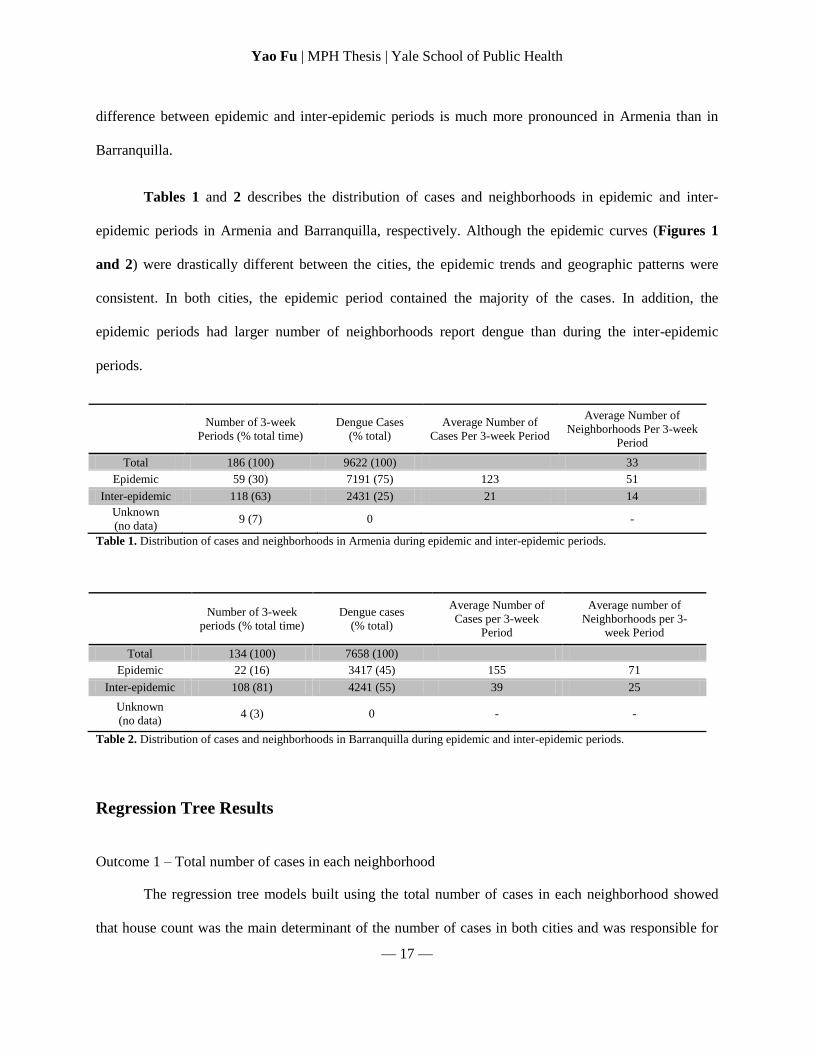
Outcome 1 – Total number of cases in each neighborhood
The regression tree models built using the total number of cases in each neighborhood showed
that house count was the main determinant of the number of cases in both cities and was responsible for
Yao Fu | MPH Thesis | Yale School of Public Health
— 18 —
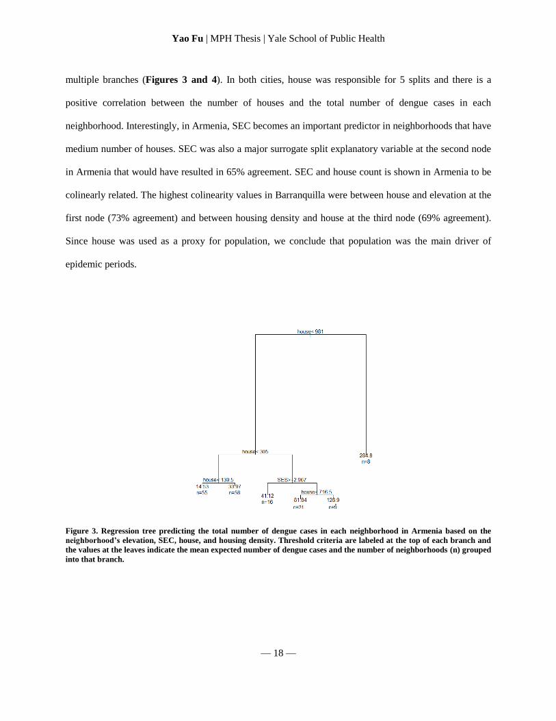
multiple branches (Figures 3 and 4). In both cities, house was responsible for 5 splits and there is a
positive correlation between the number of houses and the total number of dengue cases in each
neighborhood. Interestingly, in Armenia, SEC becomes an important predictor in neighborhoods that have
medium number of houses. SEC was also a major surrogate split explanatory variable at the second node
in Armenia that would have resulted in 65% agreement. SEC and house count is shown in Armenia to be
colinearly related. The highest colinearity values in Barranquilla were between house and elevation at the
first node (73% agreement) and between housing density and house at the third node (69% agreement).
Since house was used as a proxy for population, we conclude that population was the main driver of
epidemic periods.
Figure 3. Regression tree predicting the total number of dengue cases in each neighborhood in Armenia based on the
neighborhood’s elevation, SEC, house, and housing density. Threshold criteria are labeled at the top of each branch and
the values at the leaves indicate the mean expected number of dengue cases and the number of neighborhoods (n) grouped
into that branch.
Yao Fu | MPH Thesis | Yale School of Public Health
— 19 —
Figure 4. Regression tree predicting the total number of dengue cases in each neighborhood in Barranquilla based on the
neighborhood's elevation, SEC, house, and housing density. Threshold criteria are labeled at the top of each branch and
the values at the leaves indicate the mean expected number of dengue cases and the number of neighborhoods (n) grouped
into that branch.
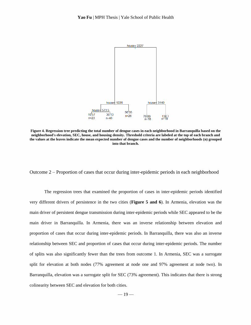
Outcome 2 – Proportion of cases that occur during inter-epidemic periods in each neighborhood
The regression trees that examined the proportion of cases in inter-epidemic periods identified
very different drivers of persistence in the two cities (Figure 5 and 6). In Armenia, elevation was the
main driver of persistent dengue transmission during inter-epidemic periods while SEC appeared to be the
main driver in Barranquilla. In Armenia, there was an inverse relationship between elevation and
proportion of cases that occur during inter-epidemic periods. In Barranquilla, there was also an inverse
relationship between SEC and proportion of cases that occur during inter-epidemic periods. The number
of splits was also significantly fewer than the trees from outcome 1. In Armenia, SEC was a surrogate
split for elevation at both nodes (77% agreement at node one and 97% agreement at node two). In
Barranquilla, elevation was a surrogate split for SEC (73% agreement). This indicates that there is strong
colinearity between SEC and elevation for both cities.
Yao Fu | MPH Thesis | Yale School of Public Health
— 20 —
Figure 5 Regression tree predicting the proportion of cases (%) that occurred during the inter-epidemic period in
Armenia.
Figure 6 Regression tree predicting the proportion of cases (%) that occurred during the inter-epidemic period in
Barranquilla.
DISCUSSION
The regression tree analysis results showed that determinants of epidemic transmission differ
from that of inter-epidemic transmission but the mechanisms behind the different drivers of transmission
during the two periods warrant further discussion.
Population was an important determinant in both cities for the epidemic models. The number of
cases was directly reflective of the extent of epidemics and is correlated with the geographic expansion of
Yao Fu | MPH Thesis | Yale School of Public Health
— 21 —
dengue in a city. This showed that epidemics occur due to multiple introductions occurring between
neighborhoods. High population levels would increase the probability that introductions would occur
through increased human movement and increased number of susceptibles. A recent R0 modeling study
showed that even if R0 was sufficiently high to favor local transmission, epidemics (propagation of
disease across a city) would not occur without a large enough population and high levels of movement9.
The sheer number of branches driven by housing suggested that the number of cases was sensitive to
population levels.
The use of proportion as an outcome in the inter-epidemic models allowed us to tease apart
introduction cases and persistent autochthonous cases. House was not present in the final proportion
models, thereby indicating that the effect of population was diminished during autochthonous
transmissions and factors that influence R become more important. For example, elevation was the main
driver of dengue persistence in Armenia, where there was a high elevation gradient within the city.
Elevation affects an area’s ambient temperature, humidity, and other climate characteristic, which in turn
affects R0 factors associated with vectorial capacity. This showed that the transmission system at high
altitudes may be sensitive to temperature changes.
In contrast, elevation was not a significant branch in the proportion model in Barranquilla. This
was probably due to the overall low elevation, low elevation gradient, and high temperature conditions
throughout Barranquilla. This observation agreed with a past study that showed where temperature and
precipitation are already high, increase in either have little effect on transmission rates11
. One study on
two neighboring cities with identical climate conditions along the US-Mexico border found different
seroprevalence levels due to differences in SEC38
. The US city have higher mosquito infestation levels
but its residents have very limited exposure to mosquitos due to continuous air-condition use and
therefore the city has essentially no dengue transmission38
. Given similar climate conditions amongst the
neighborhoods, SEC emerged as a main driver of persistence in Barranquilla.
Yao Fu | MPH Thesis | Yale School of Public Health
— 22 —
LIMITATIONS
The scope of this study was limited by the explanatory variables available for the study areas.
First, we were not able to obtain temperature and climate data at the neighborhood level. Elevation was
used as a proxy. Second, population data at the neighborhood level was not available in the two cities. We
used house count as a proxy for population, but house count did not account for variations in household
size. In addition, housing density did not account for non-urbanized areas in a neighborhood nor
variations in household size. Furthermore, there were relatively high levels of colinearity amongst the
variables used in the regression trees (60-90%). However, colinearity was expected for a vector-borne
disease study and the regression tree approach was selected as the most appropriate method to account for
colinearity.
Finally, spatial autocorrelation was not explored in the study and should be analyzed in the future.
Spatial autocorrelation could capture the effects of human movement amongst neighborhoods.
Preliminary analysis of spatial autocorrelation of residuals from the epidemic regression tree models
using Global Moran’s I in Arc GIS showed that both cities have statistically significant autocorrelation.
Local Moran’s I hot spot analysis identified various hot spots in the city at 2000 m, 3000 m, and 4000 m
radius. Spatial autocorrelation of inter-epidemic periods was not significant. Further analysis of spatial
distribution of the various response variables used in regression tree could supplement the regression tree
findings.
CONCLUSIONS
Our analysis in Colombia found that there was a geographic expansion of cases during epidemic
periods and a geographic recession of cases during inter-epidemic periods. In addition, we found that the
determinants of dengue transmission during epidemic periods differed from that of inter-epidemic periods.
Yao Fu | MPH Thesis | Yale School of Public Health
— 23 —
Epidemic transmission was driven by population while persistent transmission during inter-epidemic
periods was driven by factors unique to each city. Lower elevation was the main driver of persistence in
Armenia while lower SEC was the main driver in Barranquilla.
This study used a novel application of Levin’s Standardized Niche Breadth Index to define
dengue outbreak and persistent periods. This study also found that regression tree modeling gave insight
into factors that cause certain neighborhoods to experience persistent dengue transmission even when
there is low dengue introduction between neighborhoods and low overall dengue transmission at the city-
level is low. Elevation was the main drivers of persistence in Armenia while SEC was the main driver in
Barranquilla. Results from the models could help the identification of key neighborhoods that experience
persistent dengue transmission and the mechanism that drive the persistence. Dengue prevention
programs can benefit greatly by focusing their resources on addressing these mechanisms within key
neighborhoods during the low-transmission periods. Shifting dengue prevention and vector control
strategies towards a persistence focused direction could be effective for both short-term control of dengue
outbreaks and long term sustained halt of transmission.
Yao Fu | MPH Thesis | Yale School of Public Health
— 24 —
REFERENCES
1. Chowell, G., Cazelles, B., Broutin, H. & Munayco, C.V. The influence of geographic and
climate factors on the timing of dengue epidemics in Perú, 1994-2008. BMC infectious
diseases 11, 164 (2011).
2. de Mattos Almeida, M.C., Caiaffa, W.T., Assunção, R.M. & Proietti, F.A. Spatial
vulnerability to dengue in a Brazilian urban area during a 7-year surveillance. Journal of
urban health : bulletin of the New York Academy of Medicine 84, 334-45 (2007).
3. Honório, N.A. et al. Spatial evaluation and modeling of Dengue seroprevalence and vector
density in Rio de Janeiro, Brazil. PLoS neglected tropical diseases 3, e545 (2009).
4. Ocazionez, R.E., Cortéz, F.M., Villar, L.A. & Gómez, S.Y. Temporal distributin of
dengue virus serotypes in Colombian endemic area and dengue incidence. Re-introduction
of dengue-3 associated to mild febrile illness and primary infection. Memórias do Instituto
Oswaldo Cruz 101, 725-731 (2006).
5. Pan American Health Organization Number of Reported Cases of Dengue and Dengue
Severe (DS) in the Americas, by Country: Figures for 2011. America 2011, (2011).
6. Morrison, A.C. et al. Epidemiology of Dengue Virus in Iquitos , Peru 1999 to 2005 :
Interepidemic and Epidemic Patterns of Transmission. Boards 4, (2010).
7. Eisen, L. & Lozano-Fuentes, S. Use of mapping and spatial and space-time modeling
approaches in operational control of Aedes aegypti and dengue. PLoS neglected tropical
diseases 3, e411 (2009).
8. Mondini, A. & Neto, F.C. [Socioeconomic variables and dengue transmission]. Revista de
saúde pública 41, 923-30 (2007).
9. Cross, P.C., Johnson, P.L.F., Lloyd-Smith, J.O. & Getz, W.M. Utility of R0 as a predictor
of disease invasion in structured populations. Journal of the Royal Society, Interface / the
Royal Society 4, 315-24 (2007).
10. Wearing, H.J. & Rohani, P. Ecological and immunological determinants of dengue
epidemics. Proceedings of the National Academy of Sciences of the United States of
America 103, 11802-7 (2006).
11. Johansson, M.A., Dominici, F. & Glass, G.E. Local and Global Effects of Climate on
Dengue Transmission in Puerto Rico. 3, 1-5 (2009).
12. Barrera, R. Spatial Stability of Adult Aedes aegypti Populations. Tropical Medicine 85,
1087-1092 (2011).
Yao Fu | MPH Thesis | Yale School of Public Health
— 25 —
13. Barrera, R., Delgado, N., Jiménez, M. & Villalobos, I. Estratificación de una ciudad
hiperendémica en dengue hemorrágico. Pan America Journal of PUblic Health 8, 225-233
(2000).
14. Flauzino, R.F., Souza-Santos, R. & Oliveira, R.M. Dengue, geoprocessamento e
indicadores socioeconômicos e ambientais: um estudo de revisão. Revista Panamericana
de Salud Pública 25, 456-461 (2009).
15. Horizonte, B., Gerais, M., State, M.G. & Proietti, F.A. Dinâmica intra-urbana das
epidemias de dengue Intra-urban dynamics of dengue epidemics in. 24, 2385-2395 (2008).
16. Adams, B. & Kapan, D.D. Man bites mosquito: understanding the contribution of human
movement to vector-borne disease dynamics. PloS One 4, e6763 (2009).
17. Ooi, E.-E., Goh, K.-T. & Gubler, D.J. Dengue prevention and 35 years of vector control in
Singapore. Emerging infectious diseases 12, 887-93 (2006).
18. Cordeiro, R. et al. Spatial distribution of the risk of dengue fever in southeast Brazil,
2006-2007. BMC public health 11, 355 (2011).
19. de Castro Medeiros, L.C. et al. Modeling the dynamic transmission of dengue fever:
investigating disease persistence. PLoS neglected tropical diseases 5, e942 (2011).
20. Pongsumpun, P. et al. Dynamics of dengue epidemics in urban contexts. Tropical
medicine & international health : TM & IH 13, 1180-7 (2008).
21. Pan American Health Organization Regional Update on Dengue. (2009).at
<http://new.paho.org/hq/dmdocuments/2009/den_reg_rpt_2009_03_17.pdf>
22. Degallier, N., Favier, C., Boulanger, J.-philippe & Menkes, C. Imported and
autochthonous cases in the dynamics of dengue epidemics in Brazil Casos importados e
autóctones na dinâmica da epidemia de dengue no. Methods 43, 1-7 (2009).
23. Van Benthem, B.H.B. et al. Spatial patterns of and risk factors for seropositivity for
dengue infection. The American journal of tropical medicine and hygiene 72, 201-8
(2005).
24. Otero, M., Barmak, D.H., Dorso, C.O., Solari, H.G. & Natiello, M. a Modeling dengue
outbreaks. Mathematical Biosciences 232, 87-95 (2011).
25. Adams, B. & Boots, M. How important is vertical transmission in mosquitoes for the
persistence of dengue? Insights from a mathematical model. Epidemics 2, 1-10 (2010).
Yao Fu | MPH Thesis | Yale School of Public Health
— 26 —
26. Little, E., Barrera, R., Seto, K.C. & Diuk-Wasser, M. Co-occurrence Patterns of the
Dengue Vector Aedes aegypti and Aedes mediovitattus, a Dengue Competent Mosquito in
Puerto Rico. EcoHealth (2011).doi:10.1007/s10393-011-0708-8
27. Diez Roux, A.V. & Mair, C. Neighborhoods and health. Annals of the New York Academy
of Sciences 1186, 125-45 (2010).
28. Smedley, B. & Syme, S.L. Promoting Health: Intervention Strategies from Social and
Behavioral Research. Medicine (National Academies Press: Washington DC, 2000).
29. Cosner, C. et al. The effects of human movement on the persistence of vector-borne
diseases. Journal of theoretical biology 258, 550-60 (2009).
30. Marmot, M. Fair Society, Healthy Lives. Timing is everything. BMJ (Clinical research
ed.) 340, c1191 (2010).
31. Padmanabha, H., Soto, E., Mosquera, M., Lord, C.C. & Lounibos, L.P. Ecological links
between water storage behaviors and Aedes aegypti production: implications for dengue
vector control in variable climates. EcoHealth 7, 78-90 (2010).
32. IDEAM Instituto de Hidrología, Meteorología y Estudios Ambientales. at
<http://institucional.ideam.gov.co/jsp/index.jsf>
33. National Administrative Department of Statistics Colombia Census 2005. (2012).at
<http://www.dane.gov.co/en/index.php?option=com_content&view=article&id=307&Ite
mid=124>
34. Levins, R. Evolution in Changing Environments. (Princeton University Press: Princeton,
New Jersey, USA, 1968).
35. Shimazaki, H. & Shinomoto, S. Histogram Bin-width Optimization. at
<http://176.32.89.45/~hideaki/res/histogram.html>
36. De’ath, G. & Fabricius, K. Classification and Regression Trees: A Powerful Yet Simple
Technique for Ecological Data Analysis. Ecology 81, 3178-3192 (2000).
37. No Title.
38. Reiter, P. et al. Texas lifestyle limits transmission of dengue virus. Emerging infectious
diseases 9, 86-9 (2003).
Yao Fu | MPH Thesis | Yale School of Public Health
— 27 —
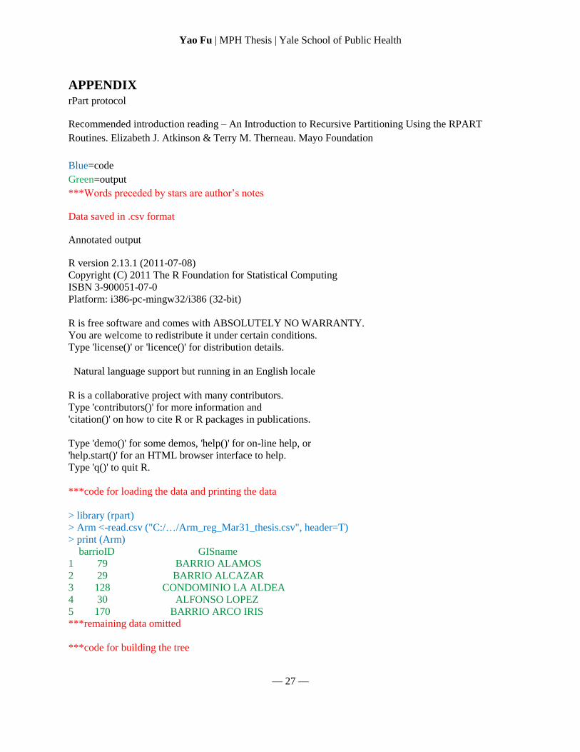
APPENDIX rPart protocol
Recommended introduction reading – An Introduction to Recursive Partitioning Using the RPART
Routines. Elizabeth J. Atkinson & Terry M. Therneau. Mayo Foundation
Blue=code
Green=output
***Words preceded by stars are author’s notes
Data saved in .csv format
Annotated output
R version 2.13.1 (2011-07-08)
Copyright (C) 2011 The R Foundation for Statistical Computing
ISBN 3-900051-07-0
Platform: i386-pc-mingw32/i386 (32-bit)
R is free software and comes with ABSOLUTELY NO WARRANTY.
You are welcome to redistribute it under certain conditions.
Type 'license()' or 'licence()' for distribution details.
Natural language support but running in an English locale
R is a collaborative project with many contributors.
Type 'contributors()' for more information and
'citation()' on how to cite R or R packages in publications.
Type 'demo()' for some demos, 'help()' for on-line help, or
'help.start()' for an HTML browser interface to help.
Type 'q()' to quit R.
***code for loading the data and printing the data
> library (rpart)
> Arm <-read.csv ("C:/…/Arm_reg_Mar31_thesis.csv", header=T)
> print (Arm)
barrioID GISname
1 79 BARRIO ALAMOS
2 29 BARRIO ALCAZAR
3 128 CONDOMINIO LA ALDEA
4 30 ALFONSO LOPEZ
5 170 BARRIO ARCO IRIS
***remaining data omitted
***code for building the tree
Yao Fu | MPH Thesis | Yale School of Public Health
— 28 —
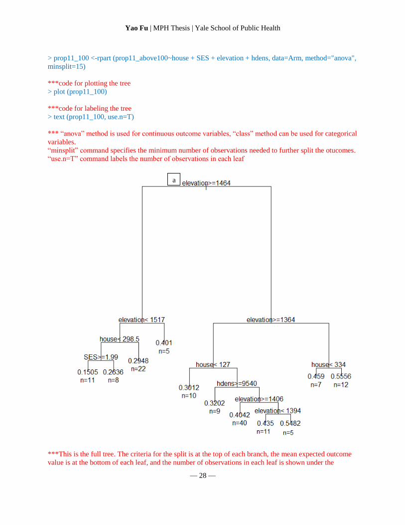
> prop11_100 <-rpart (prop11_above100~house + SES + elevation + hdens, data=Arm, method="anova",
minsplit=15)
***code for plotting the tree
> plot (prop11_100)
***code for labeling the tree
> text (prop11_100, use.n=T)
*** “anova” method is used for continuous outcome variables, “class” method can be used for categorical
variables.
“minsplit” command specifies the minimum number of observations needed to further split the otucomes.
“use.n=T” command labels the number of observations in each leaf
***This is the full tree. The criteria for the split is at the top of each branch, the mean expected outcome
value is at the bottom of each leaf, and the number of observations in each leaf is shown under the
a
Yao Fu | MPH Thesis | Yale School of Public Health
— 29 —
outcome values. Branches to the left are those that obey the criteria of the split, branches to the right are
those that do not.
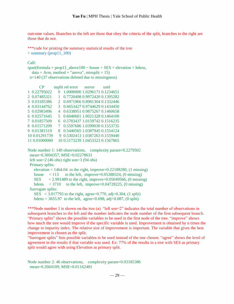
***code for printing the summary statistical results of the tree
> summary (prop11_100)
Call:
rpart(formula = prop11_above100 ~ house + SES + elevation + hdens,
data = Arm, method = "anova", minsplit = 15)
n=140 (37 observations deleted due to missingness)
CP nsplit rel error xerror xstd
1 0.22795022 0 1.0000000 1.0296171 0.1234651
2 0.07485321 1 0.7720498 0.9972420 0.1395282
3 0.03185386 2 0.6971966 0.8981304 0.1332446
4 0.03144762 3 0.6653427 0.9744629 0.1434450
5 0.02983496 4 0.6338951 0.9875267 0.1460658
6 0.02571645 5 0.6040601 1.0021328 0.1464100
7 0.01857509 6 0.5783437 1.0159742 0.1516235
8 0.01571209 7 0.5597686 1.0399030 0.1553735
9 0.01381519 8 0.5440565 1.0387945 0.1554124
10 0.01291739 9 0.5302413 1.0387263 0.1559440
11 0.01000000 10 0.5173239 1.0453323 0.1567865
Node number 1: 140 observations, complexity param=0.2279502
mean=0.3694357, MSE=0.02278631
left son=2 (46 obs) right son=3 (94 obs)
Primary splits:
elevation < 1464.04 to the right, improve=0.22188280, (1 missing)
house < 113 to the left, improve=0.05388324, (0 missing)
SES < 2.991489 to the right, improve=0.05049566, (0 missing)
hdens < 3710 to the left, improve=0.04728225, (0 missing)
Surrogate splits:
SES < 3.017793 to the right, agree=0.770, adj=0.304, (1 split)
hdens < 3655.97 to the left, agree=0.698, adj=0.087, (0 split)
***Node number 1 is shown on the tree (a). “left son=2” indicates the total number of observations in
subsequent branches to the left and the number indicates the node number of the first subsequent branch.
“Primary splits” shows the possible variables to be used in the first node of the tree. “improve” shows
how much the tree would improve if the specific variable is used. Improvement is obtained by n times the
change in impurity index. The relative size of improvement is important. The variable that gives the best
improvement is chosen as the split.
“Surrogate splits” lists possible variables to be used instead of the one chosen. “agree” shows the level of
agreement in the results if that variable was used. Ex: 77% of the results in a tree with SES as primary
split would agree with using Elevation as primary split.
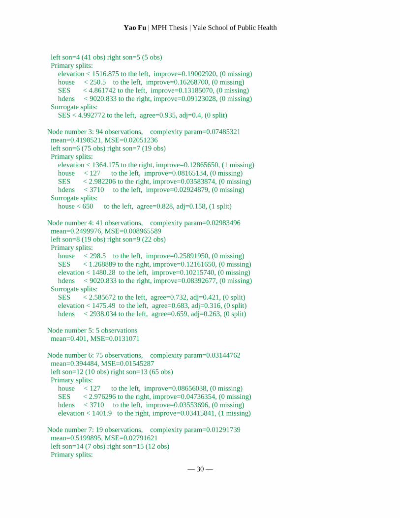
Node number 2: 46 observations, complexity param=0.03185386
mean=0.2664109, MSE=0.01162481
Yao Fu | MPH Thesis | Yale School of Public Health
— 30 —
left son=4 (41 obs) right son=5 (5 obs)
Primary splits:
elevation < 1516.875 to the left, improve=0.19002920, (0 missing)
house < 250.5 to the left, improve=0.16268700, (0 missing)
SES < 4.861742 to the left, improve=0.13185070, (0 missing)
hdens < 9020.833 to the right, improve=0.09123028, (0 missing)
Surrogate splits:
SES < 4.992772 to the left, agree=0.935, adj=0.4, (0 split)
Node number 3: 94 observations, complexity param=0.07485321
mean=0.4198521, MSE=0.02051236
left son=6 (75 obs) right son=7 (19 obs)
Primary splits:
elevation < 1364.175 to the right, improve=0.12865650, (1 missing)
house < 127 to the left, improve=0.08165134, (0 missing)
SES < 2.982206 to the right, improve=0.03583874, (0 missing)
hdens < 3710 to the left, improve=0.02924879, (0 missing)
Surrogate splits:
house < 650 to the left, agree=0.828, adj=0.158, (1 split)
Node number 4: 41 observations, complexity param=0.02983496
mean=0.2499976, MSE=0.008965589
left son=8 (19 obs) right son=9 (22 obs)
Primary splits:
house < 298.5 to the left, improve=0.25891950, (0 missing)
SES < 1.268889 to the right, improve=0.12161650, (0 missing)
elevation < 1480.28 to the left, improve=0.10215740, (0 missing)
hdens < 9020.833 to the right, improve=0.08392677, (0 missing)
Surrogate splits:
SES < 2.585672 to the left, agree=0.732, adj=0.421, (0 split)
elevation < 1475.49 to the left, agree=0.683, adj=0.316, (0 split)
hdens < 2938.034 to the left, agree=0.659, adj=0.263, (0 split)
Node number 5: 5 observations
mean=0.401, MSE=0.0131071
Node number 6: 75 observations, complexity param=0.03144762
mean=0.394484, MSE=0.01545287
left son=12 (10 obs) right son=13 (65 obs)
Primary splits:
house < 127 to the left, improve=0.08656038, (0 missing)
SES < 2.976296 to the right, improve=0.04736354, (0 missing)
hdens < 3710 to the left, improve=0.03553696, (0 missing)
elevation < 1401.9 to the right, improve=0.03415841, (1 missing)
Node number 7: 19 observations, complexity param=0.01291739
mean=0.5199895, MSE=0.02791621
left son=14 (7 obs) right son=15 (12 obs)
Primary splits:
Yao Fu | MPH Thesis | Yale School of Public Health
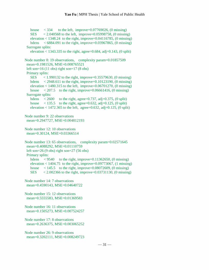
— 31 —
house < 334 to the left, improve=0.07769026, (0 missing)
SES < 2.040568 to the left, improve=0.05998758, (0 missing)
elevation < 1348.24 to the right, improve=0.04116785, (0 missing)
hdens < 6884.091 to the right, improve=0.03967865, (0 missing)
Surrogate splits:
elevation < 1343.335 to the right, agree=0.684, adj=0.143, (0 split)
Node number 8: 19 observations, complexity param=0.01857509
mean=0.1981526, MSE=0.008765521
left son=16 (11 obs) right son=17 (8 obs)
Primary splits:
SES < 1.990132 to the right, improve=0.35579630, (0 missing)
hdens < 2948.611 to the right, improve=0.10123190, (0 missing)
elevation < 1480.315 to the left, improve=0.06701270, (0 missing)
house < 207.5 to the right, improve=0.06661416, (0 missing)
Surrogate splits:
hdens < 2600 to the right, agree=0.737, adj=0.375, (0 split)
house < 135.5 to the right, agree=0.632, adj=0.125, (0 split)
elevation < 1472.365 to the left, agree=0.632, adj=0.125, (0 split)
Node number 9: 22 observations
mean=0.2947727, MSE=0.004812193
Node number 12: 10 observations
mean=0.30124, MSE=0.03366514
Node number 13: 65 observations, complexity param=0.02571645
mean=0.4088292, MSE=0.01110759
left son=26 (9 obs) right son=27 (56 obs)
Primary splits:
hdens < 9540 to the right, improve=0.11362650, (0 missing)
elevation < 1404.75 to the right, improve=0.09773067, (1 missing)
house < 145.5 to the right, improve=0.08072609, (0 missing)
SES < 2.002366 to the right, improve=0.03731130, (0 missing)
Node number 14: 7 observations
mean=0.4590143, MSE=0.04640722
Node number 15: 12 observations
mean=0.5555583, MSE=0.01369583
Node number 16: 11 observations
mean=0.1505273, MSE=0.007524257
Node number 17: 8 observations
mean=0.2636375, MSE=0.003065252
Node number 26: 9 observations
mean=0.3202111, MSE=0.008249723
Yao Fu | MPH Thesis | Yale School of Public Health
— 32 —
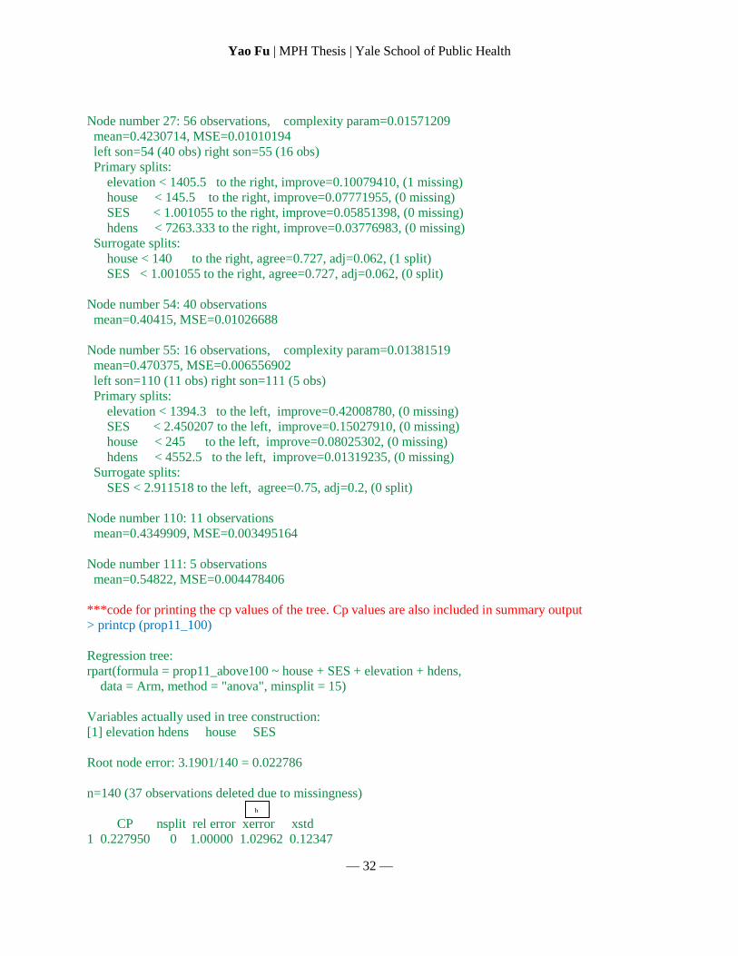
Node number 27: 56 observations, complexity param=0.01571209
mean=0.4230714, MSE=0.01010194
left son=54 (40 obs) right son=55 (16 obs)
Primary splits:
elevation < 1405.5 to the right, improve=0.10079410, (1 missing)
house < 145.5 to the right, improve=0.07771955, (0 missing)
SES < 1.001055 to the right, improve=0.05851398, (0 missing)
hdens < 7263.333 to the right, improve=0.03776983, (0 missing)
Surrogate splits:
house < 140 to the right, agree=0.727, adj=0.062, (1 split)
SES < 1.001055 to the right, agree=0.727, adj=0.062, (0 split)
Node number 54: 40 observations
mean=0.40415, MSE=0.01026688
Node number 55: 16 observations, complexity param=0.01381519
mean=0.470375, MSE=0.006556902
left son=110 (11 obs) right son=111 (5 obs)
Primary splits:
elevation < 1394.3 to the left, improve=0.42008780, (0 missing)
SES < 2.450207 to the left, improve=0.15027910, (0 missing)
house < 245 to the left, improve=0.08025302, (0 missing)
hdens < 4552.5 to the left, improve=0.01319235, (0 missing)
Surrogate splits:
SES < 2.911518 to the left, agree=0.75, adj=0.2, (0 split)
Node number 110: 11 observations
mean=0.4349909, MSE=0.003495164
Node number 111: 5 observations
mean=0.54822, MSE=0.004478406
***code for printing the cp values of the tree. Cp values are also included in summary output
> printcp (prop11_100)
Regression tree:
rpart(formula = prop11_above100 ~ house + SES + elevation + hdens,
data = Arm, method = "anova", minsplit = 15)
Variables actually used in tree construction:
[1] elevation hdens house SES
Root node error: 3.1901/140 = 0.022786
n=140 (37 observations deleted due to missingness)
CP nsplit rel error xerror xstd
1 0.227950 0 1.00000 1.02962 0.12347
b
Yao Fu | MPH Thesis | Yale School of Public Health
— 33 —
2 0.074853 1 0.77205 0.99724 0.13953
3 0.031854 2 0.69720 0.89813 0.13324
4 0.031448 3 0.66534 0.97446 0.14345
5 0.029835 4 0.63390 0.98753 0.14607
6 0.025716 5 0.60406 1.00213 0.14641
7 0.018575 6 0.57834 1.01597 0.15162
8 0.015712 7 0.55977 1.03990 0.15537
9 0.013815 8 0.54406 1.03879 0.15541
10 0.012917 9 0.53024 1.03873 0.15594
11 0.010000 10 0.51732 1.04533 0.15679
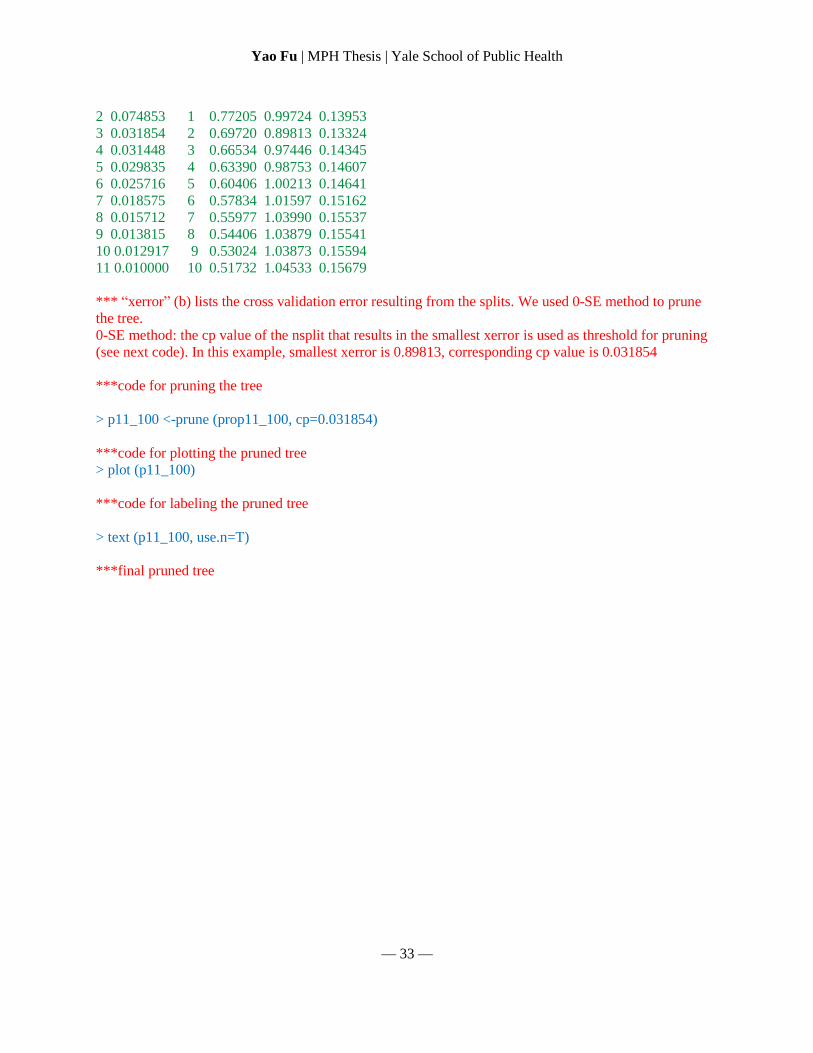
*** “xerror” (b) lists the cross validation error resulting from the splits. We used 0-SE method to prune
the tree.
0-SE method: the cp value of the nsplit that results in the smallest xerror is used as threshold for pruning
(see next code). In this example, smallest xerror is 0.89813, corresponding cp value is 0.031854
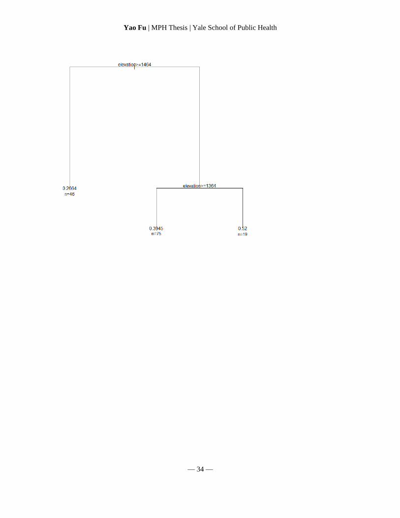
***code for pruning the tree
> p11_100 <-prune (prop11_100, cp=0.031854)
***code for plotting the pruned tree
> plot (p11_100)
***code for labeling the pruned tree
> text (p11_100, use.n=T)
***final pruned tree
Yao Fu | MPH Thesis | Yale School of Public Health
— 34 —


![Relating Topological Determinants of Complex Networks to ... · the behavior of many dynamical systems on complex net-works, such as epidemic spreading [7], synchronization of weakly](https://img.pdfslide.net/doc/110x75/5edafabb09ac2c67fa689da6/relating-topological-determinants-of-complex-networks-to-the-behavior-of-many.jpg)