Determinants of Exchange Rate in Tanzania

Linus LugaiyamuE–mail:linusluge@gmail.com

A thesis submitted in partial fulfillment for the

degree of Master of Social Science

in Economics

Department of Economics

Uppsala University

Supervisor: Prof. Nils Gottfries

June 19, 2015

Abstract

In this thesis I develop a theoretical model to capture Tanzania’s unique structure of imports

and exports. The model implies that the value of real exchange rate, measured as the relative

price of foreign goods, should be positively related to tax, negatively related to government

consumption, positively related to the expenditure on imports of oil, negatively related to the

earnings from gold exports, negatively related to foreign income and positively related to natural

or long run output. The empirical analysis of the model was conducted based on data from

Tanzania and major trading partners focusing on flexible exchange rate regime period from 1987

to 2012. Graphical analysis reveals that a large component of real exchange rate fluctuations are

nominal exchange rate fluctuations. Although unit root and cointegration tests show theoretical

implications do not hold empirically in the long run, short run co–movements of taxes and

real exchange rate were in line with the predictions of the theoretical model. The theoretical

discussion backed by both graphical analysis and granger–causality test results identifies taxation

as significant determinant of changes in real exchange rate in Tanzania; at least in the short

run. Therefore, a fiscal policy based on tax smoothing and stabilization of nominal exchange

rate fluctuations can stabilize real exchange rate fluctuations.

i

Acknowledgements

I would like to express my sincere gratitudes to the Swedish Institute , through the Swedish

Institute Study Scholarship Program, for financing my master’s studies at Uppsala Uni-

versity. I’m very thankful and greatly indebted to my supervisor, Professor Nils Gottfries, for his

guidance and dearest assistance for my thesis. I would like to thank Johan Grip and Rachatar

Nilavongse, Ph.D. students at the department of economics, for their technical advice. I would

like to thank my Brother, Erick, for helpful comments, my parents, Mr. & Mrs. Lugeiyamu, my

young Sisters, Dafrosa & Firmina, and my youngest brother Vitalis for their encouragement,

inspiration and material support throughout the two years of my master’s studies in Sweden. All

remaining errors are my own

ii

Contents

Abstract i

Acknowledgements ii

Contents iv

List of Figures v

List of Tables v

1 Introduction 1

2 Macroeconomic Developments in Tanzania 3

2.1 The external sector . . . . . . . . . . . . . . . . . . . . . . . . . . . . . . . . . . . 3

2.2 Institutional Developments . . . . . . . . . . . . . . . . . . . . . . . . . . . . . . 5

3 Brief review of the literature 6

4 The model 8

4.1 Set-up . . . . . . . . . . . . . . . . . . . . . . . . . . . . . . . . . . . . . . . . . . 8

4.2 Preferences . . . . . . . . . . . . . . . . . . . . . . . . . . . . . . . . . . . . . . . 9

4.3 Equilibrium . . . . . . . . . . . . . . . . . . . . . . . . . . . . . . . . . . . . . . . 10

4.4 Comparative statics . . . . . . . . . . . . . . . . . . . . . . . . . . . . . . . . . . 11

5 Data and graphical analysis 12

5.1 Data . . . . . . . . . . . . . . . . . . . . . . . . . . . . . . . . . . . . . . . . . . . 12

5.2 Components of Real exchange rate . . . . . . . . . . . . . . . . . . . . . . . . . . 14

5.3 Graphical analysis of the real exchange rate and explanatory variables . . . . . . 16

6 Testing long run relationship 21

6.1 Methodology . . . . . . . . . . . . . . . . . . . . . . . . . . . . . . . . . . . . . . 21

6.2 Results . . . . . . . . . . . . . . . . . . . . . . . . . . . . . . . . . . . . . . . . . . 22

7 Tests for short run relationships 23

7.1 Methodology . . . . . . . . . . . . . . . . . . . . . . . . . . . . . . . . . . . . . . 23

7.2 Results . . . . . . . . . . . . . . . . . . . . . . . . . . . . . . . . . . . . . . . . . . 24

iii

8 Summary and conclusion 25

References 30

Appendix A 31

Data . . . . . . . . . . . . . . . . . . . . . . . . . . . . . . . . . . . . . . . . . . . . . . 31

Appendix B 32

Unit root tests . . . . . . . . . . . . . . . . . . . . . . . . . . . . . . . . . . . . . . . . 32

Unit root tests results . . . . . . . . . . . . . . . . . . . . . . . . . . . . . . . . . . . . 33

Cointegration test results . . . . . . . . . . . . . . . . . . . . . . . . . . . . . . . . . . 34

Appendix C 36

Lag length selection for ADF tests . . . . . . . . . . . . . . . . . . . . . . . . . . . . . 36

iv

List of Figures

1 Exchange rate dynamics in Tanzania . . . . . . . . . . . . . . . . . . . . . . . . . 2

2 Tanzania’s Primary Goods Imports, as a share of Total Goods Imports, in 2011 . 4

3 Tanzania’s Primary Exports, as a share of Total Exports, in 2010 and 2002 . . . 4

4 Tanzania trade balance and current account . . . . . . . . . . . . . . . . . . . . . 5

5 Inflation Dynamics in Tanzania . . . . . . . . . . . . . . . . . . . . . . . . . . . . 6

6 Relating changes of real exchange rate to changes in nominal exchange rate . . . 14

7 Relating changes of real exchange rate to domestic inflation . . . . . . . . . . . . 15

8 Relating changes of real exchange rate to foreign inflation . . . . . . . . . . . . . 15

9 Relating the the real exchange rate with the tax to GDP ratio . . . . . . . . . . 17

10 Relating the real exchange rate with the government consumption to GDP ratio 18

11 Relating the real exchange rate and the real world price of oil . . . . . . . . . . . 19

12 Relating real exchange rate with the real price of gold . . . . . . . . . . . . . . . 19

13 Relating the real exchange rate with the ratio of foreign output to domestic output 20

14 Time series plot of residuals . . . . . . . . . . . . . . . . . . . . . . . . . . . . . . 35

15 Lag selection for real exchange rate . . . . . . . . . . . . . . . . . . . . . . . . . . 36

16 Lag selection for Tax to GDP ratio . . . . . . . . . . . . . . . . . . . . . . . . . . 36

17 Lag selection for Government consumption to GDP ratio . . . . . . . . . . . . . . 36

18 Lag selection for Real price of oil . . . . . . . . . . . . . . . . . . . . . . . . . . . 37

19 Lag selection for Real price of gold . . . . . . . . . . . . . . . . . . . . . . . . . . 37

20 Lag selection for Foreign output to domestic output ratio . . . . . . . . . . . . . . 37

21 Lag selection for Natural output to actual output ratio . . . . . . . . . . . . . . . 37

List of Tables

1 Estimation results . . . . . . . . . . . . . . . . . . . . . . . . . . . . . . . . . . . 23

2 Estimation results . . . . . . . . . . . . . . . . . . . . . . . . . . . . . . . . . . . 25

3 ADF unit root test results . . . . . . . . . . . . . . . . . . . . . . . . . . . . . . . 34

4 PP unit root test results . . . . . . . . . . . . . . . . . . . . . . . . . . . . . . . . 35

5 Unit root test for residuals . . . . . . . . . . . . . . . . . . . . . . . . . . . . . . . 35

v

1 Introduction

Developing countries like Tanzania desperately need to achieve and maintain higher

growth rates in order to have any hope of overcoming poverty. One of the most important source

of growth is the external sector. A well functioning external sector can enable Tanzania to have

competitive exports and a favourable domestic investment climate to attract foreign capital and

technology. The achievement of these conditions ultimately depends on the dynamics of prices

in Tanzania relative to those of its trading partners and competitors or the real exchange rate.

Higher volatility in the real exchange rate has been found to reduce much needed foreign

direct investment(FDI) in Africa (Suliman et al., 2015, p. 222). Higher real exchange rate

misalignment has been found to cause disincentives to exporters of primary goods in Africa and

reduced their ability to exploit new opportunities in the world market (Sekkat and Varoudakis,

1998, p. 7). Evidence show that growth and investment have had a tendency to increase after

the improvement of terms of trade and eradication of real exchange rate overvaluation (Bleaney

and Greenaway, 2001, p. 498). Real currency depreciation has been found to improve country’s

balance of payments position (Kodongo and Ojah, 2013).

Therefore, it is very crucial that policy makers in Tanzania are equipped with knowledge

of how and why the real exchange rate would move in particular direction overtime. Figure 1

shows both nominal exchange rate and real exchange rate have been highly unstable with a

general trend of depreciation.

There is an extensive literature devoted to gaining insights into real exchange rate dy-

namics with theoretical frameworks formulated and, in most cases, tested in developed countries.

Unfortunately, the literature offers mixed empirical results. For example, while several studies

have found empirical evidence of the purchasing power parity(PPP) theory (Papell, 1997; Frankel

and Rose, 1996), other studies have found evidence against the PPP theory (Mark, 1990; Pe-

droni, 2001). Another hypothesis popular among researchers of this topic, the Balassa-Samuelson

(BS), has not been free of mixed empirical results. Studies like that of Hsieh (1982), Strauss

(1999) and Candelon et al. (2007) have found strong evidence for the hypothesis; Canzoneri et

al. (1999) find empirical evidence against fundamental assumptions of BS hypothesis whereas

NBER-East Asia Seminar on Economics (1999) finds that BS only works for some few Asian

countries.

Not only that there are few studies done in Tanzania but also the existing few studies

derive their theoretical frameworks from studies that were not originally formulated to study the

Tanzanian economy (e.g. Hobdari (2008) and Li and Rowe (2007)). Tanzania, unlike developed

countries and most other developing nations, has a very skewed export-import structure. Oil

1

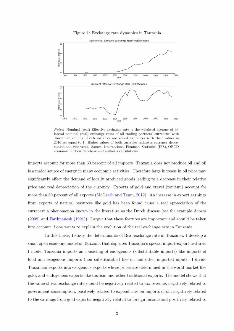
Figure 1: Exchange rate dynamics in Tanzania

0.5

11.

5N

EE

R(in

dex

2010

=1)

1960 1965 1970 1975 1980 1985 1990 1995 2000 2005 2010 2015year

(a) Nominal Effective exchange Rate(NEER) Index

.2.4

.6.8

11.

2R

EE

R(in

dex

2010

=1)

1960 1965 1970 1975 1980 1985 1990 1995 2000 2005 2010 2015year

(b) Real Effective Exchange Rate(REER) Index

Notes: Nominal (real) Effective exchange rate is the weighted average of bi-lateral nominal (real) exchange rates of all trading partners’ currencies withTanzanian shilling. Both variables are scaled as indices with their values in2010 set equal to 1. Higher values of both variables indicates currency depre-ciation and vice versa. Source: International Financial Statistics (IFS), OECDeconomic outlook database and author’s calculations

imports account for more than 30 percent of all imports. Tanzania does not produce oil and oil

is a major source of energy in many economic activities. Therefore large increase in oil price may

significantly affect the demand of locally produced goods leading to a decrease in their relative

price and real depreciation of the currency. Exports of gold and travel (tourism) account for

more than 50 percent of all exports (McGrath and Temu, 2012). An increase in export earnings

from exports of natural resources like gold has been found cause a real appreciation of the

currency; a phenomenon known in the literature as the Dutch disease (see for example Acosta

(2009) and Fardmanesh (1991)). I argue that these features are important and should be taken

into account if one wants to explain the evolution of the real exchange rate in Tanzania.

In this thesis, I study the determinants of Real exchange rate in Tanzania. I develop a

small open economy model of Tanzania that captures Tanzania’s special import-export features.

I model Tanzania imports as consisting of endogenous (substitutable imports) like imports of

food and exogenous imports (non substitutable) like oil and other imported inputs. I divide

Tanzanian exports into exogenous exports whose prices are determined in the world market like

gold, and endogenous exports like tourism and other traditional exports. The model shows that

the value of real exchange rate should be negatively related to tax revenue, negatively related to

government consumption, positively related to expenditure on imports of oil, negatively related

to the earnings from gold exports, negatively related to foreign income and positively related to

2

natural or long run output.

The empirical analysis of the model was conducted based on data from Tanzania and

major trading partners focusing on flexible exchange rate regime period from 1987 to 2012.

Graphical analysis reveals that the large component of real exchange rate fluctuations are nom-

inal exchange rate fluctuations. Although unit root and cointegration tests show theoretical

implications do not hold empirically in the long run, short run co–movements of taxes and real

exchange rate were in line with the predictions of the theoretical model. The theoretical discus-

sion backed by both graphical analysis and granger–causality test results identifies taxation as

a significant factor influencing changes in real exchange rate in Tanzania; at least in the short

run.

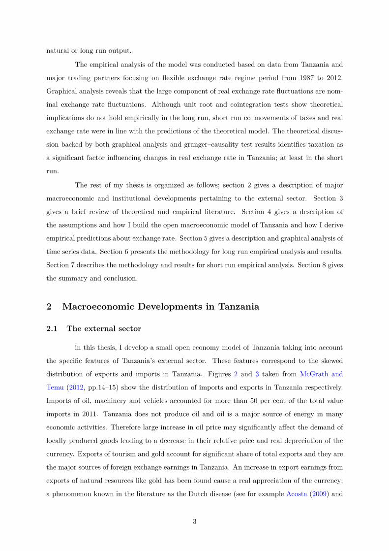
The rest of my thesis is organized as follows; section 2 gives a description of major

macroeconomic and institutional developments pertaining to the external sector. Section 3

gives a brief review of theoretical and empirical literature. Section 4 gives a description of

the assumptions and how I build the open macroeconomic model of Tanzania and how I derive

empirical predictions about exchange rate. Section 5 gives a description and graphical analysis of

time series data. Section 6 presents the methodology for long run empirical analysis and results.

Section 7 describes the methodology and results for short run empirical analysis. Section 8 gives

the summary and conclusion.

2 Macroeconomic Developments in Tanzania

2.1 The external sector

in this thesis, I develop a small open economy model of Tanzania taking into account

the specific features of Tanzania’s external sector. These features correspond to the skewed

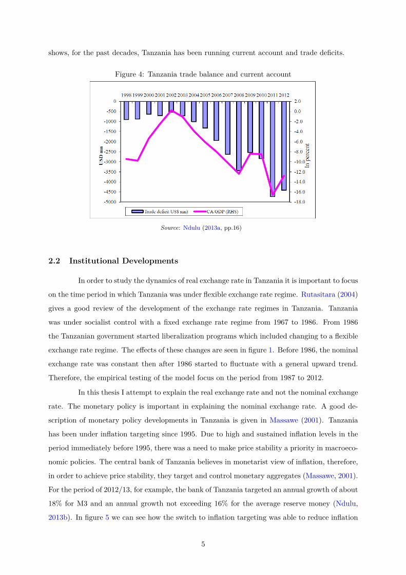
distribution of exports and imports in Tanzania. Figures 2 and 3 taken from McGrath and

Temu (2012, pp.14–15) show the distribution of imports and exports in Tanzania respectively.

Imports of oil, machinery and vehicles accounted for more than 50 per cent of the total value

imports in 2011. Tanzania does not produce oil and oil is a major source of energy in many

economic activities. Therefore large increase in oil price may significantly affect the demand of

locally produced goods leading to a decrease in their relative price and real depreciation of the

currency. Exports of tourism and gold account for significant share of total exports and they are

the major sources of foreign exchange earnings in Tanzania. An increase in export earnings from

exports of natural resources like gold has been found cause a real appreciation of the currency;

a phenomenon known in the literature as the Dutch disease (see for example Acosta (2009) and

3

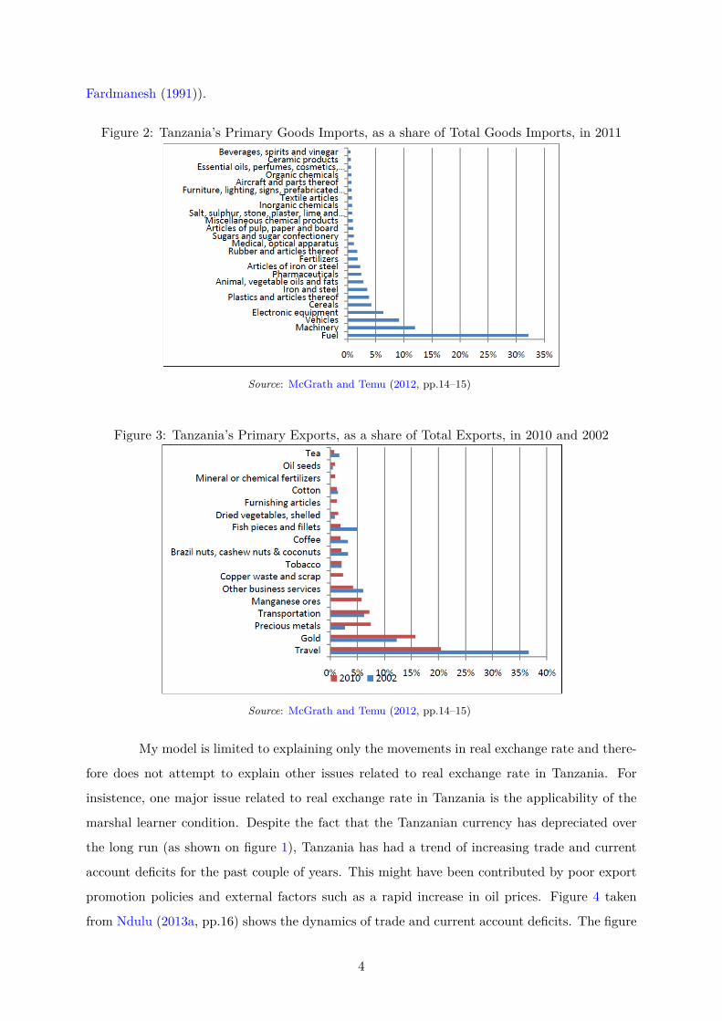
Fardmanesh (1991)).

Figure 2: Tanzania’s Primary Goods Imports, as a share of Total Goods Imports, in 2011

Source: McGrath and Temu (2012, pp.14–15)

Figure 3: Tanzania’s Primary Exports, as a share of Total Exports, in 2010 and 2002

Source: McGrath and Temu (2012, pp.14–15)

My model is limited to explaining only the movements in real exchange rate and there-

fore does not attempt to explain other issues related to real exchange rate in Tanzania. For

insistence, one major issue related to real exchange rate in Tanzania is the applicability of the

marshal learner condition. Despite the fact that the Tanzanian currency has depreciated over

the long run (as shown on figure 1), Tanzania has had a trend of increasing trade and current

account deficits for the past couple of years. This might have been contributed by poor export

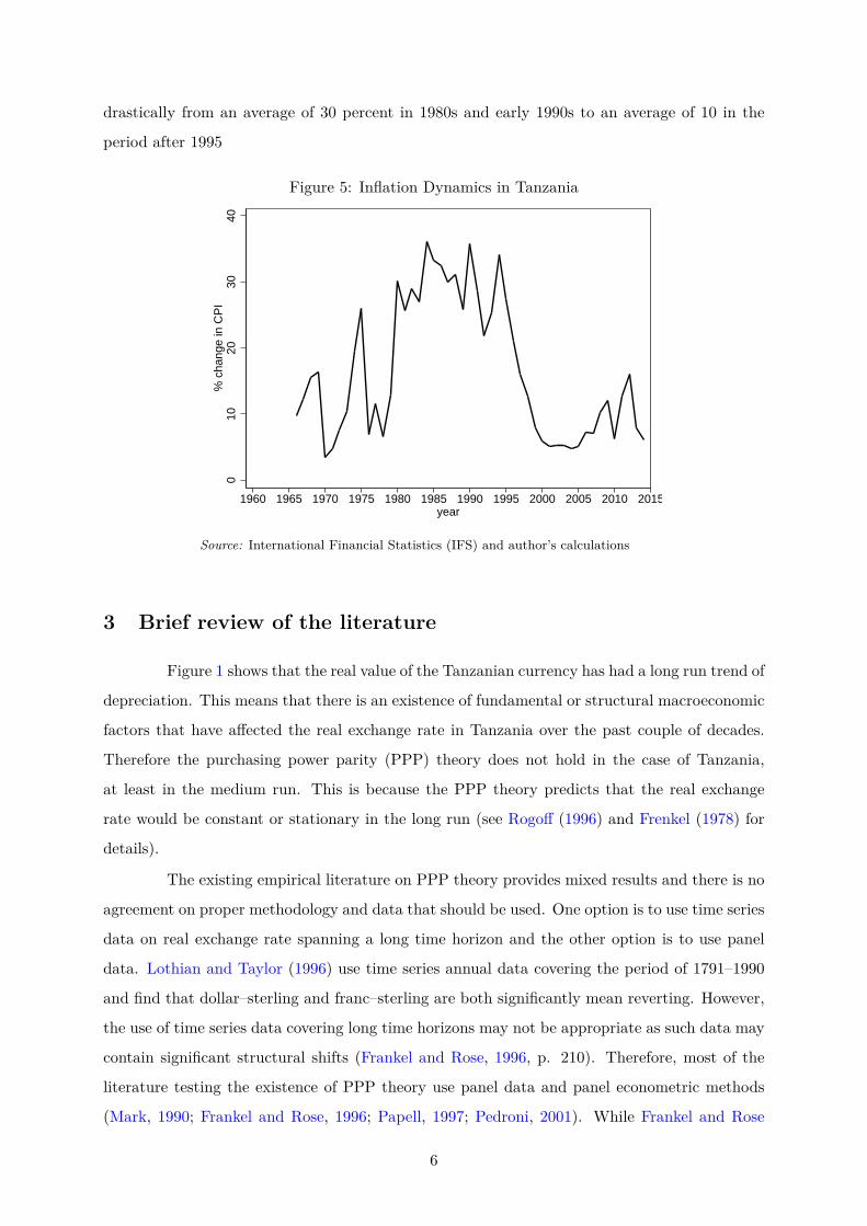
promotion policies and external factors such as a rapid increase in oil prices. Figure 4 taken

from Ndulu (2013a, pp.16) shows the dynamics of trade and current account deficits. The figure

4

shows, for the past decades, Tanzania has been running current account and trade deficits.

Figure 4: Tanzania trade balance and current account

Source: Ndulu (2013a, pp.16)

2.2 Institutional Developments

In order to study the dynamics of real exchange rate in Tanzania it is important to focus

on the time period in which Tanzania was under flexible exchange rate regime. Rutasitara (2004)

gives a good review of the development of the exchange rate regimes in Tanzania. Tanzania

was under socialist control with a fixed exchange rate regime from 1967 to 1986. From 1986

the Tanzanian government started liberalization programs which included changing to a flexible

exchange rate regime. The effects of these changes are seen in figure 1. Before 1986, the nominal

exchange rate was constant then after 1986 started to fluctuate with a general upward trend.

Therefore, the empirical testing of the model focus on the period from 1987 to 2012.

In this thesis I attempt to explain the real exchange rate and not the nominal exchange

rate. The monetary policy is important in explaining the nominal exchange rate. A good de-

scription of monetary policy developments in Tanzania is given in Massawe (2001). Tanzania

has been under inflation targeting since 1995. Due to high and sustained inflation levels in the

period immediately before 1995, there was a need to make price stability a priority in macroeco-

nomic policies. The central bank of Tanzania believes in monetarist view of inflation, therefore,

in order to achieve price stability, they target and control monetary aggregates (Massawe, 2001).

For the period of 2012/13, for example, the bank of Tanzania targeted an annual growth of about

18% for M3 and an annual growth not exceeding 16% for the average reserve money (Ndulu,

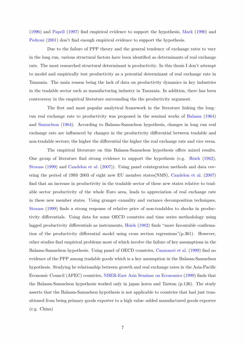
2013b). In figure 5 we can see how the switch to inflation targeting was able to reduce inflation

5

drastically from an average of 30 percent in 1980s and early 1990s to an average of 10 in the

period after 1995

Figure 5: Inflation Dynamics in Tanzania

010

2030

40%

cha

nge

in C

PI

1960 1965 1970 1975 1980 1985 1990 1995 2000 2005 2010 2015year

Source: International Financial Statistics (IFS) and author’s calculations

3 Brief review of the literature

Figure 1 shows that the real value of the Tanzanian currency has had a long run trend of

depreciation. This means that there is an existence of fundamental or structural macroeconomic

factors that have affected the real exchange rate in Tanzania over the past couple of decades.

Therefore the purchasing power parity (PPP) theory does not hold in the case of Tanzania,

at least in the medium run. This is because the PPP theory predicts that the real exchange

rate would be constant or stationary in the long run (see Rogoff (1996) and Frenkel (1978) for

details).

The existing empirical literature on PPP theory provides mixed results and there is no

agreement on proper methodology and data that should be used. One option is to use time series

data on real exchange rate spanning a long time horizon and the other option is to use panel

data. Lothian and Taylor (1996) use time series annual data covering the period of 1791–1990

and find that dollar–sterling and franc–sterling are both significantly mean reverting. However,

the use of time series data covering long time horizons may not be appropriate as such data may

contain significant structural shifts (Frankel and Rose, 1996, p. 210). Therefore, most of the

literature testing the existence of PPP theory use panel data and panel econometric methods

(Mark, 1990; Frankel and Rose, 1996; Papell, 1997; Pedroni, 2001). While Frankel and Rose

6

(1996) and Papell (1997) find empirical evidence to support the hypothesis, Mark (1990) and

Pedroni (2001) don’t find enough empirical evidence to support the hypothesis.

Due to the failure of PPP theory and the general tendency of exchange rates to vary

in the long run, various structural factors have been identified as determinants of real exchange

rate. The most researched structural determinant is productivity. In this thesis I don’t attempt

to model and empirically test productivity as a potential determinant of real exchange rate in

Tanzania. The main reason being the lack of data on productivity dynamics in key industries

in the tradable sector such as manufacturing industry in Tanzania. In addition, there has been

controversy in the empirical literature surrounding the the productivity argument.

The first and most popular analytical framework in the literature linking the long–

run real exchange rate to productivity was proposed in the seminal works of Balassa (1964)

and Samuelson (1964). According to Balassa-Samuelson hypothesis, changes in long run real

exchange rate are influenced by changes in the productivity differential between tradable and

non-tradable sectors; the higher the differential the higher the real exchange rate and vice versa.

The empirical literature on this Balassa-Samuelson hypothesis offers mixed results.

One group of literature find strong evidence to support the hypothesis (e.g. Hsieh (1982),

Strauss (1999) and Candelon et al. (2007)). Using panel cointegration methods and data cov-

ering the period of 1993–2003 of eight new EU member states(NMS), Candelon et al. (2007)

find that an increase in productivity in the tradable sector of these new states relative to trad-

able sector productivity of the whole Euro area, leads to appreciation of real exchange rate

in these new member states. Using granger–causality and variance decomposition techniques,

Strauss (1999) finds a strong response of relative price of non-tradables to shocks in produc-

tivity differentials. Using data for some OECD countries and time series methodology using

lagged productivity differentials as instruments, Hsieh (1982) finds “more favourable confirma-

tion of the productivity differential model using cross section regressions”(p.361). However,

other studies find empirical problems most of which involve the failure of key assumptions in the

Balassa-Samuelson hypothesis. Using panel of OECD countries, Canzoneri et al. (1999) find no

evidence of the PPP among tradable goods which is a key assumption in the Balassa-Samuelson

hypothesis. Studying he relationship between growth and real exchange rates in the Asia-Pacific

Economic Council (APEC) countries, NBER-East Asia Seminar on Economics (1999) finds that

the Balassa-Samuelson hypothesis worked only in japan korea and Taiwan (p.126). The study

asserts that the Balassa-Samuelson hypothesis is not applicable to countries that had just tran-

sitioned from being primary goods exporter to a high value–added manufactured goods exporter

(e.g. China)

7

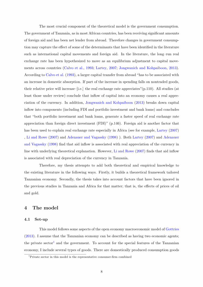
The most crucial component of the theoretical model is the government consumption.

The government of Tanzania, as in most African countries, has been receiving significant amounts

of foreign aid and has been net lender from abroad. Therefore changes in government consump-

tion may capture the effect of some of the determinants that have been identified in the literature

such as international capital movements and foreign aid. In the literature, the long–run real

exchange rate has been hypothesized to move as an equilibrium adjustment to capital move-

ments across countries (Calvo et al., 1993; Lartey, 2007; Jongwanich and Kohpaiboon, 2013).

According to Calvo et al. (1993), a larger capital transfer from abroad “has to be associated with

an increase in domestic absorption. If part of the increase in spending falls on nontraded goods,

their relative price will increase–[i.e.] the real exchange rate appreciates”(p.110). All studies (at

least those under review) conclude that inflow of capital into an economy causes a real appre-

ciation of the currency. In addition, Jongwanich and Kohpaiboon (2013) breaks down capital

inflow into components (including FDI and portfolio investment and bank loans) and concludes

that “both portfolio investment and bank loans, generate a faster speed of real exchange rate

appreciation than foreign direct investment (FDI)” (p.146). Foreign aid is another factor that

has been used to explain real exchange rate especially in Africa (see for example, Lartey (2007)

, Li and Rowe (2007) and Adenauer and Vagassky (1998) ). Both Lartey (2007) and Adenauer

and Vagassky (1998) find that aid inflow is associated with real appreciation of the currency in

line with underlying theoretical explanation. However, Li and Rowe (2007) finds that aid inflow

is associated with real depreciation of the currency in Tanzania.

Therefore, my thesis attempts to add both theoretical and empirical knowledge to

the existing literature in the following ways. Firstly, it builds a theoretical framework tailored

Tanzanian economy. Secondly, the thesis takes into account factors that have been ignored in

the previous studies in Tanzania and Africa for that matter; that is, the effects of prices of oil

and gold.

4 The model

4.1 Set-up

This model follows some aspects of the open economy macroeconomic model of Gottries

(2013). I assume that the Tanzanian economy can be described as having two economic agents;

the private sector1 and the government. To account for the special features of the Tanzanian

economy, I include several types of goods. There are domestically produced consumption goods1Private sector in this model is the representative consumer-firm combined

8

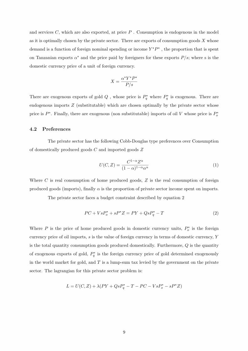
and services C, which are also exported, at price P . Consumption is endogenous in the model

as it is optimally chosen by the private sector. There are exports of consumption goods X whose

demand is a function of foreign nominal spending or income Y ∗P ∗ , the proportion that is spent

on Tanzanian exports α∗ and the price paid by foreigners for these exports P/s; where s is the

domestic currency price of a unit of foreign currency.

X = α∗Y ∗P ∗

P/s

There are exogenous exports of gold Q , whose price is P ∗q where P ∗

q is exogenous. There are

endogenous imports Z (substitutable) which are chosen optimally by the private sector whose

price is P ∗. Finally, there are exogenous (non substitutable) imports of oil V whose price is P ∗o

4.2 Preferences

The private sector has the following Cobb-Douglas type preferences over Consumption

of domestically produced goods C and imported goods Z

U(C,Z) = C1−αZα

(1− α)1−ααα(1)

Where C is real consumption of home produced goods, Z is the real consumption of foreign

produced goods (imports), finally α is the proportion of private sector income spent on imports.

The private sector faces a budget constraint described by equation 2

PC + V sP ∗o + sP ∗Z = PY +QsP ∗

q − T (2)

Where P is the price of home produced goods in domestic currency units, P ∗o is the foreign

currency price of oil imports, s is the value of foreign currency in terms of domestic currency, Y

is the total quantity consumption goods produced domestically. Furthermore, Q is the quantity

of exogenous exports of gold, P ∗q is the foreign currency price of gold determined exogenously

in the world market for gold, and T is a lump-sum tax levied by the government on the private

sector. The lagrangian for this private sector problem is:

L = U(C,Z) + λ(PY +QsP ∗q − T − PC − V sP ∗

o − sP ∗Z)

9

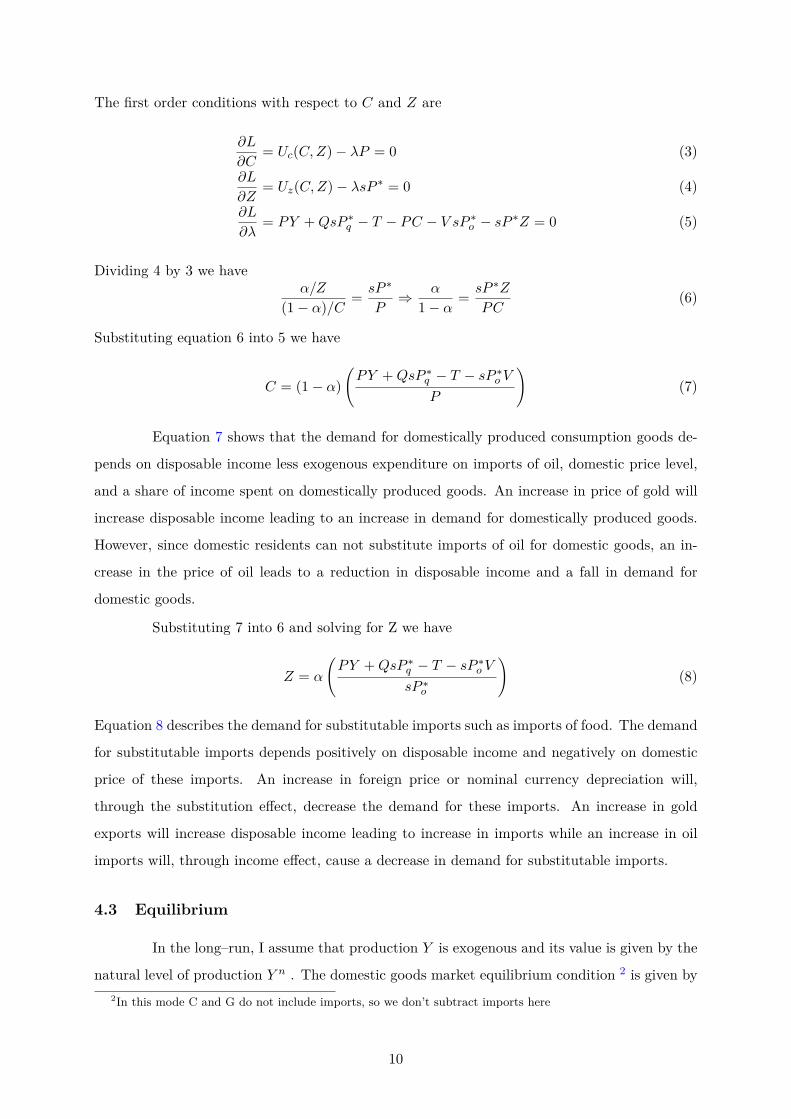
The first order conditions with respect to C and Z are

∂L

∂C= Uc(C,Z)− λP = 0 (3)

∂L

∂Z= Uz(C,Z)− λsP ∗ = 0 (4)

∂L

∂λ= PY +QsP ∗

q − T − PC − V sP ∗o − sP ∗Z = 0 (5)

Dividing 4 by 3 we haveα/Z

(1− α)/C = sP ∗

P⇒ α

1− α = sP ∗Z

PC(6)

Substituting equation 6 into 5 we have

C = (1− α)(PY +QsP ∗

q − T − sP ∗o V

P

)(7)

Equation 7 shows that the demand for domestically produced consumption goods de-

pends on disposable income less exogenous expenditure on imports of oil, domestic price level,

and a share of income spent on domestically produced goods. An increase in price of gold will

increase disposable income leading to an increase in demand for domestically produced goods.

However, since domestic residents can not substitute imports of oil for domestic goods, an in-

crease in the price of oil leads to a reduction in disposable income and a fall in demand for

domestic goods.

Substituting 7 into 6 and solving for Z we have

Z = α

(PY +QsP ∗

q − T − sP ∗o V

sP ∗o

)(8)

Equation 8 describes the demand for substitutable imports such as imports of food. The demand

for substitutable imports depends positively on disposable income and negatively on domestic

price of these imports. An increase in foreign price or nominal currency depreciation will,

through the substitution effect, decrease the demand for these imports. An increase in gold

exports will increase disposable income leading to increase in imports while an increase in oil

imports will, through income effect, cause a decrease in demand for substitutable imports.

4.3 Equilibrium

In the long–run, I assume that production Y is exogenous and its value is given by the

natural level of production Y n . The domestic goods market equilibrium condition 2 is given by2In this mode C and G do not include imports, so we don’t subtract imports here

10

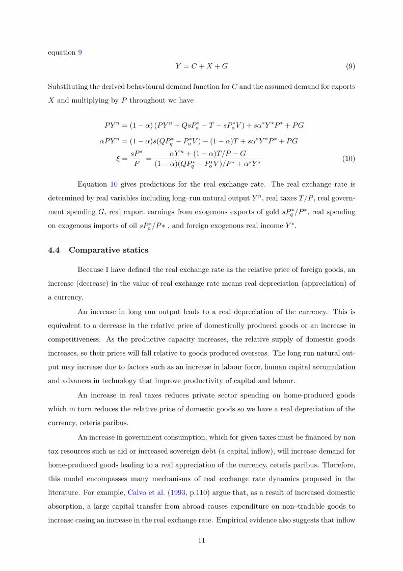
equation 9

Y = C +X +G (9)

Substituting the derived behavioural demand function for C and the assumed demand for exports

X and multiplying by P throughout we have

PY n = (1− α) (PY n +QsP ∗o − T − sP ∗

o V ) + sα∗Y ∗P ∗ + PG

αPY n = (1− α)s(QP ∗q − P ∗

o V )− (1− α)T + sα∗Y ∗P ∗ + PG

ξ = sP ∗

P= αY n + (1− α)T/P −G

(1− α)(QP ∗q − P ∗

o V )/P ∗ + α∗Y ∗ (10)

Equation 10 gives predictions for the real exchange rate. The real exchange rate is

determined by real variables including long–run natural output Y n, real taxes T/P , real govern-

ment spending G, real export earnings from exogenous exports of gold sP ∗q /P

∗, real spending

on exogenous imports of oil sP ∗o /P∗ , and foreign exogenous real income Y ∗.

4.4 Comparative statics

Because I have defined the real exchange rate as the relative price of foreign goods, an

increase (decrease) in the value of real exchange rate means real depreciation (appreciation) of

a currency.

An increase in long run output leads to a real depreciation of the currency. This is

equivalent to a decrease in the relative price of domestically produced goods or an increase in

competitiveness. As the productive capacity increases, the relative supply of domestic goods

increases, so their prices will fall relative to goods produced overseas. The long run natural out-

put may increase due to factors such as an increase in labour force, human capital accumulation

and advances in technology that improve productivity of capital and labour.

An increase in real taxes reduces private sector spending on home-produced goods

which in turn reduces the relative price of domestic goods so we have a real depreciation of the

currency, ceteris paribus.

An increase in government consumption, which for given taxes must be financed by non

tax resources such as aid or increased sovereign debt (a capital inflow), will increase demand for

home-produced goods leading to a real appreciation of the currency, ceteris paribus. Therefore,

this model encompasses many mechanisms of real exchange rate dynamics proposed in the

literature. For example, Calvo et al. (1993, p.110) argue that, as a result of increased domestic

absorption, a large capital transfer from abroad causes expenditure on non–tradable goods to

increase casing an increase in the real exchange rate. Empirical evidence also suggests that inflow

11

of capital into an economy causes a real appreciation of the currency (Calvo et al., 1993; Lartey,

2007; Jongwanich and Kohpaiboon, 2013). Both Lartey (2007) and Adenauer and Vagassky

(1998) find that aid inflow is associated with real appreciation of the currency.

An increase in gold earnings will increase spending on home produced goods leading

to an increase in relative price of these goods and real appreciation of the currency.

An increase in foreign income will increase the demand for home-produced goods lead-

ing to an increase in their relative price, i.e. a real appreciation of the currency, ceteris paribus.

The magnitude of the effect of foreign income depends on the proportion of income spent by

foreigners on domestically produced goods. The lower this proportion is, the weaker will be the

effect.

The assumption that domestic residents can not substitute imports of oil for domestic

goods implies an increase in price of oil leads to a reduction in disposable income and a fall in

demand for domestic goods. This fall in demand leads to a fall in domestic price level and a

real depreciation of the currency. I assume that the supply side effect of oil price is negligible in

the case of Tanzania.

5 Data and graphical analysis

5.1 Data

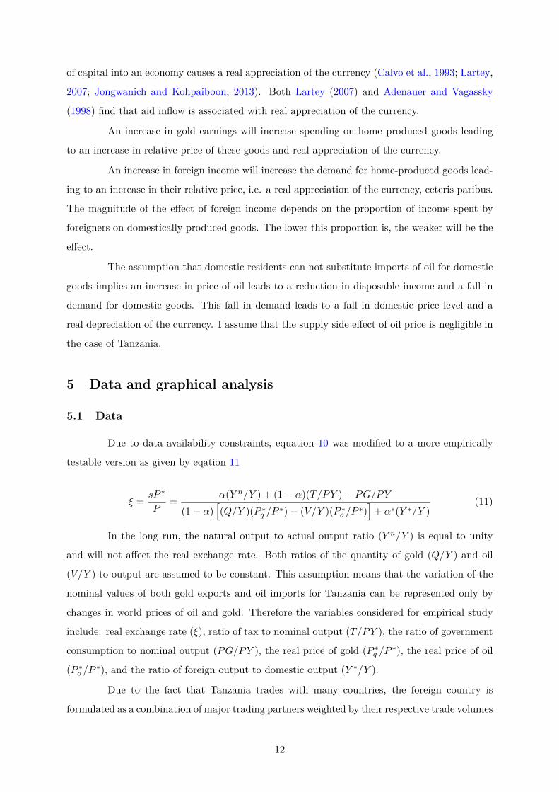
Due to data availability constraints, equation 10 was modified to a more empirically

testable version as given by eqation 11

ξ = sP ∗

P= α(Y n/Y ) + (1− α)(T/PY )− PG/PY

(1− α)[(Q/Y )(P ∗

q /P∗)− (V/Y )(P ∗

o /P∗)]

+ α∗(Y ∗/Y )(11)

In the long run, the natural output to actual output ratio (Y n/Y ) is equal to unity

and will not affect the real exchange rate. Both ratios of the quantity of gold (Q/Y ) and oil

(V/Y ) to output are assumed to be constant. This assumption means that the variation of the

nominal values of both gold exports and oil imports for Tanzania can be represented only by

changes in world prices of oil and gold. Therefore the variables considered for empirical study

include: real exchange rate (ξ), ratio of tax to nominal output (T/PY ), the ratio of government

consumption to nominal output (PG/PY ), the real price of gold (P ∗q /P

∗), the real price of oil

(P ∗o /P

∗), and the ratio of foreign output to domestic output (Y ∗/Y ).

Due to the fact that Tanzania trades with many countries, the foreign country is

formulated as a combination of major trading partners weighted by their respective trade volumes

12

(the sum of exports and imports) with Tanzania. Data on imports and exports of all countries

that traded with Tanzania in 19913 was taken from Direction of Trade Statistics (DOS) database

of the IMF. 15 countries4 are identified as major trading partners with Tanzania based their

respective trade volumes with Tanzania. Trade weight of a particular trading partner was

calculated as a proportion of country’s trade volume with Tanzania to the total trade volume

for the 14 countries (see the appendix A for further details).

The nominal exchange rate is calculated as a weighted average of the bilateral exchange

rates of all trading partners’ currencies with Tanzanian shilling. The bilateral exchange rates

are obtained by multiplying the exchange rate of trading partner’s currency with the dollar (us

dollar per unit of trading partner’s currency) by the exchange rate of Tanzania shillings with

the dollar (Tanzanian shillings per 1 dollar). All bilateral exchange rate data is obtained from

IMF’s IFS database except for Euro zone countries in the trading partners list. The exchange

rates for these countries are obtained from OECD economic outlook database.

The foreign price level is calculated as a geometric weighed average of CPIs of all 14

trading partners. Domestic price level is the Tanzania CPI. The tax variable is proxied by

Tanzania total government revenue divided by the nominal GDP for Tanzania. Government ex-

penditure is the nominal government consumption expenditure divided by the nominal GDP for

Tanzania. The data for CPI, total government revenue, nominal GDP and nominal government

consumption expenditure comes from the same IFS database5

The real price of oil is calculated as the ratio of nominal world dollar price of oil to

the price level in the United States. Price level in the US is the US CPI and data is taken from

IFS. The dollar price of oil (USD per barrel) was obtained from BP statistical review of world

energy (2013). This is the ratio of world dollar price of gold to the price level in the United

States. The nominal price of gold is US–dollars per troy ounce6 sourced from Global Economic

Monitor (GEM) for commodities database of the World Bank.

Foreign output is calculated as a geometrically weighted average of real gross national

products (GDP) of 14 major trading partners with Tanzania. Domestic output is Tanzanian

real GDP. The natural or long-run output is estimated by the quadratic time trend of Tanzanian3The motivation for using year 1991 is the fact that this year lies at the center of the study period 1968-2012.

The trade volumes for the entire period are assumed to be the same as they were in 19914Countries include United Kingdom, Germany, Japan, Saudi Arabia, Italy, Netherlands, India, Belgium, United

States, Kenya, United Arab Emirates, Singapore, Pakistan, France and Sweden. Due to data constraints, theUnited Arab Emirates was dropped from the list before the weights were calculated and 14 countries made thefinal list

5However, the observation of total government revenue for the year 1996 is missing in this database thereforeit is assumed to be equal to the previous year’s value. I replaced the missing observation with the value in theprevious year.

6One troy ounce is 31.1034768 grams, or 0.0311034768 kilograms

13

real GDP. All the data on GDP were taken from IFS database of the IMF.

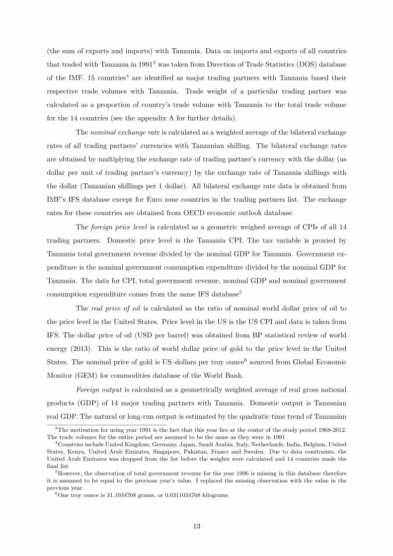
5.2 Components of Real exchange rate

The real exchange rate is constructed from data on the nominal exchange rate, the

foreign price level and the domestic price level. We first decompose the real exchange rate into

its components and examine how these components evolve in relation to the real exchange rate7. Figures 6, 8 and 7 display time series graphs of the yearly percentage changes in real exchange

rate against the yearly percentage changes in the nominal exchange rate, foreign inflation and

domestic inflation respectively . In all three figures, the dotted vertical lines mark Tanzania’s

major macroeconomic events. The first dotted line marks the year 1986 when Tanzania abolished

fixed exchange rate system while the later dotted line marks the year 1995 corresponding to the

adoption of inflation targeting and strict control of money growth.

Figure 6: Relating changes of real exchange rate to changes in nominal exchange rate

-20

020

4060

80C

hang

e (in

%)

1960 1965 1970 1975 1980 1985 1990 1995 2000 2005 2010 2015year

Change in real exchange rateChange in nominal exchange rate

Notes: The first vertical line marks the year 1986 when Tanzania abolishedfixed exchange rate system while the later vertical line marks the year 1995corresponding to the adoption of inflation targeting and strict control of moneygrowth. Source: International Financial Statistics (IFS), OECD economic out-look database and author’s calculations

Figure 6 shows that changes in nominal exchange rate are the major component of

yearly changes in real exchange rate, at least in the short run. Almost all movements in the

nominal exchange rate are replicated by movements in the real exchange rate.

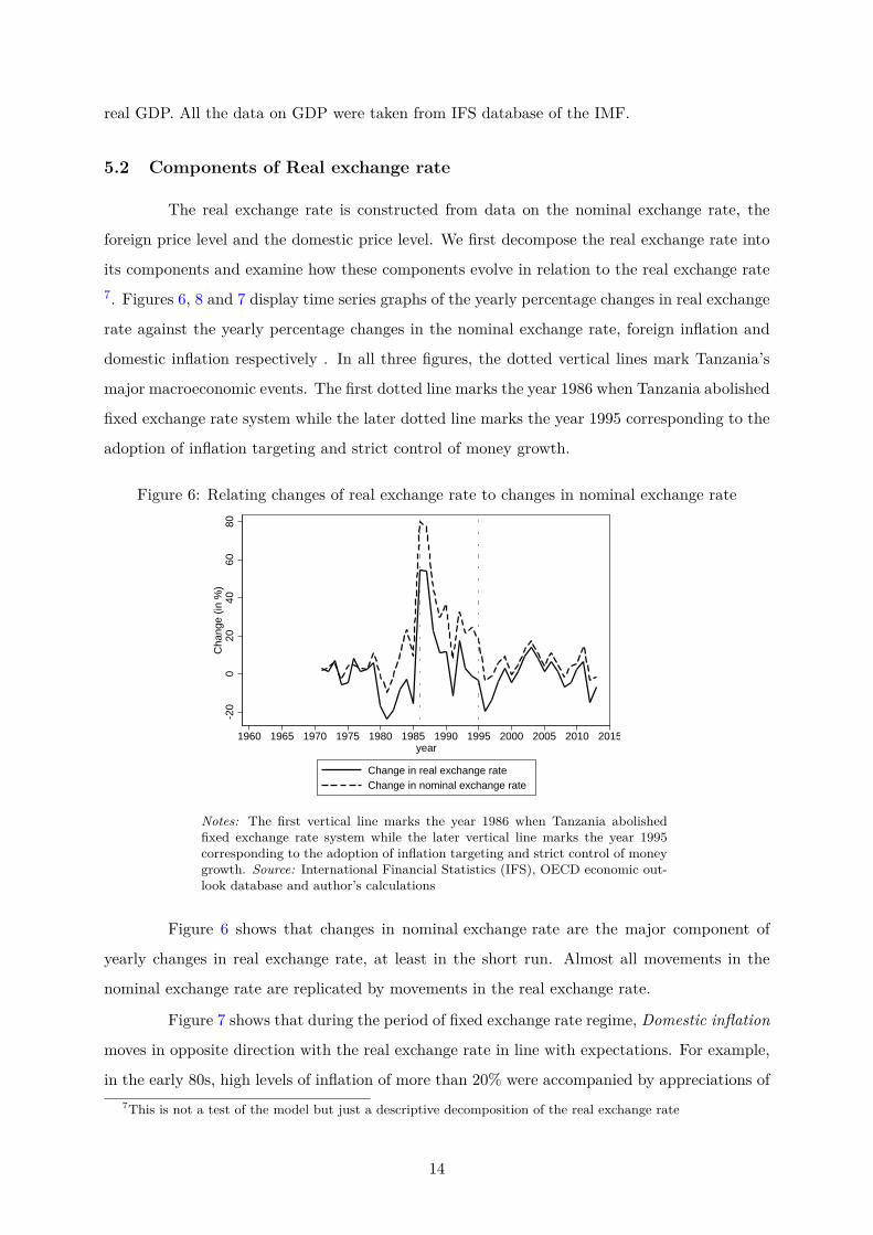
Figure 7 shows that during the period of fixed exchange rate regime, Domestic inflation

moves in opposite direction with the real exchange rate in line with expectations. For example,

in the early 80s, high levels of inflation of more than 20% were accompanied by appreciations of7This is not a test of the model but just a descriptive decomposition of the real exchange rate

14

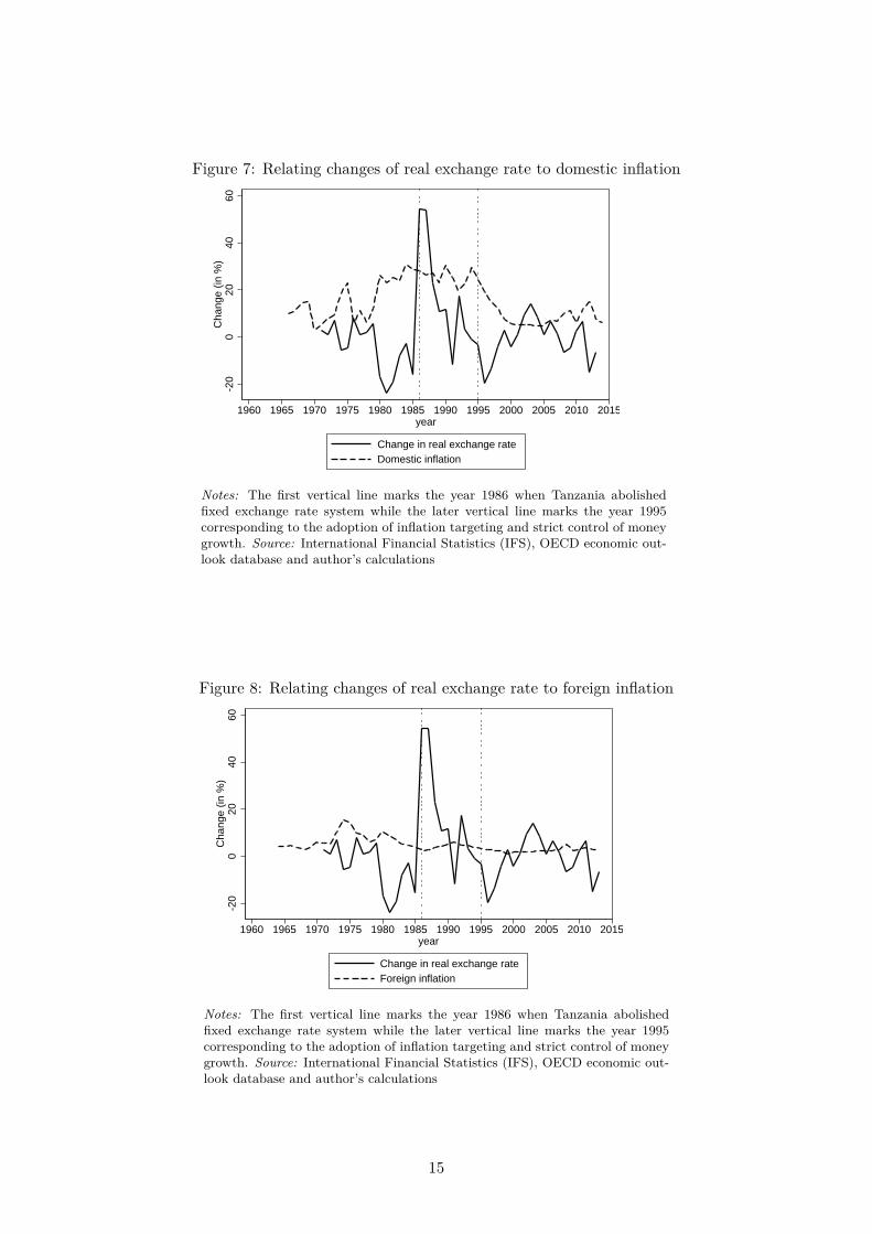
Figure 7: Relating changes of real exchange rate to domestic inflation

-20

020

4060

Cha

nge

(in %

)

1960 1965 1970 1975 1980 1985 1990 1995 2000 2005 2010 2015year

Change in real exchange rateDomestic inflation

Notes: The first vertical line marks the year 1986 when Tanzania abolishedfixed exchange rate system while the later vertical line marks the year 1995corresponding to the adoption of inflation targeting and strict control of moneygrowth. Source: International Financial Statistics (IFS), OECD economic out-look database and author’s calculations

Figure 8: Relating changes of real exchange rate to foreign inflation

-20

020

4060

Cha

nge

(in %

)

1960 1965 1970 1975 1980 1985 1990 1995 2000 2005 2010 2015year

Change in real exchange rateForeign inflation

Notes: The first vertical line marks the year 1986 when Tanzania abolishedfixed exchange rate system while the later vertical line marks the year 1995corresponding to the adoption of inflation targeting and strict control of moneygrowth. Source: International Financial Statistics (IFS), OECD economic out-look database and author’s calculations

15

more than 20%. The relationship is weak in the years 1985 and 1986 due to real exchange rate

devaluation associated with the transition to a a flexible exchange rate. The negative relationship

is again evident in post transition period from 1987 to the late 90’s where by high sustained

levels of inflation likely caused the trend of real exchange rate to decrease until late 90s. In the

period after 1995, the relationship is generally weak. After the shift to “inflation targeting”in

1995, domestic inflation was stable while the real exchange rate continued to fluctuate.

In figure 8, Foreign inflation appears to be stable and does not move together with the

real exchange rate.

5.3 Graphical analysis of the real exchange rate and explanatory variables

In order to assess the theoretical implications of the model developed in section 4, the

real exchange rate is plotted against each of its equilibrium determinants identified in the theo-

retical model. We focus on the period after 1986 when the nominal exchange rate in Tanzania

was allowed to fluctuate in response to foreign exchange market conditions. One reason for

limiting the sample in this manner is to avoid possible structural break in the time series caused

by devaluations associated with the transition from fixed to a flexible exchange rate regime. In

figure 1, we can see the significant jump in the real exchange rate time series in the year 1986 in

which the exchange rate reform program was implemented. The visual inspection of the plots is

used to identify the presence of trend movements in the real exchange rate and these movements

are compared with corresponding movements of the empirical measures of the theoretical deter-

minants. We expect, for example, if the real exchange rate has a tendency to increase8, then the

corresponding equilibrium determinant should show an appropriate movement as predicted by

the theoretical model. In each of Figures 9, 10, 11, 12 and 13, the real exchange rate is plotted

along one of the structural determinants. in each graph, the vertical doted line at the year 1986

marks the transition form fixed to flexible exchange rate in Tanzania. For comparison purposes,

each variable is normalized in such a way that its value in 2010 is equal to 19.

Tax revenue

The theoretical model predicts a positive relationship between tax revenue and the real

exchange rate. An increase in real tax revenue reduces private sector spending which in turn8The way exchange rate is defined here, increase in numerical value of the real exchange rate means depreciation

of the real value of the Tanzanian shilling. To keep things simple, when I say a determinant has a positiverelationship with the real exchange rate this means that increase in value of that determinant leads to increasein the numerical value of the real exchange rate and vice versa. In the literature this is usually interpreted as anegative relationship because increases in the determinant’s value leads to the actual depreciation of the currency.

9The normalized variable is essentially an index and its actual value is meaningless but the focus of this analysisis on relative changes which are effectively captured by the index

16

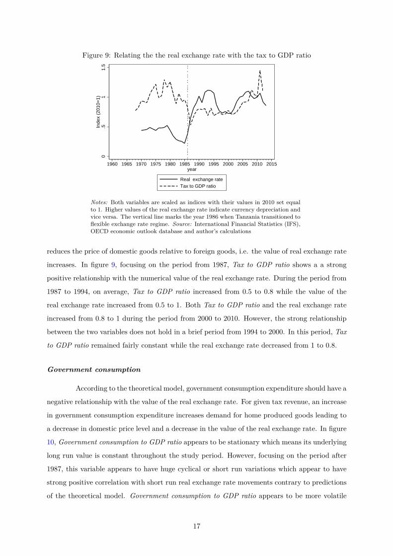
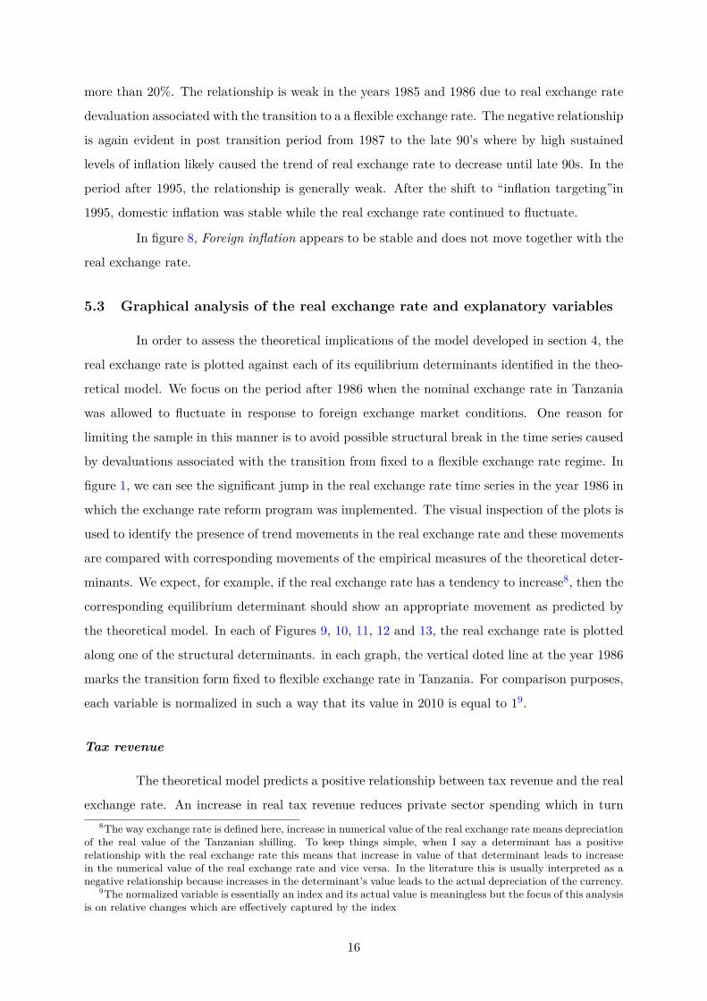
Figure 9: Relating the the real exchange rate with the tax to GDP ratio

0.5

11.

5In

dex

(201

0=1)

1960 1965 1970 1975 1980 1985 1990 1995 2000 2005 2010 2015year

Real exchange rateTax to GDP ratio

Notes: Both variables are scaled as indices with their values in 2010 set equalto 1. Higher values of the real exchange rate indicate currency depreciation andvice versa. The vertical line marks the year 1986 when Tanzania transitioned toflexible exchange rate regime. Source: International Financial Statistics (IFS),OECD economic outlook database and author’s calculations

reduces the price of domestic goods relative to foreign goods, i.e. the value of real exchange rate

increases. In figure 9, focusing on the period from 1987, Tax to GDP ratio shows a a strong

positive relationship with the numerical value of the real exchange rate. During the period from

1987 to 1994, on average, Tax to GDP ratio increased from 0.5 to 0.8 while the value of the

real exchange rate increased from 0.5 to 1. Both Tax to GDP ratio and the real exchange rate

increased from 0.8 to 1 during the period from 2000 to 2010. However, the strong relationship

between the two variables does not hold in a brief period from 1994 to 2000. In this period, Tax

to GDP ratio remained fairly constant while the real exchange rate decreased from 1 to 0.8.

Government consumption

According to the theoretical model, government consumption expenditure should have a

negative relationship with the value of the real exchange rate. For given tax revenue, an increase

in government consumption expenditure increases demand for home produced goods leading to

a decrease in domestic price level and a decrease in the value of the real exchange rate. In figure

10, Government consumption to GDP ratio appears to be stationary which means its underlying

long run value is constant throughout the study period. However, focusing on the period after

1987, this variable appears to have huge cyclical or short run variations which appear to have

strong positive correlation with short run real exchange rate movements contrary to predictions

of the theoretical model. Government consumption to GDP ratio appears to be more volatile

17

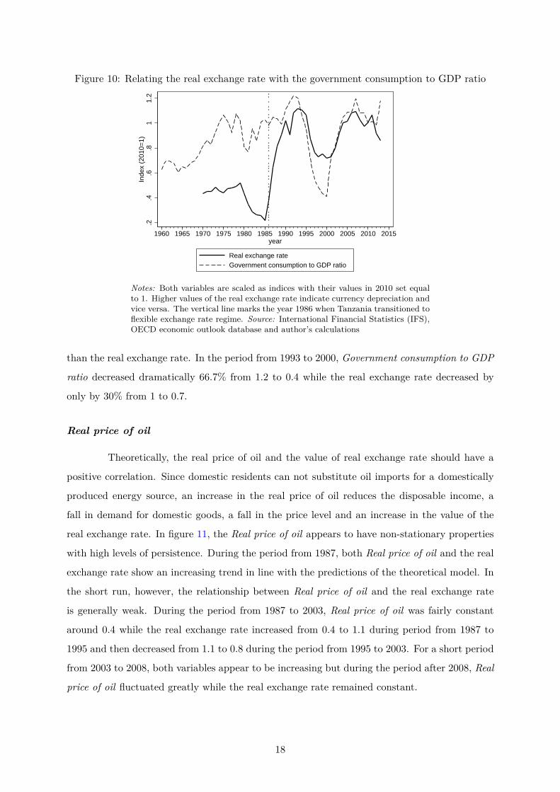
Figure 10: Relating the real exchange rate with the government consumption to GDP ratio

.2.4

.6.8

11.

2In

dex

(201

0=1)

1960 1965 1970 1975 1980 1985 1990 1995 2000 2005 2010 2015year

Real exchange rateGovernment consumption to GDP ratio

Notes: Both variables are scaled as indices with their values in 2010 set equalto 1. Higher values of the real exchange rate indicate currency depreciation andvice versa. The vertical line marks the year 1986 when Tanzania transitioned toflexible exchange rate regime. Source: International Financial Statistics (IFS),OECD economic outlook database and author’s calculations

than the real exchange rate. In the period from 1993 to 2000, Government consumption to GDP

ratio decreased dramatically 66.7% from 1.2 to 0.4 while the real exchange rate decreased by

only by 30% from 1 to 0.7.

Real price of oil

Theoretically, the real price of oil and the value of real exchange rate should have a

positive correlation. Since domestic residents can not substitute oil imports for a domestically

produced energy source, an increase in the real price of oil reduces the disposable income, a

fall in demand for domestic goods, a fall in the price level and an increase in the value of the

real exchange rate. In figure 11, the Real price of oil appears to have non-stationary properties

with high levels of persistence. During the period from 1987, both Real price of oil and the real

exchange rate show an increasing trend in line with the predictions of the theoretical model. In

the short run, however, the relationship between Real price of oil and the real exchange rate

is generally weak. During the period from 1987 to 2003, Real price of oil was fairly constant

around 0.4 while the real exchange rate increased from 0.4 to 1.1 during period from 1987 to

1995 and then decreased from 1.1 to 0.8 during the period from 1995 to 2003. For a short period

from 2003 to 2008, both variables appear to be increasing but during the period after 2008, Real

price of oil fluctuated greatly while the real exchange rate remained constant.

18

Figure 11: Relating the real exchange rate and the real world price of oil

0.2

.4.6

.81

1.2

1.4

Inde

x (2

010=

1)

1960 1965 1970 1975 1980 1985 1990 1995 2000 2005 2010 2015year

Real exchange rateReal price of oil

Notes: Both variables are scaled as indices with their values in 2010 set equalto 1. Higher values of the real exchange rate indicate currency depreciation andvice versa. The vertical line marks the year 1986 when Tanzania transitioned toflexible exchange rate regime. Source: International Financial Statistics (IFS),OECD economic outlook database, BP statistical review of world energy (2013)and author’s calculations

Figure 12: Relating real exchange rate with the real price of gold

.2.4

.6.8

11.

21.

4In

dex

(201

0=1)

1960 1965 1970 1975 1980 1985 1990 1995 2000 2005 2010 2015year

Real exchange rateReal price of gold

Notes: Both variables are scaled as indices with their values in 2010 set equalto 1. Higher values of the real exchange rate indicate currency depreciation andvice versa. The vertical line marks the year 1986 when Tanzania transitioned toflexible exchange rate regime. Source: International Financial Statistics (IFS),OECD economic outlook database, Global Economic Monitor (GEM) for com-modities database of the World Bank and author’s calculations

19

Real price of gold

The theoretical model predicts a negative relationship between the value of the real

exchange rate and the real price of gold. An increase in gold earnings will increase spending on

home produced goods leading to an increase in the relative price of these goods and a decrease

in the value of the real exchange rate. In figure 12, focusing on the period after 1986, the

relationship between the real exchange rate and Real price of gold appears to be ambiguous.

During period of from 1987 to 1995, the Real price of gold decreased from 0.6 to 0.5 while the

real exchange rate increased from 0.5 to 1. Both variables increased during the period from 2000

to 2010 with Real price of gold increasing from 0.3 to 1 and the real exchange rate increasing

from 0.7 to 1.

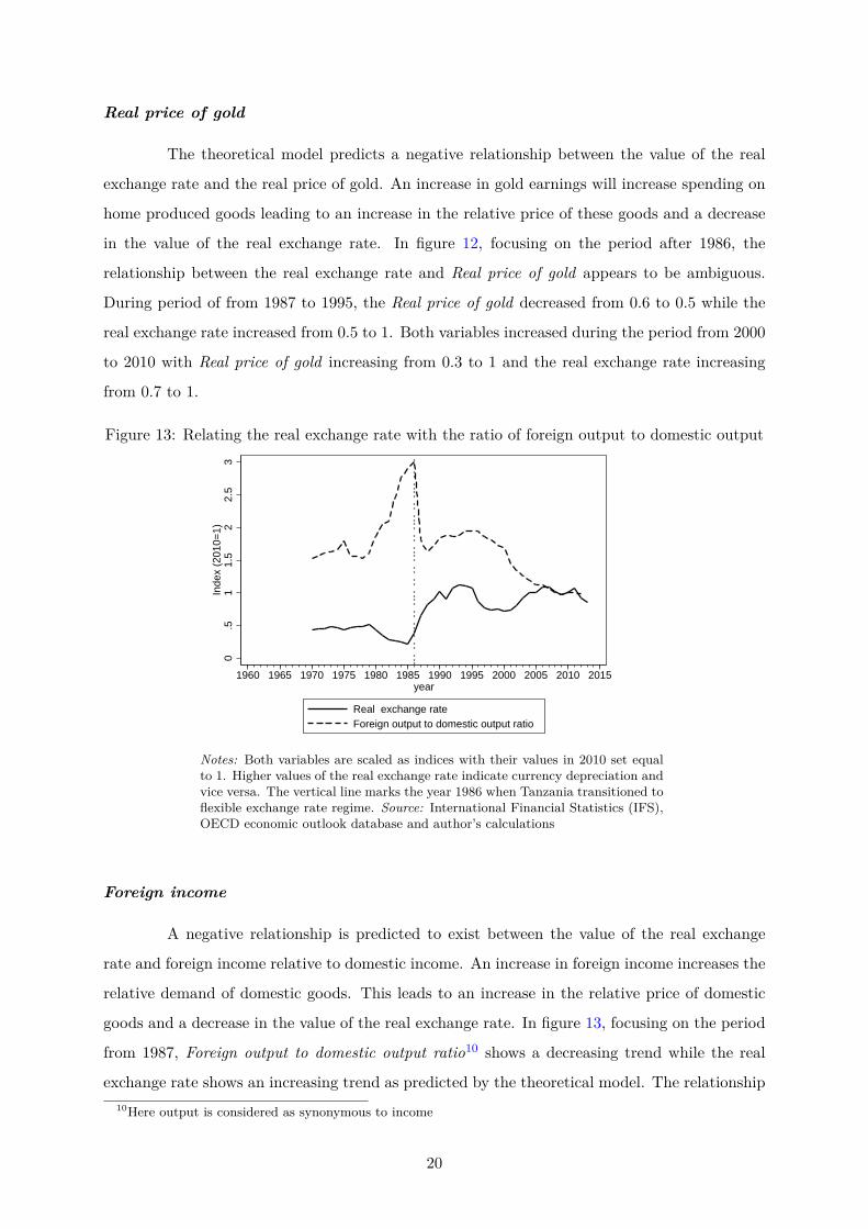
Figure 13: Relating the real exchange rate with the ratio of foreign output to domestic output

0.5

11.

52

2.5

3In

dex

(201

0=1)

1960 1965 1970 1975 1980 1985 1990 1995 2000 2005 2010 2015year

Real exchange rateForeign output to domestic output ratio

Notes: Both variables are scaled as indices with their values in 2010 set equalto 1. Higher values of the real exchange rate indicate currency depreciation andvice versa. The vertical line marks the year 1986 when Tanzania transitioned toflexible exchange rate regime. Source: International Financial Statistics (IFS),OECD economic outlook database and author’s calculations

Foreign income

A negative relationship is predicted to exist between the value of the real exchange

rate and foreign income relative to domestic income. An increase in foreign income increases the

relative demand of domestic goods. This leads to an increase in the relative price of domestic

goods and a decrease in the value of the real exchange rate. In figure 13, focusing on the period

from 1987, Foreign output to domestic output ratio10 shows a decreasing trend while the real

exchange rate shows an increasing trend as predicted by the theoretical model. The relationship10Here output is considered as synonymous to income

20

in the short run is difficult to determine and perhaps ambiguous. During the period from 1987

to 1995, both variables increased slightly. During the period from 1995 to 2010, Foreign output

to domestic output ratio decreased consistently while the real exchange rate first decreased in

the period from 1995 to 1998, stayed constant until 2002, then increased in the period after

2002.

According to the above graphical analysis, there is weak empirical evidence that the

theoretical implications hold in the long run. However in the short run, tax revenue shows a

positive relationship with the value of real exchange rate which is consistent with the prediction

of the model. In the text sections, we test formally, through regression techniques, the predictions

of the theoretical model.

6 Testing long run relationship

In this section I test the existence of the long-run equilibrium relationship between

the real exchange rate and its structural determinants. I use the technique developed by Engle

and Granger (1987). The absence of statistical evidence to support the existence of equilibrium

relationship would indicate that the real exchange rate in Tanzania permanently deviates from

its proposed long run equilibrium value.

6.1 Methodology

We test the long run relationship in the sample limited to the floating exchange rate

regime (i.e period from 1987 to 2012). The static equation to estimate the long run equilibrium

relation between RER and its determinants is specified by equation 12

rt = α+ β1xt + β2et + β3ot + β4gt + β5ft + εt (12)

Where rt is the real exchange rate, xt is the tax to GDP ratio, et is the government consumption

to GDP ratio, ot is the real price of oil, gt is the real price of gold, ft is the foreign output to

domestic output ratio, εt is the error term capturing other factors not included in the regression,

α is the intercept. β1, β2, β3, β4 and β5 are population coefficients on, tax to GDP ratio,

government consumption to GDP ratio, real price of oil, real price of gold and foreign output to

domestic output ratio respectively.

Regressions based on specifications described by equation 12 are prone to spurious re-

gression results if the variables involved are non–stationary (Stock and Watson, 2011). However,

Engle and Granger (1987) show if the variables involved in the regression are integrated of the

21

same order and residuals are stationary, then the results from regression based on equation 12

may not be spurious. Following Engle and Granger (1987), I first test all variables for existence

of unit roots. Unit root tests are conducted in line with procedures described by Phillips and

Perron (1988) and Dickey and Fuller (1979) (see appendix B for explanation of the two tests).

Secondly, in order to test for cointegration between real exchange rate and its determinants,

the residuals from equation 12 are tested for unit root based on Dickey and Fuller (1979). The

appropriate critical values taken from Davidson and MacKinnon (1993)11.

6.2 Results

Unit root test was done based on Dickey and Fuller (1979). In this test the null

hypothesis is that the variable has a unit root against the alternative that it is stationary

(see Appendix for details). Results show the null hypothesis can’t be rejected for all variables in

their levels except for Natural output to actual output ratio. This indicates that all variables have

trending behaviour except Natural output to actual output ratio which appears to be stationary.

To determine the order of integration, all variables were tested for unit roots in first difference

form. The results show we can reject the null hypothesis for Real exchange rate, tax to GDP

ratioand foreign output to domestic output ratio at 10%. The null hypothesis was also rejected at

1% level for real price of oil. However, the null hypothesis could not be rejected for government

consumption to GDP ratio and real price of gold. Therefore, the test according to Dickey and

Fuller (1979) concludes that Natural output to actual output ratio is I(0) ;Real exchange rate,

tax to GDP ratio, foreign output to domestic output ratio and real price of oil are I(1) while

government consumption to GDP ratio and real price of gold are integrated with order greater

than one.

Another test for unit root known as Philips-perron test was used (see Phillips and

Perron (1988) for details of the test). The null hypothesis is that the variable has a unit root

against the alternative that it is stationary. For level variables the test fails to reject the null

hypothesis for all variables except Real exchange rate. Tests on first difference indicate we can

reject the null hypothesis for all variables. The conclusion from this test is that all variables in

the model are I(1) except Real exchange rate which is I(0)

The foregoing unit root analysis indicate that all variables are I(1). Therefore, the

static specification in equation 12 was estimated using ordinary least squares method. The

simple OLS results are presented in table 1. The results show tax, government consumption,11Residuals are not observed and are therefore estimated. To account for uncertainly associated with estimation,

Davidson and MacKinnon (1993) recommend appropriate critical values that take into account the uncertainlyinvolved in the estimation of residuals. Therefore, the Davidson and MacKinnon (1993) critical values are signif-icantly larger than usual ADF critical values.

22

and real price of gold have significant effects on the long run real exchange rate. However, Engle

and Granger (1987) show that these results are spurious if the errors from the ols regression

contain unit roots. To this end, I conducted unit root test on the residuals of the regression. The

results show that we cannot reject the null hypothesis of a unit root using both the usual dickey

fuller critical values and the Davidson and MacKinnon (1993) critical values (see the appendix

B for details).

The conclusion from this long-run analysis is that the real exchange rate permanently

deviates from its proposed long run equilibrium value; that is there is no long run equilibrium

relationship between the real exchange rate and the structural determinants.

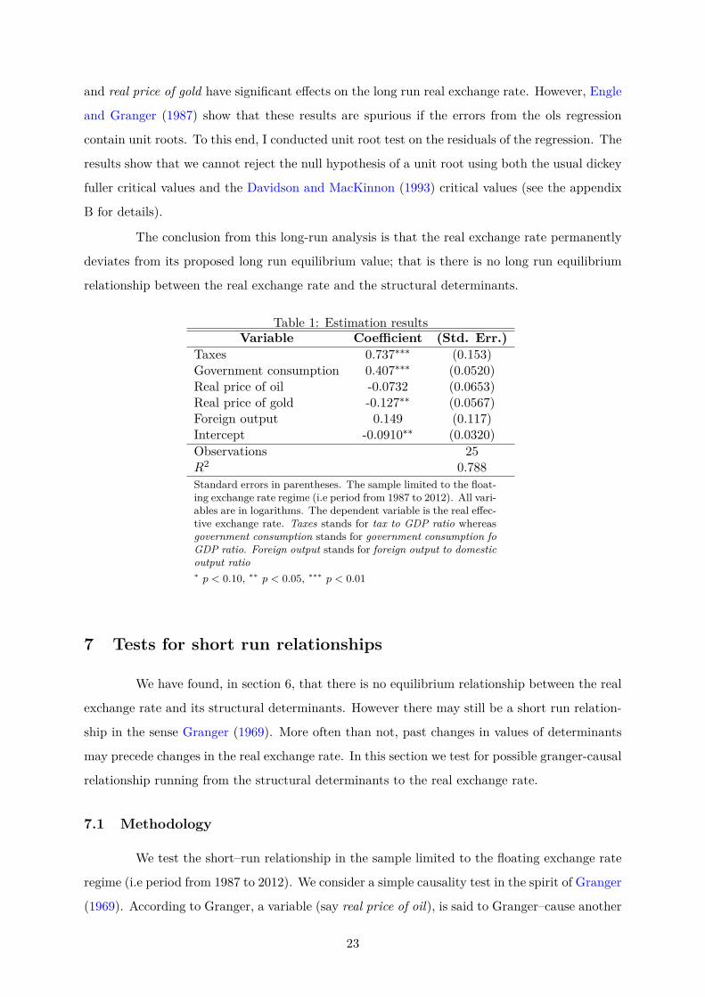
Table 1: Estimation resultsVariable Coefficient (Std. Err.)

Taxes 0.737∗∗∗ (0.153)Government consumption 0.407∗∗∗ (0.0520)Real price of oil -0.0732 (0.0653)Real price of gold -0.127∗∗ (0.0567)Foreign output 0.149 (0.117)Intercept -0.0910∗∗ (0.0320)Observations 25R2 0.788Standard errors in parentheses. The sample limited to the float-ing exchange rate regime (i.e period from 1987 to 2012). All vari-ables are in logarithms. The dependent variable is the real effec-tive exchange rate. Taxes stands for tax to GDP ratio whereasgovernment consumption stands for government consumption foGDP ratio. Foreign output stands for foreign output to domesticoutput ratio∗ p < 0.10, ∗∗ p < 0.05, ∗∗∗ p < 0.01

7 Tests for short run relationships

We have found, in section 6, that there is no equilibrium relationship between the real

exchange rate and its structural determinants. However there may still be a short run relation-

ship in the sense Granger (1969). More often than not, past changes in values of determinants

may precede changes in the real exchange rate. In this section we test for possible granger-causal

relationship running from the structural determinants to the real exchange rate.

7.1 Methodology

We test the short–run relationship in the sample limited to the floating exchange rate

regime (i.e period from 1987 to 2012). We consider a simple causality test in the spirit of Granger

(1969). According to Granger, a variable (say real price of oil), is said to Granger–cause another

23

variable (in this case, Real exchange rate) if, given the past values of Real exchange rate, past

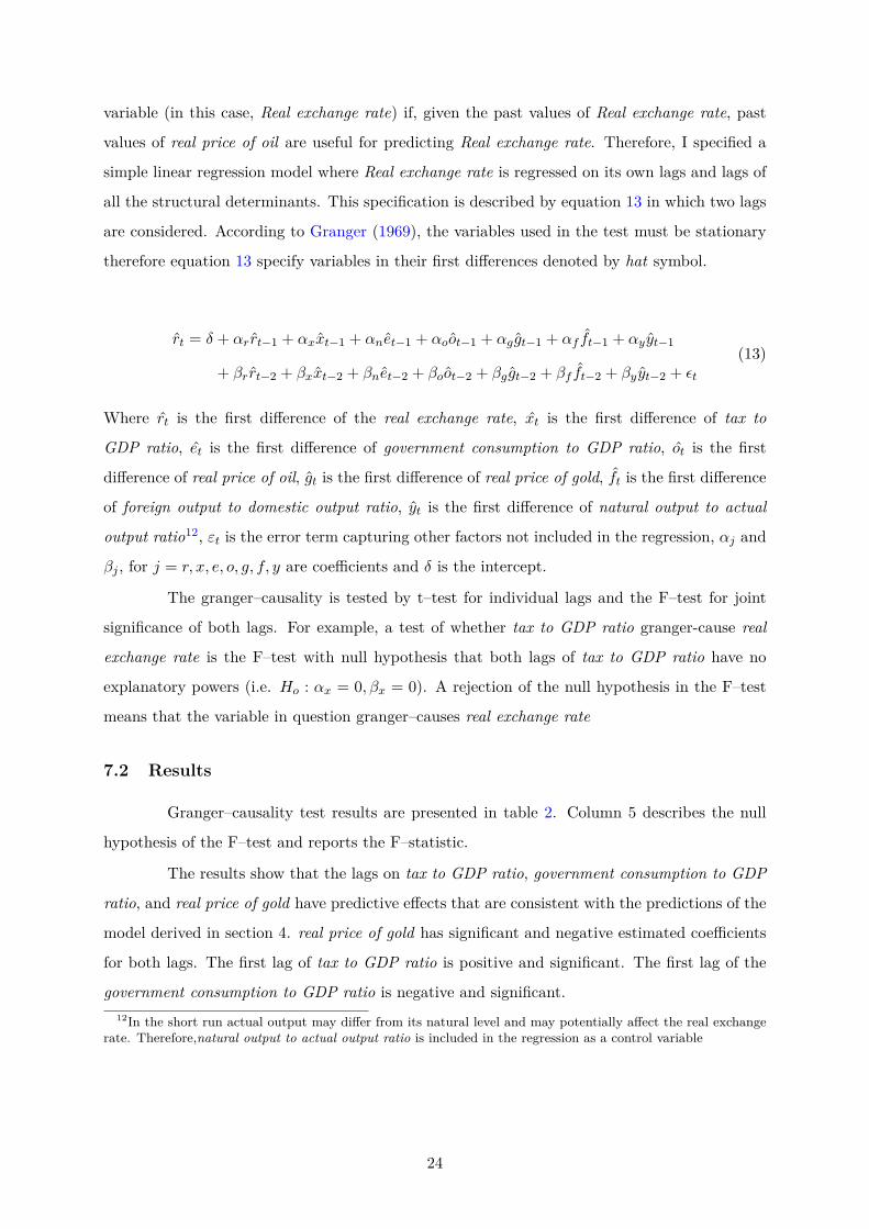
values of real price of oil are useful for predicting Real exchange rate. Therefore, I specified a

simple linear regression model where Real exchange rate is regressed on its own lags and lags of

all the structural determinants. This specification is described by equation 13 in which two lags

are considered. According to Granger (1969), the variables used in the test must be stationary

therefore equation 13 specify variables in their first differences denoted by hat symbol.

rt = δ + αrrt−1 + αxxt−1 + αnet−1 + αoot−1 + αg gt−1 + αf ft−1 + αyyt−1

+ βrrt−2 + βxxt−2 + βnet−2 + βoot−2 + βg gt−2 + βf ft−2 + βyyt−2 + εt

(13)

Where rt is the first difference of the real exchange rate, xt is the first difference of tax to

GDP ratio, et is the first difference of government consumption to GDP ratio, ot is the first

difference of real price of oil, gt is the first difference of real price of gold, ft is the first difference

of foreign output to domestic output ratio, yt is the first difference of natural output to actual

output ratio12, εt is the error term capturing other factors not included in the regression, αj and

βj , for j = r, x, e, o, g, f, y are coefficients and δ is the intercept.

The granger–causality is tested by t–test for individual lags and the F–test for joint

significance of both lags. For example, a test of whether tax to GDP ratio granger-cause real

exchange rate is the F–test with null hypothesis that both lags of tax to GDP ratio have no

explanatory powers (i.e. Ho : αx = 0, βx = 0). A rejection of the null hypothesis in the F–test

means that the variable in question granger–causes real exchange rate

7.2 Results

Granger–causality test results are presented in table 2. Column 5 describes the null

hypothesis of the F–test and reports the F–statistic.

The results show that the lags on tax to GDP ratio, government consumption to GDP

ratio, and real price of gold have predictive effects that are consistent with the predictions of the

model derived in section 4. real price of gold has significant and negative estimated coefficients

for both lags. The first lag of tax to GDP ratio is positive and significant. The first lag of the

government consumption to GDP ratio is negative and significant.12In the short run actual output may differ from its natural level and may potentially affect the real exchange

rate. Therefore,natural output to actual output ratio is included in the regression as a control variable

24

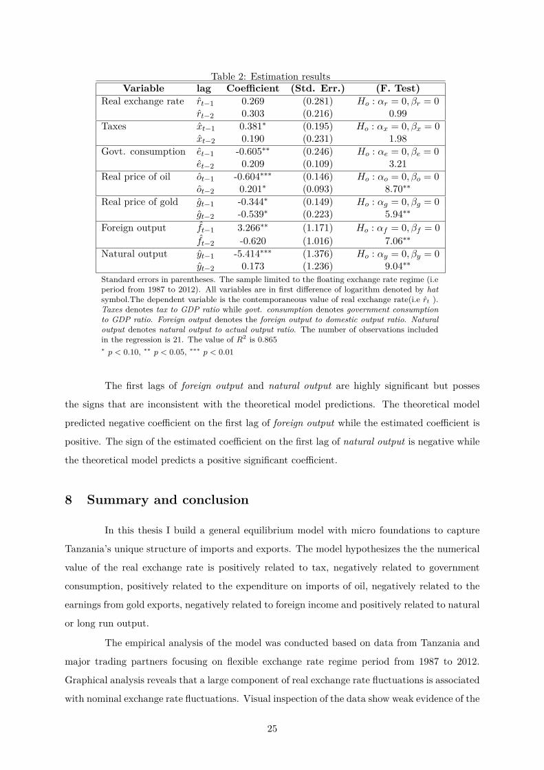
Table 2: Estimation resultsVariable lag Coefficient (Std. Err.) (F. Test)

Real exchange rate rt−1 0.269 (0.281) Ho : αr = 0, βr = 0rt−2 0.303 (0.216) 0.99

Taxes xt−1 0.381∗ (0.195) Ho : αx = 0, βx = 0xt−2 0.190 (0.231) 1.98

Govt. consumption et−1 -0.605∗∗ (0.246) Ho : αe = 0, βe = 0et−2 0.209 (0.109) 3.21

Real price of oil ot−1 -0.604∗∗∗ (0.146) Ho : αo = 0, βo = 0ot−2 0.201∗ (0.093) 8.70∗∗

Real price of gold gt−1 -0.344∗ (0.149) Ho : αg = 0, βg = 0gt−2 -0.539∗ (0.223) 5.94∗∗

Foreign output ft−1 3.266∗∗ (1.171) Ho : αf = 0, βf = 0ft−2 -0.620 (1.016) 7.06∗∗

Natural output yt−1 -5.414∗∗∗ (1.376) Ho : αy = 0, βy = 0yt−2 0.173 (1.236) 9.04∗∗

Standard errors in parentheses. The sample limited to the floating exchange rate regime (i.eperiod from 1987 to 2012). All variables are in first difference of logarithm denoted by hatsymbol.The dependent variable is the contemporaneous value of real exchange rate(i.e rt ).Taxes denotes tax to GDP ratio while govt. consumption denotes government consumptionto GDP ratio. Foreign output denotes the foreign output to domestic output ratio. Naturaloutput denotes natural output to actual output ratio. The number of observations includedin the regression is 21. The value of R2 is 0.865∗ p < 0.10, ∗∗ p < 0.05, ∗∗∗ p < 0.01

The first lags of foreign output and natural output are highly significant but posses

the signs that are inconsistent with the theoretical model predictions. The theoretical model

predicted negative coefficient on the first lag of foreign output while the estimated coefficient is

positive. The sign of the estimated coefficient on the first lag of natural output is negative while

the theoretical model predicts a positive significant coefficient.

8 Summary and conclusion

In this thesis I build a general equilibrium model with micro foundations to capture

Tanzania’s unique structure of imports and exports. The model hypothesizes the the numerical

value of the real exchange rate is positively related to tax, negatively related to government

consumption, positively related to the expenditure on imports of oil, negatively related to the

earnings from gold exports, negatively related to foreign income and positively related to natural

or long run output.

The empirical analysis of the model was conducted based on data from Tanzania and

major trading partners focusing on flexible exchange rate regime period from 1987 to 2012.

Graphical analysis reveals that a large component of real exchange rate fluctuations is associated

with nominal exchange rate fluctuations. Visual inspection of the data show weak evidence of the

25

existence of the implications of the theoretical model in the long run. Only the co–movements

of taxes and real exchange rate were in line with the predictions of the theoretical model.

Unit root and cointegration tests confirm that the OLS regression results of a static

linear specification of the theoretical model may be spurious. Therefore, cointegration tests

confirm the graphical analysis results that shows absence of long run relationship between real

exchange rate and its structural determinants. However, granger–causality tests show past

changes in gold price, government consumption and taxes have effects on real exchange rate

that are consistent with the predictions of the theoretical model.

The theoretical discussion backed by both graphical analysis and granger–causality test

results identifies taxes as an important factor influencing the real exchange rate in Tanzania;

at least in the short run. The policy implication emerging from this thesis is that, through the

adoption of a fiscal policy whose main objective is to smooth tax revenue overtime, Tanzanian

government can stabilize the real exchange rate fluctuations. However any effort to stabilize

the real exchange rate must be accompanied by central bank’s efforts to stabilize short run

fluctuations of the nominal exchange rate.

26

References

A., Lartey Emmanuel K. K. Mandelman Federico S. Acosta Pablo, “Remittances and

the Dutch disease,” Journal of International Economics, 2009, 79 (1), 102–116.

Adenauer, Isabell and Laurence Vagassky, “Aid and the real exchange rate: Dutch disease

effects in African countries,” Intereconomics, 1998, 33 (4), 177–185.

Balassa, Bela, “The Purchasing-Power Parity Doctrine: A Reappraisal,” Journal of Political

Economy, December 1964, 72 (6), 584–596.

Bleaney, Michael and David Greenaway, “The impact of terms of trade and real exchange

rate volatility on investment and growth in sub-Saharan Africa,” Journal of development

Economics, 2001, 65 (2), 491–500.

Calvo, Guillermo A., Leonardo Leiderman, and Carmen M. Reinhart, “Capital Inflows

and Real Exchange Rate Appreciation in Latin America: The Role of External Factors,” Staff

Papers - International Monetary Fund, March 1993, 40 (1), 108.

Candelon, Bertrand, Clemens Kool, Katharina Raabe, and Tom van Veen, “Long-run

real exchange rate determinants: Evidence from eight new EU member states, 1993–2003,”

Journal of Comparative Economics, March 2007, 35 (1), 87–107.

Canzoneri, Matthew B., Robert E. Cumby, and Behzad Diba, “Relative labor produc-

tivity and the real exchange rate in the long run: evidence for a panel of OECD countries,”

Journal of international economics, 1999, 47 (2), 245–266.

Davidson, Russell and James G. MacKinnon, Estimation and Inference in Econometrics,

Oxford University Press, January 1993.

Dickey, David A. and Wayne A. Fuller, “Distribution of the Estimators for Autoregressive

Time Series With a Unit Root,” Journal of the American Statistical Association, June 1979,

74 (366), 427–431.

Engle, Robert F. and C. W. J. Granger, “Cointegration and Error Correction: Represen-

tation, Estimation, and Testing,” Econometrica, March 1987, 55 (2), 251–276.

Fardmanesh, Mohsen, “Dutch disease economics and oil syndrome: An empirical study,”

World Development, 1991, 19 (6), 711–717.

27

Frankel, Jeffrey A. and Andrew K. Rose, “A panel project on purchasing power parity:

Mean reversion within and between countries,” Journal of International Economics, February

1996, 40 (1–2), 209–224.

Frenkel, Jacob A., “Purchasing power parity: Doctrinal perspective and evidence from the

1920s,” Journal of International Economics, May 1978, 8 (2), 169–191.

Gottries, Nils, Macroeconomics, first edition ed., London: Palgrave Macmillan, 2013.

Granger, C. W. J., “Investigating Causal Relations by Econometric Models and Cross-spectral

Methods,” Econometrica, 1969, 37 (3), pp. 424–438.

Hobdari, Niko, “Tanzania’s Equilibrium Real Exchange Rate,” IMF Working Papers, 2008,

pp. 1–23.

Hsieh, David A., “The determination of the real exchange rate: The productivity approach,”

Journal of International Economics, May 1982, 12 (3–4), 355–362.

Jongwanich, Juthathip and Archanun Kohpaiboon, “Capital flows and real exchange

rates in emerging Asian countries,” Journal of Asian Economics, February 2013, 24, 138–146.

Kodongo, Odongo and Kalu Ojah, “Real exchange rates, trade balance and capital flows in

Africa,” Journal of Economics and Business, March 2013, 66, 22–46.

Lartey, Emmanuel K. K., “Capital inflows and the real exchange rate: An empirical study of

sub-Saharan Africa,” The Journal of International Trade & Economic Development, Septem-

ber 2007, 16 (3), 337–357.

Li, Ying and Francis Rowe, “Aid inflows and the real effective exchange rate in Tanzania,”

World Bank Policy Research Working Paper Series, Vol, 2007.

Lothian, James R. and Mark P. Taylor, “Real Exchange Rate Behavior: The Recent Float

from the Perspective of the Past Two Centuries,” Journal of Political Economy, June 1996,

104 (3), 488–509.

Mark, Nelson C., “Real and nominal exchange rates in the long run: An empirical investiga-

tion,” Journal of International Economics, February 1990, 28 (1–2), 115–136.

Massawe, Joseph, “Monetary Policy Framework in Tanzania,” Comference report, Bank of

Tanzania, Dar Es Salaam 2001.

28

McGrath, John and Andrew Temu, “Study on Danish Support to Trade Related Capac-

ity Building in Tanzania,” Technical Report, Danish International Development Coopera-

tion(DANIDA), Dar Es Salaam 2012.

NBER-East Asia Seminar on Economics, Changes in exchange rates in rapidly developing

countries: theory, practice, and policy issues number v. 7, Chicago, Ill: University of Chicago

Press, 1999.

Ndulu, Benno, “Financial Stability Report,” Comference report, Bank of Tanzania, Dar Es

Salaam 2013.

, “Monetary Policy Statement,” Comference report, Bank of Tanzania, Dar Es Salaam 2013.

Papell, David H, “Searching for stationarity: Purchasing power parity under the current

float,” Journal of International Economics, November 1997, 43 (3–4), 313–332.

Pedroni, Peter, “Purchasing Power Parity Tests in Cointegrated Panels,” The Review of Eco-

nomics and Statistics, November 2001, 83 (4), 727–731.

Phillips, Peter C. B. and Pierre Perron, “Testing for a unit root in time series regression,”

Biometrika, June 1988, 75 (2), 335–346.

Rogoff, Kenneth, “The Purchasing Power Parity Puzzle,” Journal of Economic Literature,

June 1996, 34 (2), 647–668.

Rutasitara, Longinus, Exchange rate regimes and inflation in Tanzania number 138. In

‘AERC research paper.’, Nairobi: African Economic Research Consortium, 2004.

Samuelson, Paul A., “Theoretical Notes on Trade Problems,” The Review of Economics and

Statistics, May 1964, 46 (2), 145–154.

Sekkat, Khalid and Aristomene Varoudakis, “Exchange-Rate Management and Manufac-

tured Exports in Sub-Saharan Africa,” OECD Development Centre Working Papers, Organ-

isation for Economic Co-operation and Development, Paris March 1998.

Stock, James and Mark Watson, Introduction to Econometrics (3rd edition), Addison Wes-

ley Longman, 2011.

Strauss, Jack, “Productivity differentials, the relative price of non-tradables and real exchange

rates,” Journal of International Money and Finance, 1999, 18 (3), 383–409.

Sukati, Mphumuzi, “Cointegration Analysis of Oil Prices and Consumer Price Index in South

Africa using STATA Software,” September 2013.

29

Suliman, Adil, Khaled Elmawazini, and Mohammed Zakaullah Shariff, “Exchange

Rates and Foreign Direct Investment: Evidence for Sub-Saharan Africa,” The Journal of

Developing Areas, 2015, 49 (2), 203–226.

30

Appendix A

Data

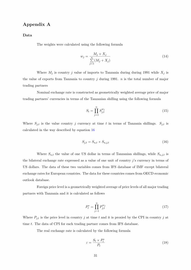
The weights were calculated using the following formula

wj = Mj +Xjn∑j=1

(Mj +Xj)(14)

Where Mj is country j value of imports to Tanzania during during 1991 while Xj is

the value of exports from Tanzania to country j during 1991. n is the total number of major

trading partners

Nominal exchange rate is constructed as geometrically weighted average price of major

trading partners’ currencies in terms of the Tanzanian shilling using the following formula

St =n∏j=1

Swj

j,t (15)

Where Sj,t is the value country j currency at time t in terms of Tanzania shillings. Sj,t is

calculated in the way described by equation 16

Sj,t = Su,t × Su,j,t (16)

Where Su,t the value of one US dollar in terms of Tanzanian shillings, while Su,j,t is

the bilateral exchange rate expressed as a value of one unit of country j’s currency in terms of

US dollars. The data of these two variables comes from IFS database of IMF except bilateral

exchange rates for European countries. The data for these countries comes from OECD economic

outlook database.

Foreign price level is a geometrically weighted average of price levels of all major trading

partners with Tanzania and it is calculated as follows

P ∗t =

n∏j=1

Pwj

j,t (17)

Where Pj,t is the price level in country j at time t and it is proxied by the CPI in country j at

time t. The data of CPI for each trading partner comes from IFS database.

The real exchange rate is calculated by the following formula

ε = St × P ∗t

Pt(18)

31

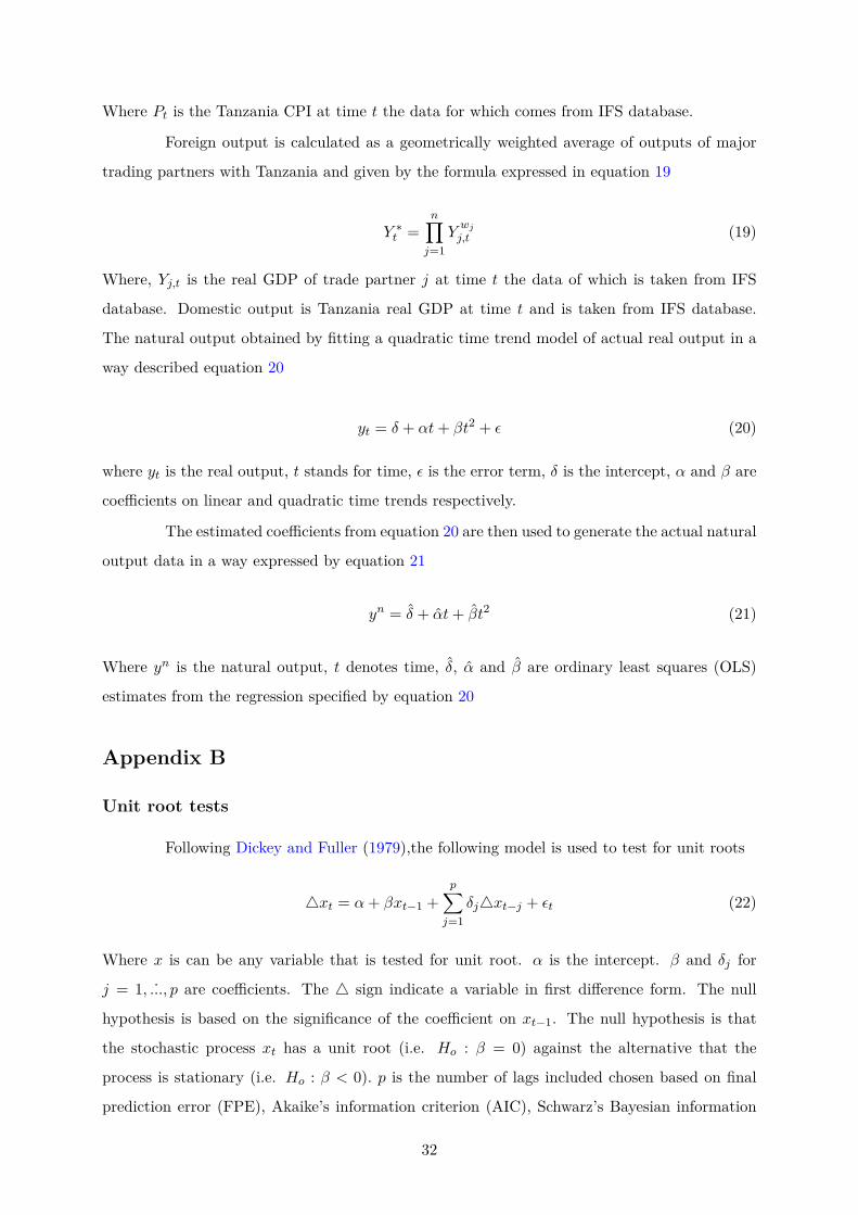
Where Pt is the Tanzania CPI at time t the data for which comes from IFS database.

Foreign output is calculated as a geometrically weighted average of outputs of major

trading partners with Tanzania and given by the formula expressed in equation 19

Y ∗t =

n∏j=1

Ywj

j,t (19)

Where, Yj,t is the real GDP of trade partner j at time t the data of which is taken from IFS

database. Domestic output is Tanzania real GDP at time t and is taken from IFS database.

The natural output obtained by fitting a quadratic time trend model of actual real output in a

way described equation 20

yt = δ + αt+ βt2 + ε (20)

where yt is the real output, t stands for time, ε is the error term, δ is the intercept, α and β are

coefficients on linear and quadratic time trends respectively.

The estimated coefficients from equation 20 are then used to generate the actual natural

output data in a way expressed by equation 21

yn = δ + αt+ βt2 (21)

Where yn is the natural output, t denotes time, δ, α and β are ordinary least squares (OLS)

estimates from the regression specified by equation 20

Appendix B

Unit root tests

Following Dickey and Fuller (1979),the following model is used to test for unit roots

4xt = α+ βxt−1 +p∑j=1

δj4xt−j + εt (22)

Where x is can be any variable that is tested for unit root. α is the intercept. β and δj for

j = 1, ˙..., p are coefficients. The 4 sign indicate a variable in first difference form. The null

hypothesis is based on the significance of the coefficient on xt−1. The null hypothesis is that

the stochastic process xt has a unit root (i.e. Ho : β = 0) against the alternative that the

process is stationary (i.e. Ho : β < 0). p is the number of lags included chosen based on final

prediction error (FPE), Akaike’s information criterion (AIC), Schwarz’s Bayesian information

32

criterion (SBIC), the Hannan Quinn Information Criterion(HQIC), the log likelihood (LL) and

likelihood-ratio (LR)13. The number of lags is actually selected on ”majority rule” basis where by

the lag leve suggested my most criteria is chosen. The estimates of these criteria are calculated

by varsoc command of stata

The results of the test by Dickey and Fuller (1979) depends on the number of lags

included. Therefore and additional unit root test based on Phillips and Perron (1988) is used.

The Phillips–Perron (PP) test is based on the estimation of equation 23

xt = α+ ρxt−1 + εt (23)

Where xt can be any variable being tested for unit root. The difference between this test and

the augmented dickey–fuller (ADF) test is the way serial correlation of the error term εt is

addressed. The ADF test uses more lagged values of the dependent variable while the PP uses

non–parametrically corrected t–tests for testing the significance of the coefficient on xt−1. The

null hypothesis in PP test is that the series has a unit root (i.e. Ho : ρ = 1) against the

alternative hypothesis that the series is stationary (i.e. Ho : ρ < 1).

Unit root test results

Tables 3 and 4 report unit root tests done based on Dickey and Fuller (1979) and

Phillips and Perron (1988) respectively.

13Please see Sukati (2013), for explanation on FPE, AIC, SBIC, HQIC, LL, LR and LR

33

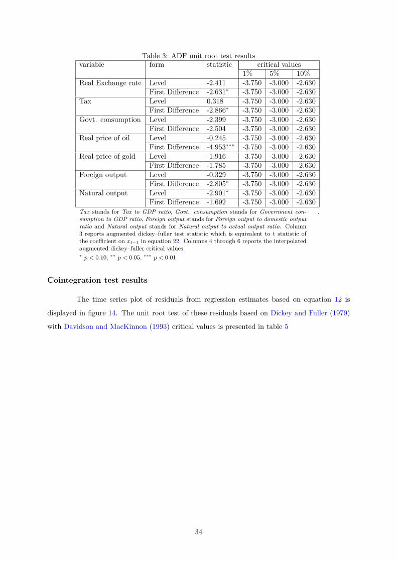
Table 3: ADF unit root test resultsvariable form statistic critical values

1% 5% 10%Real Exchange rate Level -2.411 -3.750 -3.000 -2.630

First Difference -2.631∗ -3.750 -3.000 -2.630Tax Level 0.318 -3.750 -3.000 -2.630

First Difference -2.866∗ -3.750 -3.000 -2.630Govt. consumption Level -2.399 -3.750 -3.000 -2.630

First Difference -2.504 -3.750 -3.000 -2.630Real price of oil Level -0.245 -3.750 -3.000 -2.630

First Difference -4.953∗∗∗ -3.750 -3.000 -2.630Real price of gold Level -1.916 -3.750 -3.000 -2.630

First Difference -1.785 -3.750 -3.000 -2.630Foreign output Level -0.329 -3.750 -3.000 -2.630

First Difference -2.805∗ -3.750 -3.000 -2.630Natural output Level -2.901∗ -3.750 -3.000 -2.630

First Difference -1.692 -3.750 -3.000 -2.630Tax stands for Tax to GDP ratio, Govt. consumption stands for Government con-sumption to GDP ratio, Foreign output stands for Foreign output to domestic outputratio and Natural output stands for Natural output to actual output ratio. Column3 reports augmented dickey–fuller test statistic which is equivalent to t statistic ofthe coefficient on xt−1 in equation 22. Columns 4 through 6 reports the interpolatedaugmented dickey–fuller critical values

.

∗ p < 0.10, ∗∗ p < 0.05, ∗∗∗ p < 0.01

Cointegration test results

The time series plot of residuals from regression estimates based on equation 12 is

displayed in figure 14. The unit root test of these residuals based on Dickey and Fuller (1979)

with Davidson and MacKinnon (1993) critical values is presented in table 5

34

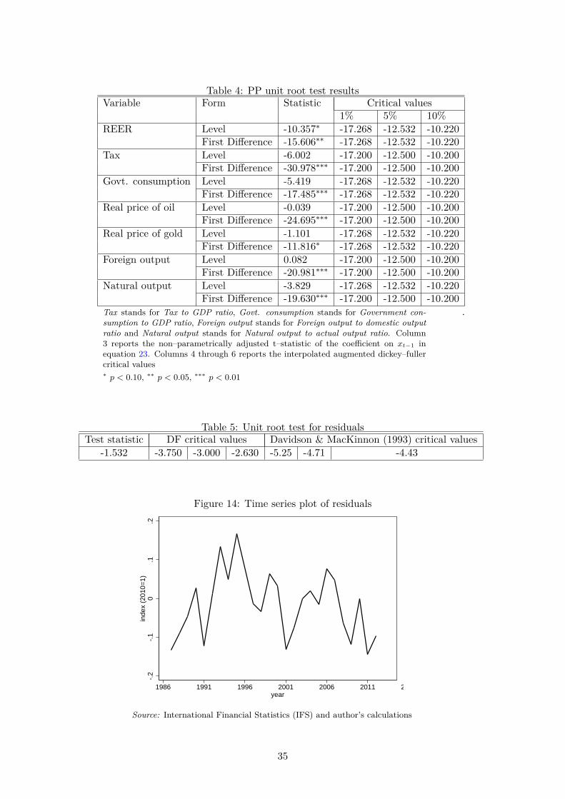
Table 4: PP unit root test resultsVariable Form Statistic Critical values

1% 5% 10%REER Level -10.357∗ -17.268 -12.532 -10.220

First Difference -15.606∗∗ -17.268 -12.532 -10.220Tax Level -6.002 -17.200 -12.500 -10.200

First Difference -30.978∗∗∗ -17.200 -12.500 -10.200Govt. consumption Level -5.419 -17.268 -12.532 -10.220

First Difference -17.485∗∗∗ -17.268 -12.532 -10.220Real price of oil Level -0.039 -17.200 -12.500 -10.200

First Difference -24.695∗∗∗ -17.200 -12.500 -10.200Real price of gold Level -1.101 -17.268 -12.532 -10.220

First Difference -11.816∗ -17.268 -12.532 -10.220Foreign output Level 0.082 -17.200 -12.500 -10.200

First Difference -20.981∗∗∗ -17.200 -12.500 -10.200Natural output Level -3.829 -17.268 -12.532 -10.220

First Difference -19.630∗∗∗ -17.200 -12.500 -10.200Tax stands for Tax to GDP ratio, Govt. consumption stands for Government con-sumption to GDP ratio, Foreign output stands for Foreign output to domestic outputratio and Natural output stands for Natural output to actual output ratio. Column3 reports the non–parametrically adjusted t–statistic of the coefficient on xt−1 inequation 23. Columns 4 through 6 reports the interpolated augmented dickey–fullercritical values

.

∗ p < 0.10, ∗∗ p < 0.05, ∗∗∗ p < 0.01

Table 5: Unit root test for residualsTest statistic DF critical values Davidson & MacKinnon (1993) critical values

-1.532 -3.750 -3.000 -2.630 -5.25 -4.71 -4.43

Figure 14: Time series plot of residuals

-.2

-.1

0.1

.2in

dex

(201

0=1)

1986 1991 1996 2001 2006 2011 2016year

Source: International Financial Statistics (IFS) and author’s calculations

35

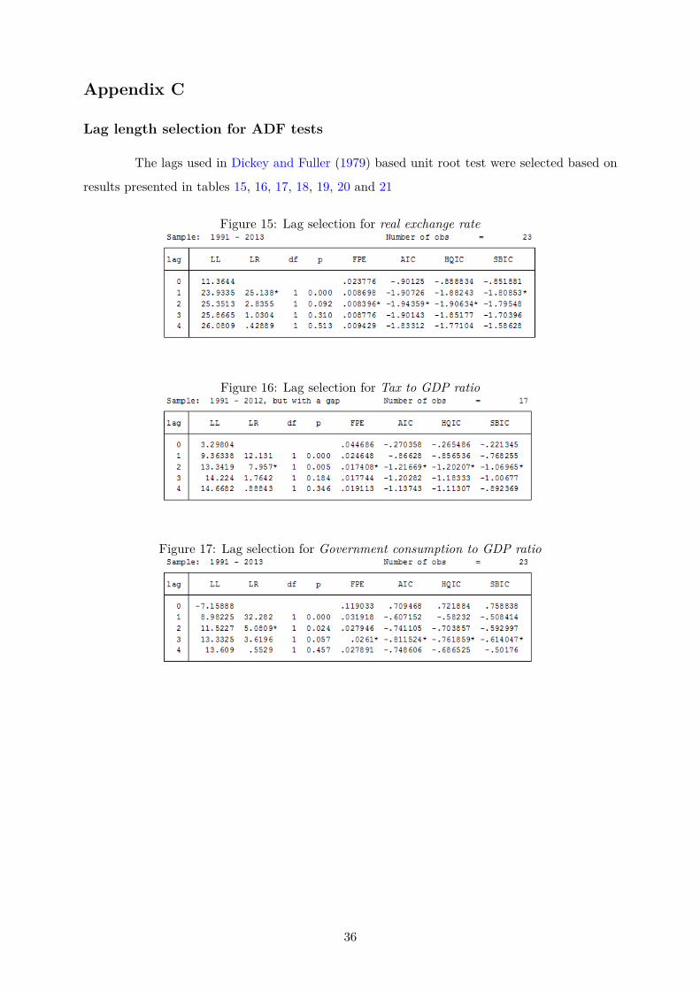
Appendix C

Lag length selection for ADF tests

The lags used in Dickey and Fuller (1979) based unit root test were selected based on

results presented in tables 15, 16, 17, 18, 19, 20 and 21

Figure 15: Lag selection for real exchange rate

Figure 16: Lag selection for Tax to GDP ratio

Figure 17: Lag selection for Government consumption to GDP ratio

36

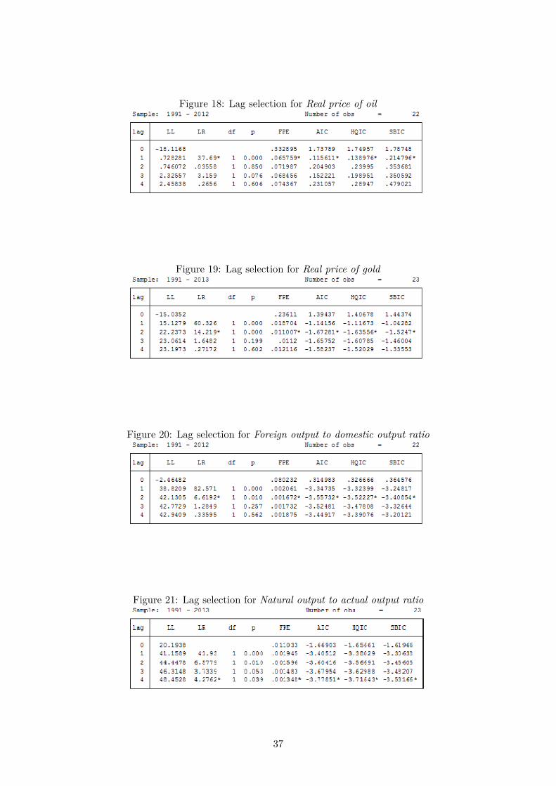
Figure 18: Lag selection for Real price of oil

Figure 19: Lag selection for Real price of gold

Figure 20: Lag selection for Foreign output to domestic output ratio

Figure 21: Lag selection for Natural output to actual output ratio

37