Embed Size (px)
Citation preview

Determinants of House Prices in NineAsia-Pacific Economies∗
Eloisa T. Glindro,a Tientip Subhanij,b Jessica Szeto,c andHaibin Zhud
aCenter for Monetary and Financial Policy, Bangko Sentral ng PilipinasbEconomic Research Department, Bank of Thailand
cEconomic Research, Hong Kong Monetary AuthoritydBank for International Settlements
The paper investigates the characteristics of house pricedynamics and the role of institutional factors in nine Asia-Pacific economies during 1993–2006. On average, house pricestend to be more volatile in markets with lower supply elastic-ity and a more flexible business environment. At the nationallevel, the current run-up in house prices mainly reflects adjust-ment to improved fundamentals rather than speculative hous-ing bubbles. However, evidence of bubbles does exist in somemarket segments.
JEL Codes: G12, R31.
∗This paper is a joint research project of the Bank for International Set-tlements, Bangko Sentral ng Pilipinas, the Bank of Thailand, and the HongKong Monetary Authority under the auspices of the Asian Research Programof the Bank for International Settlements. The authors are particularly grate-ful to Eli Remolona for his initiation of this research project and for hisinsightful comments at various stages. The authors would like to thank ClaudioBorio, Jacob Gyntelberg, Charles Leung, Frank Leung, Chu-Chia Lin, PatrickMcGuire, Dubravko Mihaljek, Pichit Patrawimolpon, Marc Oliver Rieger, NilokaTarashev, Kostas Tsatsaronis, Goetz von Peter, two anonymous referees, andworkshop participants at HKIMR, BSP, BOT, BIS, the 2008 Asian FinanceAssociation annual meeting, and the 2008 Asian Real Estate Society annualconference for helpful comments. Gert Schnabel provided valuable support fordata compilation. The views expressed herein are those of the authors anddo not necessarily reflect those of the authors’ affiliated institutions. AuthorE-mails: Glindro: [email protected]; Subhanij: [email protected]; Szeto:jessica wk [email protected]; Zhu: [email protected].
163

164 International Journal of Central Banking September 2011
1. Introduction
House price risk has attracted much attention in recent years. Anumber of industrialized economies, including the United States, theUnited Kingdom, and Spain, had witnessed a protracted period ofsignificant increases in house prices in the mid-2000s. The perceivedlower risk encouraged lax lending criteria in mortgage markets,which greatly contributed to the U.S. subprime crisis and the conse-quent global financial crisis. Just as suggested by previous studies,house price fluctuations have caused a major impact on householdconsumption,1 the banking system, and the real economy.2
By comparison, housing markets in most Asian economies wererelatively tranquil during the same period. In recent years, however,there have been growing concerns about the housing market in afew economies. China, Hong Kong SAR (Hong Kong hereafter), andSouth Korea (Korea hereafter) have witnessed very strong houseprice inflation in the past several years (see figure 1). Given the not-so-distant experience of financial crises in this region (such as the1997 Asian crisis and the so-called lost decade in Japan), in whichbooms and busts in real estate markets played a crucial role, thequestion is whether the observed house price growth can potentiallylead to bubble episodes.
There are two opposite views regarding the issue of possible hous-ing bubbles in Asia. A pessimistic view argues that house prices havebeen overvalued in many countries and will face downward correc-tions in the near future. At the extreme, some consider it evidence ofnew speculative housing bubbles and call for supervisors and centralbanks to adopt prudential measures to contain them. By contrast,the optimistic view considers this round of house price growth as amanifestation of recovery from the previous crisis episode. The opti-mists argue that in the aftermath of previous crises, house priceswere too low compared with their fundamental values. Therefore,
1See Girouard and Blondal (2001), Cocco (2005), Yao and Zhang (2005), andCampbell and Cocco (2007). In addition, empirical findings (see Helbling andTerrones 2003; Case, Quigley, and Shiller 2005) also suggest that housing tendsto have a bigger wealth effect than financial assets.
2Bernanke and Gertler (1995), Bernanke, Gertler, and Gilchrist (1996), Kiyo-taki and Moore (1997), Aoki, Proudman, and Vlieghe (2004), and Gan (2007)show the strong linkages between the housing cycle and the credit cycle.

Vol. 7 No. 3 Determinants of House Prices 165
Figure 1. House Price Inflation (yoy) in AverageResidential Markets, 1994–2006
Note: AU: Australia; CN: China; HK: Hong Kong SAR; KR: Korea; MY:Malaysia; NZ: New Zealand; PH: the Philippines; SG: Singapore; TH: Thailand.
the rebound of house prices from the very low levels is simply a con-sequence of the mean-reversion process. Moreover, the liberalizationof housing markets and housing finance systems in the past decade,including a general trend towards more market-based housing mar-kets, greater availability of mortgage products, and more liquid sec-ondary mortgage markets, has arguably improved market efficiency,stimulated demand, and contributed to house price growth.

166 International Journal of Central Banking September 2011
The paper sheds some light on this debate by examining houseprice developments in nine economies in the Asia-Pacific area,which include Australia, China, Hong Kong, Korea, Malaysia, NewZealand, the Philippines, Singapore, and Thailand.3 Specifically,it attempts to address the following questions: What determinesthe fundamental values and short-term dynamics of house pricesin Asia? What is the impact of institutional factors on houseprice movements? How can one gauge whether there is a housingbubble? To address these questions, we adopt the error-correctionframework used by Capozza et al. (2002). The key results are asfollows.
First, we find that the patterns of national house price dynam-ics exhibit significant cross-country heterogeneity. Moreover, institu-tional factors matter. In particular, distinction in house price dynam-ics can be largely attributable to cross-country differences in landsupply and business environments.
Second, based on the econometric analysis, we characterize houseprice movements as the sum of three separate factors: (i) the funda-mental value of housing (a trend term) that is determined by longer-term economic conditions and institutional arrangements, (ii) thedeviation from fundamental values that is attributable to frictions inthe housing market (a cyclical term), and (iii) an irrational or “bub-ble” component that is likely to be driven by overly optimistic expec-tations (an error term). Applying this approach to nine economiesin Asia and the Pacific, we find that national house price movementsbefore the onset of the global financial crisis mainly reflected changesin fundamental values or cyclical adjustments towards fundamentals.In other words, there is little evidence of housing bubbles in theseeconomies, at least at the national levels.
The decomposition analysis has important policy implications. Itallows for distinction between house price overvaluation (the sum ofcyclical and error components) and a housing bubble. Policy rec-ommendations are different accordingly. To mitigate house priceovervaluation that is driven by cyclical movements related to mar-ket frictions, a policymaker should probably focus on measures that
3In this paper, we use the term “Asia” to represent the set of economiesmentioned above.

Vol. 7 No. 3 Determinants of House Prices 167
aim at reducing the magnitude and frequency of house price cycles,such as loosening land use regulation, improving information avail-ability and transparency, and enhancing the freedom in the busi-ness environment. By contrast, to contain a bubble, the policymakershould instead adopt measures that control unwarranted high expec-tations of capital gains or overconfidence of investors in the housingmarket.
The remainder of the paper is organized as follows. Section 2 pro-vides an overview of the literature and highlights the contributionsof this study. Section 3 describes the data and explains the empir-ical method used to examine the questions of interest, and section4 discusses the empirical results. Finally, section 5 concludes andprovides some policy perspectives.
2. A Review of the Literature and Our Contributions
2.1 Literature Review
To monitor the housing market, it is important to understand firstthe determinants of house prices. Housing is a special type of assetthat has a dual role as a consumption and an investment good.From the long-term perspective, the equilibrium price a householdis willing to pay for a house should be equal to the present dis-counted value of future services provided by the property, i.e., thepresent value of future rents and the discounted resale value of thehouse. From the short-term perspective, however, house prices candeviate from their fundamental values, on account of some uniquecharacteristics of the real estate market (such as asset heterogeneity,downpayment requirements, short-sale restrictions, lack of informa-tion, and lags in supply). For instance, Leung and Chen (2006) showthat land prices can exhibit cycles due to the role of intertempo-ral elasticity of substitution. Wheaton (1999) and Davis and Zhu(2004) develop a model in which there are lags in the supply of realestate and bank lending decisions depend on the property’s currentmarket value (labeled as historical dependence). They show that inresponse to a change in fundamental values, real estate prices caneither converge to or exhibit oscillation around the new equilibriumvalues.

168 International Journal of Central Banking September 2011
Existing literature suggest that house price movements areclosely related to a common set of macroeconomic variables, market-specific conditions, and housing finance characteristics. Hofmann(2004) and Tsatsaronis and Zhu (2004) examine the determinants ofhouse prices in a number of industrialized economies and find thateconomic growth, inflation, interest rates, bank lending, and equityprices have significant explanatory power. The linkage between prop-erty and bank lending is particularly remarkable, as also highlightedby Herring and Wachter (1999), Chen (2001), Hilbers, Lei, andZacho (2001), and Gerlach and Peng (2005). This is not surprisinggiven the heavy reliance on mortgage financing in the housing mar-ket. Moreover, housing markets are local in nature. Garmaise andMoskowitz (2004) find strong evidence that asymmetric informationabout local market conditions plays an important role in reshap-ing property transactions and determining the choice of financing.Green, Malpezzi, and Mayo (2005) find that house price dynam-ics differ across metropolitan areas with different degrees of supplyelasticities.
On the important issue of detecting house price bubbles, thereare several approaches adopted in the literature. Bubble episodesare sometimes assessed by market analysts in terms of the price-rent ratio or the price-income ratio. A bubble is typically identi-fied if the current ratio is well above the historical average level.These measures, however, may be inadequate barometers for policyanalysis because they ignore the variation in “equilibrium” price-rent(or price-income) ratios driven by fluctuations in economic funda-mentals (e.g., rent growth, income growth, and the desired rate ofreturn). To overcome these problems, two methods have been pro-posed. The first method compares observed price-rent ratios withtime-varying discount factors that are determined by the user costof owning a house, which consists of mortgage interest, property tax,maintenance cost, tax deductibility of mortgage interest payments,and an additional risk premium (see Himmelberg, Mayer, and Sinai2005; Ayuso and Restoy 2006; Brunnermeier and Julliard 2008).The second method compares observed house prices with funda-mental values that are predicted based on the long-run relationshipbetween house prices and macroeconomic factors (see Abraham andHendershott 1996; Kalra, Mihaljek, and Duenwald 2000; Capozza etal. 2002, and Holly, Pesaran, and Yamagata 2010, for example). In

Vol. 7 No. 3 Determinants of House Prices 169
this paper, we adopt the second method because of data limitationsand heterogeneity in what constitutes appropriate measurement ofthe user cost across countries.4
2.2 Contributions of This Study
This paper examines the determinants of house price fundamentalsand short-term dynamics in nine Asia-Pacific economies and thirty-two cities/market segments in these economies, discusses the roleof distinctive institutional arrangements, and explores the possibleemergence of housing bubbles. The empirical framework used in thisstudy follows Capozza et al. (2002), which examines the long-termand short-term dynamics of house prices in a three-step econometricanalysis and characterizes the pattern of house price dynamics viaa combination of serial correlation and mean-reversion coefficients(see section 3.2).5 However, our study extends the previous analysisin three important ways.
First, previous studies have mainly focused on the lessons fromindustrialized economies. This study is one of the first papers toinvestigate the evidence in the Asia-Pacific, which has gained anincreasing importance in the global economy. Given the remarkableexperience of housing bubbles in many of the Asian economies inthe 1990s, it is interesting to examine the house price movementsafter the crisis episode. In addition, Asia-Pacific housing marketsdiffer substantially from those of industrialized economies in termsof the level of economic and financial market developments as well asinstitutional arrangements. In this regard, the results could providecomplementary views to existing studies.
4Rent data in our sample economies are often not available or not comparablewith the house price data (referring to different samples). It is also difficult toquantify some key components of the user cost, such as the tax deductibility andthe risk premium in individual markets.
5The methodology is also similar to that of Holly, Pesaran, and Yamagata(2010), which determines the extent to which real house prices in forty-nine U.S.states (over a sample period of twenty-nine years) are driven by fundamentalssuch as real per capita disposable income and common shocks. Their study alsolooks into the speed of adjustment of real house prices to macroeconomic andlocal disturbances. However, it differs from ours in that it explicitly examines therole of spatial factors—in particular, the effect of contiguous states by use of aweighting matrix.

170 International Journal of Central Banking September 2011
Second, our analysis emphasizes the impact of institutional fac-tors on house price dynamics. The original paper by Capozza et al.(2002) analyzes the impact of a number of factors (such as popula-tion, income, and construction cost) on house price dynamics, butthe role of institutions in not examined.6 In this study, we constructa composite measure of institutional factors on the basis of four dif-ferent aspects of market developments. This measure not only differsacross countries but also varies over time. Indeed, our analysis showsthat the institutional factor is important in explaining house pricedetermination in the nine Asian economies.
Third, we extend the housing bubble literature by (i) distinguish-ing between house price growth and house price overvaluation, and(ii) decomposing house price overvaluation into cyclical and bub-ble components. The first distinction is quite obvious. House pricegrowth may simply reflect the increase in the fundamental value ofthe property, which is driven by income, mortgage rates, and otherfactors. By contrast, house price overvaluation refers to the situ-ation that current house prices are higher than the fundamentalvalues. The second distinction is more subtle. A bubble is necessar-ily related to house price overvaluation, but not vice versa. This isbecause frictions in the housing market, including lags in supply andcredit market imperfections, may cause house prices to deviate fromtheir fundamental values in the short term. In this paper, this cycli-cal component of house price overvaluation is captured by the serialcorrelation and mean reversion of house price dynamics. The unex-plained part is then defined as the bubble component that is morelikely to be driven by overly optimistic expectations in the housingmarket. Understanding the source of house price overvaluation shedsimportant light on the appropriate policy actions.
3. Data Description and Empirical Methodology
In this section, we briefly describe the data used in this study andoutline the empirical methodology adopted to characterize house
6One reason for the omission of institutional factors is that Capozza et al.examine the house price determination in a number of metropolitan areas in theUnited States. The institutional arrangements—such as business freedom, legalframework, and property rights protection—have little variation across areas.

Vol. 7 No. 3 Determinants of House Prices 171
price dynamics and to analyze the bubble component in house priceovervaluation.
3.1 Data Description
Quarterly data for the residential property sector in nine economiesand thirty-two cities/market segments in Asia7 were used in theanalysis. Where data are available, quarterly series spanning theperiod 1993–2006 were used.
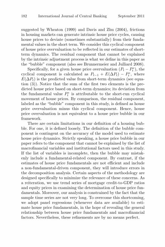
The house price data have certain limitations. There are somesubtle variations in the definition of house prices used in the esti-mation (see table 6 in the appendix). While some series are derivedusing a hedonic pricing method, some are simply based on floor-areaprices collected by land registration authorities and the private sec-tor, for which no quality adjustment was done. Moreover, the timeseries are relatively short. Except for Hong Kong, Korea, Singapore,and Thailand, quarterly house price data only cover the post-Asian-crisis period. However, longer time series of house price data maynot necessarily improve the results in the sense that many Asianeconomies have experienced a regime shift in housing markets andhousing finance systems, which has arguably led to discontinuitiesin the dynamics.
Apart from residential property prices, other series used in thisstudy include real GDP, population, construction cost index, landsupply index, mortgage credit-to-GDP ratios, real mortgage rates,real effective exchange rates, stock price index, and the first principalcomponent of four institutional indices—the business freedom index,the financial freedom index, the corruption index, and the property
7Other emerging Asian economies are excluded from this study because houseprice data are not available. At the city level, Beijing, Chongqing, Guangzhou,Shanghai, Shenzhen, and Tianjin are included in China; Busan, Daegu, Dae-jon, Gwangju, Incheon, Seoul, and Ulsan are included in Korea; Johor, KualaLumpur, Pahang, Perak, and Pinang are included in Malaysia; and Caloocan,Makati, Manila, Pasay, Pasig, and Quezon are included in the Philippines. Inaddition, for Hong Kong, Singapore, Bangkok, Manila, and Kuala Lumpur, thereare two separate sets of house prices for the average market and for the luxurymarket segments, respectively.
172 International Journal of Central Banking September 2011
rights index8—which we believe to be the most relevant representa-tion of the institutional factors that affect the housing market and,hence, house price movements. Table 1 reports summary statistics ofkey variables used in this study, for each country and for the wholesample.
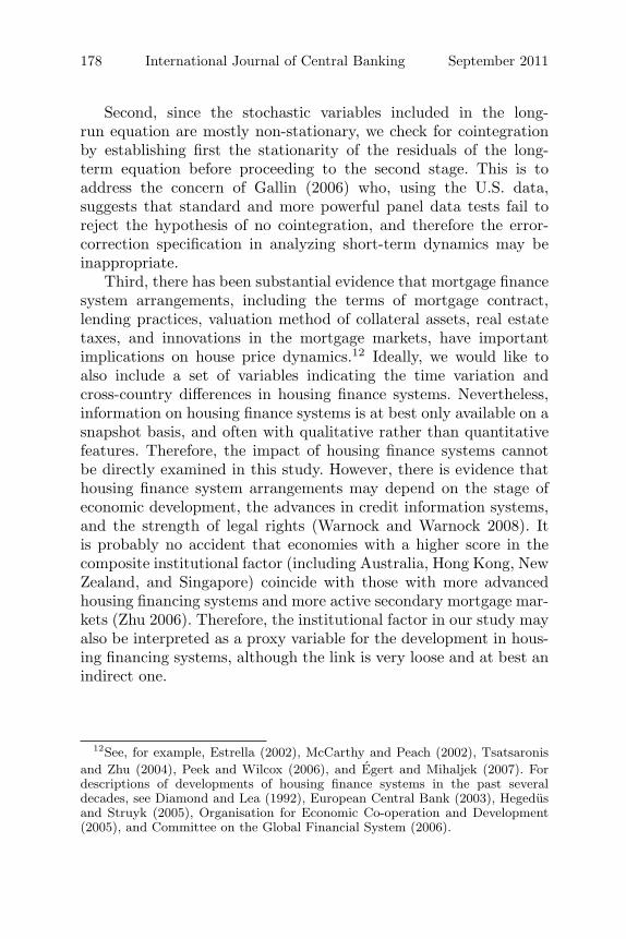
3.2 Empirical Methodology: Characterizing House PriceDynamics
We follow the framework used by Capozza et al. (2002) to inves-tigate the long-term and short-term determinants of house pricemovements. The approach can be divided into three steps. In thefirst step, the fundamental value of housing is calculated. In the sec-ond step, the short-term dynamics of house prices are characterizedby a mean-reversion process to their fundamental values and by aserial correlation movement. In the third step, the degree of persis-tence in house prices and the relative speed by which house pricesrevert to their fundamental values are assessed by interacting the ser-ial correlation and mean-reversion coefficients with macroeconomicand housing market variables as well as institutional factors.
3.2.1 The Fundamental Value of Housing
It is assumed that in each period and in each area (a country or acity), there is a fundamental value of housing that is largely deter-mined by economic conditions and institutional arrangements:
P ∗it = f(Xit), (1)
where P ∗it is the log of the real fundamental value of house prices
in country i at time t, f(·) is a function, and Xit is a vector
8The business freedom index measures the ability to create, operate, and closean enterprise quickly and easily. Burdensome, redundant regulatory rules are themost harmful barriers to business freedom. The financial freedom index is a meas-ure of banking security as well as independence from government control. Thecorruption index is a measure of the perception of corruption in the businessenvironment, including levels of governmental legal, judicial, and administrativecorruption. The property rights index measures the ability of individuals to accu-mulate private property, secured by clear laws that are fully enforced by the state(www.heritage.org).

Vol. 7 No. 3 Determinants of House Prices 173
Tab
le1.
Sum
mar
ySta
tist
ics
Var
iable
sTot
alA
UC
NH
KK
RM
YN
ZP
HSG
TH
RH
P10
9.07
109.
0510
8.35
114.
2811
6.87
102.
2911
6.87
105.
9595
.73
109.
5020
.026
.010
.027
.113
.43.
724
.620
.213
.911
.7Δ
RH
P(%
)0.
191.
080.
80−
0.25
−0.
450.
311.
41−
0.93
0.60
−0.
365.
51.
80.
96.
32.
21.
12.
012
.54.
15.
0Δ
Rea
lG
DP
(%)
5.12
3.72
9.08
4.33
5.26
5.66
3.51
4.36
6.18
34.
014.
01.
21.
54.
34.
34.
91.
72.
04.
85.
3Pop
ulat
ion
(mn)
161.
4119
.09
1249
.03
6.57
46.3
722
.62
3.87
73.7
33.
8761
.73
380.
50.
939
.50.
21.
32.
10.
25.
60.
32.
4R
MR
(%)
4.84
5.13
2.32
4.75
2.98
3.33
6.60
6.06
5.37
5.64
3.3
1.7
6.1
3.9
0.7
2.1
1.3
2.4
1.3
2.4
Mor
t/G
DP
(%)
97.0
915
1.76
8.22
164.
217.
6091
.26
252.
4920
.55
147.
1915
.38
82.1
40.6
1.7
34.5
7.6
15.1
37.5
5.9
31.3
1.4
LSI
147.
0510
5.95
108.
4791
.74
123.
1887
.94
119.
2611
5.26
138.
7544
0.68
185.
714
.556
.447
.832
.818
.329
.130
.513
7.8
448.
7R
CC
102.
5399
.39
108.
5192
.15
103.
9610
2.02
102.
3410
5.12
103.
6010
4.47
7.7
3.1
11.1
5.9
4.9
3.7
3.5
10.1
4.4
5.9
EP
I10
4.16
110.
8994
.48
93.2
410
3.46
106.
1412
0.41
102.
7210
0.31
105.
8313
.310
.48.
810
.511
.011
.113
.512
.65.
712
.0R
EE
R11
0.32
93.8
273
.67
74.1
311
0.41
99.7
610
8.94
130.
9990
.00
106.
0457
.927
.821
.217
.832
.322
.716
.741
.816
.011
.7
(con
tinu
ed)

174 International Journal of Central Banking September 2011
Tab
le1.
(Con
tinued
)
Var
iable
sTot
alA
UC
NH
KK
RM
YN
ZP
HSG
TH
BFI
60.6
460
.37
31.7
489
.78
52.8
061
.73
72.5
535
.35
90.3
652
.12
21.4
13.9
5.8
0.8
9.4
10.0
8.1
9.4
1.2
7.1
FFI
63.4
690
4088
.33
56.6
740
9048
.33
7050
21.0
010
.15.
69.
510
.10
5.6
00
CI
64.8
383
.33
31.5
8385
.67
58.7
561
.583
92.1
827
91.0
854
.58
25.1
8.1
2.1
5.3
13.5
10.1
2.5
5.5
1.5
18.5
PR
I72
.80
9030
9083
.33
6090
53.3
390
7022
.00
00
9.5
10.1
016
.20
14.3
Note
s:T
his
table
repor
tsth
esu
mm
ary
stat
isti
csof
key
vari
able
s,in
each
count
ryan
din
the
whol
esa
mple
(199
3–20
06).
For
each
vari
able
,th
enu
mber
sin
the
firs
tro
wre
pre
sent
sam
ple
mea
nan
dth
ose
inth
ese
cond
row
repre
sent
the
stan
dar
ddev
iati
on.R
HP
:re
alhou
sepri
cein
dex
;Δ
RH
P:re
alhou
sepri
cegr
owth
(quar
terl
y);R
MR
:re
alm
ortg
age
rate
;M
ort/
GD
P:m
ortg
age
cred
it/G
DP
rati
o;LSI:
land
supply
index
;R
CC
:re
alco
nst
ruct
ion
cost
index
;E
PI:
equity
pri
cein
dex
;R
EE
R:re
aleff
ecti
veex
chan
gera
te;B
FI:
busi
nes
sfr
eedom
index
;FFI:
finan
cial
free
dom
index
;C
I:co
rrupti
onin
dex
;P
RI:
pro
per
tyri
ghts
index
.

Vol. 7 No. 3 Determinants of House Prices 175
of macroeconomic and institutional variables that determine houseprice fundamentals.
We adopt a general-to-specific approach in assessing the determi-nants of house price fundamentals. We start by including all the iden-tified explanatory factors in our list to investigate their long-termrelationship with house prices, using either single-equation ordinaryleast squares (OLS) or panel data techniques.9 Only regressors foundto be significant at the 5 percent level are retained in the final modelspecification. We choose four blocks of explanatory variables basedon theoretic reasoning or previous empirical work.
The first block of explanatory variables consists of demand-sidefactors, including real GDP, population, the real mortgage rate, andthe mortgage credit-to-GDP ratio. The inclusion of the real mort-gage rate and mortgage credit is premised on the bank-dominatednature of financial systems across Asia. We posit that higher incomeand higher population tend to encourage greater demand for newhousing and housing improvements. In addition, mortgage rate isexpected to be negatively related to housing prices. A higher mort-gage rate entails higher amortization, which, in turn, impinges on thecash flow of households. This reduces the affordability of new hous-ing, dampens housing demand, and pushes down house prices. Simi-larly, the growth in mortgage credit increases the financing capacityof households and stimulates the demand for housing.
The second block of variables is made up of supply-side fac-tors consisting of the land supply index and real construction cost.The land supply index, which refers to the building permit index inmost countries, measures the flexibility of supply to demand con-ditions. In the long run, an increase in land supply tends to bringdown house prices. By contrast, the burden of higher real construc-tion costs will be shared by purchasers, and we expect a positiverelationship between real construction costs and equilibrium houseprices.
The third block of variables consists of prices of other types ofassets such as equity prices and exchange rates. It is well docu-mented that house prices tend to co-move with other asset prices.For instance, Sutton (2002) and Borio and McGuire (2004) find
9To avoid simultaneity bias, contemporaneous variables are instrumented withown lags.

176 International Journal of Central Banking September 2011
strong linkages between equity price and house price movements.The direction of such linkage, from a theoretical perspective, is notclear, as the substitution effect and wealth effect point in oppositedirections.10 Moreover, a real effective exchange rate appreciationis expected to exert positive influence on property market prices,particularly in markets where there is substantial demand fromnon-residents for investment purposes. In countries where foreigninvestment plays an important role in the economy, such as in Asia,an exchange rate appreciation is normally associated with housingbooms.
Lastly, the fourth block consists of an institutional factor thatattempts to account for the impact of market arrangements on equi-librium house prices. The institutional factor is constructed as thefirst principal component of four index variables compiled by theHeritage Foundation: the business freedom index, the corruptionindex, the financial sector index, and the property rights index.It is constructed so that we can examine the impact of business,regulatory, and financial conditions on the determination of houseprices in a parsimonious way. The first principal component hasapproximately equal weights of the four indices and accounts forabout 80 percent of the variability in the four-index series. A higherscore in the institutional factor is associated with higher businessfreedom, better regulatory conditions, lower corruption, a greaterrange of intermediation functions by the financial sector, a higherdegree of flexibility in acquiring land, and better legal protectionto land/home owners. As shown in figure 2, the institutional fac-tor exhibits substantial time variation and cross-country differences.The nine economies can be easily divided into two groups: Aus-tralia, Hong Kong, New Zealand, and Singapore are classified asmore business friendly and the other five economies as less so. Overtime, Australia and New Zealand experienced major improvements,while Malaysia and Thailand witnessed deterioration in their busi-ness environment during the period under review.
10A substitution effect predicts a negative relationship between the prices ofthe two assets, as the high return in one market tends to cause investors to leavethe other market. A wealth effect, by contrast, predicts a positive relationshipbecause the high return in one market will increase the total wealth of investorsand their capability of investing in other assets.

Vol. 7 No. 3 Determinants of House Prices 177
Figure 2. Time Series of Institutional Factors
Notes: The figure plots the time series of the institutional factor in each ofthe nine economies under review. The institutional factor is defined as the firstprincipal component of four index series: the business freedom index, the finan-cial freedom index, the corruption index, and the property rights index. Theinstitutional factor is rescaled into a range between 0 and 1.
Several remarks are worth mentioning here. First, we use thetrend component of mortgage credit-to-GDP ratios and equity pricesin explaining the long-run house price fundamentals. This modi-fication recognizes that the original raw series may contain non-fundamental components and that a housing bubble often comestogether with excessive growth in mortgage credit and sometimesinteracts with extreme equity price movements. Using the trendseries of the two variables can ensure that our estimates of houseprice fundamentals are not contaminated by the non-fundamental(or bubble) components and, by extension, minimize potential errorsin the analysis.11
11We do recognize, nonetheless, that the trend needs to be estimated over along enough sample period that is not dominated by bubble episodes. Data con-straints, however, prevented us from estimating the trend series over a longerperiod of time.
178 International Journal of Central Banking September 2011
Second, since the stochastic variables included in the long-run equation are mostly non-stationary, we check for cointegrationby establishing first the stationarity of the residuals of the long-term equation before proceeding to the second stage. This is toaddress the concern of Gallin (2006) who, using the U.S. data,suggests that standard and more powerful panel data tests fail toreject the hypothesis of no cointegration, and therefore the error-correction specification in analyzing short-term dynamics may beinappropriate.
Third, there has been substantial evidence that mortgage financesystem arrangements, including the terms of mortgage contract,lending practices, valuation method of collateral assets, real estatetaxes, and innovations in the mortgage markets, have importantimplications on house price dynamics.12 Ideally, we would like toalso include a set of variables indicating the time variation andcross-country differences in housing finance systems. Nevertheless,information on housing finance systems is at best only available on asnapshot basis, and often with qualitative rather than quantitativefeatures. Therefore, the impact of housing finance systems cannotbe directly examined in this study. However, there is evidence thathousing finance system arrangements may depend on the stage ofeconomic development, the advances in credit information systems,and the strength of legal rights (Warnock and Warnock 2008). Itis probably no accident that economies with a higher score in thecomposite institutional factor (including Australia, Hong Kong, NewZealand, and Singapore) coincide with those with more advancedhousing financing systems and more active secondary mortgage mar-kets (Zhu 2006). Therefore, the institutional factor in our study mayalso be interpreted as a proxy variable for the development in hous-ing financing systems, although the link is very loose and at best anindirect one.
12See, for example, Estrella (2002), McCarthy and Peach (2002), Tsatsaronisand Zhu (2004), Peek and Wilcox (2006), and Egert and Mihaljek (2007). Fordescriptions of developments of housing finance systems in the past severaldecades, see Diamond and Lea (1992), European Central Bank (2003), Hegedusand Struyk (2005), Organisation for Economic Co-operation and Development(2005), and Committee on the Global Financial System (2006).

Vol. 7 No. 3 Determinants of House Prices 179
3.2.2 Short-Run Dynamics of House Prices
Arguably, equilibrium is rarely observed in the short run due to theinability of economic agents to adjust instantaneously to new infor-mation. As suggested by Capozza et al. (2002), house price changesin the short run are governed by reversion to fundamental valuesand by serial correlation according to
ΔPit = αΔPi,t−1 + β(P ∗
i,t−1 − Pi,t−1)
+ γΔP ∗it, (2)
where Pit is the log of (observed) real house prices and Δ is thedifference operator.
If housing markets are efficient, prices will adjust instantaneouslysuch that γ = 1 and α = 0. Considering that housing is a slow-clearing durable asset, it is reasonable to expect that current pricechanges are partly governed by previous changes in own price levels(α > 0), by the deviation from the fundamental value (0 < β < 1),and partly by contemporaneous adjustment to changes in fundamen-tals (0 < γ < 1).
Capozza et al. (2002) shows that the above model specificationallows for rich dynamics of house price movements, depending onthe size of the coefficients α and β. The various patterns of houseprice dynamics can be summarized in figure 3.13
To summarize, the sufficient and necessary condition for a houseprice cycle to be stable is α < 1 and β > 0. If satisfied, there aretwo possible types of house price movements:
(i) If (1 + α − β)2 − 4α ≥ 0 (region I in figure 3), the houseprice will converge monotonically to the equilibrium level. Inthis case, the transitory path itself does not generate houseprice cycles. In other words, house price cycles only reflectcyclical movements in their fundamental values. The speed ofconvergence depends on the magnitude of the two coefficients:the convergence rate is generally higher when α and β arelarger.
(ii) If (1 + α − β)2 − 4α > 0 (region II in figure 3), the transi-tory path in response to changes in equilibrium house price
13The strict proof is available upon request.

180 International Journal of Central Banking September 2011
Figure 3. Characteristics of House Price Dynamics:Illustration
Note: The figure plots the characteristics of house price dynamics for differentcombinations of persistence (α) and mean-reversion (β) parameters.
values exhibits a damped fluctuation around the equilibriumlevel. The magnitude of the two coefficients, again, determinesthe property of the oscillation. Generally, a higher α impliesa higher amplitude and a higher β implies a higher frequencyof the fluctuation process.
If α ≥ 1 or β ≤ 0, then the house price cycle is unstable. Houseprices may either diverge or exhibit an amplified fluctuation awayfrom the equilibrium level, but such movements cannot be sustain-able. In general, such features should not exist in any housing marketfor a prolonged period.
3.2.3 Endogenous Adjustment in Short-Run Dynamics
Given the importance of mean-reversion and serial correlation coef-ficients, the next step is to analyze what determines α and β.
Vol. 7 No. 3 Determinants of House Prices 181
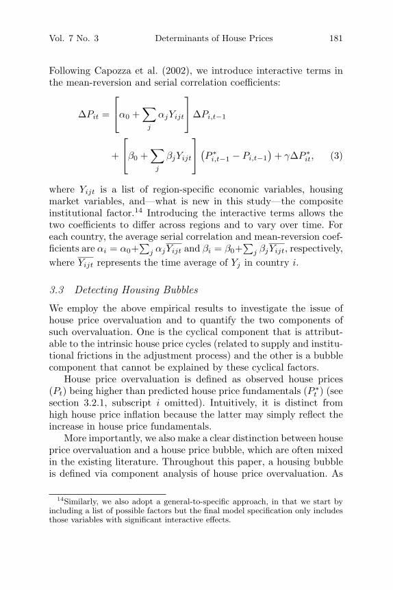
Following Capozza et al. (2002), we introduce interactive terms inthe mean-reversion and serial correlation coefficients:
ΔPit =
⎡⎣α0 +
∑j
αjYijt
⎤⎦ ΔPi,t−1
+
⎡⎣β0 +
∑j
βjYijt
⎤⎦(
P ∗i,t−1 − Pi,t−1
)+ γΔP ∗
it, (3)
where Yijt is a list of region-specific economic variables, housingmarket variables, and—what is new in this study—the compositeinstitutional factor.14 Introducing the interactive terms allows thetwo coefficients to differ across regions and to vary over time. Foreach country, the average serial correlation and mean-reversion coef-ficients are αi = α0+
∑j αjYijt and βi = β0+
∑j βjYijt, respectively,
where Yijt represents the time average of Yj in country i.
3.3 Detecting Housing Bubbles
We employ the above empirical results to investigate the issue ofhouse price overvaluation and to quantify the two components ofsuch overvaluation. One is the cyclical component that is attribut-able to the intrinsic house price cycles (related to supply and institu-tional frictions in the adjustment process) and the other is a bubblecomponent that cannot be explained by these cyclical factors.
House price overvaluation is defined as observed house prices(Pt) being higher than predicted house price fundamentals (P ∗
t ) (seesection 3.2.1, subscript i omitted). Intuitively, it is distinct fromhigh house price inflation because the latter may simply reflect theincrease in house price fundamentals.
More importantly, we also make a clear distinction between houseprice overvaluation and a house price bubble, which are often mixedin the existing literature. Throughout this paper, a housing bubbleis defined via component analysis of house price overvaluation. As
14Similarly, we also adopt a general-to-specific approach, in that we start byincluding a list of possible factors but the final model specification only includesthose variables with significant interactive effects.
182 International Journal of Central Banking September 2011
suggested by Wheaton (1999) and Davis and Zhu (2004), frictionsin housing markets can generate intrinsic house price cycles, causinghouse prices to deviate (sometimes substantially) from their funda-mental values in the short term. We consider this cyclical componentof house price overvaluation to be reflected in our estimates of short-term dynamics. The residual component that cannot be explainedby the intrinsic adjustment process is what we define in this paper asthe “bubble” component (also see Brunnermeier and Julliard 2008).
Specifically, for a given house price overvaluation (Pt − P ∗t ), the
cyclical component is calculated as Pt−1 + E(ΔPt) − P ∗t , where
E(ΔPt) is the predicted value from short-term dynamics (see equa-tion (3)). Notice that the sum of the first two elements is the pre-dicted house price based on short-term dynamics; its deviation fromthe fundamental value P ∗
t is attributable to the short-run cyclicalmovement of house prices. By comparison, the residual component,labeled as the “bubble” component in this study, is defined as houseprice overvaluation minus this cyclical component. Hence, houseprice overvaluation is not equivalent to a house price bubble in ourframework.
There are certain limitations in our definition of a housing bub-ble. For one, it is defined loosely. The definition of the bubble com-ponent is contingent on the accuracy of the model used to estimatehouse price dynamics. Strictly speaking, a house price bubble in ourpaper refers to the component that cannot be explained by the list ofmacrofinancial variables and institutional factors used in this study.If the list of variables is incomplete, then the bubble may mistak-enly include a fundamental-related component. By contrast, if theestimates of house price fundamentals are not efficient and includea non-fundamental-driven component, they will introduce errors inthe decomposition analysis. Certain aspects of the methodology aredesigned specifically to minimize the relevance of these concerns. Asa reiteration, we use trend series of mortgage credit-to-GDP ratiosand equity prices in examining the determination of house price fun-damentals. Moreover, our analysis is constrained by the fact that thesample time series are not very long. To overcome this shortcoming,we adopt panel regressions (whenever data are available) to esti-mate house price fundamentals, in the hope of revealing the generalrelationship between house price fundamentals and macrofinancialfactors. Nevertheless, these refinements are by no means perfect.

Vol. 7 No. 3 Determinants of House Prices 183
In addition, the above empirical methodology also providesanother complementary evidence on the characteristics of houseprice cycles. If α ≥ 1 or β ≤ 0, house prices are on a divergent pathand their movement cannot be sustainable. Such evidence, althoughnot directly related to the bubble component analysis, can shed lighton irrational developments in the housing markets under review.
4. Empirical Findings
The empirical results consist of two parts: the characteristics ofhouse price dynamics and the analysis on house price overvaluationand its bubble component.
To contextualize the findings, table 2 summarizes and com-pares the developments of housing markets in the nine Asia-Pacificeconomies. Culturally, there is a general trend towards encouraginghomeownership in Asia during the period under review. The prop-erty sector is normally dominated by a few major developers. Thebanking system, alongside the government housing finance system,plays an important role in meeting the demand for housing in mostsample economies. The national housing markets share certain sim-ilarities (e.g., the prevalent use of floating-rate mortgage contracts)but there exist important differences as well.
4.1 Characterizing House Price Dynamics
To investigate the characteristics of house price dynamics, we followthe Capozza et al. (2002) approach described in section 3.2. We runthree sets of regressions, which are described below sequentially. Thesecond regression is used as the benchmark for the bubble analysisdiscussed in section 4.2. The emphasis of analysis is based on the firstand third steps of each regression, i.e., the determination of long-runfundamentals and endogenous adjustment in short-term dynamics.
The first regression relies on a panel data technique to estimateboth the determinants of fundamental house prices and the short-rundynamics, with the results reported in table 3A and 3B, respectively.The regression attempts to capture the common picture, if any, ofhouse price cycles for the nine economies during the sample period,i.e., 1993–2006.

184 International Journal of Central Banking September 2011
Tab
le2.
Hou
seM
arke
tC
onditio
ns
inSel
ecte
dA
sia-
Pac
ific
Eco
nom
ies
Mor
tgag
eC
redit
Gov
ernm
ent
LTV
Mor
tgag
eLoa
nH
ousi
ng
Fin
ance
Hom
eow
ner
ship
Cou
ntr
yR
atio
Rat
eTer
mC
orpor
atio
nR
ates
a
Aus
tral
ia60
–70
Var
iabl
e25
—72
.0(2
002–
04)
Chi
na80
Var
iabl
e10
–15
HP
F59
.0(2
000)
(≤30
)H
ong
Kon
g70
Var
iabl
e20
HK
MC
57.0
(200
4)K
orea
70V
aria
ble
3–20
KH
FC
56.0
(200
0)M
alay
sia
80V
aria
ble
30C
agam
as85
.0(1
998)
New
Zea
land
80–8
5V
aria
ble
25–3
0—
68.0
(200
2–04
)P
hilip
pine
s70
Var
iabl
e10
–20
HD
MF
71.1
(200
0)Si
ngap
ore
80V
aria
ble
30–3
5H
DB
92.0
(200
5)T
haila
nd80
Var
iabl
e10
–20
GH
B82
.4(2
005)
(≤30
)
aVar
ious
surv
eyye
ars
repor
ted
inC
ruz
(200
6)fo
rSou
thea
stA
sian
and
Eas
tA
sian
count
ries
and
Ellis
(200
6)fo
rA
ust
ralia
and
New
Zea
land.
Sourc
es:G
lobal
Pro
per
tyG
uid
e(2
007)
;Zhu
(200
6);nat
ional
sourc
es.

Vol. 7 No. 3 Determinants of House Prices 185
Table 3. Panel Regression Results
A. Determinants of House Price Fundamentals(Dependent Variable: Log of Real House Prices)
Variables Coefficient t-statistics
Real GDP 0.36 2.0Real Mortgage Rate −0.033 6.4Mort/GDP Trend 0.37 4.6Land Supply Index 0.078 4.1Real Effective Exchange Rate 0.55 3.8EPI Trend −0.22 3.6Institutional Factor (IF) 0.14 3.4
Adjusted R2 0.55
B. Short-Run House Price Dynamics(Dependent Variable: Real House Price Growth)
Coefficient t-value
Persistence Parameter (α) 0.24 5.1Mean-Reversion Parameter (β) 0.22 7.8Contemporaneous Adjustment
Parameter (γ) 0.30 5.6α∗ (Change in Land Supply Index) −0.42 3.9α∗ (Change in Construction Cost) −10.95 2.9α∗ Institutional Factor 0.37 6.9β∗ (Change in Mortgage Rate) 0.14 4.4β∗ (Change in Land Supply Index) −4.67 2.4β∗ Institutional Factor −0.12 4.3
Adjusted R2 0.36
Notes: This table shows the regression results on the long-term determinants of houseprice fundamentals and short-term house price dynamics. Both regressions adopt the paneldata regressions with fixed effects. “Mort/GDP Trend” and “EPI Trend” refer to the HP-filtered trend series of mortgage credit/GDP ratios and equity price indices, respectively.The institutional factor (IF) refers to the first principal component of four institutionalvariables: BFI, FFI, CI, and RPI as defined in table 1. In panel A, all variables (except for“Real Mortgage Rate” and “Mort/GDP Trend”) are in logs. To avoid simultaneity bias,regressors are instrumented with own lags. Panel unit-root tests on the residuals rejectnull of unit-root process. Moreover, panel B uses the model as specified in equation (3).

186 International Journal of Central Banking September 2011
In the first stage, the determination of house price fundamentalsyields results that are largely consistent with the theoretical predic-tions (table 3A). First, higher income, prospects of higher capitalgains from real effective exchange rate appreciation, and greatercredit availability (mortgage credit-to-GDP ratios) are associatedwith increases in house prices in Asia-Pacific economies. Second,increases in real mortgage rates have a dampening effect on houseprices by raising the cost of housing purchase, but the magnitude isrelatively small. Third, the coefficient of the land supply index is pos-itive, which contradicts the theoretical prediction that increases inland supply have a dampening effect on house prices in the long run.This may, however, reflect a linkage in the opposite direction, i.e.,higher house prices provide an incentive for developers to build upnew residential property projects. Fourth, the institutional factor hasa positive and significant effect, suggesting that the improvement inbusiness environment (higher transparency in business regulations,lower corruption, a higher degree of financial sector development)facilitates greater transactions and exerts a positive impact on houseprices. Lastly, equity prices are negatively related to house prices,suggesting that the substitution effect dominates the wealth effectduring the sample period.
The results on the short-term dynamics, which embed the pre-dicted house price fundamentals from stage 1 regression and theinteractive terms to characterize the serial correlation and mean-reversion coefficients, are reported in table 3B. Figure 4 summa-rizes the characteristics of house price dynamics in each of the nineeconomies, by plotting the average persistence and mean-reversioncoefficients using the time average of country-specific variables. Theyare separated into two groups. Australia, Hong Kong, New Zealand,and Singapore typically observe damped oscillation of house prices ifthe fundamental values change, whereas China, Korea, Malaysia, thePhilippines, and Thailand observe a convergence to the fundamentalvalues.15
The distinction in national house price dynamics as reflected inthe persistence and mean-reversion coefficients can be explained by
15No country is in the zone of unstable divergence or amplified oscillation.

Vol. 7 No. 3 Determinants of House Prices 187
Figure 4. House Price Dynamics: Panel RegressionResults
Note: The results are based on a panel regression on the determinants of houseprice fundamentals and a panel regression on the short-run dynamics (with fixedeffects in both regressions).
differences in market arrangements, such as the supply elasticityembodied in the land supply index and real construction cost, mort-gage rate adjustability, and the institutional factor (table 3B). Theland supply index and real construction cost both have a nega-tive interactive effect on the persistence coefficient. This means thatincreases in the land supply index and the construction cost index(which proxy for higher supply elasticity) temper the magnitude ofhouse price cycles. As such, persistence of house prices is moderatedin the process.
In addition, changes in mortgage rates have a positive interactiveeffect on the mean-reversion coefficient. This is probably becauselarger changes in mortgage rates may indicate a more liberalizedmortgage market or higher flexibility in mortgage rate adjustment,thus reflecting faster speed of convergence to the equilibrium price(a higher mean-reversion coefficient).

188 International Journal of Central Banking September 2011
Lastly, the institutional factor has a positive interactive effect onthe persistence parameter and a negative interactive effect on themean-reversion parameter. That is, a higher score in the institutionalfactor tends to increase the amplitude but lower the frequency ofhouse price cycles. As the institutional factors become more favor-able to growth, the price discovery function strengthens and theincentive to participate in the market improves. Thus, one wouldexpect greater demand for housing. However, the housing market isunique because of inherent supply lags in the housing market. Theprocesses of searching for a house and completing the transactionbetween sellers and buyers take longer than those in any other assetmarkets. Improved institutional environment, thus, causes houseprice growth to persist over a longer period of time.16
It is commonly known that housing is a local product and thedetermination of house prices tends to be market specific. To reflectthis, we conduct a second regression that uses country-specific pre-dicted fundamental values.17 The results are reported in table 4.
Table 4A confirms that the driving factors of house price funda-mentals are market specific; therefore, it is important to incorporatethis heterogeneity in the analysis. Nevertheless, the results of short-run house price dynamics are quite robust, as reported in table 4B.The sign and significance of all coefficients, including the interactiveterms, are retained. The cross-country differences in terms of theaverage persistence and mean-reversion coefficients do not changein the regression that uses country-specific fundamentals (figure 5versus figure 4).
It is also worth reporting that when running the country-specific regressions on long-run fundamentals (reported in table 4A),the augmented Dickey-Fuller test confirms the stationarity of the
16This is shown in the plots of the persistence and mean-reversion parametersin figure 4. Along the same line, Zhu (2006) also suggests that house prices inHong Kong and Singapore, the two economies with the most flexible housingfinance arrangement, are much more volatile than those in a number of otherAsian economies.
17For those countries with city-level data, the country-specific analysis is basedon a panel regression within the country. This is to overcome major data limi-tations, i.e., the short time series and the quality difference in computing houseprice indices.

Vol. 7 No. 3 Determinants of House Prices 189
Tab
le4.
Pan
elR
egre
ssio
nB
ased
onC
ountr
y-S
pec
ific
Model
sof
Hou
seP
rice
Fundam
enta
ls
A.D
eter
min
ants
ofH
ouse
Pri
ceFundam
enta
ls(D
epen
den
tV
aria
ble
:Log
ofR
ealH
ouse
Pri
ces)
AU
CN
HK
KR
MY
NZ
PH
SG
TH
(OLS)
(Pan
el)
(OLS)
(Pan
el)
(Pan
el)
(OLS)
(Pan
el)
(OLS)
(OLS)
Con
stan
t4.
214.
07−
8.39
5.60
2.42
−4.
013.
50−
4.82
4.76
Rea
lG
DP
0.38
0.18
0.02
2—
0.41
0.56
——
−0.
18M
ort/
GD
PTre
nd0.
92—
——
0.24
—1.
08−
0.03
10.
98R
ealM
ortg
age
Rat
e—
—−
0.05
1−
0.03
40.
010
—0.
017
——
Lan
dSu
pply
Inde
x0.
23−
3.51
—−
0.16
——
0.16
—0.
074
Rea
lC
onst
ruct
ion
Cos
t—
0.25
——
——
—0.
78—
RE
ER
——
0.99
——
0.32
—1.
30—
Equ
ity
Pri
ceTre
nd−
0.84
—2.
22—
—0.
98—
——
Adj
uste
dR
20.
990.
770.
870.
510.
820.
980.
410.
650.
88
Note
s:T
he
resu
lts
are
bas
edon
count
ry-s
pec
ific
regr
essi
onre
sult
s,by
eith
erusi
ng
nat
ional
-lev
eldat
a(O
LS)
orpoo
led
city
-lev
elan
dnat
ional
-le
veldat
a(p
anel
).A
lleq
uat
ions
are
coin
tegr
ated
at1
per
cent
leve
lof
sign
ifica
nce
exce
pt
for
Chin
a.R
egre
ssor
sar
eex
pre
ssed
inlo
gsex
cept
for
mor
tgag
ecr
edit
-to-
GD
Pra
tio
and
real
mor
tgag
era
te.A
gener
al-t
o-sp
ecifi
cap
pro
ach
isad
opte
dso
that
the
final
mod
elsp
ecifi
cati
onin
each
econ
omy
only
incl
udes
thos
eex
pla
nat
ory
vari
able
sw
ith
stat
isti
cally
sign
ifica
ntco
effici
ents
.To
avoi
dsi
mult
anei
tybia
s,re
gres
sors
are
inst
rum
ente
dw
ith
own
lags
.
(con
tinu
ed)

190 International Journal of Central Banking September 2011
Tab
le4.
(Con
tinued
)
B.Shor
t-R
un
Hou
seP
rice
Dynam
ics
(Dep
enden
tV
aria
ble
:R
ealH
ouse
Pri
ceG
row
th)
Coeffi
cien
tt-
valu
e
Per
sist
ence
Par
amet
er(α
)0.
122.
5M
ean-
Rev
ersi
onPar
amet
er(β
)0.
262.
6C
onte
mpo
rane
ous
Adj
ustm
ent
Par
amet
er(γ
)0.
6810
.9α
∗(C
hang
ein
Lan
dSu
pply
Inde
x)−
0.46
3.7
α∗
(Cha
nge
inC
onst
ruct
ion
Cos
t)−
10.8
3.1
α∗
Inst
itut
iona
lFa
ctor
0.20
4.1
β∗
(Mor
tgag
eR
ate)
0.01
81.
8β
∗(C
hang
ein
Lan
dSu
pply
Inde
x)−
0.45
3.8
β∗
Inst
itut
iona
lFa
ctor
−0.
085
1.8
Adj
uste
dR
20.
51
Note
s:T
he
regr
essi
onis
bas
edon
apan
eldat
aof
the
nin
esa
mple
econ
omie
s(w
ith
fixe
deff
ects
).H
ouse
pri
cefu
ndam
enta
lsar
edet
erm
ined
byth
eco
unt
ry-s
pec
ific
regr
essi
onre
sult
sas
repor
ted
inta
ble
4A.T
he
inst
ituti
onal
fact
orre
fers
toth
efirs
tpri
nci
pal
com
pon
ent
offo
ur
index
vari
able
s:B
FI,
FFI,
CI,
and
RP
Ias
defi
ned
inta
ble
1.

Vol. 7 No. 3 Determinants of House Prices 191
Figure 5. House Price Dynamics: Baseline Results
Note: The results are based on country-specific regressions on the determinantsof house price fundamentals and a panel regression (with fixed effects) on theshort-run dynamics.
residual terms in all markets except in China.18 The evidence ofcointegrating relationship justifies the validity of the error-correctionspecification in analyzing short-run dynamics.19
The third regression, instead, employs city-level data. As in thesecond regression, the fundamentals are determined on the basisof country-specific or market-specific analysis. The panel regres-sion results of the endogenous adjustment equation, as reported intable 5, show significant and positive interactive effects of a dummyvariable that defines the most important or high-end market seg-ments in each economy, implying greater volatility in house price
18Similarly, in the first regression as described above, a panel unit-root testand the Kao residual cointegration test provide supporting evidence on the coin-tegration relationship among the variables included in table 3A.
19This is in contrast to the results in Gallin (2006), who reports little evidenceof cointegration relationship in the U.S. market. The longer list of explanatoryvariables used in this study may contribute to the different findings.

192 International Journal of Central Banking September 2011
Table 5. City-Level Endogenous Adjustment PanelRegression Results
Coefficient t-value
Persistence Parameter (α) −0.14 5.7Mean-Reversion Parameter (β) 0.54 11.8Contemporaneous Adjustment
Parameter (γ) 0.91 29.4α∗ (Change in Land Supply Index) 0.068 2.4α∗ (Dummy for Major Cities) 0.22 2.4β∗ (Change in Mortgage Rate) 0.084 2.6β∗ Institutional Factor −0.086 3.0β∗ (Dummy for Major Cities) 0.084 2.6
Adjusted R2 0.32
Notes: The regression is based on a panel data of thirty-two cities (markets) in sevenAsia-Pacific economies (Australia and New Zealand excluded), using the panel regressionwith fixed effects. House price fundamentals are determined by the country-specific panelregressions or market-specific regressions, which are not reported here. The institutionalfactor refers to the first principal component of four index variables: BRI, FFI, CI, andRPI as defined in table 1. The dummy for major cities (markets) equals one for the follow-ing cities (markets): Kuala Lumpur luxury, Bangkok luxury, Manila luxury, Hong Kongluxury, Singapore private, Beijing, Shanghai, and Seoul.
movements.20 In addition, the negative (positive) interactive effectbetween the institutional factor (mortgage rate adjustment) and themean-reversion parameter remains robust. However, the interactiveeffects of supply and construction cost indices are washed out.
The results suggest that the high-end markets or the leadingmarkets are more likely to be associated with lower response of sup-ply to market demand, which causes them to be more likely to facea higher volatility of house price movements. The low supply elas-ticity in these markets could be attributed to limited supply as wellas high volatility in housing demand. The demand for new hous-ing or house improvement tends to increase the most in the largest
20It equals to one for high-end markets (in Bangkok, Hong Kong, KualaLumpur, and Manila), the Singapore private housing market, and major com-mercial cities in the country (Beijing and Shanghai in China and Seoul inKorea).

Vol. 7 No. 3 Determinants of House Prices 193
cities during the urbanization process, and demand for investmentpurpose is often the most volatile in high-end markets.
4.2 Detecting Housing Bubbles
Following the methodology described in section 3.3, we try toaddress the question of whether house prices in selected Asia-Pacificeconomies are overvalued and, if so, whether there is evidence ofsome bubble being formed in this region.
The analysis is based on the second regression described above,which treats the determination of house price fundamentals as coun-try specific and relies on a panel data regression to analyze the pat-terns of short-run dynamics. In figure 6, we first plot the deviationof house prices from predicted fundamentals, represented in bars. Atthe national level, the evidence of house price overvaluation in recentyears is rather weak. Except for Hong Kong (where the house pricewas 10 precent higher than predicted fundamentals in year 2005),the deviation of house prices from fundamental values is quite small.The result contrasts sharply with results before the Asian crisis,where house prices are about 20 percent higher than their funda-mental values in Korea and Malaysia. It appears that the recentstrong house price growth (e.g., in Australia, China, Hong Kong, andKorea; see figure 1) is mainly attributable to strong macroeconomicfundamentals.
When the cyclical component, depicted by lines in figure 6, isplotted against total house price overvaluation, the evidence of ahouse price bubble is even weaker. In Hong Kong, the modest houseprice overvaluation in year 2005 was mainly driven by the cyclicalcomponent, i.e., intrinsic house price adjustment due to house pricefrictions and other market factors. Only in Korea and Thailand isthe bubble component positive, but at very low levels. Again, thiscontrasts with the findings before the Asian financial crisis, whenthe bubble component explains 7 percentage points of house priceovervaluation in Korea and Malaysia and a double-digit bubble com-ponent in the Philippines. Therefore, a general conclusion is that, atleast at the national level, there is little evidence of substantial houseprice overvaluation or house price bubbles in the selected economiesin recent years.

194 International Journal of Central Banking September 2011
Figure 6. Deviation of Country-Level House Prices fromFundamental Values
Notes: The bars represent the average annual deviation of observed house pricesfrom their fundamental values, and the lines represent the cyclical componentof this average annual deviation, i.e., the component that can be explained bythe short-term dynamics. The results are based on country-specific regressions onthe determinants of house price fundamentals and a panel regression (with fixedeffects) on the short-term dynamics (see table 4).
The analysis also extends to city-level (or market-level) houseprice dynamics. Figure 7 plots, in each economy, the house pricedeviation from fundamentals in the high-end market (or a lead-ing market) versus the average market. There are two interestingfindings. First, except for Malaysia, a more remarkable overvalua-tion has been detected in the leading market compared with theother markets in the current run-up of house prices. In other words,the house price overvaluation that is observed at the national levelcomes mainly from the leading market segment. Moreover, over the

Vol. 7 No. 3 Determinants of House Prices 195
Figure 7. Deviation of City-Level House Prices fromTheir Fundamentals
(continued)

196 International Journal of Central Banking September 2011
Figure 7. (Continued)
Notes: The bars represent the average annual deviation of observed house pricesfrom their fundamental values, and the lines represent the cyclical component ofthis average annual deviation, i.e., the component that can be explained by theshort-term dynamics. The results are based on a city-level analysis. In China,“other cities” refers to the average of Chongqing, Guangzhou, Shenzhen, andTianjin. In Korea, “other cities” refers to the average of Busan, Daegu, Daejon,Gwangju, Incheon, and Ulsan. In Malaysia, “other cities” refers to the average ofJohor, Kuala Lumpur average market, Pahang, Perak, and Pinang. In the Philip-pines, “other cities” refers to the average of Caloocan, Makati, Manila averagemarket, Pasay, Pasig, and Quezon.
whole sample period, house prices in the leading market are morelikely to deviate substantially from their fundamental values. Theseresults are consistent with the conventional view that the lead-ing market is more volatile than the average market. Second, the

Vol. 7 No. 3 Determinants of House Prices 197
breakdown analysis suggests that speculative housing bubbles mayexist at particular market segments—for instance, the luxury mar-ket in Manila and to a lesser degree in Bangkok, Seoul, Beijing,and Shanghai. From a policy perspective, it is important for policy-makers to implement market-specific diagnoses and to find the rightpolicy instruments that can ideally distinguish between cyclical andbubble components.
5. Conclusion
The study documents evidence of serial correlation and mean rever-sion in nine Asia-Pacific economies and analyzes the patterns ofhouse price dynamics in relation to local institutional features.Notwithstanding the nuances in each market, the regression resultsvalidate the hypothesis that the run-up in house prices up to 2006reflects mainly an adjustment to more buoyant fundamentals ratherthan speculative housing bubbles. Looking back, it appears thatproperty market developments in Asia and the Pacific were in linewith our assessment of house price risk. Despite the spillover effectthat hit the real economy, housing markets have only experiencedmild adjustment in most Asia-Pacific economies without causingdamage to the banking system.
Despite the relatively benign housing market environment inAsia, it remains crucial for regulators to understand the potentialrisks embedded in the evolving housing market structure. Whereasour study tries to investigate the determination of house pricedynamics and evidence of house price bubbles, the answers are farfrom complete. Further exploration calls for improvement in datacompilation and a better understanding of the mechanism of houseprice determination. For most of Asia, there appears to be a press-ing need to improve the quality and timely availability of houseprice data if these are to aid in better analysis for policy decision-making purpose. Moreover, national average house prices mask thevolatility in house price movements in leading cities/markets. There-fore, reliable information on the city level or across market segmentsis crucial to the understanding of possible local/market segmentbubbles.

198 International Journal of Central Banking September 2011
Appen
dix
.
Tab
le6.
Hou
seP
rice
s:D
efinitio
ns
and
Dat
aSou
rces
Cou
ntr
ySer
ies
Defi
nit
ion
Sou
rces
Rem
arks
Aus
tral
iaR
esid
enti
alpr
oper
typr
ice
Nat
iona
lW
eigh
ted
aver
age
ofei
ght
capi
talci
ties
inin
dex
sour
ceA
ustr
alia
,na
mel
ySy
dney
,M
elbo
urne
,B
risb
ane,
Ade
laid
e,Per
th,H
obar
t,D
arw
in,
and
Can
berr
a.C
hina
Pro
pert
ypr
ice
inde
x(b
oth
CE
ICSa
me
sour
ce:ci
ty-lev
elin
form
atio
nis
also
resi
dent
ialan
dco
mm
erci
al)
avai
labl
e.B
eijin
g,C
hong
qing
,G
uang
zhou
,Sh
angh
ai,Sh
enzh
en,an
dT
ianj
inar
ein
clud
edin
this
stud
y.H
ong
(i)
Res
iden
tial
prop
erty
(i)
CE
IC;(i
i)(i
)A
com
posi
tein
dex
for
allcl
asse
sof
Kon
gpr
ice
inde
x(r
epea
tsa
les)
;Jo
nes
Lan
gpr
ivat
edo
mes
tic,
the
mos
tco
mm
onoffi
cial
(ii)
Cap
ital
valu
eof
luxu
ryLaS
alle
(JLL)
figur
esfo
rpr
oper
typr
ice
mea
sure
men
t;re
side
ntia
lpr
oper
ty(i
i)C
apit
alva
lue
for
apr
ime-
qual
ity
resi
dent
ialpr
oper
tyin
the
best
loca
tion
.K
orea
Res
iden
tial
over
allho
use
CE
ICSa
me
sour
ce:ci
ty-lev
elin
form
atio
nis
also
pric
ein
dex
(inc
ludi
ngav
aila
ble.
Bus
an,D
aegu
,D
aejo
n,G
wan
gju,
deta
ched
hous
ean
dIn
cheo
n,Se
oul,
and
Uls
anar
ein
clud
edap
artm
ent
pric
es)
inth
isst
udy.
(con
tinu
ed)

Vol. 7 No. 3 Determinants of House Prices 199Tab
le6.
(Con
tinued
)
Cou
ntr
ySer
ies
Defi
nit
ion
Sou
rces
Rem
arks
Mal
aysi
a(i
)R
esid
enti
alho
use
pric
e(i
)N
atio
nal
(i)
Nat
ionw
ide
hous
epr
ice
inde
xis
from
inde
x;(i
i)C
apit
alva
lue
ofso
urce
;na
tion
also
urce
.C
ity-
leve
l/st
ate-
leve
llu
xury
resi
dent
ialpr
oper
ty(i
i)C
EIC
resi
dent
ialho
use
pric
esar
efr
omC
EIC
,in
Kua
laLum
pur
usin
ghe
doni
cm
etho
d.Jo
hor,
Kua
laLum
pur,
Pah
ang,
Per
ak,an
dP
inan
gar
ein
clud
edin
this
stud
y;(i
i)C
apit
alva
lue
for
apr
ime-
qual
ity
resi
dent
ialpr
oper
tyin
the
best
loca
tion
inK
uala
Lum
pur.
New
Res
iden
tial
prop
erty
Nat
iona
lso
urce
Tot
alN
ewZea
land
inde
xis
from
curr
ent
Zea
land
pric
ein
dex
valu
atio
nsof
the
rele
vant
loca
lau
thor
itie
s.T
hese
curr
ent
valu
atio
nsar
eus
edto
calc
ulat
eth
eav
erag
eva
luat
ion
and
the
pric
ein
dex
inea
chqu
arte
r.P
hilip
pine
s(i
)R
esid
enti
alpr
oper
ty(i
)N
SO;
(i)
Con
stru
cted
from
avai
labl
eva
lue
ofpr
ice
inde
x;(i
i)C
apit
al(i
i)JL
L/C
ollie
rsbu
ildin
gpe
rmit
san
dco
rres
pond
ing
floor
valu
eof
luxu
ryIn
tern
atio
nal
area
.C
ity-
leve
lin
form
atio
nis
avai
labl
efo
rre
side
ntia
lpr
oper
tyth
ena
tion
alca
pita
lre
gion
(rep
rese
nted
byC
aloo
can,
Mak
ati,
Man
ila,Pas
ig,Pas
ay,
and
Que
zon;
2000
=10
0);(i
i)C
apit
alva
lue
for
apr
ime-
qual
ity
resi
dent
ialpr
oper
tyin
the
best
loca
tion
inM
anila
,M
akat
i,an
dO
rtig
asC
ente
r.
(con
tinu
ed)
200 International Journal of Central Banking September 2011
Tab
le6.
(Con
tinued
)
Cou
ntr
ySer
ies
Defi
nit
ion
Sou
rces
Rem
arks
Sing
apor
e(i
)R
esid
enti
alpr
oper
ty(i
)C
EIC
;(i
)H
DB
resa
lepr
ice
inde
x,w
hich
ispr
ice
inde
x;(i
i)C
apit
al(i
i)JL
Lca
lcul
ated
from
the
quar
terl
yav
erag
ere
sale
valu
eof
luxu
rypr
ice
ofH
DB
flats
byda
teof
regi
stra
tion
;re
side
ntia
lpr
oper
ty(i
i)C
apit
alva
lue
for
apr
ime-
qual
ity
resi
dent
ialpr
oper
tyin
the
best
loca
tion
.T
haila
nd(i
)R
esid
enti
alpr
oper
ty(i
)B
OT
;(i
)B
angk
okan
dvi
cini
ties
,si
ngle
deta
ched
pric
ein
dex;
(ii)
Cap
ital
(ii)
JLL
hous
ean
dto
wn
hous
e,in
clud
ing
land
valu
eof
luxu
ry(h
edon
icm
etho
d);(i
i)C
apit
alva
lue
for
are
side
ntia
lpr
oper
tyin
prim
e-qu
ality
resi
dent
ialpr
oper
tyin
the
Ban
gkok
best
loca
tion
inB
angk
ok.

Vol. 7 No. 3 Determinants of House Prices 201
References
Abraham, J., and P. Hendershott. 1996. “Bubbles in MetropolitanHousing Markets.” Journal of Housing Research 7 (2): 191–207.
Aoki, K., J. Proudman, and G. Vlieghe. 2004. “House Prices,Consumption and Monetary Policy: A Financial AcceleratorApproach.” Journal of Financial Intermediation 13 (4): 414–35.
Ayuso, J., and F. Restoy. 2006. “House Prices and Rents: An Equi-librium Asset Pricing Approach.” Journal of Empirical Finance13 (3): 371–88.
Bernanke, B., and M. Gertler. 1995. “Inside the Black Box: TheCredit Channel of Monetary Policy Transmission.” Journal ofEconomic Perspectives 9 (4): 27–48.
Bernanke, B., M. Gertler, and S. Gilchrist. 1996. “The FinancialAccelerator and the Flight to Quality.” Review of Economicsand Statistics 78 (1): 1–15.
Borio, C., and P. McGuire. 2004. “Twin Peaks in Equity and HousingPrices?” BIS Quarterly Review (March): 79–93.
Brunnermeier, M., and C. Julliard. 2008. “Money Illusion and Hous-ing Frenzies.” Review of Financial Studies 21 (1): 135–80.
Campbell, J., and J. Cocco. 2007. “How Do House Prices AffectConsumption? Evidence from Micro Data.” Journal of MonetaryEconomics 54 (3): 591–621.
Capozza, D., P. Hendershott, C. Mack, and C. Mayer. 2002. “Deter-minants of Real House Price Dynamics.” NBER Working PaperNo. 9262 (October).
Case, K., J. Quigley, and R. Shiller. 2005. “Comparing WealthEffects: The Stock Market versus the Housing Market.” Insti-tute of Business and Economic Research Working Paper No.W01-004.
Chen, N. K. 2001. “Bank Net Worth, Asset Prices and EconomicActivity.” Journal of Monetary Economics 48 (2): 415–36.
Cocco, J. 2005. “Portfolio Choice in the Presence of Housing.”Review of Financial Studies 18 (2): 535–67.
Committee on the Global Financial System. 2006. “Housing Financein the Global Financial Market.” CGFS Working Group ReportNo 26. Basel, Switzerland: Bank for International Settlements.
Cruz, P. C. 2006. “Inflation, Politics and Government Intervention:How Asian Residential Markets Have Suffered.” Global Property

202 International Journal of Central Banking September 2011
Guide (website and online newsletter) (November). Available athttp://www.globalpropertyguide.com.
Davis, E. P., and H. Zhu. 2004. “Bank Lending and CommercialProperty Cycles: Some Cross-Country Evidence.” BIS WorkingPaper No. 150.
Diamond, D., and M. Lea. 1992. “Housing Finance in DevelopedCountries: An International Comparison of Efficiency.” Journalof Housing Research 3 (1): 1–260.
Egert, B., and D. Mihaljek. 2007. “Determinants of House Prices inCentral and Eastern Europe.” BIS Working Paper No. 236.
Ellis, L. 2006. “Housing and Housing Finance: The View from Aus-tralia and Beyond.” RBA Research Discussion Paper No. 2006-12.
Estrella, A. 2002. “Securitization and The Efficacy of Monetary Pol-icy.” Economic Policy Review (Federal Reserve Bank of NewYork) 8 (1): 243–55.
European Central Bank. 2003. “Structural Factors in the EU Hous-ing Markets.” Report (March).
Gallin, J. 2006. “The Long-Run Relationship between House Pricesand Income: Evidence from Local Housing Markets.” Real EstateEconomics 34 (3): 417–38.
Gan, J. 2007. “Collateral, Debt Capacity, and Corporate Investment:Evidence from a Natural Experiment.” Journal of Financial Eco-nomics 85 (3): 709–34.
Garmaise, M., and T. Moskowitz. 2004. “Confronting InformationAsymmetries: Evidence from Real Estate Markets.” Review ofFinancial Studies 17 (2): 405–37.
Gerlach, S., and W. Peng. 2005. “Bank Lending and Property Pricesin Hong Kong.” Journal of Banking and Finance 29 (2): 461–81.
Girouard, N., and S. Blondal. 2001. “House Prices and EconomicActivity.” OECD Economics Department Working Paper No.279.
Global Property Guide. 2007. Website and online newsletter. Avail-able at www.globalpropertyguide.com.
Green, R., S. Malpezzi, and S. Mayo. 2005. “Metropolitan-SpecificEstimates of the Price Elasticity of Supply of Housing, and TheirSources.” American Economic Review Papers and Proceedings 95(2): 334–39.

Vol. 7 No. 3 Determinants of House Prices 203
Hegedus, J., and R. Struyk, eds. 2005. Housing Finance: Newand Old Models in Central Europe, Russia, and Kazakhstan.Budapest: Local Government and Public Service Reform Initia-tive, Open Society Institute-Budapest.
Helbling, T., and M. Terrones. 2003. “When Bubbles Burst.” InWorld Economic Outlook, 61–94. International Monetary Fund.
Herring, R., and S. Wachter. 1999. “Real Estate Booms and BankingBusts: An International Perspective.” Center for Financial Insti-tutions Working Paper No. 99-27, University of Pennsylvania.
Hilbers, P., Q. Lei, and L. Zacho. 2001. “Real Estate Market Devel-opments and Financial Sector Soundness.” IMF Working PaperNo. 01/129.
Himmelberg, C., C. Mayer, and T. Sinai. 2005. “Assessing HighHouse Prices: Bubbles, Fundamentals and Misperceptions.”Journal of Economic Perspectives 19 (4): 67–92.
Hofmann, B. 2004. “Bank Lending and Property Prices: Some Inter-national Evidence.” Working Paper.
Holly, S., M. H. Pesaran, and T. Yamagata. 2010. “A Spatio-Temporal Model of House Prices in the USA.” Journal of Econo-metrics 158 (1): 160–73.
Kalra, S., D. Mihaljek, and C. Duenwald. 2000. “Property Pricesand Speculative Bubbles: Evidence from Hong Kong SAR.” IMFWorking Paper No. 00/2.
Kiyotaki, N., and J. Moore. 1997. “Credit Cycles.” Journal of Polit-ical Economy 105 (2): 211–48.
Leung, C., and N.-K. Chen. 2006. “Intrinsic Cycles of Land Price: ASimple Model.” Journal of Real Estate Research 28 (3): 293–320.
McCarthy, J., and R. Peach. 2002. “Monetary Policy Transmissionto Residential Investment.” Economic Policy Review (FederalReserve Bank of New York) 8 (1): 139–58.
Organisation for Economic Co-operation and Development. 2005.Housing Finance Market in Transition Economies: Trends andChallenges. OECD.
Peek, J., and J. Wilcox. 2006. “Housing, Credit Constraints,and Macro Stability: The Secondary Mortgage Market andReduced Cyclicality of Residential Investment.” American Eco-nomic Review Papers and Proceedings 96 (2): 135–40.
Sutton, G. 2002. “Explaining Changes in House Prices.” BIS Quar-terly Review (September): 46–55.

204 International Journal of Central Banking September 2011
Tsatsaronis, K., and H. Zhu. 2004. “What Drives Housing PriceDynamics: Cross-Country Evidence.” BIS Quarterly Review(March): 65–78.
Warnock, V., and F. Warnock. 2008. “Markets and HousingFinance.” Journal of Housing Economics 17 (3): 239–51.
Wheaton, W. 1999. “Real Estate ‘Cycles’: Some Fundamentals.”Real Estate Economics 27 (2): 209–30.
Yao, R., and H. Zhang. 2005. “Optimal Consumption and PortfolioChoices with Risky Housing and Borrowing Constraints.” Reviewof Financial Studies 18 (1): 197–239.
Zhu, H. 2006. “The Structure of Housing Finance Markets and HousePrices in Asia.” BIS Quarterly Review (December): 55–69.