DETERMINANTS OF PRIVATIZATION PRICES. THE

CASE OF UKRAINE.

by

Ion Cimbru

A thesis submitted in partial fulfillment of the requirements for the

degree of

Master of Arts in Economics

National University “Kyiv-Mohyla Academy” Economics Education and Research Consortium

Master’s Program in Economics

2005

Approved by ___________________________________________________ Ms.Svitlana Budagovska (Head of the State Examination Committee)

__________________________________________________

__________________________________________________

__________________________________________________

Program Authorized Master’s Program in Economics, NaUKMA to Offer Degree _________________________________________________

Date __________________________________________________________

National University “Kyiv-Mohyla Academy”

Abstract

DETERMINANTS OF PRIVATIZATION PRICES. THE

CASE OF UKRAINE.

by Ion Cimbru

Head of the State Examination Committee: Ms.Svitlana Budagovska, Economist, World Bank of Ukraine

This research studies the determinants of the privatization prices. The focus is

on the factors which affect the Ukrainian privatization. Internal political

(much controversy), geo-political (Ukraine is in the middle of attention of the

European Union, USA and Russia), the investment attractiveness of

Ukrainian enterprises and other reasons make the Ukrainian privatization

sample, interesting to analyze. This research is the first to analyze the

determinants of privatization prices in Ukraine. We use a cross-industry

sample of 173 large and medium privatization cases, which took place during

the period 1998-2004. A log-linear model is applied. Explanatory factors are

grouped in the following categories: company specific characteristics, labor

factors and dummy variables such as time dummies, industry dummies,

geographical appurtenance of the buyer dummies and cash flow and voting

rights dummies. Investors are found to care much about the power over the

entity they buy. Fixed Assets and Net Sales increase the privatization price,

and the Short Term Liabilities decrease them. Moreover we conclude that the

privatization prices depend non-linearly on the company specific factors. The

Number of Workers factor has a small positive effect on the price.

TABLE OF CONTENTS

LIST OF TABLES AND APPENDICES…………………………….i ACKNOWLEDGEMENTS………………………………………….ii Chapter 1. INTRODUCTION………………………………………..1 Chapter 2. LITERATURE REVIEW……………………………….....5 Chapter 3. DATA…………………………………………………….16 Chapter 4. METHODOLOGY…………………………………….....24 Chapter 5. EMPIRICAL ANALYSIS AND DISCUSSION…………..28 Chapter 6. CONCLUSIONS…………………………………………41 BIBLIOGRAPHY………………………………………..43 APPENDIX 0………………………………………………………..46 APPENDIX 1………………………………………………………..47 APPENDIX 2………………………………………………………..48 APPENDIX 3………………………………………………………..50 APPENDIX 4………………………………………………………..52 APPENDIX 5………………………………………………………..53 APPENDIX 6.1……………………………………………..................54 APPENDIX 6.2……………………………………………..................54 APPENDIX 7………………………………………………………..55 APPENDIX 8………………………………………………………..56 APPENDIX 9………………………………………………………..57 APPENDIX 10………………………………………………………58 APPENDIX 11………………………………………………………59 APPENDIX 12………………………………………………………60 APPENDIX 13………………………………………………………61 APPENDIX 14………………………………………………………62 APPENDIX 15………………………………………………………63

LIST OF TABLES

Table 3.1. Definition of the variables ………………………………16

Table 3.2. Descriptive statistics of the variables …………………...17

Table 5.1. Dependent variable: price ……………………………….36

Table 5.2. Dependent variable: price (squares of company specific

factors and industry dummies included) ………………………....37

ii

ACKNOWLEDGMENTS

I wish to express gratitude and kind regards to my thesis supervisor Professor

Tom Coupe for his guidance and permanent feedback during this research.

Also I would like to thank Professor Volodymyr Bilotkach for his valuable

comments and Volodymyr Vakhitov for providing a part of the data. And of

course the remaining errors are mine.

iii

GLOSSARY

IFG. Industrial Financial Group.

NGR. Net Government Revenue.

SOE. State Owned Enterprise.

IPO. Initial Public Offering

iv

C h a p t e r 1

INTRODUCTION

The privatization process in a former socialist country is usually associated

with a transition period the country is experiencing. Most of the times the

transition in the framework of which the privatization is considered is the one

from a central planned economy to a market one, like in the countries of

former USSR and Central and Eastern Europe. What we observed in those

countries were massive privatization programs with different strategies,

velocities, and efficiency. Another framework of transition in which

privatization might happen is the change of political regime in already

developed countries i.e. coming to power of more liberal leaders. The process

of privatization can be regarded as a huge reallocation of public assets, an

outflow of business power from the state to certain groups of people – the

shareholders. It is a benefic phenomenon, from one side because of

considerable proceeds to the state budget, from another due to an outbreak

of investment activity (Okten and Arin n.d.) into the newly acquired

enterprises, which stimulates growth of the economy.

Different countries pursue very different goals when privatizing enterprises.

Those goals to a great extent depend on the political maturity (commitment)

of the country leaders. Some of the countries incepted the privatization

programs in order to conform to the requirements of international

organizations like the IMF, the World Bank, etc, for receiving foreign

assistance. Other countries relied heavily on privatization in order to revive

their dying economies, showing the will to adhere to the principles of a

market economy and to position themselves as steadily growing economies. A

very demonstrative example of such a country is the Czech Republic which is

currently one of the leading transition countries in Europe. The third type of

political regimes regards privatization more as a source of personal

enrichment and is involved to a higher degree in the privatization process.

This is the case of Russia, Ukraine and some Asian countries - former USSR

republics. What can often be observed in those countries is that strategic

enterprises are sold to the financial-industrial groups, domestic as well as the

foreign ones, close to a number of people leading the country (case of

Krivorizhstali).

The more distanced is a country from the former USSR frontiers the higher is

the political will of the politicians to reanimate the country and the lesser

personal interests are involved in such economic processes as privatization.

This phenomenon is greatly explained by the degree of remoteness from the

former USSR and its influence is felt less and less the farther one goes to

Europe. Kopstein and Reilly (2000) provide evidence of this phenomenon.

And probably this would be one of the explanatory factors of such a big

difference in the speed of development between former communist countries

in Central and Eastern Europe and the former USSR republics. In the former,

cases when the government inserts their own interest in privatization are rare

compared to the post soviet republics in which we even became used to the

fact that many enterprises are controlled by business groups close to the

country leaders.

The Ukrainian privatization is characterized by a certain degree of controversy

especially the privatization of big and the medium firms. Ukraine is a strategic

country politically and economically, having a huge agricultural and industrial

potential as well as transportation networks. Both the European Union and

the Russian Federation are interested in acquiring stakes in the perspective

Ukrainian enterprises. Firstly, Ukraine has a significant debt to Russia and the

Russian authorities have repeatedly declared (for instance Mr. Kasianov-

former prime minister of the Russian Federation) that they would be willing

to swap a part of the debt for the equity in Ukrainian enterprises. Secondly

2

there is a good portion of the natural gas and oil pipelines going from Russia

to the EU through Ukraine. The interest of the Russian private sector in this

industry of Ukraine is obvious; it already has controlling shareholding in many

oil refinery plants in Ukraine (Odesa Refinery Plant, Lisichansk Refinery

Plant, etc.). A significant presence of the Russian capital is observed in other

industries of Ukraine as well, for instance the dairy products sector, mobile

telecommunications sector and others. From another side, Ukraine wishes to

join the EU and become a member of the WTO, therefore it has to conform

to the requirements set forth by these organizations. So one of the goals of

the Ukrainian policy makers would be to stimulate the FDI which are fairly

small (according to the statistics of Derjcomstat) compared to other transition

countries. Therefore Ukraine really has to find a balancing position between

all these factors. In the described conditions of an interesting geo-political

situation it is interesting to observe the process of privatization and the

process of pricing the sold entities. Usually a privatization competition has

several stages. First the participant must conform to several requirements and

then he is admitted further. There were cases when proposals from world

industry leaders, offering a higher price were rejected because they did not

fulfill these controversial requirements. The most vivid example is the case of

Krivorizhstali, when the plant was sold to an IFG one of the co-owners of

which being the son in law of the president of Ukraine. Disqualified remained

several world recognized bidders, which offered much more.

Therefore what we intend to do in this research is to see what determines the

privatization prices in Ukraine, whether those are some company specific

features, industry factors, or something else. One of the most interesting

questions is whether the geographical appurtenance of the buyers matter for

privatization price. Expectedly geography should matter due to geopolitical

situation of Ukraine (West vs. East). This reason as well as the fact that

Ukraine is among world leaders in a number of industries (iron ore, etc),

makes the Ukrainian sample a very interesting one to analyze. Factors

3

influencing the privatization prices in Ukraine were not analyzed before. Most

of the research done around the world was in the framework of labor factors.

This research makes more stress on company specific factors and the

characteristics of the privatized stake.

The analyzed data sample consists of 173 large and medium privatizations

from different industries occurred during 1998-2004 period. This is the most

representative period of the Ukrainian privatization because the lion’s share of

large and medium privatization happened exactly during these years. The

majority of entities of this size are targeted by the foreign investors and the

domestic IFGs.

Main findings consist in the fact that the investors care a lot about the power

over the entity they are acquiring. Fixed Assets and Revenues (Net Sales) are

found to influence positively the privatization prices and the Short Term

Liabilities – negatively. The marginal effect of Fixed Assets and Net Sales on

the prices is declining proving a non linear relationship. Generally the industry

dummies are insignificant however they have a great explanatory power

proven by the test of joint significance. The price for a domestic buyer is

shown to be lower compared to a western one.

The structure of this thesis is as follows: chapter 2 presents a literature review

on the topic, chapter 3 describes the data, chapter 4 introduces the reader to

the methodology used, chapter 5 presents the results and discussions of the

regression analysis and chapter 6 concludes.

4

C h a p t e r 2

LITERATURE REVIEW

The topic of privatization is subject to more and more research and the

literature related to it is growing rather fast. There even was done a literature

survey on the papers written on this subject, which I consider a corner stone

review in the domain of privatization and namely Megginson and Netter

(2001). To provide a general context to my research we will start this review

with a number of papers that focus on different aspects of privatization.

The research papers analyzing different aspects of privatization can be

generally divided in several groups. The question to what extent the

government should interfere in the economic processes of a country remains

open for discussion. It is generally agreed that privately owned enterprises

perform better than the state owned ones (Boubakri and Cosset (1998),

Sabirianova, Svejnar, Terell (2004), etc). One of the major examples in

support to this statement was the USSR. Seemingly they were doing great,

with high rates of development, stable macroeconomic situation, etc. But the

system collapsed, and one of the reasons was that the USSR’s planned

economy was maximizing the output disregarding the costs (Krugman

(1994)), which was not efficient. The capitalist economies resort to more

liberal market set ups, with lower degrees of government interference, letting

the businesses to do business. Thus a major strand of literature is dedicated to

the efficiency analysis of the enterprises before and after privatization. The

second category deals with the ownership issues of the privatized entities.

However the subject of efficiency and ownership are strongly related one to

the other. Many researchers claim that one of the most significant

determinants of the efficiency improvement is exactly the change in

ownership, and the papers, which evidence this fact will be described later.

5

We do not aim to separate exactly the pure efficiency from ownership studies

because the majority of them consider those two topics together. The third

group of researchers tries to asses the degrees of government involvement in

the privatization process across countries. The role and the goals which

governments pursue at different stages of privatization are controversial. The

method of sale of state owned enterprises, which is chosen by the

government according to different characteristics of the firms, is a big area of

research.

We will start with a paper which compares the efficiencies of the state owned

entities and private owned entities in a very interesting and specific way.

Karpoff (2001) assesses the efficiency of those two categories by examining a

rather unique life experiment and namely the arctic expeditions which were to

locate the North Pole and discover several arctic regions. The data sample

which he took as a basis for analysis comprised 35 government-funded and

57 private-funded expeditions over the period 1818-1909. In his regression

analysis Karpoff used a set of indicators like the number of major discoveries,

crew deaths, ships lost, tonnage of ships lost, incidence of sea diseases like

scurvy, level of expedition accomplishment including a dummy for private

expeditions and state expeditions. Also he controlled for such factors as the

country of origin of the expedition, previous experience of the expedition

leaders, the decade in which the expedition occurred or the exploratory

objectives. He showed that basically in each expedition the private ones

performed better. He also stressed that private expeditions made more

discoveries and had lower degrees of human losses, concluding that private

organized expeditions were based on stronger incentives.

What is interesting to see is that the privatized firms perform differently,

depending for example on the ownership structure, compared to the state

owned ones. Sabirianova, Svejnar and Terell (2004), in their paper answer the

question of whether the transition economies are catching up with the world

6

standard or not. The authors base their research on a 1992-2000 years range

data comprising 1000 Czech firms and 16000 firms from Russia. The

approach adopted to answer the research question was to compare the

productive efficiencies among three types of domestic firms: state owned

enterprises (SOE), private enterprise, mixed owned ones and foreign owned

firms. Sabirianova, Svejnar and Terell (2004) claim that both countries had

similar initial conditions but the privatization itself took place in a rather

different fashion. The striving of the Czech Republic to access the European

Union helped them to create an articulate market economy open to FDI and

trade with proper legal and political institutions. Russia however failed to do

that selling most of their entities to domestic owners remaining relatively

closed to FDI and thus to world standards. The main finding was that there

are differences between the best private firms and the best foreign firms and

the worst private and foreign ones in favor of the foreign entities. Moreover

the gap is much larger between the best ones than the worst ones. The

explanation of this phenomenon lies generally in two reasons: first, foreign

investors might buy better domestic firms and second, foreign firms might be

more likely to move up the ranks of efficiency from one year to the next

whereas domestic are more likely to remain at the same level or decline in

ranks (Sabirianova, Svejnar and Terell (2004)).

Many studies have shown the performance improvement of privatized firms

in developed as well as in developing countries. A representative survey is

done by Dewenter and Malaesta (1997). They describe the history of

privatization in such developed countries as Canada, France, Japan etc, and

developing ones such as Hungary, Poland etc. Each country had its own goals

when incepting privatization but the relevant fact being that in all of them

entities started to perform better on average. The same evidence provide

Megginson, Nash and van Randenborgh (1994); Boubakri and Cosset (1998);

D’Souza and Megginson (1999); and others. An earlier study of Boubakri and

Cosset (1998) has shown on the basis of a sample of 79 firms from 21

7

countries privatized between 1980 and 1992 that the operating and financial

performance has increased. A consequent study in this vein Boubakri, Cosset

and Guedhami (2001), is analyzing the factors which cause the performance

improvement in greater detail. They go beyond the facts documented by

Megginson, Nash and van Randenborgh (1994); Boubakri and Cosset (1998),

etc, and namely that entities’ performance varies with the level of country

development and the market structure. Boubakri, Cosset and Guedhami

(2001) took a sample of 189 newly privatized firms from 32 developing

countries and tried to determine the factors which provoke performance

improvement. The uniqueness of the paper comparing to earlier ones such as

D'Souza, Megginson and Nash (2000), Shirley (1999) consist in the fact that

the authors are controlling for such variables as specific characteristics of the

countries like trade liberalization policy, the level of institutional development,

etc. The main result found by the authors is that the performance varies with

economic reforms like liberalization, environment and general corporate

variables like the involvement of the foreign investors in the ownership

structure.

A different measure of performance efficiency has been used by Choi and

Nam (2000). Taking a sample of 185 privatization initial public offerings

(PIPO) of SOE in 30 countries during 1981 – 1997 they compare the returns

on them to the returns on initial public offering of privately owned

enterprises. An important conclusion which they make is that in total the

privatization initial public offerings are considerably under priced comparing

to the IPO of the privately owned entities. An obvious reason for that

consists in the fact that much higher degree of uncertainty is associated with

the state owned enterprises and according to Choi and Nam:” public

ownership weakens the relationships between marginal utility and firm profit

and thereby adversely affects the efficiency of the firm”. However other

possible explanations exist. First, governments on purpose sell with a

discount, stakes in entities. Second, after being privatized they continue to

8

hold considerable portions in the ownership of the enterprises, which

contributes to confer uncertainty to their further developments. Those

findings were documented as well by Jenkinson and Mayer (1988) and

Menyah and Paudyal (1996) analyzing the situation in United Kingdom.

However Steen, Kalev and Turpie (n.d.) seriously criticize the findings of

Choi and Nam on the example of Australian entities, which were included in

the sample that Choi and Nam used, basically reporting that the difference

between the returns is much larger than reported by Choi and Nam. Steen,

Kalev and Turpie (n.d.) claim that the study made by Choi and Nam has a

large selection bias and that they did not account for many specific factors like

industry and company feature. However the general conclusion that

privatization IPOs are under priced compared to private sector IPOs holds.

Konings, Van Cayseele and Warzynski (2002) use another approach. On a

sample of 1701 Bulgarian and 2047 Romanian manufacturing firms they try to

asses market power reflected in price-cost margins and see how it is

influenced by privatization. The authors point out that state owned

enterprises have lower margins and give two explanations for this

phenomenon. One being that usually state owned enterprises are less efficient

than the private ones and they have higher cost, the second is that the

government is trying to maximize social welfare and thus sets somewhat

lower prices. In the market economy optimization by the government of the

social welfare generally loses its sense (except for in the health care, education

and other) because of market liberalization, increased private ownership and

competition. It is rather easy to check whether the government sets lower

prices or has higher cost, by doing simple comparison of prices charged by

both categories or of costs that they have. And the results obtained by

Konings, Van Cayseele and Warzynski (2002) are quiet in line with what was

exposed, however they accept the fact that the government is concerned with

the social welfare. They found that private firms have higher margins than the

9

state owned ones highlighting the fact that the entities with foreign ownership

have even higher margins.

Jones and Mygind (1998) come to the same conclusions which made a study

of the ownership of the privatized firms in the Baltic countries. But the way

they do it is quite different. Gathering a sample of 1500 privatized firms they

dive in the ownership analysis of the 3 countries distinguishing between

insider ownership and outsider ownership. Through the prism of this analysis

they consider different aspects of entities’ activity controlling for

appurtenance to industries and country specifics, they came (among other

results) to a rather expected conclusion that companies are more efficient

(with different degrees among the 3 countries) with outside ownership.

So far we have been looking at the studies relating to the efficiency and

ownership, next we turn to the role of the government involvement in the

privatization process. The government proved itself to be a not very good

corporate manager; however this does not mean that it behaves irrationally

when privatizing entities. Gupta, Ham, and Svejnar (2001) suggest that

governments adopt certain strategies when privatizing enterprises, and one of

the most widely used is the so called sequencing. The authors in their research

based on the information for the Czech Republic basically test the hypothesis

whether the government pursues the following objectives when privatizing

entities: maximizing efficiency through resource allocation, minimizing

political costs, maximizing privatization revenues, maximizing public goodwill

from the free transfers of shares to the public and maximizing efficiency

through information gains. First, what they found is that the government

privatizes profitable firms first, which is the evidence to the fact of

maximizing public goodwill and revenue as well as to increase efficiency

through informational gain, a fact which was documented by Glaeser and

Scheinkman (1996) as well. However the hypothesis that the government

10

increases the Pareto efficiency through improved resource allocation and the

one that it minimizes the political costs are inconsistent.

The privatization process in Ukraine until now has not benefited from the

same attention which was paid to this process in other countries, meaning

that there is not much research done on this; probably because the process is

relatively young compared to other countries. There is a relatively early (for

privatization in Ukraine) paper by Snelbecker (1995) on the political economy

of the privatization in Ukraine. It analyses several mistakes (in the opinion of

the author) done by the authorities in the matter of privatization. The major

mistakes Snelbecker considers were: 1. the government from the beginning

adopted a “go slow” approach, privatizations were basically done on a case by

case basis; 2. when the authorities realized that it doesn’t work they adopted a

mass privatization plan, which also proved to be inefficient the way it was

done. The author concludes that the government should develop and

implement sound auction, policy and legislative tools to stimulate an efficient

privatization.

The research papers appeared gradually with the need for serious changes in

different problematic situations in sectors of economy. For instance a

descriptive paper by Bondar and Lilje (2002) addresses the issue of land

privatization in Ukraine. The authors consider different aspects of the land

privatization like the underlying legislation, different multilateral land projects

with participation of foreign countries, etc. The conclusions that the authors

make have a recommendation character. They state that the legislation should

be improved, that there must be a political commitment to establish grounds

and to undertake administrative actions; that the banking system should install

a proper mortgage system in order the privatization of land to succeed.

More attention has been dedicated to the question of efficiency improvement

of the privatized entities and what are the reasons for it. Andreyeva and Dean

11

(n.d.) provide evidence that in Ukraine the privatization itself does not lead to

efficiency improvement. Significant is the post-privatization ownership

structure. They claim that ownership concentrated private entities perform

better than the ownership diluted, which in their turn outperform the state

owned enterprises, everything else equal. The research is based on the labor

productivity analysis of 190 Ukrainian entities.

There is no disagreement that the private ownership positively influences the

firm performance in Ukraine. A recent paper by Grygorenko and Lutz (2004)

analyzees the labor productivity efficiency like Andreyeva and Dean (n.d.), but

they use different explanatory variables. The analysis of 466 Ukrainian Joint-

Stock Companies shows a positive relationship between labor productivity

and increased competition after the privatization. They also found that the

majority state ownership indicates a significantly worse performance, however

despite that; they evidence a truly controversial result and namely the

performance seems to increase with the percentage of state ownership. The

soundest explanation brought by the authors is that state ownership provides

business ties, which facilitates the performance. Similar conclusions makes

Warszynski (2003) who shows that ownership (because of the disciplining

effect) and competition positively influence the performance of the privatized

entities in Ukraine.

The influence of the ownership effect on the privatized entities in Ukraine is

fairly exploited. Melnychenko and Ernst (2002) use a rather interesting

approach. They develop an “agency problem index” from one side, and see

whether it has an influence on the performance of the privatized entities;

from another side, they asses the impact of privatization in transition

economies on the productivity and efficiency. Their findings are generally

consistent with the conclusions made by other authors and namely that the

enterprise performance declines with the increasing level of state ownership

12

and that the performance improves with the lower incidence of the agency

problem.

Finally Wood (2004) shows that private ownership brings gains to the society

in the case when it has strong institutional framework like in the already

developed countries, which is not the case in many transition economies.

The papers that we have discussed until now have no direct relationship to

the questions we are going to address in my study. However we consider that

it is necessary in order to give the reader a general understanding of the topic.

The goal of this research is to see what determines the privatization prices in

Ukraine. There are several studies for other countries completed on this topic.

A rather similar (by methodology but different by target privatization group

and by the method of privatization – sale through auctions and further resale

on the secondary market - stock exchanges) research was done by Claessens

(1995). This early paper focuses on the voucher privatization (mass

privatization) prices in Czech and Slovak Republics (more than 1469

observations). The author uses as the dependent variable 3 types of prices: the

bids from the 5th round (last round), and the trading prices for two different

stock exchange systems (Prague Stock Exchange and the Czech RM-system).

Ownership variables, firm data (output, profit, credit, employment, book

value of equity, etc), concentration, etc are used as explanatory variables. The

dependent variable is in logarithms because of 1) fat-tailed distribution of raw

data and 2) in order to convert shares per point (1 right) to prices in currency

equivalent. Claessens finds that concentrated ownership and high absolute

ownership have positive effects on prices. Domestic ownership has a higher

positive effect on the price than the foreign however the state ownership has

a negative effect on the price. Firm specific factors like profits have a positive

influence on the price and the employment and surprisingly book value a

negative one.

13

Claessens (1995) is a logical continuation to the research conducted by Shafik

(1994b). Here the stress is on the influence of the stepwise revelation of the

information on the bids in consecutive rounds during the mass privatization

auction in the Czech and Slovak Republics. OLS technique is applied on a

sample of 1491 observations. First the author runs 4 regressions for each of

the rounds and shows the declining effect of the company specific factors on

the price and the increasing importance of the relative price information and

the lagged price. The explanation is that this information is absorbed by the

next bid. In the 4th round according to the author the equilibrium emerges

and those prices are used to determine the prices in the 5th - last round. Then

the author tries to find the determinants of the equilibrium price levels, the

dependent variable being the price in the 5th round defined as shares per

number of points (rights). The book value, employment characteristics and

appurtenance to Slovakia (more industrialized than the Czech Republic) have

a positive influence on the price. Profit per output and participation of the

foreign investor influence negatively the prices. The author mentions that the

log model has greater explanatory power.

A relevant study on privatization prices was done by Lopez-de-Silanes (1996),

who analyzed 361 privatized Mexican companies. The author puts in the base

of the study the idea that the government’s main objective in privatization is

to generate revenues. As the dependent variable Lopez-de-Silanes had the so

called “Privatization Q” calculated as the net government price (present value

of the price stipulated in the sale contract) adjusted for total assets, total debt

and the size of the stake sold. Explanatory variables were divided in 3

categories: company performance and industry parameters, auction process

and requirements and prior restructuring made by the government. He

documented that the price of privatization negatively depends on the degree

of strength of the labor unions. That labor restructuring, for instance the

firing of the CEO increases the price of the companies. Generally labor

factors and industry characteristics like costs and have a significant impact on

14

the price. Profitability of the companies has a positive influence on the price.

If foreign investors are allowed to participate the price increases. Costs of

prior restructuring policies are also shown to be positively related to the

privatization price. Similar research was conducted by Arin and Okten (2003)

on the basis of 68 privatized firms in Turkey. The authors provide evidence

that the revenues and the market characteristics of the entity are significant

for the price determination while current cost and profit indicators are not.

The state owned enterprises are considered to be inefficient therefore their

cost structure and profits are irrelevant. A significant importance has the

unexploited capacity, and the complete private ownership. Somewhat

different approach use Chong and Galdo (2003), who have taken a sample of

84 telecommunication enterprises across several countries (which was not

done before) to analyze the factors which determine the privatization prices.

Their findings are consistent to those of Lopez-de-Silanes (1996) and Arin

and Okten (2003). A research, which focuses on the influence of the labor

restructuring measures prior to privatization on the privatization prices, is

performed by Chong and Lopez-de-Silanes in 2002. A cross-country analysis

on 400 observations shows that in general there is no significant impact of

labor retrenchment (for instance) and other restructuring policies on the

privatization prices.

My research focuses on the influence of company specific characteristics,

peculiarities of the privatized stake and geographical appurtenance of the

participants on the privatization prices. Using a sample of 173 cross-industry

observations on Ukrainian privatization we will check the findings of previous

researches and maybe reveal new results

15

C h a p t e r 3

DATA

The data set used in this research was constructed on the basis of the

information provided by the State Property Fund of Ukraine (SPFU) upon a

formal request. It consists of 190 privatization cases representing mainly

medium and large sales of State Owned Enterprises (SOE), which occurred in

the period starting with 1998 till October 1994. The information provided by

the State Property Fund of Ukraine was the following: the name of the

privatized entity, the privatization price, the stake in the sold entity and the

name of the entity which bought (privatized the proposed enterprise). All the

privatized entities were open joint stock companies (OJSC) and that’s

probably why those enterprises are medium and large ones. Afterwards

several electronic public sources were used to obtain the second part of the

data – the explanatory variables. The web sites: www.istock.com.ua and

www.corporation.com.ua provide the financial information for almost all

open joint stock companies registered in Ukraine. Labor related data was

provided by the State Statistics Committee of Ukraine. Table 3.1 presents the

definitions and expected influence on the privatization price. Table 3.2

presents descriptive statistics of the variables.

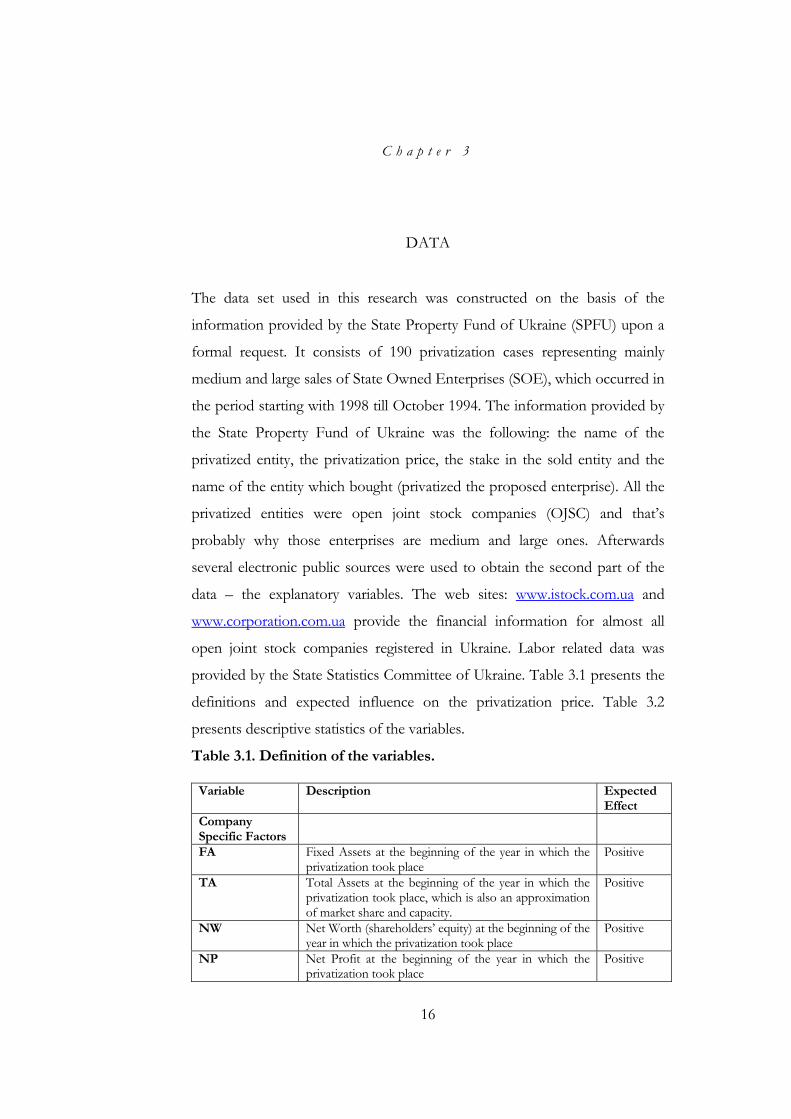
Table 3.1. Definition of the variables.

Variable Description Expected Effect

Company Specific Factors

FA Fixed Assets at the beginning of the year in which the privatization took place

Positive

TA Total Assets at the beginning of the year in which the privatization took place, which is also an approximation of market share and capacity.

Positive

NW Net Worth (shareholders’ equity) at the beginning of the year in which the privatization took place

Positive

NP Net Profit at the beginning of the year in which the privatization took place

Positive

16

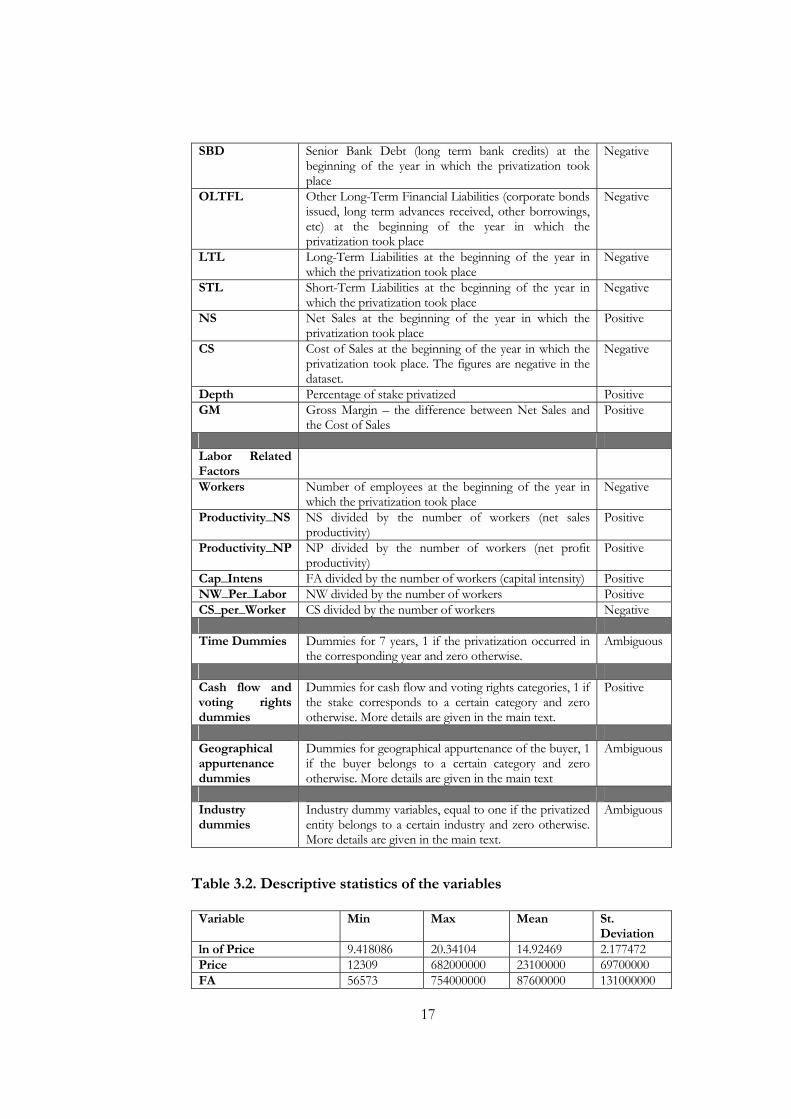
SBD Senior Bank Debt (long term bank credits) at the beginning of the year in which the privatization took place

Negative

OLTFL Other Long-Term Financial Liabilities (corporate bonds issued, long term advances received, other borrowings, etc) at the beginning of the year in which the privatization took place

Negative

LTL Long-Term Liabilities at the beginning of the year in which the privatization took place

Negative

STL Short-Term Liabilities at the beginning of the year in which the privatization took place

Negative

NS Net Sales at the beginning of the year in which the privatization took place

Positive

CS Cost of Sales at the beginning of the year in which the privatization took place. The figures are negative in the dataset.

Negative

Depth Percentage of stake privatized Positive GM Gross Margin – the difference between Net Sales and

the Cost of Sales Positive

Labor Related Factors

Workers Number of employees at the beginning of the year in which the privatization took place

Negative

Productivity_NS NS divided by the number of workers (net sales productivity)

Positive

Productivity_NP NP divided by the number of workers (net profit productivity)

Positive

Cap_Intens FA divided by the number of workers (capital intensity) Positive NW_Per_Labor NW divided by the number of workers Positive CS_per_Worker CS divided by the number of workers Negative Time Dummies Dummies for 7 years, 1 if the privatization occurred in

the corresponding year and zero otherwise. Ambiguous

Cash flow and voting rights dummies

Dummies for cash flow and voting rights categories, 1 if the stake corresponds to a certain category and zero otherwise. More details are given in the main text.

Positive

Geographical appurtenance dummies

Dummies for geographical appurtenance of the buyer, 1 if the buyer belongs to a certain category and zero otherwise. More details are given in the main text

Ambiguous

Industry dummies

Industry dummy variables, equal to one if the privatized entity belongs to a certain industry and zero otherwise. More details are given in the main text.

Ambiguous

Table 3.2. Descriptive statistics of the variables

Variable Min Max Mean St. Deviation

ln of Price 9.418086 20.34104 14.92469 2.177472 Price 12309 682000000 23100000 69700000 FA 56573 754000000 87600000 131000000

17

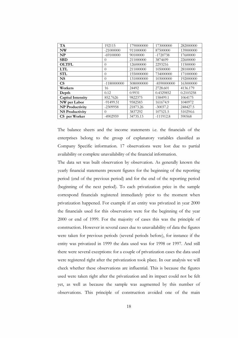
TA 192115 1790000000 173000000 282000000 NW -21000000 911000000 87500000 139000000 NP -69100000 90100000 -1720738 17600000 SBD 0 211000000 3874699 22600000 OLTFL 0 126000000 2293216 11500000 LTL 0 211000000 10500000 28100000 STL 0 1550000000 734000000 171000000 NS 0 1310000000 103000000 192000000 CS -1180000000 5080000000 -8590000000 163000000 Workers 16 24492 2728.601 4136.179 Depth 0.12 0.9931 0.4329852 0.2103258 Capital Intensity 852.7626 9822375 158499.1 1064175 NW per Labor -91499.51 9582583 161674.9 1040972 NP Productivity -2309958 21873.26 -30037.2 248427.5 NS Productivity 0 3837292 107521.5 510294.6 CS per Worker -4902959 34735.13 -111912.8 590568

The balance sheets and the income statements i.e. the financials of the

enterprises belong to the group of explanatory variables classified as

Company Specific information. 17 observations were lost due to partial

availability or complete unavailability of the financial information.

The data set was built observation by observation. As generally known the

yearly financial statements present figures for the beginning of the reporting

period (end of the previous period) and for the end of the reporting period

(beginning of the next period). To each privatization price in the sample

correspond financials registered immediately prior to the moment when

privatization happened. For example if an entity was privatized in year 2000

the financials used for this observation were for the beginning of the year

2000 or end of 1999. For the majority of cases this was the principle of

construction. However in several cases due to unavailability of data the figures

were taken for previous periods (several periods before), for instance if the

entity was privatized in 1999 the data used was for 1998 or 1997. And still

there were several exceptions: for a couple of privatization cases the data used

were registered right after the privatization took place. In our analysis we will

check whether these observations are influential. This is because the figures

used were taken right after the privatization and its impact could not be felt

yet, as well as because the sample was augmented by this number of

observations. This principle of construction avoided one of the main

18

problems – endogeneity. All the company specific variables were inflation

adjusted to the base year 1998. This procedure is logically necessary in order

to “bring the sample to the same denominator”, to get rid of the inflationary

noise which can spoil the estimations.

As previously mentioned the first group of variables represents the financials.

There are 12 variables which are classified to this group. The second group is

represented by labor data. The initial principle is preserved. We took the

number of workers and respectively their productivities and other labor

related variables (see tables 3.1 and 3.2) at the beginning of the year for each

privatization case.

The third group that we use represents four sets of dummy variables: (1)

industry dummies, (2) year dummies, (3) dummy variables set for geographical

appurtenance of the winner in the privatization contest and (4) voting and

cash flow rights dummies of the privatized stake and. The industry

breakdown of my sample is the following: 16 enterprises belong to the energy

generating sector (oblenergos); there are 21 enterprises belonging to the

mining industry (iron ore and coal mining); 28 enterprises belong to the

metals manufacturing industry; 10 enterprises in the construction industry; 36

enterprises in the machine building industry; 16 enterprises in the chemistry

industry; 11 enterprises in the oil and gas industry; 3 enterprises in the food

industry; 5 enterprises in the trade industry; 9 enterprises in the paper and

textile industry; 9 enterprises in the transportation industry; 6 enterprises in

the car industry; 3 enterprises in the tourism industry and 1 insurance

company (finance). For each of these industries were created dummy

variables to capture the difference between sectors of economy.

The second group of dummies is time (year dummies). The purpose of having

them in the regression analysis is to capture the difference between

mentioned time periods.

According to the geographical feature we classified the winners in the

privatization contests (the actual buyers) in three categories: (a) entities which

are registered in Ukraine so domestic entities – they constitute the majority –

19

139 cases, (b) the ones which countries of origination are situated in Europe

or Northern America or Western companies (my sample does not contain

acquisitions by companies which originate from Asia or other region of the

world not mentioned above except for one case in which an entity was

bought by a citizen of Lebanon whom we also classified to the west) – 31

cases, and (c) companies which are registered in Russian Federation or other

countries from the Commonwealth of the Independent States or Eastern

companies – 3 cases. The motivation and the reason for such a classification

is the following: We expect that there is certain difference in the pricing

distribution between the domestic winners and the foreign ones, because one

might expect that some government officials to be biased towards certain

categories of investors. Especially it is interesting to see how the West differs

from the East. However there is a problem with the western companies. One

third of them are off shore companies most probably owned by domestic

Industrial Financial Groups (IFG) or by eastern (Russian companies). So the

question is to what category these off shores should be classified. One option

would be to put them to the group of western companies because it is

difficult to distinguish which one is owned by a domestic IFG, a Russian

company or a foreign investor (there are cases like that). The second option is

to include a separate dummy for the off shores. The second approach will

allow to see whether there is any difference between western companies and

off shores ones from one side and the difference between off shores and the

domestic from another.

The fourth group of dummy variables is intended to see whether certain

blocks of shares have influence on the privatization price. The classification

was done according to 4 groups of blocks: 1) 25% of shares or less (38

observations), 2) range between 25% + 1 share and 50% (73 observations), 3)

range between 50% + 1 share and 75% (39 observations) and 4) range

between 75% +1 share and 100% (23 observations). All those categories have

different cash flow and voting rights, or better to say if all of them are

common shares (and they are) then they have the same voting rights but

20

different cash flow rights, however obviously different sizes of the stakes have

different voting power. Also according to the Law of Ukraine on joint-stock

companies a 25% +1 block of shares has a blocking right, so anyone who

owns 25% +1 can block certain decisions taken on the general shareholder’s

meeting. A block of 60% of shares is a quorum. So everything what is higher

than 60% is an extremely powerful block of shares. Therefore there is sense

to include in the analysis another set of CFVR dummies and namely: 1) <

25%; 2) 25% + 1 share – 50%; 3) 50 + 1 share – 60% - 1 share and 4) 60% -

100%. This set up will allow to analyze the influence of the CFVR from a

slightly different point of view.

Lopez-de-Silanes (1996) uses a much more complete set of explanatory

variables allowing for a deeper analysis. A great part of the data used by

Lopez-de-Silanes is just not available due Ukrainian specifics of information

disclosure and physical absence of such data. However Lopez-de-Silanes

makes more stress on analyzing the influence of such factors as labor

specifics, restructuring prior to privatization and a lot of qualitative variables

(for instance the level of bureaucracy of the manager of the privatized

company, or whether the manager was fired prior to privatization or not etc)

than the company characteristics.

Other authors like Chong and Galdo (2003) or Arin and Okten (2003) use

much smaller number of explanatory variables stressing the analysis on labor

data company and industry specifics.

It is necessary to say that compared to similar researches my sample lacks

important explanatory variables, namely the number of bidders in the

privatization contest and whether it was an auction or a contest. However

there are explanations for that. Regarding the second issue – my sample

contains only contests. As for the first one – the specifics of Ukrainian

privatization consist in the fact that in a number of cases there was only one

bidder admitted to the final stage of the tender, all others were rejected at

earlier stages. The conditions for admissions where set in each case

21

individually in order to draw out of the competition unfavorable investors

(for instance in many cases the foreign ones like in the case of Krivorizhstali).

And accordingly the admitted one was entitled as the owner. There are

opinions that this is one of the strategies of the Mr. Kuchma regime to favor

certain IFGs and people who are behind them and to eliminate from the

competition participants who potentially might have bided a higher price

(http://www.ord.com.ua/categ_1/article_14323.html). This is the case of the

heavy industry enterprises (metals, mining, machine building), for the rest of

privatization cases the data on the number of participants is not available. It

would be good to have it in the regression analysis in order to test whether

the findings of other authors for other countries are applicable to Ukraine, for

instance that the privatization price is an increasing function of the number of

participants in the contest (Lopez-de-Silanes (1996) and others).

As mentioned before the data set was constructed that way in order to avoid

the endogeneity. Another problem which should be taken into consideration

is the heteroskedasticity. The distributions of the error terms of the

explanatory variables in the sample may follow different patterns. The t-

statistics will be wrongly calculated; therefore no conclusion about the

significance of the coefficients can be made. Therefore in order to check for

heteroskedasticity the White Heteroskedasticity test will be performed and if

there is heteroskedasticity the method of robust standard errors will be

applied. However expectedly, due to the log-linear model used (which will be

described later) the problem of heteroskedasticity should be weakened.

Another relevant problem of the explanatory variables is that they are

colinear. Due to the nature of the data a good part of the variables are

strongly correlated, which confuses and makes it difficult to make conclusions

about the results. In Appendix 0 can be seen how many correlating variables

there are in the sample (shadowed). It is natural that total assets correlate with

fixed assets, net worth, short-term liabilities, net sales, cost of sales and

number of workers. Net Worth is the shareholders’ equity – money

contributed by the owners to buy productive capacities in order to generate

22

revenues. So basically the net worth is fixed assets and fixed assets are the

greatest part in the total assets. Short-term liabilities represent the money

borrowed for the working capital which also naturally correlates with the

assets of the enterprise. The more assets an enterprise has, more output it can

generate thus more sales it makes (ceteris paribus), and respectively cost of

sales (with negative sign). And of course the number of workers increases

along with the productive equipment. The same relationships are preserved

by the fixed assets and net worth variables. Senior bank debt representing

long-term bank credits and other long-term financial liabilities, which usually

represent bonds issued by the entity or other long-term funding taken for

development; strongly correlate with long-term liabilities. The number of

workers variable correlate with short-term liabilities and cost of sales because

the wages represent the greatest part of the expenses. Net sales logically

negatively correlate with the cost of sales and positively with the number of

workers.

There is a possibility as well that my model is misspecified. As discussed

above certainly my data set (for instances compared to that one which Lopez-

de-Silanes uses) misses a number of explanatory variables which could better

describe what influences the privatization prices in Ukraine. Also the

multicolinearity between the variables which are available, forces to use them

separately in the regression analysis, which is also a variety of misspecification.

The company specific variables are expressed in Ukrainian hryvnias as well as

the privatization prices. As mentioned before the sample comprises the

medium and large privatization cases, among which are the largest industrial

entities of Ukraine. Therefore there are a certain small number of

observations which are relatively very large compared to others as well as a

couple of observations which are relatively very small. The regression analysis

is done both using the whole sample as well as using a sample short listed by

those outliers. The purpose is to see whether those outliers have an influence

on the results.

23

C h a p t e r 4

METHODOLOGY

The methodology described below is meant to explain two variables: the

privatization prices and the Net Government Revenue (NGR). The idea is to

investigate the determinants of privatization prices. What is the reasoning of

the investors when they decide about investing, what do they look at when

they decide about what price to offer?

The nature of the data and its construction implies no other estimation

method than Ordinary Least Squares. All the regressions will be checked for

heteroskedasticity and if its presence is detected robust estimator will be

applied. One more option to go around this problem would be to use a log-

linear model i.e. take as the dependent variable natural logarithm of prices.

The functional form of the regressions is the following:

εδφϕγβα ++++++= IDGALCFVRDCSYDprice ****** ,

where:

YD - year dummies;

CS - company specific factors;

CFVRD - cash flow and voting rights dummies;

L - labor related factors;

GA - geographical appurtenance dummies;

ID - industry dummies;

ε - disturbance term.

The expected influence of the time, industry and geographical appurtenance

dummies is ambiguous. We expect that cash flow and voting rights dummies

to have a positive influence on the privatization price. The expected influence

of the company specific factors is somewhat obvious: the assets, revenues and

24

the size of the stake will have a positive influence on the price, the liabilities

and costs respectively negative. The influence of labor related factors on the

privatization price has benefited from much research. We expect that the

number of workers will have a negative influence on the price since the

number of workers is directly proportional to costs. The idea that the number

of workers is directly proportional to revenues has also a right to exist

however entities shift more and more their production to more efficient

means - capital (equipment) thus getting rid of relatively unproductive and

inefficient labor. However the defined in Table 3.1 productivities are expected

to have a positive influence. Capital intensity and the Net Worth per worker

are expected to influence positively.

On the other hand Shleifer and Vishny (1994) say that the government has

two objectives when privatizing: first is to generate revenue and second to

stimulate efficiency improvement and depolitization of the SOEs. When the

government decides on privatization it has to solve two main problems, first

is when to privatize and second it has to decide about the pricing. Both parts

of the decision making can be theoretically modeled. Therefore it is

interesting to see the flip side of the coin – what influences the so called Net

Government Revenue. According to the law of privatization the government

from one hand guarantees the maximization of the proceeds from

privatization because the winner is announced the company which offers the

highest price. However the case of Krivorizhstali (and other) indicates that

this is not exactly true because the participants who offered much higher price

than the actual winner were disqualified.

Basically the influence of the explanatory variables a priori should be the same

as in the case of the logarithmic privatization prices, however surprises are

possible. The functional form of the main equation is the same:

εδφϕγβα ++++++= IDGALCFVRDCSYDNGR ******

The estimation technique will be the same as well.

25

Lopez-de-Silanes (1996) and Arin and Okten (2003) use in their research

the adjusted privatization prices, however they propose different methods of

adjustment. In summary basically they suggest to calculate a net privatization

price controlled for inflation, taking into account the costs of privatization,

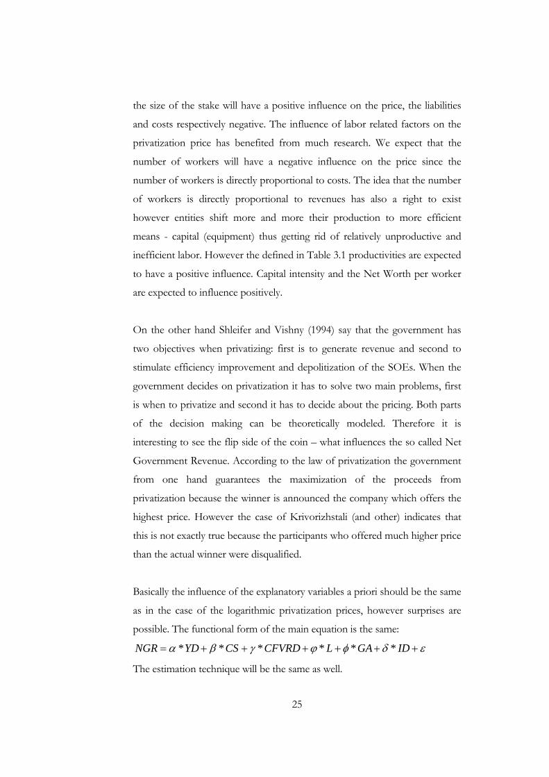
normalization by the total assets and total debt, etc. The Net Government

Revenue from privatization, which the government should optimize, can be

expressed in the following way:

ititTtitititit RIEBTtrPVDepthNWRINWPNGR ,,,,,, )*(*),( −∑+−=

(4.1), where:

),(, RINWP it , is the final price which depends on the Net Worth and RI,

itNW , , is the net worth or Total Assets – Total Debt or liabilities (TA-TD),

)*( ,itTt EBTtrPV ∑ , is the present value of the sum of the future tax

proceeds form the entity’s revenues (tax rate multiplied by the Earnings

before Tax),

itRI , , is the restructuring investments undertaken by the state before

privatization.

The experience of other countries suggests that governments usually

undertake restructuring investments in order to make the enterprise more

attractive and increase the privatization price. However this is what not always

happens in Ukraine. The Ukrainian government puts the burden of

restructuring and investments on the buyer. When an enterprise in Ukraine is

privatized the buyer assumes certain investment obligations, this is a

requirement set by the government. However in some cases this restructuring

can be observed therefore the equation still contains this component.

From the practical point of view it is almost impossible to project the future

revenues of the enterprise therefore some components of the equation (1) can

not be calculated even if we choose the discount rate, therefore further the

26

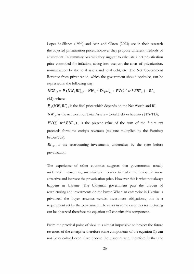
NGR will be defined as the difference between the privatization price and the

Net Worth multiplied by the Depth of privatization. The solution of the

maximization of the equation (4.1) would be the answer to the question of

pricing. The answer to the question of timing is given by the inequality below:

)*(*)(*)(1000 ∑∑ ==

+−−<T

ttttT

ttEBTtrPVDepthTDTAPDepthNPPV

(4.2), where:

NP - net profit.

And the inequality sign is strict because if the two sides are equal there is no

sense in privatizing because the government incurs some privatization costs.

The left hand side of the equation 4.2 presents the opportunity cost of

privatizing, income foregone by the government if it sells the enterprise.

The efficiency of the government decisions is measured by the two equations

(4.1 and 4.2).

27

C h a p t e r 5

EMPIRICAL ANALYSIS AND DISCUSSION

This section presents the empirical analysis on the relationship between the

privatization prices and company specific factors.

The analysis was done first on the raw prices; the purpose is to see what

determines the privatization prices as they are with no changes and

adjustments. The general specification looks as follows:

εδφϕγβα ++++++= IDGALCFVRDCSYDice ******Pr

(Equation 5.1.), where:

YD - year dummies;

CS - company specific factors;

CFVRD - cash flow and voting rights dummies;

L - labor related factors;

GA - geographical appurtenance dummies;

ID - industry dummies;

ε - disturbance term.

If we regress the raw prices on the explanatory variables specified in the

model we receive very confuse and ambiguous results. There are two reasons

for that. First is that the regressions with the dependent variable as prices

exhibit heteroskedasticity problem, which is proven using the White

Heteroskedasticity test. The second reason which we believe has the greatest

negative influence on the regression statistics is that the raw prices do not

control for the fact the prices were paid for different sizes of the stakes and

the effect of the independent variables is not proportional even if the variable

Depth (stake percentage) is included in the regressions. Therefore the

explanatory variables as well as the dependent one should be adjusted

somehow. There are two options for that. First would consist in dividing all

the variables by size of the privatized stake i.e. normalizing and adjusting over

28

the sample. The second option would be to take natural logarithm of the

prices as the dependent variable. The logarithmic function is a monotonic

transformation which first of all reduces heteroskedasticity and secondly

makes the effect of the explanatory variables comparable. The slope

coefficients give a relative change (percentage change) in the dependent

variable as a consequence of an absolute change in the respective explanatory

variable.

Other authors seem to have paid less attention to the issue of

heteroskedasticity which is so drastic in my sample. In related literature no

heteroskedasticity test was mentioned. The presence of the heteroskedasticity

would make the interpretation of the results controversial. Arin and Okten

(2003) talk about heterogeneity, which is present in their sample. They do

their analysis on a cross industry sample but then they concentrate their

analysis solely on the cement production industry. This move solves only

partially the problem because the number of observations in the new sample

(just cement production industry) becomes very small – 24, which limits the

strength of the conclusions.

Chong and Galdo (2003) analyze just one industry (telecommunication)

having 84 observations, however their sample is cross-country one which

preserves the heteroskedasticity feature anyway.

Therefore further the log-linear econometric model will be considered. The

model has the same functional form as in Equation 5.1., only that the

dependent variable is the natural logarithm of prices. Appendix 1 presents the

results of the general estimation, regression with the full set of variables.

The general estimation shows that the Capital Intensity, NW per worker and

the geographical appurtenance dummies are significant at 5% significance

level. Senior Bank Debt, Net Sales and Net Profit productivities, Cost of Sales

per worker and number of workers are significant at 10% significance level.

Almost all the variables are related to the labor factors; therefore it can be

assumed that the labor factor is one of the main determinants of the

29

privatization prices, which is also evidenced by Lopez-de-Silanes (1996),

Chong and Lopez-de-Silanes (2002), etc. However if the attention is paid to

the coefficients of the significant variables many of them are economically

counterintuitive. The reason is that many variables are colinear, therefore in

what follows the specifications will be restricted and the way we restrict the

specifications is going from general to specific.

The regression analysis (see Appendix 1) indicates that the investors in

Ukrainian economy do not really care in what industry to invest. The industry

dummies are found to be insignificant. This finding is somewhat surprising

because it means that whether: 1) investors believed that state owned

enterprises from all industries are very inefficient and the pre investment

analysis would not show much – the margins and the overall performance is

not credible and that the investors had there own scenarios of industries’

development and their conditions or 2) investors believed that all sectors of

the Ukrainian economy will exhibit high rates of development, that the

economy will grow as an emerging market, so they were investing money in

everything which was expected to generate revenues.

Appendix 2 presents the estimation results of one of the restricted

specifications coefficients of which are economically consistent.

Among the year dummies the only significant is the one for 2003. It has

negative coefficient. The result indicates that the year 2003 was different from

others and that the prices were lower compared to other years.

Since the estimation specification has an intercept, which is significant it

represents the influence of the dummy variables which were automatically

dropped. Therefore the base dummy is an enterprise privatized in 1998 with a

stake falling in the range 0-25% bought by a western entity. The second

CFVR category (25%+1 share – 50%) is statistically indistinguishable from

the first meaning that a stake ranging from 0% to 50% has the same voting

30

power, however the third (50%+1 share – 75%) and the fourth (75%+1 share

– 100%) are significant. In the data description section was stated the

expectation that each 25% +1 share stake to have importance, and the finding

suggests the opposite. It seems that the stakes: 50%, 50% +1 share - 75 %

and 75%+1 – 100% are important from the cash flow and voting rights point

of view. Therefore it can be concluded that the investors in Ukraine care

indirectly about the size of the stake they compete for. This is also indicated

by the fact that the variable Depth is significant alone (without CFVR

dummies) but it is not significant in the combination with the cash flow and

voting rights dummies in the regressions. So, obviously the privatization price

is an increasing function of the size of the stake but more important is what

power the bought stake confers to the investor over the enterprise. This

finding confirms the similar result obtained by Lopez-de-Silanes 1996.

The significance of the Geographical Appurtenance dummies is somewhat

surprising. First of all it means that the country of origination of the

participant to the tender has an influence on the privatization price. The sign

and the size of the coefficients indicate that the geographical appurtenance

has a negative influence on the price in the case of eastern and domestic

participants; in the case of western companies the influence is positive. One

of the explanations would be that certain categories of participants had

different target groups of entities and that the western companies targeted the

most expensive companies while eastern and domestic targeted the less

expensive ones. However the fact that one third (11 observations) of western

buyers are probably off shores belonging to domestic and Russian entities

somewhat contradicts this hypothesis. Definitely a conclusion would be that

the enterprises bought through the intermediary of the off shores are different

from the ones bought directly by domestic entities. Enterprises bought by off

shores belong to the oil and gas mining and energy generating industries. Also

one of the possible explanations would be that domestic and eastern

participants were favored. However another hypothesis would be that

31

western companies were more optimistic about the future prospects and

performance companies they were targeting thus offering higher price

compared to Ukrainian and Eastern peers.

As mentioned before the number of eastern companies is very small – four.

Therefore the effect of this dummy is doubtful. Since the domestic dummies

and eastern dummies both have a negative influence on the privatization price

it hints to the conclusion that those two are strongly interrelated, and there is

sense to include the four observations for the eastern companies in the

domestic category. Appendix 3 shows the estimation statistics.

The inclusion of the eastern companies in the category of domestic ones does

not change the results for Geographical Appurtenance dummies.

As discussed in the data section there is sense to analyze the specification

where we will have a dummy for an off shore company and a different set up

for the CFVR dummies, having the last two categories: 50% + 1 share – 60%

- 1 share (25 observations) and 60% - 100% (37 observations). The results are

shown in Appendix 4.

Surprisingly according to the estimations we can not distinguish between an

off shore and a western buyer, perhaps because of low number of

observations for off shores – 11, so there is no point in having a separate

dummy for off shores. Or maybe because the enterprises bought through off

shores were indeed more expensive than bought directly by domestic winners.

An expected result, which confirms previous findings, is that in the second set

up for CFVR dummies all the categories are significant.

Further we have introduced a dummy variable for a stake, which ranges from

60% to 75% (14 observations) in order to see whether it is significant and to

check whether the categories 50% + 1 share – 60% - 1 share and 75% + 1

share – 100% are still important. We have dropped the category 0 – 25% in

order to make the categories comparable. And indeed these categories are

32

significantly different from the omitted category (see Appendix 5). The

finding that the category 25% - 50% is not important is confirmed. We have

performed a t-statistic test for significance of the category 50% - 60% - 1share

from the category 60% - 75%, which showed that they are indistinguishable.

Given this result we will keep in the regressions the category 50% - 60% - 1

share to show that it differs from the category 25% +1 share – 50%.

The regression analysis evidences that among company specific factors

significant (in the mentioned specification) are Fixed Assets, Short Term

Liabilities and the Net Sales. However due to the described in chapter 3

relationships between company specific variables (correlation) in other

specifications significant are found and other variables (which will be

described somewhat later). The positive influence of the revenues which the

enterprise to be privatized generates is as well evidenced by Lopez-de-Silanes

(1996) and Arin and Okten (2002). This result indicates that the investors pay

attention to the ability of the potential enterprise to generate funds. If we

replace in the same regression the variable Net Sales by the Cost of Sales we

find that it is significant. However it has a counterintuitive negative

coefficient. Its significance is conditioned by the fact that the Cost of Sales are

an indicator of size and by the fact that Cost of Sales are highly colinear with

Net Sales (correlation coefficient is (-0.9821), so those two variables are

basically the same. Therefore no attention is going to be paid to this variable.

One more reason to exclude Cost of Sales from our consideration is that if we

include in the specification the Net Profit or The Gross Margin variables they

are absolutely insignificant meaning that indirectly Cost of Sales do not matter

for the price. This proves the similarity with Lopez-de-Silanes (1996), Arin

and Okten (2002), etc. consisting in the fact that investors do not pay a great

attention to the expenses because they believe that state enterprises are

inefficient and anyway after privatizing by implementing new strategy and

policy they will achieve the necessary efficiency. Investors in Turkey pay

attention to the revenues and not profits. So investors seem to exhibit the

33

same logic, they care about the ability of the enterprises to generate revenues

and the expenditure part can be improved.

An interesting finding which has no evidence in similar research is the fact

that Short Term Liabilities influence the privatization prices. Naturally, their

effect is negative. STL represent funds which need to be immediately or

shortly paid off. And of course investors take this into account when making

an investment decision.

Based on the results of the main regression specifications it can be concluded

that Fixed Assets are one of the factors, which investors look at. This finding

is different from previous. Country specific situation might be one of the

explanations. According to the State Statistics Committee the degree of

depreciation of the equipment of the Ukrainian enterprises is high (more than

50%), especially that one inherited from the Soviet Union. So the quality of

the equipment is the corner stone in the investors’ decisions, because they pay

a great attention to the book value of the equipment and the residual value.

The proximity of the residual value to the book value (purchase value) is an

approximation of the quality and the level of depreciation. So if the residual

value is relatively close to the book value it indicates that the depreciation is

small, which means that the quality of the equipment is relatively higher. In

our case there is positive influence of the residual value of the equipment on

the privatization price. The issue is, whether the investors have to spend a lot

of money and invest in the new equipment immediately in order to keep the

entity lucrative. Arin and Okten (1996) find somewhat different results. They

say that important is the ratio of capacity utilization and not the equipment

(Fixed Assets) itself, meaning that the investors are looking for unexploited

opportunities.

The estimation results are unchanged if outliers are excluded from the

regression specification with dependent variable as natural logarithm of price.

Therefore the estimation outcomes are robust.

34

However it must be mentioned that due to the correlation relationships

(mentioned in previous chapters) between company specific factors we can

not exactly distinguish what has the greatest influence on the prices. Because

other regression specifications indicate that Total Assets, Net Worth are also

significant (see Appendix 6.1 and 6.2).

The influence of Labor factors is interesting. In the general regression labor

related factors are the only significant, however in the restricted specifications

if they come with company specific factors like FA or NS, etc. they are not.

However (Appendix 7) in some specifications for instance the number of

workers is found to be significant and this variable has a small positive effect

on the privatization price. Also the productivity of the Net Sales is significant

at 10% significance level (see Appendix 8). This finding is not in line with the

findings of Arin and Okten (2002) for example. The reason is that like in my

sample the variable Number of Workers correlates with other company

specific factors.

The general estimation result of the influence of the explanatory variables on

the NGR is shown in Appendix 9.

It can be seen that we have a lot of significant variables but their influence is

counter intuitive. This is due to multicolinearity and heteroskedasticity. If

however we control for heteroskedasticity, running the regression with robust

error terms than we receive that (see Appendix 10) there are no significant

variables except for some year dummies with a doubtful influence. The

restricted specifications like in Appendix 11 also reveal no significant variables

except for the Senior Bank Debt, which influence is counter intuitive. Thus

the estimations show that whether the variable NGR lacks economic meaning

or the influence on it can not be estimated due to data problems.

Another functional form of the dependent variable we analyzed was the price

variable divided by the depth variable in percentage points. The intuition

35

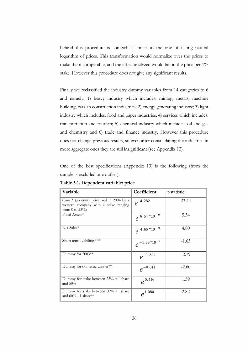
behind this procedure is somewhat similar to the one of taking natural

logarithm of prices. This transformation would normalize over the prices to

make them comparable, and the effect analyzed would be on the price per 1%

stake. However this procedure does not give any significant results.

Finally we reclassified the industry dummy variables from 14 categories to 6

and namely: 1) heavy industry which includes: mining, metals, machine

building, cars an construction industries; 2) energy generating industry; 3) light

industry which includes: food and paper industries; 4) services which includes:

transportation and tourism; 5) chemical industry which includes: oil and gas

and chemistry and 6) trade and finance industry. However this procedure

does not change previous results, so even after consolidating the industries in

more aggregate ones they are still insignificant (see Appendix 12).

One of the best specifications (Appendix 13) is the following (from the

sample is excluded one outlier):

Table 5.1. Dependent variable: price

Variable Coefficient t-statistic Const* (an entity privatized in 2004 by a western company with a stake ranging from 0 to 25%)

282.14e 23.44

Fixed Assets* 910*54.6 −

e 5.34

Net Sales* 910*66.4 −

e 4.80

Short term Liabilities*** 910*66.1 −−e -1.63

Dummy for 2003** 324.1−e -2.79

Dummy for domestic winner** 811.0−e -2.60

Dummy for stake between 25% + 1share and 50%

416.0e 1.39

Dummy for stake between 50% + 1share and 60% - 1 share**

084.1e 2.82

36

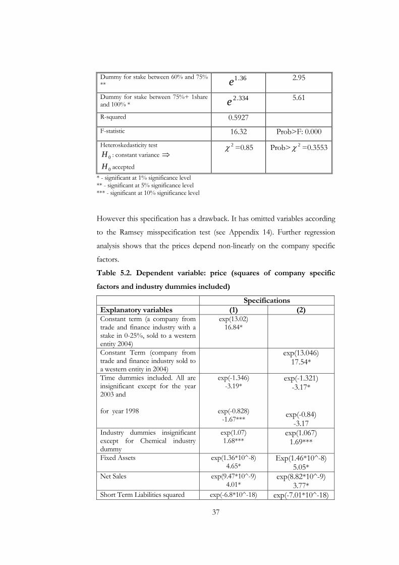
Dummy for stake between 60% and 75% **

36.1e 2.95

Dummy for stake between 75%+ 1share and 100% *

334.2e 5.61

R-squared 0.5927 F-statistic 16.32 Prob>F: 0.000 Heteroskedasticity test

0H : constant variance ⇒

0H accepted

2χ =0.85 Prob> =0.3553 2χ

* - significant at 1% significance level ** - significant at 5% significance level *** - significant at 10% significance level

However this specification has a drawback. It has omitted variables according

to the Ramsey misspecification test (see Appendix 14). Further regression

analysis shows that the prices depend non-linearly on the company specific

factors.

Table 5.2. Dependent variable: price (squares of company specific

factors and industry dummies included)

Specifications Explanatory variables (1) (2) Constant term (a company from trade and finance industry with a stake in 0-25%, sold to a western entity 2004)

exp(13.02) 16.84*

Constant Term (company from trade and finance industry sold to a western entity in 2004)

exp(13.046) 17.54*

Time dummies included. All are insignificant except for the year 2003 and for year 1998

exp(-1.346) -3.19*

exp(-0.828) -1.67***

exp(-1.321) -3.17*

exp(-0.84) -3.17

Industry dummies insignificant except for Chemical industry dummy

exp(1.07) 1.68***

exp(1.067) 1.69***

Fixed Assets exp(1.36*10^-8) 4.65*

Exp(1.46*10^-8) 5.05*

Net Sales exp(9.47*10^-9) 4.01*

exp(8.82*10^-9) 3.77*

Short Term Liabilities squared exp(-6.8*10^-18) exp(-7.01*10^-18)

37

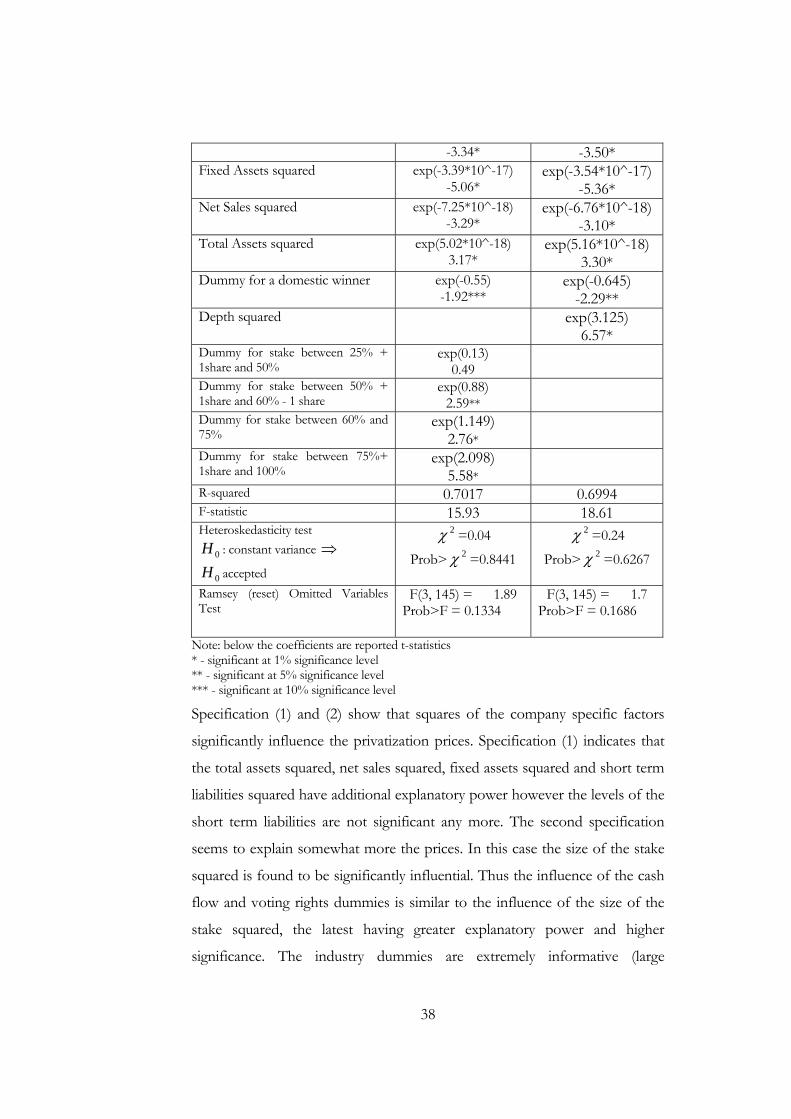
-3.34* -3.50* Fixed Assets squared exp(-3.39*10^-17)

-5.06* exp(-3.54*10^-17)

-5.36* Net Sales squared exp(-7.25*10^-18)

-3.29* exp(-6.76*10^-18)

-3.10* Total Assets squared exp(5.02*10^-18)

3.17* exp(5.16*10^-18)

3.30* Dummy for a domestic winner exp(-0.55)

-1.92*** exp(-0.645)

-2.29** Depth squared exp(3.125)

6.57* Dummy for stake between 25% + 1share and 50%

exp(0.13) 0.49

Dummy for stake between 50% + 1share and 60% - 1 share

exp(0.88) 2.59**

Dummy for stake between 60% and 75%

exp(1.149) 2.76*

Dummy for stake between 75%+ 1share and 100%

exp(2.098) 5.58*

R-squared 0.7017 0.6994 F-statistic 15.93 18.61 Heteroskedasticity test

0H : constant variance ⇒

0H accepted

2χ =0.04

Prob> =0.8441 2χ

2χ =0.24

Prob> =0.6267 2χ

Ramsey (reset) Omitted Variables Test

F(3, 145) = 1.89 Prob>F = 0.1334

F(3, 145) = 1.7 Prob>F = 0.1686

Note: below the coefficients are reported t-statistics * - significant at 1% significance level ** - significant at 5% significance level *** - significant at 10% significance level Specification (1) and (2) show that squares of the company specific factors

significantly influence the privatization prices. Specification (1) indicates that

the total assets squared, net sales squared, fixed assets squared and short term

liabilities squared have additional explanatory power however the levels of the

short term liabilities are not significant any more. The second specification

seems to explain somewhat more the prices. In this case the size of the stake

squared is found to be significantly influential. Thus the influence of the cash

flow and voting rights dummies is similar to the influence of the size of the

stake squared, the latest having greater explanatory power and higher

significance. The industry dummies are extremely informative (large

38

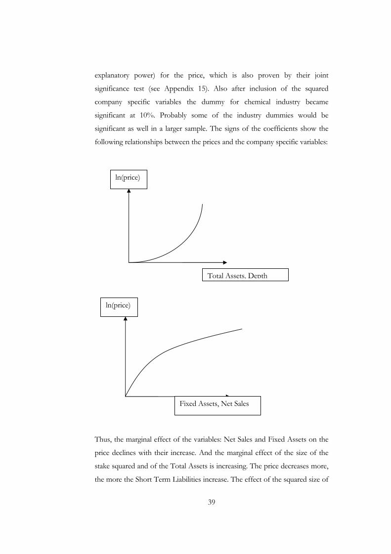
explanatory power) for the price, which is also proven by their joint

significance test (see Appendix 15). Also after inclusion of the squared

company specific variables the dummy for chemical industry became

significant at 10%. Probably some of the industry dummies would be

significant as well in a larger sample. The signs of the coefficients show the

following relationships between the prices and the company specific variables:

ln(price)

Total Assets, Depth

ln(price)

Fixed Assets, Net Sales

Thus, the marginal effect of the variables: Net Sales and Fixed Assets on the

price declines with their increase. And the marginal effect of the size of the

stake squared and of the Total Assets is increasing. The price decreases more,

the more the Short Term Liabilities increase. The effect of the squared size of

39

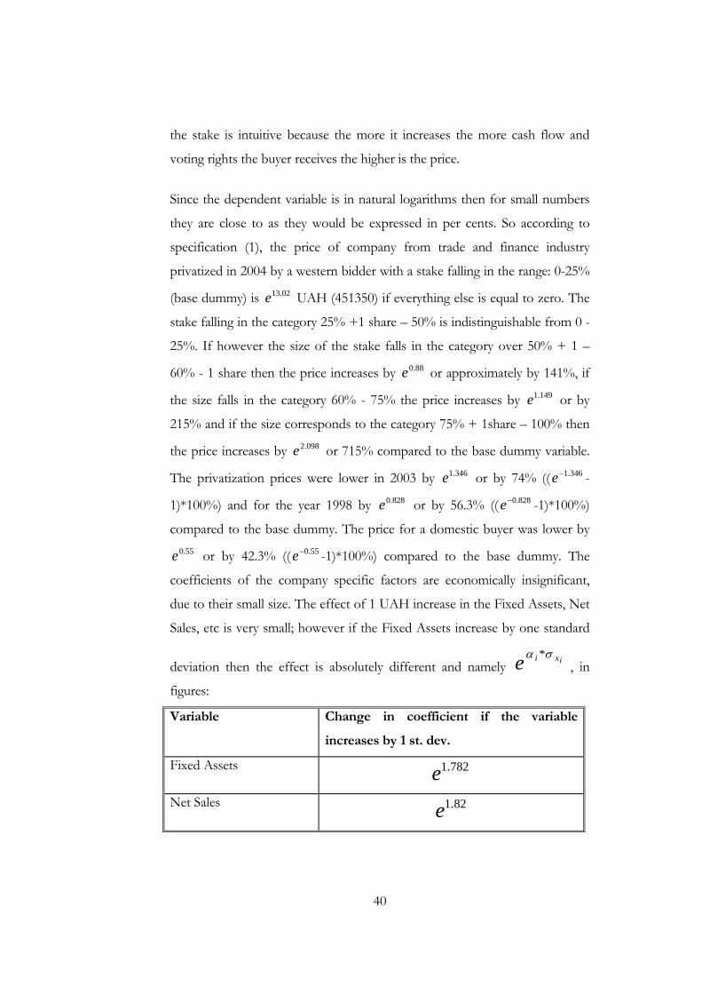
the stake is intuitive because the more it increases the more cash flow and

voting rights the buyer receives the higher is the price.

Since the dependent variable is in natural logarithms then for small numbers

they are close to as they would be expressed in per cents. So according to

specification (1), the price of company from trade and finance industry

privatized in 2004 by a western bidder with a stake falling in the range: 0-25%

(base dummy) is UAH (451350) if everything else is equal to zero. The

stake falling in the category 25% +1 share – 50% is indistinguishable from 0 -

25%. If however the size of the stake falls in the category over 50% + 1 –

60% - 1 share then the price increases by or approximately by 141%, if

the size falls in the category 60% - 75% the price increases by or by

215% and if the size corresponds to the category 75% + 1share – 100% then

the price increases by or 715% compared to the base dummy variable.

The privatization prices were lower in 2003 by or by 74% (( -

1)*100%) and for the year 1998 by or by 56.3% (( -1)*100%)

compared to the base dummy. The price for a domestic buyer was lower by

or by 42.3% (( -1)*100%) compared to the base dummy. The

coefficients of the company specific factors are economically insignificant,

due to their small size. The effect of 1 UAH increase in the Fixed Assets, Net

Sales, etc is very small; however if the Fixed Assets increase by one standard

deviation then the effect is absolutely different and namely , in

figures:

02.13e

88.0e149.1e

098.2e346.1e 346.1−e

828.0e 828.0−e

55.0e 55.0−e

ixie σα *

Variable Change in coefficient if the variable

increases by 1 st. dev.

Fixed Assets 782.1e

Net Sales 82.1e

40

C h a p t e r 6

CONCLUSIONS

This research analyzes the determinants of privatization prices in Ukraine.

The privatization process in this country is characterized as controversial due

to cases of corruption and favoritism. The analysis is based on a cross-

industry sample comprising the period starting from 1998 till 2004. The

sample contains large and medium privatization cases, which took place

during the most representative period in the history of Ukrainian privatization

and economic reforms. The case of Ukraine presents interest due to the

following reasons. Internal political issues involved (controversy). External

geo-political position of Ukraine – this country is among world leaders in a

number of industries; it is in the middle of cross attention of the west (EU

and USA) and the East (Russian Federation). On this background it is

interesting to see the process of pricing of privatized entities in Ukraine, what

do investors look at when taking decisions and does the government behave

rationally. This research is the first to analyze the privatization prices in

Ukraine. The research answers the questions: what company specific factors

matter for the privatization price, whether the geographical appurtenance of

the buyer matters, how the peculiarities of the sold stake influence the price,

etc.

The analysis shows that the investors did not differentiate among industries,

because they are found to be insignificant for the determination of the price

as in the disaggregated case (14 industries) as in the aggregated one (6

industries) except for the case when the specification contains squares of

company specific variables. However industry dummies are informative

which is shown by the test of joint significance in the case of 6 industry

dummies. Net Sales and Fixed Assets influence positively the privatization

41

price and the Short Term Liabilities –negatively. Moreover their effect is non-

linear, meaning that the marginal effect is not constant with the

increase/decrease in the variable. The price for the domestic investor is found

to be lower than for a western one. Interesting thing being that the regression

analysis shows that we can not differentiate between a western company and

off shores belonging to domestic and eastern buyers. Investors are found to

care indirectly about the depth of privatization, because they are interested

more in the power they receive over the company acquiring the stake than in

the stake itself.

There are several interesting and important topics in the Ukrainian

privatization, which deserve to be researched. For instance it would be

interesting to see what are the characteristics of the winning enterprise in a

privatization contest. Until recently Ukraine never had billionaires. However

according to Forbes ratings of the richest individuals across the world in

Ukraine suddenly appeared a number of them. Does this fact have any link to

the privatization? Was it possible due to certain country specific conditions,

favoritism of the political leadership of the country or something else?

Also it is interesting to see whether the Ukrainian government had a certain

plan or strategy when privatizing, or this happened randomly. Finally the

efficiency of Ukrainian privatization merits attention.

42

BIBLIOGRAPHY

1. Andreyeva, Tatyana and Dean James W. (), “Privatization ownership structure and Company Performance: Case of Ukraine”

2. Arin, Kerim Peren and Okten, Cagla, (2003), “The Determinants of Privatization Prices: Evidence from Turkey”, journal: Applied Economics, Volume 35 (2003), Issue 12 August, Pages: 1393-1404.

3. Bondar, Anatoliy and Lilje, Boo (April 19-26, 2002), “Land Privatization in Ukraine”.

4. Boubakri, Narjess and Jean-Claude Cosset. 1998. “The Financial and Operating Performance of Newly-Privatized Firms: Evidence From Developing Countries,” J. Fin., 53, pp. 1081-1110.

5. Boubakri, Narjess, Cosset, Jean-Claude and Guedhami, Omrane (March, 2001). “Economic Reform, Corporate Governance and Privatization: Evidence from Developing Countries”, Laval University, (Quebec, Canada)

6. Choi, Seung-Doo and Sang-Koo Nam. 2000. “The Short-Run Performance of IPOs of Privately- and Publicly-Owned Firms: International Evidence,”

Multinational Fin. J., forthcoming.

7. Chong, Alberto, and Galdo, Virgilio, 2003. “Streamlining and Privatization Prices in the Telecommunications Industry”, Inter-American Development Bank, Research Department, Working Paper #480

8. Chong, Alberto, and López-de-Silanes Florencio, 2002. “Privatization and Labor Force Restructuring Around the World.” New Haven, United States: Yale University. NBER Working Paper.

9. Claessens, Stijn, 1995. “Corporate Governance and Equity Prices. Evidence from Czech and Slovak Republics”, World Bank working paper # 1427.

10. D’Souza, Juliet, Robert Nash, and William L. Megginson. 2000. “Determinants of Performance Improvement in Newly-Privatized Firms: Does Restructuring and Corporate Governance Matter?” working paper, University of Oklahoma, Norman, OK.

11. Dewenter, Kathryn and Paul H. Malatesta. 1997. “Public Offerings of State-Owned and Privately-Owned Enterprises: An International Comparison,” J. Fin., 52, pp. 1659-1679.

43

12. Glaeser, E.L. and J.A. Scheinkman. “The Transition to Free Markets: Where to Begin Privatization.” Journal of Comparative Economics 22 (1996): 23-42.

13. Grygorenko, Galyna and Lutz, Stefan (24 October 2004), “Firm Performance and Privatization in Ukraine”, (McCann Erickson; University of Manchester and ZEI)

14. Gupta, Nandini, Ham John C. and Svejnar, Jan (September 2001). “Priorities and Sequencing in Privatization: Theory and Evidence from the Czech Republic”.

15. Jenkinson, Timothy and Colin Mayer. 1988. “The Privatisation Process in France and the U.K.,” European Econ.Rev., 32, pp. 482-490.

16. Jones, Derek and Mygind, Niels (August 1998). “Ownership Patterns and Dynamics in Privatized Firms in Transition Economies: Evidence from the Baltics” CEES Working Paper No. 15.

17. Karpoff, Jonathan. 2001. “Public versus Private Initiative in Arctic Exploration: The Effects of Incentives and Organizational Form,” J. Pol. Econ.

18. Konings, Josef, Van Cayseele, Patrick and Warzynski, Frederic (November 2002). “The

Effect of Privatization and Competitive Pressure on Firms’ Price-Cost Margins: Micro Evidence from Emerging Economies” Centre for Transition Economies Economics Department K.U.Leuven, Belgium.

19. Kopstein, Jeffrey S. and Reilly,David A. (October 2000). “Geographic Diffusion and the Transformation of the Postcommunist World ”, World Politics 53

20. Krugman, Paul (1994), “The myth of Asia’s miracle”, Foreign Affairs Journal.

21. Lopez-De-Silanes, Florencio, (1996), “Determinants of Privatization Prices” NBER W P No. W5494.

22. Megginson, William L. and Netter, Jeffry M. (June 2001). “From State To Market: A Survey Of Empirical Studies On Privatization”; Journal of Economic Literature

23. Megginson, William, Robert Nash, and Matthias van Randenborgh. 1994. “The Financial and Operating Performance of Newly Privatized Firms: An International Empirical Analysis,” J. Fin., 49, pp. 403-452.

24. Menyah, Kojo and Krishna Paudyal. 1996. “Share Issue Privatisations: The UK Experience,” in Empirical Issues inRaising Equity Capital. Mario Levis. Ed.

44

Amsterdam: Elsevier Science.

25. Okten, Cagla and Arin, Peren K. (n.d.). “How Does Privatization Affect the Firm’s Efficiency and Technology Choice?: Evidence from Turkey”, JEL Classification: HO, L32, L33

26. Sabirianova, Klara, Svejnar, Jan and Terrell, Katherine (May 2004). “Foreign Investment, Privatization and Development:Are Firms in Emerging Markets catching up to the World Standard?” JEL classification: C33, D20, G32, L20

27. Shafik, Nemat (1994b). “Information and Price Determination Under Mass Privatization," PR Working Paper, # 1305, the World Bank.

28. Shirley, Mary M. 1999. “Bureaucrats in Business: The Role of Privatization in State Owned Enterprise Reform,”World Develop., 27:1, pp. 115-136.

29. Shleifer, Andrei, and Robert Vishny (1994). “Politicians and Firms.” Quarterly Journal of Economics 109: 995-1025

30. Snelbecker, David (1995), “Political Economy of the Privatization in Ukraine”, Center for Social and Economic Research

31. Steen, Adam, Kalev, Petko and Turpie, Keith (n.d.). “The Short-Run Performance of IPOs of

Privately Owned and Publicly Owned Firms: A Note from Australia”.

32. Warszynski, Frederic (2003), “Managerial change, competition, and privatization in Ukraine”

33. Wood, Randal S. (May 2004), “Privatization of Public Utilities: What are the gains, Why the Popular opposition?”

34. http://www.ord.com.ua/categ_1/article_14323.html, “Как Ахметов и Пинчук дошли до Forbes”, April 6, 2005

45

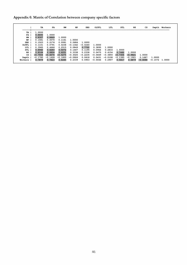
46

Appendix 0. Matrix of Correlation between company specific factors | TA FA NW NP SBD OLTFL LTL STL NS CS Depth Workers ------+----------------------------------------------------------------------------------------------------------- TA | 1.0000 FA | 0.8693 1.0000 NW | 0.8307 0.8869 1.0000 NP | 0.1581 0.0070 0.1161 1.0000 SBD | 0.1523 0.2176 0.0081 0.0684 1.0000 OLTFL | 0.1101 0.0791 0.0238 -0.1342 -0.0240 1.0000 LTL | 0.3965 0.4666 0.2515 0.0849 0.7722 0.3895 1.0000 STL | 0.8940 0.6283 0.5072 0.1467 0.1195 0.0964 0.2833 1.0000 NS | 0.8164 0.6804 0.6251 0.3338 0.2338 0.0475 0.4154 0.7482 1.0000 CS | -0.7554 -0.6076 -0.5275 -0.3025 -0.2235 -0.0649 -0.3893 -0.7306 -0.9821 1.0000 Depth | -0.1780 -0.1628 -0.1800 -0.0926 0.0618 0.0431 -0.0108 -0.1385 -0.1921 0.1687 1.0000 Workers | 0.7879 0.7823 0.8285 0.2339 0.0953 -0.0046 0.2907 0.5617 0.6879 -0.6088 -0.1572 1.0000

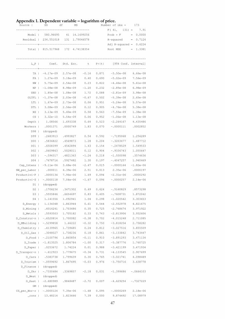
47

Appendix 1. Dependent variable – logarithm of price. Source | SS df MS Number of obs = 173

-------------+------------------------------ F( 41, 131) = 7.91

Model | 580.96695 41 14.1699256 Prob > F = 0.0000

Residual | 234.551018 131 1.79046578 R-squared = 0.7124

-------------+------------------------------ Adj R-squared = 0.6224

Total | 815.517968 172 4.74138354 Root MSE = 1.3381

------------------------------------------------------------------------------

L_P | Coef. Std. Err. t P>|t| [95% Conf. Interval]

-------------+----------------------------------------------------------------

TA | -4.17e-09 2.57e-08 -0.16 0.871 -5.50e-08 4.66e-08

FA | 1.27e-09 3.18e-09 0.40 0.690 -5.02e-09 7.56e-09

NW | 5.75e-09 2.54e-08 0.23 0.822 -4.46e-08 5.61e-08

NP | -1.08e-08 8.98e-09 -1.20 0.232 -2.85e-08 6.98e-09

SBD | 1.85e-08 1.08e-08 1.72 0.088 -2.81e-09 3.98e-08

OLTFL | -1.37e-08 2.03e-08 -0.67 0.502 -5.39e-08 2.65e-08

LTL | 1.67e-09 2.73e-08 0.06 0.951 -5.24e-08 5.57e-08

STL | 3.08e-09 2.56e-08 0.12 0.905 -4.76e-08 5.38e-08

NS | 3.13e-09 5.40e-09 0.58 0.563 -7.55e-09 1.38e-08

CS | 3.32e-10 5.54e-09 0.06 0.952 -1.06e-08 1.13e-08

Depth | 1.08566 1.693338 0.64 0.523 -2.264167 4.435486

Workers | .0001371 .0000749 1.83 0.070 -.0000111 .0002852

D98 | (dropped)

D99 | .2683913 .4993827 0.54 0.592 -.7195068 1.256289

D00 | .5836822 .4569873 1.28 0.204 -.3203477 1.487712

D01 | .6508399 .4542894 1.43 0.154 -.2478529 1.549533

D02 | .0609863 .5028011 0.12 0.904 -.9336743 1.055647

D03 | -.596317 .4821363 -1.24 0.218 -1.550098 .3574636

D04 | .7678716 .5927482 1.30 0.197 -.4047257 1.940469

Cap_Intens | -9.11e-06 3.68e-06 -2.47 0.015 -.0000164 -1.82e-06

NW_per_Labor | .000011 4.39e-06 2.51 0.013 2.35e-06 .0000197

Productivi~P | .0000134 7.96e-06 1.69 0.094 -2.31e-06 .0000292

Productivi~S | -.0000118 7.04e-06 -1.67 0.096 -.0000257 2.14e-06

D1 | (dropped)

D2 | .1706234 .3471302 0.49 0.624 -.5160829 .8573298

D3 | .5555846 .6654697 0.83 0.405 -.7608731 1.872042

D4 | 1.141556 1.092941 1.04 0.298 -1.020542 3.303653

D_Energy | 1.134348 1.863944 0.61 0.544 -2.552978 4.821675

D_Mining | .6016241 1.703686 0.35 0.725 -2.768674 3.971922

D_Metals | .5593503 1.705182 0.33 0.743 -2.813906 3.932606

D_Construc~n | -.6520814 1.700082 -0.38 0.702 -4.015248 2.711085

D_MBuilding | -.5299858 1.66222 -0.32 0.750 -3.818254 2.758282

D_Chemistry | .4139965 1.739685 0.24 0.812 -3.027516 3.855509

D_Oil_Gas | .3048027 1.738236 0.18 0.861 -3.133842 3.743447

D_Food | -.2100796 1.860854 -0.11 0.910 -3.891293 3.471134

D_Trade | -1.813525 1.806784 -1.00 0.317 -5.387776 1.760725

D_Paper | .0253672 1.74224 0.01 0.988 -3.421199 3.471934

D_Transpor~n | -.612923 1.779675 -0.34 0.731 -4.133545 2.907699

D_Cars | .5383738 1.799639 0.30 0.765 -3.021741 4.098489

D_Tourism | -.0559692 1.867695 -0.03 0.976 -3.750716 3.638778

D_Finance | (dropped)

D_Ukr | -.7330484 .3369857 -2.18 0.031 -1.399686 -.0664103

D_West | (dropped)

D_East | -2.680989 .9848487 -2.72 0.007 -4.629254 -.7327229

GM | (dropped)

CS_per_Wor~r | -.0000124 7.35e-06 -1.68 0.095 -.0000269 2.18e-06

_cons | 13.48214 1.823666 7.39 0.000 9.874492 17.08979

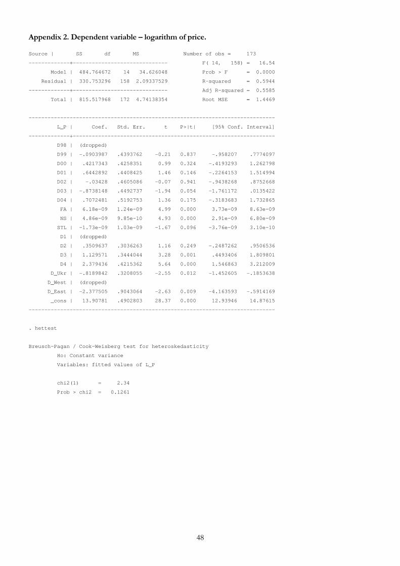
48

Appendix 2. Dependent variable – logarithm of price. Source | SS df MS Number of obs = 173

-------------+------------------------------ F( 14, 158) = 16.54

Model | 484.764672 14 34.626048 Prob > F = 0.0000

Residual | 330.753296 158 2.09337529 R-squared = 0.5944

-------------+------------------------------ Adj R-squared = 0.5585

Total | 815.517968 172 4.74138354 Root MSE = 1.4469

------------------------------------------------------------------------------

L_P | Coef. Std. Err. t P>|t| [95% Conf. Interval]

-------------+----------------------------------------------------------------

D98 | (dropped)

D99 | -.0903987 .4393762 -0.21 0.837 -.958207 .7774097

D00 | .4217343 .4258351 0.99 0.324 -.4193293 1.262798

D01 | .6442892 .4408425 1.46 0.146 -.2264153 1.514994

D02 | -.03428 .4605086 -0.07 0.941 -.9438268 .8752668

D03 | -.8738148 .4492737 -1.94 0.054 -1.761172 .0135422

D04 | .7072481 .5192753 1.36 0.175 -.3183683 1.732865

FA | 6.18e-09 1.24e-09 4.99 0.000 3.73e-09 8.63e-09

NS | 4.86e-09 9.85e-10 4.93 0.000 2.91e-09 6.80e-09

STL | -1.73e-09 1.03e-09 -1.67 0.096 -3.76e-09 3.10e-10

D1 | (dropped)

D2 | .3509637 .3036263 1.16 0.249 -.2487262 .9506536

D3 | 1.129571 .3444044 3.28 0.001 .4493406 1.809801

D4 | 2.379436 .4215362 5.64 0.000 1.546863 3.212009

D_Ukr | -.8189842 .3208055 -2.55 0.012 -1.452605 -.1853638

D_West | (dropped)

D_East | -2.377505 .9043064 -2.63 0.009 -4.163593 -.5914169

_cons | 13.90781 .4902803 28.37 0.000 12.93946 14.87615

------------------------------------------------------------------------------

. hettest

Breusch-Pagan / Cook-Weisberg test for heteroskedasticity

Ho: Constant variance

Variables: fitted values of L_P

chi2(1) = 2.34

Prob > chi2 = 0.1261

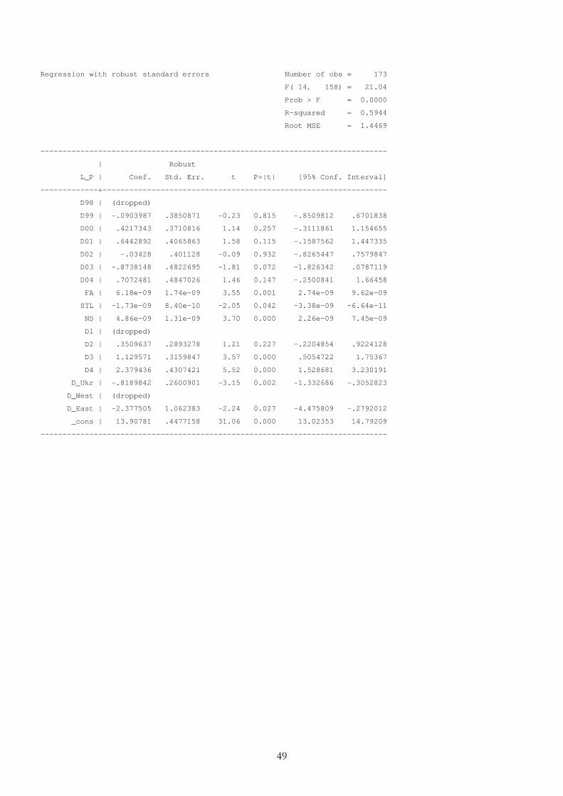
49

Regression with robust standard errors Number of obs = 173

F( 14, 158) = 21.04

Prob > F = 0.0000

R-squared = 0.5944

Root MSE = 1.4469

------------------------------------------------------------------------------

| Robust

L_P | Coef. Std. Err. t P>|t| [95% Conf. Interval]

-------------+----------------------------------------------------------------

D98 | (dropped)

D99 | -.0903987 .3850871 -0.23 0.815 -.8509812 .6701838

D00 | .4217343 .3710816 1.14 0.257 -.3111861 1.154655

D01 | .6442892 .4065863 1.58 0.115 -.1587562 1.447335

D02 | -.03428 .401128 -0.09 0.932 -.8265447 .7579847

D03 | -.8738148 .4822695 -1.81 0.072 -1.826342 .0787119

D04 | .7072481 .4847026 1.46 0.147 -.2500841 1.66458

FA | 6.18e-09 1.74e-09 3.55 0.001 2.74e-09 9.62e-09

STL | -1.73e-09 8.40e-10 -2.05 0.042 -3.38e-09 -6.64e-11

NS | 4.86e-09 1.31e-09 3.70 0.000 2.26e-09 7.45e-09

D1 | (dropped)

D2 | .3509637 .2893278 1.21 0.227 -.2204854 .9224128

D3 | 1.129571 .3159847 3.57 0.000 .5054722 1.75367

D4 | 2.379436 .4307421 5.52 0.000 1.528681 3.230191

D_Ukr | -.8189842 .2600901 -3.15 0.002 -1.332686 -.3052823

D_West | (dropped)

D_East | -2.377505 1.062383 -2.24 0.027 -4.475809 -.2792012

_cons | 13.90781 .4477158 31.06 0.000 13.02353 14.79209

------------------------------------------------------------------------------

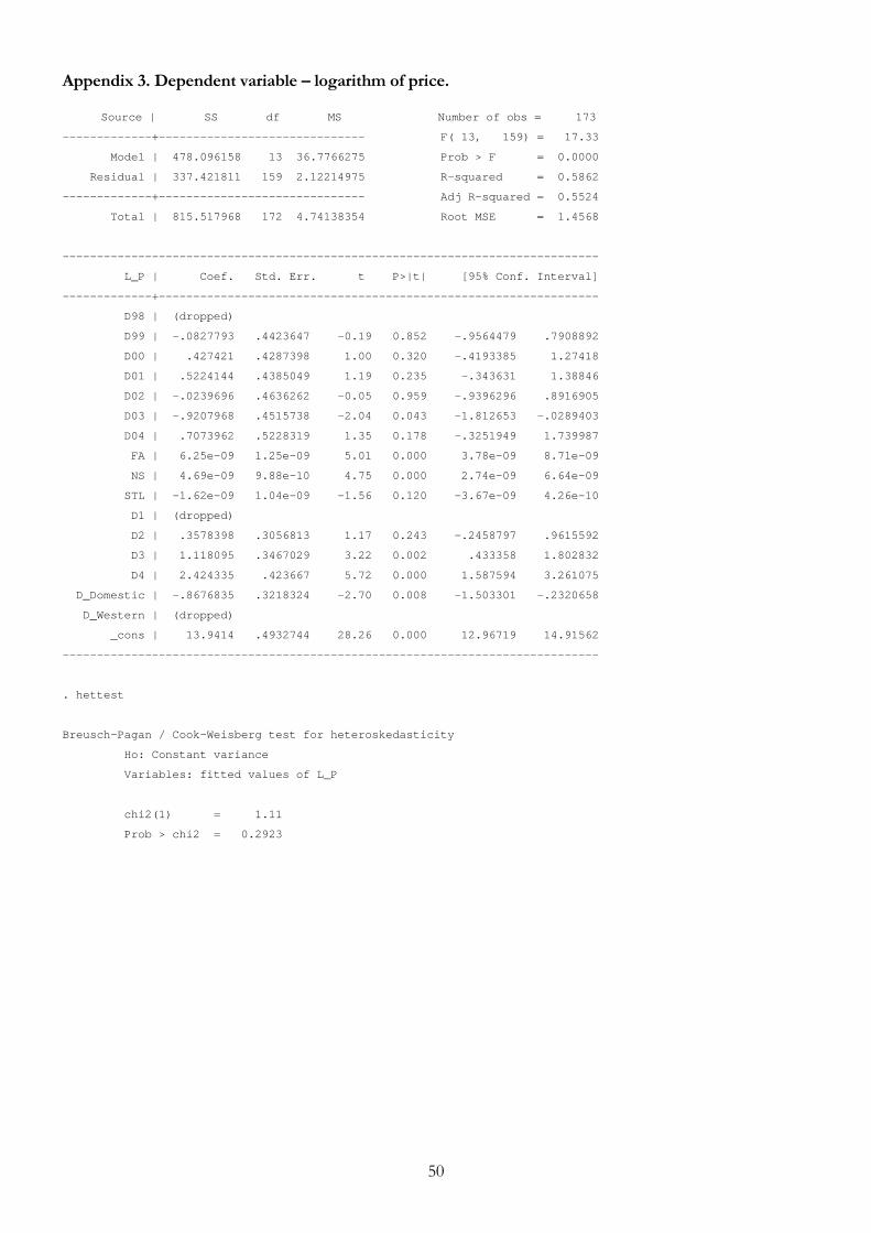
50

Appendix 3. Dependent variable – logarithm of price. Source | SS df MS Number of obs = 173

-------------+------------------------------ F( 13, 159) = 17.33

Model | 478.096158 13 36.7766275 Prob > F = 0.0000

Residual | 337.421811 159 2.12214975 R-squared = 0.5862

-------------+------------------------------ Adj R-squared = 0.5524

Total | 815.517968 172 4.74138354 Root MSE = 1.4568

------------------------------------------------------------------------------

L_P | Coef. Std. Err. t P>|t| [95% Conf. Interval]

-------------+----------------------------------------------------------------

D98 | (dropped)

D99 | -.0827793 .4423647 -0.19 0.852 -.9564479 .7908892

D00 | .427421 .4287398 1.00 0.320 -.4193385 1.27418

D01 | .5224144 .4385049 1.19 0.235 -.343631 1.38846

D02 | -.0239696 .4636262 -0.05 0.959 -.9396296 .8916905

D03 | -.9207968 .4515738 -2.04 0.043 -1.812653 -.0289403

D04 | .7073962 .5228319 1.35 0.178 -.3251949 1.739987

FA | 6.25e-09 1.25e-09 5.01 0.000 3.78e-09 8.71e-09

NS | 4.69e-09 9.88e-10 4.75 0.000 2.74e-09 6.64e-09

STL | -1.62e-09 1.04e-09 -1.56 0.120 -3.67e-09 4.26e-10

D1 | (dropped)

D2 | .3578398 .3056813 1.17 0.243 -.2458797 .9615592

D3 | 1.118095 .3467029 3.22 0.002 .433358 1.802832

D4 | 2.424335 .423667 5.72 0.000 1.587594 3.261075

D_Domestic | -.8676835 .3218324 -2.70 0.008 -1.503301 -.2320658

D_Western | (dropped)

_cons | 13.9414 .4932744 28.26 0.000 12.96719 14.91562

------------------------------------------------------------------------------

. hettest

Breusch-Pagan / Cook-Weisberg test for heteroskedasticity

Ho: Constant variance

Variables: fitted values of L_P

chi2(1) = 1.11

Prob > chi2 = 0.2923

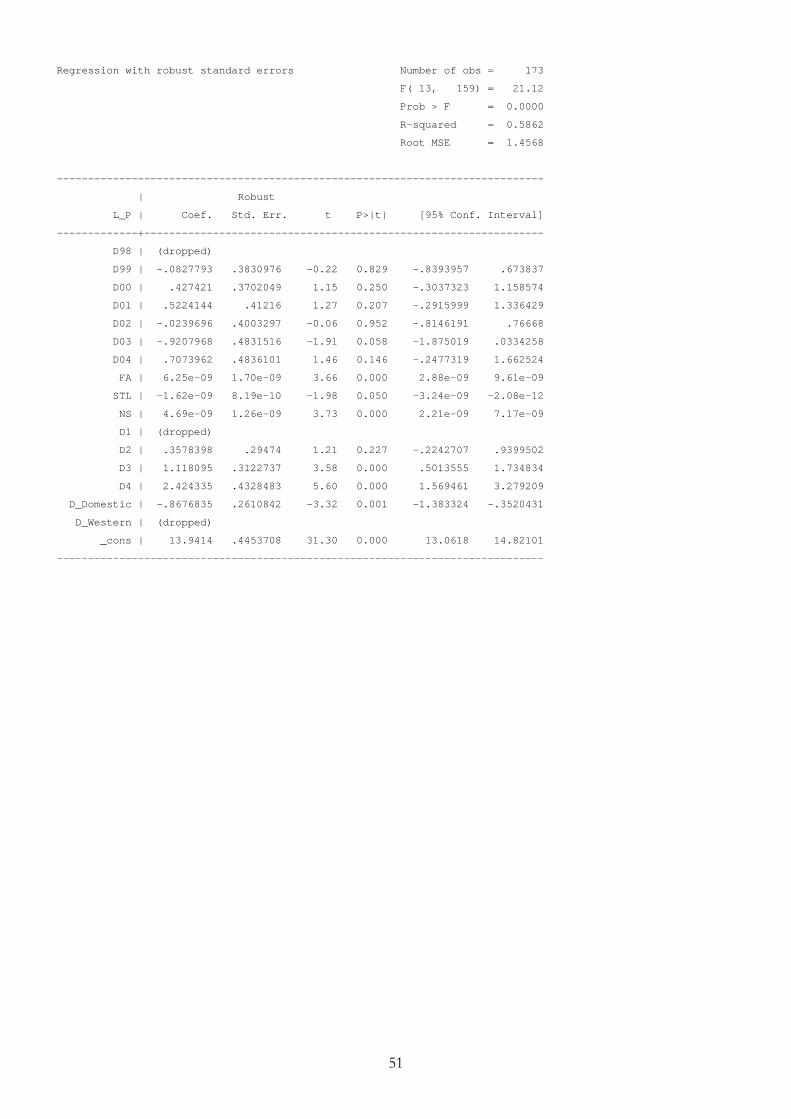
51

Regression with robust standard errors Number of obs = 173

F( 13, 159) = 21.12

Prob > F = 0.0000

R-squared = 0.5862

Root MSE = 1.4568

------------------------------------------------------------------------------

| Robust

L_P | Coef. Std. Err. t P>|t| [95% Conf. Interval]

-------------+----------------------------------------------------------------

D98 | (dropped)

D99 | -.0827793 .3830976 -0.22 0.829 -.8393957 .673837

D00 | .427421 .3702049 1.15 0.250 -.3037323 1.158574

D01 | .5224144 .41216 1.27 0.207 -.2915999 1.336429

D02 | -.0239696 .4003297 -0.06 0.952 -.8146191 .76668

D03 | -.9207968 .4831516 -1.91 0.058 -1.875019 .0334258

D04 | .7073962 .4836101 1.46 0.146 -.2477319 1.662524

FA | 6.25e-09 1.70e-09 3.66 0.000 2.88e-09 9.61e-09

STL | -1.62e-09 8.19e-10 -1.98 0.050 -3.24e-09 -2.08e-12

NS | 4.69e-09 1.26e-09 3.73 0.000 2.21e-09 7.17e-09

D1 | (dropped)

D2 | .3578398 .29474 1.21 0.227 -.2242707 .9399502

D3 | 1.118095 .3122737 3.58 0.000 .5013555 1.734834

D4 | 2.424335 .4328483 5.60 0.000 1.569461 3.279209

D_Domestic | -.8676835 .2610842 -3.32 0.001 -1.383324 -.3520431

D_Western | (dropped)

_cons | 13.9414 .4453708 31.30 0.000 13.0618 14.82101

------------------------------------------------------------------------------

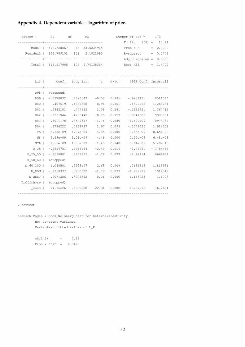
52

Appendix 4. Dependent variable – logarithm of price. Source | SS df MS Number of obs = 173

-------------+------------------------------ F( 14, 158) = 15.41

Model | 470.728867 14 33.6234905 Prob > F = 0.0000

Residual | 344.789101 158 2.1822095 R-squared = 0.5772

-------------+------------------------------ Adj R-squared = 0.5398

Total | 815.517968 172 4.74138354 Root MSE = 1.4772

------------------------------------------------------------------------------

L_P | Coef. Std. Err. t P>|t| [95% Conf. Interval]

-------------+----------------------------------------------------------------

D98 | (dropped)

D99 | -.0370032 .4496549 -0.08 0.935 -.9251131 .8511066

D00 | .407619 .4357328 0.94 0.351 -.4529933 1.268231

D01 | .4842101 .447322 1.08 0.281 -.3992921 1.367712

D02 | -.0251944 .4703449 -0.05 0.957 -.9541689 .9037801

D03 | -.8011175 .4549617 -1.76 0.080 -1.699709 .0974737

D04 | .8784222 .5244747 1.67 0.096 -.1574636 1.914308

FA | 6.15e-09 1.27e-09 4.85 0.000 3.65e-09 8.65e-09

NS | 4.49e-09 1.01e-09 4.46 0.000 2.50e-09 6.48e-09

STL | -1.53e-09 1.05e-09 -1.45 0.148 -3.61e-09 5.49e-10

D_25 | -.9554781 .3934154 -2.43 0.016 -1.73251 -.1784464

D_25_50 | -.6150881 .3453265 -1.78 0.077 -1.29714 .0669634

D_50_60 | (dropped)

D_60_100 | 1.040501 .3923107 2.65 0.009 .2656516 1.815351

D_DOM | -.9358337 .5250822 -1.78 0.077 -1.972919 .1012519

D_WEST | .0071386 .5924592 0.01 0.990 -1.163023 1.1773

D_Offshore | (dropped)

_cons | 14.96626 .6552288 22.84 0.000 13.67213 16.2604

------------------------------------------------------------------------------

. hettest

Breusch-Pagan / Cook-Weisberg test for heteroskedasticity

Ho: Constant variance

Variables: fitted values of L_P

chi2(1) = 0.88

Prob > chi2 = 0.3473

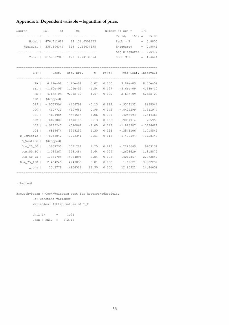
53

Appendix 5. Dependent variable – logarithm of price. Source | SS df MS Number of obs = 173

-------------+------------------------------ F( 14, 158) = 15.88

Model | 476.711624 14 34.0508303 Prob > F = 0.0000

Residual | 338.806344 158 2.14434395 R-squared = 0.5846

-------------+------------------------------ Adj R-squared = 0.5477

Total | 815.517968 172 4.74138354 Root MSE = 1.4644

------------------------------------------------------------------------------

L_P | Coef. Std. Err. t P>|t| [95% Conf. Interval]

-------------+----------------------------------------------------------------

FA | 6.29e-09 1.25e-09 5.02 0.000 3.82e-09 8.76e-09

STL | -1.60e-09 1.04e-09 -1.54 0.127 -3.66e-09 4.58e-10

NS | 4.65e-09 9.97e-10 4.67 0.000 2.69e-09 6.62e-09

D98 | (dropped)

D99 | -.0567594 .4458799 -0.13 0.899 -.9374132 .8238944

D00 | .4107723 .4309683 0.95 0.342 -.4404299 1.261974

D01 | .4694985 .4429504 1.06 0.291 -.4053693 1.344366

D02 | -.0628007 .4670115 -0.13 0.893 -.9851914 .85959

D03 | -.9295247 .4540862 -2.05 0.042 -1.826387 -.0326628

D04 | .6819674 .5248252 1.30 0.196 -.3546106 1.718545

D_Domestic | -.8055042 .3203341 -2.51 0.013 -1.438194 -.1728148

D_Western | (dropped)

Dum_25_50 | .3837235 .3071201 1.25 0.213 -.2228669 .9903139

Dum_50_60 | 1.039367 .3931484 2.64 0.009 .2628629 1.815872

Dum_60_75 | 1.339789 .4724096 2.84 0.005 .4067367 2.272842

Dum_75_100 | 2.464249 .4243035 5.81 0.000 1.62621 3.302287

_cons | 13.8779 .4904528 28.30 0.000 12.90921 14.84659

------------------------------------------------------------------------------

. hettest

Breusch-Pagan / Cook-Weisberg test for heteroskedasticity

Ho: Constant variance

Variables: fitted values of L_P

chi2(1) = 1.21

Prob > chi2 = 0.2717

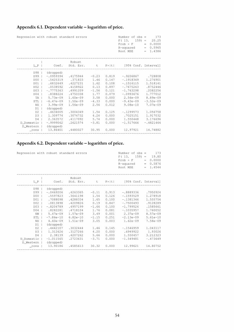
54

Appendix 6.1. Dependent variable – logarithm of price. Regression with robust standard errors Number of obs = 173 F( 13, 159) = 20.25 Prob > F = 0.0000 R-squared = 0.5965 Root MSE = 1.4386 ------------------------------------------------------------------------------ | Robust L_P | Coef. Std. Err. t P>|t| [95% Conf. Interval] -------------+---------------------------------------------------------------- D98 | (dropped) D99 | -.0959394 .4175944 -0.23 0.819 -.9206867 .728808 D00 | .5425319 .371833 1.46 0.147 -.1918369 1.276901 D01 | .6832649 .4227231 1.62 0.108 -.1516115 1.518141 D02 | .0538592 .4158922 0.13 0.897 -.7675263 .8752446 D03 | -.7775363 .4991209 -1.56 0.121 -1.763298 .2082256 D04 | .8388224 .4750338 1.77 0.079 -.0993676 1.777012 TA | 5.73e-09 1.60e-09 3.58 0.000 2.56e-09 8.89e-09 STL | -6.47e-09 1.50e-09 -4.33 0.000 -9.43e-09 -3.52e-09 NS | 3.99e-09 1.56e-09 2.56 0.012 9.08e-10 7.07e-09 D1 | (dropped) D2 | .4634005 .3004349 1.54 0.125 -.1299573 1.056758 D3 | 1.309774 .3074732 4.26 0.000 .7025151 1.917032 D4 | 2.363572 .4117092 5.74 0.000 1.550448 3.176696 D_Domestic | -.9999062 .2621574 -3.81 0.000 -1.517666 -.4821464 D_Western | (dropped) _cons | 13.86401 .4480027 30.95 0.000 12.97921 14.74882 ------------------------------------------------------------------------------

Appendix 6.2. Dependent variable – logarithm of price. Regression with robust standard errors Number of obs = 173 F( 13, 159) = 19.80 Prob > F = 0.0000 R-squared = 0.5876 Root MSE = 1.4544 ------------------------------------------------------------------------------ | Robust L_P | Coef. Std. Err. t P>|t| [95% Conf. Interval] -------------+---------------------------------------------------------------- D98 | (dropped) D99 | -.0469206 .4263365 -0.11 0.913 -.8889336 .7950924 D00 | .5597823 .3641198 1.54 0.126 -.1593529 1.278918 D01 | .7088098 .4288334 1.65 0.100 -.1381346 1.555754 D02 | .0813898 .4209826 0.19 0.847 -.7500493 .9128289 D03 | -.8204789 .4957199 -1.66 0.100 -1.799524 .1585661 D04 | .8282281 .4718104 1.76 0.081 -.1035957 1.760052 NW | 5.47e-09 1.57e-09 3.49 0.001 2.37e-09 8.57e-09 STL | -7.86e-10 6.82e-10 -1.15 0.251 -2.13e-09 5.61e-10 NS | 4.60e-09 1.51e-09 3.05 0.003 1.62e-09 7.58e-09 D1 | (dropped) D2 | .4442107 .3032444 1.46 0.145 -.1546959 1.043117 D3 | 1.312626 .3127266 4.20 0.000 .6949922 1.93026 D4 | 2.38139 .4207262 5.66 0.000 1.550457 3.212323 D_Domestic | -1.011565 .2723631 -3.71 0.000 -1.549481 -.473649 D_Western | (dropped) _cons | 13.90186 .4585613 30.32 0.000 12.99621 14.80752 ------------------------------------------------------------------------------

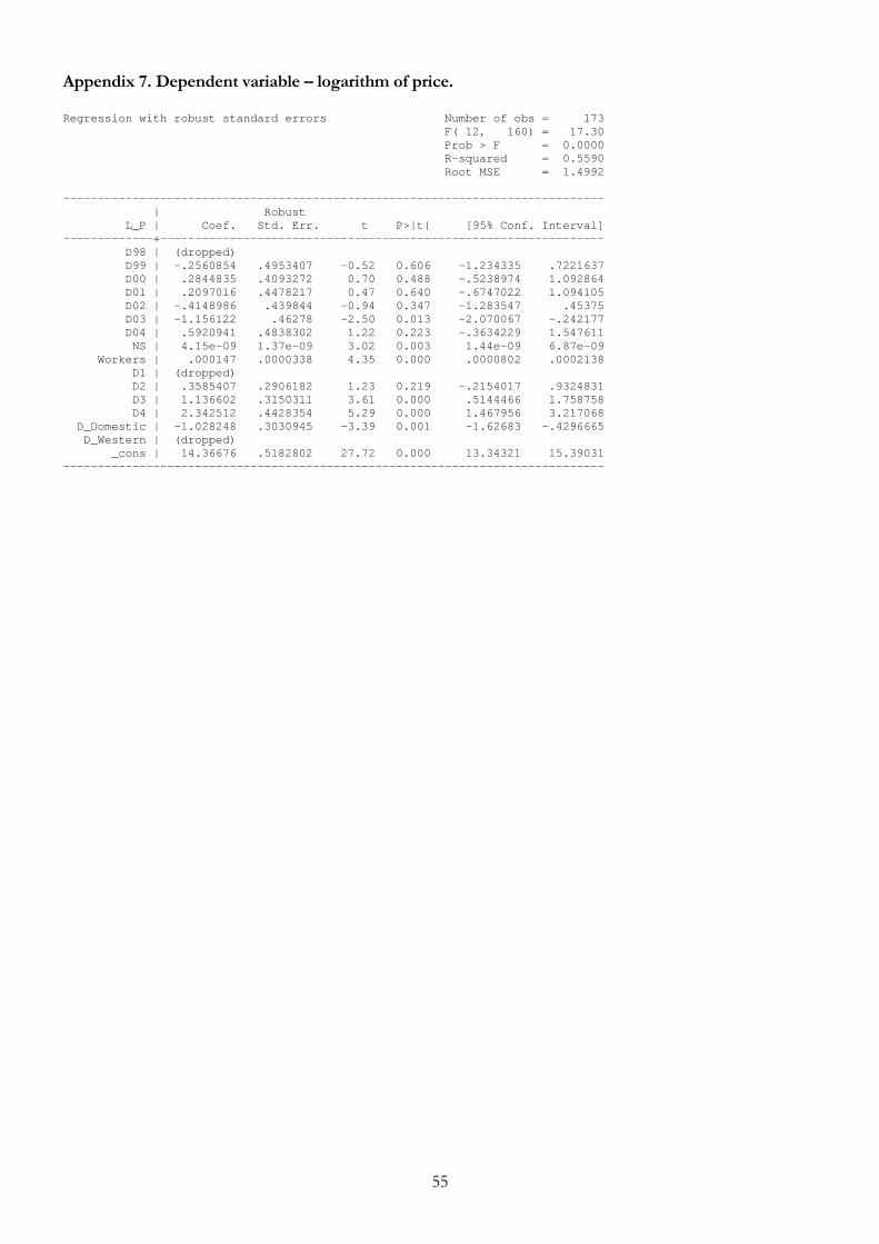
55

Appendix 7. Dependent variable – logarithm of price. Regression with robust standard errors Number of obs = 173 F( 12, 160) = 17.30 Prob > F = 0.0000 R-squared = 0.5590 Root MSE = 1.4992 ------------------------------------------------------------------------------ | Robust L_P | Coef. Std. Err. t P>|t| [95% Conf. Interval] -------------+---------------------------------------------------------------- D98 | (dropped) D99 | -.2560854 .4953407 -0.52 0.606 -1.234335 .7221637 D00 | .2844835 .4093272 0.70 0.488 -.5238974 1.092864 D01 | .2097016 .4478217 0.47 0.640 -.6747022 1.094105 D02 | -.4148986 .439844 -0.94 0.347 -1.283547 .45375 D03 | -1.156122 .46278 -2.50 0.013 -2.070067 -.242177 D04 | .5920941 .4838302 1.22 0.223 -.3634229 1.547611 NS | 4.15e-09 1.37e-09 3.02 0.003 1.44e-09 6.87e-09 Workers | .000147 .0000338 4.35 0.000 .0000802 .0002138 D1 | (dropped) D2 | .3585407 .2906182 1.23 0.219 -.2154017 .9324831 D3 | 1.136602 .3150311 3.61 0.000 .5144466 1.758758 D4 | 2.342512 .4428354 5.29 0.000 1.467956 3.217068 D_Domestic | -1.028248 .3030945 -3.39 0.001 -1.62683 -.4296665 D_Western | (dropped) _cons | 14.36676 .5182802 27.72 0.000 13.34321 15.39031 ------------------------------------------------------------------------------

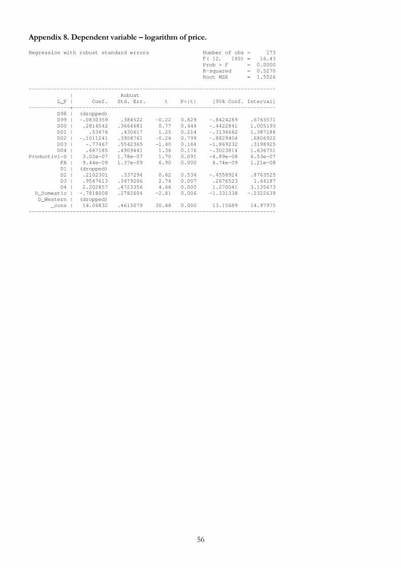
56

Appendix 8. Dependent variable – logarithm of price. Regression with robust standard errors Number of obs = 173 F( 12, 160) = 16.43 Prob > F = 0.0000 R-squared = 0.5270 Root MSE = 1.5526 ------------------------------------------------------------------------------ | Robust L_P | Coef. Std. Err. t P>|t| [95% Conf. Interval] -------------+---------------------------------------------------------------- D98 | (dropped) D99 | -.0830359 .384522 -0.22 0.829 -.8424289 .6763571 D00 | .2814542 .3664681 0.77 0.444 -.4422841 1.005193 D01 | .53676 .430617 1.25 0.214 -.3136662 1.387186 D02 | -.1011241 .3958761 -0.26 0.799 -.8829404 .6806922 D03 | -.77467 .5542365 -1.40 0.164 -1.869232 .3198925 D04 | .667185 .4909441 1.36 0.176 -.3023814 1.636751 Productivi~S | 3.02e-07 1.78e-07 1.70 0.091 -4.89e-08 6.53e-07 FA | 9.44e-09 1.37e-09 6.90 0.000 6.74e-09 1.21e-08 D1 | (dropped) D2 | .2102301 .337294 0.62 0.534 -.4558924 .8763525 D3 | .9547613 .3479206 2.74 0.007 .2676523 1.64187 D4 | 2.202857 .4723356 4.66 0.000 1.270041 3.135673 D_Domestic | -.7818008 .2782604 -2.81 0.006 -1.331338 -.2322639 D_Western | (dropped) _cons | 14.06832 .4615079 30.48 0.000 13.15689 14.97975 ------------------------------------------------------------------------------

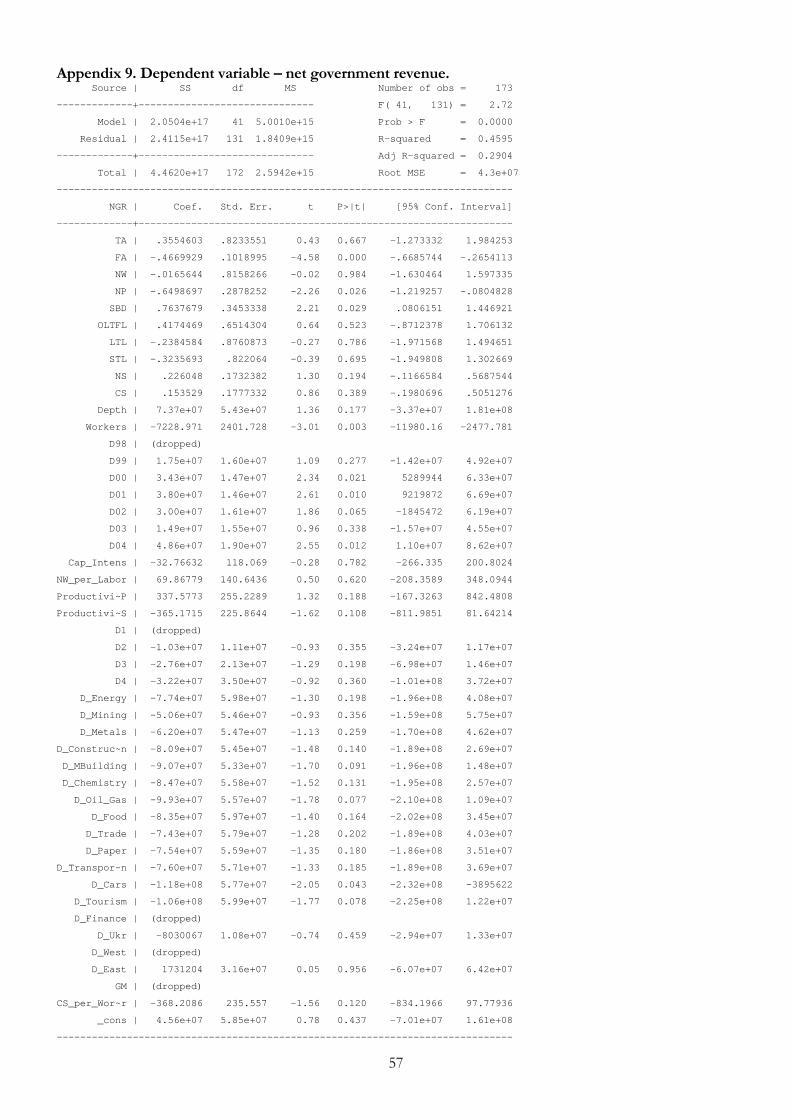
57

Appendix 9. Dependent variable – net government revenue. Source | SS df MS Number of obs = 173

-------------+------------------------------ F( 41, 131) = 2.72

Model | 2.0504e+17 41 5.0010e+15 Prob > F = 0.0000

Residual | 2.4115e+17 131 1.8409e+15 R-squared = 0.4595

-------------+------------------------------ Adj R-squared = 0.2904

Total | 4.4620e+17 172 2.5942e+15 Root MSE = 4.3e+07

------------------------------------------------------------------------------

NGR | Coef. Std. Err. t P>|t| [95% Conf. Interval]

-------------+----------------------------------------------------------------

TA | .3554603 .8233551 0.43 0.667 -1.273332 1.984253

FA | -.4669929 .1018995 -4.58 0.000 -.6685744 -.2654113

NW | -.0165644 .8158266 -0.02 0.984 -1.630464 1.597335

NP | -.6498697 .2878252 -2.26 0.026 -1.219257 -.0804828

SBD | .7637679 .3453338 2.21 0.029 .0806151 1.446921

OLTFL | .4174469 .6514304 0.64 0.523 -.8712378 1.706132

LTL | -.2384584 .8760873 -0.27 0.786 -1.971568 1.494651

STL | -.3235693 .822064 -0.39 0.695 -1.949808 1.302669

NS | .226048 .1732382 1.30 0.194 -.1166584 .5687544

CS | .153529 .1777332 0.86 0.389 -.1980696 .5051276

Depth | 7.37e+07 5.43e+07 1.36 0.177 -3.37e+07 1.81e+08

Workers | -7228.971 2401.728 -3.01 0.003 -11980.16 -2477.781

D98 | (dropped)

D99 | 1.75e+07 1.60e+07 1.09 0.277 -1.42e+07 4.92e+07

D00 | 3.43e+07 1.47e+07 2.34 0.021 5289944 6.33e+07

D01 | 3.80e+07 1.46e+07 2.61 0.010 9219872 6.69e+07

D02 | 3.00e+07 1.61e+07 1.86 0.065 -1845472 6.19e+07

D03 | 1.49e+07 1.55e+07 0.96 0.338 -1.57e+07 4.55e+07

D04 | 4.86e+07 1.90e+07 2.55 0.012 1.10e+07 8.62e+07

Cap_Intens | -32.76632 118.069 -0.28 0.782 -266.335 200.8024

NW_per_Labor | 69.86779 140.6436 0.50 0.620 -208.3589 348.0944

Productivi~P | 337.5773 255.2289 1.32 0.188 -167.3263 842.4808

Productivi~S | -365.1715 225.8644 -1.62 0.108 -811.9851 81.64214

D1 | (dropped)

D2 | -1.03e+07 1.11e+07 -0.93 0.355 -3.24e+07 1.17e+07

D3 | -2.76e+07 2.13e+07 -1.29 0.198 -6.98e+07 1.46e+07

D4 | -3.22e+07 3.50e+07 -0.92 0.360 -1.01e+08 3.72e+07

D_Energy | -7.74e+07 5.98e+07 -1.30 0.198 -1.96e+08 4.08e+07

D_Mining | -5.06e+07 5.46e+07 -0.93 0.356 -1.59e+08 5.75e+07

D_Metals | -6.20e+07 5.47e+07 -1.13 0.259 -1.70e+08 4.62e+07

D_Construc~n | -8.09e+07 5.45e+07 -1.48 0.140 -1.89e+08 2.69e+07

D_MBuilding | -9.07e+07 5.33e+07 -1.70 0.091 -1.96e+08 1.48e+07

D_Chemistry | -8.47e+07 5.58e+07 -1.52 0.131 -1.95e+08 2.57e+07

D_Oil_Gas | -9.93e+07 5.57e+07 -1.78 0.077 -2.10e+08 1.09e+07

D_Food | -8.35e+07 5.97e+07 -1.40 0.164 -2.02e+08 3.45e+07

D_Trade | -7.43e+07 5.79e+07 -1.28 0.202 -1.89e+08 4.03e+07

D_Paper | -7.54e+07 5.59e+07 -1.35 0.180 -1.86e+08 3.51e+07

D_Transpor~n | -7.60e+07 5.71e+07 -1.33 0.185 -1.89e+08 3.69e+07

D_Cars | -1.18e+08 5.77e+07 -2.05 0.043 -2.32e+08 -3895622

D_Tourism | -1.06e+08 5.99e+07 -1.77 0.078 -2.25e+08 1.22e+07

D_Finance | (dropped)

D_Ukr | -8030067 1.08e+07 -0.74 0.459 -2.94e+07 1.33e+07

D_West | (dropped)

D_East | 1731204 3.16e+07 0.05 0.956 -6.07e+07 6.42e+07

GM | (dropped)

CS_per_Wor~r | -368.2086 235.557 -1.56 0.120 -834.1966 97.77936

_cons | 4.56e+07 5.85e+07 0.78 0.437 -7.01e+07 1.61e+08

------------------------------------------------------------------------------

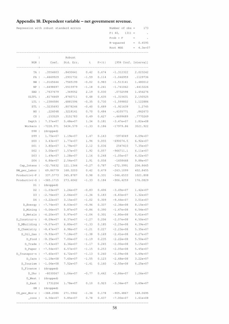
58

Appendix 10. Dependent variable – net government revenue. Regression with robust standard errors Number of obs = 173

F( 40, 131) = .

Prob > F = .

R-squared = 0.4595

Root MSE = 4.3e+07

------------------------------------------------------------------------------

| Robust

NGR | Coef. Std. Err. t P>|t| [95% Conf. Interval]

-------------+----------------------------------------------------------------

TA | .3554603 .8430641 0.42 0.674 -1.312322 2.023242

FA | -.4669929 .2931732 -1.59 0.114 -1.046959 .1129736

NW | -.0165644 .7565199 -0.02 0.983 -1.513141 1.480012

NP | -.6498697 .5515979 -1.18 0.241 -1.741062 .4413226

SBD | .7637679 .349052 2.19 0.030 .0732598 1.454276

OLTFL | .4174469 .8760711 0.48 0.635 -1.315631 2.150525

LTL | -.2384584 .6881596 -0.35 0.730 -1.599802 1.122886

STL | -.3235693 .8078246 -0.40 0.689 -1.921639 1.2745

NS | .226048 .3218141 0.70 0.484 -.4105771 .862673

CS | .153529 .3151783 0.49 0.627 -.4699689 .7770269

Depth | 7.37e+07 5.48e+07 1.34 0.181 -3.47e+07 1.82e+08

Workers | -7228.971 5434.579 -1.33 0.186 -17979.86 3521.922

D98 | (dropped)

D99 | 1.75e+07 1.19e+07 1.47 0.143 -5974049 4.09e+07

D00 | 3.43e+07 1.77e+07 1.94 0.055 -690074.5 6.92e+07

D01 | 3.80e+07 1.79e+07 2.12 0.036 2547410 7.35e+07

D02 | 3.00e+07 1.57e+07 1.92 0.057 -966711.1 6.11e+07

D03 | 1.49e+07 1.28e+07 1.16 0.248 -1.05e+07 4.02e+07

D04 | 4.86e+07 2.54e+07 1.91 0.058 -1658468 9.88e+07

Cap_Intens | -32.76632 121.1344 -0.27 0.787 -272.3991 206.8665

NW_per_Labor | 69.86779 168.3203 0.42 0.679 -263.1099 402.8455

Productivi~P | 337.5773 345.8787 0.98 0.331 -346.6533 1021.808

Productivi~S | -365.1715 273.6042 -1.33 0.184 -906.4259 176.0829

D1 | (dropped)

D2 | -1.03e+07 1.24e+07 -0.83 0.406 -3.49e+07 1.42e+07

D3 | -2.76e+07 2.06e+07 -1.34 0.183 -6.83e+07 1.32e+07

D4 | -3.22e+07 3.15e+07 -1.02 0.309 -9.44e+07 3.01e+07

D_Energy | -7.74e+07 8.03e+07 -0.96 0.337 -2.36e+08 8.15e+07

D_Mining | -5.06e+07 5.87e+07 -0.86 0.390 -1.67e+08 6.54e+07

D_Metals | -6.20e+07 5.97e+07 -1.04 0.301 -1.80e+08 5.61e+07

D_Construc~n | -8.09e+07 6.37e+07 -1.27 0.206 -2.07e+08 4.50e+07

D_MBuilding | -9.07e+07 6.80e+07 -1.33 0.185 -2.25e+08 4.39e+07

D_Chemistry | -8.47e+07 6.98e+07 -1.21 0.227 -2.23e+08 5.35e+07

D_Oil_Gas | -9.93e+07 7.18e+07 -1.38 0.169 -2.41e+08 4.27e+07

D_Food | -8.35e+07 7.00e+07 -1.19 0.235 -2.22e+08 5.50e+07

D_Trade | -7.43e+07 6.36e+07 -1.17 0.245 -2.00e+08 5.15e+07

D_Paper | -7.54e+07 6.57e+07 -1.15 0.253 -2.05e+08 5.45e+07

D_Transpor~n | -7.60e+07 6.72e+07 -1.13 0.260 -2.09e+08 5.69e+07

D_Cars | -1.18e+08 7.60e+07 -1.55 0.123 -2.68e+08 3.22e+07

D_Tourism | -1.06e+08 7.52e+07 -1.41 0.160 -2.55e+08 4.25e+07

D_Finance | (dropped)

D_Ukr | -8030067 1.04e+07 -0.77 0.442 -2.86e+07 1.26e+07

D_West | (dropped)

D_East | 1731204 1.78e+07 0.10 0.923 -3.34e+07 3.69e+07

GM | (dropped)

CS_per_Wor~r | -368.2086 271.5942 -1.36 0.178 -905.4867 169.0695

_cons | 4.56e+07 5.85e+07 0.78 0.437 -7.00e+07 1.61e+08

------------------------------------------------------------------------------

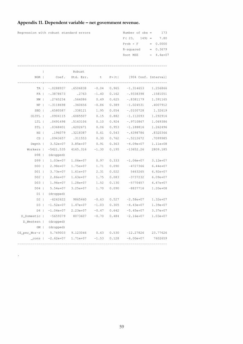
59

Appendix 11. Dependent variable – net government revenue. Regression with robust standard errors Number of obs = 173

F( 23, 149) = 7.80

Prob > F = 0.0000

R-squared = 0.3679

Root MSE = 4.4e+07

------------------------------------------------------------------------------

| Robust

NGR | Coef. Std. Err. t P>|t| [95% Conf. Interval]

-------------+----------------------------------------------------------------

TA | -.0288937 .6506838 -0.04 0.965 -1.314653 1.256866

FA | -.3878673 .2763 -1.40 0.162 -.9338398 .1581051

NW | .2765234 .564086 0.49 0.625 -.8381179 1.391165

NP | -.3118698 .360656 -0.86 0.389 -1.024531 .4007912

SBD | .6580587 .338121 1.95 0.054 -.0100728 1.32619

OLTFL | .0904115 .6085507 0.15 0.882 -1.112093 1.292916

LTL | .0491498 .5163106 0.10 0.924 -.9710867 1.069386

STL | .0368401 .6202671 0.06 0.953 -1.188816 1.262496

NS | .196079 .3218387 0.61 0.543 -.4398786 .8320366

CS | .0943657 .311553 0.30 0.762 -.5212672 .7099985

Depth | 3.52e+07 3.85e+07 0.91 0.363 -4.09e+07 1.11e+08

Workers | -5421.535 4165.316 -1.30 0.195 -13652.26 2809.185

D98 | (dropped)

D99 | 1.03e+07 1.06e+07 0.97 0.333 -1.06e+07 3.12e+07

D00 | 2.98e+07 1.75e+07 1.71 0.090 -4727366 6.44e+07

D01 | 3.73e+07 1.61e+07 2.31 0.022 5463265 6.92e+07

D02 | 2.86e+07 1.63e+07 1.75 0.083 -3737232 6.09e+07

D03 | 1.94e+07 1.28e+07 1.52 0.130 -5770457 4.47e+07

D04 | 5.54e+07 3.25e+07 1.70 0.090 -8837716 1.20e+08

D1 | (dropped)

D2 | -6262622 9865460 -0.63 0.527 -2.58e+07 1.32e+07

D3 | -1.52e+07 1.47e+07 -1.03 0.305 -4.43e+07 1.39e+07

D4 | -1.04e+07 2.23e+07 -0.47 0.642 -5.45e+07 3.37e+07

D_Domestic | -5659379 8073607 -0.70 0.484 -2.16e+07 1.03e+07

D_Western | (dropped)

GM | (dropped)

CS_per_Wor~r | 5.749003 9.123046 0.63 0.530 -12.27826 23.77626

_cons | -2.62e+07 1.71e+07 -1.53 0.128 -6.00e+07 7602659

------------------------------------------------------------------------------

.

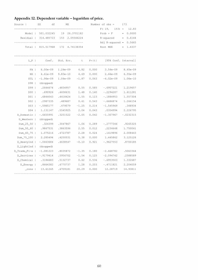
60

Appendix 12. Dependent variable – logarithm of price.

Source | SS df MS Number of obs = 173

-------------+------------------------------ F( 19, 153) = 12.83

Model | 501.032245 19 26.3701182 Prob > F = 0.0000

Residual | 314.485723 153 2.05546224 R-squared = 0.6144

-------------+------------------------------ Adj R-squared = 0.5665

Total | 815.517968 172 4.74138354 Root MSE = 1.4337

------------------------------------------------------------------------------

L_P | Coef. Std. Err. t P>|t| [95% Conf. Interval]

-------------+----------------------------------------------------------------

FA | 6.00e-09 1.24e-09 4.82 0.000 3.54e-09 8.45e-09

NS | 4.61e-09 9.83e-10 4.69 0.000 2.66e-09 6.55e-09

STL | -1.96e-09 1.04e-09 -1.87 0.063 -4.02e-09 1.06e-10

D98 | (dropped)

D99 | .2644674 .4834957 0.55 0.585 -.6907221 1.219657

D00 | .690926 .4658631 1.48 0.140 -.2294287 1.611281

D01 | .6844043 .4418424 1.55 0.123 -.1884953 1.557304

D02 | .2987335 .489687 0.61 0.543 -.6686874 1.266154

D03 | -.5985177 .479579 -1.25 0.214 -1.545969 .348934

D04 | 1.131147 .5545925 2.04 0.043 .0354994 2.226795

D_Domestic | -.6655991 .3251522 -2.05 0.042 -1.307967 -.0232315

D_Western | (dropped)

Dum_25_50 | .324399 .3047867 1.06 0.289 -.2777346 .9265325

Dum_50_60 | .9867531 .3863596 2.55 0.012 .2234648 1.750041

Dum_60_75 | 1.075216 .4723787 2.28 0.024 .1419896 2.008443

Dum_75_100 | 2.285494 .4250031 5.38 0.000 1.445862 3.125126

D_HeavyInd | -.0463684 .4638547 -0.10 0.921 -.9627553 .8700185

D_LightInd | (dropped)

D_Trade_Fi~e | -1.081223 .8035872 -1.35 0.180 -2.668782 .5063364

D_Services | -.9179414 .5956702 -1.54 0.125 -2.094742 .2588589

D_Chemical | .3186683 .5132737 0.62 0.536 -.6953503 1.332687

D_Energy | .8664382 .6770737 1.28 0.203 -.4711821 2.204059

_cons | 13.61265 .6709181 20.29 0.000 12.28719 14.93811

------------------------------------------------------------------------------

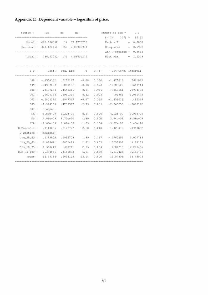
61

Appendix 13. Dependent variable – logarithm of price.

Source | SS df MS Number of obs = 172 -------------+------------------------------ F( 14, 157) = 16.32

Model | 465.886058 14 33.2775756 Prob > F = 0.0000

Residual | 320.124461 157 2.03900931 R-squared = 0.5927

-------------+------------------------------ Adj R-squared = 0.5564

Total | 786.01052 171 4.59655275 Root MSE = 1.4279

------------------------------------------------------------------------------

L_P | Coef. Std. Err. t P>|t| [95% Conf. Interval]

-------------+----------------------------------------------------------------

D98 | -.4554182 .5172165 -0.88 0.380 -1.477019 .5661823

D99 | -.4987283 .5087106 -0.98 0.328 -1.503528 .5060714

D00 | -.0197234 .4643316 -0.04 0.966 -.9368661 .8974193

D01 | .0604188 .4931319 0.12 0.903 -.91361 1.034448

D02 | -.4808294 .4947367 -0.97 0.333 -1.458028 .496369

D03 | -1.324133 .4739397 -2.79 0.006 -2.260253 -.3880122

D04 | (dropped)

FA | 6.54e-09 1.22e-09 5.34 0.000 4.12e-09 8.96e-09

NS | 4.66e-09 9.72e-10 4.80 0.000 2.74e-09 6.58e-09

STL | -1.66e-09 1.02e-09 -1.63 0.104 -3.67e-09 3.47e-10

D_Domestic | -.8110835 .3123727 -2.60 0.010 -1.428079 -.1940882

D_Western | (dropped)

Dum_25_50 | .4158803 .2996703 1.39 0.167 -.1760252 1.007786

Dum_50_60 | 1.083611 .3836493 2.82 0.005 .3258307 1.84139

Dum_60_75 | 1.360413 .460711 2.95 0.004 .4504219 2.270405

Dum_75_100 | 2.334066 .4159802 5.61 0.000 1.512426 3.155705

_cons | 14.28156 .6093129 23.44 0.000 13.07805 15.48506

------------------------------------------------------------------------------

62

Appendix 14. Ramsey omitted variables test.

Ramsey RESET test using powers of the fitted values of L_P

Ho: model has no omitted variables

F(3, 154) = 7.10

Prob > F = 0.0002

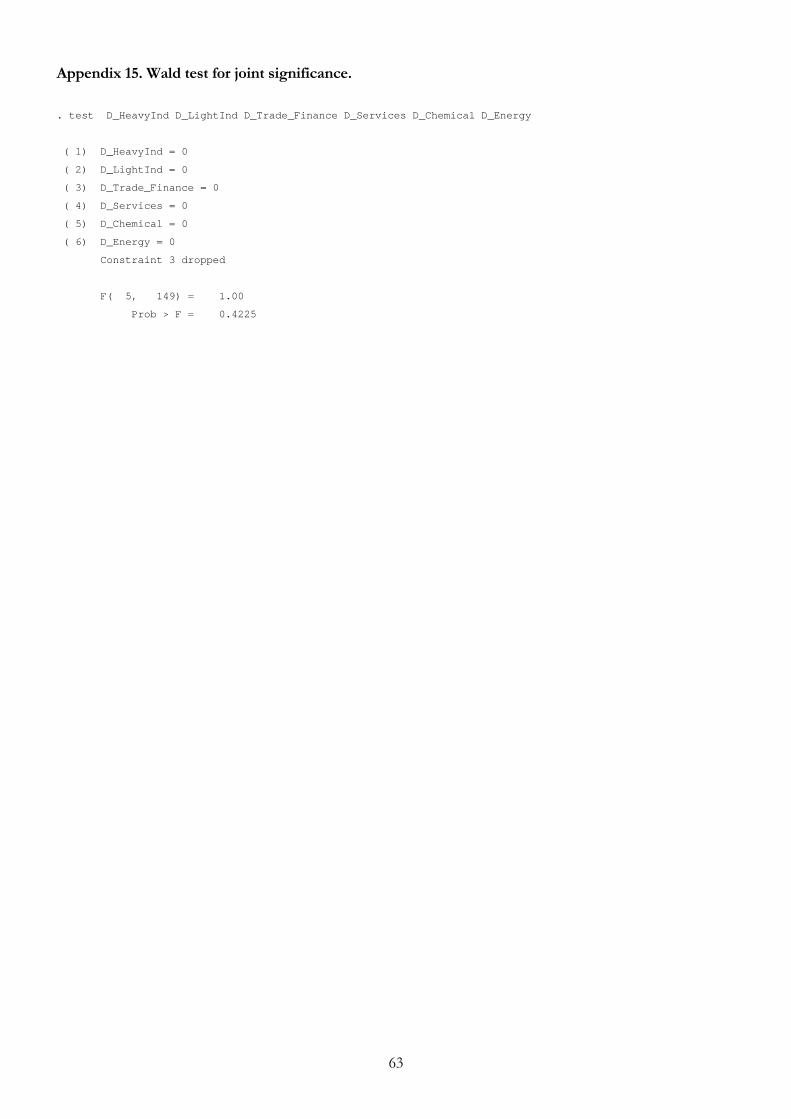
63

Appendix 15. Wald test for joint significance.

. test D_HeavyInd D_LightInd D_Trade_Finance D_Services D_Chemical D_Energy

( 1) D_HeavyInd = 0

( 2) D_LightInd = 0

( 3) D_Trade_Finance = 0

( 4) D_Services = 0

( 5) D_Chemical = 0

( 6) D_Energy = 0

Constraint 3 dropped

F( 5, 149) = 1.00

Prob > F = 0.4225