Determination and climatology of the planetary boundary ... · tive boundary layer heights in good agreement with the radio sounding ... the analysis of the diurnal variation of the

Atmos. Chem. Phys., 14, 13205–13221, 2014

www.atmos-chem-phys.net/14/13205/2014/

doi:10.5194/acp-14-13205-2014

© Author(s) 2014. CC Attribution 3.0 License.

Determination and climatology of the planetary boundary layer

height above the Swiss plateau by in situ and remote sensing

measurements as well as by the COSMO-2 model

M. Collaud Coen1, C. Praz1,*, A. Haefele1, D. Ruffieux1, P. Kaufmann1, and B. Calpini1

1Federal Office of Meteorology and Climatology, MeteoSwiss, 1530 Payerne/8044 Zurich, Switzerland*now at: ESA Advanced Concept Team, ESTEC, Keplerlaan 1, 2201 AZ Noordwijk, the Netherlands

Correspondence to: M Collaud Coen ([email protected])

Received: 17 April 2014 – Published in Atmos. Chem. Phys. Discuss.: 12 June 2014

Revised: 23 October 2014 – Accepted: 10 November 2014 – Published: 11 December 2014

Abstract. The planetary boundary layer (PBL) height is a

key parameter in air quality control and pollutant dispersion.

The PBL height cannot, however, be directly measured, and

its estimation relies on the analysis of the vertical profiles

of the temperature, turbulence or the atmospheric composi-

tion. An operational PBL height detection method including

several remote sensing instruments (wind profiler, Raman li-

dar, microwave radiometer) and several algorithms (Parcel

and bulk Richardson number methods, surface-based temper-

ature inversion, aerosol or humidity gradient analysis) was

developed and tested with 1 year of measurements, which

allows the methods to be validated against radio sounding

measurements. The microwave radiometer provides convec-

tive boundary layer heights in good agreement with the radio

sounding (RS) (median bias < 25 m, R2 > 0.70) and allows

the analysis of the diurnal variation of the PBL height due to

its high temporal resolution. The Raman lidar also leads to

a good agreement with RS, whereas the wind profiler yields

some more dispersed results mostly due to false attribution

problems. A comparison with the numerical weather predic-

tion model COSMO-2 has shown a general overestimation of

the model PBL height by some hundreds to thousand meters.

Finally the seasonal cycles of the daytime and nighttime PBL

heights are discussed for each instrument and each detection

algorithm for two stations on the Swiss plateau.

1 Introduction

The height of the planetary (or atmospheric) boundary layer

(PBL) is a key parameter for air quality analysis, pollu-

tants dispersion and quantification of pollutant emissions and

sources. The PBL controls the interactions of the atmosphere

with the oceans and land and determines the air volume avail-

able for the dispersion of all atmospheric constituents, in-

cluding anthropogenic pollution and water vapor, emitted at

the Earth’s surface. Hence the PBL contributes to the assess-

ment of the pollutant concentration near the surface and the

PBL height is thus a key parameter of all air pollution mod-

els. Despite its critical importance, the PBL cannot be di-

rectly measured but has to be estimated by upper-air instru-

ments.

The COST (European Cooperation in Science and Tech-

nology) action 710 (Harmonisation of the pre-processing of

meteorological data for atmospheric dispersion models) de-

fined the daytime PBL height as “the height of the layer

adjacent to the ground over which pollutants or any con-

stituents emitted within this layer or entrained into it become

vertically dispersed by convection or mechanical turbulence

within a time scale of about an hour” (COST action 710 –

Final report, 1998). The PBL height can consequently be es-

timated by the measurement of mechanical turbulence, of the

temperature enabling convection or of the concentration of

PBL constituents. These detection methods are based on var-

ious atmospheric parameters, various measuring instruments

and different analysis algorithms, leading to several PBL

height estimations that are not always consistent with each

other. The first measurements of the PBL were performed us-

Published by Copernicus Publications on behalf of the European Geosciences Union.

13206 M. Collaud Coen et al.: Determination and climatology of the planetary boundary layer height

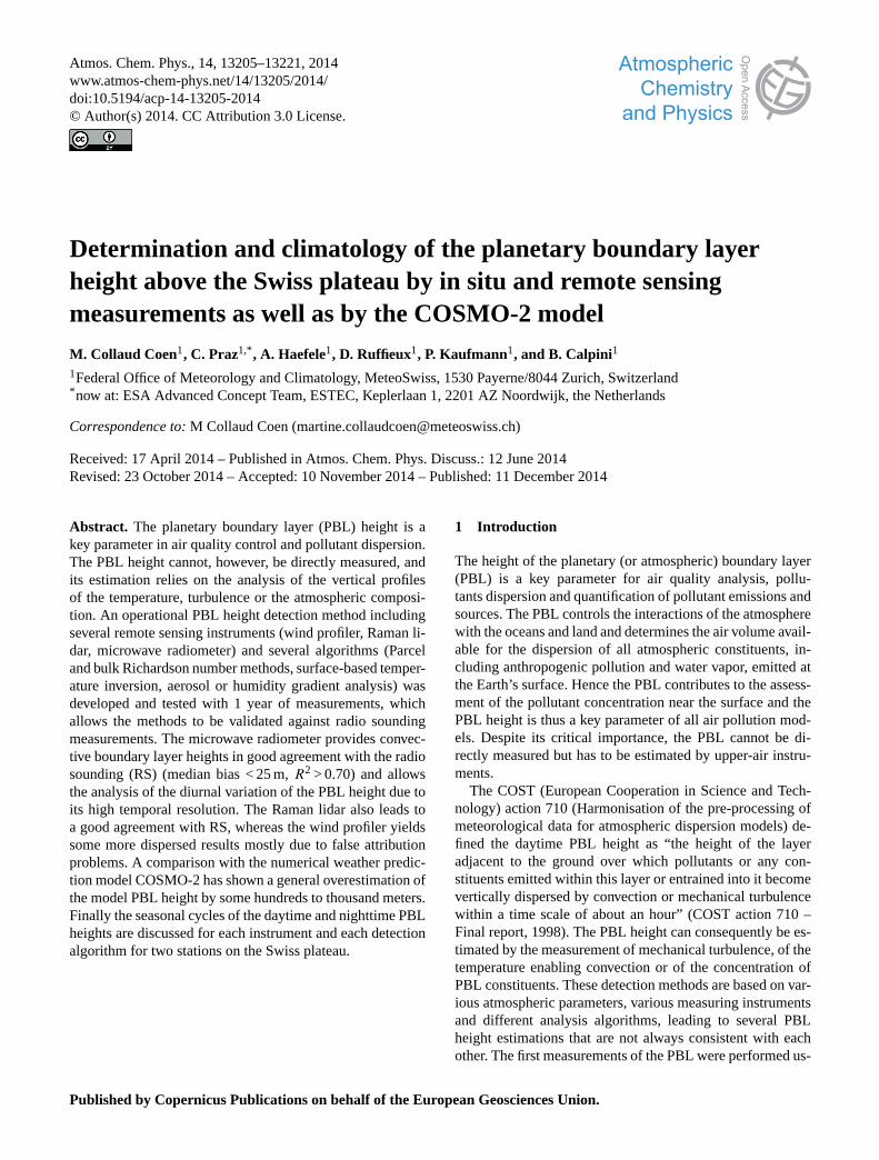
Figure 1. Diurnal cycle of the PBL height over land for a clear

convective day (adapted from Stull, 1988).

ing surface and tower observations of vertical wind profiles

and deeply investigating wind turbulence. The intense de-

velopment of remote sensing instruments nowadays offers a

wide field of vertical profiles up to several kilometers, which

allows PBL height detection from the surface with high tem-

poral resolution.

The PBL experiences a marked diurnal cycle that depends

on both the synoptic and local weather conditions. In the case

of fair weather days, the PBL height has a well-defined struc-

ture and diurnal cycle (Fig. 1), leading to the development

of a convective boundary layer (CBL), also called a mixing

layer, during the day and of a stable boundary layer (SBL),

which is capped by a residual layer (RL) during the night

(Stull, 1988). In the case of cloudy or rainy conditions and

in the case of advective weather conditions, free convection

is no longer driven primarily by solar heating, but by ground

thermal inertia, cold air advection, forced mechanical con-

vection and/or cloud top radiative cooling. In those cloudy

cases, the CBL development remains weaker than in the case

of clear sky conditions, with slower growth and lower max-

imum height. The boundary layer is said to be neutral if the

buoyancy is near zero; these neutral cases are found for over-

cast conditions with strong winds but little temperature dif-

ferences between the air and the ground. Neutral conditions

are frequently met in the RL but rarely near the surface. The

PBL development under clear sky conditions (i.e., more than

50 % of solar radiation during the CBL development) that

leads to strong convection driven principally by solar heating

will be called CBL. For all “no clear-sky” cases with partial

or total cloud coverage but without precipitation, the PBL

will be called cloudy-CBL.

While the definition and the measurement of the CBL, the

neutral boundary layer (NBL) and the cloudy-CBL are well

established, the nocturnal SBL presents a more complicated

internal structure. It is comprised of a stable layer caused by

radiative cooling from the ground, which gradually merges

into a neutral layer called the RL (Stull, 1988; Salmond and

McKendry, 2005; Mahrt et al., 1998). The stable layer can

be characterized by a surface-based temperature inversion

(SBI), and its top can be estimated by the height at which the

gradient of the potential temperature (θ) equals zero. Small-

scale and short-term turbulence can occur within this stable

layer. The RL height is the top of the neutral layer and the be-

ginning of the stable free troposphere. The pollutants emitted

from the surface during the night are trapped into the SBI,

whereas the pollutants released on past days tend to stay in

the RL.

Contrary to radio sounding (RS), launched usually only

twice a day, continuous remote sensing measurements al-

low the determination of the diurnal cycle of the different

layers constituting the PBL. The use of remote sensing in-

strumentation to detect the PBL height was recently summa-

rized by Emeis (2009). Recent studies compared several de-

tection methods or retrieval techniques (Bianco and Wilczac,

2002; Seidel et al., 2010; Beyrich and Leps, 2012; Haeffe-

lin et al., 2012; Summa et al., 2013), remote sensing with

RS measurements (Baars et al., 2008, Liu and Liang 2010,

Granados-Muñoz et al., 2012; Milroy et al., 2012; Sawyer

and Li, 2013; Cimini et al., 2013) and/or several remote sens-

ing instruments (Wang et al., 2012; Zahng et al., 2012). In

most of these studies, good correlations are found in the case

of strong or weak convective weather conditions with differ-

ences of 100–300 m between the various instruments and/or

methods. Non-convective weather conditions corresponding

in most of the cases to cloudy and rainy conditions lead to

much greater discrepancies in the PBL height estimations. In

these cases, the difference becomes even greater if the meth-

ods/instruments are designed to detect various types of PBL

such as CBL, NBL or RL. If temperature profiles are mea-

sured, bulk Richardson number (bR) or Parcel (PM) meth-

ods are usually considered as the most relevant methods for

daytime PBL height detection. Some studies also compared

measurements with models predictions (Baars et al., 2008;

Seidel et al., 2012; Ketterer et al., 2014), the results depend-

ing on both the model and the measurement type.

Climatologies of PBL height have been performed on time

series from 1 to 25 years long in Europe and the United

States (Baars et al., 2008; Schmid and Niyogy, 2012; Beyrich

and Leps, 2012; Granados-Muñoz et al., 2012; Sawyer and

Li, 2013) and over continents (Seidel et al., 2010, 2012).

For continental stations, a clear CBL seasonal cycle is usu-

ally found with a maximum height reaching 1000 to 2000 m

above ground level (a.g.l.) in summer and and a minimum

height reaching 500 to 1200 m a.g.l in winter. The seasonal

cycle of the nocturnal SBL was only addressed on the basis

of temperature (T ) profiles from RS measurements (Seidel et

al., 2010, 2012; Beyrich and Leps, 2012). Both papers found

a minimum height in summer and a maximum height in win-

ter, which was attributed to greater wind speeds and conse-

quently stronger mechanical turbulence during winter. Few

of the PBL height detections run operationally, meaning that

they run as fully automatic systems delivering routine PBL

Atmos. Chem. Phys., 14, 13205–13221, 2014 www.atmos-chem-phys.net/14/13205/2014/

M. Collaud Coen et al.: Determination and climatology of the planetary boundary layer height 13207

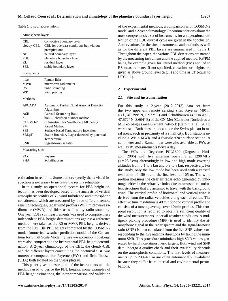
Table 1. List of abbreviations.

Atmospheric layers

CBL convective boundary layer

cloudy-CBL CBL for overcast conditions but without

precipitations

NBL neutral boundary layer

PBL planetary boundary layer

RL residual layer

SBL stable boundary layer

Instruments

lidar Raman lidar

MWR microwave radiometer

RS radio sounding

WP wind profiler

Methods

APCADA Automatic Partial Cloud Amount Detection

Algorithm

ASR Aerosol Scattering Ratio

bR bulk Richardson number method

COSMO-2 COnsortium for Small-scale MOdeling

PM Parcel Method

SBI Surface-based Temperature Inversion

SBLpT Stable Boundary Layer detected by potential

Temperature

SNR Signal-to-noise ratio

Measuring sites

PAY Payerne

SHA Schaffhausen

estimation in realtime. Some authors specify that a visual in-

spection is necessary to increase the results reliability.

In this study, an operational system for PBL height de-

tection has been developed based on the analysis of vertical

atmospheric profiles of T , wind turbulence and atmospheric

constituents, which are measured by three different remote

sensing techniques, radar wind profiler (WP), microwave ra-

diometer (MWR) and lidar, as well as by radio sounding.

One year (2012) of measurements was used to compare these

independent PBL height determinations against a reference

method, here taken as the RS or MWR PBL heights derived

from the PM. The PBL heights computed by the COSMO-2

model (numerical weather prediction model of the Consor-

tium for Small Scale Modeling; see www.cosmo-model.org)

were also compared to the instrumental PBL height determi-

nation. A 2-year climatology of the CBL, the cloudy-CBL

and the different layers constituting the nocturnal SBL was

moreover computed for Payerne (PAY) and Schaffhausen

(SHA) both located on the Swiss plateau.

This paper gives a description of the instruments and the

methods used to derive the PBL heights, some examples of

PBL height estimations, the inter-comparison and validation

of the experimental methods, a comparison with COSMO-2

model and a 2-year climatology. Recommendations about the

most comprehensive set of instruments for an operational de-

tection of the PBL diurnal cycle are given in the conclusion.

Abbreviations for the sites, instruments and methods as well

as for the different PBL layers are summarized in Table 1.

Throughout the paper, the various PBL detections are named

by the measuring instrument and the applied method, RS/PM

being for example given for Parcel method (PM) applied to

RS measurements. If not specified, elevations or heights are

given as above ground level (a.g.l.) and time as LT (equal to

UTC+ 1).

2 Experimental

2.1 Site and instrumentation

For this study, a 2-year (2012–2013) data set from

the two upper-air remote sensing sites Payerne (491 m

a.s.l., 46.799◦ N, 6.932◦ E) and Schaffhausen (437 m a.s.l.,

47.672◦ N, 8.604◦ E) of the CN-Met (Centrales Nucléaires et

METéorologie) measurement network (Calpini et al., 2011)

were used. Both sites are located on the Swiss plateau in ru-

ral areas, each in proximity of a small city. Both stations in-

clude a WP, a MWR and a SwissMetNet surface station. A

ceilometer and a Raman lidar were also available at PAY, as

well as RS measurements twice a day.

The WPs are Degreane PCL1300 (Degreane Hori-

zon, 2006) with five antennas operating at 1290 MHz

(λ= 23.3 cm) alternatingly in low and high mode covering

altitudes from 0.1 to 3 km and 0.3 to 8 km, respectively. For

this study, only the low mode has been used with a vertical

resolution of 150 m and the first level at 105 m. The wind

profiler measures the clear air radar echo generated by inho-

mogeneities in the refractive index due to atmospheric turbu-

lent structures that are assumed to travel with the background

wind. The vertical profile of horizontal and vertical wind is

derived from the radial velocities along each direction. The

effective time resolution is 40 min for one vertical profile and

consists of a moving average over 10 min profiles. This tem-

poral resolution is required to obtain a sufficient quality of

the wind measurements under all weather conditions. A mul-

tipeak picking procedure (MPP) is used to identify the at-

mospheric signal in the radar spectra and the signal-to-noise

ratio (SNR) is then calculated from the five SNR values cor-

responding to the five antenna directions by taking the mini-

mum SNR. This procedure minimizes high SNR values gen-

erated by hard, non-atmospheric targets. Both wind and SNR

data undergo a quality check and their availability depends

on the atmospheric conditions. The first levels of measure-

ments up to 200–400 m are often automatically invalidated

because they suffer from internal and environmental pertur-

bations.

www.atmos-chem-phys.net/14/13205/2014/ Atmos. Chem. Phys., 14, 13205–13221, 2014

www.cosmo-model.org


The MWR is a passive remote sensing instrument that

measures electromagnetic radiation emitted from the atmo-

sphere in the microwave band. From the measured radiation

spectrum, the atmospheric T profile between 0 and 5 km is

retrieved. The MWRs employed in this study are TEMPRO

radiometers manufactured by Radiometer Physics GMbH

(RPG; 2011) with seven channels between 51 and 58 GHz

for T profiling. The radiometer alternates between elevation

scanning (six elevations between 5 and 90◦) and zenith ob-

servations. Statistical regressions models are used to convert

the radiation measurements from the elevation scan and from

the zenith observations in two temperature profile covering

0–2 km and 0–5 km, respectively. The two temperature pro-

files are merged into one single T profile using the profile de-

rived from the elevation scan and the upper part (2–5 km) of

the profile derived from the zenith observations. The vertical

resolution decreases with altitude, from 50 m for z< 1200 m

to 200 m at 3000 m according to the manufacturer. These val-

ues are however derived from the averaging kernels, which

depend slightly on the atmospheric conditions. Hence, ele-

vated T inversions (above approximately 1500 m) cannot be

resolved by the MWR. The time resolution is set to one pro-

file every 10 min.

The PAY aerological station is equipped with a fully auto-

mated and operational Raman lidar designed for continuous

measurements of tropospheric water vapor, aerosols and tem-

perature in dry conditions (Dinoev et al., 2013). The trans-

mitter is a Nd:YAG-laser emitting UV pulses (300 mJ per

pulse, 30 Hz repetition rate) at a wavelength of 355 nm. The

receiver consists of four telescopes of 0.3 m diameter each,

which are fiber coupled to the polychromator, which spec-

trally separates the backscattered light. Separate photomulti-

pliers simultaneously detect vibrational Raman scatter from

nitrogen (387 nm) and water vapor (407 nm) signals, two por-

tions of the pure rotational Raman spectrum and the elas-

tic backscatter. The aerosol scattering ratio is then derived

from the sum of the rotational Raman signals and the elas-

tic signal (Dinoev et al., 2010). The maximum range varies

from 4000 m during the day up to 8000 m during the night

for the water vapor measurements and from 7000 m (day) to

12 000 m (night) for aerosol backscatter ratio measurements.

The first range level is located at 110 m. The vertical resolu-

tion is dynamically adapted to the measurement conditions,

varying from 30 m near the surface to a maximum of 300 m

in the upper troposphere. However, the signal-to-noise ratio

is very high in the boundary layer and the vertical resolu-

tion remains constant (30 m). The effective time resolution

of profiles is 30 min. No measurements are possible during

precipitation and in the presence of low clouds, i.e., the lidar

powers down if the clouds are below 900 m or there is precip-

itation and powers up as soon as the cloud base rises above

2000 m and there is no precipitation.

A ceilometer (CBME80 from Eliasson) measuring at

λ= 905 nm with a time resolution of a few seconds is inter-

faced to the lidar system to provide independent cloud infor-

mation. This model was not configured to record backscatter

profiles but only to provide the height of the cloud bases de-

tected by a strong gradient in the backscattered signal.

In addition to the remote sensing instruments, the Payerne

station performs routine RS providing pressure (p), T , hu-

midity and wind speed and direction profiles up to 32 km.

Meteolabor SRS 400 C34 radiosondes are launched twice a

day at 00:00 and 12:00 LT. The horizontal displacement of

the sonde can reach up to 200 km. However, only the first

vertical 3500 m corresponding to approximately 12 min of

rise are used to determine the PBL height, allowing one to

neglect the RS horizontal displacement. RS has a constant

height resolution of 5 to 6 m corresponding to a 1 s time res-

olution.

The COSMO-2 model (http://www.cosmo-model.org)

was used in assimilation mode. It has a horizontal grid spac-

ing of 2.2 km and a total of 60 vertical levels, of which 15

lie within the first 500 m. The time step is 20 s and data are

written out every 1 h. The bulk Richardson number method is

used to estimate the boundary layer height in the model (see

Sect. 2.2.1).

The SwissMetNet meteorological surface network pro-

vides surface T , humidity, p, wind direction and speed as

well as sunshine duration and precipitation every 10 min. As

recommended by the standard procedures of the World Me-

teorological Organization (WMO), the wind components are

measured at 10 m and all the other parameters at 2 m. In ad-

dition, the PAY station is equipped with a sonic anemometer

on a 10 m mast measuring several parameters related to tur-

bulence, including the sensible heat flux, which characterizes

the thermal energy exchanges. The sensitive heat flux is then

used to estimate the intensity of convective forcing.

The cloud cover is detected by an automatic partial cloud

amount detection algorithm (APCADA) that estimates in re-

altime the sky cloud cover from surface-based measurements

of long-wave downward radiation, T and humidity (Dürr and

Philipona, 2004). APCADA does not take into account cirrus

clouds.

Measurements from both the MWR and lidar are necessary

to calculate the virtual potential temperature (θv), and they

are combined with WP data to calculate the bulk Richardson

number (see Sect. 2.2.1). These three instruments have how-

ever different vertical levels and time constants. For these

cases, a vertical scale (35 levels of 100 m between 0 and

3500 m) is set, and the mean of the parameters in each level

are used. Despite the rather long integration times in the case

of the wind profiler and lidar, all measurements have been as-

sumed to be instantaneous. These different time granularities

are sometimes manifested by a time shift of the CBL growth

measured by MWR/PM and WP/SNR or lidar/ASR.


http://www.cosmo-model.org


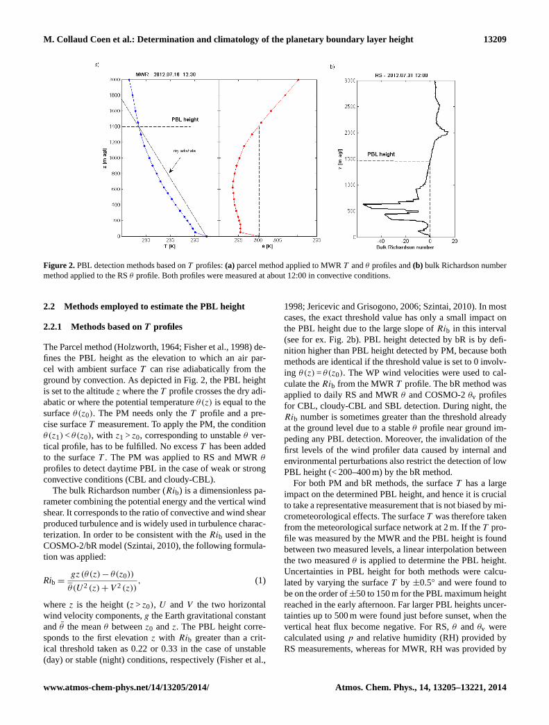
Figure 2. PBL detection methods based on T profiles: (a) parcel method applied to MWR T and θ profiles and (b) bulk Richardson number

method applied to the RS θ profile. Both profiles were measured at about 12:00 in convective conditions.

2.2 Methods employed to estimate the PBL height

2.2.1 Methods based on T profiles

The Parcel method (Holzworth, 1964; Fisher et al., 1998) de-

fines the PBL height as the elevation to which an air par-

cel with ambient surface T can rise adiabatically from the

ground by convection. As depicted in Fig. 2, the PBL height

is set to the altitude z where the T profile crosses the dry adi-

abatic or where the potential temperature θ(z) is equal to the

surface θ(z0). The PM needs only the T profile and a pre-

cise surface T measurement. To apply the PM, the condition

θ(z1)< θ(z0), with z1 > z0, corresponding to unstable θ ver-

tical profile, has to be fulfilled. No excess T has been added

to the surface T . The PM was applied to RS and MWR θ

profiles to detect daytime PBL in the case of weak or strong

convective conditions (CBL and cloudy-CBL).

The bulk Richardson number (Rib) is a dimensionless pa-

rameter combining the potential energy and the vertical wind

shear. It corresponds to the ratio of convective and wind shear

produced turbulence and is widely used in turbulence charac-

terization. In order to be consistent with the Rib used in the

COSMO-2/bR model (Szintai, 2010), the following formula-

tion was applied:

Rib =gz(θ(z)− θ(z0))

θ(U2 (z)+V 2 (z)), (1)

where z is the height (z > z0), U and V the two horizontal

wind velocity components, g the Earth gravitational constant

and θ the mean θ between z0 and z. The PBL height corre-

sponds to the first elevation z with Rib greater than a crit-

ical threshold taken as 0.22 or 0.33 in the case of unstable

(day) or stable (night) conditions, respectively (Fisher et al.,

1998; Jericevic and Grisogono, 2006; Szintai, 2010). In most

cases, the exact threshold value has only a small impact on

the PBL height due to the large slope of Rib in this interval

(see for ex. Fig. 2b). PBL height detected by bR is by defi-

nition higher than PBL height detected by PM, because both

methods are identical if the threshold value is set to 0 involv-

ing θ(z)= θ(z0). The WP wind velocities were used to cal-

culate the Rib from the MWR T profile. The bR method was

applied to daily RS and MWR θ and COSMO-2 θv profiles

for CBL, cloudy-CBL and SBL detection. During night, the

Rib number is sometimes greater than the threshold already

at the ground level due to a stable θ profile near ground im-

peding any PBL detection. Moreover, the invalidation of the

first levels of the wind profiler data caused by internal and

environmental perturbations also restrict the detection of low

PBL height (< 200–400 m) by the bR method.

For both PM and bR methods, the surface T has a large

impact on the determined PBL height, and hence it is crucial

to take a representative measurement that is not biased by mi-

crometeorological effects. The surface T was therefore taken

from the meteorological surface network at 2 m. If the T pro-

file was measured by the MWR and the PBL height is found

between two measured levels, a linear interpolation between

the two measured θ is applied to determine the PBL height.

Uncertainties in PBL height for both methods were calcu-

lated by varying the surface T by ±0.5◦ and were found to

be on the order of±50 to 150 m for the PBL maximum height

reached in the early afternoon. Far larger PBL heights uncer-

tainties up to 500 m were found just before sunset, when the

vertical heat flux become negative. For RS, θ and θv were

calculated using p and relative humidity (RH) provided by

RS measurements, whereas for MWR, RH was provided by



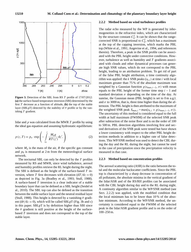
Figure 3. Detection of the SBL from RS T profile of 17/07/2012:

(a) the surface-based temperature inversion (SBI) determined by the

first T decrease as a function of altitude, (b) the top of the stable

layer (SBLpT) detected by the stability of θ profile or by the van-

ishing T gradient.

lidar and p was calculated from the MWR T profile by using

the ideal gas equation and assuming hydrostatic equilibrium:

p(z,T )= po · exp

− z∫z0

Mag

RT (z′)dz′,

(2)

where Ma is the mass of the air, R the specific gas constant

and p0 is measured at 2 m from the meteorological surface

network.

The nocturnal SBL can only be detected by the T profiles

measured by RS and MWR, since wind turbulence, aerosol

and humidity profiles retrieve the RL height during the night.

The SBI is defined as the height of the surface-based T in-

version, where T first decreases with elevation (dT/dz= 0)

as depicted in Fig. 3a (Bradley et al., 1993; Stull, 1988).

A surface-based T inversion is a clear indicator of a stable

boundary layer that can be defined as a SBL height (Seidel et

al., 2010). The SBL top can also be defined as the transition

between the stable surface layer and the neutral residual layer

(Stull, 1988). This height is detected by a vanishing θ gradi-

ent (dθ/dz= 0), which will be called SBLpT (Fig. 3b and c)

in this paper. SBLpT is by definition higher than SBI since

the θ gradient is still positive at the height of the surface-

based T inversion and does not correspond to the top of the

stable layer.

2.2.2 Method based on wind turbulence profiles

The radar echo measured by the WP is generated by inho-

mogeneities in the refractive index, which are characterized

by the structure constant C2n . It can be shown that the range-

corrected SNR is proportional to C2n , which has a maximum

at the top of the capping inversion, which marks the PBL

top (White et al., 1991; Angevine et al., 1994, and references

therein). Therefore, a peak in the SNR profile can be associ-

ated with the PBL height under convective conditions. How-

ever, turbulence as well as humidity and T gradients associ-

ated with clouds and other dynamical processes can gener-

ate high SNR values, which do not correspond to the PBL

height, leading to an attribution problem. To get rid of part

of the false PBL height attribution, a time continuity algo-

rithm was applied: the k SNR peaks (sk,i) at time i with local

maximum greater than 75 % of the absolute maximum was

weighted by a Gaussian function g(smax,i−1, σ) with mean

equals to the PBL height of the former time step i− 1 and

standard deviation σ depending on the time of the day. At

sunrise, the Gaussian mean (PBL height) is set to 0 m a.g.l.

and σ to 3000 m, that is, three time higher than during the af-

ternoon. The PBL height is then attributed to the maximum of

the weighted SNR peak Smax,i = max(sk,i × g(smax,i−1, σ)).

The uncertainty of this method is considered equal to the full

width at half maximum (FWHM) of the selected SNR peak

after subtraction of the noise floor and is on the order of 100

to 500 m. PBL detection algorithms involving first and sec-

ond derivatives of the SNR peak were tested but have shown

a lower consistency with respect to the other PBL height de-

tection methods in addition to a higher rate of false detec-

tions. This WP/SNR method was used to detect the CBL dur-

ing the day and the RL during the night, but cannot be used

in the case of precipitation since the precipitation velocity is

measured in that case.

2.2.3 Method based on concentration profiles

The aerosol scattering ratio (ASR) is the ratio between the to-

tal and the molecular backscatter coefficients. Since the PBL

top is characterized by a sharp decrease in concentration of

all pollutants, the absolute minima in the vertical gradient of

the lidar/ASR and of the RS/RH profiles can be associated

with the CBL height during day and to the RL during night.

A continuity algorithm similar to the WP/SNR method (see

Sect. 2.2.2) was applied, with the modified condition that

the local minimum has to be lower than 10 % of the abso-

lute minimum. According to the WP/SNR method, the un-

certainty is considered equal to the FWHM of the selected

peak in the lidar/ASR gradient profile and is on the order of

100–250 m.



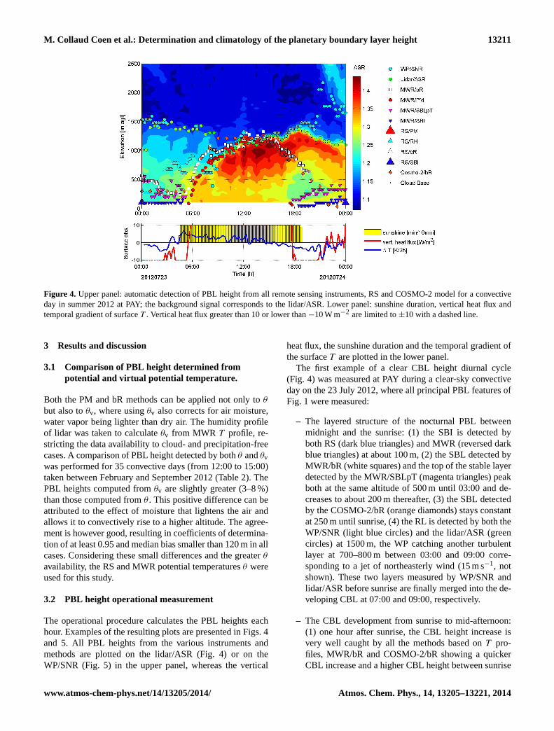
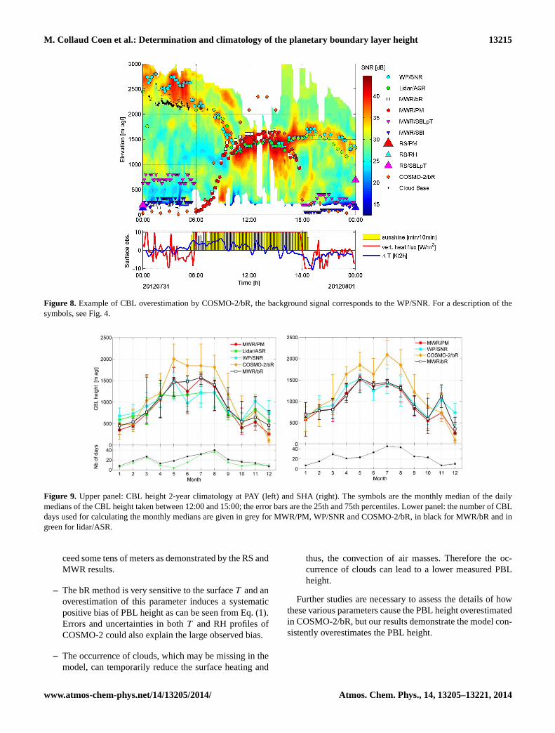
Figure 4. Upper panel: automatic detection of PBL height from all remote sensing instruments, RS and COSMO-2 model for a convective

day in summer 2012 at PAY; the background signal corresponds to the lidar/ASR. Lower panel: sunshine duration, vertical heat flux and

temporal gradient of surface T . Vertical heat flux greater than 10 or lower than −10 W m−2 are limited to ±10 with a dashed line.

3 Results and discussion

3.1 Comparison of PBL height determined from

potential and virtual potential temperature.

Both the PM and bR methods can be applied not only to θ

but also to θv, where using θv also corrects for air moisture,

water vapor being lighter than dry air. The humidity profile

of lidar was taken to calculate θv from MWR T profile, re-

stricting the data availability to cloud- and precipitation-free

cases. A comparison of PBL height detected by both θ and θv

was performed for 35 convective days (from 12:00 to 15:00)

taken between February and September 2012 (Table 2). The

PBL heights computed from θv are slightly greater (3–8 %)

than those computed from θ . This positive difference can be

attributed to the effect of moisture that lightens the air and

allows it to convectively rise to a higher altitude. The agree-

ment is however good, resulting in coefficients of determina-

tion of at least 0.95 and median bias smaller than 120 m in all

cases. Considering these small differences and the greater θ

availability, the RS and MWR potential temperatures θ were

used for this study.

3.2 PBL height operational measurement

The operational procedure calculates the PBL heights each

hour. Examples of the resulting plots are presented in Figs. 4

and 5. All PBL heights from the various instruments and

methods are plotted on the lidar/ASR (Fig. 4) or on the

WP/SNR (Fig. 5) in the upper panel, whereas the vertical

heat flux, the sunshine duration and the temporal gradient of

the surface T are plotted in the lower panel.

The first example of a clear CBL height diurnal cycle

(Fig. 4) was measured at PAY during a clear-sky convective

day on the 23 July 2012, where all principal PBL features of

Fig. 1 were measured:

– The layered structure of the nocturnal PBL between

midnight and the sunrise: (1) the SBI is detected by

both RS (dark blue triangles) and MWR (reversed dark

blue triangles) at about 100 m, (2) the SBL detected by

MWR/bR (white squares) and the top of the stable layer

detected by the MWR/SBLpT (magenta triangles) peak

both at the same altitude of 500 m until 03:00 and de-

creases to about 200 m thereafter, (3) the SBL detected

by the COSMO-2/bR (orange diamonds) stays constant

at 250 m until sunrise, (4) the RL is detected by both the

WP/SNR (light blue circles) and the lidar/ASR (green

circles) at 1500 m, the WP catching another turbulent

layer at 700–800 m between 03:00 and 09:00 corre-

sponding to a jet of northeasterly wind (15 m s−1, not

shown). These two layers measured by WP/SNR and

lidar/ASR before sunrise are finally merged into the de-

veloping CBL at 07:00 and 09:00, respectively.

– The CBL development from sunrise to mid-afternoon:

(1) one hour after sunrise, the CBL height increase is

very well caught by all the methods based on T pro-

files, MWR/bR and COSMO-2/bR showing a quicker

CBL increase and a higher CBL height between sunrise



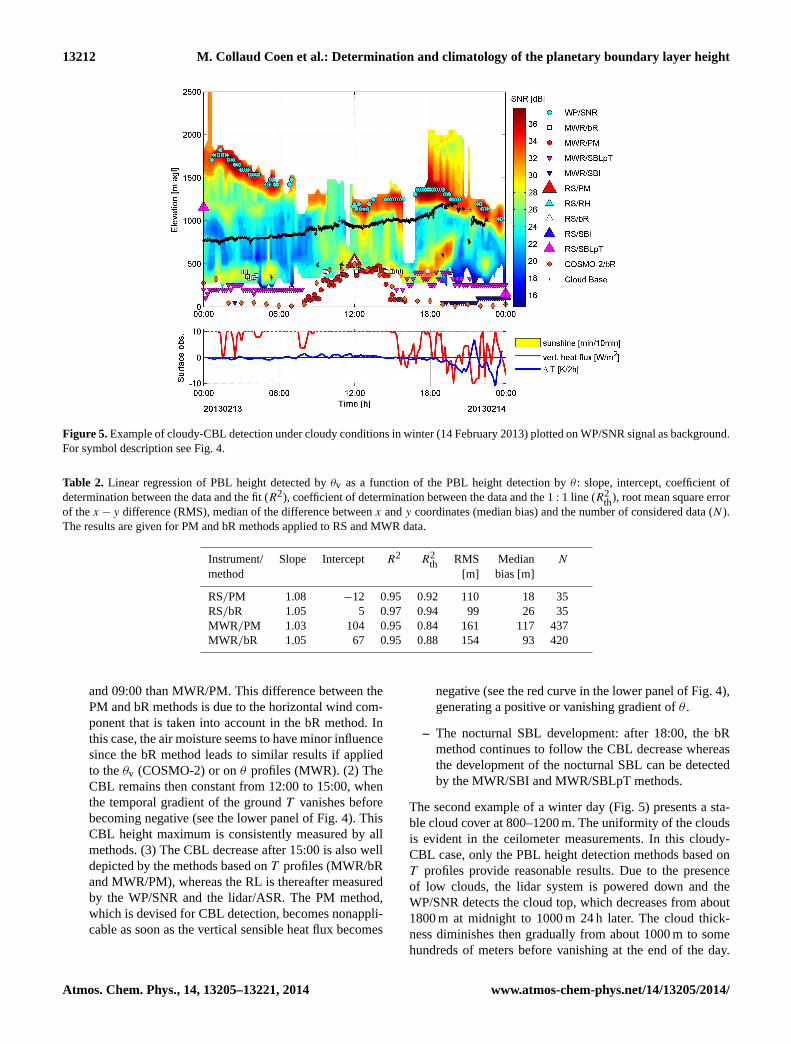
Figure 5. Example of cloudy-CBL detection under cloudy conditions in winter (14 February 2013) plotted on WP/SNR signal as background.

For symbol description see Fig. 4.

Table 2. Linear regression of PBL height detected by θv as a function of the PBL height detection by θ : slope, intercept, coefficient of

determination between the data and the fit (R2), coefficient of determination between the data and the 1 : 1 line (R2th

), root mean square error

of the x− y difference (RMS), median of the difference between x and y coordinates (median bias) and the number of considered data (N ).

The results are given for PM and bR methods applied to RS and MWR data.

Instrument/ Slope Intercept R2 R2th

RMS Median N

method [m] bias [m]

RS/PM 1.08 −12 0.95 0.92 110 18 35

RS/bR 1.05 5 0.97 0.94 99 26 35

MWR/PM 1.03 104 0.95 0.84 161 117 437

MWR/bR 1.05 67 0.95 0.88 154 93 420

and 09:00 than MWR/PM. This difference between the

PM and bR methods is due to the horizontal wind com-

ponent that is taken into account in the bR method. In

this case, the air moisture seems to have minor influence

since the bR method leads to similar results if applied

to the θv (COSMO-2) or on θ profiles (MWR). (2) The

CBL remains then constant from 12:00 to 15:00, when

the temporal gradient of the ground T vanishes before

becoming negative (see the lower panel of Fig. 4). This

CBL height maximum is consistently measured by all

methods. (3) The CBL decrease after 15:00 is also well

depicted by the methods based on T profiles (MWR/bR

and MWR/PM), whereas the RL is thereafter measured

by the WP/SNR and the lidar/ASR. The PM method,

which is devised for CBL detection, becomes nonappli-

cable as soon as the vertical sensible heat flux becomes

negative (see the red curve in the lower panel of Fig. 4),

generating a positive or vanishing gradient of θ .

– The nocturnal SBL development: after 18:00, the bR

method continues to follow the CBL decrease whereas

the development of the nocturnal SBL can be detected

by the MWR/SBI and MWR/SBLpT methods.

The second example of a winter day (Fig. 5) presents a sta-

ble cloud cover at 800–1200 m. The uniformity of the clouds

is evident in the ceilometer measurements. In this cloudy-

CBL case, only the PBL height detection methods based on

T profiles provide reasonable results. Due to the presence

of low clouds, the lidar system is powered down and the

WP/SNR detects the cloud top, which decreases from about

1800 m at midnight to 1000 m 24 h later. The cloud thick-

ness diminishes then gradually from about 1000 m to some

hundreds of meters before vanishing at the end of the day.



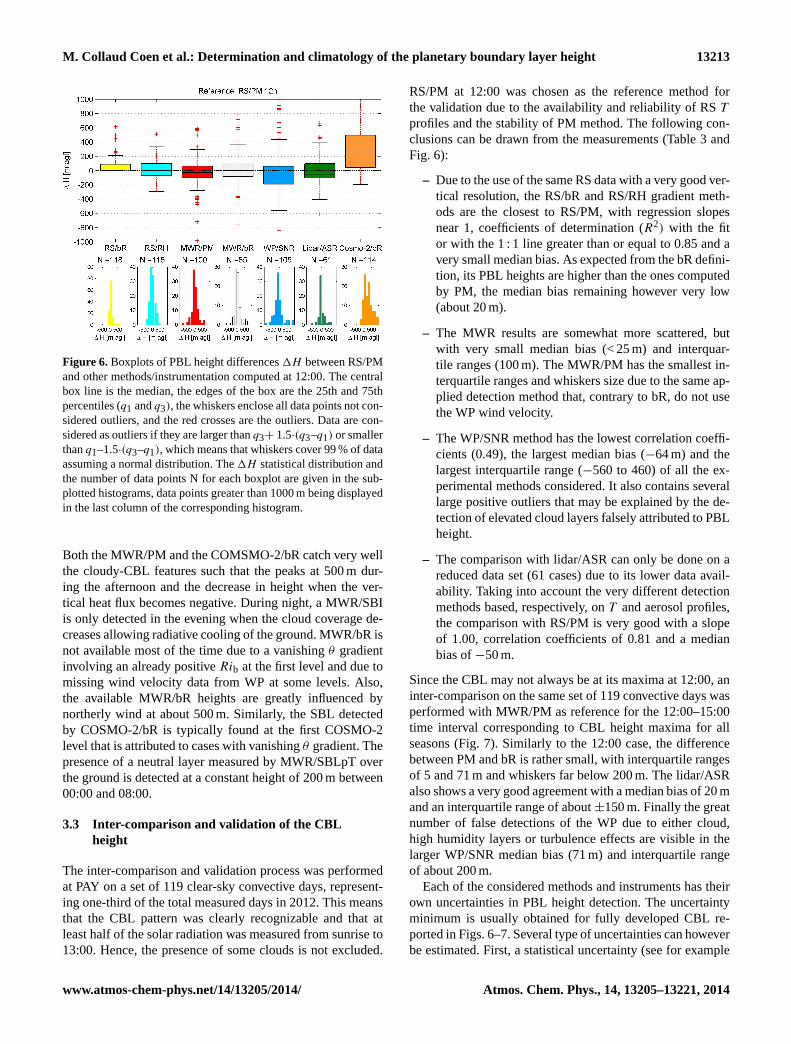
Figure 6. Boxplots of PBL height differences1H between RS/PM

and other methods/instrumentation computed at 12:00. The central

box line is the median, the edges of the box are the 25th and 75th

percentiles (q1 and q3), the whiskers enclose all data points not con-

sidered outliers, and the red crosses are the outliers. Data are con-

sidered as outliers if they are larger than q3+ 1.5·(q3–q1) or smaller

than q1–1.5·(q3–q1), which means that whiskers cover 99 % of data

assuming a normal distribution. The1H statistical distribution and

the number of data points N for each boxplot are given in the sub-

plotted histograms, data points greater than 1000 m being displayed

in the last column of the corresponding histogram.

Both the MWR/PM and the COMSMO-2/bR catch very well

the cloudy-CBL features such that the peaks at 500 m dur-

ing the afternoon and the decrease in height when the ver-

tical heat flux becomes negative. During night, a MWR/SBI

is only detected in the evening when the cloud coverage de-

creases allowing radiative cooling of the ground. MWR/bR is

not available most of the time due to a vanishing θ gradient

involving an already positive Rib at the first level and due to

missing wind velocity data from WP at some levels. Also,

the available MWR/bR heights are greatly influenced by

northerly wind at about 500 m. Similarly, the SBL detected

by COSMO-2/bR is typically found at the first COSMO-2

level that is attributed to cases with vanishing θ gradient. The

presence of a neutral layer measured by MWR/SBLpT over

the ground is detected at a constant height of 200 m between

00:00 and 08:00.

3.3 Inter-comparison and validation of the CBL

height

The inter-comparison and validation process was performed

at PAY on a set of 119 clear-sky convective days, represent-

ing one-third of the total measured days in 2012. This means

that the CBL pattern was clearly recognizable and that at

least half of the solar radiation was measured from sunrise to

13:00. Hence, the presence of some clouds is not excluded.

RS/PM at 12:00 was chosen as the reference method for

the validation due to the availability and reliability of RS T

profiles and the stability of PM method. The following con-

clusions can be drawn from the measurements (Table 3 and

Fig. 6):

– Due to the use of the same RS data with a very good ver-

tical resolution, the RS/bR and RS/RH gradient meth-

ods are the closest to RS/PM, with regression slopes

near 1, coefficients of determination (R2) with the fit

or with the 1 : 1 line greater than or equal to 0.85 and a

very small median bias. As expected from the bR defini-

tion, its PBL heights are higher than the ones computed

by PM, the median bias remaining however very low

(about 20 m).

– The MWR results are somewhat more scattered, but

with very small median bias (< 25 m) and interquar-

tile ranges (100 m). The MWR/PM has the smallest in-

terquartile ranges and whiskers size due to the same ap-

plied detection method that, contrary to bR, do not use

the WP wind velocity.

– The WP/SNR method has the lowest correlation coeffi-

cients (0.49), the largest median bias (−64 m) and the

largest interquartile range (−560 to 460) of all the ex-

perimental methods considered. It also contains several

large positive outliers that may be explained by the de-

tection of elevated cloud layers falsely attributed to PBL

height.

– The comparison with lidar/ASR can only be done on a

reduced data set (61 cases) due to its lower data avail-

ability. Taking into account the very different detection

methods based, respectively, on T and aerosol profiles,

the comparison with RS/PM is very good with a slope

of 1.00, correlation coefficients of 0.81 and a median

bias of −50 m.

Since the CBL may not always be at its maxima at 12:00, an

inter-comparison on the same set of 119 convective days was

performed with MWR/PM as reference for the 12:00–15:00

time interval corresponding to CBL height maxima for all

seasons (Fig. 7). Similarly to the 12:00 case, the difference

between PM and bR is rather small, with interquartile ranges

of 5 and 71 m and whiskers far below 200 m. The lidar/ASR

also shows a very good agreement with a median bias of 20 m

and an interquartile range of about±150 m. Finally the great

number of false detections of the WP due to either cloud,

high humidity layers or turbulence effects are visible in the

larger WP/SNR median bias (71 m) and interquartile range

of about 200 m.

Each of the considered methods and instruments has their

own uncertainties in PBL height detection. The uncertainty

minimum is usually obtained for fully developed CBL re-

ported in Figs. 6–7. Several type of uncertainties can however

be estimated. First, a statistical uncertainty (see for example



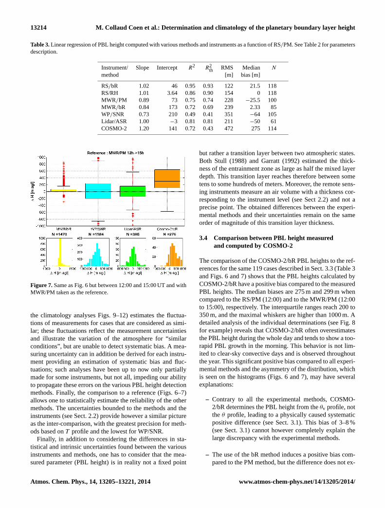
Table 3. Linear regression of PBL height computed with various methods and instruments as a function of RS/PM. See Table 2 for parameters

description.

Instrument/ Slope Intercept R2 R2th

RMS Median N

method [m] bias [m]

RS/bR 1.02 46 0.95 0.93 122 21.5 118

RS/RH 1.01 3.64 0.86 0.90 154 0 118

MWR/PM 0.89 73 0.75 0.74 228 −25.5 100

MWR/bR 0.84 173 0.72 0.69 239 2.33 85

WP/SNR 0.73 210 0.49 0.41 351 −64 105

Lidar/ASR 1.00 −3 0.81 0.81 211 −50 61

COSMO-2 1.20 141 0.72 0.43 472 275 114

Figure 7. Same as Fig. 6 but between 12:00 and 15:00 UT and with

MWR/PM taken as the reference.

the climatology analyses Figs. 9–12) estimates the fluctua-

tions of measurements for cases that are considered as simi-

lar; these fluctuations reflect the measurement uncertainties

and illustrate the variation of the atmosphere for “similar

conditions”, but are unable to detect systematic bias. A mea-

suring uncertainty can in addition be derived for each instru-

ment providing an estimation of systematic bias and fluc-

tuations; such analyses have been up to now only partially

made for some instruments, but not all, impeding our ability

to propagate these errors on the various PBL height detection

methods. Finally, the comparison to a reference (Figs. 6–7)

allows one to statistically estimate the reliability of the other

methods. The uncertainties bounded to the methods and the

instruments (see Sect. 2.2) provide however a similar picture

as the inter-comparison, with the greatest precision for meth-

ods based on T profile and the lowest for WP/SNR.

Finally, in addition to considering the differences in sta-

tistical and intrinsic uncertainties found between the various

instruments and methods, one has to consider that the mea-

sured parameter (PBL height) is in reality not a fixed point

but rather a transition layer between two atmospheric states.

Both Stull (1988) and Garratt (1992) estimated the thick-

ness of the entrainment zone as large as half the mixed layer

depth. This transition layer reaches therefore between some

tens to some hundreds of meters. Moreover, the remote sens-

ing instruments measure an air volume with a thickness cor-

responding to the instrument level (see Sect 2.2) and not a

precise point. The obtained differences between the experi-

mental methods and their uncertainties remain on the same

order of magnitude of this transition layer thickness.

3.4 Comparison between PBL height measured

and computed by COSMO-2

The comparison of the COSMO-2/bR PBL heights to the ref-

erences for the same 119 cases described in Sect. 3.3 (Table 3

and Figs. 6 and 7) shows that the PBL heights calculated by

COSMO-2/bR have a positive bias compared to the measured

PBL heights. The median biases are 275 m and 299 m when

compared to the RS/PM (12:00) and to the MWR/PM (12:00

to 15:00), respectively. The interquartile ranges reach 200 to

350 m, and the maximal whiskers are higher than 1000 m. A

detailed analysis of the individual determinations (see Fig. 8

for example) reveals that COSMO-2/bR often overestimates

the PBL height during the whole day and tends to show a too-

rapid PBL growth in the morning. This behavior is not lim-

ited to clear-sky convective days and is observed throughout

the year. This significant positive bias compared to all experi-

mental methods and the asymmetry of the distribution, which

is seen on the histograms (Figs. 6 and 7), may have several

explanations:

– Contrary to all the experimental methods, COSMO-

2/bR determines the PBL height from the θv profile, not

the θ profile, leading to a physically caused systematic

positive difference (see Sect. 3.1). This bias of 3–8 %

(see Sect. 3.1) cannot however completely explain the

large discrepancy with the experimental methods.

– The use of the bR method induces a positive bias com-

pared to the PM method, but the difference does not ex-



Figure 8. Example of CBL overestimation by COSMO-2/bR, the background signal corresponds to the WP/SNR. For a description of the

symbols, see Fig. 4.

29

Figure 9: Upper panel: CBL height two-years climatology at PAY (left) and SHA (right). The symbols are the monthly median of the daily medians of the CBL height taken between 12:00 and 15:00; the error bars are the 25th and 75th percentiles. Lower panel: the number of CBL days used for calculating the monthly medians are given in grey for MWR/PM, WP/SNR and COSMO-2/bR, in black for MWP/bR and in green for lidar/ASR.

Figure 10: Upper panel: cloudy-CBL height climatology at PAY (left) and SHA (right). Lower panel: number of cloudy-CBL days used to calculate the monthly medians. Symbols and colors as in Fig. 9.

Figure 9. Upper panel: CBL height 2-year climatology at PAY (left) and SHA (right). The symbols are the monthly median of the daily

medians of the CBL height taken between 12:00 and 15:00; the error bars are the 25th and 75th percentiles. Lower panel: the number of CBL

days used for calculating the monthly medians are given in grey for MWR/PM, WP/SNR and COSMO-2/bR, in black for MWR/bR and in

green for lidar/ASR.

ceed some tens of meters as demonstrated by the RS and

MWR results.

– The bR method is very sensitive to the surface T and an

overestimation of this parameter induces a systematic

positive bias of PBL height as can be seen from Eq. (1).

Errors and uncertainties in both T and RH profiles of

COSMO-2 could also explain the large observed bias.

– The occurrence of clouds, which may be missing in the

model, can temporarily reduce the surface heating and

thus, the convection of air masses. Therefore the oc-

currence of clouds can lead to a lower measured PBL

height.

Further studies are necessary to assess the details of how

these various parameters cause the PBL height overestimated

in COSMO-2/bR, but our results demonstrate the model con-

sistently overestimates the PBL height.



29

Figure 9: Upper panel: CBL height two-years climatology at PAY (left) and SHA (right). The symbols are the monthly median of the daily medians of the CBL height taken between 12:00 and 15:00; the error bars are the 25th and 75th percentiles. Lower panel: the number of CBL days used for calculating the monthly medians are given in grey for MWR/PM, WP/SNR and COSMO-2/bR, in black for MWP/bR and in green for lidar/ASR.

Figure 10: Upper panel: cloudy-CBL height climatology at PAY (left) and SHA (right). Lower panel: number of cloudy-CBL days used to calculate the monthly medians. Symbols and colors as in Fig. 9.

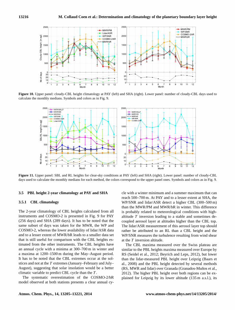
Figure 10. Upper panel: cloudy-CBL height climatology at PAY (left) and SHA (right). Lower panel: number of cloudy-CBL days used to

calculate the monthly medians. Symbols and colors as in Fig. 9.

30

Fig. 11: Upper panel: SBL and RL heights for clear-sky conditions at PAY (left) and SHA (right). Lower panel: number of cloudy-CBL days used to calculate the monthy medians for each method, the colors correspond to the upper panel ones. Symbols and colors as in Fig. 9.

Fig. 12: Upper panel: SBL and RL heights for cloudy conditions at PAY (left) and SHA (right). Lower panel: number of cloudy-CBL days used to calculate the monthly medians, the colors correspond to the upper panel ones. Symbols and colors as in Fig. 9.

Figure 11. Upper panel: SBL and RL heights for clear-sky conditions at PAY (left) and SHA (right). Lower panel: number of cloudy-CBL

days used to calculate the monthly medians for each method, the colors correspond to the upper panel ones. Symbols and colors as in Fig. 9.

3.5 PBL height 2-year climatology at PAY and SHA

3.5.1 CBL climatology

The 2-year climatology of CBL heights calculated from all

instruments and COSMO-2 is presented in Fig. 9 for PAY

(256 days) and SHA (289 days). It has to be noted that the

same subset of days was taken for the MWR, the WP and

COSMO-2, whereas the lower availability of lidar/ASR data

and to a lesser extent of MWR/bR leads to a smaller data set

that is still useful for comparison with the CBL heights es-

timated from the other instruments. The CBL heights have

an annual cycle with a minima at 300–700 m in winter and

a maxima at 1200–1500 m during the May–August period.

It has to be noted that the CBL extremes occur at the sol-

stices and not at the T extremes (January–February and July–

August), suggesting that solar insolation would be a better

climatic variable to predict CBL cycle than the T .

The systematic overestimation of the COSMO-2/bR

model observed at both stations presents a clear annual cy-

cle with a winter minimum and a summer maximum that can

reach 500–700 m. At PAY and to a lesser extent at SHA, the

WP/SNR and lidar/ASR detect a higher CBL (300–500 m)

than the MWR/PM and MWR/bR in winter. This difference

is probably related to meteorological conditions with high-

altitude T inversion leading to a stable and sometimes de-

coupled aerosol layer at altitudes higher than the CBL top.

The lidar/ASR measurement of this aerosol layer top should

rather be attributed to an RL than a CBL height and the

WP/SNR measures the turbulence resulting from wind shear

at the T inversion altitude.

The CBL maxima measured over the Swiss plateau are

similar to the PBL heights maxima measured over Europe by

RS (Seidel et al., 2012; Beyrich and Leps, 2012), but lower

than the lidar-measured PBL height over Leipzig (Baars et

al., 2008) and the PBL height detected by several methods

(RS, MWR and lidar) over Granada (Granados-Muños et al.,

2012). The higher PBL height over both regions can be ex-

plained for Leipzig by its lower altitude (135 m a.s.l.), its



30

Fig. 11: Upper panel: SBL and RL heights for clear-sky conditions at PAY (left) and SHA (right). Lower panel: number of cloudy-CBL days used to calculate the monthy medians for each method, the colors correspond to the upper panel ones. Symbols and colors as in Fig. 9.

Fig. 12: Upper panel: SBL and RL heights for cloudy conditions at PAY (left) and SHA (right). Lower panel: number of cloudy-CBL days used to calculate the monthly medians, the colors correspond to the upper panel ones. Symbols and colors as in Fig. 9.

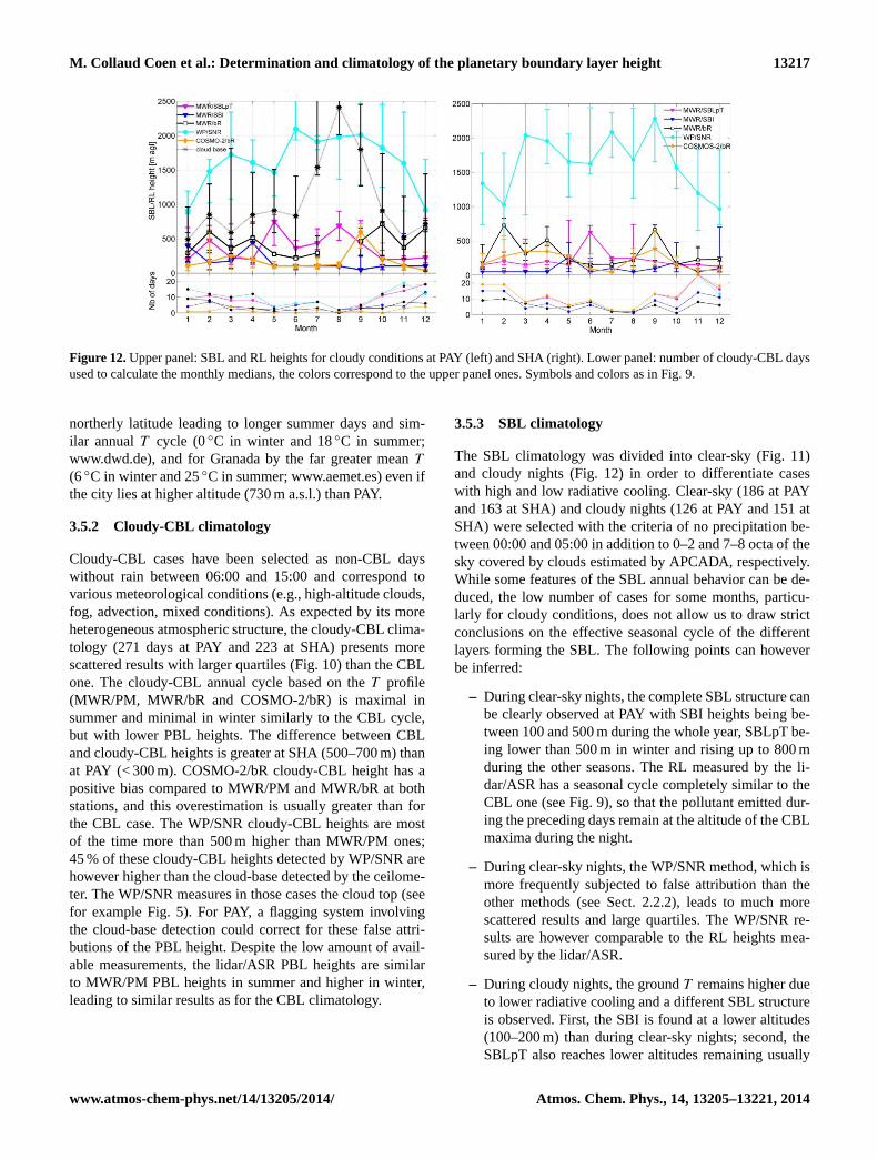
Figure 12. Upper panel: SBL and RL heights for cloudy conditions at PAY (left) and SHA (right). Lower panel: number of cloudy-CBL days

used to calculate the monthly medians, the colors correspond to the upper panel ones. Symbols and colors as in Fig. 9.

northerly latitude leading to longer summer days and sim-

ilar annual T cycle (0 ◦C in winter and 18 ◦C in summer;

www.dwd.de), and for Granada by the far greater mean T

(6 ◦C in winter and 25 ◦C in summer; www.aemet.es) even if

the city lies at higher altitude (730 m a.s.l.) than PAY.

3.5.2 Cloudy-CBL climatology

Cloudy-CBL cases have been selected as non-CBL days

without rain between 06:00 and 15:00 and correspond to

various meteorological conditions (e.g., high-altitude clouds,

fog, advection, mixed conditions). As expected by its more

heterogeneous atmospheric structure, the cloudy-CBL clima-

tology (271 days at PAY and 223 at SHA) presents more

scattered results with larger quartiles (Fig. 10) than the CBL

one. The cloudy-CBL annual cycle based on the T profile

(MWR/PM, MWR/bR and COSMO-2/bR) is maximal in

summer and minimal in winter similarly to the CBL cycle,

but with lower PBL heights. The difference between CBL

and cloudy-CBL heights is greater at SHA (500–700 m) than

at PAY (< 300 m). COSMO-2/bR cloudy-CBL height has a

positive bias compared to MWR/PM and MWR/bR at both

stations, and this overestimation is usually greater than for

the CBL case. The WP/SNR cloudy-CBL heights are most

of the time more than 500 m higher than MWR/PM ones;

45 % of these cloudy-CBL heights detected by WP/SNR are

however higher than the cloud-base detected by the ceilome-

ter. The WP/SNR measures in those cases the cloud top (see

for example Fig. 5). For PAY, a flagging system involving

the cloud-base detection could correct for these false attri-

butions of the PBL height. Despite the low amount of avail-

able measurements, the lidar/ASR PBL heights are similar

to MWR/PM PBL heights in summer and higher in winter,

leading to similar results as for the CBL climatology.

3.5.3 SBL climatology

The SBL climatology was divided into clear-sky (Fig. 11)

and cloudy nights (Fig. 12) in order to differentiate cases

with high and low radiative cooling. Clear-sky (186 at PAY

and 163 at SHA) and cloudy nights (126 at PAY and 151 at

SHA) were selected with the criteria of no precipitation be-

tween 00:00 and 05:00 in addition to 0–2 and 7–8 octa of the

sky covered by clouds estimated by APCADA, respectively.

While some features of the SBL annual behavior can be de-

duced, the low number of cases for some months, particu-

larly for cloudy conditions, does not allow us to draw strict

conclusions on the effective seasonal cycle of the different

layers forming the SBL. The following points can however

be inferred:

– During clear-sky nights, the complete SBL structure can

be clearly observed at PAY with SBI heights being be-

tween 100 and 500 m during the whole year, SBLpT be-

ing lower than 500 m in winter and rising up to 800 m

during the other seasons. The RL measured by the li-

dar/ASR has a seasonal cycle completely similar to the

CBL one (see Fig. 9), so that the pollutant emitted dur-

ing the preceding days remain at the altitude of the CBL

maxima during the night.

– During clear-sky nights, the WP/SNR method, which is

more frequently subjected to false attribution than the

other methods (see Sect. 2.2.2), leads to much more

scattered results and large quartiles. The WP/SNR re-

sults are however comparable to the RL heights mea-

sured by the lidar/ASR.

– During cloudy nights, the ground T remains higher due

to lower radiative cooling and a different SBL structure

is observed. First, the SBI is found at a lower altitudes

(100–200 m) than during clear-sky nights; second, the

SBLpT also reaches lower altitudes remaining usually


www.dwd.de

www.aemet.es


under 500 m; third, the cloud base is found between

500 and 2400 m; finally, the cloud top is measured by

the WP/SNR between 1000 and 2000 m. A mean cloud

depth between 200 and 1000 m is therefore measured

over PAY. One can say that the various SBL heights

measured by T profiles are all compressed under 500–

800 m by the cloud base.

– The COSMO-2/bR frequently computes SBL height

lower than 50 m that can hardly represent a real phys-

ical PBL height. These false estimations are due to a

stable θ profile near ground leading to an already pos-

itive bR number at the first levels and occurring more

frequently during calm and clear-sky nights with large

ground radiative cooling than during cloudy nights with

higher surface T and less turbulence. This phenomenon

is clearly visible in Fig. 11: in the case of clear-sky

nights, COSMO-2/bR SBL heights are always lower

or equal to 50 m whereas MWR/bR measures a higher

valid SBL height but in much fewer cases (see lower

panels). During cloudy nights (Fig. 12), COSMO-2/bR

produces more reliable results with SBL heights on the

same order of magnitude than the MWR/SBI, MWR/bR

and MWR/SBLpT methods.

– The MWR/bR method gives results usually similar to

SBI in the case of clear-sky but clearly higher in the

case of cloudy nights. This difference is probably due

to the direct dependence of SBI height on the ground

radiative cooling, whereas the bR method is more af-

fected by wind turbulence and katabatic jets that are not

discriminated by the cloud amount.

Few SBL climatologies have been yet published probably

due to the greater complexity of PBL heights detection

during night than during day. Cimini et al. (2013) found

MWR/SBL height lower than 500 m near Paris during the

March–August period that are comparable to our climatol-

ogy over the Swiss plateau. Martucci et al. (2007) found

nighttime RL heights detected by lidar/ASR between 500

and 1500 m in Neuchâtel (Switzerland), similar to our re-

sults. Additionally, Beyrich and Leps (2012) and Seidel et

al. (2010) studied the 10-year climatology of PBL height de-

tected by RS measurements (twice a day). The SBL seasonal

cycles over Europe were found to depend on the method ap-

plied to the RS profiles: the PM method leads to almost con-

stant SBL during the whole year, whereas SBI has a seasonal

minima in summer and a maxima in winter. Unfortunately,

our 2-year data set restricted by the cloud coverage is not

large enough to compare our SBL seasonal cycles with these

results. Finally, similarly to our results, the gradient method

applied to the RH or specific humidity profiles is maximal

during summer and minimal during winter. As expected, they

also found that SBI yields the smallest heights, followed by

the PM method, while the humidity and the ASR profiles

similarly lead to much greater heights, corresponding to RL

top.

4 Conclusion: strengths and limitations of an

operational mode

The difficulty of the PBL height detection comes first from

the complexity of the troposphere itself, which can be

composed of several layers with different thermal struc-

tures, wind regimes and concentrations of atmospheric con-

stituents. Secondly, each detection method has good perfor-

mances only for defined PBL structures and under specific

meteorological conditions. Only the combination of several

methods and instruments allows one to follow the complete

diurnal cycle of the complex PBL layered structure.

For this study a system for automatic realtime detection

of the PBL height based on several methods applied to var-

ious remote sensing observations was implemented and op-

erated for 2 years (2012–2013) for two upper-air stations on

the Swiss plateau to quantify the advantages and disadvan-

tages of several techniques. The numerical weather predic-

tion model COSMO-2/bR PBL height was also compared to

the experimentally determined PBL heights. Relative RS/PM

at 12:00 or the MWR/PM between 12:00 and 15:00 as a

reference, the remote sensing and model results were then

validated on a subset of 119 convective days. A 2-year cli-

matology for daytime and nighttime PBL heights was cal-

culated for convective days and clear-sky nights, as well as

for cloudy convective days and nights without precipitation.

The system for automatic detection of the PBL height is now

implemented in an operational environment and the data are

visualized and provided to end users in realtime.

The advantages and limitations of each detec-

tion/measurement method as an operational mode are

summarized in Table 4. The greatest advantage of PBL

detection by the various profiles measured by RS is its very

good measurement precision and vertical resolution. Its

temporal resolution (two measurements per day), however,

does not provide the PBL diurnal cycle.

The MWR provides T profiles under all non-precipitating

conditions with a lower vertical but a higher temporal reso-

lution than RS, allowing the analysis of the whole PBL diur-

nal cycle. The four PBL height detection methods applied to

MWR data allow the following conclusion to be drawn:

1. The PBL increases after sunrise, reaching its maximal

elevation at the beginning of the afternoon and then de-

creasing as soon as the vertical heat flux vanishes after

sunset.

2. The SBI development and maximal height from sunset

to sunrise that corresponds to the layer in which the pol-

lutants emitted during the night are trapped.

3. MWR/SBLpT measures the top of the nocturnal stable

layer. MWR is therefore able to detect the daytime and



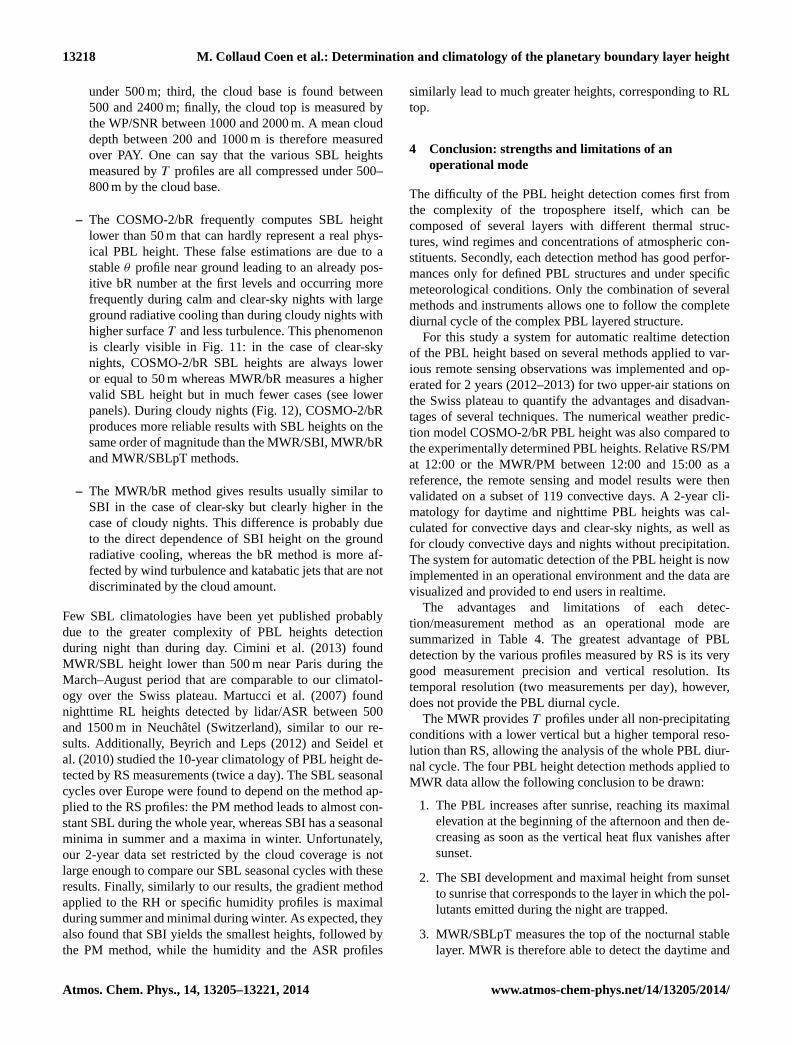
Table 4. Advantages and limits of detection methods and instruments to estimate the PBL height.

Method Profiles PBL height

detected

Advantages Limits

PM θ or θv CBL, cloudy-

CBL

– also efficient under weak

convective condition

– early growth after sunrise until

decrease when temporal gradient

of surface T and vertical heat flux

become negative

– requires negative gradient

in θ at the ground

– not available during night

bR θ or θv+

wind

CBL, cloudy-

CBL, SBL

– nighttime and daytime

detection

– transition between SBL and

CBL at sunrise

– CBL decrease also after the ver-

tical heat flux and temporal T

gradient become negative

– requires wind profiles

from WP or RS

– often false SBL detection

in the case of constant θ

profile

SBI T SBL – SBI formation after sunset

– describe the layer where the

pollutants emitted during night

are trapped

SBLpT θ or θv SBL – Formation and top of the stable

nocturnal layer

– no well-defined limit of

the SBL layered structure

Aerosol/

humidity

gradient

ASR, RH CBL, RL – measures the dynamics of

aerosol dispersion

– a real measure of the pollutants

ML

– no measure of the SBL

SNR

maxima

wind CBL, (RL) – sometimes retrieves PBL height

early growth after sunrise

– only method based on the

vertical structure of turbulence.

– large number of outliers

due to false attributions

– can also retrieve the cloud

top

Instrument Profiles PBL height

detected

Advantages Limits

Microwave

radiometer

T , RH, wind CBL, cloudy-

CBL, SBL

– captures diurnal cycle

– good data availability

– good temporal resolution

– low vertical resolution

Wind profiler Wind, SNR

ratio

CBL, RL – daily cycle

– can also retrieve the cloud top-

based on the vertical structure of

turbulence.

– no PBL detection in the

case of precipitation

– low data availability at

low altitude

Lidar ASR, RH CBL, RL – daily cycle

– direct measurement of

atmospheric composition

– no data in the case of fog,

low clouds

– needs maintenance

Radio

sounding

T , p, RH,

wind

CBL, cloudy-

CBL, SBL

– most accurate and precise data

– best vertical resolution

– only twice a day at 00:00

and 12:00

nighttime layers in which ground-emitted atmospheric

constituents are trapped, but not the RL corresponding

to the air volume trapping the atmospheric constituents

emitted some hours/days before.

The Raman lidar has a higher vertical resolution than MWR

but its data availability is restricted by fog, low cloud cover-

age and precipitation. The profiles of the aerosol or the hu-

midity concentrations allow one to measure the dynamics of

atmospheric constituents and are consequently a direct deter-

mination of the pollutant dispersion in the PBL. The compar-

ison with RS/PM and MWR/PM proves that the lidar/ASR is

able to detect the CBL maxima during the afternoon with a

good precision and also sometimes part of the CBL forma-

tion. During night, this method provides the RL height and

can therefore be considered as complementary to the MWR

methods.

The comparison of WP/SNR with RS/PM and MWR/PM

shows that, in most cases, the CBL maximum is well de-



tected by WP, but with a lower precision and a greater amount

of outliers. De facto WP/SNR maxima can be generated by

turbulence at the PBL top, but also at cloud top or at wind

shears. An operational PBL height measurement by WP is

therefore much more difficult to implement without a hu-

man visual control to attribute the SNR maxima to the real

atmospheric phenomena. In the case of cloudy condition,

the WP/SNR tends to measure the cloud top instead of the

PBL height, which could be exploited for other applications.

For this study, the WP and the Raman lidar have been used

in their operational configuration. However, it would techni-

cally be possible for both systems to go to higher temporal

and vertical resolutions optimized for PBL height detection,

which could slightly improve their performance. Moreover,

more complex procedures for the CBL height detection and

for the selection of clear CBL cases can greatly increase the

accuracy of the results, but decrease the availability of the

CBL height detection (see for example Bianco et al. 2008).

The forecast model COSMO-2 uses the bR method applied

to the θv profile and relies therefore on bR qualities (day and

night detection, detection of CBL growth, maxima and de-

crease) and weaknesses (often false detection during night

particularly in the case of clear-sky conditions). COSMO-

2/bR is found to often overestimate both CBL and cloudy-

CBL by 500–1000 m. The most probable causes for this dis-

crepancy are systematic differences in terms of surface T , T

or RH profiles. This issue will be addressed in future work.

The SBL detection during night is attributed to the lowest

level in the case of stable θv gradient, which could lead to

a misinterpretation of this value that does not really corre-

spond to a PBL height. To avoid such a misunderstanding, a

missing or flagged value should be introduced instead of the

lowest level for these cases.

We conclude that the MWR/PM is the most robust among

the experimental methods under consideration and best

suited for automatic realtime detection of the PBL height.

It provides good results under a wide range of meteorolog-

ical conditions. Moreover, the MWR/SBI and SBLpT allow

the characterization of the nocturnal SBL. It is however nec-

essary to have access to a ceilometer or lidar to monitor the

RL height.

Taking advantage of all available upper-air measurements,

the principal features of the PBL are well depicted by the 2-

year climatology. The annual cycle of the CBL height with its

maxima at 1500 m during the May–August period is detected

by all instruments and seems to follow the solar radiation cy-

cle rather than the T cycle. During partial or total cloud con-

ditions, a similar annual cycle occurs, but with lower PBL

heights. The WP results are however strongly influenced by

wind turbulence at the cloud top. The nocturnal PBL struc-

ture can be clearly observed under clear-sky conditions, with

the SBI height remaining rather constant throughout the year

at 200–300 m, the top of the stable layer at 800 m for most of

the non-winter months and finally the RL nocturnal seasonal

cycle following the CBL diurnal maximal. In the case of to-

tal cloud coverage, the SBI height is lower than in the case

of clear sky, and the SBL layers seems to be compressed and

not well structured under the cloud base. Further meteorolog-

ical phenomena such as fog, neutral boundary layer height,

main pollutant advection or nocturnal jets will be further ad-

dressed either as case studies or statistically after a longer

measurement period.

Acknowledgements. The authors greatly acknowledge Robert Sica

for reviewing the manuscript.

Edited by: J.-Y. C. Chiu

References

Angevine, W. M., White, A. B., and Avery, S. K.: Boundary-layer

depth and entrainment one characterization with a boundary

layer profiler. Bound.-Lay. Meteorol., 68, 375–385, 1994.

Baars, H., Ansmann, A., Engelmann, R., and Althausen, D.: Con-

tinuous monitoring of the boundary-layer top with lidar, At-

mos. Chem. Phys., 8, 7281–7296, doi:10.5194/acp-8-7281-2008,

2008.

Beyrich, F. and Leps, J.-P.: An operational mixing height data set

from routine radiosoundings at Lindenberg: methodology, Mete-

orol. Z., 21, 337–348, 2012.

Bianco, L. and Wilczac, J. M.: Convective boundary layer depth:

improved measurement by doppler radar wind profiler using

fuzzy logic methods, J. Atmos. Ocean. Technol., 19, 1745–1758,

2002.

Bianco, L., Wilczak, J. M., and White, A. B.: Convective

boundary layer depth estimation from wind profilers: statis-

tical comparison between an automated algorithm and ex-

pert estimations, J. Atmos. Ocean. Technol., 25, 1397–1413,

doi:10.1175/2008JTECHA981.1, 2008.

Bradley, R. S., Keimig, F. T., and Diaz, H. F.: Recent changes in

the North American Arctic boundary layer in winter, J. Geophys.

Res., 98, 8851–8858, doi:10.1029/93JD00311, 1993.

Calpini, B., Ruffieux, D., Bettems, J.-M., Hug, C., Huguenin, P.,

Isaak, H.-P., Kaufmann, P., Maier, O., and Steiner, P.: Ground-

based remote sensing profiling and numerical weather predic-

tion model to manage nuclear power plants meteorological

surveillance in Switzerland, Atmos. Meas. Tech., 4, 1617–1625,

doi:10.5194/amt-4-1617-2011, 2011.

Cimini, D., De Angelis, F., Dupont, J.-C., Pal, S., and Haeffelin, M.:

Mixing layer height retrievals by multichannel microwave ra-

diometer observations, Atmos. Meas. Tech. Discuss., 6, 4971–

4998, doi:10.5194/amtd-6-4971-2013, 2013.

Cost Action 710 – Final report “Harmonisation of the pre-

Processing of meteorological data for atmospheric dispersion

models”, edited by: Fisher, B. E. A., Erbrink, J. J., Finardi, S.,

Jeannet, P., Joffre, S., Morselli, M. G., Pechinger, U., Siebert, P.,

and Thomson, D. J., European Communities, ISBN 92–828-

3302-X, Belgium, 1998.

Degreane Horizon: Degrewind PCL 1300 Processing Computer

User Manual, Cuers, France, 2006.


http://dx.doi.org/10.5194/acp-8-7281-2008

http://dx.doi.org/10.1029/93JD00311

http://dx.doi.org/10.5194/amt-4-1617-2011

http://dx.doi.org/10.5194/amtd-6-4971-2013


Dinoev, T. S., Simeonov, V. B., Calpini, B., Parlange, M. B., Mon-

itoring of Eyjafjallajökull Ash Layer Evolution over Payerne

Switzerland with a Raman Lidar, in: Proceedings of the TECO

2010, Helsinki, Finland, 30 August to 1 September, Keynote 2,

2010.

Dinoev, T., Simeonov, V., Arshinov, Y., Bobrovnikov, S., Ris-

tori, P., Calpini, B., Parlange, M., and van den Bergh, H.: Ra-

man Lidar for Meteorological Observations, RALMO – Part

1: Instrument description, Atmos. Meas. Tech., 6, 1329–1346,

doi:10.5194/amt-6-1329-2013, 2013.

Dürr, B. and Philipona, R.: Automatic cloud amount detection by

surface longwave downward radiation measurements, J. Geo-

phys. Res., 109, D05201, doi:10.1029/2003JD004182, 2004.

Emeis, S.: Surface-based remote sensing of the atmospheric layer,

in: Atmospheric and Oceanographic Sciences Library, vol. 40,

edited by: Mysak, L. A. and Hamilton, K., Springer, Dordrecht,

Heidelberg, London, New York, 171 pp., 2009.

Fisher, B. E. A., Erbrink, J. J., Finardi, S., Jeannet, P., Jof-

fre, S., Morselli, M. G., Pechinger, U., Seibert, P., and Thom-

son, D. J.: Cost Action 710-Final report: Harmonisation of the

Pre-processing of meteorological data for atmospheric dispersion

models, Office for Official Publications of the European Commu-

nities, Belgium, 1998.

Garrett, J. R.: The atmospheric boundary layer, Cambridge atmo-

spheric and space science series, Cambridge University Press,

Cambridge, 1992.

Granados-Muñoz, M. J., Navas-Guzmán, F., Bravo-Aranda, J. A.,

Guerrero-Rascado, J. L., Lyamani, H., Fernández-Gálvez, J.,

and Alados-Arboledas, L.: Automatic determination of the

planetary boundary layer height using lidar: one-year analy-

sis over southeastern Spain, J. Geophys. Res., 117, D18208,

doi:10.1029/2012JD017524, 2012.

Haeffelin, M., Angelini, F., Morille, Y., Martucci, G., Frey, S.,

Gobbi, G. P., Lolli, S., O’Dowd, C. D., Sauvage, L., Xueref-

Rémy, I., Wastine, B., and Feist, D. G.: Evaluation of mixing-

height retrievals from automatic profiling lidars and ceilometers

in view of future integrated networks in Europe, Bound.-Lay.

Meteorol., 143, 49–75, doi:10.1007/s10546-011-9643-z, 2012.

Holzworth, G. C.: Estimates of mean maximum mixing depths in

the contiguous united states, Mon. Weather Rev., 92, 235–242,

1964.

Jericevic, A. and Grisogono, B.: The critical bulk Richardson num-

ber in urban areas: verification and application in a numerical

weather prediction model, Tellus A, 58, 19–27, 2006.

Ketterer, C., Zieger, P., Bukowiecki, N., Collaud Coen, M.,

Maier, O., Ruffieux, D., and Weingartner, E.: Investigation of the

planetary boundary layer in the Swiss Alps using remote sens-

ing and in-situ measurements, Bound.-Lay. Meteorol., 151, 317–

334, doi:10.1007/s10546-013-9897-8, 2014.

Liu, S. and Liang, X.-Z.: Observed diurnal cycle climatology of

planetary boundary layer height, J. Climate, 23, 5790–5809,

doi:10.1175/2010JCLI3553.1, 2010.

Mahrt, L., Sun, J., Blumen, W., Delany, T., and Oncley, S.: Noc-

turnal boundary-layer regimes, Bound.-Lay. Meteorol., 88, 255–

278, 1998.

Martucci, G., Matthey, R., Mitev, V., and Richner, H.: Comparison

between backscatter lidar and radiosonde measurements of the

diurnal and nocturnal stratification in the lower troposphere, J.

Atmos. Ocean. Technol., 24, 1231–1244, 2007.

Milroy, C., Martucci, G., Lolli, S., Loaec, S., Sauvage, L., Xueref-

Remy, I., Lavric, J. V., Ciais, P., Feist, D. G., Biavati, G., and

O’Dowd, C. D.: An Assessment of Pseudo-Operational Ground-

Based Light Detection and Ranging Sensors to Determine the

Boundary-Layer Structure in the Coastal Atmosphere, Advances

in Meteorology, 18 pp., doi:10.1155/2012/929080, 2012.

Radiometer Physics GMbH: Technical Instrument Manual, Meck-

enheim, Germany, 2011.

Salmond, J. A. and McKendry, J. A.: A review of turbulence in the

very stable nocturnal boundary layer and its implications for air

quality, Prog. Phys. Geog., 29, 171–188, 2005.

Sawyer, V. and Li, Z.: Detection, variations and intercomparison of

the planetary boundary layer depth from radiosonde, lidar and

infrared spectrometer, Atmos. Environ., 79, 518–528, 2013.

Schmid, P. and Niyogi, D.: A method for estimating planetary

boundary layer heights and its application over the ARM South-

ern Great Plains Site, J. Atmos. Ocean. Technol., 29, 316–322,

doi:10.1175/JTECH-D-11-00118.1, 2012.

Seidel, D. J., Ao, C. O., and Li, K.: Estimating climatological plane-

tary boundary layer heights from radiosonde observations: com-

parison of methods and uncertainty analysis, J. Geophys. Res.,

115, D16113, doi:10.1029/2009JD013680, 2010.

Seidel, D. J., Zhang, Y., Beljaars, A. C. M., Golaz, J.-C., Jacob-

son, A. R., and Medeiros, B.: Climatology of the planetary

boundary layer over the continental United States and Europe, J.

Geophys. Res., 117, D17106, doi:10.1029/2012JD018143, 2012.

Stull, R. B.: An Introduction to Boundary Layer Meteorology,

vol. 13, Kluwer Academic Publishers, the Netherlands, Dor-

drecht/Boston/London, 1988.

Summa, D., Di Girolamo, P., Stelitano, D., and Cacciani, M.: Char-

acterization of the planetary boundary layer height and struc-

ture by Raman lidar: comparison of different approaches, Atmos.

Meas. Tech. Discuss., 6, 5195–5216, doi:10.5194/amtd-6-5195-

2013, 2013.

Szintai, B.: Improving the turbulence coupling between high reso-

lution numerical weather prediction models and Lagrangian par-

ticle dispersion models, Ph.D. thesis, Swiss Federal Institute of

Technology, Zürich, Switzerland, 2010.

Wang, Z., Cao, X., Zhang, L., Notholt, J., Zhou, B., Liu, R.,

and Zhang, B.: Lidar measurement of planetary boundary layer

height and comparison with microwave profiling radiometer ob-

servation, Atmos. Meas. Tech., 5, 1965–1972, doi:10.5194/amt-

5-1965-2012, 2012.

White, A. B., Fairrall, C. W., and Wolfe, D. E.: Use of 915-mHz

wind profiler data to describe the diurnal variability of the mixed

layer, AMS, in : Proc 7th Joint Conf. Appli. Poll. Meteor., AMS,

14–18 January, New Orleans, LA, J161–J166, 1991.

Zahng, N., Chen, Y., and Zhao, W.: Lidar and microwave radiometer

observations of planetary boundary layer structure under light

wind weather, J. Appl. Rem. Sensing, 6, 063513-1–063513-8,

doi:10.1117/1.JRS.6.063513, 2012.



http://dx.doi.org/10.1029/2003JD004182

http://dx.doi.org/10.1029/2012JD017524

http://dx.doi.org/10.1007/s10546-011-9643-z

http://dx.doi.org/10.1007/s10546-013-9897-8

http://dx.doi.org/10.1175/2010JCLI3553.1

http://dx.doi.org/10.1155/2012/929080

http://dx.doi.org/10.1175/JTECH-D-11-00118.1

http://dx.doi.org/10.1029/2009JD013680

http://dx.doi.org/10.1029/2012JD018143





http://dx.doi.org/10.1117/1.JRS.6.063513

Documents

Determination and climatology of the planetary boundary ... · tive boundary layer heights in good agreement with the radio sounding ... the analysis of the diurnal variation of the