Vol. 7 No. 1 CHIN. J. OCEANOL.LIMNOL. 1989

DETERMINATION OF GEOSTROPHIC FLOW BY APPLYING THE PRINCIPLE OF MINIMUM

ENERGY AND THE INVERSE METHOD*

Zou Jiansheng (~1~'~) and Yuan Yeli ( ~ ) ( Institute of Oceanology, Academia Sinica)

Received August 22, 1987

Al~raet

This article gives a computing method to calculate the geostrophic current. The fact that kinetic energy of 8eostrophic motion and geostrophic potential energy reach minimum simultaneously, Fomin~" principle of minimum kinetic energy" is equivalent to the principle of minimum geostrophic poten- tial energy. We concluded that horizontal geostrophic velocities at different depths are along the same diree tion. Combining our method with C. Wunseh's inverse method we can obtain the velocity components along and normal to the hydrographic sections. We used and analysed CTD and current meter data of " Experiment No. 3 "exploration, December 1985 -January 1986, in the west Pacific Ocean - Philippine a r e a .

I. INTRODUCTION

To determine geostrophic motion, we must know the absolute velocity at a cer- tain depth, otherwise there will be infinite solutions that satisfy the geostrophic equa- tions. Direct measurement of the velocity cannot yield the stable and unstable compo- nents of geostrophic motion. Some scientists determined geostrophic current by assum- ing the existence of a "zero" surface. C. Wunsch (1978) devised the inverse method to calculate the reference velocity. He used the material surface as a demarcation to vertically divide the sea, then established conservation equations for each layer and showed that there are infinite possible geostrophic motions in the ocean. He selected the intuitively simplest solution by the least squares method.In an indeterminate syst- em the fewer the equations, the greater the indeterminate degree. To get more indep- endent equations for a better result, it is essential to find as many conservative qua- ntities as possible. But in a physical sense, the meaning of the least square is still not clear. Besides this, his solution depends on the level chosen. Maybe we shuld impose the condition that any reference level chosen will yield the same result.

It is often a fact that of all kinds of possible existences, certain physical quantities at the extremum often reach the stable state naturally. By applying Fomin's "principle of minimum kinetic energy" geostrophic motion can be derived by taking the

*Contribution No. 1513 from Institute of Oceanology, Academia Sink:a,

44 C H I N E S E J O U R N A L O F O C E A N O L O G Y A N D L I M N O L O G Y Vol.7

vertical integral of the kinetic energy at the minimum. Ofcourse the validity of this method should be verified further. Also, in this met hod ther elative velocity values in the two different directions must be known. In actual calculations this method is suitable for cornered stations only.

In this study, we try to prove that kinetic energy and potential energy can simultaneously be at the extremum in geostrophic motion. In fact, it is an allowable suggestion from intuition. When the kinetic energy is at minimum, the horizontal pres- sure gradient is also at minimum. Based on the hydrostatic equation, the isopycnal sur- face tends to reach the equilibrium state. This conclusion is not contradictory to the en- ergy conservation and transform law governing the motion process of the system. We also notice that in quasi-geostrophic motion horizontal geostrophic velocities at differ- ent depths are along the same direction. Geostrophic motion can affect the thermodynamic state so that the horizontal isobaric lines coincide with the horizontal isopycnal lines. This does not mean that the fluid is barotrophic. The above conclu- sion does not coincide with the Taylor-Proudman theorem.

We use the concept of the minimum energy as the criterion of the inverse method and can obtain the velocity components along and normal to the hydrographic sec- tion.

II. FUNDAMENTAL EQUATIONS AND VERTICAL STRUCTURE OF THE GEOSTROPHIC CURRENT

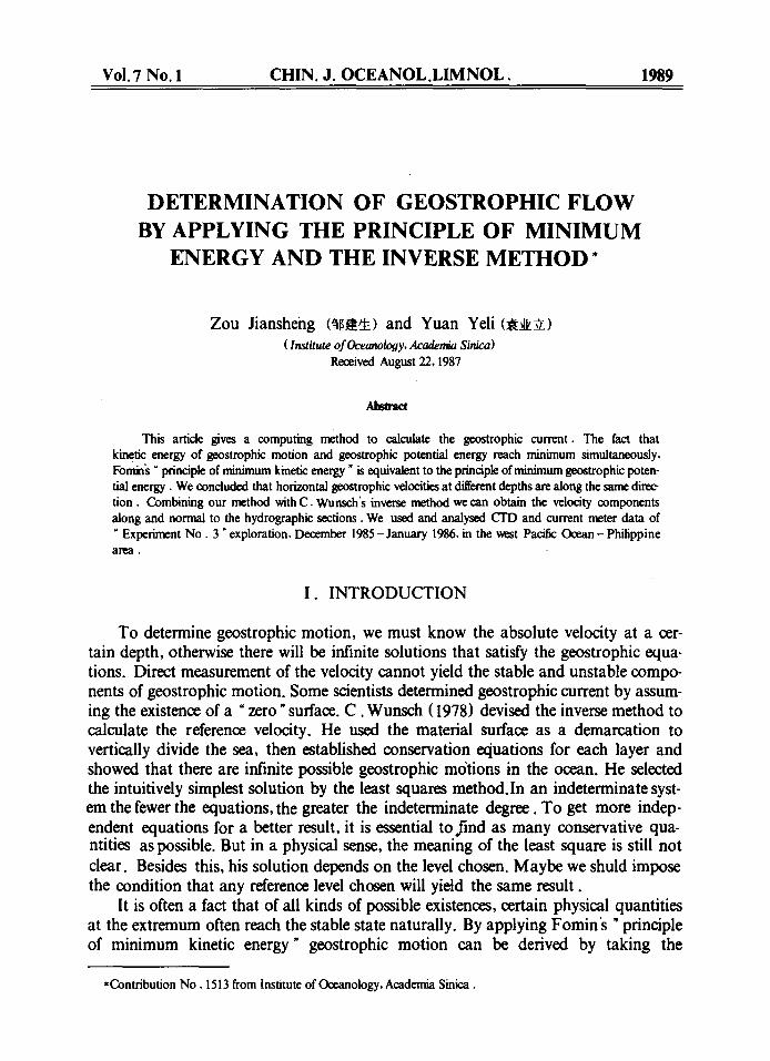
We begin with the analysis of large scale motion in the "Experiment No. 3 "( 1985. 12- 1986.1)explored region (the West Pacific Philippine area, Fig. 1). Fig. 2 is the

20 ~ 125 ~ 130 ~ 135 ~ 140 ~ 1 4 5 ~ 20 ~ N ,

15~ i~, r ~.L . . . . . . . . . . . . 114

' " ; 115 /

10~ ~ ~ . A II " ~ ~ 0 1 i

5 = \

0o

5oS , , ~

Fig. 1 The sailing route and investigated region of" Experiment No. 3 " (I 985.12- ! 986.1 )

N o . 1 D E T E R M I N A T I O N O F G E O S T R O P H I C F L O W 45

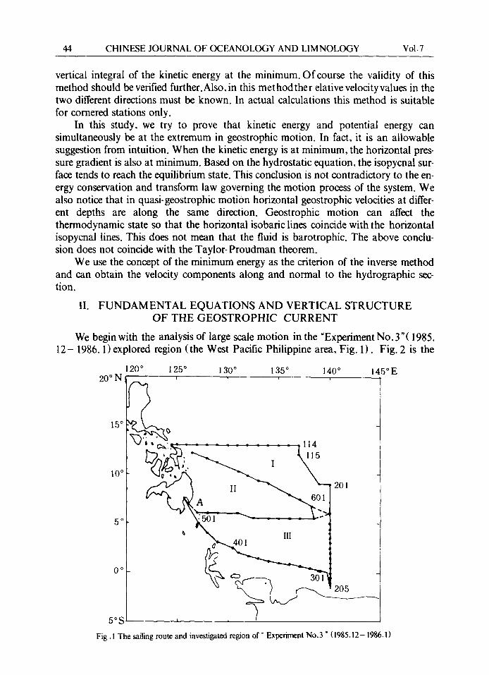
sea surface flow map in the North Pacific Ocean drawn by the Scripps Institute of Oceanology (1972). We can see clearly in Fig.2 that the region is a converging area of the north and south equatorial currents, the equatorial adverse current, the south equa- torial current, and the source area of the Kuroshio.

� 9 _..~--~ -.-- ~ " Z _ ~ /

3

~ . / - r - f

' 1~ " i. . ! - . . .

( ' . 5 ( " - ~ " ~ " " " ~

Fig. 2 The sea surface current field in winter. The straight lines show the sailing route o f" Experiment No .3"

I. Geostrophie model We now give the governing equations in the local rectangular coordinate system

O-xyz. z is upward. We take

L= 100km D = 4 k m U= 30crnA

L is the horizontal typical length, D is the vertical typical depth, U is the hor- izontal typical velocity.

We should pay attention to the estimation of the Rossby number because of the great change of latitude in the region.

Taking

we have the Rossby number

We also have

001>3 ~ (2.1)

U - O ( 0 . 2 ) <1 (2.2a) ~<~ fo L

L U tg00 r - 0 (0 .2) < 1, and r - l _ _ _ _ O(1) (2.2b) r0 L2

r- l is the planetary vorticity gradient. In the region away from the boundary layer, we can neglect the friction force.

(2.2a) and (2.2b) indicate that in the main area (0t> 3 ~ of our calculation the mo- tion is basically quasi-geostrophic and quasi-hydrostatic. The governing equations a r e

46 CHINESE JOURNAL OF OCEANOLOGY AND LIMNOLOGY Vol. 7

- f v = - 1 . O__PP (2.3a) P Ox

fi~= __ 1 . 0p (2.3b) p dy

0 = - 1 Op _ 9 (2.3c) p Oz

Thecontinuityequation is

O(pu) + O(pv) + O(pw) =0 (2.4) Ox Oy Oz

We can derive the thermo-wind equation

f O (pv) Op (2.5) ?~z = - 9 Ox

We select a reference level z 0 and integrate (2.5) form z 0 to z ,

also,

fZ Z - g g pdz+ v(z o)

v(z) = fpo Ox 0

(2.6a)

~Z Z ~] O pdz+ u (z o) (2.6b) u (z) = fPo Oy o

In the region near the equator, we cannot use ( 2.3a, b), as f here is very small, but take the differential form of (2.3a,b) .Then we have

- ~ 02 p d z + v (z o) (2.7) v ( z ) = Of po �9 gx2

- - 0

Ox

We also can have the expression of u (z). The geostrophic motion consists of two parts : one is the density flow due to the

unevenness of the sea water density, the other is the absolute speed in the reference lev- el. We can calculate the first part from the dynamic height. The determination of the geostrophic motion refers to the calculation of the reference velocity.

2. The vertical structure of the geostrophic motion

We divide (2.3b) by (2.3a) to obtain

Op Oy

D

v ap Ox

(2.8)

Then we differentiate (2.8)with respect to z and use the quasi-hydrostatic equation

No. I DETERMINATION O F GEOSTROPHIC FLOW 47

(2.3c) to get

u J (p,p) (2.9)

We use the density conservation equation and non-divergence equation to replace the continuity equation.

dp = 0 (2. lOa) dt

d__E_u + t3v + d w - 0 (2.10b) dx dY t3z

Using (2.3a, b) and (2. lOa) we have

dz = - g pfv 2 " tgz

Using (2.3a,b) and (2. lOa, b) we have

f d(pw) -~x of (2.11) p ~gz =u +v cgy

Using (2.11)and the surface boundary condition w (0) = 0, we have

yo = g dP ~f~Y pVn dz (2.12) ,~z p 'vn dz " f

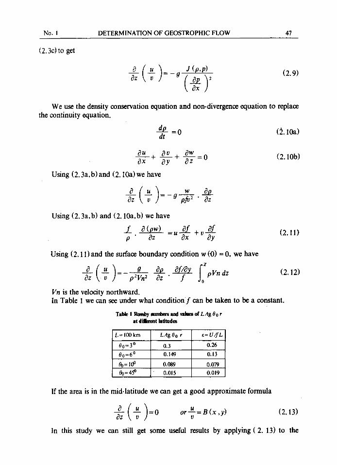
Vn is the velocity northward. In Table 1 we can see under what condi t ionf can be taken to be a constant.

Table I R c ~ nmnim~ ~ ,nd~ of L Ag O o r at d i l ~ t hlitndes

L= I00 km LAg Oo r ~= U/ fL

00=3 0 0.3 0.26

00=6 0 0.149 0.13

0o= Io ~ 0.0~ 0.079 0o=450 0.015 0.019

If the area is in the mid-latitude we can get a good approximate formula

a ( - - - u ) = 0 orU=B(x,y) (2.13) ~z v v

In this study we can still get some useful results by applying (2. 13) to the

48 CHINESE JOURNAL OF OCEANOLOGY AND LIMNOLOGY Vol. 7

computing region even if the results are not as good as in the mid-latitude region. It should be noted that 1 2. 12)differs from the barotrophic condition p=p (p),

which indicates that in every horizontal surface z = zo, the isobaric lines coincide with the isopycnal lines. In quasi-geostrophic motion although the horizontal current field may change with depth, the direction of current does not basically change with depth.

III. THE EQUILIBRIUM BETWEEN THE MINIMUM KINETIC ENERGY AND THE MINIMUM GEOSTROPHIC POTENTIAL ENERGY

Geostrophic motion is accompanied by a declination of the isobaric surface. We are not interested in the nonstationary motion but in the relationship between the densi- ty field or pressure field and the geostrophic motion, i . e . , the relationship between the potential energy and the kinetic energy. When the fluid is in a static state, the isobaric and isopycnal surfaces are horizontal and coincide with each other. If we de- fine the gravitational potential energy of this state as the basic potential energy, the dif- ference between the stable geostrophic potential energy and the basic potential energy is what we consider. We call this difference the geostrophic potential energy. Because of the geostrophic balance, geostrophic energy cannot be transformed to kinetic ener- gy, which is equal to the work adiabatically done by an Archimedes force when the static state changes to the geostrophic balanced state. It is difficult for us to know how the fluid particles move. The problem of baroclinic instability will be involved. Below, we only consider the simplest case when the fluid particles move up and down.

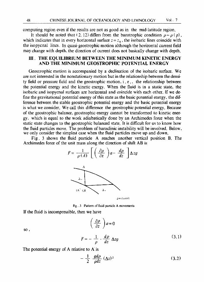
Fig. 3 shows the fluid particle A reaches another vertical position B. The Archimedes force of the unit mass along the direction of shift AB is

A

, O ~ C O n .',:, t

[Zig. 3 Pattern of fluid panicle A movements

If the fluid is incompressible, then we have

SO ,

F = - 1 . dp Az9 p dz

The potential energy of A relative to A is

1 9dp 2 pdz

(3.1)

(Az) 2 (3.2)

No. I DETERMINATION OF GEOSTROPHIC FLOW 49

Let us consider the kinetic energy in the geostrophic motion. For convenience, we suppose the motion is perpendicular to the paper, so the kinetic energy of unit mass is

v-'- 1 if2 1 (Az) 2 (3.3) 2 2 f~ Ax 2

Ax is a given horizontal length. The potential energy and the kinetic energy in (3.2) and (3.3) depend on the val-

ue of the vertical deviation from the static position of the isobaric surface. Of all possi- ble geostrophic motions, if the geostrophic balance makes the geostrophic potential and kinetic energies minimum simultaneously, then total mechanical energy is at the minimum. Thus F o m i n s minimum kinetic energy is equivalent to the minimum po- tential energy or the mechanical energy. Now we express (2.6a, b)as

u(z) =Uo+ u (z) (3.4a)

v(z) =v0+ v ( z ) (3.4b)

From the geostrophic equations and the boundary conditions we derive the same confining condition as Fo min s .

here,

i0 cf u 'dz- 1 OH �9 Ox _, f " Ox u ( - H) ;o

1 Of v d z - 1 OH v ' ( - H ) d e f + - f i Oy _. f " ~ -

=(2 (3.5)

1 A~u~ A~ 'v~ f

A~- Ox ---f-

On the condition stipulated by (3.5)we find the solution which makes fo E= Pa [ u o + u ' ) 2 + ( v o + v ' ) 2 ] d z

2 -H

= minimum

So , we have

1 v d z - Ay udz u~ =(Ax2+ A~2 )- ' Ax+ AxA~' ~ -H H _

u d z - A .~ 'dz v~ A~Z)-I QA~'+ AxA~'--~ -n H

(3.7a)

(3.7b)

50 CHINESE JOURNAL OF OCEANOLOGY AND LIMNOLOGY Vol .7

We introduce the total flux function,

U = Huo+ f o u dz - H

(3 .8a )

and have

f O

V= Hvo+ v 'dz (3.8b) - H

A x V- Ay U=0 (3.9)

So the total flux of the geostrophic current is directed normal to the isolines

H - const

f Now we integrate (2.13) from the bottom to surface to obtain

thus

SO

U = B ( x , y ) V (3.10)

B (x ,y) = A , Av

u= A--~-v (3.11) A

Y

If the reference levels of u and v are the same, we also have

u'= h'v" A~

A, U~ = ay v~

(3.12a)

(3.12b)

then, (3.7a ,b) reduce to

uo=QA x/(A~+ A~) (3.13 a)

vo=QAy/(A2~+Ay) (3.13 b)

H If we know the distribution of --7- and the geostrophic relative speed component

in one direction, we can obtain the geostrophic current at the energy minimum.

IV. INVERSE METHOD

We adopt Worthington and Wunsch's method and use the isopycnal surface as the demarcation. We can get the linear algebraic equations of the reference speed in the station pairs by establishing the mass conservation equation in each layer. So we

No. I DETERMINATION OF GI~OSTROPHIC FLOW 51

have a linear algebraic equation group with M equations and N unknowns.

Ab=g here

A = ( a , ) ,,.~

b = (b) ~ .1

g=(gi) ,, .i a~i=p~jA xjd~j

(4.1)

bs= vj(z o) is the reference velocity on the z0 level of the jth station pair,

N

~ti=- ~ a i~ v , ( i , j ) j=l

A xj is the distance of jth station pairs, d~j is the average thickness of the j th station pair in the ith layer, M is the number of layers, N is the number of the enclosed station pairs v, (i ,j) is the relative velocity above the z o reference level.

As a whole, it is an indeterminate system. So we should establish more conserva- tion equations by finding a conservation quantity to serve as the " tracer" of the sea current. Chemical analysis of seawater shows that 1) the conservation equatio n of metal elements in the ionic state is linearly related to the salinity conservation equa- tion ; 2) the conservation equation of trace elements is linearly related to the mass con- servation equation. Radio isotopes can be used as " tracers", but we do not have enough data to make the calculation. Wellance S. Droecher (1974) used some chemi- cal and biological compouds (" 9NO3+ O 2 " , i . e . , "NO "and " 135PO4+ O2", i . e . , "PO ") as tracers. As chemical reaction is sensitive to environmental conditions, we do not know whether the same result can be obtained in the Pacific Ocean. C. Wunsch et al (1983) used P O , N O , mass, salinity, temperature, Si as " tracers" So far no one has estimated the precision of his equations based on the above parameters, which must involve a complex phenomenon like turbulent diffusion. In this study, we did not have enough chemical data to carry out our calculation. In the process of applying the salinity conservation equation, we found that it was very rel- evant with the mass conservation equation.

(4. 1) can be solved by applying the theory of pseudoinverse matrix and the meth- od of orthogonalization. In the sense of the least square IIb I12-- min (4. 1) has a solution

b = ~ uh.g v~ r= rang (A) (4.2) K = 1 O ' k

here { u, }, { v, } is a series of orthogonal standard bases of AA ", A "A. {Q, }is a

series of singular values of AA : But in fact, (4.2) gives an unstable solution, i . e . , a small variance of A and g

will cause a bigger variance of b , if the equations have small eigenvalues. In this case

52 CHINESE JOURNAL OF OCEANOLOGY AND LIMNOLOGY Vol .7

we take the SVD form, i . e . , neglect the items of small eigenvalues and consider them as the part of null space.

Here r, means

b= ~ u~.~q vk (4.3) k ~ ! 0" k

0"rl >~ ~t0> 0

0"r~.1<~

Besides this method, there is a stable computing method, Tehonov orthogonalized method, within the range of precision of the equation, which uses the minimum norm of the vectors satisfying the inequality to get a solution of this prob- lem. On the condition Ilax- b II ~< ~ the solution of II b II 2 = min is

b=(A " A + a I ) - ' A "g

u~' .g 2., a~ vk (4.4) k=t 0"2+ 0~

here, ~ can be determined from II A x - b II = 6

1. The principle of the averaged distribution

Obviously, if we take a different form of the norm there will be different results. The least principle often means that a certain physical quantity at an extremum corre- sponds to the physical quantity distributed averagely. If there is no weight, where there is little space i . e . , the coefficient of some quantity is small, there is little mass distributed. Weighting can make flux distributed evenly and does not rely on the choice of the space. So for our question we may choose weight as Wunsch did and the mini mum of IIb II turns to be

here

I1 Wb I1 = min (4.5)

W = diag (--. , (A xj h I ) ,/2 ,... ) (4.6)

Solving (4.1) is equal to solving

here A t b t = 9 (4.7)

A W - I = A I Wb=bz

2. The principle of the averaged distribution of the density flow plus the reference flow

If we take the contribution of both the reference flow and the density flow into consideration, the following

min v 2 dzd ~, (4.8) E -

N o . 1 D E T E R M I N A T I O N O F G E O S T R O P H I C F L O W 53

Will be chosen as the criterion of the inverse method. Here Y~ is the lateral area of the closed area in the whole depth.

L. f ~ In the discrete form min v 2 dzd ~ is equal to - H

min II Wi (b+ c)ll M , )1/2 . . .] W , = d i a g [... (Ax., ,~ d~,, , i = !

M

p,/d,/Vg (i,j) C ~ = ~-:~ M

i=l

(4.9)

(4.10)

-3. The principle of the minimum kinetic energy

In section 3 we calculated the geostrophic current satisfying the minimum energy. Here we require it to be a criterion of the inverse method. Thus we will obtain a cur- rent of minimum energy with mass conservativity in the whole region. So we choose

f ~ , ~ 0 ( U 2 + v 2 ) d z d ~ = m i n i m u m

-H

(4.11)

120 ~ 3)~

1 5 ~ P

10 ~ t

125 ~ 30 ~ 135 r 140 ~ 145 ~ E . . . . . "f: . . . . . . , - - - -- i -- ,

5 0 c m / s

_. ~ 2o/~F1 zso

~ ~ ~ ' , o o - . " ~ 15~ "[ZIL- 14oo

,/.-.% . ; 50

% , E ~ ~~176 :--ISl~o

V - 300 r ,50

20 N

5 o

0 o

5:

0 ~

5oS

20 ~ 125 r 130 ~ 135 ~ 140 ~ t ' - t

~"~ 5oc'-~/s / I,, o L ~ 5~o~-=~-1800

~-~..L'~L"-~ 7 r 6oe ' - - I ' , . 1850 �9 ~-.~ ,,~.-, ' J ~ �9 , = ~ . : . . . . . - - ~ = ~ 6 5 0 1 " - - I " - . I 9 0 0

5 0 0 - .

I Gooor = z o o ~ ' t woo~. ~ iooo

. L _ [ ~

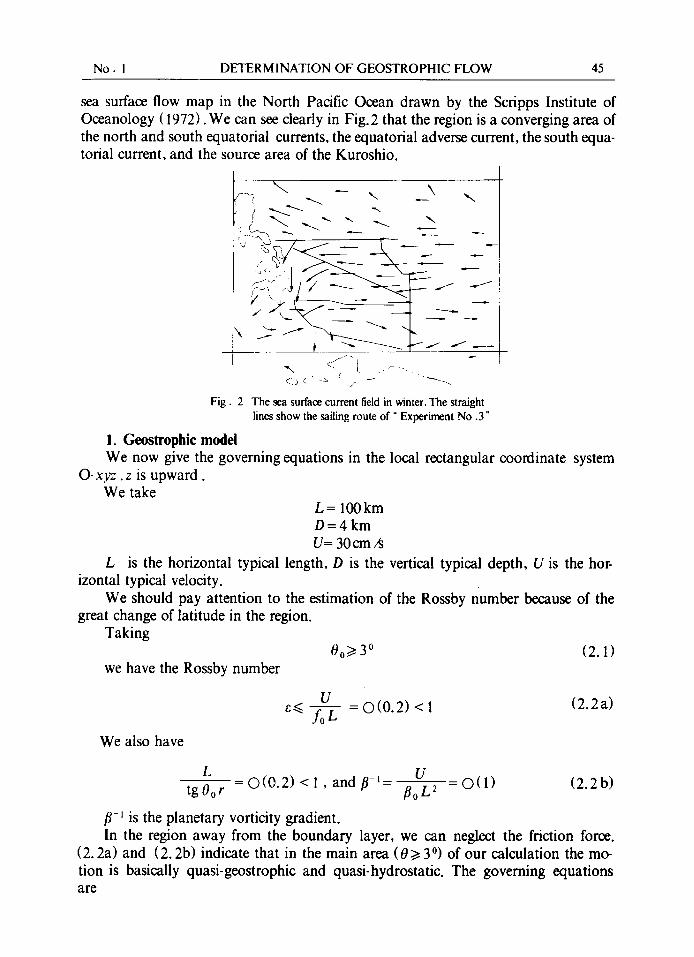
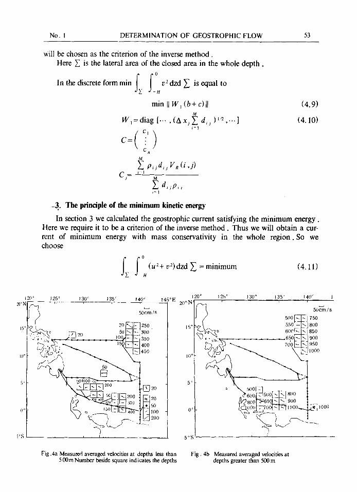
Fig .4a Measu red ave raged velocities a t dep th s less than F i g . 4b M e a s u r e d ave raged velocities a t 5 0 0 m N u m b e r beside squa re i nd i ca t e s the dep ths d e p t h s grea ter t han 500 m

54 CHINESE JOURNAL OF OCEANOLOGY AND L1MNOLOGY Vol. 7

here, ~ is either the horizontal curve or the horizontal area. In the region we consider, we choose ~ as the curve enclosed by the station

pairs. (4. i 1) needs the relative speed along the station pairs, which can be solved by equation (2.12) . The calculation of equation (4.1) is equal to redefining the weight matrix W, in (4.10) . We substitute W 2 for W, and refer to the problem (4.9).

M

W2=diag{... ,[Axj()-" d,j). ( l + n 2 ( x , y ) ) ] , / 2 , . . . } (4.12) i = l

From the measured velocity data in some stations, we can see that the geostrophic current along the same direction in the whole depth coincides with the real fluid field quite well (see Fig.4a. b)). At stations 114,307,401, at every depth, the fluid moves in almost the same direction.

V. COMPUTING RESULTS

The data we used came directly from CTD. We used a thertnodynamic formula to calculate the density field fronl the values of temperature, salinity, and pressure in every station. Taking note of the shape of the isopycnal surfaces we chose 6 density values, tr, = 23.4,0"2 = 26, or3= 26.7,0"4= 27, tr5 = 27.25,0"6= 27.389. We used the Lagrange formula to calculate the depth of the isopycnal surfaces and the dynamic height of the isopycnal between the station pairs. Then we calculated the relative velocity after choosing 1500 m as zero surface. What we chose as the value between layers and station pairs was the centric arithmetic averaged value. We ignored the unreasonable values, but used the interpolated and extrapolated values of the neigh- bouring positions. For the station with a depth less than 1500 m we chose the sea bottom as the reference level.

We used historical data (Fig .2)and measured flow meter values of "Experiment No. 3 "(Fig .4a and Fig.4b) as the criterion to judge the result.

1. The calculation by the inverse method of the averaged distribution of the reference flow and the error analysis

We established the mass and salinity conservation equations of each layer in the re- gion I , II, III, each of which had 6 layers and 12 equations. In the calculation of re- gion III, we did not include 301 - 401, but used the section 401 - 301-215 to form the independent equations. Thus we had two equation systems, one from I, II, III (not including 301 - 401), which had 38 equations and 58 unknowns, the other from 2 1 5 - 3 0 1 - 4 0 1 , which had 12 equations and 9 unknowns. We chose the weight matrix

W=diag [ (A xl d,) l~ ,... (Ax58d.~)l/2]

Then we did the calculation for the pseudoinverse matrix and the orthogonalization to the equation (4. 7). Because of the existence of 18 small eigenvalues, the salinity conservation cannot give the equations independent of the mass conservation equations. We had to regard them as extra equations and only used 18 mass conservation equations for calculation. In the results of the reference velocities obtained from all of the items of (4.2) we found at the 1500 m depth the absolute ve- locities near the equator and near the offshore area were very high, and so were the

No. I DET[ 'RMINATION OF GEOSTROPHIC FLOW 55

sea surface velocity fields. One explanation may be that the small eigenvalues caused the great variance be-

cause of the ill coefficients of the linear algebraic equations. In fact, the variance was inevitable. The unstationary nature of the sea defined itself in different thermodynamic and dynamic states at different times. Analysis of data in all stations showed that the structure of the temperature and salinity in two neighbouring stations were not the same at different times. The way the layers are divided isopycnally is the main factor affecting the relevance of the equations. Because of the hydrostatic stabili- ty of the ocean in the vertical direction, the tracers move almost along the horizontal direction. In the vertical direction we cannot divide many isopycnal surfaces not paral- lel to each other. In general, the number of the independent equations is smaller than the number of unknowns. There are some methods for dealing with small eigenvalues. One is the deployment of none- zero eigenvalue items of (4 .3 ) , i . e . , SVD solution (Wunsch , 1978), the other is Tehonov s orthogonalization. ~ The SVD solution in which we choose k = 16 and the reference velocity calculated by the Tehonov orthogonalization method in which we take ct = 0. 1, are also calculated. Both structures and values are similar. When we take ct= 0. 1, the variance of the equations allows only 0. 1 cm/s net speed in every station pair.

2. The calculation result by the inverse method based on the principle of the averaged distribution of the density flow plus the reference flow

The result of the inverse calculation of (4.9) by choosing the norm as (4. 10) is roughly the same as result 1), except that the adverse current has a larger value.

3. "lhe computed result based on the principle of the minimum energy

As the methods 1 ) , 2) cannot give the velocity component along the sections, es- pecially when the section angle and the velocity are not big, we cannot get the main part of the velocity from them. In Fig. 3, we can see that the angle between sections 101 - 114,601 - 611,501 - 508 and the direction of the surface current is not big, so the flux normal to the section is also small, and the flux along the section is larger. We expect that inverse calculation of (4.11) of the weight matrix (4. 12) might give a better result.

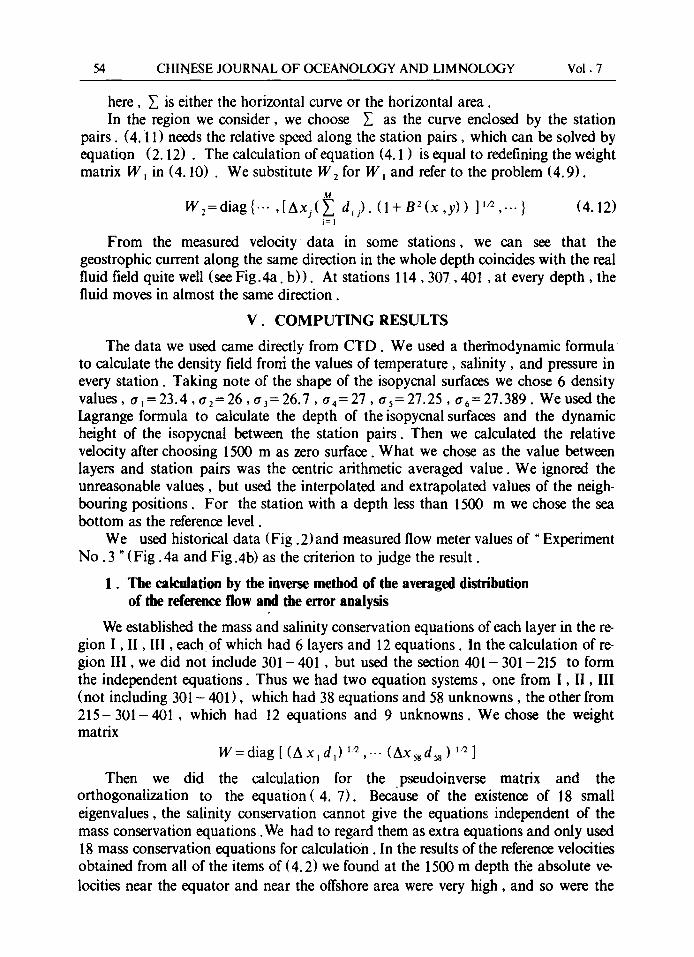
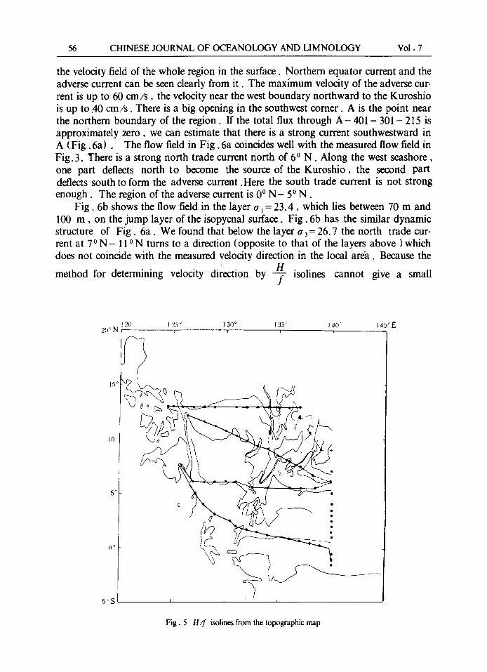
H Fig. 5 is the map of 7 - isolines. What we want to know is the gradient direc-

t ion, not the gradient value. The distance between adjacent isolines does not necessari- / \

ly have the same variance A ( ~ ) .In the place where there are enough data , we \ ~ J /

have dense isolines. In the other place we cannot get more isolines (608- 611 ), so we

have to estimate the direction of the isolines from the neighbouring isolines. Near the �9 H

equator where the change o f f lsgreat, the isolines of _-7- tend to be parallel to the lat-

itude. The flow cannot be expected to be along the lorigitude, as the geostrophic mod- el is not well suited for the equator region. We roughly estimate the flow direction and give the values of B (x ,y).

The computing results of the Tehonov orthogonalization method are shown. Here we take a= 0.05 .The velocity at the depth of 1500 m is 10- 30 cm/s. Fig. 6a shows

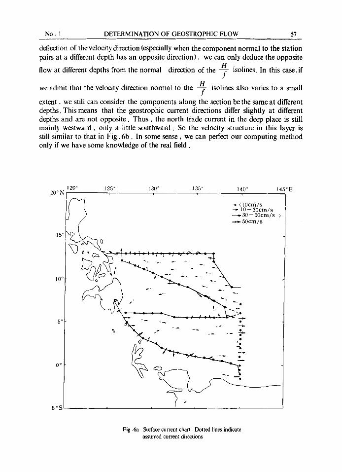
56 CHINESE JOURNAL OF OCEANOLOGY AND L I M N O L O G Y Vol. 7

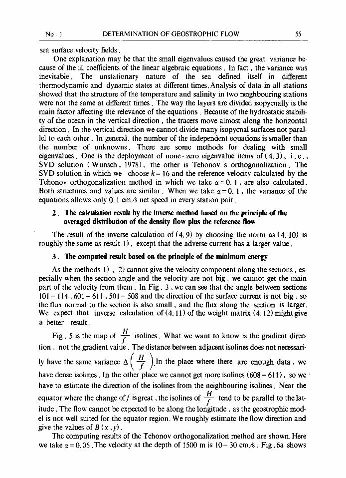
the velocity field of the whole region in the surface. Northern equator current and the adverse current can be seen clearly from it . The maximum velocity of the adverse cur- rent is up to 60 cm/s , the velocity near the west boundary northward to the Kuroshio is up to .40 cm/s . There is a big opening in the southwest comer. A is the point near the northern boundary of the region. If the total flux through A - 401 - 301 - 215 is approximately zero, we can estimate that there is a strong current southwestward in A (Fig. 6a) . The flow field in Fig. 6a coincides well with the measured flow field in Fig. 3. There is a strong north trade current north of 6 o N . Along the west seashore, one part deflects north to become the source of the Kuroshio, the second part deflects south to form the adverse current. Here the south trade current is not strong enough. The region of the adverse current is 0 ~ N - 50 N .

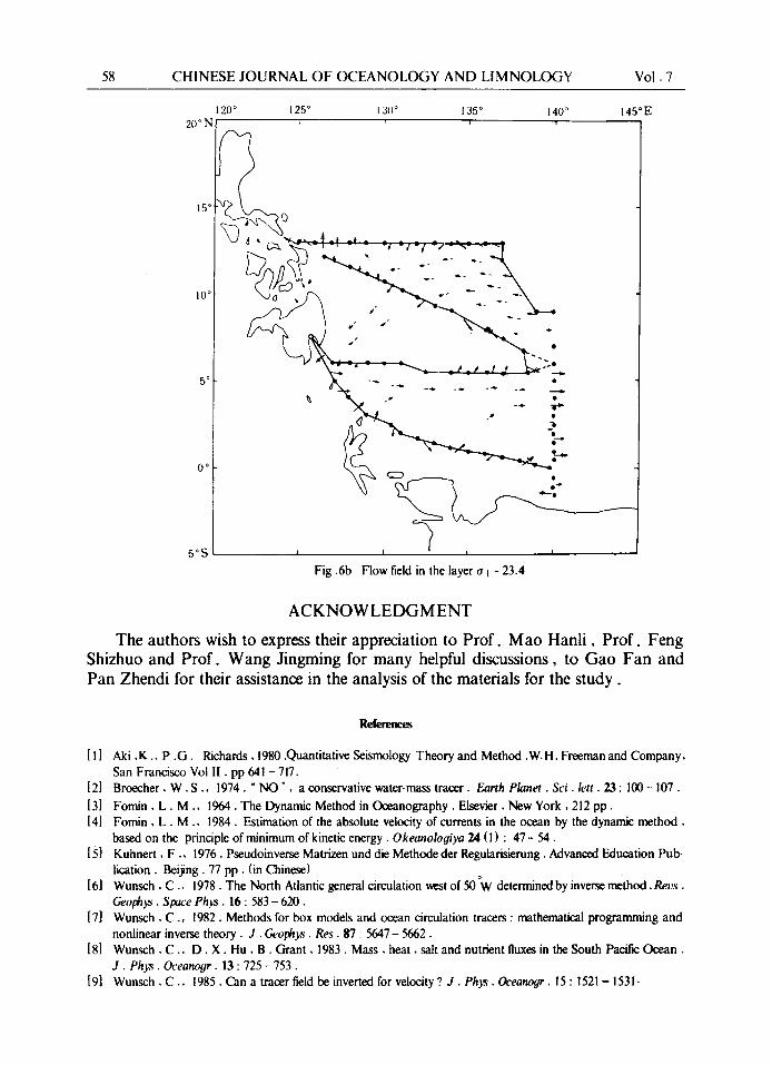
Fig. 6b shows the flow field in the layer t~t--23.4, which lies between 70 m and 100 m , on the jump layer of the isopycnal surface. Fig. 6b has the similar dynamic structure of Fig. 6a. We found that below the layer ~3= 26.7 the north trade cur- rent at 70 N - 110 N turns to a direction (opposite to that of the layers above )which does not coincide with the measured velocity direction in the local are~. Because the

H method for determining velocity direction by - 7 isolines cannot give a small

1 2 o 1 2 5 ~ 1 3 0 ~ 1 3 5 : 1 4 0 ~ 2o ~ N

15~ ~4~ \ ~ / - ~

t \ , "

O e _ - - -

i

5 . s l ,

145oE

Fig. 5 H/f isolines from the topographic map

N o . I D E T E R M I N A T I O N O F G E O S T R O P H I C F L O W 5 7

deflection of the velocity direction (especially when the component normal to the station pairs at a different depth has an opposite direction), we can only deduce the opposite

H flow at different depths from the normal direction of the --f- isolines. In this case,if

H we admit that the velocity direction normal to the - f - isolines also varies to a small

extent, we still can consider the components along the section be the same at different depths. This means that the geostrophic current directions differ slightly at different depths and are not opposite. Thus , the north trade current in the deep place is still mainly westward, only a little southward. So the velocity structure in this layer is still similar to that in Fig . 6b. In some sense, we can perfect our computing method only if we have some knowledge of the real field.

120 ~ 20~ I

~ ~ 1 0 c m / s I 0 - - 3 0 c r n / s

- - - ~ 3 0 - - 5 0 c r n / s 50crn / s

15 ~

10 ~

125 ~ 130 ~ 1 3 5 " 140 ~ 145 ~ I i , i

5 ~

0 ~

5 ~

~ . . . . ~~

) . I A I i

Fig .6a Surface current chart. Dotted lines indicate assumed current directions

58 C H I N E S E J O U R N A L O F O C E A N O L O G Y A N D L I M N O L O G Y V o l . 7

20 ~ N

15 ~

10 ~

5 +

0 ~

5~

120 ~ 125 ~ 130 ~ 135 ~ 140 ~ 145 ~ E L i !

I I ' I I

Fig .6b Flow field in the layer a 1 = 23.4

ACKNOWLEDGMENT

The authors wish to express their appreciation to Prof. Mao Hanli, Prof. Feng Shizhuo and Prof. Wang Jingming for many helpful discussions, to Gao Fan and Pan Zhendi for their assistance in the analysis of the materials for the study.

Refereaees

[ I ] Aki ,K. , P .G . Richards, 1980 .Quantitative Seismology Theory and Method .W.H. Freeman and Company, San Francisco Voi I I . pp 641 - 717.

[2] Broecher, W . S . , 1974. " N O " , a conservative water-mass tracer. Earth Planet. Sci. lett. 23 : 100- 107.

[3] Fomin, L . M . , 1964. The Dynamic Method in Oceanography. Elsevier, New York, 212 pp . [4] Fomin , L . M . , 1984. Estimation of the absolute velocity of currents in the ocean by the dynamic method,

based on the principle of minimum of kinetic energy. Okeanoloyiya 2,4 (1) : 47 - 54. [5] Kuhnert , F . , 1976. Pseudoinverse Matrizen und die Methode der Regularisierung. Advanced Education Pub-

lication. Beijng. 77 pp . (in Chinese) [6] Wunsch, C . , 1978. The North Atlantic general circulation w s t of 50 ~ determined by inverse method. Ret, s .

Geophys. Space Phys. 16 : 583 - 620. [7] Wunsch, C . , 1982. Methods for box models and ocean circulation tracers : mathematical programming and

nonlinear inverse theory. J . C, eophys. Res. 87 : 5647- 5662. [8] Wunsch, C . , D . X. Hu , B . Grant , 1983. Mass, heat , ,salt and nutrient fluxes in the South Pacific Ocean .

J . Phys. Oceanogr. 13 : 725 - 753. [9] Wunsch, C . , 1985. Can a tracer field be inverted for velocity ? J . Phys. Oceanow. 15 : 1521 - 1531-