Embed Size (px)
Citation preview

Determination of Human-Use Pharmaceuticals in Filtered Water by Direct Aqueous Injection–High-Performance Liquid Chromatography/Tandem Mass Spectrometry
Chapter 10 of Section B, Methods of the National Water Quality LaboratoryBook 5, Laboratory Analysis
U.S. Department of the InteriorU.S. Geological Survey
Techniques and Methods 5–B10


Determination of Human-Use Pharmaceuticals in Filtered Water by Direct Aqueous Injection–High-Performance Liquid Chromatography/Tandem Mass Spectrometry
By Edward T. Furlong, Mary C. Noriega, Christopher J. Kanagy, Leslie K. Kanagy, Laura J. Coffey, and Mark R. Burkhardt
Chapter 10 of Section B, Methods of the National Water Quality LaboratoryBook 5, Laboratory Analysis
Techniques and Methods 5–B10
U.S. Department of the InteriorU.S. Geological Survey

U.S. Department of the InteriorSALLY JEWELL, Secretary
U.S. Geological SurveySuzette M. Kimball, Acting Director
U.S. Geological Survey, Reston, Virginia: 2014
For more information on the USGS—the Federal source for science about the Earth, its natural and living resources, natural hazards, and the environment, visit http://www.usgs.gov or call 1–888–ASK–USGS.
For an overview of USGS information products, including maps, imagery, and publications, visit http://www.usgs.gov/pubprod
To order this and other USGS information products, visit http://store.usgs.gov
Any use of trade, firm, or product names is for descriptive purposes only and does not imply endorsement by the U.S. Government.
Although this information product, for the most part, is in the public domain, it also may contain copyrighted materials as noted in the text. Permission to reproduce copyrighted items must be secured from the copyright owner.
Suggested citation: Furlong, E.T., Noriega, M.C., Kanagy, C.J., Kanagy, L.K., Coffey, L.J., and Burkhardt, M.R., 2014, Determination of human-use pharmaceuticals in filtered water by direct aqueous injection–high-performance liquid chromatography/tandem mass spectrometry: U.S. Geological Survey Techniques and Methods, book 5, chap. B10, 49 p., http://dx.doi.org/10.3133/tm5B10.
An electronic version of the standard operating procedure for the analytical method is available upon request to [email protected]
ISNN 2328-7055 (online)

iii
Contents
Abstract ...........................................................................................................................................................1Introduction.....................................................................................................................................................1Analytical Method..........................................................................................................................................2
1. Scope and Application of Method .................................................................................................32. Summary of Method .........................................................................................................................33. Safety Precautions and Waste Disposal ......................................................................................44. Interferences .....................................................................................................................................45. Apparatus and Instrumentation .....................................................................................................5
5.1. Glassware and Laboratory Equipment ..............................................................................55.2 Analytical Instrumentation ...................................................................................................6
6. Reagents and Consumable Materials ...........................................................................................76.1. Neat Reagents .......................................................................................................................76.2. Reagent Solutions .................................................................................................................76.3. Standards ...............................................................................................................................7
7. Sample Analysis ..............................................................................................................................107.1. Sample Preparation in the Field and Laboratory Receipt of Environmental
Samples ........................................................................................................................107.2. Laboratory Filtration ...........................................................................................................107.3. Assembly of Sample Prep Sets for Analysis ..................................................................117.4. Preparation of Environmental and Quality-Assurance Samples for Instrumental
Analysis ..........................................................................................................................137.5. Sample Analysis ..................................................................................................................137.6. Post-Analysis Data Processing and Evaluation ............................................................16
8. Calculation of Results ....................................................................................................................198.1. Calculation of Pharmaceutical Response Factors ........................................................198.2. Calculation of Sample Pharmaceutical Concentrations ..............................................198.3. Recovery of Isotope-Dilution Standard Compounds as Surrogates ..........................208.4. Recovery of Pharmaceuticals from Laboratory Reagent Spike Samples .................20
9. Reporting Results ............................................................................................................................209.1. Reporting Units ....................................................................................................................209.2. Detection Limits and Reporting Levels ............................................................................20
10. Quality Assurance/Quality Control (QA/QC) .............................................................................2110.1. Surrogates..........................................................................................................................2110.2. Laboratory Reagent Blank (LRB) Samples ...................................................................2110.3. Laboratory Reagent Spike (LRS) Samples ....................................................................2210.4. Continuing Calibration Verification (CCV) Samples .....................................................2210.5. Continuing Calibration Blank (CCB) Samples ...............................................................2210.6. Limit of Quantitation (LOQ) Samples ..............................................................................2310.7. Field Equipment Blank (FEB) Samples ...........................................................................2310.8. Laboratory Matrix Spike (LMS) Samples ......................................................................2410.9. Isotope-Dilution Standard (IDS) Performance Criteria ..............................................2410.10. Statistical Derivation of Quality-Control Limits ..........................................................2410.11. Secondary Data Review ................................................................................................24

iv
Results and Discussion of Method Validation ........................................................................................25Sample Matrix Description ...............................................................................................................25Validation Results and Discussion ...................................................................................................26
Reagent Water ...........................................................................................................................26Groundwater ...............................................................................................................................28Treated Drinking Water .............................................................................................................31Surface Water ............................................................................................................................31Wastewater Effluent ..................................................................................................................34Wastewater Influent ..................................................................................................................37Complex Matrixes and Blank Samples ..................................................................................38
Reporting Limits............................................................................................................................................38Sample Holding-Time Study .......................................................................................................................42Summary and Conclusions .........................................................................................................................44References Cited..........................................................................................................................................45Appendix 1.....................................................................................................................................................49
Figures 1. Boxplots of A, median recovery and B, relative standard deviation of recovery of all
110 pharmaceuticals in reagent-water samples fortified at 1; 2; 4; 10; 20; 40; 80; 100; 200; 400; 800; 2,000; 4,000; and 8,000 nanograms per liter ....................................................27
2. Boxplots of A, median recovery and B, relative standard deviation of recovery of all 110 pharmaceuticals in domestic-well groundwater samples fortified at 4; 80; 200; and 2,000 nanograms per liter. Recoveries were corrected for ambient environmental concentrations or laboratory reagent blank concentrations, as appropriate ..................................................................................................................................29
3. Boxplots of A, median recovery and B, relative standard deviation of recovery of all 110 pharmaceuticals in community supply well groundwater samples fortified at 4; 20; 80; 140; 200; and 2,000 nanograms per liter. Recoveries were corrected for ambient environmental concentrations or laboratory reagent blank concentrations, as appropriate .............................................................................................................................30
4. Boxplots of A, median recovery and B, relative standard deviation of recovery of all 110 pharmaceuticals in treated drinking-water samples fortified at 4; 80; 200; and 2,000 nanograms per liter. Recoveries were corrected for ambient environmental concentrations or laboratory reagent blank concentrations, as appropriate ..................32
5. Boxplots of A, median recovery and B, relative standard deviation of recovery of all 110 pharmaceuticals in surface-water samples fortified at 4; 80; 200; and 2,000 nanograms per liter. Recoveries were corrected for ambient environmental concentrations or laboratory reagent blank concentrations, as appropriate ..................33
6. Boxplots of A, median recovery and B, relative standard deviation of recovery of all 110 pharmaceuticals in wastewater-effluent samples fortified at 4; 80; 200; and 2,000 nanograms per liter. Recoveries were corrected for ambient environmental concentrations or laboratory reagent blank concentrations, as appropriate ..................35
7. Boxplots of median recovery plotted in A, logarithmic scale and B, arithmetic scale; and C, relative standard deviation of recovery of all 110 pharmaceuticals in wastewater-influent samples fortified at 4; 80; 200; and 2,000 nanograms per liter. Recoveries were corrected for ambient environmental concentrations or laboratory reagent blank concentrations, as appropriate ...................................................36

v
8. Method detection limits (MDLs), in nanograms per liter, calculated from seven replicate reagent-water analyses ...........................................................................................40
9. Median recovery and relative standard deviation (RSD) of recovery of all 110 pharmaceuticals from surface water fortified at 2,000 nanograms per liter; stored at 4 degrees Celsius; and analyzed at 1, 9, 23, and 30 days after fortification. Recoveries have been corrected for ambient environmental concentrations or laboratory reagent blank concentrations, as appropriate ...................................................41
10. First-order decay curves fitted to recoveries, in percent, of selected pharmaceuticals measured in the holding-time study .........................................................42
11. Boxplots of median loss of all 110 pharmaceuticals from surface water fortified at 2,000 nanograms per liter; stored at 4 degrees Celsius; and analyzed at 1, 9, 23, and 30 days after fortification. Recoveries have been corrected for ambient environmental concentrations or laboratory reagent blank concentrations, as appropriate ..................................................................................................................................43
Tables 1. Human-health pharmaceuticals determined by method O–2440–14, active
pharmaceutical ingredient name, alternative brand or compound names commonly used, typical uses, National Water Information System parameter code, and Chemical Abstracts Service Registry Numbers ................................................................. link
2. Suggested solvents for dissolving neat standards and expected final operational range of the direct aqueous injection, high-performance liquid chromatography/tandem mass spectrometry technique for each pharmaceutical determined by this method ..................................................................................................... link
3. Isotope-dilution standard compounds, National Water Information System parameter codes, operational concentrations, and suggested dissolution solvents for the direct aqueous injection, high-performance liquid chromatography/tandem mass spectrometry technique used in this method ........................................................... link
4. Concentrations of the calibration solutions used in this method, in order of decreasing concentration ...................................................................................................... link
5. Suggested analytical sequence using direct aqueous injection, high-performance liquid chromatography/tandem mass spectrometry for determining method pharmaceuticals with complete calibration ....................................................................... link
6. Mass spectrometer settings used to produce the precursor and product ions and the corresponding quantitation and first and second qualification transitions of pharmaceuticals and isotope-dilution standard compounds determined in this method ....................................................................................................................................... link
7. Bias and variability determined for recoveries, in percent, of pharmaceuticals in reagent-water samples fortified at per component concentrations of 1; 2; 4; 10; 20; 40; 80; 100; 200; 400; 800; 2,000; 4,000; and 8,000 nanograms per liter ............................. link
8. Bias and variability determined for concentrations and recoveries, in percent, of pharmaceuticals in domestic-well groundwater samples fortified at per component concentrations of 4; 80; 200; and 2,000 nanograms per liter ............................................. link
9. Bias and variability determined for concentrations and recoveries, in percent, of pharmaceuticals in community supply well groundwater samples fortified at per component concentrations of 4; 20; 80; 140; 200; and 2,000 nanograms per liter ......... link
10. Bias and variability determined for concentrations and recoveries, in percent, of pharmaceuticals in treated drinking-water samples fortified at per component concentrations of 4; 80; 200; and 2,000 nanograms per liter ............................................. link

vi
11. Bias and variability determined for concentrations and recoveries, in percent, of pharmaceuticals in surface-water samples fortified at per component concentrations of 4; 80; 200; and 2,000 nanograms per liter ............................................. link
12. Bias and variability determined for concentrations and recoveries, in percent, of pharmaceuticals in wastewater-effluent samples fortified at per component concentrations of 4; 80; 200; and 2,000 nanograms per liter ............................................. link
13. Bias and variability determined for concentrations and recoveries, in percent, of pharmaceuticals in wastewater-influent samples fortified at per component concentrations of 4; 80; 200; and 2,000 nanograms per liter ............................................. link
14. Frequency of detection of method pharmaceuticals in 80 blank samples determined by this method after analysis of a set of complex matrix samples. Individual pharmaceuticals are listed from most frequently detected to the least frequently detected. A pharmaceutical is listed if it was detected in a minimum of three blank samples ..................................................................................................................................... link
15. Method detection limits and interim reporting levels, in nanograms per liter, for pharmaceuticals determined in this method. .................................................................... link
16. Recovery of pharmaceuticals from filtered surface water fortified at 2,000 nanograms per liter and held at 4 degrees Celsius over a 30-day period for a sample holding-time study ..................................................................................................... link
Appendix Tables 1–1. Typical instrument operating conditions specific to the Agilent Technologies 6460
triple-quadrupole tandem mass spectrometer ................................................................... link 1–2. General quality-control guidelines for performance criteria and corrective actions
applied to quality-control samples ....................................................................................... link 1–3. Examples of Laboratory Information System Management data actions applied by
analysts using entries to the MassHunter™ software user annotation field ................ link 1–4. General quality-control guidelines for performance criteria and corrective actions
applied to potentially unacceptable isotope-dilution standard response ..................... link

vii
Conversion FactorsSI to Inch/Pound
Multiply By To obtainLength
centimeter (cm) 0.3937 inch (in.)micrometer (µm) 0.00003937 inch (in.)millimeter (mm) 0.03937 inch (in.)
Volumeliter (L) 33.82 ounce, fluid (fl. oz)liter (L) 2.113 pint (pt)liter (L) 1.057 quart (qt)liter (L) 0.2642 gallon (gal)liter (L) 61.02 cubic inch (in3) microliter (µL) 0.000000264 gallon (gal)milliliter (mL) 0.000264 gallon (gal)
Flow ratemilliliter per minute (mL/min) 0.1585 gallon per minute (gal/min)
Massgram (g) 0.03527 ounce, avoirdupois (oz)milligram (mg) 0.00003527 ounce, avoirdupois (oz)microgram (µg) 0.00000003527 ounce, avoirdupois (oz)
Pressurekilopascal (kPa) 0.009869 atmosphere, standard (atm)kilopascal (kPa) 0.01 barkilopascal (kPa) 0.2961 inch of mercury at 60°F (in Hg)kilopascal (kPa) 0.1450 pound-force per inch (lbf/in) kilopascal (kPa) 20.88 pound per square foot (lb/ft2) kilopascal (kPa) 0.1450 pound per square inch (lb/in2)
Temperature in degrees Celsius (°C) may be converted to degrees Fahrenheit (°F) as follows:
°F=(1.8×°C)+32
Abbreviated Water-Quality Units and Units of Measureµg/L microgram(s) per liter
µL microliter(s)
µm micrometer(s)
mg/mL milligram(s) per milliliter
mL/min milliliter(s) per minute
mL milliliter
M molar (molarity; moles per liter)
ng/L nanogram(s) per liter
ng/mL nanogram(s) per milliliter

viii
Abbreviations, Acronyms, and SymbolsCCB continuing calibration blank
CCV continuing calibration verification
CSV comma-separated value
ESI electrospray ionization
FEB field equipment blank
HPLC high-performance liquid chromatography (or chromatograph)
HPLC/MS/MS high-performance liquid chromatography/tandem mass spectrometry
ICMS intermediate concentration mixed standard
IDS isotope-dilution standard
IRL interim reporting level
I-TPC intermediate third-party check solution
LIMS Laboratory Information Management System
LMS laboratory matrix spike
LOQ limit of quantitation
LRB laboratory reagent blank
LRS laboratory reagent spike
MDL method detection limit
MRM multiple reaction monitoring
MS/MS tandem mass spectrometry (or tandem mass spectrometer)
m/z mass-to-charge ratio
NWIS National Water Information System
NWQL National Water Quality Laboratory
PTFE polytetrafluoroethylene
QA quality assurance
QA/QC quality assurance/quality control
QC quality control
QUAN quantitative analysis (component of MassHunter™ software)
RSD relative standard deviation
SRM selected reaction monitoring
TPC third-party check solution
USEPA U.S. Environmental Protection Agency
USGS U.S. Geological Survey
registered trademark
™ trademark
± plus or minus
= equals

Abstract
This report describes a method for the determination of 110 human-use pharmaceuticals using a 100-microliter aliquot of a filtered water sample directly injected into a high-performance liquid chromatograph coupled to a triple-quadrupole tandem mass spectrometer using an electrospray ionization source operated in the positive ion mode. The pharmaceuticals were separated by using a reversed-phase gradient of formic acid/ammonium formate-modified water and methanol. Multiple reaction monitoring of two fragmen-tations of the protonated molecular ion of each pharmaceu-tical to two unique product ions was used to identify each pharmaceutical qualitatively. The primary multiple reaction monitoring precursor-product ion transition was quantified for each pharmaceutical relative to the primary multiple reaction monitoring precursor-product transition of one of 19 isotope-dilution standard pharmaceuticals or the pesticide atrazine, using an exact stable isotope analogue where possible. Each isotope-dilution standard was selected, when possible, for its chemical similarity to the unlabeled pharmaceutical of interest, and added to the sample after filtration but prior to analysis.
Method performance for each pharmaceutical was determined for reagent water, groundwater, treated drinking water, surface water, treated wastewater effluent, and waste-water influent sample matrixes that this method will likely be applied to. Each matrix was evaluated in order of increasing complexity to demonstrate (1) the sensitivity of the method in different water matrixes and (2) the effect of sample matrix, particularly matrix enhancement or suppression of the precur-sor ion signal, on the quantitative determination of pharma-ceutical concentrations. Recovery of water samples spiked (fortified) with the suite of pharmaceuticals determined by this method typically was greater than 90 percent in reagent water, groundwater, drinking water, and surface water. Correction for ambient environmental concentrations of pharmaceuti-cals hampered the determination of absolute recoveries and method sensitivity of some compounds in some water types, particularly for wastewater effluent and influent samples.
The method detection limit of each pharmaceutical was determined from analysis of pharmaceuticals fortified at mul-tiple concentrations in reagent water. The calibration range for each compound typically spanned three orders of magnitude of concentration. Absolute sensitivity for some compounds, using isotope-dilution quantitation, ranged from 0.45 to 94.1 nanograms per liter, primarily as a result of the inherent ionization efficiency of each pharmaceutical in the electrospray ionization process.
Holding-time studies indicate that acceptable recoveries of pharmaceuticals can be obtained from filtered water samples held at 4 °C for as long as 9 days after sample collection. Freezing samples to provide for storage for longer periods currently (2014) is under evaluation by the National Water Quality Laboratory.
IntroductionOver the last decade, several reports have documented
the presence and distribution of human-use pharmaceuticals in surface-water, groundwater, and drinking-water samples world-wide (Kolpin and others, 2002; Glassmeyer and others, 2008; Kümmerer, 2008; Richardson and Ternes, 2011). In particular, the results of Kolpin and others (2002) have documented the ubiquitous presence of pharmaceuticals, wastewater indicator compounds, and other emerging contaminants in U.S. surface waters and have initiated a rapid expansion of interest in the accurate and specific determination of pharmaceuticals at con-centrations at or less than 1 microgram per liter (µg/L).
As a result, numerous methods have been published for the determination of pharmaceuticals in water at ambient envi-ronmental concentrations (Petrović and others, 2005; Petrović and others, 2006; Vanderford and Snyder, 2006; Batt and others, 2008; Lavén and others, 2009; Trenholm and others, 2009; Buchberger, 2011; Richardson and Ternes, 2011). As these new methods have been published, a trend of increasing numbers of pharmaceuticals (along with decreasing report-ing levels) can be observed, particularly in methods meant for broad-scale surveys and monitoring. For example, the high-performance liquid chromatography/mass spectrometry
Determination of Human-Use Pharmaceuticals in Filtered Water by Direct Aqueous Injection–High-Performance Liquid Chromatography/Tandem Mass Spectrometry
By Edward T. Furlong, Mary C. Noriega, Christopher J. Kanagy, Leslie K. Kanagy, Laura J. Coffey, and Mark R. Burkhardt

2 Determination of Human-Use Pharmaceuticals in Filtered Water by Direct Aqueous Injection
method used by Kolpin and others (2002) and documented by Cahill and others (2004) provided determination of 22 pharmaceuticals at reporting levels averaging 0.022 µg/L or 22 nanograms per liter (ng/L). Batt and others (2008) recently documented a method to determine 54 pharmaceuticals and pharmaceutical degradates, with reporting levels ranging from 1 to 51 ng/L. Similarly, Gros and others (2009) documented a method to determine 73 pharmaceuticals, with reporting limits ranging from 0.1 to 55 ng/L, depending on sample matrix.
The increased number of pharmaceuticals measured in a given method at decreasing reporting levels reflects advances in mass spectrometry technology and a better understanding of the potential range of pharmaceutical concentrations likely to be present in environmental samples. Tandem mass spectrometry (MS/MS), typically using a triple-quadrupole mass spectrom-eter or a quadrupole time-of-flight mass spectrometer, is the instrumental approach common to many of these methods. This technology has become a commonly accepted standard for confirmed qualitative identification of pharmaceuticals (Nielen and others, 2008), although validation and analyst expertise is necessary to ensure that appropriate conditions are chosen and false positive identifications are avoided (Lehotay and others, 2008). When the sample or sample extract is fortified with sta-ble-isotope analogues of the compounds of interest (commonly referred to as isotope-dilution analysis) routine quantitative estimation of pharmaceuticals is achievable at concentrations of nanograms per liter or lower (Vanderford and Snyder, 2006).
The acceptance of MS/MS as the standard analytical approach stems from the specificity and sensitivity gains achieved when coupling MS/MS with high-performance liquid chromatography (HPLC) by using electrospray ionization (ESI). Polar, thermally labile compounds such as pharmaceuticals can be efficiently separated on a reversed phase HPLC column operated under an aqueous-to-organic gradient of solvent flow (Van de Steene and Lambert, 2008) with improved separation as the particle size of the stationary phase decreases. The separated pharmaceuticals are trans-ferred to the ESI source in this typically acidic eluent flow (or mobile phase). The mobile phase assists in the ionization of the neutral pharmaceuticals by providing a source of protons that adduct to the pharmaceuticals as the eluent flow is dispersed into fine droplets by the electrospray source. The eluent is almost immediately removed by evaporation from the electrospray plume as the charged droplets transit the source and enter as protonated ions into the low-vacuum region of the mass spectrometer, where they are analyzed.
The ESI process has been comprehensively reviewed in Cole (1997), particularly in the chapter by Kebarle and Ho (1997). High-performance liquid chromatography/tandem mass spectrometry (HPLC/MS/MS) using an ESI source has been applied to identification and quantification of many polar organic constituents, including pharmaceuticals (Debska and others, 2004; Zuehlke and others, 2004; Petrović and others, 2005; Batt and others, 2008; Shao and others, 2009; Trenholm and others, 2009; Wang and others, 2011). Additionally, the use of multiple reaction monitoring (MRM) with HPLC/MS/MS
to measure one or more unique transitions from a precursor ion for each pharmaceutical commonly has enhanced the specific-ity and sensitivity of electrospray HPLC/MS/MS (de Hoffmann and Stroobant, 2002). When two MRM transitions are used, the HPLC/MS/MS technique with ESI and MRM meets the guide-lines promulgated by the European Union (and documented in European Union Commission Decision 2002/657/EC) for unambiguous identification of trace organic compound residues in regulatory analyses (Stolker and others, 2000; European Commission, 2002). The European Union Commission’s deci-sion provides the only internationally promulgated guidelines for minimally acceptable conditions for qualitative mass spec-trometric identification of trace residues in a regulatory context, as in the analysis of meat or other foodstuffs for antibiotics. This standard, initially developed for regulatory analyses, is being increasingly accepted as the standard for data quality for science driven, non-regulatory environmental analyses of pharmaceuticals (Stolker and others, 2004; Petrović and others, 2006; Rodil and others, 2009). For the reader new to HPLC and MS/MS, Ardrey (2003) provides a general explanation of liquid chromatography/mass spectrometry.
The purpose of this report is to document a method for the determination of 110 human-use pharmaceuticals using a 100-microliter (µL) aliquot of a filtered water sample directly injected into a high-performance liquid chromato-graph coupled to a triple-quadrupole tandem mass spectrom-eter using an ESI source operated in the positive ion mode. Method performance was evaluated for each pharmaceutical in reagent water, groundwater, treated drinking water, surface water, treated wastewater effluent, and wastewater influent sample matrixes that this method will likely be applied to. Each matrix was evaluated in order of increasing complexity to demonstrate the sensitivity of the method in different water matrixes and the effect of sample matrix on the quantitative determination of pharmaceutical concentrations. The method detection limit (MDL) of each pharmaceutical was deter-mined from analysis of pharmaceuticals fortified at multiple concentrations in reagent water. The goal for this method was to provide sensitivity sufficient that the MDL for most of the pharmaceuticals would be less than 50 ng/L.
Analytical MethodThe analytical method for determination of human-use
pharmaceuticals (table 1) in filtered water by direct aqueous injection with HPLC/MS/MS is described in this section of the report. The pharmaceuticals are analyzed using U.S. Geological Survey method number O–2440–14 (National Water Quality Laboratory [NWQL] laboratory schedule 2440) for filtered water.
Table 1. Human-health pharmaceuticals determined by method O–2440–14, active pharmaceutical ingredient name, alternative brand or compound names commonly used, typical uses, National Water Information System parameter code, and Chemical Abstracts Service Registry Numbers.

Analytical Method 3
1. Scope and Application of Method
This method is designed primarily for the determination of human-use pharmaceuticals, pharmaceutical metabolites, and select polar organic compounds of environmental interest (table 1) in filtered water samples. Note that the select polar organic compounds of environmental interest are included to allow comparison of results from this method with results from other methods developed by the NWQL or others. Throughout the rest of this report, the term pharmaceuticals is used when referring in aggregate or in general to the com-pounds determined in this method. The method is applicable to those compounds that can be reliably separated by HPLC, efficiently ionized using an ESI interface operated in the posi-tive ionization mode, and identified and quantified by MS/MS.
This method is applicable to filtered water samples, which in this case refers to water samples with both natural and anthropogenically derived components that have been filtered with a pre-ashed glass-fiber filter using the method of Wilde and others (2004 with updates through 2009) or its equivalent. When necessary (for example, when precipitates occur in previously filtered samples after shipment) additional sample filtration is performed at the NWQL prior to analysis because an aliquot of the filtered sample is analyzed without any additional treatment. The presence of particles in samples will decrease performance of, or possibly damage, the HPLC/MS/MS used in the analysis. The performance of this method was assessed using reagent-water, groundwater, surface-water, treated drinking-water, wastewater-effluent, and wastewater-influent samples. These matrixes are representative of the water types that this method is likely to be applied to. Performance assessment was limited to a single sample of each matrix type analyzed in replicate. Inclusion of environmental matrix spike samples is a critical component of a study’s quality-control (QC) plan because of the potential for sample-specific matrix effects documented during the validation of this method. An environmental (field) matrix spike sample is a sample spiked (fortified) in the field with a known concentration of selected compounds and is used to assess the effects of degradation, sorption, or other sources of compound loss in a sample.
Users of this method need to recognize that performance characteristics of the method determined from spiked samples of one water matrix may not apply to similar sample types from other sources or to other water matrixes. Any determina-tions made in new matrixes are appropriately qualified until an analogous performance evaluation has been made. Matrixes, such as septage, wastewater influents (or other liquids col-lected in wastewater-treatment facilities prior to full treat-ment), and liquids collected from confined animal-feeding operations, among others, are known to contain complex chemical interferences that may suppress or enhance ioniza-tion of the pharmaceuticals of interest through competition for available protons during electrospray ionization (Enke, 1997). Thus, routine analyses of matrix-spike samples collected within the study area are necessary and should be a routine component of a study’s QC plan when this method is used.
2. Summary of Method
This method is suitable for determining 110 individual pharmaceuticals in filtered water at concentrations greater than 1 to 100 ng/L, depending on the specific pharmaceuti-cal. All samples must be filtered prior to analysis. Using the procedure of Wilde and others (2004 with updates through 2009) for filtering samples at the time of sample collection removes much of the naturally occurring microbiota; this reduces the potential for degradation of pharmaceuticals dur-ing sample shipment. Samples are filtered in the field using 0.7-micro-meter (µm) pre-ashed glass-fiber filters, adding as much as 10 or 20 milliliters (mL) of sample to a 20- or 40-mL, respectively, amber glass vial with a Teflon-lined screw cap, and shipping the samples on ice to the laboratory by over-night express. Upon receipt, samples are stored refrigerated until analyzed. If a sample requires additional filtration upon request or after inspection, the sample is again passed through a 0.7-µm pre-ashed glass-fiber filter prior to analysis. For sam-ple analysis, approximately 1 mL of the sample is withdrawn from the sample vial and placed into a 1.5-mL autosampler vial, and an aliquot of a mixture of isotope-dilution standard (IDS) pharmaceuticals is added to the vial. After thoroughly mixing the vials, environmental, laboratory QC, calibration, and other analytical samples are placed in the autosampler in a predetermined sequence.
Under automated computer control, a 100-microliter (µL) aliquot of the 1-mL aqueous filtered sample aliquot is injected directly into the flowing mobile phase of the HPLC system, where the injected sample plug passes through a 0.2-µm in-line filter. The pharmaceutical components of the sample are separated from each other by using a reverse-phase HPLC column. The separated components sequentially elute from the column and are ionized in the electrospray interface of the HPLC/MS/MS, operated in positive ion mode. In the MS/MS, also under automated computer control, a precursor ion for each pharmaceutical is selected and frag-mented, and two product ions unique to the precursor ion are analyzed. The precursor ions and their product ions for each pharmaceutical are monitored in elution order. The timing of fragmentation of each of the two precursor-ion/product-ion pairs for each pharmaceutical is optimized by operating the MS/MS in dynamic MRM mode. The two precursor-ion/product-ion transitions for each pharmaceutical produce at least two chromatographic peaks, which are evaluated to determine qualitative detection by comparison to the same two peaks collected from authentic standards.
One transition, designated the quantitation transition, is integrated, and the resulting area is used to determine the concentration by comparison to a calibration curve developed using authentic standards. The second transition for each pharmaceutical is designated the confirmation transition. The presence of the confirmation and quantitation transitions, the ratio of the peak areas of the confirmation transition to the quantitation transition, and the peak-retention time provide the criteria for qualitative identification when compared to the

4 Determination of Human-Use Pharmaceuticals in Filtered Water by Direct Aqueous Injection
same criteria collected from authentic standards. Quantita-tion is by the internal standard method using IDS compounds added prior to analysis (Pickup and McPherson, 1976; Colby and others, 1981). The concentrations of the 110 pharma-ceuticals determined in this method are reported in units of nanograms per liter. The recoveries of the IDS compounds are reported as percentages.
Because the responses of the individual pharmaceuti-cals of interest, the QC surrogate compounds, and the IDS compounds can be suppressed or enhanced by the sample matrix, results from several QC sample types are necessary to properly interpret the ambient environmental concentra-tions of pharmaceuticals in aqueous samples. Results from laboratory QC samples, including laboratory reagent spike (LRS) samples and laboratory reagent blank (LRB) samples, provide insight into the performance of the method in the absence of a sample matrix. The LRS sample is a sample of reagent water that is spiked (fortified) in the laboratory with a known concentration of selected compounds. The LRB sample is a sample of reagent water consisting of deionized water prepared at the laboratory; the sample is treated to remove organic contaminants by irradiation with ultraviolet light and is assumed to be void of the compounds of interest.
Three additional field QC sample types identify the effect of sample matrix upon aquatic pharmaceutical concentra-tions. Specifically, results from environmental (field) matrix spike samples and replicate environmental samples, collected from representative sample matrix types within the aquatic system(s) being investigated as an integral part of the study’s QC plan, can be used to assess accuracy and precision of the method specific to the environmental conditions of the study area. Field blank samples provide an assessment of potential contamination inadvertently introduced to the sample during collection and processing. Field replicate samples provide an assessment of concentration precision at ambient environmen-tal concentrations; they incorporate all sources of field and laboratory variation.
3. Safety Precautions and Waste Disposal
Adherence to best practices requires that all steps in the method that use organic solvents, such as making and dilut-ing standard solutions, occur in a fume hood. Eye protection, nitrile gloves, and protective clothing are worn in the labo-ratory area and when handling reagents, solvents, or any corrosive materials. All chemical preparations are performed in a fume hood.
The liquid waste stream produced during sample filtration and instrumental analysis is about 95 percent water, with the rest of the volume made up of organic solvents, reagents, and trace amounts of the pharmaceuticals of interest dissolved in water/solvent mixtures. The solvent used is methanol, and the primary organic reagents are ammonium formate and formic acid. The waste stream is collected in thick-walled carboys and disposed of according to local regulations for nonchlori-nated waste streams. Solvents used to clean or rinse glassware,
equipment, and cartridges are disposed of in waste containers designated for solvent waste. The solid-waste stream produced during sample analysis consists of used filters and assorted disposable glassware and plastics, such as sample vials and pipette tips. The solid-waste stream is disposed of according to local regulations.
It is important to ensure that the electrospray source exhaust and the vacuum pump exhaust tubes of the HPLC/MS/MS are vented out of the ambient laboratory atmosphere through ventilation ducting expressly specified for this pur-pose. Exposure to electrical current at high voltages as well as thermally hot surfaces may occur during some mainte-nance procedures. Supervisors, safety personnel, manufac-turer’s representatives, or other experienced persons can be consulted if uncertainties arise concerning proper and safe procedures for operating or maintaining the HPLC/MS/MS used in this method.
4. Interferences
A wide variety of additional compounds, dissolved organic carbon, and other organic and inorganic chemical matrix components are likely present in water samples. Their presence may result in potential interferences to the process of efficiently separating, accurately identifying, and quantifying the pharmaceuticals determined by this method. Further, this method is purposely designed for the determination of an array of pharmaceuticals that comprise a wide range of chemical characteristics and elemental and functional group composi-tions. Consequently, the potential is substantial for co-eluting interferences that may limit the qualitative identification of a pharmaceutical or may enhance or suppress the formation of a precursor ion during electrospray ionization.
By using ESI, the pharmaceuticals in this method are converted from neutral molecules to gas phase ions that can be identified and quantified. It is an electrochemical phenomenon (Abonnenc and others, 2010) in which the chromatographi-cally separated pharmaceutical competes for excess protons with other sample components eluting concurrently. This com-petition for available charge may result in either an apparent enhancement or reduction of compound concentration because of the effects of unknown matrix constituents competing for charge with the internal standard or pharmaceutical (Furlong and others, 2008).
Careful attention to the results produced during instru-mental analysis is necessary to ensure that matrix interferences do not compromise the determination of pharmaceuticals. Three aspects of matrix effects bear consideration:1. interferences in the sample that degrade chromato-
graphic performance and characteristics, such as peak shape and retention time, thereby decreasing the abil-ity to separate and identify pharmaceuticals of interest chromatographically;
2. interferences persisting in the sample after chromato-graphic separation that alter ionization efficiency of

Analytical Method 5
the pharmaceutical of interest or compete for available charges during ESI, thereby altering the responses of pharmaceuticals of interest, which can result in apparent quantitative matrix enhancement or suppression; and
3. interferences persisting in the sample after chromatographic separation that produce a precursor-ion/product-ion transi-tion that is the same as one of the two transitions used to identify the pharmaceutical of interest, thereby altering the MRM area ratios used for qualitative identification.The HPLC/MS/MS uses two quadrupole analyzers
separated by a hexapole collision cell to produce highly spe-cific precursor-ion/product-ion transitions. Nevertheless, the sample matrix still may affect the relative abundances of two precursor-ion/product-ion transitions used for qualitative iden-tification, resulting in ion-area ratios that deviate substantially from the expected ratio for the compound of interest. These deviations alert the analyst to the probability that ions from an interfering substance have been detected and included in the compound mass spectrum because the mass spectrometer was unable to discriminate between the pharmaceutical of interest and the interference.
It is not surprising that matrix-derived suppression or enhancement occurs (Enke, 1997) given the complex hetero-geneous mixture of chemicals present in an environmental sample. A careful choice of internal standards and surrogates is necessary to minimize the possibility of matrix enhance-ment or suppression effects. Optimally, the IDS compound used for quantitation is a stable-isotope analog of the parent analyte, which is a pharmaceutical in the method. Where exact stable isotopic analogs are not available, a closely related stable isotopically labeled compound, preferably in the same chemical class, may be substituted and will consti-tute the IDS for that pharmaceutical. Acceptable quantitation across the calibration range of the method must be demon-strated when using an IDS compound that is not an exact isotopically labeled analogue of the compound. This can be verified by analysis of matrix spike samples.
Contamination is another source of error that can result in false positives. Many of the pharmaceuticals in this method are commonly used. Thus, the potential for inadver-tent transfer from the analyst or field personnel to the sample exists. Careful monitoring of blank QC samples associated with each analytical batch is necessary to assess the pres-ence of contaminants. The primary blank samples used in this method are (1) instrument blanks and preparation-set blanks (both consisting of reagent water containing the suite of IDS compounds) routinely analyzed as a part of labora-tory QC and (2) field blank samples processed on-site at the time of sample collection. In the laboratory, contamination may occur from (1) impurities in the mobile phase or labeled compounds, (2) preparation of the samples or laboratory matrix spike samples, (3) residues present in the laboratory environment from use of these pharmaceuticals by laboratory personnel, or (4) carryover of constituents or interferences in analytical equipment between injections. Contamination can
result from prior analysis of samples with pharmaceutical concentrations of tens of micrograms per liter or higher, such as wastewater influent or effluent.
Because different matrixes can affect qualitative iden-tification and quantitation, the types and kinds of field QC samples submitted and analyzed for studies using this method require careful consideration. The inclusion of one or more each of (1) field blank samples and (2) field matrix spike sam-ples is warranted. Fortified matrix spike samples are fortified with the method compounds and processed along with a cor-responding unfortified environmental sample. These field QC samples assist in (1) assessing possible field-derived contami-nation to samples, particularly important for commonly used pharmaceuticals, and (2) assessing potential matrix effects from the specific water types that are a part of a study, respectively.
5. Apparatus and Instrumentation
The apparatus and instrumentation used for the method are outlined in this section of the report. Alternative apparatus and instrumentation from those listed for this method may be substituted if shown, or known from the literature, to provide comparable or superior performance and analyte recoveries. Some materials are common laboratory items; therefore, they are not described in detail.
5.1. Glassware and Laboratory EquipmentNote that prior to use, glassware, glass-fiber filters, and
glass consumables are ashed at 450 degrees Celsius (°C) for a minimum of 4 hours (hr).
5.1.1. Microdispensers: variable volume microdispens-ers, digital, 10-, 25-, 50-, and 100-μL capacities (Drummond Scientific Company, Broomall, Pennsylvania [Pa.]; or VWR International, Radnor, Pa.).
5.1.2. Bores: borosilicate bores, 100–200-μL (VWR International), and 10-, 25-, and 50-μL bores (Thermo Fisher Scientific, Inc., Waltham, Massachusetts [Mass.], catalog num-bers 21–169D, 21–169C, and 21–169A, respectively).
5.1.3. Motorized microliter pipettes: variable volume pipettes, 10- to 2,500-μL capacities, liquid end (Rainin EDP-Plus™, Mettler-Toledo International, Inc., Columbus, Ohio).
5.1.4. Disposable tips: pipette tips (Rainin, catalog num-bers RC–2500, RC–1000, RC–250, and RC–10).
5.1.5. Pipettes: class A pipettes, varied volumes from 0.5- to 10-mL.
5.1.6. Pasteur pipettes: glass pipettes, 5¾-inch (in.) or 9-in.; for use with a standard laboratory rubber pipette bulb.
5.1.7. Volumetric flasks: class A flasks, varied volumes from 1 to 1,000 mL. Low actinic (red) glass volumetric flasks are used if available.
5.1.8. Glass beakers: borosilicate beakers, 50- and 600-mL volumes.
5.1.9. Glass funnels: borosilicate funnels, 100 millimeters (mm) by 185 mm, long stem (Thermo Fisher Scientific, Inc., catalog number 10–325E).

6 Determination of Human-Use Pharmaceuticals in Filtered Water by Direct Aqueous Injection
5.1.10. Analytical balance: top loading balance, capable of weighing 200 plus or minus (±) 0.0001 grams (g) (Mettler-Toledo International, Inc., model XP205). The bal-ance calibration must be traceable to a National Institute of Standards and Technology standard, and annual calibration verification is recommended.
5.1.11. Weighing boats: disposable, 1⅝-in. diameter (VWR International, catalog number 12577–005). An ashed or solvent-rinsed stainless-steel weighing spatula or scoop is used when loading solid chemical materials onto the weighing boats.
5.1.12. Wash bottle: low-density polyethylene wash bottle for dispensing organic-free water (VWR International, catalog number 16650–107).
5.1.13. Liquid dispensers: adjustable-volume, bottle-top dispensers for dispensing methanol and isopropyl alcohol (BrandTech Scientific, Essex, Connecticut, Dispensette Bottletop Dispenser, catalog numbers 4701131 and 4701161).
5.1.14. Autosampler vials: 1.8-mL graduated amber glass, screw-top vials (National Scientific Company, Rock-wood, Tennessee, catalog number C4000–2W). Used with screw-top caps that have 11-mm dual Teflon-faced silicone rubber septa (National Scientific Company, catalog number C4000–53B).
5.1.15. Vial racks: holds 48 or 50 autosampler vials per rack (Supelco, Inc., Bellefonte, Pa., catalog number 23205–U or 2–3207, respectively); sample rack holds up to 50 sample vials per rack (Wheaton, Millville, New Jersey [N.J.], catalog number Z252433). Used for preparing samples and standard solutions for analysis.
5.1.16. Vials, large volume capacity: 12-mL amber glass screw-top vials (Supelco, Inc., catalog number 27115–U), with 13-mm diameter polytetrafluoroethylene (PTFE)-lined solid caps (Supelco, Inc., catalog number 27141). Ashed before using to store aliquots of environmental samples.
5.1.17. Sample or standard vials: 20- or 40-mL amber glass screw-top vials with PTFE-lined caps (EP Scientific Products, Miami, Oklahoma, catalog numbers 139–20A and 141–40A).
5.1.18. 3-Ply tissue: Kimwipes (Kimtech Science, Kim-berly-Clark, Inc., Neenah, Wisconsin, catalog number 34155).
5.1.19. Muffle furnace: furnace capable of two-stage tem-perature increase that can be properly ventilated (Ney Model 2-1350 Series II; J.M. Ney Co. Barkmeyer Division, Yucaipa, California [Calif.]). This furnace is used to ash glass-fiber filters and vials.
5.1.20. Glass-fiber filter: 14.2-centimeter (cm) diameter, 0.7-μm glass-fiber filter, Grade GF/F (Whatman Inc., Piscat-away, N.J., catalog number 1825–142). Ashed before use.
5.1.21. Filtering apparatus: 150-mL glass beakers, washed and ashed, for use with 14.2-cm filters.
5.1.22. Syringe-tip filter: Disposable, 25-mm diameter, polypropylene housing with glass fiber filter (Whatman GF/F graded multifiber [GMF], 0.7-µm nominal pore diameter, Whatman Inc., catalog number 6902–2504).
5.1.23. Syringe: Disposable, high-purity polypropylene, 30-mL, Luer-lock tip (Norm-Ject 30 mL, polypropylene, no
rubber, latex or silicone oil, VWR International, catalog num-ber 80076–426).
5.1.24. Water purification system: Solution 2000 water purification system (Aqua Solutions, Inc., Jasper, Georgia, model 2002AL).
5.2 Analytical Instrumentation
5.2.1. Triple-quadrupole HPLC/MS/MS system: Agilent Technologies (Santa Clara, Calif.) 1200 Series HPLC system, including a 108-position high performance Autosampler SL Plus with autosampler racks, a sample injection loop capable of accurately and precisely injecting a 100-µL sample aliquot, an autosampler cooling plate module, a heated column oven, and a binary solvent delivery system. This is coupled to an Agilent Technologies 6460 triple-quadrupole tandem mass spectrometry (MS/MS) system using the Agilent Jet Stream ESI interface, capable of operating in both positive and nega-tive ionization modes.
5.2.2. Instrument control, data acquisition, and data processing software: Agilent Technologies MassHunter Workstation, version B.03.01 or higher computerized instru-ment control software or equivalent, installed on a desktop personal computer (B2065 Firmware A.00.05.40 or higher). Software modules necessary for processing acquired data are qualitative analysis (Build 3.1.346.0 or higher), and quan-titative analysis (Build 3.1.170.0 or higher). Production of electronic data reports requires Microsoft Office Excel 2007 or equivalent spreadsheet software that can read and modify Excel spreadsheets.
5.2.3. Chromatographic column: Zorbax Eclipse Plus-C18 HPLC Column, 1.8-µm particle size, 3.0-mm inside diameter by 100-mm length, 600-bar (60,000-kilopascal) pressure limit (Agilent Technologies, catalog number 959964–302).
5.2.4. RRLC in-line filter: stainless steel filter, 4.6 mm, 0.2 µm (Agilent Technologies, catalog number 5067–1553).
5.2.5. Solvent-inlet filter: 12–14 µm, stainless steel filter (Agilent Technologies, catalog number 01018–60025).
5.2.6. HPLC purge valve frits: PTFE frits (Agilent Tech-nologies, catalog number 01018–22707).
5.2.7. Mass spectrometer inlet filter: 5-µm filter, stain-less steel and PTFE (Agilent Technologies, catalog number 0100–2051).
5.2.8. Springs: canted coil springs (Agilent Technologies, catalog number 1460–2571).
5.2.9. ES nebulizer assembly: nebulizer needle within adjustable sleeve (Agilent Technologies, catalog number G1958–60098).
5.2.10. High gain electron multiplier horn assembly: (Agilent Technologies, catalog number G2571–80103).
5.2.11. Electrospray tuning mixture: ESI low con-centration mixture (Agilent Technologies, catalog number G1969–85000).
5.2.12. Microabrasive sheet: grit paper, mesh 8,000 (Agilent Technologies, catalog number 8660–0852).

Analytical Method 7
5.2.13. Cleaning cloth: lint-free cloth (Agilent Technologies, catalog number 05980–60051).
5.2.14. Nebulizer magnifier: 25X magnifier (Agilent Technologies, catalog number G1946–80049).
6. Reagents and Consumable Materials
The reagents and consumable materials used for the method are outlined in this section of the report. Alternative materials from those listed for this method may be substituted if shown, or known from the literature, to provide comparable or superior performance and analyte recoveries.
Note: It is important that Material Safety Data Sheets for all materials described herein be read prior to using any of these materials to ensure safe handling and proper disposal. Unless otherwise specified (that is, “Standards,” section 6.3), solutions are stored at room temperature and discarded after 6 months. At the NWQL, all solutions are labeled in accordance with the Quality Management System, U.S. Geological Survey (USGS) National Water Quality Laboratory (D.L. Stevenson, written commun., 2013). Good laboratory practice requires that all prepared reagents be properly labeled with reagent name, lot number(s) of source materials, date of preparation, the initials of the person who prepared the solution, and expiration date. This information must be recorded in a bound laboratory logbook as part of the method historical record.
6.1. Neat Reagents
6.1.1. High-purity water: Organic-free deionized water that is free from interfering organic compounds and chlorine; used as reagent water. Water is either produced in-house by using a water purification system that incorporates carbon fil-tration/adsorption, deionization, and ultraviolet (UV) irradia-tion (Solution 2000, Aqua Solutions, model 2002AL) or from a commercially prepared source (B&J Brand, HPLC grade, Honeywell International, Inc., Muskegon, Michigan, catalog number AH365–4) demonstrated to be of equivalent quality.
6.1.2. Isopropyl alcohol: HPLC grade solution (B&J Brand, Honeywell International, Inc.).
6.1.3. Methanol: HPLC grade solution (B&J Brand, Honeywell International, Inc.).
6.1.4. Ammonium formate: 96-percent minimum assay (JT Baker, Avantor Performance Materials, Center Valley, Pa., catalog number M530–08).
6.1.5. Formic acid: 98-percent solution (EMD Millipore Corp., Billerica, Mass., catalog number FX0440–7).
6.1.6. Acetonitrile: HPLC grade solution (B&J Brand, Honeywell International, Inc.).
6.1.7. Other solvents: other solvents are used in quanti-ties of less than 10 mL to assist in dissolution of neat standards (less than 10-mL quantity) and include acetone, chloroform, dimethyl sulfoxide (methyl sulfoxide), and ethyl acetate (B&J Brand, Honeywell International, Inc., HPLC grade).
6.2. Reagent Solutions
6.2.1. Aqueous 1 molar (M) formic acid solution: this solution is made by measuring 38.8 mL of 98-percent formic acid into a 1-liter (L) class A volumetric flask (section 5.1.7) partially filled with organic-free water. Organic-free water is then added to fill up the volumetric flask to 1 L. The solution is stored at room temperature in a properly labeled amber 1-L glass bottle. Label should include stock number traceable to the standards logbook. The expiration of this solution is 1 year (yr) from preparation and may be recertified if shown to be viable.
6.2.2. Aqueous 1M ammonium formate solution: this solution is made by weighing 65.69 g of ammonium formate into a 1-L class A volumetric flask. The ammonium formate is dissolved with organic-free water and diluted to a final volume of 1 L in the flask. The solution is stored at room temperature in a properly labeled amber 1-L glass bottle. Label should include stock number traceable to the standards logbook. The expiration of this solution is 1 yr from preparation and may be recertified if shown to be viable.
6.2.3. Aqueous mobile phase solution: prepared with organic-free water modified with aqueous 1M formic acid and 1M ammonium formate. Twelve milliliters of the aqueous 1M formic acid solution and 10 mL of the 1M ammonium formate solution are added to a 1-L class A volumetric flask and diluted with organic-free water to a final volume of 1 L. A stopper is placed on the flask, and the solution is mixed thoroughly, then transferred to an HPLC eluent reservoir labeled “A” on the liq-uid chromatograph. There is no explicit expiration date for this solution. Aqueous mobile phase solution can be added to exist-ing solution in the reservoir. Although there is no evidence that the age of the mobile phase solution affects instrument sensi-tivity performance, the age of the mobile phase solution can affect chromatographic retention times. Retention times of the method pharmaceuticals should be evaluated from calibration standards analyzed within each analytical batch and adjusted as required by the method standard operating procedure.
6.3. Standards
6.3.1. Stock single-component standard solutions: method pharmaceuticals and IDS compounds are obtained as neat materials at greater than 99-percent purity, if pos-sible, from commercial vendors. If greater than 99-percent purity is not available, lower purity standards may be used, but the purity must be documented and the purity taken into account when calculating concentration. Typically, these solutions are prepared at concentrations of 10 milligrams per milliliter (mg/mL), although the compound solubility in the chosen solvent is checked, if known. Suggested solvents for making up the stock single-component standard solutions for each pharmaceutical are listed in table 2 to ensure that formulation at this concentration will not result in incomplete dissolution or precipitation from solution. In addition, these solutions are monitored after preparation, and final concentra-tions are adjusted to avoid solution saturation and resulting

8 Determination of Human-Use Pharmaceuticals in Filtered Water by Direct Aqueous Injection
precipitation. Some method and surrogate compounds are only available from vendors as single component solutions, typi-cally at concentrations of 1 mg/mL.
After formulation, all solutions are put into 1.8-mL amber glass screw-top autosampler vials (section 5.1.14), using suf-ficient vials to hold all solution prepared, sealed with Teflon-faced, silicone rubber-lined screw caps, and stored in a freezer suitable for flammable storage at –10 °C or lower. Unless otherwise specified by the vendor, the expiration date of neat compounds, purchased single-component solutions, and inter-mediate solutions prepared from neat materials is set at 1 yr from receipt or preparation. For those pharmaceuticals that are controlled substances, the Drug Enforcement Administration requirements for storage of controlled substances as described in the Controlled Substances Security Manual (http://www.deadiversion.usdoj.gov/pubs/manuals/sec/index.html; last accessed January 3, 2013) are followed.
6.3.2. Intermediate concentration mixed standard cali-bration solution: the individual single-component solutions prepared as described in section 6.3.1 are combined into one or more intermediate concentration mixed standard (ICMS) solutions so that all pharmaceuticals in table 1 are present at approximately the same concentration, typically 0.02 mg/mL, and can be diluted to make a set of calibration standard solutions for all method pharmaceuticals. The ICMS solutions can be prepared either as a single mixed solution or as two or more solutions that can be combined into a single, lower-concentration mixed standard calibration or spiking solution. The number of solutions used to prepare the ICMS solutions is left to the discretion of the analyst. Two ICMS solutions, each containing subsets of the 110 pharmaceuticals determined, were prepared for this method. Although preparing and using multiple solutions are somewhat more operationally complex, multiple solutions offer the opportunity for easier correction if dilution errors occur or if a standard becomes unstable and compromises the accuracy of the final mixed solution. A red low actinic 10-mL volumetric flask (section 5.1.7) is used to make the two ICMS solution components, using methanol as the solvent to bring each solution to final volume.
The individual component concentrations should be the same in any one intermediate mixed standard solution, and tar-get concentrations between 0.02 and 0.05 mg/mL are appropri-ate for convenience in subsequent dilutions. For this method, a target concentration of 0.02 mg/mL was used. Because prepa-ration of the ICMS calibration solutions can take 1–3 hr, the mixed standard solution can be chilled as it is being prepared and warmed to room temperature only when it is brought to final volume. Similarly, individual single-component standard solutions can be kept chilled and warmed to room tempera-ture just prior to adding the appropriate aliquot volume to the mixed standard solution. Motorized microliter pipettes (section 5.1.3) and disposable tips (section 5.1.4) are used to dispense a volume of the individual single-component neat solution or intermediate solution necessary to produce a final concentration of 20,000 nanograms per milliliter (ng/mL; 0.02 mg/mL), calculated as follows:
= f
ns fns
VV C C
(1)
where Vns is the neat solution volume used, in
microliters; Cf is the final solution concentration desired, in
nanograms per milliliter; Vf is the final solution volume, in microliters;
and Cns is the neat solution concentration, in
nanograms per milliliter.The ICMS solution is diluted to volume with methanol
after all components have been added, stoppered tightly, and mixed thoroughly. Each ICMS calibration solution is trans-ferred to a clean 20-mL amber glass vial (section 5.1.17) with Teflon-lined screw cap and labeled with the solution name, date prepared, the per-component concentration of the solution, the name of the preparing analyst, and expiration date (1 yr from date of preparation). This procedure is repeated for each mixed standard solution. All solutions are stored in a freezer suitable for flammable storage at –10 °C or lower.
6.3.3.Isotope-dilution standard (IDS) solution: the IDS solution is used to quantify the pharmaceuticals determined in this method. Recovery of the IDS compounds as surrogates is determined relative to an internal standard that is not a pharmaceutical and responds well under positive electrospray conditions. In this method, the isotopically labelled pesticide atrazine (atrazine-d5) fulfills this role. Table 3 lists the IDS compounds used in this method. These isotopically labeled compounds typically are received from the manufacturer as single-component solutions, usually at a concentration of 0.1 mg/mL in methanol. When available as a neat standard, IDS compounds are purchased at a known purity, preferably not less than 98 percent labeled, then diluted to no more than 8 mg/mL in a compatible solvent. The multiple component IDS solution is prepared at a final concentration of 0.00008 mg/mL (80 µg/L) per compound in methanol.
Table 3. Isotope-dilution standard compounds, National Water Information System parameter codes, operational concentrations, and suggested dissolution solvents for the direct aqueous injection, high-performance liquid chromatography/tandem mass spectrometry technique used in this method.
Table 4. Concentrations of the calibration solutions used in this method, in order of decreasing concentration.
Table 2. Suggested solvents for dissolving neat standards and expected final operational range of the direct aqueous injection, high-performance liquid chromatography/tandem mass spectrometry technique for each pharmaceutical determined by this method.
Analytical Method 9
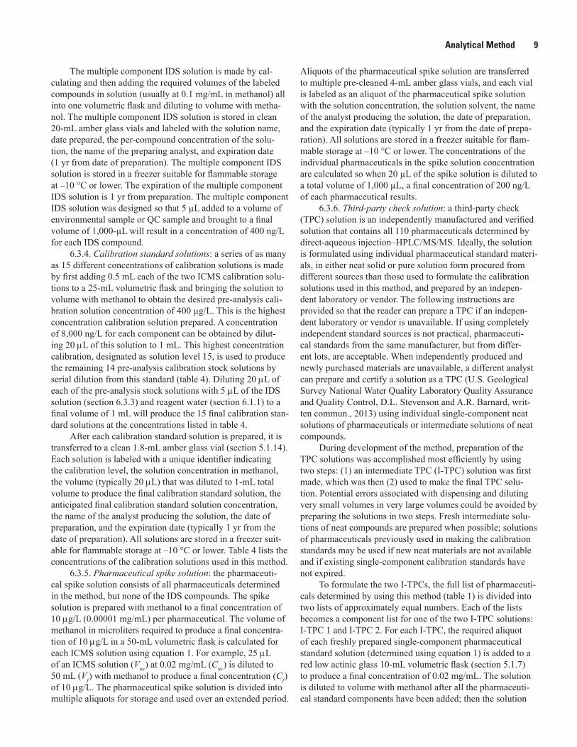
The multiple component IDS solution is made by cal-culating and then adding the required volumes of the labeled compounds in solution (usually at 0.1 mg/mL in methanol) all into one volumetric flask and diluting to volume with metha-nol. The multiple component IDS solution is stored in clean 20-mL amber glass vials and labeled with the solution name, date prepared, the per-compound concentration of the solu-tion, the name of the preparing analyst, and expiration date (1 yr from date of preparation). The multiple component IDS solution is stored in a freezer suitable for flammable storage at –10 °C or lower. The expiration of the multiple component IDS solution is 1 yr from preparation. The multiple component IDS solution was designed so that 5 µL added to a volume of environmental sample or QC sample and brought to a final volume of 1,000-µL will result in a concentration of 400 ng/L for each IDS compound.
6.3.4. Calibration standard solutions: a series of as many as 15 different concentrations of calibration solutions is made by first adding 0.5 mL each of the two ICMS calibration solu-tions to a 25-mL volumetric flask and bringing the solution to volume with methanol to obtain the desired pre-analysis cali-bration solution concentration of 400 µg/L. This is the highest concentration calibration solution prepared. A concentration of 8,000 ng/L for each component can be obtained by dilut-ing 20 µL of this solution to 1 mL. This highest concentration calibration, designated as solution level 15, is used to produce the remaining 14 pre-analysis calibration stock solutions by serial dilution from this standard (table 4). Diluting 20 µL of each of the pre-analysis stock solutions with 5 µL of the IDS solution (section 6.3.3) and reagent water (section 6.1.1) to a final volume of 1 mL will produce the 15 final calibration stan-dard solutions at the concentrations listed in table 4.
After each calibration standard solution is prepared, it is transferred to a clean 1.8-mL amber glass vial (section 5.1.14). Each solution is labeled with a unique identifier indicating the calibration level, the solution concentration in methanol, the volume (typically 20 µL) that was diluted to 1-mL total volume to produce the final calibration standard solution, the anticipated final calibration standard solution concentration, the name of the analyst producing the solution, the date of preparation, and the expiration date (typically 1 yr from the date of preparation). All solutions are stored in a freezer suit-able for flammable storage at –10 °C or lower. Table 4 lists the concentrations of the calibration solutions used in this method.
6.3.5. Pharmaceutical spike solution: the pharmaceuti-cal spike solution consists of all pharmaceuticals determined in the method, but none of the IDS compounds. The spike solution is prepared with methanol to a final concentration of 10 µg/L (0.00001 mg/mL) per pharmaceutical. The volume of methanol in microliters required to produce a final concentra-tion of 10 µg/L in a 50-mL volumetric flask is calculated for each ICMS solution using equation 1. For example, 25 µL of an ICMS solution (Vns) at 0.02 mg/mL (Cns) is diluted to 50 mL (Vf) with methanol to produce a final concentration (Cf) of 10 µg/L. The pharmaceutical spike solution is divided into multiple aliquots for storage and used over an extended period.
Aliquots of the pharmaceutical spike solution are transferred to multiple pre-cleaned 4-mL amber glass vials, and each vial is labeled as an aliquot of the pharmaceutical spike solution with the solution concentration, the solution solvent, the name of the analyst producing the solution, the date of preparation, and the expiration date (typically 1 yr from the date of prepa-ration). All solutions are stored in a freezer suitable for flam-mable storage at –10 °C or lower. The concentrations of the individual pharmaceuticals in the spike solution concentration are calculated so when 20 µL of the spike solution is diluted to a total volume of 1,000 µL, a final concentration of 200 ng/L of each pharmaceutical results.
6.3.6. Third-party check solution: a third-party check (TPC) solution is an independently manufactured and verified solution that contains all 110 pharmaceuticals determined by direct-aqueous injection–HPLC/MS/MS. Ideally, the solution is formulated using individual pharmaceutical standard materi-als, in either neat solid or pure solution form procured from different sources than those used to formulate the calibration solutions used in this method, and prepared by an indepen-dent laboratory or vendor. The following instructions are provided so that the reader can prepare a TPC if an indepen-dent laboratory or vendor is unavailable. If using completely independent standard sources is not practical, pharmaceuti-cal standards from the same manufacturer, but from differ-ent lots, are acceptable. When independently produced and newly purchased materials are unavailable, a different analyst can prepare and certify a solution as a TPC (U.S. Geological Survey National Water Quality Laboratory Quality Assurance and Quality Control, D.L. Stevenson and A.R. Barnard, writ-ten commun., 2013) using individual single-component neat solutions of pharmaceuticals or intermediate solutions of neat compounds.
During development of the method, preparation of the TPC solutions was accomplished most efficiently by using two steps: (1) an intermediate TPC (I-TPC) solution was first made, which was then (2) used to make the final TPC solu-tion. Potential errors associated with dispensing and diluting very small volumes in very large volumes could be avoided by preparing the solutions in two steps. Fresh intermediate solu-tions of neat compounds are prepared when possible; solutions of pharmaceuticals previously used in making the calibration standards may be used if new neat materials are not available and if existing single-component calibration standards have not expired.
To formulate the two I-TPCs, the full list of pharmaceuti-cals determined by using this method (table 1) is divided into two lists of approximately equal numbers. Each of the lists becomes a component list for one of the two I-TPC solutions: I-TPC 1 and I-TPC 2. For each I-TPC, the required aliquot of each freshly prepared single-component pharmaceutical standard solution (determined using equation 1) is added to a red low actinic glass 10-mL volumetric flask (section 5.1.7) to produce a final concentration of 0.02 mg/mL. The solution is diluted to volume with methanol after all the pharmaceuti-cal standard components have been added; then the solution

10 Determination of Human-Use Pharmaceuticals in Filtered Water by Direct Aqueous Injection
is stoppered tightly, inverted three times, and vortexed. The I-TPC solution is then poured into a clean 20-mL amber glass vial with Teflon-lined screw cap. The I-TPC solution is labeled appropriately (either “I-TPC Solution Part 1” or “I-TPC Solution Part 2”) and with other necessary informa-tion including preparation date and the initials of the analyst preparing the solutions. The solutions are stored in a freezer suitable for flammable storage at –10 °C or lower. The expira-tion date of the I-TPC solutions is 1 yr from preparation.
For the final TPC solution, individual pharmaceutical concentrations of 0.00001 mg/mL (10 µg/L) in methanol are targeted so that when 20 µL of the solution is diluted to a total volume of 1,000 µL in reagent water, a concentration of 200 ng/L results. The final TPC solution is prepared by adding 25 μL each of the two I-TPC solutions to a 50-mL low actinic glass volumetric flask and diluting to volume with methanol. This solution is then stoppered and thoroughly mixed. The final TPC solution is transferred to pre-cleaned 20-mL or 40-mL amber glass vials that are labeled with the expected final con-centration of each component in methanol, the name of the ana-lyst producing or packaging the solution, the preparation date, and the expiration date (typically 1 yr from the date of prepara-tion for this solution). All solutions are stored in a freezer suit-able for flammable storage at –10 °C or lower. This information is recorded in an electronic or paper standards logbook.
7. Sample Analysis
7.1. Sample Preparation in the Field and Laboratory Receipt of Environmental Samples
The method described in this report is applicable only to filtered water samples. All samples should be filtered, prefer-ably in the field at the time of collection. Filtration in the field reduces the likelihood of compound degradation after collection by removing particulate-associated bacteria and minimizing post-collection partitioning of compounds between the sample’s aqueous and solid phases (Wilde and others, 2004 with updates through 2009). Each sample is filtered through a 0.7-µm glass-fiber filter in the field. For field filtration, the USGS uses the procedure of Wilde and others (2004 with updates through 2009). Filtered samples are collected in the field in 20- or 40-mL amber glass vials; then the vials are filled approximately three-fourths full and sealed with a Teflon septum screw cap. If free chlorine is expected to be present in the sample (as is the case for most drinking-water samples), 12 mg or 25 mg of ascorbic acid is added to a 20- or 40-mL amber glass vial, respectively, before filling the vial approximately three-fourths full with filtered sample. The filtered samples are protected from sunlight and stored at 4 °C until shipment, on water ice, to the laboratory.
Upon receipt at the laboratory, samples are refrigerated typically at 4 ± 2 °C until sample preparation that occurs within 48 hr of arrival, which is standard practice at the NWQL and consistent with other USGS methods. As speci-fied, samples are filtered in the field according to the proce-dure of Wilde and others (2004 with updates through 2009). If
samples are not filtered in the field, or if a field-filtered sample is cloudy or shows other evidence of needing filtration prior to instrumental analysis, the procedure of Wilde and others (2004 with updates through 2009) or an equivalent method that pro-vides filtration through a 0.7-μm glass-fiber filter is used at the laboratory (see section 7.2).
A 10-mL aliquot of the filtered sample is transferred to a baked 12-mL amber glass vial (section 5.1.16). The vial is labeled with matching sample identifying information and stored frozen at –20 °C. If desired, additional aliquots can be identically filtered and frozen, labeled with matching sample identifying information, and numerically distinguished as subse-quent sample aliquots so that after one sample has been thawed and used, a second aliquot can be saved as an archived sample should reanalysis or analysis by other methods be desired. Typi-cally, the first aliquots are held frozen until sufficient numbers of samples are accumulated for a complete set, as the headspace in the vial allows for sample expansion; samples typically are filtered and frozen within 48 hr of receipt by the laboratory. Frozen filtered samples should be analyzed within 30 days. Extended storage beyond this 30-day limit is under evaluation.
For this method, samples typically are prepared for analysis in groups, or prep sets, that consist of as many as 17 environmental samples (including environmental field QC samples), one reagent blank sample, and one reagent spike sample, for a total of 19 samples in the prep set. Greater efficiency is achieved when the set is at capacity. For tracking and QC, each prep set is given a unique prep set identification number. At the laboratory, a laboratory identification number is assigned based on the year, Julian day, and a four-digit num-ber assigned to the samples as they are logged in upon receipt. Sample submittal forms for those samples submitted to the laboratory that require laboratory filtration contain a request code, added in the field, to indicate this requirement.
The sample prep set is assembled (see additional details in section 7.3). The filtered and labeled liquid sample aliquots are assembled for analysis, and if previous samples were frozen because there were not enough samples available for composing a sample prep set, these frozen samples are removed from the freezer and thawed. The sample identification or label information on each sample vial is carefully matched to any documentation provided with the sample to ensure that the correct sample is ana-lyzed. If a sample is to be a laboratory matrix spike sample, the vial is noted and marked with a visual identifier (such as a colored adhesive dot) to ensure that this sample is spiked with the suite of method pharmaceuticals when the sample prep set is assembled.
7.2. Laboratory Filtration
As previously noted (section 7.1), some samples may be received by the laboratory unfiltered; or, if they have been filtered in the field, may need to be filtered again, as indicated by cloudiness or visible particulate material in the sample. Suspended sediments in samples will clog the in-line filter of the HPLC/MS/MS and increase the need for maintenance. At the NWQL, the filtration procedure of Wilde and others (2004
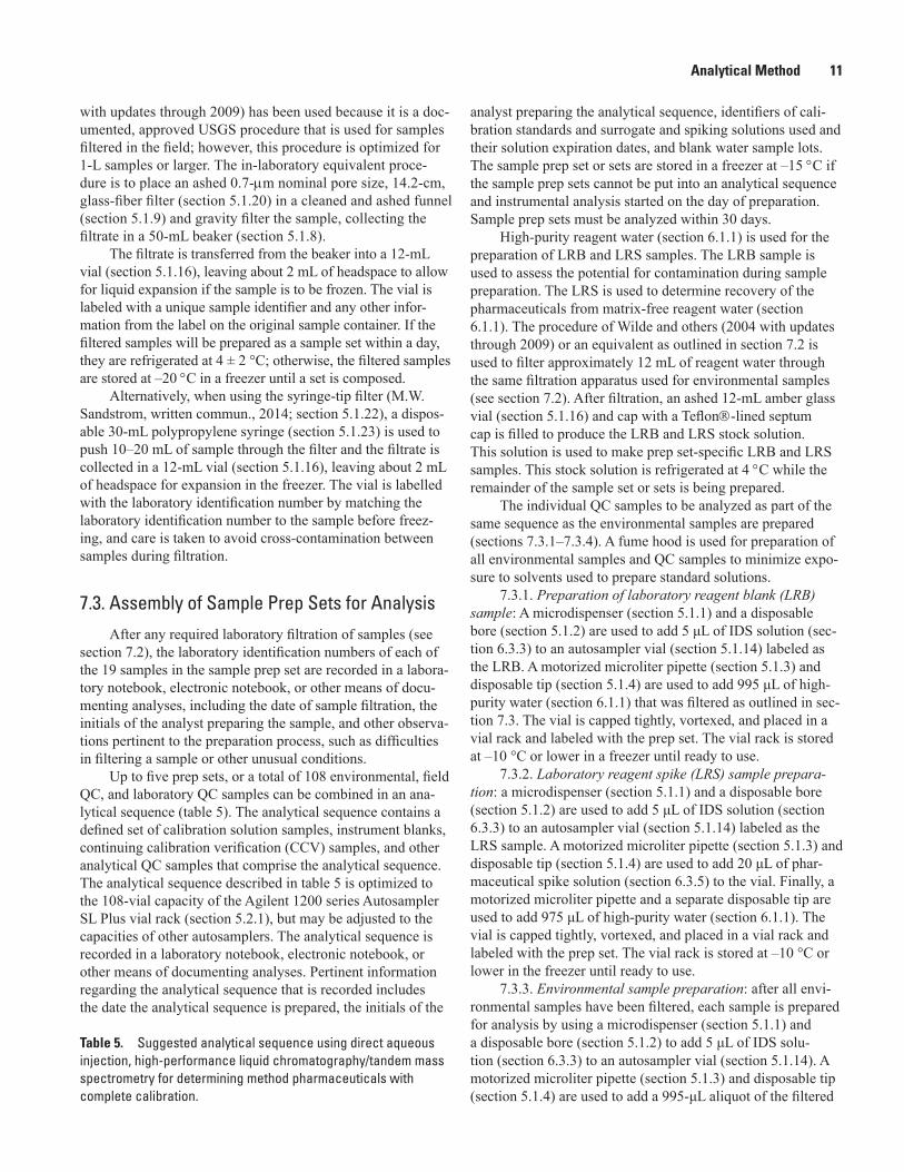
Analytical Method 11
with updates through 2009) has been used because it is a doc-umented, approved USGS procedure that is used for samples filtered in the field; however, this procedure is optimized for 1-L samples or larger. The in-laboratory equivalent proce-dure is to place an ashed 0.7-µm nominal pore size, 14.2-cm, glass-fiber filter (section 5.1.20) in a cleaned and ashed funnel (section 5.1.9) and gravity filter the sample, collecting the filtrate in a 50-mL beaker (section 5.1.8).
The filtrate is transferred from the beaker into a 12-mL vial (section 5.1.16), leaving about 2 mL of headspace to allow for liquid expansion if the sample is to be frozen. The vial is labeled with a unique sample identifier and any other infor-mation from the label on the original sample container. If the filtered samples will be prepared as a sample set within a day, they are refrigerated at 4 ± 2 °C; otherwise, the filtered samples are stored at –20 °C in a freezer until a set is composed.
Alternatively, when using the syringe-tip filter (M.W. Sandstrom, written commun., 2014; section 5.1.22), a dispos-able 30-mL polypropylene syringe (section 5.1.23) is used to push 10–20 mL of sample through the filter and the filtrate is collected in a 12-mL vial (section 5.1.16), leaving about 2 mL of headspace for expansion in the freezer. The vial is labelled with the laboratory identification number by matching the laboratory identification number to the sample before freez-ing, and care is taken to avoid cross-contamination between samples during filtration.
7.3. Assembly of Sample Prep Sets for AnalysisAfter any required laboratory filtration of samples (see
section 7.2), the laboratory identification numbers of each of the 19 samples in the sample prep set are recorded in a labora-tory notebook, electronic notebook, or other means of docu-menting analyses, including the date of sample filtration, the initials of the analyst preparing the sample, and other observa-tions pertinent to the preparation process, such as difficulties in filtering a sample or other unusual conditions.
Up to five prep sets, or a total of 108 environmental, field QC, and laboratory QC samples can be combined in an ana-lytical sequence (table 5). The analytical sequence contains a defined set of calibration solution samples, instrument blanks, continuing calibration verification (CCV) samples, and other analytical QC samples that comprise the analytical sequence. The analytical sequence described in table 5 is optimized to the 108-vial capacity of the Agilent 1200 series Autosampler SL Plus vial rack (section 5.2.1), but may be adjusted to the capacities of other autosamplers. The analytical sequence is recorded in a laboratory notebook, electronic notebook, or other means of documenting analyses. Pertinent information regarding the analytical sequence that is recorded includes the date the analytical sequence is prepared, the initials of the
analyst preparing the analytical sequence, identifiers of cali-bration standards and surrogate and spiking solutions used and their solution expiration dates, and blank water sample lots. The sample prep set or sets are stored in a freezer at –15 °C if the sample prep sets cannot be put into an analytical sequence and instrumental analysis started on the day of preparation. Sample prep sets must be analyzed within 30 days.
High-purity reagent water (section 6.1.1) is used for the preparation of LRB and LRS samples. The LRB sample is used to assess the potential for contamination during sample preparation. The LRS is used to determine recovery of the pharmaceuticals from matrix-free reagent water (section 6.1.1). The procedure of Wilde and others (2004 with updates through 2009) or an equivalent as outlined in section 7.2 is used to filter approximately 12 mL of reagent water through the same filtration apparatus used for environmental samples (see section 7.2). After filtration, an ashed 12-mL amber glass vial (section 5.1.16) and cap with a Teflon-lined septum cap is filled to produce the LRB and LRS stock solution. This solution is used to make prep set-specific LRB and LRS samples. This stock solution is refrigerated at 4 °C while the remainder of the sample set or sets is being prepared.
The individual QC samples to be analyzed as part of the same sequence as the environmental samples are prepared (sections 7.3.1–7.3.4). A fume hood is used for preparation of all environmental samples and QC samples to minimize expo-sure to solvents used to prepare standard solutions.
7.3.1. Preparation of laboratory reagent blank (LRB) sample: A microdispenser (section 5.1.1) and a disposable bore (section 5.1.2) are used to add 5 μL of IDS solution (sec-tion 6.3.3) to an autosampler vial (section 5.1.14) labeled as the LRB. A motorized microliter pipette (section 5.1.3) and disposable tip (section 5.1.4) are used to add 995 μL of high-purity water (section 6.1.1) that was filtered as outlined in sec-tion 7.3. The vial is capped tightly, vortexed, and placed in a vial rack and labeled with the prep set. The vial rack is stored at –10 °C or lower in a freezer until ready to use.
7.3.2. Laboratory reagent spike (LRS) sample prepara-tion: a microdispenser (section 5.1.1) and a disposable bore (section 5.1.2) are used to add 5 μL of IDS solution (section 6.3.3) to an autosampler vial (section 5.1.14) labeled as the LRS sample. A motorized microliter pipette (section 5.1.3) and disposable tip (section 5.1.4) are used to add 20 μL of phar-maceutical spike solution (section 6.3.5) to the vial. Finally, a motorized microliter pipette and a separate disposable tip are used to add 975 μL of high-purity water (section 6.1.1). The vial is capped tightly, vortexed, and placed in a vial rack and labeled with the prep set. The vial rack is stored at –10 °C or lower in the freezer until ready to use.
7.3.3. Environmental sample preparation: after all envi-ronmental samples have been filtered, each sample is prepared for analysis by using a microdispenser (section 5.1.1) and a disposable bore (section 5.1.2) to add 5 μL of IDS solu-tion (section 6.3.3) to an autosampler vial (section 5.1.14). A motorized microliter pipette (section 5.1.3) and disposable tip (section 5.1.4) are used to add a 995-μL aliquot of the filtered
Table 5. Suggested analytical sequence using direct aqueous injection, high-performance liquid chromatography/tandem mass spectrometry for determining method pharmaceuticals with complete calibration.

12 Determination of Human-Use Pharmaceuticals in Filtered Water by Direct Aqueous Injection
environmental sample to the autosampler vial, matching the laboratory identification number on the autosampler vial to the laboratory identification number on the environmental sample vial. If the prepared sample is a laboratory duplicate, the laboratory duplicate is designated with a “D” after the labora-tory identification number on the autosampler label. The vial is capped tightly, vortexed, and placed in a vial rack (section 5.1.15) labeled with the prep set (section 7.1). The vial rack is stored at –10 °C or lower in a freezer until ready to use.
If an aliquot of the environmental sample will be ana-lyzed as a laboratory matrix spike (LMS) sample, a micro-dispenser and a disposable bore are used to add 5 μL of IDS solution (section 6.3.3) to an autosampler vial. A motorized microliter pipette and disposable tip are used to add 975 μL of the environmental sample that is to be fortified with the spiking solution. Finally, a motorized microliter pipette and a separate disposable tip are used to add 20 μL of pharmaceuti-cal spike solution (section 6.3.5) to the environmental sample in the autosampler vial. The prepared sample is designated as a laboratory matrix spike with an “L” after the laboratory iden-tification number on the autosampler vial. The vial is capped tightly, vortexed, and placed in a vial rack labeled with the prep set. The vial rack is stored at –10 °C or lower in a freezer until ready to use.
7.3.4. Preparation of instrument blanks and instru-ment standards: instrument blanks and standards are instru-ment QC samples analyzed at the beginning of an analytical sequence (as is the case for the working calibration standard solutions) or dispersed within the analytical sequence. These instrument QC samples monitor instrument performance during the analysis of the sequence and ensure comparability between environmental samples and environmental (field) QC samples analyzed at the beginning and end of the sequence. These instrument QC samples, along with calibration stan-dard solutions (section 6.3.4) are prepared on the day that the analytical sequence, comprising one or more prep sets, is started. The primary instrument QC samples are listed in the following subsections.
7.3.4.1. Instrument blank preparation: two types of instrument blanks are used in this method. Two water blanks (WBLK in table 5) are analyzed at the start of the analytical sequence to verify the absence of interferences in the analyti-cal system and to verify the absence of method compounds prior to beginning analysis. The continuing calibration blank (CCB) is interspersed in the analytical sequence immediately following the CCV to monitor for carryover during the ana-lytical sequence. Both types of blanks are prepared identically.
A microdispenser (section 5.1.1) and a disposable bore (section 5.1.2) are used to add 5 μL of IDS solution (section 6.3.3) to an autosampler vial (section 5.1.14). A motorized microliter pipette (section 5.1.3) and disposable tip (section 5.1.4) are used to add 995 μL of high-purity water (section 5.1.1). The vial is capped tightly, vortexed, and placed in a vial rack labeled with the prep set. The vial rack is stored at –10 °C or lower in a freezer until ready to use. The small amount of methanol added from the IDS solution is enough to
keep the autosampler vial of water from cracking when stored in the freezer. The instrument blanks are checked to ensure that they are not frozen when ready to inject into the instru-ment. If the sequence outlined in table 5 is used, at least 10 CCBs are required.
7.3.4.2. Preparation of working instrument calibration standards: This method uses 15 calibration levels (section 6.3.4) to ensure calibration across the expected range of envi-ronmental concentrations and to account for the compound-specific sensitivities of each pharmaceutical in the method. The 15 calibration levels are outlined in table 4. Table 4 is used to identify the level of the calibration standard solution matching the desired calibration concentration. An autosam-pler vial (section 5.1.14) is labeled for each desired calibration level concentration, and 5 μL of IDS solution (section 6.3.3) is added to that vial using a microdispenser (section 5.1.1) and a disposable bore (section 5.1.2). A motorized microliter pipette (section 5.1.3) and disposable tip (section 5.1.4) are used to add 975 μL of high-purity water (section 6.1.1). Finally, a motorized microliter pipette and a separate disposable tip are used to add 20 μL of the final calibration solution (table 4) indicated for the calibration level desired to the water in the autosampler vial labeled for that level to produce the work-ing instrument calibration standard. The vial is capped tightly, vortexed, and placed in a vial rack labeled with the prep set. The vial rack is stored at –10 °C or lower in the freezer.
7.3.4.3. Preparation of continuing calibration verification (CCV) samples: the CCVs are prepared from the calibration solution that will give the desired concentration of 200 ng/L (level 9 in table 4). The CCVs are prepared by first adding 5 μL of IDS solution (section 6.3.3), using a microdispenser (section 5.1.1) and a disposable bore (section 5.1.2), to each of the autosampler vials (section 5.1.14) labeled CCV. A motorized microliter pipette (section 5.1.3) and disposable tip (section 5.1.4) are used to add 975 μL of high-purity water (section 6.1.1) to each vial. A motorized microliter pipette and a separate disposable tip are used to add 20 μL of the level 9 calibration solution (table 4) to the water in each of the autosampler vials. The vials are capped tightly, vortexed, and placed in a vial rack labeled with the prep set. The vial rack is stored at –10 °C or lower in the freezer. Typically, seven CCV samples are needed in the sequence outlined in table 5.
7.3.4.4. Preparation of instrument limit of quantitation (LOQ) samples: two LOQ samples are prepared from the cali-bration standard solutions that will give the desired concentra-tions of 4 ng/L and 80 ng/L on the instrument (levels 3 and 7, respectively, in table 4).
A microdispenser (section 5.1.1) and a disposable bore (section 5.1.2) are used to add 5 μL of IDS solution (section 6.3.3) to an autosampler vial (section 5.1.14); then 975 μL of high-purity water (section 6.1.1) is added using a motorized microliter pipette (section 5.1.3) and disposable tip (section 5.1.4). Finally, a motorized microliter pipette and a separate disposable tip are used to add 20 μL of the calibration solu-tion (section 6.3.4) to the autosampler vial. The vial is capped tightly, vortexed, and placed in a vial rack labeled with the

Analytical Method 13
prep set. The vial rack is stored at –10 °C or lower in the freezer. Typically, one of each LOQ sample is required for the analytical sequence outlined in table 5.
7.3.4.5. Loading the analysis sequence into the mass spec-trometer: after verification of the sequence of environmental and QC samples in the vial rack with the list stored in a paper or digital notebook, this analytical sequence is transferred to the appropriate section of the instrument operating software. Agilent Technologies MassHunter software (section 5.2.2) was used in development of this method. This transfer produces an instrument analysis sequence that can be invoked to analyze each vial in the sequence automatically and store the results on the computer for later evaluation and review.
7.4. Preparation of Environmental and Quality-Assurance Samples for Instrumental Analysis
After the instrument blanks, working instrument stan-dards, and other analysis QC samples have been prepared (section 7.3.4), any previously prepared environmental sample sets (section 7.3.3) are obtained from frozen storage. Envi-ronmental sample sets that are prepared on the same day they will be analyzed can be stored refrigerated at about 4 °C until all analysis QC samples are prepared. Time is allowed for the previously frozen samples to thaw until cold to the touch; this takes about 30 minutes (min) at room temperature. All the sample and standard solution vials are vortexed to ensure they are homogeneously mixed.
The sequence for instrumental analysis of multiple sets of environmental samples, associated laboratory and environmen-tal (field) QC samples, and a complete calibration is summa-rized in table 5. The environmental sample vials, the instrument blanks, and the working instrument standards are inserted into their respective instrument autosampler tray positions accord-ing to the sequence entered into the instrument software (sec-tion 7.3.4.5). The labeling on and placement of the vial in the tray are verified to correspond with the sample identification and position in the sequence to avoid transcription errors. The coolant plate of the autosampler (section 5.2.1) is checked to ensure that it is cold to the touch (approximately 4 °C) prior to placing the autosampler vial rack into the autosampler.
7.5. Sample AnalysisIn this method, HPLC is used to at least partially sepa-
rate the 110 pharmaceuticals determined by this method from each other prior to ionization. The ESI interface converts the separated pharmaceuticals into protonated pseudomolecular ions, which are introduced from the atmospheric pressure region of the interface through a capillary and lenses into the low-pressure region of the mass spectrometer. These ions are selectively isolated in the first stage of MS/MS, that is, within the first quadrupole of the triple-quadrupole mass spectrometer. The selected pseudomolecular ion specific to each pharmaceutical in this method is then fragmented with
the second quadrupole of the mass spectrometer acting as a collision cell (this is also referred to as the second stage of analysis). From within the array of fragment ions produced in the collision cell, two diagnostic fragment ions—a quantitation ion and a confirmation ion—are selected in the third and final stage of mass analysis, which occurs in the third quadrupole of the triple-quadrupole mass spectrometer. The quantitation and confirmation ions are transmitted to an electron multiplier, where the signals they produce are amplified and the signals are integrated. The selectivity and specificity provided by MS/MS also provides identification and quantitation certainty for each pharmaceutical, even in cases where two or more phar-maceuticals are incompletely separated by the HPLC.
This form of MS/MS commonly is referred to as MRM or selected reaction monitoring (SRM). When coupled with the retention time of the pharmaceutical during HPLC, the MS/MS provides sufficient specificity for identification and quantitation of the 110 pharmaceuticals of interest. A vari-ant of MRM, which commonly is referred to as dynamic or scheduled MRM, focuses MRM analysis around the retention window of each pharmaceutical, and is used in this method to further optimize sensitivity and specificity.
Prior experience with analyses at the NWQL has shown that any HPLC/MS/MS instrument will have specific settings whose optimization are critical to successful method imple-mentation. The Agilent Technologies 6460 triple-quadrupole MS/MS (section 5.2.1) was used to develop and validate the method described in this report, and some of the procedures and terms referred to in the following method description may be specific to the operation of that instrument. Others applying this method using a different HPLC/MS/MS system will need to carefully consult the manufacturers’ operating manuals and electronic documentation to ensure that the system settings and operating conditions are equivalent to the description that follows. When others using the Agilent Technologies 6460 triple-quadrupole MS/MS apply this method, they should also closely consult printed or electronic user’s manuals, online resources, and this report. The operation of the MS/MS is a highly complex process requiring very specific timing and control of many compound-specific data collection events by operator programming of the instrument through the MassHunter (section 5.2.2) or equivalent software.
7.5.1. Pre-analysis instrument preparation7.5.1.1. Cleaning the electrospray source prior to
instrument analysis: Prior to any initial instrument operation, such as performing an automated, computer-controlled mass spectrometer tune (autotune) or computer-controlled check of a prior mass spectrometer tune (check tune), the electrospray chamber is opened. The tip of the nebulizer needle is washed with a 50:50 mixture of isopropyl alcohol (section 6.1.2) and high-purity water (section 6.1.1) and the waste collected. This is routine practice.
Periodically, the nebulizer needle is inspected, especially if autotune or check tune fails. Nitrile gloves are worn to avoid contaminating instrument surfaces. The gas line that is con-nected to the nebulizer is disconnected, and the electrospray

14 Determination of Human-Use Pharmaceuticals in Filtered Water by Direct Aqueous Injection
needle assembly (nebulizer) is carefully removed from the chamber without allowing the needle tip to touch any surfaces. The nebulizer tip is inspected with a nebulizer magnifier (sec-tion 5.2.14) to ensure that the position of the needle tip is flush with or just projecting from the needle housing. If not, the position is adjusted until the needle tip is flush for proper spray conditions. Low ion abundances in the autotune—a cause of autotune failure—may result from a plugged nebulizer needle. If the needle is plugged, the entire needle assembly is cleaned in a sonic bath by placing the assembly upright in a cylinder of iso-propyl alcohol (section 6.1.2) and operating the sonic bath for 5 min. It is important that the needle position is verified when the nebulizer needle is reinstalled in the electrospray chamber.
After installation, the gas line is reconnected to the nebu-lizer. The nebulizer needle is flushed (using the HPLC switch-ing valve) to remove the HPLC column from eluent flow, and a piece of metal capillary tubing is temporarily installed to connect the HPLC column switching valve directly to the top of the nebulizer. The binary pump is set to flow 2 milliliters per minute (mL/min) of a 50:50 mixture of isopropyl alcohol and high-purity water for at least 5 min, and the waste solvent that drips to the bottom of the open electrospray chamber is collected. After this rinse is complete, all lines for normal analytical operation are reconnected and the waste is disposed of properly according to local regulations. The metal mounting posts below the needle assembly are cleaned with a 50:50 mix-ture of isopropyl alcohol and high-purity water, abrasive grit paper (section 5.2.12), and lint-free cloth (section 5.2.13). The spray shield cap of the mass spectrometer is unscrewed and cleaned using a 50:50 mixture of isopropyl alcohol and high-purity water, abrasive grit paper, and lint-free cloth. Finally, the thinly plated metal end cap on the sampling capillary entering the mass spectrometer is removed—very carefully so not to kink and damage the spring (section 5.2.8) inside—and cleaned with a 50:50 mixture of isopropyl alcohol and high-purity water and a lint-free cloth. These cleaning steps prior to analy-sis ensure that the mass spectrometer is operating at optimum ionization efficiency at the start of the analytical sequence.
7.5.1.2. Initiating operation through the instrument control software: the Agilent Technologies 6460 triple-quad-rupole MS/MS (section 5.2.1) used to develop this method uses MassHunter software (section 5.2.2) for all instrument control and post-analysis data processing and reporting opera-tions. The instrumental analysis of an analytical sequence is controlled through an operator-specified acquisition method. The acquisition method contains the specific settings and oper-ating conditions for control of the HPLC separation, operation of the ESI source, and computer-controlled operation of mass-spectrometer conditions for collection of the dynamic MRM signals for each pharmaceutical as it elutes from the HPLC and enters the mass spectrometer. A specific description of the process of entering the settings of the HPLC and the control and collection of dynamic MRM data with the Agilent Tech-nologies 6460 triple-quadrupole MS/MS is beyond the scope of this method report. The reader is referred to the instrument documentation for the triple-quadrupole mass spectrometer
used to conduct this analysis for details on how to implement this method using his or her instrument’s operation-control software. The specific instrument settings used to acquire the MRM ion transitions for the pharmaceuticals in this method are contained in table 6 and table 1–1 in the appendix.
After an acquisition method has been initially added to the MassHunter software, that method will need to be revised to match minor changes in chromatographic and mass spectrometric characteristics. These minor changes, such as shifts in the retention times of a pharmaceutical as the HPLC column ages, typically occur during long-term operation of the HPLC/MS/MS. The method most recently used for analysis is loaded to check, edit, or create acquisition and/or analysis parameters in the acquisition method prior to analysis. Data acquisition parameters are adjusted as needed to ensure that each pharmaceutical is detected by the method as it elutes from the HPLC column. The edited method is saved under a new name to ensure retention of the revised instrument data acquisition and analysis parameters. A naming conven-tion is used that provides a unique identifier, for example APOS222.m, where A is an instrument identifier character; POS, for positive, refers to the type of ionization mode; and 222 is the Julian date when the method was revised and ana-lyst began using it.
The HPLC aqueous and organic mobile phase solutions are prepared from the reagent solutions (section 6.2) and meth-anol (section 6.1.3), respectively. Inverting the capped flasks 20 times ensures homogeneous mixing. The HPLC aqueous mobile-phase reservoir (in MassHunter software referred to as A1) is filled with high-purity water modified with formic acid and ammonium formate (section 6.2.3), and the HPLC organic-solvent reservoir (in MassHunter software referred to as B1) is filled with methanol (section 6.1.3). Some HPLC control software permits or requires that the volume of solvent in each reservoir be noted in an appropriate data window in the software, allowing the estimation of the actual solvent volumes in each reservoir during analyses, which activate low-solvent shutoff triggers to avoid inadvertently introducing air into the HPLC pumping system during an extended analytical sequence. It is important to use this instrument control soft-ware feature if available.
The HPLC/MS/MS system is turned on; for most sys-tems, this typically is done by selecting the “On” button in the data acquisition window of the instrument control software module. Note that for most mass spectrometers, the pumps, oven, and mass spectrometer usually turn on simultaneously. The solvent-delivery system pumps are primed by opening the purge valve and allowing 100 percent of flow from reservoir A1 to discharge at a rate of 5 mL/min for several minutes, fol-lowed by switching to 100 percent of flow from reservoir B1.
Table 6. Mass spectrometer settings used to produce the precursor and product ions and the corresponding quantitation and first and second qualification transitions of pharmaceuticals and isotope-dilution standard compounds determined in this method.
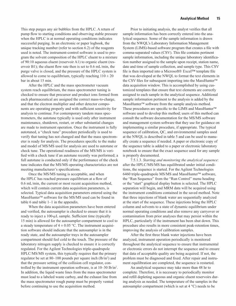
Analytical Method 15
This step purges any air bubbles from the HPLC. A return of pump flow to starting conditions and observing stable pressure when the HPLC is at normal operating conditions indicates successful purging. In an electronic or paper logbook, the unique tracking number (refer to section 6.2) of the reagents used is noted. The instrument-control software is used to pro-gram the solvent composition of the HPLC eluent to a mixture of 90:10 aqueous eluent (reservoir A1) to organic eluent (res-ervoir B1); the eluent flow rate then is set to 0.6 mL/min, the purge valve is closed, and the pressure of the HPLC system is allowed to come to equilibrium, typically reaching 110 ± 20 bar in about 15 min.
After the HPLC and the mass spectrometer vacuum system reach equilibrium, the mass spectrometer tuning is checked to ensure that precursor and product ions formed from each pharmaceutical are assigned the correct mass-to-charge, and that the electron multiplier and other detector compo-nents are operating properly and with sufficient sensitivity for analysis to continue. For contemporary tandem mass spec-trometers, the autotune typically is used only after instrument maintenance, shutdown, restart, or other substantial changes are made to instrument operation. Once the instrument is fully autotuned, a “check tune” procedure periodically is used to verify that tuning has not changed and that the mass spectrom-eter is ready for analysis. The procedures specific to the make and model of MS/MS used for analysis are used to autotune or check tune. The operational readiness of the MS/MS is veri-fied with a check tune if an autotune recently was performed; a full autotune is conducted only if the performance of the check tune indicates that the MS/MS operating characteristics are not meeting manufacturer’s specifications.
Once the MS/MS tuning is acceptable, and when the HPLC has reached pressure equilibrium at a flow of 0.6 mL/min, the current or most recent acquisition method, which will contain current data acquisition parameters, is selected. Typical data acquisition parameters entered using the MassHunter software for the MS/MS used can be found in table 6 and table 1–1 in the appendix.
When the data acquisition parameters have been entered and verified, the autosampler is checked to ensure that it is ready to inject a 100-µL sample. Sufficient time (typically 15 min) is allowed for the autosampler compartment to cool to a steady temperature of 4 ± 0.05 °C. The instrument acquisi-tion software should indicate that the autosampler is in the ready state, and the autosampler trays in the autosampler compartment should feel cold to the touch. The pressure of the laboratory nitrogen supply is checked to ensure it is correctly regulated. For the Agilent Technologies triple-quadrupole HPLC/MS/MS system, this typically requires that the primary regulator be set at 80–100 pounds per square inch (lb/in2) and that the pressure setting of the collision cell regulator, con-trolled by the instrument operation software, is at 10–30 lb/in2. In addition, the liquid waste lines from the mass spectrometer must lead to a labeled waste carboy, and the exhaust line from the mass spectrometer rough pump must be properly vented before continuing to use the acquisition method.
Prior to initiating analysis, the analyst verifies that all sample information has been correctly entered into the ana-lytical sequence. Some of the sample information is drawn from the NWQL’s Laboratory Information Management System (LIMS)-based software program that creates a file with comma-separated values (CSV). This file contains pertinent sample information, including the unique laboratory identifica-tion number assigned to the sample upon receipt, station name, date and time of sample collection, and sample type. This CSV file is then imported into a Microsoft Excel™ template file that was developed at the NWQL to format the text elements in the CSV files for subsequent importing into the MassHunter data acquisition window. This is accomplished by using cus-tomized templates that ensure that text elements are correctly assigned to each sample in the analytical sequence. Additional sample information pertinent to the analysis is added by the MassHunter software from the sample analysis method. These procedures are specific to the LIMS and MassHunter software used to develop this method; users of this method can consult the software documentation for the MS/MS software and management system software that they use for guidance on implementing a similar procedure, if appropriate. The typical sequence of calibration, QC, and environmental samples used at the NWQL is described in table 5 and can be used to manu-ally create a sequence if needed. A paper or electronic copy of the sequence table is added to a paper or electronic laboratory notebook to ensure that the exact sequence used for any sample is properly documented.
7.5.1.3. Starting and monitoring the analytical sequence: after the HPLC/MS/MS has equilibrated under initial condi-tions, the sequence is started. For the Agilent Technologies 6460 triple-quadrupole MS/MS and MassHunter software, the “Run Sequence” from the “Run Control” menu heading or the “start” graphical display button is selected. The HPLC separation will begin, and MRM data will be acquired using the instrument conditions contained in the saved method. Note that three injections of blank water are sequentially analyzed at the start of the sequence. These injections bring the HPLC column and solvents to a state of dynamic equilibrium under normal operating conditions and also remove any carryover or contamination from prior analyses that may persist within the HPLC, particularly if the instrument has been shut down. This procedure also results in more consistent peak-retention times, improving the analysis of calibration samples.
After the first three blank water injections have been analyzed, instrument operation periodically is monitored throughout the analytical sequence to ensure that instrumental or electronic errors do not interrupt the sequence and to ensure that data of acceptable quality are being acquired. If not, the problem must be diagnosed and fixed. After repair and instru-ment equilibration are completed, the sequence is restarted.
An analytical sequence may take more than 48 hr to complete. Therefore, it is necessary to periodically monitor and refill depleting aqueous and organic eluent reservoirs dur-ing analysis as needed. The temperature of the samples in the autosampler compartment (which is set at 4 °C) needs to be

16 Determination of Human-Use Pharmaceuticals in Filtered Water by Direct Aqueous Injection
monitored; the autosampler sample tray should remain cold to the touch throughout the analysis of the sequence. It is impor-tant that the samples not be allowed to come to room tem-perature. Any interruptions of the sequence, instrument errors, anomalous instrument performance, or maintenance performed before, during, or after analysis of the sequence should be documented in the instrument logbook or by other means of documenting instrument operation, such as an electronic laboratory notebook. For the MassHunter software used in this method, electronic error logs can be reviewed within the instrument control software component.
Additionally, assessing the real-time performance of CCVs during the analysis of the sequence can provide diagnostic information, identifying possible chromatographic or quantitation problems that are not indicated by computer-provided instrument errors or other electronic diagnostic tools (for example, loss of chromatographic resolution due to col-umn contamination or stationary phase degradation). If CCV peak shapes are misshapen or asymmetric when compared to a Gaussian peak shape or if the peak areas are inconsistent with prior results, the instrument operation needs to be critically evaluated to determine if it is appropriate to stop the analytical sequence, diagnose and correct any errors, perform any neces-sary maintenance (documenting any maintenance performed), and restart the analytical sequence. Following completion of the analytical sequence, a post-analysis data review is con-ducted to determine the acceptability of results that met real-time performance criteria. Table 1–2 in the appendix shows the criteria used to determine the acceptability of results from a completed analytical sequence when the data are reviewed post-analysis.
7.6. Post-Analysis Data Processing and Evaluation
Data are evaluated using the quantitative analysis component of the Agilent MassHunter Workstation soft-ware. In-depth information on the creation and editing of MassHunter quantitation methods are beyond the scope of this report. Users are referred to the software manuals for the specific HPLC/MS/MS system used for analysis to determine the specific software and procedures necessary to identify and quantify the pharmaceuticals determined in an analyti-cal sequence. Table 6 documents the transitions used in the method, and table 1–1 in the appendix documents the electron-ics settings used in the quantitative analysis component of the MassHunter software to identify and quantify pharmaceu-ticals in filtered water samples. The reader is cautioned when reviewing these tables that the specific settings and conditions contained therein apply only to the NWQL’s implementation of this method. The user also should critically evaluate these data when used with systems other than the Agilent Technolo-gies 6460 triple-quadrupole MS/MS system to ensure chro-matographic peaks are properly integrated. A brief overview of the NWQL’s evaluation process follows.
7.6.1. Processing and evaluating analysis results: upon completion of the analytical sequence, the quantitative analysis (QUAN) component of the MassHunter software is used to process instrument results. Readers of this report are referred to the documentation for the software for the specific HPLC/MS/MS system used to determine the analogous software compo-nent; the process described in this report can be used as a guide to develop a procedure for consistently and accurately deter-mining compound identities and concentrations.
The analyst consistently applies the following six steps to each analysis file when reviewing the results of an analytical batch:1. verifying acceptable qualitative identification and instru-
ment response during the analytical sequence;
2. producing a calibration curve for each pharmaceutical that can be applied to all qualitatively identified pharmaceuti-cal detections in environmental samples;
3. verifying any qualitatively identified environmental sample detections and ensuring that all qualitatively identifiable detections were correctly made by the initial automated data processing step undertaken by the QUAN software;
4. verifying that the integrated peak areas of the quantita-tion precursor-ion/product-ion pair (quantitation product ion) and the confirmation precursor-ion/product-ion pair (confirmation product ion) for each environmental sample detection are accurate and that the ratio of the areas of confirmation to quantitation product ions are correctly calculated and fall within the relative abundance-based tolerances indicated in European Commission (2002) used for this method;
5. verifying that the concentrations produced from applica-tion of the calibration curve to the environmental results are correctly calculated; and
6. evaluating the qualitative and quantitative results for labo-ratory QC samples processed concurrently with environ-mental samples.
These steps are all necessary to ensure results of acceptable quality.
During sample analysis, the CCV and CCB samples interspersed in the sequence are evaluated to verify that instru-ment calibration met criteria throughout the sequence and that contamination between injections did not occur. Because the CCV and CCB samples are periodically evaluated during the sequence, failure for CCV and CCB to meet acceptance criteria does not usually affect the data quality of the entire analytical sequence and is used to identify subsets of samples in the sequence where CCV or CCB failures may require reanalysis of the environmental sample. Assuming that evalu-ation of CCV and CCB results indicates that sample results do not require reanalysis, qualitatively identified detections in the environmental sample and other field and laboratory

Analytical Method 17
QC samples are quantified using a calibration curve produced for each pharmaceutical from results in the calibration table file. The processing software calibration table file contains the quantitation product-ion response data from the analysis of the calibration standards for each pharmaceutical and the IDS compounds determined in the method. The QUAN software uses this information (as well as the concentrations of the standards, the injected sample volume, and the compound-specific calibration curves calculated for each pharmaceutical) to determine a concentration for each detected pharmaceutical or surrogate compound in each sample.
7.6.2. Identification and quantitation of pharmaceuticals in environmental samples: environmental and QC sample concentrations of pharmaceuticals are determined after an acceptable calibration curve is produced for each pharmaceuti-cal. The determination of a pharmaceutical in an environmen-tal or QC sample is a two-step process in which the compound is first qualitatively identified and once identity is established, a quantitative concentration is determined.
7.6.2.1. Qualitative identification criteria: several criteria are used to determine that a compound identification is quali-tatively correct. Correct identification is based on (1) the reten-tion time at which the apex of the chromatographic peaks of the quantitation product ion and confirmation product ion elute from the HPLC into the MS/MS, and (2) the presence of both the quantitation and confirmation product ions at a consistent relative ratio. These criteria are determined from analysis of authentic standards and are verified by analysis of standards in each batch to compensate for possible long-term changes in HPLC/MS/MS systems.
Compounds are qualitatively detected when quantitation and confirmation product ions are (1) both produced from the precursor ion of the pharmaceutical of interest (as determined by analysis of an authentic standard of the pharmaceutical of interest) and the produced ions can be distinguished from background, typically at three times the background signal within the MRM window; (2) these product ions have coinci-dent retention time maxima; and (3) the ratio of the quantita-tion product ion to confirmation product ion for the pharma-ceutical of interest is similar to the same ratio of quantitation product ion to confirmation product ion from an authentic standard. The precursor ion, quantitation product ion, confir-mation product ion, and the ratio of the confirmation to quanti-tation ions for each pharmaceutical determined in this method are summarized in table 6.
7.6.2.1.1. Quantitation product ion: the quantitation product ion is produced from fragmentation of a precursor ion (typically the protonated molecular ion of the pharmaceuti-cal of interest) that is fragmented in the MS/MS to produce a unique product ion that is a predominant ion in the product-ion mass spectrum and characteristic of the pharmaceutical being identified. Typically, the quantitation product ion also is present with minimal interference, as indicated by a chro-matographically resolved peak with a signal-to-noise ratio of at least 3:1 (Food and Drug Administration, 1994). Peak tailing can interfere with quantitation, so a peak-tailing factor
of two or less is recommended (Food and Drug Administra-tion, 1994). The precision of the peak area integration of the quantitation product ion is critical to reproducible quantita-tion, and although criteria for integration precision are not readily available, an estimate of typical peak area precision in environmental samples can be made based on results of Li and others (1996). They observed that for a single tuning period (typical for how MS/MS are operated), product ion transitions of greater than 50 percent relative abundance were reproducible within 10 percent relative standard deviation, and for product ion transitions between 7 and 50 percent relative abundance, the reproducibility was within 20 percent relative standard deviation.
The ratio of the integrated peak area of the quantitation product ion (also known as abundance) to the abundance of a second additional characteristic precursor-ion/product-ion pair—that is, the confirmation product ion—when combined with the peak-retention time of both product ions, provides the qualitative detection criteria for this method. The phar-maceutical concentration is determined from the abundance of the quantitation product ion in a sample compared to the abundances of the quantitation product ions produced from the calibration standards of the pharmaceutical of interest, after normalization to the quantitation product ion of an IDS com-pound and mathematical transformation in a calibration curve.
7.6.2.1.2. Confirmation product ion: the confirmation product ion is a second detectable precursor-ion/product-ion pair that is produced by and characteristic of the same pharma-ceutical as the quantitation product ion. Confirming product ions must have integrated peak response maxima that coincide with or coelute with the quantitation product-ion maximum. Variation of as much as 2.5 percent in retention time is accept-able between quantitation and confirmation product-ion peak maxima, typically resulting from inherent variation or instru-ment electronic “noise” (European Commission, 2002). Similar criteria for peak signal, quality, and precision apply to the confirmation product-ion peaks as they do to the quantitation product-ion peaks. The relative abundances of the confirmation product ions typically are of lower relative abundance, thus greater variation is likely to occur in the reproducibility of the confirmation product-ion peak areas compared to the quantita-tion product-ion peak areas, as noted by Li and others (1996).
These lower abundance ions also are likely to vary slightly from ideal peak shape, although a maximum tail-ing factor of 2 and a minimum signal-to-noise ratio of 3:1 are necessary (Food and Drug Administration, 1994) even if instrument electronic “noise ” is apparent. The integrated abundance ratio of these two product ions (expressed as a percentage of the area of the corresponding quantitation ion, also referred to as a product-ion ratio) must match the ion ratio from a standard analyzed under the same instrumental conditions. Expected product-ion ratios are listed in table 6. To obtain an acceptable qualitative identification in a sample, both the quantitation and the confirmation product ions must be present. In addition, the ratio of confirmation to quantita-tion product ion(s) of the pharmaceutical in the sample should

18 Determination of Human-Use Pharmaceuticals in Filtered Water by Direct Aqueous Injection
fall within the specifications for allowable range (as a function of the allowable absolute-abundances), as determined from ratios obtained for the same compound from the analysis of a standard solution under the same measurement conditions (European Commission, 2002).
7.6.2.1.3. Retention time: the intensities of the quantita-tion and confirmation product ions of a compound are at a maximum that should coincide within ±2.5 percent of the selected pharmaceutical’s retention time, based on the analysis of an authentic standard, which is well within the relative (to the IDS compound) retention time specification listed in Euro-pean Commission (2002). Table 6 lists typical retention times for each pharmaceutical in this method. Under the relative retention time specifications of European Commission (2002), the maxima of the quantification and confirmation product-ion peaks should be within 0.05 min of each other. In practice, matrix effects and sample-to-sample pH variations can affect peak shapes and HPLC retention times, resulting in some compound-specific variations from absolute retention time reproducibility. Thus, an absolute retention-time criterion is evaluated in comparison to previously analyzed standards and samples and with an understanding of these potential effects.
7.6.2.1.4. Qualitative identification: careful judgment is needed in making qualitative identification, given the potential for interferences, greater signal variation, and other complicat-ing factors inherent in identifying pharmaceuticals or other organic compounds at low nanogram-per-liter concentrations in environmental samples. The use of retention time, two unique MRM quantitation and confirmation product ions, and the ratio of these two product ions considerably reduces the potential for false positive identifications from interferences and are the basis for the only official accepted criteria for qualitative identification by HPLC/MS/MS using MRM results (European Commission, 2002). However, the potential for both false positive and false negative identifications remains, particularly as signals approach the instrument detection limit.
Several specific problems can make environmental phar-maceutical identification difficult. Sample components that are not resolved chromatographically and yield product-ion signals containing evidence of interference that contributes to either the quantitation or confirmation product ions may alter the product-ion ratio from that expected for the pharmaceuti-cal of interest. A chromatographic peak shape that is not the expected near-Gaussian form (a broadened peak, shoulders, or a valley between two or more maxima) strongly indicates that more than one sample component is present. Paying careful attention to the shape and comparability of quantitation and confirmation product-ion peaks and peak-retention times will assist in determining whether an interference is contributing to one of the product ions and thus skewing the expected prod-uct-ion ratio. At concentrations near the instrument detection limit, the product-ion signal can be noisy and the product-ion ratio of chromatographically separated pharmaceuticals may differ slightly from the reference product-ion ratio produced from analysis of a standard at a substantially higher concen-tration. Comparing product-ion ratios of these environmental
samples to ratios from the lowest available standard will assist in determining whether a compound is detected.
7.6.2.2. Quantitative determinations: after a pharma-ceutical is qualitatively identified in a sample, a quantitative determination of the compound concentration is made. This method uses an internal standard calibration technique where 20 isotopically labeled compounds (19 isotopically labelled pharmaceuticals plus atrazine-d5) are employed as IDS compounds (table 3). An aliquot of the IDS solution (section 6.3.3) is added and mixed with an aliquot of the environmental sample or QC samples after each sample is filtered (sections 7.3.1–7.3.4). Internal standard quantitation using an IDS as an internal standard is preferred for this method because the use of a well-chosen internal standard can compensate for apparent matrix enhancement or suppression of pharmaceu-ticals during analysis (Boyd and others, 2008). Every phar-maceutical in this method is quantified using a specific IDS compound as an internal standard. Each pharmaceutical with an exact IDS analogue is quantified relative to the analogous isotopically labeled IDS (table 6). Pharmaceuticals without an exact IDS analogue are quantified relative to another IDS compound, typically atrazine-d5 (table 6). Each IDS compound is itself quantified relative to atrazine-d5, using the quantified IDS recoveries as surrogates for assessing method perfor-mance among different sample matrixes.
Users of this method have the opportunity to evaluate both the internal and external standard procedure for their samples, because external standard calibration can be used even if the internal standard has been added to the sample. The most reliable way to determine whether internal or external standard calibration should be used routinely is through the analysis of laboratory matrix spike samples that are repre-sentative of the sample types to which the method is applied. Regardless of the calibration method used, it is important to always indicate whether internal or external standard calibra-tion is used for quantitation of pharmaceutical concentrations in any data report. Additional explanation of the calibration models available for quantitation and insights into their appli-cation can be found in de Hoffmann and Stroobant (2002) and Ardrey (2003).
External calibration can be used as an alternative method of quantitation. However, using external calibration requires paying strict attention to, and maintaining control of, sample final volume and injection volume because the accuracy of these volumes will strongly affect the accuracy of the final concentration. In contrast, the use of an internal standard com-pensates for variations in these steps. The potential for matrix suppression or enhancement of the internal standard ions dur-ing electrospray ionization, however, may be a factor in choos-ing external calibration as described in Furlong and others (2008). Differences in the magnitude of suppression between the internal standard product ions and the product ions of the pharmaceutical being quantified can introduce greater error than if external standard calibration were used.
The concentration of a qualitatively identified pharmaceuti-cal is based on (1) integrated area from the primary quantitation

Analytical Method 19
product ion of that compound; (2) the regression line fitted to the integrated areas of calibration standards of the identified pharmaceutical; and (3) in the case of internal standard quan-titation, the area of the internal standard in the sample and the internal standard response factors relative to the internal standard response factor from the calibration standards. A weighted qua-dratic regression without forcing through the origin was selected as the calibration model for all pharmaceuticals determined by this method. A weighted quadratic regression model is ideal when calibration results are not linear and the variance at differ-ence concentrations is not constant. The review by Lavagnini and Magno (2006) provides a comparison of calibration models and factors to consider in choosing any one model; Van Loco and others (2003) provide a practical, environmentally relevant example. In practice, linear, quadratic, and exponential curve regressions can provide equally acceptable results; the choice of curve fit used for quantitation should be based on a fundamen-tal knowledge of mass spectrometer response under MS/MS conditions, including the detector’s signal-saturation character-istics, compound-specific responses, and the observed relations between the amount of each compound and the corresponding response observed in the calibration dataset.
Contributions to the quantitation ion signal from interfer-ing compounds present in the sample matrix may make accurate measurement of compound concentration difficult or impossible. In such cases, the interim reporting level (IRL) can be raised or the compound can be reported as “unable to determine because of interference.” The NWQL also uses a series of alphabeti-cal codes to qualify reported results for such occurrences (U.S. Geological Survey National Water Quality Laboratory Qual-ity Assurance and Quality Control, D.L. Stevenson and A.R. Barnard, written commun., 2013; Dupré and others, 2013); for example, when a quantified concentration is less than the IRL, or when a pharmaceutical is detected in a blank sample. Table 1–3 in the appendix lists some of the most commonly used remark and value qualifier codes used in this method to qualify results in the USGS’s National Water Information System (NWIS) database (Dupré and others, 2013), as do sections of this report where it is pertinent, such as in the description of blanks (section 10.5). Note also that additional NWIS value qualifier codes can be applied to results as needed and are contained in appendix 1, table 11 of Dupré and others (2013).
8. Calculation of Results
In this method, the calculation of the final concentration of a pharmaceutical in a filtered water sample requires mul-tiple steps, as outlined in the following sections.
8.1. Calculation of Pharmaceutical Response Factors
The relative response factors for each pharmaceutical from the results of the working calibration standards (section 7.3.4.2) are calculated by using a quadratic regression model:
y = ax2 + bx + c (2)where y is cmpd
IDS
areaarea
x is cmpd
IDS
concconc
a, b, and c are experimental constants determined from the fitted curve by iterative mathematical extraction with curve-fitting algorithms included in the MassHunter™ software used in this method;
areacmpd is the integrated peak area of the pharmaceutical of interest;
areaIDS is the integrated peak area of the internal standard used for the pharmaceutical of interest;
conccmpd is concentration, in nanograms per liter, of the pharmaceutical of interest; and
concIDS is concentration, in nanograms per liter, of the IDS added to the sample prior to analysis.
In practice, iterative mathematical extraction of sample concentration (that is, conccmpd) by rearrangement of y = ax2+bx+c by the MassHunter calibration software module uses matrix algebra to solve for the best fit of the regression line using a 3- by 3-matrix and required specifi-cation of several starting conditions to come to a solution. The quadratic regression model selected during method development is a best-fit regressed quadratic curve that is not forced through the origin of the x-y plot and uses 1 ⁄x2 weighting, where x is defined above, to minimize the effect of increasing imprecision with increasing concentration across the calibration range of the method. Claeys and others (1977) and the software manuals for the MS/MS used can provide additional guidance on when to use weighting in calibration.
8.2. Calculation of Sample Pharmaceutical Concentrations
If the pharmaceutical of interest has met the qualitative identification criteria listed in section 7.6.2.1, the pharmaceuti-cal concentration is determined directly by the MassHunter quantitation software component from the iterative solution of the rearranged calibration regression equation (equation 2 in section 8.1) without additional calculation because the sample is analyzed directly. If a sample is reanalyzed after dilution, the final concentration is increased in inverse proportion to the dilution used. That is, if a sample is diluted 1:10, the concen-tration in the undiluted sample would be 10 times the concen-tration measured in the diluted sample aliquot. When dilution is required, a dilution function within the MassHunter quantitation software is used to correct for dilution automati-cally. The use of IDS compounds corrects for losses during the analysis. Because the IDS solution is added to the filtered

20 Determination of Human-Use Pharmaceuticals in Filtered Water by Direct Aqueous Injection
sample prior to analysis and no additional sample preparation steps are required, the IDS pharmaceuticals and atrazine-d5 function as isotope-dilution standards (de Hoffmann and Stroobant, 2002).
8.3. Recovery of Isotope-Dilution Standard Compounds as Surrogates
In this method, the IDS compounds serve two functions: (1) they are used as internal standards for calculating concen-trations of pharmaceuticals, and (2) their own concentrations are determined as surrogates (section 6.3.3). The percent recovery of the surrogate compounds in each environmental or QC sample is calculated by using:
100sample
asurrogate
CRC = × (3)
where Ra is recovery of surrogate in sample, in percent; Csample is concentration of surrogate in sample, in
nanograms per liter, calculated by using equation 2 to solve for conccmpd; and
Csurrogate is expected concentration of the surrogate, in nanograms per liter, when 5 μL of IDS solution (section 6.3.3) is diluted to 1 mL (1,000 µL).
Recoveries are automatically calculated using the embed-ded recovery function within the MassHunter quantitation software, a function common to quantitation software for most tandem mass spectrometers.
8.4. Recovery of Pharmaceuticals from Laboratory Reagent Spike Samples
The percent recovery of pharmaceuticals from the set LRS sample (section 7.3.2) is calculated by using:
100sample
bstandard
CRC = × (4)
where Rb is recovery of the fortified pharmaceutical in
the set LRS sample, in percent; Csample is concentration of the pharmaceutical
of interest in the set LRS sample, in nanograms per liter, calculated using equation 2 to solve for conccmpd; and
Cstandard is expected concentration of the pharmaceutical of interest, in nanograms per liter, when 20 μL of LRS solution (section 6.3.5) is diluted to 1 mL (1,000 μL).
9. Reporting Results
9.1. Reporting UnitsPharmaceutical concentrations for field samples are
reported in nanograms per liter to two decimal places, but no more than three significant figures. Data for pharmaceu-ticals that are reported as qualified estimates are reported to two decimal places, but no more than two significant figures. Surrogate data for each sample type are reported as percent recovered to one decimal place (tenths of a percent), but no more than three significant figures. Data for the LRS samples are reported as percent recovered to one decimal place, but no more than three significant figures. Compounds quantified in the LRB sample are reported in nanograms per liter to two decimal places, but no more than three significant figures. Note that concentration and percent recoveries provided in subsequent tables in this report documenting method valida-tion (“Results and Discussion of Method Validation” section) are not rounded per number of significant figures as described in this section of the report in order to provide complete docu-mentation of the method validation.
9.2. Detection Limits and Reporting LevelsThe MDLs for this method were calculated by using
the procedure outlined by the U.S. Environmental Protection Agency (2005) and are described later in this report in the “Results and Discussion of Method Validation” section. Note that at this time (2014), the U.S. Environmental Protection Agency (EPA) is reviewing the approach used to determine MDLs, so the MDLs produced using the current procedure may not be comparable to reporting levels promulgated in the future by the EPA and determined using revised procedures. Additional information regarding the current status of EPA MDL calculations can be obtained at http://water.epa.gov/scitech/methods/cwa/det/index.cfm.
The IRL for each compound determined using this method is calculated according to Childress and others (1999) and in most cases is twice the MDL. Because qualitatively identified detections that fall below the MDL can provide useful information (Childress and others, 1999), qualitatively identified compound concentrations—that is, those pharma-ceutical detections that meet the qualitative identification criteria described in section 7.6.2 of this report—that are either less than the MDL or less than the lowest calibration standard are reported as estimated concentrations. Quali-tatively identified pharmaceutical concentrations that are less than 10 percent of the MDL for that pharmaceutical are censored and reported as less than the IRL because of the inability to discriminate mass spectra signals from instru-ment or chemical noise sufficiently. Compounds that are not detected are reported as less than the IRL.

Analytical Method 21
10. Quality Assurance/Quality Control (QA/QC)
This section of this report describes typical laboratory and field QA/QC samples, the frequency with which they are analyzed at the NWQL, and the aspects of the analyti-cal process they control. Table 1–2 in the appendix describes the laboratory QC samples used in this method, the perfor-mance criteria used to evaluate results from these samples, and the corrective actions undertaken when these laboratory QC samples do not meet performance criteria. A systematic overview of how the NWQL defines and uses results produced from laboratory QC samples is available (U.S. Geological Survey National Water Quality Laboratory Quality Assurance and Quality Control, D.L. Stevenson and A.R. Barnard, writ-ten commun., 2013). Field equipment blanks and matrix spike samples provide additional QA/QC data that allow the field scientist to verify that the quality of the data produced meets the objectives of the study (Wilde, 2004 with updates through 2009).
Environmental samples are grouped into sample prep sets (each of which consists of as many as 17 environmental sam-ples) plus LRS and LRB samples, for a total of 19 samples. Multiple sample prep sets are included in an analytical batch. For the purpose of ordering sample sets and analytical batches, field equipment blanks and laboratory matrix spike samples are treated as environmental samples. The frequency at which field QC samples are analyzed typically is determined by the study’s QC plan, and a prescribed frequency is not included in the analytical batch described in table 5. However, the suggestions of Furlong and others (2008) under the section “Application of This Method to Environmental Studies” apply to samples analyzed by this MS/MS method as they did for samples analyzed by the earlier single-quadrupole mass spectrometry method; that is, to assess the number of primary water types (such as surface water, groundwater, or wastewa-ter effluent) and to plan on at least one matrix spike for each primary water type, and perhaps more as study duration and changes in hydrologic condition during the study warrant.
10.1. Surrogates
Surrogates are organic compounds added to all filtered water samples prior to analysis and quantified as a means of assessing overall method performance for each sample. Ide-ally, surrogate compounds are not present in environmental samples; in this method, IDSs of 19 pharmaceuticals included in the method achieve this purpose (table 3).
The method documented in this report follows the approach and terminology of Foreman and others (2012); the 19 isotopically labelled pharmaceuticals used in this method (table 3) are used both as internal standards and as surrogates. The 19 IDS pharmaceuticals in this method are used to quan-tify their respective unlabeled anaologues; one additional IDS compound, atrazine-d5, is used only as an internal standard. Atrazine-d5 is used as an injection internal standard to quantify the remainder of the method compounds, which are unlabeled
pharmaceuticals that do not have an appropriate isotopic ana-log (table 6). In addition, the recoveries of the 19 pharmaceuti-cal IDSs are calculated relative to the atrazine-d5, providing surrogate recoveries for physicochemically identical pharma-ceuticals that do not occur in ambient water samples and thus do not require correction for ambient sample contributions. It is assumed that the IDS compounds will behave identically to their unlabeled pharmaceutical analogues and similarly to pharmaceuticals from within the same chemical class hav-ing the similar physicochemical properties. Thus, the IDS compounds provide an assessment of method performance in environmental samples that have not been fortified with the 110 method pharmaceuticals.
Surrogate recoveries from individual samples are used to assess method performance for that particular sample and can be compared to performance criteria derived from a larger set of matrix-free laboratory QC samples—the LRS and LRB samples. Under routine operating conditions at the NWQL, the long-term control limits are initially determined by applying statistical process-control techniques to surrogate recoveries from an extended sequence of LRS and LRB samples, prefer-ably more than 30 samples analyzed over an extended period of time as a part of normal method operation (U.S. Geological Survey National Water Quality Laboratory Quality Assur-ance and Quality Control, D.L. Stevenson and A.R. Barnard, written commun., 2013). Then, the surrogate recoveries of individual samples are compared to these control limits. If sur-rogate recoveries in an individual sample are below or above these control limits, the surrogate recoveries for other environ-mental samples, the LRS, and the LRB sample in the same set are scrutinized, along with any anomalous observations noted during sample preparation, to assess cause where possible. Table 1–4 in the appendix provides the specific performance criteria applied to surrogate recoveries and the corrective action implemented by the NWQL.
10.2. Laboratory Reagent Blank (LRB) SamplesAn LRB sample is made by fortifying 1 mL of organic-
free water with method surrogates only (section 7.3.1). An LRB sample is included with each sample set and processed through the same analytical procedure as the environmental samples. The LRB is used to monitor for laboratory interfer-ences and other contaminants, and the possible introduction of method pharmaceuticals during the analytical process by inadvertent sample-to-sample carryover. If a target pharma-ceutical is qualitatively identified in an LRB, then an assess-ment is needed of whether the presence of that pharmaceuti-cal in the environmental samples within that set could have resulted, in part or in whole, from contributions by labora-tory contamination. If a pharmaceutical is detected in an LRB, the concentration typically is substantially lower than the IRL. This analytical method can measure pharmaceuti-cal concentrations in LRB samples that are less than the IRL because mass-spectrometric analysis can result in a qualita-tively identified detection whose quantified concentration is

22 Determination of Human-Use Pharmaceuticals in Filtered Water by Direct Aqueous Injection
less than the statistically based IRL (section 9.2). Detections of pharmaceuticals in LRB samples are monitored and the results aggregated and reviewed to assess potential sources of non-sample pharmaceutical contributions that may occur in the sample preparation process, such as sample filtration in the laboratory (section 7.2) and transfer to autosampler vials (section 5.1.14).
10.3. Laboratory Reagent Spike (LRS) Samples
An LRS sample is made by fortifying 1 mL of organic-free water with a concentration of 200 ng/L each for all pharmaceuticals determined in this method (section 7.3.2). An LRS sample is included with each sample set and pro-cessed through the same analytical procedure as environ-mental water samples. The set LRS recoveries reflect method performance in the absence of any environmental sample matrix. The recoveries from each set LRS are used to evalu-ate whether overall set recoveries are acceptable or whether a gross change in method performance occurred during analy-sis. Recoveries from individual LRS samples are evaluated in the context of a larger dataset of LRS recoveries, which are collected over time periods of months to years and can reflect method performance of multiple operators and instruments. Ideally, this larger dataset should consist of 30 or more LRS samples, analyzed over a period of 6 months or more and, if applicable, processed by multiple operators using more than one instrument for pharmaceutical identification and quan-titation. These conditions are specified to incorporate the widest range of potential sources of variation that could con-tribute to variation in LRS results under routine operation. As described for surrogates (section 10.1), this larger dataset is used with statistical process-control analysis techniques to calculate control limits and define recovery acceptance crite-ria (U.S. Geological Survey National Water Quality Labora-tory Quality Assurance and Quality Control, D.L. Stevenson and A.R. Barnard, written commun., 2013).
If the recoveries of a set-specific LRS sample were unacceptable (that is, greater than three standard deviations of the long-term mean LRS recovery from greater than 30 observations), other measures of set-specific performance are evaluated, such as surrogate recoveries (section 10.1) in the environmental samples and the LRB sample for that sample set to determine if there were set-specific recovery problems. First, any observations recorded during preparation of the samples in the set are reviewed. If it is apparent that poor recovery in the set LRS sample resulted from a sample-processing error, then whether the error also adversely affected the environmental samples associated with that set is determined, and if so, the appropriate corrective action or data qualification is applied. If surrogate recoveries and internal standard response in the environmental samples and LRB sample for that sample set were acceptable, then the results for any environmental sample detections are reported; however, these results are qualified as estimated concentra-tions because the LRS results do not confirm that the method
performed acceptably during the processing and analysis of that set. The NWQL uses data-qualifier codes that are part of the USGS’s NWIS database to indicate specific conditions that cause a result to be qualified as an estimated concentra-tion (table 1–3 in the appendix; Dupré and others, 2013).
10.4. Continuing Calibration Verification (CCV) Samples
A set of seven 1-mL organic-free water samples is forti-fied at concentrations of 200 ng/L each for all pharmaceuti-cals and IDS compounds determined in this method to make the CCV samples in an analytical batch (section 7.3.4.3). The CCV vials are interspersed in the analytical sequence, between the environmental and prep set QA/QC samples (table 5). The CCV samples are used to verify that the cali-bration of the HPLC/MS/MS system is maintained within statistically determined acceptance limits. If CCV control limits are exceeded for more than five compounds, environ-mental samples that followed the last CCV that fell within control limits are reanalyzed after taking appropriate correc-tive actions and recalibrating the instrument (U.S. Geological Survey National Water Quality Laboratory Quality Assur-ance and Quality Control, D.L. Stevenson and A.R. Barnard, written commun., 2013; table 1–2 in the appendix). If the sample could not be reanalyzed, results reported for environ-mental detections of the compounds in question are qualified as estimated concentrations. During development of this method, less than 5 percent of the CCV samples exceeded control limits.
10.5. Continuing Calibration Blank (CCB) SamplesThe CCB samples are made by fortifying a 995-µL
aliquot of organic-free water with a 5-µL aliquot of the IDS compounds (section 7.3.4.1) and then placing the solution in an autosampler vial. Ten autosampler vials containing CCB samples are prepared. One CCB sample is placed near the beginning of the analytical sequence (table 5), a second CCB sample follows the highest concentration calibration standard, one CCB vial is placed immediately after each CCV sample interspersed in the analytical sequence, and the last CCB sam-ple is placed at the end of the sequence. By placing the CCB samples at the beginning of the analytical sequence, immedi-ately after the CCV samples dispersed in the sequence, and at the end of the sequence, potential carryover resulting from the prior analytical sequence, occurring between samples during analysis, and remaining after the sequence has been completed can be quantitatively monitored. The results of CCB samples are used in two ways: to qualify individual environmental sample results within an analytical sequence, and, when aggregated, to identify chronic or episodic sample-to-sample carryover contamination.
At the NWQL, analysts use a conservative, tiered approach to qualify detections of pharmaceuticals in

Analytical Method 23
environmental samples (U.S. Geological Survey, 2011) when that pharmaceutical also is detected in one of the two CCB samples that bracket the environmental sample (table 5). First, analysts quantify any pharmaceuticals detected in the CCBs. Then they use an automated, Microsoft Excel-based algorithm written to compare whether a compound is detected in neither, one, or both of the CCBs that bracket a sequence of environmental and QA/QC samples. The algo-rithm identifies whether there is a detection in either of the CCBs. If there are no detections in the two CCB samples, no censoring or qualification is required. If a detection occurs in one or both of the CCBs, the algorithm uses the higher of the two CCB concentrations to qualify results with a remark reflecting the potential for blank contributions or censors the result. Censoring is triggered when a sample result is within three times the highest concentration in either of the two CCBs that bracketed the samples, and the environmental sample result is reported as less than the concentration in the CCB that had the higher concentration. Pharmaceutical detections in environmental samples are reported without qualification when those concentrations are greater than 10 times the concentration of the detected pharmaceutical in the associated set CCB; laboratory contributions that are less than 10 percent of the environmental detection, if present, are assumed to be negligible. In all cases, pharmaceutical concentrations detected in CCB samples are not subtracted from concentrations of the same pharmaceutical detected in environmental samples.
Pharmaceutical detections in environmental samples that are between 3 and 10 times the concentration of the detected pharmaceuticals in the associated set CCB samples are qualified, and the numerical result is flagged with a lower-case “v” to indicate potential contributions to the envi-ronmental sample from analytical contamination. The “v” code is specified in the NWIS database, which is the USGS database for water data. The NWIS manual (Dupré and oth-ers, 2013) specifies that the “v” code for qualifying environ-mental sample results be used for results that may contain contributions from laboratory contamination.
For all pharmaceuticals in the CCB samples, at least 30 analyses are aggregated to determine the frequency of occurrence and typical concentrations of any pharmaceuti-cals present using statistical process-control software. The frequency of detection and the mean, standard deviation, median, and percentiles (5th, 25th, 75th, and 95th) of phar-maceutical concentrations are determined for the aggre-gated set of CCB results. Using these statistics, the analyst can infer whether carryover of a particular pharmaceutical occurs chronically, and, knowing that the concentration of the CCV preceding each CCB is 200 ng/L, can calculate the carryover as a fraction of the concentration in the CCB as a percentage of the CCV, or knowing, the injected sample volume, can calculate the mass of carryover, in nanograms. Chronic CCB contamination is monitored, sources evalu-ated, and, where possible, corrective actions initiated as follows. If a pharmaceutical is detected frequently in a set
of CCB samples (that is, in greater than 10 percent of the CCB samples) those pharmaceutical concentrations can be plotted chronologically within and between sets to assess whether a specific instrument, repair, or other characteristic or process in the analytical method could be responsible for the observed episodic contamination.
10.6. Limit of Quantitation (LOQ) SamplesTwo LOQ samples are prepared from the calibration
standard solutions, at concentrations of 4 ng/L and 80 ng/L (sec-tion 7.3.4.4) to reflect the range of IRLs determined for most pharmaceuticals in this method. The results from the analysis of the LOQ samples are used to determine whether sufficient instrument sensitivity was maintained throughout the sequence, especially for determination of pharmaceuticals at concentra-tions near the IRL. The LOQ samples are analyzed near the end of a sample analytical sequence (table 5). If pharmaceuticals at the concentration in the respective LOQ sample (4 ng/L or 80 ng/L) cannot be qualitatively determined (for example, incorrect analyte retention times, ion peaks not seen in signal, incorrect mass spectra), insufficient instrument sensitivity is likely and corrective action necessary. When a pharmaceutical is not detected in an LOQ sample, all “not detected” results for that pharmaceutical (that is, where no detection occurred) in the samples in the analytical sequence are reported as less than the lowest detectable standard, often referred to as “raising the reporting level.” A specific comment to this effect also is noted in LIMS. Detections in environmental samples for pharmaceu-ticals that failed in the LOQ analysis and whose concentrations are below the lowest detectable calibration standard are quali-fied using a “b” qualifier, indicating that results fall below the lowest detectable calibration standard, but above the reporting level (U.S. Geological Survey National Water Quality Labora-tory Quality Assurance and Quality Control, D.L. Stevenson and A.R. Barnard, written commun., 2013). For environmental samples where no detection occurred, the IRL is raised to the concentration of the lowest detectable standard. Operationally, failure of the LOQ indicates a need for routine maintenance and corrective actions to restore HPLC/MS/MS sensitivity before the next set is analyzed.
10.7. Field Equipment Blank (FEB) SamplesAn FEB sample is a volume of organic-free water that
is processed exactly as environmental samples by using all appropriate onsite sampling equipment and techniques (Wilde, 2004 with updates through 2009) for analysis by this method. Processing includes the sampling equipment, any compositing, splitting, or filtering of the sample in the field, transfer of the filtered sample to a vial (section 5.1.17), and shipment to the laboratory. Ideally, an FEB sample is processed at the start of sampling and then after about every 15 to 20 samples in a sampling schedule. Results from the FEB sample help the user monitor for possible contamina-tion or carryover into environmental samples resulting from

24 Determination of Human-Use Pharmaceuticals in Filtered Water by Direct Aqueous Injection
field sampling and sample handling, and equipment clean-ing techniques. Many of the pharmaceuticals determined using this method are commonly used, so the FEB provides a valuable means of assessing possible contributions from sample collectors during the collection and processing of field samples. Equipment cleaning, typically conducted prior to sample collection, is expected to be effective because the physicochemical properties of most pharmaceuticals indicate minimal adsorption to field equipment or sample bottle sur-faces. Systematic collection of FEB samples and FEB testing is underway to assess field contributions to sample collec-tion as part of the third cycle of the National Water-Quality Assessment Program (Rowe and others, 2010). The physico-chemical properties of some likely nonspecific interferences that may occur on sampling equipment, such as residual detergents from equipment cleaning, are more likely to be present in FEB samples and may limit or interfere in accurate identification (section 7.6.2.1.4) and quantitation (section 7.6.2.2) of pharmaceuticals. Additional information about the use of FEB samples and precautions to take when collect-ing samples for analysis of pharmaceuticals can be found in Wilde and others (2004 with updates through 2009).
10.8. Laboratory Matrix Spike (LMS) Samples
An LMS sample is a duplicate environmental sample that is fortified in the laboratory at 200 ng/L for all pharma-ceuticals determined in this method. Ambient pharmaceutical concentrations determined in the unfortified environmental sample are subtracted from concentrations in the fortified LMS sample prior to determining recoveries of method phar-maceuticals in the LMS sample. The recoveries determined from the LMS samples quantify potential effects of the sample matrix on the recovery of method pharmaceuticals. During method development, several effects were observed, including matrix-enhanced compound degradation, matrix-introduced coeluting interferences, and matrix enhancement and sup-pression of compound response. Study-specific data-quality objectives determine the frequency of LMS analyses. The sample matrixes likely to be tested using this method may be complex, may contain substantial fractions of wastewater, and matrix-specific effects can affect method performance. Inclu-sion of study-specific LMS samples that are representative of the water types studied are strongly encouraged as a means to verify method performance for any particular study. Wilde and others (2004 with updates through 2009) provides additional information about the use and interpretation of LMS samples.
10.9. Isotope-Dilution Standard (IDS) Performance Criteria
The IDS response—that is, the integrated peak area of each IDS—is routinely evaluated by NWQL analysts to determine whether sample evaporation, ionization suppres-sion or enhancement of the IDS (matrix effects), or other
factors are affecting quantitation. Review of the results of Foreman and others (2012) indicates that, as a rule of thumb, IDS responses should be between 50 and 150 percent of the long-term IDS response in LRS and LRB samples. Responses outside of this range indicate that detection of any pharmaceuticals in environmental samples should be criti-cally evaluated and the sample reanalyzed if a correctable problem can be identified, or if detections are reported, they should be reported as estimated concentrations. The effect of a matrix suppression or enhancement is likely if IDS recover-ies exceed control limits. Table 1–4 in the appendix lists the symptoms of potentially unacceptable IDS response, proba-ble causes, and corrective actions as applied by the NWQL if IDS recoveries exceed control limits. Assigning the cause of the change in recovery to either suppression or enhancement requires careful examination of the signal response of the IDS pharmaceutical and the atrazine-d5 used to determine the recovery of the IDS pharmaceutical. Boyd and others (2008) provides specific insight and suggestions for identifying and ameliorating matrix effects.
10.10. Statistical Derivation of Quality-Control Limits
At the NWQL, analysts routinely derive long-term control limits from the relevant QC sample types included in a method (including CCV, LRS, CCB, and LRB samples) using data accumulated over an extended period (typically a calen-dar year). The data collected and analyzed, and the control limits determined from these data, are compared to previous limits or to provisional limits if insufficient previous data exist. Multiple publications and statistical software packages are available that can be used to calculate control limits and interpret the results. These limits need to be stored so that the results from ongoing set QC samples can be readily compared to prior historical results. The NWQL provides access and tools for USGS scientists at http://nwqlqc.cr.usgs.gov (last accessed January 6, 2014) that are used to interpret current and historical QC results (Pirkey and Glodt, 1998).
10.11. Secondary Data Review
A critical component of overall QA for this method is secondary data review. A separate, independent analyst, who is qualified to perform this analysis, reviews all results and docu-mentation to verify that the original analyst correctly identified and quantified the method pharmaceuticals in consideration of the available QC data and the sample preparation and analysis documentation. The secondary data reviewer ensures that false positive detections, incorrect precursor or product ions or ion ratios, typographical or transcription errors, or other inadvertent errors do not affect the reported results. Secondary data review is conducted for every environmental sample; the results of that review are documented and returned to the primary analyst for response and correction, if necessary, before any results are

Results and Discussion of Method Validation 25
transmitted. A discussion of secondary data review is available (U.S. Geological Survey National Water Quality Laboratory Quality Assurance and Quality Control, D.L. Stevenson and A.R. Barnard, written commun., 2013).
Results and Discussion of Method Validation
The results of method validation for the determination of human-use pharmaceuticals in filtered water by direct aqueous injection–HPLC/MS/MS are described in this section of the report. The method performance for each pharmaceutical was determined for reagent water, groundwater, treated drinking water, surface water, wastewater effluent, and wastewater influent that this method will likely be applied to. Note that the sample analyses used to estimate method performance for the six test matrixes were conducted on a single instrument by a single operator. The performance documented by these results will not fully reflect the sources of variation anticipated for analytical laboratory conditions if multiple instruments or operators are used to analyze samples.
Sample Matrix Description
Method performance was assessed by determining recovery of 110 pharmaceuticals (that are likely to be analyzed using this method) fortified in six different water types. The six water types, in order of increasing matrix complexity, were reagent water, groundwater, treated drinking water, surface water, wastewater effluent, and wastewater influent. Except for reagent water, all matrixes were fortified at a minimum concentration of 4 ng/L and at a maximum concentration of 2,000 ng/L. Additional replicate samples were fortified at intermediate concentrations. In almost all cases, eight replicate samples were fortified at each concentration.
Reagent water produced with an in-house purification system (section 5.1.24) was used to determine method perfor-mance in the absence of either organic or inorganic constitu-ents that could affect ionization efficiency of the analytes in the electrospray source of the HPLC/MS/MS. Reagent-water samples were fortified at 14 concentrations (1; 2; 4; 10; 20; 40; 80; 100; 200; 400; 800; 2,000; 4,000; and 8,000 ng/L), and eight replicates were analyzed for each concentration, with the exception of the 1- and 2-ng/L fortifications, for which seven and six replicates, respectively, were analyzed. All other matrixes were fortified at four concentrations (4; 80; 200; and 2,000 ng/L); with rare exceptions, eight replicates for each fortification were analyzed. Three unfortified samples were analyzed to quantify and correct for ambient pharmaceutical concentrations when determining recoveries.
The groundwater samples used for recovery determi-nation were collected from two sources: a single-family domestic supply well near Evergreen, Colorado (Colo.), and a community supply well in California. Samples from
the single-family domestic supply well had been previously used for method validation by Furlong and others (2008); characteristics of water from this well, geological setting, and groundwater hydrology are described in Bossong and others (2003). The well penetrates 85 m into a fractured rock aquifer with minimal overlying soil. This well (USGS sta-tion 393459105165701) was part of a joint USGS–Jefferson County, Colo., groundwater monitoring study near Evergreen, Colo. (Bossong and others, 2003). The domestic supply groundwater sample was collected on October 28, 2010, from an exterior tap into a precleaned, 1-L amber glass bottle after a sustained period of domestic use to minimize contributions of water that had been stored in a butyl rubber-lined system pressurization tank. The sample was filtered in the labora-tory on the same day as collection by using the procedure of Wilde and others (2004 with updates through 2009). A smaller aliquot was collected into a 40-mL sample vial (section 5.1.17) to use for preparation of environmental samples (section 7.3.3) for fortification and analysis.
The second groundwater sample, from a community supply well in California, was collected as part of a larger joint USGS–EPA study and was analyzed as received. Addi-tional information regarding the date of sample collection and the exact location are not provided in the description of this sample in order to remain within the sampling anonymity provisions of this joint study. The sample contained a small amount of ascorbic acid, approximately 25 milligrams (mg), which was added to the 40-mL sample vial (section 5.1.17) prior to sample collection to act as a chlorine scavenger (Win-slow and others, 2001) for chlorinated finished water samples collected in the joint study, although water from this well was not chlorinated at the point of sample collection. The sample was shipped to the NWQL by overnight courier and held at 4 °C until analysis. The sample was filtered in the laboratory (section 7.2) just prior to analysis.
A treated drinking-water sample, collected as part of a joint USGS–EPA study, was used to determine recovery from treated drinking water. Additional information regarding the date of sample collection and the exact location are not provided in the description for this sample in order to remain within the sampling anonymity provisions of this joint study. The treated drinking-water sample was collected at a drinking-water treatment plant on the Ohio River that used coagulation, flocculation, sand filtration, and extended granular active carbon treatment prior to disinfection with sodium hypochlo-rite to produce treated drinking water. Approximately 25 mg of ascorbic acid was added to the 40-mL sample vial (section 5.1.17) prior to sample collection (Winslow and others, 2001). The sample was shipped to the NWQL by overnight courier and held at 4 °C until analysis. The sample was filtered in the laboratory (section 7.2) just prior to analysis.
A surface-water sample, collected as part of a joint USGS–EPA study, was used to determine pharmaceutical recoveries from surface water. Additional information regard-ing the date of sample collection and the exact location are not provided in the description for this sample in order to

26 Determination of Human-Use Pharmaceuticals in Filtered Water by Direct Aqueous Injection
remain within the sampling anonymity provisions of this joint study. The surface-water sample was collected at the intake of a drinking-water treatment plant in the southeastern United States, prior to any treatment steps. As part of the study pro-tocol, 25 mg of ascorbic acid was added to the 40-mL sample vial (section 5.1.17) prior to sample collection (Winslow and others, 2001). The sample was shipped to the NWQL by over-night courier and held at 4 °C until analysis. The sample was filtered in the laboratory (section 7.2) just prior to analysis.
A sample collected as part of another USGS study (Lee and others, 2011) was used to determine recovery from waste-water effluent. The plant producing this effluent uses primary treatment and a secondary stabilization pond for treatment prior to discharge. A sample of the outflow was collected at USGS station 442415095523001 on November 23, 2009, using standard USGS water-quality sampling practices (Wilde and others, 2004 with updates through 2009), and shipped to the laboratory in a precleaned, 1-L amber glass bottle by overnight courier and held at 4 °C until analysis. This sample was filtered in the laboratory within 48 hr of receipt using the procedure of Wilde and others (2004 with updates through 2009). A smaller aliquot of the sample was withdrawn into a 40-mL sample vial (section 5.1.17) to use for preparation of samples (section 7.3.3) for fortification and analysis.
A wastewater influent sample from a wastewater treatment plant near Yorktown, New York (Patrick Phillips, U.S. Geologi-cal Survey, written commun., January 12, 2011), a site fre-quently sampled as part of another USGS study, was collected specifically for determining recovery of pharmaceuticals from wastewater influent. The influent enters a trickling filter treat-ment plant. The influent sample was collected at USGS station 411700073452099 on January 18, 2011, using standard USGS water-quality sampling practices (Wilde and others, 2004 with updates through 2009); the sample was filtered on site, col-lected in a 1-L polyethylene bottle, and stored frozen. The fro-zen sample was shipped to the laboratory March 8, 2011, and held at 4 °C until analysis. A smaller aliquot was transferred to a 40-mL sample vial (section 5.1.17) to use for preparation of samples (section 7.3.3) for fortification and analysis.
Validation Results and Discussion
Validation results are presented in this section of the report for reagent water, groundwater, treated drinking water, surface water, wastewater effluent, wastewater influent, and complex matrixes and blank samples (tables 7–14). As noted previously in section 9.1, the concentration and percent recoveries provided in tables presented in this section of the report documenting method validation are not rounded per number of significant figures as described in section 9.1 of the report in order to provide complete documentation of the method validation.
Isotope-dilution standards (IDSs) were added to the method incrementally and thereafter optimized during the development of the direct aqueous injection, HPLC/MS/MS method. The final method includes 19 IDS pharmaceuticals;
performance of the full suite of IDS pharmaceuticals is illus-trated for three matrixes: reagent water (table 7), community supply well groundwater samples (table 9), and surface-water samples (table 11). Performance data for the IDS pharma-ceuticals including concentrations, percent recovery, relative standard deviation (RSD) and percent RSD, are included in these tables.
Reagent WaterThe reagent water was fortified at 14 concentrations (1;
2; 4; 10; 20; 40; 80; 100; 200; 400; 800; 2,000; 4,000; and 8,000 ng/L) in sets of between 6 and 24 samples; 8 samples were randomly selected for determining recovery when more than 8 samples had been fortified. At fortifications of 1 and 2 ng/L, seven and six replicates, respectively, were available and were used. Summaries of mean recovery, median recov-ery, standard deviation of recovery, relative standard devia-tion (RSD) of recovery, minimum recovery, and maximum recovery at each fortification concentration for each pharma-ceutical in reagent-water samples are listed in table 7. The mean recoveries and RSDs of recoveries of each pharmaceuti-cal are flagged in light green or light blue, respectively, if the values met method validation guidelines for bias (as reflected by mean recovery between 60 and 130 percent) or variability (as reflected by the RSD of recovery of less than 25 percent). This same color flagging is used to indicate acceptable bias or variability for each pharmaceutical in other validation matrixes in subsequent tables.
No method pharmaceuticals were detected in any unfor-tified reagent-water samples, so no corrections were needed for ambient pharmaceutical concentrations. Any potential carryover between fortified samples was corrected by evalu-ating results from CCB samples interspersed between the fortified samples and then censoring as described previously in this report (section 10.5); carryover censoring rarely was required. The recoveries of all 110 pharmaceuticals in the reagent-water samples are summarized using boxplots of the median recovery (fig. 1A) and the RSD of recovery (fig. 1B) at each fortified concentration. Each boxplot represents the distribution of the recoveries as follows: the top, bottom, and the line through the middle of the box correspond to the 75th percentile, 25th percentile, and 50th percentile (or median), respectively, of recovery or RSD of recovery calculated for each pharmaceutical from the eight replicates at the labeled fortification concentration, with the exception of the forti-fications of 1 and 2 ng/L, where seven and six replicates, respectively, were used. The whiskers extending from the bottom and top of the box define the 10th and 90th percen-tiles, respectively, of the distribution of these same results. The blue square in each box represents the mean of the distribution of these same results.
Recoveries and precision improve at higher concentra-tions, particularly at concentrations of 20 ng/L and greater, and are reflected in the decreasing range of the boxplots for median recovery and decreasing RSD of recovery as

Results and Discussion of Method Validation 27
1 2 4 10 20 40 80 100 200 400 800 2,000 4,000 8,0000
20
40
60
80
100
120
140
160
Rela
tive
stan
dard
dev
iatio
n, in
per
cent
Fortification concentration, in nanograms per liter
90th percentile
75th percentile
Mean (blue square) 50th percentile
25th percentile
10th percentile
EXPLANATION
1 2 4 10 20 40 80 100 200 400 800 2,000 4,000 8,00050
100
1,000
1,500
Reco
very
, in
perc
ent
Fortification concentration, in nanograms per liter
A
B
Figure 1. Boxplots of A, median recovery and B, relative standard deviation of recovery of all 110 pharmaceuticals in reagent-water samples fortified at 1; 2; 4; 10; 20; 40; 80; 100; 200; 400; 800; 2,000; 4,000; and 8,000 nanograms per liter.
Table 7. Bias and variability determined for recoveries, in percent, of pharmaceuticals in reagent-water samples fortified at per component concentrations of 1; 2; 4; 10; 20; 40; 80; 100; 200; 400; 800; 2,000; 4,000; and 8,000 nanograms per liter.

28 Determination of Human-Use Pharmaceuticals in Filtered Water by Direct Aqueous Injection
fortification concentrations increase (fig. 1). The single-operator median recovery for all pharmaceuticals in organic-free reagent water samples fortified at nine concentrations between 40 and 8,000 ng/L ranged from 89.6 to 110 percent. The median standard deviation of recovery from reagent-water samples fortified at nine concentrations between 40 and 8,000 ng/L ranged between 4.5 and 19.9 percent. Note also that as fortification concentrations increase, the mean and median in each boxplot converge; this indicates (1) fewer outlier recoveries or RSDs, and (2) a population of recoveries that increasingly approximates an ideal normal distribution. Individual pharmaceutical response was insufficient for 8 pharmaceuticals fortified at 1-ng/L concentrations and for 21 pharmaceuticals fortified at 2-ng/L concentrations, including codeine, hydrocortisone, and prednisone, and these phar-maceuticals were not detected. As can be seen in the box-plots for fortification concentrations of 1, 2, 4, and 10 ng/L, response was sufficiently low that calculated concentrations of standards and samples were more variable than at higher concentrations, resulting in wider variability in recoveries at the lowest concentrations. This is expected as concentrations approach the MDL.
As shown in figure 1A, fortifications of 40 ng/L and greater had minimal variability in median reagent-water recoveries, which is reflected in the ranges encompassed by each boxplot. Boxplots of RSDs of recovery (fig. 1B) also decreased in range at fortifications of 40 ng/L or greater, and the median RSD of recovery for each fortification typically decreased at higher concentrations, with the exception of slightly higher median RSDs at the 2,000- and 8,000-ng/L fortifications. The trends in distribution encapsulated in the boxplots of median recovery and median RSD of recovery are expected, particularly at concentrations less than 40 ng/L, because the specific responses of several pharmaceuticals approach the instrument detection limit, and the detection precision and accuracy consequently decrease substantially.
Groundwater
All environmental matrixes, including groundwater, were fortified at a minimum of four concentrations: 4; 80; 200; and 2,000 ng/L, encompassing the range of likely environmental detections of pharmaceuticals. The groundwater sample from the domestic supply well was fortified at those four concentra-tions. The groundwater sample from the community supply well in California also was fortified at 20 and 140 ng/L, for a total of six fortifications.
Recoveries of all fortifications of all pharmaceuticals from the groundwater sample collected from the domestic supply well are summarized in table 8 and plotted in figure 2A. Note that, where appropriate, the fortified sample concen-tration for each pharmaceutical was corrected for any ambi-ent pharmaceutical concentrations by subtracting the mean concentration of that pharmaceutical detected in at least two of three environmental samples that were analyzed concur-rently but not fortified. These mean ambient concentrations in
the unfortified samples, when detected, are reported in table 8 and subsequent validation tables. Thus, recoveries tabulated in table 8 and plotted in figure 2A are corrected recoveries.
In contrast to the observations for the reagent-water samples, domestic-well groundwater recoveries indicate an increase in recovery with increasing fortification concentra-tion. The grand median of median recoveries of all pharma-ceuticals at 4; 80; 200; and 2,000 ng/L were 105, 133, 149, and 207 percent, respectively (fig. 2A). The grand median RSDs of recovery, that is, the median of all RSDs calculated for all pharmaceuticals at each fortification, did not show this same trend (fig. 2B), with RSDs of 25.5, 19.9, 34.5, and 17.8 percent for fortifications of 4; 80; 200; and 2,000 ng/L, respectively. The observed increase in overall recovery for all pharmaceuticals with increasing fortifications is surprising, in that matrix effects resulting from groundwater constituents were expected to be minimal, and these results indicate a potential matrix enhancement for all compounds.
This domestic-well groundwater sample was held chilled at 4 °C for several months because it was used during development of the method prior to validation. Also, as noted in table 8, some low concentrations of pharmaceuticals were detected in the unfortified groundwater sample and LRB sample. Prior to calculating recoveries of method pharma-ceuticals from fortified samples, these potential contributions were subtracted from the fortified sample concentrations, so the overall increasing recoveries calculated and reported in table 8 and figure 2A were minimally affected by these back-ground contributions. It appears that changes to the sample domestic-well groundwater matrix occurred during stor-age that altered the sample matrix and induced this matrix enhancement. Possible sources of this matrix change include the growth of microbial fauna, condensation of naturally occurring organic matter, or precipitation of organic or inor-ganic constituents. Other authors have demonstrated com-pound- and matrix-specific enhancement and suppression for pesticides and pharmaceuticals (Benijts and others, 2004; Rivera and others, 2011). Based on discussions in those two publications, it is hypothesized that dissolved solids pres-ent in this domestic-well groundwater sample used in this study may have been a factor in the observed concentration-dependent matrix enhancement.
Because the concentration-dependent matrix enhance-ment observed in the domestic-well groundwater sample was unexpected, the fortifications were repeated in a different groundwater matrix: the sample from the California commu-nity supply well. The number of fortification concentrations was increased from four to six, adding 20 ng/L and 140 ng/L fortifications to the 4-; 80-; 200-; and 2,000-ng/L fortifica-tions to better encompass the expected range of ambient groundwater concentrations. The results from these experi-ments are summarized in table 9 and shown in figure 3. Unlike the domestic supply groundwater, overall recoveries did not exhibit a concentration-dependent matrix effect, as reflected by the boxplots of the median recoveries of all pharmaceu-ticals at the six fortifications. The grand medians of median

Results and Discussion of Method Validation 29
90th percentile
75th percentile
Mean (blue square) 50th percentile
25th percentile
10th percentile
EXPLANATION
A
B
4 80 200 2,0000
50
100
150
200
250
300Re
cove
ry, i
n pe
rcen
t
Fortification concentration, in nanograms per liter
4 80 200 2,0000
10
20
30
40
50
60
70
Rela
tive
stan
dard
dev
iatio
n, in
per
cent
Fortification concentration, in nanograms per liter
Figure 2. Boxplots of A, median recovery and B, relative standard deviation of recovery of all 110 pharmaceuticals in domestic-well groundwater samples fortified at 4; 80; 200; and 2,000 nanograms per liter. Recoveries were corrected for ambient environmental concentrations or laboratory reagent blank concentrations, as appropriate.
Table 8. Bias and variability determined for concentrations and recoveries, in percent, of pharmaceuticals in domestic-well groundwater samples fortified at per component concentrations of 4; 80; 200; and 2,000 nanograms per liter.

30 Determination of Human-Use Pharmaceuticals in Filtered Water by Direct Aqueous Injection
Figure 3. Boxplots of A, median recovery and B, relative standard deviation of recovery of all 110 pharmaceuticals in community supply well groundwater samples fortified at 4; 20; 80; 140; 200; and 2,000 nanograms per liter. Recoveries were corrected for ambient environmental concentrations or laboratory reagent blank concentrations, as appropriate.
90th percentile
75th percentile
Mean (blue square) 50th percentile
25th percentile
10th percentile
EXPLANATION
4 20 80 140 200 2,0000
50
100
150
200
250
300
Reco
very
, in
perc
ent
Fortification concentration, in nanograms per liter
4 20 80 140 200 2,0000
10
20
30
40
50
60
70
Rela
tive
stan
dard
dev
iatio
n, in
per
cent
Fortification concentration, in nanograms per liter
B
A
Table 9. Bias and variability determined for concentrations and recoveries, in percent, of pharmaceuticals in community supply well groundwater samples fortified at per component concentrations of 4; 20; 80; 140; 200; and 2,000 nanograms per liter.

Results and Discussion of Method Validation 31
recoveries of all pharmaceuticals were 118, 90.2, 98.0, 93.1, 104, and 96.0 percent for the fortifications of 4; 20; 80; 140; 200; and 2,000 ng/L, respectively (fig. 3A). These results indicate that systematic matrix enhancement was not evident in this groundwater sample. The two groundwater samples differed from each other in that the sample from the California community supply well was preserved with ascorbic acid; this preservation step could have contributed to the lack of system-atic matrix enhancement.
Distinct differences were observed in the distributions in the RSD of recoveries at different fortification concentrations of the California community supply well sample (fig. 3B). Specifically, the distributions of the RSDs of recovery for the 4- and 200-ng/L fortifications were substantially wider than the other fortifications, as summarized in the boxplots for all pharmaceuticals at the six fortifications. The grand median of the RSDs of recovery for the 4- and 200-ng/L fortifica-tions were 19.9 and 18.3 percent, respectively, whereas the grand medians of the RSDs of recovery for the 20; 80; 140; and 2,000 ng/L fortifications were 12.1, 11.9, 12.4, and 13.2 percent, respectively.
The grand medians of median recoveries for the 4-; 20-; 80-; 140-; 200-; and 2,000-ng/L fortifications were 118, 91.0, 98.0, 93.1, 104, and 96.0 percent, respectively, and are within range for this method (60 to 130 percent; fig. 3A). The somewhat higher grand medians of RSDs of recovery at the 4- and 200-ng/L fortifications indicate that the overall precision of recovery was more variable at these two fortifications. The span of the boxplots of RSDs of recovery for the 4- and 200-ng/L fortifications differ substantially from the boxplots for the 20-; 80-; 140-; and 2,000-ng/L fortifications, as reflected by the interquartile ranges (that is, the absolute difference between the 25th and 75th percentile of the RSDs of recover-ies). The interquartile ranges for the 4- and 200-ng/L fortifica-tions were 24.3 and 21.1 percent, respectively, whereas the interquartile ranges for the 20-; 80-; 140-; and 2,000-ng/L fortifications were 10.7, 3.68, 3.48, and 2.64 percent, respec-tively, indicating that the pharmaceuticals were most uni-formly recovered in these latter fortifications.
It is difficult to identify a specific systematic cause for the differences in the distribution of RSDs of recovery at the different fortifications because uniform aliquots of this water were fortified using the same procedure (section 7.3.3) for all fortifications. This indicates the possibility that a specific event may have occurred during analysis that was limited to the analyses of the replicate samples fortified at 4 and 200 ng/L, but this is not reflected in results from the CCV or CCB samples analyzed in the same analytical sequence.
Treated Drinking WaterTreated drinking-water samples were preserved with
about 25 mg of ascorbic acid placed in the 40-mL sampling vial prior to sample collection, after the approach of Winslow and others (2001). Statistical summaries of the concentra-tions and recoveries from all samples for each fortification
are contained in table 10 and plotted in figure 4. As expected, median recoveries at the lowest fortification concentration, 4 ng/L, were most variable. This was primarily a result of fewer compounds detectable at this concentration and, second-arily from the presence of some pharmaceuticals in the unfor-tified ambient sample. Ambient contributions of pharmaceu-ticals at concentrations of similar or greater magnitude as the fortified concentration made accurate correction for ambient contributions difficult. The grand median of median recover-ies for all pharmaceuticals at the four fortification levels were 99.6, 105, 111, and 107 percent at fortifications of 4; 80; 200; and 2,000 ng/L, respectively (fig. 4A). The grand medians of RSDs of recovery were 23.0, 10.1, 8.7, and 8.6 percent at for-tifications of 4; 80; 200; and 2,000 ng/L, respectively (fig. 4B). Interquartile ranges are quantitative indicators of the spread of the median recoveries at each fortification and are 35.8, 17.0, 17.9, and 13.6 percent for the fortifications of 4; 80; 200; and 2,000 ng/L, respectively. The similarity of the interquartile ranges for the fortifications of 80; 200; and 2,000 ng/L can be seen in the respective boxplots (fig. 4A).
The wider range of recoveries at the 4-ng/L fortifica-tion than at the other fortifications (table 10; fig. 4) is likely the result of poorer quantitation of the 93 pharmaceuticals detected at that fortification. Precision, as a fraction of the measured concentration and herein expressed as RSD, decreases as the detection limit of the method is approached (Gibbons and others, 1997), so the suboptimal performance observed at 4 ng/L is not surprising. The more uniform recov-eries at 80 ng/L and higher indicate that the method performs well across almost a 1,000-fold calibration range, while still providing acceptable results for many pharmaceuticals at concentrations less than 80 ng/L in treated drinking-water samples preserved with ascorbic acid. The range of RSDs in the drinking-water fortifications decreased from the 4-ng/L fortification to comparatively similar ranges for the 80-; 200-; and 2,000-ng/L fortifications (fig. 4B).
Surface Water
Statistical summaries of recovered concentrations and calculated recoveries of all fortifications from surface water are contained in table 11 and plotted in figure 5. Unlike the unfortified samples of reagent water, unfortified surface-water samples contained detectable (in at least two of three unforti-fied samples) concentrations of 11 pharmaceuticals (table 11). The mean concentration of each pharmaceutical detected in the analysis of at least two of three unfortified surface-water samples was subtracted from the fortified concentrations at each fortification level for each of these 11 pharmaceuticals prior to determining recovery.
The grand median recoveries were 105, 78.4, 109, and 100 percent at fortifications of 4; 80; 200; and 2,000 ng/L, respectively. The grand median RSDs of recovery were 36.2, 13.1, 17.9, and 7.6 percent at fortifications of 4; 80; 200; and 2,000 ng/L, respectively. The spread of median recoveries for all pharmaceuticals at each fortification level is reflected in the
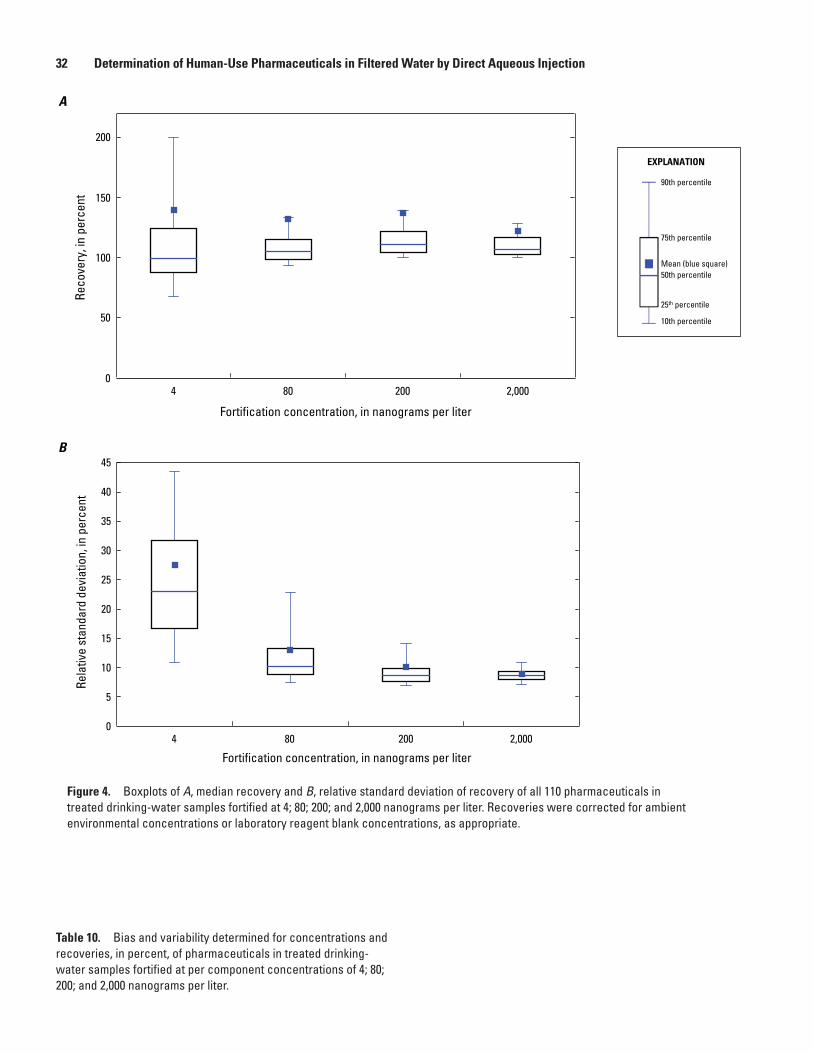
32 Determination of Human-Use Pharmaceuticals in Filtered Water by Direct Aqueous Injection
Figure 4. Boxplots of A, median recovery and B, relative standard deviation of recovery of all 110 pharmaceuticals in treated drinking-water samples fortified at 4; 80; 200; and 2,000 nanograms per liter. Recoveries were corrected for ambient environmental concentrations or laboratory reagent blank concentrations, as appropriate.
90th percentile
75th percentile
Mean (blue square) 50th percentile
25th percentile
10th percentile
EXPLANATION
4 80 200 2,0000
50
100
150
200
Reco
very
, in
perc
ent
Fortification concentration, in nanograms per liter
A
B
4 80 200 2,0000
5
10
15
20
25
30
35
40
45
Rela
tive
stan
dard
dev
iatio
n, in
per
cent
Fortification concentration, in nanograms per liter
Table 10. Bias and variability determined for concentrations and recoveries, in percent, of pharmaceuticals in treated drinking-water samples fortified at per component concentrations of 4; 80; 200; and 2,000 nanograms per liter.

Results and Discussion of Method Validation 33
Figure 5. Boxplots of A, median recovery and B, relative standard deviation of recovery of all 110 pharmaceuticals in surface-water samples fortified at 4; 80; 200; and 2,000 nanograms per liter. Recoveries were corrected for ambient environmental concentrations or laboratory reagent blank concentrations, as appropriate.
90th percentile
75th percentile
Mean (blue square) 50th percentile
25th percentile
10th percentile
EXPLANATION
4 80 200 2,0000
50
100
150
200
250
Reco
very
, in
perc
ent
Fortification concentration, in nanograms per liter
4 80 200 2,0000
10
20
30
40
50
60
70
80
Rela
tive
stan
dard
dev
iatio
n, in
per
cent
Fortification concentration, in nanograms per liter
B
A
Table 11. Bias and variability determined for concentrations and recoveries, in percent, of pharmaceuticals in surface-water samples fortified at per component concentrations of 4; 80; 200; and 2,000 nanograms per liter.

34 Determination of Human-Use Pharmaceuticals in Filtered Water by Direct Aqueous Injection
interquartile range calculated from the results in table 11 and displayed in the boxplots shown in figure 5A. Similar to the treated drinking-water fortifications, the widest interquartile range, 80.3 percent, occurred at the lowest fortification of 4 ng/L. A narrower spread in median recoveries, as reflected in the interquartile range, is observed at higher fortifications: 24.8, 40.5, and 38.3 percent for the fortifications of 80; 200; and 2,000 ng/L, respectively.
At these higher fortifications, the interquartile ranges are wider than those observed for treated drinking water at these same fortifications. This likely reflects the varying effect of surface-water sample matrix on quantitation and thus recov-ery calculations. Correction for ambient concentration in the unfortified surface-water sample likely is of secondary impor-tance because 10 percent of the recoveries at each fortification (11 of 110 pharmaceuticals) are corrected for ambient contri-butions. Also, the mean concentrations of those pharmaceuti-cals observed in ambient environmental samples are low, with a median concentration of 1.8 ng/L and a maximum concentra-tion of 33.4 ng/L.
The distributions of RSDs of recovery, as indicated by the interquartile ranges shown in the boxplots of figure 5B, are widest at the 4-ng/L fortification and decrease dramatically in the 80-; 200-; and 2,000-ng/L fortifications. The dramatic decrease in magnitude and range of RSDs of recovery at the higher fortifications indicates that the precision of the determi-nation of most pharmaceuticals was quite acceptable, except very close to the lowest range of the method calibration, near the method detection limit (MDL), as would be expected (Childress and others, 1999).
Wastewater EffluentStatistical summaries of the recovered pharmaceutical
concentrations and the calculated recoveries from wastewa-ter effluent at all fortifications are contained in table 12 and plotted in figure 6. As observed with unfortified domestic-well groundwater, community-well groundwater, treated drinking water, and surface-water samples, unfortified wastewater-effluent samples contained detectable concentrations of pharmaceuticals (table 12). However, as expected, wastewater effluent contained more of the pharmaceuticals determined by this method and at higher concentrations than observed in surface water. Of the 110 pharmaceuticals determined by this method, 62 were detected in at least two of the three unforti-fied wastewater-effluent samples used for validation, with a median concentration of the detected pharmaceuticals of 4.7 ng/L. The 25th and 75th percentiles of these concentrations were 1.7 and 21.9 ng/L, respectively. These two quartiles define the middle 50 percent of concentrations (interquartile range) in this wastewater effluent and as such, approximate the range of concentrations of pharmaceuticals likely present in this matrix. A few compounds were detected at relatively high concentrations and this is reflected in the disparity between the mean concentration, at 41.4 ng/L, and the much lower median concentration of 4.7 ng/L. The maximum concentration
detected for any pharmaceutical in this wastewater effluent was 865 ng/L for metformin. Similar to the fortification results for the surface-water validation, the mean concentration of each pharmaceutical detected in at least two of three unforti-fied wastewater-effluent samples was subtracted from the forti-fied concentrations at each fortification level for each of the 62 detected pharmaceuticals prior to determining recovery.
Similar to the surface-water fortifications, the widest range of recoveries for the wastewater effluent was at the low-est fortification, with more uniform recoveries at higher fortifi-cations (fig. 6A). The grand medians of median recovery were 126, 117, 108, and 109 percent at fortifications of 4; 80; 200; and 2,000 ng/L, respectively. These grand medians are similar to those of the fortified samples of community supply ground-water, drinking water, and surface water; the grand medians are lower than the somewhat elevated grand medians of recovery observed in the fortified sample of domestic supply ground-water, and are similar to the corresponding grand median recoveries of reagent water (138, 93.3, 103, and 110 percent at fortifications of 4; 80; 200; and 2,000 ng/L, respectively).
The grand medians of RSDs of recovery from wastewater effluent were 34.2, 15.3, 18.1, and 7.8 percent at respective fortifications of 4; 80; 200; and 2,000 ng/L; this is similar to other matrixes, including those of reagent water (grand medi-ans of RSDs of recovery of 57.3, 13.6, 7.6, and 12.6 percent at fortifications of 4; 80; 200; and 2,000 ng/L, respectively). The overall similarities in the medians of RSDs of recoveries between the 80- and 2,000-ng/L fortifications in wastewater effluent are likely reflective of compound-specific precision in the instrumental analysis and indicate that at fortifications of 80 ng/L or greater, quantitation of individual pharmaceuticals in replicate effluent samples are acceptably (within 25 percent) precise. As noted for other matrixes, the largest range in distribution of RSDs of recovery was for the 4-ng/L fortifica-tion, with a substantial decrease in the absolute range of RSDs and a lower overall distribution of RSDs at fortifications of 80; 200; and 2,000 ng/L (fig. 6B).
With the exception of the 4-ng/L fortification, the inter-quartile ranges of median recoveries observed in wastewater effluent were relatively narrow (fig. 6A), between 20 and 30 percent, indicating that at fortifications of 80 ng/L or greater, recoveries of most pharmaceuticals were relatively uniform. The median recoveries were just greater than 100 percent, which indicate minimal matrix enhancement or suppression. The wide interquartile range of 94 percent for the 4-ng/L forti-fication is considered to be a result of the imprecision intro-duced by background correction when determining recoveries, as well as overall greater variability expected at this lower concentration fortification, which is near or below the IRL for several method pharmaceuticals. The ambient environmental concentrations of pharmaceuticals in the unfortified wastewa-ter effluent samples frequently were similar to or greater than the fortification concentration, and the subtraction of a mean value from single concentrations of individual analytes may exacerbate imprecision. Also, in the 4-ng/L fortification, 83 pharmaceuticals were quantified of the 110 pharmaceuticals

Results and Discussion of Method Validation 35
Figure 6. Boxplots of A, median recovery and B, relative standard deviation of recovery of all 110 pharmaceuticals in wastewater-effluent samples fortified at 4; 80; 200; and 2,000 nanograms per liter. Recoveries were corrected for ambient environmental concentrations or laboratory reagent blank concentrations, as appropriate.
90th percentile
75th percentile
Mean (blue square) 50th percentile
25th percentile
10th percentile
EXPLANATION
4 80 200 2,0000
50
100
150
200
250
300
350
400
450
500
Reco
very
, in
perc
ent
Fortification concentration, in nanograms per liter
A
4 80 200 2,0000
10
20
30
40
50
60
70
80
Rela
tive
stan
dard
dev
iatio
n, in
per
cent
Fortification concentration, in nanograms per liter
B
Table 12. Bias and variability determined for concentrations and recoveries, in percent, of pharmaceuticals in wastewater-effluent samples fortified at per component concentrations of 4; 80; 200; and 2,000 nanograms per liter.

36 Determination of Human-Use Pharmaceuticals in Filtered Water by Direct Aqueous Injection
Figure 7. Boxplots of median recovery plotted in A, logarithmic scale and B, arithmetic scale; and C, relative standard deviation of recovery of all 110 pharmaceuticals in wastewater-influent samples fortified at 4; 80; 200; and 2,000 nanograms per liter. Recoveries were corrected for ambient environmental concentrations or laboratory reagent blank concentrations, as appropriate.
4 80 200 2,0000
500
1,000
1,500
2,000
2,500
3,000
3,500
4,000
Reco
very
, in
perc
ent
Fortification concentration, in nanograms per liter
B
90th percentile
75th percentile
Mean (blue square) 50th percentile
25th percentile
10th percentile
EXPLANATION
4 80 200 2,0001
10
100
1,000
4,000
Reco
very
, in
perc
ent
Fortification concentration, in nanograms per liter
A
Table 13. Bias and variability determined for concentrations and recoveries, in percent, of pharmaceuticals in wastewater-influent samples fortified at per component concentrations of 4; 80; 200; and 2,000 nanograms per liter.

Results and Discussion of Method Validation 37
determined using this method. At this low fortification, most of the 27 unquantifiable pharmaceuticals were so because of non-specific chemical interferences that obscured at least one of each pharmaceutical’s MRM transitions.
Wastewater InfluentWastewater influent is among the most complex sample
matrixes likely to be analyzed with this method. Statistical summaries of the recovered pharmaceutical concentrations and the calculated recoveries from wastewater influent at all forti-fications are contained in table 13 and plotted in figure 7. As expected, unfortified wastewater-influent samples contained sub-stantial detectable concentrations of pharmaceuticals (table 13). The wastewater-influent samples contained detectable concentra-tions of 104 of 110 pharmaceuticals determined in this method. The median concentration detected was 86.5 ng/L, and the maximum concentration detected of any one pharmaceutical was 65,900 ng/L (estimated) for caffeine. The 25th percentile of con-centrations was 11.8 ng/L, and the 75th percentile of concentra-tions was 397 ng/L; this resulted in an interquartile range of 385 ng/L. These results indicate that 76 of the 105 pharmaceuticals detected had a measurable concentration greater than 12 ng/L; thus, with the possible exception of the 2,000 ng/L fortification, corrections for ambient pharmaceutical contributions likely substantially affected the precision of recoveries calculated at all fortifications of wastewater influent.
The grand medians of median recovery of all pharma-ceuticals from wastewater influent were 207, 100, 105, and
123 percent at fortifications of 4; 80; 200; and 2,000 ng/L, respectively. The recoveries at all fortifications varied more for wastewater influent than for other matrixes, as reflected by the spread of the recoveries displayed in the boxplots of median recovery (figs. 7A and 7B) and as indicated quantitatively by the quartiles of median recovery calculated from the results in table 13. The 25th percentiles of median recovery from waste-water influent were 104, 83.7, 86.5, and 107 percent at fortifi-cations of 4; 80; 200; and 2,000 ng/L, respectively. The 75th percentiles of recovery were 592, 145, 131, and 142 percent at fortifications of 4; 80; 200; and 2,000 ng/L, respectively. The resulting interquartile ranges, calculated from unrounded results, are 488, 61.2, 44.1, and 35.1 percent at fortifications of 4; 80; 200; and 2,000 ng/L, respectively.
The grand median of RSDs of recovery were 57.8, 34.5, 12.4, and 29.5 percent at fortifications of 4; 80; 200; and 2,000 ng/L, respectively (fig. 7C ), indicating that quantitation and thus calculated precision were lowest at the lowest fortifica-tion and improved at higher fortifications. The overall higher median RSDs of recovery observed at the 4 and 80 ng/L forti-fications reflect variation that is not acceptable for many ana-lytes; however, this unacceptable variation is more reflective of the difficulty in accurately correcting for ambient pharma-ceutical contributions to the fortified sample than of inherent method precision. For this matrix, the ambient precision of the method as applied to wastewater influent is more accurately reflected by the replicate analyses of the unfortified samples (table 13). The mean, median, 25th percentile, and 75th percentile of the RSD of concentration of all pharmaceuticals
Figure 7. Boxplots of median recovery plotted in A, logarithmic scale and B, arithmetic scale; and C, relative standard deviation of recovery of all 110 pharmaceuticals in wastewater-influent samples fortified at 4; 80; 200; and 2,000 nanograms per liter. Recoveries were corrected for ambient environmental concentrations or laboratory reagent blank concentrations, as appropriate.—Continued
90th percentile
75th percentile
Mean (blue square) 50th percentile
25th percentile
10th percentile
EXPLANATION
4 80 200 2,0000
10
20
30
40
50
60
70
80
90
100
Rela
tive
stan
dard
dev
iatio
n, in
per
cent
Fortification concentration, in nanograms per liter
C

38 Determination of Human-Use Pharmaceuticals in Filtered Water by Direct Aqueous Injection
detected in at least two of three unfortified samples were 22.2, 11.6, 6.28, and 28.0 percent, respectively. This level of preci-sion is acceptable for assessing concentration, particularly for such a complex and heterogeneous sample matrix.
Overall, the recovery results indicate the difficulty in accurately and precisely determining recovery for many phar-maceuticals in wastewater influent at all levels of fortification. In addition, the complex concentrated mixture of organic and inorganic constituents present in wastewater influent also may result in matrix enhancement or suppression of individual phar-maceutical response or in nonspecific chemical interferences that may preclude accurate quantitation. Of the 110 pharma-ceuticals determined by this method, detections and quantifica-tions were made of 82, 108, 106, and 109 pharmaceuticals at fortifications of 4; 80; 200; and 2,000 ng/L, respectively. The inability to detect 28 pharmaceuticals at the lowest fortifica-tion and at least one other pharmaceuticals at higher fortifica-tions indicates that nonspecific chemical interferences may hinder detection in complex matrixes like wastewater influent. Nevertheless, the results in table 13 and figure 7 indicate that although achieving acceptable quantitative bias and variability in wastewater influent is very challenging, at least as reflected by low-concentration fortifications, acceptable results can be produced for many pharmaceuticals, particularly at concentra-tions corresponding to the higher fortifications used.
Complex Matrixes and Blank SamplesThe validation results presented previously in this section
for complex sample matrixes (such as wastewater effluent and influent) strongly indicate the need to routinely prepare and analyze laboratory matrix spike (LMS) samples fortified at higher concentrations. These LMS samples can provide crucial method-performance information to support interpretation of detected pharmaceutical concentrations. Fortification at higher concentrations is necessary because these matrixes contribute substantial concentrations of ambient pharmaceuticals, as well as nonspecific chemical interferences, to the analysis. Despite the presence of ambient pharmaceuticals in unfortified samples and other effects of matrix interferences in these complex samples, many pharmaceuticals fortified in wastewater effluent and influent (even at the 4-ng/L level) were detected and had quantifiable concentrations with acceptable bias and variability at the three higher fortifications in effluent and at the highest fortification in influent. This demonstrates the robustness of the direct aqueous injection–HPLC/MS/MS method in the pres-ence of challenging environmental water samples.
Complex sample matrixes also may contaminate the HPLC/MS/MS system if the high concentrations of pharmaceu-ticals, nonspecific sample interferences, and other sample matrix components are insufficiently swept from the interior surfaces of the instrument by routine washing procedures and operations incorporated into the method. The analytical protocol described herein has substantial safeguards to ensure that the surfaces to which the sample aliquot is exposed are adequately washed. Table 1–1 in the appendix documents the wash conditions used
in this method, which are based on the manufacturer’s recom-mendations. Nevertheless, blank QC samples interspersed within the analytical sequence (table 5) are necessary to allow monitoring and correction of potential contamination from highly complex sample matrixes. Table 14 contains results for pharmaceuticals that were detected in at least 3 of 80 blank samples (6 LRB and 74 CCB samples) analyzed in multiple sets. Note that these sample sets included a series of complex sample matrixes (primarily wastewater effluent) and that the CCBs were immediately preceded by a CCV sample. These results were used to qualify results as noted in sections 10.2 and 10.5. These results demonstrate the potential for within-instrument blank contamination and the necessity of using CCB sample results to qualify environmental sample results. Current (2014) NWQL practice is to treat field blank samples (sections 2 and 4) identically to environmental samples during all aspects of sample analysis and data review, and thus field blank sample results are qualified by comparison to LRB and CCB sample results using the same criteria as environmental samples. Data treatment practices and result reporting conventions for labora-tory and field blank samples are under active development at the NWQL and will evolve as better statistical and interpretive understanding of laboratory and field blank results develop.
The results in table 14 indicate the need for detailed evalu-ation of blank samples to ensure that environmental sample detections are not reported when instrument contamination from complex, high-concentration samples may be particularly difficult to control. Sixty-four pharmaceuticals were detected at least three times in the 80 blank samples. The median number of pharmaceuticals detected was 9; the 25th and 75th percentiles of detections, describing the interquartile range, were 5 and 20, respectively. Although frequently detected, the mean concentra-tion of any individual pharmaceutical typically was low. The median of the mean concentrations measured was 2.96 ng/L; the 25th and 75th percentiles of the mean concentrations measured were 1.28 and 6.10 ng/L, respectively. Thus, detailed evalua-tion of blank samples is necessary when using this method, and a protocol similar to the automated blank evaluation protocol described in section 10.5 is necessary to ensure that false posi-tive detections attributable to carryover or other contamination in the HPLC/MS/MS system are avoided.
Reporting LimitsMethod detection limits (MDLs) were determined for
this method using the procedures of the U.S. Environmen-tal Protection Agency (2005). The MDL is defined as the
Table 14. Frequency of detection of method pharmaceuticals in 80 blank samples determined by this method after analysis of a set of complex matrix samples. Individual pharmaceuticals are listed from most frequently detected to the least frequently detected. A pharmaceutical is listed if it was detected in a minimum of three blank samples.

Reporting Limits 39
minimum concentration of a substance that can be measured and reported with 99-percent confidence that the com-pound concentration is greater than zero. Initial MDLs were determined from eight replicate analyses of reagent-water samples of 1-mL volume. The range of response to electro-spray ionization necessitated iteratively estimating the MDL by fortifying at one concentration, evaluating the results according to the requirements outlined in U.S. Environmen-tal Protection Agency (2005), and then conducting the MDL experiment at lower or higher fortifications as needed. For this method, eight iterative fortifications at concentrations from 4 to 400 ng/L were required.
The MDL was calculated using the following equation (U.S. Environmental Protection Agency, 2005):
MDL = S × t(n–1, 1–α = 0.99) (5)
where S is standard deviation of replicate
analyses, in nanograms per liter; n is number of replicate analyses; and
t(n–1, 1–α = 0.99) is Student’s t-value for the 99-percent confidence level with n–1 degrees of freedom.
According to the EPA procedure, at least seven replicate samples are fortified with compounds at concentrations of two to five times the estimated MDL. For the MDL deter-mination, reagent water fortified at eight concentrations (4, 10, 20, 40, 80, 100, 200, and 400 ng/L) in sets of 7 replicate samples were used. After evaluating the results from each fortification, the appropriate fortification for determin-ing the MDL for each pharmaceutical was identified on a pharmaceutical-by-pharmaceutical basis, based on the guidance in U.S. Environmental Protection Agency (2005). This allowed for the selection of results that met the EPA’s criteria of fortifying at two to five times the anticipated MDL, taking into account the compound-specific response for each pharmaceutical. The resulting MDLs determined for this method are presented in table 15, as are the IRLs, which are at least two times the MDL. The factor of two times the MDL used to derive an IRL was adopted by the NWQL because it reduces the risk of reporting false positives, as was noted by Childress and others (1999) in their development of long-term method reporting levels. However, the data used for calculating the IRL, that is, seven replicates from a single instrument used to determine the MDL, differ from the data used in the approach of Childress and others (1999), which are a larger data set, typically 30 or more samples, collected from multiple instruments and operators, and, ideally, are collected over a one-year period. Some pharmaceutical IRLs were adjusted to greater than two times the MDL to reflect consistently lower instrument response.
The MDLs also are displayed in figure 8, ordered from the lowest to highest concentration. The MDLs for method pharmaceuticals range from 0.45 ng/L for diazepam to 94.1 ng/L for phenytoin, primarily as a result of the inherent ion-ization efficiency of each pharmaceutical in the electrospray
ionization process; the median MDL for all pharmaceuticals is 5.38 ng/L. As defined by the 25th and 75th percentiles, most of the MDLs for this method are between 2.83 and 18.0 ng/L, an interquartile range of 15.2 ng/L. The goal for this method was to provide sensitivity such that the MDLs for most of the pharmaceuticals would be less than 50 ng/L, a level shown graphically in figure 8 with a dashed red line. For this method only 8 of the 110 pharmaceuticals deter-mined had MDLs greater than 50 ng/L. Overall, these MDLs are similar to the MDLs calculated for the previous USGS method used for determining pharmaceuticals (Furlong and others, 2008), where the MDLs for 17 pharmaceuticals ranged from 6.9 ng/L to 14.2 ng/L; the median MDL for 17 pharmaceuticals determined in that method was 10.7 ng/L.
The MDLs and IRLs listed in table 15 are a statisti-cally defined metric for method quantitative sensitivity. The MDLs are based upon the standard deviation (that is, the variability) of quantitation of a pharmaceutical in at least seven replicate samples fortified at a concentration near the limit of the HPLC/MS/MS system’s capability to accurately identify that pharmaceutical (U.S. Environmental Protec-tion Agency, 2005). The observation that in routine use of an information-rich method–such as direct aqueous injec-tion–HPLC/MS/MS–qualitatively identified compounds can be quantified at concentrations less than the IRL or MDL is addressed by Childress and others (1999). Qualitatively identified compounds for which calculated concentra-tions are less than the IRL are reported as estimated and noted with the “E” remark code because this method is an “information-rich” method, as are other mass spectrometry methods the NWQL provides (Childress and others, 1999). These estimated concentrations below reporting levels provide a richer dataset that may be explored to understand environmental distributions with greater accuracy (Helsel, 2010) and are superior to substitutions for censored values, as long as all qualitative identification criteria used for mass spectral methods are met. Estimated concentrations below reporting levels also provide important informa-tion about the distribution of environmental concentrations that can be used to improve analytical methods. Pharma-ceutical concentrations that are less than 10 percent of the MDL are not reported due to the increased variability observed as peak areas decrease, as well as the difficulty operators observe in reliably distinguishing typical instru-ment responses for most pharmaceuticals from background instrument noise. As described herein, the well-defined use of qualitatively identified pharmaceutical detections for which concentrations are less than the MDL provides results that better address the USGS’s requirement to provide objective information describing the quality and quantity of the Nation’s water resources.
Table 15. Method detection limits and interim reporting levels, in nanograms per liter, for pharmaceuticals determined in this method.

40
Determination of Hum
an-Use Pharmaceuticals in Filtered W
ater by Direct Aqueous Injection
Diaz
epam
Glyb
urid
eTh
iabe
ndaz
ole
Carb
amaz
epin
eVe
nlaf
axin
eFlu
ticas
one
prop
iona
teCh
lorp
heni
ram
ine
Albu
tero
lFe
nofib
rate
Cotin
ine
Cita
lopr
amLo
rata
dine
Fadr
ozol
eHy
drox
yzin
ePi
pero
nyl b
utox
ide
Dext
rom
etho
rpha
n10
-Hyd
roxy
-am
itrip
tylin
eNo
rver
apam
ilHy
droc
odon
eFa
mot
idin
eNo
reth
indr
one
Desm
ethy
ldilt
iaze
mCa
risop
rodo
lTr
iam
tere
neAt
enol
olPh
enaz
opyr
idin
eM
orph
ine
Omep
razo
le +
eso
mep
razo
leDi
phen
hydr
amin
eOs
elta
miv
irW
arfa
rinNe
virap
ine
Tram
adol
Lidoc
aine
Vera
pam
ilLa
mivu
dine
Sertr
alin
ePr
opox
yphe
neAc
etam
inop
hen
Bupr
opio
nDe
sven
lafa
xine
Trim
etho
prim
Met
hado
neFe
xofe
nadi
neAm
phet
amin
eAb
acav
irPa
roxe
tine
Alpr
azol
amM
etho
carb
amol
Acyc
lovir
Pent
oxify
lline
Ralo
xife
neDe
hydr
onife
dipi
neOx
ycod
one
Dilti
azem
Fluo
xetin
ePs
eudo
ephe
derin
e +
ephe
drin
eCi
met
idin
eLo
pera
mid
eM
etfo
rmin
Dulo
xetin
eM
etax
alon
eBe
nztro
pine
Penc
iclo
vir
Theo
phyll
ine
Tiot
ropi
umTe
maz
epam
Niza
tidin
eAt
razin
ePr
omet
hazin
eTa
mox
ifen
Met
hotre
xate
Ezet
imib
eSu
lfam
etho
xazo
lePr
opra
nolo
lM
etop
rolo
lPh
endi
met
razin
eQu
inin
eN
adal
olM
epro
bam
ate
Glip
izide
1,7-D
imet
hylxa
nthi
neCa
ffein
eAm
itrip
tylin
eSi
tagl
iptin
Nord
iaze
pam
Sulfa
met
hizo
leOr
lista
tEr
ythr
omyc
inFl
uvox
amin
eOx
azep
amM
ethy
l-1H-
benz
otria
zole
Nico
tine
Hydr
ocor
tison
eCl
onid
ine
Vala
cycl
ovir
Sulfa
dim
etho
xine
Fluco
nazo
leNo
rser
tralin
eRa
nitid
ine
Norfl
uoxe
tine
Code
ine
Keto
cona
zole
Beta
met
haso
neAn
tipyr
ine
Lora
zepa
mIm
inos
tilbe
nePr
edni
solo
nePr
edni
sone
Phen
ytoi
n
0.1
1
10
100
Met
hod
dete
ctio
n lim
it, in
nan
ogra
ms
per l
iter
Compound
Method Development Goal
Figure 8. Method detection limits (MDLs), in nanograms per liter, calculated from seven replicate reagent-water analyses.

Sample Holding-Time Study 41
90th percentile
75th percentile
Mean (blue square) 50th percentile
25th percentile
10th percentile
EXPLANATION
Day 1 M
edian Recovery
Day 1 RSD of R
ecovery
Day 9 M
edian Recovery
Day 9 RSD of R
ecovery
Day 23 M
edian Recovery
Day 23 R
SD of Recove
ry
Day 30 M
edian Recovery
Day 30 R
SD of Recove
ry0
20
40
60
80
100
120Re
cove
ry o
r RSD
, in
perc
ent
Figure 9. Median recovery and relative standard deviation (RSD) of recovery of all 110 pharmaceuticals from surface water fortified at 2,000 nanograms per liter; stored at 4 degrees Celsius; and analyzed at 1, 9, 23, and 30 days after fortification. Recoveries have been corrected for ambient environmental concentrations or laboratory reagent blank concentrations, as appropriate.
Sample Holding-Time StudyA sample holding-time study was conducted using filtered surface water fortified at 2,000 ng/L. Eight replicate samples were prepared and stored at 4 °C. The samples were then periodically removed from refrigeration and analyzed at 1, 9, 23, and 30 days after fortification. Table 16 contains a summary of the mean, median, standard deviation, and RSD of recovery for each pharmaceutical on each day of analysis. The results indicate that overall pharmaceutical recoveries become more variable by day 9, but remain about the same through days 23 and 30.
Distributions of median recovery and RSD of recovery at 1, 9, 23, and 30 days after fortification are summarized as boxplots in figure 9. From these results, overall recoveries remain approximately the same between days 1 and 9 (median of median recovery of 90.8 and 99.4 percent, respectively), then drop to approximately the same level on days 23 and 30 (73.0 and 69.4 percent, respectively). For a subset of phar-maceuticals determined, figure 10 illustrates the first-order
decay function that best fit the results for most pharmaceu-ticals, based on the coefficient of determination (R2) of the curve type, calculated using the curve-fitting capabilities of the Deltagraph™ scientific plotting software program. A relatively consistent decay in recovered concentration occurs over the 30 days of the holding-time study for the subset of pharmaceuticals plotted, regardless of the starting point of recovery. This first-order decay was consistent for most of the pharmaceuticals determined. This pattern of decrease over the 30 days of the holding-time study also is reflected in figure 11, where percent median losses between days 1 and 9, days 1 and 23, and days 1 and 30 are displayed as boxplots. Individual pharmaceutical median recoveries also are variable over time, as indicated by the spread of the boxplots and quantified in the interquartile range for the data in each boxplot (fig. 9); the interquartile ranges were 6.84, 22.0, 23.5, and 18.8 percent on days 1, 9, 23, and 30, respectively.
The greater variability in recoveries from days 9, 23, and 30, as reflected in the boxplots of median recover-ies in figure 9, could result from variability of recovery

42 Determination of Human-Use Pharmaceuticals in Filtered Water by Direct Aqueous Injection
60
70
80
90
100
110
120
0 5 10 15 20 25 30 35
Reco
very
, in
perc
ent
Elapsed time, in days
1,7-Dimethylxanthine
10-Hydroxy-amitriptyline
Abacavir
Caffeine
Carbamazepine
Bupropion
EXPLANATION
Figure 10. First-order decay curves fitted to recoveries, in percent, of selected pharmaceuticals measured in the holding-time study.
Table 16. Recovery of pharmaceuticals from filtered surface water fortified at 2,000 nanograms per liter and held at 4 degrees Celsius over a 30-day period for a sample holding-time study.

Sample Holding-Time Study 43
90th percentile
75th percentile
Mean (blue square) 50th percentile
25th percentile
10th percentile
EXPLANATION
Between day 1
and day 9
Between day 1
and day 23
Between day 1
and day 30
–20
–10
0
10
20
30
40M
edia
n of
per
cent
loss
Loss between days of holding time study
Figure 11. Boxplots of median loss of all 110 pharmaceuticals from surface water fortified at 2,000 nanograms per liter; stored at 4 degrees Celsius; and analyzed at 1, 9, 23, and 30 days after fortification. Recoveries have been corrected for ambient environmental concentrations or laboratory reagent blank concentrations, as appropriate.
for individual pharmaceuticals among the eight replicates analyzed. The apparently uniform distribution of RSDs of recovery across the holding-time study (as reflected in the boxplots of RSDs of recovery in fig. 9) indicates that recov-ery from the eight replicates at any point during the holding-time study remained relatively constant. No replicate-specific variability appears to contribute to the spread in median recoveries after day 1 of the holding-time study; this indi-cates that the variation observed in median recoveries results from variation in the recovery of individual pharmaceuticals. Pharmaceutical-specific differences in recovery also are reflected in the array of decay curves fitted to a selected set of pharmaceuticals in figure 10. Note that the distribution of median percent loss of the 110 pharmaceuticals deter-mined was widest between days 1 and 9 (fig. 11), although there was no significant median loss, and perhaps a slight increase, between days 1 and 9. The distribution of median losses between days 1 and 23 and between days 1 and 30 are narrower, as reflected in the spread of the boxplots (fig. 11), although the median of the percent loss for these intervals
was higher. These results indicate that pharmaceutical losses during sample holding were most likely to happen between days 9 and 23, with smaller losses during subsequent storage.
On the basis of results of the holding-time study, filtered samples, shipped to the laboratory on ice and stored at 4 °C, should be analyzed no later than 9 days from collection, preferably within 4 days, to ensure that sample results are minimally affected by degradation. The holding-time study also indicates that for most of the pharmaceuticals, accept-able results can be obtained from prepared samples stored at 4 °C for as long as 30 days. This period is substantially longer than prepared samples are held in the chilled autosampler of the HPLC/MS/MS, even when sample sets are combined into larger analytical batches. Currently (2014), the effect of long-term storage of filtered samples at temperatures of –20 °C is being determined by the NWQL to assess the loss of pharmaceuticals from samples held from months to years. This long-term study will identify conditions appropriate for holding samples in an archive for later analysis by this or other comparably performing methods.

44 Determination of Human-Use Pharmaceuticals in Filtered Water by Direct Aqueous Injection
Summary and ConclusionsThe U.S. Geological Survey (USGS) National Water Qual-
ity Laboratory has developed an analytical method for the deter-mination of 110 human-use pharmaceuticals in filtered aqueous samples, including groundwater, surface water, treated drinking water, and wastewater influent and effluent. Direct aqueous injection of a filtered sample aliquot with analysis using high-performance liquid chromatography/tandem mass spectrometry in the dynamic multiple reaction monitoring mode selectively and sensitively detects these compounds at the expected ambi-ent environmental concentrations, in the range between 1 and 1,000 nanograms per liter (ng/L). This method provides an efficient means of detecting and quantifying pharmaceutically active compounds that typically might not be reported because they are unregulated or not included in other official methods used by the USGS, U.S. Environmental Protection Agency, American Water Works Association, or other agencies.
In this method, the concentrations of 110 pharmaceuticals are reported; four of these pharmaceuticals are reported as two pairs because they are structural isomers and are not separable under the analytical conditions used. Concentrations of some qualitatively identified pharmaceuticals may be reported as estimates or potentially affected by cross contamination based on set- and sample-specific observation of suboptimal recov-ery or potential carryover from highly contaminated samples, as reflected in laboratory reagent spike recoveries or continu-ing calibration blank monitoring, respectively.
The pharmaceuticals in this method are representative of a range of pharmacologically active compound classes that are reflective of contemporary prescribing and human-use patterns. Because human wastewater is an important source for these compounds to surface or groundwater, this method complements other official methods of the USGS that measure wastewater indicators in water, such as ethoxylate surfactants, fragrances, food additives, antioxidants, phosphate flame retardants, plasti-cizers, industrial solvents, disinfectants, and fecal sterols.
The pharmaceuticals are separated by using a reversed-phase gradient of formic acid/ammonium formate-modified water and methanol. The pharmaceuticals of interest are determined by analyzing a filtered 100-microliter aliquot of the sample by high-performance liquid chromatography/tan-dem mass spectrometry using positive electrospray ionization operated in the dynamic multiple reaction monitoring mode to reduce chemical noise and to improve specificity. Multiple reaction monitoring (MRM) of two fragmentations of the pro-tonated molecular ion of each pharmaceutical to two unique product ions was used to identify each pharmaceutical quali-tatively. The primary MRM precursor-product ion transition was quantified for each pharmaceutical relative to the primary MRM precursor-product transition of 1 of 19 isotope-dilution standard pharmaceuticals or the pesticide atrazine, using an exact stable isotope analogue where possible. Each isotope-dilution standard was selected, when possible, for its chemical similarity to the unlabeled pharmaceutical of interest and was added to the sample after filtration but prior to analysis.
The method performance for each pharmaceutical was determined for reagent water, groundwater, treated drink-ing water, surface water, and treated wastewater effluent and wastewater influent sample matrixes that this method will likely be applied to. Each matrix was evaluated in order of increasing complexity to demonstrate the sensitivity of the method in different water matrixes and the effect of sample matrix on the quantitative determination of pharmaceutical concentrations. The single-operator median recovery for all pharmaceuticals in organic-free reagent water samples forti-fied at nine concentrations between 40 and 8,000 ng/L ranged from 89.6 to 110 percent. The median standard deviation of recovery from reagent-water samples fortified at 9 concen-trations between 40 and 8,000 ng/L ranged from 4.5 to 19.9 percent. Pharmaceutical recoveries were more variable in surface-water, wastewater-effluent, and wastewater-influent samples than in reagent-water, groundwater, or drinking-water samples. This reflects matrix enhancement or suppression affecting electrospray ionization, co-occurring non-specific chemical interferences, and the presence of ambient contribu-tions of method pharmaceuticals that complicated recovery calculation. However, the single-operator, single-instrument validation data, and quality-control data reported here provide strong evidence for the application of high-performance liquid chromatography/tandem mass spectrometry to large-scale, routine monitoring programs for pharmaceuticals in surface water, groundwater, treated drinking water, and wastewater effluent and influent for environmental concentrations as low as or less than 10 ng/L (10 parts per trillion).
The method detection limits and interim reporting levels for the pharmaceuticals determined by this method were cal-culated from recoveries of pharmaceuticals in reagent-water samples fortified at several concentrations, and ranged from 0.45 to 94.1 ng/L; the median method detection limit for all pharmaceuticals is 5.38 ng/L. Unless set-specific blank, spike, or other quality-control results indicate otherwise, the con-centrations of 110 pharmaceuticals in environmental samples are reported by National Water Quality Laboratory without qualification. Pharmaceutical concentrations that are less than 10 percent of the method detection limit are not reported because, at this concentration, typical instrument responses for most pharmaceuticals cannot be reliably distinguished from background instrument noise.
Holding-time studies were conducted for water samples and water-sample extracts. Results from the water sample holding-time study indicate that samples should be stored at 4 degrees Celsius and analyzed within 9 days of collection to ensure that sample results are minimally affected by degrada-tion. Freezing samples to provide for storage for longer peri-ods currently (2014) is under evaluation. The water-sample extract holding-time study revealed that for most pharmaceuti-cals, acceptable results can be obtained from extracts stored at 4 degrees Celsius for as long as 30 days.
This report documents the effects of sample matrixes upon the quantitative results for pharmaceuticals determined by this method. Thus, laboratory matrix-spike samples

References Cited 45
collected from representative water types within a study can provide critical insight for assessing water type-specific matrix effects upon the results from environmental water samples col-lected to determine the presence and distribution of pharma-ceuticals. These laboratory matrix-spike samples are collected and analyzed in addition to replicate water samples and field equipment blank samples and their inclusion is an important consideration for a study’s quality-control plan.
References Cited
Abonnenc, Mélanie, Qiao, Liang, Liu, BaoHong, and Girault, H.H., 2010, Electrochemical aspects of electrospray and laser desorption/ionization for mass spectrometry: Annual Review of Analytical Chemistry, v. 3, p. 231–254. (Also available at http://dx.doi.org/10.1146/annurev.anchem.111808.073740.)
American Medical Association, 2012, United States adopted names: Chicago, Ill., American Medical Association, accessed October 17, 2012, at http://www.ama-assn.org/ama/pub/physician-resources/medical-science/united-states-adopted-names-council.page.
Ardrey, R.E., 2003, Liquid chromatography-mass spectrom-etry—An introduction: Chichester, West Sussex, England, John Wiley and Sons, Limited, 276 p.
Batt, A.L., Kostich, M.S., and Lazorchak, J.M., 2008, Analysis of ecologically relevant pharmaceuticals in wastewater and surface water using selective solid-phase extraction and UPLC-MS/MS: Analytical Chemistry, v. 80, no. 13, p. 5021–5030. (Also available at http://dx.doi.org/10.1021/ac800066n.)
Benijts, Tom, Dams, Riet, Lambert, Willy, and De Leenheer, André, 2004, Countering matrix effects in environmental liquid chromatography-electrospray ionization tandem mass spectrometry water analysis for endocrine disrupting chemicals: Journal of Chromatography A, v. 1029, no. 1–2, p. 153–159. (Also available at http://dx.doi.org/10.1016/j.chroma.2003.12.022.)
Bossong, C.R., Caine, J.S., Stannard, D.I., Flynn, J.L., Ste-vens, M.R., and Heiny-Dash, J.S., 2003, Hydrologic condi-tions and assessment of water resources in the Turkey Creek watershed, Jefferson County, Colorado, 1998–2001: U.S. Geological Survey Water-Resources Investigations Report 03–4034, 140 p., at http://pubs.usgs.gov/wri/wri03-4034/.
Boyd, R.K., Basic, Cecilia, and Bethem, R.A., 2008, Trace quantitative analysis by mass spectrometry: Chichester, West Sussex, England, John Wiley and Sons, Limited, 724 p.
Buchberger, W.W., 2011, Current approaches to trace analy-sis of pharmaceuticals and personal care products in the environment: Journal of Chromatography A, v. 1218, no. 4, p. 603–618. (Also available at http://dx.doi.org/10.1016/j.chroma.2010.10.040.)
Cahill, J.D., Furlong, E.T., Burkhardt, M.R., Kolpin, D.W., and Anderson, L.G., 2004, Determination of pharmaceu-tical compounds in surface- and ground-water samples by solid-phase extraction and high-performance liquid chromatography-electrospray ionization mass spectrom-etry: Journal of Chromatography A, v. 1041, no. 1–2, p. 171–180. (Also available at http://dx.doi.org/10.1016/j.chroma.2004.04.005.)
Childress, C.J.O., Foreman, W.T., Connor, B.F., and Maloney, T.J., 1999, New reporting procedures based on long-term method detection levels and some considerations for interpre-tations of water-quality data provided by the U.S. Geological Survey National Water Quality Laboratory: U.S. Geological Survey Open-File Report 99–193, 19 p. (Also available at http://water.usgs.gov/owq/OFR_99-193/index.html.)
Claeys, Magda, Markey, S.P., and Maenhaut, W., 1977, Vari-ance analysis of error in selected ion monitoring assays using various internal standards: Biomedical Mass Spectrometry, v. 4, no. 2, p. 122–128. (Also available at http://dx.doi.org/10.1002/bms.1200040213.)
Colby, B.N., Rosecrance, A.E., and Colby, M.E., 1981, Measurement parameter selection for quantitative isotope dilution gas chromatography/mass spectrometry: Analytical Chemistry, v. 53, no. 12, p. 1907–1911. (Also available at http://dx.doi.org/10.1021/ac00235a042.)
Cole, R.B., 1997, Electrospray ionization mass spectrome-try—Fundamentals, instrumentation, and applications: New York, John Wiley and Sons, 577 p.
de Hoffmann, Edmond, and Stroobant, Vincent, 2002, Mass spectrometry—Principles and applications (2d ed.): Chich-ester, West Sussex, England, John Wiley and Sons, 407 p.
Debska, Jolanta, Kot-Wasik, Agata, and Namiesnik, Jacek, 2004, Fate and analysis of pharmaceutical residues in the aquatic environment: Critical Reviews in Analytical Chem-istry, v. 34, no. 1, p. 51–67. (Also available at http://dx.doi.org/10.1080/10408340490273753.)
Dupré, D.H, Scott, J.C., Clark, M.L., Canova, M.G, and Stoker, Y.E., 2013, User’s manual for the National Water Information System of the U.S. Geological Survey—Water-quality sys-tem, version 5.0: U.S. Geological Survey Open-File Report 2013–1054, 730 p., at http://pubs.usgs.gov/of/2013/1054/.
Enke, C.G., 1997, A predictive model for matrix and analyte effects in electrospray ionization of singly-charged ionic analytes: Analytical Chemistry, v. 69, no. 23, p. 4885–4893. (Also available at http://dx.doi.org/10.1021/ac970095w.)
European Commission, 2002, European Commission Deci-sion (2002/657/EC) of 12 August 2002 concerning the performance of analytical methods and the interpretation of results: Official Journal of the European Communities Legislation, v. L221, p. 8–36.

46 Determination of Human-Use Pharmaceuticals in Filtered Water by Direct Aqueous Injection
Food and Drug Administration, 1994, Reviewer guid-ance—Validation of chromatographic methods: Center for Drug Evaluation and Research, unnumbered report, 30 p., accessed May 6, 2013 at: http://www.fda.gov/downloads/Drugs/Guidances/UCM134409.pdf.
Foreman, W.T., Gray, J.L., ReVello, R.C., Lindley, C.E., Losche, S.A., and Barber, L.B., 2012, Determination of steroid hormones and related compounds in filtered and unfiltered water by solid-phase extraction, derivatization, and gas chromatography with tandem mass spectrometry: U.S. Geological Survey Techniques and Methods, book 5, sec. B, chap. 9, 118 p., at http://pubs.usgs.gov/tm/5b9/.
Furlong, E.T., Werner, S.L., Anderson, B.D., Cahill, J.D., 2008, Determination of human-health pharmaceuticals in filtered water by chemically modified styrene-divinylben-zene resin-based solid-phase extraction and high-perfor-mance liquid chromatography/mass spectrometry: U.S. Geological Survey Techniques and Methods, book 5, sec. B, chap. 5, 54 p., at http://pubs.usgs.gov/tm/tm5b5.
Gerbino, P.P., 2005, Remington—The science and practice of pharmacy (21 ed.): Philadelphia, Pa., Lippincott Williams and Wilkins, 2415 p.
Gibbons, R.D., Coleman, D.E., and Maddalone, R.F., 1997, An alternative minimum level definition for analytical quantifi-cation: Environmental Science and Technology, v. 31, no. 7, p. 2071–2077. (Also available at http://dx.doi.org/10.1021/es960899d.)
Glassmeyer, S.T., Kolpin, D.W., Furlong, E.T., and Focazio, M.J., 2008, Environmental presence and persistence of pharmaceuticals—An overview, in Aga, D.S, ed., Fate of pharmaceuticals in the environment and in water treatment systems: Boca Raton, Florida, CRC Press, p. 3–51.
Gros, Meritxell, Petrović, Mira, and Barceló, Damià, 2009, Tracing pharmaceutical residues of different therapeutic classes in environmental waters by using liquid chroma-tography/quadrupole-linear ion trap mass spectrometry and automated library searching: Analytical Chemistry, v. 81, no. 3, p. 898–912. (Also available at http://dx.doi.org/10.1021/ac801358e.)
Helsel, Dennis, 2010, Much ado about next to nothing—Incor-porating nondetects in science: Annals of Occupational Hygiene, v. 54, no. 3, p. 257–262. (Also available at http://dx.doi.org/10.1093/annhyg/mep092.)
Kebarle, Paul, and Ho, Yeunghaw, 1997, On the mechanism of electrospray mass spectrometry, in Cole, R.B., ed., Electrospray ionization mass spectrometry—Fundamentals, instrumentation and applications: New York, John Wiley and Sons, Inc., p. 3–63.
Kolpin, D.W., Furlong, E.T., Meyer, M.T., Thurman, E.M., Zaugg, S.D., Barber, L.B., and Buxton, H.T., 2002, Phar-maceuticals, hormones, and other organic waste- water contaminants in US streams, 1999–2000—A national reconnaissance: Environmental Science and Technology, v. 36, no. 6, p. 1202–1211. (Also available at http://dx.doi.org/10.1021/es011055j.)
Kümmerer, Klaus, 2008, Pharmaceuticals in the environ-ment—Sources, fate, effects and risk (3d ed.): Berlin, Germany, Springer-Verlag, 521 p.
Lavagnini, Irma, and Magno, Franco, 2006, A statistical overview on univariate calibration, inverse regression, and detection limits—Application to gas chromatography/mass spectrometry technique: Mass Spectrometry Review, v. 26, no. 1, p. 1–18. (Also available at http://dx.doi.org/10.1002/mas.20100.)
Lavén, Martin, Alsberg, Tomas, Yu, Yong, Adolfsson-Erici, Margaretha, and Sun, Hongwen, 2009, Serial mixed-mode cation- and anion-exchange solid-phase extraction for separation of basic, neutral and acidic pharmaceuticals in wastewater and analysis by high-performance liquid chromatography-quadrupole time-of-flight mass spec-trometry: Journal of Chromatography A, v. 1216, no. 1, p. 49–62. (Also available at http://dx.doi.org/10.1016/j.chroma.2008.11.014.)
Lee, K.E., Langer, S.K., Barber, L.B., Writer, J.H., Ferrey, M.L., Schoenfuss, H.L., Furlong, E.T., Foreman, W.T., Gray, J.L., ReVello, R.C., Martinovic, Dalma, Woodruff, O.P., Keefe, S.H., Brown, G.K., Taylor, H.E., Ferrer, Imma, and Thurman, E.M., 2011, Endocrine active chemicals, pharmaceuticals, and other chemicals of concern in surface water, wastewater-treatment plant effluent, and bed sedi-ment, and biological characteristics in selected streams, Minnesota—Design, methods, and data, 2009: U.S. Geological Survey Data Series 575, 54 p., with appen-dixes, accessed May 13, 2013, at http://pubs.er.usgs.gov/publication/ds575.
Lehotay, S.J. , Mastovska, Katerina, Amirav, Aviv, Fialkov, A.B., Martos, P.A., de Kok, André, and Fernández-Alba, A.R., 2008, Identification and confirmation of chemical residues in food by chromatography-mass spectrometry and other techniques: Trends in Analytical Chemistry, v. 27, no. 11, p. 1070–1090. (Also available at http://dx.doi.org/10.1016/j.trac.2008.10.004.)
Li, L.Y., Campbell, D.A., Bennett, P.K., and Henion, Jack, 1996, Acceptance criteria for ultratrace HPLC-tandem mass spectrometry—Quantitative and qualitative determination of sulfonylurea herbicides in soil: Analytical Chemistry, v. 68, no. 19, p. 3397–3404. (Also available at http://dx.doi.org/10.1021/ac960375w.)

References Cited 47
Nielen, M.W.F., Lasaroms, J.J.P., Essers, M.L., Oosterink, J.E., Meijer, T., Sanders, M.B., Zuidema, T., and Stolker, A.A.M., 2008, Multiresidue analysis of beta-agonists in bovine and porcine urine, feed and hair using liquid chro-matography electrospray ionisation tandem mass spectrom-etry: Analytical and Bioanalytical Chemistry, v. 391, no. 1, p. 199–210. (Also available at http://dx.doi.org/10.1007/s00216-007-1760-7.)
Petrović, Mira, Gros, Meritxell, and Barceló, Damià, 2006, Multi-residue analysis of pharmaceuticals in wastewater by ultra-performance liquid chromatography-quadrupole-time-of-flight mass spectrometry: Journal of Chromatography A, v. 1124, no. 1–2, p. 68–81. (Also available at http://dx.doi.org/10.1016/j.chroma.2006.05.024.)
Petrović, Mira, Hernando, M.D., Díaz-Cruz, M.S., and Bar-celó, Damià, 2005, Liquid chromatography-tandem mass spectrometry for the analysis of pharmaceutical residues in environmental samples—A review: Journal of Chromatog-raphy A, v. 1067, no. 1–2, p. 1–14. (Also available at http://dx.doi.org/10.1016/j.chroma.2004.10.110.)
Pickup, J.F., and McPherson, Klim, 1976, Theoretical con-siderations in stable isotope dilution mass spectrometry for organic analysis: Analytical Chemistry, v. 48, no. 13, p. 1885–1890. (Also available at http://dx.doi.org/10.1021/ac50007a019.)
Pirkey, K.D., and Glodt, 1998, Quality control at the U.S. Geological Survey National Water Quality Laboratory: U.S. Geological Survey Fact Sheet FS–026–98, 4 p., accessed October 29, 2012, at http://pubs.usgs.gov/fs/1998/0026/report.pdf.
Richardson, S.D., and Ternes, T.A., 2011, Water analysis—Emerging contaminants and current issues: Analytical Chemistry, v. 83, no. 12, p. 4614–4648. (Also available at http://dx.doi.org/10.1021/ac200915r.)
Rivera, Z.H., Oosterink, Efraim, Rietveld, Luuk, Schout-sen, Frans, and Stolker, Linda, 2011, Influence of natural organic matter on the screening of pharmaceuticals in water by using liquid chromatography with full scan mass spectrometry: Analytica Chimica Acta, v. 700, no. 1–2, p. 114–125. (Also available at http://dx.doi.org/10.1016/j.aca.2010.12.040.)
Rodil, Rosario, Quintana, J.B., López-Mahía, Purificación, Muniategui-Lorenzo, Soledad, and Prada-Rodríguez, Darío, 2009, Multi-residue analytical method for the determina-tion of emerging pollutants in water by solid-phase extrac-tion and liquid chromatography-tandem mass spectrom-etry: Journal of Chromatography A, v. 1216, no. 14, p. 2958–2969. (Also available at http://dx.doi.org/10.1016/j.chroma.2008.09.041.)
Rowe, G.L., Jr., Belitz, Kenneth, Essaid, H.I., Gilliom, R.J., Hamilton, P.A., Hoos, A.B., Lynch, D.D., Munn, M.D., and Wolock, D.W., 2010, Design of cycle 3 of the National Water-Quality Assessment Program, 2013–2023—Part 1—Framework of water-quality issues and potential approaches: U.S. Geological Survey Open-File Report 2009–1296, 54 p., at http://pubs.usgs.gov/of/2009/1296/.
Shao, Bing, Chen, Dong, Zhang, Jing, Wu, Yongning, and Sun, Chengjun, 2009, Determination of 76 pharmaceutical drugs by liquid chromatography-tandem mass spectrometry in slaughterhouse wastewater: Journal of Chromatography A, v. 1216, no. 47, p. 8312–8318. (Also available at http://dx.doi.org/10.1016/j.chroma.2009.08.038.).
Stolker, A.A.M., Stephany, R.W., and van Ginkel, L.A., 2000, Identification of residues by LC-MS—The appli-cation of new EU guidelines: Analusis, v. 28, no. 10, p. 947–951. (Also available at http://dx.doi.org/10.1051/analusis:2000280947.)
Stolker, A.A.M., Niesing, W., Hogendoorn, E.A., Versteegh, J.F.M., Fuchs, R., and Brinkman, U.A.T., 2004, Liquid chromatography with triple-quadrupole or quadrupole-time of flight mass spectrometry for screening and confirmation of residues of pharmaceuticals in water: Analytical and Bioanalytical Chemistry, v. 378, no. 4, p. 955–963. (Also available at http://dx.doi.org/10.1007/s00216-003-2253-y.)
Trenholm, R.A., Vanderford, B.J., and Snyder, S.A., 2009, On-line solid phase extraction LC-MS/MS analysis of pharmaceutical indicators in water—A green alterna-tive to conventional methods: Talanta, v. 79, no. 5, p. 1425–1432. (Also available at http://dx.doi.org/10.1016/j.talanta.2009.06.006.)
U.S. Environmental Protection Agency, 2005, Part 136, Appendix B—Definition and procedure for the determi-nation of the method detection limit—Revision 1.11, in Guidelines establishing test procedures for the analysis of pollutants: U.S. Code of Federal Regulations, Title 40, revised as of December 30, 2005, p. 319–322.
U.S. Geological Survey, 2011, Application of the result-level ‘v’ value qualifier code and ‘E’ remark code to selected organic results reported by the National Water Quality Laboratory (NWQL): U.S. Geological Survey Office of Water Quality Technical Memorandum 2012.01, accessed May 13, 2013, at http://water.usgs.gov/admin/memo/QW/qw12.01.pdf.
Van Loco, J., Hanot, V., Huysmans, G., Elskens, M., Degroodt, J.M., and Beenaert, H., 2003, Estimation of the minimum detectable value for the determination of PCBs in fatty food samples by GC-ECD—A curvilinear calibration case: Ana-lytica Chimica Acta, v. 483, no. 1–2, p. 413–418. (Also avail-able at http://dx.doi.org/10.1016/S0003-2670(02)01533-7.)

48 Determination of Human-Use Pharmaceuticals in Filtered Water by Direct Aqueous Injection
Vanderford, B.J., and Snyder, S.A., 2006, Analysis of pharma-ceuticals in water by isotope dilution liquid chromatogra-phy/tandem mass spectrometry: Environmental Science and Technology, v. 40, no. 23, p. 7312–7320. (Also available at http://dx.doi.org/10.1021/es0613198.)
Van de Steene, J.C., and Lambert, W.E., 2008, Comparison of matrix effects in HPLC-MS/MS and UPLC-MS/MS analy-sis of nine basic pharmaceuticals in surface waters: Journal of the American Society for Mass Spectrometry, v. 19, no. 5, p. 713–718. (Also available at http://dx.doi.org/10.1016/j.jasms.2008.01.013.)
Wang, Chuan, Shi, Honglan, Adams, C.D., Gamagedara, Sanjeewa, Stayton, Isaac, Timmons, Terry, and Ma, Yinfa, 2011, Investigation of pharmaceuticals in Missouri natural and drinking water using high performance liquid chro-matography-tandem mass spectrometry: Water Research, v. 45, no. 4, p. 1818–1828. (Also available at http://dx.doi.org/10.1016/j.watres.2010.11.043.)
Wilde, F.D., Radtke, D.B., Gibs, Jacob, and Iwatsubo, R.T., 2004 with updates through 2009, Processing of water samples (version 2.2): U.S. Geological Survey Tech-niques of Water-Resources Investigations, book 9, chap. A5, accessed July 2, 2012, at http://water.usgs.gov/owq/FieldManual/chapter5/html/Ch5_contents.html.
Winslow, S.D., Prakash, Brahm, Domino, M.M., Pepich, B.V., and Munch, D.J., 2001, Considerations necessary in gather-ing occurrence data for selected unstable compounds in the USEPA Unregulated Contaminant Candidate List in USEPA Method 526: Environmental Science and Technology, v. 35, no. 9, p. 1851–1858. (Also available at http://dx.doi.org/10.1021/es001683l.)
World Health Organization, 2012, International nonpropri-etary names: Geneva, Switzerland, World Health Organi-zation, accessed October 17, 2012, at http://www.who.int/medicines/services/inn/en/index.html.
Zuehlke, Sebastian, Duennbier, Uwe, and Heberer, Thomas, 2004, Determination of polar drug residues in sewage and surface water applying liquid chromatography–tandem mass spectrometry: Analytical Chemistry, v. 76, no. 22, p. 6548–6554. (Also available at http://dx.doi.org/10.1021/ac049324m.)
Publishing support provided by: Denver Publishing Service Center
For more information concerning this publication, contact:Chief, USGS National Water Quality Laboratory
Box 25585, Mail Stop 407 Denver, CO 80225-0585 (303) 236-2000
Or visit the National Water Quality Laboratory Web site at: http://nwql.usgs.gov/

Appendix 1 49
Appendix 1
Table 1–1. Typical instrument operating conditions specific to the Agilent Technologies 6460 triple-quadrupole tandem mass spectrometer.
Table 1–2. General quality-control guidelines for performance criteria and corrective actions applied to quality-control samples.
Table 1–3. Examples of Laboratory Information System Management data actions applied by analysts using entries to MassHunterTM software user annotation field.
Table 1–4. General quality-control guidelines for performance criteria and corrective actions applied to potentially unacceptable isotope-dilution standard response.

Furlong and others— Determ
ination of Human-Use Pharm
aceuticals in Filtered Water by Direct Aqueous Injection—
Techniques and Methods 5–B10
ISNN 2328-7055 (online)http://dx.doi.org/10.3133/tm5b10