Embed Size (px)
Citation preview

ABSTRACT
Determination of Pharmaceuticals and Personal Care Products in Fish
Using High Performance Liquid Chromatography-Tandem Mass
Spectrometry and Gas Chromatography-Mass Spectrometry
Alejandro Javier Ramirez, Ph.D.
Mentors: C. Kevin Chambliss, Ph.D. and Bryan W. Brooks, Ph.D.
Labeled as emerging organic contaminants, pharmaceuticals and personal care
products (PPCPs) have been the focus of global environmental research for over a
decade. PPCPs have caused widespread concern due to their extensive use. As PPCPs
were designed to correct, enhance, or protect a specific physiological or endocrine
condition, their target effects in humans and/or farm stocks are relatively well understood
and documented. However, there is limited knowledge about their unintended effects in
the environment.
To address the occurrence, distribution and fate of PPCPs in the environment,
efficient and reliable analytical methods are needed. The relatively low concentration,
high polarity, and thermal lability of some PPCPs, together with their interaction with
complex environmental matrices, makes their analysis challenging. Sample preparation
followed by GC or HPLC separation and mass spectrometry (MS) detection has become
the standard approach for evaluating PPCPs in environmental samples.

PPCPs have been widely reported in water, sediment and biosolids, but reports of
their occurrence in aquatic organisms have been limited by the difficulty of analysis.
Herein, we report the first HPLC-MS/MS screening method for the analysis of 23
pharmaceuticals and 2 metabolites representing multiple therapeutic classes in fish
tissues. The developed methodology was successfully applied to assess the occurrence of
target analytes in fish collected from 8 locations throughout the United States (6 effluent-
dominated rivers and two reference sites). A complementary GC-MS method was
developed for the analysis of 12 additional compounds belonging to either personal care
product or industrial use compound classes in fish muscle. This approach was also
applied to screen for target analytes in fish collected from a regional effluent-dominated
stream.

Determination of Pharmaceuticals and Personal Care Products in Fish
Using High Performance Liquid Chromatography-Tandem Mass
Spectrometry and Gas Chromatography-Mass Spectrometry
by
Alejandro Javier Ramirez, B.S.
A Dissertation
Approved by the Department of Chemistry and Biochemistry
_________________________________________
David E. Pennington, Ph.D., Interim Chairperson
Submitted to the Graduate Faculty of
Baylor University in Partial Fulfillment of the
Requirements for the Degree
of
Doctor of Philosophy
Approved by the Dissertation Committee
___________________________________
C. Kevin Chambliss, Ph.D., Chairperson
___________________________________
Bryan W. Brooks, Ph.D.
___________________________________
Kenneth W. Busch, Ph.D.
___________________________________
Stephen L. Gipson, Ph.D.
___________________________________
Carlos E. Manzanares, Ph.D.
Accepted by the Graduate School
December 2007
___________________________________
J. Larry Lyon, Ph.D., Dean

Copyright © 2007 by Alejandro Javier Ramirez
All rights reserved

iii
TABLE OF CONTENTS
LIST OF FIGURES ................................................................................................... VI
LIST OF TABLES ..................................................................................................... VIII
ACKNOWLEDGMENTS ......................................................................................... X
ABBREVIATIONS ................................................................................................... XI
CHAPTER ONE ........................................................................................................ 1
Introduction ............................................................................................................ 1
Pharmaceuticals and Personal Care Products .................................................... 1
Occurrence and Pathway to the Environment .................................................... 2
PPCPs in Aquatic Organisms: State of the Science ........................................... 3
Mass Spectrometry and Environmental Analysis .............................................. 10
Quality Control and Quality Assurance ............................................................. 12
Scope of the Dissertation ................................................................................... 12
CHAPTER TWO ....................................................................................................... 16
Analysis of Pharmaceuticals in Fish Using Liquid Chromatography-
Tandem Mass Spectrometry .................................................................................. 16
Introduction ........................................................................................................ 16
Experimental Section ......................................................................................... 18
Chemicals ....................................................................................................... 18
Sample Collection and Preservation .............................................................. 18
Analytical Sample Preparation ...................................................................... 19
LC-MS/MS Method ....................................................................................... 20

iv
Extraction Recoveries .................................................................................... 22
Results and Discussion ...................................................................................... 22
LC-MS/MS Methodology .............................................................................. 22
Extraction of Target Analytes from Fish Tissue ............................................ 31
Matrix Effects ................................................................................................ 36
Analytical Performance Metrics .................................................................... 41
Analysis of Environmental Samples .............................................................. 43
CHAPTER THREE ................................................................................................... 48
Development of a Gas Chromatography-Mass Spectrometry Screening
Method for Simultaneous Determination of Select UV Filters, Synthetic
Musks, Alkylphenols, an Antimicrobial Agent, and an Insect Repellent
in Fish .................................................................................................................... 48
Introduction ........................................................................................................ 48
Experimental Section ......................................................................................... 50
Chemicals and Materials ................................................................................ 50
Sample Collection and Preservation .............................................................. 51
Determination of Tissue Lipid Content ......................................................... 51
Extraction of Target Analytes ........................................................................ 52
Sample Clean-up and Derivatization ............................................................. 53
GC-MS Analysis ............................................................................................ 53
Quantitation.................................................................................................... 54
Quality Control .............................................................................................. 58
Results and Discussion ...................................................................................... 58
Method Validation ......................................................................................... 58
Analysis of Environmental Samples .............................................................. 59

v
Conclusions ........................................................................................................ 66
CHAPTER FOUR ...................................................................................................... 67
Multi-residue Screening of Pharmaceuticals in Fish - A National
Pilot Study in the US ............................................................................................. 67
Introduction ........................................................................................................ 67
Background on Wastewater Treatment .............................................................. 68
Experimental Section ......................................................................................... 69
Chemicals ....................................................................................................... 69
Study Site Selection ....................................................................................... 70
Sampling and Preservation ............................................................................ 71
Preparation of Composite Tissue Specimens ................................................. 73
Determination of Lipid Content ..................................................................... 74
Analytical Sample Preparation ...................................................................... 75
HPLC-MS/MS Analysis ................................................................................ 76
Quality Control .............................................................................................. 80
Results and Discussion ...................................................................................... 81
Analytical Observations from Control Samples ............................................ 81
Surrogate and Control Sample Data .............................................................. 84
Matrix Spike Data .......................................................................................... 86
Environmental Occurrence ............................................................................ 90
CHAPTER FIVE ....................................................................................................... 98
Conclusions ............................................................................................................ 98
APPENDIX ................................................................................................................ 101
REFERENCES .......................................................................................................... 137

vi
LIST OF FIGURES
Figure 2.1. Time-schedule chromatogram of a spiked ‘clean’ muscle sample
collected from Clear Creek. ....................................................................................... 30
Figure 2.2. Average recoveries observed for extraction of target analytes from
‘clean’ muscle tissues using noted solvents. Solvents were prepared by combining
equal volumes of liquid in a binary mixture. Nominal aqueous concentrations
of acetic acid, trifluoroacetic acid and phosphate buffers were 0.1 M ...................... 35
Figure 2.3. LC-MS/MS reconstituted ion chromatograms displaying analyte-
specific quantitation and qualifier ions for (A) a tissue extract from a fish
(Lepomis sp.) collected in Pecan Creek and (B) an extract from ‘clean’ tissue
spiked with known amounts of diphenhydramine (1.6 ng/g), diltiazem (2.4 ng/g),
carbamazepine (16 ng/g) and norfluoxetine (80 ng/g). The higher m/z fragment
is more intense in all cases ......................................................................................... 45
Figure 3.1.Time-scheduled chromatogram of a calibration standard. ....................... 54
Figure 3.2. GC-SIM-MS reconstituted ion chromatogram and mass spectra for
galaxolide in (A) fortified reference fish containing 120 ng/g galaxolide and
(B) environmental sample collected from an effluent-dominated stream. ................ 63
Figure 3.3. Plots of detected tissue concentrations (Denton, TX) versus lipid
content for (A) galaxolide and (B) benzophenone, tonalide and triclosan ................ 65
Figure 4.1. Overlaid MS/MS chromatograms for lincomycin calibration
standards and liver control matrix.............................................................................. 84
Figure 4.2. Average retention times observed for MS/MSD samples in
A) fillet and B) liver tissue extracts ........................................................................... 89
Figure 4.3. Plots of detected concentrations of pharmaceuticals versus lipid
content for fish collected from IL; A) fillet and B) liver tissue. ................................ 95
Figure 4.4. Average concentrations of pharmaceuticals detected in fish
(A) fillet (B) liver tissues from each collection site ................................................... 96
APPENDIX FIGURES
Figure A. 1. Calibration curves for acetaminophen, atenolol, cimetidine and
codeine in fillet tissue ................................................................................................ 102

vii
Figure A. 2. Calibration curves for 1,7-Dimethylxanthine, lincomycin,
trimethoprim and thiabendazole in fillet tissue ......................................................... 103
Figure A. 3. Calibration curves for caffeine, sulfamethoxazole, metoprolol and
propranolol in fillet tissue .......................................................................................... 104
Figure A. 4. Calibration curves for diphenhydramine, diltiazem, carbamazepine
and tylosin in fillet tissue ........................................................................................... 105
Figure A. 5. Calibration curves for fluoxetine, norfluoxetine, sertraline and
erythromycin in fillet tissue ....................................................................................... 106
Figure A. 6. Calibration curves for warfarin, miconazole, ibuprofen and
gemfibrozil in fillet tissue .......................................................................................... 107
Figure A. 7. Calibration curves for acetaminophen-d4, diphenhydramine-d3,
carbamazepine-d10 and ibuprofen-13
C3 in fillet tissue ............................................... 108
Figure A. 8. Calibration curves for acetaminophen, atenolol, cimetidine and
codeine in liver tissue................................................................................................. 109
Figure A. 9. Calibration curves for 1,7-Dimethylxanthine, lincomycin,
trimethoprim and thiabendazole in liver tissue .......................................................... 110
Figure A. 10. Calibration curves for caffeine, sulfamethoxazole, metoprolol
and propranolol in liver tissue.................................................................................... 111
Figure A. 11. Calibration curves for diphenhydramine, diltiazem, carbamazepine
and tylosin in liver tissue ........................................................................................... 112
Figure A. 12. Calibration curves for fluoxetine, norfluoxetine, sertraline and
warfarin in liver tissue ............................................................................................... 113
Figure A. 13. Calibration curves for ibuprofen, gemfibrozil, acetaminophen-d4
and diphenhydramine-d3 in liver tissue ...................................................................... 114
Figure A. 14. Calibration curves for carbamazepine-d10 and ibuprofen-13
C3
in liver tissue .............................................................................................................. 115
Figure A. 15. Plots of detected concentrations of pharmaceuticals versus lipid
content for fish collected from PA; A) fillet and B) liver tissue ................................ 116
Figure A. 16. Plots of detected concentrations of pharmaceuticals versus lipid
content for fish collected from AZ; A) fillet and B) liver tissue ............................... 117
Figure A. 17. Plots of detected concentrations in liver of pharmaceuticals versus
lipid content for fish collected from A) FL and B) TX .............................................. 118

viii
LIST OF TABLES
Table 1.1. Occurrence and analytical methodologies for PPCPs in aquatic
organisms ................................................................................................................... 4
Table 2.1. HPLC gradient elution profile .................................................................. 21
Table 2.2. Analyte-dependent mass spectrometry parameters for target
analytes ...................................................................................................................... 24
Table 2.3. Individual extraction recoveries (%) for tested solvent systems .............. 32
Table 2.4. Observed matrix effects for extracted tissue samples ............................... 37
Table 2.5. Retention time (tR), investigated linear range, LOD, LOQ,
and MDL for target analytes in fish muscle tissue .................................................... 42
Table 2.6. Concentrations of analytes (ng/g tissue) detected in muscle tissues
from fish collected in Pecan Creek, Denton County, TX, USA ................................ 44
Table 3.1. Brand and IUPAC names, use, group, structure, CAS number
and SIM ions for selected target analytes .................................................................. 55
Table 3.2. Retention time, investigated linear range, spiking level, average
recovery and MDL for target analytes in fish muscle tissue ..................................... 60
Table 3.3. Occurrence of target analytes in fish collected from Pecan Creek,
Denton County,TX, USA ........................................................................................... 61
Table 3.4. Matrix spiked and matrix spiked duplicate performance.......................... 62
Table 4.1. Sampling locations .................................................................................... 72
Table 4.2. Low calibration level, MDL and PQL for target analytes in
fillet and liver tissues ................................................................................................. 78
Table 4.3. Average matrix spike recoveries (n = 2) for target analytes ..................... 87
Table 4.4. Average concentrations of pharmaceutical (ng/g tissue)
detected in 6 independent fillet composites from each sampling site ........................ 91
Table 4.5. Average concentrations of pharmaceuticals (ng/g tissue)
detected in 6 independent liver composites from each sampling site ........................ 92

ix
APPENDIX TABLES
Table A.1. Fish fillet initial calibration data .............................................................. 119
Table A.2. Continuing calibration check for fillet in the Illinois batch ..................... 121
Table A.3. Fish liver initial calibration data .............................................................. 123
Table A.4. Illinois batch surrogate recoveries ........................................................... 126
Table A.5. Illinois batch LCS1 control sample.......................................................... 127
Table A.6. Illinois batch LCS2 control sample.......................................................... 129
Table A.7. Concentrations of target analytes (ng/g tissue) in individual fillet
and liver composites from New Mexico .................................................................... 131
Table A.8. Concentrations of target analytes (ng/g tissue) in individual fillet
and liver composites from Illinois ............................................................................. 132
Table A.9. Concentrations of target analytes (ng/g tissue) in individual fillet
and liver composites from Arizona ............................................................................ 133
Table A.10. Concentrations of target analytes (ng/g tissue) in individual fillet
and liver composites from Florida ............................................................................. 134
Table A.11. Concentrations of target analytes (ng/g tissue) in individual fillet
and liver composites from Pennsylvania ................................................................... 135
Table A.12. Concentrations of target analytes (ng/g tissue) in individual fillet
and liver composites from Texas ............................................................................... 136

x
ACKNOWLEDGMENTS
I would like to express my most sincere appreciation to Dr. Kevin Chambliss for
not only being an excellent advisor, but also a good friend and family to me during my
graduate studies at Baylor. I am particularly thankful for all the great inputs Dr. Bryan
Brooks added to my formation as a scientist.
Special thanks must be extended to Dr. Mohammad Mottaleb and my laboratory
colleagues for sharing many good times with me in the laboratory and in the field.
Additional thanks must also go to my committee members Dr. Kenneth Busch, Dr.
Stephen Gipson, Dr. Carlos Manzanares and Dr. Charles Garner.
My appreciation also goes to the Department of Chemistry and Biochemistry, as
well as Baylor University for allowing me to study here and for financial support. I
would also like to thank my friends for all the support.
My family means all to me. It is very difficult to express how happy I feel for
having the family I have, especially my parents that have always been there for me.
Finally I would like to thank my wife for being patient, loving, caring and most
important, for representing the center of my life. My soul enjoys your presence.

xi
ABBREVIATIONS
AHTN tonalide
API atmospheric pressure ionization
APs alkylpenol surfactants
AZ Arizona
BP-3 benzophenone-3
BCF bioconcentration factor
CCV continuous calibration verification
CP chlorophene
desser desmethylsertraline
DL detection limit
diclo diclofenac
%D percent difference
EDC endocrine disrupting compound
EHMC ethylhexyl methoxyciannamate
EI electron impact
ESB Environmental Specimen Bank
ESI electrospray ionization
FL Florida
fluox fluoxetine
GC gas chromatography

xii
GPC gel permeation chromatography
gem gemfibrozil
HPLC high performance liquid chromatography
HPLC-MS/MS high performance liquid chromatography-tandem mass spectrometry
HHCB galaxolide
HRMS high resolution mass spectrometry
HAc 0.1 M acetic acid buffer
ibupro ibuprofen
IL Illinois
IS internal standard
keto ketoprofen
KOW octanol-water partition coefficient
LCS laboratory control sample
LOD limit of detection
LOQ limit of quantitation
4-MBC 4-methylbenzylidene camphor
MDL method detection limit
MeCN acetonitrile
MeOH methanol
MK musk ketone
MM musk moskene
MS mass spectrometry
MS/MSD matrix spike and matrix spike duplicate
xiii
MTC methyl-triclosan
MT musk tibetene
MX musk xylene
na non applicable
napro naprofen
nd non detected
NM New Mexico
NP nonylphenol
NPE1 4-nonylphenolmonoethoxylate
NPE2 4-nonylphenoldiethoxylate
NPE3 4-nonylphenoltriethoxylate
NPE4 4-nonylphenoltetraethoxylate
nor norfluoxetine
OC octocrylene
OP octylphenol
OPE octylphenolethoxylate
OWCs Organic wastewater contaminants
PA Pennsylvania
PCBs Polychlorinated Biphenyls
PCP personal care product
PQL quantitation threshold defined at 2 to 5 times above MDL
PO4 0.1 M Phosphate buffer
PPCPs pharmaceuticals and personal care products

xiv
QA/QC quality assurance/ quality control
QAPP quality assurance project plan
%R percent recovery
RPD relative percent difference
RSD relative standard deviation
RRF relative response factor
SEC size exclusion chromatography
ser sertraline
SIM selected ion monitoring
SMs synthetic musks
sp species
SPE solid phase extraction
TCS triclosan
TFA 0.1 M trifluoroaceticacid buffer
4-t-op 4-tert-octylphenol
TX Texas
UV ultra-violet
UVFs ultra-violet filters
WWTP wastewater treatment plant

1
CHAPTER ONE
Introduction
Pharmaceuticals and Personal Care Products
During the last three decades, research in ecotoxicology has been focused almost
exclusively on conventional pollutants, especially those highly toxic and/or carcinogenic
pesticides and industrial intermediates exhibiting persistence in the environment.
Another diverse group of bioactive chemicals receiving comparatively little attention as
potential environmental pollutants includes both human and veterinary pharmaceuticals
and active ingredients in personal care products (collectively called PPCPs). The term
PPCPs refers not only to prescription drugs and biological medicines, but also diagnostic
agents, food with medicinal effects, fragrances, sun-screens agents, and numerous other
compounds. Today about 3000 different pharmaceuticals are being used in medicines
such as painkillers, antibiotics, contraceptives, beta-blockers, lipid regulators,
tranquilizers, and impotence drugs. During and after treatment, humans and animals
excrete a combination of intact and metabolized pharmaceuticals. Consequently, many
bioactive compounds enter wastewater and receiving bodies without any test for specific
environmental effects. In addition, chemicals that compose personal care products also
number in the thousands. The world‟s population consumes enormous quantities of skin
care products, dental care products, soaps, sunscreen agents, and hair styling products.
PPCPs are typically classified as emerging contaminants due to the paucity of
information available for these compounds in comparison to conventional pollutants.

2
Occurrence and Pathway to the Environment
PPCPs, either in their native form or as metabolites, are continuously introduced
into wastewater via excreta, disposal of unused or expired products, or directly from
commercial discharges. Because most wastewater treatment processes do not effectively
remove all PPCPs, they are subsequently introduced into the environment in wastewater
treatment plant (WWTP) effluents. Discharge of PPCPs into the environment via this
pathway is dependent upon human use, compound-specific pharmacokinetic and
physicochemical properties, and the specific wastewater treatment process(es) employed
at a particular site.1 Alternative pathways also exist for direct introduction of PPCPs into
the environment. For example, PCPs can be released directly into recreational waters
(e.g., sunscreen) or volatilized into air (e.g., musks). Pharmaceuticals can also be directly
introduced into surface waters via run-off from agricultural areas that utilize veterinary
therapeutics.2, 3
Because of this direct release they can bypass possible degradation in
wastewater treatment plants (WWTPs).
Much of the scientific attention given to these emerging contaminants has resulted
from an absence of aquatic life based regulations for surface waters.4 Numerous studies
have reported occurrence data for surface waters, wastewater, soil, sediment, and
biosolids. These reports have been summarized in recent reviews.5-9
In contrast,
relatively few studies have documented the occurrence of PPCPs in aquatic organisms.
Such data are necessary to promote ecological and human health risk assessments
documenting potential consequences of environmental PPCP exposures. Recent reports
from our laboratory10
and others11-31
have demonstrated that continuous introduction of
PPCPs into surface waters generates the ideal exposure condition for accumulation of

3
contaminants and their metabolites in aquatic biota and emphasize the necessity of
research focused on understanding partitioning, fate and secondary effects of these
compounds in aquatic systems.
PPCPs in Aquatic Organisms: State of the Science
A comprehensive summary of proven analytical methodologies and
environmental occurrence data for PPCPs in aquatic organisms, primarily fish, is
presented in Table 1.1.10-37
These data definitively demonstrate that the release of PPCPs
into aquatic ecosystems results in accumulation of a variety parent chemicals and/or
metabolites. Tissue concentrations vary by compound and generally range from a few
tenths of a ng to a few g per g tissue on a wet-weight basis. The highest concentrations
of accumulated contaminants have been reported for PCPs, especially fragrance
compounds. For example, galaxolide has been detected at concentrations up to 6400 ng/g
wet weight.18
Relatively high concentrations of the surfactant metabolite nonylphenol-
monoethoxylate have also been reported (ca. 250 ng/g wet weight).22, 23
In contrast,
environmental concentrations of accumulated pharmaceuticals are typically lower,
ranging from 0.1 to approximately 15 ng/g wet weight, and have been shown to be
variable within different tissues dissected from a single organism.10, 25
Note that some concentrations given in Table 1.1 have been normalized based on
lipid content of the organism. Such normalization stems from the historical viewpoint
that accumulated organic compounds are most likely partitioned into fatty tissues (i.e.,
lipids). This view is supported by multiple observations of a predictive correlation
between octanol-water partition coefficients (KOW) and bioconcentration of contaminants

Table 1.1. Occurrence and analytical methodologies for PPCPs in aquatic organisms
Group sample and environmental method reference
target analytes concentration
PCP/ Swiss lake fish, Low conc. detected 20 g of fillet homogenized with Na2SO4, mixed Balmer et al.
UV- BP-3, OC, EHMC, 4-MBC ↑ 166, BP-3 with 150 ml CH2Cl2/cyclohexane 1:1, transferred Environ. Sci.
filter 4-MBC and MTCS ↑ 123, EHMC ↑ 64, OC to a glass column and row extract cleaned Technol. 2005,
↑ 25 ng/g lipid weight up by GPC, silica chromatography, GC-MS 39, 953-962
PCP/ Swiss river fish, 4-MBC ↑ 1800, 10-25 g of fillet suspended in 100 ml of water Buser et al.
UV- OC and 4-MBC OC ↑ 2400 ng/g and blended, 2 L separation funnel with 2 ml Environ. Sci.
filter lipid weight K2C2O4 35%, 100 ml ethanol, 50ml diethylether, Technol. 2006,
70 ml n-pentane, GPC, silica gel clean up, GC-MS 40, 1427-1431
PCP/ laboratory fish, 10 g of fillet homogenized in a blender, and Meinerling et al.
UV- 4-MBC, OC, BP-3 na extracted by soxhlet using a solvent mixture Anal. Bioanal.
filter and EHMC of 200 ml n-hexane/acetone (9/1, v/v), Chem. 2006, 386,
GPC, SPE, GC-MS 1465-1473
PCP/ fish, TCS and 10 g homogenized in MeCN, hexane and water Okumura et al.
anti its 3-chlorinated na washed, mixed with NaOH, NaCl and Hexane, Anal. Chim.
microbial derivates extracted with HCl-hexane, dehydrated and Acta, 1996,
saponificated, SPE, GC-MS 325, 175-184
PCP/ Swiss river and ↑ 35 ng/g 25 g of fillet homogenized with Na2SO4, mixed Balmer et al.
anti lake fish, MTCS wet weight with 150 ml CH2Cl2/cyclohexane 1:1, GPC, Environ. Sci. Technol.
microbial silica chromatography, GC-MS 2004, 38, 390-395
4
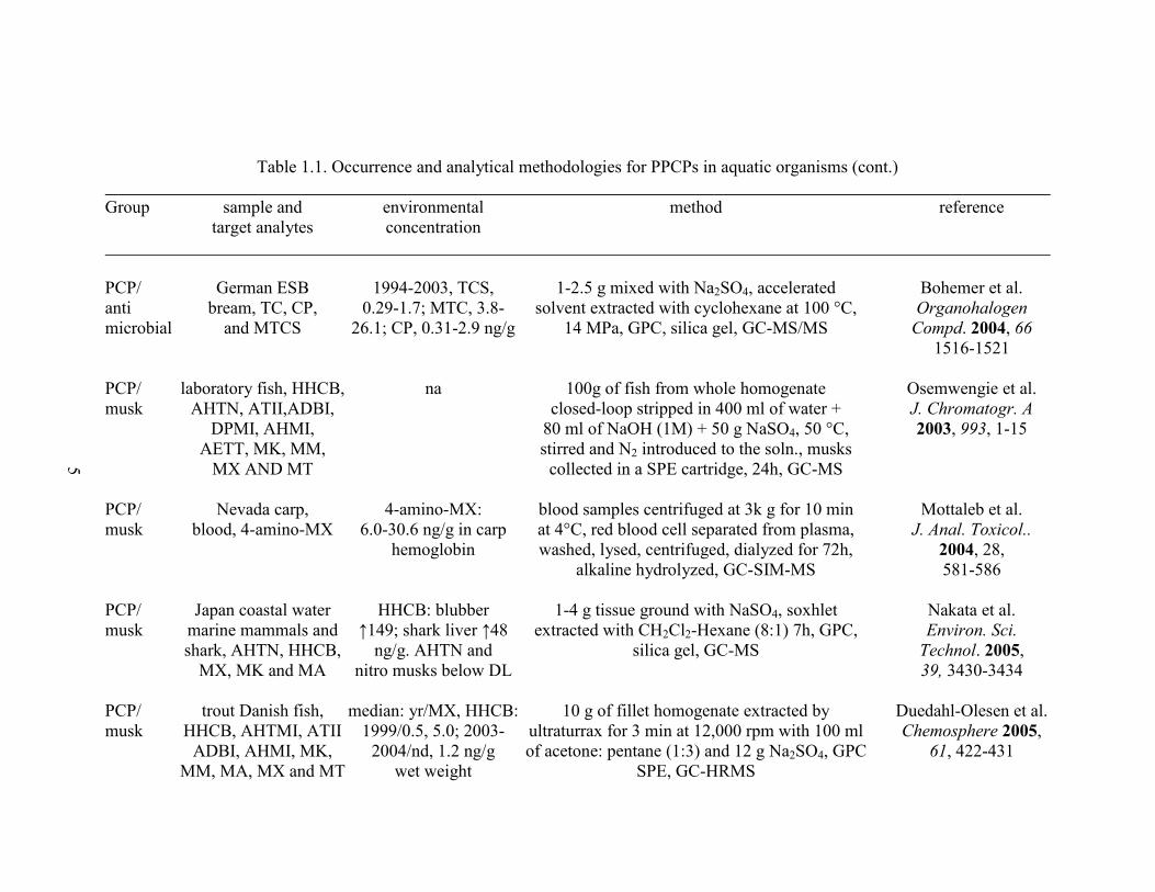
Table 1.1. Occurrence and analytical methodologies for PPCPs in aquatic organisms (cont.)
Group sample and environmental method reference
target analytes concentration
PCP/ German ESB 1994-2003, TCS, 1-2.5 g mixed with Na2SO4, accelerated Bohemer et al.
anti bream, TC, CP, 0.29-1.7; MTC, 3.8- solvent extracted with cyclohexane at 100 °C, Organohalogen
microbial and MTCS 26.1; CP, 0.31-2.9 ng/g 14 MPa, GPC, silica gel, GC-MS/MS Compd. 2004, 66
1516-1521
PCP/ laboratory fish, HHCB, na 100g of fish from whole homogenate Osemwengie et al.
musk AHTN, ATII,ADBI, closed-loop stripped in 400 ml of water + J. Chromatogr. A
DPMI, AHMI, 80 ml of NaOH (1M) + 50 g NaSO4, 50 °C, 2003, 993, 1-15
AETT, MK, MM, stirred and N2 introduced to the soln., musks
MX AND MT collected in a SPE cartridge, 24h, GC-MS
PCP/ Nevada carp, 4-amino-MX: blood samples centrifuged at 3k g for 10 min Mottaleb et al.
musk blood, 4-amino-MX 6.0-30.6 ng/g in carp at 4°C, red blood cell separated from plasma, J. Anal. Toxicol..
hemoglobin washed, lysed, centrifuged, dialyzed for 72h, 2004, 28,
alkaline hydrolyzed, GC-SIM-MS 581-586
PCP/ Japan coastal water HHCB: blubber 1-4 g tissue ground with NaSO4, soxhlet Nakata et al.
musk marine mammals and ↑149; shark liver ↑48 extracted with CH2Cl2-Hexane (8:1) 7h, GPC, Environ. Sci.
shark, AHTN, HHCB, ng/g. AHTN and silica gel, GC-MS Technol. 2005,
MX, MK and MA nitro musks below DL 39, 3430-3434
PCP/ trout Danish fish, median: yr/MX, HHCB: 10 g of fillet homogenate extracted by Duedahl-Olesen et al.
musk HHCB, AHTMI, ATII 1999/0.5, 5.0; 2003- ultraturrax for 3 min at 12,000 rpm with 100 ml Chemosphere 2005,
ADBI, AHMI, MK, 2004/nd, 1.2 ng/g of acetone: pentane (1:3) and 12 g Na2SO4, GPC 61, 422-431
MM, MA, MX and MT wet weight SPE, GC-HRMS
5

Table 1.1. Occurrence and analytical methodologies for PPCPs in aquatic organisms (cont.)
Group sample and environmental method reference
target analytes concentration
PCP/ German ESB mussel HHCB, AHTN: mussel 1-5 g of sample, Na2SO4 added, accelerated Rudel et al.
musk and bream, HHCB, 0.5-1.7, 0.4-2.5; bream solvent extracted (n-hexane, 80 °C, 14 MPa, J. Environ. Monit.
AHTN, AHMI, AETT, 545-6400, 48-2130 10 min), GPC, activated silica gel, GC-MS/MS 2006, 8, 812-823
ADBI, MK and MX ng/g wet weight
PCP/ Alpine lake fish, AHTN: 20-54; HHCB: different fillet species homogenized in 300 g Schmid et al.
musk ADBI, AHMI, AHTM 42-230; MX 1.3-12; pools, GPC, GC-MS Chemosphere 2007,
ATII, HHCB, MK and MK: 2.0-2.9 67, S16-S21
and MX ng/g lipid weight
PCP/ marine Ariake Sea clam: HHCB 1-4 g tissue ground with NaSO4, soxhlet Nakata et al. Environ.
musk organisms, AHTM, MX 258-2730 ng/g lipid extracted with CH2Cl2-hexane (8:1) 7h, GPC, Sci. Technol. 2007,
HHCB, MK and MA weight, AHTN smaller silica gel, GC-MS 41, 2216-2222
PCP/ MA, IL and CO fish average: mussel-HHCB aliquot mixed with 30g Na2SO4, Peck et al.
musk and mussel, MX, 14.9, AHTN 10.0; fish- pressurize fluid extracted with CH2Cl2 at Anal. Bioanal.
HHCB, AHTN, ADBI HHCB 1.12 ng/g 13.79 MPa 1-4 h, SEC, SPE 5% Chem. 2007, 387,
AHMI, ATII and MK wet weight deactivated alumina, GC-MS 2381-2388
EDC/ laboratory fish na 5 g in MeCN, lipids eliminated with Tsuda et al.
surfactant and shellfish, OP hexane-MeCN, MeCN fraction evaporated, J. Chromatogr. B 1999,
and NPs reconstituted in hexane, SPE cleaned up, GC-MS 723, 273-279
6

Table 1.1. Occurrence and analytical methodologies for PPCPs in aquatic organisms (cont.)
Group sample and environmental method reference
target analytes concentration
EDC/ laboratory fish and na 5 g in MeCN, lipids eliminated with hexane-MeCN, Tsuda et al.
surfactant shellfish, NP, NPE1, MeCN fraction evaporated, reconstituted in J. Chromatogr. B 2000,
NPE2 and 4-t-OP hexane, SPE cleaned up, HPLC fluorescence 746, 305-309
EDC/ Michigan fish, NP NP 3.3-29.1 ng/g 20 g into 2L flask with 20 g NaCl, 3 ml H2SO4, Keith et al. Environ.
surfactant and NPE1-NPE3 wet weight, rest steam distillated 3h, concentrated to1 ml of Sci. Technol. 2001,
below MDL isooctane HPLC- fluorescence clean up, GC-MS 35, 10-13
EDC/ Adriatic Sea seafood, NP ↑ 696, OP ↑ 18.6, no skin or internal organs, 100 g of homogenized Ferrara et al.
surfactant NP, OP, OPE, and OPE ↑ 0.43 ng/g sample from each pool, 1-1.5 g, lipid removed Environ. Sci.
NPE1-NPE4 lipid weight with a mixture MeCN: 0.1 M NaOH 1:1, acidified Technol. 2001,
and put into organic solvent, GC-MS 35, 3109-3112
EDC/ Las Vegas Bay of average NP 184, 20 g + 350 ml of water, blended, mixed with 20 g Snyder et al. Environ.
surfactant lake Mead carp, NPE1 242 ng/g NaCl, 3 ml H2SO4, steam distillated 3h, concentrated Toxicol. Chem.
NP and NPE1-NPE3 wet weight to 1 ml in isooctane, HPLC-fluorescence, GC-MS 2001, 20, 1870-1873
EDC/ German ESB mussel bream 1994: NP ↑ 1 g, digested with 25% (CH3)4NOH, 60 °C for Wenzel et al.
surfactant and bream, NP 112, NPE1 ↑ 259, OP 1h, 10 ml of hexane and centrifuged, organic Environ. Sci.
NPE1 and OPE1 ↑ 5.5, OPE1 ↑ 2.6; mussel: layer dried, 50 ul of Grignard reagent added, Technol. 2004,
NP ↑ 41 n/g wet weight silica gel clean up and GC-MS 38, 1654-1661
Pharma laboratory fish na organs kept at -20 °C until analyzed, clean up Schwaiger et al.
ceuticals/ diclofenac procedure included SPE (Extrelut NT 20) Aquat. Toxicol.
anti-inflamatory and methylation with TMSH, GC-MS 2004, 68, 141-150
7

Table 1.1. Occurrence and analytical methodologies for PPCPs in aquatic organisms (cont.)
Group sample and environmental method reference
target analytes concentration
Pharma Texas muscle, brain & mean (brain): fluox tissue homogenized, 1:5 diluted with Brooks et al.
ceuticals/ liver fish, fluoxetine 1.58, nor 8.86, ser 4.27 PO4 0.1 M pH 6, vortexed 10 min, ice cold Environ. Toxicol.
anti- and sertraline, and desser 15.6 ng/g wet w. MeCN added, centrifuged at 820 g 5 min, Chem. 2005, 24,
depressants its metabolites brain conc.>liver>muscle evaporated, reconstituted, SPE, and GC-MS 464-469
Pharma laboratory fish, eight na 5 g of homogenized fish mixed 50 ml MeCN, Stubbings et al.
ceuticals/ veterinary anti- centrifuged at 1700 g for 1 min, supernatant Anal. Chim.
antibiotics biotics representing through 15 g Na2SO4, filtrated, 5 ml of HAc, Acta. 2005, 547,
three classes SPE, HPLC-MS and HPLC 262-268
Pharma laboratory fish na 10 µl of plasma, acidified to pH 2 with H2SO4, SPE, Mimeault et al.
ceuticals/ blood, gem eluted with 1 ml of ethanol, HLC-MS Aquat. Toxicol.
atilipemic 2005, 73,
44-54
Pharma laboratory fish, na 1 g of fillet, 0.01 M EDTA added (pH 4), pureed for Wen et al.
ceuticals/ four tetracycline 5 min, kept in the dark for 30 min at 4 °C, centrifuged Talanta
antibiotics antibiotics 16k rpm for 5min, supernatant extracted in a monolithic 2006, 70,
capillary column, HPLC-UV 153-159
Pharma Canada fish, three analytes at conc. 3 g of ground fish pressurize liquid Chu et al.
ceuticals/ fluox, paroxetine, ↑ 1 ng/g wet weight extracted with MeOH, rotary evaporated, J. Chromatogr. A.
anti- and norfluoxetine SPE, eluted and HPLC-APCI-MS/MS 2007, 1163, 112-118
depressants
8
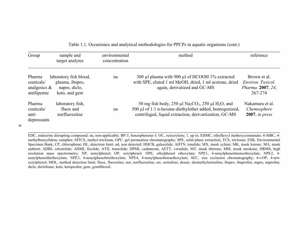
Table 1.1. Occurrence and analytical methodologies for PPCPs in aquatic organisms (cont.)
Group sample and environmental method reference
target analytes concentration
Pharma laboratory fish blood, na 300 µl plasma with 900 µl of HCOOH 1% extracted Brown et al.
ceuticals/ plasma, ibupro, with SPE, eluted 1 ml MeOH, dried, 1 ml acetone, dried Environ. Toxicol.
analgesics & napro, diclo, again, derivatized and GC-MS Pharma. 2007, 24,
antilipemic keto, and gem 267-274
Pharma laboratory fish, 50 mg fish body, 250 µl Na2CO3, 250 µl H2O, and Nakamura et al.
ceuticals/ fluox and na 500 µl of 1:1 n-hexane-diethylether added, homogenized, Chemosphere
anti- norfluoxetine centrifuged, liquid extraction, derivartization, GC-MS 2007, in press
depressants
EDC, endocrine disrupting compound; na, non-applicable; BP-3, benzophenone-3; OC, octocrylene; ↑, up to; EHMC, ethylhexyl methoxycinnamate; 4-MBC, 4-
methylbenzylidene camphor; MTCS, methyl-triclosan; GPC, gel permeation chromatography; SPE, solid phase extraction; TCS, triclosan; ESB, Environmental
Specimen Bank; CP, chlorophene; DL, detection limit; nd, non detected; HHCB, galaxolide; AHTN, tonalide; MX, musk xylene; MK, musk ketone; MA, musk
ambrett; ADBI, celestolide; AHMI, fixolide; ATII, traseolide; DPMI, cashmeran; AETT, versalide; MT, musk tibetene; MM, musk moskene; HRMS, high
resolution mass spectrometry; NP, nonylphenol; OP, octylphenol, OPE, ethylphenol ethoxylate; NPE1, 4-nonylphenolmonoethoxylate; NPE2, 4-
nonylphenoldiethoxylate; NPE3, 4-nonylphenoltriethoxylate; NPE4, 4-nonylphenoltetraethoxylate; SEC, size exclusion chromatography; 4-t-OP, 4-tert-
octylphenol; MDL, method detection limit; fluox, fluoxetine; nor, norfluoxetine; ser, sertraline; desser, desmethylsertraline; ibupro, ibuprofen; napro, naprofen;
diclo, diclofenac; keto, ketoprofen; gem, gemfibrozil.
9

10
from aqueous solution.38-41
However, it is important to point out that these correlations
were developed for neutral molecules possessing relatively large values of KOW (e.g., log
KOW > 4). The physicochemical properties of PPCPs do not always conform to this
stipulation. This is especially true for some pharmaceuticals which are expected to be
charged at environmentally-relevant pH. Consequently, the historical models that have
proven to be effective at predicting accumulation of pesticides or PCBs may not be
applicable to partitioning of PPCPs in aquatic systems. Nevertheless, both normalized
and un-normalized data continue to appear in literature.
An important analytical observation from Table 1.1 is that while methodologies
for determination of PPCPs in aquatic organisms are numerous, each is limited in scope.
That is, each methodology focuses on a select group of compounds, typically from the
same analyte class. Additionally, it is important to note that the number of reported
methodologies for assessment of pharmaceuticals is relatively small compared to the
number reported for assessment of PCPs.
Mass Spectrometry and Environmental Analysis
Gas chromatography-mass spectrometry (GC-MS) was the primary analytical tool
used to assess the environmental occurrence of PPCPs in initial studies. The popularity
of GC-MS in early work was due to its widespread availability and historical use in
contract service laboratories. The availability of electron-impact spectral libraries was
also seen as a plus, increasing confidence in analyte identification, and the distinctive
non-polar operating range of GC-MS was consistent with analysis of most PCPs. In
contrast, the use of GC-MS for analysis of pharmaceuticals, which are relatively polar
compared to PCPs, typically requires derivatization prior to analysis. These reactions are

11
often unpredictable for complex samples and can limit the quality of quantitative data.
Consequently, liquid chromatography-mass spectrometry (LC-MS) has become the
technique of choice for analyzing pharmaceuticals in environmental samples.
Numerous studies have demonstrated the distinct advantages of LC-MS for
analysis of pharmaceuticals. The LC-MS approach enables identification and
quantification without derivatization, and typically results in lower detection limits
(below 1 ng/L and 1 ng/g for liquid and solid samples, respectively) and better precision
than comparable GC-MS methodologies. In environmental applications, LC is typically
combined with tandem MS (i.e., MS/MS) to promote enhanced selectivity and sensitivity
for target analytes. In a routine MS/MS analysis, a molecular ion is selected and
subsequently fragmented to produce one or more distinctive product ions that enable both
qualitative and quantitative monitoring.
It is important to note, however, that LC-MS is not exempt from limitations. One
of the limitations of LC-MS is that atmospheric pressure ionization (API) processes are
influenced by co-extracted matrix components. Matrix effects typically result in
suppression or less frequently enhancement of analyte signal. There have been a number
of methods proposed to compensate for matrix effects, including the method of standard
addition,42-46
surrogate monitoring,47, 48
and isotope dilution.45, 46, 49-53
Although isotope
dilution is the most highly-recommended approach,45, 53
isotopically-labeled standards are
not always readily available.49, 54
An alternative approach involves the use of an
appropriate internal standard (i.e., a structurally-similar compound expected to mimic the
behavior of a target analyte(s)) with or without matrix-matched calibration. However, a
given internal standard is typically effective over a limited retention time window.55

12
Accordingly, the use of more than one internal standard is recommended to compensate
for matrix effects throughout the chromatographic run. Finally, it is important to point
out that strategies to compensate for matrix effects should take into account the
variability of matrix within each set of samples to be analyzed (e.g., river water, WWTP
effluent, sediment extracts, fish, etc.).
Quality Control and Quality Assurance
Due to potential regulatory implications, environmental analyses typically include
rigorous quality assurance and quality control (QA/QC) metrics to confirm reliability of
analytical data. Initial method validation provides essential performance parameters,
such as method recoveries, precision, and limits of detection (LODs). Recurring analysis
of quality control (QC) samples (e.g., method blanks, matrix spikes, and laboratory
control samples) is not only important to verify performance of the method over time, but
also to assess potential matrix effects. Considering the unpredictable nature of matrix
interference in LC-MS analysis and the lack of effective strategies to deal with this
difficulty, it has become imperative to use QA/QC data to document and qualify
analytical results. This is especially important when reporting concentrations at or near
the limit of detection for a given analytical method.
Scope of the Dissertation
In order for the reader to appreciate the broader context of experimental work
described herein, it is important to discuss the chronological development of research
focused on accumulation of PPCPs in aquatic organisms that has occurred over the
previous five years. Our efforts in this area were initiated in the later part of 2002, as

13
occurrence of PPCPs in surface water and wastewater was frequently being reported. As
demonstrated by the publication dates shown in Table 1.1, surfactants were the only
PPCPs that had been shown to accumulate in aquatic organisms at this time. However,
there was increasing interest in assessment of a larger group of PPCP analytes, and
methodologies for determination of musk fragrances in tissues were beginning to appear
in literature. In the summer of 2003, a collaborative study, led by Dr. Bryan Brooks and
involving additional Baylor researchers (including this author) and co-workers from the
City of Denton Watershed Resources Program and Federal Aviation Administration Civil
Aerospace Medical Institute, established for the first time that select human
pharmaceuticals (i.e., antidepressants) could also be accumulated in fish residing in
surface waters impacted by wastewater treatment effluent. Although resulting data did
not appear in the primary literature until 2005, results of this benchmark study led to the
primary research question that ultimately shaped this dissertation. Namely, whether
alternative pharmaceuticals were also accumulated in fish residing in effluent-dominated
streams?
The critical first step in being able to address this question was the development
of suitable analytical methodology to monitor pharmaceuticals in fish tissue. While
numerous methods for monitoring pharmaceuticals in water were available in literature,
none had been reported that were applicable to tissues. In an effort to obtain maximum
information with minimum analytical effort, the decision was made to focus on the
development of a broad screening method, incorporating analytes with diverse
physicochemical properties and belonging to multiple therapeutic classes.

14
The development and application of the first liquid chromatography-tandem mass
spectrometry (LC-MS/MS) screening method for pharmaceuticals in fish is described in
Chapter 2. Key steps in method development were identification of a suitable extraction
solvent for recovery of 25 target compounds from fish muscle tissue and implementation
of a quantitative protocol that compensated for observed matrix interference on
electrospray ionization. The environmental relevance of the analytical approach was
assessed by screening fish collected from a regional effluent-dominated stream (i.e., a
stream significantly impacted by wastewater effluent). This initial study not only
confirmed our previous report on antidepressants, but also resulted in the detection of
three novel contaminants. This work was recently published in the American Chemical
Society journal Analytical Chemistry.
During the course of method development for pharmaceuticals, it was determined
that a multi-residue method for screening PCPs in fish tissue would also be a novel
contribution to the literature. In Chapter 3, GC-MS methodology, employing selected ion
monitoring (SIM), for simultaneous determination of 10 extensively used PCPs and 2
alkylphenol surfactants in fish is described. This work represents the first approach
enabling routine monitoring of select UV-filters, fragrances, surfactants, an antimicrobial
agent and an insect repellent in a single chromatographic run. The method was also
applied to assess the presence of PCPs in the fish collected from a regional effluent-
dominated stream that were also analyzed by LC-MS/MS (see above). Four compounds
were detected at concentrations in general agreement with literature values determined
using methods designed for a select group of compounds. It is important to note that
much of this work was performed in collaboration with Dr. Mohammad A. Mottaleb.

15
In the spring of 2006, our group received notification that it had been selected to
carry out analytical activities affiliated with the first National Pilot Study of PPCPs in
Fish sponsored by the United States Environmental Protection Agency. That our
laboratory was selected in an open competition further supports the novelty of work
reported in Chapters 2 and 3. All sampling activities related to the pilot study were
performed by personnel from TetraTech, Inc., and whole fish were sent to Baylor on dry
ice for sample compositing and analysis. This study enabled assessment of PPCP
accumulation in fish collected from 6 sites across the United States (5 effluent-dominated
streams and one reference site). Results of LC-MS/MS screening analyses affiliated with
this study are reported in Chapter 4 and clearly demonstrate: 1) that accumulation, and
thereby exposure, of pharmaceuticals is likely limited to surface waters that are impacted
by wastewater effluents and 2) that accumulated concentrations in fish are variable,
depending on the type of process used to treat wastewater at a given site. Analytical
observations resulting in slight modification of the method described in Chapter 2 are
also presented.
16
CHAPTER TWO
Analysis of Pharmaceuticals in Fish Using Liquid Chromatography-
Tandem Mass Spectrometry*
Introduction
The occurrence of pharmaceuticals and personal care products (PPCPs) in the
environment has received broad interest over the last decade.1, 2, 56, 57
PPCPs have been
increasingly detected in water, wastewater, soil, sediments, and biosolids. More recently,
reports from our laboratory10
and others12, 13, 15, 17, 28
have demonstrated that
environmental exposures to PPCPs may result in accumulation of parent compounds
and/or their metabolites in tissues of aquatic organisms. These reports have heightened
interest in secondary effects of PPCPs and impart a sense of urgency to research focused
on understanding fate and partitioning of these compounds in aquatic systems.
Analytical methodologies for determination of PPCPs in water, sediment and
biosolids are numerous and have been summarized in recent reviews.7-9, 58
Due to the
complexity of environmental samples, analyses typically employ detailed sample
preparation followed by chromatographic separation of analytes and mass spectrometry
detection. While methods focused on a single compound or unique compound class (e.g.,
antibiotics) continue to be reported,59-63
increasing emphasis on simultaneous analysis of
compounds with dissimilar physicochemical properties is evident in recent literature.8, 48,
64-67 This shift in philosophy stems from a desire to gain diverse knowledge with
minimal analytical expenditure.
* Reproduced with permission from [Ramirez, A. J.; Mottaleb, M. A.; Brooks, B. W.; Chambliss, C. K.
Anal. Chem. 2007, 79, 3155-3163.] Copyright © 2007 American Chemical Society

17
At present, analytical methodologies for determination of PPCPs in aquatic
organisms are numerous, but lack in scope of analytes. Procedures for measuring select
compounds in fish tissues have been reported for diclofenac,37
two antidepressants and
their active metabolites,10
4 UV filters and methyl-triclosan,12, 13
12 musk fragrances,15, 17
four tetracycline antibiotics,26
and 8 veterinary antibiotics representing three structural
classes.27
The general approach employed for analysis of personal care products involved
extraction of homogenized tissue with nonpolar solvents, followed by successive size-
exclusion and silica gel cleanup procedures prior to gas chromatography- mass
spectrometry (GC-MS) analysis.12, 13, 15, 17
In contrast, pharmaceuticals were extracted
from tissue using relatively polar solvents (i.e., aqueous buffer or acetonitrile), and
extracts were cleaned up by solid phase extraction prior to GC-MS,10, 37
HPLC26, 27
or LC-
MS27
analysis.
Herein, we report the first multi-residue screening method for pharmaceuticals
representing multiple therapeutic classes in fish tissue. This protocol enables
simultaneous monitoring of 25 compounds using LC-MS/MS. Key steps in method
development involved optimizing extraction of acidic, basic, and neutral analytes from 1-
gram tissue homogenates and using matrix-matched calibration to compensate for
observed matrix interference. As compared to previous methods for analysis of PPCPs in
fish tissue, developed methodology offers relatively simple sample preparation in that
tissue extracts are centrifuged and directly injected into the LC-MS/MS, following
reconstitution in chromatographic mobile phase. The method was subsequently applied
to assess the occurrence of target analytes in environmental samples. Four

18
pharmaceuticals were detected in all analyzed specimens, and accumulation of three of
these compounds in fish tissues is reported here for the first time.
Experimental Section
Chemicals
All chemicals were reagent grade or better, obtained from commercial vendors,
and used as received. The positive ESI internal standards 7-aminoflunitrazepam-d7, and
fluoxetine-d6 (100.0 µg/ml in acetonitrile), surrogates (100.0 µg/ml in acetonitrile)
acetaminophen-d4, and diphenhydramine-d3, and reference standards (1000.0 µg/ml in
MeOH): fluoxetine, norfluoxetine, sertraline, codeine, diphenhydramine, propranolol and
ibuprofen were purchased as certified analytical standards (Cerilliant Corporation, Round
Rock, TX). Atenolol was purchased in solid form (99% purity), also from Cerilliant.
The negative ESI internal standard meclofenamic acid and reference standards: 1,7
dimethylxanthine, acetaminophen, caffeine, miconazole, carbamazepine, erythromycin,
gemfibrozil, trimethoprim, diltiazem, cimetidine, warfarin, thiabendazole,
sulfamethoxazole, lincomycin, metoprolol, tylosin, clofibric acid were purchased in the
highest available purity (Sigma-Aldrich, Milwaukee, WI). Surrogates (100.0 µg/ml in
acetonitrile) carbamazepine-d10 and ibuprofen-13
C3 were purchased from Cambridge
Isotopes Lab. Inc., Andover, MA. Distilled water was purified and deionized to 18 M
with a Barnstead Nanopure Diamond UV water purification system.
Sample Collection and Preservation
Pecan Creek and Clear Creek (two streams located in Denton County, TX, USA)
were chosen for field sampling activities. Clear Creek is not impacted by effluent

19
discharges and is routinely used as a local reference stream by the City of Denton, Texas
Watershed Protection program. In contrast, annual flows in Pecan Creek are comprised
almost entirely of effluent discharge from the Pecan Creek Water Reclamation Plant.
Effluent-dominated streams are likely worse case scenarios for investigating
environmental exposures to PPCPs. Because these streams receive limited upstream
dilution, wastewater contaminants may be considered „pseudopersistent‟, and resident
organisms may receive continuous life-cycle exposures. Fish (Lepomis sp.) were
sampled from Pecan Creek (n = 11) and Clear Creek (n = 20) to serve as test and
reference specimens, respectively. The approximate size of fish collected from these
sites was similar and ranged from 8.8 cm to 11.5 cm (total length) and 29.4 g to 49.0 g.
Lateral fillets were dissected from fish collected at both sites and homogenized using a
Tissuemiser (Fisher Scientific, Fair Lawn, NJ) set to rotate at 30,000 rpm. Pecan creek
homogenates were stored individually, while Clear Creek homogenates were composited
into a single sample. All tissues were stored at 20 °C prior to analysis. No target
analytes were detected in the Clear Creek composite. Accordingly, this tissue is hereafter
referred to as „clean‟.
Analytical Sample Preparation
Approximately 1.0 g tissue was combined with 8 ml extraction solvent (see Fig.
2.2 for tested solvent compositions) in a 20 ml borosilicate glass vial (Wheaton; VWR
Scientific, Rockwood, TN), and the mixture was homogenized using a Tissuemiser
(Fisher Scientific, Fair Lawn, NJ) set to rotate at 30,000 rpm. Five surrogates were added
to each sample: acetaminophen-d4 (454 ng), fluoxetine-d6 (636 ng), diphenhydramine-d3
(8.9 ng), carbamazepine-d10 (38.5 ng) and ibuprofen-13
C3 (789 ng). Samples were shaken

20
vigorously and mixed on a rotary extractor for five minutes. Following extraction,
samples were rinsed into 50-ml polypropylene copolymer round-bottomed centrifuge
tubes (Nalge Company; Nalgene® Brand Products, Rochester, New York) using 1 ml
extraction solvent and centrifuged at 16,000 rpm for 40 min at 4 °C. The supernatant was
decanted into 18-ml disposable borosilicate glass culture tubes (VWR Scientific,
Rockwood, TN), and the solvent was evaporated to dryness under a stream of nitrogen at
45 °C using a Zymark Turbovap LC concentration workstation (Zymark Corp.,
Hopkinton, MA). Samples were reconstituted in 1 ml of mobile phase, and a constant
amount of the internal standards 7-aminoflunitrazapam-d7 (100 ng) and meclofenamic
acid (1000 ng) was added. Prior to analysis, samples were sonicated for 1 min and
filtered using Pall Acrodisc hydrophobic Teflon Supor membrane syringe filters (13 mm
diameter; 0.2-µm pore size; VWR Scientific, Suwanee, GA).
LC-MS/MS Method
A Varian ProStar Model 210 binary pump equipped with a Model 410
autosampler was used in this study. Analytes were separated on a 15 cm × 2.1 mm (5
m, 80 Å) Extend-C18 column (Agilent Technologies, Palo Alto, CA) connected with an
Extend-C18 guard cartridge 12.5 mm x 2.1 mm (5 m, 80 Å) (Agilent Technologies,
Palo Alto, CA). A binary gradient consisting of 0.1% (v/v) formic acid in water and
100% methanol was employed to achieve chromatographic separation and is defined in
Table 2.1. Additional chromatographic parameters were as follows: injection volume, 10
µl; column temperature, 30 ºC; flow rate, 350 l/min. Eluted analytes were monitored by
MS/MS using a Varian model 1200L triple-quadrupole mass analyzer equipped with an
electrospray interface (ESI).

21
Table 2.1. HPLC gradient elution profile
Mobile phase composition, %
_____________________________________
Time (min) 0.1 % formic acid Methanol
0 93 7
2 93 7
7 85 15
12 85 15
21 52 48
28 52 48
34 41 59
45 2 98
50 2 98
51 93 7
65 93 7
_______________________________________________________________________
To determine the best ionization mode (ESI + or −) and optimal MS/MS
transitions for target analytes, each compound was infused individually into the mass
spectrometer at a concentration of 1 g/ml in aqueous 0.1% (v/v) formic acid at a flow
rate of 10 L/min. All analytes were initially tested using both positive and negative
ionization modes while the first quadrupole was scanned from m/z 50 to [M + 100]. This
enabled identification of the optimal source polarity and most intense precursor ion for
each compound. Once these parameters were defined, the energy at the collision cell was

22
varied, while the third quadrupole was scanned to identify and optimize the intensity of
product ions for each compound. Additional instrumental parameters held constant for
all analytes were as follows: nebulizing gas, N2 at 60 psi; drying gas, N2 at 19 psi;
temperature, 300 °C; needle voltage, 5000 V ESI+, 4500 V ESI-; declustering potential,
40 V; collision gas, argon at 2.0 mTorr.
Extraction Recoveries
Two groups of control samples prepared from „clean‟ tissue were employed to
determine extraction efficiency for target analytes. Group 1 samples were spiked with
internal standards and each analyte, while group 2 samples were spiked with internal
standards only. Both groups of samples were carried through the sample preparation
procedure described above. Following syringe filtration, group 2 samples were spiked
with the same amount of each analyte added to group 1. All samples were analyzed by
LC-MS/MS, and individual analyte recoveries were calculated using the following
equation:
%100AA
AArecovery
IS2X2
IS1X1 (2.1)
where AX1, AIS1, AX2 and AIS2 represent peak areas for the analyte (X) and internal
standard (IS) in groups 1 and 2, respectively.
Results and Discussion
LC-MS/MS Methodology
Three factors were considered in selecting target analytes (Table 2.2): i) number
of prescriptions dispensed in the United States during 2005,68
ii) variability in structure,

23
physicochemical properties and therapeutic use, and iii) relative frequency of occurrence
in soils, sediments and biosolids. Excluding potential ion-exchange phenomena, the
physicochemical properties favoring compound partitioning from water to solid
environmental matrices may also promote accumulation of water-borne chemicals in
aquatic biota via diffusion across biological membranes. Additionally, compounds
residing in sediment may be taken up by aquatic organisms via ingestion. Furlong et. al.
summarized results from several U.S. Geological Survey occurrence studies targeting
PPCPs in environmental matrices and demonstrated that the frequency of detection for
fluoxetine in analyzed sediment, soil and biosolid samples (64-100%) was much higher
than in water (5%).69
This general trend was observed for seventeen additional
compounds assessed in their work. Since fluoxetine was previously shown by our group
to accumulate in fish tissues,10
it seemed reasonable to target compounds with a similar
occurrence pattern in screening activities.
Compound-dependent mass spectrometry parameters were investigated by direct
infusion of individual analytes into the electrospray source. Optimized MS/MS
transitions and collision energies employed for detection and quantitation of each analyte
are provided in Table 2.2, along with the molecular structure and most common
therapeutic use for each analyte. With the exception of erythromycin, selected precursors
represent the molecular ion [M + H]+ or [M − H]
− for each analyte. The most abundant
precursor for erythromycin was found to be the [M + H − H2O]+ ion at m/z 716,
consistent with previous observations.48, 58
Selected product ions represent the most
abundant fragment observed for each precursor at the noted collision energy.

Table 2.2. Analyte-dependent mass spectrometry parameters for target analytes
Compound use structure precursor collision product pKaa
ion energy (eV) ion
ESI POSITIVE ANALYTES
Acetaminophen analgesic 152 -11.0 110 9.86
[M + H]+
Atenolol anti-hypertension 267 -21.5 145 9.16
[M + H]+
Cimetidine anti-acid reflux 253 -13.5 159 7.07
[M + H]+
Codeine analgesic 300 -38.0 215 8.25
[M + H]+
1,7-dimethylxanthine caffeine metabolite 181 -15.5 124 8.50
[M + H]+
NH
OOH
O
O
H2N
HN
OH
N
NH
SN
NH
HN
N
O
N
OH
OH
N
HN
N
NO
O
24

Table 2.2. Analyte-dependent mass spectrometry parameters for target analytes (cont.)
Compound use structure precursor collision product pKaa
ion energy (eV) ion
Lincomycin antibiotic 407 -15.5 359 8.78
[M + H]+
Trimethoprim antibiotic 291 -17.5 261 7.20
[M + H]+
Thiabendazole antibiotic 202 -23.0 175
[M + H]+
Caffeine stimulant 195 -16.0 138
[M + H]+
Sulfamethoxazole antibiotic 254 -13.0 156 5.81
[M + H]+
OH
OH
S
OHNH
O
N
HO
O
O
O
N
N
NH2
NH2
NH
N
S
N
N
N
N
NO
O
H2N
S
HN
ON
O O
25

Table 2.2. Analyte-dependent mass spectrometry parameters for target analytes (cont.)
Compound use structure precursor collision product pKaa
ion energy (eV) ion
Metoprolol anti-hypertension 268 -15.5 191 9.17
[M + H]+
Propranolol anti-hypertension 260 -11.0 116 9.14
[M + H]+
Diphenhydramine antihistamine 256 -11.5 167 8.76
[M + H]+
Diltiazem anti-hypertension 415 -22.0 178 8.94
[M + H]+
Carbamazepine anti-seizure 237 -13.5 194
[M + H]+
O
O
HN
OH
OHN
OH
S
O
O
O
ON
N
NH2O
ON
26
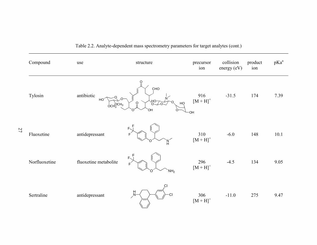
Table 2.2. Analyte-dependent mass spectrometry parameters for target analytes (cont.)
Compound use structure precursor collision product pKaa
ion energy (eV) ion
Tylosin antibiotic 916 -31.5 174 7.39
[M + H]+
Fluoxetine antidepressant 310 -6.0 148 10.1
[M + H]+
Norfluoxetine fluoxetine metabolite 296 -4.5 134 9.05
[M + H]+
Sertraline antidepressant 306 -11.0 275 9.47
[M + H]+
O
OOO
CHO
OHO
OO
OH
HO
NHOHO
OCH3OCH3
O
O
F
F
F
O NH
F
F
F
O NH2
HN Cl
Cl
27
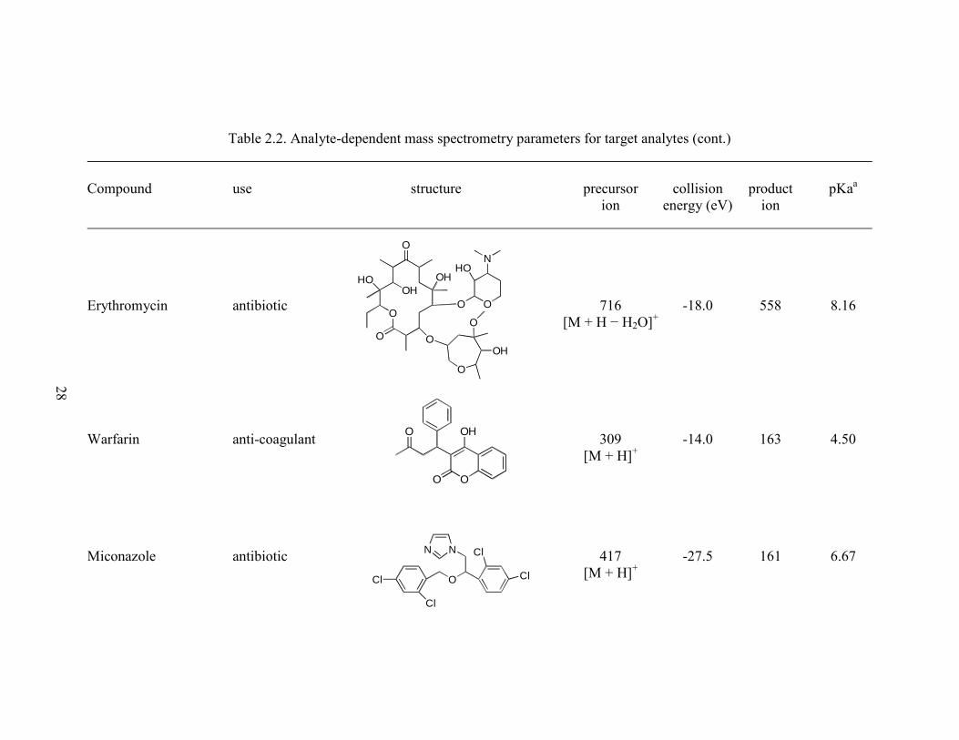
Table 2.2. Analyte-dependent mass spectrometry parameters for target analytes (cont.)
Compound use structure precursor collision product pKaa
ion energy (eV) ion
Erythromycin antibiotic 716 -18.0 558 8.16
[M + H − H2O]+
Warfarin anti-coagulant 309 -14.0 163 4.50
[M + H]+
Miconazole antibiotic 417 -27.5 161 6.67
[M + H]+
O
N
O
OH
O
O
OH
O
O
O
OHHO
O
HO
O
O
O
OH
O
Cl
Cl
NN
Cl
Cl
28

Table 2.2. Analyte-dependent mass spectrometry parameters for target analytes (cont.)
Compound use structure precursor collision product pKaa
ion energy (eV) ion
ESI NEGATIVE ANALYTES
Clofibric Acid antilipemic 213 15.4 127 3.18
[M − H]−
Ibuprofen analgesic 205 7.0 161 4.41
[M − H]−
Gemfibrozil antilipemic 249 13.0 121 4.75
[M − H]−
a Calculated values obtained from the SciFinder database (© 2006 American Chemical Society).
OOH
O
Cl
HO
O
O OH
O
29

30
Once suitable MS/MS transitions were identified for each analyte, an aqueous
mixture of reference standards was employed to optimize chromatographic parameters.
A non-linear gradient consisting of 0.1% (v/v) formic acid and methanol resulted in near-
baseline resolution of the majority of analytes in approximately 50 minutes (Fig. 1.1). A
15-minute isocratic hold (93:7 formic acid-methanol) was added to the end of each run to
allow for column equilibration between injections. While the majority of analytes were
eluted as single peaks, erythromycin was consistently eluted as two partially-resolved
peaks. Similar chromatographic behavior for erythromycin has been observed previously
and attributed to differing retention characteristics for presumed sterioisomers.48, 70
Figure 2.1. Time-schedule chromatogram of a spiked ‘clean’ muscle sample collected from Clear Creek.
Peak identifications are as follows: (1) acetaminophen, (2) acetaminophen-d4, (3) atenolol, (4) cimetidine,
(5) codeine, (6) 1,7-dimethylxanthine, (7) lincomycin, (8) trimethoprim, (9) thiabendazole, (10) caffeine,
(11) sulfamethoxazole, (12) 7-aminoflunitrazepam-d7 (+IS), (13) metoprolol, (14) propranolol, (15)
diphenhydramine, (16) diphenhydramine-d3, (17) diltiazem, (18) carbamazepine, (19) carbamazepine-d10,
(20) tylosin, (21) fluoxetine, (22) fluoxetine-d6, (23) norfluoxetine, (24) sertraline, (25) erythromycin, (26)
clofibric acid, (27) warfarin, (28) miconazole, (29) ibuprofen, (30) ibuprofen-13
C3, (31) meclofenamic acid
(-IS), (32) gemfibrozil.
Inte
nsi
ty,
MC
ou
nts
3,4
1,2
5
7
68, 9
11
10
14-16
12
20
18
21-23 25,26
24
29,30
17
28
31
32
27
0
1
2
20
3
4
5
10 30 40 50 min
19
13
Inte
nsi
ty,
MC
ou
nts
3,4
1,2
5
7
68, 9
11
10
14-16
12
20
18
21-23 25,26
24
29,30
17
28
31
32
27
0
1
2
20
3
4
5
10 30 40 50 min
19
13

31
Additionally, isotope effects on retention behavior were observed for
carbamazepine-d10 and fluoxetine-d6. As evident in Figure 2.1 (peaks 18 and 19), the
observed retention time for carbamazepine-d10 (30.08 min) was shorter than that observed
for carbamazepine (30.53 min) by almost 30 seconds. Though not evident in Figure 2.1
due to co-elution of norfluoxetine (35.13 min), a 20-second difference in retention time
was also observed for fluoxetine-d6 (34.58 min) relative to that observed for fluoxetine
(34.93 min). These differences are admittedly small but were very reproducible, and
observed behavior for these analytes is consistent with previous studies demonstrating
stronger retention for unlabeled compounds than deuterated analogs in reverse-phase
chromatography.71-73
Presumably, isotope effects were not observed for acetaminophen
(peaks 1 and 2) and diphenhydramine (peaks 15 and 16) due to a lower degree of
deuterium substitution and decreased resolution at shorter retention times.
Extraction of Target Analytes from Fish Tissue
Due to considerable variation in lipophilicity and pKa among pharmaceuticals, a
systematic study of extraction behavior was conducted with the goal of identifying a
single solvent system affording optimized recoveries for the full range of analytes from
„clean‟ muscle tissue. Ten solvents, differing in pH and/or polarity, were tested. Mean
recoveries (n=3) were calculated for individual analytes in each solvent system and are
tabulated in Table 2.3. These data are summarized in Fig. 2.2, where individual analyte
recoveries were averaged for each solvent system. „Error bars‟ in this plot represent one
standard deviation from the average and provide an assessment of variability among
mean recoveries for individual analytes. While these data have no statistical relevance,

Table 2.3. Individual extraction recoveries (%) for tested solvent systems
__________________________________________________________________________________________________________
Average (n = 3) plus minus one standard deviation
________________________________________________________________________________________
Analyte CH2Cl2 CH2Cl2 MeOH TFA HAc HAc PO4 TFA HAc PO4
-C6H14 -MeOH -MeCN pH 2.4 pH 4 pH 4 pH 6 pH 2.4 pH 4 pH 6
-MeOH -MeOH -MeCN -MeOH
__________________________________________________________________________________________________________
Acetaminophen 8 ± 2 78 ± 22 85 ± 17 89 ± 4 92 ± 4 102 ± 4 98 ± 7 79 ± 6 61 ± 10 68 ± 8
Atenolol 25 ± 6 73 ± 11 85 ± 3 84 ± 5 97 ± 4 109 ± 2 97 ± 7 81 ± 6 71 ± 6 73 ± 8
Cimetidine 14 ± 1 79 ± 22 89 ± 9 92 ± 7 95 ± 4 108 ± 3 95 ± 8 77 ± 7 68 ± 11 71 ± 8
Codeine 100 ± 21 64 ± 25 90 ± 18 82 ± 4 86 ± 5 101 ± 3 90 ± 9 70 ± 4 45 ± 14 61 ± 7
1,7-Dimethylxanthine 9 ± 4 84 ± 10 93 ± 2 93 ± 5 92 ± 2 95 ± 7 92 ± 7 78 ± 5 60 ± 5 63 ± 8
Lincomycin 26 ± 1 65 ± 9 76 ± 8 86 ± 4 90 ± 5 98 ± 2 92 ± 3 73 ± 6 67 ± 5 72 ± 6
Trimethoprim 88 ± 26 68 ± 30 79 ± 9 90 ± 4 95 ± 3 104 ± 5 86 ± 11 66 ± 3 60 ± 3 65 ± 7
Thiabendazole 57 ± 15 65 ± 32 78 ± 9 82 ± 3 84 ± 4 97 ± 7 88 ± 4 54 ± 4 40 ± 6 45 ± 9
Caffeine 98 ± 8 80 ± 11 92 ± 2 84 ± 4 85 ± 3 96 ± 8 86 ± 7 80 ± 6 60 ± 9 67 ± 6
Sulfamethoxazole 11 ± 3 67 ± 11 78 ± 2 81 ± 3 79 ± 3 81 ± 6 84 ± 8 61 ± 4 42 ± 5 53 ± 7
32

Table 2.3. Individual extraction recoveries (%) for tested solvent systems (cont.)
__________________________________________________________________________________________________________
Average (n = 3) plus minus one standard deviation
______________________________________________________________________________________
Analyte CH2Cl2 CH2Cl2 MeOH TFA HAc HAc PO4 TFA HAc PO4
-C6H14 -MeOH -MeCN pH 2.4 pH 4 pH 4 pH 6 pH 2.4 pH 4 pH 6
-MeOH -MeOH -MeCN -MeOH
__________________________________________________________________________________________________________
Metoprolol 98 ± 31 65 ± 28 71 ± 13 73 ± 3 91 ± 4 96 ± 6 91 ± 6 69 ± 3 65 ± 8 66 ± 7
Propranolol 49 ± 8 47 ± 9 64 ± 14 44 ± 11 89 ± 3 90 ± 12 73 ± 4 27 ± 2 49 ± 10 36 ± 6
Diphenhydramine 35 ± 5 57 ± 6 68 ± 16 35 ± 8 75 ± 6 86 ± 11 83 ± 5 36 ± 4 47 ± 10 42 ± 9
Diltiazem 39 ± 12 50 ± 20 70 ± 1 18 ± 2 92 ± 3 100 ± 9 73 ± 4 45 ± 3 59 ± 9 50 ± 9
Carbamazepine 80 ± 9 70 ± 11 82 ± 4 83 ± 5 87 ± 3 98 ± 11 92 ± 6 47 ± 4 35 ± 6 39 ± 12
Tylosin 56 ± 13 40 ± 6 54 ± 9 61 ± 6 31 ± 4 60 ± 5 82 ± 4 65 ± 3 42 ± 9 64 ± 9
Fluoxetine 26 ± 4 47 ± 20 62 ± 16 18 ± 4 72 ± 1 66 ± 9 57 ± 1 8 ± 1 21 ± 10 16 ± 5
Norfluoxetine 24 ± 9 27 ± 13 58 ± 14 21 ± 4 71 ± 3 64 ± 10 53 ± 1 5 ± 1 19 ± 8 13 ± 4
Sertraline 27 ± 10 37 ± 14 54 ± 14 20 ± 4 59 ± 11 44 ± 11 42 ± 2 5 ± 1 10 ± 4 15 ± 5
33

Table 2.3. Individual extraction recoveries (%) for tested solvent systems (cont.)
__________________________________________________________________________________________________________
Average (n = 3) plus minus one standard deviation
______________________________________________________________________________________
Analyte CH2Cl2 CH2Cl2 MeOH TFA HAc HAc PO4 TFA HAc PO4
-C6H14 -MeOH -MeCN pH 2.4 pH 4 pH 4 pH 6 pH 2.4 pH 4 pH 6
-MeOH -MeOH -MeCN -MeOH
__________________________________________________________________________________________________________
Erythromycin 79 ± 33 56 ± 10 70 ± 30 78 ± 5 91 ± 4 101 ± 10 92 ± 2 66 ± 4 63 ± 5 64 ± 9
Clofibric Acid 8 ± 1 75 ± 15 97 ± 30 89 ± 3 60 ± 8 93 ± 10 83 ± 7 63 ± 11 28 ± 1 46 ± 5
Warfarin 23 ± 9 75 ± 22 97 ± 23 90 ± 7 64 ± 2 85 ± 9 89 ± 8 53 ± 11 14 ± 2 56 ± 3
Miconazole 13 ± 4 16 ± 5 64 ± 9 20 ± 8 60 ± 1 15 ± 2 35 ± 1 7 ± 1 22 ± 1 5 ± 2
Ibuprofen 7 ± 3 75 ± 16 83 ± 19 86 ± 3 55 ± 10 64 ± 12 83 ± 5 55 ± 11 10 ± 1 43 ± 5
Gemfibrozil 12 ± 2 75 ± 17 73 ± 15 87 ± 1 60 ± 10 59 ± 6 80 ± 2 40 ± 10 11 ± 3 28 ± 6
__________________________________________________________________________________________________________ All solvent systems were prepared by dissolving equal volumes of liquid in a binary mixture unless noted otherwise. Solvent system notations are
as follows: HAc, 0.1 M acetic acid buffer; MeCN, acetonitrile; TFA, 0.1 M trifluoroacetic acid buffer; MeOH, methanol; PO4, phosphate buffer;
CH2Cl2, dichloromethane; C6H14, hexane.
34
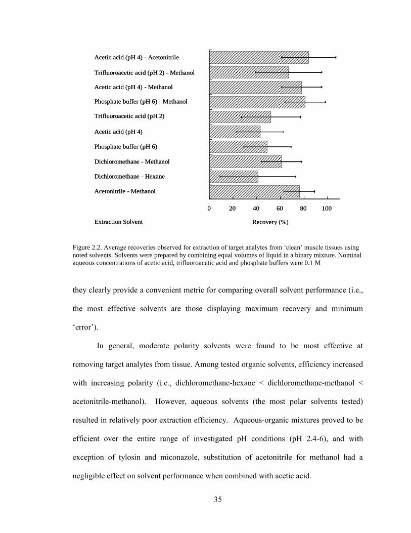
35
Figure 2.2. Average recoveries observed for extraction of target analytes from ‘clean’ muscle tissues using
noted solvents. Solvents were prepared by combining equal volumes of liquid in a binary mixture. Nominal
aqueous concentrations of acetic acid, trifluoroacetic acid and phosphate buffers were 0.1 M
they clearly provide a convenient metric for comparing overall solvent performance (i.e.,
the most effective solvents are those displaying maximum recovery and minimum
„error‟).
In general, moderate polarity solvents were found to be most effective at
removing target analytes from tissue. Among tested organic solvents, efficiency increased
with increasing polarity (i.e., dichloromethane-hexane < dichloromethane-methanol <
acetonitrile-methanol). However, aqueous solvents (the most polar solvents tested)
resulted in relatively poor extraction efficiency. Aqueous-organic mixtures proved to be
efficient over the entire range of investigated pH conditions (pH 2.4-6), and with
exception of tylosin and miconazole, substitution of acetonitrile for methanol had a
negligible effect on solvent performance when combined with acetic acid.
0 20 40 60 80 100
Recovery (%)
Acetic acid (pH 4) - Acetonitrile
Trifluoroacetic acid (pH 2) - Methanol
Acetic acid (pH 4) - Methanol
Phosphate buffer (pH 6) - Methanol
Trifluoroacetic acid (pH 2)
Acetic acid (pH 4)
Phosphate buffer (pH 6)
Dichloromethane - Methanol
Dichloromethane - Hexane
Acetonitrile - Methanol
Extraction Solvent

36
Since most analytes included in this study are basic (Table 2.2) and expected to be
protonated at pH 6, it is not surprising that pH had little effect on recovery as charted in
Figure 2.2. Recovery of acidic analytes into these solvents was expected to decrease with
decreasing pH. However, mean recoveries for clofibric acid, ibuprofen and gemfibrozil
were greater for pH 2.4 trifluoroacetic acid-methanol and pH 6 phosphate buffer-
acetonitrile than for pH 4 acetic acid-methanol (Table 2.3). The origin of this behavior is
presently unknown.
Matrix Effects
It is widely recognized that co-extracted matrix components can affect analyte
ionization in analyses employing electrospray interfaces.9, 48, 55
Accordingly, an approach
reported by Vanderford et al.48
was employed to evaluate matrix effects for extraction
solvents promoting recovery > 60% in Figure 2.2. „Clean‟ muscle tissue (1 g) was
extracted, centrifuged, and reconstituted in 0.1% formic acid. Extracts were spiked with
a known amount of each analyte prior to analysis. Aqueous formic acid (0.1% v/v) was
also spiked with the same concentration of target compounds and analyzed as a matrix-
free reference sample. Concentrations of analytes derived from an internal standard
calibration curve prepared using standards constituted in 0.1 % formic acid are tabulated
in Table 2.4.
As expected, the degree of matrix interference was found to depend on both
analyte and extraction solvent. Co-extracted matrix components were found to have
minimal effect on the analytical response of early-eluting analytes (retention time < 25
min). In contrast, matrix suppression was observed for most other ESI+ analytes;
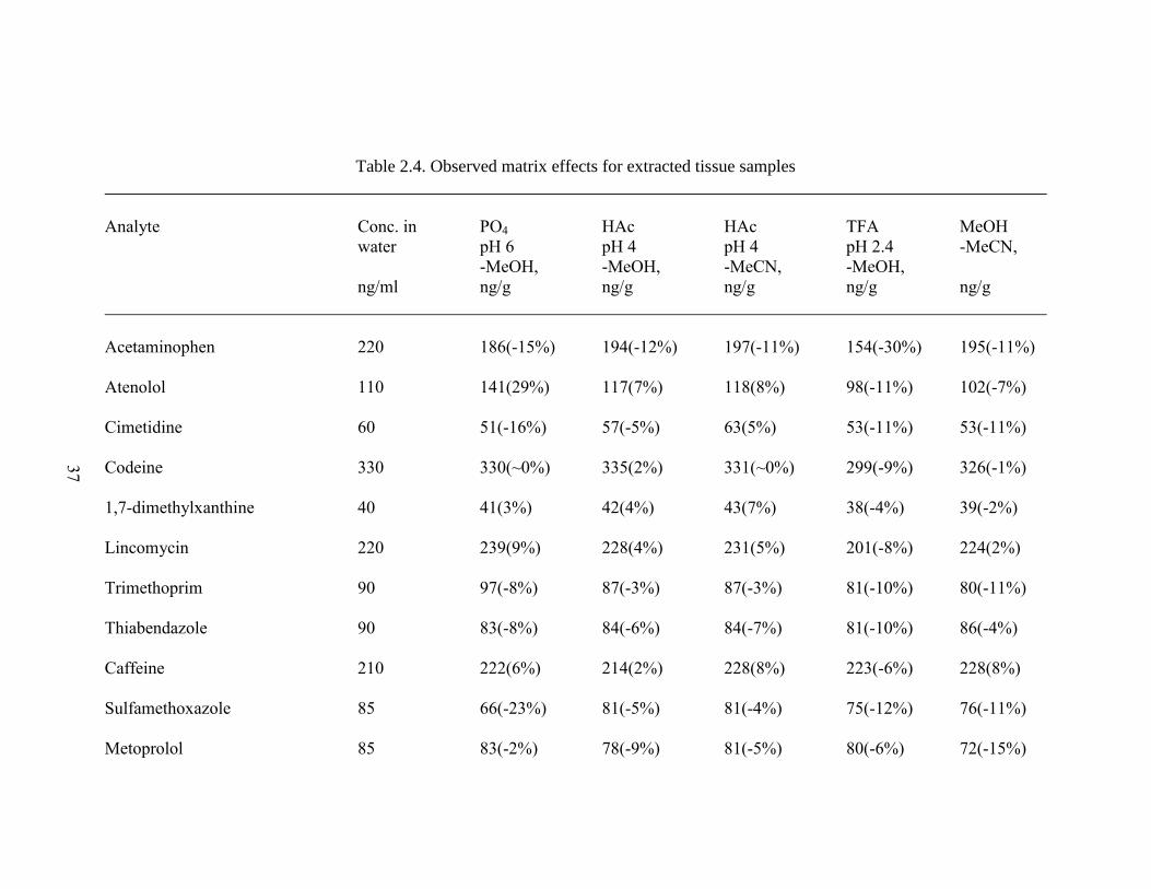
Table 2.4. Observed matrix effects for extracted tissue samples
Analyte Conc. in PO4 HAc HAc TFA MeOH
water pH 6 pH 4 pH 4 pH 2.4 -MeCN,
-MeOH, -MeOH, -MeCN, -MeOH,
ng/ml ng/g ng/g ng/g ng/g ng/g
Acetaminophen 220 186(-15%) 194(-12%) 197(-11%) 154(-30%) 195(-11%)
Atenolol 110 141(29%) 117(7%) 118(8%) 98(-11%) 102(-7%)
Cimetidine 60 51(-16%) 57(-5%) 63(5%) 53(-11%) 53(-11%)
Codeine 330 330(~0%) 335(2%) 331(~0%) 299(-9%) 326(-1%)
1,7-dimethylxanthine 40 41(3%) 42(4%) 43(7%) 38(-4%) 39(-2%)
Lincomycin 220 239(9%) 228(4%) 231(5%) 201(-8%) 224(2%)
Trimethoprim 90 97(-8%) 87(-3%) 87(-3%) 81(-10%) 80(-11%)
Thiabendazole 90 83(-8%) 84(-6%) 84(-7%) 81(-10%) 86(-4%)
Caffeine 210 222(6%) 214(2%) 228(8%) 223(-6%) 228(8%)
Sulfamethoxazole 85 66(-23%) 81(-5%) 81(-4%) 75(-12%) 76(-11%)
Metoprolol 85 83(-2%) 78(-9%) 81(-5%) 80(-6%) 72(-15%)
37
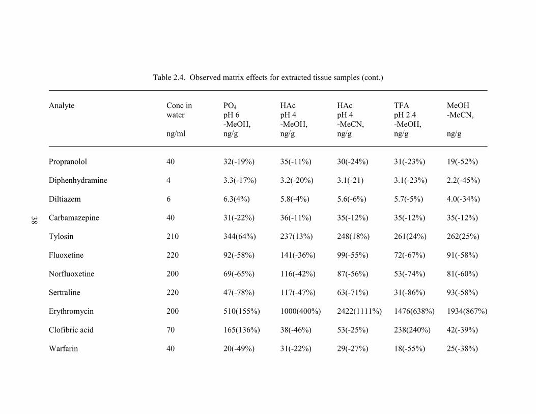
Table 2.4. Observed matrix effects for extracted tissue samples (cont.)
Analyte Conc in PO4 HAc HAc TFA MeOH
water pH 6 pH 4 pH 4 pH 2.4 -MeCN,
-MeOH, -MeOH, -MeCN, -MeOH,
ng/ml ng/g ng/g ng/g ng/g ng/g
Propranolol 40 32(-19%) 35(-11%) 30(-24%) 31(-23%) 19(-52%)
Diphenhydramine 4 3.3(-17%) 3.2(-20%) 3.1(-21) 3.1(-23%) 2.2(-45%)
Diltiazem 6 6.3(4%) 5.8(-4%) 5.6(-6%) 5.7(-5%) 4.0(-34%)
Carbamazepine 40 31(-22%) 36(-11%) 35(-12%) 35(-12%) 35(-12%)
Tylosin 210 344(64%) 237(13%) 248(18%) 261(24%) 262(25%)
Fluoxetine 220 92(-58%) 141(-36%) 99(-55%) 72(-67%) 91(-58%)
Norfluoxetine 200 69(-65%) 116(-42%) 87(-56%) 53(-74%) 81(-60%)
Sertraline 220 47(-78%) 117(-47%) 63(-71%) 31(-86%) 93(-58%)
Erythromycin 200 510(155%) 1000(400%) 2422(1111%) 1476(638%) 1934(867%)
Clofibric acid 70 165(136%) 38(-46%) 53(-25%) 238(240%) 42(-39%)
Warfarin 40 20(-49%) 31(-22%) 29(-27%) 18(-55%) 25(-38%)
38

Table 2.4. Observed matrix effects for extracted tissue samples (cont.)
Analyte Conc in PO4 HAc HAc TFA MeOH
water pH 6 pH 4 pH 4 pH 2.4 -MeCN,
-MeOH, -MeOH, -MeCN, -MeOH,
ng/ml ng/g ng/g ng/g ng/g ng/g
Miconazole 400 43(-89%) 87(-78%) 73(-82%) 19(-95%) 196(-51%)
Ibuprofen 1600 4045(152%) 1271(-20%) 1289(-19%) 5491(243%) 859(-46%)
Gemfibrozil 200 307(54%) 129(-35%) 119(-41%) 275(38%) 110(-45%)
Values in parenthesis represent the relative percent difference in concentrations. Negative sign inside parenthesis indicates suppression of the signal. Solvent
system notations are as follows: PO4, phosphate buffer; MeOH, methanol; HAc, 0.1 M acetic acid buffer; MeCN, acetonitrile; TFA, 0.1 M trifluoroacetic acid
buffer.
39

40
especially for fluoxetine, norfluoxetine, sertraline and miconazole. Exceptions include
tylosin and erythromycin, for which significant signal enhancements were observed in a
number of cases. Data for clofibric acid, ibuprofen and gemfibrozil in Table 2.4 are
misleading for extracts resulting from extraction with phosphate buffer-methanol and
trifluoroacetic acid-methanol. In each of these cases data in Table 2.4 suggest an
apparent signal enhancement. In fact, the analytical response for these analytes was
suppressed in all cases, but more pronounced suppression of the ESI internal standard
(meclofenamic acid) in these extracts resulted in calculated concentrations exceeding the
reference condition.
Matrix effects identified in Table 2.4 collectively demonstrate that accurate
quantitation of analytes in tissue extracts is not feasible using calibration standards
prepared in aqueous formic acid. Common approaches for dealing with matrix
interference include spiking each sample with a known amount of labeled analyte(s) prior
to analysis (i.e., isotope dilution), employing the method of standard additions, or using
matrix-matched calibration standards. While isotope dilution is perhaps the best
approach for compensation of matrix interference in analyses employing mass
spectrometry,53
cost and limited availability of labeled standards are problematic for
broad screening methods. A primary limitation for standard addition methods is related
to sample mass and/or volume, which is often limited in tissue analyses. Furthermore,
quality assessment of standard addition data is difficult to monitor using standard QA/QC
performance metrics. In contrast, matrix-matched calibration is relatively simple to
implement, provided that „clean‟ reference tissue is available.

41
For reasons discussed above, matrix-matched calibration was employed to
minimize matrix interference in the analysis of environmental samples. Calibration
standards were prepared by adding a known amount of each target analyte and five
labeled surrogates to 1 g „clean‟ muscle tissue. Tissues were homogenized and carried
through the entire sample preparation procedure prior to analysis. Acetic acid (pH 4)-
methanol was selected as the extraction solvent, since observed matrix effects were
minimized in this extract (Table 2.4). Linear calibration curves (r2 > 0.99 for
concentration ranges specified in Table 2.5) were constructed by plotting the response
factor for each analyte versus tissue spiking levels (ng/g tissue) and used to determine
analyte concentrations in all subsequent analyses.
Analytical Performance Metrics
Analyte-specific limits of detection (LOD), limits of quantitation (LOQ) and
method detection limits (MDL) are defined and reported in Table 2.5. Although LOD
and LOQ are recognized performance metrics within academic circles, MDL is more
appropriate for establishing detection thresholds in environmental analyses with potential
regulatory implications. LOD74
and LOQ75
are derived from analyses of a „blank‟ sample
and thus, do not account for potential matrix effects. In contrast, MDL is derived from
replicate analyses of a matrix spike and represents the lowest concentration of analyte
that can be detected in a given matrix with 99% confidence that the concentration is non-
zero.76
As shown in Table 2.5, MDLs for fish tissue were typically higher than either
LOD or LOQ, irrespective of the level of matrix interference identified in Table 2.4.
These results clearly suggest that use of LOD and LOQ as detection and quantitation

42
Table 2.5. Retention time (tR), investigated linear range, LOD, LOQ, and MDL for target
analytes in fish muscle tissue
________________________________________________________________________
Analyte tR, linear range, LOD,b LOQ,
c MDL,
d
min ng/g ng/g ng/g ng/g
________________________________________________________________________
Acetaminophen 6.4 3.12-400 0.30 0.99 4.40
Atenolol 9.1 1.25-160 0.48 1.62 1.48
Cimetidine 8.9 0.625-80 0.24 0.81 1.04
Codeine 10.4 4.69-600 1.07 3.55 6.11
1,7-dimethylxanthine 11.8 0.625-80 0.17 0.58 1.02
Lincomycin 14.0 3.12-400 0.63 2.09 5.53
Trimethoprim 15.8 1.25-160 0.79 2.63 2.15
Thiabendazole 15.6 1.25-160 0.14 0.47 2.63
Caffeine 17.2 3.12-400 0.34 1.15 3.93
Sulfamethoxazole 19.8 1.25-160 0.23 0.76 2.29
Metoprolol 21.9 1.25-160 0.25 0.85 2.50
Propranolol 25.3 0.625-80 0.01 0.03 1.07
Diphenhydramine 25.8 0.0625-8 0.01 0.03 0.05
Diltiazem 27.7 0.094-12 0.04 0.13 0.12
Carbamezepine 30.6 0.625-80 0.03 0.12 0.54
Tylosin 32.9 3.12-400 1.18 3.93 5.02
Fluoxetine 34.9 4.69-600 0.76 2.54 6.73
Norfluoxetine 35.2 3.12-400 0.32 1.08 2.90
Sertraline 37.2 3.12-400 0.21 0.71 3.57

43
Table 2.5. Retention time (tR), investigated linear range, LOD, LOQ, and MDL for target
analytes in fish muscle tissuea (cont.)
________________________________________________________________________
Analyte tR, linear range, LOD,b LOQ,
c MDL,
d
min ng/g ng/g ng/g ng/g
________________________________________________________________________
Erythromycin 42.0 3.12-400 0.85 2.84 6.42
Clofibric Acid 42.4 1.25-160 0.10 0.32 2.69
Warfarin 45.0 0.625-80 0.09 0.29 0.86
Miconazole 47.5 3.12-400 0.39 1.32 10.8
Ibuprofen 50.6 25-3200 3.14 10.4 45.9
Gemfibrozil 52.5 3.12-400 0.25 0.85 6.68
________________________________________________________________________ a „Clean‟ tissues employed in the determination of these parameters were extracted using a 1:1 mixture of
0.1 M acetic acid buffer (pH 4) and methanol. See text for details. b Limit of detection (LOD), calculated
as three times the standard deviation in the background signal. c Limit of quantitation (LOQ), calculated as
ten times the standard deviation in the background signal. d Method detection limit (MDL), determined by
multiplying the one sided 99 percent student‟s t-statistic (t0.99) by the standard deviation from eight
replicates analysis of spiked sample.
thresholds in practical applications of this method could lead to acceptance of
questionable data. For this reason, MDLs were employed as a single
detection/quantitation threshold in screening analyses (see below). Additionally, it is
important to note that relative standard deviations derived from replicate analyses of the
matrix spike (data not shown) were 6% for all analytes, demonstrating excellent
reproducibility.
Analysis of Environmental Samples
In order to confirm the utility of LC-MS/MS methodology for analysis of
environmental samples, fish were sampled approximately 650 m downstream from the

44
effluent discharge into Pecan Creek and screened for target analytes. Four compounds
were detected in all analyzed specimens at concentrations exceeding statistically-derived
MDLs (Table 2.6). Identification of analytes in environmental samples was confirmed by
monitoring two fragment ions and comparing their retention time and relative intensity
with a spiked sample. Representative reconstituted ion chromatograms are shown in
Figure 2.3. Note that collision induced dissociation of norfluoxetine produced only one
fragment ion of sufficient intensity to be observed under these conditions.
Fluoxetine and sertraline have been detected previously in fish from Pecan
Creek.10
However, it is not surprising that these compounds were not detected in this
study, as reported concentrations in fish muscle (1.1 ng/g and 0.34 ng/g, respectively) fall
below MDLs defined in Table 2.5. While norfluoxetine has also been observed
previously in fish tissues,10
accumulation of diphenhydramine, diltiazem and
carbamazepine is reported here for the first time.
Table 2.6. Concentrations of analytes (ng/g tissue) detected in muscle tissues from fish
collected in Pecan Creek, Denton County, TX, USA
________________________________________________________________________
Analyte Range Mean
(n = 11) (n = 11)
________________________________________________________________________
Diphenhydramine 0.66 – 1.32 0.96
Diltiazem 0.11 – 0.27 0.21
Carbamazepine 0.83 – 1.44 1.16
Norfluoxetine 3.49 – 5.14 4.37
________________________________________________________________________

45
Figure 2.3. LC-MS/MS reconstituted ion chromatograms displaying analyte-specific quantitation and
qualifier ions for (A) a tissue extract from a fish (Lepomis sp.) collected in Pecan Creek and (B) an extract
from ‘clean’ tissue spiked with known amounts of diphenhydramine (1.6 ng/g), diltiazem (2.4 ng/g),
carbamazepine (16 ng/g) and norfluoxetine (80 ng/g). The higher m/z fragment is more intense in all cases
25 30 35 min
25 30 35 min
Diphenhydramine
256 > 167
256 > 152
Diltiazem
415 > 178
415 > 150
Carbmazepine
237 > 194
237 > 165
Norfluoxetine
296 > 134
A)
Diphenhydramine
256 > 167
256 > 152 Diltiazem
415 > 178
415 > 150
Carbmazepine
237 > 194
237 > 165
Norfluoxetine
296 > 134
B)
25 30 35 min
25 30 35 min
Diphenhydramine
256 > 167
256 > 152
Diltiazem
415 > 178
415 > 150
Carbmazepine
237 > 194
237 > 165
Norfluoxetine
296 > 134
A)
Diphenhydramine
256 > 167
256 > 152 Diltiazem
415 > 178
415 > 150
Carbmazepine
237 > 194
237 > 165
Norfluoxetine
296 > 134
B)

46
Duplicate analysis of a matrix spike prepared from a Pecan Creek tissue specimen
was conducted to assess method accuracy. Analyte spiking levels in this sample
corresponded to the upper third of the calibration range for each analyte (ca. 15 × MDL).
Excepting fluoxetine, norfluoxetine and sertraline, mean spike recoveries ranged from
88%-120% (data not shown), demonstrating that target compounds can be quantified with
acceptable accuracy in environmental samples. Relative percent difference for duplicate
analyses was 16% for all compounds. It is important to point out that positive bias was
observed for clofibric acid and ibuprofen (recovery = 186% and 145%, respectively)
when matrix-matched internal standard calibration was employed. However, improved
accuracy for these analytes was achieved (97% recovery in both cases) by using a matrix-
matched external standard calibration curve (i.e., a plot of analyte peak area versus tissue
spiking level). Improvements in surrogate recovery for ibuprofen-13
C3 in unspiked
samples were also observed using the external standard approach. These results suggest
that meclofenamic acid is not a suitable internal standard for clofibric acid and ibuprofen
in environmental samples.
Mean recoveries for fluoxetine, norfluoxetine and sertraline were less than
quantitative in the matrix spike (44%, 64%, and 46%, respectively), and surrogate
recoveries for fluoxetine-d6 in unspiked samples ranged from 60-97%. Matrix-matched
external standard calibration did not significantly improve accuracy for these compounds.
However, quantitation of fluoxetine based on isotope dilution with fluoxetine-d6 resulted
in 110% recovery for the matrix spike. It is reasonable to expect that additional
compounds, not present in „clean‟ tissue extracts, may be present in Pecan Creek samples
since this stream is significantly impacted by wastewater effluent and previous studies

47
have demonstrated that wastewater contaminants not classified as PPCPs are accumulated
in fish residing in effluent-dominated ecosystems.77
Therefore, it is possible that
compounds not monitored in this study co-elute with target antidepressants and result in
unforeseen matrix effects. To the extent that this proves to be a general occurrence in
future applications of reported methodology, it may become necessary to employ isotope
dilution for accurate quantitation of these compounds.
48
CHAPTER THREE
Development of a Gas Chromatography-Mass Spectrometry Screening Method for
Simultaneous Determination of Select UV Filters, Synthetic Musks, Alkylphenols, an
Antimicrobial Agent, and an Insect Repellent in Fish
Introduction
The occurrence of personal care products (PCPs), such as ultra-violet filters
(UVFs), synthetic musks (SMs), antimicrobials, and insect repellents has been
increasingly reported in literature.1, 2, 57, 78
Much of the recent scientific attention given to
these emerging contaminants has resulted from an absence of aquatic life based
regulations for surface waters. Of particular relevance are effluent-dominated streams,
which represent “worse case scenarios” for studying PCPs and other organic wastewater
contaminants.79
In these streams, even compounds with relatively short environmental
half-lives may be considered pseudopersistent due to their continuous introduction from a
WWTP. As a result, organisms residing in these aquatic systems receive continuous
exposures to wastewater-derived contaminants over their entire life cycle.79
Recent
reports from several research groups12, 14, 17, 28
have demonstrated that environmental
exposure to PPCPs results in accumulation of parent compounds, their metabolites, or
both in tissues of aquatic organisms. More significantly, a series of studies has also
identified that nitromusk fragrances are not only accumulated but are subsequently
metabolized to reactive intermediates that form covalent protein adducts.28, 80
Alkylphenol surfactants (APs) represent a second class of organic wastewater
contaminants that has also received broad coverage in literature. These compounds are

49
ubiquitous constituents of industrial products such as, emulsifiers, paints, detergents and
other cleaning products. They are perhaps the most widely-studied wastewater
contaminants due to their ability to promote endocrine disruption in aquatic organisms.81
Multiple studies have demonstrated their occurrence in a variety of environmental
matrices, including tissues.21-24, 82-84
Continued investigation of partitioning and
accumulation for these and alternative organic wastewater contaminants (OWCs) is
critical to comprehensive assessment of potential consequences of environmental
exposures.
Analytical protocols for determination of OWCs in water, soil, sediment, and
biosolids are numerous and have been summarized in recent reviews.6, 9, 85
While
targeted analytical methods for determination of UVFs,86-88
SMs,67, 89-93
APs,82-84
antimicrobials,94, 95
and insect repellents96, 97
continue to be reported, an increasing trend
in environmental chemistry is the development of protocols affording simultaneous
analysis of compounds belonging to different classes.67, 78, 98-100
It is important to note
that due to similarities in physicochemical properties, PCPs and APs are amenable to
assessment using a single analytical method. 78
In contrast, methods for determination of
OWCs in tissue continue to focus almost exclusively on a specific class of analytes. For
example, protocols have recently appeared for 4 UV filters and methyl-triclosan,12, 13, 32
12 musk fragrances,16-20
9 alkylphenol surfactants,21, 23, 24, 36
and chlorophene, triclosan
and its 3-chlorinated derivatives.11, 14, 33
The first multi-residue approach for
determination of pharmaceuticals in fish using LC-MS/MS was described in Chapter 2.
In this chapter, a complementary GC-MS method affording simultaneous analysis
of 3 UVFs, 5 SMs, 2 APs, the antimicrobial agent triclosan and the insect repellent m-
50
toluamide is described. An important step in method development that imparts a distinct
advantage, as compared to previous methods for analysis of similar OWCs in fish, was
alleviation of gel-permeation chromatography from the sample preparation protocol.
Centrifuged extracts were simply cleaned using silica gel, reconstituted in hexane, and
injected directly into the GC-MS. Target analytes were monitored with the mass analyzer
operated in selected ion monitoring (SIM) mode. Initial method validation involved
determination of statistically-derived MDLs using spiked muscle tissue. The method was
subsequently applied to assess the occurrence of target analytes in environmental
samples. Four compounds were detected at concentrations in general agreement with
literature values determined using methods designed for a single class of compounds.
Experimental Section
Chemicals and Materials
All chemicals were reagent grade or better, obtained from commercial vendors,
and used as received. The reference standards, benzophenone, 4-methylbenxylidine
camphor, m-toluamide, p-octylphenol, galaxolide, tonalide, musk xylene, musk ketone,
triclosan, octocrylene, and p-nonylphenol, and surrogate standards, 2,2‟-dinitrobiphenyl,
pentachloronitrobenzene, and benzophenone-d10 were purchased in the highest available
purity from Sigma-Aldrich (Milwaukee, WI, USA). Celestolide was obtained from
Cambridge Corporation (San Diego, CA, USA). Surrogate standards 3,3‟,4,4‟-
tetrachlorobiphenyl-13
C12 (PCB # 77) and p-n-nonylphenol-13
C6 were acquired from
Cambridge Isotopes Labortatories, Inc. (Andover, MA, USA). The internal standard
mirex was purchased from Cerilliant Corporation (Round Rock, TX, USA). The
51
derivatizing agent N-methyl-N-(trimethylsilyl)trifluoracetamide (MSTFA) was obtained
from VWR Scientifics (Irving, TX, USA). Silica gel (grade 60, 70-230 mesh, 60 Å), n-
hexane (HPLC grade), and acetone (spectrophotometric grade) were also obtained from
Sigma-Aldrich Inc. Distilled water was purified and deionized to 18 MΩ with a
Barnstead Nanopure Diamond UV water purification system.
Sample Collection and Preservation
Sampling activities related to this work were described in detail in Chapter 2. It is
important to recall that annual flows in Pecan Creek are comprised almost entirely of
effluent discharge from the Pecan Creek Water Reclamation Plant. In contrast, Clear
Creek is not impacted by effluent discharges. Fish (Lepomis sp.) were sampled from
Pecan Creek (n = 11) and Clear Creek (n = 20). Tissue from the Clear Creek composite
was used for initial evaluations of method performance, determination of statistically-
derived MDLs, and as control matrix in the analysis of Pecan Creek samples. The same
11 Pecan Creek fish analyzed in Chapter 2 were also employed here to evaluate the
environmental relevance of developed methodology.
Determination of Tissue Lipid Content
Lipid content was determined for each fish collected from Pecan Creek using a
modified literature procedure.101
Approximately 2 grams of homogenized muscle tissue
were taken from each fish and mixed with 15 ml 1:1 hexane-dichloromethane (50% v/v)
in a glass vial. Samples were re-homogenized using a Tissuemiser (Fisher Scientific) set
to rotate at 30,000 rpm. Homogenized samples were then equilibrated on a rotary
extractor (15 rotations/min) for 18 h at 35 oC. The phases were separated, and the

52
resulting organic layer was transferred to a Pyrex test tube using disposable borosilicate
glass pipettes. The tissue residue was rinsed with an additional 15 ml solvent, and the
extracts were combined in a single test tube. Residual water was removed by passing
extracts through laboratory assembled glass columns packed with anhydrous Na2SO4 and
collected in a pre-weighed test tube. The solvent was evaporated to dryness under a
stream of nitrogen at 45 oC and dried to constant weight in a vacuum oven at 40 °C.
Lipid content was calculated by dividing the weight of extracted residue by the wet
weight of tissue prior to extraction. (This procedure was carried out by Dr. Mohammad
A. Mottaleb and Mr. Christopher Pankow.)
Extraction of Target Analytes
Approximately 1.0 g of tissue was combined with 10 ml of acetone in a 20 ml
VWR Wheaton borosilicate glass vial (Rockwood, TN, USA), and the mixture was
homogenized using a Tissuemiser set to rotate at 30 000 rpm. Five surrogates were
added to each sample as an acetone solution: PCB # 77 (200 ng), p-n-nonylphenol-13
C6
(80 ng), 2,2‟-dinitrobiphenyl (500 ng), pentachloronitrobenzene (500 ng), and
benzophenone-d10 (120 ng). Samples were then shaken vigorously and mixed on a rotary
extractor for 5 min. Following extraction, samples were transferred into 50-ml
polypropylene copolymer round-bottomed centrifuge tubes (Nalgene, Rochester, NY,
USA) using 1 ml of acetone as a rinse and centrifuged at 16000 rpm for 40 min at 4°C.
The supernatant was then transferred into VWR Scientific 18-ml disposable borosilicate
glass tubes (Irving, TX, USA), and the solvent was evaporated to dryness under a stream
of nitrogen at 40 oC using a Zymark Turbovap (Hopkinton, MA, USA). Finally, samples
were reconstituted in 200 µl of 65:35 hexane-acetone (v/v).

53
Sample Clean-up and Derivatization
One gram of silica gel (Sigma-Aldrich Inc) was stirred in 4 ml hexane and the
slurry was transferred to a borosilicate glass Pasteur pipette. Approximately 10 mg of
glass wool was used as a porous plug, keeping silica confined to the pipette. Silica-gel
columns were preconditioned with 8 ml of 65:35 hexane-acetone (v/v). The extract was
loaded onto the column using a second Pasteur pipette, and analytes were eluted using 10
ml of the hexane-acetone mixture. The eluate was subsequently collected and evaporated
to dryness at 40 °C under dry nitrogen. Residues were again dissolved in 200 µl of
solvent mixture, and 100 µl of MSTFA derivatizing agent was added. The resulting
mixture was transferred into a GC vial and heated in an oven at 60 oC for 45 min.
Subsequently, the mixture was evaporated to dryness and reconstituted in 180 µl of n-
hexane. Finally, a constant amount of the internal standard mirex (200 ng) was added
prior to GC-MS analysis.
GC-MS Analysis
A Varian CP-3800 GC system equipped with a Varian CP-8400 auto sampler was
used in this study. Analytes were separated on a 30 m x 0.25 mm I.D. x 0.25 µm film
thickness, XTI-5 capillary column (VWR Scientific, West Chester, PA, USA) using the
following temperature program: initial temperature, 100 °C, ramped to 180 °C at 15
°C/min, held for 5 min, ramped to 290 °C at 6 °C/min, and held for 31 min. Helium was
used as carrier gas at a constant flow rate of 1 ml/min. Injections of 1.0 µl were made
using splitless mode and an injection port temperature of 275 °C. The transfer line was
kept at 280 °C. Eluted analytes were monitored by electron-impact (EI) ionization mass
spectrometry in SIM mode using a Varian model 1200L quadrupole mass spectrometer.

54
A representative total ion chromatogram is shown in Figure 3.1, and ions (m/z) used for
quantitation and identification of each target analyte are shown in Table 3.1. Mass
spectrometry parameters held constant for all analytes were as follows: ion source
temperature, 250 °C; manifold temperature, 40 °C; EI ionization energy, 70 eV; scan
time, 35 min.
Figure 3.1.Time-scheduled chromatogram of a calibration standard.
Key: (1) m-toluamide, (2) Benzophenone, (S1) Benzophenone-d10, (3) Celestolide, (S2)
pentachloronitrobenzene, (4) p-octylphenol, (5) galaxolide, (6) Tonalide, (7) musk xylene, (8) p-
nonylphenol, (S3) p-n-nonylphenol-13
C6, (9) 4-methylbenxylidine camphor, (S4) 2,2‟-dinitrobiphenyl, (10)
musk ketone, (11) triclosan, (S5) PCB # 77, (IS) mirex, and (12) octocrylene.
Quantitation
Ten calibration standards were prepared by dissolving varying concentrations of
all target analytes and surrogates in acetone. Calibration curves were constructed for
each analyte by plotting the response factor (i.e., peak area of analyte divided by the peak
area of internal standard) versus analyte concentration (ng/ l). Calibration data were fit
min10 20 2515
1
2
3
4
Inte
nsi
ty,
MC
oun
ts 6
5
0
7
1
2,S1
3
S2
4
5
6,7
8,S3
9
10
11IS
12
S5
S4
min10 20 2515
1
2
3
4
Inte
nsi
ty,
MC
oun
ts 6
5
0
7
1
2,S1
3
S2
4
5
6,7
8,S3
9
10
11IS
12
S5
S4

Table 3.1. Brand and IUPAC names, use, group, structure, CAS number and SIM ions for selected target analytes
Analyte use group chemical structure CAS Number SIM ions
m-Toluamide
(N,N-diethyl-m- insect repellent 134-62-3 91, 119, a 190
methylbenzamide)
Benzophenone sun screen UVF 119-61-9 77, 105, 182
(diphenyl ketone)
Celestolide
(4-Acetyl-1,1-
dimethyl-6-tert- fragrance SM 13171-00-1 173, 229, 244
butylindane)
p-Octylphenol surfactant AP 1806-26-4 165, 180, 278
Galaxolide
(1,3,4,6,7,8-hexahydro-
4,6,6,7,8,8-hexamethyl fragrance SM 1222-05-5 213, 243, 258
cyclo-penta[g]-2-
benzo pyrane)
CN(C2H5)2
O
C
O
C
C(CH3)3
O OH
HO
(CH2)7
O
55

Table 3.1. Brand and IUPAC names, use, group, structure, CAS number and SIM ions for selected target analytes (cont.)
Analyte use group chemical structure CAS Number SIM ions
Tonalide
(7-acetyl-1,1,3,4,4,6- fragrance SM 21145-77-7 201, 243, 258
hexamethyltetralin)
Musk xylene
(1-tert-butyl-3,5-
dimethyl-2,4,6- fragrance SM 81-15-2 282, 283, 297
trinitrobenzene)
p-Nonylphenol surfactant AP 104-40-5 149, 179, 292
4-MBC
(4-methylbenzylidine sun screen UVF 36861-47-9 115, 211, 254
camphor)
Musk ketone
(4-aceto-3,5-dimethyl-
2,6-dinitro-tert- fragrance SM 81-14-1 217, 261, 366
butylbenzene)
C
O
OH
C(CH3)3
NO2O2N
NO2
HO
(CH2)8
C
O
C(CH3)3
NO2C
NO2
O
HO
56

Table 3.1. Brand and IUPAC names, use, group, structure, CAS number and SIM ions for selected target analytes (cont.)
Analyte use group chemical structure CAS Number SIM ions
Triclosan
(4-chloro-2-hydroxyphenyl- anti-microbial 3380-34-5 200, 345, 362
2,4-dichlorophenyl ether)
Octocrylene
(2-ethylhexyl-2-cyano- sun screen UVF 6197-30-4 177, 249, 361
3,3-diphenylacrylate)
a
Bold print indicates m/z used for quantitation. UVF, ultra-violet filter; SM, synthetic musk; AP, alkylphenol.
CN
C
O
O
O
OHCl
Cl Cl
57

58
to a linear regression forced through the origin, resulting in correlation coefficients (r2)
exceeding 0.99 in all cases. In the analysis of unfortified control matrix (i.e., unspiked
tissue from Clear Creek), benzophenone, galaxolide and triclosan were detected at
average concentrations (n = 3) of 24.1, 12.4 and 12.1 ng/g, respectively, with less than
12% RSD. Therefore, measured concentrations in fortified control samples used to
determine MDLs and monitor method performance in the analysis of Pecan Creek
samples were corrected by subtracting the corresponding blank values.
Quality Control
In the analysis of samples from Pecan Creek, method performance was monitored
via analysis of a procedural blank, laboratory control sample, and matrix spike-matrix
spike duplicate pair. Surrogates were added to all tissue samples prior to extraction. No
analytes were detected in the blank, and recoveries for the laboratory control sample and
MS/MSD pair were acceptable for all analytes. (MS/MSD recoveries are presented in
Table 3.4 and discussed in more detail below.) Additionally, surrogate monitoring
revealed that the RSDs of mean recoveries calculated for each analyte varied between 2
and 13 percent, indicating a controlled method throughout analysis.
Results and Discussion
Method Validation
Analyte recoveries and method detection limits (MDLs) were evaluated using
spiked muscle tissue derived from fish collected in Clear Creek and are reported in Table
3.2. Due to variability in physicochemical properties of target analytes included in this
work (Table 3.1), the choice of extraction solvent was an important consideration. The

59
following solvents were evaluated in initial studies: n-hexane, dichloromethane, acetone,
acetonitrile, methanol, 1:1 n-hexane-acetone, 1:1 methanol-acetonitrile, and 1:1
methanol-acetate buffer (pH 4). When dichloromethane or hexane was used, either alone
or in combination, the tissue did not mix well with the solvent and formed a sticky
dispersed residue, resulting in poor reproducibility for replicate extractions. Among
remaining solvent systems tested, acetone was selected as optimal for extracting all target
compounds from fish muscle tissue. Mean recoveries in reference fish ranged from 87 to
114 % with RSDs < 13 %, demonstrating efficient extraction and good reproducibility.
Statistically-derived MDLs, determined using an EPA-approved protocol,76
were < 10
ng/g for most analytes, and as low as 2.4 ng/g for p-nonylphenol. MDL was employed as
a single detection/quantitation threshold in subsequent screening analyses of Pecan Creek
samples.
Analysis of Environmental Samples
In order to confirm the utility of GC-MS methodology for analysis of
environmental samples, eleven fish were sampled ~650 m downstream from the effluent
discharge into Pecan Creek and screened for target analytes. Four compounds were
detected in all analyzed specimens at concentrations exceeding statistically derived
MDLs (Table 3.3). Average concentrations of benzophenone, galaxolide, tonalide, and
triclosan in tissues were 57 ng/g, 1020 ng/g, 58 ng/g, and 21 ng/g, respectively. Detected
concentrations of benzophenone, galaxolide, and tonalide were consistent with previous
studies. For example, Balmer et al. found concentrations of benzophenone up to 123
ng/g in fish from Swiss lakes.12
Boehmer et al. detected triclosan in bream from the
German Environmental Specimen Bank (ESB) at concentrations up to 1.7 ng/g,14
and its

60
Table 3.2. Retention time, investigated linear range, spiking level, average recovery and
MDL for target analytes in fish muscle tissue
Analyte retention time, linear range, spiking level,a recovery,
b MDL,
c
min ng/µl ng/g % ng/g
m-Toluamide 6.79 0.003 - 6.0 12 110 10 3.48
Benzophenone 7.51 0.004 - 8.0 16 101 5 7.46
Celestolide 8.77 0.005 - 9.0 18 97 3 4.03
p-Octylphenol 10.73 0.006 - 12.0 24 114 12 2.92
Galaxolide 11.66 0.008 - 16.0 32 105 6 9.05
Tonalide 11.88 0.006 - 12.0 24 87 9 4.81
Musk xylene 11.89 0.012 - 24.0 48 102 3 7.29
p-Nonylphenol 12.97 0.003 - 6.0 12 111 7 2.38
4-MBC 15.79 0.015 - 30.0 60 99 3 5.34
Musk ketone 16.28 0.048 - 96.0 192 101 4 16.9
Triclosan 17.04 0.006 - 12.0 24 98 4 5.33
Octocrylene 24.92 0.036 - 72.0 144 98 2 16.6
a Spiked control matrix from Clear Creek were employed in the determination of recovery and MDL.
b
Reported values represent mean recovery plus or minus one standard deviation (n = 11). Spike
concentrations for determination of recovery were ca. 10 times MDL. c Determined by multiplying the one-
sided Student‟s t-statistic at the 99% confidence limit times the standard deviation observed for eight
replicate analyses of control matrix spiked at the noted concentrations.
metabolite, methyl-triclosan, was commonly found at concentrations up to 35 ng/g in fish
from Swiss rivers and lakes.11
Ruedel et al. reported galaxolide and tonalide
concentrations ranging from 545-6400 ng/g and 48-2130 ng/g, respectively, in bream
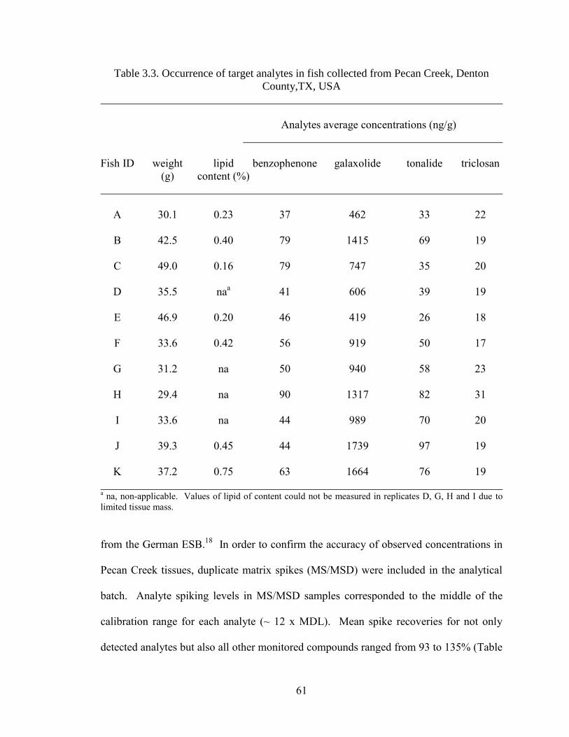
61
Table 3.3. Occurrence of target analytes in fish collected from Pecan Creek, Denton
County,TX, USA
Analytes average concentrations (ng/g)
Fish ID weight lipid benzophenone galaxolide tonalide triclosan
(g) content (%)
A 30.1 0.23 37 462 33 22
B 42.5 0.40 79 1415 69 19
C 49.0 0.16 79 747 35 20
D 35.5 naa 41 606 39 19
E 46.9 0.20 46 419 26 18
F 33.6 0.42 56 919 50 17
G 31.2 na 50 940 58 23
H 29.4 na 90 1317 82 31
I 33.6 na 44 989 70 20
J 39.3 0.45 44 1739 97 19
K 37.2 0.75 63 1664 76 19
a na, non-applicable. Values of lipid of content could not be measured in replicates D, G, H and I due to
limited tissue mass.
from the German ESB.18
In order to confirm the accuracy of observed concentrations in
Pecan Creek tissues, duplicate matrix spikes (MS/MSD) were included in the analytical
batch. Analyte spiking levels in MS/MSD samples corresponded to the middle of the
calibration range for each analyte (~ 12 x MDL). Mean spike recoveries for not only
detected analytes but also all other monitored compounds ranged from 93 to 135% (Table

62
3.4), suggesting that target analytes were quantified with acceptable accuracy in Pecan
Creek samples. Also note that values of relative percent difference (RPD) for MS/MSD
samples were generally less than 20%, demonstrating acceptable precision.
Table 3.4. Matrix spiked and matrix spiked duplicate performance
Analyte amount sample MS MSD MS % MSD % %
spiked conc. conc. conc. recovery recovery RPD
ng/g ng/g ng/g ng/g
m-Toluamide 41 nd 44 46 108 114 5
Benzophenone 87 41 125 124 97 95 2
Celestolide 47 nd 57 63 121 134 11
p-Octylphenol 34 nd 39 33 115 96 18
Galaxolide 106 606 732 748 119 135 12
Tonalide 56 38.9 108 103 124 114 9
Musk xylene 85 nd 103 94 121 110 10
p-nonylphenol 28 nd 34 30 122 108 12
4-MBC 62 nd 67 70 107 113 5
Musk ketone 197 nd 184 209 93 106 13
Triclosan 62 19.3 84 99 103 128 21
Octocrylene 194 nd 187 198 97 102 6
MS, matrix spiked; MSD, matrix spiked duplicate; RPD, relative percentage difference; nd, non detected
Identification of detected analytes was confirmed by comparing relative ion
abundance ratios and retention times observed for environmental samples with those
observed for standards spiked in control matrix. Three ions (one quantitation and two

63
qualifiers) were used for monitoring each analyte in all analyses (Table 3.1). The criteria
imposed for positive identification were matching retention times and 15-percent
agreement in relative ion abundance ratios. Representative ion chromatograms and mass
spectra are shown in Figure 3.2 for galaxolide, displaying excellent agreement in both
retention time and relative ion abundance.
Figure 3.2. GC-SIM-MS reconstituted ion chromatogram and mass spectra for galaxolide in (A) fortified
reference fish containing 120 ng/g galaxolide and (B) environmental sample collected from an effluent-
dominated stream.
An interesting observation from Table 3.3 is that although analyses reported in
Chapters 2 and 3 were conducted on identical tissues collected from the same fish, the
220 230 240 250 m/z
220 230 240 250 m/z
25%
50%
75%
110%
25%
50%
75%
110%
213
243
258
213
243
258
11.55 11.60 11.65 11.70 min
11.55 11.60 11.65 11.70 min
2.5
5.0
10.0
10
20
30
40
Inte
nsi
ty,
MC
ounts
Inte
nsi
ty,
MC
ounts
Rel
ativ
e ab
un
dan
ceR
elat
ive
abun
dan
ce
A)
B)
220 230 240 250 m/z
220 230 240 250 m/z
25%
50%
75%
110%
25%
50%
75%
110%
213
243
258
213
243
258
11.55 11.60 11.65 11.70 min
11.55 11.60 11.65 11.70 min
2.5
5.0
10.0
10
20
30
40
Inte
nsi
ty,
MC
ounts
Inte
nsi
ty,
MC
ounts
Rel
ativ
e ab
un
dan
ceR
elat
ive
abun
dan
ce
A)
B)

64
RSDs for detected concentrations of personal care products (Chapter 3) were
significantly higher than those observed for pharmaceuticals (Chapter 2). RSDs
calculated using data from Table 3.3 were 32%, 45%, 40%, and 19% for benzophenone,
galaxolide, tonalide, and triclosan, respectively. In contrast, RSDs for detected
pharmaceuticals in Chapter 2 were 26%, 36%, 17% and 14% for diphenhydramine,
diltiazem, carbamazepine and norfluoxetine, respectively. Previous investigations of
nonpolar organic contaminants have identified useful correlations between accumulation
and octanol-water partition coefficients, which may also be roughly correlated with lipid
content.38-41
Concentrations of detected personal care products in the present study are plotted
versus lipid content in Figure 3.3. It can be seen in Figure 3.3 (A) that galaxolide has an
apparent tendency to display higher concentrations with increasing lipid content. Nakata
et al. also attributed large variations in galaxolide concentrations between individuals of
the same species to differences in lipid content among analyzed tissues.16
Although less
clear, the tonalide data in Figure 3.3 (B) demonstrate a similar trend. In contrast,
triclosan concentrations did not show monotonic dependence with lipid content, and it
was difficult to discern a definitive trend for benzophenone due to the relatively high
concentration observed in the sample with lowest lipid content. All concentrations were
subsequently normalized by lipid content (i.e., ng/g lipid) in an effort to further clarify
possible correlations. In the case of galaxolide and tonalide, RSDs for normalized
concentrations improved to 36% and 29%, respectively. On the other hand, RSDs for
benzophenone and triclosan were increased to 70% and 56% respectively. This analysis
clearly suggests that observed accumulation trends for some PPCPs may not be

65
rationalized using historical partitioning models developed using data for alternative
pollutants.
Figure 3.3. Plots of detected tissue concentrations (Denton, TX) versus lipid content for (A) galaxolide and
(B) benzophenone, tonalide and triclosan
0
20
40
60
80
100
120
140
0 0.1 0.2 0.3 0.4 0.5 0.6 0.7 0.8
Benzophenone
Tonalide
Triclosan
Linear (Triclosan)
Linear (Tonalide)
Linear (Benzophenone)
0
0.2
0.4
0.6
0.8
1
1.2
1.4
1.6
1.8
2
0 0.1 0.2 0.3 0.4 0.5 0.6 0.7 0.8
Galaxolide
Linear (Galaxolide)
Con
cen
trat
ion
(µ
g/g
)
Lipid (%)
Con
cen
trat
ion
(n
g/g
)
Lipid (%)
A)
B)
R2=0.6575
R2=0.5512
0
20
40
60
80
100
120
140
0 0.1 0.2 0.3 0.4 0.5 0.6 0.7 0.8
Benzophenone
Tonalide
Triclosan
Linear (Triclosan)
Linear (Tonalide)
Linear (Benzophenone)
0
0.2
0.4
0.6
0.8
1
1.2
1.4
1.6
1.8
2
0 0.1 0.2 0.3 0.4 0.5 0.6 0.7 0.8
Galaxolide
Linear (Galaxolide)
Con
cen
trat
ion
(µ
g/g
)
Lipid (%)
Con
cen
trat
ion
(n
g/g
)
Lipid (%)
A)
B)
R2=0.6575
R2=0.5512
Con
cen
trat
ion
(µ
g/g
)
Lipid (%)
Con
cen
trat
ion
(n
g/g
)
Lipid (%)
A)
B)
R2=0.6575
R2=0.5512

66
Conclusions
A multi-residue method has been developed and validated for the determination
of select personal care products and alkylphenols in fish muscle tissue. The method was
successfully applied to fish collected from an effluent-dominated stream and resulted in
the detection of 4 contaminants. It is important to point out that analyzed tissues were
derived from lateral fillets, excluding skin and belly flap, and that the reported approach
may not be applicable to alternative tissues. While the elimination of GPC from the
sample preparation protocol is noted advantage of reported methodology, the author
concedes that analyzed tissues had a significantly lower lipid content than specimens
analyzed in other studies. Accordingly, GPC may become necessary in future
applications of this approach for more fatty tissues.

67
CHAPTER FOUR
Multi-residue Screening of Pharmaceuticals in Fish - A National Pilot Study in the US
Introduction
In Chapter 2, a liquid chromatography-tandem mass spectrometry (LC-MS/MS)
screening method was developed targeting 23 pharmaceuticals and 2 metabolites with
differing physicochemical properties in fish muscle tissue. It was found that tissue
extracts influenced the LC-MS/MS response for several analytes, therefore matrix-
matched calibration standards were employed to determine analyte concentrations in
environmental samples. This method was subsequently used to screen for target analytes
in fish from one effluent-dominated stream in central Texas.
In this chapter, developed LC-MS/MS methodology was applied to assess the
occurrence of target analytes in fish collected from six locations throughout the United
States (5 effluent-dominated streams and one reference site). This work was conducted
as part of the first national pilot study of pharmaceuticals in fish tissue sponsored by the
U.S. Environmental Protection Agency. The analytical method was slightly modified to
overcome limitations related to matrix effects that were noted in Chapter 2, and the new
approach was successfully applied to both fillet and liver tissues. Concentrations of
detected pharmaceuticals varied with geographic location and tissue type and site-to-site
variations are rationalized in terms of the type of wastewater treatment process that was
operational at each location. While findings in this study add definitive support to the
work reported in Chapter 2, it is important to note that one novel contaminant was also
68
identified in liver specimens from two different locations. Additionally, the analysis of
multiple biological tissues derived from diverse fish species collected at different
locations enabled an expanded assessment of matrix effects on the observed analytical
response for target analytes. Perhaps the most significant finding in this work was the
absence of a correlation between tissue concentrations and lipid content.
Background on Wastewater Treatment
Pharmaceuticals, either in their native form or as metabolites, are continuously
introduced to sewage waters through excreta and disposal of unused or expired drugs.
Previous work has demonstrated that the ability of wastewater treatment processes to
remove pharmaceuticals is compound-specific and variable, depending on the treatment
process employed in a particular study. For example, in one study comparing removal
efficiencies for a variety of wastewater-derived contaminants, percent removal observed
for clofibric acid ranged from 34-51%, while that observed for ibuprofen was near
quantitative (90%).102
Also, it has been demonstrated that removal of -blockers in
secondary wastewater treatments employing activated sludge was only 8%, while that
observed for biological filtration was 60%.103
Finally, it is important to appreciate that
the rate of removal for some compounds depends not only on the nature of the treatment
process, but also on other factors like, hydraulic retention time,103
seasonal temperature,59
and potentially the age of activated sludge. Compounds which persist following
municipal wastewater treatment are typically discharged to surface waters and have
potential to accumulate in aquatic organisms.
A brief discussion of municipal sewage treatment is included here to provide the
reader with pertinent background to understand the rationalization of analytical data

69
reported in this chapter. A majority of wastewater in the United States is subjected to
primary and secondary treatments at municipal facilities. Primary treatment involves
mechanical separation of fats, oils, and grease as well as rocks, gravel, and other solids
from sewage. In secondary treatment, the primary effluent is routed over a bed of coarse
stones or plastic media covered with biomass (i.e., bacteria, protozoa, and fungi). At this
stage in the treatment process soluble organic compounds (including select
pharmaceuticals) are absorbed, digested, and metabolized by microorganisms into more
stable inorganic and oxidized organic forms that resist further metabolism. An additional
tertiary treatment capable of degrading pharmaceuticals that are not removed by
biological degradation is also employed at some but not all sewage treatment facilities
because these processes (i.e., activated carbon adsorption, membrane filtration, ozonation
or photocatalysis) are relatively expensive and are still largely viewed as emerging
technologies.104
Experimental Section
Chemicals
All chemicals were reagent grade or better, obtained from commercial vendors,
and used as received. The positive ESI internal standards 7-aminoflunitrazepam-d7, and
fluoxetine-d6 (100.0 µg/ml in acetonitrile), surrogates (100.0 µg/ml in acetonitrile)
acetaminophen-d4, and diphenhydramine-d3, and reference standards (1000.0 µg/ml in
MeOH): fluoxetine, norfluoxetine, sertraline, codeine, diphenhydramine, propranolol and
ibuprofen were purchased as certified analytical standards (Cerilliant Corporation, Round
Rock, TX). Atenolol was purchased in solid form (99% purity), also from Cerilliant.

70
The negative ESI internal standard meclofenamic acid and reference standards: 1,7
dimethylxanthine, acetaminophen, caffeine, miconazole, carbamazepine, erythromycin,
gemfibrozil, trimethoprim, diltiazem, cimetidine, warfarin, thiabendazole,
sulfamethoxazole, lincomycin, metoprolol, tylosin, clofibric acid were purchased in the
highest available purity (Sigma-Aldrich, Milwaukee, WI). Surrogates (100.0 µg/ml in
acetonitrile) carbamazepine-d10 and ibuprofen-13
C3 were purchased from Cambridge
Isotopes Lab. Inc., Andover, MA.
Study Site Selection
All aspects of the pilot study were carried out using protocols defined in a
publically accessible Quality Assurance Project Plan (QAPP).105
Information pertinent to
analytical work is summarized below. All sampling activities related to the pilot study
were performed by personnel from TetraTech, Inc, and whole fish were sent to Baylor on
dry ice for sample compositing and analysis. Six geographic locations (five effluent-
dominated streams and one reference site) were selected as sampling sites. Five streams
utilized in this pilot study had a viable fish population of resident species which spend
most of its life stages within effluent-dominated waters. These sites were targeted in
mid- to large-sized cities representing diverse geographic regions of the country.
Information on WWTP design capacity, average discharge, and in-stream waste
concentration was collected for each site through publically-accessible data (i.e., NPDES
permits, WWTP websites, and USGS flow data) and through phone calls to state officials
and permitting agencies. The site selection criteria used was:
High effluent flow versus ambient flow
High population density

71
Large fraction of elderly residents
Large volume of PPCP sales/consumption
Fish availability
Demographic information for each of these sites is summarized in Table 4.1. Fish were
also collected from the Gila River (New Mexico, USA). The Gila River is not impacted
by wastewater effluent discharges; therefore no accumulation of pharmaceuticals was
expected in fish collected from this site. Accordingly, these fish were included in the
study as a reference condition and also used to provide a clean control matrix.
Sampling and Preservation
In order to maintain consistency with existing EPA programs focused on
accumulation of contaminants in fish tissue, this pilot study included composite sampling
of fish fillets and fish livers from each sample site. Six composite samples were prepared
at each site. At least three adult individuals were collected per composite such that the
combined biomass of the specimens was adequate to provide sufficient tissue for lipid
determination and complementary screening analyses for personal care products and
pharmaceuticals, respectively. Each sample consisted of adult-sized fish that are
typically consumed by wildlife and humans. All fish used to prepare a single composite
were from the same species, were collected at the same time, and were of similar size
such that the smallest individual in a composite was no less than 75% of the total length
of the largest individual. The sampling period was from summer to early fall, since lipid
content is usually highest and water levels lowest at that time. Species were identified by
experienced personnel as soon as fish were removed from the collection device.
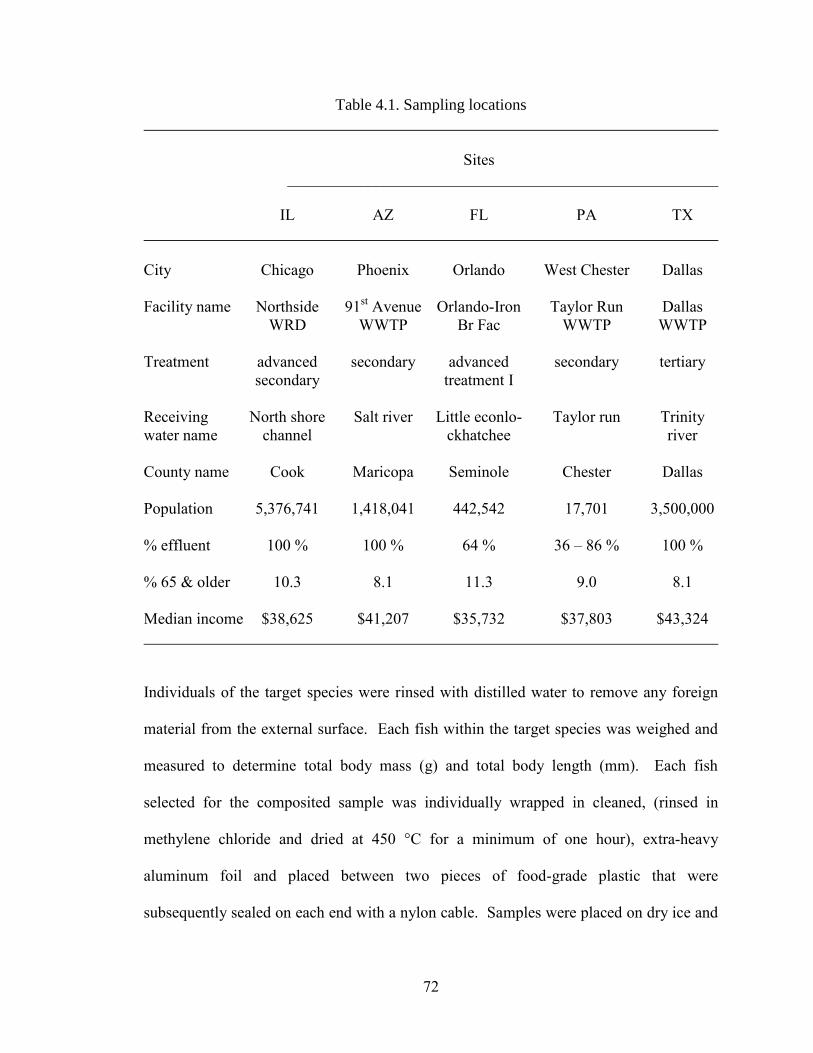
72
Table 4.1. Sampling locations
Sites
______________________________________________________
IL AZ FL PA TX
City Chicago Phoenix Orlando West Chester Dallas
Facility name Northside 91st Avenue Orlando-Iron Taylor Run Dallas
WRD WWTP Br Fac WWTP WWTP
Treatment advanced secondary advanced secondary tertiary
secondary treatment I
Receiving North shore Salt river Little econlo- Taylor run Trinity
water name channel ckhatchee river
County name Cook Maricopa Seminole Chester Dallas
Population 5,376,741 1,418,041 442,542 17,701 3,500,000
% effluent 100 % 100 % 64 % 36 – 86 % 100 %
% 65 & older 10.3 8.1 11.3 9.0 8.1
Median income $38,625 $41,207 $35,732 $37,803 $43,324
Individuals of the target species were rinsed with distilled water to remove any foreign
material from the external surface. Each fish within the target species was weighed and
measured to determine total body mass (g) and total body length (mm). Each fish
selected for the composited sample was individually wrapped in cleaned, (rinsed in
methylene chloride and dried at 450 °C for a minimum of one hour), extra-heavy
aluminum foil and placed between two pieces of food-grade plastic that were
subsequently sealed on each end with a nylon cable. Samples were placed on dry ice and

73
shipped to Baylor via next-day air. Upon receipt, all samples were catalogued and stored
at 20 °C prior to dissection and homogenization. Freezer temperature was recorded
daily to ensure proper storage conditions.
Preparation of Composite Tissue Specimens
Samples were composited using the “batch” method, in which like tissues from all
individual specimens that comprise a composite are homogenized together, regardless of
each individual‟s respective portion (as opposed to the “individual” method, in which
equal weights of each specimen are combined). For preparation of composite samples,
each fish was rinsed with distilled water, scaled, and fillet (including skin and belly flap)
and liver tissues were dissected independently (tissue dissections were carried out by Ms.
Laura Dobbins). Each fillet was cut into approximately 2.5 cm cubes using high-quality
stainless steel aluminum scissors. Individual cubes were combined and frozen (at 20
°C) prior to being ground to a fine powder using a high speed blender. Note that
successive addition of small amounts of dry ice during grinding was critical in
maintaining the consistency of frozen tissues and greatly simplified this aspect of sample
preparation. The ground sample was then divided into quarters, opposite quarters were
combined, and the resulting halves were mixed together by hand. After applying this
procedure to at least three fish from one site, portions were combined again by dividing
them into quarters and mixing halves to prepare a composite. This procedure was applied
to prepare six different composite samples for each field site. Liver samples did not
require the preparation of frozen cubes or the use of a high speed blender for
homogenization. Instead, livers corresponding to each composite (at least three livers per
composite) were combined in a clean glass container and homogenized using a
74
Tissuemiser (Fisher Scientific, Fair Lawn, NJ) set to rotate at 30,000 rpm. (Preparation
of composite samples was carried out in collaboration with Dr. Mohammad A. Mottaleb
and Ms. Pilar Perez-Hurtado).
Determination of Lipid Content
Lipids were extracted from three replicate fillet tissues (ca. 2 g) using 15 ml of 1:1
dichloromethane:hexane (v/v). Each mixture was homogenized for 3 min using a
Tissuemiser (Fisher Scientific), and the vials were subsequently placed in an incubator
for 24 h at 35 °C and agitated by gentle end-over-end rotation. Following extraction,
solid anhydrous sodium sulfate was added to each sample (g Na2SO4 = 2 × g tissue), and
the mixture was filtered through Grade 415 Filter Paper. The solid residue was then
washed with an additional 15 ml of 1:1 dichloromethane:hexane, and the combined
filtrate for each sample was collected in a pre-weighed test tube. The solvent was
evaporated for 8 h at 45 °C using a Zymark Turbovap LC Concentration Workstation.
After evaporation, each residue was dried to constant weight in a vacuum oven at 40 °C.
Lipid content was determined gravimetrically by weighing three replicates of each
sample. (This experiment was conducted by Ms. Pilar Perez-Hurtado.)
This procedure was modified slightly to determine lipid content of liver
specimens. Approximately 2 g liver tissue was combined with 15 ml of 1:1
dichloromethane-hexane and ca. 2 g solid Na2SO4 in a borosilicate glass vial. Samples
were sonicated for 30 min in an ultrasonic water bath at room temperature. The vials
were subsequently placed in an incubator for 24 h at 35 °C and agitated by gentle end-
over-end rotation. Following extraction, samples were centrifuged at 16,000 rpm for 40
min at 4 °C to ensure complete phase disengagement. The supernatant was collected by
75
filtration, and the solid residue was washed with an additional 15 ml of 1:1
dichloromethane:hexane that was also passed through the filter and collected in a pre-
weighed test tube. The solvent was evaporated and residues were dried to constant
weight in a vacuum oven at 40 °C. Due to limited sample mass, triplicate measurements
were made for only one composite from each sampling site. All other determinations
were based on a single measurement. (This experiment was conducted in collaboration
with Ms. Pilar Perez-Hurtado.)
Analytical Sample Preparation
Each analytical sample, either 1.0 g fillet composite or 0.5 g liver composite, was
placed into a 20-ml borosilicate glass vial (Wheaton; VWR Scientific, Rockwood, TN).
Four surrogates were added to each sample, acetaminophen-d4 (500 ng),
diphenhydramine-d3 (10 ng), carbamazepine-d10 (40 ng) and ibuprofen-13
C3 (840 ng). 8
ml of extraction solvent (1:1 mixture of 0.1 M aqueous acetic acid and methanol) was
added to the sample and the mixture was sonicated for 15 min at 25 °C. Following
extraction, samples were rinsed into 50-ml polypropylene copolymer round-bottomed
centrifuge tubes (Nalge Company; Nalgene® Brand Products, Rochester, New York)
using 1 ml extraction solvent and centrifuged at 16,000 rpm for 40 min at 4 °C. The
supernatant was decanted into 18 ml disposable borosilicate glass culture tubes (VWR
Scientific, Rockwood, TN), and the solvent was evaporated to dryness under a stream of
nitrogen at 45 °C using a Zymark Turbovap LC concentration workstation (Zymark
Corp., Hopkinton, MA). Samples were reconstituted in mobile phase (1 ml for fillet
composites and 0.5 ml for liver composites) and a constant amount of the internal
standards 7-aminoflunitrazapam-d7 (100 ng), fluoxetine-d6 (585 ng), and meclofenamic

76
acid (995 ng) was added (half of these amounts were added to liver composites). Prior to
analysis, samples were sonicated for 1 min and filtered using Pall Acrodisc hydrophobic
Teflon Supor membrane syringe filters (13 mm diameter; 0.2-µm pore size; VWR
Scientific, Suwanee, GA).
HPLC-MS/MS Analysis
All samples were screened for 24 target analytes using the HPLC-MS/MS
approach described in Chapter 2. It is important to point out that fluoxetine-d6 replaced
7-aminoflunitrazepam-d7 as the internal standard for quantification of fluoxetine,
norfluoxetine and sertraline. Similarly, 7-aminoflunitrazepam-d7 replaced meclofenamic
acid as the internal standard for quantification of ibuprofen. These changes were made in
an effort to more effectively account for expected matrix effects on the analytical
response for these analytes. Finally, note that clofibric acid was dropped from the analyte
list to overcome a persistent instrumental limitation that prohibited the use of positive and
negative electrospray ionization within the same chromatographic segment.
Calibration standards were prepared in fillet or liver control matrix, as
appropriate, and carried through the entire sample preparation protocol prior to analysis.
Note that in the preparation of calibration samples, varying concentrations of all target
analytes and surrogates were added prior to extraction. Calibration curves were
constructed from a minimum of five points by plotting the ratio of observed peak areas
for the analyte and internal standard, respectively, versus analyte concentration.
Calibration data were subjected to a linear regression that was forced through the origin,
and the resulting equation was used to calculate analyte and surrogate concentrations in
all subsequent analyses. This approach resulted in regression coefficients (r2) exceeding

77
0.99 for all target compounds. Calibration plots employed for quantification of target
compounds in both fillet and liver tissues are included in the Appendix (Figures A.1 to
A.14). Analyte-specific MS/MS transitions monitored for quantitation were given in
Chapter 2 (Table 2.2). Qualifier transitions monitored for detected analytes in
environmental samples were as follows: diphenhydramine, m/z 256 > 152; diltiazem, m/z
415 > 150; carbamazepine, m/z 237 > 165; fluoxetine m/z 310 > 44; sertraline m/z 306 >
159, gemfibrozil, 249 > 127. Note that collision-induced dissociation of norfluoxetine
results in only one product ion of sufficient intensity to be observed in environmental
samples.25
Therefore, a qualifying transition was not confirmed for this analyte.
The determination of experimentally-derived method detection limits (MDLs) for
fish muscle tissue was discussed in Chapter 2, and it was initially assumed that these
previously determined values would be appropriate for establishing detection and
quantitation thresholds for the present study. Recall that the MDL corresponds to the
lowest concentration of analyte that can be reported in a defined matrix with 99%
confidence that the concentration is non-zero.76
For data qualification purposes, a more
conservative quantitation threshold for each analyte (PQL) was set 2 to 5 times above
MDL. However, since analyte identification was supported by both chromatographic
retention time and the relative response of two MS/MS product ions, each target
compound was calibrated at or near the MDL and quantitative information for all positive
identifications are reported. Over the course of this investigation it was determined that
matrix interference encountered in the analysis of liver samples was more pronounced

78
Table 4.2. Low calibration level, MDL and PQL for target analytes in fillet and liver
tissues
Fillet Liver
_________________________ _______________
Low cal MDL,a PQL,
b Low Cal MDL,
Analyte level, ng/g ng/g ng/g level, ng/g ng/g
Diphenhydramine 0.10 0.05 0.25 0.10 0.26
Diltiazem 0.10 0.12 0.25 0.10 0.26
Carbamazepine 0.80 0.54 2.00 0.80 1.86
Warfarin 0.80 0.86 2.00 2.00 2.70
Cimetidine 2.00 1.04 5.00 5.00 5.18
Propranolol 2.00 1.07 5.00 2.00 3.77
1,7 Dimethylxanthine 2.00 1.10 5.00 2.00 5.84
Atenolol 2.00 1.48 5.00 12.5 12.86
Trimethoprim 3.20 2.15 8.00 3.20 8.00
Sulfamethoxazole 3.20 2.29 8.00 3.20 13.95
Metoprolol 3.20 2.50 8.00 3.20 8.90
Thiabendazole 3.20 2.63 8.00 3.20 7.84
Norfluoxetine 3.20 2.90 8.00 20.0 15.31
Sertraline 3.20 3.56 8.00 20.0 17.29
Caffeine 6.00 3.93 15.0 6.00 25.47
Acetaminophen 6.00 4.40 15.0 15.0 34.28
Fluoxetine 6.00 6.74 15.0 15.0 12.41
Tylosin 8.00 5.02 20.0 8.00 34.67

79
Table 4.2. Low calibration level, MDL and PQL for target analytes in fillet and liver
tissues (Cont.)
Fillet Liver
_________________________ _______________
Low cal MDL,a PQL,
b Low Cal MDL,
Analyte level, (ng/g) (ng/g) (ng/g) level, (ng/g) (ng/g)
Lincomycin 8.00 5.53 20.0 50.0 56.14
Codeine 8.00 6.11 20.0 20.0 31.49
Erythromycin 8.00 6.42 20.0 8.00 43.03
Gemfibrozil 8.00 6.68 20.0 8.00 24.82
Miconazole 12.0 10.83 30.0 na na
Ibuprofen 60.0 45.96 150 60.0 172.81
a „Clean‟ tissues employed in the determination of liver and fillet method detection limits (MDLs). Samples
were extracted using a 1:1 mixture (v/v) of 0.1 M acetic acid buffer (pH 4) and methanol. See text for
details. MDLs determined by multiplying the one sided 99 percent student‟s t-statistic (t0.99) by the standard
deviation from eight replicates analysis of spiked sample. b PQL was assigned in this study as two to three
times the MDL values (depending upon lower calibration point behavior in the matrix).
than that observed for fillet tissues. Consequently, independent MDLs were determined
for liver using an identical approach to that employed previously for fillet specimens.
Adjusted MDLs and calibration limits for liver are reported in Table 4.2 along with the
calibration limits, MDLs, and PQLs noted above for fillet tissues.
Starting with fillet specimens, all composite tissues were grouped into batches of
less than 20 samples. Each batch contained one blank (i.e., control matrix spiked with
surrogates only) and two laboratory control samples (LCS 1 and 2; control matrix spiked
with surrogates and a known amount of each target analyte). LCS1 was a low-level
control sample spiked with analyte concentrations corresponding to the PQL values

80
reported in Table 4.2, while LCS2 was spiked with analyte concentrations that were
approximately 10-fold greater than the lowest concentration calibration standard.
Composite samples from no more than two sites were also included in each batch, and
one composite sample from each site was randomly selected and used to prepare two
identical matrix spikes (i.e., one matrix spike-matrix spike duplicate pair, MS/MSD).
Spike concentrations employed in the preparation of MS/MSD samples were equivalent
to concentrations added to LCS2. Each batch was analyzed independently, and once
fillet analyses were complete, an identical approach was employed for analysis of liver
tissues.
Quality Control
The following quality control criteria were used throughout the study to monitor
performance of the employed analytical method. Acceptable initial calibration required
that the relative standard deviation of independent relative response factors (RRF defined
in equation 4.1 below) for each analyte and surrogate was less than 30%.
x
is
is
x
C
C
A
ARRF (4.1)
In this equation Ax and Ais are the peak areas for the target chemical and internal standard,
respectively, and Cx and Cis are their respective concentrations in each calibration
standard. The high-level laboratory control sample (LCS2) was not only employed to
evaluate analyte and surrogate recoveries as defined in more detail below, but also
doubled as a continuing calibration verification (CCV) sample in each analytical batch.
Instrument calibration was evaluated by monitoring the percent difference (%D) between
the RRF calculated for LCS2 and the average RRF from initial calibration data.

81
100%nom
nomobs
RRF
RRFRRFD (4.2)
In this equation RRFobs corresponds to LCS2 and RRFnom is the average RRF resulting
from initial calibration. A result ≤ 25% demonstrated acceptable calibration for
continued sample analysis. Method performance was monitored on a continuing basis by
evaluating analyte and surrogate recoveries (%R) in laboratory control samples (LCS 1
and 2) and matrix spikes (MS/MSD).
100%s
x
C
CR (4.3)
In this equation Cx and Cs represent the observed sample concentration and spiking level,
respectively. For the purposes of this study, recoveries ranging from 60% to 150% were
deemed acceptable. Note that the same criteria were used to evaluate surrogates in every
sample. Precision was evaluated by monitoring the relative percent difference (RPD)
between duplicate matrix spikes:
1002/21
21
CC
CCRPD (4.7)
where C1 and C2 are the first and second of 2 measurements. In general, observed RPDs
were less than 15%.
Results and Discussion
Analytical Observations from Control Samples
Results for initial and continuing calibration verification data in fillet tissues
demonstrated acceptable performance with one exception. Evaluation of initial
calibration data revealed that the RSDs of RRFs for 27 of 28 target compounds ranged
82
from 3 to 17% with an average of 9%. In contrast, the initial RSD observed for
miconazole fell outside the 30% quality assurance threshold. Visual inspection of
chromatograms demonstrated that miconazole response was suppressed to a greater
extent than anticipated in this control matrix. Therefore, the calibration range for this
analyte was adjusted to exclude concentrations that did not resolve from the baseline (i.e.,
the two lowest concentration calibration standards). As a result, the lowest concentration
calibrated for miconazole was 75 ng/g, and the RSD improved to 27%. Initial calibration
data for fillet analyses is included in the Appendix Table A.1. Percent difference (%D)
for all continuing calibration verification samples ranged from -24% to 19%,
demonstrating adherence to established criteria for continued sample analysis (see Table
A.2 for representative CCV data, corresponding to the first analytical batch of fillet
tissues).
Matrix suppression of analyte response and/or increased background required that
the calibration range for a larger number of compounds be adjusted in analyses of liver
tissues. Due to matrix suppression similar to that described above for miconazole, an
analytical response for acetaminophen, codeine, cimetidine, fluoxetine, norfluoxetine,
sertraline, and warfarin was not observed in one or more low concentration standards
prepared in liver. Accordingly, these standards were eliminated in the construction of
calibration curves for these analytes (Table A.3). In contrast, visual inspection of
chromatograms for atenolol revealed significant peak-shaped responses of approximately
equal area for samples spiked with 2, 5, and 12.5 ng of this compound. A peak-shaped
response of similar magnitude was observed at the atenolol retention time upon
subsequent analysis of a liver blank. However, the qualifier ion for atenolol was not

83
observed in the blank, confirming that atenolol was not present (i.e., the observed
response was due to an unidentified compound native to control matrix). As a result, the
three lowest concentrations were eliminated from atenolol calibration curves to overcome
background interference. A similar situation required that the two lowest calibration
levels for lincomycin be eliminated. As demonstrated in Figure 4.1, lincomycin was
unresolved from a background peak eluting at slightly shorter retention time, and the
concentration of the unidentified component was of sufficient magnitude to mask the
lincomycin response at concentrations below 50 ng/g. A non-peak shaped background
response was present in chromatograms for miconazole of sufficient magnitude to
prohibit quantitative (or even qualitative) analysis of calibration data for this analyte in
liver extracts.
After making the noted adjustments, initial calibration criteria were satisfied for
all analytes (except miconazole) in liver tissue. As demonstrated in Table A.3, the RSDs
of RRFs for target compounds ranged from 6 to 21% (with an average of 12%). In
continuing analyses, observed values of %D for CCV samples ranged from -19 % to 23%
with three exceptions. The %D for lincomycin was -29% and -38% in the IL and TX
batches, respectively, and %D for norfluoxetine was -28.6 % in the TX batch. Although
these values fall outside the CCV control limit specified for the pilot study (±25%), it was
determined that corrective action (i.e., recalibration and repeated analysis of samples
from the IL and TX batches) was not necessary since lincomycin was not detected in
environmental samples and recoveries calculated for norfluoxetine in control samples
(LCS 1 and 2) corresponding to the TX batch fell within the 60-150% limit.

84
Figure 4.1. Overlaid MS/MS chromatograms for lincomycin calibration standards and liver control matrix
Surrogate and Control Sample Data
Surrogate monitoring was employed to evaluate method performance for each
individual sample. A representative surrogate report corresponding to the first analytical
batch is provided in Table A.4. Surrogate recoveries for samples derived from muscle
tissue were within defined control limits (60-150%) and fell into the following ranges:
acetaminophen-d4, 87 – 110%; diphenhydramine-d3, 63 – 80%; carbamazepine-d10, 63 –
112%; and ibuprofen-13
C3, 84 – 137%. It is noteworthy that recoveries for
diphenhydramine-d3 exhibited low bias. The origin of this behavior is presently
unknown. Surrogate recoveries in liver samples also demonstrated acceptable
performance with one exception: acetaminophen-d4, 112 – 150 % (except for TX batch);
12.75 13.0 13.25 13.5 13.75 14.0 min
0
5
4
3
2
1
Inte
nsi
ty,
MC
ounts
1600 ng/g
800 ng/g
400 ng/g
200 ng/g
100 ng/gLiver reference blank
14.25
50 ng/g
20 ng/g
8 ng/g
12.75 13.0 13.25 13.5 13.75 14.0 min
0
5
4
3
2
1
Inte
nsi
ty,
MC
ounts
1600 ng/g
800 ng/g
400 ng/g
200 ng/g
100 ng/gLiver reference blank
14.25
50 ng/g
20 ng/g
8 ng/g

85
diphenhydramine-d3, 71 – 120 %; carbamazepine-d10, 75 – 119 %; and ibuprofen-13
C3, 63
– 138 %. Acetaminophen-d4 recoveries in the TX batch ranged from 131 to 234 %.
However, acceptable recoveries were observed for acetaminophen-d4 in CCV and LCS
samples and for unlabeled acetaminophen in MS/MSD samples from this batch. Thus, it
is possible that acetaminophen-d4 experienced unique matrix interference in samples
derived from the TX site.
Two laboratory control samples (LCS 1 and 2) were also included in each
analytical batch to monitor instrumental performance. Representative control sample
data corresponding to the first analytical batch is shown in Tables A.5 and A.6 for LCS 1
and 2, respectively. The LCS1 sample was employed to demonstrate quantitative
accuracy near the MDL, and LCS2 demonstrated accuracy near the middle of the
calibration range. Recoveries for all but two analytes in LCS1 samples prepared from
muscle tissue ranged from 84 to 119%. The range of recoveries observed for
erythromycin and miconazole in these samples was somewhat broader (88 – 136% and
86 – 147%, respectively) yet still within control limits. A similar trend was observed for
LCS2 samples prepared from muscle tissue. Recoveries ranged from 84 – 120% for all
compounds, excepting erythromycin (92 – 133%) and miconazole (105 – 133%).
In general, control sample data also validated quantitative accuracy for
determination of analyte concentrations in liver extracts. With the exception of atenolol
and lincomycin, observed recoveries for LCS1 and LCS2 samples ranged from 85 –
148% and 75 – 136%, respectively. As noted above, a background signal native to
control matrix prohibited quantitation of atenolol and lincomycin at LCS1 spiking levels.
86
In LCS2 samples, lincomycin recoveries ranged from 94 – 133% while recoveries for
atenolol still exhibited high bias 113 – 155%.
Matrix Spike Data
Matrix spike samples (i.e., MS/MSD samples) were included in each
analytical batch to evaluate the influence of sample matrix on the analytical response for
each analyte. Average MS/MSD recoveries observed for muscle and liver samples from
each site are reported in Table 4.3. Consistent with matrix effect data presented in
Chapter 2, these data clearly demonstrate that variability of sample matrix between sites
had a negligible effect on the analytical response of early eluting analytes. That is,
observed analyte recoveries in the present study were essentially quantitative for
compounds eluting at retention times 30 minutes (i.e., all compounds preceding and
including carbamazepine in Table 4.3). In contrast, with the exception of ibuprofen,
observed recoveries for all analytes eluting at longer retention time fell outside of control
limits (60-150%) in one or more MS/MSD samples (these occurrences are denoted in
italics in Table 4.3). In general, matrix effects were more pronounced in liver extracts
than in extracts derived from fillet tissue. Note that the data in Table 4.3 are essentially
normalized to the NM sample, since this matrix was also employed for instrument
calibration. Signal enhancement relative to the NM reference condition was the effect
observed for the majority of influenced analytes, resulting in increased recoveries by a
factor of ca. 2-6. Suppression was also observed in some cases (e.g., tylosin in both fillet
and liver samples from the IL site and warfarin in the fillet sample from AZ).
Interestingly, gemfibrozil response was suppressed in the fillet extract from IL but

87
Table 4.3. Average matrix spike recoveries (n = 2) for target analytes
Fillet / liver
______________________________________________
Analyte IL NM AZ FL PA TX
Acetaminophen 92/97 94/89 99/94 89/110 87/100 84/125
Atenolol 98/109 109/88 120/114 105/96 107/92 105/120
Cimetidine 89/107 101/105 119/112 99/107 101/106 99/118
Codeine 100/97 102/107 114/89 98/98 103/102 103/112
1,7 dimethylxanthine 102/117 94/110 105/110 91/106 92/101 90/129
Lincomycin 108/96 96/124 111/86 98/103 99/101 93/104
Trimethoprim 108/109 110/109 117/113 107/108 110/119 114/115
Thiabendazole 117/102 104/107 110/108 117/101 112/93 114/116
Caffeine 112/106 99/111 102/105 95/109 100/105 94/109
Sulfamethoxazole 104/85 101/111 97/84 90/107 89/95 90/108
Metoprolol 112/100 103/99 111/94 89/87 103/89 97/86
Propranolol 105/99 100/95 111/106 98/87 100/104 103/108
Diphenhydramine 104/88 97/88 94/69 87/89 102/114 90/105
Diltiazem 98/75 95/100 104/103 93/89 93/95 92/105
Carbamazepine 100/81 90/97 85/97 98/83 90/80 86/80
Tylosin 9/53a 113/111 118/78 113/99 100/106 110/99
Fluoxetine 90/144 92/105 97/271 105/349 94/362 100/335
Norfluoxetine 138/92 99/115 108/197 152/350 125/247 134/398
Sertraline 119/96 91/120 99/172 144/407 93/473 126/584

88
Table 4.3. Matrix spike average recoveries (n = 2) for selected analytes (Cont.)
Fillet / liver
______________________________________________
Analyte IL NM AZ FL PA TX
Erythromycin 68/115 127/108 135/139 160/240 197/297 174/123
Warfarin 94/84 91/85 50/78 110/92 93/69 79/76
Miconazole 353/nab 125/na 107/na 414/na 296/na 199/na
Ibuprofen 114/112 96/83 99/95 85/94 106/76 104/102
Gemfibrozil 42/172 88/106 126/246 149/527 94/218 86/166
a italic numbers represent values outside control limit (60 - 150%);
b a non-peak shaped background
response was present in chromatograms for miconazole of sufficient magnitude to prohibit quantitative (or
even qualitative) analysis of calibration data for this analyte.
enhanced to varying degrees in liver extracts. These results were somewhat surprising
but clearly demonstrate that extracts from fish collected at different sites exert variable
influence on electrospray ionization, despite the fact that they were derived from a single
biological tissue (i.e., muscle or liver).
Variation of sample matrix between sites also resulted in a noticeable shift in
retention time for some analytes. Average retention times observed in analyses of fillet
and liver MS/MSD samples are plotted as a function of collection site in Figure 4.2.
Calculated RSDs for analyte retention times plotted in Figure 4.2A were 1% in all
cases, demonstrating that retention times were essentially constant in analyses of fillet
extracts, independent of collection site. Similar RSDs were observed for most
compounds in analyses of liver extracts as well. However, RSDs calculated using data

89
Figure 4.2. Average retention times observed for MS/MSD samples in A) fillet and B) liver tissue extracts
plotted for atenolol, cimetidine, codeine, lincomycin, trimethoprim and thiabendazole in
Figure 4.2B ranged from 2 – 7%, demonstrating that co-extracted matrix components
0
10
20
30
40
50
60
NM IL AZ FL PA TX
Gemfibrozil
Ibuprofen
Miconazole
Warfarin
Erythromycin
Sertraline
Norfluoxetine
Fluoxetine
Tylosin
Carbamazepine
Diltiazem
Diphenhydramine
Propranolol
Metoprolol
Sulfamethoxazole
Caffeine
Thiabendazole
Trimethoprim
Lincomycin
1,7Dimethylxanthine
Codeine
Cimetidine
Atenolol
Acetaminophen
0
10
20
30
40
50
60
NM IL AZ FL PA TX
Gemfibrozil
Ibuprofen
Warfarin
Sertraline
Norfluoxetine
Fluoxetine
Tylosin
Carbamazepine
Diltiazem
Diphenhydramine
Propranolol
Metoprolol
Sulfamethoxazole
Caffeine
Thiabendazole
Trimethoprim
Lincomycin
1,7Dimethylxanthine
Codeine
Cimetidine
Atenolol
Acetaminophen
Erythromycin
A)
B)
Sites
Sites
Ret
enti
on t
ime,
min
Ret
enti
on t
ime,
min
0
10
20
30
40
50
60
NM IL AZ FL PA TX
Gemfibrozil
Ibuprofen
Miconazole
Warfarin
Erythromycin
Sertraline
Norfluoxetine
Fluoxetine
Tylosin
Carbamazepine
Diltiazem
Diphenhydramine
Propranolol
Metoprolol
Sulfamethoxazole
Caffeine
Thiabendazole
Trimethoprim
Lincomycin
1,7Dimethylxanthine
Codeine
Cimetidine
Atenolol
Acetaminophen
0
10
20
30
40
50
60
NM IL AZ FL PA TX
Gemfibrozil
Ibuprofen
Warfarin
Sertraline
Norfluoxetine
Fluoxetine
Tylosin
Carbamazepine
Diltiazem
Diphenhydramine
Propranolol
Metoprolol
Sulfamethoxazole
Caffeine
Thiabendazole
Trimethoprim
Lincomycin
1,7Dimethylxanthine
Codeine
Cimetidine
Atenolol
Acetaminophen
Erythromycin
A)
B)
Sites
Sites
Ret
enti
on t
ime,
min
Ret
enti
on t
ime,
min
90
derived from liver had a pronounced effect on the chromatographic behavior of these
analytes. This can be attributed to the presence of co-eluting compounds that either
interact with target analytes in the mobile phase or compete for stationary-phase
adsorption sites. It is important to mention that within the same matrix, analyte retention
times of atenolol, cimetidine, codeine, lincomycin, trimethoprim and thiabendazole were
constant.
Environmental Occurrence
Analytical concentrations of pharmaceuticals detected in fillet and liver tissues
from each sampling location are summarized in Tables 4.4 and 4.5, respectively. Plus-or-
minus values presented in these tables represent one standard deviation from the mean
concentration observed upon screening independent composite samples from each site.
Accordingly, the standard deviation provides a qualitative estimate of the range of
concentrations detected at each site rather than an estimate of analytical variability. Data
for independent composites corresponding to each collection site are included in Tables
A.7– A.12. It is important to point out that no analytes were detected in fish sampled
from the NM site, definitively demonstrating that environmental accumulation of these
compounds is a consequence of point-source distribution of pharmaceuticals to surface
waters.
Diphenhydramine, diltiazem, carbamazepine, fluoxetine, norfluoxetine, and
sertraline were detected at concentrations above MDLs in all 6 composite fillet samples
from one or more study site(s) (Table 4.4), confirming results included in Chapter 2 and
previous reports citing accumulation of these compounds in fish tissues.10, 25
Inspection

Table 4.4. Average concentrations of pharmaceutical (ng/g tissue) detected in 6 independent fillet composites from each sampling site
Mean concentrations ± SD, (ng/g)a
________________________________________________________________
Site spb length weight lipid % diphenhy- diltiazem carbama- fluoxetine norflu- sertraline gemfibrozil
(cm) (kg) mean ± SD dramine zepine xetine
NM ss 33-34 0.7-0.9 4.9 ± 1.6 nd nd nd nd nd nd nd
IL lmb 27-36 0.4-0.9 2.3 ± 0.6 1.38 ± 0.27 0.13 ± 0.02 2.3 ± 0.5 nd 2.3 ± 0.4c 2 ± 1
c nd
AZ carp 35-55 0.8-2.0 3.9 ± 0.8 1.20 ± 0.12 0.04 ± 0.01c N.D 1.5 ± 0.4
c 3 ± 1 5 ± 1 nd
FL b 34-44 0.4-2.2 1.0 ± 0.7 nd nd nd nd nd nd nd
PA ws 29-36 0.3-0.6 1.9 ± 0.4 1.74 ± 0.42 0.13 ± 0.04 0.3 ± 0.1c 3 ± 1 4 ± 1 11 ± 5 nd
TX smb 43-60 1.4-4.6 2.2 ± 1.1 nd nd nd nd 1.5 ± 0.3c,d
nd nd
a Reported analytes were detected in 6 of 6 composite samples for each site (n = 6) unless otherwise noted. See Tables A.7-A.12 for details.
b sp, species; ss, sonora sucker; lmb, large mouth bass; b, bowfin; ws, white sucker; smb, small mouth buffalo
c reported concentration < MDL and/or lowest calibration standard reported in Table 4.2
d analyte detected in 2 of 6 composite samples (n = 2)
91
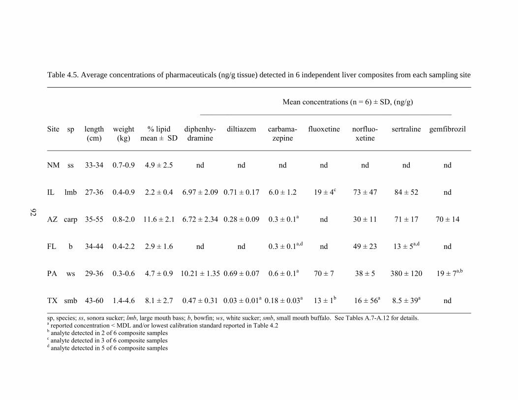
Table 4.5. Average concentrations of pharmaceuticals (ng/g tissue) detected in 6 independent liver composites from each sampling site
Mean concentrations (n = 6) ± SD, (ng/g)
________________________________________________________________
Site sp length weight % lipid diphenhy- diltiazem carbama- fluoxetine norfluo- sertraline gemfibrozil
(cm) (kg) mean ± SD dramine zepine xetine
NM ss 33-34 0.7-0.9 4.9 ± 2.5 nd nd nd nd nd nd nd
IL lmb 27-36 0.4-0.9 2.2 ± 0.4 6.97 ± 2.09 0.71 ± 0.17 6.0 ± 1.2 19 ± 4c 73 ± 47 84 ± 52 nd
AZ carp 35-55 0.8-2.0 11.6 ± 2.1 6.72 ± 2.34 0.28 ± 0.09 0.3 ± 0.1a nd 30 ± 11 71 ± 17 70 ± 14
FL b 34-44 0.4-2.2 2.9 ± 1.6 nd nd 0.3 ± 0.1a,d
nd 49 ± 23 13 ± 5a,d
nd
PA ws 29-36 0.3-0.6 4.7 ± 0.9 10.21 ± 1.35 0.69 ± 0.07 0.6 ± 0.1a 70 ± 7 38 ± 5 380 ± 120 19 ± 7
a,b
TX smb 43-60 1.4-4.6 8.1 ± 2.7 0.47 ± 0.31 0.03 ± 0.01a 0.18 ± 0.03
a 13 ± 1
b 16 ± 56
a 8.5 ± 39
a nd
sp, species; ss, sonora sucker; lmb, large mouth bass; b, bowfin; ws, white sucker; smb, small mouth buffalo. See Tables A.7-A.12 for details. a reported concentration < MDL and/or lowest calibration standard reported in Table 4.2
b analyte detected in 2 of 6 composite samples
c analyte detected in 3 of 6 composite samples
d analyte detected in 5 of 6 composite samples
92

93
of Table 4.5 demonstrates that this statement also applies to liver data, with the additional
detection of one novel contaminant. Although one previous report has demonstrated
bioconcentration of gemfibrozil in a laboratory setting,31
the present study represents the
first example of environmental accumulation for this compound. In general,
concentrations of detected analytes were increased and more variable in liver relative to
fillet tissues. This finding is consistent with results reported in a previous investigation
of environmental accumulation focused on antidepressants,10
but the origin of this
behavior is presently unknown.
In a recent study citing bioaccumulation of alternative organic wastewater
compounds, Barber et al. rationalized higher analyte concentrations in same samples as
being a consequence of higher lipid content.77
Such rationalization is based on a
collection of studies demonstrating a correlation between experimentally-derived
bioconcentration factors and analyte-specific physicochemical properties, most
commonly the octanol-water partition coefficient (KOW). Multiple observations of
increased bioaccumulation with increasing KOW have led to the supposition that organic
contaminants are most likely partitioned to fatty tissues (i.e., lipids.) Consequently, it is
expected that higher lipid content will promote increased concentrations of accumulated
chemicals. Recall that this trend was roughly demonstrated for galaxolide and tonalide in
Chapter 3 (Figure 3.2). Occurrence data in Tables 4.4 and 4.5 corresponding to samples
from TX, PA, FL, and AZ are consistent with this trend. However, increased liver
concentrations were also observed in samples collected from the IL site, despite the fact
that lipid content for muscle and liver tissues from this site was essentially identical. This
result leads to divergent hypotheses that either data observed for tissues from the IL site

94
are anomalous or that conventional wisdom relevant to environmental accumulation of
these pharmaceuticals is flawed.
In order to further investigate this issue, analytical concentrations of detected
analytes were plotted versus lipid content. It is important to note that accumulation is
expected to depend on the aqueous concentration of contaminants, which likely differ
from site to site. Accordingly, it is only valid to inspect potential correlations for data
corresponding to a single site. Representative plots for fillet and liver tissues
corresponding to the IL site are given in Figure 4.3. Similar plots corresponding to other
collection sites are shown in Figures A.15 – A.18. In no case, were analytical
concentrations of detected analytes correlated with lipid content, clearly demonstrating
that historical models developed for neutral, lipophilic contaminants are not likely to be
useful in predicting accumulation trends for these and similar pharmaceuticals. Improved
models are likely to include considerations of contaminant ionization state, differential
metabolic and partitioning processes in vivo, and receptor-binding interactions. These
factors may in part explain much of the variability observed in analyte concentrations
between independent samples from the same site and between different biological tissues
in the present study. Variability in tissue concentrations between sites is likely to be a
function of the concentration of contaminants in the aqueous stream. While these
concentrations are not yet available, they are expected to be dependent upon a number of
site-specific factors listed in Table 4.1, including human population, the efficiency of
employed wastewater treatment processes, and the percentage of stream flow represented
by wastewater treatment effluent (i.e., % effluent). Average concentrations detected in

95
samples from all sites are displayed graphically in Figures 4.4 A and B for fillet and liver
tissues, respectively. It is important to note that concentrations in Figure 4.4B have been
Figure 4.3. Plots of detected concentrations of pharmaceuticals versus lipid content for fish collected from
IL; A) fillet and B) liver tissue.
0
20
40
60
80
100
120
140
160
1.0 1.5 2.0 2.5 3.0 3.5
Diphenhydramine
Diltiazem
Carbamazepine
Norfluoxetine
Sertraline
0
0.5
1
1.5
2
2.5
3
3.5
1.0 1.5 2.0 2.5 3.0 3.5
Diphenhydramine
Diltiazem
Carbamazepine
Norfluoxetine
Sertraline
Con
cen
trat
ion
(n
g/g
)
Lipid (%)
Con
cen
trat
ion
(n
g/g
)
Lipid (%)
A)
B)
0
20
40
60
80
100
120
140
160
1.0 1.5 2.0 2.5 3.0 3.5
Diphenhydramine
Diltiazem
Carbamazepine
Norfluoxetine
Sertraline
0
0.5
1
1.5
2
2.5
3
3.5
1.0 1.5 2.0 2.5 3.0 3.5
Diphenhydramine
Diltiazem
Carbamazepine
Norfluoxetine
Sertraline
Con
cen
trat
ion
(n
g/g
)
Lipid (%)
Con
cen
trat
ion
(n
g/g
)
Lipid (%)
A)
B)
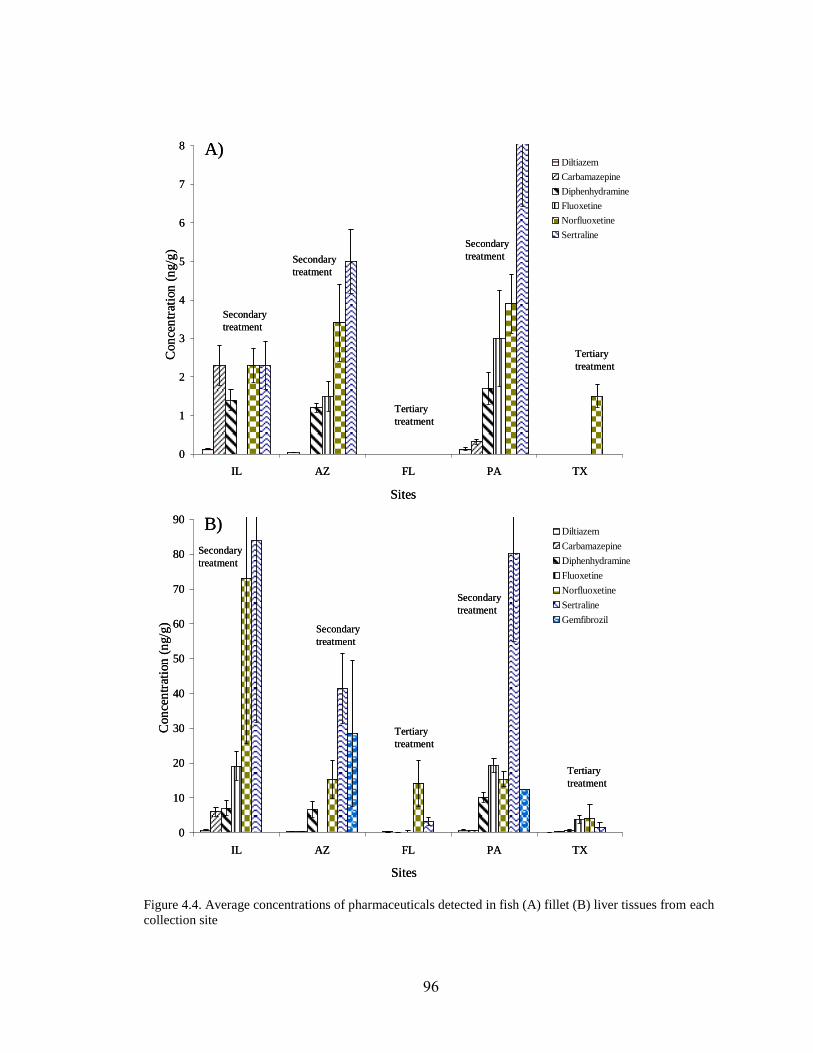
96
Figure 4.4. Average concentrations of pharmaceuticals detected in fish (A) fillet (B) liver tissues from each
collection site
0
10
20
30
40
50
60
70
80
90
IL AZ FL PA TX
Diltiazem
Carbamazepine
Diphenhydramine
Fluoxetine
Norfluoxetine
Sertraline
Gemfibrozil
Con
cen
trat
ion
(n
g/g
)C
on
cen
trat
ion
(n
g/g
)
Sites
Sites
Tertiary
treatment
Secondary
treatment
Secondary
treatment
Secondary
treatment
Tertiary
treatment
Tertiary
treatment
Secondary
treatment
Secondary
treatment
Secondary
treatment
Tertiary
treatment
A)
B)
0
1
2
3
4
5
6
7
8
IL AZ FL PA TX
Diltiazem
Carbamazepine
Diphenhydramine
Fluoxetine
Norfluoxetine
Sertraline
0
10
20
30
40
50
60
70
80
90
IL AZ FL PA TX
Diltiazem
Carbamazepine
Diphenhydramine
Fluoxetine
Norfluoxetine
Sertraline
Gemfibrozil
Con
cen
trat
ion
(n
g/g
)C
on
cen
trat
ion
(n
g/g
)
Sites
Sites
Tertiary
treatment
Secondary
treatment
Secondary
treatment
Secondary
treatment
Tertiary
treatment
Tertiary
treatment
Secondary
treatment
Secondary
treatment
Secondary
treatment
Tertiary
treatment
A)
B)
0
1
2
3
4
5
6
7
8
IL AZ FL PA TX
Diltiazem
Carbamazepine
Diphenhydramine
Fluoxetine
Norfluoxetine
Sertraline

97
corrected to account for matrix enhancements noted in Table 4.3, as appropriate. These
plots clearly demonstrate that the highest analyte concentrations were detected in samples
from the IL, AZ, and PA sites. Inspection of detection frequency in Tables A.7 – A.12
revealed a similar trend. These findings do not appear to be strongly correlated with
either human population or % effluent, as the PA site maintains the lowest population and
lowest % effluent. However, the relatively low concentrations and frequency of
detections observed for FL and TX sites are consistent with the application of more
rigorous wastewater treatments. Tertiary treatments are employed at the FL and TX sites
while secondary treatments are operable in IL, AZ, and PA. Observed variability
between sites may also reflect differences in bioavailability of contaminants, but
assessment of this factor is beyond the scope of the present study.

98
CHAPTER FIVE
Conclusions
The development and application of two complementary multi-residue screening
methodologies, collectively assessing 37 target analytes in fish tissues, revealed a number
of novel observations of significance. Work reported here demonstrated environmental
accumulation of 11 chemicals (5 of which were novel) belonging to the PPCP class of
emerging contaminants. This finding clearly establishes that environmental PPCP
exposures are realistic and justifies continued efforts to understand PPCP fate in aquatic
systems as well as effects of aquatic exposures. Of particular significance to
environmental chemistry, much of the data reported here support the conclusion that
traditional models for predicting contaminant partitioning to aquatic organisms are not
likely to be applicable for many PPCP analytes. This is expected to be especially true for
more polar compounds that may also be ionized in environmental systems.
Key factors promoting successful implementation of developed LC-MS/MS
methodology for pharmaceuticals were diversion of chromatographic mobile phase away
from the mass analyzer and implementation of matrix-matched calibration employing
multiple internal standards. Although not explicitly stated in the body of this dissertation,
chromatographic flow was not introduced into the electrospray source for the first 6
minutes of each chromatographic run. During this timeframe, all salts remaining in
samples are expected to be eluted in reversed-phase separations and thus, are prevented
from clogging the electrospray capillary or otherwise disturbing analyte ionization in the
99
electrospray source. When combined with the matrix-matched calibration approach
described in Chapter 2, these procedures were successful in reducing the effect of sample
matrix on observed analytical response for most analytes. However, even though
multiple internal standards were employed to mimic the range of influences exerted by
sample matrix, observed recoveries for matrix-spike samples reported in Chapter 4
demonstrated that matrix could alter the analytical response for select analytes by as
much as a factor of 2-6. This finding supports the conclusion that isotope dilution should
likely be incorporated for analyte quantitation to improve quality assurance in future
applications of reported methodology.
A potential limitation of reported LC-MS/MS methodology is sensitivity. Many
concentrations reported for fillet tissues in Chapter 4 required qualification (i.e., the
detected concentration was at or below statistically-derived MDLs for each analyte). If
more tissue were used in the extraction procedure (e.g., 10 g instead of 1 g of fillet), the
concentration of analytes would be expected to increase in extracts. This would also
likely result in a predictable decrease in MDL (10-fold for the example given above). In
order to accommodate more tissue mass, it may also become necessary to incorporate
more rigorous sample preparation. It is well known that gel permeation chromatography
(GPC) helps to isolate analytes of interest away from large biomolecules and lipids that
typically complicate analyses of biological samples.
Differences in accumulated concentrations of detected pharmaceuticals between
sites were rationalized in Chapter 4 in terms of the type of wastewater treatment process
employed. However, it is important to point out that this most likely reflects differing
aqueous concentrations of target compounds in effluent receiving waters. Therefore it is

100
very important that aqueous concentrations be determined before drawing definitive
conclusions. The availability of aqueous concentrations will also promote estimation of
effective bioconcentration factors (BCF = concentration of analyte in tissue/concentration
of analyte in water). Once calculated it should be interesting to examine potential
correlations of these data with analyte physicochemical properties such as KOW. This and
similar comparisons may be useful in establishing whether PPCP accumulation is due
primarily to partitioning of contaminants across membranes in direct contact with water
(e.g., gills) or other factors such as ingestion of sediments or biomagnification.

101
APPENDIX
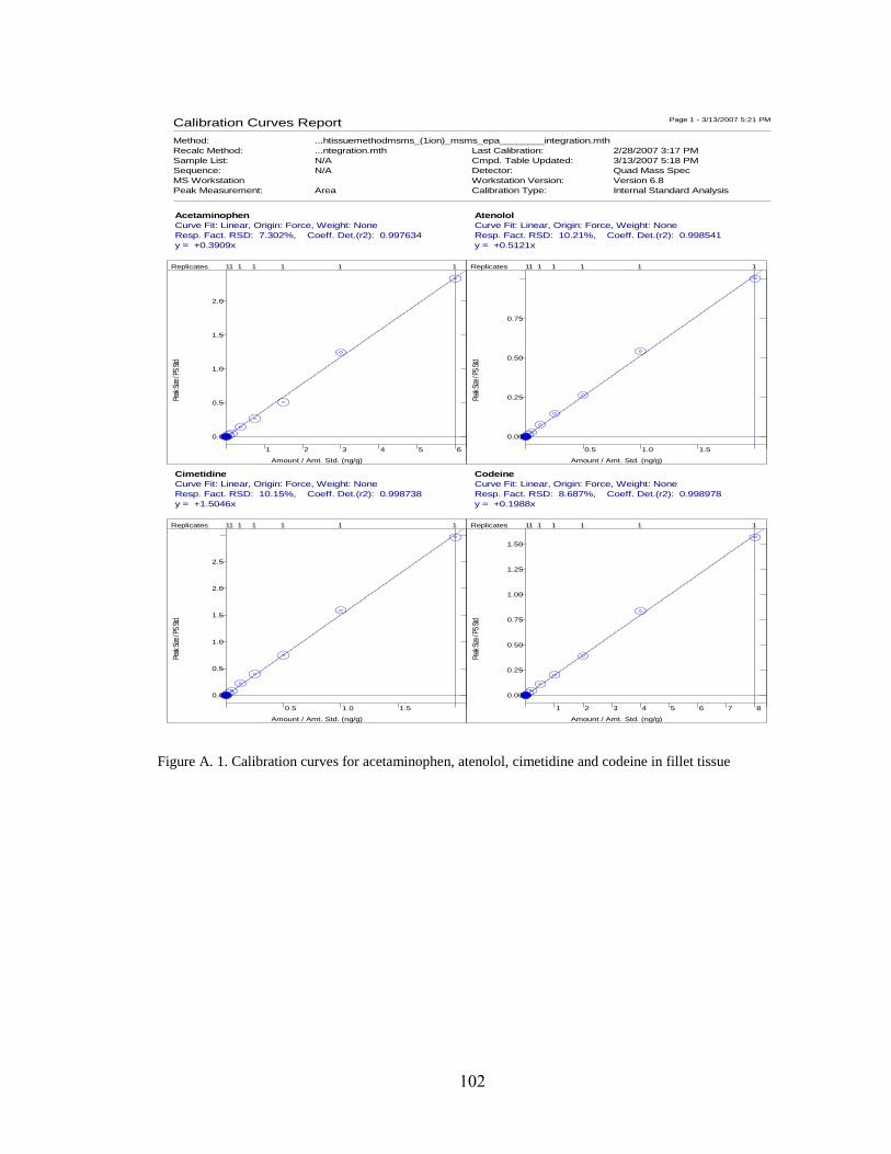
102
Calibration Curves Report Page 1 - 3/13/2007 5:21 PM
Method: ...htissuemethodmsms_(1ion)_msms_epa________integration.mth
Recalc Method: ...ntegration.mth Last Calibration: 2/28/2007 3:17 PM
Sample List: N/A Cmpd. Table Updated: 3/13/2007 5:18 PM
Sequence: N/A Detector: Quad Mass Spec
MS Workstation Workstation Version: Version 6.8
Peak Measurement: Area Calibration Type: Internal Standard Analysis
Acetaminophen
Curve Fit: Linear, Origin: Force, Weight: None
Resp. Fact. RSD: 7.302%, Coeff. Det.(r2): 0.997634
y = +0.3909x
Peak
Size
/ PS
Std
.
Amount / Amt. Std. (ng/g)
1 2 3 4 5 6
0.0
0.5
1.0
1.5
2.0
Replicates 11 1 1 1 1 1
Atenolol
Curve Fit: Linear, Origin: Force, Weight: None
Resp. Fact. RSD: 10.21%, Coeff. Det.(r2): 0.998541
y = +0.5121x
Peak
Size
/ PS
Std
.
Amount / Amt. Std. (ng/g)
0.5 1.0 1.5
0.00
0.25
0.50
0.75
Replicates 11 1 1 1 1 1
Cimetidine
Curve Fit: Linear, Origin: Force, Weight: None
Resp. Fact. RSD: 10.15%, Coeff. Det.(r2): 0.998738
y = +1.5046x
Peak
Size
/ PS
Std
.
Amount / Amt. Std. (ng/g)
0.5 1.0 1.5
0.0
0.5
1.0
1.5
2.0
2.5
Replicates 11 1 1 1 1 1
Codeine
Curve Fit: Linear, Origin: Force, Weight: None
Resp. Fact. RSD: 8.687%, Coeff. Det.(r2): 0.998978
y = +0.1988x
Peak
Size
/ PS
Std
.
Amount / Amt. Std. (ng/g)
1 2 3 4 5 6 7 8
0.00
0.25
0.50
0.75
1.00
1.25
1.50
Replicates 11 1 1 1 1 1
Figure A. 1. Calibration curves for acetaminophen, atenolol, cimetidine and codeine in fillet tissue

103
Calibration Curves Report Page 2 - 3/13/2007 5:21 PM
Method: ...htissuemethodmsms_(1ion)_msms_epa________integration.mth
Recalc Method: ...ntegration.mth Last Calibration: 2/28/2007 3:17 PM
Sample List: N/A Cmpd. Table Updated: 3/13/2007 5:18 PM
Sequence: N/A Detector: Quad Mass Spec
MS Workstation Workstation Version: Version 6.8
Peak Measurement: Area Calibration Type: Internal Standard Analysis
1,7Dimethylxanthine
Curve Fit: Linear, Origin: Force, Weight: None
Resp. Fact. RSD: 3.156%, Coeff. Det.(r2): 0.999476
y = +0.6702x
Peak
Size
/ PS
Std
.
Amount / Amt. Std. (ng/g)
0.5 1.0 1.5
0.00
0.25
0.50
0.75
1.00
1.25
Replicates 11 1 1 1 1 1
Lincomycin
Curve Fit: Linear, Origin: Force, Weight: None
Resp. Fact. RSD: 6.262%, Coeff. Det.(r2): 0.999338
y = +0.2711x
Peak
Size
/ PS
Std
.Amount / Amt. Std. (ng/g)
1 2 3 4 5 6 7 8
0.0
0.5
1.0
1.5
2.0
Replicates 11 1 1 1 1 1
Trimethoprim
Curve Fit: Linear, Origin: Force, Weight: None
Resp. Fact. RSD: 11.94%, Coeff. Det.(r2): 0.998146
y = +0.3331x
Peak
Size
/ PS
Std
.
Amount / Amt. Std. (ng/g)
0.5 1.0 1.5 2.0 2.5 3.0
0.00
0.25
0.50
0.75
1.00
Replicates 11 1 1 1 1 1
Thiabendazole
Curve Fit: Linear, Origin: Force, Weight: None
Resp. Fact. RSD: 6.008%, Coeff. Det.(r2): 0.999549
y = +1.3077x
Peak
Size
/ PS
Std
.
Amount / Amt. Std. (ng/g)
0.5 1.0 1.5 2.0 2.5 3.0
0
1
2
3
4
Replicates 11 1 1 1 1 1
Figure A. 2. Calibration curves for 1,7-Dimethylxanthine, lincomycin, trimethoprim and thiabendazole in
fillet tissue

104
Calibration Curves Report Page 3 - 3/13/2007 5:21 PM
Method: ...htissuemethodmsms_(1ion)_msms_epa________integration.mth
Recalc Method: ...ntegration.mth Last Calibration: 2/28/2007 3:17 PM
Sample List: N/A Cmpd. Table Updated: 3/13/2007 5:18 PM
Sequence: N/A Detector: Quad Mass Spec
MS Workstation Workstation Version: Version 6.8
Peak Measurement: Area Calibration Type: Internal Standard Analysis
Caffeine
Curve Fit: Linear, Origin: Force, Weight: None
Resp. Fact. RSD: 12.38%, Coeff. Det.(r2): 0.997545
y = +0.7831x
Peak
Size
/ PS
Std
.
Amount / Amt. Std. (ng/g)
1 2 3 4 5 6
0
1
2
3
4
Replicates 11 1 1 1 1 1
Sulfamethoxazole
Curve Fit: Linear, Origin: Force, Weight: None
Resp. Fact. RSD: 5.250%, Coeff. Det.(r2): 0.999763
y = +0.6222x
Peak
Size
/ PS
Std
.Amount / Amt. Std. (ng/g)
0.5 1.0 1.5 2.0 2.5 3.0
0.0
0.5
1.0
1.5
Replicates 11 1 1 1 1 1
Metoprolol
Curve Fit: Linear, Origin: Force, Weight: None
Resp. Fact. RSD: 6.750%, Coeff. Det.(r2): 0.998171
y = +0.5121x
Peak
Size
/ PS
Std
.
Amount / Amt. Std. (ng/g)
0.5 1.0 1.5 2.0 2.5 3.0
0.00
0.25
0.50
0.75
1.00
1.25
1.50
Replicates 11 1 1 1 1 1
Propranolol
Curve Fit: Linear, Origin: Force, Weight: None
Resp. Fact. RSD: 6.502%, Coeff. Det.(r2): 0.999392
y = +0.6352x
Peak
Size
/ PS
Std
.
Amount / Amt. Std. (ng/g)
0.5 1.0 1.5
0.00
0.25
0.50
0.75
1.00
Replicates 11 1 1 1 1 1
Figure A. 3. Calibration curves for caffeine, sulfamethoxazole, metoprolol and propranolol in fillet tissue

105
Calibration Curves Report Page 4 - 3/13/2007 5:21 PM
Method: ...htissuemethodmsms_(1ion)_msms_epa________integration.mth
Recalc Method: ...ntegration.mth Last Calibration: 2/28/2007 3:17 PM
Sample List: N/A Cmpd. Table Updated: 3/13/2007 5:18 PM
Sequence: N/A Detector: Quad Mass Spec
MS Workstation Workstation Version: Version 6.8
Peak Measurement: Area Calibration Type: Internal Standard Analysis
Diphenhydramine
Curve Fit: Linear, Origin: Force, Weight: None
Resp. Fact. RSD: 7.440%, Coeff. Det.(r2): 0.998402
y = +15.0757x
Peak
Size
/ PS
Std
.
Amount / Amt. Std. (ng/g)
0.025 0.050 0.075
0.00
0.25
0.50
0.75
1.00
1.25
Replicates 11 1 1 1 1 1
Diltiazem
Curve Fit: Linear, Origin: Force, Weight: None
Resp. Fact. RSD: 7.071%, Coeff. Det.(r2): 0.999210
y = +8.6640x
Peak
Size
/ PS
Std
.Amount / Amt. Std. (ng/g)
0.025 0.050 0.075
0
100
200
300
400
500
600
700
800
m
Replicates 11 1 1 1 1 1
Carbamazepine
Curve Fit: Linear, Origin: Force, Weight: None
Resp. Fact. RSD: 6.169%, Coeff. Det.(r2): 0.999309
y = +3.3740x
Peak
Size
/ PS
Std
.
Amount / Amt. Std. (ng/g)
0.1 0.2 0.3 0.4 0.5 0.6 0.7
0.0
0.5
1.0
1.5
2.0
2.5
Replicates 11 1 1 1 1 1
Tylosin
Curve Fit: Linear, Origin: Force, Weight: None
Resp. Fact. RSD: 10.23%, Coeff. Det.(r2): 0.996670
y = +0.1295x
Peak
Size
/ PS
Std
.
Amount / Amt. Std. (ng/g)
1 2 3 4 5 6 7 8
0.00
0.25
0.50
0.75
Replicates 11 1 1 1 1 1
Figure A. 4. Calibration curves for diphenhydramine, diltiazem, carbamazepine and tylosin in fillet tissue

106
Calibration Curves Report Page 5 - 3/13/2007 5:21 PM
Method: ...htissuemethodmsms_(1ion)_msms_epa________integration.mth
Recalc Method: ...ntegration.mth Last Calibration: 2/28/2007 3:17 PM
Sample List: N/A Cmpd. Table Updated: 3/13/2007 5:18 PM
Sequence: N/A Detector: Quad Mass Spec
MS Workstation Workstation Version: Version 6.8
Peak Measurement: Area Calibration Type: Internal Standard Analysis
Fluoxetine
Curve Fit: Linear, Origin: Force, Weight: None
Resp. Fact. RSD: 3.266%, Coeff. Det.(r2): 0.999930
y = +0.7223x
Peak
Size
/ PS
Std
.
Amount / Amt. Std. (ng/g)
0.25 0.50 0.75
0
100
200
300
400
500
600
700
m
Replicates 11 1 1 1 1 1
Norfluoxetine
Curve Fit: Linear, Origin: Force, Weight: None
Resp. Fact. RSD: 17.38%, Coeff. Det.(r2): 0.995134
y = +0.6440x
Peak
Size
/ PS
Std
.Amount / Amt. Std. (ng/g)
0.1 0.2 0.3 0.4 0.5
0
50
100
150
200
250
300
350
m
Replicates 11 1 1 1 1 1
Sertraline
Curve Fit: Linear, Origin: Force, Weight: None
Resp. Fact. RSD: 8.641%, Coeff. Det.(r2): 0.994335
y = +0.6997x
Peak
Size
/ PS
Std
.
Amount / Amt. Std. (ng/g)
0.1 0.2 0.3 0.4 0.5
0
100
200
300
m
Replicates 11 1 1 1 1 1
Erythromycin
Curve Fit: Linear, Origin: Force, Weight: 1/nX2
Resp. Fact. RSD: 8.988%, Coeff. Det.(r2): 0.999138
y = +0.0507x
Peak
Size
/ PS
Std
.
Amount / Amt. Std. (ng/g)
1 2 3 4 5 6 7 8
0
100
200
300
m
Replicates 11 1 1 1 1 1
Figure A. 5. Calibration curves for fluoxetine, norfluoxetine, sertraline and erythromycin in fillet tissue

107
Calibration Curves Report Page 6 - 3/13/2007 5:21 PM
Method: ...htissuemethodmsms_(1ion)_msms_epa________integration.mth
Recalc Method: ...ntegration.mth Last Calibration: 2/28/2007 3:17 PM
Sample List: N/A Cmpd. Table Updated: 3/13/2007 5:18 PM
Sequence: N/A Detector: Quad Mass Spec
MS Workstation Workstation Version: Version 6.8
Peak Measurement: Area Calibration Type: Internal Standard Analysis
Warfarin
Curve Fit: Linear, Origin: Force, Weight: None
Resp. Fact. RSD: 7.058%, Coeff. Det.(r2): 0.999456
y = +1.7819x
Peak
Size
/ PS
Std
.
Amount / Amt. Std. (ng/g)
0.1 0.2 0.3 0.4 0.5 0.6 0.7
0.00
0.25
0.50
0.75
1.00
1.25
Replicates 11 1 1 1 1 1
Miconazole
Curve Fit: Linear, Origin: Force, Weight: None
Resp. Fact. RSD: 9.192%, Coeff. Det.(r2): 0.996703
y = +0.0051x
Peak
Size
/ PS
Std
.Amount / Amt. Std. (ng/g)
2.5 5.0 7.5 10.0
0
10
20
30
40
50
m
Replicates 11 1 1 1 1 1
Ibuprofen
Curve Fit: Linear, Origin: Force, Weight: None
Resp. Fact. RSD: 10.86%, Coeff. Det.(r2): 0.999320
y = +0.0093x
Peak
Size
/ PS
Std
.
Amount / Amt. Std. (ng/g)
10 20 30 40 50
0
100
200
300
400
500
m
Replicates 11 1 1 1 1 1
Gemfibrozil
Curve Fit: Linear, Origin: Force, Weight: None
Resp. Fact. RSD: 14.32%, Coeff. Det.(r2): 0.993291
y = +3.4477x
Peak
Size
/ PS
Std
.
Amount / Amt. Std. (ng/g)
0.1 0.2 0.3 0.4 0.5 0.6 0.7
0.0
0.5
1.0
1.5
2.0
2.5
Replicates 11 1 1 1 1 1
Figure A. 6. Calibration curves for warfarin, miconazole, ibuprofen and gemfibrozil in fillet tissue

108
Calibration Curves Report Page 7 - 3/13/2007 5:21 PM
Method: ...htissuemethodmsms_(1ion)_msms_epa________integration.mth
Recalc Method: ...ntegration.mth Last Calibration: 2/28/2007 3:17 PM
Sample List: N/A Cmpd. Table Updated: 3/13/2007 5:18 PM
Sequence: N/A Detector: Quad Mass Spec
MS Workstation Workstation Version: Version 6.8
Peak Measurement: Area Calibration Type: Internal Standard Analysis
S1_AcetaminophenD4
Curve Fit: Linear, Origin: Force, Weight: None
Resp. Fact. RSD: 5.961%, Coeff. Det.(r2): 0.995322
y = +0.4599x
Peak
Size
/ PS
Std
.
Amount / Amt. Std. (ng/g)
2.5 5.0 7.5
0
1
2
3
4
Replicates 1 1 1 1 1
S4_DiphenhydramineD3
Curve Fit: Linear, Origin: Force, Weight: None
Resp. Fact. RSD: 2.522%, Coeff. Det.(r2): 0.999242
y = +12.5793x
Peak
Size
/ PS
Std
.Amount / Amt. Std. (ng/g)
0.05 0.10 0.15
0.0
0.5
1.0
1.5
2.0
Replicates 1 1 1 1 1
S5_CarbamazepineD10
Curve Fit: Linear, Origin: Force, Weight: None
Resp. Fact. RSD: 5.683%, Coeff. Det.(r2): 0.994596
y = +3.5067x
Peak
Size
/ PS
Std
.
Amount / Amt. Std. (ng/g)
0.1 0.2 0.3 0.4 0.5 0.6 0.7
0.0
0.5
1.0
1.5
2.0
2.5
Replicates 1 1 1 1 1
S2_Ibuprofen13C3
Curve Fit: Linear, Origin: Force, Weight: None
Resp. Fact. RSD: 11.65%, Coeff. Det.(r2): 0.995171
y = +0.0105x
Peak
Size
/ PS
Std
.
Amount / Amt. Std. (ng/g)
2.5 5.0 7.5 10.0 12.5 15.0
0
25
50
75
100
125
150
m
Replicates 1 1 1 1 1
Figure A. 7. Calibration curves for acetaminophen-d4, diphenhydramine-d3, carbamazepine-d10 and
ibuprofen-13
C3 in fillet tissue

109
Calibration Curves Report Page 1 - 5/3/2007 3:39 AM
Method: ...ms_(1ion)_msms_epa1________liverintegrationreprocess.mth
Recalc Method: ...nreprocess.mth Last Calibration: 5/2/2007 11:53 PM
Sample List: N/A Cmpd. Table Updated: 5/3/2007 3:39 AM
Sequence: N/A Detector: Quad Mass Spec
MS Workstation Workstation Version: Version 6.8
Peak Measurement: Area Calibration Type: Internal Standard Analysis
Acetaminophen
Curve Fit: Linear, Origin: Force, Weight: None
Resp. Fact. RSD: 16.30%, Coeff. Det.(r2): 0.997794
y = +0.1505x
Peak
Size
/ PS
Std
.
Amount / Amt. Std. (ng/g)
2.5 5.0 7.5 10.0
0.00
0.25
0.50
0.75
1.00
1.25
1.50
1.75
Replicates 2 1 1 1 1 1 1
Atenolol
Curve Fit: Linear, Origin: Force, Weight: None
Resp. Fact. RSD: 24.52%, Coeff. Det.(r2): 0.992576
y = +0.4487x
Peak
Size
/ PS
Std
.
Amount / Amt. Std. (ng/g)
1 2 3 4
0.00
0.25
0.50
0.75
1.00
1.25
1.50
Replicates 2 1 1 1 1 1 1
Cimetidine
Curve Fit: Linear, Origin: Force, Weight: None
Resp. Fact. RSD: 15.23%, Coeff. Det.(r2): 0.995625
y = +1.0857x
Peak
Size
/ PS
Std
.
Amount / Amt. Std. (ng/g)
1 2 3 4
0
1
2
3
4
Replicates 2 1 1 1 1 1 1
Codeine
Curve Fit: Linear, Origin: Force, Weight: None
Resp. Fact. RSD: 9.270%, Coeff. Det.(r2): 0.999297
y = +0.2095x
Peak
Size
/ PS
Std
.
Amount / Amt. Std. (ng/g)
2.5 5.0 7.5 10.0 12.5 15.0
0.0
0.5
1.0
1.5
2.0
2.5
3.0
Replicates 2 1 1 1 1 1 1
Figure A. 8. Calibration curves for acetaminophen, atenolol, cimetidine and codeine in liver tissue

110
Calibration Curves Report Page 2 - 5/3/2007 3:39 AM
Method: ...ms_(1ion)_msms_epa1________liverintegrationreprocess.mth
Recalc Method: ...nreprocess.mth Last Calibration: 5/2/2007 11:53 PM
Sample List: N/A Cmpd. Table Updated: 5/3/2007 3:39 AM
Sequence: N/A Detector: Quad Mass Spec
MS Workstation Workstation Version: Version 6.8
Peak Measurement: Area Calibration Type: Internal Standard Analysis
1,7Dimethylxanthine
Curve Fit: Linear, Origin: Force, Weight: None
Resp. Fact. RSD: 16.45%, Coeff. Det.(r2): 0.992753
y = +0.4008x
Peak
Size
/ PS S
td.
Amount / Amt. Std. (ng/g)
1 2 3 4
0.00
0.25
0.50
0.75
1.00
1.25
1.50
Replicates 2 1 1 1 1 1 1
Lincomycin
Curve Fit: Linear, Origin: Force, Weight: None
Resp. Fact. RSD: 16.34%, Coeff. Det.(r2): 0.995036
y = +0.4459x
Peak
Size
/ PS S
td.
Amount / Amt. Std. (ng/g)
2.5 5.0 7.5 10.0 12.5 15.0
0
1
2
3
4
5
6
Replicates 2 1 1 1 1 1 1
Trimethoprim
Curve Fit: Linear, Origin: Force, Weight: None
Resp. Fact. RSD: 12.11%, Coeff. Det.(r2): 0.995816
y = +0.4502x
Peak
Size
/ PS S
td.
Amount / Amt. Std. (ng/g)
1 2 3 4 5 6
0.0
0.5
1.0
1.5
2.0
2.5
Replicates 2 1 1 1 1 1 1
Thiabendazole
Curve Fit: Linear, Origin: Force, Weight: None
Resp. Fact. RSD: 9.673%, Coeff. Det.(r2): 0.996753
y = +1.3707x
Peak
Size
/ PS S
td.
Amount / Amt. Std. (ng/g)
1 2 3 4 5 6
0
1
2
3
4
5
6
7
8
Replicates 2 1 1 1 1 1 1
Figure A. 9. Calibration curves for 1,7-Dimethylxanthine, lincomycin, trimethoprim and thiabendazole in
liver tissue

111
Calibration Curves Report Page 3 - 5/3/2007 3:39 AM
Method: ...ms_(1ion)_msms_epa1________liverintegrationreprocess.mth
Recalc Method: ...nreprocess.mth Last Calibration: 5/2/2007 11:53 PM
Sample List: N/A Cmpd. Table Updated: 5/3/2007 3:39 AM
Sequence: N/A Detector: Quad Mass Spec
MS Workstation Workstation Version: Version 6.8
Peak Measurement: Area Calibration Type: Internal Standard Analysis
Caffeine
Curve Fit: Linear, Origin: Force, Weight: None
Resp. Fact. RSD: 20.43%, Coeff. Det.(r2): 0.996841
y = +0.7491x
Peak
Size
/ PS S
td.
Amount / Amt. Std. (ng/g)
2.5 5.0 7.5 10.0
0
1
2
3
4
5
6
7
8
Replicates 2 1 1 1 1 1 1
Sulfamethoxazole
Curve Fit: Linear, Origin: Force, Weight: None
Resp. Fact. RSD: 14.49%, Coeff. Det.(r2): 0.998615
y = +0.4364x
Peak
Size
/ PS S
td.
Amount / Amt. Std. (ng/g)
1 2 3 4 5 6
0.0
0.5
1.0
1.5
2.0
2.5
Replicates 2 1 1 1 1 1 1
Metoprolol
Curve Fit: Linear, Origin: Force, Weight: None
Resp. Fact. RSD: 8.335%, Coeff. Det.(r2): 0.998897
y = +0.9027x
Peak
Size
/ PS S
td.
Amount / Amt. Std. (ng/g)
1 2 3 4 5 6
0
1
2
3
4
5
Replicates 2 1 1 1 1 1 1
Propranolol
Curve Fit: Linear, Origin: Force, Weight: None
Resp. Fact. RSD: 16.96%, Coeff. Det.(r2): 0.995025
y = +0.8942x
Peak
Size
/ PS S
td.
Amount / Amt. Std. (ng/g)
1 2 3 4
0.0
0.5
1.0
1.5
2.0
2.5
3.0
Replicates 2 1 1 1 1 1 1
Figure A. 10. Calibration curves for caffeine, sulfamethoxazole, metoprolol and propranolol in liver tissue
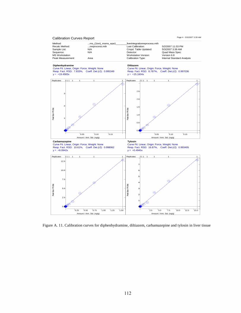
112
Calibration Curves Report Page 4 - 5/3/2007 3:39 AM
Method: ...ms_(1ion)_msms_epa1________liverintegrationreprocess.mth
Recalc Method: ...nreprocess.mth Last Calibration: 5/2/2007 11:53 PM
Sample List: N/A Cmpd. Table Updated: 5/3/2007 3:39 AM
Sequence: N/A Detector: Quad Mass Spec
MS Workstation Workstation Version: Version 6.8
Peak Measurement: Area Calibration Type: Internal Standard Analysis
Diphenhydramine
Curve Fit: Linear, Origin: Force, Weight: None
Resp. Fact. RSD: 7.933%, Coeff. Det.(r2): 0.995349
y = +19.4583x
Peak
Size
/ PS S
td.
Amount / Amt. Std. (ng/g)
0.05 0.10 0.15
0
1
2
3
Replicates 2 1 1 1 1 1 1
Diltiazem
Curve Fit: Linear, Origin: Force, Weight: None
Resp. Fact. RSD: 8.787%, Coeff. Det.(r2): 0.997036
y = +15.1604x
Peak
Size
/ PS S
td.
Amount / Amt. Std. (ng/g)
0.05 0.10 0.15
0.0
0.5
1.0
1.5
2.0
2.5
Replicates 2 1 1 1 1 1 1
Carbamazepine
Curve Fit: Linear, Origin: Force, Weight: None
Resp. Fact. RSD: 10.61%, Coeff. Det.(r2): 0.998062
y = +8.0942x
Peak
Size
/ PS S
td.
Amount / Amt. Std. (ng/g)
0.25 0.50 0.75 1.00 1.25 1.50
0.0
2.5
5.0
7.5
10.0
12.5
Replicates 2 1 1 1 1 1 1
Tylosin
Curve Fit: Linear, Origin: Force, Weight: None
Resp. Fact. RSD: 16.87%, Coeff. Det.(r2): 0.993405
y = +0.4945x
Peak
Size
/ PS S
td.
Amount / Amt. Std. (ng/g)
2.5 5.0 7.5 10.0 12.5 15.0
0
1
2
3
4
5
6
7
Replicates 2 1 1 1 1 1 1
Figure A. 11. Calibration curves for diphenhydramine, diltiazem, carbamazepine and tylosin in liver tissue

113
Calibration Curves Report Page 5 - 5/3/2007 3:39 AM
Method: ...ms_(1ion)_msms_epa1________liverintegrationreprocess.mth
Recalc Method: ...nreprocess.mth Last Calibration: 5/2/2007 11:53 PM
Sample List: N/A Cmpd. Table Updated: 5/3/2007 3:39 AM
Sequence: N/A Detector: Quad Mass Spec
MS Workstation Workstation Version: Version 6.8
Peak Measurement: Area Calibration Type: Internal Standard Analysis
Fluoxetine
Curve Fit: Linear, Origin: Force, Weight: None
Resp. Fact. RSD: 5.730%, Coeff. Det.(r2): 0.998344
y = +0.2187x
Peak
Size
/ PS S
td.
Amount / Amt. Std. (ng/g)
0.5 1.0 1.5
0
100
200
300
400
m
Replicates 2 1 1 1 1 1 1
Norfluoxetine
Curve Fit: Linear, Origin: Force, Weight: None
Resp. Fact. RSD: 12.28%, Coeff. Det.(r2): 0.997890
y = +0.3260x
Peak
Size
/ PS S
td.
Amount / Amt. Std. (ng/g)
0.25 0.50 0.75 1.00
0
50
100
150
200
250
300
m
Replicates 2 1 1 1 1 1 1
Sertraline
Curve Fit: Linear, Origin: Force, Weight: None
Resp. Fact. RSD: 14.26%, Coeff. Det.(r2): 0.997195
y = +0.3688x
Peak
Size
/ PS S
td.
Amount / Amt. Std. (ng/g)
0.25 0.50 0.75 1.00
0
100
200
300
m
Replicates 2 1 1 1 1 1 1
Warfarin
Curve Fit: Linear, Origin: Force, Weight: None
Resp. Fact. RSD: 9.760%, Coeff. Det.(r2): 0.997583
y = +4.4414x
Peak
Size
/ PS S
td.
Amount / Amt. Std. (ng/g)
0.25 0.50 0.75 1.00 1.25 1.50
0
1
2
3
4
5
6
Replicates 2 1 1 1 1 1 1
Figure A. 12. Calibration curves for fluoxetine, norfluoxetine, sertraline and warfarin in liver tissue
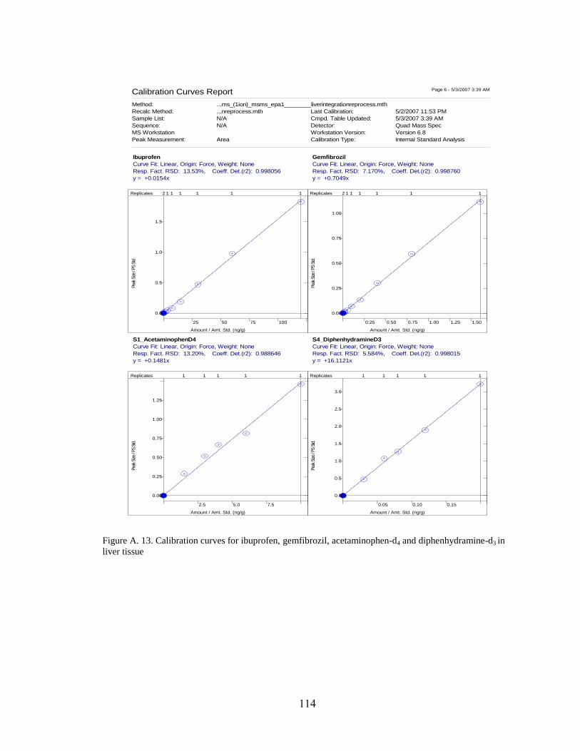
114
Calibration Curves Report Page 6 - 5/3/2007 3:39 AM
Method: ...ms_(1ion)_msms_epa1________liverintegrationreprocess.mth
Recalc Method: ...nreprocess.mth Last Calibration: 5/2/2007 11:53 PM
Sample List: N/A Cmpd. Table Updated: 5/3/2007 3:39 AM
Sequence: N/A Detector: Quad Mass Spec
MS Workstation Workstation Version: Version 6.8
Peak Measurement: Area Calibration Type: Internal Standard Analysis
Ibuprofen
Curve Fit: Linear, Origin: Force, Weight: None
Resp. Fact. RSD: 13.53%, Coeff. Det.(r2): 0.998056
y = +0.0154x
Peak
Size
/ PS S
td.
Amount / Amt. Std. (ng/g)
25 50 75 100
0.0
0.5
1.0
1.5
Replicates 2 1 1 1 1 1 1
Gemfibrozil
Curve Fit: Linear, Origin: Force, Weight: None
Resp. Fact. RSD: 7.170%, Coeff. Det.(r2): 0.998760
y = +0.7049x
Peak
Size
/ PS S
td.
Amount / Amt. Std. (ng/g)
0.25 0.50 0.75 1.00 1.25 1.50
0.00
0.25
0.50
0.75
1.00
Replicates 2 1 1 1 1 1 1
S1_AcetaminophenD4
Curve Fit: Linear, Origin: Force, Weight: None
Resp. Fact. RSD: 13.20%, Coeff. Det.(r2): 0.988646
y = +0.1481x
Peak
Size
/ PS S
td.
Amount / Amt. Std. (ng/g)
2.5 5.0 7.5
0.00
0.25
0.50
0.75
1.00
1.25
Replicates 1 1 1 1 1
S4_DiphenhydramineD3
Curve Fit: Linear, Origin: Force, Weight: None
Resp. Fact. RSD: 5.584%, Coeff. Det.(r2): 0.998015
y = +16.1121x
Peak
Size
/ PS S
td.
Amount / Amt. Std. (ng/g)
0.05 0.10 0.15
0.0
0.5
1.0
1.5
2.0
2.5
3.0
Replicates 1 1 1 1 1
Figure A. 13. Calibration curves for ibuprofen, gemfibrozil, acetaminophen-d4 and diphenhydramine-d3 in
liver tissue

115
Calibration Curves Report Page 7 - 5/3/2007 3:39 AM
Method: ...ms_(1ion)_msms_epa1________liverintegrationreprocess.mth
Recalc Method: ...nreprocess.mth Last Calibration: 5/2/2007 11:53 PM
Sample List: N/A Cmpd. Table Updated: 5/3/2007 3:39 AM
Sequence: N/A Detector: Quad Mass Spec
MS Workstation Workstation Version: Version 6.8
Peak Measurement: Area Calibration Type: Internal Standard Analysis
S5_CarbamazepineD10
Curve Fit: Linear, Origin: Force, Weight: None
Resp. Fact. RSD: 7.214%, Coeff. Det.(r2): 0.995446
y = +7.3840x
Peak
Size
/ PS S
td.
Amount / Amt. Std. (ng/g)
0.1 0.2 0.3 0.4 0.5 0.6 0.7
0
1
2
3
4
5
Replicates 1 1 1 1 1
S2_Ibuprofen13C3
Curve Fit: Linear, Origin: Force, Weight: None
Resp. Fact. RSD: 11.58%, Coeff. Det.(r2): 0.986942
y = +0.0149x
Peak
Size
/ PS S
td.
Amount / Amt. Std. (ng/g)
2.5 5.0 7.5 10.0 12.5 15.0
0
50
100
150
200
m
Replicates 1 1 1 1 1
Figure A. 14. Calibration curves for carbamazepine-d10 and ibuprofen-13
C3 in liver tissue

116
Figure A. 15. Plots of detected concentrations of pharmaceuticals versus lipid content for fish collected
from PA; A) fillet and B) liver tissue
0
2
4
6
8
10
12
14
16
18
20
1.0 1.2 1.4 1.6 1.8 2.0 2.2 2.4
Diphenhydramine
Diltiazem
Norfluoxetine
Sertraline
Fluoxetine
CarbamazepineCon
cen
trat
ion
(n
g/g
)
Lipid (%)
0
20
40
60
80
100
120
140
3.5 4.0 4.5 5.0 5.5 6.0
Diphenhydramine
Diltiazem
Norfluoxetine
Sertraline
Fluoxetine
Carbamazepine
Con
cen
trat
ion
(n
g/g
)
Lipid (%)
A)
B)
0
2
4
6
8
10
12
14
16
18
20
1.0 1.2 1.4 1.6 1.8 2.0 2.2 2.4
Diphenhydramine
Diltiazem
Norfluoxetine
Sertraline
Fluoxetine
CarbamazepineCon
cen
trat
ion
(n
g/g
)
Lipid (%)
0
20
40
60
80
100
120
140
3.5 4.0 4.5 5.0 5.5 6.0
Diphenhydramine
Diltiazem
Norfluoxetine
Sertraline
Fluoxetine
Carbamazepine
Con
cen
trat
ion
(n
g/g
)
Lipid (%)
A)
B)
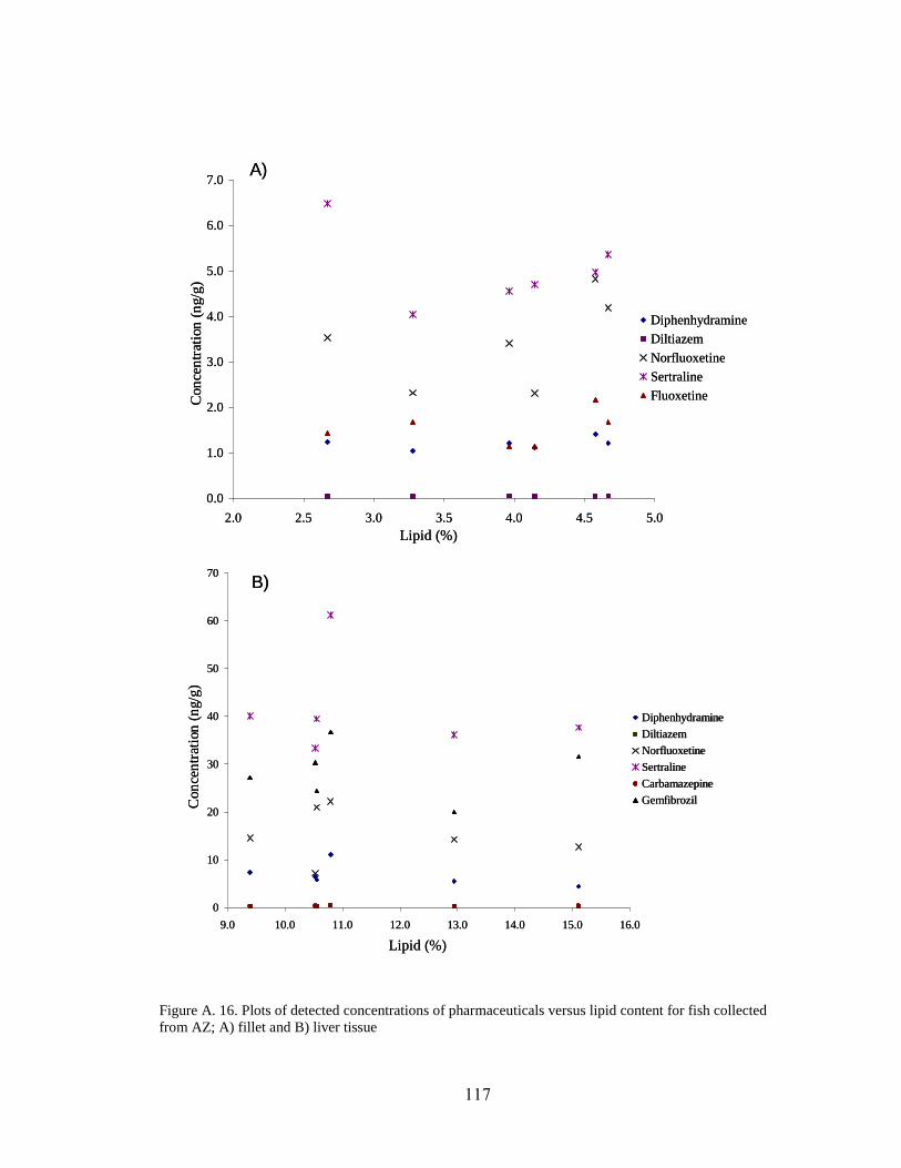
117
Figure A. 16. Plots of detected concentrations of pharmaceuticals versus lipid content for fish collected
from AZ; A) fillet and B) liver tissue
0
10
20
30
40
50
60
70
9.0 10.0 11.0 12.0 13.0 14.0 15.0 16.0
Diphenhydramine
Diltiazem
Norfluoxetine
Sertraline
Carbamazepine
GemfibrozilCon
cen
trat
ion
(n
g/g
)
Lipid (%)
0.0
1.0
2.0
3.0
4.0
5.0
6.0
7.0
2.0 2.5 3.0 3.5 4.0 4.5 5.0
Diphenhydramine
Diltiazem
Norfluoxetine
Sertraline
Fluoxetine
Lipid (%)
Con
cen
trat
ion
(n
g/g
)
A)
B)

118
Figure A. 17. Plots of detected concentrations in liver of pharmaceuticals versus lipid content for fish
collected from A) FL and B) TX
0
5
10
15
20
25
30
3.0 4.0 5.0 6.0 7.0 8.0 9.0 10.0 11.0
Diphenhydramine
Diltiazem
Norfluoxetine
Sertraline
Carbamazepine
Con
cen
trat
ion
(n
g/g
)
Lipid (%)
0
5
10
15
20
25
30
35
40
45
1.0 2.0 3.0 4.0 5.0 6.0
Diltiazem
Norfluoxetine
Sertraline
Carbamazepine
Con
cen
trat
ion
(n
g/g
)
Lipid (%)
A)
B)
0
5
10
15
20
25
30
3.0 4.0 5.0 6.0 7.0 8.0 9.0 10.0 11.0
Diphenhydramine
Diltiazem
Norfluoxetine
Sertraline
Carbamazepine
Con
cen
trat
ion
(n
g/g
)
Lipid (%)
0
5
10
15
20
25
30
35
40
45
1.0 2.0 3.0 4.0 5.0 6.0
Diltiazem
Norfluoxetine
Sertraline
Carbamazepine
Con
cen
trat
ion
(n
g/g
)
Lipid (%)
A)
B)

119
Table A.1. Fish fillet initial calibration data
Compound RRF1a RRF2 RRF3 RRF4 RRF5 RRF6 RRF7 RRF
b %
c
RSD
Acetaminophen 0.388 0.346 0.384 0.356 0.339 0.414 0.389 0.374 7.3
Atenolol 0.680 0.572 0.595 0.590 0.525 0.542 0.502 0.572 10.2
Cimetidine 1.952 1.729 1.770 1.591 1.498 1.593 1.480 1.659 10.2
Codeine 0.245 0.231 0.223 0.203 0.197 0.209 0.196 0.215 8.7
1,7Dimethylxanthine 0.663 0.696 0.702 0.679 0.642 0.693 0.666 0.677 3.2
Lincomycin 0.323 0.291 0.297 0.285 0.273 0.283 0.268 0.288 6.3
Trimethoprim 0.438 0.373 0.450 0.403 0.364 0.348 0.326 0.386 11.9
Thiabendazole 1.482 1.341 1.365 1.402 1.222 1.321 1.308 1.349 6.0
Caffeine 1.067 0.901 0.897 0.815 0.750 0.847 0.768 0.863 12.4
Sulfamethoxazole 0.555 0.574 0.639 0.621 0.610 0.637 0.619 0.608 5.2
Metoprolol 0.606 0.530 0.599 0.565 0.543 0.545 0.501 0.555 6.7
Propranolol 0.598 0.646 0.712 0.711 0.634 0.656 0.629 0.655 6.5
Diphenhydramine 17.111 16.688 15.225 15.101 13.681 15.899 14.955 15.523 7.4
Diltiazem 7.221 7.991 8.672 8.523 8.190 9.025 8.606 8.318 7.1
Carbamazepine 2.983 3.084 3.437 3.416 3.095 3.462 3.369 3.264 6.2
Tylosin 0.141 0.121 0.163 0.151 0.141 0.140 0.126 0.140 10.2
Fluoxetine 0.758 0.782 0.711 0.748 0.733 0.730 0.719 0.740 3.3
Norfluoxetine 0.922 0.685 0.577 0.722 0.644 0.571 0.661 0.683 17.4
Sertraline 0.695 0.621 0.591 0.733 0.638 0.615 0.725 0.660 8.6

120
Table A.1. Fish fillet initial calibration data (cont.)
Compound RRF1a RRF2 RRF3 RRF4 RRF5 RRF6 RRF7 RRF
b %
c
RSD
Erythromycin 0.054 0.057 0.053 0.044 0.045 0.051 0.050 0.051 9.0
Warfarin 1.515 1.705 1.848 1.884 1.687 1.735 1.798 1.739 7.1
Miconazole nad na 0.005 0.008 0.005 0.004 0.005 0.005 27.4
Ibuprofen 0.009 0.007 0.009 0.010 0.009 0.009 0.009 0.009 10.9
Gemfibrozil 4.807 3.674 3.749 4.724 4.274 3.638 3.329 4.028 14.3
Acetaminophend4e 0.490 0.469 0.521 0.463 0.448 0.478 6.0
Diphenhydramined3 12.800 12.547 13.263 12.595 12.462 12.734 2.5
Carbamazepined10 3.480 3.445 3.886 3.672 3.393 3.575 5.7
Ibuprofen13
C3 0.008 0.009 0.010 0.011 0.010 0.010 11.7
a
RRF = (Area(sample)/(Amount(sample))/(Area(standard)/Amount(standard)); b average relative response
factor for calibration standards spiked in reference fish; c relative standard deviation of response factor;
d
non-applicable, miconazole response was suppressed in the control matrix, therefore projected calibration
range excluded concentrations that did not resolve from the baseline (i.e., calibration level one and two); e
only five calibration levels were prepared for surrogates

121
Table A.2. Continuing calibration check for fillet in the Illinois batch
Compound AvgRRF RRF %D Max
Acetaminophen 0.374 0.366 2.1 25.0
Atenolol 0.572 0.560 2.2 25.0
Cimetidine 1.659 1.581 4.7 25.0
Codeine 0.215 0.202 6.1 25.0
1,7Dimethylxanthine 0.677 0.641 5.4 25.0
Lincomycin 0.288 0.277 3.9 25.0
Trimethoprim 0.386 0.382 0.9 25.0
Thiabendazole 1.349 1.260 6.6 25.0
Caffeine 0.863 0.809 6.3 25.0
Sulfamethoxazole 0.608 0.617 -1.4 25.0
Metoprolol 0.555 0.535 3.6 25.0
Propranolol 0.655 0.654 0.1 25.0
Diphenhydramine 15.523 15.781 -1.7 25.0
Diltiazem 8.318 8.440 -1.5 25.0
Carbamazepine 3.264 3.217 1.4 25.0
Tylosin 0.140 0.145 -3.4 25.0
Fluoxetine 0.740 0.728 1.6 25.0
Norfluoxetine 0.683 0.563 17.6 25.0
Sertraline 0.660 0.693 -5.0 25.0
Erythromycin 0.051 0.047 7.4 25.0

122
Table A.2. Continuing calibration check for fillet in the Illinois batch (cont.)
Compound AvgRRF RRF %D Max
Warfarin 1.739 1.863 -7.1 25.0
Miconazole 0.005 0.005 1.9 25.0
Ibuprofen 0.009 0.009 -5.6 25.0
Gemfibrozil 4.028 3.463 14.0 25.0
Acetaminophend4 0.478 0.487 -1.9 25.0
Diphenhydramined3 12.734 13.039 -2.4 25.0
Carbamazepined10 3.575 3.583 -0.2 25.0
Ibuprofen13
C3 0.010 0.011 -12.3 25.0

Table A.3. Fish liver initial calibration data
Compound RRF1a RRF2 RRF3 RRF4 RRF5 RRF6 RRF7 RRF8 R
2 RRF
b %RSD
c
Acetaminophen 0.130 0.134 0.101 0.119 0.165 0.155 0.149 0.9978 0.136 16.3
Atenolol 0.562 0.476 0.595 0.457 0.436 0.9926 0.505 13.7
Cimetidine 1.040 1.473 1.066 1.045 1.345 1.054 1.078 0.9956 1.157 15.2
Codeine 0.175 0.180 0.182 0.194 0.219 0.216 0.208 0.9993 0.196 9.3
1,7Dimethylxanthine 0.523 0.373 0.489 0.400 0.347 0.526 0.392 0.396 0.9928 0.431 16.5
Lincomycin 0.346 0.391 0.395 0.549 0.451 0.439 0.9950 0.429 16.3
Trimethoprim 0.503 0.542 0.583 0.434 0.440 0.559 0.457 0.442 0.9958 0.495 12.1
Thiabendazole 1.247 1.375 1.524 1.347 1.274 1.659 1.383 1.351 0.9968 1.395 9.7
Caffeine 1.125 0.946 0.854 0.630 0.634 0.893 0.747 0.743 0.9968 0.821 20.4
Sulfamethoxazole 0.291 0.425 0.455 0.358 0.381 0.468 0.416 0.441 0.9986 0.404 14.5
Metoprolol 0.888 0.989 0.991 0.822 0.806 1.001 0.893 0.901 0.9989 0.911 8.3
Propranolol 0.678 1.220 0.996 0.890 0.909 1.095 0.950 0.867 0.9950 0.951 17.0
123

Table A.3. Fish liver initial calibration data (cont)
Compound RRF1a RRF2 RRF3 RRF4 RRF5 RRF6 RRF7 RRF8 R
2 RRF
b %RSD
c
Diphenhydramine 23.385 19.758 20.403 20.113 18.718 22.296 21.256 18.839 0.9953 20.596 7.9
Diltiazem 13.206 15.281 15.929 13.980 14.148 17.288 16.086 14.816 0.9970 15.092 8.8
Carbamazepine 7.219 8.514 8.205 6.837 6.855 9.171 8.235 8.016 0.9981 7.881 10.6
Tylosin 0.424 0.486 0.471 0.401 0.332 0.585 0.532 0.482 0.9934 0.464 16.9
Fluoxetine 0.216 0.244 0.206 0.221 0.227 0.233 0.215 0.9983 0.223 5.7
Norfluoxetine 0.426 0.325 0.308 0.344 0.348 0.320 0.9979 0.345 12.3
Sertraline 0.437 0.318 0.297 0.399 0.390 0.363 0.9972 0.367 14.3
Warfarin 4.013 4.667 4.115 3.977 5.187 4.363 4.423 0.9976 4.392 9.8
Ibuprofen 0.016 0.013 0.014 0.011 0.013 0.016 0.016 0.015 0.9981 0.014 13.5
Gemfibrozil 0.695 0.794 0.640 0.679 0.663 0.750 0.739 0.694 0.9988 0.707 7.2
Acetaminophen-d4 0.190 0.173 0.167 0.136 0.146 0.9886 0.162 13.2
Diphenhydramine-d3 15.858 17.927 15.849 15.816 16.103 0.9980 16.311 5.6
124
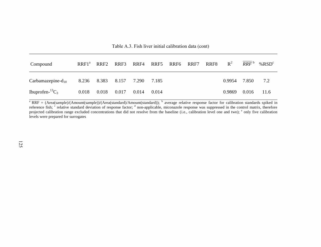
Table A.3. Fish liver initial calibration data (cont)
Compound RRF1a RRF2 RRF3 RRF4 RRF5 RRF6 RRF7 RRF8 R
2 RRF
b %RSD
c
Carbamazepine-d10 8.236 8.383 8.157 7.290 7.185 0.9954 7.850 7.2
Ibuprofen-13
C3 0.018 0.018 0.017 0.014 0.014 0.9869 0.016 11.6
a
RRF = (Area(sample)/(Amount(sample))/(Area(standard)/Amount(standard)); b average relative response factor for calibration standards spiked in
reference fish; c relative standard deviation of response factor;
d non-applicable, miconazole response was suppressed in the control matrix, therefore
projected calibration range excluded concentrations that did not resolve from the baseline (i.e., calibration level one and two); e only five calibration
levels were prepared for surrogates
125
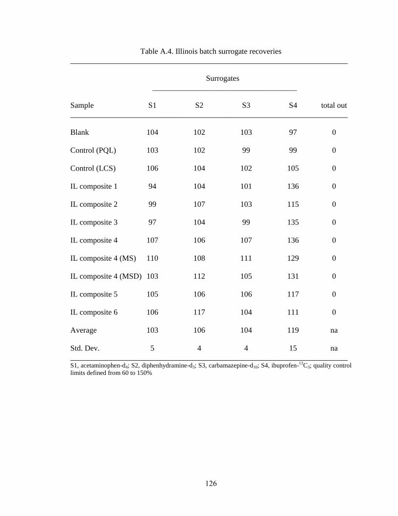
126
Table A.4. Illinois batch surrogate recoveries
_______________________________________________________________________
Surrogates
_____________________________________
Sample S1 S2 S3 S4 total out
_______________________________________________________________________
Blank 104 102 103 97 0
Control (PQL) 103 102 99 99 0
Control (LCS) 106 104 102 105 0
IL composite 1 94 104 101 136 0
IL composite 2 99 107 103 115 0
IL composite 3 97 104 99 135 0
IL composite 4 107 106 107 136 0
IL composite 4 (MS) 110 108 111 129 0
IL composite 4 (MSD) 103 112 105 131 0
IL composite 5 105 106 106 117 0
IL composite 6 106 117 104 111 0
Average 103 106 104 119 na
Std. Dev. 5 4 4 15 na
_______________________________________________________________________ S1, acetaminophen-d4; S2, diphenhydramine-d3; S3, carbamazepine-d10; S4, ibuprofen-
13C3; quality control
limits defined from 60 to 150%

127
Table A.5. Illinois batch LCS1 control sample
_____________________________________________________________________
Compound conc. units amount accuracy limits status
_____________________________________________________________________
Acetaminophen 14 ng/g 15 96 % 60 - 150 PASS
Atenolol 5 ng/g 5 104 % 60 - 150 PASS
Cimetidine 5 ng/g 5 104 % 60 - 150 PASS
Codeine 20 ng/g 20 101 % 60 - 150 PASS
1,7Dimethylxanthine 5 ng/g 5 102 % 60 - 150 PASS
Lincomycin 21 ng/g 20 104 % 60 - 150 PASS
Trimethoprim 9 ng/g 8 109 % 60 - 150 PASS
Thiabendazole 8 ng/g 8 101 % 60 - 150 PASS
Caffeine 15 ng/g 15 103 % 60 - 150 PASS
Sulfamethoxazole 8 ng/g 8 99 % 60 - 150 PASS
Metoprolol 8 ng/g 8 105 % 60 - 150 PASS
Propranolol 5.5 ng/g 5.0 109 % 60 - 150 PASS
Diphenhydramine 0.25 ng/g 0.25 101 % 60 - 150 PASS
Diltiazem 0.24 ng/g 0.25 97 % 60 - 150 PASS
Carbamazepine 1.9 ng/g 2.0 97 % 60 - 150 PASS
Tylosin 22 ng/g 20 108 % 60 - 150 PASS
Fluoxetine 15 ng/g 15 102 % 60 - 150 PASS
Norfluoxetine 8 ng/g 8 104 % 60 - 150 PASS
Sertraline 8 ng/g 8 104 % 60 - 150 PASS
Erythromycin 18 ng/g 20 88 % 60 - 150 PASS

128
Table A.5. Illinois batch LCS1 control sample (cont.)
_____________________________________________________________________
Compound conc. units amount accuracy limits status
_____________________________________________________________________
Warfarin 1.9 ng/g 2 98 % 60 - 150 PASS
Miconazole 26 ng/g 30 86 % 60 - 150 PASS
Ibuprofen 151 ng/g 150 101 % 60 - 150 PASS
Gemfibrozil 22 ng/g 20 109 % 60 - 150 PASS
_____________________________________________________________________

129
Table A.6. Illinois batch LCS2 control sample
_____________________________________________________________________
Compound conc. units amount accuracy limits status
_____________________________________________________________________
Acetaminophen 70 ng/g 75 94 % 60 - 150 PASS
Atenolol 27 ng/g 25 109 % 60 - 150 PASS
Cimetidine 26 ng/g 25 105 % 60 - 150 PASS
Codeine 101 ng/g 100 101 % 60 - 150 PASS
1,7Dimethylxanthine 24 ng/g 25 96 % 60 - 150 PASS
Lincomycin 102 ng/g 100 102 % 60 - 150 PASS
Trimethoprim 46 ng/g 40 115 % 60 - 150 PASS
Thiabendazole 39 ng/g 40 96 % 60 - 150 PASS
Caffeine 78 ng/g 75 103 % 60 - 150 PASS
Sulfamethoxazole 40 ng/g 40 99 % 60 - 150 PASS
Metoprolol 42 ng/g 40 104 % 60 - 150 PASS
Propranolol 25.8 ng/g 25.0 103 % 60 - 150 PASS
Diphenhydramine 1.31 ng/g 1.25 105 % 60 - 150 PASS
Diltiazem 1.22 ng/g 1.25 97 % 60 - 150 PASS
Carbamazepine 9.5 ng/g 10.0 95 % 60 - 150 PASS
Tylosin 112 ng/g 100 112 % 60 - 150 PASS
Fluoxetine 76 ng/g 75 101 % 60 - 150 PASS
Norfluoxetine 35 ng/g 40 87 % 60 - 150 PASS
Sertraline 40 ng/g 40 99 % 60 - 150 PASS
Erythromycin 93 ng/g 100 93 % 60 - 150 PASS

130
Table A.6. Illinois batch LCS2 control sample (cont.)
_____________________________________________________________________
Compound conc. units amount accuracy limits status
_____________________________________________________________________
Warfarin 10.5 ng/g 10.0 105 % 60 - 150 PASS
Miconazole 157 ng/g 150. 105 % 60 - 150 PASS
Ibuprofen 743 ng/g 750 99 % 60 - 150 PASS
Gemfibrozil 100 ng/g 100 100 % 60 - 150 PASS
_____________________________________________________________________
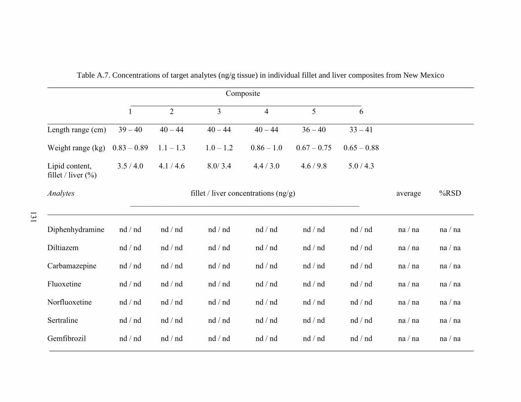
Table A.7. Concentrations of target analytes (ng/g tissue) in individual fillet and liver composites from New Mexico
Composite
1 2 3 4 5 6
Length range (cm) 39 – 40 40 – 44 40 – 44 40 – 44 36 – 40 33 – 41
Weight range (kg) 0.83 – 0.89 1.1 – 1.3 1.0 – 1.2 0.86 – 1.0 0.67 – 0.75 0.65 – 0.88
Lipid content, 3.5 / 4.0 4.1 / 4.6 8.0/ 3.4 4.4 / 3.0 4.6 / 9.8 5.0 / 4.3
fillet / liver (%)
Analytes fillet / liver concentrations (ng/g) average %RSD
__________________________________________________________
Diphenhydramine nd / nd nd / nd nd / nd nd / nd nd / nd nd / nd na / na na / na
Diltiazem nd / nd nd / nd nd / nd nd / nd nd / nd nd / nd na / na na / na
Carbamazepine nd / nd nd / nd nd / nd nd / nd nd / nd nd / nd na / na na / na
Fluoxetine nd / nd nd / nd nd / nd nd / nd nd / nd nd / nd na / na na / na
Norfluoxetine nd / nd nd / nd nd / nd nd / nd nd / nd nd / nd na / na na / na
Sertraline nd / nd nd / nd nd / nd nd / nd nd / nd nd / nd na / na na / na
Gemfibrozil nd / nd nd / nd nd / nd nd / nd nd / nd nd / nd na / na na / na
131

Table A.8. Concentrations of target analytes (ng/g tissue) in individual fillet and liver composites from Illinois
Composite
1 2 3 4 5 6
Length range (cm) 27 – 29 30 – 35 32 – 35 31 – 36 34 – 36 34 – 36
Weight range (kg) 0.38 – 0.46 0.48 - 0.76 0.72 – 0.87 0.48 – 0.82 0.75 – 0.99 0.76 – 0.83
Lipid content, 1.4 / 2.3 2.2 / 1.6 2.1 / 2.0 2.5 / 2.3 3.3 / 2.8 2.6 / 2.2
fillet / liver (%)
Analytes fillet / liver concentrations (ng/g) average %RSD
___________________________________________________________
Diphenhydramine 1.12 / 5.20 1.15 / 4.54 1.24 / 7.46 1.68 / 9.13 1.33 / 5.91 1.74 / 9.59 1.38 / 6.97 19 / 30
Diltiazem 0.14 / 0.50 0.12 / 0.54 0.10 / 0.78 0.12 / 0.88 0.12 / 0.64 0.16 / 0.90 0.13 / 0.71 16 / 24
Carbamazepine 1.8 / 4.3 2.0 / 5.6 2.0 / 6.6 2.6 / 6.8 2.6 / 5.3 3.1 / 7.5 2.3 / 6.0 22 / 21
Fluoxetine nd / nd nd / nd nd / 18 nd / 14 nd / nd nd / 23 na / 19 na / 22
Norfluoxetine 3 / 41 2 / 21 3 / 128 3 / 81 3 / 38 3 / 129 2 / 73 16 / 65
Sertraline 3 / 41 2 / 42 2 / 96 3 / 148 1 / 34 3/ 141 2/ 84 27 / 62
Gemfibrozil nd / nd nd / nd nd / nd nd / nd nd / nd nd / nd na / na na / na
132

Table A.9. Concentrations of target analytes (ng/g tissue) in individual fillet and liver composites from Arizona
Composite
1 2 3 4 5 6
Length range (cm) 47 – 49 38 – 42 35 – 41 40 – 42 37 – 46 52 – 55
Weight range (kg) 1.6 – 1.9 1.1 – 1.2 0.81 – 0.96 0.92 – 1.13 1.4 – 2.0 1.9 – 2.6
Lipid content, 3.3 / 10 4.0 / 15 4.6 / 11 4.7 / 13 4.1 / 9.4 2.7 / 11
fillet / liver (%)
Analytes fillet / liver concentrations (ng/g) average %RSD
___________________________________________________________
Diphenhydramine 1.04 / 6.32 1.20 / 4.38 1.41 / 5.79 1.21 / 5.48 1.12 / 7.28 1.24 / 11.1 1.20 / 6.72 10 / 35
Diltiazem 0.03 / 0.24 0.05 / 0.18 0.05 / 0.29 0.05 / 0.28 0.04 / 0.28 0.05 / 0.44 0.04 / 0.28 15 / 31
Carbamazepine nd / 0.3 nd / 0.3 nd / 0.2 nd / 0.3 nd / 0.2 nd / 0.4 na / 0.3 na / 25
Fluoxetine 2 / nd 1 / nd 2 / nd 2 / nd 1 / nd 1 / nd 2 / na 25 / na
Norfluoxetine 2 / 14 3 / 25 5 / 41 4 / 28 2 / 29 4 / 44 3 / 30 29 / 36
Sertraline 4 / 57 5 / 65 5 / 68 5 / 62 5 / 69 7 / 105 5 / 71 17 / 24
Gemfibrozil nd / 74 nd / 78 nd / 60 nd / 49 nd / 67 nd / 90 na / 70 na / 21
133

Table A.10. Concentrations of target analytes (ng/g tissue) in individual fillet and liver composites from Florida
Composite
1 2 3 4 5 6
Length range (cm) 52 – 59 44 – 49 38 – 41 38 – 40 34 – 38 37 – 42
Weight range (kg) 1.3 – 2.2 0.84 – 1.1 0.62 – 0.66 0.56 – 0.63 0.38 – 0.52 0.48 – 0.89
Lipid content, 2.3 / 3.6 1.5 / 5.6 0.9 / 3.0 0.5 / 1.1 0.5 / 1.7 0.6 / 2.5
fillet / liver (%)
Analytes fillet / liver concentrations (ng/g) average %RSD
__________________________________________________________
Diphenhydramine nd / nd nd / nd nd / nd nd / nd nd / nd nd / nd na / na na / na
Diltiazem nd / nd nd / nd nd / nd nd / nd nd / nd nd / nd na / na na / na
Carbamazepine nd / 0.4 nd / 0.2 nd / 0.3 nd / 0.4 nd / 0.3 nd / nd na / 0.3 na / 45
Fluoxetine nd / nd nd / nd nd / nd nd / nd nd / nd nd / nd na / na na / na
Norfluoxetine nd / 48 nd / 44 nd / 49 nd / 78 nd / 63 nd / 9 na / 49 na / 48
Sertraline nd / 13 nd / nd nd / 9 nd / 21 nd / 9 nd / 15 na / 13 na / 37
Gemfibrozil nd / nd nd / nd nd / nd nd / nd nd / nd nd / nd na / na na / na
134

Table A.11. Concentrations of target analytes (ng/g tissue) in individual fillet and liver composites from Pennsylvania
Composite
1 2 3 4 5 6
Length range (cm) 31 – 34 29 – 32 34 – 36 29 – 33 28 – 33 30 – 32
Weight range (kg) 0.39 – 0.43 0.33 – 0.42 0.52 – 0.59 0.33 – 0.40 0.31 – 0.46 0.32 – 0.41
Lipid content, 1.5 / 4.6 2.2 / 5.2 2.2 / 5.9 1.9 / 3.7 2.3 / 5.4 1.3 / 3.8
fillet / liver (%)
Analytes fillet / liver concentrations (ng/g) average %RSD
__________________________________________________________
Diphenhydramine 1.23 / 7.86 1.49 / 9.40 1.82 / 10.7 1.74 / 11.4 1.67 / 10.73 2.48 / 11.2 1.74 / 10.21 24 / 13
Diltiazem 0.10 / 0.59 0.10 / 0.60 0.11 / 0.71 0.14 / 0.75 0.12 / 0.72 0.20 / 0.76 0.13 / 0.69 31 / 11
Carbamazepine 0.3 / 0.5 0.3 / 0.6 0.3 / 0.5 0.3 / 0.7 0.4 / 0.6 0.4 / 0.7 0.3 / 0.6 19 / 11
Fluoxetine 2 / 63 2 / 66 3 / 66 3 / 65 3 / 80 5 / 78 3 / 70 42 / 10
Norfluoxetine 3 / 38 3 / 48 4 / 33 4 / 38 4 / 34 5 / 38 4 / 38 20 / 10
Sertraline 7 / 359 7 / 432 14 / 432 13 / 545 10 / 326 19 / 190 11 / 380 40 / 32
Gemfibrozil nd / na nd / na nd / 27 nd / na nd / 27 nd / na na / 27 na / 1.2
135

Table A.12. Concentrations of target analytes (ng/g tissue) in individual fillet and liver composites from Texas
Composite
1 2 3 4 5 6
Length range (cm) 56 – 60 50 – 54 48 – 49 48 – 56 43 – 45 45 – 47
Weight range (kg) 3.5 – 4.6 2.3 – 2.8 2.0 – 2.3 2.4 – 2.9 1.4 – 1.7 1.6 – 1.8
Lipid content, 1.6 / 5.9 2.1 / 8.9 0.9 / 9.4 3.0 / 10 4.0 / 10 1.7 / 3.6
fillet / liver (%)
Analytes fillet / liver concentrations (ng/g) average %RSD
__________________________________________________________
Diphenhydramine nd / 0.93 nd / 0.23 nd / 0.26 nd / 0.80 nd / 0.31 nd / 0.28 na / 0.47 na / 66
Diltiazem nd / 0.04 nd / 0.04 nd / 0.04 nd / 0.03 nd / 0.03 nd / 0.03 na / 0.03 na / 20
Carbamazepine nd / 0.2 nd / 0.2 nd / 0.2 nd / 0.2 nd / 0.2 nd / 0.2 na / 0.2 na / 19
Fluoxetine nd / 12 nd / nd nd / nd nd / 14 nd / nd nd / nd na / 13 na / 37
Norfluoxetine nd / 46 2 / 15 nd / 27 nd / 48 nd / 27 1.3 / 8 2 / 29 0.3 / 56
Sertraline nd / 28 nd / 13 nd / 28 nd / 23 nd / 28 nd / 9 na / 22 na / 39
Gemfibrozil nd / nd nd / nd nd / nd nd / nd nd / nd nd / nd na / na na / na
136

137
REFERENCES
(1) Daughton, C. G.; Ternes, T. A. Environ. Health Perspect. 1999, 107, 907-938.
(2) Kolpin, D. W.; Furlong, E. T.; Meyer, M. T.; Thurman, E. M.; Zaugg, S. D.; Barber,
L. B.; Buxton, H. T. Environ. Sci. Technol. 2002, 36, 1202-1211.
(3) Boxall, A. B. A.; Fogg, L. A.; Blackwell, P. A.; Kay, P.; Pemberton, E. J.; Croxford,
A. Rev. Environ. Contam. Toxicol. 2004, 180, 1-91.
(4) Ankley, G. T.; Brooks, B. W.; Huggett, D. B.; Sumpter, J. P. Environ. Sci. Technol.
2007, press.
(5) Hao, C.; Zhao, X.; Yang, P. Trends Anal. Chem. 2007, 26, 569-580.
(6) Koester, C. J.; Moulik, A. Anal. Chem. 2005, 77, 3737-3754.
(7) Kim, S. C.; Carlson, K. Trends Anal. Chem. 2005, 24, 635-644.
(8) Gros, M.; Petrovic, M.; Barcelo, D. Anal. Bioanal. Chem. 2006, 386, 941-952.
(9) Richardson, S. D.; Ternes, T. A. Anal. Chem. 2005, 77, 3807-3838.
(10) Brooks, B. W.; Chambliss, C. K.; Stanley, J. K.; Ramirez, A. J.; Banks, K. E.;
Johnson, R. D.; Lewis, R. J. Environ. Toxicol. Chem. 2005, 24, 464-469.
(11) Balmer, M. E.; Poiger, T.; Droz, C.; Romanin, K.; Bergqvist, P. A.; Mueller, M. D.;
Buser, H. R. Environ. Sci. Technol. 2004, 38, 390-395.
(12) Balmer, M. E.; Buser, H. R.; Mueller, M. D.; Poiger, T. Environ. Sci. Technol. 2005,
39, 953-962.
(13) Buser, H. R.; Balmer, M. E.; Schmid, P.; Kohler, M. Environ. Sci. Technol. 2006,
40, 1427-1431.
(14) Bohmer, W.; Rudel, H.; Wenzel, A.; Schroter-Kermani, C. Organohalogen Compd.
2004, 66, 1516-1521.
(15) Nakata, H. Environ. Sci. Technol. 2005, 39, 3430-3434.
(16) Nakata, H.; Sasaki, H.; Takemura, A.; Yoshioka, M.; Tanabe, S.; Kannan, K.
Environ. Sci. Technol. 2007, 41, 2216-2222.
(17) Olesen, L. D.; Cederberg, T.; Pedersen, K. H.; Hojgard, A. Chemosphere 2005, 61,
422-431.

138
(18) Rudel, H.; Bohmer, W.; Schroter-Kermani, C. J. Environ. Monit. 2006, 8, 812-823.
(19) Schmid, P.; Kohler, M.; Gujer, E.; Zennegg, M.; Lanfranchi, M. Chemosphere 2007,
67, S16-S21.
(20) Peck, A.; Kucklick, J. R.; Schantz, M. Anal. Bioanal. Chem. 2007, 387, 2381-2388.
(21) Ferrara, F.; Fabietti, F.; Delise, M.; Bocca, A. P.; Funari, E. Environ. Sci. Technol.
2001, 35, 3109-3112.
(22) Snyder, S. A.; Keith, T. L.; Naylor, C. G.; Staples, C. A.; Giesy, J. P. Environ.
Toxicol. Chem. 2001, 20, 1870-1873.
(23) Wenzel, A.; Bohmer, W.; Mueller, J.; Rudel, H. Environ. Sci. Technol. 2004, 38,
1654-1661.
(24) Keith, T. L.; Snyder, S. A.; Naylor, C. G.; Staples, C. A.; Summer, C.; Kannan, K.;
Giesy, J. P. Environ. Sci. Technol. 2001, 35, 10-13.
(25) Chu, S.; Metcalfe, C. D. J. Chromatogr. A 2007, 1163, 112-118.
(26) Wen, Y.; Wang, Y.; Feng, Y. Q. Talanta 2006, 70, 153-159.
(27) Stubbings, G.; Tarbin, J.; Cooper, A.; Sharman, M.; Bigwood, T.; Robb, P. Anal.
Chim. Acta 2005, 547, 262-268.
(28) Mottaleb, M. A.; Brumley, W. C.; Sovocol, G. W. J. Anal. Toxicol. 2004, 28, 581-
586.
(29) Brown, J. N.; Paxeus, N.; Forlin, L.; Larsson, D. G. J. Environ. Toxicol. Pharma.
2007, 24, 267-274.
(30) Nakamura, Y.; Yamamoto, H.; Sekizawa, J.; Kondo, T.; Hirai, N.; Tatarazako, N.
Chemosphere 2007, press.
(31) Mimeault, C.; Woodhouse, A. J.; Miao, X. -.; Metcalfe, C. D.; Moon, T. W.;
Trudeau, V. L. Aquat. Toxicol. 2005, 73, 44-54.
(32) Meinerling, M.; Daniels, M. Anal. Bioanal. Chem. 2006, 386, 1465-1473.
(33) Okumura, T.; Nishikawa, Y. Anal. Chim. Acta 1996, 325, 175-184.
(34) Osemwengie, L. I.; Steinberg, S. J. Chromatogr. A 2003, 993, 1-15.
(35) Tsuda, T.; Takino, A.; Kojima, M.; Harada, H.; Muraki, K. J. Chromatogr. B 1999,
723, 273-279.
(36) Tsuda, T.; Suga, K.; Kaneda, E.; Ohsuga, M. J. Chromatogr. B 2000, 746, 305-309.
139
(37) Schwaiger, J.; Ferling, H.; Mallow, U.; Wintermayr, H.; Negele, R. D. Aquat.
Toxicol. 2004, 68, 141-150.
(38) Clayton Jr., J. R.; Pavlou, S. P.; Breitner, N. F. Environ. Sci. Technol. 1977, 11, 676-
682.
(39) Mackay, D. Environ. Sci. Technol. 1982, 16, 274-278.
(40) Blerman Jr., V. J. Environ. Sci. Technol. 1990, 24, 1407-1412.
(41) Thomann, R. V.; Connolly, J. P.; Parkerton, T. F. Environ. Toxicol. Chem. 1992, 11,
615-629.
(42) Linsey, M. E.; Meyer, M.; Thurman, E. M. Anal. Chem. 2001, 73, 4640-4646.
(43) Quintana, J. B.; Reemtsma, T. Rapid Commun. Mass Spectrom. 2004, 18, 765-774.
(44) Reemtsma, T. J. Chromatogr. A 2003, 1000, 477-501.
(45) Stuber, M.; Reemtsma, T. Anal. Bioanal. Chem. 2003, 378, 910-916.
(46) Benijts, R.; Dams, W.; Lambert, A.; Leenheer, A. D. J. Chromatogr. A 2004, 1029,
153-159.
(47) Ferguson, P. L.; Iden, C. R.; Brownawell, B. J. Anal. Chem. 2000, 72, 4322-4330.
(48) Vanderford, B. J.; Pearson, R. A.; Rexing, D. J.; Snyder, S. A. Anal. Chem. 2003,
75, 6265-6274.
(49) Schluesener, M. P.; Bester, K. Rapid Commun. Mass Spectrom. 2005, 19, 3269-
3278.
(50) Stoob, K.; Singer, H. P.; Goetz, C. W.; Ruff, M.; Mueller, S. R. J. Chromatogr. A
2005, 1097, 138-147.
(51) Delatour, T. Anal. Bioanal. Chem. 2004, 380, 515-523.
(52) Reddy, S.; Iden, C. R.; Brownawell, B. J. Anal. Chem. 2005, 77, 7032-7038.
(53) Matuszewski, B. K.; Constanzer, M. L.; Chavez-Eng, C. M. Anal. Chem. 2003, 75,
3019-3030.
(54) Kloepfer, A.; Quintana, J. B.; Reemtsma, T. J. Chromatogr. A 2005, 1067, 153-160.
(55) Vanderford, B. J.; Snyder, S. A. Environ. Sci. Technol. 2006, 40, 7312-7320.
(56) Snyder, S. A.; Westerhoff, P.; Yoon, Y.; Sedlak, D. L. Environ. Eng. Sci. 2003, 20,
449-469.

140
(57) Ternes, T. A.; Joss, A.; Siegrist, H. Environ. Sci. Technol. 2004, 38, 293A-398A.
(58) Petrovic, M.; Hernando, M. D.; Diaz-Cruz, M. S.; Barcelo, D. J. Chromatogr. A
2005, 1067, 1-14.
(59) Castiglioni, S.; Zuccato, E.; Crisci, E.; Chiabrando, C.; Fanelli, R.; Bagnati, R. Anal.
Chem. 2006, 78, 8421-8429.
(60) Balakrishnan, V. K.; Terry, K. A.; Toito, J. J. Chromatogr. A 2006, 1131, 1-10.
(61) Miao, X. S.; Yang, J. J.; Metcalfe, C. D. Environ. Sci. Technol. 2005, 39, 7469-7475.
(62) Zuehlke, S.; Duennbier, U.; Heberer, T. Anal. Chem. 2004, 76, 6548-6554.
(63) Gobel, A.; Thomsen, A.; McArdell, C. S.; Alder, A. C.; Giger, W.; Theib, N.;
Loffler, D.; Ternes, T. A. J. Chromatogr. A 2005, 1085, 179-189.
(64) Petrovic, M.; Gros, M.; Barcelo, D. J. Chromatogr. A 2006, 1124, 68-81.
(65) Gomez, M. J.; Petrovic, M.; Fernandez-Alba, A. R.; Barcelo, D. J. Chromatogr. A
2006, 1114, 224-233.
(66) Morales-Munoz, S.; Luque-Garcia, J. L.; Ramos, M. J.; Fernandez-Alba, A.; Luque
de Castro, M. D. Anal. Chim. Acta 2005, 552, 50-59.
(67) Ternes, T. A.; Bonerz, M.; Herrmann, N.; Loffler, D.; Keller, E.; Lacida, B. B.;
Alder, A. C. J. Chromatogr. A 2005, 1067, 213-223.
(68) RxList The Internet Drug Index, Top 300 Prescriptions for 2005 by Number of U.S.
Prescriptions Dispensed. http://www.rxlist.com/top200.htm (accessed November,
2006).
(69) Furlong, E. T.; Kinney, C. A.; Ferrer, I.; Werner, S. L.; Cahill, J. D.; Ratterman, G.
Pharmaceuticals and personal-care products in solids: Analysis and field results for
sediment, soil and biosolid samples. Extended Abstracts of Papers, 228th ACS
National Meeting, Division of Environmental Chemistry, 2004; 44, 1320-1324.
(70) Yang, S.; Carlson, K. H. J. Chromatogr. A 2004, 1038, 141-155.
(71) Tanaka, N.; Thornton, E. R. J. Am. Chem. Soc. 1976, 98, 1617-1619.
(72) Shibasaki, H.; Futura, T.; Kasuya, Y. J. Chromatogr. B 1997, 692, 7-14.
(73) Kato, K.; Jingu, S.; Ogawa, N.; Higuchi, S. J. Pharm. Biomed. Anal. 2000, 24, 237-
249.
(74) Kaiser, H. Anal. Chem. 1970, 42, 26-59.

141
(75) Skoog, D. A.; Holler, F. J.; Nieman, T. A. Principles of instrumental analysis, 5th
ed.; Harcourt Brace & Co.: Philadelphia, PA, 1998; pp 11-15.
(76) Definition and Procedure for the Determination of the Method Detection Limit.
Code of Federal Regulations, Title 40, Section 136, Apendix B, 1986.
(77) Barber, L. B.; Keefe, S. H.; Antweiler, R. C.; Taylor, H. E.; Wass, R. D. Environ.
Sci. Technol. 2006, 40, 603-611.
(78) Lee, C. J.; Rasmussen, T. J. Sci. Total Environ. 2006, 371, 258-269.
(79) Brooks, B. W.; Riley, T. M.; Taylor, R. D. Hydrobiologia 2006, 556, 365-379.
(80) Mottaleb, M. A.; Moy, T. W.; Zimmerman, J. H. Int. J. Environ. Anal. Chem. 2006,
86, 743-756.
(81) McLachlan, J. A. Endocr. Rev. 2001, 22, 319-341.
(82) Ballesteros, O.; Zafra, A.; Navalon, A.; Vilchez, J. L. J. Chromatogr. A 2006, 1121,
154-162.
(83) Petrovic, M.; Lacorte, S.; Viana, P.; Barcelo, D. J. Chromatogr. A 2002, 959, 15-23.
(84) Meesters, R. J.; Schroder, H. F. Anal. Chem. 2002, 74, 3566-3574.
(85) Morley, M. C.; Snow, D. D.; Cecrle, C.; Denning, P.; Miller, L. Water Environ. Res.
2006, 78, 1017-1053.
(86) Poiger, T.; Buser, H. R.; Balmer, M. E.; Bergqvist, P. A.; Mueller, M. D.
Chemosphere 2004, 55, 951-963.
(87) Giokas, D. L.; Sakkas, V. A.; Albanis, T. A.; Lampropoulou, D. A. J. Chromatogr.
A 2005, 1077, 19-27.
(88) Jeon, H. K.; Chung, Y.; Ryu, J. C. J. Chromatogr. A 2006, 1131, 192-202.
(89) Berset, J. D.; Bigler, P.; Herren, D. Anal. Chem. 2000, 72, 2124-2131.
(90) Simonich, S. L.; Begley, G. D.; Eckhoff, W. S. Environ. Sci. Technol. 2000, 34, 959-
965.
(91) Osemwengie, L. I.; Steinberg, S. J. Chromatogr. A 2001, 932, 107-118.
(92) Einsle, T.; Paschke, H.; Bruns, K.; Schrader, S.; Popp, P.; Moeder, M. J.
Chromatogr. A 2006, 1124, 196-204.
(93) Smyth, S. A.; Lishman, L.; Alaee, M.; Kleywegt, S.; Svoboda, L.; Yang, J. J.; Lee,
H. B.; Seto, P. Chemosphere 2007, 67, 267-275.
142
(94) Lindstrom, A.; Buerge, I. J.; Poiger, T.; Bergqvist, P. A.; Mueller, M. D.; Buser, H.
R. Environ. Sci. Technol. 2002, 36, 2322-2329.
(95) Halden, R. U.; Paull, D. H. Environ. Sci. Technol. 2005, 39, 1420-1426.
(96) Knepper, T. P. J. Chromatogr. A 2004, 1046, 156-159.
(97) Sandstrom, M. W.; Kolpin, D. W.; Thurman, E. M.; Zaugg, S. D. Environ. Toxicol.
Chem. 2005, 24, 1029-1034.
(98) Lee, H. B.; Peart, T. E.; Svoboda, M. L. J. Chromatogr. A 2005, 1094, 122-129.
(99) Gatidou, G.; Thomaidis, N. S.; Stasinakis, A. S.; Lekkas, T. D. J. Chromatogr. A
2007, 1138, 32-41.
(100) Cuderman, P.; Heath, E. Anal. Bioanal. Chem. 2007, 387, 1343-1350.
(101) Honeycutt, M. E.; McFarland, V. A.; McCant, D. D. Bull. Environ. Contam.
Toxicol. 1995, 55, 469-472.
(102) Ternes, T. A. Water Res. 1998, 32, 3245-3260.
(103) Gros, M.; Petrovic, M.; Barcelo, D. Environ. Toxicol. Chem. 2007, 26, 1553-1562.
(104) Metcalfe, C. D.; Koeing, B. G.; Bennie, D. T.; Servos, M.; Ternes, T. A.; Hirsch, R.
Environ. Toxicol. Chem. 2003, 22, 2872-2880.
(105) U.S. Environmental Protection Agency (USEPA). 2006. Quality Assurance Project
Plan for Sample analysis for a Pilot Study to Investigate the Occurrence of
Pharmaceuticals and Personal Care Products (PPCPs) in Fish Tissue. EPA Office
of Water, Office of Science and Technology, Washington, DC.