DETERMINATION OF THE BUNDLE PRICE FOR DIGITAL …

DETERMINATION OF THE BUNDLE PRICE

FOR DIGITAL INFORMATION GOODS

Gündüz Ulusoy

Manufacturing Systems Engineering Program Sabancı University

Orhanlı, Tuzla, 81474 Istanbul

Kaan Karabulut

Industrial Engineering Department Boğaziçi University

Bebek, 80815 Istanbul

February 2003

Revised April 2003

1

DETERMINATION OF THE BUNDLE PRICE

FOR DIGITAL INFORMATION GOODS

ABSTRACT

The fast emergence of Internet as a media to distribute digital information goods

created many new opportunities for the packaging and pricing of these goods. The pricing

of information goods introduces a challenge since the cost structure of information goods

differs from that of conventional physical goods in that they can be costly to introduce but

are relatively cheap to reproduce. The bundling strategy for digital information goods

helps producers to extract more value from customers and can result in cost savings due

to the presence of economies of scale.

This study aims to determine the optimum price a producer of digital information

goods has to charge for a bundle in order to maximize his gross margin. The bundle

pricing model is constructed for both uniform and exponential distributions of the fraction

of information goods in the bundle that has positive value for the customers.

2

1. INTRODUCTION

In this paper, a pricing model for a bundle of digital information goods under

different distributions of the fraction of goods in the bundle that has positive value for the

customer is presented. The price for a bundle of digital information goods is determined

so as to maximize the producer’s gross margin. It is interesting to note that although

bundling is widely applied in practice and pricing is a major issue in bundling, optimal

pricing of a bundle has not been treated extensively.

Bundling can be considered as a kind of packaging, where bundled individual

goods are sold together as a package at a single price. The price is different than the sum

of the prices of the individual goods in the bundle. Bundling has been applied to physical

goods such as machine tools or personal computer tools as well as to information goods

such as the Microsoft Office 2000. The Internet allows producers to offer more

customized products to customers. For example, a customer can get a personalized

newspaper by choosing a set of categories according to his/her interests. So, the user can

read his/her customized bundle of news.

Shapiro and Varian (1998) define information goods as goods capable of being

distributed in digital form. The definition covers anything that can be digitized: Computer

softwares, research reports, journals, music, movies, weather reports, video clips, stock

quotes, photographs, newspapers are all examples of information goods.

Varian (1998) describes three main properties of information goods, which need

to be taken into account in the marketing of these goods. The first main property of an

information good is that it is an experience good. One has to experience an information

good before being able to value it. Being an experience good is not limited to digital

information goods. In fact, any physical product entering the market for the first time,

such as the first fax machine, or the first photocopying machine, faces the same problem.

Promotional pricing and free samples are some strategies in order to introduce the new

goods to the consumer. Previews and reviews such as book reviews, film reviews, music

reviews are some further marketing strategies. Reputation and branding are other means

of overcoming the experience good problem.

3

The second main property of information goods is that they share some properties

of public goods. A good is a public good, if it is still available for consumption by other

consumers, even if being consumed by another consumer (Begg et al., 1994). Air,

national defence, and public safety are some examples of public goods. Public goods are

both non-rival and non-excludable. Non-rival means that one’s consumption of one good

doesn’t diminish the amount of that good available to other people. Non-excludability

means that one person cannot exclude another person from consuming or using the good.

In terms of non-excludability and non-rivalness, information goods resemble public

goods. Relative to physical goods, it is more difficult to exclude other people to use, to

consume and to enjoy information goods. Such an attempt requires additional costs such

as detection cost and is less guaranteed since it is easy to copy information goods. The

handling of excludability through enforcement or other means is a delicate legal and

technological issue of utmost importance for the survival of the information goods'

producers. Shapiro and Varian (1998) do not recommend overprotection of digital

information goods as a protection strategy for producers. Cheng and Png (2003) consider

how government should set the fine for copying, tax on copying medium, and subsidy on

legitimate purchases and how a monopoly producer sets price and spending on detection.

They conclude that society prefers the producer to manage piracy through lower prices

rather than increased enforcement; that a tax on the copying medium is welfare superior

to the penalty; and that it is optimal to subsidize legitimate purchases.

The third significant property of information goods is the returns to scale.

Information goods are costly to produce but cheap to reproduce. The cost structure of

information goods differs from that of physical goods. That information goods are

relatively cheap to reproduce results a major difference in the cost structure of

information goods as compared to physical goods. This leads to a relatively high ratio of

fixed costs to total cost in comparison to physical goods. The fixed cost for information

goods consists of first-copy sunk costs, marketing and promotion costs. First-copy sunk

costs are costs incurred before production such as development costs and costs of creating

the associated production and delivery facilities. In additon to first-copy sunk costs,

producers of information goods need to invest heavily in marketing of their products in

order to attract the attention of consumers and to increase the brand loyalty. Distribution

costs constitute another component of the cost structure of information goods. With the

developing technology, distribution costs are decreasing leading to further increase in the

4

ratio of fixed cost to total cost. This is particularly true for information goods distributed

over the Internet. The relatively high ratio of fixed costs to total cost results in substantial

returns to scale such that the average cost of production decreases as the number of goods

produced increases. The key to delivering a low-cost product or service is not effective

process management but high cumulative output (Hayes, 2002).

It is interesting to note that not only the ratio but also the nature of the fixed cost

and the variable cost of information goods differ from those of physical goods (Shapiro

and Varian, 1998). In case of information goods, the fixed cost to a large extend is sunk

cost. Once for some reason, production is either terminated or has not even started, large

portion of fixed cost can not be recovered. In case of physical goods, a much larger

portion of fixed cost can be salvaged. Physical goods differ from digital information

goods also by the capacity constraint imposed on their production. Once the production of

a physical good reaches the capacity constraint, then the variable cost of producing an

additional unit increases. Relatively heavy investment has to be made to increase the

production capacity. This is usually not the case with information goods. The production

of information goods faces few capacity constraints. Thus, the variable cost of producing

an additional unit remains roughly the same over a large range of production levels. But

the need to service customers might introduce additional capacity constraints and might

lead to substantial costs (Hayes, 2002).

Further interesting characteristics of digital information goods distributed over the

Internet in contrast with the physical goods are that most inventory costs are absent and

that reproduction and distribution operations take negligible time. But for particular

categories of information goods there are other cost categories, capacity limits, and time

delays substantial enough to raise serious managerial questions (Geoffrion, 2002).

The structure of the market for information goods is a description of the behaviour

of sellers and buyers in that market (Begg et al., 1994). The market for information goods

is neither a perfectly competitive market nor an auction market. Recall that a perfectly

competitive market implies the existence of several producers of an identical commodity,

which indeed does not reflect the characteristics of a market for information goods

because of the relative ease of product differentiation among information goods. In

auction markets, on the other hand, a good is sold to the customer who pays the highest

value. Auction markets work well for goods with fixed supply such as airline seats, which

5

is not the case for information goods. The market for information goods can be classified

as a monopolistically competitive market. In this type of market, there are several slightly

different products, which are close substitutes. In order to build some market power in the

market and to be able to remain in the market, a producer of information goods should

distinguish its goods from those of other producers. In differentiating its product, a

producer will have no close competitors. But for success in the market it is not enough to

differentiate the product. In addition, the producer should customize its products

according to the needs and interests of its customers. By customizing the product, the

most value can be generated from customers. In a monopolistically competitive market,

the primary concern of producers becomes the customers’ willingness to pay for the

product rather than their competition’s behaviour (Varian, 1998).

Sometimes it might be difficult to differentiate a product enough from the

competitors’ products. In such a case, a strategy to compete is to decrease the price. For

producers of physical goods, it is possible to decrease the average production cost

through proper supply chain management and to reduce the price without reducing the

profit margin. But for information goods, the incremental production cost is relatively

small. Thus, it is not possible to compensate for the reduction in prices by reducing the

incremental production costs. This implies that a reduction in the price will lead to a

reduction in the profit margin in that case. In order to avoid the decrease in the profit

margin, the sales volume should be increased. Hence, in the case of information goods,

the producer has to focus on increasing the sales in order to support the strategy to

compete through price reduction.

The general economic principle that the price of a product should at least be equal

to its marginal cost may not be feasible for information goods because the perfect copies

of information goods can be reproduced at a small cost. This cost structure introduces a

challenge for the pricing of information goods.

Two basic pricing policies for information goods would be flat pricing and

differential pricing. In flat pricing policy, each customer is charged the same price for a

standart product. But in order to extract the maximum value from customers, the products

need to be customized. If the product is personalized for the needs and interests of the

customers, the producer has more flexibility to price its goods, since it is much less

affected by its competitors’ pricing policies. The customization of products also allows

6

for the customization of prices. In addition, the maximum reservation price differs for

each customer. All these arguments lead to differential pricing policy.

Shapiro and Varian (1999) describe three types of differential pricing:

1. Personalized pricing,

2. Group pricing,

3. Versioning.

In “personalized pricing”, the producer charges each customer a different price.

This method of pricing is used by some airlines. There are many factors influencing the

price charged. This enables the producer to charge almost every customer a different

price.

In “group pricing”, certain groups of customers are charged different prices than

individual customers, who don’t belong to a certain group. People who have similar

characteristics are assumed to belong to a certain group. For instance; members of a

group can attend the same department or take the same course in a university, they can be

at the same age, they can use the same library, they can have a similar income structure,

etc.

The third strategy for differential pricing is “versioning” in which producers offer

different versions of a good for different market segments. These market segments have

different values of reservation prices for a particular good.

2. BUNDLING

Adams and Yellen (1976) define bundling as the practice of package selling.

Sporting organizations offering season tickets, restaurants providing fixed menu dinners,

banks offering travelers’ check services for a single fee and garment manufacturers

selling their retailers clothing grab bags comprised of assorted styles, sizes and colors all

provide examples of package selling. Bundling also applies when firms sell the same

physical commodity, such as detergents and toothpaste, in different container sizes. For

instance, an electronic journal is a bundle of issues, each of which is a bundle of articles,

each of which is a bundle of bibliographic information, abstract, references, text, and

figures. It is often straightforward to rebundle any of these elements in different ways,

7

when the source material is archived in electronic form such that one might obtain all

abstracts matching a given keyword search, or all citations appearing in a particular

article, or just the bibliographic headers from the issue in a given year.

There are several implementation forms of bundling (Simon and Wuebker, 1999).

In pure bundling, only the bundle is sold. The products cannot be bought individually.

For example, a movie rental company offering a theater owner only a bundle of movies

rather than the option of choosing from a set of movies is exercising pure bundling. In

mixed bundling, on the other hand, both the bundle and the individual products are

offered to the customer. McDonald’s value meals would be an example of mixed

bundling. Giving a discount to a second good if the first one is purchased at full price is

another form of of mixed bundling. A special form of bundling is the so called add-on

bundling. An add-on product is not sold unless the lead product is purchased. For

example, an automobile can be interpreted as a package of accessories and transport

service. The transport service (the automobile – the lead product) can be purchased

without accessories such as ABS or airbags. Accessories are added in order to add value

to the good offered.

2.1. Benefits of Bundling

There are many reasons that make the bundling of information goods attractive for

producers.

It is impossible to know the willingness to pay of each customer for each good

offered by producers. Uncertainty about consumer valuations creates difficulties for

effective pricing and efficient transactions. A producer might try to maximize its profits

by charging a price for each good that excludes some customers with low valuations for

that good and forgoes some revenue from customers with high valuations. But in this

case, the producer can lose some potential customers and forgoes some revenue, which

might make this mechanism inefficient. Stigler (1963) suggested an alternative price

discrimination technique such as packaging two or more products in bundles rather than

selling them separately. So, bundling is suggested as a selling strategy which makes it

easier for the producer to extract value from a given set of goods by enabling a form of

price discrimination. Bundling reduces the uncertainty about customer valuations such

that it reduces the dispersion in reservation prices.

8

Bundling reduces the heterogeneity of the reservation prices and makes the

valuations of customers more predictable. This enables the producer to increase its profits

by enabling effective pricing. So, if customers have different reservation prices and the

producer can’t price discriminate, all customers can purchase the good at a price equal to

the reservation price of the customer with the lowest value. But by creating the bundle,

the producer can sell its goods at a price equal to the average reservation price of the

customers and this will increase the producer’s profits.

A customer may not currently need to use an information good in the bundle but

later, if he decides to use an information good in the bundle, he might use this good in the

future. This is called the option value of bundling. In this case, the incremental cost of

bundling seems to be zero since customers don’t pay for using another good in the bundle

but they have already paid during the purchase of the bundle. But producers usually offer

the bundle at a price which is less than the sum of the prices of goods constituting the

bundle.

Bundling can result in cost savings due to the presence of economies of scale.

Chae (1992) applied the bundling model in the study of subscription policies for the

cable television market. He assumed extreme economies of scale in the production and

distribution of information goods in the cable television market. This means that

economies of scale index is assumed to be zero such that marginal cost of producing and

distributing a bundle of information goods is equal to the marginal cost of producing and

distributing an individual information good. Coase (1960) and Demsetz (1968) also

focused on the cost savings in production and transactions associated with package

selling.

Bundling serves to introduce new products to customers. A producer can add a new

product into a bundle and can introduce this new product without any need for special

advertisement. For a customer, it may be risky to buy a new product. But when the new

product is included in a bundle of information goods, then the customer’s purchasing

decision is made easier and its perceived risk is reduced.

In addition, bundling introduces complementarities in production, distribution and

consumption of bundle components. Bakos (1997) reported that bundling can directly

9

increase the value available from a set of goods due to the technological

complementarities in production, distribution or consumption.

Differently, Carbajo et al.(1990) and Whinston (1990) argued about the strategic

leverage of bundling such that producers in imperfectly competitive markets may choose

to bundle their products for strategic reasons.

Moreover, low marginal cost of production for information goods makes bundling

attractive. It is not economical to offer goods at a price below their marginal costs of

production. Since the marginal cost of producing information goods is very low, it will

not be profitable to offer the good to a customer who values that good below its marginal

cost of production. In addition, there exist economies of scale in the distribution of these

goods. So, profitability can be increased by providing maximum number of goods in the

bundle to the maximum number of customers.

Finally, bundling helps to reduce the search cost of customers, which is defined as

the cost incurred by the buyer to locate an appropriate seller and to purchase a product.

This would include the opportunity cost of time spent searching as well as associated

expenditures such as telephone calls, computer fees, magazine subscriptions. By bundling

information goods, search cost for customers can be decreased.

2.2. The Effect of Bundling on Demand

2.2.1. The case for an individual information good

In order to investigate the effect of bundling on demand, first the case for an

individual information good is analyzed. The demand curve for an individual information

good is seen in Figure 1. For ease of discussion, the price is taken to be a linear

decreasing function of quantity demanded.

As can be seen in Figure 1, if q units of this good are purchased, then the producer

charges a price of p per unit and generates a revenue by an amount of (p*q). The marginal

cost of producing one unit of an information good is represented by c. It is low compared

to the price level p. Some customers may be willing to pay a price less than p but higher

than c. In this case, the customer can’t purchase the good and a deadweight loss is

created, which is given by the area of the triangle (FBE). Aside from these customers, a

customer may be willing to pay more than p. Although it is enough to pay p to purchase

10

the good, his willingness to pay for the good is more than p. As a result, consumers’

surplus is created, which is given by the area of the triangle (GpF). In order to eliminate

the deadweight loss, the producer should set the price of his goods equal to the marginal

costs. But, this price might be too low to cover for the fixed costs of production and cause

the profitability of the producer to decrease.

Figure 1. Demand curve for an individual information good

So far it is assumed that the producer applies flat-pricing. Let us relax this

assumption and assume that the producer is able to price discriminate instead of flat-

pricing. In case of differential pricing, the producer charges customers according to their

willingness to pay and deadweight loss is not created. In case of perfect price

discrimination, profits will be maximized and both customers’ surplus and deadweight

loss are eliminated.

2.2.2. The case for for a bundle of two goods

Salinger (1995) developed a graphical framework in order to analyze the demand

for a bundle of two goods with independent linear demand functions. To investigate the

effect of bundling on demand, it is assumed that there are two goods, denoted as good 1

and good 2 and each customer purchases either zero or one unit of each of the goods that

can be bundled.

In order to understand the situation assume that there are two information goods: a

video clip and stock quotes. It is supposed that the value of each information good is

Quantity

Price

Demand Consumers’ surplus

Deadweight loss

G

p

c

A q I H

F

B E

between zero and one. The demand curve for each of these information goods is assumed

to be like the one in Figure 1. In addition, it is assumed that valuation of one good is

uncorrelated with the valuation for the other good such that if the customer gets one of

the two goods, then the other good doesn’t become less/more attractive to him and

therefore valuation for that good doesn’t decrease/increase. Now, assume that the

producer bundles video clip and stock quotes and sells the two goods as a bundle instead

of selling them separately. The reservation price for the bundle is the sum of the

reservation prices for the individual goods. The demand curve for the bundle is seen in

Figure 2. In Figure 2, the horizontal axis represents the quantity demanded for the bundle

and the vertical axis the reservation price for the bundle. The area under the demand

curve for the bundle represents the total potential surplus. This area is also equal to the

sum of areas under the demand curves for the individual goods. The demand curve for the

individual goods is linear but the demand curve for the bundle is not linear.

The demand curve for the bundle is flatter around 0.5 and steeper around zero and

one. In other words, it becomes more elastic around 0.5 and less elastic around zero and

one. This means that the quantity demanded for the bundle increases more around 0.5

than around zero and one for a unit change in the price of the bundle. So, if the producer

charges a price of 0.5, then half of the customers will buy the bundle.

Figure

0

1

5

5

e

2. Demand curve for a bu

1

0.

0.

ndle of tw

Quantity

Pric

11

o information goods

12

2.2.3. The case for for a bundle of more than two goods

Bakos (1997) argued that as the number of information goods in the bundle

increases, the distribution for the valuation of the bundle has an increasing fraction of

customers with moderate valuations near the mean as implied by the law of large

numbers. So, the producer better matches the heterogenous distribution of customers by

decreasing the heterogeneity of customers' reservation prices instead of increasing the

menu of prices in order to perform a more effective price discrimination. This enables the

producer to charge a single price, that almost fits all customers.

2.3. Profitability of Bundling

For the case of two goods and a single producer, Adams and Yellen (1976) showed

through the use of numerical examples that mixed bundling can increase profits under the

assumptions that the reservation prices for the two goods in the bundle are negatively

correlated and are additive.

Taking Adams–Yellen model as a starting point, Schmalensee (1984) assumed

further that the reservation prices of the customers’ follow a bivariate Gaussian

distribution. He found that as long as reservation prices are not perfectly correlated, the

standart deviation of reservation prices for the bundle are less than the sum of the standart

deviations for the two component goods. He emphasized that the reason for the

enhancement of the profitability through bundling is that bundling reduces the dispersion

of the reservation prices and thus the producer can extract a greater fraction of the

consumers’ surplus. Schmalensee demostrated further that mixed bundling combines

advantages of both pure bundling and unbundled sales.

Salinger (1995) argued that if bundling doesn’t lower costs, bundling tends to be

profitable when reservation prices are negatively correlated and are high relative to costs.

On the contrary, if bundling lowers costs and these costs are high relative to average

reservation prices, the incentive to bundle increases when reservation prices are positively

correlated.

Bakos (1997) pointed out that bundling reduces the average deadweight loss and

leads to higher average profits. He proposed that if it is more profitable to bundle certain

number of goods than to sell them separately and the optimal price per good for the

13

bundle is less than the mean valuation, then bundling any number of goods greater than

that certain number will further increase profits compared to the case where the additional

goods are sold separately.

Based on empirical studies Simon and Wuebker (1999) claim that mixed bundling

always exploits profit potential better than separate pricing or pure bundling. Pure

bundling appears to result in the lowest profits in all applications. They interpret this

result by the resentment of the customers feeling they are forced to buy a bundle. They

report that through mixed bundling, multi-product firms often obtain profit improvements

in the range of 10 to 40%.

2.4. The Effect of Marginal Costs

Schmalensee (1984) pointed out that bundling can increase profits of producers by

reducing the dispersion of the valuations of customers. But this is valid only if marginal

costs are small. If the marginal costs are large, the producers want to increase the

dispersion of reservation prices instead of reducing it. If the marginal cost is less than the

mean valuation of customers, then the producer will try to reduce the dispersion of the

reservation prices. This helps the producer to extract higher profits from all customers.

On the contrary, if the marginal cost is greater than the mean valuation of customers,

bundling will decrease profits. Bundling reduces the dispersion of valuations of

customers but since marginal costs are large, the fraction of customers with valuations in

excess of the total marginal cost of the bundle and profits will decrease considerably. So,

in case of great marginal costs, it is not preferable to form a bundle.

Bakos (1997) proposed that there is a marginal cost for each information good that

makes bundling result in lower profits and higher deadweight loss than selling the goods

separately. He stated that very large bundles will typically continue to be profitable even

in the presence of non-zero but not very large marginal costs and substantial marginal

costs make bundling unprofitable. If the bundle includes goods which have negative

values for some customers, the benefits of bundling for the producer might be lost. For

example, if there are too many advertisements, then the valuations of customers can be

negative. So, bundling can decrease profits even if the marginal costs are zero.

With the developments in technology and the resulting rapid decreases in marginal

costs, customers might still need to spend excessive time and energy in order to identify

14

an information good suitable for their purposes. This situation can lead to customer

dissatisfaction and can prevent producers from increasing their profits even if they have

attained very small marginal cost levels. Brynjolfsson and Kemerer (1996) found that the

cognitive cost of learning the software accounts for a substantial fraction of the price of

the software. Thus, the producers should help customers to learn and to identify their

products in a more effective and fast manner.

3. DETERMINING THE BUNDLE PRICE OF INFORMATION GOODS

The main objective in this study is to find the optimal price for a bundle

containing N information goods for a producer whose aim is to maximize his surplus. The

producer’s surplus is also called the gross margin and defined as the difference between

the value received and the cost incurred for a bundle of N goods.

A study on optimal bundle pricing, which is complementary with this study is the

one by Hanson and Martin (1990). They presented a linear mixed integer optimization

model for maximizing the profit of a monopolist firm. The firm establishes a price list for

all possible bundles of components. Based on this price list customers purchase bundles

so as to maximize their consumer’s surplus, which is included as a constraint in the

optimization model. Reservation prices of each possible bundle for all customer segments

are assumed to be known. In this context, for example, our model would generate the

optimal price for each bundle on the price list.

3.1. The Bundling Model

In the bundling model used in this study, there are N goods in the bundle. It is

allowed that each customer to rank the N goods in the bundle in decreasing order of

preference such that a customer’s most favorite good in the bundle is ranked first and the

least favourable one is ranked last. The customer may have zero or positive valuations for

any number of goods in the bundle. By assuming a linear demand function for all

positive-valued goods, an individual customer’s valuation for good n in the bundle, v(n),

can be modeled as

−=

Npnvnv.

1.)( 0 (1)

15

where:

v0 : reservation price of a customer for the most favored good in the bundle,

p : fraction of goods in the bundle that has non-zero value to the customer,

N : number of goods in the bundle.

Figure 3 shows the valuation of individual goods in the bundle by an individual

customer. The valuation function is linear and decreasing as suggested by (1). The

variable p represents the slope of the linear demand curve and also indicates the fraction

of goods in the bundle that has positive value to the customer. For instance, a customer

with p=0.02 is willing to pay a non-zero value for only two goods in a bundle of hundred

goods. The most highly valued good for the customer is represented by v0 and obtained

by putting n=0 in (1) and it is also the y-intercept in Figure 3. Valuations of N goods in

the bundle are ranked in decreasing order of preference and linearly decreases starting

from v0. The valuation for the subsequently ranked goods is assumed to fall down at a

constant rate until it reaches zero at n=pN, which represents the number of positively

valued goods in the bundle. (N-pN) goods have zero valuation for the customer.

Figure 3. Valuation of goods in the bundle by an individual customer

v(n)= v0 [1- ( n / p.N) ]

v(n)

0 p.N N n

16

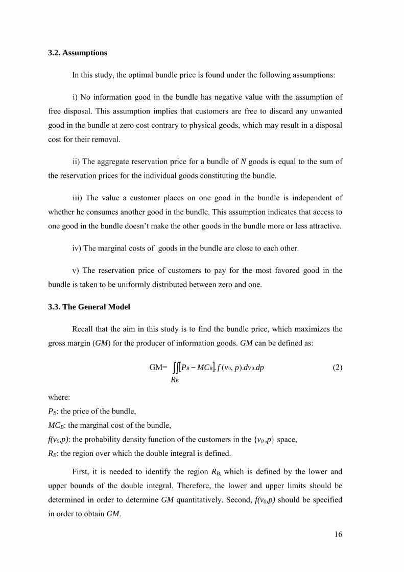
3.2. Assumptions

In this study, the optimal bundle price is found under the following assumptions:

i) No information good in the bundle has negative value with the assumption of

free disposal. This assumption implies that customers are free to discard any unwanted

good in the bundle at zero cost contrary to physical goods, which may result in a disposal

cost for their removal.

ii) The aggregate reservation price for a bundle of N goods is equal to the sum of

the reservation prices for the individual goods constituting the bundle.

iii) The value a customer places on one good in the bundle is independent of

whether he consumes another good in the bundle. This assumption indicates that access to

one good in the bundle doesn’t make the other goods in the bundle more or less attractive.

iv) The marginal costs of goods in the bundle are close to each other.

v) The reservation price of customers to pay for the most favored good in the

bundle is taken to be uniformly distributed between zero and one.

3.3. The General Model

Recall that the aim in this study is to find the bundle price, which maximizes the

gross margin (GM) for the producer of information goods. GM can be defined as:

GM= [ ]∫∫ −B

BB

RdpdvpvfMCP .).,(. 00 (2)

where:

PB: the price of the bundle,

MCB: the marginal cost of the bundle,

f(v0,p): the probability density function of the customers in the {v0 ,p} space,

RB: the region over which the double integral is defined.

First, it is needed to identify the region RB, which is defined by the lower and

upper bounds of the double integral. Therefore, the lower and upper limits should be

determined in order to determine GM quantitatively. Second, f(v0,p) should be specified

in order to obtain GM.

17

Since the random variables v0 and p are independent, f(v0 ,p) becomes f(v0)f(p).

Then (2) becomes:

GM= [ ]∫ ∫=

=

=

=−

2

2

10

10

00 .).().(.up

lp

uv

lvdpdvpfvfMCP BB (3)

Next, the lower and upper bounds in (3) should be determined. The lower bound

for p is (1/N) and upper bound to be 1 such that the range becomes [1/N ≤ p ≤ 1].

Figure 4. Valuation of goods in the bundle by an individual customer

The upper bound for v0 is 1 and the lower bound for v0 need to be determined. The

necessary condition to form a bundle is that the net benefit obtained from purchasing the

bundle should at least be equal to or greater than zero such that UB ≥ 0. So, the critical net

benefit value to form a bundle is UB = 0 such that:

UB = vB-PB = 0 (4)

where vB is the total valuation for the bundle. In (4) , the price of the bundle isn’t known

and the optimal bundle price that maximizes GM will be determined. The total valuation

for the bundle, vB is defined as

n=1 n=2 n=3 n

1

1

1

v(n)

v0-v(1)=Np

v.0

v(1)-v(2)

v(2)-v(3)

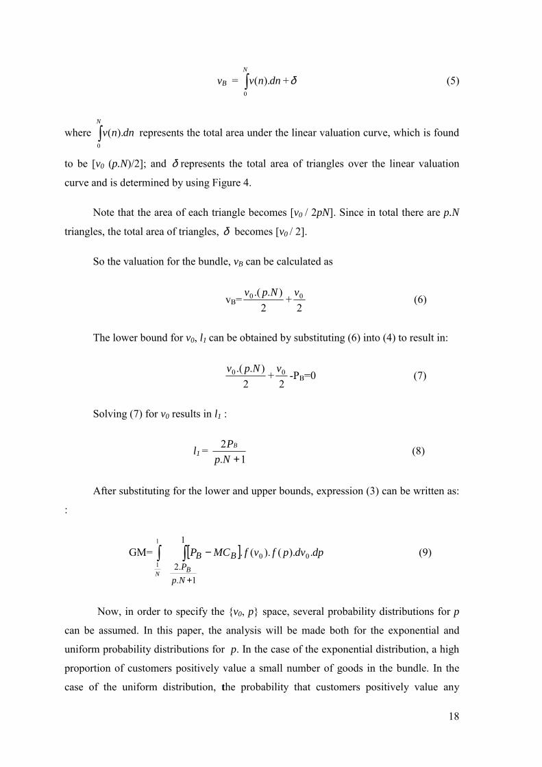
18

vB = ∫N

dnnv0

).( +δ (5)

where ∫N

dnnv0

).( represents the total area under the linear valuation curve, which is found

to be [v0 (p.N)/2]; and δ represents the total area of triangles over the linear valuation

curve and is determined by using Figure 4.

Note that the area of each triangle becomes [v0 / 2pN]. Since in total there are p.N

triangles, the total area of triangles, δ becomes [v0 / 2].

So the valuation for the bundle, vB can be calculated as

vB=2

)..(0 Npv+

20v

(6)

The lower bound for v0, l1 can be obtained by substituting (6) into (4) to result in:

2

)..(0 Npv+

20v

-PB=0 (7)

Solving (7) for v0 results in l1 :

l1 = 1.

2+Np

PB (8)

After substituting for the lower and upper bounds, expression (3) can be written as:

:

GM= ∫1

1N

[ ] dpdvpfvfMCP

NpP

BBB

.).().(. 00

1

1..2∫

+

− (9)

Now, in order to specify the {v0, p} space, several probability distributions for p

can be assumed. In this paper, the analysis will be made both for the exponential and

uniform probability distributions for p. In the case of the exponential distribution, a high

proportion of customers positively value a small number of goods in the bundle. In the

case of the uniform distribution, the probability that customers positively value any

19

number of goods in the bundle is equal. After integrating GM with respect to PB in (9),

the optimal bundle price PB* and the corresponding optimal gross margin GM* will be

determined. This will be performed for two different models: The model incorporating

economies of scale and the model incorporating transaction and transmission cost.

3.4. The Model Incorporating Economies of Scale

In this section, the optimal bundle price and the corresponding GM will be

determined by incorporating the economies of scale index e into the expression for MCB

in terms of the marginal cost of individual goods, MCg:

MCB=Ne.MCg (10)

The economies of scale index e varies in the range [0.0,1.0]. Note that when e<1.0,

then the bundle of N information goods is cheaper to produce and sell than N individual

goods. Therefore, the producer can realize cost savings through the bundling of goods.

When e=1.0, then there are no economies of scale in the production and selling of the

bundle of N goods. No cost savings can be realized by bundling. When e=0.0, then

extreme economies of scale exists and this increases the cost savings to such an extent,

that the cost of producing and selling a bundle of N goods is same as the corresponding

cost for only one individual good in the bundle.

3.4.1. The Case with the Uniform Probability Distribution for the Fraction of the

Positively Valued Goods in the Bundle

First, the optimal bundle price and the corresponding gross margin will be found

for uniformly distributed p. The probability distribution functions for p and v0 can be

written as:

1, 11 ≤≤ pN

f(p)= (11) 0, otherwise

and

1, 10 0 ≤≤ v

f(v0)= (12)

0, otherwise

20

Substituting their corresponding expressions for MCB, f(p) and f(v0) into (9), the

following result for the gross margin GM is obtained:

GM =N

NPPNNMCP BBe

gB ))1log(.22log..21).(.( +−+−− (13)

In order to maximize GM, the first derivative of expression (13) with respect to PB

is taken and is solved to find the optimal bundle price PB*. A check on second derivative

is performed to secure that the following expression is indeed a maximizing one:

PB* =

( ) ( )( )

( ) ( )( )2log.41log.4

12log.21log.2... 1

−+

−+−+−

NN

NNNMCN eg

(14)

The optimal gross margin GM* obtained by substituting for PB* into (13) is

reported in Appendix 1.

3.4.2. The Case with the Exponential ProbabilityDistribution for the Fraction of the


Next, the optimal bundle price PB* and the corresponding optimal gross margin

GM* will be determined for exponentially distributed p. The probability distribution

functions for p and v0 are written as:

ββ

p

e−

1 , 11 ≤≤ pN

f(p)= (15) 0, otherwise

and

1, 10 0 ≤≤ v f(v0)= (16) 0,otherwise

Substituting their corresponding expressions for MCB, f(p) and f(v0) into (9), the

following result for the gross margin GM is obtained:

21

GM=N

NlEiExpIntegraPeNeeNMCPe B

NN

NegB

NN

.

.2...2..)...( .

2.11

.1

β

ββ ββββ

−+

−−++−

) )

NNNlEiExpIntegra

..

1

ββ

+−− (17)

where ExpIntegralEi[z] is defined as:

ExpIntegralEi[z]=- ∫∞

−

−

z

t

te .dt

−−−

−

−−−

−

NN

NlEiExpIntegraeN

lEiExpIntegrae

NN

NlEiExpIntegraeN

lEiExpIntegraeNMC

NN

NN

eg

.1.

.2.

.4

.1..2

.2..2

..

.1

.1

.1

.1

ββ

ββ

ββ

ββ

(18)

PB*= +

−−−

−

−−−

−

NN

NlEiExpIntegraeN

lEiExpIntegrae

ee

NN

NN

.1.

.2.

.4

.

.1

.1

.1

11

ββ

β

ββ

ββ

22



is performed to secure that PB* given in expression (18) indeed results in maximum GM.



3.5. The Model Incorporating Transaction and Transmitting Costs

In section 3.4, the economies of scale was incorporated into the model. In this

section, the marginal cost for the bundle of information goods is stated in its components.

The marginal cost for the bundle of information goods is assumed to consists

mainly of transaction and transmitting costs. The transaction costs can be subdivided into

fixed and variable costs. Fixed cost of transaction denoted here by F is the cost

component incurred for each transaction independent of the value of that transaction

represented by the bundle price PB. The variable cost of transaction, on the other hand, is

the cost component charged in proportion r to the value of the transaction, namely PB.

Thus, the larger PB is, the greater the variable component of the transaction cost becomes.

Aside from transaction costs, another cost component is the transmitting cost, incurred

due to downloading of information goods. It is assumed that customers are given the

chance to download as many goods as they wish from the bundle. As the number of

goods downloaded increases, the cost of transmitting increases with the same proportion.

In addition, in this study the expected fraction of information goods required to be

downloaded by customers is calculated in order to estimate the expected number of goods

to be downloaded from the bundle. So the marginal cost for a bundle of N information

goods is written as:

MCB=F + r.PB + mf.N.D (19)

where D is the unit cost of transmitting and mf .N represents the expected number of

goods required to be downloaded by customers with mf being defined as:

23

∫ ∫

∫ ∫

+

+= 1

1

1

1..2

00

1

1

1

1..2

00

.).().(

.).().(.

N NpP

N NpP

f

B

B

dpdvpfvf

dpdvpfvfp

m (20)

Now, the optimal bundle price PB* and the corresponding optimal gross margin

GM* will be calculated for both uniform and exponential distributions of p.

3.5.1. The Case with the Uniform Probability Distribution for the Fraction of the


When f(p) and f(v0) are substituted into (20) and the integrations are performed, mf

becomes:

mf = ( )

( )( )1log..24log.1.21log..42log..4..4.412

+−+−++−−+−

NPPNNNPPPNPN

BB

BBBB (21)

Substituting mf into expression (19), the following expression is obtained for MCB :

MCB= DNPrF B .. ++ . ( )( )( )

+−+−++−−+−

1log..24log.1.21log..42log..4..4.412

NPPNNNPPPNPN

BB

BBBB (22)

Then the expression (22) for MCB is substituted into the expression (9) to obtain

GM:

GM=( )( ) ( )( )( )

NPNrPFPDPNND BBBB

.24log1.1..22log...4.41.1. +−−++−−+−

−

( ) ( )

NNrPPFDP BBB

.21log....4 +−+−

+ (23)



is performed to secure that the following expression is indeed a maximizing one:

24

PB*= ( )( ) ( ) ( ) ( )

( ) ( )( )1log.24log.1.21log..24log..21.1

+−−+−+−+−+−

NrNDFFDrDN (24)



3.5.2. The Case with the Exponential Probability Distribution for the Fraction of the


Next, the optimal bundle price and the corresponding gross margin will be

determined for exponentially distributed p. When f(p) and f(v0) are substituted into (20)

and the integrations are performed, the mf becomes:

mf=( ) ( )

)

+−−

−

+

−

−+−−++

NNlEiExpIntegra

NlEiExpIntegraPeNeeN

PNNNePNNe

BN

NN

BN

B

.1

.2...2...

.2.....2.1...

.2

.11

.11

βββ

ββββ

βββ

ββ

)

+−−

−

+

−

+−−

−

−+

+

NNlEiExpIntegra


NnlEiExpIntegra

NlEiExpIntegraPe

BN

NN

BN

N

.1

.2...2...

.1

.2...2

.2

.11

.2

βββ

ββ

βββ

β

(25)

mf is substituted into (19) and the MCB becomes:

MCB = DNPrF B .. ++ .

( ( ) ( )

)

+−−

−

+

−

−+−−++

NNlEiExpIntegra


PNNNePNNe

BN

NN

BN

B

.1

.2...2...

.2.....2.1...

.2

.11

.11

βββ

ββββ

βββ

ββ

25

)

+−−

−

+

−

+−−

−

−+

+

NNlEiExpIntegra


NnlEiExpIntegra

NlEiExpIntegraPe

BN

NN

BN

N

.1

.2...2...

.1

.2...2

.2

.11

.2

βββ

ββ

βββ

β

(26)

The expression (26) for MCB is substituted into the expression (9) to obtain GM:

( ) ( )( ) ( )( BBBN PNNDFerPPNDFeGM .2...1..2.1..

1.1

−+++−+−++−=−−

ββ ββ

+ ( ) ) ( )N

rPPFDPerP BBBN

B .....21.

.1

β

β −+−+−

NNNlEiExpIntegra

NlEiExpIntegra

..

1.2

βββ

+−−

−

(27)

After similar calculations as above, PB* is found to be:

PB* =

( )

( )

+−−

−−

−+

−

+−

NNlEiExpIntegra

NlEiExpIntegrar

rDNeee NNN

.1

.2.1.4

.21.... .11

.2

ββ

β βββ

( ) )

+−−

−

+−−

−−+

+

NNlEiExpIntegra

NlExpIntegra

NNlEiExpIntegra

NlEiExpIntegraFDe N

N

.1

.2

.1

.2...2 .

2

ββ

βββ

(28)

The optimal gross margin GM* is obtained by substituting for PB* into (27) and

is reported in Appendix 4.

4. NUMERICAL EXAMPLES

In this section, some numerical illustrations of the two models of uniform and

exponential distributions for the fraction of the positively valued goods in the bundle,

26

namely p are presented. Recall that for the case of the exponential distribution, the

probability that a customer positively values a number of goods in a bundle of N goods

becomes less as the number of positively valued goods increases. For the case of the

uniform distribution, on the other hand, the probability that customers positively value

any number of goods in a bundle of N goods is equal.

In both scenarios following, the optimal gross margin GM* will be found for both

uniform and exponential distributions. In the first scenario, the impact of different levels

of economies of scale on GM* is investigated. In the second scenario, transaction and

transmitting costs for information goods are taken into account and GM* is determined

for various levels of transaction and transmitting costs.

4.1. First Scenario

First set of experiments. The first set of experiments investigates the effect of

economies of scale on the optimal gross margin. The number of goods in the bundle N

and the marginal cost for an individual information good MCg are taken to be 50 and 0.1,

respectively for both uniform and exponential distributions. The β parameter for the

exponential distribution is assumed to be 1.0. The optimal gross margin for both uniform

and exponential models is obtained for different economies of scale index values by

solving expressions (29) and (30), respectively. The corresponding optimal gross margin

values are reported in Table 1 under GM*(Uni) for the uniform model and under

GM*(Exp) for the exponential model.

Table 1. The effect of economies of scale (e) [First set of experiments]

e GM*(Uni) GM*(Exp)

0.00 0.902 0.900

0.25 0.863 0.841

0.50 0.762 0.716

0.75 0.523 0.424

1.00 0.227 0.059

As seen from Table 1, the smaller the economies of scale index, the larger the

gross margin obtained by the producer. Recall that when the economies of scale index is

27

less than one, then there exists economies of scale and the bundle of N information goods

is cheaper to produce and sell than N individual goods. Therefore, the producer can

realize cost savings through the bundling of goods. The gross margin obtained under the

uniform distribution for the positively valued goods is consistently larger than the case

under the exponential distribution with the difference decreasing though as the economies

of scale index e approaches zero.

Second set of experiments. Under the second set of experiments, the effect of the

bundle size on the optimal gross margin is investigated first for the model employed in

the first set of experiments. For different bundle sizes, the optimal gross margin for both

uniform and exponential distributions is obtained by solving expressions (29) and (30),

respectively. The corresponding optimal gross margin values are displayed in Table 2.

Table 2. The effect of bundle size (N) [Second set of experiments]

N GM*(Uni) GM*(Exp)

2 0.060 0.056

5 0.140 0.134

10 0.270 0.265

20 0.439 0.427

40 0.520 0.517

From Table 2, it is clear that as the number of goods comprising the bundle

increases, the optimal gross margin obtained by the producer increases. The optimal gross

margin values are slightly but consistently better for the uniform distribution.

4.2. Second Scenario

Third set of experiments. In the third set of experiments, transaction and

transmitting costs for information goods are incorporated into the model employed in the

first set of experiments. The effect of different levels of transaction and transmitting costs

on the optimal gross margin is analyzed. The economies of scale index, namely e is taken

to be 0.50. The optimal gross margin is found for different transaction and transmitting

cost values for both uniform and exponential models by solving expressions (31) and

(32), respectively. The calculated optimal gross margin values are presented in Table 3.

28

Table 3 reveals that the gross margin for the producer increases as the transaction

and transmitting costs of information goods decrease. The optimal gross margin values

are consistently better for the uniform distribution. But the difference between the optimal

gross margins for both distributions decreases as the transaction and transmitting costs

decrease. With improving data transmission and compression technologies, the gross

margin of the producer is expected to increase further.

Table 3. The effect of transaction and transmitting costs (D) [Third set of experiments]

D GM*(Uni) GM*(Exp)

0.1 0.866 0.844

0.2 0.786 0.750

0.3 0.683 0.603

0.4 0.551 0.412

Fourth set of experiments. The effect of the bundle size on the optimal gross

margin is investigated under the parameter setting of the second set of experiments with

the transaction and transmitting costs being set at the 0.1 level for both uniform and

exponential distributions. The optimal gross margin is found for different bundle sizes by

substituting into expressions (31) and (32). The corresponding optimal gross margin

values are shown in Table 4.

Table 4. The effect of bundle size (N) [Fourth set of experiments]

N GM*(Uni) GM*(Exp)

2 0.069 0.051

5 0.152 0.141

10 0.283 0.271

20 0.448 0.437

40 0.532 0.524

As seen in Table 4, the optimal gross margin increases as the bundle size becomes

larger. As has been the case in the third set of experiments, the optimal gross margin

values are slightly but consistently better for the uniform distribution.

29

5. CONCLUSIONS

The determination of the price of information goods introduces problems for the

producers of these goods. The problem encountered in the pricing of these goods arises

from their cost structure. The cost of producing the first unit of an information good is

relatively large compared to the cost of producing an additional perfect copy, which is

relatively small. On the other hand, competitive market mechanism may force prices to

drop to the level of marginal costs of information goods. But, if producers determine the

price of information goods equal to their marginal costs, they can not recover their initial

costs. Producers might prefer to sell their goods in the form of a bundle instead of selling

them individually. The bundling strategy enables producers to increase their surplus by

extracting more value from customers.

In this study, the optimal price for a bundle of information goods is to be

determined. The objective is to maximize the producer’s gross margin.

In the bundling model presented here, it is assumed that each customer ranks the

goods in the bundle in decreasing order of preference in a linear trend. The valuation for

each good in the bundle is described in terms of the reservation price for the most favored

good in the bundle. The value of each good in the bundle is not allowed to have negative

value. In addition, it is assumed that the valuation of a customer for a good in the bundle

is independent with his valuation for other goods in the bundle. Aside from that, the total

sum of the reservation price for each individual good in the bundle is equal to the

reservation price for the aggregated bundle.

In order to determine the producer’s surplus, the lower bound for the reservation

price of the most favored good in the bundle is found in terms of the bundle price, while

the upper bound is taken to be one.

The study involves two models according to which the optimal bundle price is

determined. In the first model, economies of scale index is incorporated into the

producer’s surplus function. In that way, the effect of cost savings with the presence of

economies of scale introduced by bundling is investigated. In the second model, the

transaction and transmitting costs of information goods are incorporated into the surplus

function. The marginal cost is assumed to consist mainly of transaction and transmitting

costs. Transaction costs are taken to have fixed and variable components. Aside from

30

that, customers are allowed to download as many goods as required from the bundle and

transmitting costs are calculated accordingly.

The valuation for the goods in the bundle differs for each customer. Therefore, the

fraction of information goods in the bundle with non-zero value to each customer varies.

So, the fraction of information goods positively valued by customers is assumed to be

distributed uniformly and exponentially. The optimal bundle price for the first and second

models is obtained for these two different distributions.

Some numerical results are given for the two models. Two effects are investigated

for each model. For the first model incorporating economies of scale, the effect of the

change in economies of scale and in the size of the bundle on the producer’s surplus are

investigated. It is seen that as the economies of scale index decreases, the surplus of the

producer increases. As the economies of scale index decreases, the increase in the

producer’s surplus is more steep for the exponential distribution compared to the uniform

distribution. Concerning the bundle size, it is observed that the larger the bundle size the

greater the producer’s surplus obtained. In this case, for both uniform and exponential

distributions the results are very similar. The distribution of the fraction of goods in the

bundle with non-zero value for each customer doesn’t have any considerable effect on the

producer’s surplus.

For the second model incorporating the transaction and transmitting costs, the

effect of the changes in transmitting costs and in the bundle size on the producer’s surplus

is illustrated. It is found that with decreasing transmitting costs parallel to the

developments in data transmission and compression technologies, the producer’s surplus

increases further. The decrease in the producer’s surplus is more steep for the exponential

distribution compared to the uniform distribution as the transmitting costs increase.

Similar to the first model, as the bundle size becomes larger, the producer’s surplus

increases and the type of the distribution of the fraction of goods in the bundle that have

non-zero value for each customer doesn’t have any considerable impact on the producer’s

surplus.

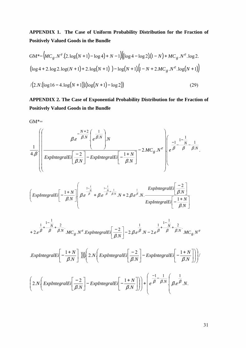
31

APPENDIX 1. The Case of Uniform Probability Distribution for the Fraction of


GM*= ( )( )( ) ( )( )( .2log..1.2log4log.14log1log.2.. eg

eg NMCNNNNMC +−−−+−+

( ) ( ) ) ( ) ( )( )1log...21.1log1log.21log(.2log.24log ++−+−++++ NNMCNNNN eg

( )( ) ( )( )( )2log1log.1log.416log..2/ −++− NNN (29)

APPENDIX 2. The Case of Exponential Probability Distribution for the Fraction of


GM*=

−

+−−

−

−−

−−

+−

....2

.1

.2

...

..41 .

1111

.1

.2

NN

eg

NNN

eNMC

NNlEiExpIntegra

NlEiExpIntegra

Nee

βββ

ββ

ββ

β

β

+−

−

++

+−+

−−

NNlEiExpIntegra

NlEiExpIntegra

NeNeeNNlEiExpIntegra N

NN

.1

.2

....2.....

1 1.1

1112

β

ββββ

βββββ

eg

NN

eg

NN

NMCeNeN

lEiExpIntegraNMCe ..

.2

1111..2

111

..2...2.2....2 βββββββ β

β

+−

++−

+−−

−+

)))

+−−

−

+−NNlEiExpIntegra

NlEiExpIntegraN

NNlEiExpIntegra

.1

.2..2.

.1.

βββ/

+

+−−

− −−

.....

1.2..2

1.11

NeeNNlEiExpIntegra

NlEiExpIntegraN N βββ β

ββ

32

....2....2 .

21

.2.

1e

gN

NN NMCelEiExpIntegraNe

NlEiExpIntegra ββ

βββ

β

+− +

+

−

...2.

1....2.2 .

2112

gN MCe

NNlEiExpIntegraNe

NlEiExpIntegra βββ

ββ

β

+−

+−−

−

))

+−

−NNlEiExpIntegra

NlEiExpIntegraN e

.1.

.2.

ββ (30)

APPENDIX 3. The Case of Uniform Probability Distribution for the Fraction of

Positively Valued Goods in the Bundle with Transaction and Transmission Costs

Included

GM* = ( ) ( )( ) ( ) ( )( 2222 2log1N.D.41r.N.1Nlog2log.1r.N.8

1 +−−−+−−

( ) ( ) ( )( ) ( ) )( 4log.2log1N.F1r.D.42log.1N.N1N.1r.D.4 2 +−−−−++−−−

+ ( ) ( )( ) ( )16log.2.16log..4log..1..214log. 22 FrrNFrFrNF +−+++−−−

+ ( ) ( ) ( )( )( )( ) ( ) )( 1r.F1r.2NF.2.DD.2.1N.1Nlog.4 2 −+−++−−−+

- ( ) ( ) ( ) ))1log.2log..2 22 +−+− NFDFD (31)

APPENDIX 4. The Case of Exponential Probability Distribution for the Fraction of

Positively Valued Goods in the Bundle with Transaction and Transmission Costs

Included

GM* = ( )

β+−−

−β ββ

+βββ

+−

.eN..e.4D.2r1.N.ee..e N.1

N.2N

22

2

N.11

2N.2N

( )( )( )( ) ( )( ) )(( N..2F.2D.23.DF.er1.F1rN.1.21F.2.DD.21

2 β+−−++−+−β+++−− β

( )( ) ) ) ( )

−−+++−+

NlEiExpIntegraFDerNDF N

N

.2.....23. 2.

2

ββ β

33

)) ))

+−−

−

+−−NNlEiExpIntegra

NlEiExpIntegra

NNlEiExpIntegra

.1

.2.

.1

βββ

( )( ) ( )( ) ( ) ( ) ( ) ))( 1log..24log..21.1.1log2log. +−+−++−−−+− NFDDFDrNN

/ ( ) ( ) ( )

−++−

−−

+

...2.21....1.4 .2

.11

FDeDrNeerN NN

N ββββ

)

−

+−−

−N

lEiExpIntegraNNlEiExpIntegra

NlEiExpIntegra

.2.

.1

.2.

βββ

) ( )( ) )1log.24log..

1 +−

+−− NNNlEiExpIntegra

β (32)

REFERENCES

Adams, W.J. and Yellen, J.L. Commodity bundling and the burden of monopoly. Quarterly Journal of Economics, 90 (1976), 475-498.

Bakos, Y. Reducing buyer search costs: Implications for electronic marketplaces. Management Science, 43 (1997), 617-643.

Begg, D.; Fischer, S.; and Dornbusch, R. Economics. Berkshire: McGraw Hill, 1994. Brynjolfsson, E. and Kemerer, J.F. Network externalities in microcomputer software: An

econometric analysis of the spreadsheet market. Management Science, 42, (1996), 1627-1642.

Carbajo, J.; de Meza, D.; Seidman, D. J. A strategic motivation for commodity bundling. Journal of Industrial Economics, 38 (1990), 283-298.

Chae, S. Bundling subscription TV channels: a case of natural bundling. International Journal of Industrial Organization, 10 (1992), 213-230.

Chen, Y-N. and Png, I. Information goods pricing and copyright enforcement: Welfare analysis. Information Systems Research, 14, 1 (2003), 107-123.

Coase, R. The problem of social cost. Journal of Law and Economics, 3 (1960), 1-44. Demsetz, H. The cost of transacting. Quarterly Journal of Economics. 82 (1968), 33-53. Geoffrion, A.M. Progress in operations management. Production and Operations

Management. 11, 1 (2002), 92-100. Hanson, W. and Martin, R.K. Optimal bundle pricing. Management Science. 36, 2 (1990),

155-172. Hayes, R.H. Challenges posed to operations management by the “new economy”.

Production and Operations Management. 11, 1 (2002), 21-32. Salinger, M.A. A graphical analysis of bundling. Journal of Business, 68, 1 (1995), 85-

98. Schmalensee, R.L. Gaussian demand and commodity bundling. Journal of Business, 57, 1

pt 2 (1984), S212-S230.

34

Shapiro, C. and Varian, H. Information Rules. Boston: Harvard Business School Press, 1999.

Shapiro, C. and Varian, H. Versioning: The smart way to sell information. Harvard Business Review, 76, 6 (1998), 106-114.

Simon, H. and Wuebker, G. Bundling – a powerful method to better exploit profit potential. In R. Fuerderer, A. Hermann, G. Wuebker (eds). Optimal Bundling, Berlin: Springer Verlag, 1999, pp. 7-28.

Stigler, G. J. United States v. Loew’s Inc.: A note on block-booking. The Supreme Court Review, (1963), 152-157.

Varian, H. Markets for information goods. Working Paper, School of Information Management and Systems, University of California, Berkeley, (1998).

Whinston, M.D. Tying, foreclosure and exclusion. American Economic Review, 80 (1990), 837-859.

Documents

DETERMINATION OF THE BUNDLE PRICE FOR DIGITAL …