Embed Size (px)
Citation preview

DETERMINATION OF UNCERTAINTY IN RESERVES ESTIMATE FROM
ANALYSIS OF PRODUCTION DECLINE DATA
A Thesis
by
YUHONG WANG
Submitted to the Office of Graduate Studies of Texas A&M University
in partial fulfillment of the requirements for the degree of
MASTER OF SCIENCE
May 2006
Major Subject: Petroleum Engineering

DETERMINATION OF UNCERTAINTY IN RESERVES ESTIMATE FROM
ANALYSIS OF PRODUCTION DECLINE DATA `
A Thesis
by
YUHONG WANG
Submitted to the Office of Graduate Studies of Texas A&M University
in partial fulfillment of the requirements for the degree of
MASTER OF SCIENCE
Approved by:
Co-Chairs of Committee, John Lee Duane McVay Committee Members, Yalchin Efendiev Head of Department, Stephen A. Holditch
May 2006
Major Subject: Petroleum Engineering

iii
ABSTRACT
Determination of Uncertainty in Reserves Estimate From Analysis of
Production Decline Data.
(May 2006)
Yuhong Wang, B.S., Southwest Petroleum Institute, China
Co-Chairs of Advisory Committee: Dr. John Lee Dr. Duane McVay
Analysts increasingly have used probabilistic approaches to evaluate the uncertainty in
reserves estimates based on a decline curve analysis. This is because the results represent
statistical analysis of historical data that usually possess significant amounts of noise.
Probabilistic approaches usually provide a distribution of reserves estimates with three
confidence levels (P10, P50 and P90) and a corresponding 80% confidence interval. The
question arises: how reliable is this 80% confidence interval? In other words, in a large
set of analyses, is the true value of reserves contained within this interval 80% of the
time? Our investigation indicates that it is common in practice for true values of reserves
to lie outside the 80% confidence interval much more than 20% of the time using
traditional statistical analyses. This indicates that uncertainty is being underestimated,
often significantly. Thus, the challenge in probabilistic reserves estimation using a
decline curve analysis is not only how to appropriately characterize probabilistic
properties of complex production data sets, but also how to determine and then improve
the reliability of the uncertainty quantifications.
This thesis presents an improved methodology for probabilistic quantification of reserves
estimates using a decline curve analysis and practical application of the methodology to
actual individual well decline curves. The application of our proposed new method to 100
oil and gas wells demonstrates that it provides much wider 80% confidence intervals,
which contain the true values approximately 80% of the time. In addition, the method
yields more accurate P50 values than previously published methods. Thus, the new

iv
methodology provides more reliable probabilistic reserves estimation, which has
important impacts on economic risk analysis and reservoir management.

v
DEDICATION
To my beloved husband, my mother, my father and my loving family.

vi
ACKNOWLEDGMENTS
First of all, I’d like to thank my advisor and committee chair, Dr. John Lee, for his
continuous encouragement, financial support, and especially for his academic and
creative guidance. I’d also like to thank my committee co-chair, Dr. Duane McVay, for
his thoughtful and challenging ideas and Dr. Yueming Cheng for her priceless help and
friendship.
Last but not least, my great gratitude to those members in our uncertainty group.
Thank you very much.
vii
TABLE OF CONTENTS
Page
ABSTRACT…. .............................................................................................................. iii
DEDICATION.. ...............................................................................................................v
ACKNOWLEDGMENTS .............................................................................................. vi
TABLE OF CONTENTS............................................................................................... vii
LIST OF FIGURES ........................................................................................................ ix
LIST OF TABLES......................................................................................................... xii
CHAPTER I INTRODUCTION .................................................................................1
1.1 Objective of Study ........................................................................2 CHAPTER II DECLINE CURVE ANALYSIS AND PROBABILISTIC
APPROACHES .....................................................................................4
2.1 Overview of Decline Curve Analysis ...........................................4 2.2 Challeges in Probabilistic Reserves Estimation............................4
CHAPTER III METHODOLOGY……………………………… .............................10
3.1 Modified Bootstap and Block Resampling .................................10 3.2 Backward Analysis Scheme........................................................18 3.3 Sample Size and Reproducibility................................................21 3.4 Coverage Index ...........................................................................22 3.5 Confidence Interval Corrections .................................................22 3.6 Summary of Our Approach.........................................................28
CHAPTER IV RESULTS AND APPLICATIONS .....................................................29
4.1 Application to Oil and Gas Wells ...............................................29 CHAPTER V DISCUSSION......................................................................................37
5.1 Why Does Our Approach Work?................................................37
CHAPTER VI CONCLUSIONS AND RECOMMENDATIONS ..............................38
6.1 Conclusions.................................................................................38 6.2 Recommendations.......................................................................38
NOMENCLATURE………………………………………………………...……….....39
REFERENCES……………………………………………………………...……….....40

viii
Page
APPENDIX A DERIVATION OF VARIANCE OF BOOTSTRAP
ESTIMATE IN DECLINE CURVE ANALYSIS ...............................41
APPENDIX B SIMPLIFIED DOUBLE BOOTSTRAP APPROACH........................45
VITA…………………………………………………………………………………....46

ix
LIST OF FIGURES
FIGURE Page
2.1 Uncertainty quantification of DCA production forecast of an oil well with a 2-year production history. ......................................................8
2.2 Uncertainty quantification of DCA production forecast of an oil well with a 6-year production history. ...................................................... 9
3.1 Conventional bootstrap sequence. .................................................................... 11
3.2 Modified bootstrap sequence. ........................................................................... 11
3.3 Original data for conventional bootstrap example............................................ 12
3.4 Synthetic data set 1 from conventional bootstrap resampling .......................... 12
3.5 Synthetic data set 2 from conventional bootstrap resampling .......................... 13
3.6 Generating residuals from original data and regressed model for modified bootstrap example ........................................................................ 15
3.7 Determining block size using confidence band and autocorrelation plot of residuals................................................................................................. 16
3.8 Plot of residuals with blocks ............................................................................ 16
3.9 Synthetic data set 1 from modified bootstrap resampling ................................ 17
3.10 Synthetic data set 2 from modified bootstrap resampling ................................ 17
3.11 Schematic diagram illustrating multiple backward scenarios...........................18
3.12 Conventional approach: 6-year production history was used for regression with DCA. The actual performance is outside the 80% confidence interval. data set example 1 from Jochen and Spivey Bootstrap resampling ..................................................................... 19
3.13 Backward 2-year scenario: 6-year production history is known but only 2 years of backward data were used for regression with DCA. The actual performance is within the 80% confidence interval ............. 20
3.14 Backward 4-year scenario: 6-year production history is known but only 4 years of backward data were used for regression with

x
FIGURE Page
DCA. The actual performance is outside the 80% confidence interval ............20
3.15 Effect of bootstrap sample size on reserves estimation .................................... 21
3.16 Percentile 80% confidence interval estimation................................................. 23
3.17 Basic bootstrap 80% confidence interval estimation ........................................ 24
3.18 Confidence interval correction ─ basic CI: 6-year production history is known but only 3 years of backward data were used for regression with DCA. The actual performance is within the 80% confidence interval. .................................................................................. 26
3.19 Confidence interval correction ─ studentized CI: 6-year production history is known but only 3 years of backward data were used for regression with DCA. The actual performance is within the 80% confidence interval. ........................................ 26
3.20 Confidence interval correction ─ double basic CI: 6-year production history is known but only 3 years of backward data were used for regression with DCA. The actual performance is within the 80% confidence interval. ........................................ 27
3.21 Absolute value of coverage index for different types of confidence intervals. Percentile CI does not cover the true value, while the three corrected confidence intervals do. ................................. 27
4.1 Gas well 1─production forecast using conventional bootstrap method. The actual performance is outside the 80% confidence interval. ....... 31
4.2 Gas well 1─production forecast using modified bootstrap method. The actual performance is within the 80% confidence interval.......... 31
4.3 Oil well 1─ production forecast using conventional bootstrap method. The actual performance is outside the 80% confidence interval. ....... 32
4.4 Oil well 1─production forecast using modified bootstrap method. The actual performance is within the 80% confidence interval.......... 32
4.5 Gas well 2─ production forecast using conventional bootstrap method. The actual performance is outside the 80% confidence interval. ....... 33
4.6 Gas well 2─production forecast using modified bootstrap method. The actual performance is within the 80% confidence interval.......... 33

xi
FIGURE Page
4.7 Oil well 2─production forecast using conventional bootstrap method. The actual performance is outside the 80% confidence interval. ....... 34
4.8 Oil well 2─production forecast using modified bootstrap method. The actual performance is within the 80% confidence interval..........34

xii
LIST OF TABLES
TABLE Page
2.1 Statistics of Coverage Rate from Analysis of 100 Wells Using Conventional Bootstrap Method ......................................................................... 7
4.1 Statistics of Coverage Rate from Analysis of 100 Wells Using Conventional Bootstrap Method ...................................................................... 29
4.2 Statistics of Coverage Rate from Analysis of 100 Wells Using Modified, Block Bootstrap Method .................................................................. 30
4.3 Comparison of Remaining Production Estimates for 100 wells Using Conventional Bootstrap and Modified, Block Bootstrap Method .................... 36

1
CHAPTER I
INTRODUCTION
Decline curve analysis is the most commonly used method for reserve estimation when
production data are available. It is traditionally used to provide deterministic estimates
for future performance and remaining reserves. Often, however, the deterministic
prediction of future decline is far from the actual future production trend and, thus, the
single deterministic value of reserves is not close to the true reserves. The “deterministic”
estimate in fact contains significant uncertainty. Thompson and Wright1 provided
evidence that estimated reserves using decline curve analysis (DCA) can have significant
error. Furthermore, they found that the accuracy of predicted remaining reserves
estimates is not necessarily improved with additional production history, contrary to
expectations.
Unlike single-point deterministic estimates, probabilistic approaches provide a measure
of uncertainty in the reserves estimates. They provide a range of estimates within
prescribed confidence levels and, thus, attempt to bracket the true value. Probabilistic
reserve estimates are able to fulfill multiple purposes of internal decision-making and
public reporting. However, many engineers have long had the indelible impression, that
quantifying uncertainty of estimates is largely subjective.2 This impression has led the
industry to be reluctant to search for appropriate probabilistic methods for reserves
estimation and use probabilistic methods to quantify uncertainty of estimates. Existing
practices for probabilistic estimation of reserves often assume prior knowledge of
distributions of relevant parameters or reservoir properties. For example, prior
distributions of drainage area, net pay, porosity, hydrocarbon saturation, formation
volume factor, and recovery factor are needed to run Monte Carlo simulations when the
volumetric method is used in probabilistic reserves estimation.3 A variety of distribution
This thesis follows the style of SPE Journal.
2
types, such as log-normal, triangular or uniform, are often imposed on these parameters
subjectively.
Another reason for this situation may be that we are not familiar with them.2 Hefner and
Thompson4 presented probabilistic results of reserve estimates using production data for
5 oil wells. The probabilistic estimates at confidence levels of P90, P50 and P10 were
provided by 12 professional evaluators. The majority of the evaluators used the results of
DCA as the basis for the probabilistic estimates, but their probabilistic estimates were
highly subjective and based on their personal experiences. None of them applied
statistical methodologies for their probabilistic estimations.
Analysts have begun to use probabilistic approaches to evaluate the uncertainty in
reserves estimates based on decline curve analysis. To avoid assuming prior distributions
of parameters, the Bootstrap method has been used to directly construct probabilistic
estimates with specified confidence intervals from real data sets. It is a statistical
approach and is able to assess uncertainty of estimates objectively. To the best of our
knowledge, Jochen and Spivey5 first applied the bootstrap method to decline curve
analysis for reserves estimation. They used ordinary bootstrap to resample the original
production data set so as to generate multiple pseudo data sets for probabilistic analysis.
The ordinary bootstrap method they used assumes that the original production data are
independent and identically distributed (IID), so the data will be independent of time.
However, this assumption is usually improper for time series data, such as production
data, because the time series data structure often contains correlation between data points.
1.1. Objective of Study
The main objective of this research is to develop an improved probabilistic approach to
estimate reserves from production decline data. Followings are the basic objectives:
• Investigate challenges in probabilistic reserve estimates from Decline Curve
Analysis (DCA).

3
• Develop new approaches to improve quantification of reserves estimation
uncertainty using DCA.
• Determine reliable confidence intervals associated with probabilistic reserves
estimates
• Implementation of this procedure in a VBA program for applying our new
approaches and showing the improvement results.
• Compare the results with existing method to examine the accuracy and
improvements of our new approaches.

4
CHAPTER II
DECLINE CURVE ANALYSIS AND PROBABILISTIC APPROACHES 2.1. Overview of Decline Curve Analysis We use the Arps decline curve equations for hyperbolic decline,
bbtDqq ii
1
)1( −+= ……………...………………. (2.1) and exponential decline,
)exp( Dtqq i −= ……………...….…………….. (2.2)
There are a number of assumptions and restrictions applicable to conventional decline
curve analysis (DCA) using these equations. Theoretically, DCA is applicable to
stabilized flow only, for wells producing at constant flowing bottomhole pressure. Thus,
data from the transient flow period should be excluded from DCA. In addition, use of the
equation implies that there are no changes in completion or stimulation, no changes in
operating conditions, and that the well produces from a constant drainage area.
The hyperbolic decline exponent, b, has physical meaning in reservoir engineering, 6
should be within 0 and 1. We have imposed the constraint of 0≤b≤1 in our work, as well
as the constraint that Di≥0.
In general, we think of decline exponent, b, as a constant. But for a gas well, b varies
with time. Chen7 showed that instantaneous b decreases as the reservoir depletes at
constant BHP condition and can be larger than 1 under some conditions. He also proved
that the average b over the depletion stage is indeed less than 1.
2.2. Challenges in Probabilistic Reserves Estimation Since the assumptions and conditions required for rigorous use of the Arps’ decline curve
equations rarely apply to actual wells over significant time periods, there is potentially

5
much uncertainty in reserves estimates using conventional DCA. With probabilistic
approaches, confidence intervals can be provided for the reserves estimates. In the
petroleum industry, reserves values are typically calculated at three confidence levels,
P90, P50 and P10. There is a 90% probability that the actual reserves are greater than the
P90 quantile; there is a 50% probability that the actual reserves are greater than the P50
quantile; and there is a 10% probability that the actual reserves are greater than the P10
quantile. The interval between P90 and P10 represents an 80% confidence interval. The
confidence interval is a probabilistic result; i.e., there is an 80% probability that the actual
value will fall within the range of values specified. What this really means is that, if we
were to make a large number of independent predictions with 80% confidence intervals
using similar methodology, we would expect to be right (the true value falls within the
range) about 80% of the time and wrong (the true value falls outside the range) about
20% of the time.
For probabilistic reserves estimation, an important question remains that is rarely
addressed. Do 80% confidence intervals truly correspond to 80% probability, i.e., are
they reliable? Since confidence intervals are probabilistic results, we cannot determine
the reliability of a single confidence interval, since the test of the estimate using a
confidence interval yields only a single result, or sample. After time passes and we
determine the true value, we can establish that the true value is either within the predicted
range or it is outside the range. As Capen8 illustrated, it is only by evaluation of many
predictions (by letting time pass and comparing the true values to the predicted ranges)
made using similar methodology that we can determine the reliability of our estimations
of uncertainty and, thus, our methodology for estimating uncertainty. These evaluations
are difficult in the petroleum industry because of the long times associated with oil and
gas production. Thus, we seldom verify the reliability of uncertainty estimates in our
industry.
To illustrate the challenge of calculating reliable confidence intervals using probabilistic
DCA methods, we analyzed the production data for 100 oil and gas wells obtained from
public data sources. We selected wells with long production histories and no large

6
anomalies in declines. We analyzed the data using the conventional bootstrap approach
applied by Jochen and Spivey.5 We analyzed only a portion of the production data for
each well and calculated probabilistic estimates of “remaining production” between the
last date of analyzed production and the last date of actual production. These estimates
were then compared to the true remaining production between the last date of analyzed
production and the last date of actual production. Table 1 summarizes the statistical
results from the study. The columns in Table 1 represent results corresponding to
different lengths of production history used for DCA. For example, “¼ Prod. History”
means that only one-quarter of the production history was assumed known and used in
the analysis, while the remaining three-quarters of production were assumed unknown
and used only for validation of the predictions of remaining production.
Coverage rate is defined as the percentage by which a set of estimated confidence
intervals with a prescribed level of confidence cover, or bracket, the true values. It is a
measure of the reliability of the uncertainty quantification. The Realized Coverage Rate
(RCR) is defined as the percentage by which a set of estimated confidence intervals
actually cover the true values given a prescribed level of confidence. The Expected
Coverage Rate (ECR) is defined as the percentage by which a set of estimated confidence
intervals should cover the true values, and is equal to the probability associated with the
confidence interval. The third row in Table 1 shows the RCR for cases in which transient
data were included in the analysis. It can be seen that the RCRs are only 21% to 42%, far
below the ECR of 80%. This indicates that the conventional bootstrap method
underestimates the uncertainty in these reserves estimations significantly.
Since DCA is applicable to stabilized flow only, data from the transient flow period
should be excluded from the analysis. The fourth row shows the results of the RCR
obtained by excluding transient data identified using Fetkovich type curves.6 Note that it
can be very difficult to identify the transition point from transient to stabilized flow,
particularly for wells with short production times. The results excluding transient data
indicate that the RCR ranges from 22% to 42%. Exclusion of transient data did not
improve coverage rate significantly, and uncertainty is still being underestimated. These

7
results are not inconsistent with those obtained by Hefner and Thompson4 and by
Huffman and Thompson9 in their probabilistic studies based on individual evaluators’
estimates of reserves from analysis of five oil wells. The realized coverage rate in their
studies ranged from 40% to 60%.
Another question we addressed is whether the coverage rate improves as more production
data become available. Confidence intervals will typically narrow as more production
data become available, because the extrapolation is based upon more data. However, this
does not necessarily imply that the reliability of the confidence intervals will improve
with more production data. This is demonstrated in Table 2.1, where coverage rate
decreased as the amount of production data increased.
Table 2.1— Statistics of Coverage Rate from Analysis of 100 Wells Using Conventional Bootstrap Method
22%30%42%Realized coverage rate of 80% CI, transient data excluded
21%32%41%Realized coverage rate of 80% CI, transient data included
80%80%80%Expected coverage rate of 80% CI
3/4 Prod.History
2/4 Prod.History
1/4 Prod.History
Production data used in DCA
22%30%42%Realized coverage rate of 80% CI, transient data excluded
21%32%41%Realized coverage rate of 80% CI, transient data included
80%80%80%Expected coverage rate of 80% CI
3/4 Prod.History
2/4 Prod.History
1/4 Prod.History
Production data used in DCA
We can explain this result using Figs. 2.1 and 2.2. For illustration purposes, we present a
single-well example even though, strictly speaking, we cannot fully evaluate reliability of
confidence intervals with a single sample. With only 2 years of production data available,
the production forecast (P50) is far from the actual future performance (Fig. 2.1). The
80% confidence interval is large but not large enough to cover the actual future
production performance. As 6 years of production data become available, the production
forecast (P50) moves closer to the actual future performance (Fig. 2.2). In addition, the

8
80% confidence interval for the production estimates becomes much smaller and, as a
result, the actual future performance still falls outside the confidence interval. Thus,
while narrowing of confidence intervals with more production data might imply more
confidence in the reserves estimate, this can be misleading. It does not necessarily mean
that the new probabilistic forecast is more reliable; it could possibly be less reliable.
Of course, what we desire is a probabilistic method that is consistently reliable. In other
words, we desire a method that yields a realized coverage rate of 80%, for 80%
confidence intervals, regardless of the amount of production data available.
1
10
100
0 2000 4000 6000 8000
Time, Days
Prod
uctio
n R
ate,
BB
L/D
ay
Bootstrap percentile CIFitting curve with DCA
Actual data (light blue)
P50
P90
P10
2 yrsHistory
Prediction
Fig.2.1—Uncertainty quantification of DCA production forecast of an oil well with a 2-
year production history

9
1
10
100
0 2000 4000 6000 8000
Time, Days
Prod
uctio
n R
ate,
BB
L/D
ay
Bootstrap percentile CIFitting curve with DCA
Actual data (light blue)
P50P90
P106 yrs History
Prediction
Fig.2.2—Uncertainty quantification of DCA production forecast of an oil well with a 6-
year production history
.
10
CHAPTER III
METHODOLOGY
In this study, we present a new probabilistic approach, which aims to improve
probabilistic reserves estimation and to generate consistently reliable confidence
intervals. The major components of this new approach are presented in following
sections.
3.1. Modified Bootstrap and Block Resampling
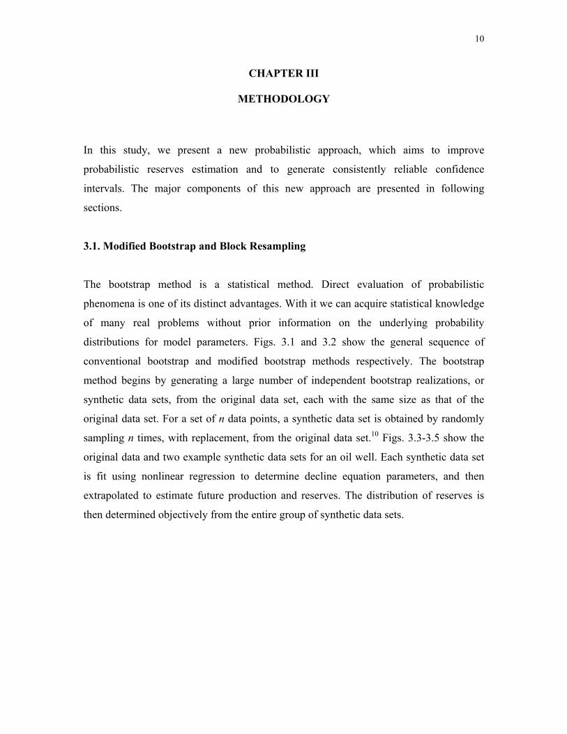
The bootstrap method is a statistical method. Direct evaluation of probabilistic
phenomena is one of its distinct advantages. With it we can acquire statistical knowledge
of many real problems without prior information on the underlying probability
distributions for model parameters. Figs. 3.1 and 3.2 show the general sequence of
conventional bootstrap and modified bootstrap methods respectively. The bootstrap
method begins by generating a large number of independent bootstrap realizations, or
synthetic data sets, from the original data set, each with the same size as that of the
original data set. For a set of n data points, a synthetic data set is obtained by randomly
sampling n times, with replacement, from the original data set.10 Figs. 3.3-3.5 show the
original data and two example synthetic data sets for an oil well. Each synthetic data set
is fit using nonlinear regression to determine decline equation parameters, and then
extrapolated to estimate future production and reserves. The distribution of reserves is
then determined objectively from the entire group of synthetic data sets.

11
SyntheticProd. Set # 1
SyntheticProd. Set # 2
SyntheticProd. Set # 3
SyntheticProd. Set # n
ProductionData
DCA Parameter
Set # 1
DCA Parameter
Set # 2
DCA Parameter
Set # 3
DCA Parameter
Set # n
Nonlinear Regression
Random Samples
Generator
b
Reserves
Di
qi
Parameters & ReservesDistributions
SyntheticProd. Set # 1
SyntheticProd. Set # 2
SyntheticProd. Set # 3
SyntheticProd. Set # n
ProductionData
DCA Parameter
Set # 1
DCA Parameter
Set # 2
DCA Parameter
Set # 3
DCA Parameter
Set # n
Nonlinear Regression
Random Samples
Generator
b
Reserves
Di
qi
Parameters & ReservesDistributions
Fig. 3.1—Conventional bootstrap sequence
SyntheticProd. Set # 1
SyntheticProd. Set # 2
SyntheticProd. Set # 3
SyntheticProd. Set # n
DCA ParameterSet # 1
DCA ParameterSet # 2
DCA ParameterSet # 3
DCA ParameterSet # n
Nonlinear Regression Parameters & ReservesDistributions
b
Reserves
Di
qi
ProductionData
Nonlinear Regression
RegressedProduction Data
Residuals
BlocksAut
ocor
rela
t i on
SyntheticProd. Set # 1
SyntheticProd. Set # 2
SyntheticProd. Set # 3
SyntheticProd. Set # n
DCA ParameterSet # 1
DCA ParameterSet # 2
DCA ParameterSet # 3
DCA ParameterSet # n
Nonlinear Regression Parameters & ReservesDistributions
b
Reserves
Di
qi
b
Reserves
Di
qi
ProductionData
Nonlinear Regression
RegressedProduction Data
Residuals
BlocksAut
ocor
rela
t i on
Fig. 3.2—Modified bootstrap sequence

12
1000
10000
100000
1000000
0 20 40 60 80 100 120 140 160t, month
q,bb
lOriginal data
Regression data
qi=37784.68b=0.99Di=0.04666
Fig. 3.3—Original data for conventional bootstrap example
1000
10000
100000
1000000
0 20 40 60 80 100 120 140 160t, month
q,bb
l
Synthetic data set #1
Regression data
qi=42372.43b=0.99Di=0.05454
2
23
2
2 2 543
2
422
22
Fig. 3.4—Synthetic data set 1 from conventional bootstrap resampling
q, S
TB/D
t, months
q, S
TB/D
1
t, months

13
1000
10000
100000
1000000
0 20 40 60 80 100 120 140 160t, month
q,bb
l
Synthetic data set #18
Regression data
qi=36101.91b=0.99Di=0.04162
22
2
2
2
22 3
2
22
224
2
2
Fig. 3.5—Synthetic data set 2 from conventional bootstrap resampling
In the conventional bootstrap algorithm, bootstrap realizations are generated from a data
set in which the points are assumed to be independent and identically distributed.
However, production data are not independent points, but are a sequence of observations
arising in succession, i.e., a time series, with an overall decline trend. Previous
implementations5 of the conventional bootstrap method for DCA attempted to preserve
the overall decline trend by preserving a “time index” for each data point. However, this
procedure does not satisfy the requirement for independent and identically distributed
data.
In our work, we employ a more rigorous model-based bootstrap algorithm to preserve
data structure. It uses the decline models (hyperbolic or exponential equations) to fit the
production data and constructs residuals from the fitted model and observed data. Fig. 3.6
which uses the same production data as Fig. 3.3 illustrates the residuals generating
process. New series are then generated by incorporating random samples from the
q, S
TB/D
2
t, months
14
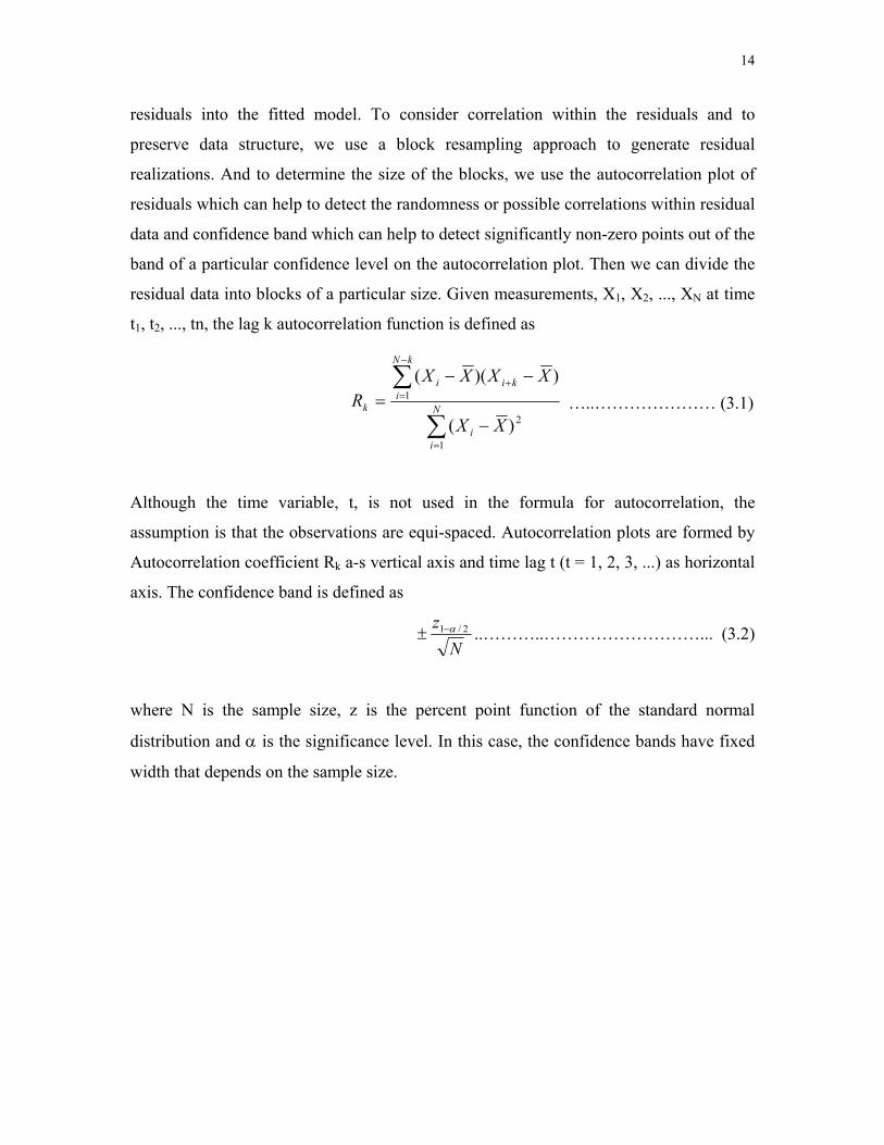
residuals into the fitted model. To consider correlation within the residuals and to
preserve data structure, we use a block resampling approach to generate residual
realizations. And to determine the size of the blocks, we use the autocorrelation plot of
residuals which can help to detect the randomness or possible correlations within residual
data and confidence band which can help to detect significantly non-zero points out of the
band of a particular confidence level on the autocorrelation plot. Then we can divide the
residual data into blocks of a particular size. Given measurements, X1, X2, ..., XN at time
t1, t2, ..., tn, the lag k autocorrelation function is defined as
∑
∑
=
−
=+
−
−−= N
ii
kN
ikii
k
XX
XXXXR
1
2
1
)(
))(( …..………………… (3.1)
Although the time variable, t, is not used in the formula for autocorrelation, the
assumption is that the observations are equi-spaced. Autocorrelation plots are formed by
Autocorrelation coefficient Rk a-s vertical axis and time lag t (t = 1, 2, 3, ...) as horizontal
axis. The confidence band is defined as
N
z 2/1 α−± ..………..………………………... (3.2)
where N is the sample size, z is the percent point function of the standard normal
distribution and α is the significance level. In this case, the confidence bands have fixed
width that depends on the sample size.

15
1000
10000
100000
1000000
0 20 40 60 80 100 120 140 160
t, months
q,ST
B/D
Original data
Regression data
qi=37784.68b=0.99Di=0.04666
Residuals
Fig. 3.6—Generating residuals from original data and regressed model for modified bootstrap example
Fig. 3.7 shows the autocorrelation plot of residuals with a 99% confidence band based on
the residual data generated from Fig. 3.6. Fig. 3.8 is the relevant residual plot constructed
from Fig. 3.6 and blocked of a particular size determined from Fig. 3.7. Figs. 3.9 and 3.10
show two example synthetic data series generated using the modified bootstrap method.
Each of the synthetic data sets is the same size as the original data set. This new
resampling approach does not require that the original production data be independent
and identically distributed.
q, S
TB/D

16
-1
-0.5
0
0.5
1
0 10 20 30 40 50 60 70 80 90
Lag
Aut
ocor
rela
tion
of re
sid Block size
Fig. 3.7—Determining block size using confidence band and autocorrelation plot of residuals
-20000
-15000
-10000
-5000
0
5000
10000
15000
20000
0 10 20 30 40 50 60 70 80 90
t, months
Res
idua
ls,S
TB
Fig. 3.8—Plot of residuals with blocks
Aut
ocor
rela
tion
of re
sidu
als
Res
idua
ls, S
TB/D

17
1000
10000
100000
1000000
0 20 40 60 80 100 120 140 160t, months
q,ST
B/D
Synthetic data set 1
Regression data
qi=37173.84b=0.91791Di=0.04154
Fig. 3.9—Synthetic data set 1 from modified bootstrap resampling
1000
10000
100000
1000000
0 20 40 60 80 100 120 140 160
t, month
q,ST
B/D
Synthetic data set 2
Regression data
qi=36947.65b=0.99Di=0.04746
Fig. 3.10—Synthetic data set 2 from modified bootstrap resampling
q, S
TB/D
q,
STB
/D
t, months

18
3.2. Backward Analysis Scheme
To address problems due to transient flow and/or changing operating conditions and to
further enhance the reliability of our probabilistic DCA methodology, we applied a
backward analysis scheme. The approach is illustrated in Fig.3.11, in which we have 10
years of production history. For scenario 1, we use only the most recent 2 years of data
for regression and prediction. Similarly, for scenario 2, we use only the most recent 4
years of data. After working backward in this fashion and generating multiple forecasts
from the same time, we then combine them to form an overall probabilistic forecast. The
overall P50 value is determined by averaging the P50 values from the multiple backward
forecasts. The overall P90 value is determined by taking the minimum of the P90 values
from the multiple forecasts while, similarly, the overall P10 value is determined by taking
the maximum of the P10 values from the multiple forecasts. Using this backward analysis
scheme, we emphasize the most recent production data in forecasting performance, but
we also allow changes in operating conditions and other fluctuations in the data to
influence the confidence intervals associated with the reserves estimates.
0 2 4 6 8 10 12 14 16 18 20
Scenario 1
Scenario 2
Scenario 3
Scenario 4
Scenario 5Forecast
Forecast
Forecast
Forecast
Forecast
Production Time, year
Fitting
Fitting
Fitting
Fitting
Fitting
Fig. 3.11—Schematic diagram illustrating multiple backward scenarios
19
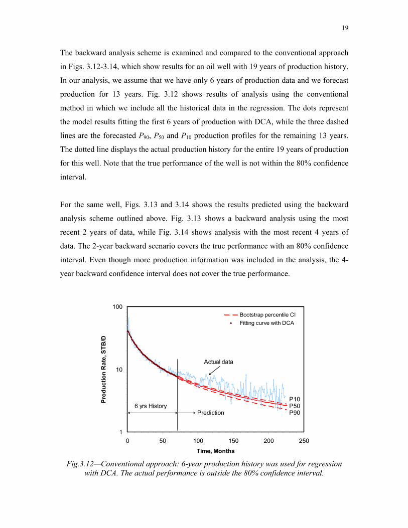
The backward analysis scheme is examined and compared to the conventional approach
in Figs. 3.12-3.14, which show results for an oil well with 19 years of production history.
In our analysis, we assume that we have only 6 years of production data and we forecast
production for 13 years. Fig. 3.12 shows results of analysis using the conventional
method in which we include all the historical data in the regression. The dots represent
the model results fitting the first 6 years of production with DCA, while the three dashed
lines are the forecasted P90, P50 and P10 production profiles for the remaining 13 years.
The dotted line displays the actual production history for the entire 19 years of production
for this well. Note that the true performance of the well is not within the 80% confidence
interval.
For the same well, Figs. 3.13 and 3.14 shows the results predicted using the backward
analysis scheme outlined above. Fig. 3.13 shows a backward analysis using the most
recent 2 years of data, while Fig. 3.14 shows analysis with the most recent 4 years of
data. The 2-year backward scenario covers the true performance with an 80% confidence
interval. Even though more production information was included in the analysis, the 4-
year backward confidence interval does not cover the true performance.
1
10
100
0 50 100 150 200 250
Time, Months
Prod
uctio
n R
ate,
STB
/D
Bootstrap percentile CIFitting curve with DCA
Actual data
P50P90
P106 yrs History
Prediction
Fig.3.12—Conventional approach: 6-year production history was used for regression
with DCA. The actual performance is outside the 80% confidence interval.

20
1
10
100
0 50 100 150 200 250
Time, Months
Prod
uctio
n R
ate,
STB
/D
Bootstrap percentile CIFitting curve with DCAActual data
Prediction
History
Backward 2 year
P10
P50
P90
Fig.3.13—Backward 2-year scenario: 6-year production history is known but only 2
years of backward data were used for regression with DCA. The actual performance is within the 80% confidence interval.
1
10
100
0 50 100 150 200 250
Time, Months
Prod
uctio
n R
ate,
STB
/D
Bootstrap percentile CIFitting curve with DCAActual data
Prediction
History
Backward 4 year
P10P50
P90
Fig. 3.14—Backward 4-year scenario: 6-year production history is known but only 4
years of backward data were used for regression with DCA. The actual performance is outside the 80% confidence interval.
21
For the results of the 100-well analysis that we present in following sections of this
thesis, we use three backward analyses to obtain the overall probabilistic forecast. These
analyses consider the most recent 20%, 30% and 50% of the known production data. The
choice of number and lengths of backward analyses considered is arbitrary, but seems to
provide reasonable results, as shown later.
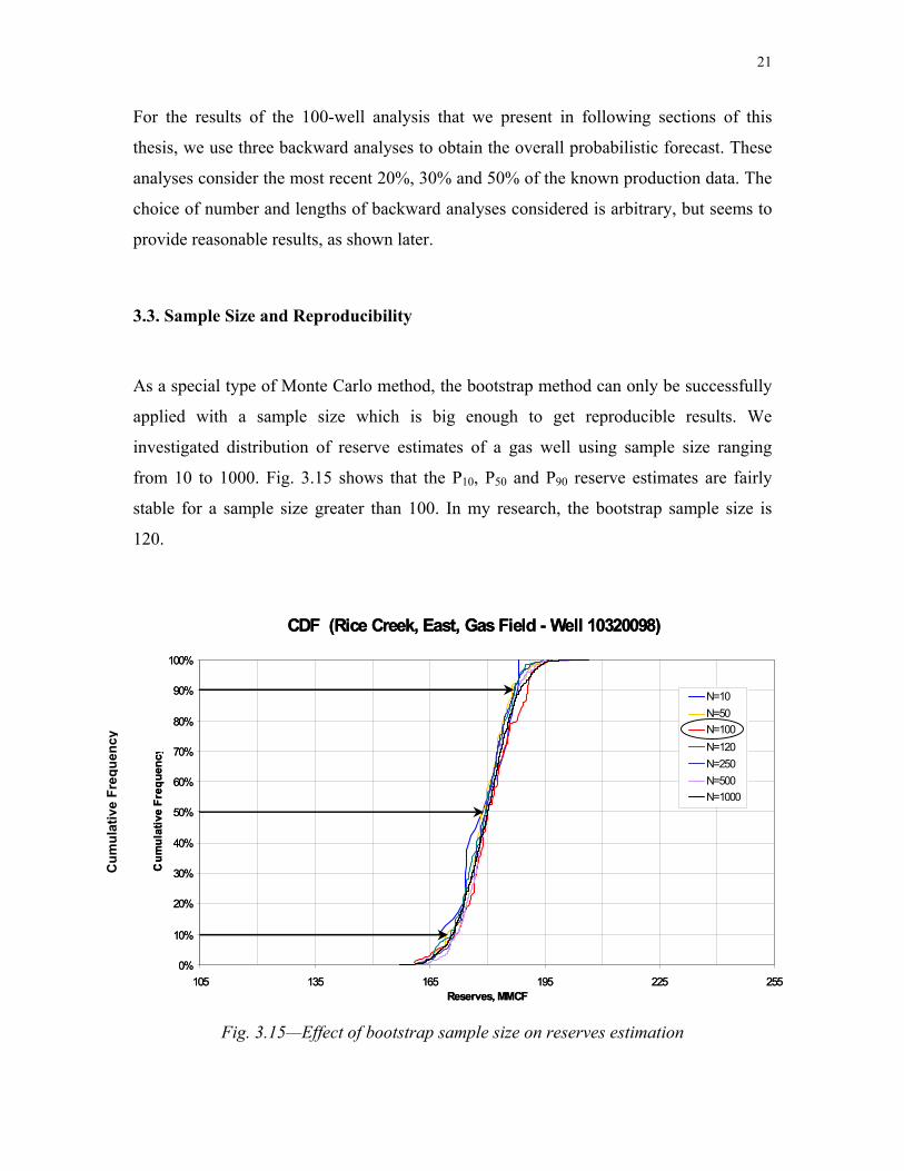
3.3. Sample Size and Reproducibility
As a special type of Monte Carlo method, the bootstrap method can only be successfully
applied with a sample size which is big enough to get reproducible results. We
investigated distribution of reserve estimates of a gas well using sample size ranging
from 10 to 1000. Fig. 3.15 shows that the P10, P50 and P90 reserve estimates are fairly
stable for a sample size greater than 100. In my research, the bootstrap sample size is
120.
CDF (Rice Creek, East, Gas Field - Well 10320098)
0%
10%
20%
30%
40%
50%
60%
70%
80%
90%
100%
105 135 165 195 225 255Reserves, MMCF
Cum
ulat
ive
Freq
uenc
y
N=10N=50N=100N=120N=250N=500N=1000
CDF (Rice Creek, East, Gas Field - Well 10320098)
0%
10%
20%
30%
40%
50%
60%
70%
80%
90%
100%
105 135 165 195 225 255Reserves, MMCF
Cum
ulat
ive
Freq
uenc
y
N=10N=50N=100N=120N=250N=500N=1000
Fig. 3.15—Effect of bootstrap sample size on reserves estimation
Cum
ulat
ive
Freq
uenc
y

22
3.4. Coverage Index
Although not an integral part of the methodology, we define a coverage index, I, to help
assess the coverage of individual confidence intervals. The definition is as follows
)( 5090
50
PPPPI true
−−
= if Ptrue > P50 …...………………… (3.3)
)( 1050
50
PPPPI true
−−
= if Ptrue < P50 ……..……………… (3.4)
where Ptrue represents the true value of reserves. When |I| ≤1, the true reserves are within
the estimated confidence intervals; when |I| >1, the true reserves are outside the estimated
confidence intervals. A negative value of I indicates that P50 is less than the true reserve,
and a positive value of I indicates that P50 is higher than the true reserve.
Note that the coverage index takes into account two quantities: first, the distance between
the P50 and true values and, second, the confidence range between the P50 value and the
upper or lower bound. Thus, a small coverage index could reflect either that an estimate
is close to the true value or that the confidence interval is large. Note also that the
coverage index is a measure associated with a single confidence interval and, thus, is not
a measure of reliability of the uncertainty estimations. Despite these limitations, we have
found the coverage index to be useful in the assessment of probabilistic approaches.
3.5. Confidence Interval Corrections
Our intend in investigating confidence interval corrections is to improve the coverage of
bootstrap confidence intervals. When not specified, the term “confidence interval”
generally refers to the percentile confidence interval. This type of confidence interval is
relatively small compared to those calculated by other methods. A two-sided, equal-tailed
100(1-2) % percentile CI is given by

23
],[ **1 αα θθ −=PBCI ……….……………………….. (3.5)
where CIPB is the percentile bootstrap CI, � represents estimators of reserves or
production rates from bootstrap realizations, and � equals 0.1 for an 80% confidence
interval. Fig. 3.16 illustrates the determination of a percentile CI. In decline curve
analysis, there are many cases where the decline exponent b tends to be larger than 1
when a constraint of 0≤b≤1 is not imposed. The bootstrap realizations generated from
resampling the original production data will have a similar tendency. As a result, the
probabilistic distribution of production and reserves estimates is highly skewed with the
b≤1 constraint applied in nonlinear regression (as we have done in our work). In these
cases, coverage accuracy of percentile CIs can be very poor.
CDF of Reserves
0%
10%
20%
30%
40%
50%
60%
70%
80%
90%
100%
1250 1350 1450 1550Reserve Value, MMCF
Cum
ulat
ive
Freq
uenc
y
P10= 1361.65
P50= 1369.85
P90= 1379.19
C.I.= 17.54
Index= -0.087
CDF of Reserves
0%
10%
20%
30%
40%
50%
60%
70%
80%
90%
100%
1250 1350 1450 1550Reserve Value, MMCF
Cum
ulat
ive
Freq
uenc
y
P10= 1361.65
P50= 1369.85
P90= 1379.19
C.I.= 17.54
Index= -0.087
Fig. 3.16─Percentile 80% confidence interval estimation
We consider three types of two-sided symmetric confidence intervals for confidence
interval corrections. They are the basic bootstrap CI, the studentized bootstrap CI, and the
P10=1316.65 P50=1369.85 P90=1379.19 Index=-0.087

24
double basic bootstrap CI. A two-sided symmetric 100(1-2) % basic bootstrap CI is given
by
],[21
*
21
*
ααθθθθθθ
−−−+−−=BBCI …..…………….. (3.6)
where CIBB is the basic bootstrap CI and θ is the estimator of reserves or production rates
from the original sample. Fig. 3.17 illustrates the determination of a basic bootstrap CI.
Fig. 3.17─Basic bootstrap 80% confidence interval estimation
A two-sided symmetric 100(1-2) % studentized bootstrap CI is given by
)](),([21
*21
* θσθθσθαα −−
+−= ttCISB ……………….... (3.7)
in which the variable t∗ is defined as
)(/)( **** θσθθ −=t ……………………...….. (3.8)
CISB is the studentized bootstrap CI, σ2 is an estimator of variance of θ, and σ*2 is an
estimator of variance of θ*. Appendix A gives equations for the variance calculation.
Cum
ulat
ive
Freq
uenc
y

25
For the double bootstrap CI, the realizations are obtained through two steps. First, single
bootstrap realizations are resampled from the original data set and, second, double
bootstrap realizations are generated by resampling each of the single bootstrap
realizations.11 In general, computational cost of the double bootstrap CI is prohibitive. In
this study, we have developed a simplified algorithm to evaluate the double bootstrap CI
based on estimators from single bootstrap realizations. Detailed discussion of this
simplified double bootstrap method is given in Appendix B.
Basic bootstrap, studentized bootstrap and double bootstrap confidence intervals are
compared to the percentile confidence interval for an example well in Figs. 3.18 to 3.20,
respectively. The corrected confidence intervals are displayed as solid lines, while the
percentile CI is also shown in each figure with dashed lines for comparison. In these
figures, we assume that only 6 years of production history are analyzed, and we used a 3-
year backward analysis for DCA and prediction. The symbols in the figures represent the
fitting curve, while the dotted line gives the actual 19-year production history for the oil
well. The figures show that the true performance of the well is covered better by these
corrected confidence intervals. Fig. 3.21 shows the absolute values of coverage index for
the different types of confidence intervals illustrated in Figs. 3.18 to 3.20. The percentile
CI has a coverage index greater than 1, which indicates that the percentile CI does not
contain the true value. The three corrected confidence intervals all have a coverage index
less than 1, and the double bootstrap CI has the lowest coverage index. We use the basic
bootstrap confidence interval in our probabilistic DCA methodology.

26
1
10
100
0 2000 4000 6000 8000
Time, Days
Pro
duct
ion
Rat
e, B
BL/
Da
Bootstrap basic CIBootstrap percentile CIFitting curve with DCA
Actual data (light blue)
Prediction
History
Backward 3 year
P10P50
P90
Fig.3.18─Confidence interval correction ─ basic CI: 6-year production history is known
but only 3 years of backward data were used for regression with DCA. The actual performance is within the 80% confidence interval
1
10
100
0 2000 4000 6000 8000
Time, Days
Pro
duct
ion
Rat
e, B
BL/
Da
Bootstrap percentile CIBootstrap studentized CIFitting curve with DCA
Actual data (light blue)
Prediction
History
Backward 3 year
P10P50
P90
Fig.3.19─Confidence interval correction ─ studentized CI: 6-year production history is known but only 3 years of backward data were used for regression with DCA. The actual
performance is within the 80% confidence interval
27
1
10
100
0 2000 4000 6000 8000
Time, Days
Pro
duct
ion
Rat
e, B
BL/
Da
Double Bootstrap CIBootstrap percentile CIFitting curve with DCA
Actual data (light blue)
Prediction
History
Backward 3 year
P10P50
P90
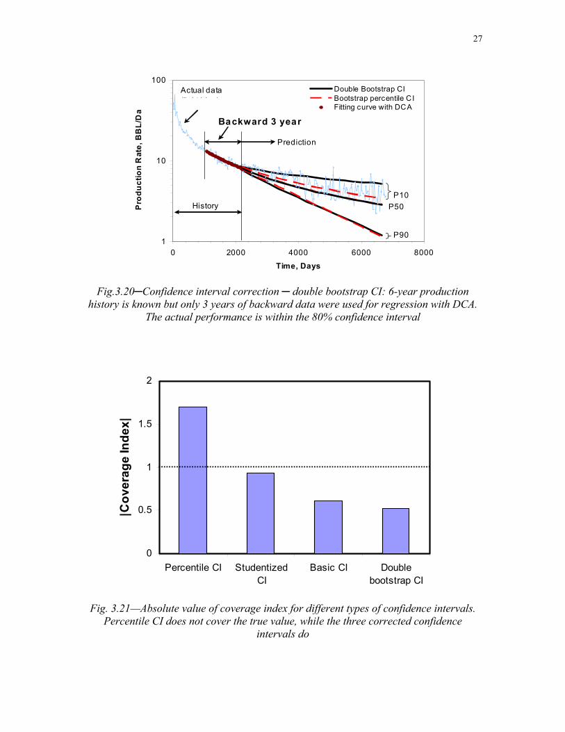
Fig.3.20─Confidence interval correction ─ double bootstrap CI: 6-year production
history is known but only 3 years of backward data were used for regression with DCA. The actual performance is within the 80% confidence interval
0
0.5
1
1.5
2
Percentile CI StudentizedCI
Basic CI Doublebootstrap CI
|Cov
erag
e In
dex|
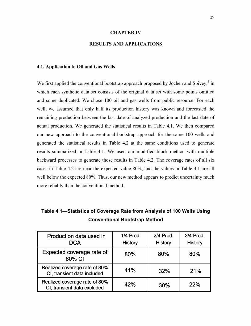
Fig. 3.21—Absolute value of coverage index for different types of confidence intervals.
Percentile CI does not cover the true value, while the three corrected confidence intervals do

28
3.6. Summary of Our Approach
The procedure for our new approach is summarized as follows:
1. Generate multiple synthetic data sets (realizations) using block resampling with
modified bootstrap.
2. Conduct a backward analysis using the most recent 20% of production data
a. Conduct DCA on each synthetic data set and obtain probabilistic predictions of
production and reserves.
b. Calculate confidence intervals for production and reserves using the basic
bootstrap method.
3. Repeat Step 2 using the most recent 30% and 50% of production data and determine
overall P90, P50 and P10 values.
29
CHAPTER IV
RESULTS AND APPLICATIONS
4.1. Application to Oil and Gas Wells
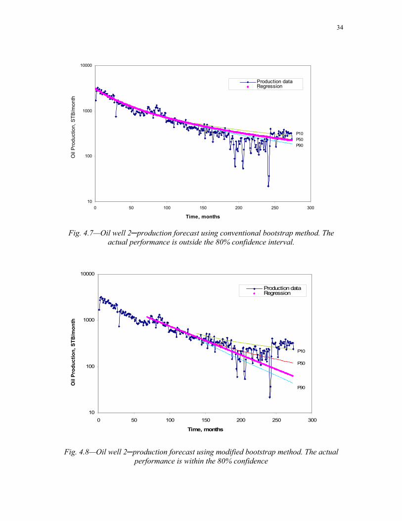
We first applied the conventional bootstrap approach proposed by Jochen and Spivey,5 in
which each synthetic data set consists of the original data set with some points omitted
and some duplicated. We chose 100 oil and gas wells from public resource. For each
well, we assumed that only half its production history was known and forecasted the
remaining production between the last date of analyzed production and the last date of
actual production. We generated the statistical results in Table 4.1. We then compared
our new approach to the conventional bootstrap approach for the same 100 wells and
generated the statistical results in Table 4.2 at the same conditions used to generate
results summarized in Table 4.1. We used our modified block method with multiple
backward processes to generate those results in Table 4.2. The coverage rates of all six
cases in Table 4.2 are near the expected value 80%, and the values in Table 4.1 are all
well below the expected 80%. Thus, our new method appears to predict uncertainty much
more reliably than the conventional method.
Table 4.1—Statistics of Coverage Rate from Analysis of 100 Wells Using Conventional Bootstrap Method
22%30%42%Realized coverage rate of 80% CI, transient data excluded
21%32%41%Realized coverage rate of 80% CI, transient data included
80%80%80%Expected coverage rate of 80% CI
3/4 Prod.History
2/4 Prod.History
1/4 Prod.History
Production data used in DCA
22%30%42%Realized coverage rate of 80% CI, transient data excluded
21%32%41%Realized coverage rate of 80% CI, transient data included
80%80%80%Expected coverage rate of 80% CI
3/4 Prod.History
2/4 Prod.History
1/4 Prod.History
Production data used in DCA

30
Table 4.2—Statistics of Coverage Rate from Analysis of 100 Wells Using Modified, Block Bootstrap Method
75%80%83%Realized coverage rate of 80% CI, transient data excluded
75%85%85%Realized coverage rate of 80% CI, transient data included
80%80%80%Expected coverage rate of 80% CI
3/4 Prod.History
2/4 Prod.History
1/4 Prod.History
Production data used in DCA
75%80%83%Realized coverage rate of 80% CI, transient data excluded
75%85%85%Realized coverage rate of 80% CI, transient data included
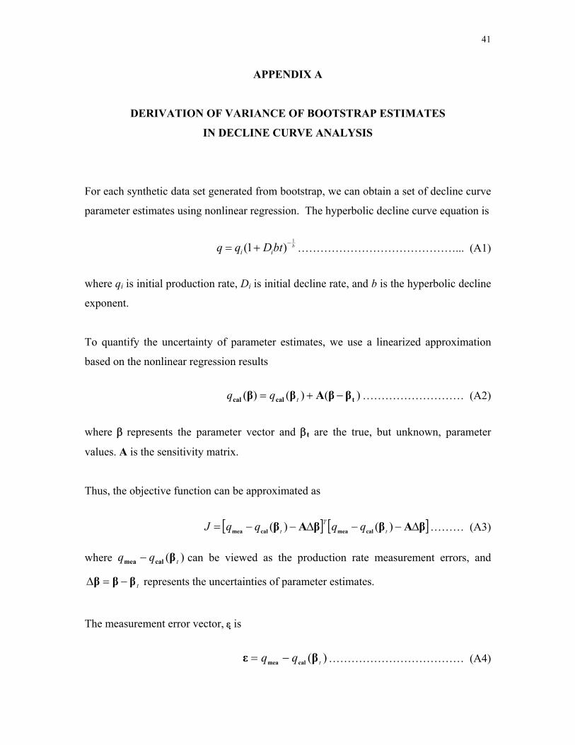
80%80%80%Expected coverage rate of 80% CI
3/4 Prod.History
2/4 Prod.History
1/4 Prod.History
Production data used in DCA
Figs. 4.1-4.8 compare results from the two methods for two oil wells and two gas wells
from our 100 wells. The symbols in the figures represent the nonlinear regression curve,
while the dotted line gives the actual production data. Figs. 4.1, 4.3, 4.5 and 4.7 show the
probabilistic production forecasts using the conventional bootstrap approach overlaying
the actual remaining production profiles, while Figs. 4.2, 4.4, 4.6 and 4.8 show the same
for our new modified bootstrap approach. The conventional bootstrap approach produces
relatively narrow confidence intervals that generally do not bracket the actual production
profiles. The modified bootstrap approach produces significantly larger confidence
intervals that bracket most of the production profiles.

31
10
100
1000
10000
100000
0 50 100 150 200 250
Time, months
Gas
Pro
duct
ion,
Mcf
/mo
Production dataRegressionP10
P10P50P90
Fig. 4.1—Gas well 1─production forecast using conventional bootstrap method. The
actual performance is outside the 80% confidence interval.
10
100
1000
10000
100000
0 50 100 150 200 250
Time, months
Gas
Pro
duct
ion,
Mcf
/mo
Production dataRegressionP10
P10P50
P90
Fig. 4.2—Gas well 1─production forecast using modified bootstrap method. The actual
performance is within the 80% confidence interval.
Gas
Pro
duct
ion,
Mcf
/mon
th
Gas
Pro
duct
ion,
Mcf
/mon
th

32
10
100
1000
10000
0 50 100 150 200 250
Time, months
Oil
Prod
uctio
n, S
TB/m
oProduction dataRegressionP10
P10P50P90
Fig. 4.3—Oil well 1─ production forecast using conventional bootstrap method. The
actual performance is outside the 80% confidence interval.
10
100
1000
10000
0 50 100 150 200 250
Time, months
Oil
Prod
uctio
n, S
TB/m
o
Production dataRegressionP10
P10
P50
P90
Fig. 4.4—Oil well 1─production forecast using modified bootstrap method. The actual performance is within the 80% confidence interval.
Oil
Prod
uctio
n, S
TB/m
onth
O
il Pr
oduc
tion,
STB
/mon
th

33
100
1000
10000
100000
0 50 100 150 200 250
Time, months
Gas
Pro
duct
ion,
Mcf
/mo
Production dataRegressionP10
P10P50P90
Fig. 4.5—Gas well 2─ production forecast using conventional bootstrap method. The actual performance is outside the 80% confidence interval.
100
1000
10000
100000
0 50 100 150 200 250
Time, months
Gas
Pro
duct
ion,
Mcf
/mo
Production dataRegressionP10
P10P50
P90
Fig. 4.6—Gas well 2─production forecast using modified bootstrap method. The actual
performance is within the 80% confidence interval.
Gas
Pro
duct
ion,
Mcf
/mon
th
Gas
Pro
duct
ion,
Mcf
/mon
th
34
10
100
1000
10000
0 50 100 150 200 250 300
Time, months
Oil
Prod
uctio
n, S
TB/m
oProduction dataRegressionP10
P10P50P90
Fig. 4.7—Oil well 2─production forecast using conventional bootstrap method. The
actual performance is outside the 80% confidence interval.
10
100
1000
10000
0 50 100 150 200 250 300
Time, months
Oil
Prod
uctio
n, S
TB/m
o
Production dataRegressionP10
P10
P50
P90
Fig. 4.8—Oil well 2─production forecast using modified bootstrap method. The actual
performance is within the 80% confidence
Oil
Prod
uctio
n, S
TB/m
onth
O
il P
rodu
ctio
n, S
TB/m
onth

35
Statistics of the analysis results for the set of 100 wells are compared in Table 4.3. First,
we note that the realized coverage rate for the new method is 85%, very close to the
expected rate of 80%, while the realized coverage rate for the conventional bootstrap
approach is only 32%. After we got the confidence interval for remaining production of
each well, we used Monte Carlo simulation to get the confidence interval for total
remaining production of those 100 wells under two extreme assumptions: perfect,
positive correlation between wells and no correlation between wells. The actual
estimation of the 100-well total remaining recovery should be between those results of
the above two extreme assumptions. We can see from Table 4.3 that the new approach
predicts a much wider 80% confidence interval for total remaining production for the 100
wells, 1902-7226 MSTBOE, versus a range of 4831-6597 MSTBOE for the conventional
bootstrap approach assuming perfect, positive correlation between wells; and 3482-5396
MSTBOE, versus a range of 5393-5924 MSTBOE for the conventional bootstrap
approach assuming no correlation between wells. And the confidence intervals for total
remaining production under two extreme assumptions generated by modified bootstrap
method can both cover the true remaining recovery of those 100 wells.
As an additional benefit of the new approach, we note that the relative and absolute errors
in P50 values are significantly smaller for the new approach than for the conventional
bootstrap approach. This should not be unexpected, as Capen8 pointed out that better
range can lead to better most-likely estimates.

36
Table 4.3—Comparison of Remaining Production Estimates for 100 Wells Using Conventional Bootstrap and Modified, Block Bootstrap Method
50% production data analyzed - transient data included
Conventional Bootstrap Method
(Forward analysis - percentile CI)
Modified Bootstrap Method (Multi-
backward analysis (50%, 30%,20%)-
Basic Bootstrap CI)
Coverage Rate, % 32 85
Percent error 20.43 4.52
Percent error
53.57 37.48
0.5542 1.4118
Sum of P50 Values, MSTBOE 5495.22 4029.45
True Remaining Recovery, MSTBOE 4114.54 4114.54
Pecent Error in Remaining Recovery, % 33.56 -2.07
80% CI Assuming Perfect, Positive Correlation, MSTBOE 4,831-6,597 1,902-7,226
80% CI Assuming No Correlation, MSTBOE 5,393-5,924 3,482-5,396
%10050 ×⎟⎟⎠
⎞⎜⎜⎝
⎛ −
true
true
RRPAverage
)..(50PICAverage
%10050 ×⎟⎟⎠
⎞⎜⎜⎝
⎛ −
true
true
RRP
Average

37
CHAPTER V
DISCUSSION
5.1. Why Does Our Approach Work?
As discussed previously, for a gas well, b is variable. The b-value usually obtained by
nonlinear regression represents an average value on the fitted period. As a result, this
value could be far from the b-value of the future period since the instantaneous b is not
constant. However, with the backward approach, we can capture the latest characteristics
of b and therefore improve production forecast effectiveness.
There are other factors that influence the behavior of actual decline curves and the results
of DCA. One of them is transient-period data. Determining the beginning of the
stabilized flow period is a difficult problem in practice, especially with short-term
production data. The backward approach helps to overcome this problem by focusing on
more recent data. The prevailing changing operating conditions during the production life
of a well often make the application of DCA problematic. Similarly, our approach can
help mitigate this problem, because the latest features of performance can be captured
and used for future prediction.
Compared with previous approaches, the approach proposed here has several advantages:
1. No prior distributions of qi, Di, and b are required (with bootstrap algorithm).
2. No assumption of independent and identically distributed data is required for the
original data set (with modified bootstrap).
3. The method effectively preserves the original data time correlation (with block
resampling).
4. The method improves the reliability of uncertainty quantification (with backward
analysis and corrected confidence interval methods).

38
CHAPTER VI
CONCLUSIONS AND RECOMMENDATIONS
6.1. Conclusions
A new probabilistic approach has been developed that can improve the coverage
rate of confidence intervals and enable more accurate reserves estimation with
increasing production data availability. The approach is robust and objective in
that it is purely production data driven.
Application to 100 individual oil and gas wells cases demonstrates that this
approach provides reliable confidence interval estimations.
We have compared the results with the conventional method, comparing the
accuracy of reserves forecast and estimation errors of 100 oil and gas wells. And
the results show that our proposed method can significantly improve the coverage
rate and decrease the estimation errors.
6.2. Recommendations
We developed some VBA programs to fulfill the whole process of reserves and
production forecast using modified bootstrap method based on production decline data.
Although we have already edited our code to make the whole process automatically, it
will be much better if the similar commercial software can be developed to make those
code more integrated and provide friendly input and output windows, which could help
managers of petroleum industry make better decisions in buying, selling, and operating
properties.

39
NOMENCLATURE A = sensitivity matrix b = hyperbolic decline exponent CI = confidence interval CIBB = basic bootstrap CI CIPB = percentile bootstrap CI CISB = Studentized bootstrap CI Di = initial decline rate ECR = expected coverage rate g = production rate estimate or reserves estimate I = coverage index J = objective function M = number of model parameters N = number of data points P10 = value at confidence level 90% P50 = value at confidence level 50% P90 = value at confidence level 10% Ptrue = true value q = production rate qi = initial production rate RCR = realized coverage rate t = production time t∗ = t-distribution variable Z-1 = inverse of standard normal distribution function β = model parameter vector ε = measurement error vector θ = estimators from the original sample θ∗ = estimators from bootstrap samples σ2 = estimator of variance of θ σ∗2 = estimators of variance of θ∗ Superscripts T = matrix transpose Subscripts cal = calculated mea = measured t = true

40
REFERENCES
1. Thompson, R.S. and Wright, J.D.: “The Error in Estimating Reserve Using Decline Curves,” paper SPE 16295 presented at the 1987 SPE Hydrocarbon Economics and Evaluation Symposium, Dallas, 2-3 March.
2. Laherrere, J.H.: “Discussion of an Integrated Deterministic/Probabilistic
Approach to Reserve Estimations,” JPT (Dec. 1995) 1082. 3. Patricelli, J.A. and McMichael, C.L.: “An Integrated Deterministic/Probabilistic
Approach to Reserve Estimations,” JPT (Jan. 1995) 49. 4. Hefner, J.M. and Thompson, R.S.: “A Comparison of Probabilistic and
Deterministic Reserve Estimates: A Case Study,” SPERE (Feb. 1996) 43. 5. Jochen, V.A. and Spivey, J.P.: “Probabilistic Reserves Estimation Using Decline
curve Analysis with the Bootstrap Method,” SPE 36633 presented at the 1996 SPE Annual Technical Conference and Exhibition, Denver, 6-9 October.
6. Fetkovich, M.J., Fetkovich, E.J. and Fetkovich, M.D.: “Useful Concepts for
Decline-Curve Forecasting, Reserve Estimation and Analysis,” SPERE (Feb. 1996) 13.
7. Chen, Her-Yuan.: “Estimating Gas Decline-Exponent before Decline-Curve
Analysis,” paper SPE 75693 presented at the 2002 SPE Gas Technology Symposium, Calgary, Alberta, Canada, 30 April-2 May.
8. Capen, E.C.: “The Difficulty of Assessing Uncertainty,” JPT (Aug. 1976) 843. 9. Huffman, C.H. and Thompson, R.S.: “Probabilistic Ranges for Reserve Estimates
from Decline Curve Analysis,” paper SPE 28333 presented at the 1994 SPE Annual Technical Conference and Exhibition, New Orleans, 25-28 September.
10. Efron, B. and Tibshirani, R.J.: An Introduction to the Bootstrap, Chapman &Hall,
New York City, 1993. 11. Nankervis, J.C.: “Computational Algorithms for Double Bootstrap Confidence
Interval,” Computational Statistics and Data Analysis, (April 2005) 461.
41
APPENDIX A
DERIVATION OF VARIANCE OF BOOTSTRAP ESTIMATES
IN DECLINE CURVE ANALYSIS
For each synthetic data set generated from bootstrap, we can obtain a set of decline curve
parameter estimates using nonlinear regression. The hyperbolic decline curve equation is
bbtDqq ii
1
)1( −+= ……………………………………... (A1)
where qi is initial production rate, Di is initial decline rate, and b is the hyperbolic decline
exponent.
To quantify the uncertainty of parameter estimates, we use a linearized approximation
based on the nonlinear regression results
)()()( tcalcal ββAββ −+= tqq ……………………… (A2)
where β represents the parameter vector and βt are the true, but unknown, parameter
values. A is the sensitivity matrix.
Thus, the objective function can be approximated as
[ ] [ ]βAββAβ calmeacalmea Δ−−Δ−−= )()( t
Tt qqqqJ ……… (A3)
where )( tqq βcalmea − can be viewed as the production rate measurement errors, and
tβββ −=Δ represents the uncertainties of parameter estimates.
The measurement error vector, ε is
)( tqq βε calmea −= ……………………………… (A4)

42
A necessary condition for a minimum of the objective function is
0=∇J ……………………………………… (A5)
or
( ) 0)(2 =Δ−−=∇ βAβA calmea tT qqJ ……….…….….. (A6)
So, we have
εβA =Δ ….……………………………..…. (A7)
or
εAAAβ TT 1)( −=Δ ……………………….. (A8)
We assume that measurement error (ε) follows the multi-variant Gaussian distribution
with ε ~ N (0, σ2I). σ2 is the variance for each component of measurement error, and I is
the unit matrix.
An optimal estimation of σ2 can be obtained as
MN
MNJ
N
jjcaljmea
−
−=
−≈
∑=1
2,,
2
))(( *βσ
……………. (A9)
where N is the number of data points, and M is the number of model parameters.
As a result, Δβ follows a normal distribution, Δβ ~ N (0, σ2(ATA)-1). ATA can be viewed
as the approximate Hessian matrix. Hence, the covariance matrix of Δβ is equal to the
product of σ2 and the inverse of the Hessian matrix. If we express the inverse of the
Hessian matrix as

43
⎥⎥⎥⎥⎥⎥
⎦
⎤
⎢⎢⎢⎢⎢⎢
⎣
⎡
== −−
MMMM
M
M
T
aaa
aaaaaa
Hessian
........................
....
....
)(
21
22221
11211
11 AA
……………......... (A10)
then the covariance of Δβ can be written as
⎥⎥⎥⎥⎥⎥
⎦
⎤
⎢⎢⎢⎢⎢⎢
⎣
⎡
==Δ −
221
22221
11221
12
........................
....
....
)()(
MMM
M
M
TCov
σσσ
σσσσσσ
σ AAβ
………….……... (A11)
where σjk represents covariance between βj and βk, defined as
1
))((1
−
−−=
∑=
N
N
ikkijji
jk
ββββσ
…….……………. (A12)
i = 1, 2,…, N
j, k = 1, 2,…M
To evaluate the variance of production rate or reserves estimates, we derive the following
approximations. Based on the definition of variance of an estimate, we have
( )( )1
1
2*,,
2
−
−=
∑=
N
ggN
jjcaljmea
g
βσ
…….…...................... (A13)
where g represents flow rate or reserves and σ is the variance of estimated g. Taking the
Taylor series expansion and using the first derivative term, we can approximate the
difference term in the parentheses of Eq. A13 as

44
( ) MM
jcaljcaljcaljmea
gggg β
ββ
βΔ
∂
∂+⋅⋅⋅⋅⋅⋅+Δ
∂
∂≈− ,
11
,*,, β
……... (A14)
Substituting Eq. (14) into Eq. (13), we obtain
GCovGT
g )(2 βΔ=σ ……………...……..……. (A15) Here,
⎟⎟⎠
⎞⎜⎜⎝
⎛∂∂
⋅⋅⋅⋅⋅⋅∂∂
=M
calcalT ggGββ
,,1
Eq. A15 can be used to calculate the variances needed in Eqs. 5 and 6 for the studentized
CI calculation, and is also used in our simplified double bootstrap CI calculation.

45
APPENDIX B
SIMPLIFIED DOUBLE BOOTSTRAP APPROACH
Reference 11 proposed a stopping rule to simplify calculation of the double bootstrap CI.
We simplified this computationally prohibitive operation by resampling the predicted
estimates (such as production rates at each future time point and reserves), instead of
resampling each single bootstrap realization to generate double bootstrap realizations.
With our approach, we can save a great amount of time in the nonlinear regression of
double bootstrap realizations. For example, if we have 100 single bootstrap realizations
(generated from the original data set), and if we want the double bootstrap sample size
also equal to 100 (generated from each of the single bootstrap realizations), then 10,000
nonlinear regression runs are required since 10,000 synthetic data sets are generated. This
is very expensive computationally. When we directly resample on the predicted
production rate or reserves estimates, we need to perform only 100 nonlinear regression
runs on 100 single bootstrap realizations to calculate the predicted estimates. To resample
those predicted estimates, a variance of each estimate is needed. We assume each
estimate follows a Gaussian distribution with mean equal to itself and variance estimated
by Eq. A15. In this way we can obtain sufficient estimates for the double bootstrap CI
calculation.

46
VITA
Yuhong Wang
Petroleum Eng. Dept.
3116 TAMU
College Station, TX USA, 77840
Ph: (979) 862-9478
PROFILE
Petroleum engineer with two years of academic and research experience in reservoir
engineering and four years in oil and gas storage and transportation. Specific knowledge
in reservoir simulation, decline curve analysis, reservoir evaluation and management, gas
station and pipeline design and software development. Currently, involved in research
concerning probabilistic reserves and production forecast simulation. Special interest in
the development and application of decline curve analysis and statistic method for
reservoir simulation plus software design and development.
EDUCATION
Master of Science. Petroleum Engineering. Texas A&M University. May 2006
Bachelor of Science. Petroleum Engineering. Southwest Petroleum Institute, China
June 2003
EXPERIENCE
Texas A&M University. Research Assistant. 2003-2005
Southwest Petroleum Institute. Research Assistant. 2001-2003