DETERMINING AN OPTIMUM BIOLOGICAL DOSE OF A … · Determining an Optimum Biological Dose of a Metronomic Chemotherapy However, in case of MC the toxicity is not a concern. As the

Journal of Data Science 15(2017), 77-94

DETERMINING AN OPTIMUM BIOLOGICAL DOSE OF A

METRONOMIC CHEMOTHERAPY

Atanu Bhattacharjee1, Vijay M Patil2

1Department of Biometrics, Chiltern Clinical Research Ltd 2Department of Medical Oncology, Tata Memorial Hospital

Abstract: The surrogate markers(SM) are the important factor for angiogenesis in

cancer patients.In Metronomic Chemotherapy (MC) , physicians administer

subtoxic doses of chemotherapy (without break) for long periods, to the target

tumor angiogenesis. We propose a semiparametric approach, predictive risk

modeling and time to control the level of surrogate marker to detect the perfect

dose level of MC. It is based on the controlled level of surrogate marker, and the

aim is to detect an Optimum Biological Dose (OBD) finding rather than a

traditional Maximum Tolerated Dose (MTD) approach. The methods are

illustrated with MC trial dataset to determine the best OBD and we investigate the

performance of the model through simulation studies.

Key words: MCMC, Angiogenesis, OBD, Predictive Risk Modeling

1. Introduction

The doses of chemotherapy selected in clinical practice are routinely derived by the MTD

approaches. It is believed that an increase in dose will lead to an increase in tumor response.

The dose selected for phase 2 and further studies is one dose level below the MTD level in

Phase I studies [Skipper 1970, Devita 2008, Briasoulis 2009]. However, this conventional

dosing of chemotherapy has routinely compromised the QOL of patients and may lead to

selection of chemo-resistant clones [Schmid 2005, Golfinopoulos 2007, Saltz 2008]. The MC

has been suggested as an alternative strategy to overcome such effects. The strategy in MC is to

administer sub-toxic doses of same chemotherapy drugs for long periods to target angiogenesis

[Bhattacharjee 2016, Patil 2015,Kerbel 2002, Kerbel 2004,Scharovsky 2009]. The effect on

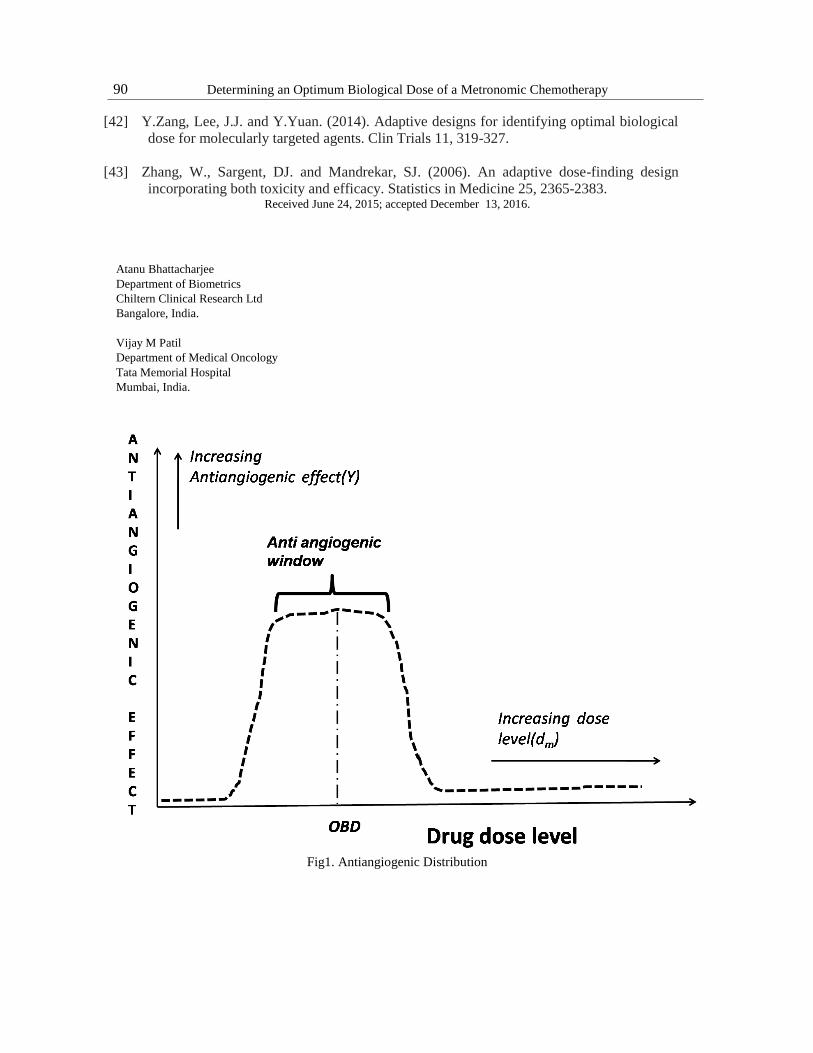
angiogenesis is achieved by targeting CEC. The effect on CEC is restricted to an antiangiogenic

window in tumor cell line studies [skipper 1970, Hobson 1984, Vacca 1999]. In tumor cell line

studies a drug would start exerting an antiangiogenic effect at a low dose level and it would

continue to exert it till an upper dose level. Drug levels below the lower dose level and above

the upper dose level won't exert an antiangiogenic effect (Figure 1). The challenge is to

establish the optimal biological dose (OBD) of MC which would have maximized inhibiting

effect on CEC. The aims of any phase I traditional clinical trial is to detect the MTD of

chemotherapy. As when conventional chemotherapy is administered toxicity is a concern.

78 Determining an Optimum Biological Dose of a Metronomic Chemotherapy

However, in case of MC the toxicity is not a concern. As the Metronomic doses are nearly 1

10𝑡ℎ

of MTD of conventional chemotherapy. Therefore the aims of phase 1 MC clinical trial is to

obtain OBD of a drug [Marshall2012].

The simple phase I trial design is to obtain MTD of a cytotoxic agent through standard '3+3'

design accrues patients in cohorts of three and escalates until a pre-defined DLT is observed

[Rosemarie1993]. The Continual Reassessment Method (CRM), is an another dose-response

finding model and recently gained popularity [O'Quigley2006]. But both the models directly

failed to detect the aim of any MC i.e. OBD . This paper is aimed to illustrate the application

of OBD in MC. The OBD of MC is determined based on the performance of desired level of

Surrogate Marker(SM). The serum creatinine (Scr) is considered as a choice of SM in this study.

The OBD for dose-finding designs to search the perfect dose in MC has been proposed in this

article.

2. MC trial data set

It is a partial data set considered from ongoing 7-years duration of a longitudinal study.

This study is continuing under the supervision of the authors as principal investigator and is not

matured enough to state more about it. This work is dedicated only on dose-response modeling

section. It is expected that the full data will be matured enough by the end of the year 2020 in

terms of completed follow-up of the patients with strong enough statistical power to serve the

primary objective as the event of interest i.e. death. In this manuscript, we focused only on

initial dose-response modeling of MC with cancer patients. A total of 110 patients MC therapy

data has been utilized in this paper. In MC the main goal is to find out the OBD among all

different low dose levels. The serum creatinine (SCr) is considered as response of interest for

OBD. A total of six doses-levels coded as 10mg/m2,15 mg/m2,20 mg/m2, 25 mg/m2,30

mg/m2 and 35 mg/m2 of IV docetaxel are considered in this study. The data set is observed

with individual-specific information for patient 's with doses and corresponding marker levels.

The Scr measurements are retrospectively observed for six different cycles of MC therapy.

This study is focused on Scr data observed till end of first few weeks of MC Trial.

3. Methods

3.1 Data Exploration with Mixture Distribution

The parametric model is assumed for dose-response curve preparation. The challenge is to

specify the dose-response for the optimum biological response modeling. The literature for

dose-response modeling is well established through different types of MLE assumptions

[islam2016,Aghamohammadi2010,Schmoyer1984], and Kernel estimator [Muller1988].The

non-parametric setup has been found suitable for dose-response through Dirichlet Process Prior

[Mukhopadhyay 2000] and quantile response [Dette 2010].The application of semi-parametric

through mixture of parametric and non-parametric explored for continuous variable [Einsporn

1987]. This mixture approach for density estimation [Olkin 1987], hazard function [Kouassi

Atanu Bhattacharjee1, Vijay M Patil2 79

1997], robust regression [Mays2001] and the linear mixed model [Waterman 2007] are already

established for repeated [Pickle 2008] and non-repeated measurement [Robinson 2010]. This

work is extended with the application of semi-parametric estimates of the dose-response

relation for the exploratory data analysis. The weight is used to reduce the bias balanced the

adaptively borrowed across the two method, i.e. parametric and non-parametric The scenario of

parametric model correctly specified, the weights towards the parametric model will be more

otherwise non-parametric portion will gain more weight. Let the response of interest is denoted

as Y following the Bernoulli distribution with the probability f(x). The dose-response f(x) is

estimated through the semi-parametric modeling. The effective dose-response is denoted as

𝐸𝐷𝛼 = 𝑓−1(𝛼)for 0 < 𝛼 < 1$. The inverse functions f(x) is 𝑓−1(𝑥)$. The aim of any

toxicology studies is to estimate 𝐸𝐷𝛼 for smaller values of𝛼. The dose-response relation is

estimated through parametric and non-parametric modeling. The parametric model is assumed

as 𝑓(𝑥, 𝜃) for the dose - response curve and 𝜃 is the unknown parameter. Suppose the

nonparametric and parametric estimates are 𝑓̅(𝑥) and 𝑓(𝑥, 𝜃) respectively. The estimated value

of the parameter of interest is 𝜃 obtained by MLE .The dose is denoted as x and corresponding

response as Y. The dose-response relation is observed through the mixture of parametric and

non-parametric modeling.

The equation is defined as

𝑓𝜔(𝑥, 𝜃) = (1 − 𝜔)𝑓̅(𝑥) + 𝜔𝑓(𝑥, 𝜃) (3.1)

The weight (𝜔 ∈ [0,1]) factor is used to make balance between parametric and non-

parametric estimates. The equation (3.1) provides the option to incorporate the parametric and

non-parametric both the options simultaneously. The estimates (either parametric or non-

parametric) fits more appropriately will gain more weight and complementary value of 𝜔 i.e 1-

𝜔 will be gained by another one. The dose range is denoted as (𝑥𝑚𝑎𝑥, 𝑥𝑚𝑖𝑛). The estimated

value of $\omega$ is obtained from the minimum estimated value of the mean integrated

squared error(MISE) (Yuan2011)

𝑀𝐼𝑆𝐸 (𝑝𝜔(𝑥, 𝜃)) = 𝐸 [∫ {𝑝(𝑥) − 𝑝𝜔(𝑥, 𝜃)}2𝑥𝑚𝑎𝑥

𝑥𝑚𝑖𝑛𝑑𝑥] (3.2)

The dose-response relation is explored through semi-parametric estimation. The function

values of the above equation are defined as

𝑃𝑟𝑜𝑏𝑖𝑡1: −𝑝(𝑥) = 𝜑(𝑥−0.5

0.25) (3.3)

𝑃𝑟𝑜𝑏𝑖𝑡2: −𝑝(𝑥) = 𝜑(𝑥−0.5

0.5) (3.4)

The optimum dose level is selected with 𝐸𝐷𝛼 =0.5.

Further, x is defined as 𝑥 =𝑑−1

5 for d=1,2,….6.The Probit model in parametric portion and

Kernel estimation for non-parametric portion assumed to perform the analysis. A total of 1000

boot strapping has been carried to obtain the estimates of weight ω. The value of 𝐸𝐷𝛼has been

observed through 0.05,0.1,0.15,0.20,0.25,0.30 to avoid the complicated estimation of 𝐸𝐷𝛼 Bias


and MSE estimates of 𝐸𝐷𝛼 observed simulations of parametric and non-parametric estimates

are detailed in Table 1 and Table 2 respectively.

3.2 Predicted Risk Modeling for Optimum Biological Dose (OBD) of a Surrogate

Marker (SM)

The event is defined as the presence of a Surrogate Marker (SM) within the controlled limit.

Let SM under consideration is Y. The objective is to reduce or induce the level of response Y

through specific dose i.e. x. The target level of Y to be controlled by x is decided based on

supportive literature of trial. Suppose patients i is having response value 𝑌𝑖 and if 𝑌𝑖=𝑗 ,

patients has experienced the controlled level of SM in the jth interval of time,𝑡𝑗−1 < 𝑇𝑖 < 𝑡𝑗 for

j=1,2,....C and the sequence of time denoted as 0 < 𝑡0 < 𝑡1 < ⋯ … < 𝑡𝑒 < ∞ where

[𝑡0, 𝑡𝑒−1] = [0, 𝑡∗] is the maximum window of observation.

Further, 𝑇𝑖0 is the event of time or right censoring time. The indicator ∆𝑖= 1 if 𝑇𝑖

0 = 𝑇𝑖 and

∆0= 0 if 𝑇𝑖0 < 𝑇𝑖. The value of 𝑌𝑖

0is the current interval value for the ith patients. Let dose

under consideration denoted as 𝑑1 < 𝑑2 < ⋯ . 𝑑𝑚and m=1,...M gives the standard normal cdf

of Φ(. ). The binary-time event function is defined as

𝛷(𝛽𝑗,𝑚) = 𝑃𝑟 (𝑌𝑖 = 𝑗/𝑑𝑚) = ∏ {1 − 𝛷(𝛽ℎ,𝑚) }𝑗ℎ=1 (3.5)

for 𝑗 ≤ 𝐶 − 1 . Let βj,m is the effective dose k on the event in the jth interval. The

probability of event for the jth interval is

𝑃𝑟 (𝑌𝑖 = 𝑗/𝑑𝑚) = Φ(βj,m) ∏ {1 − Φ(βh,m) }j−1h=1 (3.6)

and not occurrence of event Pr(𝑌 ≥ 𝑗|𝑑𝑚) = ∏ { 1 − Φ(𝛽ℎ,𝑚)}𝑗ℎ=1 for 𝑗 ≤ C − 1 at any

specific point of time, the binary data for the nth patients take the form 𝐷𝑛 =

{(𝑌𝑖0, 𝑚(𝑖), 𝛿𝑖), 𝑖 = 1,2, … . 𝑛} and denoted as 𝛽 = (𝛽1,1, … . . 𝛽𝐶−1,𝑚. The likelihood is defined

as

𝐿(𝛽|𝐷𝑛) = ∏ Φ(𝛽𝑌𝑖0, 𝑚(𝑖))𝛿𝑖𝑛

𝑖=1 ∏ {1 − Φ(βh,m(i))} 𝑌𝑖

0−1

ℎ=1 (3.7)

The conditional probability is defined as

𝜋(𝛽, 𝑑𝑚, 𝑗) = 𝑃(𝑌 ≤ 𝐶 − 1|𝑌 ≥ 𝑗, 𝛽, 𝑑𝑚)for𝑗 = 1,2, … 𝐶 − 1 and m = 1, … . M (3.8)

Further, 𝜋(𝛽, 𝑑𝑚, 𝑌0) gives the probability that a patients who successes in 𝑌0 − 1 without

event will expereinced by 𝑡∗ = 𝑡𝐶 − 1 at dose 𝑑𝑘.

Let the window is [0, 𝑡∗] is 𝜋(𝛽, 𝑑𝑚, 1.The binary-time event is defined as

𝜋(𝛽, 𝑑𝑚, 𝑗) = 1 − ∏ {1 − Φ(𝛽ℎ,𝑚)}𝐶−1ℎ=1 and 𝜋(𝛽, 𝑑𝑚, 𝑗) = 1 − ∏ {1 − Φ(𝛽ℎ,𝑚)}𝐶

ℎ=1 .


For the patients i, the vector of latent variable 𝑍𝑖 = (𝑍𝑖,1, … . 𝑍𝐼,𝑌𝑖0) if 𝑌𝑖

0 =C, with

𝑍𝐼,𝑗~𝑁(𝛽𝑗,𝑘 , 1) , if the ith patients received the dose 𝑑𝑚. Let 𝑁(𝜇, 𝜎2)shows the density by

(𝑧; 𝜇, 𝜎2) .

The likelihood is expressed as

𝐿(𝛽|𝐷𝑛) =

∏ {∫ 𝜑(𝛽 𝑌𝑖0, 𝑚(𝑖)𝑍𝑖 , 𝑌𝑖

0, 1)𝑑𝑍𝑖,𝑌𝑖0 , 1)𝑑𝑍𝑖,𝑌𝑖

0}∞

−∞

𝛿𝑖∏ ∫ 𝜙(𝑍𝑖,𝑗; 𝛽𝑗,𝑚(𝑖),1)𝑑𝑍𝑖,𝑗

∞

0

𝑌𝑖0−1

𝑗=1𝑛𝑖=1 (3.9)

The extended function through consideration of latent variable is

𝐿(𝛽|𝐷𝑛, 𝑍) = ∏ 𝜑(𝛽 𝑌𝑖0, 𝑚(𝑖)𝑍𝑖 , 𝑌𝑖

0, 1){𝐼(𝑍𝑖 , 𝑌𝑖0 < 0)} ∏ 𝜙(𝑍𝑖,𝑗; 𝛽𝑗,𝑚(𝑖),1)𝐼(𝑍𝑖,𝑗 > 0)

𝑌𝑖0−1

𝑗=1𝑛𝑖=1

(3.10)

Patients safety also been considered to obtain the OBD controlled surrogate markers. It is

assumed that when a group of new patients entered in a trial and treated with specific dose but

not fully followed then two scenario may occurs to them either all of them are having

controlled surrogate markers or none of them have controlled surrogate markers at time 𝑡∗.

Since, none of the dose is having problem for occurrence of high toxicity level so six different

desirable doses are administered simultaneously to the randomly selected patient and level of

surrogate markers observed in the follow-up visits. The basic intention is to develop

probability measures of either tiny or large surrogate markers levels observed at the specific

dose $d_{k}$ to be fixed and OBD dose or move their dose to near at dose 𝑑𝑚+1 or 𝑑𝑚−1.

Let the random variable 𝛽(𝑎𝑚, 𝑏𝑘) having the mean 𝐸{�̅�(𝛽, 𝑑𝑚|𝐷𝑛)} and variance

𝑉𝑎𝑟{(𝛽, 𝑑𝑚|𝐷𝑛)} . Suppose, 𝑣𝑚 is the number of patients treated with 𝑑𝑚 and not fully

evaluated levels are as 𝑖1, 𝑖2 … . . 𝑖𝑣𝑚.. Further , the indicator 𝑊𝑖𝑟=I(𝑌𝑖𝑟 ≤ 𝐶 − 1) that patients

𝑖𝑟 have the controlled surrogate level in the assessment period and total number of patients not

𝑆(𝑊𝑚) = 𝑊𝑖1+. . +𝑊𝑖𝑣𝑚

properly evaluated and failed to achieve controlled surrogate markers

is 𝑡∗ . The prior probability is obtained from 𝛽(𝑎𝑚 + 𝑆(𝑊𝑚, 𝑏𝑚 + 𝑘𝑚 − 𝑆(𝑊𝑚))) . The

criteria is fixed with

𝑃1𝑚(𝐷𝑛) = ∑ 𝐼[(Pr {𝑝𝑚(𝑤, 𝑣𝑚, 𝑎𝑚, 𝑏𝑚) > 𝜋∗} ≤ 𝜉]Pr (𝑊𝑛 = 𝑤|𝐷𝑛)𝑤 (3.11)

and

𝑃2𝑚(𝐷𝑛) = ∑ 𝐼[(Pr {𝑝𝑘(𝑤, 𝑣𝑚, 𝑎𝑚, 𝑏𝑚) > 𝜋∗} ≤ 𝜉]Pr (𝑊𝑚 = 𝑤|𝐷𝑛)𝑤 (3.12)

The above equations gives the probability measures that 𝑑𝑘 with either tiny or large

surrogate markers levels and 𝑃𝑚(𝐷𝑛) = 1 − 𝑃1𝑚(𝐷𝑛) − 𝑃2𝑚(𝐷𝑛) is measured probability with

dose level 𝑑𝑚 . The marginal posterior of 𝛽 is defined as 𝑓(𝛽, 𝐷𝑛) and 𝐸(𝑊𝑖𝑟|𝛽, 𝐷𝑛) =

�̅�(𝛽, 𝑑𝑚, 𝑌𝑖𝑟0). The summation over above equations is computed through MCMC and is

defined as


Pr(𝑊𝑚 = 𝑤|𝐷𝑛) = ∫ ∏ {𝜋(𝛽, 𝑑𝑚, 𝑌𝑖𝑟0)}

𝑤𝑟{1 − 𝜋(𝛽, 𝑑𝑚, 𝑌𝑖𝑟

0)}1−𝑤𝑟𝑓(𝛽|𝐷𝑛)𝑑𝛽𝑣𝑚𝑟=1 (3.13)

Further, suppose dose is mentioned as $m$, the total number of patients received the dose

denoted as 𝑘𝑚, and partially evaluated patients for dose m is 𝑛𝑚 . Now

�̅�1𝑚(𝐷𝑛) = {1 𝑖𝑓 𝑘𝑚 = 0

𝑃1𝑚(𝐷𝑛)𝑖𝑓 𝑘𝑚 > 0 (3.14)

�̅�2𝑚(𝐷𝑛) = {1 𝑖𝑓 𝑘𝑚 = 0

𝑃2𝑚(𝐷𝑛)𝑖𝑓 𝑘𝑚 > 0 (3.15)

Further �̅�1𝑚(𝐷𝑛) = 1 if all 𝑛𝑚 all patients fully evaluated, and �̅�2𝑚(𝐷𝑛) =𝑃2𝑚(𝐷𝑛)otherwise. Here, we didn't check the de-escalation process and simultaneously applied

different dose to the patients.

4. Probability Model for Surrogate Marker(SM) levels Distribution

Let the duration between initiation of trial and evaluation of surrogate marker is $"t^{*}"$

about the decision of 𝑛∗, the number of patients enrolled up to "𝑡∗”, the study duration when

the patients enrolled is 𝑒𝑖 and i=1,2,... 𝑛∗ . Suppose 𝑇𝑖 the duration and possibly unobserved

duration when patient 'i' successes the controlled level of surrogate marker. The amount of

time patients $i$ is observed that

𝑌𝑖 = {𝑇𝑖 if 𝑒𝑖 + 𝑇𝑖 ≤ 𝑡∗

𝑡∗ − 𝑒𝑖 if 𝑒𝑖 + 𝑇𝑖 > 𝑡∗ (4.16)

It is defined as Δi = 1 if 𝑌𝑖 = 𝑇𝑖 otherwise Δi = 0 . Let 𝑆𝑖 = {𝑠𝑖,1, … . 𝑠𝑖,𝑚𝑖 } gives the

successive patient times at which the ith patient receives the MC agent. This notation is useful

to capture the actual patients administration time to deviate from his/her scheduled times. It is

the provision that if the investigator wish to study m treatment i.e. 𝑆(1), 𝑆(2), … . . 𝑆(𝑞)where

𝑠(𝑗) = (𝑠1, 𝑠2, … … . , 𝑠𝑞𝑗) and that the jth dose has a total of 𝑠(𝑗) administration. Further,

$q_{i}$ gives the index of the last administration received by patient 'i' at the interim study

time 𝑡∗. However, 𝑞(𝑗) administration are scheduled for any patient to schedule 𝑠(𝑗)at 𝑡∗it may

be 𝑞𝑖 < 𝑞(𝑗) due to administrative reason.

Let 𝜏 shows the maximum duration of follow-up of each patients decided by oncologist. A

fixed target probability 𝑝𝜏 is decided from the medical oncologist to define the targeted

threshold changes of the surrogate marker for any time from enrollment to 𝜏.

4.1 Monitoring

Let the total number of patients are N, and each patient assigned to a treatment dose. Each

patient is assumed to follow 𝜏days. Let the desired threshold value of surrogate marker is 𝑝𝜏 for

𝐹(𝜏|𝜃, 𝑣(𝑗).Here, two criteria's are selected

𝐶1:- time 𝑡∗, for each j=1,2,...k calculate 𝜑𝑗(𝜏) =Pr {F(𝜏|v,𝑠(𝑗)>𝑝𝜏|𝐷∗}.


It follows that 𝜑1(𝜏) ≤ 𝜑2(𝜏) ≤ ⋯ . ≤ 𝜑𝑘(𝜏).. Further the best dose is defined as

𝜑𝑗(𝜏), �̅�.

𝐶2 time 𝑡∗, for each j=1,2,...k calculate 𝐹𝑗∗(𝜏) = 𝐸{𝐹(𝜏|𝑣; 𝑠(𝑗))|𝐷∗}.

The best dose is defined as having

𝐹𝑗∗(𝜏) near to �̅�𝜏 , by minimizing |𝐹𝑗

∗(𝜏) − 𝑝𝜏|

The processes are similar to the CRM criteria [O'Quigley 2006]. The best dose is assigned

to the patients 𝑛∗ + 1.

4.2 Surrogate Marker Distribution

The patient index is i. It is assumed that same dose of MC has been administered in

different visits. Let ℎ(𝜇|𝑣) is the event of high CEC level (i.e. more than 166 cells/ml)

attributes to a single administration and parameter of interest is v. The event at time t for a

patient treated with schedule s is defined as

𝜆(𝑌|𝑣, 𝑠) = ∑ ℎ(𝑌 − 𝑠𝑙|𝑣)𝑚𝑖=1 (4.17)

with ℎ(𝜇|𝑣)=0 if 𝜇 <0 . The patient's i event i.e. surrogate failure is defined as (4.17) Y,

the patient's time to study (2)The number of administrations and received up to 𝑡∗ , Further the

patients cumulative hazard function at time 𝑡∗ is defined as

∆(𝑌|𝑣, 𝑠) = ∫ ∑ ℎ(𝜇 − 𝑠𝑙|𝑣)𝑑𝜇𝑚𝑙=1

𝑌

0 (4.18)

∆(𝑌|𝑣, 𝑠) = ∫ ∑ 𝐻(𝑌 − 𝑠𝑙|𝑣)𝑑𝜇𝑚𝑙=1

𝑌

0 (4.19)

where

𝐻(𝑌 − 𝑠𝑙|𝑣) = ∫ ℎ(𝜇 − 𝑠𝑙|𝑣)𝑑𝜇𝑌0

0 (4.20)

4.3 Specifying the Single-Administration to Control Surrogate Marker

The single-administration's treatment failure ℎ(𝜇|𝑣) can be quite general, provided that it

reasonably reflects the risk of toxicity for the agent under study and is sufficiently tractable to

facilitate the necessary computations. In general, because certain toxicities may be hard to

identify before the trial, one can include in the definition of toxicity any adverse event

sufficiently severe that it precludes further administration of the agent. We assume that the

hazard of toxicity from a single administration has a finite duration and vanishes to zero within

𝑣3days. In this trial, based on the physicians' experience, it is assumed that the hazard vanishes

after 𝑣3 = 18 days. Because we assume that ℎ(. )has a finite duration, we cannot model ℎ(. )as

the hazard of a typical parametric lifetime distribution, such as the gamma or Weibull, unless

ℎ(. ) is truncated appropriately. As a simple, practical alternative, we assume that $h$ increases

linearly to a maximum and decreases linearly thereafter. Therefore it is defined as,


ℎ(𝜇|𝑣) = {

𝑣2𝜇

𝑣1 0≤𝜇≤𝑣1

𝑣2𝑣3−𝜇

𝑣3−𝑣1 𝑣1≤𝜇≤𝑣3

0, 𝜇 > 𝑣3𝑜𝑟 𝜇 < 0

(4.21)

Thus, 𝑣(𝑣1, 𝑣2, 𝑣3) with 𝑣1the time at which ℎ(𝜇|𝑣) reaches its maximum, 𝑣2, and 𝑣3the

time when h(.) vanishes to zero. Figure 4 illustrates this function. Initially, we assumed that

ℎ(. )had only the two parameters 𝑣1and 𝑣2, with 𝑣3 fixed and assumed known. However, we

found that fixing 𝑣3 severely hindered the method's ability to locate the optimal schedule when

the actual duration of ℎ.was much longer than the assumed value of 𝑣3.

Other forms for ℎ(𝜇|𝑣)are possible, depending on the particular application. For example,

the Weibull hazard ℎ1(𝜇|𝑣) = 𝑣1𝑣2(𝑣1𝜇)𝑣2−1 allows the risk of toxicity to continue

indefinitely, with the shape parameter 𝑣2 determining whether the risk increases, decreases, or

remains constant over time. One also could vary the hazard of toxicity for each administration.

4.4 Likelihood and Posterior

The most recent data at study time 𝑡∗ collected on patient i for 𝑖 = 1,2, … 𝑛∗ , are 𝐷𝑖 =(𝑠𝑖, 𝑌𝑖 , 𝛿𝑖).. The optimal treatment sequence assigned to patient 𝑛∗ + 1$ who enters the trial at

𝑡∗ is based on the posterior of v given the data available at 𝑡∗ , which we denote by 𝐷∗ =(𝑡∗, 𝐷1, 𝐷2, … . 𝐷𝑛

∗).

The likelihood at 𝐷∗ is

𝐿(𝐷∗|𝑣) = ∏ { 𝑓(𝑌𝑖|𝑣, 𝑠𝑖)𝛿𝑖{1 − 𝐹(𝑌𝑖|𝑣, 𝑠𝑖)}1−𝛿𝑖𝑛𝑖=1 (4.23)

through the prior of p(v) , the posterior of v is

𝑔(𝑣|𝐷 ∗) =𝐿(𝐷∗

|𝑣)𝑝(𝑣)

∫ 𝐿(𝐷∗|𝑣)𝑝(𝑣)𝑑𝑣

(4.23)

because the above integral cannot be obtained analytically under the assumed model, we

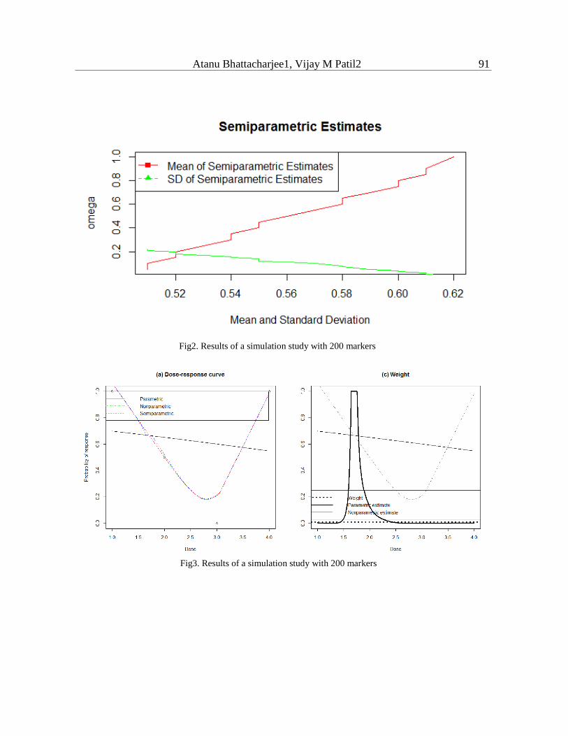
compute posterior quantities via Markov chain Monte Carlo(MCMC). The simulation study

results with semi-parametric approach are given in Figure 2. The Dose-Curve modeling

simulation is shown Figure 3.

5. Application to MC trial data set

The idea is to study the level of Scr to a restricted cycles of $m=6$ for duration of

administration 1,3,5,7,9 and 11th weeks. The maximum days to monitor the controlled level of

SM is specified as 𝜏 = 80 days. However, during the MC therapy the schedule has been

finalized for each patient. With individual specific prognostic function. The physician assumed

that the event of controlled level of SM for a single administration will be achieved by 10 days,


with a range of 7 to 80 days. The therapy is assigned to administer with different dose level

with 110 patients with parameter 𝜋𝑖∗ = 0.30, 휀 = 0.05, 𝜉 = 0.30 and 휀̅ = 0.90. It is assumed

that patients will attend the clinic in 7 days intervals. It is assumed that the parameter 𝑣1 will be

having the maximum value at the end of 7 days after the first administration. The derivation of

𝑎3, 𝑏3, for 𝑝(𝑣3), and 𝑎1 and 𝑏1 for 𝑝(𝑣1/𝑣3) are computed. The probabilities of event for

80days for each are detailed in Table6.

The proposed method has been illustrated on MC therapy. The results are detailed in Table

6 and corresponding data explored in Figure 4. It gives the dose-response estimation through

parametric, non-parametric and semi-parametric methods. The estimation of dose-increases

rapidly from 0.05 to 0.15, and thereafter slowly increases with dose. For doses, 0.20 and above

response started to decrease. Parametric, non-parametric and semi-parametric fits are more or

less identical with different doses. The weight assigned through semi-parametric method is 0.3

and parametric close to 0.4 and non-parametric with 0.05.

Criteria 1 and 2 are selected with 0.2< �̅� <0.6. It has been found that �̅�=0.60 performed best

over others. The table is formulated for $\bar{p}=0.6$ for both the criteria. The parameter 𝑣1is

assumed to be occurring at 7 days and 𝑣2 as 10 days to 40 days. The designs performed are

observed for criteria 1 and criteria 2. In different scenarios, the value of 𝑣2 is varied to reflect

which schedule is optimal for different values in Table1. The decision is obtained from the

Table of detailed value of 𝜂𝑚,𝑃1𝑚(𝐷𝑛), �̅�1𝑚(𝐷𝑛), and �̅�2𝑛+1(𝐷𝑛). The numerical values of the

different states are also detailed in Table 3. The Operating Characteristics of PRMOBD design

based on the choice of six different doses choice for the maximum duration of 80 days are

detailed in Table 4. The corresponding simulation result for the OBD design for the maximum

duration of 80 on 𝑃1𝑚(𝐷𝑛), �̅�2𝑚(𝐷𝑛), and�̅�2𝑚+1(𝐷𝑛) with the space of 5,10,20,40,60 and 80

days are given in table 5.The PRMOBD model suggests deciding the OBD with $0.20mg$ for

20days. It is expected that the trial with dose 0.35mg because it provides𝜉 = 0.20. It's the value

of $\eta=1$, then there would be a fixed OBD decided based on particular observed all cases.

Similarly, 𝜂 = 0 may influence to observe a less number of patients towards control the CEC

and the decision about OBD.

6. Discussion

The trinomial continual reassessment method is found suitable for OBD through highest

probability of but failed to consider the toxic effect suitably [Zhang2006]. The two stage

design is proposed on interim analysis for detecting the optimal dose [Polley 2008, Zang 2014]

proposed dose-finding designs to search for the OBD by three adaptive dose-finding designs

on molecularly targeted agents. Low-dose chemotherapy drugs are more effective to suppress

tumors by restraining tumor vessel growth and preventing the repair of damaged vascular

endothelial cells [Shen 2010]. High dose chemotherapy drugs like Cisplatin contributes to

serious side effects [Shen 2010]. The target of MC therapy is the vascular endothelial cells

[Shaked 2006,Wu 2007]. The growth of new vessels for a long run survival time treated with

traditional maximum tolerated dose (MTD) through high dose chemotherapy has been

confirmed [Lam 2007]. The anti-angiogenic plays the important role as clinical potential [Lu


2007]. The metastasis and the growth of tumor cells depends on neovascularization [Folkman

2003]. The anti-tumor drugs could cause inhibition of tumor neovascularity [Moreira 2007].

The Scr have emerged as a promising candidate surrogate marker to assess the efficacy of

antiangiogenic therapies [Malka 2011,Jubb 2006,Bhatt 2007,Bertolini 2006].The low-dose

chemotherapy drugs, as one-tenth of the MTD, administered continuously and frequently, could

selectively suppress vessel growth in tumor tissues and prevent the repair of damaged vascular

endothelial cells (VECs) [Shen 2010].This model is appropriate in dose-response modeling

having the avoidable level of toxicity in any clinical trial. Based on our knowledge this is the

first statistical methodological attempt that has been considered to deal with OBD in MC trial.

It is expected that this above mentioned methods will be useful for OBD detection in MC trials

in future as well.

Acknowledgments

The authors would like to thank the two anonymous referees for their cautious reading and

constructive suggestions which have led to improvement on earlier versions of the manuscript.

Conflict of Interest

None declared.

References

[1] Aghamohammadi, A, Meshkani, MR and Mohammadzadeh, M. (2010). A bayesian

approach to successive comparisons. Journal of Data Science 8(4), 541-553.

[2] Bertolini, F., Y.Shaked, Mancso, P. and others. (2006). The multifaceted circulating

endothelial cell in cancer:towards marker and target identi_cation. . Nat Rev Cancer 6,

835-845.

[3] Bhatt, RS., Seth, P. and Sukhatme, VP. (2007). Biomarkers for monitoring antiangiogenic

therapy. Clin Cancer Res 13, 777-780.

[4] Bhattacharjee, Atanu and Patil, Vijay M. (2016). Time-dependent area under the roc curve

for optimum biological dose detection. Turkiye Klinikleri Journal of Biostatistics

8(2),103-109.

[5] Briasoulis, Evangelos, Pappas, Periklis, Puozzo, Christian, Tolis, Christos, Fountzilas,

George, Dafni, Urania, Marselos, Marios and Pavlidis, Nicholas. (2009). Dose-ranging

study of metronomic oral vinorelbine in patients with advanced refractory cancer. Clinical

Cancer Research 15(20), 6454-6461.


[6] Dette, H. and Scheder, R. (2010). A _nite sample comparison of nonparametric estimates

of the effective dose in quantal bioassay. Journal of Statistical Computation and

Simulation 80,527-544.

[7] DeVita, T, Vincent and Chu, Edward. (2008). A history of cancer chemotherapy. Cancer

research 68(21), 8643-8653.

[8] Einsporn, R.L. (1987). A link between least squares regression and nonparametric curve

estimation. PhD Dissertation, Virginia Tech. Blacksburg.

[9] Folkman, J. (2003). Angiogenesis and apoptosis. Semin. Cancer Biol 13, 159-167.

[10] Golfinopoulos, Vassilis, Salanti, Georgia, Pavlidis, Nicholas and Ioannidis, John PA.

(2007). Survival and disease-progression benefits with treatment regimens for advanced

colorectal cancer: a meta-analysis. The lancet oncology 8(10), 898-911.

[11] Hobson, B and Denekamp, J. (1984). Endothelial proliferation in tumours and normal

tissues: continuous labelling studies. British journal of cancer 49(4), 405.

[12] Islam, Tamanna and Tsuiki, Mikinori. (2016). Spatial distribution of air dose rate in

grazing grassland. Journal of Data Science 14(1), 133-148.

[13] Jubb, Am., Oates, AJ., Holden, S. and others. (2006). Predicting bene_t for monitoring

antiangiogenic agent in malingnancy. Nat Rev Cancer 6, 626-635.

[14] Kerbel, RS., G.Klement, Pritchard, K. and B.Kamen. (2002). Continuous low-dose

antiangiogenic/metronomic chemotherapy: from the research laboratory into the oncology

clinic. Ann Oncol 13, 12-15.

[15] Kerbel, Robert S and Kamen, Barton A. (2004). The anti-angiogenic basis of metronomic

chemotherapy. Nature Reviews Cancer 4(6), 423-436.

[16] Kouassi, D.A. and Singh, J. (1997). A semiparametric approach to hazard estimation with

randomly censored observations. Journal of the American Statistical Association 92,

1351-1355.

[17] Lam, T., Hetherington, J.W., Greenman, J., Little, S. and Maraveyas, A. (2007).

Metronomic chemotherapy dosing-schedules with estramustine and temozolomide act

synergistically with anti-vegfr-2 antibody to cause inhibition of human umbilical venous

endothelial cell growth. Acta Oncol 46, 1169-1177.

[18] Lu, Q .B. (2007). Molecular reaction mechanisms of combination treatments of low-dose

cisplatin with radiotherapy and photodynamic therapy. J. Med. Chem 50, 2601-2604.


[19] Malka, D., V.Boige, N.Jacques, N.Vimond, .Adenis, A, E.Boucher, Pierga, J.Y.,T.Conroy,

B.Chauffert, E.Francois, Gichard, P., Galais, M.P. and others. (2011). Clinical value of

circulating endothelial cell levels in metastatic colorectal cancer patients treated with first-

line chemotherapy and behacizumab. Annals of Oncology 23, 919-927.

[20] Marshall, J.L. and Ruech, O.J. (2012). Maximum-tolerated dose, optimum biologic dose,or

optimum clinical value: Dosing determination of cancer therapies. Journal of Clinical

Oncology 30(23), 2815-2816.

[21] Mays, J. E., Birch, J.B and, B. A.Starnes. (2001). Model robust regression: Combining

parametric, nonparametric, and semiparametric methods. Journal of Nonparametric

Statistics 13, 245-277.

[22] Moreira, I.S., Fernandes, P.A. and Ramos, M.J. (2007). Vascular endothelial growth factor

(vegf) inhibition aAS a critical review. Anticancer Agents Med. Chem 7, 223-245.

[23] Mukhopadhyay, S. (2000). Bayesian nonparametric inference on the dose level with

specified response rate. Lancet Oncol 56, 220-226.

[24] Muller, H.G. and Schmitt, T. (1988). Kernel and probit estimates in quantal bioassay.

Journal of the American Statistical Association 83, 750-759.

[25] Olkin, I. and Spiegelman, C.H. (1987). A semiparametric approach to density

estimation.Journal of the American Statistical Association 82, 858-865.

[26] O'Quigley, J., Pepe, M. and L.Fisherr. (2006). Continual reassessment method: A practical

design for phase 1 clinical trials in cancerl. Biometrics 46(1), 33-48.

[27] Patil, Vijay Maruti, Noronha, Vanita, Joshi, Amit, Muddu, Vamshi Krishna, Dhumal,

Sachin, Bhosale, Bharatsingh, Arya, Supreeta, Juvekar, Shashikant, Banavali, Shripad,

D^a_A _ZCruz, Anil and others. (2015). A prospective randomized phase ii study

comparing metronomic chemotherapy with chemotherapy (single agent cisplatin), in

patients with metastatic, relapsed or inoperable squamous cell carcinoma of head and neck.

Oral oncology 51(3), 279-286.

[28] Pickle, M. G. S. M., T. J. Robinsonand, J. B. Birch and .Anderson-Cook, C. (2008). A

semi-parametirc approach to robust parameter design. Journal of Statistical Planning and

Inference 138, 114-131.

[29] Polley, M.Y. and Cheung, Y.K. (2008). Two-stage designs for dose-finding trials with a

biologic end-point using stepwise tests. Biometrics 64, 232-241.

[30] Robinson, T. J., Birch, J. B. and Starnes, A. (2010). A semiparametric approach to dual

modeling when no replication exists. Journal of Statistical Planning and Inference 140,

2860-2869.


[31] Rosemarie, M. and Ratain, M. J. (1993). Model-guided determination of maximum

tolerated dose in phase i clinical trials: Evidence for increased precision. JNCI J Natl

Cancer Inst 85(3), 217-223.

[32] Saltz, Leonard B. (2008). Progress in cancer care: the hope, the hype, and the gap between

reality and perception. Journal of Clinical Oncology 26(31), 5020-5021.

[33] Scharovsky, O.G., Mainetti, L.E. and Rozados, V.R. (2009). Metronomic chemotherapy:

changing the paradigm that more is better. Curr Oncol 16(2), 7-15.

[34] Schmid, Peter, Schippinger, Walter, Nitsch, Thorsten, Huebner, Gerdt, Heilmann, Volker,

Schultze, Wolfgang, Hausmaninger, Hubert, Wischnewsky, Manfred and Possinger, Kurt.

(2005). Up-front tandem high-dose chemotherapy compared with standard chemotherapy

with doxorubicin and paclitaxel in metastatic breast cancer: results of a randomized trial.

Journal of clinical oncology 23(3), 432-440.

[35] Schmoyer, R.L. (1984). Sigmoidally constrained maximum likelihood estimation in

quantal bioassay. Journal of the American Statistical Association 79, 448-453.

[36] Shaked, Y., Ciarrocchi, A., Franco, M. and others. (2006). Therapyinduced acute

recruitment of circulating endothelial progenitor cells to tumors. Science 313,

1785^a_A_S1787.

[37] Shen, F.Z., Wang, J., Liang, J., Mu, K., Hou, J.Y. and Wang, Y.T. (2010). Low-dose

metronomic chemotherapy with cisplatin: can it suppress angiogenesis in h22

hepatocarcinoma cells? Int J Exp Pathol 91(1), 10-16.

[38] Skipper, Howard E, Schabel Jr, Frank M, Mellett, L Bruce, Montgomery, John A, Wilkoff,

Lee J, Lloyd, Harris H and Brockman, R Wallace. (1970). Implications of biochemical,

cytokinetic, pharmacologic, and toxicologic relationships in the design of optimal

therapeutic schedules. Cancer chemotherapy reports. Part 1 54(6), 431.

[39] Vacca, Angelo, Iurlaro, Monica, Ribatti, Domenico, Minischetti, Monica, Nico, Beatrice,

Ria, Roberto, Pellegrino, Antonio and Dammacco, Franco. (1999). Antiangiogenesis is

produced by nontoxic doses of vinblastine. Blood 94(12), 414-4155.

[40] Waterman, M. J., Birch, J. B. and Schabengerger, O. (2007). Linear mixed model robust

regression. Wu, H., Chen, H. and Hu, P.C. (2007). Circulating endothelial cells and

endothelial progenitors as surrogate biomarkers in vascular dysfunction. Clin. Lab 53,

285-295.

[41] Yuan, Y. and Ying, G. (2011). Dose-response curve estimation: A semiparametric mixture.

Biometrics 67, 1543-1554.


[42] Y.Zang, Lee, J.J. and Y.Yuan. (2014). Adaptive designs for identifying optimal biological

dose for molecularly targeted agents. Clin Trials 11, 319-327.

[43] Zhang, W., Sargent, DJ. and Mandrekar, SJ. (2006). An adaptive dose-finding design

incorporating both toxicity and efficacy. Statistics in Medicine 25, 2365-2383. Received June 24, 2015; accepted December 13, 2016.

Atanu Bhattacharjee

Department of Biometrics

Chiltern Clinical Research Ltd

Bangalore, India.

Vijay M Patil

Department of Medical Oncology

Tata Memorial Hospital

Mumbai, India.

Fig1. Antiangiogenic Distribution


Fig2. Results of a simulation study with 200 markers

Fig3. Results of a simulation study with 200 markers


Fig4. Single administration of surrogate marker's distribution


Table 1 Simulation Different Dose Levels with 10 subject per dose

Model Different Dose Level

0.05 0.10 0.15 0.20 0.25 0.30

Probit 1 0 1.2 0 0 0 0.02

Probit 2 0 63.2 18.3 2.3 4.7 4.2

Table 2 Different Dose Levels with 10 subject per dose

Model Method Value of 𝐸𝐷𝛼 for 𝛼

0.1 0.20 0.3 0.4 0.5

Probit 1 Kernal Bias(x10−3) 9 3 2 1 0

MSE(x10−3) 4 3 3 2 2

Probit 2 Kernal Bias (x10−3) -8 -5 -3 0 1

MSE(x10−3) 30 15 6 4 3

Table 3 Simulation Study Results of PRMOBD design

True Probability

Total

Duration

𝑑1 𝑑2 𝑑3 𝑑4 𝑑5 𝑑6

S1 0.05 0.10 0.15 0.20 0.25 0.30

%Selected 0.10 0.20 0.13 0.06 0.26 0.31 60 days

No. of

Patients

5 9 6 3 12 14 45

No .of

Successive

Event

3 8 5 4 2 8

S2 0.10 0.15 0.20 0.25 0.30 0.35

%Selected 0.07 0.11 0.16 0.19 0.23 0.21 60 days

No. of

Patients

5 8 12 14 17 15 45

No .of

Successive

Event

4 5 3 5 7 6

S3 0.10 0.12 0.17 0.20 0.22 0.25

%Selected 0.26 0.22 0.12 0.16 0.16 0.08 60 days

No. of

Patients

13 11 6 8 8 4 45

No .of

Successive

Event

5 4 4 7 6 3


Table4 Operating Characteristics of PRMOBD Design

True Probability

Total

Duration

𝑑1 𝑑2 𝑑3 𝑑4 𝑑5 𝑑6

10 15 20 25 30 35

PRMOBD

%Selected 0.12 0.17 0.20 0.19 0.14 0.15 80 days

No. of

Patients

8 11 13 12 9 10 63

No .of

Successive

Event

6 8 7 6 5 1

Table5: Simulation Results for OBD Design

5 10 20 40 60 80

휀1 0.12 0.14 0.06 0.32 0.25 0.49

�̅�1𝑚(𝐷𝑛) 0.56 0.51 0.52 0.49 0.47 0.39

�̅�2𝑚(𝐷𝑛) 0.32 0.36 0.29 0.31 0.35 0.33

�̅�2𝑚+1(𝐷𝑛) 0.18 0.12 0.19 0.20 0.18 0.28

Table6: Decision Table for OBD in Different Days

7 10 20 40 80

휀1 0.15 0.12 0.03 0.85 0.36

�̅�1𝑚(𝐷𝑛) 0.53 0.57 0.69 0.39 0.35

�̅�2𝑚(𝐷𝑛) NA NA NA 0.02 0.03

�̅�2𝑚+1(𝐷𝑛) NA NA 0.01 NA NA

Table7: The surrogate Marker performance during MC Trial

Scenario Duration

of Event

100𝑣2 Different Schedule in Weeks

1(1) 2(3) 3(5) 4(7) 5(0) 6(11)

1 7 3.32 0.4 0.46 0.49 0.53 0.59 0.61

40 4.09 0.4 0.46 0.49 0.53 0.59 0.61

2 7 3.56 0.23 0.29 0.31 0.35 0.52 0.59

40 4.23 0.23 0.23 0.31 0.35 0.52 0.59

3 7 3.89 0.17 0.23 0.33 0.39 0.52 0.57

40 4.38 0.17 0.23 0.33 0.39 0.43 0.57

4 7 4.01 0.11 0.17 0.31 0.4 0.43 0.57

40 4.52 0.11 0.17 0.31 0.4 0.51 0.57

5 7 3.95 0.09 0.11 0.17 0.29 0.51 0.49

40 4.49 0.09 0.11 0.17 0.23 0.45 0.49

6 7 3.79 0.05 0.1 0.17 0.23 0.4 0.59

40 4.29 0.05 0.1 0.15 0.26 0.42 0.57

Documents

DETERMINING AN OPTIMUM BIOLOGICAL DOSE OF A … · Determining an Optimum Biological Dose of a Metronomic Chemotherapy However, in case of MC the toxicity is not a concern. As the