Embed Size (px)
Citation preview
PNNL-20030
Prepared for the U.S. Department of Energy under Contract DE-AC05-76RL01830
Determining Columbia and Snake River Project Tailrace and Forebay Zones of Hydraulic Influence Using MASS2 Modeling CL Rakowski MC Richmond JA Serkowski WA Perkins 2010
DISCLAIMER This report was prepared as an account of work sponsored by an agency of the United States Government. Neither the United States Government nor any agency thereof, nor Battelle Memorial Institute, nor any of their employees, makes any warranty, express or implied, or assumes any legal liability or responsibility for the accuracy, completeness, or usefulness of any information, apparatus, product, or process disclosed, or represents that its use would not infringe privately owned rights. Reference herein to any specific commercial product, process, or service by trade name, trademark, manufacturer, or otherwise does not necessarily constitute or imply its endorsement, recommendation, or favoring by the United States Government or any agency thereof, or Battelle Memorial Institute. The views and opinions of authors expressed herein do not necessarily state or reflect those of the United States Government or any agency thereof. PACIFIC NORTHWEST NATIONAL LABORATORY operated by BATTELLE for the UNITED STATES DEPARTMENT OF ENERGY under Contract DE-AC05-76RL01830 Printed in the United States of America Available to DOE and DOE contractors from the Office of Scientific and Technical Information,
P.O. Box 62, Oak Ridge, TN 37831-0062; ph: (865) 576-8401 fax: (865) 576-5728
email: [email protected] Available to the public from the National Technical Information Service, U.S. Department of Commerce, 5285 Port Royal Rd., Springfield, VA 22161
ph: (800) 553-6847 fax: (703) 605-6900
email: [email protected] online ordering: http://www.ntis.gov/ordering.htm
This document was printed on recycled paper.
(9/2003)
PNNL-20030
Determining Columbia and Snake River Project Tailrace and Forebay Zones of Hydraulic Influence Using MASS2 Modeling
CL Rakowski MC Richmond JA Serkowski WA Perkins
2010
Prepared for
U.S. Army Corps of Engineers
Portland District and Walla Walla District
Pacific Northwest National Laboratory
Richland, Washington 99352

Summary
Fisheries biology studies are frequently performed at U.S. Army Corps of Engineers (USACE)projects along the Columbia and Snake Rivers, and the results are presented relative to the “fore-bay” and “tailrace” regions. At this time, each study may use somewhat arbitrary locations (e.g.,the Boat Restriction Zone) to define the upstream and downstream limits of the study. The arbi-trariness of the delineations could create inconsistencies between projects and make it difficultto draw conclusions involving multiple projects. To overcome this concern, USACE fisheriesresearchers are interested in establishing a consistent definition of project forebay and tailraceregions for the hydroelectric projects on the lower Columbia and Snake rivers.
The hydraulic extent of a project was defined by USACE CENWP(a) as follows: The riverreach directly upstream (forebay) and downstream (tailrace) of a project that is influenced by thenormal range of dam operations. Outside this reach, for a particular river discharge, changes indam operations cannot be detected by hydraulic measurement.
In other words, the hydraulic extent is the zone where the flow direction or velocity can beinfluened by how the flow is distributed through the powerhouse and spillway bays at a project,i.e., the percent of spill flow, the spill pattern, and the turbines that are operational.
The purpose of this study was to develop and apply a consistent set of criteria for determining thehydraulic extent of each of the projects in the lower Columbia and Snake rivers. This was donein consultation with USACE and regional representatives,
A 2D depth-averaged river model, MASS2, was applied to the Snake and Columbia Rivers.New computational meshes were developed for most reaches, and the underlying bathymetricdata were updated to include the most current survey data. These computational meshes weresufficient to resolve each spillway bay and turbine unit at each project, and they extended fromthe tailrace of one project to the forebay of the downstream project.
MASS2 was run for a range of total river flows and, for each total river flow, a range of projectoperations at each project. The modeled flow was analyzed to determine the range of velocitymagnitude differences and the range of flow direction differences at each location in the com-putational mesh for each total river flow. Maps of the differences in flow direction and velocitymagnitude were created.
After reviewing the preliminary results, USACE fishery biologists requested data analysis todetermine the project hydraulic extent based on the following criteria:
• If mean water velocity is less than 4 ft/s, the differences in the magnitude water velocitybetween operations are not greater than 0.5 ft/s or the differences in water flow direction(azimuth) are not greater than 10°.
(a) Brad Eppard, USACE, CENWP in “Project Boundaries for Bonneville, The Dalles, and JohnDay Dams,” April 2010.
iii
• If mean water velocity is 4.0 ft/s or greater, the project hydraulic extent is determined usingthe differences in water flow direction (i.e., not greater than 10°).
Based on these criteria, and excluding areas with a mean velocity of less than 0.1 ft/s (within theerror of the model), a final set of graphics was developed that included data from all flows and alloperations.
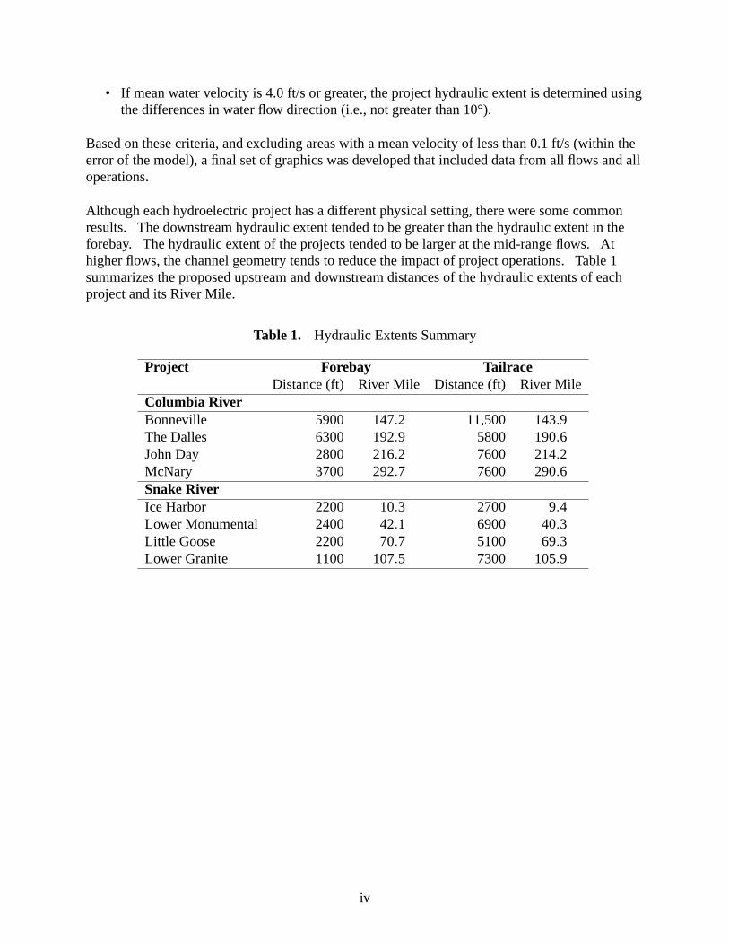
Although each hydroelectric project has a different physical setting, there were some commonresults. The downstream hydraulic extent tended to be greater than the hydraulic extent in theforebay. The hydraulic extent of the projects tended to be larger at the mid-range flows. Athigher flows, the channel geometry tends to reduce the impact of project operations. Table 1summarizes the proposed upstream and downstream distances of the hydraulic extents of eachproject and its River Mile.
Table 1. Hydraulic Extents Summary
Project Forebay TailraceDistance (ft) River Mile Distance (ft) River Mile
Columbia RiverBonneville 5900 147.2 11,500 143.9The Dalles 6300 192.9 5800 190.6John Day 2800 216.2 7600 214.2McNary 3700 292.7 7600 290.6Snake RiverIce Harbor 2200 10.3 2700 9.4Lower Monumental 2400 42.1 6900 40.3Little Goose 2200 70.7 5100 69.3Lower Granite 1100 107.5 7300 105.9
iv
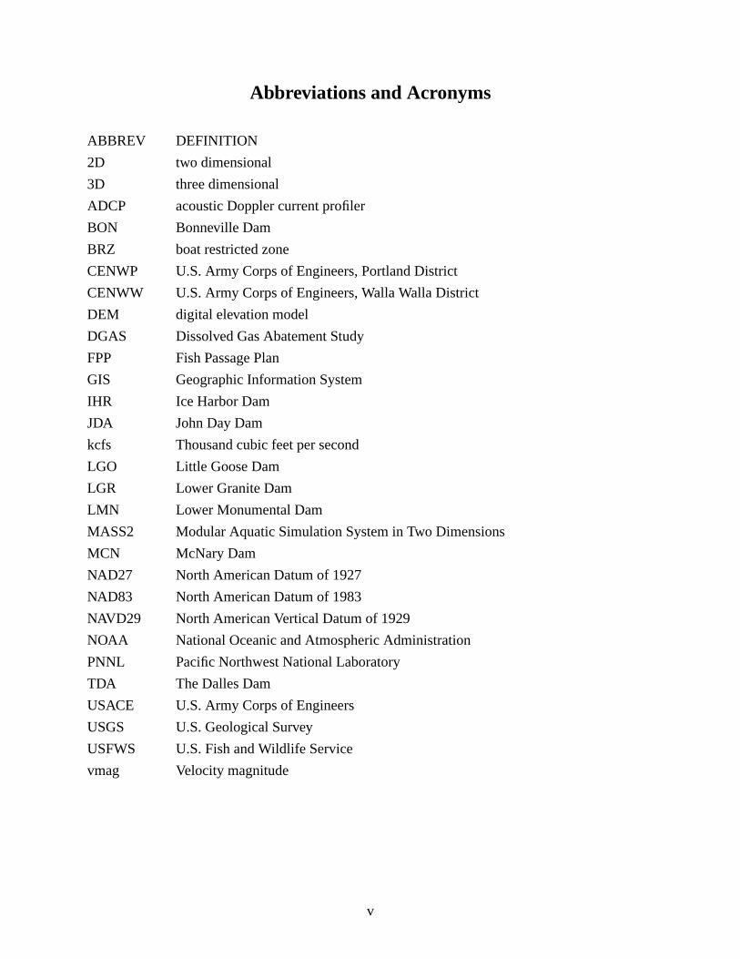
Abbreviations and Acronyms
ABBREV DEFINITION
2D two dimensional
3D three dimensional
ADCP acoustic Doppler current profiler
BON Bonneville Dam
BRZ boat restricted zone
CENWP U.S. Army Corps of Engineers, Portland District
CENWW U.S. Army Corps of Engineers, Walla Walla District
DEM digital elevation model
DGAS Dissolved Gas Abatement Study
FPP Fish Passage Plan
GIS Geographic Information System
IHR Ice Harbor Dam
JDA John Day Dam
kcfs Thousand cubic feet per second
LGO Little Goose Dam
LGR Lower Granite Dam
LMN Lower Monumental Dam
MASS2 Modular Aquatic Simulation System in Two Dimensions
MCN McNary Dam
NAD27 North American Datum of 1927
NAD83 North American Datum of 1983
NAVD29 North American Vertical Datum of 1929
NOAA National Oceanic and Atmospheric Administration
PNNL Pacific Northwest National Laboratory
TDA The Dalles Dam
USACE U.S. Army Corps of Engineers
USGS U.S. Geological Survey
USFWS U.S. Fish and Wildlife Service
vmag Velocity magnitude
v


Acknowledgments
Financial support for this study was provided by the U.S. Army Corps of Engineers (USACE)under MIPR W66QKZ93383147. The authors would like to thank Laurie Ebner, Brad Eppard(USACE, Portland District) and Ryan Laughery and Ann Setter (USACE, Walla Walla District)for the discussions, support, and insight that improved this study. Lyle Hibler provided com-ments that improved this report.
vii

Contents
Summary . . . . . . . . . . . . . . . . . . . . . . . . . . . . . . . . . . . . . . . . . iii
Abbreviations and Acronyms. . . . . . . . . . . . . . . . . . . . . . . . . . . . . . . v
Acknowledgments. . . . . . . . . . . . . . . . . . . . . . . . . . . . . . . . . . . . . vii
1.0 Introduction. . . . . . . . . . . . . . . . . . . . . . . . . . . . . . . . . . . . . . 1.1
2.0 Methods . . . . . . . . . . . . . . . . . . . . . . . . . . . . . . . . . . . . . . . 2.1
2.1 MASS2 Model—General Description . . . . . . . . . . . . . . . . . . . . . . . 2.1
2.2 Bathymetry and Shorelines . . . . . . . . . . . . . . . . . . . . . . . . . . . . . 2.1
2.3 Computational Meshes . . . . . . . . . . . . . . . . . . . . . . . . . . . . . . . 2.12
2.3.1 Bonneville Tailrace and Tidal Reach . . . . . . . . . . . . . . . . . . . 2.12
2.3.2 Bonneville Pool . . . . . . . . . . . . . . . . . . . . . . . . . . . . . . 2.12
2.3.3 The Dalles Pool . . . . . . . . . . . . . . . . . . . . . . . . . . . . . . 2.12
2.3.4 John Day Pool . . . . . . . . . . . . . . . . . . . . . . . . . . . . . . . 2.15
2.3.5 McNary Pool up to Ice Harbor Dam . . . . . . . . . . . . . . . . . . . . 2.15
2.3.6 Lower Monumental Pool . . . . . . . . . . . . . . . . . . . . . . . . . . 2.15
2.4 Model Configuration and Scenarios . . . . . . . . . . . . . . . . . . . . . . . . 2.22
2.4.1 General MASS2 Configuration . . . . . . . . . . . . . . . . . . . . . . 2.22
2.4.2 Bonneville Project . . . . . . . . . . . . . . . . . . . . . . . . . . . . . 2.23
2.4.3 The Dalles Project . . . . . . . . . . . . . . . . . . . . . . . . . . . . . 2.25
2.4.4 John Day Project . . . . . . . . . . . . . . . . . . . . . . . . . . . . . . 2.27
2.4.5 McNary Project . . . . . . . . . . . . . . . . . . . . . . . . . . . . . . 2.29
2.4.6 Ice Harbor Project . . . . . . . . . . . . . . . . . . . . . . . . . . . . . 2.31
2.4.7 Lower Monumental Project . . . . . . . . . . . . . . . . . . . . . . . . 2.33
ix
2.4.8 Little Goose Project . . . . . . . . . . . . . . . . . . . . . . . . . . . . 2.34
2.4.9 Lower Granite Project . . . . . . . . . . . . . . . . . . . . . . . . . . . 2.35
2.5 Analysis of Simulation Data . . . . . . . . . . . . . . . . . . . . . . . . . . . . 2.36
3.0 Results and Discussion. . . . . . . . . . . . . . . . . . . . . . . . . . . . . . . . 3.1
3.1 Bonneville Project . . . . . . . . . . . . . . . . . . . . . . . . . . . . . . . . . 3.1
3.2 The Dalles Project . . . . . . . . . . . . . . . . . . . . . . . . . . . . . . . . . 3.7
3.3 John Day Project . . . . . . . . . . . . . . . . . . . . . . . . . . . . . . . . . . 3.12
3.4 McNary Project . . . . . . . . . . . . . . . . . . . . . . . . . . . . . . . . . . . 3.17
3.5 Ice Harbor Project . . . . . . . . . . . . . . . . . . . . . . . . . . . . . . . . . 3.22
3.6 Lower Monumental Project . . . . . . . . . . . . . . . . . . . . . . . . . . . . 3.27
3.7 Little Goose Project . . . . . . . . . . . . . . . . . . . . . . . . . . . . . . . . 3.32
3.8 Lower Granite Project . . . . . . . . . . . . . . . . . . . . . . . . . . . . . . . 3.37
3.9 Hydraulic Extents . . . . . . . . . . . . . . . . . . . . . . . . . . . . . . . . . . 3.42
4.0 Conclusions. . . . . . . . . . . . . . . . . . . . . . . . . . . . . . . . . . . . . . 4.1
5.0 References. . . . . . . . . . . . . . . . . . . . . . . . . . . . . . . . . . . . . . 5.1
x
Figures
1.1 Location of the Walla Walla District Projects and Portland District Projects . . . . . 1.2
2.1 Bathymetry and Computational Mesh near the Bonneville Project . . . . . . . . . . 2.13
2.2 Bathymetry and Computational Mesh near The Dalles Project . . . . . . . . . . . . 2.14
2.3 Bathymetry and Computational Mesh near the John Day Project . . . . . . . . . . . 2.16
2.4 Bathymetry and Computational Mesh near the McNary Project . . . . . . . . . . . 2.17
2.5 Bathymetry and Computational Mesh near the Ice Harbor Project . . . . . . . . . . 2.18
2.6 Bathymetry and Computational Mesh near the Lower Monumental Project . . . . . 2.19
2.7 Bathymetry and Computational Mesh near the Little Goose Project . . . . . . . . . 2.20
2.8 Bathymetry and Computational Mesh near the Lower Granite Project . . . . . . . . 2.21
3.1 Bonneville Dam for 150 kcfs . . . . . . . . . . . . . . . . . . . . . . . . . . . . . 3.3
3.2 Bonneville Dam for 250 kcfs . . . . . . . . . . . . . . . . . . . . . . . . . . . . . 3.4
3.3 Bonneville Dam for 350 kcfs . . . . . . . . . . . . . . . . . . . . . . . . . . . . . 3.5
3.4 Bonneville Dam for 450 kcfs . . . . . . . . . . . . . . . . . . . . . . . . . . . . . 3.6
3.5 The Dalles Project for 150 kcfs . . . . . . . . . . . . . . . . . . . . . . . . . . . . 3.8
3.6 The Dalles Project for 250 kcfs . . . . . . . . . . . . . . . . . . . . . . . . . . . . 3.9
3.7 The Dalles Project for 270 kcfs . . . . . . . . . . . . . . . . . . . . . . . . . . . . 3.10
3.8 The Dalles Project for 450 kcfs . . . . . . . . . . . . . . . . . . . . . . . . . . . . 3.11
3.9 John Day Project for 150 kcfs . . . . . . . . . . . . . . . . . . . . . . . . . . . . . 3.13
3.10 John Day Project for 250 kcfs . . . . . . . . . . . . . . . . . . . . . . . . . . . . . 3.14
3.11 John Day Project for 320 kcfs . . . . . . . . . . . . . . . . . . . . . . . . . . . . . 3.15
3.12 John Day Project for 450 kcfs . . . . . . . . . . . . . . . . . . . . . . . . . . . . . 3.16
3.13 McNary Project for 100 kcfs . . . . . . . . . . . . . . . . . . . . . . . . . . . . . 3.18
xi
3.14 McNary Project for 150 kcfs . . . . . . . . . . . . . . . . . . . . . . . . . . . . . 3.19
3.15 McNary Project for 250 kcfs . . . . . . . . . . . . . . . . . . . . . . . . . . . . . 3.20
3.16 McNary Project for 350 kcfs . . . . . . . . . . . . . . . . . . . . . . . . . . . . . 3.21
3.17 Ice Harbor Project for 19 kcfs . . . . . . . . . . . . . . . . . . . . . . . . . . . . . 3.23
3.18 Ice Harbor Project for 30 kcfs . . . . . . . . . . . . . . . . . . . . . . . . . . . . . 3.24
3.19 Ice Harbor Project for 85 kcfs . . . . . . . . . . . . . . . . . . . . . . . . . . . . . 3.25
3.20 Ice Harbor Project for 120 kcfs . . . . . . . . . . . . . . . . . . . . . . . . . . . . 3.26
3.21 Lower Monumental Project for 19 kcfs . . . . . . . . . . . . . . . . . . . . . . . . 3.28
3.22 Lower Monumental Project for 30 kcfs . . . . . . . . . . . . . . . . . . . . . . . . 3.29
3.23 Lower Monumental Project for 85 kcfs . . . . . . . . . . . . . . . . . . . . . . . . 3.30
3.24 Lower Monumental Project for 120 kcfs . . . . . . . . . . . . . . . . . . . . . . . 3.31
3.25 Little Goose Project for 19 kcfs . . . . . . . . . . . . . . . . . . . . . . . . . . . . 3.33
3.26 Little Goose Project for 30 kcfs . . . . . . . . . . . . . . . . . . . . . . . . . . . . 3.34
3.27 Little Goose Project for 85 kcfs . . . . . . . . . . . . . . . . . . . . . . . . . . . . 3.35
3.28 Little Goose Project for 120 kcfs . . . . . . . . . . . . . . . . . . . . . . . . . . . 3.36
3.29 Lower Granite Project for 19 kcfs . . . . . . . . . . . . . . . . . . . . . . . . . . . 3.38
3.30 Lower Granite Project for 30 kcfs . . . . . . . . . . . . . . . . . . . . . . . . . . . 3.39
3.31 Lower Granite Project for 85 kcfs . . . . . . . . . . . . . . . . . . . . . . . . . . . 3.40
3.32 Lower Granite Project for 120 kcfs . . . . . . . . . . . . . . . . . . . . . . . . . . 3.41
3.33 Bonneville Proposed Hydraulic Extents . . . . . . . . . . . . . . . . . . . . . . . . 3.43
3.34 The Dalles Project Proposed Hydraulic Extents . . . . . . . . . . . . . . . . . . . 3.44
3.35 John Day Project Proposed Hydraulic Extents . . . . . . . . . . . . . . . . . . . . 3.45
3.36 McNary Project Proposed Hydraulic Extents . . . . . . . . . . . . . . . . . . . . . 3.46
xii

3.37 Ice Harbor Project Proposed Hydraulic Extents . . . . . . . . . . . . . . . . . . . . 3.47
3.38 Lower Monumental Project Proposed Hydraulic Extents . . . . . . . . . . . . . . . 3.48
3.39 Little Goose Project Proposed Hydraulic Extents . . . . . . . . . . . . . . . . . . . 3.49
3.40 Lower Granite Project Proposed Hydraulic Extents . . . . . . . . . . . . . . . . . . 3.50
xiii
Tables
1 Hydraulic Extents Summary . . . . . . . . . . . . . . . . . . . . . . . . . . . . . . iv
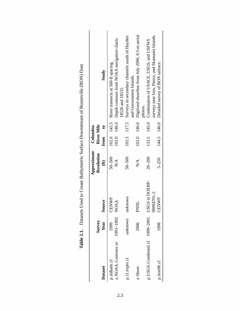
2.1 Datasets Used to Create Bathymetric Surface Downstream of Bonneville (BON)Dam . . . . . . . . . . . . . . . . . . . . . . . . . . . . . . . . . . . . . . . . . . 2.3
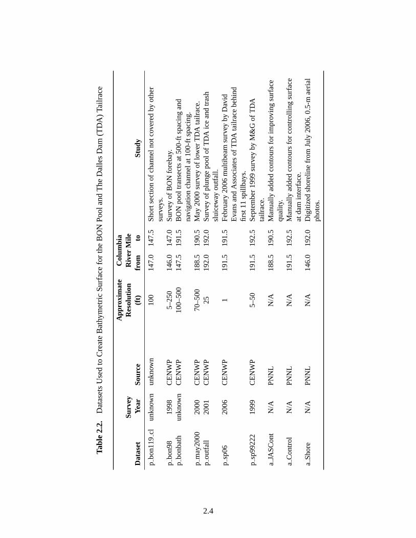
2.2 Datasets Used to Create Bathymetric Surface for the BON Pool and The Dalles Dam(TDA) Tailrace . . . . . . . . . . . . . . . . . . . . . . . . . . . . . . . . . . . . . 2.4
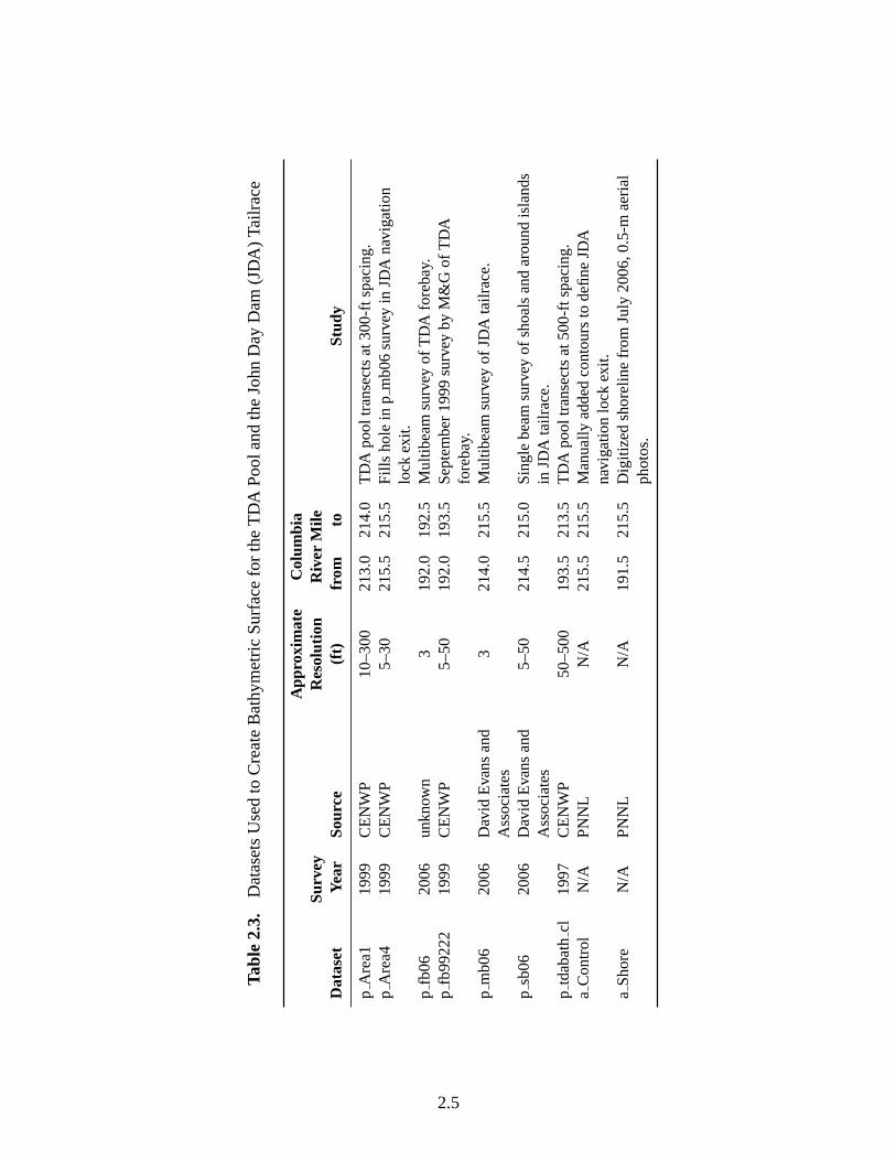
2.3 Datasets Used to Create Bathymetric Surface for the TDA Pool and the John DayDam (JDA) Tailrace . . . . . . . . . . . . . . . . . . . . . . . . . . . . . . . . . . 2.5
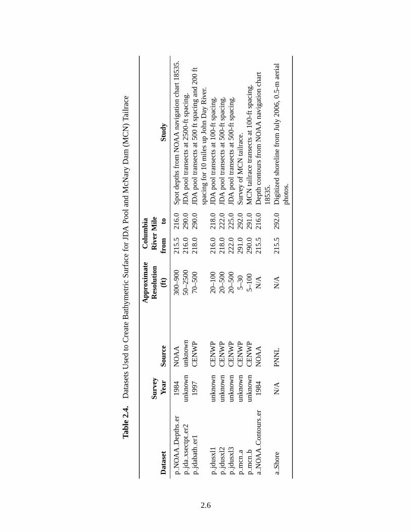
2.4 Datasets Used to Create Bathymetric Surface for JDA Pool and McNary Dam (MCN)Tailrace . . . . . . . . . . . . . . . . . . . . . . . . . . . . . . . . . . . . . . . . 2.6
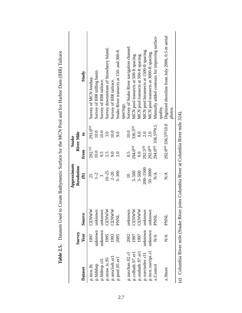
2.5 Datasets Used to Create Bathymetric Surface for the MCN Pool and Ice HarborDam (IHR) Tailrace . . . . . . . . . . . . . . . . . . . . . . . . . . . . . . . . . . 2.7
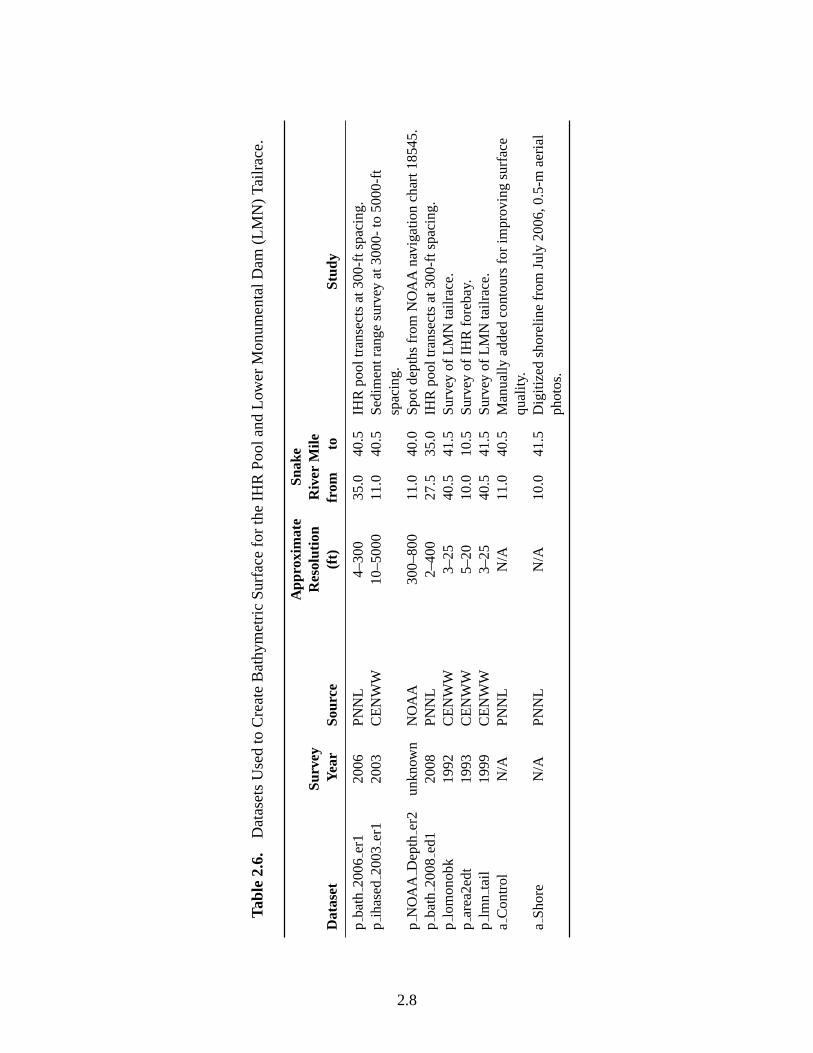
2.6 Datasets Used to Create Bathymetric Surface for the IHR Pool and Lower Mon-umental Dam (LMN) Tailrace. . . . . . . . . . . . . . . . . . . . . . . . . . . . . 2.8
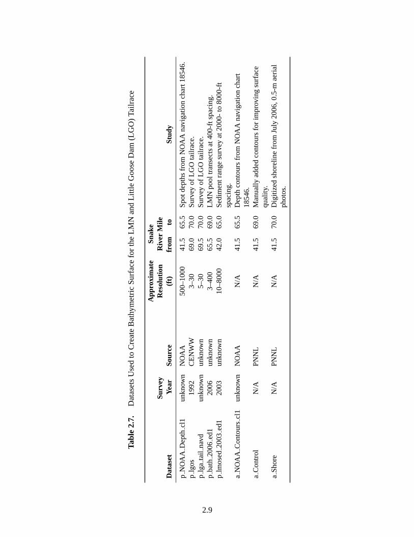
2.7 Datasets Used to Create Bathymetric Surface for the LMN and Little Goose Dam(LGO) Tailrace . . . . . . . . . . . . . . . . . . . . . . . . . . . . . . . . . . . . 2.9
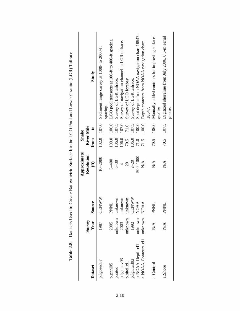
2.8 Datasets Used to Create Bathymetric Surface for the LGO Pool and Lower Gran-ite (LGR) Tailrace . . . . . . . . . . . . . . . . . . . . . . . . . . . . . . . . . . . 2.10
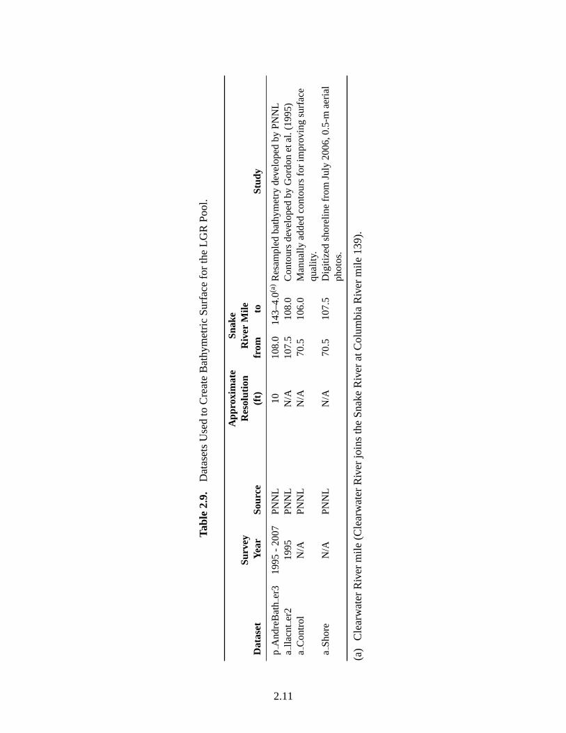
2.9 Datasets Used to Create Bathymetric Surface for the LGR Pool. . . . . . . . . . . . 2.11
2.10 Bonneville Scenarios . . . . . . . . . . . . . . . . . . . . . . . . . . . . . . . . . 2.23
2.11 Bonneville Powerhouse 1 and Powerhouse 2 Operations . . . . . . . . . . . . . . . 2.24
2.12 The Dalles Scenarios . . . . . . . . . . . . . . . . . . . . . . . . . . . . . . . . . 2.25
2.13 The Dalles Operations . . . . . . . . . . . . . . . . . . . . . . . . . . . . . . . . . 2.26
2.14 John Day Project Scenarios . . . . . . . . . . . . . . . . . . . . . . . . . . . . . . 2.27
2.15 John Day Operations . . . . . . . . . . . . . . . . . . . . . . . . . . . . . . . . . 2.28
2.16 McNary Scenarios . . . . . . . . . . . . . . . . . . . . . . . . . . . . . . . . . . . 2.29
2.17 McNary Operations . . . . . . . . . . . . . . . . . . . . . . . . . . . . . . . . . . 2.30
xiv
2.18 Ice Harbor Scenarios . . . . . . . . . . . . . . . . . . . . . . . . . . . . . . . . . 2.31
2.19 Ice Harbor Operations . . . . . . . . . . . . . . . . . . . . . . . . . . . . . . . . . 2.32
2.20 Lower Monumental Scenarios . . . . . . . . . . . . . . . . . . . . . . . . . . . . . 2.33
2.21 Lower Monumental Operations . . . . . . . . . . . . . . . . . . . . . . . . . . . . 2.33
2.22 Little Goose Scenarios . . . . . . . . . . . . . . . . . . . . . . . . . . . . . . . . . 2.34
2.23 Little Goose Operations . . . . . . . . . . . . . . . . . . . . . . . . . . . . . . . . 2.34
2.24 Lower Granite Scenarios . . . . . . . . . . . . . . . . . . . . . . . . . . . . . . . 2.35
2.25 Lower Granite Operations . . . . . . . . . . . . . . . . . . . . . . . . . . . . . . . 2.35
3.1 Hydraulic Extents Summary . . . . . . . . . . . . . . . . . . . . . . . . . . . . . . 3.42
xv

1.0 Introduction
Although fisheries biology studies are frequently performed at U.S. Army Corps of Engineers(USACE) projects along the Columbia and Snake Rivers, currently there is no consistent defini-tion of the “forebay” and “tailrace” regions for these studies. At this time, each study may usesomewhat arbitrary lines (e.g., the Boat Restriction Zone) to define the upstream and downstreamlimits of the study, which may be significantly different at each project. Fisheries researchers areinterested in establishing a consistent definition of project forebay and tailrace regions that definethe hydraulic extent of a project. The hydraulic extent was defined by USACE (Brad Eppard,USACE Portland District (CENWP)) as follows: The river reach directly upstream (forebay)and downstream (tailrace) of a project that is influenced by the normal range of dam operations.Outside this reach, for a particular river discharge, changes in dam operations cannot be detectedby hydraulic measurement.
The purpose of this project is to develop standard procedures to determine the operationallyinfluenced extent of the forebay and tailrace regions in accordance with the following definitions:
• Forebay: The segment of river immediately upstream of a dam where operations at thedam are the primary contributing factor to velocity and direction of water flow. Theupstream boundary defines the upstream limit where operational changes affect watervelocity magnitude and direction.
• Tailrace: The segment of river immediately downstream of a dam where operations atthe dam are the primary contributing factor to velocity and direction of water flow. Thedownstream boundary defines the downstream limit where operational changes affect watervelocity magnitude and direction.
In 2008, Pacific Northwest National Laboratory (PNNL) used the John Day project as the testcase to establish the modeling methodology and criteria to define areas affected by project oper-ations at John Day in both the forebay and tailrace (Rakowski et al. 2008a). It was assumedthat the forebay and tailrace definition could be adequately defined using a two-dimensional(2D) depth-averaged modeling approach instead of a true three-dimensional (3D) modelingeffort. Using the 2D MASS2 model (Perkins and Richmond 2004b) saves significant compu-tational time, especially given the large number of operational scenarios that must be simulated.Assessment criteria included the selection of river flows and hydraulic comparisons (velocitymagnitude, direction, and/or tolerances).
In this study, the methodology and criteria established in Rakowski et al. (2008a) were applied toother projects on the Columbia and Snake Rivers (Figure 1.1) to define their respective forebayand tailrace regions for CENWP and USACE Walla Walla District (CENWW). Based on inputfrom regional fisheries biologists, some of the criteria were modified for this work.
1.1
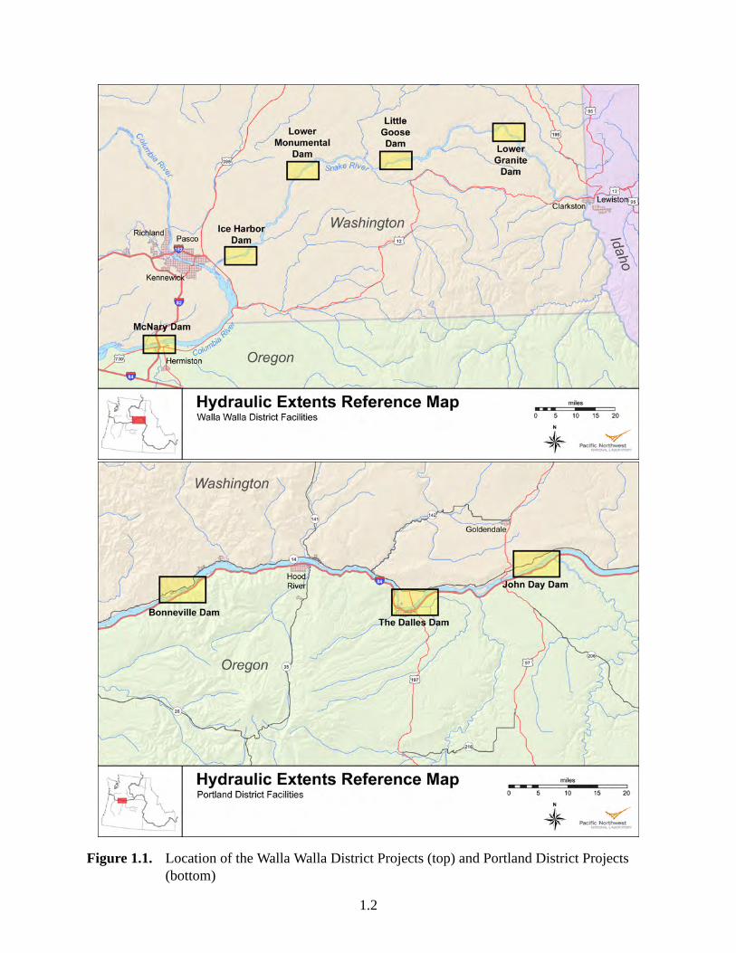
Figure 1.1. Location of the Walla Walla District Projects (top) and Portland District Projects(bottom)
1.2
2.0 Methods
This work used the approach described by Rakowski et al. (2008a). However, rather than relyingon existing computational meshes, the meshes used in the present study had increased resolutionnear the hydro projects. The bathymetry was updated to incorporate the most current survey dataavailable.
2.1 MASS2 Model—General Description
The Modular Aquatic Simulation System in 2 Dimensions (MASS2) was developed at PNNL(Perkins and Richmond 2004a,c) and has been successfully applied to a variety of river andestuarine flows (Richmond et al. 1999a, Rakowski and Richmond 2001, 2003, Rakowski et al.2008b), water quality (Richmond et al. 1999b,c, 2000, Kincaid et al. 2001) and aquatic habitat(McMichael et al. 2003, Perkins et al. 2004, Hanrahan et al. 2007) problems.
MASS2 is formulated using the general finite-volume principles described by Patankar (1980).The model uses a structured multi-block scheme using a curvilinear computational mesh. Spa-sojevic and Holly (1990) give an example of a 2D model of this type. The momentum and massconservation equations are coupled with a variation of the Patankar (1980) SIMPLE algorithmextended to shallow-water flows by Zhou (1995). In MASS2, Zhou’s method has been appliedto orthogonal curvilinear coordinates. In this method, the continuity equation is discretized andsolved for a depth correction in lieu of the pressure correction in the original SIMPLE algorithm.The solution to the depth correction equation is used to correct the estimated velocity fromthe solution of the momentum equations. A portion of the depth correction is used to adjustdepth. An in-depth description of the underlying theory for MASS2 is in Perkins and Richmond(2004a).
MASS2 is a depth-averaged river model. Although it works well and matches validation data inthe river, the results in areas with highly 3D flows should be used with caution. The meshes ofthis study were designed for testing the upstream and downstream extents of impacts of projectflow distributions rather than the details of flow very near the projects.
2.2 Bathymetry and Shorelines
Bathymetric surfaces were created with point and contour elevation data from a variety ofsources. Datasets consisted primarily of point soundings from single- and multi-beam acous-tic surveys provided by USACE. Where such surveys were unavailable, National Oceanic andAtmospheric Administration (NOAA) navigation charts filled in the gaps. The channel shore-lines were manually digitized from high-resolution (0.5 m) aerial photography obtained fromthe U.S. Geological Survey (USGS) seamless server (http://seamless.usgs.gov), and assigned anelevation appropriate for the date of the imagery. That elevation was determined using the dateof the photo, and then the elevation was estimated from the average of the DART forebay ele-vations measured during the month when the photo was taken. Typically, the elevations duringJuly 2006 (when the photos were taken) fluctuated no more than about 1 ft. Thirty-meter digitalelevation model (DEM) points, also from the USGS, provided near-shore topography data toproduce a smoother transition between the shoreline and bathymetric datasets.
2.1
The elevation datasets were imported into ArcGISTM version 9.3.1 (ESRI, Inc.), a geographicinformation system (GIS), for storage, display, and processing. All datasets were projected intoWashington State Plane South coordinates (in meters) using the North American Datum of 1983(NAD83). Elevation data were generally received in the North American Vertical Datum of1929 (NAVD29) and this was established as the standard. The point positions and elevationswere examined for anomalies, and problem data were rejected. Where domains overlapped, bothdatasets were generally used, unless one of the datasets was considerably less reliable than theother, in which case it was excluded. The shoreline dataset defined the boundary between thetopographic (DEM) and bathymetric data, and bathymetric points residing on the upland side ofthe shoreline were rejected.
Each bathymetric surface was produced with a script run in ArcGIS. The script gathered theappropriate datasets for the reach, interpolated the elevations onto a uniform raster grid, andprojected the result into Oregon State Plane North coordinates (in feet) using the North AmericanDatum of 1927 (NAD27). The raster grid cell size was set to 10 m, which is somewhat smallerthan the smallest hydrodynamic model grid cell size.
Tables 2.1 to 2.9 summarize the source datasets used to create each of the bathymetric surfaces.Figures 2.1 to 2.8 show the bathymetric surfaces near each project. Note that in these figures,the overlying mesh is the MASS2 mesh,not the bathymetric surface mesh, and the contourintervals are different for each mesh.
2.2
Tabl
e2.
1.D
atas
ets
Use
dto
Cre
ate
Bat
hym
etric
Sur
face
Dow
nstr
eam
ofB
onne
ville
(BO
N)
Dam
App
roxi
mat
eC
olum
bia
Sur
vey
Res
olut
ion
Riv
erM
ileD
atas
etYe
arS
ourc
e(f
t)fr
omto
Stu
dy
ptid
bath
cl19
99C
EN
WP
50–5
0010
2.0
145.
5R
iver
tran
sect
sat
500-
ftsp
acin
g.a
NO
AA
Con
tour
ser
1991
–199
2N
OA
AN
/A10
2.0
146.
0D
epth
cont
ours
from
NO
AA
navi
gatio
nch
arts
1852
6an
d18
531.
pcl
expt
scl
unkn
own
unkn
own
50–5
0010
2.5
117.
5S
urve
ysin
seco
ndar
ych
anne
lsso
uth
ofH
ayde
nan
dG
over
nmen
tIsl
ands
.a
Sho
re20
06P
NN
LN
/A10
2.0
146.
0D
igiti
zed
shor
elin
efr
omJu
ly20
06,0
.5-m
aeria
lph
otos
.p
US
GS
Com
bine
dcl
1999
–200
1U
SG
Sin
DO
EB
P-
0000
4701
-220
–200
133.
514
5.0
Com
bina
tion
ofU
SA
CE
,US
GS
,and
US
FW
Ssu
rvey
sne
arIv
es,P
ierc
e,an
dS
kam
ania
Isla
nds.
pbo
n98
cl19
98C
EN
WP
5–25
014
4.5
146.
0D
etai
led
surv
eyof
BO
Nta
ilrac
e.
2.3
Tabl
e2.
2.D
atas
ets
Use
dto
Cre
ate
Bat
hym
etric
Sur
face
for
the
BO
NP
oola
ndT
heD
alle
sD
am(T
DA
)Ta
ilrac
e
App
roxi
mat
eC
olum
bia
Sur
vey
Res
olut
ion
Riv
erM
ileD
atas
etYe
arS
ourc
e(f
t)fr
omto
Stu
dy
pbo
n119
clun
know
nun
know
n10
014
7.0
147.
5S
hort
sect
ion
ofch
anne
lnot
cove
red
byot
her
surv
eys.
pbo
n98
1998
CE
NW
P5–
250
146.
014
7.0
Sur
vey
ofB
ON
fore
bay.
pbo
nbat
hun
know
nC
EN
WP
100–
500
147.
519
1.5
BO
Npo
oltr
anse
cts
at50
0-ft
spac
ing
and
navi
gatio
nch
anne
lat1
00-f
tspa
cing
.p
may
2000
2000
CE
NW
P70
–500
188.
519
0.5
May
2000
surv
eyof
low
erT
DA
tailr
ace.
pou
tfall
2001
CE
NW
P25
192.
019
2.0
Sur
vey
ofpl
unge
pool
ofT
DA
ice
and
tras
hsl
uice
way
outfa
ll.p
sp06
2006
CE
NW
P1
191.
519
1.5
Feb
ruar
y20
06m
ultib
eam
surv
eyby
Dav
idE
vans
and
Ass
ocia
tes
ofT
DA
tailr
ace
behi
ndfir
st11
spill
bays
.p
sp99
222
1999
CE
NW
P5–
5019
1.5
192.
5S
epte
mbe
r19
99su
rvey
byM
&G
ofT
DA
tailr
ace.
aJA
SC
ont
N/A
PN
NL
N/A
188.
519
0.5
Man
ually
adde
dco
ntou
rsfo
rim
prov
ing
surf
ace
qual
ity.
aC
ontr
olN
/AP
NN
LN
/A19
1.5
192.
5M
anua
llyad
ded
cont
ours
for
cont
rolli
ngsu
rfac
eat
dam
inte
rfac
e.a
Sho
reN
/AP
NN
LN
/A14
6.0
192.
0D
igiti
zed
shor
elin
efr
omJu
ly20
06,0
.5-m
aeria
lph
otos
.
2.4
Tabl
e2.
3.D
atas
ets
Use
dto
Cre
ate
Bat
hym
etric
Sur
face
for
the
TD
AP
oola
ndth
eJo
hnD
ayD
am(J
DA
)Ta
ilrac
e
App
roxi
mat
eC
olum
bia
Sur
vey
Res
olut
ion
Riv
erM
ileD
atas
etYe
arS
ourc
e(f
t)fr
omto
Stu
dy
pA
rea1
1999
CE
NW
P10
–300
213.
021
4.0
TD
Apo
oltr
anse
cts
at30
0-ft
spac
ing.
pA
rea4
1999
CE
NW
P5–
3021
5.5
215.
5F
ills
hole
inpm
b06
surv
eyin
JDA
navi
gatio
nlo
ckex
it.p
fb06
2006
unkn
own
319
2.0
192.
5M
ultib
eam
surv
eyof
TD
Afo
reba
y.p
fb99
222
1999
CE
NW
P5–
5019
2.0
193.
5S
epte
mbe
r19
99su
rvey
byM
&G
ofT
DA
fore
bay.
pm
b06
2006
Dav
idE
vans
and
Ass
ocia
tes
321
4.0
215.
5M
ultib
eam
surv
eyof
JDA
tailr
ace.
psb
0620
06D
avid
Eva
nsan
dA
ssoc
iate
s5–
5021
4.5
215.
0S
ingl
ebe
amsu
rvey
ofsh
oals
and
arou
ndis
land
sin
JDA
tailr
ace.
ptd
abat
hcl
1997
CE
NW
P50
–500
193.
521
3.5
TD
Apo
oltr
anse
cts
at50
0-ft
spac
ing.
aC
ontr
olN
/AP
NN
LN
/A21
5.5
215.
5M
anua
llyad
ded
cont
ours
tode
fine
JDA
navi
gatio
nlo
ckex
it.a
Sho
reN
/AP
NN
LN
/A19
1.5
215.
5D
igiti
zed
shor
elin
efr
omJu
ly20
06,0
.5-m
aeria
lph
otos
.
2.5
T abl
e2.
4.D
atas
ets
Use
dto
Cre
ate
Bat
hym
etric
Sur
face
for
JDA
Poo
land
McN
ary
Dam
(MC
N)
Tailr
ace
App
roxi
mat
eC
olum
bia
Sur
vey
Res
olut
ion
Riv
erM
ileD
atas
etYe
arS
ourc
e(f
t)fr
omto
Stu
dy
pN
OA
AD
epth
ser
1984
NO
AA
300–
900
215.
521
6.0
Spo
tdep
ths
from
NO
AA
navi
gatio
nch
art1
8535
.p
jda
xsec
tpte
r2un
know
nun
know
n50
–250
021
6.0
290.
0JD
Apo
oltr
anse
cts
at25
00-f
tspa
cing
.p
jdab
ath
er1
1997
CE
NW
P70
–500
218.
029
0.0
JDA
pool
tran
sect
sat
500
ftsp
acin
gan
d20
0ft
spac
ing
for
10m
iles
upJo
hnD
ayR
iver
.p
jdus
xl1
unkn
own
CE
NW
P20
–100
216.
021
8.0
JDA
pool
tran
sect
sat
100-
ftsp
acin
g.p
jdus
xl2
unkn
own
CE
NW
P20
–500
218.
022
2.0
JDA
pool
tran
sect
sat
500-
ftsp
acin
g.p
jdus
xl3
unkn
own
CE
NW
P20
–500
222.
022
5.0
JDA
pool
tran
sect
sat
500-
ftsp
acin
g.p
mcn
aun
know
nC
EN
WP
5–30
291.
029
2.0
Sur
vey
ofM
CN
tailr
ace.
pm
cnb
unkn
own
CE
NW
P5–
100
290.
029
1.0
MC
Nta
ilrac
etr
anse
cts
at10
0-ft
spac
ing.
aN
OA
AC
onto
urse
r19
84N
OA
AN
/A21
5.5
216.
0D
epth
cont
ours
from
NO
AA
navi
gatio
nch
art
1853
5.a
Sho
reN
/AP
NN
LN
/A21
5.5
292.
0D
igiti
zed
shor
elin
efr
omJu
ly20
06,0
.5-m
aeria
lph
otos
.
2.6
Tabl
e2.
5.D
atas
ets
Use
dto
Cre
ate
Bat
hym
etric
Sur
face
for
the
MC
NP
oola
ndIc
eH
arbo
rD
am(I
HR
)Ta
ilrac
e
App
roxi
mat
eS
nake
Sur
vey
Res
olut
ion
Riv
erM
ileD
atas
etYe
arS
ourc
e(f
t)fr
omto
Stu
dy
pm
cnfb
1997
CE
NW
W25
292.(a
)29
3.0(a
)S
urve
yof
MC
Nfo
reba
y.p
hlds
bsp
unkn
own
unkn
own
1–2
10.0
10.0
Sur
vey
ofIH
Rst
illin
gba
sin.
phl
dtrs
pcl
1un
know
nun
know
n3
9.5
10.0
Sur
vey
ofIH
Rta
ilrac
e.p
stra
wis
9519
95C
EN
WW
10–2
52.
53.
0S
urve
ydo
wns
trea
mof
Str
awbe
rry
Isla
nd.
par
ea1e
dter
119
93C
EN
WW
2–20
9.0
10.0
Sur
vey
ofIH
Rta
ilrac
e.p
pnnl
05er
120
05P
NN
L5–
300
2.0
9.0
Sna
keR
iver
tran
sect
sat
150-
and
300-
ftsp
acin
gs.
pna
vcha
n02
cl20
02un
know
n10
0.5
10.0
Sur
vey
ofS
nake
Riv
erna
viga
tion
chan
nel.
pco
lbat
h97
er1
1997
CE
NW
W5–
500
294.
0(a)
336.
5(a)
MC
Npo
oltr
anse
cts
at50
0-ft
spac
ing.
psn
abat
h97
er1
1997
CE
NW
W5–
500
0.0
8.0
MC
Npo
oltr
anse
cts
at50
0-ft
spac
ing.
pxs
ects
elev
cl1
unkn
own
unkn
own
200–
1500
292.
5(a)
2.0
MC
Npo
olbt
rans
ects
at15
00-f
tspa
cing
.p
mcn
xsec
tptc
lun
know
nun
know
n50
–300
029
2.0(a
)2.
0M
CN
pool
tran
sect
sat
3000
-fts
paci
ng.
aC
ontr
olN
/AP
NN
LN
/A29
4.0(a
)33
6.5(a
) -9.
5M
anua
llyad
ded
cont
ours
for
impr
ovin
gsu
rfac
equ
ality
.a
Sho
reN
/AP
NN
LN
/A29
2.0(a
)33
6.5(a
) -10
.0D
igiti
zed
shor
elin
efr
omJu
ly20
06,0
.5-m
aeria
lph
otos
.
(a)
Col
umbi
aRiv
erm
ile(S
nake
Riv
erjo
ins
Col
umbi
aR
iver
atC
olum
bia
Riv
erm
ile32
4).
2.7
Tabl
e2.
6.D
atas
ets
Use
dto
Cre
ate
Bat
hym
etric
Sur
face
for
the
IHR
Poo
land
Low
erM
onum
enta
lDam
(LM
N)
Tailr
ace.
App
roxi
mat
eS
nake
Sur
vey
Res
olut
ion
Riv
erM
ileD
atas
etYe
arS
ourc
e(f
t)fr
omto
Stu
dy
pba
th20
06er
120
06P
NN
L4–
300
35.0
40.5
IHR
pool
tran
sect
sat
300-
ftsp
acin
g.p
ihas
ed20
03er
120
03C
EN
WW
10–5
000
11.0
40.5
Sed
imen
tran
gesu
rvey
at30
00-
to50
00-f
tsp
acin
g.p
NO
AA
Dep
ther
2un
know
nN
OA
A30
0–80
011
.040
.0S
potd
epth
sfr
omN
OA
Ana
viga
tion
char
t185
45.
pba
th20
08ed
120
08P
NN
L2–
400
27.5
35.0
IHR
pool
tran
sect
sat
300-
ftsp
acin
g.p
lom
onob
k19
92C
EN
WW
3–25
40.5
41.5
Sur
vey
ofLM
Nta
ilrac
e.p
area
2edt
1993
CE
NW
W5–
2010
.010
.5S
urve
yof
IHR
fore
bay.
plm
nta
il19
99C
EN
WW
3–25
40.5
41.5
Sur
vey
ofLM
Nta
ilrac
e.a
Con
trol
N/A
PN
NL
N/A
11.0
40.5
Man
ually
adde
dco
ntou
rsfo
rim
prov
ing
surf
ace
qual
ity.
aS
hore
N/A
PN
NL
N/A
10.0
41.5
Dig
itize
dsh
orel
ine
from
July
2006
,0.5
-mae
rial
phot
os.
2.8
Tabl
e2.
7.D
atas
ets
Use
dto
Cre
ate
Bat
hym
etric
Sur
face
for
the
LMN
and
Littl
eG
oose
Dam
(LG
O)
Tailr
ace
App
roxi
mat
eS
nake
Sur
vey
Res
olut
ion
Riv
erM
ileD
atas
etYe
arS
ourc
e(f
t)fr
omto
Stu
dy
pN
OA
AD
epth
cl1
unkn
own
NO
AA
500–
1000
41.5
65.5
Spo
tdep
ths
from
NO
AA
navi
gatio
nch
art1
8546
.p
lgos
1992
CE
NW
W3–
3069
.070
.0S
urve
yof
LGO
tailr
ace.
plg
ata
ilna
vdun
know
nun
know
n5–
3069
.570
.0S
urve
yof
LGO
tailr
ace.
pba
th20
06ed
120
06un
know
n3–
400
65.5
69.0
LMN
pool
tran
sect
sat
400-
ftsp
acin
g.p
lmos
ed20
03ed
120
03un
know
n10
–800
042
.065
.0S
edim
entr
ange
surv
eyat
2000
-to
8000
-ft
spac
ing.
aN
OA
AC
onto
ursc
l1un
know
nN
OA
AN
/A41
.565
.5D
epth
cont
ours
from
NO
AA
navi
gatio
nch
art
1854
6.a
Con
trol
N/A
PN
NL
N/A
41.5
69.0
Man
ually
adde
dco
ntou
rsfo
rim
prov
ing
surf
ace
qual
ity.
aS
hore
N/A
PN
NL
N/A
41.5
70.0
Dig
itize
dsh
orel
ine
from
July
2006
,0.5
-mae
rial
phot
os.
2.9
Tabl
e2.
8.D
atas
ets
Use
dto
Cre
ate
Bat
hym
etric
Sur
face
for
the
LGO
Poo
land
Low
erG
rani
te(L
GR
)Ta
ilrac
e
App
roxi
mat
eS
nake
Sur
vey
Res
olut
ion
Riv
erM
ileD
atas
etYe
arS
ourc
e(f
t)fr
omto
Stu
dy
plg
osed
8719
87C
EN
WW
10–2
000
102.
010
7.0
Sed
imen
tran
gesu
rvey
at10
00-
to20
00-f
tsp
acin
g.p
pnnl
0520
05P
NN
L3–
400
100.
010
6.0
LGO
pool
tran
sect
sat
100-
ftto
400-
ftsp
acin
g.p
site
cun
know
nun
know
n5–
3010
6.0
107.
5S
urve
yof
LGR
tailr
ace.
plg
rna
v03
2003
unkn
own
410
6.0
107.
0S
urve
yof
navi
gatio
nch
anne
lin
LGR
tailr
ace.
psi
teic
l1un
know
nun
know
n20
70.5
71.0
Sur
vey
ofLG
Ofo
reba
y.p
lgr
tail9
219
92C
EN
WW
2–20
106.
010
7.5
Sur
vey
ofLG
Rta
ilrac
e.p
NO
AA
Dep
thcl
1un
know
nN
OA
A50
0–10
0071
.010
0.0
Spo
tdep
ths
from
NO
AA
navi
gatio
nch
art1
8547
.a
NO
AA
Con
tour
scl1
unkn
own
NO
AA
N/A
71.5
100.
0D
epth
cont
ours
from
NO
AA
navi
gatio
nch
art
1854
7.a
Con
trol
N/A
PN
NL
N/A
70.5
106.
0M
anua
llyad
ded
cont
ours
for
impr
ovin
gsu
rfac
equ
ality
.a
Sho
reN
/AP
NN
LN
/A70
.510
7.5
Dig
itize
dsh
orel
ine
from
July
2006
,0.5
-mae
rial
phot
os.
2.10
Tabl
e2.
9.D
atas
ets
Use
dto
Cre
ate
Bat
hym
etric
Sur
face
for
the
LGR
Poo
l.
App
roxi
mat
eS
nake
Sur
vey
Res
olut
ion
Riv
erM
ileD
atas
etYe
arS
ourc
e(f
t)fr
omto
Stu
dy
pA
ndre
Bat
her
319
95-
2007
PN
NL
1010
8.0
143–
4.0(a
)R
esam
pled
bath
ymet
ryde
velo
ped
byP
NN
La
llacn
ter2
1995
PN
NL
N/A
107.
510
8.0
Con
tour
sde
velo
ped
byG
ordo
net
al.(
1995
)a
Con
trol
N/A
PN
NL
N/A
70.5
106.
0M
anua
llyad
ded
cont
ours
for
impr
ovin
gsu
rfac
equ
ality
.a
Sho
reN
/AP
NN
LN
/A70
.510
7.5
Dig
itize
dsh
orel
ine
from
July
2006
,0.5
-mae
rial
phot
os.
(a)
Cle
arwa
ter
Riv
erm
ile(C
lear
wat
erR
iver
join
sth
eS
nake
Riv
erat
Col
umbi
aR
iver
mile
139)
.
2.11
2.3 Computational Meshes
All meshes were created in GridgenTM(Pointwise, Inc 2003), and the extents were based onthe shorelines discussed in Section 2.2. For some sections of the river far from the projects,shorelines from the Dissolved Gas Abatement Study (DGAS, Richmond et al. 2000) were usedfor areas for which no new bathymetry data were available. The areas of interest were nearthe projects; hence, the mesh resolution in these areas is much finer. Minimum cross-streamresolution included at least one cell per inflow/outflow location, i.e., at least one cell for each spillbay and turbine unit. Areas of increased cross-stream resolution were created for areas largerthan the expected hydraulic extents.
The new meshes take advantage of the wetting and drying capabilities of the MASS2 (Perkinsand Richmond 2004b) model. Multiple mesh blocks were used around some island features,although the shorelines were simplified and included some upland and island areas to improvemesh orthogonality. The wetting and drying feature of MASS2 creates “shorelines” in appropri-ate locations, thus accommodating changing water surface elevations.
2.3.1 Bonneville Tailrace and Tidal Reach
The tidal reach starts at Bonneville and has its downstream extent at Portland, OR, just upstreamof the Willamette River confluence. The cross-stream resolution from the Ives Island complexis about double that found in the DGAS work (Figure 2.1). The purple lines in the bathymetryfigures delineate the boat restriction zone (BRZ). The river through and to the north of the IvesIsland complex was not included.
2.3.2 Bonneville Pool
The Bonneville Pool is from The Dalles to Bonneville Dam. At Bonneville (Figure 2.1), thereare two cells per bay for the powerhouses, one per bay at the spillway. The increased cross-stream resolution extends from Cascade Locks down to the Bonneville Project. At TDA, theincreased cross-stream resolution extends from the project to approximately 3.75 miles down-stream. There are two cells per spill bay; however, the powerhouse is not resolved bay-by-bay. The powerhouse flow is specified as a single total value and the inflow boundary is locatedupstream of the flow constriction between the powerhouse and the spillway tailrace.
Below the TDA spillway (Figure 2.2), the bridge islands were included in the mesh to allow forlarge variations in water surface elevation. The new TDA spillwall was included in the mesh,although the navigation lock was not.
2.3.3 The Dalles Pool
In the TDA forebay (Figure 2.2), the spillbays had one cell per bay, the location of the navigationlock wall was included, and the powerhouse had two cells per turbine unit. The area of increasedcross-stream resolution extends about 3.7 miles upstream.
2.12
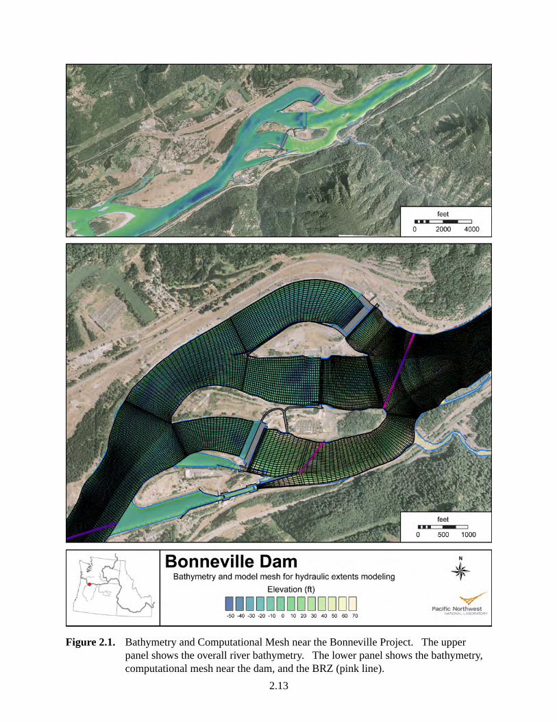
Figure 2.1. Bathymetry and Computational Mesh near the Bonneville Project. The upperpanel shows the overall river bathymetry. The lower panel shows the bathymetry,computational mesh near the dam, and the BRZ (pink line).
2.13
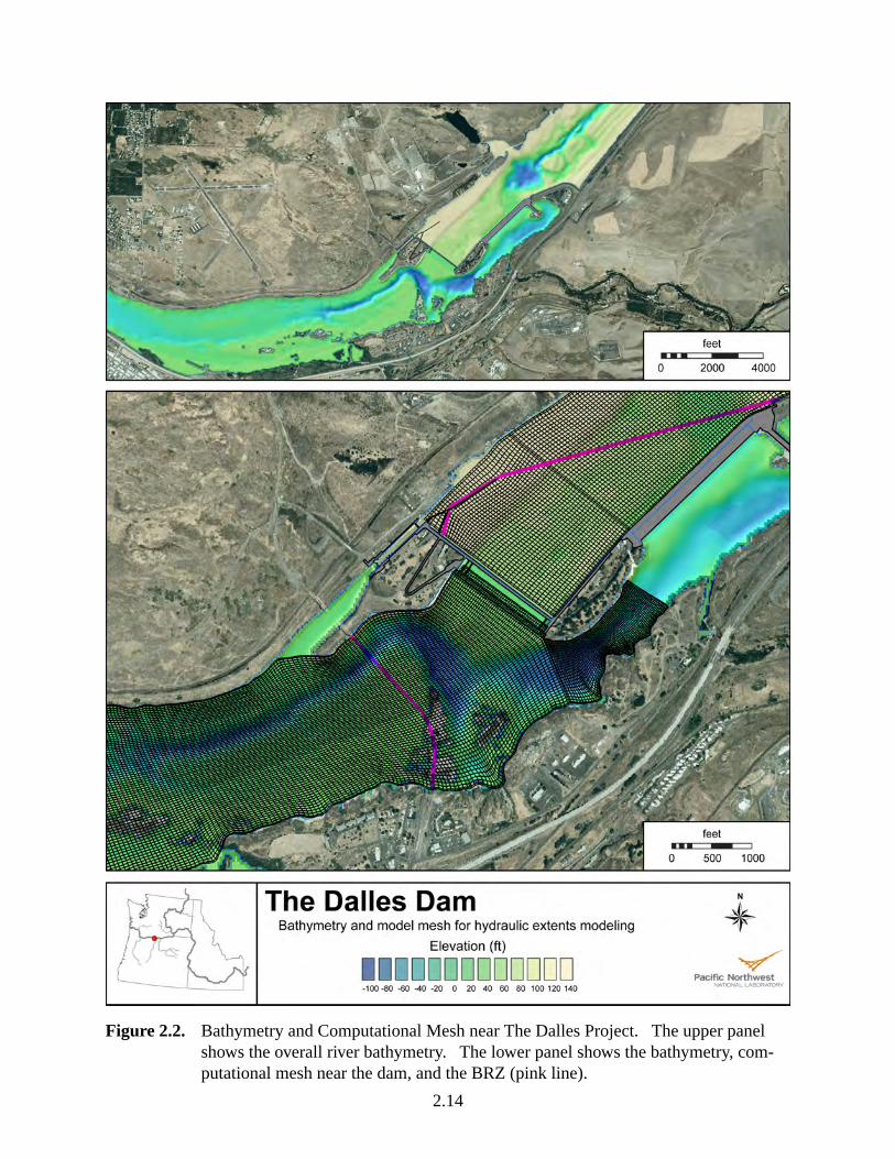
Figure 2.2. Bathymetry and Computational Mesh near The Dalles Project. The upper panelshows the overall river bathymetry. The lower panel shows the bathymetry, com-putational mesh near the dam, and the BRZ (pink line).
2.14
In the JDA tailrace (Figure 2.3), the mesh had one cell per spillbay, two per turbine unit. Theisland complex just downstream of the project was included in the mesh, allowing the modelingof the inundation of this complex. The area of increased cross-stream resolution extended 4.5miles downstream.
2.3.4 John Day Pool
In the JDA forebay (Figure 2.3), the mesh has one cell per spillbay and per turbine unit. Thearea of increased cross-stream resolution extends 5.5 miles upstream.
At the MCN tailrace, the area of increased resolution extends only 2 miles downstream; however,a flow constriction makes the reduction in cross-stream cell numbers not as much of a change incross-stream spatial resolution. At the dam, (Figure 2.4) there is one cell per spill bay, and twoper turbine unit.)
2.3.5 McNary Pool up to Ice Harbor Dam
In the MCN forebay, the spillbays and turbine units have one cell each (Figure 2.4), and thearea of increased cross-stream resolution extends 6 miles upstream. This mesh includes a shortsection of the Columbia upstream of its confluence with the Snake River and a well-resolvedsection of the Snake from Ice Harbor Dam to the Columbia River confluence.
At IHR, the mesh was taken from another study (Hanrahan et al. 2007). This well-resolvedmesh has two cells per spillway bay and per turbine unit (Figure 2.5). This mesh has twolocations, both near the confluence, where the mesh has 2:1 cross-stream matches across blockboundaries to reduce the number of cells.
Above IHR, the river tends to have more convoluted shorelines. In many places, the meshboundaries are outside the convolutions to increase mesh orthogonality while letting the wet-ting/drying capabilities determine the portions of the mesh that are within the flowing river. Inthe IHR forebay, there is one cell per bay and turbine unit (Figure 2.5), but more cells were addedin upstream blocks to maintain cross stream resolution because the river and mesh are wider. Inthe LMN tailrace, there are two cells per turbine unit and spillbay (Figure 2.6).
2.3.6 Lower Monumental Pool
In the LMN forebay, there is one cell per turbine unit and spillbay (Figure 2.6). The shorelinesfor this pool extend outside much of the pool to include shoreline complexity and side channelswhile maintaining a sufficient number of cells in the main channel. In the Little Goose tailrace,there is one cell per spillbay, two per turbine unit (Figure 2.7).
In the LGO forebay, the computational mesh has one cell per turbine unit and spillbay (Fig-ure 2.7). In the LGR tailrace, there are two cells per turbine unit and spillbay (Figure 2.8).
The mesh extends from LGR to 3.5 miles upstream of the Clearwater confluence and includes
2.15

Figure 2.3. Bathymetry and Computational Mesh near the John Day Project. The upper panelshows the overall river bathymetry. The lower panel shows the bathymetry, com-putational mesh near the dam, and the BRZ (pink line).
2.16
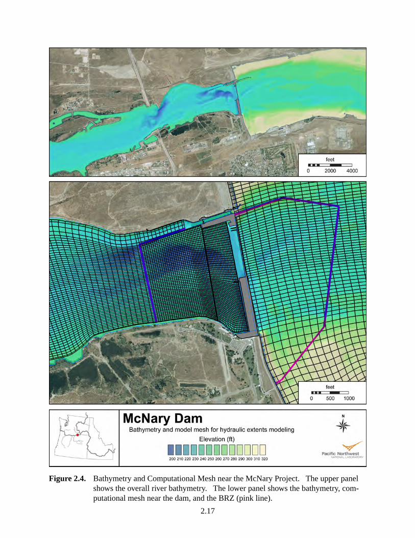
Figure 2.4. Bathymetry and Computational Mesh near the McNary Project. The upper panelshows the overall river bathymetry. The lower panel shows the bathymetry, com-putational mesh near the dam, and the BRZ (pink line).
2.17
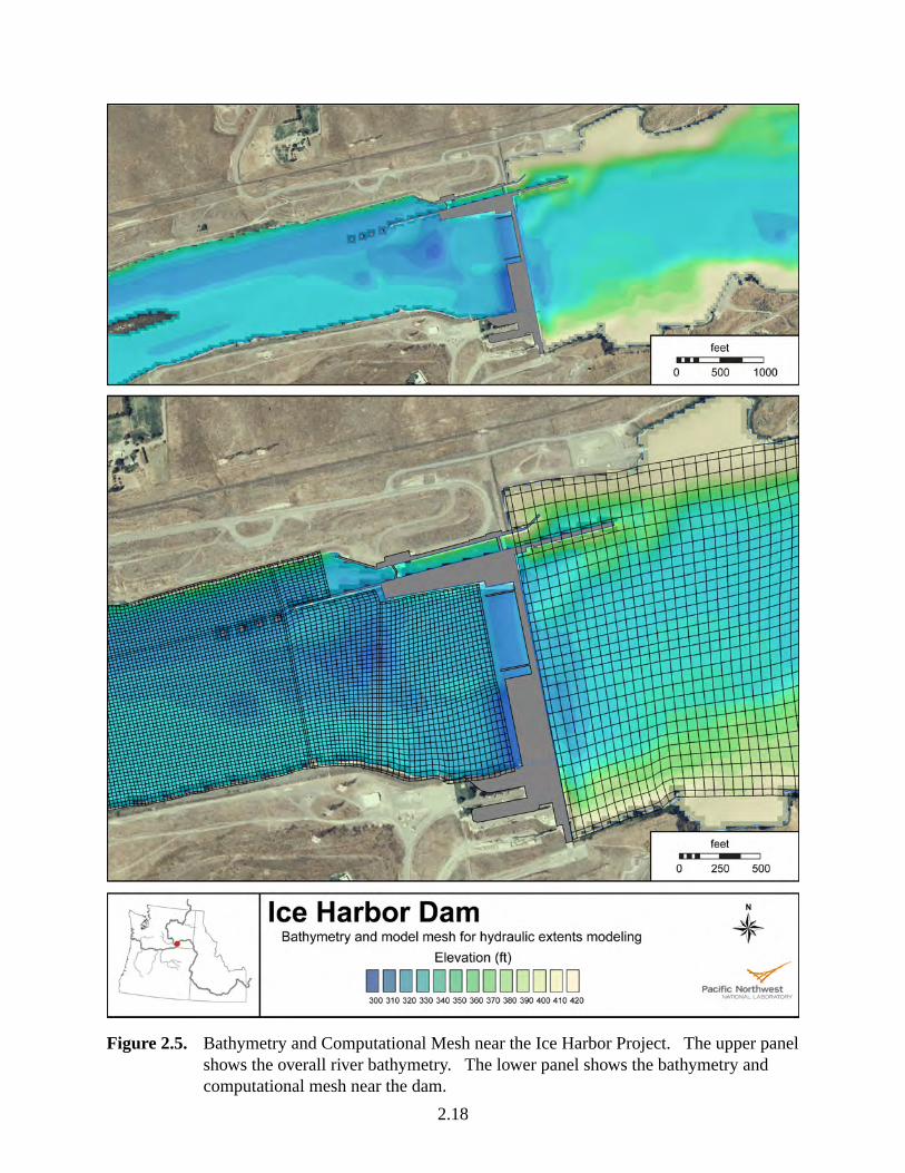
Figure 2.5. Bathymetry and Computational Mesh near the Ice Harbor Project. The upper panelshows the overall river bathymetry. The lower panel shows the bathymetry andcomputational mesh near the dam.
2.18
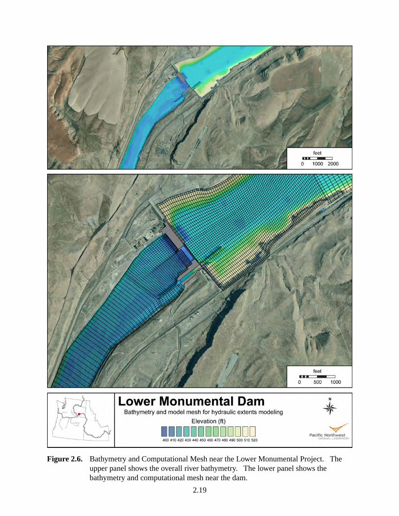
Figure 2.6. Bathymetry and Computational Mesh near the Lower Monumental Project. Theupper panel shows the overall river bathymetry. The lower panel shows thebathymetry and computational mesh near the dam.
2.19
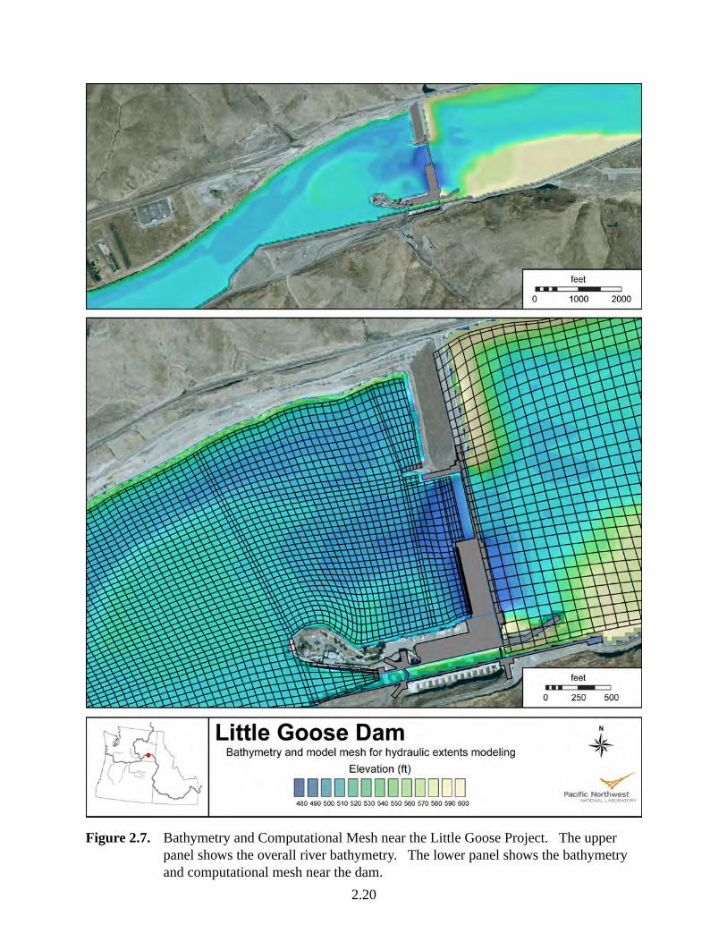
Figure 2.7. Bathymetry and Computational Mesh near the Little Goose Project. The upperpanel shows the overall river bathymetry. The lower panel shows the bathymetryand computational mesh near the dam.
2.20
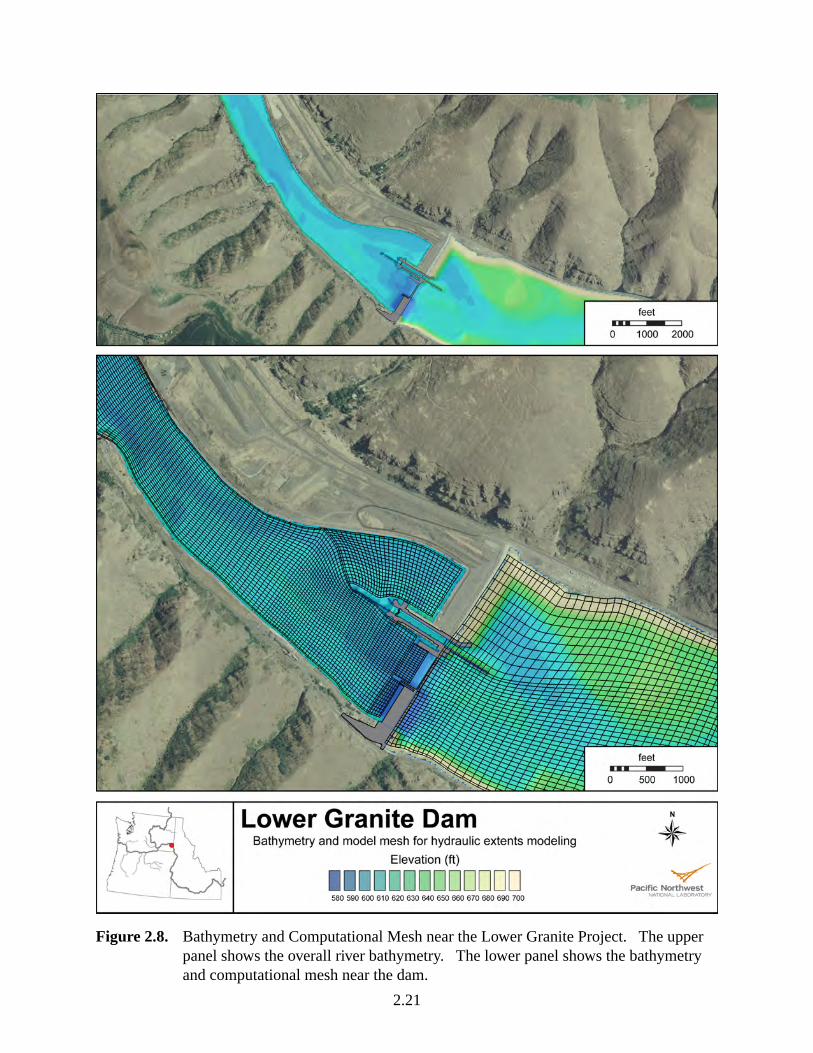
Figure 2.8. Bathymetry and Computational Mesh near the Lower Granite Project. The upperpanel shows the overall river bathymetry. The lower panel shows the bathymetryand computational mesh near the dam.
2.21
a 7-mile segment of the Clearwater River. In the LGR forebay, there are two cells per turbineunit and one per spill bay (Figure 2.8). The shallow draft boom that extends attaches betweenthe powerhouse and spillway and extends upstream to the south shore was ignored, per guidancefrom CENWW.
2.4 Model Configuration and Scenarios
The project operations were specified by CENWP and CENWW for each project. For eachproject, the forebay and tailrace models both needed to be configured and run for each specifiedoperation.
The forebay models were configured with a specified total river flow at the next dam upstreamand bay-by-bay, unit-by-unit operations in the forebay. A single bay was specified as a watersurface elevation boundary so as to not over constrain the model. As model conditions changed,this “open” boundary allowed the forebay hydraulics to adjust more quickly to changing bound-ary conditions. Travel time data provided by CENWP and CENWW were used to estimate thetime needed for a steady state to be achieved after changing the total river flow for a given reachand flow. One day of time was typically used for changing project operations for the same totalriver flow.
For the tailrace models, bay-by-bay, unit-by-unit operations were specified at the project, and thedownstream boundary was run as a specified water surface elevation.
For all river reaches, the most recent validated Manning’s n value was used. New meshes,however, were not re-validated against field measured data. Time steps small enough to haveconvergent models were used. Time steps were typically 30 s, although 15 s were used in somemodels.
The boundary condition spreadsheets were used to create the ASCII text files required as inputfiles for MASS2. Each total river flow was run to to a converged steady-state solution for par-ticular total river discharge, and then the model was run for an additional 24 h before writing themodeled flows for each operational scenario. MASS2 writes out the dates associated with modeloutput, and those dates are used to track the scenario.
Water mass imbalances were checked for all model runs to ensure convergence. The typicalallowed imbalance was 100 cfs; however, most runs had a much smaller block imbalance (1̃ cfs).Flow volumes were checked to make sure the model was properly configured and converged.Inflow and outflow locations at the projects were checked to make sure that the unit numberingwas correct in the configuration files and flow locations were properly assigned.
2.4.1 General MASS2 Configuration
A MASS2 simulation case is configured using a series of text files for the computational mesh,model parameters, and flow conditions (see Perkins and Richmond (2004b) for details). In thisstudy, a large range of flows was simulated. In the lower Columbia, the range of total river flows
2.22
were from the lower typical summers flows to the maximum flows at which the Fish PassagePlan (FPP) (USACE–Northwestern Division 2008) can be used. At higher flows, there wouldbe involuntary spill. The operations at each project were for the minimum and maximum pow-erhouse loading. For the Snake River dams and McNary Dam, the range was from minimumflow to high flows. The specified project operations were selected to explore the largest possibledifferences by modeling maximum powerhouse or minimum powerhouse flow. Additional runshad the flow centered mid-river for the maximum momentum concentration. Specific projectoperations are detailed in the sections below.
2.4.2 Bonneville Project
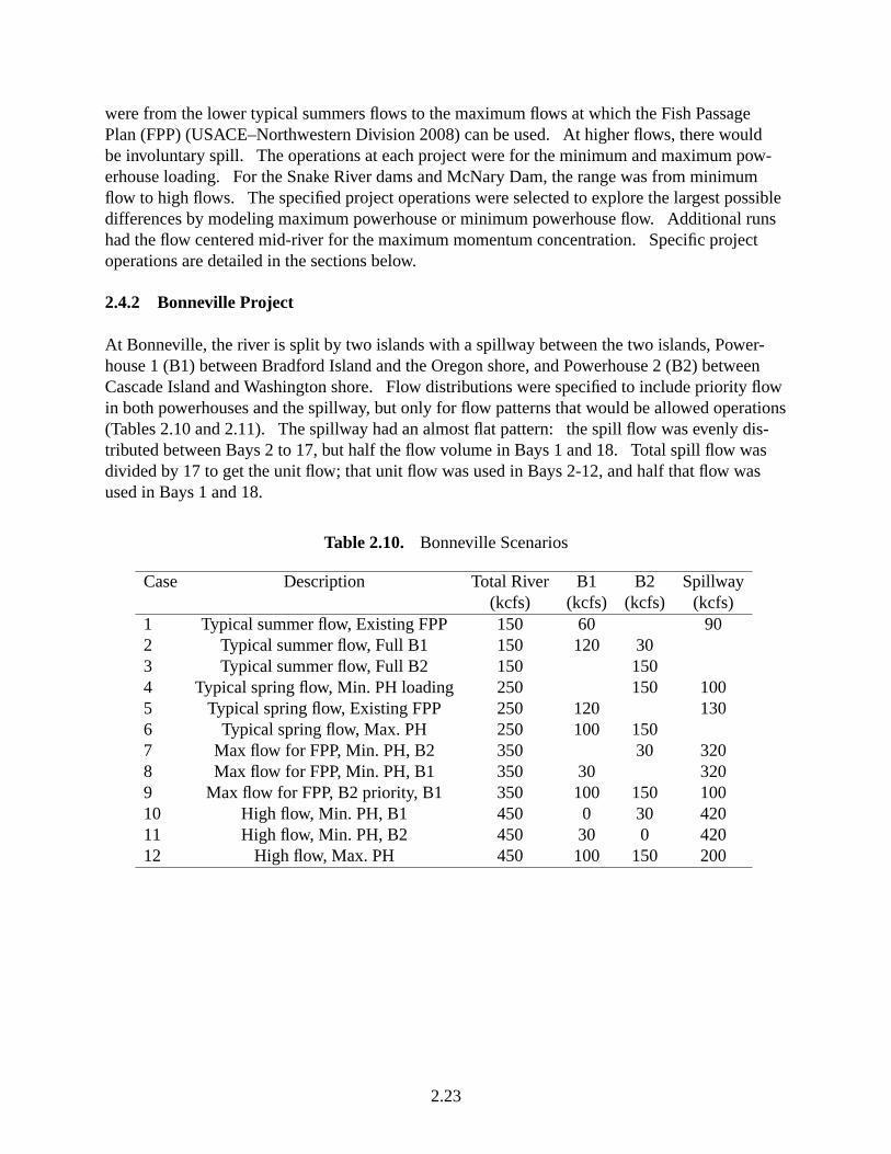
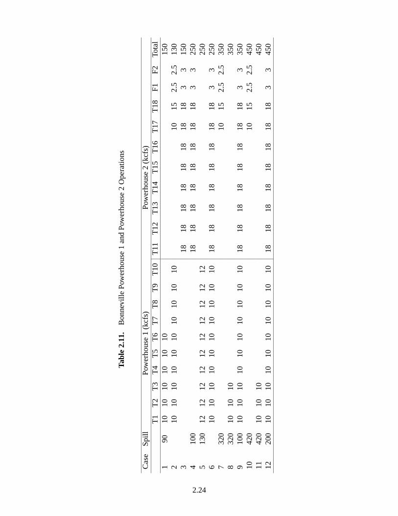
At Bonneville, the river is split by two islands with a spillway between the two islands, Power-house 1 (B1) between Bradford Island and the Oregon shore, and Powerhouse 2 (B2) betweenCascade Island and Washington shore. Flow distributions were specified to include priority flowin both powerhouses and the spillway, but only for flow patterns that would be allowed operations(Tables 2.10 and 2.11). The spillway had an almost flat pattern: the spill flow was evenly dis-tributed between Bays 2 to 17, but half the flow volume in Bays 1 and 18. Total spill flow wasdivided by 17 to get the unit flow; that unit flow was used in Bays 2-12, and half that flow wasused in Bays 1 and 18.
Table 2.10. Bonneville Scenarios
Case Description Total River B1 B2 Spillway(kcfs) (kcfs) (kcfs) (kcfs)
1 Typical summer flow, Existing FPP 150 60 902 Typical summer flow, Full B1 150 120 303 Typical summer flow, Full B2 150 1504 Typical spring flow, Min. PH loading 250 150 1005 Typical spring flow, Existing FPP 250 120 1306 Typical spring flow, Max. PH 250 100 1507 Max flow for FPP, Min. PH, B2 350 30 3208 Max flow for FPP, Min. PH, B1 350 30 3209 Max flow for FPP, B2 priority, B1 350 100 150 10010 High flow, Min. PH, B1 450 0 30 42011 High flow, Min. PH, B2 450 30 0 42012 High flow, Max. PH 450 100 150 200
2.23
Tabl
e2.
11.
Bon
nevi
lleP
ower
hous
e1
and
Pow
erho
use
2O
pera
tions
Cas
eS
pill
Pow
erho
use
1(k
cfs)
Pow
erho
use
2(k
cfs)
T1
T2
T3
T4
T5
T6
T7
T8
T9
T10
T11
T12
T13
T14
T15
T16
T17
T18
F1
F2
Tota
l1
9010
1010
1010
1015
02
1010
1010
1010
1010
1010
1015
2.5
2.5
130
318
1818
1818
1818
183
315
04
100
1818
1818
1818
1818
33
250
513
012
1212
1212
1212
1212
1225
06
1010
1010
1010
1010
1010
1818
1818
1818
1818
33
250
732
010
152.
52.
535
08
320
1010
1035
09
100
1010
1010
1010
1010
1010
1818
1818
1818
1818
33
350
1042
010
152.
52.
545
011
420
1010
1045
012
200
1010
1010
1010
1010
1010
1818
1818
1818
1818
33
450
2.24
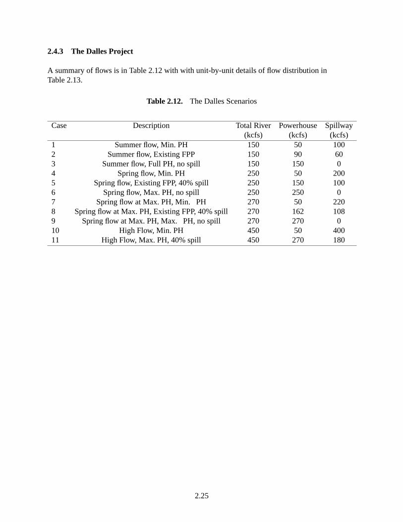
2.4.3 The Dalles Project
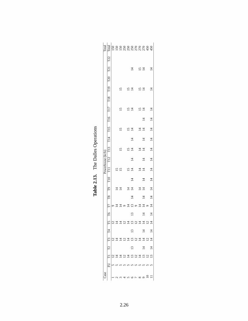
A summary of flows is in Table 2.12 with with unit-by-unit details of flow distribution inTable 2.13.
Table 2.12. The Dalles Scenarios
Case Description Total River Powerhouse Spillway(kcfs) (kcfs) (kcfs)
1 Summer flow, Min. PH 150 50 1002 Summer flow, Existing FPP 150 90 603 Summer flow, Full PH, no spill 150 150 04 Spring flow, Min. PH 250 50 2005 Spring flow, Existing FPP, 40% spill 250 150 1006 Spring flow, Max. PH, no spill 250 250 07 Spring flow at Max. PH, Min. PH 270 50 2208 Spring flow at Max. PH, Existing FPP, 40% spill 270 162 1089 Spring flow at Max. PH, Max. PH, no spill 270 270 010 High Flow, Min. PH 450 50 40011 High Flow, Max. PH, 40% spill 450 270 180
2.25
Tabl
e2.
13.
The
Dal
les
Ope
ratio
ns
Cas
eP
ower
hous
e(k
cfs)
Tota
lF
UT
1T
2T
3T
4T
5T
6T
7T
8T
9T
10T
11T
12T
13T
14T
15T
16T
17T
18T
19T
20T
21T
22To
tal
15
1212
129
150
25
1414
1414
1415
150
35
1414
1414
1415
1515
1515
150
45
1212
129
250
55
1414
1414
1415
1515
1515
250
65
1313
1313
1313
1314
1414
1414
1414
1414
1414
250
75
1212
129
270
85
1414
1414
1414
1414
1515
1527
09
513
1414
1414
1414
1414
1414
1414
1414
1414
1414
270
105
1212
129
450
115
1314
1414
1414
1414
1414
1414
1414
1414
1414
1445
0
2.26
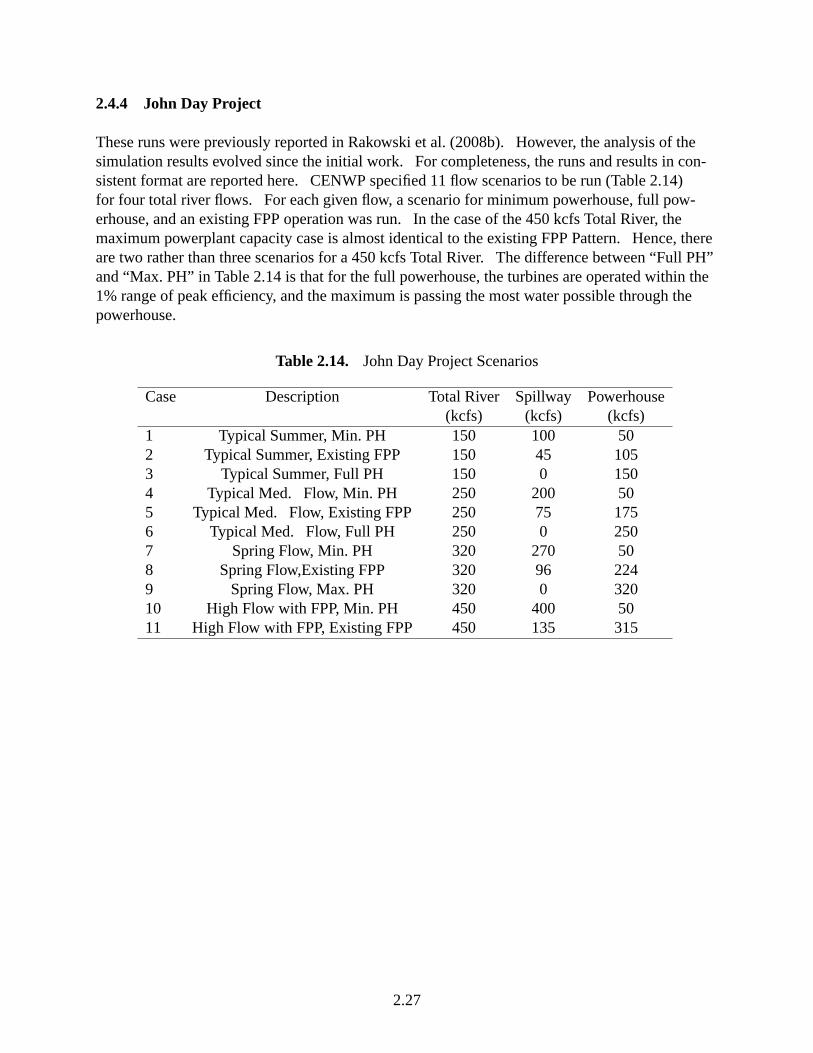
2.4.4 John Day Project
These runs were previously reported in Rakowski et al. (2008b). However, the analysis of thesimulation results evolved since the initial work. For completeness, the runs and results in con-sistent format are reported here. CENWP specified 11 flow scenarios to be run (Table 2.14)for four total river flows. For each given flow, a scenario for minimum powerhouse, full pow-erhouse, and an existing FPP operation was run. In the case of the 450 kcfs Total River, themaximum powerplant capacity case is almost identical to the existing FPP Pattern. Hence, thereare two rather than three scenarios for a 450 kcfs Total River. The difference between “Full PH”and “Max. PH” in Table 2.14 is that for the full powerhouse, the turbines are operated within the1% range of peak efficiency, and the maximum is passing the most water possible through thepowerhouse.
Table 2.14. John Day Project Scenarios
Case Description Total River Spillway Powerhouse(kcfs) (kcfs) (kcfs)
1 Typical Summer, Min. PH 150 100 502 Typical Summer, Existing FPP 150 45 1053 Typical Summer, Full PH 150 0 1504 Typical Med. Flow, Min. PH 250 200 505 Typical Med. Flow, Existing FPP 250 75 1756 Typical Med. Flow, Full PH 250 0 2507 Spring Flow, Min. PH 320 270 508 Spring Flow,Existing FPP 320 96 2249 Spring Flow, Max. PH 320 0 32010 High Flow with FPP, Min. PH 450 400 5011 High Flow with FPP, Existing FPP 450 135 315
2.27
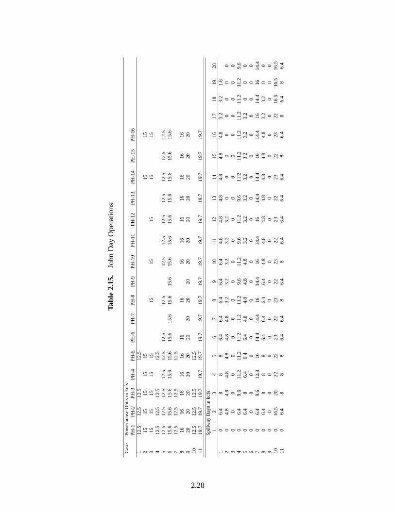
Tabl
e2.
15.
John
Day
Ope
ratio
ns
Cas
eP
ower
hous
eU
nits
inkc
fsP
H-1
PH
-2P
H-3
PH
-4P
H-5
PH
-6P
H-7
PH
-8P
H-9
PH
-10
PH
-11
PH
-12
PH
-13
PH
-14
PH
-15
PH
-16
112
.512
.512
.512
.52
1515
1515
1515
153
1515
1515
1515
1515
1515
412
.512
.512
.512
.55
12.5
12.5
12.5
12.5
12.5
12.5
12.5
12.5
12.5
12.5
12.5
12.5
12.5
12.5
615
.615
.615
.615
.615
.615
.615
.615
.615
.615
.615
.615
.615
.615
.615
.615
.67
12.5
12.5
12.5
12.5
816
1616
1616
1616
1616
1616
1616
169
2020
2020
2020
2020
2020
2020
2020
2020
1012
.512
.512
.512
.511
19.7
19.7
19.7
19.7
19.7
19.7
19.7
19.7
19.7
19.7
19.7
19.7
19.7
19.7
19.7
19.7
Spi
llway
Bay
sin
kcfs
12
34
56
78
910
1112
1314
1516
1718
1920
10
6.4
88
86.
46.
46.
46.
46.
44.
84.
84.
84.
84.
84.
83.
23.
21.
62
04.
84.
84.
84.
84.
84.
83.
23.
23.
23.
23.
20
00
00
00
03
00
00
00
00
00
00
00
00
00
00
40
6.4
9.6
11.2
11.2
11.2
11.2
11.2
9.6
11.2
9.6
11.2
9.6
11.2
11.2
11.2
11.2
11.2
11.2
9.6
50
6.4
86.
46.
46.
44.
84.
84.
84.
83.
23.
23.
23.
23.
23.
23.
20
00
60
00
00
00
00
00
00
00
00
00
07
06.
49.
612
.816
14.4
14.4
1614
.416
14.4
1614
.414
.416
14.4
1614
.416
14.4
80
6.4
88
86.
46.
46.
46.
44.
84.
84.
84.
84.
84.
84.
83.
23.
20
09
00
00
00
00
00
00
00
00
00
00
100
16.5
2022
2223
2223
2223
2223
2223
2223
2216
.516
.516
.511
06.
48
88
6.4
6.4
86.
48
6.4
6.4
6.4
6.4
86.
48
6.4
86.
4
2.28
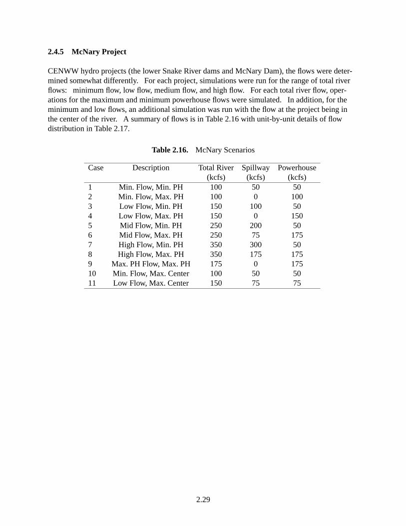
2.4.5 McNary Project
CENWW hydro projects (the lower Snake River dams and McNary Dam), the flows were deter-mined somewhat differently. For each project, simulations were run for the range of total riverflows: minimum flow, low flow, medium flow, and high flow. For each total river flow, oper-ations for the maximum and minimum powerhouse flows were simulated. In addition, for theminimum and low flows, an additional simulation was run with the flow at the project being inthe center of the river. A summary of flows is in Table 2.16 with unit-by-unit details of flowdistribution in Table 2.17.
Table 2.16. McNary Scenarios
Case Description Total River Spillway Powerhouse(kcfs) (kcfs) (kcfs)
1 Min. Flow, Min. PH 100 50 502 Min. Flow, Max. PH 100 0 1003 Low Flow, Min. PH 150 100 504 Low Flow, Max. PH 150 0 1505 Mid Flow, Min. PH 250 200 506 Mid Flow, Max. PH 250 75 1757 High Flow, Min. PH 350 300 508 High Flow, Max. PH 350 175 1759 Max. PH Flow, Max. PH 175 0 17510 Min. Flow, Max. Center 100 50 5011 Low Flow, Max. Center 150 75 75
2.29
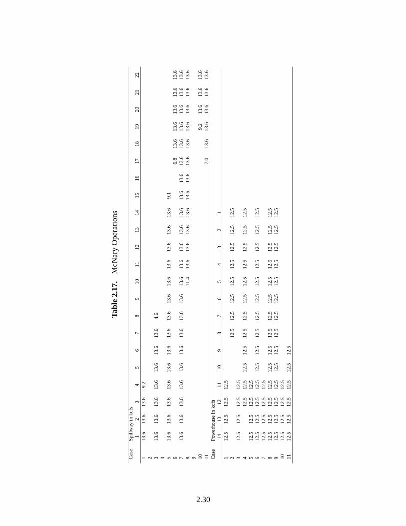
Tabl
e2.
17.
McN
ary
Ope
ratio
ns
Cas
eS
pillw
ayin
kcfs
12
34
56
78
910
1112
1314
1516
1718
1920
2122
113
.613
.613
.69.
22 3
13.6
13.6
13.6
13.6
13.6
13.6
13.6
4.6
4 513
.613
.613
.613
.613
.613
.613
.613
.613
.613
.613
.613
.613
.613
.69.
16
6.8
13.6
13.6
13.6
13.6
13.6
713
.613
.613
.613
.613
.613
.613
.613
.613
.613
.613
.613
.613
.613
.613
.613
.613
.613
.613
.613
.613
.613
.68
11.4
13.6
13.6
13.6
13.6
13.6
13.6
13.6
13.6
13.6
13.6
13.6
13.6
9 109.
213
.613
.613
.611
7.0
13.6
13.6
13.6
13.6
13.6
Cas
eP
ower
hous
ein
kcfs
1413
1211
109
87
65
43
21
112
.512
.512
.512
.52
12.5
12.5
12.5
12.5
12.5
12.5
12.5
12.5
312
.512
.512
.512
.54
12.5
12.5
12.5
12.5
12.5
12.5
12.5
12.5
12.5
12.5
12.5
12.5
512
.512
.512
.512
.56
12.5
12.5
12.5
12.5
12.5
12.5
12.5
12.5
12.5
12.5
12.5
12.5
12.5
12.5
712
.512
.512
.512
.58
12.5
12.5
12.5
12.5
12.5
12.5
12.5
12.5
12.5
12.5
12.5
12.5
12.5
12.5
912
.512
.512
.512
.512
.512
.512
.512
.512
.512
.512
.512
.512
.512
.510
12.5
12.5
12.5
12.5
1112
.512
.512
.512
.512
.512
.5
2.30
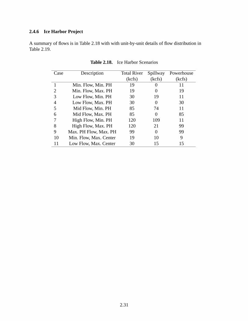
2.4.6 Ice Harbor Project
A summary of flows is in Table 2.18 with with unit-by-unit details of flow distribution inTable 2.19.
Table 2.18. Ice Harbor Scenarios
Case Description Total River Spillway Powerhouse(kcfs) (kcfs) (kcfs)
1 Min. Flow, Min. PH 19 0 112 Min. Flow, Max. PH 19 0 193 Low Flow, Min. PH 30 19 114 Low Flow, Max. PH 30 0 305 Mid Flow, Min. PH 85 74 116 Mid Flow, Max. PH 85 0 857 High Flow, Min. PH 120 109 118 High Flow, Max. PH 120 21 999 Max. PH Flow, Max. PH 99 0 9910 Min. Flow, Max. Center 19 10 911 Low Flow, Max. Center 30 15 15
2.31
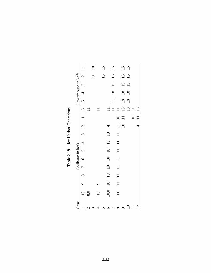
Tabl
e2.
19.
Ice
Har
bor
Ope
ratio
ns
Cas
eS
pillw
ayin
kcfs
Pow
erho
use
inkc
fs1
109
87
65
43
21
65
43
21
28.
011
39
104
109
115
1515
610
.010
1010
1010
1010
411
711
1118
1515
158
1111
1111
1111
1111
1110
119
1011
1818
1815
1515
1018
1818
1515
1511
109
124
1115
2.32
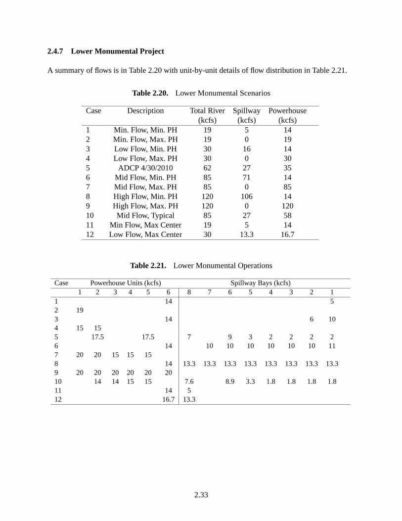
2.4.7 Lower Monumental Project
A summary of flows is in Table 2.20 with unit-by-unit details of flow distribution in Table 2.21.
Table 2.20. Lower Monumental Scenarios
Case Description Total River Spillway Powerhouse(kcfs) (kcfs) (kcfs)
1 Min. Flow, Min. PH 19 5 142 Min. Flow, Max. PH 19 0 193 Low Flow, Min. PH 30 16 144 Low Flow, Max. PH 30 0 305 ADCP 4/30/2010 62 27 356 Mid Flow, Min. PH 85 71 147 Mid Flow, Max. PH 85 0 858 High Flow, Min. PH 120 106 149 High Flow, Max. PH 120 0 12010 Mid Flow, Typical 85 27 5811 Min Flow, Max Center 19 5 1412 Low Flow, Max Center 30 13.3 16.7
Table 2.21. Lower Monumental Operations
Case Powerhouse Units (kcfs) Spillway Bays (kcfs)1 2 3 4 5 6 8 7 6 5 4 3 2 1
1 14 52 193 14 6 104 15 155 17.5 17.5 7 9 3 2 2 2 26 14 10 10 10 10 10 10 117 20 20 15 15 158 14 13.3 13.3 13.3 13.3 13.3 13.3 13.3 13.39 20 20 20 20 20 2010 14 14 15 15 7.6 8.9 3.3 1.8 1.8 1.8 1.811 14 512 16.7 13.3
2.33
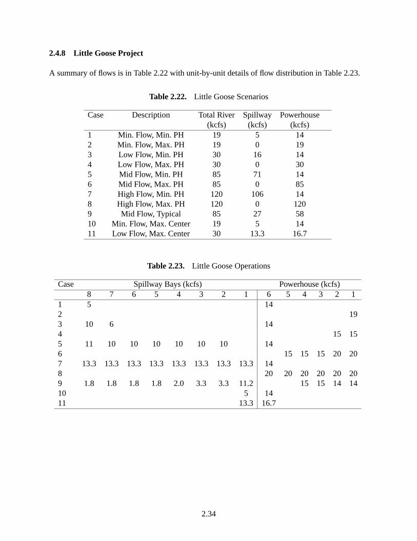
2.4.8 Little Goose Project
A summary of flows is in Table 2.22 with unit-by-unit details of flow distribution in Table 2.23.
Table 2.22. Little Goose Scenarios
Case Description Total River Spillway Powerhouse(kcfs) (kcfs) (kcfs)
1 Min. Flow, Min. PH 19 5 142 Min. Flow, Max. PH 19 0 193 Low Flow, Min. PH 30 16 144 Low Flow, Max. PH 30 0 305 Mid Flow, Min. PH 85 71 146 Mid Flow, Max. PH 85 0 857 High Flow, Min. PH 120 106 148 High Flow, Max. PH 120 0 1209 Mid Flow, Typical 85 27 5810 Min. Flow, Max. Center 19 5 1411 Low Flow, Max. Center 30 13.3 16.7
Table 2.23. Little Goose Operations
Case Spillway Bays (kcfs) Powerhouse (kcfs)8 7 6 5 4 3 2 1 6 5 4 3 2 1
1 5 142 193 10 6 144 15 155 11 10 10 10 10 10 10 146 15 15 15 20 207 13.3 13.3 13.3 13.3 13.3 13.3 13.3 13.3148 20 20 20 20 20 209 1.8 1.8 1.8 1.8 2.0 3.3 3.3 11.2 15 15 14 1410 5 1411 13.3 16.7
2.34

2.4.9 Lower Granite Project
A summary of flows is in Table 2.24 with unit-by-unit details of flow distribution in Table 2.25.
Table 2.24. Lower Granite Scenarios
Case Description Total River Spillway Powerhouse(kcfs) (kcfs) (kcfs)
1 Min. Flow, Min. PH 19 5 142 Min. Flow, Max. PH 19 0 193 Low Flow, Min. PH 30 16 144 Low Flow, Max. PH 30 0 305 Mid Flow, Min. PH 85 71 146 Mid Flow, Max. PH 85 0 857 High Flow, Min. PH 120 106 148 High Flow, Max. PH 120 0 1209 Mid Flow, Typical 85 27 5810 Min. Flow, Max. PH 19 5 1411 Low Flow, Min. PH 30 13.3 16.7
Table 2.25. Lower Granite Operations
Case Spillway Bays (kcfs) Powerhouse (kcfs)8 7 6 5 4 3 2 1 6 5 4 3 2 1
1 5 142 193 10 6 144 15 155 11 10 10 10 10 10 10 146 15 15 15 20 207 13.3 13.3 13.3 13.3 13.3 13.3 13.3 13.3148 20 20 20 20 20 209 1.8 1.8 1.8 1.8 2 3.3 3.3 11.2 15 15 14 1410 5 1411 13.3 16.7
2.35
2.5 Analysis of Simulation Data
Hydraulic influence is defined as the zone where project flow distributions (operations) impactriver flow up- and downstream of the dam. Each distribution of discharges through a dam resultsin a unique set of hydraulic characteristics, such as flow velocity and water-surface elevation,in the river channel adjacent to the project. As one moves away from the project, the rivergradually reverts to a stable flow configuration that is unaffected by flow distributions at the dam.The point at which project operations no longer influence the hydraulic characteristics of theriver is the hydraulic extent. Because, theoretically, any change in operations will have at leastsome infinitesimal influence at all points in the flow domain, a threshold level must be defined toestablish a definite boundary.
The strategy presented in this document for locating the hydraulic extent is to simulate a widerange of plausible operating conditions and calculate the differences in hydraulic characteristicsamong the scenarios. The scenarios typically include maximum spill, maximum powerhouse,and balanced patterns for each of four total river discharges. Only scenarios with the same totalriver discharge are compared. Velocity magnitude and direction are the two hydraulic charac-teristics used in this study. The comparison metrics are the maximum spread (S) in velocitymagnitude and velocity direction at each point in the model, computed as:
Svmag=|U |max− |U |min
Sdir =| θmax−θmin |
where|U | is the velocity magnitude, andθ is the velocity direction, in degrees.
Comparison metrics are computed using a script developed in Tecplot360TM (Tecplot, Inc.). Thescript adds the comparison metrics to a model grid dataset and plots the values for analysis. Themetrics are contoured according to proposed threshold spread values.
USACE fishery biologists requested data analysis to determine the project hydraulic extent basedon the following criteria:
• For areas where the mean velocities are less than 4 ft/s, the differences in the magnitudewater velocity between operations are not greater than 0.5 ft/sec, and/or the differences inwater flow direction (azimuth) are not greater than 10°.
• If mean water velocity is 4.0 ft/s or greater, the boundary is determined using the differ-ences in water flow direction (i.e., not greater than 10°)
Based on these criteria, and not including areas with a mean velocity of less than 0.1 ft/s (withinthe error of the model), a final set of graphics was developed that included data from all flows andall operations.
2.36
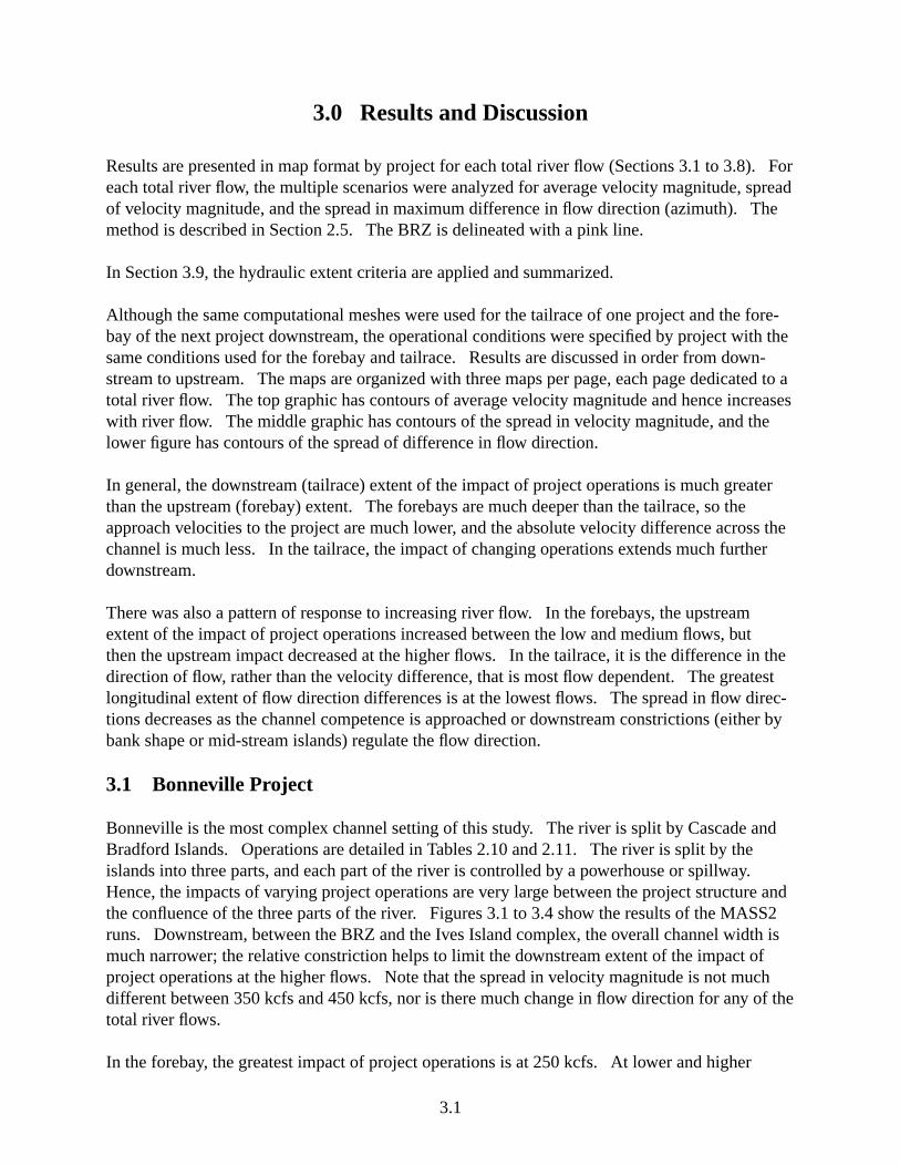
3.0 Results and Discussion
Results are presented in map format by project for each total river flow (Sections 3.1 to 3.8). Foreach total river flow, the multiple scenarios were analyzed for average velocity magnitude, spreadof velocity magnitude, and the spread in maximum difference in flow direction (azimuth). Themethod is described in Section 2.5. The BRZ is delineated with a pink line.
In Section 3.9, the hydraulic extent criteria are applied and summarized.
Although the same computational meshes were used for the tailrace of one project and the fore-bay of the next project downstream, the operational conditions were specified by project with thesame conditions used for the forebay and tailrace. Results are discussed in order from down-stream to upstream. The maps are organized with three maps per page, each page dedicated to atotal river flow. The top graphic has contours of average velocity magnitude and hence increaseswith river flow. The middle graphic has contours of the spread in velocity magnitude, and thelower figure has contours of the spread of difference in flow direction.
In general, the downstream (tailrace) extent of the impact of project operations is much greaterthan the upstream (forebay) extent. The forebays are much deeper than the tailrace, so theapproach velocities to the project are much lower, and the absolute velocity difference across thechannel is much less. In the tailrace, the impact of changing operations extends much furtherdownstream.
There was also a pattern of response to increasing river flow. In the forebays, the upstreamextent of the impact of project operations increased between the low and medium flows, butthen the upstream impact decreased at the higher flows. In the tailrace, it is the difference in thedirection of flow, rather than the velocity difference, that is most flow dependent. The greatestlongitudinal extent of flow direction differences is at the lowest flows. The spread in flow direc-tions decreases as the channel competence is approached or downstream constrictions (either bybank shape or mid-stream islands) regulate the flow direction.
3.1 Bonneville Project
Bonneville is the most complex channel setting of this study. The river is split by Cascade andBradford Islands. Operations are detailed in Tables 2.10 and 2.11. The river is split by theislands into three parts, and each part of the river is controlled by a powerhouse or spillway.Hence, the impacts of varying project operations are very large between the project structure andthe confluence of the three parts of the river. Figures 3.1 to 3.4 show the results of the MASS2runs. Downstream, between the BRZ and the Ives Island complex, the overall channel width ismuch narrower; the relative constriction helps to limit the downstream extent of the impact ofproject operations at the higher flows. Note that the spread in velocity magnitude is not muchdifferent between 350 kcfs and 450 kcfs, nor is there much change in flow direction for any of thetotal river flows.
In the forebay, the greatest impact of project operations is at 250 kcfs. At lower and higher
3.1

flows, the upstream extent is more limited. In the tailrace, the hydraulic extent increases withincreasing discharge.
3.2
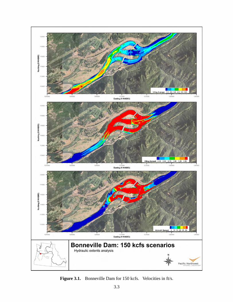
Figure 3.1. Bonneville Dam for 150 kcfs. Velocities in ft/s.
3.3
Figure 3.2. Bonneville Dam for 250 kcfs. Velocities in ft/s.
3.4
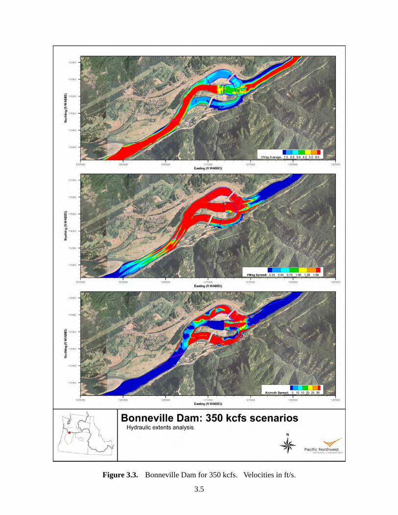
Figure 3.3. Bonneville Dam for 350 kcfs. Velocities in ft/s.
3.5
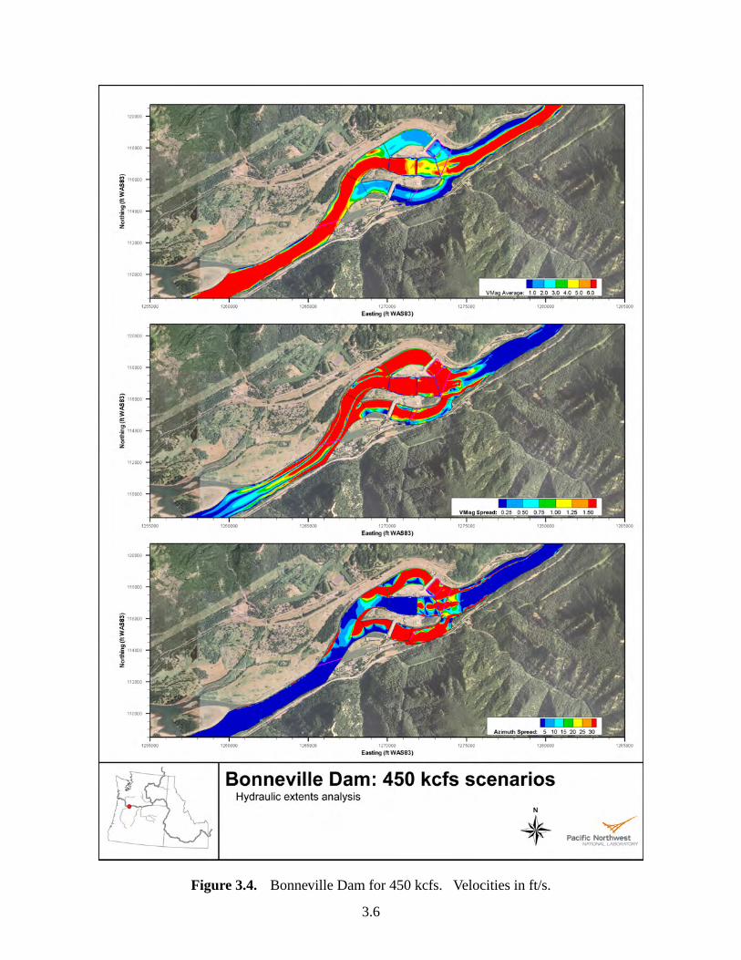
Figure 3.4. Bonneville Dam for 450 kcfs. Velocities in ft/s.
3.6
3.2 The Dalles Project
The Dalles has the powerhouse located perpendicular to the thalweg in the forebay, and thespillway and powerhouse are well separated. In addition, the spillway is operated by spillingpreferentially from the north shore, that is, as far from the powerhouse as possible. Operationsare detailed in Tables 2.12 and 2.13.
The Dalles tailrace has very complex bathymetry (Figure 2.2). From previous work with 3Dnumerical models and reduced-scale physical models as well as from prototype velocity mea-surements, we know the flow structure is very 3D in some locations. As such, results in thenear-project areas should be used with caution.
In the tailrace, the spillwall limits the extent of spill flow influence (Figures 3.5 to 3.8). Thewide separation of the powerhouse and spillway flows ensures that the downstream extent ofhydraulic influence is downstream of the bridge islands. The channel geometry limits the down-stream extent, and like in the Bonneville forebay, the extent is greatest at 250 kcfs, and muchmore limited at 450 kcfs.
In the forebay, there is little difference in the hydraulic extents between the 250-, 270-, and 450-kcfs flows.
3.7
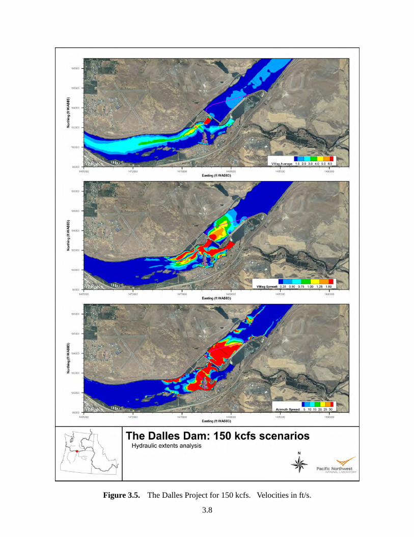
Figure 3.5. The Dalles Project for 150 kcfs. Velocities in ft/s.
3.8
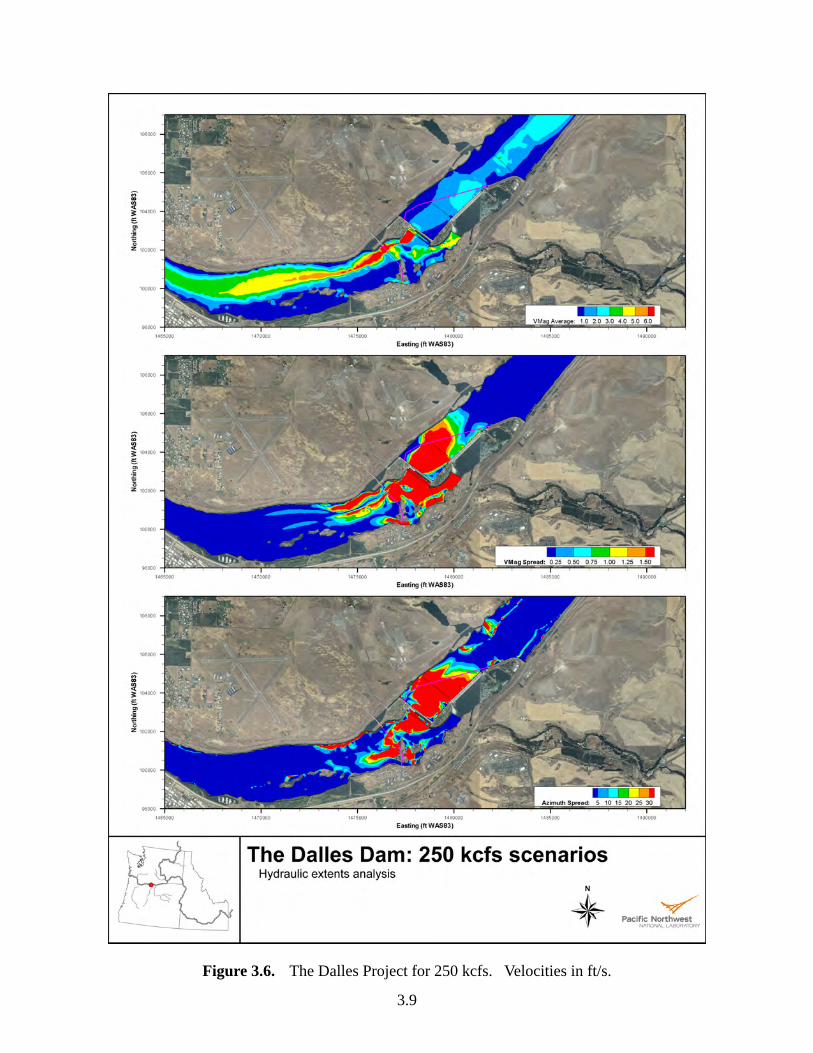
Figure 3.6. The Dalles Project for 250 kcfs. Velocities in ft/s.
3.9
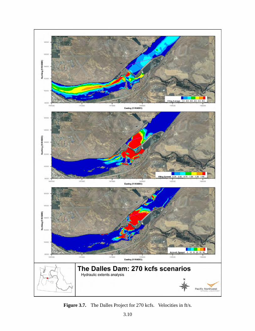
Figure 3.7. The Dalles Project for 270 kcfs. Velocities in ft/s.
3.10
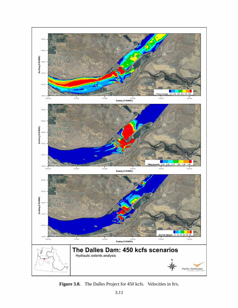
Figure 3.8. The Dalles Project for 450 kcfs. Velocities in ft/s.
3.11
3.3 John Day Project
Operations are detailed in Tables 2.14 and 2.15. Figures 3.9 to 3.12 show the results of theMASS2 runs. Downstream of John Day, the channel constricts and a mid-channel island exists.These features limit the extent of the downstream impact of operations at the higher flows. Atthis project, it is known that both the physical and 2D model under predict the lateral entrainmentof flow from the powerhouse and hence the downstream extent of the influence of operations.However, the channel flow constrictions rather than operations will tend to limit the downstreamhydraulic extent. Upstream of the dam, the average velocities are much less, and the hydraulicextent of project operations is mostly contained within the BRZ for all flows modeled.
3.12
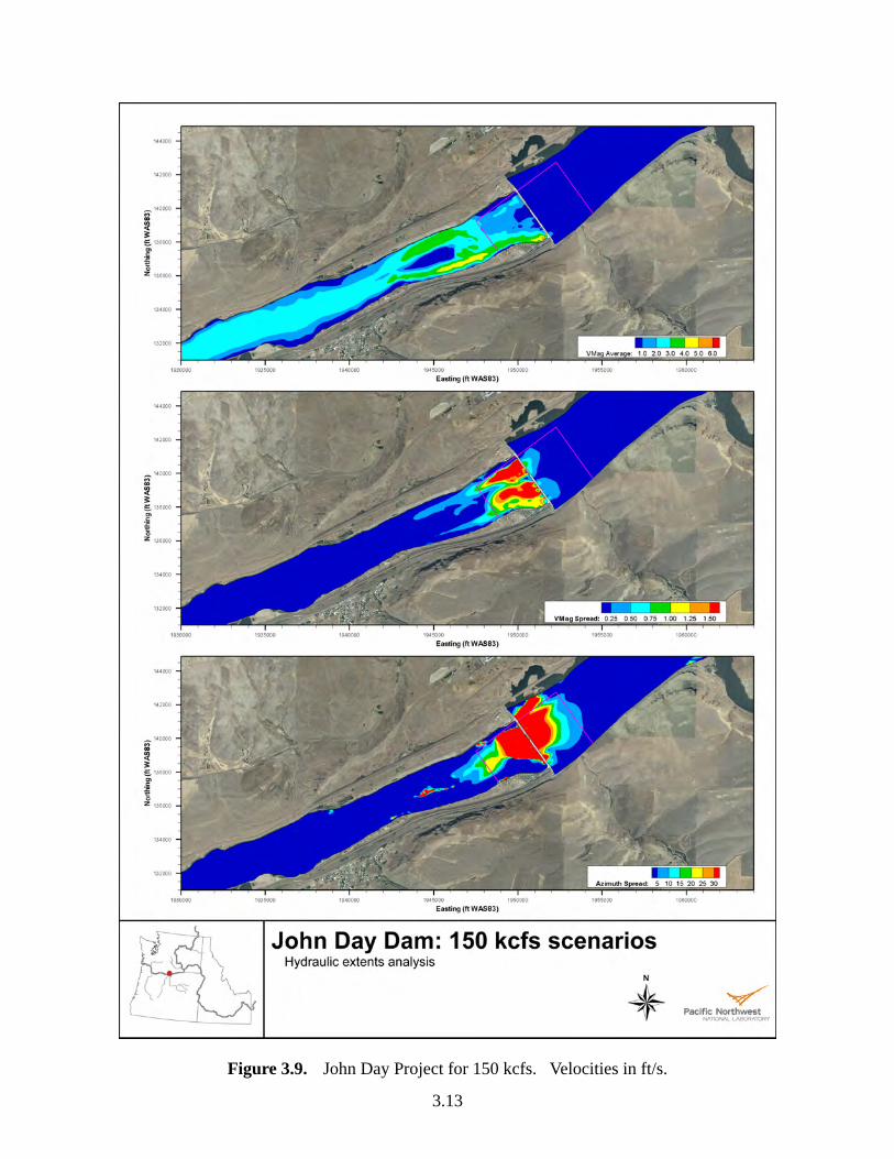
Figure 3.9. John Day Project for 150 kcfs. Velocities in ft/s.
3.13
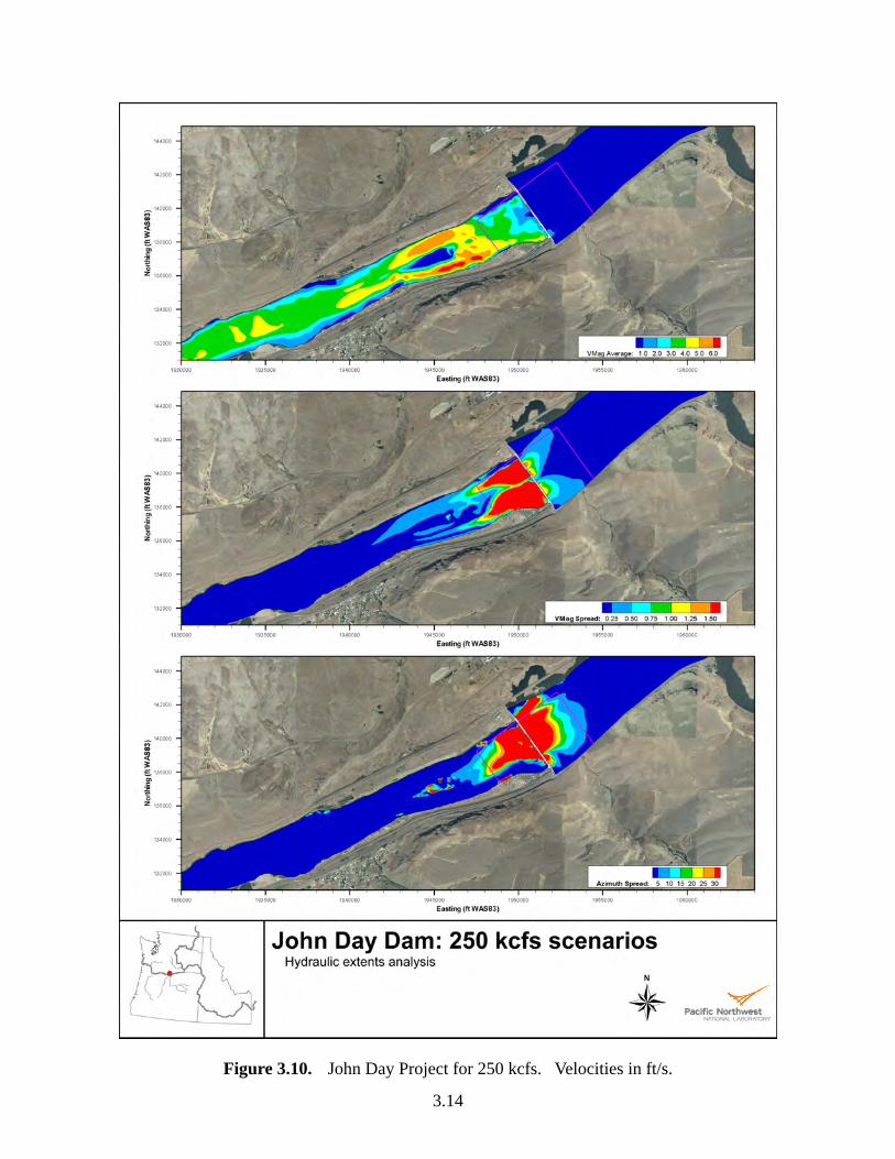
Figure 3.10. John Day Project for 250 kcfs. Velocities in ft/s.
3.14
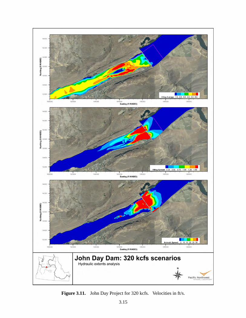
Figure 3.11. John Day Project for 320 kcfs. Velocities in ft/s.
3.15
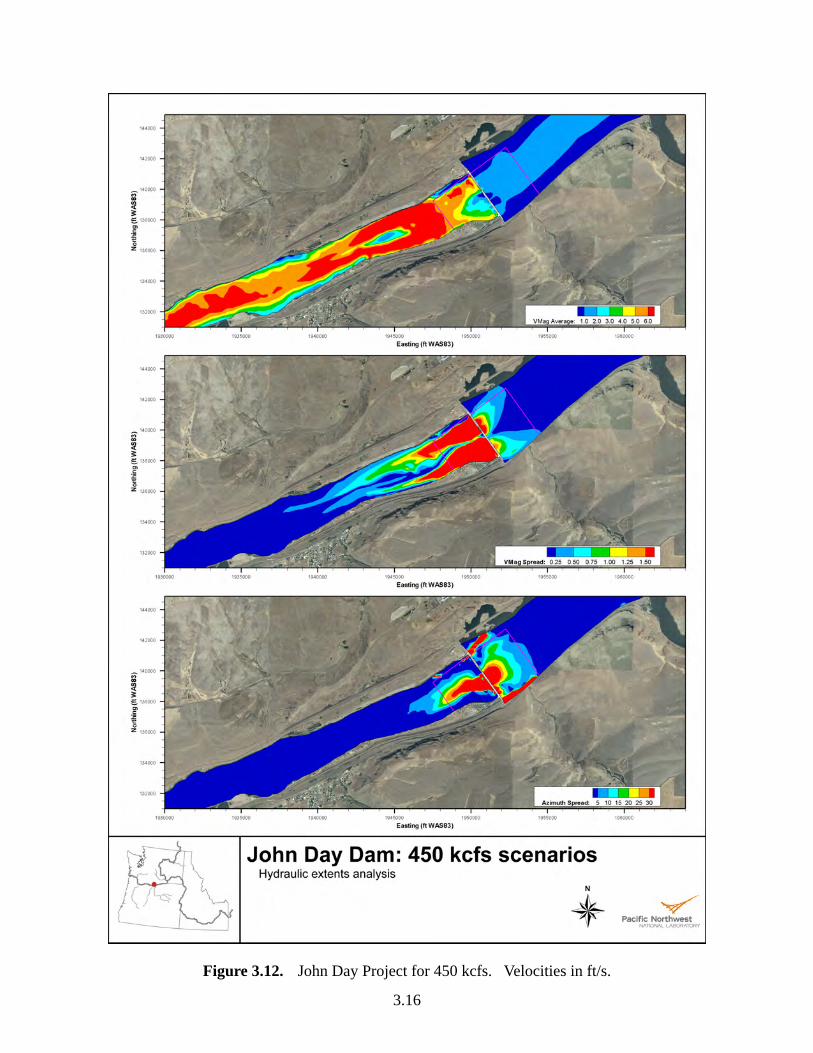
Figure 3.12. John Day Project for 450 kcfs. Velocities in ft/s.
3.16

3.4 McNary Project
Operations are detailed in Tables 2.16 and 2.17. Figures 3.13 to 3.16 show the results of theMASS2 runs. At McNary, the hydraulic extent is greatest at the mid-range flows. At 350-kcfs total river, both the upstream and downstream extent is reduced for both flow-directionand velocity-magnitude differences. For flow direction, the largest downstream extent is at thelowest modeled total river (Figure 3.13), while the greatest downstream extent of differences invelocity magnitude is at 150 and 250 kcfs total river (Figures 3.14 and 3.15).
3.17
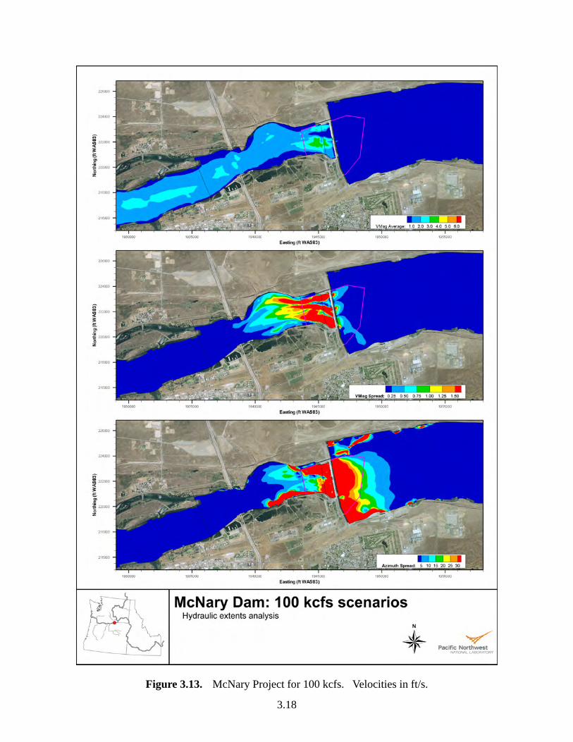
Figure 3.13. McNary Project for 100 kcfs. Velocities in ft/s.
3.18
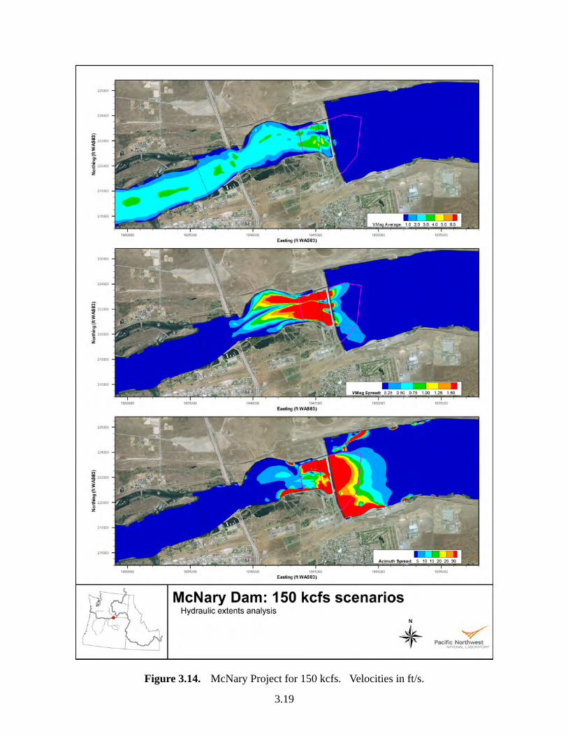
Figure 3.14. McNary Project for 150 kcfs. Velocities in ft/s.
3.19
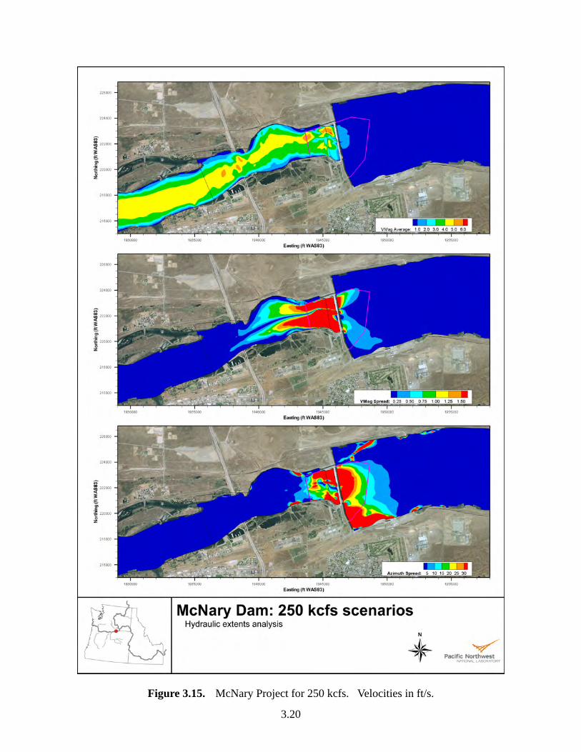
Figure 3.15. McNary Project for 250 kcfs. Velocities in ft/s.
3.20
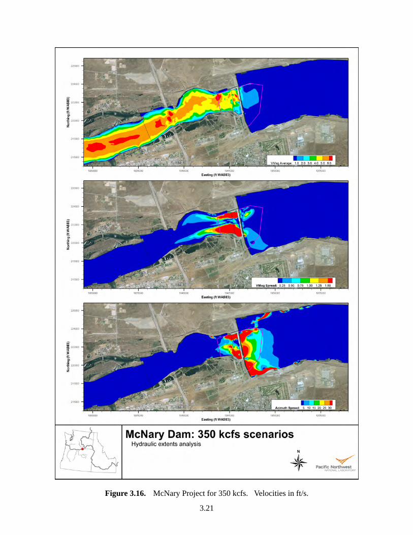
Figure 3.16. McNary Project for 350 kcfs. Velocities in ft/s.
3.21
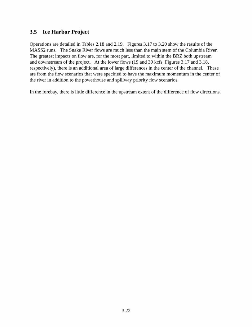
3.5 Ice Harbor Project
Operations are detailed in Tables 2.18 and 2.19. Figures 3.17 to 3.20 show the results of theMASS2 runs. The Snake River flows are much less than the main stem of the Columbia River.The greatest impacts on flow are, for the most part, limited to within the BRZ both upstreamand downstream of the project. At the lower flows (19 and 30 kcfs, Figures 3.17 and 3.18,respectively), there is an additional area of large differences in the center of the channel. Theseare from the flow scenarios that were specified to have the maximum momentum in the center ofthe river in addition to the powerhouse and spillway priority flow scenarios.
In the forebay, there is little difference in the upstream extent of the difference of flow directions.
3.22
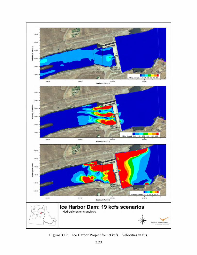
Figure 3.17. Ice Harbor Project for 19 kcfs. Velocities in ft/s.
3.23
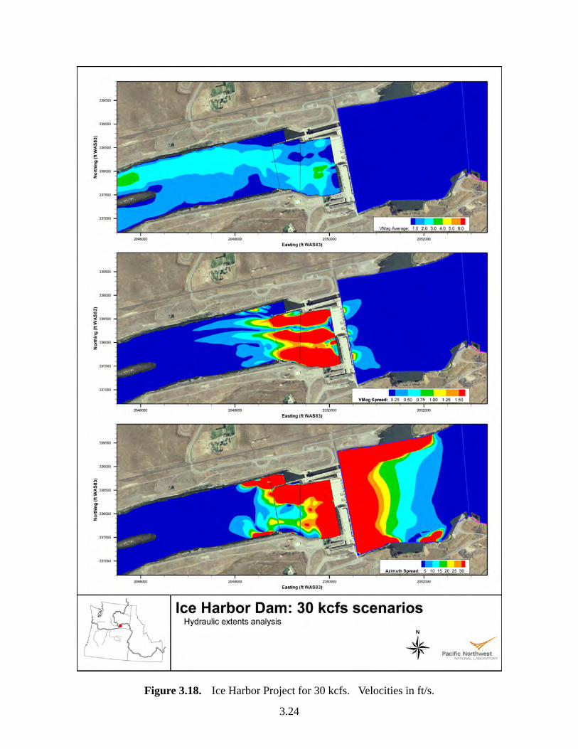
Figure 3.18. Ice Harbor Project for 30 kcfs. Velocities in ft/s.
3.24
Figure 3.19. Ice Harbor Project for 85 kcfs. Velocities in ft/s.
3.25
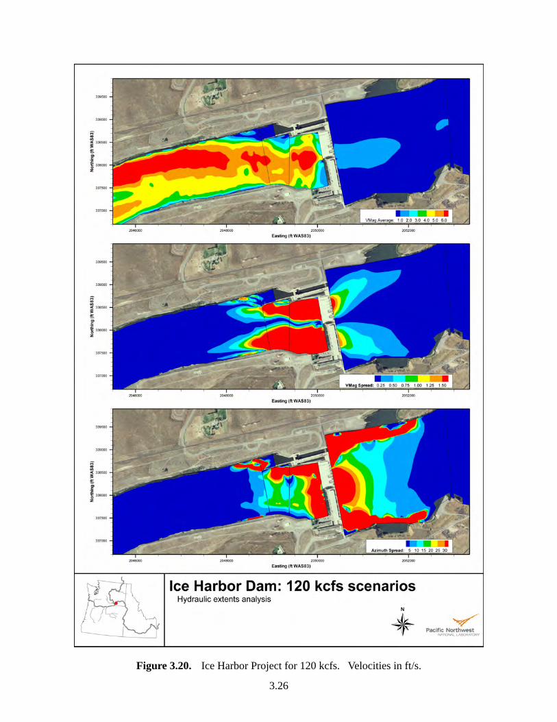
Figure 3.20. Ice Harbor Project for 120 kcfs. Velocities in ft/s.
3.26

3.6 Lower Monumental Project
Operations are detailed in Tables 2.20 and 2.21. Figures 3.21 to 3.24 show the results of theMASS2 runs. At Lower Monumental, the downstream extent in the spread of velocity magni-tude is largest at 30 kcfs (Figure 3.22). The downstream hydraulic extent is probably reducedby the slight channel constriction. In the forebay, the upstream extent of spread in velocity mag-nitude and flow direction increases with total river flow; however, at 120 kcfs both extents arereduced.
3.27
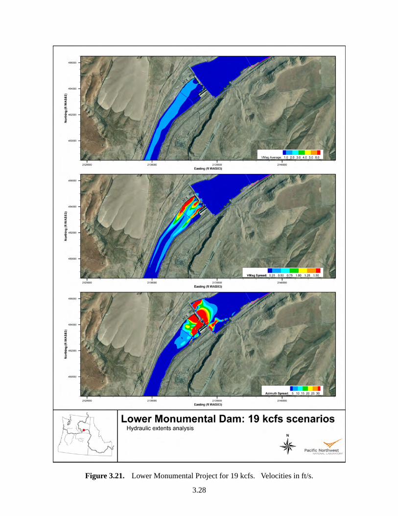
Figure 3.21. Lower Monumental Project for 19 kcfs. Velocities in ft/s.
3.28
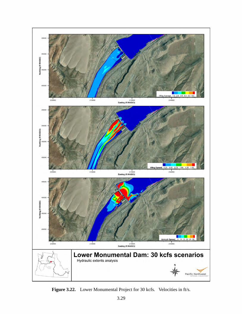
Figure 3.22. Lower Monumental Project for 30 kcfs. Velocities in ft/s.
3.29
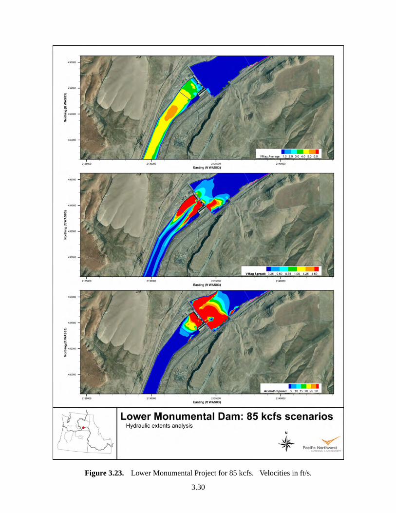
Figure 3.23. Lower Monumental Project for 85 kcfs. Velocities in ft/s.
3.30
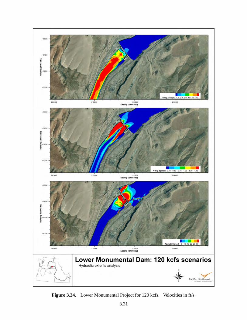
Figure 3.24. Lower Monumental Project for 120 kcfs. Velocities in ft/s.
3.31

3.7 Little Goose Project
Operations are detailed in Tables 2.22 and 2.23. Figures 3.25 to 3.28 show the results of theMASS2 runs. At Little Goose, the largest downstream hydraulic extent is at 30 kcfs (Fig-ure 3.26). There is a flow constriction downstream of the project that reduces the hydraulicextent at the higher flows. In the forebay, the upstream extent of the spread in velocity magni-tude increases with increasing flow volume. However, the magnitude and extent of the differ-ences in flow direction are very similar for all river flows.
3.32
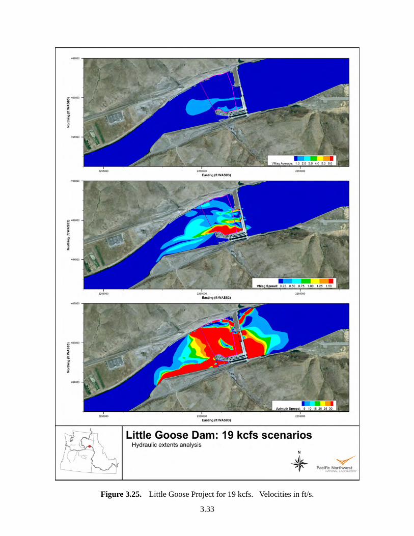
Figure 3.25. Little Goose Project for 19 kcfs. Velocities in ft/s.
3.33
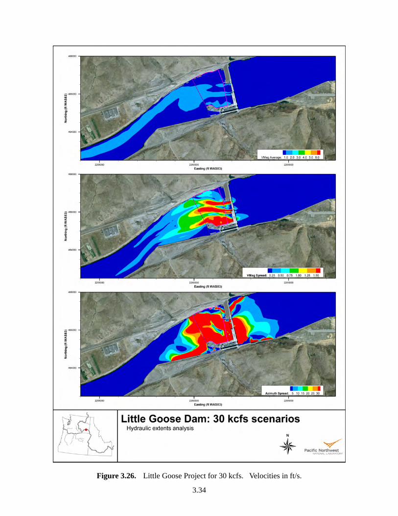
Figure 3.26. Little Goose Project for 30 kcfs. Velocities in ft/s.
3.34
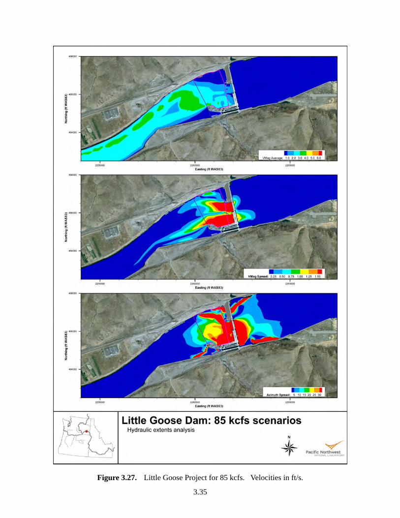
Figure 3.27. Little Goose Project for 85 kcfs. Velocities in ft/s.
3.35
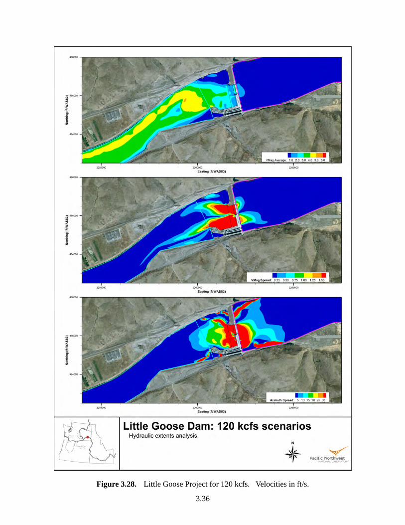
Figure 3.28. Little Goose Project for 120 kcfs. Velocities in ft/s.
3.36

3.8 Lower Granite Project
Operations are detailed in Tables 2.24 and 2.25. Figures 3.29 to 3.32 show the results of theMASS2 runs. In the tailrace, the downstream hydraulic extent of velocity magnitude differencesis very similar for all flows. For flow direction, however, the greatest downstream impact is atthe lowest flows with the least extent at the largest total river flow. In the forebay, the upstreamhydraulic extent is limited.
3.37
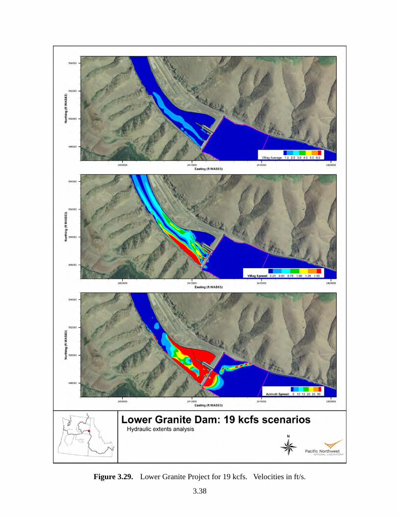
Figure 3.29. Lower Granite Project for 19 kcfs. Velocities in ft/s.
3.38
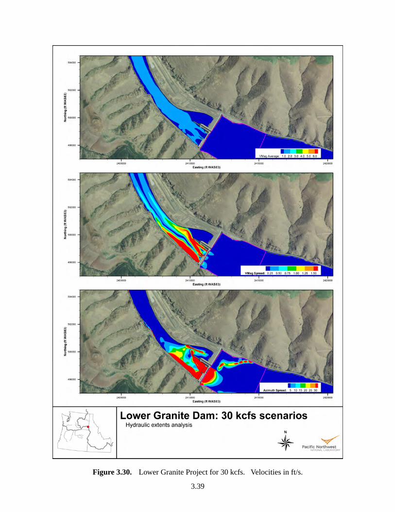
Figure 3.30. Lower Granite Project for 30 kcfs. Velocities in ft/s.
3.39

Figure 3.31. Lower Granite Project for 85 kcfs. Velocities in ft/s.
3.40
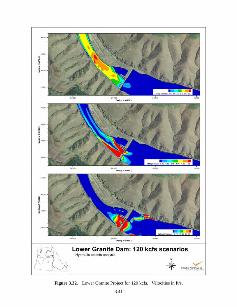
Figure 3.32. Lower Granite Project for 120 kcfs. Velocities in ft/s.
3.41
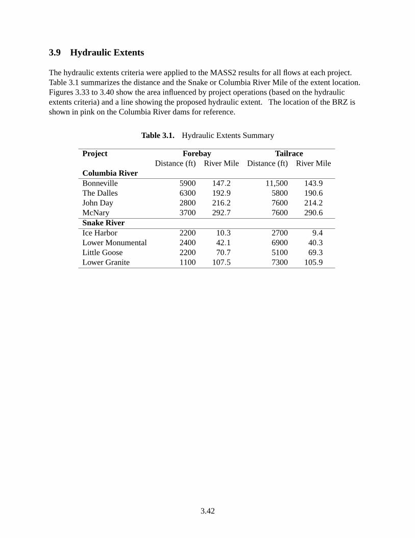
3.9 Hydraulic Extents
The hydraulic extents criteria were applied to the MASS2 results for all flows at each project.Table 3.1 summarizes the distance and the Snake or Columbia River Mile of the extent location.Figures 3.33 to 3.40 show the area influenced by project operations (based on the hydraulicextents criteria) and a line showing the proposed hydraulic extent. The location of the BRZ isshown in pink on the Columbia River dams for reference.
Table 3.1. Hydraulic Extents Summary
Project Forebay TailraceDistance (ft) River Mile Distance (ft) River Mile
Columbia RiverBonneville 5900 147.2 11,500 143.9The Dalles 6300 192.9 5800 190.6John Day 2800 216.2 7600 214.2McNary 3700 292.7 7600 290.6Snake RiverIce Harbor 2200 10.3 2700 9.4Lower Monumental 2400 42.1 6900 40.3Little Goose 2200 70.7 5100 69.3Lower Granite 1100 107.5 7300 105.9
3.42
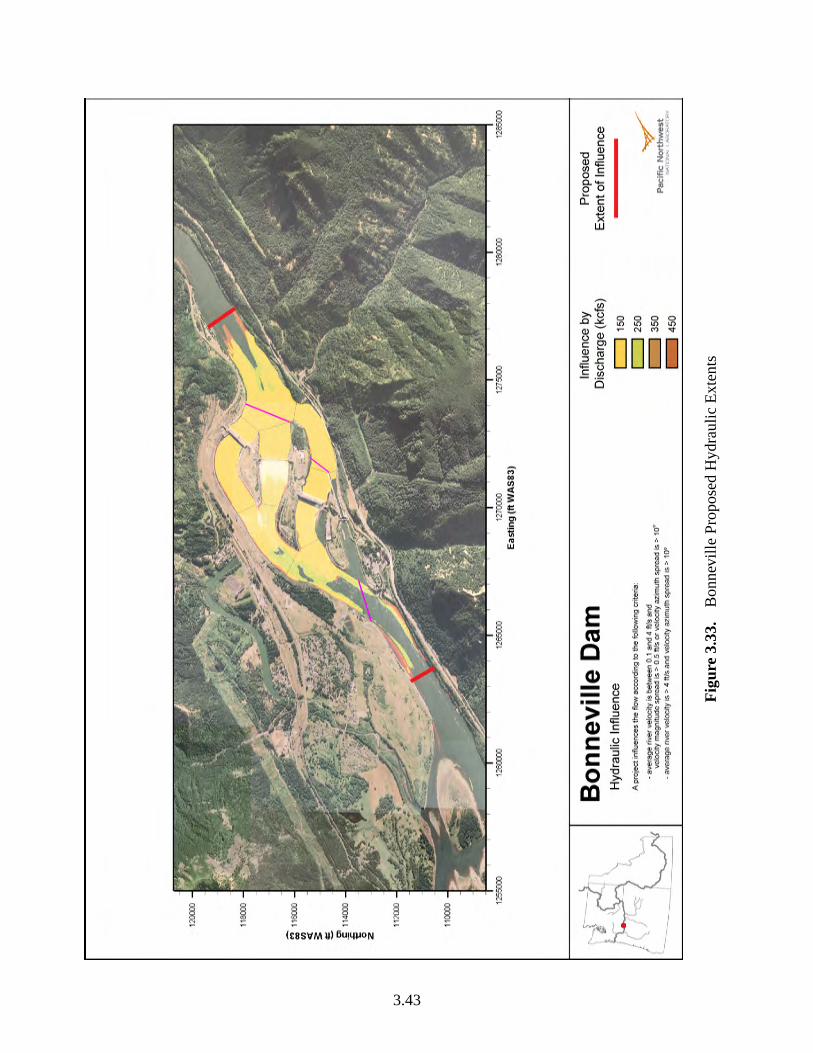
Fig
ure
3.33
.B
onne
ville
Pro
pose
dH
ydra
ulic
Ext
ents
3.43
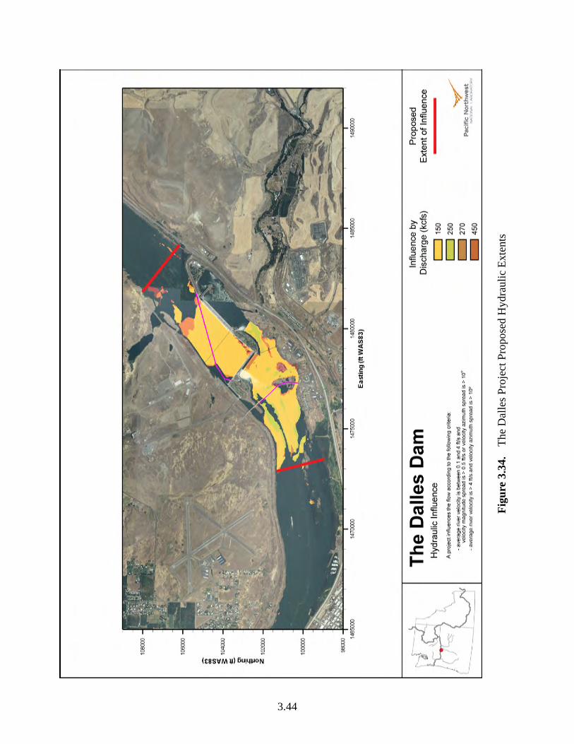
Fig
ure
3.34
.T
heD
alle
sP
roje
ctP
ropo
sed
Hyd
raul
icE
xten
ts
3.44
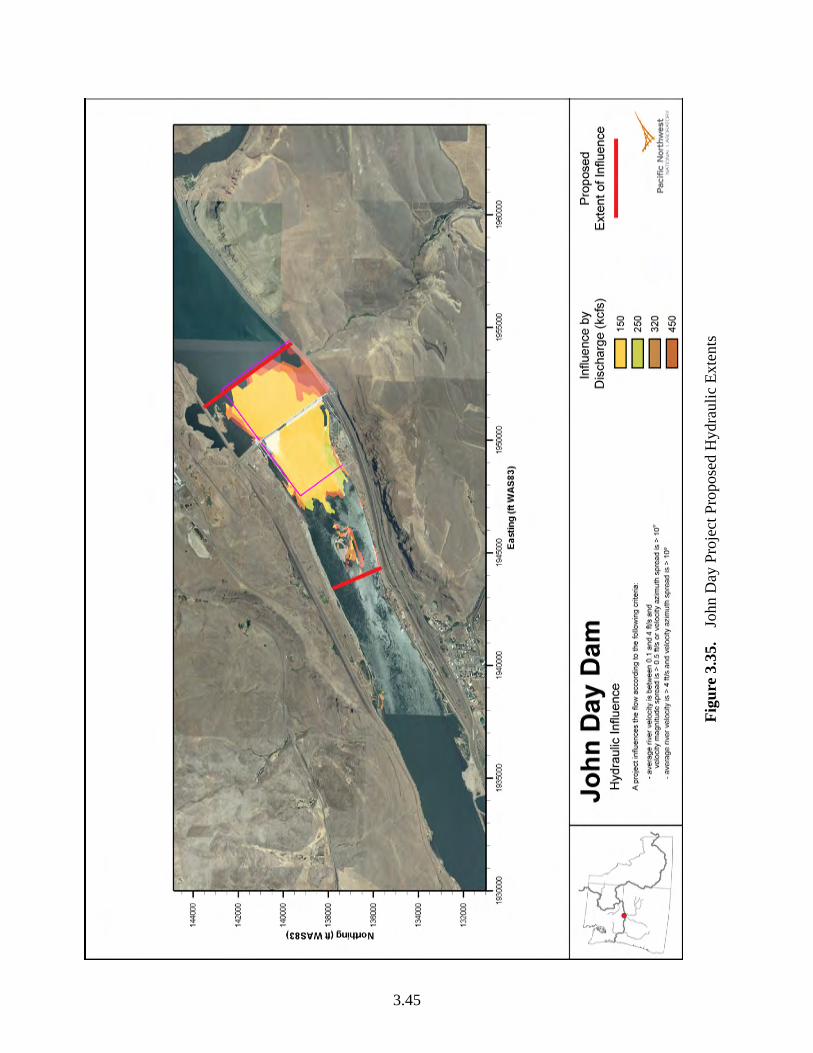
Fig
ure
3.35
.Jo
hnD
ayP
roje
ctP
ropo
sed
Hyd
raul
icE
xten
ts
3.45
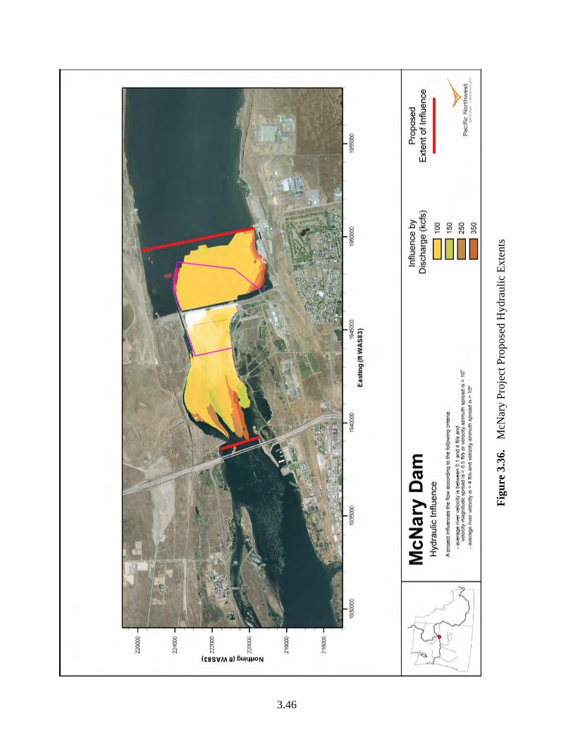
Fig
ure
3.36
.M
cNar
yP
roje
ctP
ropo
sed
Hyd
raul
icE
xten
ts
3.46
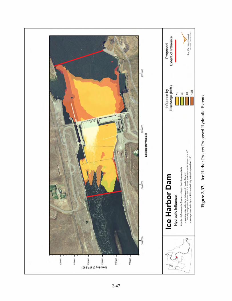
Fig
ure
3.37
.Ic
eH
arbo
rP
roje
ctP
ropo
sed
Hyd
raul
icE
xten
ts
3.47
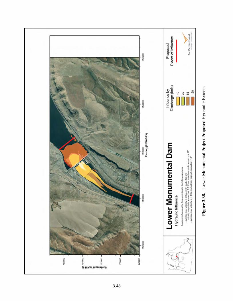
Fig
ure
3.38
.Lo
wer
Mon
umen
talP
roje
ctP
ropo
sed
Hyd
raul
icE
xten
ts
3.48
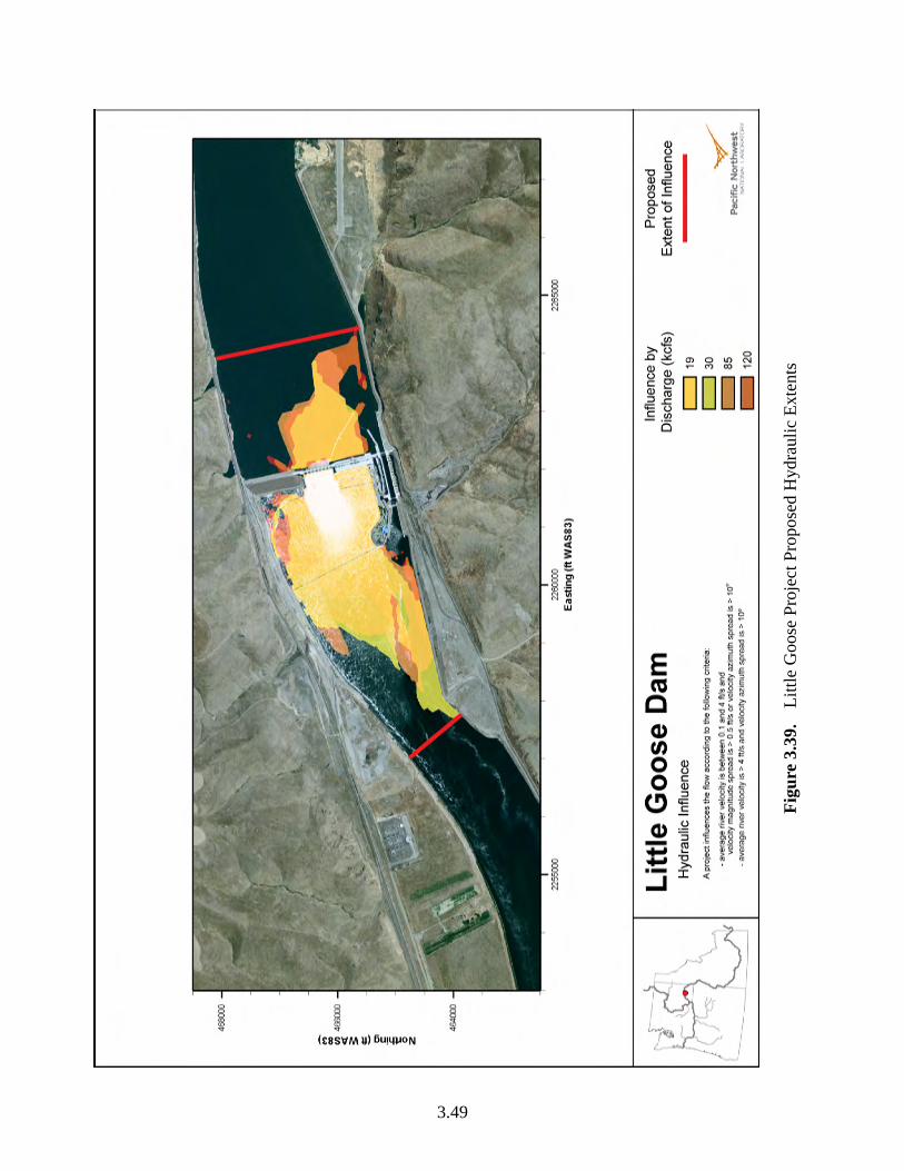
Fig
ure
3.39
.Li
ttle
Goo
seP
roje
ctP
ropo
sed
Hyd
raul
icE
xten
ts
3.49
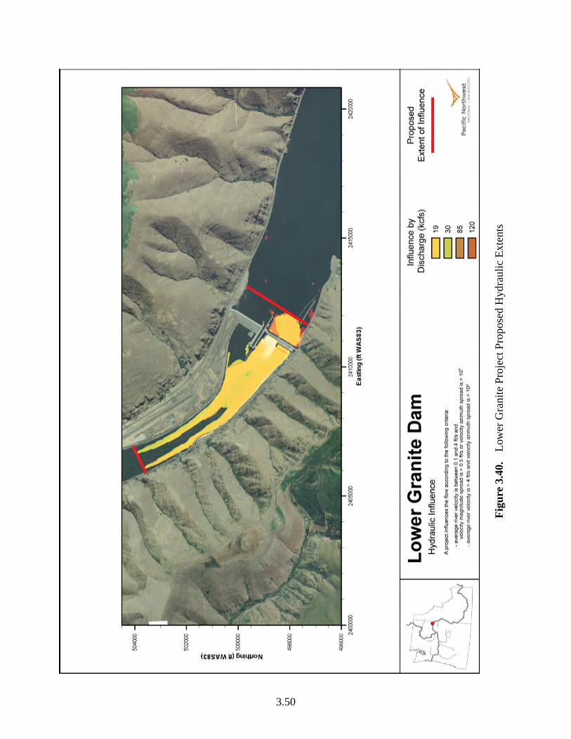
Fig
ure
3.40
.Lo
wer
Gra
nite
Pro
ject
Pro
pose
dH
ydra
ulic
Ext
ents
3.50
4.0 Conclusions
The purpose of this study was to delineate the hydraulic extents of the hydroelectric projectson the lower Columbia and lower Snake rivers in a consistent manner. Based on results from a2D depth-averaged river model, MASS2, and criteria from USACE-CENWP, the extents weredelineated for each project.
In many studies, the location of the BRZ has been used for the hydraulic extent in the lowerColumbia River, and the feasibility project at John Day supported the BRZ as largely encom-passing the area of project influence. For all these Columbia River projects, however, this is notconsistently the case.
Although each hydroelectric project has a different physical setting, there were some commonresults. The downstream hydraulic extent tended to be greater than the hydraulic extent inthe forebay; The Dalles is the exception. The hydraulic extent of the projects was generallylarger at the mid-range flows. At higher flows, the channel geometry (in particular the channelconstrictions) reduced the impact of project operations.
4.1

5.0 References
Gordon J, B Evans, and E Perry. 1995.Lower Granite GIS Data Description and CollectionGuidelines. PNL-10889, Pacific Northwest National Laboratory, Richland, Washington.
Hanrahan TP, MC Richmond, EV Arntzen, AM Coleman, KB Larson, WA Perkins, andJD Tagestad. 2007.Effects of Hydroelectric Dam Operations on the Restoration Potential ofSnake River Fall Chinook Salmon (Oncorhynchus tshawytscha) Spawning Habitat, Final Report,October 2005-September 2007. PNNL-16944, Pacific Northwest National Laboratory, RichlandWA.
Kincaid CT, RW Bryce, PW Eslinger, JM Becker, CA Brandt, AL Bunn, CR Cole, EJ Freeman,GR Guensch, DG Horton, GV Last, TB Miley, WA Perkins, WE Nichols, M Oostrom, MC Rich-mond, DL Strenge, and PD Thorne. 2001. “Development of a Site-Wide System AssessmentCapability.” Presented at the Waste Management 2001 Symposium, February 25 - March 1,2001, sponsored by the University of Arizona, Tuscon, Arizona.
McMichael GA, WA Perkins, CJ McMurray, YJ Chien, CL Rakowski, A Coleman, MC Rich-mond, J Vucelick, EV Arntzen, RP Mueller, CA Duberstein, and J Lukas. 2003.SubyearlingChinook Salmon Stranding in the Hanford Reach of the Columbia River. PNWD-3308, Battelle–Pacific Northwest Division, Richland, Washington. Prepared for Grant County Public UtilityDistrict No. 2.
Patankar S. 1980.Numerical Heat Transfer and Fluid Flow.Hemisphere, New York, New York.
Perkins WA and MC Richmond. 2004a.MASS2, Modular Aquatic Simulation System in TwoDimensions, Theory and Numerical Methods.PNNL-14820-1, Pacific Northwest NationalLaboratory, Richland, Washington.
Perkins WA and MC Richmond. 2004b.MASS2, Modular Aquatic Simulation System in TwoDimensions, User Guide and Reference. PNNL-14820-2, Pacific Northwest National Laboratory,Richland, Washington.
Perkins WA and MC Richmond. 2004c.MASS2, Modular Aquatic Simulation System in TwoDimensions, User Guide and Reference. PNNL-14820-2, Pacific Northwest National Laboratory,Richland, Washington.
Perkins WA, MC Richmond, and G McMichael. 2004. “Two-Dimensional Modeling of Time-Varying Hydrodynamics and Juvenile Chinook Salmon Habitat in the Hanford Reach of theColumbia River.” InCritical Transitions in Water and Environmental Resources Management,Proceedings of the 2004 World Water and Environmental Resources Congress, June 27-July 1,Salt Lake City, Utah, Sehlke G, DF Hayes, and DK Stevens, eds. Reston, Virginia. ASCE.
Pointwise, Inc. 2003.Gridgen User Manual, Version 15.
Rakowski CL, WA Perkins, MC Richmond, and J Serkowski. 2008a.Determing John DayProject Tailrace and Forebay Zones Using the MASS2 Model. PNNL-SA-60840, PacificNorthwest National Laboratory, Richland, Washington. Prepared for the U.S. Army Corps ofEngineers, Portland District.
5.1
Rakowski CL, WA Perkins, MC Richmond, and JA Serkowski. 2008b.Determining JohnDay Project Tailrace and Forebay Zones Using the MASS2 Model. PNNL-SA-60840, PacificNorthwest National Laboratory, Richland, Washington.
Rakowski CL and MC Richmond. 2001.Dalles Tailwater Predator Study: Numerical Analysisof Tailwater Flow Conditions. PNNL-13594, Pacific Northwest National Laboratory, Richland,Washington.
Rakowski CL and MC Richmond. 2003.John Day Tailrace MASS2 Hydraulic Modeling.PNNL-14491, Pacific Northwest National Laboratory, Richland, Washington.
Richmond MC, WA Perkins, and Y Chien. 2000.Numerical Model Analysis of System-wideDissolved Gas Abatement Alternatives. PNWD-3245, Battelle–Pacific Northwest Division,Richland, Washington. Prepared for the U.S. Army Corps of Engineers, Walla Walla Districtunder Contract DACW68-96-D-0002.
Richmond MC, WA Perkins, and CL Rakowski. 1999a.Two-Dimensional Analysis of FlowConditions and Sediment Mobility in the Lower Snake River for Impounded and Natural RiverConditions. U.S. Department of Energy, Pacific Northwest National Laboratory, P.O. Box 999,Richland, Washington. Prepared for the U.S. Army Corps of Engineers, Walla Walla District.
Richmond MC, WA Perkins, and T Scheibe. 1999b.Summary and Model Formulation. Part 1in Two-Dimensional Hydrodynamic, Water Quality, and Fish Exposure Modeling of the Columbiaand Snake Rivers. Battelle–Pacific Northwest Division, Richland, Washington. Prepared for theU.S. Army Corps of Engineers, Walla Walla District under Contract DACW68-96-D-0002.
Richmond MC, WA Perkins, and T Scheibe. 1999c. “Two-Dimensional Simulation of Hydrody-namics, Water Quality, and Fish Exposure in the Columbia/Snake River System.” InProceedingsof WaterPower99.
Spasojevic M and F Holly, Jr. 1990. “2-D Bed Evolution in Natural Watercourses New Simula-tion Approach.” J. of Waterway, Port, Coastal, and Ocean Engineering116(4):425–443.
USACE–Northwestern Division. 2008.Fish Passage Plan Corps of Engineers Project. USArmy Corps of Engineers. http://www.nwd-wc.usace.army.mil/tmt/documents/fpp/.
Zhou J. 1995. “Velocity-Depth Coupling in Shallow-Water Flows.”J. of Hydraulic Engineering121(10):717–724.
5.2