DETERMINING THE OPTIMAL SITE LOCATION OF GNSS BASE STATIONS

Bol. Ciênc. Geod., sec. Artigos, Curitiba, v. 18, no 1, p. 154-169, jan-mar, 2012.

DETERMINING THE OPTIMAL SITE LOCATION OF GNSS

BASE STATIONS

Determinação da melhor localização de uma estação gnss de referência

JEN-YU HAN

YU WU ROU-YU LIU

Department of Civil Engineering

National Taiwan University No. 1, Sec. 4, Roosevelt Rd., Taipei 106, Taiwan.

{jyhan, r98521114, r98521113}@ntu.edu.tw

ABSTRACT The relative positioning technique plays an essential role in Global Navigation Satellite System (GNSS) surveys. Simultaneous observation at base and rover stations eliminates the majority of error sources thus the quality of a positioning solution can be substantially improved. However, topographic obstruction is still a key issue affecting positioning quality. In this study, an integrated approach for analyzing the impact of topographic obstruction on GNSS relative positioning has been developed. By considering varied satellite geometry according to actual terrain variation, this approach can be used to realistically determine satellite visibility condition for a specific base station with respect to any rover station. Furthermore, a base station quality index (BSQI) is proposed as an explicit indication of the sufficiency in a relative positioning. By incorporating the proposed approach, one can immediately identify an optimal site location for a GNSS base station with subsequent GNSS field survey thus achieved in a more reliable and cost-efficient manner. Keywords: Global Navigation Satellite System; Relative Positioning; Visibility Analysis; Digital Surface Model; Base Station Quality Index

RESUMO Técnica de posicionamento relativo tem desempenhado um papel essencial em pesquisas de Sistema de Navegação Global via Satélites (GNSS). Coletando observações simultâneas entre estações base e móvel, uma grande parte das fontes

Han, J. et al..

Bol. Ciênc. Geod., sec. Artigos, Curitiba, v. 18, no 1, p.154-169, jan-mar, 2012.

1 5 5

de erro é eliminada; portanto a qualidade de solução do posicionamento pode ser substancialmente melhorada. No entanto, a obstrução topográfica ainda é uma questão-chave que afeta a qualidade de posicionamento. Neste estudo, uma abordagem integrada para analisar o impacto da obstrução topográfica em posicionamento relativo GNSS foi desenvolvida. Esta abordagem considera a geometria variada dos satélites de acordo com variações reais do terreno, e as condições de visibilidade do satélite para uma estação base específica com relação a qualquer estação móvel pode ser realisticamente determinada. Além disso, uma base de índice de qualidade da estação (BSQI) é proposta como uma indicação explícita para sua eficiência em um posicionamento relativo. Conseqüentemente, pode-se identificar imediatamente um local otimizado para uma estação base do GNSS, incorporando a abordagem proposta de antemão, e uma pesquisa de campo GNSS, podendo assim alcançar uma forma mais confiável e de custo-eficiente. Palavras-chave: Sistema de Navegação Global via Satélites; Posicionamento Relativo; Análise de Visibilidade; Modelo Digital de Superfície; Índice de Qualidade da Estação de Referência 1. INTRODUCTION Global Navigation Satellite System (GNSS) provides precise positioning and timing solutions that are unaffected by weather and without the need for a clear line of sight between ground stations. Such systems are therefore widely used in various surveying and navigation tasks. GNSS works under the basic principle that the range observations of satellites to a receiver can be used to define the coordinates of that receiver. Consequently, both the number of visible satellites and the geometry constituted by these satellites will directly affect the quality of GNSS positioning. The most basic GNSS positioning method is single-point positioning, which only requires the reception of four satellite signals in order to obtain the necessary coordinates and clock offset of the measurement point. However, single-point positioning accuracy is compromised by various factors such as errors in satellite orbits, clocks, and signal propagation. Therefore, in order to meet accuracy requirements for geodetic or engineering applications, a relative positioning method must be used to reduce these errors and thus obtain a more precise coordinate measurement for the receiver (LEICK, 2004).

Relative positioning operates on the basic principle of using two GNSS receivers to simultaneously observe a GNSS satellite. One receiver, known as the base station, is set to the known coordinates of a control point; while the other receiver, typically referred to as the rover or mobile station, is set to the coordinates of an unknown point. With both receivers observing the same satellite simultaneously, range measurements to the two receivers will share common clock errors and partially satellite orbital errors (converge with the decrease of baseline length). Furthermore, as the distance between the base and rover stations decreases, the ionospheric and tropospheric delays affecting the range measurements will also

Determining the optimal site location of GNSS base stations...


1 5 6

converge. As a result, differentiation of range measurements obtained at the rover and base stations can effectively eliminate or weaken the impact of these errors, leading to an improvement in the positioning precision of the rover station.

A number of positioning applications utilize the relative GNSS positioning technique, including Real Time Kinematic (RTK) GNSS positioning (e.g., CINTRA et al., 2011; TANAJURA et al., 2011), Continuously Operating Reference Stations (CORS) (SNAY and SOLER, 2008), and Electrical Global Satellite Real-Time Kinematic Positioning System (e-GPS, see CHIANG et al., 2009). While RTK involves users establishing their own base station during the surveying process, CORS and e-GPS both involve the use of fixed base stations set up by government agencies to provide long-term user access. In particular, the e-GPS receives continuous GPS observations at permanent stations and computes required correction parameters for subscribed users. Furthermore, GNSS range observations rely on the passing of radio signal transmissions between satellite and receiver. Both the satellite and the receiver must maintain a clear line of sight to each other, since obstructions in the form of mountains, buildings and other objects will reduce positioning accuracy. Consequently, when estimating the positioning accuracy of GNSS, the impact of environmental factors on satellite signal transmission should be of significant concern.

Regardless of whether a base station used for relative positioning has been set up temporarily by the user (campaign station) or permanently by a government agency, poor location selection will inevitably affect the quality of the subsequent rover station positioning. In recent studies, increasing numbers of researchers are focusing their research on the impact of topography on the quality of GNSS positioning; some of these researchers include Chen et al. (2009), Beesley (2003), Xavier and Costa (2007), Taylor et al. (2007), Zhang et al. (2008), and Han and Li (2010). However, these studies mainly considered the impact of terrain obstruction on single-point positioning; for applications that require a higher order of precision, a relative positioning technique must be used in order to remove any systematic errors in range observables. The geometry of a relative positioning model is more complicated and has higher requirements for satellite visibility conditions. For these reasons, it is necessary to extend the study and carry out an in-depth analysis of this model when evaluating positioning quality.

The main purpose of this study is to include the topography effect in the process of GNSS relative positioning quality assessment, while also taking into account the geometry of the network formed by the visible satellites under the influence of terrain variation. This serves as the basis for estimating relative GNSS positioning quality. Using this concept, a base station quality index (BSQI) will then be established as an explicit indication of its sufficiency in relative positioning, thus enabling the optimization of base station location selection.

Han, J. et al..


1 5 7

2. MATHEMATICAL MODELS 2.1 Single-Point Positioning Model

The most fundamental form of GNSS positioning, the basic idea behind single-point positioning is the measurement of the ranges from multiple satellites to a single receiver. When the satellites’ position isx ( 1~i n= ) are given, one can write the following phase equation for each measurement (Hofmann-Wellenhof et al., 2001):

i i i i is s s s s

r r r r atm rp c t Nϕ λ δ ε λ= = − + + −x x (1) where is

rp denotes the pseudo range from satellite is to receiver r , isrϕ the

corresponding phase measurement, λ the wavelength of the carrier signal, rx the

receiver’s position, c the propagation speed of the signal, isrtδ the clock offset,

atmε the error associated with atmospheric delay, and isrN the integer ambiguity. In

cases where the satellite’s orbits are known, integer ambiguity resolved, and atmospheric delay properly modeled, 4 unknowns (3 in rx and 1 in is

rtδ ) remain to be solved. Consequently, one requires at least 4 range measurements in order for these parameters to be individually determined. 2.2 Relative Positioning Model In a single-point positioning model, it is assumed that satellite orbits are known perfectly and the errors associated with clock offsets and atmospheric delays accurately modeled. However, these prerequisites are usually not fulfilled and thus a large degree of uncertainty in terms of the associated positioning solution is produced. In order to eliminate the impact of these error sources - for instance as part of a GNSS survey with a higher standard of quality requirements - a relative positioning model is usually implemented. These models require two receivers, one at a base station (known point k) and the other at a rover station (unknown point i), to simultaneously collect range measurements from common satellites (Figure 1). Consequently, the two receivers share common clock errors, while the orbital error and atmospheric delay from each satellite to the two receivers are approximate when the receivers are close to each other. Once the range measurements are differenced, the above-mentioned errors can be removed or significantly reduced.



1 5 8

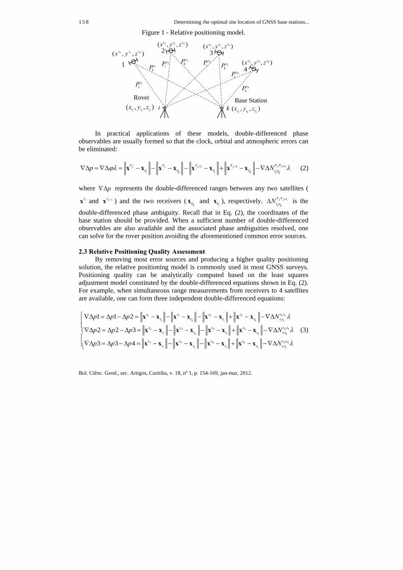
Figure 1 - Relative positioning model.

In practical applications of these models, double-differenced phase observables are usually formed so that the clock, orbital and atmospheric errors can be eliminated:

11 1 j jj j j j

i k i k i k

s ss s s sr r r r r rp Nϕλ λ++ +∇Δ = ∇Δ = − − − − − + − −∇Δx x x x x x x x (2)

where p∇Δ represents the double-differenced ranges between any two satellites (

jsx and 1js +x ) and the two receivers (krx and

irx ), respectively. 1j j

i k

s sr rN +Δ is the

double-differenced phase ambiguity. Recall that in Eq. (2), the coordinates of the base station should be provided. When a sufficient number of double-differenced observables are also available and the associated phase ambiguities resolved, one can solve for the rover position avoiding the aforementioned common error sources. 2.3 Relative Positioning Quality Assessment

By removing most error sources and producing a higher quality positioning solution, the relative positioning model is commonly used in most GNSS surveys. Positioning quality can be analytically computed based on the least squares adjustment model constituted by the double-differenced equations shown in Eq. (2). For example, when simultaneous range measurements from receivers to 4 satellites are available, one can form three independent double-differenced equations:

1 1 2 2 1 2

3 3 2 32 2

3 3 3 44 4

1 1 2

2 2 3

3 3 4

i k i k i k

i k i k i k

i k i k i k

s s s s s sr r r r r r

s s s ss sr r r r r r

s s s ss sr r r r r r

p p p N

p p p N

p p p N

λ

λ

λ

⎧∇Δ = Δ − Δ = − − − − − + − −∇Δ⎪⎪∇Δ = Δ − Δ = − − − − − + − −∇Δ⎨⎪∇Δ = Δ −Δ = − − − − − + − −∇Δ⎪⎩

x x x x x x x x

x x x x x x x x

x x x x x x x x

(3)

1

i

2

k( , , )i i ir r rx y z

1 1 1( , , )s s sx y z

( , , )k k kr r rx y z

4

32 2 2( , , )s s sx y z 3 3 3( , , )s s sx y z

4 4 4( , , )s s sx y z

1siP

1skP

2siP

2skP 3s

iP4s

iP3s

kP

4skP

Base Station Rover

Han, J. et al..


1 5 9

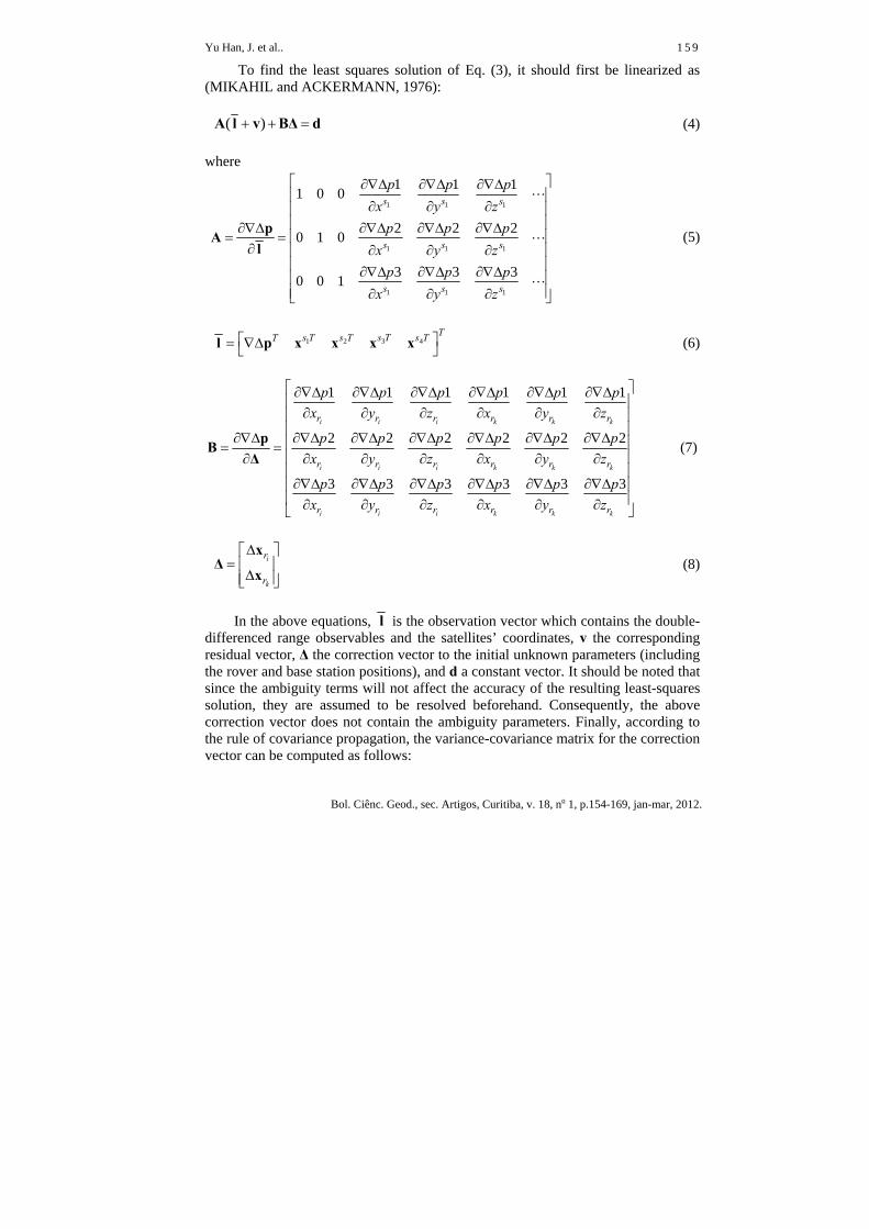
To find the least squares solution of Eq. (3), it should first be linearized as (MIKAHIL and ACKERMANN, 1976):

( )+ + =A l v BΔ d (4) where

1 1 1

1 1 1

1 1 1

1 1 11 0 0

2 2 20 1 0

3 3 30 0 1

s s s

s s s

s s s

p p px y z

p p px y z

p p px y z

⎡ ⎤∂∇Δ ∂∇Δ ∂∇Δ⎢ ⎥

∂ ∂ ∂⎢ ⎥⎢ ⎥∂∇Δ ∂∇Δ ∂∇Δ ∂∇Δ

= = ⎢ ⎥∂ ∂ ∂ ∂⎢ ⎥

⎢ ⎥∂∇Δ ∂∇Δ ∂∇Δ⎢ ⎥⎢ ⎥∂ ∂ ∂⎣ ⎦

pAl

L

L

L

(5)

31 2 4

Ts Ts T s T s TT⎡ ⎤= ∇Δ⎣ ⎦l p x x x x (6)

1 1 1 1 1 1

2 2 2 2 2 2

3 3 3 3 3 3

i i i k k k

i i i k k k

i i i k k k

r r r r r r

r r r r r r

r r r r r r

p p p p p px y z x y z



⎡ ⎤∂∇Δ ∂∇Δ ∂∇Δ ∂∇Δ ∂∇Δ ∂∇Δ⎢ ⎥

∂ ∂ ∂ ∂ ∂ ∂⎢ ⎥⎢ ⎥∂∇Δ ∂∇Δ ∂∇Δ ∂∇Δ ∂∇Δ ∂∇Δ ∂∇Δ⎢ ⎥= =⎢ ⎥∂ ∂ ∂ ∂ ∂ ∂ ∂⎢ ⎥∂∇Δ ∂∇Δ ∂∇Δ ∂∇Δ ∂∇Δ ∂∇Δ⎢ ⎥⎢ ⎥∂ ∂ ∂ ∂ ∂ ∂⎣ ⎦

pBΔ

(7)

i

k

r

r

Δ⎡ ⎤= ⎢ ⎥

Δ⎢ ⎥⎣ ⎦

xΔ

x (8)

In the above equations, l is the observation vector which contains the double-

differenced range observables and the satellites’ coordinates, v the corresponding residual vector, Δ the correction vector to the initial unknown parameters (including the rover and base station positions), and d a constant vector. It should be noted that since the ambiguity terms will not affect the accuracy of the resulting least-squares solution, they are assumed to be resolved beforehand. Consequently, the above correction vector does not contain the ambiguity parameters. Finally, according to the rule of covariance propagation, the variance-covariance matrix for the correction vector can be computed as follows:



1 6 0

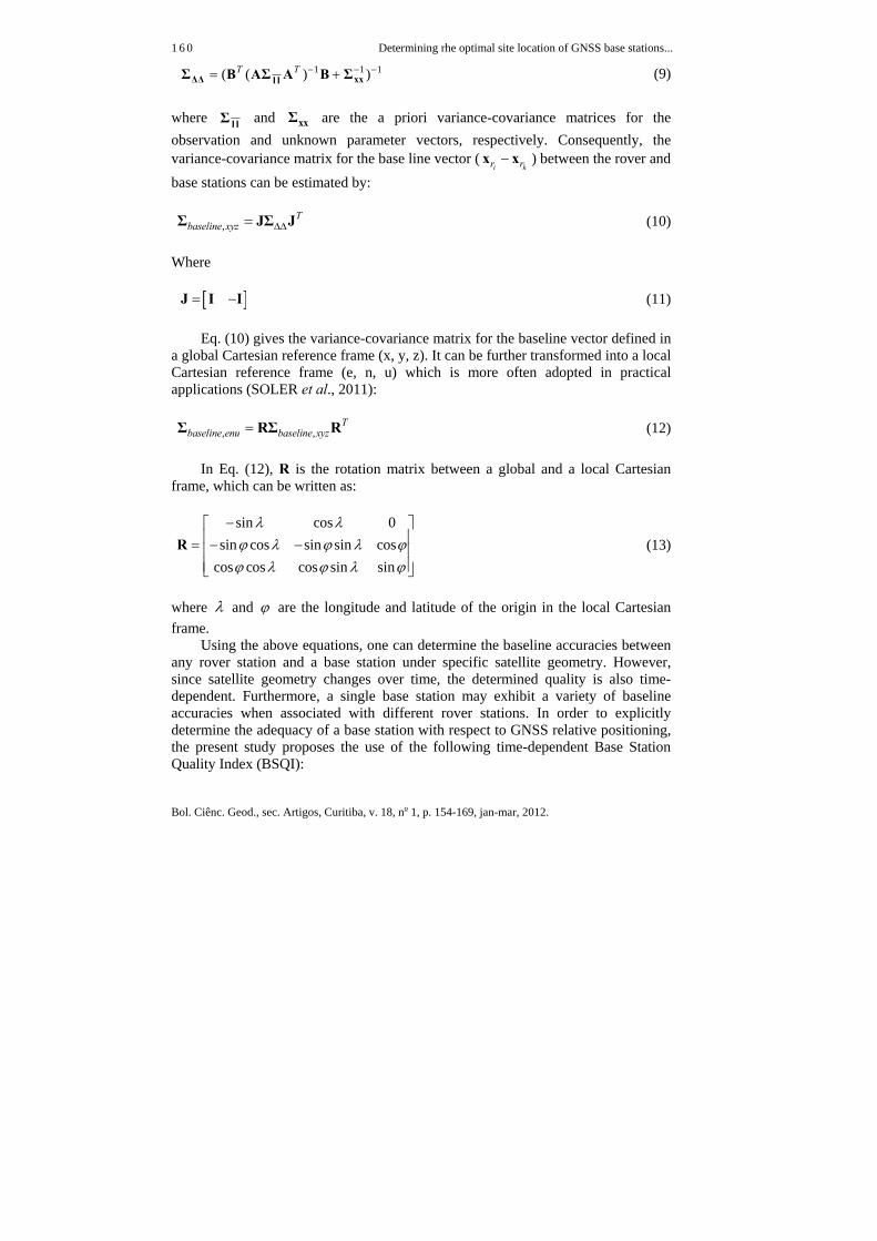
1 1 1( ( ) )T T − − −= +ΔΔ xxl lΣ B AΣ A B Σ (9) where l lΣ and xxΣ are the a priori variance-covariance matrices for the observation and unknown parameter vectors, respectively. Consequently, the variance-covariance matrix for the base line vector (

i kr r−x x ) between the rover and base stations can be estimated by:

,T

baseline xyz ΔΔ=Σ JΣ J (10) Where

[ ]= −J I I (11)

Eq. (10) gives the variance-covariance matrix for the baseline vector defined in a global Cartesian reference frame (x, y, z). It can be further transformed into a local Cartesian reference frame (e, n, u) which is more often adopted in practical applications (SOLER et al., 2011):

, ,T

baseline enu baseline xyz=Σ RΣ R (12)

In Eq. (12), R is the rotation matrix between a global and a local Cartesian frame, which can be written as:

sin cos 0

sin cos sin sin coscos cos cos sin sin

λ λϕ λ ϕ λ ϕϕ λ ϕ λ ϕ

−⎡ ⎤⎢ ⎥= − −⎢ ⎥⎢ ⎥⎣ ⎦

R (13)

where λ and ϕ are the longitude and latitude of the origin in the local Cartesian frame.

Using the above equations, one can determine the baseline accuracies between any rover station and a base station under specific satellite geometry. However, since satellite geometry changes over time, the determined quality is also time-dependent. Furthermore, a single base station may exhibit a variety of baseline accuracies when associated with different rover stations. In order to explicitly determine the adequacy of a base station with respect to GNSS relative positioning, the present study proposes the use of the following time-dependent Base Station Quality Index (BSQI):

Han, J. et al..


1 6 1

( ), ,1

,

N

baseline enu k ii t

k t

traceBSQI

N=

Σ=∑

(14)

where ( ), ,baseline enu k i

Σ denotes the variance-covariance matrix for the baseline vector

between a specific base station k and any rover station i, N the total number of rover stations and t the epoch at which the baseline accuracies are analyzed. A smaller BSQI value indicates a better ability of the specified base station to be used in GNSS relative positioning. Additionally, one can also compute an averaged BSQI value for a specific time period (e.g. 0 ~ st t t= ):

0

0

,0

,

j

s

s

s

k tj

k t tt t

BSQIBSQI

N==∑

(15)

where

0 st tN represents the number of BQSI occurrences being analyzed during the

time period 0 ~ st t . In many cases a GNSS field survey is performed only during a certain time

period (e.g. daytime). With the above index, one can easily determine the best location for a base station according to the time period during which field data are to be collected.

2.4 Satellite Visibility Determination

When the quality of a baseline is to be analyzed (for instance as described in the previous section), usable range measurements must be determined before they can be considered in the analysis. In other words, satellite visibility with respect to a specific base or rover station must be identified beforehand. The classical approach to such a problem typically involves the establishment of a constant mask angle. When the elevation from a satellite to a receiver is larger than the preset mask angle, the satellite in question is identified as visible to the receiver. However, in reality the actual visibility is greatly affected by terrain variation. As a constant mask angle fails to provide a realistic criterion for satellite visibility analysis, in the present study the adaptive line-of-sight (LOS) analysis approach (Han and Li 2010) is utilized in order to determine satellite visibility based on actual terrain variation. Such an approach also necessitates the use of digital terrain data (e.g. DSM). Radial profiles originated from a receiver are analyzed and the maximum obstruction angle of each profile computed (Fig. 2). These angles are then used as visibility criteria above which a satellite will be identified as being visible to the receiver.



1 6 2

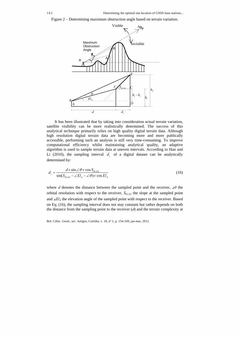
Figure 2 – Determining maximum obstruction angle based on terrain variation.

It has been illustrated that by taking into consideration actual terrain variation, satellite visibility can be more realistically determined. The success of this analytical technique primarily relies on high quality digital terrain data. Although high resolution digital terrain data are becoming more and more publically accessible, performing such an analysis is still very time-consuming. To improve computational efficiency whilst maintaining analytical quality, an adaptive algorithm is used to sample terrain data at uneven intervals. According to Han and Li (2010), the sampling interval sd of a digital dataset can be analytically determined by:

1. 2

1. 2

sin cossin( ) cos

h hs

h h A A

d Sd

S El Elθ

θ× ∠ ×

=−∠ −∠ ×

(16)

where d denotes the distance between the sampled point and the receiver, ∠θ the orbital resolution with respect to the receiver, Sh1,h2 the slope at the sampled point and ∠ElA the elevation angle of the sampled point with respect to the receiver. Based on Eq. (16), the sampling interval does not stay constant but rather depends on both the distance from the sampling point to the receiver (d) and the terrain complexity at

1. 2h hS

θ1 rh h−

d sd

2h

R

A

B

1h

rh

C

AElD

Invisible

Visible

Maximum Obstruction Angle

R

B

A

Han, J. et al..


1 6 3

each sampling point (characterized by ∠ElA and Sh1,h2). Consequently, the total number of points to be analyzed is substantially reduced and thus reliable visibility analysis can be performed with better computational efficiency. Finally, all identified satellites visible to the base and rover stations are used to form the range equations, with the positioning quality under such satellite geometry then determined based on the approach outlined in the previous section. 3. NUMERICAL VALIDATIONS

Two example analyses will now be outlined in order to demonstrate the feasibility of the proposed approach. First, the satellite visibility and baseline accuracy of a test area are estimated with and without considering topographic obstructions. The predicted results are then compared to actual values obtained in the field. Secondly, BSQI values are estimated for this area for different periods of observation time. An averaged BSQI value is then obtained and used as an explicit indicator in determining optimal base station location.

3.1 Visibility and Baseline Accuracy Analyses

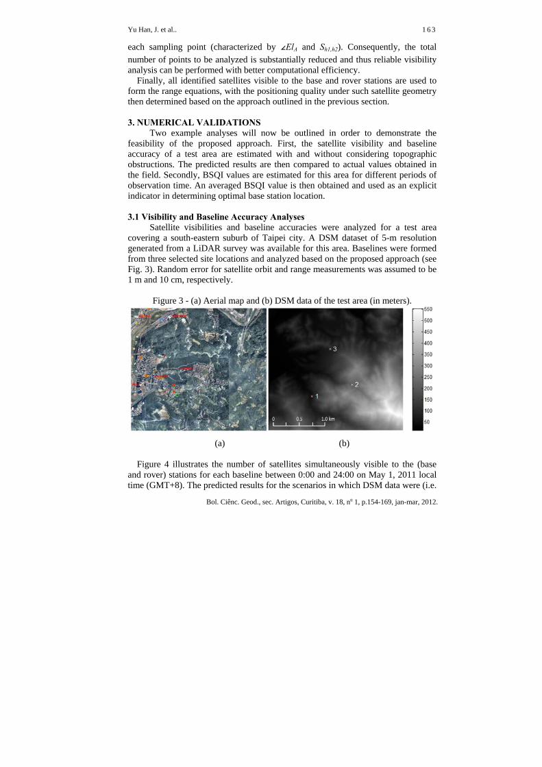
Satellite visibilities and baseline accuracies were analyzed for a test area covering a south-eastern suburb of Taipei city. A DSM dataset of 5-m resolution generated from a LiDAR survey was available for this area. Baselines were formed from three selected site locations and analyzed based on the proposed approach (see Fig. 3). Random error for satellite orbit and range measurements was assumed to be 1 m and 10 cm, respectively.

Figure 3 - (a) Aerial map and (b) DSM data of the test area (in meters).

(a) (b)

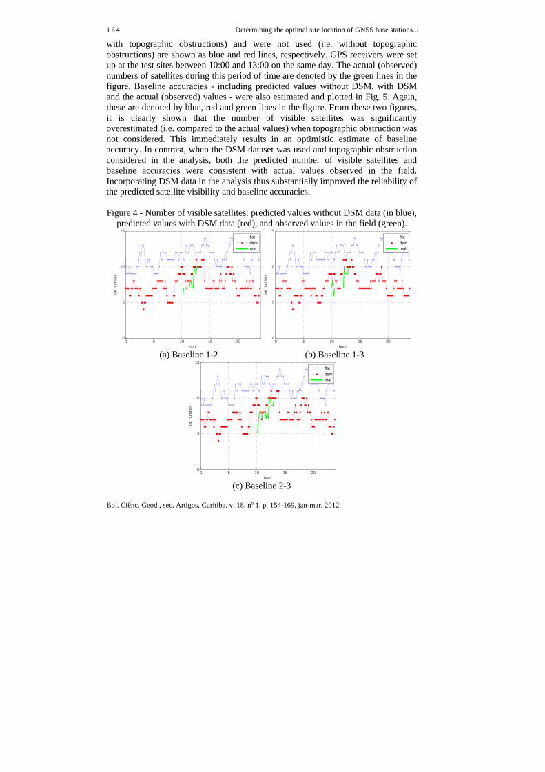
Figure 4 illustrates the number of satellites simultaneously visible to the (base and rover) stations for each baseline between 0:00 and 24:00 on May 1, 2011 local time (GMT+8). The predicted results for the scenarios in which DSM data were (i.e.



1 6 4

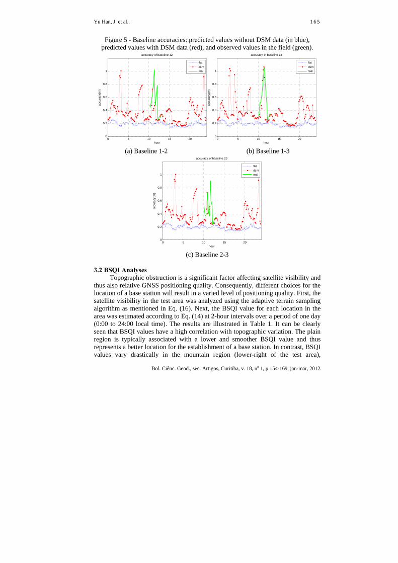
with topographic obstructions) and were not used (i.e. without topographic obstructions) are shown as blue and red lines, respectively. GPS receivers were set up at the test sites between 10:00 and 13:00 on the same day. The actual (observed) numbers of satellites during this period of time are denoted by the green lines in the figure. Baseline accuracies - including predicted values without DSM, with DSM and the actual (observed) values - were also estimated and plotted in Fig. 5. Again, these are denoted by blue, red and green lines in the figure. From these two figures, it is clearly shown that the number of visible satellites was significantly overestimated (i.e. compared to the actual values) when topographic obstruction was not considered. This immediately results in an optimistic estimate of baseline accuracy. In contrast, when the DSM dataset was used and topographic obstruction considered in the analysis, both the predicted number of visible satellites and baseline accuracies were consistent with actual values observed in the field. Incorporating DSM data in the analysis thus substantially improved the reliability of the predicted satellite visibility and baseline accuracies.

Figure 4 - Number of visible satellites: predicted values without DSM data (in blue),

predicted values with DSM data (red), and observed values in the field (green).

0 5 10 15 200

5

10

15

hour

sat n

umbe

r

flatdsmreal

0 5 10 15 200

5

10

15

hour

sat n

umbe

r

flatdsmreal

(a) Baseline 1-2 (b) Baseline 1-3

0 5 10 15 200

5

10

15

hour

sat n

umbe

r

flatdsmreal

(c) Baseline 2-3

Han, J. et al..


1 6 5

Figure 5 - Baseline accuracies: predicted values without DSM data (in blue),

predicted values with DSM data (red), and observed values in the field (green).

0 5 10 15 200

0.2

0.4

0.6

0.8

1

hour

accu

racy

(m)

accuracy of baseline 12

flatdsmreal

0 5 10 15 200

0.2

0.4

0.6

0.8

1

hour

accu

racy

(m)


flatdsmreal

(a) Baseline 1-2 (b) Baseline 1-3

0 5 10 15 200

0.2

0.4

0.6

0.8

1

hour

accu

racy

(m)


flatdsmreal

(c) Baseline 2-3

3.2 BSQI Analyses

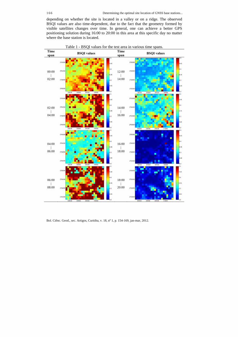
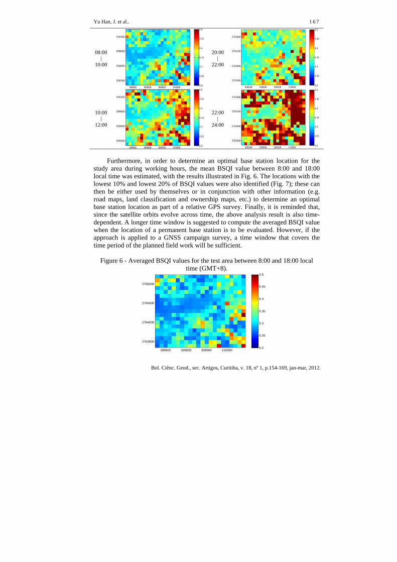
Topographic obstruction is a significant factor affecting satellite visibility and thus also relative GNSS positioning quality. Consequently, different choices for the location of a base station will result in a varied level of positioning quality. First, the satellite visibility in the test area was analyzed using the adaptive terrain sampling algorithm as mentioned in Eq. (16). Next, the BSQI value for each location in the area was estimated according to Eq. (14) at 2-hour intervals over a period of one day (0:00 to 24:00 local time). The results are illustrated in Table 1. It can be clearly seen that BSQI values have a high correlation with topographic variation. The plain region is typically associated with a lower and smoother BSQI value and thus represents a better location for the establishment of a base station. In contrast, BSQI values vary drastically in the mountain region (lower-right of the test area),



1 6 6

depending on whether the site is located in a valley or on a ridge. The observed BSQI values are also time-dependent, due to the fact that the geometry formed by visible satellites changes over time. In general, one can achieve a better GPS positioning solution during 16:00 to 20:00 in this area at this specific day no matter where the base station is located.

Table 1 - BSQI values for the test area in various time spans. Time span BSQI values Time

span BSQI values

00:00 |

02:00

12:00 |

14:00

02:00 |

04:00

14:00 |

16:00

04:00 |

06:00

16:00 |

18:00

06:00 |

08:00

18:00 |

20:00

Han, J. et al..


1 6 7

08:00 |

10:00

20:00 |

22:00

10:00 |

12:00

22:00 |

24:00

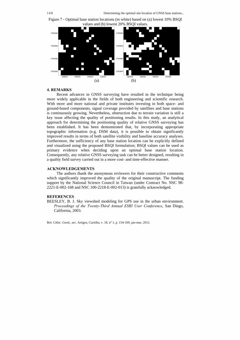
Furthermore, in order to determine an optimal base station location for the study area during working hours, the mean BSQI value between 8:00 and 18:00 local time was estimated, with the results illustrated in Fig. 6. The locations with the lowest 10% and lowest 20% of BSQI values were also identified (Fig. 7); these can then be either used by themselves or in conjunction with other information (e.g. road maps, land classification and ownership maps, etc.) to determine an optimal base station location as part of a relative GPS survey. Finally, it is reminded that, since the satellite orbits evolve across time, the above analysis result is also time-dependent. A longer time window is suggested to compute the averaged BSQI value when the location of a permanent base station is to be evaluated. However, if the approach is applied to a GNSS campaign survey, a time window that covers the time period of the planned field work will be sufficient.

Figure 6 - Averaged BSQI values for the test area between 8:00 and 18:00 local

time (GMT+8).

308500 309000 309500 310000

2765000

2764500

2764000

2763500

0.2

0.25

0.3

0.35

0.4

0.45

0.5



1 6 8

Figure 7 - Optimal base station locations (in white) based on (a) lowest 10% BSQI values and (b) lowest 20% BSQI values.

308500 309000 309500 310000

2765000

2764500

2764000

2763500

308500 309000 309500 310000

2765000

2764500

2764000

2763500

(a) (b)

4. REMARKS

Recent advances in GNSS surveying have resulted in the technique being more widely applicable in the fields of both engineering and scientific research. With more and more national and private institutes investing in both space- and ground-based components, signal coverage provided by satellites and base stations is continuously growing. Nevertheless, obstruction due to terrain variation is still a key issue affecting the quality of positioning results. In this study, an analytical approach for determining the positioning quality of relative GNSS surveying has been established. It has been demonstrated that, by incorporating appropriate topographic information (e.g. DSM data), it is possible to obtain significantly improved results in terms of both satellite visibility and baseline accuracy analyses. Furthermore, the sufficiency of any base station location can be explicitly defined and visualized using the proposed BSQI formulation; BSQI values can be used as primary evidence when deciding upon an optimal base station location. Consequently, any relative GNSS surveying task can be better designed, resulting in a quality field survey carried out in a more cost- and time-effective manner. ACKNOWLEDGEMENTS

The authors thank the anonymous reviewers for their constructive comments which significantly improved the quality of the original manuscript. The funding support by the National Science Council in Taiwan (under Contract No. NSC 98-2221-E-002-168 and NSC 100-2218-E-002-013) is gratefully acknowledged. REFERENCES BEESLEY, B. J. Sky viewshed modeling for GPS use in the urban environment.

Proceedings of the Twenty-Third Annual ESRI User Conference, San Diego, California, 2003.

Documents

DETERMINING THE OPTIMAL SITE LOCATION OF GNSS BASE STATIONS