Deterministic convergence of conjugate gradientmethod for feedforward neural networks I

Jian Wanga,b,c, Wei Wua, Jacek M. Zuradab,∗

aSchool of Mathematical Sciences, Dalian University of Technology, Dalian, 116024, P. R. ChinabDepartment of Electrical and Computer Engineering, University of Louisville, Louisville, KY

40292, USAcSchool of Mathematics and Computational Sciences, China University of Petroleum, Dongying,

257061, P. R. China

Abstract

Conjugate gradient methods have many advantages in real numerical experiments,such as fast convergence and low memory requirements. This paper considersa class of conjugate gradient learning methods for backpropagation (BP) neuralnetworks with three layers. We propose a new learning algorithm for almost cyclicBP neural networks based on PRP conjugate gradient method. We then establishthe deterministic convergence properties for three different learning fashions, i.e.,batch mode, cyclic and almost cyclic learning. There are mainly two deterministicconvergence properties including weak and strong convergence which indicate thegradient of the error function goes to zero and the weight sequence goes to a fixedpoint, respectively. Learning rate plays an important role in the training processof BP neural networks. The deterministic convergence results based on differentlearning fashions are dependent on different selection strategies of learning rate.

Keywords: Deterministic convergence, conjugate gradient, PRP, feedforwardneural networks

1. Introduction

The feedforward neural networks with backpropagation (BP) training proce-dure have been widely used in various fields of scientific researches and engineer-

IProject supported by the National Natural Science Foundation of China (No.10871220)∗Corresponding author.Email address: jmzura02@louisville.edu (Jacek M. Zurada )

Preprint submitted to Neural Networks November 8, 2010

ing applications. The BP algorithm attempts to minimize the least squared error ofobjective function, defined by the differences between the actual network outputsand the desired outputs (Rumelhart, Hinton, & Williams, 1986). There are twopopular ways of learning with training samples to implement the backpropagationalgorithm: batch mode and incremental mode (Heskes & Wiegerinck, 1996). Inbatch training, weight changes are accumulated over an entire presentation of thetraining samples before being applied, while incremental training updates weightsafter the presentation of each training sample (Wilson & Martinez, 2003).

There are three incremental learning strategies according to the order that thesamples are applied (Heskes & Wiegerinck, 1996; Xu, Zhang, & Jin, 2009; Wu, W.et al, 2010; Wang, Yang, & Wu, 2010). The first strategy is online learning (com-pletely stochastic order). The second strategy is almost-cyclic learning (specialstochastic order). The third strategy is cyclic learning (fixed order).

In most cases, the feedforward neural networks are performed by using super-vised neural learning techniques, employing the steepest descent method (Park et al,1991; Saini & Soni, 2002). We mention that the steepest descent method takesconsecutive steps in the direction of negative gradient of the performance surface.There has been considerable research on the methods to accelerate the conver-gence of the steepest descent method (Liu, Liu, & Vemuri, 1993; Papalexopou-los, Hao, & Peng, 1994). Unfortunately, in practice, even with these modifica-tions, the method exhibits oscillatory behavior when it encounters steep valleys,and also progresses too slowly to be effective. An important reason is that thesteepest descent method is a simple first order gradient descent method with poorconvergence properties.

There have been a number of reports describing the use of second order nu-merical optimization methods, such as conjugate gradient method (CG), Newtonmethod, to accelerate the convergence of backpropagation algorithm (Saini & Soni,2002; Goodband, Haas, & Mills, 2008). It is well known that the steepest descentmethod is the simplest algorithm, but is often slow in converging. Newton methodis much faster, but requires the Hessian matrix and its inverse to be calculated. TheCG method is something of a compromise; it does not require the calculation ofsecond derivatives, and yet it still has the quadratic convergence property (Ha-gan, Demuth, & Beale, 1996).

In general, conjugate gradient methods are much more effective than the steep-est descent method and are almost as simple to compute. These methods do notattain the fast convergence rates of Newton or quasi-Newton methods, but theyhave the advantage of not requiring storage of matrices (Nocedal & Wright, 2006).The linear conjugate gradient method was first proposed in (Hestenes & Stiefel,

2

1952) as an iterative method for solving linear systems with positive definite coef-ficient matrices. The first nonlinear conjugate gradient method was introduced in(Fletcher & Reeves, 1964). It is one of the earliest known techniques for solvinglarge scale nonlinear optimization problems. Different conjugate gradient meth-ods have been proposed in recent years which depend on the different choices ofthe descent directions (Dai & Yuan, 2000; Gonzalez & Dorronsor, 2008). Thereare three classical CG methods such as FR (Fletcher & Reeves, 1964), PRP (Po-lak & Ribiere, 1969; Polyak, 1969) and HS (Hestenes & Stiefel, 1952) conjugategradient methods. Among these methods, the PRP method is often regarded asthe best one in some practical computations (Shi & Shen, 2007).

The batch mode is common performed by employing the PRP method in feed-forward neural networks (Jiang, M. H. et al, 2003). The cyclic learning for PRPmethod was first presented in (Cichocki, A. et al, 1997). The learning rate is ad-justed automatically providing relatively fast convergence at early stages of adap-tation while ensuring small final misadjustment for cases of stationary environ-ments. For non-stationary environments, the cyclic learning method proposedhave good tracking ability and quick adaptation to abrupt changes, as well as, toproduce a small steady state misadjustment.

In (Shen, Shi, & Meng, 2006), a novel algorithm is proposed for blind sourceseparation based on the cyclic PRP conjugate gradient method. The line searchmethod is applied to find the best learning rate. Simulations show the algorithm’sability to perform the separation even with an ill-conditioned mixed matrix. Toour best knowledge, the almost cyclic learning for the PRP method has not beendiscussed until now.

Convergence property for neural networks is an interesting research topic whichoffers an effective guarantee in practical applications. However, the existing con-vergence results mainly concentrate upon the steepest descent method. Someweak and strong convergence results based on batch mode training process areproven with special assumptions in recent paper (Xu, Zhang, & Liu, 2010). Theconvergence results for online learning are mostly asymptotic convergence due tothe arbitrariness in the presentation order of the training samples (Terence, 1989;Finnoff, 1994; Chakraborty & Pal, 2003; Zhang, Wu, Liu & Yao, 2009). On theother hand, deterministic convergence lies in cyclic and almost cyclic learningmainly because every sample of the training set is fed exactly once in each train-ing epoch (Xu, Zhang, & Jin, 2009; Wu et al, 2005; Li, Wu, & Tian, 2004; Wu, W.et al, 2010; Wang, Yang, & Wu, 2010).

In this paper, we present a novel study of the deterministic convergence ofBP neural networks based on PRP method, including both weak and strong con-

3

vergence. The weak convergence indicates that the gradient of the error functiongoes to zero while the weight sequence itself goes to a unique fixed point for thestrong convergence. Learning rate is an important parameter in the training pro-cess of BP neural networks. From the point of view of mathematical theory, weobtain the convergence results with a constant learning rate for batch mode and amore general choice instead of line search for cyclic and almost cyclic learning.Specially, we demonstrate the following novel contributions:

A) The almost cyclic learning of PRP conjugate gradient method is presentedin this paper;

The almost cyclic learning is common for BP neural networks by employing thesteepest descent method (Li, Wu, & Tian, 2004). However, there is no reports foralmost cyclic learning BP neural networks with PRP conjugate gradient method.We claim that the order of samples can be randomly arranged after each trainingcycle for almost cyclic PRP learning method.

B) The deterministic convergence of BCG is obtained which includes the strongconvergence, i.e., weight sequence goes to a fixed point.

For BCG method, we consider the case of a constant learning rate rule. The weakconvergence for general nonlinear optimal problems is proved in (Dai & Yuan,2000). However, we extend the convergence result including the strong conver-gence result as well in this paper. Xu, Zhang, & Liu (2010) prove the weak andstrong convergence based on batch mode learning of steepest descent method forthree complex-valued recurrent neural networks. We mention that BCG methodwould become the steepest descent method once the conjugate coefficients are setto zero. In additional, the assumptions of the activation functions and the station-ary points of error function in this paper are more relaxed and easier to extend theresults to the complex-valued recurrent neural networks.

C) The deterministic convergence including weak convergence and strong con-vergence of CCG for feedforward neural networks are obtained for the firsttime.

The PRP conjugate gradient method has no global convergence in many situa-tions. Some modified PRP conjugate gradient methods with global convergencewere proposed (Grippo & Lucidi, 1997; Khoda, Liu, & Storey, 1992; Nocedal,1992; Shi, 2002) via adding some strong assumptions or using complicated line

4

searches. To our best knowledge, the deterministic convergence results in this pa-per are novel for CCG and ACCG for feedforward neural networks. We note thatcyclic learning with steepest descent method is a special case of CCG which basedon PRP conjugate gradient method. A dynamic learning strategy is considered in(Cichocki, A. et al, 1997) which depends on the instant conjugate direction. How-ever, from mathematical point of view, a more general case for learning rate ispresented below instead of line search strategy.

D) The above deterministic convergence results are also valid for ACCG.

Similarly, almost cyclic learning for steepest descent method is a special case ofACCG once the conjugate coefficients are set to zero in this paper. The conver-gence assumptions of ACCG for feedforward neural networks are more relaxedthan those in (Li, Wu, & Tian, 2004).

The rest of this paper is organized as follows. In Section 2, three updatingmethods including BCG, CCG and ACCG are introduced. The main convergenceresults are presented in Section 3 and their proofs are gathered in the Appendix.Some conclusions are drawn in Section 4.

2. Algorithms

2.1. Conjugate Gradient MethodsConsider an unconstrained minimization problem

min f(x), x ∈ Rn. (1)

where Rn denotes an n-dimensional Euclidean space and f : Rn → R1 is acontinuously differentiable function.

Generally, a line search method takes the form

xk+1 = xk + αkdk, k = 0, 1, · · · , (2)

where dk is a descent direction of f(x) at xk and αk is a step size. For con-venience, we denote ∇f(xk) by gk, f(xk) by fk and ∇2f(xk) by Gk . If Gk

is available and inverse, then dk = −G−1k gk leads to the Newton method and

dk = −gk results in the steepest descent method (Nocedal & Wright, 2006).In line search methods, the well-known conjugate gradient method has the

formulation (2) in which

dk =

−gk, if k = 0,−gk + βkdk−1, if k ≥ 1.

(3)

5

where

βHSk =

gTk (gk − gk−1)

dTk−1 (gk − gk−1)

, (4)

βFRk =

‖gk‖2

‖gk−1‖2, (5)

βPRPk =

gTk (gk − gk−1)

‖gk−1‖2, (6)

or βk is defined by other formulae (Shi & Guo, 2008). The corresponding methodsare called the HS (Hestenes & Stiefel, 1952), FR (Fletcher & Reeves, 1964) andPRP (Polak & Ribiere, 1969; Polyak, 1969) conjugate gradient methods.

2.2. BCG, CCG and ACCGIn this paper, we consider the backpropagation neural networks with three

layers based on the PRP conjugate gradient method which corresponding to thethree different weight updating fashions: batch mode, cyclic and almost cycliclearning. Suppose the numbers of neurons for the input, hidden and output layersare p, n and 1, respectively. The training sample set is xj, OjJ−1

j=0 ⊂ Rp ×R, where xj and Oj are the input and the corresponding ideal output of the j-th sample, respectively. Let V = (vi,j)n×p be the weight matrix connecting theinput and hidden layers, and write vi = (vi1, vi2, · · · , vip)

T for i = 1, 2, · · · , n.The weight vector connecting the hidden and output layers is denoted by u =(u1, u2, · · · , un)T ∈ Rn. To simplify the presentation, we combine the weightmatrix V with the weight vector u, and write w =

(uT ,vT

1 , · · · ,vTn

)T ∈ Rn(p+1).Let g, f : R → R be given activation functions for the hidden and output layers,respectively. For convenience, we introduce the following vector valued function

G (z) = (g (z1) , g (z2) , · · · , g (zn))T , ∀ z ∈ Rn. (7)

For any given input x ∈ Rp, the output of the hidden neurons is G(Vx), and thefinal actual output is

y = f (u ·G (Vx)) . (8)

6

For any fixed weight w, the error of the neural networks is defined as

E(w) =1

2

J−1∑j=0

(Oj − f(u ·G(Vxj)))2

=J−1∑j=0

fj(u ·G(Vxj)), (9)

where fj(t) = 12(Oj − f(t))2, j = 0, 1, · · · , J − 1, t ∈ R. The gradients of the

error function with respect to u and vi are, respectively, given by

Eu(w) = −J−1∑j=0

(Oj − yj

)f ′(u ·G(Vxj))G(Vxj)

=J−1∑j=0

f ′j(u ·G(Vxj))G(Vxj), (10)

Evi(w) = −

J−1∑j=0

(Oj − yj

)f ′(u ·G(Vxj))uig

′(vi · xj)xj

=J−1∑j=0

f ′j(u ·G(Vxj))uig′(vi · xj)xj. (11)

Write

EV(w) =(Ev1(w)T , Ev2(w)T , · · · , Evn(w)T

)T, (12)

Ew(w) =(Eu(w)T , EV(w)T

)T. (13)

For the sake of brevity, we define the three different learning algorithms basedon PRP conjugate gradient method: BCG for batch mode, CCG for cyclic andACCG for almost cyclic learning, respectively.

2.2.1. BCGFor BCG, we assume that the learning rate of the training process is a positive

constant η. For simplicity, we introduce the following notations:

Gm, k = G(Vmxk), Emw = Ew(wm), (14)

Emu = Eu(wm), Em

vi= Evi

(wm), (15)m = 1, 2, · · · ; k = 0, 1, · · · , J − 1; i = 1, 2, · · · , n.

7

Starting from an arbitrary initial weight w0, we proceed to refine it iterativelyby the sequential expressions

wm+1 = wm + ηdm, m = 1, 2, · · · , (16)

dm = −Emw + βmdm−1, m = 1, 2, · · · (17)

where

βm =

0 m = 1,(Em

w )T (Emw−Em−1

w )‖Em−1

w ‖2 m ≥ 2,(18)

2.2.2. CCGSuppose that the learning rate of the training procedure for each cycle is fixed

as ηm > 0. Some notations are simplified as follows:

GmJ+j, k = G(VmJ+jxk), ymJ+j, k = f(umJ+j ·GmJ+j, k), (19)

gm, ju, k = f ′k

(umJ+j ·GmJ+j, k

)GmJ+j, k, (20)

gm, jvi, k

= f ′k(umJ+j ·GmJ+j, k

)umJ+j

i g′(vmJ+ji · xk)xk, (21)

gm, jk =

((gm, ju, k

)T,(gm, jv1, k

)T, · · · ,

(gm, jvn, k

)T)T

. (22)

βm, j, k =

0 m = 0, j = 0,gm, j

k ·(gm, jk −gm, j−1

k )‖gm, j−1

k ‖2 others. (23)

m ∈ N; i = 1, 2, · · · , n; j, k = 0, 1, · · · , J − 1.

With the above notations and equations, the cyclic conjugate gradient (CCG) train-ing procedure can be formulated as the following iteration:

wmJ+j+1 = wmJ+j + ηmdmJ+j, (24)dmJ+j = −gm, j

j + βm, j, jdmJ+j−1, (25)m ∈ N, j = 0, 1, · · · , J − 1.

where

βm, j, j =

0 m = 0, j = 0,gm, j

j ·(gm, jj −gm, j−1

j )‖gm, j−1

j ‖2 others. (26)

8

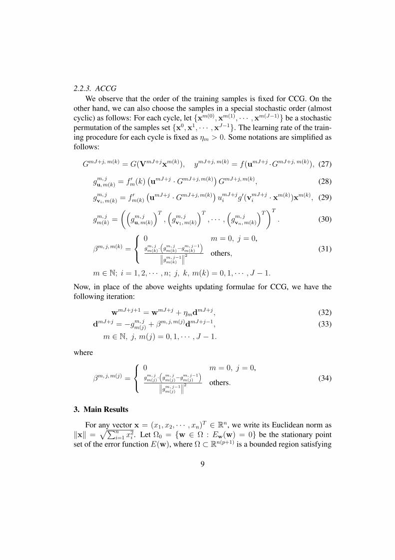
2.2.3. ACCGWe observe that the order of the training samples is fixed for CCG. On the

other hand, we can also choose the samples in a special stochastic order (almostcyclic) as follows: For each cycle, let xm(0),xm(1), · · · ,xm(J−1) be a stochasticpermutation of the samples set x0,x1, · · · ,xJ−1. The learning rate of the train-ing procedure for each cycle is fixed as ηm > 0. Some notations are simplified asfollows:

GmJ+j, m(k) = G(VmJ+jxm(k)), ymJ+j, m(k) = f(umJ+j ·GmJ+j, m(k)), (27)

gm, ju, m(k) = f ′m(k)

(umJ+j ·GmJ+j, m(k)

)GmJ+j, m(k), (28)

gm, jvi, m(k) = f ′m(k)

(umJ+j ·GmJ+j, m(k)

)umJ+j

i g′(vmJ+ji · xm(k))xm(k), (29)

gm, jm(k) =

((gm, ju, m(k)

)T

,(gm, jv1, m(k)

)T

, · · · ,(gm, jvn, m(k)

)T)T

. (30)

βm, j, m(k) =

0 m = 0, j = 0,gm, j

m(k)·(gm, j

m(k)−gm, j−1

m(k)

)∥∥∥gm, j−1

m(k)

∥∥∥2 others, (31)

m ∈ N; i = 1, 2, · · · , n; j, k, m(k) = 0, 1, · · · , J − 1.

Now, in place of the above weights updating formulae for CCG, we have thefollowing iteration:

wmJ+j+1 = wmJ+j + ηmdmJ+j, (32)dmJ+j = −gm, j

m(j) + βm, j, m(j)dmJ+j−1, (33)

m ∈ N, j, m(j) = 0, 1, · · · , J − 1.

where

βm, j, m(j) =

0 m = 0, j = 0,gm, j

m(j)·(gm, j

m(j)−gm, j−1

m(j)

)∥∥∥gm, j−1

m(j)

∥∥∥2 others. (34)

3. Main Results

For any vector x = (x1, x2, · · · , xn)T ∈ Rn, we write its Euclidean norm as‖x‖ =

√∑ni=1 x2

i . Let Ω0 = w ∈ Ω : Ew(w) = 0 be the stationary pointset of the error function E(w), where Ω ⊂ Rn(p+1) is a bounded region satisfying

9

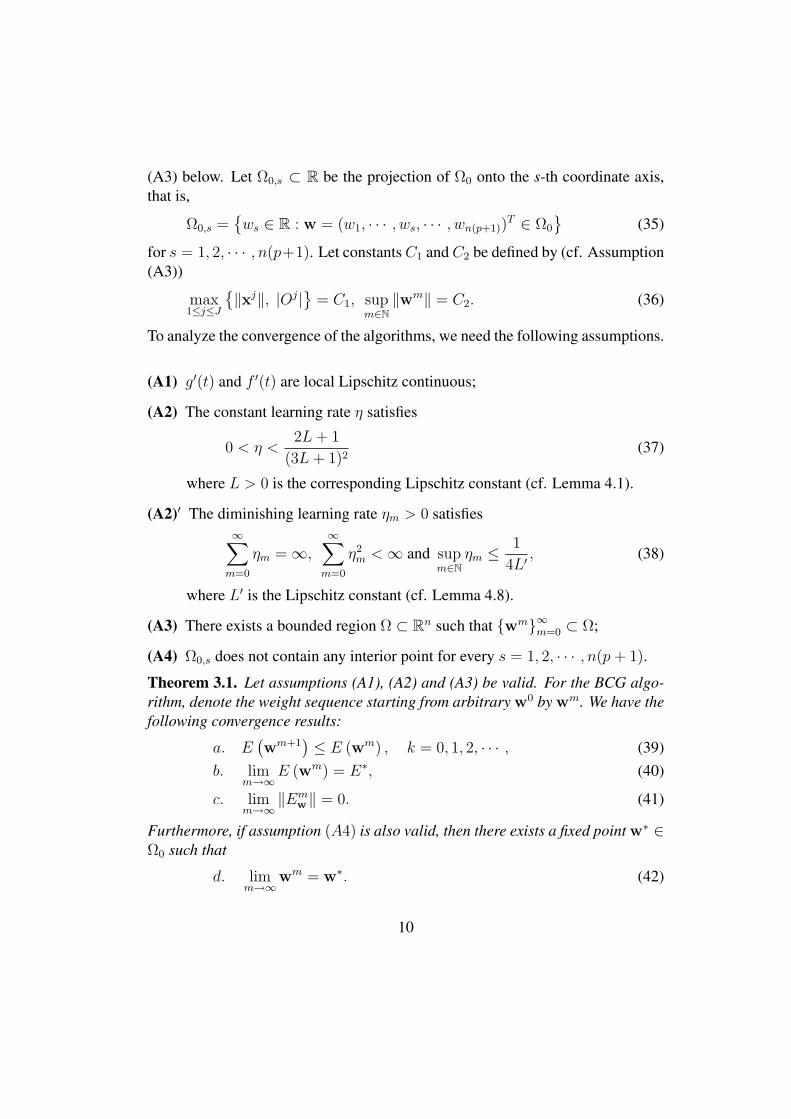
(A3) below. Let Ω0,s ⊂ R be the projection of Ω0 onto the s-th coordinate axis,that is,

Ω0,s =ws ∈ R : w = (w1, · · · , ws, · · · , wn(p+1))

T ∈ Ω0

(35)

for s = 1, 2, · · · , n(p+1). Let constants C1 and C2 be defined by (cf. Assumption(A3))

max1≤j≤J

‖xj‖, |Oj| = C1, supm∈N

‖wm‖ = C2. (36)

To analyze the convergence of the algorithms, we need the following assumptions.

(A1) g′(t) and f ′(t) are local Lipschitz continuous;

(A2) The constant learning rate η satisfies

0 < η <2L + 1

(3L + 1)2(37)

where L > 0 is the corresponding Lipschitz constant (cf. Lemma 4.1).

(A2)′ The diminishing learning rate ηm > 0 satisfies∞∑

m=0

ηm = ∞,∞∑

m=0

η2m < ∞ and sup

m∈Nηm ≤ 1

4L′, (38)

where L′ is the Lipschitz constant (cf. Lemma 4.8).

(A3) There exists a bounded region Ω ⊂ Rn such that wm∞m=0 ⊂ Ω;

(A4) Ω0,s does not contain any interior point for every s = 1, 2, · · · , n(p + 1).

Theorem 3.1. Let assumptions (A1), (A2) and (A3) be valid. For the BCG algo-rithm, denote the weight sequence starting from arbitrary w0 by wm. We have thefollowing convergence results:

a. E(wm+1

) ≤ E (wm) , k = 0, 1, 2, · · · , (39)b. lim

m→∞E (wm) = E∗, (40)

c. limm→∞

‖Emw‖ = 0. (41)

Furthermore, if assumption (A4) is also valid, then there exists a fixed point w∗ ∈Ω0 such that

d. limm→∞

wm = w∗. (42)

10

Theorem 3.2. Suppose that the assumptions (A1), (A2)′ and (A3) are valid. Forthe CCG and ACCG algorithms, starting from an arbitrary initial value w0, theweight sequence wm satisfies the following convergence:

1). limm→∞

E (wm) = E∗, (43)

2). limm→∞

Ew (wm) = 0. (44)

Moreover, if the assumption (A4) is also valid, there holds the strong convergence:There exists w∗ ∈ Ω0 such that

3). limm→∞

wm = w∗. (45)

Let us make the following three remarks on the above deterministic conver-gence results:

(I). The learning rate is the big difference of the convergence assumptions be-tween BCG and CCG, ACCG. It is well known that the convergence resultsare guaranteed with constant learning rate for batch mode (Xu, Zhang, & Liu,2010) while the diminishing learning rate for incremental mode for neuralnetworks based on the steepest gradient method (Chakraborty & Pal, 2003;Wu et al, 2005; Xu, Zhang, & Jin, 2009; Zhang, Wu, Liu & Yao, 2009;Wu, W. et al, 2010). For the similar reason, we consider the case of aconstant learning rate for BCG. However, the diminishing learning rule isadopted for CCG and ACCG.

(II). The monotonicity of the error function is the remarkable difference of theconvergence results between BCG and CCG, ACCG. The main reason isthat different updating directions are adopted in these different learningfashions. We mention that the descent direction of BCG is dependent onthe true conjugate gradient while the instant conjugate gradient is employedin CCG and ACCG. Basically, the BCG method in this paper is a class ofsolutions for standard unconstrained optimal problems.

(III). We claim that the same convergence results are available for both CCGmethod and ACCG method. The only difference between these two algo-rithms is the order of samples which are fed in each training process. It iseasy to see that the corresponding lemmas are not influenced by the differentupdating formulae.

11

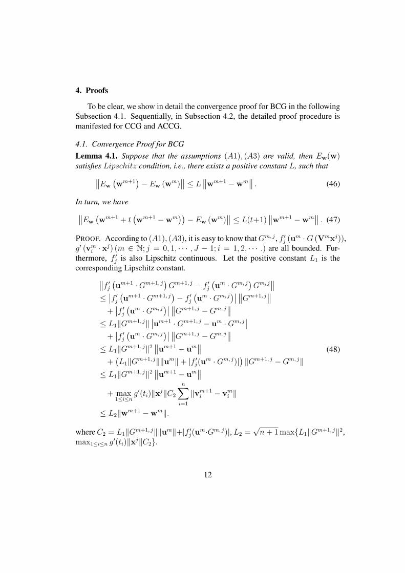
4. Proofs

To be clear, we show in detail the convergence proof for BCG in the followingSubsection 4.1. Sequentially, in Subsection 4.2, the detailed proof procedure ismanifested for CCG and ACCG.

4.1. Convergence Proof for BCGLemma 4.1. Suppose that the assumptions (A1), (A3) are valid, then Ew(w)satisfies Lipschitz condition, i.e., there exists a positive constant L, such that

∥∥Ew

(wm+1

)− Ew (wm)∥∥ ≤ L

∥∥wm+1 −wm∥∥ . (46)

In turn, we have∥∥Ew

(wm+1 + t

(wm+1 −wm

))− Ew (wm)∥∥ ≤ L(t+1)

∥∥wm+1 −wm∥∥ . (47)

PROOF. According to (A1), (A3), it is easy to know that Gm, j , f ′j (um ·G (Vmxj)),g′ (vm

i · xj) (m ∈ N; j = 0, 1, · · · , J − 1; i = 1, 2, · · · .) are all bounded. Fur-thermore, f ′j is also Lipschitz continuous. Let the positive constant L1 is thecorresponding Lipschitz constant.

∥∥f ′j(um+1 ·Gm+1, j

)Gm+1, j − f ′j

(um ·Gm, j

)Gm, j

∥∥≤

∣∣f ′j(um+1 ·Gm+1, j

)− f ′j(um ·Gm, j

)∣∣ ∥∥Gm+1, j∥∥

+∣∣f ′j

(um ·Gm, j

)∣∣ ∥∥Gm+1, j −Gm, j∥∥

≤ L1‖Gm+1, j‖∣∣um+1 ·Gm+1, j − um ·Gm, j

∣∣+

∣∣f ′j(um ·Gm, j

)∣∣ ∥∥Gm+1, j −Gm, j∥∥

≤ L1‖Gm+1, j‖2∥∥um+1 − um

∥∥+

(L1‖Gm+1, j‖‖um‖+ |f ′j(um ·Gm, j)|) ‖Gm+1, j −Gm, j‖

≤ L1‖Gm+1, j‖2∥∥um+1 − um

∥∥

+ max1≤i≤n

g′(ti)‖xj‖C2

n∑i=1

‖vm+1i − vm

i ‖

≤ L2‖wm+1 −wm‖.

(48)

where C2 = L1‖Gm+1, j‖‖um‖+|f ′j(um·Gm, j)|, L2 =√

n + 1 maxL1‖Gm+1, j‖2,max1≤i≤n g′(ti)‖xj‖C2.

12

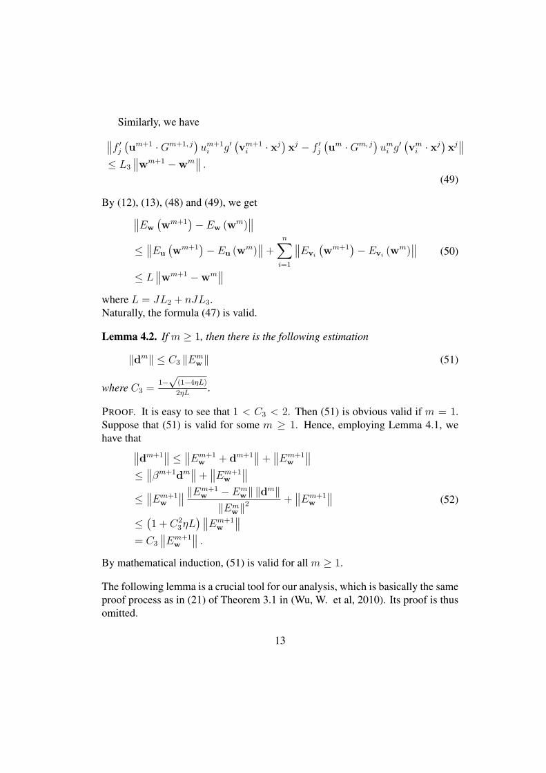
Similarly, we have∥∥f ′j

(um+1 ·Gm+1, j

)um+1

i g′(vm+1

i · xj)xj − f ′j

(um ·Gm, j

)um

i g′(vm

i · xj)xj

∥∥≤ L3

∥∥wm+1 −wm∥∥ .

(49)

By (12), (13), (48) and (49), we get∥∥Ew

(wm+1

)− Ew (wm)∥∥

≤∥∥Eu

(wm+1

)− Eu (wm)∥∥ +

n∑i=1

∥∥Evi

(wm+1

)− Evi(wm)

∥∥

≤ L∥∥wm+1 −wm

∥∥

(50)

where L = JL2 + nJL3.Naturally, the formula (47) is valid.

Lemma 4.2. If m ≥ 1, then there is the following estimation

‖dm‖ ≤ C3 ‖Emw‖ (51)

where C3 =1−√

(1−4ηL)

2ηL.

PROOF. It is easy to see that 1 < C3 < 2. Then (51) is obvious valid if m = 1.Suppose that (51) is valid for some m ≥ 1. Hence, employing Lemma 4.1, wehave that

∥∥dm+1∥∥ ≤

∥∥Em+1w + dm+1

∥∥ +∥∥Em+1

w

∥∥≤

∥∥βm+1dm∥∥ +

∥∥Em+1w

∥∥

≤∥∥Em+1

w

∥∥ ‖Em+1w − Em

w‖ ‖dm‖‖Em

w‖2 +∥∥Em+1

w

∥∥

≤ (1 + C2

3ηL) ∥∥Em+1

w

∥∥= C3

∥∥Em+1w

∥∥ .

(52)

By mathematical induction, (51) is valid for all m ≥ 1.

The following lemma is a crucial tool for our analysis, which is basically the sameproof process as in (21) of Theorem 3.1 in (Wu, W. et al, 2010). Its proof is thusomitted.

13

Lemma 4.3. Let F : Φ ⊂ Rp → R, (p ≥ 1) be continuous for a bounded closedregion (Φ), and Φ0 = z ∈ Φ : F (z) = 0. If the projection of Φ0 on eachcoordinate axis does’t contain any interior point. Let the sequence zn satisfy:

(i). limn→∞ F (zn) = 0;

(ii). limn→∞ ‖zn+1 − zn‖ = 0.

Then, there exists an unique z∗ ∈ Φ0 such that

limn→∞

zn = z∗.

Proof to (39).Using the differential mean value theorem, there exists a constant θ ∈ [0, 1], suchthat

E(wm+1

)− E (wm)

=(Ew

(wm + θ

(wm+1 −wm

)))T (wm+1 −wm

)

= η (Emw )T dm + η

[Ew

(wm + θ

(wm+1 −wm

))− Ew (wm)]T

dm

≤ −η ‖Emw‖2 + η

‖Emw‖2 ‖Em

w − Em−1w ‖ ‖dm−1‖

‖Em−1w ‖2 + η2 (L + 1) ‖dm‖2

≤ −η(1− C2

3η (2L + 1)) ‖Em

w‖2 ,

(53)

Applying (37) and C3 =1−√

(1−4ηL)

2ηL, we have that 1 − C2

3η (2L + 1) > 0. Themonotone decreasing property of the error function of BCG is thus proved. ¤

Proof to (40).By (9), it is to see that E (wm) ≥ 0 (m ∈ N). Combining with (39), we thenconclude that there exists E∗ ≥ 0 such that

limm→∞

E (wm) = E∗.

¤

Proof to (41).According to (53) and the fact that (40), we deduce that

∑∞m=1 ‖Em

w‖2 < ∞.Then, we have

limm→∞

‖Emw‖ = 0, (54)

14

i.e., the weak convergence for BCG is valid. ¤

Proof to (42).By the assumption (A1), it is easy to see that Ew (w) is continuous. Applying(16), (41) and Lemma ??, we have

limm→∞

‖wm+1 −wm‖ = η limm→∞

‖dm‖ = 0. (55)

Furthermore, the assumption (A4) is valid. Then, using the Lemma 4.3, thereexists an unique w∗ ∈ Ω0, such that

limm→∞

wm = w∗.

This completes the strong convergence proof for BCG.

4.2. Convergence Proof for CCG and ACCGThe following three lemmas are very useful tools in convergence analysis for

CCG and ACCG methods, and the specific proofs are presented in (Wu, W. et al,2010).

Lemma 4.4. Let q(x) be a function defined on a bounded closed interval [a, b]such that q′(x) is Lipschitz continuous with Lipschitz constant K > 0. Then,q′(x) is differentiable almost everywhere in [a, b] and

|q′′(x)| ≤ K, a.e. [a, b]. (56)

Moreover, there exists a constant C > 0 such that

q(x) ≤ q(x0) + q′(x0)(x− x0) + C(x− x0)2, ∀x0, x ∈ [a, b]. (57)

Lemma 4.5. Suppose that the learning rate ηm satisfies (A2) and that the se-quence am (m ∈ N) satisfies am ≥ 0,

∑∞m=0 ηmaβ

m < ∞ and |am+1 − am| ≤µηm for some positive constants β and µ. Then we have

limm→∞

am = 0. (58)

Lemma 4.6. Let bm be a bounded sequence satisfying limm→∞(bm+1−bm) = 0.Write γ1 = limn→∞ infm>n bm, γ2 = limn→∞ supm>n bm and S = a ∈ R : Thereexists a subsequence bik of bm such that bik → a as k →∞. Then we have

S = [γ1, γ2]. (59)

15

Lemma 4.7. Let Yt,Wt and Zt be three sequences such that Wt is nonnegativeand Yt is bounded for all t. If

Yt+1 ≤ Yt −Wt + Zt, t = 0, 1, · · · . (60)

and the series Σ∞t=0Zt is convergent, then Yt converges to a finite value and Σ∞

t=0Wt <∞

PROOF. This Lemma is directly from (Xu, Zhang, & Jin, 2009).

Lemma 4.8. If the assumptions (A1) and (A3) are valid, then Ew(w) satisfiesthe Lipschitz condition, i.e., there exists a positive constant L′, such that

‖gm,J+1j − gm,j

j ‖ ≤ L′‖wmJ+j+1 −wmJ+j‖, (61)∥∥Ew

(wl

)− Ew

(wk

)∥∥ ≤ L′′∥∥wl −wk

∥∥ , l, k ∈ N. (62)

PROOF. The procedure of the detailed proof for this Lemma is similar with theLemma 4.1 and then omitted.

Lemma 4.9. Consider the learning algorithm (24), (25) and (26). The assump-tions (A1), (A2)′ and (A3) are valid, then

∥∥dmJ+j∥∥ ≤ 2

∥∥gm, jj

∥∥ , m ∈ N, j = 0, 1, · · · , J − 1. (63)

PROOF. By (26), it is easy to see that∥∥dmJ+j

∥∥ =∥∥gm, j

j

∥∥ for m = 0, j = 0, and(63) is valid in turn.

Suppose that (63) is valid for mJ + j > 0, then according to the assumption(A2)′ and the Lipschitz property in Lemma 4.8, we have

∥∥dmJ+j+1∥∥ ≤

∥∥gm, j+1j + dmJ+j+1

∥∥ +∥∥gm, j+1

j

∥∥≤

∥∥βmJ+j+1dmJ+j∥∥ +

∥∥gm, j+1j

∥∥

≤∥∥gm, j+1

j

∥∥∥∥gm, j+1

j − gm, jj

∥∥∥∥dmJ+j∥∥

∥∥gm, jj

∥∥2 +∥∥gm, j+1

j

∥∥

≤ (1 + 4ηmL′)∥∥gm, j+1

j

∥∥≤ 2

∥∥gm, j+1j

∥∥ .

(64)

Thus, by mathematical induction, (63) is valid for m ∈ N, j = 0, 1, · · · , J − 1.

16

Lemma 4.10. Let the sequence wmJ+j be generated by (24), (25) and (26).Under assumptions (A1), (A2)′ and (A3), there holds

E(w(m+1)J

) ≤ E(wmJ

)− ηm

∥∥Ew

(wmJ

)∥∥2+ C4η

2m. (65)

where C4 is a positive constant independent of m and ηm

PROOF. Applying the assumptions (A1), (A3) and the Lemma 4.4, we get

gj

(w(m+1)J · xj

) ≤ gj

(wmJ · xj

)+ g′j

(wmJ · xj

) (w(m+1)J −wmJ

) · xj

+ C5

((w(m+1)J −wmJ

) · xj)2

.

(66)

Summing the above equation from j = 0 to j = J − 1, we deduce that

E(w(m+1)J

) ≤ E(wmJ

)+ Ew

(wmJ

) ·Dm, J + JC21C5

∥∥Dm, J∥∥2

≤ E(wmJ

)− ηm

∥∥Ew

(wmJ

)∥∥2+ δm.

(67)

where

Dm, J = w(m+1)J −wmJ = ηm

J−1∑j=0

dmJ+j,

δm = −ηmEw

(wmJ

) · (Ew

(wmJ+j

)− Ew

(wmJ

))

+ ηmEw

(wmJ

) ·(

J−1∑j=0

βmJ+jdmJ+j−1

)+ JC2

1C5

∥∥Dm, J∥∥2

.

By (36) and the boundedness of g′j(t),∥∥Ew

(wmJ+j

)∥∥ (m ∈ N, j = 0, 1, · · · , J−1) is also bounded. According to Lemma 4.8 and Lemma 4.9, we conclude that

− ηmEw

(wmJ

) · (Ew

(wmJ+j

)− Ew

(wmJ

))

≤ L′′ηm

∥∥Ew

(wmJ

)∥∥ ∥∥wmJ+j −wmJ∥∥

≤ L′′η2m

∥∥Ew

(wmJ

)∥∥j−1∑

k=0

∥∥dmJ+k∥∥ ≤ C6η

2m.

(68)

17

Similarly, there exists C7, C8 > 0 such that

ηmEw

(wmJ

) ·(

J−1∑j=0

βmJ+jdmJ+j−1

)≤ C7η

2m, (69)

JC21C5

∥∥Dm, J∥∥2 ≤ C8η

2m. (70)

Thus, the desired estimate (65) is deduced by setting C4 = C6 + C7 + C8.

Proof to (43) .According to Lemma 4.7 and Lemma 4.10, there exists a fixed value E∗ ≥ 0 suchthat

limm→∞

E(wmJ

)= E∗. (71)

By the assumption (A2), there holds limm→∞ ηm = 0. Similar to the provingprocess of (67), it is easy to conclude that

limm→∞

∣∣E (wmJ+j

)− E(wmJ

)∣∣ = 0, j = 0, 1, · · · , J − 1.

Sequentially, we have

limm→∞

E(wmJ+j

)= lim

m→∞E

(wmJ

)= E∗.

This completes the proof. ¤

Proof to (44)According to Lemma 4.7 and Lemma 4.10, we get

∞∑m=0

ηm

∥∥Ew

(wmJ

)∥∥2< ∞, (72)

Applying the Lemma 4.8, we find that∣∣∥∥Ew

(w(m+1)J

)∥∥−∥∥Ew

(wmJ

)∥∥∣∣ ≤∥∥Ew

(w(m+1)J

)− Ew

(wmJ

)∥∥≤ L2

∥∥Dm, J∥∥ ≤ C9ηm.

(73)

Using (72), (73) and the Lemma 4.5, we see that

limm→∞

∥∥Ew

(wmJ

)∥∥ = 0. (74)

18

Similar to the proving process of (73), there exists a constant C10 > 0, such that∥∥Ew

(wmJ+j

)− Ew

(wmJ

)∥∥ ≤ C10ηm. (75)

It is easy to see that∥∥Ew

(wmJ+j

)∥∥ ≤ ∥∥Ew

(wmJ+j

)− Ew

(wmJ

)∥∥ +∥∥Ew

(wmJ

)∥∥≤ C10ηm +

∥∥Ew

(wmJ

)∥∥ ,(76)

Thus, we have limm→∞∥∥Ew

(wmJ+j

)∥∥ = 0, j = 1, 2, · · · , J − 1. The weakconvergence of CCG method is completed. ¤

Proof to (45).By the assumption (A1), we can deduce that Ew (w) is continuous. Combining(24), (25) and (44), we get

limm→∞

‖w(m+1)J −wmJ‖ = 0. (77)

According the assumption (A4) and Lemma 4.3, there exists an unique w∗, suchthat

limm→∞

wmJ = w∗.

By (24), (25), (44) and Lemma 4.9, it is easy to see that

limm→∞

‖wmJ+j −wmJ‖ = 0, j = 0, 1, · · · .

Thus, we conclude that

limm→∞

wmJ+j = w∗, j = 0, 1, · · · . (78)

This immediately gives the strong convergence for CCG. ¤

Remark for deterministic convergence of ACCG:We note that the big difference between CCG and ACCG is the order of the sam-ples in each training cycle. However, every sample is fed exactly once in eachcycle. On the basis of this factor, the convergence results for CCG are all avail-able for ACCG. The detailed proof is omitted.

19

5. Conclusion

Almost cyclic learning for BP neural networks based on conjugate gradientmethod is presented in this paper. From the mathematical point view, it is novelthat the deterministic convergence results for BCG, CCG and ACCG are obtained.On the basis of the selecting strategies of learning rate, the convergence results areguaranteed for BCG and CCG, ACCG, respectively. It makes a big difference tothe monotonicity property of the error function whether the updating direction isthe true conjugate gradient or not.

References

Chakraborty, D., & Pal, N. R. (2003). A novel training scheme for multilayeredperceptrons to realize proper generalization and incremental learning. IEEETransactions on Neural Networks, 14, 1-14.

Cichocki, A., Orsier, B., Back, A., & Amari, S. I. (1997). On-line adaptive al-gorithms in non-stationary environments using amodified conjugate gradientapproach. Neural Networks for Signal Processing [1997] VII. Proceedings ofthe 1997 IEEE Workshop, 316–325.

Dai, Y. H., & Yuan, Y. X. (2000). Nonlinear conjugate gradient methods. Shang-hai: Shanghai Scientific and Technical Press.

Finnoff, W. (1994). Diffusion approximations for the constant learning rate back-propagation algorithm and resistance to local minima. Neural Computation, 6,242-254.

Fletcher, R., Reeves, C. M. (1964). Function minimization by conjugate gradients.The Computer Journal, 7, 149C154.

Gonzalez, A., Dorronsoro, J. R. (2008). Natural conjugate gradient training ofmultilayer perceptrons. Neurocomputing, 71, 2499-2506.

Goodband, J. H., Haas, O. C. L., & Mills, J. A. (2008). A comparison of neuralnetwork approaches for on-line prediction in IGRT. The international Journalof Medical Physics Research and Practice, 35, 1113-1112.

Grippo, L., Lucidi, S. (1997). A globally convergent version of the Polak-Ribiereconjugate gradient method. Mathematical Programming, 78, 375-391.

20

Hagan, M. T., Demuth, H. B., & Beale, M. H. (1996). Neural network design.Boston: PWS Publishing.

Heskes, T., & Wiegerinck, W. (1996). A Theoretical Comparison of Batch-Mode,On-Line, Cyclic, and Almost-Cyclic Learning. IEEE Transactions on NeuralNetworks, 7, 919-925.

Hestenes, M. R., Stiefel, E. (1952). Method of conjugate gradient for solvinglinear systems. Journal of Research of the National Bureau of Standards. 49,409C436.

Jiang, M. H., Gielen, G., Zhang, B., & Luo, Z. S. (2003). Fast learning algorithmsfor feedforward neural networks. Applied Intelligence, 18, 37-54.

Khoda, K. M., Liu, Y., & Storey, C. (1992). Contributed Papers GeneralizedPolak-Ribiere algorithm. Journal of Optimization Theory and Applications, 75,345-354.

Li, Z. X., & Ding, X. S. (2005). Prediction of Stock Market by BP Neural Net-works with Technical Indexes as Input. Numerical Mathematics: A Journal ofChinese Universities, 27, 373-377.

Li, Z. X., Wu, W., & Tian, Y. L. (2004). Convergence of an online gradient methodfor feedforward neural networks with stochastic inputs. Journal of Computa-tional and Applied Mathematics, 163, 165-176.

Liu, C. N., Liu, H. T., & Vemuri, S. (1993). Neural network-based short term loadforecasting. IEEE Transactions on Power Systems, 8, 336C342.

Nakama, T. (2009). Theoretical analysis of batch and on-line training for gradientdescent learning in neural networks. Neurocomputing, 73, 151-159.

Nocedal, J. (1992). Theory of algorithms for unconstrained optimization. ActaNumerica, 1, 199-242.

Nocedal, J., & Wright, S. J. (2006). Numerical optimization (2nd ed.). New York:Springer, (Chapter).

Papalexopoulos, A. D., Hao, S., & Peng, T. M. (1994). An implementation of aneural network-based load forecasting model for the EMS. IEEE Transactionson Power Systems, 9, 1956C1962.

21

Park, D. C., Marks, R. J., Atlas, L. E., & Damborg, M. J. (1991). Electric loadforecasting using an artificial neural network. IEEE Transactions on Power Sys-tems, 6, 442C449.

Polak, E., Ribiere, G. (1969). Note sur la convergence de directions conjuguees.Rev Francaise Infomat Recherche Operatonelle, 16, 35-43.

Polyak, B. T. (1969). The conjugate gradient method in extreme problems. USSRComputational Mathematics and Mathematical Physics. 9, 94-112.

Rumelhart, D. E., Hinton, G. E., & Williams, R. J. (1986). Learning representa-tions by back-propagating errors. Nature, 323, 533-536.

Saini, L. M., & Soni, M. K. (2002). Artificial Neural Network-Based Peak LoadForecasting Using Conjugate Gradient Methods. IEEE Transactions on PowerSystems, 17, 907-912.

Shen, X. Z., Shi, X. Z., & Meng, G. (2006). Online algorithm of blind source sepa-ration based on conjugate gradient method. Circuits Systems Signal Processing,25, 381-388.

Shi, Z. J. (2002). Restricted PR conjugate gradient method and its global conver-gence. Advances In Mathematics, 1, 47-55. (in Chinese).

Shi, Z. J., & Guo, J. H. (2008). A new algorithm of nonlinear conjugate gradientmethod with strong convergence. Computational & Applied Mathematics, 27,93-106.

Shi, Z. J., & Shen, J. (2007). Convergence of the Polak-Ribiere-Polyak conjugategradient method. Nonlinear Analysis, 66, 1428-1441.

Terence, D.S. (1989). Optimal unsupervised learning in a single-layer linear feed-forward neural network. Neural Networks, 2, 459-473.

Wang, J., Yang, J., & Wu, W. (2010). Convergence of Cyclic and Almost-Cycliclearning with momentum for feedforward neural networks. Ieee Transactionson Neural Networks, Submitted.

Wilson, D. R., & Martinez, T. R. (2003). The general inefficiency of batch trainingfor gradient descent learning. Neural Networks, 16, 1429-1451.

22

Wu, W., Feng, G. R., Li, Z. X., & Xu, Y. S. (2005). Deterministic convergenceof an online gradient method for BP neural networks. IEEE Transactions onNeural Networks, 16, 533-540.

Wu, W., Wang, J., Cheng, M., & Li, Z. (2010). Convergence analysis of onlinegradient method for BP neural networks. Neural Networks, In Press, CorrectedProof.

Wu, W., & Xu, Y. S. (2002). Deterministic convergence of an on-line gradientmethod for neural networks. Journal of Computational and Applied Mathemat-ics, 144, 335-347.

Xu, D. P., Zhang, H. S., & Liu, L. J. (2010). Convergence Analysis of ThreeClasses of Split-Complex Gradient Algorithms for Complex-Valued RecurrentNeural Networks. Neural Computation, 22, 2655-2677.

Xu, Z. B., Zhang, R., & Jin, W. F. (2009). When Does Online BP Training Con-verge?. IEEE Transactions on Neural Networks, 20, 1529-1539.

Zhang, H. S., Wu, W., Liu, F., & Yao, M. C. (2009). Boundedness and Conver-gence of Online Gradient Method With Penalty for Feedforward Neural Net-works. IEEE Transactions on Neural Networks, 20, 1050-1054.

23