Developing a spatial epidemiological model to estimate

Developing a spatial epidemiological model to estimate Xylella fastidiosa dispersal and spread

Daniel Chapman1, Flavia Occhibove2, Pieter Beck3, James Bullock2, Alex Mastin4, Juan A. Navas-Cortés5, Stephen Parnell4 and Steven White2

1University of Stirling, UK2UK Centre for Ecology & Hydrology, UK 3European Commission Joint Research Centre, Italy4University of Salford, UK5Consejo Superior de Investigaciones Científicas (CSIC), Spain

[email protected] @dchap79

2

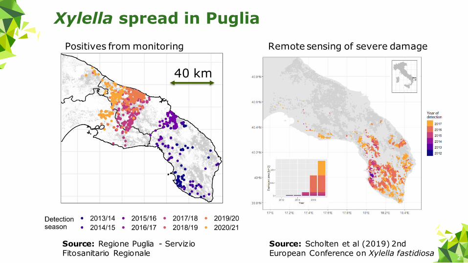
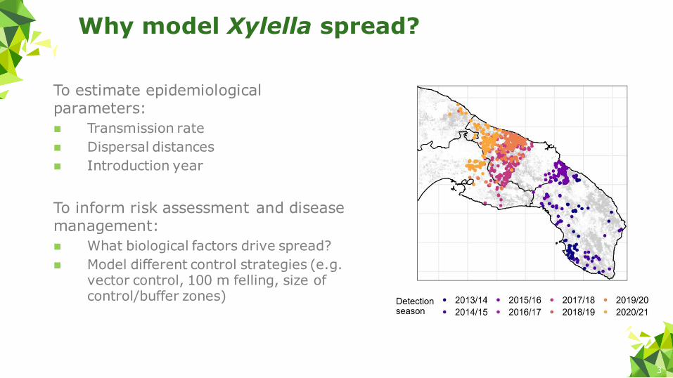
Xylella spread in Puglia

Source: Regione Puglia - Servizio Fitosanitario Regionale

Source: Scholten et al (2019) 2nd European Conference on Xylella fastidiosa

40 km

Positives from monitoring Remote sensing of severe damage

3

To estimate epidemiological parameters:

◼ Transmission rate

◼ Dispersal distances

◼ Introduction year

To inform risk assessment and disease management:

◼ What biological factors drive spread?

◼ Model different control strategies (e.g. vector control, 100 m felling, size of control/buffer zones)

Why model Xylella spread?

4

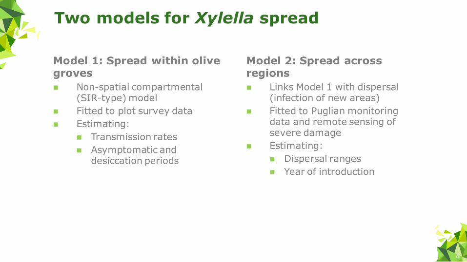
Model 1: Spread within olive groves

◼ Non-spatial compartmental (SIR-type) model

◼ Fitted to plot survey data

◼ Estimating:

◼ Transmission rates

◼ Asymptomatic and desiccation periods

Model 2: Spread across regions

◼ Links Model 1 with dispersal (infection of new areas)

◼ Fitted to Puglian monitoring data and remote sensing of severe damage

◼ Estimating:

◼ Dispersal ranges

◼ Year of introduction

Two models for Xylella spread

5

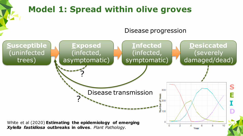
Model 1: Spread within olive groves

Susceptible(uninfected

trees)

Exposed(infected,

asymptomatic)

Infected(infected,

symptomatic)

Desiccated(severely

damaged/dead)

Disease transmission

Disease progression

?

?

White et al (2020) Estimating the epidemiology of emerging Xylella fastidiosa outbreaks in olives. Plant Pathology.

SEID

6

Estimating model parameters


Susceptible

Exposed

Symptomless (S+E)

Infected

Desiccated

◼ 3-year snapshots of disease progression in 17 olive grove plots (symptomless, symptomatic and dessicated trees)

◼ Fitted model by aligning snapshots to the model disease curves

7

◼ High transmission from symptomatic trees

◼ Little/no transmission from asymptomatic trees

◼ Cannot estimate infectivity of desiccated trees!

◼ Mean asymptomatic period of 1.2 years (1.07-1.27)

◼ Mean desiccation period 4.3 years (4.0-4.6), but not before 3 years

Conclusions from fitting Model 1

Use these parameter estimates in the spatial model


8

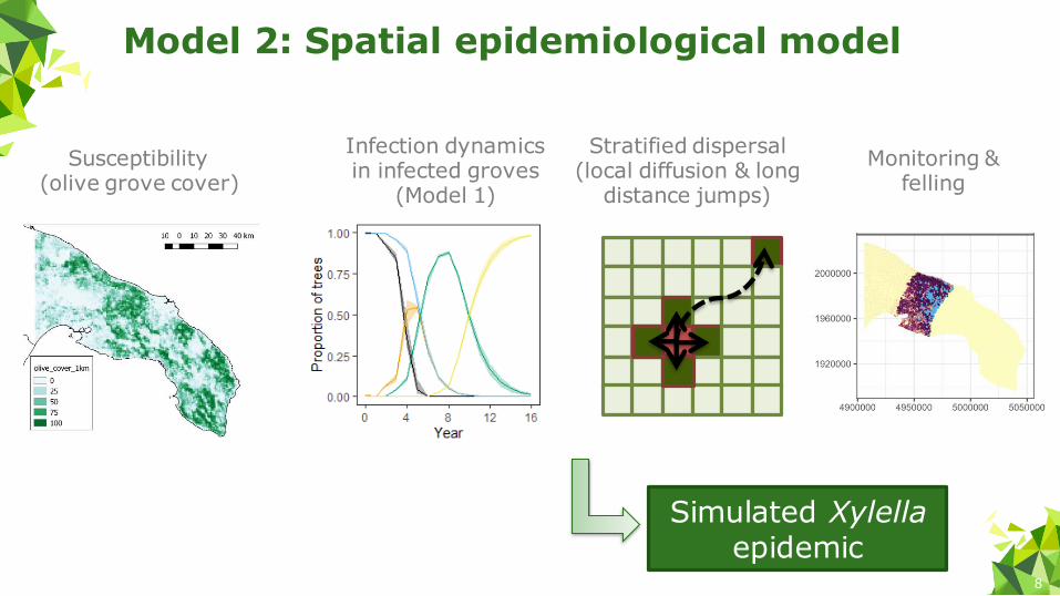
Model 2: Spatial epidemiological model

Susceptibility(olive grove cover)

Stratified dispersal (local diffusion & long

distance jumps)

Infection dynamics in infected groves

(Model 1)

Simulated Xylellaepidemic

Monitoring & felling

9

Gaussian kernel for local diffusion

◼ Bodino et al (2021) recaptured Philaenus spumarius up to 120m from release point

◼ Estimated movement range in the hundreds of metres per year.

Negative exponential kernel for long distance dispersal jumps

◼ Lago et al (2021) recaptured Neophilaenus campestris up to 2.4 km from release point and recorded individual flights up to 1.4 km

Stratified dispersal model

Bodino et al (2021) Dispersal of Philaenus spumarius (Hemiptera: Aphrophoridae), a Vector of Xylellafastidiosa, in Olive Grove and Meadow Agroecosystems. Environmental Entomology.Lago et al (2021) Dispersal of Neophilaenus campestris, a vector of Xylella fastidiosa, from olive groves to over-summering hosts. Journal of Applied Entomology.

10

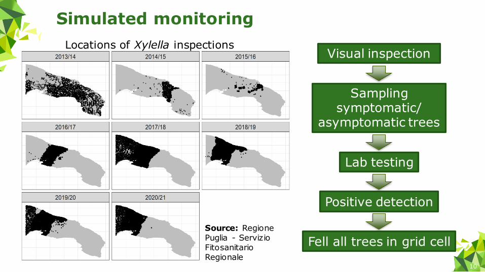
Simulated monitoring

Visual inspection

Sampling symptomatic/

asymptomatic trees

Lab testing

Positive detection

Fell all trees in grid cell

Locations of Xylella inspections

Source: Regione Puglia - Servizio Fitosanitario Regionale

11

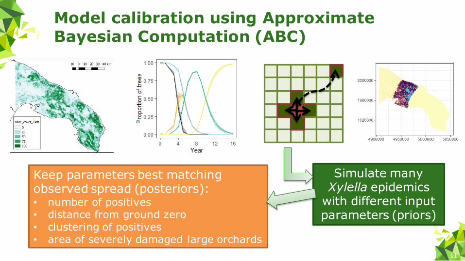
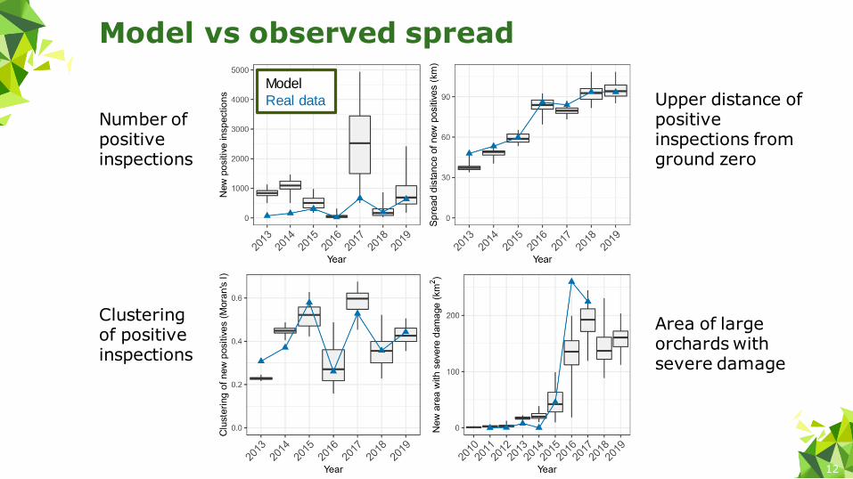
Model calibration using Approximate Bayesian Computation (ABC)

Simulate many Xylella epidemics

with different input parameters (priors)

Keep parameters best matching observed spread (posteriors):• number of positives• distance from ground zero• clustering of positives• area of severely damaged large orchards

12

Model vs observed spread

Number of positive inspections

Clustering of positive inspections

Upper distance of positive inspections from ground zero

Area of large orchards with severe damage

Model

Real data

13

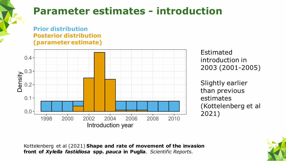
Parameter estimates - introduction

Prior distributionPosterior distribution (parameter estimate)

Estimated introduction in 2003 (2001-2005)

Slightly earlier than previous estimates (Kottelenberg et al 2021)

Kottelenberg et al (2021) Shape and rate of movement of the invasion front of Xylella fastidiosa spp. pauca in Puglia. Scientific Reports.

14

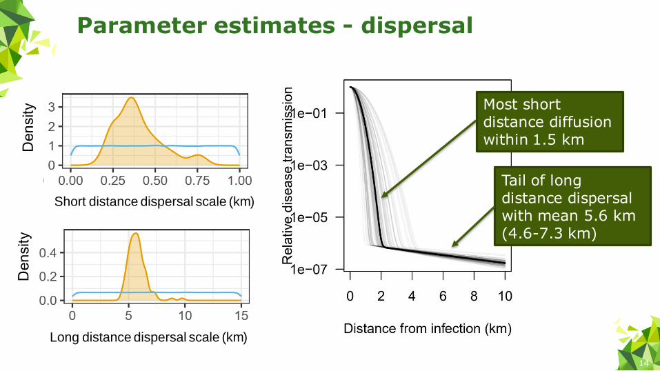
Parameter estimates - dispersal

Short distance dispersal scale (km)

Long distance dispersal scale (km)

Most short distance diffusion within 1.5 km

Tail of long distance dispersal with mean 5.6 km (4.6-7.3 km)

15

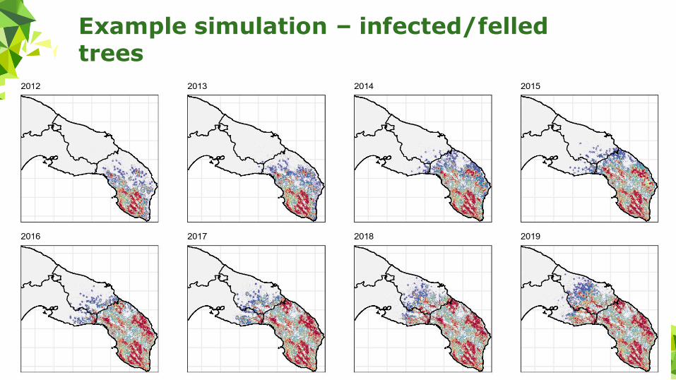
Example simulation – infected/felled trees

16

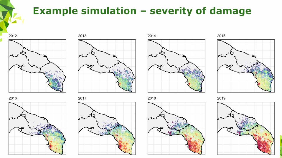
Example simulation – severity of damage

17

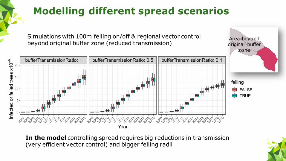
Modelling different spread scenarios

In the model controlling spread requires big reductions in transmission (very efficient vector control) and bigger felling radii

Simulations with 100m felling on/off & regional vector control beyond original buffer zone (reduced transmission)

Area beyond original buffer

zone

18

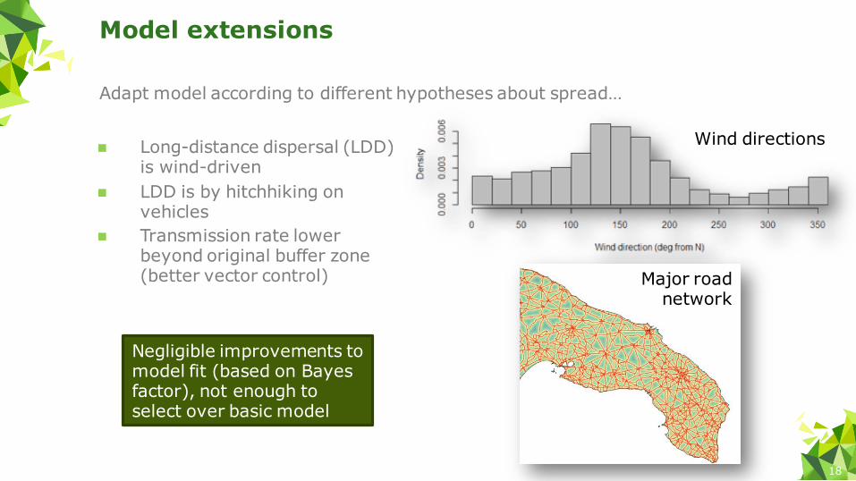
◼ Long-distance dispersal (LDD) is wind-driven

◼ LDD is by hitchhiking on vehicles

◼ Transmission rate lower beyond original buffer zone (better vector control)

Model extensions

Adapt model according to different hypotheses about spread…

Negligible improvements to model fit (based on Bayes factor), not enough to select over basic model

Wind directions

Major road network

19

Our models are simplified representations of real world disease dynamics, e.g.

◼ No explicit vector dynamics

◼ No olive cultivar variation

◼ No climate/weather effects

◼ Spatial monitoring is imposed, not reactive to ongoing spread

But gives a reasonable representation of Xylella spread in Puglia:

◼ Introduction around 2003

◼ Local spread driven by very high transmission from symptomatic trees and diffusion within ~1.5 km

◼ Regional-scale spread driven by rarer long-distance dispersal events (mean ~6 km)

◼ To slow the spread need to reduce transmission by controlling vectors and expand felling radius

Conclusions

20

See how we are applying the model to detection and eradication of hypothetical British outbreaks…

Flavia Occhibove - Inferring the potential spread of Xylella fastidiosa in Great Britain

Friday 09:30

Thank you!

Acknowledgements:▪ Support from XF-Actors & CURE-XF (EU H2020),

EFSA, BRIGIT (BBSRC, Defra & Scottish Government) & Scottish Plant Health Centre.

▪ Collaborators across XF-Actors and beyond▪ Regione Puglia - Servizio Fitosanitario Regionale

for official monitoring data

Documents

Developing a spatial epidemiological model to estimate