Embed Size (px)
Citation preview
Biodivers Conserv (2008) 17:2197–2218 DOI 10.1007/s10531-007-9281-4
ORIGINAL PAPER
Developing landscape habitat models for rare amphibians with small geographic ranges: a case studyof Siskiyou Mountains salamanders in the western USA
Nobuya Suzuki · Deanna H. Olson · Edward C. Reilly
Received: 9 February 2007 / Accepted: 24 October 2007 / Published online: 10 November 2007© Springer Science+Business Media B.V. 2007
Abstract To advance the development of conservation planning for rare species withsmall geographic ranges, we determined habitat associations of Siskiyou Mountains sala-manders (Plethodon stormi) and developed habitat suitability models at Wne (10 ha),medium (40 ha), and broad (202 ha) spatial scales using available Geographic InformationSystems data and logistic regression analysis with an information theoretic approach.Across spatial scales, there was very little support for models with structural habitat fea-tures, such as tree canopy cover and conifer diameter. Model-averaged 95% conWdenceintervals for regression coeYcients and associated odds ratios indicated that the occurrenceof Siskiyou Mountains salamanders was positively associated with rocky soils and PaciWcmadrone (Abutus menziesii) and negatively associated with elevation and white Wr (Abiesconcolor); these associations were consistent across 3 spatial scales. The occurrence of thisspecies also was positively associated with hardwood density at the medium spatial scale.Odds ratios projected that a 10% decrease in white Wr abundance would increase the oddsof salamander occurrence 3.02–4.47 times, depending on spatial scale. We selected themodel with rocky soils, white Wr, and Oregon white oak (Quercus garryana) as the bestmodel across 3 spatial scales and created habitat suitability maps for Siskiyou Mountainssalamanders by projecting habitat suitability scores across the landscape. Our habitatsuitability models and maps are applicable to selection of priority conservation areas forSiskiyou Mountains salamanders, and our approach can be easily adapted to conservationof other rare species in any geographical location.
N. Suzuki (&)Department of Zoology, Oregon State University, Corvallis, OR 97331, USAe-mail: [email protected]
D. H. OlsonUSDA Forest Service, PaciWc Northwest Research Station, 3200 SW JeVerson Way, Corvallis, OR 97331, USA
E. C. ReillyUSDI Bureau of Land Management, Medford District, 3040 Biddle Road, Medford, OR 97504, USA
1 C
2198 Biodivers Conserv (2008) 17:2197–2218
Keywords GIS · Habitat suitability · Information theoretic · Logistic regression · Plethodon stormi · Spatial scale
AbbreviationsAICc Akaike’s information criterion corrected for small sample sizeDBH quadratic mean diameter at breast heightDEM Digital Elevation ModelGeoBOB Geographic Biotic ObservationHS Habitat SuitabilityISMS the U.S. federal Interagency Species Management SystemNRIS Natural Resource Information SystemPRISM Parameter-elevation Regressions on Independent Slopes ModelTM Thematic MapperTPH number of trees per hectareUSDA United States Department of AgricultureUSDI United States Department of InteriorBLM Bureau of Land Management
Introduction
With changing landscapes, conservation of rare species requires a clear understanding ofspecies’ habitat associations to prevent loss of suitable habitat through human activities andnatural events. Conservation of rare endemic species with small geographic ranges is par-ticularly critical in the Klamath–Siskiyou region of the PaciWc Northwestern USA becauseof its exceptional concentration of rare endemic species among global temperate coniferousforest ecosystems and the accelerated rate of habitat loss in this biodiversity hotspot (Della-Sala et al. 1999; Myers et al. 2000).
The Siskiyou Mountains salamander (Plethodon stormi) is 1 of 3 closely-related raresalamander species endemic to the Klamath–Siskiyou region that straddles the Oregon–California border (Bury and Bury 2005). Because of the potential association of the SiskiyouMountains salamander with late-successional forests, there is a concern that land manage-ment activities in forests, including timber harvesting, road building and rock quarrying,may adversely impact populations and habitats of this salamander (Thomas et al. 1993;Blaustein et al. 1995; Clayton and Nauman 2005; Clayton et al. 2005). Despite thispresumed threat of land management activities, very little is known about the ecology orbiology of the Siskiyou Mountains salamander. More importantly, to our knowledge, nostudy previously has demonstrated an eVective way to integrate locally available resourceor habitat inventory information, Geographic Information Systems (GIS) technology, andspecies-habitat relationships into conservation strategies across landscapes for this or otherrare endemic species in the region.
Previously, habitat relationship models for rare Plethodon salamanders in the Klamath–Siskiyou region were developed primarily from Weld-measured micro- and macro-habitatdata at site to forest stand scales (Diller and Wallace 1994; Welsh and Lind 1995; Ollivieret al. 2001). However, these habitat models generally are limited in their applicability to theconservation of species at broad landscape scales for a couple of reasons. First, Weld sur-veys to compile these types of data often are too labor intensive and costly to be conductedover a broad landscape. Second, use of existing landscape habitat data, typically availablein the form of GIS layers, as surrogates for Weld-collected data is problematic. Landscape
1 C
Biodivers Conserv (2008) 17:2197–2218 2199
data may not match variables used in these Weld-derived models. For example, landscapevariables may diVer from Weld-measured data in accuracy, precision, and spatial scale.Therefore, these Weld-derived models may not produce reliable predictions when existinglandscape habitat data are applied.
Recent advances in remote sensing and GIS technologies not only make it possible toexamine habitat relationships of organisms across broad landscapes, but they also allow forXexibility in developing conservation assessments at multiple spatial scales (Torgersen et al.1999; Fleishman et al. 2001; Fuhlendorf et al. 2002; Luoto et al. 2002). Researchers havesuccessfully incorporated GIS information into habitat relationship models for many verte-brate species (Murkin et al. 1997; Cox et al. 2001; Maehr and Cox 1995; Gros and Rejmánek1999), including amphibians (Gustafson et al. 2001; Ray et al. 2002). However, there is noGIS-based habitat association model for Siskiyou Mountains salamanders for use in conser-vation planning across the landscape. We propose that GIS layers of habitat features acrosslandscapes can be eVectively used to determine habitat associations and to develop habitatsuitability models that can be readily used for regional conservation planning.
The Siskiyou Mountains salamander occupies one of the most xeric portions of therange of the western Plethodon species (Blaustein et al. 1995; Bury and Pearl 1999). Thelocal availability of cool and moist habitat is considered essential for the survival of thisspecies during the hot and dry summers of the Klamath–Siskiyou region (Bury and Pearl1999). Physiological constraints may explain why Siskiyou Mountains salamanders aredocumented to reach their highest abundance on north-facing, dense forest stands withtalus slopes (Nussbaum et al. 1983; Leonard et al. 1993). Talus slopes and rocky substratesappear to provide these salamanders with a stable microclimate as well as reliable cover ina region where down wood often is not available (Bury and Pearl 1999). These observa-tions have led some to suggest a close association of Siskiyou Mountains salamanders withlate-successional forests (Thomas et al. 1993; Blaustein et al. 1995; Clayton and Nauman2005; Clayton et al. 2005).
Our Wrst research objective was to determine associations of Siskiyou Mountains sala-mander with abiotic factors, forest stand structure, and tree-species abundance by quantifyingGIS information at 3 spatial scales. To guide our analyses, we formulated the followinghypotheses about species-habitat associations from current knowledge of the SiskiyouMountains salamander’s range, life history, and patterns of habitat use as summarizedbelow. Because salamanders avoid extreme heat and dry conditions as well as cold areas inhigh elevations, we hypothesized that Siskiyou Mountains salamanders are positively asso-ciated with rocky substrates and negatively associated with elevation and solar illumina-tion. Solar illumination is an estimate of solar radiation inputs in GIS (see methods).Furthermore, we hypothesized that Siskiyou Mountains salamanders are positively associ-ated with closed canopy conditions and large-diameter conifers. Cool and moist microcli-mates are maintained on the forest Xoor under closed canopies, and large conifers are anindicator of late-successional forest. Finally we used the abundance of 4 common treespecies in the Klamath–Siskiyou region as indicators of microclimate conditions becauseeach species occupies a diVerent microclimate regime. We hypothesized that SiskiyouMountains salamanders are negatively associated with white Wr (Abies concolor), a speciesfound in cold high-elevation habitats (Laacke 1990), Oregon white oak (Quercusgarryana), a species found in hot and dry low-elevation habitats (Stein 1990), and PaciWcmadrone (Abutus menziesii), a species frequently associated with dry sites (McDonald andTappeiner 1990), and positively associated with Douglas-Wr (Pseudotsuga menziesii), anabundant species in mesic habitats (Herman and Lavender 1990). We additionally testedthe relationship of Siskiyou Mountains salamanders with hardwood density based on a
1 C

2200 Biodivers Conserv (2008) 17:2197–2218
previous observation of a positive association (Ollivier et al. 2001). Our second researchobjective was to develop habitat suitability models based on the Wndings under our Wrstresearch objective and map habitat suitability for Siskiyou Mountains salamanders acrossthe landscape at 3 spatial scales.
Materials and methods
Study area
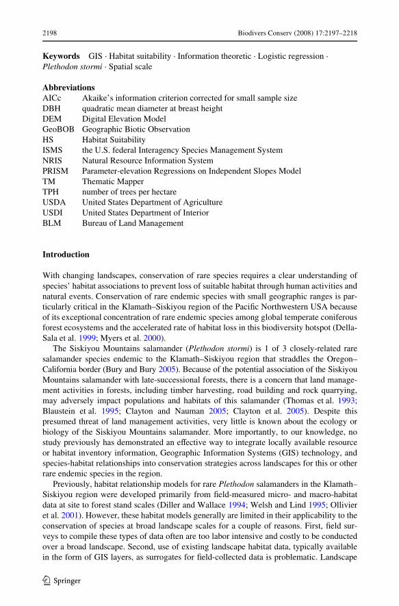
The Applegate River Watershed is located at the Oregon–California border in the Klamath–Siskiyou ecoregion of the western USA (Fig. 1). For model development, we used avail-able habitat and species data from a 121,406-ha area in the Applegate River Watershedwithin the range of the Siskiyou Mountains salamander. Elevations in the area range from364 to 2067 m. Over 90% of the study area was in Jackson County, Oregon; the remaining<10% was in eastern Josephine County, Oregon, and northern Siskiyou County, California.The climate across this area is generally cold and wet in winter, and hot and dry in summer.Mean annual temperatures range from 8.3 to 10.5°C, and precipitation ranges from 60 to170 cm at mid elevations (Franklin and Dyrness 1988). Mid-elevation vegetation fallswithin the Mixed-Evergreen zone in the western Siskiyou Mountains and the Mixed-Conifer zone in the eastern Siskiyou Mountains; the Interior Valley zone is found at lowerelevations (<»700 m) and the White-Wr zone occurs at upper elevations (»1400–1800 m;Franklin and Dyrness 1988).
Salamander location data and survey methods
We obtained 260 localities of Siskiyou Mountains salamanders from an existing spatialdatabase, the U.S. federal Interagency Species Management System (ISMS; Molina et al.2003) compiled by the U.S. Department of Interior, Bureau of Land Management (USDIBLM), and the U.S. Department of Agriculture, Forest Service (USDA Forest Service).Distinct localities of Siskiyou Mountains salamanders referred to as “known sites” hadbeen archived in the spatial database as part of the U.S. federal Protection BuVer and Sur-vey & Manage provisions of the federal Northwest Forest Plan (Molina et al. 2003). ISMSdata have been subsequently migrated to the Geographic Biotic Observation (GeoBOB)and Natural Resource Information System (NRIS) databases, and these have been main-tained by USDI BLM and USDA Forest Service, respectively (Pres. Comm. Kelli VanNorman, BLM Oregon State OYce, Portland). The 260 known sites of Siskiyou Mountainssalamanders included all the localities of Siskiyou Mountains salamanders ever recorded inour study area up to the end of 2003, thus representing the most comprehensive distributionof this species at the initiation of this study. Of the 260 known sites, 213 (82%) were iden-tiWed after 1993 based on surveys conducted by the USDI BLM and USDA Forest Service,and 47 sites (18%) were identiWed prior to 1993, largely from museum records archived bynatural historians and Weld researchers (Nauman and Olson 1999). Of the 213 federallyidentiWed sites, 130 sites (50% of all 260 known sites) were identiWed as a result of surveysrequired under the U.S. federal Northwest Forest Plan when proposed land managementactivities were considered potentially disturbing to Siskiyou Mountains salamanders andtheir habitat (referred to as pre-disturbance survey); these potentially disturbing landmanagement activities included timber harvesting, mining, road and trail development, andrecreational development (Olson 1999; Nauman and Olson 1999). Other USDA Forest
1 C

Biodivers Conserv (2008) 17:2197–2218 2201
Service projects identiWed 49 sites (19%) using a stratiWed random sampling during a Weldstudy (Ollivier et al. 2001) and 34 sites (13%) during surveys to Wll the gaps in the speciesdistribution (Nauman and Olson 2004).
Spatial habitat sampling with GIS Layers
From the GIS layer of 260 known Siskiyou Mountains salamander sites, we randomlyselected 2 sets of 53 known salamander sites (hereafter, salamander sites) and 133 sites thatwere not known to have salamanders (hereafter, unoccupied sites) within 10-ha square
Fig. 1 Map of the study area in the Applegate River Watershed of the Klamath–Siskiyou region, Oregon–California border, USA
1 C
2202 Biodivers Conserv (2008) 17:2197–2218
areas. Because of the rarity of the Siskiyou Mountains salamander, we assumed that thechances of these salamanders being present at randomly selected locations in the landscapewere low. The 10-ha area approximates the typical size of a forest stand that is beingconsidered for Siskiyou Mountains salamander conservation areas as well as for manyproposed forest management projects. To our knowledge, there is no relevant biological orecological information, such as home range size or movement pattern, to determine aspatial scale for the analyses of habitat associations of this species. Sample sizes for sala-mander (53) and unoccupied sites (133) were based on the observed ratio of salamander tounoccupied sites (approximately 2:5) from a previous Weld study of Siskiyou Mountainssalamanders (Ollivier et al. 2001). We used the Wrst 186 sites (53 + 133) to analyze habitatassociations and to develop habitat suitability models; we used the second set to validatethe habitat suitability models. The distance between any 2 selected sites was >1425 m toavoid redundant sampling, and we sampled no more than 1 site per 202 ha area. On aver-age, this resulted in 1 site per 650 ha across the study area.
For each sample site, we quantiWed habitat features using GIS layers at Wne (10 ha[25 acres]), medium (40 ha [100 acres]), and broad (202 ha [500 acres]) spatial scales, andwe used a square as the sample shape to make our results compatible with pixel-shaped GISgrid layers. Fine and medium spatial scales approximated the sizes of common and largeforest stands that are typically considered for land management and species conservationareas, and the broad spatial scale represented a small landscape. We quantiWed 10 habitatvariables for the analyses of habitat associations. These habitat variables included 3 abioticfactors (abundance of rocky soils [%], elevation [m], solar illumination [index valuebetween 0 and 254]), 3 stand structural features (tree canopy cover [%], conifer diameter[quadratic mean diameter at breast height in cm, DBH], and hardwood density [no. trees/hectare, TPH]), and abundance (%) of 4 common tree species (Douglas-Wr, white Wr,Oregon white oak, and PaciWc madrone).
The abundance of rocky soils was determined from digital soil survey maps from Jack-son (1993) and Josephine Counties (1983), Oregon (USDA Natural Resources Conserva-tion, available at http://www.or.nrcs.usda.gov/pnw_soil/or_data.html) and from USDAForest Service Level 2 Soil Resource Inventory maps (Badura and Jahn 1977). Soil typesassociated with rocky deposits known to have interstitial spaces and those with ¸50%gravel or cobble content were classiWed as rocky soils (D. Clayton, personal communica-tion). At each site, we estimated the proportion of 25-m pixels classiWed as rocky soilsamong all 25-m pixels in 10 ha (Wne scale), 40 ha (medium scale), and 202 ha (broadscale).
Elevation and solar illumination at sites were taken from a 10-m resolution U.S.Geological Survey Digital Elevation Model (DEM; Gesch et al. 2002). Solar illuminationis an index that represents the amount and extent of solar radiation reaching the groundsurface, and it accounts for various topographic features that might cast shade over a givenpoint. The solar illumination model was developed using the hillshade command inArcView (Environmental Systems Research Institute 1996). The position of the sun atnoon on June 21, 2003 for the speciWc longitude and latitude of each site was used tocalculate solar illumination values. June 21 is the day each year that the sun is at its highestposition. Solar illumination values ranged from 0 to 254, where smaller values indicatedlower solar radiation inputs.
Three features of stand structure and abundance of 4 tree species were estimated from25-m GIS grid layers of a remote sensing vegetation classiWcation map based on the imageanalysis of Landsat Thematic Mapper (TM) data conducted by Geographic ResourceSolutions in Arcata, California, in 1993 (Hill 1996). We calculated the average value
1 C
Biodivers Conserv (2008) 17:2197–2218 2203
of 25-m pixels in 10 ha (Wne scale), 40 ha (medium scale), and 202 ha (broad scale) at eachsample site for percent tree canopy cover, conifer DBH, and hardwood density. To quantifythe abundance of the 4 most common tree species in the region (Douglas-Wr, Oregon whiteoak, white Wr, and PaciWc madrone), we estimated the proportion of 25-m pixels for whicheach tree species was classiWed as most abundant among all 25-m pixels in 10 ha, 40 ha,and 202 ha at each sample site. We used ArcGIS 9.0 to estimate all variables except solarillumination, which was estimated in ArcView (Environmental Systems Research Institute2004).
In the image analysis of Landsat TM data, Weld data and Landsat imagery werecompared to develop spectral classes of habitat variables referred to as supervised trainingsets, and the supervised classiWcation method (Howard 1991) was used to initially producehabitat values for areas where Weld data were available (Hill 1996). Following the initialsupervised classiWcation, a maximum likelihood classiWcation based on the supervisedtraining sets was performed at a 90% probability threshold to estimate habitat values acrossthe landscape. After calibrating the discrepancy in value between the supervised trainingsets and the initial maximum likelihood estimation, 3 additional maximum likelihoodclassiWcations were performed, 2 at a 95% probability threshold followed by 1 at a 100%probability threshold to estimate habitat values for the entire 25 m pixels in the ApplegateRiver Watershed (Hill 1996). Ground truthing was conducted, and the accuracy of theimage analyses for habitat variables ranged from 86 to 92% at the 2-ha aggregation level(Hill 1996).
The timeframes of our diverse data sets diVer, leading to several assumptions in ouranalyses. Because the Landsat TM image was produced in 1993, our analysis comparedhabitat conditions in 1993 between the salamander sites and unoccupied sites. Salamandersites identiWed after 1993 are assumed to have been occupied by Siskiyou Mountains sala-manders in 1993 when the Landsat imagery was produced, and sites identiWed before 1993are assumed to be occupied in 1993. These assumptions are supported by the following. Forthe salamander sites identiWed after 1993 (213 of 260 sites), no land management activityor natural disturbance had signiWcantly altered habitat conditions at these sites between1993 and the time when these sites were identiWed. It also is unlikely that a signiWcantnumber of these sites had been newly established well after 1993 because the SiskiyouMountains salamander is suspected to be a low mobility species with high site Wdelity, andtheir primary habitat component (i.e., rocky substrate) is patchily distributed across thelandscape. For the known sites identiWed before 1993 (47 of 260 sites), aging of forestsfrom the time when the sites were identiWed until 1993 is not likely to have adverselyimpacted habitat conditions for Siskiyou Mountains salamanders because they are knownto occur in relatively high abundance in older forests (Nussbaum et al. 1983; Leonard et al.1993; Blaustein et al. 1995; Clayton and Nauman 2005; Clayton et al. 2005). However, wewere unable to determine the history of management activities and natural disturbance atthese sites identiWed before 1993, hence it is possible that habitat conditions had beenaltered by 1993, potentially aVecting species’ occupancy of sites.
Data analysis
We used logistic regression analysis (PROC LOGIST, PROC GENMOD; SAS Institute1999a) with an information theoretic approach (Burnham and Anderson 2002) to assesscompeting hypotheses about species-habitat associations and to develop Siskiyou Moun-tains salamander habitat suitability models from these results. We developed 26 a priorimodels from combinations of 10 habitat variables in 3 categories (abiotic habitat, stand
1 C
2204 Biodivers Conserv (2008) 17:2197–2218
structure, and tree species abundance) underlining our hypotheses (Table 1) that couldexplain the habitat association of Siskiyou Mountains salamanders. Based on currentknowledge of the biology and ecology of Siskiyou Mountains salamanders, we hypothe-sized positive associations of this species with 5 variables (tree canopy cover, conifer DBH,hardwood density, rocky soils, and Douglas-Wr) and negative associations with 5 variables(elevation, solar illumination, white Wr, Oregon white oak, and PaciWc madrone). To avoidmulticollinearity in regression analysis, correlations between variables were screened withPearson’s correlation coeYcient using all selected sites (n = 186; PROC CORR; SAS Insti-tute 1999b). Variables with a moderate to strong correlation (r ¸ 0.4) were assessed in sep-arate models in the logistic regression analysis. We tested for spatial autocorrelation in thedeviance residuals from logistic regression models by calculating Moran’s I statistic inArcGIS 9.0 (CliV and Ord 1981). Z-tests were used to examine the signiWcance of Moran’sI for the presence of spatial autocorrelation.
We calculated Akaike’s Information Criterion corrected for small sample size (AICc)for each model and ranked the 26 a priori models from most- to least-supported given thedata based on AICc values. We calculated �i, the diVerence between the AICc value of a
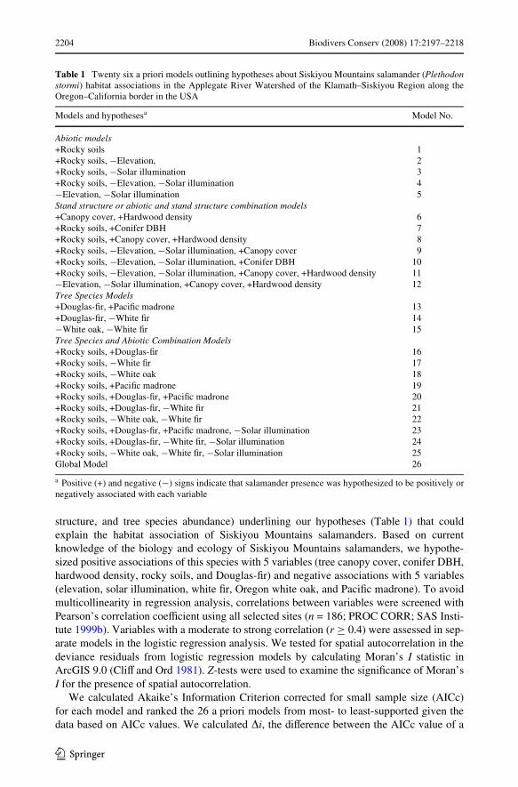
Table 1 Twenty six a priori models outlining hypotheses about Siskiyou Mountains salamander (Plethodonstormi) habitat associations in the Applegate River Watershed of the Klamath–Siskiyou Region along theOregon–California border in the USA
a Positive (+) and negative (¡) signs indicate that salamander presence was hypothesized to be positively ornegatively associated with each variable
Models and hypothesesa Model No.
Abiotic models+Rocky soils 1+Rocky soils, ¡Elevation, 2+Rocky soils, ¡Solar illumination 3+Rocky soils, ¡Elevation, ¡Solar illumination 4¡Elevation, ¡Solar illumination 5Stand structure or abiotic and stand structure combination models+Canopy cover, +Hardwood density 6+Rocky soils, +Conifer DBH 7+Rocky soils, +Canopy cover, +Hardwood density 8+Rocky soils, ¡Elevation, ¡Solar illumination, +Canopy cover 9+Rocky soils, ¡Elevation, ¡Solar illumination, +Conifer DBH 10+Rocky soils, ¡Elevation, ¡Solar illumination, +Canopy cover, +Hardwood density 11¡Elevation, ¡Solar illumination, +Canopy cover, +Hardwood density 12Tree Species Models+Douglas-Wr, +PaciWc madrone 13+Douglas-Wr, ¡White Wr 14¡White oak, ¡White Wr 15Tree Species and Abiotic Combination Models+Rocky soils, +Douglas-Wr 16+Rocky soils, ¡White Wr 17+Rocky soils, ¡White oak 18+Rocky soils, +PaciWc madrone 19+Rocky soils, +Douglas-Wr, +PaciWc madrone 20+Rocky soils, +Douglas-Wr, ¡White Wr 21+Rocky soils, ¡White oak, ¡White Wr 22+Rocky soils, +Douglas-Wr, +PaciWc madrone, ¡Solar illumination 23+Rocky soils, +Douglas-Wr, ¡White Wr, ¡Solar illumination 24+Rocky soils, ¡White oak, ¡White Wr, ¡Solar illumination 25Global Model 26
1 C
Biodivers Conserv (2008) 17:2197–2218 2205
particular model and the lowest AICc value of all the models, and Akaike weight (�i).Akaike weight is the proportional likelihood of each model over the sum of likelihood of allthe a priori models. For a given spatial scale, we considered a model with �i · 2 as havingsubstantial support in making inference, and only reported those models with �i · 7 ashaving some level of support (Burnham and Anderson 2002:127–128). We considered anymodel with �i > 7 as having insuYcient evidence to support it as the best model.
Best model selection took into account the number of competing models with �i · 2,Akaike weight, and number of parameters in the model. For example, when more than onemodel had �i · 2, the best model was the one with the highest Akaike weight and the few-est parameters. The best a priori model selected for each spatial scale was cross-validatedwith the second data set of 53 salamander and 133 unoccupied sites (validation data) inlogistic regression analyses, and correct classiWcation rates were calculated.
For each spatial scale, we developed a habitat suitability model to estimate relative like-lihoods of species occurrence as a measure of habitat suitability using the odds ratio equa-tion for habitat variables in the best a priori model: Habitat Suitability (HS) = exp(�1�1+�2�2+……+�n¡1�n¡1+ �n�n), where � is the coeYcient and � is the value for a particularhabitat variable (Manly et al. 2002; Pearce and Boyce 2006). We did not use the logisticregression equation as a habitat-suitability model because the retrospective approach in ourstudy limited our ability to estimate the prospective intercept and prospective probability ofspecies occurrence (Ramsey and Schafer 1997, pp. 586–587), and relative likelihoods ofoccurrence based on the exponential function is an alternative approach suggested for rarespecies when probabilities of occupancy are low (Keating and Cherry 2004; Manly et al2002; Pearce and Boyce 2006). We used our habitat suitability models to calculate HSscores of relative likelihoods of species occurrence from GIS layers of habitat variable.These HS scores were projected in pixels across the landscape to develop habitat suitabilitymaps of Siskiyou Mountains salamanders at 3 spatial scales.
We addressed model-selection uncertainty by providing model-averaged coeYcientswith 95% conWdence intervals in logistic regression analysis across the set of a priori mod-els. The model averaged coeYcient for a habitat variable was calculated by summing themultiples of normalized Akaike weights and the original coeYcient across the a priori mod-els with the variable in common, and the model-averaged 95% conWdence interval for thecoeYcient was from the unconditional standard error (Burnham and Anderson 2002,pp. 118–158). From these model-averaged statistics, we calculated the odds ratio and 95%conWdence interval of the odds ratio for each variable. We interpreted a habitat variable ashaving a signiWcant association with Siskiyou Mountains salamanders when the model-averaged 95% conWdence interval for the variable coeYcient did not include 0, whichindicated the habitat association of the salamanders with the variable was consistent acrossa priori models regardless of the presence of other habitat variables in these models. Thesame conclusion could be made by interpreting a habitat variable as having a signiWcantassociation when the model-averaged 95% conWdence interval of odds ratio for the variabledid not include 1. We reported odds ratios and associated 95% conWdence intervals for each1- and 10-unit change for habitat variables to describe the strengths of habitat association ofSiskiyou Mountains salamanders with each variable. Additional odds ratios and associated95% conWdence intervals for the change in 100-units (100 m) and 400-units (400 m) forelevation and the change in 100-units (100 trees per hectare) for hardwood density werereported because a change in 1 or 10 units generally is not biologically meaningful forthese habitat variables.
1 C

2206 Biodivers Conserv (2008) 17:2197–2218
Results
Correlations among habitat features
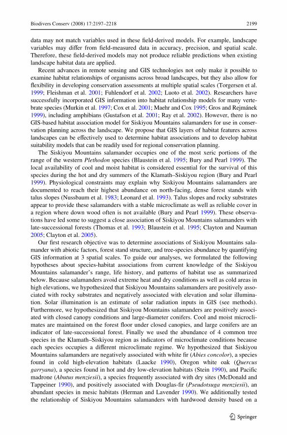
There were moderate to strong correlations between stand structure and tree species abun-dance (Fig. 2). Tree canopy cover increased as Douglas-Wr increased (r range: 0.850 to0.899) at all 3 spatial scales and decreased as Oregon white oak increased at medium(r = ¡0.422) and broad (r = ¡0.503) spatial scales. Conifer DBH increased as white Wrincreased at all spatial scales (r range: 0.652 to 0.730). Hence, tree canopy tended to beclosed in areas where Douglas-Wr was abundant and open in areas where Oregon white oak
Fig. 2 Relationships between tree species abundance and stand structure in the Applegate River Watershedof the Klamath–Siskiyou region, Oregon–California border, USA
1 C
Biodivers Conserv (2008) 17:2197–2218 2207
was abundant, and many large-diameter trees tended to be found in areas where white Wrwas abundant.
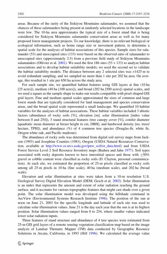
Among abiotic habitat factors, elevation showed moderate to strong correlations withthe abundance of most tree species (Fig. 3), with the exception of Douglas-Wr, which wasequally abundant across elevations (r range: ¡0.083 to ¡0.138). White Wr increased withelevation at all spatial scales (r range: 0.698 to 0.819), whereas PaciWc madrone (r range:¡0.539 to ¡0.754) and Oregon white oak (r range: ¡0.437 to ¡0.612) decreased withelevation. The decrease in these 2 hardwood species coincided with the decrease in hard-wood density with elevation (r range: ¡0.659 to ¡0.754).
Correlations between tree species also were apparent. PaciWc madrone decreased as whiteWr increased with elevation, and this pattern was detected at all spatial scales (r range: ¡0.534to ¡0.710). Furthermore, PaciWc madrone increased as Oregon white oak increased at thebroad spatial scale (r = 0.507); however, the correlation between these 2 hardwood specieswas weak at medium (r = 0.390) and Wne (r = 0.319) spatial scales. Douglas-Wr and Oregonwhite oak showed moderate negative correlations (r range: ¡0.401 to ¡0.449) at all spatialscales, indicating that Douglas-Wr tended to increase as Oregon white oak decreased.
Species habitat associations
Overall, a priori habitat models of Siskiyou Mountains salamanders that received somesupport (�i · 7) were similar across 3 spatial scales (Table 2). Explanatory variables forthese models consisted of some combination of tree species abundance and 2 abiotic factors(rocky soils and solar illumination); however, no stand-structural features were present inthese models. Two closely-related models (model with rocky soil, Oregon white oak, andwhite Wr; and model with rocky soil, Oregon white oak, white Wr, and solar illumination)received substantial support (�i · 2) with combined Akaike weights of 74% and 67 % atWne and medium spatial scales. Three additional a priori models received substantial sup-port at the broad spatial scale (�i · 2). Although the same 2 models at the Wner spatialscales remained as the top models at the broad spatial scale, the support for these modelsrelative to other models, judged by the combined Akaike weight of 57%, was not nearly ashigh as that at Wner spatial sales. In contrast, the relative support based on Akaike weightsfor the 3 bottom models (among the 5 top models) at the broad spatial scale was higher thanthat for the same models at Wner spatial scales. Consequently, a total of 5 competinga priori models received substantial support at the broad spatial scale, whereas only 2a priori models received substantial support at 2 Wner spatial scales.
Across 3 spatial scales, model-averaged 95% conWdence intervals for the logistic regres-sion coeYcients and associated odds ratios did not include 0 and 1, respectively, for eleva-tion and abundance of rocky soils, white Wr, and PaciWc madrone, indicating that SiskiyouMountains salamanders were positively associated with rocky soils and PaciWc madroneand negatively associated with elevation and white Wr across 3 spatial scales (Table 3).Only at the medium spatial scale did the coeYcient and odds ratio for hardwood density notinclude 0 and 1, respectively, indicating that there was an additional positive associationwith hardwood density at the medium spatial scale.
On average across the models, a 10% increase in rocky soils increased the odds of sala-mander occurrence by »1.22–1.27 times across 3 spatial scales (Table 4). In comparison, a10% decrease in white Wr and a 10% increase in PaciWc madrone increased the odds ofsalamander occurrence by »3.02–4.47 times and by »1.87–3.12 times, respectively,depending on spatial scales. Considerable changes in elevation are required to aVect theodds of salamander occurrence compared to abundance of tree species. A decrease in
1 C

2208 Biodivers Conserv (2008) 17:2197–2218
Fig. 3 Relationships between tree species abundance and elevation in the Applegate River Watershed of the Klamath–Siskiyou region, Oregon–California border, USA
1 C
Biodivers Conserv (2008) 17:2197–2218 2209
elevation of 10 m increased the odds of salamander occurrence by only »1.02 times across3 spatial scales, whereas a decrease in 100 m increased the odds by »1.20 times. The oddsof salamander occurrence almost doubled (»1.98–2.16 times) with a decrease in elevationof 400 m. An increase in hardwood density by 10 trees per hectare increased the odds ofsalamander occurrence by only »1.04 times at the medium spatial scale, whereas anincrease by 100 trees per hectare increased the odds by 1.42 times at the same scale (oddsratio/100TPH = 1.421; CI = 1.072–1.887).
Habitat suitability models
To develop habitat suitability models for the species across the landscape, we chose ana priori model that was comprised of 3 explanatory variables (rocky soils, Oregon whiteoak, and white Wr) as the best model across 3 spatial scales. This model was consistentlymore parsimonious than the second-best a priori model (rocky soils, Oregon white oak,white Wr, solar illumination) and had the lowest AICc values and the highest Akaike
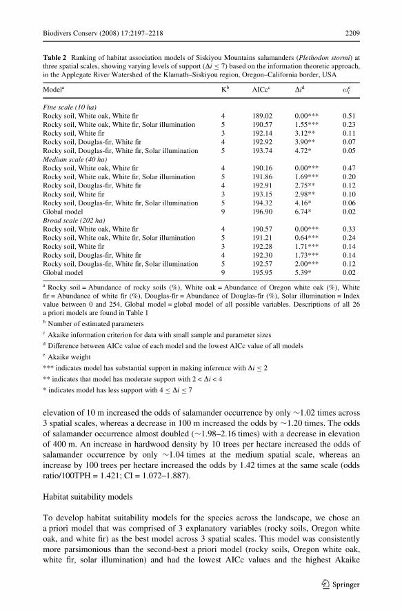
Table 2 Ranking of habitat association models of Siskiyou Mountains salamanders (Plethodon stormi) atthree spatial scales, showing varying levels of support (�i · 7) based on the information theoretic approach,in the Applegate River Watershed of the Klamath–Siskiyou region, Oregon–California border, USA
a Rocky soil = Abundance of rocky soils (%), White oak = Abundance of Oregon white oak (%), WhiteWr = Abundance of white Wr (%), Douglas-Wr = Abundance of Douglas-Wr (%), Solar illumination = Indexvalue between 0 and 254, Global model = global model of all possible variables. Descriptions of all 26a priori models are found in Table 1b Number of estimated parametersc Akaike information criterion for data with small sample and parameter sizesd DiVerence between AICc value of each model and the lowest AICc value of all modelse Akaike weight
*** indicates model has substantial support in making inference with �i · 2
** indicates that model has moderate support with 2 < �i < 4
* indicates model has less support with 4 · �i · 7
Modela Kb AICcc �id �ie
Fine scale (10 ha)Rocky soil, White oak, White Wr 4 189.02 0.00*** 0.51Rocky soil, White oak, White Wr, Solar illumination 5 190.57 1.55*** 0.23Rocky soil, White Wr 3 192.14 3.12** 0.11Rocky soil, Douglas-Wr, White Wr 4 192.92 3.90** 0.07Rocky soil, Douglas-Wr, White Wr, Solar illumination 5 193.74 4.72* 0.05Medium scale (40 ha)Rocky soil, White oak, White Wr 4 190.16 0.00*** 0.47Rocky soil, White oak, White Wr, Solar illumination 5 191.86 1.69*** 0.20Rocky soil, Douglas-Wr, White Wr 4 192.91 2.75** 0.12Rocky soil, White Wr 3 193.15 2.98** 0.10Rocky soil, Douglas-Wr, White Wr, Solar illumination 5 194.32 4.16* 0.06Global model 9 196.90 6.74* 0.02Broad scale (202 ha)Rocky soil, White oak, White Wr 4 190.57 0.00*** 0.33Rocky soil, White oak, White Wr, Solar illumination 5 191.21 0.64*** 0.24Rocky soil, White Wr 3 192.28 1.71*** 0.14Rocky soil, Douglas-Wr, White Wr 4 192.30 1.73*** 0.14Rocky soil, Douglas-Wr, White Wr, Solar illumination 5 192.57 2.00*** 0.12Global model 9 195.95 5.39* 0.02
1 C

2210 Biodivers Conserv (2008) 17:2197–2218
weights among all 26 a priori models across all spatial scales (Table 2). We did not detect asigniWcant spatial autocorrelation in the best model across 3 spatial scales; the Moran’s Ifor Wne, moderate, and broad spatial scales were ¡0.075 (P = 0.756), ¡0.010 (P = 0.466),and ¡0.012 (P = 0.297), respectively. The overall correct classiWcation rates of the besta priori models assessed with validation data were 67% at the Wne spatial scale (75% forsalamander and 64% for unoccupied sites), 70% at the medium spatial scale (77% for sala-mander and 68% for unoccupied sites), and 68 % at the broad spatial scale (83% for sala-mander and 62% for unoccupied sites).
Table 3 Associations of Siskiyou Mountains salamanders with habitat variables at Wne (10 ha), medium(40 ha), and broad (202 ha) spatial scales assessed from model-averaged estimates and 95% conWdence inter-vals of coeYcients and odds ratios
These model-averaged statistics were based on the full set of a priori logistic regression models (Table 2).Evidence for either positive or negative association of Siskiyou Mountains salamanders with a variable isindicated by an asterisk (*), and bold letters indicate when the conWdence interval for coeYcients and oddsratios did not include 0 and 1, respectivelya <0.000 indicates value less than 0.000 before the value was rounding to 3 signiWcant digitsb <1.000 indicates value less than 1.000 before the value was rounding to 3 signiWcant digits
Variable Model averaged coeYcient Odds ratio 95% CI of oddsratio
Estimate 95% CI
Fine scaleRocky soils* 0.020 (0.008, 0.031) 1.020 (1.008, 1.031)Elevation* ¡0.002 (¡0.003, ¡0.001) 0.998 (0.997, 0.999)Solar illumination ¡0.007 (¡0.024, 0.010) 0.993 (0.976, 1.010)Canopy cover 0.005 (¡0.017, 0.026) 1.005 (0.983, 1.026)Conifer DBH ¡0.030 (¡0.075, 0.015) 0.970 (0.927, 1.016)Hardwood density 0.002 (¡0.001, 0.005) 1.002 (0.999, 1.005)Douglas-Wr 0.008 (¡0.008, 0.024) 1.008 (0.992, 1.025)White Fir* ¡0.111 (¡0.171, ¡0.050) 0.895 (0.843, 0.951)White Oak ¡0.041 (¡0.084, 0.002) 0.960 (0.919, 1.002)Madrone* 0.062 (0.016, 0.109) 1.064 (1.016, 1.115)Medium scaleRocky soils* 0.022 (0.009, 0.035) 1.022 (1.009, 1.035)Elevation* ¡0.002 (¡0.003, <0.000)a 0.998 (0.997, <1.000)b
Solar illumination ¡0.007 (¡0.029, 0.015) 0.993 (0.971, 1.015)Canopy cover 0.018 (¡0.009, 0.045) 1.018 (0.991, 1.046)Conifer DBH ¡0.032 (¡0.085, 0.022) 0.969 (0.918, 1.022)Hardwood density* 0.004 (0.001, 0.006) 1.004 (1.001, 1.006)Douglas-Wr 0.014 (¡0.006, 0.033) 1.014 (0.994, 1.034)White Fir* ¡0.118 (¡0.185, ¡0.052) 0.888 (0.831, 0.950)White Oak ¡0.052 (¡0.107, 0.002) 0.950 (0.899, 1.002)Madrone* 0.082 (0.025, 0.139) 1.086 (1.026, 1.149)Broad scaleRocky soils* 0.024 (0.008, 0.040) 1.024 (1.008, 1.041)Elevation* ¡0.002 (¡0.003, <0.000) 0.998 (0.997, <1.000)
Solar illumination ¡0.020 (¡0.053, 0.012) 0.980 (0.949, 1.012)Canopy cover 0.029 (¡0.004, 0.062) 1.029 (0.996, 1.064)Conifer DBH ¡0.036 (¡0.109, 0.036) 0.964 (0.897, 1.036)Hardwood density 0.004 (<0.000, 0.007) 1.004 (<1.000, 1.00711)Douglas¡Wr 0.016 (¡0.012, 0.048) 1.016 (0.988, 1.045)White Fir* ¡0.150 (¡0.236, ¡0.064) 0.861 (0.790, 0.938)White Oak ¡0.050 (¡0.107, 0.009) 0.952 (0.899, 1.009)Madrone* 0.114 (0.037, 0.190) 1.120 (1.038, 1.209)
1 C

Biodivers Conserv (2008) 17:2197–2218 2211
Using the best a priori models, we developed the following habitat suitability models for3 spatial scales (Table 5): (1) Habitat Suitability = exp(0.020*Rocky soils ¡0.115*whiteWr ¡0.043*Oregon white oak) at the Wne spatial scale; (2) Habitat Suitability =
Table 4 Projected change in the odds of detecting Siskiyou Mountains salamanders per 10-unit increase and10-unit decrease in values of 10 habitat variables estimated at Wne (10 ha), medium (40 ha), and broad(202 ha) spatial scales in the Applegate River Watershed of the Klamath–Siskiyou region, Oregon–Californiaborder, USA
A signiWcant association of Siskiyou Mountains salamanders with a variable is indicated by an asterisk (*),and bold letters indicate when the conWdence interval around odds ratios did not include 1a A decrease in elevation of 100 m would increase odds only about 1.20 times at all the spatial scales (oddsratio/100 m = 1.212, 95% CI = 1.062–1.383 for Wne scale; odds ratio/100 m = 1.201, 95% CI = 1.035–1.395for medium scale; odds ratio/100 m = 1.187, 95% CI = 1.018–1.384 for broad scale), whereas odds of sala-mander occurrence would increase by 1.98–2.16 times with a 400 m decrease in elevation (odds ratio/400 m = 2.155, 95% CI = 1.271–3.655 for Wne scale; odds ratio/400 m = 2.083, 95% CI = 1.147–3.783 formedium scale; odds ratio/400 m = 1.985, 95% CI = 1.074–3.669 for broad scale)b number of tree stems per hectarec <1.000 indicates value less than 1.000 before the value was rounded to 3 signiWcant digits
Variable 10-unit increase 10-unit decrease
Odds ratio 95% CI of odds ratio
Odds ratio 95% CI of odds ratio
Fine scaleRocky soils (%)* 1.218 1.088–1.363 0.821 0.734–0.919Elevation (m)a* 0.981 0.968–0.994 1.019 1.006–1.033Solar illumination (Index value) 0.934 0.786–1.109 1.071 0.901–1.272Canopy cover (%) 1.046 0.845–1.295 0.956 0.772–1.184Conifer DBH (cm) 0.741 0.470–1.167 1.350 0.857–2.127Hardwood density (TPH)b 1.019 0.993–1.047 0.981 0.955–1.007Douglas-Wr (%) 1.083 0.921–1.274 0.923 0.785–1.086White Fir (%)* 0.331 0.181–0.604 3.023 1.654–5.525White Oak (%) 0.663 0.431–1.021 1.508 0.979–2.322Madrone (%)* 1.868 1.170–2.982 0.535 0.335–0.855Medium scale Rocky soils (%)* 1.245 1.097–1.414 0.803 0.707–0.912Elevation (m)a* 0.982 0.967–0.997 1.019 1.003–1.034Solar illumination (Index) 0.929 0.745–1.159 1.076 0.863–1.342Canopy cover (%) 1.198 0.917–1.564 0.835 0.639–1.090Conifer DBH (cm) 0.729 0.427–1.246 1.371 0.802–2.344Hardwood density (TPH)* 1.036 1.007–1.066 0.965 0.938–0.993Douglas-Wr (%) 1.145 0.943–1.390 0.874 0.719–1.061White Fir (%)* 0.306 0.157–0.597 3.267 1.676–6.364White Oak (%) 0.592 0.345–1.017 1.689 0.983–2.90Madrone (%)* 2.276 1.288–4.024 0.439 0.249–0.777Broad scale Rocky soils (%) * 1.270 1.082–1.491 0.787 0.671–0.925Elevation (m)a* 0.983 0.968–0.998 1.017 1.002–1.033Soar illumination (Index value) 0.816 0.589–1.129 1.226 0.886–1.696Canopy cover (%) 1.333 0.956–1.854 0.750 0.539–1.043Conifer DBH (cm) 0.695 0.338–1.428 1.440 0.700–2.960Hardwood density (TPH) 1.040 <1.000–1.073c 0.965 0.932–1.000Douglas-Wr (%) 1.173 0.889–1.549 0.852 0.646–1.125White Fir (%)* 0.224 0.095–0.528 4.467 1.893–10.540White Oak (%) 0.613 0.345–1.092 1.630 0.916–2.901Madrone (%)* 3.116 1.451–6.695 0.321 0.149–0.689
1 C
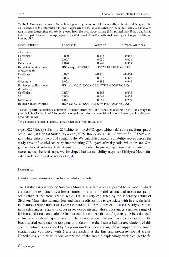
2212 Biodivers Conserv (2008) 17:2197–2218
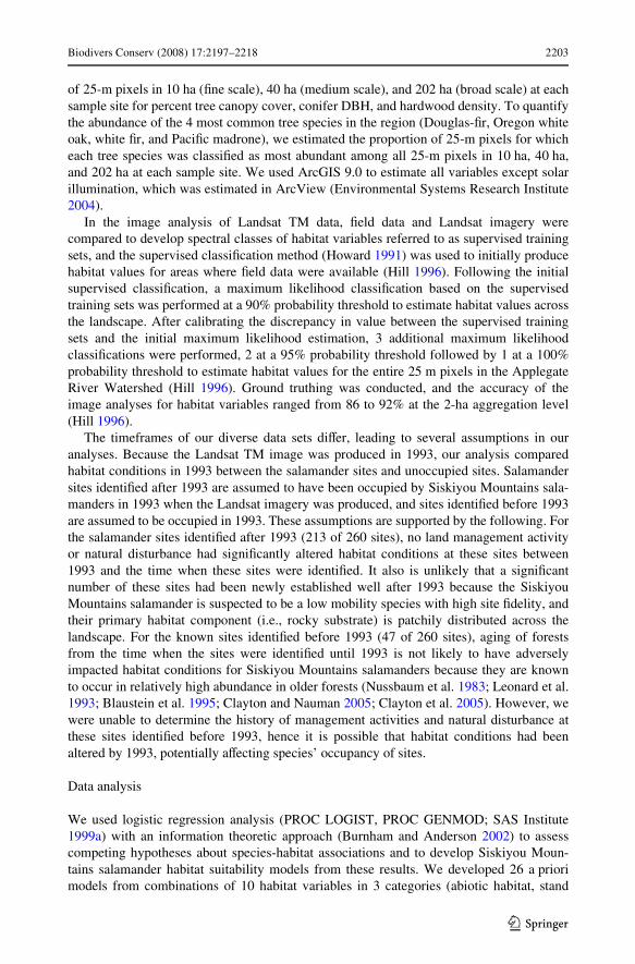
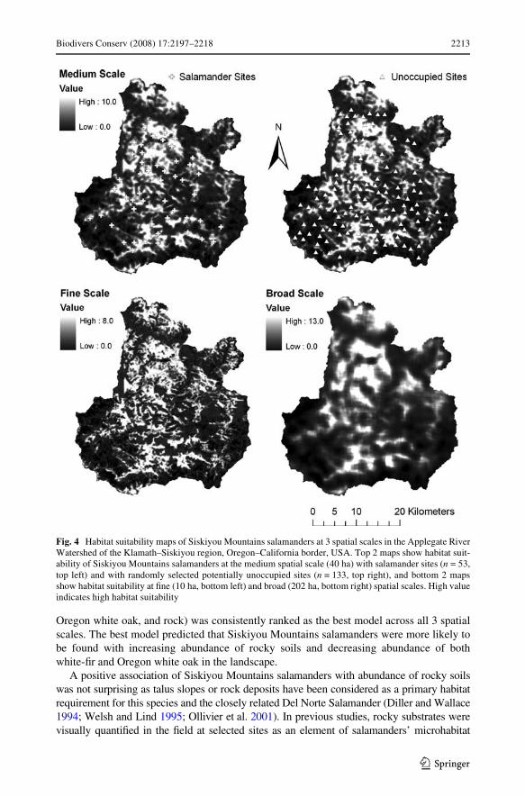
exp(0.022*Rocky soils ¡0.125*white Wr ¡0.054*Oregon white oak) at the medium spatialscale; and (3) Habitat Suitability = exp(0.025*Rocky soils ¡0.162*white Wr ¡0.052*Ore-gon white oak) at the broad spatial scale. We calculated habitat suitability scores across thestudy area at 3 spatial scales by incorporating GIS layers of rocky soils, white Wr, and Ore-gon white oak into our habitat suitability models. By projecting these habitat suitabilityscores across the landscape, we developed habitat suitability maps for Siskiyou Mountainssalamanders at 3 spatial scales (Fig. 4).
Discussion
Habitat associations and landscape habitat models
The habitat associations of Siskiyou Mountains salamanders appeared to be more distinctand could be explained by a fewer number of a priori models at Wne and moderate spatialscales than at the broad spatial scale. This is likely explained by the sedentary nature ofSiskiyou Mountains salamanders and their predisposition to associate with Wne-scale habi-tat features (Nussbaum et al. 1983; Leonard et al. 1993; Jones et al. 2005). Siskiyou Moun-tains salamanders appear to occur in rock deposits and talus slopes under a narrow range ofhabitat conditions, and suitable habitat conditions near these refugia may be best detectedat Wne and moderate spatial scales. The coarse-grained habitat features measured at thebroad spatial scale may be too general to determine the distinct habitat associations of thisspecies, which is evidenced by 5 a priori models receiving signiWcant support at the broadspatial scale compared with 2 a priori models at the Wne and moderate spatial scales.Nonetheless, an a priori model comprised of the same 3 explanatory variables (white-Wr,
Table 5 Parameter estimates for the best logistic regression model (rocky soils, white Wr, and Oregon whiteoak) selected in the information theoretic approach and the habitat suitability model for Siskiyou Mountainssalamanders (Plethodon stormi) developed from the best model at Wne (10 ha), medium (40 ha), and broad(202 ha) spatial scales in the Applegate River Watershed of the Klamath–Siskiyou region, Oregon–Californiaborder, USA
a Model speciWc coeYcients, conditional standard errors (SE), and associated odds ratio per 1 unit change areprovided. See Tables 4 and 5 for model averaged coeYcients, unconditional standard errors, and model aver-aged odds ratiosb HS indicates habitat suitability scores calculated from the equation
Model statisticsa Rocky soils White Wr Oregon White oak
Fine scaleCoeYcient 0.020 ¡0.115 ¡0.043SE 0.005 0.030 0.021Odds ratio 1.020 0.891 0.958Habitat suitability model HSb = exp(0.020*ROCK-0.115*WFIR-0.043*WOAK)Medium scaleCoeYcient 0.022 ¡0.125 ¡0.054SE 0.006 0.032 0.027Odds ratio 1.022 0.882 0.948Habitat suitability model HS = exp(0.022*ROCK-0.125*WFIR-0.054*WOAK)Broad scaleCoeYcient 0.025 ¡0.162 ¡0.052SE 0.008 0.041 0.028Odds ratio 1.025 0.851 0.949Habitat Suitability Model HS = exp(0.025*ROCK-0.162*WFIR-0.052*WOAK)
1 C
Biodivers Conserv (2008) 17:2197–2218 2213
Oregon white oak, and rock) was consistently ranked as the best model across all 3 spatialscales. The best model predicted that Siskiyou Mountains salamanders were more likely tobe found with increasing abundance of rocky soils and decreasing abundance of bothwhite-Wr and Oregon white oak in the landscape.
A positive association of Siskiyou Mountains salamanders with abundance of rocky soilswas not surprising as talus slopes or rock deposits have been considered as a primary habitatrequirement for this species and the closely related Del Norte Salamander (Diller and Wallace1994; Welsh and Lind 1995; Ollivier et al. 2001). In previous studies, rocky substrates werevisually quantiWed in the Weld at selected sites as an element of salamanders’ microhabitat
Fig. 4 Habitat suitability maps of Siskiyou Mountains salamanders at 3 spatial scales in the Applegate RiverWatershed of the Klamath–Siskiyou region, Oregon–California border, USA. Top 2 maps show habitat suit-ability of Siskiyou Mountains salamanders at the medium spatial scale (40 ha) with salamander sites (n = 53,top left) and with randomly selected potentially unoccupied sites (n = 133, top right), and bottom 2 mapsshow habitat suitability at Wne (10 ha, bottom left) and broad (202 ha, bottom right) spatial scales. High valueindicates high habitat suitability
1 C
2214 Biodivers Conserv (2008) 17:2197–2218
(Diller and Wallace 1994; Welsh and Lind 1995; Ollivier et al. 2001), but such Weld data onrocky substrates are not readily available across the landscape to facilitate conservation plan-ning. Our study is the Wrst to demonstrate the association of Siskiyou Mountains salamanderswith rocky soils across the landscape based on widely available GIS soil conservation mapsand to facilitate the application of these maps for conservation purposes.
In northwestern California, Siskiyou Mountain salamanders increased in abundancewith a decrease in elevation (Ollivier et al. 2001). We similarly found their tendency tooccur in low elevation habitats in southwestern Oregon. Paradoxically, a priori modelscontaining elevation as an explanatory variable were not as eVective at predicting salaman-der occurrence as models containing tree species abundances. Change in tree speciesabundance, which occurred along the elevation gradient, appeared to be more directlylinked to the shift in salamander occupancy than elevation itself. Siskiyou Mountains sala-manders were less likely to occur in areas of the landscape with higher abundance of whiteWr, which generally indicates cold and dry environments at high elevations (Laacke 1990),and were more likely to occur in areas with higher abundance of PaciWc madrone at lowelevations. Although we initially hypothesized a negative association of Siskiyou Moun-tains salamanders with PaciWc madrone because it indicates potentially dry environmentalconditions, our Wnding suggests that the salamanders may be able to tolerate some dry con-ditions within the distribution of PaciWc madrone, perhaps because PaciWc madrone cangrow in rocky soils to which the salamanders are adapted. PaciWc madrone was not anexplanatory variable in the best models simply because it was negatively correlated withwhite Wr to a high degree; therefore, the inclusion of white Wr in the models indirectlyaccounted for PaciWc madrone. In contrast to expectations, Douglas-Wr also was not a goodpredictor of the occurrence of Siskiyou Mountains salamanders. This may be explainedbecause Douglas-Wr was well distributed across elevations while Siskiyou Mountains sala-manders mainly occurred in the lower half of elevations within the Douglas-Wr distribution.
Structural habitat features (e.g., tree canopy cover and conifer DBH) were not eVectivein predicting salamander occurrence likely due to their associations with tree species abun-dances. A positive association of the salamanders with an increasing density of hardwoodprobably was a result of an increase in hardwood, particularly PaciWc madrone, at low ele-vation habitats, where the salamanders tended to occur. Alternatively, researchers hypothe-sized that higher densities of hardwood trees might positively aVect Siskiyou Mountainssalamanders by increasing the availability of cover objects, mainly downed hardwoodmaterials on the forest Xoor (Ollivier et al. 2001) and that the presence of hardwood treesmight enhance a multi-layered stand structure, cool and stable forest-Xoor microclimate,and biomass of invertebrate prey (Welsh and Lind 1995).
We also did not Wnd solar illumination to be a good predictor of salamander occurrencein southwestern Oregon, and our Wnding is consistent with a previous Weld study conductedin our study area (Ollivier et al. 2001). However, in the southern portion of the salaman-der’s range in northwestern California, where the climate is hotter and drier than that insouthwestern Oregon, Siskiyou Mountains salamanders were most frequently found in theareas of landscape with low solar illumination (Ollivier et al. 2001). Therefore, theresponse of Siskiyou Mountains salamanders to solar illumination appears to vary withgeographic location, perhaps depending on local climate conditions.
Management implications
Our habitat suitability models and maps are directly applicable to the conservation of SiskiyouMountains salamanders in the Applegate River Watershed along the Oregon–California
1 C

Biodivers Conserv (2008) 17:2197–2218 2215
border, USA. For example, our GIS maps of habitat suitability can aid conservationists andmanagers in selection of high priority conservation sites by allowing them to evaluatepotential habitat quality and habitat connectivity in relation to locations of existing conserva-tion reserves. Furthermore, ecological risk to the conservation of Siskiyou Mountains sala-manders, including adverse human activities and natural disturbances, can be evaluatedacross the landscape using our habitat suitability map along with maps of Wre hazard, landuse allocations, road networks, or proposed management activities. Managers also can useour habitat suitability maps along with other available information to develop land manage-ment plans or modify existing ones to minimize adverse impacts on the salamander’ssuitable habitat. Importantly, conservation of Siskiyou Mountains salamanders based on ourhabitat suitability maps enhances protection of forested rocky-rubble habitats and may indi-rectly protect rare mollusks endemic to the region, many of which appear to occur in moistrocky substrates (Bury and Pearl 1999; Jules et al. 1999). Finally, our approach to develop alandscape habitat suitability model from locally available GIS data can be easily adapted andapplied to conservation of a wide variety of rare species in diVerent geographic regions.
Scope and limitation
We identify the scope and limitations of this study to ensure the appropriate use of ourresearch results and to improve future research designs for the conservation of SiskiyouMountains salamanders and advancement of landscape habitat studies. Because we lackedhome range and movement information of Siskiyou Mountains salamanders, the 3 spatialscales used in this study were determined based on practical conservation and managementconsiderations, rather than the species’ biology or ecology. Therefore, our understanding ofhow the Siskiyou Mountains salamander responds to ecological or environmental factorsacross a range of spatial scales is still incomplete. Further studies are needed to determinehome range size, activity pattern, or ecologically and biologically meaningful spatial scalesfor the better assessment of habitat association of Siskiyou Mountains salamanders acrossthe landscape.
We also were limited by the availability of GIS data in the analysis of habitat associa-tions and development of habitat suitability models. Although we considered all the habitatvariables available in GIS data when formulating a priori models, the occurrence ofSiskiyou Mountains salamanders might be aVected by habitat or ecological factors thatwere not available for our analyses. For example, we were unable to analyze the associationof Siskiyou Mountains salamanders with climate data (precipitation, minimum and maxi-mum temperature) because the spatial resolution of digital climate data (1600 ha/ 4000-mpixel) from Parameter-elevation Regressions on Independent Slopes Model (PRISM; Dalyet al. 1994)) was too coarse for the spatial scale of our study, even at the broad spatial scale(500 ha/1425-m pixel). Therefore, some elements of climate conditions were indirectlyassessed using surrogate climate variables, such as solar illumination and tree species abun-dance. Furthermore, our current habitat suitability maps are based on the image analysis of1993 Landsat TM data. Therefore, updating habitat suitability maps, when the latest spatialhabitat data becomes available, would improve precision and accuracy of current condi-tions and reduce bias of estimated habitat suitability; however, our current habitat suitabil-ity models and maps are applicable for management and conservation purposes becauseabundance of rocky soils and tree species across the study area has not signiWcantlychanged since 1993.
Our models can eVectively be used to compare relative habitat suitability scores acrossthe landscape; however, our retrospective approach limited the ability of our models to
1 C

2216 Biodivers Conserv (2008) 17:2197–2218
estimate the probability of species occurrence as well as to predict species presence orabsence in relation to some objective threshold value (Ramsey and Schafer 1997,pp. 586–587). Data from a prospective study, in which outcomes of presence or absenceare not known prior to the survey, are necessary to model predictive logistic regressionequations (Ramsey and Schafer 1997, pp. 586–587).
This study focused on the northern genetic population of the Siskiyou Mountain sala-mander in the Applegate River Watershed at the Oregon–California border and did notinclude any part of the range of the southern genetic population in northwestern California(Mahoney 2004; Mead et al. 2005). A future study could determine whether there arediVerences in habitat associations between these 2 populations and test the applicability ofour habitat models or develop new landscape habitat models for the southern population.
Acknowledgments We thank R. S. Nauman, D. R. Clayton, H. H. Welsh, Jr., and B. C. McComb forreviewing this manuscript. D. R. Clayton provided insights regarding the ecological implication of soil andgeology maps. We also thank anonymous reviewers for their constructive suggestions and comments. R. S.Nauman assisted with data compilation for known salamander sites. S. J. Arnold of Department of Zoologysupported this research through an Oregon State University Cooperative Agreement. K. Vance-Borland andK. Christiansen provided useful suggestions for troubleshooting in GIS. Funding for this research was pro-vided by the U.S. Federal Survey and Manage Program of the Northwest Forest Plan and the USDA ForestService, PaciWc Northwest Research Station, Aquatic and Land Interactions Research Program.
References
Badura GJ, Jahn PN (1977) Soil Resource Inventory for the Rogue River National Forest. U. S. Departmentof Agriculture, Forest Service, Medford, Oregon
Blaustein AR, Beatty JJ, Olson DH, Storm RM (1995) The biology of amphibians and reptiles in old-growthforests in the PaciWc Northwest. General Technical Report PNW-337, U. S. Department of Agriculture,Forest Service, Portland, Oregon
Burnham KP, Anderson DR (2002) Model selection and multimodel inference: a practical information-theoreticapproach. Springer-Verlag, New York
Bury RB, Bury GW (2005) Biogeographic patterns. In: Jones LLC, Leonard WP, Olson DH (eds) Amphibiansof the PaciWc Northwest. Seattle Audubon Society, Seattle
Bury RB, Pearl CA (1999) Klamath-Siskiyou herpetofauna: biogeographic patterns and conservation strategies.Nat Areas J 19:341–350
Clayton DR, Nauman RS (2005) Siskiyou Mountains salamander: Plethodon stormi Highton and Brame. In:Jones LLC, Leonard WP, Olson DH (eds) Amphibians of the PaciWc Northwest. Seattle Audubon Society,Seattle
Clayton DR, Olson DH, Nauman RS (2005) Conservation assessment for the Siskiyou Mountains salamander(Plethodon stormi), Version 1.3. USDA Forest Service, Region 6, and USDI Bureau of Land Manage-ment, Oregon, Interagecy Special-Status and Sensitive Species Program. Portland, OR. Available viaDIALOG. http://www.or.blm.gov/ISSSP/Conservation_Planning-and-Tools.htm. Cited 20 Dec 2006
CliV AD, Ord JK (1981) Spatial processes: models & applications. Pion Limited, LondonCox JA, Baker WW, Engstrom RT (2001) Red-cockaded woodpackers in the Red Hills region: a GIS-based
assessment. Wildl Soc Bull 29:1278–1288Daly C, Neilson RP, Phillips DL (1994) A statistical-topographic model for mapping climatological precipi-
tation over mountainous terrain. J Appl Meteorol 33:140–158DellaSala DA, Reid SB, Frest TJ, Strittholt JR, Olson DM (1999) A global perspective on the biodiversity of
the Klamath-Siskiyou ecoregion. Nat Areas J 19:300–319Diller LV, Wallace RL (1994) Distribution and habitat of Plethodon elongatus on managed, young growth
forests in north coastal California. J Herpetol 28:310–318Environmental Systems Research Institute Inc (1996) ArcView version 3.2 and ArcView Spatial Analyst.
Redlands, CaliforniaEnvironmental Systems Research Institute Inc (2004) ArcGIS version 9.0. Redlands, CaliforniaFleishman E, Mac Nally R, Fay JP, Murphy DD (2001) Modeling and predicting species occurrence using
broad-scale environmental variables: an example with butterXies of the Great Basin. Conserv Biol15:1647–1685
1 C
Biodivers Conserv (2008) 17:2197–2218 2217
Franklin JF, Dyrness CT (1988) Natural vegetation of Oregon and Washington. Oregon State UniversityPress, Corvallis, Oregon
Fuhlendorf SD, Woodward AJW, Leslie DM Jr, Shackford JS (2002) Multi-scale eVects of habitat loss andfragmentation on lesser prairie-chicken populations of the US southern Great Plains. Landscape Ecol17:617–628
Gesch D, Oimoen M, Greenlee S, Nelson C, Steuck M, Tyler D (2002) The National Elevation Dataset.Photogrammetric Engineering and Remote Sensing 68:5–11
Gros PM, Rejmánek M (1999) Status and habitat preferences of Uganda cheetahs: an attempt to predictcarnivore occurrence based on vegetation structure. Biodivers Conserv 8:1561–1583
Gustafson EJ, Murphy NL, Crow TR (2001) Using a GIS model to assess terrestrial salamander response toalternative forest management plans. J Environ Manage 63:281–292
Herman RK, Lavender DP (1990) Pseudotsuga menziesii (Mirb.) Franco: Douglas-Wr. In: Burns RM, HonkalaBH (technical coordinators), Silvics of North America, vol 1, Conifers, Agriculture Handbook 654. U. S.Department of Agriculture, Forest Service, Washington, DC
Hill TB (1996) Forest biometrics from space. Geographic Resource Solutions, Arcata, CaliforniaHoward JA (1991) Remote sensing of forest resources: theory and application. Chapman & Hall, LondonJones LLC, Leonard WP, Olson DH (2005) Amphibians in the PaciWc Northwest. Seattle Audubon Society,
SeattleJules ES, DellaSalla DA, Marsden JK (1999) The Klamath-Siskiyou region. Nat Areas J 19:295–299Keating KA, Cherry S (2004) Use and interpretation of logistic regression in habitat-selection studies. J Wildl
Manage 68:774–789Laacke RJ (1990) Abies concolor (Gord. & Glend.) Lindl. Ex Hildebr.: white Wr. In: Burns RM, Honkala BH
(technical coordinators) Silvics of North America, vol 1, Conifers, Agriculture Handbook 654. U. S.Department of Agriculture, Forest Service, Washington, DC
Leonard WP, Brown HA, Jones LLC, McAllister KR, Storm RM (1993) Amphibians of Washington andOregon. Seattle Audubon Society, Seattle
Luoto M, Kuussaari M, Toivonen T (2002) Modeling butterXy distribution based on remote sensing data.J Biogeogr 29:1027–1037
Maehr DS, Cox JA (1995) Landscape features and panthers in Florida. Conserv Biol 9:1008–1019Mahoney MJ (2004) Molecular systematics and phylogeography of the Plethodon elongatus species group:
combining phylogenetic and population genetic methods to investigate species history. Mol Ecol13:149–166
Manly BFJ, McDonald LL, Thomas DL, McDonald TL, Erikson WP (2002) Resource selection by animals,2nd edn. Kluwer Press, New York
McDonald PM, Tappeiner JC II (1990) Arbutus menziesii Pursh: PaciWc madrone, In: Burns RM, HonkalaBH (technical coordinators). Silvics of North America, vol 2, Hardwoods, Agriculture Handbook 654.U. S. Department of Agriculture, Forest Service, Washington, DC
Mead LS, Clayton DR, Nauman RS, Olson DH, Pfrender ME (2005) Newly discovered populations of sala-manders from Siskiyou county California represent a species distinct from Plethodon stormi. Herpeto-logica 61:158–177
Molina R, McKenzie D, Lesher R, Ford J, Alegria J, Culter R (2003) Strategic survey framework for theNorthwest Forest Plan survey and manage program. General Technical Report, PNW-GTR 573, U. S.Department of Agriculture, Forest Service, PaciWc Northwest Research Station, Portland, Oregon
Murkin HR, Murkin EJ, Ball JP (1997) Avian habitat selection and prairie wetland dynamics: a 10-yearexperiment. Ecol Appl 7:1144–1159
Myers N, Mittermeier RA, Mittermeier CG, da Fonseca GAB, Kent J (2000) Biodiversity hotspots forconservation priorities. Nature 403:853–858
Nauman RS, Olson DH (1999) Survey and Manage salamander known sites. In: Olson DH (eds) Surveyprotocols for amphibians under the Survey & Manage provision of the Northwest Forest Plan, Version3.0, October 1999. Interagency Publication of the Regional Ecosystem OYce, Portland, Oregon. BLMpublication, BLM/OR/WA/PT-00/033+1792, U.S. GPO: 2000-589-124/04022 Region No. 10. Avail-able via DIALOG. www.or.blm.gov/surveyandmanage/SP/Amphibians99/protoch.pdf. Cited 10 Nov 2006
Nauman RS, Olson DH (2004) Strategic survey annual report, Siskiyou Mountains salamander northernpopulation. The publication available at: USDA Forest Service, Region 6 and USDI Bureau of LandManagement, Oregon and Washington, Interagency special-status and sensitive species program,Regional OYce, Portland, Oregon
Nussbaum RA, Brodie ED Jr, Storm RM (1983) Amphibians and reptiles of the PaciWc Northwest. Universityof Idaho Press, Moscow, Idaho
Ollivier LM, Welsh HH Jr, Clayton DR (2001) Habitat correlates of the Siskiyou Mountains Salamander,Plethodon stormi (Caudata: Plethodontidae); with comments on the species’ range. Report to the
1 C
2218 Biodivers Conserv (2008) 17:2197–2218
California Fish and Game. U.S. Department of Agriculture Forest Service, Redwood Science Labora-tory, 1700 Bayview Drive, Arcata, CA 95521. June, 2001. Available via DIALOG. http://www.fs.usda.gov/psw/publications/4251/ollivier2.pdf. Cited 9 Nov 2006
Olson DH (1999) Standardized survey protocols for amphibians under the Survey and Manage and ProtectionBuVer Provisions. In: Olson DH (ed) Survey protocols for amphibians under the Survey & Manage pro-vision of the Northwest Forest Plan, Version 3.0, October 1999. Interagency Publication of the RegionalEcosystem OYce, Portland, Oregon. BLM publication, BLM/OR/WA/PT-00/033+1792, U.S. GPO:2000-589-124/04022 Region No. 10. Available via DIALOG. http://www.or.blm.gov/surveyandmanage/SP/Amphibians99/protoch.pdf. Cited 9 Nov 2006
Pearce JL, Boyce MS (2006) Modelling distribution and abundance with presence-only data. J Appl Ecol43:405–412
Ramsey FL, Schafer DW (1997) The statistical sleuth, a course in methods of data analysis. Wadsworth, New YorkRay N, Lehmann A, Joly P (2002) Modeling spatial distribution of amphibian populations: a GIS approach
based on habitat matrix permeability. Biodiversity and Conservation 11:2143–2165SAS Institute (1999a) SAS/ STATS users guide, version 8, Cary, North CarolinaSAS Institute (1999b) SAS procedures guide, version 8, Cary, North CarolinaStein WI (1990) Quercus garryana Dougl. Ex Hook: Oregon white oak. In: Burns RM, Honkala BH (technical
coordinators) Silvics of North America, vol 2, Hardwoods, Agriculture Handbook 654. U. S. Depart-ment of Agriculture, Forest Service, Washington, DC
Thomas JW, Rphael MG, Anthony RG et al (1993) Viability assessment and management considerations forspecies associated with late successional and old-growth forests of the PaciWc Northwest. Report byScientiWc Analysis Team, U. S. Department of Agriculture, Forest Service, Portland, Oregon
Torgersen CE, Price DM, Li HW, McIntosh BA (1999) Multiscale thermal refugia and stream habitat asso-ciations of chinook salmon in northeastern Oregon. Ecol Appl 9:301–319
Welsh HH Jr, Lind AJ (1995) Habitat correlates of the Del Norte salamander, Plethodon elongatus (Caudata:Plethodontidae), in northwestern California. J Herpetol 29:198–210
1 C