Embed Size (px)
Citation preview

DEVELOPING TRADING STRATEGIES UNDER THE
DIRECTIONAL CHANGES FRAMEWORK
With application in the FX Market
Amer Bakhach
A thesis submitted for the degree of Doctor of Philosophy
School of Computer Science and Electronic Engineering
Centre for Computational Finance and Economic Agents (CCFEA)
University of Essex
November 2018

Acknowledgements II
Acknowledgements
First and foremost, I wish to thank my supervisor, Prof. Edward Tsang. Without his guidance,
support, and endless patience throughout the years of my degree this thesis would not have been
possible. Both his wisdom and his expertise in computational finance taught me a great deal. I was
very lucky to be one of his students. I also want to thank Dr. Carmine Ventre who co-supervise
my research. His patience and feedback have been always helpful.
It is with immense gratitude that I acknowledge the support and help of my brother-in-law, Prof.
Hassan El-Rifai (Sharjah University, UAE). It was his on advice that I chose to undertake my Ph.D.
studies in the UK. Furthermore, as a self-funded student, I could not have afforded my tuition fees
without his financial support.
My heartfelt thanks to the examiners Dr. Andreas Krause (University of Bath) and Dr. Michael
Fairbank (University of Essex). Their insightful comments have helped me to improve the value
of this thesis.
I would also like to thank Dr. Wing Lon Ng (former lecturer at the University of Essex) and Dr.
Raju V.L. Chinthalapati (University of Greenwich). Their scientific notes were inspiring. My
appreciation also goes to my fellow students Mateusz Gątkowski, Hamid Jalalian, Ran Tao and
James Chun. Our discussions were a great source of knowledge and inspiration.
Last but not least, this thesis would not have been possible without the person who was always
behind me - my wife Ola. Her unconditional support was a constant source of encouragement that
kept me going during the research journey.
Abstract III
Abstract
Directional Changes (DC) is a framework for studying price movements. Many studies have
reported that the DC framework is useful in analysing financial markets. Other studies have
suggested that, theoretically, a trading strategy that exploits the full promise of the DC framework
could be astonishingly profitable. However, such a strategy is yet to be discovered. In this thesis,
we explore, and consequently provide proof of, the usefulness of the DC framework as the basis
of a profitable trading strategy.
Existing trading strategies can be categorised into two groups: the first comprising those that
rely on forecasting models; the second comprising all other strategies. In line with existing research,
this thesis develops two trading strategies: the first relies on forecasting Directional Changes in
order to decide when to trade; whereas the second strategy, whilst based on the DC framework,
uses no forecasting models at all.
This thesis comprises three original research elements:
1. We formalize the problem of forecasting the change of a trend’s direction under the DC
framework. We propose a solution for the defined forecasting problem. Our solution
includes discovering a novel indicator, which is based on the DC framework.
2. We develop the first trading strategy that relies on the forecasting approach established
above (Point 1) to decide when to trade.
3. We develop a second trading strategy which does not rely on any forecasting model. This
is trading strategy employs a DC-based procedure to examine historical prices in order to
discover profitable trading rules.
We examine the performance of these two trading strategies in the foreign exchange market.
The results indicate that both can be profitable and that both outperform other DC-based trading
strategies. The results additionally suggest that none of these two trading strategies outperforms
the other in terms of profitability and risk simultaneously.
List of Figures IV
List of Figures
2.1 A typical forex quote of the EUR/USD currency pair . . . . . . . . . . . . . . . . . . . . 6
2.2 GBP/CHF mid-prices sampled minute by minute . . . . . . . . . . . . . . . . . . . . . . . 7
4.1 GBP/CHF mid-prices sampled minute by minute . . . . . . . . . . . . . . . . . . . . . . . 22
4.2 An example of a DC-based summary of the price series shown in Fig. 4.1. theta
= 0.10% . . . . . . . . . . . . . . . . . . . . . . . . . . . . . . . . . . . . . . . . . . . . . . . . . . . . . . . . 24
4.3 An example of a DC-based summary of the price series shown in Fig. 4.1. theta
= 0.20% . . . . . . . . . . . . . . . . . . . . . . . . . . . . . . . . . . . . . . . . . . . . . . . . . . . . . . . . 25
4.4.a Modification of the DC analysis when started at different times. . . . . . . . . . . . 26
4.4.b Modification of the DC analysis when started at different times. . . . . . . . . . . . 26
4.5 An illustration of two scaling laws related to the DC and OS events . . . . . . . . . 29
4.6 A sample individual GP tree: internal nodes are represented by Boolean
functions, while terminal nodes correspond to different DC thresholds . . . . . . . 32
5.1 An example of a downward DC event [AABTheta] of threshold BTheta which
embraces another downward DC event of a smaller threshold STheta [AASTheta] 43
5.2 An example of an upward DC event [BBBTheta] of threshold BTheta which
embraces another upward DC event of a smaller threshold STheta [BBSTheta]. . 43
5.3 The synchronization of the two DC summaries using two thresholds. . . . . . . . . 44
5.4 The synchronization of the two DC summaries using two thresholds . . . . . . . . 50
5.5 Illustration of one in-sample and the corresponding out-of-sample sets. . . . . . . 52
5.6 Illustration of the accuracy of a dummy prediction as a function of the True-
False imbalance . . . . . . . . . . . . . . . . . . . . . . . . . . . . . . . . . . . . . . . . . . . . . . . . . . 54
5.7 An illustration of the variation of the accuracy of our forecasting model as a
function of BTheta . . . . . . . . . . . . . . . . . . . . . . . . . . . . . . . . . . . . . . . . . . . . . . . 60
6.1 The synchronization of two DC summaries with two thresholds: STheta =
0.10% and BTheta = 0.20% . . . . . . . . . . . . . . . . . . . . . . . . . . . . . . . . . . . . . . . . 64
6.2 Normalized daily exchange rates of the 8 selected currency pairs . . . . . . . . . . . 71
6.3 Illustration of n rolling windows . . . . . . . . . . . . . . . . . . . . . . . . . . . . . . . . . . . . . 74
6.4 A sample individual GP tree: internal nodes are represented by Boolean
functions, while terminal nodes correspond to different DC thresholds . . . . . . . 88
9.1 Number of DC events of thresholds 0.03% and 0.10% in different periods . . . . 139

List of Tables V
List of Tables
4.1 Example of how the value of 𝑃𝐸𝑋𝑇𝑛𝑒𝑥𝑡change as price movements continues . . . . 23
5.1 Example of how to compute the Boolean variable BBTheta . . . . . . . . . . . . . . . 45
5.2 The synchronization of the two DC events . . . . . . . . . . . . . . . . . . . . . . . . . . . . . 47
5.3 The results of applying our forecasting approach to eight currency pairs . . . . . 55
5.4 Analyzing the impact of BTheta on the accuracy of our forecasting approach
applied to the currency pair EUR/CHF . . . . . . . . . . . . . . . . . . . . . . . . . . . . . . . .
57
5.5 Analyzing the impact of BTheta on the accuracy of our forecasting approach
applied to the currency pair GBP/CHF . . . . . . . . . . . . . . . . . . . . . . . . . . . . . . . . 57
5.6 Analyzing the impact of BTheta on the accuracy of our forecasting approach
applied to the currency pair EUR/USD . . . . . . . . . . . . . . . . . . . . . . . . . . . . . . . 58
5.7 Analyzing the impact of BTheta on the accuracy of our forecasting approach
applied to the currency pair GBP/AUD . . . . . . . . . . . . . . . . . . . . . . . . . . . . . . . 58
6.1 The synchronization of two DC summaries . . . . . . . . . . . . . . . . . . . . . . . . . . . . 67
6.2 The average and standard deviation of the bid-ask spread of the considered
currency pairs . . . . . . . . . . . . . . . . . . . . . . . . . . . . . . . . . . . . . . . . . . . . . . . . . . .
72
6.3 An example of a DC summary using GBP/CHF mid-prices . . . . . . . . . . . . . . . 73
6.4 The start and end dates of the training and applied periods of each composed
window . . . . . . . . . . . . . . . . . . . . . . . . . . . . . . . . . . . . . . . . . . . . . . . . . . . . . . . .
75
6.5 Trading performance of TSFDC-down and TSFDC-up . . . . . . . . . . . . . . . . . . . 80
6.6 Monthly RR of applying TSFDC-down to the eight currency pairs . . . . . . . . . . 81
6.7 Monthly RR of applying TSFDC-up to the eight currency pairs . . . . . . . . . . . . 81
6.8 The interest rates of the selected currencies. . . . . . . . . . . . . . . . . . . . . . . . . . . . 82
6.9 The employed MAR and risk-free rate of each considered currency pair. . . . . . 82
6.10 The Sortino and Sharpe ratios of the two versions of TSFDC . . . . . . . . . . . . . . 82
6.11 Summary of the monthly RR (%) obtained by applying the buy and hold (B&H)
approach to each of the eight considered currency pairs . . . . . . . . . . . . . . . . . .
83
6.12 The values of Jensen’s Alpha and Beta of TSFDC with reference to the buy and
hold as benchmark . . . . . . . . . . . . . . . . . . . . . . . . . . . . . . . . . . . . . . . . . . . . . . . 83
6.13 The Sharpe ratio of the buy and hold, TSFDC-down and TSFDC-up. . . . . . . . . 84
6.14 The p-values of the Wilcoxon tests resultant from the comparison of Sharpe
ratios. . . . . . . . . . . . . . . . . . . . . . . . . . . . . . . . . . . . . . . . . . . . . . . . . . . . . . . . . . . 84
6.15 The win ratio of dummy prediction, TSFDC-down and TSFDC-up. . . . . . . . . . 84
6.16 The p-values of the Wilcoxon tests resultant from the comparison of win ratios. 84
6.17 The summaries of RR and MDD rustled from trading with TSFDC-down and
TSFDC-up . . . . . . . . . . . . . . . . . . . . . . . . . . . . . . . . . . . . . . . . .. . . . . . . . . . . . . 87
6.18 The test statistics ‘W’ of the conducted Wilcoxon tests of comparing the RR
and MDD of TSFDC-down and TSFDC-up . . . . . . . . . . . . . . . . . . . . . . . . . . . 88
List of Tables VI
7.1 An example of a DC summary of GBP/CHF mid-prices . . . . . . . . . . . . . . . . . . 97
7.2 Summary of the evaluation of the best performance of applying SBA-down . . 107
7.3 Summary of the evaluation of the worst performance of applying SBA-down . 107
7.4 Summary of the evaluation of the best performance of applying SBA-up . . . . . 108
7.5 Summary of the evaluation of the worst performance of applying SBA-up . . . 109
7.6 The values of down_ind corresponding to the highest RR generated by SBA-
down for each month . . . . . . . . . . . . . . . . . . . . . . . . . . . . . . . . . . . . . . . . . . . . . .
110
7.7 The values of parameter up_ind corresponding to the highest RR generated by
SBA-up for each month . . . . . . . . . . . . . . . . . . . . . . . . . . . . . . . . . . . . . . . . . . . 111
7.8 Summary of trading performance of the DBA-down and DBA-up . . . . . . . . . . 113
7.9 Summary of monthly RR of trading with the DBA-down . . . . . . . . . . . . . . . . . 114
7.10 Summary of monthly RR of trading with the DBA-up . . . . . . . . . . . . . . . . . . . . 114
7.11 The Sharpe ratio of the buy and hold, DBA-down and DBA-up. . . . . . . . . . . . . 115
7.12 The employed MAR and risk-free rate of each considered currency pair. . . . . . 115
7.13 The Sortino and Sharpe ratios of the two versions of DBA . . . . . . . . . . . . . 115
7.14 Summary of the monthly RR (%) obtained by applying the buy and hold
strategy to the eight currency pairs . . . . . . . . . . . . . . . . . . . . . . . . . . . . . . . . . . .
115
7.15 The values of Jensen’s Alpha and Beta of both versions of DBA with reference
to the buy and hold approach as benchmark . . . . . . . . . . . . . . . . . . . . . . . . . . . . 116
7.16 The Sharpe ratio of the buy and hold, DBA-down and DBA-up. . . . . . . . . . . . . 116
7.17 The p-values of the Wilcoxon tests resultant from the comparison of Sharpe
ratios. . . . . . . . . . . . . . . . . . . . . . . . . . . . . . . . . . . . . . . . . . . . . . . . . . . . . . . . . . . 116
7.18 The values of the probability γ (%) for the considered currency pairs . . . . . . . . 119
7.19 The summaries of RR and MDD rustled from trading with DBA-down and
DBA-up . . . . . . . . . . . . . . . . . . . . . . . . . . . . . . . . . . . . . . . . .. . . . . . . . . . . . . . . 120
7.20 The test statistics ‘W’ of the conducted Wilcoxon tests of comparing the RR
and MDD of DBA-down and DBA-up . . . . . . . . . . . . . . . . . . . . . . . . . . . . . . . . 120
8.1 Comparing the profitability, measured as ‘Rate of returns (RR)’, of TSFDC and
DBA . . . . . . . . . . . . . . . . . . . . . . . . . . . . . . . . . . . . . . . . . . . . . . . . . . . . . . . . . . 128
8.2 Comparing the Maximum Drawdown (MDD) of TSFDC and DBA . . . . . . . . . 129
8.3 Comparing the risk-adjusted return, in terms of the Sharpe Ratio, of TSFDC
and DBA . . . . . . . . . . . . . . . . . . . . . . . . . . . . . . . . . . . . . . . . . . . . . . . . . . . . . . . 129
9.1 An illustration of profiling indicators and evaluation metrics of the same rolling
window . . . . . . . . . . . . . . . . . . . . . . . . . . . . . . . . . . . . . . . . . . . . . . . . . . . . . . . . 140

Glossary VII
Glossary
Base and Counter Currency: For a given currency pair (e.g. EUR/USD in the figure below),
the first listed currency of a currency pair (i.e. EUR) is called the base currency, and the second
currency (i.e. USD) is called the counter currency. The currency pair indicates how much of the
counter currency is needed to purchase one unit of the base currency. The counter currency is also
referred to as the quoted currency.
Bid and Ask price: The term ‘bid and ask’ refers to a two-way price quotation that indicates
the price at which a currency can be sold and bought at a given point in time. The bid price
represents the price that a buyer (usually a trader) needs to pay for a currency. The ask price
represents the price that a seller (usually a market maker) wants to receive. For example, in the
figure above the bid price of EUR/USD is 1.08691; while the ask price is 1.08703.
Bull and Bear market: The opposite of a bull market is a bear market, which is characterized
by falling prices and typically shrouded in pessimism. These notions are used to express the
movement of a market. If the trend is up, it is a bull market. If the trend is down, it is a bear market.
Buy and Hold: Buy and hold is a passive trading strategy in which a trader buys stocks (or
currencies) and holds them for a relatively long period, regardless of fluctuations in the market.
The basic idea is that the trader buys a given stock or currency and holds it throughout the trading
period. The basic assumption is that, in the long run, values of stocks (or currencies) will eventually
increase.
Contrarian trading strategy: Contrarian trading is an investment style that goes against
prevailing market trends. A contrarian trader buys a specific stock or currency when the market
exhibits a downtrend and sells when the market exhibits an uptrend.
Foreign exchange (Forex): Forex (FX) is the market in which currencies are traded. The forex
market is the largest, most liquid market in the world, with average traded values that can be
trillions of dollars per day. It includes all of the currencies in the world.
G10: The G10 consists of eleven industrialized nations that meet on an annual basis (or more
frequently, as necessary) to consult, debate and cooperate on international financial matters (see
http://www.investopedia.com/terms/g/groupoften.asp).
Glossary VIII
Intra-day trader: An intra-day trader is a particular type of trader that both opens and closes a
new position in a stock in the same trading day. Usually, they do not hold over-night positions.
Margin call: A margin call occurs when the account value falls below the broker's required
minimum value. Simply put, this is the edge at which the market maker typically decides that a
trader does not have sufficient capital to continue trading.
Market maker: A market maker is a "market participant" or member firm of an exchange that
also buys and sells currencies at prices it displays in an exchange’s trading system for its own
account. Using these systems, a market maker can enter and adjust quotes to buy or sell, enter and
execute orders, and clear those orders.
Risk-adjusted return: Risk-adjusted return refines an investment's return by measuring how
much risk is involved in producing that return, which is generally expressed as a number or rating.
Risk-adjusted returns are applied to individual securities, investment funds and portfolios.
Risk-free rate: The risk-free rate of return is the theoretical rate of return of an investment with
zero risk. The risk-free rate represents the interest an investor would expect from an absolutely
risk-free investment over a specified period of time.
Transaction cost: Transaction costs are expenses incurred when buying or selling goods or
services. Transaction costs represent the labor required to bring these goods or services to market,
giving rise to entire industries dedicated to facilitating exchanges. In a financial sense, transaction
costs include brokers' commissions and spreads, which are the differences between the price the
dealer paid for a security and the price the buyer pays.
Transaction: In the context of this thesis, we define “transaction” as an agreement between two
parties (usually a trader and market maker) to buy one currency against selling another currency
at an agreed price (e.g. bid or ask).

List of Acronyms IX
List of Acronyms
ANN: Artificial Neural Network
ARIMA: Auto-Regressive Integrated Moving Average
B&H: buy and hold
BIS: bank of international settlement
CT: contrarian trader
DC: Directional Changes
GA: Genetic Algorithm
NN: Neural Network
OS: Overshoot
OSV: Overshoot Value
MDD: maximum drawdown
RR: rate of return
TF: trend’s follower
TTR: technical trading rule
List of Publications X
List of Publications
A. Bakhach, E. P. K. Tsang and H. Jalalian, "Forecasting directional changes in the FX
markets," 2016 IEEE Symposium on Computational Intelligence for Financial Engineer &
Economic (CIFEr’ 2016), Athens, Greece, 2016, pp. 1-8. doi: 10.1109/SSCI.2016.7850020.
A. Bakhach, E. P. K. Tsang, Wing Lon Ng and V. L. R. Chinthalapati, "Backlash Agent:
A trading strategy based on Directional Change," 2016 IEEE Symposium on
Computational Intelligence for Financial Engineer & Economic (CIFEr’ 2016), Athens,
Greece, 2016, pp. 1-9. doi: 10.1109/SSCI.2016.7850004.
A. Bakhach, E. P. K. Tsang and V. L. R. Chinthalapati, "TSFDC: A Trading Strategy
Based on Forecasting Directional Changes", Journal of “Intelligent Systems in
Accounting, Finance and Management” volume 25; pp. 105–123, 2018
https://doi.org/10.1002/isaf.1425
Table of Contents XI
Table of Contents
Acknowledgements .................................................................................................................... II
Abstract ..................................................................................................................................... III
List of Figures ........................................................................................................................... IV
List of Tables ............................................................................................................................. V
Glossary .................................................................................................................................. VII
List of Acronyms ...................................................................................................................... IX
List of Publications .................................................................................................................... X
Table of Contents ...................................................................................................................... XI
1 Introduction.......................................................................................................................... 1
1.1 The foreign exchange market and the Directional Changes framework ....................... 1
1.2 Thesis motivations and objectives ................................................................................. 2
1.3 Thesis outline ................................................................................................................ 4
2 The Foreign Exchange Market ............................................................................................ 5
2.1 Introduction ................................................................................................................... 5
2.2 Essential terminologies for FX trading ......................................................................... 6
2.3 About the profitability of FX trading ............................................................................ 8
2.4 Summary ....................................................................................................................... 9
3 Trading Strategies for Financial Markets .......................................................................... 11
3.1 Introduction ................................................................................................................. 11
3.2 The first category: Trading strategies based on forecasting models ........................... 11
3.3 The second category: Trading strategies with no embedded forecasting models ....... 13
3.3.1 Technical trading.................................................................................................. 14
3.3.2 Momentum strategy ............................................................................................. 15
3.3.3 Carry trade ........................................................................................................... 15
3.4 Evaluating the performance of a trading strategy ....................................................... 16
3.5 Summary ..................................................................................................................... 19
4 The Directional Changes Framework ................................................................................ 21
4.1 Introduction ................................................................................................................. 21
4.2 Directional Changes .................................................................................................... 22
4.2.1 The basic concept ................................................................................................. 22
4.2.2 The DC summary ................................................................................................. 25
4.2.3 DC notations ........................................................................................................ 27
4.3 Applying DC to analyse financial markets .................................................................. 28
4.4 DC-based trading strategies......................................................................................... 30

Table of Contents XII
4.4.1 The ‘DCT1’ .......................................................................................................... 30
4.4.2 A DC-based trading strategy ................................................................................ 31
4.4.3 The ‘DC + GA’ .................................................................................................... 33
4.4.4 The ‘Alpha Engine’ .............................................................................................. 35
4.5 Notions and concepts similar to DC ............................................................................ 37
4.6 Summary ..................................................................................................................... 37
5 Forecasting Directional Changes: Problem Formulation and Solution ............................. 40
5.1 Introduction ................................................................................................................. 40
5.2 The concept of Big-Theta ............................................................................................ 42
5.2.1 Big-Theta ............................................................................................................. 42
5.2.2 The Boolean variable BBTheta ............................................................................ 44
5.3 Formulation of the forecasting problem ...................................................................... 46
5.4 Our approach to forecasting the end of a trend ........................................................... 48
5.4.1 The independent variable ..................................................................................... 48
5.4.2 The decision tree procedure J48 .......................................................................... 51
5.5 Evaluation of our approach to forecasting DC: Experiments ...................................... 51
5.5.1 Measuring the True-False imbalance ................................................................... 51
5.5.2 Experiment 5.1: Evaluating the accuracy of our forecasting approach ............... 52
5.5.3 Experiment 5.2: The impact of BTheta on the accuracy of our forecasting model
53
5.6 Evaluation of our approach to forecasting DC: Results and discussion...................... 54
5.6.1 Experiment 5.1: Evaluating accuracy of our forecasting approach ..................... 54
5.6.2 Experiment 5.2: The impact of BTheta on forecasting accuracy ......................... 56
5.7 Summary and conclusion ............................................................................................ 61
6 TSFDC: A Trading Strategy Based on Forecasting Directional Changes ......................... 63
6.1 Introduction ................................................................................................................. 63
6.2 Forecasting DC: A brief overview .............................................................................. 64
6.3 Introducing the trading strategy TSFDC ..................................................................... 65
6.3.1 TSFDC-down ....................................................................................................... 65
6.3.2 TSFDC-up ............................................................................................................ 68
6.4 Preparation of the datasets and other considerations................................................... 70
6.4.1 Data selection ....................................................................................................... 70
6.4.2 Evaluating the performance of a trading strategy ................................................ 71
6.4.3 Bid and ask prices ................................................................................................ 71
6.4.4 Model training and testing process ...................................................................... 72
Table of Contents XIII
6.4.5 Preparing the rolling windows ............................................................................. 72
6.5 Evaluation of TSFDC: The experiments ..................................................................... 75
6.5.1 Money management approach ............................................................................. 75
6.5.2 Experiment 6.1: Evaluation of the performance of TSFDC ................................ 76
6.5.3 Experiment 6.2: Compare the return and risk of both versions of TSFDC ......... 78
6.6 Evaluation of TSFDC: Results and discussion............................................................ 78
6.6.1 Experiment 6.1: Evaluation of the performance of TSFDC ................................ 78
6.6.2 Experiment 6.2: Compare the return and risk of both versions of TSFDC ......... 87
6.7 Comparing TSFDC to other DC-based strategies ....................................................... 88
6.7.1 The DC-based trading strategy by Gypteau et al. ................................................ 88
6.7.2 The DC-based trading strategy: ‘DC+GA’ .......................................................... 90
6.8 Summary and conclusion ............................................................................................ 92
7 Backlash Agent: A Trading Strategy Based on Directional Changes ............................... 94
7.1 Introduction ................................................................................................................. 94
7.2 DC notations ................................................................................................................ 94
7.3 Backlash Agent............................................................................................................ 95
7.3.1 Static BA-down (SBA-down) .............................................................................. 96
7.3.2 Static BA-up (SBA-up) ........................................................................................ 98
7.3.3 Dynamic Backlash Agent .................................................................................... 99
7.4 Evaluation of the Backlash Agent: Methodology and experiments .......................... 100
7.4.1 Experiment 7.1: Evaluation of Static BA .......................................................... 101
7.4.2 Experiment 7.2: Is there one optimal value for the parameters down_ind and
up_ind? 102
7.4.3 Experiment 7.3: Evaluating the performance of DBA-down and DBA-up ....... 103
7.4.4 Experiment 7.4: Comparing the RR of DBA and SBA ..................................... 104
7.4.5 Experiment 7.5: Comparing the returns and risk of both versions of DBA ...... 105
7.5 Evaluation of Backlash Agent: Results and discussion............................................. 106
7.5.1 Experiment 7.1: Evaluation of Static BA .......................................................... 106
7.5.2 Experiment 7.2: Is there one optimal value for the parameter down_ind or up_ind?
110
7.5.3 Experiment 7.3: Evaluation of the performance of DBA-down and DBA-up .. 112
7.5.4 Experiment 7.4: Comparing the RR of DBA and SBA ..................................... 118
7.5.5 Experiment 7.5: Compare the RR and risk of both versions of DBA ................ 119
7.6 DBA vs. other DC-based trading strategies .............................................................. 120
7.6.1 The DC-based trading strategy: DCT1 .............................................................. 120
7.6.2 The DC-based trading strategy: The ‘Alpha Engine’ ........................................ 122
Table of Contents XIV
7.7 Summary and conclusion .......................................................................................... 124
8 Comparing TSFDC with DBA ........................................................................................ 126
8.1 Introduction ............................................................................................................... 126
8.2 Comparing the performances of TSFDC and DBA: Criteria of comparison ............ 127
8.3 Comparing the performances of TSFDC and DBA: The results .............................. 128
8.4 Comparing TSFDC and DBA ................................................................................... 129
8.4.1 In terms of profitability ...................................................................................... 129
8.4.2 In terms of maximum drawdown ....................................................................... 130
8.4.3 In term of risk-adjusted performance ................................................................. 130
8.5 Conclusion ................................................................................................................. 130
9 Conclusions ..................................................................................................................... 132
9.1 Summary ................................................................................................................... 132
9.2 In a nutshell: TSFDC and DBA ................................................................................ 133
9.2.1 TSFDC: A trading strategy based on forecasting Directional Changes............. 133
9.2.2 DBA: The second DC-based trading strategy .................................................... 133
9.3 Comparing TSFDC and DBA with other DC-based trading strategies..................... 134
9.3.1 Comparing TSFDC with other DC-based trading strategies ............................. 134
9.3.2 Comparing DBA with other DC-based trading strategies ................................. 136
9.4 Contributions ............................................................................................................. 137
9.5 Future works .............................................................................................................. 138
9.5.1 Money management: Controlling order size ...................................................... 138
9.5.2 Identifying favorable markets conditions .......................................................... 140
References ............................................................................................................................... 141
Appendix A: R-Code to Detect Directional Changes ............................................................. 150
Appendix B: An alternative definition of the concept of Big-Theta ...................................... 153
Appendix C: The Impact of BTheta on the Accuracy of our Forecasting Model ................... 162
Appendix D: Pseudo code of TSFDC-down ........................................................................... 165
Appendix E: Annualized rate of return produced by TSFDC and DBA ................................ 167

Part I
Introduction, Background and Literature Review
Chapter 1. Introduction 1
1 Introduction
In this introductory chapter, we describe the adopted rationale which was utilized to conduct
this research. Firstly, we outline two concepts, namely: the Foreign Exchange (FX) market and
the Directional Change (DC) framework. We then discuss the thesis’ motivations and objectives,
before ending with a succinct description of the thesis structure.
1.1 The foreign exchange market and the Directional Changes framework
Currency trading is the act of buying and selling different world currencies. The foreign
exchange (FX) market is the market on which these currencies are traded. The importance of the
FX markets has developed due to increased global trade, capital flows and investment. The main
participants in the FX market are central banks, commercial banks, institutional investors, traders,
hedge funds, corporations and retail investors [1] [2]. The objectives pursued by these participants
range from pure profit generation (hedge funds, financial institutions) to hedging cash flows; from
business core activities (corporations) to implementing macroeconomic and monetary policy
objectives (central banks). The analysis of the FX market is a common objective of all market
participants. Institutional and retail investors are particularly interested in discovering
moneymaking trading strategies for currency trading (i.e. the devising of a set of rules to indicate
when to buy or sell a given currency). Many studies have been published with this goal in mind
(e.g. [3] [4] [5] [6] [7] [8]).
Directional Changes (DC) is a technique that summarizes market prices [9] [10]. Under the DC
framework the market is cast into alternating upward and downward trends. A DC trend is
identified as a change in market price larger than, or equal to, a given threshold. This threshold,
named theta, is set by the observer and usually expressed as a percentage. A DC trend ends
whenever a price change of the same threshold theta is observed in the opposite direction. For
example, a market downtrend ends when we observe a price rise of magnitude 𝑡ℎ𝑒𝑡𝑎; in which
case we say that the market changes its direction to an uptrend. Similarly, a market’s uptrend ends
when we observe a price decline of magnitude 𝑡ℎ𝑒𝑡𝑎; in which case we say that the market changes
its direction to a downtrend. Many studies have proven the DC framework to be useful for
analysing the FX market (e.g. [11] [12] [13] [14]). A DC-based trading strategy is a model that
employs the DC framework to analyse, and sometimes to forecast, price movements in order to
establish profitable trading rules as to when to buy or to sell a given asset. Some studies have tried
Chapter 1. Introduction 2
to develop profitable DC-based trading strategies (e.g. [15] [16] [17]). However, the full promise
of the DC framework as the basis of a trading strategy has not yet been completely exploited [16].
1.2 Thesis motivations and objectives
A very important, and also very attractive, research area is trading strategy design. This thesis is
motivated by the following factors:
a. Studies (e.g. [18] [19]) have suggested that the profits produced by an idealistic DC-based
trading strategy could be of up to 1600% per year, assuming perfect foresight of market
trends under the DC context. Even though perfect forecasting is not practically feasible,
this estimated profit is still attractive from a trader's viewpoint.
b. In 2017, Golub at al., [16] suggested that the full promise of the DC framework as the basis
of a trading strategy is yet to be exploited [16].
Thus, the objective of this thesis is to explore, and subsequently to prove, the usefulness of the
DC framework as the basis of a profitable trading strategy. To this end, we aim to develop trading
strategies based on the DC framework.
Most existing trading strategies can be classified into two groups: 1) strategies that do rely on
forecasting models, and 2) strategies that do not. In keeping with the existing research, this thesis
proposes two trading strategies, both of which are based on the DC framework. The first one
comprises a forecasting model that aims to predict the change of direction of a market trend under
the DC context. The proposed trading strategy, then, uses this forecasting model to decide when
to initiate a buy or sell order. Our second intended DC-based trading strategy employs no
forecasting model. It examines historical prices, using a DC-based computational approach, to
unveil profitable conditions of when to buy or sell a given asset.
In order to reach our stated goal certain steps must be taken, the first of which being to provide
answers to the following questions.
A. Are Directional Changes predictable?
A common objective for traders is to predict the direction of a market trend (either up or
down). Based on this forecasting, the trader makes the decision to buy or sell a particular asset.
In this thesis, we address the following questions: how does one formulate the problem of
forecasting a trend’s direction under the DC framework?; how would one solve this problem?;
and, how accurate is the proposed forecasting model when compared to other existing
forecasting techniques?
Chapter 1. Introduction 3
We answer these questions in Chapter 5. We consider the problem of whether the current
trend will continue for a specific threshold of price change before the trend changes. We also
propose a solution for this problem. We compare the accuracy of our approach to the traditional
forecasting technique called ARIMA [20].
B. How to develop a successful trading strategy based on forecasting DC?
Even an accurate forecasting model does not necessarily guarantee profit in trading. To
translate accurate forecasting into profit, a trader needs a trading strategy that can utilize the
forecasting effectively [21]. Therefore, we need to answer the question of how to develop a
successful trading strategy based on forecasting the change of a trend’s direction, i.e.
Directional Changes of a given price series?
In Chapter 6, we present a DC-based trading strategy which relies on the forecasting
approach from question A, above, to decide when to initiate a trade. We will examine the
performance of the proposed trading strategy and compare it to other DC-based trading
strategies.
C. What would be a useful DC-based analysis of historical prices to establish a profitable
trading strategy?
Some trading strategies do not employ any forecasting models. A common approach is to
examine historical price movements to discover lucrative conditions of when to buy or sell a
particular asset. In this part of the thesis, we address the question of what a useful DC-based
approach might be to examine historical market price movements in order to develop a
profitable trading strategy?
In Chapter 7, we introduce a new DC-based trading strategy that does not rely on any
forecasting model. Instead, it examines the historical prices of a given asset, using a DC-based
approach, to discover profitable trading rules. We will examine the performance of this second
proposed trading strategy and compare it to other DC-based trading strategies.
Naturally, one might ask why we introduce two trading strategies if one of them is better
than the other? We answer this question in Chapter 8, where we compare the performances of
the two proposed trading strategies and argue that either of them could be more attractive to
different types of traders.
Chapter 1. Introduction 4
1.3 Thesis outline
The organization of this thesis is as follows:
Chapter 2 provides a general overview of the FX market and looks at the basic terminology of
FX trading. Chapter 3 reviews some existing trading strategies in the financial markets. We also
list and explain some evaluation metrics that are utilized to evaluate the performance of a given
trading strategy. In Chapter 4, we explain in detail the Directional Changes concept and clarify
how market price movements are sampled under the DC framework. We list some studies that
provide evidence as to the importance of the DC framework in analysing the FX market. We also
review some trading strategies that are based on the DC concept.
In Chapter 5 we propose a formalism of the problem of forecasting the change of a trend’s
direction based on the DC framework. We also offer a solution to the established forecasting
problem. We prove that our approach provides better accuracy than the ARIMA model. In Chapter
6 we introduce a trading strategy, named TSFDC. TSFDC relies on the forecasting model,
developed in Chapter 5, to decide when to trade. We apply TSFDC to eight currency pairs. We
evaluate the performance of TSFDC using a rolling window approach. We measure the
profitability, risk and risk-adjusted return of TSFDC. We compare TSFDC with other DC-based
trading strategies.
In Chapter 7 we present a second trading strategy, named Dynamic Backlash Agent (DBA). We
clarify how DBA uses a DC-based procedure to discover profitable trading rules. The performance
of DBA will be evaluated the same way as TSFDC in Chapter 6. We compare TSFDC with other
DC-based trading strategies.
In Chapter 8 we compare the performances of TSFDC and DBA. The objective of Chapter 8 is
to answer the question as to whether either TSFDC or DBA can simultaneously provide greater
profit and less risk than the other. Finally Chapter 9 presents our conclusions, which will wrap up
this thesis and propose possible future works.
Chapter 2. The Foreign Exchange Market 5
2 The Foreign Exchange Market
In this chapter we provide a brief introduction to the Foreign Exchange (FX) market. We list
essential vocabularies related to FX trading. Finally, we review some studies that have examined
the profitability of FX trading.
2.1 Introduction
The foreign exchange (FX) market is the market on which currencies are traded. This includes
all aspects of buying, selling and exchanging currencies at determined prices. In terms of volume
of trading, it is by far the largest market in the world with an average daily turnover of 5.1 trillion
US dollars as of April 2016 [1]. The FX market determines the exchange rates for global trade.
Thus, it is critical to the support of imports and exports around the world.
The FX market is largely organized as an over-the-counter (OTC) market. In other words, there
is no centralized exchange. In centralized exchange-based markets, there is a single price obtaining
at any point in time – the market price. However, the FX market is a global decentralized market
for the trading of currencies. In decentralized markets, by default, there is no visible common price.
The FX market is the largest market of this kind. Unlike stock markets, FX trading is not dealt
across a trading floor during a fixed period of several hours a day. Instead, trading is done online
(e.g. via computer networks) between dealers in different trading centres around the world.
In the last decade, the study of the FX market has gained increasing interest in the literature.
Some studies have focused on the relationship between the FX market and international economics
(e.g. [22]), or the relationship between capital flows and trade balance (e.g. [23]). Other studies
have focused on the impact of the intervention of the central banks on the FX market (e.g. the case
of the Bank of Japan [24] [25] [26], the case of the Czech National Bank [27], the case of the Bank
of Canada [28]). In addition, many studies have concentrated on the discovery of statistical
properties (e.g. scaling laws and seasonality statistics in the FX market [14] [29] [30]). Further
studies (e.g. [3] [4] [5] [6]) have focused on developing profitable trading strategies that specify
when to buy or sell a given currency (i.e. FX trading).
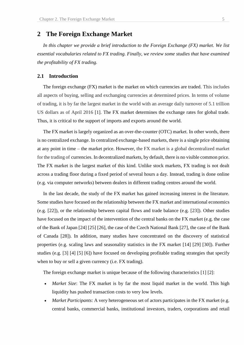
The foreign exchange market is unique because of the following characteristics [1] [2]:
Market Size: The FX market is by far the most liquid market in the world. This high
liquidity has pushed transaction costs to very low levels.
Market Participants: A very heterogeneous set of actors participates in the FX market (e.g.
central banks, commercial banks, institutional investors, traders, corporations and retail

Chapter 2. The Foreign Exchange Market 6
investors). These market participants, often, do not share the same interests when trading
currencies.
Global Decentralized Market: There is no specific physical centre to exchange currencies.
This chapter continues as follows: we list and explain some essential terminologies related to
FX trading in Section 2.2. In Section 2.3 we review some studies those have examined how
profitable the FX trading could be.
2.2 Essential terminologies for FX trading
In this section we describe some essential vocabularies related to FX trading [31]:
Exchange Rate: In a typical foreign exchange transaction, a party purchases a quantity of
one currency by paying with a quantity of another currency. The exchange rate represents
the number of units of one currency that can be exchanged for a unit of another.
Currency Pair: A currency pair is the quotation and pricing structure of currencies traded
in the FX market. The value of a currency is known as a ‘rate’ and is determined by its
comparison to another currency. For example, the currency pair quoted as ‘EUR/USD’
represents the number of US dollars that can be bought with one euro (see Fig. 2.1 for
example).
Fig. 2.1. A typical quote of the EUR/USD currency pair. The bid price is 1.08691, the ask price is 1.08703.
Base and Counter Currency: For a given currency pair (e.g. EUR/USD in Fig. 2.1), the
first listed currency of a currency pair (i.e. EUR) is called the base currency, and the second
currency (i.e. USD) is called the counter currency. The currency pair indicates how much
of the counter currency is needed to purchase one unit of the base currency. The counter
currency is also referred to as the quoted currency.
Bid, Ask, and Mid-price: The bid price represents how much of the counter currency you
need in order to purchase one unit of the base currency. The ask price for the currency pair
represents how much you will acquire of the counter currency for selling one unit of base
currency. For example, in Fig. 2.1 above the bid price of EUR/USD is 1.08691; while the
ask price is 1.08703. The mid-price is defined as the average of the bid and ask prices being
quoted. For example, in Fig. 2.1 the mid-price would be: (1.08691 + 1.08703) / 2 =
Chapter 2. The Foreign Exchange Market 7
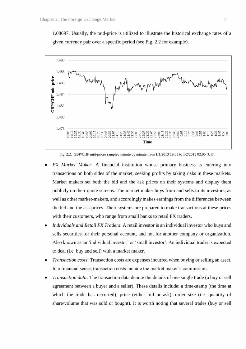
1.08697. Usually, the mid-price is utilized to illustrate the historical exchange rates of a
given currency pair over a specific period (see Fig. 2.2 for example).
Fig. 2.2. GBP/CHF mid-prices sampled minute by minute from 1/1/2013 19:05 to 1/2/2013 02:05 (UK).
FX Market Maker: A financial institution whose primary business is entering into
transactions on both sides of the market, seeking profits by taking risks in these markets.
Market makers set both the bid and the ask prices on their systems and display them
publicly on their quote screens. The market maker buys from and sells to its investors, as
well as other market-makers, and accordingly makes earnings from the differences between
the bid and the ask prices. Their systems are prepared to make transactions at these prices
with their customers, who range from small banks to retail FX traders.
Individuals and Retail FX Traders: A retail investor is an individual investor who buys and
sells securities for their personal account, and not for another company or organization.
Also known as an ‘individual investor’ or ‘small investor’. An individual trader is expected
to deal (i.e. buy and sell) with a market maker.
Transaction costs: Transaction costs are expenses incurred when buying or selling an asset.
In a financial sense, transaction costs include the market maker’s commission.
Transaction data: The transaction data denote the details of one single trade (a buy or sell
agreement between a buyer and a seller). These details include: a time-stamp (the time at
which the trade has occurred), price (either bid or ask), order size (i.e. quantity of
share/volume that was sold or bought). It is worth noting that several trades (buy or sell
1.478
1.480
1.482
1.484
1.486
1.488
1.490
19
:05
19
:15
19
:25
19
:35
19
:45
19
:55
20
:05
20
:15
20
:25
20
:35
20
:45
20
:55
21
:05
21
:15
21
:25
21
:35
21
:45
21
:55
22
:05
22
:15
22
:25
22
:35
22
:45
22
:55
23
:05
23
:15
23
:25
23
:35
23
:45
23
:55
0:0
5
0:1
5
0:2
5
0:3
5
0:4
5
0:5
5
1:0
5
1:1
5
1:2
5
1:3
5
1:4
5
1:5
5
2:0
5
GB
P/C
HF
mid
-pri
ce
Time

Chapter 2. The Foreign Exchange Market 8
orders) may occur within one second. Data gathered at the transaction level are usually
referred to as ‘high frequency data’.
2.3 About the profitability of FX trading
In this section we review those studies that have researched the profitability of FX trading.
tMost of these studies focus on a specific trading style named ‘technical trading’. Typically, a
technical trader tries to discover patterns in the historical price movements of a security using
technical indicators. Technical indicators are statistics used to measure current conditions, as well
as to forecast financial trends. Technical indicators are used to predict changes in market trends or
price patterns in any traded asset [32] [33]. Eventually, a technical trader establishes a trading
strategy (i.e. buy and sell rules) based on the discovered pattern(s). A Technical Trading Rule
(TTR) is an instruction that is based on technical indicators and indicates whether the security
displays a suitable behaviour to buy or to sell.
In 2013, Neely and Weller [34] studied the convenience of technical trading in the FX market.
They reported that technical trading can produce profit in the FX market, especially when applied
to emerging markets’ currencies (e.g. Latin America). They reported that technical trading on the
FX market can produce better returns in comparison to risk than it does in the S&P500. Their
results suggested that it would be better not to embrace fixed technical trading rules or fixed
portfolios of these rules, but rather to employ a strategy that switches between different rules and
currency pairs according to past performance. Finally, they reported that technical trading in the
FX market could generate profits even during financial crisis.
In 2016, Coakley, et al. [35] provided an empirical investigation of the profitability of more
than 100,000 technical trading rules (TTR) in the FX market for 22 currency pairs. They reported
that technical trading can achieve annualised returns of up to 30%.
In 2016, Hsu et al. [36] carried out an investigation of more than 20,000 technical trading rules
(TTR) in the foreign exchange market, using daily data sampled over 45 years for 30 developed
and emerging market currencies. They reported that technical trading can generate attractive
returns. Moreover, they concluded that these returns are not, in general, wiped out when realistic
allowance is made for transaction costs; which confirms the findings of other studies (e.g. [3] [36]
[37]).
In 2017, Zarrabi et al. [3] examined the profitability of technical trading rules (TTR) in the
foreign exchange market, taking into account transaction costs. They considered a universe of
Chapter 2. The Foreign Exchange Market 9
7,650 trading rules and six currencies: SEK, CHF, GBP, NOK, JPY and CAD. The findings
indicated that technical trading could generate positive returns even during financial crisis (e.g.
between January 2007 and December 2009). In addition, their results suggested that, rather than
sticking to a specific set of TTRs, investors should update their portfolios frequently in order to
adapt to changes in the economy; thus confirming the findings of Neely and Weller [34]. They also
reported that technical trading can still achieve an attractive level of risk-adjusted return after
taking into account transaction costs; which conforms to the deduction of Hsu et al., [36].
In 2016, Davison [38] examined the profitability of retail traders in the FX market. He
considered the quarterly data collected from 19 US market makers and aggregated by the on-line
website Finance Magnates (Finance Magnates [39]) during the period 1/10/2010 to 31/3/2014. He
reported that, on average, 20% of the retail traders ended up with profitable accounts, which
concurs with the results of Heimer and Simon [40]. Davison [38] concluded that around 40% of the
remaining retail traders might have expected their accounts to be subject to a margin calla. He also
reported that there was no conclusive evidence that the success of the profitable retail traders was
due to their knowledge or skills edge.
So, the studies conducted in [3] [35] [36] examined the profitability of thousands of technical
trading rules (TTRs). They concluded that many TTRs can generate profits in the FX market.
However, Davison [38] reported that, on average, only 20% of retail traders do, in reality, make a
profit. A possible reason for the inconsistency of these conclusions could be that it is not easy for
most retail traders to examine several thousands of TTRs, to examine the profitability of certain
trading rules, before starting trading with real money. Besides, some studies (e.g. [34] [3]) reported
that, in order to make consistent profits using TTRs, traders must update their TTRs often to adjust
to the variations in the market, rather than sticking to a particular set of TTRs. This necessity to
update TTRs continuously makes FX trading harder for retail traders.
2.4 Summary
The FX market is the market on which currencies are traded. It comprises a wide range of
heterogeneous participants (e.g. central banks, retail investors). In Section 2.2, we described some
essential terminologies related to FX trading (e.g. base and counter currencies, mid-price rate). We
also reviewed the studies (e.g. [3] [35] [36]) that highlighted the profitability of FX trading (Section
a A margin call occurs when the account value falls below the broker's required minimum value. Simply put, this is the edge at
which the market maker decides that a trader does not have sufficient capital to continue trading.

Chapter 2. The Foreign Exchange Market 10
2.3). Some studies (e.g. [3] [36]) concluded that FX trading can be attractively profitable even after
taking into account the transaction costs. However, other studies (e.g. [38]) warned that, in reality,
most retail traders do not make the profits they might have expected.
Chapter 3. Trading Strategies for Financial Markets 11
3 Trading Strategies for Financial Markets
In this chapter, we review some of the existing trading strategies and list selected evaluation
metrics to assess the performance of a trading strategy.
3.1 Introduction
A trading strategy is a set of objective ‘trading rules’. Trading rules are the conditions that must
be met to initiate a buy or sell order. In this chapter we review previous research into existing
trading strategies. In general, these trading strategies can be classified into two categories:
1. The first consists of strategies that aim, firstly, to forecast market prices or changes in a
trend’s direction and, secondly, to create trading strategies based on the established
forecasting model. The trading strategies in this category usually employ machine learning
models to predict market prices or a trend’s direction. They then employ these forecasting
models to decide when to initiate buy or sell orders.
2. The second category embraces trading models that do not rely on any forecasting model.
We want to highlight that in this chapter we review those studies not based on the directional
changes framework [10] and therefore, provide only a brief review for each study. This chapter
continues as follows: we review trading strategies from the first and second categories outlined in
Sections 3.2 and 3.3 respectively. In Section 3.4 we list and explain essential evaluation metrics
that aim to measure the performance of a given trading strategy. We conclude with Section 3.5.
3.2 The first category: Trading strategies based on forecasting models
As stated, this section considers trading strategies that are not based on the DC framework.
Instead of providing an extensive literature review, our objective is, rather, to provide general
examples as to the approaches currently prevailing for the development of trading strategies.
Strategies that are based on the DC framework will be revised in Chapter 4.
Generally, trading strategies based on forecasting models try to forecast the prices or the
direction of a financial market’s trend before then building trading strategies upon the established
forecasting model. The following outlines some trading strategies belonging to this category:
In 2009, Li et al. [41] proposed a framework for predicting turning points. The proposed model
combined chaotic dynamic analysis with an Ensemble Artificial Neural Network (EANN) model.
The sought objective was to capture the non-linear and chaotic behaviour of the financial market
in order to forecast potential turning points. A Genetic Algorithm (GA) module was then added to
Chapter 3. Trading Strategies for Financial Markets 12
optimize predefined trading parameters to maximize the produced profit of the proposed trading
strategy. They applied their forecasting, and trading, strategy to the Dow Jones Industrial Average
(DJIA) index time series and TESCO stock (UK). Experimental results suggested that applying
the proposed trading strategy to the TESCO stock (UK) could produce an annualized return of
69.78%.
In 2012, Huang et al. [42] proposed a methodology for stock selection using Support Vector
Regression (SVR) and a Genetic Algorithm (GA). They used an SVR model to predict, and classify,
the profitability of stocks. This classification process included the usage of fundamental stock
criteria (e.g. share price rationality, growth, profitability, liquidity). The stocks classified as ‘most
profitable’ were then employed to form a portfolio. On top of this model, a GA was employed for
the optimization of the trading model’s parameters. The reported experiment consisted of building
a portfolio using 30 stocks. Experimental results suggested that, in the best case, the proposed
trading system could produce an annualized return of 17.57%.
In 2013, Evans et al., [6] introduced a prediction and decision making model based on Artificial
Neural Networks (ANN) and Genetic Algorithms (GA) to predict the changes in a market’s trend
direction. The dataset utilized for this research comprised 70 weeks of historical exchange rates of
GBP/USD, EUR/GBP, and EUR/USD currency pairs. They reported that the proposed trading
strategy could produce an annualized return of 23.3%.
In 2015, Giacomel et al. [43] proposed an ANN model to predict the direction of price
movements. They actually proposed two ANN models: the first one trained to predict the expected
opening and closing values for the next period; whereas the second was trained to predict the stock
direction in the next period. These two ANN models were combined to form a trading strategy.
The proposed model was tested using 18 stocks selected from the North American and the
Brazilian stock markets. Experimental results suggested that the proposed trading strategy could
yield an annualized return of up to 76%.
In 2016, Chourmouziadis and Chatzoglou [44] presented a trading fuzzy system. They used a
mixture of four technical indicators to predict stock prices. Two of these indicators are very rarely
used in research papers, namely Parabolic SAR and GANN-HiLo. They presented 16 fuzzy rules
in total, based on these four technical indicators. The fuzzy system assigned a weight to each rule
based on its profitability during the training (in-sample) period. The experiments were conducted
using daily data from the Athens Stock Exchange over a period of more than 15 years. This data
was divided into bull and bear market periods. The results suggested that the proposed system
Chapter 3. Trading Strategies for Financial Markets 13
produced fewer losses during bear market periods and smaller gains during bull market periods
compared with the buy and holdb strategy.
In 2016, Chen and Chen [45] proposed an intelligent pattern recognition model to predict the
turning point of an upwards trend (i.e. the bullish turning point). The proposed model used nine
technical indicators as pattern recognition factors for recognizing stock pattern. They employed
the rough sets theory and genetic algorithms for forecasting the bullish turning point. Then, the
authors established a trading strategy based on the proposed forecasting model. In the model
verification, they evaluated the proposed model in two stock databases (TAIEX and NASDAQ).
They reported that the proposed trading strategy could generate on average an annualized return
of 57%.
In 2016, Göçken et al. [46] presented a model to predict stock prices on the Istanbul Stock
Exchange. The proposed model employed a hybrid Artificial Neural Network where the inputs
were technical indicators chosen via a model that combined Harmony Search (HS) and Genetic
Algorithm (GA). They established a trading strategy based on the proposed forecasting model and
applied the proposed trading strategy to Turkey’s stock index BIST 100. They reported a positive
return of 6.04% during 160 trading days.
Finally, we should note that in spite of the fact that forecasting financial time series has proven
a very attractive objective, many studies (e.g. [47] [48] [49] [50] [51]) have not supported their
forecasting model with any trading strategy. The establishment of a trading strategy is important
in order to give some empirical guarantee that the proposed forecasting method can be used in a
real-world situation [21] [52].
3.3 The second category: Trading strategies with no embedded forecasting models
This category encompasses a variety of trading styles that do not rely on any forecasting model.
In this section we provide three examples of trading styles that fall under this category, namely:
technical trading, momentum strategy and carry trade. Keep in mind that a detailed review of these
trading styles is out of the scope of this thesis as they are not based on the DC framework.
b Buy and hold is an investment strategy in which an investor buys stocks and holds them for a long period of time (a
month or years), regardless of fluctuations in the market. The principle of this strategy is based on the view that in the
long run financial markets give a good rate of return to investors.
Chapter 3. Trading Strategies for Financial Markets 14
3.3.1 Technical trading
The first trading style we consider is ‘technical trading’. Typically, a technical trader analyses
price charts to develop theories as to what direction the market is likely to move. This sort of
analysis employs a large set of technical indicators. Technical indicators look to predict future
price levels, or simply the general price direction, of a security by looking at past patterns.
Eventually, the discovery of such pattern(s) can help in establishing trading strategies (i.e. buy and
sell rules). Examples of traditional technical indicators include: Moving Average Convergence
Divergence; Average Directional Index; Relative Strength Index; Stochastic Oscillator; and
Bollinger Bands [32] [33]. Developing trading strategies based on technical indicators is very
common in the literature (e.g. [53] [54] [55] [56]). In this section we outline some technical trading
strategies.
In 2009, Watson [57] established a new approach to studying the profitability of two technical
indicators, namely: head and shoulders and point and figure. He applied his approach to daily data
of 4,983 stocks traded on the London Stock Exchange sampled from January 1st 1980 to December
31st 2003. He concluded that the head and shoulders pattern generated a mean excess return of 5.5%
on an annual basis. He also concluded that point and figure was particularly suited to the intra-day
traderc.
In 2009, Schulmeister [54] examined the profitability of 2,580 technical trading rules (TTR).
He reported that the profitability of these TTRs has steadily declined since 1960, and has been
unprofitable since the early 1990s when using daily data. However, when based on 30-minute-data
the same TTRs produce an average return of 7.2% per year. He reported that technical trading can
be particularly profitable for intra-day trading.
In 2015, Cervelló-Royo at al. [58] proposed a risk-adjusted technical trading rule. They
proposed a modified version of a technical indicator named ‘flag pattern’ that aims to “strengthen
the robustness of the flag pattern and its use in the design of the trading rule” [58]. They generated
96 different configurations of trading rules and applied these trading rules to three indexes: the US
Dow Jones (DJIA), the German DAX and the British FTSE. Experimental results suggest that the
trading rules were able to produce returns of up to 94.9% in the period from November 26th 2004
to February 27th 2007.
c The name “intra-day trader” refers to a trader who opens and closes a position in a security in the same trading day.
Chapter 3. Trading Strategies for Financial Markets 15
3.3.2 Momentum strategy
The second considered trading style, which does not depend on any trading model, is
‘Momentum strategy’. In general terms, a momentum strategy consists of buying assets with high
recent returns and selling assets with low recent returns.
In 2011, a study by the Monetary and Economic Department at the Bank of International
Settlement (BIS) [7] provided a broad empirical investigation concerning the profitability of
momentum strategies in the FX market. The authors found that momentum portfolios are
significantly skewed towards minor currencies (i.e. currencies that are not actively traded in the
FX markets) that have relatively high transaction costs (sometimes these transactions are estimated
as high as 50% of momentum returns). They also argued that momentum strategies may deliver
higher returns in the FX markets than in stock markets.
In 2013, Daryl et al. [59] proposed a momentum strategy that embedded a security selection
approach based on a new risk-return ratio criterion. They sought to create portfolios based on the
introduced risk-return ratio criterion. They applied their model to the stock market index of South
Korea (KOSPI 200) over the period June 2006 to June 2012. They reported that the proposed
momentum strategy did produce attractive positive returns.
3.3.3 Carry trade
The carry trade is a strategy in which traders borrow a currency that has a low interest rate and
use the funds to buy a different currency that is paying a higher interest rate. The FX carry trade is
of major practical relevance since it represents an important investment style implemented by FX
managers [60].
In 2011, Bertolini [8] examined the profitability of several carry portfolio strategies. He
analysed whether different asset allocation, market-timing and money management methodologies
had the potential to improve the performance of a simple carry portfolio. The experiments were
directed using datasets from the G10 currency universed in the period 1st January 1999 to 5th March
2010. He considered various FX carry portfolio strategies and found that the best performance was
achieved by ranking the currencies according to the yields with the shortest maturity (i.e. 1-week
yields).
In 2014, Laborda et al., [61] proposed an asset allocation strategy that aimed to improve the
performance of the currency carry trade, where currencies were selected from the G10 currency
d For more information about G10, see http://www.investopedia.com/terms/g/groupoften.asp.

Chapter 3. Trading Strategies for Financial Markets 16
universe. The proposed model assigned weights dynamically for long and short positions in a carry
trade portfolio. These weights were determined by a combination of financial variables that
reflected variations in macroeconomic conditions, as well as the likelihood of crash risk across
periods. They reported that the proposed asset allocation strategy produced markedly more returns
than a naive currency carry trade during the out-of-sample period between January 2009 and
February 2012.
3.4 Evaluating the performance of a trading strategy
A trading strategy can be analysed on historical data to project the future performance of the
strategy. This process is known as ‘backtesting’. Backtesting is accomplished by reconstructing,
with historical data, trades that would have occurred in the past using the rules defined by a given
strategy. The result of backtesting offers statistics that can be utilized to gauge the effectiveness of
the strategy. Using a rule-based trading strategy has some benefits:
It helps remove human emotion from decision making.
Models can be easily backtested on historical data to check their worth before taking the
risk with real money.
There exist many metrics that attempt to evaluate the performance of a given trading strategy.
In this thesis, we choose the following metrics to measure the performance of our planned trading
strategies. These metrics have been reported as appropriate for a decent assessment ( [52] [62]).
Rates of return: The rate of return (RR) symbolizes the bottom line for a trading system over
a definite period of time. Total Profit (TP) represents the profitability of total trades. TP is
computed by removing the sum of all losing trades from the sum of all winning trades (3.1).
TP can be negative when the loss is greater than the gain. We denote by RR (3.2) the gain
or loss on an investment over a given evaluation period expressed as a percentage of the
amount invested. In (3.2) INV denote the initial capital employed in investment.
𝑇𝑃 = sum of all profits − sum of all losses (3.1)
𝑅𝑅 =𝑇𝑃
𝐼𝑁𝑉× 100
(3.2)
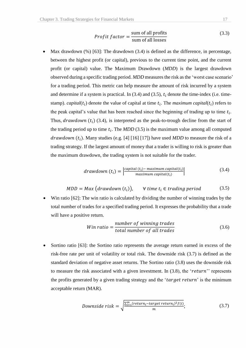
Profit factor [62]: The profit factor is defined as the sum of profits of all profitable trades
divided by the sum of losses of all losing trades for the entire trading period. This metric
measures the amount of profit per unit of risk, with values greater than one signifying a
profitable system.
Chapter 3. Trading Strategies for Financial Markets 17
𝑃𝑟𝑜𝑓𝑖𝑡 𝑓𝑎𝑐𝑡𝑜𝑟 =sum of all profits
sum of all losses
(3.3)
Max drawdown (%) [63]: The drawdown (3.4) is defined as the difference, in percentage,
between the highest profit (or capital), previous to the current time point, and the current
profit (or capital) value. The Maximum Drawdown (MDD) is the largest drawdown
observed during a specific trading period. MDD measures the risk as the ‘worst case scenario’
for a trading period. This metric can help measure the amount of risk incurred by a system
and determine if a system is practical. In (3.4) and (3.5), 𝑡𝑖 denote the time-index (i.e. time-
stamp). capital(𝑡𝑖) denote the value of capital at time 𝑡𝑖. The maximum capital(𝑡𝑖) refers to
the peak capital’s value that has been reached since the beginning of trading up to time 𝑡𝑖.
Thus, 𝑑𝑟𝑎𝑤𝑑𝑜𝑤𝑛 (𝑡𝑖) (3.4), is interpreted as the peak-to-trough decline from the start of
the trading period up to time 𝑡𝑖. The MDD (3.5) is the maximum value among all computed
𝑑𝑟𝑎𝑤𝑑𝑜𝑤𝑛 (𝑡𝑖). Many studies (e.g. [4] [16] [17]) have used MDD to measure the risk of a
trading strategy. If the largest amount of money that a trader is willing to risk is greater than
the maximum drawdown, the trading system is not suitable for the trader.
𝑑𝑟𝑎𝑤𝑑𝑜𝑤𝑛 (𝑡𝑖) = |𝑐𝑎𝑝𝑖𝑡𝑎𝑙 (𝑡𝑖)− 𝑚𝑎𝑥𝑖𝑚𝑢𝑚 𝑐𝑎𝑝𝑖𝑡𝑎𝑙(𝑡𝑖)
𝑚𝑎𝑥𝑖𝑚𝑢𝑚 𝑐𝑎𝑝𝑖𝑡𝑎𝑙(𝑡𝑖)| (3.4)
𝑀𝐷𝐷 = 𝑀𝑎𝑥 (𝑑𝑟𝑎𝑤𝑑𝑜𝑤𝑛 (𝑡𝑖)), ∀ 𝑡𝑖𝑚𝑒 𝑡𝑖 ∈ 𝑡𝑟𝑎𝑑𝑖𝑛𝑔 𝑝𝑒𝑟𝑖𝑜𝑑 (3.5)
Win ratio [62]: The win ratio is calculated by dividing the number of winning trades by the
total number of trades for a specified trading period. It expresses the probability that a trade
will have a positive return.
𝑊𝑖𝑛 𝑟𝑎𝑡𝑖𝑜 =𝑛𝑢𝑚𝑏𝑒𝑟 𝑜𝑓 𝑤𝑖𝑛𝑛𝑖𝑛𝑔 𝑡𝑟𝑎𝑑𝑒𝑠
𝑡𝑜𝑡𝑎𝑙 𝑛𝑢𝑚𝑏𝑒𝑟 𝑜𝑓 𝑎𝑙𝑙 𝑡𝑟𝑎𝑑𝑒𝑠 (3.6)
Sortino ratio [63]: the Sortino ratio represents the average return earned in excess of the
risk-free rate per unit of volatility or total risk. The downside risk (3.7) is defined as the
standard deviation of negative asset returns. The Sortino ratio (3.8) uses the downside risk
to measure the risk associated with a given investment. In (3.8), the ‘𝑟𝑒𝑡𝑢𝑟𝑛’’ represents
the profits generated by a given trading strategy and the ‘𝑡𝑎𝑟𝑔𝑒𝑡 𝑟𝑒𝑡𝑢𝑟𝑛’ is the minimum
acceptable return (MAR).
𝐷𝑜𝑤𝑛𝑠𝑖𝑑𝑒 𝑟𝑖𝑠𝑘 = √∑ (𝑟𝑒𝑡𝑢𝑟𝑛𝑖−𝑡𝑎𝑟𝑔𝑒𝑡 𝑟𝑒𝑡𝑢𝑟𝑛𝑖)2𝑓(𝑖)𝑚
𝑖=1
𝑚; (3.7)
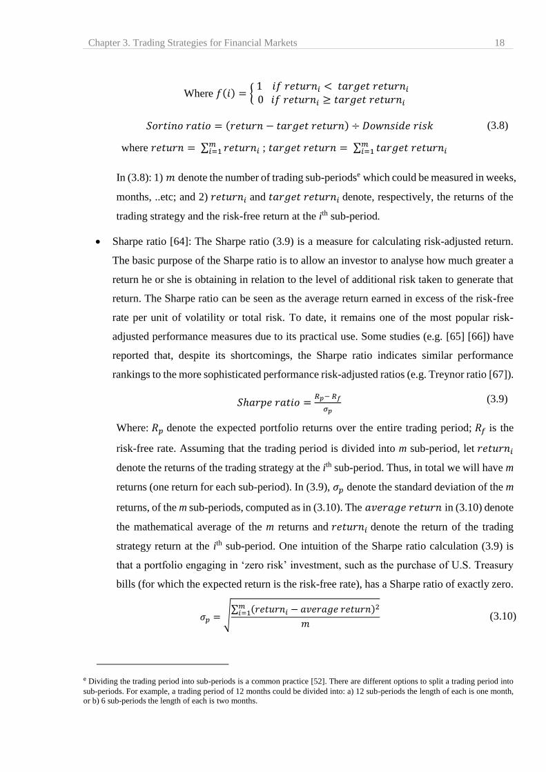
Chapter 3. Trading Strategies for Financial Markets 18
Where 𝑓(𝑖) = { 1 𝑖𝑓 𝑟𝑒𝑡𝑢𝑟𝑛𝑖 < 𝑡𝑎𝑟𝑔𝑒𝑡 𝑟𝑒𝑡𝑢𝑟𝑛𝑖
0 𝑖𝑓 𝑟𝑒𝑡𝑢𝑟𝑛𝑖 ≥ 𝑡𝑎𝑟𝑔𝑒𝑡 𝑟𝑒𝑡𝑢𝑟𝑛𝑖
𝑆𝑜𝑟𝑡𝑖𝑛𝑜 𝑟𝑎𝑡𝑖𝑜 = (𝑟𝑒𝑡𝑢𝑟𝑛 − 𝑡𝑎𝑟𝑔𝑒𝑡 𝑟𝑒𝑡𝑢𝑟𝑛) ÷ 𝐷𝑜𝑤𝑛𝑠𝑖𝑑𝑒 𝑟𝑖𝑠𝑘 (3.8)
where 𝑟𝑒𝑡𝑢𝑟𝑛 = ∑ 𝑟𝑒𝑡𝑢𝑟𝑛𝑖𝑚𝑖=1 ; 𝑡𝑎𝑟𝑔𝑒𝑡 𝑟𝑒𝑡𝑢𝑟𝑛 = ∑ 𝑡𝑎𝑟𝑔𝑒𝑡 𝑟𝑒𝑡𝑢𝑟𝑛𝑖
𝑚𝑖=1
In (3.8): 1) 𝑚 denote the number of trading sub-periodse which could be measured in weeks,
months, ..etc; and 2) 𝑟𝑒𝑡𝑢𝑟𝑛𝑖 and 𝑡𝑎𝑟𝑔𝑒𝑡 𝑟𝑒𝑡𝑢𝑟𝑛𝑖 denote, respectively, the returns of the
trading strategy and the risk-free return at the ith sub-period.
Sharpe ratio [64]: The Sharpe ratio (3.9) is a measure for calculating risk-adjusted return.
The basic purpose of the Sharpe ratio is to allow an investor to analyse how much greater a
return he or she is obtaining in relation to the level of additional risk taken to generate that
return. The Sharpe ratio can be seen as the average return earned in excess of the risk-free
rate per unit of volatility or total risk. To date, it remains one of the most popular risk-
adjusted performance measures due to its practical use. Some studies (e.g. [65] [66]) have
reported that, despite its shortcomings, the Sharpe ratio indicates similar performance
rankings to the more sophisticated performance risk-adjusted ratios (e.g. Treynor ratio [67]).
𝑆ℎ𝑎𝑟𝑝𝑒 𝑟𝑎𝑡𝑖𝑜 =𝑅𝑝− 𝑅𝑓
𝜎𝑝 (3.9)
Where: 𝑅𝑝 denote the expected portfolio returns over the entire trading period; 𝑅𝑓 is the
risk-free rate. Assuming that the trading period is divided into m sub-period, let 𝑟𝑒𝑡𝑢𝑟𝑛𝑖
denote the returns of the trading strategy at the ith sub-period. Thus, in total we will have m
returns (one return for each sub-period). In (3.9), 𝜎𝑝 denote the standard deviation of the m
returns, of the m sub-periods, computed as in (3.10). The 𝑎𝑣𝑒𝑟𝑎𝑔𝑒 𝑟𝑒𝑡𝑢𝑟𝑛 in (3.10) denote
the mathematical average of the m returns and 𝑟𝑒𝑡𝑢𝑟𝑛𝑖 denote the return of the trading
strategy return at the ith sub-period. One intuition of the Sharpe ratio calculation (3.9) is
that a portfolio engaging in ‘zero risk’ investment, such as the purchase of U.S. Treasury
bills (for which the expected return is the risk-free rate), has a Sharpe ratio of exactly zero.
𝜎𝑝 = √∑ (𝑟𝑒𝑡𝑢𝑟𝑛𝑖 − 𝑎𝑣𝑒𝑟𝑎𝑔𝑒 𝑟𝑒𝑡𝑢𝑟𝑛)2𝑚
𝑖=1
𝑚 (3.10)
e Dividing the trading period into sub-periods is a common practice [52]. There are different options to split a trading period into
sub-periods. For example, a trading period of 12 months could be divided into: a) 12 sub-periods the length of each is one month,
or b) 6 sub-periods the length of each is two months.

Chapter 3. Trading Strategies for Financial Markets 19
Beta [68]: Beta is a measure of the volatility, or systematic risk, of a security or a portfolio,
in comparison to a benchmark. Beta measures how the strategy responds to a benchmark.
A Beta of greater than 1 indicates that the security's price will be more volatile than the
considered benchmark. For example, if an asset’s Beta is 1.3, then it is theoretically 30%
more volatile than the benchmark. Essentially, Beta denote the vital trade-off between
reducing risk and maximizing return. Ruppert [69] reports that (3.11) gives the estimated
value of Beta (see equations (7.9) and (7.10), p. 230-231 [69]). Let 𝑚 denote the number
of sub-trading periods.
𝐵𝑒𝑡𝑎𝑝,𝑏 = ∑ (𝑅𝑏
𝑖 − �̅�𝑏)(𝑅𝑝𝑖 − �̅�𝑝) 𝑚
𝑖=1
∑(𝑅𝑏𝑖 − �̅�𝑏)
2 (3.11)
Where, 𝐵𝑒𝑡𝑎𝑝,𝑏 is the Beta of the portfolio 𝑝 computed with reference to a benchmark
𝑏. 𝑅𝑝𝑖 and 𝑅𝑏
𝑖 denote, respectively, the return of the portfolio and the benchmark over the
ith sub-trading periods. �̅�𝑝 and �̅�𝑏 are the average of the returns over the 𝑚 sub-periods of
the portfolio and the selected benchmark respectively.
Jensen’s Alpha [70]: Jensen’s Alpha is a measure of an investment's performance on a risk-
adjusted basis. Jensen’s Alpha (3.12) measures the trading return in excess of a security, or
portfolio of securities, over the theoretical expected return. For example, a positive Jensen’s
Alpha of 1.0 means the fund has outperformed its benchmark index by 1%. The Jensen’s
Alpha is computed as:
𝐽𝑒𝑛𝑠𝑒𝑛′𝑠 𝐴𝑙𝑝ℎ𝑎 = 𝑅𝑝 − 𝑅𝑓 − 𝐵𝑒𝑡𝑎𝑝,𝑏 × (𝑅𝑏 − 𝑅𝑓) (3.12)
Where, 𝑅𝑝is the total return of the portfolio, 𝑅𝑓 is the risk free rate, 𝑅𝑏 denote the return of
the selected benchmark, and 𝐵𝑒𝑡𝑎𝑝,𝑏 is computed as in (3.11).
All of these evaluation metrics will be used later in this thesis to evaluate the performance of our
proposed trading strategies as we shall describe in Chapters 6 and 7.
3.5 Summary
In this chapter, we briefly reviewed some of the existing trading strategies from the literature.
We identified two categories of trading strategies. The first category contains trading strategies
that employ forecasting models. Strategies under this category, usually, embed a machine learning,
or artificial intelligence, model to predict market prices or a trend’s direction (Section 3.2). The

Chapter 3. Trading Strategies for Financial Markets 20
second category consists of those strategies that do not rely on any forecasting model. Under this
category, we reviewed three trading styles, namely: technical trading, momentum strategy, and
carry trade (Section 3.3). None of the trading strategies reviewed in this chapter is based on the
directional changes framework.
In Section 3.4, we listed and explained selected evaluation metrics usually employed to evaluate
the performance of a given trading strategy. All of these metrics will be used later to assess the
performance of our intended trading strategies.
Chapter 4. The Directional Changes Framework 21
4 The Directional Changes Framework
Directional Changes (DC) is a framework for summarizing price movements. In this chapter,
we provide a detailed explanation of the concept of DC. We review several studies that have
concluded that the DC framework is useful in analysing the foreign exchange (FX) market. We
also review some existing trading strategies that are based on the DC framework. To conclude, we
clarify the difference between the DC concept and other similar notions.
4.1 Introduction
A common way to summarize raw data in the financial markets is to first choose a time interval,
and then sample raw data at fixed time points based on the chosen interval; for example, hourly,
daily or monthly. We call data summarized this way ‘interval-based summary’. Naturally, an
interval-based summary becomes a time series. A time series is a sequence of numerical data
observations recorded sequentially in time [71].
The Foreign Exchange (FX) market is open 24 hours a day. Trading activities in the FX market
can be affected by many factors. For instance, on the announcement of political or economic news,
there tends to be a sharp rise in market trading activity in response to the news. Similarly, during
weekends, trading activity has a tendency to decline [12]. Due to these fluctuations, an interval-
based summary may not appropriately capture irregularity in traders’ activities. This raises an
essential need to come up with a time-framework that, adequately, captures significant price
movements in financial time series beyond the notion of the interval-based summary. This need is
particularly important for the analysis of high-frequency data [72].
The concept of ‘intrinsic time’ is an approach to studying financial time series [73]. Intrinsic
time is defined by events. In this context, events are price movements considered as vital by the
observer. The objective of using the event-based approach to summarize a time series is to
eliminate irrelevant details of price evolution. Although there are many ways of defining events,
in this thesis, we consider a specific type of event named Directional Change (or DC for short)
which was established by Guillaume et al., [9].
This chapter continues as follows: in Section 4.2, we provide a detailed explanation of how the
DC concept summarizes a market’s activities (as explained in Guillaume et al., [9]; Ao and Tsang
[10]). In Section 4.3 we discuss those studies that have examined the DC framework’s usefulness
in analyzing the FX market. We review some existing DC-based trading strategies in Section 4.4.

Chapter 4. The Directional Changes Framework 22
In Section 4.5, we clarify the difference between the concept of the Directional Changes framework,
adopted in this thesis, and other similar notions. We conclude with Section 4.6.
4.2 Directional Changes
4.2.1 The basic concept
In this section, we explain how market prices are summarized based on the DC concept.
Directional changes (DC) is an approach to summarizing price changes. Under the DC framework,
the market is represented as alternating uptrends and downtrends. The basic idea is that the
magnitude of price change during an uptrend, or a downtrend, must be at least equal to a specific
threshold 𝑡ℎ𝑒𝑡𝑎 . Here, 𝑡ℎ𝑒𝑡𝑎 is a percentage that the observer considers substantial (usually
expressed as a percentage). For example, Fig. 4.1, shown below, depicts a price’s drop between
points A and A0.1. This price drop is equal to the selected, hypothetical, threshold of 0.1%. In this
case, we say that we have a DC downtrend that starts at point A. Any price change less than the
identified threshold, 𝑡ℎ𝑒𝑡𝑎, will not be considered as a trend when summarizing price movements
[9] [10].
Fig. 4.1. The black line indicates GBP/CHF mid-prices sampled minute by minute from 1/1/2013 19:05:00 to
1/2/2013 02:05:00 (UK). The red line exemplifies what is a DC downtrend looks like.
Under the DC framework, each uptrend is followed by a downtrend and vice versa. The
detection of a new uptrend, or downtrend, is a crucial task. The detection of a new downtrend, or
uptrend, is a two-steps algorithmic approach:
1.478
1.480
1.482
1.484
1.486
1.488
1.490
19
:05
19
:15
19
:25
19
:35
19
:45
19
:55
20
:05
20
:15
20
:25
20
:35
20
:45
20
:55
21
:05
21
:15
21
:25
21
:35
21
:45
21
:55
22
:05
22
:15
22
:25
22
:35
22
:45
22
:55
23
:05
23
:15
23
:25
23
:35
23
:45
23
:55
0:0
5
0:1
5
0:2
5
0:3
5
0:4
5
0:5
5
1:0
5
1:1
5
1:2
5
1:3
5
1:4
5
1:5
5
2:0
5
GB
P/C
HF
ra
te
Time
A0.1
A
0.1%
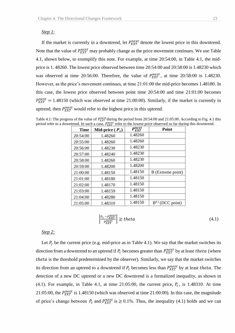
Chapter 4. The Directional Changes Framework 23
Step 1:
If the market is currently in a downtrend, let 𝑃𝐸𝑋𝑇𝑛𝑒𝑥𝑡 denote the lowest price in this downtrend.
Note that the value of 𝑃𝐸𝑋𝑇𝑛𝑒𝑥𝑡 may probably change as the price movement continues. We use Table
4.1, shown below, to exemplify this note. For example, at time 20:54:00, in Table 4.1, the mid-
price is 1. 48260. The lowest price observed between time 20:54:00 and 20:58:00 is 1.48230 which
was observed at time 20:56:00. Therefore, the value of 𝑃𝐸𝑋𝑇𝑛𝑒𝑥𝑡 , at time 20:58:00 is 1.48230.
However, as the price’s movement continues, at time 21:01:00 the mid-price becomes 1.48180. In
this case, the lowest price observed between point time 20:54:00 and time 21:01:00 becomes
𝑃𝐸𝑋𝑇𝑛𝑒𝑥𝑡 = 1.48150 (which was observed at time 21:00:00). Similarly, if the market is currently in
uptrend, then 𝑃𝐸𝑋𝑇𝑛𝑒𝑥𝑡 would refer to the highest price in this uptrend.
Table 4.1: The progress of the value of 𝑃𝐸𝑋𝑇𝑛𝑒𝑥𝑡during the period from 20:54:00 and 21:05:00. According to Fig. 4.1 this
period refer to a downtrend. In such a case, 𝑃𝐸𝑋𝑇𝑛𝑒𝑥𝑡 refer to the lowest price observed so far during this downtrend.
Time Mid-price ( 𝑷𝒄) 𝑷𝑬𝑿𝑻𝒏𝒆𝒙𝒕 Point
20:54:00 1.48260 1.48260
20:55:00 1.48260 1.48260
20:56:00 1.48230 1.48230
20:57:00 1.48240 1.48230
20:58:00 1.48260 1.48230
20:59:00 1.48200 1.48200
21:00:00 1.48150 1.48150 B (Extreme point)
21:01:00 1.48180 1.48150
21:02:00 1.48170 1.48150
21:03:00 1.48159 1.48150
21:04:00 1.48280 1.48150
21:05:00 1.48310 1.48150 B0.1 (DCC point)
|𝑃𝑐 −𝑃𝐸𝑋𝑇
𝑛𝑒𝑥𝑡
𝑃𝐸𝑋𝑇𝑛𝑒𝑥𝑡 | ≥ 𝑡ℎ𝑒𝑡𝑎 (4.1)
Step 2:
Let 𝑃𝑐 be the current price (e.g. mid-price as in Table 4.1). We say that the market switches its
direction from a downtrend to an uptrend if 𝑃𝑐 becomes greater than 𝑃𝐸𝑋𝑇𝑛𝑒𝑥𝑡 by at least 𝑡ℎ𝑒𝑡𝑎 (where
𝑡ℎ𝑒𝑡𝑎 is the threshold predetermined by the observer). Similarly, we say that the market switches
its direction from an uptrend to a downtrend if 𝑃𝑐 becomes less than 𝑃𝐸𝑋𝑇𝑛𝑒𝑥𝑡 by at least 𝑡ℎ𝑒𝑡𝑎. The
detection of a new DC uptrend or a new DC downtrend is a formalized inequality, as shown in
(4.1). For example, in Table 4.1, at time 21:05:00, the current price, 𝑃𝑐 , is 1.48310. At time
21:05:00, the 𝑃𝐸𝑋𝑇𝑛𝑒𝑥𝑡 is 1.48150 (which was observed at time 21:00:00). In this case, the magnitude
of price’s change between 𝑃𝑐 and 𝑃𝐸𝑋𝑇𝑛𝑒𝑥𝑡 is ≥ 0.1%. Thus, the inequality (4.1) holds and we can

Chapter 4. The Directional Changes Framework 24
confirm the observation of a new DC uptrend. In other words, at time 21:05:00, we can confirm
the observation of a new DC uptrend which has started at time 21:00:00. If the inequality (4.1)
holds, then the time at which the market traded at 𝑃𝐸𝑋𝑇𝑛𝑒𝑥𝑡 is called an ‘extreme point’ (e.g. point B
in Table 4.1) and the time at which the market trades at 𝑃𝑐 is called a DC confirmation point, or
DCC point for short point’ (e.g. point B0.1 in Table 4.1). By definition, the extreme point of an
uptrend has the lowest price amongst all points of current uptrend and the immediately preceding
downtrend. Similarly, the extreme point of a downtrend has the highest price amongst all points of
current downtrend and the immediately preceding uptrend.
Fig. 4.2 shown below illustrates the identification of extreme and DCC points. In Fig. 4.2, points
A, B, C, D, E, F and G are the ‘extreme points’. Whereas, points A0.1, B0.1, C0.1, D0.1, E0.1, F0.1, and
G0.1 are the ‘DCC points’. An extreme point can be seen as a local minima (e.g. point D in Fig.
4.2) or a local maxima (e.g. point C in Fig. 4.2). An extreme point is only recognized in hindsight;
precisely at the DCC point (i.e. when the inequality (4.1) becomes true). For example, in Fig. 4.2,
at point A0.1 we confirm that point A is an extreme point. Similarly, in Fig. 4.2, at point D0.1 we
confirm that point D is an extreme point. We denote by ‘price extreme’ (𝑃𝐸𝑋𝑇) the price at which
a trend starts. Eventually, when (4.1) holds, i.e. when a new DC trend is recognized (either uptrend
or downtrend), the 𝑃𝐸𝑋𝑇𝑛𝑒𝑥𝑡 becomes the 𝑃𝐸𝑋𝑇 of this new DC trend.
Fig. 4.2. An example of a DC-based summary of the price series shown in Fig. 4.1. Threshold 𝑡ℎ𝑒𝑡𝑎 = 0.1%. The
black line indicates GBP/CHF mid-prices sampled minute by minute. Solid red lines represent DC events. Dashed red
lines represent OS events. Each of the points A, B, C, D, E, F, and G is an extreme point. Each of the points A0.1, B0.1,
C0.1, D0.1, E0.1, F0.1, and G0.1 is a DC confirmation point (DCC point).
1.478
1.480
1.482
1.484
1.486
1.488
1.490
19
:05
19
:15
19
:25
19
:35
19
:45
19
:55
20
:05
20
:15
20
:25
20
:35
20
:45
20
:55
21
:05
21
:15
21
:25
21
:35
21
:45
21
:55
22
:05
22
:15
22
:25
22
:35
22
:45
22
:55
23
:05
23
:15
23
:25
23
:35
23
:45
23
:55
0:0
5
0:1
5
0:2
5
0:3
5
0:4
5
0:5
5
1:0
5
1:1
5
1:2
5
1:3
5
1:4
5
1:5
5
2:0
5
GB
P/C
HF
ra
te
Time
GBP/CHF
DC summary. theta = 0.1%
DC event
B
C
D
E
F
G A0.1
B0.1
C0.1
D0.1 E0.1
F0.1
G0.1
OS event
A
0.1% C
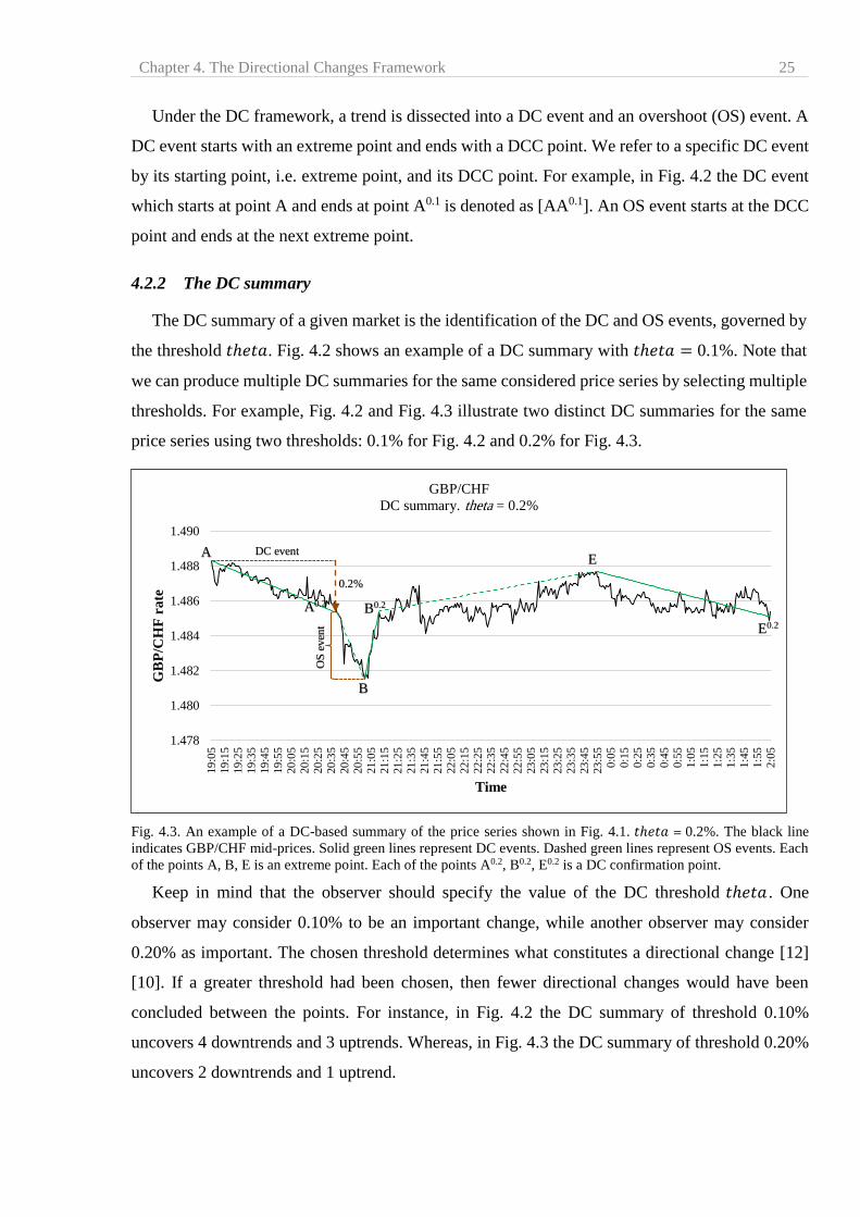
Chapter 4. The Directional Changes Framework 25
Under the DC framework, a trend is dissected into a DC event and an overshoot (OS) event. A
DC event starts with an extreme point and ends with a DCC point. We refer to a specific DC event
by its starting point, i.e. extreme point, and its DCC point. For example, in Fig. 4.2 the DC event
which starts at point A and ends at point A0.1 is denoted as [AA0.1]. An OS event starts at the DCC
point and ends at the next extreme point.
4.2.2 The DC summary
The DC summary of a given market is the identification of the DC and OS events, governed by
the threshold 𝑡ℎ𝑒𝑡𝑎. Fig. 4.2 shows an example of a DC summary with 𝑡ℎ𝑒𝑡𝑎 = 0.1%. Note that
we can produce multiple DC summaries for the same considered price series by selecting multiple
thresholds. For example, Fig. 4.2 and Fig. 4.3 illustrate two distinct DC summaries for the same
price series using two thresholds: 0.1% for Fig. 4.2 and 0.2% for Fig. 4.3.
Fig. 4.3. An example of a DC-based summary of the price series shown in Fig. 4.1. 𝑡ℎ𝑒𝑡𝑎 = 0.2%. The black line
indicates GBP/CHF mid-prices. Solid green lines represent DC events. Dashed green lines represent OS events. Each
of the points A, B, E is an extreme point. Each of the points A0.2, B0.2, E0.2 is a DC confirmation point.
Keep in mind that the observer should specify the value of the DC threshold 𝑡ℎ𝑒𝑡𝑎 . One
observer may consider 0.10% to be an important change, while another observer may consider
0.20% as important. The chosen threshold determines what constitutes a directional change [12]
[10]. If a greater threshold had been chosen, then fewer directional changes would have been
concluded between the points. For instance, in Fig. 4.2 the DC summary of threshold 0.10%
uncovers 4 downtrends and 3 uptrends. Whereas, in Fig. 4.3 the DC summary of threshold 0.20%
uncovers 2 downtrends and 1 uptrend.
1.478
1.480
1.482
1.484
1.486
1.488
1.490
19
:05
19
:15
19
:25
19
:35
19
:45
19
:55
20
:05
20
:15
20
:25
20
:35
20
:45
20
:55
21
:05
21
:15
21
:25
21
:35
21
:45
21
:55
22
:05
22
:15
22
:25
22
:35
22
:45
22
:55
23
:05
23
:15
23
:25
23
:35
23
:45
23
:55
0:0
5
0:1
5
0:2
5
0:3
5
0:4
5
0:5
5
1:0
5
1:1
5
1:2
5
1:3
5
1:4
5
1:5
5
2:0
5
GB
P/C
HF
ra
te
Time
GBP/CHF
DC summary. theta = 0.2%
A
A0.2
B
B0.2
E
E0.2
OS
even
t
DC event
0.2%
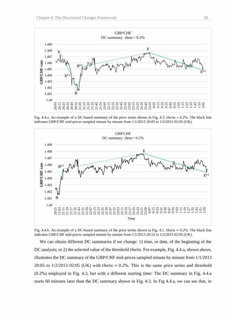
Chapter 4. The Directional Changes Framework 26
Fig. 4.4.a. An example of a DC-based summary of the price series shown in Fig. 4.3. 𝑡ℎ𝑒𝑡𝑎 = 0.2%. The black line
indicates GBP/CHF mid-prices sampled minute by minute from 1/1/2013 20:05 to 1/2/2013 02:05 (UK).
Fig. 4.4.b. An example of a DC-based summary of the price series shown in Fig. 4.1. 𝑡ℎ𝑒𝑡𝑎 = 0.2%. The black line
indicates GBP/CHF mid-prices sampled minute by minute from 1/1/2013 20:55 to 1/2/2013 02:05 (UK).
We can obtain different DC summaries if we change: 1) time, or date, of the beginning of the
DC analysis; or 2) the selected value of the threshold 𝑡ℎ𝑒𝑡𝑎. For example, Fig. 4.4.a, shown above,
illustrates the DC summary of the GBP/CHF mid-prices sampled minute by minute from 1/1/2013
20:05 to 1/2/2013 02:05 (UK) with 𝑡ℎ𝑒𝑡𝑎 = 0.2%. This is the same price series and threshold
(0.2%) employed in Fig. 4.3, but with a different starting time: The DC summary in Fig. 4.4.a
starts 60 minutes later than the DC summary shown in Fig. 4.3. In Fig 4.4.a, we can see that, in
1.48
1.481
1.482
1.483
1.484
1.485
1.486
1.487
1.488
1.489
20:0
5
20:1
5
20:2
5
20:3
5
20:4
5
20:5
5
21:0
5
21:1
5
21:2
5
21:3
5
21:4
5
21:5
5
22:0
5
22:1
5
22:2
5
22:3
5
22:4
5
22:5
5
23:0
5
23:1
5
23:2
5
23:3
5
23:4
5
23:5
5
0:0
5
0:1
5
0:2
5
0:3
5
0:4
5
0:5
5
1:0
5
1:1
5
1:2
5
1:3
5
1:4
5
1:5
5
2:0
5
GB
P/C
HF
ra
te
GBP/CHF
DC summary. theta = 0.2%
1.48
1.481
1.482
1.483
1.484
1.485
1.486
1.487
1.488
1.489
20:5
5
21:0
3
21:1
1
21:1
9
21:2
7
21:3
5
21:4
3
21:5
1
21:5
9
22:0
7
22:1
5
22:2
3
22:3
1
22:3
9
22:4
7
22:5
5
23:0
3
23:1
1
23:1
9
23:2
7
23:3
5
23:4
3
23:5
1
23:5
9
0:0
7
0:1
5
0:2
3
0:3
1
0:3
9
0:4
7
0:5
5
1:0
3
1:1
1
1:1
9
1:2
7
1:3
5
1:4
3
1:5
1
1:5
9
GB
P/C
HF
ra
te
Time
GBP/CHF
DC summary. theta = 0.2%
B0.2
B
E
E0.2
X0.2
X
B0.2
B
E
E0.2
Chapter 4. The Directional Changes Framework 27
this case, the first confirmed DC event is [XX0.2] (and not [AA0.2] anymore). The new extreme
point ‘X’ is observed at time 20:17 and the new DCC point, X0.2, is confirmed at time 20:45.
Fig. 4.4.b, shown above, provides another example of how the DC summary may differ if we
select a different starting time-point. In this case, we can see that the first confirmed DC event is
[BB0.2] which is an uptrend. In Fig. 4.4.b, the DC events [AA0.2] (observed in Fig. 4.3) and [XX0.2]
(observed in Fig. 4.4.a) cannot be recognized anymore.
4.2.3 DC notations
In this section, we introduce some DC-based notations that will help in clarifying our
forecasting and trading models later in this thesis:
- 𝑃𝑐: Denote the current price.
- 𝑃𝐸𝑋𝑇: Is the price at an extreme point. This is the price at which a trend starts; i.e. a local
minima or local maxima. In the case of a downtrend, 𝑃𝐸𝑋𝑇 will refer to the highest price in
this downtrend. In the case of an uptrend, 𝑃𝐸𝑋𝑇 will refer to the lowest price in this uptrend.
- 𝑃𝐸𝑋𝑇𝑛𝑒𝑥𝑡 : If the market exhibits a downtrend, then 𝑃𝐸𝑋𝑇
𝑛𝑒𝑥𝑡 would refer to the lowest price
observed so far in this particular downtrend. Similarly, if the market exhibits an uptrend,
then 𝑃𝐸𝑋𝑇𝑛𝑒𝑥𝑡 would refer to the highest price observed in this uptrend.
- 𝑃𝐷𝐶𝐶↓ and 𝑃𝐷𝐶𝐶↑: We associate two variables to each DC trend— namely 𝑃𝐷𝐶𝐶↓ and 𝑃𝐷𝐶𝐶↑.
However, the interpretation of these two variables depend on whether the market is in
uptrend or downtrend:
o If the market is in uptrend then, 𝑃𝐷𝐶𝐶↑ would denote the minimum price required to
confirm the current uptrend. It is computed based on the extreme point of the current
uptrend as in equation (4.2.a). For example, in the case of the upward DC event
[BB0.2] in Fig. 4.4.b shown above, 𝑃𝐷𝐶𝐶↑ is computed by replacing 𝑃𝐸𝑋𝑇, in equation
(4.2.a) below, with the price at point B, namely ‘𝑃𝐵’ (see 4.2.b). Whereas 𝑃𝐷𝐶𝐶↓
(equation 4.3.a) would denote the price required to confirm the next DC downtrend
(i.e. a price drop of threshold 𝑡ℎ𝑒𝑡𝑎). It is computed as a function of 𝑃𝐸𝑋𝑇𝑛𝑒𝑥𝑡. In Fig.
4.4.b, assume that point E is observed at time 23:54. For any price recorded after the
observation of point E (i.e. after 23:54), 𝑃𝐷𝐶𝐶↓ is computed by replacing 𝑃𝐸𝑋𝑇𝑛𝑒𝑥𝑡 (see
equation 4.3.a), with the price at point E, namely 𝑃𝐸 (see equation 4.3.b). If the
market is in uptrend and if 𝑃𝑐 ≤ 𝑃𝐷𝐶𝐶↓ then we can confirm the observance of a new
downward DC event (i.e. we say that the market has changed its direction to
downtrend).
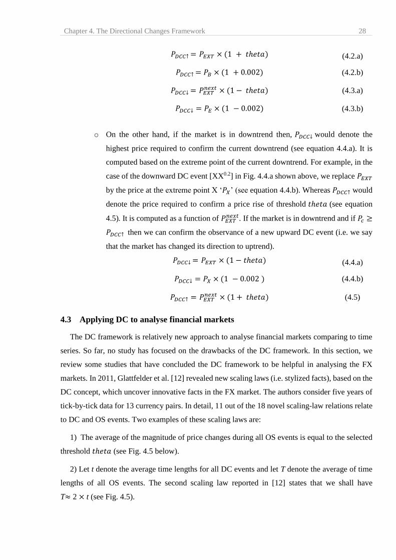
Chapter 4. The Directional Changes Framework 28
𝑃𝐷𝐶𝐶↑ = 𝑃𝐸𝑋𝑇 × (1 + 𝑡ℎ𝑒𝑡𝑎) (4.2.a)
𝑃𝐷𝐶𝐶↑ = 𝑃𝐵 × (1 + 0.002) (4.2.b)
𝑃𝐷𝐶𝐶↓ = 𝑃𝐸𝑋𝑇𝑛𝑒𝑥𝑡 × (1 − 𝑡ℎ𝑒𝑡𝑎) (4.3.a)
𝑃𝐷𝐶𝐶↓ = 𝑃𝐸 × (1 − 0.002) (4.3.b)
o On the other hand, if the market is in downtrend then, 𝑃𝐷𝐶𝐶↓ would denote the
highest price required to confirm the current downtrend (see equation 4.4.a). It is
computed based on the extreme point of the current downtrend. For example, in the
case of the downward DC event [XX0.2] in Fig. 4.4.a shown above, we replace 𝑃𝐸𝑋𝑇
by the price at the extreme point X ‘𝑃𝑋’ (see equation 4.4.b). Whereas 𝑃𝐷𝐶𝐶↑ would
denote the price required to confirm a price rise of threshold 𝑡ℎ𝑒𝑡𝑎 (see equation
4.5). It is computed as a function of 𝑃𝐸𝑋𝑇𝑛𝑒𝑥𝑡. If the market is in downtrend and if 𝑃𝑐 ≥
𝑃𝐷𝐶𝐶↑ then we can confirm the observance of a new upward DC event (i.e. we say
that the market has changed its direction to uptrend).
𝑃𝐷𝐶𝐶↓ = 𝑃𝐸𝑋𝑇 × (1 − 𝑡ℎ𝑒𝑡𝑎) (4.4.a)
𝑃𝐷𝐶𝐶↓ = 𝑃𝑋 × (1 − 0.002) (4.4.b)
𝑃𝐷𝐶𝐶↑ = 𝑃𝐸𝑋𝑇𝑛𝑒𝑥𝑡 × (1 + 𝑡ℎ𝑒𝑡𝑎) (4.5)
4.3 Applying DC to analyse financial markets
The DC framework is relatively new approach to analyse financial markets comparing to time
series. So far, no study has focused on the drawbacks of the DC framework. In this section, we
review some studies that have concluded the DC framework to be helpful in analysing the FX
markets. In 2011, Glattfelder et al. [12] revealed new scaling laws (i.e. stylized facts), based on the
DC concept, which uncover innovative facts in the FX market. The authors consider five years of
tick-by-tick data for 13 currency pairs. In detail, 11 out of the 18 novel scaling-law relations relate
to DC and OS events. Two examples of these scaling laws are:
1) The average of the magnitude of price changes during all OS events is equal to the selected
threshold 𝑡ℎ𝑒𝑡𝑎 (see Fig. 4.5 below).
2) Let t denote the average time lengths for all DC events and let T denote the average of time
lengths of all OS events. The second scaling law reported in [12] states that we shall have
T≈ 2 × t (see Fig. 4.5).
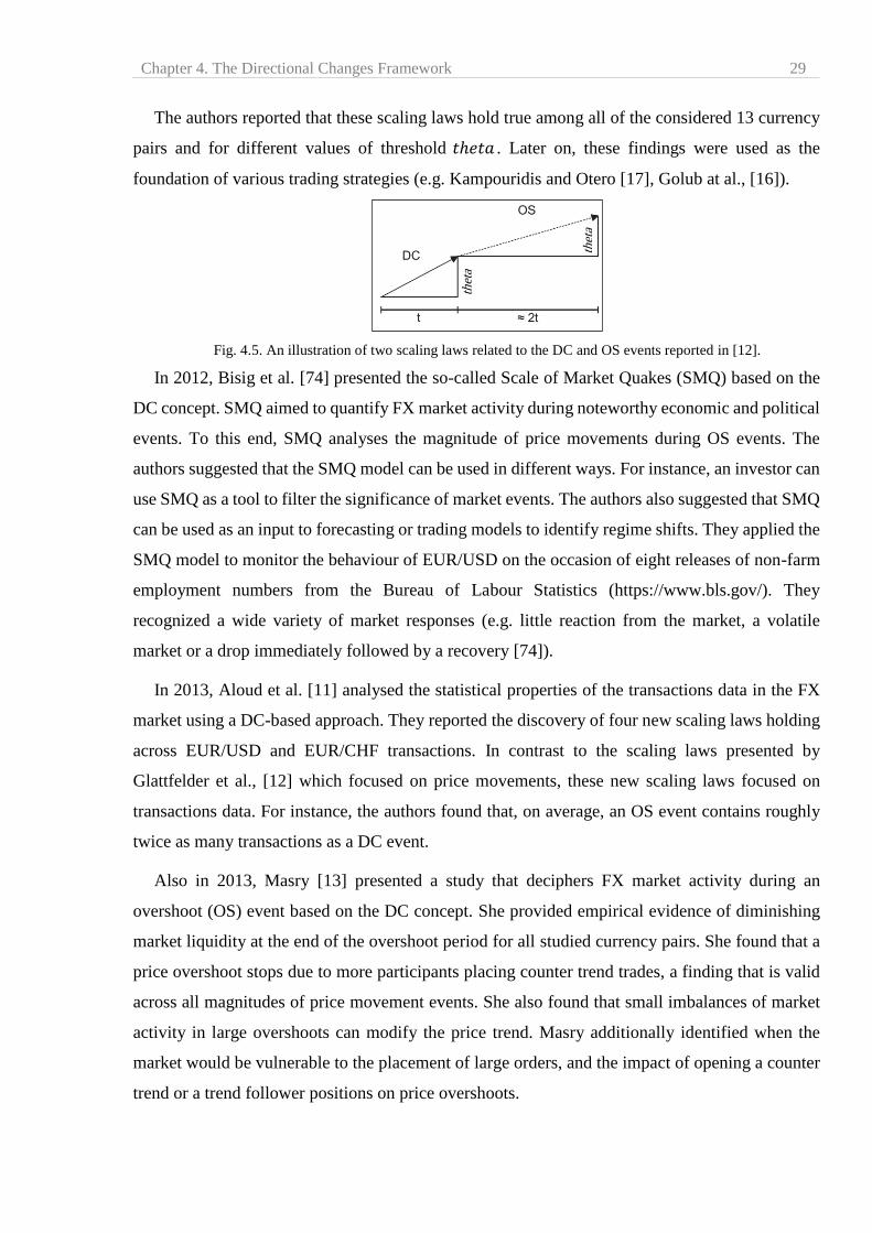
Chapter 4. The Directional Changes Framework 29
The authors reported that these scaling laws hold true among all of the considered 13 currency
pairs and for different values of threshold 𝑡ℎ𝑒𝑡𝑎 . Later on, these findings were used as the
foundation of various trading strategies (e.g. Kampouridis and Otero [17], Golub at al., [16]).
Fig. 4.5. An illustration of two scaling laws related to the DC and OS events reported in [12].
In 2012, Bisig et al. [74] presented the so-called Scale of Market Quakes (SMQ) based on the
DC concept. SMQ aimed to quantify FX market activity during noteworthy economic and political
events. To this end, SMQ analyses the magnitude of price movements during OS events. The
authors suggested that the SMQ model can be used in different ways. For instance, an investor can
use SMQ as a tool to filter the significance of market events. The authors also suggested that SMQ
can be used as an input to forecasting or trading models to identify regime shifts. They applied the
SMQ model to monitor the behaviour of EUR/USD on the occasion of eight releases of non-farm
employment numbers from the Bureau of Labour Statistics (https://www.bls.gov/). They
recognized a wide variety of market responses (e.g. little reaction from the market, a volatile
market or a drop immediately followed by a recovery [74]).
In 2013, Aloud et al. [11] analysed the statistical properties of the transactions data in the FX
market using a DC-based approach. They reported the discovery of four new scaling laws holding
across EUR/USD and EUR/CHF transactions. In contrast to the scaling laws presented by
Glattfelder et al., [12] which focused on price movements, these new scaling laws focused on
transactions data. For instance, the authors found that, on average, an OS event contains roughly
twice as many transactions as a DC event.
Also in 2013, Masry [13] presented a study that deciphers FX market activity during an
overshoot (OS) event based on the DC concept. She provided empirical evidence of diminishing
market liquidity at the end of the overshoot period for all studied currency pairs. She found that a
price overshoot stops due to more participants placing counter trend trades, a finding that is valid
across all magnitudes of price movement events. She also found that small imbalances of market
activity in large overshoots can modify the price trend. Masry additionally identified when the
market would be vulnerable to the placement of large orders, and the impact of opening a counter
trend or a trend follower positions on price overshoots.
thet
a
thet
a
Chapter 4. The Directional Changes Framework 30
In 2014, Golub et al., [75] proposed a new way to measure liquidity in the FX market based on
the DC framework. Their new approach sought to model market dynamics to predict stress in
financial markets. They defined an information theoretic measurement termed liquidity that
characterises the instability of price curves during an overshoot event and argued that the new
metric could forecast stress in financial markets. They proposed that their model to quantify
liquidity in the FX market could be used as an early warning system [75].
In 2017, Aloud and Fasli [76] presented an agent-based model which aimed to reproduce, to a
certain extent, the stylized facts (e.g. seasonality, scaling laws) previously discovered in FX market
transactions data by Aloud et al. [11]. The presented study examined the existence of a relation
between the functionality of a DC-based trading strategy and a discovered stylized fact in the FX
market. They suggested that the proposed model could be utilized to help in the design of agent
trading strategies and decision support systems for the FX market.
In 2017, Tsang et al., [77] presented a new approach to profiling companies and financial
markets. They proposed several DC-based indicators to characterize the high-frequency price
movements of a given market. They suggested that these indicators helped to compare markets in
terms of volatility and potential profit. They concluded that information obtained through DC-
based analysis and from time series complement each other.
4.4 DC-based trading strategies
Recently, some studies have tried to develop trading strategies based on the DC framework (i.e.
DC-based trading strategies). In this section, we review four of these studies.
4.4.1 The ‘DCT1’
In 2012, Aloud et al., [14] presented a DC-based trading strategy named Zero Intelligence
Directional Change Trading (ZI-DCT0). ZI-DCT0 runs a DC summary with a threshold named
‘∆xDC’. ZI-DCT0 has two trading rules:
a. It initiates a trade at the DC confirmation point of a DC event. The type of trade can be
either: counter trend (CT) or trend follow (TF)f. In the case of CT, ZI-DCT0 opens a
position against the market’s trend. TF does the opposite. The user must specify the type
of trade: either CT or TF.
f A CT (contrarian) trader opens a position (i.e. makes a buy or sell order) with the expectation that the current trend will reverse.
A TF (trend follower) trader opens their position with the expectation that the current trend will continue.
Chapter 4. The Directional Changes Framework 31
b. ZI-DCT0 closes the position at the DC confirmation point of the succeeding DC event.
When trading with ZI-DCT0, the trader must determine two parameters:
The type of trade: CT or TF.
The threshold ∆xDC to be used for conducting the DC summary.
In 2015, Aloud [15] presented a trading strategy called ‘DCT1’. The DCT1 was presented as
an updated version of ZI-DCT0. The trading rules of DCT1 are the same as ZI-DCT0 (i.e. rules a.
and b. shown above); however DCT1 is designed to automatically compute the two parameters:
the DC threshold ∆xDC and the type of trade (CT or TF). Firstly, the trader defines a range of
thresholds. Secondly, DCT1 automatically examines the profitability of each threshold, included
in the specified range, using historical price data (as the training set). To this end, for each threshold
value, the DCT1 applies the trading rules of ZI-DCT0 from two points of view: counter trend (CT)
and trend follow (TF). In other words, during the training period, the DCT1 examines the
profitability of all possible combinations of: 1) threshold, included in the range, and 2) the trade
type (CT or TF). DCT1 returns the threshold ∆xDC and the type of trade (CT or TF) corresponding
to the highest produced returns during the training period. It then uses these values to trade over
the trading period.
DCT1 was tested using high frequency data of the EUR/USD currency pair. The author reported
that DCT1 was able to produce a rate of return of 6.2% during a testing period of one year (with
bid-ask spread being taken into concern). The author did not report any: a) comparison to a
benchmark, b) measurement of risk (e.g. MDD), or c) evaluation of risk-adjusted metrics (e.g.
Sharpe ratio).
4.4.2 A DC-based trading strategy
In 2015, Gypteau et al., [78] presented a DC-based trading strategy. The proposed approach
follows the standard tree-based Genetic Programming (GP) configuration. Each individual GP tree
comprises internal and terminal nodes. The internal nodes are Boolean functions {AND, OR, NOR,
XOR, NOT}.
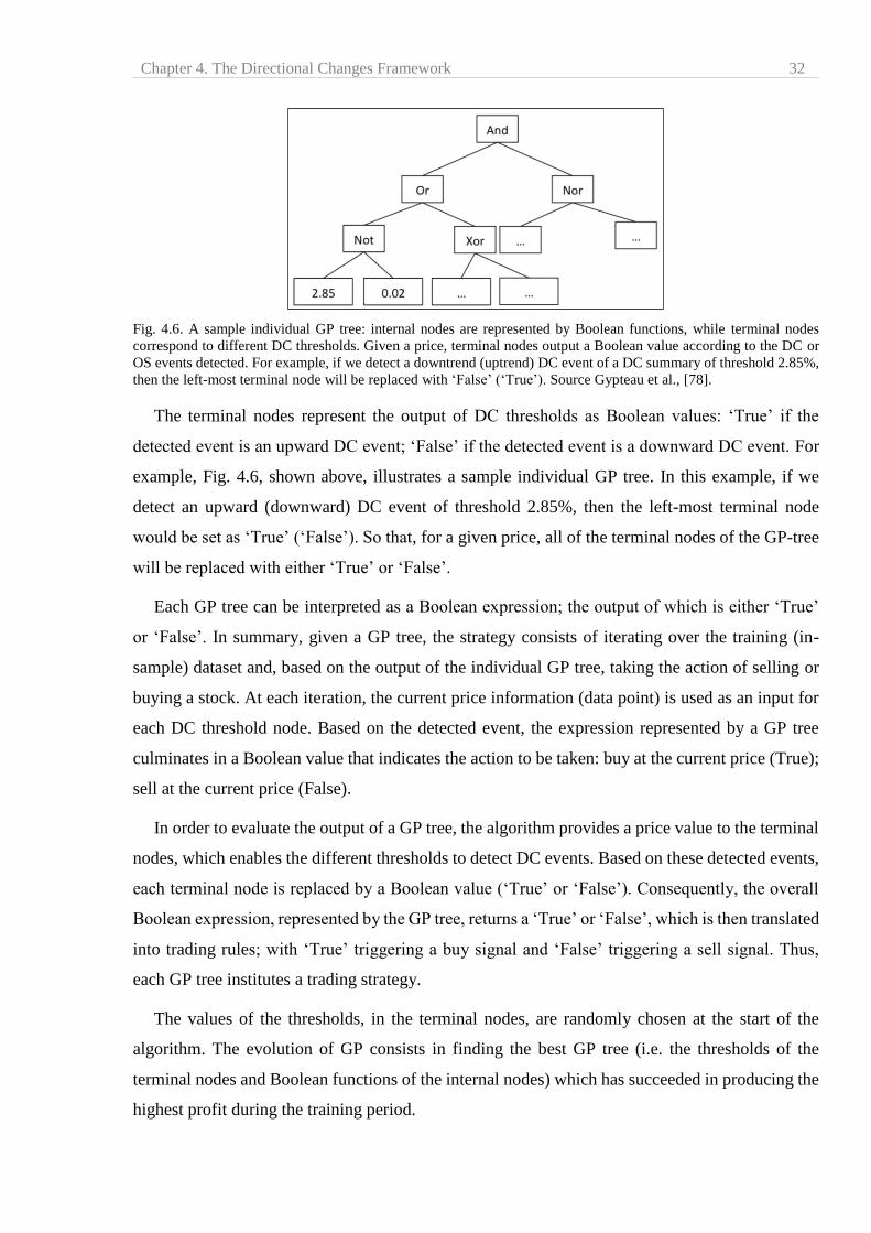
Chapter 4. The Directional Changes Framework 32
Fig. 4.6. A sample individual GP tree: internal nodes are represented by Boolean functions, while terminal nodes
correspond to different DC thresholds. Given a price, terminal nodes output a Boolean value according to the DC or
OS events detected. For example, if we detect a downtrend (uptrend) DC event of a DC summary of threshold 2.85%,
then the left-most terminal node will be replaced with ‘False’ (‘True’). Source Gypteau et al., [78].
The terminal nodes represent the output of DC thresholds as Boolean values: ‘True’ if the
detected event is an upward DC event; ‘False’ if the detected event is a downward DC event. For
example, Fig. 4.6, shown above, illustrates a sample individual GP tree. In this example, if we
detect an upward (downward) DC event of threshold 2.85%, then the left-most terminal node
would be set as ‘True’ (‘False’). So that, for a given price, all of the terminal nodes of the GP-tree
will be replaced with either ‘True’ or ‘False’.
Each GP tree can be interpreted as a Boolean expression; the output of which is either ‘True’
or ‘False’. In summary, given a GP tree, the strategy consists of iterating over the training (in-
sample) dataset and, based on the output of the individual GP tree, taking the action of selling or
buying a stock. At each iteration, the current price information (data point) is used as an input for
each DC threshold node. Based on the detected event, the expression represented by a GP tree
culminates in a Boolean value that indicates the action to be taken: buy at the current price (True);
sell at the current price (False).
In order to evaluate the output of a GP tree, the algorithm provides a price value to the terminal
nodes, which enables the different thresholds to detect DC events. Based on these detected events,
each terminal node is replaced by a Boolean value (‘True’ or ‘False’). Consequently, the overall
Boolean expression, represented by the GP tree, returns a ‘True’ or ‘False’, which is then translated
into trading rules; with ‘True’ triggering a buy signal and ‘False’ triggering a sell signal. Thus,
each GP tree institutes a trading strategy.
The values of the thresholds, in the terminal nodes, are randomly chosen at the start of the
algorithm. The evolution of GP consists in finding the best GP tree (i.e. the thresholds of the
terminal nodes and Boolean functions of the internal nodes) which has succeeded in producing the
highest profit during the training period.
Chapter 4. The Directional Changes Framework 33
With respect to the evaluation of the proposed DC-based strategy, the authors applied their
trading model to four markets: two stocks from the UK FTSE100 market (Barclays and Marks &
Spencer) and two indices (NASDAQ and the NYSE), sampled using daily closing price or index.
For each market, they considered a training period of 1000 days in length to train their GP model.
Then, they considered a testing (out-of-sample) period of 500 days in length for evaluation.
However, the authors did not report the dates of the training and testing periods!
The authors reported only the returns of the proposed trading strategy [78]. These were less
than 10% over a trading period of 500 days for each of the four considered markets. Furthermore,
they did not report any: a) measurement of risk (e.g. MDD), b) comparison to a benchmark, or c)
evaluation of risk-adjusted metrics (e.g. Sharpe ratio).
4.4.3 The ‘DC + GA’
In 2017, Kampouridis and Otero [17] proposed a DC-based trading strategy named ‘DC+GA’.
DC+GA runs multiple DC summaries concurrently (using multiple thresholds). For each threshold,
DC+GA calculates the average time length of each DC and OS event for every DC trend during a
training (in-sample) period. DC+GA employs two variables to express the average ratio of the OS
event length over the DC event length. These two variables are ru and rd, where ru is the average
ratio of the upwards OS event and rd is the average ratio of the downwards OS event. Thus,
DC+GA analyses uptrends and downtrends separately. The objective is to be able to anticipate the
end of an uptrend, or downtrend (approximately) and, as a result, make trading decisions (buy or
sell) once an OS event has reached the average ratio of ru or rd. Theoretically, DC+GA initiates a
trade when the length of an OS event exceeds ru or rd.
Based on the established scaling laws in [12] ru and rd are both equal to 1; which was confirmed
by Kampouridis and Otero [17]. However, in reality, it is generally expected that the OS event
might last longer, or be over earlier, than the estimated average values ru and rd (which are both 1).
To address this issue, the authors created two parameters, namely b1 and b2, that define a range of
time within the OS period in which trading is allowed. For instance, if a trader expects the OS
event to last for 2 hours (this expectation is based on the calculus of ru and rd) and assuming that
the range of [b1, b2] is [0.9, 1.0], then this means that DC+GA is going to trade (buy or sell) in the
last 10% of 1 hour’s duration, i.e. in the last 6 minutes.
Recall that DC+GA runs multiple DC summaries simultaneously (using multiple thresholds)
for a given currency pair. Let Ntheta be the number of employed DC thresholds. The user/trader
should choose the values of the Ntheta thresholds. DC+GA assigns a weight to each DC threshold.

Chapter 4. The Directional Changes Framework 34
For a given price observation, each threshold provides a recommendation (buy, sell or hold) based
on the values of b1, b2, ru and rd. At a given time, the Ntheta thresholds provide Ntheta
recommendations. These Ntheta recommendations are grouped into two groups based on the
produced recommendation: the first group contains the DC thresholds recommending to buy; the
second group contains the DC thresholds with sell recommendations. In order to decide which
recommendation (buy, sell, or hold) to adopt, DC+GA sums the weights of the thresholds of the
two groups: if the sum of the weights for all thresholds recommending a buy (sell) action is greater
than the sum of the weights for all thresholds recommending a sell (buy) action, then the strategy’s
action will be to buy (sell).
To optimize the weights of these Ntheta thresholds and the associated trading parameters,
DC+GA employs a Genetic Algorithm (GA). DC+GA symbolizes a trading strategy as a GA gene.
In this context, a GA’s gene comprises: the weights of the Ntheta thresholds, b1, b2, and Q, with Q
being the order size (i.e. how much to buy or to sell). During the in-sample (training) period, the
evolution of GA consists in discovering the best GA gene. The best GA gene is the one that returns
the maximum profit during the training period. This best gene will be used for trading during the
out-of-sample (trading) period. DC+GA employs a fitness function that aims to minimize the
maximum drawdown (MDD) and maximize returns at the same time.
To evaluate the performance of DC+GA, the authors considered five currency pairs sampled
within a 10-minute interval over one year. They adopted a daily-basis rolling window approach,
with the training period being 1 day. When examining the reported monthly returns (in Tables 5
and A1, pages 156 and 158 respectively, Kampouridis and Otero [17]) one can easily note that the
proposed trading models incur losses in about 50% of the cases! The authors concluded that the
proposed model “…could not consistently return profitable strategies and thus their mean returns
were negative.” Kampouridis and Otero [17] reported the average monthly returns of applying
DC+GA to five currency pairs (shown in Table 6, page 158 [17]). We note that DC+GA incurs
overall losses in two out of the five cases.
As for the risk-adjusted performance, the authors did not provide any risk-adjusted
measurement explicitly. However, based on the reported monthly returns (Table 5, page 158, [17]),
we can compute the Sharpe ratio. If we consider a risk-free rate of 0.5% per annum, then we find
that DC+GA produced a positive Sharpe ratio in only two out of the five considered currency pairs
as follow:
In the case of EUR/GBP: 0.00
Chapter 4. The Directional Changes Framework 35
In the case of EUR/JPY: 0.25
In the case of EUR/USD: – 0.35
In the case of GBP/CHF: – 0.30
In the case of GBP/USD: 0.10
The authors adopted the buy and hold approach as a benchmark. They reported that the
proposed trading strategy “ …return a similar average return with BH” . We should finally
note that the reported MDD of DC+GA was less than 0.15% (measured on a daily basis) in all
considered cases (Table 8, [17]). We consider this value to be an attractive level of drawdown
risk.
4.4.4 The ‘Alpha Engine’
In 2017, Golub at al., [16] presented a DC-based trading strategy called ‘Alpha Engine’. The
Alpha Engine is a contrarian trading strategy. The mechanism of initialization of new positions
and the management of existing positions in the market works as follows:
Initially, the Alpha Engine opens a new position against the market trend during an OS event
in which the price’s change exceeds a certain threshold named ‘ 𝜔 ’. 𝜔 is a function of the
predetermined DC threshold 𝑡ℎ𝑒𝑡𝑎 and a parameter named 𝛼 (4.4). The value of 𝛼 is governed by
a money management module that we shall describe next.
𝜔 = 𝛼 × 𝑡ℎ𝑒𝑡𝑎 (4.6)
The Alpha Engine does not have an explicit stop-loss rule. Instead, it employs a sophisticated
money management approach. Each time the Alpha Engine opens a new position, it names this
position a ‘trading agent’. The Alpha Engine is capable of opening and managing multiple
positions (i.e. multiple trading agents) concurrently. When Alpha Engine opens a new position (i.e.
initiates a new trading agent), it keeps managing the size of this position until it closes in a profit.
The Alpha Engine increases and decreases the size of the position (i.e. the quantity of inventory
held by a trading agent) as the price progresses. The basic idea is that an existing position is
increased by some increment in case of a loss, bringing the average closer to the current price. For
a de-cascading event, an existing position is decreased, realizing a profit.
When triggering a new trade, a trading agent must decide the ‘time’ and the ‘size’ of that trade.
For this purpose, the Alpha Engine takes into concern two main factors:
a. The accumulation of inventory sizes as the market price moves up and down: the threshold
𝜔 is essentially utilized to control the time at which a trading agent should initiate a new
order. More particularly, the Alpha Engine manages a parameter 𝛼 to control the value of
Chapter 4. The Directional Changes Framework 36
𝜔 (4.3). The value of 𝛼 is a function of the inventory size. Let I denote the overall inventory
size held by all generated trading agents altogether. The authors considered I as a proxy for
the market. The Alpha Engine uses the value of I to manage the parameter 𝛼 ; and,
consequently, the threshold 𝜔.
b. A probability indicator, denoted as ‘ℒ’: The value of ℒ is interpreted as the probability that
the trend will go up or down given the current state. More specifically, ℒ is computed using
a transition network which has two states: 𝜔 and 𝑡ℎ𝑒𝑡𝑎. This transition network is designed
so that, in the case of an unlikely price trajectory (i.e. abnormal market behavior), ℒ ≈ 0.
On the other hand, if the markets show normal behavior, i.e. no strong trend can be
recognized, then ℒ ≈ 1. The Alpha Engine uses ℒ to control the size of a new order. The
size of a new order increases (decreases) as ℒ approaches 1 (0). It follows from the previous
description that ℒ helps the trading agents not to build up large positions that they cannot
unload. Besides, by slowing down the increase of the inventory of a trading agent during
market overshoots, the overall trading model experiences smaller drawdowns and better
risk-adjusted performance. The concept of ℒ was introduced by Golub et al. [75] to
discover if a market exhibits normal, or abnormal, behavior.
Moreover, the Alpha Engine uses asymmetric thresholds for uptrends and downtrends. The
authors found that the market is most likely to exhibit different behaviors during uptrends and
downtrends. To cover this dilemma, the Alpha Engine employs two different DC thresholds
(instead of just one: ‘𝑡ℎ𝑒𝑡𝑎); one for uptrends (𝑡ℎ𝑒𝑡𝑎up) and another for downtrends (𝑡ℎ𝑒𝑡𝑎down).
Similarly, the Alpha Engine has two different 𝜔 thresholds — the so-called 𝜔𝑢𝑝 and 𝜔𝑑𝑜𝑤𝑛 ,
with 𝜔𝑢𝑝 = 𝛼𝑢𝑝 × 𝑡ℎ𝑒𝑡𝑎 up and 𝜔𝑑𝑜𝑤𝑛 = 𝛼𝑑𝑜𝑤𝑛 × 𝑡ℎ𝑒𝑡𝑎 down. 𝛼𝑢𝑝 and 𝛼𝑑𝑜𝑤𝑛 are two trading
parameters, the values of which rely on the inventory I as explained in point a. above.
The details of this money management mechanism are quite complicated, so for.more
information on it, we would recommend Golub et al., [16]. Overall, we would note that this money
management approach is an integrated module of the Alpha Engine.
The Alpha Engine was extensively back-tested using a portfolio of 23 currency rates sampled
tick-by-tick over a period of eight years, from the beginning of 2006 until the beginning of 2014.
Alpha Engine produced a return of 21.34% over eight years (they used the bid and ask prices),
with a maximum drawdown of 0.71% (calculated on a daily basis). The authors reported an annual
Sharpe ratio (4.6) of 3.06. However, they did not specify the used risk-free rate! The authors made
the code of the Alpha Engine available online at Github [79].
Chapter 4. The Directional Changes Framework 37
4.5 Notions and concepts similar to DC
In this section, we distinguish the DC concept adopted in this thesis from other similar notions.
Despite the similarity in the names, the DC concept as described in this thesis is completely
different from both the ‘Change Direction’ [80] and ‘Direction– of– Change’ [81]concepts. In both
studies, [80] and [81] the authors used interval– based datasets (daily close value); neither a
threshold 𝑡ℎ𝑒𝑡𝑎 was used, nor a DC event defined. Instead, they tried to forecast when a given
stock index would switch its trend direction (upward or downward) at the daily closing price
without measuring the magnitude of the price change. Their models aimed to answer the question:
“will today’s close price extend yesterday’s trend?”
The DC concept is similar to the zigzag indicator, however. The zigzag approach models price
movement as alternating uptrend and downtrend [82] [83] [84]. The price change during an uptrend
or a downtrend must be at least equal to a specific threshold. The literature comprises another
similar notion: the ‘turning points’. In general, price movement can be symbolized as alternating
uptrends and downtrends, separated by ‘turning points’. Turning points are essentially local
minimum and maximum points in a time series, or in practical terms, the peaks and troughs [41].
Turning points are the points at which the trend’s direction reverses, usually for a magnitude
predetermined by the observer. Turning points can be interpreted as the extreme points under the
DC context.
The zigzag indicator and turning points concepts are pretty similar to the DC framework with
the main difference being that a trend, under the DC methodology, is dissected into: 1) a DC event
of fixed percentage equal to the selected threshold and 2) an OS event represented by the remaining
part of the trend before it reverses. Such partitioning is not part of the zigzag indicator nor of the
turning point model. Keep in mind that the dissection of a trend into DC and OS events, under the
DC framework, has been reported to be helpful in analysing and characterizing the financial
markets in many studies (e.g. [11] [12] [77] [74] [85]).
4.6 Summary
In this chapter, we have explained the concept of Directional Changes (DC). The DC framework
is an approach to summarizing prices in the financial markets. A directional change is defined by
a threshold that the observer considers significant, e.g. 5%. A 𝑡ℎ𝑒𝑡𝑎 % directional change is
basically a price change of 𝑡ℎ𝑒𝑡𝑎 % from the last peak or bottom price. Under the DC framework
the market is seen as a series of alternating uptrends and downtrends. A trend is dissected into a
DC event (of fixed threshold 𝑡ℎ𝑒𝑡𝑎) and an OS event (consisting of the remaining part of the trend).

Chapter 4. The Directional Changes Framework 38
In Section 4.2.3, we listed some important DC-based notations that will be used later in this thesis
(e.g. 𝑃𝐷𝐶𝐶↓ , 𝑃𝐷𝐶𝐶↑, 𝑃𝐸𝑋𝑇).
Reviewing the literature in Section 4.3, we found that many studies have concluded that the DC
framework is helpful in gaining more insight into the analysis of the FX market. This comprised
the discovery of new scaling laws, understanding the impact of new trades on a market’s trend,
and measuring the impact of political and economic events on the market. We also noticed that
only recently, some studies have tried to develop trading strategies based on the DC framework.
We reviewed four of these studies in Section 4.4. Later in this thesis, we will compare these four
DC-based trading strategies with our planned trading strategies in Chapters 6 and 7.
In this thesis we aim to explore, and consequently to provide a proof of, the usefulness of the
DC framework as a foundation for successful trading strategies. It is important to note that our
planned DC-based trading strategies in this thesis are not based on any other DC-based strategy.
However, some similar features may exist, as we shall discuss in Chapters 6 and 7.

39
Part II
Thesis Contributions
Chapter 5. Forecasting Directional Changes: Problem Formulation and Solution 40
5 Forecasting Directional Changes: Problem Formulation and
Solution
Many studies have tried to forecast the change in direction of a market trend. To the best of our
knowledge, no study has considered this problem within the DC context. In this chapter, we study
this problem under the DC framework. The central research question which we pose here is
whether the current trend will continue for a specific percentage before the direction of the trend
reverses.
In this chapter, we formalize this forecasting problem from the DC perspective and propose a
solution. We evaluate the accuracy of our approach using eight currency pairs from the FX market.
The experimental results suggest that the accuracy of the proposed forecasting model is very good;
in some cases, prediction accuracy is over 80%.
5.1 Introduction
Forecasting financial time series is a common objective for financial institutions and traders.
This task has proven to be very challenging [86]. Many studies have focused on the issue of next-
value prediction, which entails forecasting the future value of time series at the oncoming time
step, given the historical observations up to the current time. There may, however, be advantages
in predicting the change of a market trend’s direction directly (i.e. without explicitly predicting the
future value of the series). For example, traders may take decisions based on their estimation of
whether the price of a particular market will rise or fall [81].
Many studies have tried to predict when a given market would switch its trend direction. These
studies usually aim to answer the question: will today’s close price extend yesterday’s trend? In
other words, these studies consider the market prediction problem as a classification problem,
where the question is whether the market goes up or down. Usually this problem is referred to as
forecasting the change of direction. For instance, Park et al. [80] proposed a continuous Hidden
Markov Model (HMM) to predict the change of direction of a financial time series. They proposed
to split the data, consisting of daily closing prices, into two classes based on direction changes in
the next day’s closing price, and to train two HMMs (one for each class). The two formed HMM
models would then beemployed to forecast changes in direction of the next day’s closing price.
Skabar [81] presented a Bayesian multilayer perceptron model to predict the direction of the daily
close value of the Australian financial index. Skabar [87] proposed another forecasting model in
which he used a similarity-based classification model to predict the trend direction of tomorrow’s
Chapter 5. Forecasting Directional Changes: Problem Formulation and Solution 41
close price. He admitted that both models, introduced in [81] and [87], have almost equal accuracy.
Giacomel et al. [43] proposed an ensemble of two ANNs to predict the direction of price
movement. The proposed model was tested using two cases: the North American and the Brazilian
stock markets for a total of 18 stocks. Evans et al. [6] introduced a model which combined Artificial
Neural Networks (ANN) and Genetic Algorithms (GA) to predict intra-day market price direction.
They employed a GA module to search the best network topology of a multiple layer perceptron
(MLP) in order to improve forecasting accuracy. It is important to note that the objective of these
studies is to forecast whether the next price observation will be greater, or smaller, than the last
recorded price. In this chapter we consider a different forecasting problem that we shall describe
next.
Price movements can be symbolized as alternating uptrends and downtrends, separated by
‘turning points’. Turning points are essentially local minimum and maximum points on a time
series or, in practical terms, the peaks and troughs [41]. Turning points are the points at which the
trend’s direction reverses, usually for a magnitude predetermined by the observer. An investor who
can trade exactly at the turning points (e.g. buying at minima and selling at maxima) would gain
the maximum possible profit. Therefore, a common objective for traders in the financial markets
is to forecast turning points. Predicting turning points has long been a tough task in the field of
time series analysis. Many machine learning models have been developed for this purpose, with
the majority of cases focusing on stock markets.
For instance, Azzini et al. [83] tried to predict a turning point in the S&P500 index. Their
objective was to predict the magnitude of the price change of the entire trend (i.e. between two
consecutive turning points) before the trend reversed. They used two models for this purpose: fuzzy
logic and neural networks. Li et al. [41] proposed a framework for turning point prediction that
combines chaotic dynamic analysis with a neural network. Their proposed model tries to predict
whether the next time step in the time series is a peak, a trough or none. El-Yaniv and Faynburd
[88] proposed a model for the prediction of turning points based on support vector regression.
Many studies have concluded that the directional change (DC) framework is useful in analysing
the FX market (e.g. [11] [12] [14] [74]). In this chapter, we consider the problem of forecasting
the change of a trend’s direction from the DC perspective. The task is to forecast whether the
current trend, either uptrend or downtrend, will continue in the same direction for a specific
percentage before it reverses (i.e. before the occurrence of the next extreme point). Answering this
question can be useful for investment decisions. For example, it could help a trader to make a buy
or a sell decision (as we shall argue in Chapter 6).
Chapter 5. Forecasting Directional Changes: Problem Formulation and Solution 42
Forecasting crucially depends on the variables used. As a first attempt to tackle the proposed
forecasting problem, we introduce an original DC-based independent variable. We prove that it is
useful for the proposed forecasting problem. Our forecasting model, in this chapter, is novel
because:
In terms of problem formulation: We consider the problem of ‘forecasting whether the
current trend will continue in the same direction for a specific percentage before it reverses’
from the DC perspective. To the best of our knowledge, no previous study has considered
this problem from the DC perspective.
In terms of the proposed solution: We will introduce an original DC-based indicator and
prove that it is helpful in predicting the change of a trend’s direction with very good
accuracy. Most of the existing forecasting approaches use traditional technical indicators
[21].
The rest of this chapter is organized as follows: we introduce a new concept named Big-Theta,
which is based on the DC concept, in Section 5.2. Then we provide the formal definition of our
proposed forecasting problem in Section 5.3. In Section 5.4, we present our approach to solving
the introduced forecasting problem. We describe a set of experiments in Section 5.5, designed to
examine the accuracy of our forecasting model. The experimental results are reported and
discussed in Section 5.6. We conclude with Section 5.7.
5.2 The concept of Big-Theta
5.2.1 Big-Theta
In this section, we introduce a new concept named Big-Theta. The notion of Big-Theta refers
to the situation at which the price movements of a DC event of threshold STheta may possibly
continue in the same direction (either upward or downward) so that the magnitude of price change,
during this particular DC trend, reaches another threshold named BTheta (with STheta < BTheta).
To clarify the notion of Big-Thetag, we provide the following examples: Fig. 5.1, shown below,
illustrates a downward DC event, named [AASTheta], of an unknown threshold STheta. At the time
of the observation of point ASTheta, we can confirm a price drop of magnitude STheta from point A.
The total magnitude of price change, for this particular DC trend, increases as the price’s
movement continues in the same downward direction. Later on, at point ABTheta this magnitude
g An alternative, and more rigorous, definition of the concept of Big-Theta would be: “Each DC event of threshold
BTheta will embrace another DC event of threshold STheta such that they both have the same extreme point”. We
provide more in-depth discussion and proof for this alternative definition in Appendix B.
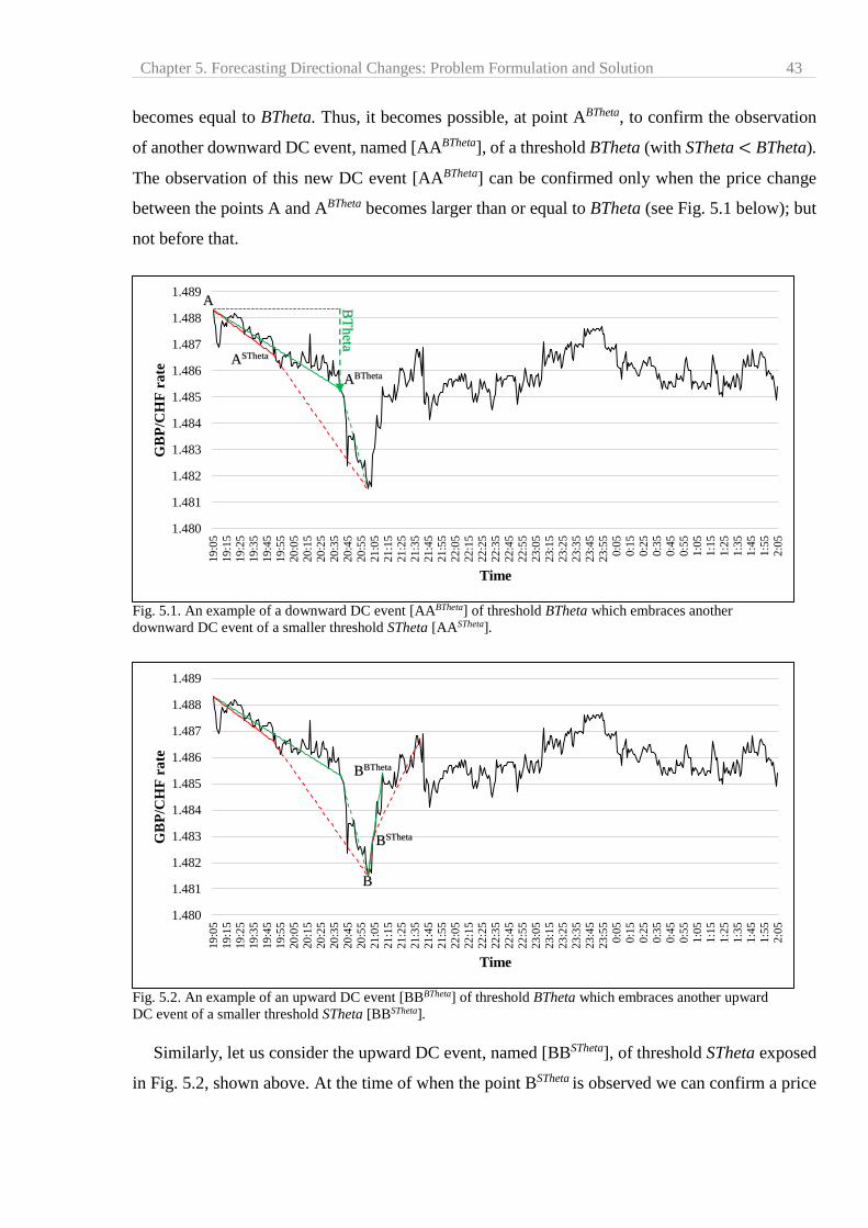
Chapter 5. Forecasting Directional Changes: Problem Formulation and Solution 43
becomes equal to BTheta. Thus, it becomes possible, at point ABTheta, to confirm the observation
of another downward DC event, named [AABTheta], of a threshold BTheta (with STheta < BTheta).
The observation of this new DC event [AABTheta] can be confirmed only when the price change
between the points A and ABTheta becomes larger than or equal to BTheta (see Fig. 5.1 below); but
not before that.
Fig. 5.1. An example of a downward DC event [AABTheta] of threshold BTheta which embraces another
downward DC event of a smaller threshold STheta [AASTheta].
Fig. 5.2. An example of an upward DC event [BBBTheta] of threshold BTheta which embraces another upward
DC event of a smaller threshold STheta [BBSTheta].
Similarly, let us consider the upward DC event, named [BBSTheta], of threshold STheta exposed
in Fig. 5.2, shown above. At the time of when the point BSTheta is observed we can confirm a price
1.480
1.481
1.482
1.483
1.484
1.485
1.486
1.487
1.488
1.489
19
:05
19
:15
19
:25
19
:35
19
:45
19
:55
20
:05
20
:15
20
:25
20
:35
20
:45
20
:55
21
:05
21
:15
21
:25
21
:35
21
:45
21
:55
22
:05
22
:15
22
:25
22
:35
22
:45
22
:55
23
:05
23
:15
23
:25
23
:35
23
:45
23
:55
0:0
5
0:1
5
0:2
5
0:3
5
0:4
5
0:5
5
1:0
5
1:1
5
1:2
5
1:3
5
1:4
5
1:5
5
2:0
5
GB
P/C
HF
ra
te
Time
ABTheta
A
ASTheta
B
BBTheta
BSTheta
BT
heta

Chapter 5. Forecasting Directional Changes: Problem Formulation and Solution 44
rise of threshold STheta. As the price movements continues in the same upward direction, the total
magnitude of price change, for this particular DC trend, increases. At point BBTheta, this total
magnitude becomes equal to BTheta. Thus, at point BBTheta we are able to confirm the observation
of another upward DC event, named [BBBTheta], of threshold BTheta.
Fig. 5.3, shown below, illustrates two DC summaries of a GBP/CHF price series using two
thresholds: STheta (0.1%) and BTheta (0.2%). We will use Fig. 5.3 to illustrate the notion of Big-
Theta. As explained in Chapter 4, for the same price series, we may produce several DC summaries
by using multiple thresholds [10] [12]. In Fig. 5.3 we consider the two DC events of threshold
STheta (0.1%); namely [AA0.1] and [BB0.1] (shown in solid red lines). We can see that the price
movements of each of these two DC events was prolonged so that later on, as the price movements
continues, we can confirm another DC event of threshold BTheta namely [AA0.2] and [BB0.2].
Fig. 5.3. The synchronization of the two DC summaries using two thresholds: STheta (0.1%) and BTheta (0.2%).
The black line indicates GBP/CHF mid-prices sampled minute by minute from 1/1/2013 19:05 to 1/2/2013 02:05.
Solid red lines represent DC events. Dashed red lines represent OS events for threshold STheta. Solid red lines
represent DC events. Dashed red lines represent OS events for threshold BTheta.
5.2.2 The Boolean variable BBTheta
In this section, we use the concept of ‘Big-Theta’ to introduce a new Boolean variable named
BBTheta. Fig. 5.3, shown above, illustrates the synchronization of two DC summaries of same
price series using two threshold 0.1% and 0.2%. For each DC event of threshold STheta, we
associate a value of the Boolean variable BBTheta. For example, let BBTheta1 denote the value of
BBTheta associated to the first DC event of threshold STheta, which is [AA0.1] in this case (see
1.478
1.480
1.482
1.484
1.486
1.488
1.490
19
:05
19
:15
19
:25
19
:35
19
:45
19
:55
20
:05
20
:15
20
:25
20
:35
20
:45
20
:55
21
:05
21
:15
21
:25
21
:35
21
:45
21
:55
22
:05
22
:15
22
:25
22
:35
22
:45
22
:55
23
:05
23
:15
23
:25
23
:35
23
:45
23
:55
0:0
5
0:1
5
0:2
5
0:3
5
0:4
5
0:5
5
1:0
5
1:1
5
1:2
5
1:3
5
1:4
5
1:5
5
2:0
5
GB
P/C
HF
ra
te
Time
A0.2
A
B
B0.2
E0.2
E
B0.1
C
C0.1
D0.1
D
F0.1
E0.1
F
G
G0.1
A0.1

Chapter 5. Forecasting Directional Changes: Problem Formulation and Solution 45
Fig. 5.3). In general, let BBThetai be the value of BBTheta associated with the ith DC event of the
DC summary of threshold STheta. BBThetai can be only True or False. The value of BBThetai is
defined as follows:
If the total price change during the ith DC trend, of the DC summary of threshold STheta, is at
least equal to BTheta, then BBThetai = True; otherwise BBThetai = False. In other words,
BBThetai is ‘True’ only if the price change between the ith and (i+1)th extreme points is larger than
or equal to BTheta.
We use Table 5.1, shown below, to clarify this definition. The first column from the left in
Table 5.1 represents the index of the DC events observed under threshold STheta (i.e. 1st, 2nd, etc.)
in Fig. 5.3. The column ‘Extreme point’ contains the extreme points resulting from the DC
summary of threshold STheta (according to Fig. 5.3 shown above). The column ‘Mid-price at
extreme point’ shows the market’s price at the indicated extreme point. We can catch the value of
BBThetai by calculating the magnitude of price changes between the ith and (i+1)th extreme points
detected under the threshold STheta.
Table 5.1: Example of DC events of threshold STheta and the computation of corresponding BBThetai based on Fig.
5.3.
DC event index
(STheta)
Extreme
point
Mid-price at
extreme point DCC point BBTheta
1 A 1.48831 A0.1 BBTheta1= True
2 B 1.48150 B0.1 BBTheta2= True
3 C 1.48690 C0.1 BBTheta3= False
4 D 1.48412 D0.1 BBTheta4= False
5 E 1.48770 E0.1 BBTheta5= True
6 F 1.48499 F0.1 BBTheta6= False
7 G 1.48680 G0.1 BBTheta7= False
For example, to compute BBTheta1 we calculate the price change between the prices of the 1st
and 2nd extreme points shown in column ‘Extreme point’ (i.e. points A and B). In this example,
the price change is:
(PA − PB)/ PA = (1.48831−1.48150)/ 1.48831 = 0.00458 (5.1)
The value of (5.1), i.e. 0.00458, is larger than BTheta (0.2%). Thus, BBTheta1= True as shown
in column ‘BBTheta’. Similarly, to compute BBTheta3 we calculate the price change between the

Chapter 5. Forecasting Directional Changes: Problem Formulation and Solution 46
prices of the 3rd and 4th extreme points shown in column ‘Extreme point’ (i.e. points C and D). In
this case, the price change is:
(PC − PD)/ PC = (1.48690 −1.48412)/ 1.48690 = 0.00187 (5.2)
The value of (5.2), i.e. 0.00187, is less than BTheta (0.2%). Thus, BBTheta3= False as shown
in column ‘FBBTheta’. The column ‘BBTheta’ embraces the set of all instances of BBThetai. We
refer to this set as BBTheta. Given two DC summaries of the same price series, corresponding to
two different thresholds, STheta and BTheta, we compute BBThetai for each DC event of threshold
STheta as exemplified in Table 5.1.
5.3 Formulation of the forecasting problem
In this chapter, our task is to forecast the value of BBTheta. In other words, we are looking to
forecast, at the DCC point of a DC event of threshold STheta (e.g. points A0.1, B0.1 from Table 5.1),
whether the associated instance of BBTheta (shown in the column ‘BBTheta’ Table 5.1) is True or
False. In this section, we introduce our proposed forecasting problem.
Table 5.2, shown below, simplifies the synchronization of the two DC summaries. We use Table
5.2 to provide an example of the proposed forecasting problem. Based on Table 5.2, we consider
two uptrend DC events:
1. The DC event [BB0.1] of threshold 0.1%. [BB0.1] starts at time 21:00:00 and ends at time
21:05:00.
2. The DC event [BB0.2] of threshold 0.2%. [BB0.2] starts at time 21:00:00 and ends at time
21:10:00.
In the column ‘Point’, B0.1 denote the DCC point of the DC event [BB0.1], and B0.2 denote the
DCC point of the DC event [BB0.2]. We also note two facts:
1. Both DC events, [BB0.1] and [BB0.2], start at the same point B.
2. Point B0.1 (which is observed at time 21:05:00, column ‘Time’) occurred before we observed
point B0.2 (at time 21:10:00).
Note that at point B0.1 (i.e. at time 21:05:00) we can confirm that point B is the extreme point
of an uptrend DC event of threshold STheta = 0.1%. In this example, [BB0.1] is the second DC
event of threshold STheta (see Table 5.1). Therefore, our objective is to forecast whether BBTheta2
is True. In other words, we want to predict at point B0.1, whether the current uptrend will continue
so that its total magnitude will reach a threshold of 0.2% (i.e. BTheta). Note that at point B0.1 we
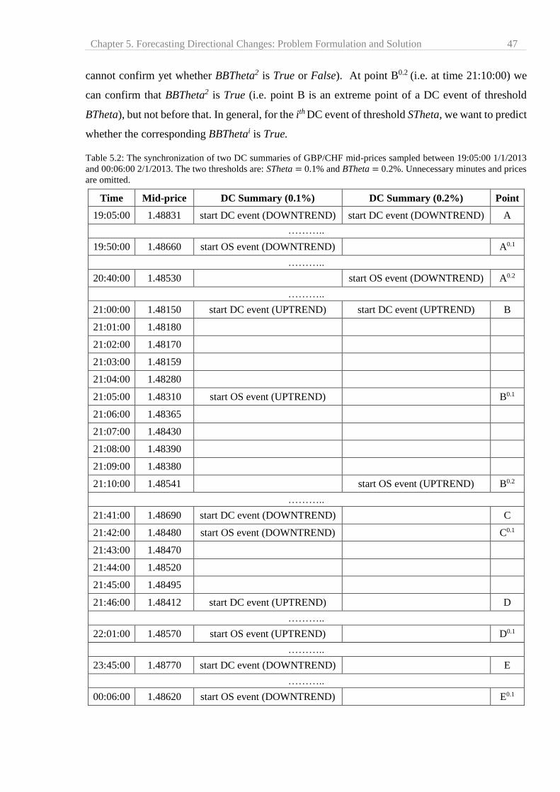
Chapter 5. Forecasting Directional Changes: Problem Formulation and Solution 47
cannot confirm yet whether BBTheta2 is True or False). At point B0.2 (i.e. at time 21:10:00) we
can confirm that BBTheta2 is True (i.e. point B is an extreme point of a DC event of threshold
BTheta), but not before that. In general, for the ith DC event of threshold STheta, we want to predict
whether the corresponding BBThetai is True.
Table 5.2: The synchronization of two DC summaries of GBP/CHF mid-prices sampled between 19:05:00 1/1/2013
and 00:06:00 2/1/2013. The two thresholds are: STheta = 0.1% and BTheta = 0.2%. Unnecessary minutes and prices
are omitted.
Time Mid-price DC Summary (0.1%) DC Summary (0.2%) Point
19:05:00 1.48831 start DC event (DOWNTREND) start DC event (DOWNTREND) A
………..
19:50:00 1.48660 start OS event (DOWNTREND) A0.1
………..
20:40:00 1.48530 start OS event (DOWNTREND) A0.2
………..
21:00:00 1.48150 start DC event (UPTREND) start DC event (UPTREND) B
21:01:00 1.48180
21:02:00 1.48170
21:03:00 1.48159
21:04:00 1.48280
21:05:00 1.48310 start OS event (UPTREND) B0.1
21:06:00 1.48365
21:07:00 1.48430
21:08:00 1.48390
21:09:00 1.48380
21:10:00 1.48541 start OS event (UPTREND) B0.2
………..
21:41:00 1.48690 start DC event (DOWNTREND) C
21:42:00 1.48480 start OS event (DOWNTREND) C0.1
21:43:00 1.48470
21:44:00 1.48520
21:45:00 1.48495
21:46:00 1.48412 start DC event (UPTREND) D
………..
22:01:00 1.48570 start OS event (UPTREND) D0.1
………..
23:45:00 1.48770 start DC event (DOWNTREND) E
………..
00:06:00 1.48620 start OS event (DOWNTREND) E0.1

Chapter 5. Forecasting Directional Changes: Problem Formulation and Solution 48
To recap, in this chapter we propose to tackle the following forecasting problem: ‘to forecast
whether the current DC trend of threshold STheta will continue so that the total price change of
this particular DC trend will be at least equal to BTheta’. This forecasting objective is shortened to
predict the Boolean variable BBTheta. To the best of our knowledge, no previous study has
provided a similar formalization of this forecasting problem under the DC context. We believe that
solving such a forecasting problem under the DC framework could be the basis of a successful
trading strategy (as we shall argue in Chapter 6).
5.4 Our approach to forecasting the end of a trend
In this section, we propose an approach to solving the forecasting problem presented in Section
5.3. The objective is to forecast for the ith DC event of threshold STheta whether the corresponding
BBThetai is True. To this end, we introduce a novel DC-based indicator, which is also based on
the concept of Big-Theta. We use the J48 procedure to make the forecast. Firstly, we introduce the
novel DC-based indicator which will be used as the independent variable. Then, we briefly
describe the adopted machine learning procedure, J48, which we will use to forecast BBTheta.
5.4.1 The independent variable
The accuracy of a forecasting model depends on the independent variable(s) used. Many
forecasting models rely on technical indicators to make a forecast (e.g. [6] [44] [46]). Our task is
particularly difficult because, so far, no published work has provided a formal method as to how
to apply existing technical indicators (e.g. Ehler Leading Indicator [89], Aroon indicator [32], RSI
or ADX [90]) can be applied under the DC framework. Recently, Kampouridis and Otero [17]
suggested that more research should be undertaken into defining new indicators emerging from the
DC concept, in a manner similar to how technical indicators exist within traditional time series.
Tsang et al., [77] introduced several DC-based indicators with the aim of profiling the financial
markets. However, they did not examine the usefulness of these indicators for forecasting purposes.
In this section, we introduce a novel DC-based indicator named 𝑂𝑆𝑉𝐵𝑇ℎ𝑒𝑡𝑎𝑆𝑇ℎ𝑒𝑡𝑎. The abbreviation
𝑂𝑆𝑉 stands for Over Shoot Value. The 𝑂𝑆𝑉 is intended to measure the magnitude of price
movements during the overshoot event. Keep in mind that a large DC trend embraces smaller DC
trend(s) ( [10] [12]). We introduce the variable 𝑂𝑆𝑉𝐵𝑇ℎ𝑒𝑡𝑎𝑆𝑇ℎ𝑒𝑡𝑎 in order to unveil the possible relation
which may exist between the overshoot event of a large DC trend (as observed under BTheta) and
a smaller DC trend (as observed under STheta). We believe that such a relation could be helpful to
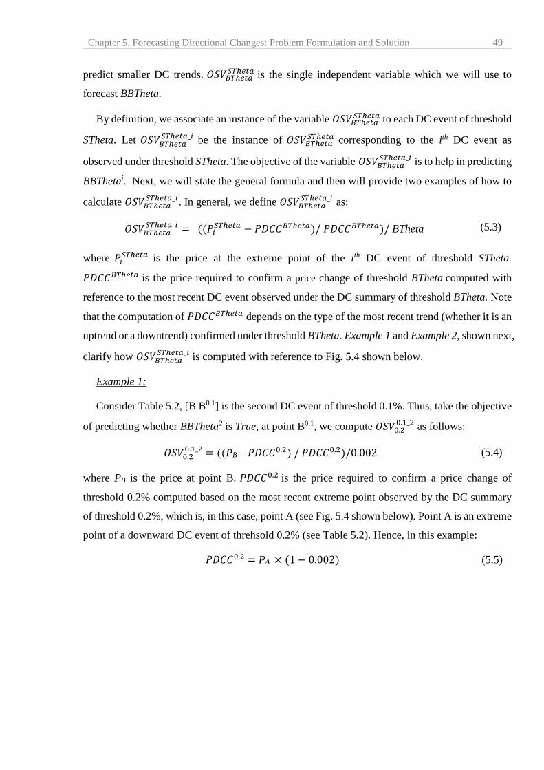
Chapter 5. Forecasting Directional Changes: Problem Formulation and Solution 49
predict smaller DC trends. 𝑂𝑆𝑉𝐵𝑇ℎ𝑒𝑡𝑎𝑆𝑇ℎ𝑒𝑡𝑎 is the single independent variable which we will use to
forecast BBTheta.
By definition, we associate an instance of the variable 𝑂𝑆𝑉𝐵𝑇ℎ𝑒𝑡𝑎𝑆𝑇ℎ𝑒𝑡𝑎 to each DC event of threshold
STheta. Let 𝑂𝑆𝑉𝐵𝑇ℎ𝑒𝑡𝑎𝑆𝑇ℎ𝑒𝑡𝑎_𝑖 be the instance of 𝑂𝑆𝑉𝐵𝑇ℎ𝑒𝑡𝑎
𝑆𝑇ℎ𝑒𝑡𝑎 corresponding to the ith DC event as
observed under threshold STheta. The objective of the variable 𝑂𝑆𝑉𝐵𝑇ℎ𝑒𝑡𝑎𝑆𝑇ℎ𝑒𝑡𝑎_𝑖 is to help in predicting
BBThetai. Next, we will state the general formula and then will provide two examples of how to
calculate 𝑂𝑆𝑉𝐵𝑇ℎ𝑒𝑡𝑎𝑆𝑇ℎ𝑒𝑡𝑎_𝑖. In general, we define 𝑂𝑆𝑉𝐵𝑇ℎ𝑒𝑡𝑎
𝑆𝑇ℎ𝑒𝑡𝑎_𝑖 as:
𝑂𝑆𝑉𝐵𝑇ℎ𝑒𝑡𝑎𝑆𝑇ℎ𝑒𝑡𝑎_𝑖 = ((𝑃𝑖
𝑆𝑇ℎ𝑒𝑡𝑎 − 𝑃𝐷𝐶𝐶𝐵𝑇ℎ𝑒𝑡𝑎)/ 𝑃𝐷𝐶𝐶𝐵𝑇ℎ𝑒𝑡𝑎)/ BTheta (5.3)
where 𝑃𝑖𝑆𝑇ℎ𝑒𝑡𝑎 is the price at the extreme point of the ith DC event of threshold STheta.
𝑃𝐷𝐶𝐶𝐵𝑇ℎ𝑒𝑡𝑎 is the price required to confirm a price change of threshold BTheta computed with
reference to the most recent DC event observed under the DC summary of threshold BTheta. Note
that the computation of 𝑃𝐷𝐶𝐶𝐵𝑇ℎ𝑒𝑡𝑎 depends on the type of the most recent trend (whether it is an
uptrend or a downtrend) confirmed under threshold BTheta. Example 1 and Example 2, shown next,
clarify how 𝑂𝑆𝑉𝐵𝑇ℎ𝑒𝑡𝑎𝑆𝑇ℎ𝑒𝑡𝑎_𝑖 is computed with reference to Fig. 5.4 shown below.
Example 1:
Consider Table 5.2, [B B0.1] is the second DC event of threshold 0.1%. Thus, take the objective
of predicting whether BBTheta2 is True, at point B0.1, we compute 𝑂𝑆𝑉0.20.1_2 as follows:
𝑂𝑆𝑉0.20.1_2 = ((PB −𝑃𝐷𝐶𝐶0.2) / 𝑃𝐷𝐶𝐶0.2)/0.002 (5.4)
where PB is the price at point B. 𝑃𝐷𝐶𝐶0.2 is the price required to confirm a price change of
threshold 0.2% computed based on the most recent extreme point observed by the DC summary
of threshold 0.2%, which is, in this case, point A (see Fig. 5.4 shown below). Point A is an extreme
point of a downward DC event of threhsold 0.2% (see Table 5.2). Hence, in this example:
𝑃𝐷𝐶𝐶0.2 = PA × (1 − 0.002) (5.5)
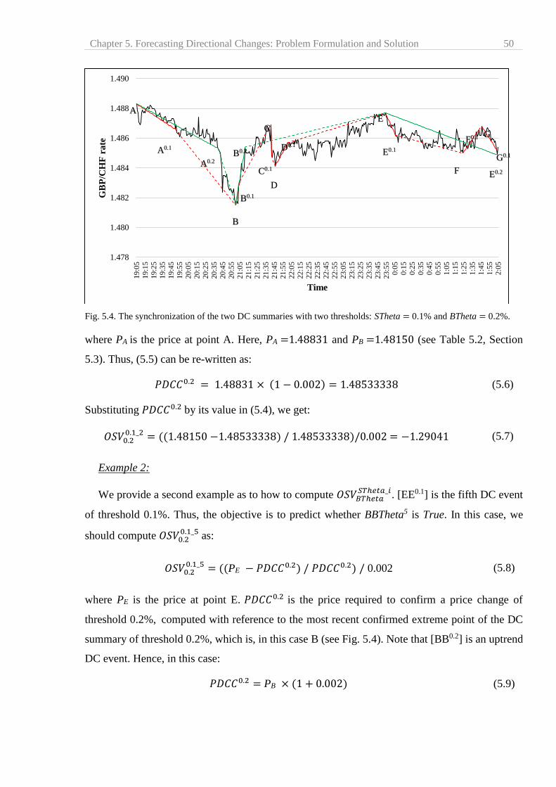
Chapter 5. Forecasting Directional Changes: Problem Formulation and Solution 50
Fig. 5.4. The synchronization of the two DC summaries with two thresholds: STheta = 0.1% and BTheta = 0.2%.
where PA is the price at point A. Here, PA =1.48831 and PB =1.48150 (see Table 5.2, Section
5.3). Thus, (5.5) can be re-written as:
𝑃𝐷𝐶𝐶0.2 = 1.48831 × (1 − 0.002) = 1.48533338 (5.6)
Substituting 𝑃𝐷𝐶𝐶0.2 by its value in (5.4), we get:
𝑂𝑆𝑉0.20.1_2 = ((1.48150 −1.48533338) / 1.48533338)/0.002 = −1.29041 (5.7)
Example 2:
We provide a second example as to how to compute 𝑂𝑆𝑉𝐵𝑇ℎ𝑒𝑡𝑎𝑆𝑇ℎ𝑒𝑡𝑎_𝑖. [EE0.1] is the fifth DC event
of threshold 0.1%. Thus, the objective is to predict whether BBTheta5 is True. In this case, we
should compute 𝑂𝑆𝑉0.20.1_5 as:
𝑂𝑆𝑉0.20.1_5 = ((PE − 𝑃𝐷𝐶𝐶0.2) / 𝑃𝐷𝐶𝐶0.2) / 0.002 (5.8)
where PE is the price at point E. 𝑃𝐷𝐶𝐶0.2 is the price required to confirm a price change of
threshold 0.2%, computed with reference to the most recent confirmed extreme point of the DC
summary of threshold 0.2%, which is, in this case B (see Fig. 5.4). Note that [BB0.2] is an uptrend
DC event. Hence, in this case:
𝑃𝐷𝐶𝐶0.2 = PB × (1 + 0.002) (5.9)
1.478
1.480
1.482
1.484
1.486
1.488
1.490
19
:05
19
:15
19
:25
19
:35
19
:45
19
:55
20
:05
20
:15
20
:25
20
:35
20
:45
20
:55
21
:05
21
:15
21
:25
21
:35
21
:45
21
:55
22
:05
22
:15
22
:25
22
:35
22
:45
22
:55
23
:05
23
:15
23
:25
23
:35
23
:45
23
:55
0:0
5
0:1
5
0:2
5
0:3
5
0:4
5
0:5
5
1:0
5
1:1
5
1:2
5
1:3
5
1:4
5
1:5
5
2:0
5
GB
P/C
HF
ra
te
Time
A0.2
A
B
B0.2
E0.2
E
B0.1
C
C0.1
D0.1
D
F0.1
E0.1
F
G
G0.1 A0.1
Chapter 5. Forecasting Directional Changes: Problem Formulation and Solution 51
where PB is the price at point B. Here, PE =1.48770 and PB =1.48150 (see Table 5.2 above).
Thus, (5.6) can be re-written as:
𝑃𝐷𝐶𝐶0.2 = 1.48150 × (1 + 0.002) = 1.484463 (5.10)
Replacing 𝑃𝐷𝐶𝐶0.2 by its value in (5.8), we obtain:
𝑂𝑆𝑉0.20.1_5 = ((1.48770 −1.484463) / 1.484463)/0.002 = 1.09029 (5.11)
5.4.2 The decision tree procedure J48
In this chapter, we employ the decision tree procedure, J48, to find the relation between the two
variables BBTheta and 𝑂𝑆𝑉𝐵𝑇ℎ𝑒𝑡𝑎𝑆𝑇ℎ𝑒𝑡𝑎 . J48 is the open-source Java implementation of the C4.5
algorithm [91]. J48 has three main steps. First, for each attribute λ it computes the normalized
information gain ratio from splitting on λ. Let λ_best be the attribute with the highest normalized
information gain. Second, it creates a decision node nd that splits on λ_best. Third, it recurs on the
sub-lists obtained by splitting on λ_best and adds those nodes as children of node nd. The three
steps are repeated until a base case is reached.
5.5 Evaluation of our approach to forecasting DC: Experiments
In Section 5.4, we explained our approach to forecasting the change of a market trend’s direction
under the DC context. In this section, we aim to examine the accuracy of our proposed forecasting
approach. We test this approach in the FX market using eight currency pairs. We provide two sets
of experiments: 1) the objective of the first set is to evaluate the accuracy of our forecasting
approach, 2) the objective of the second set is to evaluate the impact of the value of BTheta on the
accuracy of our forecasting approach. We firstly introduce a variable, named α, which we will use
to measure the True-False imbalance in BBTheta.
5.5.1 Measuring the True-False imbalance
In Section 5.3 we introduced BBTheta as the Boolean dependent variable to be predicted. Some
studies (e.g. [92]) have reported that the performance of some machine learning algorithms can be
affected by the True-False imbalance in the dependent variable. In this section, we introduce a
new variable named α. The objective of α is to measure the levels of True-False imbalance in the
dependent variable BBTheta. α is measured as the fraction of True instances of BBTheta.
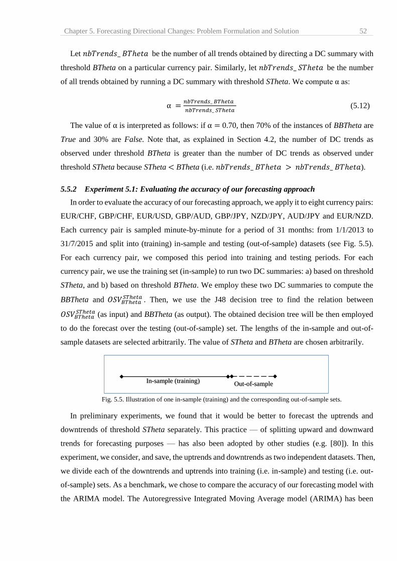
Chapter 5. Forecasting Directional Changes: Problem Formulation and Solution 52
Let 𝑛𝑏𝑇𝑟𝑒𝑛𝑑𝑠_ 𝐵𝑇ℎ𝑒𝑡𝑎 be the number of all trends obtained by directing a DC summary with
threshold BTheta on a particular currency pair. Similarly, let 𝑛𝑏𝑇𝑟𝑒𝑛𝑑𝑠_ 𝑆𝑇ℎ𝑒𝑡𝑎 be the number
of all trends obtained by running a DC summary with threshold STheta. We compute α as:
α =𝑛𝑏𝑇𝑟𝑒𝑛𝑑𝑠_ 𝐵𝑇ℎ𝑒𝑡𝑎
𝑛𝑏𝑇𝑟𝑒𝑛𝑑𝑠_ 𝑆𝑇ℎ𝑒𝑡𝑎 (5.12)
The value of α is interpreted as follows: if α = 0.70, then 70% of the instances of BBTheta are
True and 30% are False. Note that, as explained in Section 4.2, the number of DC trends as
observed under threshold BTheta is greater than the number of DC trends as observed under
threshold STheta because STheta < BTheta (i.e. 𝑛𝑏𝑇𝑟𝑒𝑛𝑑𝑠_ 𝐵𝑇ℎ𝑒𝑡𝑎 > 𝑛𝑏𝑇𝑟𝑒𝑛𝑑𝑠_ 𝐵𝑇ℎ𝑒𝑡𝑎).
5.5.2 Experiment 5.1: Evaluating the accuracy of our forecasting approach
In order to evaluate the accuracy of our forecasting approach, we apply it to eight currency pairs:
EUR/CHF, GBP/CHF, EUR/USD, GBP/AUD, GBP/JPY, NZD/JPY, AUD/JPY and EUR/NZD.
Each currency pair is sampled minute-by-minute for a period of 31 months: from 1/1/2013 to
31/7/2015 and split into (training) in-sample and testing (out-of-sample) datasets (see Fig. 5.5).
For each currency pair, we composed this period into training and testing periods. For each
currency pair, we use the training set (in-sample) to run two DC summaries: a) based on threshold
STheta, and b) based on threshold BTheta. We employ these two DC summaries to compute the
BBTheta and 𝑂𝑆𝑉𝐵𝑇ℎ𝑒𝑡𝑎𝑆𝑇ℎ𝑒𝑡𝑎 . Then, we use the J48 decision tree to find the relation between
𝑂𝑆𝑉𝐵𝑇ℎ𝑒𝑡𝑎𝑆𝑇ℎ𝑒𝑡𝑎 (as input) and BBTheta (as output). The obtained decision tree will be then employed
to do the forecast over the testing (out-of-sample) set. The lengths of the in-sample and out-of-
sample datasets are selected arbitrarily. The value of STheta and BTheta are chosen arbitrarily.
Fig. 5.5. Illustration of one in-sample (training) and the corresponding out-of-sample sets.
In preliminary experiments, we found that it would be better to forecast the uptrends and
downtrends of threshold STheta separately. This practice — of splitting upward and downward
trends for forecasting purposes — has also been adopted by other studies (e.g. [80]). In this
experiment, we consider, and save, the uptrends and downtrends as two independent datasets. Then,
we divide each of the downtrends and uptrends into training (i.e. in-sample) and testing (i.e. out-
of-sample) sets. As a benchmark, we chose to compare the accuracy of our forecasting model with
the ARIMA model. The Autoregressive Integrated Moving Average model (ARIMA) has been
In-sample (training) Out-of-sample
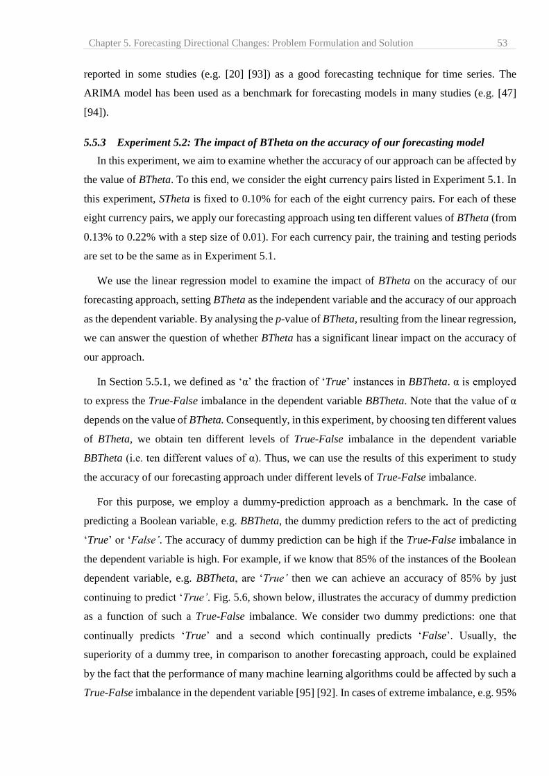
Chapter 5. Forecasting Directional Changes: Problem Formulation and Solution 53
reported in some studies (e.g. [20] [93]) as a good forecasting technique for time series. The
ARIMA model has been used as a benchmark for forecasting models in many studies (e.g. [47]
[94]).
5.5.3 Experiment 5.2: The impact of BTheta on the accuracy of our forecasting model
In this experiment, we aim to examine whether the accuracy of our approach can be affected by
the value of BTheta. To this end, we consider the eight currency pairs listed in Experiment 5.1. In
this experiment, STheta is fixed to 0.10% for each of the eight currency pairs. For each of these
eight currency pairs, we apply our forecasting approach using ten different values of BTheta (from
0.13% to 0.22% with a step size of 0.01). For each currency pair, the training and testing periods
are set to be the same as in Experiment 5.1.
We use the linear regression model to examine the impact of BTheta on the accuracy of our
forecasting approach, setting BTheta as the independent variable and the accuracy of our approach
as the dependent variable. By analysing the p-value of BTheta, resulting from the linear regression,
we can answer the question of whether BTheta has a significant linear impact on the accuracy of
our approach.
In Section 5.5.1, we defined as ‘α’ the fraction of ‘True’ instances in BBTheta. α is employed
to express the True-False imbalance in the dependent variable BBTheta. Note that the value of α
depends on the value of BTheta. Consequently, in this experiment, by choosing ten different values
of BTheta, we obtain ten different levels of True-False imbalance in the dependent variable
BBTheta (i.e. ten different values of α). Thus, we can use the results of this experiment to study
the accuracy of our forecasting approach under different levels of True-False imbalance.
For this purpose, we employ a dummy-prediction approach as a benchmark. In the case of
predicting a Boolean variable, e.g. BBTheta, the dummy prediction refers to the act of predicting
‘True’ or ‘False’. The accuracy of dummy prediction can be high if the True-False imbalance in
the dependent variable is high. For example, if we know that 85% of the instances of the Boolean
dependent variable, e.g. BBTheta, are ‘True’ then we can achieve an accuracy of 85% by just
continuing to predict ‘True’. Fig. 5.6, shown below, illustrates the accuracy of dummy prediction
as a function of such a True-False imbalance. We consider two dummy predictions: one that
continually predicts ‘True’ and a second which continually predicts ‘False’. Usually, the
superiority of a dummy tree, in comparison to another forecasting approach, could be explained
by the fact that the performance of many machine learning algorithms could be affected by such a
True-False imbalance in the dependent variable [95] [92]. In cases of extreme imbalance, e.g. 95%
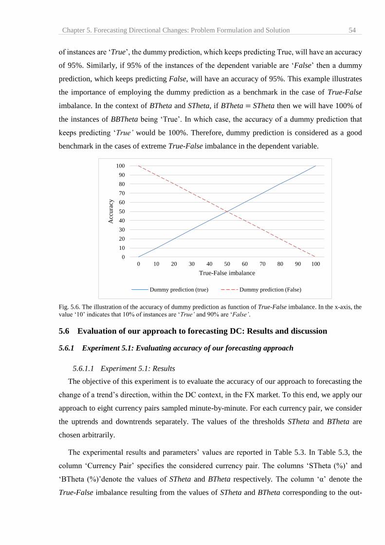
Chapter 5. Forecasting Directional Changes: Problem Formulation and Solution 54
of instances are ‘True’, the dummy prediction, which keeps predicting True, will have an accuracy
of 95%. Similarly, if 95% of the instances of the dependent variable are ‘False’ then a dummy
prediction, which keeps predicting False, will have an accuracy of 95%. This example illustrates
the importance of employing the dummy prediction as a benchmark in the case of True-False
imbalance. In the context of BTheta and STheta, if BTheta = STheta then we will have 100% of
the instances of BBTheta being ‘True’. In which case, the accuracy of a dummy prediction that
keeps predicting ‘True’ would be 100%. Therefore, dummy prediction is considered as a good
benchmark in the cases of extreme True-False imbalance in the dependent variable.
Fig. 5.6. The illustration of the accuracy of dummy prediction as function of True-False imbalance. In the x-axis, the
value ‘10’ indicates that 10% of instances are ‘True’ and 90% are ‘False’.
5.6 Evaluation of our approach to forecasting DC: Results and discussion
5.6.1 Experiment 5.1: Evaluating accuracy of our forecasting approach
5.6.1.1 Experiment 5.1: Results
The objective of this experiment is to evaluate the accuracy of our approach to forecasting the
change of a trend’s direction, within the DC context, in the FX market. To this end, we apply our
approach to eight currency pairs sampled minute-by-minute. For each currency pair, we consider
the uptrends and downtrends separately. The values of the thresholds STheta and BTheta are
chosen arbitrarily.
The experimental results and parameters’ values are reported in Table 5.3. In Table 5.3, the
column ‘Currency Pair’ specifies the considered currency pair. The columns ‘STheta (%)’ and
‘BTheta (%)’denote the values of STheta and BTheta respectively. The column ‘α’ denote the
True-False imbalance resulting from the values of STheta and BTheta corresponding to the out-
0
10
20
30
40
50
60
70
80
90
100
0 10 20 30 40 50 60 70 80 90 100
Acc
ura
cy
True-False imbalance
Dummy prediction (true) Dummy prediction (False)
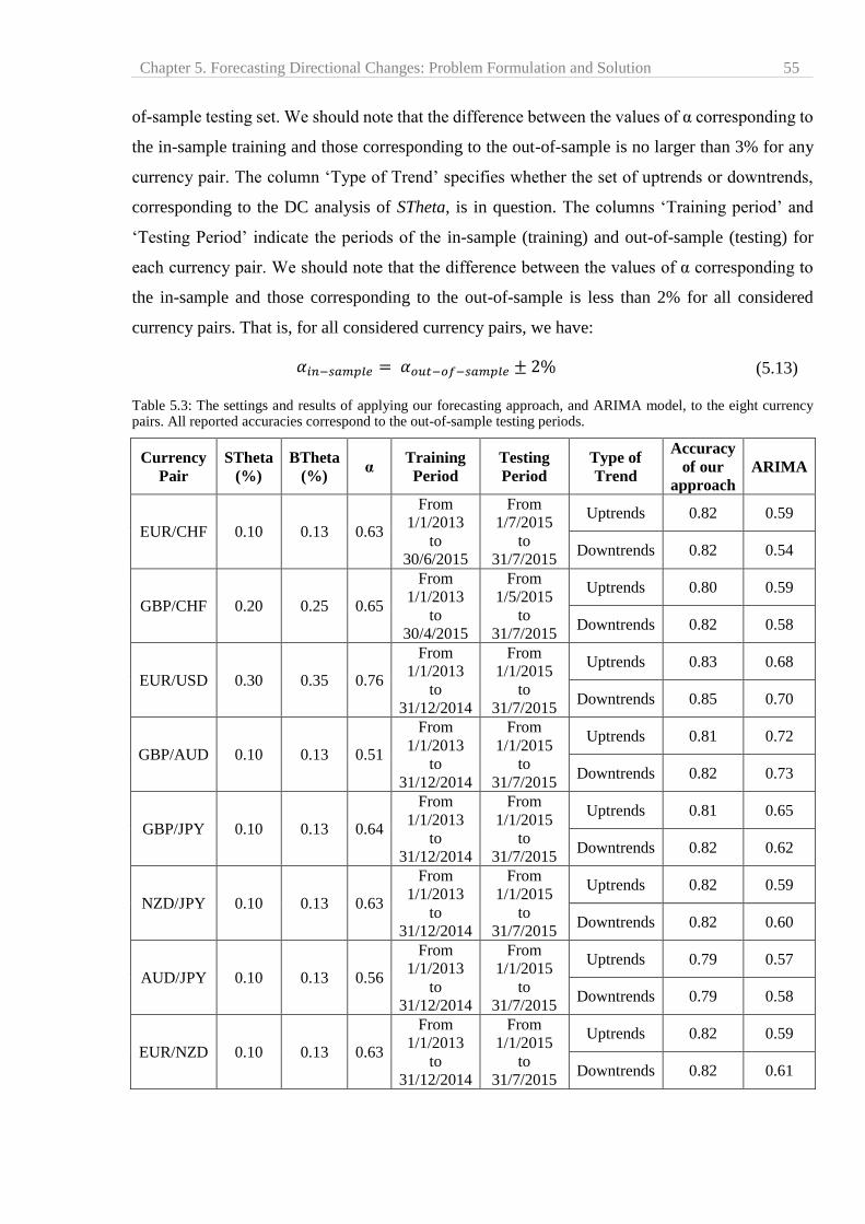
Chapter 5. Forecasting Directional Changes: Problem Formulation and Solution 55
of-sample testing set. We should note that the difference between the values of α corresponding to
the in-sample training and those corresponding to the out-of-sample is no larger than 3% for any
currency pair. The column ‘Type of Trend’ specifies whether the set of uptrends or downtrends,
corresponding to the DC analysis of STheta, is in question. The columns ‘Training period’ and
‘Testing Period’ indicate the periods of the in-sample (training) and out-of-sample (testing) for
each currency pair. We should note that the difference between the values of α corresponding to
the in-sample and those corresponding to the out-of-sample is less than 2% for all considered
currency pairs. That is, for all considered currency pairs, we have:
𝛼𝑖𝑛−𝑠𝑎𝑚𝑝𝑙𝑒 = 𝛼𝑜𝑢𝑡−𝑜𝑓−𝑠𝑎𝑚𝑝𝑙𝑒 ± 2% (5.13)
Table 5.3: The settings and results of applying our forecasting approach, and ARIMA model, to the eight currency pairs. All reported accuracies correspond to the out-of-sample testing periods.
Currency
Pair
STheta
(%)
BTheta
(%) α
Training
Period
Testing
Period
Type of
Trend
Accuracy
of our
approach
ARIMA
EUR/CHF 0.10 0.13 0.63
From
1/1/2013
to
30/6/2015
From
1/7/2015
to
31/7/2015
Uptrends 0.82 0.59
Downtrends 0.82 0.54
GBP/CHF 0.20 0.25 0.65
From
1/1/2013
to
30/4/2015
From
1/5/2015
to
31/7/2015
Uptrends 0.80 0.59
Downtrends 0.82 0.58
EUR/USD 0.30 0.35 0.76
From
1/1/2013
to
31/12/2014
From
1/1/2015
to
31/7/2015
Uptrends 0.83 0.68
Downtrends 0.85 0.70
GBP/AUD 0.10 0.13 0.51
From
1/1/2013
to
31/12/2014
From
1/1/2015
to
31/7/2015
Uptrends 0.81 0.72
Downtrends 0.82 0.73
GBP/JPY 0.10 0.13 0.64
From
1/1/2013
to
31/12/2014
From
1/1/2015
to
31/7/2015
Uptrends 0.81 0.65
Downtrends 0.82 0.62
NZD/JPY 0.10 0.13 0.63
From
1/1/2013
to
31/12/2014
From
1/1/2015
to
31/7/2015
Uptrends 0.82 0.59
Downtrends 0.82 0.60
AUD/JPY 0.10 0.13 0.56
From
1/1/2013
to
31/12/2014
From
1/1/2015
to
31/7/2015
Uptrends 0.79 0.57
Downtrends 0.79 0.58
EUR/NZD 0.10 0.13 0.63
From
1/1/2013
to
31/12/2014
From
1/1/2015
to
31/7/2015
Uptrends 0.82 0.59
Downtrends 0.82 0.61

Chapter 5. Forecasting Directional Changes: Problem Formulation and Solution 56
The column ‘Accuracy’ shows the accuracy of our approach, computed as:
Accuracy =𝑇𝑃+𝑇𝑁
𝑁 (5.14)
where N is either the total number of upward or downward DC events (see the column ‘Type of
Trend’ to know) obtained from running the DC summary of threshold STheta. TP is the number of
correctly forecasted True instances of BBTheta. TN is the number of correctly forecasted False
instances of BBTheta. All reported accuracies in Table 5.3 are measured for the out-of-sample
period of each currency pair. We then compare the accuracy of our approach with the ARIMA
forecasting technique. For this purpose, we symbolize the ‘True’ and ‘False’ instances of BBTheta
as ‘1’ and ‘0’ respectively. Then we apply ARIMA to the composed sequence of ‘1’ and ‘0’. We
use the function auto.arima() from the package ‘forecast’ of the statistical software R to predict
BBTheta. The forecasting accuracy of the ARIMA model is reported in column ‘ARIMA’ in Table
5.3.
5.6.1.2 Experiment 5.1: Results’ discussion
The objective of this experiment is to examine the accuracy of our forecasting approach. As can
be seen in Table 5.3, for different testing periods and different selected values of STheta and
BTheta, each of the obtained accuracies of our forecasting approach is above 0.78 (i.e. 78%). These
results indicate that the proposed independent variable, 𝑂𝑆𝑉𝐵𝑇ℎ𝑒𝑡𝑎𝑆𝑇ℎ𝑒𝑡𝑎, is very useful for forecasting
BBTheta. The column ‘ARIMA’ in Table 5.3 shows the accuracy obtained by forecasting BBTheta
using the ARIMA model. By comparing the accuracies of our approach (reported in column
‘Accuracy of our approach’) and the accuracy of the ARIMA technique (reported in column
‘ARIMA’) we notice that our approach outperforms ARIMA in all cases.
5.6.2 Experiment 5.2: The impact of BTheta on forecasting accuracy
The objective of this experiment is to examine whether the value of BTheta may affect the
accuracy of the forecasting approach proposed in this chapter. To this end, we apply our forecasting
approach to each of the considered eight currency pairs using ten different values of BTheta. For
each value of BTheta, we measure the corresponding accuracy for downtrends and uptrends
separately. To avoid tedious results we report the results of four currency pairs in this section. The
results of the remaining four currency pairs are reported in Appendix C.
5.6.2.1 Experiment 5.2: Results
The results of this experiment relating to the currency pairs EUR/CHF, GBP/CHF, EUR/USD
and GBP/AUD are reported in Tables 5.4, 5.5, 5.6 and 5.7 respectively. Each table, with self-

Chapter 5. Forecasting Directional Changes: Problem Formulation and Solution 57
explanatory column headings, reports the results of applying our forecasting approach to the
uptrends and downtrends of one currency pair. We will also use the results of this experiment to
evaluate the performance of our forecasting approach under different levels of True-False
imbalance in the dependent variable BBTheta.
Table 5.4: Analyzing the impact of BTheta on the accuracy of our forecasting approach on the currency pair EUR/CHF.
STheta is fixed to 0.10%. The testing period is 4 weeks in length. The reported accuracy corresponds to the testing
(out-of-sample) period. The number of DC events of threshold STheta (0.1%) is 327 (i.e. number of instances of
BBTheta is 327).
Uptrends of DC summary with STheta
= 0.10%
Downtrends of DC summary with STheta =
0.10%
BTheta (%) Accuracy α BTheta (%) Accuracy α
0.13 0.82 0.63 0.13 0.82 0.63
0.14 0.78 0.54 0.14 0.78 0.54
0.15 0.74 0.48 0.15 0.75 0.48
0.16 0.72 0.42 0.16 0.72 0.42
0.17 0.70 0.37 0.17 0.70 0.37
0.18 0.67 0.33 0.18 0.67 0.33
0.19 0.65 0.30 0.19 0.66 0.30
0.20 0.64 0.27 0.20 0.64 0.27
0.21 0.63 0.25 0.21 0.64 0.25
0.22 0.62 0.22 0.22 0.62 0.22
Table 5.5: Analysing the impact of BTheta on the accuracy of our forecasting approach on the currency pair GBP/CHF:
STheta is fixed to 0.10%. The testing period is 3 months. The reported accuracy corresponds to the testing (out-of-
sample) period. The number of DC events of threshold 0.1% is 1245 (i.e. number of instances of BBTheta is 1245).
Uptrends of DC summary with STheta
= 0.10%
Downtrends of DC summary with STheta
= 0.10%
BTheta (%) Accuracy α BTheta (%) Accuracy α
0.13 0.82 0.64 0.13 0.81 0.64
0.14 0.79 0.55 0.14 0.77 0.55
0.15 0.75 0.49 0.15 0.75 0.49
0.16 0.73 0.42 0.16 0.71 0.42
0.17 0.71 0.37 0.17 0.70 0.37
0.18 0.69 0.33 0.18 0.68 0.33
0.19 0.67 0.30 0.19 0.66 0.30
0.20 0.64 0.27 0.20 0.64 0.27
0.21 0.64 0.25 0.21 0.64 0.25
0.22 0.62 0.23 0.22 0.63 0.23

Chapter 5. Forecasting Directional Changes: Problem Formulation and Solution 58
Table 5.6: Analysing the impact of BTheta on the accuracy of our forecasting approach on the currency pair EUR/USD:
STheta is fixed to 0.10%. The testing period is 7 months and 2 weeks. The reported accuracy corresponds to the testing
(out-of-sample) period. The number of DC events of threshold 0.1% is 1962 (i.e. number of instances of BBTheta is
1962).
Uptrends of DC summary with STheta
= 0.10%
Downtrends of DC summary with STheta
= 0.10%
BTheta (%) Accuracy α BTheta (%) Accuracy α
0.13 0.82 0.64 0.13 0.80 0.64
0.14 0.80 0.56 0.14 0.77 0.56
0.15 0.77 0.50 0.15 0.74 0.50
0.16 0.74 0.45 0.16 0.72 0.45
0.17 0.71 0.40 0.17 0.70 0.40
0.18 0.70 0.36 0.18 0.67 0.36
0.19 0.68 0.33 0.19 0.65 0.33
0.20 0.64 0.30 0.20 0.66 0.30
0.21 0.65 0.28 0.21 0.63 0.28
0.22 0.64 0.26 0.22 0.62 0.26
Table 5.7: Analysing the impact of BTheta on the accuracy of our forecasting approach on the currency pair GBP/AUD:
STheta is fixed to 0.10%. The testing period is 7 months. The reported accuracy corresponds to the testing (out-of-
sample) period. The number of DC events of threshold 0.1% is 3682 (i.e. number of instances of BBTheta is 3682).
Uptrends of DC summary with STheta
= 0.10%
Downtrends of DC summary with STheta
= 0.10%
BTheta (%) Accuracy α BTheta (%) Accuracy α
0.13 0.81 0.51 0.13 0.82 0.51
0.14 0.78 0.49 0.14 0.78 0.49
0.15 0.75 0.47 0.15 0.75 0.47
0.16 0.72 0.45 0.16 0.72 0.45
0.17 0.70 0.41 0.17 0.70 0.41
0.18 0.68 0.37 0.18 0.68 0.37
0.19 0.67 0.34 0.19 0.67 0.34
0.20 0.66 0.30 0.20 0.65 0.30
0.21 0.65 0.28 0.21 0.64 0.28
0.22 0.63 0.26 0.22 0.63 0.26
5.6.2.2 Experiment 5.2: Results’ discussion
The objective of this experiment was to ascertain whether the value of BTheta affects the
accuracy of our approach. In each of the Tables 5.4 through 5.7, we note that the values in column
‘Accuracy’ increase as ‘BTheta (%)’ decreases. To statistically validate this observation, we apply
a linear regression model in which the column ‘BTheta (%)’ symbolises the independent variable
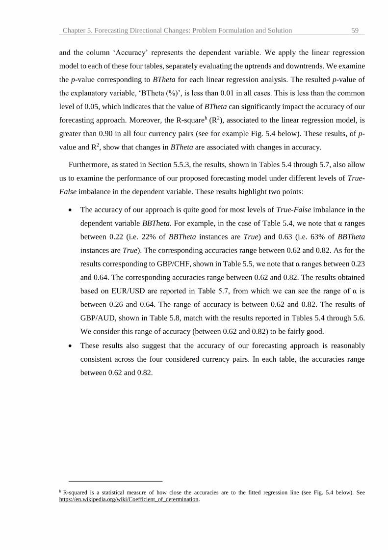
Chapter 5. Forecasting Directional Changes: Problem Formulation and Solution 59
and the column ‘Accuracy’ represents the dependent variable. We apply the linear regression
model to each of these four tables, separately evaluating the uptrends and downtrends. We examine
the p-value corresponding to BTheta for each linear regression analysis. The resulted p-value of
the explanatory variable, ‘BTheta (%)’, is less than 0.01 in all cases. This is less than the common
level of 0.05, which indicates that the value of BTheta can significantly impact the accuracy of our
forecasting approach. Moreover, the R-squareh (R2), associated to the linear regression model, is
greater than 0.90 in all four currency pairs (see for example Fig. 5.4 below). These results, of p-
value and R2, show that changes in BTheta are associated with changes in accuracy.
Furthermore, as stated in Section 5.5.3, the results, shown in Tables 5.4 through 5.7, also allow
us to examine the performance of our proposed forecasting model under different levels of True-
False imbalance in the dependent variable. These results highlight two points:
The accuracy of our approach is quite good for most levels of True-False imbalance in the
dependent variable BBTheta. For example, in the case of Table 5.4, we note that α ranges
between 0.22 (i.e. 22% of BBTheta instances are True) and 0.63 (i.e. 63% of BBTheta
instances are True). The corresponding accuracies range between 0.62 and 0.82. As for the
results corresponding to GBP/CHF, shown in Table 5.5, we note that α ranges between 0.23
and 0.64. The corresponding accuracies range between 0.62 and 0.82. The results obtained
based on EUR/USD are reported in Table 5.7, from which we can see the range of α is
between 0.26 and 0.64. The range of accuracy is between 0.62 and 0.82. The results of
GBP/AUD, shown in Table 5.8, match with the results reported in Tables 5.4 through 5.6.
We consider this range of accuracy (between 0.62 and 0.82) to be fairly good.
These results also suggest that the accuracy of our forecasting approach is reasonably
consistent across the four considered currency pairs. In each table, the accuracies range
between 0.62 and 0.82.
h R-squared is a statistical measure of how close the accuracies are to the fitted regression line (see Fig. 5.4 below). See
https://en.wikipedia.org/wiki/Coefficient_of_determination.
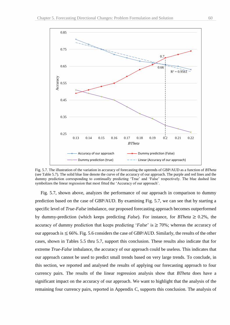
Chapter 5. Forecasting Directional Changes: Problem Formulation and Solution 60
Fig. 5.7. The illustration of the variation in accuracy of forecasting the uptrends of GBP/AUD as a function of BTheta
(see Table 5.7). The solid blue line denote the curve of the accuracy of our approach. The purple and red lines and the
dummy prediction corresponding to continually predicting ‘True’ and ‘False’ respectively. The blue dashed line
symbolizes the linear regression that most fitted the ‘Accuracy of our approach’.
Fig. 5.7, shown above, analyzes the performance of our approach in comparison to dummy
prediction based on the case of GBP/AUD. By examining Fig. 5.7, we can see that by starting a
specific level of True-False imbalance, our proposed forecasting approach becomes outperformed
by dummy-prediction (which keeps predicting False). For instance, for BTheta ≥ 0.2%, the
accuracy of dummy prediction that keeps predicting ‘False’ is ≥ 70%; whereas the accuracy of
our approach is ≤ 66%. Fig. 5.6 considers the case of GBP/AUD. Similarly, the results of the other
cases, shown in Tables 5.5 thru 5.7, support this conclusion. These results also indicate that for
extreme True-False imbalance, the accuracy of our approach could be useless. This indicates that
our approach cannot be used to predict small trends based on very large trends. To conclude, in
this section, we reported and analysed the results of applying our forecasting approach to four
currency pairs. The results of the linear regression analysis show that BTheta does have a
significant impact on the accuracy of our approach. We want to highlight that the analysis of the
remaining four currency pairs, reported in Appendix C, supports this conclusion. The analysis of
0.66
0.7
R² = 0.9561
0.25
0.35
0.45
0.55
0.65
0.75
0.85
0.13 0.14 0.15 0.16 0.17 0.18 0.19 0.2 0.21 0.22
Acc
ura
cy
BTheta
Accuracy of our approach Dummy prediction (False)
Dummy prediction (true) Linear (Accuracy of our approach)

Chapter 5. Forecasting Directional Changes: Problem Formulation and Solution 61
the same results also suggest that our forecasting model can be outperformed by dummy prediction
under specific conditions.
5.7 Summary and conclusion
In this chapter, we addressed the problem of forecasting the change of a trend’s direction within
the DC framework. Our first objective was to formalize the considered forecasting problem under
the DC context. The second objective was to provide a solution for this problem.
The first contribution of this chapter was in formulating the prediction of the change of direction
of a market’s trend under the DC framework. For this purpose we proposed tracking price
movements using 2 concurrent DC thresholds: STheta and BTheta. Our task was to forecast
whether a DC trend, as observed under threshold STheta, would continue so that its total magnitude
could be at least equal to BTheta. We introduced a new concept named Big-Theta that originates
from the DC framework. The notion of Big-Theta states that a DC event of threshold BTheta will
embrace at least one DC event of a smaller threshold STheta (with BTheta > STheta). We used the
concept of Big-Theta to introduce the Boolean variable named BBTheta (Section 5.2.1). The value
of BBTheta expresses whether the total price change of a DC trend, as observed under the threshold
STheta, reaches BTheta (Section 5.3). Thus, our objective was to forecast BBTheta.
Our second contribution was in identifying one novel DC-based indicator as the independent
variable and in proving that it is relevant to our prediction problem. This DC-based indicator, also
based on the concept of Big-Theta, is 𝑂𝑆𝑉𝐵𝑇ℎ𝑒𝑡𝑎𝑆𝑇ℎ𝑒𝑡𝑎(Section 5.4). We used the machine learning
procedure J48 to detect the relation between 𝑂𝑆𝑉𝐵𝑇ℎ𝑒𝑡𝑎𝑆𝑇ℎ𝑒𝑡𝑎 and BBTheta.
We examined the performance of our forecasting approach using eight currency pairs sampled
minute-by-minute (Section 5.5). The results demonstrated that our approach outperforms the
traditional forecasting technique ARIMA (Table 5.4, Section 5.6.1), with the accuracy of our
approach ranging between 62% and 80% (Section 5.6.2). We consider this range as pretty good.
However, the results also suggested that the accuracy of our approach decreases as the difference
between STheta and BTheta increases. When this difference reaches a specific level, our approach
is outperformed by a dummy prediction, which keeps predicting False (Section 5.6.2).
To conclude, we believe that this is the first attempt to forecast the change of a trend’s direction
under the DC-framework. Our contribution is in formulating the forecasting problem and
proposing a solution. We shortened the formalization of this problem in order to forecast one
Boolean variable named BBTheta. The proposed solution comprises the discovery of a novel DC-

Chapter 5. Forecasting Directional Changes: Problem Formulation and Solution 62
based indicator named 𝑂𝑆𝑉𝐵𝑇ℎ𝑒𝑡𝑎𝑆𝑇ℎ𝑒𝑡𝑎 . We demonstrated that 𝑂𝑆𝑉𝐵𝑇ℎ𝑒𝑡𝑎
𝑆𝑇ℎ𝑒𝑡𝑎 is helpful in forecasting
BBTheta. We argued that our forecasting approach is more accurate than the ARIMA model and
that the change of a trend’s direction is predictable under the DC framework with pretty good
accuracy.
Chapter 6. TSFDC: A Trading Strategy Based on Forecasting Directional Changes 63
6 TSFDC: A Trading Strategy Based on Forecasting Directional
Changes
The previous chapter introduced an approach to forecasting the change in direction of a
market’s trend under the Directional Changes (DC) framework. Based on our findings in Chapter
5, this chapter aims to develop a successful trading strategy founded on the established forecasting
model. In order to examine the success of this proposed trading strategy, called TSFDC, we
provide several experiments using eight currency pairs from the FX market. The results suggest
that, after deducting the bid and ask spread (but not the transaction costs), TSFDC can generate
returns of more than 40% within seven months. We argue that TSFDC outperforms another DC-
based trading strategy.
6.1 Introduction
The objective of this thesis is to explore, and consequently to provide a proof of, the usefulness
of the DC framework as the basis of a profitable trading strategy. In Chapter 3, we suggested that
existing trading strategies can mostly be categorised into two groups (see Sections 3.2 and 3.3).
The first group contains trading strategies that are based on forecasting models (e.g. [6] [41] [42]
[43] [44] [45]). The second group consists of trading strategies that do not rely on any forecasting
model (e.g. [3] [57] [58] [59] [96]). In line with the literature, in this thesis we aim to develop two
DC-based trading strategies – one strategy belongs to the first identified group of trading strategies
and the second strategy belongs to the second group.
In Chapter 5, we formalized the problem of forecasting the change of a trend’s direction under
the DC framework. In this chapter, we develop a trading strategy named ‘Trading Strategy based
on Forecasting DC’, henceforth TSFDC. TSFDC relies on the forecasting model developed in
Chapter 5 to decide when to start a trade. We provide a set of experiments to examine the
performance of TSFDC using eight currency pairs from the FX market.
The chapter continues as follows: Section 6.2 provides a brief summary of the forecasting model
introduced in Chapter 5. We present TSFDC and its trading rules in Section 6.3. We discuss the
selection and preparation of the used datasets in Section 6.4. The details of the experiments,
conducted to evaluate the performance of TSFDC, are provided in Section 6.5. Section 6.6 reports
and discusses the results of these experiments. We compare our trading strategy with other DC-
based strategies in Section 6.7. Finally, we summarize the major findings of this chapter in Section
6.8.
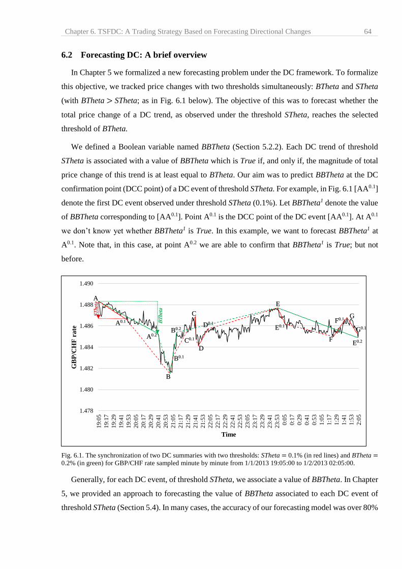
Chapter 6. TSFDC: A Trading Strategy Based on Forecasting Directional Changes 64
6.2 Forecasting DC: A brief overview
In Chapter 5 we formalized a new forecasting problem under the DC framework. To formalize
this objective, we tracked price changes with two thresholds simultaneously: BTheta and STheta
(with BTheta > STheta; as in Fig. 6.1 below). The objective of this was to forecast whether the
total price change of a DC trend, as observed under the threshold STheta, reaches the selected
threshold of BTheta.
We defined a Boolean variable named BBTheta (Section 5.2.2). Each DC trend of threshold
STheta is associated with a value of BBTheta which is True if, and only if, the magnitude of total
price change of this trend is at least equal to BTheta. Our aim was to predict BBTheta at the DC
confirmation point (DCC point) of a DC event of threshold STheta. For example, in Fig. 6.1 [AA0.1]
denote the first DC event observed under threshold STheta (0.1%). Let BBTheta1 denote the value
of BBTheta corresponding to [AA0.1]. Point A0.1 is the DCC point of the DC event [AA0.1]. At A0.1
we don’t know yet whether BBTheta1 is True. In this example, we want to forecast BBTheta1 at
A0.1. Note that, in this case, at point A0.2 we are able to confirm that BBTheta1 is True; but not
before.
Fig. 6.1. The synchronization of two DC summaries with two thresholds: STheta = 0.1% (in red lines) and BTheta =
0.2% (in green) for GBP/CHF rate sampled minute by minute from 1/1/2013 19:05:00 to 1/2/2013 02:05:00.
Generally, for each DC event, of threshold STheta, we associate a value of BBTheta. In Chapter
5, we provided an approach to forecasting the value of BBTheta associated to each DC event of
threshold STheta (Section 5.4). In many cases, the accuracy of our forecasting model was over 80%
1.478
1.480
1.482
1.484
1.486
1.488
1.490
19:0
5
19:1
7
19:2
9
19:4
1
19:5
3
20:0
5
20:1
7
20:2
9
20:4
1
20:5
3
21:0
5
21:1
7
21:2
9
21:4
1
21:5
3
22:0
5
22:1
7
22:2
9
22:4
1
22:5
3
23:0
5
23:1
7
23:2
9
23:4
1
23:5
3
0:0
5
0:1
7
0:2
9
0:4
1
0:5
3
1:0
5
1:1
7
1:2
9
1:4
1
1:5
3
2:0
5
GB
P/C
HF
ra
te
Time
A0.2
A
B
B0.2
E0.2
E
B0.1
C
C0.1
D0.1
D
F0.1
E0.1
F
G
G0.1 A0.1
ST
het
a
BT
het
a
Chapter 6. TSFDC: A Trading Strategy Based on Forecasting Directional Changes 65
(see Table 5.4, Section 5.6.1). In this chapter, our objective is to develop a successful trading
strategy based on this forecasting model.
6.3 Introducing the trading strategy TSFDC
In this section we introduce a DC based trading strategy named ‘Trading Strategy based on
Forecasting DC’ (TSFDC). TSFDC is designed as a contrarian trading strategy (i.e. TSFDC
generates buy and sell signals against the market’s trend) and is based on the forecasting model
established in Chapter 5. We present two versions of TSFDC: TSFDC-down and TSFDC-up. The
former is to be applied if the market exhibits a downward trend under the DC context, with the
latter employed in the opposite case. We want to highlight that TSFDC-down and TSFDC-up are
two different and independent strategies. They will be trained and tested separately. The following
explains how TSFDC-down and TSFDC-up operate.
6.3.1 TSFDC-down
TSFDC-down is only applicable when the market is in a downtrend. TSFDC-down relies on the
forecasting approach presented in Chapter 5 to decide when to trigger a buy signal. Let BBThetai
be the value of BBTheta associated with the ith DC event of threshold STheta (Section 5.2.2). Let
FBBThetai denote the forecasted value of BBThetai. The value of FBBThetai is determined based
on the forecasting model described in Chapter 5. Note that we compute the value of FBBThetai at
the DCC point of the ith DC event of threshold STheta (e.g. FBBTheta1 is calculated at point A0.1
in Fig. 6.1 above). If FBBThetai is True, then we anticipate that the total price change of the ith DC
trend, observed under threshold STheta, will be at least equal to BTheta. TSFDC-down relies on
FBBThetai to decide when to trigger a buy signal. More particularly, there are two conditions under
which TSFDC-down generates a buy signal (depending on whether FBBThetai is True or False):
At the DCC point for the ith DC trend (STheta), we predict FBBThetai:
Rule TSFDC-down.1 (generate buy signal):
If FBBThetai = False then generate buy signal.
Rule TSFDC-down.2 (generate buy signal):
If (FBBThetai = True) and (we confirm a new DC event of threshold BTheta) then
generate buy signal.
Rule TSFDC-down.3 (generate sell signal):
If (𝑃𝑐 ≥ PDCC↑) and (a buy order has been fulfilled) then generate sell signal.
with 𝑃𝑐 denoting the current price and PDCC↑ denoting the minimum prices required to confirm the
occurrence of the succeeding uptrend DC event of threshold STheta (see Section 4.2.3). If the

Chapter 6. TSFDC: A Trading Strategy Based on Forecasting Directional Changes 66
condition of Rule TSFDC-down.1 is satisfied, then TSFDC-down generates a buy signal at the
DCC point as observed under the threshold STheta. On the other hand, if both conditions of Rule
TSFDC-down.2 are fulfilled then TSFDC-down generates a buy signal at the DCC point as
observed under the threshold BTheta. The first condition of Rule TSFDC-down.3, i.e. 𝑃𝑐 ≥ PDCC↑,
denote the case under which we confirm the DCC point of a new uptrend DC event of threshold
STheta. It is important to note that Rule TSFDC-down.3 is not a stand-alone rule in the sense that
it does not open any short position. Rule TSFDC-down.3 initiates a sell signal only if a buy order
has been previously triggered and executed (either by TSFDC-down.1 or TSFDC-down.2).
TSFDC-down.3 plays two simultaneous roles: take-profit and stop-loss. When TSFC-down.3
triggers a sell signal, it may incur losses (hence, functioning as stop-loss) or generates profit (thus,
working as take-profit). In our experiments we will consider the bid and ask prices. When TSFDC-
down triggers a buy (sell) signal we use the ask (bid) price as quoted by the market maker.
Appendix D provides a pseudo-code that clarifies how TSFDC-down uses the forecasting model
established in Chapter 5 and the three trading rules to trade.
Table 6.1, shown below, exemplifies two DC summaries with two different thresholds: 0.10%
(STheta) and 0.20% (BTheta). We use Table 6.1 to provide two trading scenarios that demonstrate
the function of TSFDC-down’s trading rules. Scenario 1: Consider the DC event [AA0.1] (of
threshold STheta = 0.10%) which starts at point A (see column ‘Point’, Table 6.1).
a) [AA0.1] refers to a downward DC event of threshold 0.10% which starts at time 19:05:00
(shown in column ‘Time’, Table 6.1). Point A0.1 is the DCC point of [AA0.1] as observed
at time at time 19:50:00. At point A0.1, assume that we predicti FBBTheta1 is True (as
shown in column ‘FBBTheta’).
b) [AA0.2] refers to a downward DC event of threshold 0.20% which starts at time 19:05:00.
Point A0.2 is the DCC point of [AA0.2] as observed at time 20:40:00.
c) Based on a) and b), the conditions of Rule TSFDC-down.2 are fulfilled at point A0.2.
Thus, TSFDC-down initiates a buy signal at point A0.2 (i.e. at time 20:40:00).
d) [BB0.1] refers to the uptrend DC event, of the threshold 0.10%, that directly follows
[AA0.1]. At time 21:05:00, we confirm the DCC point of [BB0.1], which is B0.1.
Following Rule TSFDC-down.3, TSFDC-down will trigger a sell signal at point B0.1.
i As [AA0.1] is the first DC event in Table 6.1, our objective is to forecast the value of BBTheta1. Here, we denote by FBBTheta1
the forecasted value of BBTheta1.

Chapter 6. TSFDC: A Trading Strategy Based on Forecasting Directional Changes 67
Table 6.1: The synchronization of two DC summaries of GBP/CHF mid-prices sampled between 19:05:00 1/1/2013
and 00:06:00 2/1/2013. The two thresholds are: STheta = 0.10% and BTheta = 0.20%. Unnecessary minutes and
prices are omitted. The ‘True’ and ‘False’ shown in column ‘FBBTheta’ are hypothetical (for explanation purpose
only).
Time Mid-
price
DC Summary
(STheta = 0.1%)
DC Summary
(BTheta = 0.2%) Point FBBTheta
19:05:00 1.48831 start DC event
(DOWNTREND)
start DC event
(DOWNTREND) A
…………
19:50:00 1.48660 start OS event
(DOWNTREND) A0.1 True
…………
20:40:00 1.48530 start OS event
(DOWNTREND) A0.2
…………
21:00:00 1.48150 start DC event
(UPTREND)
start DC event
(UPTREND) B
21:01:00 1.48180
21:02:00 1.48170
21:03:00 1.48159
21:04:00 1.48280
21:05:00 1.48310 start OS event
(UPTREND) B0.1 True
21:06:00 1.48365
21:07:00 1.48430
21:08:00 1.48390
21:09:00 1.48380
21:10:00 1.48541 start OS event
(UPTREND) B0.2
…………
21:41:00 1.48690 start DC event
(DOWNTREND) C
21:42:00 1.48480 start OS event
(DOWNTREND) C0.1 False
21:43:00 1.48470
21:44:00 1.48520
21:45:00 1.48495
21:46:00 1.48412 start DC event
(UPTREND) D
…………
22:01:00 1.48570 start OS event
(UPTREND) D0.1 False
…………
23:45:00 1.48770 start DC event
(DOWNTREND) E
…………
00:06:00 1.48620 start OS event
(DOWNTREND) E0.1
Chapter 6. TSFDC: A Trading Strategy Based on Forecasting Directional Changes 68
Scenario 2: Consider the downward DC event [CC0.1] which starts at time 21:41:00.
a) [CC0.1] refers to a downward DC event of threshold 0.10% which starts at time 21:41:00.
[CC0.1] is the third DC event in Table 6.1. At point C0.1 (at time 21:42:00) assume that
we predict FBBTheta3 is False (as shown in column ‘FBBTheta’).
b) Based on a), the condition of Rule TSFDC-down.1 holds at point C0.1. Thus, TSFDC-
down initiates a buy signal at point C0.1.
c) [DD0.1] refers to the upward DC event of threshold 0.10% which directly follow [CC0.1].
At time 22:01:00, we confirm the DCC point of [DD0.1], which is D0.1. Following Rule
TSFDC-down.3, TSFDC-down will trigger a sell signal at point D0.1.
6.3.2 TSFDC-up
Firstly, we want to highlight that TSFDC-up is completely independent from TSFDC-down.
The two versions of TSFDC are not run concurrently. They are two different strategies that are
trained, applied and evaluated separately. TSFDC-up could be considered as the mirror of TSFDC-
down in that it is only applicable when the market exhibits an upward trend. TSFDC-up uses
FBBThetai (i.e. the forecasted value of BBThetai) to decide when to open a position. TSFDC-up
relies on FBBThetai to decide when to trigger a sell signal. More particularly, there are two
conditions under which TSFDC-up generates a sell signalj (depending on whether FBBThetai is
True or False):
At the DCC point for the ith DC trend (STheta), we predict FBBThetai:
Rule TSFDC-up.1 (generate sell signal):
If FBBThetai = False then generate sell signal.
Rule TSFDC-up.2 (generate sell signal):
If (FBBThetai = True) and (we confirm a new DCC point of DC event of threshold
BTheta) then generate sell signal.
Rule TSFDC-up.3 (generate buy signal):
If (𝑃𝑐 ≤ PDCC↓) and (a sell order has been fulfilled) then generate buy signal.
Note that if the condition of Rule TSFDC-up.1 is True then TSFDC-up generates a sell signal
at the DCC point observed under threshold STheta. On the other hand, if the conditions of Rule
TSFDC-up.2 are both True then TSFDC-up triggers a sell signal at the DCC point observed under
j We want to highlight that no short selling is allowed. In case of a sell signal, we assume that we use the counter currency to buy
base currency.
Chapter 6. TSFDC: A Trading Strategy Based on Forecasting Directional Changes 69
threshold BTheta. In this context, a ‘sell’ signal means that TSFDC-up sells the base currency in
exchange for the counter currency, whereas a ‘buy’ signal means that TSFDC-up buys the base
currency using the counter currency (see Section 2.2 for more detail about base and counter
currencies).
The first condition of Rule TSFDC-up.3, i.e. 𝑃𝑐 ≤ PDCC↓, denote the case under which we
confirm the DCC point for a new DC downtrend of threshold STheta. PDCC↓ denote the price
required to confirm the right-next downtrend (see Section 4.2.3). Rule TSFDC-up.3 is applicable
only if a sell signal has been triggered and executed (either by TSFDC-up.1 or TSFDC-up.2). When
TSFDC-up triggers a buy signal, it may generate profits or losses. Rule TSFDC-up.3 has the same
role as Rule TSFDC-down.3: to take-profits and stop-loss.
We use Table 6.1, shown above, to provide two trading scenarios in demonstration of how
TSFDC-up’s rules are applied. Scenario 1: Consider the uptrend DC event [BB0.1] (of threshold
STheta = 0.10%):
a) [BB0.1] refers to an upward DC event of threshold 0.10% that starts at time 21:00:00
(shown in column ‘Time’, Table 6.1). Point B0.1 is the DCC point of [BB0.1] as observed
at time at time 21:05:00. At point B0.1, assume that we predict FBBTheta2 is True (as
shown in column ‘FBBTheta’).
b) [BB0.2] refers to an upward DC event of threshold 0.20% that starts at time 21:00:00.
Point B0.2 is the DCC point of [BB0.2] as observed at time 21:10:00.
c) Based on a) and b), the conditions of Rule TSFDC-up.2 are fulfilled at point B0.2. Thus,
TSFDC-up initiates a sell signal at point B0.2 (i.e. at time 21:10:00).
d) [CC0.1] refers to the uptrend DC event, of the threshold 0.10%, that directly follows
[BB0.1]. At time 21:42:00, we confirm the DCC point of [CC0.1], which is C0.1. Following
Rule TSFDC-up.3, TSFDC-up will trigger a buy signal at point C0.1.
Scenario 2: Consider the upward DC event [DD0.1] (of threshold STheta = 0.10%).
a) At time 22:01:00, at point D0.1, assume that we predict FBBTheta4 is False (as shown in
column ‘FBBTheta’).
b) Based on a), the condition of Rule TSFDC-up.1 holds at point D0.1. Thus, TSFDC-up
initiates a sell signal at point D0.1.
c) [EE0.1] refers to the downward DC event of threshold 0.10% that directly follows [DD0.1].
At time 00:06:00, we confirm the DCC point [EE0.1], which is E0.1. Following Rule
TSFDC-up.3, TSFDC-up will trigger a buy signal at point E0.1.

Chapter 6. TSFDC: A Trading Strategy Based on Forecasting Directional Changes 70
6.4 Preparation of the datasets and other considerations
This section provides essential notes regarding the selection and preparation of the datasets used
in our experiments. When designing our experiment approach, we paid attention to important
concerns put forward by other studies (e.g. [52] [97]) that highlight serious experimental flaws
presented in several published papers. In the context of our experiments, we consider the following
points:
6.4.1 Data selection
Pardo [52] emphasizes the importance of backtesting (see Section 3.4 for the definition of
backtesting) using a set of assets with different trends. Such variation in the selected dataset will
help to test the performance of the trading strategy under different market scenarios. This
broadening helps in avoiding any bias towards particular patterns. In this chapter, we consider
eight currency pairs, namely: EUR/CHF, GBP/CHF, EUR/USD, GBP/AUD, GBP/JPY, NZD/JPY,
AUD/JPY, and EUR/NZD. The mid-prices of these currency pairs are sampled minute-by-minute
during a period of 31 months between 01/01/2013 and 31/07/2015. Our focus, in this section, is to
examine the variation of the trends of these currency pairs during the (out-of-sample) trading
period which lasts from 1/1/2015 to 31/7/2015. The training (in-sample) period took place between
1/1/2013 and 31/12/2014. Holidays and weekends are not included in our datasets.
In this section, we investigate the variation of the trends of the selected currency pairs. Variation
is important because some studies (e.g. [52]) have shown that trend changes can have a large and
often negative impact on trading performance. Fig. 6.2, shown below, depicts the normalized daily
exchange rates of the selected eight currency pairs throughout the considered trading period of
seven months (from 1/1/2015 to 31/7/2015). It provides a visual indication as to the existence of a
variety of trends in our dataset over the considered trading period. The variation of the trends, as
visualized in Fig. 6.2, indicate that we avoid possible bias in our experiment, which would have
occurred had we only picked currency pairs with similar trends during the selected trading period.
Fig. 6.2 indicates that the selected currency pairs exhibit different trends during the trading
period. The trends of the training period, considered from 1/1/2013 to 31/12/2014, were not studied
as this data is not specifically related to the evaluation of the performance of TSFDC during the
out-of-sample period. Note that although our initial datasets in this experiment (i.e. the eight
currency pairs) are sampled as a time series (with a time interval of one minute), the TSFDC’s
trading rules (presented in Section 6.3) are based on variables (e.g. FBBTheta) that originate from
the DC concept.
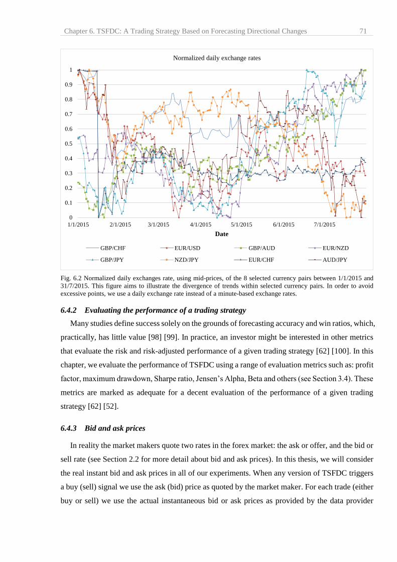
Chapter 6. TSFDC: A Trading Strategy Based on Forecasting Directional Changes 71
Fig. 6.2 Normalized daily exchanges rate, using mid-prices, of the 8 selected currency pairs between 1/1/2015 and
31/7/2015. This figure aims to illustrate the divergence of trends within selected currency pairs. In order to avoid
excessive points, we use a daily exchange rate instead of a minute-based exchange rates.
6.4.2 Evaluating the performance of a trading strategy
Many studies define success solely on the grounds of forecasting accuracy and win ratios, which,
practically, has little value [98] [99]. In practice, an investor might be interested in other metrics
that evaluate the risk and risk-adjusted performance of a given trading strategy [62] [100]. In this
chapter, we evaluate the performance of TSFDC using a range of evaluation metrics such as: profit
factor, maximum drawdown, Sharpe ratio, Jensen’s Alpha, Beta and others (see Section 3.4). These
metrics are marked as adequate for a decent evaluation of the performance of a given trading
strategy [62] [52].
6.4.3 Bid and ask prices
In reality the market makers quote two rates in the forex market: the ask or offer, and the bid or
sell rate (see Section 2.2 for more detail about bid and ask prices). In this thesis, we will consider
the real instant bid and ask prices in all of our experiments. When any version of TSFDC triggers
a buy (sell) signal we use the ask (bid) price as quoted by the market maker. For each trade (either
buy or sell) we use the actual instantaneous bid or ask prices as provided by the data provider
0
0.1
0.2
0.3
0.4
0.5
0.6
0.7
0.8
0.9
1
1/1/2015 2/1/2015 3/1/2015 4/1/2015 5/1/2015 6/1/2015 7/1/2015
Date
Normalized daily exchange rates
GBP/CHF EUR/USD GBP/AUD EUR/NZD
GBP/JPY NZD/JPY EUR/CHF AUD/JPY
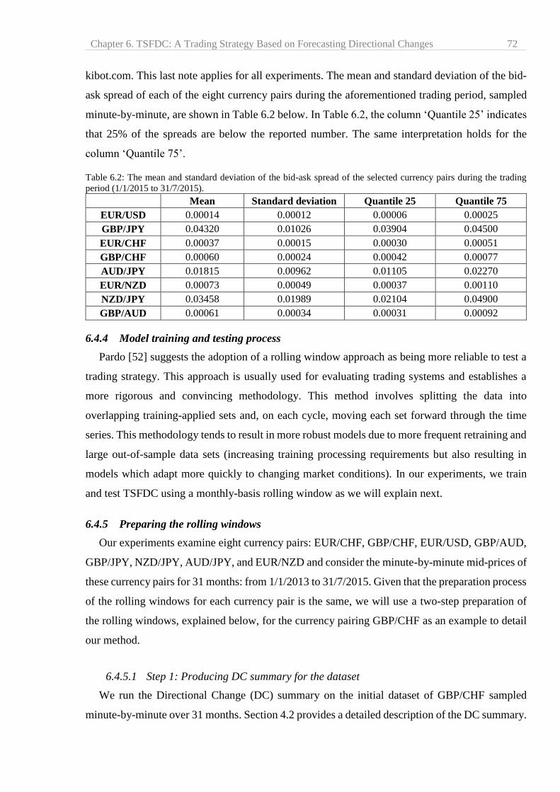
Chapter 6. TSFDC: A Trading Strategy Based on Forecasting Directional Changes 72
kibot.com. This last note applies for all experiments. The mean and standard deviation of the bid-
ask spread of each of the eight currency pairs during the aforementioned trading period, sampled
minute-by-minute, are shown in Table 6.2 below. In Table 6.2, the column ‘Quantile 25’ indicates
that 25% of the spreads are below the reported number. The same interpretation holds for the
column ‘Quantile 75’.
Table 6.2: The mean and standard deviation of the bid-ask spread of the selected currency pairs during the trading
period (1/1/2015 to 31/7/2015).
Mean Standard deviation Quantile 25 Quantile 75
EUR/USD 0.00014 0.00012 0.00006 0.00025
GBP/JPY 0.04320 0.01026 0.03904 0.04500
EUR/CHF 0.00037 0.00015 0.00030 0.00051
GBP/CHF 0.00060 0.00024 0.00042 0.00077
AUD/JPY 0.01815 0.00962 0.01105 0.02270
EUR/NZD 0.00073 0.00049 0.00037 0.00110
NZD/JPY 0.03458 0.01989 0.02104 0.04900
GBP/AUD 0.00061 0.00034 0.00031 0.00092
6.4.4 Model training and testing process
Pardo [52] suggests the adoption of a rolling window approach as being more reliable to test a
trading strategy. This approach is usually used for evaluating trading systems and establishes a
more rigorous and convincing methodology. This method involves splitting the data into
overlapping training-applied sets and, on each cycle, moving each set forward through the time
series. This methodology tends to result in more robust models due to more frequent retraining and
large out-of-sample data sets (increasing training processing requirements but also resulting in
models which adapt more quickly to changing market conditions). In our experiments, we train
and test TSFDC using a monthly-basis rolling window as we will explain next.
6.4.5 Preparing the rolling windows
Our experiments examine eight currency pairs: EUR/CHF, GBP/CHF, EUR/USD, GBP/AUD,
GBP/JPY, NZD/JPY, AUD/JPY, and EUR/NZD and consider the minute-by-minute mid-prices of
these currency pairs for 31 months: from 1/1/2013 to 31/7/2015. Given that the preparation process
of the rolling windows for each currency pair is the same, we will use a two-step preparation of
the rolling windows, explained below, for the currency pairing GBP/CHF as an example to detail
our method.
6.4.5.1 Step 1: Producing DC summary for the dataset
We run the Directional Change (DC) summary on the initial dataset of GBP/CHF sampled
minute-by-minute over 31 months. Section 4.2 provides a detailed description of the DC summary.
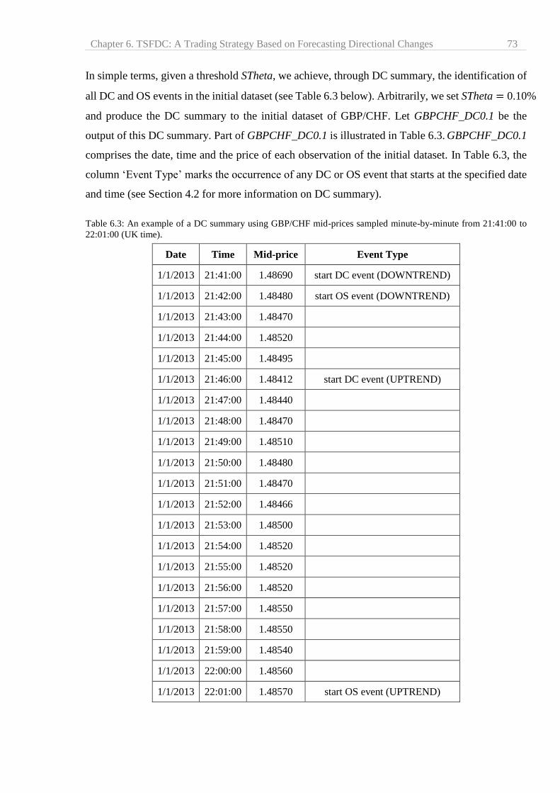
Chapter 6. TSFDC: A Trading Strategy Based on Forecasting Directional Changes 73
In simple terms, given a threshold STheta, we achieve, through DC summary, the identification of
all DC and OS events in the initial dataset (see Table 6.3 below). Arbitrarily, we set STheta=0.10%
and produce the DC summary to the initial dataset of GBP/CHF. Let GBPCHF_DC0.1 be the
output of this DC summary. Part of GBPCHF_DC0.1 is illustrated in Table 6.3. GBPCHF_DC0.1
comprises the date, time and the price of each observation of the initial dataset. In Table 6.3, the
column ‘Event Type’ marks the occurrence of any DC or OS event that starts at the specified date
and time (see Section 4.2 for more information on DC summary).
Table 6.3: An example of a DC summary using GBP/CHF mid-prices sampled minute-by-minute from 21:41:00 to
22:01:00 (UK time).
Date Time Mid-price Event Type
1/1/2013 21:41:00 1.48690 start DC event (DOWNTREND)
1/1/2013 21:42:00 1.48480 start OS event (DOWNTREND)
1/1/2013 21:43:00 1.48470
1/1/2013 21:44:00 1.48520
1/1/2013 21:45:00 1.48495
1/1/2013 21:46:00 1.48412 start DC event (UPTREND)
1/1/2013 21:47:00 1.48440
1/1/2013 21:48:00 1.48470
1/1/2013 21:49:00 1.48510
1/1/2013 21:50:00 1.48480
1/1/2013 21:51:00 1.48470
1/1/2013 21:52:00 1.48466
1/1/2013 21:53:00 1.48500
1/1/2013 21:54:00 1.48520
1/1/2013 21:55:00 1.48520
1/1/2013 21:56:00 1.48520
1/1/2013 21:57:00 1.48550
1/1/2013 21:58:00 1.48550
1/1/2013 21:59:00 1.48540
1/1/2013 22:00:00 1.48560
1/1/2013 22:01:00 1.48570 start OS event (UPTREND)

Chapter 6. TSFDC: A Trading Strategy Based on Forecasting Directional Changes 74
6.4.5.2 Step 2: Composing the rolling windows
Motivated by the recommendation of Pardo [52], we use a rolling window approach (see Fig.
6.3 below) to evaluate the performance of our proposed trading strategy. As the dataset
GBPCHF_DC0.1 covers 31 months, we compose seven rolling windows — each of which
comprises a training window (24 months in length) and an applied window (1 month in length).
This means that the overall trading period, throughout the seven rolling windows, is seven months.
The lengths of the training and applied windows are set arbitrarily. Note that we measure the length
of the training and applied windows as a function of months, not as a fixed number of days. For
example, the training period of the second rolling window lasts from 1/2/2013 to 31/1/2015 (i.e.
24 months). The associated applied window lasts from 1/2/2015 00:01:00 to 28/2/2015 23:59:00
(i.e. the month of February 2015). The start and end dates of the training and ending period of each
rolling window are reported in Table 6.4 (shown below). Let GBPCHF_RWDC0.1 represent the
set of these seven rolling windows. Similarly, we construct seven sets of rolling windows (one for
each of the remaining currency pairs). For example, let EURCHF_RWDC0.1 be the set of the seven
rolling windows corresponding to EUR/CHF and let EURUSD_RWDC0.1 be the set of the seven
rolling windows corresponding to EUR/USD and so on. These sets are compiled in the same two
steps as GBPCHF_RWDC0.1 with a threshold STheta = 0.10%. Finally, we get the following eight
sets of rolling windows: EURCHF_RWDC0.1, GBPCHF_RWDC0.1, EURUSD_RWDC0.1,
GBPAUD_RWDC0.1, GBPJPY_RWDC0.1, NZDJPY_RWDC0.1, AUDJPY_RWDC0.1, and
EURNZD_RWDC0.1.
Fig. 6.3. Illustration of one set composed of n rolling windows. The dashed lines represent the applied windows.
Window 1:
Window 2:
Window n:
Training window (in sample) Applied window (out-of-sample)
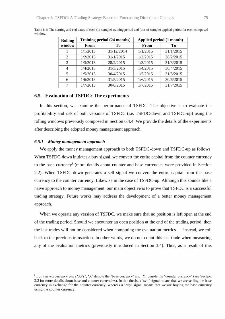
Chapter 6. TSFDC: A Trading Strategy Based on Forecasting Directional Changes 75
Table 6.4: The starting and end dates of each (in-sample) training period and (out-of-sample) applied period for each composed
window.
Rolling
window
Training period (24 months) Applied period (1 month)
From To From To
1 1/1/2013 31/12/2014 1/1/2015 31/1/2015
2 1/2/2013 31/1/2015 1/2/2015 28/2/2015
3 1/3/2013 28/2/2015 1/3/2015 31/3/2015
4 1/4/2013 31/3/2015 1/4/2015 30/4/2015
5 1/5/2013 30/4/2015 1/5/2015 31/5/2015
6 1/6/2013 31/5/2015 1/6/2015 30/6/2015
7 1/7/2013 30/6/2015 1/7/2015 31/7/2015
6.5 Evaluation of TSFDC: The experiments
In this section, we examine the performance of TSFDC. The objective is to evaluate the
profitability and risk of both versions of TSFDC (i.e. TSFDC-down and TSFDC-up) using the
rolling windows previously composed in Section 6.4.4. We provide the details of the experiments
after describing the adopted money management approach.
6.5.1 Money management approach
We apply the money management approach to both TSFDC-down and TSFDC-up as follows.
When TSFDC-down initiates a buy signal, we convert the entire capital from the counter currency
to the base currencyk (more details about counter and base currencies were provided in Section
2.2). When TSFDC-down generates a sell signal we convert the entire capital from the base
currency to the counter currency. Likewise in the case of TSFDC-up. Although this sounds like a
naïve approach to money management, our main objective is to prove that TSFDC is a successful
trading strategy. Future works may address the development of a better money management
approach.
When we operate any version of TSFDC, we make sure that no position is left open at the end
of the trading period. Should we encounter an open position at the end of the trading period, then
the last trades will not be considered when computing the evaluation metrics — instead, we roll
back to the previous transaction. In other words, we do not count this last trade when measuring
any of the evaluation metrics (previously introduced in Section 3.4). Thus, as a result of this
k For a given currency pairs ‘X/Y’, ‘X’ denote the ‘base currency’ and ‘Y’ denote the ‘counter currency’ (see Section
2.2 for more details about base and counter currencies). In this thesis, a ‘sell’ signal means that we are selling the base
currency in exchange for the counter currency; whereas a ‘buy’ signal means that we are buying the base currency
using the counter currency.
Chapter 6. TSFDC: A Trading Strategy Based on Forecasting Directional Changes 76
approach, if TSFDC opens a position it will not be able to open any other positions until the current
position is closed.
In Section 4.4 we reviewed four DC-based trading strategies ( [15] [16] [17] [78]). None of the
authors of these trading strategies considered transaction costs in their experiments. Therefore, in
our experiments, we do not account for the transaction costs either. This helps to provide a fairer
comparison between our planned trading strategies and the four DC-based trading strategies we
reviewed earlier. Generally speaking, the impact of transaction costs on the performance of trading
strategy is controversial. Some studies (e.g. [97] [101] [102] [103]) have concluded that, in general,
transaction costs can have a tremendous impact on a strategy’s profitability and that the impact of
transaction costs should not be neglected when backtesting a trading strategy. However, by contrast,
other studies (e.g. [3] [36] [37] [104]) have concluded that transaction costs are not expected to
have a substantial negative impact on the profitability of FX trading. In this thesis, while there is
no direct transaction fee, we consider the bid–ask spread as a kind of indirect charge as in ( [6] [15]
[16]).
We should also point out that we ignore the effect of ‘slippage’ in our trading simulations. In
trading, ‘slippage’ refers to the difference between what a trader expects to pay for a trade and the
actual price at which the trade is executed. Normally, slippage happens because there might be a
slight time delay between the trader initiating the trade and the time the broker receives the order.
During this time delay, the price may have changed. It can either work in favour of, or against, the
trader [105].
6.5.2 Experiment 6.1: Evaluation of the performance of TSFDC
The objective of this experiment is to evaluate the performance of TSFDC-down and TSFDC-
up. Each of TSFDC-down and TSFDC-up run independently from the other. For this purpose, we
apply each version to the eight sets of rolling windows: EURCHF_RWDC0.1,
GBPCHF_RWDC0.1, EURUSD_RWDC0.1…etc. (previously composed in Section 6.4.4). For
each of these eight sets, the training period of each rolling window (24 months) is utilized to train
the forecasting model (developed in Chapter 5). Next, the forecasting model is employed to
compute the value of FBBTheta (i.e. to forecast BBTheta) for each DC event, of threshold STheta,
during the trading period (i.e. the associated applied window of 1 month). TSFDC uses FBBTheta
to decide when to initiate a trade, as described in Section 6.3, during the trading period. The overall
trading period of each set is seven months in length: from 1/1/2015 to 31/7/2015. For each of the
Chapter 6. TSFDC: A Trading Strategy Based on Forecasting Directional Changes 77
eight sets, BTheta is fixed, arbitrarily, to 0.13%. We measure the evaluation metrics previously
listed in Section 3.4 to evaluate the performance of TSFDC.
The evaluation metrics, Jensen’s Alpha and Beta, serve to evaluate, respectively, the
profitability and risk of a given trading strategy, with reference to a benchmark (Section 3.4). In
this thesis, we consider the buy and hold approach as our benchmark. Thus, we apply the buy and
hold approach to each considered currency pair (buying at the opening price on a monthly basis;
holding it over the course of the trading month, and selling at the closing price). For each currency
pair, we compute the monthly returns resulting from applying the buy and hold to the specified
trading periods (from 1st January 2015 to 31st July 2015). We then use these monthly returns to
compute Jensen’s Alpha and Beta of TSFDC.
Furthermore, as we consider the buy and hold (B&H) as a benchmark, we compare the Sharpe
ratios of both versions of TSFDC with the Sharpe ratio obtained by the buy and hold approach. To
validate this comparison statistically, we employ the Wilcoxon rank sum test (sometimes called
Mann Whitney U Test) [106] twice. Firstly, we apply the Wilcoxon test with the null hypothesis
being that ‘the median difference between the Sharpe ratio produced by TSFDC-Down and B&H
is zero’. Secondly, we apply the Wilcoxon test with the null hypothesis being that
‘the median difference between the Sharpe ratio produced by TSFDC-Up and B&H is zero’.
Likewise, we apply the Wilcoxon test to compare the win ratio of TSFDC-down and TSFDC-
up to that of dummy prediction. The dummy prediction of a Boolean variable (e.g. BBTheta) refers
to the act of continuously predicting True or False (Section 5.6.2). The win ratio of a trading
strategy, which is based on dummy prediction, is estimated as the accuracy of the dummy
prediction l. In the context of our experiment, the win ratio of dummy prediction for a given
currency pair is the level of True-False imbalance of BBTheta (Section 5.6.2).
We apply the Wilcoxon rank sum test to compare the win ratio of TSFDC-down and TSFDC-
up with the expected win ratio of a trading strategy which is based on dummy prediction. We
therefore employ the Wilcoxon test twice: a) The first time with the null hypothesis being that
‘the median difference between the win ratio of TSFDC-Up and dummy prediction is zero’; and b)
The second time we examine the null hypothesis of ‘the median difference between the win ratio
of TSFDC-Down and dummy prediction is zero’.
l This is only from a theoretical perspective. In reality, the actual win ratio will depend also on the trading rules
established based on the dummy prediction.
Chapter 6. TSFDC: A Trading Strategy Based on Forecasting Directional Changes 78
6.5.3 Experiment 6.2: Compare the return and risk of both versions of TSFDC
The objective of this experiment is to test whether TSFDC-down and TSFDC-up have similar
performance. More particularly, we want to compare the return and risk of both versions of TSFDC.
For simplicity, we consider the maximum drawdown (MDD) as a measure of risk (similarly to [4],
[17] and [18]). We use the rate of returns (RR) and maximum drawdown (MDD) resulting from
applying both versions of TSFDC to the eight currency pairs from Experiment 6.1 (Section 6.5.2).
In details, in this experiment, we want to find out whether TSFDC-down and TSFDC-up provide
similar RR and MDD.
In order to validate our test statistically, we apply the non-parametric Wilcoxon rank sum test
twice [106]. Firstly, we apply the Wilcoxon test with the null hypothesis that the median difference
between the two sets of RR of TSFDC-down and TSFDC-up is zero. In this instance, based on
Experiment 6.1, we consider the RR generated by applying TSFDC-down to the eight currency
rates as the first set (Section 6.5.2). Similarly, the second set comprises the RR generated by
applying TSFDC-up to the eight currency rates. Each of these set consists of 8 observations (8
currency rates with 1 RR for each currency rate).
Secondly, we seek to compare the risk of both versions of TSFDC. Based on Experiment 6.1,
Taking the maximum drawdown as an indicator of risk (as in [16] [17]), we compose a first set by
applying TSFDC-down to the eight currency rates. This set comprises 8 observations (8 currency
rates with 1 MDD for each currency rate). We compose a second set of MDD by trading with
TSFDC-up over the eight currency rates. We apply the Wilcoxon Rank Sum test with the null
hypothesis that the median difference between these two sets of MDD, of TSFDC-down and
TSFDC-up, is zero.
6.6 Evaluation of TSFDC: Results and discussion
6.6.1 Experiment 6.1: Evaluation of the performance of TSFDC
The objective of this experiment is to evaluate the performance of TSFDC-down and TSFDC-
up using eight currency pairs sampled minute-by-minute. To this end, we applied the two versions
of TSFDC to the eight sets of rolling windows composed in Section 6.4.4. We followed the money
management approach outlined in Section 6.5.1 and measured the evaluation metrics listed in
Section 3.4. These evaluation metrics are:
- Rate of returns (RR): RR is interpreted as the gain or loss on an investment over a given
evaluation period expressed as a percentage of the amount invested.
Chapter 6. TSFDC: A Trading Strategy Based on Forecasting Directional Changes 79
- Profit factor: This is calculated by dividing the sum of profits produced by all profitable
trades by the sum of losses incurred by all losing trades. This metric measures the amount
of profit per unit of risk.
- Max drawdown: This is the largest difference, in percentage, between the maximum amount
(i.e. peak) and the minimum amount (i.e. through) of capital during a trading period. It
measures the risk as the worst peak-to-trough decline in capital.
- Win ratio: This is the probability that a trade produces a positive return.
- Sharpe ratio: This measures the risk-adjusted return. It represents the average return earned
in excess of the risk-free rate per unit of volatility.
- Sortino ratio: Denote the excess return over the risk-free rate divided by the downside semi-
variance, and so measures the return to ‘bad’ volatility.
- Jensen’s Alpha: Indicates whether a trading strategy is earning the proper return for its level
of risk.
- Beta: Serves to measure the volatility, or systematic risk, of a security or a portfolio, in
comparison to a benchmark.
In order to avoid tedious detail, this section reports TSFDC’s general trading performance
during the overall trading period for the eight currency pairs. Keep in mind that we consider the
bid and ask prices in our experiments. While there is no direct transaction fee, the instantaneous
actual bid–ask spread is a kind of indirect charge.
6.6.1.1 Experiment 6.1: The results
For each currency pair, we use the same values of STheta (0.10%) and BTheta (0.13%). These
values are chosen arbitrarily. Bear in mind that, for each currency pair, we compose seven rolling
windows. Each window comprises a trading period of one month. At the beginning of the first
trading period, i.e. January 2015, both TSFDC-down and TSFDC-up start with a capital of
1,000,000 monetary unitsm; this represents the initial, hypothetically, invested amount of money.
We consider the instantaneous actual bid and ask spread for each made trade; but not the
transaction costs.
Table 6.5, shown below, reports the general performance of both versions of TSFDC during the
overall trading period of seven months. Keep in mind that TSFDC-down and TSFDC-up are not
m In the case of trading with TSFDC-down, for each currency pair, we assume that we start trading with 1,000,000
monetary units of the counter currency. For example: in the case of EUR/CHF, we start trading with 1,000,000 CHF.
Whereas in the case of NZD/JPY, we start with 1,000,000 JPY. However, in the case of TSFDC-up we assume that
we start trading with 1,000,000 monetary units of the base currency.

Chapter 6. TSFDC: A Trading Strategy Based on Forecasting Directional Changes 80
run concurrently. They are evaluated separately. In Table 6.5, the column ‘Currency Pair’ denote
the considered currency pair. The column ‘Trading Strategy’ indicates which version of TSFDC
is applied. The columns ‘RR’, ‘Profit Factor’, ‘Max Drawdown (%)’, and ‘Win Ratio’ refer to the
chosen evaluation metrics. The last row in Table 6.5 is interpreted as follows: applying TSFDC-
up to EUR/NZD generates a total return of 41.22% during the trading period of seven months
(from 1/1/2015 to 31/7/2015). In this case, TSFDC-up executes 4218 trades with an overall Win
Ratio of 0.70. The maximum drawdown in capital is – 7.2%. The details of monthly Rates of
Return (RR) of applying TSFDC-down and TSFDC-up to these currency pairs are shown in Tables
6.6 and 6.7 respectively. The annualized returns are reported in Appendix E.
Table 6.5: Trading performance of TSFDC-down and TSFDC-up models following the seven months out-of-sample
period (from 1/1/2015 to 31/7/2015) of the eight currency pairs.
Currency
Pair
Trading
Strategy RR
Profit
Factor
Total Number
of Trades
Max
Drawdown (%)
Win
Ratio
EUR/CHF TSFDC-down 9.13 1.66 2056 – 19.4 0.66
TSFDC -up 4.83 1.72 2009 – 21.1 0.64
GBP/CHF TSFDC-down 10.82 1.58 2489 – 14.0 0.66
TSFDC -up 12.07 1.61 2531 – 13.8 0.67
EUR/USD TSFDC-down – 1.46 0.96 1431 – 10.5 0.56
TSFDC-up 0.67 1.09 1453 – 9.1 0.60
GBP/AUD TSFDC-down 9.02 1.60 3021 – 6.4 0.64
TSFDC-up 4.59 1.32 2960 – 6.5 0.63
GBP/JPY TSFDC-down – 2.72 0.91 1585 – 7.8 0.60
TSFDC-up – 4.93 0.85 1601 – 7.7 0.59
NZD/JPY TSFDC-down 26.98 1.85 3046 – 5.9 0.65
TSFDC-up 26.37 1.78 3010 – 6.5 0.66
AUD/JPY TSFDC-down 12.09 1.56 2885 – 6.9 0.67
TSFDC-up 15.4 1.62 2860 – 7.2 0.67
EUR/NZD TSFDC-down 41.87 2.14 3961 – 7.0 0.69
TSFDC-up 41.22 2.16 4218 – 7.2 0.69
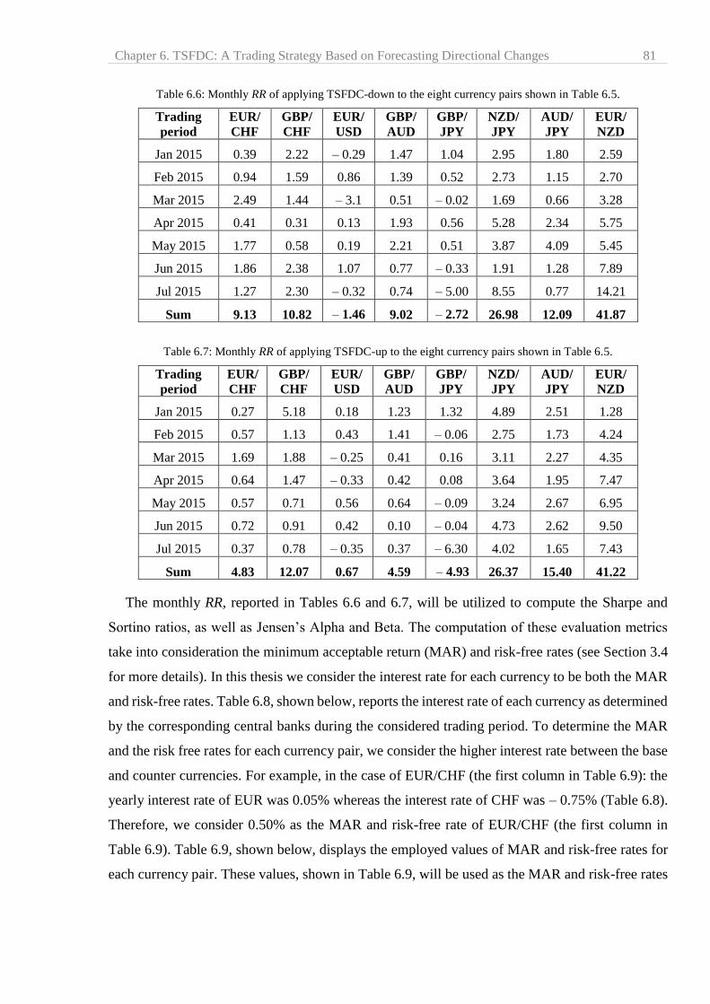
Chapter 6. TSFDC: A Trading Strategy Based on Forecasting Directional Changes 81
Table 6.6: Monthly RR of applying TSFDC-down to the eight currency pairs shown in Table 6.5.
Trading
period
EUR/
CHF
GBP/
CHF
EUR/
USD
GBP/
AUD
GBP/
JPY
NZD/
JPY
AUD/
JPY
EUR/
NZD
Jan 2015 0.39 2.22 – 0.29 1.47 1.04 2.95 1.80 2.59
Feb 2015 0.94 1.59 0.86 1.39 0.52 2.73 1.15 2.70
Mar 2015 2.49 1.44 – 3.1 0.51 – 0.02 1.69 0.66 3.28
Apr 2015 0.41 0.31 0.13 1.93 0.56 5.28 2.34 5.75
May 2015 1.77 0.58 0.19 2.21 0.51 3.87 4.09 5.45
Jun 2015 1.86 2.38 1.07 0.77 – 0.33 1.91 1.28 7.89
Jul 2015 1.27 2.30 – 0.32 0.74 – 5.00 8.55 0.77 14.21
Sum 9.13 10.82 – 1.46 9.02 – 2.72 26.98 12.09 41.87
Table 6.7: Monthly RR of applying TSFDC-up to the eight currency pairs shown in Table 6.5.
Trading
period
EUR/
CHF
GBP/
CHF
EUR/
USD
GBP/
AUD
GBP/
JPY
NZD/
JPY
AUD/
JPY
EUR/
NZD
Jan 2015 0.27 5.18 0.18 1.23 1.32 4.89 2.51 1.28
Feb 2015 0.57 1.13 0.43 1.41 – 0.06 2.75 1.73 4.24
Mar 2015 1.69 1.88 – 0.25 0.41 0.16 3.11 2.27 4.35
Apr 2015 0.64 1.47 – 0.33 0.42 0.08 3.64 1.95 7.47
May 2015 0.57 0.71 0.56 0.64 – 0.09 3.24 2.67 6.95
Jun 2015 0.72 0.91 0.42 0.10 – 0.04 4.73 2.62 9.50
Jul 2015 0.37 0.78 – 0.35 0.37 – 6.30 4.02 1.65 7.43
Sum 4.83 12.07 0.67 4.59 – 4.93 26.37 15.40 41.22
The monthly RR, reported in Tables 6.6 and 6.7, will be utilized to compute the Sharpe and
Sortino ratios, as well as Jensen’s Alpha and Beta. The computation of these evaluation metrics
take into consideration the minimum acceptable return (MAR) and risk-free rates (see Section 3.4
for more details). In this thesis we consider the interest rate for each currency to be both the MAR
and risk-free rates. Table 6.8, shown below, reports the interest rate of each currency as determined
by the corresponding central banks during the considered trading period. To determine the MAR
and the risk free rates for each currency pair, we consider the higher interest rate between the base
and counter currencies. For example, in the case of EUR/CHF (the first column in Table 6.9): the
yearly interest rate of EUR was 0.05% whereas the interest rate of CHF was – 0.75% (Table 6.8).
Therefore, we consider 0.50% as the MAR and risk-free rate of EUR/CHF (the first column in
Table 6.9). Table 6.9, shown below, displays the employed values of MAR and risk-free rates for
each currency pair. These values, shown in Table 6.9, will be used as the MAR and risk-free rates
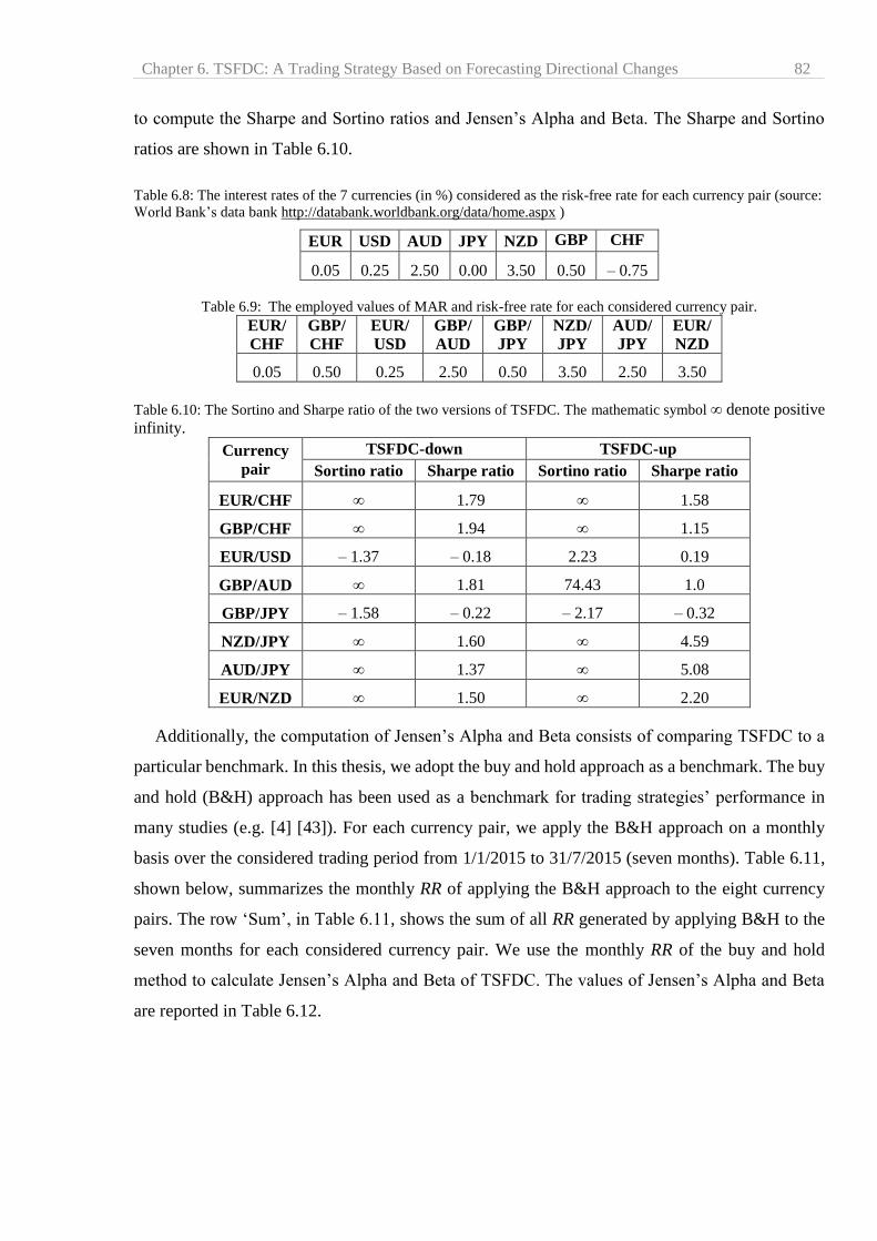
Chapter 6. TSFDC: A Trading Strategy Based on Forecasting Directional Changes 82
to compute the Sharpe and Sortino ratios and Jensen’s Alpha and Beta. The Sharpe and Sortino
ratios are shown in Table 6.10.
Table 6.8: The interest rates of the 7 currencies (in %) considered as the risk-free rate for each currency pair (source:
World Bank’s data bank http://databank.worldbank.org/data/home.aspx )
EUR USD AUD JPY NZD GBP CHF
0.05 0.25 2.50 0.00 3.50 0.50 – 0.75
Table 6.9: The employed values of MAR and risk-free rate for each considered currency pair.
EUR/
CHF
GBP/
CHF
EUR/
USD
GBP/
AUD
GBP/
JPY
NZD/
JPY
AUD/
JPY
EUR/
NZD
0.05 0.50 0.25 2.50 0.50 3.50 2.50 3.50
Table 6.10: The Sortino and Sharpe ratio of the two versions of TSFDC. The mathematic symbol ∞ denote positive
infinity.
Currency
pair
TSFDC-down TSFDC-up
Sortino ratio Sharpe ratio Sortino ratio Sharpe ratio
EUR/CHF ∞ 1.79 ∞ 1.58
GBP/CHF ∞ 1.94 ∞ 1.15
EUR/USD – 1.37 – 0.18 2.23 0.19
GBP/AUD ∞ 1.81 74.43 1.0
GBP/JPY – 1.58 – 0.22 – 2.17 – 0.32
NZD/JPY ∞ 1.60 ∞ 4.59
AUD/JPY ∞ 1.37 ∞ 5.08
EUR/NZD ∞ 1.50 ∞ 2.20
Additionally, the computation of Jensen’s Alpha and Beta consists of comparing TSFDC to a
particular benchmark. In this thesis, we adopt the buy and hold approach as a benchmark. The buy
and hold (B&H) approach has been used as a benchmark for trading strategies’ performance in
many studies (e.g. [4] [43]). For each currency pair, we apply the B&H approach on a monthly
basis over the considered trading period from 1/1/2015 to 31/7/2015 (seven months). Table 6.11,
shown below, summarizes the monthly RR of applying the B&H approach to the eight currency
pairs. The row ‘Sum’, in Table 6.11, shows the sum of all RR generated by applying B&H to the
seven months for each considered currency pair. We use the monthly RR of the buy and hold
method to calculate Jensen’s Alpha and Beta of TSFDC. The values of Jensen’s Alpha and Beta
are reported in Table 6.12.
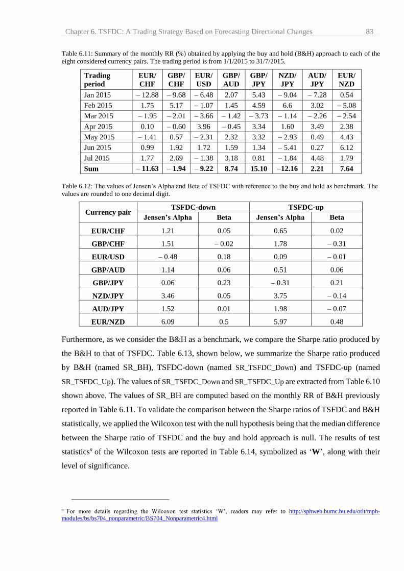
Chapter 6. TSFDC: A Trading Strategy Based on Forecasting Directional Changes 83
Table 6.11: Summary of the monthly RR (%) obtained by applying the buy and hold (B&H) approach to each of the
eight considered currency pairs. The trading period is from 1/1/2015 to 31/7/2015.
Trading
period
EUR/
CHF
GBP/
CHF
EUR/
USD
GBP/
AUD
GBP/
JPY
NZD/
JPY
AUD/
JPY
EUR/
NZD
Jan 2015 – 12.88 – 9.68 – 6.48 2.07 5.43 – 9.04 – 7.28 0.54
Feb 2015 1.75 5.17 – 1.07 1.45 4.59 6.6 3.02 – 5.08
Mar 2015 – 1.95 – 2.01 – 3.66 – 1.42 – 3.73 – 1.14 – 2.26 – 2.54
Apr 2015 0.10 – 0.60 3.96 – 0.45 3.34 1.60 3.49 2.38
May 2015 – 1.41 0.57 – 2.31 2.32 3.32 – 2.93 0.49 4.43
Jun 2015 0.99 1.92 1.72 1.59 1.34 – 5.41 0.27 6.12
Jul 2015 1.77 2.69 – 1.38 3.18 0.81 – 1.84 4.48 1.79
Sum – 11.63 – 1.94 – 9.22 8.74 15.10 –12.16 2.21 7.64
Table 6.12: The values of Jensen’s Alpha and Beta of TSFDC with reference to the buy and hold as benchmark. The
values are rounded to one decimal digit.
Currency pair TSFDC-down TSFDC-up
Jensen’s Alpha Beta Jensen’s Alpha Beta
EUR/CHF 1.21 0.05 0.65 0.02
GBP/CHF 1.51 – 0.02 1.78 – 0.31
EUR/USD – 0.48 0.18 0.09 – 0.01
GBP/AUD 1.14 0.06 0.51 0.06
GBP/JPY 0.06 0.23 – 0.31 0.21
NZD/JPY 3.46 0.05 3.75 – 0.14
AUD/JPY 1.52 0.01 1.98 – 0.07
EUR/NZD 6.09 0.5 5.97 0.48
Furthermore, as we consider the B&H as a benchmark, we compare the Sharpe ratio produced by
the B&H to that of TSFDC. Table 6.13, shown below, we summarize the Sharpe ratio produced
by B&H (named SR_BH), TSFDC-down (named SR_TSFDC_Down) and TSFDC-up (named
SR_TSFDC_Up). The values of SR_TSFDC_Down and SR_TSFDC_Up are extracted from Table 6.10
shown above. The values of SR_BH are computed based on the monthly RR of B&H previously
reported in Table 6.11. To validate the comparison between the Sharpe ratios of TSFDC and B&H
statistically, we applied the Wilcoxon test with the null hypothesis being that the median difference
between the Sharpe ratio of TSFDC and the buy and hold approach is null. The results of test
statisticsn of the Wilcoxon tests are reported in Table 6.14, symbolized as ‘W’, along with their
level of significance.
n For more details regarding the Wilcoxon test statistics ‘W’, readers may refer to http://sphweb.bumc.bu.edu/otlt/mph-
modules/bs/bs704_nonparametric/BS704_Nonparametric4.html
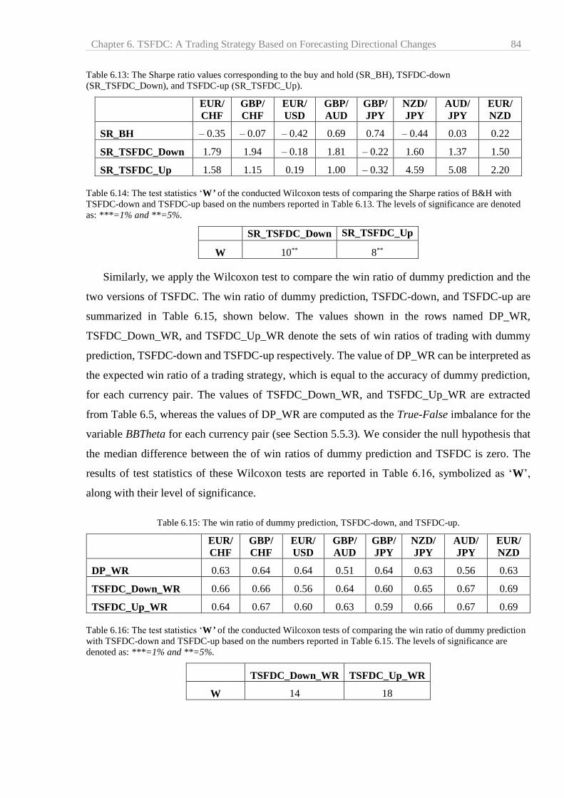
Chapter 6. TSFDC: A Trading Strategy Based on Forecasting Directional Changes 84
Table 6.13: The Sharpe ratio values corresponding to the buy and hold (SR_BH), TSFDC-down
(SR_TSFDC_Down), and TSFDC-up (SR_TSFDC_Up).
EUR/
CHF
GBP/
CHF
EUR/
USD
GBP/
AUD
GBP/
JPY
NZD/
JPY
AUD/
JPY
EUR/
NZD
SR_BH – 0.35 – 0.07 – 0.42 0.69 0.74 – 0.44 0.03 0.22
SR_TSFDC_Down 1.79 1.94 – 0.18 1.81 – 0.22 1.60 1.37 1.50
SR_TSFDC_Up 1.58 1.15 0.19 1.00 – 0.32 4.59 5.08 2.20
Table 6.14: The test statistics ‘W’ of the conducted Wilcoxon tests of comparing the Sharpe ratios of B&H with
TSFDC-down and TSFDC-up based on the numbers reported in Table 6.13. The levels of significance are denoted
as: ***=1% and **=5%.
SR_TSFDC_Down SR_TSFDC_Up
W 10** 8**
Similarly, we apply the Wilcoxon test to compare the win ratio of dummy prediction and the
two versions of TSFDC. The win ratio of dummy prediction, TSFDC-down, and TSFDC-up are
summarized in Table 6.15, shown below. The values shown in the rows named DP_WR,
TSFDC_Down_WR, and TSFDC_Up_WR denote the sets of win ratios of trading with dummy
prediction, TSFDC-down and TSFDC-up respectively. The value of DP_WR can be interpreted as
the expected win ratio of a trading strategy, which is equal to the accuracy of dummy prediction,
for each currency pair. The values of TSFDC_Down_WR, and TSFDC_Up_WR are extracted
from Table 6.5, whereas the values of DP_WR are computed as the True-False imbalance for the
variable BBTheta for each currency pair (see Section 5.5.3). We consider the null hypothesis that
the median difference between the of win ratios of dummy prediction and TSFDC is zero. The
results of test statistics of these Wilcoxon tests are reported in Table 6.16, symbolized as ‘W’,
along with their level of significance.
Table 6.15: The win ratio of dummy prediction, TSFDC-down, and TSFDC-up.
EUR/
CHF
GBP/
CHF
EUR/
USD
GBP/
AUD
GBP/
JPY
NZD/
JPY
AUD/
JPY
EUR/
NZD
DP_WR 0.63 0.64 0.64 0.51 0.64 0.63 0.56 0.63
TSFDC_Down_WR 0.66 0.66 0.56 0.64 0.60 0.65 0.67 0.69
TSFDC_Up_WR 0.64 0.67 0.60 0.63 0.59 0.66 0.67 0.69
Table 6.16: The test statistics ‘W’ of the conducted Wilcoxon tests of comparing the win ratio of dummy prediction
with TSFDC-down and TSFDC-up based on the numbers reported in Table 6.15. The levels of significance are
denoted as: ***=1% and **=5%.
TSFDC_Down_WR TSFDC_Up_WR
W 14 18
Chapter 6. TSFDC: A Trading Strategy Based on Forecasting Directional Changes 85
6.6.1.2 Experiment 6.1: Results’ Discussion
We begin with an examination of the results obtained from the B&H (shown in Table 6.11).
For each currency pair (i.e. each column), we note that the B&H approach does generate profit in
some months, but incurs losses in others. This observation indicates that none of the selected
currency pairs exhibit a monotonic trend during the trading period. Besides, the numbers shown in
the last row in Table 6.11 (named ‘Sum’) demonstrate that, overall, the B&H method generates
profit in four cases: GBP/AUD, GBP/JPY, AUD/JPY, and EUR/NZD (with a total rate of return,
RR, of up to 15.10% in the case of GBP/JPY). The same row also shows that the buy and hold
method incurs losses in the other four cases (with total RR equal to –12.16% in the case of
NZD/JPY). These observations support our claim regarding the variation of the trends of the
selected currency rates in Section 6.4.1.
We then examine the profitability of both versions of TSFDC. The monthly rates of return (RR)
reported in Tables 6.6 and 6.7 suggest that both versions of TSFDC are mostly profitable (except
in a few cases; e.g. trading with TSFDC-down on EUR/USD in March 2015 when it incurred losses
of – 3.1%, Table 6.6). The results in column (RR), shown in Table 6.5, suggest that TSFDC can
be highly profitable (with RR of up to 41.22 %, as in the case of applying TSFDC-up to EUR/NZD,
the last row in Table 6.5). However, the profitability of TSFDC is not guaranteed for all currency
pairs. For example, in Table 6.7 one can easily observe an important difference between the
produced total RR (from – 4.93% for GBP/JPY, compared to 41.22% for EUR/NZD). This
indicates that, whilst TSFDC may generate profits in most cases, its performance may vary
substantially from one currency rate to another. It follows then that a trader may want to consider
other currency pairs as TSFDC may, possibly, perform better on these currencies than on those
reported in this chapter. Moreover, we want to declare that 41.22% is the highest RR that we have
ever obtained in our preliminary experiments. Thus, EUR/NZD could be possibly the currency for
which TSFDC performs best. We also want to point out that, if we had considered only the mid-
price instead of bid/ask prices, the RR in the case of EUR/NZD would raise to 500%. Therefore,
we also believe that if we had considered the transaction costs, it would be a good chance that the
reported RR in Table 6.6 could have decreased.
Furthermore, when comparing the win ratio of TSFDC-down and TSFDC-up, shown in Table
6.5, to the accuracy of your forecasting model reported in Table 5.3 (Chapter 5), one can easily
note a remarkable difference. For example, according to Table 6.5 the accuracy of our forecasting
approach introduced in Chapter 5, range between 0.75 and 0.82; whereas the win ratio of both
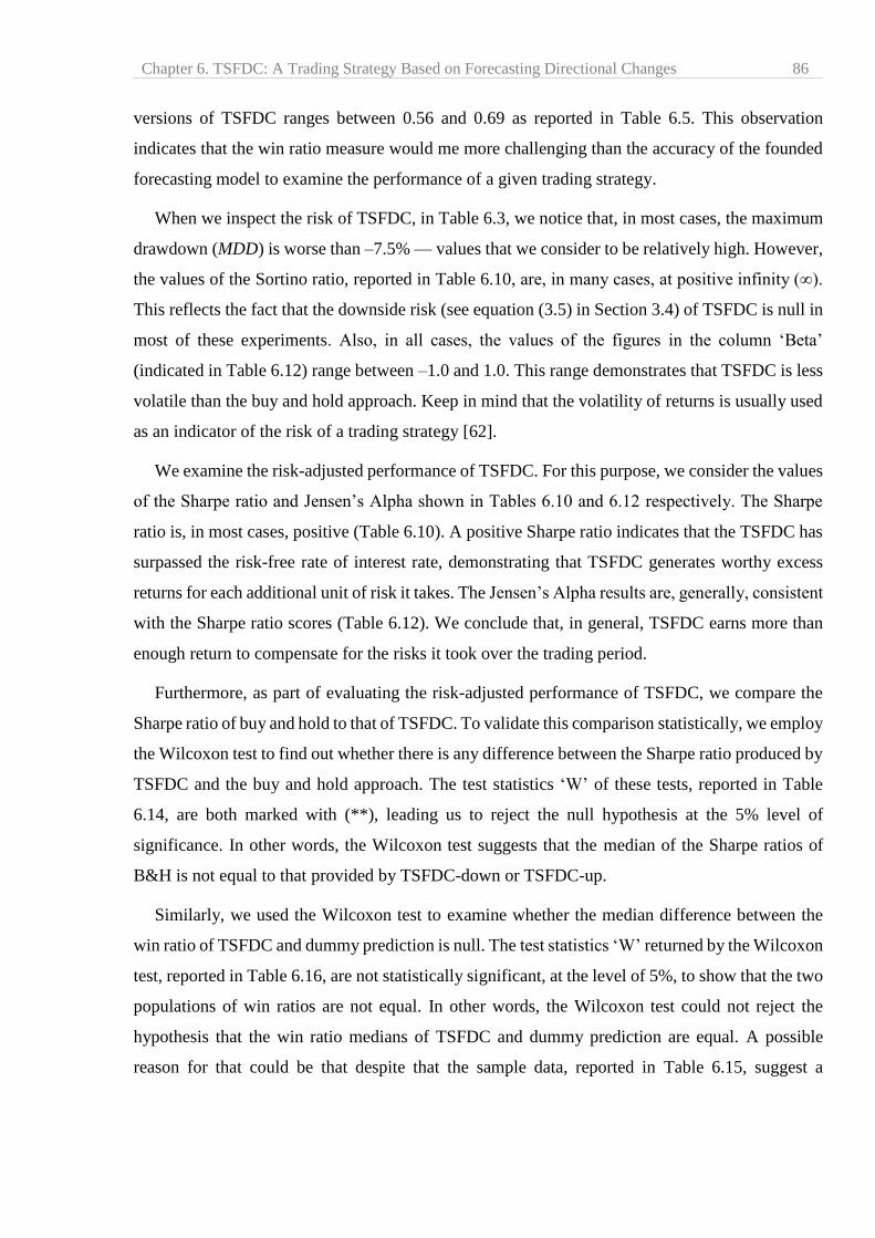
Chapter 6. TSFDC: A Trading Strategy Based on Forecasting Directional Changes 86
versions of TSFDC ranges between 0.56 and 0.69 as reported in Table 6.5. This observation
indicates that the win ratio measure would me more challenging than the accuracy of the founded
forecasting model to examine the performance of a given trading strategy.
When we inspect the risk of TSFDC, in Table 6.3, we notice that, in most cases, the maximum
drawdown (MDD) is worse than –7.5% — values that we consider to be relatively high. However,
the values of the Sortino ratio, reported in Table 6.10, are, in many cases, at positive infinity (∞).
This reflects the fact that the downside risk (see equation (3.5) in Section 3.4) of TSFDC is null in
most of these experiments. Also, in all cases, the values of the figures in the column ‘Beta’
(indicated in Table 6.12) range between –1.0 and 1.0. This range demonstrates that TSFDC is less
volatile than the buy and hold approach. Keep in mind that the volatility of returns is usually used
as an indicator of the risk of a trading strategy [62].
We examine the risk-adjusted performance of TSFDC. For this purpose, we consider the values
of the Sharpe ratio and Jensen’s Alpha shown in Tables 6.10 and 6.12 respectively. The Sharpe
ratio is, in most cases, positive (Table 6.10). A positive Sharpe ratio indicates that the TSFDC has
surpassed the risk-free rate of interest rate, demonstrating that TSFDC generates worthy excess
returns for each additional unit of risk it takes. The Jensen’s Alpha results are, generally, consistent
with the Sharpe ratio scores (Table 6.12). We conclude that, in general, TSFDC earns more than
enough return to compensate for the risks it took over the trading period.
Furthermore, as part of evaluating the risk-adjusted performance of TSFDC, we compare the
Sharpe ratio of buy and hold to that of TSFDC. To validate this comparison statistically, we employ
the Wilcoxon test to find out whether there is any difference between the Sharpe ratio produced by
TSFDC and the buy and hold approach. The test statistics ‘W’ of these tests, reported in Table
6.14, are both marked with (**), leading us to reject the null hypothesis at the 5% level of
significance. In other words, the Wilcoxon test suggests that the median of the Sharpe ratios of
B&H is not equal to that provided by TSFDC-down or TSFDC-up.
Similarly, we used the Wilcoxon test to examine whether the median difference between the
win ratio of TSFDC and dummy prediction is null. The test statistics ‘W’ returned by the Wilcoxon
test, reported in Table 6.16, are not statistically significant, at the level of 5%, to show that the two
populations of win ratios are not equal. In other words, the Wilcoxon test could not reject the
hypothesis that the win ratio medians of TSFDC and dummy prediction are equal. A possible
reason for that could be that despite that the sample data, reported in Table 6.15, suggest a
Chapter 6. TSFDC: A Trading Strategy Based on Forecasting Directional Changes 87
difference, however the sample size could be too small to conclude that there is a statistical
significant difference.
We conclude from the above analysis that TSFDC-down and TSFDC-up provide better Sharpe
ratios and less risk than the buy and hold method. Additionally, both versions of TSFDC can be
highly profitable, with RR of more than 41% (Table 6.5). However, TSFDC may incur losses in a
few cases. We also argue that TSFDC can, in most cases, deliver a positive Sharpe ratio. Finally,
the established variety of the selected currency pairs in the initial dataset (Section 6.4.1) suggest
that TSFDC can be profitably applied to a wide range of currency rates.
6.6.2 Experiment 6.2: Compare the return and risk of both versions of TSFDC
The objective of this experiment is to compare the return and risk of TSFDC-up and TSFDC-
down. We consider the rates of return (RR) and maximum drawdown (MDD) resulting from
applying both versions of TSFDC to the eight currency pairs in the previous experiment (Section
6.6.1). These values of RR and MDD of TSFDC-down and TSFDC-up are summarized in Table
6.17 shown below. These values are extracted from Table 6.5 in Section 6.6.1. Firstly, we apply
the Wilcoxon test with the null hypothesis that the median difference between the two sets of RR
(shown in the column named RR in Table 6.17) of TSFDC-down and TSFDC-up is zero. Secondly,
we apply the Wilcoxon test with the null hypothesis being that the median difference between the
two sets of MDD (shown in the column named MDD in Table 6.17) of TSFDC-down and TSFDC-
up is zero. The values of the test statistics ‘W’ are reported in Table 6.18 below.
Table 6.17: The summaries of RR and MDD rustled from trading with TSFDC-down and TSFDC-up
Currency
Pair
RR MDD
TSFDC-down TSFDC-up TSFDC-down TSFDC-up
EUR/CHF 9.13 4.83 – 19.4 – 21.1
GBP/CHF 10.82 12.07 – 14.0 – 13.8
EUR/USD 0.67 – 1.46 – 10.5 – 9.1
GBP/AUD 9.02 4.59 – 6.4 – 6.5
GBP/JPY – 2.72 – 4.93 – 7.8 – 7.7
NZD/JPY 26.98 26.37 – 5.9 – 6.5
AUD/JPY 12.09 15.4 – 6.9 – 7.2
EUR/NZD 41.87 41.22 – 7.0 – 7.2

Chapter 6. TSFDC: A Trading Strategy Based on Forecasting Directional Changes 88
Table 6.18: The test statistics ‘W’ of the conducted Wilcoxon tests of comparing the RR and MDD of TSFDC-down
and TSFDC-up based on the numbers reported in Table 6.17. The levels of significance are denoted as: ***=1% and
**=5%. The table of critical value of ‘W’ can be found at http://sphweb.bumc.bu.edu/otlt/mph-
modules/bs/bs704_nonparametric/BS704_Nonparametric4.html
RR MDD
W 35 35
The test statistics ‘W’ returned by the Wilcoxon test, reported in Table 6.18, are not statistically
significant, at the level of 5%. In other words, the Wilcoxon test could not reject the hypothesis
that the medians of RR of TSFDC-down and TSFDC-up are equal. Similarly, the Wilcoxon test
could not reject the hypothesis that the medians of MDD of TSFDC-down and TSFDC-up are
equal. We consider these results as sensible; because both versions of TSFDC, TSFDC-down and
TSFDC-up, are based on the same forecasting model (established in Chapter 5) and have, basically,
mirrored trading rules (as described in Section 6.3).
6.7 Comparing TSFDC to other DC-based strategies
In Section 4.4, we reviewed some existing trading strategies that are based on the DC
framework. In this section, we compare TSFDC with two other DC-based trading strategies: (a)
the one presented by Gypteau et al., [78] and (b) the trading strategy named ‘DC+GA’ by
Kampouridis and Otero [17]. The details of these two strategies can be found in Section 4.4.
6.7.1 The DC-based trading strategy by Gypteau et al.
In this section, we highlight the differences between TSFDC and the DC-based trading strategy
presented by Gypteau et al., [78] which was reviewed in detail in Section 4.4.2. We will start with
a brief recap on the functionality of this DC-based trading strategy before comparing it to TSFDC.
Fig. 6.4. A sample individual GP tree: internal nodes are represented by Boolean functions, while terminal nodes
correspond to different DC thresholds. Given a price, terminal nodes output a Boolean value according to the DC or
OS events detected. For example, if we detect a downtrend (uptrend) DC event of a DC summary of threshold 2.85%,
then the left- most terminal node will be evaluated as ‘False’ (‘True’). Source Gypteau et al., [78].
Chapter 6. TSFDC: A Trading Strategy Based on Forecasting Directional Changes 89
The proposed approach follows the standard tree-based Genetic Programming (GP)
configuration. It runs multiple DC summaries, using different DC thresholds, concurrently. For
example, Fig. 6.4, shown above, illustrates a sample individual GP tree. Each GP individual tree
comprises internal and terminal nodes. The internal nodes are Boolean functions and the terminal
nodes are DC thresholds. In Fig. 6.4 each threshold, shown in terminal nodes, is replaced with a
‘True’ or ‘False’ value, depending whether an uptrend or downtrend DC event of the stated
threshold is detected. For example, in Fig. 6.4, if we detect an upward (downward) DC event of
threshold 2.85% the left-most terminal node would be set to ‘True’ (‘False’).
These ‘True’ and ‘False’ values at the terminal nodes are, then, combined together using the
Boolean functions (e.g. AND, Nor, Xor) presented in the internal nodes to form a GP-tree (see Fig.
6.4). As such, a GP tree can be interpreted as a Boolean expression; the output of which can be
only True or False. This output is translated into trading rules with ‘True’ triggering a buy signal
and ‘False’ triggering a sell signal. Consequently, each GP tree represents a trading strategy. The
profitability of the GP tree (i.e. trading strategy) is measured based on the returns resulting from
the triggered buy and sell orders over an in-sample dataset. The evolution of the objective function
of the Genetic Programming (GP) aims to find the best GP-tree that yields the highest returns.
The authors applied their trading strategy to four markets: two stocks from the UK FTSE100
market (Barclays Bank and Marks & Spencer), and two international indices (NASDAQ and the
NYSE). For each market, they used a training period of 1000 days to train their GP model. Then
followed a testing period of 500 days for evaluation. Unfortunately, the authors did not report the
dates of the training or testing periods! (For more detail on this trading model, see Section 4.4.2).
We provide the following two comments on the study of Gypteau et al. [78]:
1. The authors stated that: “… the proposed approach aims to find an optimal trading strategy to
forecast the future price moves of a financial market” [78]. However, having investigated the
study [78], we could not find a formal representation of any forecasting problem. The authors,
in [78], did not identify any dependent or independent variables. Besides, they did not report
any forecasting measurements (e.g. mean squared error, accuracy). Therefore, we could not
conclude that the proposed strategy, in [78], does clearly employ a forecasting model.
2. With respect to the evaluation of the proposed DC-based strategy, the authors reported only
the returns of the proposed trading strategy [78]. The reported returns are less than 10% over a
trading period of 500 days for each considered market. Furthermore, they did not report any
of: a) comparison to a benchmark (e.g. buy and hold), b) measurement of risk (e.g. MDD), nor

Chapter 6. TSFDC: A Trading Strategy Based on Forecasting Directional Changes 90
c) evaluation of risk-adjusted metrics (e.g. Sharpe ratio). Therefore we believe that the reported
returns are not sufficiently convincing regarding the feasibility of the proposed strategy.
In contrast, we consider TSFDC to be founded on a well-formulated forecasting model. This
forecasting model, established in Chapter 5, aims to forecast the change of a trend’s direction under
the DC framework. It has a clear objective and dependent and independent variables (see Section
5.4). By contrast, the study of Gypteau et al. [78] does not define any dependent or independent
variables. Another difference is, that, in contrast to the study of Gypteau et al. [78], we provided a
thorough evaluation of the risk and profitability of TSFDC (Section 6.6).
We should also note that TSFDC and the trading strategy proposed by Gypteau et al., have
different trading approaches: TSFDC forecasts the change of a trend’s direction to decide when to
trigger a new trade, whilst Gypteau et al. employs a GP approach to develop an expression of a
Boolean function, and several DC thresholds, which are then converted to trading rules.
Finally, we want to highlight that applying the strategy of Gypteau et al. to stock markets
produced a maximum profit of less than 10% (over a trading period of more than 1 year). In Section
6.6.1, we examined the profitability of TSFDC in the FX market and concluded that it can produce
rates of return of more than 41% in less than 7 months (after taking the bid-ask spread into concern).
The authors in [78] evaluated the proposed trading strategy in a stock market where prices are
sampled on a daily basis (i.e. with a time-interval of 24 hours). In contrast, TSFDC was evaluated
in the FX market using minute-by-minute mid-prices (i.e. with a time-interval of 1 minute). Despite
the fact that the RR results would indicate that TSFDC is much more profitable than the strategy
of Gypteau et al., it would be better to evaluate both strategies using the same dataset in order to
prove definitively that TSFDC is more profitable.
6.7.2 The DC-based trading strategy: ‘DC+GA’
In this section, we compare TSFDC with the trading strategy named ‘DC+GA’ (Kampouridis
and Otero [17]). The authors in [17] stated that their objective was “to offer a more complete
analysis on the directional changes paradigm from a financial forecasting perspective.” The
details of this strategy were reviewed in Section 4.4.3. Here we briefly recap the mechanism of
this strategy, then compare it with TSFDC.
DC+GA consists of running Ntheta DC summaries concurrently using Ntheta thresholds, these
Ntheta thresholds to be chosen by the trader. DC+GA uses some parameters: b1, b2, and Q (see
Section 4.4.3 for more detail about these parameters). The first two parameters (b1 and b2) help
DC+GA to decide when to initiate a trade during an OS event. The third parameter ‘Q’ denote the
Chapter 6. TSFDC: A Trading Strategy Based on Forecasting Directional Changes 91
order size. For a given market’s price, each DC threshold generates a buy or sell recommendation
based upon the type of the detected DC event (either downward or upward). In addition, each DC
threshold is assigned a ‘weight’. For a given market’s price, the Ntheta DC-thresholds may produce
Ntheta recommendations. These thresholds are, then, clustered in two groups based on the proposed
recommendations: the first group covers the thresholds that recommend a buy action, the second
group covers those recommending a sell action. To make a buy or sell decision, DC+GA sums the
weights of the thresholds belonging to each group: if the sum of the weights for all thresholds
recommending a buy (sell) action is greater than the sum of the weights for all thresholds
recommending a sell (buy) action, then the strategy’s action will be to buy (sell).
The evolution of their GA module consists of finding the best set of weights of the Ntheta DC
thresholds along with the trading parameters (e.g. b1, b2, and Q) that maximize the total profits
during the training process. The best set of the DC thresholds, and their associated weight and
trading parameters, will be used for trading during the out-of-sample trading period (see Section
4.4.3). The employed fitness function is designed so that it maximizes RR and minimizes the MDD
at the same time.
A common feature between TSFDC and DC+GA is that they both analyse uptrends and
downtrends separately. Though, we can identify the following differences between TSFDC and
DC+GA:
DC+GA initiates a trade when the OS event lasts longer than a specific time-threshold.
Whereas, TSFDC initiates a trade when the magnitude of a price’s change reaches a certain
value (see the trading rules in section 6.3).
TSFDC relies on the forecasting approach presented in Chapter 5 to decide whether to initiate
a trade when a new DC event is detected, whereas, DC+GA employs a GA module to
anticipate the best time-threshold at which it should initiate a trade.
TSFDC uses only two DC thresholds (STheta and BTheta), whereas DC+GA takes into
consideration Ntheta DC summaries at the same time.
Kampouridis and Otero [17] reported the mean RR results of applying DC+GA to five currency
pairs (Table 6, page 158, [17]). We note that, overall, DC+GA incurred losses in two out of the
five considered currency pairs. Moreover, when examining the detailed monthly returns (Table 5,
page 158, [17]) we note that, in most months, DC+GA reported losses. By contrast, when
inspecting the monthly returns of TSFDC reported in Tables 6.6 and 6.7, we note that in the
majority of cases, TSFDC’s monthly returns are positive. Furthermore, the overall RR of applying
Chapter 6. TSFDC: A Trading Strategy Based on Forecasting Directional Changes 92
TSFDC to the eight currency pairs (over the trading period of seven months) are mostly positive
(Table 6.5). Thus, we can conclude that TSFDC is more profitable than DC+GA.
We then examine the risk-adjusted returns of DC+GA and TSFDC. The authors in [17] did not
provide any risk-adjusted measurement for DC+GA. However, based on their reported monthly
returns listed in Table 5 (page 158, [17]), we are able to compute the Sharpe ratio. If we consider
a risk-free rate of 0.5% per annum, then we find that DC+GA will have a positive Sharpe ratio
only in two out of the five considered currency pairs (see Section 4.4.3 for details). Whereas, our
results shown in Table 6.10 (Section 6.6.1) indicate that TSFDC-up produces a positive Sharpe
ratio in 7 out of 8 considered currency pairs. Based on this analysis, we conclude that TSFDC
outperforms ‘DC+GA’ in terms of profitability and risk-adjusted returns. Obviously, the
transaction costs is a function of the number of executed trades. However, the author that the
authors in [17] did not report the number of trades executed by DC+GA. Therefore, it is hard to
compare the impact of transaction cost on the RR produced by DC+GA and TSFDC. Finally, we
should note that the authors in [17] did not consider the bid and ask prices in their experiments.
Finally, we compare the risk of TSFDC and DC+GA measured in terms of MDD. The MDD of
DC+GA reported in [17] is no worse than – 0.15% (Table 8, [17]) in all considered currency pairs.
This is better than the MDD of TSFDC reported in Table 6.5. To conclude, by comparing the
results of DC+ GA (reported in [17]) and the results of TSFDC (Section 6.6.1) we deduce that
TSFDC outperforms DC+GA in terms of RR and risk-adjusted returns. However, the results of
MDD suggest that DC+GA is less risky than TSFDC.
6.8 Summary and conclusion
In this chapter, our objective was to develop a successful trading strategy based on forecasting
DC. Following our findings in Chapter 5 concerning forecasting the change of the direction of a
DC trend, this chapter used this forecasting model to develop a trading strategy named TSFDC.
TSFDC is a contrarian trading strategy that relies on the forecasting model (summarized in Section
6.2) to decide when to generate a trade (Section 6.3). The trading rules of TSFDC were presented
in Section 6.3.
The performance of TSFDC was examined using eight currency pairs. We utilized 1-minute
trade records for these eight currency pairs covering the period between 1/1/2013 and 31/7/2015.
We argued that these currency pairs exhibited various trend patterns during the considered trading
period of seven months (Section 6.4.1). We evaluated TSFDC using a monthly-basis rolling
window approach. Each rolling window comprised 1) a training period (24 months in length),
Chapter 6. TSFDC: A Trading Strategy Based on Forecasting Directional Changes 93
which we used to train the forecasting model developed in Chapter 5, and 2) a trading period (1
month in length) to which we applied the trading rules of TSFDC (Section 6.4.4). We utilized a
set of evaluation metrics to assess the performance of TSFDC. We considered the instantaneous
bid and ask prices throughout the backtesting process. However, it should be noted that, like many
other DC-based trading strategies (e.g. [15] [16] [17] [78]), the transaction costs were not
considered in our experiments.
In our experiment, as a benchmark model, we implemented the buy and hold (B&H) strategy,
buying at the opening price on a monthly basis, holding it over the course of the trading month and
selling at the closing price. The inclusion of this zero-intelligence benchmark model was to assess
the usefulness and potential outperformance of our trading strategies in general.
The experimental results (reported in Section 6.6.1) suggest that TSFDC is profitable in most
cases. By examining the returns reported in Table 6.5 (Section 6.6.1), we concluded that TSFDC
can be highly profitable (with an RR of more than 41%, as per EUR/NZD) but it suffers from a
non-trivial level of risk (with MDD equal to – 7.2%). When examining the values of Jensen’s
Alpha (shown in Table 6.12, Section 6.6.1), we concluded that TSFDC generated promising rates
of return compared to the level of risk it took in relation to the buy and hold method. From the
Beta results detailed in Table 6.12 (Section 6.6.1), we see that in the majority of cases TSFDC was
less volatile than the buy and hold method. This indicates that TSFDC is less risky than the buy
and hold approach. In Section 6.7 we also argued that TSFDC outperforms other DC-based trading
strategies. Finally, the conducted Wilcoxon tests suggest that the Buy and Hold approach cannot
provides equal Sharpe ratio to that provided by TSFDC.
To conclude, in this chapter we developed a DC-based trading strategy, named TSFDC, which
we believe to be the first DC-based trading strategy that is based on a well-formulated forecasting
model. As our main contribution, we argued that TSFDC is more profitable than other DC-based
trading strategies (Section 6.7). The experimental results indicate that TSFDC can be highly
profitable (except in a few cases, Section 6.6.1). We examined the effectiveness of TSFDC over
eight different currency rates that have different patterns. As a result, we believe that TSFDC could
be successful in a broad range of currency pairs. Despite what would be considered as experimental
weaknesses (e.g. ignoring the transaction costs), we consider these results as a proof of the
usefulness of the DC framework as a basis of trading strategies.
Chapter 7. Backlash Agent: A Trading Strategy Based on Directional Changes 94
7 Backlash Agent: A Trading Strategy Based on Directional
Changes
In this chapter, we introduce a trading strategy named Backlash Agent, or BA for short. BA is
designed so that it does not employ any forecasting model. We evaluate the performance of BA the
same way we evaluated TSFDC in Chapter 6. The results indicate that: BA can generate profits of
more than 30% within seven months after deducting the bid and ask spread; but not the transaction
costs. We argue that BA outperforms another DC-based trading strategy.
7.1 Introduction
As stated in Section 1.2, the objective of this thesis is to explore, and consequently to provide
a proof of, the usefulness of the DC framework as the basis of profitable trading strategies.
Surveying the literature in Chapter 3, we observed that most trading strategies can be classified
into two classes based on whether they rely on forecasting models or not. In keeping with the
existing research, this thesis aims to establish two trading strategies based on the DC framework:
the first relies on a forecasting model and the second does not employ any forecasting approach.
This first strategy, named TSFDC, was introduced in Chapter 6 and relies on the forecasting model
previously established in Chapter 5.
This chapter develops the second trading strategy, which is also based on the DC framework,
but does not rely on any forecasting model. This strategy is called Backlash Agent, or BA for short.
The chapter continues as follows: Section 7.2 is a brief recap of some essential DC notations. The
trading rules of BA are provided in Section 7.3. The details of the experiments conducted to
examine the performance of BA are described in Section 7.4. We report and discuss the
experimental results in Section 7.5. Then, we compare the performance of BA with other DC-
based strategies in Section 7.6. Finally, the major findings of this chapter are summarized in
Section 7.7.
7.2 DC notations
This section is essentially a revision of the DC notations previously explained in Section 4.2.
These notations are based on the study of Tsang et al., [77]. In the context of this chapter we recap
that:
- 𝑃𝑐: denote the current price.
- Extreme point: is the point at which the current DC event starts.

Chapter 7. Backlash Agent: A Trading Strategy Based on Directional Changes 95
- 𝑃𝐸𝑋𝑇: Is the price at the extreme point of the current DC event. In the case of a downward
DC event, 𝑃𝐸𝑋𝑇 will refer to the highest price in this trend. In the case of an upward DC
event, 𝑃𝐸𝑋𝑇 will refer to the lowest price in this trend.
- 𝑃𝐸𝑋𝑇𝑛𝑒𝑥𝑡 : If the market is in a downtrend (uptrend), then 𝑃𝐸𝑋𝑇
𝑛𝑒𝑥𝑡 would refer to the lowest
(highest) price in this downtrend (uptrend).
- 𝑃𝐷𝐶𝐶↓ and 𝑃𝐷𝐶𝐶↑: The interpretations of these two variables depend on whether the market
is in uptrend or downtrend:
o If the market is in uptrend, then 𝑃𝐷𝐶𝐶↑ would denote the minimum price required to
confirm the current uptrend. If the market is in downtrend then 𝑃𝐷𝐶𝐶↑ would denote
the minimum price required to confirm the next downtrend (see Section 4.2.3).
o If the market is in downtrend, then 𝑃𝐷𝐶𝐶↓ would denote the highest price required to
confirm the current downtrend. If the market is in downtrend then 𝑃𝐷𝐶𝐶↓ would
denote the highest price required to confirm the next uptrend.
- 𝑃𝐷𝐶𝐶: This is the price of the directional change confirmation point of the current trend. If
the current trend is down then we have = 𝑃𝐷𝐶𝐶↓; otherwise 𝑃𝐷𝐶𝐶 = 𝑃𝐷𝐶𝐶↑. In the case of a
downtrend, we compute 𝑃𝐷𝐶𝐶 as:
𝑃𝐷𝐶𝐶 = 𝑃𝐸𝑋𝑇 × (1 − 𝑡ℎ𝑒𝑡𝑎) (7.1.a)
Otherwise, 𝑃𝐷𝐶𝐶 is computed as:
𝑃𝐷𝐶𝐶 = 𝑃𝐸𝑋𝑇 × (1 + 𝑡ℎ𝑒𝑡𝑎) (7.1.b)
- 𝑂𝑆𝑉: The objective of Overshoot Value (𝑂𝑆𝑉) is to measure the magnitude of an overshoot
event. Instead of using the absolute value of the price change, we would like this measure
to be relative to the threshold, 𝑡ℎ𝑒𝑡𝑎. In relation to the variable named 𝑂𝑆𝑉𝐵𝑇ℎ𝑒𝑡𝑎𝑆𝑇ℎ𝑒𝑡𝑎, which
was introduced in Chapter 5 (Section 5.4.1), 𝑂𝑆𝑉 = 𝑂𝑆𝑉𝑆𝑇ℎ𝑒𝑡𝑎𝑆𝑇ℎ𝑒𝑡𝑎. In other words, 𝑂𝑆𝑉 is a
special case of 𝑂𝑆𝑉𝐵𝑇ℎ𝑒𝑡𝑎𝑆𝑇ℎ𝑒𝑡𝑎 in which we have STheta = BTheta. 𝑂𝑆𝑉 was initially
formalized by Tsang et al. [77] as:
𝑂𝑆𝑉 = ((𝑃𝑐 − 𝑃𝐷𝐶𝐶 )/𝑃𝐷𝐶𝐶)/𝑡ℎ𝑒𝑡𝑎 (7.2)
Where 𝑃𝐷𝐶𝐶 denote the variable from equation (7.1.a), if the market is in downtrend, or
(7.1.b) if the market is in uptrend.
7.3 Backlash Agent
In this section, we present the trading rules of BA. BA is a contrarian trading strategy. It
generates buy and sell signals against the market’s trend. We introduce two types of BA: Static
Chapter 7. Backlash Agent: A Trading Strategy Based on Directional Changes 96
BA (SBA) and Dynamic BA (DBA). For each of SBA and DBA we provide two versions: down
and up. In this way, we introduce four versions of BA in total: two static (SBA-down and SBA-
up) and two dynamic (DBA-down and DBA-up). We provide the trading rules of SBA-down and
SBA-up in Section 7.3.1 and Section 7.3.2 respectively. The two versions of dynamic BA (i.e.
DBA-down and DBA-up) will be presented in Section 7.3.3. Each of these four versions consists
of tracking a price’s movements using only one threshold 𝑡ℎ𝑒𝑡𝑎, as we shall explain in this section.
7.3.1 Static BA-down (SBA-down)
In this section, we introduce a trading strategy named Static BA-down, or SBA-down for short.
SBA-down is only applicable when the market is in a downtrend (hence its name). SBA-down
consists of two rules:
Rule SBA-down.1: (generate buy signal)
If (the current OS event is on a downtrend) and (𝑂𝑆𝑉 ≤ down_ind) then generate buy signal.
Rule SBA-down.2: (generate sell signal)
If (𝑃𝑐 ≥ 𝑃𝐷𝐶𝐶↑) and (a buy order has been fulfilled) then generate sell signal.
In Rule SBA-down.1: 𝑂𝑆𝑉 is the variable previously defined in Section 7.2 and down_ind is a
trading parameter. In simple terms, SBA-down generates a buy signal when the Overshoot Value
(𝑂𝑆𝑉) drops below a certain threshold, down_ind, during a downtrend’s OS event. The value of
down_ind is the choice of the trader. SBA-down generates a sell signal when the DC confirmation
point of the next upward DC event is confirmed.
In Rule SBA-down.2, 𝑃𝐷𝐶𝐶↑ denote the minimum price required to confirm the observation of
the subsequent uptrend DC event (see Section 7.2). The condition of Rule SBA-down.2 denote the
case under which we confirm the DCC point of the next uptrend DC event of threshold 𝑡ℎ𝑒𝑡𝑎.
Note that Rule SBA-down.2 is applicable only if a buy signal has been triggered (i.e. no short
position is allowed). In other words, no short selling is allowed. SBA-down.2 plays two roles at the
same time: take-profit and stop-loss. When SBA-down.2 triggers a sell signal, it may incur losses
(hence, functioning as stop-loss) or generate profits (thus, working as take-profit).
Table 7.1, shown below, illustrates an example of a DC summary. We use Table 7.1 to provide
an example of how the trading rules of SBA-down function by examining the downward DC event
[CC0.1], of threshold 0.10%, which starts at time 21:41:00:
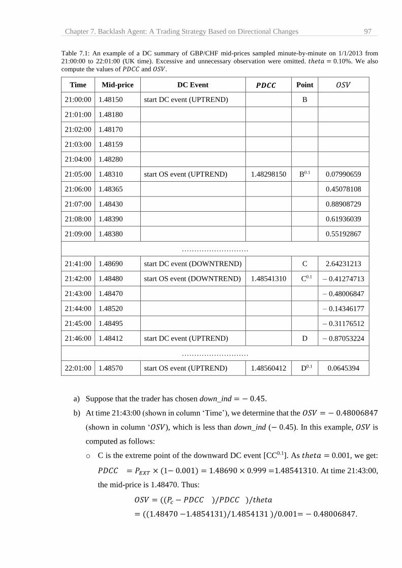
Chapter 7. Backlash Agent: A Trading Strategy Based on Directional Changes 97
Table 7.1: An example of a DC summary of GBP/CHF mid-prices sampled minute-by-minute on 1/1/2013 from
21:00:00 to 22:01:00 (UK time). Excessive and unnecessary observation were omitted. 𝑡ℎ𝑒𝑡𝑎 = 0.10%. We also
compute the values of 𝑃𝐷𝐶𝐶 and 𝑂𝑆𝑉.
Time Mid-price DC Event 𝑷𝑫𝑪𝑪 Point 𝑂𝑆𝑉
21:00:00 1.48150 start DC event (UPTREND) B
21:01:00 1.48180
21:02:00 1.48170
21:03:00 1.48159
21:04:00 1.48280
21:05:00 1.48310 start OS event (UPTREND) 1.48298150 B0.1 0.07990659
21:06:00 1.48365 0.45078108
21:07:00 1.48430 0.88908729
21:08:00 1.48390 0.61936039
21:09:00 1.48380 0.55192867
………………………
21:41:00 1.48690 start DC event (DOWNTREND) C 2.64231213
21:42:00 1.48480 start OS event (DOWNTREND) 1.48541310 C0.1 – 0.41274713
21:43:00 1.48470 – 0.48006847
21:44:00 1.48520 – 0.14346177
21:45:00 1.48495 – 0.31176512
21:46:00 1.48412 start DC event (UPTREND) D – 0.87053224
………………………
22:01:00 1.48570 start OS event (UPTREND) 1.48560412 D0.1 0.0645394
a) Suppose that the trader has chosen down_ind = − 0.45.
b) At time 21:43:00 (shown in column ‘Time’), we determine that the 𝑂𝑆𝑉 = − 0.48006847
(shown in column ‘𝑂𝑆𝑉), which is less than down_ind (− 0.45). In this example, 𝑂𝑆𝑉 is
computed as follows:
o C is the extreme point of the downward DC event [CC0.1]. As 𝑡ℎ𝑒𝑡𝑎 = 0.001, we get:
𝑃𝐷𝐶𝐶 = 𝑃𝐸𝑋𝑇 × (1− 0.001) = 1.48690 × 0.999 =1.48541310. At time 21:43:00,
the mid-price is 1.48470. Thus:
𝑂𝑆𝑉 = ((𝑃𝑐 − 𝑃𝐷𝐶𝐶 )/𝑃𝐷𝐶𝐶 )/𝑡ℎ𝑒𝑡𝑎
= ((1.48470 −1.4854131)/1.4854131 )/0.001= − 0.48006847.
Chapter 7. Backlash Agent: A Trading Strategy Based on Directional Changes 98
c) Based on a) and b), both conditions of Rule SBA-down.1 are fulfilled. Therefore SBA-down
generates a buy signal at time 21:43:00.
d) [DD0.1] is the upward DC event, which immediately follows the downward DC event
[CC0.1]. At time 22:01:00, we confirm the DCC point of [DD0.1] — which is D0.1. Based on
Rule SBA-down.2, SBA-down will generate a sell signal at time 22:01:00.
7.3.2 Static BA-up (SBA-up)
In this section, we introduce the second version of SBA named SBA-up. SBA-up is the mirror
of SBA-down. SBA-up generates a sell signal while the market is in an uptrend and only if the
value of OSV exceeds a certain threshold, named up_ind. SBA-up generates a buy signal when a
new downward DC event is observed. SBA-up consists of two rules:
Rule SBA-up.1: (generate sell signal)
If (the current event is OS on an uptrend) and (𝑂𝑆𝑉 ≥ up_ind) then generate sell signal.
Rule SBA-up.2: (generate buy signalo)
If (𝑃𝑐 ≤ 𝑃𝐷𝐶𝐶↓) and (a sell order has been fulfilled) then generate buy signal.
Here, 𝑃𝐷𝐶𝐶↓ denote the highest price required to confirm the observation of the next downward
DC event. up_ind is a trading parameter. The condition of Rule SBA-up.2 indicates the case under
which we confirm the DCC point of the next downward DC event of threshold theta. Note that
Rule SBA-up.2 is applicable only if a sell signal has been triggered. Rule SBA-up.2 plays two roles
at the same time: take-profit and stop-loss. When Rule SBA-up.2 triggers a buy signal, it may incur
losses (hence, functioning as stop-loss) or generate profits (thus, working as take-profit).
We use Table 7.1 above to provide an example of how the trading rules of SBA-up function,
by examining the upward DC event [BB0.1], of threshold 0.10%, which starts at time 21:00:00.
a) Suppose that the trader sets up_ind = 0.80.
b) At time 21:07:00, we determine that 𝑂𝑆𝑉 = 0.88908729. OSV is larger than up_ind
(0.80).
o B is the extreme point of the upward DC event [BB0.1]. In this case, with theta =
0.001, we get 𝑃𝐷𝐶𝐶 = 𝑃𝐸𝑋𝑇 × (1 + 0.001) = 1.48150 × 1.001 = 1.48298150.
At time 21:07:00, the mid-price is 1.48430. Thus,
𝑂𝑆𝑉 = ((𝑃𝑐 − 𝑃𝐷𝐶𝐶 )/𝑃𝐷𝐶𝐶 )/𝑡ℎ𝑒𝑡𝑎
o We want to highlight that no short selling is allowed. In the case of trading SBA-up, we assume that the initial capital is provided
in base currency. When SBA-up initiates a sell signal (based on Rule SBA-up.1), we use the base currency to buy counter currency.
Chapter 7. Backlash Agent: A Trading Strategy Based on Directional Changes 99
= ((1.48430 −1.48298150 )/1.48298150)/ 0.001= 0.88908729
c) Based on a) and b) both conditions of Rule SBA-up.1 are fulfilled and therefore SBA-up
generates a sell signal at time 21:07:00.
d) [CC0.1] is the downward DC event which follows the upward DC event [BB0.1]. At time
21:42:00, we confirm the DCC point, C0.1, of the next downtrend DC event, which is
[CC0.1]. Based on Rule SBA-up.2, SBA-up will generate a buy signal.
7.3.3 Dynamic Backlash Agent
When trading with static BA, we have no hint as to how SBA-down, or SBA-up, will perform
if the value of down_ind or up_ind is chosen arbitrarily. Theoretically, the investor should use
his/her expertise to choose the value of the parameters down_ind or up_ind. However, in some
cases, the investor may not have sufficient experience to do so. Moreover, there is no guarantee,
should SBA-down perform well for a given value of down_ind during a trading period, x that it
will behave similarly during another trading period, y using the same value of down_ind. The same
holds true for SBA-up. These facts are the motivation behind the development of the two versions
of dynamic BA, namely DBA-down and DBA-up respectively.
7.3.3.1 Dynamic BA-down (DBA-down)
DBA-down comprises two stages. In the first stage, DBA-down automatically determines the
value of the parameter down_ind. For this purpose, DBA-down applies a procedure, named
FIND_DOWN_IND, to a training (i.e. in-sample) dataset to determine the value of down_ind. In
the second stage, DBA-down uses the same two rules of SBA-down to trade over a trading, out-
of-sample, dataset using the value of down_ind returned by FIND_DOWN_IND.
The objective of the procedure FIND_DOWN_IND is to find an appropriate value for the
parameter down_ind to be utilized in trades with SBA-down during the applied period. The output
of the procedure FIND_DOWN_IND is one numerical variable, named best_down_ind. In order
to determine best_down_ind, FIND_DOWN_IND applies the trading rules of SBA-down to the
training dataset using 100 different values of down_ind (from – 0.01 to –1.00, with a step size of –
0.01). For each value of down_ind, we compute the returns, either profits or losses, obtained by
applying SBA-down to the training dataset. Thus, for a given training period we get 100 returns
— one return for each distinct value of down_ind. We define best_down_ind as the value of
down_ind under which SBA-down generated the highest returns using the training dataset. In the
second stage of DBA-down, we follow the trading rules (SBA-down.1 and SBA-down.2) with the

Chapter 7. Backlash Agent: A Trading Strategy Based on Directional Changes 100
input parameter ‘down_ind’ being assigned the value of best_down_ind to trade over the trading
dataset.
7.3.3.2 Dynamic BA-up (DBA-up)
DBA-up is the dynamic version of SBA-up, as DBA-down is to SBA-down. DBA-up also has
two stages, like DBA-down. The first stage consists of automatically finding an appropriate value
of up_ind, using the training period. This is done by a procedure called FIND_UP_IND.
FIND_UP_IND has the same role as FIND_DOWN_IND. FIND_UP_IND uses the training
dataset to compute one numerical variable named best_up_ind. To determine best_up_ind,
FIND_UP_IND applies the trading rules of SBA-up to the training dataset using 100 different
values of up_ind (from 0.01 to 1.00, with a step size of 0.01). For each value of up_ind, we compute
the returns, either profits or losses, obtained by applying SBA-up to the training period.
Consequently, for a given training dataset we get 100 returns — one return for each value of
up_ind. We define best_up_ind as the value of up_ind under which SBA-up has generated the
highest returns during the training period. The second stage of DBA-up follows the trading rules
(SBA-up.1 and SBA-up.2) with the input parameter ‘up_ind’ being assigned the value of
best_up_ind to trade over the trading period.
7.4 Evaluation of the Backlash Agent: Methodology and experiments
To evaluate the performance of all BA versions, we consider the minute-by-minute mid-prices
of the eight currency pairs (EUR/CHF, GBP/CHF, EUR/USD, GBP/AUD, GBP/JPY, NZD/JPY,
AUD/JPY, and EUR/NZD) for 31 months: from 1/1/2013 to 31/7/2015. For each currency pair,
we run the DC analysis with 𝑡ℎ𝑒𝑡𝑎 = 0.10%, and we compose a set of seven rolling windows.
Each rolling window comprises a training window of 24 months in length and an applied (i.e.
trading) period of 1 month in length. Basically, we use the same eight sets of rolling windows
previously composed in Section 6.4.4; namely: EURCHF_RWDC0.1, GBPCHF_RWDC0.1,
EURUSD_RWDC0.1, GBPAUD_RWDC0.1, GBPJPY_RWDC0.1, NZDJPY_RWDC0.1,
AUDJPY_RWDC0.1, and EURNZD_RWDC0.1. . See Section 6.4.4 for details on how these eight
sets are prepared.
In this chapter, we provide five sets of experiments: 1) the first experiment is designed to
estimate the best and the worst performance of SBA-down and SBA-up; 2) the second examines
whether there are specific values of the parameters down_ind and up_ind for which SBA-down
and SBA-up perform best; 3) the third evaluates the performance of DBA-down and DBA-up; 4)
Chapter 7. Backlash Agent: A Trading Strategy Based on Directional Changes 101
the fourth compares the profitability of SBA and DBA; 5) the fifth experiment aims to compare
the performances of DBA-down and DBA-up.
We use the same money management approach described in Section 6.5.1 for each of these
experiments. In summary: when any version of BA generates a buy or sell signal, it uses the entire
capital to trade. When we apply any version of the Backlash Agent, we make sure that no position
is left open at the end of the trading period. Should we encounter an open position at the end of the
trading period, then the last transaction will not be considered when computing the results —
instead, we roll back to the previous transaction. In other words, we do not count this last trade
when measuring any of the considered evaluation metrics. We consider the instantaneous bid and
ask prices in all of our experiments, but not the transaction costs.
7.4.1 Experiment 7.1: Evaluation of Static BA
The objective of this section is to evaluate the best and the worst performance of static BA (both
versions: SBA-down and SBA-up).
7.4.1.1 Experiment 7.1.1: Estimating the best and worst RR of SBA-down
For simplicity, we consider the rate of return (RR) as the primary performance indicator. RR is
defined as the gain or loss on an investment, expressed as a percentage of the amount invested (see
Section 3.4).We will use the currency pair EUR/CHF to describe our approach to estimating the
maximum and minimum RR that could be produced by applying SBA-down to EUR/CHF, or more
particularly to the set of rolling windows named EURCHF_RWDC0.1. The same method will
apply to each of the remaining seven sets of rolling windows.
As stated in Section 7.2, static BA is not applicable unless the investor knows what values to
assign to the parameters. Keep in mind that EURCHF_RWDC0.1 includes seven applied windows.
To provide a reasonable evaluation, we apply SBA-down to each applied window in
EURCHF_RWDC0.1, using 100 different values of down_ind (from – 0.01 to –1.00, with a step
size of –0.01). Consequently, for each applied window we will have 100 RR (each RR
corresponding to one distinct value of down_ind). For each applied window, we consider the
maximum and the minimum generated RR. So that, in total, we get seven maximum RR and seven
minimum RR. To estimate the overall maximum RR of trading with SBA-down over
EURCHF_RWDC0.1, we sum the seven maximum RR of these seven applied windows (starting
from 1/12015 to 31/7/2015). This is complemented by other measures, mainly the profit factor,
MDD and win ratio. Similarly, we apply SBA-down to the applied windows of each of the
Chapter 7. Backlash Agent: A Trading Strategy Based on Directional Changes 102
remaining seven sets of rolling windows (previously composed in Section 6.4.4) and we measure
the maximum and the minimum produced RR of applying SBA-down to each set. In this
experiment, as well as in the following experiments, we apply the money management approach
described in Section 6.5.1. While there is no direct transaction fee, we consider the bid–ask spread
as a kind of indirect charge as in ( [6] [15] [16]).
7.4.1.2 Experiment 7.1.2: Estimating the best and worst RR of SBA-up
This experiment aims to evaluate the best and the worst performance of SBA-up. In line with
the previous experiment, we apply SBA-up to each applied window in EURCHF_RWDC0.1 using
100 different values of up_ind (from 0.01 to 1.00, with a step size of 0.01). Consequently, for each
applied window we will have 100 RR (each RR corresponding to a distinct value of up_ind).
EURCHF_RWDC0.1 has seven applied periods. For each applied window we consider the
maximum and the minimum generated RR. So that, in total we get seven maximum RR and seven
minimum RR. To compute the maximum RR of trading with SBA-up over EURCHF_RWDC0.1
we sum the seven maximum RR. We also measure additional metrics: the profit factor, MDD and
win ratio. Similarly, we apply SBA-up to the applied windows of each of the remaining seven sets
of rolling windows (previously composed in Section 6.4.4) and we measure the maximum and the
minimum produced RR of applying SBA-up to each set.
7.4.2 Experiment 7.2: Is there one optimal value for the parameters down_ind and up_ind?
This experiment investigates whether there are specific values for the parameters down_ind and
up_ind, under which SBA-down and SBA-up will consistently produce the maximum RR. For this
purpose, we apply SBA-down and SBA-up to the eight currency pairs: EUR/CHF, GBP/CHF,
EUR/USD, GBP/AUD, NZD/JPY, AUD/JPY, GBP/JPY, and EUR/NZD. In this experiment, we
consider the period from 01/08/2014 to 31/07/2015 (12 months) as the trading period.
For each currency pair, for each month, we simulate 100 trades with SBA-down. For each trade,
we use a different value of the down_ind parameter (from 0.01 to 1.00, with a step size of
0.01). Consequently, for each month we will have 100 returns (each return corresponds to a
distinct value of down_ind). For each currency pair, and for each trading month, we compute the
maximum RR generated by SBA-down. We select and report the values of the down_ind parameter
that correspond to these maximum RR. In total, for each currency pair we obtain 12 values of
down_ind that represent the best performance of SBA-down during the12 months (one value for
each trading month).
Chapter 7. Backlash Agent: A Trading Strategy Based on Directional Changes 103
A naïve assumption would be to consider up_ind = down_ind. This would not be an intelligent
decision as some studies (e.g. [77]) have reported that the downtrends and uptrends for financial
time series will, probably, have different characteristics. We perform the same 100 trade
simulations, in the same trading period (12 months) and on the same eight currency pairs, using
SBA-up — each time using a different value of the up_ind parameter. For each currency pair, we
get another 12 values of up_ind corresponding to the highest possible RR generated by SBA-up
during the12 months. We analyse these values of down_ind, or up_ind, to find out whether there
exists a particular value for which SBA-down, or SBA-up, will deliver the best possible
performance consistently.
7.4.3 Experiment 7.3: Evaluating the performance of DBA-down and DBA-up
If choosing the value of the parameters down_ind or up_ind arbitrarily, a trader cannot have any
precise perception of how good, or otherwise, would be the performance of the static BA. With
this point in mind, we developed the dynamic version, DBA, as explained in Section 7.2.3. In this
experiment, we aim to evaluate the performance of both versions of DBA. To this end, we apply
DBA-down and DBA-up to the eight sets of rolling windows detailed in Section 6.4.4; namely,
EURCHF_RWDC0.1, GBPCHF_RWDC0.1, EURUSD_RWDC0.1, GBPAUD_RWDC0.1,
GBPJPY_RWDC0.1, NZDJPY_RWDC0.1, AUDJPY_RWDC0.1, and EURNZD_RWDC0.1.
Each window comprises: 1) a training period (of 24 months in length), and 2) a trading window
(of 1 month in length). For each rolling window, the training period is utilized to find the values
of the down_ind or up_ind parameters, based on the procedures FIND_DOWN_IND or
FIND_UP_IND described in Section 7.3.3. Then, we use these values in the trading period
associated with the specified rolling window. The performance of DBA is evaluated by measuring
the metrics reported in Section 3.3.
Furthermore, as we consider the buy and hold strategy (B&H) as a benchmark, we compare the
Sharpe ratio of both versions of DBA with the Sharpe ratio obtained by the buy and hold approach.
To validate this comparison statistically, we employ the Wilcoxon rank sum test [106] twice.
Firstly, we apply the Wilcoxon test with the null hypothesis being that ‘the median difference
between the Sharpe ratio produced by DBA-Down and B&H is zero’. Secondly, we apply the
Wilcoxon test with the null hypothesis being that ‘the median difference between the Sharpe ratio
produced by DAB-Up and B&H is zero’.
Chapter 7. Backlash Agent: A Trading Strategy Based on Directional Changes 104
7.4.4 Experiment 7.4: Comparing the RR of DBA and SBA
The objective of this experiment is to figure out what is the probability that DBA produces
higher RR than SBA provided that when trading with SBA, the parameters down_ind and up_ind
are assigned random values. This probability will help us to evaluate the efficiency of the proposed
procedures: FIND_DOWN_IND and FIND_UP_IND (Section 7.3.3) that are designed to find
appropriate values for the parameters down_ind and up_ind. Note that when trading with the static
versions, it is the trader who must choose the values of the parameters down_ind and up_ind.
Choosing these randomly offers a way of assessing the relative performance of SBA-down, and
SBA-up, against DBA-down, and DBA-up.
Consider that a trader assigns a random value to the parameter down_ind, or up_ind, when
trading with SBA-down, or SBA-up. In such a case, the question is: What is the probability that
the dynamic BA (DBA-down or DBA-up) will produce higher returns than the static BA (SBA-
down or SBA-up)? Let γ denote this probability. To compute γ, we estimate the performance of
the static version using a set of randomly chosen values for input parameters down_ind and up_ind.
The following provides an example of how to estimate γ based on the EUR/CHF dataset.
We simulate trading with SBA-down on EURCHF_RWDC0.1 10,000 timesp. Each time, we
trade with SBA-down on each applied window in EURCHF_RWDC0.1. Every time, and for each
applied window, we assign a new random value to the parameter down_ind. In other words, each
time that we trade with SBA-down we use seven random values of down_ind, each random value
being ranged between – 0.01 and – 1.00 and used for one applied window. With every trading
simulation, we measure the RR generated by SBA-down. Hence, we obtain 10,000 RR. Each RR
corresponds to one trade with SBA-down on the seven rolling windows of EURCHF_RWDC0.1.
γ can be calculated as the fraction of how many of these 10,000 RR are less than the RR generated
by the dynamic version, DBA-down, in Experiment 7.3 (Section 7.4.3). Similarly, we apply SBA-
up to the applied windows of EURCHF_RWDC0.1 10,000 times with randomly picked values for
parameter up_ind. Each time and for each applied window, we assign a new random value to the
parameter up_ind. We obtain another 10,000 RR. Each return corresponds to one trade with SBA-
up on the seven rolling windows of EURCHF_RWDC0.1. Again, γ is computed as the fraction of
how many of these 10,000 RR are less than the RR generated by DBA-up in Experiment 7.3
(Section 7.4.3).
p In a preliminary experiment we considered various numbers of trading simulations to determine γ. We found that for
more than 10,000 trading simulations (e.g. 13,000; 15,000) the value of γ changed (less than 0.5%).

Chapter 7. Backlash Agent: A Trading Strategy Based on Directional Changes 105
The entire procedure is repeated for each of the remaining seven sets of rolling windows:
GBPCHF_RWDC0.1, EURUSD_RWDC0.1, GBPAUD_RWDC0.1, GBPJPY_RWDC0.1,
NZDJPY_RWDC0.1, AUDJPY_RWDC0.1, and EURNZD_RWDC0.1. For each of these sets, we
apply SBA-down and SBA-up with randomly chosen parameters, down_ind and up_ind, to each
of the seven applied periods 10,000 times. Hence, we obtain 10,000 RR resulting from trading with
SBA-down and another 10,000 RR resulting from trading with SBA-up. For each set of rolling
windows, we evaluate γ as the percentage of how many of these 10,000 RR are less than the RR
generated by DBA-down and DBA-up in Experiment 7.3.
7.4.5 Experiment 7.5: Comparing the returns and risk of both versions of DBA
The objective of this experiment is to test whether there is difference between the performances
of DBA-down and DBA-up. To this end, we compare the returns and risk of both versions of DBA.
In this experiment, we consider the rate of returns (RR) and maximum drawdown (MDD) resulting
from applying both versions of DBA to the eight currency pairs from Experiment 7.3. That is, we
want to find out whether DBA-down and DBA-up provide similar RR and MDD. To validate this
comparison statistically, we will apply the Wilcoxon Rank Sum test [106].
Initially, we compare the RR of DBA-down and DBA-up by composing two sets of RR based
on the results of Experiment 7.3. The first set consists of the 8 RR resulting from trading with
DBA-down over the eight currency pairs (1 RR for each currency pair). The second set consists of
the 8 RR obtained by applying DBA-up to the eight considered currency pairs. Then, we apply the
non-parametric Wilcoxon rank sum test with the null hypothesis being that the median difference
of the two sets of monthly RR is zero.
Secondly, we compare the risks of DBA-down and DBA-up. To this end, we compare the MDD
resulting from applying DBA-down and DBA-up to the eight currency rates. We compose two sets
of MDD data. The first set contains the 8 MDD (1 MDD for each currency pair) corresponding to
trading with DBA-down. Likewise, the second set contains the MDD resulting from applying
DBA-up to the eight currency rates. We apply the Wilcoxon Rank Sum test to these sets with the
null hypothesis being that the median difference of the two sets of MDD is zero.
Chapter 7. Backlash Agent: A Trading Strategy Based on Directional Changes 106
7.5 Evaluation of Backlash Agent: Results and discussion
7.5.1 Experiment 7.1: Evaluation of Static BA
7.5.1.1 Experiments 7.1.1: Evaluating the performance of SBA-down
The objective of this experiment is to estimate the best and the worst possible performance of
SBA-down. For simplicity, we consider the maximum and the minimum produced RR as the
primary indicators of the best and the worst performance respectively. We consider eight currency
pairs. We compose eight sets of rolling windows (one set for each currency pair). Each set is
composed of seven rolling windows (see Section 6.4.4). We apply SBA-down to the applied
windows of each set of rolling windows using 100 different values of down_ind. We adopt the
money management approach described in Section 6.5.1. In this experiment, we are not concerned
with a detailed monthly evaluation. Instead, we focus on the general performance of SBA-down
during the overall seven months (i.e. the entire trading period) of each set of rolling windows. We
also measure the overall profit factor, MDD, and win ratio. We consider the instantaneous actual
bid and ask prices for each trade (either to buy or to sell) in all of our experiments.
Table 7.2 and Table 7.3 display, respectively, the best and the worst, estimated, performances
of SBA-down when applied to the composed sets of rolling windows (see Section 7.3.1). These
tables include the following metrics: rates of return (RR), profit factor, maximum drawdown, and
win ratio (see Section 3.4 for more details about these metrics). For each currency pair, at the
beginning of the first applied window, i.e. January 2015, SBA-down starts with capital =
1,000,000 monetary unitsq, this represents the initial, hypothetically, invested amount of money.
From Table 7.2, let us consider the case of EUR/CHF. The reported results have the following
interpretation: the cumulative rates of return (RR) are 7.48% as shown in column ‘RR’. This
represents the maximum total RR that can be produced by applying SBA-down to the seven applied
windows of EURCHF_RWDC0.1. In this case, SBA-down generates 1798 trades, as shown in
column ‘Total Number of Trades’, with an overall win ratio of 0.73 as shown in column ‘Win
Ratio’. Whereas, in Table 7.3, in the case of EUR/CHF, we note that the minimum RR, during the
trading period of seven months, is – 2.09%. In this case, SBA-down generates 1167 trades with an
overall win ratio of 0.73. Based on Table 7.2, in the best case, SBA-down can generate RR of
q For each currency pair, trading with SBA-down, or DBA-down, we assume that we start with 1,000,000 units of
counter currency. For example: in the case of EUR/CHF, we start with 1,000,000 CHF. Whereas in the case of
NZD/JPY, we start with 1,000,000 JPY. However, in the case of SBA-up, or DBA-up, we assume that we start with
1,000,000 units of the base currency.

Chapter 7. Backlash Agent: A Trading Strategy Based on Directional Changes 107
36.86% (see EUR/NZD, the last row in Table 7.2). Based on Table 7.3, in the worst case, SBA-
down can generate RR of – 6.50% (see EUR/USD, as shown in Table 7.3).
Table 7.2: Summary of the best performance of the SBA-down model following the seven months out-of-sample
period of the eight currency rates from 1/1/2015 to 31/7/2015.
Currency
Pairs RR
Profit
Factor
Total Number
of Trades
Max
Drawdown (%) Win Ratio
EUR/CHF 7.48 1.98 1798 – 4.3 0.73
GBP/CHF 8.53 1.92 2539 – 5.1 0.72
EUR/USD 1.90 1.15 1935 – 7.3 0.75
GBP/AUD 7.29 1.67 2707 – 5.6 0.74
GBP/JPY 2.64 1.22 1748 – 8.5 0.72
NZD/JPY 23.96 2.03 3409 – 2.7 0.73
AUD/JPY 10.33 1.97 2861 – 3.2 0.74
EUR/NZD 36.86 2.26 3919 – 1.3 0.71
Table 7.3: Summary of the worst performance of the SBA-down model following the seven months out-of-sample
period of the eight currency rates.
Currency
Pairs RR
Profit
Factor
Total Number of
Trades
Max Drawdown
(%) Win Ratio
EUR/CHF – 2.09 0.82 1167 – 8.0 0.59
GBP/CHF – 2.41 0.83 1270 – 8.2 0.51
EUR/USD – 6.50 0.65 1649 – 10.9 0.55
GBP/AUD 2.62 1.09 2571 – 11.5 0.61
GBP/JPY – 5.89 0.60 1290 – 15.8 0.48
NZD/JPY 2.77 1.07 2515 – 7.4 0.62
AUD/JPY 3.41 1.28 2111 – 8.1 0.62
EUR/NZD 5.03 1.14 2873 – 6.3 0.63
When examining the difference between the maximum and minimum RR produced by SBA-
down, by comparing the RR shown in Tables 7.2 and 7.3, it is evident that this difference can be
significant. For example, in the case of AUD/JPY, the maximum RR estimated for SBA-down is
10.33% (Table 7.2). This is more than double the minimum RR obtained by applying SBA-down
to AUD/JPY (which is 3.41%, as reported in Table 7.3). The same note holds true for the RR
obtained by SBA-down for all other currency rates. Keep in mind that this difference between the
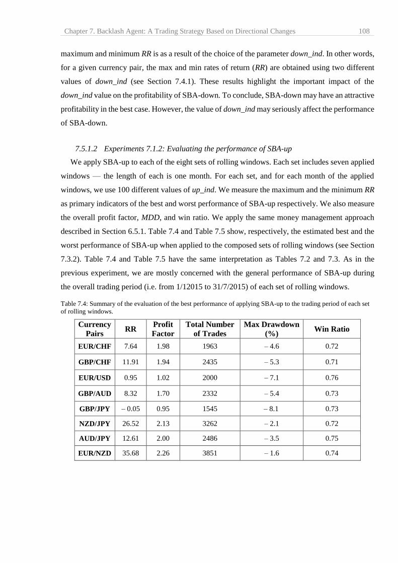
Chapter 7. Backlash Agent: A Trading Strategy Based on Directional Changes 108
maximum and minimum RR is as a result of the choice of the parameter down_ind. In other words,
for a given currency pair, the max and min rates of return (RR) are obtained using two different
values of down_ind (see Section 7.4.1). These results highlight the important impact of the
down_ind value on the profitability of SBA-down. To conclude, SBA-down may have an attractive
profitability in the best case. However, the value of down_ind may seriously affect the performance
of SBA-down.
7.5.1.2 Experiments 7.1.2: Evaluating the performance of SBA-up
We apply SBA-up to each of the eight sets of rolling windows. Each set includes seven applied
windows — the length of each is one month. For each set, and for each month of the applied
windows, we use 100 different values of up_ind. We measure the maximum and the minimum RR
as primary indicators of the best and worst performance of SBA-up respectively. We also measure
the overall profit factor, MDD, and win ratio. We apply the same money management approach
described in Section 6.5.1. Table 7.4 and Table 7.5 show, respectively, the estimated best and the
worst performance of SBA-up when applied to the composed sets of rolling windows (see Section
7.3.2). Table 7.4 and Table 7.5 have the same interpretation as Tables 7.2 and 7.3. As in the
previous experiment, we are mostly concerned with the general performance of SBA-up during
the overall trading period (i.e. from 1/12015 to 31/7/2015) of each set of rolling windows.
Table 7.4: Summary of the evaluation of the best performance of applying SBA-up to the trading period of each set
of rolling windows.
Currency
Pairs RR
Profit
Factor
Total Number
of Trades
Max Drawdown
(%) Win Ratio
EUR/CHF 7.64 1.98 1963 – 4.6 0.72
GBP/CHF 11.91 1.94 2435 – 5.3 0.71
EUR/USD 0.95 1.02 2000 – 7.1 0.76
GBP/AUD 8.32 1.70 2332 – 5.4 0.73
GBP/JPY – 0.05 0.95 1545 – 8.1 0.73
NZD/JPY 26.52 2.13 3262 – 2.1 0.72
AUD/JPY 12.61 2.00 2486 – 3.5 0.75
EUR/NZD 35.68 2.26 3851 – 1.6 0.74
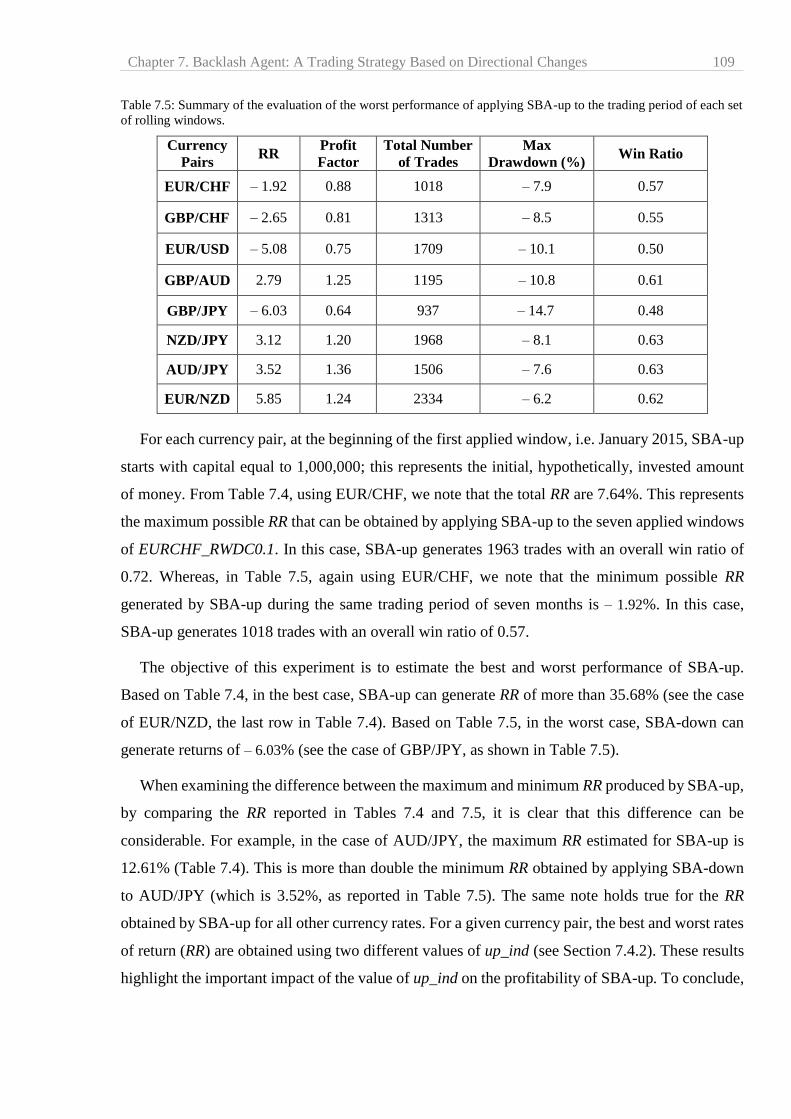
Chapter 7. Backlash Agent: A Trading Strategy Based on Directional Changes 109
Table 7.5: Summary of the evaluation of the worst performance of applying SBA-up to the trading period of each set
of rolling windows.
Currency
Pairs RR
Profit
Factor
Total Number
of Trades
Max
Drawdown (%) Win Ratio
EUR/CHF – 1.92 0.88 1018 – 7.9 0.57
GBP/CHF – 2.65 0.81 1313 – 8.5 0.55
EUR/USD – 5.08 0.75 1709 – 10.1 0.50
GBP/AUD 2.79 1.25 1195 – 10.8 0.61
GBP/JPY – 6.03 0.64 937 – 14.7 0.48
NZD/JPY 3.12 1.20 1968 – 8.1 0.63
AUD/JPY 3.52 1.36 1506 – 7.6 0.63
EUR/NZD 5.85 1.24 2334 – 6.2 0.62
For each currency pair, at the beginning of the first applied window, i.e. January 2015, SBA-up
starts with capital equal to 1,000,000; this represents the initial, hypothetically, invested amount
of money. From Table 7.4, using EUR/CHF, we note that the total RR are 7.64%. This represents
the maximum possible RR that can be obtained by applying SBA-up to the seven applied windows
of EURCHF_RWDC0.1. In this case, SBA-up generates 1963 trades with an overall win ratio of
0.72. Whereas, in Table 7.5, again using EUR/CHF, we note that the minimum possible RR
generated by SBA-up during the same trading period of seven months is – 1.92%. In this case,
SBA-up generates 1018 trades with an overall win ratio of 0.57.
The objective of this experiment is to estimate the best and worst performance of SBA-up.
Based on Table 7.4, in the best case, SBA-up can generate RR of more than 35.68% (see the case
of EUR/NZD, the last row in Table 7.4). Based on Table 7.5, in the worst case, SBA-down can
generate returns of – 6.03% (see the case of GBP/JPY, as shown in Table 7.5).
When examining the difference between the maximum and minimum RR produced by SBA-up,
by comparing the RR reported in Tables 7.4 and 7.5, it is clear that this difference can be
considerable. For example, in the case of AUD/JPY, the maximum RR estimated for SBA-up is
12.61% (Table 7.4). This is more than double the minimum RR obtained by applying SBA-down
to AUD/JPY (which is 3.52%, as reported in Table 7.5). The same note holds true for the RR
obtained by SBA-up for all other currency rates. For a given currency pair, the best and worst rates
of return (RR) are obtained using two different values of up_ind (see Section 7.4.2). These results
highlight the important impact of the value of up_ind on the profitability of SBA-up. To conclude,

Chapter 7. Backlash Agent: A Trading Strategy Based on Directional Changes 110
SBA-up may have an attractive profitability level in the best case. However, the value of up_ind
may seriously affect the performance of SBA-up.
7.5.2 Experiment 7.2: Is there one optimal value for the parameter down_ind or up_ind?
The objective of this experiment is to investigate whether there exists a specific value for the
parameters down_ind, or up_ind, for which SBA-down, or SBA-up, will consistently generate the
highest possible RR. We consider the same eight currency pairs as in Section 7.4 and apply SBA-
down and SBA-up to each of these 100 times for a trading period of 12 months. Each time, for
each month, we assign different values for the parameters down_ind and up_ind and measure the
produced returns. In this experiment, our main interest is the values of the parameters down_ind
and up_ind associated with the highest RR. Our goal is to analyse the values of these parameters.
Table 7.6 shows the values of down_ind associated with the maximum monthly RR produced by
SBA-down. For each currency pair (i.e. for each column in Table 7.6), the largest and the smallest
values of down_ind are formatted in bold and italic respectively. For example, in column
‘EUR/CHF’ the numbers – 0.01 and – 0.84 denote, respectively, the largest and the smallest values
of down_ind under this column. These bold and italic figures, for the same column, indicate the
range of the parameter down_ind in which the specified trading model performs best. Similarly,
Table 7.7 shows the values of up_ind associated with the best monthly RR generated by SBA-up
for each of the 12 trading months considered in this experiment.
Table 7.6: The values of down_ind corresponding to the highest RR generated by SBA-down for each month. For each
currency pair, the figures in bold and italic indicate, respectively, the largest and the smallest values of down_ind.
Trading
period
EUR/
CHF
GBP/
CHF
EUR/
USD
GBP/
AUD
AUD/
JPY
NZD/
JPY
GBP/
JPY
EUR/
NZD
2014
Aug – 0.82 – 0.17 – 0.32 – 0.34 – 0.08 – 0.09 – 0.74 – 0.29
Sep – 0.08 – 0.04 – 0.92 – 0.02 – 0.15 – 0.43 – 0.62 – 0.16
Oct – 0.27 – 0.05 – 0.90 – 0.36 – 0.23 – 0.62 – 0.76 – 0.56
Nov – 0.40 – 0.93 – 0.07 – 0.13 – 0.45 – 0.27 – 0.53 – 0.73
Dec – 0.01 – 0.31 – 0.53 – 0.10 – 0.62 – 0.33 – 0.40 – 0.50
2015
Jan – 0.84 – 0.30 – 0.96 – 0.36 – 0.32 – 0.69 – 0.25 – 0.06
Feb – 0.43 – 0.08 – 0.12 – 0.16 – 0.07 – 0.03 – 0.05 – 0.46
Mar – 0.01 – 0.01 – 0.57 – 0.49 – 0.11 – 0.07 – 0.05 – 0.49
Apr – 0.04 – 0.10 – 0.23 – 0.34 – 0.15 – 0.32 – 0.12 – 0.54
May – 0.07 – 0.02 – 0.38 – 0.37 – 0.16 – 0.46 – 0.22 – 0.67
Jun – 0.14 – 0.12 – 0.07 – 0.18 – 0.10 – 0.08 – 0.15 – 0.38
Jul – 0.39 – 0.02 – 0.05 – 0.41 – 0.07 – 0.13 – 0.98 – 0.28
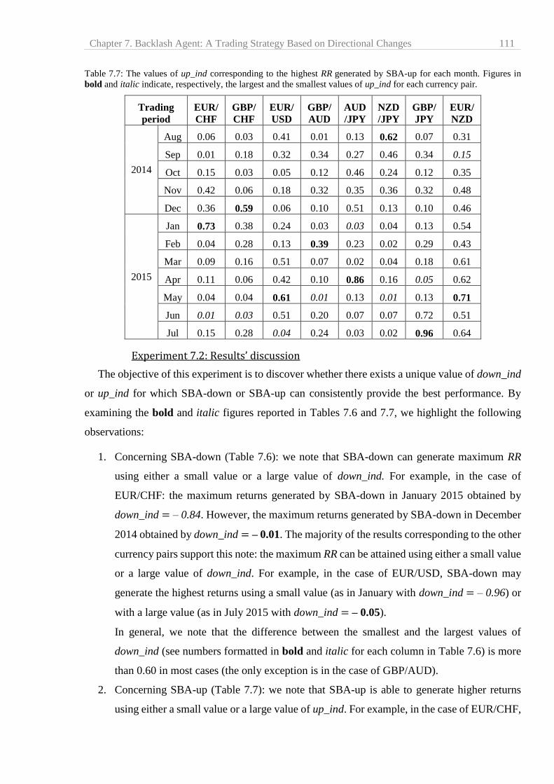
Chapter 7. Backlash Agent: A Trading Strategy Based on Directional Changes 111
Table 7.7: The values of up_ind corresponding to the highest RR generated by SBA-up for each month. Figures in
bold and italic indicate, respectively, the largest and the smallest values of up_ind for each currency pair.
Trading
period
EUR/
CHF
GBP/
CHF
EUR/
USD
GBP/
AUD
AUD
/JPY
NZD
/JPY
GBP/
JPY
EUR/
NZD
2014
Aug 0.06 0.03 0.41 0.01 0.13 0.62 0.07 0.31
Sep 0.01 0.18 0.32 0.34 0.27 0.46 0.34 0.15
Oct 0.15 0.03 0.05 0.12 0.46 0.24 0.12 0.35
Nov 0.42 0.06 0.18 0.32 0.35 0.36 0.32 0.48
Dec 0.36 0.59 0.06 0.10 0.51 0.13 0.10 0.46
2015
Jan 0.73 0.38 0.24 0.03 0.03 0.04 0.13 0.54
Feb 0.04 0.28 0.13 0.39 0.23 0.02 0.29 0.43
Mar 0.09 0.16 0.51 0.07 0.02 0.04 0.18 0.61
Apr 0.11 0.06 0.42 0.10 0.86 0.16 0.05 0.62
May 0.04 0.04 0.61 0.01 0.13 0.01 0.13 0.71
Jun 0.01 0.03 0.51 0.20 0.07 0.07 0.72 0.51
Jul 0.15 0.28 0.04 0.24 0.03 0.02 0.96 0.64
Experiment 7.2: Results’ discussion
The objective of this experiment is to discover whether there exists a unique value of down_ind
or up_ind for which SBA-down or SBA-up can consistently provide the best performance. By
examining the bold and italic figures reported in Tables 7.6 and 7.7, we highlight the following
observations:
1. Concerning SBA-down (Table 7.6): we note that SBA-down can generate maximum RR
using either a small value or a large value of down_ind. For example, in the case of
EUR/CHF: the maximum returns generated by SBA-down in January 2015 obtained by
down_ind = – 0.84. However, the maximum returns generated by SBA-down in December
2014 obtained by down_ind = – 0.01. The majority of the results corresponding to the other
currency pairs support this note: the maximum RR can be attained using either a small value
or a large value of down_ind. For example, in the case of EUR/USD, SBA-down may
generate the highest returns using a small value (as in January with down_ind = – 0.96) or
with a large value (as in July 2015 with down_ind = – 0.05).
In general, we note that the difference between the smallest and the largest values of
down_ind (see numbers formatted in bold and italic for each column in Table 7.6) is more
than 0.60 in most cases (the only exception is in the case of GBP/AUD).
2. Concerning SBA-up (Table 7.7): we note that SBA-up is able to generate higher returns
using either a small value or a large value of up_ind. For example, in the case of EUR/CHF,
Chapter 7. Backlash Agent: A Trading Strategy Based on Directional Changes 112
the maximum return generated by SBA-up in June 2015 is obtained with a low value of
up_ind = 0.01. However, the maximum profits produced by SBA-up in January 2015 are
obtained with a large up_ind = 0.73. The majority of the results corresponding to the other
currency pairs validate this note. For example, in the case of AUD/JPY, SBA-up may
generate the highest returns with a small value of up_ind (as in January 2015 with up_ind
= 0.03) or using a large value of up_ind (as in April 2015, with up_ind = 0.86).
In general, we note that the difference between the smallest and the largest values of up_ind
shown in bold in Table 7.7 is more than 0.50 in most cases (the only exception is the case
of GBP/AUD).
3. The results of Tables 7.6 and 7.7 suggest that it would be wrong to assume that up_ind =
down_ind. This indicates that downtrends and uptrends may have different behaviours;
which conforms to the findings of Tsang et al. [77].
To conclude, these two observations above (1. and 2.) suggest that, in most cases, there is no
specific value, or a tight range, for the parameters down_ind and up_ind for which SBA-down and
SBA-up will exhibit the best performance consistently. This conclusion raises the need for a
dynamic version of BA.
7.5.3 Experiment 7.3: Evaluation of the performance of DBA-down and DBA-up
In this experiment we apply DBA-down and DBA-up to the eight sets of rolling windows
(previously composed in Section 6.4.4). For each of DBA-down and DBA-up, we start with
1,000,000 monetary units as the initially invested capital. We use the same money management
approach described in Section 6.5.1. Table 7.8 reports the general performance, during the overall
trading period of seven months, of both versions of DBA in this experiment. We consider the bid
and ask prices in our experiments. When DBA-down or DBA-up triggers a buy (or sell) signal we
use the ask (or bid) price as quoted by the market maker. The annualized RR are reported in
Appendix E.
The column ‘Currency Pair’ denote the considered currency pair. The column ‘Trading Strategy’
indicates which version of DBA is applied. The column ‘RR’ is the total RR. The column ‘Profit
Factor’ is calculated by dividing the sum of all generated returns by the sum of incurred losses
during the overall trading period of seven months. The column ‘Max Drawdown (%)’ refers to the
worst scenario measured as the worst peak-to-trough decline in capital during the trading period
of seven months. The column ‘Win Ratio’ is the overall probability of having a wining trade. The
last row in Table 7.8 is interpreted as follows: applying DBA-up to EUR/NZD generates a rate of
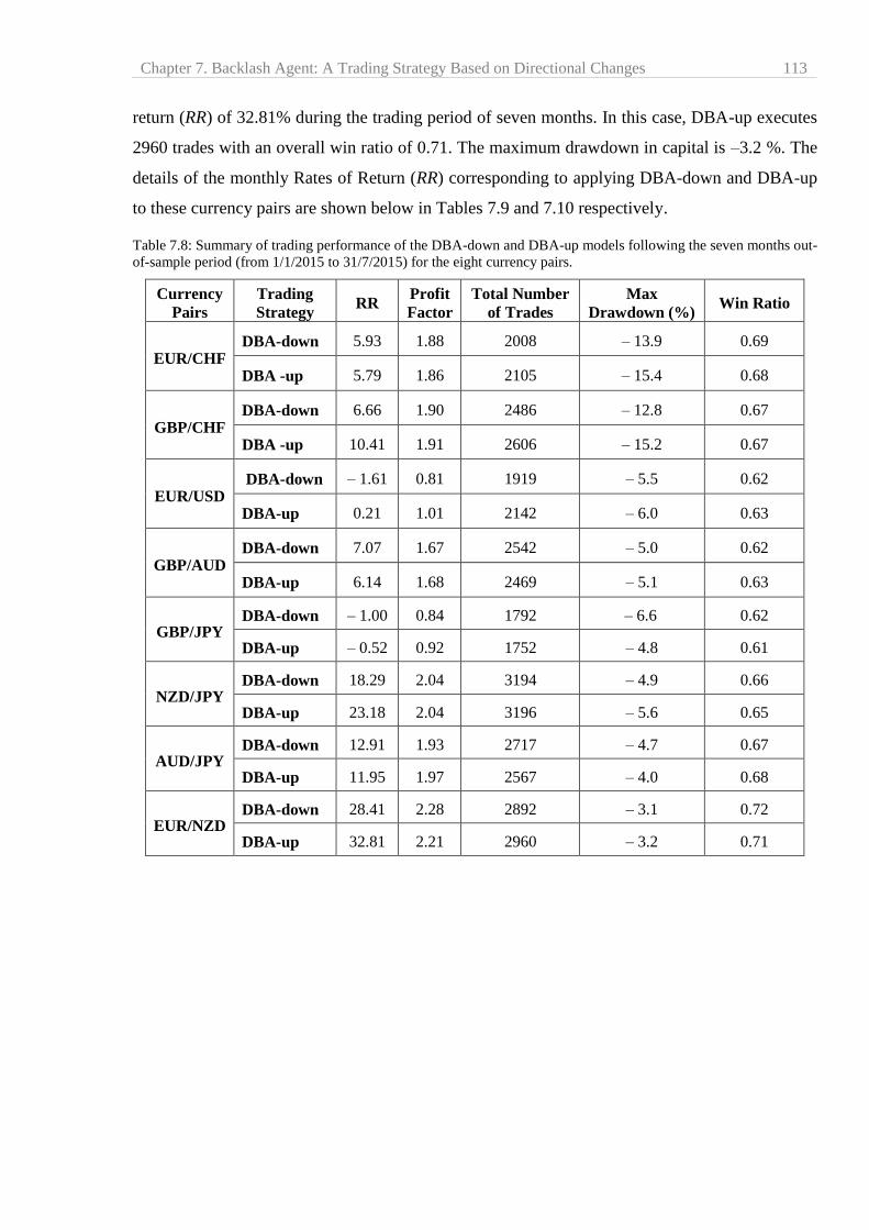
Chapter 7. Backlash Agent: A Trading Strategy Based on Directional Changes 113
return (RR) of 32.81% during the trading period of seven months. In this case, DBA-up executes
2960 trades with an overall win ratio of 0.71. The maximum drawdown in capital is –3.2 %. The
details of the monthly Rates of Return (RR) corresponding to applying DBA-down and DBA-up
to these currency pairs are shown below in Tables 7.9 and 7.10 respectively.
Table 7.8: Summary of trading performance of the DBA-down and DBA-up models following the seven months out-
of-sample period (from 1/1/2015 to 31/7/2015) for the eight currency pairs.
Currency
Pairs
Trading
Strategy RR
Profit
Factor
Total Number
of Trades
Max
Drawdown (%) Win Ratio
EUR/CHF DBA-down 5.93 1.88 2008 – 13.9 0.69
DBA -up 5.79 1.86 2105 – 15.4 0.68
GBP/CHF DBA-down 6.66 1.90 2486 – 12.8 0.67
DBA -up 10.41 1.91 2606 – 15.2 0.67
EUR/USD DBA-down – 1.61 0.81 1919 – 5.5 0.62
DBA-up 0.21 1.01 2142 – 6.0 0.63
GBP/AUD DBA-down 7.07 1.67 2542 – 5.0 0.62
DBA-up 6.14 1.68 2469 – 5.1 0.63
GBP/JPY DBA-down – 1.00 0.84 1792 – 6.6 0.62
DBA-up – 0.52 0.92 1752 – 4.8 0.61
NZD/JPY DBA-down 18.29 2.04 3194 – 4.9 0.66
DBA-up 23.18 2.04 3196 – 5.6 0.65
AUD/JPY DBA-down 12.91 1.93 2717 – 4.7 0.67
DBA-up 11.95 1.97 2567 – 4.0 0.68
EUR/NZD DBA-down 28.41 2.28 2892 – 3.1 0.72
DBA-up 32.81 2.21 2960 – 3.2 0.71
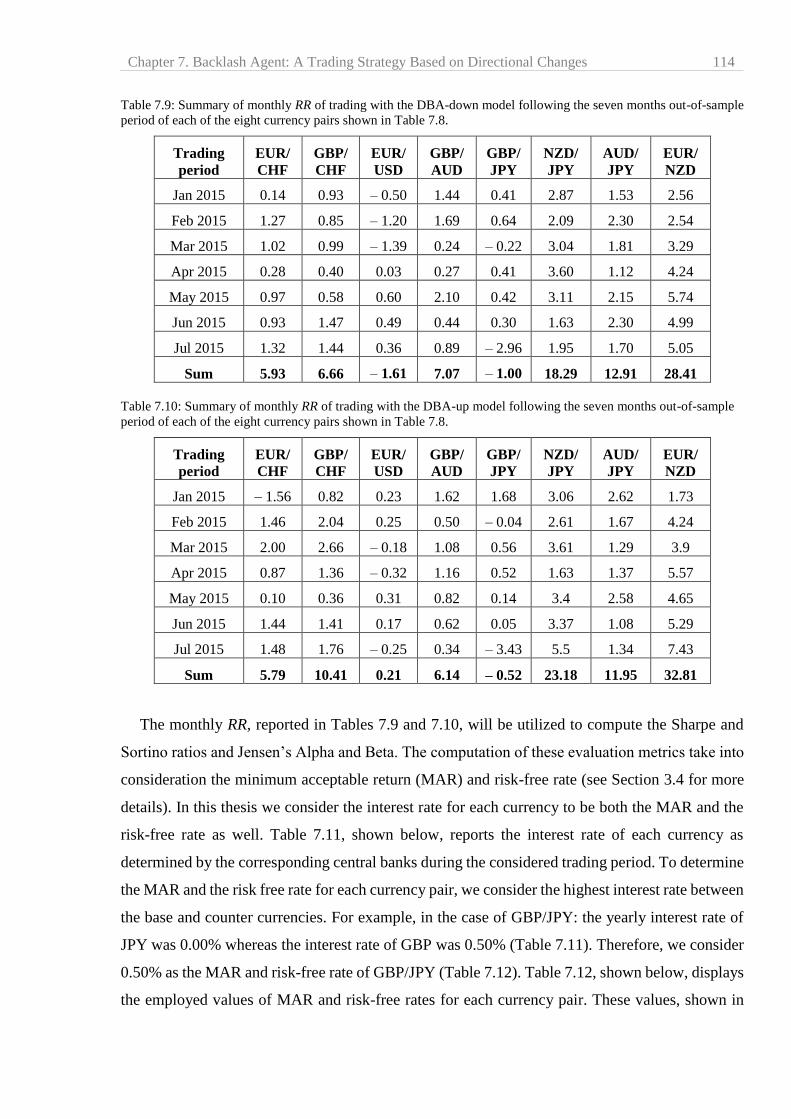
Chapter 7. Backlash Agent: A Trading Strategy Based on Directional Changes 114
Table 7.9: Summary of monthly RR of trading with the DBA-down model following the seven months out-of-sample
period of each of the eight currency pairs shown in Table 7.8.
Trading
period
EUR/
CHF
GBP/
CHF
EUR/
USD
GBP/
AUD
GBP/
JPY
NZD/
JPY
AUD/
JPY
EUR/
NZD
Jan 2015 0.14 0.93 – 0.50 1.44 0.41 2.87 1.53 2.56
Feb 2015 1.27 0.85 – 1.20 1.69 0.64 2.09 2.30 2.54
Mar 2015 1.02 0.99 – 1.39 0.24 – 0.22 3.04 1.81 3.29
Apr 2015 0.28 0.40 0.03 0.27 0.41 3.60 1.12 4.24
May 2015 0.97 0.58 0.60 2.10 0.42 3.11 2.15 5.74
Jun 2015 0.93 1.47 0.49 0.44 0.30 1.63 2.30 4.99
Jul 2015 1.32 1.44 0.36 0.89 – 2.96 1.95 1.70 5.05
Sum 5.93 6.66 – 1.61 7.07 – 1.00 18.29 12.91 28.41
Table 7.10: Summary of monthly RR of trading with the DBA-up model following the seven months out-of-sample
period of each of the eight currency pairs shown in Table 7.8.
Trading
period
EUR/
CHF
GBP/
CHF
EUR/
USD
GBP/
AUD
GBP/
JPY
NZD/
JPY
AUD/
JPY
EUR/
NZD
Jan 2015 – 1.56 0.82 0.23 1.62 1.68 3.06 2.62 1.73
Feb 2015 1.46 2.04 0.25 0.50 – 0.04 2.61 1.67 4.24
Mar 2015 2.00 2.66 – 0.18 1.08 0.56 3.61 1.29 3.9
Apr 2015 0.87 1.36 – 0.32 1.16 0.52 1.63 1.37 5.57
May 2015 0.10 0.36 0.31 0.82 0.14 3.4 2.58 4.65
Jun 2015 1.44 1.41 0.17 0.62 0.05 3.37 1.08 5.29
Jul 2015 1.48 1.76 – 0.25 0.34 – 3.43 5.5 1.34 7.43
Sum 5.79 10.41 0.21 6.14 – 0.52 23.18 11.95 32.81
The monthly RR, reported in Tables 7.9 and 7.10, will be utilized to compute the Sharpe and
Sortino ratios and Jensen’s Alpha and Beta. The computation of these evaluation metrics take into
consideration the minimum acceptable return (MAR) and risk-free rate (see Section 3.4 for more
details). In this thesis we consider the interest rate for each currency to be both the MAR and the
risk-free rate as well. Table 7.11, shown below, reports the interest rate of each currency as
determined by the corresponding central banks during the considered trading period. To determine
the MAR and the risk free rate for each currency pair, we consider the highest interest rate between
the base and counter currencies. For example, in the case of GBP/JPY: the yearly interest rate of
JPY was 0.00% whereas the interest rate of GBP was 0.50% (Table 7.11). Therefore, we consider
0.50% as the MAR and risk-free rate of GBP/JPY (Table 7.12). Table 7.12, shown below, displays
the employed values of MAR and risk-free rates for each currency pair. These values, shown in
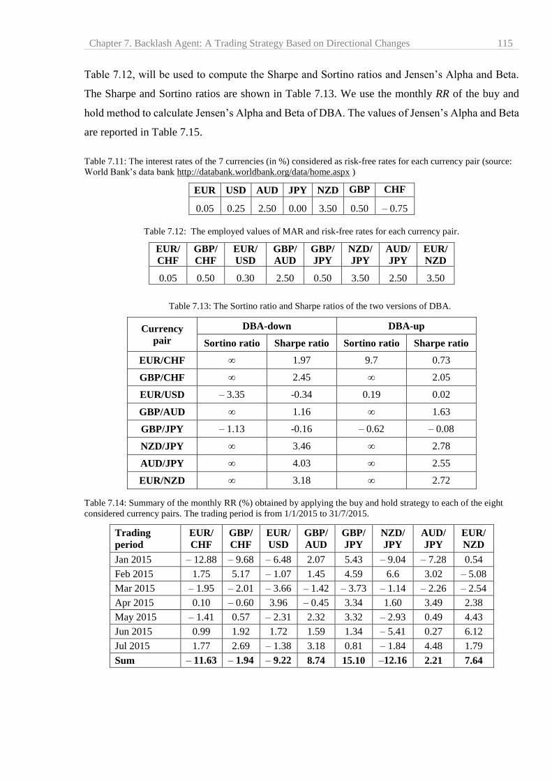
Chapter 7. Backlash Agent: A Trading Strategy Based on Directional Changes 115
Table 7.12, will be used to compute the Sharpe and Sortino ratios and Jensen’s Alpha and Beta.
The Sharpe and Sortino ratios are shown in Table 7.13. We use the monthly RR of the buy and
hold method to calculate Jensen’s Alpha and Beta of DBA. The values of Jensen’s Alpha and Beta
are reported in Table 7.15.
Table 7.11: The interest rates of the 7 currencies (in %) considered as risk-free rates for each currency pair (source:
World Bank’s data bank http://databank.worldbank.org/data/home.aspx )
EUR USD AUD JPY NZD GBP CHF
0.05 0.25 2.50 0.00 3.50 0.50 – 0.75
Table 7.12: The employed values of MAR and risk-free rates for each currency pair.
EUR/
CHF
GBP/
CHF
EUR/
USD
GBP/
AUD
GBP/
JPY
NZD/
JPY
AUD/
JPY
EUR/
NZD
0.05 0.50 0.30 2.50 0.50 3.50 2.50 3.50
Table 7.13: The Sortino ratio and Sharpe ratios of the two versions of DBA.
Currency
pair
DBA-down DBA-up
Sortino ratio Sharpe ratio Sortino ratio Sharpe ratio
EUR/CHF ∞ 1.97 9.7 0.73
GBP/CHF ∞ 2.45 ∞ 2.05
EUR/USD – 3.35 -0.34 0.19 0.02
GBP/AUD ∞ 1.16 ∞ 1.63
GBP/JPY – 1.13 -0.16 – 0.62 – 0.08
NZD/JPY ∞ 3.46 ∞ 2.78
AUD/JPY ∞ 4.03 ∞ 2.55
EUR/NZD ∞ 3.18 ∞ 2.72
Table 7.14: Summary of the monthly RR (%) obtained by applying the buy and hold strategy to each of the eight
considered currency pairs. The trading period is from 1/1/2015 to 31/7/2015.
Trading
period
EUR/
CHF
GBP/
CHF
EUR/
USD
GBP/
AUD
GBP/
JPY
NZD/
JPY
AUD/
JPY
EUR/
NZD
Jan 2015 – 12.88 – 9.68 – 6.48 2.07 5.43 – 9.04 – 7.28 0.54
Feb 2015 1.75 5.17 – 1.07 1.45 4.59 6.6 3.02 – 5.08
Mar 2015 – 1.95 – 2.01 – 3.66 – 1.42 – 3.73 – 1.14 – 2.26 – 2.54
Apr 2015 0.10 – 0.60 3.96 – 0.45 3.34 1.60 3.49 2.38
May 2015 – 1.41 0.57 – 2.31 2.32 3.32 – 2.93 0.49 4.43
Jun 2015 0.99 1.92 1.72 1.59 1.34 – 5.41 0.27 6.12
Jul 2015 1.77 2.69 – 1.38 3.18 0.81 – 1.84 4.48 1.79
Sum – 11.63 – 1.94 – 9.22 8.74 15.10 –12.16 2.21 7.64

Chapter 7. Backlash Agent: A Trading Strategy Based on Directional Changes 116
Table 7.15: The values of Jensen’s Alpha and Beta of both versions of DBA with reference to the buy and hold
approach as benchmark. The values are rounded to one decimal digit.
Currency pair DBA-down DBA-up
Jensen’s Alpha Beta Jensen’s Alpha Beta
EUR/CHF 0.74 0.06 0.49 0.20
GBP/CHF 0.90 0.02 1.43 0.05
EUR/USD – 0.38 0.09 0.05 – 0.03
GBP/AUD 1.10 0.28 0.56 – 0.11
GBP/JPY 0.15 0.16 0.16 0.13
NZD/JPY 2.32 0.00 3.16 – 0.07
AUD/JPY 1.64 0.00 1.49 – 0.08
EUR/NZD 3.98 0.27 4.51 0.15
Furthermore, as we consider the B&H as a benchmark, we compare the Sharpe ratio produced by
the B&H to that of DBA. Table 7.16, shown below, summarizes the Sharpe ratios produced by
B&H (named SR_BH), DBA-down (named SR_DBA_Down) and DBA-up (named SR_DBA_Up).
The values of SR_DBA_Down and SR_DBA_Up are extracted from Table 7.13, shown above. The
Sharpe ratios of the buy and hold approach (denoted as SR_BH in Table 7.16) are computed based
on the monthly RR of the B&H previously reported in Table 7.14. To validate the comparison
between the Sharpe ratios of DBA and B&H statistically, we applied the Wilcoxon test with the
null hypothesis being that the median difference between the Sharpe ratios of DBA and the buy
and hold approach is null. The test statistics ‘W’ resulting from the two Wilcoxon tests are reported
in Table 7.17.
Table 7.16: The Sharpe ratio values corresponding to the buy and hold (SR_BH), DBA-down (SR_DBA_Down),
and DBA-up (SR_DBA_Up).
EUR/
CHF
GBP/
CHF
EUR/
USD
GBP/
AUD
GBP/
JPY
NZD/
JPY
AUD/
JPY
EUR/
NZD
SR_BH – 0.35 – 0.07 – 0.42 0.69 0.74 – 0.44 0.03 0.22
SR_DBA_Down 1.97 2.45 – 0.34 1.16 – 0.16 3.46 1.4 3.18
SR_DBA_Up 0.73 2.05 0.02 1.63 – 0.08 2.78 1.65 2.72
Table 7.17: The test statistics ‘W’ of the conducted Wilcoxon tests of comparing the Sharpe ratios of B&H with
DBA-down and DBA-up based on the values reported in Table 7.16. The level of significance are denoted as:
***=1% and **=5%.
SR_DBA_Down SR_DBA_Up
W 10** 10**
Chapter 7. Backlash Agent: A Trading Strategy Based on Directional Changes 117
Experiment 7.3: Results’ Discussion and Analysis
To begin, we examine the profitability of both versions of DBA. The monthly RR reported in
Tables 7.9 and 7.10 indicate that both versions of DBA are, in most cases, profitable (except in a
few cases; e.g. trading with DBA-down on EUR/CHF in January 2015, seen in Table 7.10). The
total rates of return (RR), reported in Table 7.8, suggest that DBA can be attractively profitable
(with RR of up to 32.81%; as in the case of applying DBA-up to EUR/NZD). The overall win ratio
of DBA (i.e. the probability of having a winning trade) ranges between 0.72 (as in the case of
applying DBA-down to EUR/NZD, see Table 7.8) and 0.62 (as in the case of applying DBA-down
to EUR/USD, see Table 7.8). We consider this range to be reasonably acceptable.
We also note that the profitability of DBA can vary largely from one currency pair to another.
For instance, from Table 7.8 we can observe that in the case of EUR/NZD, DBA-up generates RR
of 32.81%; whereas it incurs losses of –1.61% in the case of EUR/USD (in the same table). This
indicates that the performance of DBA may vary substantially from one currency pair to another.
This in turn suggests that a trader may want to consider other currencies, given that DBA may,
possibly, perform better with these than those reported in this chapter. We want to iterate that we
consider the instantaneous actual bid and ask prices for every trade in all experiments.
We then inspect the risk of DBA. Based on the results reported in Table 7.8, we identify that,
in most cases, the maximum drawdown (MDD) is no worse than – 6.0% (except in a few cases).
We consider these values of MDD to be reasonably low. Furthermore, the downside risk (Section
3.3) of DBA is null in most of these experiments, which is why most values of the Sortino ratio
reported in Table 7.13 are at positive infinity (denoted as ∞). Also, all the values of the figures in
the ‘Beta’ column (indicated in Table 7.15) range between –1.0 and 1.0. This range indicates that
DBA is less volatile than the buy and hold approach. Keep in mind that the volatility of RR is
usually used as an indicator of risk.
Furthermore, we examine the risk-adjusted performance of DBA. For this purpose, we consider
the values of the Sharpe ratio and Jensen’s Alpha shown in Tables 7.13 and 7.15 respectively. The
Sharpe ratio is mostly positive. A positive Sharpe ratio indicates that the DBA has surpassed the
chosen risk-free rate of interest shown in Table 7.13. This result indicates that, in most cases, DBA
generates worthy excess returns for each additional unit of risk it takes. The Jensen’s Alpha results
(in Table 7.15) are, generally, consistent with the Sharpe ratio scores. We conclude that, generally,
DBA earns more than enough returns to be compensated for the risks it took over the trading period.
Chapter 7. Backlash Agent: A Trading Strategy Based on Directional Changes 118
Lastly, as part of evaluating the risk-adjusted performance of DBA, we compare the Sharpe
ratio of buy and hold to that of DBA. To validate this comparison statistically, we employ the
Wilcoxon test to find out whether there is any difference between the Sharpe ratio produced by
DBA and the buy and hold approach. The test statistics ‘W’ of these tests, reported in Table 7.17,
are both marked as (**). Therefore, we reject the null hypothesis at the 5% level of significance.
In other words, the Wilcoxon test suggests that the B&H approach cannot provide equal Sharpe
ratios to that provided by DBA-down and DBA-up.
We conclude from the above analysis that DBA-down and DBA-up generate more returns and
are less risky than the buy and hold method. Additionally, both versions of DBA can be highly
profitable, with total RR of more than 30% (Table 7.8). We also argue that DBA can, in most cases,
deliver a positive Sharpe ratio. Finally, the established variety of the selected currency pairs in the
initial dataset (Section 6.4.1) suggests that DBA can be profitably applied to a wide range of
currency pairs.
7.5.4 Experiment 7.4: Comparing the RR of DBA and SBA
In this section we compare the RR of DBA to SBA (with SBA being assigned randomly picked
parameters). We should mention that in Section 7.4.1 we evaluated the maximum possible RR of
both versions of SBA. Rationally, DBA is not capable of producing higher RR than the estimated
maximum RR of SBA (reported in Tables 7.2 and 7.4). Our objective in this experiment is rather
to answer the question: What is the probability that the dynamic BA will produce higher RR than
the static BA provided that the parameters of SBA (i.e. down_ind and up_ind) have been assigned
random values?
To answer this question, in the case of EUR/CHF, we apply each of SBA-down and SBA-up
10,000 times to the seven applied windows of EURCHF_RWDC0.1 using randomly picked values
for the down_ind and up_ind parameters. Thus we obtain 10,000 RR for simulated trading with
SBA-down and another 10,000 RR for simulating trading with SBA-up. We define γ as the fraction
of how many of these 10,000 RR are lower than the returns obtained by DBA-down and DBA-up
(reported in Table 7.9). The EURCHF_RWDC0.1 is one out of eight sets of rolling windows
composed in Section 6.4.4. We repeat the same procedure to compute γ based on each of the
remaining seven sets of rolling windows.
The results of γ are shown below in Table 7.18. The number shown in the last row of column
‘EUR/USD’ is 89. This indicates that the probability that DBA-up generates higher RR than SBA-
up (with randomly selected values of up_ind) is 89%. Similarly, the number shown in the last row
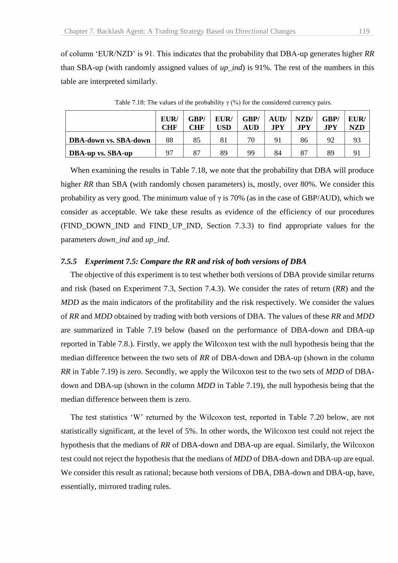
Chapter 7. Backlash Agent: A Trading Strategy Based on Directional Changes 119
of column ‘EUR/NZD’ is 91. This indicates that the probability that DBA-up generates higher RR
than SBA-up (with randomly assigned values of up_ind) is 91%. The rest of the numbers in this
table are interpreted similarly.
Table 7.18: The values of the probability γ (%) for the considered currency pairs.
EUR/
CHF
GBP/
CHF
EUR/
USD
GBP/
AUD
AUD/
JPY
NZD/
JPY
GBP/
JPY
EUR/
NZD
DBA-down vs. SBA-down 88 85 81 70 91 86 92 93
DBA-up vs. SBA-up 97 87 89 99 84 87 89 91
When examining the results in Table 7.18, we note that the probability that DBA will produce
higher RR than SBA (with randomly chosen parameters) is, mostly, over 80%. We consider this
probability as very good. The minimum value of γ is 70% (as in the case of GBP/AUD), which we
consider as acceptable. We take these results as evidence of the efficiency of our procedures
(FIND_DOWN_IND and FIND_UP_IND, Section 7.3.3) to find appropriate values for the
parameters down_ind and up_ind.
7.5.5 Experiment 7.5: Compare the RR and risk of both versions of DBA
The objective of this experiment is to test whether both versions of DBA provide similar returns
and risk (based on Experiment 7.3, Section 7.4.3). We consider the rates of return (RR) and the
MDD as the main indicators of the profitability and the risk respectively. We consider the values
of RR and MDD obtained by trading with both versions of DBA. The values of these RR and MDD
are summarized in Table 7.19 below (based on the performance of DBA-down and DBA-up
reported in Table 7.8.). Firstly, we apply the Wilcoxon test with the null hypothesis being that the
median difference between the two sets of RR of DBA-down and DBA-up (shown in the column
RR in Table 7.19) is zero. Secondly, we apply the Wilcoxon test to the two sets of MDD of DBA-
down and DBA-up (shown in the column MDD in Table 7.19), the null hypothesis being that the
median difference between them is zero.
The test statistics ‘W’ returned by the Wilcoxon test, reported in Table 7.20 below, are not
statistically significant, at the level of 5%. In other words, the Wilcoxon test could not reject the
hypothesis that the medians of RR of DBA-down and DBA-up are equal. Similarly, the Wilcoxon
test could not reject the hypothesis that the medians of MDD of DBA-down and DBA-up are equal.
We consider this result as rational; because both versions of DBA, DBA-down and DBA-up, have,
essentially, mirrored trading rules.
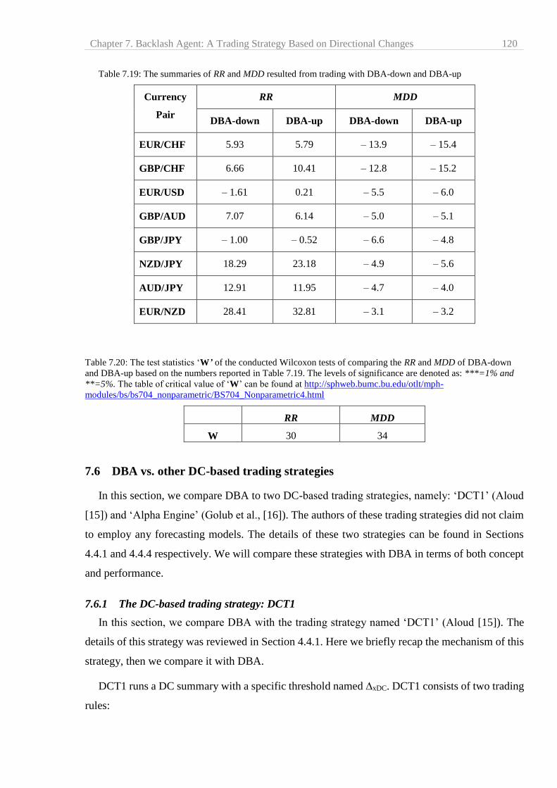
Chapter 7. Backlash Agent: A Trading Strategy Based on Directional Changes 120
Table 7.19: The summaries of RR and MDD resulted from trading with DBA-down and DBA-up
Currency
Pair
RR MDD
DBA-down DBA-up DBA-down DBA-up
EUR/CHF 5.93 5.79 – 13.9 – 15.4
GBP/CHF 6.66 10.41 – 12.8 – 15.2
EUR/USD – 1.61 0.21 – 5.5 – 6.0
GBP/AUD 7.07 6.14 – 5.0 – 5.1
GBP/JPY – 1.00 – 0.52 – 6.6 – 4.8
NZD/JPY 18.29 23.18 – 4.9 – 5.6
AUD/JPY 12.91 11.95 – 4.7 – 4.0
EUR/NZD 28.41 32.81 – 3.1 – 3.2
Table 7.20: The test statistics ‘W’ of the conducted Wilcoxon tests of comparing the RR and MDD of DBA-down
and DBA-up based on the numbers reported in Table 7.19. The levels of significance are denoted as: ***=1% and
**=5%. The table of critical value of ‘W’ can be found at http://sphweb.bumc.bu.edu/otlt/mph-
modules/bs/bs704_nonparametric/BS704_Nonparametric4.html
RR MDD
W 30 34
7.6 DBA vs. other DC-based trading strategies
In this section, we compare DBA to two DC-based trading strategies, namely: ‘DCT1’ (Aloud
[15]) and ‘Alpha Engine’ (Golub et al., [16]). The authors of these trading strategies did not claim
to employ any forecasting models. The details of these two strategies can be found in Sections
4.4.1 and 4.4.4 respectively. We will compare these strategies with DBA in terms of both concept
and performance.
7.6.1 The DC-based trading strategy: DCT1
In this section, we compare DBA with the trading strategy named ‘DCT1’ (Aloud [15]). The
details of this strategy was reviewed in Section 4.4.1. Here we briefly recap the mechanism of this
strategy, then we compare it with DBA.
DCT1 runs a DC summary with a specific threshold named ∆xDC. DCT1 consists of two trading
rules:
Chapter 7. Backlash Agent: A Trading Strategy Based on Directional Changes 121
DCT1 initiates a new position (either buy or sell) at the DC confirmation point of one DC
event.
DCT1 closes this trade at the DC confirmation point of the following DC event.
Initially, the trader defines a range of thresholds. DCT1 examines this range to automatically
compute: (1) the DC threshold ∆xDC, and (2) the type of trade (whether contrarian or trend follower).
For this purpose, DCT1 examines the profitability of each threshold in the specified range using
historical price data (as a training set). For each threshold value, DCT1 will apply the above trading
rules from two points of view: counter trend (CT) and trend follow (TF). Based on its produced
RR during the training period, DCT1 returns the type of trade (CT or TF) and the threshold ∆xDC
corresponding to the highest produced returns. These parameters (type of trade and threshold) are
then utilized to trade over the applied (out-of-sample) period.
We highlight the following differences between DBA and DCT1:
Both versions of DBA, DBA-up and DBA-down, are contrarian. Whereas, DCT1 could be
either contrarian or trend follower.
DBA triggers a new trade only if the price change during the OS event exceeds a certain
threshold. DCT1 triggers a new trade exactly at the DCC point of a DC event.
Nevertheless, DCT1 and DBA have a common feature which is: they both close trade at the DC
confirmation point of the next DC event.
In terms of the evaluation of DCT1 and DBA, we have the following observations:
DCT1 was backtested using high frequency data of one currency pair: EUR/USD.
Evaluating a trading strategy using one asset is not convincing according to Pardo [52],
who emphasizes the importance of backtesting using a set of assets with different trends.
In this chapter, DBA was backtested using eight currency pairs that exhibit different trends
(see Section 6.4.1).
The author reported that DCT1 was able to produce a rate of return of 6.2% during a testing
period of one year using data sampled with time-intervals of 1 millisecond. The RR
produced by DBA-up is 0.21% within seven months using minute-by-minute data (the case
of EUR/USD, Table 7.8, Section 7.5.3). Therefore, it would be oppressive to confirm that
DCT1 outperforms DBA.

Chapter 7. Backlash Agent: A Trading Strategy Based on Directional Changes 122
The author in [15] did not report any measurement of risk (e.g. MDD) or risk-adjusted
metrics (e.g. Sharpe ratio) of DCT1. Therefore we cannot compare DCT1 with DBA from
these perspectives.
The author that the authors in [15] did not report the number of trades executed by DCT1.
Therefore, it is hard to compare the impact of transaction costs on the RR produced by
DCT1 and DBA.
7.6.2 The DC-based trading strategy: The ‘Alpha Engine’
In this section, we compare DBA with the trading strategy named ‘Alpha Engine’ (introduced
by Golub et al., [16]). The details of this strategy were reviewed in Section 4.4.4. Here we briefly
recap the mechanism of this strategy, then compare it with DBA.
The Alpha Engine consists of opening a counter-trend position when the overshoot value (OSV)
exceeds a specific threshold named ‘𝜔’:
𝜔 = 𝛼 × 𝑡ℎ𝑒𝑡𝑎 (7.3)
Where, 𝑡ℎ𝑒𝑡𝑎 is the employed DC threshold and 𝛼 is a parameter. The value of 𝛼 depends on
the inventory size denoted as ‘I’.
The Alpha Engine does not have an explicit stop-loss rule. Instead, it employs a sophisticated
money management approach: When the Alpha Engine opens a position, it keeps increasing and
decreasing the size of this position until a profit is reached. The increasing and decreasing of the
position is designed to mitigate the accumulation of large inventory sizes during trending markets.
The generation of a new trade (either buy or sell) depends on two factors:
The inventory size denoted as ‘I’; which is used to manage the value of 𝛼 in (7.1). Thus, I
serves to control the time at which Alpha Engine triggers a new trade.
The size of a trade is a factor of a probability indicator (denoted as ‘ℒ’). The value of ℒ is
used as an estimation of the probability that the trend will move up or down provided the
current state. The value of ℒ is determined using a transition network model which has two
states: the DC threshold 𝑡ℎ𝑒𝑡𝑎 and the threshold ‘𝜔’. If the markets show normal behavior
then ℒ ≈ 1. On the other hand, in the case of abnormal market behavior ℒ ≈ 0. The
objective of ℒ is to prevent the Alpha Engine from building up large positions which it
cannot unload.
To summarize, the management of the position is a function of two variables: the size of
inventory ‘I’ and the probability indicator ‘ℒ’. This approach of computing, and managing, the
Chapter 7. Backlash Agent: A Trading Strategy Based on Directional Changes 123
size of a position is an integrated part of the Alpha Engine. The Alpha Engine considers the
uptrends and downtrends separately so that it adopts two instances of the parameter 𝜔; namely
𝜔down and 𝜔up. For more details about the mechanism of Alpha Engine see Golub et al., [16].
The Alpha Engine has three common features with Dynamic Backlash Agent (DBA):
The positions of both trading strategies are countertrend, meaning that a price move down
triggers a buy; a price move up, a sell.
They both try to analyse the uptrends and downtrends separately.
They both open positions when the OSV exceeds certain thresholds. In the case of DBA, we
have two thresholds (denoted as down_ind and up_ind). Similarly, in the case of the Alpha
Engine, the authors identified two thresholds (denoted as 𝜔down and 𝜔up).
As for the differences between DBA and Alpha Engine, we have the following observations:
The most important difference between DBA and Alpha Engine is that the former has an
explicit stop-loss rule (Section 7.3.3) whereas the latter does not. The money management
approach employed by Alpha Engine makes it pretty complicated in comparison to DBA.
The Alpha Engine may manage multiple positions simultaneously. Whereas, at any time,
DBA can have only one position opened (based on the adopted money management approach
described in Section 6.5.1).
Both DBA and Alpha Engine employ some parameters to decide when to initiate a new
trade (i.e. down_ind and up_ind in the case of DBA; 𝜔down and 𝜔up in case of Alpha Engine).
However, they have different approaches to compute these parameters. DBA adopts a
computational approach, as explained in Section 7.3.3, whereas, Alpha Engine uses the size of
the inventory ‘I’ to manage 𝜔down and 𝜔up.
An important advantage of Alpha Engine is that the authors did not fine-tune any
parameters to maximize performance. In the case of DBA, the value of DC threshold 𝑡ℎ𝑒𝑡𝑎 is
to be set by the user. Further experiments should be done in this regard. For instance, we do not
know how the value of the DC threshold 𝑡ℎ𝑒𝑡𝑎 may affect the performance of DBA.
The performance of Alpha Engine was examined using a portfolio comprising 23 currency rates,
sampled tick-by-tick, over a period of 8 years and yielded a return of 21.34% (including bid and
ask price). As can be seen in Table 7.8 (Section 7.5.3), DBA may have generated RR of more than
30% within 7 months (see the last row in Table 7.8). These results indicate that DBA is able to
produce higher RR than Alpha Engine. However, the author that the authors in [16] did not report
Chapter 7. Backlash Agent: A Trading Strategy Based on Directional Changes 124
the number of trades executed by the Alpha Engine. Therefore, it is hard to compare the impact of
transaction costs on the RR produced by the Alpha Engine and DBA.
The authors in [16] reported that Alpha Engine has an annual Sharp ratio of 3.06. The Sharpe
ratio is intended to measure the return earned in excess of the risk-free rate per unit of volatility
(7.2). However, the authors did not specify the risk-free rate in [16]! On the other hand, the results,
shown in Table 7.13 (Section 7.5.3) suggest that DBA-down delivered a higher Sharpe ratio than
Alpha Engine (e.g. in the case of NZD/JPY the Sharpe ratio was 3.46 and in the case of EUR/NZD
it was 3.18).
Sharpe ratio =𝑅𝑝− 𝑅𝑓
𝜎𝑝 (7.4)
where: 𝑅𝑝 denote the expected portfolio return and 𝑅𝑓 is the risk-free rate. 𝜎𝑝 refers to the standard
deviation of the portfolio’s returns and is utilized to measure the volatility of the returns.
To conclude, we argue that DBA has simpler trading rules than Alpha Engine. We also argue
that DBA could be more profitable than Alpha Engine. However, it could be argued that Alpha
Engine is more robust than DBA, in the sense that a trader does not have to fine-tune any parameter
to maximize the performance.
7.7 Summary and conclusion
In this chapter, we introduced a contrarian trading strategy, named BA, which is based on the
DC framework. BA opens a position when the overshoot value (OSV) exceeds the values of
specific parameters (Section 7.2). BA has two types: Static and Dynamic. The static type of BA,
SBA, relies on the expertise of the investor to set these parameters. By contrast, the dynamic type
of BA, DBA, applies a DC-based computational approach to examine historical prices to
automatically find appropriate values for the parameters. Then, DBA uses these values to trade
over the out-of-sample (trading) period (Section 7.3). We consider DBA, the autonomous type of
BA, as our original trading strategy, whereas, SBA serves to compute the best and worst possible
performances of BA (Section 7.5.1).
To evaluate the performance of DBA we adopted the same methodology employed in Chapter
6 to assess the performance of TSFDC: We applied DBA to the eight sets of rolling windows
previously composed in Section 6.4.4, each set corresponding to one currency pair. Each set
comprises a training period to which we applied the predetermined DC-based computational
approach to compute the values of the parameters. We used a set of evaluation metrics to measure
the profitability and risk of DBA, taking into account the instantaneous actual bid and ask prices
Chapter 7. Backlash Agent: A Trading Strategy Based on Directional Changes 125
throughout the backtesting process. However, like all other DC-based trading strategies (e.g. [15]
[16] [17] [78]), the transaction costs were not considered in our experiments. As a benchmark
model, we implemented the standard buy and hold strategy. We also compared the performance of
DBA to other DC-based trading strategies (Section 7.6).
The experimental results (reported in Section 7.4.2) suggest that DBA is mostly profitable. By
examining the returns reported in Table 7.8 (Section 7.4.2), we can conclude that DBA can be
attractively profitable (with total RR of more than 30%) and yet retain an attractive level of risk
(with an MDD equal to –3.2%). When examining the values of Jensen’s Alpha (shown in Table
7.15, Section 7.4.2), we can see that DBA generates promising returns compared to the level of
risk it takes in relating to the buy and hold method. The values of Beta (Table 7.15, Section 7.4.2)
would indicate that in all cases DBA is less volatile than the buy and hold method. We compared
the DBA to two other DC-based trading strategies (Section 7.6) and argued that DBA outperforms
one of them. Finally, the conducted Wilcoxon tests suggest that the Buy and Hold approach cannot
provides equal Sharpe ratio to that provided by DBA.
To conclude, in this chapter we developed a DC-based trading strategy, named DBA; which
does not rely on any forecasting model. As our main contribution, we argue that DBA can be highly
profitable. We also argue that DBA can provide better Sharpe ratios and RR than another DC-
based trading strategy (Section 7.6.2). We examined the effectiveness of DBA over eight different
currency pairs that have different patterns, leading us to conclude that DBA could be successful in
a broad range of currency pairs. Despite what would be considered as experimental weaknesses
(e.g. ignoring the transaction costs), we argue that these results provide an evidence as to the
usefulness of the DC framework as a basis for trading strategies.
Chapter 8. Comparing TSFDC with DBA 126
8 Comparing TSFDC with DBA
In this thesis, we have presented two trading strategies TSFDC (Chapter 6) and DBA (Chapter
7). In this chapter, we aim to compare the performances of TSFDC and DBA. The objective is to
find out whether one of them outperforms the other. More particularly, we focus on three aspects:
profitability, drawdown and risk-adjusted returns. We rely on the results of the experiments
organized in Chapters 6 and 7 to compare TSFDC and DBA.
We start this chapter with a brief summary of the two trading strategies, TSFDC and DBA. We
then list the adopted metrics that will be utilized to compare TSFDC and DBA. Next, we summarize
the results of our experiments (carried out in Chapters 6 and 7). Finally, we compare TSFDC and
DBA based on these results.
8.1 Introduction
In Chapter 5, we presented a forecasting model that aims to predict the change in direction of a
market’s trend under the DC framework. In Chapter 6, we introduced a trading strategy named
TSFDC, which is based on the forecasting model proposed in Chapter 5. TSFDC uses the historical
prices of a given currency pair as an in-sample dataset to train this forecasting model. It then relies
on the formed prediction model to decide when to trigger a buy or a sell signal during the out-of-
sample (i.e. trading) period.
In Chapter 7, we introduced a trading strategy named DBA. In contrast to TSFDC, DBA does
not employ any forecasting model. DBA initiates a trade when the magnitude of price change
exceeds specific thresholds. DBA runs a predefined procedure, which examines historical (in-
sample) prices using a DC-based approach, to determine the value of these thresholds. Then, DBA
uses the values of these thresholds to decide when to start a trade during the out-of-sample (i.e.
trading) period.
Both TSFDC and DBA are contrarian strategies. We have evaluated both strategies using the
same methodology and datasets. We utilized eight currency pairs from the FX market, sampled
minute-by-minute. For each currency pair, we composed seven rolling windows (see Section 6.4.4)
and applied both strategies to these rolling windows. Our results indicated that both strategies could
be attractively profitable. We concluded that both strategies, TSFDC and DBA, outperform the
buy and hold approach as well as other DC-based trading strategies.
In this chapter, we compare the performances of TSFDC and DBA with the objective of
studying whether one of them outperforms the other. Mainly, we focus on three fundamental

Chapter 8. Comparing TSFDC with DBA 127
aspects: profitability, maximum drawdown and risk-adjusted returns. For this purpose, we use the
results of the experiments undertaken and discussed in Chapters 6 and 7.
8.2 Comparing the performances of TSFDC and DBA: Criteria of comparison
In this section, we list the metrics that will be considered to compare the performance of TSFDC
and DBA. The detailed description of these metrics has been provided in Section 3.4, but we
provide a recap of each metric here. These metrics are selected to represent three aspects:
Profitability: We consider the ‘Rate of Return (RR)’ as the main metric to evaluate the
profitability of a trading model. Let Total Profit (TP) represent the overall losses or gains
during the entire trading period. We define RR as the gain or loss expressed as a percentage
of the amount invested. In (8.1) INV denote the initial capital employed for investment.
𝑅𝑅 =𝑇𝑃
𝐼𝑁𝑉∗ 100
(8.1)
Maximum Drawdown: We use the Maximum Drawdown (MDD) to measure the risk of a
trading strategy (as in [4] [16] [17]). The MDD measures the risk as the worst-case-scenario
of a given trading strategy. In (8.2), 𝑐𝑎𝑝𝑖𝑡𝑎𝑙 (𝑡𝑖) denote the value of capital at time (𝑡𝑖).
The maximum capital(𝑡𝑖) refers to the maximum capital’s value that has been reached since
the beginning of trading up to time (𝑡𝑖). Thus, 𝑑𝑟𝑎𝑤𝑑𝑜𝑤𝑛 (𝑡𝑖), (8.2), is interpreted as the
peak-to-trough decline in capital from the start of the trading period up to time (𝑡𝑖). The
MDD (8.3) is the maximum value of all computed 𝑑𝑟𝑎𝑤𝑑𝑜𝑤𝑛 (𝑡𝑖).
𝑑𝑟𝑎𝑤𝑑𝑜𝑤𝑛 (𝑡𝑖) = |𝑐𝑎𝑝𝑖𝑡𝑎𝑙 (𝑡𝑖)− 𝑚𝑎𝑥𝑖𝑚𝑢𝑚 𝑐𝑎𝑝𝑖𝑡𝑎𝑙(𝑡𝑖)
𝑚𝑎𝑥𝑖𝑚𝑢𝑚 𝑐𝑎𝑝𝑖𝑡𝑎𝑙(𝑡𝑖)| (8.2)
𝑀𝐷𝐷 = 𝑀𝑎𝑥 (𝑑𝑟𝑎𝑤𝑑𝑜𝑤𝑛 (𝑡𝑖)), ∀ 𝑡𝑖𝑚𝑒 𝑡𝑖 ∈ 𝑡𝑟𝑎𝑑𝑖𝑛𝑔 𝑝𝑒𝑟𝑖𝑜𝑑 (8.3)
Risk-adjusted return: To assess this aspect, we use the ‘Sharpe ratio’ [68]. The Sharpe ratio
is the average return earned in excess of the risk-free rate per unit of volatility. The formula
to calculate the Sharpe ratio is:
Sharpe ratio =𝑅𝑝− 𝑅𝑓
𝜎𝑝 (8.4)
Where: 𝑅𝑝 denote the expected portfolio returns; 𝑅𝑓 is the risk-free rate; 𝜎𝑝 designs the
standard deviation of the portfolio’s returns.
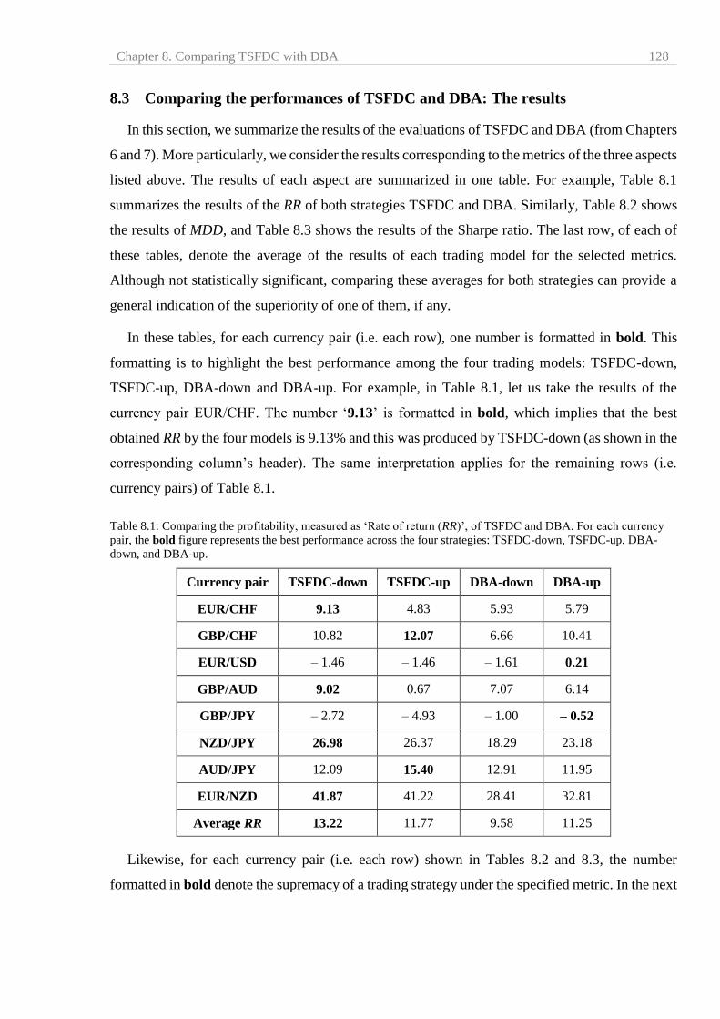
Chapter 8. Comparing TSFDC with DBA 128
8.3 Comparing the performances of TSFDC and DBA: The results
In this section, we summarize the results of the evaluations of TSFDC and DBA (from Chapters
6 and 7). More particularly, we consider the results corresponding to the metrics of the three aspects
listed above. The results of each aspect are summarized in one table. For example, Table 8.1
summarizes the results of the RR of both strategies TSFDC and DBA. Similarly, Table 8.2 shows
the results of MDD, and Table 8.3 shows the results of the Sharpe ratio. The last row, of each of
these tables, denote the average of the results of each trading model for the selected metrics.
Although not statistically significant, comparing these averages for both strategies can provide a
general indication of the superiority of one of them, if any.
In these tables, for each currency pair (i.e. each row), one number is formatted in bold. This
formatting is to highlight the best performance among the four trading models: TSFDC-down,
TSFDC-up, DBA-down and DBA-up. For example, in Table 8.1, let us take the results of the
currency pair EUR/CHF. The number ‘9.13’ is formatted in bold, which implies that the best
obtained RR by the four models is 9.13% and this was produced by TSFDC-down (as shown in the
corresponding column’s header). The same interpretation applies for the remaining rows (i.e.
currency pairs) of Table 8.1.
Table 8.1: Comparing the profitability, measured as ‘Rate of return (RR)’, of TSFDC and DBA. For each currency
pair, the bold figure represents the best performance across the four strategies: TSFDC-down, TSFDC-up, DBA-
down, and DBA-up.
Currency pair TSFDC-down TSFDC-up DBA-down DBA-up
EUR/CHF 9.13 4.83 5.93 5.79
GBP/CHF 10.82 12.07 6.66 10.41
EUR/USD – 1.46 – 1.46 – 1.61 0.21
GBP/AUD 9.02 0.67 7.07 6.14
GBP/JPY – 2.72 – 4.93 – 1.00 – 0.52
NZD/JPY 26.98 26.37 18.29 23.18
AUD/JPY 12.09 15.40 12.91 11.95
EUR/NZD 41.87 41.22 28.41 32.81
Average RR 13.22 11.77 9.58 11.25
Likewise, for each currency pair (i.e. each row) shown in Tables 8.2 and 8.3, the number
formatted in bold denote the supremacy of a trading strategy under the specified metric. In the next
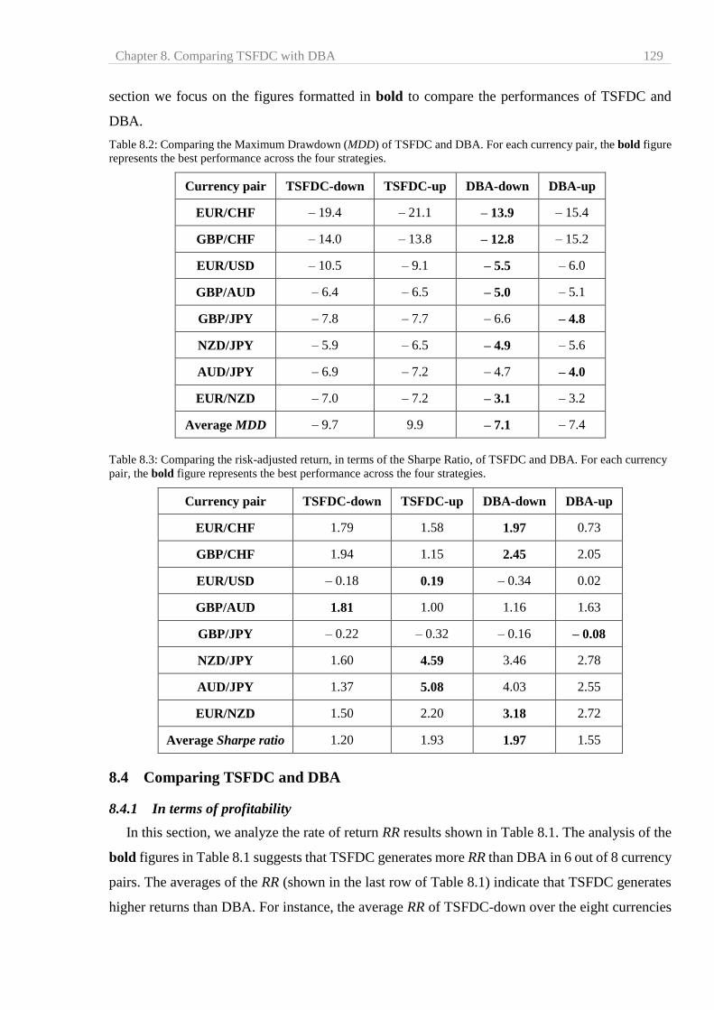
Chapter 8. Comparing TSFDC with DBA 129
section we focus on the figures formatted in bold to compare the performances of TSFDC and
DBA.
Table 8.2: Comparing the Maximum Drawdown (MDD) of TSFDC and DBA. For each currency pair, the bold figure
represents the best performance across the four strategies.
Currency pair TSFDC-down TSFDC-up DBA-down DBA-up
EUR/CHF – 19.4 – 21.1 – 13.9 – 15.4
GBP/CHF – 14.0 – 13.8 – 12.8 – 15.2
EUR/USD – 10.5 – 9.1 – 5.5 – 6.0
GBP/AUD – 6.4 – 6.5 – 5.0 – 5.1
GBP/JPY – 7.8 – 7.7 – 6.6 – 4.8
NZD/JPY – 5.9 – 6.5 – 4.9 – 5.6
AUD/JPY – 6.9 – 7.2 – 4.7 – 4.0
EUR/NZD – 7.0 – 7.2 – 3.1 – 3.2
Average MDD – 9.7 9.9 – 7.1 – 7.4
Table 8.3: Comparing the risk-adjusted return, in terms of the Sharpe Ratio, of TSFDC and DBA. For each currency
pair, the bold figure represents the best performance across the four strategies.
Currency pair TSFDC-down TSFDC-up DBA-down DBA-up
EUR/CHF 1.79 1.58 1.97 0.73
GBP/CHF 1.94 1.15 2.45 2.05
EUR/USD – 0.18 0.19 – 0.34 0.02
GBP/AUD 1.81 1.00 1.16 1.63
GBP/JPY – 0.22 – 0.32 – 0.16 – 0.08
NZD/JPY 1.60 4.59 3.46 2.78
AUD/JPY 1.37 5.08 4.03 2.55
EUR/NZD 1.50 2.20 3.18 2.72
Average Sharpe ratio 1.20 1.93 1.97 1.55
8.4 Comparing TSFDC and DBA
8.4.1 In terms of profitability
In this section, we analyze the rate of return RR results shown in Table 8.1. The analysis of the
bold figures in Table 8.1 suggests that TSFDC generates more RR than DBA in 6 out of 8 currency
pairs. The averages of the RR (shown in the last row of Table 8.1) indicate that TSFDC generates
higher returns than DBA. For instance, the average RR of TSFDC-down over the eight currencies
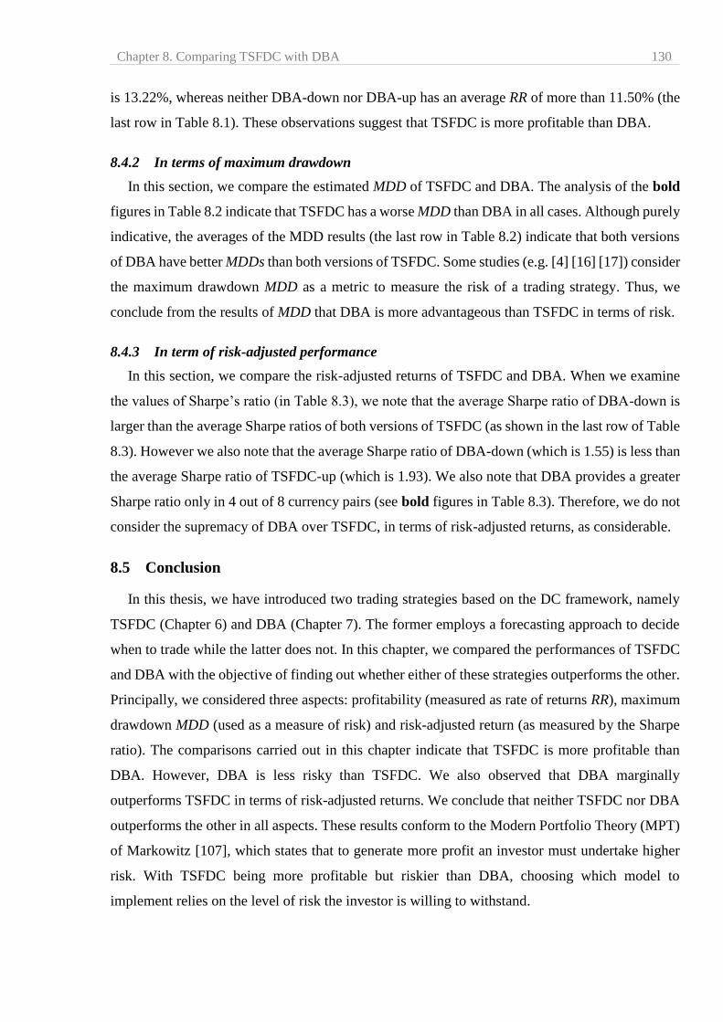
Chapter 8. Comparing TSFDC with DBA 130
is 13.22%, whereas neither DBA-down nor DBA-up has an average RR of more than 11.50% (the
last row in Table 8.1). These observations suggest that TSFDC is more profitable than DBA.
8.4.2 In terms of maximum drawdown
In this section, we compare the estimated MDD of TSFDC and DBA. The analysis of the bold
figures in Table 8.2 indicate that TSFDC has a worse MDD than DBA in all cases. Although purely
indicative, the averages of the MDD results (the last row in Table 8.2) indicate that both versions
of DBA have better MDDs than both versions of TSFDC. Some studies (e.g. [4] [16] [17]) consider
the maximum drawdown MDD as a metric to measure the risk of a trading strategy. Thus, we
conclude from the results of MDD that DBA is more advantageous than TSFDC in terms of risk.
8.4.3 In term of risk-adjusted performance
In this section, we compare the risk-adjusted returns of TSFDC and DBA. When we examine
the values of Sharpe’s ratio (in Table 8.3), we note that the average Sharpe ratio of DBA-down is
larger than the average Sharpe ratios of both versions of TSFDC (as shown in the last row of Table
8.3). However we also note that the average Sharpe ratio of DBA-down (which is 1.55) is less than
the average Sharpe ratio of TSFDC-up (which is 1.93). We also note that DBA provides a greater
Sharpe ratio only in 4 out of 8 currency pairs (see bold figures in Table 8.3). Therefore, we do not
consider the supremacy of DBA over TSFDC, in terms of risk-adjusted returns, as considerable.
8.5 Conclusion
In this thesis, we have introduced two trading strategies based on the DC framework, namely
TSFDC (Chapter 6) and DBA (Chapter 7). The former employs a forecasting approach to decide
when to trade while the latter does not. In this chapter, we compared the performances of TSFDC
and DBA with the objective of finding out whether either of these strategies outperforms the other.
Principally, we considered three aspects: profitability (measured as rate of returns RR), maximum
drawdown MDD (used as a measure of risk) and risk-adjusted return (as measured by the Sharpe
ratio). The comparisons carried out in this chapter indicate that TSFDC is more profitable than
DBA. However, DBA is less risky than TSFDC. We also observed that DBA marginally
outperforms TSFDC in terms of risk-adjusted returns. We conclude that neither TSFDC nor DBA
outperforms the other in all aspects. These results conform to the Modern Portfolio Theory (MPT)
of Markowitz [107], which states that to generate more profit an investor must undertake higher
risk. With TSFDC being more profitable but riskier than DBA, choosing which model to
implement relies on the level of risk the investor is willing to withstand.

131
Part III
Concluding Remarks
Chapter 9. Conclusions 132
9 Conclusions
The Directional Change (DC) Framework is an approach to studying price movements in
financial markets. Many studies have reported that the DC framework is helpful in analysing the
price movements and traders’ behaviors in the FX market. Some studies have tried to develop
trading strategies based on the DC framework. This study set out to explore, and consequently to
provide a proof of, the potential of the Directional Changes framework as the basis of a profitable
trading strategy. This chapter provides a summary of the thesis, points out its contributions, and
discusses possible future research work.
9.1 Summary
The DC framework is an event-based technique to summarize price movements in the financial
market. Under the DC framework the market is cast into alternating upward and downward trends.
A trend is identified as a change in market price larger than, or equal to, a given threshold. This
threshold, named 𝑡ℎ𝑒𝑡𝑎, is set by the observer and usually expressed as a percentage. In Section
4.3 we reviewed some studies (e.g. [11] [12] [13] [77]) that have demonstrated the usefulness of
the DC framework in analyzing price movements in the FX market. The consensus amongst these
studies is that, whilst an ideal DC-based trading strategy could be amazingly profitable,
nonetheless, the full promise of the DC framework for developing trading strategies has not been
completely exploited [16] [19]. In Chapter 3, we arranged existing trading strategies into two
groups: 1) strategies that embed forecasting approaches (e.g. [6] [41] [42] [43] [44] [45] [46]); and
2) strategies that do not rely on any forecasting model (e.g. [7] [8] [54] [57] [58] [59] [61]).
Our intended aim of this research was to explore, and consequently to provide a proof of, the
convenience of the Directional Changes (DC) framework as a basis of a profitable trading strategy.
To attain our stated objective, and in line with existing research, we developed two DC-based
trading strategies: one strategy, named TSFDC, which is based on forecasting DC (Chapter 6); and
a second strategy, named DBA, which is based on the DC framework but does not employ any
forecasting method (Chapter 7). We examined the performance of TSFDC and DBA in the foreign
exchange (FX) market using the same methodology and datasets.
In this chapter, we summarize the functionalities of TSFDC and DBA. We also highlight the
differences between our proposed trading strategies, TSFDC and DBA, and some existing DC-
based trading strategies. Finally, we list our contributions and suggest future research.
Chapter 9. Conclusions 133
9.2 In a nutshell: TSFDC and DBA
9.2.1 TSFDC: A trading strategy based on forecasting Directional Changes
In Chapter 6 we introduced our first DC-based trading strategy, named TSFDC. TSFDC was
designed as a forecasting-based trading strategy. Forecasting the change of a trend’s direction in a
financial time series is a common problem (e.g. [41] [80] [81] [87]), however, this problem has
never been formalized under the DC context. Therefore, as a first step, we provided a formalization
of the problem of forecasting the change of a trend’s direction under the DC framework (Section
5.2.2). To this end, we tracked price movements using two DC thresholds: STheta and BTheta. We
formalized the problem as the following: ‘to forecast whether the magnitude of total price change
of a DC trend, as observed under STheta, will be at least equal to BTheta before the trend changes’.
We also discovered an original DC-based indicator, named 𝑂𝑆𝑉𝐵𝑇ℎ𝑒𝑡𝑎𝑆𝑇ℎ𝑒𝑡𝑎 , and selected an
appropriate machine learning procedure to propose a solution for the established forecasting
problem (Section 5.4.1). We applied our forecasting model to eight currency pairs from the foreign
exchange market. The experimental results suggested that the accuracy of our prediction model
ranged between 62% and 82%, outperforming the traditional ARIMA technique (Section 5.6.1).
These results indicate that our proposed indicator, 𝑂𝑆𝑉𝐵𝑇ℎ𝑒𝑡𝑎𝑆𝑇ℎ𝑒𝑡𝑎, is useful for forecasting purposes
under the DC framework.
The second step consisted of employing the established forecasting model to develop a trading
strategy named ‘TSFDC’ (Chapter 6). TSFDC relies on this forecasting model to decide when to
initiate a new trade. To evaluate the performance of TSFDC, we applied it to eight currency pairs,
using a monthly-based rolling windows approach, for an overall out-of-sample trading period of
seven months. The experimental results suggested that TSFDC can be highly profitable (Section
6.6). We also argued that TSFDC outperforms another DC-based trading strategy (Section 6.7).
9.2.2 DBA: The second DC-based trading strategy
The second trading strategy, named DBA, was introduced in Chapter 7. The objective was to
develop a successful DC-based trading strategy that does not rely on any forecasting model. DBA
opens a position when the overshoot value exceeds a particular threshold. DBA examines historical
prices using a DC-based computational approach to determine the threshold. To evaluate the
performance of DBA, we followed the same experimental methodology and utilized the same
datasets previously adopted to evaluate the performance of TSFDC in Chapter 6. Our experimental
results suggested that DBA can be highly profitable (Section 7.5.3). We also argued that DBA
outperforms another DC-based trading strategy (Section 7.6).
Chapter 9. Conclusions 134
It is worth highlighting an important difference between TSFDC and DBA: in contrast to DBA,
TSFDC relies on a forecasting model which: 1) has clearly-defined dependent and independent
variables and 2) employs a machine learning procedure to predict the dependent variable (Section
5.4). Thus, in contrast to DBA, we consider TSFDC to be a forecasting-based trading strategy.
A comparison between the performances of TSFDC and DBA was carried out in Chapter 8.
The objective was to find out whether either TSFDC or DBA could outperform the other. This
comparison focused on three principle aspects: profitability, drawdown and risk-adjusted returns.
The results suggested that, in general, TSFDC generates higher returns than DBA (Section 8.3).
However, they also suggested that DBA has a better maximum drawdown than TSFDC (Section
8.3). In addition, the results indicated that DBA has a slightly better risk-adjusted performance
than TSFDC (Section 8.3). We concluded that neither DBA nor TSFDC could outperform the other
in every aspect. These results suggest that either DBA or TSFDC could be an attractive choice for
different types of traders. Choosing which strategy to adopt, TSFDC or DBA, would depend on
the level of risk the trader is willing to undertake.
Despite what would be considered as defects in our experiments (e.g. ignoring the transaction
costs), we argue that the results of the evaluation of the performances of TSFDC (Section 6.6.1)
and DBA (Section 6.5.3) support our objective of providing proof of the usefulness of the DC
framework as a basis for profitable trading strategies.
9.3 Comparing TSFDC and DBA with other DC-based trading strategies
In Section 4.4 we reviewed some existing DC-based trading strategies. In Chapters 6 and 7 we
compared TSFDC and DBA to some of these trading strategies. In this section we review the
differences between our proposed strategies, TSFDC and DBA, and other existing DC-based
trading strategies.
9.3.1 Comparing TSFDC with other DC-based trading strategies
In Section 6.7, we compared TSFDC to two DC-based trading strategies proposed by Gypteau
et al., [78] and Kampouridis and Otero [17]. The reason for choosing these particular trading
strategies was that the authors of both studies, [17] and [78], stated that they were proposing trading
strategies that employed forecasting models. In this section we summarize these comparisons.
1. It was in Section 6.7.1 that we compared TSFDC to the trading strategy presented by Gypteau
et al., [78] and we recap the following differences here:
Chapter 9. Conclusions 135
TSFDC is founded on the well-articulated forecasting approach established in Chapter 5
which has clearly identified dependent and independent variables. Despite the fact that the
authors in [78] declared that they aimed “…to find an optimal trading strategy to forecast
the future price moves of a financial market”; they did not identify any dependent or
independent variables.
TSFDC relies on forecasting the change in direction of a market’s trend to decide when to
start a new trade, whereas the trading strategy by Gypteau et al., [78] was presented as a
GP-tree. This GP-tree comprises multiple DC thresholds. The detection of DC events at
these thresholds is interpreted as ‘True’ or ‘False’ values. Based on the detected event(s),
the expression represented by a GP tree is a Boolean value that indicates the action (either
buy or sell) to be taken.
In Section 6.7.1 we argued that TSFDC was able to generate higher RR than the trading
strategy introduced by Gypteau et al., [78].
2. We compared the trading strategy named DC+GA presented by Kampouridis and Otero [17]
with TSFDC in Section 6.7.2. Here, we recap the following remarks:
TSFDC has different trading rules as to when to start or end a trade than DC+GA: For
instance, TSFDC focuses on the magnitude of price change (e.g. STheta and BTheta) to
decide when to start a trade. Whilst, DC+GA initiates a trade when the time length of an
OS event lasts longer than a specific time-threshold (see Section 6.7.1 for details).
TSFDC relies on the forecasting approach presented in Chapter 5 to decide when to trigger
a new trade. Whereas, DC+ GA employs a GA module to anticipate the best time-threshold
at which it should initiate a trade.
TSFDC uses two DC thresholds, whilst DC+GA may consider up to Ntheta thresholds to
decide when to initiate a trade.
The authors in [17] claimed that their objective was “to offer a more complete analysis on
the directional changes paradigm from a financial forecasting perspective.” However, in
contrast to our forecasting approach established in Chapter 5, they did not identify any
dependent or independent variables!
We compared the results of TSFDC and DC+GA in Section 6.7.2. We argued that TSFDC
outperforms DC+GA in terms of produced RR and risk-adjusted returns.
However, the results of MDD suggest that DC+GA is less risky than TSFDC.

Chapter 9. Conclusions 136
A common feature between TSFDC and DC+GA is that they both try to analyse the
uptrends and downtrends separately.
9.3.2 Comparing DBA with other DC-based trading strategies
In Section 7.6 we compared DBA to two other DC-based trading strategies, namely ‘DCT1’
[15] and ‘the Alpha Engine’ [16]. The authors of DCT1 and Alpha Engine did not state that their
proposed trading strategies employed any forecasting model. In this section we briefly recap the
differences and similarities between these trading strategies and DBA.
1. As for the differences between DBA and DCT1 [15], we have the following comments:
DBA is a contrarian strategy. Whereas DCT1 can be either contrarian or a trend follower.
DBA triggers a new trade only if the price change during the OS event exceeds certain
thresholds. DCT1 does not use ‘thresholds’. DCT1 triggers a new trade when a DC event is
confirmed (i.e. at the DCC point).
In contrast to DBA, the performance of DCT1 was evaluated using only one currency pair
(the EUR/USD). Furthermore, the authors did not report any measurement of risk or risk-
adjusted performance for DCT1 in [15]. Therefore, we concluded that the employed
methodology to evaluate the performance of DCT1 is not convincing.
Nevertheless, DCT1 and DBA have a common feature which is: they both close trade at
the next DC confirmation point.
2. As for the differences between DBA and Alpha Engine [16], we have the following
observations:
The most important difference between DBA and Alpha Engine is that the former has an
explicit stop-loss rule (Section 7.3.3), whereas the latter does not. Alpha Engine employs a
sophisticated money management approach. The Alpha Engine uses a transition network
model to control the size of each new trade (Section 4.4.4).
As a result of the above point, Alpha Engine is able to manage multiple positions
simultaneously, whereas at any time DBA can have only one open position.
DBA employs a computational approach to decide the OSV at which it should make a new
trade. Whereas, Alpha Engine takes into consideration the total amount of inventory to decide
the value of OSV at which it should make a new trade.
An important advantage of Alpha Engine is its robustness, in the sense that it automatically
fine-tunes its own parameters. In the case of DBA, the user must specify the DC threshold
Chapter 9. Conclusions 137
𝑡ℎ𝑒𝑡𝑎. Further experiments should be done to examine how the value of 𝑡ℎ𝑒𝑡𝑎 may affect the
performance of DBA.
According to our experiments, DBA can produce higher RR than Alpha Engine. For
instance, in the case of EUR/NZD, DBA was able to produce an RR of more than 28% in just
seven months (see Table 7.8, Section 7.5.3), whereas the RR produced by Alpha Engine over
a trading period of eight years was 21.34%!
Nevertheless, we can note some similarities between DBA and Alpha Engine:
They both trigger contrarian trades.
They both open positions during the overshoot when the price change reaches a specific
threshold.
They both try to analyse the uptrends and downtrends separately.
9.4 Contributions
This thesis contributes toward providing evidence as to the potential of the DC framework as a
foundation for trading strategies. The major contributions of this work can be summarized as
follows:
We formulated the problem of forecasting the change of a trend’s direction under the DC
framework (Chapter 5). The objective was to forecast whether the current DC trend, of
threshold STheta, will continue so that its total price change will reach another threshold
named BTheta (Section 5.3). This objective was shortened in order to predict one
Boolean variable named BBTheta.
The second contribution was discovering a useful DC-based indicator named 𝑂𝑆𝑉𝐵𝑇ℎ𝑒𝑡𝑎𝑆𝑇ℎ𝑒𝑡𝑎.
We proved that this indicator is helpful in forecasting the change in direction of a
market’s trend within the DC context. We used this indicator to establish a forecasting
model that demonstrated relatively good accuracy ranging between 62% and 82%
(Section 5.6.2). We also proved that our forecasting model has better accuracy than the
ARIMA model (Table 5.4, Section 5.6.1).
We employed the proposed forecasting model to develop a successful trading strategy,
named TSFDC (Chapter 6). We argued that TSFDC outperforms another DC-based
trading strategy (Section 6.7). The results of the preliminary tests suggested that TSFDC
could produce a positive Sharpe ratio in most cases (Section 6.6.1).
We presented a second trading strategy, named DBA, which although based on the DC
concept, does not rely on any forecasting model (Chapter 7). DBA follows a
Chapter 9. Conclusions 138
computational approach to examine the historical prices in order to discover profitable
trading rules as to when to initiate a trade. We argued that DBA can be highly profitable
(Sections 7.6.1). We also argued that DBA outperforms another DC-based trading
strategy. The results of the preliminary tests suggested that DBA could produce a positive
Sharpe ratio in most cases (Section 7.5.3).
The comparison of TSFDC and DBA, carried out in Chapter 8, suggested that TSFDC
produces more profit than DBA; but, DBA is less risky than TSFDC. Therefore, either
strategy could be more advantageous for different types of traders, based on the level of
risk the trader is willing to withstand (Section 8.4).
To conclude, the objective of this thesis was to explore, and consequently to provide a proof of,
the usefulness of the DC framework as the basis of profitable trading strategies. Despite some
experimental flaws (e.g. ignoring the transaction costs), the results of the evaluation of the
performances of our proposed trading strategies, TSFDC (Section 6.6.1) and DBA (Section 7.5.3),
support our stated objective. Although the rates of return (RR) generated by TSFDC and DBA are
much less than the estimated maximum annual RR that could be possibly generated by a DC-based
trading strategy (which is 1600% [19]), in our opinion, our strategies nevertheless represent a vital
step in the right direction.
9.5 Future works
We believe that both the strategies introduced in this thesis, TSFDC and DBA, can be further
improved in many ways.
9.5.1 Money management: Controlling order size
In this thesis we focused on discovering profitable trading rules under the DC framework.
However, a trading system must consider two other essential parts: risk control and money
management [33]. Money management refers to the actual size of the trade to be initiated [86].
Some studies (e.g. [52] [100]) reported that models that do not take into consideration effective
money management decisions can lead to sub-optimal solutions. In this thesis we adopted a naïve
approach to money management (previously described in Section 6.5.1). Thus, the overall
performances of TSFDC and DBA could be improved by developing a good money management
module. For this purpose, a worthy objective would be to relate the sizing of a new trade to periodic
patterns of market activity. In other words, to discover the time at which TSFDC or DBA would
mostly be profitable and, then, to use this discovery to decide the size of a new trade. Aloud el al.,
[19] reported that periodic patterns do exist under the DC framework. For example, Fig. 9.1, shown

Chapter 9. Conclusions 139
below, reports the number of events of two DC thresholds (0.03% and 0.10%) in different time
periods of the 5th, 7th and 9th January 2009 in a EUR/CHF mid-price time series. This figure
pinpoints two important observations: (a) the same periods of time with the same threshold size on
different days may contain a different number of events, and (b) with the same threshold size, some
periods on the same day have more events than others [19].
Fig. 9.1 Number of DC events of threshold 0.03% and 0.10% in different periods of the 5th (Monday), 7th (Wednesday)
and 9th (Friday) January 2009 in a EUR/CHF mid-price time series. Source Aloud et al. [19]
Based on these observations, a DC-based trading strategy will probably perform differently
during different time periods. As a future work, we propose to analyze the returns of TSFDC and
DBA as a function of a time period (similar to Fig. 9.1). In other words, we would suggest
discovering a relationship between time periods (i.e. hours of the day, days of the week) and the
generated returns of each trade triggered by TSFDC and DBA. For this purpose, we can examine
the existence of ‘association rules’ between the returns of all trades and time periods. Association
rules can be utilized to discover and analyze the existence of strong rules among several variables,
in databases, using some measures of interest [108]. Some machine learning algorithms (e.g. A
priori algorithm [109], OPUS search algorithm [110]) could be of use for such a task. Then, the
discovered association rules could be utilized to establish a function which determines the size of
a trade.

Chapter 9. Conclusions 140
9.5.2 Identifying favorable markets conditions
The experimental results reported in Chapters 6 and 7 showed that the performance of TSFDC
and DBA can vary substantially from one currency pair to another. Knowing the market
characteristics under which TSFDC and DBA perform best is an interesting topic. This knowledge
could be achieved by applying the DC-based market profiling approach introduced by Tsang et al.,
[77]. They proposed a set of DC-based indicators that aim to characterize price dynamics (e.g.
volatility, fluctuation, and maximum possible returns) over a specified period of a given market.
They suggested that the proposed indicators can help a trader to decide which market to trade in
(e.g. normal market condition, stress market condition).
The performance of TSFDC and DBA was tested using a rolling window approach (Section
6.5.1). In this context, we can consider the training period of a rolling window as the profiling
period (i.e. we compute the profiling indictors based on the dataset of training periods of each
rolling window). We could then measure selected evaluation metrics (e.g. rate of return, RR,
maximum drawdown, MDD) when trading with TSFDC and DBA during the associated trading
period of the same window. Table 9.1, shown below, illustrates our idea. The columns ‘TMV’, ‘R’,
and ‘T’ are profiling indicators identified in Tsang et al., [77]. They would be utilized to
characterize a given market during the training period of a rolling window. The columns ‘RR’ and
‘MDD’ represent the performance of TSFDC, or DBA, during the corresponding trading period.
The objective would be to find a relation between these profiling indicators and the selected
evaluation metrics. The establishment of such a relationship will be useful in order to better
anticipate the performance of TSFDC and DBA during the trading period. The examination of
such a relationship could be effected using many machine learning algorithms. For example, if we
consider RR as a set of qualitative elements (e.g. ‘profitable’, ‘unprofitable’) then the problem of
finding such a relation becomes a classification problem which can be solved using algorithms
such as C5.0 and J48graft. On the other hand, if we measure RR as a number (e.g. 2.1%, –1.5%),
then we would have other algorithms at our disposal, such as M5P, to examine that relationship.
Either route would enable us to decide whether a specific market is ‘favorable’ or ‘unfavorable’
for trading with TSFDC or DBA. Such market classification would allow us to allocate our capital
more efficiently.
Table 9.1. An illustration of potential profiling indicators (which would be computed based on a training period) and
evaluation metrics (which would be computed based on the associated trading period) of the same rolling window.
The column named ‘….’ symbolises other profiling indicators presented in the study of Tsang et al. [77].
Market profiling during training period Evaluation of TSFDC and DBA
during trading period
TMV R T …. RR MDD
References 141
References
[1] Department Monetary and Economic, “Triennial Central Bank Survey Foreign exchange
turnover in April 2016,” Bank for International Settlements, 2016.
[2] M. R. King, C. Osler and D. Rime, “Foreign Exchange Market Structure, Players And
Evolution,” Norges Bank, Working Paper 10/2011, Norway, 2011.
[3] N. Zarrabia, S. Snaithb and J. Coakleya, “FX technical trading rules can be profitable
sometimes!,” International Review of Financial Analysis, vol. 49, p. 113–127, 2017.
[4] B. J. Vanstone, T. Hahn and G. Finnie, “Developing High-Frequency Foreign Exchange
Trading Systems,” in 25th Australasian Finance and Banking Conference, Sydney,
2012.
[5] A. Mahdi, A. Hussain and D. Al-Jumeily, “Adaptive neural network model using the
immune system for financial time series forecasting,” in Computational Intelligence,
Modelling and Simulation, 2009. CSSim '09. International Conference on, 2009.
[6] C. Evans, K. Pappasa and F. Xhafab, “Utilizing artificial neural networks and genetic
algorithms to build an algotrading model for intra-day foreign exchange speculation,”
Mathematical and Computer Modelling, vol. 58, no. 5-6, pp. 1249-1266, 2013.
[7] L. Menkhoff, L. Sarno, M. Schmeling and A. Schrimpf, “Currency Momentum
Strategies,” BIS Monetary and Economic Department BIS Working Papers No 366,
2011.
[8] L. Bertolini, “Trading Foreign Exchange Carry Portfolios,” Ph.D. thesis, Cass Business
School, Faculty of Finance, City University, London, 2011.
[9] D. Guillaume, M. Dacorogna, R. Davé, U. Müller, R. Olsen and O. Pictet, “From the
bird's eye to the microscope: A survey of new stylized facts of the intra-daily foreign
exchange markets,” Finance and stochastic, vol. 1, no. 2, pp. 95-129, 1997.
[10] H. Ao and E. Tsang, “Capturing Market Movements with Directional,” Working Paper
WP069-13, Centre for Computational Finance & Economic Agents (CCFEA),
University of Essex, Colchester, 2013.
[11] M. Aloud, M. Fasli, E. Tsang, A. Dupuis and R. Olsen, “Stylized Facts of the FX Market
Transactions Data: An Empirical Study,” Journal of Finance and Investment Analysis,
vol. 2, pp. 145-183, 2013.
[12] J. Glattfelder, A. Dupuis and R. Olsen, “Patterns in high-frequency FX data: Discovery
of 12 empirical scaling laws,” Quantitative Finance, vol. 11, no. 4, pp. 599-614, 2011.
References 142
[13] S. Masry, “Event-Based Microscopic Analysis of the FX Market,” Ph.D. thesis, Centre
for Computational Finance & Economic Agents (CCFEA), University of Essex,
Colchester, 2013.
[14] M. Aloud, E. K. Tsang and R. Olsen, “Modelling the FX market traders’ behaviour: an
agent-based approach,” in Simulation in Computational Finance and Economics: Tools
and Emerging Applications, B. Alexandrova-Kabadjova, S. Martinez-Jaramillo, A.
Garcia-Almanza and E. Tsang, Eds., Hershey, PA, IGI Global, 2012.
[15] M. E. Aloud, “Directional-Change Event Trading Strategy: Profit-Maximizing Learning
Strategy,” in Seventh International Conference on Advanced Cognitive Technologies
and Applications, Nice, France, 2015.
[16] A. Golub, J. B. Glattfelder and R. B. Olsen, “The Alpha Engine: Designing an
Automated Trading Algorithm,” in High-Performance Computing in Finance:
Problems, Methods, and Solutions, E. Vynckier, J. Kanniainen, J. Keane and M. A. H.
Dempster, Eds., CRC Press, 2017.
[17] M. Kampouridis and F. E. Otero, “Evolving trading strategies using directional
changes,” Expert Systems With Applications, vol. 73, pp. 145-160, 2017.
[18] A. Dupuis and R. Olsen, “High Frequency Finance: Using Scaling Laws to Build
Trading Models,” in Handbook of Exchange Rates, J. James et al, Ed., NJ,USA, Wiley,
2012, pp. 563-582.
[19] M. Aloud, E. P. K. Tsang, R. Olsen and A. Dupuis, “A Directional-Change Events
Approach for Studying Financial Time Series,” Economics Papers, no. 2011-28, 2011.
[20] T. C. Mills, Time Series Techniques for Economists, Cambridge University Press, UK,
1990.
[21] R. C. Cavalcante, R. C. Brasileiro, V. L. Souza, J. P. Nobrega and A. L. Oliveira,
“Computational intelligence and financial markets: A survey and future directions,”
Expert Systems with Applications, vol. 55, pp. 194-211, 2016.
[22] O. Kodongoa and K. Ojah, “The dynamic relation between foreign exchange rates and
international portfolio flows: Evidence from Africa's capital markets,” International
Review of Economics & Finance, vol. 24, pp. 71-87, 2012.
[23] O. Kodongoa and K. Ojah, “Real exchange rates, trade balance and capital flows in
Africa,” Journal of Economics and Business, vol. 66, pp. 22-46, 2013.
[24] M. Frenkela, C. Pierdzioch and G. Stadtmann, “The effects of Japanese foreign exchange
market interventions on the yen/U.S. dollar exchange rate volatility,” International
Review of Economics & Finance, vol. 14, no. 1, pp. 27-39, 2005.
References 143
[25] G. Galati, W. Melick and M. Micu, “Foreign exchange market intervention and
expectations: The yen/dollar exchange rate,” Journal of International Money and
Finance, vol. 24, no. 6, pp. 982-1011, 2005.
[26] T. Hoshikawa, “The effect of intervention frequency on the foreign exchange market:
The Japanese experience,” Journal of International Money and Finance, vol. 27, no. 4,
pp. 547-559, 2008.
[27] A. Scalia, “Is foreign exchange intervention effective? Some microanalytical evidence
from the Czech Republic,” Journal of International Money and Finance, vol. 27, no. 4,
pp. 529-546, 2008.
[28] R. Fatum, “Daily effects of foreign exchange intervention: Evidence from official Bank
of Canada data,” Journal of International Money and Finance, vol. 27, no. 3, pp. 438-
454, 2008.
[29] T. Ito and Y. Hashimoto, “Intraday seasonality in activities of the foreign exchange
markets: Evidence from the electronic broking system,” Journal of the Japanese and
International Economies, vol. 20, pp. 637-664, 2006.
[30] J. Cotter and K. Dowd, “Intra-day seasonality in foreign exchange market transactions,”
International Review of Economics & Finance, vol. 19, no. 2, pp. 287-294, 2010.
[31] J. James, I. W. Marsh and L. Sarno, Handbook of Exchange Rates, New Jersey: John
Wiley & Sons, Inc., 2012.
[32] T. Chande and S. Kroll, The new technical trader, New York, USA: John Wiley & Sons,
1994.
[33] T. S. Chande, Beyond technical analysis: How to develop and implement a winning
trading system (2nd ed), John Wiley & Sons, 1999.
[34] C. J. Neely and P. A. Weller, “Lessons from the Evolution of Foreign Exchange Trading
Strategies,” Journal of Banking & Finance, vol. 37, p. 3783–3798, 2013.
[35] J. Coakley, M. Marzano and J. Nankervis, “How profitable are FX technical trading
rules?,” International Review of Financial Analysis, vol. 45, pp. 273-282, 2016.
[36] P.-H. Hsu, M. P. Taylor and Z. Wang, “Technical trading: Is it still beating the foreign
exchange market?,” Journal of International Economics, vol. 102, pp. 188-208, 5 May
2016.
[37] M. Qi and Y. Wu, “Technical trading-rule profitability, data snooping, and reality check:
Evidence from the foreign exchange market,” Journal of Money, Credit and Banking,
vol. 38, pp. 2135-2158, 2006.
References 144
[38] C. J. Davison, “The Retail FX Trader: Random Trading and the Negative Sum Game,”
5 January 2016. [Online]. Available: http://ssrn.com/abstract=2711214. [Accessed 5
August 2017].
[39] F. Magnates, “Finance Magnates,” Finance Magnates, 10 August 2017. [Online].
Available: http://www.financemagnates.com/forex/. [Accessed 10 August 2017].
[40] R. Z. Heimer and D. Simon, “Facebook Finance: How Social Interaction Propagates
Active Investing,” Federal Reserve Bank of Cleveland, Cleveland, 2015.
[41] X. Li, Z. Deng and J. Luo, “Trading strategy design in financial investment through a
turning points prediction scheme,” Expert System With Application, vol. 36, pp. 7818-
7826, 2009.
[42] C.-F. Huang, “A hybrid stock selection model using genetic algorithms and support
vector regression,” Applied Soft Computing, vol. 12, no. 2, pp. 807-818, 2012.
[43] F. Giacomel, R. Galante and A. Pereira, “An Algorithmic Trading Agent based on a
Neural Network Ensemble: a Case of Study in North,” in IEEE/WIC/ACM International
Conference on Web Intelligence and Intelligent Agent Technology, 2015.
[44] K. Chourmouziadis and P. D. Chatzoglou, “An intelligent short term stock trading fuzzy
system for assisting investors in portfolio management,” Expert Systems with
Applications, vol. 43, pp. 298-311, 2016.
[45] T. L. Chen and F. Y. Chen, “An intelligent pattern recognition model for supporting
investment decisions in stock market,” International Journal of Information Sciences,
vol. 346, pp. 261-274, 2016.
[46] M. Göçkena, M. Özçalıcıb, A. Borua and A. T. Dosdo˘gru, “Integrating metaheuristics
and Artificial Neural Networks for improved stock price prediction,” Expert Systems
with Applications, vol. 44, p. 320–331, 2016.
[47] F. Bahramy and S. F. Crone, “Forecasting foreign exchange rates using Support Vector
Regression,” in IEEE Conference on Computational Intelligence for Financial
Engineering & Economics (CIFEr), Singapore, 2013.
[48] L. Szu-Yin, C. Chi-Hua and L. Chi-Chun, “Currency Exchange Rates Prediction based
on Linear Regression Analysis Using Cloud Computing,” International Journal of Grid
and Distributed Computing, vol. 6, no. 2, pp. 1-9, 2013.
[49] V. Pacelli, “Forecasting Exchange Rates: a Comparative Analysis,” International
Journal of Business and Social Science, vol. 3, no. 10, pp. 145-156, 2012.
[50] J. L. Ticknor, “A Bayesian regularized artificial neural network for stock market
forecasting,” Expert Systems with Applications, vol. 40, no. 14, pp. 5501-5506, 2013.
References 145
[51] B. Aluko, D. Smonou, M. Kampouridis and E. Tsang, “Combining different meta-
heuristics to improve the predictability of a financial forecasting algorithm,” in IEEE
Computational Intelligence for Financial Engineering & Finance (CIFEr), London, UK,
2014.
[52] R. Pardo, The evalution and optimization of trading strategy, NJ, USA: John Wiley &
Sons, 2011.
[53] J. Stanković, I. Marković and M. Stojanović, “Investment Strategy Optimization Using
Technical Analysis and Predictive Modeling in Emerging Markets,” Procedia
Economics and Finance, vol. 19, pp. 51-62, 2015.
[54] S. Schulmeister, “Profitability of technical stock trading: Has it moved from daily to
intraday data?,” Review of Financial Economics, vol. 18, pp. 190-201, 2009.
[55] A. Boris S. and J. A. Doukas, “Is Technical Analysis Profitable for Individual Currency
Traders?,” Journal of Portfolio Management, vol. 39, pp. 142-150, 2012.
[56] U. Bonenkamp, C. Homburg and A. Kempf, “Fundamental Information in Technical
Trading Strategies,” journal of Business Finance & Accounting, vol. 38, no. 7-8, pp.
842-860, 2011.
[57] T. D. Watson, “On the profitability of technical trading,” Department of Economics and
Finance, Durham Business School, Ph.D., Durham university, Durham, 2009.
[58] R. Cervelló-Royo, F. Guijarro and K. Michniuk, “Stock market trading rule based on
pattern recognition and technical analysis: Forecasting the DJIA index with intraday
data.,” Expert Systems with Applications, vol. 4, no. 14, pp. 5963-5975, 2015.
[59] C. R. M. Daryl, L. K. J. Shawn and C. H. Y. Sabrina, “Return and Risk-Return Ratio
Based Momentum Strategies: A Fresh Perspective,” Journal of Finance and Investment
Analysis, vol. 2, no. 1, pp. 1-13, 2013.
[60] M. T. Pojarliev and R. M. Levich., “Do professional currency managers beat the
benchmark?,” Financial Analysts Journal, vol. 64, no. 5, pp. 18-32, 2008.
[61] J. Laborda, R. Laborda and J. Olmo, “Optimal currency carry trade strategies,”
International Review of Economics and Finance, vol. 33, pp. 52-66, 2014.
[62] I. Aldridge, High-Frequency Trading, New Jersey, USA.: John Wiley & Sons, Wiley
Trading series, 2013.
[63] F. Sortino and R. van der Meer, “Downside risk,” Journal of Portfolio Management, vol.
17, no. 4, pp. 27-31, 1991.
[64] W. F. Sharpe, “Asset allocation: Management Style and Performance Measurement,”
Journal of Portfolio Management, vol. Winter, pp. 7-19, 1992.
References 146
[65] J. Prokop, “Further evidence on the role of ratio choice in hedge fund performance
evaluation,” Journal of Finance and Investment Analysis, vol. 1, no. 3, p. 181–195, 2012.
[66] B. R. Auer and F. Schuhmacher, “Robust evidence on the similarity of sharpe ratio and
drawdown-based hedge fund performance rankings,” Journal of international financial
markets, institutions and money, vol. 24, pp. 153-165, 2013.
[67] J. L. Treynor, “How to rate management of investment funds,” Harvard Business
Review, vol. 43, no. 1, pp. 63-75, 1965.
[68] W. F. Sharpe, “Capital asset prices: a theory of market equilibrium under conditions of
risk,” Journal of Finance, vol. 19, no. 3, pp. 425-442, 1964.
[69] D. Ruppert, Statistics and Finance, an Introduction, New York: Springer Sciences +
Business Media, 2004.
[70] M. Jensen, “The Performance of Mutual Funds in the Period 1945-1964,” Journal of
Finance , vol. 23, no. 2, pp. 389-416, 1967.
[71] P. J. Brockwell and R. A. Davis, Time series: Theory and methods (2nd ed), Springer,
2009.
[72] M. M. Dacorogna, C. Gen, R. Muller, R. B. Olsen and O. V. Pictet, An introduction to
high-frequency finance, San Diego: Academic Press, 2001.
[73] B. B. Mandelbrot and H. W. Taylor, “On the Distribution of Stock Price Differences,”
Operations Research, vol. 15, pp. 1057-1062, 1967.
[74] T. Bisig, A. Dupuis, V. Impagliazzo and R. Olsen, “The scale of market quake,”
Quantitative Finance, vol. 12, no. 4, pp. 501-508, 2012.
[75] A. Golub, G. Chliamovitch, A. Dupuis and B. Chopard, “Multiscale representation of
high frequency market liquidity,” Algorithmic Finance, vol. 5, no. 1, 2016.
[76] M. Aloud and M. Fasli, “Exploring Trading Strategies and their Effects in the Foreign
Exchange Market,” Computational Intelligence, vol. 33, no. 2, pp. 280-307, 2017.
[77] E. P. K. Tsang, R. Tao, A. Serguieva and S. Ma, “Profiling Financial Market Dynamics
under Directional Changes,” Quantitative finance, vol. 17, no. 2, pp. 217-225, 2017.
[78] J. Gypteau, F. Otero and M. Kampouridis, “Directional Changes based trading strategy
with genetci programming,” in EvoStar, EvoApplication, Copenhagen, 2015.
[79] A. V. Golub, “www.github.com,” Lykke Corp, 1 April 2017. [Online]. Available:
https://github.com/AntonVonGolub/Code/blob/master/code.java. [Accessed 20 August
2017].
References 147
[80] S.-H. Park, J.-H. Lee, J.-W. Song and T.-S. Park, “Forecasting Change Directions for
Financial Time Series Using Hidden Markov Model,” in Rough Sets and Knowledge
Technology, vol. 5589, Springer Berlin Heidelberg, 2009, pp. 184-191.
[81] A. Skabar, “Direction-of-Change Financial Time Series Forecasting using Bayesian
Learning for MLPs,” in Proceedings of the World Congress on Engineering, London,
UK., 2008.
[82] A. Sklarew, Techniques of a Professional Commodity Chart Analyst, New York:
Commodity Research Bureau, 1980.
[83] A. Azzini, C. d. C. Pereira and A. G. Tettamanzi, “Predicting Turning Points in Financial
Markets with Fuzzy-Evolutionary and Neuro-Evolutionary Modeling,” in Applications
of Evolutionary Computing, Lecture Notes in Computer Science, vol 5484., Berlin,
Heidelberg, Springer-Verlag, 2009, pp. 213-222.
[84] S. Raftopoulos, “The Zigzag Trend Indicator,” Technical Analysis of Stocks and
Commodities, vol. 21, no. 11, p. 26–32, 2003.
[85] S. Masry and E. Tsang, “Simulating market clearance dynamics under a simple event
calculus market model,” in 3rd Computer Science and Electronic Engineering
Conference, Colchester, UK, 2011.
[86] B. Vanstone and G. Finnie, “An empirical methodology for developing stock market
trading systems using artificial neural networks.,” Expert Systems with Applications, vol.
36, no. 3, pp. 6668-6680, 2009.
[87] A. Skabar, “Direction-of-Change Financial Time Series Forecasting using a Similarity-
Based Classification Model,” Journal of Forecasting, vol. 32, no. 5, pp. 409-422, 2013.
[88] R. El-Yaniv and A. Faynburd, “Autoregressive short-term prediction of turning points
using support vector regression,” 24 Sep 2012. [Online]. Available:
https://arxiv.org/pdf/1209.0127v2. [Accessed 26 Nov 2016].
[89] J. Ehlers, MESA and Trading Market Cycles: Forecasting and Trading Strategies from
the Creator of MESA, New York, USA: John Wiley & Sons, 2002.
[90] J. Wilder, New Concepts in Technical Trading Systems, N.C., USA: Hunter Publishing
Company, 1978.
[91] J. Quinlan, C4.5: Programs for Machine Learning, San Francisco, CA,USA: Morgan
Kaufmann Publishers Inc., 1993.
[92] K. McCarthy, B. Zabar and G. Weiss, “Does cost-sensitive learning beat sampling for
classifying rare classes?,” in Proceedings of the 1st international workshop on Utility-
based data mining,, Chicago, USA, 2005.
References 148
[93] D. Asteriou and S. G. Hall, ARIMA Models and the Box–Jenkins Methodology,
Palgrave, 2011, p. 265–286.
[94] R. de A. Araújo, A. L. Oliveira and S. Meira, “A hybrid model for high-frequency stock
market forecasting,” Expert Systems with Applications, vol. 42, pp. 4081-4096, 2015.
[95] N. Japkowicz, “The class imbalance problem: Significance and strategies,” in
International Conference on Artificial Intelligence, pp. 111–117., Las Vegas, Nevada,
USA., 2000.
[96] J. Grant, “Trading Strategies in Futures Markets,” Ph.D. thesis; Imperial College
London- Business School, London, 2015.
[97] M. K. A. a. N. Y. Kearns, “Empirical limitations on High-Frequency Trading
Profitability,” Journal of Trading, vol. 5, no. 4, p. 50–62, 2010.
[98] E. de Faria, M. P. Albuquerque, J. Gonzalez, J. Cavalcante and M. P. Albuquerque,
“Predicting the Brazilian stock market through neural networks and adaptive exponential
smoothing methods,” Expert Systems with Applications, vol. 36, no. 10, p. 12506–12509,
2009.
[99] B. Krollner, B. Vanstone and G. Finnie, “Financial time series forecasting with machine
learning techniques: A survey,” in European Symposium on Artificial Neural Networks:
Computational and Machine Learning, Bruges, Belgium, 2010.
[100] V. Vella and W. L. Ng, “A Dynamic Fuzzy Money Management Approach for
Controlling the Intraday Risk-Adjusted Performance of AI Trading Algorithms,”
Intelligent Systems in Accounting, Finance and Management, vol. 22, no. 2, pp. 153-
178, 2015.
[101] C. J. Neely and P. A. Weller, “Intraday technical trading in the foreign exchange
market,” Journal of International Money and Finance, vol. 22, no. 2, pp. 223-237, 2003.
[102] L. Mendes, P. Godinho and J. Dias, “A forex trading system based on a genetic
algorithm.,” Journal of Heuristics, vol. 18, no. 4, pp. 627-656, 2012.
[103] P. Godinho., “Can abnormal returns be earned on bandwidth-bounded currencies?
evidence from a genetic algorithm.,” Economic Issues, vol. 17, no. 1, pp. 1-26, 2012.
[104] P.-H. Hsu and M. P. Taylor, “Forty Years, Thirty Currencies and 21,000 Trading Rules:
A Large-Scale, Data-Snooping Robust Analysis of Technical Trading in the Foreign
Exchange Market,” 5 May 2013. [Online]. Available: Available at SSRN:
https://ssrn.com/abstract=2517125. [Accessed 30 June 2017].
[105] S. Bohn, “The slippage paradox,” 14 March 2011. [Online]. Available:
http://arxiv.org/pdf/1103.2214. [Accessed 22 June 2017].
References 149
[106] F. Wilcoxon., “ Individual comparisons by ranking methods,” Biometrics Bulletin , vol.
1, pp. 80-83, 1945.
[107] H. Markowitz, “Portfolio Selection,” The Journal of Finance, vol. 7, no. 1, pp. 77-91,
1952.
[108] G. Piatetsky-Shapiro, “Discovery, analysis, and presentation of strong rules,” in
Knowledge Discovery in Databases, G. Piatetsky-Shapiro and W. J. Frawley, Eds.,
Cambridge, MA., AAAI/MIT Press,, 1991.
[109] R. Agrawal and R. Srikant, “Fast algorithms for mining association rules,” in 20th
International Conference on Very Large Data Bases, VLDB,, Santiago, Chile,
September 1994.
[110] G. I. Webb, “OPUS: An Efficient Admissible Algorithm for Unordered Search,” Journal
of Artificial Intelligence Research, vol. 3, pp. 431-465, 1995.
[111] K. McCarthy, B. Zabar and G. Weiss, “Does cost-sensitive learning beat sampling for
classifying rare classes?,” in Proceedings of the 1st international workshop on Utility-
based data mining, pp. 69–77,, Chicago, USA , 2005.
[112] A. Bakhach, E. P. Tsang and H. Jalalian, “Forecasting Directional Changes in the FX
Markets,” in IEEE Symposium on Computational Intelligence for Financial Engineer &
Economic (CIFEr’ 2016), Athens, Greece,, 2016.
[113] M. Kearns, A. Kulesza and Y. Nevmyvaka, “Empirical limitations on High-Frequency
Trading Profitability,” Journal of Trading, vol. 5, no. 4, pp. 50-62, 2010.
[114] H. B. Mann and D. R. Whitney, “On a Test of Whether one of Two Random Variables
is Stochastically Larger than the Other,” Annals of Mathematical Statistics, vol. 18, no.
1, pp. 50-60, 1947.
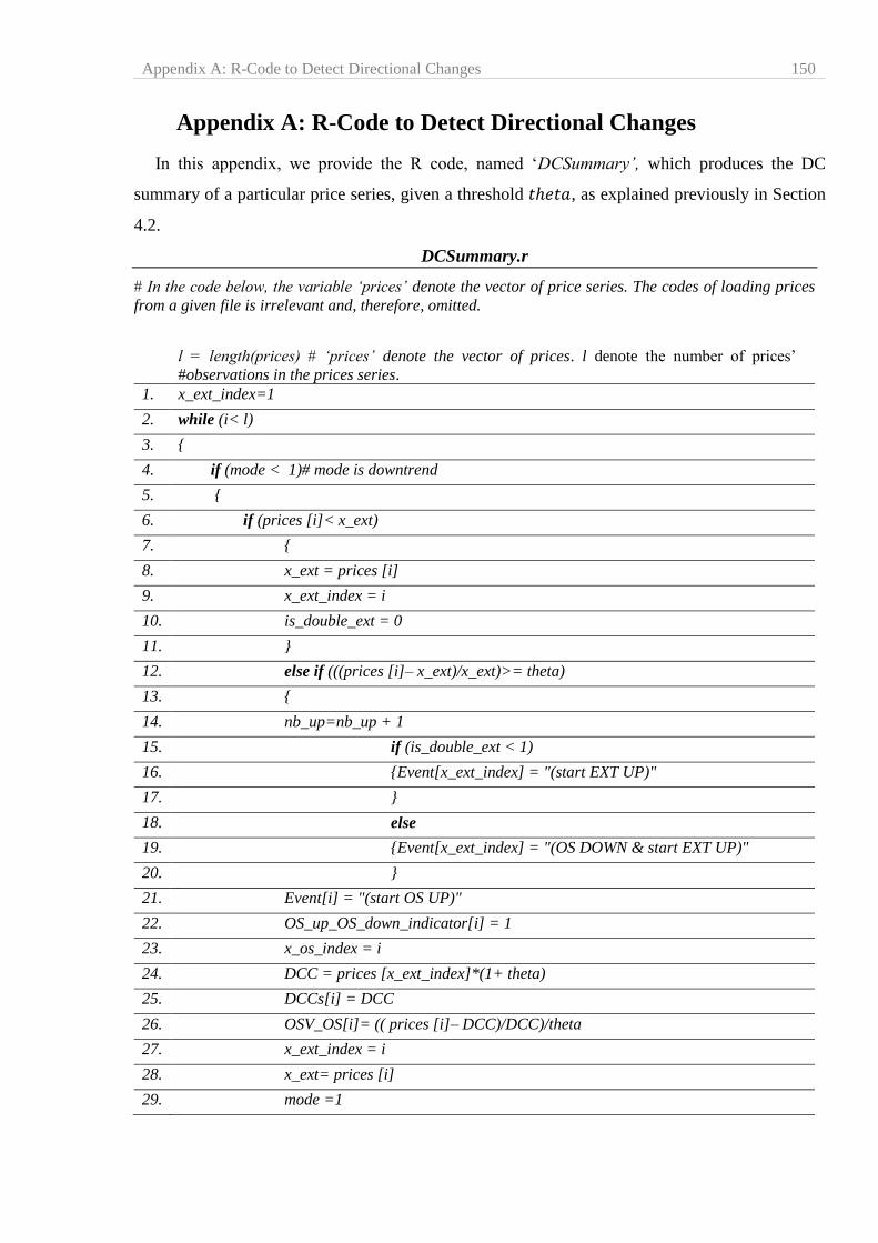
Appendix A: R-Code to Detect Directional Changes 150
Appendix A: R-Code to Detect Directional Changes
In this appendix, we provide the R code, named ‘DCSummary’, which produces the DC
summary of a particular price series, given a threshold 𝑡ℎ𝑒𝑡𝑎, as explained previously in Section
4.2.
DCSummary.r
# In the code below, the variable ‘prices’ denote the vector of price series. The codes of loading prices
from a given file is irrelevant and, therefore, omitted.
l = length(prices) # ‘prices’ denote the vector of prices. l denote the number of prices’
#observations in the prices series.
1. x_ext_index=1
2. while (i< l)
3. {
4. if (mode < 1)# mode is downtrend
5. {
6. if (prices [i]< x_ext)
7. {
8. x_ext = prices [i]
9. x_ext_index = i
10. is_double_ext = 0
11. }
12. else if (((prices [i]– x_ext)/x_ext)>= theta)
13. {
14. nb_up=nb_up + 1
15. if (is_double_ext < 1)
16. {Event[x_ext_index] = "(start EXT UP)"
17. }
18. else
19. {Event[x_ext_index] = "(OS DOWN & start EXT UP)"
20. }
21. Event[i] = "(start OS UP)"
22. OS_up_OS_down_indicator[i] = 1
23. x_os_index = i
24. DCC = prices [x_ext_index]*(1+ theta)
25. DCCs[i] = DCC
26. OSV_OS[i]= (( prices [i]– DCC)/DCC)/theta
27. x_ext_index = i
28. x_ext= prices [i]
29. mode =1
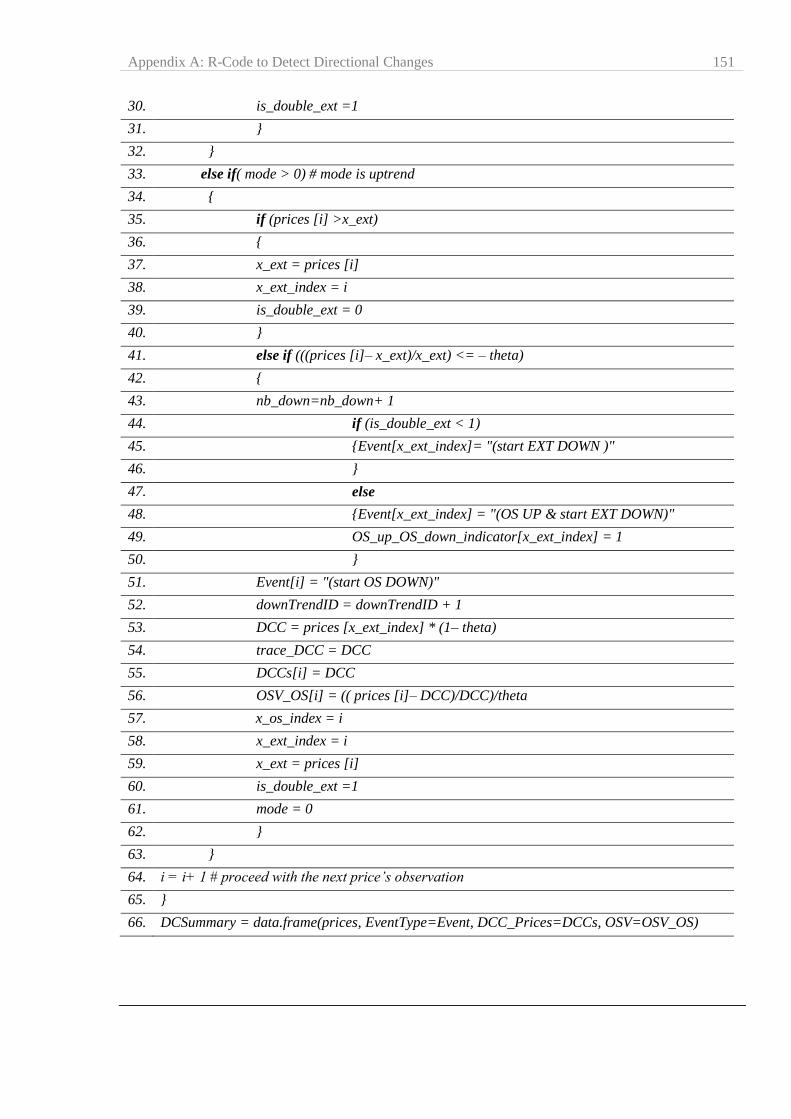
Appendix A: R-Code to Detect Directional Changes 151
30. is_double_ext =1
31. }
32. }
33. else if( mode > 0) # mode is uptrend
34. {
35. if (prices [i] >x_ext)
36. {
37. x_ext = prices [i]
38. x_ext_index = i
39. is_double_ext = 0
40. }
41. else if (((prices [i]– x_ext)/x_ext) <= – theta)
42. {
43. nb_down=nb_down+ 1
44. if (is_double_ext < 1)
45. {Event[x_ext_index]= "(start EXT DOWN )"
46. }
47. else
48. {Event[x_ext_index] = "(OS UP & start EXT DOWN)"
49. OS_up_OS_down_indicator[x_ext_index] = 1
50. }
51. Event[i] = "(start OS DOWN)"
52. downTrendID = downTrendID + 1
53. DCC = prices [x_ext_index] * (1– theta)
54. trace_DCC = DCC
55. DCCs[i] = DCC
56. OSV_OS[i] = (( prices [i]– DCC)/DCC)/theta
57. x_os_index = i
58. x_ext_index = i
59. x_ext = prices [i]
60. is_double_ext =1
61. mode = 0
62. }
63. }
64. i = i+ 1 # proceed with the next price’s observation
65. }
66. DCSummary = data.frame(prices, EventType=Event, DCC_Prices=DCCs, OSV=OSV_OS)

Appendix A: R-Code to Detect Directional Changes 152
At the end of the above R code, the dataframe named DCSummary will comprise four
vectors:
‘prices’: the initial price series,
‘EventType’: comprising all DC and OS events detected
‘DCC_Prices’: denote the price required to confirm the detection of a new DC event of
the specified threshold theta.
‘OSV’: the overshoot values computed at the DCC point of each DC event.
The DCC prices and the OSV are computed at the DCC point of each DC event (See Section
4.2.3).
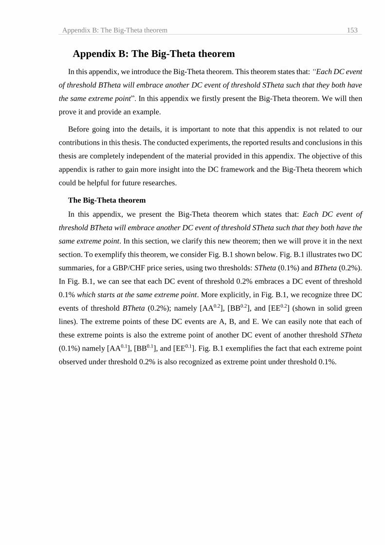
Appendix B: The Big-Theta theorem 153
Appendix B: The Big-Theta theorem
In this appendix, we introduce the Big-Theta theorem. This theorem states that: “Each DC event
of threshold BTheta will embrace another DC event of threshold STheta such that they both have
the same extreme point”. In this appendix we firstly present the Big-Theta theorem. We will then
prove it and provide an example.
Before going into the details, it is important to note that this appendix is not related to our
contributions in this thesis. The conducted experiments, the reported results and conclusions in this
thesis are completely independent of the material provided in this appendix. The objective of this
appendix is rather to gain more insight into the DC framework and the Big-Theta theorem which
could be helpful for future researches.
The Big-Theta theorem
In this appendix, we present the Big-Theta theorem which states that: Each DC event of
threshold BTheta will embrace another DC event of threshold STheta such that they both have the
same extreme point. In this section, we clarify this new theorem; then we will prove it in the next
section. To exemplify this theorem, we consider Fig. B.1 shown below. Fig. B.1 illustrates two DC
summaries, for a GBP/CHF price series, using two thresholds: STheta (0.1%) and BTheta (0.2%).
In Fig. B.1, we can see that each DC event of threshold 0.2% embraces a DC event of threshold
0.1% which starts at the same extreme point. More explicitly, in Fig. B.1, we recognize three DC
events of threshold BTheta (0.2%); namely [AA0.2], [BB0.2], and [EE0.2] (shown in solid green
lines). The extreme points of these DC events are A, B, and E. We can easily note that each of
these extreme points is also the extreme point of another DC event of another threshold STheta
(0.1%) namely [AA0.1], [BB0.1], and [EE0.1]. Fig. B.1 exemplifies the fact that each extreme point
observed under threshold 0.2% is also recognized as extreme point under threshold 0.1%.
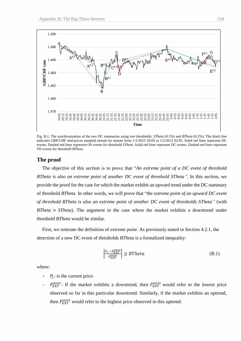
Appendix B: The Big-Theta theorem 154
Fig. B.1. The synchronization of the two DC summaries using two thresholds: STheta (0.1%) and BTheta (0.2%). The black line
indicates GBP/CHF mid-prices sampled minute by minute from 1/1/2013 19:05 to 1/2/2013 02:05. Solid red lines represent DC
events. Dashed red lines represent OS events for threshold STheta. Solid red lines represent DC events. Dashed red lines represent
OS events for threshold BTheta.
The proof
The objective of this section is to prove that “An extreme point of a DC event of threshold
BTheta is also an extreme point of another DC event of threshold STheta”. In this section, we
provide the proof for the case for which the market exhibit an upward trend under the DC summary
of threshold BTheta. In other words, we will prove that “the extreme point of an upward DC event
of threshold BTheta is also an extreme point of another DC event of thresholds STheta” (with
BTheta > STheta). The argument in the case where the market exhibits a downtrend under
threshold BTheta would be similar.
First, we reiterate the definition of extreme point. As previously stated in Section 4.2.1, the
detection of a new DC event of thresholds BTheta is a formalized inequality:
|𝑃𝑐 −𝑃𝐸𝑋𝑇
𝑛𝑒𝑥𝑡
𝑃𝐸𝑋𝑇𝑛𝑒𝑥𝑡 | ≥ 𝐵𝑇ℎ𝑒𝑡𝑎 (B.1)
where:
- 𝑃𝑐: is the current price.
- 𝑃𝐸𝑋𝑇𝑛𝑒𝑥𝑡 : If the market exhibits a downtrend, then 𝑃𝐸𝑋𝑇
𝑛𝑒𝑥𝑡 would refer to the lowest price
observed so far in this particular downtrend. Similarly, if the market exhibits an uptrend,
then 𝑃𝐸𝑋𝑇𝑛𝑒𝑥𝑡 would refer to the highest price observed in this uptrend.
1.478
1.480
1.482
1.484
1.486
1.488
1.490
19
:05
19
:15
19
:25
19
:35
19
:45
19
:55
20
:05
20
:15
20
:25
20
:35
20
:45
20
:55
21
:05
21
:15
21
:25
21
:35
21
:45
21
:55
22
:05
22
:15
22
:25
22
:35
22
:45
22
:55
23
:05
23
:15
23
:25
23
:35
23
:45
23
:55
0:0
5
0:1
5
0:2
5
0:3
5
0:4
5
0:5
5
1:0
5
1:1
5
1:2
5
1:3
5
1:4
5
1:5
5
2:0
5
GB
P/C
HF
ra
te
Time
A0.2
A
B
B0.2
E0.2
E
B0.1
C
C0.1
D0.1
D
F0.1
E0.1
F
G
G0.1 A0.1
Appendix B: The Big-Theta theorem 155
- If the inequality (B.1) holds, the time at which the market traded at 𝑃𝐸𝑋𝑇𝑛𝑒𝑥𝑡 is called an
‘extreme point’. Let 𝑃𝐸𝑋𝑇_𝐵𝑇ℎ𝑒𝑡𝑎𝑛𝑒𝑥𝑡 denote the variable 𝑃𝐸𝑋𝑇
𝑛𝑒𝑥𝑡 as observed under the DC
summary of threshold BTheta.
According to the DC framework, given a particular threshold, BTheta, an uptrend must be
preceded by a downtrend with the same threshold (Section 4.2.1). Thus, the detection of a new
uptrend under threshold BTheta can be done by analysing the preceding downtrend. If the market
exhibits a downtrend under threshold BTheta, then, by definition, 𝑃𝐸𝑋𝑇_𝐵𝑇ℎ𝑒𝑡𝑎𝑛𝑒𝑥𝑡 will refer to the
lowest price for this particular downtrend. Let 𝐸𝑥𝑡𝐵𝑇ℎ𝑒𝑡𝑎𝑑𝑜𝑤𝑛 denote the extreme points of this
particular downtrend observed under threshold BTheta. Similarly, let 𝐸𝑥𝑡𝐵𝑇ℎ𝑒𝑡𝑎𝑢𝑝
denote the
extreme points of the following uptrend observed under threshold BTheta. 𝐸𝑥𝑡𝐵𝑇ℎ𝑒𝑡𝑎𝑢𝑝
is detected
once we have
𝑃𝑐 −𝑃𝐸𝑋𝑇_𝐵𝑇ℎ𝑒𝑡𝑎𝑛𝑒𝑥𝑡
𝑃𝐸𝑋𝑇_𝐵𝑇ℎ𝑒𝑡𝑎𝑛𝑒𝑥𝑡 ≥ 𝐵𝑇ℎ𝑒𝑡𝑎 (B.2)
Suppose that we are tracking price movement of one price series with two DC thresholds STheta
and BTheta simultaneously (with BTheta > STheta). Let 𝑃𝐸𝑋𝑇_𝑆𝑇ℎ𝑒𝑡𝑎𝑛𝑒𝑥𝑡 denote the variable 𝑃𝐸𝑋𝑇
𝑛𝑒𝑥𝑡 as
observed under the DC summary of threshold STheta.
Lemma B.1:
If the market exhibits a downtrend, as observed under threshold BTheta, then 𝐸𝑥𝑡𝐵𝑇ℎ𝑒𝑡𝑎𝑢𝑝
can occur
only during a downward DC trend as observed under threshold STheta (for STheta < BTheta).
Proof B.1:
Reasoning by contradiction, suppose that 𝐸𝑥𝑡𝐵𝑇ℎ𝑒𝑡𝑎𝑢𝑝
has occurred during an uptrend under
threshold STheta. Let 𝐸𝑥𝑡𝑆𝑇ℎ𝑒𝑡𝑎𝑢𝑝
denote the extreme point of this particular DC uptrend under
threshold STheta. Note that 𝐸𝑥𝑡𝑆𝑇ℎ𝑒𝑡𝑎𝑢𝑝
must be observed after 𝐸𝑥𝑡𝐵𝑇ℎ𝑒𝑡𝑎𝑑𝑜𝑤𝑛 (for STheta < BTheta).
This is because, based on the DC concept, we can identify a price drop, of threshold BTheta, which
starts at the extreme point 𝐸𝑥𝑡𝐵𝑇ℎ𝑒𝑡𝑎𝑑𝑜𝑤𝑛 . Thus, we can implicitly, deduce the existence of a price drop
of threshold STheta which starts at, or after, the observation of 𝐸𝑥𝑡𝐵𝑇ℎ𝑒𝑡𝑎𝑑𝑜𝑤𝑛 (as STheta < BTheta).
In other words, the market must have shown a downtrend, under threshold STheta. Let
down_STheta denote this downtrend (with down_STheta being observed after the observation
of 𝐸𝑥𝑡𝐵𝑇ℎ𝑒𝑡𝑎𝑑𝑜𝑤𝑛 ). Consequently, if 𝐸𝑥𝑡𝐵𝑇ℎ𝑒𝑡𝑎
𝑢𝑝 was observed during an uptrend under a threshold
STheta, then the extreme point 𝐸𝑥𝑡𝑆𝑇ℎ𝑒𝑡𝑎𝑢𝑝
must be observed after down_STheta and, consequently,

Appendix B: The Big-Theta theorem 156
after 𝐸𝑥𝑡𝐵𝑇ℎ𝑒𝑡𝑎𝑑𝑜𝑤𝑛 as well. In this scenario, we have an uptrend under threshold STheta that was
preceded by down_STheta.
Provided that the market exhibits downtrend under threshold BTheta, then, by definition,
𝑃𝐸𝑋𝑇_𝐵𝑇ℎ𝑒𝑡𝑎𝑛𝑒𝑥𝑡 will refer to the lowest price for this particular downtrend (Section 4.2). Following our
reasoning by contradiction, if 𝐸𝑥𝑡𝐵𝑇ℎ𝑒𝑡𝑎𝑢𝑝
, with price 𝑃𝐸𝑋𝑇_𝐵𝑇ℎ𝑒𝑡𝑎𝑛𝑒𝑥𝑡 , has occurred during an uptrend
observed under a threshold STheta; then we have two possible cases:
Case A: 𝐸𝑥𝑡𝐵𝑇ℎ𝑒𝑡𝑎𝑢𝑝
is actually overlapped with 𝐸𝑥𝑡𝑆𝑇ℎ𝑒𝑡𝑎𝑢𝑝
(i.e. 𝐸𝑥𝑡𝑆𝑇ℎ𝑒𝑡𝑎𝑢𝑝
and 𝐸𝑥𝑡𝐵𝑇ℎ𝑒𝑡𝑎𝑢𝑝
are
actually the same point). In this case, the two uptrend DC events of thresholds STheta and BTheta
have actually the same extreme point. In this case, the proof is done.
Case B: 𝐸𝑥𝑡𝑆𝑇ℎ𝑒𝑡𝑎𝑢𝑝
is a distinct point other than 𝐸𝑥𝑡𝐵𝑇ℎ𝑒𝑡𝑎𝑢𝑝
and 𝐸𝑥𝑡𝑆𝑇ℎ𝑒𝑡𝑎𝑢𝑝
is observed before
𝐸𝑥𝑡𝐵𝑇ℎ𝑒𝑡𝑎𝑢𝑝
. In this case, there must exist a point X, that fits in the uptrend of threshold STheta, such
that 𝑃𝑋 < 𝑃𝐸𝑋𝑇_𝐵𝑇ℎ𝑒𝑡𝑎𝑛𝑒𝑥𝑡 (𝑃𝑋 denote the price at point X). This, however, contradicts with the fact that
𝑃𝐸𝑋𝑇_𝐵𝑇ℎ𝑒𝑡𝑎𝑛𝑒𝑥𝑡 must be the lowest price for the preceding downtrend under threshold BTheta. Thus,
Case B can never hold true, and the anticipated assumption that 𝐸𝑥𝑡𝐵𝑇ℎ𝑒𝑡𝑎𝑢𝑝
has occurred during an
uptrend under threshold STheta was wrong.
Based on the above analysis, we can conclude that 𝐸𝑥𝑡𝐵𝑇ℎ𝑒𝑡𝑎𝑢𝑝
can occur only during a
downward DC trend as observed under threshold STheta (for STheta < BTheta). Note that this
analysis is independent from any other uptrends or downtrends those could possibly have occurred
before the observation of 𝐸𝑥𝑡𝐵𝑇ℎ𝑒𝑡𝑎𝑑𝑜𝑤𝑛 . This is because, by definition, the value of 𝑃𝐸𝑋𝑇_𝐵𝑇ℎ𝑒𝑡𝑎
𝑛𝑒𝑥𝑡 is
calculated with reference to the current trend only (Section 4.2.3).
Lemma B.2:
Let 𝑃𝑐 denote the current price. Given that the market exhibits a downtrend under threshold
BTheta, if 𝑃𝑐 < 𝑃𝐸𝑋𝑇_𝐵𝑇ℎ𝑒𝑡𝑎𝑛𝑒𝑥𝑡 (i.e. if the current price turns out to be the lowest price observed so far
in this particular downtrend under threshold BTheta), then we will have 𝑃𝑐 < 𝑃𝐸𝑋𝑇_𝑆𝑇ℎ𝑒𝑡𝑎𝑛𝑒𝑥𝑡 (i.e. the
current price is also the lowest price observed so far for another downtrend as observed under
threshold STheta).
Proof B.2:
If the market exhibits a downward trend under DC summary of thresholds BTheta then, by
definition, 𝑃𝐸𝑋𝑇_𝐵𝑇ℎ𝑒𝑡𝑎𝑛𝑒𝑥𝑡 denote the lowest price in this particular downtrend. From the description
of the DC framework, we know that the value of 𝑃𝐸𝑋𝑇_𝐵𝑇ℎ𝑒𝑡𝑎𝑛𝑒𝑥𝑡 may vary as the price movement
Appendix B: The Big-Theta theorem 157
continues (Section 4.2.1). By definition, in the case of a DC downtrend of threshold BTheta, the
value of 𝑃𝐸𝑋𝑇_𝐵𝑇ℎ𝑒𝑡𝑎𝑛𝑒𝑥𝑡 changes only if we encounter a new ‘lowest price’ (i.e. if 𝑃𝑐 < 𝑃𝐸𝑋𝑇_𝐵𝑇ℎ𝑒𝑡𝑎
𝑛𝑒𝑥𝑡 ).
In such a case, the value of 𝑃𝐸𝑋𝑇_𝐵𝑇ℎ𝑒𝑡𝑎𝑛𝑒𝑥𝑡 will be assigned the value of the current price (𝑃𝑐); that is
𝑃𝐸𝑋𝑇_𝐵𝑇ℎ𝑒𝑡𝑎𝑛𝑒𝑥𝑡 = 𝑃𝑐 (see Section 4.2.1).
We consider the following notes:
a. At the time of when 𝑃𝐸𝑋𝑇_𝐵𝑇ℎ𝑒𝑡𝑎𝑛𝑒𝑥𝑡 is observed, the market exhibits downward trend under both
thresholds BTheta and STheta (based on Lemma B.1).
b. By definition, 𝑃𝐸𝑋𝑇_𝑆𝑇ℎ𝑒𝑡𝑎𝑛𝑒𝑥𝑡 refers to the lowest price in a downtrend under threshold STheta.
c. By definition, 𝑃𝐸𝑋𝑇_𝐵𝑇ℎ𝑒𝑡𝑎𝑛𝑒𝑥𝑡 refers to the lowest price in a downtrend under threshold BTheta.
d. Based on the points b. and c. above, both variables 𝑃𝐸𝑋𝑇_𝑆𝑇ℎ𝑒𝑡𝑎𝑛𝑒𝑥𝑡 and 𝑃𝐸𝑋𝑇_𝐵𝑇ℎ𝑒𝑡𝑎
𝑛𝑒𝑥𝑡 must refer to
the lowest price observed so far in this particular downtrend.
Based on the four points above, if 𝑃𝑐 turns out to be the lowest price observed so far for a
particular downtrend under threshold BTheta (i.e. if 𝑃𝑐 < 𝑃𝐸𝑋𝑇_𝐵𝑇ℎ𝑒𝑡𝑎𝑛𝑒𝑥𝑡 ), then we must have
𝑃𝑐 < 𝑃𝐸𝑋𝑇_𝑆𝑇ℎ𝑒𝑡𝑎𝑛𝑒𝑥𝑡 . In such a case, the values of both variables 𝑃𝐸𝑋𝑇_𝐵𝑇ℎ𝑒𝑡𝑎
𝑛𝑒𝑥𝑡 and 𝑃𝐸𝑋𝑇_𝑆𝑇ℎ𝑒𝑡𝑎𝑛𝑒𝑥𝑡 must be
updated so that they both become equal to 𝑃𝑐. In other words, if 𝑃𝑐 is the lowest price of the current
downtrend, under threshold BTheta, then we will have 𝑃𝐸𝑋𝑇_𝐵𝑇ℎ𝑒𝑡𝑎𝑛𝑒𝑥𝑡 = 𝑃𝑐 and 𝑃𝐸𝑋𝑇_𝑆𝑇ℎ𝑒𝑡𝑎
𝑛𝑒𝑥𝑡 = 𝑃𝑐.
Summary
Based on Lemma B.1 and Lemma B.2, the above analysis can be summarized as follow:
If (the market exhibits a downtrend under threshold BTheta) then
If (𝑃𝑐 < 𝑃𝐸𝑋𝑇_𝐵𝑇ℎ𝑒𝑡𝑎𝑛𝑒𝑥𝑡 ) then
𝑃𝐸𝑋𝑇𝑆𝑇ℎ𝑒𝑡𝑎
𝑛𝑒𝑥𝑡 = 𝑃𝑐
𝑃𝐸𝑋𝑇𝐵𝑇ℎ𝑒𝑡𝑎
𝑛𝑒𝑥𝑡 = 𝑃𝑐
The objective of this section is to prove that the extreme point of an upward DC event of
threshold BTheta is also an extreme point of another DC event of thresholds STheta. This can be
proved as follows:
a. Based on the DC framework, if the market currently exhibits a downtrend under threshold
BTheta, then the next DC event will be an upward DC event of the same threshold (Section
4.2.1).
b. By definition, if the market exhibits a downtrend under threshold BTheta, then
𝑃𝐸𝑋𝑇_𝐵𝑇ℎ𝑒𝑡𝑎𝑛𝑒𝑥𝑡 would refer to the lowest price observed so far in this particular downtrend. As
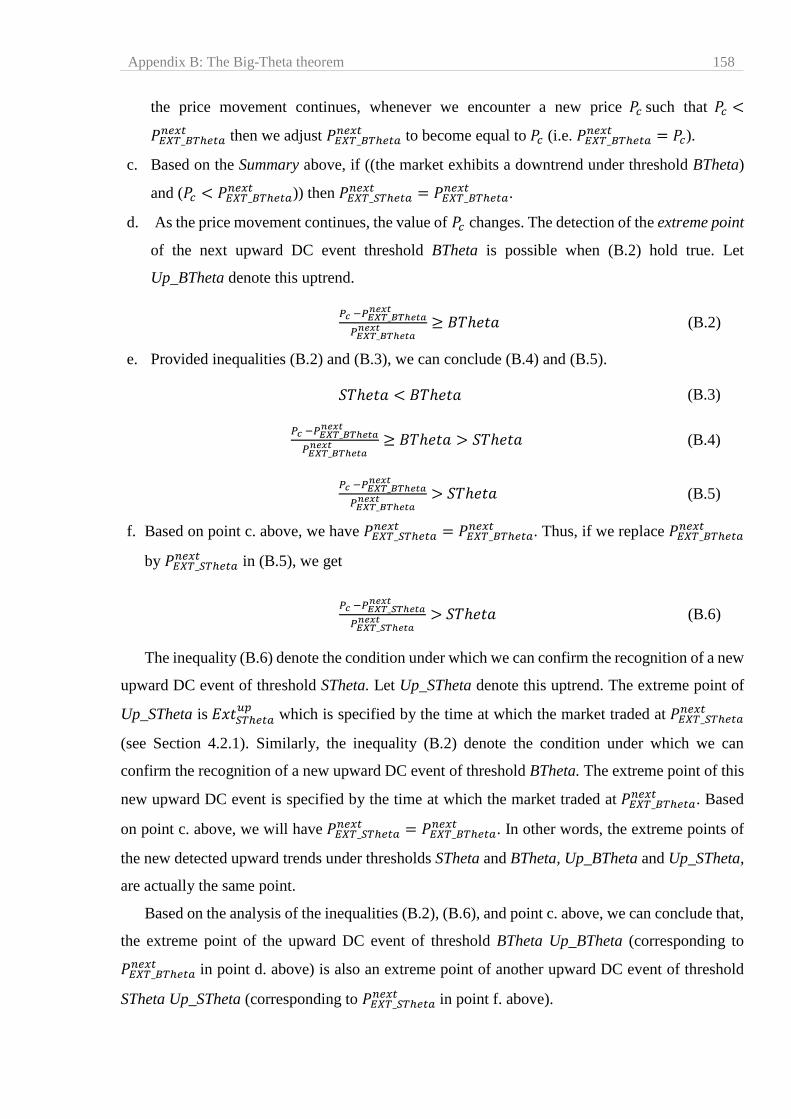
Appendix B: The Big-Theta theorem 158
the price movement continues, whenever we encounter a new price 𝑃𝑐 such that 𝑃𝑐 <
𝑃𝐸𝑋𝑇_𝐵𝑇ℎ𝑒𝑡𝑎𝑛𝑒𝑥𝑡 then we adjust 𝑃𝐸𝑋𝑇_𝐵𝑇ℎ𝑒𝑡𝑎
𝑛𝑒𝑥𝑡 to become equal to 𝑃𝑐 (i.e. 𝑃𝐸𝑋𝑇_𝐵𝑇ℎ𝑒𝑡𝑎𝑛𝑒𝑥𝑡 = 𝑃𝑐).
c. Based on the Summary above, if ((the market exhibits a downtrend under threshold BTheta)
and (𝑃𝑐 < 𝑃𝐸𝑋𝑇_𝐵𝑇ℎ𝑒𝑡𝑎𝑛𝑒𝑥𝑡 )) then 𝑃𝐸𝑋𝑇_𝑆𝑇ℎ𝑒𝑡𝑎
𝑛𝑒𝑥𝑡 = 𝑃𝐸𝑋𝑇_𝐵𝑇ℎ𝑒𝑡𝑎𝑛𝑒𝑥𝑡 .
d. As the price movement continues, the value of 𝑃𝑐 changes. The detection of the extreme point
of the next upward DC event threshold BTheta is possible when (B.2) hold true. Let
Up_BTheta denote this uptrend.
𝑃𝑐 −𝑃𝐸𝑋𝑇_𝐵𝑇ℎ𝑒𝑡𝑎𝑛𝑒𝑥𝑡
𝑃𝐸𝑋𝑇_𝐵𝑇ℎ𝑒𝑡𝑎𝑛𝑒𝑥𝑡 ≥ 𝐵𝑇ℎ𝑒𝑡𝑎 (B.2)
e. Provided inequalities (B.2) and (B.3), we can conclude (B.4) and (B.5).
𝑆𝑇ℎ𝑒𝑡𝑎 < 𝐵𝑇ℎ𝑒𝑡𝑎 (B.3)
𝑃𝑐 −𝑃𝐸𝑋𝑇_𝐵𝑇ℎ𝑒𝑡𝑎𝑛𝑒𝑥𝑡
𝑃𝐸𝑋𝑇_𝐵𝑇ℎ𝑒𝑡𝑎𝑛𝑒𝑥𝑡 ≥ 𝐵𝑇ℎ𝑒𝑡𝑎 > 𝑆𝑇ℎ𝑒𝑡𝑎 (B.4)
𝑃𝑐 −𝑃𝐸𝑋𝑇_𝐵𝑇ℎ𝑒𝑡𝑎𝑛𝑒𝑥𝑡
𝑃𝐸𝑋𝑇_𝐵𝑇ℎ𝑒𝑡𝑎𝑛𝑒𝑥𝑡 > 𝑆𝑇ℎ𝑒𝑡𝑎 (B.5)
f. Based on point c. above, we have 𝑃𝐸𝑋𝑇_𝑆𝑇ℎ𝑒𝑡𝑎𝑛𝑒𝑥𝑡 = 𝑃𝐸𝑋𝑇_𝐵𝑇ℎ𝑒𝑡𝑎
𝑛𝑒𝑥𝑡 . Thus, if we replace 𝑃𝐸𝑋𝑇_𝐵𝑇ℎ𝑒𝑡𝑎𝑛𝑒𝑥𝑡
by 𝑃𝐸𝑋𝑇_𝑆𝑇ℎ𝑒𝑡𝑎𝑛𝑒𝑥𝑡 in (B.5), we get
𝑃𝑐 −𝑃𝐸𝑋𝑇_𝑆𝑇ℎ𝑒𝑡𝑎𝑛𝑒𝑥𝑡
𝑃𝐸𝑋𝑇_𝑆𝑇ℎ𝑒𝑡𝑎𝑛𝑒𝑥𝑡 > 𝑆𝑇ℎ𝑒𝑡𝑎 (B.6)
The inequality (B.6) denote the condition under which we can confirm the recognition of a new
upward DC event of threshold STheta. Let Up_STheta denote this uptrend. The extreme point of
Up_STheta is 𝐸𝑥𝑡𝑆𝑇ℎ𝑒𝑡𝑎𝑢𝑝
which is specified by the time at which the market traded at 𝑃𝐸𝑋𝑇_𝑆𝑇ℎ𝑒𝑡𝑎𝑛𝑒𝑥𝑡
(see Section 4.2.1). Similarly, the inequality (B.2) denote the condition under which we can
confirm the recognition of a new upward DC event of threshold BTheta. The extreme point of this
new upward DC event is specified by the time at which the market traded at 𝑃𝐸𝑋𝑇_𝐵𝑇ℎ𝑒𝑡𝑎𝑛𝑒𝑥𝑡 . Based
on point c. above, we will have 𝑃𝐸𝑋𝑇_𝑆𝑇ℎ𝑒𝑡𝑎𝑛𝑒𝑥𝑡 = 𝑃𝐸𝑋𝑇_𝐵𝑇ℎ𝑒𝑡𝑎
𝑛𝑒𝑥𝑡 . In other words, the extreme points of
the new detected upward trends under thresholds STheta and BTheta, Up_BTheta and Up_STheta,
are actually the same point.
Based on the analysis of the inequalities (B.2), (B.6), and point c. above, we can conclude that,
the extreme point of the upward DC event of threshold BTheta Up_BTheta (corresponding to
𝑃𝐸𝑋𝑇_𝐵𝑇ℎ𝑒𝑡𝑎𝑛𝑒𝑥𝑡 in point d. above) is also an extreme point of another upward DC event of threshold
STheta Up_STheta (corresponding to 𝑃𝐸𝑋𝑇_𝑆𝑇ℎ𝑒𝑡𝑎𝑛𝑒𝑥𝑡 in point f. above).
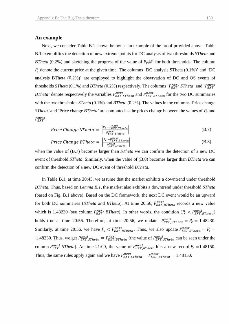
Appendix B: The Big-Theta theorem 159
An example
Next, we consider Table B.1 shown below as an example of the proof provided above. Table
B.1 exemplifies the detection of new extreme points for DC analysis of two thresholds STheta and
BTheta (0.2%) and sketching the progress of the value of 𝑃𝐸𝑋𝑇𝑛𝑒𝑥𝑡 for both thresholds. The column
𝑃𝑐 denote the current price at the given time. The columns ‘DC analysis STheta (0.1%)’ and ‘DC
analysis BTheta (0.2%)’ are employed to highlight the observation of DC and OS events of
thresholds STheta (0.1%) and BTheta (0.2%) respectively. The columns ‘𝑃𝐸𝑋𝑇𝑛𝑒𝑥𝑡 STheta’ and ‘𝑃𝐸𝑋𝑇
𝑛𝑒𝑥𝑡
BTheta’ denote respectively the variables 𝑃𝐸𝑋𝑇_𝑆𝑇ℎ𝑒𝑡𝑎𝑛𝑒𝑥𝑡 and 𝑃𝐸𝑋𝑇_𝐵𝑇ℎ𝑒𝑡𝑎
𝑛𝑒𝑥𝑡 for the two DC summaries
with the two thresholds STheta (0.1%) and BTheta (0.2%). The values in the columns ‘Price change
STheta’ and ‘Price change BTheta’ are computed as the prices change between the values of 𝑃𝑐 and
𝑃𝐸𝑋𝑇𝑛𝑒𝑥𝑡:
𝑃𝑟𝑖𝑐𝑒 𝐶ℎ𝑎𝑛𝑔𝑒 𝑆𝑇ℎ𝑒𝑡𝑎 = |𝑃𝑐 −𝑃𝐸𝑋𝑇_𝑆𝑇ℎ𝑒𝑡𝑎
𝑛𝑒𝑥𝑡
𝑃𝐸𝑋𝑇_𝑆𝑇ℎ𝑒𝑡𝑎𝑛𝑒𝑥𝑡 | (B.7)
𝑃𝑟𝑖𝑐𝑒 𝐶ℎ𝑎𝑛𝑔𝑒 𝐵𝑇ℎ𝑒𝑡𝑎 = |𝑃𝑐 −𝑃𝐸𝑋𝑇_𝐵𝑇ℎ𝑒𝑡𝑎
𝑛𝑒𝑥𝑡
𝑃𝐸𝑋𝑇_𝐵𝑇ℎ𝑒𝑡𝑎𝑛𝑒𝑥𝑡 | (B.8)
when the value of (B.7) becomes larger than STheta we can confirm the detection of a new DC
event of threshold STheta. Similarly, when the value of (B.8) becomes larger than BTheta we can
confirm the detection of a new DC event of threshold BTheta.
In Table B.1, at time 20:45, we assume that the market exhibits a downtrend under threshold
BTheta. Thus, based on Lemma B.1, the market also exhibits a downtrend under threshold STheta
(based on Fig. B.1 above). Based on the DC framework, the next DC event would be an upward
for both DC summaries (STheta and BTheta). At time 20:56, 𝑃𝐸𝑋𝑇_𝐵𝑇ℎ𝑒𝑡𝑎𝑛𝑒𝑥𝑡 records a new value
which is 1.48230 (see column 𝑃𝐸𝑋𝑇𝑛𝑒𝑥𝑡 BTheta). In other words, the condition (𝑃𝑐 < 𝑃𝐸𝑋𝑇_𝐵𝑇ℎ𝑒𝑡𝑎
𝑛𝑒𝑥𝑡 )
holds true at time 20:56. Therefore, at time 20:56, we update 𝑃𝐸𝑋𝑇_𝐵𝑇ℎ𝑒𝑡𝑎𝑛𝑒𝑥𝑡 = 𝑃𝑐 = 1.48230.
Similarly, at time 20:56, we have 𝑃𝑐 < 𝑃𝐸𝑋𝑇_𝐵𝑇ℎ𝑒𝑡𝑎𝑛𝑒𝑥𝑡 . Thus, we also update 𝑃𝐸𝑋𝑇_𝑆𝑇ℎ𝑒𝑡𝑎
𝑛𝑒𝑥𝑡 = 𝑃𝑐 =
1.48230. Thus, we get 𝑃𝐸𝑋𝑇_𝑆𝑇ℎ𝑒𝑡𝑎𝑛𝑒𝑥𝑡 = 𝑃𝐸𝑋𝑇_𝐵𝑇ℎ𝑒𝑡𝑎
𝑛𝑒𝑥𝑡 (the value of 𝑃𝐸𝑋𝑇_𝑆𝑇ℎ𝑒𝑡𝑎𝑛𝑒𝑥𝑡 can be seen under the
column 𝑃𝐸𝑋𝑇𝑛𝑒𝑥𝑡 STheta). At time 21:00, the value of 𝑃𝐸𝑋𝑇_𝐵𝑇ℎ𝑒𝑡𝑎
𝑛𝑒𝑥𝑡 hits a new record 𝑃𝑐 =1.48150.
Thus, the same rules apply again and we have 𝑃𝐸𝑋𝑇_𝑆𝑇ℎ𝑒𝑡𝑎𝑛𝑒𝑥𝑡 = 𝑃𝐸𝑋𝑇_𝐵𝑇ℎ𝑒𝑡𝑎
𝑛𝑒𝑥𝑡 = 1.48150.
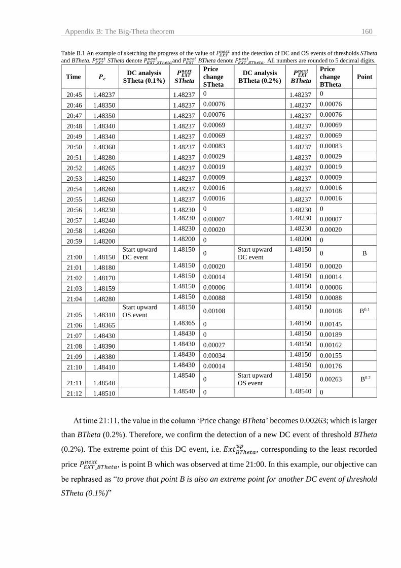
Appendix B: The Big-Theta theorem 160
Table B.1 An example of sketching the progress of the value of 𝑃𝐸𝑋𝑇
𝑛𝑒𝑥𝑡 and the detection of DC and OS events of thresholds STheta
and BTheta. 𝑃𝐸𝑋𝑇𝑛𝑒𝑥𝑡 STheta denote 𝑃𝐸𝑋𝑇_𝑆𝑇ℎ𝑒𝑡𝑎
𝑛𝑒𝑥𝑡 and 𝑃𝐸𝑋𝑇𝑛𝑒𝑥𝑡 BTheta denote 𝑃𝐸𝑋𝑇_𝐵𝑇ℎ𝑒𝑡𝑎
𝑛𝑒𝑥𝑡 . All numbers are rounded to 5 decimal digits.
Time 𝑷𝒄 DC analysis
STheta (0.1%)
𝑷𝑬𝑿𝑻𝒏𝒆𝒙𝒕
STheta
Price
change
STheta
DC analysis
BTheta (0.2%)
𝑷𝑬𝑿𝑻𝒏𝒆𝒙𝒕
BTheta
Price
change
BTheta
Point
20:45 1.48237 1.48237 0 1.48237 0
20:46 1.48350 1.48237 0.00076 1.48237 0.00076
20:47 1.48350 1.48237 0.00076 1.48237 0.00076
20:48 1.48340 1.48237 0.00069 1.48237 0.00069
20:49 1.48340 1.48237 0.00069 1.48237 0.00069
20:50 1.48360 1.48237 0.00083 1.48237 0.00083
20:51 1.48280 1.48237 0.00029 1.48237 0.00029
20:52 1.48265 1.48237 0.00019 1.48237 0.00019
20:53 1.48250 1.48237 0.00009 1.48237 0.00009
20:54 1.48260 1.48237 0.00016 1.48237 0.00016
20:55 1.48260 1.48237 0.00016 1.48237 0.00016
20:56 1.48230 1.48230 0 1.48230 0
20:57 1.48240 1.48230 0.00007 1.48230 0.00007
20:58 1.48260 1.48230 0.00020 1.48230 0.00020
20:59 1.48200 1.48200 0 1.48200 0
21:00 1.48150
Start upward
DC event
1.48150 0
Start upward
DC event
1.48150 0 B
21:01 1.48180 1.48150 0.00020 1.48150 0.00020
21:02 1.48170 1.48150 0.00014 1.48150 0.00014
21:03 1.48159 1.48150 0.00006 1.48150 0.00006
21:04 1.48280 1.48150 0.00088 1.48150 0.00088
21:05 1.48310
Start upward
OS event
1.48150 0.00108
1.48150 0.00108 B0.1
21:06 1.48365 1.48365 0 1.48150 0.00145
21:07 1.48430 1.48430 0 1.48150 0.00189
21:08 1.48390 1.48430 0.00027 1.48150 0.00162
21:09 1.48380 1.48430 0.00034 1.48150 0.00155
21:10 1.48410 1.48430 0.00014 1.48150 0.00176
21:11 1.48540
1.48540 0
Start upward
OS event
1.48150 0.00263 B0.2
21:12 1.48510 1.48540 0 1.48540 0
At time 21:11, the value in the column ‘Price change BTheta’ becomes 0.00263; which is larger
than BTheta (0.2%). Therefore, we confirm the detection of a new DC event of threshold BTheta
(0.2%). The extreme point of this DC event, i.e. 𝐸𝑥𝑡𝐵𝑇ℎ𝑒𝑡𝑎𝑢𝑝
, corresponding to the least recorded
price 𝑃𝐸𝑋𝑇_𝐵𝑇ℎ𝑒𝑡𝑎𝑛𝑒𝑥𝑡 , is point B which was observed at time 21:00. In this example, our objective can
be rephrased as “to prove that point B is also an extreme point for another DC event of threshold
STheta (0.1%)”

Appendix B: The Big-Theta theorem 161
In this example, we can detect a DC event for threshold STheta when the value of the column
‘Price change STheta’ exceeds STheta (0.1%). At time 21:05, the value of ‘Price change STheta’
is 0.00108 which is larger than 0.1%. Thus, at time 21:05 we can confirm the observation of a DC
event of threshold STheta. The extreme point of this DC event, i.e. 𝐸𝑥𝑡𝑆𝑇ℎ𝑒𝑡𝑎𝑢𝑝
, is also point B as
shown in Table B.1 at time 21:00 (as 𝑃𝐸𝑋𝑇_𝑆𝑇ℎ𝑒𝑡𝑎𝑛𝑒𝑥𝑡 = 𝑃𝐸𝑋𝑇_𝐵𝑇ℎ𝑒𝑡𝑎
𝑛𝑒𝑥𝑡 ).
To conclude, in this appendix we proved that when the market exhibits an uptrend under
threshold BTheta, the extreme point of a DC event of threshold BTheta is also an extreme point of
another DC event of threshold STheta. However, the same logic (Lemma B.1 and Lemma B.2)
holds true in the case for which the market exhibits a downtrend under the threshold BTheta.
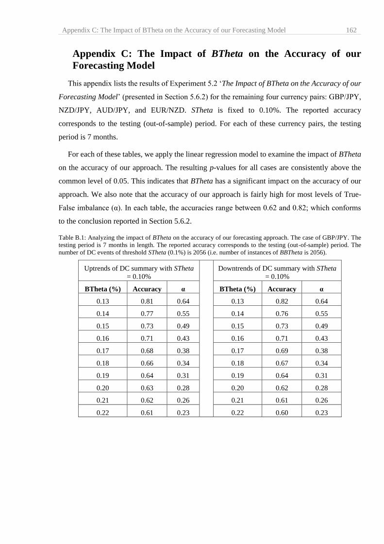
Appendix C: The Impact of BTheta on the Accuracy of our Forecasting Model 162
Appendix C: The Impact of BTheta on the Accuracy of our
Forecasting Model
This appendix lists the results of Experiment 5.2 ‘The Impact of BTheta on the Accuracy of our
Forecasting Model’ (presented in Section 5.6.2) for the remaining four currency pairs: GBP/JPY,
NZD/JPY, AUD/JPY, and EUR/NZD. STheta is fixed to 0.10%. The reported accuracy
corresponds to the testing (out-of-sample) period. For each of these currency pairs, the testing
period is 7 months.
For each of these tables, we apply the linear regression model to examine the impact of BTheta
on the accuracy of our approach. The resulting p-values for all cases are consistently above the
common level of 0.05. This indicates that BTheta has a significant impact on the accuracy of our
approach. We also note that the accuracy of our approach is fairly high for most levels of True-
False imbalance (α). In each table, the accuracies range between 0.62 and 0.82; which conforms
to the conclusion reported in Section 5.6.2.
Table B.1: Analyzing the impact of BTheta on the accuracy of our forecasting approach. The case of GBP/JPY. The
testing period is 7 months in length. The reported accuracy corresponds to the testing (out-of-sample) period. The
number of DC events of threshold STheta (0.1%) is 2056 (i.e. number of instances of BBTheta is 2056).
Uptrends of DC summary with STheta
= 0.10%
Downtrends of DC summary with STheta
= 0.10%
BTheta (%) Accuracy α BTheta (%) Accuracy α
0.13 0.81 0.64 0.13 0.82 0.64
0.14 0.77 0.55 0.14 0.76 0.55
0.15 0.73 0.49 0.15 0.73 0.49
0.16 0.71 0.43 0.16 0.71 0.43
0.17 0.68 0.38 0.17 0.69 0.38
0.18 0.66 0.34 0.18 0.67 0.34
0.19 0.64 0.31 0.19 0.64 0.31
0.20 0.63 0.28 0.20 0.62 0.28
0.21 0.62 0.26 0.21 0.61 0.26
0.22 0.61 0.23 0.22 0.60 0.23

Appendix C: The Impact of BTheta on the Accuracy of our Forecasting Model 163
Table B.2: Analyzing the impact of BTheta on the accuracy of our forecasting approach. The case of NZD/JPY. The
testing period is 7 months in length. The reported accuracy corresponds to the testing (out-of-sample) period. The
number of DC events of threshold STheta (0.1%) is 3609 (i.e. number of instances of BBTheta is 3609).
Uptrends of DC summary with STheta
= 0.10%
Downtrends of DC summary with STheta
= 0.10%
BTheta (%) Accuracy α BTheta (%) Accuracy α
0.13 0.82 0.63 0.13 0.82 0.63
0.14 0.78 0.54 0.14 0.78 0.54
0.15 0.74 0.48 0.15 0.74 0.48
0.16 0.72 0.42 0.16 0.72 0.42
0.17 0.70 0.37 0.17 0.70 0.37
0.18 0.67 0.33 0.18 0.67 0.33
0.19 0.65 0.30 0.19 0.65 0.30
0.20 0.64 0.27 0.20 0.64 0.27
0.21 0.63 0.25 0.21 0.63 0.25
0.22 0.62 0.22 0.22 0.62 0.22
Table B.3: Analyzing the impact of value of BTheta to the accuracy of our forecasting approach. The case of
AUD/JPY. The testing period is 7 months in length. The reported accuracy corresponds to the testing (out-of-sample)
period. The number of DC events of threshold STheta (0.1%) is 3184 (i.e. number of instances of BBTheta is 3184).
Uptrends of DC summary with STheta
= 0.10%
Downtrends of DC summary with STheta
= 0.10%
BTheta (%) Accuracy α BTheta (%) Accuracy α
0.13 0.79 0.56 0.13 0.79 0.56
0.14 0.78 0.53 0.14 0.77 0.53
0.15 0.75 0.51 0.15 0.76 0.51
0.16 0.70 0.49 0.16 0.70 0.49
0.17 0.68 0.48 0.17 0.69 0.48
0.18 0.66 0.45 0.18 0.66 0.45
0.19 0.65 0.42 0.19 0.66 0.42
0.20 0.64 0.35 0.20 0.64 0.35
0.21 0.64 0.31 0.21 0.65 0.31
0.22 0.63 0.28 0.22 0.63 0.28

Appendix C: The Impact of BTheta on the Accuracy of our Forecasting Model 164
Table B.4: Analyzing the impact of BTheta on the accuracy of our forecasting approach. The case of EUR/NZD. The
testing period is 7 months in length. The reported accuracy corresponds to the testing (out-of-sample) period. The
number of DC events of threshold STheta (0.1%) is 4735 (i.e. number of instances of BBTheta is 4735).
Uptrends of DC summary with STheta
= 0.10%
Downtrends of DC summary with STheta
= 0.10%
BTheta (%) Accuracy α BTheta (%) Accuracy α
0.13 0.82 0.63 0.13 0.82 0.63
0.14 0.78 0.55 0.14 0.78 0.55
0.15 0.74 0.50 0.15 0.74 0.50
0.16 0.72 0.47 0.16 0.72 0.47
0.17 0.70 0.40 0.17 0.70 0.40
0.18 0.67 0.39 0.18 0.67 0.39
0.19 0.65 0.33 0.19 0.65 0.33
0.20 0.64 0.29 0.20 0.64 0.29
0.21 0.63 0.27 0.21 0.63 0.27
0.22 0.62 0.25 0.22 0.62 0.25
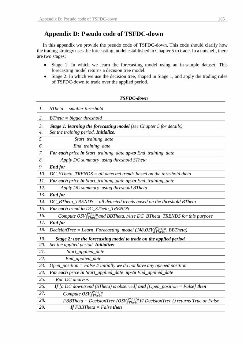
Appendix D: Pseudo code of TSFDC-down 165
Appendix D: Pseudo code of TSFDC-down
In this appendix we provide the pseudo code of TSFDC-down. This code should clarify how
the trading strategy uses the forecasting model established in Chapter 5 to trade. In a nutshell, there
are two stages:
Stage 1: In which we learn the forecasting model using an in-sample dataset. This
forecasting model returns a decision tree model.
Stage 2: In which we use the decision tree, shaped in Stage 1, and apply the trading rules
of TSFDC-down to trade over the applied period.
TSFDC-down
1. STheta = smaller threshold
2. BTheta = bigger threshold
3. Stage 1: learning the forecasting model (see Chapter 5 for details)
4. Set the training period. Initialize:
5. Start_training_date
6. End_training_date
7. For each price in Start_training_date up-to End_training_date
8. Apply DC summary using threshold STheta
9. End for
10. DC_STheta_TRENDS = all detected trends based on the threshold theta
11. For each price in Start_training_date up-to End_training_date
12. Apply DC summary using threshold BTheta
13. End for
14. DC_BTheta_TRENDS = all detected trends based on the threshold BTheta
15. For each trend in DC_STheta_TRENDS
16. Compute 𝑂𝑆𝑉𝐵𝑇ℎ𝑒𝑡𝑎𝑆𝑇ℎ𝑒𝑡𝑎and BBTheta. //use DC_BTheta_TRENDS for this purpose
17. End for
18. DecisionTree = Learn_Forecasting_model (J48,𝑂𝑆𝑉𝐵𝑇ℎ𝑒𝑡𝑎𝑆𝑇ℎ𝑒𝑡𝑎, BBTheta)
19. Stage 2: use the forecasting model to trade on the applied period
20. Set the applied period. Initialize:
21. Start_applied_date
22. End_applied_date
23. Open_position = False // initially we do not have any opened position
24. For each price in Start_applied_date up-to End_applied_date
25. Run DC analysis
26. If [a DC downtrend (STheta) is observed] and [Open_position = False] then
27. Compute 𝑂𝑆𝑉𝐵𝑇ℎ𝑒𝑡𝑎𝑆𝑇ℎ𝑒𝑡𝑎
28. FBBTheta = DecisionTree (𝑂𝑆𝑉𝐵𝑇ℎ𝑒𝑡𝑎𝑆𝑇ℎ𝑒𝑡𝑎)// DecisionTree () returns True or False
29. If FBBTheta = False then

Appendix D: Pseudo code of TSFDC-down 166
30. Trigger buy signal
31. Open_position = True
32. Else
33. If a DC downtrend (BTheta) is observed then
34. Trigger buy signal
35. Open_position = True
36. End if
37. End if
38. End if //line 25
39. If [Open_position = True] and [a DC uptrend (STheta) is confirmed] then
40. Trigger sell signal
41. Open_position = False
42 End if
43. End for //line 23
44. End TFDC-down

Appendix E: Annualized rate of return produced by TSFDC and DBA 167
Appendix E: Annualized rate of return produced by TSFDC and
DBA
In this appendix we estimate the annualized rate of return of the developed trading strategies
TSFDC and DBA. We follow a simple mathematical rule to compute the estimated annualized rate
of return based on the results of the experiments described in Section 6.6.1 and 7.5.3:
𝐴𝑛𝑛𝑢𝑙𝑎𝑡𝑖𝑧𝑒𝑑 𝑅𝑅 =12
7 × 𝑅𝑅
where 𝑅𝑅 denote the rates of return produced by a trading strategy throughout the trading period
of 7 months for a given currency pair (see Sections 6.6.1 and 7.5.3)
Table E.1: Annualized RR for TSFDC and DBA
TSFDC-down TSFDC-up DBA-down DBA-up
EUR/CHF 15.65 8.28 10.16 9.93
GBP/CHF 18.54 20.69 11.42 17.85
EUR/USD – 2.50 1.15 – 2.76 0.36
GBP/AUD 15.46 7.87 12.12 10.53
GBP/JPY – 4.66 – 8.45 – 1.71 – 0.89
NZD/JPY 46.25 45.21 31.35 39.74
AUD/JPY 20.73 26.40 22.13 20.48
EUR/NZD 71.78 70.67 48.70 56.25