Developing Turnaround Maintenance (TAM) Model to …operating conditions and the residual life of critical equipment of plants to carry out the major activities: inspection and maintenance

International Journal of Industrial Engineering and Operations Management (IJIEOM) Volume. 1, No. 1, pp. 12-31, May 2019

© IEOM Society International

IEOM Society International

International Journal of Industrial Engineering and Operations Management (IJIEOM)

Volume 1, No. 1, May 2019 pp. 12 - 31

Developing Turnaround Maintenance (TAM) Model to Optimize TAM Performance Based on the Critical Static Equipment (CSE) of

GAS Plants Abdelnaser Elwerfalli, M. Khurshid Khan and J. Eduardo Munive-Hernandez

School of Engineering, Faculty of Engineering and Informatics, University of Bradford, Bradford, UK [email protected], [email protected], [email protected]

ABSTRACT

Many oil and gas companies have suffered major production losses, and higher cost of maintenance due to the total shutdown of their plants to conduct TAM event during a certain period and according to scope of work. Therefore, TAM is considered the biggest maintenance activity in oil and gas plant in terms of manpower, material, time and cost. These plants usually undergo other maintenance strategies during normal operation of plants such as preventive, corrective and predictive maintenance. However, some components or units cannot be inspected or maintained during normal operation of plant unless plant facilities are a totally shut downed due to operating risks. These risks differ from a company to another due to many factors such as fluctuated temperatures and pressures, corrosion, erosion, cracks and fatigue caused by operating conditions, geographical conditions and economic aspects. The aim of this paper is to develop a TAM model to optimize the TAM scheduling associated with decreasing duration and increasing interval of the TAM of the gas plant. The methodology that this paper presents has three stages based on the critical and non-critical pieces of equipment. At the first stage, identifying and removing Non-critical Equipment pieces (NEs) from TAM activity to proactive maintenance types. During the second stage, the higher risk of each selected equipment is assessed in order to prioritize critical pieces of equipment based on Risk Based Inspection (RBI). At the third stage, failure probability and reliability function for those selected critical pieces of equipment are assessed. The results of development of the TAM model is led to the real optimization of TAM scheduling of gas plants that operated continuously around the clock in order to achieve a desired performance of reliability and availability of the gas plant, and reduce cost of TAM resulting from the production shutdown and cost of inspection and maintenance.

ARTICLE INFO

Received March 5, 2018

Received in revised form

August 2018 Accepted

January 5, 2019

KEYWORDS Turnaround

Maintenance (TAM), Optimization of TAM Scheduling, Critical Static Equipment of

Gas Plant, Risk-Based Inspection (RBI),

Failure Distributions

1. IntroductionOil and gas plants consist of hundreds pieces of rotating and static equipment that operate continuously under harsh operating conditions resulting from excessive pressures and fluctuated temperatures. Some pieces of equipment usually subject to various maintenance strategies during the normal operation of plant such as preventive, corrective

12



and predictive maintenance. However, there are critical pieces of these equipment cannot be inspected and maintained during the normal operation of plants unless plant facilities are totally shut downed to conduct the TAM event in order to overcome all expected failures, which may be caused high risks during the operation periods. This is justified to use widely TAM for most oil and gas plants during a certain period (TAM duration) at every few years (TAM interval). TAM can be defined as the largest maintenance activities in the oil and gas plants in terms of cost and time (Elfeituri and Elemnifi, 2007). Duffuaa and Ben Daya (2004); Lawrence (2012) also reported that TAM is a total shutdown of plants during a certain time period to carry out TAM activities associated with inspection, repair, modification, and replacement of new part or equipment according to Scope of Work (SoW) of TAM. Neikirk (2011) stated that TAM is a periodic activity of the plant that isolates all items from the service during a certain time. Consequently, TAMs have become necessary event for any processing plant operated continuously under rigorous operating conditions to mitigate risks between TAM periods (Prasad, 2014). Consequently, TAMs have become necessary event for any processing plant operated continuously under rigorous operating conditions to mitigate risks between TAM periods (Prasad, 2014).

Since the 1970s, interest in shutdown issues of gas plants has significantly increased due to the production losses and the inspection and maintenance cost. Many oil and gas companies have suffered losses in the production and enormity in the cost of TAM due to a stochastic estimation of duration and interval of TAM. The stochastic and permanent estimation of TAM scheduling (decreasing duration and increasing interval of TAM) based on the recommended periods of the Original Equipment Manufacturers (OEMs) mean that TAM scheduling was neither adopted on the residual life of the critical equipment and nor a real planning associated with operating conditions and maintenance strategy of the gas plant. TAM scheduling of the gas plant can be conducted based on the suggested period of the OEMs in the short-term. However, this strategy of OEMs cannot be represented the most optimum TAM scheduling in the medium and long-term, because operating conditions vary significantly from a company to another. Therefore, plant facilities must be shut downed during a certain time at every few years according to the operating conditions and the residual life of the critical pieces of equipment.

Through previous studies, it was found that there is a need to identify knowledge gap to solve TAM scheduling problem in the TAM field of gas plants to assist in the decision making, and bridge the existing gap in the literature. A few of previous studies focused on the improvement of interval of TAM based on an individual equipment during a planned and unplanned shutdown period without taking critical pieces of equipment into account. Large number of studies also focused on the improvement of TAM duration from business and management perspective such as an increase of human resources, development of contracts, skill development of TAM crew, culture and conflict resolution during TAM activities.

In addition, some previous studies have used a variety of application to optimise TAM scheduling. However, they have not adopted a model of the TAM event employed for any a processing plant run continuously under operating conditions in order to determine both duration and interval of TAM in the medium and long-term, and also have not covered all CEs of gas plants. Many previous studies also have covered the redundant rotating equipment from Preventive (PM), Corrective (CM) and Predictive (PdM) perspective. PM is a set of action should be taken before failure occurs. PdM is a step forward in PM, and CM is a step backward in PM as shown in Figure 1. These classifications are not able to overcome all failures related to inspection, repairs, replacement, development and renewal in the oil and gas plants. Therefore, it is arguably that TAM event is an evil unavoidable.

Utne et al. (2012) reported that shutdown can be a planned or unforeseen shutdown. However, In general, the planned shutdown is TAM event the predetermined scheduled in terms of TAM duration, TAM interval, allocated budget, contracts, manpower and spare parts to prepare for pre-shutdown (Duffuaa and Ben Daya, 2004). Unplanned shutdown can be broken down into expected or unexpected shutdown. Expected shutdown is a total shutdown of plant which occur based on pre-warning (run-to-failure) without planning of the maintenance duration. Unexpected shutdown is a total shutdown of plant which occur without any pre-warning due to unknown defects (these defect need to long time to its realization, access, and then its diagnosis.

Therefore, most processing plants are subjected to the previously planned shutdown during a certain time based on operating conditions and the residual life of critical equipment of plants to carry out the major activities: inspection and maintenance activities, modifications and replacements (Duffuaa and Ben Daya, 2004). Levitt (2004) stated that planned shutdown of any processing plant is the major maintenance activity that required the biggest financial supports.

13



MAINTENANCE

Improvement

Reactive: occurring after failure Proactive: occurring before failure

PLANNED MAINTENANCEUNPLANNED MAINTENANCE

BreakdownEmergency

Predictive Preventive Corrective

Condition based Routine

Opportunity

Shutdown preventive

Run-to-failure

Shutdown corrective

Deferred

ShutdownImprovement

Design-out

Time based

Turnaround Maintenance (TAM)

Figure 1. Maintenance classification

Figure 2 shows the life cycle of TAM that consists of four phases. These phases aim to achieve optimum TAM and enhance its performance. Therefore, each phase includes a specific set of critical activities during a given time period in which depends on several factors, weight of activity, budget, time, material and manpower.

Planning Preparation Execution Start-up

Evaluation

TAM interval (MTTF)

Frozen SOW Ready to TAM TAM

completedPre-TAM1-3 days

TAM duration (MTTR)

TAM interval (MTTF)

C C

6 – 12 mths 5 – 10 mths 21–45 days

C C

Life Cycle of TAM(MTBF)

3 – 15 days

Termination

commissioning

Figure 2. Life cycle of TAM

Duffuaa and Ben-Daya (2004); Levitt (2004); Lenahan (2006) highlighted the execution phase of TAM from a management perspective. Krings (2001); Oliver (2002); Mclay (2003) all reported that successful TAM depends on the planning phase in the long term to estimate budget and time of TAM. However, Brown (2004) discussed the planning and executing phases of TAM cycle life.

2. Related WorkThe scheduling TAM has several effects on the operational performance of plants in terms of time, cost, and risk. The relation between the duration and cost of TAMs are considered direct relationship, the relation between the interval and risk are also considered direct relationship. This means that, once a decrease of TAM duration would lead to the decreased cost of TAM, and increased interval of TAM. However, an increase of TAM interval may result in increasing risk unless taking RBI approach of CSE pieces into account. For this reason, oil and gas companies have spent thousands of man-hours on volume of the work in the execution phase of TAM because of their voluminous activities.

Number of contractors should also be consistent with size of TAM activities to avoid the prolonging TAM duration of and complete all activities according to a previously planned duration of TAM. Duration of TAM is the time period which a plant subjects to a total shut down to conduct TAM activities. These activities include two stages: execution and termination phase that require considerable time, cost and efforts to execute it. Oliver (2002) identified many performance aspects to measure TAM, which included duration, budget, Start-up incidents and safety. Lenahan (2006) also identified several performance indicators that contributed in the improvement of TAM performance such as

14



safety, cost and efficiency. Elfeituri, and Elemnifi (2007) also presented the optimisation of TAM duration for refinery plant by removing redundancy rotating pieces which can be maintained during the normal operation of plant to routine maintenance plan in order to minimise downtime of a plant. The results of optimisation were recommended to reduce duration of TAM to 23 days rather than 30 days. Schroeder and Vichich (2009) studied essential relationships between costs, quality and duration of TAM. (Halib et al., 2010), suggested four weeks as an average to execute the TAM duration of petrochemical companies and 11 days to carry out the TAM duration of refinery plants. This means that estimation of TAM duration is not based on the residual of the critical equipment life. (Megow et al., 2011) developed a model of scheduling TAM for chemical plants contained two phases. At first phase supported the project manager to find a good duration and observe risks priorities, and the 2nd phase was associated with optimizing resources used during the chosen duration of TAM. However, this study focused on only optimisation of TAM duration in terms of different features time-cost, trade-off external resource equipment, resource levelling, and risk analysis, also it has not covered interval between TAM periods.

Emiris (2014) highlighted the challenges encountered in development of TAM using Project Management Office (PMO) based on high cost, short duration, risk, and scope of work according to the standards recommended by the Project Management Institute. Consequently, random planning of TAM duration can impact availability and financial performance of a plant. Therefore, any additional day of duration of TAM can result in increasing cost of TAM, and lost millions of dollars due to shutdown of production (Rajagopalan et al., 2017). Rajagopalan et al. (2017) also proposed a systematic approach via a multistage stochastic programming model that developed TAM reschedule. (Akbar and Ghazali, 2017) developed a model of an organizational and management for a processing plant in Malaysian associated with management functions of leading and performance for processing plant to enhance the performance of TAM duration using team alignment. The TAM Interval is the time period which plant facilities is normally under operation. The suggested TAM intervals may not be the most optimum time to TAM strategy due to operating conditions that may vary significantly from a company to another. Most oil and gas industries are continuously subjected to the pre-planned shutdown every life cycle of a plant according to several aspects availability, reliability, risk, production rate of plant to attain optimal performance and revitalise efficiency, and reliability of plants (Halib, et al., 2010). However, pre-planned TAM every life cycle should be based on CEs which cannot be inspected or maintained during the normal operation of the plant and that represented a high risk on the plant in order to achieve the optimal performance to the next cycle of the TAM.

Tam, et al. (2006) reported that interval of shutdown is often determined by the Original Equipment Manufacturers (OEMs). However, OEMs suggestions of TAM interval may be perfect only during warrantee period (early failures period) for some pieces of equipment. However, OEMs suggestions are not feasible in the medium and long term due to operating conditions and the production requirements for plant facilities. Therefore, the optimization of TAM interval for any a processing plant identifies according to specific conditions associated with a real operating conditions and the residual life of CEs. Megow, et al. (2011) stated that the TAM interval of a large plant can be repeated every more than one year. Swart (2015) reported that historically, intervals of TAM identified without any real strategic associated with operating process.

Dyke (2004) presented several steps in the improvement of TAM performances of the refinery plants using best practice model and as well as applied benchmarking technique to measure performance of TAM that included duration and interval of each major process units. Krishnasamy et al., (2005) identified the critical pieces of equipment using risk assessment along with the Weibull and Exponential approach to develop cost-effective maintenance policies of critical equipment by reducing the overall risk of the power plant. Elfeituri and Elemnifi (2007) applied RBI approach to identify vessels that have high risk on the refinery plant to inspect and maintain them during TAM periods. Khan et al. (2008) presented a risk-based methodology to estimate the optimal inspection and maintenance intervals using availability modelling to minimize failure risk and enhance the overall availability of the system. Ghosh and Roy (2009) proposed methodology for optimising the maintenance intervals using maximising the reliability function based on cost and benefit ratio. Keshavarz et al. (2011) proposed a risk-based shutdown management of maintenance using active and stand-by redundancy to optimize the TAM interval for liquefied natural gas equipment pieces. Shuai et al. (2012) applied RBI technique to predict inspection interval for shell and bottom of crude oil tank in China to determine rate of corrosion and thickness of shell and bottom.

Obiajunwa (2012) reported that interval of TAM for petrochemical and refinery plants were conducted every two years and power plant executed every four years. Rusin and Wojaczek (2012) presented optimizing maintenance intervals of power machine by taking the risk into account. Hameed and Khan (2014) also presented a framework to identify the risk-based shutdown interval to prolong intervals between TAM periods based on heat exchangers for a

15



processing plant, taking risk-based shutdown interval into account. Hameed and Khan (2014) stated that is very difficult that a shutdown period included totally inspection and maintenance of equipment of pieces. Hameed and Khan (2014) also presented a framework to estimate the risk-based shutdown interval in order to extend intervals between shutdowns for a processing plant based on the individual equipment. They also proposed the Weibull model to determine interval of TAM based on the Probability of Failure (PoF) and Consequences of Failure (CoF). Swart (2015) also stated that the cause of the current interval of TAM is either indiscriminate or has become as a redundant.

The random and permanent estimation of the TIME interval, means that TAM activity is not based on the residual life of the equipment that can increase the risk due to fixed-interval. Therefore, the important aspects associated with both duration and interval of TAM were covered in most previous studies. Most previous studies were focused on the improvement of the TAM interval based on the individual equipment whether series or parallel system. Other previous studies were concerned with improving of the TAM duration based on an increase of human resources, development of contracts, skill development of TAM crew, quality maintenance management and conflict resolution during TAM activities. In addition, both shape and scale parameters were randomly estimated outside of operating conditions of gas plants. Many previous studies focused on redundant rotating pieces of equipment from PM, CM and PdM perspective.

3. Research ContributionThis study is to develop the TAM model in order to address TAM scheduling associated with decreasing duration and increasing interval of TAM in the medium and long-term. The development of TAM model will go further to reduce cost of TAM and production losses, and improve reliability and availability of gas plants. This model includes three stages, as given in Figures 3, 4 and 5.

Stage 1: Removing Non-critical Equipment (NE) from TAM to Proactive Maintenance Identifying TAM activity depends on several factors associated with size, technology, reliability and safety of plant (Halib, et al., 2010). However, the size of plant is the main characteristic that involves all static and rotating equipment pieces. Consequently, this stage focused on the identification of all equipment pieces listed within gas plant to classify and remove non-critical pieces from TAM list as shown in Figure 3. This Stage involves a precise description of each static and rotating equipment for removing non-critical static and rotating equipment "which can be inspected and maintained without the need to a total shutdown of the plant" from SoW of TAM to combine to proactive maintenance plan in order to decrease duration and increase interval according to the following steps:

a) Pieces of equipment were identified related to the gas plant,b) Pieces of equipment were separated into Static Equipment (SEs) and Rotating Equipment pieces (REs),c) Static equipment pieces were classified into Critical and Non-critical Static Equipment (NSEs and CSEs).

Based on Equation (1) given in the Figure 3, NSEs was excluded from a TAM index and CSEs was included to the next stage to consider in the stage II. This equation is a tool used to assess effects of equipment pieces on the functional performance of the plant in terms of cost, availability, production and safety (Afefy, 2010; Vishnu and Regikumar, 2016).

EC (Critical Equipment) =15% C + 25% A + 30% P + 30% S

3 (1)

Table 1 shows the impact levels of each equipment on the operational performance of a plant in terms of Cost (C), Availability (A), Production, and Safety (S) according to weights of the affecting (15%, 25%, 30% and 30%). These weights were considered indicator for many oil and gas companies to assign critical equipment pieces. Many companies have used 50%P and 50%S as a scale to identify CEs. Therefore, these weights identified based on layout of the gas plant and experts of Metallurgy and Inspection (M&I), Mechanical Analyses Group (MAG), Operation & Maintenance engineers of SOC gas plant. In addition, the scale used to determine the score for the variables P, S, C, A is a three point scale: (3) Very important, (2) Important, and (1) Normal (a minimum effect on all these parameters due to failures).

16



Figure 3. 1st Stage of removing NE from TAM to proactive activity

Table 1. Classifying critical and non-critical equipment

Factors Affecting Critical Weight

(%)

Scales 1 2 3

Level % Level % Level % Cost (C) 15 L 15 M 30 H 45

Availability (A) 25 H 25 M 50 L 75 Production (P) 30 N 30 I 60 V 90

Safety (S) 30 N 30 I 60 V 90 L: Low, M: Medium, H: High, N: Normal, I: Important, V: Very important.

Stage 2: Risk Assessment of CSE Using RBI Approach Most processing plants are started with focusing on RBI techniques due to the complex processes that required a higher availability and reliability (Kumar, 1998). RBI is a crucial approach in decision-making process that plays an important role in the optimization of maintenance (Ahmed et al., 2015). Based on RBI, the second stage is focused on the CSEs extracted from the first stage to identify CSEs that represented the highest risk on the production, company assets and environment issues in terms of corrosion, erosion factors, fluctuating in pressure and temperatures due to continuously operation and under rigorous operating conditions. Figure 4 illustrates the process that can identify pieces

Categorise Equipment

Gas Plant

Rotating Equipment Static Equipment

Estimation of Cost, Availability, Production, and Safety effects on the plant performance

CE = (15% C + 25% A + 30% P + 30% S) / 3

CE ≤ 45%

45% < CE ≤ 59%

CE > 59%

Non-critical Equipment (NE)

Decreasing TAM Duration

Removing NE from TAM to Routine Maintenance Redundant

standby

DowntimeCritical Equipment (CE)

Yes

No

No

Yes

Yes

No

CSE CREA Rotating

1st Stage : Removing NE from TAM to Routine

Maintenance

D

17



of equipment that have the highest risk on the company/plant to assist the operation and maintenance engineers in the estimation of the TAM interval for gas plants.

Add CSE to 2nd Stage

Classification of CSE According to Operation Conditions

Collection and Analysis of Common Failures for each item Based on RBI Approach

Risk Assessment Based on POF and COF

Compare Estimated risk (Re) against Risk Criteria (Rc)

Re > Rc

A

Insp

ectio

n Pr

iorit

y

Next TAMNext ScenarioNo

Yes

2nd Stage : Application of RBI

3rd Stage

Add to SoW of TAM

Figure 4. 2nd Stage of risk assessment of CSE based on the RBI approach

RBI is a commonly used risk analysis technique employed in the higher risks zones, especially oil and gas plants, where one estimates PoF and CoF and compare the estimated risk against a pre-defined criteria to prioritise critical pieces of static equipment according to the risk (5x5) matrix.

Stage 3: Application of Failure Distribution on the Highest Risk CSE Pieces: At the third stage, failure probability and reliability function for those selected components are assessed through the stage 2. Figure 5 shows applications of failures distributions to determine optimum interval of TAM based on shape and scale parameters (β, η), which estimated according to failures behaviour Time-to-Failure (TTF). Minitab software is a tool used to compute R(t) and h(t) in order to determine a failure mode for each critical equipment. A failure mode is an indicator which can specify any value of random variable falling within a range of curve. An availability was also implemented in this stage as an indicator to optimise TAM scheduling.

A = TAM IntervalTAM Interval+TAM duration

(2)

The downtime is equivalent to the duration of TAM and the uptime is equivalent to the interval of TAM.

18



Parameter evaluation β , η

3rd Stage Failure Distributions

Add the Highest Risk CSE Add CRE

Identify the best – fitted distribution

- Failure data collection - Chronologically ordered TTF’s

R(t),and h(t)

Identify interval of each equipment

Availability

End

D

Optimum interval of TAM scheduling of the gas plant

Failure mode

DowntimeUptime

Figure 5. 3rd Stage of estimation of interval of TAM

4. Results and DiscussionsThe main purpose of this study is to develop the TAM model that consists of three stages for optimizing TAM scheduling associated with decreasing duration and increasing intervals of TAM for gas plants in order to reduce production losses and TAM cost and improve reliability and availability of plants.

4.1 Decreasing Duration of TAM Gas plants consist of thousands pieces of static and rotating equipment that operate continuously under harsh operating conditions. Some of these pieces can be inspected and maintained during normal operation of the plant. Therefore, this stage is designed to identify and remove pieces that can be inspected and maintained during normal operation of plant (Non-critical Equipment-NE) from TAM worklist to proactive maintenance plan to decrease the TAM duration in order to reduce the TAM cost and the production losses. Table 2 illustrates number of NSEs which were removed from TAM worklist to proactive maintenance plan. These NSEs identified according to a layout of the gas plant that included Gas Liquid Recovery Unit (GLRU), Treating, Drying and Fractionation (T, D &F), Salt Water Bay (SWB) and utilities unit.

Table 2. Identified and removed NSES and NRES of the gas plant Stage No Static Equipment Rotating Equipment

1st In out In Out

186 + 91 pipe 120 + 56 118 114

2nd In (186-120, 91-56) In (118-114) 66 + 35 (S) Pipelines 4

19



Based on the Equation (1) that consists of four constrains: Cost, Availability, Production, and Safety effects on the plant performance as shown in Figure 3, 120 NSEs out of 186 static equipment pieces and also all safety and relief valves were removed. Consequently, this is obvious that, once the number of equipment pieces are reduced, the duration of TAM is expected to 21 days rather than 30 days and total cost of TAM to 2 million or less rather than 2.5 million. 21 days is represented plant downtime to perform TAM event based Critical Static Equipment (CSEs).

4.2 Increasing Interval between TAM Periods This case presents approach to prioritize CSEs that represented the highest risks on the production losses, operating assets and environment issues to increase the TAM interval in order for potential improvements in all reliability, availability, and maintainability aspects. In this stage highlighted 66 vessels and 35 pipelines, which exposed to fouling, leakage, corrosion, and crack resulting from continuously operating condition based on descriptive information was collected by Metallurgy and Inspection (M&I), the operation and maintenance experts, and failure records of the Libyan gas plant. These vessels and pipelines could be conveniently divided into four categories: heat exchangers, drums, processing columns, and pipelines as shown Table 3.

Table 3. Classification of CSEs

CSE No Codes

Heat exchangers 18 E-401, E-410, E-601, ME-601, E-601A, E-601B, E-602A, etc.HP Drums 32 D-701, D-702/703, D-704/757, D-705A/B, D-706, D-712, etc.Columns 16 DR-401 C/D, T-701, T-702, T-703, T- 401, T-402, etc. Pipelines 35 lines (PL.20"- 84")

Total 68 + 35

According to the above results, Stage II of the TAM model includes four categories of equipment pieces. These pieces are considered critical elements (CSE) in the gas plant that can be contributed in the estimation of interval between the TAM periods based on the RBI approach. Consequently, CSE pieces were distributed on the risk (5x5) matrix according to two factors namely; PoF and CoF to avoid an expected and unexpected consequences. These factors can be expressed as illustrated in Equations (2, 3, 4, and 5).

Risk = Probability of failure x Consequence of failure RENC = POF X COF Environment (2) RPL = POF X COF Production Losses (3)

RAD = POF X COF Operating Assets Damage (4) The highest risk (Rs) can be selected using the equation (5):

Rs = Max (RENC, RPL, RAD) (5)

4.2.1 Risk Assessment of 18 Heat Exchangers Table 4 shows risk ranking limits arising from PoF and CoF which can have an impact on the plant performance. The risk ranking limits between 3 and 12, where 10 and 12 represent high-risk zone that consider an unacceptable risk zone. Heat exchangers pieces located in this zone should be added to the TAM list to represent TAM event, because these pieces of equipment have the highest risk due to the fouling effect. These pieces should be taken into consideration to consider in the next stage and to avoid the main causes of leakage and corrosion in the middle and long-term.

20



Table 4. Estimated risk and risk criteria Rating Failure

Scale Re Rc Decision

1 Very Low Risk 0 < Re ≤ 3 Insignificant

Risks Omitting Equipment from TAM list to next TAM (Priority).

2 Low Risk 3 < Re ≤ 6 Acceptable Risks

Omitting Equipment from TAM list to next TAM (Priority).

3 Moderate 6 < Re ≤ 9 Acceptable Risks

Omitting Equipment from TAM list to next TAM (Priority).

4 High Risk 9 < Re ≤ 12 Unacceptable Risks

Adding Equipment to next stage IV

5 Very High Risk Re > 12 Catastrophic

Risk Plant Shutdown

Six pieces out of 18 pieces of heat exchangers were classified in the high risk zone as shown in Table 5. These pieces included a cooling, a Cryogenic Colum Heat Exchanger (MCHC), and 4 pieces of Feed Gas Heat Exchangers (shell and tube heat exchangers) of gas plant. These heat exchangers were rated in the high risk zone due to accumulated fouling layers through the tubes. This table shows 6 pieces located in the high risk zone require immediate attention by preparing to commence shutdown of a plant and conduct further control measures to implement TAM activity in order to avoid the increase in both PoF and CoF and the jumping to very high risk zone. Table 5. Estimated risk of heat exchangers

Figure 6 shows distribution of 18 pieces of heat exchangers located in the gas plant based on accumulated fouling layers through tubes. Two pieces of heat exchangers were rated in the very low risk zone, 6 heat exchangers were

Code Equipment No PoF CoF Estimated Risk

Priority Risk Level

E-601 Cooling 1 3 4 12 1 E-601A Feed Gas

1 4 3 12 2 E-601B Feed Gas

1 4 3 12 3 E-602A Feed Gas

1 4 3 12 4 E-602B Feed Gas

1 4 3 12 5 ME-601 Main Cryogenic

1 2 5 10 6 E-424 Butane cooler 1 3 3 9 7 E-411 Reboiler 1 2 4 8 8 E-413 Kettle reboiler 1 2 4 8 9 E-415 Reboiler 1 2 4 8 10 E-401 Catacarb reg.

1 2 3 6 11 E-412 Condenser 1 2 2 4 12 E-414 Condenser 1 2 2 4 13 E-423 Caustic solution

1 2 2 4 14 E-1500 LPG cooler 1 2 2 4 15 E-410 Overhand

1 4 1 4 16 E-426 1 2 1 2 17 E-428 1 2 1 2 18

21



estimated in low risk zone, 4 pieces were located in moderate risk zone, 6 heat exchangers were classified in high risk zone, and no pieces in very high risk zone. Therefore, 12 pieces of heat exchangers that are rated in very low risk, low risk, and moderate risk zone do not need to TAM activities. 12 pieces of heat exchangers should be dropped from TAM list to inspect during the next cycle of TAM. However, 6 equipment pieces that are classified in high risk zone require TAM activities. Thus, these heat exchangers can be added to TAM list work to consider in the stage III of the TAM model to estimate interval between TAM periods in order to inspect and maintain during the plant shutdown.

Figure 6. Risk assessment of 18 heat exchangers 4.2.2 Risk Assessment of 32 Drums Out of 32 static drums included in the study, 12 drums (3, 2, 2, 2, 3) were classified in the very low risk zone, 9 (1, 5, 3) drums were rated in low risk area, 9 (3, 4, 2) were estimated in moderate risk zone, 2 (1, 1) drums were located in high risk zone due to corrosion resulting from decreasing in shell thickness of shell, and no pieces in very high risk area as shown in Figure 7. Therefore, 29 drums that located in very low, low and moderate risk zone can be dropped from TAM list to inspect during next cycle of the TAM according to risks priority, because these equipment pieces do not represent a high risk on the production, asset of plant and environment due to corrosion factor. However, equipment pieces (D-409 and D-704) that rated in the high risk zone require TAM activities. Therefore, D-409 and D-704 can be added to TAM list to consider in 3rd Stage in order to identify optimum interval of the TAM and to maintain or inspect during plant shutdown to avoid unexpected consequences associated with environmental contamination, losses in production or asset damage, etc.

Figure 7. Risk assessment of 32 drums 4.2.3 Risk Assessment of 16 Processing Columns Out of 16 columns included in this study as shown in Figure 8. Seven columns (DR-402 C/D, DR-401 C/D, T-402 and T-403, and T-401) were rated in the low risk zone, 7 pieces of columns (T-405, T-406, T-407, T-408, T-404, T-703, and T-410) were estimated in moderate risk zone, 2 columns (T-701 and T-702) were classified in high risk

No effect Minor Moderate Major Massive

Less 5 % 5 – 10 % 10 - 30 % 30 - 60 % More 60 %

Very Low Low Moderate High Very High

1 2 3 4 5

5 10 15 20 25

4 ① 8 12 ④ 16 20

3 6 9 12 15

2 4 ④ 6 8 ③ 10 1 2 3 4 5

5

4

3

2

1

Risk Matrix

Rating

Consequnces

Asset Damage (AD)

Production Losses (PL)

Environmental Contamination (EC)

FOF / COFFailure Frequency

High Probable

Probable

Possible

Unlikely

Very Unlikely

No effect Minor Moderate Major Massive

Less 5 % 5 – 10 % 10 - 30 % 30 - 60 % More 60 %

Very Low Low Moderate High Very High

1 2 3 4 5

5 10 15 20 25

4 8 ③ 12 16 20

3 6 ① 9 12 15

2 4 ⑤ 6 8 10

1 2 3 ③ 4 5

5

4

3

2

1

Risk Matrix

Rating

Consequnces

Asset Damage (AD)

Production Losses (PL)

Environmental Contamination (EC)

FOF / COFFailure Frequency

High Probable

Probable

Possible

Unlikely

Very Unlikely

22



zone, and no pieces in very high risk area. As a result, fourteen pieces of columns are located in low risk, and moderate risk zone. Therefore, these columns are not required TAM program and should be dropped from TAM list to inspect during next cycle of TAM. However, there are two columns are classified in high risk zone require TAM activities. These pieces should be added to TAM list to consider in 3rd Stage of the TAM model in order to identify interval of between the TAM periods.

Figure 8. Risk assessment of 16 processing columns

4.2.4 Risk assessment of 35 pipelines 12 samples of pipelines were located in very low risk zone, 20 samples were rated in the low risk zone, a sample was rated in the moderate risk zone, 2 samples were located in the high risk zone, and without any samples were located in very high risk zones. Thus, 12 samples of pipelines were rated as (2+5+5) in very low risk, 20 samples were rated as (3+10+2+1+4) in the low risk zone and a sample was rated in the moderate risk zones. These samples must be dropped from the current TAM list to the next TAM. However, 2 samples of gas pipelines that were rated as (2) in the high risk zone must be taken into account to add to TAM list in order to maintain or repair during plant shutdown to carry out TAM activities, and to avoid disastrous consequences, which may generate environmental contamination, losses in production or asset damage, etc. Therefore, these samples located in the high risk region that include PL5-26" and PL6-26" in which located underground of SWB and utility unit, respectively require immediate attention by 3rd Stage to identify the interval of TAM to execute TAM tasks with a minimum cost. Concentrating on the high risk equipment can be improved the level of availability and reliability of the plant.

Figure 9. Risk assessment of 35 pipelines

No effect Minor Moderate Major MassiveLess 5 % 5 – 10 % 10 - 30 % 30 - 60 % More 60 %Very Low Low Moderate High Very High

Range per Mth P(t) FOF / COF 1 2 3 4 5

t ≥ 24 1 5 5 10 15 20 25

18 ≤ t < 24 0.8 4 4 8 12 16 20

12 ≤ t < 18 0.5 3 3 6 ③ 9 12 15

06 ≤ t < 12 0.3 2 2 ② 4 ⑩ 6 ② 8 ① 10 ②

03 ≤ t < 06 0.1 1 1 2 ⑤ 3 ⑤ 4 ① 5 ④

R ≤ 3 3 < R ≤ 6 6 < R ≤ 9 9 < R ≤12 R > 12V. Low Low Moderate High V. High

Rating

Probable

Possible

Unlikely

High Probable

Consequnces Environmental Contamination (EC)Production Losses (PL)Asset Damage (AD)

Failure Frequency

Very Unlikely

Risk RankingRisk CatogeryRisk Level

Key for Ranking

No effect Minor Moderate Major MassiveLess 5 % 5 – 10 % 10 - 30 % 30 - 60 % More 60 %Very Low Low Moderate High Very High

Range per Mth P(t) FOF / COF 1 2 3 4 5

t ≥ 24 1 5 5 10 15 20 25

18 ≤ t < 24 0.8 4 4 8 12 16 20

12 ≤ t < 18 0.5 3 3 6 9 ④ 12 ① 15

06 ≤ t < 12 0.3 2 2 4 ⑤ 6 ② 8 ③ 10 ①

03 ≤ t < 06 0.1 1 1 2 3 4 5

R ≤ 3 3 < R ≤ 6 6 < R ≤ 9 9 < R ≤12 R > 12V. Low Low Moderate High V. High

Risk Matrix

Rating

Probable

Possible

Unlikely

High Probable

Consequnces Environmental Contamination (EC)Production Losses (PL)Asset Damage (AD)

Failure Frequency

Very Unlikely

Risk RankingRisk CatogeryRisk Level

Key for Ranking

23



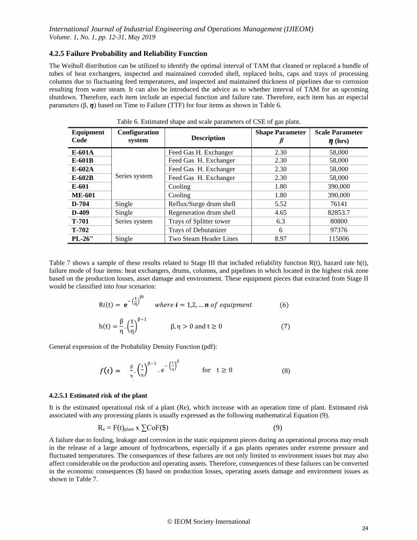
4.2.5 Failure Probability and Reliability Function The Weibull distribution can be utilized to identify the optimal interval of TAM that cleaned or replaced a bundle of tubes of heat exchangers, inspected and maintained corroded shell, replaced bolts, caps and trays of processing columns due to fluctuating feed temperatures, and inspected and maintained thickness of pipelines due to corrosion resulting from water steam. It can also be introduced the advice as to whether interval of TAM for an upcoming shutdown. Therefore, each item include an especial function and failure rate. Therefore, each item has an especial parameters (β, 𝞰𝞰) based on Time to Failure (TTF) for four items as shown in Table 6.

Table 6. Estimated shape and scale parameters of CSE of gas plant.

Table 7 shows a sample of these results related to Stage III that included reliability function R(t), hazard rate h(t), failure mode of four items: heat exchangers, drums, columns, and pipelines in which located in the highest risk zone based on the production losses, asset damage and environment. These equipment pieces that extracted from Stage II would be classified into four scenarios:

R𝑖𝑖(t) = 𝐞𝐞− �tη�βi

𝑤𝑤ℎ𝑒𝑒𝑒𝑒𝑒𝑒 𝒊𝒊 = 1,2, …𝒏𝒏 𝑜𝑜𝑜𝑜 𝑒𝑒𝑒𝑒𝑒𝑒𝑖𝑖𝑒𝑒𝑒𝑒𝑒𝑒𝑒𝑒𝑒𝑒 (6)

h(t) =βη

. �tη�β−1

β,η > 0 and t ≥ 0 (7)

General expression of the Probability Density Function (pdf):

𝑜𝑜(𝑒𝑒) = β

η. �

t

η�β−1

. e− � t

η�β

for t ≥ 0

(8)

4.2.5.1 Estimated risk of the plant

It is the estimated operational risk of a plant (Re), which increase with an operation time of plant. Estimated risk associated with any processing plants is usually expressed as the following mathematical Equation (9).

Re = F(t)plant x ∑CoF($) (9) A failure due to fouling, leakage and corrosion in the static equipment pieces during an operational process may result in the release of a large amount of hydrocarbons, especially if a gas plants operates under extreme pressure and fluctuated temperatures. The consequences of these failures are not only limited to environment issues but may also affect considerable on the production and operating assets. Therefore, consequences of these failures can be converted in the economic consequences ($) based on production losses, operating assets damage and environment issues as shown in Table 7.

Equipment Code

Configuration system Description

Shape Parameter β

Scale Parameter 𝞰𝞰 (hrs)

E-601A Series system

Feed Gas H. Exchanger 2.30 58,000 E-601B Feed Gas H. Exchanger 2.30 58,000 E-602A Feed Gas H. Exchanger 2.30 58,000 E-602B Feed Gas H. Exchanger 2.30 58,000 E-601 Cooling 1.80 390,000 ME-601 Cooling 1.80 390,000 D-704 Single Reflux/Surge drum shell 5.52 76141 D-409 Single Regeneration drum shell 4.65 82853.7 T-701 Series system Trays of Splitter tower 6.3 80800 T-702 Trays of Debutanizer 6 97376 PL-26" Single Two Steam Header Lines 8.97 115006

24



Table 7: Economic consequences of failures

Critical Equipment Production Losses ($)

Operating Assets ($)

Environment Issues ($)

Sum CoF ($)

Heat exchangers 16,047,000 11,479,768 1,105,499 28,632,268

Drum-704 10,698,000 51,067,767 3,703,000 65,468,767

Drums-409 1,248,1000 55,048,950 4,025,690 71,555,640 Processing columns 2,852,8000 35,070,000 2,460,000 66,058,000 Pipelines 5,349,000 85,185,300 5,807,915 96,342,215

In order to estimate risk plant should be taken acceptable risk into consideration to compare with estimating risk according to Equation (9) that subjects to the following constraint:

Re ≤ Riskacceptable

In general, acceptable risk varies from a company to another due to operating conditions and economic aspects. Based on the economic aspects, each processing company has its own tolerable risk criteria can be used in the estimation of TAM scheduling associated RBI (API 581, 2008).

Table 8. R(t), h(t), and f(t) scenarios of results of CSEs

CSE Scenarios

TAM interval R(t) PoF h(t) FM Re ($)

1st Scenario of six heat exchangers

(series system)

23,000 hr 0.620 0.379 4.901E-05 2.9594E-05 471.97 24000 hr 0.591 0.408 5.174E-05 2.9781E-05 487.73 24,700 hr 0.570 0.429 5.257E-05 2.9824E-05 498.10 24,800 hr 0.567 0.432 5.284E-05 2.9825E-05 499.53 24,900 hr 0.564 0.435 5.312E-05 2.9824E-05 500.96 25,000 hr 0.561 0.438 5.450E-05 2.9821E-05 502.37 30,000 hr 0.415 0.584 7.323E-05 2.7979E-05 557.83

2nd Scenario of D-704

70,000 hr 0.533 0.466 4.957E-05 2.6781E-05 436.47 72,000 hr 0.479 0.520 5.630E-05 2.7107E-05 473.02 73,000 hr 0.452 0.547 5.992E-05 2.713E-05 490.83 73,500 hr 0.439 0.560 6.180E-05 2.714E-05 499.57 73,600 hr 0.436 0.563 6.218E-05 2.712E-05 501.31 74,000 hr 0.425 0.574 6.372E-05 2.698E-05 508.20 75,000 hr 0.398 0.601 6.771E-05 2.671E-05 525.05

3rd Scenario of trays of T-701&T-

702

70,000 hr 0.581 0.418 4.829E-05 2.8099E-05 394.56 72,000 hr 0.524 0.475 5.598E-05 2.9354E-05 436.38 75,000 hr 0.434 0.565 6.935E-05 3.01509E-05 497.86 75,100 hr 0.431 0.568 6.984E-05 3.01519E-05 499.85 75,150 hr 0.430 0.569 7.008E-05 3.01517E-05 500.84 80,000 hr 0.287 0.712 9.731E-05 2.79788E-05 588.31 100,000 0.006 0.993 0.0003140 2.06347E-06 656.24

4th Scenario of PL-26"

113,000 0.425 0.574 6.778E-05 2.8859E-05 489.62 113,100 0.422 0.577 6.826E-05 2.8866E-05 491.65 113,200 0.419 0.580 6.87E-05 2.8871E-05 493.67 113,300 0.417 0.582 6.923E-05 2.8875E-05 495.69 113,500 0.411 0.588 7.0217E-

2.8879E-05 499.72

113,600 0.408 0.591 7.0712E-

2.8878E-05 501.73 114,000 0.396 0.603 7.2721E-

2.8858E-05 509.73

25



An acceptable risk criterion for SOC is assumed to be equal or lower than 500$/h. Any criterion higher than this, the risk is considered unacceptable.

Re (S) = F(t)HE x ∑ [PL($) + OA($) + EI($)]

Re (S) = [1 – R(t)HE] x [$16,047,000 + $11,479,768 + $1,105,499]

Re (S) = 0.432 x $28,632,268 = 499.5$/hr

The operational risk of each critical equipment was determined based on Probability of Failure (PoF) and economic consequences as shown in Table 8. Consequently, the optimum TAM interval of heat exchangers, drums, processing columns and pipelines were found as followed: 24800 hr, 73500 hr, 75100 and 113500 hr, respectively when compared operational risk for each equipment to an acceptable risk (500 $/hr).

On the other hand, based on shape and scale parameters as shown in Table 6. It is normal that, reliability function usually decreases gradually with TAM interval for all equipment pieces that operated continuously, especially in oil and gas industries. Hazard rate also increases continuously with TAM interval for all equipment pieces. Although, a decrease of reliability and increase of hazard rate, the failure mode would also be increased with TAM interval to reach a peak 0.00003, 0.000027, 0.00003, and 0.000029 at 24800, 73500, 75100, and 113500 hrs for heat exchanger, drum, column, and pipeline and to become R(t) 57%, 44%, 43% and 41%, and h(t) 5 failures, 6 failures, 7 failures, and 7 failures per 105 hours, respectively. A peak point is an indicator to address issues associated with these equipment pieces. When R(t) and h(t) reach to these values, this means that, it is prudent to make decision to select an optimum TAM interval of the plant among the following critical times: 24800, 73500, 75100, and 113500 hrs of heat exchangers, drums, columns, and pipelines, respectively.

Table 9 shows the current availability of gas plant and the suggested availability for duration and interval of TAM. As can be seen from this table that an increase in the TAM interval from 2 years to 2 years and 10 months and decrease in the TAM duration from 30 days to 21 days would result in the increased availability from 95.89% to 98%. In addition, the processing cost of TAM could also be reduced during the TAM event when compared to previous and current TAMs. Therefore, the gas plant must be completely shut downed at 24800 operational hours to greatly reduce the TAM costs and production losses avoid any threats may cause in the production losses, damage of company asset and environment. Consequently, these Stages II and III have illustrated great optimizations in the interval of TAM for static equipment.

Table 9. Gas plant availability

Year Duration

Interval

Availability (A) Status Downtime

(day) Uptime

(Yr.) 1960 30 1 OM 2000 30 1 91.78% Previous 2001 30 1 91.78% Previous 2002 30 1 91.78% Previous 2004 30 2 95.89% Previous 2006 45 2 93.84% Previous 2008 30 2 95.89% Previous 2010 30 2 95.89% Current

Suggested 21 2.10 98% Target Year = 365 days OM: Original Manufacturer

26



Figure 10. R(t), h(t) and FM of heat exchanger, drums and columns

27



Since the interval of TAM is equivalent the plant uptime, therefore, the optimum TAM interval of the gas plant is the period that represents the lowest period to avoid an unexpected shutdown and risks consequences due to deterioration in the critical pieces of equipment between TAM cycles caused by fluctuating temperatures and overpressures. 24800 operational hour of heat exchangers is the optimum TAM interval of gas plants when compared to other pieces of equipment. Consequently, the gas plant facilities must be totally shut downed during this the time to execute the TAM event based on 6 pieces of heat exchangers due to cumulated fouling layers through tubes of heat exchangers that could be caused in the detraction of the flow of fluid, an increase in the pressure drop, change in heat transfer during the operating process, increase in overall heat transfer coefficient loss, increase in electrical consumption and high vibrations throughout the bundle.

Table 10. Optimal interval of TAM of the gas plant 2nd Stage

Risk Category Heat Exch. Drums

Columns Piping Total equipment 18 32 16 35

V. Low 2 12 0 12 Low 6 9 7 20

Moderate 4 9 7 1 High 6 2 2 2

V. High 0 0 0 0

Major equipment ⑥ Series

② Separated

② Series

② An item

Main Causes Fouling Shell

corrosion

Trays, Caps, bolts

Wall corrosion

3rd Stage

Scenarios 1st Scenario 2nd Scenario

3rd Scenario 4th Scenario

R(t) 0.57 0.44/0.49 0.43 0.41 h(t) 0.00005 6/5E-5 0.00007 0.00007 MF 0.00003 2.7/2E-5 0.00003 0.000029

TAM Interval (hr) 24800 73500

75100 113500 Optimum Interval [minimum time] = 24800 hrs ( 2 years and 9 months)

5. Summary and Conclusions The purpose of the paper was to develop the TAM model to optimize scheduling the TAM at gas plants. The TAM model included three stages:

• 120 and 65 of 186 and 91 vessels and pipelines were removed, respectively from TAM worklist to proactive maintenance plan.

• 66 vessels and 35 pipelines were assessed based on RBI and risk matrix approach. • Then Weibull distribution model was applied on six pieces of heat exchangers, two drums, two of process

columns, and two 26"- steam water lines, which represented the highest risk on the plant performance to determine optimum interval of the TAM in order to improve reliability productivity, and availability of the plant.

The frequency of scheduling TAM during a fixed period and constantly, means that there are two concerns: - The plant will undergo a fixed duration to conduct TAM activities, every a fixed TAM cycle. This is an

indicator to operational risk. - The estimation of TAM budget will also be a fixed during duration of TAM. This means that TAM activities

be always similar to the pervious events of TAM without taking critical equipment into account.

These concerns can drive to a high cost due to plant shutdown for a long time and TAM cost, or unscheduled outage occur between cycles of TAM due to an unplanned TAM interval in which can effect on the functional performance

28



of the plant. Therefore, application of the TAM model is considered a vital to address these concerns in order to improve outage planning, minimize TAM costs, avoid unanticipated consequences of failure between TAM intervals, and insure operation of the plant more safely and effectively. The results of the developing TAM model in the gas plant illustrated that scheduling TAM could be optimized without any threats on the plant performance due to decreasing duration and increasing interval of TAM.

Analysis showed that the TAM duration of the gas plant could be decreased from 30 to 21 days with reduced in the budget of TAM to less $2 million rather than $2.5 million, and interval of TAM could be prolonged from 2 years to 2 years and 10 months, without any threats of fouling layers that accumulated through tubes of heat exchangers. Availability could also be improved to 98% rather than 95.89%, which supports the TAM optimization in the gas plant. Consequently, TAM is not only necessary for minimizing the risk of failures resulting from rigorous operating conditions, but is also essential to improve productivity and increasing availability of the plant.

References Afefy, I, Reliability-Centered Maintenance Methodology and Application: A Case Study, Engineering, 2(11), pp. 863-

873, 2010. Ahmed, Q., Moghaddam, K., Raza, S. and Khan, F, A multi-constrained maintenance scheduling optimization model

for a hydrocarbon processing facility, J Risk and Reliability, pp.1-18, 2015. Akbar, J. and Ghazali, Z, Plant turnaround maintenance leading and plant turnaround maintenance performance

in Malaysian process based industry: The mediating role of team alignment, Global Business and Management Research, 9(1), pp.85-101, 2017.

Rajagopalan, S., Sahinidis, N., Amaran, S., Agarwal, A. and Wassick, J, ‘Risk analysis of turnaround reschedule planning in integrated chemical sites', Computers and Chemical Engineering, no. of pages14, 2017.

Brown, V, Shutdowns, Turnarounds, or Outages, Audel managing shutdowns, Turnarounds, and Outages. Chapter 6, France: Lavoisier, 2004.

Duffuaa, S., Raouf, A. and Campbell, D, Planning and Control of Maintenance System: Modeling and Analysis, New York, John Wiley & Sons, 1999.

Duffuaa, S. and Ben Daya, M, Turnaround maintenance in petrochemical industry: practices and suggested improvements. Journal of Quality Maintenance Engineering, 2004.

Dyke, S, Optimizing plant turnarounds. Petroleum Technology Quarterly, 2, pp. 145-151, 2004. Elfeituri, F. and Elemnifi, S, Optimising turnaround maintenance performance' the eighth pan-pacific conference on

occupational ergonomics Bangkok, Thailand, 2007. Elwerfalli, A., Khan, M. and Munive, J., A, Application of the Turnaround Maintenance (TAM) Model to Gas Plants

in Case Study for Heat Exchangers, International Conference on Industrial Engineering and Operations Management, pp. 1-9, Rabat, 2017.

Ghosh, D. and Roy, S. ‘Maintenance optimization using probabilistic cost-benefit analysis’, Journal of Loss Prevention in the Process Industries, (22), pp. 403–407. 2009.

Halib, M., Ghazali, Z. and Nordin, S, Plant Turnaround Maintenance in Malaysian Petrochemical Industries: A study on Organizational size and structuring processes, 9, 2010.

Hameed, A. & Khan, F, A framework to estimate the risk-based shutdown interval for a process plant, Journal of Loss Prevention in the Process Industries, 32, pp. 18-29, 2014.

Emiris, D, Organizational context approach in the establishment of a PMO for turnaround projects, experiences from the Oil & Gas industry, PM World Journal, 3(2), pp. 1-15, 2014.

Keshavarz, G., Thodi, P. and Khan, F. ‘Risk based shutdown management of LNG units’, J Loss Prev Process Ind, 25, pp.159–165, 2011.

Khan, F., Haddara, M. and Krishnasamy, L, A New methodology for risk-based availability analysis, transactions on reliability, 57 (1), pp.103-112 2008.

Krings, D, Proactive Approach to shutdowns Reduces Potlatch Maintenance costs. A maintenance planning and scheduling article focusing on management of shutdowns, 2001.

Krishnasamy, L., Khan, F. and Haddara, M, Development of a risk-based maintenance (RBM) strategy for a power-generating plant. Journal of Loss Prevention in the Process Industries, 18, pp.69–81, 2005.

Kumar, U, Maintenance strategies for mechanized and automated mining systems: a reliability and risk analysis based approach, Journal of Mines, Metals and Fuels, Annual review, pp.343–347, 1998.

Lawrence, G, Cost Estimating for Turnarounds, Petroleum Technology quarterly Q1, 2012.

29

http://bradford.summon.serialssolutions.com/2.0.0/link/0/eLvHCXMwzV1Lj9MwELbYPSA4IN4sDyknDkRZkth1bGlZKUKglcoF1D1HfkXtks1W25Yj4qcz49hJiwRnbrUjJZU_Zzwzme8bQmh5mmd_2AQtpWJCczlrhVEtdUrAOSFnzAhOS4Pk5Pk38bXmCyT1j50S8esuBI028Kr-lXD7L6Gu0zaWWKEriboZ4Ie6oXpwtfme4VFl081yt7UQdHuJiNsfA3MxVel64Ap4Wnqn-oNk_Z6_-gWO0zQqPk0FkoFpkMYeIFNNYq3trksv4J8FApXXfFxt4HbzZdiUId9QsEC8G5NgkQgTbc9UfTRkFfMMPLR838CGBOZgIYO1PdS4pjNaUiakKN6i4vm1XZntB9dnl_MjcgQBF9ip059j6U5R5b7x4fiwQ5_i8Ej1fsLiIXkQFiypB5gekTuuf0zu78k-PiG_6uRMn4-Ynb3X58n2BucidMPU0uEcIojjDH57IP1FGEQ84zjC6scAbaJwdkLXz3uEn5LLz58WHy-y0AkjM-Bu0oxLZssWnGMKL0-rIYbFzsXgKs44hfBI68oYxsuq0NzpiklbtKUTYK61rVpVGPqMHPc3vXtBEkq1MrwwZUEV46xAcR6hULRJaatleULexbVs1oPgSRMrAa-aq27d4KZocixbkCfkeVztxnZdM-H48q9XXpF707Z6TY63tzv3htzF1xzpHL8BijlVvA



Lenahan, T, Turnaround Shutdown and Outage Management, Effective planning and step-by-step execution of planned maintenance operations, Butterworth Heinemann, 2006.

Levitt, J, Managing Maintenance Shutdowns and Outages, Industrial, Press, New York, 2004. McLay, A, Practical Management for Plant Turnarounds, 2003. Megow, N., Möhring, H. and Schulz, J, Decision support and optimization in shutdown and turnaround scheduling,

INFORMS Journal on Computing, 23(2), pp. 189-204, 2011. Neikirk, D, Turnaround/Shutdown Optimization Plan for the 5 phases of a Plant Maintenance Shutdown, Published

in Plant Services, pp. 1-5, 2011. Obiajunwa, C. 'A framework for the evaluation of turnaround maintenance projects'. Journal of Quality in

Maintenance Engineering, 18(4), pp.368-383, 2012. Oliver, R, Complete planning for maintenance turnarounds will ensure Successes. Oil & Gas Journal, Meridium, Inc,

2002. Rajagopalan, S., Sahinidis, N., Amaran, S., Agarwal, A. and Wassick, J. 'Risk analysis of turnaround reschedule

planning in integrated chemical sites', Computers and Chemical Engineering, no. of pages14, 2017. Rusin, A. and Wojaczek, A, Optimization of power machines maintenance intervals taking the risk into consideration.

Eksploatacjai Niezawodnosc, e-Maintenance and Reliability, 14(1), pp.72-76, 2012. Shuai J., Han K. and Xu X. (2012) ‘Risk-based inspection for large-scale crude oil tanks’, Journal of Loss Prevention

in the Process Industries, 25, pp.166-175. Schroeder, B. and Vichich, R. (2009) Trade-off economics in plant turnarounds, NPRA Reliability and Maintenance

Conference and Exhibition, pp. 94-103. Swart, P, An Asset Investment Decision Framework to Prioritise Shutdown Maintenance Tasks, MSc thesis,

University of Stellenbosch, 2015. Tam, B., Chan, M. and Price, H, A generic maintenance optimisation framework, Proceedings of the 7th Asia Pacific

Industrial Engineering and Management Systems Conference, Bangkok, Thailand, 2006b. Utne, I., Thuestad L., Finbak, K. and Thorstensen, T, Shutdown preparedness in oil and gas production, Journal of

Quality in Maintenance Engineering, 18 (2), pp. 154-170, 2012. Vishnu, C. and Regikumar, V, Reliability Based Maintenance Strategy Selection in Process Plants: A Case Study,

Procedia Technology, 25, pp.1080 – 1087, 2016.

Acronyms and abbreviations A Availability P Effect of equipment downtime on the FM Failure mode S Effect of equipment downtime on the safety h(t) Hazard rate Re Estimated risk of system R(t) Reliability function CE Critical Equipment F(t) Unreliability function Rc Risk criteria β Shape parameter TAM Turnaround Maintenance η Scale parameter PL Production Losses MTBF Mean Time Between Failures AD Asset Damage MTTF Mean Time To Failure ED Environment Damage MTTR Mean Time To Repair SoW Scope of Work RBD Reliability Block Diagram NE Non-critical Equipment PoF Probability of Failure NRE Non-critical Rotating Equipment CoF Consequences of Failure NSE Non-critical Static Equipment RBI Risk-Based Inspection CRE Critical Rotating Equipment RBD Reliability Block Diagram CSE Critical Static Equipment TTF Time to failure

30



Biographies Mr. A. Elwerfalli received his MSc degree in Quality assurance from the University of Teesside, United Kingdom in 2003. He is currently a PhD candidate in the Automotive Research Centre at University of Bradford. He has worked as a head of engineers in Maintenance Engineering Division (MED) at Sirte Oil Company, Libya, since 1997. His research interests include optimizing turnaround maintenance scheduling to oil and gas plants. Professor M. Khurshid Khan received his BEng, PhD and MBA degrees from the University of Bradford in 1983, 1987 and 1997, respectively. His PhD area of research was experimental and theoretical study of air turbulence. During 1987 to 1990, he worked for Pepsi-Cola International as a Technical Services Manager in the Middle East, Far East and Africa Regions. In 1990, he joined the School of Engineering, University of Bradford, where he is currently a Professor of Manufacturing Systems Engineering. His research interests are in the area of Artificial Intelligence (AI)/Knowledge-Based Systems and their applications to Manufacturing & Quality Systems, Strategy, Planning, Control, Scheduling, and Supply Chain Management. Dr. J. Eduardo Munive-Hernandez is a Lecturer in Advanced Manufacturing Engineering at the Faculty of Engineering and Informatics, University of Bradford. He received his Ph. D in Total Technology from the University of Manchester Institute of Science and Technology in 2003. His major research interests include the analysis, development and implementation of knowledge management initiatives to support strategic management decisions in the context of manufacturing organizations, their supply chains and other operational functions, including SMEs.

31

Documents

Developing Turnaround Maintenance (TAM) Model to …operating conditions and the residual life of critical equipment of plants to carry out the major activities: inspection and maintenance