Embed Size (px)
Citation preview

Development and Analysis of an Algorithm forthe Linear Transport Equation
Abhigyan Ghosh
November 14, 2013
1

This work is dedicated to my mentor R. Massjung, without whose help I wouldnot have been able to write this paper.

Abhigyan Ghosh 3
AbstractIn my Extended Essay I will deal with a particular partial differential
equation called the linear transport equation. This differential equation isvery important in modeling the behavior of fluids using computer simula-tions. The exact solution of the differential equation is often not possibleto calculate and thus an approximation has to be made by an algorithm.My Extended Essay will deal with the question: How does such an algo-rithm work, what are the requirements for such an algorithm and to whatextent can I improve the algorithm. My scope will be the analysis of twoalgorithms, one using piecewise constant functions as an approximationand the other one using piecewise linear functions, whereupon I will tryto develop an improved version of the algorithm. My algorithm will makeuse of piecewise quadratic functions, while keeping the additional require-ments of such an algorithm in mind. After writing the algorithm I willcompare the three different algorithms. I will show that the algorithmusing piecewise linear functions is significantly better than the one us-ing piecewise constant functions. My algorithm using piecewise quadraticfunctions works just as well as the one using piecewise linear functions.That means that I succeeded in developing an algorithm using piecewisequadratic functions while considering the additional requirements, but thealgorithm has not augmented the quality of the results.
Abhigyan Ghosh 4
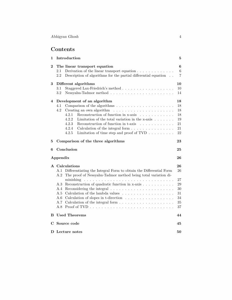
Contents1 Introduction 5
2 The linear transport equation 62.1 Derivation of the linear transport equation . . . . . . . . . . . . . 62.2 Description of algorithms for the partial differential equation . . 7
3 Different algorithms 103.1 Staggered Lax-Friedrich’s method . . . . . . . . . . . . . . . . . . 103.2 Nessyahu-Tadmor method . . . . . . . . . . . . . . . . . . . . . . 14
4 Development of an algorithm 184.1 Comparison of the algorithms . . . . . . . . . . . . . . . . . . . . 184.2 Creating an own algorithm . . . . . . . . . . . . . . . . . . . . . 18
4.2.1 Reconstruction of function in x-axis . . . . . . . . . . . . 184.2.2 Limitation of the total variation in the x-axis . . . . . . . 194.2.3 Reconstruction of function in t-axis . . . . . . . . . . . . 214.2.4 Calculation of the integral form . . . . . . . . . . . . . . . 214.2.5 Limitation of time step and proof of TVD . . . . . . . . . 22
5 Comparison of the three algorithms 23
6 Conclusion 25
Appendix 26
A Calculations 26A.1 Differentiating the Integral Form to obtain the Differential Form 26A.2 The proof of Nessyahu-Tadmor method being total variation di-
minishing . . . . . . . . . . . . . . . . . . . . . . . . . . . . . . . 27A.3 Reconstruction of quadratic function in x-axis . . . . . . . . . . . 29A.4 Reconsidering the integral . . . . . . . . . . . . . . . . . . . . . . 30A.5 Calculation of the lambda values . . . . . . . . . . . . . . . . . . 31A.6 Calculation of slopes in t-direction . . . . . . . . . . . . . . . . . 34A.7 Calculation of the integral form . . . . . . . . . . . . . . . . . . . 35A.8 Proof of TVD . . . . . . . . . . . . . . . . . . . . . . . . . . . . . 37
B Used Theorems 44
C Source code 45
D Lecture notes 50

Abhigyan Ghosh 5
1 IntroductionMy Extended Essay will deal with the linear transport equation which is a par-tial differential equation describing the transport and preservation of a quantitysuch as fluids. Computational methods are used to simulate such fluid flows.In my essay I will look at two algorithms for the simulation. My question is:How does such an algorithm work, what are the requirements for such an al-gorithm and to what extent can I improve the algorithm. The improvement ofalgorithms saves resources, which is why it is of great significance.
Throughout this essay I will mainly be relying on the works of Randall J.LeVeque [1], Nessyahu-Tadmor [3] and Ralf Massjung [2] (see Appendix D).
Due to the nature of my subject I expect my reader to have a knowledge ofintegration and differentiation.

Abhigyan Ghosh 6
2 The linear transport equation2.1 Derivation of the linear transport equationThe linear transport equation is the following time-based partial differentialequation
∂u
∂t+ a · ∂u
∂x= 0 (1)
where u is a function of x and time t. In this section we will see how thisequation is derived. Usually partial differential equations (PDE) are gainedfrom physical phenomena, so I will demonstrate the PDE with the aid of aphysical example. Imagine a cylindrical glass tube filled with gas. The valueof x ∈ [x1, x2] describes a certain position in the tube, with x1 and x2 beingthe endpoints of the tube. If we look at a time t0, then the function ρ(x, t0)describes the density of the gas at a certain position x. We get the mass of thegas in the tube by integrating.
m =∫ x2
x1
ρ(x, t0)dx (2)
The amount of gas in the tube can only change if a certain amount goes out ofthe tube or a certain amount comes in through the endpoints. For this exampleI will say that a constant amount of gas comes into the tube at x1 with thevelocity v1 and leaves the tube at x2 with the velocity v2. Starting from thetime t0 if we want to find out how much more gas there is in the tube at time t1,we have to integrate at x1 and x2 and consider the difference. Note that eventhough the incoming or outgoing gas has a constant velocity, the density of itmight not be constant, which is why we have to consider the density functionρ(x, t) when integrating.
change in mass from time t0 to t1 =∫ t1
t0
v1 · ρ(x1, t)dt︸ ︷︷ ︸gas coming in at x1
−∫ t1
t0
v2 · ρ(x2, t)dt︸ ︷︷ ︸gas going out at x2
(3)If we want to know how much mass there is at time t1 we can add the changein mass during the time period to the original amount of gas in the tube. Thisgives us an equation involving only integrals called the integral form.∫ x2
x1
ρ(x, t1)dx︸ ︷︷ ︸mass at time t1
=∫ x2
x1
ρ(x, t0)dx︸ ︷︷ ︸mass at time t0
+∫ t1
t0
v1 · ρ(x1, t)dt−∫ t1
t0
v2 · ρ(x2, t)dt︸ ︷︷ ︸change in mass from time t0 to t1
(4)
In this example I set the velocity to be constant. But this might not always bethe case. Generally the velocity can be described as a function of the density,thus we can rewrite v · ρ = v(ρ) · ρ = f(ρ). The integral form becomes∫ x2
x1
ρ(x, t1)dx =∫ x2
x1
ρ(x, t0)dx+∫ t1
t0
f(ρ(x1, t))dt−∫ t1
t0
f(ρ(x2, t))dt. (5)

Abhigyan Ghosh 7
If we look at any interval I ⊂ [x1, x2], we can assert that the integral form holdsfor that interval too, since the mass at t1 is the mass at t0 plus the change inmass during the time period. Similarly we can extend our glass tube definition,and say that if the glass tube is in R, then for any interval I ⊂ R the integralform holds. This equation is of fundamental importance, since it preservesthe given quantity, in this case the mass. This means that the mass in Rstays constant.
Since the integral form does not give us enough information, we can dif-ferentiate it to get the following differential equation (see Appendix A.1 forcalculations).
∂ρ
∂t+ ∂
∂xf(ρ) = 0 (6)
This form is called the differential form. This equation is very useful, sincefor every point (x, t) one can calculate the derivative in t-direction if one hasthe derivative in x−direction.
From this point on I will use a simpler notation for partial derivatives, namely∂ρ∂t = ρt. Thus the differential form can be rewritten as
ρt + f(ρ)x = 0 (7)
The linear transport equation is a special case of this partial differential equa-tion, namely when f(ρ) = a · ρ. Beginning from the next section I will use thefunction u instead of ρ. Rewriting the integral form and generalizing it for anyinterval [xi, xi+1] and time tn yields∫ xi+1
xi
u(x, tn)dx =∫ xi+1
xi
u(x, tn)dx+∫ tn+1
tn
a·u(xi, t)dt−∫ tn+1
tn
a·u(xi+1, t)dt.
(8)For futher reading refer to LeVeque [1].
2.2 Description of algorithms for the partial differentialequation
Now that we know the equation, we will look at the problem. If we get a startingstate u(x, t0) and a function f(u) which describes the velocity of each point inthe x-axis, how will the function u develop?Since it is often not possible to calculate the exact solution of this problem,an algorithm is used to approximate the solution. For that we first divide thex-axis with the function u(x, t0) into several segments or cells Ωi, all havingthe width ∆x. Then we calculate the intermediate values ui of this segments,so that ui · ∆x =
∫Ωiu(x, t0)dx (see Figure 1). It is easier to calculate with
these ui-values than with the function as a whole. In the algorithm we have tocompute how these ui-values develop. For that we set a time step ∆t and lookhow the values in a cell Ωi have progressed during that time.
Note that this means that the ui-values will change over time and thus re-quire an index of time. For simplicity this index will be omitted and ui will

Abhigyan Ghosh 8
(a) Original function u(x, t0) (b) Intermediate values ui
Figure 1: Distribution of ui-values
signify the value at the current time step. Where it is important to distinguishI will write uni to be the intermediate value of u on the cell Ωi at time tn.
For my essay I will use the simple function f(u) = a · u. The benefit of thefunction becomes evident once we think about its implications. Any value uiwill be transported with the velocity a to the right. This means that the func-tion u(x, t0) as a whole will be shifted to the right as the time progresses. If wedefine the starting state as u(x, t0) = u0(x), the solution of the PDE would beu(x, t) = u0(x− at). We can easily verify this by putting this function into thedifferential form. By using the chain rule we get
∂
∂tu0(x− at) + a
∂
∂xu0(x− at)
= u′0(x− at) · (−a) + a · u′0(x− at) · 1= (−a+ a) · u′0(x− at)= 0. (9)
Thus the benefit of this simple function f is that we know the exact solution.If we write an algorithm we can test it by comparing its results to the exactsolution.
The study of simple cases such as this is often used in mathematical practiceto gain insight about the problem and afterwards apply the knowledge to morecomplex versions of the problem.
A difficulty that we will face is that we only can calculate in a finite area.We can not calculate all the ui values from −∞ to ∞. Due to this we willdefine an interval where we will compute our ui values and we will set up someconditions for the boundaries. I will say that left and right of the boundary thefunction value will be constant, namely cl and cr. If our interval is [xl, xr] then

Abhigyan Ghosh 9
Figure 2: Algorithm with oscillations Figure 3: The TVD of the sine function
that means the function u will be defined as follows:
u =
cl if x < xl
u(x, t) if x ∈ [xl, xr]cr if x > xr
(10)
Since the transport of the quantity u has a certain known limited velocity, inour case a, we know how far the ui-values will have been transported at most ina given time frame. Thus even after a given time we can say in which intervalthe significant ui-values are located.
There is an additional condition that the algorithm has to fulfill. If analgorithm produces unrealistic results, that is if the function values get negativeor if some values form unnatural peaks, then the validity of the solution willbe impaired (see Figure 2). With time the algorithm will start to producemore and more unrealistic values and it will start to oscillate. But since thisis against our interests the question is how can we supress such an oscillation.To do this we define the Total Variation of our function u at time tn to beTV(un) =
∑i |ui+1−ui|. This sum describes the distance between the different
ui-values in the u-axis, and if we sum it up it describes the distance between theextrema of the function. For example the total variation of the sine functionin the interval [0, 2π] is 4 (see Figure 3). The sum of the total variation istaken over all the i-values from −∞ to ∞. However since the function becomesconstant beyond the boundary, there only exists a finite amount of positivesummands, so we can limit ourselves to the sum of all the |ui+1−ui| within theboundary.
To avoid oscillations this total variation must not increase in the next timestep. Thus if we take the next time step to be tn+1, then the following musthold:
TV(un+1) ≤ TV(un) (11)
If we can find such an algorithm, then we say the algorithm is total variation

Abhigyan Ghosh 10
Figure 4: The cells Ωi and Ωi+1
diminishing (TVD).
Summing up an algorithm needs to preserve the quantity and it needs to beTVD.
3 Different algorithmsThe following two algorithms have a similar method to calculate the new ui-values. I will first look at the simpler algorithm.
3.1 Staggered Lax-Friedrich’s methodThis algorithm uses piecewise constant functions to approximate the valuesin the integral form (8). With the time step ∆t = tn+1 − tn one calculates theLHS, namely the integral at time tn+1.∫ xi+1
xi
u(x, tn+1)dx =∫ xi+1
xi
u(x, tn)dx︸ ︷︷ ︸approximation using
xi-values
+∫ tn+1
tn
a · u(xi, t)dt−∫ tn+1
tn
a · u(xi+1, t)dt︸ ︷︷ ︸approximation using xi-values
and the differential form of the equation(12)
To describe the algorithm we will look at two neighboring cells Ωi and Ωi+1.These two cells have the intermediate values ui and ui+1 (see Figure 4). Wewill approximate the integrals in the integral form (12) to find the ui-values inthe next time step. First we can calculate the integral from xi to xi+1.∫ xi+1
xi
u(x, tn)dx = ui + ui+1
2 ·∆x (13)

Abhigyan Ghosh 11
On the LHS of (12) we will get an integral for the time tn+1. As before we willdescribe this integral as∫ xi+1
xi
u(x, tn+1)dx = un+1i+ 1
2·∆x (14)
where un+1i+ 1
2describes the intermediate value at time tn+1 in the cell Ωi+ 1
2. Note
that in a time step the cells get shifted by ∆x2 , but that does not constitute
a problem since after two steps the cells are back in their original positions.Plugging in the integrals (13) and (14) in (12) yields
un+1i+ 1
2·∆x = ui + ui+1
2 ·∆x+∫ tn+1
tn
a · u(xi, t)dt−∫ tn+1
tn
a · u(xi+1, t)dt. (15)
Since we assumed that the value of u is constant on the cell Ωi, we will likewiseassume that the value of u is constant along the t-axis. So u(xi, t) = ui. Thismeans that ∫ tn+1
tn
a · u(xi, t)dt = a ·∫ tn+1
tn
u(xi, t)︸ ︷︷ ︸is constant
dt
= a ·∫ tn+1
tn
uidt
= a · ui ·∆t. (16)
Analogously ∫ tn+1
tn
a · u(xi+1, t)dt = a · ui+1 ·∆t. (17)
Again plugging it into the integral form (15) yields
un+1i+ 1
2·∆x = ui + ui+1
2 ·∆x+ a · ui ·∆t− a · ui+1 ·∆t (18)
Solving for un+1i+ 1
2gives us
un+1i+ 1
2= ui + ui+1
2 + a · ∆t∆x (ui − ui+1). (19)
Now that we have an expression for un+1i+ 1
2, the intermediate value in the next
time step, the only remaining question is whether it fulfills the TVD-property(11). We will adjust the time step ∆t so that the algorithm becomes TVD. Forthat we have to look at figure 5.
In (a) we see how the cell is at time tn. At the point xi+1/2 there is adiscontinuity (compare with Figure 4). We can continue calculating as long asthis discontinuity does not pass over to the next cell (b). If that were the case

Abhigyan Ghosh 12
(a) at time tn (b) at time tn+1
Figure 5: The cell grid from above
it could be that more quantity would go out of the cell than come in, resultingin negative values. But since we want to avoid that, we have to limit the timestep. That means we have to see how long it takes for the point xi+ 1
2to cross
the border of the cell at xi+1, that is we have to see how long it takes for thepoint to travel the distance of ∆x
2 . This is easily calculated since we know thevelocity to be a. Hence our time step can be at most
∆t ≤ ∆x2a (20)
This inequality is often expressed with a κ which limits the time step. Due tothe TVD-condition the time step is often restricted further. In the case of thepiecewise constant method with the function f(u) = a · u, the time steplimitation is
∆t = κ∆x2a with k ≤ 1. (21)
The only thing remaining to show in this algorithm is that it is TVD if κ ≤ 1.Therefore we have to show that TV(un+1) ≤ TV(un). Since I did not find aproof in my sources I set out to prove the following myself.
TV(un+1)
=∑i
∣∣∣un+1i+ 1
2− un+1
i− 12
∣∣∣=∑i
∣∣∣∣ui + ui+1
2 + a∆t∆x (ui − ui+1)− ui−1 + ui
2 − a∆t∆x (ui−1 − ui)
∣∣∣∣

Abhigyan Ghosh 13
Rearranging the terms ui+ui+12 and ui−1+ui
2 gives us
=∑i
∣∣∣∣ui − ui−1
2 + a∆t∆x (ui − ui−1) + ui+1 − ui
2 − a∆t∆x (ui+1 − ui)
∣∣∣∣=∑i
∣∣∣∣(ui − ui−1)(
12 + a
∆t∆x
)+ (ui+1 − ui)
(12 − a
∆t∆x
)∣∣∣∣Defining ∆ui− 1
2= ui − ui−1 and ∆ui+ 1
2= ui+1 − ui and using the inequality
|a+ b| ≤ |a|+ |b| yields
≤∑i
∣∣∣∣∆ui− 12
(12 + a
∆t∆x
) ∣∣∣∣+∣∣∣∣∆ui+ 1
2
(12 − a
∆t∆x
) ∣∣∣∣Assuming that the factors in the brackets are non-negative, we can take themout of the absolute value.
=∑i
|∆ui− 12|(
12 + a
∆t∆x
)︸ ︷︷ ︸assuming ≥0
+|∆ui+ 12|(
12 − a
∆t∆x
)︸ ︷︷ ︸assuming ≥0
If we were to write the sum out and collect all the terms with the factor ∆ui+ 12
we would see that what is left is
=∑i
|∆ui+ 12|(
12 − a
∆t∆x + 1
2 + a∆t∆x
)=∑i
|∆ui+ 12|
=∑i
|ui+1 − ui|
= TV(un). (22)
Note that this only works since we have a finite amount of positive summandsas described earlier. This means that the piecewise constant method is TVD,but only if our assumption of the factors in the bracket being larger or equal tozero is true. Thus it still remains to show that our assumption was correct. Wehave to show that
0 ≤ 12 ± a
∆t∆x (23)
or equivalently±a∆t
∆x ≤12 . (24)
If we look at our definition of ∆t (21) we can see that the following holds.
±a∆t∆x ≤
∣∣∣∣a∆t∆x
∣∣∣∣ =∣∣∣∣a · κ∆x
2a︸ ︷︷ ︸=∆t
· 1∆x
∣∣∣∣ =∣∣∣κ2 ∣∣∣ ≤ 1
2 (25)

Abhigyan Ghosh 14
(a) ui-values (b) minmod slopes
Figure 6: The reconstruction of linear functions
Thus our assumption was correct and we have proved that the piecewise constantmethod is TVD if κ ≤ 1.
3.2 Nessyahu-Tadmor methodThe following algorithm will be a bit more complex than the previous one,because instead of using piecewise constant functions it will use piecewise linearfunctions. As a first step we must reconstruct a function in the x-axis. Theonly values given are the ui values. The algorithm now reconstructs some linearfunctions on the cells Ωi (see Figure 6). To do this the algorithm uses theminmod function. It is defined the following way:
minmod(x, y) =
0 if x · y ≤ 0x if |x| ≤ |y|y if |y| < |x|
(26)
This means that whenever the input values have opposite signs, the functionvalue is 0. However, if both x and y have the same sign, then the output of thefunction will be the value closer to 0.
The linear function is constructed in such a way, that the function passesthrough ui, and the slope is the smaller one between ui−ui−1
∆x = ∆ui+1/2∆x and
ui+1−ui
∆x = ∆ui−1/2∆x . If we define the function on Ωi to be ui(x), then we construct
it the following way:
ui(x) = ui + Si∆x (x− xi) where Si = minmod(∆ui+ 1
2,∆ui− 1
2) (27)
If we insert x = xi into the function, we will get ui as a result. However sincewe only want to calculate the integral we can shift the function by xi to obtain
ui(x) = ui + Si∆xx where Si = minmod(∆ui+ 1
2,∆ui− 1
2) (28)

Abhigyan Ghosh 15
This is done so that it is easier to calculate with the values, since one does notneed to know where exactly in the x-axis the cell is located, but only that thecell boundary goes from −∆x
2 to ∆x2 . If we calculate the integral in this cell,
it still gives∫
Ωiui(x)dx = ui · ∆x. This is essential since we do not want to
increase the quantity in the cell with our reconstruction.Further it needs to be remarked that our linear reconstruction of the ui-
values does not exceed the total variation of the values before reconstruction.This is crucial since an increase in total variation renders it impossible to showthat the algorithm is total variation diminishing.
The next step would be to reconstruct the function in the t-axis. As discussedthis algorithm uses linear functions, so the reconstruction in t-direction has tobe linear too. To construct it we will use the differential equation
ut + f(u)x = 0 (29)
or rewritten
ut = −f(u)x= (−a · u)x= −a · ux. (30)
This means that the derivative or the slope in the t-axis is the slope in thex-axis multiplied by −a. Further we can assume that the function in t-axis willgo through the point ui. With this information we can construct our function.I will call the function vi.
vi(t) = ui + t · ut= ui + t · (−a) · ux
= ui − a · t ·Si∆x (31)
Note that for every function ui(x) there will be a function vi(t). This functionvi(t) is set so that for t = 0 we get ui. As in the previous algorithm, we havenow both the function along the x- and the t-axis. This means that we cancalculate its integrals and thus get the quantity at the next time step with the

Abhigyan Ghosh 16
help of the integral form (12). The integral at time tn is∫ xi+1
xi
u(x, tn)dx
=∫ xi+1/2
xi
u(x, tn)dx+∫ xi+1
xi−1/2
u(x, tn)dx
=∫ ∆x/2
0ui(x, tn)dx+
∫ 0
−∆x/2ui+1(x, tn)dx
=[ui · x+ Si
∆xx2
2
]∆x/2
0+[ui+1 · x+ Si+1
∆xx2
2
]0
−∆x/2
= ui ·∆x2 + Si
∆x∆x2
8 + ui+1 ·∆x2 − Si+1
∆x∆x2
8
= ∆x2 (ui + ui+1) + ∆x
8 (Si − Si+1) (32)
As a next step we have to evaluate the integrals at xi and xi+1 in t-direction.∫ tn+1
tn
vi(t)dt =∫ ∆t
0ui − a · t ·
Si∆xdt
=[uit− a
Si∆x
t2
2
]∆t
0
= ui∆t− aSi∆x
∆t2
2 (33)
and similarly ∫ tn+1
tn
vi+1(t)dt = ui+1∆t− aSi+1
∆x∆t2
2 . (34)
Putting it all in the integral form yields∫ xi+1
xi
u(x, tn+1)dx =∫ xi+1
xi
u(x, tn)dx+ a ·∫ tn+1
tn
vi(t)dt− a ·∫ tn+1
tn
vi+1(t)dt
= ∆x2 (ui + ui+1) + ∆x
8 (Si − Si+1)
+ a
(ui∆t− a
Si∆x
∆t2
2 − ui+1∆t− aSi+1
∆x∆t2
2
)(35)
We can rewrite the LHS of the integral form as ∆x · un+1i+1/2 to obtain
∆x · un+1i+1/2 = ∆x
2 (ui + ui+1) + ∆x8 (Si − Si+1)
+ a
(ui∆t− a
Si∆x
∆t2
2 − ui+1∆t+ aSi+1
∆x∆t2
2
)⇔ un+1
i+1/2 = ui + ui+1
2 + Si − Si+1
8 + a∆t∆x (ui − ui+1)− a2
2∆t2
∆x2 (Si − Si+1)(36)

Abhigyan Ghosh 17
Thus we now have an expression for un+1i+1/2. The only remaining thing to do
in this algorithm is to limit the time step and show that with that time stepthe algorithm is TVD. This is done in Appendix A.2. By doing so we get alimitation for our time step, namely
∆t = κ∆x2a with κ ≤
√2− 1 (37)
Refer to Nessyahu-Tadmor [3] for further reading.

Abhigyan Ghosh 18
4 Development of an algorithmNow that I have listed two algorithms, I will start to analyze and comparethem, and then try to develop an own improved version of the algorithm withthe gained knowledge.
4.1 Comparison of the algorithmsAs a first step both algorithms fit a function in the cells Ωi, one being a constantfunction, and the other being a linear one. Both reconstructions preserve thequantity in the cell. In the Nessyahu-Tadmor method this linear function isconstructed in such a way that the total variation of the reconstructed functionis not bigger than the original total variation. Also in the Lax-Friedrich methodthis holds true, but here the total variation of the reconstruction is exactly asbig as the original total variation. As a next step an approximation of thefunction is made in t-direction at the points ui. In both cases the function goesthrough the point ui, in the Lax-Friedrich method it is a constant function, inthe Nessyahu-Tadmor method it is linear. The slope of the function is calculatedusing the differential form in the second algorithm. It is noteworthy that in thefirst algorithm the differential form holds too, since it states that the slopein t-direction is the same as the slope in x-direction, namely 0. After havingreconstructed the function in x- and t-direction one can calculate the integralform. As a last step one has to show that the algorithm is TVD. To do this wehave to limit the time step. If we succeed to show that the total variation doesnot increase with a certain time step, then we have shown that the algorithmdoes not produce any oscillations. So when developing an algorithm I have toconsider the following steps:
1. Reconstruction of function in x-axis, with preservation of quantity
2. Limitation of the total variation in x-axis
3. Reconstruction of function in t-axis
4. Calculation of the integral form
5. Limit time step / Proof of TVD
4.2 Creating an own algorithmIn this section I will try to employ piecewise quadratic functions to improve thealgorithm. To do this I will follow the steps from the previous section.
4.2.1 Reconstruction of function in x-axis
First I have to think about how I want to reconstruct the piecewise quadraticfunction. The function has to be reconstructed in the cell Ωi using only thevalues ui−1, ui and ui+1. Since a quadratic function has three parameters, I

Abhigyan Ghosh 19
will have to find three conditions which our function has to fulfill. The firstof these conditions is given by the fact that the quantity in the cell has to bepreserved. This means that
∆x · ui =∫
Ωi
ui(x)dx (38)
where ui is our reconstructed quadratic function on the cell Ωi. We have to settwo more conditions for our function. We have not yet considered the valuesui−1 and ui+1. When considering these values we have to find conditions whichare symmetrical, this means that if we change the values ui−1 and ui+1, ourfunction should only be mirrored but otherwise remain unchanged. If that werenot the case we would give preference to a certain side which is to be avoided.After some consideration I came up with the condition that the slope at ∆x
2 hasto be the same as the slope ui+1−ui
∆x , and similarly the slope at −∆x2 has to be
ui−ui−1∆x . This means that the three given conditions are the following:
• ∆x · ui =∫
Ωiui(x)dx
• u′i(−∆x2 ) = ui−ui−1
∆x
• u′i(∆x2 ) = ui+1−ui
∆x
whereui(x) = q′′
2 x2 + q′x+ q (39)
with q′′, q′ and q being the parameters of the quadratic function. Note that q,q′ and q′′ are different on each cell and thus require an index. For simplicitythis index is omitted where it is not of necessity. Solving the conditions for theparameters yields (see Appendix A.3)
q = ui −ui+1 + ui−1 − 2ui
24 (40a)
q′ = ui+1 − ui−1
2∆x (40b)
q′′ = ui+1 + ui−1 − 2ui∆x2 (40c)
4.2.2 Limitation of the total variation in the x-axis
Next we have to consider whether our reconstruction has a bigger total varia-tion. If that were the case, we would have to adapt our function so that the totalvariation does not increase. Recalling our definition of ∆u1+1/2 = ui+1−ui and∆ui−1/2 = ui − ui−1, we will consider the case when the two slopes have oppo-site signs, that is when ∆u1+1/2 ·∆u1−1/2 ≤ 0 (see Figure 7). This implies thatui is an extrema (or a saddle point). If we reconstruct a quadratic function onthis cell, it will either violate the extremum, leading to a bigger total variation,or it will violate the integral. So our only option is to say that our function on

Abhigyan Ghosh 20
Figure 7: The value ui is an extremum Figure 8: Increase of total variation
this cell will have to be constant, namely with the value ui.The other case is when both slopes are positive. In this case the total varia-tion might increase when at a point xi+1/2 the functions ui−1 and ui have twodifferent values (see Figure 8). To limit this possible increase we will have toadapt our quadratic function. I will introduce a λi which will locally decreasethe total variation on the cell Ωi. This will be done the following way: First Iwill rewrite my function (39) as
ui(x) = λiq′′
2 x2 + λiq
′x+ q (41)
The only thing that has changed is that I have inserted the λi in two places.The λi should have a value between 1 and 0. If the value is 1, then our originalreconstruction remains unchanged, meaning that the total variation has notincreased with our reconstruction. However if we choose a λi < 1 our totalvariation will decrease. It is easily seen that as λi tends to 0 our function uitends to a constant function with value q. This is not optimal since we wantour function to tend to ui as λi gets smaller. Else it would violate our conditionof preservation of quantity. This means that I have to reconsider the integralcondition
∆x · ui =∫
Ωi
ui(x)dx. (42)
Recalculating q (see Appendix A.4) yields
q = ui − λiui+1 + ui−1 − 2ui
24 . (43)
As can be seen now q also depends on λi. As a next step we can considerlimiting our total variation with the aid of λi. To do that we will say that ourfunction may not exceed the value of ui−ui−1
2 at −∆x2 , and similarly the value of
ui+1−ui
2 may not be exceeded at ∆x2 (see Figure 17). Calculating the λi-values
gives us 2 different values which are both smaller than one (see Appendix A.5),

Abhigyan Ghosh 21
one for the right side, and one for the left. We will have to use the smaller ofthe values, with which we will limit the total variation of our reconstruction.
λi =
0 when ∆ui+1 ·∆ui−1 ≤ 0min
(3 ui−1−ui
2ui−1−ui−ui+1, 3 ui+1−ui
2ui+1−ui−ui−1
)otherwise
(44)
4.2.3 Reconstruction of function in t-axis
In the piecewise linear method we reconstructed the function in the t-axis withthe help of the differential form, namely by calculating the slope of the function.In the case of piecewise quadratic functions the slope does not suffice but weneed the second derivative too. To do this, we can differentiate the differentialform (1) to obtain information about the second derivative (see Appendix A.6)and then reconstruct our function, which we will call vi(t). The function isan approximation by a Taylor-Polynomial of second order around the value ui.Doing this yields
vi(t) = q − aλiq′t+ a2λiq′′ t
2
2 . (45)
4.2.4 Calculation of the integral form
This step is very tedious, but it does not need much explanation. That is why itis done in the Appendix A.7, and in this section only the results are presented.∫ xi+1
xi
ui(x)dx = ∆x16 (λiui+1 + λi+1ui − λiui−1 − λi+1ui+2) + ∆x
2 (ui + ui+1)
(46)
a
∫ tn+1
tn
vi(t)dt = κ∆x2 ui + (κ3 − κ)λi
∆x48 (ui+1 + ui−1 − 2ui)
− κ2λi∆x16 (ui+1 − ui−1) (47)
a
∫ tn+1
tn
vi+1(t)dt = κ∆x2 ui+1 + (κ3 − κ)λi+1
∆x48 (ui+2 + ui − 2ui+1)
− κ2λi+1∆x16 (ui+2 − ui) (48)
This leads to the calculation of the value un+1i+1/2.
un+1i+1/2 = λiui+1 + λi+1ui − λiui−1 − λi+1ui+2
16 + ui + ui+1
2 + κui − ui+1
2
+ (κ3 − κ)λi(ui+1 + ui−1 − 2ui)− λi+1(ui+2 + ui − 2ui+1)48
− κ2λiui+1 + λi+1ui − λiui−1 − λi+1ui+2
16 (49)

Abhigyan Ghosh 22
4.2.5 Limitation of time step and proof of TVD
This will be the most important step in the algorithm. Without the TVD-property the algorithm is inutile.I will have to develop a strategy to prove that the algorithm is indeed TVD. Thestrategy to prove this will be very similar to the proof in the Nessyahu-Tadmormethod. I will namely compare my expression of the total variation with theirexpression, and I will try to find similar terms. Then I will try to deal with thoseterms like they did (see Appendix A.8). Calculating this gives us the limitationfor our time step.
∆t = κ∆x2a with κ ≤ 0.18144 (50)

Abhigyan Ghosh 23
Figure 9: The function s1 Figure 10: The function s2
5 Comparison of the three algorithmsNow I will compare the three different algorithms. To do that I wrote a programwhich calculates the ui-values (see Appendix C). First I had to define a startingstate u(x0, t). I chose the following two functions (see Figure 9 and 10)
s1(x) =
0 if x < 01 if x ∈ [0, 1]0 if x > 1
(51)
and
s2(x) =
0 if x < 0sin2(x · π) if x ∈ [0, 1]0 if x > 1
(52)
I had to consider functions which fulfilled property (10). Note that both func-tions have positive values only in the interval [0, 1]. Next I could compare thedifferent algorithms by looking at the different ui-values they produced aftera certain amount of time. In the following page I evaluated the different al-gorithms with κ = 0.25, κ = 0.15, and κ = 0.05 (see Figures 11-16). I chose∆x = 1
20 . The amount of time steps was chosen in such a way so that the exactsolution would be located between x = 5 and x = 6.
We see that there is a significant difference between the piecewise constantmethod and the piecewise linear method. However the piecewise quadraticmethod is only slightly better than the piecewise linear method. This meansthat my method does not improve the quality of solution significantly.
Instead of using the minmod function (26) in the piecewise linear methodone can also use other so called flux limiter functions (see Nessyahu-Tadmor[3]). With these flux limiters a better result is achieved, however this comes atthe cost of the unability to prove the TVD-property.

Abhigyan Ghosh 24
Figure 11: s1, κ = 0.25
Figure 12: s1, κ = 0.15
Figure 13: s1, κ = 0.05
Figure 14: s2, κ = 0.25
Figure 15: s2, κ = 0.15
Figure 16: s2, κ = 0.05

Abhigyan Ghosh 25
In my algorithm I could rewrite (44) as
λi = minmod(
3 ui−1 − ui2ui−1 − ui − ui+1
, 3 ui+1 − ui2ui+1 − ui − ui−1
)(53)
With this notation I have a minmod function too, and thus a better result mightbe achieved by using a different flux limiter function. However the analysis ofother flux limiters would go beyond the scope of this essay.
6 ConclusionIn my essay I analyzed two methods and showed how they worked. I success-fully managed to extend the existing algorithm, so that it works with piecewisequadratic functions. This was done under the required conditions of such an al-gorithm. However the extent of improvement of my algorithm was minimal. Thequestion remains whether a different flux limiter would significantly increase theexactness of the algorithm. Further I only worked with the function f(u) = a ·u.It needs to be investigated how one can extend the existing algorithm to a moregeneral function f .

Abhigyan Ghosh 26
A CalculationsA.1 Differentiating the Integral Form to obtain the Dif-
ferential Form∫ x2
x1
ρ(x, t1)dx =∫ x2
x1
ρ(x, t0)dx+∫ t1
t0
f(ρ(x1, t))dt−∫ t1
t0
f(ρ(x2, t))dt. (54)
First we rewrite the equation as follows.∫ x2
x1
ρ(x, t1)dx−∫ x2
x1
ρ(x, t0)dx =∫ t1
t0
f(ρ(x1, t))dt−∫ t1
t0
f(ρ(x2, t))dt. (55)
To get the differential form, we will need to differentiate (partially) with respectto x2 and t1. For this purpose, we will interpret the values x2 and t1 as vari-ables. In addition, I will assume the functions f and ρ to be differentiable. Letρt(x, t) = ∂ρ
∂t and fx(x, t) = ∂f∂x . Using the fundamental theorem of calculus,
and the Schwarz theorem for mixed partial derivatives, we can evaluate the LHSand the RHS of the equation.The LHS gives us
∂2
∂t1∂x2
(∫ x2
x1
ρ(x, t1)dx−∫ x2
x1
ρ(x, t0)dx)
= ∂
∂t1
(∂
∂x2
∫ x2
x1
ρ(x, t1)dx− ∂
∂x2
∫ x2
x2
ρ(x, t0)dx)
= ∂
∂t1(ρ(x2, t1)− ρ(x2, t0)) (56)
Rewriting this term using the fundamental theorem of calculus yields∂
∂t1(ρ(x2, t1)− ρ(x2, t0))︸ ︷︷ ︸
= ∂
∂t1
∫ t1
t0
ρt(x2, t)dt
= ρt(x2, t1) (57)
Analogously the RHS yields
∂2
∂x2∂t1
(∫ t1
t0
f(ρ(x1, t))dt−∫ t1
t0
f(ρ(x2, t))dt)
= −fx(ρ(x2, t1)) (58)
Note that in (56) and (58) the sequence of differentiation is different. Howeverwe can equate the two integrals according to Schwarz’ Theorem (112). Equatingboth sides yields
ρt(x2, t1) = −fx(ρ(x2, t1))ρt(x2, t1) + fx(ρ(x2, t1)) = 0 (59)

Abhigyan Ghosh 27
Since we know that this equation holds for any (x2, t1), we can generalize theequation to obtain the differential form.
ρt + fx(ρ) = 0 (60)
A.2 The proof of Nessyahu-Tadmor method being totalvariation diminishing
We want to prove thatTV(un+1) ≤ TV(un) (61)
Since from equation (36) I have given the expression for un+1i+1/2 I can write down
TV(un+1).
TV(un+1)
=∑i
∣∣∣un+1i+1/2 − u
n+1i−1/2
∣∣∣=∑i
∣∣∣∣ui + ui+1
2 − ui−1 + ui2 + Si − Si+1
8 − Si−1 − Si8
+ a∆t∆x (ui − ui+1)− a∆t
∆x (ui−1 − ui)
− a2
2∆t2
∆x2 (Si − Si+1) + a2
2∆t2
∆x2 (Si−1 − Si)∣∣∣∣
Rearranging the terms and rewriting ui − ui−1 = ∆ui−1/2 and ui+1 − ui =∆ui+1/2 gives us
=∑i
∣∣∣∣∆ui+1/2 ·(
12 + 1
8Si − Si+1
∆ui+1/2− a∆t
∆x −a2
2∆t2
∆x21
∆ui+1/2(Si − Si+1)
)+ ∆ui−1/2 ·
(12 −
18Si−1 − Si∆ui−1/2
+ a∆t∆x + a2
2∆t2
∆x21
∆ui−1/2(Si−1 − Si)
)∣∣∣∣Using the inequality |a+ b| ≤ |a|+ |b| we get
≤∑i
∣∣∣∣∆ui+1/2 ·(
12 + 1
8Si − Si+1
∆ui+1/2− a∆t
∆x −a2
2∆t2
∆x21
∆ui+1/2(Si − Si+1)
)∣∣∣∣+∣∣∣∣∆ui−1/2 ·
(12 −
18Si−1 − Si∆ui−1/2
+ a∆t∆x + a2
2∆t2
∆x21
∆ui−1/2(Si−1 − Si)
)∣∣∣∣We define Ei+1/2 = 1
8Si−Si+1∆ui+1/2
− a∆t∆x −
a2
2∆t2∆x2
1∆ui+1/2
(Si − Si+1).
≤∑i
∣∣∣∣∆ui+1/2 ·(
12 + Ei+1/2
)∣∣∣∣+∣∣∣∣∆ui−1/2 ·
(12 − Ei−1/2
)∣∣∣∣

Abhigyan Ghosh 28
We will assume that |Ei| ≤ 12 , which means that the factor 1
2±Ei is non-negativeand that we can take it out of the absolute value.
=∑i
∣∣∆ui+1/2∣∣ (1
2 + Ei+1/2
)+∣∣∆ui−1/2
∣∣ (12 − Ei−1/2
)Writing the sum out and collecting only the ∆ui+1/2 terms in a summand leavesus with
=∑i
|∆ui+1/2|(
12 + Ei+1/2 + 1
2 − Ei+1/2
)=∑i
|∆ui+1/2|
=∑i
|ui+1 − ui|
= TV(un) (62)
But this only works if our assumption of |Ei| ≤ 12 is true, which means that we
still have to prove that.
|Ei+1/2| =∣∣∣∣18 Si − Si+1
∆ui+1/2− a∆t
∆x −a2
2∆t2
∆x21
∆ui+1/2(Si − Si+1)
∣∣∣∣First I will substitute ∆t = κ∆x
2a .
=∣∣∣∣18 Si − Si+1
∆ui+1/2− κ
2 −κ2
81
∆ui+1/2(Si − Si+1)
∣∣∣∣Then I will use the inequality |a+ b| ≤ |a|+ |b| multiple times to get
≤∣∣∣∣18 Si − Si+1
∆ui+1/2
∣∣∣∣+∣∣∣κ2 ∣∣∣+
∣∣∣∣κ2
8Si − Si+1
∆ui+1/2
∣∣∣∣≤∣∣∣∣18 Si
∆ui+1/2
∣∣∣∣+∣∣∣∣18 Si+1
∆ui+1/2
∣∣∣∣+∣∣∣κ2 ∣∣∣+
∣∣∣∣κ2
8Si
∆ui+1/2
∣∣∣∣+∣∣∣∣κ2
8Si+1
∆ui+1/2
∣∣∣∣Next we use the following inequalities,|Si| = |minmod(∆ui+1/2,∆ui−1/2)| ≤ |∆ui+1/2| and|Si+1| = |minmod(∆ui+1/2,∆ui+3/2)| ≤ |∆ui+1/2|, to obtain
≤∣∣∣∣18 ∆ui+1/2
∆ui+1/2
∣∣∣∣+∣∣∣∣18 ∆ui+1/2
∆ui+1/2
∣∣∣∣+∣∣∣κ2 ∣∣∣+
∣∣∣∣κ2
8∆ui+1/2
∆ui+1/2
∣∣∣∣+∣∣∣∣κ2
8∆ui+1/2
∆ui+1/2
∣∣∣∣= 1
4 + κ
2 + κ2
4(63)

Abhigyan Ghosh 29
This expression still has to be smaller than 12 . Solving for κ yields.
14 + κ
2 + κ2
4 ≤12
1 + 2κ+ κ2 ≤ 2(κ+ 1)2 ≤ 2
Since κ > 0 we can take the root.
κ+ 1 ≤√
2κ ≤√
2− 1 (64)
This means that we have proved that this method is TVD if κ ≤√
2− 1.
A.3 Reconstruction of quadratic function in x-axisWe have given the system of equations
∆x · ui =∫
Ωi
ui(x)dx (65a)
u′i(−∆x2 ) = ui − ui−1
∆x (65b)
u′i(∆x2 ) = ui+1 − ui
∆x (65c)
with ui(x) = q′′
2 x2 + q′x + q. This means that u′i(x) = q′′x + q′. Solving (65c)
for q′ yields
u′i(∆x2 ) = q′′
∆x2 + q′ = ui+1 − ui
∆x
⇒ q′ = ui+1 − ui∆x − q′′∆x2 (66)
Plugging this into (65b) yields
ui − ui−1
∆x = −q′′∆x2 + q′
= −q′′∆x2 + ui+1 − ui∆x − q′′∆x2
= −q′′∆x+ ui+1 − ui∆x
q′′∆x = ui+1 − ui∆x − ui − ui−1
∆x⇒ q′′ = ui+1 + ui−1 − 2ui
∆x2 (67)

Abhigyan Ghosh 30
Put this back into (65c) to obtain
q′ = ui+1 − ui∆x − q′′∆x2
= ui+1 − ui∆x − ui+1 + ui−1 − 2ui
∆x2 · ∆x2
= 2ui+1 − 2ui − ui+1 − ui−1 + 2ui2∆x
⇒ q′ = ui+1 − ui−1
2∆x (68)
Finally solving (65a) gives us
∆x · ui =∫
Ωi
ui(x)dx
=∫ ∆x/2
−∆x/2ui(x)dx
=[q′′
6 x3 + q′
2 x2 + qx
]∆x/2
−∆x/2
= q′′∆x3
48 + q′∆x2
8 + q∆x2 + q′′∆x3
48 − q′∆x2
8 + q∆x2
= q′′∆x3
24 + q∆x
∆x · ui = q′′∆x3
24 + q∆x
⇔ ui = q′′∆x2
24 + q
or equivalently
q = ui −q′′∆x2
24 (69)
A.4 Reconsidering the integralThe parameters q′′ and q′ will remain unchanged, however they will be tunedby a factor λi. That means that our function will gradually become a constantfunction as λi approaches 0. Since the function changes with the λi we will haveto reevaluate whether the integral still holds, and possibly adapt it. So looking

Abhigyan Ghosh 31
at condition (38), we see that
∆x · ui =∫
Ωi
ui(x)dx
=∫ ∆x/2
−∆x/2ui(x)dx
=[λiq′′
6 x3 + λi
q′
2 x2 + qx
]∆x/2
−∆x/2
= λiq′′∆x3
48 + λiq′∆x2
8 + q∆x2 + λi
q′′∆x3
48 − λiq′∆x2
8 + q∆x2
= λiq′′∆x3
24 + q∆x
∆x · ui = λiq′′∆x3
24 + q∆x
⇔ ui = λiq′′∆x2
24 + q (70)
or equivalently
q = ui − λiq′′∆x2
24= ui − λi
ui+1 + ui−1 − 2ui24 . (71)
A.5 Calculation of the lambda valuesWe have to limit the function at the points −∆x
2 and ∆x2 . I will begin with
the right side first, namely at the point ∆x2 . We said that the function value at
that point may not exceed ui+ui+12 (see Figure 17). But we have to distinguish
between the cases where the slope is positive and the one where it is negative.I will first begin with the case that the slope is positive. That means that∆ui+1/2 > 0. So our restriction can be formulated as
ui + ui+1
2 ≥ ui(∆x2 ) (72)

Abhigyan Ghosh 32
Figure 17: The boundaries of the function on the cell Ωi
Calculating ui(∆x2 ) yields
ui(∆x2 ) = q + λiq
′∆x2 + λi
q′′
2∆x2
4
= ui − λiui+1 + ui−1 − 2ui
24 + λiui+1 − ui−1
2∆x∆x2 + λi
ui+1 + ui−1 − 2ui2 ·∆x2
∆x2
4
= ui + λi
(−ui+1 + ui−1 − 2ui
24 + ui+1 − ui−1
4 + ui+1 + ui−1 − 2ui8
)= ui + λi
(−ui+1 + ui−1 − 2ui
24 + 6ui+1 − 6ui−1
24 + 3ui+1 + 3ui−1 − 6ui24
)= ui + λi
(8ui+1 − 4ui − 4ui−1
24
)= ui + λi
(2ui+1 − ui − ui−1
6
)(73)
Now we can solve (72) for λi.ui + ui+1
2 ≥ ui(∆x2 )
ui + ui+1
2 ≥ ui + λi
(2ui+1 − ui − ui−1
6
)ui + ui+1 ≥ 2ui + λi
(2ui+1 − ui − ui−1
3
)ui+1 − ui ≥ λi
(2ui+1 − ui − ui−1
3
)3(ui+1 − ui) ≥ λi(2ui+1 − ui − ui−1) (74)
The next step would be to take the factor on the RHS to the left, but for thatwe have to consider that it could be negative, which in turn could reverse the

Abhigyan Ghosh 33
inequality sign. But we can easily verify that the factor is positive. Since weknow that ∆ui+1/2 is positive, we can assume that ∆ui−1/2 is positive too. Ifthat were not the case λi would be 0 consequently. This implies that
2ui+1−ui−ui−1 = 2(ui+1−ui) + (ui−ui−1) = 2∆ui+1/2 + ∆ui−1/2 > 0 (75)
That means we can take the factor in (74) to the left to obtain
3(ui+1 − ui) ≥ λi(2ui+1 − ui − ui−1)
3 ui+1 − ui2ui+1 − ui − ui−1
≥ λi (76)
We can calculate the restriction for a negative slope in a similar fashion, becauseui(∆x
2 ) will still give the same value as in (73). The only difference is that now∆ui+1/2 and ∆ui−1/2 are both negative. So our restriction (with same steps asin (74)) simplifies to
ui + ui+1
2 ≤ ui(
∆x2
)ui + ui+1
2 ≤ ui + λi
(2ui+1 − ui − ui−1
6
)3(ui+1 − ui) ≤ λi(2ui+1 − ui − ui−1)
(77)
Since the factor on the RHS is now negative, the inequality sign changes whentaking the factor to the left, yielding
3 ui+1 − ui2ui+1 − ui − ui−1
≥ λi (78)
This is the exact same as in (76).Now I have to calculate the restriction for the point−∆x
2 . Since this situationis symmetric to the situation at point ∆x
2 I will use a simple trick to solve thisproblem. If I change the values of ui+1 and ui−1 I will have the same situationas before, but instead of at the point −∆x
2 it will be at the point ∆x2 . Since we
have already calculated the solution to this one, we can simply switch back thevalues ui+1 and ui−1 to get the desired restriction at −∆x
2 . This means thatthe restriction there is
3 ui−1 − ui2ui−1 − ui − ui+1
≥ λi (79)
Now the question is which of the two λi I have to take. The answer is thesmaller one. Both conditions must be fulfilled, and that can only be achievedby taking the smaller λi value. However if both of these values are greater than1, then we have to take λi = 1, since we want λi to be in the interval [0, 1]. But

Abhigyan Ghosh 34
as the following calculation shows, that can not be the case.
3 ui+1 − ui2ui+1 − ui − ui−1
≤ 1 3 ui−1 − ui2ui−1 − ui − ui+1
≤ 1
3∆ui+1/2
2∆ui+1/2 + ∆ui−1/2≤ 1 3
∆ui−1/2
2∆ui−1/2 + ∆ui+1/2≤ 1
3∆ui+1/2 ≤ 2∆ui+1/2 + ∆ui−1/2 3∆ui−1/2 ≤ 2∆ui−1/2 + ∆ui+1/2
∆ui+1/2 ≤ ∆ui−1/2 ∆ui−1/2 ≤ ∆ui+1/2 (80)
Since one of the above inequalities will be true, it implies that one of the λivalues will be less or equal 1. Note that in the above equalities it is assumedthat ∆ui+1/2 and ∆ui−1/2 are both positive. This follows from the fact that elsethe λi-value would be 0 to avoid an increase in the total variation (see Figure 7).The other case is when both of the values are negative. In that case (80) wouldhave the inequality sign in the other direction, but one of the two inequalitieswould still be true. That means that λi will be defined the following way.
λi =
0 when ∆ui+1 ·∆ui−1 ≤ 0min
(3 ui−1−ui
2ui−1−ui−ui+1, 3 ui+1−ui
2ui+1−ui−ui−1
)otherwise
(81)
A.6 Calculation of slopes in t-directionIf we want to reconstruct the function in t-direction we will need the first andsecond derivative at the point ui. The first derivative is easily given by (1),namely
ut = −a · ux (82)Now we want to have the second derivative. We can differentiate (1) to obtain
utt = −a · uxt (83)
Note that I am using the notation ∂2u∂t∂x = uxt. The problem with (83) is that we
dont know the value of uxt. But we know from Theorem (112) that uxt = utx,if both uxt and utx are continuous in an open disk R containing our x and t.We assume that to be true. So if we differentiate (82) with respect to x we getthe value of utx.
utx = −a · uxx (84)Here we can calculate uxx. If we plug (84) into (83) we obtain
utt = −a · uxt= −a · utx= −a · (−a · uxx)= a2 · uxx (85)

Abhigyan Ghosh 35
Since we know the first and second derivative, we can reconstruct a quadraticfunction around the point xi, which has the value q. I will call this reconstructionvi(t).
vi(t) = q + ut · t+ utt2 · t
2 (86)
All that remains now is to calculate the exact values of ut and utt.
ut = −a · ux= −a · u′i(0)= −a · (λiq′′ · 0 + λiq
′)= −aλiq′ (87)
utt = a2 · uxx= a2 · u′′i (0)= a2λiq
′′ (88)
This means our function in t-axis is
vi(t) = q − aλiq′ · t+ a2λiq′′ · t
2
2 (89)
A.7 Calculation of the integral formFirst I will calculate the integral in the x-axis.∫ xi+1
xi
u(x, tn)dx =∫ ∆x/2
0ui(x)dx+
∫ 0
−∆x/2ui+1(x)dx (90)
The first integral is equivalent to∫ ∆x/2
0ui(x)dx =
[16λiq
′′i x
3 + 12λiq
′ix
2 + qix
]∆x/2
0
= 148λiq
′′i ∆x3 + 1
8λiq′i∆x2 + 1
2qi∆x
= ∆x3
48 λiui+1 + ui−1 − 2ui
∆x2 + ∆x2
8 λiui+1 − ui−1
2∆x
+ ∆x2
(ui − λi
ui+1 + ui−1 − 2ui24
)= ∆x
48 λi(ui+1 + ui−1 − 2ui) + ∆x16 λi(ui+1 − ui−1)
− ∆x48 λi(ui+1 + ui−1 − 2ui) + ∆x
2 ui
= ∆x16 λi(ui+1 − ui−1) + ∆x
2 ui (91)

Abhigyan Ghosh 36
Similarly the second integral yields∫ 0
−∆x/2ui+1(x)dx =
[16λi+1q
′′i+1x
3 + 12λi+1q
′i+1x
2 + qi+1x
]0
−∆x/2
= 148λi+1q
′′i+1∆x3 − 1
8λi+1q′i+1∆x2 + 1
2qi+1∆x
= ∆x3
48 λi+1ui+2 + ui − 2ui+1
∆x2 − ∆x2
8 λi+1ui+1 − ui
2∆x
− ∆x2
(ui+1 −
ui+1 + ui − 2ui+1
24
)= ∆x
48 λi+1(ui+2 + ui − 2ui+1)− ∆x16 (ui+2 − ui)
− ∆x48 λi+1(ui+2 + ui − 2ui+1) + ∆x
2 ui+1
= −∆x16 λi+1(ui+2 − ui) + ∆x
2 ui+1 (92)
Adding up (91) and (92) yields∫ xi+1
xi
u(x, tn)dx = ∆x16(λi(ui+1−ui−1)−λi+1(ui+2−ui)
)+ ∆x
2 (ui+ui+1) (93)
Next I will calculate the integral in t-direction.∫ tn+1
tn
u(xi, t)dt =∫ ∆t
0vi(t)dt
=∫ ∆t
0qi − aλiq′it+ 1
2a2λiq
′′i t
2dt
=[qit−
12aλiq
′it
2 + 16a
2λiq′′i t
3]∆t
0
= qi∆t−12aλiq
′i∆t2 + 1
6a2λiq
′′i ∆t3
=(ui − λi
ui+1 + ui−1 − 2ui24
)∆t− 1
2aλiui+1 − ui−1
2∆x ∆t2
+ 16a
2λiui+1 + ui−1 − 2ui
∆x2 ∆t3

Abhigyan Ghosh 37
Setting our time step as ∆t = κ∆x2a (see (21)) yields
=(ui − λi
ui+1 + ui−1 − 2ui24
)κ
∆x2a −
12aλi
ui+1 − ui−1
2∆x κ2 ∆x2
4a2
+ 16a
2λiui+1 + ui−1 − 2ui
∆x2 κ3 ∆x3
8a3
= κ∆x2a ui − κλi
∆x48a (ui+1 + ui−1 − 2ui)− κ2λi
∆x16a (ui+1 − ui−1)
+ κ3λi∆x48a (ui+1 + ui−1 − 2ui) (94)
Since we want to have this integral multiplied by the velocity we get
a
∫ tn+1
tn
u(xi, t)dt = κ∆x2 ui + (κ3 − κ)λi
∆x48 (ui+1 + ui−1 − 2ui)
− κ2λi∆x16 (ui+1 − ui−1)
(95)
By incrementing the index in (95) we get
a
∫ tn+1
tn
u(xi+1, t)dt = κ∆x2 ui+1 + (κ3 − κ)λi+1
∆x48 (ui+2 + ui − 2ui+1)
− κ2λi+1∆x16 (ui+2 − ui)
(96)
A.8 Proof of TVDWe have the expression for un+1
i+1/2, namely
un+1i+1/2 = λiui+1 + λi+1ui − λiui−1 − λi+1ui+2
16 + ui + ui+1
2 + κui − ui+1
2
+ (κ3 − κ)λi(ui+1 + ui−1 − 2ui)− λi+1(ui+2 + ui − 2ui+1)48
− κ2λiui+1 + λi+1ui − λiui−1 − λi+1ui+2
16 (97)

Abhigyan Ghosh 38
Thus we can calculate the total variation in the (n+ 1)-th time step.
TV(un+1)
=∑i
|un+1i+1/2 − u
n+1i−1/2|
=∑i
∣∣∣∣λiui+1 + λi+1ui − λiui−1 − λi+1ui+2
16 + ui + ui+1
2 + κui − ui+1
2
+ (κ3 − κ)λi(ui+1 + ui−1 − 2ui)− λi+1(ui+2 + ui − 2ui+1)48
− κ2λiui+1 + λi+1ui − λiui−1 − λi+1ui+2
16
− λi−1ui + λiui−1 − λi−1ui−2 − λiui+1
16 − ui−1 + ui2 − κui−1 − ui
2
− (κ3 − κ)λi−1(ui + ui−2 − 2ui−1)− λi(ui+1 + ui−1 − 2ui)48
+ κ2λi−1ui + λiui−1 − λi−1ui−2 − λiui+1
16
∣∣∣∣Rearranging the terms ui+ui+1
2 and ui−1+ui
2 yields
=∑i
∣∣∣∣ui+1 − ui2 + λiui+1 + λi+1ui − λiui−1 − λi+1ui+2
16 + κui − ui+1
2
+ (κ3 − κ)λi(ui+1 + ui−1 − 2ui)− λi+1(ui+2 + ui − 2ui+1)48
− κ2λiui+1 + λi+1ui − λiui−1 − λi+1ui+2
16
+ ui − ui−1
2 − λi−1ui + λiui−1 − λi−1ui−2 − λiui+1
16 − κui−1 − ui2
− (κ3 − κ)λi−1(ui + ui−2 − 2ui−1)− λi(ui+1 + ui−1 − 2ui)48
+ κ2λi−1ui + λiui−1 − λi−1ui−2 − λiui+1
16
∣∣∣∣

Abhigyan Ghosh 39
Similarly to the proof of Nessyahu-Tadmor, I will rewrite ui − ui−1 = ∆ui−1/2and ui+1 − ui = ∆ui+1/2 and factor these out.
=∑i
∣∣∣∣∆ui+1/2
(12 + λiui+1 + λi+1ui − λiui−1 − λi+1ui+2
16(∆ui+1/2) + κ12
+ (κ3 − κ)λi(ui+1 + ui−1 − 2ui)− λi+1(ui+2 + ui − 2ui+1)48(∆ui+1/2)
− κ2λiui+1 + λi+1ui − λiui−1 − λi+1ui+2
16(∆ui+1/2)
)+ ∆ui−1/2
(12 −
λi−1ui + λiui−1 − λi−1ui−2 − λiui+1
16(∆ui−1/2) − κ12
− (κ3 − κ)λi−1(ui + ui−2 − 2ui−1)− λi(ui+1 + ui−1 − 2ui)48(∆ui−1/2)
+ κ2λi−1ui + λiui−1 − λi−1ui−2 − λiui+1
16(∆ui−1/2)
)∣∣∣∣Next I will define the terms in the brackets to be 1
2 +Ei+1/2 and 12 −Ei−1/2 to
simplify.
=∑i
∣∣∣∣∆ui+1/2 ·(
12 + Ei+1/2
)+ ∆ui−1/2 ·
(12 − Ei−1/2
) ∣∣∣∣≤∑i
∣∣∣∣∆ui+1/2 ·(
12 + Ei+1/2
) ∣∣∣∣+∣∣∣∣∆ui−1/2 ·
(12 − Ei−1/2
) ∣∣∣∣Assuming the values in the brackets are non-negative I take them out of theabsolute value.
≤∑i
|∆ui+1/2|(
12 + Ei+1/2
)+ |∆ui−1/2| ·
(12 − Ei−1/2
)As in the previous proof, I will write the sum out and collect all terms with∆ui+1/2 to obtain
=∑i
|∆ui+1/2| ·(
12 + Ei+1/2 + 1
2 − Ei+1/2
)=∑i
|∆ui+1/2| ·(
12 + 1
2
)=∑i
|∆ui+1/2|
=∑i
|ui+1 − ui|
= TV(un) (98)

Abhigyan Ghosh 40
Again as before I am left to prove that the values |Ei| ≤ 12 , since only then the
proof works. I will divide Ei+1/2 into several terms and estimate each of theterms individually.
|Ei+1/2| =∣∣∣∣λiui+1 + λi+1ui − λiui−1 − λi+1ui+2
16(∆ui+1/2) + κ12
+ (κ3 − κ)λi(ui+1 + ui−1 − 2ui)− λi+1(ui+2 + ui − 2ui+1)48(∆ui+1/2)
− κ2λiui+1 + λi+1ui − λiui−1 − λi+1ui+2
16(∆ui+1/2)
∣∣∣∣≤∣∣∣∣λiui+1 + λi+1ui − λiui−1 − λi+1ui+2
16(∆ui+1/2)
∣∣∣∣ (99a)
+∣∣∣∣κ1
2
∣∣∣∣ (99b)
+∣∣∣∣(κ3 − κ)λi(ui+1 + ui−1 − 2ui)− λi+1(ui+2 + ui − 2ui+1)
48(∆ui+1/2)
∣∣∣∣ (99c)
+∣∣∣∣κ2λiui+1 + λi+1ui − λiui−1 − λi+1ui+2
16(∆ui+1/2)
∣∣∣∣ (99d)
First I will evaluate (99a).∣∣∣∣λiui+1 + λi+1ui − λiui−1 − λi+1ui+2
16(∆ui+1/2)
∣∣∣∣=∣∣∣∣λi(ui+1 − ui−1) + λi+1(ui − ui+2)
16(∆ui+1/2)
∣∣∣∣=∣∣∣∣λi(ui+1 − ui + ui − ui−1) + λi+1(ui − ui+1 + ui+1 − ui+2)
16(∆ui+1/2)
∣∣∣∣=∣∣∣∣λi(∆ui+1/2 + ∆ui−1/2)− λi+1(∆ui+1/2 + ∆ui+3/2)
16(∆ui+1/2)
∣∣∣∣≤∣∣∣∣λi(∆ui+1/2 + ∆ui−1/2)
16(∆ui+1/2)
∣∣∣∣+∣∣∣∣λi+1(∆ui+1/2 + ∆ui+3/2)
16(∆ui+1/2)
∣∣∣∣ (100)
Next I will use the inequalities
|λi| =∣∣∣∣min
(3 ui−1 − ui
2ui−1 − ui − ui+1, 3 ui+1 − ui
2ui+1 − ui − ui−1
)∣∣∣∣=∣∣∣∣min
(3
∆ui−1/2
2∆ui−1/2 + ∆ui+1/2, 3
∆ui+1/2
2∆ui+1/2 + ∆ui−1/2
)∣∣∣∣≤∣∣∣∣3 ∆ui+1/2
2∆ui+1/2 + ∆ui−1/2
∣∣∣∣ (101)

Abhigyan Ghosh 41
and
|λi+1| =∣∣∣∣min
(3 ui − ui+1
2ui − ui+1 − ui+2, 3 ui+2 − ui+1
2ui+2 − ui+1 − ui
)∣∣∣∣=∣∣∣∣min
(3
∆ui+1/2
2∆u1+1/2 + ∆ui+3/2, 3
∆ui+3/2
2∆ui+3/2 + ∆ui+1/2
)∣∣∣∣≤∣∣∣∣3 ∆ui+1/2
2∆ui+1/2 + ∆ui+3/2
∣∣∣∣ (102)
Note that I can obtain inequalities (101) and (102) only because I know thatthe λi-values are non-negative. Plugging this into (100) gives us∣∣∣∣λi (∆ui+1/2 + ∆ui−1/2)
16(∆ui+1/2)
∣∣∣∣+∣∣∣∣λi+1
(∆ui+1/2 + ∆ui+3/2)16(∆ui+1/2)
∣∣∣∣≤∣∣∣∣ 316 ·
∆ui+1/2
2∆ui+1/2 + ∆ui−1/2·
∆ui+1/2 + ∆ui−1/2
∆ui+1/2
∣∣∣∣+∣∣∣∣ 316 ·
∆ui+1/2
2∆ui+1/2 + ∆ui+3/2·
∆ui+1/2 + ∆ui+3/2
∆ui+1/2
∣∣∣∣=∣∣∣∣ 316 ·
∆ui+1/2 + ∆ui−1/2
2∆ui+1/2 + ∆ui−1/2
∣∣∣∣+∣∣∣∣ 316 ·
∆ui+1/2 + ∆ui+3/2
2∆ui+1/2 + ∆ui+3/2
∣∣∣∣We know that ∆ui+1/2 and ∆ui−1/2 have the same sign, since otherwise theλi-value would be 0. This means that
∣∣∣ ∆ui+1/2+∆ui−1/22∆ui+1/2+∆ui−1/2
∣∣∣ ≤ 1. Similarly∣∣∣ ∆ui+1/2+∆ui+3/22∆ui+1/2+∆ui+3/2
∣∣∣ ≤ 1. Using this yields
∣∣∣∣ 316 ·
∆ui+1/2 + ∆ui−1/2
2∆ui+1/2 + ∆ui−1/2
∣∣∣∣+∣∣∣∣ 316 ·
∆ui+1/2 + ∆ui+3/2
2∆ui+1/2 + ∆ui+3/2
∣∣∣∣≤ 3
16 + 316 = 3
8 (103)

Abhigyan Ghosh 42
I can not simplify (99b) so I will move on to (99c). Factoring out |κ3 − κ| andusing the inequalities (101) and (102) for the λi-values yields∣∣∣∣(κ3 − κ)λi(ui+1 + ui−1 − 2ui)− λi+1(ui+2 + ui − 2ui+1)
48(∆ui+1/2)
∣∣∣∣=|κ3 − κ|
∣∣∣∣λi(∆ui+1/2 −∆ui−1/2)− λi+1(∆ui+3/2 −∆ui+1/2)48(∆ui+1/2)
∣∣∣∣≤|κ3 − κ|
(∣∣∣∣λi (∆ui+1/2 −∆ui−1/2)48(∆ui+1/2)
∣∣∣∣+∣∣∣∣λi+1
(∆ui+3/2 −∆ui+1/2)48(∆ui+1/2)
∣∣∣∣)≤|κ3 − κ|
(∣∣∣∣ 348 ·
∆ui+1/2
2∆ui+1/2 + ∆ui−1/2·
∆ui+1/2 −∆ui−1/2
∆ui+1/2
∣∣∣∣+∣∣∣∣ 348 ·
∆ui+1/2
2∆ui+1/2 + ∆ui+3/2·
∆ui+3/2 −∆ui+1/2
∆ui+1/2
∣∣∣∣)=|κ3 − κ|
(∣∣∣∣ 348 ·
∆ui+1/2 −∆ui−1/2
2∆ui+1/2 + ∆ui−1/2
∣∣∣∣+∣∣∣∣ 348 ·
∆ui+3/2 −∆ui+1/2
2∆ui+1/2 + ∆ui+3/2
∣∣∣∣)≤ 3
48 |κ3 − κ|
( |∆ui+1/2|+ |∆ui−1/2||2∆ui+1/2 + ∆ui−1/2|
+|∆ui+3/2|+ |∆ui+1/2||2∆ui+1/2 + ∆ui+3/2|
)(104)
Again using that ∆ui+1/2 and ∆ui−1/2 have the same signs, I can say that|∆ui+1/2|+|∆ui−1/2||2∆ui+1/2+∆ui−1/2|
≤ 1 and analogously |∆ui+3/2|+|∆ui+1/2||2∆ui+1/2+∆ui+3/2|
≤ 1. This meansthat
348 |κ
3 − κ|( |∆ui+1/2|+ |∆ui−1/2||2∆ui+1/2 + ∆ui−1/2|
+|∆ui+3/2|+ |∆ui+1/2||2∆ui+1/2 + ∆ui+3/2|
)≤ 3
48 |κ3 − κ|(1 + 1) = 1
8 |κ3 − κ| (105)
The last term (99d) is exactly the same as the first term (99a), if we factor out|κ2|. This means that∣∣∣∣κ2λiui+1 + λi+1ui − λiui−1 − λi+1ui+2
16(∆ui+1/2)
∣∣∣∣ ≤ |κ2|38 (106)

Abhigyan Ghosh 43
Putting all estimations into (99) yields∣∣∣∣λiui+1 + λi+1ui − λiui−1 − λi+1ui+2
16(∆ui+1/2)
∣∣∣∣+∣∣∣∣κ1
2
∣∣∣∣+∣∣∣∣(κ3 − κ)λi(ui+1 + ui−1 − 2ui)− λi+1(ui+2 + ui − 2ui+1)
48(∆ui+1/2)
∣∣∣∣+∣∣∣∣κ2λiui+1 + λi+1ui − λiui−1 − λi+1ui+2
16(∆ui+1/2)
∣∣∣∣≤ 3
8 + |κ|12 + |κ3 − κ|18 + |κ2|38 (107)
This term still has to be smaller than 12 . Since κ ∈ [0, 1] we know that |κ3−κ| =
κ− κ3. Solving the inequality gives us
38 + 1
2κ+ 18(κ− κ3) + 3
8κ2 ≤ 1
238 + 4
8κ+ 18κ−
18κ
3 + 38κ
2 ≤ 48
3 + 4κ+ κ− κ3 + 3κ2 ≤ 4−κ3 + 3κ2 + 5κ− 1 ≤ 0
This gives us the value
κ ≤ 0.18144 (108)

Abhigyan Ghosh 44
B Used TheoremsFirst fundamental theorem of calculusLet f be continuous on the closed interval [a, b] and let F be the indefiniteintegral of f on [a, b]. Then∫ b
a
f(x)dx = F (b)− F (a) (109)
Second fundamental theorem of calculusLet f be a continuous function on an open interval I. Let a be any point in I.Let
F (x) :=∫ x
a
f(t)dt (110)
thenF ′(x) = d
dx
∫ x
a
f(t)dt = f(x). (111)
Schwarz’ Theorem - equality of mixed partialsLet f be a function of x and y. Let fxy and fyx both be continuous in an opendisk R. Then
fxy(x, y) = fyx(x, y) ∀(x, y) ∈ R (112)

Abhigyan Ghosh 45
C Source codeThe following is the code from Scilab which was used to compute the develop-ment of the ui-values. The code was written by myself.
// s e t t i n g sclear a l l ;c l f ;n=10; //Number o f c e l l s between two i n t e g e r sa=−1; // I n t e r v a l boundaryb=11;v=3; // v e l o c i t yi t e r =100; // i t e r a t i o n sve r s i on =1; // s t a r t d i s t r i b u t i o na lgor i thm=3; //1−constant , 2− l i n ea r , 3−quadrat ic , 4− o s c i l l a t i o n sk=0.2; //kappa−va lue
function f=minmod(a , b)i f a∗b<=0 then f=0e l s e i f abs ( a)>=abs (b) then f=belse f=aend
endfunction
de lx=1/n ;amount=n∗(b−a )+1; //amount o f i n t e r v a l sxdata = linspace ( a , b , amount ) //Even d i s t r i b u t i o n o f i n t e r v a l s in [ a , b ]Un=zeros ( amount , 1 ) ;U=zeros ( amount , 1 ) ;
//Def in ing s t a r t va l u e sselect ve r s i on
case 1 thenU(n+1:2∗n)=1; // f ( x)=1 when 0<x<1, e l s e 0
case 2 thenfunction y = anything (x )y ( find ( x < 0) ) = 0 ;
x2 = x(0 <= x & x <= 1 ) ;y ( find (0 <= x& x<= 1)) = sin ( x2∗%pi )^2 ;
y ( find (1 < x ) ) = 0 ;

Abhigyan Ghosh 46
endfunction// p l o t ( xdata , anyth ing )
function g=ig (x )g= x/2 − sin (2∗%pi∗x )/(4∗%pi ) ;
endfunction// p l o t ( xdata , i g )
for i=n+1:1:2∗nU( i )= i g ( ( i−n)∗ de lx)− i g ( ( i−n−1)∗de lx ) ;U( i )=U( i )/ de lx ;
endend
plot ( xdata , U, ’ . ’ )
// S ta r t o f a l gor i thmselect a lgor i thm
case 1 then// 1 . us ing cons tant f unc t i on sde l t=k∗ de lx /(2∗v ) ;
for j =1: i t e rfor i =1:amount−1
Un( i )=(U( i )+U( i +1))/2 + v∗ de l t ∗(U( i )−U( i +1))/ de lx ;end
delete ( ) ;plot ( xdata+delx /2 , Un, ’ g . ’ ) ;
for i =2:amountU( i )=(Un( i−1)+Un( i ) )/2 + v∗ de l t ∗(Un( i−1)−Un( i ) )/ de lx ;
end
delete ( ) ;plot ( xdata , U, ’ g . ’ ) ;
endcase 2 then
// 2 . us ing l i n e a r f unc t i on sde l t=k∗ de lx /(2∗v ) ;
for j =1: i t e rS=zeros ( amount , 1 ) ;

Abhigyan Ghosh 47
for i =2:amount−1S( i )=minmod(U( i )−U( i −1) , U( i+1)−U( i ) ) ;
endfor i =2:amount−2
Un( i )=0.5∗(U( i )+U( i +1)) + 0 .125∗ ( S( i )−S( i +1))− de l t ∗v∗(U( i+1)−U( i ) )/ de lx − ( d e l t ^2)∗( v^2)∗(S( i )−S( i +1))∗0 . 5/ ( de lx ^2 ) ;
end
delete ( ) ;plot ( xdata+delx /2 ,Un, ’ . ’ )
for i =2:amount−1S( i )=minmod(Un( i )−Un( i −1) , Un( i+1)−Un( i ) ) ;
end
for i =2:amount−1U( i )=0.5∗(Un( i−1)+Un( i ) ) + 0 .125∗ ( S( i−1)−S( i ) )
− de l t ∗v∗(Un( i )−Un( i −1))/ de lx − ( d e l t ^2)∗( v^2)∗(S( i−1)−S( i ) )∗0 . 5/ ( de lx ^2 ) ;
end
delete ( ) ;plot ( xdata ,U, ’ . ’ ) ;
endcase 3 then
// 3 . us ing quadra t i c f unc t i on sfor j =1: i t e r
L=zeros ( amount , 1 ) ;
for i =2:amount−1i f (U( i )−U( i −1))∗(U( i+1)−U( i ))<=0 then
L( i )=0;else
L( i )=3∗min( (U( i+1)−U( i ) )/ (2∗U( i+1)−U( i )−U( i −1)) ,(U( i−1)−U( i ) )/ (2∗U( i−1)−U( i )−U( i +1)) ) ;
endend
for i =2:amount−2Un( i )=0.0625∗(L( i )∗U( i+1)+L( i +1)∗U( i )−L( i )∗U( i −1)
−L( i +1)∗U( i +2))+0.5∗(U( i )+U( i +1))+ k ∗0 . 5∗ (U( i )−U( i +1))

Abhigyan Ghosh 48
+(k^3−k )∗ (L( i )∗ (U( i+1)+U( i −1)−2∗U( i ) ) − L( i +1)∗(U( i +2)+U( i )−2∗U( i +1)))/48 −k^2∗0.0625∗(L( i )∗U( i+1)+L( i +1)∗U( i )−L( i )∗U( i−1)−L( i +1)∗U( i +2)) ;
end
delete ( ) ;plot ( xdata+delx /2 ,Un, ’ r . ’ ) ;
for i =2:amount−1i f (Un( i )−Un( i −1))∗(Un( i+1)−Un( i ))<=0 then
L( i )=0;else
L( i )=3∗min( (Un( i+1)−Un( i ) )/ (2∗Un( i+1)−Un( i )−Un( i −1)) ,(Un( i−1)−Un( i ) )/ (2∗Un( i−1)−Un( i )−Un( i +1)) ) ;
endend
for i =3:amount−1U( i )=0.0625∗(L( i −1)∗Un( i )+L( i )∗Un( i−1)−L( i −1)∗Un( i −2)
−L( i )∗Un( i +1))+0.5∗(Un( i−1)+Un( i ) ) + k ∗0 . 5∗ (Un( i−1)−Un( i ) )+(k^3−k )∗ (L( i −1)∗(Un( i )+Un( i −2)−2∗Un( i −1)) − L( i )∗ (Un( i +1)+Un( i −1)−2∗Un( i ) ) )/48 −k^2∗0.0625∗(L( i −1)∗Un( i )+L( i )∗Un( i−1)−L( i −1)∗Un( i−2)−L( i )∗Un( i +1)) ;
end
delete ( ) ;plot ( xdata ,U, ’ r . ’ ) ;
endcase 4 then
for j =1: i t e r
d e l t=k∗ de lx /(2∗v ) ;for i =2:amount−1
Un( i )=−a∗ de l t ∗0 . 5∗ (U( i+1)−U( i −1))/ de lx+U( i ) ;enddelete ( ) ;plot ( xdata ,U, ’ k . ’ ) ;for i =2:amount−1
U( i )=−a∗ de l t ∗0 . 5∗ (Un( i+1)−Un( i −1))/ de lx+Un( i ) ;end
delete ( ) ;

Abhigyan Ghosh 49
plot ( xdata ,U, ’ k . ’ ) ;end
end
disp ( "U" ) ;disp (U) ;

rc2\
I
I4,\ a
,"
J''il^4ve;ri
Ci'=
o
,1.t6#f "- -t
L,!^ '.t
Vpa,o,-. ,n i& 0r l- )
F4^&; [ 'r ,
d
Y*v/F-tr44,J
I/n, t^-1 Y ,A*:
.l.V
J na [t,-,., x ),A"n !z
.
e',- Ax /r";1.:(
',/V'^ a
('r, *,..) - |t^ttrY, \ l*l^
rA;* *Z
\**----\r-*--=---J\- **^"J
J^
l,.,x) /" +
.,
+ oo([trri.]-(**,\\**_-,-r
n -h, Cf-t I$"J,
A/!\
^14 ^- ,^+n \.''_.*___*.__lzl
/ltl",
I=ry IL,
AtAN
A&,'+,rA
Z
r.At I
a7
I ,".
( l""' +" ,:) -
o Vr:lt= - 7t1*i'h '
4a^ f \ *A,,lt \xl-
1^1',,,* pr( u
lr,
(ln .r r
4x - &^.*;'t.
Xh,f""X.f"..^*- *^f t(r *J
/;, i'',cr.r.-W *,-,'*"*" V*"lutLr.U
14:t' (Aiz',*i;lk-)r -f, . :I- ^, Ahgr:rn ?q
X.fu. o"z
Cr"
'(nn n
J -l I n , x,,.)) -- r,,x /, v,,) ) d#'ftr ^-.\+-*^--.-\**--.
-,A lr Ytr-a . Yl^'^& *'^(e,f4/Yf
# (r,-q,-) rAf $f.r:)-(^i.,3)
Abhigyan Ghosh 50
D Lecture notes

J rlq ftr)/*d4.
,trTr^= t(nu'n+"i,)+ -! tS,-J,*.)
r^^i'- nt^" 1 = ;^i -- S -&
.t *l-uJ ; p- ,.\ - -- - & oo
\ '/
1
;* >- 4t^l N=-LMx -: A'^- ?l'-l '[*") *
/,1*-'(^u1'd
W'-a'l
u; Lt) = ,L(^ + '
\
(,';:;)(;',,
i
,#('l' o^:
V ^= ["y- ^i, ^1o
,,fr
,.;':
n*t
! *t* 8. "t
,,L'i f
\l*-, \1r, ".,'L-' v\e- N**/nl1 * Y^*kon (
j*,. Tvtl- Vr, Lue..^-
S, s n^;^^^*J (a,,*'l*
J& cFt*l)'-,,
/r.,. - n / \ rrkur\ l/ 7r )( 't'"^1ileVtu\ t
I
0< lk
"t,4 ,^ j .
J c-A J.f , A ru'lu \J".
t^*l
At'"^P^.i.t
*.J
4 lra ,'\-) 1\,'"'l \.= 0 24,.,<_ \ ,./
L9"' ^.' r'|r A1yytxJ^-o'';!* \'^,,r^ n:*n"
'\
Abhigyan Ghosh 51

f,,o""**r.'* ',
-fV( t'"u ) =: 5- | ';;; * ^:"; I
2 12 (r,^n-A)
,4+'tn"f'A.n
t" I hr *rr-" )
( s,*. * s, ) -+- IB
( rr",i) -,f r,r''"")) . # ("**) +";:ij
('</"fadl=lal.fi Ai.ft abTro I f
Fry-"r*Zo \
! 2'_ t,.rE.'i i \ i* tJF*;l \;!n: ,: ino,:^-; I - -r-V (^^)
D ,t t,.r-ut" ua"-*r-l.* "a
*",&--rhJtrLu.
'
l^ Jl ( lrl. lbl d
€.-* !+iz.
\< l^ \r,e vl
Af,t"+)
A-b-+
AX| (&,;1) -(ld,t
= \l'('"f) I
| ,^*l rr
,l^"n- llt4
Abhigyan Ghosh 52

Arr', M* €
, nx 4/L/wi :
q
€>
*=+
^r!1, lh- " I
)e
F,tI Mu i
Wnnn
/Ai Si
.-h\*)
/k,
'fr$'(^^)
c(4zs2. Y .ArMAACV
AY7?
- nfuk'")
r4l+) ln
=+ d^** €
=+ 1 1'/*- )
'(,'u')
V^
n :4 S, = y,,!^^^-ol(
w^|(n
* v^
o- I r,,; s,,-.- 9, Iffi;\r x
I 5,1 = 1 ,rr;* (ar"'! , au^,; ) [
\ S,'.-j l. l&;"*t (o*,nr, oq-il I n l6q.g I
*.i *'o, , r l+ /n
1 1"';=- !:' 1 l i^-: - ffi 0"d@_t-1)jI aw-,i I ll 4vt^r2
K +=L_t!pI AM.'nt. | -
t<+ *tL **11't,,u4( - Mr, ?
A44+t
:l
lf,*,'2. "Yr!:lf .:.f: L,"
r K_?_9_ _ *..:---\ **
() *I t\ ; -= c,24,,,,,
+
Abhigyan Ghosh 53

Abhigyan Ghosh 54
FiguresAll Figures in my Extended Essay were made by myself using the free softwaresScilab and PhotoFiltre.
References[1] R. LeVeque, Numerical Methods for Conservation Laws. Birkhäuser Ver-
lag, Basel (1992)
[2] R. Massjung, Numerik von Transportgleichungen. Unpublished lecturenotes. RWTH Aachen (2003) [see Appendix D]
[3] H. Nessyahu, E. Tadmor, Non-oscillatory Central Differencing for Hy-perbolic Conservation Laws. Journal of Computational Physics, Vol. 87,408–463 (1990)
![Introduction to Algorithm Analysis - Nanjing Universitycs.nju.edu.cn/algorithm/slides/01.pdfIntroduction to Algorithm Analysis Algorithm : Design & Analysis [1] As soon as an Analytical](https://img.pdfslide.net/doc/110x75/5b336a807f8b9adf6c8cd516/introduction-to-algorithm-analysis-nanjing-to-algorithm-analysis-algorithm-design.jpg)