Embed Size (px)
Citation preview

Development and Implementation of a Self-Building Global
Map for Autonomous Navigation
Philip Redleaf Kedrowski
Thesis submitted to the Faculty of the
Virginia Polytechnic Institute and State University
in partial fulfillment of the requirements for the degree of
Master of Science in
Mechanical Engineering
Dr. Charles F. Reinholtz, Chairman
Dr. Harry H. Robertshaw
Dr. Don J. Leo
April 24, 2001
Blacksburg, Virginia
Keywords: Mobile Robots, Autonomous Vehicles, Robotics, Artificial Intelligence,
Mapping, Calibration, Optimization, Simulation
Copyright 2001, Philip R. Kedrowski

To Jeannine
“grams”

iii
Development and Implementation of a Self-Building Global
Map for Autonomous Navigation
Philip R. Kedrowski
Committee Chairman: Dr. Charles F. Reinholtz
Mechanical Engineering Department
(ABSTRACT)
Students at Virginia Tech have been developing autonomous vehicles for the past
five years. The purpose of these vehicles has been primarily for entry in the annual
international Intelligent Ground Vehicle Competition (IGVC), however further
applications for autonomous vehicles range from UneXploded Ordinance (UXO)
detection and removal to planetary exploration. Recently, Virginia Tech developed a
successful autonomous vehicle named Navigator. Navigator was developed primarily for
entry in the IGVC, but also intended for use as a research platform. For navigation,
Navigator uses a local obstacle avoidance method known as the Vector Field Histogram
(VFH). However, in order to form a complete navigation scheme, the local obstacle
avoidance algorithm must be coupled with a global map.
This work presents a simple algorithm for developing a quasi-free space global
map. The algorithm is based on the premise that the robot will be given multiple
attempts at a particular goal. During early attempts, Navigator explores using solely local
obstacle avoidance. While exploring, Navigator records where it has been and uses this
information on subsequent attempts. Further, this thesis outlines the look-ahead method
by which the global map is implemented. Finally, both simulated and experimental
results are presented.
The aforementioned global map building algorithm uses a common method of
localization known as odometry. Odometry, also referred to as dead reckoning, is subject

iv
to inaccuracy caused by systematic and non-systematic errors. In many cases, the most
dominant source of inaccuracy is systematic errors. Systematic errors are inherent to the
vehicle; therefore, the dead reckoning inaccuracy grows unbounded. Fortunately, it is
possible to largely eliminate systematic errors by calibrating the parameters such that the
differences between the nominal dimensions and the actual dimensions are minimized.
This work presents a method for calibration of mobile robot parameters using
optimization. A cost function is developed based on the well-known UMBmark
(University of Michigan Benchmark) test pattern. This method is presented as a simple
time efficient calibration tool for use during startup procedures of a differentially driven
mobile robot. Results show that this tool consistently gives greater than 50%
improvement in overall dead reckoning accuracy on an outdoor mobile robot.

v
Acknowledgments
I would like to acknowledge and thank God, the only creator of truly autonomous agents. As committee chairman, Professor Charles Reinholtz always treated me with
respect and encouraged me to think creatively. Despite his many impressive professional
achievements, he makes everyone feel as though they are his equals. He is the master at
balancing between giving guidance and allowing his students to learn on their own. As a
friend, Charlie is always willing to extend a helping hand whether it be a ride home or the
use of his tools for a personal project. While this thesis work was in progress, Dr.
Reinholtz demonstrated his selfless nature in a particularly extraordinary way. His
cousin needed a kidney transplant and he volunteered to be the donor. In this particular
operation, the organ receiver is out of the hospital the next day while the donor is
typically bedridden for two to three weeks. He never wavered in his decision. Dr.
Reinholtz has impeccable character in both his professional and personal life. Thank you
Dr. Reinholtz, you are a true mentor.
Thanks, to my committee members Dr. Harry Robertshaw and Dr. Don Leo. Dr.
Robertshaw, I never had the pleasure of taking one of your classes, however I did learn a
lot working as your graduate teaching assistant in ME 4006. I’ve always enjoyed our
kayaking discussions and you’ll get the free kayak bilge pump if they are ever actual
made. Dr. Leo, Advanced Controls I and II are among the most stimulating and
challenging courses that I have taken. You are an organized and talented educator.
Next, I want to thank my parents. They not only gave me life, but they never let
me develop any misconceptions about how to live it. They are two of the most
intelligent, creative, and talented people that I know; yet, they were always honest
enough to let me see their faults. The only two stipulations they have ever put on me are
that I do what makes me happy and that I always do my best. I’m trying guys, so far it’s
been a good formula for life. I love you both more than you will ever know.
To David Conner, while working on this project I have come to really understand
and appreciate your skill as a designer and programmer. Countless details of the project
were performed to perfection. In short, continuing a project that you started was a

vi
pleasure. I have learned a great deal from you and I know you will be an excellent
professor. Thanks.
Finally, I thank all of the students, both graduate and undergraduate, who have
helped to enhance my academic experience here at Virginia Tech. In particular, I would
like to thank the students involved with the Navigator project, both years.
Mr. Bojangles, I’m finished buddy lets go play fetch!

vii
Table of Contents
List of Figures
1 Introduction
1.1 Definition of local and global maps....................................................................2
1.2 Thesis motivation................................................................................................3
1.3 Previous work .....................................................................................................6
1.4 Objective .............................................................................................................8
1.5 Thesis outline ......................................................................................................9
2 Literature review
2.1 Artificial Intelligence ..........................................................................................11
• Definition ..............................................................................................11
• Artificial vs. natural intelligence ...........................................................14
2.2 AI sub-fields and their relevance to navigation..................................................18
• Problem solving.....................................................................................18
• Pattern perception..................................................................................20
• Parallel processing and multi-agent systems.........................................23
• Fuzzy logic ............................................................................................25
2.3 Navigation control architectures.........................................................................28
• Behavioral-based control architectures .................................................28
• GOFAI control architectures.................................................................30
• Hybrid control architectures..................................................................32
2.4 World representation..........................................................................................33
• Dead Reckoning....................................................................................34
• Free space maps ....................................................................................35
• Object-oriented maps ............................................................................36
• Composite maps....................................................................................37

viii
3 Platform vehicle
3.1 Navigator hardware design ...............................................................................40
• Mechanical..........................................................................................40
• Electrical .............................................................................................42
• Modifications......................................................................................44
3.2 Navigator kinematics ........................................................................................48
4 Global map development, implementation, and simulation
4.1 Vector Field Histogram.....................................................................................52
4.2 Global map developing .....................................................................................54
4.3 Global map look-ahead .....................................................................................56
4.4 Navigation simulations .....................................................................................61
5 Optimized calibration of vehicle parameters
5.1 UMBmark test...................................................................................................69
5.2 Optimization technique and procedure .............................................................73
• Hooke and Jeeves optimization ..........................................................74
• Objective function ..............................................................................77
• Calibration procedure .........................................................................80
5.3 Calibration results .............................................................................................82
6 Implementation results
6.1 Practice course results..........................................................................................89
6.2 Conclusions and recommendations ....................................................................96
References .............................................................................................................................100
Appendix A. C++ code for look-ahead algorithm............................................................105
Appendix B. Matlab code for optimized vehicle parametric calibration.......................118
Appendix C. UMBmark Test Data ....................................................................................136
Vita ........................................................................................................................................140

ix
List of Figures
1.1 Global and expanded local map of the vehicle’s environment ..................................3
1.2 Course used in the 2000 IGVC competition (Orlando, FL).......................................4
1.3 Problematic situation for local obstacle avoidance....................................................5
1.4 Some team members posing with Navigator and Artemis at the 2000 IGVC ...........7
2.1 Intelligent vehicle behaviors through connectionism ................................................12
2.2 Simplified block diagram of main computing components used in modern PC .......15
2.3 Typical string of neurons ...........................................................................................16
2.4 State space of two coin problem ................................................................................18
2.5 Map and search tree for traveling salesman...............................................................19
2.6 Three studies showing the increased computing speed in relation to increasing the
number of processors used.........................................................................................24
2.7 Example fuzzy set for determining temperature in a shower faucet ..........................26
2.8 Block diagram of a typical fuzzy control system.......................................................27
2.9 Simple subsumption control architecture for a robot traversing a maze....................29
2.10 Linear decomposition of functional modules in a mobile robot control system........31
2.11 Intelligent subsumption control architecture for an autonomous vehicle ..................32
2.12 Cog, the humanoid robot developed at MIT ..............................................................33
2.13 Conventional GVG, reduced GVG, and internal free space representation of
reduced GVG .............................................................................................................36
3.1 Navigator, the platform vehicle .................................................................................40
3.2 Main Navigator components prior to assembly .........................................................41
3.3 Sensing and computing hardware architecture in place on Navigator .......................42
3.4 Navigator functional block diagram ..........................................................................43
3.5 Free body diagram and equations for relating motor torque to drive force ...............45
3.6 Navigator just before installing new aluminum frame...............................................46

x
3.7 Motor mounting plates and new motor mounting bracket.........................................46
3.8 New caster wheel and old caster wheel respectively .................................................47
3.9 Completed redesign of Navigator ..............................................................................47
3.10 Elevation side view of wheel .....................................................................................48
3.11 Plan view of Navigator ..............................................................................................49
3.12 Rotational motion of differentially driven vehicle about the instantaneous center ...49
4.1 Vector representation of obstacles in front of mobile robot ......................................53
4.2 Example Vector Field Histogram ..............................................................................54
4.3 Global map building in Cartesian coordinates, using dead reckoning.......................55
4.4 Illustration of the global look-ahead algorithm..........................................................57
4.5 Flow chart for the global look-ahead algorithm.........................................................58
4.6 Situation in which the VFH will override the global look-ahead algorithm..............60
4.7 Theoretical vehicle trajectory with global map building over multiple attempts ......61
4.8 Navigation Manager, the user interface to the controls on Navigator .......................62
4.9 Simulation test course with one trap..........................................................................64
4.10 Simulation on course that is more similar to the IGVC course .................................64
4.11 Vehicle using global map to avoid traps....................................................................65
4.12 Vehicle path and dead reckoned path with error due to 0.5% decrease in right
wheel diameter ...........................................................................................................66
4.13 Second run using imperfect global map that was developed on the first run ............67
4.14 Vehicle path and dead reckoned path with error due to 3% decrease in the left
wheelbase...................................................................................................................68
5.1 Dominant systematic dead reckoning errors cancel each other out when test is run
in only one direction ..................................................................................................70
5.2 Aerial view of grid used for UMBmark dead reckoning test.....................................71
5.3 Six-yard square UMBmark test with no calibration ..................................................72
5.4 Flow chart for the Hooke and Jeeve’s optimization method .....................................76
5.5 UMBmark test results from a three-yard square and a six-yard square .....................78
5.6 Objective function vehicle simulations both clockwise and counterclockwise.........80

xi
5.7 Non-calibrated and calibrated UMBmark test ...........................................................82
5.8 Non-calibrated and calibrated UMBmark test ...........................................................83
5.9 Non-calibrated and calibrated UMBmark test ...........................................................84
5.10 Non-calibrated and calibrated UMBmark test ...........................................................84
5.11 Three-yard test with no calibration ............................................................................86
5.12 Three-yard test, calibrated at three-yards ...................................................................86
5.13 Three-yard test, calibrated at six-yard........................................................................86
5.14 Six-yard test with no calibration ................................................................................87
5.15 Six-yard test, calibrated at three-yards.......................................................................87
5.16 Six-yard test, calibrated at six-yard............................................................................87
6.1 Outdoor test course for Navigator..............................................................................90
6.2 Counterclockwise test with a 2.5 meter look-ahead ..................................................91
6.3 Counterclockwise test with a 3.5 meter look-ahead ..................................................91
6.3 Clockwise test with a 3.5 meter look-ahead ..............................................................92
6.4 Demonstration that the look-ahead angle is useful even though the dead reckoned
position differs from the actual position, due to dead reckoning errors.....................93
6.5 Photo sequence of Navigator on first attempt at the course with a trap.....................94
6.6 Clockwise test with a 3.5 meter look-ahead on course with a trap............................95
6.7 Three more runs in the clockwise direction with a 3.5 meter look-ahead on course
with a trap ..................................................................................................................95
6.8 Example composite map array using evidence grid technique ..................................98

2001 Philip R. Kedrowski 1
Chapter 1
Introduction
Over the past century, particularly the later decades, much work has been done in
the field of robotics. Much of the initial literature on this topic is science fiction and
depicts robots as human-like, or anthropomorphic, having intelligence and form, and
interacting with humans as peers. Unfortunately, the capabilities shown by these fictional
robots are anything but realistic [Conner, 2000a]. In 1968, Isaac Asimovs’ book, “Robot
I,” developed the three laws of robotics and introduced the world to the concept of ethics
and robotics [Asimov, 2000]. The three laws are as follows:
1. A robot may not harm a human being or, through inaction, allow a human
being to come to harm.
2. A robot must obey the orders given it by human beings, except where such
orders would conflict with the First Law.
3. A robot must protect its own existence, as long as such protection does not
conflict with the First or Second Law.
Although Asimov is often credited for coining the term “Robot,” Karel Capek
actually used the term in 1917 to mean “worker [Fernandez, 2000].” This leads to the
question, “What does the term robot actually mean?”
Many widely accepted definitions of the word “robot” are found in the literature.
David Conner reviews several of these and the interested reader is referred to his work.
Conner goes on to establish his own definition. Conners’ definition, generally accepted
by the author of this thesis, of the word robot is: a machine that uses its intelligence to
interact autonomously with its changing environment [Conner, 2000a]. This leads to the
question of autonomy. What does it mean to be autonomous? Merriam Webster defines
autonomy as: existing or capable of existing independently [Merriam-Webster, 2000]. In
the case of a robot, this is generally taken to mean independent of humans. However, this

2001 Philip R. Kedrowski 2
poses a contradiction to Asimovs’ second law of robotics. Further, in extreme cases, this
could lead to breaking Asimovs’ first law. An example of this is presented in the popular
new science fiction movie The Matrix. In this film, the robots, originally developed by
humans, evolve and begin farming humans in order to use them as their source of power.
This is an example of the robots protecting their own existence at the expense of normal
human existence. This is an extreme case of Asimovs’ third law leading to the violation
of his first and second laws, and thus the third as well.
As previously mentioned, the fictional representation of a robot is a long way
from reality, and therefore so is the above example. However, this author believes that it
is necessary to consider the future repercussions of work being done in the present. For
this reason the author would like to extend Conner’s definition. Hereinafter the term
robot will be taken to mean: A machine that uses its intelligence to interact
autonomously with its changing environment, such that it obeys Asimovs’ three laws of
robotics. That said, it should be noted that a robot can take on many different forms and
a can be designed to interact in many different environments. This thesis addresses a
robot in the form of a vehicle navigating in the environment of the Intelligent Ground
Vehicle Competition (IGVC) obstacle course. In particular, an algorithm is developed
that allows an autonomous vehicle to build a global map of the environment and use it, in
conjunction with a local map, to navigate through the IGVC obstacle course. This course
is described in detail in later sections.
1.1 Definitions of Local and Global Maps
In order for a vehicle to operate autonomously, it must have an adequate
representation of the environment in which it is operating. Hereinafter, this is referred to
as the vehicles’ map. The word map is both a noun and a verb. One definition of the
word map used as a noun is: a representation, usually on a flat surface, of the whole or a
part of an area [Merriam-Webster, 2000]. Note the distinction between representation of
either whole or part of an area. This work refers to a map of the part of an area near the
autonomous vehicle as the vehicles’ local map. The map of the whole area in which the
autonomous vehicle is operating is referred to as the vehicles’ global map. Typically, the

2001 Philip R. Kedrowski 3
local map has a reference frame that is vehicle coincident and the global map has an
external reference frame. This concept is illustrated in Figure 1.1.
The word map, used as a verb, is defined as: to make a survey of for, or as if for,
the purpose of making a map [Merriam-Webster, 2000]. To better understand this
definition, the definition of the word survey is reviewed. Survey is defined as follows: to
determine and delineate the form, extent, and position of (as a tract of land) by taking
linear and angular measurements and by applying the principles of geometry and
trigonometry [Merriam-Webster, 2000]. So to map an area is to examine it, record data,
and reduce that data into a form that is understandable. The question remains,
“Understandable to who?” In this work, “who” is Navigator, the autonomous vehicle
developed at Virginia Tech in the academic year 1999/2000. This thesis focuses on
autonomously exploring, recording position data, and using that data to better understand
the global environment on the next exploratory run.
Figure 1.1 Global and expanded local map of the vehicle’s environment.
Vehicle
Goal
Sand Trap
Obstacle

2001 Philip R. Kedrowski 4
1.2 Thesis Motivation
The primary motivation for this work is to represent Virginia Tech competitively
at the 10th annual IGVC. This competition requires graduate and undergraduate students
to design and construct intelligent vehicles such that they can navigate an obstacle course
autonomously. White lines bound the course on a grass surface and the layout varies
from year to year. The obstacles include traffic cones and barrels, simulated asphalt, a
hill, and a sand trap. A picture of the 2000 IGVC obstacle course, shown in Figure 1.2,
illustrates a sample of all of these obstacles. IGVC’s objective in this event is for the
student projects to be multidisciplinary, theory-based, hands-on, team implemented,
outcome assessed, and based on product realization [IGVC, 2000]. Motivation for
autonomous vehicles in general includes but is not limited to planetary exploration,
unexploded ordnance (UXO) detection and removal, convoys, surveillance, security
patrol, radioactive waste handling, and motor vehicle safety.
Motivation for this thesis stems from the need for a global map when navigating
the course at competition. Many mobile robot systems combine a global path-planning
module with a local avoidance module to perform
Figure 1.2 Course used in the 2000 IGVC competition (Orlando, FL).

2001 Philip R. Kedrowski 5
Figure 1.3 Problematic situation for local avoidance [Ulrich, 2000]. .
navigation [Ulrich, 2000]. A global path-planning module gives look-ahead information
that can help the vehicle avoid potential trap situations, Figure 1.3. In Figure 1.3, the
local path avoidance module uses the only information within the radius of the dashed
circle. Based solely on this information, paths A and B are equal candidates for traversal,
however a global planning module would override choice A and allow the vehicle to
choose the correct path B. At point p the vehicle would choose path C. Further, a global
path-planning module will allow the vehicle to know whether it is going the correct
direction on the IGVC obstacle course. A local obstacle avoidance module alone will
keep the vehicle on the course and moving,
but it has no way of deciphering whether or
not it is going in the correct direction.
Global planning modules use some
sort of global map. Typically, this map is
initialized using prior knowledge of the
environment in which the mobile robot is
interacting. The rules of the IGVC state that
the autonomous vehicles are to have no prior
knowledge of the course [IGVC, 2000].
This is due to the fact there exists no prior
knowledge of the environment in many of
the applications for autonomous vehicles
(planetary exploration, etc.). In addition, if
the course is pre-programmed, is the vehicle
considered intelligent?
However, multiple attempts are
encouraged at the competition and if the vehicle learns the course on its own, through
trial and error, it is considered intelligent. This work develops and tests a control
algorithm that allows the vehicle to acquire data about the course during each run and use
that information during each subsequent run. As the vehicle “learns” the course, it will
develop smoother runs that are more efficient and allow it to generally explore further

2001 Philip R. Kedrowski 6
with each attempt. The number of attempts before completely mapping a course is
expected to vary depending on the course difficulty.
1.3 Previous Work
Graduate and Undergraduate students have been developing autonomous vehicles
at Virginia Tech for the past five years. Although autonomous vehicles have many
applications, these students have primarily focused on developing vehicles for entry in
the annual IGVC. A table, detailing these vehicle’s and their successes, is found in
Conner’s thesis [Conner, 2000a]. However, Virginia Tech’s most recent entries are not
included and so the vehicles of the 1999/2000 academic year are shown here.
Vehicle Name Chassis Computation Design Awards Dynamic Results
Artemis 3-wheeled differentially driven
Pentium Laptop Bisection Method Laser Range Finder Camera
5th Place 1st Place Obstacle 1st Place Debris 1st Place Follow the Leader
Navigator 3-wheeled differentially driven
Duel Pentium III Industrial PLC VFH Laser Range Finder Dual Cameras
1st Place 5th Place Obstacle 3rd Place Debris 2nd Place Follow the Leader
As shown in Table 1.1, Artemis swept all three of the dynamic events. Artemis
was originally developed in 1998 and entered the competition under the name Nevel. In
1999, Nevel was redesigned and renamed Artemis. Then in 2000 effort was put into the
software and navigation algorithm. The key to its success is its simple and well-tested
mechanical, electrical, and software design. This has been Virginia Tech’s most
successful entry.
Each year during its five-year tenure entering vehicles in the IGVC, Virginia Tech
has won first place in the design competition. In 2000 the award went to Navigator.
Navigator implements a modular design in the mechanical, assembly, computing
Table 1.1 Virginia Tech entries in the 2000 Intelligent Ground Vehicle Competition.

2001 Philip R. Kedrowski 7
hardware, and also in the navigation software. From a design perspective, this offers
advantages in that it can be easily maintained and upgraded. Figure 1.4 shows some of
the Autonomous Vehicle Team (AVT) members posing with Navigator and Artemis at
the 2000 IGVC in Orlando, Fl. Note, the banner displays the original competition name
“International Unmanned Ground Robotics Competition” instead of the new competition
name “Intelligent Ground Vehicle Competition.”
Both Artemis and Navigator traverse the course using navigation modules that are
based on local map information. Artemis uses a simplified Voronoi method in which it
locates the brightest pixel on each side of the camera image and chooses a navigation
point that is the bisector of these two pixels. This navigation scheme assumes that the
white course boundary lines will be the brightest pixels. If an obstacle falls in the path of
the navigation point, the Laser Range Finder (LRF) detects it and the obstacle is avoided
using subsumption. Voronoi diagrams and subsumption control architectures will be
explained in more depth in chapter two. Navigator uses a local obstacle avoidance
Figure 1.4 Some team members posing with Navigator (left) and Artemis (right) at the 2000 IGVC.

2001 Philip R. Kedrowski 8
module known as the Vector Field Histogram (VFH). Line position data is obtained,
using duel cameras, and converted to polar coordinates. Further, obstacle position data is
captured in polar coordinates directly using the (LRF). These data sets are fused and
presented in a VFH, which is a convenient method of representing the obstacles and lines
in front of the vehicle. Velocity and heading commands are then issued based on the
VFH. This navigation module sends the vehicle in the direction of low obstacle density.
The VHF local obstacle avoidance method is discussed at length in chapters three and
four.
Since both vehicles navigate based on local sensor data, they have no global
representation of their environment. The main disadvantage of this is that these vehicles
have no preference as to which way they are traversing the course. In other words, the
navigation modules can be working perfectly while the vehicles are going the wrong
direction. Another disadvantage is that the vehicles have to move slowly, first sensing a
necessary turn then executing it. If the vehicles had a global map, they could look ahead
and initiate turns early thus giving a smoother motion profile and higher velocity through
out the turn.
1.4 Objective
This thesis starts with the proven base mechanical platform vehicle, Navigator,
and addresses higher-level artificial intelligence issues. Specifically, a global path-
planning module is added to the existing local obstacle avoidance module known as the
VFH. However, an extra level of complexity exists since the vehicle has no prior
knowledge of the global environment. In other words, the global path-planning module
cannot use an initialized global map. Hence, Navigator must first explore, and acquire
data in order to map the environment. The quality of this map will increase with each
successive exploratory run. As the global map quality increases, the global path
planners’ navigation commands are given a higher weighting relative to the VFH
navigation commands. In effect, during early exploratory runs navigation decisions are
made almost solely by the VFH and as the map quality increases the navigation decisions
shift to being based almost solely on the global path planning module. An analogy to this

2001 Philip R. Kedrowski 9
is a person who moves to a new town with a new job and a new house. At first, the
person will inspect every turn, and probably make a few mistakes, on the path from
his/her new home to his/her new job, but after going to and from work every day for a
few weeks the person will surely know the route and put relatively little thought into each
individual turn.
1.5 Thesis Outline
This thesis presents the development and implementation of the aforementioned
objective. Chapter two begins by defining artificial intelligence (AI) coupled with a brief
discussion of AI verse natural intelligence. It then goes on to survey many AI areas and
give their relevance to navigation. Chapter two then proceeds to discuss navigation
control architectures including behavioral-based, sense-model-act, and hybrid systems.
Chapter two finishes with a discussion of machine world representation methods, i.e. map
techniques. Chapter three lays out the electrical and mechanical design of the platform
vehicle, Navigator. This includes the changes made during 2000/2001 academic year.
This chapter ends with the development of the vehicle kinematic equations. Chapter four
describes the global map building technique and the architecture of the global path-
planning module. This chapter gives some results of simulating this method under
perfect conditions and then goes on to simulate the effects of systematic dead reckoning
errors. Chapter five begins by quantifying Navigator’s dead reckoning error using a
procedure known as the UMBmark test. Next, a calibration tool is developed for use in
optimizing the vehicle parameters such that the systematic dead reckoning errors are
minimized. Last, chapter five gives the results showing increased dead reckoning
accuracy using this calibration tool. Finally, chapter six presents actual implementation
results on a real course. A comparison is made between the theoretical and actual results,
and then chapter six finishes with conclusions and future recommendations.

2001 Philip R. Kedrowski 10
Chapter 2
Literature Review
Can computers think? “Exactly what the computer provides is the ability not to
be rigid and unthinking but, rather, to behave conditionally. That is what it means to
apply knowledge to action: It means to let the action taken reflect knowledge of the
situation, to be sometimes this way, sometimes that, as appropriate [AAAI, 2000].” If
intelligence is simply complex conditional behaviors, then it follows that the complexity
of the behaviors computers exhibit should increase at the same rate as computing power
and memory increases. Today a hand held computer has as much computing power as a
computer that once filled an entire room. Yet, advances in artificial intelligence (AI)
research have shown relatively little progress. In fact, Raj Reddy was forced to defend
AI research in his 1988 American Association of Artificial Intelligence (AAAI)
Presidential Address, because after twenty-five years of sustained support, Defense
Advanced Research Projects Agency (DARPA) program managers were asking the tough
questions [Reddy, 1988]:
-What are the major accomplishments in the field?
-How can we tell whether you are succeeding or failing?
-What breakthroughs might be possible over the next decade?
-How much money will it take?
-What impact will it have?
-How can you effect technology transfer of promising results to industry?
Reddy makes a good case for AI in his address, but this example gives reveals
that advances in AI have not been as evident nor as rapid as advances in computing
resources.
Computers simply do what humans instruct or program them to do. As
technology improves, computers can perform more of these instructions at a faster rate.

2001 Philip R. Kedrowski 11
In effect the computers are doing their job well, so perhaps rather than asking the
question, “Do computers think?” we should ask the question, “Are humans intelligent
enough to understand intelligence?” In his book published in 1985, Jackson states that
understanding intelligence remains an unsolved challenge to our intelligence [Jackson,
1985]. Today, despite much effort, the question of intelligence is still unanswered.
Massachusetts Institute of Technology has an AI lab whose efforts are focused directly
on this goal. Their aims are two-fold: to understand human intelligence at all levels,
including reasoning, perception, language, development, learning, and social levels, and
to build useful artifacts based on intelligence [MIT AI, 2000]. However, regardless of
whether or not machines can ever be truly intelligent, AI research has shown that even
limited forms of machine intelligence have great utility [Jackson, 1985]. In particular, AI
research has had a positive impact in the area of autonomous vehicle navigation.
2.1 Artificial Intelligence
Definition - Merriam-Webster gives two definitions of artificial intelligence [Merriam-
Webster, 2000]:
1) The capability of a machine to imitate intelligent human behavior.
2) A branch of computer science dealing with the simulation of intelligent
behavior in computers.
This leaves room for individual interpretation and ambiguous answers for what
exactly AI really is. This leads to much debate on what constitutes an intelligent
machine. For instance, is a computer that is programmed to distinguish between a circle
and a square intelligent? The answer is maybe. It depends on how it does it. If it could
use the same algorithm it uses to detect the circle and square to detect a triangle, then yes,
it is considered AI. However, if it is choosing based on matching a preprogrammed
circle and square, and would be stumped by any other shape, then it is not considered AI.
So one test of a true AI solution is to ask, “Is it scaleable to larger problems and is it
adaptive to variations of the problem [Schank, 1991]?” This still does not concretely

2001 Philip R. Kedrowski 12
address the issue of what really constitutes AI. Shank gives four prevailing viewpoints of
what AI means:
1) AI means magic bullets.
2) AI means inference engines.
3) AI means the “gee whiz” view.
4) AI means having a machine learn.
The magic bullet view asserts that intelligence is difficult to put into a machine
because it is knowledge dependant. Since the knowledge-acquisition process is complex,
one way to address it is to let the machine be computationally efficient such that it can
connect things without having to explicitly represent anything [Schank, 1991]. This is
the basis for connectionism. Consider Figure 2.1 for a simple example of a machine that
could be considered intelligent based on connectionism. This vehicle is equipped with
two heat sensing devices that positively excite the actuators at a rate proportional to the
amount of heat to which they are exposed. It is easily seen that the vehicle can be
designed to be either attracted to or repelled from the heat source based on the
connections between the sensors and the actuators. From the perspective of the casual
observer, this machine is intelligent and seems to either “fear” the heat or exhibit
“aggression” toward the heat. Obviously, the complexity of the behaviors is increased
with an increase in connections between senses and actions. This method of AI has been
used extensively in the field of robotics.

2001 Philip R. Kedrowski 13
Figure 2.1 Intelligent vehicle behaviors through connectionism a) fear b) aggression
Heat source
The inference engine is a key element in the success of expert systems. Expert
systems are a development in which the AI scientists would study experts in a field then
put this expert knowledge into the computer in a form that it could follow. Once
initialized with a base of knowledge in a particular area, these expert systems can make
some interesting and useful decisions [Schank, 1991]. Some examples of the broad uses
for expert systems include [Reddy, 1988]:
• Kodak has used an Injection Molding Advisor to diagnose faults and suggest
repairs for plastic injection molding mechanisms.
• American Express uses a Credit Authorization System to authorize and screen
credit requests.
• Federal Express uses an Inventory Control Expert to decide whether or not to
store spares.
Some critics would argue that although these expert systems are impressive and
useful, they are not AI. They take the standpoint that the real AI in these systems lies in
the ability of the AI scientist to find out what the experts know and to represent the
information in some reasonable way. The counter argument to this is that the AI exists in

2001 Philip R. Kedrowski 14
the computers’ ability to infer the next set of knowledge from the previous set. In other
words, the AI is in the inference engine of the expert system, not in developing the
knowledge base of the expert system [Schank, 1991].
The gee whiz view maintains that for a particular task, if no machine ever did it
before, it must be AI. An example of this is chess playing programs, these were
considered AI years ago, but today most would say that they are not. They were AI as
long as it was unclear how they worked, but once this became clear, it looked a lot more
like software engineering than AI. This gee whiz phenomena stems from peoples
eagerness to confuse getting a machine to do something intelligent with getting it to be a
model of human intelligence.
The fourth view that Shank discusses is the one he personally espouses. It is the
view that AI entails learning. This is to say that the machines’ intelligence should get
better over time. He maintains that no system that is static, that fails to change as a result
of its experiences, looks smart. The problem with this, he states, is that according to the
definition, no one has actually implemented AI [Shank, 1991].
Depending on your perspective, the assertion that no AI has actually been
accomplished is either disheartening or exciting. It is disheartening if one believes that
much work has proven fruitless, but it is exciting when considering the proverbial “brass
ring” is still out there waiting to be grasped. However, less stringent viewpoints exist
concerning the issue of AI. Raj Reddy gives a short list, provided by Alan Newell, of
intelligent system characteristics. It states an intelligent system must [Reddy, 1988]:
• operate in real time;
• exploit vast amounts of knowledge;
• tolerate error-full, unexpected and possibly unknown input;
• use symbols and abstractions;
• communicate using natural language;
• learn from the environment; and
• exhibit adaptive goal oriented behavior.

2001 Philip R. Kedrowski 15
The degree to which an intelligent machine exhibits the above characteristics still
lends itself to much ambiguity and individual interpretation, depending on the machines
application. Regardless of whether or not AI has been or ever will be truly accomplished,
many useful advances have been achieved in its pursuit. This may be an area in which
success lies in the journey and not the destination.
Artificial Versus Natural Intelligence – A classic experiment to determine whether
a machine exhibits intelligence is the Turing Test. This is a test in which there is a
machine in one room and a human in another, they are given communication through a
screen and keyboard to a person in a third room. If this third party is unable to
distinguish between the human and the machine, then the machine is intelligent. This test
has not yet been seriously attempted, since no machine has displayed enough intelligence
to perform well [Jackson, 1985]. However, this underlying fascination with replicating
human intelligence on a machine leads to some discussion comparing the two.
When comparing human and machine intelligence, one must first inspect the
hardware implemented in each. First let us inspect the modern Personal Computer (PC),
Figure 2.2. The PC has two main modes of memory storage. Long term memory is
stored on the hard drive and the short-term memory is in the Random Access Memory
(RAM). Note, the PC also implements a third type of memory called Read Only Memory
(ROM). ROM, located permanently on the motherboard, contains boot up information
and initializes contact between the hard drive and the RAM. When working on a
computer, all things seen and done immediately are stored in the RAM. In order to store
information permanently, it must be transferred to the hard drive. If the computer looses
power before the information is transferred to the hard drive, the information will be lost.
Further, if the RAM is full, information must be stored temporarily on the hard drive in
order to make room for new information. The processor serves as the “middle man”
between the RAM and the hard drive. The higher the processor speed, the faster
information can be processed and transferred between the hard drive and the RAM.
Some specialized or industrial computers use two or more processors in parallel. As
shown in chapter three, the Navigator vehicle implements two processors. Real time
calculation speed is limited by the processor speed and amount of RAM. Permanent

2001 Philip R. Kedrowski 16
memory storage is limited by the size of the hard drive. The PC processes information in
the form of 5-volt electrical pulses, a group of eight of these binary pulses is referred to
as a byte. Today, for around $2,000 one can purchase a PC with a 1,000MHz processor,
128megabytes of RAM, and 40gigabytes of hard drive space [Gateway, 2000].
For comparison, it has been discovered experimentally that a human has three
types of memory. The first one that will be discussed is Sensory Information Storage
(SIS). SIS occurs in tenths of a second, it is the after image one sees when rapidly
closing his or her eyes. The second type of memory is Short Term Memory (STM). This
is somewhat analogous to the RAM in a PC. STM lasts for about 30 seconds and the
information stored there is rapidly replaced when a subject is presented with new
information. Finally, Long Term Memory (LTM) can last up to the duration of a humans
life. Observations have been made leading to the idea that STM traces are transient
electric events that eventually consolidate into LTM through chemical and biological
changes in the brain [Jackson, 1985].
HARD DRIVE
PROCESSOR
RAM
Figure 2.2 Simplified block diagram of main computing components used in a modern PC.

2001 Philip R. Kedrowski 17
Figure 2.3 Typical string of neurons [Jubak, 1992].
The nerve cell or neuron is the
fundamental building block of the
brain, Figure 2.3. The human brain
contains approximately 12 billion
neurons. Figure 2.3 shows how the
neurons connect to one another. The
dendrites serve as the input signal
carriers and the axonal branches serve
as the output signal carriers. Each
neuron has between 5,600 and 60,000
dendritic-axonal connections. These
connections are made through what is
known as the synapse, by process of
synapses. Electrical impulses
transmitted at the synapses add or
subtract from the magnitude of the
voltage. When the magnitude reaches
approximately 10 millivolts, an
impulse is fired down the neuron’s
axon. This is somewhat different from
the binary “on-off” method by which
the computer transmits information.
Note, the myelin sheath is a layer of fat surrounding the longer axons, Figure 2.3. It
serves to increase conduction in the axon and insulate it from neighboring electrical
activity [Jackson, 1985].
The power of the brain, it seems, lies not in vast amounts of memory storage, but
in its’ ability to process information through trillions of parallel connections. Assuming
an average number (27,200) of dendritic-axonal connections per neuron pair, there is
approximately 160 trillion connections in the average human brain. Knowing that the
brain operates at around 200 Hz (note, this is small compared to a 1,000MHz processor
of a PC) and approximately 1% of the dendritic-axonal connections are active at any

2001 Philip R. Kedrowski 18
given time, the brain can perform on the order of 300 trillion operations per second
[Reddy, 1988].
Although some analogies can be drawn between the functions of the computer
and the brain, much still needs to be learned about the operations of the brain. One
distinction to be noted is that the power of the brain is not its processor speed but its
parallel processing abilities. Thus, fundamentally the computer and brain don’t operate
similarly and therefore have differing strengths and weaknesses. For example, the
average human brain can function faster than 1,000 supercomputers when processing
vision and language, yet a 4 bit microprocessor can outperform the average brain in
multiplication. This suggests that artificial intelligence, if ever achieved, will have
different attributes than natural intelligence [Reddy, 1988].
The next debate that arises when comparing artificial and natural intelligence is
concerning philosophical issues involving conscious thought, the conscience, and the
soul. Is it possible for a machine to decipher right from wrong? Will intelligent
machines try to better their own lives? Can they experience emotions such as love, hate,
fear, anger, forgiveness, and compassion? This debate leads to discussions concerning
the existence of god and the soul. This thesis will not delve too deeply into the subject.
However, it should be noted that this author, in all of his research, has never seen any
indication that machines will ever be capable of achieving conscious thought, a
conscience, or a soul. They are, in fact, machines and we as the designers of these
machines are not gods. Conners’ work presents an eloquently written section concerning
philosophical foundations on this subject [Conner, 2000a].
2.2 AI Sub-fields and Their Relevance to Navigation
Many different approaches have been used in the pursuit of artificial intelligence.
Although the general goal of all of these approaches is to unlock the secret of human
intelligence, the differing techniques tend to be best suited for differing applications.
This thesis is concerned with the problem of navigating an autonomous vehicle, so this
section will focus on the areas of AI research that have proven useful, to varying degrees,
for this application. These sub-fields include problem solving, pattern perception,

2001 Philip R. Kedrowski 19
parallel processing/multi-agent systems, and fuzzy logic. In no way does this survey
make the claim that navigation research is limited to these areas of AI. Further, no claims
are made that these areas have been exhausted when it comes to navigation.
Problem Solving - When describing problem solving techniques, one must start by
explaining the situation space. The situation space, also referred to as the state space, of
a problem consists of the initial state, all other possible states, a set of possible actions to
get through those states, and the final goal state [Jackson, 1985]. A simplified example
of this is the state space of a two-coin problem, as illustrated in Figure 2.4. These include
the initial state and goal state where both coins are heads and tails respectively, the
operators A (first coin is flipped) and B (second coin is flipped) and finally the other two
possible states in which one coin is heads and the other is tails.
Figure 2.4 gives an example of a finite state space problem. Many everyday
problems, however, have an infinite state space. In the above example both solution
paths have two steps, but larger problems have many solution paths, each varying in the
number of steps required to obtain a solution. The goal in problem solving then becomes
choosing the shortest, or optimal, path to the solution. This leads to the need for
implementing search methods.
Start H H
T H Finish
H T
B
A
B
A
Figure 2.4 State space of two coin problem.

2001 Philip R. Kedrowski 20
An example that is more relevant to navigation is the traveling salesman problem.
In this problem, a salesman needs to visit a number of cities and return home, but he
wants to do it in the shortest distance. Figure 2.5a shows a map of five cities and the
distance between each. Figure 2.5b shows the corresponding search tree for the traveling
salesman who starts at city A.
Note in Figure 2.5b, all of the path options are tried until the shortest, or lowest
cost, path is discovered. This then becomes the solution to the problem and the salesman
will visit the cities in that order. Search trees can be constructed by two methods
breadth-first searching and depth-first searching. In order to understand these methods,
node expansion must first be described. Considering each city a node, node expansion
involves looking at all possible paths from that node. In the example above, node A has
an expansion of four paths. For generality, these paths are refered to as arcs and each arc
has a cost associated with it. In this case the cost is the distance traveled. Breadth-first
searching is to check every arc cost before expanding the next set of nodes. Deapth-first,
A) B)
Figure 2.5 A) Map, B) Search tree for traveling salesman [Nilsson, 1980].

2001 Philip R. Kedrowski 21
on the other hand, exhausts a particular path, or sequence of arcs, before moving to the
next possible path. Both methods terminate as soon as a solution is discovered [Nilsson,
1980].
Solution searching by this method can get computationally combersome for more
complex problems. For this reason, heuristics are generally applied to help reduce the
search. Heuristics are task-dependant information that can vary with varying problems.
An example of a heuristic rule for the traveling salesman problem is to allow the start city
to be visited twice and all other cities visited only once. A popular heuristic search
method is the A* algorithm [Nilsson, 1980].
The A* and variations of the A* method have been widely implemented in global
path planning for autonomous vehicle navigation. The A* search algorithm has proven
useful for navigation in many mobile robot applications, however it poses two
disadvanteges for the International Ground Vehicle Competition (IGVC). It requires
global map initialization and is computationally intensive. Variations of the A* algorithm
have been developed that focus the search, lowering the computational burden, and allow
for a low-resolution global map. In these cases, the global map is updated by the local
obstical avoidance module when the vehicle encounters obstacles. While this is an
improvement, these techniques all require, as a minimun, the goal to be initialized using
prior knowledge of the environment [Brumitt, 1992; Singh, 2000; Yahja, 1998; Stentz,
1994, 1995, Stentz and Hebert, 1995; Ulrich, 2000].
Pattern Perception – Perception is a crucial element in successful robotic systems.
Many different sensors exist for acquiring data about the environment. Examples of
these are cameras, tactile sensors, proximity sensors, range finders, and microphones.
Once environmental data is obtained, it is necessary to derive useful information from it.
In systems that utilize multiple sensors, it is necessary to reduce the data from each into a
compatible format. This process is known as sensor fusion [Conner, 2000a]. Pattern
perception is the ability of a machine to obtain and recognize patterns in this data.
Typically, the initial data or “environmental description” is very complex. Contrary to
intuition, complex descriptions are of little utility in allowing a machine to understand its
environment. It is more useful to identify a property (form, design, or regularity) of the

2001 Philip R. Kedrowski 22
complex description. If the complex description exhibits such a property, it is known as a
pattern. Patterns can be perceived in either physical or abstract things, thus it is common
to hear of “visual patterns,” “audio patterns,” “symbol patterns,” “spatial patterns,” and
“reasoning patterns [Jackson, 1985].”
Although much AI work has been done in audio, symbol, and reasoning pattern
recognition, these are less valuable for vehicle navigation than recognizing visual and
spatial patterns. The field of pattern perception is extremely broad, hence the problem
will be broken into smaller problems that are more basic. Jackson gives four areas of
concern that are general to all areas of perception [Jackson, 1985]:
Classification - Given an object and a set of pattern rules, determine which
pattern rules are satisfied by the object.
Matching - Given a pattern rule and a collection of objects, find those
objects which satisfy the pattern rule.
Description or Articulation - Given and object, find a description for it in terms of
pattern rules that are satisfied by the parts of the object, or
by the object itself.
Learning - Given a collection of objects, some of which do and some
of which do not belong to a given pattern, determine a
pattern rule for those that do belong to the given pattern.
A pattern rule is a criterion specifying a certain property of the object that is to be
perceived. An example of a visual pattern rule is to say that all aluminum soda cans have
at least two parallel straight edges. Thus any pattern that does not have at least two
parallel straight edges is not an aluminum can. Note, this does not mean that every
pattern that does have at least two parallel edges is an aluminum can, it could be a door or
a computer screen. This simple example gives light to the heuristic complexity of

2001 Philip R. Kedrowski 23
developing pattern rules. In many cases, the most elegant solution requires the fewest
pattern rules.
The AI field of pattern perception is extremely vast and the applications are
seemingly limitless. For this reason, a complete survey is not attempted here. However,
it is relevant to consider a couple of examples specific to navigation. The first is an
extremely complex work developed at MIT that used only a vision system to navigate in
an indoor office environment. This system used four cameras and implemented forward
and rotational motion vision rules to locate doors and rooms for the purpose of
topological map building. This system was robust enough to develop these maps without
the use of odometry or trajectory integration [Sarachik, 1989].
A second example of perception is the method by which the Virginia Tech
autonomous vehicles Artemis and Navigator detect three-dimensional spatial objects for
use in navigation. These vehicles use a laser range finder to acquire position data of
obstacles. The laser range finder provides this data in polar coordinates. The laser range
finder has a range of 20 meters. If no obstacles are present, the data is continuous at 20
meters for every angle. The presence of an obstacle will yield a discontinuity in the
range data. Thus, detecting the start and finish of an obstacle involves two pattern rules.
One, if the derivative value at any angle exceeds a negative threshold, then that is the
leading edge of an object. Two, if the derivative value at any angle exceeds a positive
threshold, then that is the trailing edge of an object. This elegant set of pattern rules,
based on the derivative of the position data, allows easy distinction between individual
objects [Conner, 2000a]. This robust method of perception helped Artemis win first
place in the follow-the-leader event at the 1999 and 2000 IGVC’s and Navigator to take
second place in that event in 2000.
Parallel Processing and Multi-Agent Systems – The concept of parallelism deals
with coexistence in time. Parallel actions take on many different abstractions. For
instance, acting in parallel could involve a single agent doing more than one thing at a
time or multiple identical agents doing the same or different things at the same time. A
survey of parallelism in computing is presented below. It deals with issues related to

2001 Philip R. Kedrowski 24
robot navigation, starting with simple parallel processing systems and building up to
complicated multi-agent systems.
Although some actions actually require accomplishment of more than one task at
a time, the fundamental goal of parallel processing is to increase the response time of
actions taken by computers. First, it is relevant to introduce the concept of parallel
processing in a single processor. Processors have traditionally been perceived to have
two fundamental cycles of operation, the “I” cycle and the “E” cycle. The I cycle is
when an instruction is acquired and stabilized in the processor and the E cycle is when
the particular function is actually performed. It was discovered that the I cycle is only
truly busy approximately one fourth of the time. This is a nontrivial fraction of time so
computer scientists developed methods to utilize the I cycle during this idle time. Thus
parallel processing was implemented in a single processor in order to speed up the
machine without increasing its raw power [Lorin, 1972].
The next level of abstraction is actually implementing two or more processors on
one machine. This increases the input and output I/O rate of senses and action. For
example, Navigator implements two 450MHz processors in parallel. This allows it to
capture, process, and make navigation decisions based on two charge coupled device
(CCD) camera images at the same time [Conner, 2000a]. Previously, one camera image
would have been processed first and then the other, or the images would be processed at
the same rate, by toggling between the two. Note, the second method gives the illusion
of parallel processing but requires the same, or more, time than the first. While
increasing the number of parallel processors does increase the speed of the machine, there
is a point of diminishing return, Figure 2.6.

2001 Philip R. Kedrowski 25
A third level of parallel processing is the implementation of multiple computer
systems in parallel. A multi-computer system is a connection of two or more computer
systems, each of which was designed primarily to operate as a stand alone system, but
have been interfaced so as to allow some coordination of activities [Lorin, 1972]. The
power of these systems is evident in the mass amounts of information that can be
processed and transferred from place to place using the internet. The primary limiting
factor of these systems is the transfer rate of the connecting lines between computers.
This has lead to a revolutionary change in infrastructure converting from traditional
telephone lines to fiber optic cables. Fiber optic cables allow information to be
transferred at the speed of light. Although many advances are being made with hard line
computer connections, much work is also being done with wireless communication.
Wireless communication allows parallelism to evolve into multi-agent
autonomous robotic systems. Further, the power of parallelism allows the computing
power of each robot to decrease with an increase in the number of total robots. In effect,
many dumb robots may be able to accomplish the same tasks as few smart robots.
Research in these multi-agent robot systems covers topics ranging from biomimicry to
autonomous UXO detection [Fleischer, 1999; Gage, 1995]. Although conceptually vast
Figure 2.6 Three studies showing the increased computing speed in relation to increasing the number of processors used [Culler, 1999].

2001 Philip R. Kedrowski 26
numbers of simple robots will yield positive results, few actual working systems are in
existence. These systems are generally plagued with constant mechanical maintenance
issues, and problems with synchronizing the communication signals [Gage, 1993].
However, smaller numbers of autonomous agents operating in parallel shows
promising future results. Virginia Tech will be implementing a wireless ethernet hub in
order to allow communication between Navigator and their newest autonomous vehicle
(currently in development). This communication, coupled with the work done in this
thesis, will allow the robots to help each other build a global map of their environment.
Further, this ethernet connection will allow off-board programming and real time
observation of the vehicles during competition. Via the internet, it will be possible to
view the course through the vehicle sensors from anywhere in the world.
Fuzzy Logic – Fuzzy logic based systems exhibit tolerance for imprecision and
uncertainty in order to achieve tractability and robustness in control [Jamshidi, 1993].
Fuzzy logic is built on the premise that things are usually not simply true or false, many
things fall in the middle, being partially true or partially false. A simple real world
example of this is water in a shower faucet. It could be very cold, cold, warm, hot, or
very hot each of these having a different temperature range. The process of converting
crisp knowledge (as would be obtained from a heat sensor in this case) into linguistic
fuzzy knowledge is called fuzzification. During fuzzification, groups of mathematical
formulations that represent the knowledge, called membership functions, are developed.
These groups of membership functions are called fuzzy sets, the fuzzy set for the shower
faucet example is shown in Figure 2.7.

2001 Philip R. Kedrowski 27
These sets are then used as the basis for a set of “IF-THEN” rules in an inference
engine. These rules are the result of human operators knowledge. An example of these
rules is as follows:
IF the temperature is very hot,
THEN close the hot water valve a lot.
Notice, the output of the inference engine is also fuzzy, thus it must be
deffuzzified. Deffuzzification is the process of converting the fuzzy command “close the
hot water valve a lot” to a crisp useful command, for example, the armature voltage of
the actuator controlling the hot water valve. Typically, a fuzzy control system is
implemented as shown in Figure 2.8. However, an alternative way of implementing
fuzzy control is to use a standard crisp logic controller such as a PID controller, and then
add fuzzy IF-THEN rules to tune the gains Kp, Ki, and Kd [Jamshidi, 1993].
1 0.5 0
70 98 Temperature
M e m b e r s h I p
Very Cold
Cold Warm
Hot
Very Hot
Figure 2.7 Example fuzzy set for determining temperature in a shower faucet.

2001 Philip R. Kedrowski 28
Navigation of an autonomous vehicle in an unstructured environment involves
ambiguities and imprecision. These range from issues dealing with perception to issues
dealing with navigation commands, i.e. when the camera picks up an image it could be a
line, a partial line, or not a line at all depending on the intensity of the pixels. Further, if
it is a line, is could be either in the path, partially in the path, or out of the path of the
vehicle. These are just two, of many, examples where a fuzzy controller might be a
useful solution for issues dealing with autonomous vehicle navigation. Recent research
has been done using a fuzzy controller to supplement dead reckoning on a small tracked
vehicle that is navigating in a forested environment. When errors in dead reckoning
occur (due to wheel slippage, etc.), the fuzzy controller uses feedback through ultrasonic
range finding sensors to determine just how far away from the desired path the vehicle
has strayed. It then outputs vehicle heading correction commands. Computer
simulations of this system show promising results [Carlson, 2000].
PLANT
SENSOR
FUZZY CONTROLLER
D/A DE- FUZZ
INFERENCE ENGINE
FUZZ A/D
REF
+ _
INPUT OUTPUT
Figure 2.8 Block diagram for a typical fuzzy control system.

2001 Philip R. Kedrowski 29
2.3 Navigation Control Architectures
“There has long been a dichotomy in styles used in designing and implementing
robots whose task is to navigate about in the real world [Brooks, 1997].” The first of
these styles was implemented in 1950/51 when Walter developed simple robots that used
reflex actions and simple associative learning. This method saw little use for many years
until Brooks reintroduced it in the form of the subsumption control architecture [Brooks,
1985]. This style is commonly known as behavioral-based robotics. The second style is
more traditional to AI. It consists of taking perceptual inputs (from various types of
sensors), building a world model, proving theorems about what must be true in that
model, assessing the robots goals, and producing long term plans to achieve those goals.
For this method Brooks coins the name good old fashioned artificial intelligence
(GOFAI) [Brooks, 1997]. In recent years, a third style, hybrid architectures, has emerged
from this dichotomy. Hybrid methods, which are much less defined than the others,
strive to take the best most effective qualities from each and combine them in order to
make successful robotic systems.
Behavioral-Based Control Architectures – Motivation for behavioral-based
robotics stems from the notion that building a world model from sensor inputs in order to
accomplish tasks is unnecessary. Instead, the robot only needs to process aspects of the
world that are relevant to its task [Brooks, 1990]. Imagine an autonomous vehicle
maneuvering through a maze for example. In order to achieve success, it need not build a
complete map of the maze; it could simply follow one wall to the end. Using
subsumption, this complex task could be achieved by a simple robot with one tactile
sensor. The behaviors are developed in levels, in this case starting at the base with the
simple behavior of moving, then (once contact with a wall is achieved) maintaining
contact with the wall while moving, possibly a third level would be added to allow back
tracking if contact is disrupted, Figure 2.9. It is noted that each of these behaviors is
simple when taken individually, but taken as a whole, the vehicle exhibits a complex
behavior, seemingly making intelligent decisions about how to interact with its

2001 Philip R. Kedrowski 30
environment and find its way out of the maze. Further, these behaviors are modular,
having very little cross communication, allowing them to be added and removed as
needed.
This method is known as subsumption because each higher-level behavior, or
competence, includes the lower levels as a subset. Further, higher levels subsume the
lower levels by suppressing their output. Each new level adds to the overall competence
of the robot. As a designer, this is advantageous because each level can be completely
debugged and tested before moving on to the next level [Brooks, 1985]. Another
characteristic of subsumption architectures is that a short connection between perception
and action is maintained. Further, designers using the subsumption architecture should
minimize interaction between layers [Brooks, 1997].
A chief characteristic found in systems using this type of control architecture is
emergent behaviors. These behaviors are never explicitly designed into the robot, they
simply “emerge” from complex interactions between the multitude of behaviors, which
are designed into the robot, and the environment in which the robot exists. However, the
designer is usually aware of the emergent behavior, or specifically designs to induce an
emergent behavior. For example, successful negotiation of the maze is an emergent
behavior of the system mentioned above. However, emergent behaviors can be
Actuators
Back Tracking
Maintaining Contact
Moving or Wandering
Sensors
Figure 2.9 Simple subsumption control architecture for a robot traversing a maze [adapted from Brooks, 1985].

2001 Philip R. Kedrowski 31
unpredictable and sometimes detrimental to the process of accomplishing a particular
goal. These emergent behaviors are often credited with giving the robot its’
“intelligence.”
Since it requires no internal model of the environment, the behavioral-based
approach to robotics offers the advantage of extremely quick processing [Haynie, 1998].
Thus, it is ideally suited to allow the real time computing that is necessary in mobile
robotics. Virginia Tech has used this method for navigation of autonomous ground
vehicles in the past [Johnson, 1996]. Although many successes have been achieved with
this type of control architecture, two main problems stand out [Brooks, 1990]:
• It is not known how well it will scale. There exists nothing like a Turing
equivalence theorem that states, at least in principle, whether these schemes
can be used to accomplish anything that may be desired of them.
• There is no analytic tools for understanding in advance what sort of conflicts
and other unexpected interactions might arise from the ways behaviors are
combined using these methodologies.
These seem to be the main hurdles in allowing behavioral-based systems to
evolve from performing tasks equal to those of simple insects to performing the tasks of
more complex beings.
GOFAI Control Architectures – Good old fashioned artificial intelligence, as Brooks
calls it, shows potential for accomplishing more complex tasks. Researchers in the
Robotics Institute at Carnegie Mellon University used it to successfully navigate a
vehicle across the country [Brumitt, 1992]. At the Stanford Research Institute AI Center,
a robot named Shakey was developed that could move physical objects around a room
using traditional AI techniques [Nilsson, 1984]. The Autonomous Vehicle team at
Virginia Tech used AI, without planning, in the Navigator to negotiate the obstacle
course at the 2000 IGVC [Conner, 2000a]. Although all of these examples vary in their
individual sensing and modeling methodology, they are similarly GOFAI control
architectures because they use the sense-model-plan-act framework. Figure 2.10 shows a

2001 Philip R. Kedrowski 32
linear decomposition of the functional modules used in this type of mobile robot control
system.
Per
cep
tio
n
(pat
tern
rec
og
nit
ion
an
d s
enso
r
fusi
on
)
Mo
del
ing
(map
bu
ildin
g, V
FH
, etc
.)
Pla
nn
ing
(A*,
D*,
pat
h s
elec
tio
n)
Tas
k E
xecu
tio
n
(vel
oci
ty a
nd
hea
din
g
com
man
ds)
Mo
tor
Co
ntr
ol
(PID
)
Both behavioral based and GOFAI robotic systems typically use many different
types of sensors, i.e. tactile sensors, cameras, range finders, etc. However, behavioral
based robots directly link each sensor to an action while GOFAI robots fuse the varying
sensor data in order to develop some sort of world model. This world model is then used
in reasoning (to varying degrees) and planning an action. Finally, the action is executed.
Systems that implement the GOFAI control architecture are plagued with two main
problems:
• They are very sensitive to sensor noise and uncertainty in sensor
measurements.
• They are computationally cumbersome and require large expensive computers
in order to execute tasks in real time.
As sensors and computers increase in quality, these problems are becoming less
of an issue.
Sensors Actuators
Figure 2.10 Linear decomposition of functional modules in a mobile robot control system [adapted from Brooks, 1985]. Note, examples in parenthesis are not exclusive, they are intended to give the reader
a feel for the methods of executing each module.

2001 Philip R. Kedrowski 33
Hybrid Control Architectures - As robotic technology progresses, there seems to be
more and more of a “middle ground” in this dichotomy of thought concerning control
architectures. It is becoming evident that, in many cases, these two methods compliment
each other. For example, the behavioral-based approach offers the advantages of easy
implementation and fast response. This is perfect for a trap avoidance or trap escape
module in an autonomous vehicle. Conversely, GOFAI offers the advantage of
understanding goals and recognizing task accomplishment. In this case, the subsumption
control architecture could be developed in which each level (behavior) is a bit more
complex (intelligent) than those of the traditional subsumption control architectures.
Figure 2.11 shows a possible intelligent subsumption architecture that researchers,
including this author, at Virginia Tech are considering for implementation in an
autonomous vehicle. In this configuration, the base behavior includes the world model
and overall goal representation that are characteristic of GOFAI systems. However, this
behavior can be subsumed by the next, more pertinent, behavior of local obstacle
avoidance. Notice, this second behavior includes a local world model but not overall
goal representation. The third behavior shown subsumes both of the first two, but is only
active in the worst-case scenario, in which, the vehicle is trapped and must find a way to
escape.
Actuators
Trap Detection and Escape
Local Map Building and Obstacle Avoidance
Global Map Building and Goal Recognition
Sensors
Figure 2.11 Intelligent subsumption control architecture for an autonomous vehicle [adapted from Brooks, 1985].

2001 Philip R. Kedrowski 34
Brooks, the main proponent of purely behavioral-based robotics, made a shift
towards a hybrid architecture in an attempt to build a cognitive humanoid robot. This
robot, named Cog, shown in Figure 2.12 uses a set of neural networks to correlate
particular sounds and their locations
with their visual location. These
networks started as a simple model of
the cerebellum and, after eight hours
of training, were able to compensate
for the visual slip induced in the eyes
by neck motion [Brooks, 1997].
Researchers at the University
of Madrid in Spain used a hybrid
approach that combined a local
reactive navigation module with a
topological map builder module that
allowed overall goal recognition
[Maravall, 2000]. This is an example
of a hybrid control architecture that is
similar to the one mentioned above, Figure 2.11. It was implemented on a mobile robot
called the Nomad-200 and proved successful in office-like environments [Maravall,
2000].
2.4 World Representation
As mentioned in chapter one, there is a distinction between local and global maps.
Assuming the distinction is fully understood by the reader, this section will discuss
common abstractions of maps and map building techniques for both local and global
maps. Typically, local maps are developed by the autonomous vehicle through sensing
and perception of objects and landmarks then structuring that information in a manner
that is understandable to the vehicle. Global maps, however are usually initialized using
prior knowledge of the world in which the vehicle is interacting [Brumitt, 1992; Singh,
Figure 2.12 Cog, the humanoid robot developed at MIT [MIT AI, 2000].

2001 Philip R. Kedrowski 35
2000; Yahja, 1998; Stentz, 1994, 1995, Stentz and Hebert, 1995; Ulrich, 2000]. In
chapter four, this thesis directly addresses the issue of global map building without prior
knowledge of the environment. Global map initialization can be very low resolution, in
extreme cases only giving the goal location. In these situations, the global map can be
updated and improved using local map information. In order to do this successfully, the
vehicle must be able to localize itself accurately in the global map. The most widely used
method of localization is odometry also known as dead reckoning. This section will
discuss the method of dead reckoning and a its shortcomings. Global sensors such as
Global Positioning Systems (GPS) can be used for localization, however these are low
resolution (±10 meters global accuracy) and can provide poor results. In recent years,
probabilistic methods for localization have been implemented. These methods use
maximum-likelihood estimations of landmark and vehicle locations based on sensor
readings [Thrun, 1997; 1998].
Localization is important in systems that exploit local and global maps and much
valuable work is being done in this area. However, as mentioned above, this section will
focus on the dead reckoning method of localization and then go on to discuss map types
and techniques for map building. Specifically it will survey free space maps, object-
oriented maps, and composite maps.
Dead Reckoning – Dead reckoning, also referred to as odometry, is the most common
method of determining a mobile robots’ location with respect to an external frame.
Given the geometric and kinematic constraints, as well as, knowing the motor rotations
(typically provided via encoder counts) it is easy to calculate the vehicles expected or
present position. Dead reckoning is widely used in both path planning and path
recording.
Although there has been much success in mobile robotics using dead reckoning,
dead reckoning accuracy is subject to systematic and non-systematic errors. Systematic
errors are internal to the vehicle while non-systematic errors are external. Table 2.1
shows the most common systematic and non-systematic errors for a typical differential-
drive mobile robot [Borenstein and Feng, 1995]. Non-systematic errors are random and
do not accumulate as the vehicle progresses. Conversely, systematic errors such as

2001 Philip R. Kedrowski 36
uneven wheel diameters will grow unbounded as the vehicle moves. In extreme cases,
these errors can accumulate such that the vehicle’s internal position estimate is totally
wrong after traveling as little as 10m [Borenstein and Feng, 1995]. However, systematic
errors are predictable and can be largely eliminated by properly calibrating the vehicle
parameters such as wheel diameter and wheelbase measurements. The kinematics and
calibration method for the vehicle used in this thesis are discussed at length in chapters
three and four.
Free Space Maps – Free space maps give a representation of the area not occupied by
objects. As the autonomous vehicle moves about an area, it senses and records the
regions that are not occupied. These then become safe regions and the robot strives to
stay within them. A common approach to free space mapping is the Generalized Voronoi
Graphing (GVG) method. The GVG is the locus of points which are equidistant from
object boundaries [McKerrow, 1991]. Recent research has shown a reduced GVG to be
useful in indoor robot navigation [Nagatani and Choset, 1999]. This is illustrated in
Figure 2.13. It shows the conventional GVG, reduced GVG, and finally the free space
representation that would be internal to the vehicle for an indoor hallway environment.
Systematic Errors Non-systematic Errors
Unequal wheel diameters Travel over uneven surfaces
Average of both wheel diameters Travel over unexpected
differs from nominal diameter objects on suface
Misalignment of wheels Wheel slippage due to:
Uncertainty about the effective slippery floors
wheelbase (due to footprint of over-acceleration
tire-ground interface) fast turning (skidding)
Limited encoder resolution external forces (contact with humans, etc.)
Limited encoder sampling rate internal forces (castor wheels, etc.)
non-point wheel contact with terrain surface
Table 2.1 Dead reckoning errors for a typical differential drive mobile robot.

2001 Philip R. Kedrowski 37
Figure 2.13c shows a free space representation of a safe path, however free space
maps can also be developed by breaking a large region into many smaller regions. Each
of these is then determined to be either occupied or unoccupied. The autonomous vehicle
then plans the shortest path through the unoccupied regions to the goal. Haynie describes
this method in more detail [Haynie, 1998].
Object-Oriented Maps – Object-oriented maps give a representation of the areas in a
region that are occupied. Converse to free space maps, object-oriented maps are
developed by sensing and recording the locations of objects. Here the vehicle strives to
avoid the regions containing these objects. These are usually detailed maps giving the
coordinates, either Cartesian or polar, of the vertices of the objects. The vertices of an
object are its’ outermost protrusions, i. e. the corners of a square table. The benefit of
object-oriented maps is that they can produce a small data set for a given environment.
However, a disadvantage is they are highly dependant on accurate sensor data
[McKerrow, 1991; Haynie, 1998].
A) B) C)
Figure 2.13 A) Conventional GVG, B) Reduced GVG, and C) Internal free space representation of reduced GVG [adapted from
Nagatani and Choset, 1999].

2001 Philip R. Kedrowski 38
Composite Maps – In many applications, a robot or autonomous vehicle must be
aware of both the free and occupied space in a region. This is so it can move around
avoiding objects yet still be able to approach and interact with objects. Examples of this
are autonomous docking operations and the robot Shakey who detected and moved
objects around in a room [McKerrow, 1991; Nilsson, 1984]. Composite Maps are
generally developed in the form of occupancy grids. Occupancy grids are formed by
breaking an area into a finite number of smaller square regions. The size of these regions
corresponds to the resolution of the map. When little is known about the environment,
occupancy grids have a low resolution.
These smaller square regions are then characterized as being occupied,
unoccupied, or unknown based on sensor readings. A problem with low-resolution
occupancy grids is that a region may only contain a small object or a small part of an
object, yet the entire area is marked as occupied. The two main methods for increasing
occupancy grid resolution are quadtree and evidence grids. Quadtree recursively divides
space into equal area quadrants as sensor data accumulates. This recursive process
terminates when either the minimum quadrant size is reached or the quadrants are
homogeneous [McKerrow, 1991]. The evidence grid method breaks the region into many
small regions initially, then builds confidence in the occupancy of each region based on
readings from multiple sensors (sensors can be of the same type or of different types),
multiple readings from a single sensor, or a combination of multiple sensors and multiple
readings. Many sensor fusion techniques use the evidence grid method. Evidence grids
also prove useful in eliminating or drastically reducing sensor noise [Martin and
Moravec, 1996].

2001 Philip R. Kedrowski 39
Chapter 3
Platform Vehicle
The navigation algorithms shown and developed in this work are designed for
implementation on any autonomous vehicle platform. However, variations will exist
depending on the differing geometry and kinematic constraints associated with the
vehicle used. Further, the sensors and computing power available on various platforms
will affect the method of implementation as well as the performance of the navigation
algorithms. The vehicle chosen for implementation and testing of the global map
building algorithm presented in this thesis is Navigator, shown in Figure 3.1. Navigator
was developed at Virginia Tech during the 1999/2000 academic year. Navigator
competed in the year 2000 International Ground Vehicle Competition (IGVC) and
performed remarkably well, see Table 1.1. Navigator is an excellent candidate for
implementation and testing of the global map building algorithm for many reasons. First,
it is a real working autonomous vehicle. So many navigation algorithms are developed
and tested only in simulations. It is the opinion of this researcher that a navigation
algorithm should be tested on actual hardware in a real environment, in addition to
simulations, in order to truly prove its’ usefulness. Navigator is well tested and has
proven to be a dependable mechanical design. Second, the sensors and computing power
in place on Navigator are well suited for the self-building global map algorithm that this
thesis presents. Third, navigator already has a local obstacle avoidance module in place.
As mentioned in chapter one, a complete navigation scheme requires both a local obstacle
avoidance module and a global map. The local obstacle avoidance module in place on
Navigator is the Vector Field Histogram (VFH). The VFH is described in chapter four.
This chapter outlines the mechanical hardware and electrical hardware design of
Navigator. It then goes on to briefly discuss the various modifications made during the
2000/01 academic year. Finally, the kinematic equations used in modeling the vehicle’s
trajectory (dead reckoning) are developed. The author believes that an overview of the
platform vehicle’s design is relevant to the navigation algorithms developed in this thesis.

2001 Philip R. Kedrowski 40
Figure 3.1 Navigator, the platform vehicle.
However, since the vehicle design is not the focus of this work, this discussion will be
brief. If a more rigorous description of Navigator’s mechanical and electrical design is
desired, the reader is referred to the work accomplished over the 1999-2000 academic
year [Conner et al, 2000a, b, c, d].
3.1 Navigator Hardware Design
Mechanical – As seen in Figure 3.1, Navigator implements a differentially steered three
wheeled configuration. This simple mechanical design is inherently stable and allows for
zero radius turns [Kedrowski, 2000]. All of the components were designed to be modular
and allow for easy assembly and disassembly. Further, this modular design facilitates
redesign and replacement of the mechanical components as they wear or prove to be
ineffective during testing.
The main components, shown in Figure 3.2, that comprise this modular design are
the chassis, drive wheels, caster wheel, lower bay, user consol, battery modules, and
drive motors. The planar chassis is a welded steel tubing structure. All of the sub-
assemblies require four or fewer bolts to assemble on the chassis. The lower bay houses
the drive motors, amplifiers, and batteries. It serves to protect them from the elements, as

2001 Philip R. Kedrowski 41
Figure 3.2 Main Navigator components prior to assembly [Conner, 2000b].
Chassis
Console Lower Bay
Battery
Caster
Drive Motor
Drive Wheels
well as, provide an elegant looking lower exterior. The fiberglass composite cover shell,
shown in Figure 3.1, provides a water resistant, elegant looking upper exterior. All of the
mechanical and electrical components are protected from all sides. Finally, the console
serves as an attractive interface that gives the operator control over the navigation
software. It also has two key-type switches, one for the main system power and one for
the computer and monitor power. The console contains various status and feedback
indicators such as voltage gages and LED’s that show the control mode (autonomous or
teleoperated) under which the vehicle is operating [Conner, 2000b].
The drive train consists of the two drive wheels, which are attached to ¾ inch
drive shafts via custom-made hubs. Power is transferred to the drive shafts from the
motors through a 33:1, 90-degree, gearhead. This gearhead is directly coupled to the
motor housing. The motors are 24 volt, 15 amp, brush-type DC servomotors that are
manufactured by Bodine electronics. Shaft encoders are included on these motors. They
provide position and velocity data from each wheel for use in closed-loop control and
dead reckoning. An important feature on each motor is the fail-safe brake. These fail-
safe brakes are held in the disengaged position by electromagnets when the vehicle is in
operation. Upon the occurrence of an emergency stop or loss of power, the
electromagnets lose power thus engaging the brakes and bringing Navigator to a rapid
stop [Conner, 2000b].

2001 Philip R. Kedrowski 42
Electrical – Similar to the mechanical design, the sensing and computing equipment
that make up the electrical design on Navigator were chosen and combined as modular
components. These components consist of two color Charge Coupled Device (CCD)
board cameras and frame grabbers, a Sick LMS-200 Laser Measurement System, a
Personal Computer (PC) consisting of duel 450 MHz Pentium III processors and 524 MB
of RAM, an Ethernet hub, and a GE Fanuc Series 90-30 Programmable Logic Controller
(PLC) [Conner, 2000a]. The physical architecture of these components is shown in
Figure 3.3.
Figure 3.3 illustrates all of the components and how they are physically
connected; however, the function of each component is still unclear. Figure 3.4 is a
functional block diagram that shows the various control loops. It also indicates the
hardware components responsible for each task.
Figure 3.3 Sensing and computing hardware architecture in place on Navigator
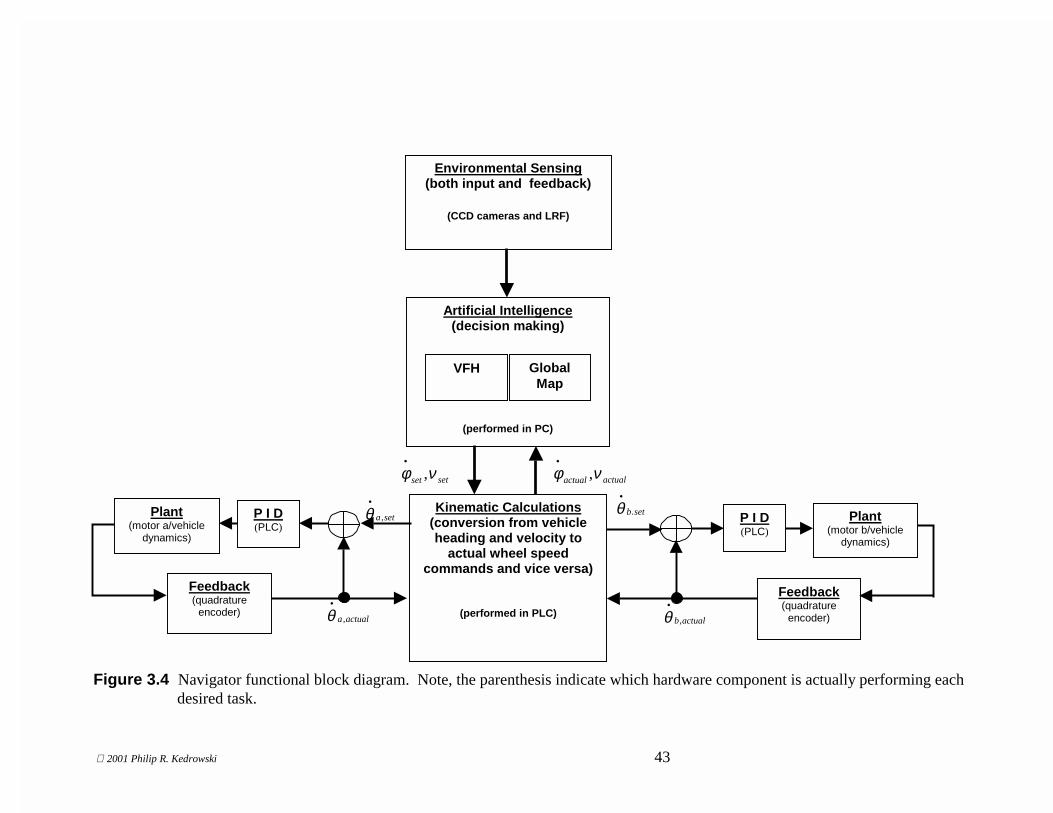
2001 Philip R. Kedrowski 43
Environmental Sensing (both input and feedback)
(CCD cameras and LRF)
Artificial Intelligence (decision making)
(performed in PC)
VFH Global Map
Kinematic Calculations (conversion from vehicle heading and velocity to
actual wheel speed commands and vice versa)
(performed in PLC)
P I D (PLC)
Plant (motor a/vehicle
dynamics)
Feedback (quadrature
encoder)
Feedback (quadrature
encoder)
Plant (motor b/vehicle
dynamics)
P I D (PLC)
setset νφ ,•
actualactual νφ ,•
seta ,
•θ
actuala ,
•θ actualb,
•θ
setb.
•θ
Figure 3.4 Navigator functional block diagram. Note, the parenthesis indicate which hardware component is actually performing each desired task.

2001 Philip R. Kedrowski 44
Modifications - Although the initial prototype of Navigator established itself as a
dependable and successful platform vehicle, testing revealed mechanical and electrical
alterations that could further enhance its performance.
When developing the initial prototype of Navigator, the target vehicle weight was
220 lbs (100 kg) and the nominal drive wheel diameter was 26 inches (0.6604 m)
[Conner, 2000a]. These specified parameters were used to size the 0.45 hp Bodine
motors, previously mentioned. However, upon Navigators completion it weighed nearly
twice the target value, 380 lbs (172 kg). This deviation didn’t render Navigator
immobile, however it decreased Navigator’s desired dynamic performance. For example,
initial calculations predicted that Navigator would be able to maintain top competition
speed (5 mph) up a 15% slope, but the finished prototype could barely ascend this slope
at all [Conner, 2000a]. In fact, this inability to consistently climb the slope was the cause
of failure during one of the attempts at the competition. In addition, the increased vehicle
mass caused Navigator to have difficulty performing zero radius turns.
In the early stages of redesigning Navigator, two major design goals were
established. The first was to increase the drive force and the second was to reduce the
overall vehicle mass. It was deemed that if these design criteria were met, Navigator’s
dynamic performance would improve. However, these criteria are not completely
decoupled and there were some resulting tradeoffs between the two.
To achieve a higher drive force, the first (and most obvious) option was to install
larger drive motors. However, larger drive motors are heavier and thus contradict the
second design criterion. Further, new motors have differing geometries and thus would
require substantial redesign of the motor mounting brackets, lower bay, and drive wheel
coupling. The next option for increasing the drive force was to decrease the diameter of
the drive wheels. This idea was favorable because it both increased the drive force and
decreased the overall vehicle weight.
It was decided to replace the 26 inch diameter drive wheels with 20 inch (0.508
m) diameter drive wheels. This gives a 30% percent increase in drive force. For a better
illustration of this concept, a free body diagram and the corresponding static equations
are given in Figure 3.5.

2001 Philip R. Kedrowski 45
Given a maximum drive torque, provided by the motors, the increased drive force
is easily calculated by looking at the ratio between the wheel radii. Equation 3.1 gives
this ratio for the aforementioned wheel diameters.
%)("
"130100
10
13
l
l
lT
lT
F
F
new
old
old
max
new
max
old
new ==== (3.1)
One disadvantage of reducing the drive wheel diameter is lowered ground
clearance. In order to maintain the necessary ground clearance, the motor mounts had to
be lowered three inches. This meant a substantial redesign of the frame. At first, this
idea was discouraged. However, it was determined that a large amount of weight could
be trimmed if the existing steal frame was replaced with an aluminum frame. Therefore,
it was decided to replace the drive wheels and redesign the frame using aluminum.
In order to quickly manufacture and assemble the new frame, Bosch aluminum
framing material was used. The pre-manufactured connectors and T-slotted aluminum
tubing allowed the frame to be constructed with no welds. Figure 3.6 shows the new
aluminum frame just before it was installed on Navigator. This frame saved an estimated
19 lbs (8.62 kg).
Tmax
l
Fmax l
TF
lFT
maxmax
maxmax
=
=
Figure 3.5 Free body diagram and equations that relate motor torque to drive force.
Where, Tmax = maximum motor torque, Fmax = maximum drive force, l = drive wheel radius.

2001 Philip R. Kedrowski 46
Further, an estimated 2 lbs (0.91 kg) was saved by machining the motor mounting
plates out of 3/8” aluminum sheet instead of the existing 1/2” aluminum sheet. Figures
3.7 a and b show the smaller mounting plate and mounting bracket respectively.
In addition to the new drive wheels, an industrially manufactured caster wheel
Figure 3.6 Navigator just before installing new aluminum frame.
A)
B)
New Mounting Plate
Old Mounting Plate
Figure 3.7 A) Motor mounting plates. B) New motor mounting bracket.

2001 Philip R. Kedrowski 47
was chosen to replace the existing custom castor wheel. This caster uses thrust bearings
that allow it to rotate more easily when loaded vertically. The new caster wheel and the
old caster wheel are shown in Figure 3.8.
Although the bulk of Navigators modifications where mechanical, one electrical
modification allowed for a further reduction in weight. This was the addition of wireless
Ethernet, developed by Cisco systems. Using wireless Ethernet allows an off-board
interface to Navigator’s computer via a portable laptop computer. Therefore, it was
possible to remove the on-board monitor and accompanying power supply. This further
reduced the overall weight by an estimated 25 lbs (11.3 kg). Additional weight
reduction was achieved by
efficiently rerouting the wiring
busses and eliminating excess wire,
as well as, eliminating as much
excess hardware as possible. The
result was a total overall weight
reduction of 54 lbs (24.5 kg),
approximately 15%. The
completely redesigned Navigator
is shown in Figure 3.9.
Thrust Bearing Revolute
Bushing Revolute
Figure 3.8 New caster wheel and old caster wheel, respectively.
Figure 3.9 Completed redesign of Navigator.

2001 Philip R. Kedrowski 48
3.2 Navigator Kinematics
In order to convert vehicle velocity and heading commands into individual wheel
speed commands, it is necessary to solve the vehicle kinematics. This section develops
the kinematic equations that describe Navigator’s motion on the ground plane. It should
be noted, however, that these equations are general to all differentially driven vehicles.
Currently, all of the vehicles that are being developed by the Autonomous Vehicle Team
(AVT) at Virginia Tech implement a differentially driven mechanical architecture, thus
each vehicle uses these equations.
Figure 3.10 shows the wheel elevation and Figure 3.11 is the plan view of the
platform vehicle, Navigator. Many of the dimensions could be assumed symmetrical
(e.g. a=b, ra=rb, etc), however it is desirable to develop the kinematic equations in the
most general form possible. This allows for calibration of the individual vehicle
parameters, which helps eliminate many systematic dead reckoning errors.
θ
S
r
Dimensions θ = wheel rotation (m) r = wheel radius (m) S = arc length (m)
Figure 3.10 Elevation side view of wheel.

2001 Philip R. Kedrowski 49
ψ
d
r c
c
a b
r bra
c g
e
c t
While in motion through an arbitrary curve, Navigator rotates about an
instantaneous center, O. Analyzing about the instantaneous center O allows Navigator’s
motion to be described as purely rotational, Figure 3.12.
r1
r2
β
ρ
vv
s a
s b
a b
φ
O
c t
9 0 -β
9 0 -β
Dimensions
a = left wheel to center line distance (m) b = right wheel to center line distance(m) ra = left wheel loaded radius (m) rb = right wheel loaded radius (m) rc = caster wheel loaded radius (m) c = axle to caster pivot distance (m) d = caster pivot to axle distance (m) e = axle to center of gravity (m) ψ = caster angle to center line (radians)
(positive as shown) cg = center of gravity ct = turning center
Figure 3.11 Plan view of Navigator [Conner, 2000c].
Dimensions/Coordinates Vv = vehicle velocity (m/s) φ = vehicle heading (rad) ρ = instantaneous turning
radius (m) β = instantaneous turning
angle equal to φ (rad) r1 = instantaneous turning radius of wheel a (m) r2 = instantaneous turning radius of wheel b (m) Sa = wheel a arc length (m) Sb = wheel b arc length (m)
Figure 3.12 Rotational motion of differentially driven vehicle about the instantaneous center [Conner, 2000c].

2001 Philip R. Kedrowski 50
By inspecting Figure 3.12, it can be seen that the instantaneous turning angle β is
equal to the vehicle heading angle φ. Using this equality, the wheel arc lengths Sa and Sb
are related to the vehicle heading angle via Equations 3.1 a and b.
φ1rSa = (a) φ2rSb = (b) (3.2)
The individual wheel rotations are related to the arc length by their respective radii,
through Equations 3.2 a and b.
aaa rS θ= (a) bbb rS θ= (b) (3.3)
Applying a no slip constraint and combining Equations 3.1 and 3.2 yields the relations
between individual wheel rotation and vehicle heading, Equations 3.3 a and b.
aarr θφ =1 (a) bbrr θφ =2 (b) (3.4)
Now it is possible to eliminate an unknown by representing the instantaneous turning
radii r1 and r2 of the respective wheels in terms of the instantaneous turning radius ρ of
the vehicle and the two known wheel base values a and b.
( ) aara θφρ =− (a) ( ) bbrb θφρ =+ (b) (3.5)
From here, the instantaneous turning radius ρ is easily eliminated through substitution.
This allows for the vehicle heading φ to be shown in terms of the vehicle parameters and
the individual wheel rotations.
ab
rr aabb
+−
=θθ
φ (3.6)
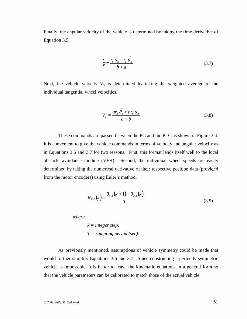
2001 Philip R. Kedrowski 51
Finally, the angular velocity of the vehicle is determined by taking the time derivative of
Equation 3.5.
ab
�r�r aabb
+−
=••
•φ (3.7)
Next, the vehicle velocity Vv is determined by taking the weighted average of the
individual tangential wheel velocities.
ba
�br�arV bbaa
v ++
=••
(3.8)
These commands are passed between the PC and the PLC as shown in Figure 3.4.
It is convenient to give the vehicle commands in terms of velocity and angular velocity as
in Equations 3.6 and 3.7 for two reasons. First, this format lends itself well to the local
obstacle avoidance module (VFH). Second, the individual wheel speeds are easily
determined by taking the numerical derivative of their respective position data (provided
from the motor encoders) using Euler’s method.
( ) ( ) ( )T
kkk baba
ba,,
,
1 θθθ
−+=
•
(3.9)
where,
k = integer step,
T = sampling period (sec).
As previously mentioned, assumptions of vehicle symmetry could be made that
would further simplify Equations 3.6 and 3.7. Since constructing a perfectly symmetric
vehicle is impossible, it is better to leave the kinematic equations in a general form so
that the vehicle parameters can be calibrated to match those of the actual vehicle.

2001 Philip R. Kedrowski 52
Chapter 4
Global Map Developing, Implementation, and Simulation
Chapters one through three of this thesis have periodically noted that a complete
navigation scheme includes both a local obstacle avoidance module and a global map.
Chapter three outlined the base mechanical platform, Navigator, and mentioned the local
Vector Field Histogram (VFH) obstacle avoidance module, that is in place on Navigator.
This chapter gives a brief outline of the VFH and then goes on to explain the self-
building global mapping algorithm. Finally, simulations of the complete navigation
scheme are shown on various courses and their results are discussed.
4.1 Vector Field Histogram
The VFH is a method for real time local obstacle avoidance on mobile robots that
was originally developed at the University of Michigan [Borenstein and Koren, 1991]. A
later development called the VFH+ offered the improvements of smoother robot
trajectories and greater reliability [Ulrich and Borenstein, 1998]. The latest version
involved coupling the VFH+ with an initialized global map. It then used the well-known
A* search algorithm to find the optimal path through the global map. This is called the
VFH* [Ulrich and Borenstein, 2000].
The VFH was chosen for implementation on Navigator because it is a well-proven
method for local obstacle avoidance and it is well suited for the sensors used on
Navigator. Conceptually, the VFH used on Navigator is most similar to the VFH+
mentioned above, however the details involved in implementation vary. This section
describes the VFH in general. Details of the exact implementation (i.e. sensor fusion,
passability, polar obstacle density calculations, etc.) on Navigator can be found in the
documentation of the work done over the 1999-2000 academic year [Conner et al,
2000a,b,d].

2001 Philip R. Kedrowski 53
The VFH represents the obstacles in front of the vehicle in polar coordinates.
Obstacles are impassible areas, which may be a physical object or a course boundary line.
Figure 4.1 is an example of a mobile robot encountering a typical set of obstacles on the
course at the Intelligent Ground Vehicle Competition (IGVC).
The cameras and laser range finder determine the magnitude ρ and direction θ of
the two and three-dimensional obstacles such as lines and barrels. The number of vectors
in the vector field corresponds to the resolution of the sensors. The resolution of the Sick
LMS-200 laser rangefinder is 0.5 degrees and the resolution of the cameras varies
depending on thresholding and decrementing done during image processing. Conner’s
work describes these concepts in greater detail [Conner et al, 2000a,b,d].
Next, the Polar Obstacle Density (POD) is calculated for developing the bar graph
known as the VFH. The POD calculation is designed to suite individual applications, and
the designer can take into account factors such as vehicle dynamics and desired response
time. The POD is typically an inverse function of the vector’s magnitude ρ. Thus, the
higher the POD value the closer the vehicle is to an obstacle. These POD values are then
+90o -90o
0o
Barrel Line
ρn
θn
Figure 4.1 Vector representation of obstacles in front of mobile robot. Note, ρn and θn are the magnitude and direction of each vector, respectively.

2001 Philip R. Kedrowski 54
plotted at each angle in a bar graph, giving a diagram such as the one shown in Figure
4.2. This is the Vector Field Histogram.
The VFH can be thought of as a series of peaks and valleys. The vehicle
navigates by choosing a valley and driving through it. The valley opening must be wide
enough for the vehicle to physically pass through it. The actual opening size is related to
the angle of the valley opening and the magnitude of the peaks. In this case, the angle
opening of a valley can be small if the peaks adjacent are also small. In effect, if the
obstacles are farther away, then the angle between them, as viewed from the vehicle, can
be smaller. Through this methodology, many candidate valleys can be eliminated
because they are too small for the vehicle to pass through. However, assuming the course
is passable, it does not eliminate all possible valleys. Therefore, it is desireable to have a
global map such that it can favor the valley that most efficiently directs the vehicle
toward the goal.
4.2 Global Map Developing
In most autonomous vehicle navigation schemes, the global map is initialized
using prior knowledge of the environment in which the vehicle is used. In indoor
environments, this knowledge can come from the building construction plans. In outdoor
+90o -90o 0o
P O D
Figure 4.2 Sample Vector Field Histogram (VFH). Note, this VFH corresponds to the vector field shown in Figure 4.1.

2001 Philip R. Kedrowski 55
environments, it can be provided by surveying the territory or taking aerial photographs.
Various situations (such as heavy foliage) can prevent getting accurate global map
information. In order to instigate creative solutions for these cases, the IGVC does not
allow prior knowledge of the obstacle course. Thus, global map initialization is not
permitted. However, in the spirit of encouraging success and keeping the competition
interesting to spectators, the IGVC rules allow the vehicles to make multiple attempts at
completing the course. This spurred the idea of using information acquired during initial
attempts to help in navigation of later attempts. A concept for doing this is described
below.
A free space map is built by recording where the vehicle has been during early
exploratory runs. This method of dead reckoning is achieved by using the vehicle
velocity Vv and vehicle angular velocity •φ , provided via wheel encoder feedback (as
shown in chapter 3), to determine the vehicle position through numerical integration.
The method for doing this is as follows. Figure 4.3 shows the vehicle represented as a
point in a Cartesian reference frame.
The arrays Xg and Yg used for plotting the global path are easily obtained by
numerically integrating over time as shown in equations 4.1 and 4.2.
Y
X
•φ
Vv
dx
dy
Dead Reckoning (Xg, Yg)
Figure 4.3 Global map building in Cartesian coordinates, using dead reckoning.
Vehicle
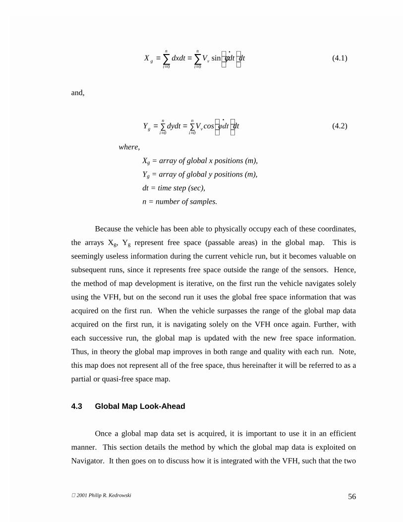
2001 Philip R. Kedrowski 56
∑∑=
•
=
==
n
iv
n
ig dtdtVdxdtX
00
sin φ (4.1)
and,
∑
=∑=
=
•
=
n
0iv
n
0ig dt���cosVdydtY (4.2)
where,
Xg = array of global x positions (m),
Yg = array of global y positions (m),
dt = time step (sec),
n = number of samples.
Because the vehicle has been able to physically occupy each of these coordinates,
the arrays Xg, Yg represent free space (passable areas) in the global map. This is
seemingly useless information during the current vehicle run, but it becomes valuable on
subsequent runs, since it represents free space outside the range of the sensors. Hence,
the method of map development is iterative, on the first run the vehicle navigates solely
using the VFH, but on the second run it uses the global free space information that was
acquired on the first run. When the vehicle surpasses the range of the global map data
acquired on the first run, it is navigating solely on the VFH once again. Further, with
each successive run, the global map is updated with the new free space information.
Thus, in theory the global map improves in both range and quality with each run. Note,
this map does not represent all of the free space, thus hereinafter it will be referred to as a
partial or quasi-free space map.
4.3 Global Map Look-Ahead
Once a global map data set is acquired, it is important to use it in an efficient
manner. This section details the method by which the global map data is exploited on
Navigator. It then goes on to discuss how it is integrated with the VFH, such that the two

2001 Philip R. Kedrowski 57
navigation modules can work together forming a complete navigation scheme.
Implementation of the global map is done using a global look-ahead algorithm. This
global look-ahead algorithm is most easily understood by first viewing an illustration of
the vehicle in relation to the global map data.
Figure 4.4 shows the vehicle on the verge of starting its second attempt at the
obstacle course. It has already developed a rough global map of the course using dead
reckoned data from the first run. Notice how the vehicle path oscillated through the
course on the first run. This oscillatory behavior is characteristic of the VFH obstacle
avoidance module. At each abrupt change in direction, the vehicle decelerates nearly to a
complete stop, turns, then accelerates again after completing the turn. Thus, the vehicle
not only oscillates in trajectory but it also oscillates in velocity when navigating solely
using the VFH. Figure 4.4 also shows an expanded view of the area directly in front of
the vehicle. This is to illustrate the look-ahead algorithm. The VFH sees no obstacles
thus it would give a zero vehicle angular velocity command ( 0=•φ , exactly like the first
run), however looking ahead at the previous data shows free space to the left of the
vehicle. Armed with this knowledge, the vehicle can initiate the turn earlier and thus
have a smoother motion profile and maintain a more constant velocity throughout the
turn.
X
Y
φla
Dla
(xc, yc)
Sensor Range
E-stop
Global Path
Figure 4.4 Illustration of the global look-ahead algorithm. Note, dimensions are not exactly to scale.
(xp, yp)
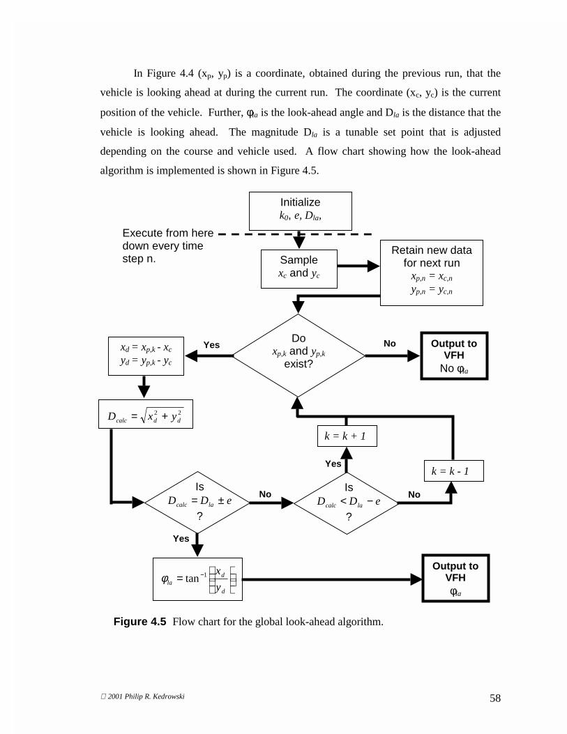
2001 Philip R. Kedrowski 58
In Figure 4.4 (xp, yp) is a coordinate, obtained during the previous run, that the
vehicle is looking ahead at during the current run. The coordinate (xc, yc) is the current
position of the vehicle. Further, φla is the look-ahead angle and Dla is the distance that the
vehicle is looking ahead. The magnitude Dla is a tunable set point that is adjusted
depending on the course and vehicle used. A flow chart showing how the look-ahead
algorithm is implemented is shown in Figure 4.5.
Output to VFH φla
= −
d
dla y
x1tanφ
Yes
No
k = k - 1
Is eDD lacalc −<
?
Is eDD lacalc ±=
?
22ddcalc yxD +=
Yes xd = xp,k - xc yd = yp,k - yc
Output to VFH
No φla
No Do xp,k and yp,k
exist?
Initialize k0, e, Dla,
Sample xc and yc
Retain new data for next run
xp,n = xc,n
yp,n = yc,n
Execute from here down every time step n.
k = k + 1
Yes
No
Figure 4.5 Flow chart for the global look-ahead algorithm.

2001 Philip R. Kedrowski 59
In Figure 4.5, n is a counter that points to the current sample and k is a counter
that points to data in the previous global path array Xg, Yg. Another way to interpret this
is that the kth data point occurred previously in time but is located ahead of the vehicle.
As shown in Figure 4.5, when running, the current vehicle position (xc, yc) is periodically
sampled and immediately stored in the global map. Next, it is determined whether look-
ahead data exists. If not, the algorithm immediately outputs no look-ahead angle. This is
the case if the global map doesn’t exist or the vehicle has surpassed the global map data.
Here, the vehicle will navigate solely from the VFH. If look-ahead data does exist, the
next steps are to calculate the difference between the look-ahead position and the current
position and determine its vector magnitude Dcalc. At this point, the calculated look-
ahead distance Dcalc is compared to the set point look-ahead distance Dla. If they are
equal within a set tolerance ±e, then the look-ahead angle φla is calculated and output
directly. Otherwise, the look-ahead counter k is either incremented or decremented and
the process is repeated until the calculated look-ahead distance Dcalc equals the set point
look-ahead Dla distance within the tolerance e.
The look-ahead algorithm is executed once per time step, it can also be thought of
as a distance traveled. The higher the sampling rate, the more continuous the global map
will be. However, in this application it is not necessary to have an extremely high
resolution. A resolution varying between 1 cm and 10 cm (depending on vehicle speed)
is adequate. Each time the look-ahead algorithm is executed, the look-ahead angle (if it
exists) is sent to the VFH. The VFH is then biased to favor this heading and the vehicle
will travel directly toward the look-ahead point. However, if the vehicle encounters an
obstacle, the VFH overrides the look-ahead command and the obstacle is avoided. In this
case, the look-ahead command is not completely ignored because the chosen valley in the
VFH will be the one closest to the look-ahead angle φla. This concept is illustrated in
Figure 4.6. All of the code for the global look-ahead algorithm is presented in Appendix
A of this thesis.

2001 Philip R. Kedrowski 60
Given multiple attempts at the course, the global path should increase in both
length (more progress along the course before failure) and quality. This is because
during each new run, the global map is updated with the newest data. As mentioned
before, when navigating solely using the VFH, the vehicle will oscillate in both trajectory
and velocity throughout the course. It is not expected that all of these oscillations will
dampen completely during the second attempt at running the course. Rather, it is
expected that after multiple attempts, the vehicle will settle on a steady state path through
the course. Figure 4.7 illustrates this concept.
Figure 4.6 Situation in which the VFH will override the global look-ahead algorithm.
X
Y
Dla
(xp, yp)
(xc, yc) φla
Global Path
New Path
Barrel

2001 Philip R. Kedrowski 61
4.4 Navigation Simulations
In order to better understand the feasibility, performance advantages, and
performance disadvantages of the self-building global mapping algorithm, it was decided
to develop a computer simulator of the mobile robot system. The navigation simulator is
written in the C++ programming language. C++ is the language that was used to write
the “Navigation Manager” software that is in place on Navigator. The Navigation
Third Attempt
First Attempt
Second Attempt
Fourth Attempt
Figure 4.7 Theoretical vehicle trajectory with global map building over multiple attempts.

2001 Philip R. Kedrowski 62
Manager is a Graphical User Interface (GUI) that gives the user access to the controls on
Navigator [Conner, 2000a]. Figure 4.8 is what the user sees when operating the
Navigation Manager on Navigator. The C++ language was chosen because it is object
oriented and offers the advantage of modular programming. This means that additional
software components, such as the look-ahead algorithm, can be written separately and
then interfaced with the existing code with relatively little trouble.
Writing the code for the look-ahead simulator in C++ gives two distinct
advantages. First, it allows the simulations to be as much like the real vehicle as
possible. This is because the look-ahead algorithm is fused with the code for the VHF
and interface that is already in use on Navigator. Second, converting the code from
simulation to actual implementation is easier if they are both written in the same
programming language. The C++ code for the look-ahead algorithm can be found in
appendix A.
Some modifications were made to the existing code in order to use it for
simulations. Instead of capturing bitmap images from the CCD board cameras, bitmaps
are input directly from a picture that is drawn in Microsoft Paint. This allows the
Figure 4.8 Navigation Manager, the user interface to the controls on Navigator.

2001 Philip R. Kedrowski 63
designer to draw courses with various shapes and obstacle locations and then use it to test
the vehicle navigation algorithms. A Region Of Interest (ROI) is then taken from this
large course image. This data is processed exactly like the image data from the cameras
on the real vehicle and input into the VFH. The ROI is equivalent in scale with the area
seen by the real sensors (cameras and LRF) on Navigator. Using this ROI as the “sensor”
input allows the VFH to behave based solely on local map information as it does on the
actual vehicle. In this manner, lines and objects (such as barrels) are simulated by
drawing them as white pixels in the course image.
This simulator is used as a tool to test the effects of changing environments and
parameters. These consist of the look-ahead distance, polar obstacle density calculations,
global map resolution, various course shapes, various course dimensions, trap situations,
and dead reckoning errors. It should be noted that the simulator does not consider the
dynamic effects of the vehicle, nor does it not take into account errors in sensor readings.
It is designed as a tool used to test, understand, and calibrate the coupled VFH/global
look-ahead navigation scheme.
The next sequence of illustrations is from actual navigation simulations on
different courses. These simulations do not cover every possible scenario that the vehicle
may encounter, but it should give the reader some understanding of what the designer
must consider when using the simulator. All of the following simulations were done
using a 3 cm/pixel resolution on the course bitmap that was input into the simulator. This
converts to a course width that varies from 10 to 15 ft (approx 3 to 5 m), thus it is
approximately the same dimensions as the IGVC obstacle course. The barrels are also
approximately to scale. The vehicle is represented as a point, but the kinematics are
based on the actual vehicle dimensions. Further, the ROI that is used as the sensor input
is to scale with that of the actual sensor range on Navigator.
The look-ahead distance Dla is set 2.5 meters with a tolerance e of 0.2 meters, in
all of the following simulations. Larger look-ahead distances have been tried and they
yield a faster settling time (fewer runs) to the steady-state path. However, increasing the
look-ahead distance also increases the likelihood that an object will come between the
vehicle and the look-ahead point, shown in Figure 4.6. These occurrences disrupt the
motion profile of the vehicle and result in slower traversal of the course.

2001 Philip R. Kedrowski 64
Figure 4.10 Simulation on course that is more like the IGVC course.
Trap
First Run Second Run Third Run Fourth Run Steady-State Path
Start Finish
Figure 4.9 Simulation test course with one trap.
Barrel

2001 Philip R. Kedrowski 65
Figure 4.9 is a simulation on a basic course with one trap. Notice how the vehicle
settles on a steady-state path in only four runs. Looking ahead at the previous run allows
the vehicle to initiate the turns earlier and thus maintain a smoother motion profile
throughout the turn. Figure 4.10 is a simulation on a course that is more like those at the
IGVC. Notice, it takes five runs before coming to a steady-state path.
Next, Figure 4.11 gives an example of the vehicle getting caught in a trap on the
first two runs and using that data to avoid the trap on later runs. On the first attempt, the
vehicle falls directly into the trap when exploring using only the VFH. During the second
attempt, the vehicle uses the look-ahead data acquired during the first run and initiates the
turn sooner. Unfortunately, it doesn’t turn soon enough and falls into the trap again. On
the third attempt, looking ahead at the global map developed on the second attempt helps
the vehicle to initiate the turn even sooner and finally it avoids being caught in the trap.
Notice, once the vehicle is able to explore past the trap, it is uses the global map to
completely avoid the trap on all subsequent runs.
As previously mentioned, the global map is built using the method of dead
reckoning. Dead reckoning is imperfect because it has two types of errors associated
First Trap
Second Trap
Figure 4.11 Vehicle using global map to avoid traps.

2001 Philip R. Kedrowski 66
with it; systematic and non-systematic. Sources of these errors are given in Table 2.1.
Systematic errors are predominant. On a differentially driven vehicle such as Navigator,
the most dominant of the systematic errors are those associated with wheel radius and
wheelbase dimensions. Errors of this sort are caused by inaccurate measurements of
wheelbase and wheel diameter and low tire air pressure. These errors lead to faulty
vehicle localization. For example, if the kinematic model (developed in section 3.2),
internal to the vehicle, has these parameters set to a certain value and the actual vehicle
parameters are a different value, then the model will incorrectly predict the location of
the vehicle.
The simulator allows the user to input systematic errors and visualize the
imperfect dead reckoned global path. Figure 4.12 shows the vehicle path on its first run
along with the inexact dead reckoned path. This imperfection is due to a 0.5% (3.3mm)
decrease in the right wheel diameter in the simulation. This magnitude of error could
easily occur due to a decrease in the air pressure of the right tire. Notice how the dead
reckoning error gets larger as the vehicle traverses further along the course. However, in
this case, turning counteracts this growth a small amount.
Figure 4.12 Vehicle path and dead reckoned path with error due to 0.5% decrease in right wheel diameter.
Real Vehicle Path Dead Reckoned Path

2001 Philip R. Kedrowski 67
Figure 4.13 is given to show what happens when the vehicle takes a second run
using the imperfect global path as the look-ahead data. This figure illustrates that even
with a flawed global map, the vehicle is able to establish a better trajectory through the
course on the second run than it did on the first run. Further, the quality of the global
path improves on the second run.
Finally, an illustration of the inaccuracy caused by an error in wheelbase
measurement is shown in Figure 4.14. In this simulation, the error is caused by a 3%
(1.14 cm) smaller left wheelbase. Errors in wheelbase dimensions are typically caused
by imprecise measuring techniques. However, this error can also be caused by wheel
cant that is not accounted for in the model. 1.14 cm is considered large for this type of
error, because accuracy up to a couple of millimeters is easily achieved using a common
tap measure. By comparing Figure 4.14 to Figure 4.12, it is seen that the dead reckoning
inaccuracy caused by an inaccurate wheelbase dimension is much less dramatic than that
caused by an inaccurate wheel radius.
Figure 4.13 Second run using imperfect global map that was developed on the first run.
Real Vehicle Path Dead Reckoned Path
Global Path

2001 Philip R. Kedrowski 68
This is just a sample of the infinite number of scenarios and courses that can be
tested with the simulator. These are given in order familiarize the reader with some of
the main areas of concern that were tested in order to determine the feasibility of the
global look-ahead algorithm. As shown, the main problem associated with the global
look-ahead algorithm is the errors associated with dead reckoning. Figure 4.13 shows
that an imperfect global map is still useful. It is desirable, however, to eliminate as many
dead reckoning errors as possible. The next chapter presents a tool that was to minimize
systematic dead reckoning errors.
Figure 4.14 Vehicle path and dead reckoned path with error due to 3% decrease in the left wheelbase.
Real Vehicle Path Dead Reckoned Path

2001 Philip R. Kedrowski 69
Chapter 5
Optimized Calibration of Vehicle Parameters
As described in section 4.2, the global map building technique developed in this
thesis uses odometry, also referred to as dead reckoning. Dead reckoning accuracy is
subject to both systematic and non-systematic errors. Table 2.1 outlined the main sources
for both types of error. In section 4.4, systematic errors were introduced into the
simulation to illustrate their effects on the global map look-ahead algorithm. It was
determined that these dead reckoning errors do not render the algorithm useless.
Nevertheless, it is desirable to minimize them order to maximize the effectiveness of the
global look-ahead algorithm.
This chapter begins by determining the nature and magnitude of the dead
reckoning errors associated with Navigator using a standard test known as the UMBmark
(University of Michigan Benchmark). Next, a tool is developed for optimizing the
calibration of the vehicle kinematic parameters (wheelbases and radii) in order to
minimize systematic dead reckoning errors. This calibration uses Hooke and Jeeve’s
optimization technique to search for the minimum error values. It will be shown that a
substantial improvement in dead reckoning accuracy is achieved by utilizing this tool to
optimize the vehicle calibration.
5.1 UMBmark Test
Checking the dead reckoning performance on specified test patterns helps uncover
whether an error is systematic or non-systematic. This is done by determining the
difference between where the vehicle actually is and where it “thinks” it is after running a
chosen pattern. This difference is referred to as the dead reckoning error. By nature,
systematic dead reckoning errors are repeatable. Because of this, if the dead reckoning
error is consistent in magnitude and direction over multiple tests, then it is likely due to a

2001 Philip R. Kedrowski 70
systematic inaccuracy. However, determining which systematic parameter is in error is
less obvious. The UMBmark test is designed to uncover certain systematic errors that are
likely to compensate for each other and thus remain undetected in less rigorous tests
[Borenstein and Feng, 1995].
The two most prevalent systematic errors are inaccurate wheel diameters and
uncertainty about the wheelbase measurements. The wheelbase measurement is defined
as the distance between
the ground contact
points of the two drive
wheels. For this work,
it is broken into the left
and right wheelbase
measurements. These
are the distance
between the respective
wheel/ground contact
points and the vehicle
centerline. These are
measurements a and b
described in section 3.2
of this thesis.
Borenstein gives a
visual example of how
these two errors could
compensate for one
another and thus remain undetected. This visualization is shown in Figure 5.1. However,
in this case, the dead reckoning error would compound if the vehicle were run in the
opposite direction. For this reason, Borenstein and Feng developed a simple bi-
directional square path test procedure for uncovering sources of systematic errors. They
refer to it as the UMBmark test.
Figure 5.1 Dominant systematic dead reckoning errors cancel each other out when test is run in only one direction [Borenstein and Feng, 1995].
Curved instead of straight path (due to unequal wheel diameters). In this example, it causes a 3o orientation error.
93o-turn instead of 90o-turn (due to uncertainty about the effective wheelbase)
93o

2001 Philip R. Kedrowski 71
The UMBmark test procedure consists of running the vehicle through a specified
square pattern in both the clockwise and counterclockwise direction and measuring the
dead reckoning error at the end of each run. This test was performed on Navigator to
better undersand the magnitude and type of dead reckoning error that it possesses. Since
Navigator is designed to perform in an outdoor environment, a large test grid was painted
in a grass field on the Virginia Tech campus. Figure 5.2 is an aerial view of this test grid.
Further, Navigator was physically pushed through the course in order to eliminate non
systematic wheel slippage that can occur when the vehicle accelerates and decelerates
under its own power.
The UMBmark test was performed on both 3-yard and 6-yard square test patterns.
Figure 5.3 shows the results from the 6-yard UMBmark test. The continuous line shows
the path that Navigator “thought” it took based on dead reckoning. The actual path that
Navigator took is shown as a dotted line. This test was performed using measured
Figure 5.2 Aerial view of grid used for UMBmark dead reckoning test.
3yrd
3yrd

2001 Philip R. Kedrowski 72
vehicle parameters in order to get an idea of what sort of calibration is needed. In this
test, the error vector (also referred to here as the dead reckoning error) is the vector from
where the vehicle is actually located (the origin) to where the vehicle “thinks” it is
located (based on dead reckoning) after completion of the test.
For this UMBmark test, five runs were performed in both the clockwise and
counterclockwise direction. Notice the predictability of the dead reckoned runs; this is
characteristic of systematic errors. Further, notice that the dead reckoned path curves to
the right when the vehicle is actually going straight. This is an indication that the left
wheel is slightly smaller in radius than the measured value. If this is the case, when the
vehicle is going straight, the left wheel will have to rotate more times than the right wheel
to keep up. Thus, if the wheel radius parameters are set equal in the kinematic model,
integrating to find position will show that the vehicle is actually moving through an arc as
shown. Thus, in this case, the vehicle will better predict where it is if the left wheel
radius is set to a lower value.
This suggests an iterative trial-and-error calibration technique. In this procedure,
one would change the vehicle parameters, check the UMBmark results and repeat until
the best results are achieved. This process could be tedious and take a long time.
Further, it is not guaranteed to give the optimal vehicle parameters. Borenstein and Feng
A)
Figure 5.3 Six-yard square UMBmark test with no calibration. A) Counterclockwise direction. B) Clockwise direction.
B)
Start
Actual Path
Dead Reckoning

2001 Philip R. Kedrowski 73
give another calibration technique that they developed along with the UMBmark test
[Borenstein and Feng, 1996]. This elegant method analytically derives correction factors
from experimental results. Using these correction factors for calibration Borenstein and
Feng made remarkable dead reckoning improvements on several indoor mobile robots
[Borenstein and Feng, 1996]. However, prior to calibration, these robots all had dead
reckoning errors on the order of 3 to 4 cm on a 4m (4.37 yrd) UMBmark test pattern.
This allowed Borenstein and Feng to use a small angle assumption in the analytical
derivation of the correction factors [Borenstein and Feng, 1996]. Conversely, Navigator
is an outdoor mobile robot with dead reckoning errors, prior to calibration, on the order
of 60 to 70 cm when run in a 3 yard (2.74 m) UMBmark test pattern. Since the dead
reckoning errors on Navigator are approximately 1.5 or 2 orders of magnitude greater, the
small angle assumption is no longer valid. As a result, this analytic calibration method
produced erroneous parametric values when used for calibration of Navigator in an
outdoor environment. This thesis develops a third technique for parameter calibration
that implements the Hooke and Jeeve’s optimization method in order to minimize the
total dead reckoning error.
5.2 Optimization Technique and Procedure
Optimization is the act of obtaining the best result under a given set of
circumstances [Rao, 1979]. The subject of optimization has existed for many years and
numerous techniques, both analytical and numerical, have been developed. The ultimate
goal of all these techniques is to either minimize the effort required or maximize the
desired benefit. Two excellent introductory texts covering optimization techniques are
those written by Rao [1979] and Vanderplaats [1984]. Optimization has been used
extensively here at Virginia Tech in the area of kinematic/robotic design and calibration
[Soper, 1995; Calkins, 1994].
This section starts by introducing the Hooke and Jeeve’s method for solving
unconstrained minimization problems. Next, it describes the method by which the
objective function is developed. The objective function is the function that is minimized
in the Hooke and Jeeve’s optimization algorithm. Finally, the startup procedure is shown

2001 Philip R. Kedrowski 74
such that this can be used as a tool for parametric calibration of a differentially driven
vehicle. This tool is developed such that any person operating the vehicle can calibrate
the vehicle using the optimal parameters on any particular day with minimal effort.
Hooke and Jeeve’s Optimization – First, it should be understood that any
optimization method for solving an unconstrained minimization problem could be used
for vehicle parametric calibration. A short list of various other methods is as follows
[Vanderplaats, 1984]:
1) Powell’s method.
2) Steepest descent.
3) Fletcher-Reeves conjugate direction method.
4) Davidson-Fletcher-Powell variable metric method.
5) Broydon-Fletcher-Goldfarb-Shanno variable metric method.
6) Newtons Method.
It is possible that using one of these other methods will yield a faster convergence than
the Hooke and Jeeve’s method in the application of vehicle parametric calibration that is
presented here. The reasons for choosing the Hooke and Jeeve’s method are twofold.
First, it is a robust pattern search technique that the author is familiar with and
comfortable coding. Second, it is not necessary that the optimization algorithm give the
absolute fastest convergence as long as it gives the correct results in a relatively timely
fashion.
An unconstrained minimization problem is one where a value of the design
vector, Equation 5.1, is sought such that it minimizes a designed objective function f(X).
This is an unconstrained minimization problem, because the solution parametric vector X
need not satisfy any constraint [Rao, 1979]. However, in many design scenarios
constraints can and are applied. An example of this is to apply the constraint that the
parameters (link lengths) must allow closure when using the Hooke and Jeeve’s method
in the synthesis of a planar four-bar mechanism.

2001 Philip R. Kedrowski 75
•••
=
nx
x
x
X
2
1
(5.1)
where,
x1, x2,…xn = the individual design parameters,
n = the total number of design parameters.
The Hooke and Jeeve’s pattern search method iterates on a sequence of two types
of moves. These are the exploratory move and the pattern move. During the exploratory
move, each design parameter is changed individually and the effects on the objective
function are monitored. The magnitude of these changes is referred to as the step size. If
a change yields a good result (lower objective function), the step size is increased and
stored in the step size array ∆X. Conversely, if the change yields a poor result (higher
objective function), the step size is decreased and stored in the step size array. The
pattern move shifts the entire parametric array X to the next position that yields the
lowest objective function. This process is repeated until the magnitude of the step size
array is less than an initialized minimum step size array magnitude |∆X|min, thus
indicating a local minimum value for the objective function. To better visualize this
sequence, a flowchart is given in Figure 5.4. In this chart, the superscripts denote an
entire parametric array, while the subscripts denote individual parameters in the
parametric arrays.
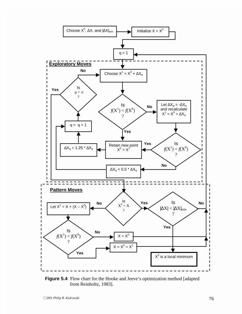
2001 Philip R. Kedrowski 76
Choose X0, ∆X, and |∆X|min Initialize X = X0
q = 1
Choose X1 = X0 + ∆Xq
Is f(X1) < f(X0)
?
Is f(X1) < f(X0)
?
Let ∆Xq = -∆Xq
and recalculate X1 = X0 + ∆Xq
Is q > n
?
q = q + 1
∆Xq = 1.25 * ∆Xq Retain new point
X0 = X1
∆Xq = 0.5 * ∆Xq
Is X0 = X
? Let X1 = X + (X – X0)
Is f(X1) < f(X0)
? X = X0
X = X0 = X1
Is |∆X| < |∆X|min
?
X0 is a local minimum
Yes
Yes
Yes
Yes
Yes
No No
No
No
No
No Yes
Exploratory Moves
Pattern Moves
Figure 5.4 Flow chart for the Hooke and Jeeve’s optimization method [adapted from Reinholtz, 1983].

2001 Philip R. Kedrowski 77
Objective Function – As previously mentioned, the objective function is the
mathematical function that is to be minimized. It is, either directly or indirectly, a
function of the design parameters. For calibration of a differentially driven vehicle, these
parameters consist of the left and right wheelbase and the two wheel radius values. In
this case, the goal is to minimize the total dead reckoning error by adjusting (calibrating)
these parameters. The total dead reckoning error is the sum of the error vector
magnitudes Ecgcw and Ecgccw for the clockwise and counterclockwise test patterns
respectively. When data from multiple tests exists, the error vectors are defined from the
actual location of the vehicle to the center of gravity (CG) of the cluster of points where
the vehicle “thinks” (based on dead reckoning) it is. The CG and resulting vector
magnitude are found using equations 5.2 a, b, and 5.3.
( )
∑ −=
=
n
0iiactualdeadcg xx
n
1x (a) ( )
∑ −=
=
n
0iiactualdeadcg yy
n
1y (b) (5.2)
where,
xactual, yactual = actual vehicle position,
xdead, ydead = dead reckoned vehicle position,
n = number of attempts.
and,
2cg
2cgcg yxE += (5.3)
Figures 5.5 a and b illustrate the CG position and Ecg for a complete UMBmark
test run on a three-yard and six-yard square respectively. As previously mentioned, the
vehicle was physically pushed when performing the UMBmark tests. This allows the
vehicle to move through nearly perfect square patterns, as well as, eliminates many non-
systematic errors. For all of the UMB mark tests, the ending vehicle position (xactual,
yactual) was at the origin. For both tests, Navigator was pushed in the clockwise and
counterclockwise test patterns a total of five times a piece. Notice, the dead reckoning

2001 Philip R. Kedrowski 78
error is greater when run in the six-yard pattern than when run in the three-yard pattern.
This is characteristic of a systematic error that grows as a function of distance traveled.
In order to develop the objective function, it was necessary to simulate the
vehicle’s final position based on the design parameters (wheel bases and radii) and the
size of the square test pattern. To achieve this, an algorithm was developed that
numerically integrates the kinematic Equation 3.6 and 3.7 in order to simulate the vehicle
position. This integration is done using nearly the same procedure that was presented in
section 4.2, except now the wheel velocities are specified in the code instead of being fed
back from the encoders, and the equations are integrated over a specified range instead of
the entire time the vehicle is running. This range corresponds to the size of the square
pattern being tested, i.e. three-yard, six-yard, or other.
At this point, an additional level of complexity exists. If the nominal (i.e. those
that produced incorrect results in the actual vehicle UMBmark test) parametric values are
UMBmark 3yrd (2.743m) Square
-40
-20
0
20
40
60
80
100
120
-80 -60 -40 -20 0
X (cm)
Y (
cm)
UMBmark 6yrd (5.486m) Square
-200
-100
0
100
200
300
400
-250 -200 -150 -100 -50 0
X (cm)
Y (
cm)
A) B)
Ecg,cw=110.4 cm
Ecg,ccw=27.5 cm
Ecg,ccw=213.4 cm
Ecg,cw=333.2 cm
Etotal=137.9 cm Etotal=546.6 cm
Figure 5.5 UMBmark test results from A) three-yard square, B) six-yard square. Both tests were done on the same day as the test shown in Figure 5.3.
CG

2001 Philip R. Kedrowski 79
used, then the simulation yields a perfect square pattern resulting in the vehicle’s final
position being at the origin. In this case, the error, as presented in Figure 5.5, would be
driven to zero without any parametric adjustment. However, it is known from the
UMBmark test that these are not the correct parametric values. At this point, two other
options exist. The first would be to design the objective function such that optimization
would adjust the parameters until the final simulated position is as close as possible to the
CG position. This method is flawed because it yields parametric values that will result in
a compounded dead reckoning error when they are used on the vehicle. The second, and
chosen, method is to design the objective function such that optimization adjusts the
parameters until the final simulated position is as close as possible to the negative of the
CG position. In this manner, optimization will output parameters that have been
calibrated to compensate for the systematic dead reckoning inaccuracies.
The resulting objective function is shown in Equation 5.4. In this equation, (xsim,
ysim) is the final position of the vehicle when simulated on the UMBmark test pattern.
These are functions of the design parameters, because the simulation is done using the
equations for vehicle velocity and vehicle angular velocity (Equations 3.6 and 3.7).
Therefore, the objective function is indirectly a function of the vehicle parameters.
( ) ( ){ } ( ) ( ){ }ccwsimcgsimcgcwsimcgsimcg yyxxyyxx)X( 2222f −−+−−+−−+−−= (5.4)
where,
xsim, ysim = the final simulated vehicle position.
Figure 5.6 is an example of a typical optimization run on a three-yard UMBmark
test pattern. This particular example uses the CG set points, clockwise and counter
clockwise, obtained from Figure 5.5a. Notice how it converges on a point in quadrant
four in the clockwise simulation and a point in quadrant one in the counter clockwise
simulation. This is opposite the CGcw,ccw points, which are in quadrants two and three, in
Figure 5.5a, respectively.

2001 Philip R. Kedrowski 80
As shown in the figure text, the parameters that are most drastically changed by
the optimization routine are the wheel radii. With these new values, the left wheel radius
is 65 mm smaller than the right wheel radius. These parametric values are logical,
because looking at the vehicle path in Figure 5.3 indicates that the left wheel is likely
smaller in radius.
At this point, the tool for optimized parametric calibration has been developed.
Next, it is necessary to establish an easy procedure, that can be followed by any operator,
to calibrate a differentially driven robot.
Calibration Procedure – There are two goals for developing the aforementioned
optimized parametric calibration tool. First, to eliminate as many dead reckoning errors
-300 -200 -100 0 100 200 300-50
0
50
100
150
200
250
300
350
400
450
X (cm)
Y (
cm
)
(xsim,ccw, ysim,ccw) (xsim,cw, ysim,cw)
Nominal Vehicle Parameters Left wheelbase = 38.1 cm Left wheel radius = 33.02 cm Right wheelbase = 38.1 cm Right wheel radius = 33.02 cm Calibrated Vehicle Parameters Left wheelbase = 38.58 cm Left wheel radius = 32.72 cm Right wheelbase = 38.53 cm Right wheel radius = 33.37 cm
Figure 5.6 Objective function vehicle simulations both clockwise and counter clockwise. This uses set point data from Figure 5.5a.

2001 Philip R. Kedrowski 81
as possible in order to maximize the benefits of the global look-ahead algorithm. Second
to allow for a timely and efficient calibration procedure.
Before explaining the procedure, it is interesting to note the relative preciseness of
the data points in Figures 5.5 a and b. This phenomenon was consistent in all of the
UMBmark tests that were performed. Because of this consistency in the data, not much
accuracy is lost if only one data point is used, instead of five, to determine the position of
CG. However, taking only one data point for the clockwise and counterclockwise
directions speeds up the calibration procedure by nearly a factor of five. This is because
the bulk of the time is spent pushing the vehicle through the UMBmark test when
performing the optimized calibration procedure. The optimized calibration procedure is
as follows:
1) Measure out and mark two perfect squares with sides of size three-yards or
larger. These squares should be configured such that they share one side.
One corner on this shared side is to be established as the origin.
2) Position the vehicle at the origin such that it is facing in the direction of the
shared side. Zero the dead reckoned position in the vehicle software.
3) Push the vehicle in the clockwise direction, around the square on the right,
and finish at the origin. Be careful to follow the square as closely as possible.
Note, the vehicle reference is the point where the centerline and the wheel axis
cross.
4) Record the final position (xcg, ycg) where the vehicle “thinks” it is, based on
dead reckoning.
5) Reposition the vehicle at the origin in its initial position and re-zero the dead
reckoned position in the vehicle software.
6) Push the vehicle in the counterclockwise direction, around the square on the
right, and finish at the origin. Again, be careful to follow the square as closely
as possible.
7) Record the position (xcg, ycg) where the vehicle “thinks” it is, based on dead
reckoning.
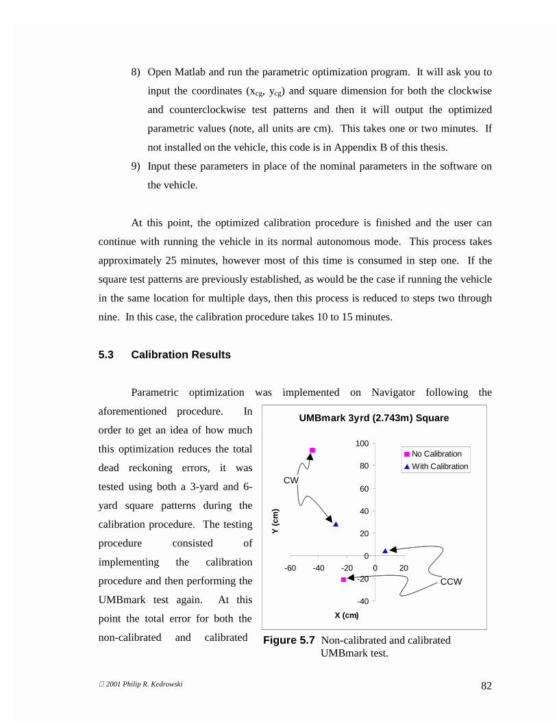
2001 Philip R. Kedrowski 82
8) Open Matlab and run the parametric optimization program. It will ask you to
input the coordinates (xcg, ycg) and square dimension for both the clockwise
and counterclockwise test patterns and then it will output the optimized
parametric values (note, all units are cm). This takes one or two minutes. If
not installed on the vehicle, this code is in Appendix B of this thesis.
9) Input these parameters in place of the nominal parameters in the software on
the vehicle.
At this point, the optimized calibration procedure is finished and the user can
continue with running the vehicle in its normal autonomous mode. This process takes
approximately 25 minutes, however most of this time is consumed in step one. If the
square test patterns are previously established, as would be the case if running the vehicle
in the same location for multiple days, then this process is reduced to steps two through
nine. In this case, the calibration procedure takes 10 to 15 minutes.
5.3 Calibration Results
Parametric optimization was implemented on Navigator following the
aforementioned procedure. In
order to get an idea of how much
this optimization reduces the total
dead reckoning errors, it was
tested using both a 3-yard and 6-
yard square patterns during the
calibration procedure. The testing
procedure consisted of
implementing the calibration
procedure and then performing the
UMBmark test again. At this
point the total error for both the
non-calibrated and calibrated
UMBmark 3yrd (2.743m) Square
-40
-20
0
20
40
60
80
100
-60 -40 -20 0 20
X (cm)
Y (
cm)
No Calibration
With Calibration
Figure 5.7 Non-calibrated and calibrated UMBmark test.
CW
CCW

2001 Philip R. Kedrowski 83
tests was compared. Figure 5.7 gives the results for a 3-yard square test pattern.
Figure 5.8 gives
the results for a 6-yard
square test pattern Both of
these tests were performed
on the same day. Table
5.1 quantifies the results
shown in Figures 5.7 and
5.8. Remember that the
total dead reckoning error
is the sum of the error
vectors for both the
clockwise and
counterclockwise runs.
Interestingly, calibrating
the vehicle on the smaller
(3-yard) test pattern gave
slightly better results on this particular day. Further, it should be noted that these results
are expected to vary from day to day. The purpose of these sample tests is to demonstrate
the typical reduction in error that is achieved using the optimized calibration procedure.
Test No Calibration (cm) Calibrated (cm) % Reduction in Error
Figure 5.7 134.1 48.0 64.3
Figure 5.8 579.0 235.1 60.6
It is interesting to see what improvements in dead reckoning can be gained on a
six-yard test pattern when the calibration was done using a three-yard test pattern. It was
also desired to see what improvements in dead reckoning can be gained on a three-yard
test pattern when the calibration was done using a six-yard test pattern. Figures 5.9 and
5.10 give the results of these respective tests. These test were performed on a different
day than those shown above.
UMBmark 6yrd (5.486m) Square
-150
-100
-50
0
50
100
150
200
250
300
350
-300 -200 -100 0
X (cm)
Y (
cm)
No Calibration
With Calibration
Figure 5.8 Non-calibrated and calibrated UMBmark test.
CW
CCW
Table 5.1 Total dead reckoning errors.

2001 Philip R. Kedrowski 84
UMBmark 3yrd (2.743m) Square
-40
-20
0
20
40
60
80
100
-50 0 50
X (cm)
Y (
cm)
No Calibration
With Calibrationon 3yrd Square
With Calibrationon 6yrd Square
Figure 5.9 Non-calibrated and calibrated UMBmark test.
CCW
CW
UMBmark 6yrd (5.486m) Square
-200
-100
0
100
200
300
400
-300 -200 -100 0
X (cm)
Y (
cm)
No Calibration
With Calibrationon 3yrd Square
With Calibrationon 6yrd Square
Figure 5.10 Non-calibrated and calibrated UMBmark test.
CW
CCW

2001 Philip R. Kedrowski 85
These results are quantified in Table 5.2. Again, the results show that calibrating
on a three-yard test pattern yields a higher reduction in error than calibrating on a six-
yard test pattern. Many possible reasons for this could exist. One contributing factor to
this is that, over a longer running distance, the vehicle is subject to more errors that are
non-systematic. Discontinuous terrain could be a large contributing factor of these non-
systematic errors. These tests do not prove that calibrating on a smaller test pattern is
better. What they do show, however, is that calibrating on a smaller test pattern gives
reasonable results compared to calibrating on a larger test pattern. This knowledge is
useful, because it means that the calibration procedure can be made less labor intensive
and time consuming by calibrating on a smaller test pattern, yet the benefits of the
optimized parametric calibration tool are not sacrificed.
Test No
Calibration
(cm)
Calibrated
on 3yrd
pattern
(cm)
Calibrated
on 6yrd
pattern
(cm)
% Error
Reduction
When
Calibrated on
3yrd pattern
(cm)
% Error
Reduction
When
Calibrated on
6yrd pattern
(cm)
Figure 5.9 134.9 78.8 103.8 41.6 23.1
Figure 5.10 610.6 172.6 209.4 71.7 65.7
The next sequence of figures show Navigator’s actual path when performing the
UMBmark tests discussed above. Figures 5.11, 5.12, and 5.13 are the test runs that were
inspected in Figure 5.9. Figures 5.14, 5.15, and 5.16 are the test runs that were inspected
in Figure 5.10. These are presented in order to give the reader a feel for the dead
reckoning performance of the actual vehicle, Navigator, in action. When viewing these
tests, remember that Navigator actually traveled in a near perfect square as illustrated in
Figure 5.3.
Table 5.2 Total dead reckoning errors.

2001 Philip R. Kedrowski 86
Figure 5.11 Three-yard test with no calibration.
Figure 5.13 Three-yard test, calibrated at six-yards.
Figure 5.12 Three-yard test, calibrated at three-yards.

2001 Philip R. Kedrowski 87
Figure 5.14 Six-yard test with no calibration.
Figure 5.16 Six-yard test, calibrated at six-yards.
Figure 5.15 Six-yard test, calibrated at three-yards.

2001 Philip R. Kedrowski 88
Notice that the dead reckoning was less accurate when running in the
clockwise direction than when running in the counter clockwise direction. This
could be due to the irregular terrain on which the testing took place. Three
possible contributing factors, which were noticed, are as follows. First, there was
a gradual slope ascending from right to left. Second, the terrain on the clockwise
run was slightly bumpier than the terrain on the counterclockwise run. Third, the
grass was thicker and less trampled on the counterclockwise run than on the
clockwise run. The details of how and why this affected the dead reckoning in
this particular way are not explored here. Regardless, optimized calibration
significantly decreased the errors due to dead reckoning in both the
counterclockwise and clockwise direction. The raw data for all of the calibration
testing that was performed is presented in Appendix C.

2001 Philip R. Kedrowski 89
Chapter 6
Implementation Results
This chapter presents the results of implementing the self-building global map and
look-ahead algorithm that was developed in the preceding chapters of this thesis. In
order to insure the minimum amount of dead reckoning error and thus maximize the
usefulness of the global map building algorithm, Navigator was calibrated using the
method presented in chapter five. Results show that using the self-building map
algorithm, Navigator can successfully develop a quasi-free space global map of the
course. Further, the quality of the maps improves with multiple runs. The first section of
this chapter discusses these results at greater length.
This chapter also presents conclusions and recommendations for future research.
It is the opinion of this author that some of the topics open for future research in this area
are complex and new enough to be Ph.D. dissertation material. Some areas in which this
research is directly applicable are also discussed.
6.1 Practice Course Results
An outdoor oval course was chosen for testing of the global map building and
look-ahead algorithm. This course, shown in Figure 6.1, has outer dimensions of
approximately 10 X 18 meters. The actual course width is 3 meters (10 feet) on average.
This is consistent with the course width at the IGVC. An oval course was chosen
because it is difficult, yet symmetric. Using a symmetric course facilitates extracting
distinguishing features from the data. The 3-yard square patterns at the bottom of Figure
6.1 were used for calibration, by following the procedure in Chapter 5, before the test
runs that follow.

2001 Philip R. Kedrowski 90
Initially, the algorithm was tested on the course with no obstacles. The ambient
conditions on the first day of testing were particularly good. There was consistent cloud
cover but no rain. This allowed the errors associated with image processing to be lower
than normal. Given bright sunlight, many light spots in the grass show up as obstacles,
thus Navigator oscillates more frequently in attempt to avoid these imaginary obstacles.
Further, bright sunlight can completely wash out an image in some cases. When this
occurs, Navigator is incapable of sensing and avoiding lines.
The first test, shown schematically in Figure 6.2 was performed in the
counterclockwise direction using a look-ahead distance (Dla) of 2.5 meters. Notice the
complete course is successfully mapped on the first run. On subsequent runs, Navigator
initiates the turns sooner and thus finds a shorter path around the course. However,
notice that the later runs oscillate more than the initial runs. This is possibly due to a
relatively short look-ahead distance. If looking further ahead, the look-ahead angle will
change less dramatically and help the vehicle to initiate turns more smoothly. Note, that
Figure 6.1 Outdoor test course for Navigator. Note, 3-yard calibration test pattern.

2001 Philip R. Kedrowski 91
the map is not an exact match to the real course. An exact match would result in both the
start and finish being at the origin. This inexactness is due to dead reckoning errors.
Next, the same test was run with a 3.5 meter look-ahead in an attempt to smooth
the oscillations.
-8.0
-6.0
-4.0
-2.0
0.0
2.0
4.0
6.0
8.0
10.0
-20.0 -15.0 -10.0 -5.0 0.0 5.0
X (meters)
Y (
met
ers)
Run #1 Run #2 Run #3
Figure 6.2 Counterclockwise test with a 2.5 meter look-ahead.
-6.0-4.0-2.00.02.04.06.08.0
10.0
-20.0 -15.0 -10.0 -5.0 0.0
X (meters)
Y (
met
ers)
Run #1 Run #2 Run #3 Run #4
Figure 6.2 Counterclockwise test with a 3.5 meter look-ahead.

2001 Philip R. Kedrowski 92
By looking at Figure 6.2, it can be seen that using a larger look-ahead distance
does tend to smooth the oscillations in the global path. However, many other factors
contribute to these oscillations. Some of these are the aforementioned bright spots in the
grass. Another contributor to the oscillatory motion is the fact that the sensors are subject
to different inputs when Navigator takes a different path.
Figure 6.3, is a test on the same course in the counterclockwise direction. In this
and all subsequent tests, a 3.5 meter look-ahead distance is used. Again, notice that with
each run, the vehicle begins to travel along the inner radius of the turns, thus reducing the
distance traveled. This trend is similar to that shown in the look-ahead simulations that
were discussed in chapter four.
Notice that the global map is more accurate when Navigator is run in the
clockwise direction. This could be due to non-systematic errors caused by uneven terrain
in the later portion of the course. During the counterclockwise tests, this uneven terrain
-5.0
-3.0
-1.0
1.0
3.0
5.0
7.0
-3.0 2.0 7.0 12.0 17.0
X (meters)
Y (
met
ers)
Run #1 Run #2 Run #3 Run #4
Figure 6.3 Clockwise test with a 3.5 meter look-ahead. Note, dotted line represents portion expanded for Figure 6.4.

2001 Philip R. Kedrowski 93
was in the early portion of the course. This could have possibly been the cause of the
greater overall dead reckoning errors during the counterclockwise tests.
One key concept is that the look-ahead angle is determined by looking from one
dead reckoned vehicle location to a previous dead reckoned vehicle location. Therefore,
the look-ahead angle is still useful when implemented on the vehicle in its actual
location. This concept is illustrated, by expanding a section of Figure 6.3, in Figure 6.4.
This is an illustration of the vehicle attempting run #3 and looking at global map data
from run #2.
Next, the global mapping and look-ahead algorithm was tested on the course with
the addition of a trap caused by traffic barrels. The traffic barrels were placed at a
position partially into the second turn in the course. This position was chosen for testing,
because it gives a high likelihood that the vehicle will be trapped when using only the
Vector Field Histogram (no look-ahead) for navigation. Figure 6.5 is a photo sequence of
Navigator on its first attempt at the course. Notice that it gets caught in the trap.
φla
φla
Vv
Vv
Course Boundary
Dla
Dla Actual Position
Dead Reckoned Position
Figure 6.4 Demonstration that the look-ahead angle is useful even though the dead reckoned position differs from the actual postion due to dead reckoning errors. Note, this does not represent actual data it is exaggerated for illustration purposes.

2001 Philip R. Kedrowski 94
This test was performed in order to determine if the global map and look-ahead
algorithm aids in avoiding the trap. Figure 6.6 shows the data obtained during the first
five attempts at this course. On both of the first attempts, Navigator falls into the trap.
On the third attempt, Navigator avoids the barrels but is forced to turn too sharply and
defaults by going over the inner course boundary line. During both the fourth and fifth
attempts, Navigator uses its global map to easily traverse past the trap. However,
Navigator was not able to complete the course due to sensor failure. The sun was bright
on this day and the failures in runs five and six were caused by camera washout, as
previously discussed.
1
3
2
4
Figure 6.5 Photo sequence of Navigator on first attempt at the course with a trap.

2001 Philip R. Kedrowski 95
Finally, on the sixth attempt, Navigator was able to successfully negotiate the
entire course. Figure 6.7 illustrates attempt six as well as two more successful attempts.
-6.0
-4.0
-2.0
0.0
2.0
4.0
6.0
-5.0 0.0 5.0 10.0 15.0 20.0
X (meters)
Y (
met
ers)
Run #1 Run #2 Run #3 Run #4 Run #5
Line Barrels
Figure 6.6 Clockwise test with a 3.5 meter look-ahead on course with a trap.
-6.0
-1.0
4.0
9.0
-2.0 3.0 8.0 13.0 18.0
X (meters)
Y (
met
ers)
Run #1 Run #2 Run #3 Run #4 Run #5
Run #6 Run #7 Run #8Figure 6.7 Three more runs in the clockwise direction with a 3.5 meter look-ahead
on course with a trap.

2001 Philip R. Kedrowski 96
By looking at Figure 6.7, it is seen that, using the global look-ahead algorithm,
Navigator always traverses further on the course than it did on the preceding attempt.
Also, notice that once Navigator successfully mapped free space past the trap, it was able
to avoid the trap on all subsequent attempts. Notice that on Run #8 Navigator completed
one lap and continued on a second lap until it was caught in the trap. On the second lap,
Navigator was exploring again using solely the Vector Field Histogram for navigation.
6.2 Conclusions and Recommendations
Autonomous development of a global map that completely describes an area
remains an exceedingly difficult task with many problems yet to be solved. However, the
quasi-free space global mapping technique presented in this thesis is shown to be a useful
aid in completing a course that is similar to the obstacle course at the Intelligent Ground
Vehicle Competition (IGVC). The global look-ahead algorithm developed in this thesis
has shown to be a simple and effective method by which to use the global map in
conjunction with the local obstacle avoidance module (VFH). Further, the optimized
parametric calibration tool, presented in this thesis, significantly reduces vehicle dead
reckoning errors. Although much success has been achieved with the three main topics
presented in this work, each can be improved with more effort. Some ideas for
improvement are as follows.
First, some suggestions for improving the optimized parametric calibration tool.
More testing could be done in order to determine the optimum size of the square test
pattern. This may involve a tradeoff between time and energy put into calibrating (a
larger square would require more effort) and calibration benefits (a larger square might
offer more precise calibration). Further, a module could be added to the objective
function that accounts for non-systematic errors. This could be done by statistically
averaging the magnitude of non-systematic dead reckoning errors when doing a 90o zero
radius turn or traveling straight over a certain distance (square size). This would involve
extensive testing on many different terrain surfaces in order to acquire a substantial data
set. These average errors would then be modularly input into the objective function as
mentioned before. This would result in parameter dimensions that would not match the

2001 Philip R. Kedrowski 97
actual parameter dimensions, but are calibrated such that the overall dead reckoning error
is minimized.
Second, further testing could help to improve the look-ahead algorithm. It is
known that the optimum look-ahead distance Dla varies depending upon the terrain and
type of course. Further testing will help pinpoint exactly what is the best look-ahead
distance for every particular scenario that the vehicle might encounter. This information
could then be used to write a self-tuning look-ahead algorithm. This would involve the
vehicle choosing the best look-ahead distance in real time for each situation that it
encounters as it traverses the course. This could be implemented as an inference engine
in much the same way as the expert systems that are discussed in chapter two.
Third, suggestions for improving the self-building global map algorithm are as
follows. As mentioned, the global mapping presented in this thesis is a quasi, or partial,
representation of the free space. Further research could involve autonomous
development of a composite free space and object-oriented map. This could be done
using an evidence grid technique. A separate file would be developed containing an
array with enough cells to represent the entire area that is desired to be mapped. Each of
these cells would initially contain some specified median value. As the vehicle traversed
the terrain discovering free space, the values in the cells in the array corresponding to the
free space location would be decremented. Further, as the vehicle detects objects, the
values in the cells in the array that correspond to the object locations would be
incremented. Thus, the values in each cell would be incremented or decremented
depending upon the object density. An illustration of how this array might appear is
given in Figure 6.8. This example is given such that it corresponds to the course in
Figure 6.5. The specified median value for this example is 10. The number of cells in
the array corresponds to the resolution of the map. It is theorized that the map quality
will improve with multiple attempts.
Using this map, the vehicle could navigate by taking the lowest cost path from the
start to the goal. In developing a map of this type, there are many underlying
complexities and problems that need to be addressed, two of which are localization and
sensor accuracy. For this reason, the author believes that this work is beyond the scope
of a masters thesis and recommends it as dissertation level research.

2001 Philip R. Kedrowski 98
10 10 10 10 10 10 10 10 10 10 10 10 10 10 10
10 10 15 15 14 14 14 13 13 12 11 11 10 10 10
10 15 14 4 4 4 4 4 4 4 4 12 11 10 10
14 4 4 4 4 4 4 4 4 4 4 5 11 12 10
15 4 4 5 5 5 5 5 5 5 5 5 6 11 10
15 4 4 5 15 14 13 13 12 12 5 15 8 12 10
15 4 4 14 11 10 10 10 10 13 5 7 14 11 10
11 6 6 11 10 10 10 10 10 12 5 6 10 10 10
11 6 6 11 11 10 10 10 10 11 5 6 10 10 10
12 6 6 6 12 12 12 12 11 8 5 6 9 10 10
12 7 6 6 6 7 7 8 7 6 6 7 9 11 10
12 8 7 6 6 6 6 6 6 6 6 8 9 11 10
10 12 7 7 6 6 6 6 6 6 7 8 9 12 10
10 10 12 12 13 13 13 13 14 14 14 13 12 10 10
10 10 10 10 10 10 10 10 10 10 10 10 10 10 10
Figure 6.8 Example composite map array using evidence grid technique. Note, this
example corresponds to the course in Figure 6.5.
0
5
10
15
Object Density
1
5
9
13
S1
S3
S5
S7
S9
S11
S13
S15
Y (meters)
X (meters)

2001 Philip R. Kedrowski 99
In conclusion, there are many direct applications, other than the IGVC, for which
parametric optimization, global mapping, and global look-ahead implementation can be
used. Presently, much research is taking place in the area of navigation using a Global
Positioning System (GPS). GPS allows the vehicle to accurately (± 10 meters) determine
its position anywhere in the world. This is used to aid navigation of passenger vehicle as
well as heavy farm machinery. However, the GPS signal is lost when the vehicle passes
between large buildings (as in an urban setting) or when traveling through a tight canyon
(as in a mountain setting). Further, the GPS signal is also lost when the vehicle travels
through a tunnel or under an overpass. The work presented in this thesis could be used to
supplement the GPS signal and allow the vehicle to continue navigation when the signal
is lost.
Further, dead reckoning is often used in indoor applications such as autonomous
surveillance, floor cleaning, and part delivery/transport. In many situations such as these,
the vehicles navigate using dead reckoning between markers that are embedded in the
floor. The optimized parametric calibration technique presented in chapter five of this
thesis could be used to increase the positioning accuracy of these vehicles between
waypoints.
Finally, given further research, a global map as presented in Figure 6.8 could be
used to survey and map geologic features in uninhabitable environments. Some
examples of these uninhabitable environments are radioactive test fields and facilities,
landmine (UXO) fields, and extra-terrestrial planets/moons.

2001 Philip R. Kedrowski 100
References AAAI (American Association for Artificial Intelligence). 2000. < http://aaai.org/>. Asimov, Isaac. 2000. <http://www.jamesthin.co.uk/sfasimov.htm>. Borenstein, j., Koren, Y., “Histogramic In-Motion Mapping for Mobile Robot Obstacle Avoidance,” IEEE Transactions on Robotics and Automation, August 1991, pp. 535-539. Borenstein, J., Feng, L., “UMBmark: A Benchmark Test for Measuring Odometry Errors in Mobile Robots,” SPIE Conference on Mobile Robots, Philadelphia, Oct. 22-26, 1995. Borenstein, J., Feng, L., “Measurement and Correction of Systematic Odometry Errors in Mobile Robots,” IEEE Transactions on Robotics and Automation, Vol 12, No 6 Oct. 1996. Braitenburg, V., VEHICLES Experiments in Synthetic Psychology, MIT Press, 1984. Brumitt, B. L., Coulter, R. C., Kelly, A., Stentz, A., “A System For Autonomous Cross Country Navigation,” SPIE Symposium on Mobile Robots, 1992. Brooks, R. A., “A Robust Layered Control System For a Mobile Robot,” A. I. Memo 864, M. I. T. Sept. 1985. Brooks, R. A., “Challenges for Complete Creature Architectures,” First International Conference on Simulation of Adaptive Behavior, Paris, France, Sept. 1990. Brooks, R. A., “From Earwigs To Humans,” Robotics and Autonomous Systems, Vol. 20, 1997. Calkins, J. M., Real-Time Compensation of Static Deflections in Robotic Manipulators, Masters Thesis, Virginia Polytechnic Institute and State University, Blacksburg, VA, December, 1994. Carlson, A., Edwards, D. B., Anderson, M. J., “Fuzzy Quality Measures For Use In A Hierarchical Fuzzy Controller,” Proceeding of Computer and Information in Engineering Conference, ASME, Baltimore, MD, Sept. 2000.

2001 Philip R. Kedrowski 101
Conner, D. C., Sensor Fusion, Navigation, and Control of Autonomous Vehicles, Masters Thesis, Virginia Polytechnic Institute and State University, Blacksburg, VA, July 2000a. Conner, D. C., Reinholtz, C., F., Colin, C., Navigator, Technical Report for 2000 International Ground Vehicle Competition (IGVC), Virginia Tech, Blacksburg, VA. 2000b. Conner, D. C., Kedrowski, P. R., Reinholtz, C. F., Bay, J.S., Improved dead reckoning using caster wheel sensing on a differentially steered 3-wheeled autonomous vehicle. SPIE Mobile Robots XV, Boston, MA, 2000c. Conner, D. C., Kedrowski, P. R., Reinholtz, C. F., Multiple camera, laser rangefinder, and encoder data fusion for navigation of a differentially steered 3-wheeled autonomous vehicle. SPIE Mobile Robots XV, Boston, MA, 2000d. Culler, D. E., Lecture in Parallel Computer Architecture, Berkely, 1999. <http://www.cs.berkely.edu/~culler/cs258-s99/lec01.ppt> Fernandez, Andrew. 2000. < http://www.stanford.edu/~afernand/content/asimov/asimov.htm>. Fleischer, J. G., A method for biomimetic design of a cooperative mobile robot system to accomplish a foraging task, Masters Thesis, Colorado State University, Ft. Collins, CO, 1999. Gage, D. W., “How to Communicate with Zillions of Robots”, Proceedings of SPIE Mobile Robots VIII, Boston, MA, September, 1993. Gage, D. W., "Many-Robot MCM Search Systems", Proceedings of the Autonomous Vehicles in Mine Countermeasures Symposium, Monterey, CA, April, 1995. Gateway. 2000. < http://www.gateway.com/promotion/per_1000gamer/index.shtml>. Haynie, C. D., Development of a Novel Zero-Turn-Radius Autonomous Vehicle, Masters Thesis, Virginia Polytechnic Institute and State University, Blacksburg, VA, August, 1998. IGVC. 2000. < http://www.secs.oakland.edu/SECS_prof_orgs/PROF_AUVSI/index.html>. Jackson, P. C. Jr., Introduction to Artificial Intelligence, 2nd Enlarged Edition, Dover Publications, Inc., New York, 1985. Jamshidi, M., Vadiee, N., Ross, T. J., Fuzzy Logic and Control: software and hardware applications, Prentice Hall, Englewood Cliffs, NJ, 1993.

2001 Philip R. Kedrowski 102
Johnson, P. J., Chapman, K. L., and Bay, J., S., “Navigation of an Autonomous Ground Vehicle Using the Subsumption Architecture,” Mobile Robots XI and Automated Vehicle Systems, SPIE, Vol. 2903, November, 1996. Jubak, J., IN THE IMAGE OF THE BRAIN Breaking the Barrier Between the Human Mind and Intelligent Machines, Little, Brown and Company, Boston, Toronto, London, 1992. Kedrowski, P. R., Reinholtz, C. F., Abbott, M. S., Conner, D. C., Biplanar bicycle as a base vehicle for autonomous applications. SPIE Mobile Robots XV, Boston, MA, 2000. Lorin, H., PARALLELISM IN HARDWARE AND SOFTWARE: Real and Apparent Concurrency, Prentice-Hall Inc., Englewood Cliffs, NJ, 1972. Maravall, D., de Lope, J., Serradilla, F., “Combination of Model-based and Reactive Methods in Autonomous Navigation,” Proceedings of the IEEE International Conference on Robotics & Automation, San Francisco, CA, April, 2000. Martin, M. C., Moravec, H., “Robot Evidence Grids,” Technical Report CMU-RI-TR-96-06, Robotics Institute, Carnegie Mellon University, Pittsburgh, PA, March, 1996. Massachusetts Institute of Technology AI Lab. 2000. <http://www.ai.mit.edu> Massachusetts Institute of Technology AI Lab.(The robot Cog) 2000. <http://www.ai.mit.edu/people/brooks/brooks.html> McKerrow, P. J., Introduction to Robotics, Addison-Wesley Publishing Co., Sydney, 1991. Merriam-Webster. 2000. < http://www.m-w.com/> Nagatani, K., Choset, H., “Toward Robust Sensor Based Exploration by Constructing Reduced Generalized Voronoi Graph,” Proceedings of IROS ’99, 1999. Nilsson, J., PRINCIPLES OF ARTIFICIAL INTELLIGENCE, Tioga Publishing Company, Palo Alto, California, 1980. Nilsson, N. J., Shakey the Robot, Stanford Research Institute AI Center, Technical Note 323, 1984.

2001 Philip R. Kedrowski 103
Rao, S. S., Optimization, A Halsted Press Book John Wiley and Sons, Inc., New York, Chichester, Brisbrane, and Toronto, 1979. Reddy, R., Foundations and Grand Challenges of Artificial Intelligence, Presidential Address, AAAI, Menlo Park, CA, Winter 1988. Reinholtz, C. F., Optimization of Spatial Mechanisms, Doctorate Dissertation, University of Florida, Gainesville, FL, 1983. Schank, R. C., Where’s the AI?, AI Magazine, AAAI, Menlo Park, CA, 1991. Sarachik, K. B., “Visual Navigation: Constructing and Utilizing Simple Maps of an Indoor Environment,” AI Technical Report 1113, Cambridge, MA, March 1989, 91 pages. Singh, S., Simmons, R., Smith, T., Stentz, A., Verma, V., Yahja, A., Schwehr, K., “Recent Progress in Local and Glogal Traversability for Planetary Rovers,” IEEE Conference on Robotics and Automation, San Francisco, April, 2000. Soper, R. R., Synthesis of Planar Four-Link Mechanisms for Force Generation, Masters Thesis, Virginia Polytechnic Institute and State University, Blacksburg, VA, August, 1995. Stentz, A., Hebert, M., “A Complete Navigation System Goal Acquisition in Unknown Environments,” Autonomous Robots, Volume 2, Number 2, August 1995a. Stentz, A., “The Focused D* Algorithm for Real-Time Replanning,” International Joint Conference on Artificial Intelligence, August, 1995b. Stentz, A., “Optimal and Efficient Path Planning for Partially Known Environments,” IEEE International Conference on Robotics and Automation, May, 1994. Thrun, S., Burgard, W., Fox, D., “A Probabilistic Approach to Concurrent Mapping and Localization for Mobile Robots,” Machine Learning and Autonomous Robots, Kluwer Academic Publishers, Boston, 1998. Thrun, S., “Bayesian Landmark Learning for Mobile Robot Localization,” Machine Learning, April, 4, 1997. Ulrich, I., Borenstein, J., “VFH*: Local Obstacle Avoidance with Look Ahead Verification,” IEEE International Conference on Robotics and Automation, San Francisco, CA, April 8, 2000, pp. 2505-2511. Ulrich, I., Borenstein, J., “VFH+: Reliable Obstacle Avoidance for Fast Mobile Robots,” IEEE International Conference on Robotics and Automation, Leuven, Belgium, May 16-21, 1998, pp. 1572-1577.

2001 Philip R. Kedrowski 104
Vanderplaats G. V., NUMERICAL OPTIMIZATION TECHNIQUES FOR ENGINEERING DESIGN With Applications. McGraw-Hill, Inc., New York, St. Louis, San Francisco, etc. 1984. Winston, P. H., ARTIFICIAL INTELLIGENCE Third Edition, Addison-Wesley Publishing Company, Reading, Massachusetts, 1992. Yahja, A., Singh, S., Stentz., A., “Recent Results in Path Planning for Mobile Robots Operating in Vast Outdoor Environments,” Symposium on Image, Speech, Signal Processing, and Robotics, The Chinese University of Hong Kong, Sept. 1998.

2001 Philip R. Kedrowski 105
Appendix A
C++ code for look-ahead algorithm

2001 Philip R. Kedrowski 106
LookAhead.cpp /////////////////////////////////////////////////////////// // Look_Ahead_Algorithm.cpp : Algorithm that looks ahead // at data from previous run and gives a heading and speed // command that is then combined with the heading and // speed command given by the local obstacle avoidance // module (VFH). // // Author: Philip Kedrowski ([email protected]) // Origin: 1/9/01 // // Revision History // Date Rev By Comments // 01/09/01 0 Philip Kedrowski Original Develop // 01/13/01 1 PRK/DCConner Import into NavSim /////////////////////////////////////////////////////////// #include "stdafx.h" #include <iostream.h> #include <iomanip.h> #include <math.h> #include <stdlib.h> #include <time.h> #include <stdio.h> #include <memory.h> #include "LookAhead.h" #include "PLCcomm.h" CLookAhead::CLookAhead() { m_iSize = 2000; // initializes size of global map
// array m_fXp = new float[m_iSize]; // alots memory for
// global map, subject // to change
m_fYp = new float[m_iSize]; // alots memory for // global map, subject // to change
// initializes global map arrays to 0.0 memset(m_fXp,0,m_iSize*sizeof(float)); memset(m_fYp,0,m_iSize*sizeof(float));

2001 Philip R. Kedrowski 107
LookAhead.cpp
m_fMinMovement = 0.25f; // minimum vehicle
// movement (meters) // before updating global // path
m_iLastMapNdx = 0; // this is to keep track // of where the global map // ends
m_fMagSet = 2.5f; // setpoint look ahead
// distance of the vehicle
m_fError = 0.2f; // error tolerance of look // ahead distance
m_iLookAheadNdx = 1; // location in array of // data being looked to
m_iCurrentPsnNdx = -1; // location in array of // current position data m_bPostWarnings = TRUE; // post some warnings m_bSaveGlobalMap = TRUE; // save the global map at
// the end of the run? m_pLogFile = fopen("LookAhead.log","wt"); initialize_map(); // load the latest map } CLookAhead::~CLookAhead() // destructor for class CLookAhead { update_global_path(); if (m_fXp) delete[] m_fXp; if (m_fYp) delete[] m_fYp;

2001 Philip R. Kedrowski 108
LookAhead.cpp
if (m_pLogFile != NULL) fclose(m_pLogFile); } // algorithm that looks ahead at previous data and give a // heading recommendation also updates previous data array // with current data. NOTE: This is relative to Y-axis, // adjust bias relative to the vehicle in the navigation // thread. float CLookAhead::look_ahead(float Xc, float Yc, float fHeading) { float Xd, Yd, Phi_look_ahead; CPoint pixLocation; CSingleLock slock(&m_mtxLookAhead); // protect against
// multithread // data corruption // overiding old data with new (better) data if vehicle // moves the minimum distance specified above float dX = m_fXp[m_iCurrentPsnNdx] - Xc; float dY = m_fYp[m_iCurrentPsnNdx] - Yc; float Mag = (float)sqrt(dX*dX + dY*dY); // default look ahead angle of zero if no look ahead // data is available Phi_look_ahead = 0.0; if (Mag > m_fMinMovement) { m_iCurrentPsnNdx++; if (m_iCurrentPsnNdx < m_iSize) // don't go off end
// of array { m_fXp[m_iCurrentPsnNdx] = Xc; m_fYp[m_iCurrentPsnNdx] = Yc; } else

2001 Philip R. Kedrowski 109
LookAhead.cpp
} TRACE(" Position index greater than array
size\n"); m_iLookAheadNdx = 0; // Flag invalid for
// save routine m_iCurrentPsnNdx--; // Keep valid range if (m_pLogFile != NULL) { fprintf(m_pLogFile," Position index greater
than array size:\n"); fprintf(m_pLogFile," (x,y) ndx = (%f,%f)
%d\n", Xc,Yc,m_iCurrentPsnNdx); fflush(m_pLogFile); } return Phi_look_ahead; // can't do anything
else } }; if (m_iCurrentPsnNdx > m_iLastMapNdx) { // extending global map data index if exploring
// further
// No need to process look ahead because there is no // valid data
m_iLastMapNdx = m_iCurrentPsnNdx; TRACE0(" past valid lookahead data\n"); } else { /////////////////////////////////////////////////////////// // Calculate the difference between current and look ahead // positions then compare magnitude to set point magnitude // and adjust counter until they are within tolerance. /////////////////////////////////////////////////////////// if(m_iLookAheadNdx <= m_iLastMapNdx && m_iLookAheadNdx >=0) { float MagCalc;

2001 Philip R. Kedrowski 110
LookAhead.cpp
int a=-99, b;
do {
// difference between current look ahead x data Xd = m_fXp[m_iLookAheadNdx]-Xc; //difference between current look ahead y data
Yd = m_fYp[m_iLookAheadNdx]-Yc; //calculating magnitude of look ahead vector
MagCalc = (float)sqrt(Xd * Xd + Yd * Yd); // now index through global path array in order to
// adjust magnitude of look ahead vector (comparing it // to the magnitude setpoint)
if (MagCalc > (m_fMagSet + m_fError)) { b = m_iLookAheadNdx - 1; } else if (MagCalc < (m_fMagSet – m_fError)) { // assume we need to always look further // down the previous list b = m_iLookAheadNdx + 1; } else break; // must be in a valid
// look ahead range if (a == b) // if toggling between two break; // look ahead points, break a=m_iLookAheadNdx; m_iLookAheadNdx=b; } while ( m_iLookAheadNdx > m_iCurrentPsnNdx &&
m_iLookAheadNdx <= m_iLastMapNdx); // now calculate global look-ahead angle that will be used // to bias the local avoidance module (VFH) command towards // the look-ahead direction. If there is no data to look

2001 Philip R. Kedrowski 111
LookAhead.cpp // ahead to then default is to send no Phi and not bias VFH
if ( m_iLookAheadNdx > m_iCurrentPsnNdx && m_iLookAheadNdx <= m_iLastMapNdx) { if (Xd == 0.0 && Yd==0.0) Phi_look_ahead = 0.0f; else Phi_look_ahead = (float)atan2(-
Xd,Yd)/DEG2RAD; // adjust bias relative to vehicle since the atan2
// function returns bias relative to the Y-axis
Phi_look_ahead -= fHeading; if (Phi_look_ahead > 180.0) Phi_look_ahead -= 360.0; else if (Phi_look_ahead < -180.0) Phi_look_ahead += 360.0; } } } if (m_pLogFile != NULL) { fprintf(m_pLogFile," Current Position (%f,%f) %d\n", Xc,Yc,m_iCurrentPsnNdx); fprintf(m_pLogFile," Look Ahead bias %f (%d) at Posn (%f,%f) (heading %f)\n", Phi_look_ahead, m_iLookAheadNdx, m_fXp[m_iLookAheadNdx], m_fYp[m_iLookAheadNdx], fHeading); //printing Phi and its index to screen for debugging purposes fflush(m_pLogFile); } return Phi_look_ahead; // returns look-ahead angle to VFH

2001 Philip R. Kedrowski 112
LookAhead.cpp
} // initialize global path array from global_path file // Note: elements are initially set to zero with the memset // command in constructor int CLookAhead::initialize_map() { FILE * fin; char line[255]; float fX,fY; int iLine = 0; CPoint pixLocation; CSingleLock slock(&m_mtxLookAhead); // Protect against
// multithread // data corruption // opening global path data file (must be in same directory // that program is run from) fin = fopen(GLOBAL_PATH_MAP_FILE,"rt"); //error message if global_path file does not exist if (fin == NULL) { CString str; str.Format("The global path file (%s)\n does not
exist!\n", GLOBAL_PATH_MAP_FILE); TRACE0(str); if (m_bPostWarnings) AfxMessageBox(str); } else {//read in global_path data while( fgets( line, 255, fin ) != NULL) { int cnt; if ((cnt = sscanf(line,"%f %f\n",&fX,&fY))
== 2) { m_fXp[iLine] = fX; m_fYp[iLine] = fY;

2001 Philip R. Kedrowski 113
LookAhead.cpp
m_iLastMapNdx = iLine; iLine = iLine + 1; } else { CString str; str.Format("Global Map File Error:\n
invalid number of items on line %d\n",iLine);
TRACE(str); TRACE( "%s", line); AfxMessageBox(str); // Error fcloseall(); return -1; } } fclose(fin); } return iLine; } // write new data to global_path file, this destroys the // previous data file first void CLookAhead::update_global_path() { if (!m_bSaveGlobalMap) return; CPoint pixLocation; CSingleLock slock(&m_mtxLookAhead); // Protect against
// multithread // data corruption
FILE*fout; fout = fopen(GLOBAL_PATH_MAP_FILE, "wt"); if (fout == NULL)

2001 Philip R. Kedrowski 114
LookAhead.cpp { AfxMessageBox("Error could not create the file
global_path.\n"); return; } for (int i = 0; i <= m_iCurrentPsnNdx; i++) fprintf(fout,"%f %f\n", m_fXp[i], m_fYp[i]); if ((m_iCurrentPsnNdx+1) >= m_iSize) AfxMessageBox(" Map array was not big enough - data
truncated!\n"); // See if there is valid data from previous run ahead // in the array, and save if there is if (m_iLookAheadNdx > m_iCurrentPsnNdx) { for (i = m_iLookAheadNdx; i <= m_iLastMapNdx; i++) fprintf(fout,"%f %f\n", m_fXp[i], m_fYp[i]); } fclose(fout); } // function to plot out the look ahead data void CLookAhead::PlotLookAhead(CDC * pDC,double dScale,
CPoint origin) { CPoint pixLocation; CSingleLock slock(&m_mtxLookAhead); // Protect against
// multithread // data corruption for (int i=0;i<= m_iLastMapNdx; i++) { pixLocation.x = origin.x + (int)floor(m_fXp[i]/dScale + 0.5); // minus because Y increases in pixel number as you go down pixLocation.y = origin.y - (int)floor(m_fYp[i]/dScale +
0.5); // Join old location
LookAhead.cpp pDC->MoveTo(pixLocation.x,pixLocation.y); // Draw the line pDC->LineTo(pixLocation.x+1,pixLocation.y+1); } }

2001 Philip R. Kedrowski 115
void CLookAhead::ZeroReset() { m_iLookAheadNdx = 1; m_iCurrentPsnNdx = -1;
}

2001 Philip R. Kedrowski 116
LookAhead.h /////////////////////////////////////////////////////////// // LookAhead.h Header file to declare the CLookAhead // class. It constructs the class member functions. // // Authors: Philip Kedrowski and David Conner // // Revision History // Origin: 1/13/01 // /////////////////////////////////////////////////////////// #define GLOBAL_PATH_MAP_FILE "global_path.map" //function declarations //Look ahead navigation class class CLookAhead { private: int m_iSize; // allots memory for global map,
// subject to change float *m_fXp; // points to memory for global
// map, subject to change float *m_fYp; // points to memory for global
// map, subject to change float m_fMagSet; // set point look ahead dist float m_fError; // error tolerance for look
// ahead distance float m_fMinMovement; // Minimum vehicle
// movement before // updating global path
int m_iLastMapNdx; // this keeps track of
// where the global map // data ends
int m_iLookAheadNdx; // location in array of // data that is // currently being // looked at

2001 Philip R. Kedrowski 117
LookAhead.h
int m_iCurrentPsnNdx; // location in array of
// current location data BOOL m_bPostWarnings; BOOL m_bSaveGlobalMap; FILE * m_pLogFile; CCriticalSection m_mtxLookAhead; // protect against
// multithread public: CLookAhead(); // Constructor ~CLookAhead(); // Destructor int initialize_map(); float look_ahead(float, float,float); void update_global_path(); void PlotLookAhead(CDC * pDC,double
dScale,CPoint origin); void ZeroReset(); };

2001 Philip R. Kedrowski 118
Appendix B
Matlab code for optimized vehicle parametric calibration
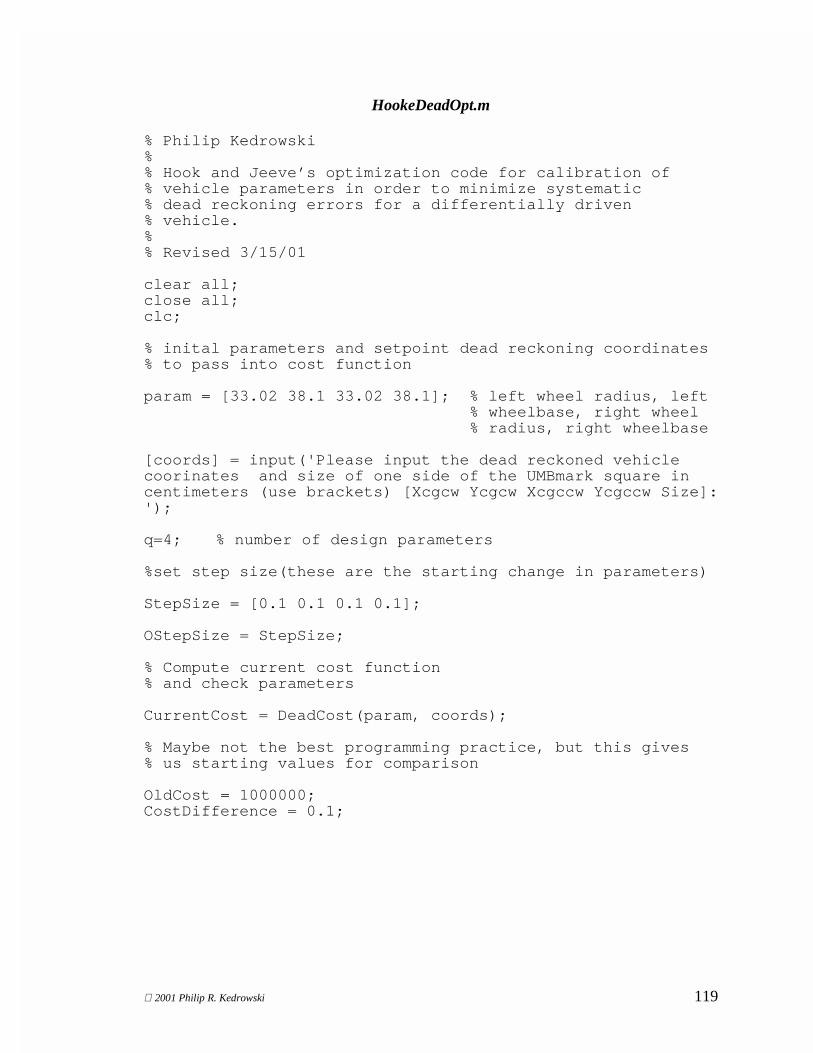
2001 Philip R. Kedrowski 119
HookeDeadOpt.m % Philip Kedrowski % % Hook and Jeeve’s optimization code for calibration of % vehicle parameters in order to minimize systematic % dead reckoning errors for a differentially driven % vehicle. % % Revised 3/15/01 clear all; close all; clc; % inital parameters and setpoint dead reckoning coordinates % to pass into cost function param = [33.02 38.1 33.02 38.1]; % left wheel radius, left % wheelbase, right wheel % radius, right wheelbase
[coords] = input('Please input the dead reckoned vehicle coorinates and size of one side of the UMBmark square in centimeters (use brackets) [Xcgcw Ycgcw Xcgccw Ycgccw Size]: '); q=4; % number of design parameters %set step size(these are the starting change in parameters) StepSize = [0.1 0.1 0.1 0.1]; OStepSize = StepSize; % Compute current cost function % and check parameters CurrentCost = DeadCost(param, coords); % Maybe not the best programming practice, but this gives % us starting values for comparison OldCost = 1000000; CostDifference = 0.1;

2001 Philip R. Kedrowski 120
HookeDeadOpt.m
StepCheck = [0.01 0.01 0.01 0.01]; iteration=0; % Start Optimization Loop using while loops % The comparison below is clever. It uses the OR command % to check to see if the cost is still improving and, at % the same time, checks to see of the if all of the steps % sizes are below their preset minimum while abs(OldCost-CurrentCost)>CostDifference|sum(StepCheck<StepSize)>0 newparam = param; OldCost = CurrentCost; % Exploratory Search, the steps have a magnitude (stepsize) % and a + or % - sense determined by the Direction vector. % During the exploratory loop below, the direction may also % be set to zero to indicate that neither a plus or a minus % step in that direction lowered the cost. Direction = [1 1 1 1]; % step in each direction and check for improvements (set % Direction(j)=0 is both directions fail) for j=1:q newparam(j) = param(j)+StepSize(j)*Direction(j); NewCost = DeadCost(newparam, coords); if NewCost > CurrentCost Direction(j) = -Direction(j); newparam(j) = param(j)+StepSize(j)*Direction(j); NewCost = DeadCost(newparam, coords); if NewCost > CurrentCost Direction(j) = 0; StepSize(j) = StepSize(j)/2; end end end

2001 Philip R. Kedrowski 121
HookeDeadOpt.m
% End of the Exploratory Search move = StepSize; % Start the Pattern Move newparam = param + StepSize.*Direction; newcost = DeadCost(newparam, coords); while newcost < CurrentCost param = param + move.*Direction; CurrentCost = newcost; move = move*1.25; newparam = param + move.*Direction; param; newcost = DeadCost(newparam, coords); end iteration=iteration+1 end param newcost

2001 Philip R. Kedrowski 122
DeadCost.m % Philip R. Kedrowski % % This is a function that integrates the vehicle position % based on commanded values for vehicle angular velocity % and velocity and the kinematic equations for a % differentially driven vehicle. It then uses the final % position after integrating through the UMBmark test % pattern to develop an objective function value that is % passed back to the Hooke and Jeeve's optimization % (HookeDeadOpt.m). % % Revised 3/15/01 function[OF] = DeadCost(param, coords) [L] = [param(1) param(2) param(3) param(4)]; % note, L = % [Leftwheelradius Leftwheelbase Rightwheelradius % Rightwheelbase] [C] = -[coords(1) coords(2) coords(3) coords(4)]; % note, % C = [Xcgcw, Ycgcw, Xcgccw, Ycgccw], Negative to adjust % vehicle correctly % initialize variables X = 0; Ang = 0; DPhi = 0; dx = 0; dy = 0; Xp(1) = 0; Yp(1) = 0; k = 1; n = 1; sample = 15; % sample every 15 time steps for plotting % (Plotting is for debugging and % visualization purposes, don't plot every % time) dt = 0.02; % time step (sec) Theta_a_dot = 1.515; % wheel a setpoint(rad/sec) Theta_b_dot = 1.515; % wheel b setpoint(rad/sec) Theta_adot = 0.15; % wheel a setpoint for right % turn (rad/sec)

2001 Philip R. Kedrowski 123
DeadCost.m
Theta_bdot = -0.15; % wheel b setpoint for right % turn (rad/sec) Command_distance = coords(5); % dimension of square for % UMBmark (centimeters) Command_angle = pi/2; % ninety degree turn %%%%%%%%%%SIMULATE CLOCKWISE DIRECTION%%%%%%%%%%%%%%%%%%%% % Now integrate course using given parameters while X < Command_distance, V = (L(1)*L(2)*Theta_a_dot + L(3)*L(4)*Theta_b_dot)/(L(2)+L(4));% kinematic equation % for vehicle velocity Phi_dot = (L(3)*Theta_b_dot - L(1)*Theta_a_dot)/(L(2)+L(4));% kinema % vehicle angular velocity DPhi = DPhi + Phi_dot*dt; % calculate heading dx = dx - V*sin(DPhi)*dt;% dead reckoned coords by % numerical integration dy = dy + V*cos(DPhi)*dt;% dead reckoned coords by % numerical integration X = X + V*dt; % distance traveled k=k+1; % sampling position data for plotting if k/sample == fix(k/sample) Xp(n)=dx; Yp(n)=dy; n=n+1; end end while abs(Ang) < Command_angle, % ninety degree zero % radius turn V = (L(1)*L(2)*Theta_adot + L(3)*L(4)*Theta_bdot)/(L(2)+L(4)); % kinematic equation for % vehicle velocity

2001 Philip R. Kedrowski 124
DeadCost.m
Phi_dot = (L(3)*Theta_bdot – L(1)*Theta_adot)/(L(2)+L(4)); % kinematic equation for % vehicle angular velocity DPhi = DPhi + Phi_dot*dt; % calculate heading dx = dx - V*sin(DPhi)*dt;% dead reckoned coords by % numerical integration dy = dy + V*cos(DPhi)*dt;% dead reckoned coords by % numerical integration Ang = Ang + Phi_dot*dt; % angle turned k=k+1; % sampling position data for plotting if k/sample == fix(k/sample) Xp(n)=dx; Yp(n)=dy; n=n+1; end end % Reset variables X = 0; while X < Command_distance, V = (L(1)*L(2)*Theta_adot + L(3)*L(4)*Theta_bdot)/(L(2)+L(4)); % kinematic equation for % vehicle velocity Phi_dot = (L(3)*Theta_bdot – L(1)*Theta_adot)/(L(2)+L(4)); % kinematic equation for % vehicle angular velocity DPhi = DPhi + Phi_dot*dt; % calculate heading dx = dx - V*sin(DPhi)*dt;% dead reckoned coords by % numerical integration dy = dy + V*cos(DPhi)*dt;% dead reckoned coords by % numerical integration

2001 Philip R. Kedrowski 125
DeadCost.m
X = X + V*dt; % distance traveled k=k+1; % sampling position data for plotting if k/sample == fix(k/sample) Xp(n)=dx; Yp(n)=dy; n=n+1; end end % Reset variables Ang = 0; while abs(Ang) < Command_angle, % ninety degree zero % radius turn V = (L(1)*L(2)*Theta_adot + L(3)*L(4)*Theta_bdot)/(L(2)+L(4)); % kinematic equation for % vehicle velocity Phi_dot = (L(3)*Theta_bdot – L(1)*Theta_adot)/(L(2)+L(4)); % kinematic equation for % vehicle angular velocity DPhi = DPhi + Phi_dot*dt; % calculate heading dx = dx - V*sin(DPhi)*dt;% dead reckoned coords by % numerical integration dy = dy + V*cos(DPhi)*dt;% dead reckoned coords by % numerical integration Ang = Ang + Phi_dot*dt; % angle turned k=k+1; % sampling position data for plotting if k/sample == fix(k/sample) Xp(n)=dx; Yp(n)=dy; n=n+1; end end % Reset variables X = 0;

2001 Philip R. Kedrowski 126
DeadCost.m
while X < Command_distance, V = (L(1)*L(2)*Theta_adot + L(3)*L(4)*Theta_bdot)/(L(2)+L(4)); % kinematic equation for % vehicle velocity Phi_dot = (L(3)*Theta_bdot – L(1)*Theta_adot)/(L(2)+L(4)); % kinematic equation for % vehicle angular velocity DPhi = DPhi + Phi_dot*dt; % calculate heading dx = dx - V*sin(DPhi)*dt;% dead reckoned coords by % numerical integration dy = dy + V*cos(DPhi)*dt;% dead reckoned coords by % numerical integration X = X + V*dt; % distance traveled k=k+1; % sampling position data for plotting if k/sample == fix(k/sample) Xp(n)=dx; Yp(n)=dy; n=n+1; end end % Reset variables Ang = 0; while abs(Ang) < Command_angle, % ninety degree zero % radius turn V = (L(1)*L(2)*Theta_adot + L(3)*L(4)*Theta_bdot)/(L(2)+L(4)); % kinematic equation for % vehicle velocity Phi_dot = (L(3)*Theta_bdot – L(1)*Theta_adot)/(L(2)+L(4)); % kinematic equation for % vehicle angular velocity DPhi = DPhi + Phi_dot*dt; % calculate heading dx = dx - V*sin(DPhi)*dt;% dead reckoned coords by % numerical integration

2001 Philip R. Kedrowski 127
DeadCost.m
dy = dy + V*cos(DPhi)*dt;% dead reckoned coords by % numerical integration Ang = Ang + Phi_dot*dt; % angle turned k=k+1; % sampling position data for plotting if k/sample == fix(k/sample) Xp(n)=dx; Yp(n)=dy; n=n+1; end end % Reset variables X = 0; while X < Command_distance, V = (L(1)*L(2)*Theta_adot + L(3)*L(4)*Theta_bdot)/(L(2)+L(4)); % kinematic equation for % vehicle velocity Phi_dot = (L(3)*Theta_bdot – L(1)*Theta_adot)/(L(2)+L(4)); % kinematic equation for % vehicle angular velocity DPhi = DPhi + Phi_dot*dt; % calculate heading dx = dx - V*sin(DPhi)*dt;% dead reckoned coords by % numerical integration dy = dy + V*cos(DPhi)*dt;% dead reckoned coords by % numerical integration X = X + V*dt; % distance traveled k=k+1; % sampling position data for plotting if k/sample == fix(k/sample) Xp(n)=dx; Yp(n)=dy; n=n+1; end end

2001 Philip R. Kedrowski 128
DeadCost.m
% Reset variables Ang = 0; while abs(Ang) < Command_angle, % ninety degree zero % radius turn V = (L(1)*L(2)*Theta_adot + L(3)*L(4)*Theta_bdot)/(L(2)+L(4)); % kinematic equation for % vehicle velocity Phi_dot = (L(3)*Theta_bdot – L(1)*Theta_adot)/(L(2)+L(4)); % kinematic equation for % vehicle angular velocity DPhi = DPhi + Phi_dot*dt; % calculate heading dx = dx - V*sin(DPhi)*dt;% dead reckoned coords by % numerical integration dy = dy + V*cos(DPhi)*dt;% dead reckoned coords by % numerical integration Ang = Ang + Phi_dot*dt; % angle turned k=k+1; % sampling position data for plotting if k/sample == fix(k/sample) Xp(n)=dx; Yp(n)=dy; n=n+1; end end figure(1); % plot vehicle position for % clockwise direction plot(Xp,Yp) % compute objective functions for clockwise direction OFXcgcw = (C(1) - dx); OFYcgcw = (C(2) - dy); %%%%%%%%%%HERE SIMULATE COUNTER CLOCKWISE DIRECTION%%%%%%%% % initialize variables X = 0;

2001 Philip R. Kedrowski 129
DeadCost.m
Ang = 0; DPhi = 0; dx = 0; dy = 0; Xp2(1) = 0; Yp2(1) = 0; k = 1; n = 1; Theta_adot = -0.15; % wheel a setpoint for left turn % (rad/sec) Theta_bdot = 0.15; % wheel b setpoint for left turn % (rad/sec) % Now integrate course using given parameters while X < Command_distance, V = (L(1)*L(2)*Theta_a_dot + L(3)*L(4)*Theta_b_dot)/(L(2)+L(4));% kinematic equation % for vehicle velocity Phi_dot = (L(3)*Theta_b_dot - L(1)*Theta_a_dot)/(L(2)+L(4));% kinema % vehicle angular velocity DPhi = DPhi + Phi_dot*dt; % calculate heading dx = dx - V*sin(DPhi)*dt;% dead reckoned coords by % numerical integration dy = dy + V*cos(DPhi)*dt;% dead reckoned coords by % numerical integration X = X + V*dt; % distance traveled k=k+1; % sampling position data for plotting if k/sample == fix(k/sample) Xp2(n)=dx; Yp2(n)=dy; n=n+1; end end while abs(Ang) < Command_angle, % ninety degree zero

2001 Philip R. Kedrowski 130
DeadCost.m
% radius turn V = (L(1)*L(2)*Theta_adot + L(3)*L(4)*Theta_bdot)/(L(2)+L(4)); % kinematic equation for % vehicle velocity Phi_dot = (L(3)*Theta_bdot – L(1)*Theta_adot)/(L(2)+L(4)); % kinematic equation for % vehicle angular velocity DPhi = DPhi + Phi_dot*dt; % calculate heading dx = dx - V*sin(DPhi)*dt;% dead reckoned coords by % numerical integration dy = dy + V*cos(DPhi)*dt;% dead reckoned coords by % numerical integration Ang = Ang + Phi_dot*dt; % angle turned k=k+1; % sampling position data for plotting if k/sample == fix(k/sample) Xp2(n)=dx; Yp2(n)=dy; n=n+1; end end % Reset variables X = 0; while X < Command_distance, V = (L(1)*L(2)*Theta_adot + L(3)*L(4)*Theta_bdot)/(L(2)+L(4)); % kinematic equation for % vehicle velocity Phi_dot = (L(3)*Theta_bdot – L(1)*Theta_adot)/(L(2)+L(4)); % kinematic equation for % vehicle angular velocity DPhi = DPhi + Phi_dot*dt; % calculate heading

2001 Philip R. Kedrowski 131
DeadCost.m
dx = dx - V*sin(DPhi)*dt;% dead reckoned coords by % numerical integration dy = dy + V*cos(DPhi)*dt;% dead reckoned coords by % numerical integration X = X + V*dt; % distance traveled k=k+1; % sampling position data for plotting if k/sample == fix(k/sample) Xp2(n)=dx; Yp2(n)=dy; n=n+1; end end % Reset variables Ang = 0; while abs(Ang) < Command_angle, % ninety degree zero % radius turn V = (L(1)*L(2)*Theta_adot + L(3)*L(4)*Theta_bdot)/(L(2)+L(4)); % kinematic equation for % vehicle velocity Phi_dot = (L(3)*Theta_bdot – L(1)*Theta_adot)/(L(2)+L(4)); % kinematic equation for % vehicle angular velocity DPhi = DPhi + Phi_dot*dt; % calculate heading dx = dx - V*sin(DPhi)*dt;% dead reckoned coords by % numerical integration dy = dy + V*cos(DPhi)*dt;% dead reckoned coords by % numerical integration Ang = Ang + Phi_dot*dt; % angle turned k=k+1; % sampling position data for plotting if k/sample == fix(k/sample) Xp2(n)=dx; Yp2(n)=dy;

2001 Philip R. Kedrowski 132
DeadCost.m
n=n+1; end end % Reset variables X = 0; while X < Command_distance, V = (L(1)*L(2)*Theta_adot + L(3)*L(4)*Theta_bdot)/(L(2)+L(4)); % kinematic equation for % vehicle velocity Phi_dot = (L(3)*Theta_bdot – L(1)*Theta_adot)/(L(2)+L(4)); % kinematic equation for % vehicle angular velocity DPhi = DPhi + Phi_dot*dt; % calculate heading dx = dx - V*sin(DPhi)*dt;% dead reckoned coords by % numerical integration dy = dy + V*cos(DPhi)*dt;% dead reckoned coords by % numerical integration X = X + V*dt; % distance traveled k=k+1; % sampling position data for plotting if k/sample == fix(k/sample) Xp2(n)=dx; Yp2(n)=dy; n=n+1; end end % Reset variables Ang = 0; while abs(Ang) < Command_angle, % ninety degree zero % radius turn V = (L(1)*L(2)*Theta_adot + L(3)*L(4)*Theta_bdot)/(L(2)+L(4)); % kinematic equation for
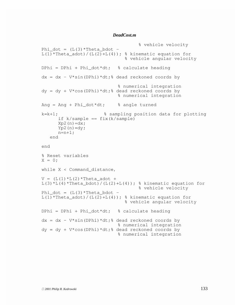
2001 Philip R. Kedrowski 133
DeadCost.m
% vehicle velocity Phi_dot = (L(3)*Theta_bdot – L(1)*Theta_adot)/(L(2)+L(4)); % kinematic equation for % vehicle angular velocity DPhi = DPhi + Phi_dot*dt; % calculate heading dx = dx - V*sin(DPhi)*dt;% dead reckoned coords by % numerical integration dy = dy + V*cos(DPhi)*dt;% dead reckoned coords by % numerical integration Ang = Ang + Phi_dot*dt; % angle turned k=k+1; % sampling position data for plotting if k/sample == fix(k/sample) Xp2(n)=dx; Yp2(n)=dy; n=n+1; end end % Reset variables X = 0; while X < Command_distance, V = (L(1)*L(2)*Theta_adot + L(3)*L(4)*Theta_bdot)/(L(2)+L(4)); % kinematic equation for % vehicle velocity Phi_dot = (L(3)*Theta_bdot – L(1)*Theta_adot)/(L(2)+L(4)); % kinematic equation for % vehicle angular velocity DPhi = DPhi + Phi_dot*dt; % calculate heading dx = dx - V*sin(DPhi)*dt;% dead reckoned coords by % numerical integration dy = dy + V*cos(DPhi)*dt;% dead reckoned coords by % numerical integration

2001 Philip R. Kedrowski 134
DeadCost.m
X = X + V*dt; % distance traveled k=k+1; % sampling position data for plotting if k/sample == fix(k/sample) Xp2(n)=dx; Yp2(n)=dy; n=n+1; end end % Reset variables Ang = 0; while abs(Ang) < Command_angle, % ninety degree zero % radius turn V = (L(1)*L(2)*Theta_adot + L(3)*L(4)*Theta_bdot)/(L(2)+L(4)); % kinematic equation for % vehicle velocity Phi_dot = (L(3)*Theta_bdot – L(1)*Theta_adot)/(L(2)+L(4)); % kinematic equation for % vehicle angular velocity DPhi = DPhi + Phi_dot*dt; % calculate heading dx = dx - V*sin(DPhi)*dt;% dead reckoned coords by % numerical integration dy = dy + V*cos(DPhi)*dt;% dead reckoned coords by % numerical integration Ang = Ang + Phi_dot*dt; % angle turned k=k+1; % sampling position data for plotting if k/sample == fix(k/sample) Xp2(n)=dx; Yp2(n)=dy; n=n+1; end end hold on;

2001 Philip R. Kedrowski 135
DeadCost.m plot(Xp2,Yp2) xlabel('X (cm)'); ylabel('Y (cm)'); axis([-350 350 -50 480]); %Compute objective functions for counterclockwise direction OFXcgccw = (C(3) - dx); OFYcgccw = (C(4) - dy); %compute total objective function
OF = ((OFXcgcw)^2 + (OFYcgcw)^2)^0.5 + ((OFXcgccw)^2 + (OFYcgccw)^2)^0.5

2001 Philip R. Kedrowski 136
Appendix C
UMBmark Test Data

2001 Philip R. Kedrowski 137
Philip R. Kedrowski
Implementation of Optimization for Increased Dead Reckoning Accuracy
2/19/2001
Initial parameters Parameters optimized using three yard square
Wheel Base A = 38.1 cm Wheel Base A = 38.58 cm
Wheel Base B = 38.1 cm Wheel Base B = 38.53 cm
Wheel Radius A = 33.02 cm Wheel Radius A = 32.72 cm
Wheel Radius B = 33.02 cm Wheel Radius B = 33.37 cm
Three yard square
Xcgcw Ycgcw Error_cw % Error Reduction Xcgccw Ycgccw Error_ccw % Error Reduction
-44.2 93.5 103.4 -22.5 -20.9 30.7
Xcgcw_opt Ycgcw_opt 61.6 Xcgccw_opt Ycgccw_opt 73.3
-27.8 28.4 39.7 6.8 4.6 8.2
Total Error % Total Error Reduction
No Calibration = 134.1 64.3
With Calibration = 48.0
Parameters optimized using six yard square
Wheel Base A = 41.0 cm
Wheel Base B = 41.04 cm
Wheel Radius A = 35.24 cm
Wheel Radius B = 35.88 cm
Six yard square
Xcgcw Ycgcw Error_cw % Error Reduction Xcgccw Ycgccw Error_cw % Error Reduction
-104.1 325.6 341.8 -231.4 -107.4 255.1
Xcgcw_opt Ycgcw_opt 38.8 Xcgccw_opt Ycgccw_opt 89.8
-105.7 180.5 209.2 -20.6 -15.8 26.0
Total Error % Total Error Reduction
No Calibration = 596.9 60.6
With Calibration = 235.1

2001 Philip R. Kedrowski 138
2/20/2001
Here testing whether it is better to optimize using a six yard square or whether it doesn't matter.
Parameters optimized using three yard square
Wheel Base A =38.86 cm
Wheel Base B =38.29 cm Average Percent Reduction of Dead Reckoning Errors When Calibrated on 3yrd =
Wheel Radius A =32.99 cm
Wheel Radius B =33.67 cm
Three yard square
Xcgcw YcgcwError_cw % Error Reduction Xcgccw Ycgccw Error_cw % Error Reduction
-46.3 91.6 102.6 -27.1 -17.5 32.3
Xcgcw_opt Ycgcw_opt 45.7 Xcgccw_opt Ycgccw_opt 28.5
-31.5 46 55.8 19.5 12.3 23.1
Total Error % Total Error Reduction
No Calibration = 134.9 41.6
With Calibration = 78.8
Six yard square
Xcgcw YcgcwError_cw % Error Reduction Xcgccw Ycgccw Error_cw % Error Reduction
-95.3 347.3 360.1 -224.6 -110.8 250.4
Xcgcw_opt Ycgcw_opt 55.3 Xcgccw_opt Ycgccw_opt 95.3
-85.5 136.2 160.8 -2.1 -11.6 11.8
Total Error % Total Error Reduction
No Calibration = 610.6 71.7
With Calibration = 172.6
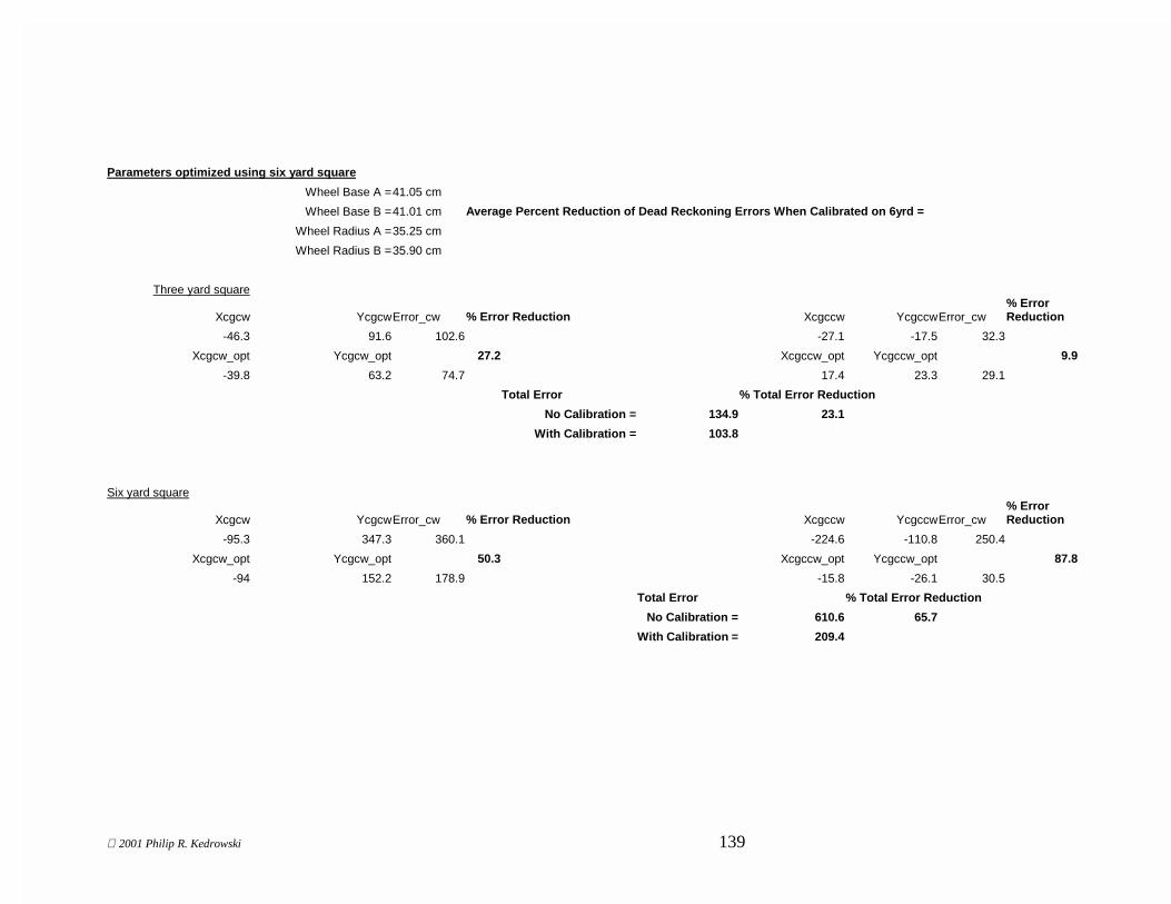
2001 Philip R. Kedrowski 139
Parameters optimized using six yard square
Wheel Base A = 41.05 cm
Wheel Base B = 41.01 cm Average Percent Reduction of Dead Reckoning Errors When Calibrated on 6yrd =
Wheel Radius A = 35.25 cm
Wheel Radius B = 35.90 cm
Three yard square
Xcgcw YcgcwError_cw % Error Reduction Xcgccw Ycgccw Error_cw % Error Reduction
-46.3 91.6 102.6 -27.1 -17.5 32.3
Xcgcw_opt Ycgcw_opt 27.2 Xcgccw_opt Ycgccw_opt 9.9
-39.8 63.2 74.7 17.4 23.3 29.1
Total Error % Total Error Reduction
No Calibration = 134.9 23.1
With Calibration = 103.8
Six yard square
Xcgcw YcgcwError_cw % Error Reduction Xcgccw Ycgccw Error_cw % Error Reduction
-95.3 347.3 360.1 -224.6 -110.8 250.4
Xcgcw_opt Ycgcw_opt 50.3 Xcgccw_opt Ycgccw_opt 87.8
-94 152.2 178.9 -15.8 -26.1 30.5
Total Error % Total Error Reduction
No Calibration = 610.6 65.7
With Calibration = 209.4

2001 Philip R. Kedrowski 140
Vita
Philip Redleaf Kedrowski was born on 17 October 1975 to Thomas J. Kedrowski
and Sharon A. Tate in a tipi in the Rocky Mountains near Crested Butte, CO. Philip grew
up in Colorado and graduated from Bayfield High School in 1994. He then studied at
Fort Lewis College in Durango, CO for two years before transferring to Colorado State
University. While at CSU, Philip interned one summer at a gold processing plant in
Pocone, Brazil. He obtained his Bachelor of Science Degree in Mechanical Engineering
in May of 1999. Upon graduation, Philip spent the summer in Alaska climbing on Denali
and started his graduate work at Virginia Polytechnic Institute and State University that
fall. He graduated with a Master of Science Degree in Mechanical Engineering in May
of 2001. Philip took the following summer off to help his mother build a log home
before starting his career as a Controls Engineer in the Engines and Systems division of
Honeywell, Phoenix, AZ.
Philip is a member of the Pi Tau Sigma Mechanical Engineering Honor Society.
Philip has taken the oath of The Order of the Engineer.