Embed Size (px)
Citation preview

Development and Implementation of a Water Quality Monitoring Plan to Support
the Creation of a Geographic Information System to Assess Water Quality
Conditions of Rivers in the State of Veracruz in Mexico
Miguel A. Medina
A project submitted to the faculty of Brigham Young University
in partial fulfillment of the requirements for the degree of
Master of Science
E. James Nelson, Chair Gustavious P. Williams
Rollin H. Hotchkiss A. Woodruff Miller
Department of Civil and Environmental Engineering
Brigham Young University
December 2011
Copyright © 2011 Miguel A. Medina
All Rights Reserved


ABSTRACT
Development and Implementation of a Water Quality Monitoring Plan to Support the Creation of a Geographic Information System to Assess Water Quality
Conditions of Rivers in the State of Veracruz in Mexico
Miguel A. Medina Department of Civil and Environmental Engineering, BYU
Master of Science
Geographic information has always played a crucial role in the decision making process of many fields because the visual nature of the information adds important understanding that translates into better decision making. A Geographic Information System (GIS) integrates computer software and data to visualize, understand, and use information in many ways. A GIS stores many different types of information, including environmental and water quality information. Regardless of what type of information is to be used within a GIS, the information must be properly gathered using a systematic approach.
For this project, a water quality monitoring plan was developed and implemented at the
University of Veracruz (UV) to collect water quality data to assist the creation of a GIS. This GIS will support the decision making process in environmental concerns at a watershed level for some of the main rivers in the state of Veracruz in Mexico. This GIS will also serve as a tool to monitor and evaluate river conditions over time and at different locations, determine sources of contamination, identify solutions to mitigate effects of contamination, and to present the results to interest groups.
This plan considered the acquisition of water quality monitoring equipment, training of a
group of environmental engineering students, and determining monitoring points along the rivers and the logistics accompanying monitoring at those points. The water quality data that was produced as a result of this project can be used as input data for a GIS, and will also be a source of information for other environmental and water resources agencies. Furthermore, this plan played and will continue playing an important role in educating environmental engineering students at the UV who will learn and benefit from this project.
The plan was successfully implemented at the UV and it included a set of methodologies
and guidelines to standardize the work to be performed by the students. It also made a very positive impact as it stimulated the interest of students and faculty to continue working on this project and in other similar projects in the long run.
Keywords: geographic information systems, decision support system, input data, water quality data, CONAGUA, CIATEJ, UV, monitoring points, monitoring plan, water quality parameters.

ACKNOWLEDGMENTS
This work and the opportunity I had to be part of it would not have been possible without
the help and support of my professor and advisor, Dr. E. James Nelson. I thank him for helping
open doors for me and for the development of this project, for his guidance, for trusting me, and
for his concern in water resources-related projects in developing countries.
I thank the Mosaic Foundation and the CEEN Department at BYU for their interest in
water resources-related projects and for providing the funds needed to purchase the equipment
for this project.
I thank my friend and colleague Dr. Gustavo Davila, researcher at CIATEJ, for the data
provided for this project, for the equipment and laboratory supplies donated, and for his
continuous support during the development of the project. I thank Dr. Miguel Morales, professor
at the University of Veracruz (UV), for being the link between BYU-CIATEJ and the UV, and
for his overall invaluable help and support at the UV. I also thank the amazing group of students
and professors at the UV who have been involved directly or indirectly in this project for
providing invaluable help and support during its implementation; without them, this project
would not have been possible.
I thank my parents for everything they do and have done for me, and for their
unconditional support. And last but not least, I thank God, knowing that words would never be
enough to express my gratitude.


v
TABLE OF CONTENTS
LIST OF TABLES ...................................................................................................................... vii
LIST OF FIGURES ..................................................................................................................... ix
1 Introduction ........................................................................................................................... 1
2 Geographic Information Systems (GIS) ............................................................................. 3
2.1 Importance of Geographic Information .......................................................................... 3
2.1.1 Components of a Geographic Information System ..................................................... 4
2.2 Applications of GIS ........................................................................................................ 5
2.3 Applications of GIS in Mexico ....................................................................................... 6
2.4 Applications of GIS in the Area of Study: Veracruz, Mexico ........................................ 7
2.4.1 Creation of a GIS-Based Decision Support System in the Area of Study .................. 7
3 Water Quality ........................................................................................................................ 9
3.1 Importance of Monitoring Water Quality ....................................................................... 9
3.2 Available Water Quality Data ....................................................................................... 11
3.3 Water Quality Index ...................................................................................................... 12
4 Methodology ........................................................................................................................ 17
4.1 The Need for a Systematic Plan .................................................................................... 17
4.2 Monitoring Points ......................................................................................................... 18
4.2.1 Location of Monitoring Points .................................................................................. 18
4.3 Water Quality Monitoring Equipment .......................................................................... 21
4.3.1 List and Description of the Equipment ..................................................................... 22
4.3.2 Operating Expenses .................................................................................................. 22
4.4 Training ......................................................................................................................... 25
4.5 Field and Laboratory Work ........................................................................................... 28

vi
4.5.1 Field Work and Logistics .......................................................................................... 28
4.5.2 Data Collection ......................................................................................................... 31
5 Data Analysis and Processing ............................................................................................ 35
5.1 Pre-Processing and Post-Processing ............................................................................. 35
5.2 Discussion of Results .................................................................................................... 35
5.3 Further Use of Data ....................................................................................................... 37
6 Academic Impact and Future Goals ................................................................................. 39
6.1 Continuity of the Project and Improvements ................................................................ 39
7 Conclusion ........................................................................................................................... 41
REFERENCES ............................................................................................................................ 43
Appendix A. Results Reported by the UV for the Tecolutla River ..................................... 45
Appendix B. Results Reported by the UV for the Cazones River ....................................... 91
Appendix C. Results Reported by the UV for the Tuxpan River ...................................... 121
Appendix D. Comparison of Results at Puente Alamo – Alamo Jugeras ......................... 137
Appendix E. Comparison of Results at Puente Alamo – Alamo ....................................... 143
Appendix F. Comparison of Results at Villa Lazaro Cardenas – Lazaro Cardenas ...... 149
vii
LIST OF TABLES
Table 3–1: Maximum Allowable Limits for Contaminants ...............................................10
Table 4–1: CONAGUA’s Monitoring Points ....................................................................19
Table 4–2: UV’s Monitoring Points ...................................................................................19
Table 4–3: Water Quality Monitoring Equipment for this Project .....................................23
Table 4–4: Template Used to Record the Results ..............................................................33
Table A–1: Results Reported by the UV for Puente Progreso de Zaragoza .......................45
Table A–2: Results Reported by the UV for Puente Las Lomas ........................................50
Table A–3: Results Reported by the UV for Puente Oriente Medio Dia ............................55
Table A–4: Results Reported by the UV for El Espinal .....................................................60
Table A–5: Results Reported by the UV for Bado San Gotardo ........................................65
Table A–6: Results Reported by the UV for Puente El Remolino .....................................70
Table A–7: Results Reported by the UV for Puente Tecolutla Entrada a Gtz Zamora ......75
Table A–8: Results Reported by the UV for Salida de Gutierrez Zamora .........................80
Table A–9: Results Reported by the UV for Bocana de Tecolutla .....................................85
Table B–1: Results Reported by the UV for San Marcos ...................................................91
Table B–2: Results Reported by the UV for Villa Lazaro Cardenas (La Uno) ..................96
Table B–3: Results Reported by the UV for Bocatoma ......................................................101
Table B–4: Results Reported by the UV for Puente Cazones 3 .........................................106
Table B–5: Results Reported by the UV for Puente Colgante ............................................111
Table B–6: Results Reported by the UV for Panga ............................................................116
Table C–1: Results Reported by the UV for Puente Alamo ...............................................121
Table C–2: Results Reported by the UV for Jardines de Tuxpan Residencial (Tuxpan 1) .......................................................................................................126
viii
Table C–3: Results Reported by the UV for Parque Ribereño (Tuxpan 2) ........................131
Table D–1: Comparison of Results at Puente Alamo – Alamo Jugureas ...........................137
Table E–1: Comparison of Results at Alamo – Puente Alamo ...........................................143
Table F–1: Comparison of Results at Lazaro Cardenas – Villa Lazaro Cardenas.............149

ix
LIST OF FIGURES
Figure 3–1: Cover Page of Documents Received from CONAGUA ..............................11
Figure 3–2: WQI for the Tuxpan River in 2003 ..............................................................13
Figure 3–3: Variations in the WQI for the Tuxpan River ................................................13
Figure 3–4: WQI for the Cazones River in 1999 .............................................................14
Figure 3–5: Variations in the WQI for the Cazones River ..............................................14
Figure 3–6: WQI for the Tecolutla River in 2002 ...........................................................15
Figure 3–7: Variations in the WQI for the Tecolutla River .............................................15
Figure 4–1: Monitoring Points in the Cazones River ......................................................20
Figure 4–2: Monitoring Points in the Tuxpan River ........................................................20
Figure 4–3: Monitoring Points in the Tecolutla River .....................................................21
Figure 4–4: HI 98185 Multiparameter Meter and Electrodes; Similar to the 98186 and 98188 .....................................................................................................24
Figure 4–5: Phosphate Meter and Turbidity Meter .........................................................24
Figure 4–6: Training Students in March 2010 .................................................................26
Figure 4–7: Training New Students in October 2011 ......................................................27
Figure 4–8: Styrofoam and Glass Bottles to Transport Samples to the Lab ....................29
Figure 4–9: A Student Bringing Water from the River ...................................................30
Figure 4–10: Students Working in the Field ......................................................................31
Figure 5–1: Comparison of DO Content for the Puente Alamo and Alamo Monitoring Points .........................................................................................37
Figure A–1: Temperature at Puente Progreso de Zaragoza ..............................................46
Figure A–2: TDS at Puente Progreso de Zaragoza ...........................................................46
Figure A–3: Turbidity at Puente Progreso de Zaragoza ...................................................46
Figure A–4: Resistivity at Puente Progreso de Zaragoza .................................................46

x
Figure A–5: Salinity at Puente Progreso de Zaragoza ......................................................47
Figure A–6: ORP at Puente Progreso de Zaragoza ...........................................................47
Figure A–7: Conductivity at Puente Progreso de Zaragoza ..............................................47
Figure A–8: pH at Puente Progreso de Zaragoza ..............................................................47
Figure A–9: Sulfates at Puente Progrezo de Zaragoza .....................................................48
Figure A–10: Chlorides at Puente Progreso de Zaragoza ...................................................48
Figure A–11: Phosphates at Puente Progreso de Zaragoza ................................................48
Figure A–12: Ammonia Nitrogen at Puente Progreso de Zaragoza ...................................48
Figure A–13: Nitrate Nitrogen at Puente Progreso de Zaragoza ........................................49
Figure A–14: Dissolved Oxygen at Puente Progreso de Zaragoza .....................................49
Figure A–15: BOD at Puente Progreso de Zaragoza ..........................................................49
Figure A–16: Temperature at Puente Las Lomas ...............................................................51
Figure A–17: TDS at Puente Las Lomas ............................................................................51
Figure A–18: Turbidity at Puente Las Lomas.....................................................................51
Figure A–19: Resistivity at Puente Las Lomas...................................................................51
Figure A–20: Salinity at Puente Las Lomas .......................................................................52
Figure A–21: ORP at Puente Las Lomas ............................................................................52
Figure A–22: Conductivity at Puente Las Lomas ...............................................................52
Figure A–23: pH at Puente Las Lomas ...............................................................................52
Figure A–24: Sulfates at Puente Las Lomas .......................................................................53
Figure A–25: Chlorides at Puente Las Lomas ....................................................................53
Figure A–26: Phosphates at Puente Las Lomas ..................................................................53
Figure A–27: Ammonia Nitrogen at Puente Las Lomas ....................................................53
Figure A–28: Nitrate Nitrogen at Puente Las Lomas .........................................................54
Figure A–29: Dissolved Oxygen at Puente Las Lomas ......................................................54

xi
Figure A–30: BOD at Puente Las Lomas ...........................................................................54
Figure A–31: Temperature at Puente Oriente Medio Dia ...................................................56
Figure A–32: TDS at Puente Oriente Medio Dia................................................................56
Figure A–33: Turbidity at Puente Oriente Medio Dia ........................................................56
Figure A–34: Resistivity at Puente Oriente Medio Dia ......................................................56
Figure A–35: Salinity at Puente Oriente Medio Dia ...........................................................57
Figure A–36: ORP at Puente Oriente Medio Dia ...............................................................57
Figure A–37: Conductivity at Puente Oriente Medio Dia ..................................................57
Figure A–38: pH at Puente Oriente Medio Dia ..................................................................57
Figure A–39: Sulfates at Puente Oriente Medio Dia ..........................................................58
Figure A–40: Chlorides at Puente Oriente Medio Dia ........................................................58
Figure A–41: Phosphates at Puente Oriente Medio Dia .....................................................58
Figure A–42: Ammonia Nitrogen at Puente Oriente Medio Dia ........................................58
Figure A–43: Nitrate Nitrogen at Puente Oriente Medio Dia .............................................59
Figure A–44: Dissolved Oxygen at Puente Oriente Medio Dia .........................................59
Figure A–45: BOD at Puente Oriente Medio Dia ...............................................................59
Figure A–46: Temperature at El Espinal ............................................................................61
Figure A–47: TDS at El Espinal .........................................................................................61
Figure A–48: Turbidity at El Espinal..................................................................................61
Figure A–49: Resistivity at El Espinal................................................................................61
Figure A–50: Salinity at El Espinal ....................................................................................62
Figure A–51: ORP at El Espinal .........................................................................................62
Figure A–52: Conductivity at El Espinal ............................................................................62
Figure A–53: pH at El Espinal ............................................................................................62
Figure A–54: Sulfates at El Espinal ....................................................................................63

xii
Figure A–55: Chlorides at El Espinal .................................................................................63
Figure A–56: Phosphates at El Espinal ...............................................................................63
Figure A–57: Ammonia Nitrogen at El Espinal .................................................................63
Figure A–58: Nitrate Nitrogen at El Espinal ......................................................................64
Figure A–59: Dissolved Oxygen at El Espinal ...................................................................64
Figure A–60: BOD at El Espinal ........................................................................................64
Figure A–61: Temperature at Bado San Gotardo ...............................................................66
Figure A–62: TDS at Bado San Gotardo ............................................................................66
Figure A–63: Turbidity at Bado San Gotardo .....................................................................66
Figure A–64: Resistivity at Bado San Gotardo ...................................................................66
Figure A–65: Salinity at Bado San Gotardo .......................................................................67
Figure A–66: ORP at Bado San Gotardo ............................................................................67
Figure A–67: Conductivity at Bado San Gotardo ...............................................................67
Figure A–68: pH at Bado San Gotardo ...............................................................................67
Figure A–69: Sulfates at Bado San Gotardo .......................................................................68
Figure A–70: Chlorides at Bado San Gotardo ....................................................................68
Figure A–71: Phosphates at Bado San Gotardo ..................................................................68
Figure A–72: Ammonia Nitrogen at Bado San Gotardo ....................................................68
Figure A–73: Nitrate Nitrogen at Bado San Gotardo .........................................................69
Figure A–74: Dissolved Oxygen at Bado San Gotardo ......................................................69
Figure A–75: BOD at Bado San Gotardo ...........................................................................69
Figure A–76: Temperature at Puente El Remolino .............................................................71
Figure A–77: TDS at Puente El Remolino .........................................................................71
Figure A–78: Turbidity at Puente El Remolino ..................................................................71
Figure A–79: Resistivity at Puente El Remolino ................................................................71

xiii
Figure A–80: Salinity at Puente El Remolino ....................................................................72
Figure A–81: ORP at Puente El Remolino .........................................................................72
Figure A–82: Conductivity at Puente El Remolino ............................................................72
Figure A–83: pH at Puente El Remolino ............................................................................72
Figure A–84: Sulfates at Puente El Remolino ....................................................................73
Figure A–85: Chlorides at Puente El Remolino .................................................................73
Figure A–86: Phosphates at Puente El Remolino ...............................................................73
Figure A–87: Ammonia Nitrogen at Puente El Remolino ..................................................73
Figure A–88: Nitrate Nitrogen at Puente El Remolino .......................................................74
Figure A–89: Dissolved Oxygen at Puente El Remolino ...................................................74
Figure A–90: BOD at Puente El Remolino .........................................................................74
Figure A–91: Temperature at Puente Tecolutla-Gutierrez Zam .........................................76
Figure A–92: TDS at Puente Tecolutla-Gutierrez Zam ......................................................76
Figure A–93: Turbidity at Puente Tecolutla-Gutierrez Zam ..............................................76
Figure A–94: Resistivity at Puente Tecolutla-Gutierrez Zam ............................................76
Figure A–95: Salinity at Puente Tecolutla-Gutierrez Zam .................................................77
Figure A–96: ORP at Puente Tecolutla-Gutierrez Zam ......................................................77
Figure A–97: Conductivity at Puente Tecolutla-Gutierrez Zam.........................................77
Figure A–98: pH at Puente Tecolutla-Gutierrez Zam .........................................................77
Figure A–99: Sulfates at Puente Tecolutla-Gutierrez Zam .................................................78
Figure A–100: Chlorides at Puente Tecolutla-Gutierrez Zam ..............................................78
Figure A–101: Phosphates at Puente Tecolutla-Gutierrez Zam ...........................................78
Figure A–102: Ammonia Nitrogen at Puente Tecolutla-Gutierrez Zam ..............................78
Figure A–103: Nitrate Nitrogen at Puente Tecolutla-Gutierrez Zam ...................................79
Figure A–104: Dissolved Oxygen at Puente Tecolutla-Gutierrez Zam ................................79

xiv
Figure A–105: BOD at Puente Tecolutla-Gutierrez Zam .....................................................79
Figure A–106: Temperature at Salida de Gutierrez Zamora ................................................81
Figure A–107: TDS at Salida de Gutierrez Zamora .............................................................81
Figure A–108: Turbidity at Salida de Gutierrez Zamora ......................................................81
Figure A–109: Resistivity at Salida de Gutierrez Zamora ....................................................81
Figure A–110: Salinity at Salida de Gutierrez Zamora ........................................................82
Figure A–111: ORP at Salida de Gutierrez Zamora .............................................................82
Figure A–112: Conductivity at Salida de Gutierrez Zamora ................................................82
Figure A–113: pH at Salida de Gutierrez Zamora ................................................................82
Figure A–114: Sulfates at Salida de Gutierrez Zamora ........................................................83
Figure A–115: Chlorides at Salida de Gutierrez Zamora .....................................................83
Figure A–116: Phosphates at Salida de Gutierrez Zamora ...................................................83
Figure A–117: Ammonia Nitrogen at Salida de Gutierrez Zamora ......................................83
Figure A–118: Nitrate Nitrogen at Salida de Gutierrez Zamora ...........................................84
Figure A–119: Dissolved Oxygen at Salida de Gutierrez Zamora .......................................84
Figure A–120: BOD at Salida de Gutierrez Zamora ............................................................84
Figure A–121: Temperature at Bocana de Tecolutla ............................................................86
Figure A–122: TDS at Bocana de Tecolutla .........................................................................86
Figure A–123: Turbidity at Bocana de Tecolutla .................................................................86
Figure A–124: Resistivity at Bocana de Tecolutla ...............................................................86
Figure A–125: Salinity at Bocana de Tecolutla ....................................................................87
Figure A–126: ORP at Bocana de Tecolutla .........................................................................87
Figure A–127: Conductivity at Bocana de Tecolutla ...........................................................87
Figure A–128: pH at Bocana de Tecolutla ...........................................................................87
Figure A–129: Sulfates at Bocana de Tecolutla ...................................................................88
xv
Figure A–130: Chlorides at Bocana de Tecolutla .................................................................88
Figure A–131: Phosphates at Bocana de Tecolutla ..............................................................88
Figure A–132: Ammonia Nitrogen at Bocana de Tecolutla .................................................88
Figure A–133: Nitrate Nitrogen at Bocana de Tecolutla ......................................................89
Figure A–134: Dissolved Oxygen at Bocana de Tecolutla ...................................................89
Figure A–135: BOD at Bocana de Tecolutla ........................................................................89
Figure B–1: Temperature at San Marcos ..........................................................................92
Figure B–2: TDS at San Marcos .......................................................................................92
Figure B–3: Turbidity at San Marcos ...............................................................................92
Figure B–4: Resistivity at San Marcos .............................................................................92
Figure B–5: Salinity at San Marcos ..................................................................................93
Figure B–6: ORP at San Marcos .......................................................................................93
Figure B–7: Conductivity at San Marcos ..........................................................................93
Figure B–8: pH at San Marcos..........................................................................................93
Figure B–9: Sulfates at San Marcos ..................................................................................94
Figure B–10: Chlorides at San Marcos ...............................................................................94
Figure B–11: Phosphates at San Marcos ............................................................................94
Figure B–12: Ammonia Nitrogen at San Marcos ...............................................................94
Figure B–13: Nitrate Nitrogen at San Marcos ....................................................................95
Figure B–14: Dissolved Oxygen at San Marcos .................................................................95
Figure B–15: BOD at San Marcos ......................................................................................95
Figure B–16: Temperature at Villa Lazaro Cardenas .........................................................97
Figure B–17: TDS at Villa Lazaro Cardenas ......................................................................97
Figure B–18: Turbidity at Villa Lazaro Cardenas ..............................................................97
Figure B–19: Resistivity at Villa Lazaro Cardenas ............................................................97

xvi
Figure B–20: Salinity at Villa Lazaro Cardenas .................................................................98
Figure B–21: ORP at Villa Lazaro Cardenas ......................................................................98
Figure B–22: Conductivity at Villa Lazaro Cardenas .........................................................98
Figure B–23: pH at Villa Lazaro Cardenas.........................................................................98
Figure B–24: Sulfates at Villa Lazaro Cardenas.................................................................99
Figure B–25: Chlorides at Villa Lazaro Cardenas ..............................................................99
Figure B–26: Phosphates at Villa Lazaro Cardenas ...........................................................99
Figure B–27: Ammonia Nitrogen at Villa Lazaro Cardenas ..............................................99
Figure B–28: Nitrate Nitrogen at Villa Lazaro Cardenas ...................................................100
Figure B–29: Dissolved Oxygen at Villa Lazaro Cardenas ................................................100
Figure B–30: BOD at Villa Lazaro Cardenas .....................................................................100
Figure B–31: Temperature at Bocatoma .............................................................................102
Figure B–32: TDS at Bocatoma ..........................................................................................102
Figure B–33: Turbidity at Bocatoma ..................................................................................102
Figure B–34: Resistivity at Bocatoma ................................................................................102
Figure B–35: Salinity at Bocatoma .....................................................................................103
Figure B–36: ORP at Bocatoma .........................................................................................103
Figure B–37: Conductivity at Bocatoma ............................................................................103
Figure B–38: pH at Bocatoma ............................................................................................103
Figure B–39: Sulfates at Bocatoma ....................................................................................104
Figure B–40: Chlorides at Bocatoma ..................................................................................104
Figure B–41: Phosphates at Bocatoma ...............................................................................104
Figure B–42: Ammonia Nitrogen at Bocatoma ..................................................................104
Figure B–43: Nitrate Nitrogen at Bocatoma .......................................................................105
Figure B–44: Dissolved Oxygen at Bocatoma ...................................................................105
xvii
Figure B–45: BOD at Bocatoma .........................................................................................105
Figure B–46: Temperature at Puente Cazones 3 .................................................................107
Figure B–47: TDS at Puente Cazones 3 .............................................................................107
Figure B–48: Turbidity at Puente Cazones 3 ......................................................................107
Figure B–49: Resistivity at Puente Cazones 3 ....................................................................107
Figure B–50: Salinity at Puente Cazones 3 ........................................................................108
Figure B–51: ORP at Puente Cazones 3 .............................................................................108
Figure B–52: Conductivity at Puente Cazones 3 ................................................................108
Figure B–53: pH at Puente Cazones 3 ................................................................................108
Figure B–54: Sulfates at Puente Cazones 3 ........................................................................109
Figure B–55: Chlorides at Puente Cazones 3 .....................................................................109
Figure B–56: Phosphates at Puente Cazones 3 ...................................................................109
Figure B–57: Ammonia Nitrogen at Puente Cazones 3 ......................................................109
Figure B–58: Nitrate Nitrogen at Puente Cazones 3 ...........................................................110
Figure B–59: Dissolved Oxygen at Puente Cazones 3 .......................................................110
Figure B–60: BOD at Puente Cazones 3.............................................................................110
Figure B–61: Temperature at Puente Colgante ...................................................................112
Figure B–62: TDS at Puente Colgante................................................................................112
Figure B–63: Turbidity at Puente Colgante ........................................................................112
Figure B–64: Resistivity at Puente Colgante ......................................................................112
Figure B–65: Salinity at Puente Colgante ...........................................................................113
Figure B–66: ORP at Puente Colgante ...............................................................................113
Figure B–67: Conductivity at Puente Colgante ..................................................................113
Figure B–68: pH at Puente Colgante ..................................................................................113
Figure B–69: Sulfates at Puente Colgante ..........................................................................114

xviii
Figure B–70: Chlorides at Puente Colgante ........................................................................114
Figure B–71: Phosphates at Puente Colgante .....................................................................114
Figure B–72: Ammonia Nitrogen at Puente Colgante ........................................................114
Figure B–73: Nitrate Nitrogen at Puente Colgante .............................................................115
Figure B–74: Dissolved Oxygen at Puente Colgante .........................................................115
Figure B–75: BOD at Puente Colgante ...............................................................................115
Figure B–76: Temperature at Panga ...................................................................................117
Figure B–77: TDS at Panga ................................................................................................117
Figure B–78: Turbidity at Panga.........................................................................................117
Figure B–79: Resistivity at Panga.......................................................................................117
Figure B–80: Salinity at Panga ...........................................................................................118
Figure B–81: ORP at Panga ................................................................................................118
Figure B–82: Conductivity at Panga ...................................................................................118
Figure B–83: pH at Panga ...................................................................................................118
Figure B–84: Sulfates at Panga ...........................................................................................119
Figure B–85: Chlorides at Panga ........................................................................................119
Figure B–86: Phosphates at Panga ......................................................................................119
Figure B–87: Ammonia Nitrogen at Panga ........................................................................119
Figure B–88: Nitrate Nitrogen at Panga .............................................................................120
Figure B–89: Dissolved Oxygen at Panga ..........................................................................120
Figure B–90: BOD at Panga ...............................................................................................120
Figure C–1: Temperature at Puente Alamo ......................................................................122
Figure C–2: TDS at Puente Alamo ...................................................................................122
Figure C–3: Turbidity at Puente Alamo ............................................................................122
Figure C–4: Resistivity at Puente Alamo..........................................................................122

xix
Figure C–5: Salinity at Puente Alamo ..............................................................................123
Figure C–6: ORP at Puente Alamo ...................................................................................123
Figure C–7: Conductivity at Puente Alamo ......................................................................123
Figure C–8: pH at Puente Alamo ......................................................................................123
Figure C–9: Sulfates at Puente Alamo ..............................................................................124
Figure C–10: Chlorides at Puente Alamo ...........................................................................124
Figure C–11: Phosphates at Puente Alamo .........................................................................124
Figure C–12: Ammonia Nitrogen at Puente Alamo ...........................................................124
Figure C–13: Nitrate Nitrogen at Puente Alamo ................................................................125
Figure C–14: Dissolved Oxygen at Puente Alamo .............................................................125
Figure C–15: BOD at Puente Alamo ..................................................................................125
Figure C–16: Temperature at Jardines de Tuxpan (Tuxpan 1) ...........................................127
Figure C–17: TDS at Jardines de Tuxpan (Tuxpan 1) ........................................................127
Figure C–18: Turbidity at Jardines de Tuxpan (Tuxpan 1) ................................................127
Figure C–19: Resistivity at Jardines de Tuxpan (Tuxpan 1) ..............................................127
Figure C–20: Salinity at Jardines de Tuxpan (Tuxpan 1) ...................................................128
Figure C–21: ORP at Jardines de Tuxpan (Tuxpan 1) ........................................................128
Figure C–22: Conductivity at Jardines de Tuxpan (Tuxpan 1)...........................................128
Figure C–23: pH at Jardines de Tuxpan (Tuxpan 1)...........................................................128
Figure C–24: Sulfates at Jardines de Tuxpan (Tuxpan 1) ...................................................129
Figure C–25: Chlorides at Jardines de Tuxpan (Tuxpan 1) ................................................129
Figure C–26: Phosphates at Jardines de Tuxpan (Tuxpan 1) .............................................129
Figure C–27: Ammonia Nitrogen at Jardines de Tuxpan(Tuxpan 1) .................................129
Figure C–28: Nitrate Nitrogen at Jardines de Tuxpan (Tuxpan 1) .....................................130
Figure C–29: Dissolved Oxygen at Jardines de Tuxpan (Tuxpan 1) ..................................130

xx
Figure C–30: BOD at Jardines de Tuxpan (Tuxpan 1) ...................................................130
Figure C–31: Temperature at Parque Ribereño (Tuxpan 2) ...............................................132
Figure C–32: TDS at Parque Ribereño (Tuxpan 2) ............................................................132
Figure C–33: Turbidity at Parque Ribereño (Tuxpan 2) .....................................................132
Figure C–34: Resistivity at Parque Ribereño (Tuxpan 2) ...................................................132
Figure C–35: Salinity at Parque Ribereño (Tuxpan 2) ....................................................133
Figure C–36: ORP at Parque Ribereño (Tuxpan 2) ............................................................133
Figure C–37: Conductivity at Parque Ribereño (Tuxpan 2) ...............................................133
Figure C–38: pH at Parque Ribereño (Tuxpan 2) ...............................................................133
Figure C–39: Sulfates at Parque Ribereño (Tuxpan 2) ....................................................134
Figure C–40: Chlorides at Parque Ribereño (Tuxpan 2) ...................................................134
Figure C–41: Phosphates at Parque Ribereño (Tuxpan 2) ..................................................134
Figure C–42: Ammonia Nitrogen at Parque Ribereño (Tuxpan 2) .....................................134
Figure C–43: Nitrate Nitrogen at Parque Ribereño (Tuxpan 2) .........................................135
Figure C–44: Dissolved Oxygen at Parque Ribereño (Tuxpan 2) ......................................135
Figure C–45: BOD at Parque Ribereño (Tuxpan 2) ...........................................................135
Figure D–1: Chlorides Comparison at Puente Alamo – Alamo Jugueras ........................137
Figure D–2: Conductivity Comparison at Puente Alamo – Alamo Jugueras ...................138
Figure D–3: Biochemical Oxygen Demand Comparison at Puente Alamo – Alamo Jugueras ........................................................................................................138
Figure D–4: Phosphates Comparison at Puente Alamo – Alamo Jugueras ......................139
Figure D–5: Ammonia Nitrogen Comparison at Puente Alamo – Alamo Jugueras .........139
Figure D–6: Nitrate Nitrogen Comparison at Puente Alamo – Alamo Jugueras ..............140
Figure D–7: Dissolved Oxygen Comparison at Puente Alamo – Alamo Jugueras ..........140
Figure D–8: pH Comparison at Puente Alamo – Alamo Jugueras ...................................141
Figure D–9: Total Dissolved Solids Comparison at Puente Alamo – Alamo Jugueras ....141

xxi
Figure D–10: Turbidity Comparison at Puente Alamo – Alamo Jugueras .........................142
Figure E–1: Chlorides Comparison at Puente Alamo – Alamo ........................................143
Figure E–2: Conductivity Comparison at Puente Alamo – Alamo ...................................144
Figure E–3: Biochemical Oxygen Demand Comparison at Puente Alamo – Alamo .......144
Figure E–4: Phosphates Comparison at Puente Alamo – Alamo .....................................145
Figure E–5: Ammonia Nitrogen Comparison at Puente Alamo – Alamo ........................145
Figure E–6: Nitrate Nitrogen Comparison at Puente Alamo – Alamo .............................146
Figure E–7: Dissolved Oxygen Comparison at Puente Alamo – Alamo ..........................146
Figure E–8: pH Comparison at Puente Alamo – Alamo ...................................................147
Figure E–9: Total Dissolved Solids Comparison at Puente Alamo – Alamo ...................147
Figure E–10: Turbidity Comparison at Puente Alamo – Alamo ........................................148
Figure F–1: Chlorides Comparison at Villa Lazaro Cardenas – Lazaro Cardenas ...........149
Figure F–2: Conductivity Comparison at Villa Lazaro Cardenas – Lazaro Cardenas .....150
Figure F–3: Biochemical Oxygen Demand Comparison at Villa Lazaro Cardenas – Lazaro Cardenas ............................................................................................150
Figure F–4: Phosphates Comparison at Villa Lazaro Cardenas – Lazaro Cardenas ........151
Figure F–5: Ammonia Nitrogen Comparison at Villa Lazaro Cardenas – Lazaro Cardenas ........................................................................................................151
Figure F–6: Nitrate Nitrogen Comparison at Villa Lazaro Cardenas – Lazaro Cardenas ........................................................................................................152
Figure F–7: Dissolved Oxygen Comparison at Villa Lazaro Cardenas – Lazaro Cardenas ........................................................................................................152
Figure F–8: pH Comparison at Puente Villa Lazaro Cardenas – Lazaro Cardenas ..........153
Figure F–9: Total Dissolved Solids Comparison at Villa Lazaro Cardenas – Lazaro Cardenas ........................................................................................................153
Figure F–10: Turbidity Comparison at Villa Lazaro Cardenas – Lazaro Cardenas ...........154

xxii

1
1 INTRODUCTION
Geographic Information Systems (GIS) are setting new standards on how we manage
information in engineering and many other fields; they integrate information technology tools
with geographic tools to visualize and analyze data that aid in making educated decisions. The
amount and accuracy of information will determine the quality of the decisions we make in many
engineering and environmental fields. A GIS stores and manages geographic-related information
of any type including environmental and water quality information which can later be used as
part of a Decision Support System (DSS).
This project consists of the development and implementation of a water quality
monitoring plan to collect water quality data to assist the creation of a larger GIS which will be
used as a DSS at a watershed level for some of the main rivers in Veracruz, Mexico. The rivers
that will be monitored in this project are the Cazones River, the Tuxpan River, and the Tecolutla
River. The project will focus on gathering and monitoring water quality data which can later be
used as input data for the GIS previously mentioned.
This project considers the acquisition of water quality monitoring equipment that will be
used to gather data directly in the field and in the laboratory, training for students who will be
collecting the data, and the logistics involved in the work.
The objectives of this project are to develop a water quality monitoring plan that includes
fixed guidelines and methodologies to gather and process data; to train environmental
engineering students at the University of Veracruz and provide them with hands-on experience;

2
to provide reliable water quality data of the rivers that comprise the area of study so that it can be
used as input data for a GIS or for other applications; and to create an ongoing program
conducted by students and faculty members at the University of Veracruz (UV) to monitor water
quality in critical bodies of water and thus create a highly positive academic impact.
As mentioned previously, this water quality monitoring plan will also assist the creation
of a larger GIS which ultimately will serve as a tool to monitor and evaluate environmental and
water conditions over time at a watershed level. This GIS will also help to determine sources of
contamination, to develop action plans to mitigate the effects of contamination, to identify
technical solutions, and to present the results to groups of interest.

3
2 GEOGRAPHIC INFORMATION SYSTEMS (GIS)
Technology plays a crucial role in most decision making processes; nowadays,
Geographic Information Systems (GIS) are setting new standards on how we manage
information in engineering and in many other fields, and for this project it is important to
understand the importance and applications of GIS. GIS integrates information technology tools
with geographic tools which allow us to visualize, understand, use, and analyze data to make
educated decisions.
2.1 Importance of Geographic Information
Throughout history, geographic information has been used in countless applications all
over the world, and history has shown that knowledge and information will always give us a
significant advantage in any field.
Geographic information is usually represented in maps, which is something we owe to
cartography. Cartography is the discipline of map making and has always been a part of human
history due to our human need to represent and understand our surroundings. Cartography and
the use of geographic information have evolved from rudimentary two dimensional drawings to
comprehensive Geographic Information Systems that integrate computer hardware, software,
geographic tools, and large amounts of data.
The amount and accuracy of information determines the quality of the decisions we
make. A GIS stores and manages geographic related information of any type such as

4
environmental and water quality information that can later be used as part of a DSS. The use of a
DSS can be compared to putting all the needed information regarding an area of study on a table
in front of us so we can see the big picture and analyze every component individually as needed,
and then, make educated decisions regarding the area of study.
2.1.1 Components of a Geographic Information System
A GIS allows us to analyze every possible map and any type of information that could
not be represented graphically in a traditional map or earth model. Similar to a traditional map, a
GIS uses coordinate systems and scales to display the geographic data. It also allows us to
analyze data in many ways so we can reveal trends, relationships, patterns, etc. [1].
Basically the components of a GIS are computer hardware, software and spatial data.
Computer hardware refers to the computer in which a GIS operates and the software refers to the
software package that operates as a database management system.
The data within a GIS are stored in geodatabases. A geodatabase may contain datasets
which are smaller collections of data. Within a geodatabase there are layers or coverages of
information, and depending on the GIS program used these layers are known as feature classes
which are homogeneous collections of common features. A geodatabase may also contain raster
datasets and tables of information [1]. A map generated from a GIS is a group of feature classes
or layers of information overlapping each other in a similar way Computer-aided Design (CAD)
programs organize information.
Each geographic object in a layer is called a feature, and depending on what each object
represents in real life, it can use polygons, lines, or points. For instance, a city, a lake, or a
country can be represented using a polygon, a river can be represented using a line, and trees can
be represented using points. These objects collectively are called vector data.

5
Surfaces, on the other hand, represent a vast continue expanse that change continuously
from one location to another. Unlike features, surfaces have no distinct shape, rather they have
measurable values such as temperature, rainfall, depth, etc.; a common example of a surface used
within a GIS would be a raster dataset representing the elevations in the sea. While features use
vector data to represent geographic objects, surfaces use data known as raster data to represent
values that change from one location to another and have numeric values rather than shapes;
these numeric values are stored in a grid-like format in a raster dataset.
Features not only have shapes but also additional information regarding the object they
represent in real life. A GIS can store and manage any type of information regarding the area of
study and this information is stored in tables. A table contains different categories of
information, these categories are called attributes. Within a table, attributes are shown in
columns and each record of information for each feature is presented as a row within the table.
2.2 Applications of GIS
As mentioned before, a GIS is used to present information to aid the decision making
process in a variety of fields. The applications of GIS are too broad, from the creation of
professional maps to the prediction of flooding events and landslides when data and trends are
analyzed. GIS are used in many industries such as business, education, defense and intelligence,
public safety, transportation, utilities and communications, natural resources, water resources,
etc. In the field of water resources, GIS are used for watershed management, flood management,
groundwater, water quality, etc. [2].
The focus of this project is to develop a water quality monitoring plan that will generate
data that can be used in a GIS for the area of study. The resulting GIS will serve as a DSS for the

6
area of study. Similar projects have been developed over the years; an example of one of those
projects was the assessment of the state of the Yellowstone River’s ecosystem, the prediction of
its future conditions, and the distribution of data to decision makers.
The goals of this project were to develop best management practices for managing the
river and to collect geospatial data and produce a continuous terrain model of the river channel
floodplain. For this project the U.S. Army Corps of Engineers (USACE), Omaha District, and
the Yellowstone River Conservation District Council entered into an agreement to perform the
needed studies to assess the river conditions.
The obtained results included three specific scopes of work which were: scientific
analysis of hydraulics, hydrology, and geomorphology. In addition, some of the information
gathered would serve other purposes because it also included information about vegetation,
wetlands, water quality, etc.
This great task could not have been accomplished efficiently without the use of GIS. GIS
provided the tools needed to visualize the information gathered so the river conditions could be
assessed. This information would eventually be used in the decision making process for future
works in the river area [3].
2.3 Applications of GIS in Mexico
In Mexico there are government agencies and private companies working with GIS to
improve the country’s cartography, distribute geographic data, and analyze data for research
purposes. The government agencies working with GIS in Mexico are agencies similar to the U.S.
Geological Survey (USGS), or the National Geophysical Data Center (NGDC) which is a part of
National Oceanic & Atmospheric Administration (NOAA). In Mexico the main government

7
agencies working with GIS are the National Institute of Statistics and Geography (INEGI), and
the National Council on Science and Technology (CONACYT). Furthermore, there are also
some other agencies and research institutes that are part of CONACYT who are working with
GIS in the country.
2.4 Applications of GIS in the Area of Study: Veracruz, Mexico
The Center for Research and Applied Technology in Jalisco (CIATEJ) is part of
CONACYT, and is a research institute that is currently working in the development of a DSS at a
watershed level for controlling sources of contamination in the Tuxpan, Cazones, and Tecolutla
Rivers in Veracruz, Mexico. This DSS will be GIS-based and will contain hydrologic, land use,
soil type, and water quality data; with the latter being the focus of this project [4].
2.4.1 Creation of a GIS-Based Decision Support System in the Area of Study
The area of study comprises the watersheds for the Tuxpan, Cazones, and Tecolutla
Rivers. For each river, the GIS-based DSS will help determine the point and non-point sources of
contamination, manage the monitored water quality data, develop water quality models, evaluate
water quality conditions, aid in the development of action plans to mitigate contamination, and
present the results to groups of interest [4].


9
3 WATER QUALITY
Water quality can be defined as the physical, chemical, and biological characteristics of
the water. Depending on what a water stream or a water body is to be used for, different
regulations regarding water quality apply to it, e.g., a water stream used to cool down power
generators will have different water quality requirements than a water stream used for irrigation
purposes.
3.1 Importance of Monitoring Water Quality
The river-water in the area of study is mainly for public use and irrigation purposes;
therefore, its quality needs to be monitored constantly to ensure it meets the requirements
established by the official environmental regulations in Mexico and to detect when the water
quality is unsatisfactory.
Since the rivers in the area of study are considered by Mexican laws national waters, the
Official Mexican Standard (NOM) NOM-001-ECOL-1996 applies to them. This NOM
establishes the maximum permissible limits of contaminants and heavy metals as shown in Table
3–1 [5].

10
Table 3–1: Maximum Allowable Limits for Contaminants
Maximum allowable limits for basic contaminants and heavy metals for rivers
Parameter Irrigation Purposes
Public and Urban Use
Aquatic Life Protection
(mg/L) D.A. M.A. D.A. M.A. D.A. M.A.
Temperature (°C ) N.A. N.A. 40 40 40 40
Grease and Fat 15 25 15 25 15 25
Total Suspended Solids 150 200 75 125 40 60
BOD5 150 200 75 150 30 60
Total Nitrogen 40 60 40 60 15 25
Total Phosphorus 20 30 20 30 5 10
Arsenic 0.2 0.4 0.1 0.2 0.1 0.2
Cadmium 0.2 0.4 0.1 0.2 0.1 0.2
Cyanide 1 3 1 2 1 2
Copper 4 6 4 6 4 6
Chromium 1 1.5 0.5 1 0.5 1
Mercury 0.01 0.02 0.005 0.01 0.005 0.01
Nickel 2 4 2 4 2 4
Lead 0.5 1 0.2 0.4 0.2 0.4
Zinc 10 20 10 20 10 20
D.A. Daily Average
M.A. Monthly Average
N.A. Does not apply
For these rivers, the National Commission of Water (CONAGUA) has been monitoring
the following water quality parameters: Conductivity, Dissolved Oxygen, pH, Sulfates,
Turbidity, Chlorides, Biochemical Oxygen Demand, Phosphates, Ammonia Nitrogen, Nitrate
Nitrogen, Total Dissolved Solids.
For this project we monitored the same 11 physical and chemical water quality
parameters; this was also for the purpose of developing water quality indices for each river to
determine the overall conditions of the rivers.

3.2 Av
F
Cazones
project,
period, a
develop
documen
vailable Wat
rom 1999 t
River, and A
CONAGUA
and these da
a continuou
nts received f
Figu
ter Quality
to 2008 CO
Actopan Riv
A provided
ata served a
us plan to m
from CONA
ure 3–1: C
Data
ONAGUA m
ver, at differ
documents
as a referenc
monitor wate
AGUA.
Cover Page of
11
monitored th
rent location
containing
ce since one
er quality. F
f Documents R
he water qu
ns along the
water quali
e of the obj
Figure 3–1 s
Received from
uality in the
rivers. Whe
ity data col
jectives of t
shows the c
m CONAGUA
e Tuxpan R
en we started
llected over
this project
over page o
River,
d this
r that
is to
of the

12
3.3 Water Quality Index
A Water Quality Index (WQI) is a weighted average that comprises a number of water
quality parameters into one single number. This index was developed by the National Sanitation
Foundation (NSF) as a method to evaluate the overall water quality conditions in a water body.
The WQI is calculated by using the following common water quality parameters: dissolved
oxygen, fecal coliform, pH, BOD5, total phosphorus, nitrates, turbidity, temperature, and total
dissolved solids. The values in a WQI range from 0 – 100 and these values express the overall
water quality conditions. Values in the range 90 – 100 express excellent conditions, 70 – 90
express good conditions, 50 – 70 express medium conditions, 25 – 50 express bad conditions,
and values in the range 0 – 25 express poor conditions. [4]
With the data provided by CONAGUA, CIATEJ produced a WQI for each monitoring
point for the 1999-2008 periods. These WQI were created using the methodology proposed by
the NSF and online tools. CIATEJ also delineated the contributing watershed for each river using
Digital Elevation Maps (DEM) and the Watershed Management System (WMS) program to
present the information to groups of interest [4]. Figure 3–2 to Figure 3–7 show the WQI
CIATEJ calculated at each monitoring point along the rivers and their variations with time.

Figure 3
Figure 3–3:
3–2: WQI
Variation
13
I for the Tuxp
ns in the WQI
pan River in 2
I for the Tuxpa
2003
an River

Figure 3
Figure 3–5:
3–4: WQI
Variation
14
I for the Cazo
ns in the WQI
ones River in 1
for the Cazon
1999
nes River

Figure 3–
Figure 3–7:
–6: WQI
Variations
15
for the Tecol
s in the WQI f
lutla River in 2
for the Tecolu
2002
utla River


17
4 METHODOLOGY
The focus of this project is the development of a water quality monitoring plan. This plan
consists of the methodology followed to produce data that can be used in a GIS or other database
management system.
4.1 The Need for a Systematic Plan
In order to develop an efficient monitoring program, a methodology must be followed to
minimize errors and to standardize operations. This will also help to reproduce this plan in other
institutions or to monitor water quality in other water bodies and to ensure homogeneity of
results despite the high rotation of students working on similar projects.
A plan was first presented at the UV in March of 2010 as part of the activities of the
Mexico Engineering Study Abroad (MESA) program. When the plan was presented, we knew
what water quality parameters were going to be monitored and where the monitoring points were
but we were not sure how we would actually implement the plan because we did not know the
area; as time went by we made some changes and the logistics also had to be worked out.
In July 2010 and March 2011 I visited the students at the UV to follow up. In July 2010 I
went by myself and joined them for a day of field work and in March 2011 I accompanied
personnel from CIATEJ and joined the students in three days of field work. During those visits I
noticed that they were doing things differently and that there were new students working in the
program who didn’t know how to use the equipment. I also started noticing inconsistencies in the

18
data they were reporting periodically. This made evident the need for a standardized
methodology of work similar to the methodologies followed at the Civil and Environmental
Engineering (CEEN) department at Brigham Young University (BYU) for monitoring water
quality in water bodies like Deer Creek in Utah [6].
4.2 Monitoring Points
The criteria to select monitoring points for this project was to select points that would
represent the overall conditions of the water quality in the rivers; some of these points are located
upstream right before communities with a population above twenty-five hundred people, and
some points are downstream right before the same communities, and some points are located in
between communities. This was to help determine how the water quality varies along the river in
the upstream and downstream directions. Also, the location for some points is similar to the
location of some of CONAGUA’s monitoring points, and this was so that we could have a
reference to compare the results and monitor the variations in water quality with time.
4.2.1 Location of Monitoring Points
CONAGUA has 9 monitoring points in the area of study, 4 points along the Tuxpan
River, 3 points along the Cazones River, and 2 points along the Tecolutla River; the names and
coordinates of these points are shown in Table 4–1. For this project, 18 monitoring points were
selected, 3 points along the Tuxpan River, 6 points along the Cazones River, and 9 points along
the Tecolutla River. For each river, the points are numbered from the upstream to downstream
direction. Table 4–2 shows the names and coordinates of the monitoring points selected for this
project and Figure 4–1 to Figure 4–3 show the aerial view of the location of these points.

19
Table 4–1: CONAGUA’s Monitoring Points
MONITORING POINT LATITUDE LONGITUDE
RIO CAZONES Lazaro Cardenas 20° 26' 43.87"N 97° 42' 8.74"W Puente Cazones (Est Hidrometrica) 20° 32' 35.71"N 97° 28' 31.04"W Panga Cazones 20°36' 6.91'' N 97° 25' 58.47''W
RIO TUXPAN Barra de Tuxpan 20° 58' 21.36"N 97° 18' 10.98"W El Suchilt 20° 55' 0.87"N 97° 33' 56.48" N Alamo 20° 55' 14.8" N 97° 38' 30.69" NAlamo (Jugueras) 20°54'54'' N 97°42'7'' N
RIO TECOLUTLA Puente Tecolutla 20° 26' 11" N 97° 04' 57" N Barra de Tecolutla 20° 28' 20.06" N 97° 00' 04.68" N
Table 4–2: UV’s Monitoring Points
MONITORING POINT LATITUDE LONGITUDE
RIO CAZONES San Marcos 20°27'11.90"N 97°43'58.00"W Villa Lazaro Cardenas (La Uno) 20°26'46.91"N 97°42'9.78"W Bocatoma 20°29'2.76"N 97°32'46.20"W Puente Cazones 3 20°38'8.66"N 97°23'57.07"W Puente Colgante 20°42'22.73"N 97°18'49.25"W Panga 20°42'37.02"N 97°14'22.69"W
RIO TUXPAN Puente Alamo 20°55'42.27"N 97°40'47.67"W Jardines de Tuxpan Residencial (Tuxpan 1) 20°56'33.87"N 97°25'4.93"W Parque Ribereño (Tuxpan 2) 20°56'53.54"N 97°21'15.72"W
RIO TECOLUTLA Puente Progreso de Zaragoza 20°16'21.97"N 97°42'16.86"W Puente Las Lomas 20°15'52.62"N 97°36'4.89"W Puente Oriente Medio Dia 20°16'28.28"N 97°29'16.75"W El Espinal 20°15'6.99"N 97°23'35.10"W Bado San Gotardo 20°17'58.15"N 97°17'37.64"W Puente El Remolino 20°23'53.50"N 97°14'20.93"W Puente Tecolutla-Entrada a Gtz Zamora 20°26'12.96"N 97° 5'2.42"W Salida de Gutierrez Zamora 20°28'51.36"N 97° 4'0.49"W Bocana de Tecolutla 20°28'28.51"N 97° 0'12.45"W

Figure 4–1
Figure 4–2
1: Monito
2: Monito
20
oring Points in
oring Points in
n the Cazones
n the Tuxpan
River
River

4.3 Wa
T
planning
operate
environm
would al
we origin
budget o
some mu
ater Quality
The selection
out the pro
since the e
mental equip
low us to mo
nally contem
f about $5,0
ulti-paramete
Figure 4–3
y Monitorin
n of equipm
oject in Janu
nd users w
pment. Anot
onitor all the
mplated buyi
000.00 dollar
er probes, bu
: Monito
ng Equipme
ment for this
uary 2010, w
would be stu
her consider
e parameters
ing was proh
rs. The type
ut that kind o
21
ring Points in
nt
s project wa
we needed to
udents with
ration was c
s or at least m
hibitively ex
of equipme
of equipment
n the Tecolutla
as an impor
o find equip
h little or n
cost, we wa
most of them
xpensive con
ent we origin
t was too ex
a River
rtant task. W
pment that w
no experienc
anted to find
m, but most
nsidering we
nally wanted
xpensive for t
When we st
would be ea
ce working
d equipment
of the equip
e had an ori
d to purchase
this project.
tarted
asy to
with
t that
pment
iginal
e was

22
4.3.1 List and Description of the Equipment
After considering and evaluating different options for water quality monitoring
equipment, we decided to buy equipment from the company HANNA, which is a company that
offers environmental and laboratory equipment at more affordable prices in comparison to some
leading companies like HACH or YSI. Table 4–3 shows a list of the equipment we bought for
this project and a brief description of it while Figure 4–4 and Figure 4–5 show the type
equipment we bought.
4.3.2 Operating Expenses
This water quality monitoring program is an ongoing project which makes it important to
consider the operating expenses in the long run. Buying the equipment was just an initial
expense, the equipment was purchased through a grant donation from The Mosaic Foundation
and it was later donated to the UV for ongoing and future work [7]. Upon receiving the
equipment, the team at the UV began being fully responsible for it and all the associated
expenses when using the equipment. At first, this was a concern since the university would have
to absorb all of the expenses; however, CIATEJ has supported this project by donating
laboratory equipment such as plastic and glass laboratory bottles and standards to calibrate the
equipment.
After over a year and a half since we started the project, the engineering department at
the UV has received support and resources from CIATEJ and the UV to continue working with
this project.

23
Tab
le 4
–3:
W
ater
Qu
alit
y M
onit
orin
g E
qu
ipm
ent
for
this
Pro
ject
Pri
ce
$ 77
5.0
0
$ 83
5.0
0
$ 72
5.4
0
$ 90
9.0
0
$ 43
3.0
0
$ 49
3.0
0
$ 42
4.0
0
$ 57
0.0
0
$ 17
9.0
0
$ 11
2.0
0
$
15.0
0
$
15.0
0
$
15.0
0
$
15.0
0
$
14.0
0
$
14.0
0
$
26.0
0
$
57.0
0
$
32.0
0
$
77.0
0
$
59.0
0
$ 5
,794
.40
Des
crip
tio
n, p
ara
met
ers
it m
easu
res
Por
tabl
e m
eter
and
pro
bes
to m
easu
re c
ond
uctiv
ity, T
DS
, sal
inity
, res
istiv
ity.
Dis
solv
ed O
xyge
n a
nd B
OD
Met
er. I
t als
o m
easu
res
tem
pera
ture
an
d b
arom
etric
pr
essu
re.
Tur
bidi
ty m
eter
pH, O
RP
, and
Ion-
Se
lect
ive
(IS
E)
mul
ti se
nsor
met
er
Am
mon
ia IS
E e
lect
rode
. It i
s us
ed w
ith th
e H
I981
85 m
eter
and
it m
easu
res
amm
oniu
m
Chl
orid
e IS
E e
lect
rode
. It i
s us
ed w
ith th
e H
I981
85
met
er a
nd
it m
easu
res
chlo
ride
ions
Lea
d/S
ulfa
te I
SE
ele
ctro
de.
It is
use
d w
ith th
e H
I98
185
met
er a
nd it
me
asu
res
lead
/sul
fate
ions
Nitr
ate
ISE
ele
ctro
de. I
t is
used
with
the
HI9
818
5 m
eter
and
it m
easu
res
nitr
ates
Pho
spha
te, l
ow
ran
ge,
pho
tom
eter
OR
P e
lect
rod
e.
It is
use
d to
mea
sure
OR
P u
sing
the
HI9
8185
Zer
o ox
yge
n ca
libra
tion
solu
tion
for
the
HI9
818
6, 5
00m
l
141
3 µ
S/c
m E
C c
alib
ratio
n so
lutio
n fo
r th
e H
I981
88, 5
00
ml
128
80 µ
S/c
m E
C c
alib
ratio
n so
lutio
n fo
r th
e H
I981
88,
500
ml
Gen
era
l Pur
po
se C
lean
ing
So
lutio
n fo
r el
ectr
odes
and
pro
bes
4.01
pH
Buf
fer
calib
ratio
n so
lutio
n fo
r th
e H
I981
85
7.01
pH
Buf
fer
calib
ratio
n so
lutio
n fo
r th
e H
I981
85
Rea
gent
kit
for
the
HI9
3713
pho
spha
te m
ete
r, 1
00 te
sts
0.1
M A
mm
onia
sta
nda r
d to
cal
ibra
te th
e H
I410
1
0.1
M C
hlor
ide
stan
dard
to c
alib
rate
the
HI4
107
0.1
M S
ulfa
te s
tand
ard
to c
alib
rate
the
HI4
112
0.1
M N
itrat
e st
and
ard
to c
alib
rate
the
HI4
10
3
To
tal
Eq
uip
men
t
HI 9
818
8 -
EC
/Res
ist/T
DS
/Na
Cl M
eter
HI 9
818
6 -
DO
and
BO
D M
ete
r
HI 9
870
3 -
Tur
bidi
ty m
eter
HI 9
818
5 -
Mul
tipar
amet
er m
ete
r
HI 4
101
- A
mm
onia
ISE
ele
ctro
de
HI4
107
- C
hlor
ide
ISE
ele
ctro
de
HI4
112
- S
ulfa
te IS
E e
lect
rod
e
HI4
113
- N
itrat
e IS
E e
lect
rod
e
HI 9
371
3 -
Pho
spha
te (
LR
) ph
otom
eter
HI 3
230B
- O
RP
ele
ctro
de
HI7
040L
- Z
ero
Oxy
gen
solu
tion
HI7
031L
- 1
41
3 µ
S/c
m E
C s
olut
ion
HI7
0310
- 1
28
80 µ
S/c
m E
C s
olut
ion
HI7
037L
- G
ener
al P
urpo
se C
lea
nin
g S
olut
ion
HI7
004L
- 4
.01
pH
Buf
fer
Sol
utio
n
HI7
007L
- 7
.01
pH
Buf
fer
Sol
utio
n
HI9
3713
-01
- P
hosp
hate
LR
rea
gen
t kit
HI4
001-
01 -
0.1
M A
mm
onia
sta
ndar
d
HI4
007-
01 -
0.1
M C
hlor
ide
stan
dar
d
HI4
012-
21 -
0.1
M S
ulfa
te s
tand
ard
HI4
013-
01 -
0.1
M N
itrat
e st
anda
rd

Figuure 4–4: HHI 98185 Mul
Figure 4–
ltiparameter M
5: Phosp
24
Meter and Ele
hate Meter an
ectrodes; Simi
nd Turbidity M
ilar to the 981
Meter
86 and 98188

25
4.4 Training
Training is an essential part of this program, especially because one of the main
objectives of this project is to train Environmental Engineering students at UV on how to operate
water quality monitoring equipment and implement an ongoing program to collect water quality
data.
Before our first visit in March 2010, our BYU team spent time learning how to use the
equipment because we would train a group of students at the UV. During our first visit we spent
some hours on our first day training students before heading to the field and we also spent time
training them in the field; Figure 4–7 is a picture taken on our first day in the field while training
students. In March 2011, one year later, there were new students working on this project who
were not familiar with GIS, monitoring water quality, or using water quality monitoring
equipment so I gave them a presentation about GIS and trained them on how to use the
equipment.
It is worth mentioning that most of the UV students involved in this project did not have
previous experience operating water quality monitoring equipment but they showed full interest
as they were taught how to use it. These students were also volunteers who found the time to
work on the project between their classes or on their spare time. Likewise, some of the professors
working with the group of students involved in the project were taught how to use the equipment
and they were also able to work off the clock.

D
would be
students
quality, t
applicatio
manuals
D
to use th
collecting
in March
During that v
e expected
joining the
the use of G
ons besides
for the equip
During our la
he equipment
g could be u
h 2011 have
Figure
visit it becam
almost ever
team we w
GIS, and that
school. Als
pment.
ast visit in O
t and had a
used for furt
been active
4–6: Tra
me evident th
ry semester.
would make
the informa
so, I helped
ctober 2011
better under
ther applicat
ely involved
26
aining Student
here was a n
We determ
them aware
ation they w
them transla
, I noticed th
rstanding of
tions. Furthe
in it and th
ts in March 20
need to train
mined that e
e of the imp
would gather
ate importan
hat students
f the project
ermore, stud
hey were help
010
n new studen
every time t
portance of m
could later
nt informati
were more c
and how th
ents who joi
ping the new
nts since rot
there where
monitoring w
be used for
on from the
confident on
he data they
ined the pro
wcomers on
tation
e new
water
other
e user
n how
were
ogram
their

first day.
joined in
T
program
working
when cal
the data c
Figure 4–7
October 20
The standard
would help
on, use and
librating and
collected in t
is a picture
11.
Figure 4–7
d for training
p new stude
d application
d using the e
the field and
of two stude
7: Trainin
g in this pro
ents become
ns of GIS, w
equipment. A
d in the lab u
27
ents who join
ng New Stude
ogram is tha
e aware of
water quality
Also, they m
using the tem
ned in Marc
ents in Octobe
at students w
the importa
in water bo
must teach n
mplates that w
h 2010 and t
r 2011
who have be
ance of the
odies, and ov
new students
were created
two who rec
een longer in
project they
verall proce
s how to ma
d for this pro
cently
n this
y are
dures
anage
oject.

28
4.5 Field and Laboratory Work
For this project it is important to combine field and laboratory work to produce reliable
results. Logistics also play an important role when combining field and laboratory work. We
established that monitoring campaigns would be done every three months so we can obtain data
during different seasons of the year.
Many of the changes we implemented at the UV were made after the work methodologies
followed at BYU when monitoring water quality in places like Deer Creek.
4.5.1 Field Work and Logistics
Most of the work for this project is performed in the field; therefore, it is very important
to be efficient in order to optimize the time spent in the field. In March of 2010 we did a rough
estimate of driving distances and times to cover all the points but we didn’t know the area and
the conditions of the roads, also we didn’t take into account that working with inexperienced
students would require more time.
When we started working on this program we would go to the first monitoring point,
measure all of the parameters there, then go to the next point measure all of the parameters and
do the same for all the points. Starting in March 2011 we changed this and decided to measure in
the field the parameters that needed to be measured in-situ and take samples back to the
laboratory to measure the rest of the parameters.
We established this as a standard of work. We bought about ten one-liter plastic bottles
on March 2011 to transport the samples back to the laboratory at the UV; however, these bottles
were not laboratory bottles, they were just plastic bottles we bought at a local store. In October
2011 CIATEJ donated about 20 laboratory plastic bottles, half dark glass bottles, half incubation

bottles fo
transport
picture o
analyzed
T
including
when mo
which re
samples
field and
for the BOD
ting and pro
of one of the
d.
Figure 4
The field wor
g a faculty m
onitoring the
equires that
to the lab to
d lab work to
D5 test, plus
ocessing the
e Styrofoam
4–8: Styr
rk methodol
member or t
e Tecolutla
all particip
o be analyze
become pro
s 2 styrofoa
samples in
coolers con
ofoam and Gl
ogy we defi
eam leader t
River); divi
pants becom
ed by a seco
oficient at bo
29
am coolers.
a more reli
taining samp
lass Bottles to
ined consists
to supervise
iding the wo
me familiar
ond team of
oth.
These new
iable and ef
ples that wo
Transport Sa
s of working
e the work; l
ork at every
with using
students. Th
bottles and
fficient way.
ould be taken
amples to the L
g in groups o
leaving the U
y point to b
the equipm
hese teams a
d coolers ar
. Figure 4–8
n to the lab
Lab
of about 5 p
UV at 7am
be more effic
ment; and ta
alternate bet
re for
8 is a
to be
eople
(5am
cient,
aking
tween

A
bottles th
coolers t
temperatu
Spring-S
bucket is
take wate
the bottle
water fro
analyzing
At every field
hey take with
to transport
ure in the ar
ummer; and
s that we tos
er from the b
es and take t
om the river
g water from
d trip studen
h them depen
the bottles
rea of study
d a bucket a
ss it to the ri
bucket to an
them to the l
to be analyz
m the river.
Figure 4–9:
nts take plas
nds on how
and one bag
y ranges betw
and a rope t
iver and fill
nalyze it, then
lab. Figure 4
zed, and Figu
A Stude
30
stic and glas
many points
g of ice to
ween 60 and
o take wate
it up with w
n the proces
4–9 is a pictu
ure 4–10 is a
ent Bringing W
ss bottles to
s are in the r
keep the bo
d 85 during
er from the r
water and the
ss is repeated
ure of a stud
a picture of
Water from th
take sample
river plus one
ottles cool s
Fall and 85
rivers. What
en bring it b
d and we tak
dent bringing
students wo
he River
es, the numb
e; two Styro
since the av
5 and 105 d
t we do wit
back to shore
ke water to f
g a bucket fu
orking in the
ber of
ofoam
erage
during
th the
e and
fill up
full of
e field
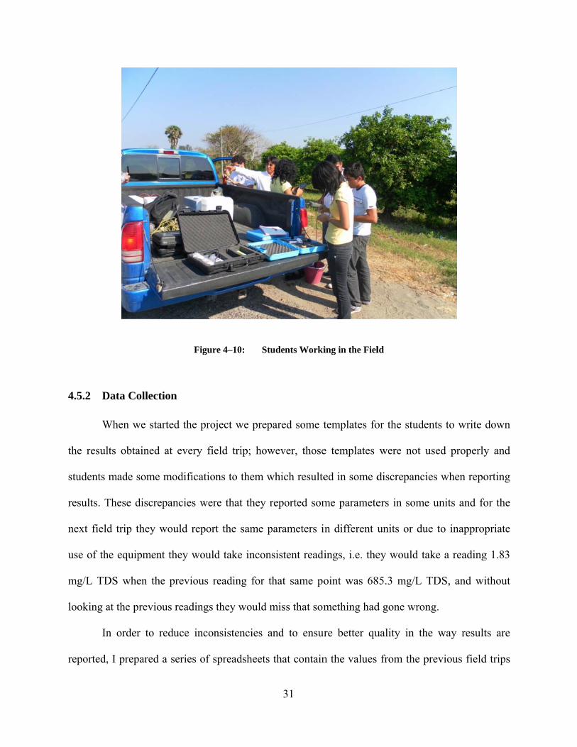
4.5.2 D
W
the resul
students
results. T
next field
use of th
mg/L TD
looking a
In
reported,
Data Collect
When we sta
lts obtained
made some
These discre
d trip they w
he equipment
DS when the
at the previo
n order to r
, I prepared
Figur
ion
rted the proj
at every fie
modification
pancies wer
would report
t they would
e previous r
us readings
reduce incon
a series of s
re 4–10: St
ject we prep
eld trip; how
ns to them w
re that they r
t the same p
d take incon
reading for t
they would m
nsistencies a
spreadsheets
31
tudents Worki
pared some t
wever, those
which resulte
reported som
parameters i
nsistent readi
that same po
miss that som
and to ensur
that contain
ing in the Fiel
templates fo
e templates
ed in some d
me paramete
in different u
ings, i.e. the
oint was 68
mething had
ure better qu
n the values
ld
or the studen
were not us
discrepancie
ers in some
units or due
ey would tak
85.3 mg/L T
d gone wrong
uality in the
from the pr
nts to write d
sed properly
es when repo
units and fo
e to inapprop
ke a reading
TDS, and wi
g.
e way result
revious field
down
y and
orting
or the
priate
g 1.83
ithout
ts are
d trips

32
and graphs that update automatically once new values are entered. This is a practical and easy
way to see if the values reported are consistent and to see if they follow a trend. From these
spreadsheets students can print out a template to take with them and easily detect possible
inconsistencies when the readings vary dramatically from the previous field trip at the same
point. This new template also indicates the units in which each parameter must be measured.
Table 4–4 is the template used to collect data for this project and Appendix A through Appendix
C show all the actual data recorded and reported by the UV for each of the monitoring points.

33
Table 4–4: Template Used to Record the Results
Rio: Latitud Longitud
# punto: Coordenadas:Nombre de punto de Monitoreo:
Fecha
Hora
Temperatura (°C)
SDT (ppm)
Turbiedad (FTU)
Resistividad (KΩ)
Salinidad (%)
ORP (mV)
Conductividad (µS)
pH (Unidades de pH)
Sulfatos (mg/L)
Cloruros (ppm)
Fosfatos (ppm)
Nitrogeno Amoniacal, N- NH3 (mg/L)
Nitrogeno de Nitratos, N- NO3-
(mg/L)
Oxigeno Disuelto, OD (mg/L)
DBO (mg/L)
Coliformes Totales
Coliformes Fecales
Plomo (µg/L)
Arsenico (ppb)
Dureza (ppm)
Hierro (ppm)
Manganeso (mg/L)
Aluminio (mg/L)
Cromo (mg/L)


35
5 DATA ANALYSIS AND PROCESSING
5.1 Pre-Processing and Post-Processing
Since one of the objectives of this project is to produce data that can be used as input data
in a GIS and further applications, the data collected at the field and in the lab needs to be
analyzed to detect inconsistencies. The use of a template helps to reduce inconsistencies because
it shows the units in which each parameter must be measured and reported. The equipment used
for this project allows the user to choose the display units and a common mistake was that some
readings were reported in parts per million (ppm) or mg/L one time and the next time they were
reported in parts per billion (ppb), such was the case when reporting chlorides content. Another
error was reporting conductivity in units of micro-siemens (µS/cm) one time and then using
milli-siemens (mS/cm), or reporting resistivity in micro-ohms (µΩ) one time and then milli-
ohms the next time (mΩ).
Once the data were collected I made corrections where it was easy to see that the wrong
units were used e.g., when reporting using units of ppb instead of ppm; however, some values
remain as they were reported even when they might be inconsistent.
5.2 Discussion of Results
The data collected so far represent a year and a half of work, and six monitoring trips.
The data collected might have inconsistencies or might not be complete; the main reasons for
36
these inconsistencies are most likely inadequate use of the equipment, lack of calibration of the
equipment, and lack of maintenance of the equipment.
Due to the rotation of personnel working on this project at the UV, some students didn’t
really know how to use the equipment and they may have not used it properly which affects the
quality of the results, also with time some of the standards used for calibration got contaminated
or are about to expire which produces inaccurate calibration, and finally, since we bought the
equipment in March 2010 it has not received any type of maintenance even when it is
recommended to give the equipment maintenance at least every six months, and this also affects
the quality of the results.
However, in order to evaluate the consistency of the results produced I took some random
points and compared the results reported by CONAGUA from three different years with the
results we are reporting over a period of one year. The points I am comparing are Puente Alamo
which is one our points with Alamo-Jugueras and Alamo which are two points monitored by
CONAGUA. These points are within a distance of 5 kilometers from each other; Alamo-
Jugueras is about 4 km upstream of Puente Alamo and Alamo is about 5 km downstream of
Puente Alamo. The time periods used for the comparisons are about a year starting during the
Spring and going to the next Spring the following year. For these points the periods compared
are: Spring 2004 – Spring 2005 for Alamo-Jugueras, Spring 2006 – Spring 2007 for Alamo-
Jugureas, and Spring 2010 – Spring 2011 for Alamo.
A total of 10 parameters were analyzed to determine how consistent the values were in
comparison to values reported in previous years for the same place. Figure 3–1 shows the
variations in Dissolved Oxygen for the previously mentioned monitoring points and periods, this
graph shows that most values are within a ±3 unit margin which can be used to consider that the

37
values reported by the UV are valid. A similar analysis was performed for the Lazaro Cardenas
monitoring points in the Tecolutla River. Appendix D through Appendix F contains the complete
results of these analyses and they show that most results are within a reasonable margin.
However, there are results for some other points that might be inconsistent due to the reasons
previously mentioned.
Figure 5–1: Comparison of DO Content for the Puente Alamo and Alamo Monitoring Points
5.3 Further Use of Data
As mentioned before, the data produced can be used as input data for a GIS, it also can be
stored in a database that can be shared with students, research organizations, other universities,
etc. The data can be shared and operated in a similar way the Consortium of Universities for the
Advancement of Hydrologic Science, Inc. (CUAHSI) shares and manages data. The data can
also be used in database management software like ArcHydro and/or shared using servers like
0.00
2.00
4.00
6.00
8.00
10.00
12.00
16‐Feb
18‐Mar
17‐Apr
18‐May
17‐Jun
18‐Jul
17‐Aug
17‐Sep
17‐Oct
17‐Nov
17‐Dec
17‐Jan
16‐Feb
19‐Mar
18‐Apr
19‐May
Dissolved
Oxygen, m
g/L
Date
CONAGUA(Spring04‐Spring05) CONAGUA(Spring06‐Spring07) UV(Spring10‐Spring11)

38
the CUAHSI Hydrologic Information System (HIS) [8]. It can also be used as input data for
water quality computer models like QUAL2K to perform water quality simulations. Further
sharing of the data and its use for modeling purposes are out of the scope of this project.

39
6 ACADEMIC IMPACT AND FUTURE GOALS
This is an ongoing project that had a positive impact at the UV already and it will
continue to benefit students working on environmental projects and not only on this particular
project.
One of the objectives of this project is to train environmental engineering students at the
UV and provide them with hands-on experience, this objective has been achieved and it is a goal
from now on to continue training new students and teach them how to combine the type of
information gathered in a project like this and use data management tools like GIS.
6.1 Continuity of the Project and Improvements
The project has been active for at least 18 months to this day and it is expected to
continue for as long and it is needed to monitor the water quality in the rivers comprising the
area of study. Also, having water quality monitoring equipment will benefit environmental
engineering students during their learning process at school since many of them will work on
similar environmental projects during their careers.
As mentioned earlier, financial constraints were a concern to give continuity to this
project, year and a half after having started it still is a concern; however, the positive response of
students, who so far have been volunteers, and the positive response of professors who have been
willing to work off the clock with the students, has shown school officials that it is worth
investing in projects like this one.
40
During my last visit in October 2011 I was informed that the school had recently
purchased two multiparameter probes more advanced than the ones we donated. These two new
probes will be used for this same project and for other environmental projects that the
engineering department may have students involved in. This is a remarkable achievement
considering that the school is run on a tight budget with state funds. Before we started this
project their environmental laboratory had some limited equipment and now they have the
equipment we donated plus two HI 9828 multiparameter probes by HANNA Instruments. These
new probes measure various water quality parameters and are easier to use and calibrate. They
have a cost of around $2,000.00 dollars which was absorbed by the school. Furthermore, the
school will send in the equipment we donated for maintenance so that it can be in optimum
conditions by the time they resume the field work
In addition to the equipment purchased by the school, Dr. Gustavo Davila, CIATEJ
researcher, donated additional laboratory equipment such as laboratory glass and plastic bottles
and containers, and calibration standards for the existing equipment. Dr. Davila has also been a
great support to the UV and during our last visit he had the students and professors analyze
samples to detect the content of heavy metals and coli forms which from now on are new water
quality parameters that will also be monitored; Dr. Davila also donated some equipment to the
UV to monitor these new parameters.
The achievements in this project show that it has been a successful project, and it also
shows that it created a very positive academic impact at the UV.

41
7 CONCLUSION
This project started in January 2010 with its first planning stage and the initial field trips
in March 2010. It started as part of the activities of the MESA 2010 program at BYU going
alongside a development of a larger GIS project conducted by CIATEJ, with time this project
evolved into an ongoing field monitoring project involving and training students at the UV who
benefit from the results produced as they may use them for further applications.
The objectives of this project were accomplished as we developed and implemented a
water quality monitoring plan for the Cazones River, Tuxpan River, and the Tecolutla River in
Veracruz, Mexico, and the data produced can be used as input data for a GIS that will be used as
a DSS at a watershed level for the area of study. We trained environmental engineering students
at the UV on monitoring water quality and applications of GIS, and also provided them with
hands-on experience. We produced water quality data of the rivers that comprise the area and it
can be used for future projects and research activities. And finally we created an ongoing
program conducted by students and faculty members at the UV to monitor water quality in water
bodies which made a highly positive academic impact.
This project gave me the opportunity to work on a real-life application of engineering that
will produce results even in the long run and thus it will continue making a positive impact. It
also gave me the opportunity to develop technical and leadership skills as I worked coordinating
activities both in the field and in the lab and also here at BYU and in Mexico at the UV.


43
REFERENCES
[1] Ormsby T., Napoleon E., Burke R., Groessl C., and Feaster L., (2004) Getting to know ArcGIS desktop, ESRI Press.
[2] www.gis.com/content/what-gis [3] www.esri.com/library/ [4] Davila, G., (2011). “Desarrollo de un sistema de soporte para la toma de decisiones a nivel
cuenca para el control de la contaminación en los ríos Tuxpan, Cazones y Tecolutla en el estado de Veracruz. Informe Tecnico Segunda Etapa”, CIATEJ
[5] www.ingenieria.unam.mx/~enriquecv/TAR/normas_TAR.html [6] http://deercreek.groups.et.byu.net/ [7] www.mosaicfound.org/home/home.php
[8] www.cuahsi.org


45
Appendix A. Results Reported by the UV for the Tecolutla River
Table A–1: Results Reported by the UV for Puente Progreso de Zaragoza
Rio: Tecolutla Latitud Longitud
# punto: 1 Coordenadas: 20°16'21.97"N 97°42'16.86"WNombre de punto de Monitoreo: Puente Progreso de Zaragoza
Fecha 23-Apr-10 7-Jul-10 15-Oct-10 25-Mar-11 27-May-11 12-Oct-11
Hora 8:47 AM 7:10 AM 8:47 AM 7:45 AM
Temperatura (°C) 26.0 28.1 27.0 21.4
SDT (ppm) 109.00 97.30 78.09 67.18 73.20 53.87
Turbiedad (FTU) 5.65 8.65 11.56 1.66 7.49 8.60
Resistividad (KΩ)
4.60 6.34 10.90 6.87 9.35
Salinidad (%) 0.40 0.30 0.20 0.07 0.20
ORP (mV) 47.00 97.60 121.70 23.87
Conductividad (µS)
216.00 157.62 142.10 138.40 109.10
pH (Unidades de pH)
7.45 7.15 6.97 7.23
Sulfatos (mg/L) 1.17E-01 1.18E-01 2.07E-01 6.25E-01
Cloruros (ppm) 1.40 3.04 4.66 12.50
Fosfatos (ppm) 0.17 0.12 0.02 0.14 0.24 0.21
Nitrogeno Amoniacal, N- NH3 (mg/L)
16.60
Nitrogeno de Nitratos, N- NO3-
(mg/L)3.70 15.20 23.30
Oxigeno Disuelto, OD (mg/L)
9.82 9.43 9.70 8.21 7.15 8.10
DBO (mg/L) 1.35 53.17 5.65 7.13 3.33 5.10
Coliformes Totales
17.00
Coliformes Fecales
28.00
Plomo (µg/L) 2.00
Arsenico (ppb) 10.00
Dureza (ppm) 50.00
Hierro (ppm) 0.00
Manganeso (mg/L)
0.00
Aluminio (mg/L) 0.00
Cromo (mg/L) 0.00

46
Figure A–1: Temperature at Puente Progreso de Zaragoza
Figure A–2: TDS at Puente Progreso de Zaragoza
Figure A–3: Turbidity at Puente Progreso de Zaragoza
Figure A–4: Resistivity at Puente Progreso de Zaragoza
0.0
5.0
10.0
15.0
20.0
25.0
30.0
Jan‐10
May‐10
Aug‐10
Nov‐10
Feb‐11
Jun‐11
Sep‐11
Dec‐11
Temp, C
Date
0.00
20.00
40.00
60.00
80.00
100.00
120.00
Jan‐10
May‐10
Aug‐10
Nov‐10
Feb‐11
Jun‐11
Sep‐11
Dec‐11
TDS, ppm
Date
0.00
2.00
4.00
6.00
8.00
10.00
12.00
14.00
Jan‐10
May‐10
Aug‐10
Nov‐10
Feb‐11
Jun‐11
Sep‐11
Dec‐11
Turbidity, FTU
Date
0.00
2.00
4.00
6.00
8.00
10.00
12.00
Jan‐10
May‐10
Aug‐10
Nov‐10
Feb‐11
Jun‐11
Sep‐11
Dec‐11
Res, KΩ
Date

47
Figure A–5: Salinity at Puente Progreso de Zaragoza
Figure A–6: ORP at Puente Progreso de Zaragoza
Figure A–7: Conductivity at Puente Progreso de Zaragoza
Figure A–8: pH at Puente Progreso de Zaragoza
0.00
0.05
0.10
0.15
0.20
0.25
0.30
0.35
0.40
0.45
Jan‐10
May‐10
Aug‐10
Nov‐10
Feb‐11
Jun‐11
Sep‐11
Dec‐11
Salinity, %
Date
0.00
20.00
40.00
60.00
80.00
100.00
120.00
140.00
Jan‐10
May‐10
Aug‐10
Nov‐10
Feb‐11
Jun‐11
Sep‐11
Dec‐11
OPR, m
VDate
0.00
50.00
100.00
150.00
200.00
250.00
Jan‐10
May‐10
Aug‐10
Nov‐10
Feb‐11
Jun‐11
Sep‐11
Dec‐11
Conductivity, m
S
Date
6.90
7.00
7.10
7.20
7.30
7.40
7.50
Jan‐10
May‐10
Aug‐10
Nov‐10
Feb‐11
Jun‐11
Sep‐11
Dec‐11
pH , pH units
Date

48
Figure A–9: Sulfates at Puente Progrezo de Zaragoza
Figure A–10: Chlorides at Puente Progreso de Zaragoza
Figure A–11: Phosphates at Puente Progreso de Zaragoza
Figure A–12: Ammonia Nitrogen at Puente Progreso de Zaragoza
0.00E+00
1.00E‐01
2.00E‐01
3.00E‐01
4.00E‐01
5.00E‐01
6.00E‐01
7.00E‐01
Jan‐10
May‐10
Aug‐10
Nov‐10
Feb‐11
Jun‐11
Sep‐11
Dec‐11
Sulfates, ppm
Date
0.00
2.00
4.00
6.00
8.00
10.00
12.00
14.00
Jan‐10
May‐10
Aug‐10
Nov‐10
Feb‐11
Jun‐11
Sep‐11
Dec‐11
Chlorides, ppm
Date
0.00
0.05
0.10
0.15
0.20
0.25
0.30
Jan‐10
May‐10
Aug‐10
Nov‐10
Feb‐11
Jun‐11
Sep‐11
Dec‐11
Tot Phosphate, ppm
Date
0.00
2.00
4.00
6.00
8.00
10.00
12.00
14.00
16.00
18.00
Jan‐10
May‐10
Aug‐10
Nov‐10
Feb‐11
Jun‐11
Sep‐11
Dec‐11
Ammonia Nitrogen, m
g/L
Date

49
Figure A–13: Nitrate Nitrogen at Puente Progreso de Zaragoza
Figure A–14: Dissolved Oxygen at Puente Progreso de Zaragoza
Figure A–15: BOD at Puente Progreso de Zaragoza
0.00
5.00
10.00
15.00
20.00
25.00
Jan‐10
May‐10
Aug‐10
Nov‐10
Feb‐11
Jun‐11
Sep‐11
Dec‐11
Nitrate Nitrogen, m
g/L
Date
0.00
2.00
4.00
6.00
8.00
10.00
12.00
Jan‐10
May‐10
Aug‐10
Nov‐10
Feb‐11
Jun‐11
Sep‐11
Dec‐11
Dissolved Oxygen, mg/L
Date
0.00
10.00
20.00
30.00
40.00
50.00
60.00
Jan‐10
May‐10
Aug‐10
Nov‐10
Feb‐11
Jun‐11
Sep‐11
Dec‐11
BOD, m
g/L
Date

50
Table A–2: Results Reported by the UV for Puente Las Lomas
Rio: Tecolutla Latitud Longitud
# punto: 2 Coordenadas: 20°15'52.62"N 97°36'4.89"WNombre de punto de Monitoreo: Puente Las Lomas
Fecha 23-Apr-10 7-Jul-10 15-Oct-10 25-Mar-11 27-May-11 12-Oct-11
Hora 10:36 AM 9:03 AM 10:36 AM 8:10 AM 10:42 AM
Temperatura (°C) 26.0 28.2 28.0 23.3
SDT (ppm) 118.70 104.73 80.61 80.49 72.90 66.33
Turbiedad (FTU) 2.35 5.41 7.72 0.65 7.02 9.33
Resistividad (KΩ)
4.24 5.99 6.39 6.85 7.49
Salinidad (%) 0.40 0.30 0.30 0.07 0.20
ORP (mV) 117.20 98.32 129.80 19.03
Conductividad (µS)
232.70 165.36 162.40 146.07 133.10
pH (Unidades de pH)
7.60 7.52 7.50 8.11 7.23
Sulfatos (mg/L) 5.91E-01 1.90E-02 1.83E-01 2.77E-02
Cloruros (ppm) 5.21 3.91 14.70 10.97
Fosfatos (ppm) 0.23 0.20 0.11 0.06 0.20 0.20
Nitrogeno Amoniacal, N- NH3 (mg/L)
15.00
Nitrogeno de Nitratos, N- NO3-
(mg/L)3.40 14.17 24.40
Oxigeno Disuelto, OD (mg/L)
10.00 9.46 9.48 8.03 6.73 8.59
DBO (mg/L) 2.56 58.47 4.64 8.03 7.59 5.60
Coliformes Totales
13.00
Coliformes Fecales
30.00
Plomo (µg/L) 1.00
Arsenico (ppb) 0.00
Dureza (ppm) 120.00
Hierro (ppm) 0.15
Manganeso (mg/L)
0.10
Aluminio (mg/L) 0.00
Cromo (mg/L) 0.00

51
Figure A–16: Temperature at Puente Las Lomas
Figure A–17: TDS at Puente Las Lomas
Figure A–18: Turbidity at Puente Las Lomas
Figure A–19: Resistivity at Puente Las Lomas
0.0
5.0
10.0
15.0
20.0
25.0
30.0
Jan‐10
May‐10
Aug‐10
Nov‐10
Feb‐11
Jun‐11
Sep‐11
Dec‐11
Tem
p, C
Date
0.00
20.00
40.00
60.00
80.00
100.00
120.00
140.00
Jan‐10
May‐10
Aug‐10
Nov‐10
Feb‐11
Jun‐11
Sep‐11
Dec‐11
TDS, ppm
Date
0.00
1.00
2.00
3.00
4.00
5.00
6.00
7.00
8.00
9.00
10.00
Jan‐10
May‐10
Aug‐10
Nov‐10
Feb‐11
Jun‐11
Sep‐11
Dec‐11
Turbidity, FTU
Date
0.00
1.00
2.00
3.00
4.00
5.00
6.00
7.00
8.00
Jan‐10
May‐10
Aug‐10
Nov‐10
Feb‐11
Jun‐11
Sep‐11
Dec‐11
Res, KΩ
Date

52
Figure A–20: Salinity at Puente Las Lomas
Figure A–21: ORP at Puente Las Lomas
Figure A–22: Conductivity at Puente Las Lomas
Figure A–23: pH at Puente Las Lomas
0.00
0.05
0.10
0.15
0.20
0.25
0.30
0.35
0.40
0.45
Jan‐10
May‐10
Aug‐10
Nov‐10
Feb‐11
Jun‐11
Sep‐11
Dec‐11
Salin
ity, %
Date
0.00
20.00
40.00
60.00
80.00
100.00
120.00
140.00
Jan‐10
May‐10
Aug‐10
Nov‐10
Feb‐11
Jun‐11
Sep‐11
Dec‐11
OPR, m
V
Date
0.00
50.00
100.00
150.00
200.00
250.00
Jan‐10
May‐10
Aug‐10
Nov‐10
Feb‐11
Jun‐11
Sep‐11
Dec‐11
Conductivity, m
S
Date
7.10
7.20
7.30
7.40
7.50
7.60
7.70
7.80
7.90
8.00
8.10
8.20
Jan‐10
May‐10
Aug‐10
Nov‐10
Feb‐11
Jun‐11
Sep‐11
Dec‐11
pH , pH units
Date

53
Figure A–24: Sulfates at Puente Las Lomas
Figure A–25: Chlorides at Puente Las Lomas
Figure A–26: Phosphates at Puente Las Lomas
Figure A–27: Ammonia Nitrogen at Puente Las Lomas
0.00E+00
1.00E‐01
2.00E‐01
3.00E‐01
4.00E‐01
5.00E‐01
6.00E‐01
7.00E‐01
Jan‐10
May‐10
Aug‐10
Nov‐10
Feb‐11
Jun‐11
Sep‐11
Dec‐11
Sulfates, ppm
Date
0.00
2.00
4.00
6.00
8.00
10.00
12.00
14.00
16.00
Jan‐10
May‐10
Aug‐10
Nov‐10
Feb‐11
Jun‐11
Sep‐11
Dec‐11
Chlorides, ppm
Date
0.00
0.05
0.10
0.15
0.20
0.25
Jan‐10
May‐10
Aug‐10
Nov‐10
Feb‐11
Jun‐11
Sep‐11
Dec‐11
Tot Phosphate, p
pm
Date
0.00
2.00
4.00
6.00
8.00
10.00
12.00
14.00
16.00
Jan‐10
May‐10
Aug‐10
Nov‐10
Feb‐11
Jun‐11
Sep‐11
Dec‐11
Ammonia Nitrogen, m
g/L
Date

54
Figure A–28: Nitrate Nitrogen at Puente Las Lomas
Figure A–29: Dissolved Oxygen at Puente Las Lomas
Figure A–30: BOD at Puente Las Lomas
0.00
5.00
10.00
15.00
20.00
25.00
30.00
Jan‐10
May‐10
Aug‐10
Nov‐10
Feb‐11
Jun‐11
Sep‐11
Dec‐11
Nitrate Nitrogen, m
g/L
Date
0.00
2.00
4.00
6.00
8.00
10.00
12.00
Jan‐10
May‐10
Aug‐10
Nov‐10
Feb‐11
Jun‐11
Sep‐11
Dec‐11
Dissolved Oxygen, m
g/L
Date
0.00
10.00
20.00
30.00
40.00
50.00
60.00
70.00
Jan‐10
May‐10
Aug‐10
Nov‐10
Feb‐11
Jun‐11
Sep‐11
Dec‐11
BOD, m
g/L
Date
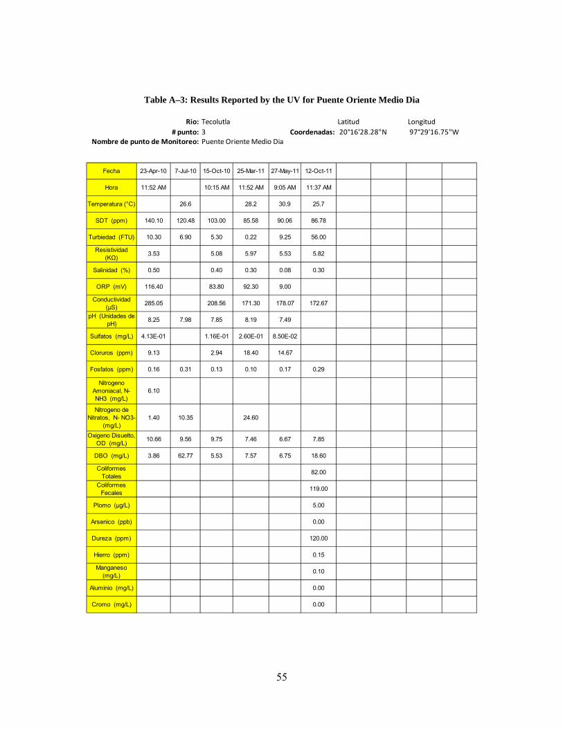
55
Table A–3: Results Reported by the UV for Puente Oriente Medio Dia
Rio: Tecolutla Latitud Longitud
# punto: 3 Coordenadas: 20°16'28.28"N 97°29'16.75"WNombre de punto de Monitoreo: Puente Oriente Medio Dia
Fecha 23-Apr-10 7-Jul-10 15-Oct-10 25-Mar-11 27-May-11 12-Oct-11
Hora 11:52 AM 10:15 AM 11:52 AM 9:05 AM 11:37 AM
Temperatura (°C) 26.6 28.2 30.9 25.7
SDT (ppm) 140.10 120.48 103.00 85.58 90.06 86.78
Turbiedad (FTU) 10.30 6.90 5.30 0.22 9.25 56.00
Resistividad (KΩ)
3.53 5.08 5.97 5.53 5.82
Salinidad (%) 0.50 0.40 0.30 0.08 0.30
ORP (mV) 116.40 83.80 92.30 9.00
Conductividad (µS)
285.05 208.56 171.30 178.07 172.67
pH (Unidades de pH)
8.25 7.98 7.85 8.19 7.49
Sulfatos (mg/L) 4.13E-01 1.16E-01 2.60E-01 8.50E-02
Cloruros (ppm) 9.13 2.94 18.40 14.67
Fosfatos (ppm) 0.16 0.31 0.13 0.10 0.17 0.29
Nitrogeno Amoniacal, N- NH3 (mg/L)
6.10
Nitrogeno de Nitratos, N- NO3-
(mg/L)1.40 10.35 24.60
Oxigeno Disuelto, OD (mg/L)
10.66 9.56 9.75 7.46 6.67 7.85
DBO (mg/L) 3.86 62.77 5.53 7.57 6.75 18.60
Coliformes Totales
82.00
Coliformes Fecales
119.00
Plomo (µg/L) 5.00
Arsenico (ppb) 0.00
Dureza (ppm) 120.00
Hierro (ppm) 0.15
Manganeso (mg/L)
0.10
Aluminio (mg/L) 0.00
Cromo (mg/L) 0.00

56
Figure A–31: Temperature at Puente Oriente Medio Dia
Figure A–32: TDS at Puente Oriente Medio Dia
Figure A–33: Turbidity at Puente Oriente Medio Dia
Figure A–34: Resistivity at Puente Oriente Medio Dia
0.0
5.0
10.0
15.0
20.0
25.0
30.0
35.0
Jan‐10
May‐10
Aug‐10
Nov‐10
Feb‐11
Jun‐11
Sep‐11
Dec‐11
Temp, C
Date
0.00
20.00
40.00
60.00
80.00
100.00
120.00
140.00
160.00
Jan‐10
May‐10
Aug‐10
Nov‐10
Feb‐11
Jun‐11
Sep‐11
Dec‐11
TDS, ppm
Date
0.00
10.00
20.00
30.00
40.00
50.00
60.00
Jan‐10
May‐10
Aug‐10
Nov‐10
Feb‐11
Jun‐11
Sep‐11
Dec‐11
Turbidity, FTU
Date
0.00
1.00
2.00
3.00
4.00
5.00
6.00
7.00
Jan‐10
May‐10
Aug‐10
Nov‐10
Feb‐11
Jun‐11
Sep‐11
Dec‐11
Res, KΩ
Date

57
Figure A–35: Salinity at Puente Oriente Medio Dia
Figure A–36: ORP at Puente Oriente Medio Dia
Figure A–37: Conductivity at Puente Oriente Medio Dia
Figure A–38: pH at Puente Oriente Medio Dia
0.00
0.10
0.20
0.30
0.40
0.50
0.60
Jan‐10
May‐10
Aug‐10
Nov‐10
Feb‐11
Jun‐11
Sep‐11
Dec‐11
Salin
ity, %
Date
0.00
20.00
40.00
60.00
80.00
100.00
120.00
140.00
Jan‐10
May‐10
Aug‐10
Nov‐10
Feb‐11
Jun‐11
Sep‐11
Dec‐11
OPR, m
V
Date
0.00
50.00
100.00
150.00
200.00
250.00
300.00
Jan‐10
May‐10
Aug‐10
Nov‐10
Feb‐11
Jun‐11
Sep‐11
Dec‐11
Conductivity, m
S
Date
7.40
7.50
7.60
7.70
7.80
7.90
8.00
8.10
8.20
8.30
Jan‐10
May‐10
Aug‐10
Nov‐10
Feb‐11
Jun‐11
Sep‐11
Dec‐11
pH , pH units
Date

58
Figure A–39: Sulfates at Puente Oriente Medio Dia
Figure A–40: Chlorides at Puente Oriente Medio Dia
Figure A–41: Phosphates at Puente Oriente Medio Dia
Figure A–42: Ammonia Nitrogen at Puente Oriente Medio Dia
0.00E+00
5.00E‐02
1.00E‐01
1.50E‐01
2.00E‐01
2.50E‐01
3.00E‐01
3.50E‐01
4.00E‐01
4.50E‐01
Jan‐10
May‐10
Aug‐10
Nov‐10
Feb‐11
Jun‐11
Sep‐11
Dec‐11
Sulfates, ppm
Date
0.00
2.00
4.00
6.00
8.00
10.00
12.00
14.00
16.00
18.00
20.00
Jan‐10
May‐10
Aug‐10
Nov‐10
Feb‐11
Jun‐11
Sep‐11
Dec‐11
Chlorides, ppm
Date
0.00
0.05
0.10
0.15
0.20
0.25
0.30
0.35
Jan‐10
May‐10
Aug‐10
Nov‐10
Feb‐11
Jun‐11
Sep‐11
Dec‐11
Tot Phosphate, p
pm
Date
0.00
1.00
2.00
3.00
4.00
5.00
6.00
7.00
Jan‐10
May‐10
Aug‐10
Nov‐10
Feb‐11
Jun‐11
Sep‐11
Dec‐11
Ammonia Nitrogen, m
g/L
Date
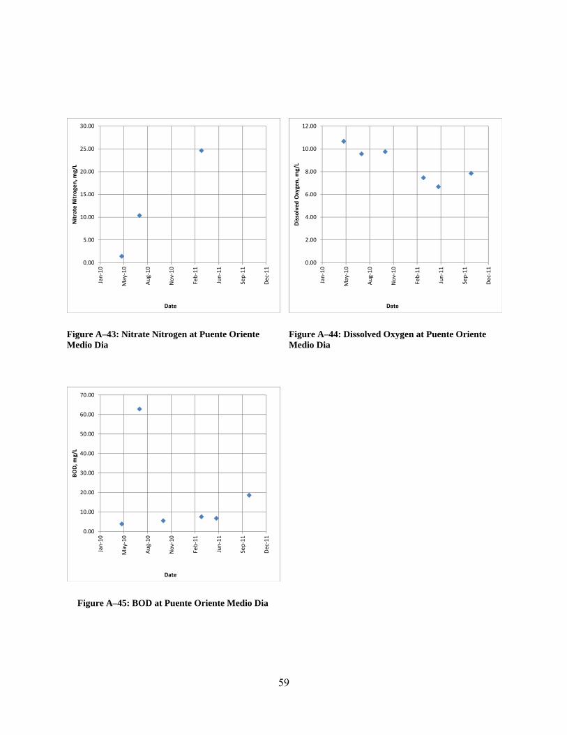
59
Figure A–43: Nitrate Nitrogen at Puente Oriente Medio Dia
Figure A–44: Dissolved Oxygen at Puente Oriente Medio Dia
Figure A–45: BOD at Puente Oriente Medio Dia
0.00
5.00
10.00
15.00
20.00
25.00
30.00
Jan‐10
May‐10
Aug‐10
Nov‐10
Feb‐11
Jun‐11
Sep‐11
Dec‐11
Nitrate Nitrogen, m
g/L
Date
0.00
2.00
4.00
6.00
8.00
10.00
12.00
Jan‐10
May‐10
Aug‐10
Nov‐10
Feb‐11
Jun‐11
Sep‐11
Dec‐11
Dissolved Oxygen, m
g/L
Date
0.00
10.00
20.00
30.00
40.00
50.00
60.00
70.00
Jan‐10
May‐10
Aug‐10
Nov‐10
Feb‐11
Jun‐11
Sep‐11
Dec‐11
BOD, m
g/L
Date

60
Table A–4: Results Reported by the UV for El Espinal
Rio: Tecolutla Latitud Longitud
# punto: 4 Coordenadas: 20°15'6.99"N 97°23'35.10"WNombre de punto de Monitoreo: El Espinal
Fecha 23-Apr-10 7-Jul-10 15-Oct-10 25-Mar-11 27-May-11 12-Oct-11
Hora 11:40 AM 1:20 PM 10:00 AM 12:35 PM
Temperatura (°C) 32.0 32.1 28.3
SDT (ppm) 183.35 110.80 130.40 138.83
Turbiedad (FTU) 6.57 1.55 19.30 46.50
Resistividad (KΩ)
2.75 5.58 3.83 3.59
Salinidad (%) 0.70 0.40 0.50 0.50
ORP (mV) 113.83 114.80 45.70
Conductividad (µS)
365.86 221.00 259.90 272.77
pH (Unidades de pH)
6.75 8.24 8.00
Sulfatos (mg/L) 6.48E-01 4.63E-01 1.28E-01
Cloruros (ppm) 18.50 19.90 11.80
Fosfatos (ppm) 0.06 0.10 0.23 0.36
Nitrogeno Amoniacal, N- NH3 (mg/L)
Nitrogeno de Nitratos, N- NO3-
(mg/L)27.60
Oxigeno Disuelto, OD (mg/L)
11.33 10.57 11.42 6.70
DBO (mg/L) 0.73 10.82 11.41 15.00
Coliformes Totales
40.00
Coliformes Fecales
121.00
Plomo (µg/L) 1.00
Arsenico (ppb) 30.00
Dureza (ppm) 120.00
Hierro (ppm) 0.15
Manganeso (mg/L)
0.12
Aluminio (mg/L) 0.00
Cromo (mg/L) 0.20

61
Figure A–46: Temperature at El Espinal
Figure A–47: TDS at El Espinal
Figure A–48: Turbidity at El Espinal
Figure A–49: Resistivity at El Espinal
28.0
28.5
29.0
29.5
30.0
30.5
31.0
31.5
32.0
32.5
Jan‐10
May‐10
Aug‐10
Nov‐10
Feb‐11
Jun‐11
Sep‐11
Dec‐11
Temp, C
Date
0.00
20.00
40.00
60.00
80.00
100.00
120.00
140.00
160.00
180.00
200.00
Jan‐10
May‐10
Aug‐10
Nov‐10
Feb‐11
Jun‐11
Sep‐11
Dec‐11
TDS, ppm
Date
0.00
5.00
10.00
15.00
20.00
25.00
30.00
35.00
40.00
45.00
50.00
Jan‐10
May‐10
Aug‐10
Nov‐10
Feb‐11
Jun‐11
Sep‐11
Dec‐11
Turbidity, FTU
Date
0.00
1.00
2.00
3.00
4.00
5.00
6.00
Jan‐10
May‐10
Aug‐10
Nov‐10
Feb‐11
Jun‐11
Sep‐11
Dec‐11
Res, KΩ
Date

62
Figure A–50: Salinity at El Espinal
Figure A–51: ORP at El Espinal
Figure A–52: Conductivity at El Espinal
Figure A–53: pH at El Espinal
0.00
0.10
0.20
0.30
0.40
0.50
0.60
0.70
0.80
Jan‐10
May‐10
Aug‐10
Nov‐10
Feb‐11
Jun‐11
Sep‐11
Dec‐11
Salin
ity, %
Date
0.00
20.00
40.00
60.00
80.00
100.00
120.00
140.00
Jan‐10
May‐10
Aug‐10
Nov‐10
Feb‐11
Jun‐11
Sep‐11
Dec‐11
OPR, m
V
Date
0.00
50.00
100.00
150.00
200.00
250.00
300.00
350.00
400.00
Jan‐10
May‐10
Aug‐10
Nov‐10
Feb‐11
Jun‐11
Sep‐11
Dec‐11
Conductivity, m
S
Date
0.00
1.00
2.00
3.00
4.00
5.00
6.00
7.00
8.00
9.00
Jan‐10
May‐10
Aug‐10
Nov‐10
Feb‐11
Jun‐11
Sep‐11
Dec‐11
pH , pH units
Date

63
Figure A–54: Sulfates at El Espinal
Figure A–55: Chlorides at El Espinal
Figure A–56: Phosphates at El Espinal
Figure A–57: Ammonia Nitrogen at El Espinal
0.00E+00
1.00E‐01
2.00E‐01
3.00E‐01
4.00E‐01
5.00E‐01
6.00E‐01
7.00E‐01
Jan‐10
May‐10
Aug‐10
Nov‐10
Feb‐11
Jun‐11
Sep‐11
Dec‐11
Sulfates, ppm
Date
0.00
5.00
10.00
15.00
20.00
25.00
Jan‐10
May‐10
Aug‐10
Nov‐10
Feb‐11
Jun‐11
Sep‐11
Dec‐11
Chlorides, ppm
Date
0.00
0.05
0.10
0.15
0.20
0.25
0.30
0.35
0.40
Jan‐10
May‐10
Aug‐10
Nov‐10
Feb‐11
Jun‐11
Sep‐11
Dec‐11
Tot Phosphate, p
pm
Date
0.00
0.20
0.40
0.60
0.80
1.00
1.20
Jan‐10
May‐10
Aug‐10
Nov‐10
Feb‐11
Jun‐11
Sep‐11
Dec‐11
Ammonia Nitrogen, m
g/L
Date

64
Figure A–58: Nitrate Nitrogen at El Espinal
Figure A–59: Dissolved Oxygen at El Espinal
Figure A–60: BOD at El Espinal
0.00
5.00
10.00
15.00
20.00
25.00
30.00
Jan‐10
May‐10
Aug‐10
Nov‐10
Feb‐11
Jun‐11
Sep‐11
Dec‐11
Nitrate Nitrogen, m
g/L
Date
0.00
2.00
4.00
6.00
8.00
10.00
12.00
Jan‐10
May‐10
Aug‐10
Nov‐10
Feb‐11
Jun‐11
Sep‐11
Dec‐11
Dissolved Oxygen, m
g/L
Date
0.00
2.00
4.00
6.00
8.00
10.00
12.00
14.00
16.00
Jan‐10
May‐10
Aug‐10
Nov‐10
Feb‐11
Jun‐11
Sep‐11
Dec‐11
BOD, m
g/L
Date

65
Table A–5: Results Reported by the UV for Bado San Gotardo
Rio: Tecolutla Latitud Longitud
# punto: 5 Coordenadas: 20°17'58.15"N 97°17'37.64"WNombre de punto de Monitoreo: Bado San Gotardo
Fecha 23-Apr-10 7-Jul-10 15-Oct-10 25-Mar-11 27-May-11 12-Oct-11
Hora 1:20 PM 12:55 PM 2:50 PM 1:37 PM
Temperatura (°C) 26.5 31.2 35.9 25.7
SDT (ppm) 151.30 109.87 94.07 75.10 78.05 70.02
Turbiedad (FTU) 459.50 12.93 6.82 0.52 19.20 51.93
Resistividad (KΩ)
3.28 5.32 6.90 6.42 7.12
Salinidad (%) 0.50 0.40 0.30 0.30 0.30
ORP (mV) 75.80 86.43 122.10 54.00
Conductividad (µS)
264.25 188.06 150.20 150.47 137.43
pH (Unidades de pH)
7.90 7.28 6.65 8.67 8.30
Sulfatos (mg/L) 5.91E-01 3.55E-01 3.71E-01 1.19E-01
Cloruros (ppm) 12.70 3.26 28.20 7.05
Fosfatos (ppm) 0.23 0.35 0.16 0.23 0.27 0.23
Nitrogeno Amoniacal, N- NH3 (mg/L)
22.50
Nitrogeno de Nitratos, N- NO3-
(mg/L)5.10 16.57 25.80
Oxigeno Disuelto, OD (mg/L)
9.21 8.77 10.33 10.93 9.54 7.56
DBO (mg/L) 0.58 69.00 5.91 10.93 9.00 16.10
Coliformes Totales
42.00
Coliformes Fecales
120.00
Plomo (µg/L) 6.00
Arsenico (ppb) 30.00
Dureza (ppm) 120.00
Hierro (ppm) 0.00
Manganeso (mg/L)
0.05
Aluminio (mg/L) 0.00
Cromo (mg/L) 0.00
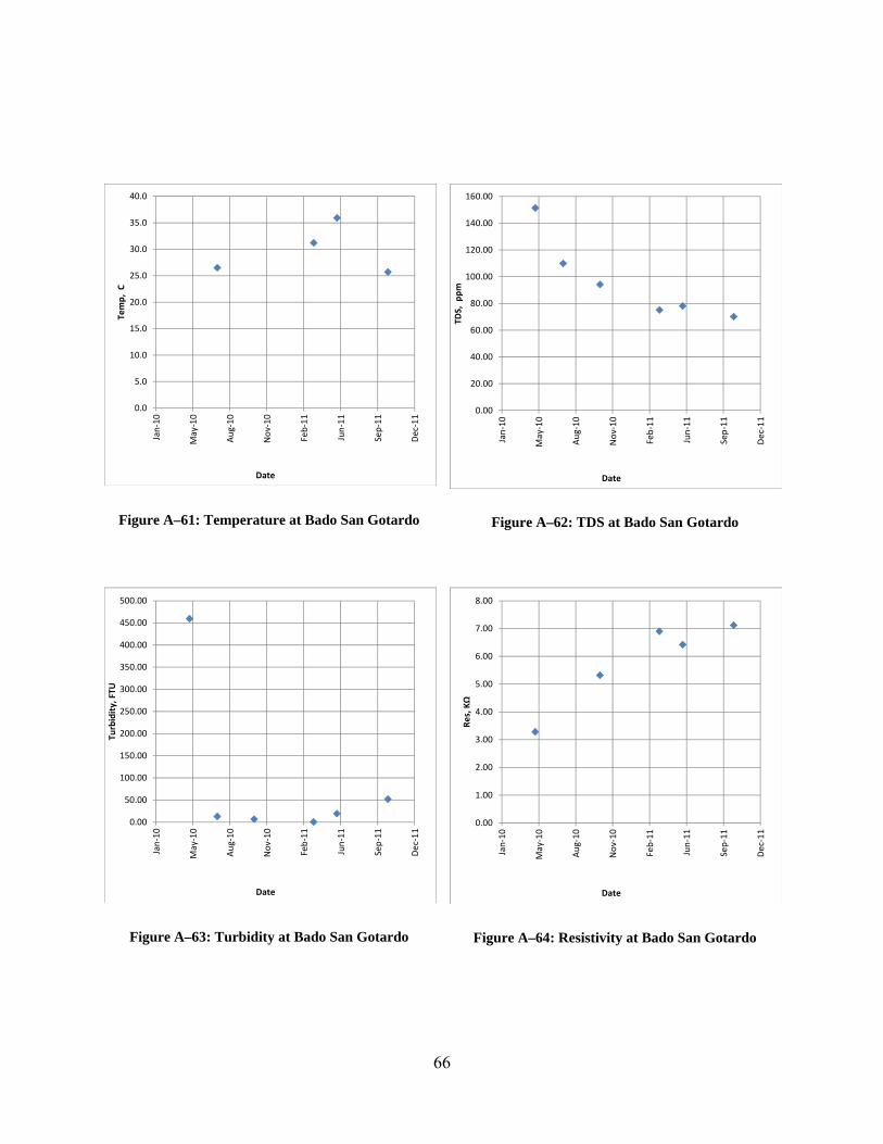
66
Figure A–61: Temperature at Bado San Gotardo
Figure A–62: TDS at Bado San Gotardo
Figure A–63: Turbidity at Bado San Gotardo
Figure A–64: Resistivity at Bado San Gotardo
0.0
5.0
10.0
15.0
20.0
25.0
30.0
35.0
40.0
Jan‐10
May‐10
Aug‐10
Nov‐10
Feb‐11
Jun‐11
Sep‐11
Dec‐11
Temp, C
Date
0.00
20.00
40.00
60.00
80.00
100.00
120.00
140.00
160.00
Jan‐10
May‐10
Aug‐10
Nov‐10
Feb‐11
Jun‐11
Sep‐11
Dec‐11
TDS, p
pm
Date
0.00
50.00
100.00
150.00
200.00
250.00
300.00
350.00
400.00
450.00
500.00
Jan‐10
May‐10
Aug‐10
Nov‐10
Feb‐11
Jun‐11
Sep‐11
Dec‐11
Turbidity, FTU
Date
0.00
1.00
2.00
3.00
4.00
5.00
6.00
7.00
8.00
Jan‐10
May‐10
Aug‐10
Nov‐10
Feb‐11
Jun‐11
Sep‐11
Dec‐11
Res, KΩ
Date

67
Figure A–65: Salinity at Bado San Gotardo
Figure A–66: ORP at Bado San Gotardo
Figure A–67: Conductivity at Bado San Gotardo
Figure A–68: pH at Bado San Gotardo
0.00
0.10
0.20
0.30
0.40
0.50
0.60
Jan‐10
May‐10
Aug‐10
Nov‐10
Feb‐11
Jun‐11
Sep‐11
Dec‐11
Salin
ity, %
Date
0.00
20.00
40.00
60.00
80.00
100.00
120.00
140.00
Jan‐10
May‐10
Aug‐10
Nov‐10
Feb‐11
Jun‐11
Sep‐11
Dec‐11
OPR, m
V
Date
0.00
50.00
100.00
150.00
200.00
250.00
300.00
Jan‐10
May‐10
Aug‐10
Nov‐10
Feb‐11
Jun‐11
Sep‐11
Dec‐11
Conductivity, m
S
Date
0.00
1.00
2.00
3.00
4.00
5.00
6.00
7.00
8.00
9.00
10.00
Jan‐10
May‐10
Aug‐10
Nov‐10
Feb‐11
Jun‐11
Sep‐11
Dec‐11
pH , pH units
Date

68
Figure A–69: Sulfates at Bado San Gotardo
Figure A–70: Chlorides at Bado San Gotardo
Figure A–71: Phosphates at Bado San Gotardo
Figure A–72: Ammonia Nitrogen at Bado San Gotardo
0.00E+00
1.00E‐01
2.00E‐01
3.00E‐01
4.00E‐01
5.00E‐01
6.00E‐01
7.00E‐01
Jan‐10
May‐10
Aug‐10
Nov‐10
Feb‐11
Jun‐11
Sep‐11
Dec‐11
Sulfates, ppm
Date
0.00
5.00
10.00
15.00
20.00
25.00
30.00
Jan‐10
May‐10
Aug‐10
Nov‐10
Feb‐11
Jun‐11
Sep‐11
Dec‐11
Chlorides, p
pm
Date
0.00
0.05
0.10
0.15
0.20
0.25
0.30
0.35
0.40
Jan‐10
May‐10
Aug‐10
Nov‐10
Feb‐11
Jun‐11
Sep‐11
Dec‐11
Tot Phosphate, p
pm
Date
0.00
5.00
10.00
15.00
20.00
25.00
Jan‐10
May‐10
Aug‐10
Nov‐10
Feb‐11
Jun‐11
Sep‐11
Dec‐11
Ammonia Nitrogen, m
g/L
Date
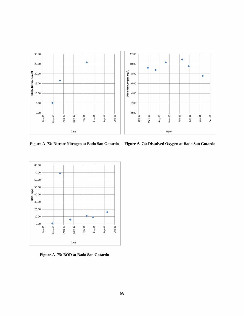
69
Figure A–73: Nitrate Nitrogen at Bado San Gotardo
Figure A–74: Dissolved Oxygen at Bado San Gotardo
Figure A–75: BOD at Bado San Gotardo
0.00
5.00
10.00
15.00
20.00
25.00
30.00
Jan‐10
May‐10
Aug‐10
Nov‐10
Feb‐11
Jun‐11
Sep‐11
Dec‐11
Nitrate Nitrogen, m
g/L
Date
0.00
2.00
4.00
6.00
8.00
10.00
12.00
Jan‐10
May‐10
Aug‐10
Nov‐10
Feb‐11
Jun‐11
Sep‐11
Dec‐11
Dissolved Oxygen, m
g/L
Date
0.00
10.00
20.00
30.00
40.00
50.00
60.00
70.00
80.00
Jan‐10
May‐10
Aug‐10
Nov‐10
Feb‐11
Jun‐11
Sep‐11
Dec‐11
BOD, m
g/L
Date

70
Table A–6: Results Reported by the UV for Puente El Remolino
Rio: Tecolutla Latitud Longitud
# punto: 6 Coordenadas: 20°23'53.50"N 97°14'20.93"WNombre de punto de Monitoreo: Puente El Remolino
Fecha 23-Apr-10 7-Jul-10 15-Oct-10 25-Mar-11 27-May-11 12-Oct-11
Hora 2:50 PM 2:02 PM 4:35 PM 2:30 PM
Temperatura (°C) 26.7 30.4 38.0 26.6
SDT (ppm) 151.30 126.07 113.50 75.70 83.00 78.69
Turbiedad (FTU) 459.50 8.09 5.10 1.73 26.43 44.66
Resistividad (KΩ)
3.28 4.40 6.73 6.00 6.53
Salinidad (%) 0.60 0.40 0.30 0.30 0.30
ORP (mV) 40.20 98.80 116.30 65.75
Conductividad (µS)
304.30 227.00 151.20 166.60 157.37
pH (Unidades de pH)
7.90 7.43 7.12 8.84 8.00
Sulfatos (mg/L) 3.04E-01 1.40E-01 4.36E-01 1.77E-02
Cloruros (ppm) 16.06 10.76 25.30 7.53
Fosfatos (ppm) 0.07 0.43 0.04 0.21 0.23 0.22
Nitrogeno Amoniacal, N- NH3 (mg/L)
17.80
Nitrogeno de Nitratos, N- NO3-
(mg/L)3.10 16.57 27.00
Oxigeno Disuelto, OD (mg/L)
9.21 9.45 10.43 11.68 6.62 8.15
DBO (mg/L) 0.51 63.67 3.39 11.56 6.53 14.00
Coliformes Totales
41.00
Coliformes Fecales
99.00
Plomo (µg/L) 0.00
Arsenico (ppb) 30.00
Dureza (ppm) 120.00
Hierro (ppm) 0.00
Manganeso (mg/L)
0.10
Aluminio (mg/L) 0.00
Cromo (mg/L) 0.00

71
Figure A–76: Temperature at Puente El Remolino
Figure A–77: TDS at Puente El Remolino
Figure A–78: Turbidity at Puente El Remolino
Figure A–79: Resistivity at Puente El Remolino
0.0
5.0
10.0
15.0
20.0
25.0
30.0
35.0
40.0
Jan‐10
May‐10
Aug‐10
Nov‐10
Feb‐11
Jun‐11
Sep‐11
Dec‐11
Temp, C
Date
0.00
20.00
40.00
60.00
80.00
100.00
120.00
140.00
160.00
Jan‐10
May‐10
Aug‐10
Nov‐10
Feb‐11
Jun‐11
Sep‐11
Dec‐11
TDS, ppm
Date
0.00
50.00
100.00
150.00
200.00
250.00
300.00
350.00
400.00
450.00
500.00
Jan‐10
May‐10
Aug‐10
Nov‐10
Feb‐11
Jun‐11
Sep‐11
Dec‐11
Turbidity, FTU
Date
0.00
1.00
2.00
3.00
4.00
5.00
6.00
7.00
8.00
Jan‐10
May‐10
Aug‐10
Nov‐10
Feb‐11
Jun‐11
Sep‐11
Dec‐11
Res, KΩ
Date

72
Figure A–80: Salinity at Puente El Remolino
Figure A–81: ORP at Puente El Remolino
Figure A–82: Conductivity at Puente El Remolino
Figure A–83: pH at Puente El Remolino
0.00
0.10
0.20
0.30
0.40
0.50
0.60
0.70
Jan‐10
May‐10
Aug‐10
Nov‐10
Feb‐11
Jun‐11
Sep‐11
Dec‐11
Salin
ity, %
Date
0.00
20.00
40.00
60.00
80.00
100.00
120.00
140.00
Jan‐10
May‐10
Aug‐10
Nov‐10
Feb‐11
Jun‐11
Sep‐11
Dec‐11
OPR, m
V
Date
0.00
50.00
100.00
150.00
200.00
250.00
300.00
350.00
Jan‐10
May‐10
Aug‐10
Nov‐10
Feb‐11
Jun‐11
Sep‐11
Dec‐11
Conductivity, m
S
Date
0.00
1.00
2.00
3.00
4.00
5.00
6.00
7.00
8.00
9.00
10.00
Jan‐10
May‐10
Aug‐10
Nov‐10
Feb‐11
Jun‐11
Sep‐11
Dec‐11
pH , pH units
Date

73
Figure A–84: Sulfates at Puente El Remolino
Figure A–85: Chlorides at Puente El Remolino
Figure A–86: Phosphates at Puente El Remolino
Figure A–87: Ammonia Nitrogen at Puente El Remolino
0.00E+00
5.00E‐02
1.00E‐01
1.50E‐01
2.00E‐01
2.50E‐01
3.00E‐01
3.50E‐01
4.00E‐01
4.50E‐01
5.00E‐01
Jan‐10
May‐10
Aug‐10
Nov‐10
Feb‐11
Jun‐11
Sep‐11
Dec‐11
Sulfates, ppm
Date
0.00
5.00
10.00
15.00
20.00
25.00
30.00
Jan‐10
May‐10
Aug‐10
Nov‐10
Feb‐11
Jun‐11
Sep‐11
Dec‐11
Chlorides, ppm
Date
0.00
0.05
0.10
0.15
0.20
0.25
0.30
0.35
0.40
0.45
0.50
Jan‐10
May‐10
Aug‐10
Nov‐10
Feb‐11
Jun‐11
Sep‐11
Dec‐11
Tot Phosphate, p
pm
Date
0.00
2.00
4.00
6.00
8.00
10.00
12.00
14.00
16.00
18.00
20.00
Jan‐10
May‐10
Aug‐10
Nov‐10
Feb‐11
Jun‐11
Sep‐11
Dec‐11
Ammonia Nitrogen, m
g/L
Date

74
Figure A–88: Nitrate Nitrogen at Puente El Remolino
Figure A–89: Dissolved Oxygen at Puente El Remolino
Figure A–90: BOD at Puente El Remolino
0.00
5.00
10.00
15.00
20.00
25.00
30.00
Jan‐10
May‐10
Aug‐10
Nov‐10
Feb‐11
Jun‐11
Sep‐11
Dec‐11
Nitrate Nitrogen, m
g/L
Date
0.00
2.00
4.00
6.00
8.00
10.00
12.00
14.00
Jan‐10
May‐10
Aug‐10
Nov‐10
Feb‐11
Jun‐11
Sep‐11
Dec‐11
Dissolved Oxygen, m
g/L
Date
0.00
10.00
20.00
30.00
40.00
50.00
60.00
70.00
Jan‐10
May‐10
Aug‐10
Nov‐10
Feb‐11
Jun‐11
Sep‐11
Dec‐11
BOD, m
g/L
Date

75
Table A–7: Results Reported by the UV for Puente Tecolutla Entrada a Gtz Zamora
Rio: Tecolutla Latitud Longitud
# punto: 7 Coordenadas: 20°26'12.96"N 97° 5'2.42"WNombre de punto de Monitoreo: Puente Tecolutla_Entrada a Gtz Zamora
Fecha 23-Apr-10 7-Jul-10 15-Oct-10 25-Mar-11 27-May-11 12-Oct-11
Hora 4:35 PM 3:20 PM 5:15 PM 1:50 PM 4:03 PM
Temperatura (°C) 26.8 30.5 34.8 27.3
SDT (ppm) 163.80 137.23 138.13 81.96 74.37 81.44
Turbiedad (FTU) 82.00 11.24 11.53 6.38 43.72 20.71
Resistividad (KΩ)
3.05 3.61 6.10 5.61 6.23
Salinidad (%) 0.60 0.50 0.30 0.30 0.30
ORP (mV) 173.05 115.40 131.20 2.37
Conductividad (µS)
329.00 275.16 163.20 178.07 165.00
pH (Unidades de pH)
7.80 7.53 7.39 8.67 8.02
Sulfatos (mg/L) 2.14E-01 2.43E-01 6.32E-01 4.81E-02
Cloruros (ppm) 39.25 7.56 23.60 16.73
Fosfatos (ppm) 0.39 0.27 0.18 0.09 0.28 0.21
Nitrogeno Amoniacal, N- NH3 (mg/L)
13.80
Nitrogeno de Nitratos, N- NO3-
(mg/L)4.00 11.77 23.70
Oxigeno Disuelto, OD (mg/L)
7.14 8.33 9.97 8.20 6.67 7.41
DBO (mg/L) 0.76 63.00 3.40 8.38 6.76 8.19
Coliformes Totales
272.00
Coliformes Fecales
134.00
Plomo (µg/L) 3.00
Arsenico (ppb) 0.00
Dureza (ppm) 120.00
Hierro (ppm) 0.00
Manganeso (mg/L)
0.00
Aluminio (mg/L) 0.00
Cromo (mg/L) 0.00
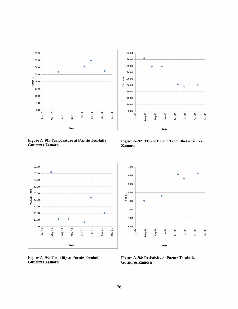
76
Figure A–91: Temperature at Puente Tecolutla-Gutierrez Zamora
Figure A–92: TDS at Puente Tecolutla-Gutierrez Zamora
Figure A–93: Turbidity at Puente Tecolutla-Gutierrez Zamora
Figure A–94: Resistivity at Puente Tecolutla-Gutierrez Zamora
0.0
5.0
10.0
15.0
20.0
25.0
30.0
35.0
40.0
Jan‐10
May‐10
Aug‐10
Nov‐10
Feb‐11
Jun‐11
Sep‐11
Dec‐11
Temp, C
Date
0.00
20.00
40.00
60.00
80.00
100.00
120.00
140.00
160.00
180.00
Jan‐10
May‐10
Aug‐10
Nov‐10
Feb‐11
Jun‐11
Sep‐11
Dec‐11
TDS, p
pm
Date
0.00
10.00
20.00
30.00
40.00
50.00
60.00
70.00
80.00
90.00
Jan‐10
May‐10
Aug‐10
Nov‐10
Feb‐11
Jun‐11
Sep‐11
Dec‐11
Turbidity, FTU
Date
0.00
1.00
2.00
3.00
4.00
5.00
6.00
7.00
Jan‐10
May‐10
Aug‐10
Nov‐10
Feb‐11
Jun‐11
Sep‐11
Dec‐11
Res, KΩ
Date

77
Figure A–95: Salinity at Puente Tecolutla-Gutierrez Zamora
Figure A–96: ORP at Puente Tecolutla-Gutierrez Zamora
Figure A–97: Conductivity at Puente Tecolutla-Gutierrez Zamora
Figure A–98: pH at Puente Tecolutla-Gutierrez Zamora
0.00
0.10
0.20
0.30
0.40
0.50
0.60
0.70
Jan‐10
May‐10
Aug‐10
Nov‐10
Feb‐11
Jun‐11
Sep‐11
Dec‐11
Salin
ity, %
Date
0.00
20.00
40.00
60.00
80.00
100.00
120.00
140.00
160.00
180.00
200.00
Jan‐10
May‐10
Aug‐10
Nov‐10
Feb‐11
Jun‐11
Sep‐11
Dec‐11
OPR, m
V
Date
0.00
50.00
100.00
150.00
200.00
250.00
300.00
350.00
Jan‐10
May‐10
Aug‐10
Nov‐10
Feb‐11
Jun‐11
Sep‐11
Dec‐11
Conductivity, m
S
Date
7.20
7.40
7.60
7.80
8.00
8.20
8.40
8.60
8.80
Jan‐10
May‐10
Aug‐10
Nov‐10
Feb‐11
Jun‐11
Sep‐11
Dec‐11
pH , pH units
Date

78
Figure A–99: Sulfates at Puente Tecolutla-Gutierrez Zamora
Figure A–100: Chlorides at Puente Tecolutla-Gutierrez Zamora
Figure A–101: Phosphates at Puente Tecolutla-Gutierrez Zamora
Figure A–102: Ammonia Nitrogen at Puente Tecolutla-Gutierrez Zamora
0.00E+00
1.00E‐01
2.00E‐01
3.00E‐01
4.00E‐01
5.00E‐01
6.00E‐01
7.00E‐01
Jan‐10
May‐10
Aug‐10
Nov‐10
Feb‐11
Jun‐11
Sep‐11
Dec‐11
Sulfates, ppm
Date
0.00
5.00
10.00
15.00
20.00
25.00
30.00
35.00
40.00
45.00
Jan‐10
May‐10
Aug‐10
Nov‐10
Feb‐11
Jun‐11
Sep‐11
Dec‐11
Chlorides, p
pm
Date
0.00
0.05
0.10
0.15
0.20
0.25
0.30
0.35
0.40
0.45
Jan‐10
May‐10
Aug‐10
Nov‐10
Feb‐11
Jun‐11
Sep‐11
Dec‐11
Tot Phosphate, p
pm
Date
0.00
2.00
4.00
6.00
8.00
10.00
12.00
14.00
16.00
Jan‐10
May‐10
Aug‐10
Nov‐10
Feb‐11
Jun‐11
Sep‐11
Dec‐11
Ammonia Nitrogen, m
g/L
Date

79
Figure A–103: Nitrate Nitrogen at Puente Tecolutla-Gutierrez Zamora
Figure A–104: Dissolved Oxygen at Puente Tecolutla-Gutierrez Zamaro
Figure A–105: BOD at Puente Tecolutla-Gutierrez Zamora
0.00
5.00
10.00
15.00
20.00
25.00
Jan‐10
May‐10
Aug‐10
Nov‐10
Feb‐11
Jun‐11
Sep‐11
Dec‐11
Nitrate Nitrogen, m
g/L
Date
0.00
2.00
4.00
6.00
8.00
10.00
12.00
Jan‐10
May‐10
Aug‐10
Nov‐10
Feb‐11
Jun‐11
Sep‐11
Dec‐11
Dissolved Oxygen, m
g/L
Date
0.00
10.00
20.00
30.00
40.00
50.00
60.00
70.00
Jan‐10
May‐10
Aug‐10
Nov‐10
Feb‐11
Jun‐11
Sep‐11
Dec‐11
BOD, m
g/L
Date

80
Table A–8: Results Reported by the UV for Salida de Gutierrez Zamora
Rio: Tecolutla Latitud Longitud
# punto: 8 Coordenadas: 20°28'51.36"N 97° 4'0.49"WNombre de punto de Monitoreo: Salida de Gutierrez Zamora
Fecha 23-Apr-10 7-Jul-10 15-Oct-10 25-Mar-11 27-May-11 12-Oct-11
Hora 5:15 PM 4:20 PM 5:54 PM 2:20 PM 4:38 PM
Temperatura (°C) 27.0 27.1 34.1
SDT (ppm) 290.30 218.28 142.60 31.89 249.50 81.94
Turbiedad (FTU) 64.50 10.10 7.94 6.15 33.86 16.76
Resistividad (KΩ)
1.74 3.54 146.00 2000.00 6.12
Salinidad (%) 0.90 0.50 228.00 9.00 3.50
ORP (mV) 37.45 134.43 76.90 10.50
Conductividad (µS)
584.40 281.90 64.12 500.00 163.97
pH (Unidades de pH)
7.80 7.62 7.60 7.80 7.90
Sulfatos (mg/L) 1.69E-01 1.56E-01 3.22E-01 7.54E-02
Cloruros (ppm) 120.00 15.50 58.10 311.33
Fosfatos (ppm) 0.25 0.20 0.13 0.04 0.33 0.18
Nitrogeno Amoniacal, N- NH3 (mg/L)
14.30
Nitrogeno de Nitratos, N- NO3-
(mg/L)3.10 11.77 96.30
Oxigeno Disuelto, OD (mg/L)
7.80 8.63 10.76 6.40 6.02 7.89
DBO (mg/L) 0.54 59.00 5.28 6.75 6.20
Coliformes Totales
36.00
Coliformes Fecales
46.00
Plomo (µg/L) 3.00
Arsenico (ppb) 0.00
Dureza (ppm) 120.00
Hierro (ppm) 0.15
Manganeso (mg/L)
0.00
Aluminio (mg/L) 0.00
Cromo (mg/L) 0.00

81
Figure A–106: Temperature at Salida de Gutierrez Zamora
Figure A–107: TDS at Salida de Gutierrez Zamora
Figure A–108: Turbidity at Salida de Gutierrez Zamora
Figure A–109: Resistivity at Salida de Gutierrez Zamora
0.0
5.0
10.0
15.0
20.0
25.0
30.0
35.0
40.0
Jan‐10
May‐10
Aug‐10
Nov‐10
Feb‐11
Jun‐11
Sep‐11
Dec‐11
Temp, C
Date
0.00
50.00
100.00
150.00
200.00
250.00
300.00
350.00
Jan‐10
May‐10
Aug‐10
Nov‐10
Feb‐11
Jun‐11
Sep‐11
Dec‐11
TDS, ppm
Date
0.00
10.00
20.00
30.00
40.00
50.00
60.00
70.00
Jan‐10
May‐10
Aug‐10
Nov‐10
Feb‐11
Jun‐11
Sep‐11
Dec‐11
Turbidity, FTU
Date
0.00
500.00
1000.00
1500.00
2000.00
2500.00
Jan‐10
May‐10
Aug‐10
Nov‐10
Feb‐11
Jun‐11
Sep‐11
Dec‐11
Res, KΩ
Date
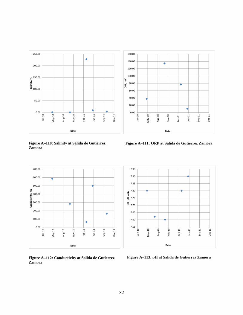
82
Figure A–110: Salinity at Salida de Gutierrez Zamora
Figure A–111: ORP at Salida de Gutierrez Zamora
Figure A–112: Conductivity at Salida de Gutierrez Zamora
Figure A–113: pH at Salida de Gutierrez Zamora
0.00
50.00
100.00
150.00
200.00
250.00
Jan‐10
May‐10
Aug‐10
Nov‐10
Feb‐11
Jun‐11
Sep‐11
Dec‐11
Salin
ity, %
Date
0.00
20.00
40.00
60.00
80.00
100.00
120.00
140.00
160.00
Jan‐10
May‐10
Aug‐10
Nov‐10
Feb‐11
Jun‐11
Sep‐11
Dec‐11
OPR, m
V
Date
0.00
100.00
200.00
300.00
400.00
500.00
600.00
700.00
Jan‐10
May‐10
Aug‐10
Nov‐10
Feb‐11
Jun‐11
Sep‐11
Dec‐11
Conductivity, m
S
Date
7.55
7.60
7.65
7.70
7.75
7.80
7.85
7.90
7.95
Jan‐10
May‐10
Aug‐10
Nov‐10
Feb‐11
Jun‐11
Sep‐11
Dec‐11
pH , pH units
Date

83
Figure A–114: Sulfates at Salida de Gutierrez Zamora
Figure A–115: Chlorides at Salida de Gutierrez Zamora
Figure A–116: Phosphates at Salida de Gutierrez Zamora
Figure A–117: Ammonia Nitrogen at Salida de Gutierrez Zamora
0.00E+00
5.00E‐02
1.00E‐01
1.50E‐01
2.00E‐01
2.50E‐01
3.00E‐01
3.50E‐01
Jan‐10
May‐10
Aug‐10
Nov‐10
Feb‐11
Jun‐11
Sep‐11
Dec‐11
Sulfates, ppm
Date
0.00
50.00
100.00
150.00
200.00
250.00
300.00
350.00
Jan‐10
May‐10
Aug‐10
Nov‐10
Feb‐11
Jun‐11
Sep‐11
Dec‐11
Chlorides, ppm
Date
0.00
0.05
0.10
0.15
0.20
0.25
0.30
0.35
Jan‐10
May‐10
Aug‐10
Nov‐10
Feb‐11
Jun‐11
Sep‐11
Dec‐11
Tot Phosphate, p
pm
Date
0.00
2.00
4.00
6.00
8.00
10.00
12.00
14.00
16.00
Jan‐10
May‐10
Aug‐10
Nov‐10
Feb‐11
Jun‐11
Sep‐11
Dec‐11
Ammonia Nitrogen, m
g/L
Date

84
Figure A–118: Nitrate Nitrogen at Salida de Gutierrez Zamora
Figure A–119: Dissolved Oxygen at Salida de Gutierrez Zamora
Figure A–120: BOD at Salida de Gutierrez Zamora
0.00
20.00
40.00
60.00
80.00
100.00
120.00
Jan‐10
May‐10
Aug‐10
Nov‐10
Feb‐11
Jun‐11
Sep‐11
Dec‐11
Nitrate Nitrogen, m
g/L
Date
0.00
2.00
4.00
6.00
8.00
10.00
12.00
Jan‐10
May‐10
Aug‐10
Nov‐10
Feb‐11
Jun‐11
Sep‐11
Dec‐11
Dissolved Oxygen, m
g/L
Date
0.00
10.00
20.00
30.00
40.00
50.00
60.00
70.00
Jan‐10
May‐10
Aug‐10
Nov‐10
Feb‐11
Jun‐11
Sep‐11
Dec‐11
BOD, m
g/L
Date

85
Table A–9: Results Reported by the UV for Bocana de Tecolutla
Rio: Tecolutla Latitud Longitud
# punto: 9 Coordenadas: 20°28'28.51"N 97° 0'12.45"WNombre de punto de Monitoreo: Bocana de Tecolutla
Fecha 23-Apr-10 7-Jul-10 15-Oct-10 25-Mar-11 27-May-11 12-Oct-11
Hora 5:54 PM 5:02 PM 5:20 PM
Temperatura (°C) 27.2 28.4 28.4 32.8 26.5
SDT (ppm) 212.10 685.30 1.83 1.20 249.40
Turbiedad (FTU) 17.95 12.55 6.77 4.62 13.66 18.37
Resistividad (KΩ)
2.36 273.00 418.00 80.40 28.00
Salinidad (%) 7.80 6.80 117.50 23.40 66.60
ORP (mV) 56.36 124.33 123.90 42.43
Conductividad (µS)
18.95 3.63 2.40 12.47 17.88
pH (Unidades de pH)
7.73 7.65 8.61 7.80
Sulfatos (mg/L) 6.13E-01 4.39E-01 1.05E+00 4.68E-01
Cloruros (ppm) 1.25 1.98 44.70 4.75
Fosfatos (ppm) 0.22 0.16 0.19 0.04 0.18 0.18
Nitrogeno Amoniacal, N- NH3 (mg/L)
12.90
Nitrogeno de Nitratos, N- NO3-
(mg/L)2.90 12.30 32.90
Oxigeno Disuelto, OD (mg/L)
8.28 9.07 10.87 9.81 6.72 7.88
DBO (mg/L) 0.62 73.33 5.46 9.79 6.76
Coliformes Totales
29.00
Coliformes Fecales
44.00
Plomo (µg/L) 1.00
Arsenico (ppb) 0.00
Dureza (ppm) 250.00
Hierro (ppm) 0.00
Manganeso (mg/L)
0.05
Aluminio (mg/L) 0.00
Cromo (mg/L) 0.20

86
Figure A–121: Temperature at Bocana de Tecolutla
Figure A–122: TDS at Bocana de Tecolutla
Figure A–123: Turbidity at Bocana de Tecolutla
Figure A–124: Resistivity at Bocana de Tecolutla
0.0
5.0
10.0
15.0
20.0
25.0
30.0
35.0
Jan‐10
May‐10
Aug‐10
Nov‐10
Feb‐11
Jun‐11
Sep‐11
Dec‐11
Temp, C
Date
0.00
100.00
200.00
300.00
400.00
500.00
600.00
700.00
800.00
Jan‐10
May‐10
Aug‐10
Nov‐10
Feb‐11
Jun‐11
Sep‐11
Dec‐11
TDS, ppm
Date
0.00
2.00
4.00
6.00
8.00
10.00
12.00
14.00
16.00
18.00
20.00
Jan‐10
May‐10
Aug‐10
Nov‐10
Feb‐11
Jun‐11
Sep‐11
Dec‐11
Turbidity, FTU
Date
0.00
50.00
100.00
150.00
200.00
250.00
300.00
350.00
400.00
450.00
Jan‐10
May‐10
Aug‐10
Nov‐10
Feb‐11
Jun‐11
Sep‐11
Dec‐11
Res, KΩ
Date

87
Figure A–125: Salinity at Bocana de Tecolutla
Figure A–126: ORP at Bocana de Tecolutla
Figure A–127: Conductivity at Bocana de Tecolutla
Figure A–128: pH at Bocana de Tecolutla
0.00
20.00
40.00
60.00
80.00
100.00
120.00
140.00
Jan‐10
May‐10
Aug‐10
Nov‐10
Feb‐11
Jun‐11
Sep‐11
Dec‐11
Salin
ity, %
Date
0.00
20.00
40.00
60.00
80.00
100.00
120.00
140.00
Jan‐10
May‐10
Aug‐10
Nov‐10
Feb‐11
Jun‐11
Sep‐11
Dec‐11
OPR, m
V
Date
0.00
2.00
4.00
6.00
8.00
10.00
12.00
14.00
16.00
18.00
20.00
Jan‐10
May‐10
Aug‐10
Nov‐10
Feb‐11
Jun‐11
Sep‐11
Dec‐11
Conductivity, m
S
Date
7.60
7.80
8.00
8.20
8.40
8.60
8.80
Jan‐10
May‐10
Aug‐10
Nov‐10
Feb‐11
Jun‐11
Sep‐11
Dec‐11
pH , pH units
Date

88
Figure A–129: Sulfates at Bocana de Tecolutla
Figure A–130: Chlorides at Bocana de Tecolutla
Figure A–131: Phosphates at Bocana de Tecolutla
Figure A–132: Ammonia Nitrogen at Bocana de Tecolutla
0.00E+00
2.00E‐01
4.00E‐01
6.00E‐01
8.00E‐01
1.00E+00
1.20E+00
Jan‐10
May‐10
Aug‐10
Nov‐10
Feb‐11
Jun‐11
Sep‐11
Dec‐11
Sulfates, ppm
Date
0.00
5.00
10.00
15.00
20.00
25.00
30.00
35.00
40.00
45.00
50.00
Jan‐10
May‐10
Aug‐10
Nov‐10
Feb‐11
Jun‐11
Sep‐11
Dec‐11
Chlorides, ppm
Date
0.00
0.05
0.10
0.15
0.20
0.25
Jan‐10
May‐10
Aug‐10
Nov‐10
Feb‐11
Jun‐11
Sep‐11
Dec‐11
Tot Phosphate, p
pm
Date
0.00
2.00
4.00
6.00
8.00
10.00
12.00
14.00
Jan‐10
May‐10
Aug‐10
Nov‐10
Feb‐11
Jun‐11
Sep‐11
Dec‐11
Ammonia Nitrogen, m
g/L
Date

89
Figure A–133: Nitrate Nitrogen at Bocana de Tecolutla
Figure A–134: Dissolved Oxygen at Bocana de Tecolutla
Figure A–135: BOD at Bocana de Tecolutla
0.00
5.00
10.00
15.00
20.00
25.00
30.00
35.00
Jan‐10
May‐10
Aug‐10
Nov‐10
Feb‐11
Jun‐11
Sep‐11
Dec‐11
Nitrate Nitrogen, m
g/L
Date
0.00
2.00
4.00
6.00
8.00
10.00
12.00
Jan‐10
May‐10
Aug‐10
Nov‐10
Feb‐11
Jun‐11
Sep‐11
Dec‐11
Dissolved Oxygen, m
g/L
Date
0.00
10.00
20.00
30.00
40.00
50.00
60.00
70.00
80.00
Jan‐10
May‐10
Aug‐10
Nov‐10
Feb‐11
Jun‐11
Sep‐11
Dec‐11
BOD, m
g/L
Date

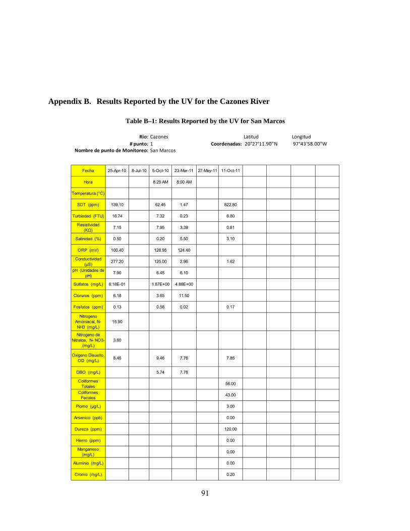
91
Appendix B. Results Reported by the UV for the Cazones River
Table B–1: Results Reported by the UV for San Marcos
Rio: Cazones Latitud Longitud
# punto: 1 Coordenadas: 20°27'11.90"N 97°43'58.00"WNombre de punto de Monitoreo: San Marcos
Fecha 25-Apr-10 8-Jul-10 5-Oct-10 23-Mar-11 27-May-11 11-Oct-11
Hora 8:25 AM 8:00 AM
Temperatura (°C)
SDT (ppm) 139.10 62.45 1.47 822.80
Turbiedad (FTU) 16.74 7.32 0.23 6.80
Resistividad (KΩ)
7.15 7.95 3.39 0.61
Salinidad (%) 0.50 0.20 5.50 3.10
ORP (mV) 100.40 128.95 124.40
Conductividad (µS)
277.20 125.00 2.96 1.62
pH (Unidades de pH)
7.90 6.45 6.10
Sulfatos (mg/L) 6.18E-01 1.87E+00 4.86E+00
Cloruros (ppm) 6.18 3.65 11.50
Fosfatos (ppm) 0.13 0.58 0.02 0.17
Nitrogeno Amoniacal, N- NH3 (mg/L)
15.90
Nitrogeno de Nitratos, N- NO3-
(mg/L)3.60
Oxigeno Disuelto, OD (mg/L)
8.46 9.46 7.76 7.85
DBO (mg/L) 5.74 7.78
Coliformes Totales
56.00
Coliformes Fecales
43.00
Plomo (µg/L) 3.00
Arsenico (ppb) 0.00
Dureza (ppm) 120.00
Hierro (ppm) 0.00
Manganeso (mg/L)
0.00
Aluminio (mg/L) 0.00
Cromo (mg/L) 0.20

92
Figure B–1: Temperature at San Marcos
Figure B–2: TDS at San Marcos
Figure B–3: Turbidity at San Marcos
Figure B–4: Resistivity at San Marcos
0.0
0.2
0.4
0.6
0.8
1.0
1.2
Jan‐10
May‐10
Aug‐10
Nov‐10
Feb‐11
Jun‐11
Sep‐11
Dec‐11
Temp, C
Date
0.00
100.00
200.00
300.00
400.00
500.00
600.00
700.00
800.00
900.00
Jan‐10
May‐10
Aug‐10
Nov‐10
Feb‐11
Jun‐11
Sep‐11
Dec‐11
TDS, p
pm
Date
0.00
2.00
4.00
6.00
8.00
10.00
12.00
14.00
16.00
18.00
Jan‐10
May‐10
Aug‐10
Nov‐10
Feb‐11
Jun‐11
Sep‐11
Dec‐11
Turbidity, FTU
Date
0.00
1.00
2.00
3.00
4.00
5.00
6.00
7.00
8.00
9.00
Jan‐10
May‐10
Aug‐10
Nov‐10
Feb‐11
Jun‐11
Sep‐11
Dec‐11
Res, KΩ
Date

93
Figure B–5: Salinity at San Marcos
Figure B–6: ORP at San Marcos
Figure B–7: Conductivity at San Marcos
Figure B–8: pH at San Marcos
0.00
1.00
2.00
3.00
4.00
5.00
6.00
Jan‐10
May‐10
Aug‐10
Nov‐10
Feb‐11
Jun‐11
Sep‐11
Dec‐11
Salin
ity, %
Date
0.00
20.00
40.00
60.00
80.00
100.00
120.00
140.00
Jan‐10
May‐10
Aug‐10
Nov‐10
Feb‐11
Jun‐11
Sep‐11
Dec‐11
OPR, m
V
Date
0.00
50.00
100.00
150.00
200.00
250.00
300.00
Jan‐10
May‐10
Aug‐10
Nov‐10
Feb‐11
Jun‐11
Sep‐11
Dec‐11
Conductivity, m
S
Date
0.00
1.00
2.00
3.00
4.00
5.00
6.00
7.00
8.00
9.00
Jan‐10
May‐10
Aug‐10
Nov‐10
Feb‐11
Jun‐11
Sep‐11
Dec‐11
pH, pH units
Date

94
Figure B–9: Sulfates at San Marcos
Figure B–10: Chlorides at San Marcos
Figure B–11: Phosphates at San Marcos
Figure B–12: Ammonia Nitrogen at San Marcos
0.00E+00
1.00E+00
2.00E+00
3.00E+00
4.00E+00
5.00E+00
6.00E+00
Jan‐10
May‐10
Aug‐10
Nov‐10
Feb‐11
Jun‐11
Sep‐11
Dec‐11
Sulfates, ppm
Date
0.00
2.00
4.00
6.00
8.00
10.00
12.00
14.00
Jan‐10
May‐10
Aug‐10
Nov‐10
Feb‐11
Jun‐11
Sep‐11
Dec‐11
Chlorides, ppm
Date
0.00
0.10
0.20
0.30
0.40
0.50
0.60
0.70
Jan‐10
May‐10
Aug‐10
Nov‐10
Feb‐11
Jun‐11
Sep‐11
Dec‐11
Tot Phosphate, p
pm
Date
0.00
2.00
4.00
6.00
8.00
10.00
12.00
14.00
16.00
18.00
Jan‐10
May‐10
Aug‐10
Nov‐10
Feb‐11
Jun‐11
Sep‐11
Dec‐11
Ammonia Nitrogen, m
g/L
Date
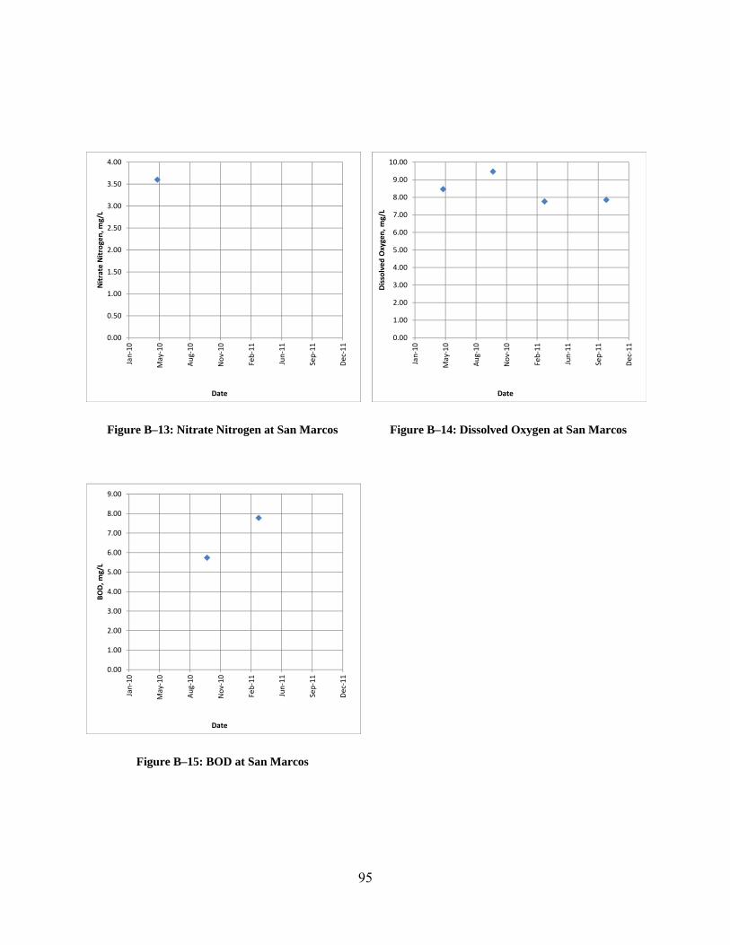
95
Figure B–13: Nitrate Nitrogen at San Marcos
Figure B–14: Dissolved Oxygen at San Marcos
Figure B–15: BOD at San Marcos
0.00
0.50
1.00
1.50
2.00
2.50
3.00
3.50
4.00
Jan‐10
May‐10
Aug‐10
Nov‐10
Feb‐11
Jun‐11
Sep‐11
Dec‐11
Nitrate Nitrogen, m
g/L
Date
0.00
1.00
2.00
3.00
4.00
5.00
6.00
7.00
8.00
9.00
10.00
Jan‐10
May‐10
Aug‐10
Nov‐10
Feb‐11
Jun‐11
Sep‐11
Dec‐11
Dissolved Oxygen, m
g/L
Date
0.00
1.00
2.00
3.00
4.00
5.00
6.00
7.00
8.00
9.00
Jan‐10
May‐10
Aug‐10
Nov‐10
Feb‐11
Jun‐11
Sep‐11
Dec‐11
BOD, m
g/L
Date
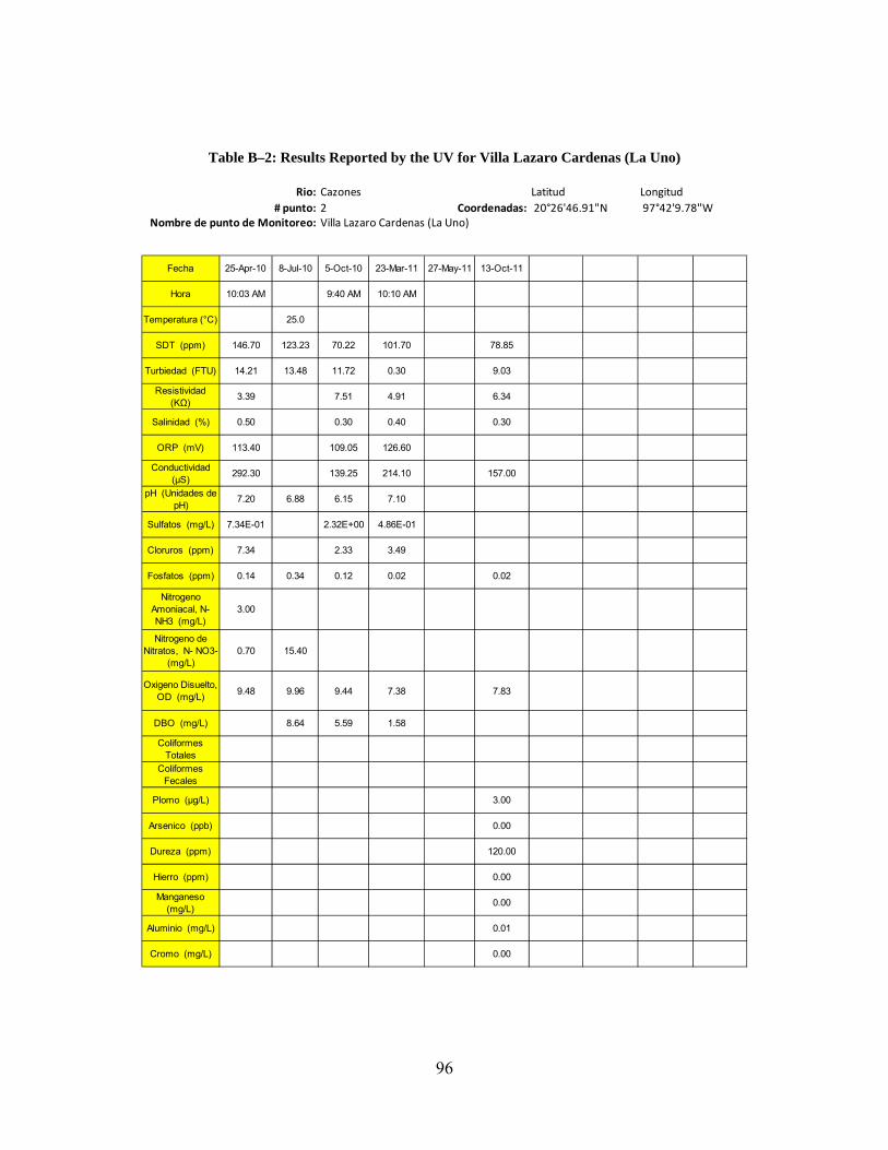
96
Table B–2: Results Reported by the UV for Villa Lazaro Cardenas (La Uno)
Rio: Cazones Latitud Longitud
# punto: 2 Coordenadas: 20°26'46.91"N 97°42'9.78"WNombre de punto de Monitoreo: Villa Lazaro Cardenas (La Uno)
Fecha 25-Apr-10 8-Jul-10 5-Oct-10 23-Mar-11 27-May-11 13-Oct-11
Hora 10:03 AM 9:40 AM 10:10 AM
Temperatura (°C) 25.0
SDT (ppm) 146.70 123.23 70.22 101.70 78.85
Turbiedad (FTU) 14.21 13.48 11.72 0.30 9.03
Resistividad (KΩ)
3.39 7.51 4.91 6.34
Salinidad (%) 0.50 0.30 0.40 0.30
ORP (mV) 113.40 109.05 126.60
Conductividad (µS)
292.30 139.25 214.10 157.00
pH (Unidades de pH)
7.20 6.88 6.15 7.10
Sulfatos (mg/L) 7.34E-01 2.32E+00 4.86E-01
Cloruros (ppm) 7.34 2.33 3.49
Fosfatos (ppm) 0.14 0.34 0.12 0.02 0.02
Nitrogeno Amoniacal, N- NH3 (mg/L)
3.00
Nitrogeno de Nitratos, N- NO3-
(mg/L)0.70 15.40
Oxigeno Disuelto, OD (mg/L)
9.48 9.96 9.44 7.38 7.83
DBO (mg/L) 8.64 5.59 1.58
Coliformes Totales
Coliformes Fecales
Plomo (µg/L) 3.00
Arsenico (ppb) 0.00
Dureza (ppm) 120.00
Hierro (ppm) 0.00
Manganeso (mg/L)
0.00
Aluminio (mg/L) 0.01
Cromo (mg/L) 0.00
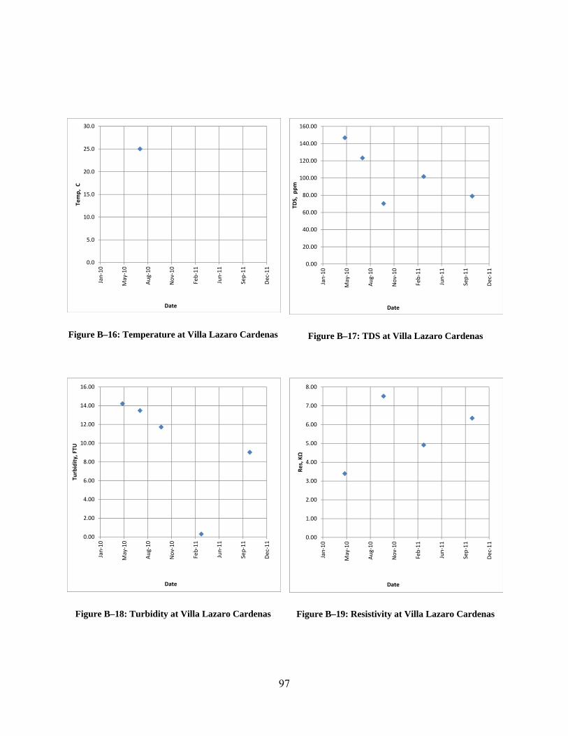
97
Figure B–16: Temperature at Villa Lazaro Cardenas
Figure B–17: TDS at Villa Lazaro Cardenas
Figure B–18: Turbidity at Villa Lazaro Cardenas
Figure B–19: Resistivity at Villa Lazaro Cardenas
0.0
5.0
10.0
15.0
20.0
25.0
30.0
Jan‐10
May‐10
Aug‐10
Nov‐10
Feb‐11
Jun‐11
Sep‐11
Dec‐11
Temp, C
Date
0.00
20.00
40.00
60.00
80.00
100.00
120.00
140.00
160.00
Jan‐10
May‐10
Aug‐10
Nov‐10
Feb‐11
Jun‐11
Sep‐11
Dec‐11
TDS, ppm
Date
0.00
2.00
4.00
6.00
8.00
10.00
12.00
14.00
16.00
Jan‐10
May‐10
Aug‐10
Nov‐10
Feb‐11
Jun‐11
Sep‐11
Dec‐11
Turbidity, FTU
Date
0.00
1.00
2.00
3.00
4.00
5.00
6.00
7.00
8.00
Jan‐10
May‐10
Aug‐10
Nov‐10
Feb‐11
Jun‐11
Sep‐11
Dec‐11
Res, KΩ
Date

98
Figure B–20: Salinity at Villa Lazaro Cardenas
Figure B–21: ORP at Villa Lazaro Cardenas
Figure B–22: Conductivity at Villa Lazaro Cardenas
Figure B–23: pH at Villa Lazaro Cardenas
0.00
0.10
0.20
0.30
0.40
0.50
0.60
Jan‐10
May‐10
Aug‐10
Nov‐10
Feb‐11
Jun‐11
Sep‐11
Dec‐11
Salin
ity, %
Date
108.00
110.00
112.00
114.00
116.00
118.00
120.00
122.00
124.00
126.00
128.00
Jan‐10
May‐10
Aug‐10
Nov‐10
Feb‐11
Jun‐11
Sep‐11
Dec‐11
OPR, m
V
Date
0.00
50.00
100.00
150.00
200.00
250.00
300.00
350.00
Jan‐10
May‐10
Aug‐10
Nov‐10
Feb‐11
Jun‐11
Sep‐11
Dec‐11
Conductivity, m
S
Date
6.00
6.20
6.40
6.60
6.80
7.00
7.20
7.40
Jan‐10
May‐10
Aug‐10
Nov‐10
Feb‐11
Jun‐11
Sep‐11
Dec‐11
pH, pH units
Date

99
Figure B–24: Sulfates at Villa Lazaro Cardenas
Figure B–25: Chlorides at Villa Lazaro Cardenas
Figure B–26: Phosphates at Villa Lazaro Cardenas
Figure B–27: Ammonia Nitrogen at Villa Lazaro Cardenas
0.00E+00
5.00E‐01
1.00E+00
1.50E+00
2.00E+00
2.50E+00
Jan‐10
May‐10
Aug‐10
Nov‐10
Feb‐11
Jun‐11
Sep‐11
Dec‐11
Sulfates, ppm
Date
0.00
1.00
2.00
3.00
4.00
5.00
6.00
7.00
8.00
Jan‐10
May‐10
Aug‐10
Nov‐10
Feb‐11
Jun‐11
Sep‐11
Dec‐11
Chlorides, ppm
Date
0.00
0.05
0.10
0.15
0.20
0.25
0.30
0.35
0.40
Jan‐10
May‐10
Aug‐10
Nov‐10
Feb‐11
Jun‐11
Sep‐11
Dec‐11
Tot Phosphate, p
pm
Date
0.00
0.50
1.00
1.50
2.00
2.50
3.00
3.50
Jan‐10
May‐10
Aug‐10
Nov‐10
Feb‐11
Jun‐11
Sep‐11
Dec‐11
Ammonia Nitrogen, m
g/L
Date
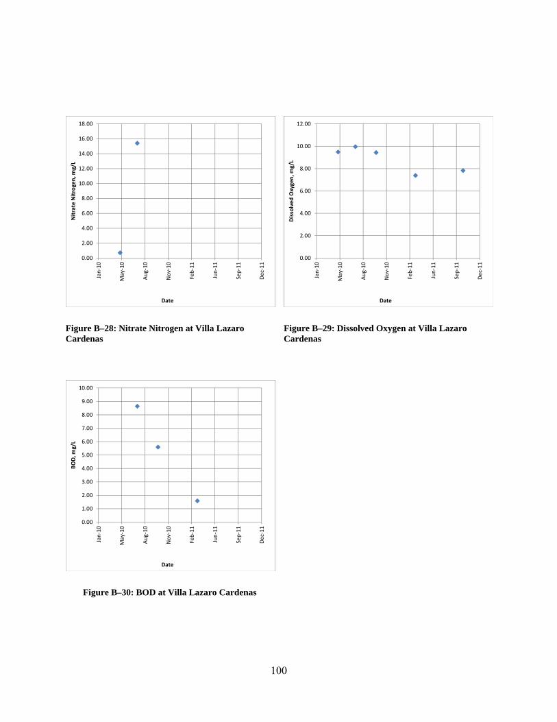
100
Figure B–28: Nitrate Nitrogen at Villa Lazaro Cardenas
Figure B–29: Dissolved Oxygen at Villa Lazaro Cardenas
Figure B–30: BOD at Villa Lazaro Cardenas
0.00
2.00
4.00
6.00
8.00
10.00
12.00
14.00
16.00
18.00
Jan‐10
May‐10
Aug‐10
Nov‐10
Feb‐11
Jun‐11
Sep‐11
Dec‐11
Nitrate Nitrogen, m
g/L
Date
0.00
2.00
4.00
6.00
8.00
10.00
12.00
Jan‐10
May‐10
Aug‐10
Nov‐10
Feb‐11
Jun‐11
Sep‐11
Dec‐11
Dissolved Oxygen, m
g/L
Date
0.00
1.00
2.00
3.00
4.00
5.00
6.00
7.00
8.00
9.00
10.00
Jan‐10
May‐10
Aug‐10
Nov‐10
Feb‐11
Jun‐11
Sep‐11
Dec‐11
BOD, m
g/L
Date

101
Table B–3: Results Reported by the UV for Bocatoma
Rio: Cazones Latitud Longitud
# punto: 3 Coordenadas: 20°29'2.76"N 97°32'46.20"WNombre de punto de Monitoreo: Bocatoma
Fecha 25-Apr-10 8-Jul-10 5-Oct-10 23-Mar-11 27-May-11 13-Oct-11
Hora 10:30 AM 12:30 PM
Temperatura (°C) 25.3
SDT (ppm) 168.37 73.49 98.68 87.21
Turbiedad (FTU) 11.16 20.87 54.00 7.17
Resistividad (KΩ)
6.81 4.99 5.78
Salinidad (%) 0.30 0.40 0.30
ORP (mV) 123.75 121.70
Conductividad (µS)
151.80 201.12 173.55
pH (Unidades de pH)
7.43 6.20 7.70
Sulfatos (mg/L) 1.25E-02 1.00E-02
Cloruros (ppm) 3.78 3.36
Fosfatos (ppm) 0.61 0.31 0.26 0.21
Nitrogeno Amoniacal, N- NH3 (mg/L)
Nitrogeno de Nitratos, N- NO3-
(mg/L)19.43
Oxigeno Disuelto, OD (mg/L)
8.93 9.55 5.59 8.48
DBO (mg/L) 6.24 6.63 5.81
Coliformes Totales
55.00
Coliformes Fecales
51.00
Plomo (µg/L)
Arsenico (ppb) 30.00
Dureza (ppm)
Hierro (ppm) 0.00
Manganeso (mg/L)
0.00
Aluminio (mg/L) 0.00
Cromo (mg/L) 0.00

102
Figure B–31: Temperature at Bocatoma
Figure B–32: TDS at Bocatoma
Figure B–33: Turbidity at Bocatoma
Figure B–34: Resistivity at Bocatoma
0.0
5.0
10.0
15.0
20.0
25.0
30.0
Jan‐10
May‐10
Aug‐10
Nov‐10
Feb‐11
Jun‐11
Sep‐11
Dec‐11
Temp, C
Date
0.00
20.00
40.00
60.00
80.00
100.00
120.00
140.00
160.00
180.00
Jan‐10
May‐10
Aug‐10
Nov‐10
Feb‐11
Jun‐11
Sep‐11
Dec‐11
TDS, ppm
Date
0.00
10.00
20.00
30.00
40.00
50.00
60.00
Jan‐10
May‐10
Aug‐10
Nov‐10
Feb‐11
Jun‐11
Sep‐11
Dec‐11
Turbidity, FTU
Date
0.00
1.00
2.00
3.00
4.00
5.00
6.00
7.00
8.00
Jan‐10
May‐10
Aug‐10
Nov‐10
Feb‐11
Jun‐11
Sep‐11
Dec‐11
Res, KΩ
Date

103
Figure B–35: Salinity at Bocatoma
Figure B–36: ORP at Bocatoma
Figure B–37: Conductivity at Bocatoma
Figure B–38: pH at Bocatoma
0.00
0.05
0.10
0.15
0.20
0.25
0.30
0.35
0.40
0.45
Jan‐10
May‐10
Aug‐10
Nov‐10
Feb‐11
Jun‐11
Sep‐11
Dec‐11
Salin
ity, %
Date
121.50
122.00
122.50
123.00
123.50
124.00
Jan‐10
May‐10
Aug‐10
Nov‐10
Feb‐11
Jun‐11
Sep‐11
Dec‐11
OPR, m
V
Date
0.00
50.00
100.00
150.00
200.00
250.00
Jan‐10
May‐10
Aug‐10
Nov‐10
Feb‐11
Jun‐11
Sep‐11
Dec‐11
Conductivity, m
S
Date
0.00
1.00
2.00
3.00
4.00
5.00
6.00
7.00
8.00
9.00
Jan‐10
May‐10
Aug‐10
Nov‐10
Feb‐11
Jun‐11
Sep‐11
Dec‐11
pH, pH units
Date

104
Figure B–39: Sulfates at Bocatoma
Figure B–40: Chlorides at Bocatoma
Figure B–41: Phosphates at Bocatoma
Figure B–42: Ammonia Nitrogen at Bocatoma
0.00E+00
2.00E‐03
4.00E‐03
6.00E‐03
8.00E‐03
1.00E‐02
1.20E‐02
1.40E‐02
Jan‐10
May‐10
Aug‐10
Nov‐10
Feb‐11
Jun‐11
Sep‐11
Dec‐11
Sulfates, ppm
Date
3.30
3.35
3.40
3.45
3.50
3.55
3.60
3.65
3.70
3.75
3.80
3.85
Jan‐10
May‐10
Aug‐10
Nov‐10
Feb‐11
Jun‐11
Sep‐11
Dec‐11
Chlorides, ppm
Date
0.00
0.10
0.20
0.30
0.40
0.50
0.60
0.70
Jan‐10
May‐10
Aug‐10
Nov‐10
Feb‐11
Jun‐11
Sep‐11
Dec‐11
Tot Phosphate, p
pm
Date
0.00
0.20
0.40
0.60
0.80
1.00
1.20
Jan‐10
May‐10
Aug‐10
Nov‐10
Feb‐11
Jun‐11
Sep‐11
Dec‐11
Ammonia Nitrogen, m
g/L
Date

105
Figure B–43: Nitrate Nitrogen at Bocatoma
Figure B–44: Dissolved Oxygen at Bocatoma
Figure B–45: BOD at Bocatoma
0.00
5.00
10.00
15.00
20.00
25.00
Jan‐10
May‐10
Aug‐10
Nov‐10
Feb‐11
Jun‐11
Sep‐11
Dec‐11
Nitrate Nitrogen, m
g/L
Date
0.00
2.00
4.00
6.00
8.00
10.00
12.00
Jan‐10
May‐10
Aug‐10
Nov‐10
Feb‐11
Jun‐11
Sep‐11
Dec‐11
Dissolved Oxygen, m
g/L
Date
5.70
5.80
5.90
6.00
6.10
6.20
6.30
6.40
6.50
6.60
6.70
Jan‐10
May‐10
Aug‐10
Nov‐10
Feb‐11
Jun‐11
Sep‐11
Dec‐11
BOD, m
g/L
Date

106
Table B–4: Results Reported by the UV for Puente Cazones 3
Rio: Cazones Latitud Longitud
# punto: 4 Coordenadas: 20°38'8.66"N 97°23'57.07"WNombre de punto de Monitoreo: Puente Cazones 3
Fecha 25-Apr-10 8-Jul-10 5-Oct-10 23-Mar-11 27-May-11 13-Oct-11
Hora 2:00 PM 11:15 AM 3:12 PM
Temperatura (°C)
SDT (ppm) 157.50 117.85 163.80 1.22
Turbiedad (FTU) 9.85 22.00 4.38 15.51
Resistividad (KΩ)
3.16 4.32 3.08 0.42
Salinidad (%) 0.60 0.40 0.60 4.50
ORP (mV) 54.50 171.85 82.60
Conductividad (µS)
315.10 225.10 324.70 3397.00
pH (Unidades de pH)
7.30 6.70 6.70
Sulfatos (mg/L) 1.16E-01 1.35E-01 2.02E-01
Cloruros (ppm) 7.45 45.55 13.30
Fosfatos (ppm) 0.30 0.27 1.37 0.54
Nitrogeno Amoniacal, N- NH3 (mg/L)
28.80
Nitrogeno de Nitratos, N- NO3-
(mg/L)6.50
Oxigeno Disuelto, OD (mg/L)
9.84 8.10 11.40 6.97
DBO (mg/L) 5.15 11.61
Coliformes Totales
35.00
Coliformes Fecales
33.00
Plomo (µg/L)
Arsenico (ppb) 0.00
Dureza (ppm)
Hierro (ppm) 0.00
Manganeso (mg/L)
0.00
Aluminio (mg/L) 0.00
Cromo (mg/L) 0.00

107
Figure B–46: Temperature at Puente Cazones 3
Figure B–47: TDS at Puente Cazones 3
Figure B–48: Turbidity at Puente Cazones 3
Figure B–49: Resistivity at Puente Cazones 3
0.0
0.2
0.4
0.6
0.8
1.0
1.2
Jan‐10
May‐10
Aug‐10
Nov‐10
Feb‐11
Jun‐11
Sep‐11
Dec‐11
Temp, C
Date
0.00
20.00
40.00
60.00
80.00
100.00
120.00
140.00
160.00
180.00
Jan‐10
May‐10
Aug‐10
Nov‐10
Feb‐11
Jun‐11
Sep‐11
Dec‐11
TDS, ppm
Date
0.00
5.00
10.00
15.00
20.00
25.00
Jan‐10
May‐10
Aug‐10
Nov‐10
Feb‐11
Jun‐11
Sep‐11
Dec‐11
Turbidity, FTU
Date
0.00
0.50
1.00
1.50
2.00
2.50
3.00
3.50
4.00
4.50
5.00
Jan‐10
May‐10
Aug‐10
Nov‐10
Feb‐11
Jun‐11
Sep‐11
Dec‐11
Res, KΩ
Date

108
Figure B–50: Salinity at Puente Cazones 3
Figure B–51: ORP at Puente Cazones 3
Figure B–52: Conductivity at Puente Cazones 3
Figure B–53: pH at Puente Cazones 3
0.00
0.50
1.00
1.50
2.00
2.50
3.00
3.50
4.00
4.50
5.00
Jan‐10
May‐10
Aug‐10
Nov‐10
Feb‐11
Jun‐11
Sep‐11
Dec‐11
Salin
ity, %
Date
0.00
20.00
40.00
60.00
80.00
100.00
120.00
140.00
160.00
180.00
200.00
Jan‐10
May‐10
Aug‐10
Nov‐10
Feb‐11
Jun‐11
Sep‐11
Dec‐11
OPR, m
V
Date
0.00
500.00
1000.00
1500.00
2000.00
2500.00
3000.00
3500.00
4000.00
Jan‐10
May‐10
Aug‐10
Nov‐10
Feb‐11
Jun‐11
Sep‐11
Dec‐11
Conductivity, m
S
Date
6.60
6.70
6.80
6.90
7.00
7.10
7.20
7.30
7.40
Jan‐10
May‐10
Aug‐10
Nov‐10
Feb‐11
Jun‐11
Sep‐11
Dec‐11
pH, pH units
Date

109
Figure B–54: Sulfates at Puente Cazones 3
Figure B–55: Chlorides at Puente Cazones 3
Figure B–56: Phosphates at Puente Cazones 3
Figure B–57: Ammonia Nitrogen at Puente Cazones 3
0.00E+00
5.00E‐02
1.00E‐01
1.50E‐01
2.00E‐01
2.50E‐01
Jan‐10
May‐10
Aug‐10
Nov‐10
Feb‐11
Jun‐11
Sep‐11
Dec‐11
Sulfates, ppm
Date
0.00
5.00
10.00
15.00
20.00
25.00
30.00
35.00
40.00
45.00
50.00
Jan‐10
May‐10
Aug‐10
Nov‐10
Feb‐11
Jun‐11
Sep‐11
Dec‐11
Chlorides, ppm
Date
0.00
0.20
0.40
0.60
0.80
1.00
1.20
1.40
1.60
Jan‐10
May‐10
Aug‐10
Nov‐10
Feb‐11
Jun‐11
Sep‐11
Dec‐11
Tot Phosphate, p
pm
Date
0.00
5.00
10.00
15.00
20.00
25.00
30.00
35.00
Jan‐10
May‐10
Aug‐10
Nov‐10
Feb‐11
Jun‐11
Sep‐11
Dec‐11
Ammonia Nitrogen, m
g/L
Date

110
Figure B–58: Nitrate Nitrogen at Puente Cazones 3
Figure B–59: Dissolved Oxygen at Puente Cazones 3
Figure B–60: BOD at Puente Cazones 3
0.00
1.00
2.00
3.00
4.00
5.00
6.00
7.00
Jan‐10
May‐10
Aug‐10
Nov‐10
Feb‐11
Jun‐11
Sep‐11
Dec‐11
Nitrate Nitrogen, m
g/L
Date
0.00
2.00
4.00
6.00
8.00
10.00
12.00
Jan‐10
May‐10
Aug‐10
Nov‐10
Feb‐11
Jun‐11
Sep‐11
Dec‐11
Dissolved Oxygen, m
g/L
Date
0.00
2.00
4.00
6.00
8.00
10.00
12.00
14.00
Jan‐10
May‐10
Aug‐10
Nov‐10
Feb‐11
Jun‐11
Sep‐11
Dec‐11
BOD, m
g/L
Date

111
Table B–5: Results Reported by the UV for Puente Colgante
Rio: Cazones Latitud Longitud
# punto: 5 Coordenadas: 20°42'22.73"N 97°18'49.25"WNombre de punto de Monitoreo: Puente Colgante
Fecha 25-Apr-10 8-Jul-10 5-Oct-10 23-Mar-11 27-May-11 13-Oct-11
Hora 11:40 AM 4:25 PM
Temperatura (°C) 25.7
SDT (ppm) 187.30 186.45 121.15 166.20 111.90
Turbiedad (FTU) 7.43 13.05 23.30 6.44 8.17
Resistividad (KΩ)
2.68 4.18 3.10 4.47
Salinidad (%) 0.70 0.40 0.60 5.00
ORP (mV) 92.75 115.65 46.00
Conductividad (µS)
371.90 240.10 332.40 223.60
pH (Unidades de pH)
7.80 7.07 6.30 8.00
Sulfatos (mg/L) 2.04E+00 1.04E-01 2.00E-01
Cloruros (ppm) 7.55 31.50 24.30
Fosfatos (ppm) 0.70 0.47 0.26 0.98 0.50
Nitrogeno Amoniacal, N- NH3 (mg/L)
21.50
Nitrogeno de Nitratos, N- NO3-
(mg/L)4.90 17.97
Oxigeno Disuelto, OD (mg/L)
11.47 8.10 7.45 6.44 6.10
DBO (mg/L) 7.04 4.24 6.70
Coliformes Totales
46.00
Coliformes Fecales
42.00
Plomo (µg/L)
Arsenico (ppb) 10.00
Dureza (ppm)
Hierro (ppm) 0.00
Manganeso (mg/L)
0.10
Aluminio (mg/L) 0.01
Cromo (mg/L) 0.00

112
Figure B–61: Temperature at Puente Colgante
Figure B–62: TDS at Puente Colgante
Figure B–63: Turbidity at Puente Colgante
Figure B–64: Resistivity at Puente Colgante
0.0
5.0
10.0
15.0
20.0
25.0
30.0
Jan‐10
May‐10
Aug‐10
Nov‐10
Feb‐11
Jun‐11
Sep‐11
Dec‐11
Temp, C
Date
0.00
20.00
40.00
60.00
80.00
100.00
120.00
140.00
160.00
180.00
200.00
Jan‐10
May‐10
Aug‐10
Nov‐10
Feb‐11
Jun‐11
Sep‐11
Dec‐11
TDS, ppm
Date
0.00
5.00
10.00
15.00
20.00
25.00
Jan‐10
May‐10
Aug‐10
Nov‐10
Feb‐11
Jun‐11
Sep‐11
Dec‐11
Turbidity, FTU
Date
0.00
0.50
1.00
1.50
2.00
2.50
3.00
3.50
4.00
4.50
5.00
Jan‐10
May‐10
Aug‐10
Nov‐10
Feb‐11
Jun‐11
Sep‐11
Dec‐11
Res, KΩ
Date

113
Figure B–65: Salinity at Puente Colgante
Figure B–66: ORP at Puente Colgante
Figure B–67: Conductivity at Puente Colgante
Figure B–68: pH at Puente Colgante
0.00
1.00
2.00
3.00
4.00
5.00
6.00
Jan‐10
May‐10
Aug‐10
Nov‐10
Feb‐11
Jun‐11
Sep‐11
Dec‐11
Salin
ity, %
Date
0.00
20.00
40.00
60.00
80.00
100.00
120.00
140.00
Jan‐10
May‐10
Aug‐10
Nov‐10
Feb‐11
Jun‐11
Sep‐11
Dec‐11
OPR, m
V
Date
0.00
50.00
100.00
150.00
200.00
250.00
300.00
350.00
400.00
Jan‐10
May‐10
Aug‐10
Nov‐10
Feb‐11
Jun‐11
Sep‐11
Dec‐11
Conductivity, m
S
Date
0.00
1.00
2.00
3.00
4.00
5.00
6.00
7.00
8.00
9.00
Jan‐10
May‐10
Aug‐10
Nov‐10
Feb‐11
Jun‐11
Sep‐11
Dec‐11
pH, p
H units
Date

114
Figure B–69: Sulfates at Puente Colgante
Figure B–70: Chlorides at Puente Colgante
Figure B–71: Phosphates at Puente Colgante
Figure B–72: Ammonia Nitrogen at Puente Colgante
0.00E+00
5.00E‐01
1.00E+00
1.50E+00
2.00E+00
2.50E+00
Jan‐10
May‐10
Aug‐10
Nov‐10
Feb‐11
Jun‐11
Sep‐11
Dec‐11
Sulfates, ppm
Date
0.00
5.00
10.00
15.00
20.00
25.00
30.00
35.00
Jan‐10
May‐10
Aug‐10
Nov‐10
Feb‐11
Jun‐11
Sep‐11
Dec‐11
Chlorides, ppm
Date
0.00
0.20
0.40
0.60
0.80
1.00
1.20
Jan‐10
May‐10
Aug‐10
Nov‐10
Feb‐11
Jun‐11
Sep‐11
Dec‐11
Tot Phosphate, p
pm
Date
0.00
5.00
10.00
15.00
20.00
25.00
Jan‐10
May‐10
Aug‐10
Nov‐10
Feb‐11
Jun‐11
Sep‐11
Dec‐11
Ammonia Nitrogen, m
g/L
Date

115
Figure B–73: Nitrate Nitrogen at Puente Colgante
Figure B–74: Dissolved Oxygen at Puente Colgante
Figure B–75: BOD at Puente Colgante
0.00
2.00
4.00
6.00
8.00
10.00
12.00
14.00
16.00
18.00
20.00
Jan‐10
May‐10
Aug‐10
Nov‐10
Feb‐11
Jun‐11
Sep‐11
Dec‐11
Nitrate Nitrogen, m
g/L
Date
0.00
2.00
4.00
6.00
8.00
10.00
12.00
14.00
Jan‐10
May‐10
Aug‐10
Nov‐10
Feb‐11
Jun‐11
Sep‐11
Dec‐11
Dissolved Oxygen, m
g/L
Date
0.00
1.00
2.00
3.00
4.00
5.00
6.00
7.00
8.00
Jan‐10
May‐10
Aug‐10
Nov‐10
Feb‐11
Jun‐11
Sep‐11
Dec‐11
BOD, m
g/L
Date
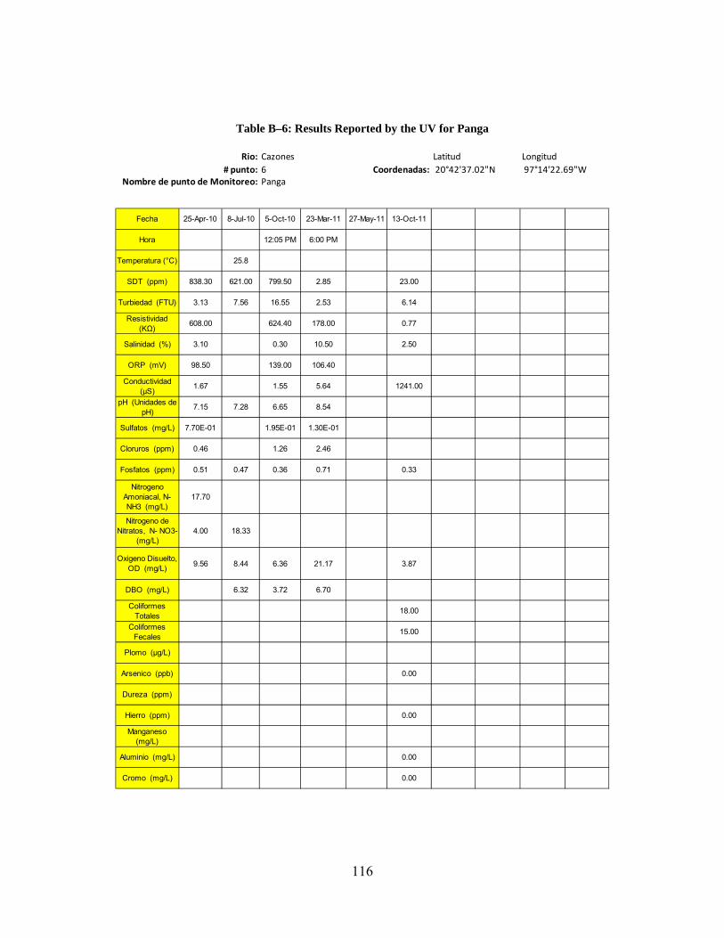
116
Table B–6: Results Reported by the UV for Panga
Rio: Cazones Latitud Longitud
# punto: 6 Coordenadas: 20°42'37.02"N 97°14'22.69"WNombre de punto de Monitoreo: Panga
Fecha 25-Apr-10 8-Jul-10 5-Oct-10 23-Mar-11 27-May-11 13-Oct-11
Hora 12:05 PM 6:00 PM
Temperatura (°C) 25.8
SDT (ppm) 838.30 621.00 799.50 2.85 23.00
Turbiedad (FTU) 3.13 7.56 16.55 2.53 6.14
Resistividad (KΩ)
608.00 624.40 178.00 0.77
Salinidad (%) 3.10 0.30 10.50 2.50
ORP (mV) 98.50 139.00 106.40
Conductividad (µS)
1.67 1.55 5.64 1241.00
pH (Unidades de pH)
7.15 7.28 6.65 8.54
Sulfatos (mg/L) 7.70E-01 1.95E-01 1.30E-01
Cloruros (ppm) 0.46 1.26 2.46
Fosfatos (ppm) 0.51 0.47 0.36 0.71 0.33
Nitrogeno Amoniacal, N- NH3 (mg/L)
17.70
Nitrogeno de Nitratos, N- NO3-
(mg/L)4.00 18.33
Oxigeno Disuelto, OD (mg/L)
9.56 8.44 6.36 21.17 3.87
DBO (mg/L) 6.32 3.72 6.70
Coliformes Totales
18.00
Coliformes Fecales
15.00
Plomo (µg/L)
Arsenico (ppb) 0.00
Dureza (ppm)
Hierro (ppm) 0.00
Manganeso (mg/L)
Aluminio (mg/L) 0.00
Cromo (mg/L) 0.00

117
Figure B–76: Temperature at Panga
Figure B–77: TDS at Panga
Figure B–78: Turbidity at Panga
Figure B–79: Resistivity at Panga
0.0
5.0
10.0
15.0
20.0
25.0
30.0
Jan‐10
May‐10
Aug‐10
Nov‐10
Feb‐11
Jun‐11
Sep‐11
Dec‐11
Temp, C
Date
0.00
100.00
200.00
300.00
400.00
500.00
600.00
700.00
800.00
900.00
Jan‐10
May‐10
Aug‐10
Nov‐10
Feb‐11
Jun‐11
Sep‐11
Dec‐11
TDS, ppm
Date
0.00
2.00
4.00
6.00
8.00
10.00
12.00
14.00
16.00
18.00
Jan‐10
May‐10
Aug‐10
Nov‐10
Feb‐11
Jun‐11
Sep‐11
Dec‐11
Turbidity, FTU
Date
0.00
100.00
200.00
300.00
400.00
500.00
600.00
700.00
Jan‐10
May‐10
Aug‐10
Nov‐10
Feb‐11
Jun‐11
Sep‐11
Dec‐11
Res, KΩ
Date

118
Figure B–80: Salinity at Panga
Figure B–81: ORP at Panga
Figure B–82: Conductivity at Panga
Figure B–83: pH at Panga
0.00
2.00
4.00
6.00
8.00
10.00
12.00
Jan‐10
May‐10
Aug‐10
Nov‐10
Feb‐11
Jun‐11
Sep‐11
Dec‐11
Salin
ity, %
Date
0.00
20.00
40.00
60.00
80.00
100.00
120.00
140.00
160.00
Jan‐10
May‐10
Aug‐10
Nov‐10
Feb‐11
Jun‐11
Sep‐11
Dec‐11
OPR, m
V
Date
0.00
200.00
400.00
600.00
800.00
1000.00
1200.00
1400.00
Jan‐10
May‐10
Aug‐10
Nov‐10
Feb‐11
Jun‐11
Sep‐11
Dec‐11
Conductivity, m
S
Date
0.00
1.00
2.00
3.00
4.00
5.00
6.00
7.00
8.00
9.00
Jan‐10
May‐10
Aug‐10
Nov‐10
Feb‐11
Jun‐11
Sep‐11
Dec‐11
pH, pH units
Date

119
Figure B–84: Sulfates at Panga
Figure B–85: Chlorides at Panga
Figure B–86: Phosphates at Panga
Figure B–87: Ammonia Nitrogen at Panga
0.00E+00
1.00E‐01
2.00E‐01
3.00E‐01
4.00E‐01
5.00E‐01
6.00E‐01
7.00E‐01
8.00E‐01
9.00E‐01
Jan‐10
May‐10
Aug‐10
Nov‐10
Feb‐11
Jun‐11
Sep‐11
Dec‐11
Sulfates, ppm
Date
0.00
0.50
1.00
1.50
2.00
2.50
3.00
Jan‐10
May‐10
Aug‐10
Nov‐10
Feb‐11
Jun‐11
Sep‐11
Dec‐11
Chlorides, p
pm
Date
0.00
0.10
0.20
0.30
0.40
0.50
0.60
0.70
0.80
Jan‐10
May‐10
Aug‐10
Nov‐10
Feb‐11
Jun‐11
Sep‐11
Dec‐11
Tot Phosphate, p
pm
Date
0.00
2.00
4.00
6.00
8.00
10.00
12.00
14.00
16.00
18.00
20.00
Jan‐10
May‐10
Aug‐10
Nov‐10
Feb‐11
Jun‐11
Sep‐11
Dec‐11
Ammonia Nitrogen, m
g/L
Date

120
Figure B–88: Nitrate Nitrogen at Panga
Figure B–89: Dissolved Oxygen at Panga
Figure B–90: BOD at Panga
0.00
2.00
4.00
6.00
8.00
10.00
12.00
14.00
16.00
18.00
20.00
Jan‐10
May‐10
Aug‐10
Nov‐10
Feb‐11
Jun‐11
Sep‐11
Dec‐11
Nitrate Nitrogen, m
g/L
Date
0.00
5.00
10.00
15.00
20.00
25.00
Jan‐10
May‐10
Aug‐10
Nov‐10
Feb‐11
Jun‐11
Sep‐11
Dec‐11
Dissolved Oxygen, m
g/L
Date
0.00
1.00
2.00
3.00
4.00
5.00
6.00
7.00
8.00
Jan‐10
May‐10
Aug‐10
Nov‐10
Feb‐11
Jun‐11
Sep‐11
Dec‐11
BOD, m
g/L
Date

121
Appendix C. Results Reported by the UV for the Tuxpan River
Table C–1: Results Reported by the UV for Puente Alamo
Rio: Tuxpan Latitud Longitud
# punto: 1 Coordenadas: 20°55'42.27"N 97°40'47.67"WNombre de punto de Monitoreo: Puente Alamo
Fecha 29-Apr-10 8-Jul-10 21-Oct-10 23-Mar-11 27-May-11 11-Oct-11
Hora 11:00 AM 8:40 AM 4:10 AM
Temperatura (°C)
SDT (ppm) 8.50 172.40 116.20
Turbiedad (FTU) 7.30 1.90 1.47
Resistividad (KΩ)
55.30 2.97 4.30
Salinidad (%) 33.50 0.60 0.40
ORP (mV) 160.50 114.80 137.90
Conductividad (µS)
18.04 344.60 231.10
pH (Unidades de pH)
7.80 7.95 7.40
Sulfatos (mg/L) 4.14E-01 4.26E+01 7.50E-01
Cloruros (ppm) 8.52 5.74 9.36
Fosfatos (ppm) 0.18 0.20 0.34
Nitrogeno Amoniacal, N- NH3 (mg/L)
0.10
Nitrogeno de Nitratos, N- NO3-
(mg/L)0.10
Oxigeno Disuelto, OD (mg/L)
10.56 8.22 9.10
DBO (mg/L) 9.57 3.00 9.28
Coliformes Totales
4.00
Coliformes Fecales
7.00
Plomo (µg/L) 2.00
Arsenico (ppb) 10.00
Dureza (ppm) 120.00
Hierro (ppm) 0.00
Manganeso (mg/L)
0.20
Aluminio (mg/L) 0.06
Cromo (mg/L) 0.00

122
Figure C–1: Temperature at Puente Alamo
Figure C–2: TDS at Puente Alamo
Figure C–3: Turbidity at Puente Alamo
Figure C–4: Resistivity at Puente Alamo
0.0
0.2
0.4
0.6
0.8
1.0
1.2
Jan‐10
May‐10
Aug‐10
Nov‐10
Feb‐11
Jun‐11
Sep‐11
Dec‐11
Temp, C
Date
0.00
20.00
40.00
60.00
80.00
100.00
120.00
140.00
160.00
180.00
200.00
Jan‐10
May‐10
Aug‐10
Nov‐10
Feb‐11
Jun‐11
Sep‐11
Dec‐11
TDS, ppm
Date
0.00
1.00
2.00
3.00
4.00
5.00
6.00
7.00
8.00
Jan‐10
May‐10
Aug‐10
Nov‐10
Feb‐11
Jun‐11
Sep‐11
Dec‐11
Turbidity, FTU
Date
0.00
10.00
20.00
30.00
40.00
50.00
60.00
Jan‐10
May‐10
Aug‐10
Nov‐10
Feb‐11
Jun‐11
Sep‐11
Dec‐11
Res, KΩ
Date

123
Figure C–5: Salinity at Puente Alamo
Figure C–6: ORP at Puente Alamo
Figure C–7: Conductivity at Puente Alamo
Figure C–8: pH at Puente Alamo
0.00
5.00
10.00
15.00
20.00
25.00
30.00
35.00
40.00
Jan‐10
May‐10
Aug‐10
Nov‐10
Feb‐11
Jun‐11
Sep‐11
Dec‐11
Salin
ity, %
Date
0.00
20.00
40.00
60.00
80.00
100.00
120.00
140.00
160.00
180.00
Jan‐10
May‐10
Aug‐10
Nov‐10
Feb‐11
Jun‐11
Sep‐11
Dec‐11
OPR, m
V
Date
0.00
50.00
100.00
150.00
200.00
250.00
300.00
350.00
400.00
Jan‐10
May‐10
Aug‐10
Nov‐10
Feb‐11
Jun‐11
Sep‐11
Dec‐11
Conductivity, m
S
Date
7.30
7.40
7.50
7.60
7.70
7.80
7.90
8.00
Jan‐10
May‐10
Aug‐10
Nov‐10
Feb‐11
Jun‐11
Sep‐11
Dec‐11
pH, pH units
Date

124
Figure C–9: Sulfates at Puente Alamo
Figure C–10: Chlorides at Puente Alamo
Figure C–11: Phosphates at Puente Alamo
Figure C–12: Ammonia Nitrogen at Puente Alamo
0.00E+00
5.00E+00
1.00E+01
1.50E+01
2.00E+01
2.50E+01
3.00E+01
3.50E+01
4.00E+01
4.50E+01
Jan‐10
May‐10
Aug‐10
Nov‐10
Feb‐11
Jun‐11
Sep‐11
Dec‐11
Sulfates, ppm
Date
0.00
1.00
2.00
3.00
4.00
5.00
6.00
7.00
8.00
9.00
10.00
Jan‐10
May‐10
Aug‐10
Nov‐10
Feb‐11
Jun‐11
Sep‐11
Dec‐11
Chlorides, ppm
Date
0.00
0.05
0.10
0.15
0.20
0.25
0.30
0.35
0.40
Jan‐10
May‐10
Aug‐10
Nov‐10
Feb‐11
Jun‐11
Sep‐11
Dec‐11
Tot Phosphate, p
pm
Date
0.00
0.02
0.04
0.06
0.08
0.10
0.12
Jan‐10
May‐10
Aug‐10
Nov‐10
Feb‐11
Jun‐11
Sep‐11
Dec‐11
Ammonia Nitrogen, m
g/L
Date
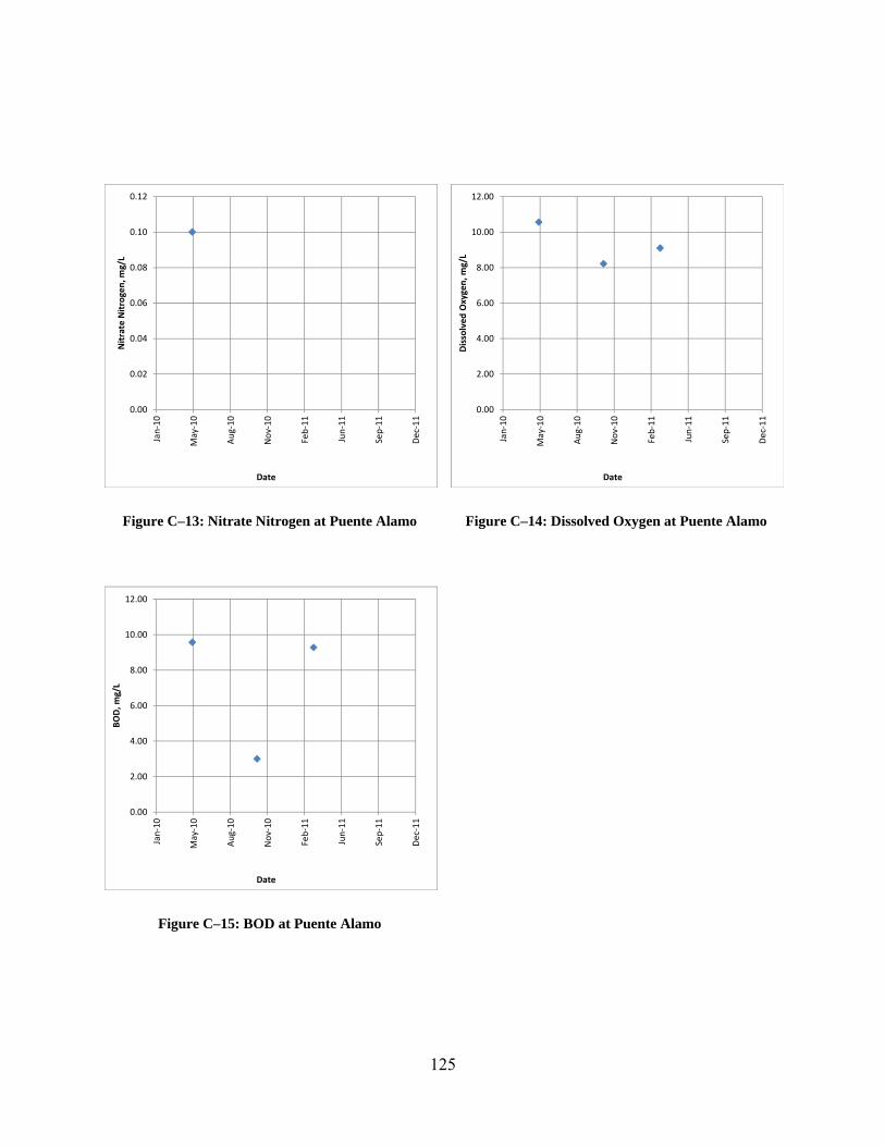
125
Figure C–13: Nitrate Nitrogen at Puente Alamo
Figure C–14: Dissolved Oxygen at Puente Alamo
Figure C–15: BOD at Puente Alamo
0.00
0.02
0.04
0.06
0.08
0.10
0.12
Jan‐10
May‐10
Aug‐10
Nov‐10
Feb‐11
Jun‐11
Sep‐11
Dec‐11
Nitrate Nitrogen, m
g/L
Date
0.00
2.00
4.00
6.00
8.00
10.00
12.00
Jan‐10
May‐10
Aug‐10
Nov‐10
Feb‐11
Jun‐11
Sep‐11
Dec‐11
Dissolved Oxygen, m
g/L
Date
0.00
2.00
4.00
6.00
8.00
10.00
12.00
Jan‐10
May‐10
Aug‐10
Nov‐10
Feb‐11
Jun‐11
Sep‐11
Dec‐11
BOD, m
g/L
Date

126
Table C–2: Results Reported by the UV for Jardines de Tuxpan Residencial (Tuxpan 1)
Rio: Tuxpan Latitud Longitud
# punto: 2 Coordenadas: 20°56'33.87"N 97°25'4.93"WNombre de punto de Monitoreo: Jardines de Tuxpan Residencial (Tuxpan 1)
Fecha 29-Apr-10 8-Jul-10 21-Oct-10 23-Mar-11 27-May-11 11-Oct-11
Hora 9:00 AM 10:15 AM 6:00 AM
Temperatura (°C)
SDT (ppm) 740.40 2.33 25.55
Turbiedad (FTU) 7.80 17.09 6.49
Resistividad (KΩ)
684.00 2.15 20.10
Salinidad (%) 2.80 8.70 95.10
ORP (mV) 604.55 107.06 42.00
Conductividad (µS)
1.48 4.56 50.67
pH (Unidades de pH)
7.00 7.77 7.70
Sulfatos (mg/L) 7.47E-01 3.00E-01
Cloruros (ppm) 16.10 7.48 1.62
Fosfatos (ppm) 1.32 0.01 6.07
Nitrogeno Amoniacal, N- NH3 (mg/L)
11.20
Nitrogeno de Nitratos, N- NO3-
(mg/L)49.80
Oxigeno Disuelto, OD (mg/L)
0.12 9.26 6.51
DBO (mg/L) 0.18 3.56 5.91
Coliformes Totales
4.00
Coliformes Fecales
1.00
Plomo (µg/L) 3.00
Arsenico (ppb) 0.00
Dureza (ppm) 425.00
Hierro (ppm) 0.00
Manganeso (mg/L)
0.18
Aluminio (mg/L) 0.00
Cromo (mg/L) 0.00
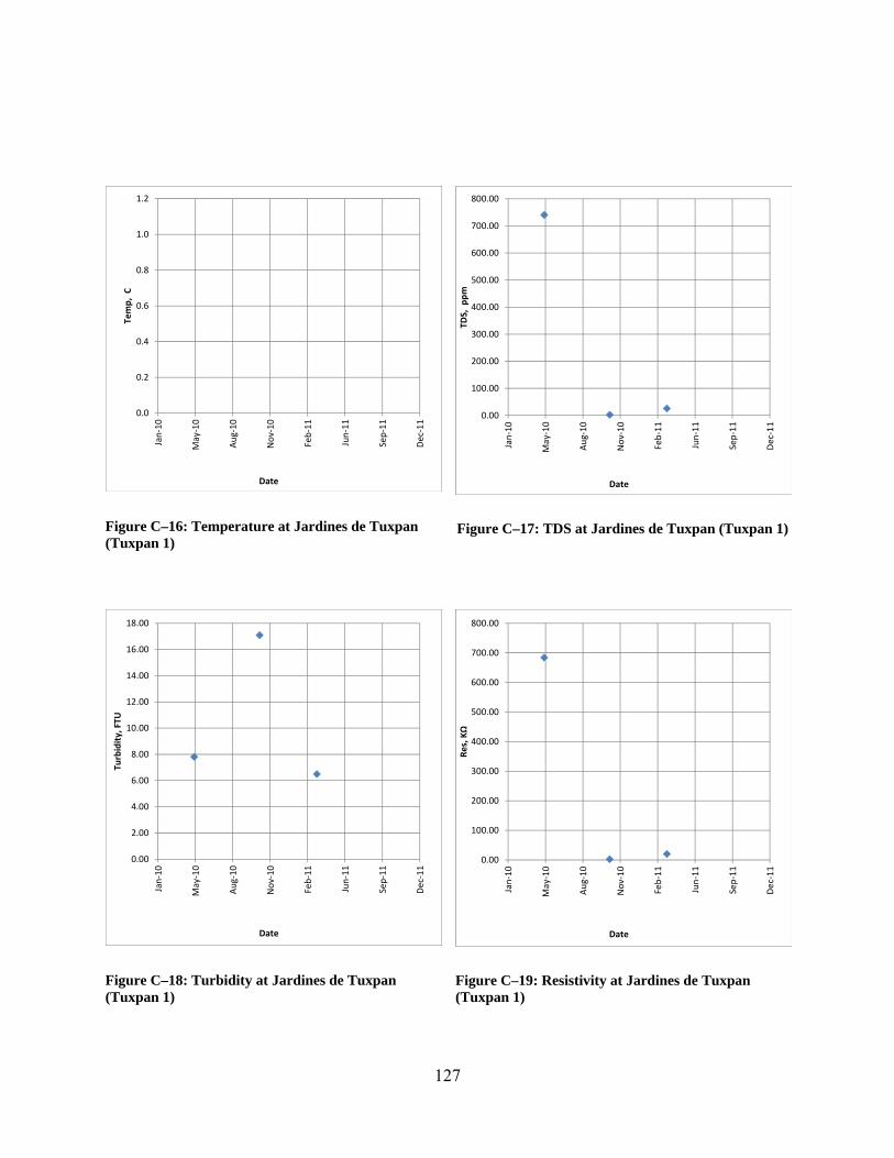
127
Figure C–16: Temperature at Jardines de Tuxpan (Tuxpan 1)
Figure C–17: TDS at Jardines de Tuxpan (Tuxpan 1)
Figure C–18: Turbidity at Jardines de Tuxpan (Tuxpan 1)
Figure C–19: Resistivity at Jardines de Tuxpan (Tuxpan 1)
0.0
0.2
0.4
0.6
0.8
1.0
1.2
Jan‐10
May‐10
Aug‐10
Nov‐10
Feb‐11
Jun‐11
Sep‐11
Dec‐11
Temp, C
Date
0.00
100.00
200.00
300.00
400.00
500.00
600.00
700.00
800.00
Jan‐10
May‐10
Aug‐10
Nov‐10
Feb‐11
Jun‐11
Sep‐11
Dec‐11
TDS, ppm
Date
0.00
2.00
4.00
6.00
8.00
10.00
12.00
14.00
16.00
18.00
Jan‐10
May‐10
Aug‐10
Nov‐10
Feb‐11
Jun‐11
Sep‐11
Dec‐11
Turbidity, FTU
Date
0.00
100.00
200.00
300.00
400.00
500.00
600.00
700.00
800.00
Jan‐10
May‐10
Aug‐10
Nov‐10
Feb‐11
Jun‐11
Sep‐11
Dec‐11
Res, KΩ
Date
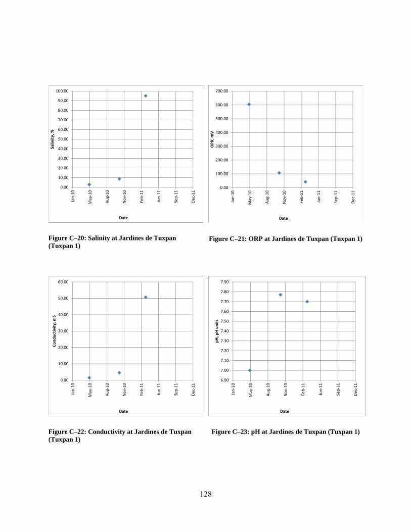
128
Figure C–20: Salinity at Jardines de Tuxpan (Tuxpan 1)
Figure C–21: ORP at Jardines de Tuxpan (Tuxpan 1)
Figure C–22: Conductivity at Jardines de Tuxpan (Tuxpan 1)
Figure C–23: pH at Jardines de Tuxpan (Tuxpan 1)
0.00
10.00
20.00
30.00
40.00
50.00
60.00
70.00
80.00
90.00
100.00
Jan‐10
May‐10
Aug‐10
Nov‐10
Feb‐11
Jun‐11
Sep‐11
Dec‐11
Salin
ity, %
Date
0.00
100.00
200.00
300.00
400.00
500.00
600.00
700.00
Jan‐10
May‐10
Aug‐10
Nov‐10
Feb‐11
Jun‐11
Sep‐11
Dec‐11
OPR, m
V
Date
0.00
10.00
20.00
30.00
40.00
50.00
60.00
Jan‐10
May‐10
Aug‐10
Nov‐10
Feb‐11
Jun‐11
Sep‐11
Dec‐11
Conductivity, m
S
Date
6.90
7.00
7.10
7.20
7.30
7.40
7.50
7.60
7.70
7.80
7.90
Jan‐10
May‐10
Aug‐10
Nov‐10
Feb‐11
Jun‐11
Sep‐11
Dec‐11
pH, p
H units
Date

129
Figure C–24: Sulfates at Jardines de Tuxpan (Tuxpan 1)
Figure C–25: Chlorides at Jardines de Tuxpan (Tuxpan 1)
Figure C–26: Phosphates at Jardines de Tuxpan (Tuxpan 1)
Figure C–27: Ammonia Nitrogen at Jardines de Tuxpan (Tuxpan 1)
0.00E+00
1.00E‐01
2.00E‐01
3.00E‐01
4.00E‐01
5.00E‐01
6.00E‐01
7.00E‐01
8.00E‐01
Jan‐10
May‐10
Aug‐10
Nov‐10
Feb‐11
Jun‐11
Sep‐11
Dec‐11
Sulfates, ppm
Date
0.00
2.00
4.00
6.00
8.00
10.00
12.00
14.00
16.00
18.00
Jan‐10
May‐10
Aug‐10
Nov‐10
Feb‐11
Jun‐11
Sep‐11
Dec‐11
Chlorides, ppm
Date
0.00
1.00
2.00
3.00
4.00
5.00
6.00
7.00
Jan‐10
May‐10
Aug‐10
Nov‐10
Feb‐11
Jun‐11
Sep‐11
Dec‐11
Tot Phosphate, p
pm
Date
0.00
2.00
4.00
6.00
8.00
10.00
12.00
Jan‐10
May‐10
Aug‐10
Nov‐10
Feb‐11
Jun‐11
Sep‐11
Dec‐11
Ammonia Nitrogen, m
g/L
Date

130
Figure C–28: Nitrate Nitrogen at Jardines de Tuxpan (Tuxpan 1)
Figure C–29: Dissolved Oxygen at Jardines de Tuxpan (Tuxpan 1)
Figure C–30: BOD at Jardines de Tuxpan (Tuxpan 1)
0.00
10.00
20.00
30.00
40.00
50.00
60.00
Jan‐10
May‐10
Aug‐10
Nov‐10
Feb‐11
Jun‐11
Sep‐11
Dec‐11
Nitrate Nitrogen, m
g/L
Date
0.00
1.00
2.00
3.00
4.00
5.00
6.00
7.00
8.00
9.00
10.00
Jan‐10
May‐10
Aug‐10
Nov‐10
Feb‐11
Jun‐11
Sep‐11
Dec‐11
Dissolved Oxygen, m
g/L
Date
0.00
1.00
2.00
3.00
4.00
5.00
6.00
7.00
Jan‐10
May‐10
Aug‐10
Nov‐10
Feb‐11
Jun‐11
Sep‐11
Dec‐11
BOD, m
g/L
Date

131
Table C–3: Results Reported by the UV for Parque Ribereño (Tuxpan 2)
Rio: Tuxpan Latitud Longitud
# punto: 3 Coordenadas: 20°56'53.54"N 97°21'15.72"WNombre de punto de Monitoreo: Parque Ribereño (Tuxpan 2)
Fecha 29-Apr-10 8-Jul-10 21-Oct-10 23-Mar-11 27-May-11 11-Oct-11
Hora 7:50 AM 12:50 PM 8:20 AM
Temperatura (°C)
SDT (ppm) 138.90 3.47 28.17
Turbiedad (FTU) 1.87 10.60 3.54
Resistividad (KΩ)
3.61 145.00 17.90
Salinidad (%) 0.50 12.90 105.10
ORP (mV) 124.25 121.60 36.60
Conductividad (µS)
277.00 6.92 56.32
pH (Unidades de pH)
6.75 7.87 7.50
Sulfatos (mg/L) 6.42E-01
Cloruros (ppm) 19.70 8.81 22.80
Fosfatos (ppm) 0.08 0.04 0.06
Nitrogeno Amoniacal, N- NH3 (mg/L)
3.50
Nitrogeno de Nitratos, N- NO3-
(mg/L)15.30
Oxigeno Disuelto, OD (mg/L)
6.44 9.05 5.07
DBO (mg/L) 2.14 4.42 4.91
Coliformes Totales
7.00
Coliformes Fecales
1.00
Plomo (µg/L) 4.00
Arsenico (ppb) 0.00
Dureza (ppm) 425.00
Hierro (ppm) 0.00
Manganeso (mg/L)
0.09
Aluminio (mg/L) 0.00
Cromo (mg/L) 0.00

132
Figure C–31: Temperature at Parque Ribereño (Tuxpan 2)
Figure C–32: TDS at Parque Ribereño (Tuxpan 2)
Figure C–33: Turbidity at Parque Ribereño (Tuxpan 2)
Figure C–34: Resistivity at Parque Ribereño (Tuxpan 2)
0.0
0.2
0.4
0.6
0.8
1.0
1.2
Jan‐10
May‐10
Aug‐10
Nov‐10
Feb‐11
Jun‐11
Sep‐11
Dec‐11
Temp, C
Date
0.00
20.00
40.00
60.00
80.00
100.00
120.00
140.00
160.00
Jan‐10
May‐10
Aug‐10
Nov‐10
Feb‐11
Jun‐11
Sep‐11
Dec‐11
TDS, ppm
Date
0.00
2.00
4.00
6.00
8.00
10.00
12.00
Jan‐10
May‐10
Aug‐10
Nov‐10
Feb‐11
Jun‐11
Sep‐11
Dec‐11
Turbidity, FTU
Date
0.00
20.00
40.00
60.00
80.00
100.00
120.00
140.00
160.00
Jan‐10
May‐10
Aug‐10
Nov‐10
Feb‐11
Jun‐11
Sep‐11
Dec‐11
Res, KΩ
Date

133
Figure C–35: Salinity at Parque Ribereño (Tuxpan 2)
Figure C–36: ORP at Parque Ribereño (Tuxpan 2)
Figure C–37: Conductivity at Parque Ribereño (Tuxpan 2)
Figure C–38: pH at Parque Ribereño (Tuxpan 2)
0.00
20.00
40.00
60.00
80.00
100.00
120.00
Jan‐10
May‐10
Aug‐10
Nov‐10
Feb‐11
Jun‐11
Sep‐11
Dec‐11
Salin
ity, %
Date
0.00
20.00
40.00
60.00
80.00
100.00
120.00
140.00
Jan‐10
May‐10
Aug‐10
Nov‐10
Feb‐11
Jun‐11
Sep‐11
Dec‐11
OPR, m
V
Date
0.00
50.00
100.00
150.00
200.00
250.00
300.00
Jan‐10
May‐10
Aug‐10
Nov‐10
Feb‐11
Jun‐11
Sep‐11
Dec‐11
Conductivity, m
S
Date
6.60
6.80
7.00
7.20
7.40
7.60
7.80
8.00
Jan‐10
May‐10
Aug‐10
Nov‐10
Feb‐11
Jun‐11
Sep‐11
Dec‐11
pH Units, pH units
Date

134
Figure C–39: Sulfates at Parque Ribereño (Tuxpan 2)
Figure C–40: Chlorides at Parque Ribereño (Tuxpan 2)
Figure C–41: Phosphates at Parque Ribereño (Tuxpan 2)
Figure C–42: Ammonia Nitrogen at Parque Ribereño (Tuxpan 2)
0.00E+00
1.00E‐01
2.00E‐01
3.00E‐01
4.00E‐01
5.00E‐01
6.00E‐01
7.00E‐01
Jan‐10
May‐10
Aug‐10
Nov‐10
Feb‐11
Jun‐11
Sep‐11
Dec‐11
Sulfates, ppm
Date
0.00
5.00
10.00
15.00
20.00
25.00
Jan‐10
May‐10
Aug‐10
Nov‐10
Feb‐11
Jun‐11
Sep‐11
Dec‐11
Chlorides, ppm
Date
0.00
0.01
0.02
0.03
0.04
0.05
0.06
0.07
0.08
0.09
Jan‐10
May‐10
Aug‐10
Nov‐10
Feb‐11
Jun‐11
Sep‐11
Dec‐11
Tot Phosphate, p
pm
Date
0.00
0.50
1.00
1.50
2.00
2.50
3.00
3.50
4.00
Jan‐10
May‐10
Aug‐10
Nov‐10
Feb‐11
Jun‐11
Sep‐11
Dec‐11
Ammonia Nitrogen, m
g/L
Date

135
Figure C–43: Nitrate Nitrogen at Parque Ribereño (Tuxpan 2)
Figure C–44: Dissolved Oxygen at Parque Ribereño (Tuxpan 2)
Figure C–45: BOD at Parque Ribereño (Tuxpan 2)
0.00
2.00
4.00
6.00
8.00
10.00
12.00
14.00
16.00
18.00
Jan‐10
May‐10
Aug‐10
Nov‐10
Feb‐11
Jun‐11
Sep‐11
Dec‐11
Nitrate Nitrogen, m
g/L
Date
0.00
1.00
2.00
3.00
4.00
5.00
6.00
7.00
8.00
9.00
10.00
Jan‐10
May‐10
Aug‐10
Nov‐10
Feb‐11
Jun‐11
Sep‐11
Dec‐11
Dissolved Oxygen, m
g/L
Date
0.00
1.00
2.00
3.00
4.00
5.00
6.00
Jan‐10
May‐10
Aug‐10
Nov‐10
Feb‐11
Jun‐11
Sep‐11
Dec‐11
BOD, m
g/L
Date


137
Appendix D. Comparison of Results at Puente Alamo – Alamo Jugeras
Table D–1: Comparison of Results at Puente Alamo – Alamo Jugureas
Figure D–1: Chlorides Comparison at Puente Alamo – Alamo Jugueras
River: Tuxpan
Note: Alamo Jugueras is about 4km upstream of Puente Alamo
Date TimeChlorides
(mg/L)Conductivity
(mS/cm)BOD
(mg/L)Phosphates
(mg/L)
Ammonia Nitrogen (mg/L)
Nitrate Nitrogen (mg/L)
Dissolved Oxygen (mg/L)
pH (pH units)
TDS (mg/L)
Turbidity (FTU)
23-Mar-04 10:50 30.33 820.00 7.28 0.67 <2.00 1.17 2.04 6.75 532.67 9.0024-Nov-04 20:30 37.11 909.00 <5.00 0.74 0.66 3.77 6.73 567.33 8.0030-Mar-05 10:20 34.47 872.33 <5.00 0.92 1.18 2.68 6.38 585.66 14.00
18-Apr-06 12:10 28.2 845.33 <5.00 <0.23 <2.00 1.86 2.46 7.06 524.50 4.00
30-Oct-06 20:00 47.72 1014.00 <5.00 1.29 6.06 6.89 656.80 10.00
9-Apr-07 12:55 51.64 1008.27 <5.00 0.28 1.24 1.16 4.21 7.18 644.00 16.00
29-Apr-10 11:00 8.52 18.04 9.57 0.18 0.10 0.10 10.56 7.80 8.50 7.3021-Oct-10 08:40 5.74 344.60 3.00 0.20 8.22 7.95 172.40 1.9023-Mar-11 04:10 9.36 231.10 9.28 0.34 9.10 7.40 116.20 1.47
CONAGUA
UV
Spring2004-Spring2005 (CONAGUA), Spring2006-Spring2007 (CONAGUA), Spring 2010-Spring 2011 (UV)
Periods and data to be compared:
Alamo-Jugueras (CONAGUA), Puente Alamo (UV)Monitoring points to be
compared:
0.00
10.00
20.00
30.00
40.00
50.00
60.00
16‐Feb
18‐Mar
17‐Apr
18‐May
17‐Jun
18‐Jul
17‐Aug
17‐Sep
17‐Oct
17‐Nov
17‐Dec
17‐Jan
16‐Feb
19‐Mar
18‐Apr
19‐May
Chlorides, m
g/L
Date
CONAGUA(Spring04‐Spring05) CONAGUA(Spring06‐Spring07) UV(Spring10‐Spring11)
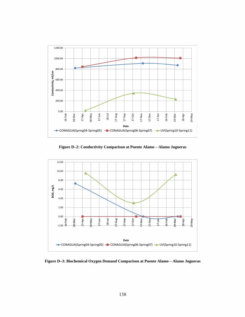
138
Figure D–2: Conductivity Comparison at Puente Alamo – Alamo Jugueras
Figure D–3: Biochemical Oxygen Demand Comparison at Puente Alamo – Alamo Jugueras
0.00
200.00
400.00
600.00
800.00
1000.00
1200.00
16‐Feb
18‐M
ar
17‐Apr
18‐M
ay
17‐Jun
18‐Jul
17‐Aug
17‐Sep
17‐Oct
17‐Nov
17‐Dec
17‐Jan
16‐Feb
19‐M
ar
18‐Apr
19‐M
ay
Conductivity, mS/cm
Date
CONAGUA(Spring04‐Spring05) CONAGUA(Spring06‐Spring07) UV(Spring10‐Spring11)
‐2.00
0.00
2.00
4.00
6.00
8.00
10.00
12.00
16‐Feb
18‐M
ar
17‐Apr
18‐M
ay
17‐Jun
18‐Jul
17‐Aug
17‐Sep
17‐Oct
17‐Nov
17‐Dec
17‐Jan
16‐Feb
19‐M
ar
18‐Apr
19‐M
ay
BOD, m
g/L
Date
CONAGUA(Spring04‐Spring05) CONAGUA(Spring06‐Spring07) UV(Spring10‐Spring11)

139
Figure D–4: Phosphates Comparison at Puente Alamo – Alamo Jugueras
Figure D–5: Ammonia Nitrogen Comparison at Puente Alamo – Alamo Jugueras
0.00
0.10
0.20
0.30
0.40
0.50
0.60
0.70
0.80
0.90
1.00
16‐Feb
18‐Mar
17‐Apr
18‐May
17‐Jun
18‐Jul
17‐Aug
17‐Sep
17‐Oct
17‐Nov
17‐Dec
17‐Jan
16‐Feb
19‐Mar
18‐Apr
19‐May
Phosphates, m
g/L
Date
CONAGUA(Spring04‐Spring05) CONAGUA(Spring06‐Spring07) UV(Spring10‐Spring11)
0.00
0.20
0.40
0.60
0.80
1.00
1.20
1.40
16‐Feb
18‐Mar
17‐Apr
18‐May
17‐Jun
18‐Jul
17‐Aug
17‐Sep
17‐Oct
17‐Nov
17‐Dec
17‐Jan
16‐Feb
19‐Mar
18‐Apr
19‐May
Ammonia Nitrogen, m
g/L
Date
CONAGUA(Spring04‐Spring05) CONAGUA(Spring06‐Spring07) UV(Spring10‐Spring11)
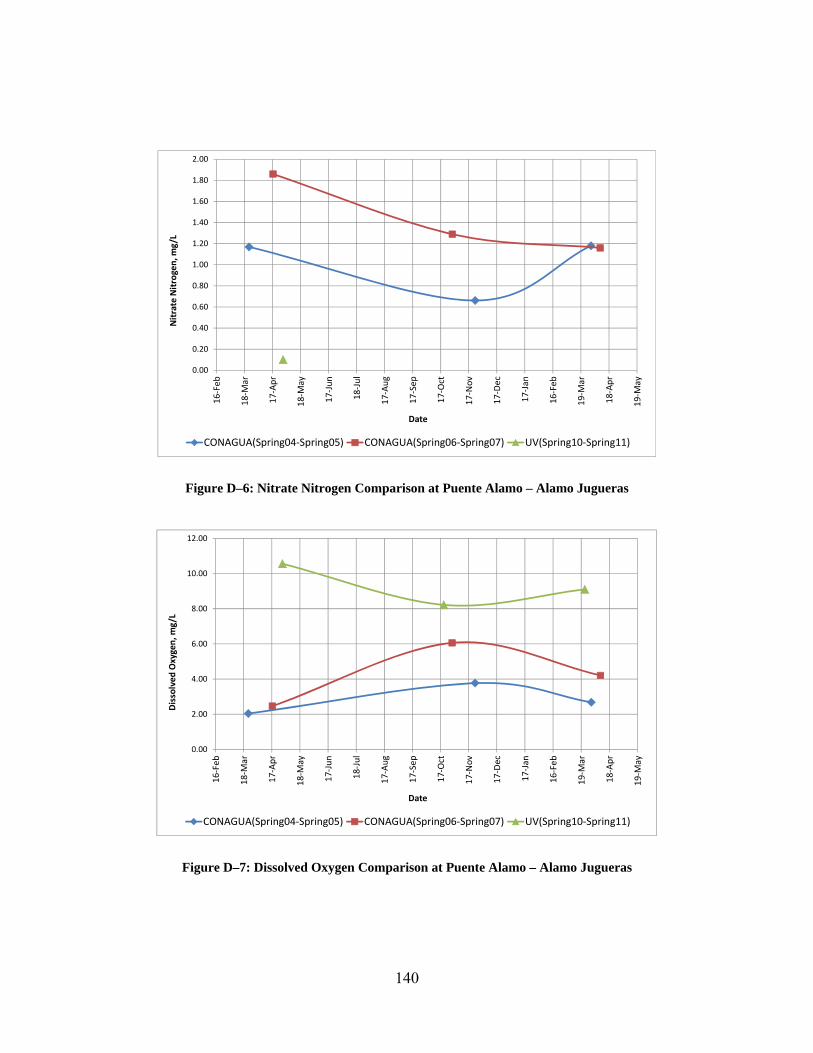
140
Figure D–6: Nitrate Nitrogen Comparison at Puente Alamo – Alamo Jugueras
Figure D–7: Dissolved Oxygen Comparison at Puente Alamo – Alamo Jugueras
0.00
0.20
0.40
0.60
0.80
1.00
1.20
1.40
1.60
1.80
2.00
16‐Feb
18‐M
ar
17‐Apr
18‐M
ay
17‐Jun
18‐Jul
17‐Aug
17‐Sep
17‐Oct
17‐Nov
17‐Dec
17‐Jan
16‐Feb
19‐M
ar
18‐Apr
19‐M
ay
Nitrate Nitrogen, m
g/L
Date
CONAGUA(Spring04‐Spring05) CONAGUA(Spring06‐Spring07) UV(Spring10‐Spring11)
0.00
2.00
4.00
6.00
8.00
10.00
12.00
16‐Feb
18‐Mar
17‐Apr
18‐May
17‐Jun
18‐Jul
17‐Aug
17‐Sep
17‐Oct
17‐Nov
17‐Dec
17‐Jan
16‐Feb
19‐Mar
18‐Apr
19‐May
Dissolved
Oxygen, m
g/L
Date
CONAGUA(Spring04‐Spring05) CONAGUA(Spring06‐Spring07) UV(Spring10‐Spring11)

141
Figure D–8: pH Comparison at Puente Alamo – Alamo Jugueras
Figure D–9: Total Dissolved Solids Comparison at Puente Alamo – Alamo Jugueras
0.00
1.00
2.00
3.00
4.00
5.00
6.00
7.00
8.00
9.00
16‐Feb
18‐Mar
17‐Apr
18‐May
17‐Jun
18‐Jul
17‐Aug
17‐Sep
17‐Oct
17‐Nov
17‐Dec
17‐Jan
16‐Feb
19‐Mar
18‐Apr
19‐May
pH, p
H units
Date
CONAGUA(Spring04‐Spring05) CONAGUA(Spring06‐Spring07) UV(Spring10‐Spring11)
0.00
100.00
200.00
300.00
400.00
500.00
600.00
700.00
16‐Feb
18‐Mar
17‐Apr
18‐May
17‐Jun
18‐Jul
17‐Aug
17‐Sep
17‐Oct
17‐Nov
17‐Dec
17‐Jan
16‐Feb
19‐Mar
18‐Apr
19‐May
TDS, m
g/L
Date
CONAGUA(Spring04‐Spring05) CONAGUA(Spring06‐Spring07) UV(Spring10‐Spring11)

142
Figure D–10: Turbidity Comparison at Puente Alamo – Alamo Jugueras
0.00
2.00
4.00
6.00
8.00
10.00
12.00
14.00
16.00
18.00
16‐Feb
18‐M
ar
17‐Apr
18‐M
ay
17‐Jun
18‐Jul
17‐Aug
17‐Sep
17‐Oct
17‐Nov
17‐Dec
17‐Jan
16‐Feb
19‐M
ar
18‐Apr
19‐M
ay
Turbidity, FTU
Date
CONAGUA(Spring04‐Spring05) CONAGUA(Spring06‐Spring07) UV(Spring10‐Spring11)

143
Appendix E. Comparison of Results at Puente Alamo – Alamo
Table E–1: Comparison of Results at Alamo – Puente Alamo
Figure E–1: Chlorides Comparison at Puente Alamo – Alamo
River: Tuxpan
Note: Alamo is about 5km downstream of Puente Alamo
Date Time Chlorides (mg/L)Conductivity
(mS/cm)BOD (mg/L)
Phosphates (mg/L)
Ammonia Nitrogen (mg/L)
Nitrate Nitrogen (mg/L)
Dissolved Oxygen (mg/L)
pH (pH units)
TDS (mg/L)Turbidity
(FTU)
16-Aug-00 13:05 1.91 236.55 2.34 1.18 7.20 0.3118-Oct-00 15:00 4.93 328.66 1.89 0.04 0.24 8.48 7.20 210.0718-May-01 7:40 2.46 242.83 1.70 0.14 0.00 0.01 5.70 7.63 172.00 14.0018-Apr-06 13:45 7.42 393.37 <5.00 <0.23 <2.00 <0.09 7.32 8.19 173.00 3.0030-Oct-06 18:15 3.48 357.40 <5.00 0.52 8.29 8.22 212.40 6.00
9-Apr-07 15:00 6.95 344.03 <5.00 <0.09 1.13 0.19 6.41 7.63 204.00 8.00
29-Apr-10 11:00 8.52 18.04 9.57 0.18 0.10 0.10 10.56 7.80 8.50 7.3021-Oct-10 8:40 5.74 344.60 3.00 0.20 8.22 7.95 172.40 1.9023-Mar-11 4:10 9.36 231.10 9.28 0.34 9.10 7.40 116.20 1.47
CONAGUA
UV
Periods and data to be compared:Spring2000-Spring2001 (CONAGUA), Spring2006-Spring2007 (CONAGUA), Spring 2010-Spring 2011 (UV)
Monitoring points to be compared: Alamo(CONAGUA), Puente Alamo (UV)
0.00
1.00
2.00
3.00
4.00
5.00
6.00
7.00
8.00
9.00
10.00
15‐Mar
14‐Apr
15‐May
14‐Jun
15‐Jul
14‐Aug
14‐Sep
14‐Oct
14‐Nov
14‐Dec
14‐Jan
13‐Feb
16‐Mar
15‐Apr
16‐May
15‐Jun
Chlorides, mg/L
Date
CONAGUA(Spring04‐Spring05) CONAGUA(Spring06‐Spring07) UV(Spring10‐Spring11)

144
Figure E–2: Conductivity Comparison at Puente Alamo – Alamo
Figure E–3: Biochemical Oxygen Demand Comparison at Puente Alamo – Alamo
0.00
50.00
100.00
150.00
200.00
250.00
300.00
350.00
400.00
450.00
15‐Mar
14‐Apr
15‐May
14‐Jun
15‐Jul
14‐Aug
14‐Sep
14‐Oct
14‐Nov
14‐Dec
14‐Jan
13‐Feb
16‐Mar
15‐Apr
16‐May
15‐Jun
Conductivity, mS/cm
Date
CONAGUA(Spring04‐Spring05) CONAGUA(Spring06‐Spring07) UV(Spring10‐Spring11)
0.00
2.00
4.00
6.00
8.00
10.00
12.00
15‐Mar
14‐Apr
15‐May
14‐Jun
15‐Jul
14‐Aug
14‐Sep
14‐Oct
14‐Nov
14‐Dec
14‐Jan
13‐Feb
16‐Mar
15‐Apr
16‐May
15‐Jun
BOD, m
g/L
Date
CONAGUA(Spring04‐Spring05) CONAGUA(Spring06‐Spring07) UV(Spring10‐Spring11)

145
Figure E–4: Phosphates Comparison at Puente Alamo – Alamo
Figure E–5: Ammonia Nitrogen Comparison at Puente Alamo – Alamo
0.00
0.05
0.10
0.15
0.20
0.25
0.30
0.35
0.40
15‐Mar
14‐Apr
15‐M
ay
14‐Jun
15‐Jul
14‐Aug
14‐Sep
14‐Oct
14‐Nov
14‐Dec
14‐Jan
13‐Feb
16‐Mar
15‐Apr
16‐M
ay
15‐Jun
Phosphates, m
g/L
Date
CONAGUA(Spring04‐Spring05) CONAGUA(Spring06‐Spring07) UV(Spring10‐Spring11)
0.00
0.20
0.40
0.60
0.80
1.00
1.20
15‐Mar
14‐Apr
15‐May
14‐Jun
15‐Jul
14‐Aug
14‐Sep
14‐Oct
14‐Nov
14‐Dec
14‐Jan
13‐Feb
16‐Mar
15‐Apr
16‐May
15‐Jun
Ammonia Nitrogen, m
g/L
Date
CONAGUA(Spring04‐Spring05) CONAGUA(Spring06‐Spring07) UV(Spring10‐Spring11)
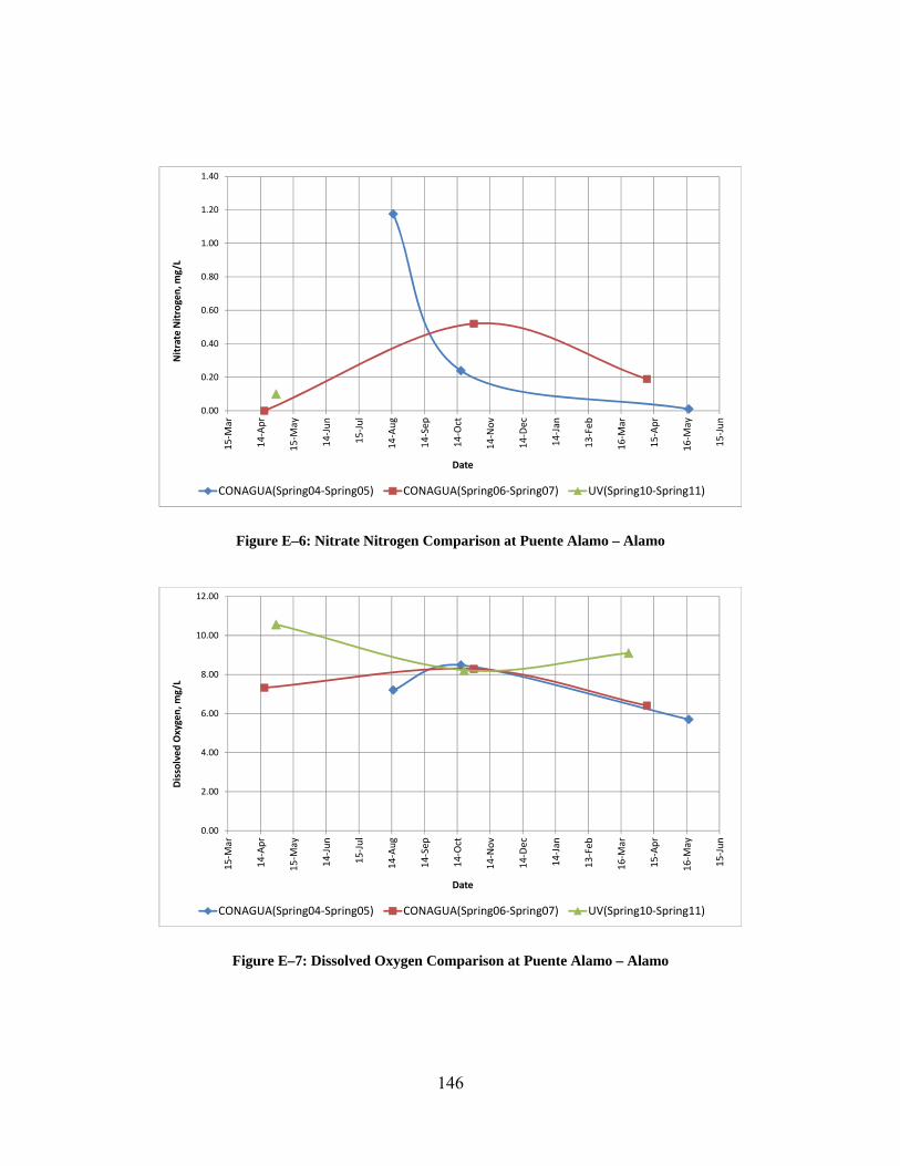
146
Figure E–6: Nitrate Nitrogen Comparison at Puente Alamo – Alamo
Figure E–7: Dissolved Oxygen Comparison at Puente Alamo – Alamo
0.00
0.20
0.40
0.60
0.80
1.00
1.20
1.40
15‐Mar
14‐Apr
15‐M
ay
14‐Jun
15‐Jul
14‐Aug
14‐Sep
14‐Oct
14‐Nov
14‐Dec
14‐Jan
13‐Feb
16‐Mar
15‐Apr
16‐M
ay
15‐Jun
Nitrate Nitrogen, m
g/L
Date
CONAGUA(Spring04‐Spring05) CONAGUA(Spring06‐Spring07) UV(Spring10‐Spring11)
0.00
2.00
4.00
6.00
8.00
10.00
12.00
15‐Mar
14‐Apr
15‐May
14‐Jun
15‐Jul
14‐Aug
14‐Sep
14‐Oct
14‐Nov
14‐Dec
14‐Jan
13‐Feb
16‐Mar
15‐Apr
16‐May
15‐Jun
Dissolved
Oxygen, m
g/L
Date
CONAGUA(Spring04‐Spring05) CONAGUA(Spring06‐Spring07) UV(Spring10‐Spring11)

147
Figure E–8: pH Comparison at Puente Alamo – Alamo
Figure E–9: Total Dissolved Solids Comparison at Puente Alamo – Alamo
0.00
1.00
2.00
3.00
4.00
5.00
6.00
7.00
8.00
9.00
15‐Mar
14‐Apr
15‐M
ay
14‐Jun
15‐Jul
14‐Aug
14‐Sep
14‐Oct
14‐Nov
14‐Dec
14‐Jan
13‐Feb
16‐Mar
15‐Apr
16‐M
ay
15‐Jun
pH, p
H units
Date
CONAGUA(Spring04‐Spring05) CONAGUA(Spring06‐Spring07) UV(Spring10‐Spring11)
0.00
50.00
100.00
150.00
200.00
250.00
15‐Mar
14‐Apr
15‐May
14‐Jun
15‐Jul
14‐Aug
14‐Sep
14‐Oct
14‐Nov
14‐Dec
14‐Jan
13‐Feb
16‐Mar
15‐Apr
16‐May
15‐Jun
TDS, m
g/L
Date
CONAGUA(Spring04‐Spring05) CONAGUA(Spring06‐Spring07) UV(Spring10‐Spring11)

148
Figure E–10: Turbidity Comparison at Puente Alamo – Alamo
0.00
2.00
4.00
6.00
8.00
10.00
12.00
14.00
16.00
15‐Mar
14‐Apr
15‐M
ay
14‐Jun
15‐Jul
14‐Aug
14‐Sep
14‐Oct
14‐Nov
14‐Dec
14‐Jan
13‐Feb
16‐Mar
15‐Apr
16‐M
ay
15‐Jun
Turbidity, FTU
Date
CONAGUA(Spring04‐Spring05) CONAGUA(Spring06‐Spring07) UV(Spring10‐Spring11)

149
Appendix F. Comparison of Results at Villa Lazaro Cardenas – Lazaro Cardenas
Table F–1: Comparison of Results at Lazaro Cardenas – Villa Lazaro Cardenas
Figure F–1: Chlorides Comparison at Villa Lazaro Cardenas – Lazaro Cardenas
River: Cazones
Note: Same point
Date Time Chlorides (mg/L)Conductivity
(mS/cm)BOD (mg/L)
Phosphates (mg/L)
Ammonia Nitrogen (mg/L)
Nitrate Nitrogen (mg/L)
Dissolved Oxygen (mg/L)
pH (pH units)
TDS (mg/L)Turbidity
(FTU)
26-Mar-00 7:15 2.34 307.80 1.90 0.04 0.15 6.53 8.08 197.4423-May-00 17:35 6.26 258.41 2.39 <0.01 0.29 6.33 7.15 202.7010-Aug-00 17:30 19.62 227.40 2.56 1.45 8.17 7.0218-Oct-00 17:30 2.46 264.75 2.36 0.06 0.64 7.83 7.00 161.0021-Mar-01 16:15 3.91 267.00 0.50 0.02 0.11 9.93 7.00 180.83 28.0027-May-03 12:15 2.36 388.40 1.07 <.2546 <0.1456 3.25 7.19 179.33 20.0015-Jul-03 15:28 1.84 245.10 0.97 <0.2546 <0.1317 9.89 8.02 154.67 21.0029-Oct-03 16:10 1.45 238.40 1.65 <0.4308 0.44 9.25 8.66 156.67 16.0019-Apr-04 14:45 4.93 293.67 <5.00 <0.4074 <2.00 <0.2576 8.38 8.00 162.00 3.006-Apr-06 12:00 <5.00 271.93 <5.00 <0.23 <2.00 <0.09 8.27 8.27 165.75 3.0025-Jul-06 13:45 <2.00 263.57 <5.00 <0.10 0.75 6.41 8.02 172.00 48.00
31-Oct-06 7:10 <2.00 363.80 <5.00 0.67 8.33 8.04 170.00 9.00
11-Apr-07 14:20 <2.00 276.63 <5.00 <0.09 <1.00 0.27 8.81 8.18 168.00 4.00
25-Apr-10 10:03 7.34 292.30 0.14 3.00 0.70 9.48 7.20 146.70 14.218-Jul-10 8.64 0.34 15.40 9.96 6.88 123.23 13.485-Oct-10 9:40 2.33 139.25 5.59 0.12 9.44 6.15 70.22 11.7223-Mar-11 10:10 3.49 214.10 1.58 0.02 7.38 7.10 101.70 0.30
CONAGUA
UV
Periods and data to be compared:Spring2000-Spring2001 (CONAGUA), Spring2003-Spring2004 (CONAGUA), Spring2006-Spring2007 (CONAGUA), Spring 2010-Spring 2011 (UV)
Monitoring points to be compared: Lazaro Cardenas(CONAGUA), Villa Lazaro Cardenas-La Uno (UV)
0.00
5.00
10.00
15.00
20.00
25.00
13‐Feb
15‐M
ar
14‐Apr
15‐M
ay
14‐Jun
15‐Jul
14‐Aug
14‐Sep
14‐Oct
14‐Nov
14‐Dec
14‐Jan
13‐Feb
16‐M
ar
15‐Apr
16‐M
ay
Chlorides, mg/L
Date
CONAGUA(Spring00‐Spring01) CONAGUA(Spring03‐Spring04)
CONAGUA(Spring06‐Spring07) UV(Spring10‐Spring11)

150
Figure F–2: Conductivity Comparison at Villa Lazaro Cardenas – Lazaro Cardenas
Figure F–3: Biochemical Oxygen Demand Comparison at Villa Lazaro Cardenas – Lazaro Cardenas
0.00
50.00
100.00
150.00
200.00
250.00
300.00
350.00
400.00
450.00
13‐Feb
15‐M
ar
14‐Apr
15‐M
ay
14‐Jun
15‐Jul
14‐Aug
14‐Sep
14‐Oct
14‐Nov
14‐Dec
14‐Jan
13‐Feb
16‐M
ar
15‐Apr
16‐M
ay
Conductivity, mS/cm
Date
CONAGUA(Spring00‐Spring01) CONAGUA(Spring03‐Spring04)
CONAGUA(Spring06‐Spring07) UV(Spring10‐Spring11)
0.00
1.00
2.00
3.00
4.00
5.00
6.00
7.00
8.00
9.00
10.00
13‐Feb
15‐M
ar
14‐Apr
15‐M
ay
14‐Jun
15‐Jul
14‐Aug
14‐Sep
14‐Oct
14‐Nov
14‐Dec
14‐Jan
13‐Feb
16‐M
ar
15‐Apr
16‐M
ay
BOD, m
g/L
Date
CONAGUA(Spring00‐Spring01) CONAGUA(Spring03‐Spring04)
CONAGUA(Spring06‐Spring07) UV(Spring10‐Spring11)

151
Figure F–4: Phosphates Comparison at Villa Lazaro Cardenas – Lazaro Cardenas
Figure F–5: Ammonia Nitrogen Comparison at Villa Lazaro Cardenas – Lazaro Cardenas
0.00
0.05
0.10
0.15
0.20
0.25
0.30
0.35
0.40
13‐Feb
15‐M
ar
14‐Apr
15‐M
ay
14‐Jun
15‐Jul
14‐Aug
14‐Sep
14‐Oct
14‐Nov
14‐Dec
14‐Jan
13‐Feb
16‐M
ar
15‐Apr
16‐M
ay
Phosphates, m
g/L
Date
CONAGUA(Spring00‐Spring01) CONAGUA(Spring03‐Spring04)
CONAGUA(Spring06‐Spring07) UV(Spring10‐Spring11)
0.00
0.50
1.00
1.50
2.00
2.50
3.00
3.50
13‐Feb
15‐M
ar
14‐Apr
15‐M
ay
14‐Jun
15‐Jul
14‐Aug
14‐Sep
14‐Oct
14‐Nov
14‐Dec
14‐Jan
13‐Feb
16‐M
ar
15‐Apr
16‐M
ay
Ammonia Nitrogen, m
g/L
Date
CONAGUA(Spring00‐Spring01) CONAGUA(Spring03‐Spring04)
CONAGUA(Spring06‐Spring07) UV(Spring10‐Spring11)

152
Figure F–6: Nitrate Nitrogen Comparison at Villa Lazaro Cardenas – Lazaro Cardenas
Figure F–7: Dissolved Oxygen Comparison at Villa Lazaro Cardenas – Lazaro Cardenas
‐2.00
0.00
2.00
4.00
6.00
8.00
10.00
12.00
14.00
16.00
18.00
13‐Feb
15‐Mar
14‐Apr
15‐May
14‐Jun
15‐Jul
14‐Aug
14‐Sep
14‐Oct
14‐Nov
14‐Dec
14‐Jan
13‐Feb
16‐Mar
15‐Apr
16‐May
Nitrate Nitrogen, m
g/L
Date
CONAGUA(Spring00‐Spring01) CONAGUA(Spring03‐Spring04)
CONAGUA(Spring06‐Spring07) UV(Spring10‐Spring11)
0.00
2.00
4.00
6.00
8.00
10.00
12.00
13‐Feb
15‐M
ar
14‐Apr
15‐M
ay
14‐Jun
15‐Jul
14‐Aug
14‐Sep
14‐Oct
14‐Nov
14‐Dec
14‐Jan
13‐Feb
16‐M
ar
15‐Apr
16‐M
ay
Dissolved
Oxygen, m
g/L
Date
CONAGUA(Spring00‐Spring01) CONAGUA(Spring03‐Spring04)
CONAGUA(Spring06‐Spring07) UV(Spring10‐Spring11)

153
Figure F–8: pH Comparison at Puente Villa Lazaro Cardenas – Lazaro Cardenas
Figure F–9: Total Dissolved Solids Comparison at Villa Lazaro Cardenas – Lazaro Cardenas
0.00
1.00
2.00
3.00
4.00
5.00
6.00
7.00
8.00
9.00
10.00
13‐Feb
15‐M
ar
14‐Apr
15‐M
ay
14‐Jun
15‐Jul
14‐Aug
14‐Sep
14‐Oct
14‐Nov
14‐Dec
14‐Jan
13‐Feb
16‐M
ar
15‐Apr
16‐M
ay
pH, p
H units
Date
CONAGUA(Spring00‐Spring01) CONAGUA(Spring03‐Spring04)
CONAGUA(Spring06‐Spring07) UV(Spring10‐Spring11)
0.00
50.00
100.00
150.00
200.00
250.00
13‐Feb
15‐M
ar
14‐Apr
15‐M
ay
14‐Jun
15‐Jul
14‐Aug
14‐Sep
14‐Oct
14‐Nov
14‐Dec
14‐Jan
13‐Feb
16‐M
ar
15‐Apr
16‐M
ay
TDS, m
g/L
Date
CONAGUA(Spring00‐Spring01) CONAGUA(Spring03‐Spring04)
CONAGUA(Spring06‐Spring07) UV(Spring10‐Spring11)

154
Figure F–10: Turbidity Comparison at Villa Lazaro Cardenas – Lazaro Cardenas
0.00
10.00
20.00
30.00
40.00
50.00
60.00
13‐Feb
15‐M
ar
14‐Apr
15‐M
ay
14‐Jun
15‐Jul
14‐Aug
14‐Sep
14‐Oct
14‐Nov
14‐Dec
14‐Jan
13‐Feb
16‐M
ar
15‐Apr
16‐M
ay
Turbidity, FTU
Date
CONAGUA(Spring00‐Spring01) CONAGUA(Spring03‐Spring04)
CONAGUA(Spring06‐Spring07) UV(Spring10‐Spring11)