Embed Size (px)
Citation preview

Development and Optimization of Artificial
Intelligence-Based Concrete Compressive
Strength Predictive Models
Nasir B. Siraj, Aminah Robinson Fayek, and Abraham A. Tsehayae , Edmonton, Canada
Email: {siraj, aminah.robinson, tsehayae}@ualberta.ca
Abstract—Accurate prediction of the compressive strength
of High-Performance Concrete (HPC) is crucial in concrete
design and construction. However, HPC is a very complex
material, as the inter-relationship between its constituent
materials is highly nonlinear and its property is affected by
several interacting factors. Hence, existing conventional
empirical and statistical methods are limited in their ability
to accurately predict the compressive strength of HPC. In
this study, the application of three artificial intelligence
techniques, namely, the Artificial Neural Network (ANN),
Fuzzy Inference System (FIS), and Adaptive Neuro-Fuzzy
Inference System (ANFIS) techniques, are explored. A data-
driven approach based on fuzzy c-means clustering (FCM)
is employed to generate both the Mamdani and Sugeno FIS
models. Different model structures and parameters—such
as number of neurons and choice of transfer function for the
ANN technique, and number of clusters and choice of
fuzzification coefficient and inference methods for the FIS
and ANFIS techniques—are optimized to improve the
accuracy of each technique. Results of this study indicate
that ANFIS and ANN perform better than the FIS models in
predicting the compressive strength of HPC. The main
contributions of this paper are: (1) providing accurate
concrete compressive strength prediction models that
represent the complex, nonlinear relationship between the
constituent materials and concrete compressive strength; (2)
presenting a data-driven methodology for the development
of FIS concrete compressive strength models; and (3)
subjecting artificial intelligence-based concrete compressive
strength models to structure and parameter optimization to
improve prediction accuracy.
Index Terms—high-performance concrete, compressive
strength, artificial neural network, fuzzy inference system,
adaptive neuro-fuzzy inference system
I. INTRODUCTION
Concrete is the most versatile and widely used
construction material. The reasons for concrete’s
dominance are varied, but among the most important are:
the economy and widespread availability of its
constituent materials; its ability to be molded into any
desired shape; its adoptability and sustainability; and its
high compressive strength, stiffness, and durability [1],
[2]. Concrete is categorized according to purpose, range
Manuscript received July 1, 2015; revised April 21, 2016.
of compositions, finishes, and performance characteristics.
Lightweight, heavyweight, high-strength, high-
performance, self-compacting, and fiber-reinforced are
among the most widely available concrete types.
According to the American Concrete Institute (ACI),
High-Performance Concrete (HPC) is that “meeting [a]
special combination of performance and uniformity
requirements that cannot always be achieved routinely
using conventional constituents and normal mixing,
placing, and curing practices” [3]. Most prevailing
definitions for HPC emphasize properties such as high
strength, high workability, dimensional stability, and
durability [4]. In addition to common concrete
ingredients (aggregates, sand, and cement),
supplementary cementitious materials—principally, fly
ash and blast furnace slag—and chemical admixtures,
such as superplasticizer, are used in preparation of HPC
to improve performance and economic return [2], [4].
Compressive strength is the most important
mechanical property of concrete, since it is primarily used
as quality control and compliance criteria in standards
and specifications. Moreover, most of the important
properties of concrete, including flexural strength, direct
tensile strength, splitting tensile strength, and modulus of
elasticity, are directly related to compressive strength [5].
Thus, proper prediction of concrete compressive strength
is vital to schedule and manage concrete works such as
formwork removal and pre- or post-tensioning activities
[6]. In the past, several techniques based on either
empirical methods (statistical evaluation of relationships)
or computational modeling have been tested, and
empirical methods based on Multi-Linear Regression
(MLR) have been commonly proposed to predict
compressive strength. However, most of the available
empirical models do not account for the mineral and
chemical admixtures used in HPC [7], [8]. Moreover, the
numbers of interacting factors influencing the
compressive strength of HPC are very high and the
relationship between these factors is not precisely known
because it is considered to be highly complex and
nonlinear [6], [8]. Therefore, the empirical methods are
limited in their ability to accurately predict the
,
such as the Artificial Neural Network (ANN), Fuzzy
International Journal of Structural and Civil Engineering Research Vol. 5, No. 3, August 2016
© 2016 Int. J. Struct. Civ. Eng. Res. 156doi: 10.18178/ijscer.5.3.156-167
University of AlbertaDepartment of Civil and Environmental Engineering,
Intelligence (AI) techniques
compressive strength of HPC. Alternative modeling
methods employing Artificial

Inference System (FIS), and Adaptive Neuro-Fuzzy
System (ANFIS) techniques, provide a flexible
environment better suited to dealing with such a complex,
nonlinear relationship.
In the past two decades, AI-based modeling methods
have been extensively used in wide-ranging civil
engineering applications including modeling of material
behavior, determination of concrete mix proportion, and
prediction of strength [9], [10]. Yeh [4] applied ANN to
predict the compressive strength of HPC, and found that
these predictions are more accurate than those obtained
from an MLR model. Similarly, Ozturan, Kutlu, and
Ozturan [11] compared the prediction accuracies of
ANN- and MLR-based models, and concluded that using
ANN provides the best result. Topcu and Saridemir [9]
developed ANN and FIS models to predict the
compressive strength of concrete containing fly ash at
different strength-gain ages. Similarly, Ozcan, Atis,
Karahan, Uncluoglu, and Tanyildizi [12], Topcu and
Saridemir [13], and Aggrawal and Aggrawal [14] adopted
ANN and FIS to predict the compressive strength of silica
fume concrete, recycled aggregate concretes containing
silica fume, and self-compacting concrete, respectively.
Overall, their findings affirmed that ANNs and FIS
models have very promising potential to accurately
predict the compressive strength of concrete. Vakshouri
and Najadi [5] applied different optimization methods
and membership functions in an ANFIS to predict the
compressive strength of High-Strength Concrete (HSC)
based on splitting tensile strength and modulus of
elasticity. Badde, Gupta, and Patki [15] used FIS- and
ANFIS-based models to predict the 28-day compressive
strength of Ready-Mixed Concrete (RMC) and concluded
that for this application, the ANFIS approach has a better
predictive capability than the FIS. Aydin, Tortum, and
Yavuz [16] employed an ANFIS to predict the elastic
modulus of normal- and high-strength concrete based on
compressive strength and compared the results with the
values obtained from codes.
The accuracy of ANN models largely depends on the
architecture, function, and parametric properties of the
network. However, the effect of these properties on
model accuracy was not thoroughly investigated in most
of the aforementioned research. In addition, most of the
FIS and ANFIS models developed for prediction of
compressive strength heavily rely on expert knowledge to
establish the fuzzy inference rules, rather than using a
data-driven approach. Expert-based models have a critical
shortcoming: their rules are highly prescriptive, very
general, and difficult to develop due to the high-
dimensionality of the problem [17]. However, a FIS’s
inability to learn from data and develop and optimize
model parameters is a major limitation. Thus, hybridizing
a model by combining the FIS technique with other AI
techniques, such ANNs, could improve learning
capabilities; however, this approach has rarely been used
to predict compressive strength of HPC.
The major objective of this paper is to develop and
compare three artificial intelligence models based on
ANN, FIS approach using fuzzy C-means clustering
(FCM), and ANFIS approach to predict the compressive
strength of HPC. The different model parameters, such as
number of neurons and type of transfer function in the
case of ANN, and number of clusters, fuzzification
coefficient (m-value), and selection of inference methods
for FIS and ANFIS will be optimized to improve model
accuracy and to overcome challenges associated with
each approach.
Section II of this paper gives an overview of AI
modeling techniques and introduces the structure and
components of each model. In Section III, the data set
used to develop the AI models is explained and the
details of each model’s implementation, including model
structure and parameters, are demonstrated. The results
obtained by adopting these models are presented and their
performances in prediction accuracy are compared and
contrasted. Finally, conclusions and recommendations are
presented in Section IV.
II. ARTIFICIAL INTELLIGENCE MODELING
TECHNIQUES
In the following sections the structure and components
of the three Artificial Intelligence (AI) modeling
techniques used in this study, namely, Artificial Neural
Networks (ANNs), Fuzzy Inference System (FIS), and
Adaptive Neuro-Fuzzy System (ANFIS) are briefly
discussed.
Figure 1. Typical architecture of an ANN with two hidden layers.
A. Artificial Neural Networks
ANNs are information-processing systems whose
architecture imitates the learning capability of the human
brain [8], [9]. Neurons are the fundamental building
blocks of ANNs and they are logically arranged into a
single or multiple layers. Fig. 1 shows the architecture of
a two-hidden-layer network with k inputs and n outputs.
The neurons in each layer are linked to all neurons in the
next layer through weighted connections. The output of
each neuron in the initial layer is communicated to the
neurons in the next layer through an activation function
[11], [14]. According to Boussabaine [18], even though
there are a range of ANN types differing in architecture
and mode of operation, ANNs generally include the
following components: (1) a set of processing neurons, (2)
a state of activation for each neuron, (3) a pattern of
connectivity among the neurons, (4) a propagation
I1
Input Layer
I2
I3
.
.
Ik-1
Ik
Hidden Layer 1
Output Layer
H11
H12
.
.
H1l
H21
H22
.
.
H2m
O1
.
.
On
Hidden Layer 2
International Journal of Structural and Civil Engineering Research Vol. 5, No. 3, August 2016
© 2016 Int. J. Struct. Civ. Eng. Res. 157

method, (5) an activation rule, (6) an external
environment, and (7) a learning method.
Most practical applications of ANNs are based on
multi-layer feedforward architecture comprised of an
input layer, one or more hidden layers, and an output
layer (Fig. 1) with a back-propagation learning algorithm
that adopts a gradient-descent method to minimize the
margin of error between the neurons of the desired target
and those of the outputs [4], [14]. References [14] and
[19] discuss ANN theory and the mathematical
formulation of the back-propagation algorithm in detail.
ANNs provide learning capability, robustness,
generalization, parallel processing, and non-linearity,
making them advantageously able to accurately model the
mechanical behavior of concrete [9], [10].
B. Fuzzy Inference System
Fuzzy sets were first introduced by Lotfi Zadeh in
1965 to deal with uncertainty and imprecision, which are
commonly encountered in real world applications [12],
[17]. The underlying notion in fuzzy sets is that an object
belongs to different classes/subsets of the universal set
with unsharp boundaries in which membership is a matter
of degree of belongingness. This is unlike set theory,
which deals with only two possibilities, i.e., 0 (non-
membership) or 1 (full-membership). The partial
belongingness to a set is easily described numerically by
using a Membership Function (MF), which assumes
values between 0 and 1, inclusively [20]. FISs are models
composed of conditional if-then rules, where a collection
of fuzzy sets represented by MFs provides a system for
reasoning about a certain problem. In the case of
Mamdani FIS models, the conclusion is represented as a
fuzzy set, and defuzzification is employed to obtain a
crisp output value. In Sugeno FIS models, the conclusion
is represented using a function [17]. Interpretability,
ability to represent complex relations, and capability to
deal with both subjective and objective variables are
some of the most important advantages of FISs. Fuzzy
rules are capable of capturing all possible relationships
between input and output variables, and are useful to
construct models of complex systems using domain
knowledge, experience, and experimental data [17]. A
typical FIS architecture has five basic components: the
input interface; the rule base, which contains the fuzzy if-
then rules; the database, which defines the MFs used in
the fuzzy rules; fuzzy inference, which performs the
inference procedure based on the rules; and the output
interface. Multiple-input single-output fuzzy rules
generally assume the following form: If input1 is Ai and
input2 is Bj …and inputn is Ct then output is Du, where Ai,
Bj,…, Ct, and Du are fuzzy sets defined in the
corresponding input and output spaces, respectively.
According to Pedrycz and Gomide [17], expert-based
and data-driven are the two fundamental approaches
available for constructing FIS models. In expert-based
FISs, the rules are formulated by experienced experts
fluent in the basic concepts and variables associated with
a problem under investigation. Expert-based FIS models
have access to readily available and easily quantified
knowledge, facilitate easy addition and modification of
rules, and are easily communicated and interpreted, as
natural language is used as descriptors for variables [17].
However, there are notable shortcomings associated with
this approach: the rules are highly prescriptive and very
general; it is difficult to establish rules when dealing with
high-dimensionality problems, as for a problem of 𝑛
input variables with 𝑝 linguistic values, the complete rule
base will require 𝑁 = 𝑝𝑛 rules; and it is challenging to
ensure completeness and consistency of the rules when
the number of rules increases [21].
The data-driven approach captures the main structure
and relationship existing in the data by automatically
transferring the numeric data into fuzzy sets, which
contribute to the construction of the rule-based system
[22]. This can be achieved by employing different
clustering techniques, such as k-means clustering,
subtractive clustering, and fuzzy c-means clustering
(FCM). In this study, the FCM technique is adopted to
generate the fuzzy if-then rules. In contrast to the expert-
based approach, the data-driven approach results in a
reduced number of rules, enables the use of existing data
to establish the rules, and is suitable for high-
dimensionality problems. However, loss of information
and semantics, and marginalization of the role of the
output are some of the drawbacks of data-driven
approach [17], [22].
FCM is one of the most frequently used fuzzy
clustering algorithms. In this technique, the data set is
partitioned into the required number of clusters and each
data point belongs to the clusters to some degree, as
specified by the membership grade; thus, the degree of
membership decreases when a data point is further from
the cluster center, and vice versa. The main components
of a FCM algorithm are: number of clusters (𝑐), objective
function (𝑄), distance function, fuzzification coefficient
(𝑚), and termination criteria [17]. For n-dimensional data
set {𝒙𝑘}, 𝑘 = 1,2, … , 𝑛 FCM develops n-dimensional
prototypes or cluster centers 𝒗𝑖(𝑖 = 1, 2, … , 𝑐) by
minimizing the objective function 𝑄, defined as:
𝑄 = ∑ ∑ 𝑢𝑖𝑘𝑚𝑑𝑖𝑘
2𝑛𝑘=1
𝑐𝑖=1 (1)
subject to
0 < ∑ 𝑢𝑖𝑘 < 𝑛𝑛𝑘=1 and ∑ 𝑢𝑖𝑘 = 1𝑐
𝑖−1 (2)
where 𝑢𝑖𝑘 is the membership degree of data 𝒙𝑘 in the ith
cluster, m is a fuzzification coefficient, and 𝑑𝑖𝑘 denotes
the Euclidean distance from data 𝒙𝑘 to cluster center 𝒗𝑖.
In FCM clustering, the values of 𝑢𝑖𝑘 and 𝒗𝑖 are iteratively
updated using equations 3 and 4, respectively, until the
termination criteria is met. The information obtained
from FCM clustering can be directly used to generate a
FIS (i.e., either a Mamdani or Sugeno FIS model) that
best represents the underlying relationship of the data set.
𝒗𝑖 =∑ 𝑢𝑖𝑘
𝑚𝑥𝑘𝑛𝑗=1
∑ 𝑢𝑖𝑘𝑚𝑛
𝑘=1 (3)
𝑢𝑖𝑘 =1
∑ (𝑑𝑖𝑘𝑑𝑗𝑘
)
2 (𝑚−1)⁄𝑐𝑗=1
(4)
International Journal of Structural and Civil Engineering Research Vol. 5, No. 3, August 2016
© 2016 Int. J. Struct. Civ. Eng. Res. 158

C. Adaptive Neuro-Fuzzy Inference System
The ANFIS was first proposed by Jang [23] for
modeling highly nonlinear functions. An ANFIS is a
hybrid and advanced FIS system that combines the
linguistic interpretability and fuzzy reasoning of FIS and
learning capability of ANN to map inputs into an output
[5], [24]. An ANFIS is a FIS implemented in the
framework of adaptive networks. According to Amani
and Moeini [25], adaptive networks are “multi-layered
feedforward structures whose overall output behavior is
determined using the value of a collection of modifiable
parameters”. The main feature of ANFIS is its ability to
tune the modifiable parameters of membership functions
in the antecedent and consequent through the learning
process so that the system output better matches the
training data. Fig. 2 depicts the architecture of a typical
ANFIS with two inputs, each with two membership
functions, two rules, and one output.
Figure 2. ANFIS structure with two inputs and two rules.
The ANFIS architecture shown in Fig. 2 comprises
five different layers. The nodes in Layer 1 generate the
membership functions of the inputs. The nodes in Layer 2
perform as a simple multiplier and determine the firing
strength of each rule, whereas the nodes in Layer 3
normalize the firing strengths. The nodes in Layer 4
compute the consequent parameters by taking the product
of the normalized firing strength and a first order
polynomial (in case of a first-order Sugeno FIS model).
Finally, the overall output of the ANFIS is computed
using the single node in Layer 5 by taking the summation
of all outputs of Layer 4 [26], [27]. Each node in Layer 1
and Layer 4 is adaptive, while the nodes in the rest of the
layers are all fixed. For a first-order Sugeno FIS model,
the two fuzzy rules can be expressed as:
Rule 1: If 𝑥 is 𝐴1 and 𝑦 is 𝐵1, then 𝑓1 = 𝑝1𝑥 + 𝑞1𝑦 + 𝑟1
Rule 2: If 𝑥 is 𝐴2 and 𝑦 is 𝐵2, then 𝑓2 = 𝑝2𝑥 + 𝑞2𝑦 + 𝑟2
where, 𝐴1 , 𝐴2 and 𝐵1 and 𝐵2 are the membership
functions for input 𝑥 and 𝑦, respectively; 𝑝1, 𝑞1, 𝑟1 and 𝑝2,
𝑞2 , 𝑟2 are the parameters of the rule 1 and rule 2
consequents, respectively [23].
III. MODEL IMPLEMENTATION AND RESULTS
For the purpose of developing and optimizing the AI-
based concrete compressive strength predictive models,
published data in HPC studies was reviewed. The most
complete data set for HPC were provided by references [4]
and [28]. The data set has 425 samples of the 28-day
compressive strength of HPCs. HPC 28-day compressive
strength is a function of seven input variables, namely,
cement, fly ash, Blast Furnace Slag (BFS), water,
superplasticizer, coarse aggregate, and fine aggregate.
Details of the input variables and descriptive statistics of
the data set are presented in Table I. For model
development and optimization, the data set was randomly
divided into two: 70% of the data (300 records) were
considered part of the training data set, and the remaining
30% (125 records) were used to verify the accuracy of the
trained models.
TABLE I. DESCRIPTIVE STATISTICS OF THE DATA SET
Attributes Minimum Maximum Mean Standard Deviation
Cement (kg/m3) 102.00 540.00 265.44 104.67
BFS (kg/m3) 0.00 359.40 86.28 87.83
Fly ash (kg/m3) 0.00 200.10 62.79 66.23
Water (kg/m3) 121.75 247.00 183.06 19.33
Superplasticizer
(kg/m3)
0.00 32.20 6.99 5.39
Coarse
Aggregate
(kg/m3)
801.00 1,145.00 956.06 83.80
Fine Aggregate
(kg/m3)
594.00 992.60 764.38 73.12
Compressive
Strength (MPa)
8.54 81.75 36.75 14.71
In line with the major objective of this paper, three AI
models based on ANN, FIS approach using fuzzy C-
means clustering (FCM), and ANFIS models are
developed and optimized so as to come up with a model
that can accurately predict the compressive strength of
high performance concrete. In the following sections,
model implementation and results using the three AI
techniques are presented.
Figure 3. Architecture of an ANN for compressive strength prediction.
A. ANN for Modeling Concrete Compressive Strength
1) ANN architecture and parameters
The predictive accuracy and generalization capability
of ANNs are mainly affected by the selected architecture,
and its associated network parameters. In this study,
ANN models were developed using MATLAB NN
Toolbox™ and different structures were examined by
varying network parameters such as number of neurons in
A1
A2
B1
B2
x
y
∏
∏
N
N
∑ z
x y
x y
W1
W2
Layer 1 Layer 2 Layer 3 Layer 4 Layer 5
Cement
Input Layer
BFS
Fly ash
Water
Superplasticizer
Coarse aggregate
Fine aggregate
Compressive
strength
Hidden Layer
Output Layer
International Journal of Structural and Civil Engineering Research Vol. 5, No. 3, August 2016
© 2016 Int. J. Struct. Civ. Eng. Res. 159
the hidden layer (n) and transfer functions in both the
hidden and output layers. The ANN models have seven
input or independent variables (cement, fly ash, BFS,
water, superplasticizer, coarse aggregate, and fine
aggregate) in the input layer and one output or dependent
variable (compressive strength) in the output layer (Fig.
3).
In developing the ANN models, a multi-layer
feedforward back-propagation network with a single
hidden layer was selected for its ability to approximate
any function provided that sufficient neurons are used in
the hidden layer [9], [12]. Ozturan, Kutlu, and Ozturan
[11] summarized the different empirical criteria (as a
function of the number of input and output variables)
proposed by researchers to determine the number of
neurons in the hidden layer.
However, in this study, the effect of number of neurons
(n) on the performance of the networks is investigated by
sequentially increasing the number of neurons (from 2 to
25 neurons). Basically, any type of differentiable transfer
functions can be employed by neurons to generate their
output. The effect of using the commonly employed
transfer functions such as Log-Sigmoid (LOGSIG), Tan-
Sigmoid (TANSIG), and Linear (PURELIN) in the
hidden and output layer is examined by considering
different combinations.
TABLE
No. Properties Types/Values
1 Architecture properties
1.1 Network type Multilayer feed forward back
propagation
1.2 Number of inputs 7
1.3 Number of network
outputs
1
1.4 Number of hidden layers 1
2. Function properties
2.1 Network adaption function Gradient descent method
(LEARNGDM)
2.2 Network initialization
function
Randomized
2.3 Network performance
function
Mean square error
2.4 Network training function Levenberg-Marquardt (LM)
3 Parameter properties
3.1 LM training parameters
Minimum gradient Validation checks
Maximum training
epochs Performance goal
Initial mu
mu decrease factor mu increase factor
Maximum mu
1x10⁻⁵ 6
1000
0 0.001
0.1
10 1x10¹⁰
The data set (300 records) used to train the ANNs was
randomly divided into three subsets, namely, training,
validation, and test sets with a ratio of 0.7, 0.15 and 0.15,
respectively. The Levenberg-Marquardt (LM) training
algorithm, which uses a gradient descent method with
momentum weight, was selected as training function,
since it is the fastest and performs better on function
fitting [29]. The performances of the networks during
training were assessed based on the mean square error
(MSE) performance function and the trainings are
terminated using minimum gradient magnitude and
validation checks (based on the number of successive
iterations that the validation performance fails to
decrease). The network parameters and values considered
common for all the networks are summarized in Table II.
The results of ANN models are presented and
discussed in the following subsection.
2) Results of ANN models
Once the training of the ANNs was completed, the
validation data set (125 records) was introduced to the
networks to evaluate their predictive accuracy using the
following error measures: Mean Absolute Error (MAE),
Mean Square Error (MSE), root mean square error
(RMSE), and coefficient of determination (R2). These are
computed based on the predicted (compressive strength
predicted by the networks) and actual values. The error
measures used to compare the performance of the ANN
models are defined as follows:
𝑀𝐴𝐸 =1
𝑁∑ |𝑡𝑖 − 𝑦𝑖|𝑁
𝑖=1 (5)
𝑀𝑆𝐸 =∑ (𝑡𝑖−𝑦𝑖)2𝑁
𝑖=1
𝑁 (6)
𝑅𝑀𝑆𝐸 = √∑ (𝑡𝑖−𝑦𝑖)2𝑁
𝑖=1
𝑁 (7)
𝑅2 = 1 −∑ (𝑡𝑖−𝑦𝑖)2𝑁
𝑖=1
∑ (𝑡𝑖−𝑡�̅�)2𝑁𝑖=1
(8)
where 𝑡𝑖 and 𝑦𝑖 are the ith
actual and predicted
compressive strengths, respectively; 𝑡�̅� is the average of
actual compressive strength; and 𝑁 is the total number of
validation data instances. A value of R2 = 1 indicates an
exact linear relationship between the predicted and actual
values. Thus, the network with minimum error values and
maximum R2 can be selected as the optimum network for
modeling the compressive strength.
A total of 216 ANN models were developed by
varying the number of neurons in the hidden layer (n) and
the type of transfer function in the hidden and output
layers. Since the predictive capability of ANN models
developed using Log-Sigmoid transfer function on the
output layer were extremely poor (R2 values ranging
between 2.04 × 10⁻³¹
and 0.53), only the MAE and R2
values of ANN models with Linear and Tan-Sigmoid
transfer functions on the output layer are shown in figures
4a and 4b, and Fig. 5a and 5b, respectively. As can be
seen from these figures, ANN models developed using
the LOGSIG and TANSIG transfer functions show better
predictive performance based on MAE and R2 compared
to models that use the PURELIN transfer function in the
hidden layer. Moreover, the improvement in model
accuracy performance due to the increase of the number
of neurons in the hidden layer—where PURELIN was
used for transfer function in the hidden layer—is not that
significant (the maximum percentage increment attained
in R2 was only 4%).
International Journal of Structural and Civil Engineering Research Vol. 5, No. 3, August 2016
© 2016 Int. J. Struct. Civ. Eng. Res. 160
UMMARY OF ETWORK ARAMETERSII. S N P

(a) (b)
Figure 4. (a) MAE and (b) R values of ANN models with linear transfer function on the output layer.
(a) (b)
Figure 5. (a) MAE and (b) R2 values of ANN models with Tan-Sigmoid transfer function on the output layer.
TABLE III. MODEL PERFORMANCE RESULTS OF BEST PERFORMING ANN MODELS
Rank
No. of
neurons in
the hidden layer (n)
Type of transfer function Error measures
R2
Hidden
layer
Output layer
MAE
MSE
RMSE
1 24 LOGSIG PURELIN 4.03 30.41 5.51 0.86
2 14 TANSIG PURELIN 4.18 30.65 5.54 0.85
3 19 LOGSIG TANSIG 4.19 30.70 5.56 0.85
4 13 LOGSIG PURELIN 4.43 34.43 5.87 0.84
5 21 LOGSIG PURELIN 4.62 35.62 5.97 0.83
6 14 LOGSIG PURELIN 4.70 37.45 6.12 0.83
7 15 LOGSIG PURELIN 4.77 37.87 6.15 0.82
8 8 TANSIG PURELIN 4.49 39.46 6.28 0.82
9 5 TANSIG PURELIN 4.78 38.38 6.20 0.82
10 25 LOGSIG TANSIG 4.83 38.19 6.18 0.82
Table III shows error measures and R2 values of the
top ten ranked ANN models along with their architecture
and parameters. The best predictive ANN model
(MAE = 4.03 and R2 = 0.86) is achieved when 24 neurons
are considered in the hidden layer and LOGSIG and
PURELIN transfer functions are used in the hidden and
output layers, respectively.
The R2 values in Table III indicate that the correlation
between the predicted and actual compressive strengths is
high enough to give a very good prediction. Overall, a
better predictive accuracy is achieved when the
PURELIN transfer function is used in the output layer.
B. FIS for Modeling Concrete Compressive Strength
1) FIS model structure and parameters
Similar to the ANN models, two data sets were
employed: the training set (300 records) was used to
construct FIS models using FCM clustering, while the
validation set (125 records) was used to evaluate the
predictive accuracy of the models. Generally,
development of FIS models from existing data is carried
out in two major stages: structure identification and
parameter estimation [30]. Structure identification deals
with determining the input and output variables, choosing
International Journal of Structural and Civil Engineering Research Vol. 5, No. 3, August 2016
© 2016 Int. J. Struct. Civ. Eng. Res. 161

the type of FIS, deciding on the type and number of
membership function for the input and output variables,
and deciding on the number of fuzzy rules, whereas,
parameter estimation addresses the following FIS
properties: number of clusters which also determine the
number of rules, the fuzzification coefficient, and
iteration information [14], [30]. In this study, FIS models
were generated using “genfis3” function of MATLAB
Fuzzy ToolboxTM
by varying the model structure and
parameters. The “genfis3” is a built-in function that
generates an FIS structure of a specified type, using FCM
clustering to capture a set of rules that best represent the
data behavior [31].
The input and output variables used in developing the
FIS models are the same as those used in ANN models.
In FCM clustering, the number of clusters determines
both the number of membership functions of the input
and output variables, and the number of rules. For
instance, if the number of clusters is three, there will be
three rules, where each cluster represents a rule, and each
input and output variable has three membership functions
(Fig. 6). Pedrycz and Gomide [17] suggested that the
number of clusters should be kept quite low (5 to 9) to
ensure the interpretability of developed FIS models.
However, in this study an attempt was made to
investigate the effect of number of clusters on the
predictive accuracy of FIS models; thus, the number of
clusters varies from 3 to 30. The fuzzification coefficient
(m) is another essential parameter that affects the
geometry of the membership function generated by FCM
algorithm. The most commonly assumed value of m
equals 2. While lower values of 𝑚 (closer to 1) result in
localized membership values around 0 or 1, higher values
of 𝑚 (m = 3, 4, etc.) yield spiky membership functions
[17]. In this study, the following 𝑚 values were
considered in developing the FIS models: 1.5, 2.0, 2.5,
3.0, 3.5, and 4.0. Additionally, the FCM clustering
process is set to terminate when the maximum number of
iterations reaches 1000 or when the minimum amount of
improvement between two consecutive iterations is less
than 1 × 10⁻⁵
.
TABLE IV. SUMMARY OF INFERENCE METHODS USED FOR MAMDANI
AND S MODELS
Inference methods Mamdani Sugeno
Fuzzy operator (AND) Min Product
Implication Min Product
Aggregation Max Sum
Defuzzification Centroid Weighted average
For comparison purposes, two sets of FIS models were
developed using Mamdani and Sugeno inference types. In
Mamdani-type inference, after the aggregation process,
each output variable is expressed as a fuzzy set that needs
to be defuzzified, whereas in Sugeno-type, the output
membership functions are either linear or constant [14]. A
Gaussian membership function is employed for the input
and output variables of Mamdani FIS (Fig. 6), and for the
input variables of Sugeno FIS. Also, the output function
of the Sugeno FIS is represented using linear functions. A
Gaussian membership function was adopted because of
its continuity and smoothness, simplicity in
representation (it needs only two parameters, modal value
𝜇 representing the typical value and 𝜎 representing the
spread), ease of construction using a data-driven
approach, faster convergence during optimization of
membership functions, and suitability for models that
seek high-control accuracy [5], [31].
Figure 6. Mamdani FIS models with three membership functions
(cluster centers).
Table IV summarizes the inference methods selected in
developing the Mamdani and Sugeno FIS models,
specifically the fuzzy operator used in the antecedent, the
type of implication employed (from the antecedent to the
consequent), the method adopted for aggregation of the
consequent across the rules, and the defuzzification
method chosen to get a single crisp predicted value from
the fuzzy output set.
Sensitivity analysis was carried out for the best
performing FIS models by considering different
combinations of inference methods (fuzzy operator,
implication, aggregation, and defuzzification). The results
of this analysis are presented and discussed in the next
subsection.
2) Results of FIS models
A total of 348 FIS models with different combinations
of inference types (Mamdani and Sugeno), numbers of
clusters (c), and fuzzification coefficients (m) were
developed and trained. The predictive accuracies of the
trained models were evaluated using the validation data
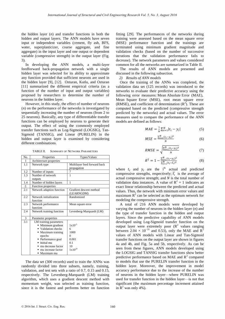
set (125 records). Fig. 7 illustrates the MAE and R2
values of the Mamdani FIS models, which each have
different number of clusters and m values. As shown in
Fig. 7, the performance of the FIS models with m values
of 2.5, 3.0, 3.5, and 4.0 is exceptionally poor. A gradual
increment in MAE and R2 values appears for models with
m values of 1.5 and 2.0 as the number of clusters
increases. Even though the R2 values are low, models
with m values of 1.5 perform better in terms of MAE than
those models with m values of 2.0 when an identical
number of clusters is used.
Cement
BFS
Fly ash
Water
Superplasticizer
Coarse aggregate
Fine aggregate
Mamdani Inference
Compressive
strength
International Journal of Structural and Civil Engineering Research Vol. 5, No. 3, August 2016
© 2016 Int. J. Struct. Civ. Eng. Res. 162
UGENO FIS
(a) (b)
Figure 7. (a) MAE and (b) R2 values of Mamdani FIS models.
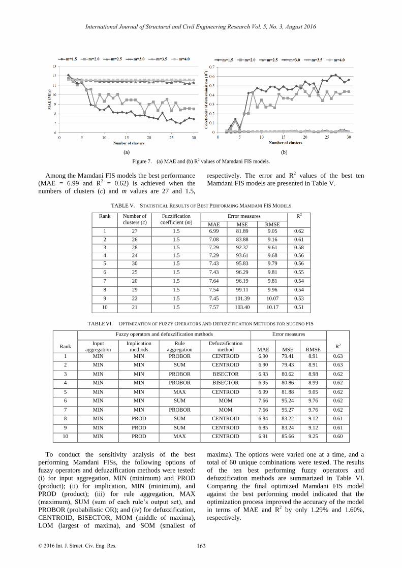
Among the Mamdani FIS models the best performance
(MAE = 6.99 and R2 = 0.62) is achieved when the
numbers of clusters (c) and m values are 27 and 1.5,
respectively. The error and R2 values of the best ten
Mamdani FIS models are presented in Table V.
TABLE V. STATISTICAL RESULTS OF BEST PERFORMING MAMDANI FIS MODELS
Rank Number of
clusters (c)
Fuzzification
coefficient (m)
Error measures R2
MAE MSE RMSE
1 27 1.5 6.99 81.89 9.05 0.62
2 26 1.5 7.08 83.88 9.16 0.61
3 28 1.5 7.29 92.37 9.61 0.58
4 24 1.5 7.29 93.61 9.68 0.56
5 30 1.5 7.43 95.83 9.79 0.56
6 25 1.5 7.43 96.29 9.81 0.55
7 20 1.5 7.64 96.19 9.81 0.54
8 29 1.5 7.54 99.11 9.96 0.54
9 22 1.5 7.45 101.39 10.07 0.53
10 21 1.5 7.57 103.40 10.17 0.51
TABLEVI. OPTIMIZATION OF FUZZY OPERATORS AND DEFUZZIFICATION METHODS FOR SUGENO FIS
Rank
Fuzzy operators and defuzzification methods Error measures
R2 Input
aggregation
Implication
methods
Rule
aggregation
Defuzzification
method
MAE
MSE
RMSE
1 MIN MIN PROBOR CENTROID 6.90 79.41 8.91 0.63
2 MIN MIN SUM CENTROID 6.90 79.43 8.91 0.63
3 MIN MIN PROBOR BISECTOR 6.93 80.62 8.98 0.62
4 MIN MIN PROBOR BISECTOR 6.95 80.86 8.99 0.62
5 MIN MIN MAX CENTROID 6.99 81.88 9.05 0.62
6 MIN MIN SUM MOM 7.66 95.24 9.76 0.62
7 MIN MIN PROBOR MOM 7.66 95.27 9.76 0.62
8 MIN PROD SUM CENTROID 6.84 83.22 9.12 0.61
9 MIN PROD SUM CENTROID 6.85 83.24 9.12 0.61
10 MIN PROD MAX CENTROID 6.91 85.66 9.25 0.60
To conduct the sensitivity analysis of the best
performing Mamdani FISs, the following options of
fuzzy operators and defuzzification methods were tested:
(i) for input aggregation, MIN (minimum) and PROD
(product); (ii) for implication, MIN (minimum), and
PROD (product); (iii) for rule aggregation, MAX
(maximum), SUM (sum of each rule’s output set), and
PROBOR (probabilistic OR); and (iv) for defuzzification,
CENTROID, BISECTOR, MOM (middle of maxima),
LOM (largest of maxima), and SOM (smallest of
maxima). The options were varied one at a time, and a
total of 60 unique combinations were tested. The results
of the ten best performing fuzzy operators and
defuzzification methods are summarized in Table VI.
Comparing the final optimized Mamdani FIS model
against the best performing model indicated that the
optimization process improved the accuracy of the model
in terms of MAE and R2 by only 1.29% and 1.60%,
respectively.
International Journal of Structural and Civil Engineering Research Vol. 5, No. 3, August 2016
© 2016 Int. J. Struct. Civ. Eng. Res. 163

In Sugeno FIS models, the error and R2 values
obtained were the same irrespective of the number of
clusters and m values considered in the models (i.e., the
models were found to be insensitive to the optimization
parameters c and m). The MAE, MSE, RMSE, and R2
values of all Sugeno FIS models were 5.08, 45.62, 6.75
and 0.78, respectively. Sensitivity analysis was carried
out by varying the input aggregation method (MIN and
PROD) and defuzzification methods (Wtaver, or
weighted average and Wtsum, or weighted sum). A total
of four combinations were tested for each Sugeno FIS, as
shown in Table VII. The results of the sensitivity analysis
confirm that the performance of FIS models is highly
influenced by applying different defuzzification methods.
According to the results, in all the Sugeno FIS concrete
compressive strength models, the Wtaver defuzzification
method (R2 = 0.78) should be adopted instead of the
Wtsum (R2 = 4.5 ×10
−4) for a better predictive accuracy.
TABLE VII. OPTIMIZATION OF FUZZY OPERATORS AND DEFUZZIFICATION METHODS FOR SUGENO FIS
Option
Fuzzy operators and defuzzification
methods
Error measures
R2 Input
aggregation
Defuzzification
method
MAE
MSE
RMSE
1 MIN Wtaver 5.08 45.62 6.75 0.78
2 PROD Wtaver 5.08 45.62 6.75 0.78
3 MIN Wtsum 35.30 1461.24 38.23 2.83x10⁻⁷
4 PROD Wtaver 30.92 1217.11 34.89 4.5 x10⁻⁴
Comparisons between Mamdani and Sugeno FIS
models based on the validation results show that Sugeno
FIS models outperform Mamdani FIS models in
predicting compressive strength. Because of the
continuity of the output surface and linear dependence of
each rule on the input variable [31], Sugeno FIS models
give better performance in mapping the relationship
between the inputs and output. Thus, Sugeno FIS models
with m values of 1.5, 2.0, 2.5, 3.0, 3.5, and 4.0 and
number of clusters ranging from 3 to 30 were used as an
initial FIS for developing the ANFIS models.
C. ANFIS for Modeling Concrete Compressive Strength
1) ANFIS model structure and parameters
As in the case of the ANN models, two data sets were
employed when evaluating the ANFIS models: the
training set (300 records) was used to construct FIS
models using FCM clustering, while the validation set
(125 records) was used to evaluate the predictive
accuracy of the models.
The ANFIS models were trained and validated using
the same training and validation data sets used in both the
ANN and FIS models. In this study, ANFIS models were
generated using the ANFIS function of MATLAB Fuzzy
Logic ToolboxTM
. Model structures such as the number
and type of membership function, type of output
membership function, and inference type, and model
parameters including learning algorithm, number of
training epochs, and training error goal must be carefully
selected in order to develop an ANFIS model with better
predictive capability. The FIS models developed using
the Sugeno inference system were used to provide the
ANFIS models with the initial membership functions for
training. Using Sugeno rather than Mamdani FISs in
ANFIS has the following advantages: (i) computational
efficiency in optimization and adaptive processes [20], (ii)
“guaranteed continuity of the output surface” [31], and (ii)
more reliable results when data driven techniques are
adopted [5]. The model structure of the initial Sugeno FIS
used for developing the ANFIS models is summarized in
Table VIII. In this study, the effects of number of
membership functions (number of clusters) and
fuzzification coefficient (m) on the performance of the
ANFIS models were investigated by varying the
membership functions from 3 to 30 and considering 𝑚
values of 1.5, 2.0, 2.5, 3.0, 3.5, and 4.0. The schematic
representation of the architecture of an ANFIS model
with 5 input membership functions based on a Sugeno
FIS is shown in Fig. 8.
TABLE VIII. MODEL STRUCTURE OF INITIAL SUGENO FIS USED TO
DEVELOP THE ANFIS MODELS
Model structures Type/value
Number of membership functions Varying (3–30)
Type of input membership function Gaussian
Type of inference Sugeno
Type of output membership function Linear
Value of fuzzification coefficient (m) Varying
Figure 8. Schematic representation of ANFIS model with 5 input MFs.
The basic learning rules available to optimize the
parameters of membership functions in ANFIS are either
back-propagation gradient descent or hybrid learning,
which combines the gradient-descent and least-square
methods [26]. According to Jang [23], the major
limitation of the back-propagation gradient descent
method is that the learning process gets trapped in the
local minima and takes more time to train. Thus, the
hybrid learning method was employed in this study. The
hybrid learning procedure works in such a way that the
consequent parameters are estimated in the forward pass
Cement
BFS
Fly ash
Water
Superplasticizer
Coarse aggregate
Fine aggregate
Input Input MFs Rules Output MFs Output
Compressive
strength
International Journal of Structural and Civil Engineering Research Vol. 5, No. 3, August 2016
© 2016 Int. J. Struct. Civ. Eng. Res. 164

using the least mean square error procedure by keeping
the premise parameters fixed; in the backward pass the
back-propagation descent method is used to modify the
premise parameters while the consequent parameters are
kept fixed [16], [23]. This procedure is repeated until
both the premise and consequent parameters are
optimized. In this case, the number of training epochs and
the training error goal were set to 1000 and 0,
respectively. The training process terminates whenever
either of these designated values are achieved.
2)
Results of FIS models
After successful training, the validation data set was
applied to evaluate the predictive capability of the models.
The MAE and R2 values of ANFIS models with different
m values and numbers of clusters (c) ranging from 2 to 17
are presented in Fig. 9 for illustration purposes, as the
performance of the models with higher number of
clusters were found to be very poor (R2 values ranging
between 8.58 ×
10−6
and 0.41). Comparatively, the
ANFIS models with m values of 1.5, 2.0 and 2.5 perform
better in predicting compressive strength than those
ANFIS models with higher m values. Moreover, higher
prediction accuracy is achieved at a lower number of
clusters (2 to 7) for all m values considered in the
models—unlike the Mamdani FIS models, which
achieved higher accuracy at a higher number of clusters.
(a)
(b)
Figure 9. (a) MAE and (b) R2 values of ANFIS models.
The performance results of the top ten ranked ANFIS
models in terms of prediction accuracy are presented in
Table IX. According to Table IX, the highest prediction
accuracy is achieved from an ANFIS model with 5
clusters and m values of 2.0. The MAE, MSE, RMSE,
and R2 vales of this model are 4.19, 29.40, 5.42, and 0.86,
respectively.
TABLE IX. STATISTICAL RESULTS OF BEST PERFORMING ANFIS
MODELS
Rank
Number of
clusters
(c)
Fuzzification
coefficient (m)
Error measures
R2 MAE MSE RMSE
1 5 2.0 4.19 29.40 5.42 0.86
2 5 1.5 4.30 29.99 5.48 0.86
3 7 2.5 4.33 30.36 5.51 0.86
4 3 2.5 4.36 31.25 5.59 0.85
5 6 1.5 4.36 31.52 5.61 0.85
6 7 1.5 4.43 31.66 5.63 0.85
7 4 2.5 4.23 32.59 5.71 0.85
8 4 2.0 4.26 32.90 5.74 0.85
9 3 1.5 4.34 33.73 5.81 0.84
10 4 1.5 4.50 34.65 5.89 0.84
Figure 10. Comparison of actual and predicted compressive strength of the best performing AI models.
D. Comparison of AI Models
To compare the performance of the three AI modeling
techniques, a scatter diagram plotting the relationship
between actual and predicted compressive strengths was
developed for the best performing ANN, Mamdani FIS,
Sugeno FIS, and ANFIS models, each of whose model
structure and parameters are described in previous
sections. The linear least square fit line (trend line) with
its corresponding linear equation and R2 values is
depicted in Fig. 10 for each best performing AI model.
The prediction accuracy of the Mamdani FIS was
relatively low (R2 = 0.629), and better prediction was
achieved with a higher number of clusters (c = 27),
resulting in limited interpretability. According to Pedrycz
and Gomide [17], the number of clusters should be
moderately low (5–9) for better interpretability. The
prediction accuracy of the Sugeno FIS remained the same
(R2 = 0.782) regardless of the number of clusters and m
values considered (i.e., it was not sensitive to parameter
optimization). The compressive strength values predicted
by the ANFIS (R2 = 0.859) and ANN (R
2 = 0.855)
models were reasonably close to the actual compressive
International Journal of Structural and Civil Engineering Research Vol. 5, No. 3, August 2016
© 2016 Int. J. Struct. Civ. Eng. Res. 165
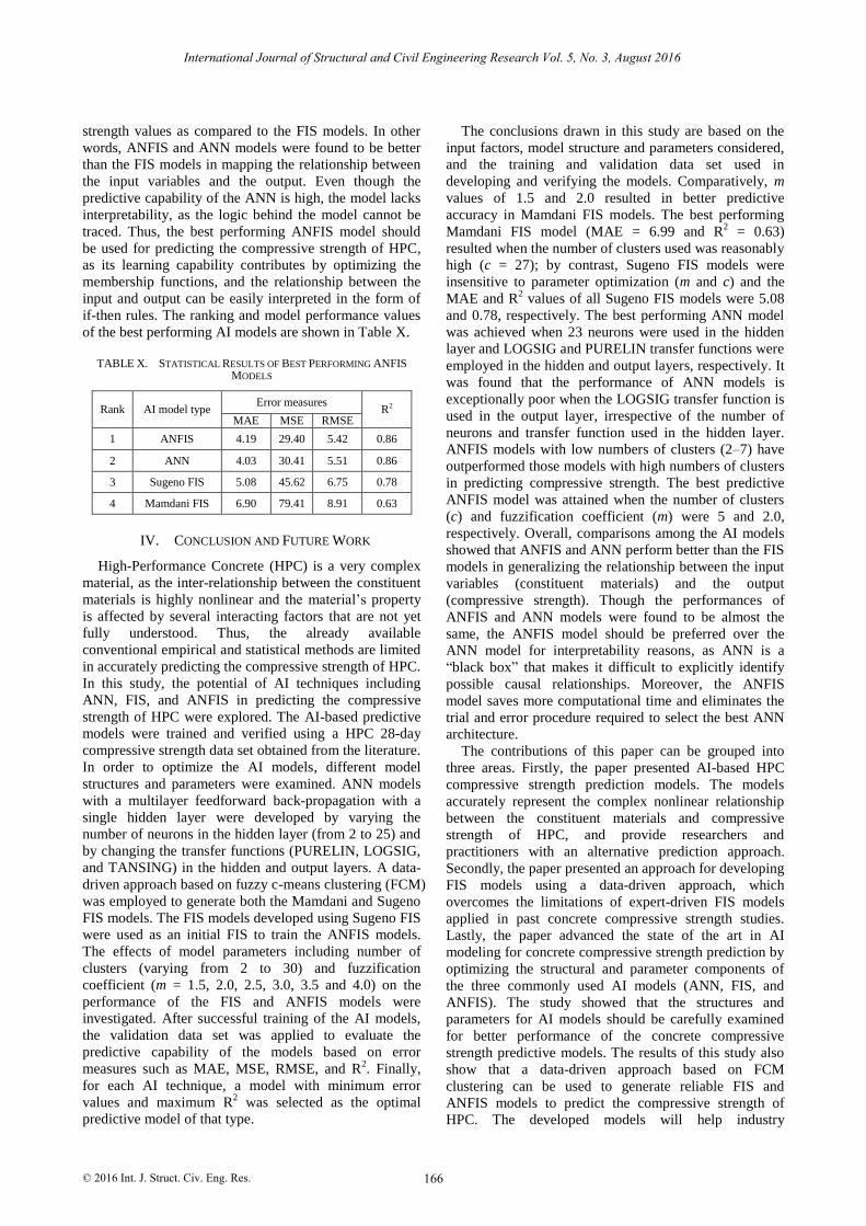
strength values as compared to the FIS models. In other
words, ANFIS and ANN models were found to be better
than the FIS models in mapping the relationship between
the input variables and the output. Even though the
predictive capability of the ANN is high, the model lacks
interpretability, as the logic behind the model cannot be
traced. Thus, the best performing ANFIS model should
be used for predicting the compressive strength of HPC,
as its learning capability contributes by optimizing the
membership functions, and the relationship between the
input and output can be easily interpreted in the form of
if-then rules. The ranking and model performance values
of the best performing AI models are shown in Table X.
TABLE X. STATISTICAL RESULTS OF BEST PERFORMING ANFIS
MODELS
Rank AI model type Error measures
R2 MAE MSE RMSE
1 ANFIS 4.19 29.40 5.42 0.86
2 ANN 4.03 30.41 5.51 0.86
3 Sugeno FIS 5.08 45.62 6.75 0.78
4 Mamdani FIS 6.90 79.41 8.91 0.63
IV. CONCLUSION AND FUTURE WORK
High-Performance Concrete (HPC) is a very complex
material, as the inter-relationship between the constituent
materials is highly nonlinear and the material’s property
is affected by several interacting factors that are not yet
fully understood. Thus, the already available
conventional empirical and statistical methods are limited
in accurately predicting the compressive strength of HPC.
In this study, the potential of AI techniques including
ANN, FIS, and ANFIS in predicting the compressive
strength of HPC were explored. The AI-based predictive
models were trained and verified using a HPC 28-day
compressive strength data set obtained from the literature.
In order to optimize the AI models, different model
structures and parameters were examined. ANN models
with a multilayer feedforward back-propagation with a
single hidden layer were developed by varying the
number of neurons in the hidden layer (from 2 to 25) and
by changing the transfer functions (PURELIN, LOGSIG,
and TANSING) in the hidden and output layers. A data-
driven approach based on fuzzy c-means clustering (FCM)
was employed to generate both the Mamdani and Sugeno
FIS models. The FIS models developed using Sugeno FIS
were used as an initial FIS to train the ANFIS models.
The effects of model parameters including number of
clusters (varying from 2 to 30) and fuzzification
coefficient (m = 1.5, 2.0, 2.5, 3.0, 3.5 and 4.0) on the
performance of the FIS and ANFIS models were
investigated. After successful training of the AI models,
the validation data set was applied to evaluate the
predictive capability of the models based on error
measures such as MAE, MSE, RMSE, and R2. Finally,
for each AI technique, a model with minimum error
values and maximum R2 was selected as the optimal
predictive model of that type.
The conclusions drawn in this study are based on the
input factors, model structure and parameters considered,
and the training and validation data set used in
developing and verifying the models. Comparatively, m
values of 1.5 and 2.0 resulted in better predictive
accuracy in Mamdani FIS models. The best performing
Mamdani FIS model (MAE = 6.99 and R2 = 0.63)
resulted when the number of clusters used was reasonably
high (c = 27); by contrast, Sugeno FIS models were
insensitive to parameter optimization (m and c) and the
MAE and R2 values of all Sugeno FIS models were 5.08
and 0.78, respectively. The best performing ANN model
was achieved when 23 neurons were used in the hidden
layer and LOGSIG and PURELIN transfer functions were
employed in the hidden and output layers, respectively. It
was found that the performance of ANN models is
exceptionally poor when the LOGSIG transfer function is
used in the output layer, irrespective of the number of
neurons and transfer function used in the hidden layer.
ANFIS models with low numbers of clusters (2–7) have
outperformed those models with high numbers of clusters
in predicting compressive strength. The best predictive
ANFIS model was attained when the number of clusters
(c) and fuzzification coefficient (m) were 5 and 2.0,
respectively. Overall, comparisons among the AI models
showed that ANFIS and ANN perform better than the FIS
models in generalizing the relationship between the input
variables (constituent materials) and the output
(compressive strength). Though the performances of
ANFIS and ANN models were found to be almost the
same, the ANFIS model should be preferred over the
ANN model for interpretability reasons, as ANN is a
“black box” that makes it difficult to explicitly identify
possible causal relationships. Moreover, the ANFIS
model saves more computational time and eliminates the
trial and error procedure required to select the best ANN
architecture.
The contributions of this paper can be grouped into
three areas. Firstly, the paper presented AI-based HPC
compressive strength prediction models. The models
accurately represent the complex nonlinear relationship
between the constituent materials and compressive
strength of HPC, and provide researchers and
practitioners with an alternative prediction approach.
Secondly, the paper presented an approach for developing
FIS models using a data-driven approach, which
overcomes the limitations of expert-driven FIS models
applied in past concrete compressive strength studies.
Lastly, the paper advanced the state of the art in AI
modeling for concrete compressive strength prediction by
optimizing the structural and parameter components of
the three commonly used AI models (ANN, FIS, and
ANFIS). The study showed that the structures and
parameters for AI models should be carefully examined
for better performance of the concrete compressive
strength predictive models. The results of this study also
show that a data-driven approach based on FCM
clustering can be used to generate reliable FIS and
ANFIS models to predict the compressive strength of
HPC. The developed models will help industry
International Journal of Structural and Civil Engineering Research Vol. 5, No. 3, August 2016
© 2016 Int. J. Struct. Civ. Eng. Res. 166

practitioners (i.e., designers and construction engineers)
to accurately predict the compressive strength of HPC
without having to conduct costly and time-consuming
laboratory experiments.
Further research will consist of: (i) investigating the
effects of different network types (perceptron,
probabilistic) and training algorithms (such as Quasi-
Newton, resilient back propagation, etc.) on ANN models;
(ii) examining the implications of using different types of
fuzzy operators and defuzzification methods, membership
functions (triangular, trapezoidal, etc.), and clustering
methods (k-means clustering, subtractive clustering, and
conditional clustering) on the performance of both FIS
and ANFIS models in predicting concrete compressive
strength; and (iii) studying the effect of using the back-
propagation learning rule to train the ANFIS models and
comparing the results to those of ANFIS models
employing the hybrid learning rule.
REFERENCES
[1] A. M. Neville, Properties of Concrete, 5th ed. New York, NY:
Prentice Hall, 2012.
[2] M. F. M. Zain and S. M. Abd, “Multiple regression model for compressive strength prediction of high performance concrete,”
Journal of Applied Sciences, vol. 9, no. 5, pp. 155-160, 2009.
[3] H. G. Russel, “ACI defines high-performance concrete,” Concrete International, vol. 21, no. 2, pp. 56-57, 1999.
[4] I. C. Yeh, “Modeling of strength of high-performance concrete
using artificial neural networks,” Cement and Concrete Research, vol. 28, no. 12, pp. 1797-1808, 1998.
[5] B. Vakhshouri and S. Nejadi, “Application of adaptive neuro-
fuzzy inference system in high strength concrete,” International Journal of Computer Applications, vol. 101, no. 5, pp. 39-48,
November 2014.
[6] C. Deepa, K. Sathiyakumari, and V. Sudha, “Prediction of the compressive strength of high performance concrete mix using tree
based modeling,” International Journal of Computer Application,
vol. 6, no. 5, pp. 18-24, September 2010. [7] J. Noorzaei, S. J. S. Hakim, M. S. Jaafar, and W. A. M. Thanoon,
“Development of artificial neural networks for predicting concrete
compressive strength,” International Journal of Engineering and Technology, vol. 4, no. 2, pp. 141-153, 2007.
[8] I. C. Yeh, “Design of high-performance concrete mixture using
neural networks and nonlinear programming,” Journal of Computing in Civil Engineering, vol. 13, no. 1, pp. 36-42, January
1999.
[9] I. B. Topcu and M. Saridemir, “Prediction of compressive strength
of concrete containing fly ash using artificial neural networks and
fuzzy logic,” Computational Material Science, vol. 41, no. 3, pp.
305-311, January 2008. [10] S. Subasi, “Prediction of mechanical properties of cement
containing class C fly ash by using artificial neural network and
regression technique,” Scientific Research and Essay, vol. 4, no. 4, pp. 289-297, April 2009.
[11] M. Ozturan, B. Kutlu, and T. Ozturan, “Comparison of concrete
strength prediction techniques with artificial neural network approach,” Building Research Journal, vol. 56, pp. 23-36, 2010.
[12] F. Ozcan, C. D. Atis, O. Karahan, E. Uncuoglu, and H. Tanyildizi,
“Comparison of artificial neural network and fuzzy logic models for prediction of long-term compressive strength of silica fume
concrete,” Advances in Engineering Software, vol. 40, no. 9, pp. 856-863, September 2009.
[13] I. B. Topcu and M. Saridemir, “Prediction of mechanical
properties of recycled aggregate concretes containing silica fume using artificial neural networks and fuzzy logic,” Computational
Material Science, vol. 42, no. 1, pp. 74-82, March 2008.
[14] P. Aggarwal and Y. Aggarwal, “Prediction of compressive strength of self- compacting concrete with fuzzy logic,” World
Academy of Science, Engineering and Technology, vol. 77, pp.
847-854, May 2011. [15] D. S. Badde, A. K. Gupta, and V. K. Patki, “Comparison of fuzzy
logic and ANFIS for prediction of compressive strength of RMC,”
IOSR Journal of Mechanical and Civil Engineering, vol. 3, pp. 07-15, May 2013.
[16] A. C. Aydin, A. Tortum, and M. Yavuz, “Prediction of concrete
and elastic modulus using adaptive neuro-fuzzy inference system,” Civil Engineering and Environmental Systems, vol. 23, no. 4, pp.
295-309, 2006.
[17] W. Pedrycz and F. Gomide, Fuzzy System Engineering Toward Human-Centric Computing, 1st ed., Hoboken, NJ: John Wiley and
Sons, Inc., 2007.
[18] A. H. Boussabaine, “The use of neural networks in construction management: A review,” Construction Management and
Economics, vol. 14, no. 5, pp. 427-436, 1996.
[19] M. T. Hagan, H. B. Demuth, and M. H. Beale, Neural Network Design, Boston, MA: PWS Publishing, 1996.
[20] C. Ozel, “Prediction of compressive strength of concrete from
volume ration and Bingham parameters using Adaptive Neuro-Fuzzy Inference System (ANFIS) and data mining,” International
Journal of Physical Science, vol. 6, no. 31, pp. 7078-7094,
November 2011. [21] S. Guillaume, “Designing fuzzy systems from data: An
interpretability-oriented review,” Transaction on Fuzzy Systems,
vol. 9, no. 3, pp. 426-443, June 2001. [22] F. Hoppner and F. Klawonn, “Improved fuzzy partitions for fuzzy
regression models,” International Journal of Approximate
Reasoning, vol. 32, no. 3, pp. 85-102, June 2001. [23] J. R. Jang, “ANFIS: Adaptive-network-based fuzzy inference
system,” Transactions on Systems, Man. and Cybernetics, vol. 23, no. 2-3, pp. 85-102, June 1993.
[24] U. J. Na, T. W. Park, M. Q. Feng, and L. Chung, “Neuro-fuzzy
application for concrete strength prediction using combined non-destructive tests,” Magazine of Concrete Research, vol. 61, no. 4,
pp. 245-256, May 2009.
[25] J. Amani and R. Moeini, “Prediction of shear strength of reinforced concrete beams using adaptive neuro-fuzzy inference
system and artificial neural network,” Scientia Iranica A, vol. 19,
no. 2, pp. 242-248, January 2012. [26] P. C. Nayak, K. P. Sudheer, D. M. Rangan, and K. S. Ramasastri,
“A neuro-fuzzy computing technique for modeling hydrological
time series,” Journal of Hydrology, vol. 291, no. 1-2, pp. 52-66, May 2004.
[27] Y. M. Wang and T. M. S. Elhag, “An adaptive neuro-fuzzy
inference system for bridge risk assessment,” Expert Systems with Application, vol. 34, no. 4, pp. 3099-3106, May 2008.
[28] I. C. Yeh. Concrete compressive strength data set. UCI Machine
Learning Repository. [Online]. Available: http://archive.ics.uci.edu/ml/datasets/Concrete+Compressive+Stre
ngth
[29] M. H. Beale, M. T. Hagan, and H. B. Demuth, Neural Network ToolboxTM: User’s Guide, Natick, MA: MathWorks, Inc., 2014.
[30] M. A. Grima and R. Babuska, “Fuzzy model for the prediction of
unconfined compressive strength of rock samples,” International Journal of Rock Mechanics and Mining Sciences, vol. 36, no. 3,
pp. 339-349, March 1999.
[31] MathWorks R2014b, Fuzzy Logic ToolboxTM: User’s Guide, Natick, MA: MathWorks, Inc., 2014.
International Journal of Structural and Civil Engineering Research Vol. 5, No. 3, August 2016
© 2016 Int. J. Struct. Civ. Eng. Res. 167