Development and Testing of a Virtual Flow Meter for Use in ...€¦ · Development and Testing of a Virtual Flow Meter for Use in Ongoing Commissioning of Commercial and Institutional

Development and Testing of a Virtual Flow Meter for Use in Ongoing

Commissioning of Commercial and Institutional Buildings

Eric McDonald

A Thesis

In the Department

of

Building, Civil and Environmental Engineering

Presented in Partial Fulfilment of the Requirements

for the Degree of

Master of Applied Science (Building Engineering) at

Concordia University

Montreal, Quebec, Canada

December 2014

© Eric McDonald, 2014

ii

CONCORDIA UNIVERSITY

School of Graduate Studies

This is to certify that the thesis prepared

By: Eric McDonald

Entitled: Development and Testing of a Virtual Flow Meter for Use in Ongoing Commissioning of Commercial and Institutional Buildings

and submitted in partial fulfillment of the requirements for the degree of

Master of Applied Science (Building Engineering)

complies with the regulations of the University and meets the accepted standards with respect to originality and quality.

Signed by the final Examining Committee:

Dr. A. Athienitis Chair

Dr. F. Haghighat Examiner

Dr. L. Kadem External Examiner

Dr. R. Zmeureanu Supervisor

Approved by s Chair of Department or Graduate Program Director

2014 d

Dean of Faculty

iii

ABSTRACT

Development and Testing of a Virtual Flow Meter for Use in Ongoing

Commissioning of Commercial and Institutional Buildings

Eric McDonald

Ongoing commissioning of commercial and institutional buildings relies on the available

trend data from a building automation systems (BAS) to be able to monitor the buildings

energy performance using developed tools. However, it is often that the BAS has no

information of the chilled and condenser water flow rates that pass through the evaporator

and condenser, respectively, of a chiller.

This thesis proposes a virtual flow meter (VFM) to estimate the chilled and condenser

water mass flow rates. The virtual flow meter uses a thermodynamic analysis of a chiller

under six different scenarios of available sensors from a BAS with some manufacturer data

to fill the gaps left by the missing sensors.

This thesis presents the use of the VFM in three case studies to estimate the chilled and

condenser water mass flow rates. The evaluation of the accuracy of the VFM model is

performed using an uncertainty analysis, statistical indices (CV-RMSE, NMBE) and a

paired difference statistical hypothesis test to provide insight into the limits of CV-RMSE

and NMBE that determine an acceptable fit. Then, the estimates from the VFM are used to

estimate the virtual COP of the chiller and the cooling plant for use with developed ongoing

commissioning methods of cooling plants.

This thesis presents the development of a graphical user interface for the VFM model and

the sensitivity of the virtual flow meter to it inputs is discussed to aid the user in achieving

accurate results.

iv

Acknowledgements

I would like to my supervisor, Dr. Radu G. Zmeureanu, for his guidance and

encouragement throughout this research project. I would like to acknowledge the financial

support received from the NSERC-Smart Net Energy Buildings Research Network and the

Faculty of Engineering and Computer Science of Concordia University.

The collaboration of the Concordia Facilities Management, Luc Lagacé, Mathieu

Laflamme was strongly appreciated. I would like to thank Mr. Daniel Giguère for his

expertise in refrigeration systems and CanmetENERGY Natural Resources Canada.

I would like to thank my friends and family for their constant support and motivation

through this journey. I would also like to thank all my friends and colleagues from

Concordia University for their help and support. Lastly, I would like to thank Dominique

for her constant love and support through my life.

v

Table of Contents

LIST OF FIGURES ........................................................................................................ IX

LIST OF TABLES ........................................................................................................ XII

LIST OF ACRONYMS ............................................................................................... XVI

NOMENCLATURE ................................................................................................... XVII

1. INTRODUCTION......................................................................................................... 1

2. LITERATURE REVIEW ............................................................................................ 3

VIRTUAL SENSORS ..................................................................................................... 5

2.1.1 VFM for the chilled and hot water flow rates in an AHU ................................. 8

2.1.2 VFM for the water flow rates after pumps ......................................................... 9

2.1.3 VFM for the chilled and condenser water flow rates through the evaporator

and condenser of a chiller ......................................................................................... 11

SUMMARY OF THE LITERATURE REVIEW .................................................................. 14

OBJECTIVE OF THESIS .............................................................................................. 14

3. DEVELOPMENT OF A VIRTUAL FLOW METER FOR USE IN THE

COMMISSIONING OF A COOLING PLANT........................................................... 17

MODULE 1: VIRTUAL FLOW METER (VFM) ............................................................. 17

3.1.1 Method for a VFM to Estimate the Mass Flow Rates through Chillers .......... 19

VFM model A ........................................................................................... 20

VFM model B ........................................................................................... 22

3.1.1.2.1 Identification of compressor parameters ............................................ 23

3.1.1.2.2 Refrigerant mass flow rates for reciprocating and centrifugal chillers

........................................................................................................................... 26

3.1.1.2.3 Chilled and condenser water mass flow rates .................................... 29

VFM model C ........................................................................................... 29

3.1.2 Description of Scenarios and Available Trend Data ........................................ 30

Scenario 1.................................................................................................. 30

Scenario 2.................................................................................................. 30

vi

Scenario 3.................................................................................................. 32

Scenario 4.................................................................................................. 33

Scenario 5.................................................................................................. 34

Scenario 6.................................................................................................. 34

3.1.3 Refrigerant Transport Properties Using REFPROP ......................................... 34

Uncertainty of Refrigerant Properties ....................................................... 36

MODULE 2: UNCERTAINTY PROPAGATION DUE TO MEASUREMENT ERRORS ........... 37

3.2.1 General uncertainty propagation from measurements ..................................... 38

Uncertainty propagation of VFM model A ............................................... 39

Uncertainty propagation of VFM model B ............................................... 41

3.2.1.2.1 Reciprocating compressor .................................................................. 41

3.2.1.2.2 Centrifugal compressor ...................................................................... 42

3.2.1.2.3 Uncertainty of the chilled water mass flow rate ................................ 43

3.2.1.2.4 Error propagation for the condenser water mass flow rate ................ 43

Uncertainty propagation of VFM model C ............................................... 44

3.2.2 Uncertainty in flow measuring equipment ....................................................... 45

Comparison an electromagnetic and an ultrasonic flow meter ................. 48

Conclusions of comparison of water flow meters ..................................... 53

3.2.3 Metrics used to determine the goodness of fit for the VFM predictions ......... 54

4. CASE STUDY: CAMILLIEN-HOUDE ICE RINK ................................................ 57

DESCRIPTION OF THE ICE RINK’S REFRIGERATION SYSTEM ..................................... 57

INSTRUMENTATION AND AVAILABLE DATA .............................................................. 59

4.2.1 Calculation of the uncertainty propagation due to measurements ................... 61

VFM MODEL DEVELOPMENT FOR THE CAMILLIEN-HOUDE ICE RINK...................... 62

4.3.1 VFM Model A.................................................................................................. 63

4.3.2 VFM Model B .................................................................................................. 67

4.3.3 VFM Model C .................................................................................................. 70

RESULTS AND DISCUSSION ....................................................................................... 71

VFM MODEL LIMITATIONS ...................................................................................... 74

CONCLUSIONS OF CASE STUDY ................................................................................ 76

vii

5. CASE STUDY: RESEARCH LABORATORY BUILDING .................................. 78

DESCRIPTION OF THE REFRIGERATION EQUIPMENT ................................................... 78

5.1.1 Instrumentation and available data .................................................................. 79

5.1.2 Control system of research laboratory ............................................................. 80

5.1.3 Uncertainty of sub-cooling measurements ....................................................... 81

VFM MODEL DEVELOPMENT .................................................................................. 84

5.2.1 VFM model A applied to research laboratory ................................................. 84

5.2.2 VFM model B applied to research laboratory .................................................. 85

5.2.3 VFM model C applied to research laboratory .................................................. 88

RESULTS AND DISCUSSION ....................................................................................... 88

5.3.1 Ice Creation (IC) Mode .................................................................................... 89

5.3.2 Results for Air-Conditioning (AC) Mode ........................................................ 93

CONCLUSIONS OF CASE STUDY ................................................................................ 97

6. CASE STUDY: LOYOLA CENTRAL PLANT ...................................................... 99

DESCRIPTION OF THE REFRIGERATION EQUIPMENT ................................................... 99

VFM MODEL DEVELOPMENT .................................................................................. 103

6.2.1 Development of inputs for VFM model B (scenario # 5) .............................. 104

6.2.2 Development of inputs for VFM model C (scenario # 6) .............................. 108

RESULTS AND DISCUSSION ..................................................................................... 109

6.3.1 Results for the summer of 2013 ..................................................................... 109

Chilled water mass flow rate ................................................................... 111

Condenser water mass flow rate ............................................................. 114

SENSITIVITY OF VFM MODEL TO INPUTS ............................................................... 116

6.4.1 VFM Limitations for centrifugal chillers ....................................................... 118

CONCLUSIONS OF CASE STUDY .............................................................................. 118

COMPARISON OF THE LIMITS OF CV(RMSE) AND NMBE FOR THREE CASE STUDIES

USING THE HYPOTHESIS TEST ....................................................................................... 119

7. MODULE 3: ONGOING COMMISSIONING OF COOLING PLANTS USING

A VFM............................................................................................................................ 121

ONGOING PERFORMANCE APPROACH .................................................................... 121

viii

7.1.1 Reciprocating Chillers ................................................................................... 122

7.1.2 Centrifugal Chillers ........................................................................................ 123

ONGOING COMMISSIONING ANALYSIS OF AN ICE RINK .......................................... 123

7.2.1 Comparison of the Virtual COP to Measured COP for the Ice Rink Case Study

................................................................................................................................. 123

7.2.2 Applying Module 3 to an Ice Rink ................................................................ 124

7.2.3 Conclusion of ongoing commissioning of the ice rink .................................. 126

ONGOING COMMISSIONING ANALYSIS OF THE LOYOLA CAMPUS CASE STUDY ...... 126

7.3.1 Comparison of the Virtual COP to Measured COP for the Loyola Case study

................................................................................................................................. 127

7.3.2 Applying Module 3 to Loyola case study ...................................................... 129

7.3.3 Conclusion of ongoing commissioning of the Loyola case study ................. 132

CONCLUSION FOR ONGOING COMMISSIONING APPROACH ....................................... 132

DEVELOPMENT OF GRAPHICAL USER INTERFACE (GUI) FOR THE VFM TOOL ....... 132

8. CONCLUSIONS AND FUTURE WORK .............................................................. 139

SUMMARY OF CONTRIBUTIONS .............................................................................. 140

FUTURE WORK ....................................................................................................... 141

9. REFERENCES .......................................................................................................... 142

APPENDICES ............................................................................................................... 146

APPENDIX A: RESULTS FROM THE HYPOTHESIS TEST FOR THE SENSITIVITY OF THE

SUPERHEATING AND SUB-COOLING ON THE CHILLED WAS MASS FLOW RATE ................ 146

APPENDIX B: RESULTS FOR ESTIMATES OF THE CHILLED AND CONDENSER WATER MASS

FLOW RATES OVER THE SUMMER OF 2014 .................................................................... 147

ix

List of Figures Figure 2.1: Life cycle of building commissioning techniques (Adapted from IEA 2010) . 3

Figure 2.2: Schematic of the analysis of the AHU (Swamy et al. 2012) ............................ 8

Figure 2.3: Operation sequence for the VFM Tool ........................................................... 15

Figure 3.1: Flow chart of thermodynamic analysis of a chiller ........................................ 17

Figure 3.2: Flowchart of VFM models A, B and C .......................................................... 20

Figure 3.3: Informational flow diagram of VFM model A ............................................... 22

Figure 3.4: Informational flow diagram of VFM model B ............................................... 23

Figure 3.5: Informational flow diagram of subroutine PISCOMP1 (adapted from

Bourdouxhe et al. 1994) .................................................................................................... 24

Figure 3.6: Informational flow diagram of CENTHID (adapted from Bourdouxhe et al.

1994) ................................................................................................................................. 25

Figure 3.7: Information flow diagram of modified CENTHID ........................................ 26

Figure 3.8: Information flow diagram of REFFLOWRATE ............................................ 26

Figure 3.9: Map of different flow meters available .......................................................... 46

Figure 3.10: Levels of uses for flow measurements ......................................................... 47

Figure 3.11: Schematic of test bench ................................................................................ 48

Figure 3.12: Diagram of electromagnetic flow meter (Endress+Hauser 2006) ................ 49

Figure 3.13: Schematic of ultrasonic flow meter (adapted from Greyline 2013) ............. 50

Figure 3.14: Comparison of both flow meters .................................................................. 51

Figure 3.15: Difference and percent difference between both flow meters ...................... 52

Figure 3.16: Effect of separation distance on measurements ........................................... 53

Figure 4.1: Schematic of refrigeration system for the Camillien-Houde ice rink

(Teyssedou 2007) .............................................................................................................. 58

Figure 4.2: Simplified layout of the none-modified compressor loop (adapted from

Teyssedou 2007) ............................................................................................................... 61

Figure 4.3: Power input during start-up for December 7th, 2005 ...................................... 64

Figure 4.4: Power input during start-up for May 13th, 2006 ............................................. 64

Figure 4.5: Input file generated from Carwin Software (Carlye 2007) ............................ 68

Figure 4.6: Validation of the compressor identified parameter for data set with

manufacturer data .............................................................................................................. 69

x

Figure 5.1: Layout of refrigeration system for CANMET (adapted from design

documents from CANMET) ............................................................................................. 79

Figure 5.2: a) Amount of sub-cooling for compressor # 1 from measurements b) Amount

of sub-cooling for compressor # 2 from measurements.................................................... 82

Figure 5.3: Manufacturer data for compressors ............................................................... 86

Figure 5.4: Comparison of power input from identified parameters versus manufacturer

data .................................................................................................................................... 87

Figure 5.5: Chilled water mass flow rate on July 2nd and 3rd during operation with

compressor #1 compared to measurements ...................................................................... 91

Figure 5.6: Chilled water mass flow rate on June 10th during operation with compressor #

2 compared to measurements ............................................................................................ 93

Figure 5.7: VFM model predictions for June 17th, 2012 compressor # 2 vs measurements

........................................................................................................................................... 96

Figure 5.8: VFM model predictions for July 17th, 2012 compressor # 2 vs measurements

........................................................................................................................................... 96

Figure 5.9: VFM model estimates for AC mode on June 18th, 2012 for compressor #1

compared to measurements ............................................................................................... 97

Figure 6.1: Schematic of central cooling plant (adapted from Monfet and Zmeureanu,

2011) ............................................................................................................................... 100

Figure 6.2: Profile of inputs for subroutine CENTHID .................................................. 104

Figure 6.3: Comparison of the predicted and measured power input to the compressor 105

Figure 6.4: PLR from manufacturer compared to power input to the chiller ................. 106

Figure 6.5: Hourly profile of chiller #1 in operation alone ............................................. 110

Figure 6.6: Hourly profile of chiller #2 in operation alone ............................................. 110

Figure 6.7: Hourly profile of both chillers in operation together ................................... 111

Figure 6.8: Estimates from VFM model B for July 1st to July 7th 2013 ......................... 112

Figure 6.9: VFM model C estimates from June 29th to July 7th 2013 ............................. 113

Figure 6.10: Condenser water mass flow rate for VFM model B for chiller #1 from June

29th to July 8th, 2013 ........................................................................................................ 115

Figure 7.1: Overview of ongoing commission method to monitor chiller performance 122

Figure 7.2: Monitoring of the COP for March 14th to 15th, 2006 ................................... 125

xi

Figure 7.3: Monitoring of the COP for May 13th to 14th, 2006 ...................................... 126

Figure 7.4: Virtual cooling plant COP compared to the measured cooling plant COP for

June 24th to 28th, 2013 ..................................................................................................... 128

Figure 7.5: Ongoing commissioning of the cooling plant COP for July 1st to 4th, 2014 131

Figure 7.6: Ongoing commissioning of the cooling plant COP for June 23rd to 24th, 2014

......................................................................................................................................... 131

Figure 7.7: Main window for the VFM Tool .................................................................. 133

Figure 7.8: Plant configuration interface ........................................................................ 134

Figure 7.9: Reciprocating part load input window ......................................................... 135

Figure 7.10: Centrifugal part load input window............................................................ 135

Figure 7.11: Fluid properties window ............................................................................. 136

Figure 7.12: Scenario inputs window ............................................................................. 137

Figure 7.13: Results window for the VFM Tool............................................................. 138

Figure B.1: Hourly profile of chiller #1 in operation alone ............................................ 148

Figure B.2: Hourly profile of chiller #2 in operation alone ............................................ 148

Figure B.3: Hourly profile of both chillers in operation together ................................... 149

Figure B.4: VFM model B estimates for chilled water mass flow rate for July 1st to 7th,

2014................................................................................................................................. 150

Figure B.5: Condenser water mass flow rate for chiller # 2 from July 5th to 28th, 2014 152

xii

List of Tables Table 2.1: Recommend parameters for monitoring the chiller to be used in

commissioning of a chiller (adapted from IEA 2010) ........................................................ 5

Table 2.2: Summary of comparison of different virtual flow meters techniques for total

chilled and condenser water flow rates ............................................................................. 13

Table 3.1: Complete list of required measurements ......................................................... 18

Table 3.2: Scenarios of available measured data .............................................................. 19

Table 3.3: Description of four input options for subroutine CENTHID ........................... 25

Table 3.4: Data set for scenario # 1 used in VFM model A ............................................. 30



Table 3.7: Data set for scenario # 4 used in VFM model B .............................................. 33

Table 3.8: Data set for scenario # 5 used in VFM model B .............................................. 34

Table 3.9: Data set for scenario # 6 used in VFM model C .............................................. 34

Table 3.10: Comparison of mean thermodynamic properties ........................................... 36

Table 3.11: Uncertainties for the calculation of properties of refrigerant R-22 ............... 37

Table 3.12: Uncertainties for the calculation of properties of refrigerant R-123 ............. 37

Table 3.13: Description of measurement bias for both devices ........................................ 48

Table 3.14: Set-up parameters for the ultrasonic flow meter ............................................ 50

Table 4.1: Manufacturer information for each component of the refrigeration system

(Teyssedou 2007) .............................................................................................................. 59

Table 4.2: Description of long-term measurements used in this study (Ouzzane et al.

2006). ................................................................................................................................ 60

Table 4.3: Description of short-term measurements used in this study (Ouzzane et al.

2006). ................................................................................................................................ 60

Table 4.4: Information of the inputs required for scenario 2 and 3 .................................. 63

Table 4.5: Average compressor power input to compressor ............................................. 65


Table 4.7: Compressor identified parameters from PISCOMP1 ...................................... 68

Table 4.8: Manufacturer data used for VFM model C taken from MD-1 ........................ 70

Table 4.9: Comparison of refrigerant mass flow rates ...................................................... 71

xiii

Table 4.10: Comparison of refrigerant effect of the evaporator for each model per

refrigerant loop .................................................................................................................. 72

Table 4.11: Average chilled water mass flow rate using the VFM models and

measurement across both chiller #1 and 2 ........................................................................ 73

Table 4.12: VFM model accuracy and t-value (hypothesis testing) for VFM models ..... 74

Table 4.13: Sensitivity of the VFM model to the amount of superheating ....................... 75

Table 4.14: Sensitivity of the VFM model to the amount of sub-cooling ........................ 75

Table 5.1: Description of refrigeration equipment (based on design documents provided

by CANMET) ................................................................................................................... 79

Table 5.2: Description of measurements used in this study. ............................................. 80

Table 5.3: Calculated average quality of liquid refrigerant leaving the condenser in the ice

creation mode .................................................................................................................... 83

Table 5.4: Calculated quality of liquid refrigerant leaving the condenser in the air-

conditioning mode ............................................................................................................ 83

Table 5.5: Information of the inputs required for scenario 1, 2 and 3 .............................. 84


Table 5.7: Identified compressor parameters from PISCOMP1 ....................................... 86

Table 5.8: Comparison of estimated refrigerant mass flow rates (kg/s) for compressor # 1

and # 2 ............................................................................................................................... 89

Table 5.9: Monthly average chilled water mass flow rates, from compressor # 1 in

operation in ice creation mode .......................................................................................... 90

Table 5.10: VFM model accuracy for compressor # 1 in the ice creation mode .............. 91

Table 5.11 Monthly average chilled water mass flow rates, from compressor # 2 in

operation in ice creation mode .......................................................................................... 92

Table 5.12: VFM model accuracy and t-value (hypothesis testing) for compressor # 2 in

the ice creation mode ........................................................................................................ 92

Table 5.13: Monthly average chilled water mass flow rates, from compressor # 1 in

operation in the air-conditioning mode ............................................................................. 94

Table 5.14 Monthly average chilled water mass flow rates, from compressor # 2 in

operation in the air-conditioning mode ............................................................................. 94

xiv

Table 5.15: VFM model accuracy and t-value (hypothesis testing) for both compressors

in the air-conditioning mode ............................................................................................. 95

Table 6.1: Description of equipment used in this case study (apdated from Tremblay

2013) ............................................................................................................................... 100

Table 6.2: Measured chilled water flow rates with a portable ultrasonic meter ............. 102

Table 6.3: Rated precision (bias errors) for the chilled and condenser water mass flow

rate measurements ........................................................................................................... 102

Table 6.4: Description of measurements from chiller (Trane 2005) .............................. 103

Table 6.5: Information of the inputs required for scenario 5 .......................................... 103

Table 6.6: Compressor identified parameters from CENTHID ...................................... 105

Table 6.7: Coefficients determined from linear regression for capacity control method 1

......................................................................................................................................... 107

Table 6.8: Manufacturer data file MD-3 ......................................................................... 108

Table 6.9: Average monthly chilled water mass flow rates for VFM models B & C for the

summer of 2013 .............................................................................................................. 113

Table 6.10: Results for the CV(RMSE), NMBE and t-value (hypothesis test) for the

chilled water flow rate for the summer of 2013 .............................................................. 114

Table 6.11: Monthly averages of the condenser water mass flow rate for the summer of

2013................................................................................................................................. 116

Table 6.12: Results for the CV(RMSE), NMBE and t-value (hypothesis test) for the

condenser water flow rate for the summer of 2013 ........................................................ 116

Table 6.13: Sensitivity of the chilled water mass flow rate for the amount of superheating

and sub-cooling ............................................................................................................... 118

Table 6.14: Maximum observed CV(RMSE) and NMBE that satisfied condition # 1 of

the hypothesis test ........................................................................................................... 120

Table 6.15: Maximum observed CV(RMSE) and NMBE that satisfied condition # 2 of

the hypothesis test ........................................................................................................... 120

Table 7.1: Values of measured and VFM COP of the cooling plant for ice rink ........... 124

Table 7.2: Design values for cooling plant components (adapted from Tremblay 2013)

......................................................................................................................................... 127

Table 7.3: Overall uncertainty of the cooling plant COP ............................................... 128

xv

Table 7.4: CV(RMSE) and NMBE for the virtual COP for the summer of 2013 .......... 128

Table 7.5: Dates used for training and testing for benchmarking model ........................ 129

Table 7.6: Coefficients for the benchmarking model for the cooling plant COP for each

mode of operation ........................................................................................................... 130

Table A.1: Results for t-value (hypothesis test) for the sensitivity testing of superheating

of the ice rink .................................................................................................................. 146

Table A.2: Results for t-value (hypothesis test) for the sensitivity testing of sub-cooling

of the ice rink .................................................................................................................. 146

Table A.3: Results for t-value (hypothesis test) for the sensitivity testing of superheating

and sub-cooling ............................................................................................................... 147

Table B.1: Average monthly chilled water mass flow rates for VFM mode B & C for the

summer of 2014 .............................................................................................................. 150

Table B.2: Results for the CV(RMSE), NMBE and t-value (hypothesis) test for the

chilled water flow rate for the summer of 2014 .............................................................. 151

Table B.3: Monthly averages of the condenser water mass flow rate for the summer of

2014................................................................................................................................. 152

Table B.4: Results for the CV(RMSE), NMBE and t-value (hypothesis test) for the

condenser water flow rate for the summer of 2014 ........................................................ 153

xvi

List of ACRONYMS Name Definition

AHU Air Handling Unit

BAS Building Automation System

COP Coefficient of Performance

CV(RSME) Coefficient of Variance of the Root-Mean Square Error

FDD Fault Detection and Diagnostics

HVAC&R Heating, Ventilation, Air Conditioning and Refrigeration

NMBE Normalized Mean Bias Error

RMSE Root-Mean Square Error

SDT Saturation Discharge Temperature

SST Saturation Suction Temperature

VSD Variable Speed Drive

VFD Variable Frequency Drive

xvii

Nomenclature Symbol Units

Roman

A Impeller exhaust area m2

Cf Clearance factor of the compressor -

Cpchw Specific heat capacity of the chilled water kJ/kg ·°C

Cpcd Specific heat capacity of the condenser water kJ/kg ·°C

Mass flow rate kg/s

I Electric current A

P Pressure kPa

Refrigeration load on evaporator kW

Refrigeration load on condenser kW

r Gas constant J / mol. K

T Temperature °C

U Peripheral speed of the impeller m/s

Ux Overall Uncertainty - V Volumetric flow rate m3/s

Vs Geometric displacement of the compressor m3/s W Power input W Wlo Electromechanical losses W Ws Isentropic compression power input W

Greek

α Loss factor -

xviii

β Angle between the direction of the vanes at the impeller

exhaust and the plane tangent to the impeller circumference radians

ε Volumetric effectiveness of the compressor -

ρ Density kg/m3

Δ Delta, difference -

σ Standard deviation -

γ Mean isentropic coefficient -

ζ Mean compressibility factor -

Subscript

ac Actual compressor power kW

cd Condenser

cdw Condenser water

chw Chilled water

comp Compressor

cp Cooling plant

CT Cooling tower

evap Evaporator

pump Pump

ref Refrigerant

1

1. INTRODUCTION Energy consumption in the commercial and institutional building sector accounts

for 12% of the secondary energy use in Canada. This accounts for almost 11% of the

Canada’s greenhouse gas emissions, which is approximately 55 megatons of

CO2 equivalent in 2010 (NRCAN 2013). In commercial and institutional buildings, cooling

plants account for the largest demand of energy during the cooling season of all the heating,

ventilation and air conditioning (HVAC) equipment. Building commissioning is a process

that verifies if the installed building components and systems perform in compliance with

the design specifications, current goals, and the owner’s project requirements (Monfet and

Zmeureanu 2011). Ongoing commissioning is a new approach used to monitor the system

continuously over an ongoing period to maintain the performance that was achieved from

the original commissioning of the buildings’ performance. Building energy performance

can degraded on an whole building scale as much as 15 to 30% over time after the building

is originally commissioned due to degradation or manual operation of the HVAC

components (Katipamula and Brambley 2005). There is a large opportunity for reduction

in energy consumption by applying energy conservation measures (ECM) to the hydronic

system of a buildings HVAC system (Deng et al. 2002). Operating the chiller with a

variable water flow rates would aid in reducing the coefficient of performance of the

cooling plant, which requires monitoring of the chilled and condenser water flow rates

(Stanford 2003).

Commissioning and ongoing commissioning are becoming important processes to achieve

the reduction in energy consumption of existing buildings to help reduce and maintain

energy consumption suitable for net-zero energy buildings. Building automation systems

(BAS) are installed in buildings for the control of the HVAC systems. The BAS provides

a large amount of trend data from sensors installed in the building to control the HVAC

system. Ongoing commissioning relies on the trend data to be able to monitor the building’s

energy performance using developed commissioning tools.

However, it is often that the BAS has no information of the chilled and condenser water

flow rates that pass through the evaporator and condenser, respectively, of a chiller. Chilled

water is the term used to denote the fluid in the chilled water loop of the cooling system,

2

which can consists of water or brine solution. Condenser water is the term used to denote

the fluid in the condenser water loop of the cooling system, which can consist of water for

water-cooled condensers or air for air-cooled condensers. The term “water” will be used as

a general term in this thesis to address all fluids within the hydronic loops of the HVAC

system.

Water flow meters are not typically installed in building systems due to the high

installation, maintenance and calibration cost associated with the meter. The measurements

used for ongoing commissioning and building energy modeling are typically a one-time

measurement of the flow rate or the design specifications of the flow rates that may differ

from the actual water flow rates in the system because of changes in the operation or design

of the system (Monfet and Zmeureanu 2011).

Flow measuring equipment can be expensive and difficult to install into existing buildings

to measure the total chilled and condenser water mass flow rates. Flow meters require a

long, straight pipe free of flow disturbances before and after the meter to provide accurate

results, which is not always available in cooling plants of commercial and institutional

buildings (Zhao et al. 2012). There is a need for a robust non-intrusive way to monitor the

chilled and condenser water flow rates for use in ongoing commissioning of commercial

and institutional buildings for multiple chillers types and available data.

Virtual sensors are indirect methods used to estimate variables where no physical sensor is

present within the system, using measurements from other installed sensors. The focus of

virtual sensors relies on the accuracy to estimate the measurement, which depends on the

overall uncertainty propagation within the virtual sensor model.

3

2. LITERATURE REVIEW This chapter introduces the concept of virtual sensors and their ability to estimate

values of pressure, temperature, and water flow rates in the Heating, Ventilation, Air

Conditioning and Refrigeration (HVAC&R) industry. Building automation systems (BAS)

and building energy management systems (BEMS) are used for the control of the building

HVAC systems to condition the building. The use of trend data from a BAS to monitor the

performance of the HVAC systems have been shown to be effective for use in the

calibration of energy models and for ongoing commissioning of cooling plants (Monfet

and Zmereanu, 2011).

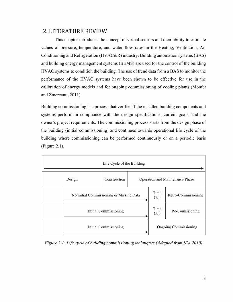
Building commissioning is a process that verifies if the installed building components and

systems perform in compliance with the design specifications, current goals, and the

owner’s project requirements. The commissioning process starts from the design phase of

the building (initial commissioning) and continues towards operational life cycle of the

building where commissioning can be performed continuously or on a periodic basis

(Figure 2.1).

No initial Commissioning or Missing Data

Initial Commissioning

Initial Commissioning

Ongoing Commissioning

Re-Comissioning

Retro-Commissioning

Time Gap

Design Operation and Maintenance PhaseConstruction

Life Cycle of the Building

Time Gap

Figure 2.1: Life cycle of building commissioning techniques (Adapted from IEA 2010)

4

The initial commissioning is a systematic process applied to the construction of a new

building or system. It consists of verifying if the installed components operate close to the

desired design specification and project goals. The initial commissioning process for

cooling plants after functional testing of the equipment consists of monitoring the operating

conditions to compare to design benchmarks to ensure the equipment is operating correctly

under normal conditions (AHRI, 2003).

It was recommended that the monitored performance be compared to design performance

curves provided by the manufacturer to verify the operation of the chiller (AHRI, 2003).

The baseline information is recommended to be obtained from manufacturer specifications

but short-term measured performance can be used to develop a baseline for comparison as

well. It was recommended that measured data could be obtained directly from the BAS or

from independent monitoring equipment (AHRI, 2003).

Retro-Commissioning is the implantation of a commissioning process of an existing

building that has never undergone any previous documented commissioning. Re-

commissioning or continuous commissioning is a commissioning process implemented

after the initial commissioning process (IEA, 2010).

Ongoing commissioning is a commissioning process conducted continually over time for

the purposes of maintaining, improving and optimizing the performance of buildings

systems after the initial commissioning or retro-commissioning of the buildings systems.

Ongoing commissioning is a complex approach to maintain optimum operation by

continuously monitoring the HVAC system and its components. The purpose of ongoing

commissioning is to 1) detect for faults and failures of the buildings systems or components

2) displays warning of unusual performance by 3) comparing measured performance

indices (PI) with benchmarked PI to help the building operators understanding how the

building is performing (Tremblay 2013).

The ongoing commissioning approach uses measured trend data from the building

automation system (BAS) with developed ongoing commissioning tools (Monfet and

Zmeureanu, 2011). Data can be analyzed, either online from the BAS to give immediate

feedback or offline where data is collected and analysed to monitor the performance over

5

a period of operation. In the offline or online mode performance indices (PI) are displayed,

and messages or reports are sent to the operating team for further analysis. The

International Energy Agency (IEA) Energy in Buildings and Communities Programme

(EBC) produced a report in 2010 on commissioning tools for improved building energy

performance (IEA 2010). Table 2.1 shows their recommended parameters required for

commissioning of a chiller.

Table 2.1: Recommend parameters for monitoring the chiller to be used in commissioning of a chiller (adapted from IEA 2010)

Description of point Symbol Schedule of monitoring Chiller Performance Data - Chilled water supply temperature Tchws Continuous monitoring Chilled water return temperature Tchwr Continuous monitoring Chilled water mass flow rate m Continuous monitoring Condenser water supply temperature Tcdws Continuous monitoring Condenser water return temperature Tcdwr Continuous monitoring Condenser water mass flow rate m Continuous monitoring Power Input to chiller W Continuous monitoring

The chilled and condenser water mass flow rates are not always measured mainly because

water flow meters are not installed in most buildings due to budget constraints or space

limitations within the system that do not allow water mass flow rates to be measured

accurately. The chilled and condenser water mass flow rates that pass through the

evaporator and condenser of chiller are important parameters for use in ongoing

commissioning and fault detection and diagnostics (FDD) of chillers and cooling plants

(Comstock et al. 1999; Monfet and Zmeurenau 2012; Zhao et al. 2012).

Virtual Sensors

The idea of virtual sensors (soft sensors) is not a new idea and is used in many

different industries such as the automotive, pulp and paper, HVAC, etc. The application of

a virtual sensor is to estimate or simulate ‘measurements’ at positions in a system where a

physical sensor does not exist, using a mathematical model along with some available

measurements from the system.

6

In the HVAC industry, virtual sensors can be used to aid in energy modeling and calibration

of energy models (Tahmasebi et al. 2013, Zach et al. 2013). It can be expensive and time

consuming to install sensors in every zone of a building for use in a building energy

management systems (BEMS) or in a building automation system (BAS). Work was

developed to provide virtual sensors or virtual data points in order to reduce the number of

sensors that are required for the calibration of energy models. A calibrated model of a

building using EnergyPlus was used to provide information from the building zones that

are not actually monitored (Tahmasebi et al. 2013). The virtual sensors use the information

from the adjacent zones to predict the temperature of the unmonitored zones.

Zach et al. (2013) developed an approach to implement “simulation-powered” virtual

sensors in a building information framework. Two prototypical virtual sensors were

introduced to demonstrate their proposed framework. The virtual sensors estimated the

radiator heating power based on the mean temperature and the standard heat output of the

radiator together with the room temperature of the respective zone and the visual conditions

at any location via solar radiance. Their method generated virtual datasets to fill in the gaps

required for the energy model where physical sensors were unavailable. This implied

identifying the missing measurements and developing virtual datasets for these missing

measurements.

Yang et al. (2013) developed a virtual outdoor air ratio (VOAR) sensor for rooftop air-

conditioning units. The outdoor air ratio is defined as the mass flow rate of the outdoor air

(OA) to that of the total mass flow rate. This parameter is important in energy modelling

and in control of the amount of fresh air supplied to the building. Because the outdoor air

mass flow rate is not measured, an energy balance of the mixing box of the return air (RA)

with the outdoor air (OA) in the air-handling unit (AHU) is used to be able to use the

temperature measurements available within the AHU. In the case where the mixed air

temperature is not measured then it is estimated by the supply air temperature and the

temperature difference across the fan. The VOAR was used in the winter and summer and

the uncertainty of the model was investigated to observe which input had the highest impact

to the sensitivity of the model. The uncertainty of the VAOR (UVAOR) ranged from 6.1 to

13.2%. The model was fine-tuned to reduce the uncertainty of the model by fine-tuning the

7

temperature increase across the fan to minimize the error between the OAR in winter and

summer at three different inlet damper positions. The uncertainty after the tuning process

was reduced to 2.4 to 4.5%.

Kusiak et al. (2010) developed a virtual indoor air quality sensor (IAQ) that used a data

driven model to estimate the air temperature, CO2, and relative humidity of a room. Data

mining techniques were used to train the artificial neural network (ANN) model with a

multi-layer perceptron (MLP) algorithm. The model can be used for on-line monitoring

and calibration of the IAQ sensors.

Li and Braun (2007, 2009a, 2009b, 2009c) developed a methodology for different virtual

sensors for air-to-air chillers (air-conditioners) and heat pumps. Virtual sensors were

applied to the refrigerant cycle of a vapour-compression for systems with reciprocating and

screw compressors. A virtual sensor for the refrigerant mass flow rate was used along with

manufacturer data and measured data from the chiller. A virtual refrigerant charge sensor

and a virtual refrigerant pressure sensor were developed for use in the monitoring and fault

diagnosis of vapor compression equipment. A quasi steady-state virtual airflow sensor was

develop for the airflow rate across the evaporator and condenser of the air-to-air chiller

using the energy balance on the evaporator and condenser. A virtual sensor was also

introduced for exit air humidity for the supply airflow. The uncertainty of the models was

investigated using the methods described in the National Institute of Standards and

technology (NIST) technical note 1297 (Taylor and Kuyatt 1994). The uncertainty for the

virtual refrigerant flow rate was 7.5% using the energy balance method on the compressor.

Five different models were found that estimate the water flow rates in the hydronic loops

of an HVAC system of the heating and cooling plant. These models used information at

the air-handling unit (AHU) level to estimate the water flow rates through the heating and

cooling coils of the AHU, at pump level where the water flow rates are estimated after

pumps and at the chiller level where the water flow rates are estimated in the chilled and

condenser water loops.

8

2.1.1 VFM for the chilled and hot water flow rates in an AHU Swamy et al. (2012) analysed the cooling and heating coils in the AHU to estimate

the water flow rate through the cooling and heating coils. Their assumptions were based

on the having a control valve in series with the cooling or heating coil and measuring the

pressure drop across each component (Figure 2.2). Then the water flow rate can be

measured by valve command, a differential pressure sensor and empirically obtained valve

characteristic curve.

Figure 2.2: Schematic of the analysis of the AHU (Swamy et al. 2012)

The differential pressure across the coil (ΔPC), the valve (ΔPV) and the total pressure (ΔPL)

across the loop of the system are used to estimate the water flow rate through the coil. The

valve authority (N) is defined as the pressure difference across the valve (ΔPV) to the

pressure difference across the loop (ΔPL) at design conditions. The virtual water flow

readings can be calculated by two measurable inputs 1) the valve stem position (X) and 2)

the differential pressure across the loop (∆PL) and three calibrated constants (Equation 2.1).

The three constants 1) the valve inherent characteristics (R), 2) the valve flow coefficient

(Cv) and 3) the valve authority (N). The valve inherent characteristics (R) requires short-

term measurements of the flow rate to provide accurate results.

Q = C ∗ R ∆P NN + R ( )(1 − N) Equation 2.1

The uncertainty of the model was investigated to determine which input the model was the

most sensitive to. It was determined that the standard deviation of the curve fit for the

9

installed valve characteristics had the largest impact on the uncertainty in values from the

virtual flow meter. The valve characteristic curves provided by manufacturers were found

to not represent the conditions in the actually system and could not be used to provide

accurate estimates of the water flow rates because they represented average characteristics

of a series of valves, not the specific valve (Swamy et al. 2012).

2.1.2 VFM for the water flow rates after pumps At the pump station level, the water flow rates after the pump can be estimated by

using the pump head (H), based on the differential pressure sensor across the pump, and

the motor power (Wmotor) along with pump characteristic data (Wang et al. 2010).

Manufacturer data for the pumps were used to obtain relationships between the efficiencies

and the power input to the motor and pump. Equation 2.2 is used to evaluate the chilled

water mass flow rate using an implicit expression of the pump flow due to the flow-related

pump efficiency, where f1 and f2 are described by Equation 2.3 and Equation 2.4.

Q = W ∗ f (W ) ∗ η ,H i = 1W ∗ f (W ) ∗ f HQH i > 1 Equation 2.2

f HQ = H ∗ QW = c HQ Equation 2.3

f (W ) = WW = −1 + 1 + 4a WW , − b2a WW , Equation 2.4

The pump speed control had a significant impact on the accuracy for the estimation of the

flow. The pump speed measurements have to be calibrated periodically to provide accurate

results. The model was also found to have a large sensitivity to the pump speed and that

small drifts or deviations in the measurements due to the sensor sensitivity caused large

deviations in the results.

10

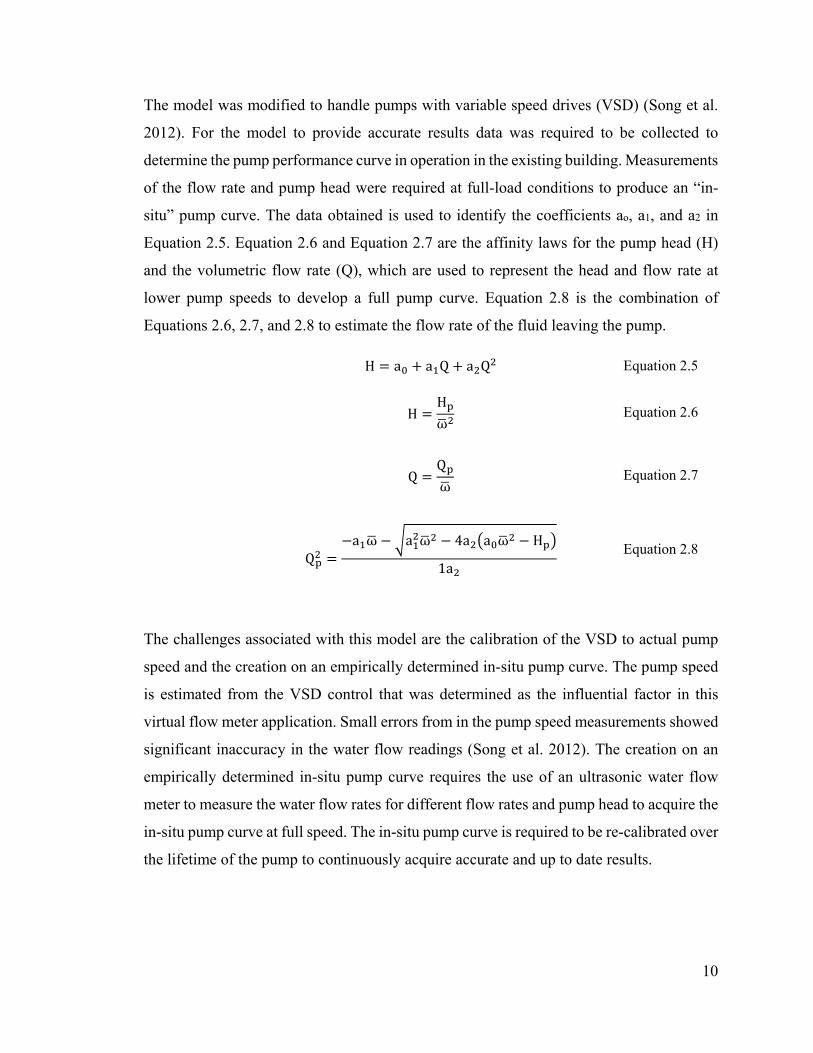
The model was modified to handle pumps with variable speed drives (VSD) (Song et al.

2012). For the model to provide accurate results data was required to be collected to

determine the pump performance curve in operation in the existing building. Measurements

of the flow rate and pump head were required at full-load conditions to produce an “in-

situ” pump curve. The data obtained is used to identify the coefficients ao, a1, and a2 in

Equation 2.5. Equation 2.6 and Equation 2.7 are the affinity laws for the pump head (H)

and the volumetric flow rate (Q), which are used to represent the head and flow rate at

lower pump speeds to develop a full pump curve. Equation 2.8 is the combination of

Equations 2.6, 2.7, and 2.8 to estimate the flow rate of the fluid leaving the pump.

H = a + a Q + a Q Equation 2.5

H = Hω Equation 2.6

Q = Qω Equation 2.7

Q = −a ω − a ω − 4a a ω − H1a Equation 2.8

The challenges associated with this model are the calibration of the VSD to actual pump

speed and the creation on an empirically determined in-situ pump curve. The pump speed

is estimated from the VSD control that was determined as the influential factor in this

virtual flow meter application. Small errors from in the pump speed measurements showed

significant inaccuracy in the water flow readings (Song et al. 2012). The creation on an

empirically determined in-situ pump curve requires the use of an ultrasonic water flow

meter to measure the water flow rates for different flow rates and pump head to acquire the

in-situ pump curve at full speed. The in-situ pump curve is required to be re-calibrated over

the lifetime of the pump to continuously acquire accurate and up to date results.

11

2.1.3 VFM for the chilled and condenser water flow rates through the evaporator and condenser of a chiller Wang (2014) developed a model to estimate the chilled and condenser water

volumetric flow rates (V) using the pressure drop across the evaporator and condenser (∆P)

and the resistance coefficients (S) (Equation 2.9). The model is based on the Bernoulli’s

equation and the Darcy-Weisbach equation for pressure loss. The resistance coefficient (S)

is required to be trained using short-term monitoring of the system using an ultrasonic flow

meter. The resistance coefficient (S) is required to be trained for each chiller and

combination of chillers in operation because the resistance coefficient is a function of the

volumetric flow rate. This method requires constant training overtime because of the

resistance coefficient can change over time due to fouling within the condenser or

evaporator.

V = ( − ) + ( − ) Equation 2.9

Zhao et al. (2012) developed a procedure to estimate the chilled and condenser water mass

flow rates through the evaporator and condenser of a chiller. A component-based model of

a chiller was used where its four main components are the compressor, the condenser, the

expansion valve and the evaporator. The developed model was used in the development of

decoupling features for fault detection and diagnostics (FDD) of a centrifugal chiller to

predict multiple simultaneous faults (Zhao et al. 2011).

Manufacturer data from 10 to 100% of the load was used to determine the theoretical

compressor power (Wth) (Equation 2.10). The theoretical compressor power input is then

used to determine the linear relationship between the actual power input to the compressor

and the theoretical power input to the compressor (Equation 2.11). The thermodynamic

energy balance on the compressor (Equation 2.12), evaporator (Equation 2.13), and

condenser (Equation 2.14) are used to determine the refrigerant, chilled and condenser

water mass flow rates respectively.

12

= − = ( − ) − ( − ) Equation 2.10

= + Equation 2.11

m = W(h − h ) Equation 2.12

= (ℎ − ℎ )( − ) Equation 2.13

= (ℎ − ℎ )( − ) Equation 2.14

The refrigerant enthalpies were calculated using established polynomial curve-fits to

refrigerant R-134a (Cleland 1994). The model was used with laboratory data for a 90-ton

centrifugal chiller from the ASHRAE research project 1043 (Comstock et al. 1999). The

datasets contained data for the chiller operation under different faults, to demonstrate the

accuracy of the model to predict the refrigerant, chilled and condenser water mass flow

rates of the centrifugal under different faults and severity of those faults. The faults under

consideration were the most common faults for centrifugal chillers: the condenser water

flow loss, evaporator water flow loss, refrigerant low charge, refrigerant overcharge,

condenser fouling, and non-condensable gas fault. It was observed that the methodology

estimated the refrigerant, chilled and condenser mass flow rates for different faults and

fault severities within a small amount of error of less than ±10% (Zhao et al. 2011).

The model was used in an existing building to estimate the chilled and condenser water

mass flow rates to monitor the chiller for two common faults: reduced condenser water

flow and reduced evaporator water flow. The evaporator flow and condenser water flow

rates were normalized by the design flow rate from manufacturers of the evaporator and

condenser. When the normalized water flow rates falls below 0.75, a reduced water flow

rate fault is present within the system.

13

After review of the four different models, the main advantages and disadvantages of

models for the total chilled and condenser water flow rates are summarized in Table 2.2.

Table 2.2: Summary of comparison of different virtual flow meters techniques for total chilled and condenser water flow rates

Authors Advantages Disadvantages

Pum

p le

vel Wang et al.

2010 Song et al. 2012

Can estimate the water flow rate after pumps and pump stations for hot, chilled and condenser water in the HVAC system.

Requires short-term measurements of flow rates for calibration of some coefficients in the model Sensitive to pump speed measurements

Chi

ller

Lev

el

Wang 2014 Can estimate the chilled and condenser water mass flow rate for individual chillers connected in parallel

Requires short-term measurements of flow rates for calibration of the resistance coefficients Requires training for each mode of operation (staging) of the chillers and can be time-consuming and complicated for cooling plant with multiple chillers. Sensitive to fouling in the condenser and to changes in the flow resistance in both the evaporator and condenser

Zhao et al. 2012

Does not require short-term measurements to train model Can be used under different degrees of common chiller faults Can estimate the chilled and condenser water mass flow rate for individual chillers connected in parallel

Requires refrigerant temperature measurements from the chiller that might not be installed in chillers included in existing buildings Sensitive to the accuracy of the sensors installed in chiller

14

Summary of the Literature Review

Different approaches and models are available to estimate the chilled water and

condenser water mass flow rate at different levels of the HVAC system. The mathematical

model developed by Zhao et al. (2012) provides the most accurate results for chilled and

condenser water mass flow rates without the need for short-term calibration using an

ultrasonic flow meter. However, the model is only able to estimate the chilled and

condenser water mass flow rates for chillers with a complete set of sensors installed within

the refrigerant cycle. For this, the mathematical model developed by Zhao et al. (2012) will

be used as the foundation in the development of a VFM to estimate the chilled and

condenser water mass flow rates to be used in the ongoing commissioning of commercial

and institutional buildings. To achieve this, the model will be required to estimate the

chilled and condenser water mass flow rates with the minimum amount of information

available.

Objective of Thesis

The main objective of this thesis is to develop a method for a virtual flow meter

(VFM) that can be easily integrated into a building automation system (BAS) using the

minimum amount of sensors and available system information. The VFM goals are to

provide a low-cost, non-intrusive method to monitor the chilled and condenser water mass

flow rates through the evaporator and condenser of a chiller on an hourly time scale within

an acceptable accuracy. The estimates from the VFM are then used to track the coefficient

of performance (COP) of the cooling plant to visualize the performance of the system over

time. This can aid building operators and commissioning agents in developing new control

and re-design strategies to reduce the energy consumption of the cooling plant and visualize

degradation of the performance of the cooling plant over time. To achieve this goal a new

framework is proposed, complied of three modules that are executed in sequence to

estimate the performance of the cooling plant (Figure 2.3). The three modules are defined

as:

15

Module 1: i. Virtual flow meter: to estimate chilled and condenser water mass flow rates.

Module 2:

ii. Uncertainty analysis: to estimate the overall uncertainty associated with the VFM.

Module 3:

iii. Virtual COP meter: to estimate the virtual COP of the chiller and cooling plant using the estimates from the VFM to compare with developed benchmarking models or PI.

Ongoing Energy Performance

(COP) Estimation

Measurements Database

Comparison Module

Chiller Manufacturer

Data

Visualization Tool

Reports & Warnings

Virtual flow meter

Pre-Process Data

Flow Measurments

Uncertainty Analysis

Graphical User Interface

Building Automation

System (BAS)

Figure 2.3: Operation sequence for the VFM Tool

Chapter three outlines the modules 1 and 2 where module 1 presents the VFM, a new

method that estimates the chilled and condenser water mass flow rate that pass through the

evaporator and condenser of a chiller. The assumptions and approaches of the mathematical

models are explained. The method for the quasi steady-state model begins using the work

of Zhao et al. (2012) as the starting point and uses the primary HVAC Toolkit (Bourdouxhe

et al. 1994). The goal is to develop a model that uses the minimum amount of sensors from

the BAS. Module 2 examines the error propagation due to measurement errors associated

with the VFM from the fixed bias error and random errors of the individual sensors that

propagate through the equations used to compute the estimates of the VFM.

Chapters four through six presents three case studies using three different building types,

to validate the methods and address the challenges associated with implementing the VFM

method into existing buildings. The sensitivity of the VFM model is examined and explores

Module 1 Module 2 Module 3

16

the key variables and parameters in the model inputs. The three buildings chosen for these

case studies were chosen for the availability of the data from their BAS and for the types

of installed systems.

The first case study is from an indoor ice arena located in Montréal, Qc, Canada, which

consists of an air-cooled reciprocating chiller and a constant speed chilled water pump with

a wide range of data to test the model over a range of scenarios. The second case study is

of a research laboratory located in Varennes, Qc, Canada, which consists of an air-cooled

reciprocating chiller with a variable speed drive (VSD) on the chilled water pump. The

third case studies uses trend data from the BAS from the central plant of the Loyola Campus

of Concordia University. This study consists of two water-chilled centrifugal chillers with

two constant speed pumps connected in parallel.

Chapter 7 explains the methods used in module 3 for the ongoing commissioning method

that uses the estimates from the VFM to compute the virtual COP of the cooling plant. The

virtual COP is used to track the performance of the cooling plant continuously on an hourly

time-scale. Module 3 is examined using case studies 1 and 3 to observe the method for two

different types of installed chillers. The method is used to track the performance of the

central plant to provide insight towards the building performance compared to developed

benchmarks. In a real-time operation of the method, the detection of a discrepancy with

respect to the benchmarks would be summed hourly to show how often the system is

behaving outside its desired performance window over a weekly period. This chapter

highlights the performance of existing buildings and the challenges associated with

monitoring that performance.

17

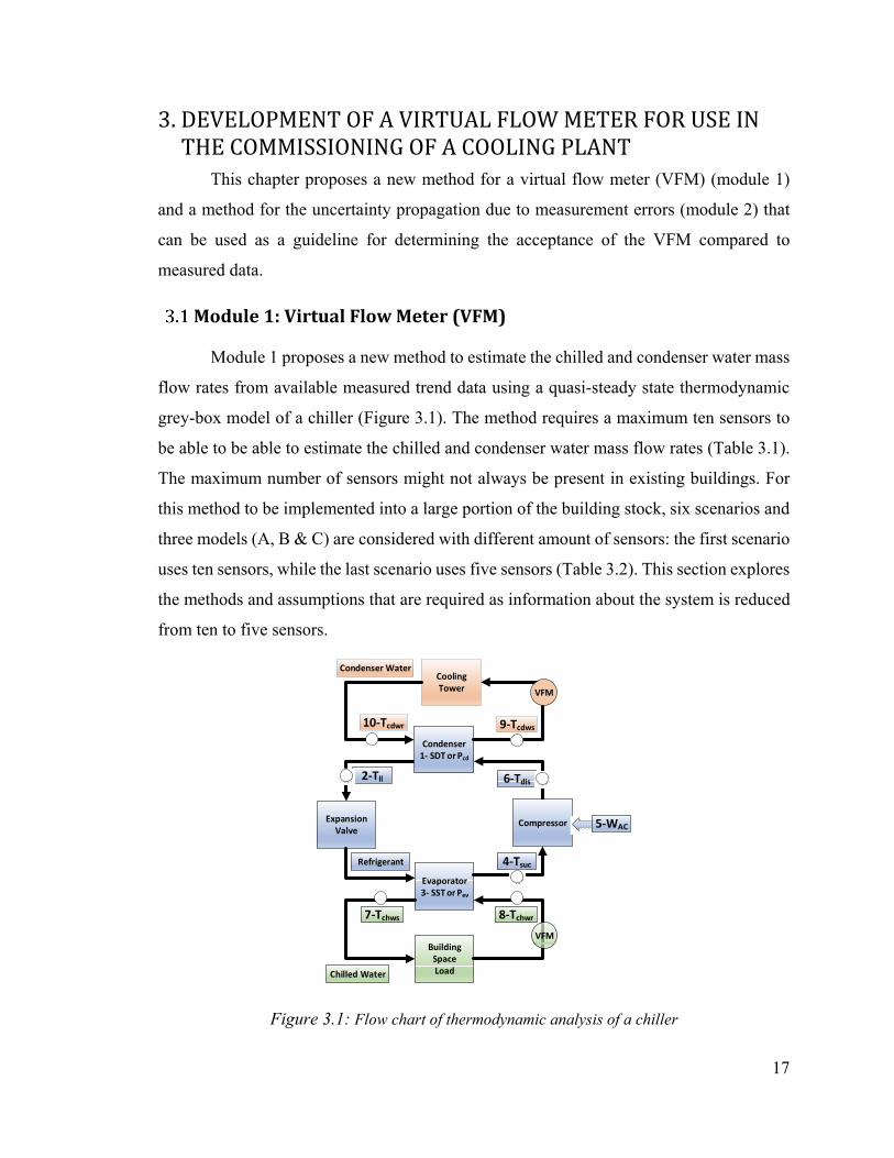
3. DEVELOPMENT OF A VIRTUAL FLOW METER FOR USE IN THE COMMISSIONING OF A COOLING PLANT This chapter proposes a new method for a virtual flow meter (VFM) (module 1)

and a method for the uncertainty propagation due to measurement errors (module 2) that

can be used as a guideline for determining the acceptance of the VFM compared to

measured data.

Module 1: Virtual Flow Meter (VFM)

Module 1 proposes a new method to estimate the chilled and condenser water mass

flow rates from available measured trend data using a quasi-steady state thermodynamic

grey-box model of a chiller (Figure 3.1). The method requires a maximum ten sensors to

be able to be able to estimate the chilled and condenser water mass flow rates (Table 3.1).

The maximum number of sensors might not always be present in existing buildings. For

this method to be implemented into a large portion of the building stock, six scenarios and

three models (A, B & C) are considered with different amount of sensors: the first scenario

uses ten sensors, while the last scenario uses five sensors (Table 3.2). This section explores

the methods and assumptions that are required as information about the system is reduced

from ten to five sensors.

Expansion Valve

Compressor

Building Space Load

Cooling Tower

Condenser1- SDT or Pcd

Evaporator 3- SST or Pev

7-Tchws 8-Tchwr

10-Tcdwr 9-Tcdws

Refrigerant

Chilled Water

Condenser Water

VFM

4-Tsuc

6-Tdis2-Tll

5-WAC

VFM

Figure 3.1: Flow chart of thermodynamic analysis of a chiller

18

Table 3.1: Complete list of required measurements

When the amount of available sensors are reduced manufacturer data can be used with

models that can predict the refrigerant mass flow rate of chillers (Bourdouxhe et al. 1994)

and the discharge temperature (Carrier Corporation 2001). There are three different types

of manufacturer data which is required for scenario #4, 5 (MD-1), scenario #2 (MD-2) and

scenario #6 (MD-3). MD-1 is the required manufacturer data that is used to estimate the

refrigerant mass flow rate for scenario 4 and 5 (section 0). MD-2 is the manufacturer data

used to estimate the discharge temperature (Tdis) which is the temperature at the exit of the

compressor. MD-3 is the manufacturer data used in scenario #6 to estimate the refrigerant

capacity of the system. The saturation suction temperature (SST) in the evaporator and

saturation discharge temperature (SDT) in the condenser are directly linked to the

saturation pressure in the evaporator (Pref,evap) and condenser (Pref,cd), respectively. The

suction temperature (Tsuc) operates at the same pressure as the evaporator and is measured

just before the compressor after heating up by the degree of super-heating (ΔTsupheat). The

liquid line temperature (Tll) is measured just before the expansion valve and operates at the

same pressure as the condenser and is lower than the saturation temperature in the

condenser by the degree of sub-cooling (ΔTsubcool).

The supply and return chilled and condenser water temperatures (Tchws, Tchwr, Tcdws, Tcdwr)

are measured at the outlet and inlet of the evaporator and condenser, respectively. The

compressor power input ( ) is measured either directly from the chillers’ onboard

measurements or by a power demand transmitter.

Item Description measured variable Symbol 1 Saturation temperature or pressure of refrigerant in condenser SST, Pref,cd 2 Temperature of refrigerant after condenser (sub-cooling) Tll 3 Saturation temperature or pressure of refrigerant in evaporator SDT, Pref,ev 4 Temperature of refrigerant after evaporator (superheating) Tsuc

5 Power input to chiller Wac 6 Temperature of refrigerant after compressor Tdis

7 Temperature of return chilled water to evaporator Tchwr 8 Temperature of supply chilled water from evaporator Tchws 9 Temperature of return condenser water to condenser Tcdwr 10 Temperature of supply condenser water from condenser Tcdws

19

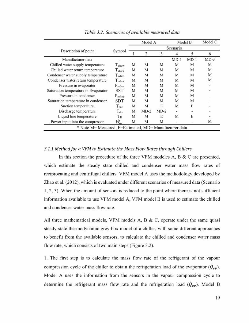
Table 3.2: Scenarios of available measured data

Model A Model B Model C

Description of point Symbol Scenario

1 2 3 4 5 6 Manufacturer data - - - - MD-1 MD-1 MD-3

Chilled water supply temperature Tchwr M M M M M M Chilled water return temperature Tchws M M M M M M

Condenser water supply temperature Tcdwr M M M M M M Condenser water return temperature Tcdws M M M M M M

Pressure in evaporator Pref,ev M M M M M - Saturation temperature in Evaporator SST M M M M M -

Pressure in condenser Pref,cd M M M M M - Saturation temperature in condenser SDT M M M M M -

Suction temperature Tsuc M M E M E - Discharge temperature Tdis M MD-2 MD-2 - - - Liquid line temperature Tll M M E M E -

Power input into the compressor M M M - - M

* Note M= Measured, E=Estimated, MD= Manufacturer data

3.1.1 Method for a VFM to Estimate the Mass Flow Rates through Chillers In this section the procedure of the three VFM modeles A, B & C are presented,

which estimate the steady state chilled and condenser water mass flow rates of

reciprocating and centrifugal chillers. VFM model A uses the methodology developed by

Zhao et al. (2012), which is evaluated under different scenarios of measured data (Scenario

1, 2, 3). When the amount of sensors is reduced to the point where there is not sufficient

information available to use VFM model A, VFM model B is used to estimate the chilled

and condenser water mass flow rate.

All three mathematical models, VFM models A, B & C, operate under the same quasi

steady-state thermodynamic grey-box model of a chiller, with some different approaches

to benefit from the available sensors, to calculate the chilled and condenser water mass

flow rate, which consists of two main steps (Figure 3.2).

1. The first step is to calculate the mass flow rate of the refrigerant of the vapour

compression cycle of the chiller to obtain the refrigeration load of the evaporator ( ).

Model A uses the information from the sensors in the vapour compression cycle to

determine the refrigerant mass flow rate and the refrigeration load ( ). Model B

20

determines the refrigerant mass flow rate from by using the compressor identification

parameters obtained from the primary HVAC Toolkit (Bourdouxhe et al. 1994) to obtain

the refrigeration load of the evaporator. Model C determines the refrigerant effect of the

evaporator ( _ ) from measuring the power input to the compressor ( ) and

interpolating through manufacturer data.

2. The second step is to calculate the chilled and condenser water mass flow rate using the

refrigerant mass flow rate and the water temperature measurements from the chilled and

condenser water fluid loops with a thermodynamic energy balance on the evaporator and

condenser.

Chilled Water Mass Flow Rate Eqn → 3.3

Model AScenarios 1,2 and 3

Model BScenarios 4 and 5

Centrifugal Refrigerant Mass

Flow Rate Eqn → 3.8

Reciprocating Refrigerant Mass

Flow Rate Eqn → 3.7

Refrigerant Mass Flow RateEqn → 3.1

Condenser Water Mass Flow Rate

Eqn → 3.4


Eqn → 3.15

Model CScenarios 6

Refrigeration Capacity Interpolation

Chilled Water Mass Flow Rate

Eqn → 3.16


Eqn → 3.17

Chilled Water Mass Flow Rate Eqn → 3.3

Figure 3.2: Flowchart of VFM models A, B and C

VFM model A

Model A is based on the work by Zhao et al. (2012) that estimate the chilled and

condenser water mass flow rate of a vapour compression chiller using a block

thermodynamic analysis of a chiller that comprises of a compressor, a condenser loop, an

expansion device and an evaporator loop (Figure 3.1). VFM model A uses the

21

measurements of the actual power input to the compressor ( ) to evaluate the refrigerant

mass flow rate in Equation 3.1 instead of the theoretical power input to the compressor

(Wth) (Zhao et al. 2012). Table 3.1 provides the description of each measurement point.

The method uses two steps to calculate the chilled and condenser water mass flow rates.

Step 1 calculates the refrigerant mass flow rate of the vapour compression cycle by using

the energy balance on the compressor assuming an adiabatic compression where no heat is

lost to the exterior, represented by Equation 3.1.

m = Wh − h Equation 3.1

where hsuc is the suction enthalpy which is calculated using the pressure in the evaporator

(Pref,ev) and the suction temperature (Tsuc), hdis is the discharge enthalpy which is calculated

from the condenser pressure (Pref,cd) and the discharge temperature (Tdis), and is the

actual compressor power input.

Step 2 calculates the chilled and condenser mass flow rates by applying an energy balance

on the evaporator and condenser, respectively, and using the measurements for the water

temperatures (Equation 3.3 and 3.3).

= mr(hsuc − hll) Equation 3.2

m = C (T − T ) = m (h − h )C (T − T ) Equation 3.3

m = C (T − T ) = m (h − h )C (T − T ) Equation 3.4

where is the refrigeration load of the evaporator, is the refrigeration load on the

condenser, hll is the liquid line enthalpy which is calculated from the pressure in the

condenser (Pref,cd) and the liquid line temperature (Tll). Tchws, Tchwr, Tcdws, Tcdwr are the

supply and return chilled water temperatures and the supply and return condenser water

temperatures.

22

VFM model A can be used for scenarios 1, 2 and 3, based on available data. When the

number of sensors is reduced to the point where there is not sufficient information to use

VFM model A, the VFM model B is used. The key difference between the models is the

discharge temperature. In the absence of a physical sensor or manufacturer data to

determine the discharge temperature, VFM model B is used to estimate the chilled and

condenser water flow rates. Figure 3.3 show the inputs and outputs of VFM model A.

Dataset file(Trend data)

Scenario 4 or 5

Selection of refrigerant

Manufacturer dataMD-2

Refrigerant, chilled and condenser

water mass flow rates:

mr ,mchw ,mcdw

INPU

TS

OUT

PUTS

Figure 3.3: Informational flow diagram of VFM model A

VFM model B

Model B proposes a new model to estimate the chilled and condenser water mass

flow rates using a minimum amount of available sensors. VFM model B first calculates the

steady-state compressor identification parameters using subroutines from the Primary

HVAC Toolkit (Bourdouxhe et al. 1994) that have been modified and re-written into

Matlab language for the development of the VFM Tool. Currently model B is designed for

23

reciprocating and centrifugal chillers, the inputs and outputs for VFM model B are shown

in Figure 3.4.

Dataset file(Trend data)

Scenario 4 or 5

Selection of refrigerant

Selection of compressor:

reciprocating or centrifugal

Manufacturer dataMD-1

Refrigerant, chilled and condenser

water mass flow rates:

mr ,mchw ,mcdw

INPU

TS

OU

TPU

TS

Figure 3.4: Informational flow diagram of VFM model B

3.1.1.2.1 Identification of compressor parameters For the reciprocating compressors, the subroutine PISCOMP1, from the primary

HVAC Toolkit (Bourdouxhe et al. 1994), was modified and written into Matlab language

to identify the following parameters: the isentropic compression power input ( ), the

electromechanical losses ( ), the loss factor (α), the clearance factor of the compressor

(Cf), and the geometric displacement of the compressor (Vs). Figure 3.5 outlines the inputs

and outputs for the subroutine PISCOMP1. The required inputs from the manufacturer data

are the SST in the evaporator and SDT in the condenser, the refrigeration load ( ), the

power input into the compressor ( ), the degree of super heating (ΔTsupheat) and sub-

cooling (ΔTsubcool).

To be able to identify the compressor parameters for a reciprocating chiller, a data file is

created comprising of six parameters. The six inputs are the refrigerant SST in the

24

evaporator, the refrigerant SDT in the condenser, the refrigerating capacity ( ), the

power input to the compressor ( ), the degree of superheating (∆Tsupheat), and the degree

of sub-cooling (∆Tsubcool). Because the subroutine uses an iterative process, the data set

needs to contain data over a large range of evaporating (SST) and condensing temperatures

(SDT). This information should be provided from the manufacturer specifications and

design information, if no short-term measurements are available from the system. The

average thermodynamic transport properties (r = gas constant, ζ = compressibility factor,

γ = mean isentropic coefficient) are obtained from a database developed using REFPROP

(Lemmon et al. 2013), which is explained in detail in section 3.1.3.

Manufacturer data:SST, SDT, Qev, Wac ∆Tsupheat, ∆TSubcool

Thermodynamic properties of refrigerant:

r, ζ, γ

Compressor Identification parameter:

Ws , Wlo, α, Cf , Vs

INPU

TS

OU

TPU

TS

Figure 3.5: Informational flow diagram of subroutine PISCOMP1 (adapted from Bourdouxhe et al. 1994)

The centrifugal compressor subroutine CENTCHID, from the primary HVAC Toolkit

(Bourdouxhe et al. 1994) was modified and written into Matlab language to identify the

following parameters: the electromechanical losses (Wlo), the loss factor (α), the impeller

exhaust area (A), the peripheral speed of the impeller (U), and the angle between the

direction of the vanes at the impeller exhaust and the plane tangent to the impeller

circumference (β). Figure 3.6 outlines the inputs and outputs for the subroutine

CENTCHID.

25

The original subroutine CENTCHID requires six inputs. They are the refrigeration load

( ), the power input to the compressor ( ), the mass flow rates of the evaporator (m )

and condenser (m ), and the supply or return temperature of the chilled water (Tchw) and

condenser (Tcdw) for one of four choices (Table 3.3) at full load capacity of the system. The

chilled and condenser water mass flow rate and the water temperatures are used in the

subroutine to calculate the pressure in the evaporator and condenser, respectively.

Table 3.3: Description of four input options for subroutine CENTHID

Choice Description Symbol 1 Chilled water and condenser water return temperatures Tchwr, Tcdwr

2 Chilled water supply and condenser water return temperatures Tchws, Tcdwr 3 Chilled water return and condenser water supply temperatures Tchwr, Tcdws 4 Chilled water and condenser water supply temperatures Tchws, Tcdws

Manufacturer data:Tchw, Tcdw,Qev, W,

mchw, mcdw


r, ζ, γ

Choice1-4


Wlo, α , U, A, βINPU

TS

OUT

PUTS

Figure 3.6: Informational flow diagram of CENTHID (adapted from Bourdouxhe et al. 1994)

For the case when manufacturer data contains information for the pressure in the evaporator

and condenser. The subroutine CENTHID was modified to remove the inputs for the

chilled and condenser water mass flow rates and the chilled and condenser water

temperatures with the appropriate choice. The inputs for the modified subroutine

CENTHID are the refrigeration load ( ), the power input to the compressor ( ), the

evaporator pressure (Pref,evap) and the condenser pressure (Pref,cd) at full load conditions as

shown in Figure 3.7.

26

Manufacturer data:Pref,evap, Pref,cd,Qev, W


r, ζ, γ


Wlo, α , U, A, βINPU

TS

OUT

PUTS

Figure 3.7: Information flow diagram of modified CENTHID 3.1.1.2.2 Refrigerant mass flow rates for reciprocating and centrifugal chillers After the compressor parameters have been identified, they can be used to calculate

the refrigerant mass flow rate for the given compressor type. Figure 3.8 highlights the

inputs and outputs of the function REFFLOWRATE that calculates of the refrigerant mass

flow rate.

Trend Data:Pref,evap, Pref,cd, Tsuc


r, ζ, γ

Refrigerant mass flow rate:

mrINPU

TS

OUT

PUTS

Compressor identification parameters:Reciprocating Centrifugal

Cf , Vs U,A,β

Figure 3.8: Information flow diagram of REFFLOWRATE

27

The compressor identification parameters are used to calculate the refrigerant mass flow

rate at full-load using the methods from the HVAC Toolkit (Bourdouxhe et al. 1994) for

reciprocating and centrifugal compressors.

For reciprocating compressors, the clearance factor of the compressor (Cf), and the

geometric displacement of the compressor (Vs) are used in Equation 3.5, Equation 3.6 and

Equation 3.7 to calculate the refrigerant mass flow rate.

ε = 1 + C + C P ,P , Equation 3.5

v = ζrTP , Equation 3.6

m = NN ε v Equation 3.7

where Nc is number of cylinders in operation, Ncfl is the number of cylinders at full-load,

εvol the volumetric effectiveness of the compressor determined by Equation 3.5, and υ1’ is

the specific volume after superheating before the compressor shown in Equation 3.6.

For centrifugal chillers, the impeller exhaust area (A), the peripheral speed of the impeller

(U), and the angle between the direction of the vanes at the impeller exhaust and the plane

tangent to the impeller circumference (β) are used to calculate the refrigerant mass flow

rate for a centrifugal compressor at full-load conditions. Equation 3.8 is used to calculate

the refrigerant mass flow rate for a single stage centrifugal compressor. The refrigerant

volume flow rate at the impeller exhaust ( ) can be determined with Equation 3.9 and for

impeller pressure ratio (πi) with Equation 3.10.

m = Vv π Equation 3.8

V = AU tan (β) γγ − 1 ζrT P ,P , − 1 − U Equation 3.9

28

π = 1 + γ − 12γ 1ζrT U − VA sin β Equation 3.10

The compressor identification parameters allow the model to estimate the refrigerant mass

flow rate in the chiller when the chiller operates at full-load conditions and hence the

chilled water flow rate at full-load conditions. To be able to account for part load conditions

the capacity control can be modelled by different approaches.

Approach 1 is to modify the full-load refrigerant mass flow rate by the part load ratio (PLR)

determined from manufacturer data (Equation 3.11). The PLR is determined as the ratio of

the instantaneous refrigeration load and the refrigeration load at full load ( _ ).

The PLR can be obtained by using manufacturer data or short-term measured data to

develop a relationship between the PLR and the power input to the compressor. This allows

the PLR to be determined from the power input to the compressor and then used in Equation

3.11 to modify the refrigerant mass flow rate.

= ∗ _ Equation 3.11

Approach 2 models the refrigerant mass flow rate through a throttling process caused by

the inlet guide vanes of the chiller, where the chilled water temperature difference between

the return and the minimum temperature (Tmin) decreases. The minimum temperature is

defined by the average refrigerant saturation temperature in the evaporator (SST). The

throttling process causes a reduction in the flow rate by increasing the specific volume and

also the pressure ratio of the impeller by decreasing the evaporating pressure. A simple

linear model can be used to model the throttle process defined by Equation 3.12, where the

coefficients a and b can be determined from using short-term measurements for the return

chilled water temperature over a week of normal operation (Browne & Bansal, 1998). The

throttling coefficient is then used to determine the evaporating pressure (P*ref,evap), which

is the evaporating pressure after the throttle process before the refrigerant enters the

compressor. This change in the evaporating pressure causes a change in the pressure ratio

of the condenser and in the specific volume of the refrigerant that are then determined by

29

Equation 3.13 and Equation 3.14, which are then used in Equation 3.8 to determine the

refrigerant mass flow rate.

∅ = + ( − ) Equation 3.12

= ,,∗ = ,∅ , Equation 3.13

v = ζrT∅P , Equation 3.14

3.1.1.2.3 Chilled and condenser water mass flow rates The refrigerant mass flow rate is estimated by using Equation 3.7 (reciprocating)

and Equation 3.8 (centrifugal). The refrigerant mass flow rate is used to determine the

chilled water mass flow rate by Equation 3.3 and the condenser water mass flow rate by

Equation 3.15. VFM model A and B use the same equation to determine the chilled water

mass flow rate but VFM model B requires an alternative method to determine the

condenser water mass flow rate in the absence of the discharge temperature.

m = C (T − T ) = m (h − h ) +C (T − T ) Equation 3.15

VFM model C

VFM model C uses the minimum amount (five) of sensors to determine the chilled

and condenser water mass flow rates. The model uses the measured power input to the

compressor with manufacturer data to determine the refrigeration load by interpolating the

power input to the compressor at the supply chilled water temperature and the return

condenser water temperatures. The manufacturer refrigeration load (Qev_MD) is used in

Equation 3.16 and Equation 3.17 to calculate the chilled and condenser water mass flow

rates. Model C is a common technique used by engineers to estimate the chilled and

condenser water mass flow rates. This model requires that the manufacturer data be at the

same supply chilled water set point temperature and return condenser water set point

temperature to provide accurate results.

30

m = _C (T − T ) Equation 3.16

m = _ +C (T − T ) Equation 3.17

3.1.2 Description of Scenarios and Available Trend Data The main challenge in existing buildings is the availability of sensors and the

information regarding the HVAC system. Six different scenarios of measured data are

presented in this section to represent the best to worst case of available inputs for existing

buildings in operation. Scenarios 1, 2 and 3 are used to evaluate model A, while scenarios

4 and 5 are used to evaluate model B and scenario 6 is used in model C. The required data

is shown in Table 3.2.

Scenario 1 Scenario 1 uses a complete data set with ten measured inputs shown in Table 3.4.

Scenario uses the equations in model A and can be evaluated directly from the obtained

measurements.

Table 3.4: Data set for scenario # 1 used in VFM model A

Description of point Symbol Scenario # 1 Manufacturer Data - -

Chilled water supply and return temperatures Tchwr, Tchws M Condenser water supply and return temperatures Tcdwr, Tcdws M

Pressure or Temperature in evaporator SST, Pref,ev M Pressure or Temperature in condenser SDT, Pref,cd M

Suction Temperature Tsuc M Discharge Temperature Tdis M Liquid line Temperature Tll M

Power input into the compressor M

Scenario 2

Scenario 2 uses nine measured inputs as shown in Table 3.5, where the discharge temperature (Tdis) is then estimated from manufacturer data.

31





Suction Temperature Tsuc M Discharge Temperature Tdis MD-2 Liquid line Temperature Tll M


The discharge temperature is an important input into model A because it is used to calculate

the refrigerant mass flow rate and is difficult to estimate without manufacturer data. Since

in most existing buildings the discharge temperature is not always measured, manufacturer

data is needed to evaluate the discharge temperature.

The discharge temperature can be estimated by either knowing the isentropic efficiency (η)

of the compressor and the adiabatic compression exponent (k), or directly knowing the

polytropic compression exponent (n) for the refrigerant along with the pressure ratio

between the evaporator and the condenser. Carrier Corporation (1981, 2001) has compiled

data from experiments for both reciprocating and centrifugal compressor to determine these

values. For reciprocating compressors the polytropic compression exponent can be

determined for pressure ratios from 2 to 12, and for refrigerants R-12, R-22 and R-502. For

centrifugal compressors values for the adiabatic compression exponent (k) and polytropic

compression exponent were tabulated for R-11, R-12, R-22, R-114 and R-500. The

polytropic compression exponent was determined by an isentropic efficiency of the

compressor of 75%. If the isentropic efficiency of the compressor is known, it should be

used with the adiabatic compression exponent (k) in Equation 3.18 to calculate the new

polytropic compression exponent (Carrier Corporation, 1981). The discharge temperature

is calculated by Equation 3.19.

nn − 1 = kk − 1 η Equation 3.18

32

T = (T + 273.15) P ,P , − 273.15 Equation 3.19

The method above can be useful to estimate this key parameter, which is used in this model

but is limited to the amount of data available. If it is not possible to provide an estimate for

the discharge temperature, VFM model A cannot be used to estimate the chilled and

condenser water mass flow rates, then VFM model B will be used with scenario 4 or 5.

Scenario 3

Scenario 3 uses seven measured inputs and three inputs that are required to be

estimated as shown in Table 3.6. This represents a common scenario for information

available to a building operator from a BAS system. The estimated inputs are the suction

temperature (Tsuc), discharge temperature (Tdis), and the liquid line temperature (Tll).





Suction Temperature Tsuc E Discharge Temperature Tdis MD-2 Liquid line Temperature Tll E


The discharge temperature can be estimated by the methods presented in scenario 2. To

estimate the suction temperature (Tsuc) a temperature sensor can be placed on the suction

line of the chiller (inlet to compressor) to measure the mean temperature at that location

for a certain period. Then the amount of superheating (∆Tsup-heat) can be determined by

Equation 3.20

∆ = − Equation 3.20

To estimate the liquid line temperature (Tll) a temperature sensor can be placed of the exit

of the condenser line to measure the mean temperature at that location for a certain period.

Then the amount of sub-cooling (∆Tsubcool) can be determined by Equation 3.21.

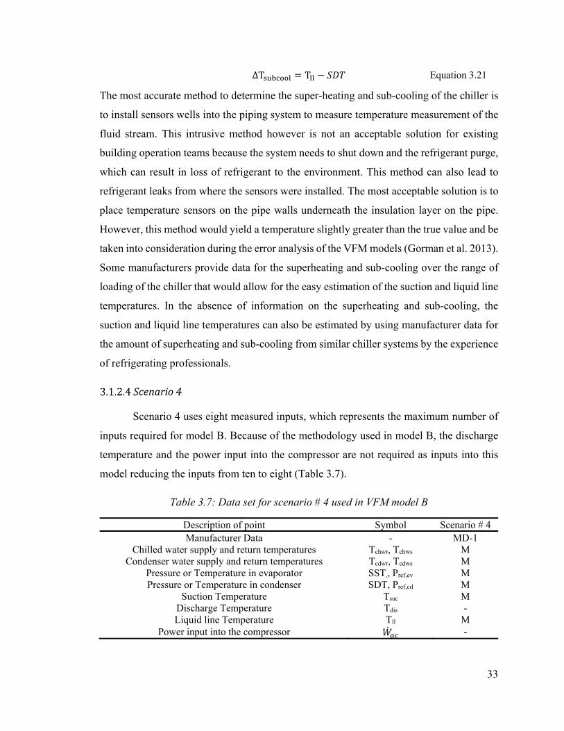
33

∆T = T − Equation 3.21

The most accurate method to determine the super-heating and sub-cooling of the chiller is

to install sensors wells into the piping system to measure temperature measurement of the

fluid stream. This intrusive method however is not an acceptable solution for existing

building operation teams because the system needs to shut down and the refrigerant purge,

which can result in loss of refrigerant to the environment. This method can also lead to

refrigerant leaks from where the sensors were installed. The most acceptable solution is to

place temperature sensors on the pipe walls underneath the insulation layer on the pipe.

However, this method would yield a temperature slightly greater than the true value and be

taken into consideration during the error analysis of the VFM models (Gorman et al. 2013).

Some manufacturers provide data for the superheating and sub-cooling over the range of

loading of the chiller that would allow for the easy estimation of the suction and liquid line

temperatures. In the absence of information on the superheating and sub-cooling, the

suction and liquid line temperatures can also be estimated by using manufacturer data for

the amount of superheating and sub-cooling from similar chiller systems by the experience

of refrigerating professionals.

Scenario 4

Scenario 4 uses eight measured inputs, which represents the maximum number of

inputs required for model B. Because of the methodology used in model B, the discharge

temperature and the power input into the compressor are not required as inputs into this

model reducing the inputs from ten to eight (Table 3.7).

Table 3.7: Data set for scenario # 4 used in VFM model B

Description of point Symbol Scenario # 4 Manufacturer Data - MD-1


Pressure or Temperature in evaporator SST,, Pref,ev M Pressure or Temperature in condenser SDT, Pref,cd M

Suction Temperature Tsuc M Discharge Temperature Tdis - Liquid line Temperature Tll M

Power input into the compressor -

34

Scenario 5

Scenario 5 uses six measured inputs, with two inputs that are estimated as shown

in Table 3.8.

Table 3.8: Data set for scenario # 5 used in VFM model B



Pressure or Temperature in evaporator SST,, Pref,ev M Pressure or Temperature in condenser SDT, Pref,cd M

Suction Temperature Tsuc E Discharge Temperature Tdis - Liquid line Temperature Tll E

Power input into the compressor -

Scenario 6

Scenario 6 uses the minimum amount of sensors (five) (Table 3.9) with

manufacturer data to provide the chilled and condenser water mass flow rates. To be able

to use VFM model C the manufacture data (MD-3) should be at the same (or close) chilled

water supply temperature and return condenser water temperature set-points to be able to

provide accurate results.

Table 3.9: Data set for scenario # 6 used in VFM model C



Pressure or Temperature in evaporator SST, Pref,ev - Pressure or Temperature in condenser SDT, Pref,cd -

Suction Temperature Tsuc - Discharge Temperature Tdis - Liquid line Temperature Tll -


3.1.3 Refrigerant Transport Properties Using REFPROP The refrigerant transport properties (enthalpy, specific heat, compressibility, etc)

for the case studies in this thesis were determined using the subroutines from REFPROP

35

(Lemmon et al. 2013). REFPROP is a computer program developed by the National

Institute of Standard and Technology (NIST). The computer program is used to determine

the fluid thermodynamic and transport properties of pure fluid and mixtures. The

REFPROP software uses published models to calculate the fluid thermodynamic and

transport properties.

The property models are coded in Fortran language and can be accessed by other softwares

via a dynamic linked library (DLL). Lemmon et al. (2013) developed DLL’s for multiple

platforms such as Excel and Matlab to link the library of subroutines for the

thermodynamic property models that were programmed in Fortran. The DLL for Matlab

was used in this thesis to be able to calculate the mean thermodynamic properties, the gas

constant (r), the mean compressibility (ζ), and the mean isentropic coefficient (γ), for each

refrigerant used in this thesis. The suction, discharge and liquid line enthalpies were

determined at each time step using the REFPROP and the DLL with MATLAB.

The HVAC Toolkit operates under the assumption that the refrigerant behaves as an ideal

gas over the normal operation conditions within the refrigeration cycle. This allows for the

use of mean thermodynamic properties of the refrigerants for vapour and liquid regions.

The HVAC Toolkit provides these mean thermodynamic values for a six different

refrigerants: R-12, R-134a, R-114, R-22, R-502, and R-717. The HVAC Toolkit does not

include the thermodynamic properties for some other common refrigerants used currently

in chillers like R-123 and R-410a.

A subroutine was developed called PROPERTYNIST that uses the methods from the

HVAC Toolkit to calculate the mean thermodynamic properties using REFPROP

(Lemmon et al. 2013) to develop a thermodynamic property database for the common

refrigerants not included within the HVAC Toolkit. The subroutine PROPERTYNIST can

calculate the mean thermodynamic properties for any refrigerant included in REFPROP

software (Lemmon et al. 2013). The gas constant (r), the mean compressibility (ζ), and the

mean isentropic coefficient (γ) were calculated using PROPERTYNIST to compare with

the HVAC Toolkit (Table 3.10).

36

Table 3.10: Comparison of mean thermodynamic properties

Refrigerant HVAC Toolkit Bourdouxhe et al. (1994) PROPERTYNIST

r ζ γ r ζ γ R-12 68.75 0.940 1.086 68.76 0.946 1.109

R-134a 81.49 0.941 1.072 81.49 0.945 1.087 R-114 48.64 0.976 1.056 48.65 0.969 1.069 R-22 96.14 0.930 1.114 96.16 0.937 1.134 R-717 488.22 0.957 1.230 488.21 0.952 1.230 R-123 - - - 54.37 0.987 1.080 R-410a - - - 114.54 0.908 1.066

Comparing the results from PROPERTYNIST to the values in the HVAC Toolkit the

highest percent difference is 2.1% for the value of the mean isentropic coefficient (γ). The

new subroutine is accurate below 2.1% as compared to the refrigerants used in the HVAC

Toolkit and can be used to determine the thermodynamic transport properties of other

refrigerants.

It is important to understand the uncertainties associated with calculation of the

thermodynamic properties for a refrigerant. The uncertainties in these thermodynamic and

transport property models can vary considerably depending on the fluid type, the property,

and the thermodynamic state. The uncertainties of the transport properties are complicated

functions of the temperature and pressure and the estimation of uncertainty from

propagation of errors from the inputs to the outputs is not possible and is beyond the scope

of this thesis. A global uncertainty for each of the thermodynamic properties is used in this

thesis (Table 3.11 and Table 3.12). To be able to understand the uncertainty for each

property it has to be determined for each fluid and each property separately due to the

uncertainties generated from each thermodynamic transport property model.

Uncertainty of Refrigerant Properties

For the three case studies that are examined in this thesis two different refrigerants

are used. To be able to understand the uncertainties regarding the calculation of the

refrigerant properties each model used by REFPROP (Lemmon et al. 2013) needs to be

examined. The uncertainty for the density (ρ), specific heat (Cp) and the vapour pressure

(Pvap) are given by REFPROP (Lemmon et al. 2013).

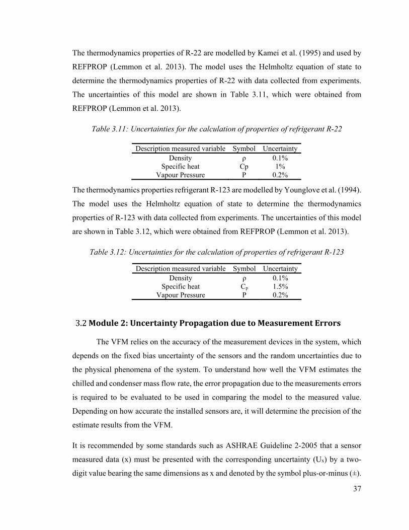
37

The thermodynamics properties of R-22 are modelled by Kamei et al. (1995) and used by

REFPROP (Lemmon et al. 2013). The model uses the Helmholtz equation of state to

determine the thermodynamics properties of R-22 with data collected from experiments.

The uncertainties of this model are shown in Table 3.11, which were obtained from

REFPROP (Lemmon et al. 2013).

Table 3.11: Uncertainties for the calculation of properties of refrigerant R-22

The thermodynamics properties refrigerant R-123 are modelled by Younglove et al. (1994).

The model uses the Helmholtz equation of state to determine the thermodynamics

properties of R-123 with data collected from experiments. The uncertainties of this model

are shown in Table 3.12, which were obtained from REFPROP (Lemmon et al. 2013).

Table 3.12: Uncertainties for the calculation of properties of refrigerant R-123

Description measured variable Symbol Uncertainty Density ρ 0.1%

Specific heat Cp 1.5% Vapour Pressure P 0.2%

Module 2: Uncertainty Propagation due to Measurement Errors

The VFM relies on the accuracy of the measurement devices in the system, which

depends on the fixed bias uncertainty of the sensors and the random uncertainties due to

the physical phenomena of the system. To understand how well the VFM estimates the

chilled and condenser mass flow rate, the error propagation due to the measurements errors

is required to be evaluated to be used in comparing the model to the measured value.

Depending on how accurate the installed sensors are, it will determine the precision of the

estimate results from the VFM.

It is recommended by some standards such as ASHRAE Guideline 2-2005 that a sensor

measured data (x) must be presented with the corresponding uncertainty (Ux) by a two-

digit value bearing the same dimensions as x and denoted by the symbol plus-or-minus (±).

Description measured variable Symbol Uncertainty Density ρ 0.1%

Specific heat Cp 1% Vapour Pressure P 0.2%

38

Unless stated otherwise, the symbol ± in this thesis refers to the uncertainty propagation of

errors due to measurements.

The uncertainties from the measuring equipment will propagate through the calculations

used in the VFM models to produce a final overall uncertainty of the predictions. The

uncertainty of the VFM models is evaluated to understand the limitations of the model and

to evaluate how well the model compares to measured data for the chilled and condenser

water mass flow rates. Models A, B and C will have different uncertainties, as well as each

scenario will have a different uncertainty because of the number of sensors used in each

model/scenario are different. Therefore, a general uncertainty analysis is presented in this

section. The case studies will highlight how this general analysis is used for each model

and scenario.

3.2.1 General uncertainty propagation from measurements The uncertainty of each sensor is calculated using Equation 3.22 (Reddy 2011).

U = B + (Ru ) Equation 3.22

where Bz is the fixed measurement bias error given by the manufacturer and Ruz are the

random errors due to the unpredictable and unknown variations in the trend data that causes

readings to take random values on either side of some mean value. The random errors for

a large number of measurements (N>30) is defined by Equation 3.23.

Ru = zs√N Equation 3.23

where Sz is the standard deviation of the input, N is the number of points used in the sample

and z=1.96 is the multiplier at 95% confidence level for large data sets. Given that the

variable X is a function of variables Z1,...Zn (Equation 3.24), and the precision errors in all

the variables (Z1- Zn) are normal distributed, a first order Taylor series of expansion can be

applied to Equation 3.24. Normalizing first order Taylor series of expansion the by variable

(X), which is the variable under investigation for the uncertainty, you obtain Equation 3.25.

Equation 3.22 determines the individual uncertainties Uz1,...Uzn used in Equation 3.25 to

determine the error propagation of the variable under investigation.

X = X(Z , Z , Z , … . , Z ) Equation 3.24

39

UX = ∂X∂Z × UX + ∂X∂Z × UX +. . . + ∂X∂Z × UX/

Equation 3.25

Uncertainty propagation of VFM model A

To evaluate the uncertainty propagation due to measurements of the chilled and

condenser water mass flow, the uncertainty of the refrigerant mass flow rate needs to be

evaluated first. Equation 3.1 is used by VFM model A to calculate the refrigerant mass

flow rate. Applying Equation 3.25 to Equation 3.1 for the overall uncertainty propagation,

results in Equation 3.26.

Um = ∂m∂Wm × U + ∂m∂hm × U + ∂m∂hm × U/

Equation 3.26

where the partial derivatives are evaluated as = ( ) , = ( ) , ( ) , which when substituted into Equation 3.26 yields Equation 3.27.

Um = U + U(h − h ) + −U(h − h ) Equation 3.27

The enthalpies are determined from temperature and pressure measurements using the

REFPROP (Lemmon et al. 2013). Because it is difficult to determine the uncertainty

propagation of the values of the enthalpies (Uh) from the subroutines in REFPROP, the

uncertainty of the enthalpy is defined as the addition of the uncertainty of the temperature

and pressure used to defined the state at which the enthalpy is calculated (Equation 3.28).

U = U + U = B + (Ru ) + B + (Ru ) Equation 3.28

where BT is the bias uncertainty of the temperature sensor, RuT is the random error from

the temperature sensor, Bp is the bias uncertainty of the pressure sensor and Rup is the

random error from the pressure sensor.

40

Equation 3.3 is used by VFM model A to evaluate the chilled water mass flow rate. The

uncertainty propagation can then be defined by Equation 3.29.

Um = ∂m∂Cm × U + ∂m∂mm × U + ∂m∂hm × U + ∂m∂hm × U + ∂m∂Tm × U+ ∂m∂Tm × U

/

Equation 3.29

where the partial derivatives are evaluated as = ( )( ), = ( )( ), = ( ), = ( ), = ( )( ) , = ( )( )

which when substituted into Equation 3.29 which yields to Equation 3.30.

= − + + (ℎ − ℎ ) + −(ℎ − ℎ )+ ( − ) + −( − )

Equation 3.30

VFM model A uses Equation 3.4 to estimate the condenser water mass flow rate. The

uncertainty associated with this equation is shown in Equation 3.31.

Um = −UC + −U(h − h ) + U(h − h )+ −U(T − T ) + U(T − T )

Equation 3.31

The virtual COP is determined from Equation 3.32 where it can be determined with

measurements from the refrigerant side or the chilled water side.

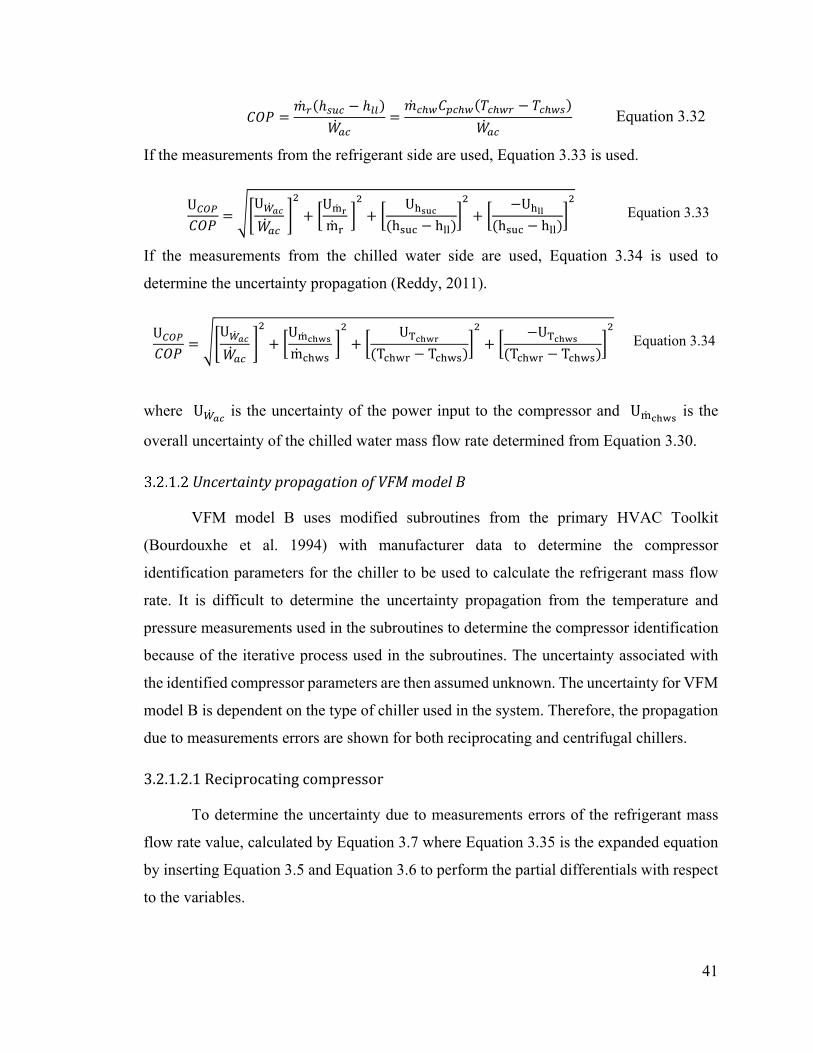
41

= (ℎ − ℎ ) = ( − ) Equation 3.32

If the measurements from the refrigerant side are used, Equation 3.33 is used.

U = U + Um + U(h − h ) + −U(h − h ) Equation 3.33

If the measurements from the chilled water side are used, Equation 3.34 is used to

determine the uncertainty propagation (Reddy, 2011).

U = U + Um + U(T − T ) + −U(T − T ) Equation 3.34

where U is the uncertainty of the power input to the compressor and U is the

overall uncertainty of the chilled water mass flow rate determined from Equation 3.30.

Uncertainty propagation of VFM model B

VFM model B uses modified subroutines from the primary HVAC Toolkit

(Bourdouxhe et al. 1994) with manufacturer data to determine the compressor

identification parameters for the chiller to be used to calculate the refrigerant mass flow

rate. It is difficult to determine the uncertainty propagation from the temperature and

pressure measurements used in the subroutines to determine the compressor identification

because of the iterative process used in the subroutines. The uncertainty associated with

the identified compressor parameters are then assumed unknown. The uncertainty for VFM

model B is dependent on the type of chiller used in the system. Therefore, the propagation

due to measurements errors are shown for both reciprocating and centrifugal chillers. 3.2.1.2.1 Reciprocating compressor To determine the uncertainty due to measurements errors of the refrigerant mass

flow rate value, calculated by Equation 3.7 where Equation 3.35 is the expanded equation

by inserting Equation 3.5 and Equation 3.6 to perform the partial differentials with respect

to the variables.

42

= , 1 + − ,, Equation 3.35

where the partial derivatives are given by Equation 3.36 to Equation 3.38, which yields to

Equation 3.39. ∂m∂P , = 1 + − − 1 , , Equation 3.36

∂m∂P , = − 1 ,, Equation 3.37

= − , 1 + − ,, Equation 3.38

=1 + − − 1 , ,

, 1 + − ,,, +

1 ,,, 1 + − ,,

, + −1

/

Equation 3.39

3.2.1.2.2Centrifugal compressor Equation 3.40 estimates the refrigerant mass flow rate for centrifugal compressors.

The partial derivatives are difficult to evaluate and therefore the uncertainty due to the

refrigerant mass flow rate is not performed for this compressor type.

43

m = AU tan(β) γγ − 1 ζrT P ,P , − 1 − UζrTP ∗

1 + − 12 1 − ( ) − 1 , , − 1 −

Equation 3.403.2.1.2.3 Uncertainty of the chilled water mass flow rate The uncertainty due to the propagations due to measurement errors of the chilled

water mass flow rate is determined by the same equation (Equation 3.3) as for VFM model

A and therefore Equation 3.31 determines the uncertainty for the chilled water mass flow

rate for VFM model B. 3.2.1.2.4 Error propagation for the condenser water mass flow rate The condenser water mass flow rate for VFM model B is estimated by Equation

3.4. The uncertainty associated with this equation is shown in Equation 3.41.

Um = ∂m∂Cm × U + ∂m∂Wm × U + ∂m∂hm × U + ∂m∂hm × U+ ∂m∂Tm × U + ∂m∂Tm × U

/

Equation 3.41

where = ( )( ) , = ( )( ) , = ( ) , = ( ) , = ( )( ) , = ( )( ) , which when substituted into Equation 3.41 yields Equation 3.42.

Equation 3.41

44

Um = −UC + 1m (h − h ) + W U + −mm (h − h ) + W U+ mm (h − h ) + W U + U(T − T ) + −U(T − T )

Equation 3.42

The case studies will use these general uncertainty propagation equations to evaluate the

uncertainty of the generated from the measurements from the sensors used to evaluate the

chilled and condenser water mass flow rates for the VFM Model used and the

corresponding scenario.

The COP for VFM model B is determined by Equation 3.36 and Equation 3.37 as for VFM

model A.

Uncertainty propagation of VFM model C

Model C uses Equation 3.16 to determine the chilled water mass flow rate and

Equation 3.17 determines the condenser water mass flow rate. Using the same approach as

VFM model A and B, the uncertainties for the chilled and condenser water mass flow rates

are described by Equation 3.43 and Equation 3.44, respectively.

= − ( − ) + −( − ) + UQev_MDQev_MD 2 Equation 3.43

Um = −UC + −U(T − T ) + U(T − T )+ 1Q _ + W U + 1Q _ + W U _

Equation 3.44

For VFM model C, scenario 6, which uses manufacturer data of the evaporating load

(Qev_MD), Equation 3.45 is used to determine the uncertainty of the COP.

45

U = U _Q _ + −UWacWac Equation 3.45

where UQev_MD is the uncertainty from the manufacturer data if provided. The uncertainty

in most cases might not be provided and will assumed to be zero. Qev_MD is the refrigeration

load from manufacturer data, UW is the uncertainty associated with the power input and W is the instantaneous power input to the compressor.

3.2.2 Uncertainty in flow measuring equipment There are different flow measuring devices available to measure the liquid flow

rates in the buildings’ hydronic systems. The flow meters can be separated into two main

groups; 1) intrusive and 2) non-intrusive meters, where each group contains different types

of flow meters (Figure 3.9).

Intrusive flow meters measure the flow rate by directly inserting a device within the flow

stream. The flow meters can be inline meters where the meter is installed directly within

the piping. Inline meters are sized according to the pipe size and as the diameter of the

piping increases so does the cost of the meter. Inline meters provide the highest accuracy

with the smallest amount of uncertainty. Insertion meters are flow meters that can be

inserted though insertion valves located within the piping system to provide the flow

measurements. For these meters the recommend amount of straight piping free of flow

disturbances before and after the valve are required for accurate results. There are three

different types of intrusive flow meters available, each with their advantages and

disadvantages. Non-intrusive meters are ultrasonic flow meter, which are installed on the

surface of the pipe and virtual flow meters that use indirect methods to obtain the water

flow rates.

46

Figure 3.9: Map of different flow meters available

Selecting the correct flow meter for the application is very important to assure the accuracy

of the measurements. The selection of the flow meters for accurate applications depends

on: (i) the application of the flow measurements; (ii) the fluid that is being measured; (iii)

and the position in the system where the measurements conducted.

There are different reasons for measuring the flow rates in the building hydronic system

and each reason requires a different amount of accuracy. The highest accuracy is required

for metering and billing purposes. For system control and optimization of the HVAC a high

accuracy is required but not as much of the metering and billing and the accuracy required

is less for measurement & verification, commissioning and trending data (Figure 3.10).

The purpose for this thesis to measure the flow rates is for measurement & verification,

commissioning and trending data.

Intrusive

Mechancial

Vortex Mass Meters Turbine

Insertion

Inline

Non-Mechanical

Electromagnetic

Insertion

Inline

Non-Intrusive

Ultrasonic Virtual (Indirect)

47

Figure 3.10: Levels of uses for flow measurements

The chilled water loop is a closed loop system, meaning the water is not exposed to external

conditions and is relatively clean water. The chilled water can be water alone or a

brine/glycol solution. The chilled water temperatures can range from -10oC to 15oC. The

condenser water loop is an open loop and is exposed to the environment through the cooling

tower. This system can contain debris and other particles. The condenser water operates

with temperatures of 20oC to 45oC. Because the meter is exposed to dirt and other particles

from the outdoor environment turbine mass flow meter are not recommended because they

are more susceptible to failure in these conditions.

The flow meter would be required to be placed as close to the chillers as possible to

measure the flow rates to each individual chiller. Insertion meters and ultrasonic meters

require a certain amount of straight piping before and after the meter to provide stable,

accurate and repeatable results. Because of space limitations, this might not always be

possible within a given cooling plant. For the application of measuring the chilled and

condenser water, mass flow rate through the evaporator and condenser of a chiller the best

meter would be an inline electromagnetic flow meter. The cost these meter increase with

the diameter of the piping and for large cooling plants where the diameter are large close

to the chillers, these meter can be very expensive. If a minimum amount of straight piping

is available then the insertion electromagnetic flow meter will provide the best accuracy

for the cost of the meter and an ultrasonic flow meter can be used as well.

Billing

System control and Optimization

Measurement and Verification

Commissioning

Trending data

Operational use for VFM

48

Comparison an electromagnetic and an ultrasonic flow meter

Tests were performed by author of this thesis on a hydraulic test bench to compare

the measurements obtained from an intrusive electromagnetic flow meter with that of a

portable ultrasonic flow meter. The purpose of the test was to highlight how ultrasonic flow

meters can estimate water flow rates compared to an electromagnetic flow meter. The test

bench consists of a variable speed pump with an inline electromagnetic flow meter (Figure

3.11). The flow measuring equipment is detailed in Table 3.13 with the flow meters given

bias errors.

VFD

Pump VFD Speed

Pump Start/Stop

Electromagnetic Flow Meter

Ultrasonic Flow Meter

Figure 3.11: Schematic of test bench

Table 3.13: Description of measurement bias for both devices

Measurement Variable Instrument Measurement Bias

Water flow rate Portable ultrasonic flow meter ± 2% of reading Electromagnetic flow meter ± 0.5% of reading

Electromagnetic flow meters are based on Faraday’s Law, which states that the voltage

induced across any conductor as it moves at right angles through a magnetic field is

proportional to the velocity of that conductor. Figure 3.12 is a diagram of an

electromagnetic flow meter where Equation 3.46 is used to determine the fluids flow rate.

20*D10*D

Pump

49

Figure 3.12: Diagram of electromagnetic flow meter (Endress+Hauser 2006)

= Equation 3.46

(Endress+Hauser 2006)

where Ue is the induced voltage, B is the magnetic induction, L is the electrode spacing,

is the volume flow rate, and A is the pipe cross-section area. These flow meters tend to

have low sensitivity and bias errors because they are install within the fluid stream.

Ultrasonic flow meters use the principal of time of flight to determine the flow rate of the

fluid inside the pipe. Two transducers that are placed on the surface of the pipe: one

upstream and one downstream as shown in Figure 3.13. Then ultrasonic signals are sent

from the upstream transducer (S1) to the downstream transducer (S2) and back to the

upstream transducer (S2). The time required for these signals is recorded by the meter.

When no flow is present the time of the signal to pass from sensor S1 to sensor S2 should

be the same as the time as from S2 to S1. When there is a flow the signal S1 velocity is

increased by the moving flow causing the time of the signal to be reduced and the signal

S2 velocity is decreased by the moving flow, and causes the time of the signal to be

increased, which is expressed by Equation 3.47.

V = ∆

Equation 3.47 (Greyline 2013)

where K is the calibration factor that account for the volume and time units used, Δt is the

time differential between the signals S1 and S2, and TL is the zero flow transit time.

50

Figure 3.13: Schematic of ultrasonic flow meter (adapted from Greyline 2013)

Two sets of tests were performed using the portable ultrasonic flow meter. To measure

accurately the flow rate using an ultrasonic flow meter the parameters detailed in Table

3.14 are required as inputs. The parameters are determined from the specifications of the

system. The most difficult parameter can be the pipe wall thickness (t), which might not

always be readily available in design documents or by the maintenance department. This

parameter, if unknown, will have to be assumed from standard pipe sizes and can contribute

to error in the final reading of the flow rate. The remaining five parameters are easily

available and can be enter into the flow meter. The flow meter then returns a computed

separation distance, based on the input parameters, for the transducers to be spaced on the

pipe surface.

Table 3.14: Set-up parameters for the ultrasonic flow meter

Parameters Value Pipe wall material PVC

Fluid type Water Pipe outside diameter 10.16 cm (4 in) Pipe wall thickness 0.574 cm (0.226 in)

Pipe lining thickness / Type - Temperature of fluid 22oC

Computed by flow meter Separation distance 3.43 cm (1.35 in)

In the first experiment, the portable ultrasonic meter was installed using the parameters in

Table 3.14 and the rotational speed of the pump was then varied using the VSD installed

on the pump, to produce different flow rates ranging about from 3 to 23 kg/s (given by the

electromagnetic meter). The flow rates were recorded at eight different points of operation

Fluid Flow

Transducers S2 Separation distanceTransducer S1

51

to compare the flow rates measured from both flow meters. Figure 3.14 shows the results

for of this test, where at low flow rates, the difference between the two meters is low and

as the flow rate is increased, the difference between the measurements begins to increase

to 11.3% difference as shown in Figure 3.15. It was observed that at the higher fluid

velocities that the readings on the ultrasonic meter would fluctuate over large intervals and

the reading was determined from an average of the readings over 5 minutes. The increase

in fluctuations in the reading could be due to the increase in the Reynolds number inside

the pipe that causes the fluid to take more displacement distance to reach steady flow and

that the upstream disturbances caused higher fluctuations in the flow readings.

Figure 3.14: Comparison of both flow meters

52

Figure 3.15: Difference and percent difference between both flow meters

The second test was conducted to explore the effects of the separation distance and its

associated error with deviations from the recommended separation distance given by the

flow meter. The transducers were placed on the pipe surface with a varying separation

distance of 0.51-5.1 cm, where the design separation distance is 3.43 cm. Measurements

were taken of the water flow rate for nine separation distances and three different flow rates

given by the electromagnetic flow meter. For this observed case it was shown that given a

separation distance of ± 0.51 cm from the design separation distance (3.43 cm) would result

in a percent difference of less than 6% for all flow rates tested (Figure 3.16). As the

separation gap increased, the fluctuations in the readings increased as well as shown on the

display of the flow meter where the readings would have large fluctuations. For this the

flow rate was measured using the flow meter counting function, which allows the meter to

count the volume of fluid passing and this was average over a five minute period to obtain

the flow rate when the meter display produced large fluctuations in the measurement.

53

Figure 3.16: Effect of separation distance on measurements

Conclusions of comparison of water flow meters

For these performed tests, the electromagnetic meter displayed less sensitivity and

drift then the ultrasonic flow meter to changes in the water flow rate. The ultrasonic flow

meter requires a large amount of straight piping to be able to provide stable measurements

for the water flow rates that are not always present in building HVAC systems. Ultrasonic

meters are more susceptible to error because of the inputs used by the meter, namely the

pipe wall thickness that might not be known from design specifications and could cause

some error in the reading.

The measurement from the ultrasonic meter were constantly less than the electromagnetic

flow meter and became more unstable as the flow rate increased, which could be caused

by increased turbulent flow and that the upstream disturbances have a larger effect on the

flow profile and the meter might require a longer distance to reach a uniform steady flow

profile. The ultrasonic flow meter was installed after the pump and it is recommended by

manufactures to be placed before valves or pumps to minimize the flow disturbances in the

fluid stream. Manufacturers recommend a larger distance greater than 20 pipe diameters

might be required when the meter is installed after pumps or valves.

54

3.2.3 Metrics used to determine the goodness of fit for the VFM predictions

The goodness of fit is determined on an hourly time interval to determine how well

the model will be able to estimate the measured values. If the model is unable to estimate

the model well on an hourly time scale then it will not be suited for on-going

commissioning because the poor estimations will cause false faults. To determine the limits

of acceptable fits the coefficient of variance of the root mean squared error CV(RMSE)

(Equation 3.48) and the normal mean biased error (NMBE) (Equation 3.49) are used to

determine how well the VFM models estimate the chilled and condenser water mass flow

rate.

( ) = × 100 Equation 3.48

= ∑ −( − ) × × 100 Equation 3.49

where the RMSE is given in Equation 3.50, Et is the estimated value at time t, is the

measured value at time t, n is the number of data points, p is the degrees of freedom and

is the mean value of measured value.

= ∑ −( − ) Equation 3.50

No guidelines or criteria exists for a VFM or component models to determine acceptable

limits for the CV(RMSE) and NMBE that determine whether a model is acceptable or not.

ASHRAE Guideline 14 (2002) suggests that for an whole energy building model to be

calibrated, the CV(RMSE) should be less than 30% and NMBE less than 10% when

determined on an hourly time-scale over a yearly period. Mihai and Zmeureanu (2013)

investigated the use of a statistical hypothesis test method to determine the acceptance for

zone calibration in a bottom-up calibration of an energy model using eQuest in relation

with the limits of the CV(RMSE) and NMBE of the ASHRAE Guideline 14 (2002).

For the VFM model, a similar method will be used to help determine if the estimates are

acceptable or not compared to measured data. A paired difference hypothesis test is used

for two independent samples (measurements and estimates) to assess whether the

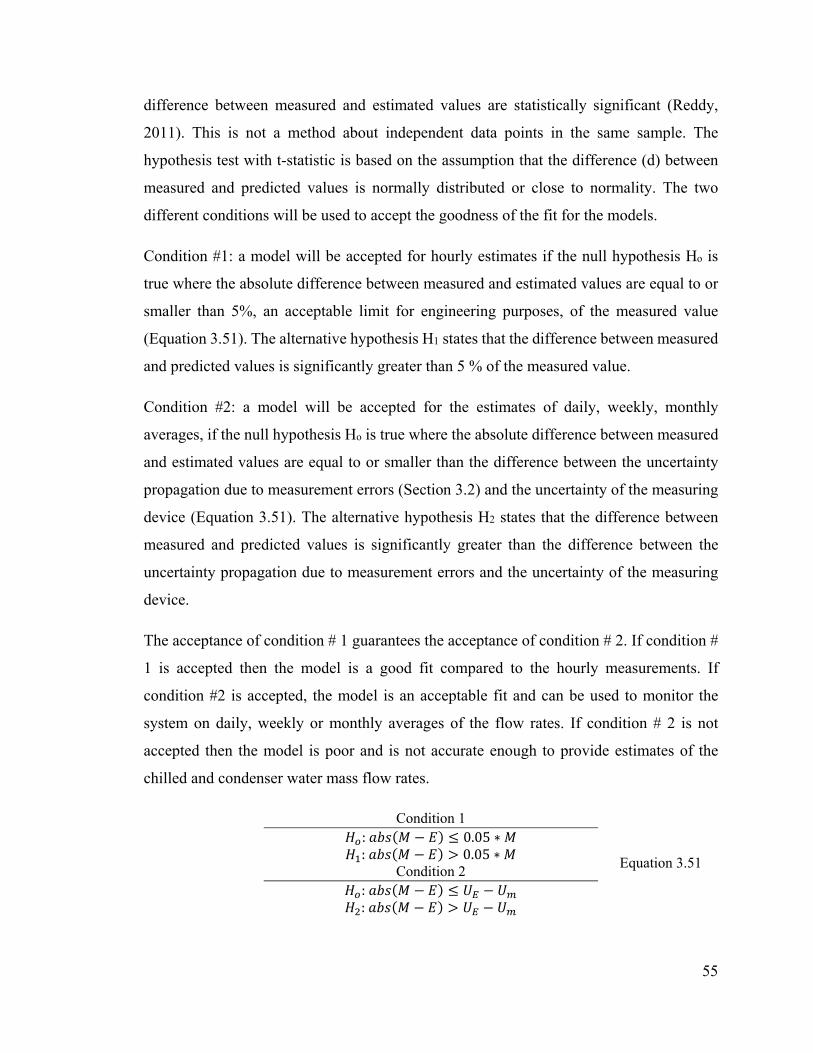
55

difference between measured and estimated values are statistically significant (Reddy,

2011). This is not a method about independent data points in the same sample. The

hypothesis test with t-statistic is based on the assumption that the difference (d) between

measured and predicted values is normally distributed or close to normality. The two

different conditions will be used to accept the goodness of the fit for the models.

Condition #1: a model will be accepted for hourly estimates if the null hypothesis Ho is

true where the absolute difference between measured and estimated values are equal to or

smaller than 5%, an acceptable limit for engineering purposes, of the measured value

(Equation 3.51). The alternative hypothesis H1 states that the difference between measured

and predicted values is significantly greater than 5 % of the measured value.

Condition #2: a model will be accepted for the estimates of daily, weekly, monthly

averages, if the null hypothesis Ho is true where the absolute difference between measured

and estimated values are equal to or smaller than the difference between the uncertainty

propagation due to measurement errors (Section 3.2) and the uncertainty of the measuring

device (Equation 3.51). The alternative hypothesis H2 states that the difference between

measured and predicted values is significantly greater than the difference between the

uncertainty propagation due to measurement errors and the uncertainty of the measuring

device.

The acceptance of condition # 1 guarantees the acceptance of condition # 2. If condition #

1 is accepted then the model is a good fit compared to the hourly measurements. If

condition #2 is accepted, the model is an acceptable fit and can be used to monitor the

system on daily, weekly or monthly averages of the flow rates. If condition # 2 is not

accepted then the model is poor and is not accurate enough to provide estimates of the

chilled and condenser water mass flow rates.

Condition 1 : ( − ) ≤ 0.05 ∗ : ( − ) > 0.05 ∗ Condition 2 : ( − ) ≤ − : ( − ) > −

Equation 3.51

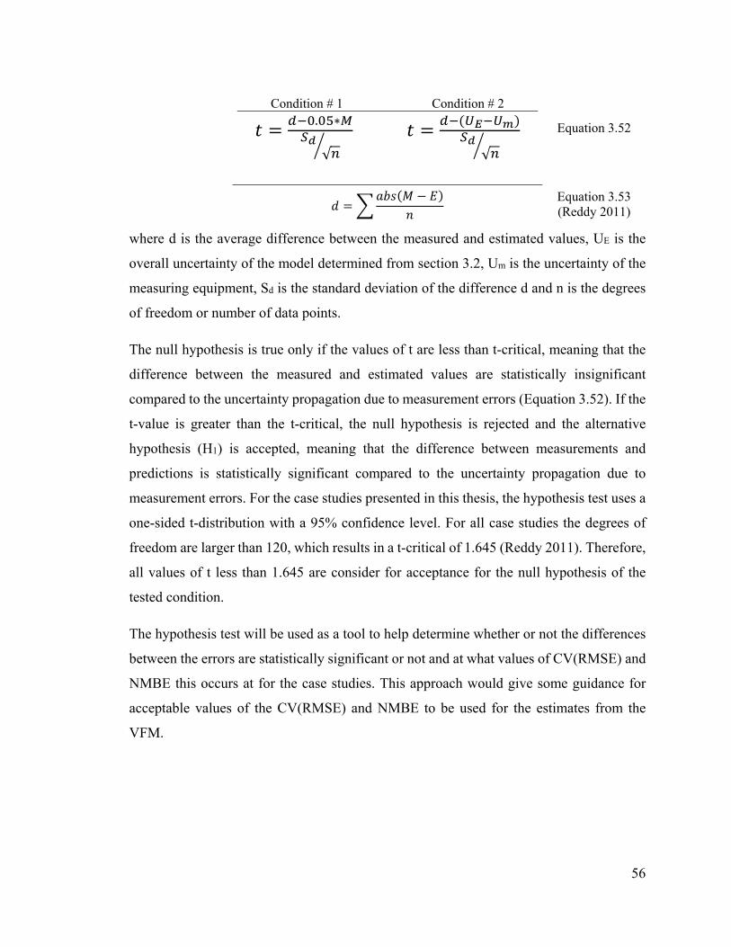
56

Condition # 1 Condition # 2 = . ∗√ = ( )√ Equation 3.52

= ( − )

Equation 3.53 (Reddy 2011)

where d is the average difference between the measured and estimated values, UE is the

overall uncertainty of the model determined from section 3.2, Um is the uncertainty of the

measuring equipment, Sd is the standard deviation of the difference d and n is the degrees

of freedom or number of data points.

The null hypothesis is true only if the values of t are less than t-critical, meaning that the

difference between the measured and estimated values are statistically insignificant

compared to the uncertainty propagation due to measurement errors (Equation 3.52). If the

t-value is greater than the t-critical, the null hypothesis is rejected and the alternative

hypothesis (H1) is accepted, meaning that the difference between measurements and

predictions is statistically significant compared to the uncertainty propagation due to

measurement errors. For the case studies presented in this thesis, the hypothesis test uses a

one-sided t-distribution with a 95% confidence level. For all case studies the degrees of

freedom are larger than 120, which results in a t-critical of 1.645 (Reddy 2011). Therefore,

all values of t less than 1.645 are consider for acceptance for the null hypothesis of the

tested condition.

The hypothesis test will be used as a tool to help determine whether or not the differences

between the errors are statistically significant or not and at what values of CV(RMSE) and

NMBE this occurs at for the case studies. This approach would give some guidance for

acceptable values of the CV(RMSE) and NMBE to be used for the estimates from the

VFM.

57

4. CASE STUDY: CAMILLIEN-HOUDE ICE RINK The first case study is based on the measurements collected by CANMET-Varennes

Energy Technology Center (Ouzzane et al. 2006) of an ice rink located in Montréal,

Québec. The refrigeration system and its components used to cool the ice sheet of the ice

rink are presented in this chapter and the measurements are used to calculate the chilled

water mass flow rate of the system using VFM models A, B and C to compare the results

with measured data for the chilled water mass flow rate. This case study was selected

because of the amount of sensors available (seven) which allows the VFM models A, B

and C to be evaluated for scenarios 2 to 6 to compare the models predictions to the

measured chilled water mass flow rate.

Description of the Ice Rink’s Refrigeration System

The follow information that describes the ice rink’s refrigeration system is

summarized from the work of Ouzzane et al. (2006) and Teyssedou (2007). The Camillien-

Houde refrigeration system consists of two reciprocating chillers that function with

refrigerant R-22. The chillers are connected in series on the evaporator side, which operates

with a brine solution composed of 20% calcium chloride (CaCl) to water concentration that

circulates through the 32 mm polyethylene pipes in a four-pass network within the concrete

slab shown in Figure 4.1.

Each chiller has three semi-hermetic reciprocating compressors driven by a 22 kW electric

motor rotating at 1750 rpm. The compressors are connected in parallel to the direct

expansion evaporators. Each compressor has a capacity of 53 kW of refrigeration (15 tons),

and is connected to an air-cooled condenser located on the roof of the building. Each of the

six condensers has six 1.6 kW fans that draw air over the cooling coil. To limit the electric

demand of the ice rink the maximum number of compressor is limited to five although

there are six installed (Teyssedou 2007). To achieve this goal, the third refrigerant line on

chiller #1 was bypassed and connected to the second compressor of chiller #1 shown in

Figure 4.1. This change in configuration causes the second compressor to operate with

approximately double the mass flow rate. The rest of the third refrigerant line is identical

to the others as it passes by an independent condenser, expansion device and evaporator.

58

The chilled water loop operates with one 12.5 kW constant speed pump to circulate the

chilled water through the evaporators of the chillers and pipe network.

Figure 4.1: Schematic of refrigeration system for the Camillien-Houde ice rink (Teyssedou 2007)

In older buildings, one of the main challenges is the availability of information and

measured data. The refrigeration system of the Camillien-Houde ice rink is over thirty

years old. Teyssedou (2007) used the collected data for the development of models to

predict the performance of ice rink. As part of his research, he was able to obtain a large

amount of information about the components of the refrigeration system, and prepared a

detail description from the manufacturer’s information, which is summarized and

presented in Table 4.1.

59

Table 4.1: Manufacturer information for each component of the refrigeration system (Teyssedou 2007)

Component Manufacturer Model Number Type Compressors Carlyle 5H40 Reciprocating Evaporators Stork Canada Unknown Direct expansion Condensers Heatcraft Refrigeration- Larkin RCX80768 R-22 Air Expansion

valve Sporlan

OVE-15 and SVE-10

Unknown

Control system Johnson Control Unknown Based on slab and

return brine temperatures

Brine pump Unknown Unknown Centrifugal

Instrumentation and available data

The Camillien-Houde ice rink was monitored by CANMET-Varennes Energy

Technology Center (Ouzzane et al. 2006) over a period of a year using sensors and data

loggers to collect information about the operating conditions of the refrigeration system to

determine the cooling load of the ice rink. Two different types of measurements were used,

long term and short term. Long-term measurements were collected over several days of

operations by permanently installed sensors. These measurements were collected on a one-

minute basis and transferred to a computer though an internet connection. The short-term

measurements were collected using portable instruments and were performed outside of

the regular hours of use of the ice rink and with all five compressors in operation (Ouzzane

et al. 2006).

There were many different types of sensors installed by CANMET-Varennes Energy

Technology Center to monitor the refrigeration system. In this case study, the relevant

measurements are those associated with the operation of the two chillers. These

measurements are presented with their associated accuracies in Table 4.2 and Table 4.3.

The measurements used in this case study extend from December 2005 to May 2006 and

October to November 2006 where a period of two days were monitored for each month.

60

Table 4.2: Description of long-term measurements used in this study (Ouzzane et al. 2006).

Measurement Variable

Name Instrument

Rated precision

Suction temperature Tsuc Thermocouple 0.1 + 0.01T oC Liquid line temperature Tll Thermocouple 0.1 + 0.01T oC

Chiller # 1: chilled water return temperature Tchwr Thermocouple 0.1 + 0.01T oC Chiller # 2: chilled water supply temperature Tchws Thermocouple 0.1 + 0.01T oC

Electric power demand Power demand

transmitter ± 5%

Table 4.3: Description of short-term measurements used in this study (Ouzzane et al. 2006).


Name Instrument Rated precision

Evaporator and condenser pressure

Pref,evap, Pref,cd

Manometer -

Refrigerant mass flow rate

Portable ultrasonic flow meter 0.5-2 % + 0.1% at 40 oC

Chilled water (Brine) mass flow

rate Portable ultrasonic flow meter 0.5-2 % + 0.1% at 40 oC

The sensors that were used by Ouzzane et al. (2006) to measure the suction and liquid line

temperature were only installed on the none-modified compressor refrigerant loop of

chiller #1. Figure 4.2 shows a simplified schematic of the refrigeration system to highlight

the installed sensors and their locations on the vapor compression cycle of the none-

modified compressor. Because the other refrigerant loops are not monitored, it is assumed

that the other five refrigerant loops perform equally as measured one.

61

Condenser

Evaporator #1

Evaporator #2

Tll

mref PevapTsuc

TchwrTchws 1

Tchws 2

Pcd

Expansion Valve Compressor

Air

Figure 4.2: Simplified layout of the none-modified compressor loop (adapted from Teyssedou 2007)

A portable ultrasonic flow meter was used just after the expansion valve to measure the

refrigerant volumetric mass flow rate. The refrigerant mass flow rate was derived from the

calculated liquid density and the measured refrigerant volumetric flow rate of 0.287 L/s

resulting in a mass flow rate of 0.335 kg/s (Ouzzane et al. 2006). The uncertainties shown

in Table 4.3 are based on measuring water or water based fluids. The uncertainty on

different fluids such as refrigerant R-22 could be significantly higher because of the

uncertainty of the sound velocity and the operating temperature that the refrigerant operates

which is beyond the temperature at which the accuracy and sensitivity are tested.

The measurements of the suction (Tsuc) and liquid line (Tll) temperatures were performed

by measuring the pipe surface temperature. This results in the measurements being slightly

higher than the true temperature of the refrigerant. This non-intrusive solution was chosen

because drilling into the pipe is expensive and it requires the interruption of the normal

operation for installation purposes and the possibility of refrigerant leakage.

4.2.1 Calculation of the uncertainty propagation due to measurements Because each scenario uses a different amount of sensors, the uncertainty

propagation of the measurements were evaluated for each scenario to determine which

62

sensors provided the highest level of uncertainty. The individual uncertainties for each

sensor were determined from Equation 3.22, which includes the bias uncertainty of the

sensor and the random uncertainty its measurements. The measured refrigerant and chilled

water mass flow rates were measured during one day and the random errors due to the

standard deviation in the measurements over time was not available. For this case the

overall uncertainty is defined by only the bias error. The uncertainty from the ultrasonic

flow meter is 0.00671 kg/s for the refrigerant flow rate and 1.3 kg/s for the chilled was

mass flow rate (Equation 3.22).

= 0.02(0.335) + 0.001(0.335) = 0.00671 kg/s according to

Equation 3.22

= 0.02(63.1) + 0.002(63.1) = 1.3 kg/s according to

Equation 3.22

The uncertainty was determined for each sensor to be used to determine the overall

uncertainty for each VFM model.

The uncertainties for the VFM models are determined using module 2. The uncertainty due

to measurements are not calculated for scenario # 4 and 5 for the refrigerant mass flow rate

because it is difficult to estimate the uncertainties due to measurements for the subroutine

PISCOMP1 and there was no information about the sensitivity of the pressure sensors to

determine the uncertainty due to the pressure sensors.

VFM Model Development for the Camillien-Houde Ice Rink

From the information available for the Camillien-Houde ice rink, VFM Models A,

B and C can be used to estimate the mass flow rate of the chilled water loop of the ice rink.

In this section, the assumptions used in each VFM model for each chosen scenario are

outlined to understand the method of the VFM models.

The first step for both models is to obtain the refrigerant mass flow rate to be used to obtain

the chilled water mass flow rate. VFM model A and B calculate the refrigerant mass flow

using different techniques while they calculate the chilled water mass flow rate using the

same equation.

63

4.3.1 VFM Model A Equation 3.1 is used to estimate the refrigerant mass flow rate for VFM model A.

The inputs for scenario 2 and 3 are shown in Table 4.4.

Table 4.4: Information of the inputs required for scenario 2 and 3

Description of point Symbol Scenario 2 3

Manufacturer Data - - - Chilled water return temperature Tchwr M M Chilled water supply temperature Tchws M M

Pressure in evaporator Pref,ev M M Pressure in condenser Pref,cd M M Suction Temperature Tsuc M E

Discharge Temperature Tdis MD-2 MD-2 Liquid line Temperature Tll M E

Power input into the compressor M M

The power input to each compressor was not measured for the Camillien-Houde ice rink,

rather the total power input ( ) to the complete refrigeration system was measured on

a minute basis which consists of the compressors, the condenser fans, and the chilled water

pump. The number of compressors in operation is required to calculate the chilled water

mass flow rate. The number of compressor in operation is determined from the total power

input of refrigeration system using the method developed by Teyssedou 2007.

When one compressor starts so does the condensers fans used to cool the coils in the

condenser to change the saturated vapour refrigerant into a compressed liquid. During the

start-up of the system in the morning, each compressor is turned on one by one until the

set-point of the chilled water temperature leaving the ice sheet is maintained at the systems

set point of -9oC. The total power input was plotted during the morning start-up time each

day under investigation to determine the average power input per compressor. Shown

below in Figure 4.3 and Figure 4.4 is the power input into the cooling system for December

7th, 2005 and May 13th, 2006 respectively. The measured power input in each jump is of a

compressor-condenser ( ) unit.

64

Figure 4.3: Power input during start-up for December 7th, 2005

Figure 4.4: Power input during start-up for May 13th, 2006

For the month of December and May the average compressor-condenser unit power input

are 23.30 and 28.12 kW respectively. If we assume that on average all five compressors

operate close to their rated power of 22 kW, then the mean condenser power consumed is

1.3 and 6.09 kW for each condenser unit for December and May, respectively. From

observation of the measured data, it is assumed that one condenser fan is in operation for

the period of investigation in December and four are in operation for the period under

investigation in May for each refrigerant loop.

0

20

40

60

80

100

120

140

Pow

er (k

W)

Time

0

20

40

60

80

100

120

140

Pow

er (k

W)

Time

Pump Power12.7 kW

Resdiual Power1.1 kW

CC unit #130.33 kW

CC unit #326.29 kW

CC unit #228.87 kW

CC unit #428.87kW

CC unit # 5 22.40 kW



Residual 1.08 kW

Pump 12.10 kW



65

The number of compressor in operation for a given time step is determined by Equation

4.1.

N = W − W − WW Equation 4.1

where is the number of compressors in operation, is the total power of the

refrigeration system, is the power input of the pump, is the residual power

input when the system is turned off, and is the determined power input of the average

compressor-condenser unit. In this case study the number of compressors cannot exceed

five compressors. However, the chillers contain three refrigerant loops each, for a total of

six. The number of refrigerant loops in operation for this case study is the number of

compressors in operation plus one.

The power input into the compressor was calculated by using Equation 4.2.

Wcomp = Wtotal − Wpump − WresidualN − Wfans Equation 4.2

where is the average compressor power input, and W is the average power input

from the condenser fans per refrigerant loop.

Table 4.5: Average compressor power input to compressor

Month

AverageDecember February March April May October November

(kW) 22.0 22.2 22.0 22.4 22.6 21.4 22.1 22.1

In the absence of a temperature sensor to measure the discharge temperature (Tdis), VFM

model A can be used with scenario 2 and 3. For this case study, the discharge temperature

can be estimated by employing an empirical Equation provided by the compressor’s

manufacturer (Carrier Corporation 2001) which relates the discharge temperature to the

suction temperature (Tsuc) by a constant C (Equation 4.3).

T = C ∗ T Equation 4.3

66

The constant C is derived from laboratory experiments which relate the condenser pressure

to the evaporator pressure by the polytropic compression exponent (n) shown in Equation

4.4.

C = P ,P , Equation 4.4

For a compressor operating with refrigerant R-22 without water-cooled heads the

polytropic compression exponent (n) is equal to 1.23, leading to a constant C=1.4 (Carrier

Corporation 2001). The discharge enthalpy (hdis) can be evaluated by using the discharge

temperature and the condenser pressure.

Scenario 3 requires that the suction (Tsuc) and liquid line temperatures (Tll) to be estimated

by using a constant degree of superheating (ΔTsupheat) and sub-cooling (ΔTsubcool). Because

the suction and liquid line temperatures are measured during the operation, the task of

estimating these values is simplified. The evaporator operates at a pressure of 260 kPa that

results in a refrigerant saturation temperature of -18.5oC. The mean measurement for the

suction temperature is 13.2 oC that results in a superheating (ΔTsupheat) of 5.26. The

condenser operates at 1550 kPa which results in a refrigerant saturation temperature of

40.4oC. The mean liquid line temperature is 30.1oC that results in a sub-cooling (ΔTsubcool)

of 10.3oC. Experts from CANMET-Varennes recommended a superheating and sub-

cooling of 6oC and 12.5 oC respectively over the range of operation the compressors

(Teyssedou 2007).

The average power input to the compressor ( ) was 22.0 kW, the average discharge

enthalpy (hdis) was 460.3 kJ/kg, the average suction enthalpy (hsuc) 400.1 kJ/kg, the average

liquid line enthalpy (hll) was 238.8 kJ/kg and the average chilled water temperature

difference across the both evaporators was 2.10oC for the month of December using

scenario # 3. The refrigerant mass flow rate is determined for scenarios #2 and 3 using the

above assumptions with Equation 3.1. The chilled water mass flow rate is calculated by

using Equation 3.3 with the trend data from the system (Table 4.11).

m = Wh − h = 22460.3 − 400.1 = 0.371 / according to Equation 3.1

67

= m (h − h ) = 0.371(400.1 − 238.8) = 60.5 kW according to Equation 3.2

m = C (T − T ) = (5)(60.5)3.03(1.75) = 57.0 kg/s according to Equation 3.3

4.3.2 VFM Model B VFM Model B can be evaluated using scenario 4 and 5. The input required for each

scenario is shown in Table 4.6.



Manufacturer Data - MD-1 MD-1 Chilled water supply and return temperatures Tchwr, Tchws M M


Discharge Temperature Tdis - - Liquid line Temperature Tll M E

Power input into the compressor - -

The refrigerant mass flow rate for VFM Model B is determined by using Equation 3.7 with

the compressor parameters generated from the modified subroutine PISCOMP1. An input

file (MD-1) composed of manufacturer data is required to identify the parameters of the

reciprocating compressor. The input file was compiled from using Carwin (Carlye 2007),

the manufacturer compressor selection software from Carrier to obtain the refrigeration

load and power of the compressor for different SST and SDT. Because PISCOMP1 uses

an iterative process, the data file needs to cover a range of evaporating and condensing

temperatures to provide accurate parameters. The data file was created to cover the range

of operation of the compressors in the Camillien-Houde ice rink. The saturation suction

temperature (SST) was ranged from -20oC to -6 oC by 2oC increments and ranging the

saturation discharge temperature (SDT) from 35 oC to 45oC by 5oC for each evaporator

temperature as shown in Figure 4.5. Carwin, the compressor software, was used to

determine the refrigeration load ( ) and the power input ( ) to the compressor for each

working point.

68

Figure 4.5: Input file generated from Carwin Software (Carlye 2007)

The identified parameters, generated from PISCOMP1, are shown in Table 4.7 and

compared to the work of Teyssedou (2007).

Table 4.7: Compressor identified parameters from PISCOMP1

Compressor Parameters PISCOMP1 (Modified)

PISCOMP1 (Teyssedou 2007) W (W) 2961.86 6330.472

α (-) 0.104 -0.0678 Cf (-) 0.0699 0.070853 (m3/s) 0.0429 0.045147

The subroutine PISCOMP1 predicts close to the parameters predicted by the work of

Teyssedou (2007) that allows the use of the parameters to be used in the VFM models. The

accuracy of the identified parameters can be verified by using the electromechanical losses

( ), and the loss factor (α) in Equation 4.5 to calculate the actual compressor power input

to compare with the manufacturer software for compressor power input.

W = Wlo + αWs + Ws Equation 4.5

-40

-30

-20

-10

0

10

20

30

40

50

60

0

20

40

60

80

100

120

140

160

1 2 3 4 5 6 7 8 9 10 11 12 13 14 15 16 17 18 19 20 21 22 23 24

Tem

pera

ture

(o C)

Pow

er (k

W)

Working Points

Refrigeration Load

Saturation Suction Temperature (SST)

Compressor Power

Saturation Discharge Temperature (SDT)

69

where is electrical shaft power, is the electromechanical losses, is the loss factor,

and is the calculated isentropic work for each working point. The identification

parameters can be used in confidence as shown in Figure 4.6 as the greatest percent

difference between the manufacturer software and the HVAC Toolkit is less than 1%.

Figure 4.6: Validation of the compressor identified parameter for data set with manufacturer data

The compressor parameters are the used in Equation 3.5, Equation 3.6 and Equation 3.7 to

determine the refrigerant mass flow rate (Table 4.9). An example determining the

refrigerant mass flow rate using scenario #5 is given below where the pressure ratio

,, is 5.962, the suction temperature (Tsuc) is 12.5oC and the evaporator pressure

(Pref,evap) is 260 kPa.

= 1 + − ,, = 1 + 0.0699 − 0.0699(5.926) .= 0. 730(−)

according to Equation 3.5

= , = 0.917 ∗ 96.15 ∗ (−12.4 + 273.15)260000 = 0. 088 according to Equation 3.6

0 5 10 15 20 2519

20

21

22

23

24

25

26

27

28

Working Points

Pow

er in

put i

nto

com

pres

sor (

kW)

HVAC ToolkitCarwin Software

Increasing SST

70

= = (1) 0.730 ∗ 0.04290.088 = 0. 354 according to Equation 3.7

The refrigerant mass flow rate for scenario #5 remains constant for this case study because

the pressure ratio is assumed to remain constant during operation.

The refrigerant mass flow rate is used to determine the refrigeration capacity (Qev) of the

evaporator, which is used in Equation 3.3 to determine the chilled water mass flow rate

(Table 4.11). For scenario #5 the suction enthalpy 401.7 is kJ/kg and the liquid line

enthalpy 233.9 is kJ/kg. The average chilled water mass temperature at full load is 2.1oC.

= m (h − h ) = (0.354)(401.7 − 233.9) = 59.4 according to Equation 3.2

m = C (T − T ) = 5(59.4)3.03(1.75) = 56.1 / according to Equation 3.3

4.3.3 VFM Model C For VFM model C the manufacturer data file MD-1 was used to determine the

refrigeration load of the evaporator. The measured compressor power input is used to

interpolate the refrigeration load of the evaporator from Table 4.8 and then used to

determine the chilled water mass flow rate (Equation 3.16).

Table 4.8: Manufacturer data used for VFM model C taken from MD-1

Power Consumed by the Compressor (kW)

Refrigeration Load (kW)

19.8 50.5 20.9 56.5 21.9 62.9 22.8 69.7 23.7 76.9 24.6 84.5 25.4 91.6 26.2 101.1

SDT=40.4oC

The difficulty in this model is the manufacturer data that is required. If the operating

conditions of the refrigeration systems changes then the manufacturer data is required to

be updated, if the data is available for the new operating conditions. This case study

71

represents a simply case where the evaporator and condenser pressure were measured once

and are assumed to operate at constant pressure throughout the operation of the system.

The average compressor power input for December 6th and 7th was 22.0 kW that leads to

an average refrigerant effect of 63.7 kW from interpolation in Table 4.8. Equation 3.16 is

used to calculate the chilled water mass flow at full load conditions.

m = _C (T − T ) = 5(63.7)3.03(1.75) = 60.1 / according to Equation 3.16

Results and Discussion

VFM models A and B first calculate the refrigerant mass flow rate to then determine

the refrigeration load on the evaporator. Table 4.9 shows the average refrigerant mass flow

rates calculated during over a two-day period of each month by the VFM models for the

four scenarios used and the refrigerant mass flow rate determined using Carwin the

compressor selection software and the measured value observed by Ouzzane et al. (2006)

for comparison. The sensors capture data on a minute basis, the refrigerant mass flow rate

were calculated on an hourly interval where the measurements obtained on a one-minute

were averaged to an hourly minute interval.

Table 4.9: Comparison of refrigerant mass flow rates

Month (kg/s)

VFM Model A VFM Model B 2 3 4 5

December 06-07 2005 0.371 0.367 0.356 0.354 February 9-10 2006 0.367 0.368 0.354 0.354 March 14-15 2006 0.367 0.367 0.354 0.354

April 14-15 2006 0.368 0.368 0.354 0.354 May 13-14 2006 0.370 0.368 0.355 0.354

October 17-18-19 2006 0.367 0.367 0.353 0.354 November 10-11 2006 0.362 0.363 0.353 0.354 Estimate average value 0.367 ± 0.02 0.367 ± 0.02 0.354 0.354

Determined by compressor software (Carlyle 2007)

0.341

Measured value (Ouzzane et al. 2006)

0.335 ± 0.00671

72

VFM model A and B estimate very closely the refrigerant mass flow rate to each other.

Scenario # 5 estimates constant values of the refrigerant mass flow rate because the suction

and liquid line enthalpy are constant. This is due to the assumption that the pressure in the

condenser and evaporator are assumed constant with a compression ratio of 5.962, and

because of the constant degree of superheating and sub-cooling. The only input that

changes is in scenario # 4 is the measured suction temperature. The average values for the

refrigerant mass flow rate for all scenarios agree well with the results from the

manufacturer and the measured value from Ouzzane et al. (2006) as the largest percent

difference is less than 10.5%.

The refrigeration load was calculated for the one modified compressor using Equation 3.2

for the VFM models A and B with scenarios # 2 to 5, to compare with (i) VFM model C,

scenario #6, (ii) Carwin manufacturer data, and (iii) measured data from the chilled water

side (Table 4.10). The uncertainty propagation due to measurement errors is greater from

the calculation from the chilled water side because of the uncertainty depends on the

uncertainty of the chilled water temperature difference.

Table 4.10: Comparison of refrigerant effect of the evaporator for each model per refrigerant loop

VFM Model A VFM Model B VFM

Model C Carwin Measurement

(Chilled water side) Scenario 2 3 4 5 6

(kW)

61.3 ± 3.3 61.5 ± 3.3 59.3 ± 0.7 59.4 ± 0.7 63.5 56.9 65.3 ± 8.2

The chilled water mass flow rate was estimated using the refrigeration load with

measurements from the temperature sensors across chiller # 1 and 2 for each time-step and

then averaged over the two-day periods (Table 4.11). The CV(RMSE) and NMBE were

used to evaluate the goodness of the fit of the estimates of the VFM models (Table 4.12)

compared to the measured value of 63.1 ± 1.3 kg/s. The CV(RMSE) ranges from 6.8 to

9.8% and the NMBE ranges from 0.9 to 7.8%. The uncertainty from the measurement is

1.3 kg/s and the uncertainty propagation due to measurement errors for the scenarios ranges

from 10.1 to 11.0 kg/s.

73

The hypothesis test was used for each scenario to verify the statistical significance of the

estimates as compared to the null hypothesis for condition #1 and 2. For condition #1 the

null hypothesis (Ho) was accepted for scenarios # 2, 3 and 6 with t-values less than the t-

critical of 1.64. This guarantees the acceptance of condition # 2. Scenarios # 4 and 5 were

not accepted for condition # 1 but were accepted for condition # 2 with t-values less than

the t-critical of 1.64 (Table 4.12). Scenarios # 2, 3 and 6 are accepted and consider good

models within an acceptable limit of error. Scenarios # 4 and 5 are accepted models within

a larger band of error.

For condition # 1 to be satisfied for this case study, it appears the CVRMSE is required to

be less than approximately 8% and a NMBE below 5%. For a model to be acceptable

currently from this case study the model can still be acceptable with CVRMSE of 9.8%

and a NMBE of 7.8% which is less than the limits of CV(RMSE) of 30 % and NMBE of

10% recommend by ASHRAE Guideline 14 (2002).

When observing the monthly averages and the values for CV(RMSE) and NMBE are the

best scenario is # 6. This agrees with Li and Braun (2007) where compressor manufacturer

data can provide results that are more accurate but will not be able to provide as accurate

results when the system is operation with in faults in the system.

Table 4.11: Average chilled water mass flow rate using the VFM models and measurement across both chiller #1 and 2

Month 2 3 4 5 6 December 06-07

2005 57.2 58.8 54.8 56.8 57.2

February 9-10 2006 62.1 62.5 59.9 60.1 60.9 March 14-15 2006 61.2 61.3 59.1 59.2 64.1 April 14-15 2006 60.5 60.7 58.3 58.4 63.1 May 13-14 2006 61.6 61.6 59.1 59.3 64.2 October 17-18-19

2006 57.6 57.8 55.7 55.8 60.9

November 10-11 2006

60.1 60.3 58.7 55.9 64.3

Average 60.0 ± 11.0 60.4 ± 11.0 58.2 ± 10.1 58.4 ± 10.1 62.1 ± 10.8Measured

(Ouzzane et al. 2006) 63.1 ± 1.3

74

Table 4.12: VFM model accuracy and t-value (hypothesis testing) for VFM models

Scenario 2 3 4 5 6 Hypothesis test

(tcr = 1.64) Condition # 1 -1.61 -2.17 8.72 7.94 -0.32Condition # 2 -19.64 -20.67 -10.01 -11.6 -16.73

CV(RMSE) (%) 7.5 7.3 9.8 9.3 6.8 NMBE (%) 4.7 4.2 7.8 7.4 0.9

VFM Model Limitations

The VFM model is sensitive to the measured chilled water temperature difference

across the evaporator, especially when this value is close or below 1oC. The chilled water

mass flow rate is inversely proportional to the chilled water temperature difference and

when the temperature difference is close to 1oC the uncertainty in the measuring equipment

becomes more significant. The chilled water mass flow rate was estimated by using the

measurements only across chiller #1 (McDonald and Zmeureanu, 2013). The main

difference in this analysis as compared to the case of both chillers is the temperature across

the evaporator is smaller ranging from 0.8 to 1.2oC. The smaller temperature difference

across the evaporator causes large fluctuations in the monthly estimated chilled water mass

flow rate (48.5 to 70.3 kg/s) and an increase in the overall uncertainty of the VFM models

to 30% from about 18% for across both chillers. When chillers are connected in series, the

VFM models should be used to evaluate all chillers together, as one chiller, to take

advantage of the larger temperature difference across the evaporators. In cases like this

where their small temperature differences, for large periods of time, like the chiller used in

the ice rink, the sensors used for the temperature difference should be as accurate as

possible.

The sensitivity of the VFM models A, B and C were investigated for changes in the input

of the superheating (ΔTsupheat), the sub-cooling (ΔTsubcool). The degree of superheating and

sub-cooling were varied over a larger range to test the sensitivity of model over a range of

guesses that are far from what is observed in the system from measurements. These two

parameters only affect scenarios # 3, 4 and 5. They affect the suction and liquid line

enthalpy of scenarios # 3 and 5 and the identification of the compressor parameters used in

scenarios # 4 and 5. The sensitivity of the chilled water mass flow rate from these inputs

75

will change depending on the refrigerant used and the compressor type. This case study

explores the sensitivity of a reciprocating compressor using refrigerant R-22. The

superheating was varied from 3 to 25oC and the sub-cooling was varied from 2 to 60oC.

The normalized flow rates are defined as the average chilled water mass flow rate at the

given amount of sub-cooling or superheating divided by the chilled water mass flow rate

at the superheating (3oC) and sub-cooling (12.5oC) used within the case study. The

CV(RMSE) and NMBE are shown to help access the limits for an acceptable fit (Table

4.13 and Table 4.14).

Table 4.13: Sensitivity of the VFM model to the amount of superheating

Scenario

∆Tsupheat

3 4 5

Norm CV(RMSE)

(%) NMBE

(%) Norm

CV(RMSE) (%)

NMBE (%)

Norm CV(RMSE)

(%) NMBE

(%)

3 1 6.7 2.7 1.02 8.6 6.3 1.02 8.2 5.9 6 1.00 7.3 4.2 1.00 9.8 7.8 1.00 9.3 7.4 9 0.98 7.9 5.3 0.99 9.8 7.9 0.99 9.3 7.5

18 0.95 10.4 8.6 0.97 12.1 10.7 0.97 11.5 10.1 25 0.96 12.2 10.8 0.95 13.5 12.3 0.95 12.8 11.6

Table 4.14: Sensitivity of the VFM model to the amount of sub-cooling

Scenario

∆Tsubool

3 4 5

Norm CV(RMSE)

(%) NMBE

(%) Norm

CV(RMSE) (%)

NMBE (%)

Norm CV(RMSE)

(%) NMBE

(%)

2 0.92 12.1 -9.0 1.01 8.9 6.7 0.93 15.0 -9.2 6 0.95 10.5 8.9 0.98 10.6 8.9 0.94 14.1 13.0

12.5 1.00 7.3 4.2 1 9.7 7.8 1.00 9.7 7.4 20 1.06 6.7 6.5 1.01 8.9 6.7 1.07 6.1 1.0 60 1.34 29.1 -27.9 0.99 9.9 8.1 1.33 24.3 -23.1

The VFM model was not very sensitivity to the degree of superheating as the normalized

chilled water ranges from 0.95 to 1.02. The hypothesis test was used with condition #2 to

verify the models acceptance. With the 2 to 5% change in the VFM models estimates for

all three scenarios the t-values were all less than t-critical of 1.64 (Table A.1).

76

The suction temperature is used for calculating the refrigerant mass flow rate and the

chilled water mass flow rate. An increase in the suction temperature causes the specific

volume after heating up to decrease causing the refrigerant mass flow rate to decrease. This

decrease in refrigerant mass flow rate helps to balance out the effect of the increase in the

suction enthalpy.

The VFM model is slightly sensitive to amount of sub-cooling in the model. As the amount

of sub-cooling was increased, it actually gave a better fit to the model because the estimates

were closer to measured chilled water flow rate. As the amount of sub-cooling was

increased from 12.5oC the chilled water mass flow rate increased because the liquid line

enthalpy increased. An increase in 7.5oC caused an increase of 6% of the chilled water

mass flow and when with an increase of 45.5oC caused an increase of 33%. For scenario #

4 there is little change in the estimates of the VFM when the amount of sub-cooling changes

and is due to only small changes in the identified parameter. The hypothesis test was used

with condition #2 to verify the models acceptance. The VFM models estimates for all three

scenarios had t-values were all less than t-critical of 1.64 expect for scenarios # 3 and 5

with a sub-cooling of 60, with a 33% present increase in the flow (Table A.2).

Conclusions of Case Study

The VFM models provided good estimates with the measured chilled water mass

flow rate using measured data across both chillers. This case study also shows good

estimates for the VFM model B with six sensors, combined with manufacturer data, with

that of VFM model A using nine sensors showing the accuracy of the model is not greatly

affected by the reduction in available sensors for reciprocating compressors. Any VFM

model can be used to estimate the chilled water mass flow rate for a reciprocating chiller.

The model is sensitive to the chilled water temperature difference across the evaporator

and is recommended for use in systems with a temperature difference greater than 1.5oC to

provide stable and accurate results. If the system does operate with small temperature

differences then high accuracy sensors for those temperature ranges should be used. From

the sensitivity analysis, the VFM model for reciprocating models is not sensitive to the

77

amount of superheating and slightly sensitive to the amount of sub-cooling used because

small changes in the estimated values cause small changes in the overall results.

The hypothesis test was used to provide insight in estimating acceptable limits of

CV(RMSE) and NMBE for the VFM model for this case study. The CV(RMSE) ranged

from 7-9.8 % and the NMBE ranged from -0.2 to 8.5% even with an overall uncertainty in

the model around close to 18%. Scenarios # 2, 3 and 6 were accepted as good models from

the hypothesis test with t-values of -1.61, -2.17 and -0.32, respectively, for condition # 1.

Scenarios # 4 and 5 were accepted models with t-values of – 10.1 and -11.6, respectively,

for condition # 2. The results from this case study represented a simple case and the

estimates were accepted within a given level of uncertainty to be used for further study on

an hourly basis for ongoing commissioning.

78

5. CASE STUDY: RESEARCH LABORATORY BUILDING The case study is based on the measurements from sensors installed in a cooling

plant collected by CANMET-Varennes Energy Technology Center from their office

building located in Varennes, Quebec. The refrigeration system used to condition the

building during the summer months (June-September) are presented in this chapter and the

measurements from the cooling system are used to estimate the chilled water mass flow

rate of the system. VFM models A and B (Scenario # 1 to 5) were used and the results were

compared with measurements for the chilled water mass flow rate taken on a 10-minute

basis to provide insight into how the reduction in available information affects the accuracy

of the estimates of the VFM models. VFM model C could not be used in this case study

and the limitations of the model towards this case study are explored. The case study

represents the best-case scenario where all eight sensors are available to estimate the chilled

water mass flow rate. The hypothesis test is used to provide insight in determining the

limits of CV(RMSE) and NMBE that bound an acceptable fit for this case study.

Description of the refrigeration equipment

The refrigeration system consist of a reciprocating chiller operating with refrigerant

R-22 with an air-cooled condenser that provides chilled water to the AHU unit and to two

ice storage tanks that are used to off-set the electric power demand for the chiller to

condition the building. The refrigeration system contains two refrigerant lines, which share

a common condenser and evaporator tanks as shown in Figure 5.1, which is adapted from

design documents provided by CANMET. The system contains two reciprocating

compressors, with the rated capacity of 211 kW (60 tons of refrigeration) each, that can

operate with two stages of unloading: 33% (with 2-pistons), 66% (with 4-pistons), and

100% (with 6-pistons). The chilled water is an ethylene glycol solution of 25% in weight

that circulates to the AHU and to the two ice storage tanks. The description of the

components for the refrigeration system are given in Table 5.1 based on design documents

provided by CANMET.

79

CHWR

T

Air-Cooled

Condenser

CHWS

Ice Tank 1 Ice Tank 2

EvaporatorT

TT

TT

T

VSD

Temperature Sensor

Pump/Compressor

Flow meter

NC

NO

VALVE 1VALVE 2

COMP 1COMP 2

Reservoir

CHWR- Chilled Water ReturnCHWS- Chilled Water SupplyNC- Normally ClosedNO-Normally OpenVSD- Variable Speed Drive

Legend 1

Legend 2

T

Figure 5.1: Layout of refrigeration system for CANMET (adapted from design documents from CANMET)

Table 5.1: Description of refrigeration equipment (based on design documents provided by CANMET)

Component Manufacturer Model Number Type Compressors Trane CRHR 600 Reciprocating Evaporator Trane S/S-D-2 Direct expansion Condenser Trane RAUC-D125 Air

Expansion valve Trane - - Control system Regulvar Unknown Outdoor air reset Glycol pump Unknown Unknown Centrifugal

5.1.1 Instrumentation and available data The system records data from all sensors on a ten-minute interval. The data was

saved into a measurement database. The system records measurements for the refrigeration

system and the description of the sensors used in this case study are given in Table 5.2.

Chilled Water loop

Refrigerant loop

80

Table 5.2: Description of measurements used in this study.


Name Instrument Rated precision

Suction temperature Tsuc Thermocouple

0.1% + 0.05% Liquid line temperature Tll 0.1% + 0.05%

Chilled water return temperature Tchwr 0.1% + 0.05% Chilled water supply temperature Tchws 0.1% + 0.05%

Electric power demand

Power demand transmitter

-

Evaporator pressure Pref,evap Pressure transducer 1% FS Condenser pressure Pref,cd Pressure transducer 1% FS

Chilled water (Glycol) mass flow rate

Portable ultrasonic

flow meter 0.5% + 0.15% of

FS

The uncertainty for the flow measuring equipment is based the bias and random errors. In

this case study, the bias errors dominate the overall uncertainty.

= (9.5)(0.005) + (9.5)(0.0015) + 1.96(2.64)√7323 = 0.08 according to

Equation 3.22

The calculation of uncertainties for the other sensors follows the same method and the

overall uncertainty propagation due to measurement errors follows the method explained

in section 3.2.

5.1.2 Control system of research laboratory The control system was designed to minimize peak electrical demand of the

refrigeration system. The control system has two main modes: (i) ice creation and (ii) air-

conditioning.

During the ice creation mode, compressor #1 or #2 operate at full load, valve #1 is closed

to cut off flow to the AHU, and valve #2 is 100% open, so that the chilled water only flows

to the two ice storage tanks. The ice creation mode lasts for eight hours (e.g., from to 20:00

to 4:00) or until the ice tanks have reached their maximum of their capacity.

In the air-conditioning mode, there are two sub-modes: (a) on peak usage, and (b) off peak

usage. During these sub-modes, there are three sequences of operation: (1) with compressor

#1; (2) with compressor # 2; and (3) with ice storage tanks. During the peak cooling

demand periods when the electric demand from air-conditioning is high, the system

operates with sequences (3-1-2), where the valve #2 is opened to maintain the chilled water

81

supply set-point temperature of 5.5oC. Compressor #1 is switched on when the ice storage

is unable to maintain the set-point temperature; compressor #2 is switched on in addition

to compressor #1 only if required to maintain the chilled water set-point. During the off

peak period the system runs with sequences (1-3-2).

To analyze the data for this case study the measurements were separated into the two modes

of operation: (1) ice creation and (2) air-conditioning. The ice creation mode is dominated

by steady-state operation of the chillers where only one compressor is in operation at a time

at full-load. In the air-conditioning mode, the compressors operate according to the control

system and the compressors can operate with different unloading of the cylinders in the

compressors to provide varying refrigeration loads on the evaporator.

5.1.3 Uncertainty of sub-cooling measurements This case study presents one challenge where the liquid line temperature (Tll) was

greater than the SDT in the condenser. Thermally, the liquid line refrigerant temperature

(Tll) is assumed to be less than the SDT by an amount of sub-cooling given by the initial

commissioning of the system. The observed sub-cooling (ΔTll) for compressors #1 and 2,

determined from measurements, were on average greater than zero (Figure 5.2), while the

observed amount of sub-cooling presented in the original commissioning of the system was

-11.1oC. Hence, it was difficult to assess if the refrigerant completely condenses in the

condenser or not. This could be due to the capacity control of the chiller or from the

temperature sensors used to measure the liquid line temperature, which measure the pipe

surface temperature, which can differ from the correct fluid flow temperature. The external

environment can have large effects on the measurements itself and cause the measurement

to be different then the true fluid value (Gorman et al. 2013).

82

Figure 5.2: a) Amount of sub-cooling for compressor # 1 from measurements b) Amount of sub-cooling for compressor # 2 from measurements

To solve this particular problem, the refrigeration load (Q*ev) was determined from the

chilled water side using short-term measurements of the measured chilled water flow rate

(m*chw), the chilled water temperature difference across the evaporator and the estimated

refrigerant mass flow rates from each scenario (mr). The refrigeration load is used to

estimate the liquid line enthalpy (h*ll) over a weekly period using Equation 5.1. The average

liquid line enthalpy was used to determine the average quality (X) of the refrigerant leaving

the condenser. The quality was determined from the average enthalpy (h*ll) and the

saturation discharge temperature (SDT). The calibrated method uses the average quality

(X) with the measured condensing pressure at each time step to determine a calibrated

liquid line enthalpy (h*ll) at each time step.

ℎ∗ = ℎ − ∗ = ℎ − ∗ C ( − ) Equation 5.1

where hsuc is the suction enthalpy, which is determined from the measured suction

temperature and the measured pressure in the evaporator; mr is the estimated refrigerant

mass flow rate from each scenario # 1 to 5; Cp is the specific heat for the chilled water

which is 3.67 kJ/(kg*k); Tchwr is the measured chilled water return temperature entering the

evaporator; and Tchws is the measured chilled water supply temperature leaving the

evaporator.

-20 -15 -10 -5 0 5 10 15 200

50

100

150

200

Amount of Sub-Cooling (ΔTll)

Num

ber

of P

oin

ts

-20 -15 -10 -5 0 5 10 15 200

50

100

150

200

Amount of Sub-Cooling (ΔTll)

Num

ber

of P

oin

ts

Degree of sub-cooling

a) b)

Degree of sub-cooling

83

Table 5.3: Calculated average quality of liquid refrigerant leaving the condenser in the ice creation mode

Scenario 1 2 3 4 5 X (%)

Compressor # 1 50.1 43.7 43.9 36.6 35.8 Compressor # 2 46.2 58.5 57.8 53.6 55.1

Table 5.4: Calculated quality of liquid refrigerant leaving the condenser in the air-conditioning mode

Scenario 1 2 3 4 5 X (%)

Compressor # 1 39.6 54.2 53.1 28.7 29.4 Compressor # 2 27.9 68.5 59.2 35.7 35.7

For both compressors the quality is greater than zero and the liquid line temperature is

greater than the SDT, which leads to the conclusion that the refrigerant is not fully

condensing in the condenser, and in this case, scenarios #1, 2 and 4 cannot be directly used

without the using the average quality method. Scenario #3 and 5 will estimate a larger

chilled water mass flow rate because it uses an estimation of the liquid line temperature

using the degree of sub-cooling obtained from the original commissioning process that will

produce a larger enthalpy difference across the evaporator. Given this situation scenarios

#3 and 5 can be used to estimate the chilled water flow if the there is no possibility for

short-term measurements, which would lead to some increased error between the

prediction and the actual flow rate. In this situation, the best case would be to perform

short-term measurement of the chilled water flow rate, with a portable flow meter, to help

in estimating the leaving refrigerant conditions from the condenser (Equation 5.1).

Once this information is available, the proposed VFM models could be used for the

ongoing estimations with any of the five scenarios. This method is similar to Song et al.

(2012) that used short-term measurements of water flow rate to calibrate the pump curve

used to obtain the chilled water mass flow rates. In this case study the average quality from

Table 5.3 is used to evaluate, from continuous measurements, the chilled water flow rate

for all five scenarios. Scenarios #3 and 5 were also determined with and without the

84

calibrated method to observe the results in both conditions for comparison. When the

calibrated quality is small, it is expected that the results will be close to that of the un-

calibrated.

VFM Model Development

From the amount of sensors available, the VFM models A and B can be used to

evaluate the chilled water mass flow rate for all five scenarios.

5.2.1 VFM model A applied to research laboratory The inputs for scenario 1, 2 and 3 are shown in Table 5.5.

Table 5.5: Information of the inputs required for scenario 1, 2 and 3

Description of point Symbol Scenario 1 2 3

Manufacturer Data - - - - Chilled water return temperature Tchwr M M M Chilled water supply temperature Tchws M M M

Pressure in evaporator Pref,ev M M M Pressure in condenser Pref,cd M M M Suction temperature Tsuc M M E

Discharge temperature Tdis M MD-2 MD-2 Liquid line temperature Tll M M E

Power input into the compressor M M M

where MD-2 is the manufacturer data used to estimate the discharge temperature (Tdis),

which is the temperature at the exit of the compressor; M is a measurement; E is a

calculated value; and (-) denotes the input is not required for the model.

Scenario 1 requires measurements for all inputs required for the methodology and allows

for the direct calculation of the refrigerant mass flow rate using Equation 3.1. Scenario 2

requires the discharge temperature to be estimated, which can be achieved by employing

an empirical equation provided by compressor manufacturers (Carrier Corporation 2001)

which relates the discharge temperature to the suction temperature (Tsuc) (Equation 4.3).

The parameter C is derived from laboratory experiments that relate the condenser pressure

to the evaporator pressure by a polytropic compression exponent (n). The compressors

operates over a range of suction and discharge pressures that vary from 270-600 kPa and

85

1200-1600 kPa, respectively. The parameter C is then calculated using interpolation

between the tabulated results given by the manufacturer. The compression ratio of the

compressors varies from 2 to 6 during operation, which results in the parameter C to vary

from 1.17 and 1.40. Equation 4.4 then estimates the discharge temperature.

Scenario 3 requires that the suction (Tsuc) and liquid line temperatures (Tll) be estimated by

using a constant degree of superheating (ΔTsupheat) and sub-cooling (ΔTsubcool) with the SST

and SDT. The SST and SDT can be directly measured, or in this case study determined

from the saturation pressure in the evaporator and condenser, respectively. The degree of

superheating and sub-cooling are assumed constant for the complete range of operation of

the compressors and can be determined by short-term measurements of the suction

temperature and liquid-line temperature. For this case study the superheating and sub-

cooling estimates are 7.22 and -11.11oC, which were observed in the original commission

of the building cooling system.

5.2.2 VFM model B applied to research laboratory VFM model B uses inputs described by scenarios # 4 and 5 to estimate the chilled

water mass flow rate. The inputs required for each scenario are shown in Table 5.6.



Manufacturer Data - MD-1 MD-1 Chilled water return temperature Tchwr M M Chilled water supply temperature Tchws M M


Discharge Temperature Tdis - - Liquid line Temperature Tll M E

Power input into the compressor M M

where MD-1 is the manufacturer data used to estimate the refrigerant mass flow rate of the

vapor compression cycle for scenarios # 4 and # 5; M is a measurement; E is a calculated

value; and (-) denotes the input is not required as inputs to the model.

86

The refrigerant mass flow rate for VFM model B is determined from the compressor

identification parameters (Vs, Cf, α, Wlo) obtained from the subroutine PISCOMP1, along

with the input file (MD-1) composed of manufacturer data. The data file was created to

cover the range of operation of the compressors using data from the manufacturer data

(Trane 2000). For this purpose, the SST was modified from 4oC to 9oC by 1oC increments,

and the SDT from 25oC to 45oC by 5oC for each evaporator temperature (Figure 5.3).

Figure 5.3: Manufacturer data for compressors

The identified parameters generated from PISCOMP1 are shown in Table 5.7.

Table 5.7: Identified compressor parameters from PISCOMP1

Compressor Parameters PISCOMP1W (W) 24483.1 α (-) 0.557 Cf (-) 0.0217 (m3/s) 0.0611

Refrigeration Load

Evaporator Temperature

Compressor Power

Condenser Temperature (SDT)

87

The accuracy of the identified parameters can be verified by using , and α in Equation

4.5 to calculate the actual compressor power input, and to compare with the manufacturer

data. The identification parameters can be used in confidence as shown in Figure 5.4 as the

greatest difference between the manufacturer data and the predictions is less than 5%.

Figure 5.4: Comparison of power input from identified parameters versus manufacturer data

The compressor parameters are used to calculate the refrigerant mass flow rate according

to Equation 3.7. The number of cylinders in operation were determined from the ratio of

the measured compressor power input to the rated compressor power input, given for the

different stages of loading of the cylinders from the manufacturer data at an SST of 7.22oC

and an SDT of 54.4oC (Equation 5.2). The difficulty in this approach is when the system is

not operating close to the SST and SDT values that the rated compressor power at different

loading might not match the true performance of the system. When operating far from these

conditions the power input to the compressor can produce false assumptions to how many

cylinders are in operation or the degree of unloading. In this case study the system operated

close to the rated conditions for the air-conditioning mode and in the ice creation mode the

systems SST was far from the rated value. It was known from the control system that the

Increasing SST

88

compressors would operate in full-load during the ice-creation mode and the method for

unloading was not required.

= , Equation 5.2

The refrigerant mass flow rate is used to determine the refrigeration load ( ) of the

evaporator, which is used in Equation 3.3 to determine the chilled water mass flow rate.

During the ice creation mode the compressors operate at full-load, therefore 6 cylinders

and only one compressor is in operation at a time.

5.2.3 VFM model C applied to research laboratory This case study represents one limitation for VFM model C where the refrigerant

does not fully condense in the condenser. The manufacturer data was tested with an 8.33oC

degree of superheating and sub-cooling. The manufacturer data for the refrigeration load

would therefore be larger than what is actually occurring in the refrigeration system and

would cause the estimated chilled water mass flow rate to be much greater than the

measured chilled water flow rate like scenarios # 3 and 5 when un-calibrated.


For this case study, the results are separated into two different operation modes; 1)

Ice creation mode and 2) Air-conditioning model. The sensors capture data on a ten-minute

basis and the refrigerant and chilled water mass flow rate were calculated on a ten-minute

basis and the results were averaged on a thirty-minute period because the chiller would

sometimes only operate for short durations, sometimes only a few hours. In the ice creation

mode the system operates with only one compressor, operating at full load and the pump

VSD is set to 65%. The monthly average measured chilled water flow rate is 6.7 kg/s and

remains relatively constant during this operation mode. In the air-conditioning mode the

pump VSD is used to vary the flow rate to reduce the power consumption of the

refrigeration system at low cooling loads. As a result, the compressors operate with a given

unloading of the cylinders to match (i) the evaporator load from the refrigerant side with

(ii) the changing evaporator load from the chilled water side.

89

5.3.1 Ice Creation (IC) Mode Table 5.8 shows the estimated average refrigerant mass flow of each month for

each compressor. The calculated uncertainty associated with the propagation errors from

the measurements is also listed. The refrigerant mass flow rates estimated for the two

compressors are different because of the difference in the measurements for each

compressor. For scenarios # 4 and 5, the main effect comes from the difference between

the measured evaporating pressure, which is about 273 kPa for compressor # 1, and about

378 kPa for compressor # 2. This difference in pressure results in a 10oC difference between

the saturation suction temperatures (SST) of both compressors, which causes differences

in the refrigerant mass flow rate from 0.62 kg/s to 0.94 kg/s. During the month of June and

July, 2012 the discharge temperature was on average 110.8oC and 75 oC for compressor #2

compared to 89oC for the remaining months of August and September. The lower discharge

temperature caused an increase in the estimated refrigerant mass flow rate for scenario #1

and as a result, the average refrigerant mass flow rate for the month of July was 1.06 kg/s.

The high discharge temperature observed in June resulted in a low refrigerant mass flow

rate of 0.6 kg/s. These changes in the refrigerant mass flow rate also cause a change in the

chilled water mass flow rate for scenario # 1 of 4.6 kg/s and 8.7 kg/s for compressor # 2.

Table 5.8: Comparison of estimated refrigerant mass flow rates (kg/s) for compressor # 1 and # 2

Scenario Compressor June July August September Average

1 Comp #1 0.75 0.83 0.84 0.91 0.83 ± 0.07 Comp #2 0.60 1.06 0.81 0.79 0.82 ± 0.05

2 Comp #1 0.78 0.75 0.79 0.75 0.77 ± 0.06 Comp #2 1.15 1.07 1.09 1.03 1.09 ± 0.06

3 Comp #1 0.79 0.79 0.80 0.78 0.79 ± 0.06 Comp #2 1.00 1.00 1.01 0.97 0.99 ± 0.06

4 Comp #1 0.67 0.66 0.66 0.64 0.66 ± 0.05 Comp #2 0.96 0.94 0.94 0.94 0.95 ± 0.05

5 Comp #1 0.68 0.68 0.68 0.66 0.68 ± 0.05 Comp #2 0.93 0.92 0.92 0.92 0.93 ± 0.05

In the absence of short-term measurements for the chilled water flow rate, scenario # 3 and

5 can be used to estimate the chilled water flow rate, but depending on how far the actual

enthalpy is from the estimated commissioning enthalpy, the error of the prediction will

90

increase. For this case study because the system is observed not to fully condense in the

condenser and have an average quality from 35 to 60% scenarios # 3 and 5 cannot be used

without using the average quality method. The results for scenarios # 3 and 5 in this thesis

use the liquid line enthalpy determined using the average quality method.

For compressor # 1, scenario # 1, the VFM estimated the chilled water mass flow rate to

be 6.2 ± 0.9 kg/s with a CV(RMSE) and NMBE of 18.9 and 11.9%. Scenario # 2 had the

lowest CV(RMSE) and NMBE of 4.6% a and 0.9%, respectively. Scenario # 3, 4 and 5

estimated well the chilled water flow rate over the monitored period with average chilled

water flow rates of 6.4 ± 0.9 kg/s each, over the monitored period (Table 5.9) with

CV(RMSE) of 18.9, 4.7, 7.0 and 6%, respectively (Table 5.10).

Table 5.9: Monthly average chilled water mass flow rates, from compressor # 1 in operation in ice creation mode

Month hours (kg/s)

Measured 1 2 3 4 5 June 6 6.7 5.6 6.5 6.5 6.4 6.4 July 23 6.7 6.3 6.5 6.5 6.6 6.6

August 34 6.6 6.0 6.3 6.3 6.2 6.2 September 9 6.7 6.8 6.4 6.4 6.3 6.3 Average - 6.7 ± 0.08 6.2 ± 0.9 6.4 ± 0.9 6.4 ± 0.9 6.4 ± 0.9 6.4 ± 0.9

Figure 5.5 shows the VFM estimates for the chilled water mass flow rate, with scenarios #

1, 2 and 4, for one day in July for compressor # 1, where the VFM models estimate close

to the measured value for that period. All scenarios were accepted models according to the

result from condition # 2 of the hypothesis test where the t-values were less than the t-

critical of 1.64 (Table 5.10). Scenario # 1, 4 and 5 were accepted for condition # 2 with t-

values of 10.92, 2.48 and 2.54, respectively (Table 5.10). From the hypothesis testing,

scenarios # 2 and 3 were determined to be good models for hourly monitoring of the

system.

91

Table 5.10: VFM model accuracy for compressor # 1 in the ice creation mode

Compressor # 1 Scenario 1 2 3 4 5

t-value tcr=1.64

Condition # 1 10.92 -0.82 -0.82 2.48 2.54 Condition # 2 -9.72 -40.65 -40.80 -32.15 -32.31

CV(RMSE) 18.9 4.6 4.7 7.0 6.0 NMBE 11.9 0.9 1.1 1.9 1.5

Figure 5.5: Chilled water mass flow rate on July 2nd and 3rd during operation with compressor #1 compared to measurements

For compressor # 2, scenario # 1 to 5 estimated the chilled water mass flow rate to be 6.5

± 0.8 kg/s and 6.4 ± 0.8 kg/s over the complete monitoring period. These estimates agree

well with the measured chilled water mass flow rate of 6.7 ± 0.08 kg/s (Table 5.11).

However, the CV(RMSE) for scenarios # 1 to 5 were 32.8, 8.5, 9.9, 9.5 and 10.2%,

respectively, and the NMBE were 31.3, 2.6, 6.3, 6.1 and 6.5%, respectively (Table 5.12).

For compressor # 2, the VFM models were not accepted as good models for hourly

monitoring, as the t-values for condition # 1 of the hypothesis test for all scenarios are

greater than the t-critical of 1.64. For condition # 2, all scenarios were accepted models,

except for scenario # 1, where the t-value was 15.19 (Table 5.12).

The average of the estimates over the complete period for scenario # 1 agree well with the

measured results but the CV(RMSE) and NMBE are larger than 30% and the t-values for

92

both conditions were greater the t-critical. The poor hourly estimates for scenario # 1 comes

from the measured discharge temperature that affects the estimates of the refrigerant mass

flow rate that cause the chilled water mass flow rate to fluctuate as well, which can be

observed in Figure 5.6.

The measured values of the suction temperature were close to those estimated for scenario

# 3 and 5. The estimates from scenario # 1 differ from that of scenario # 2 and 3 that

suggests that the measured discharge temperature differs from the estimated discharge

temperature used in scenario # 2 and 3. It is difficult to determine whether or not the

measurements are wrong or the estimates are wrong because in this case study we use a

calibrated approach and does not allow for further insight into the operation but does

provide better estimates. This is confirmed by comparing the suction temperature and

discharge temperature for each scenario. The chilled water flow rates for scenario # 1 varies

and fluctuates from month to month, which is caused by fluctuations in the measured

discharge temperature. During the month of June and July, 2012 the discharge temperature

was on average 110.8oC and 75oC for compressor #2 compared to 89oC for the remaining

months of August and September.

Table 5.11 Monthly average chilled water mass flow rates, from compressor # 2 in operation in ice creation mode

Month hours Scenario

Measured 1 2 3 4 5 June 38 6.7 4.6 6.5 6.2 6.2 6.2 July 28 6.7 8.7 6.6 6.7 6.6 6.6

August 27 6.6 6.6 6.2 6.3 6.2 6.2 September 7 6.6 6.1 6.3 6.4 6.6 6.6 Average - 6.7 ± 0.08 6.5 ± 0.8 6.4 ± 0.8 6.4 ± 0.8 6.4 ± 0.8 6.4 ± 0.8

Table 5.12: VFM model accuracy and t-value (hypothesis testing) for compressor # 2 in the ice creation mode


t-value (tcr=1.64)

Condition # 1 18.95 7.03 6.78 8.57 8.98 Condition # 2 15.19 -14.12 -15.21 -10.79 -9.78

CV(RMSE) 32.8 8.5 9.9 9.5 10.2 NMBE 31.3 2.6 6.3 6.1 6.5

93

Figure 5.6: Chilled water mass flow rate on June 10th during operation with compressor # 2 compared to measurements

5.3.2 Results for Air-Conditioning (AC) Mode In the air-conditioning mode, the chiller is used to provide chilled water to the

AHU. The two ice-storage tanks can be used to help reduce the power consumption of the

chiller. In this mode, the compressors can operate with two different loadings of the

cylinders from 2 to 4 to 6 cylinders, to control the refrigeration load to match the load

required to maintain the supply chilled water set point at 5.5oC. In order for the model to

represent the changes in the system, the number of cylinders in operation needs to be

identified. This was achieved by using the measured power input to the compressor to

determine the loading of the system. The ratio of the measured power input ( ) to the

full-load power input (WFL) is equal to the ratio of the number of cylinders in operation to

the maximum number of cylinders (Equation 5.2).

For compressor #1 and 2, the monthly averages for each scenario are shown in Table 5.13

and Table 5.14. The monthly average predictions of the VFM models range from 8.9 to 9.3

kg/s that agree well with the measured values of 9.1 and 9.2 kg/s for compressor # 1 and

2, respectively. Scenarios # 4 and 5 seem to have more stable estimates than scenario # 1,

2 and 3, which can be observed from the CV(RMSE) and NMBE (Table 5.15). The

94

CV(RMSE) for scenarios # 1 to 5, for compressor # 1, are 15.2, 22.4, 21.1, 11.5 and 11.4,

respectively. For compressor # 2, the CV(RMSE) are 18.3, 30.5, 21.3 12.0 and 12.0,

respectively (Table 5.15).

Table 5.13: Monthly average chilled water mass flow rates, from compressor # 1 in operation in the air-conditioning mode

Month Measured 1 2 3 4 5 June 9.7 8.7 8.2 8.4 9.8 9.9 July 9.5 8.6 8.3 8.3 9.3 9.4

August 9.0 9.3 9.7 9.6 8.9 9.1 September 8.7 10.2 9.9 9.8 8.7 8.7 Average 9.2 ± 0.08 9.2 ± 1.3 9.0 ± 1.3 9.0 ± 1.3 9.2 ± 1.3 9.3 ± 1.3

Table 5.14 Monthly average chilled water mass flow rates, from compressor # 2 in operation in the air-conditioning mode

Month Measured 1 2 3 4 5 June 9.3 8.8 8.5 8.5 9.3 9.4 July 9.1 8.8 7.9 7.9 8.9 8.9

August 9.2 8.8 9.4 9.3 8.9 8.9 September 8.9 9.3 10.6 9.9 8.4 8.4 Average 9.1 ± 0.08 8.9 ± 1.5 9.1 ± 1.5 8.9 ± 1.5 8.9 ± 1.5 8.9 ± 1.5

The results from the hypothesis test showed that the VFM models were not accepted for

condition # 1 because the t-values were greater than the t-critical of 1.64, meaning during

the complete monitoring period that the difference between the measured and predicated

values were statically significant compared to 5% of the measured value (Table 5.15). For

condition # 2 using the hypothesis test, scenarios # 1, 4 and 5 of compressor # 1 were

accepted with t- values of -1.47, -7.76 and -8.27, which were less than the t-critical value

of 1.64. For compressor # 2, scenarios # 4 and 5 were accepted with t-values of -2.75 and

-2.68 (Table 5.15). From the hypothesis test it seems that the limit of CV(RMSE) for this

case study is close to 12% and NMBE above 4.3%.

95

Table 5.15: VFM model accuracy and t-value (hypothesis testing) for both compressors in the air-conditioning mode


t-value (tcr=1.64)

Condition # 1 8.80 12.39 11.87 6.08 5.89 Condition # 2 -1.47 6.22 4.69 -7.76 -8.27

CV(RMSE) 15.2 24.4 21.1 11.5 11.4 NMBE 4.3 5.9 6.2 1.4 0.3


t-value (tcr=1.64)

Condition # 1 10.09 12.79 11.45 7.02 7.02 Condition # 2 3.48 8.96 6.09 -2.75 -2.68

CV(RMSE) 18.3 30.5 21.3 12.0 12.0 NMBE 2.8 1.3 3.2 3.4 2.8

Figure 5.7 shows the VFM estimates for over June 17th, 2012 for compressor # 2. Scenario

#2 seems to have trouble to estimate the chilled water mass flow rate. The main difference

from scenario # 1 to 2 is the discharge temperature is estimated using an empirical

relationship. This leads to the conclusion that that the difference between the two

predictions is caused by the measured suction which caused the estimated discharge

temperature to be on average 101.8oC in July for scenario # 1 and 56.7oC for scenario # 2

and 75.4 oC for scenario # 3. The difference in the discharge temperatures caused a higher

refrigerant mass flow rates for scenario # 2 and caused high estimates for the calibrated

liquid line enthalpies, which resulted in smaller estimates for the chilled water mass flow

rate that can be observed in Figure 5.8, which shows the VFM estimates for compressor #

2 on July 17th, 2012. Figure 5.9 shows the VFM models for scenario # 1, 2 and 4 compared

with the measured chilled water mass flow rate during June 18th, 2012 for compressor # 1.

Scenario # 2 estimates a much lower value than the measured but all models tend to follow

the trend of the measurements.

96

Figure 5.7: VFM model predictions for June 17th, 2012 compressor # 2 vs measurements

Figure 5.8: VFM model predictions for July 17th, 2012 compressor # 2 vs measurements

97

Figure 5.9: VFM model estimates for AC mode on June 18th, 2012 for compressor #1 compared to measurements


The VFM model was able to predict the chilled water flow rates for a system with

a reciprocating compressor within a given uncertainty for five different scenarios of

available sensors. A portable ultrasonic flow meter can be used to provide the estimation

on the average thermodynamic state of the refrigerant in the condenser to be used to

estimate liquid line enthalpy (hll) when the liquid line temperature (Tll) was greater or equal

to the SDT.

There is an uncertainty associated with the calibrated quality method. When the system is

operating with a constant refrigerant flow rate in the chiller, then the calibrated quality will

provide results that are more accurate. When the refrigerant mass flow rate varies, as in the

air-conditioning mode, the calibrated quality will not be able to capture the complete range

of operation of the chiller. If it is possible to measure the refrigerant mass flow rate of the

system, then that refrigerant mass flow rate should be used to determine the average

quality.

The average monthly estimates for each scenario, of the VFM model, and for both modes

of operation compared well to the measured results. The hypothesis test was used with

98

conditions # 1 and 2, to be able to determine the acceptance of the model compared to

hourly measurements. The VFM model estimated well the measurements in the ice creation

mode where all model were accepted for condition # 2, expect for scenario # 1, where there

were large fluctuations in the measured discharge temperature that caused large

fluctuations in the estimated chilled water mass flow rate. From the conclusion of the

hypothesis test, the CV(RMSE) and NMBE should be less than 18.9 and 11.9% from the

ice creation mode.

In the air-condition mode only scenarios # 4 and 5 estimated well the measured values,

even when the monthly averages for each scenario were close to the measured monthly

value. From conclusion of the hypothesis test, the CV(RMSE) and NMBE should be less

than 18% and 5% from the air-conditioning mode. For the air-conditioning mode, only

scenario # 4 and 5 can be used for hourly monitoring of the cooling plant using an ongoing

commissioning process.

99

6. CASE STUDY: LOYOLA CENTRAL PLANT This case study uses measurements obtained from sensors from the building

automation system (BAS) installed on Concordia’s Loyola campus located in Montréal,

Québec, to estimate the chilled and condenser water mass rate through the evaporator and

condenser, respectively, of the two chillers installed in the main cooling plant. The

refrigeration system in the central plant is presented in this chapter. The BAS trend data is

used to calculate the chilled and condenser water mass flow rates of the system using VFM

models B (scenario # 5) and C (scenario # 6). This case study represents the challenges

associated in most commercial buildings where there is only a small amount of installed

sensors and a minimal amount of information regarding the cooling system is available.

The measurements required for the VFM were collected starting in May 2013 from

installed sensors from the BAS. The results for this case study span the summers of 2013.

The hypothesis test was used to provide insight into the acceptable limits for the values of

CV(RMSE) and NMBE that determine acceptable models.

Description of the refrigeration equipment

The cooling plant consists of two water-cooled centrifugal chillers, CH-1 and CH2,

with a rated capacity of 3145 kW (900 ton) each, which are connected in parallel and

operate with refrigerant R-123. The chilled water loop services the cooling demand for the

complete Loyola Campus, which consists of multiple buildings. The two centrifugal

chillers supply chilled water at a set-point of 6.7oC via two constant speed pumps (P1, P2)

that are connected in parallel to circulate the chilled water from the chillers to the AHU

units located in the neighbouring buildings. Each pump is associated to one chiller, by the

controller, so that if chiller # 1 is in operation, only one pump will be in operation and when

both chillers are in operation both pumps are in operation. The chillers are cooled down by

the condenser water loop, which is achieved by two perpendicular cooling towers, CT-1

and CT-2, having a cooling capacity of 4750 kW (1350 tons) each at design conditions.

The condenser water temperature enters the cooling tower on average at 35.0°C. During

the summer, one of the chillers can operate under heat recovery mode. For that chiller, at

design conditions, 81.5 % of the condenser water is redirected to a heat exchanger (HX-3)

to pre-warm the heating water return, and then mixed with the remaining 18.5 % before

100

being sent to the cooling tower (Monfet and Zmeureanu, 2011; Tremblay and Zmeureanu,

2014). The layout of the complete cooling plant is shown in Figure 6.1 and the description

of the equipment is shown in Table 6.1.

T

M M

CWS

CWS CWS

CWS

CHWS

CHWS

CHWS

CHWS

CHWR

P2

P1 CHWR

CHWR

P3 P4

CWR

T T T

T T

T

T

CHWR- Chilled Water ReturnCHWS- Chilled Water Supply

T

Temperature Sensor

Pump

VFM

Virtual Flow Meter

VFM

VFM

VFM

VFM

VFM

Legend

Legend

Heat Exchanger

HX-3

CH1CH2

CT1CT2

To AD Building

To CSB

Heat Recovery

Loop

Flow Meter

Figure 6.1: Schematic of central cooling plant (adapted from Monfet and Zmeureanu, 2011)

Table 6.1: Description of equipment used in this case study (apdated from Tremblay 2013)

Component Manufacturer Model

Number Type

Chiller Trane CVHF-910 Two stage centrifugal chiller

Pumps Bell & Gossett VSCS

10x12x11 Centrifugal

Control system

Siemens (Science complex and Genome buildings)

Insight Building automation system

Regulvar (AD building) Orcaview Building automation system

The chilled and condenser water mass flow rates are not monitored continuously in the

cooling plant. An electromagnetic flow meter is installed in the chilled water loop to

monitor the chilled water flow rate to science complex but the total chilled water flow rate

101

that comes from the central cooling plant is not measured. The flow meter does not measure

the total chilled water flow rate supplied from to the chillers because it is positioned just

after the junction that supplies chilled water to the Administration (AD) building as shown

in Figure 6.1.

A portable ultrasonic flow meter was used to verify the total average chilled water mass

flow rate for each pump under three different operating conditions during the summer of

2014 and compared to the measurements obtained from the summers of 2008 and 2012

(Monfet and Zmeureanu, 2011). Because the pumps (P1, P2) are connected in parallel the

flow rates were measured for each pump individually in operation and together (Table 6.2).

The bias error of the water flow measuring equipment is given in Table 6.3. Due to

constraints within the piping system, the portable ultrasonic flow meter was positioned

very close to the pumps, which could cause the flow meter to produce less accurate

measurements.

To verify the reading from the portable ultrasonic meter measured close to the pumps, the

total chilled water mass flow rate was determined from using the sum of the reading from

the electromagnetic flow meter and the chilled water mass flow rate that is supplied to the

AD building. The chilled water mass flow rate that is supplied to the AD building was

measured with a portable ultrasonic flow meter. The chilled water mass flow rate to the

AD building is not constant and can be modulated by a control valve. The portable

ultrasonic meter measured the flow rate to be 20.1 ± 2.0 kg/s and the electromagnetic flow

meter reading was 77.1 ± 0.4 kg/s, for a total flow rate of 97.1 ± 2.0 kg/s that compares

close the measurement from portable ultrasonic meter measured close of the pumps of 90.1

± 2.7 kg/s. For this, the measurements from the portable ultrasonic meter measured close

to the pump are acceptable to use for comparison with the VFM model.

102

Table 6.2: Measured chilled water flow rates with a portable ultrasonic meter

Measurements

Item Diameter of Pipe

Design flow rate (kg/s)

2008 (kg/s)

2012 (kg/s)

2014 (kg/s)

Chilled water pumps P1

16.5 cm

- 86.75 ± 0.90 - 89.8 ± 2.7 P2 - - - 90.1 ± 2.7

P1 & P2

145.0 - 144.0 ± 1.2 151.7 ± 3.5

Condenser water pumps P3 P4

30.5 cm 131.5 N/A

110 ± 1.2 110.3 ± 1.3 117.0 ± 1.3

112.4 ± 3.8 -

Table 6.3: Rated precision (bias errors) for the chilled and condenser water mass flow rate measurements

Measurement Variable Name Instrument Rated precision

Chilled water mass flow rate

Ultrasonic flow meter (2008-2012) (Controlotron Strommeter)

0.5% + 0.15%

Ultrasonic flow meter (2014) (Greyline )

2% + 0.15%

Electromagnetic flow meter (Endress + Hauser Promag 50W)

0.5% +1mm/s

The uncertainty of flowmeters was determined using Equation 3.22 as shown below, where

for P1 the chilled water mass flow rate was 90.1 kg/s and the meter flickered ~ 2 kg/s

during the readings. This effect is considered as part of the random component.

U = (90.1)(0.02) 2 + ((90.1)(0.0015))2 + (2)2 = 2.7 kg/s according to

Equation 3.22

The measuring equipment used for both VFM models are given Table 6.4. The chillers

contains onboard measurement devices for the SST, SDT, the saturation pressure in the

evaporator (Pref,evap), and the saturation pressure in the condenser (Pref,cd). The chiller also

contains sensors for the chilled and condenser water supply and return temperatures

installed inside the chiller (Trane 2005).

103

Table 6.4: Description of measurements from chiller (Trane 2005)

Measurement Variable Name Instrument Sensitivity Chilled water supply temperature Tchws Thermocouple ± 0.25 oC Chilled water return temperature Tchwr Thermocouple ± 0.25 oC

Condenser water supply temperature

Tcdws Thermocouple ± 0.25 oC

Condenser water return temperature

Tcdwr Thermocouple ± 0.25 oC

Evaporator saturation temperature SST Thermocouple ± 0.25 oC Condenser saturation temperature SDT Thermocouple ± 0.25 oC

Electric power demand Power demand

transmitter 5% of FS

Evaporator and condenser pressure Pref,evap, Pref,cd Pressure transducer ± 0.3 % of FS

VFM model development

For this case study, VFM models B and C (scenarios # 5 and 6), are the only

scenarios that can be used to determine the chilled and condenser water mass flow rates

due to the limited amount of sensors available in the system. The input required for

scenarios #5 and 6 are shown in Table 6.5. For this case study, the compressor power is

used as an extra input into scenario #5 to be able to compute the chilled and condenser

water mass flow rate at part load conditions for one of the two capacity control methods.

Table 6.5: Information of the inputs required for scenario 5


Manufacturer Data - MD-1 MD-3 Condenser water return temperature Tcdwr M M Condenser water supply temperature Tcdws M M

Chilled water return temperature Tchwr M M Chilled water supply temperature Tchws M M

Pressure in evaporator Pref,ev M - Pressure in condenser Pref,cd M - Suction temperature Tsuc E -

Discharge temperature Tdis - - Liquid line temperature Tll E -

Power input into the compressor M* M

104

6.2.1 Development of inputs for VFM model B (scenario # 5) The first step of the method for VFM model B is to identify the compressors

parameters of the chiller to be able to determine the refrigerant mass flow rate at full-load.

A modified version of the subroutine CENTHID from the primary HVAC Toolkit

(Bourdouxhe et al. 1994) was developed and used to identify the compressor parameters:

the area at the exit of the impeller (A) and the peripheral speed of the impeller (U).

Modifications were made to the subroutine CENTHID to reduce the number of inputs

required from eight to six as discussed in 3.2.1.2.1.

The input data file requires the power input ( ), the refrigerant capacicty ( ), the

evaporating pressure (Pref,evap) and condensing pressure (Pref,cd) at full load conditions. Data

was not available directly from the manufacturer to develop the input file at full-load;

therefore, trend data was taken to develop an input training file. Figure 6.2 shows data from

the input file.

Figure 6.2: Profile of inputs for subroutine CENTHID

Refrigeration Load

Evaporating Pressure

Power Input

Condensing Pressure

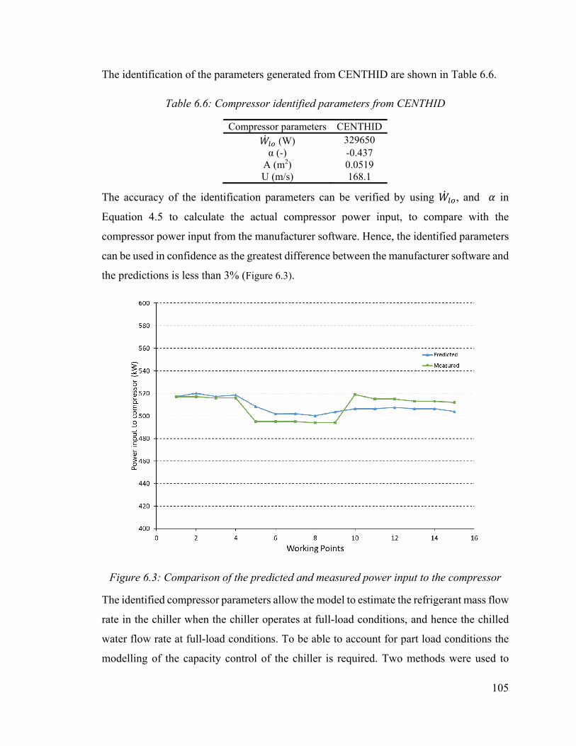
105

The identification of the parameters generated from CENTHID are shown in Table 6.6.

Table 6.6: Compressor identified parameters from CENTHID

Compressor parameters CENTHID (W) 329650

α (-) -0.437 A (m2) 0.0519 U (m/s) 168.1

The accuracy of the identification parameters can be verified by using , and in

Equation 4.5 to calculate the actual compressor power input, to compare with the

compressor power input from the manufacturer software. Hence, the identified parameters

can be used in confidence as the greatest difference between the manufacturer software and

the predictions is less than 3% (Figure 6.3).

Figure 6.3: Comparison of the predicted and measured power input to the compressor

The identified compressor parameters allow the model to estimate the refrigerant mass flow

rate in the chiller when the chiller operates at full-load conditions, and hence the chilled

water flow rate at full-load conditions. To be able to account for part load conditions the

modelling of the capacity control of the chiller is required. Two methods were used to

106

model the refrigerant mass flow rate at part load conditions; (i) the PLR method and (ii)

the Tmin method.

The PLR method uses the average full-load refrigerant mass flow rate computed from using

the identified parameters from CENTHID and the part load ratio (PLR) determine from

manufacturer data (Equation 3.11). The PLR is defined as the refrigeration load divided by

the refrigeration load at full load. Using the manufacturer data for the chiller a relationship

between the PLR and the power input to the compressor can be determined (Equation 6.1).

The PLR is plotted against the power input to the compressor (Figure 6.4) and Equation

6.1 is used to estimate the PLR from the measured power input to the compressor to modify

the refrigerant mass flow according to Equation 3.11.

PLR = 0.0022 − 0.138 Equation 6.1

Figure 6.4: PLR from manufacturer compared to power input to the chiller

The Tmin method estimates the capacity of the chillers by using the difference between the

chilled water return temperature and the refrigerant saturation temperature in the

evaporator. This capacity is then used to control the theoretical inlet guide vane to control

the refrigerant mass flow rate. After investigation, it was determined that there are three

107

modes of operation for the system: (i) chiller #1 is in operation alone, (ii) chiller #2 is in

operation alone and (iii) both chillers are in operation together. For each mode of the system

the coefficients a and b need to be determined from Equation 3.12 (Table 6.7). It was

expected that the coefficients for chiller # 1 and 2 to very close together because they are

the same model of chillers. This method is more suitable for cooling plants with two chillers

or less due to the complexity of determining the coefficients for more than two chillers.

∅ = + ( − ) according to

Equation 3.12

Table 6.7: Coefficients determined from linear regression for capacity control method 1

a b Avg. ΔT Chiller # 1 0.30 0.083 8.4 Chiller # 2 0.25 0.090 8.3

Both Chillers 0.30 0.073 9.6

The average Δt is the difference between the return chilled water temperature observed at

full load conditions and the average SST in the evaporator of the chiller.

The PLR method estimated the chilled water mass flow rate with VFM model B over the

summer of 2013 with a lower CV(RMSE) and NMBE of 5.5 and -1.4% compare to that of

the Tmin method, which estimate the chilled water mass flow rate with a CV(RMSE) and

NMBE of 7.9 and -3.9%. Both methods can be used to estimate the chilled water mass flow

rate but the PLR method is used in this chapter for comparison to the measured results. The

PLR method is also less time consuming and easier to implement in the system. If

manufacturer data is unavailable then the Tmin method can be used; if short-term

measurements of the chilled water mass flow rate are available then the PLR curve can be

determined from the measured data.

The degree of superheating and sub-cooling are required to be estimated for scenario # 5.

For centrifugal chillers, it is difficult to measure the suction and liquid line temperature

without physical sensors being installed directly within the chiller itself. Theses inputs have

a smaller impact on the final predictions then the coefficients used to model the refrigerant

mass flow rate at part load conditions. The amount of sub-cooling was set to 1oC and the

108

amount of super-heating was set to 2oC based on observations of manufacturer data for

centrifugal chillers. The sensitivity of the chilled and condenser water mass flow rates to

the superheating and sub-cooling are examined in section 0.

6.2.2 Development of inputs for VFM model C (scenario # 6)

In VFM model C, scenario # 6 the power input to the compressor ( ) is measured

and used to interpolate the evaporator load ( ) with the manufacturer data (MD-3) from

Table 6.8. The evaporator load from the manufacturer data is then used in Equation 3.16

and Equation 3.17 to determine the chilled water and condenser water mass flow rates.

Table 6.8: Manufacturer data file MD-3

Power Consumed by the Compressor (kW)

Refrigeration Load (kW)

549 3165 454 2849 377 2532 314 2216 260 1899 211 1583 179 1266 146 950 112 633 76 317

This scenario requires the least amount of sensors in order to estimate the chilled and

condenser mass flow rates but can only be applied if the chilled water supply and condenser

water return temperature set-points of the chiller in operation are consistent with the

manufacturer data. In this case, the chilled water supply temperature set-point in the system

is 6.7oC and the manufacturer data indicated 5.4oC. The condenser water return set-point

in the system is 29oC and the manufacturer data indicated 29.4oC. The chiller in operation

operates at a different chilled water supply set-point, and operates close to the condenser

water return temperature set-point. There is only a small difference in the condenser water

set-point and an 1.3oC difference in the chilled water set-point. These differences will affect

the models ability to estimate the chilled and condenser water mass flow rates. Because the

109

differences are small, the method is still used to observe how well this model is able to

estimate the flow rates.


VFM models B and C were used to estimate the chilled and condenser water flow

rates using scenarios # 5 and 6 during the summer months of 2013 from May to September.

This section presents the results of both scenarios to determine how well the estimates

compare with measured data for the chilled and condenser water mass flow rates. The water

flow rates were calculated a fifteen-minute basis and then average for an hour period. The

CV(RMSE) and NMBE were determined using the hourly averaged data. The hypothesis

test was used for both conditions # 1 and 2 to determine whether or not the models are

acceptable.

6.3.1 Results for the summer of 2013 During the summer of 2013, chiller #1 was used as the primary chiller to operate

from May to beginning of July. Then chiller # 2 becomes the primary chiller to operate for

the rest of the cooling season. The goal was to use equally both chillers throughout the

cooling season. It is important to mention that the number of hours that the chillers operate

fluctuates from day to day. Figure 6.5 and Figure 6.6 shows the distribution of the number

of hours that chiller #1 and 2 are in operation by themselves. Figure 6.7 shows the number

of hours both chillers are in operation together.

110

Figure 6.5: Hourly profile of chiller #1 in operation alone

Figure 6.6: Hourly profile of chiller #2 in operation alone

Num

ber o

f hou

rs

Num

ber o

f hou

rs

111

Figure 6.7: Hourly profile of both chillers in operation together

Chilled water mass flow rate

The VFM model B estimates well the chilled water mass flow rate for both chillers

in operation independently, and when both chillers are in operation together on a monthly

basis (Table 6.9). The average chilled water mass flow rate when chiller #1, therefore pump

#1, was in operation was 87.8 ± 2.7 kg/s which compares well with the estimates from the

VFM model B of 90.0 ± 11.6 kg/s. The average chilled water mass flow rate when chiller

#2, therefore pump #2, was in operation was 90.1 ± 2.7 kg/s which compares well with the

estimates from the VFM model of 95.1 ± 12.5 kg/s. The average chilled water mass flow

rate when chiller #1 and chiller #2, therefore pump #1 and pump #2, are in operation is

151.7 ± 3.5 kg/s which compares well with the estimates from the VFM model of 152.9 ±

28.1 kg/s. Because the system consists of two constant speed pumps, the monthly averages

can be used as good estimates of the chilled water mass flow rate. Figure 6.8 shows the

VFM model B estimates over a seven day period where the chilled water mass flow rate

was calculated hourly. VFM model B does fluctuate over time but the errors between the

measured and the estimated are close to or less than 5%.

Num

ber o

f hou

rs

112

Figure 6.8: Estimates from VFM model B for July 1st to July 7th 2013

VFM model C estimates well the measured chilled water mass flow rate compared to the

measured value for each chiller in operation alone (Table 6.9). When both chillers are in

operation, the VFM model C estimates the chilled water flow rate to be 161.5 ± 29.9 kg/s

compared to the measured value of 151.7 ± 3.5 kg/s. Figure 6.9 shows the VFM model C

estimates over the same seven day period as VFM model B (Figure 6.8) where the chilled

water mass flow rate was calculated hourly. The VFM model C estimates are within the 5

% error boundary when chiller #1 is in operation, and are higher than the 5 % error

boundary of the measured value when both chillers are in operation.

07/01/13 07/02/13 07/03/13 07/04/13 07/05/13 07/06/13 07/07/13

0

20

40

60

80

100

120

140

160

180

200

Chi

lled

Wat

er M

ass

flow

rat

e (k

g/s)

VFMMeasured5% Error

CH1 & CH2 CH1

113

Table 6.9: Average monthly chilled water mass flow rates for VFM models B & C for the summer of 2013

VFM model B (Scenario # 5) VFM model C (Scenario # 6) Measured

Month Average

(kg/s) CV(RMS

E) (%) NMBE

(%) Average

(kg/s) CV(RMSE)

(%) NMBE

(%) Average

(kg/s)

CH

1

May 91.1 7.0 -1.5 93.2 7.4 -3.8 June 88.9 6.8 1.1 92.3 6.2 -2.8 July 89.9 6.5 -0.1 92.5 4.8 -3.0

August - - - - - - September 90.1 6.6 -0.4 94.2 7.0 -4.9 Average 90.0 ± 11.6 6.8 1.7 93.1 ± 12.0 6.7 -3.3 87.8 ± 2.7

CH

2

May 99.7 13.5 -10.6 102.3 16.2 -13.9 June - - - - - - July 93.7 6.1 -4.0 97.6 9.2 -8.4

August 93.1 6.3 -3.3 97.2 9.2 -7.9 September 93.9 7.4 -4.3 96.7 8.8 -7.4 Average 95.1 ± 12.5 6.7 -2.1 98.5 ± 12.9 9.2 -8.0 90.1 ± 2.7

CH

1&

2

May 153.4 2.9 -1.1 161.2 76 -6.6 June 152.9 2.8 -0.8 162.5 7.8 -7.1

July 153.3 3.9 -1.1 162.1 8.3 -6.9

August 152.1 3.1 -0.3 161.2 7.5 -6.3 September 152.8 3.4 -0.8 160.7 7.4 -6.0 Average 152.9 ± 28.1 3.3 0.8 161.5 ± 29.9 7.8 6.7 151.7 ± 3.5

Figure 6.9: VFM model C estimates from June 29th to July 7th 2013

07/01/13 07/02/13 07/03/13 07/04/13 07/05/13 07/06/13 07/07/13

0

20

40

60

80

100

120

140

160

180

200

Chi

lled

Wat

er M

ass

flow

rat

e (k

g/s)

VFMMeasured5% Error

CH1 & CH2 CH1

114

The uncertainties due to propagation of measurement errors for both VFM models B and

C range from 13% to 18% of the estimated value. The CV(RMSE) and NMBE are used to

access how well the VFM models are able to estimate the average measured chilled water

flow rate on an hourly basis. The CV(RMSE) and the NMBE were calculated for the

complete cooling season spanning May to September as shown in Table 6.10 for both VFM

models. The CV(RMSE) ranges for 3.3 to 6.8% for VFM model B and 6.7 to 9.2% for

VFM model C.

The hypothesis test was used for both conditions # 1 and 2 to see how well the models

estimate the chilled water mass flow rate on an hourly period (Table 6.10). For VFM model

B, condition # 1, the null hypothesis was accepted for all three modes of operation where

the t-values were smaller than the t-critical of 1.64 (Table 6.10). The acceptance of

condition # 1 guarantees the acceptance of condition # 2. For VFM model C, condition #

1 of the null hypothesis was rejected for all cases as the t-values were greater than t-critical.

For Condition # 2, the null hypothesis was accepted for all cases as the t-value were smaller

than the t-critical of 1.64 (Table 6.10).

Table 6.10: Results for the CV(RMSE), NMBE and t-value (hypothesis test) for the chilled water flow rate for the summer of 2013

VFM model B VFM model C

CH1 CH2 Both

Chillers CH1 CH2

Both Chillers

Hypothesis test

(tcr = 1.64)

Condition # 1 1.46 1.06 -21.5 4.66 30.49 21.6

Condition # 2 -17.59 -26.97 -117.72 -17.33 -2.12 -55.70

Average (kg/s) 90.0 ± 11.6

95.1 ± 12.5

152.9 ± 28.1

93.1 ± 12.0

98.5 ± 12.9

161.5 ± 29.9

CV(RMSE) 6.8 6.7 3.3 6.7 9.2 7.8 NMBE 1.7 -2.1 0.8 -3.3 -8.0 -6.7

Condenser water mass flow rate

The condenser water mass flow rate for each chiller is only dependent on if the

chiller is in operation. The average condenser water mass flow rates were measured during

the summer of 2014 using an ultrasonic flow meter. The measured condenser water mass

flow rate for chiller # 1 was 112.4 ± 2.2 kg/s and for chiller # 2 was 117.0 ± 2.3 kg/s. The

115

estimated monthly values compared well over the complete monitoring period as for VFM

model B of 114.4 ± 12.0 kg/s for chiller #1 and 116.1 ± 12.6 kg/s for chiller # 2 and VFM

model C of 116.1 ± 12.5 kg/s for chiller #1 and 120.6 ± 13.1 kg/s for chiller # 2 (Table

6.11). Figure 6.10 shows the condenser water mass flow rate for VFM model B over a

twelve-day period in the month of July 2013. The VFM model does fluctuate but within

the 5% error bands. During the 2nd of July, the VFM estimates a higher condenser water

mass flow rate, which is greater than 120 kg/s. It is unclear if this is a fault within the

system or from the measuring equipment. To understand what occurred on this day further

investigation is required.

Figure 6.10: Condenser water mass flow rate for VFM model B for chiller #1 from June 29th to July 8th, 2013

06/29/13 06/30/13 07/01/13 07/02/13 07/03/13 07/04/13 07/05/13 07/06/13 07/07/13 07/08/13

0

20

40

60

80

100

120

140

160

Chi

lled

Wat

er M

ass

flow

rat

e (k

g/s)

VFMMeasured5% Error

116

Table 6.11: Monthly averages of the condenser water mass flow rate for the summer of 2013

The CV(RMSE) and NMBE for the condenser water mass flow rate were less than 10%

and 7 % respectively for both VFM models (Table 6.12). For condition # 1 the null

hypothesis was accepted for VFM model B for both chillers and was rejected for VFM

model C for both chillers. For condition # 2 the null hypothesis was accepted for both VFM

model B and C.

Table 6.12: Results for the CV(RMSE), NMBE and t-value (hypothesis test) for the condenser water flow rate for the summer of 2013

VFM model B VFM model C CH1 CH2 CH1 CH2

Hypothesis test (tcr = 1.64)

Condition # 1 -9.32 -28.03 14.92 1.83 Condition # 2 -39.76 -89.79 -19.43 -28.48

Average (kg/s) 114.4 ± 12.0 118.7 ± 12.5 116.1 ± 12.5 120.6 ± 13.1 CV(RMSE) 6.4 3.7 8.8 6.1

NMBE -1.6 0.7 -6.9 -4.6

Sensitivity of VFM model to Inputs

The sensitivity of the super-heating and sub-cooling for VFM model B, scenario #5

are explored to observe the effects of these parameters. VFM model C is not affected by

these inputs because they are not required as inputs. The sensitivity of the inputs for the

superheating and sub-cooling were studied to examine their effects on the final estimation

VFM model B VFM model C Measured

Average

(kg/s) CV(RMSE)

(%) NMBE

(%) Average

(kg/s) CV(RMSE)

(%) NMBE

(%) Average

(kg/s)

CH

1

May 117.1 9.8 -4.2 119.3 11.5 -8.3 June 113.4 6.1 -1.2 117.7 8.3 -6.4 July 112.4 2.2 -0.1 117.4 6.2 -5.8

August 112.8 1.8 -0.3 118.3 5.6 -6.4 September 116.3 7.5 -3.5 120.8 6.4 -8.9 Average 114.4 ± 12.0 6.4 -1.6 116.1 ± 12.5 8.8 -6.9 112.4 ± 2.2

CH

2

May 115.9 2.8 0.9 120.1 5.3 -4.4 June 116.0 2.1 0.8 122.3 5.9 -5.3 July 116.4 3.6 0.5 121.0 6.3 -4.9

August 115.9 3.4 0.9 120.6 5.9 -4.6 September 116.2 5.0 0.7 118.9 6.4 -3.5 Average 118.7 ± 12.5 3.7 0.7 120.6 ± 13.1 6.1 -4.6 117.0 ± 2.3

117

of the chilled and condenser water mass flow rates. The sensitivity of the model depends

on the refrigerant and the compressor type of the chiller. In this case, the refrigerant is R-

123 and the compressor is centrifugal. The null hypothesis was used to determine limits in

the CV(RMSE) and NMBE of acceptable fits for the VFM models.

VFM model B is more sensitive to the amount of sub-cooling then to the amount of

superheating. The superheating affects the refrigerant mass flow rate as well as the chilled

water flow rate by the suction enthalpy. The sub-cooling only affects the calculation of the

chilled water mass flow rate and not the refrigerant mass flow rate.

Table 6.13 show the effects of the amount of superheating and sub-cooling on the estimates

of the chilled water mass flow rate. The normalized value is defined as the chilled water

mass flow rate at the given amount of superheating or sub-cooling divided by the chilled

water mass flow rate determined with a superheating of 2 oC and sub-cooling of 1 oC. When

the superheating is less than 15oC there is a small change in the CV(RMSE) and NMBE

for all cases. For the sub-cooling, the VFM model is slightly more sensitivity then the

superheating but the model is not affected by large amounts in region of acceptable sub-

cooling of the chiller which would be less than 5oC. The hypothesis test was used with

condition # 2 on the estimates for the chilled water mass flow rate. For all cases where the

superheating was modified, the t-values remained below the t-critical values. The t-values

for Loyola campus case study are given in Table A.3 for the sensitivity testing of the

superheating and for the sub-cooling. For condition # 2, the null hypothesis is true where

the absolute difference between measured and estimated values are equal to or smaller than

the difference between the uncertainty propagation due to measurement errors and the

uncertainty of the measuring device. The uncertainty propagation due to measurement

errors was about 13% for CH1 and CH2 alone in operation. The uncertainty propagation

due to measurement errors was about 18% when both chiller are in operation together. The

uncertainty of the measuring device was close to 3%. The limit for uncertainty is therefore

10% and 15% of the measured value for the chiller in operation independently and together,

respectively. The VFM models were accepted with the highest CV(RMSE) and NMBE of

12.5 and 10.7%.

118

For the sub-cooling, the t-value were greater than t-critical for both chiller # 2 with a sub-

cooling of 15oC and for all chillers with a sub-cooling greater than 30oC. The models were

accepted with the highest CV(RMSE) and NMBE of 10.8 and 10.1%. From the hypothesis

testing, it would suggest that for the case study for the chilled water mass flow rate the

limits for the CV(RMSE) and NMBE are close to 13 and 10.7%, respectively.

Table 6.13: Sensitivity of the chilled water mass flow rate for the amount of superheating and sub-cooling

Chiller # 1 Chiller #2 Both Chillers Super-heating

Normalized CV(RMSE)

(%) NMBE

(%) Normalized

CV(RMSE) (%)

NMBE (%)

Normalized CV(RMSE)

(%) NMBE

(%)

0 1.00 7.8 -4.6 1.00 8.6 -4.3 1.00 4.2 -0.3 2 1.00 6.8 -0.1 1.00 6.7 -3.9 1.00 3.3 -0.7 4 0.99 6.9 0.7 0.99 6.3 -3.2 0.99 3.2 -0.1

10 0.97 7.3 2.7 0.97 5.5 -1.1 0.97 3.8 2.0 15 0.95 8.0 4.6 0.95 5.5 0.9 0.95 5.1 4.0 30 0.89 12.5 10.7 0.89 9.0 7.3 0.89 10.5 10.1

Chiller # 1 Chiller #2 Both Chillers Sub-

cooling Normalized

CV(RMSE) (%)

NMBE (%)

Normalized CV(RMSE)

(%) NMBE

(%) Normalized

CV(RMSE) (%)

NMBE (%)

0 0.98 7.4 2.0 0.98 5.6 -1.8 0.98 3.4 1.1 1 1.00 6.8 -0.1 1.00 6.7 -3.9 1.00 3.3 -0.7 4 1.02 7.1 -1.9 1.02 8.1 -6.0 1.02 4.3 -2.7

10 1.06 8.7 -5.6 1.06 11.3 -9.9 1.06 7.7 -6.7 15 1.09 10.8 -8.6 1.09 14.1 13.0 1.09 10.8 10.1 30 1.16 17.3 -16.3 1.16 20.6 -20.1 1.19 20.4 -19.9 60 1.24 24.1 -23.6 1.15 23.0 -19.2 1.36 37.5 -37.3

6.4.1 VFM Limitations for centrifugal chillers The VFM models for centrifugal chillers is limited to chillers where the refrigerant

mass flow rate is controlled with inlet guide vane. Centrifugal chillers with VSD drives

installed to control the refrigerant mass flow rate have not been investigated and would

require a different modelling approach for part load conditions.


This case study presented the use of a VFM to estimate the chilled and condenser

water mass flow rate of a cooling plant with two centrifugal chillers. The case study used

VFM model B, scenario #5, and VFM mode C, scenario # 6, to provide the estimates

because only the minimum amount of sensors were installed within the system. This

119

represents a typical case study for existing buildings where measured and manufacturer

data can be limited.

The VFM estimated the chilled and condenser water for the period of May to September

of 2013. The estimates from the VFM were examined for each chiller in operation alone

and when both chillers are in operation together. The uncertainty of the VFM models were

investigated and determine as 13% when one chiller was in operation and 18% of the

estimates when both chiller were operating together. It was determined that the VFM model

B is not very sensitive to the approximation on the amount of superheating. VFM model B

is sensitive to the estimates of the sub-cooling and varied by 9% with an increase in sub-

cooling from 1oC to 15oC.

The hypothesis test was used to provide insight into how well the VFM model estimates

the chilled and condenser water mass flow rates compared to hourly measurements. The

hypothesis test showed that VFM model B was accepted for condition # 1 for the chilled

and condense water mass flow rates, which means the estimates from the VFM model B is

able predict within 5% error of the measured values. For VFM model C, the null hypothesis

was accepted for only condition # 2, which represents an acceptable model because it

estimated the measured value within the overall uncertainty of the model.

Comparison of the limits of CV(RMSE) and NMBE for three case

studies using the hypothesis test

A statistical hypothesis test was used to provide insight towards acceptable values

of the CV(RMSE) and NMBE that would determine an acceptable fit of the VFM model

compared to measurements. From observation of the CV(RMSE), and NMBE with the

results from the hypothesis test, its observed that for condition #1, which defines a good

model, the limits for the CV(RMSE) and NMBE were close to 7.5% and 5%, respectively.

For condition # 2 which defines an acceptable model, the limits for the CV(RMSE) and

NMBE were close to 15% and 12%, respectively.

Condition #1 defines a model will be accepted for hourly estimates if the null hypothesis

Ho is true where the absolute difference between measured and estimated values are equal

120

to or smaller than 5% of the measured value. For the three case studies, the maximum

CV(RMSE) and NMBE are shown with their corresponding t-values (Table 6.14).

Table 6.14: Maximum observed CV(RMSE) and NMBE that satisfied condition # 1 of the hypothesis test

Ice Rink Research Building Loyola Campus Max CV(RMSE) 7.5 4.7 6.8

Max NMBE 4.7 1.1 1.7 t-value -1.61 -0.82 1.46

Condition #2 defines a model is acceptable if the null hypothesis Ho is true where the

absolute difference between measured and estimated values are equal to or smaller than the

difference between the uncertainty propagation due to measurement errors and the

uncertainty of the measuring device. For the three case studies, the maximum CV(RMSE)

and NMBE are shown with their corresponding t-values (Table 6.15).

Table 6.15: Maximum observed CV(RMSE) and NMBE that satisfied condition # 2 of the hypothesis test

Ice Rink Research Building Loyola Campus Max CV(RMSE) 13.5 10.4 18.9 15.2 12.5 10.8

Max NMBE 12.3 -8.6 11.9 4.3 10.7 -8.6 t-value 1.14 -8.55 -9.72 -2.75 1.39 -3.71

From observing the maximum CV(RMSE) and NMBE for both conditions of the

hypothesis test, the maximum CV(RMSE) and NMBE for condition # 1 is close to 7.5 and

5%, respectively. For condition # 2, the maximum CV(RMSE) and NMBE is close to

19.0% and 12.3%, respectively. Comparing the limits of condition # 2 with the

recommendations from ASHRAE Guideline 14 (2002), the limit for the NMBE for

condition # 2 is greater than that recommended of 10% but the CV(RMSE) is below the

recommended 30%. For this purpose the maximum limit for the NMBE for the VFM model

will be set to 10% and the CV(RMSE) value will be limited to 15%, which is the largest

value CV(RMSE) while the NMBE is less than 10%.

121

7. MODULE 3: ONGOING COMMISSIONING OF COOLING PLANTS USING A VFM In this chapter, module # 3 is presented to monitor the coefficient of performance

(COP) of the chillers and of the cooling plant to compare these estimates to benchmarked

values. The results are presented for two case studies, where the chilled water mass flow

rate were estimated using a VFM and then used to determine COP of the chiller and cooling

plant. The case studies highlight the challenges associated with implementing the ongoing

commissioning module in existing buildings and the uncertainties associated with this

method. The development of a graphical user interface will be presented in this chapter to

highlight the inputs required for the virtual flow meter and the visualization of the results.

Ongoing Performance Approach

The purpose of this approach is to provide an ongoing assessment by monitoring

the COP of the cooling plant and comparing it continuously with a developed benchmark

profile for the COP. The benchmark profiles are reference guidelines of how the cooling

plant should be performing under normal operating conditions in terms of COP, with the

given conditions of the system from a commissioned state. The individual performance of

each chiller can be continuously monitored to detect the degradation of performance over

time.

This method will allow building operators and commissioning engineers, the opportunity

to monitor the system performance visually compared to developed benchmarks to provide

feedback about the cooling plant performance. This chapter presents the prototype of an

automatic tool for building operators and commissioning agents, to be able to develop

strategies to reduce the energy consumption of their system well satisfying the cooling

demand based of the work from Monfet and Zmeureanu (2011).

In this module, the COP is determined on an ongoing basis from installed sensors using a

VFM. The virtual COP is compared with a values from benchmark model for the COP to

observe if the chiller is operating outside an acceptable limit of COP. The results are

presented visually and as a document detailing the report and warnings (Figure 7.1).

122

Ongoing Energy Performance

(COP) Estimation

Measurement Database

Building Automation

System (BAS)

Comparison Module

Chiller Manufacturer

Data

Visualization Tool

Reports & Warnings

Virtual flow meter

Pre-Process DataFlow

Measurments

Uncertainty Analysis

Graphical User Interface

Figure 7.1: Overview of ongoing commission method to monitor chiller performance

The goal of the benchmark model is to provide a baseline of normal operating performance

from a commissioned state. This means that every time the cooling plant is re-

commissioned, the benchmark model will be required to be re-trained. Benchmarking

models can be developed from measured data within the BAS or from manufacturer data.

For this thesis, two benchmark models were used: (i) Reciprocating chillers and (ii)

Centrifugal chillers.

7.1.1 Reciprocating Chillers For reciprocating chillers, it is easier to compare the virtual COP to a benchmark

developed from manufacturer data for the chiller or from short-term measurements of the

COP. The benchmark COP can be determined from Equation 7.1, which uses the

manufacturer refrigeration load of one compressor ( _ ) with the number of

compressors in operation (N) within the chiller and the measured power input ( ) from

the chiller (chiller COP) or the cooling plant (cooling plant COP).

= _ Equation 7.1

Module 3: Ongoing Commissioning

123

7.1.2 Centrifugal Chillers Centrifugal chillers might not always operate at the same operation conditions as

available from developed manufacturer data. Using a benchmark model developed from

trend data is a useful method to monitor the performance of the chiller from a

commissioned state. Monfet and Zmeureanu (2012) developed benchmarking models

using trend data from a BAS. Their multivariable polynomial (MP) model with a static

window training set will be used to demonstrate the use of the VFM in ongoing

commissioning process. The static window is the predefined training set size, in this case

one week, used to train the model. The benchmark model was original developed to

monitor the COP of a single chiller alone. In this thesis, the model will be used to monitor

the COP of the cooling plant. A training set of data is required to determine the five

coefficients δ1…δ5 of the MP model. The models are then used to calculate the benchmark

COP of the cooling plant over time to be compared with the virtual COP that acts as the

measured COP for the monitoring period. The coefficients for the model were identified in

MATLAB (2013) using the “regress” function.

= , + , + ( ) + + Equation 7.2

Where is the measured refrigeration load on the evaporator, Tcdws is the supply

condenser water temperature, TOA is the dry-bulb outdoor air temperature and Qev,design is

the design full-load of the refrigeration load.

Ongoing Commissioning analysis of an Ice Rink

The complete description of the cooling system for the ice rink is described in

chapter 4. The ongoing commissioning of the ice rink was performed using the trend data

from across both chillers # 1 and 2 over two-day periods for each month from December

6th, 2005 - November 11th, 2006.

7.2.1 Comparison of the Virtual COP to Measured COP for the Ice Rink Case Study The uncertainty propagation due to measurement errors for the COP (UCOP) was

determined using Equation 3.34. The measured cooling plant COP and the cooling plant

virtual COP (Table 7.1). The virtual COP estimated well the measured COP within the

124

uncertainty of the models. For this case study, scenario # 6 estimates the measured COP

the best with an average of 3.16 ± 0.58. All scenarios can be used to monitor the COP on

an hourly basis.

Table 7.1: Values of measured and VFM COP of the cooling plant for ice rink

Month COP

Measured Scenario

2 3 4 5 6 December 3.19 2.90 3.00 2.78 2.95 2.89 February 3.38 3.45 3.46 3.34 3.35 3.27

March 3.25 3.15 3.15 3.04 3.04 3.29 April 3.13 3.00 3.01 2.89 2.90 3.13 May 3.23 3.15 3.15 3.02 3.03 3.28

October 3.14 2.85 2.87 2.75 2.76 3.02 November 3.21 3.08 3.08 3.00 3.01 3.29 Average 3.22 ± 0.60 3.08 ± 0.80 3.10 ± 0.81 2.97 ± 0.76 3.00 ± 0.76 3.16 ± 0.58

7.2.2 Applying Module 3 to an Ice Rink The performance of cooling plant was monitored over each month using the

ongoing commissioning approach. The uncertainties determined for the COP (Ucop) are

used to define the boundaries of the benchmark model so that when the system is outside

these limits for longer than a two-hour period, a message will be sent to the building

operators. The number of hours will be recorded to log the number of hours the system is

performing outside normal operations.

The benchmark COP for the ice rink was determined using the manufacturer software

Carwin (Carlyle 2007) to determine the refrigeration load (56.9 kW) of one compressor at

the operating conditions of the system. When both chillers are at full-load, there are five

compressors but six refrigerant loops (N) in operation with an average power of (110.2)

kW which results in a benchmark COP of 3.09 at full load.

Figure 7.2 and Figure 7.3 show the virtual COP for scenarios # 2 and 4 with the measured

COP plotted over time with the limits from the benchmark model for March 14th to 15th,

2006 and May 13th to 14th, 2006, respectively. The limits of the benchmark COP is defined

as half of the uncertainty (Ucop), where the Ucop was 0.80 for scenario # 2. It can be observed

in both figures that scenario # 2 estimates close to the upper limit and so does the measured

125

value, while scenario # 4 estimates closer to the benchmark value. The measured COP was

sixty-five hours over the benchmark limit while scenario # 2 was eleven hours over the

benchmark limit over the complete monitored days from December 2005 to October 2006.

Scenario # 4 had zero hours outside the benchmark limits. The measured and virtual COP

never operate below the benchmark lower limit and suggest that the system is operating

close to or better than the upper limit of the bench mark. In the future a new benchmark

value can be calculated from the measured COP (or virtual) to obtain a new benchmark

value. Then the COP of the ice rink could be monitored from this newly developed

benchmark to observe if the cooling plant maintains this performance of COP over time.

Figure 7.2: Monitoring of the COP for March 14th to 15th, 2006

00:00 06:00 12:00 18:00 00:00 06:00 12:00 18:00 00:00

0

0.5

1

1.5

2

2.5

3

3.5

4

4.5

5

CO

P (

kW/k

W)

Scenario 2Scenario 4MeasuredBenchmark Limits

Coef

ficie

nt o

f per

form

ance

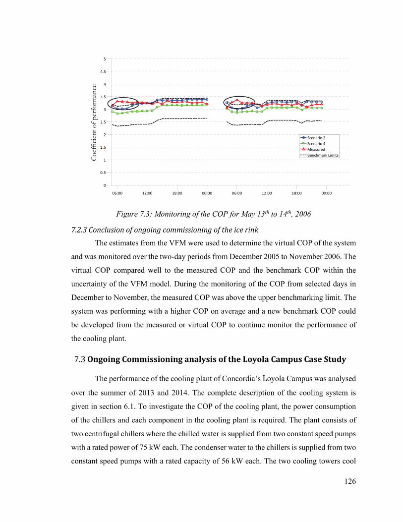
126

Figure 7.3: Monitoring of the COP for May 13th to 14th, 2006

7.2.3 Conclusion of ongoing commissioning of the ice rink The estimates from the VFM were used to determine the virtual COP of the system

and was monitored over the two-day periods from December 2005 to November 2006. The

virtual COP compared well to the measured COP and the benchmark COP within the

uncertainty of the VFM model. During the monitoring of the COP from selected days in

December to November, the measured COP was above the upper benchmarking limit. The

system was performing with a higher COP on average and a new benchmark COP could

be developed from the measured or virtual COP to continue monitor the performance of

the cooling plant.

Ongoing Commissioning analysis of the Loyola Campus Case Study

The performance of the cooling plant of Concordia’s Loyola Campus was analysed

over the summer of 2013 and 2014. The complete description of the cooling system is

given in section 6.1. To investigate the COP of the cooling plant, the power consumption

of the chillers and each component in the cooling plant is required. The plant consists of

two centrifugal chillers where the chilled water is supplied from two constant speed pumps

with a rated power of 75 kW each. The condenser water to the chillers is supplied from two

constant speed pumps with a rated capacity of 56 kW each. The two cooling towers cool

06:00 12:00 18:00 00:00 06:00 12:00 18:00 00:00

0

0.5

1

1.5

2

2.5

3

3.5

4

4.5

5

CO

P (

kW/k

W)

Scenario 2Scenario 4MeasuredBenchmark Limits

Co

effic

ient

of p

erfo

rman

ce

127

the condenser water with two perpendicular fans per cooling tower with a maximum power

input of 30 kW each, and can be modulated by a VFD. The complete description of the

cooling plant is summarized in Table 7.2.

Table 7.2: Design values for cooling plant components (adapted from Tremblay 2013)

Component Design Information CH1 & CH2 (each) Power (kW) 549 Measured

COP 5.76 Measured P1& P2 (Chilled water, each) Power (kW) 75 Assumed constant

P3 & P4 (Condenser water, each) Power (kW) 56 Assumed constant

CT1 & CT2 Cooling tower fan Max power (kW)

% VFD 30

0-100% Estimated (Equation 7.3)

Measured

Equation 7.3 is used to estimate the power of the cooling tower fans (Monfet and

Zmeureanu 2011).

= % ∗ , Equation 7.3

Where the RPM is the rated rotation per minute, 1800 RPM; RPMdesigned is the design

rotation per minute, 1800 RPM; %VFD is the percentage from the VFD which is measured

and PCT,max is the rated power of the fans at 30 kW each.

The COP of the cooling plant was analysed on fifteen-minute time scale, which is the same

time scale that the trend data is recorded. The COP was then averaged on an hourly basis

to be used to analyse the performance of the system.

7.3.1 Comparison of the Virtual COP to Measured COP for the Loyola Case study The uncertainty of the virtual COP was determined using Equation 3.34 for both

the measured and the virtual COP over the summer of 2013 (Table 7.3). The uncertainties

from the measured COP are much lower than the virtual COP; this is due to the higher

uncertainty from the chilled water mass flow rates of the VFM model. Even with the high

uncertainties, the virtual COP estimated well the measured COP, where the virtual COP

estimated within 5% error of the measured value (Figure 7.4).

128

Table 7.3: Overall uncertainty of the cooling plant COP

Chiller # 1 Chiller # 2 Both chillers VFM Model B 0.74 0.61 0.69 Measured COP 0.15 0.12 0.14

Figure 7.4: Virtual cooling plant COP compared to the measured cooling plant COP for June 24th to 28th, 2013

The virtual COP was compared to the measured COP for each chiller in operation and the

complete cooling plant. The VFM model was able to estimate well the COP with

CV(RMSE) for 2013 of 7.5% for chiller # 1, 6.9% for chiller # 2 and 6.3% for the cooling

plant and NMBE less than 5.7% (Table 7.4). The virtual COP estimated well the measured

COP and can be used to develop the benchmark model for the ongoing commission process

with module # 3.

Table 7.4: CV(RMSE) and NMBE for the virtual COP for the summer of 2013

CV(RMSE) NMBE Chiller #1 7.5 1.7 Chiller # 2 6.9 -5.7

Both chillers 6.3 -1.2

Coef

ficie

nt o

f per

form

ance

129

7.3.2 Applying Module 3 to Loyola case study The benchmark model was developed for the cooling plant COP when each chiller

#1 and chiller #2 are in operation individual and for when both chillers are in operation.

The chillers themselves can operate differently performance wise in each mode so the

coefficients were trained for each mode of operation (Table 7.6). The main disadvantage

to this approach is that three different training sets were required for this case study and if

there are more than two chillers in the cooling plant than the amount of training sets

increases.

Measured trend data from the summer of 2013 was used to train the benchmark model for

each mode of operation to be determined as the commissioned state of the cooling plant.

The benchmark model is then used during the summer of 2014 to observe how the system

is performing. The number of hours the chillers operate throughout the summer is staged

from chiller #1 at the beginning of the summer and chiller # 2 from July onwards and both

chillers operating in tandem for periods when the cooling demand is higher, typically in

July. The trainings sets were developed for one week periods in the beginning of their

operation mode and the testing dataset were the week following the training week. For

chiller # 1 the training period is May 20th - 27th, 2013 and for chiller # 2 the training period

is July 29th - August 5th, 2013 and for both chillers the training period is June 24th - July 1st,

2013 (Table 7.5). This allows the model for cooling plant to include chiller # 1, 2 and both

chillers in operation with a good set of data. The benchmarking model for the COP

estimates well the VFM COP for each individual mode as CV(RMSE) is less than 0.5%

for the training period and less than 5% for the testing period (Table 7.6).

Table 7.5: Dates used for training and testing for benchmarking model

Training Testing

Chiller # 1 May 20th - 27th, 2013 May 27th- June 3rd, 2013 Chiller # 2 July 29th – August 5th, 2013 August 5th – 12th , 2013

Both chillers June 24th – July 1st, 2013 July 1st – 8th, 2013

130

Table 7.6: Coefficients for the benchmarking model for the cooling plant COP for each mode of operation

δ1 δ2 δ3 δ4 δ5

CH1 -6.5790 9.6726 -2.7146*10^-5 -1.2352*10^-2 2.4780*10^-3 CH2 -3.0349 6.2430 -9.5207*10^-6 -1.9557*10^-3 9.5417*10^-3

Both chillers -1.3636 4.2267 -9.5207*10^-6 -1.9557*10^-3 9.5417*10^-3

R2 Training Testing CV(RMSE) NMBE CV(RMSE) NMBE

CH1 99.4 0.20 0.01 3.67 -1.56 CH2 99.4 0.50 -0.02 4.98 -1.69

Both chillers 99.9 0.05 -0.02 2.43 -1.29

After the models have been tested and accepted the benchmark model can be compared

continuously against the measured COP to monitor the performance of the cooling plant

and observe when the system is performing abnormally compared to the benchmark model.

The benchmarking model limits is determined as half of the average uncertainty due to

measurement errors.

The virtual COP was determined to operate above the upper benchmark limit at nineteen

different occasions (warnings) during the summer of 2014 for a total of 50 hours over the

complete summer of 2014, which is about 1.5% of the total number of hours that the

cooling plant is operating. This means the cooling plant is performing with a higher COP

then what is normally estimated from the benchmark model. For this case, the higher COP

is good but does show that the cooling plant does sometimes deviate from normal operating

conditions and can be useful to explore the conditions behind this increase to possible

achieve this higher COP on a continuous basis.

Figure 7.5 shows the virtual COP ongoing commissioning of the cooling plant over the

period from July 1st to 4th, 2014. The virtual COP remains within the limits of the

benchmark for this complete period or only deviates slightly from the benchmark. Figure

7.6 shows the virtual COP ongoing commissioning of the cooling plant over the period

from June 23rd to 24th, 2014 where the virtual COP is operating outside the benchmarking

limits for twenty hours out of thirty-four hours for this period. The virtual COP is outside

the benchmark limits from 11:00 to 18:00 on June 23rd, 2014 and from 9:00 to 18:00 on

131

June 24th, 2014. During these two periods, it was unclear what was causing the COP to be

higher than the benchmark and further diagnostics is required. The virtual COP over the

summer of 2014 never operated below the benchmark COP limit.

Figure 7.5: Ongoing commissioning of the cooling plant COP for July 1st to 4th, 2014

Figure 7.6: Ongoing commissioning of the cooling plant COP for June 23rd to 24th, 2014

07/01/14 07/02/14 07/03/14 07/04/14

2

2.5

3

3.5

4

4.5

5

5.5

6

Chi

lled

Wat

er M

ass

flow

rat

e (k

g/s)

VFM COPBenachmarkBenchmark Limits

04:00 09:00 14:00 19:00 00:00 04:00 09:00 14:00 19:00

2

2.5

3

3.5

4

4.5

5

5.5

6

Chi

lled

Wat

er M

ass

flow

rat

e (k

g/s)

VFM COPBenachmarkBenchmark Limits

Coef

ficie

nt o

f per

form

ance

Coef

ficie

nt o

f per

form

ance

132

7.3.3 Conclusion of ongoing commissioning of the Loyola case study This section demonstrated the use of a VFM to estimate the COP of a cooling plant

with centrifugal chillers. The VFM COP estimated well the measured COP with a

CV(RMSE) of 6.3% for 2013 and 7.2% for 2014. The uncertainty propagation due to

measurements errors of the VFM models was determined to be about 0.69 for the cooling

plant compared to about 0.14 for the measured COP.

A benchmarking model was developed and trained for a centrifugal cooling plant from

trend data from the BAS. The benchmark model was then used with limits developed from

the uncertainty of the models to continuously monitor the performance of the cooling plant.

The trend data from the summer of 2013 was used to train the model and the performance

of the system was monitored over the summer of 2014. It was observed that the

performance of the system was above the upper limit of the benchmarking COP nineteen

times and for a total of fifty hours during the summer of 2014.

Conclusion for ongoing commissioning approach

This chapter presented the use of a VFM to estimate the COP of a chiller and a

cooling plant to be used with ongoing commissioning techniques for cooling plants with

reciprocating or centrifugal chillers. The purpose of this chapter was to investigate the

accuracy and uncertainty associated with estimating the COP of the chiller and cooling

plant using the results from the VFM to then be demonstrated in developed ongoing

commissioning techniques.

For both case studies, the VFM model was able to estimate the measured COP within a

given level of uncertainty and can be used to monitor the cooling plant using an ongoing

commissioning process. The uncertainty of using the virtual COP was investigated and

then used to provide limits of benchmarking models of the COP that were used to monitor

the COP of the cooling plant.

Development of Graphical User Interface (GUI) for the VFM Tool

A GUI was developed to provide users with a simple way to enter the required

inputs to use the VFM Tool and to provide a quick visual feedback of the results generated

133

by the VFM models. The VFM tool generates a comma-separated file (*.csv) for each

chiller as well as for the plant for further analysis and use of the data. The plant, for the

case of the VFM Tool, is defined as the combination of all chillers in operation together

and excludes the chilled and condenser water pumps as well as the cooling towers to

simplify the inputs to the model.

The main window consists of two main components, the case study information tab, which

consists of the system configuration and fluid properties push buttons, and the scenario

information tab, which consists of the scenario info and inputs push buttons (Figure 7.7).

Figure 7.7: Main window for the VFM Tool

The system configuration window allows the user to select up to six different chillers to be

in combination with each other either in series or in parallel (Figure 7.8). In the plant

134

configuration menu, there are three drop down menus; (i) the chiller type (ii) chiller

refrigerant type and (iii) the part load method. Currently the chiller types available are

centrifugal and reciprocating. The list of refrigerants that are available and the methods

used for determining the refrigerant transport properties are given in section 3.1.3. The part

load methods consists of the cylinder-unloading method for reciprocating chillers and the

PLR and Tmin methods for centrifugal chillers, which are explained in section 3.1.1.2.2.

Figure 7.8: Plant configuration interface

When continue is selected the window for the part load inputs appear. Depending on the

chillers in the plant, two windows can appear, one for reciprocating chillers (Figure 7.9)

and the other for centrifugal chillers (Figure 7.10). The part load methods for reciprocating

chillers deals with the number of refrigerant loops with compressors within the chiller that

can operate at full-load or with cylinder unloading. The help button provides the user with

further description of the inputs required for each input.

135

Figure 7.9: Reciprocating part load input window

The centrifugal inputs window allow users to enter the required part load ratio coefficients

or the Tmin coefficients for each chiller.

Figure 7.10: Centrifugal part load input window

136

The VFM Tool determines the specific heat for the chilled and condenser water for the

plant by selecting the chilled and condenser water types from the fluid properties window.

The chilled water can be water, calcium-chloride/water solution or a glycol/water solution.

For the water solutions, the percentage of brine to water is required and then the specific

heat are determined from interpolation within a developed property tables for the specific

heat.

Figure 7.11: Fluid properties window

The scenario inputs window is used to input the trend data from the cooling plant. The

manufacturer data (MD-1) used to identify the compressor parameters for scenario # 4 and

5 or manufacturer data (MD-3) for scenario # 6 using the select file buttons to select the

excel or (*.csv) files. The table is used to input the superheating and sub-cooling for each

chiller for scenario # 3 and 5. The compression exponent can be enter in the table as well

for each chiller for scenario # 2 and 3. A help button is used to provide more information

about the inputs in the scenario input window.

137

Figure 7.12: Scenario inputs window

After all the inputs have been entered, the run button will initiate the VFM Tool. After

completion the results window will appear (Figure 7.13). The results window consists of

three main graphs and two tables. The three graphs are for the chilled water, condenser

water and COP of the chillers. The properties can be accessed from the top left hand side

of the window, where pressing on the corresponding button will display the graph for each

property. The default graph that appears is for the plant and can be changed to each

individual chiller by using the drop down menu. The colored markers highlight the

combination of chillers in operation during the point in time when the variable was

calculated. This help the user visualize the variables with respect to the systems operating

conditions. The average properties for the chilled water, condenser water, power and COP

of each chiller are given in the table in the bottom left hand side. For scenarios # 4 and 5,

the identification parameters are given as well in the table in the bottom right hand side.

138

Figure 7.13: Results window for the VFM Tool

The results window is used as a quick feedback to verify how well the VFM Tool estimated

the chilled water and condenser water mass flow rates. It gives the user the opportunity to

verify if large discrepancies exists between the estimated values and what is expected from

measurements, design or manufacturer data. Once the chilled and condenser water mass

flow rates are accepted by the user, they can be used for further analysis of the cooling

plant from generated (*.csv) files of the variables of the models.

139

8. CONCLUSIONS AND FUTURE WORK A new VFM model was proposed to estimate the chilled and condenser water mass

flow rates through chillers using different scenarios of available sensors that would allow

VFM to be integrated into existing building without the need for additional sensors. The

proposed VFM can be implemented without the need of short-term measurements of the

chilled or condenser water flow rates to train coefficients in the model. The VFM uses trend

data from sensors available in the BAS to provide a low-cost non-intrusive alternative to

measuring the chilled and condenser water mass flow rates.

The overall uncertainty propagation due to measurement errors was investigated. From the

uncertainty analysis and observations in the case studies, the input that dominates the

uncertainty in the models is the chilled water temperature difference and the condenser

water temperature difference across the evaporator and condenser, respectively. To reduce

the uncertainty in the estimates of the VFM model these temperature sensors should have

a high, as possible, rated accuracy. This would aid in reducing the overall uncertainty of

the model and reduce the VFM model sensitivity at low chilled and condenser temperature

differences.

The sensitivity of the VFM estimates to the superheating and sub-cooling of the refrigerant

were investigated. Both case studies showed that the VFM model is only slightly sensitive

to the guesses for the superheating and sensitive to the sub-cooling. When using scenario

# 3 and 5, which use the estimates of the superheating and sub-cooling small changes in

the guess will not cause large changes in the estimated chilled and condenser water mass

flow rate.

The VFM model was applied to three case studies with reciprocating and centrifugal

chillers. The estimates from the three case studies agree well with the measured values for

the chilled and condenser water mass flow rates for all scenario of the VFM model. A

statistical hypothesis test was used to provide insight towards acceptable values of the

CV(RMSE) and NMBE that would determine an acceptable model of the VFM compared

to measurements. From observation of the CV(RMSE), and NMBE with the results from

the hypothesis test, its observed that for condition #1, which defines a good model, the

140

limits for the CV(RMSE) and NMBE were close to 7.5% and 5%, respectively. For

condition # 2 which defines an acceptable model, the limits for the CV(RMSE) and NMBE

were close to 15 and 10%, respectively.

The estimates from the VFM were used to determine the coefficient of performance of the

chillers and cooling plant to examine how well the method was able to determine the

coefficient of performance and with what degree of uncertainty. For the two case studies

the estimates from the VFM were able to continue to provide accurate results for the

coefficient of performance compared to measurements. The virtual coefficient of

performance was compared to developed benchmark models to observe how the cooling

plant is performing over time and it the system performance is drifting or degrading over

time. The monitored virtual COP for the two case studies compared well to the benchmark

model, no direct changes were required in the cooling plants, and the method can continue

to be used to monitor the cooling plant for degradation in the future.

Summary of Contributions

1. Development a new method for a virtual flow meter using different scenarios of available sensors and information about the system.

2. Examined the uncertainty due propagation of measurements errors to provide insight to which inputs that have the greatest impact on the accuracy of the VFM model.

3. Examined the accuracy and feasibility of the proposed method in three case studies of existing buildings using the CV(RMSE), NMBE and a statically hypothesis test.

4. Determined the feasibility of using the VFM estimates of the chilled water mass rate to calculate the COP of the cooling plant and its use with developed ongoing commissioning techniques.

5. Development of a GUI (VFM Tool) to provide users with a simple way to use and visualize the results from the proposed VFM.

141

Future Work

The recommend future work focuses on extending the VFM to include more types

of chillers to expand the VFM model to more cooling plants of existing buildings. For

further development of the VFM model it is recommend to develop and test a component

for VFM model B to estimate the chilled and condenser water mass flow rates for chillers

with screw compressors and absorption chillers to further the models reach to more cooling

plants of existing buildings.

To investigate the capacity control method for centrifugal chillers with variable speed drive

compressors. To investigate the use of the VFM to provide accurate estimates for systems

with VSD, to observe how well the model behaves with continuously changing chilled or

condenser water mass flow rates.

In addition, investigating the accuracy of the model required for other uses of the chilled

and condenser water mass flow rate as for fault detection and diagnostics models of cooling

plants.

142

9. REFERENCES

AHRI (2003). Methods for automated and continuous commissioning of building systems. (No. ARTI-21CR/610-30040-01). Technical Results, System Integration Project Reports. Retrieved from http://www.osti.gov/bridge/purl.cover.jsp?purl=/810800-vomrED/native/;http://www.ahrinet.org

ASHRAE (Ed.). (2005). ASHRAE guideline 2-2005, Engineering Analysis of Experimental Data. ASHRAE, Atlanta, USA.

ASHRAE, 2002. ASHRAE Guideline 14-2002, Measurement of Energy and Demand Savings, ASHRAE, Atlanta, Georgia.

Bourdouxhe, J. P., Grodent, M. and Lebrun, J. (1994). HVAC 1 Toolkit: A Toolkit for Primary HVAC System Energy Calculations, ASHRAE, Atlanta, Georgia.

Browne, M. W., & Bansal, P. K. (1998). Steady-state model of centrifugal liquid chillers. International Journal of Refrigeration, 21(5), 343-358.

Carlyle Compressor Company (2007). ‘Carwin compressor selection software’, Version 3.0

Carrier Corporation (2001). ‘Open-Drive Compressors and 09RH Water-Cooled Condensers’, Catalogue No. 510-505

Cleland, A. C. (1994). Polynomial curve-fits for refrigerant thermodynamic properties: extension to include R134a. International Journal of Refrigeration, 17(4), 245-249.

Comstock, M.C., and J.E. Braun. (1999). Development of analysis tools for the evaluation of fault detection and diagnostics in chillers. ASHRAE Research Project 1043-RP. Atlanta, GA: ASHRAE.

Deng, S., Turner, W. D., Claridge, D. E., Liu, M., Bruner Jr, H. L., & Wei, G. (2002). Retrocommissioning of central chilled/hot water systems. ASHRAE Transactions, 108 PART 2, 75-81.

Endress + Hauser Corporation. (2006). ‘Technical Information- Proline Promag 10P” Catalogue No. TI094D/06/en/11.09

Gorman, J. M., Sparrow, E. M. & Abraham, J. P. (2013). Differences between measured pipe wall surface temperatures and internal fluid temperatures. Case Studies in Thermal Engineering, 1, 13-16.

Greyline Corporation. (2013). ‘USER’S GUIDE: Installation & Operation Instructions Portaflow Model PT400 Manual Series A.2” Retrieved from http://www.greyline.com/

143

IEA (2010). Project Summary Report: Commissioning Tools for Improved Building Energy Performance, Energy Conservation in Buildings and Community Systems Programme, International Energy Association (IEA) Annex 40 of the ECBCS, United Kingdom. Retrieved from http://www.ecbcs.org/docs/ECBCS_Annex_40_PSR.pdf

Kamei, A., Beyerlein, S.W., and Jacobsen, R.T (1995). Application of nonlinear regression in the development of a wide range formulation for HCFC-22, Int. J. Thermophysics, 16:1155-1164

Kusiak, A., Li, M., & Zheng, H. (2010). Virtual models of indoor-air-quality sensors. Applied Energy, 87(6), 2087-2094.

Katipamula, S., and D.E. Claridge. 1993. Use of simplified system models to measure retrofit energy savings. Journal of Solar Energy Engineering, 115:57-68.

Lemmon, E.W., Huber, M.L., McLinden, M.O., (2013). NIST Standard Reference Database 23: Reference Fluid Thermodynamic and Transport Properties-REFPROP, Version 9.1, National Institute of Standards and Technology, Standard Reference Data Program, Gaithersburg.

Li, H., and J.E. Braun. (2007). Decoupling features and virtual sensors for diagnosis of faults in vapor compression air conditioners. International Journal of Refrigeration 30(3):546–64.

Li, H., and J.E. Braun. (2009a). Decoupling features for diagnosis of reversing and check valve faults in heat pumps. International Journal of Refrigeration 32(2):316–26.

Li, H., and J.E. Braun. (2009b). Development, evaluation, and demonstration of a virtual refrigerant charge sensor. HVAC&R Research 15(1):117–36.

Li, H., and J.E. Braun. (2009c). Virtual refrigerant pressure sensors for use in monitoring and fault diagnosis of vapor compression equipment. HVAC&R Research 15(3):597–616.

Mihai, M., & Zmeureanu, R. (2013). Impact of the Representation of Interior Loads on the Calibration of an eQuest Energy Model for a Case Study. Paper presented at the eSim Confernce.

McDonald, E., Zmeureanu, R., (2014) Virtual Flow Meter to Estimate the Water Flow Rates in Chillers. ASHRAE Transactions, SE-14-017

Monfet, D. & Zmeureanu, R. (2011). Ongoing commissioning approach for a central cooling and heating plant. ASHRAE Transactions, 117 PART 1, 908-924.

Monfet, D., & Zmeureanu, R. (2012). Ongoing commissioning of water-cooled electric chillers using benchmarking models. Applied Energy, 92, 99-108.

144

NRCan. (2013). Energy Efficiency Trends in Canada 1990 to 2010. Natural Resources Canada, Canada. Accessed March 2014. http://publications.gc.ca/site/eng/440661/publication.html

Ouzzane, M., Sunyé, R., Zmeureanu, R., Giguère, D., Scott, J., & Bellache, O. (2006). Cooling load and environmental measurements in a Canadian indoor ice rink. ASHRAE Transactions, 112 PART 2, 538-545.

Reddy, T. Agami. (2011). Applied Data Analysis and Modeling for Energy Engineers and Scientists, Springer.

Song, L., Joo, I. S., & Wang, G. (2012). Uncertainty analysis of a virtual water flow measurement in building energy consumption monitoring. HVAC & R Research, 18(5), 997-1010.

Stanford, Herbert W. (2003). HVAC water chillers and cooling towers: fundamentals, application, and operation. New York: Marcel Dekker, Inc.

Swamy, A., Song, L., & Wang, G. (2012). A virtual chilled-water flow meter development at air handling unit level. ASHRAE Transactions, 118(PART 1), 1013-1020.

Taylor, B., & Kuyatt, C. (1994).” NIST Technical Note 1297: Guidelines for Evaluating and Expressing the Uncertainty of NIST Measurement Results”. National Institute of Standards and Technology, Gaithersburg, MD

Tahmasebi, F., & Mahdavi, A. (2013). A two-staged simulation model calibration approach to virtual sensor for building performance data. Paper presented at the Building Simulation, Chambery, France.

Teyssedou, Gabriel. (2007). Computer Model of the Refrigeration System of an Ice Rink. (Master of Science), Concordia University, Montreal, Quebec, Canada.

Trane. (2000). Split System Condensing Units and Remote Chillers; 80 through 120 Ton Remote Chillers (Vol. 2). Catalogue No. PL-UN-S/S-000-D-2-0700 S/S-D-2

Trane. (2005). Maintenance Guide; Water Cooled CenTraVac™ With CH530. Catalogue No. CVHE-SVU01E-EN

Tremblay, V. (2013). Ongoing commissioning of heat recovery process in a central heating and cooling plant. (Master of Science), Concordia University, Montreal, Quebec, Canada.

Tremblay, V., & Zmeureanu, R. (2014). Benchmarking models for the ongoing commissioning of heat recovery process in a central heating and cooling plant. Energy, 70, 194-203.

145

Wang, G., Liu, M., & Claridge, D. E. (2010). Development of an energy meter using a pump flow station. ASHRAE Transactions, 116(PART 2), 569-577.

Wang, H. (2014). Water flow rate models based on the pipe resistance and pressure difference in multiple parallel chiller systems. Energy and Buildings, 75, 181-188.

Yang, Mo, Zhao, Xinzhi, Li, Haorong, & Wang, Wei. A Smart Virtual Outdoor Air Ratio Sensor in Rooftop Air Conditioning Units. Applied Thermal Engineering. doi: http://dx.doi.org/10.1016/j.applthermaleng.2013.12.046

Younglove, B.A. and McLinden, M.O. (1994). "An International Standard Equation of State for the Thermodynamic Properties of Refrigerant 123 (2, 2-Dichloro-1, 1, 1-trifluoroethane)," J. Phys. Chem. Ref. Data, 23:731-779.

Zach, Z., Hofstatter, H., Glawischnig, S., & Mahdavi, A. (2013). Incorporation of Run-Time Simulation-Powered Virtual Sensors in Building Monitoring Systems. Paper presented at the Building Simulation, Chambery, France.

Zhao, X., Yang, M., & Li, H. (2011). Decoupling features for fault detection and diagnosis on centrifugal chillers (1486-RP). HVAC&R Research, 17(1), 86-106.

Zhao, X., Yang, M., & Li, H. (2012). Development, evaluation, and validation of a robust virtual sensing method for determining water flow rate in chillers. HVAC&R Research, 18(5), 874-889.

146

APPENDICES APPENDIX A: Results from the hypothesis test for the sensitivity of the superheating and sub-cooling on the chilled was mass flow rate The sensitivity of the chilled water mass flow rate were examined for the ice rink

and Loyola campus case studies. The CV(RMSE) and NMBE were determined for each

level of sub-cooling and superheating. The hypothesis test was used to determine if the

estimates were acceptable under condition # 2.

The t-values for ice rink case study are given in Table A.1 for the superheating and Table

A.2 for the sub-cooling. For condition # 2, the null hypothesis Ho, is true where the absolute

difference between measured and estimated values are equal to or smaller than the

difference between the uncertainty propagation due to measurement errors and the

uncertainty of the measuring device. The uncertainty propagation due to measurement

errors was about 15.8% for each scenario and the uncertainty of the measuring device was

2%. The limit for uncertainty is therefore 13.8% of the measured value of 63.1 kg/s.

Table A.1: Results for t-value (hypothesis test) for the sensitivity testing of superheating of the ice rink

Scenario ∆Tsupheat 3 4 5

3 -18.16 -13.35 -14.78 6 -16.43 -11.25 -13.83 9 -15.43 -9.82 -11.40 18 -8.55 -3.16 -4.97 25 -2.92 1.14 -0.80

Table A.2: Results for t-value (hypothesis test) for the sensitivity testing of sub-cooling of the ice rink

Scenario ∆Tsubool 3 4 5

2 -14.52 -9.87 -17.37 6 -8.02 -7.53 -2.13

12.5 -16.43 -11.25 -13.83 20 -16.98 -12.52 -19.97 60 31.16 -9.40 23.38

147

The t-values for Loyola campus case study are given in Table A.3 for the sensitivity testing

of the superheating and for the sub-cooling. For condition # 2, the null hypothesis Ho, is

true where the absolute difference between measured and estimated values are equal to or

smaller than the difference between the uncertainty propagation due to measurement errors

and the uncertainty of the measuring device. The uncertainty propagation due to

measurement errors was about 13% for CH1 and CH2 alone in operation. The uncertainty

propagation due to measurement errors was about 18% when both chiller are in operation

together. The uncertainty of the measuring device was close to 3%. The limit for

uncertainty is therefore 10% and 15% of the measured value for the chiller in operation

independently and together, respectively.

Table A.3: Results for t-value (hypothesis test) for the sensitivity testing of superheating and sub-cooling

∆Tsupheat Chiller # 1 Chiller #2 Both Chillers 0 -9.29 -14.75 -24.95 2 -17.21 -27.54 -117.72 4 -17.46 -29.07 -118.95

10 -15.65 -32.36 -113.37 15 -13.05 -31.93 -103.64 30 1.39 -11.85 -57.16

∆Tsubool Chiller # 1 Chiller #2 Both Chillers 0 -14.54 -33.06 -117.16 1 -17.59 -26.97 -117.72 4 -17.04 -19.04 -106.82

10 -11.89 0.24 -70.06 15 -3.71 17.84 -43.45 30 29.07 67.36 25.81 60 40.57 180.2 160.6

APPENDIX B: Results for estimates of the chilled and condenser water mass flow rates over the summer of 2014 During the summer of 2014, chiller #1 was used as the primary chiller to operate

from May to beginning of July, and then chiller # 2 becomes the primary chiller to operate

for the rest of the cooling season to use equally both chillers throughout the cooling season

(Figure B.1 and Figure B.2). During the summer of 2014, the chillers operate together in

tandem for a fewer number of hours than in 2013 and can be seen in Figure B.3.

148

Figure B.1: Hourly profile of chiller #1 in operation alone

Figure B.2: Hourly profile of chiller #2 in operation alone

Num

ber o

f hou

rs

Num

ber o

f hou

rs

149

Figure B.3: Hourly profile of both chillers in operation together

The VFM models estimates well the monthly average chilled water mass flow rate over the

summer of 2014 using both scenarios # 5 and 6 (Table B.1). VFM model B estimated the

chilled water mass flow rate to be 92.3 ± 12.5 kg/s for chiller # 1, 94.2 ± 11.9 kg/s and

157.8 ± 29.2 kg/s for chiller #1, 2 and both chillers in operation, respectively. VFM model

C estimated the chilled water mass flow rate to be 96.2 ± 13.1 kg/s for chiller # 1, 100.6 ±

12.7 kg/s and 169.2 ± 31.3 kg/s for chiller #1, 2 and both chillers in operation, respectively.

Figur B.4 shows the estimates of VFM model B over a period in July. The VFM model

estimates close to the constant measured value within 5% of the error of the measured

chilled water mass flow rate.

Num

ber o

f hou

rs

150

Table B.1: Average monthly chilled water mass flow rates for VFM mode B & C for the summer of 2014

VFM model B (Scenario #5) VFM model C (Scenario #6) Measured

Month Average

(kg/s) CV(RMSE)

(%) NMBE

(%) Average

(kg/s) CV(RMSE)

(%) NMBE

(%) Average

(kg/s)

CH

1

May 92.7 8.3 -3.3 96.3 9.3 -7.3

June 91.0 7.1 -1.4 95.5 8.9 -6.4

July 92.8 7.2 -3.4 97.2 9.5 -8.2

August 92.6 5.9 -3.1 95.6 7.9 -6.4

September - - - - - -

Average 92.3 ± 12.5 7.4 -2.2 96.2 ±13.1 9.0 -6.8 87.8 ± 2.7

CH

2

May - - - - - -

June - - - - - -

July 93.0 5.7 -3.3 100.0 11.7 -11.0

August 94.7 6.8 -4.4 100.6 12.6 -11.8

September 94.9 8.0 -5.4 101.1 13.4 -12.2

Average 94.2 ±

11.9 6.8 -4.5 100.6 ±12.7 12.8 -11.8 90.1 ± 2.7

CH

1 &

2

May 158.5 5.3 -4.5 170.4 13.1 -12.4

June 158.3 5.3 -4.4 169.8 12.7 -11.9

July 157.2 5.5 -3.6 168.7 12.2 -11.2

August 157.5 4.9 -3.8 168.7 12.0 -11.2

September 157.3 5.1 -3.7 168.4 11.8 -11.1

Average 157.8 ±29.2 5.2 -3.8 169.2 ± 31.3 12.1 -11.3 151.7 ± 3.5

Figure B.4: VFM model B estimates for chilled water mass flow rate for July 1st to 7th, 2014

The CV(RMSE) was determined to be 7.4, 6.8 and 5.8 for VFM model B for chiller #1,

chiller # 2 and both chillers, respectively. The CV(RMSE) was determined to be 9.0, 12.8

and 12.1 for VFM model C for chiller #1, chiller # 2 and both chillers, respectively (Table

07/01/14 07/02/14 07/03/14 07/04/14 07/05/14 07/06/14

0

20

40

60

80

100

120

140

160

180

200

Chi

lled

Wat

er M

ass

flow

rat

e (k

g/s)

VFMMeasured5% Error

151

B.2). The same trend is observed in 2014 as in 2013, where the VFM model C is unable to

estimate within 5% error the measured chilled water mass flow rate when both chillers are

in operation.

The hypothesis test was used to provide insight for the goodness the fit of the VFM models.

For both VFM models condition # 2 was accepted and the models average estimates can

be used on a daily, weekly and monthly period. When both chillers were in operation

together, VFM model B was able to estimate well the measured value as the t-value was

-5.76, which was less than the t-critical value of 1.64 (Table B.2).

For VFM model C, condition # 1, the null hypothesis was rejected for all cases and the

estimates from VFM model C can be used to monitor the chilled water mass flow rate on

a daily or monthly period.

Table B.2: Results for the CV(RMSE), NMBE and t-value (hypothesis) test for the chilled water flow rate for the summer of 2014

VFM model B VFM model C

CH1 CH2 Both

Chillers CH1 CH2

Both Chillers

Hypothesis test

(tcr = 1.64)

Condition # 1

2.78 3.63 -5.76 11.10 48.10 34.48

Condition # 2

-15.51 -39.73 -82.15 -10.74 -0.56 -10.73

Average (kg/s) 92.3.± 12.5 94.2 ± 11.9 157.8 ± 29.2 96.2 ± 13.1 100.6 ± 12 169.2 ± 31.3 CV(RMSE) 7.4 6.8 5.2 9.0 12.8 12.1

NMBE -2.2 -4.5 -3.8 -6.8 -11.8 -11.3

The condenser water mass flow rate for each chiller is only dependent on if the chiller is in

operation; therefore, the condenser water mass flow rate was determined when the chillers

were in operation. The average measured condenser water mass flow rate for chiller # 1

again is assumed to be 112.1 ± kg/s and 117.0 ± kg/s for chiller # 2. The measured value

compared well with the monthly estimates from the VFM for the condenser water mass

flow rate (Table B.4). Figure B.5 shows the VFM estimates for the condenser water mass

flow rate for chiller # 2 over a period from July 5th to 28th, 2014. The estimates from the

VFM model do fluctuate but stay within the 5% error boundary.

152

Over the complete monitoring period of 2014, VFM model B estimated the condenser

water mass flow rate to be 116.2 ± 12.2 for chiller # 1 and 115.9 ± 12.6 for chiller # 2 with

a CV(RMSE) of 7.5% and 3.8%, respectively (Table B.3).

Table B.3: Monthly averages of the condenser water mass flow rate for the summer of 2014

Figure B.5: Condenser water mass flow rate for chiller # 2 from July 5th to 28th, 2014

The CV(RMSE) and NMBE for the condenser water mass flow rate were less than 10.2%

and 8.2 %, respectively for both VFM models. This would lead to the assumptions that the

models estimated well the condenser water mass flow rate.

07/06/14 07/13/14 07/20/14 07/27/14

0

20

40

60

80

100

120

140

160

Chi

lled

Wat

er M

ass

flow

rat

e (k

g/s)

VFMMeasured5% Error

VFM model B (Scenario # 5) VFM model C ( Scenario # 6) Measured

Month Average

(kg/s) CV(RMSE)

(%) NMBE

(%) Average

(kg/s) CV(RMSE)

(%) NMBE

(%) Average

(kg/s)

CH

1

May 119.8 13.0 -6.6 123.8 14.2 -10.2 June 116.3 8.1 -3.6 121.4 10.7 -8.1 July 114.9 3.2 -2.3 120.9 7.9 -7.5

August 115.5 4.3 -2.5 121.4 8.6 -8.0 September 114.6 2.8 -2.0 121.1 7.9 -7.7

Average 116.2 ±

12.2 7.5 -3.4

121.7 ± 12.8

10.2 8.2 112.4 ± 2.2

CH

2

May 118.4 3.2 -1.2 124.7 7.3 -6.6 June 114.3 3.0 2.3 121.8 5.2 -4.1 July 116.1 2.9 0.8 123.6 6.4 -5.6

August 115.1 4.8 1.6 122.1 6.5 -4.4 September 116.0 3.6 0.8 122.7 6.3 -4.9

Average 115.9 ±

12.6 3.8 1.1

122.9 ± 13.4

6.4 5.0 117.0 ± 2.3

153

For condition # 1, the null hypothesis was accepted for VFM model B for both chillers and

was rejected for VFM model C for both chillers (Table B.4). For condition # 2, the null

hypothesis was accepted for both VFM model B and C. This leads to the conclusion that

for this case, VFM model B does estimate better the condenser water mass flow rate but in

the absence of information VFM model C can be used to estimate the condenser water

mass flow rate.

Table B.4: Results for the CV(RMSE), NMBE and t-value (hypothesis test) for the condenser water flow rate for the summer of 2014

VFM model B VFM model C CH1 CH2 CH1 CH2

Hypothesis test (tcr = 1.64)

Condition # 1 -3.38 -25.70 21.40 5.39 Condition # 2 -29.69 -92.13 -11.77 -54.11

Average (kg/s) 116.2 ± 12.2 115.9 ± 12.6 121.7 ± 12.8 122.9 ± 13.4 CV(RMSE) 7.5 3.8 10.2 6.4

NMBE -3.4 1.1 8.2 5.0

Documents

Development and Testing of a Virtual Flow Meter for Use in ...€¦ · Development and Testing of a Virtual Flow Meter for Use in Ongoing Commissioning of Commercial and Institutional