Embed Size (px)
Citation preview
Loughborough UniversityInstitutional Repository
Development andperformance
characterisation of a novelgas�liquid contacting stage
This item was submitted to Loughborough University's Institutional Repositoryby the/an author.
Additional Information:
• A Doctoral Thesis. Submitted in partial fulfilment of the requirementsfor the award of Doctor of Philosophy at Loughborough University.
Metadata Record: https://dspace.lboro.ac.uk/2134/27120
Publisher: c© M.P. Nicholls
Rights: This work is made available according to the conditions of the CreativeCommons Attribution-NonCommercial-NoDerivatives 2.5 Generic (CC BY-NC-ND 2.5) licence. Full details of this licence are available at: http://creativecommons.org/licenses/by-nc-nd/2.5/
Please cite the published version.

This item was submitted to Loughborough University as a PhD thesis by the author and is made available in the Institutional Repository
(https://dspace.lboro.ac.uk/) under the following Creative Commons Licence conditions.
For the full text of this licence, please go to: http://creativecommons.org/licenses/by-nc-nd/2.5/
Pilkington Library
• ~ L0l!ghbprough .,UmversJty
AuthorlFiIing Title ....... Y:J .. ~~.~~~ .................... .
.................................................................... -r
Vol. No. ............ Class Mark ................... ········
Please note that fines are charged on ALL overdue items.
0402222318
111111 IIIIIII~ 11 1111 I 11 I I I~ I III I I 11 11111

Development and performance characterisation of a novel gas-liquid
contacting stage.
by
M. P. Nicholls
Doctoral thesis submitted in partial fulfilment of the requirements for the
award of Doctor of Philosophy of Chemical Engineering of
Loughborough University.
Sept. 1999
© by M. P. Nicholls 1999

~~-''''''~~'-__ ''''''_J,"'~"'''.'''''_' -~~ ... .".".,.,. ~ ~,~'_A.! f·e>:, 17: ,~, _, 11
i ~\""\ rf~ l>£J1PJl.l;!(,\f\lJtm.n ~ (,!:&: .. ,.~~ '.,. ~ ~'. -.~ .~,::.--;;<~}:, k ~\\:"'{""(".'o( ~.,..Ii
i'.~~ .. . ..)1'1 ' .•. ,.!-
, 'p . • ~ ," "'fNY r.>: __ ~, ""'" ~
I~ p---" • ! e'm;:; ! ;,.. r-,'- .• " .... "r •• ' '.'~".u'I<
I ~~~ a:~~:,~~~~~1
.,
Abstract.
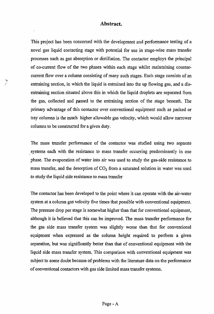
This project has been concerned with the development and perfonnance testing of a
novel gas liquid contacting stage with potential for use in stage-wise mass transfer
processes such as gas absorption or distillation. The contactor employs the principal
of co-current flow of the two phases within each stage whilst maintaining counter
current flow over a column consisting of many such stages. Each stage consists of an
entraining section, in which the liquid is entrained into the up flowing gas, and a dis
entraining section situated above this in which the liquid droplets are separated from
the gas, collected and passed to the entraining section of the stage beneath. The
primary advantage of this contactor over conventional equipment such as packed or
tray columns is the much higher allowable gas velocity, which would allow narrower
columns to be constructed for a given duty.
The mass transfer perfonnance of the contactor was studied usmg two separate
systems each with the resistance to mass transfer occurring predominantly in one
phase. The evaporation of water into air was used to study the gas-side resistance to
mass transfer, and the desorption of CO2 from a saturated solution in water was used
to study the liquid side resistance to mass transfer
The contactor has been developed to the point where it can operate with the air-water
system at a column gas velocity five times that possible with conventional equipment.
The pressure drop per stage is somewhat higher than that for conventional equipment,
although it is believed that this can be improved. The mass transfer perfonnance for
the gas side mass transfer system was slightly worse than that for conventional
equipment when expressed as the column height required to perfonn a given
separation, but was significantly better than that of conventional equipment with the
liquid side mass transfer system. This comparison with conventional equipment was
subject to some doubt because of problems with the literature data on the performance
of conventional contactors with gas side limited mass transfer systems.
Page - A
-.
In addition to describing the development processes and the mass transfer
experiments, the thesis will also give a preliminary evaluation of the industrial
potential of the new contactor and describe some of the design features which an
industrial scale contactor based on this principle would include.
Keywords: Mass transfer.
Gas-liquid.
Equipment.
Co-current.
Intensification.
Column.
Page-B
'.'

Acknowledgements.
I would like to express my gratitude to the following people.
My supervisor, Dr lain Curnming for his assistance, support and technical input
throughout this project.
Professor B. W. Brooks, my director of research, and Professor M. Streat, the Head of
Department.
Hugh Peters for his invaluable assistance in constructing the experimental rigs for this
project.
Pip Amos, Barry Powell and Graham Moody in the chemical engineering workshop,
who produced the internal parts for the experimental rigs.
Andy Milne and Dave Smith, whose knowledge of, and assistance with, analytical
techniques and reagents was much appreciated.
Steve Graver, Terry Neale, Paul Izzard and everyone else within the department who
has helped me along the way.
My fellow researchers within the department who have helped make my time here
brighter and more enjoyable than it would otherwise have been.
Page - C
Abstract
Acknowledgements
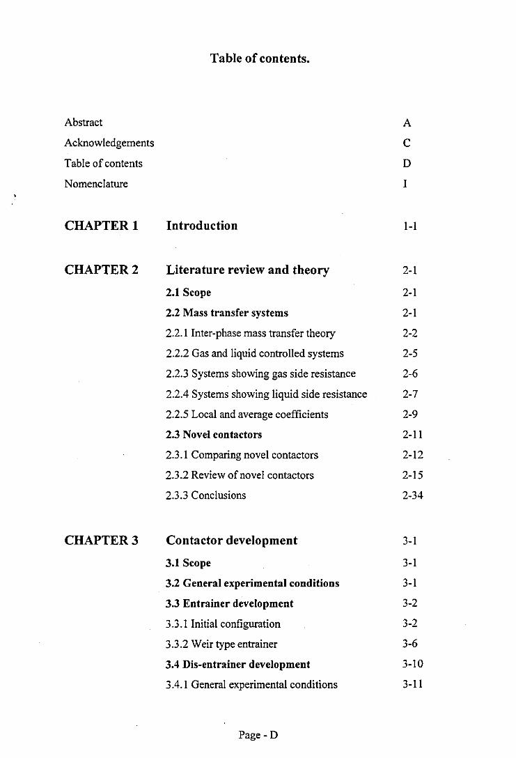
Table of contents
Nomenclature
CHAPTER 1
CHAPTER 2
CHAPTER 3
Table of contents.
Introduction
Literature review and theory
2.1 Scope
2.2 Mass transfer systems
2.2.1 Inter-phase mass transfer theory
2.2.2 Gas and liquid controlled systems
2.2.3 Systems showing gas side resistance
2.2.4 Systems showing liquid side resistance
2.2.5 Local and average coefficients
2.3 Novel contactors
2.3.1 Comparing novel contactors
2.3.2 Review of novel contactors
2.3.3 Conclusions
Contactor development
3.1 Scope
3.2 General experimental conditions
3.3 Entrainer development
3.3.1 Initial configuration
3.3.2 Weir type entrainer
3.4 Dis-entrainer development
3.4.1 General experimental conditions
Page-D
A
C
D
I
1-1
2-1
2-1
2-1
2-2
2-5
2-6
2-7
2-9
2-11
2-12
2-15
2-34
3-1
3-1
3-1
3-2
3-2
3-6
3-10
3-11
3.4.2 Initial configuration 3-13
3.4.3 Dye tracing experiments 3-16
3.4.4 Further dis-entrainer designs 3-17
3.4.5 Development of wire mesh dis-entrainer 3-26
3.4.6 Further developments 3-39
3.4.7 A model for the dis-entrainer 3-46
3.4.8 Pressure manipulation experiments 3-49 ",
3.4.9 Final dis-entrainer design 3-54
3.4.10 Effect of guide vane pitch angle 3-57
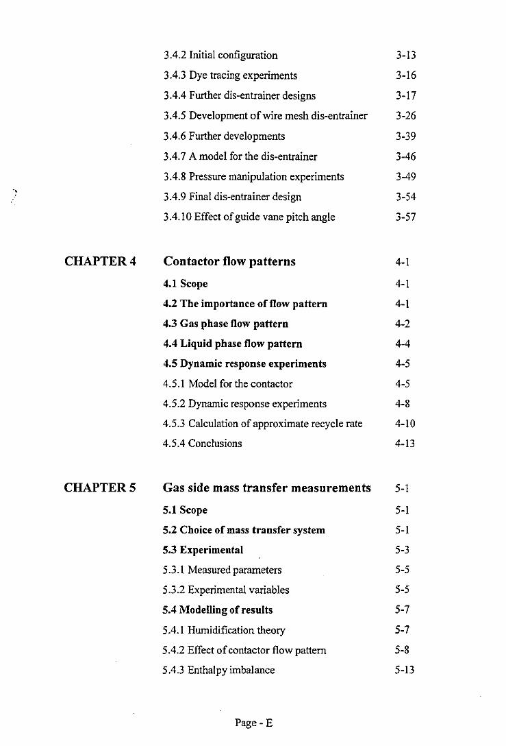
CHAPTER 4 Contactor flow patterns 4-1
4.1 Scope 4-1
4.2 The importance of flow pattern 4-1
4.3 Gas phase flow pattern 4-2
4.4 Liquid phase flow pattern 4-4
4.5 Dynamic response experiments 4-5
4.5.1 Model for the contactor 4-5
4.5.2 Dynamic response experiments 4-8
4.5.3 Calculation of approximate recycle rate 4-10
4.5.4 Conclusions 4-13
CHAPTER 5 Gas side mass transfer measurements 5-1
5.1 Scope 5-1
5.2 Choice of mass transfer system 5-1
5.3 Experimental 5-3
5.3.1 Measured parameters 5-5
5.3.2 Experimental variables 5-5
5.4 Modelling of results 5-7
5.4.1 Humidification theory 5-7
5.4.2 Effect of contactor flow pattern 5-8
5.4.3 Enthalpy imbalance 5-13
Page-E

5.5 Results 5-15
5.6 Discussion 5-25
5.6.1 Choice of flow model 5-25
5.6.2 Effect of gas flow rate 5-26
5.6.3 Effect ofliquid loading 5-27
5.6.4 Effect of water inlet temperature 5-27
5.6.5 Effect of tube size 5-28
5.6.6 Comparisons with conventional equipment 5-28
5.7 Conclusions 5-33
CHAPTER 6 Liquid side mass transfer measurements 6-1
6.1 Scope 6-1
6.2 Selection of mass transfer system 6-1
6.3 The sulphite oxidation system 6-4
6.3.1 Introduction 6-4
6.3.2 Theory 6-5
6.3.3 Experimental 6-12
6.3.4 Analysis of results 6-17
6.3.5 Results 6-20
6.3.6 Discussion 6-23
6.3.7 Conclusion 6-26
6.4 CO2 Desorption system 6-26
6.4.1 Introduction and theory 6-26
6.4.2 Experimental 6-27
6.4.3 Interpretation of results 6-31
6.4.4 Results 6-33
6.4.5 Discussion 6-38
6.4.6 Comparisons with conventional equipment 6-42
6.4.7 Conclusions from C02 desorption expts 6-46
Page - F
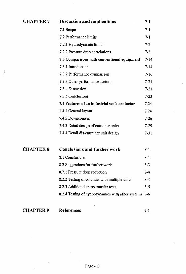
CHAPTER 7 Discussion and implications 7-1
7.1 Scope 7-1
7.2 Perfonnance limits 7-1
7.2.1 Hydrodynamic limits 7-2
7.2.2 Pressure drop correlations 7-3
7.3 Comparisons with conventional equipment 7-14
7.3.1 Introduction 7-14
7.3.2 Perfonnance comparison 7-16
7.3.3 Other perfonnance factors 7-21
7.3.4 Discussion 7-21
7.3.5 Conclusions 7-23
7.4 Features ofan industrial scale contactor 7.24
7.4.1 General layout 7.24
7.4.2 Downcomers 7-26
7.4.3 Detail design of entrainer units 7-29
7.4.4 Detail dis-entrainer unit design 7-31
CHAPTERS Conclusions and further work 8-1
8.1 Conclusions 8-1
8.2 Suggestions for further work 8-3
8.2.1 Pressure drop reduction 8-4
8.2.2 Testing of columns with multiple units 8-4
8.2.3 Additional mass transfer tests 8-5
8.2.4 Testing of hydrodynamics with other systems 8-6
CHAPTER 9 References 9-1
Page - G
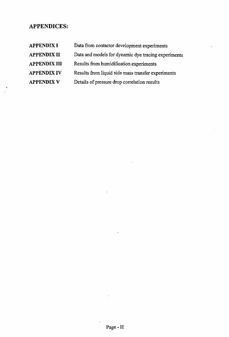
APPENDICES:
APPENDIX I
APPENDIX 11
APPENDIX III
APPENDIX IV
APPENDIX V
Data from contactor development experiments
Data and models for dynamic dye tracing experiments
Results from humidification experiments
Results from liquid side mass transfer experiments
Details of pressure drop correlation results
Page -H
Nomenclature.
a - Specific surface area for mass transfer (m2/m\
A; - Total surface area for mass transfer (m2).
A - Pressure drop correlation constant.
B - Pressure drop correlation constant.
Cab or c/ -Bulk liquid phase concentration of component a (mol/lit).
Ca; - Interfacial liquid phase concentration of component a (mol/lit).
Ca * - Equilibrium liquid phase concentration of component a (mol/lit).
C'IN - Effective inlet liquid concentration (molllit) (recycle model).
C - Pressure drop correlation constant.
CL - Liquid specific heat capacity (kJ/kg CC).
d - Entrainer tube diameter (m).
D; - Pressure vessel internal diameter (m).
Do - Liquid diffusivity of oxygen (m2/s). , ,
Dso'- - Liquid diffusivity of sulphite ions (m2/s). J
e - Pressure vessel wall thickness.
E - Mass transfer enhancement factor due to chemical reaction.
ED/E - Dis-entrainment efficiency.
Em - Murphree stage efficiency.
En - Reaction activation energy (kJ/mol)
f - Pressure vessel design stress.
F V . c: (k 112 ·112 .1) V - apour capacity lactor g m s .
F'v - Packed column capacity factor (m S·I).
G - Gas flow rate (kg/s)
HA - Air specific enthalpy (kJ/kg).
HAJ - Inlet air specific enthalpy (kJ/kg).
H.4Z - Outlet air specific enthaIpy (kJ/kg).
HOG - Height of a gas side transfer unit (m).
Hs - Saturated air specific enthalpy (kJ/kg).
Ha - Dimensionless Hatta number.
Page - I
h - Pressure drop correlation constant.
h - Pressure drop correlation constant.
h - Pressure drop correlation constant.
k - Pressure drop correlation constant.
k' - Pressure drop correlation constant.
kg - Gas side individual mass transfer coefficient.
k[ - Liquid side individual mass transfer coefficient.
k[ 0 - Physical liquid side mass transfer coefficient in the absence of reaction.
k2 - Second order reaction rate constant.
Kg - Overall gas side mass transfer coefficient.
K[ - Overall liquid side mass transfer coefficient.
I - Pressure drop correlation constant.
L - Liquid flow rate (kg/s).
m - Slope of equilibrium line.
n - Pressure drop correlation constant.
N - Mass transfer flux (mol S·l m·2)
N,oG - Total number of gas side transfer units.
N'OL - Total number of liquid side transfer units.
Pi - Internal pressure.
q - Liquid flow rate (lit/min).
R - Recycle flow ratio.
R - Gas constant.
t - time (s).
T - Temperature.
TL - Liquid temperature (OC).
TLI - Liquid inlet temperature COC).
TL2 - Liquid outlet temperature (0C).
T'LI - Effective liquid inlet temperature (0C) (recycle flow model).
Uy - Vapour or gas velocity (m/s).
Uys - Superficial vapour or gas velocity (m/s)
UrUBE - Local gas velocity in entrainer tube (m/s).
UA - Axial gas velocity in dis-entrainer tube (m/s).
Page - J
Uc - Annular gas velocity in dis-entrainer tube (m/s).
V - Contactor or liquid volume (m\
V - Reaction rate (in equation 6.1)
x - Liquid mole fraction.
X - Pressure drop correlation constant.
X' - Pressure drop correlation constant.
Y - Gas or vapour mole fraction.
Yn - Mole fraction of vapour leaving stage n.
Yn+/ - Mole fraction of vapour arriving at stage n.
Yn * - Mole fraction of vapour in equilibrium with liquid leaving stage n.
Y - Pressure drop correlation constant.
z - Stoichiometric coefficient.
Z - Contactor height (m)
a 0, - Solubility of oxygen (mol/lit atm)
a - Guide vane pitch angle (0)
~ - Absorption factor.
M'DRY - Dry pressure drop (mm WG).
M'wET- Wet pressure drop (mm WG).
M'+ - Additional pressure drop due to liquid
(mm WG).
Pab - Bulk gas phase concentration of component a.
Pal - Interfacial gas phase concentration of component a.
Pa * -Equilibrium gas phase concentration of component a.
PA - Density of air.
P L - Liquid density.
P v - Vapour or gas density (kg/m\
Page- K

CHAPTER ONE
Chapter 1.
Introduction
Equipment for contacting gases and liquids is widely used in the chemical and process
industries for a variety of unit operations, primarily absorption, stripping and
fractional distillation. These processes are conventionally carried out in large columns
in which the up-flowing gas is contacted with liquid which is flowing down the
column under gravity. The project described here was concerned with the
development of an improved gas liquid contacting device, which would allow these
operations to be conducted in more compact equipment.
The most commonly used forms of column are the tray column and the packed
column. In a tray column the liquid cascades down the column and forms pools on the
column trays. These trays enable the gas to bubble through the liquid to allow mass
transfer to occur. The liquid flows down from plate to plate by flowing over a weir on
each plate, and into a 'downcomer' which lead to the plate beneath. In a packed
column, the liquid is sprayed over a packing, either random or structured, which gives
a high surface area for mass transfer. Gas and liquid are in contact throughout the
column (provided it is being operated correctly), and there are no discrete stages, such
as those found in the plate column.
In most cases the capacity of a conventional column is limited by the maximum
allowable gas velocity, although in some cases the maximum liquid loading can
become significant. If the gas velocity becomes too high the column will cease to
operate satisfactorily due to flooding. This effectively represents the point at which
counter-current operation can no longer be maintained. In a tray column, flooding can
occur when the pressure drop from stage to stage becomes such that the liquid no
longer has sufficient hydrostatic head to flow down the column, or when liquid is
entrained from the plates and carried up the column by the gas. Packed columns
become flooded when the gas velocity becomes such that the liquid in the column is
I-I

held up, and cannot flow downwards. The aim of this project was to develop a
contactor which only exhibited flooding behaviour at much higher gas velocities than
existing equipment. This would allow smaller columns to be used for a given duty,
leading to capital cost savings.
The contacting device which has been developed for this project is a variant on the
tray column in that contact takes place in discrete stages, rather than throughout the
column as a whole. The overall flow pattern within the column is still counter-current,
and the device is based around a conventional column geometry. The flow pattern
within each contacting stage is, however, co-current. Each stage consists of two
separate sections, an entraining section and a dis-entraining section. In the entraining
section liquid from the stage above is collected and entrained into the up flowing gas.
At this point, stationary liquid contacts fast flowing gas, is atomised, and accelerated
into the gas stream. The gas liquid mixture then flows up the stage to the dis
entraining section. In this section, the liquid droplets are separated from the gas
stream, coalesced and allowed to flow down to the entraining section of the stage
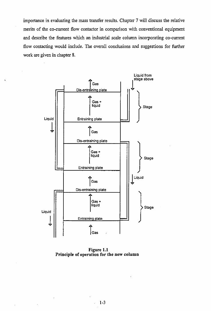
beneath. The gas continues upwards to the stage above. A schematic diagram of the
new column is shown in figure 1.1. The version depicted uses external downcomers,
although conventional internal downcomers, which would be simpler to construct,
could be used.
The research work detailed in this thesis was carried out essentially in two parts. The
first part was concerned with developing entraining and dis-entraining sections for the
column which worked hydrodynamically, in other words could provide co-current
flow within each stage whilst maintaining counter-current flow over the column as a
whole up to high gas velocities. This development work is described in detail in
chapter 3. The second part of the research project was concerned with evaluating the
mass transfer performance of the co-current flow contactor using two test systems
representing resistance to mass transfer in either the gas phase or the liquid phase.
This part of the research is described in chapters 5 and 6. The literature review and a
brief review of mass transfer theory are given in chapter 2. Chapter 4 describes
attempts which were made to describe and quantify the flow pattern, which was of
1-2
importance in evaluating the mass transfer results. Chapter 7 will discuss the relative
merits of the co-current flow contactor in comparison with conventional equipment
and describe the features which an industrial scale column incorporating co-current
flow contacting would include. The overall conclusions and suggestions for further
work are given in chapter 8.
Liquid from
Gas
= Dis-entr ininq plate
lstage above
i~· liquid Stage
Liquid Entraining plate = 1 TGas
Dis-entraining plate =
rG~. liquid Stage
~ Entraining plate
TGas
-= Dis-entraining plate
rG~. liquid
Liquid Stage
Entraining plate = TGas
1
Figure 1.1 Principle of operation for the new column
1-3

•
CHAPTER TWO
Chapter 2.
Literature review and theory
2.1 Scope
This chapter is concerned with the published literature which is of relevance to
this project, and is composed of two sections. The first section will detail
published work covering the various systems which have been used for studying
the mass transfer performance of gas-liquid contacting devices, together with a
discussion of basic mass transfer theory. This information was of importance in
deciding on and interpreting the mass transfer experiments detailed in chapters 5
and 6. The second section will deal with papers and patents which describe novel
gas-liquid contactors.
2.2 Mass transfer systems.
There are many systems which can be used for evaluating the mass transfer
performance of gas-liquid contacting devices, and the results can be expressed in a
number of ways. Perhaps the simplest way of expressing the performance of a gas
liquid contacting stage is the Murphree efficiency. This represents the fractional
approach to equilibrium, and is frequently quoted in the results of distillation
experiments. The vapour side Murphree stage efficiency for a contacting stage
separating a binary mixture is given by;
E = Y" - Y".1 m • (2.1)
YII - Y"+I
Where Y n is the mole fraction of one component in the vapour leaving stage n,
Yn+1 is the mole fraction of the component in the vapour arriving at stage n andYn •
2-1
is the mole fraction of the' component in vapour which would be in equilibrium
with the liquid stream leaving stage n.
The problem with Murphree efficiencies is that for a given contactor operating at
set flow rates, the Murphree efficiency will depend on the system being
investigated, and on the concentrations. For example, a contactor which gives a
Murphree stage efficiency of, say, 60% in an ethanol-water distillation trial, would
not give the same performance in, say a benzene-toluene distillation. Furthermore,
within one column, separating a single mixture, the Murphree efficiencies will
vary throughout the column as the concentrations change (Treybal, 1968]).
An alternative approach, which is often used for absorbers and gas-liquid reactors
is to quote the mass transfer performance in terms of mass transfer coefficients.
These will be defined in detail in section 2.3, and theoretically provide a more
'transferable' measure of mass transfer performance, i.e. one which can be used to
predict the performance of the contactor for systems other than the test system. In
practice however, there are difficulties in using mass transfer coefficients from one
system in predicting the performance of a contactor with another system. These
problems will be discussed in due course.
2.2.1. Inter-phase mass transfer theory.
The following description is based on the two-film theory, also referred to (more
correctly) as the two resistance theory. This type of model is a greatly simplified
representation of the processes occurring in gas liquid contactors, but is the only
available model for which straight forward analytical solutions are possible.
Diffusion and inter-phase mass transfer in gas-liquid contacting devices is due to
the departure from eqUilibrium between the two phases. At any point in a
contactor the bulk liquid composition will not be in equilibrium with the bulk gas
composition with which it is in contact. It is usual to assume, however that the
elements of gas and liquid at the interface itself are at equilibrium. This
2-2

assumption implies that there is negligible resistance to mass transfer at the
interface itself. The evidence appears to suggest that this is indeed the case for
most normal systems (Treybal, 1968]), the exceptions being cases involving
surface active agents and other substances which affect the interfacial properties.
Consider an arbitrary point in a gas-liquid contactor. Component A is diffusing
through an inert gas and into the liquid. Evaporation of the liquid into the gas, and
, dissolution of the inert gas in the liquid are ignored. The concentration profile
shown in figure 2. I will develop. A concentration gradient exists in both phases,
providing the driving force for the mass transfer. The diffusing component
transfers from the bulk of the gas to the interface, and then from the interface into
the bulk of the liquid.
Concentration of A
Gas
P •• ------...
Distance
Liquid
------C'b
Figure 2.1 - Typical concentration profile during inter-phase mass transfer.
The local mass transfer rate is given by a driving force, multiplied by a mass
transfer coefficient. The concentration difference between the bulk gas and bulk
liquid values cannot be used as the driving force, as these two values are
differently related to the chemical potential, which is the true driving force for
mass transfer. Any mass transfer relation, must therefore be based on the
concentration gradient which exists within anyone phase. Hence the local mass
2-3
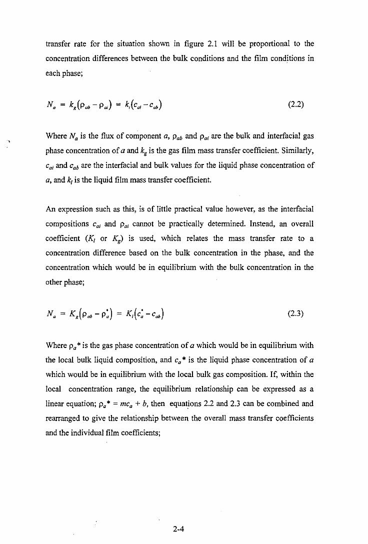
transfer rate for the situation shown in figure 2.1 will be proportional to the
concentration differences between the bulk conditions and the film conditions in
each phase;
(2.2)
Where Na is the flux of component a, Pab and Pal are the bulk and interfacial gas
phase concentration of a and kg is the gas film mass transfer coefficient. Similarly,
Ca; and Cab are the interfacial and bulk values for the liquid phase concentration of
a, and k/ is the liquid film mass transfer coefficient.
An expression such as this, is of little practical value however, as the interfacial
compositions Ca; and Pal cannot be practically determined. Instead, an overall
coefficient (K/ or Kg) is used, which relates the mass transfer rate to a
concentration difference based on the bulk concentration in the phase, and the
concentration which would be in equilibrium with the bulk concentration in the
other phase;
(2.3)
Where Pa * is the gas phase concentration of a which would be in equilibrium with
the local bulk liquid composition, and Ca * is the liquid phase concentration of a
which would be in equilibrium with the local bulk gas composition. If, within the
local concentration range, the equilibrium relationship can be expressed as a
linear equation; Pa * = mCa + b, then equations 2.2 and 2.3 can be combined and
rearranged to give the relationship between the overall mass transfer coefficients
and the individual film coefficients;
2-4

I I m = -+-
Kg kg k,
(2.4a,b)
I I I = --+-
K, mkg k,
2.2.2 Gas and liquid controlled systems.
The individual coefficients, kg and k[ represent the individual resistances in the two
phases, whereas the overall coefficients, K[ and Kg both represent the total
resistance, referenced to the concentrations in the liquid and gas phases
respectively. It can be seen from equation 2.4 that the value of m is of importance
in controlling the relative effects of the two film coefficients on the overall
coefficients. If m is very small then the value of k[ has little effect on the overall
coefficient, whereas if m is very large, then kg has little effect on the overall
coefficients.
When the resistance to mass transfer lies predominantly in one phase, the overall
mass transfer coefficient, K[ or Kg becomes equal to the corresponding film
coefficient k[ or kg. The interfacial concentration in the phase which is controlling
(ca; or Pal) will therefore become equal to that which would be in equilibrium with
the bulk concentration in the other phase (ca * or Pa *).
In evaluating the mass transfer perfonnance of a gas-liquid contacting device, it is
desirable to use mass transfer systems in which the resistance to mass transfer is
controlled by either the liquid or the gas phase. This allows the two mass transfer
resistances to be evaluated separately, and hence gives results which should be
more meaningful when applied to other systems. In a system in which one phase
controls the mass transfer, the overall mass transfer coefficient for that phase
becomes equal to the corresponding film coefficient, and is therefore only
dependent on the physical properties and hydrodynamic behaviour within that
phase and does not depend on the processes occurring in the other phase.
2-5
"
The equations given above are for a purely physical mass transfer systems. Many
systems which are used for studying mass transfer in gas-liquid contactors involve
the diffusing species undergoing a chemical reaction in the liquid phase. In this
type of system, the kinetics of the chemical reaction, and the concentrations of any
other reactants in the liquid phase will also affect the mass transfer rate.
Absorption accompanied by chemical reaction can proceed in one of a number of
regimes. Danckwerts [1970] gives a good explanation of the theory and details the
various reaction regimes. Those of interest in the testing of gas-liquid contacting
devices will be mentioned later, as required. A given system can usually be used
in a number of different reaction regimes because the reaction kinetics can be
independently altered by changing the concentrations of the reactants and of any
catalysts present.
The problem in using any chemical system to evaluate mass transfer coefficients is
that the reaction regime must be known. If the reaction regime is incorrectly
assumed then the results are likely to be meaningless.
2.2.3 Systems showing gas side mass transfer resistance.
Three main types of system can be used to evaluate the gas-side mass transfer
resistance in a contacting device (Sherwood & Pigford [1952]).
a) The absomtion or desomtion of a highly soluble gas between a liquid in an inert
carrier gas. If the gas is highly soluble, then the value of m in equation 2.4 is
small, so from equation 2.4 the overall gas-side coefficient, Kg becomes similar to
the individual fym coefficient, kg. Examples of this type of system are rare. The
absorption of ammonia from an ammonia-air mixture into water has been used to
determine the gas-side resistance of equipment, although the authors express
doubts as to whether ammonia is sufficiently soluble in water for the liquid
resistance to be neglected.
2-6
b) Absorption of a gas from a mixture into a liquid in which it undergoes an
instantaneous irreversible chemical reaction. Here, the diffusing species is
extinguished at the surface of the liquid, and so no diffusion of the transferring
species takes place in the liquid film. In order for the gas-side to solely control the
absorption rate, the chemical reaction in the liquid must be sufficiently fast that
the concentration of the diffusing species at the liquid surface, and hence at the gas
interface is zero. Danckwerts [1970] provides equations which need to be satisfied
in order that this condition is met. The most commonly used examples of this type
of system are the absorption of acid gases (not CO2) from a mixture with air into
aqueous caustic solutions (Vidwans & Sharma [1967]). Other systems, listed by
Charpentier [1981], include the reaction between ammonia or amines with
aqueous sulphuric acid and the reaction between sulphur dioxide and aqueous
sodium sulphite solution.
c) Evaporation of a pure, volatile liquid into a gas stream. Here there is no
resistance to mass transfer from the liquid phase, as there can be no concentration
gradient in a pure liquid. The most commonly used example is the humidification
of a dry air stream by water. The main problem with this type of system is that the
latent heat of vaporisation of the liquid causes the temperature of both phases to
change throughout the contacting device, and allowance for this must be made in
the analysis of the results.
2,2.4 Systems showing liquid side mass transfer resistance.
There are two main classes ofliquid side resistance limited systems.
a) The absorption or desorption of a slightly soluble gas between a gas mixture
and a liquid. In this case the value of m in equation 2.4 is very high, and so K/
becomes similar to k/. This type of system is commonly used for determining
liquid side mass transfer resistances. The most commonly used tracer gases are 02'
H2, and CO2, either pure, or mixed with air and absorbed into water. It is
2-7

important that the tracer gas chosen should not undergo any chemical reaction
with the liquid as this may affect the mass transfer rate.
b) Absorption of a gas from a pure gas stream into a liquid. Here, there is no
resistance to mass transfer in the gas phase, as, once again there cannot be a
concentration gradient in a pure gas. Other than those gases mentioned
immediately above, this type of system is rarely used.
An often used variation on the simple absorption system is absorption
accompanied by a chemical reaction. Charpentier [1981] lists some of the
chemical systems which can be used for measuring the various mass transfer and
surface area characteristics of gas-liquid contactors.
The most commonly used chemical systems are those in which oxygen is absorbed
from air, or from a pure oxygen stream, and reacts with a substance in solution.
The most commonly used reducing agents being cobalt catalysed sulphite and
copper chloride. Other systems which can operate in this regime involve the
reaction between CO2 and aqueous carbonate solutions.
As was mentioned above, the rate of absorption in chemical systems is dependent
on factors other than the physical mass transfer coefficient, and can proceed in a
number of regimes. If the physical mass transfer coefficient K{ is to be determined,
then it is usual to choose conditions such that the reaction is sufficiently fast to
maintain the bulk concentration of oxygen at zero, whilst being slow enough that
the diffusing species does not react as it diffuses into the bulk. If the reaction is too
slow, then the bulk concentration of oxygen'will rise above zero, and would have
to be measured. If the reaction is of a rate such that some of the defusing species
undergoes some reaction close to the interface then the mass transfer rate becomes
enhanced. In this case the mass transfer equation can be expressed as;
(2.5)
2-8
E is the enhancement factor due to the chemical reaction, and depends on the
reaction rate and on the value of K, itself. If the reaction rate becomes extremely
fast, then the absorption rate no longer depends on the value of k" and is a function
of the reaction rate, the interfacial surface area, and the gas-side resistance.
Fast reactions have been used by many authors as a method of determining the
total interfacial area in gas liquid absorbers. The most commonly used systems are
the absorption of oxygen into catalysed sodium sulphite solutions (Yagi & Inoue
[1962]) and the absorption of CO2 by alkali solutions (Yoshida & Akita [1965]).
Another reaction used in this regime is the absorption of carbonyl sulphide (COS),
mixed with air, into amine solutions.
Another variation on this technique is one in which an instantaneous, irreversible
reaction occurs at a certain distance from the interface and the reaction rate is
controlled by the transport of the diffusing species to the zone at which the
reaction occurs. The value of k, can hence be determined from the reaction rate.
Examples of systems which have been used in this regime are the absorption of
acid gases into caustic and amine solutions (Sharma & Danckwerts [1970]), and
the reaction between oxygen and thionate (S20/") solutions (Jharveri & Sharma
[1968]). Charpentier [1981] also lists the reaction between gaseous ammonia and
aqueous sulphuric acid as potentially operating in this regime.
2.2.5 Local and average coefficients.
The model detailed in section 2.2.1 applies to a single point in a gas-liquid
contacting device, and as such, cannot usually be applied over the contactor as a
whole. In order to quantify the mass transfer performance of real gas-liquid
contactors, an average mass transfer coefficient is employed. Treybal [1968] casts
doubts over the validity of average mass transfer coefficients, especially in
situations where different hydrodynamic conditions pertain at different points in
the contactor. Unfortunately, they represent the only straight-forward way of
characterising the mass transfer performance of gas-liquid contactor.
2-9
-,
A local mass transfer coefficient is the local mass transfer flux, divided by the
local concentration driving force. An average mass transfer coefficient is
calculated by dividing the total mass transfer rate by some form of average driving
force. It is defining the average driving force which is the major difficulty in using
average mass transfer coefficients. A typical equation giving the total mass
transfer in a contactor would be;
(2.6)
The total surface area, Ai is usually divided by the total volume of the contactor, V
and is expressed as the specific surface area, a. The product of the mass transfer
coefficient and the specific area, KrfI or Kp is known as the volumetric mass
transfer coefficient and allows contactors to be compared in terms of their
effectiveness for a given size.
In most mass transfer trials, all the inlet and outlet flows can easily be measured or
calculated from mass-balances, but the flow pattern, and hence the average driving
force are not usually known, so in the example above, ca * is not a known function
of Cab' For example, consider a contactor in which a pure gas, e.g. oxygen, is being
absorbed into a de-gassed liquid, e.g. water. The total mass transfer rate can be
calculated from the flow rates and the inlet and outlet concentrations. The flow
pattern for the gas phase will not affect the average driving force, as the gas
composition is constant. If the liquid was in plug flow then the liquid phase
oxygen concentration would be zero at the liquid inlet, rising to a value COUT at the
outlet. The average driving force would be the difference between the saturated
oxygen concentration c*, which is constant, and some mean bulk concentration,
intermediate between the inlet and outlet values. If however the liquid phase was
well mixed, then the concentration of oxygen in the liquid phase would be
constant and equal to the outlet concentration COUT' The driving force would be the
difference between this concentration and c*. Hence, for a given mass transfer
rate, assuming plug flow for the liquid phase will give a much lower calculated K,
2-10
than that calculated by assuming well mixed conditions because the driving force
is assumed to be higher.
The real flow situations within a gas liquid contactor will be somewhere between
the two extremes of plug flow and well mixed. Analysing the data in order to
determine an average mass transfer coefficient is relatively straight forward for the
two extreme cases, but less easy for any real cases in between.
Testing methods exist for providing correct mass transfer coefficient data without
the need make assumptions regarding flow patterns, for example by using a pure
substance for one of the phases, or by employing a chemical system in which the
concentration of the diffusing species is maintained at zero in one of the phases.
However, it is the opinion of this author that data such as this is of little practical
use on its own. If this mass transfer coefficient data was to be of use in predicting
the performance of the same contactor operating with a different system in which
the flow pattern was significant, then an accurate knowledge of the flow pattern
would still be required if accurate predictions were to be made. More discussion of
the importance of flow pattern in determining mass transfer behaviour is given in
chapter 4.
2.3 Novel contactors
Many researchers have suggested novel and improved forms of gas liquid
contacting devices. Many of these are concerned with solving some of the specific
problems associated with conventional equipment such as poor liquid distribution,
fouling, foaming and so on. The papers which are considered here are those which
cover novel contactors offering improved capacity by allowing higher gas
velocities.
2-11
2.3.1 Comparing novel contactors.
In comparing the relative merits of different designs of novel contactors, both with
each other and with conventional equipment, the following factors should be
considered.
Capacity
The capacity of a mass transfer column is determined by the maximum allowable
gas velocity, or in some cases, the maximum allowable column liquid loading.
The capacity of a column design will determine the diameter of the column
required to handle a given gas and liquid flow rate.
Most authors use the simple air-water system operating at atmospheric pressure
for determining the hydraulic capacity of their equipment. A conventional tray
column running with this system at atmospheric pressure would have a maximum
air velocity of around I to 2 mls, depending on tray spacing, whilst the maximum
superficial air velocity in a packed column would be around 3.5 mls depending on
the type of packing (Sinnott [1993]). Where systems other than air/water have
been used to measure the hydraulic capacity, the results can be compared with
other systems by evaluating the vapour capacity factor, F v:
(2.7)
Where Uv is the superficial vapour velocity and Pv is the vapour density.
Conventional packed columns would not normally be operated at F v values higher
than about 3.2 kgl/2 m312 S·I.
2-12
Mass transfer performance
The mass transfer performance of a column will determine the height of a column
required to perform a give separation duty. All of the novel column type
contactors are stage-wise contactors in that the contact between the gases and
liquids takes place in discreet stage which are connected to allow counter current
flow of the phases between stages. The mass transfer performance of each stage
will determine the separation efficiency of each stage, which will determine the
number of actual stages required to achieve a given separation. The total height of
the column will, of course, also be determined by the height of each stage.
The different systems for evaluating mass transfer performance were detailed
earlier in this chapter. In the papers reviewed here, the authors have used a variety
of systems, notably ethanol-water distillation, evaporation of water into air, and
absorption of CO2 into water. Performance data for distillation trials is invariably
given in the form of Murphree stage efficiencies, whilst evaporation and
absorption data are usually given in terms of the volumetric mass transfer
coefficients Kp and Kffl. Murphree efficiencies and mass transfer coefficients
quoted for conventional contactors vary widely and depend largely on the mass
transfer system being used.
A further method sometimes used to quote the mass transfer performance of a
contactor is the height of a transfer unit or H.T.V. The total height required for
mass transfer is given by the H.T.V. multiplied by the number of transfer units
(N.T.V.) required, which is calculated from the required separation duty. This
method is mostly used in comparing the mass transfer performance of different
types of tower packing, although some authors use this measure to quote
performance data for columns containing several stage wise units.
2-13
Geometry
Unless a massive reduction in size can be achieved, such as in the case of the
Higee unit mentioned later, a contacting device should ideally be based around a
conventional column shape with a circular cross-section, for ease of construction.
Several authors have produced designs for columns with a square or rectangular
cross-section. In practice, these columns could prove difficult to fabricate,
particularly for high pressures (or vacuum.)
Mechanical complexity
Ideally, the contactor, and its internals should be as simple as possible, in order to
keep fabrication costs Iow. Especially for atmospheric pressure duties, a large
column with simple internals may still prove more cost-effective than a more
compact, but complex column. At higher pressures the cost of the pressure vessel
becomes much more significant in comparison with the cost of the internals, so a
smaller, more complex column becomes more cost effective (Robinson [1991]).
Contactors with moving parts may also give problems with long term reliability
and fouling.
Pressure drop
This should ideally be as Iow as possible, although high pressure drops could be
tolerated if the apparatus could be significantly intensified. In the case of vacuum
distillation, the pressure drop determines the column bottom pressure, and hence
the bottoms temperature. If the pressure drop is too high the bottoms temperature
will become too large leading to product damage or the loss of any other
advantages for which vacuum distillation was initially selected.
A typical pressure drop range for a sieve tray operating normally would by 50 to
70 mmWG (McCabe et al [1993]). Pressure drops in packed columns vary
2-14
.,
considerably, but would typically be between 20 and 60 rnrnWG/m of packing.
(Billet [1995])
The ideal contactor for a given separation duty is the one offering the lowest total
lifetime costs, these being composed from a combination of the capital costs and
the operating costs. The capital cost of a separation column will depend on its size
and complexity, while the operating costs will depend on the pressure drop. For a
novel contactor to be of practical use, it would have to offer a good compromise
between the conflicting ideals of small size, simple construction and low pressure
drop; a compact column will not be competitive if it is prohibitively complex to
manufacture or suffers a massive pressure drop, whilst a column with a very low
pressure drop will not be competitive if it is of massive size or is prohibitively
complex.
In industrial practice the compromise tends to be weighted towards columns
offering the lowest pressure drop, as operating costs tend to be more significant
over the column lifetime than the capital costs. This is probably why none of the
contactors discussed in this review have achieved widespread industrial
application. Most recent developments in column technology have been towards
providing internals offering lower pressure drops whilst maintaining capacity and
mass transfer performance (Strigle [1994)). In some cases however, the
compromise will be weighted towards more compact columns. These cases will be
discussed further in chapter 7.
2.3.2 Review of novel contactors
Suggested designs for advanced gas liquid contactors are reviewed below. The
papers reviewed are those which suggest improvements in the capacity of gas
liquid contactors by allowing higher gas velocities. Papers which suggest co
current flow within stages, without making any claims with regard to gas velocity
are also covered. Static contactors (those with no moving parts) are reviewed first,
then rotational contactors are covered.
2-15
Static gas-liquid contactors.
Papers and patents detailing static contactors are reviewed here, in historical order.
Underwood's patent.
Underwood [1936] suggested that gas-liquid mass transfer apparatus could
become more compact if co-current flow was used within each stage, whilst
maintaining counter-current flow over the equipment as a whole. The Patent
includes a suggested apparatus which consists of a number of vertical columns,
each representing a single stage. The gas and liquid flow up the column and are
separated from each other at the top. The gas passes to the bottom of the next
column, and the liquid flows by gravity to the bottom of the previous column.
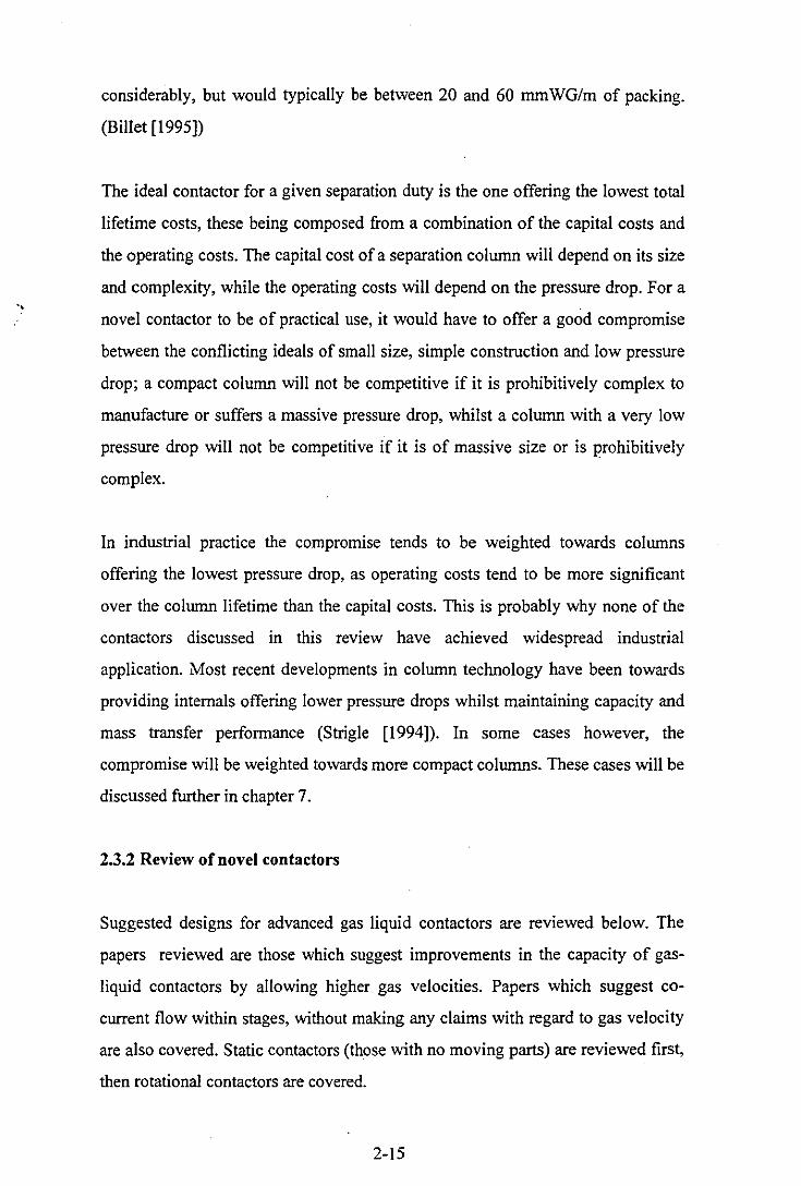
Patterson's patent, figure 2.2
Patterson [1950] suggested a form of tray in which the liquid is entrained by the
gas flowing through nozzles. The liquid fills the lower compartment of the plate
and overflows into the gas nozzles, where it is entrained. The gas liquid mixture
flows in risers through another solid plate, and impacts onto deflecting baffle
plates, dis-entraining the liquid. The liquid then collects on the upper plate, and
flows down to the plate beneath through a conventional downcomer.
No claims are made with respect to hydraulic or mass transfer performance, and
no other papers covering this device could be found.
2-16
Baffle Plates
Gas flow
Liquid from stage above
•
Entrainment nozzles
Figure 2.2 - Patterson's contactor
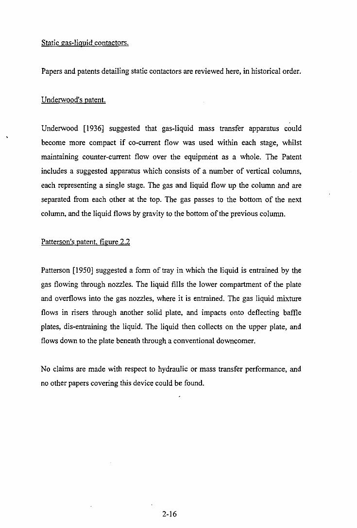
Cannon's contactor, figure 2.3.
In this device, described by Cannon [1952), the gas flow arriving underneath a
plate flows through a venturi type constriction before being mixed with liquid
flowing down from the plate above. The gas-liquid mixture then flows through a
V-tube before being directed downwards at the plate, with the aim of dis
engaging the two phases. The liquid collects on the surface of the plate and flows
down to the venturi contactor on the plate beneath. The gas reverses direction and
continues up the column. In an alternative version to that shown the figure, the
liquid entering the venturi contactor is from the pool on the plate, and the liquid
flows from plate to plate by conventional downcomers.
No performance data was given, and it is not made clear whether a test column
was ever constructed.
2-17

Ravier's patent
Downcomer
nozzle
Liquid from stage above
Gas flow
Figure 2.3- Cannon's contactor
In the device patented by Ravier [1954], the liquid and gas arriving at each stage
are mixed in a venturi-type device, in which acceleration of the gas phase is used
to create a suction effect for the liquid. The author states that the high acceleration
rate for the liquid phase and the high degree of turbulence in the venturi throat
give excellent mass transfer. The gas liquid mixture passes through a pipe to a
phase separator, such as a cyclonic device. The liquid collected is then sucked into
the venturi pump on the stage beneath, whilst the gas flows up to the stage above.
The device consists of venturi pumps and ,separators connected by a network of
pipes and would not be compatible with a conventional column geometry.
No claims are made as to the velocities which can be achieved although the author
claims that his apparatus would be significantly more compact than an equivalent
bubble cap column. A similar device has also been patented by Kruichenko
[1959].
2-18
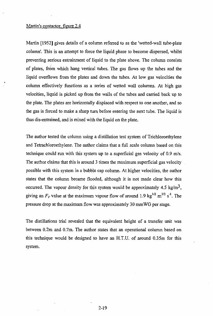
Martin's contactor, figure 2.4
Martin [1952] gives details of a column referred to as the 'wetted-wall tube-plate
column', This is an attempt to force the liquid phase to become dispersed, whilst
preventing serious entrainment of liquid to the plate above. The column consists
of plates, from which hang vertical tubes. The gas flows up the tubes and the
liquid overflows from the plates and down the tubes. At low gas velocities the
column effectively functions as a series of wetted wall columns. At high gas
velocities, liquid is picked up from the walls of the tubes and carried back up to
the plate. The plates are horizontally displaced with respect to one another, and so
the gas is forced to make a sharp turn before entering the next tube. The liquid is
thus dis-entrained, and is mixed with the liquid on the plate.
The author tested the column using a distillation test system of Trichloroethylene
and Tetrachloroethylene. The author claims that a full scale column based on this
technique could run with this system up to a superficial gas velocity of 0.9 mls.
The author claims that this is around 3 times the maximum superficial gas velocity
possible with this system in a bubble cap column. At higher velocities, the author
states that the column became flooded, although it is not made clear how this
occurred. The vapour density for this system would be approximately 4.5 kg/m3,
giving an Fv value at the maximum vapour flow of around 1.9 kgl/2 m 3/2 S·I, The
pressure drop at the maximum flow was approximately 30 mm WG per stage.
The distillations trial revealed that the equivalent height of a transfer unit was
between 0.2m and.0.7m. The author states that an operational column based on
this technique would be designed to have an H.T.U. of around 0.35m for this
system.
2-19

Column wall -----Gas flow --+-.l.
Contacting 1-+------ tubes
Figure 2.4 - Martin's contactor
Berrv's contactor. figure 2.5
In this column, detailed by Berry [1958], the liquid on each stage is picked up by
the gas which is deflected to flow across the column. The liquid is then dis
entrained from the gas flow when the gas flows upwards towards the next stage,
with the liquid impacting onto the wall of the column and dropping down onto the
stage beneath.
Investigations were carried out using air-water in a rectangular cross section
column, although a diagram for a more 'conventional circular cross sectioned
column is also given. The maximum air velocity, based on the overall column
cross section was 3.3 mls. At higher gas velocities, some form of flooding
prevented the column from operating. The pressure drop at maximum air flow was
between 25 mm WG and 50 mm WG, depending on the liquid loading.
2-20

Distillation trials, using the ethanol-water system, revealed a maximum Murphree
efficiency of 50 %.
Liquid impacts on wall
Liquid pool forms
r Gas flow .. -::;~~~u spray
H acros column
Figure 2.5 - Berry's contactor
Manning's contactor. figure 2.6.
The device detailed by Manning [1964] is based on the principle of using
centrifugal separation to allow a perforated plate to operate at a higher gas
velocity, whilst preventing excessive liquid entrainment to the stage above. In fact,
the device functions in a similar way to the other co-current flow contacting
devices described by the other authors mentioned here. The gas-liquid mixture is
formed on a small perforated tray area. This mixture then flows through guide
vanes which cause the whole gas flow to form a vortex, causing the liquid drops to
be thrown to the column wall. The gas then flows upwards to the stage above,
whilst the liquid is collected from the wall, and flows through a central
downcomer to the stage beneath.
2-21
,
Hydrodynamic investigations were carried out using air-water in a 30 cm
diameter column. The maximum superficial air velocity achieved was 4.5 mls. No
pressure drop figures were reported. The author does not state what occurs at
higher gas velocities. The device was based on a single contactor on each plate,
using the column wall as the dis-entrainment surface. Scaling up to larger column
diameters would result in large stage heights, if the LID ratio of the centrifugal
phase separator was to be preserved.
Distillation tests were carried out using a iso-octane-toluene mixture in a 7.5 cm
diameter column, and a tray efficiency of 'about 50%' was reported. The author
claims that the stage efficiency would approach 100% if complete liquid
atomisation on the tray was reached. This would seem unlikely, especially with
systems in which the gas side controls the mass transfer.
The contactor ofNikolaev and Zhavoronkov. figure 2.7
This design, given by Nikolaev and Zhavoronkov [1965], is based around the
principle of using co-current contacting within each stage whilst maintaining
counter-current flow between the stages. This device uses downward co-current
flow of liquid and gas, which the authors claim gives better mass transfer than
upward co-current flow. Using downward co-current flow has the obvious
disadvantage that the gas is forced to change direction through 1800 on entering
and leaving each stage. Each contacting device includes helical guide vanes in
order to impart a rotational motion to the gas, with the aim of directing the liquid
onto the walls of the tube.
Hydrodynamic investigations with air and water revealed a maximum superficial
air velocity of 7 mls. At higher air velocities, the authors found that liquid
entrainment to the stage above became excessive. The gas velocity in the
contacting regions at this point was 35 mls. The pressure drop per stage at the
maximum gas flow was between 300 and 500 mm of water, depending on the
liquid loading.
2-22

Mass transfer in the device was investigated by studying the absorption of C02
into water from a C02 -air mixture. The results are given in terms of Kp values.
Although the authors do not say what assumptions regarding flow pattern were
made in determining the driving force. The Kp value increased with gas flow and
with liquid load up to a ma-.:imum of 1.80 S-I. The Kp value being referred to the
effective volume of one contacting stage.
Static guide vanes
Liquid collects
".,""
,
j t Gas tlow
Perforated plate
distributor
Downcomer
Figure 2.6 - Manning's contactor
2-23
Gas vortex fonns
Gas flow
Downcomer
. . '. Liquid
distributor
Figure 2.7 - The contactor of Nikolaev and Zhavoronkov
Was' Patents. figure 2.8
This series of patents were concerned with a gas liquid contactor based on the
principle of co-current gas-liquid flow within each stage, followed by phase
separation. Many variations of this idea are presented. The first three patents
[Was, 1965a,b,c] describe a contacting device, attached to a plate, in which the
liquid is entrained into the up flowing gas by one of several means, and then dis
engaged by spinning the gas with fixed guide vanes. The disengaged liquid is then
passed to the stage beneath. The different design variations are mainly concerned
with different constructions for collecting and re-directing the liquid, The variant
shown in the figure, employs a plate with a lower compartment similar to that
suggested by Patterson (see previous description.)
2-24
The fourth patent (Was [1965d]) is concerned with a variant in which the co
current flow contactor is used to effectively replace a conventional bubble cap or
valve. The liquid entrained into the gas comes from the liquid pool on the plate,
and the dis-entrained liquid is returned to the pool. Thus the liquid has the
opportunity to re-circulate (and to by-pass the contactors on the plate).
No performance claims were made for any of the variations.
Downcomer
Liquid from stage above
~
Lower comparttnent of tray
Figure 2.8 - Was' contactor
The contactor ofEidner and Schingnitz. figure 2.9.
Gas vortex forms
~~~=tIt- Static guide vanes «
« •
Liquid collects ~-+4-,,,-:! 111111-- and flows to
stage below
Liquid spray forms
This design, patented by Eidner and Schingnitz [1969] consists of conventional
perforated plates above which are mounted wave-plate liquid separators. The
liquid collected in the separators would then drip back down the plate.
2-25
This device should allow higher gas velocities than conventional perforated plates,
although no numerical performance claims were made,
Wave plate separator
Per~ralted plate
Downcomer
t t
Figure 2,9 - The contactor of Eidner and Schingnitz
The contactor of Zhavoronkov et at figure 2.10.
Zhavoronkov et al [1969] studied a contactor based around the principle of using
co-current contacting within each stage whilst maintaining counter-current flow
between the stages. Upward co-current contacting on each stage takes place in
either circular tubes or rectangular channels attached to each plate. In both cases
the overall column cross-section is circular. The liquid flows into the channels
through small holes at the bottom and is carried up the tubes by the gas in the
annular flow regime. At the top of the tubes the liquid falls out through slits in the
channels. Two variations on the design were given. In the variant shown in the
figure, the liquid from the top of the tubes collects on a separate plate, and flows
down to the bottom of the stage beneath by an external pipe. In the alternative
design the liquid from the top of the contacting tubes is allowed to fall back to the
bottom of the tube and re-circulate. In this version the liquid flows down the
2-26

column in conventional downcomers, hence some liquid would have the
opportunity to bypass the contacting tubes altogether.
Hydrodynamic investigations were carried out using air and water, with the
maximum air velocity in the tubes being 40 mls. Based on the overall cross
section of the column, this would give a superficial gas velocity of around 10 mls
with circular tubes and around 20 mls with rectangular channels, which occupy a
greater fraction of the column area. At higher velocities, the pressure drop became
such that the liquid would not have sufficient head to flow from stage to stage
down the column. From the dimensions of the test column, the pressure drop per
stage would thus appear to be approximately 300 mmWG.
Distillation trials using the ethanol-water system were carried out. In the column
where the liquid only flows up the tube once, stage efficiencies of around 60% are
reported, and this was independent of gas velocity, once the velocity exceeded 15
mls. In the column where the liquid re-circulates through the contacting tubes, the
efficiency varied between 40% and 90% depending on the degree of liquid re
circulation. Contactors with rectangular channels had a higher capacity than those
with circular tubes, because there was less space wasted between the tubes in the
apparatus.
2-27

Phase separators
Liquid from stage above
r r r
~ Liquid to stage below
Contacting tubes
Figure 2.10 - The contactor of Zhavoronkov et aI.
The contactor of Elenkov and Minchev.
The device detailed by Elenkov and Minchev (1971] employs co-current gas
liquid flow in an inclined channel of rectangular cross section. The gas enters the
channel through a rectangular slot at the bottom, where it entrains the liquid which
is flowing across the gas stream. The mixture then flows along tha inclined
channel, upwards and towards the wall of the column. At the top of the channel,
the gas is forced to abruptly change direction, and the liquid impacts against a
curved plate, and returns to the pool above the gas inlet. Liquid flows down from
plate to plate via external pipes functioning as downcomers.
Hydrodynamic and mass transfer investigations were carried out with air-water,
with the humidification of the air being used to measure the mass transfer. The
ma'Cimum superficial gas velocity used was around 5.5m1s, and at this point the
pressure drop was around 50 mm of water for a single stage. No flooding
phenomena were reported.
2-28

•
Mass transfer data was given in terms of gas side mass transfer coefficients. The kg
value rose to a maximum of2.8 Kg sol m2, based on a driving force expressed in
kg of water per kg of dry air. The interfacial area was evaluated separately,
although the authors do not state how this was done. The interfacial area is given
as a correlation in terms of the liquid hold-up and the pressure drop.
The Patents of Tanigawa et al. figure 2.11 .
This series of patents describe devices in which a plate column is improved by the
use of 'contacting structures' which prevent excessive liquid entrainment.
The first patent (Tanigawa et al [1973a]) describes a plate design with a single
large aperture through which the gas rises. Above this is mounted the 'contacting
structure' which consists of a cylinder with a solid 'roof and a perforated wall,
with the perforations directing the flow outwards and downwards, as shown in
figure 2.11. The liquid forms a pool on the plate around the central aperture, and
flows into the gas stream through channels. The liquid is entrained into the rising
gas stream, with the gas liquid mixture flowing into the 'contacting structure'. The
mixture is then directed downwards through the perforated wall, with the liquid
falling back into the pool, and the gas continuing up to the next plate. The liquid
can thus contact the gas more than once, and a vertical baffle, positioned
perpendicular to the liquid flow across the plate prevents the liquid from by
passing the contactor altogether. Conventional downcomers are used to pass the
liquid down from plate to plate.
A second Patent (Tanigawa et al [I 973b]) describes a plate with many smaller
contacting structures similar to the one described above. The contacting structures
have a semi-circular cross section and assist the liquid flow across the plate by
blowing the liquid out of each structure in the direction of flow. Once again,
conventional downcomers are employed.
2-29
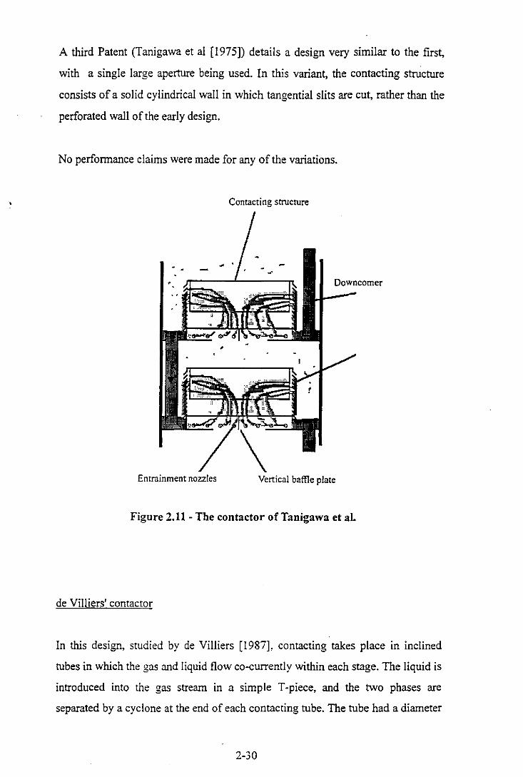
A third Patent (Tanigawa et al [1975]) details a design very similar to the first,
with a single large aperture being used. In this variant, the contacting structure
consists of a solid cylindrical wall in which tangential slits are cut, rather than the
perforated wall of the early design.
No performance claims were made for any of the variations.
Contacting structure
Downcomer
Entrainment nozzles Vertical baffle plate
Figure 2.11 - The contactor of Tanigawa et al.
de Villiers' contactor
In this design, studied by de Villiers [1987], contacting takes place in inclined
tubes in which the gas and liquid flow co-currently within each stage. The liquid is
introduced into the gas stream in a simple T-piece, and the two phases are
separated by a cyclone at the end of each contacting tube. The tube had a diameter
2-30
of approximately SOmm, and the length was varied between 0.7m and 2.2m. This
device would not be applicable to a conventional column geometry
Distillation trials were performed with the ethanol-water system. The maximum
vapour velocity in the tubes was approximately SOmls. The Murphree efficiency
varied, reaching a maximum of around 90%. Up to a vapour velocity of 30mls the
efficiency increased with the gas velocity, above 30 mls it remained more or less
constant. The author suggests that these two regions correspond to different two
phase flow regimes in the contacting tubes. The apparatus was constructed from
stainless steel, so the flow regime could not be observed directly. Using a
correlation for flow in horizontal pipes, the author calculated that the flow at all
gas velocities should be in the annular regime, although at the lower gas velocities,
the flow was close to the wavy flow regime. It was also found that the length of
the contacting tube has very little effect on the stage efficiency. This would
suggest that most of the mass transfer occurs in the gas-liquid mixing region,
rather than in the full length of the tube itself. It is in this region that the highest
levels or turbulence would occur, particularly in the liquid phase.
Centrifugal contactors.
Several researchers have developed equipment for enhanced gas liquid contacting,
based on the use of centrifugal force. In these types of apparatus, the contact takes
place in a circular contacting region which is rotated about its axis by an external
drive.
The 'Hi gee' contactor, figure 2.12.
The device which has attracted the most attention in recent years is the ICI
"Higee" unit, developed in the early 1980s and described by Ramshaw [l983a, b].
The unit consists of a packed section formed into a cylindrical rotor, which spins
inside the casing of the unit. The liquid is distributed into the 'eye' of the rotor and
flows outwards through the packing due to centrifugal force. The liquid leaving
2-31
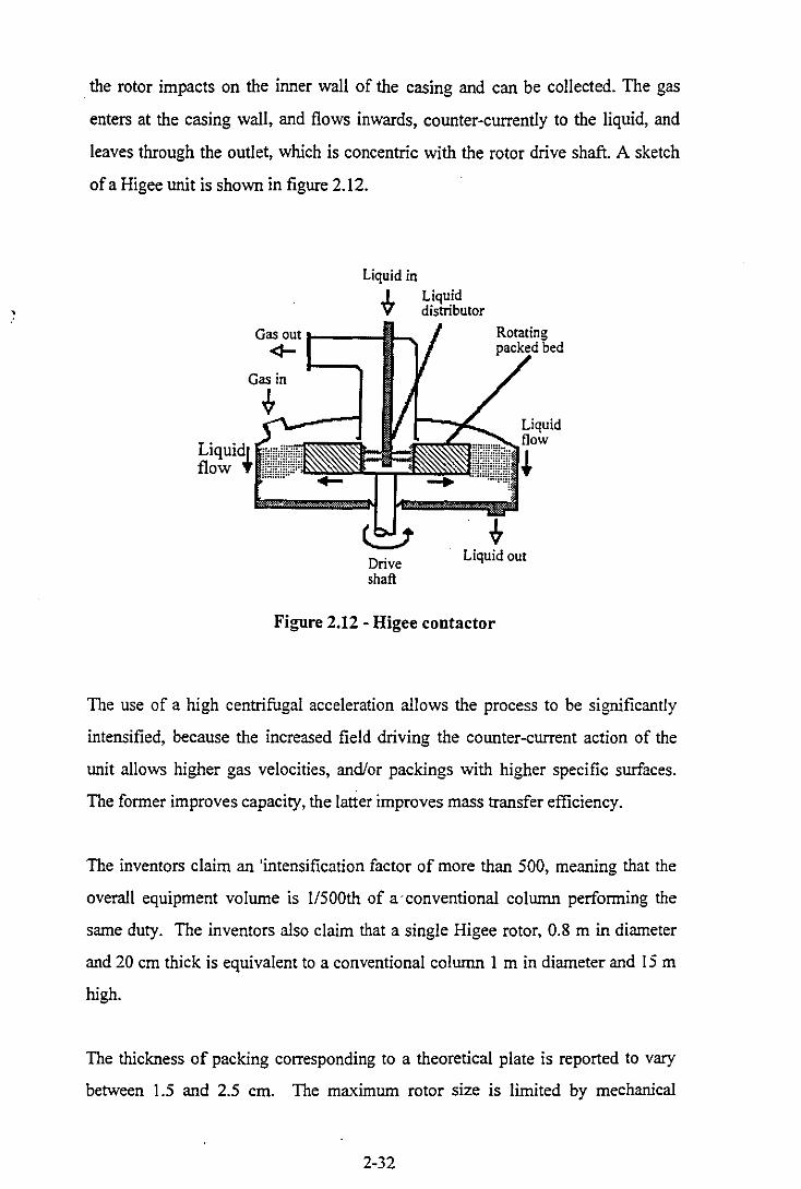
the rotor impacts on the inner wall of the casing and can be collected. The gas
enters at the casing wall, and flows inwards, counter-currently to the liquid, and
leaves through the outlet, which is concentric with the rotor drive shaft. A sketch
of a Higee unit is shown in figure 2.12.
Liquid in I Liquid V distributor
Gas out 1----q...
Drive shaft
Liquid out
Figure 2.12 - Higee contactor
The use of a high centrifugal acceleration allows the process to be significantly
intensified, because the increased field driving the counter-current action of the
unit allows higher gas velocities, and/or packings with higher specific surfaces.
The former improves capacity, the latter improves mass transfer efficiency.
The inventors claim an 'intensification factor of more than 500, meaning that the
overall equipment volume is 1I500th of a 'conventional column performing the
same duty. The inventors also claim that a single Higee rotor, 0.8 m in diameter
and 20 cm thick is equivalent to a conventional column 1 m in diameter and ISm
high.
The thickness of packing corresponding to a theoretical plate is reported to vary
between 1.5 and 2.5 cm. The maximum rotor size is limited by mechanical
2-32
engineering considerations associated with the strength of the packing and the
bearing loads.
One disadvantage of the Higee method is that intermediate feeds or products
cannot be removed from the rotating packing, therefore a single fractionation
column would require two contacting machines, one each for the rectifying and
stripping sections.
The Higee system has been commercially marketed and has found application in
several fields. A review of the commercial progress of Higee was presented more
recently by Fowler [1989]. The author states that three low pressure units were in
commercial use, and that the ability to perform three high pressure, natural gas
treatment processes had been demonstrated. The author states that Higee is only
likely to be cheaper than a conventional column when working at high pressures,
or with expensive alloys. This is because of the mechanical complexity and the
relatively high pressure drop in comparison with conventional equipment. Higee
units would be particularly suitable for offshore processes due to their very
compact size, and, especially, their insensitivity to tilting. A further advantage of
the centrifugal field is that Higee units are insensitive to solids fouling because the
high shear rates inhibit solids from depositing.
A further advantage claimed for Higee is the short residence time. This is
particularly useful in chemically enhanced absorption processes where different
species react at different rates and it is desirable to selectively absorb the quickest
reacting component. An example of such a process, for which Higee contactors
have been applied, is acid gas removal from natural gas streams using tertiary
amines, where it is desirable to selectively remove HzS over COz.
Given the massive potential for intensification that Higee offers, its usage in
industry would appear to be surprisingly limited. Many operators would appear to
be concerned about the reliability and safety of high speed rotational machinery.
2-33
The 'Power Fluidic' contactor
A device similar in principle to Higee, although mechanically simpler, has been
developed by AEA technology, and is referred to as the 'Power fluidic gas-liquid
contactor' (Hanigan, [1993]). This device consists of squat cylinder which is not
filled with any form of packing or plates. The gas enters tangentially at the outer
radius, and forms a vortex, leaving through an outlet port at the centre. Liquid is
sprayed into the centre, where it is given rotational motion by the spinning gas,
causing it to move towards the circumference of the unit. The liquid drops impact
on the wall and fall into the sump at the bottom of the contactor.
Several such contacting units can be included in one separation tower stacked on
top of another and piped together in such a way as to achieve counter current flow
of the two phases over the tower as a whole.
The authors claim that a single fluidic contactor can be equivalent to a packed
column of five times the volume. As with the Higee unit, intermediate products or
feeds cannot be connected to a single contacting unit, although a distillation
system may need more than two units anyway to achieve the desired separation.
Several of these units have been put into commercial use, finding particular
application in steam stripping for organic solvent recovery.
2.3.3 Conclusions.
Of the co-current flow type contacting devices for which capacity claims were
made, only the contactor developed by Zhavoronkov et al. [1969] appears to offer
order of magnitude capacity improvements over conventional equipment. This
was, however, achieved at the expense of an extremely high pressure drop.
Several of the other authors have produced designs which give less spectacular
improvements of between 50% and 100% in comparison with conventional
2-34

equipment. The capacity of these contactors appeared to have been limited by the
point at which entrainment of liquid droplets from each stage to the one above
becomes problematic. It would therefore seem that the most important part of
designing an effective co-current flow contacting stage for use at high gas
velocities is to develop a dis-entraining section capable of removing the liquid
droplets from the gas high velocities required.
Murphree efficiencies quoted for the co-current flow contacting stages varied
between about 50% and 90 %. These figures are broadly comparable with those
for conventional equipment.
2-35

CHAPTER THREE
Chapter 3.
Contactor development.
3.1 Scope
This chapter will be concerned with describing the development process by which the
final design for the contactor was reached. The various stages of the development will
be described in chronological sequence, as the results and conclusions from each
series of experiments, were required in setting the objectives of subsequent
experiments.
As was mentioned in the introduction, each stage of the advanced contactor consists
of an entraining section and a dis-entraining section. Section 3.3 of this chapter will
deal with the development of the entrainer, section 3.4 will deal with the development
of the dis-entrainer.
Details of the hydrodynamic performance of the contactor in its final state of
development are given in chapter 7 and include the limiting gas and liquid flow rates
and an empirical pressure drop correlation.
3.2 General experimental conditions.
All the pilot scale trials were conducted in a 50mm i.d. column constructed from QVF
glassware. The plates which made up the various internal components were
constructed from solid PVC, and were clamped between the QVF sections. Figures
will be provided in this section showing the different experimental rigs as necessary.
During the development stages, air and water were used throughout to represent the
gas and liquid phases respectively. The small scale of the pilot columns was necessary
because of the limited flow rate of air which was available from the compressed air
3-1
mains. It would not have been possible to operate a larger diameter column at gas
velocities which represented a significant improvement over conventional gas liquid
contacting equipment.
3.3 Entrainer development.
The function of the entraining section within each stage is to mix the liquid into the
up-flowing gas stream in such a way as to allow intensive mass transfer to take place
between the two phases. It was decided to achieve this by atomising the liquid into a
spray which would flow upwards with the gas. This method would give the highest
possible surface area for mass transfer, and should give a very high liquid phase mass
transfer coefficient due to the rapid creation of liquid surface and the high level of
turbulence in the liquid at the point of mixing.
The goals in developing the entraining section were to produce a simple device which
could deal with a wide range of gas and liquid flows with the minimum pressure drop,
whilst achieving good liquid atomisation, and hence good mass transfer.
3.3.1 Initial configuration.
The rig which was initially used for entrainer development is shown in figure 3.1. The
gas liquid mixture from the entrainer flowed upwards to the wider, 100 mm column
section where the liquid droplets were collected by the knit-mesh section. The liquid
dripped down from the outside of the knit-mesh cone and onto the collection plate,
from where it could flow to drain, or into it measuring cylinder so that the flow rate
could be measured. Initially the maximum gas flow rate which could be achieved was
1050 lit/min, this being set by the capacity of the rotameter used to measure the air
flow. This flow rate corresponds to a superficial column gas velocity of 8.5 mls.
3-2
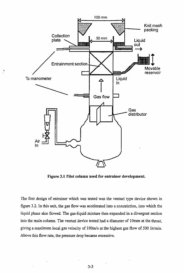
To manometer
Air In
100mm
50 mm
Knit mesh packing
Liquid out
==~~~--~~~
Entrainment section o-_.L
i Liquid in
! reservoir
Gas flow
Gas j.-~ distributor
Figure 3.1 Pilot column used for entrainer development.
The first design of entrainer which was tested was the venturi type device shown in
figure 3.2. In this unit, the gas flow was accelerated into a constriction, into which the
liquid phase also flowed. The gas-liquid mixture then expanded in a divergent section
into the main column. The venturi device tested had a diameter of 10mrn at the throat,
giving a maximum local gas velocity of 100mls at the highest gas flow of 500 lit/min.
Above this flow rate, the pressure drop became excessive.
3-3
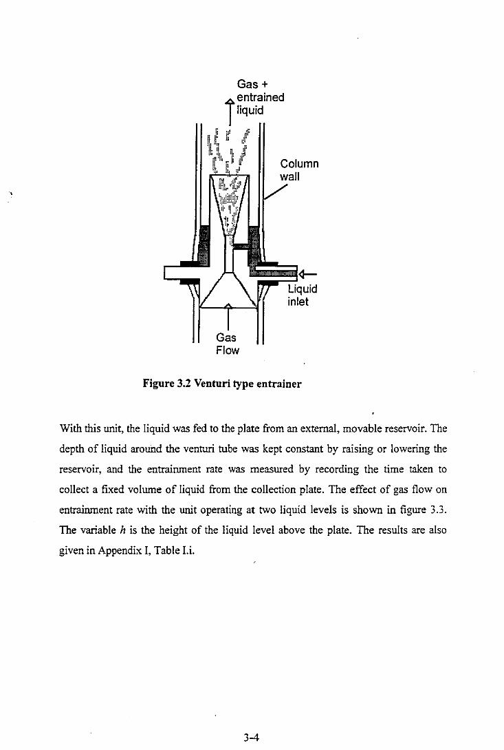
.,
Gas+
jentrained liquid
Gas Flow
Liquid inlet
Figure 3.2 Venturi type entrainer
With this unit, the liquid was fed to the plate from an external, movable reservoir. The
depth of liquid around the venturi tube was kept constant by raising or lowering the
reservoir, and the entrainment rate was measured by recording the time taken to
collect a fixed volume of liquid from the collection plate. The effect of gas flow on
entrainment rate with the unit operating at two liquid levels is shown in figure 3.3.
The variable h is the height of the liquid level above the plate. The results are also
given in Appendix I, Table Li.
3-4
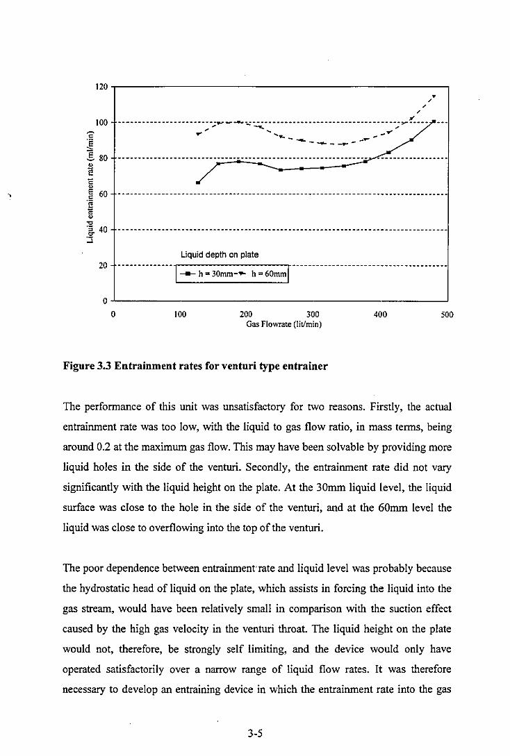
.,
" i!
120.-------------------------------------------------,
/ /
100 ---.------- ---- -------- --..,. - ..... -:,:-- -- - - ----- -- - - - -- -- ----- --- - --- -- ---,.-!----~~ ~ / .... ... ..... - _ ....
-----...--~
• /
I 60 ------------------------------------------------.----------------.-----------------'e E " ."
.~ 40 --------.-------.---------.--------------------------------------------------------::i
Liquid depth on plate
20 -00-00-0000-001 ___ h=30mm-.... h=60mml-oooooooooo-oo-oo-oooo------oooooooo---
O~--------------------------------------------~
o 100 200 300 400 500 Gas Flowr.t. (lit/min)
Figure 3_3 Entrainment rates for venturi type entrainer
The performance of this unit was unsatisfactory for two reasons. Firstly, the actual
entrainment rate was too Iow, with the liquid to gas flow ratio, in mass terms, being
around 0.2 at the maximum gas flow. This may have been solvable by providing more
liquid holes in the side of the venturi. Secondly, the entrainment rate did not vary
significantly with the liquid height on the plate. At the 30mm liquid level, the liquid
surface was close to the hole in the side of the venturi, and at the 60mm level the
liquid was close to overflowing into the top of the venturi.
The poor dependence between entrainment rate and liquid level was probably because
the hydrostatic head of liquid on the plate, which assists in forcing the liquid into the
gas stream, would have been relatively small in comparison with the suction effect
caused by the high gas velocity in the venturi throat. The liquid height on the plate
would not, therefore, be strongly self limiting, and the device would only have
operated satisfactorily over a narrow range of liquid flow rates. It was therefore
necessary to develop an entraining device in which the entrainment rate into the gas
3-5

stream was a much stronger function of the liquid height on the plate. In the venturi
device, the hydrostatic head which helped drive the liquid into the venturi throat
depended on the depth of liquid on the plate, but the area available for flow into the
throat was constant, set by the diameter of the tube which carried the liquid into the
throat. In order to increase the dependence of liquid entrainment rate on liquid height,
a device in which the area for liquid flow depended on the liquid height was required.
A construction which allowed this was a simple weir.
3.3.2 Weir type entrainer.
The weir type entrainer which was tested consisted of a section of tube extending up
from the entrainment plate (see figure 3.4). Initially, a tube of 19mrn i.d. was used.
The liquid pool on the plate overflowed the wall of this tube causing liquid droplets to
be sheared off and carried upwards with the gas stream. Using the movable reservoir
as before it became difficult to control the liquid level on the plate as the device was
capable of rapidly entraining whatever additional liquid flow it received on moving
the reservoir. The reservoir was then replaced by a peristaltic pump, which allowed
the liquid flow rate to the entrainer to be controlled.
As can be seen from figure 3.4, each entrainment plate in the test column contained
only one entrainment tube, although it is envisaged that larger scale columns would
contain plates with many such tubes, arranged similarly to bubble cap units or sieve
holes on a conventional tray. The design of an industrial scale column will be
discussed further in chapter 7.
The single weir type device proved capable of entraining a wide range of gas and
liquid flows without excessive pressure drop, although at very low gas flows (less
than about 100 lit/min) liquid weeped down through the tube. With this device,
increasing the depth ofliquid on the plate increases the area available for flow into the
gas stream (because the height of liquid above the top of the entrainment tube
increases) as well as increasing the hydrostatic head driving the flow. On changing the
flow of liquid to the plate, the liquid level changed slightly, and the device rapidly
3-6
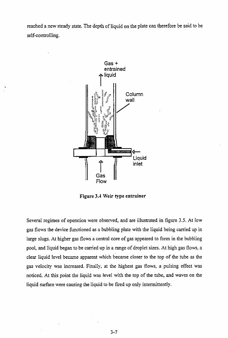
reached a new steady state. The depth of liquid on the plate can therefore be said to be
self-controlling.
Gas + entrained
,liqUid
, Gas Flow
Column wall
Liquid inlet
Figure 3.4 Weir type entrainer
Several regimes of operation were observed, and are illustrated in figure 3.5. At Iow
gas flows the device functioned as a bubbling plate with the liquid being carried up in
large slugs. At higher gas flows a central core of gas appeared to form in the bubbling
pool, and liquid began to be carried up in a range of droplet sizes. At high gas flows, a
clear liquid level became apparent which became closer to the top of the tube as the
gas velocity was increased. Finally, at the highest gas flows, a pulsing effect was
noticed. At this point the liquid was level with the top of the tube, and waves on the
liquid surface were causing the liquid to be fired up only intermittently.
3-7

Increasing gas velocity
Figure 3.5 Operating regimes for weir type entrainer
In order to prevent this pulsing effect, a minor change to the design was made. Two
V -notches 10mm wide and 20mm deep were cut in the side of the entrainment tube,
allowing the entrainment rate to vary more gradually with the liquid level. With this
design, the liquid level established itself at a point below the top of the entrainment
tube, with the liquid flowing through the V -notches into the gas stream. In this case,
the area available for flow into the gas stream would increase in proportion to the
square of the liquid height above the bottom of the notch. This design should also
ensure that, in a larger scale column with many tubes on each plate, each tube would
be functioning correctly and a situation could not arise in which some tubes were dry
and acting a by-passes for the gas. Entrainment tubes with this design of 15mm,
20mm, and 25mm i.d. were tested in order to determine how the tube diameter affects
the en trainer pressure drop.
The pressure drop results for the final entrainer design using three different tube sizes
can be seen in figures 3.6 to 3.8. The results for the 25mm entrainment tube were
obtained using the higher capacity test rig 'which will be described later. The results
can also be found in Appendix I, Table l.ii
3-8

liquid load
• Dry ,. 0.23 lit/min • 0.7 lit/min ... 1.2 lit/min :z: 1.7 IitImin I 500~========================================~ __ ~ , 400 ---------------------------------------------------------------------- ___ .. ____ _
0300 ~ E S 0.. 200 Cl
100
, 11
----------------------------------------------------------,,--------------------
i 11 .. --------------------------------------------1------.----------------------------
i .. " ,. 11
------------------i-----~----·------------------------------------------------,. 11
11 11
o+_----+-----~--~~--~-----+----_+----~----~ o 200 400 600 800
Gas flow (Iit/min)
Figure 3.6 Pressure drop curves for 15mm entrainer
Liquid load
• Dry ,. 0.23 lit/min • 0.7 lit/m in ... 1.2 lit/min :z: 1.7 lit/min I 300f=========================================L---,
250
~200
o ~ E 150 S 0.. Cl
100
ill .. • .. 11
-----------------------------------------------------------i----;;--------------,. ! 11
-------------------------------------------;;---1----;:-------------------------
I : • ---------------------------------~---~---------------- ------------------------I • ,.
:I: X i ~ ..... • . .. .... . 50 --------------------~ ___ y ________ II--- _________________________________________ _
... '" . ' 11
11
O+--~---~~-II--~--+_--+---_r---+--_+--~----~--+-~ , , o 200 400 600 800 1000 1200
Gas flow (Iit/min)
Figure 3.7 Pressure drop curves for 20mm entrainer.
3-9

ci s:
Liquid load
• Dry ... 0.7litlmin • 1.2litlmin A 1.7litlmin % 2.1litlminl 200~==================================~ ____ ~, •
150
.. i •
------------------------------------------------------ --------------~-----------
:r • .. •
E 100 .s
:r • ...
---------------------------------------------It--------------or------------------a. o i ...
• :r I , 50 ---------------~-----------------------------------------------------------------
• ... • •
• •
O+--+--+-,-+-·-+-,-+--+-,-+--+-:~--;_~--~,--~--:r_-r--r_,-r~ o 200 400 600 800 1000 1200 1400 1600 1800
Gas Flow (Iitlmin)
Figure 3.8 Pressure drop curves for 25mm entrainer.
3.4 Dis-entrainer development.
The function of the dis-entrainer is to separate the liquid droplets from the gas stream
and collect it in such a way so it can be allowed to flow by gravity to the stage
beneath. The dis-entrainer should be simple in construction, and able to function over
a wide range of gas and liquid flows, and once again, the pressure drop should be as
low as possible.
Droplet separation IS an important industrial unit operation, and many different
methods and types of equipment are in use. Burkholz [1989] reviews the main
methods for droplet separation. The important features required by the droplet
separator being used in this application were that it should be simple, and allow a
relatively uninterrupted flow path for the gas stream. This precluded the use of
devices such as wave plate separators, demistor pads and conventional cyclones. The
3-10
"
method chosen was the use of an axial flow cyclone or vortex tube. In an axial
cyclone, the up-flowing gas stream is set into a vortex motion by a static guide vane at
the bottom of the unit. The spinning motion of the gas causes the liquid droplets to be
thrown outwards by centrifugal force, where they impact on the wall and coalesce to
form a film. The gas continues to flow upwards and leaves the unit at the top.
3.4.1 General experimental conditions.
The rig used in dis-entrainer development is shown in figure 3.9. The liquid was
pumped onto the entraining section at a controlled flow rate by the peristaltic pump.
The liquid which was successfully dis-entrained by the separator was collected from
the base of the dis-entrainer and returned to the liquid reservoir. Any liquid droplets
leaving the dis-entrainer in the gas stream were collected by the knit-mesh cone in the
wider column section and collected via the larger plate. The dis-entrainment
efficiency was determined by measuring the flow rates of the dis-entrained and
carryover liquid streams and is defined by
Dis - entrained liquid flow (3.1)
Dis - entrained liquid flow + Carryover liquid flow
Evaporation of water into the gas stream could safely be neglected from the mass
balance as this could be shown to be negligible in comparison with total liquid flow
rates used. It would obviously not be possible to develop a separator which was 100%
efficient, so an arbitrary efficiency target of 95% was set. This represents the point at
which entrainment of liquid droplets would have a negligible effect on the
performance a mass transfer column containing several stages.
3-11
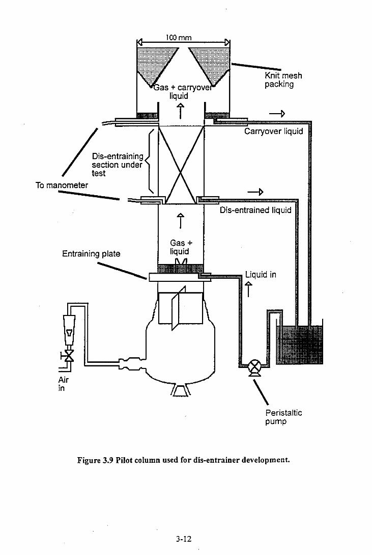
To manometer -Dis-entraining section under test
-
Entraining plate
i Gas + liquid
Knit mesh packing
Carryover liquid
Dis-entrained liquid
~C;:===!!!f-IIIII!IIIII' Liquid in
i
Air in \
Peristaltic pump
Figure 3.9 Pilot column used for dis-entrainer development.
3-12
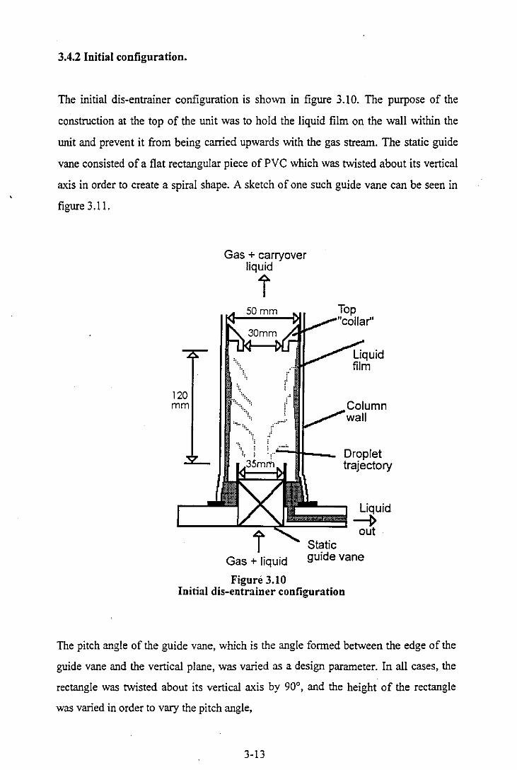
3.4.2 Initial configuration.
The initial dis-entrainer configuration is shown in figure 3.10. The purpose of the
construction at the top of the unit was to hold the liquid film on the wall within the
unit and prevent it from being carried upwards with the gas stream. The static guide
vane consisted of a flat rectangular piece of PV C which was twisted about its vertical
axis in order to create a spiral shape. A sketch of one such guide vane can be seen in
figure 3.1l.
120 mm
Gas + carryover liquid
i 50mm
,/,.; ... :. ,
Column wall
Droplet trajectory
L __ --.l.L~~~~!!!! Li~Uid out
Gas + liquid
Figure 3.10
Static guide vane
Initial dis-entrainer configuration
The pitch angle of the guide vane, which is the angle formed between the edge of the
guide vane and the vertical plane, was varied as a design parameter. In all cases, the
rectangle was twisted about its vertical axis by 90°, and the height of the rectangle
was varied in order to vary the pitch angle,
3-13
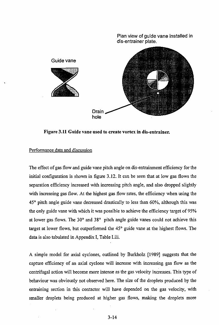
Guide vane
Drain hole
Plan view of guide vane installed in dis-entrainer plate.
Figure 3.11 Guide vane used to create vortex in dis-entrainer.
Perfonnance data and discussion
The effect of gas flow and guide vane pitch angle on dis-entrainment efficiency for the
initial configuration is shown in figure 3.12. It can be seen that at low gas flows the
separation efficiency increased with increasing pitch angle, and also dropped slightly
with increasing gas flow. At the highest gas flow rates, the efficiency when using the
45° pitch angle guide vane decreased drastically to less than 60%, although this was
the only guide vane with which it was possible to achieve the efficiency target of 95%
at lower gas flows. The 30° and 38° pitch angle guide vanes could not achieve this
target at lower flows, but outperfonned the 45° guide vane at the highest flows. The
data is also tabulated in Appendix I, Table Liii.
A simple model for axial cyclones, outlined by Burkholz [1989] suggests that the
capture efficiency of an axial cyclone will increase with increasing gas flow as the
centrifugal action will become more intense as the gas velocity increases. This type of
behaviour was obviously not observed here. The size of the droplets produced by the
entraining section in this contactor will have depended on the gas velocity, with
smaller droplets being produced at higher gas flows, making the droplets more
3-14
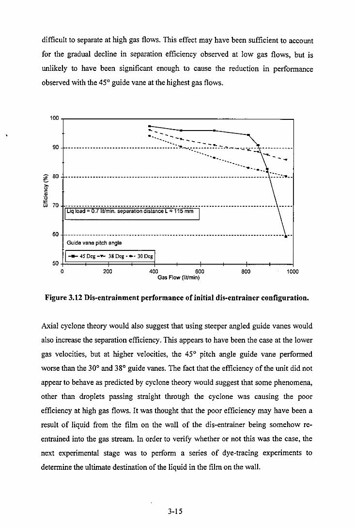
difficult to separate at high gas flows. This effect may have been sufficient to account
for the gradual decline in separation efficiency observed at low gas flows, but is
unlikely to have been significant enough to cause the reduction in performance
observed with the 45° guide vane at the highest gas flows.
100~----------________________________________________ ,
.......... - .....
90 .. --_.- --- .. -- .... -- .... ---- .... -_ .. -- .... --- -:::::: ~::' .. -; --.. -:.-::: -""= -~ - _-..: -.;.._.. .. .... ---- .. --_ .. . '.
~ 80 .... ------- ------ --- .. --- ----- ---- .. -- ---- ...... --- .. -_ .. -- -- -- -- --- -- -_ .. - _______ ...... :---_-_ ... _ .. ~
~ c:
" ~ w 70 Uq load = 0.7 lit/min. separation distance L = 115 mm I
60 .............................................................................. .
Guide vane pitch angle
--- 4S Deg - ... 38 Deg .... 30 Deg I 50+===~===F===+==~--~----~--+---~---r--~
o 200 400 600 800 1000 Gas Flow (liUmin)
Figure 3.12 Dis-entrainment performance of initial dis-entrainer configuration.
Axial cyclone theory would also suggest that using steeper angled guide vanes would
also increase the separation efficiency. This appears to have been the case at the lower
gas velocities, but at higher velocities, the 45° pitch angle guide vane performed
worse than the 30° and 38° guide vanes. The fact that the efficiency of the unit did not
appear to behave as predicted by cyclone theory would suggest that some phenomena,
other than droplets passing straight through the cyclone was causing the poor
efficiency at high gas flows. It was thought that the poor efficiency may have been a
result of liquid from the film on the wall of the dis-entrainer being somehow re
entrained into the gas stream. In order to verify whether or not this was the case, the
next experimental stage was to perform a series of dye-tracing experiments to
determine the ultimate destination of the liquid in the film on the wall.
3-15
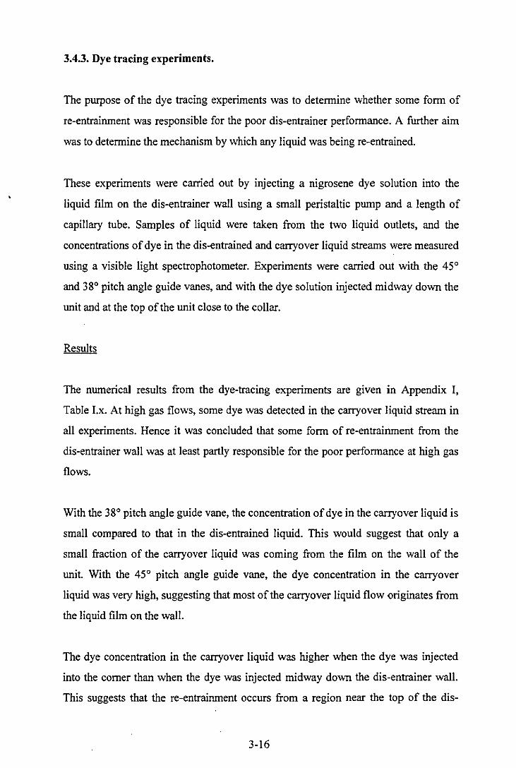
3.4.3. Dye tracing experiments.
The purpose of the dye tracing experiments was to determine whether some form of
re-entrainment was responsible for the poor dis-entrainer performance. A further aim
was to determine the mechanism by which any liquid was being re-entrained.
These experiments were carried out by injecting a nigrosene dye solution into the
liquid film on the dis-entrainer wail using a small peristaltic pump and a length of
capillary tube. Samples of liquid were taken from the two liquid outlets, and the
concentrations of dye in the dis-entrained and carryover liquid streams were measured
using a visible light spectrophotometer. Experiments were carried out with the 45°
and 38° pitch angle guide vanes, and with the dye solution injected midway down the
unit and at the top of the unit close to the collar.
Results
The numerical results from the dye-tracing experiments are given in Appendix I,
Table Lx. At high gas flows, some dye was detected in the carryover liquid stream in
ail experiments. Hence it was concluded that some form of re-entrainment from the
dis-entrainer wall was at least partly responsible for the poor performance at high gas
flows.
With the 38° pitch angle guide vane, the concentration of dye in the carryover liquid is
small compared to that in the dis-entrained liquid. This would suggest that only a
small fraction of the carryover liquid was coming from the film on the wall of the
unit. With the 45° pitch angle guide vane, the dye concentration in the carryover
liquid was very high, suggesting that most of the carryover liquid flow originates from
the liquid film on the wall.
The dye concentration in the carryover liquid was higher when the dye was injected
into the corner than when the dye was injected midway down the dis-entrainer wall.
This suggests that the re-entrainment occurs from a region near the top of the dis-
3-16

entrainer. From this, it was concluded that the re-entrainment was due to part of the
liquid film on the wall being carried upwards, around the collar by the gas stream, and
hence being re-entrained above the collar. The other mechanism which was
considered was that drops of liquid may have been sheared off from the liquid film on
the wall by the gas stream. This possibility was discounted because of the large
centrifugal forces which would have immediately thrown the. drops back outwards
towards the wall.
Conclusions
It was concluded from these experiments with the first configuration that a 45° pitch
angle guide vane was necessary in order to provide sufficient cyclonic action to
capture the droplets within the dis-entrainer, but that use of such an intensive swirl
action caused excessive re-entrainment from the liquid film on the waIl. The next
stage of design process was to develop dis-entrainer designs in which the dis
entrained liquid could be more effectively separated from the fast flowing gas stream.
3.4.4 Further dis-entrainer designs
Several further evolutions of the design were then made with the aim of providing a
means to separate the dis-entrained liquid film from the up-flowing gas in order to
prevent it from being carried upwards. The designs were made with the aim of
allowing the liquid to flow to a caIrn region with little or no gas flow, from where it
could faIl down under gravity and leave the plate. These design evolutions are
illustrated in figures 3.13, 3.15, 3.17 and 3.20. The performance data for the various
designs are given below and in Appendix I,Table l.iv.
3-17
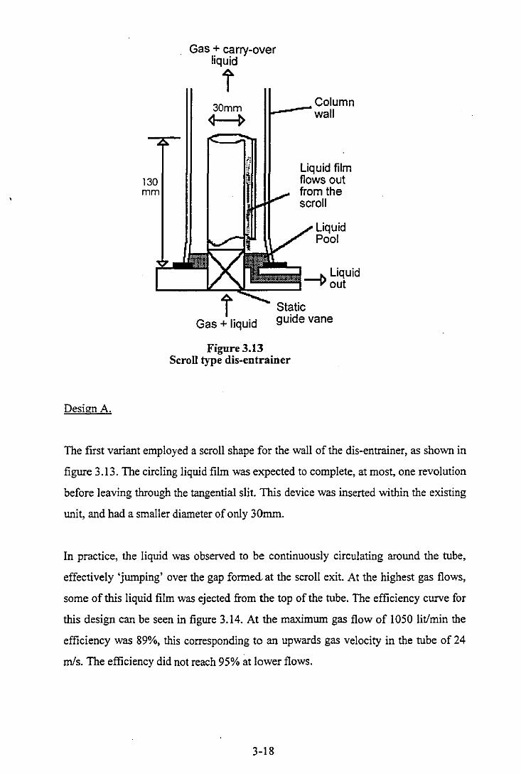
DesiQII A.
130 mm
Gas + carry-over liquid
i 30mm
~
Column '---wall
Liquid film flows out from the scroll
Liquid Pool
~::~~~~;~---" Liquid L --Yout
Static Gas + liquid guide vane
Figure 3.13 Scroll type dis-entrainer
The first variant employed a scroll shape for the wall of the dis-entrainer, as shown in
figure 3.13. The circling liquid film was expected to complete, at most, one revolution
before leaving through the tangential slit. This device was inserted within the existing
unit, and had a smaller diameter of only 30mrn.
In practice, the liquid was observed to be continuously circulating around the tube,
effectively 'jumping' over the gap formed., at the scroll exit. At the highest gas flows,
some of this liquid film was ejected from the top of the tube. The efficiency curve for
this design can be seen in figure 3.14. At the maximum gas flow of 1050 litlmin the
efficiency was 89%, this corresponding to an upwards gas velocity in the tube of 24
mfs. The efficiency did not reach 95% at lower flows.
3-18
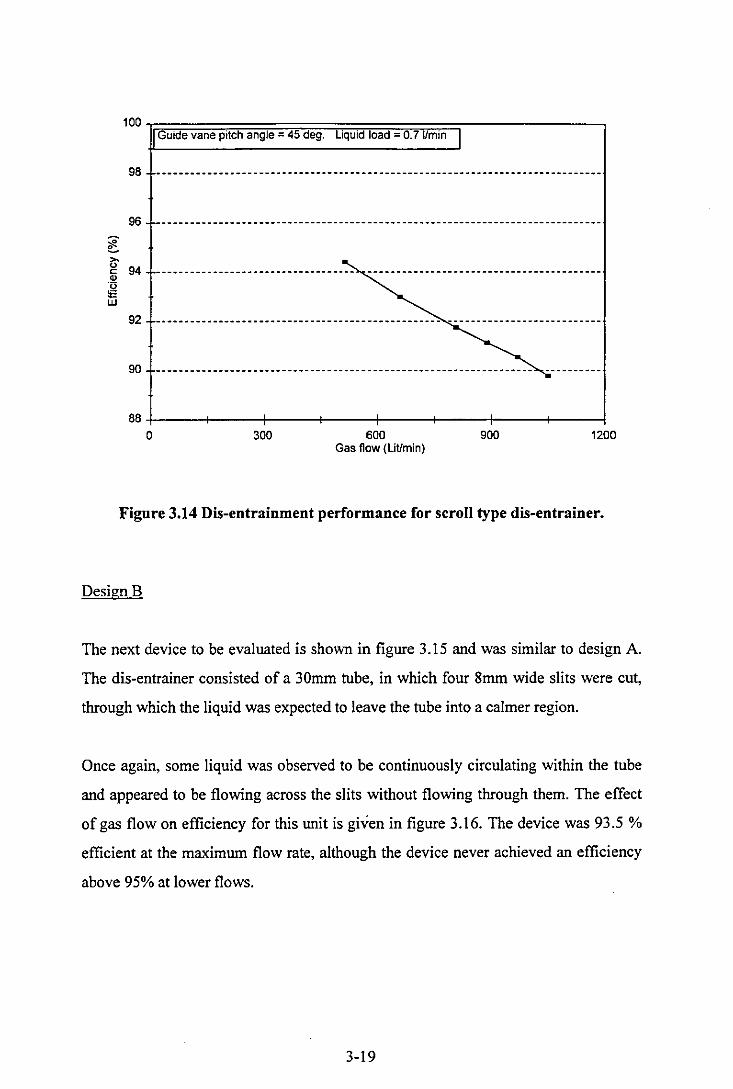
~ ~
100~~====~~~~~~~~~~~-------------, Guide vane pitch angle = 45 deg. Liquid load = 0.7 Umin
98 ------------------------------------------------------------------------------
96 ------------------------------------------------------------------------------
~ " 94 - --- - - - -- - - ---- - - - -- - ---- --- --- -- -- -- - - -- -- - --- ------------- - - - - ----- - -- - ---Q)
~ UJ
92 -------------------------------------------------- ---------------------------
90 ------------------------------------------------------------------ ----------
88+-----~----~----_r----_+----~----~~----r_--~
o 300 600 900 1200 Gas flow (Lit/min)
Figure 3.14 Dis-entrainment performance for scroll type dis-entrainer.
Design B
The next device to be evaluated is shown in figure 3.15 and was similar to design A.
The dis-entrainer consisted of a 30mm tube, in which four 8mm wide slits were cut,
through which the liquid was expected to leave the tube into a calmer region.
Once again, some liquid was observed to be continuously circulating within the tube
and appeared to be flowing across the slits without flowing through them. The effect
of gas flow on efficiency for this unit is given in figure 3.16. The device was 93.5 %
efficient at the maximum flow rate, although the device never achieved an efficiency
above 95% at lower flows.
3-19
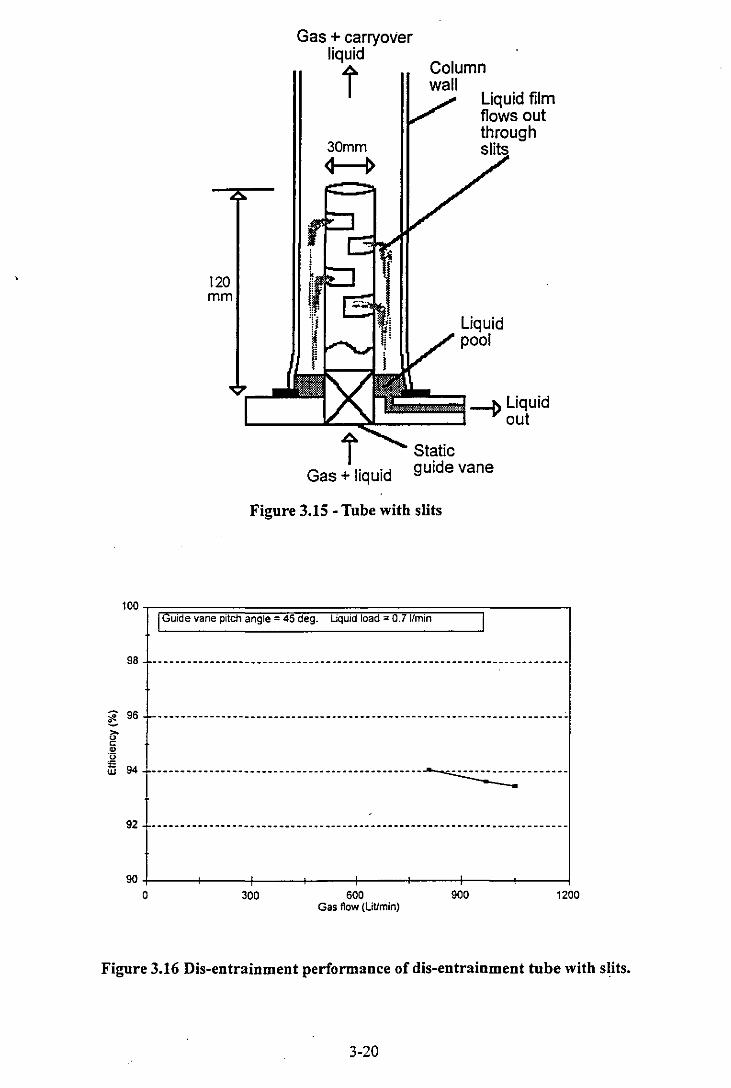
120 mm
Gas + carryover liquid
t 30mm
~
Column wall
Liquid film flows out through
Liquid pool
[~:~l2~~~~~~ Liquid out
Gas + liquid
Static guide vane
Figure 3.15 - Tube with slits
10°Tr~~~~~~~~~~~~~~====~--------' I Guide vane pitch angle = 45 deg. Uquid load = O.7l1min I
98 ••••• _ ••••••••••.••......•..•• _ ••••••••••••.•.•••.••••..........•••• _ ••.
§: 96
g " 'u ~ 94 ............................................... ~ .....•••.
92 ....................................................................... .
90+-----~--~~--~-----+----~----~--__ ~----~ o 300 600 900 1200
Gas flow (LiUmin)
Figure 3.16 Dis-entrainment performance of dis-entrainment tube with slits.
3-20
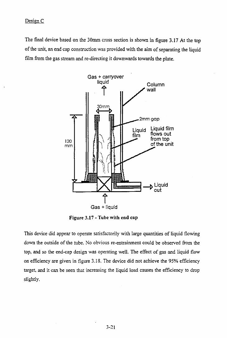
Design C
The final device based on the 30rnm cross section is shown in figure 3.17 At the top
of the unit, an end cap construction was provided with the aim of separating the liquid
film from the gas stream and re-directing it downwards towards the plate.
120 mm
Gas + carryover liquid
i
Liquid film flows out from top
the unit
r~::l2~~;;~ ~ Liquid out
i Gas + liquid
Figure 3.17 - Tube with end cap
This device did appear to operate satisfactorily with large quantities of liquid flowing
down the outside of the tube. No obvious re-entrainment could be observed from the
top, and so the end-cap design was operating well. The effect of gas and liquid flow
on efficiency are given in figure 3.18. The device did not achieve the 95% efficiency
target, and it can be seen that increasing the liquid load causes the efficiency to drop
slightly.
3-21
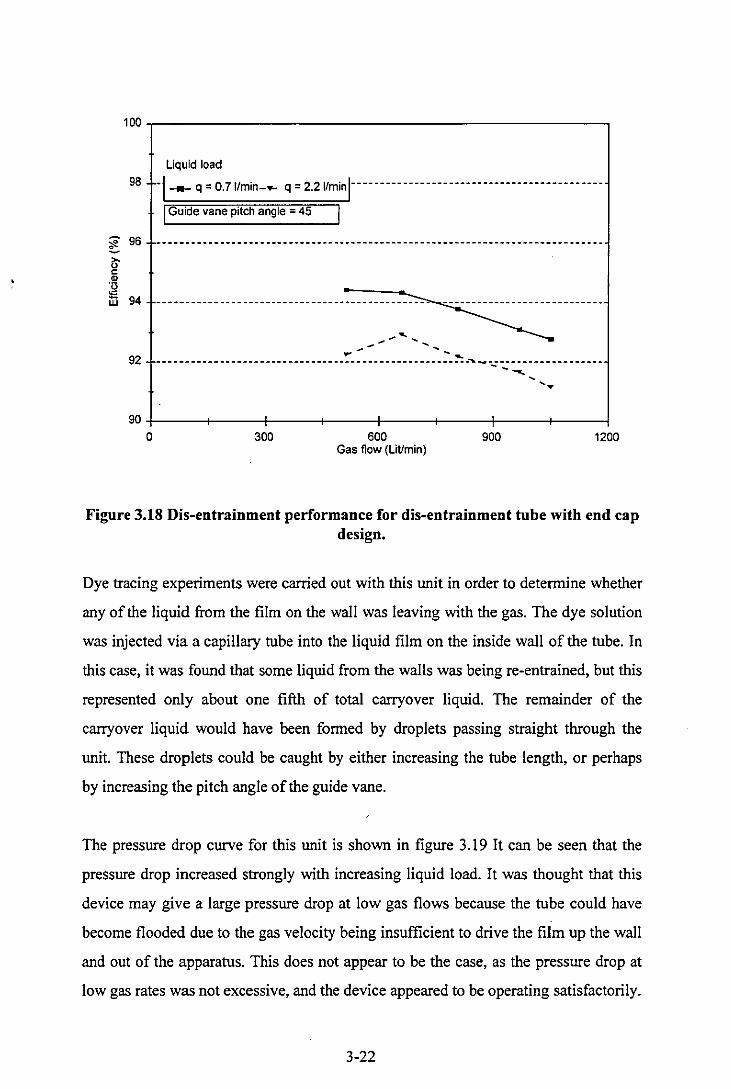
100,----------------------------------------------.
Liquid load
98 -j ___ q = O.71/min-.. q = 2.21/minlnnnnn_nn_nn_nnnnnnnnnnn-
I Guide vane pitch angle = 45
~ 96 e.. ~ c:
" ~ w 94
92 -.- - --- ---. ---.- -- ---- - --- - - --- --~- --- -- --- - - -- - - - - -~-..... _ - - - -_. - --- - - -- - - - ----- """'-
90+-----+-----+-----+-----+-----+-----+-----+---~ o 300 600 900 1200
Gas flow (LiVmin)
Figure 3.18 Dis-entrainment performance for dis-entrainment tube with end cap design.
Dye tracing experiments were carried out with this unit in order to determine whether
any of the liquid from the film on the wall was leaving with the gas. The dye solution
was injected via a capillary tube into the liquid film on the inside waIl of the tube. In
this case, it was found that some liquid from the walls was being re-entrained, but this
represented only about one fifth of total carryover liquid. The remainder of the
carryover liquid would have been formed by droplets passing straight through the
unit. These droplets could be caught by either increasing the tube length, or perhaps
by increasing the pitch angle of the guide vane.
The pressure drop curve for this unit is shown in figure 3.19 It can be seen that the
pressure drop increased strongly with increasing liquid load. It was thought that this
device may give a large pressure drop at low gas flows because the tube could have
become flooded due to the gas velocity being insufficient to drive the film up the wall
and out of the apparatus. This does not appear to be the case, as the pressure drop at
low gas rates was not excessive, and the device appeared to be operating satisfactorily.
3-22
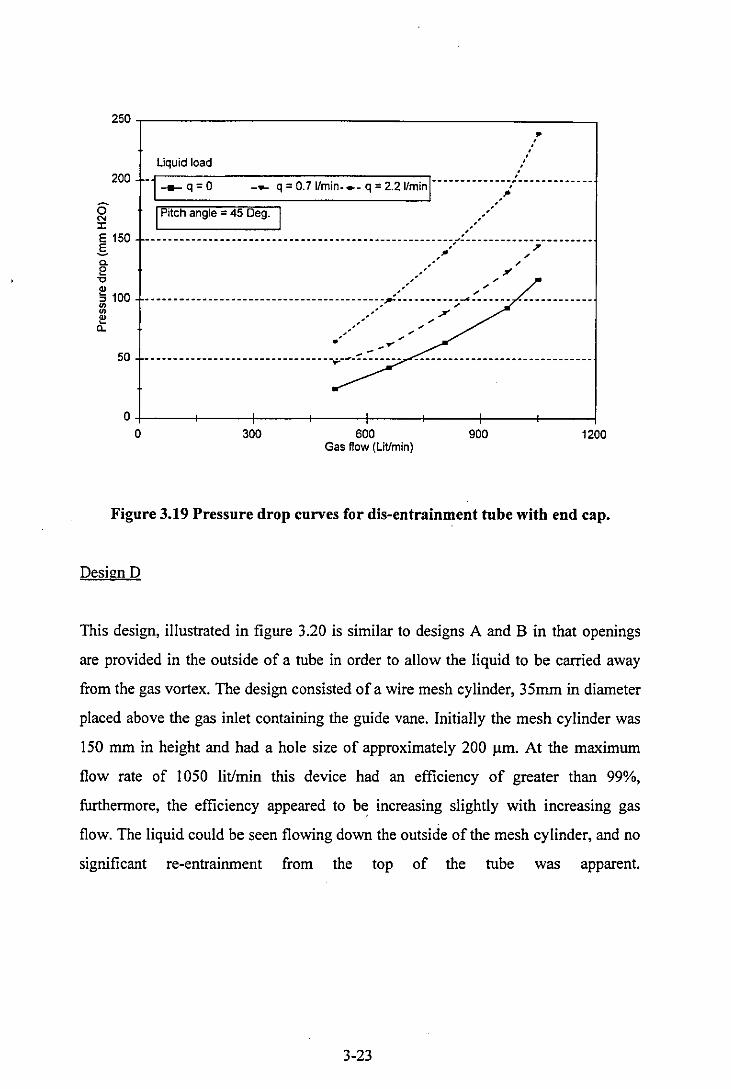
250,---__________________________________________ -.
o N J:
200
E 150 .s Cl. e '0 Q)
5100 ::: i!! 0..
~~~~ :
~ , , , ,
-1--- q = 0 - ..... q = 0.71/min-_- q = 2.21/minlnnnnnn,-;/m-m-m-
I Pitch angle = 45 Oeg. I /,,/' -----------------------------------------------------;~-------------;---------
///~ ~~;'~ " ~
------------------------------------------~-----------~------- -------------, , ,/ ~.-r
" .. ' ...... .' ~ _ ....
50 - - ---- - -- ---- ----- ____ -- .-- --- - - -.. --.-:::: -___ _
0+-----r_--~-----+----~----4-----+_----r_--~ o 300 600 900 1200
Gas flow (Lit'min)
Figure 3.19 Pressure drop curves for dis-entrainment tube with end cap.
Design D
This design, illustrated in figure 3.20 is similar to designs A and B in that openings
are provided in the outside of a tube in order to allow the liquid to be carried away
from the gas vortex. The design consisted of a wire mesh cylinder, 35mm in diameter
placed above the gas inlet containing the guide vane. Initially the mesh cylinder was
150 mm in height and had a hole size of approximately 200 IJ.m. At the maximum
flow rate of 1050 lit/min this device had an efficiency of greater than 99%,
furthermore, the efficiency appeared to b~ increasing slightly with increasing gas
flow. The liquid could be seen flowing down the outside of the mesh cylinder, and no
significant re-entrainment from the top of the tube was apparent.
3-23
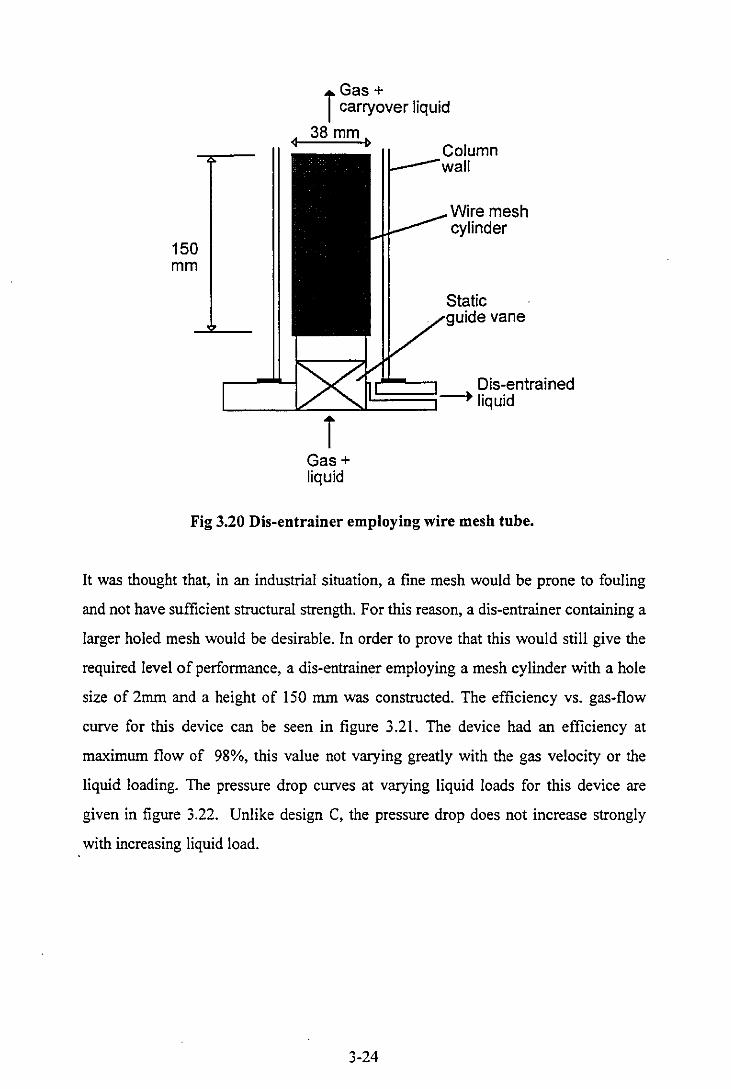
150 mm
TGas + carryover liquid
38 mm~
Static /YUIUI .. vane
[=:~12~~~~~s'-'" Dis-entrained liquid
T Gas+ liquid
Fig 3.20 Dis-entrainer employing wire mesh tube.
It was thought that, in an industrial situation, a fine mesh would be prone to fouling
and not have sufficient structural strength. For this reason, a dis-entrainer containing a
larger holed mesh would be desirable. In order to prove that this would still give the
required level of performance, a dis-entrainer employing a mesh cylinder with a hole
size of 2mm and a height of 150 mm was constructed. The efficiency vs. gas-flow
curve for this device can be seen in figure 3.21. The device had an efficiency at
maximum flow of 98%, this value not varying greatly with the gas velocity or the
liquid loading. The pressure drop curves at varying liquid loads for this device are
given in figure 3.22. Unlike design C, the pressure drop does not increase strongly
with increasing liquid load.
3-24

100,-__________________________________________________ -,
98 ----------------------------------------.. -.::. ... - - - - .... ~----------------------......... ,." .:-:. .... =-.:-: .' / / / ..
~ 96 ~
1'> " " ·0 le UJ 94
Liquid load
1 ___ 0.7 Litlmin - ..... 1.2 Lit/min. +- 1.6 lit/m in 1
92 lG~ide -;an'; pitch angie -,; 45 ---r -- u - - - - - - - - u uu um - - u u m mu -- - - m __
90+-----~----_r----~----_+----~----~r_----~--~ o 300 600 900 1200
Gas flow (Lit/min)
Figure 3.21 Dis-entrainment performance for wire mesh cylinder design with 2mm holes.
100,---------------------------------------------------~
80 - - -- -- --- ---- - --- - -------- --- -- ----- --- -- - - ------- ------ - -- --- - - -.-,:;'_ --------
/-' ",}' , /
.' .. ~ 60 - - -- -- -------- --- - ----- - -- ---- - ----- ---- - -- --- --- - - ----- -,:"'-~ -11"- -.- - -- ----- --
::. " ,. E " , ..§. Liquid load ,_ .. " ,
~ 40 _~ ___ 0.7 Lit/min - ..... 1.2 Litlmin -+- 1.6litlmin f-,/-"::~ m_mumuu _____ _
I Guide vane Pitch angle = 45 I ,/
o+_----~--~-----+----~----~----+_----~--~ o 300 600 900 1200
Gas flow (Lit/m in)
Figure 3.22. Pressure drop curves for wire mesh based dis-entrainer
3-25
Conclusions
Of the four design variants investigated, the wire-mesh based dis-entrainer (design D)
appeared to be the most satisfactory, and was used as the basis for all future dis
entrainer development. The 'end cap' based unit (design C) also showed some
promise, although it was more complicated in construction than the wire mesh based
design, and suffered from a significantly higher pressure drop which increased
strongly with increasing liquid load.
3.4.5 Further development of wire mesh dis-entrainer.
Once a design of dis-entrainer had been developed which worked well up to a gas
flow of 1050 lit/min, it was decided to increase the gas flow capacity of the test rig in
order to determine whether operation at even higher gas flows was feasible. To this
end, the rotameter which had previously been used to measure the gas flow rate was
replaced by an orifice plate which was included in the lower part of the test column, as
shown in figure 3.23. The orifice plate was calibrated with the existing rotameter in
place up to a gas flow of 1050 lit/min. The Cd value was assumed to remain constant
at higher gas flows, this assumption being justified by the fact that the Reynolds
number in the orifice would be well above 10,000 at this point. Equations for
isothermal compressible flow were used both in calibrating the orifice, and in
calculating the gas flow, although using simple non-compressible flow equations gave
very similar figures. With the rotameter removed, the maximum available gas flow
rose to 1700 lit/min, corresponding to a superficial column gas velocity of 13.8 mls.
The maximum gas flow now appeared to be set by the capacity of the regulator which
reduced the pressure from the compressed air mains.
3-26

\ Pressure tappings
T
Knit-mesh section
Dis-entrainer
\~~~~~~J~~~:_--tDis-entrained c liquid
Liquid-. inlet
Pressure tappings
Orifice plate
T Gas inlet
Entrainer
Figure 3.23 Experimental rig with orrifice plate for dis-entrainer performance studies
3-27

It quickly became apparent that the dis-entrainer employing the mesh with 2 mm
holes became ineffective at gas flows higher than about 1100 lit/min, corresponding to
a superficial gas velocity of 9.3 mls. The dis-entrainment efficiency dropped off
sharply with increasing gas flow, displaying similar behaviour to that shown by the
earlier dis-entrainers at lower gas flow rates. The mesh with the 0.2mm holes
maintained its performance much better at high flows despite being otherwise similar
to the 2mm holed mesh. It was concluded, therefore that the hole size of the mesh
cylinder, or some similar property was of vital significance in determining the
performance of the wire-mesh based dis-entrainer.
The aims of the next section of the development program were to investigate the
performance of dis-entrainers containing mesh cylinders with a variety of properties,
with a view to explaining why some mesh cylinders worked better than others
Experimental.
The test rig was similar to that described previously, and is shown in figure 3.23. Only
the mesh tubes were altered between experimental runs. All the mesh tubes were
tested with gas flow rates of between 360 IImin and 1700 lImin at liquid loadings of
0.7 lImin, 1.2 IImin and 1.7 lImin. The dis-entrainment efficiencies were calculated
from the flow rates of the dis-entrained liquid and the carryover liquid as before. The
pressure drop across the dis-entrainer was measured using the pressure tapping above
and below it.
All the mesh tubes tested were dimensionally similar, with an internal diameter of
38mm, and a height of 150 mm. All the meshes were woven wire meshes, constructed
from stainless steel. Each cylinder was formed from a single sheet of mesh, rolled into
a cylinder and joined with solder. Two varieties of mesh were tested, plain square hole
meshes and dutch weave meshes. Plain square hole meshes are meshes in which the
warp and weft wires are of the same diameter, and are spaced at equal distances, as
shown in figure 3.24. Dutch weave meshes are woven meshes in which the warp wires
have a larger diameter than the weft wires. The warp wires are woven with some
3-28
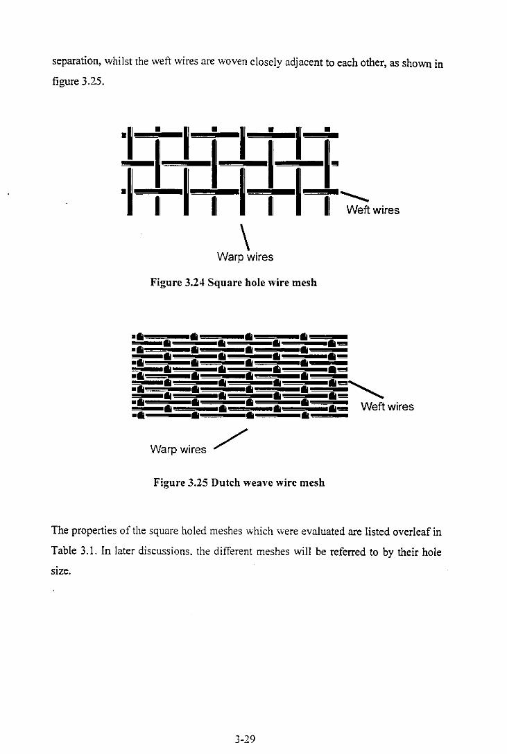
separation, whilst the weft wires are woven closely adjacent to each other, as shown in
figure 3.25.
-I · 1 · 1 · 1 · ~I 1 1 I-·1 11 I I I I I I ~ wi,e,
\ Warp wires
Figure 3.24 Square hole wire mesh
-11 11 11
11 11
11 111--11 III
III III III III III III 111-
-11 III
III III
III III
III Ill .... -11
III III
III III
III III
111-" -11 III
III III
III III
III 111--11
III III
III III
III III Ill .... Weft wires
-11 III III III
Warp wires / Figure 3.25 Dutch weave wire mesh
The properties of the square holed meshes which were evaluated are listed overleaf in
Table 3.1. In later discussions. the different meshes will be referred to by their hole
size.
3-29

Wire Diameter Mesh no. Hole size Free area
(Wires/inch)
560 f.lm 10 2000 f.lm 61 %
355 f.lm 16 1200 f.lm 60%
355 f.lm 24 700 f.lm 44%
224 f.lm 40 410 f.lm 42%
160 f.lm 60 260 f.lm 39%
112 f.lm lOO 145 f.lm 31 %
50 f.lm 200 77 f.lm 37%
Table 3.1 Properties of the square hole meshes
The properties of the two dutch weave meshes which were evaluated are listed below
in Table 3.2. In later discussions the two dutch weave meshes will be referred as No.!
and No. 2, with No. 2 being the mesh with the larger wires and holes.
Warp wire Warp wire mesh no. Weft wire Weft wire mesh no.
diameter diameter
No. 1 125 f.lm 50 wires/inch lOO f.lm 250 wires/inch
No. 2 355 f.lm 24 wires/inch 250 f.lm 100 wires/inch
Table 3.2 Properties of the dutch weave ~eshes
It is difficult to define a hole size for Dutch weave mesh, because when viewed from a
point perpendicular from the plane of the mesh, they appear to have no holes at all,
because the weft wires are woven adjacent to one another. Because the Dutch weave
meshes are asymmetric, two cylinders were made from each mesh in order to
determine whether the mesh orientation affected the dis-entrainer performance. One
3-30
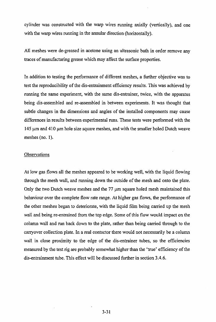
cylinder was constructed with the warp wires running axially (vertically), and one
with the warp wires running in the annular direction (horizontally).
All meshes were de-greased in acetone using an ultrasonic bath in order remove any
traces of manufacturing grease which may affect the surface properties.
In addition to testing the performance of different meshes, a further objective was to
test the reproducibility of the dis-entrainment efficiency results. This was achieved by
running the same experiment, with the same dis-entrainer, twice, with the apparatus
being dis-assembled and re-assembled in between experiments. It was thought that
subtle changes in the dimensions and angles of the installed components may cause
differences in results between experimental runs. These tests were performed with the
145 ).lm and 4l0).lm hole size square meshes, and with the smaller holed Dutch weave
meshes (no. 1).
Observations
At Iow gas flows all the meshes appeared to be working well, with the liquid flowing
through the mesh wall, and running down the outside of the mesh and onto the plate.
Only the two Dutch weave meshes and the 77 ).lm square holed mesh maintained this
behaviour over the complete flow rate range. At higher gas flows, the performance of
the other meshes began to deteriorate, with the liquid film being carried up the mesh
wall and being re-entrained from the top edge. Some of this flow would impact on the
column wall and run back down to the plate, rather than being carried through to the
carryover collection plate. In a real contactor there would not necessarily be a column
wall in close proximity to the edge of the dis-entrainer tubes, so the efficiencies
measured by the test rig are probably somewhat higher than the 'true' efficiency of the
dis-entrainment tube. This effect will be discussed further in section 3.4.6.
3-31
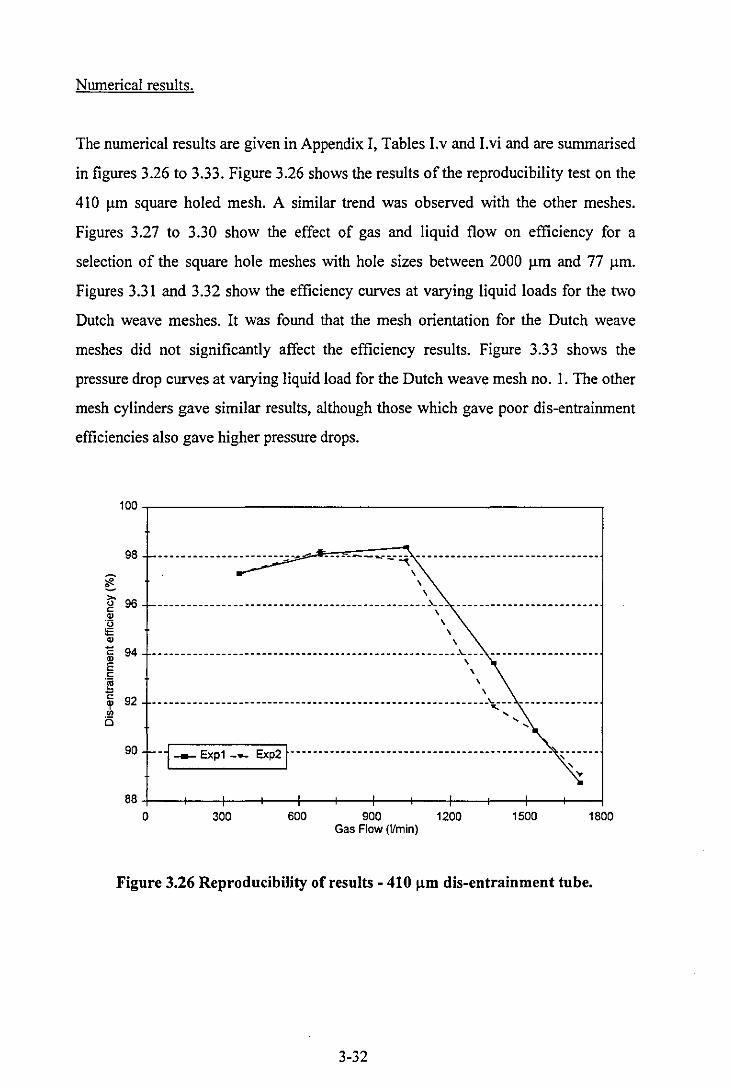
Numerical results.
The numerical results are given in Appendix I, Tables Lv and Lvi and are summarised
in figures 3.26 to 3.33. Figure 3.26 shows the results of the reproducibility test on the
410 Ilm square holed mesh. A similar trend was observed with the other meshes.
Figures 3.27 to 3.30 show the effect of gas and liquid flow on efficiency for a
selection of the square hole meshes with hole sizes between 2000 Ilm and 77 Ilm.
Figures 3.31 and 3.32 show the efficiency curves at varying liquid loads for the two
Dutch weave meshes. It was found that the mesh orientation for the Dutch weave
meshes did not significantly affect the efficiency results. Figure 3.33 shows the
pressure drop curves at varying liquid load for the Dutch weave mesh no. I. The other
mesh cylinders gave similar results, although those which gave poor dis-entrainment
efficiencies also gave higher pressure drops.
100,-----------------------------------____________ --,
98 ________________ ------- --~,d.,,-_:_: __ ""' __ c::_:-:_::~;:-~::-~~_ _ ______________________________ _
\
rl' 96 " .,
\ \
------------------------.-----------------------~--- -------------------------'13 lE .,
\ \
\ \
16 94 -----------------------.------------------------------~--- -------------.-----E \ " \
~ \ % 92 - - -- ----- ------ .-- ---------- ----------- ------ - -- --- - -------\::- - --- - ---- .-.--
is
90 --1 -- Expl -- Exp2 t---------------------------------------------- '-.:----.. 88+---+---+---+---+---r_--~--r---~--r---~--~~
o 300 600 900 1200 1500 1800 Gas Flow (1/min)
Figure 3.26 Reproducibility ofresults - 410 Ilm dis-entrainment tube.
3-32
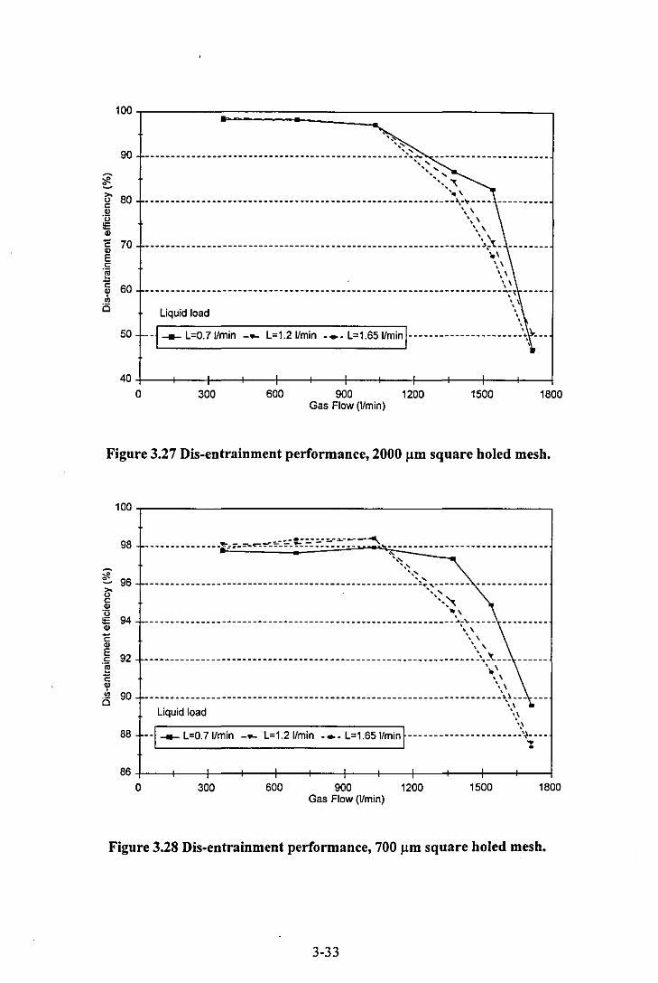
100
90
~ ~ >- 80 u <: Q)
'u lE Q)
C 70 Q)
E <:
~ <: 60 % Cl
50
40
0
'« '"
--------------------------------------------------:,~~ " , " , , ,
"" '" '. \ - - - - - - - - - - - - - - - - - - - - - - - - - - - - - - - - - - - - - - - - - - - - - - - - - - - - - - - - - - - - l,-T ___ _
'.\ '.\ '.\ , \ ______________ . _______________________________________ ___________ ~.t-.' \'
\' \'
-----------------.-.--------------.------------------- ---------------~~t
Liquid load \' , , ,
001--- L=0.7I1min _ .... L=1.21/min _+_ L=1.651/minlu-uu-u-u----uu\, ---
300 600 900 1200 1500 1800 Gas Flow (l/min)
Figure 3_27 Dis-entrainment performance, 2000 !lm square holed mesh.
~
><! ~ >-u <: Q)
'u lE Q)
C Q)
E <: .~
<: 'I' .. Cl
100,---________________________________________________ -,
98
96
94
92
90
88
86
0
~
'" '"
'" ----------------------------------------------------:~~,'------- --------------, ,
',,~
"".' --------------.--------------------------------------- ------~,~-----
'.\ , \
'. \ ________________________________________________________________ : .. .'t __ _ '. \ , \
'., --------------------------------------------------------------------.\., ~ ---
'., Liquid load '.'
" --1 ___ L=0.71/min - .... L=1.21/min - .. - L=1.651/minfuu-n-uu-u-u-u:~i---
300 600 900 1200 1500 1800 Gas Flow (1/min)
Figure 3.28 Dis-entrainment performance, 700 !lm square holed mesh.
3-33
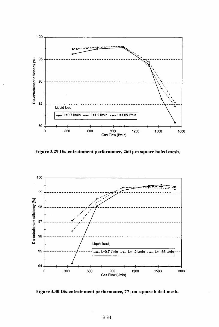
100~----------------------------------------------~
, ,
------------------------------------------------------ ~--------------------~" .. .... , . \
\ , \ .. \ .. \
--------------------------------------------------------------- ~;~----------.. \ .. \
\-" \ .. \ , \ ...... \
-------------------------------------------------------------------- ----~~---Liquid load ..
1 ___ L=0.71/min - .... L=1.21/min - .. - L=1.651/minl
80+---~--4---~---r--_+--_+---4--~----~--~--+_~ o 300 600 900 ~200 1500 1800
Gas Flow (1/min)
Figure 3.29 Dis-entrainment performance, 260 J.lm square holed mesh.
100~----------------------------------------------__,
99 -~-::.::->'-~;:..=-~-~-"'--:!.;:-:=:--:::-:::-:'::-::-:::-:::-:::--:::-C!~ ."
------------------------------------:-~:~- -----------------------------------........ ; , .' ~ " ~ "" ...
(j' 98 c:
~~ .. ~
-----------------------,,-~- ------------------------------------------------Q)
'0 ;;: Q)
"" / ~,,~ /
C 97
~ ~
~ .. ' / / ." / -------------------,----- ----------------------------------------------------/
/ .. % 96
i5 Liquid load.
95 ---0000-00---00--- oooo_ooj ___ L=0.71/min _ .... L=1.21/min _ .. _ L=1.651/minloo-
M+---~--4---~---r---+--_+--_4--~~--~--~--+_~ o 300 600 900 1200 1500 1800
Gas Flow (1/min)
Figure 3.30 Dis-entrainment performance, 77 J.lm square holed mesh.
3-34
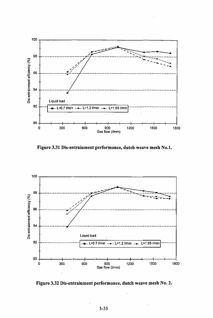
~ ~ c:
100,-________________________________________________ ~
.' . ~=--. .... ,.,._....... ....~.::. .. .::.~ .. :::.-.-------
-- -- - -_ .. - --- ---- - --- -- --- .. ~~ -_ .. ----- --- ---- - --- - -- -- -::--~::':.---- - -- ---- - - --- - ---r .............. -- ........ _~ ,,1' .................... ...
h' ,,' .... ,.-- --- -- ------_ .. -!'~(-- --- .. -- -- --_ .. -_ .. ---- --- -- --------- ---- ---- ---- ---- --- -- -- ----
~
liquid load
92 '''1--- L=0.71/min ..... L=1.21/min -- L=1.651/min ~ .......................... ..
90+---~--~--~--~--~--~--~--~---+--_+---+--_1 o 300 600 900 1200 1500 1800
Gas flow (1/min)
Figure 3.31 Dis-entrainment performance, dutch weave mesh No.l.
100~----------------------------------------------------~
98 ---_ ...... - - -- ---------_ .. - -- -_ .. -:-.---;!"!"':: -=---~~.~ .. ~.~.~ .. ~.~~ .. ~':~:-~. =-:::",-=-.:: .. ~.':'.:: .. ::.':'.",. '"- .. - - -- - --" -,,-:" -=--::..-.:::-"::.. .. _-...
''-''-, ,
.~ 96 lE
,., .--.. -------------a:;'~--- --------------------------------------------------------" ~
53 E c: 94
l '" is Liquid load
92 .. · .. · .... · ...... · .. · .. 1 __ L=0.71/min ..... L=1.21/min -_ L-1.651/min! .. • .... •
90+---~--~---+---+--~~--~--+_--~---r--_+--~--~
o 300 600 900 1200 1500 1800 Gas flow (1/min)
Figure 3.32 Dis-entrainment performance, dutch weave mesh No. 2.
3-35
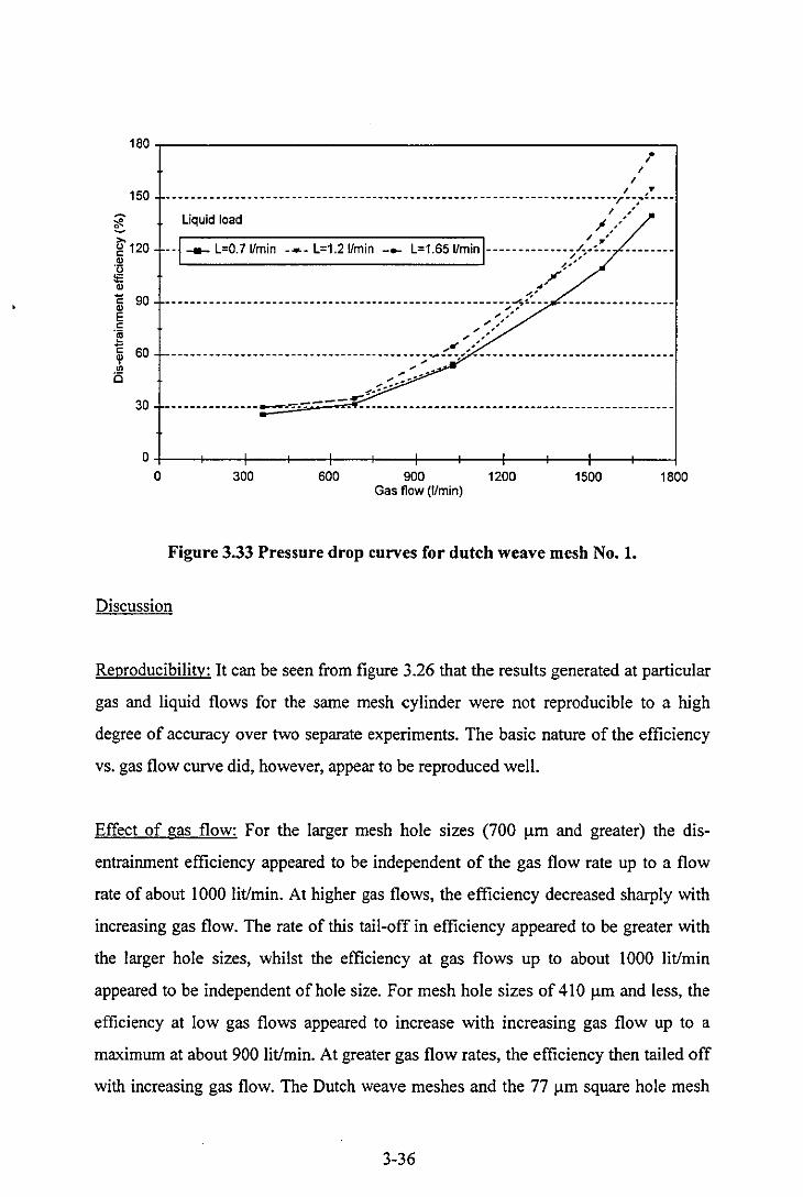
180,---------------------------------------------------,
150 / . ------ .. ----..... --------------------------------.---- ------------------r-~~!----Liquid load
/ .-~,/
1;' 120 c: Q)
'0
--j _____ L=0.71/min --.- L=1.21/min - .... L=1.651/min I------------;?;~,~:~'- --------
"' Q) .JI"
A' _ 4'
~ 90 ------------------------------------------------------;~'--- ------------------E "" ~~ c '" ~~~'
~ 60 ~., ~," ~ ---- -- - ----- - ____ we. __ - - ______________ - :_;_ .... ___ .... - __ - - - - - _______ - _______________ _
is ... -: •• -.-..... ' ~--
30 -- ------ - ___ e. - __ -~---:--- -.--:. ______ - _______________ - _______________________ . __
O+---+---r---~~~~--~---+--_+---+--_+--~--~ o 300 600 900 1200 1500 1800
Gas flow (1/min)
Figure 3,33 Pressure drop curves for dutch weave mesh No. 1.
Discussion
Reproducibility: It can be seen from figure 3.26 that the results generated at particular
gas and liquid flows for the same mesh cylinder were not reproducible to a high
degree of accuracy over two separate experiments. The basic nature of the efficiency
vs. gas flow curve did, however, appear to be reproduced well.
Effect of gas flow: For the larger mesh hole sizes (700 J.!m and greater) the dis
entrainment efficiency appeared to be independent of the gas flow rate up to a flow
rate of about 1000 lit/min. At higher gas flows, the efficiency decreased sharply with
increasing gas flow. The rate of this tail-off in efficiency appeared to be greater with
the larger hole sizes, whilst the efficiency at gas flows up to about 1000 lit/min
appeared to be independent of hole size. For mesh hole sizes of 410 J.!m and less, the
efficiency at low gas flows appeared to increase with increasing gas flow up to a
maximum at about 900 lit/min. At greater gas flow rates, the efficiency then tailed off
with increasing gas flow. The Dutch weave meshes and the 77 J.!m square hole mesh
3-36
gave poorer performance than the other meshes at low gas flows, but gave the highest
maximum efficiency, and maintained this best at the higher gas flows.
Effect of liquid load: In general, increasing the liquid loading had a negative effect on
the efficiency at the highest gas flows. At low gas flows, the liquid loading did not
appear to strongly affect the efficiency, except in the case of the 77 ).lm mesh and the
two Dutch weave meshes. For these meshes, increasing the liquid load at low gas
flows appeared to have a strong positive effect on the efficiency.
Pressure drop results: It was found that the different meshes all gave very similar
pressure drop figures. The smaller holed meshes do appear to give slightly lower
pressure drops, as well as being the best performing meshes in efficiency terms. The
most likely explanation is that, with the poorer performing meshes, the liquid film on
the inside of the mesh wall built up to a higher thickness, and was carried upwards
with the gas flow resulting in additional pressure drop. With the better performing
meshes, the liquid film would have been thinner, as liquid was continuously flowing
outwards through the mesh cylinder. There will, therefore, have been less drag on the
gas stream caused by the liquid film.
Effect of mesh characteristics: In general, the performance of the mesh cylinders
seemed to improve with decreasing hole size, although meshes with hole sizes
between 145 ).lm and 700 ).lm generated very similar results. The trend of increasing
efficiency with decreasing hole size was most apparent at high gas flow rates (above
about 1000 Htlmin). At gas flows below 1000 litlmin, the larger holed meshes
performed better, although those with holes sizes between 2000 ).lm and 700 ).lm
meshes all generated similar results. The best performing meshes overall were the 77
f.lm square hole mesh and the two Dutch weave meshes, these being the only meshes
to give an efficiency greater than 95 % at the highest gas flow (1700 litlmin).
It was mentioned above that defining an exact hole size for a Dutch weave mesh is
rather difficult because the holes themselves are not easily visible. Viewing the large
Dutch weave mesh (No 2) from an angle of 45° to the plane of the mesh showed
3-37

triangular holes with a base of approximately 150 Jlm and a height of around 250 Jlm.
Although these figures cannot be relied upon as a completely accurate reflection of the
holes size, it would probably be safe to say that the No 2. dutch weave mesh does
have larger holes than the 145 Jlm square holed mesh.
Undoubtedly, the mesh characteristics did have a very significant effect on the dis
entrainment efficiency. In the case of the large holed meshes, the liquid did not pass
through the mesh, and was re-entrained from the top by the gas flow. It would
therefore seem that the centrifugal force caused by the cyclone was not sufficient on
its own to push the liquid through the holes and into the quiescent reg~on. It would
seem that the mesh wall itself was crucial in providing some other force, or in
reducing the effect of another phenomenon in order to allow the liquid film to flow
outwards. The obvious explanation was that some form of capillary force, created in
the fine meshes, but not in the larger holed meshes, was significant. This could
explain the basic trend of the results, but could not explain the more anomalous
results, such as the way in which the larger holed dutch weave mesh performed, and
the fact that the larger holed meshes performed better at low gas flows.
The mesh orientation had little significant effect on the performance of the Dutch
weave meshes. The differences in performance between the two installations were of a
similar magnitude to those observed in the reproducibility tests.
Conclusions.
The mam conclusions drawn from this section of work were that the mesh
specification had a very significant affect on the dis-entrainer performance, and that
smaller holed meshes, on the whole, performed better than larger holed meshes. The
physical phenomena causing these effects could not be completely explained at this
stage, so gaining an understanding of these phenomena became the aim for the next
series of experiments.
3-38
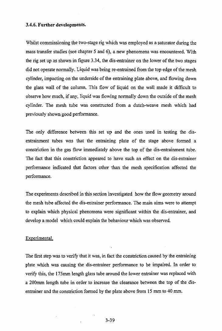
3.4.6. Further developments.
Whilst commissioning the two-stage rig which was employed as a saturator during the
mass transfer studies (see chapter 5 and 6), a new phenomena was encountered. With
the rig set up as shown in figure 3.34, the dis-entrainer on the lower of the two stages
did not operate normally. Liquid was being re-entrained from the top edge of the mesh
cylinder, impacting on the underside of the entraining plate above, and flowing down
the glass wall of the column. This flow of liquid on the wall made it difficult to
observe how much, if any, liquid was flowing normally down the outside of the mesh
cylinder. The mesh tube was constructed from a dutch-weave mesh which had
previously shown good performance.
The only difference between this set up and the ones used in testing the dis
entrainment tubes was that the entraining plate of the stage above formed a
constriction in the gas flow immediately above the top of the dis-entrainment tube.
The fact that this constriction appeared to have such an effect on the dis-entrainer
performance indicated that factors other than the mesh specification affected the
performance.
The experiments described in this section investigated how the flow geometry around
the mesh tube affected the dis-entrainer performance. The main aims were to attempt
to explain which physical phenomena were significant within the dis-entrainer, and
develop a model which could explain the behaviour which was observed.
Experimental.
The first step was to verify that it was, in fact the constriction caused by the entraining
plate which was causing the dis-entrainer performance to be impaired. In order to
verify this, the 175mm length glass tube around the lower entrainer was replaced with
a 200mm length tube in order to increase the clearance between the top of the dis
entrainer and the constriction formed by the plate above from 15 mm to 40 mm.
3-39
T
Dis-entrainer
Entrainer
Knit-mesh section
J------. Carryover 1..------1 collection plate
Top stage liquid outlet
-+
Top stage ~~~~tt==~ liquid inlet -+ c
Dis-entrainer
Bottom stage ~~~~~~t::J liquid outlet +-- ..
Entrainer
T Bottom stage gas inlet
Bottom stage liquid inlet
I Extemal "'" Downcomer
Fig 3.34 Counter-current column with two stages
3-40

It was mentioned in section 3.4.5 that the efficiency figures measured in the previous
rig were somewhat false because some of the re-entrained liquid would impact on the
column wall and return with the dis-entrained liquid. In order to quantify this effect, a
further series of experiments were carried out with the apparatus set up as shown in
figure 3.35. Any liquid being re-entrained from the top edge of the mesh tube would
be carried upwards into the knit-mesh cone, and drip down onto the carryover
collection plate. If any liquid drops were being ejected at speed from the outside
surface of the mesh tube, then these would pass over the weir, and be collected with
the carryover liquid, causing the measured dis-entrainment efficiency to be reduced.
This was not of concern at the time because this type of liquid flow had not been
observed previously.
Knit-mesh section
Carryover Carryover
collection Pla,-te_-=~~i~~~~~i~.:liqUid Dis-entrainer [ -+ plate Dis-entrained
liquid
Entrainer r::::::t:1!g:5::: +- Liquid L inlet
Fig 3.35 Dis-entrainer test rig with mesh tube moved higher.
3-41

Finally, the apparatus was set up with the area around the dis-entrainer tube
completely exposed to the atmosphere. This set up allowed a number of different
geometries around the top of the mesh tube to be investigated. These geometries are
shown in figures 3.36a to 3.36d.
Results.
With the larger clearance of 40 mm between the top of the dis-entrainer tube and the
plate above, the dis-entrainer operated satisfactorily, as it had done before during the
previous series of experiments. It was concluded from this that it was indeed the close
proximity of the constriction to the top of the mesh tube which was causing the dis
entrainer performance to suffer in the two stage column.
The results from the experiments using the apparatus shown in figure 3.35 are given
in Appendix I, Table Lvii and selected results are shown in figures 3.37 and 3.38.
These show how the column wall in the original test rig affects the measure dis
entrainment efficiency. Case 1 refers to the results from the original dis-entrainer test
rig (figure 3.23). Case 2 refers to the results from the new configuration shown in
figure 3.35. It can be seen that for the lower performing mesh, the efficiency is much
lower in case 2. Whereas for the higher performing mesh, the efficiencies are basically
similar. This demonstrated that the better performing meshes did not gain any
significant boost in performance from the presence of the column wall.
The experiments using the open mesh tube gave some interesting results. With no
additional equipment around the mesh tube, the mesh tubes appeared to perform as
they had done previously. Placing a constriction above the mesh tube without the
glass wall (figure 3.36a) did not appear to have a detrimental effect on the
performance. In fact, the larger holed meshes (e.g. the 1200 micron mesh) appeared to
operate better at high gas flows with the constriction in place. If a small constriction
was placed very close to the top of the mesh, the back pressure forced some of the gas
to be forced out through the holes in the mesh, causing droplets ofIiquid to be thrown
outwards from the surface of the mesh with some velocity.
3-42

Constriction Constriction
liquid
Fig 3.36a Fig 3.36b
J
I Glass QVF \ tube
liquid
Fig 3.36c Fig 3.36d
Glass QVF tube
liquid
Glass QVF tube
liquid
Fig 3.36 - Flow geometries around the dis-entrainment tube.
3-43
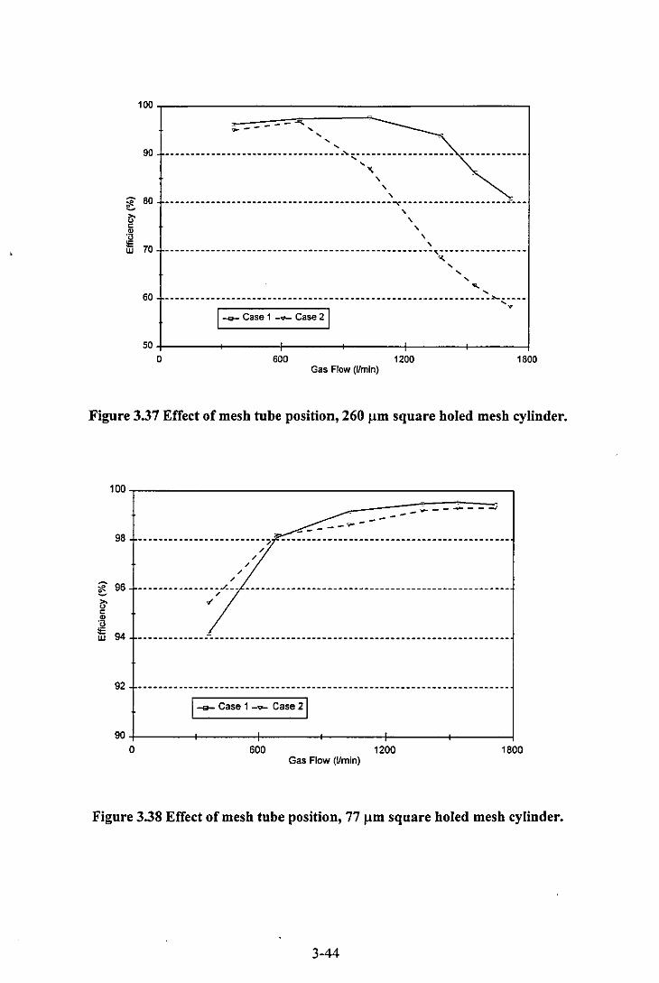
100,-____________________________________________ -,
90
C 80
g .:'; ., w 70
60
~----- ....... , , , , .... -------------------------------,--------------------, , , , , , --------------------------------------------~--------- ---------_ .. _--, , , , , ----------------------------------------------------,-----------------
'<. , , , .. , --------.--------._.--------.------------------------- ---------~-----
I-e- Case 1 -9- Case 21 '.
50+-----~~----_+------~------+_----~------_1 o 600 1200 1800
Gas Flow (Vmin)
Figure 3.37 Effect of mesh tube position, 260 Ilm square holed mesh cylinder.
"" 0:.. (;'
" " ·u ., w
100,-____________________________________________ ,
98
96
94
92
-------------------------/
/ /
/
/ /
-- -- --------1
----------------~-- ---------------------------------------------------/
'"
I-a- Case 1 -..- Case 21
90+-------~------~------~------~-------+------_1 o 600 1200 1800
Gas Flow (Vmin)
Figure 3.38 Effect of mesh tube position, 77 Ilm square holed mesh cylinder.
3-44

Placing a constriction above the mesh tube with the glass wall in place (figure 3.36b)
did cause the same problems as encountered earlier, provided the clearance between
the top of the mesh and the plate was small enough.
Placing a glass tube around the top of the mesh tube, as shown in figure 3.36c caused
a massive reduction in efficiency with all meshes. The liquid ceased to flow through
the mesh wall, and was re-entrained from the top of the mesh.
With the glass tube placed around the whole mesh, with the end left open, (figure
3.36d) the dis-entrainer appeared to operate satisfactorily, as it had done in the
original dis-entrainer test rig.
Discussion.
The fact that the dis-entrainer performance depended heavily on the flow geometry
around the mesh tube would seem to suggest that capillarity or some similar surface
phenomena associated with the mesh holes was not the only physical processes which
was of importance. The strong effect of different flow geometries suggested that
pressure effects were also of importance.
Placing a constriction close above the mesh tube without a solid wall surround would
create some back pressure within the mesh tube which would assist in pushing the
liquid through the mesh wall, and this type of behaviour was indeed observed.
The phenomena observed with the other geometries are less easy to account for.
Placing a constriction close to the mesh tube with the glass wall in place may cause
the pressure around the outside of the mesh cylinder to increase more than the
pressure inside the mesh, due to the flow field caused by the sudden contraction. This
pressure difference may prevent the liquid from flowing outwards through the mesh,
causing the reduction in efficiency.
3-45
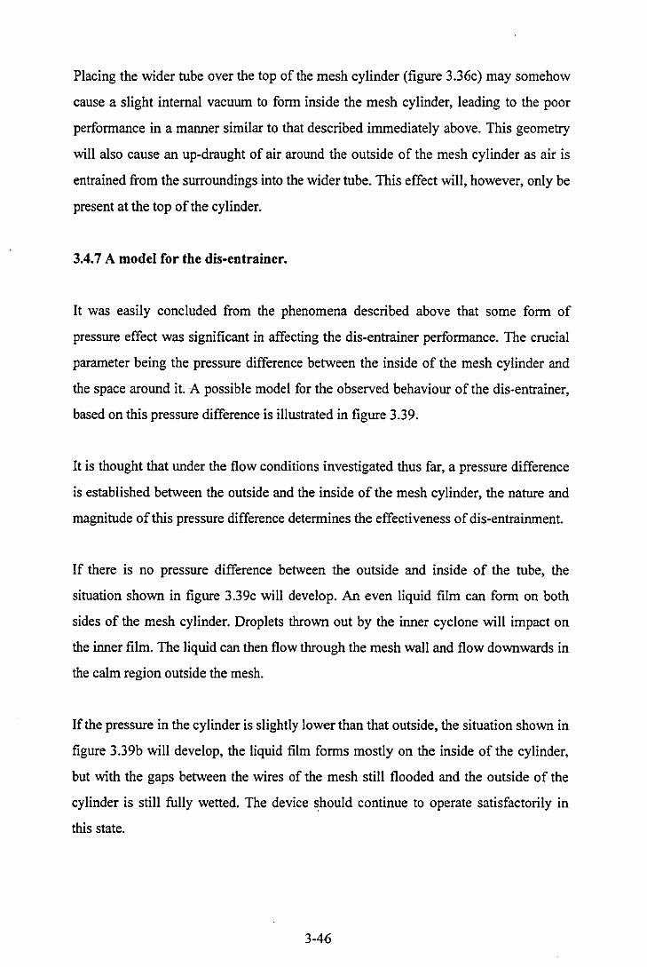
Placing the wider tube over the top of the mesh cylinder (figure 3.36c) may somehow
cause a slight internal vacuum to form inside the mesh cylinder, leading to the poor
performance in a manner similar to that described immediately above. This geometry
will also cause an up-draught of air around the outside of the mesh cylinder as air is
entrained from the surroundings into the wider tube. This effect will, however, only be
present at the top of the cylinder.
3.4.7 A model for the dis-entrainer.
It was easily concluded from the phenomena described above that some form of
pressure effect was significant in affecting the dis-entrainer performance. The crucial
parameter being the pressure difference between the inside of the mesh cylinder and
the space around it. A possible model for the observed behaviour of the dis-entrainer,
based on this pressure difference is illustrated in figure 3.39.
It is thought that under the flow conditions investigated thus far, a pressure difference
is established between the outside and the inside of the mesh cylinder, the nature and
magnitude of this pressure difference determines the effectiveness of dis-entrainment.
If there is no pressure difference between the outside and inside of the tube, the
situation shown in figure 3.39c will develop. An even liquid film can form on both
sides of the mesh cylinder. Droplets thrown out by the inner cyclone will impact on
the inner film. The liquid can then flow through the mesh wall and flow downwards in
the calm region outside the mesh.
If the pressure in the cylinder is slightly lower than that outside, the situation shown in
figure 3.39b will develop, the liquid film forms mostly on the inside of the cylinder,
but with the gaps between the wires of the mesh still flooded and the outside of the
cylinder is still fully wetted. The device should continue to operate satisfactorily in
this state.
3-46
I -+ i Liquid film Gas I
Enters. carried up w , -+ ~ I -.J
Outside Inside
(a)
Outside
(b)
4-Liquid Drops
Inside
Increasing internal pressure
Film flows down
Outside
(c)
4- Liquid Drops
Inside
Film flows down
Outside
4- Liquid Drops
Inside
(d)
Liquid sprayed
out .... '1<. +-';'~I
,- 4-..... -. Liquid .... - Drops ........
Outside Inside
(e)
Fig 3.39 Model for the effect of pressure difference on dis-entrainer performance
If the pressure inside the cylinder becomes sufficiently low to burst the capillaries in
the mesh holes, then the situation illustrated in figure 3.39a may occur. With the
capillaries no longer blocked with liquid, gas may flow into the cylinder from the
outside, and form a gap between the inner liquid film and the mesh waIl. This would
prevent much of the liquid in the inner film from travelling through the mesh. The
inner liquid film could then be carried up the inner wall and re-entrained from the top.
The liquid would only be pushed up the inner wall if the gas velocity was sufficiently
high to provide the appropriate shear force. If the gas velocity is too low to move the
liquid film, then the liquid film will increase in thickness until it can push back onto
the mesh under the centrifugal force caused by the cyclone. This would explain why
the large holed meshes operate well at low gas flows.
If the pressure inside the cylinder is slightly higher than that outside, then the situation
illustrated in figure 3.39d· will occur. The liquid film is formed mainly towards the
outside of the mesh, but not sufficiently so to rupture the liquid film and detach it
from the mesh. If the pressure difference becomes high enough to rupture the film,
then the situation depicted in figure 3.3ge will develop, with the gas flowing outwards
from the cylinder carrying entrained liquid drops.
It is thought that in dis-entrainer configurations used so far, the flow patterns create a
slight internal vacuum in the mesh cylinder, causing the devices to operate somewhere
between the regimes shown in figure 3.39a and figure 3.39c. In the case of the larger
holed meshes, above 145 microns, this is sufficient to rupture the liquid film at high
gas flows, causing the device to operate in the regime depicted in figure 3.39a, with
poor dis-entrainment efficiency. With the smaller holed meshes, the capillary forces
are stronger, and the device operates satisfactorily in the regime shown in figure
3.39b.
The model outlined above suggests that smaller holed meshes can operate over a
wider range of pressure differences than larger holed meshes because of the stronger
capillary forces. The model would also suggest that larger holed meshes could be
made to work well if the flow geometry was arranged so that the pressure inside the
mesh is slightly higher than, or equal to that outside.
3-48

Conclusions
It was concluded from this section of research that the flow geometry around the top
of the mesh tube was of importance in determining the dis-entrainer performance.
This may have been because the pressure difference between the outside and the
inside of the mesh tube was of importance in maintaining a- permanent liquid film
around the mesh wall.
It is thought that the finer holed meshes were better able to hold a liquid film over a
wider range of pressure differences than larger holed meshes, and hence gave better
dis-entrainment performance.
In order to verify this, the next stage of the experimental programme was to construct
a rig in which the pressure outside of the mesh tube could be manually varied relative
to the internal pressure. If the theories outlined above are correct, then smaller holed
meshes would operate well over a larger range of pressure differences than larger
holed meshes.
3.4.8 Pressure manipulation experiments.
The purpose of the experiments described in this section was to verify whether the
model outlined in the section above was indeed valid. To this end, a rig was
constructed in which the pressure difference between the outside and the inside of the
mesh tube could be measured, and manually varied.
Experimental
A diagram of the experimental rig used for this series of experiments can be seen in
figure 3.40. The main difference between this set-up and those used previously is that
the gas liquid mixture from the top of the dis-entrainment tube flows straight into a
solid tube, sealed onto the top of the mesh cylinder using silicone sealant. This solid
tube forms a barrier between the gas space outside the mesh tube and the main gas
3-49
stream, allowing the pressure difference between the outside and the inside of the
mesh to be manipulated.
The pressure inside the mesh cylinder could be increased by placing a variable
restriction in the gas flow above the knit-mesh cone. The restriction consisted of a flat
sheet of plastic which could be progressively slid across the opening to increase the
restriction to flow, and hence the internal pressure. The pressure outside the cylinder
was artificially increased using the air pump shown in the diagram. When air is
pumped into the sealed outer chamber, it can only leave through the liquid outlet, so a
small gas flow could cause an appreciable increase in pressure. The flow of air into
the outer chamber, and hence the pressure increase was controlled by a control valve
downstream of the air pump.
The pressure in the outer chamber could be readily measured using a manometer
connected to a tapping on the side of the chamber. The pressure inside the mesh tube
was measured by a small capillary tube, fed down into the mesh cylinder from the
plate above. Unfortunately it was not possible to measure the pressure in the tube with
liquid present, because the capillary soon became blocked with water. In order to
overcome this problem, the internal pressures were measured with the rig operating
dry.
The problem with this approach, is that there would not be a film of liquid on the
surface of the mesh cylinder, so some of the bulk gas flow would be able to flow
through the mesh, which would obviously affect the measured pressure. In order to
reduce this effect, the outer chamber was sealed whilst the internal pressure was
measured, so that all of the gas flow entering at the bottom of the mesh tube would
have to leave through the top. This was still not an ideal solution, as some gas would
flow outwards from the mesh near the bottom, .and then back into the mesh at the top,
but this approach represented the best practical method.
3-50
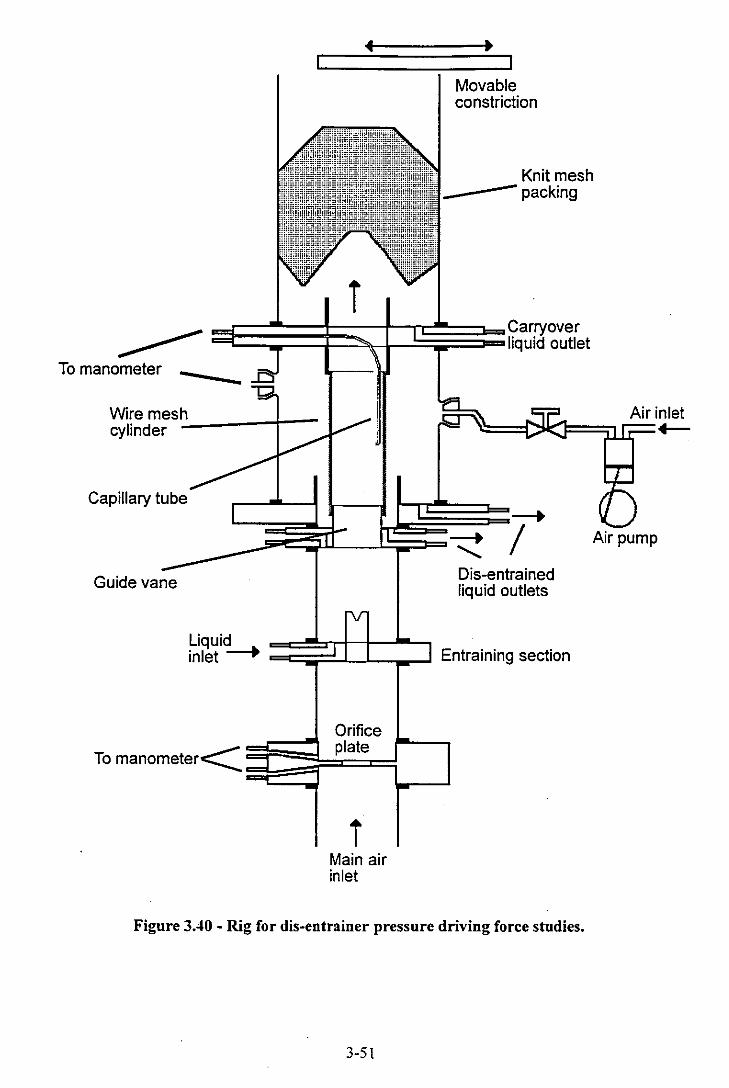
Movable constriction
Knit mesh _~---- packing
~ ==~====~==~=t:J~~~~car~over :: liquid outlet To manometer ____ _ -
Wire mesh cylinder '~ ___ -l-_-
Capilla~ tube
Guide vane
~ / Dis-entrained liquid outlets
Liquid ~~~rtj=:J inlet --+ c Entraining section
Orifice
<~~~3F~p~la~t~e~ To manometer:;; Io.--...J
i Main air inlet
Figure 3.40 - Rig for dis-entrainer pressure driving force studies.
3-51
Air pump

A further problem which was soon encountered, wasthat the pressure reading given
by the capillary tube depended strongly on the position of the end of the capillary
within the dis-entrainment tube. This was most probably due to the small restriction at
the top of the dis-entrainer caused by the silicone sealant and due to expansion and
contraction of the gas flow through the mesh wall, as described above. Because of this
problem, it was difficult to get a true measure of the pressure within the tube. It was
therefore not possible to obtain accurate quantitative results, although the theory
outlined in the section above could be verified by qualitative results. The trend could
still be picked up provided the capillary tube was kept in the same place within each
series of experiments.
Each data series consisted of the results from a number of experiments in which the
inside pressure was artificially increased using the flow restrictor on the gas outlet
(experiment type I), and results from experiments in which the outside pressure was
increased using the air pump (experiment type II). In experiment type I the pressure
inside the tube was determined with the rig operating dry, and with the outer chamber
sealed in order to prevent bulk flow of gas through the mesh cylinder. The dis
entrainment efficiency for each data point was then measured with the bungs in the
wall of the outer chamber removed, so that the pressure outside the mesh cylinder
could safely be assumed to be atmospheric. It was assumed that the liquid film on the
mesh wall would prevent bulk flow of gas through the mesh wall. The pressure inside
the cylinder was assumed to be equal to that measured with the rig operating dry and
with the chamber sealed. In experiment type IJ, the chamber was sealed, and the air
pump used to increase the external pressure. The restriction was also removed from
the gas outlet. The pressure of the outer chamber could be measured easily with liquid
present, as no liquid would reach the pressure tapping point. The pressure inside the
tube was assumed to be the same as that measured with the rig operating dry with no
flow restriction in place.
3-52

Results
Typical results are given in Appendix I, Table Lviii, and are shown in figure 3.41.
Because of the difficulties experienced in measuring the pressure inside the mesh
tube, there was little to be gained by performing the experiments with more mesh
tubes. The graphs shows how the dis-entrainment efficiency varies with the pressure
difference between the outside and the inside of the mesh tube at constant gas and
liquid flow rates.
100
-95
90
-----------------------------------~~.~---~---~~--------------------
C 85 ~ " " '0
80 -= w
75
70 -----------------------------~ .----------------------------------------------
65 -4 -2 0 2 4
P(INSIDE)-P(OUTSIDE) (cm water)
Figure 3.41 Results of pressure manipulation experiments, No.!. Dutch weave mesh
Discussion
It can be seen that qualitatively at least, the results do seem to show the behaviour
predicted by the model described in section 3.4.7 in that the pressure difference
between the outside of the mesh cylinder and the inside does affect the performance of
a dis-entrainer operating at a set combination of gas and liquid flows.
3-53
As was mentioned above, it was not possible to obtain accurate figures for the
pressure within the mesh tube because the pressure reading was highly dependent on
the position of the end of the capillary tube. It is not possible to say, therefore,
whether there was a slight internal vacuum (or positive pressure) in the mesh cylinder
or not. Because the pressure measurement position was kept consistent, however, the
trend in the results displayed in the graphs can be relied upon.
Conclusion
At this point in the development program, it was concluded that the model for the film
flow in wire mesh based dis-entrainers, given in section 3.4.7, was a fair
representation of the actual process. This explained why smaller holed meshes
performed better than larger holed ones, but suggested that larger holed meshes could
be successfully employed if the flow geometry was arranged such that the external
and internal pressures were equalised across the mesh wall.
3.4.9 Final Dis-entrainer Design
The experiments detailed in sections 3.4.5 and 3.4.6 showed that applying additional
back pressure to the inside of the mesh cylinder showed promise as a technique for
improving the efficiency of the larger holed mesh cylinders. It was thought that, for
industrial applications, coarser holed meshes would be desirable as they would be
stronger, cheaper, and less prone to fouling. Furthermore, most industrial separation
systems will have a much lower surface tension than the air/water systems, and so
capillary forces would not be as strong. For these systems, even the finest holed
meshes may not be effective unless measures are taken to prevent the low pressure
region from forming inside the mesh cylinder. Dutch weave meshes appeared to offer
better performance than their holes size would suggest, whilst having better structural
properties than plain weave meshes.
The final evolution of the dis-entrainer design which was tested is shown in figure
3.42, and consisted of a 700 flm square holed mesh cylinder, into which a small
3-54

constriction is added at the top. The purpose of the constriction was to cause the
necessary back pressure to force the liquid film out onto the wall of the cylinder.
Results.
150 mm
Gas +
rcarryover liquid
~ ~
38mm
Fixed flow constriction
700 micron wire mesh tube
[:~12S1~~s~-entrained r liquid outlet
Gas + entrained liquid
Figure 3.42 Dis-entrainment tube with flow restrictor to cause back pressure.
The performance of this dis-entrainer is compared with that of a similar tube without a
constriction in figure 3.43. For the purpose of these tests, the rig was set up as in
figure 3.23, with the column wall around the outside of the mesh cylinder. It can be
seen that the performance appears to be little altered by the presence of the
constriction. Visual observations, however showed that the dis-entrainer was
operating differently. A significant flow of liquid was observed being carried up the
column wall by a large gas flow, and into the carryover collection section. This
suggested that the constriction was causing sufficient back pressure to break the liquid
film outwards from the mesh, as shown in figure 3.3ge. Gas would then flow trough
the mesh wall, carrying entrained liquid drops. The droplets thrown outwards with the
3-55

gas flow would impact on the column wall fonning a film which could be carried up
with the gas flow.
~
~ 1;' c: ,~ le w
100
98
96
94
92
------ -- --- ----:-. :--:--~-:-- ------ '!":..:: :".:" . .:-. ~- --_ .... , ~.:..:..:.:.:..:~=~-=---~~--;.:~--.:.:..:---~--~-------------------, , , ,
-----------------------------_ .... _----_ ... ----------------'<-- ._-_ .. _---_ .. -, , , , -._ .. _. -._ .. _.,. _ ... ---- ----- _ .. -. -- --. --- .---- ._- .. __ ... --- ---_ .. \, ---._- _ ..
------------------------------------------------------ ----------------~ ------\
90 - - ....... Without constriction-..- With constriction
Liquid load = 0.7 Umin.
\ -------------------------, ---"
88+-------+-------~------~------~------~----~ o 600 1200 1800
Gas Flow (1/min)
Figure 3.43 Effect of flow constriction on the performance of the 700 /lm square holed mesh.
Placing the mesh with constriction in the more open dis-entrainer configuration shown
in figure 3.35 seemed to demonstrate that his indeed was the case. Liquid droplets
were being thrown outwards with some force from the outside of the mesh cylinder,
and there was no obvious re-entrainment from the top of the cylinder. Numerical
results were meaningless with this rig because much of the dis-entrained liquid was
being projected over the weir and into the pool on the carryover collection plate. In a
real contactor with several dis-entrainment tubes on larger plate, this would not be a
problem because the drops would impact on the other nearby tubes. This is one area in
which Dutch weave meshes may have an advantage, as the droplets would not be
projected directly outwards due to the nature of the mesh holes.
3-56

3.4.10. Effect of Guide vane pitch angle.
The wire mesh based dis-entrainer had been proven to operate up to a superficial
column velocity of 14.9 mls, and at a wide range of liquid loads. The pressure drop
was considered to be high, being as much as 180 mm WG at the highest gas and liquid
flow rates. It was thought that much of this pressure drop was being created by the
drag caused by the guide vane, and by the energy requirement of forming the vortex.
The purpose of this final series of experiments was to determine whether a dis
entrainer employing a guide vane which gave a less intense vortex action could still
achieve the required separation but with a lower pressure drop.
Guide vanes with different pitch angles had been evaluated before (see section 3.4.2).
However this was done at a time when the rest of the dis-entrainer geometry was
causing severe problems with re-entrainment.
Experimental
The test rig used was the same as the one which was used before to measure dis
entrainment efficiencies, and is shown in figure 3.23. Efficiency measurements and
pressure drop measurements were made in the usual way. The only part that was
changed between experiments was the guide vane within the dis-entrainer. The same
mesh cylinder was used throughout, one formed from dutch weave mesh No. 2. (see
table 3.2) with no constriction at the top.
The guide vanes were formed by taking a flat pieces of plastic, 35mm x 27.5mm x
3mm, heating them with a hot air gun unit they became soft, and twisting them about
their short axes to create helix shapes which could then be inserted into the 35mm
diameter tube of the dis-entrainer. The severity of the vortex action was altered by
varying the amount by which the guide vane was twisted about its axis. The most
intense guide vane was formed so that the upper edge of the guide vane was at 90° to
the lower edge when viewed from above. In the less intense guide vanes, this angle
was 30°, 45° and 60°. The effective pitch angle of the guide vane, et, was defined as
3-57
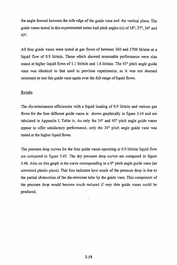
the angle formed between the side edge of the guide vane and the vertical plane. The
guide vanes tested in this experimental series had pitch angles (a) of 18°, 27°, 34° and
45°.
All four guide vanes were tested at gas flows of between 360 and 1700 lit/min at a
liquid flow of 0.9 lit/min. Those which showed reasonable performance were also
tested at higher liquid flows of 1.1 lit/min and 1.6 lit/min. The 45° pitch angle guide
vane was identical to that used in previous experiments, so it was not deemed
necessary to test this guide vane again over the full range of liquid flows.
Results
The dis-entrainment efficiencies with a liquid loading of 0.9 lit/min and various gas
flows for the four different guide vanes is shown graphically in figure 3.44 and are
tabulated in Appendix I, Table ix. As only the 34° and 45° pitch angle guide vanes
appear to offer satisfactory performance, only the 340 pitch angle guide vane was
tested at the higher liquid flows.
The pressure drop curves for the four guide vanes operating at 0.9 lit/min liquid flow
are compared in figure 3.45. The dry pressure drop curves are compared in figure
3.46. Also on this graph is the curve corresponding to a 00 pitch angle guide vane (an
untwisted plastic piece). This line indicates how much of the pressure drop is due to
the partial obstruction of the dis-entrainer tube by the guide vane. This component of
the pressure drop would become much reduced if very thin guide vanes could be
produced.
3-58
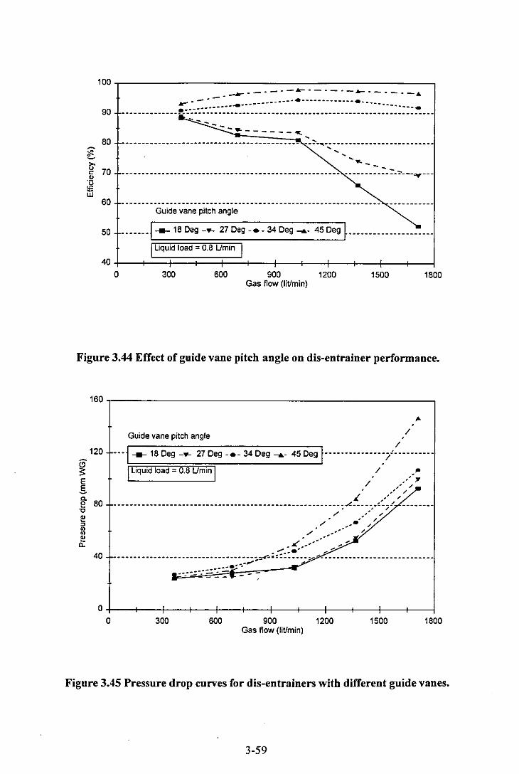
100
90
-·-·-~·-·-·-~·---·-A
--------------~-~~~-~:~-~:~~~~~~~~~~~~~~~:::~:::~~~:::-~~~::=::::::::~----.. ------~
80 ,
-------------------------------------------- --~-,---------------------------~ , ><! e....
, ,.. " 70 " Q) ------------------------------------------------------ -----------=-~---~---'0 ;: UJ
60 Guide vane pitch angle
50 ....... 1--- 18 Deg - ... 27 Deg ••• 34 Deg ...... 45 Deg ~ .................... . I liquid load = 0.8 IJmin
40
0 300 600 900 1200 1500 1800 Gas flow (lit/min)
Figure 3.44 Effect of guide vane pitch angle on dis-entrainer performance.
160,-______________________________________________ --.
Guide vane pitch angle /
120
~ E .s Co
80 e "0
i'! " U) U)
.1: 40
/ ... j ___ 18 Deg - ... 27 Deg ••• 34 Deg ...... 45 Deg t ........ · .... ·?"· ........ · \ liquid load = 0.8 IJrnin \ / • .. / /-" -- / .- /
,( .- / ________________________ . ________ . ____________________ ___ ~ _____ ~~:-f ___ . __ ._ .. ,.."
/' ,'J' /' ....... ,,"
./ .............. " .,.-..:: ......... ~ ...
-----------------------------------~~~-:::::~---~~-:-- ------------------------... -.- ...... .. -::.=. -::.:. -.-::-
o 300 600 900 1200 1500 1800 Gas flow (Iit/min)
Figure 3.45 Pressure drop curves for dis-entrainers with different guide vanes.
3-59
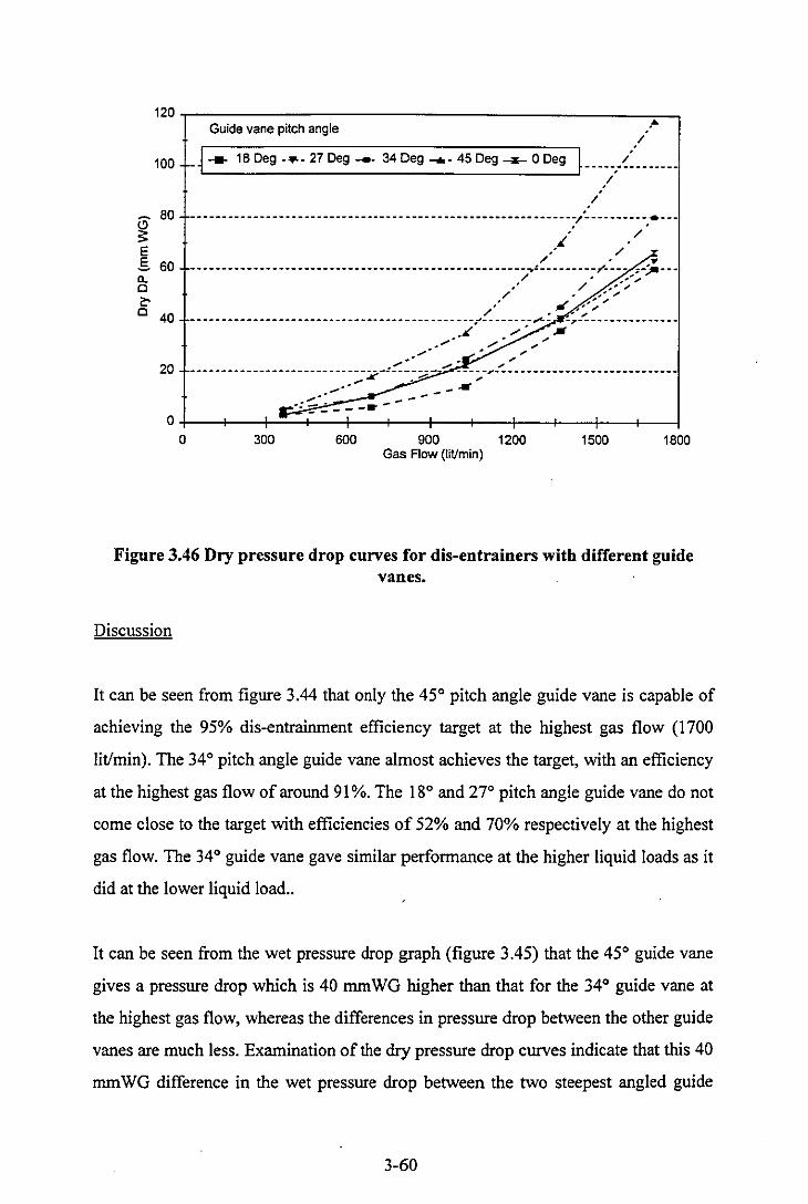
120~--------------------------________________ ~~ ." Guide vane pitch angle
/
100 _~ --- 16 Deg -.- 27 Deg _. 34 Deg ...... 45 Deg ~ 0 Deg ~ _____ ._/ _____ __
/ /
~ 60 -- ----- -- ---- --- - -------- ----- -- - - --- - -- --- -- - ---- -- -- -------/---- ______ • __ _
.' / ." / /~ • y E
~ .. --------------------------------------------------~~---------~---- ;-;.---a. / .. ,1''',. g 60
C ." / .... "" / .... .. "
~ ," ., .... ;.,. C / . ,.,
40 ---------------------------------------------r--------~- -,----------------;( '-... . ~
20 --- - ---- - ---- -- ----- -- - -- ----- -"~-----... x ~
---O+---r-~~-+--~--~--+_--+---~~--_+--~--~
o 300 600 900 1200 1500 1800 Gas Flow (IiVmin)
Figure 3.46 Dry pressure drop curves for dis-entrainers with different guide vanes.
Discussion
It can be seen from figure 3.44 that only the 45° pitch angle guide vane is capable of
achieving the 95% dis-entrainment efficiency target at the highest gas flow (1700
lit/min). The 34° pitch angle guide vane almost achieves the target, with an efficiency
at the highest gas flow of around 91 %. The 18° and 27° pitch angle guide vane do not
come close to the target with efficiencies of 52% and 70% respectively at the highest
gas flow. The 34° guide vane gave similar performance at the higher liquid loads as it
did at the lower liquid load ..
It can be seen from the wet pressure drop graph (figure 3.45) that the 45° guide vane
gives a pressure drop which is 40 mmWG higher than that for the 34° guide vane at
the highest gas flow, whereas the differences in pressure drop between the other guide
vanes are much less. Examination of the dry pressure drop curves indicate that this 40
mmWG difference in the wet pressure drop between the two steepest angled guide
3-60
vanes is also present in the dry pressure drop and would not have been caused by an
increase in the additional pressure drop due to the presence of liquid.
The dry pressure drop curves for the 18° and 27° guide vanes are similar to that for
the flat guide vane which itself still shows a considerable pressure drop. From this it
can be concluded that the pressure drop for the shallower angle guide vanes is mostly
due to the partial obstruction of the dis-entrainer tube, and not due to the energy input
in creating the cyclone. The fact that the flat guide vane still gives a considerable
pressure drop would suggest that using much thinner guide vanes which obstruct less
of the dis-entrainment tube should give lower pressure drops.
The decrease in separation efficiency with decreasing pitch angle can be readily
explained by the decrease in the intensity of the cyclone. As the cyclone intensity is
reduced, more of the smaller droplets will be able to pass straight through the dis
entrainer without reaching the walls. The pressure drop will be less for the shallower
angled guide vanes because the guide vane obstructs less of the dis-entrainment tube,
and less energy is required to give the radial flow component in the vortex.
Conclusions
These experiments showed that using a less intensive guide vane in the dis-entrainer
could give a substantial saving in pressure drop, at the expense of a reduction in
separation efficiency. The 34° guide vane gave a 30% lower pressure drop than the
45° guide vane used previously, at the expense of a 5% reduction in the separation
efficiency. Shallower angle guide vanes gave bigger reductions in separation
efficiency with little extra gain in terms of pressure drop reduction.
The fact that a flat guide vane with the same thickness as the other guide vanes still
gave a pressure drop of 60 mm WG at the highest gas flows would suggest that using
much thinner guide vanes within the existing geometry may offer improvements in
pressure drop of the order of 60 mm WG, probably with no cost in terms of reduced
separation efficiency.
3-61

CHAPTER FOUR
Chapter 4
Contactor flow patterns
4.1 Scope.
This chapter will be concerned with describing and discussing experiments,
observations and models used in attempting to define the flow patterns within the
contacting stage. Some knowledge of the flow pattern is required for correct
interpretation of the results from mass transfer experiments. The reasons for this were
discussed fully in chapter 2, section 2.2.5.
Section 4.3 of this chapter will describe the gas flow pattern which has largely been
assumed from the flow geometry of the contactor whilst section 4.4 will describe the
liquid flow pattern. Finally, section 4.5 will describe dynamic response experiments
which were used to quantify the variables in the model for the liquid flow pattern.
4.2 The importance of flow pattern.
Some knowledge of the flow pattern within a new contactor is necessary if the kp and
kl1 results obtained from mass transfer experiments are to be of any use in predicting
the perfonnance of the contactor with any real separation systems. Knowledge of the
flow pattern is required in order to detennine the effective mean driving force within
each stage from the inlet and outlet gas and liquid compositions.
Several methods exist for measuring the mass transfer rate in such a way that the
nature of the flow pattern does not affect the mean driving force. Using a pure
substance for one of the two phases will eliminate the effect of flow pattern within
that phase. Using a chemical system in which the liquid concentration of the tracer is
maintained at zero will also eliminate the effect of flow pattern within the liquid
4-1
phase. Dynamic methods are also used, and these are often employed to take account
of the deviation away from plug flow in packed columns due to axial dispersion.
If the average mass transfer coefficient for a contactor, obtained from any type of
experiment, is to be of any use in predicting the performance for other physical mass
transfer systems, then some knowledge of the flow pattern is essential. If the value of
the mass transfer coefficient is determined by a method which is insensitive to the
flow pattern, such as those mentioned above, then knowing the correct flow pattern is
still important if the results are to be applied to systems in which the flow pattern does
affect the driving force. If a physical test method is used in which the flow pattern
affects the mean driving force, then a flow pattern has to be assumed (or determined)
in order to calculate the mass transfer coefficient from the total transfer rate. This
same flow pattern would then be assumed in using the mass transfer coefficient data
for other systems. It could be argued that assuming the same, albeit incorrect, flow
pattern in interpreting experimental results and in applying kgCI or kp values would
give better results than measuring physically accurate kp and kgCI values using a flow
pattern insensitive method and then assuming an incorrect flow pattern when applying
the results to the real system.
4.3 Gas phase flow pattern.
The flow pattern for the gas phase was predicted from the contactor geometry by
assuming normal gas flow behaviour with respect to expansions, contractions and
such like. The assumed gas flow pattern is illustrated in figure 4.1, and will be more
or less independent of the gas flow rate. ,The flow pattern immediately above the
entrainment tube will be strongly affected by the presence of liquid at low gas flows.
Once the device is operating in the spray regime, the flow will assume the pattern
illustrated in the figure.
The gas flow expands from the entrainment tube to fill the full width of the column
before contracting down to the narrower width at the entrance to the dis-entrainer.
4-2
There will be circular eddies formed around the expansion and contraction points. The
gas in the dis-entrainer carries a large cyclonic motion in addition to its upwards flow.
The rotational component of velocity will decay slightly due to wall friction, although
this effect is unlikely to be highly significant over the relatively short length of the
wire mesh tube. As the gas expands outwards from the top of the dis-entrainer tube,
the cyclonic velocity component will decay due to the conservation of angular
momentum. Similarly the vortex motion will intensify as the gas contracts into the
next entrainer tube unless some attempt is made to kill the vortex downstream of the
dis-entrainment tube.
Guide
Cyclone
Recirculating Eddies
Figure 4.1 Gas phase flow pattern
It can be seen from the above description that the bulk gas flow is passing straight
through the stage, via a series of expansions and contractions. For the purposes of
modelling mass transfer results, it was assumed that the gas was effectively flowing in
plug flow up the stage. The circulating eddies formed around the expansions and
contractions were assumed to be trapped, and not to interact with the main gas flow.
The volume of gas outside of the mesh cylinder was similarly assumed to be stagnant.
4-3
There would also have been some axial mixing (dispersion) within the bulk gas flow,
but this would have been extremely difficult to quantify experimentally.
4.4 Liquid phase flow pattern
The liquid phase flow pattern will depend more strongly on the flow rates of the two
phases, as was illustrated in chapter 3, figure 3.5. At low gas flows, with the contactor
functioning in the bubbling regimes. The foaming liquid pool on the plate will
essentially be well mixed, with large drops broken off from the top forming the liquid
flow into the dis-entrainer. Once the entrainer is functioning in the spray regime, the
liquid flow pattern in the contactor will assume the formation shown in figure 4.2.
-i--':-:Ir-- Re-entrained 1;.:j.--- liquid spray
Figure 4.2 Liquid phase flow pattern
A pool of liquid forms on the plate around the entrainment tube. Droplets from this
pool are sheared off by the fast flowing gas stream and carried upwards towards the
dis-entrainer. The droplets sheared off at the entrainer tube will have sufficient
4-4
momentum from the accelerated gas motion that they are unlikely to slow with the gas
stream as it expands. Many droplets will impact on the lower surface of the dis
entrainer plate where they will coalesce into a film which will run down the column
wall and mix with the liquid on the plate. Those droplets which successfully reach the
dis-entrainer are then collected either directly by the cyclone or by impacting on the
guide vane. The liquid then flows through, and down the outside of the mesh cylinder,
onto the plate, and then out of the stage.
4.5 Dynamic response experiments
The main purpose of these experiments was to determine the fraction of the entrained
liquid flow which impacts on the underside of the dis-entrainment plate and returns to
the pool on the entrainment plate. This was achieved by carrying out dynamic
response experiments, the results from which could be compared with those from
numerical solution of a dynamic model in order to determine the flow of liquid
returning to the entrainment plate. This is the variable which is of greatest importance
in interpreting the results of mass transfer experiments.
4.5.1 Model for the contactor.
For the purpose analysing the dynamic response results, an approximate model for the
liquid and gas flow pattern was created, and is illustrated in figure 4.3. This model
will also be used in chapters 5 and 6 in the interpretation of the mass transfer results.
The liquid arrives on the plate, flowing into a well mixed pool around the entrainment
tube. A flow of liquid from the pool is then entrained into co-current plug flow with
the gas phase to the base of the dis-entrainer plate, with inter-phase mass transfer
occurring. Some of this flow impacts on the underside of the plate and returns down
the wall to the well mixed liquid pool. This flow is assumed to be in plug flow, but it
is assumed that no significant mass transfer with the gas can take place in this region
as the gas in proximity to the column wall is assumed to be stagnant, and not to
interact with main gas flow. The remainder of the liquid flows with the gas into the
4-5
dis-entrainer where further mass transfer may occurs. Most of the liquid is dis
entrained, although some liquid (less than 5%) will carryover, as demonstrated before
in chapter 3. The dis-entrained liquid forms a small pool on the dis-entrainment plate,
which is also assumed to be well mixed. The model equations themselves are given in
Appendix 11.
The above model contains several variables, notably the time delays associated with
the two plug flow sections, the volumes of the two well mixed regions, and the rate of
the recycle flow. In interpreting the results of the mass transfer experiments, which
take place under steady state conditions, the only variable which is of concern is the
rate of recycle, which will affect the liquid concentration and temperature in the liquid
pool on the entrainment plate.
4-6
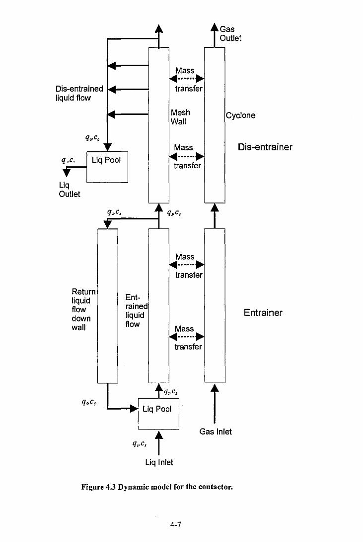
is-entrained D liq uid flow
q .. c, ,
~ ....
.. ....
.. ....
, q,c, Liq Pool
• iq L o utlet
Return liquid flow down wall
q"c,
q"c,
•
Ent-rained liquid flow
,
~
'"
Mass ~: . ..........
tr ansfer
M esh all W
M ass ~ ..
tr ansfer
~ qpc,
Mass ~:.
ansfer tr
M ass ~: ..
ansfer tr
+q~c, ... ... Liq Pool i
Gas Outlet
Cyclone
Dis-entrainer
Entrainer
q"c, t Liq Inlet
Gas Inlet
Figure 4.3 Dynamic model for the contactor.
4-7
4.5.2 Dynamic response experiments.
The purpose of these experiments was to detennine the approximate value of the
recycle flow rate. This was achieved using a series of dynamic response experiments.
The results from these experiments were then be compared with those from a dynamic
numerical solution of the model described above in order to detennine the recycle
flow.
The dynamic response experiments consisted of plotting the response curve generated
by a single contacting stage to a step change in a dye concentration in the feed. Dye
samples were taken from the dis-entrained liquid stream at five second intervals after
the change in feed dye concentration, and their concentrations were measured using a
visible light spectrophotometer.
A typical response curve generated by the experimental rig is shown in figure 4.4. It
was found from examination of the semi-log plots (an example is shown in figure 4.5)
that the response curves approximated those of a 1 st order system well mixed system
because the semi-log plot was approximately linear. This type of behaviour was also
generated by the numerical solution of the dynamic model (figure 4.6.), showing that
the complex recycle model could also generate pseudo-1st order behaviour, with an
approximately linear semi-log plot. The results from the dye tracing experiments are
given in Appendix II, Table II,i.
4-8
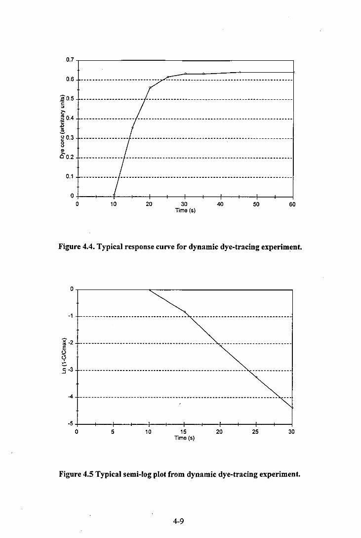
0.7 ~----------___________ ---,
0.6
~0.5 <=
" z:. ~ 0.4 ." -e .e g 0.3 8 " ~0.2
0.1
0 0 10 20 30
Time (s) 40 50 60
Figure 4.4. Typical response curve for dynamic dye-tracing experiment.
O~-------~ ______________ ~
-1
j -2 E
~ :::. 5 -3
-4
-5+--~-4---+--~--+---~~---+--~--+---~-4 o 5 10 15
Time (s) 20 25 30
Figure 4.5 Typical semi-log plot from dynamic dye-tracing experiment.
4-9
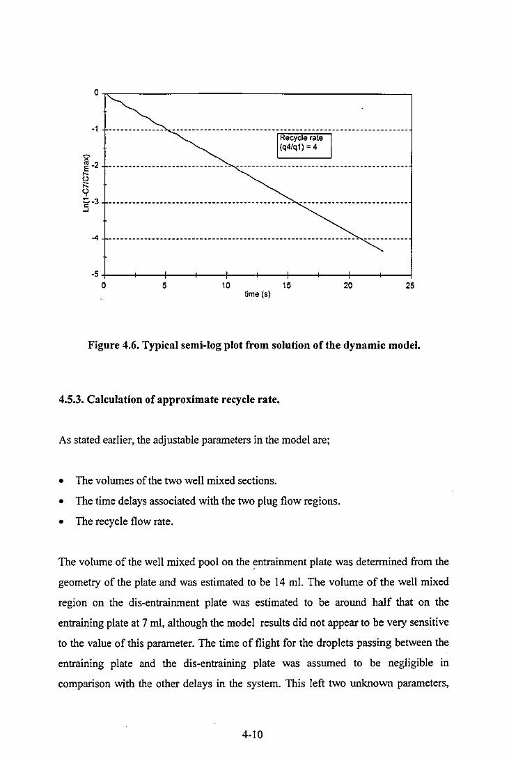
o~--__________________________________ ~
-1 --------------
'X
Recycle rate (q4/ql) = 4
E -2 ------------------------------ -------------------------------------------... ~ ~.3 .. ____ w _______ ._______________________________ _ _________________________ _
-'
-4 ----------____________________________________________ --------- --- _______ _
-5+----+----r---4---~----+---_+----~--~----~--~ o 5 10 15 20 25
time (s)
Figure 4_6. Typical semi-log plot from solution of the dynamic model.
4.5.3. Calculation of approximate recycle rate.
As stated earlier, the adjustable parameters in the model are;
• The volumes of the two well mixed sections.
• The time delays associated with the two plug flow regions.
• The recycle flow rate.
The volume of the well mixed pool on the ~ntrainment plate was determined from the
geometry of the plate and was estimated to be 14 mL The volume of the well mixed
region on the dis-entrainment plate was estimated to be around half that on the
entraining plate at 7 ml, although the model results did not appear to be very sensitive
to the value of this parameter. The time of flight for the droplets passing between the
entraining plate and the dis-entraining plate was assumed to be negligible in
comparison with the other delays in the system. This left two unknown parameters,
4-10
which were the time lag for liquid flowing down the column wall from the base of the
dis-entrainment plate to the entrainment plate, and the flow rate of liquid which is
returning down the column wall to the pool on the entrainment plate. Both these
variables were significant in affecting the output results of the numerical model, but it
is this last variable, the recycle rate which is of interest in evaluating the mass transfer
results.
The experimental results generated from the dynamic response experiments with the
rig demonstrated approximately first order behaviour with a time constant of between
3.7s and 7.8s depending on the gas and liquid flows. Pseudo first order behaviour with
the given time constants could be generated from the numerical model with various
combinations of the two significant independent variables. The time delay for liquid
flowing down the wall could not be determined experimentally and so had to be
estimated. The value of this time delay was estimated to be I second, this value being
based on observations of the liquid film flowing down the inside wall of the entrainer.
The recycle flow ratio, R, is defined as the recycle flow rate divided by the feed flow
rate:
(4.1)
q4 and ql are the liquid flow rates as defined in figure 4.3. The value of the calculated
recycle flow depended strongly on the value of the time delay which was assumed.
Estimating the time delay for liquid flowing down the wall at 1 second gave recycle
ratios of between 6.7 and 2.5.
The calculated recycle ratio, R, is plotted as a function of gas flow rate at two different
liquid loads in figure 4.7. The data can also be found in Appendix II, Table ILii. It can
be seen that the calculated recycle rate is highest at the lowest gas flows. These points
do in fact coincide with the bubbling flow regime within the entrainer, in which the
liquid could be assumed to be well mixed throughout. For the purpose of analysing
4-11

mass transfer data, assuming a high recycle rate is equivalent to assuming well mixed
behaviour because the liquid concentration in the mass transfer section will not vary
greatly between the inlet and outlet due to the high rate ofIiquid recycling.
8~-------=-----------------------------------. ~ , , , , , ,
6 -- -- - - - -------~--~-~-_"-... -~ ,--- --- - --- -- ---- - -- ---- - - - -- - -- - - --- - --- -- ---, ,
, , -----------------------------------------------~------, , , ,
----- -- -- -- :..-,-~ :'.._-
, ' , , y
r ,
2 ---------------------------------.--------------------------------------------
1 ___ L = 0.7 Vmin-... L = 1.0 vminl
o+-------~------~------_+------~------~~----~ o 600 1200 1800
Gas Flow (Vmin)
Figure 4.7. Calculated recycle rate (q/q}) as a function of gas and liquid flows.
At higher gas flow rates, with the entrainer operating in the spray regime, the liquid
recycle rate appears to increase again with increasing gas flow. This may be because
the liquid drops have more momentum as they leave the entrainment point and are
more likely to be thrown outwards and impact on the column wall or the underside of
the plate above. In these flow rates, the pl~g flow with recycle model will be a better
representation of the physical situation within the contactor, and the calculated recycle
ratio becomes more meaningful.
4-12

4.5.4 Conclusions
The dynamic response experiments showed that the liquid in the co-current flow
contactor could not be assumed to be flowing in plug flow, and gave dynamic
response results similar to a well mixed system. A numerical solution of a more
complex dynamic response model including the recycling of liquid showed that this
type of system could also generate similar results.
By comparing the results from the dynamic model with those from the dynamic
response experiments, it was possible to determine speculative values for the recycle
liquid flow rate within the contactor. Using these results in combination with KIfl and
Kp results determined using the recycle model may allow the mass transfer
phenomena within the contactor to be well modelled.
4-13
CHAPTER FIVE
Chapter 5
Gas side mass transfer measurements
5.1 Scope.
This chapter will describe the experiments used to characterise the gas-side mass
transfer performance of the novel gas liquid contactor. Some background information
on mass transfer systems was given earlier in chapter 2. The theory sections within
this chapter will elaborate on this and deal with literature information specific to the
system used here.
Section 5.2 describes the choice of an appropriate mass transfer system. Section 5.3
describes the experiments themselves and give details on the measurements made.
Section 5.4 deals with the way in which the results were analysed in order to
determine the volumetric mass transfer coefficients. The numerical results are
presented in Section 5.5 and discussed in Section 5.6. The conclusions are drawn in
section 5.7.
5.2 Choice of mass transfer system.
As was described in chapter 2, there are three classes of system which are widely used
to determine the gas side mass transfer resistance of gas liquid contactors. These are;
absorptionldesorption of a highly soluble gas between an inert gas and a liquid,
absorption of a gas into a liquid with which it undergoes an instantaneous reaction and
evaporation of a pure liquid into a gas stream.
There were a number of constraints on the choice of mass transfer system which were
specific to this project. Because of the high gas flows used, it would not have been
practical to use a system in which the gas phase was anything other than air, although
5-1
it may have been possible to use air as a carrier gas for another component present in
very Iow concentrations. Health and safety issues were also important. Due to the lack
of suitable containment facilities, it was decided to avoid the use of any harmful or
combustible substances in large quantities.
The only widely used example of a system in which a solute gas diffuses between a
gas mixture and a liquid in which it is highly soluble is the absorption of ammonia
from an ammonia/air mixture into water. This system was rejected because, firstly
there is some doubt in the literature as to whether ammonia is sufficiently soluble in
water for the liquid side resistance to be negligible (Sherwood & Pigford [1952]), and
secondly it would not have been practical or safe to provide ammonia gas in sufficient
quantities to produce a feed gas mixture with a meaningful ammonia concentration.
The most widely used examples of the second type of system, in which the diffusing
gas undergoes an instantaneous reaction in the liquid phase, are the absorption of acid
gases (other than CO2) into caustic solutions. This type of system was rejected for use
here because of the health and safety problems associated with handling acid gases
such as S02 and the impracticality of providing a suitable feed gas mixture at the
required rate. Another reason for rejecting this type of system was a general lack of
confidence in the results from systems involving chemical reactions, following
problems experienced whilst attempting to measure the liquid side mass transfer
resistance using the oxidation of aqueous sodium sulphite by oxygen diffusing from
air (see chapter 6). These problems were due to uncertainties over the kinetic
behaviour of the chemical reaction system, leading to uncertainties over whether the
diffusion/reaction system was proceeding in the correct regime. It was thought that the
same problems were likely to occur with other systems involving chemical reactions.
The first two types of mass transfer system having been rejected, the only remaining
choice was a system in which a pure liquid evaporates into the gas stream, with water
being the obvious choice for the liquid phase. This system was highly suitable for use
here, because the only requirement for the feed gas was that it should be reasonably
free of water vapour. The air from the compressed air mains met this requirement,
5-2

being of around 20% relative humidity at around 20 'c, its usual feed temperature.
Further advantages of this system are that the water vapour content of an air stream
can easily be measured using simple equipment, and that the modelling of evaporation
of water into air (humidification) is well understood and covered widely in the
literature.
5.3 Experimental
The apparatus which was used for the gas-side mass transfer experiments is shown in
figure 5.1. The water recirculated through the water bath, with a thermostatic heater
being used to maintain the required water inlet temperature. Fresh dry air was
continually drawn from the compressed air mains. The dis-entraining section of the
contactor under test was of the wire-mesh based type, employing a Dutch weave mesh
capable of maintaining at least 98% efficiency at all the gas flows used.
5-3
Gas outlet
D is-entrainer
Entrainer
Gas inlet from --+ rotameter
-@ --@
T
T
Wet and dry bulb hygrometer
Knit-mesh section
Carryover liquid
Dis-entrained liquid
--+
Fig 5.1 Experimental rig for gas-side mass transfer studies.
5-4
Thermostatic heater
5.3.1 Measured parameters.
The interpretation of the results will be discussed in section 5.4. The experimental
parameters which required measurement were:
• The water inlet and outlet temperatures.
• The gas inlet and outlet temperatures.
• The gas inlet and outlet humidities.
• The gas and liquid flow rates.
The water inlet and outlet temperatures were measured using thermocouples which
were independently calibrated using a mercury in glass thermometer. The gas
temperatures and humidities were measured using a hygrometer consisting of two
mercury in glass thermometers, one with a wet bulb, one with a dry bulb. In measuring
the outlet gas humidity, the hygrometer was held in the flow from the constriction
above the carry-over collection section. The inlet air temperature and humidity were
measured periodically from a separate compressed air main outlet using the same
hygrometer. The gas flow rate was measured by the rotameter. The liquid flow rate
was measured for each data point by measuring the time taken to collect a fixed
volume of liquid from the dis-entraining section.
5.3.2 Experimental variables.
The experimental variables which were varied were:
• The gas and liquid flow rates.
• The water inlet temperature.
• The diameter of the tube in the entraining section.
The gas flow rate was varied between 400 lit/min and 1600 lit/min, corresponding to
superficial column gas velocities of between 3.9 rnIs and 13.6 rnIs. The maximum gas
flow rate was set by the highest flow which could be extracted from the compressed
air mains via the rotameter. The minimum air velocity was chosen to give an air
5-5
velocity over the hygrometer of 5 m/s. Below this velocity it would no longer have
been safe to assume that true wet bulb temperature was being measured (Coulson and
Richardson [1990]).
The liquid flow rate was varied between 0.2 litlmin and 0.9 litlmin. The lower limit
was the minimum controllable flow which could be delivered by the pump. The upper
flow limit was the point at which the liquid began to back up on the dis-entrainment
plate. This problem will be described in chapter 7.
Entrainers with tubes of 15 mm, 20 mm and 25 mm i.d. were evaluated. It was
thought that the smaller tubes might give superior mass transfer performance at a set
gas flow rate because of the higher local gas velocities and more intensive turbulence.
Two water inlet temperatures were used, 30 0 C and 40 0 C. In theory, gas side mass
transfer coefficients should not depended strongly on the gas temperature (Treybal
[1968]), so the results should not be strongly dependent on the liquid inlet
temperatures. The liquid temperature would, however affect the calculated mass
transfer coefficient if the incorrect flow pattern was being used in calculating the Kga
value. This would be because the calculated average driving force would not correctly
reflect the dependence of the true effective driving force on the inlet and outlet
temperatures.
Each experimental run consisted of a series of measurements with constant liquid
flow, entrainer tube size and liquid inlet temperature, but with varying gas flow. The
liquid flow rate was determined separately for each data point, together with the liquid
inlet and outlet temperatures and the gas outlet temperature and humidity. The gas
inlet humidity was measured two or three times within each experimental run.
5-6
5.4 Modelling of results
As was described in chapter 2, a mass transfer coefficient can be described as the rate
at which a diffusing species transfers divided by the average driving force for mass
transfer. In the case of the system chosen here, the humidification of dry air by water
vapour, the rate of mass transfer could easily be determined from the difference in
humidity between the inlet and outlet gas streams. The effective average driving force
for mass transfer was however, rather more difficult to define.
5.4.1 Humidification theory.
The driving force for humidification at any point in the contactor is the difference
between the bulk gas water vapour concentration and the concentration of water
vapour in the gas adjacent to the surface of the liquid, which is equal to the saturated
gas humidity at the liquid surface temperature. The main problem in analysing the
results of humidification experiments is that both these concentrations will change
throughout the contactor even though a pure substance is being used for the liquid
phase. The bulk gas phase composition will change as water evaporates into the gas,
whilst the saturated concentration of water vapour at the interface will change because
the water temperature changes. This temperature change occurs because the water and
gas phases will both cool on passage through the contactor in order to provide the
latent heat of evaporation necessary to vaporise the water.
It is not therefore possible to conduct humidification experiments under true
isothermal conditions. This means that humidification operations invariably involve
simultaneous heat and mass transfer between the two phases. Fortunately analysis
methods exist which take account of this and are used in describing humidification
operations. The analyses described here are adapted from the treatment given for
humidification operations by Treybal [1968]. Essentially, the concentrations in the
mass transfer equations are replaced by the specific enthalpies of the gas at the
interface and in the bulk.
5-7

The effective average value of Kga for the contactor as a whole can be determined
from
(5.1)
G is the gas mass flow rate. PA is the gas density. V is the volume of one contacting
stage. HA is the bulk gas specific enthalpy, with HA! and HA2 referring to the inlet and
outlet conditions respectively. Hs is the saturated gas specific enthalpy, which is the
specific enthalpy of gas saturated with water at the water surface temperature. It is
assumed here that the liquid phase heat transfer coefficient is sufficiently high so that
there is no significant temperature gradient within the liquid phase, and the liquid
surface temperature is equal to the liquid bulk temperature at that point. The value of
Hs at any point in the contactor is therefore solely a function of the local liquid
temperature.
5.4.2. Effect of contactor flow pattern.
The relationship between the liquid temperature, TL (and hence Hs) and the gas phase
humidity, HA, depends on the flow pattern within the contactor. The possible flow
patterns can best be demonstrated on operating line - equilibrium line diagrams in
which the gas phase specific enthaIpy, H is plotted against the liquid temperature. The
saturation curve or equilibrium line gives the relationship between Hs and h, which is
derived from the vapour pressure curve, whilst the operating line gives the
relationship between HA and h.
From a given set of experimental results (inlet and outlet temperatures and enthalpies),
the calculated value of Kga will depend on the flow pattern which is assumed. For the
purposes of this study the gas phase will be assumed to flowing in plug flow at all
times. Two realistic extremes for the liquid flow pattern can be identified, namely
plug flow co-current and well mixed, and these correspond to the limiting values of
5-8
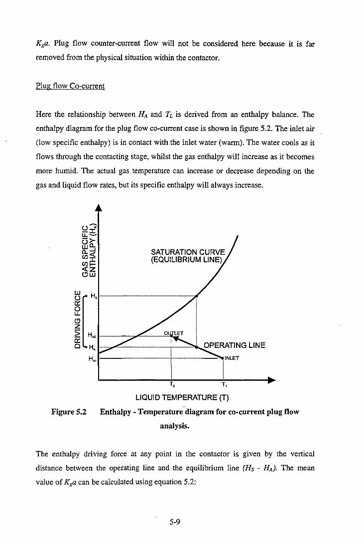
Kga. Plug flow counter-current flow will not be considered here because it is far
removed from the physical situation within the contactor.
Plug flow Co-current
Here the relationship between HA and TL is derived from an enthalpy balance. The
enthalpy diagram for the plug flow co-current case is shown in figure 5.2. The inlet air
(low specific enthalpy) is in contact with the inlet water (warm). The water cools as it
flows through the contacting stage, whilst the gas enthalpy will increase as it becomes
more humid. The actual gas temperature can increase or decrease depending on the
gas and liquid flow rates, but its specific enthalpy will always increase.
~ (J ~ -::c LL~
->-(Ja. UJ....! a.<t: C/l::c C/ll-<t:z (!)UJ
UJ (J c::: 0 LL (!) Z > H" c::: Cl
H"
Figure 5.2
SATURATION CURVE (EQUILIBRIUM LINE)
T, T,
LIQUID TEMPERATURE (T)
Enthalpy - Temperature diagram for co-current plug flow
analysis.
The enthalpy driving force at any point in the contactor is given by the vertical
distance between the operating line and the equilibrium line (Hs - HA). The mean
value of Kga can be calculated using equation 5.2:
5-9

(5.2)
The relationship between the water temperature, TL, and the gas specific enthalpy, HA,
is given by the operating line equation.
(5.3)
Well mixed
In this case the liquid phase is assumed to be well mixed so that the liquid temperature
is effectively constant throughout the contactor, and is equal to the liquid outlet
temperature. This flow pattern is illustrated on an enthalpy diagram in figure 5.3. The
gas enthalpy still increases as the gas flows through the contacting stage. The
incoming liquid, however is assumed to mix with sufficient cooler liquid so that the
liquid in contact with the gas inlet is already at the liquid outlet temperature.
Figure 5.3
w
SATURATION CURVE (EQUILIBRIUM LINE)
~ [' 1---'"7~---f; OUTlET
~ :: ___ OPERATING LINE
Cl H •• I-------~+ .. ----.- .. -- .. -lNLET
T,= CONST T,
LIQUID TEMPERATURE
Enthalpy - Temperature diagram for well mixed flow analysis.
5-10

Once again the driving force at any point within the contactor is given by the vertical
distance between the operating line and the equilibrium line. The value of Kga
assuming well mixed flow can be calculated using the same expression as for plug
flow (equation 5.4) although in this case TL, and hence Hs are constant, and not a
function of HA.
(5.4)
Recycle model
In between the two extreme cases is the recycle model outlined in chapter 4. This type
of flow pattern is illustrated on an enthalpy diagram in figure 5.4. The incoming liquid
mixes with a certain amount of recycle liquid, which has the same temperature as the
outlet liquid. The liquid which is in contact with the feed gas therefore has a
temperature somewhere between the inlet and outlet temperatures. The liquid in
contact with the gas then cools to the outlet temperature as it flows through the
contactor.
Figure 5.4
W
SATURATION CURVE (EQUILIBRIUM LINE)
In analysing data for Kga using the recycle model, the plug flow co-current model is
used, with a corrected water inlet temperature. The corrected water inlet temperature,
T'Ll reflects the temperature of the water in contact with the feed gas, and is calculated
from the predicted recycle ratio, R, using a straightforward energy balance.
T' = RTL2 + TLI LI R+1
(5.5)
R is the recycle flow ratio, as defined in chapter 4, equation (4.1). The way in which
the model used in analysing the data affects the calculated Kga value can be visualised
by comparing figures 5.2 to 5.4. For given inlet and outlet conditions, the calculated
driving force (Hs - HA) at a fixed point in the contactor will be highest for the plug
flow model, and lowest for the well mixed model. The driving force for the recycle
model will be somewhere between the two. For a given total mass transfer rate (fixed
from given inlet and outlet conditions), lower assumed driving forces will lead to
higher calculated Kga values. The well mixed model, will therefore always give higher
Kga values than the plug flow co-current model.
The recycle model can be made to represent the full spectrum of situations between
the two extremes by adjustment of the recycle flow. If the recycle flow was small, the
liquid in contact with the inlet gas would be very close to the inlet liquid temperature,
and results would be similar to the plug flow co-current model. If the recycle ratio was
very large, the corrected water inlet temperature would become close to the water
outlet temperature, and the model would give very similar results to the well mixed
model.
Each experimental result was analysed using'both the plug flow co-current model and
the well mixed model. Selected experiments using the 25 mm entrainment tube were
also analysed using the recycle model, as speCUlative recycle rate data generated by
the dye-tracing experiments were available for this entrainer size. In all the analyses
which were carried out, the integral term in the Kga equation (equation. 5.2) was
evaluated numerically using the trapezium rule.
5-12
5.4.3 Enthalpy Imbalance.
In practice it was found that in most cases the total enthalpy changes for the gas and
liquid streams were not equal, in other words the enthalpy balance did not balance.
The total calculated enthalpy change for the gas stream was typically around 70% to
80% of that calculated for the liquid stream. Several errors could have been
responsible for this imbalance;
• Errors in the liquid stream temperature readings.
• Errors in the gas stream temperature and humidity data.
• Errors in the gas and liquid stream flow measurements.
• Incorrect data for the saturated water vapour concentration.
Incorrect data for the saturated water vapour concentration was thought to be unlikely.
The liquid stream flow rates were regularly monitored directly by recording the time
taken to collect a fixed volume of liquid. The rotameter measuring the gas phase flow
rate could safely be assumed to be of good accuracy. The thermocouples used in
measuring the liquid phase temperatures had been independently calibrated, and were
known to be of good accuracy. It was therefore concluded that the most likely cause of
the enthalpy imbalance was inaccurate measurement of the gas stream temperatures
and humidities. Either the outlet gas enthalpy was being underestimated, or the inlet
gas enthalpy was being overestimated. Heat losses to the surroundings from the
contactor could not explain the discrepancy because in many cases, the main body of
the contactor was operating at below ambient temperature.
The percentage relative humidity of the outlet gas stream would typically be measured
at between 80% and 90%, whilst the dry bulb (actual) temperature of the gas varied
considerably between experiments, depending on the gas and liquid flows. If it was
assumed that the dry bulb temperature was correct, but that the percentage relative
humidity was 100%, rather than the measured value, then the enthalpy imbalance
became much less. The percentage energy loss for each experimental data point can be
calculated from:
5-13
(5.6)
Where L and G are the liquid and gas mass flow rates, and CL is the liquid specific
heat capacity. Using the raw experimental data, the average percentage energy loss
over all the experiments with the 25 mm entrainer was 23%. By assuming that the dry
bulb temperature was correct as measured, but that the gas was saturated with water
vapour, the average percentage energy loss calculated for these same experiments was
7%, with maximum and minimum calculated energy losses of 13% and -3%.
For the outlet gas humidity to be 100% would typically have required the outlet gas
wet bulb temperature to have been under-measured by between 1 and 1.5 0c. For the
inlet gas specific enthalpy to be overestimated sufficiently to explain the enthalpy
imbalance, either the dry or wet bulb thermometer would need to have been inaccurate
by between 2 °c and 4 0c. And this was thought to be unlikely. It was concluded
therefore, that the enthalpy imbalance resulting from using the measured experimental
values was caused by inaccurate measurement of the outlet gas humidity. All other
experimental values were assumed to be correct. One possible explanation for the
inaccurate measurement of the outlet gas humidity was that relatively dry ambient air
was being entrained into the outlet gas stream as it travelled the short distance
between the contactor outlet pipe and the wet bulb I dry bulb hygrometer.
In order to account for this, the values for the outlet gas specific enthalpy used in
calculating the mass transfer coefficient were corrected (adjusted upwards) in order to
satisfy the enthalpy balance with the liquid stream. In other words, the measured gas
inlet enthalpy was assumed to be correct) and the outlet gas enthalpy used in
calculating the KNa values was calculated from the liquid enthalpy change via an
enthalpy balance. The value of the mass transfer coefficients calculated using the
corrected values for the gas outlet enthalpy were typically around 30 % higher than
equivalent values calculated using the uncorrected experimental data.
5-14
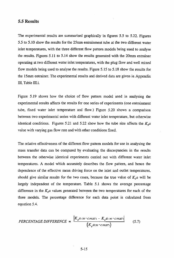
5.5 Results
The experimental results are summarised graphically in figures 5.5 to 5.22. Figures
5.5 to 5.10 show the results for the 25mm entrainment tube at the two different water
inlet temperatures, with the three different flow pattern models being used to analyse
the results. Figures 5.11 to 5.14 show the results generated with the 20mm entrainer
operating at two different water inlet temperatures, with the plug flow and well mixed
flow models being used to analyse the results. Figure 5.15 to 5.18 show the results for
the 15mm entrainer. The experimental results and derived data are given in Appendix
III, Table III.i.
Figure 5.19 shows how the choice of flow pattem model used in analysing the
experimental results affects the results for one series of experiments (one entrainment
tube, fixed water inlet temperature and flow.) Figure 5.20 shows a comparison
between two experimental series with different water inlet temperature, but otherwise
identical conditions. Figures 5.21 and 5.22 show how the tube size affects the Kga
value with varying gas flow rate and with other conditions fixed.
The relative effectiveness of the different flow pattern models for use in analysing the
mass transfer data can be compared by evaluating the discrepancies in the results
between the otherwise identical experiments carried out with different water inlet
temperatures. A model which accurately describes the flow pattern, and hence the
dependence of the effective mean driving force on the inlet and outlet temperatures,
should give similar results for the two cases, because the true value of Kga will be
largely independent of the temperature. Table 5.1 shows the average percentage
difference in the Kga values generated betw~en the two temperatures for each of the
three models. The percentage difference for each data point is calculated from
equation 5.4.
PERCENTAGE DIFFERENCE = IK,a(3oOCINLET) - K,a(400CINLEnl
(Kga(3o OCINLET»)
5-15
(5.7)
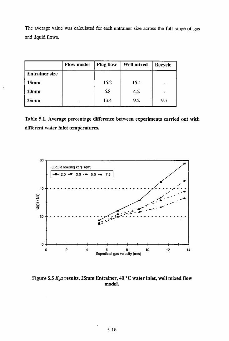
The average value was calculated for each entrainer size across the full range of gas
and liquid flows.
Flow model Plug flow Well mixed Recycle
Entrainer size
15mm 15.2 15.1 -20mm 6.8 4.2 -25mm 13.4 9.2 9.7
Table 5.1. Average percentage difference between experiments carried out with
different water inlet temperatures.
;g
'" El '"
60.-----------------------------------------------~
40
20
(Liquid loading kg/s sqm)
1--- 2.0 -. 3.6 -. 5.5'" 7.51 " ,/
- - - - - - - - - - - - - - - - - - - - - - - - - - - - - - - - -,/ - - -/' .... -
/ .... ..... ~ ... .,.".. ..
/. . ..... _c .. .,::.; .. ~ .. -... ;....-- ..
.. .. .. .. .. .. .. .. .. .. .. .. .. .. .. .. .. ~ :~- .. - .............................. -.--p::'-
0+-~--~--+-_+--4-_4~~--+_-+--4_--~_+--+-~
o 2 4 6 8 10 12 14 Superticial g,as velocity (m/s)
Figure 5.5 Kga results, 25mm Entrainer, 40°C water inlet, well mixed flow model.
5-16
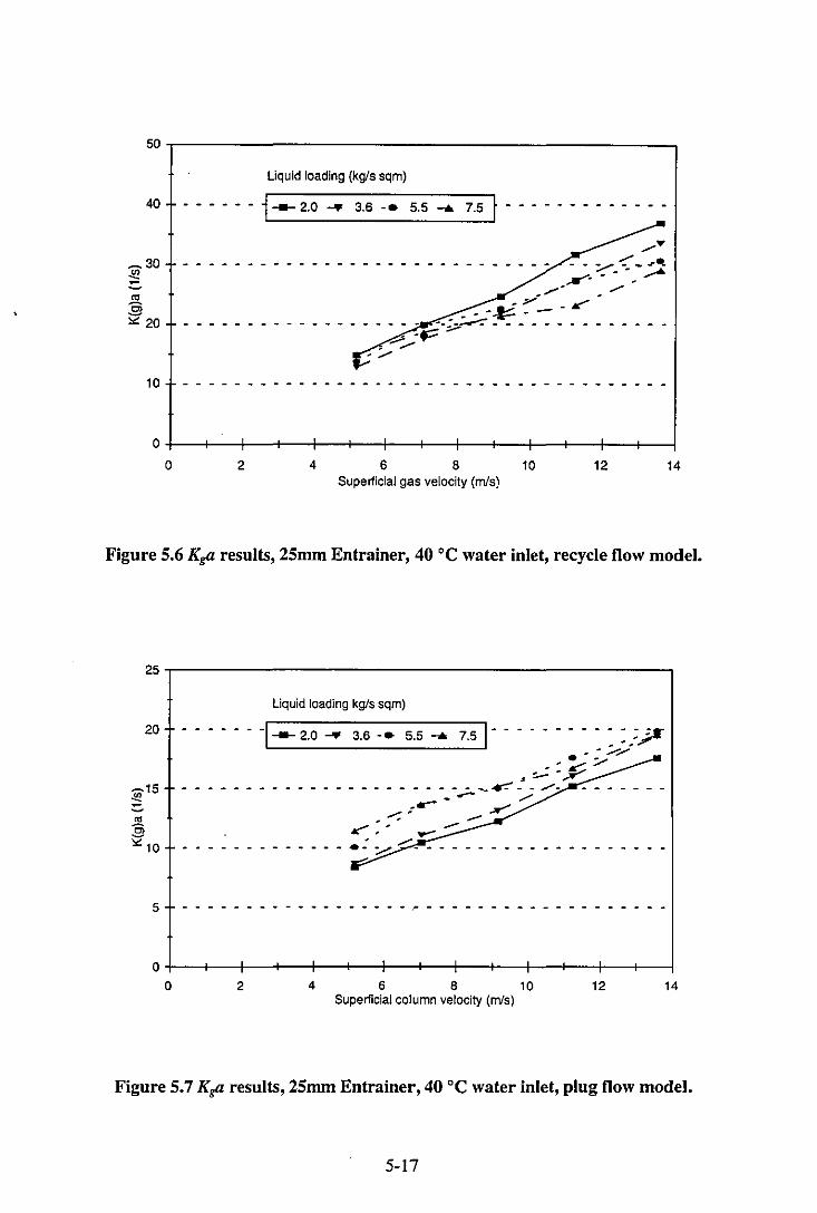
50.-----------------------------------------------~
Liquid loading (kgls sqm)
40 • - - - - - i --- 2.0 .... 3.6 •• 5.5 -. 7.5 f - - - - - - - - - - - -
~ 30
.!!1.
.9 >:: 20
10
/" _________ .. _ _ _ _ _ _ _ _ _ _ _ _ _ _ _ _ _ _ _ _ ::,....-'" ~ _ ... It .......... ~
. /
O+_~--_r--~_+--+-~--~--~-+--+_~--_r--r-~
o 2 4 6 8 10 12 14 Superiicial gas velocity (m/s)
Figure 5.6 Kga results, 25mm Entrainer, 40°C water inlet, recycle flow model.
25.-----------------------------------------------~
20
5
Liquid loading kgls sqm)
. ----1--- 2.0.... 3.6 -. 5.5 -. 7.5 1- --. -----~ :.:.J.¥ ................
. -: :::: ;:.--,- ,.. - - - - .. - - - - - - - - - - - - - - - - - - -...-::' - - /--- /
- - - - - - - - - - - - - - - - - - ~ - - - - - - - - - - - - - - - - - - -
0+-~--_r--~_+--+-_+--~~~~--+_-+--~--~_4
o 2 4 6 8 10 12 14 Superiicial column velocity (m/s)
Figure 5.7 Kga results, 25mm Entrainer, 40°C water inlet, plug flow model.
5-17
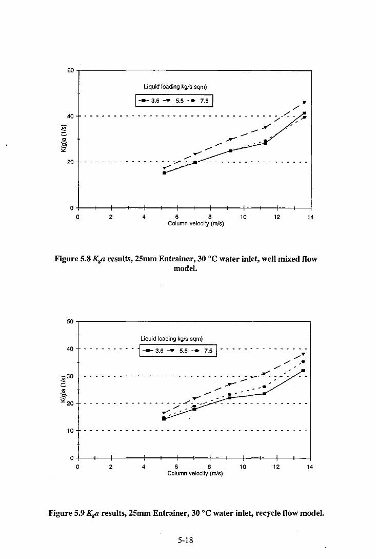
60~-------------------------------------------,
40
f .!!!. .9
'" 20
Liquid loading kg/s sqm)
1--- 3.6 -.. 5.5 -. 7.51
....-""'" - - - - - - - - - - - - - - - Y"" -,......
.. ./
- -~ - . ./ . / .
O+-~--~--r-_+--+-~--~--~-+--+-~--~--+-~
o 2 4 6 8 10 12 14 Column velocity (m/s)
Figure 5.8 Kga results, 25mm Entrainer, 30°C water inlet, well mixed flow model.
SO~---------------------------------------------,
40
-30 .!!1
'" § '" 20
Liquid loading kgls sqm)
. 1--- 3.6 -.. 5.5 .• 7.5 1 ..
~ . -----:=..--- ------ . . -
10 - - •• - ••••••••••••••• - •••••••• - - •••• - ••
0+-~--~--r-_+--+-~--~--~-+--+_~--~--+-_1
o 2 4 6 8 10 12 14 Column velocity (m/s)
Figure 5.9 Kga results, 25mm Entrainer, 30°C water inlet, recycle flow model.
5-18
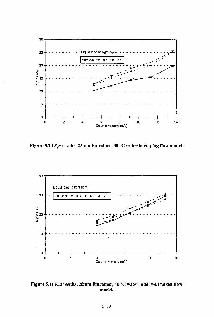
30
25
20
-!l
- - - - - - - - - - liquid loading kg/s sqm} - - - - - - - - - - - - - - ~-/- -1--- 3.6.... 5.5 -. 7.5 1 ".-' ::: --- -- - - - - - - - - - - - - - - - - - - - - - - - - - -:..- - -:.- - - - --
.>r'_--~ .
~ --';; 15
....-: --- - - - - - - - - - - - - - - ::..-:-::--.e--- - - -...i-;..;.-.;-..... - ...... - - - - - --Cl 'i2' 1""-
10
5
0
0 2 4 6 8 10 12 14 Column velocity (m/s)
Figure 5.10 Kga results, 25mm Entrainer, 30°C water inlet, plug flow model.
40~-----------------------------------------------,
Liquid loading kg/s sqm)
30 - l--- 2.0.... 3.6 -. 5.5..... 7.3 1 - - - - -
J!!
';;20 - - - - - - - - - - -.9
'" 10 - - - - - - - - - - - - - - - - - - - - - - - - - - - - - - - - - - - - - -
O+---~---+--~----~--~---r---+----r---+---~ o 2 4 6 8 10
Column velocity (m/s)
Figure 5.11 Kga results, 20mm Entrainer, 40°C water inlet, well mixed flow model.
5-19
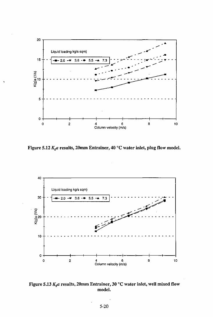
20~------------------------------------------------, ..
15
Liquid loading kgls sqm) .-- .. i I
.r" ••• . ___ 2.0 _ 3.6·. 5.5'" 7.3' • : Y'" •••• : :.- •• :;: .....
. '~.' --.:- .. - ..... -'~ . . -------••
.............................. .. --~ ............ -~ -=-'~.-
5
0+---~---+----~--+----r--~----r---1----+--~
o 2 4 6 8 10 Column velocity (mls)
Figure 5.12 Kga results, 20mm Entrainer, 40 QC water inlet, plug flow model.
40~------------------------------------------------.
Liquid loading kg/s sqm)
30 . 1--- 2.0 - 3.6'. 5.5'" 7.3 I' .. ............ - .. -~ ..
~ ~
"'20···---------------§
'" 10 •••••••••••••• - •••••••••••••••••••••••
0+---~--_+--~----+_--~--_+--~----+_--~--_1
o 2 4 6 8 10 Column velocity (mls)
Figure 5.13 Kga results, 20mm Entrainer, 30 QC water inlet, well mixed flow model.
5-20

40~-------------------------------------------,
30
10
Liquid loading kg/s sqm)
i --- 2.0'" 3.6 -.. 5.5'" 7.3 1- - - --
- _le""
-..- ...... -- ~ .. ........... _..-
~ : .... - .. -- .
....... - --..--.-: .... ~-:~-~-=-t.---:-:c-!'~:-:-:--:-" . .... ---------~..--:--lj-----. ---- .. ------
0+---~--_+--~~--+---~--_+--~----+---~---4
o 2 4 6 8 10 Column velocity (m/s)
Figure 5.14 Kga results, 20mm Entrainer, 30 cC water inlet, plug flow model.
20.---------------------------------------------------,
---- -15
Liquid loading kg!s sqm) /f /' - ,/' -i --- 2.0'" 3.6 - .. 5.5 ... 7.3 1- -~ __ ,.c - - __ ;.::-:---
".....
----/." r
- - - - - - - - - - - - - - - - - - - - -.-: - - - - - - - - - - - - - --
5
o+-------~----_+------~------+_------~----~
o 2 4 6 Column velocity (m/s)
Figure 5.15 Kga results, ISmm Entrainer, 40 cC water inlet, well mixed flow model.
5-21
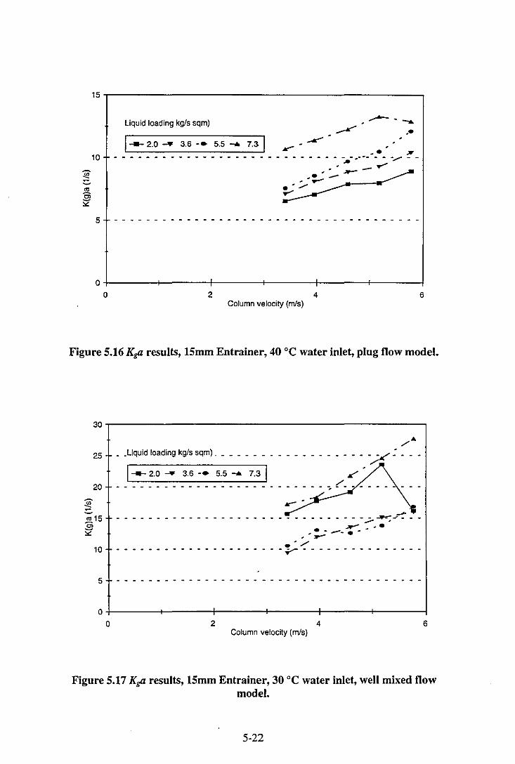
15~----------------------------------------------~
Liquid loading kgls sqm)
10
~ ~ ~
'" Ci l2'
_e ", - - - - - - - - - - - - - - - - - - - - - -.. - ~- -. - - -......... - -.... _ ........
.... "---~ -;/.- --00--.........
;..-~-
1 ___ 2.0'" 3.6 -. 5.5 ..... 7.31
5
0+-----~~----_+------~------+_----~------_4
o 2 4 6 Column velocity (m/s)
Figure 5.16 Kga results, 15mm Entrainer, 40°C water inlet, plug flow model.
30~----------------------------------------------~
25 _ .Liquid loading kgls sqm). _ _ _ _ _ _ •
1 ___ 2.0 ..... 3.6 -. 5.5 ..... 7.31 20
10
,/'"
- - - - - -~ - -,/
~ __ .,. c _______ _
-'" - - - - - ~~---- -...- .e ... - -- ..... - ,..e -,/
-y----------------
5 - - - - - - - - - - - - . - - - - - - - - - - • - - - - - - - - - - - • - -
O+----+-----~---~~---~------+-----~ o 2 4 6
Column velocity (m/s)
Figure 5.17 Kga results, 15mm Entrainer, 30°C water inlet, well mixed flow model.
5-22
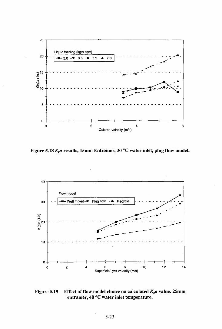
25,-----------------------------------------------~
20 Liquid loading (kg/s sqm)
-1--- 2.0 - 3.6 -. 5.5 --. 7.3 1- - - - - - - - - - - - -;,.; : ,.Ao-
---~:=.r------
• - - - - - ~-.... --=1':
..--5 - - - - - - - - - - - - - - - - - - - - - - - - - - - - - - - - - - - - - -
o+-------+-------~------~----~------~------~ o 2 4 6
Column velocity (m/s)
Figure 5.18 Kga results, 15mm Entrainer, 30 °C water inlet, plug flow model.
40~----------------------------------------------~
Flow model
30 - -1--- Well mixed_ Plug flow -. Recycle 1- •
. . ...;;:.------ ..------..---..-10 - - - - - - - - - - - - - - - - - - - - - - - - - - - - - - - - - - - - - -
0+---~~---+---+--~--+_--+_--~~--_4--_+--~--~--~
o 2 4 6 8 10 12 14 Superticial gas velocity (m/s)
Figure 5.19 Effect of flow model choice on calculated Kga value. 25mm entrainer, 40 °C water inlet temperature.
5-23
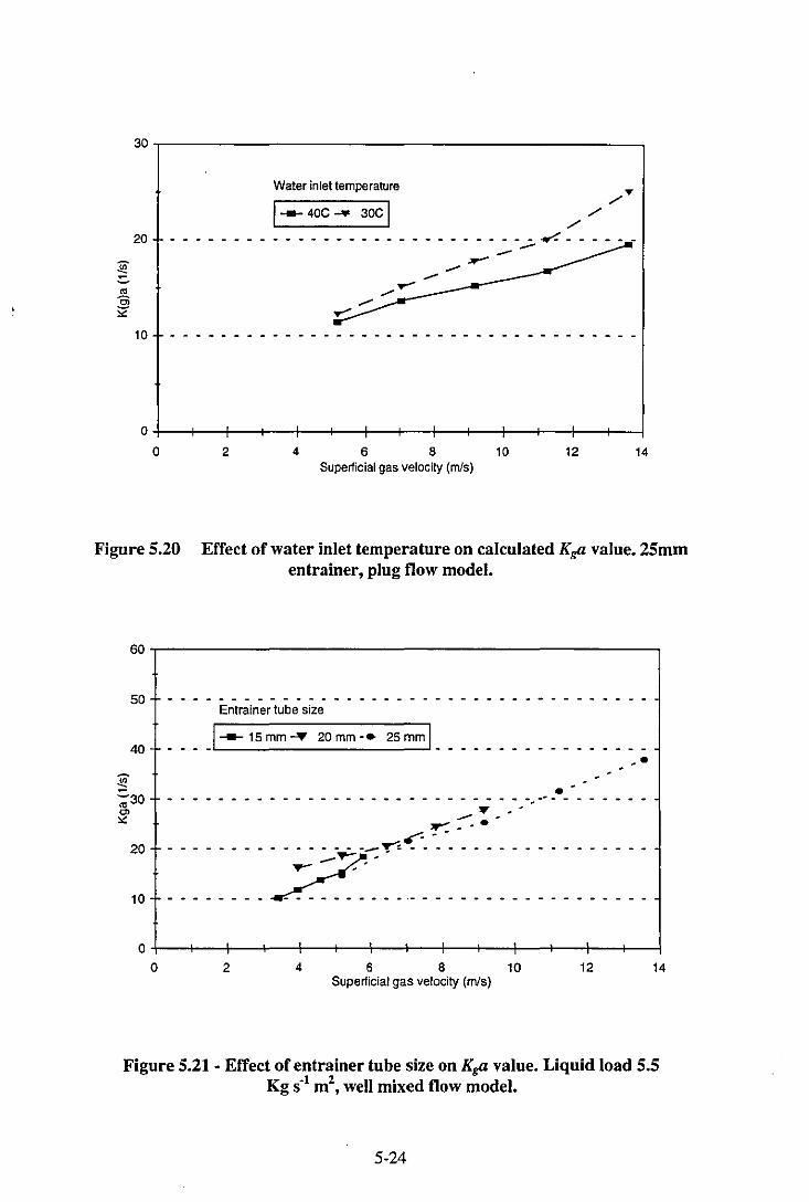
~ ~
.'!t
.9
'"
30~----------------------------------------------~
20
10
Water inlet temperature
1 ___ 40C.... 30C I
'" ","
'" - - - - - - - - - - - - - - - - - - - ..r- - - - - - --------
O+---~~---+---r--~--+-~---+---r--~--+---~~--~
o 2 4 6 B 10 12 14 Superlicial gas velocity (m1s)
Figure 5.20 Effect of water inlet temperature on calculated Kga value_ 25mm entrainer, plug flow model.
60
50 Entrainer tube size
40 __ .I---1smm-", 20mm-. 2smml __________ _
• ~ • -;30 0>
'" 20
10
- - - - - - - - - -... - - - - .. .... - -,.. -- -......:- ..... .... ---: : : : : : : ~~ : : : : : : : : : : : : : : : : : : :
0 0 2 4 6 8 10 12 14
Superlicial gas velocity (m1s)
Figure 5.21 • Effect of entrainer tube size on Kga value. Liquid load 5.5 Kg S·l m2
, well mixed flow model.
5-24
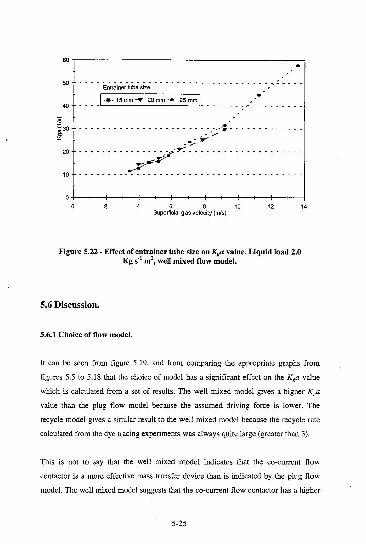
60 ,.
50 ,
- - - - E~tr~in-er-tub; siz; - - - - - - - - - - - - - - - - - - - - -, - - - - -
40 ___ .1--- 15 mm ~ 20 mm -. 25 mm L ________ :~ ______ _
~ ';;;30 C> --- - - - - - - - - - - - - - - - - - - - - - - -.-" - - - - - - - - - - - - -. ' ..... '"
20
10
,~ _______ /T'''': _ _ _ _ _ _ _ _ _ _ _ _ _ _ _ .
0
0 2 4 6 8 10 12 14 Superlicial gas velocity (m/s)
Figure 5.22 - Effect of entrainer tube size on Kga value. Liquid load 2.0 Kg S·l ml, well mixed flow model.
5.6 Discussion.
5.6.1 Choice of flow model.
It can be seen from figure 5.19, and from comparing the appropriate graphs from
figures 5.5 to 5.18 that the choice of model has a significant effect on the KKa value
which is calculated from a set of results. The well mixed model gives a higher Kga
value than the plug flow model because the assumed driving force is lower. The
recycle model gives a similar result to the well mixed model because the recycle rate
calculated from the dye tracing experiments was always quite large (greater than 3).
This is not to say that the well mixed model indicates that the co-current flow
contactor is a more effective mass transfer device than is indicated by the plug flow
model. The well mixed model suggests that the co-current flow contactor has a higher
5-25
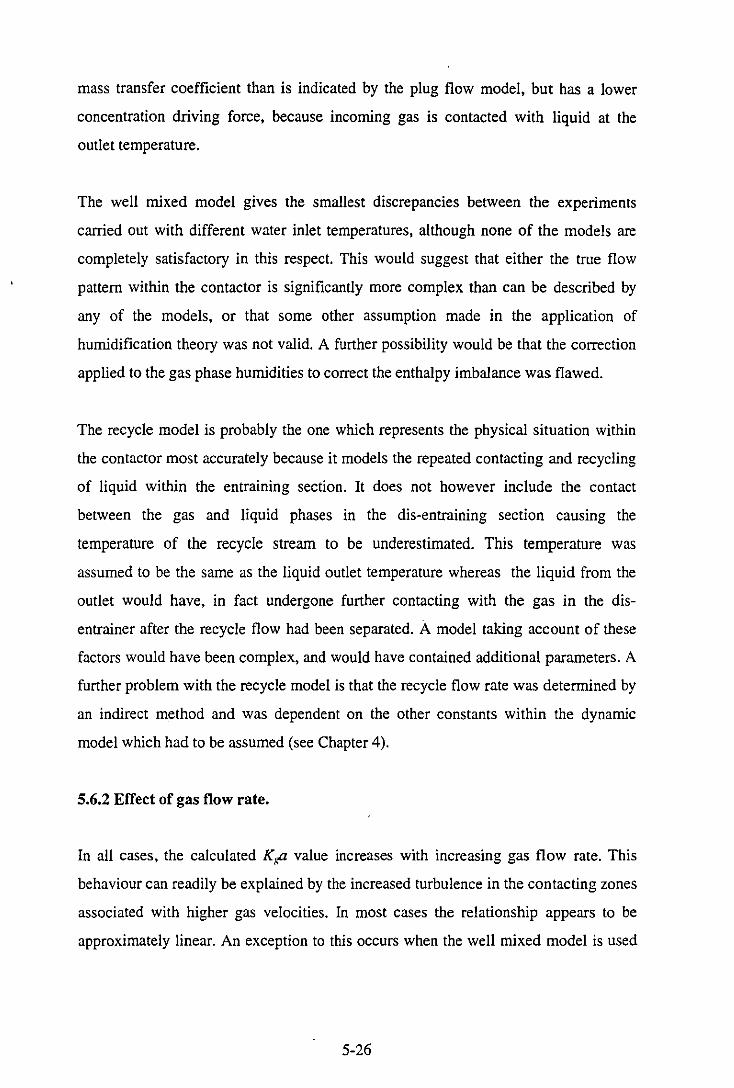
mass transfer coefficient than is indicated by the plug flow model, but has a lower
concentration driving force, because incoming gas is contacted with liquid at the
outlet temperature.
The well mixed model gives the smallest discrepancies between the experiments
carried out with different water inlet temperatures, although none of the models are
completely satisfactory in this respect. This would suggest that either the true flow
pattern within the contactor is significantly more complex than can be described by
any of the models, or that some other assumption made in the application of
humidification theory was not valid. A further possibility would be that the correction
applied to the gas phase humidities to correct the enthalpy imbalance was flawed.
The recycle model is probably the one which represents the physical situation within
the contactor most accurately because it models the repeated contacting and recycling
of liquid within the entraining section. It does not however include the contact
between the gas and liquid phases in the dis-entraining section causing the
temperature of the recycle stream to be underestimated. This temperature was
assumed to be the same as the liquid outlet temperature whereas the liquid from the
outlet would have, in fact undergone further contacting with the gas in the dis
entrainer after the recycle flow had been separated. A model taking account of these
factors would have been complex, and would have contained additional parameters. A
further problem with the recycle model is that the recycle flow rate was determined by
an indirect method and was dependent on the other constants within the dynamic
model which had to be assumed (see Chapter 4).
5.6.2 Effect of gas flow rate.
In all cases, the calculated K,a value increases with increasing gas flow rate. This
behaviour can readily be explained by the increased turbulence in the contacting zones
associated with higher gas velocities. In most cases the relationship appears to be
approximately linear. An exception to this occurs when the well mixed model is used
5-26
to analyse results for the 25mm entrainer. In this case the lines show a clear upward
curve with increasing gas flow.
5.6.3 Effect of liquid loading.
The effect of liquid loading on the calculated Kga value depends strongly on the flow
pattern model used in calculating the Kga value. When the well mixed model is used
to analyse results from the 25mm entrainer (figure 5.5), the Kga value decreases with
increasing liquid load, particularly at high gas flow rates. When the plug flow model is
used, the Kga value does not appear to vary greatly with the liquid load. With the two
smaller entrainment tubes, the Kga value increases strongly with increasing liquid load
when the plug flow model is used, but does not depend strongly on liquid load when
the well mixed model is used.
Literature data for spray chambers suggest the gas side mass transfer rate increases
with increasing liquid load. This will be because the total surface area for mass
transfer will increase with the liquid load as the droplet density will increase. With
this contactor, this may not necessarily be the case. When the liquid inflow is
increased, the liquid level around the entrainment weir will rise (see chapter 3) One
consequence of this may be that the entrainment tube would produce larger liquid
droplets, rather than more liquid drops, as the liquid load is increased, with a
consequent reduction in the total surface area.
5.6.4 Effect of water inlet temperature.
In general, the experiments carried out with a water inlet temperature of 40 'c generate lower Kga values than the equivalent experiments carried out at 30 'c, particularly when the plug flow model is used to model the results. The true value of
Kga should be largely independent of temperature, and so the differences between the
results carried out with the two different liquid inlet temperatures will largely be
because of shortcomings in the models used to estimate the effective average driving
force. It is thought that the results generated with the 40 'c water inlet temperature are
5-27
generally more reliable because the measured water temperature change was larger,
and hence less susceptible to measurement errors.
5.6.5 Effect of tube size.
The results illustrated in figures 5.21 and 5.22 suggest that the tube size does not have
a strong effect on the mass transfer performance for a given gas flow rate. This would
indicate that the mass transfer is not strongly dependent on the local gas velocity
within the tube, and hence at the point of entrainment. Given that the mass transfer
coefficient is a strong function of the gas flow for a given tube size, it would appear
that the gas phase mass transfer resistance is a function of the gas velocity at some
other point or points in the contactor. Because changing the velocity at the
entrainment point, whilst keeping the other local gas velocities the same, does not
affect the mass transfer rate, it would appear that the majority of the mass transfer is
occurring in regions away from the entrainment tube.
5.6.6 Comparisons with conventional equipment.
The mass transfer performance of conventional devices is rarely quoted in terms of
KNa values. For tray columns the mass transfer performance would usually be quoted
in terms of Murphree efficiencies, whilst for packed columns the height of a transfer
units would usually be quoted. Tray columns are rarely used for humidification duties
and so the performance of the co-current flow contactor will be compared here to that -
of packed columns performing the same duty. This is achieved by calculating the
number of counter-current transfer units which a single co-current flow contacting
stage is the equivalent of. Because the co-current flow device is not in fact a section of
a counter current column, the equivalent height of a transfer unit will depend on
factors such as the driving force and would not be constant over a whole column of
such units as it would be (more or less) over the full height of a packed column. This
method is however, probably the best way of comparing the performance of the
contactor with conventional columns based on the results from just one mass transfer
system.
5-28
The equivalent number of counter current transfer units was calculated using equation
(5.8). (Treybal [1968])
N = fH., dHA ,OG H H-H
AI S A (5.8)
Hs> the saturated vapour enthalpy was known as a function of the liquid enthalpy, HL
from the water vapour saturation data. HL was known as a function of Ha from the
equivalent operating line equation (5.9) this was calculated from the inlet and outlet
enthalpies, rather than from the flow rates. The operating line for a counter-current
analysis is shown on a temperature-enthalpy graph in figure 5.23. As with the Kga
measurements, the values of the integral terms were determined from the experimental
results by numerical integration using the trapezium rule.
w u H,·I---------7I' 0: o u.. Cl z OUTLET ~ H~I_--___::7"'----,__+_-__ 0: C H, .1-:_""------___::",
OPERAT NG LINE H INLET .. 1------""""1"
T, T,
LIQUID TEMPERATURE (T)
(5.9)
Figure 5.23 - Temperature - enthalpy diagram for equivalent counter-current
analysis.
5-29
The total height, Z, of a differential contactor is given by the number of transfer units
multiplied by the height of a transfer unit, HOG:
(5.10)
The equivalent number of transfer units for the co-current flow contactor is given as a
function of gas and liquid flow rates for the three entrainer tube sizes in figures 5.24 to
5.26. The equivalent height of a transfer unit, HOG can be obtained by dividing the
contactor height (0.35m) by the number of transfer units.
Sherwood & Pigford [1952] give HOG values for the humidification of air with water
in spray towers and packed towers. The values for the spray tower varied between
0.6m and 3.0m, with the value of HOG increasing with both gas and liquid flow rates.
The values quoted for the packed column were derived from earlier data presented by
Sherwood & Holloway [1940]. This data was obtained using 1.5 inch rings at
superficial gas velocities of between 0.25 rnIs and 1.2 rnIs at a specific liquid loading
of around 0.6 kg S·I m·2• The value of HOG varied between 0.2m and 0.36m. The HOG
value increased with increasing gas load and decreased with increasing liquid load.
The single co-current flow contacting stage of 350mm total height was equivalent to
between 0.2 and 0.6 transfer units, giving equivalent HOG values of between 0.56m
and 1.7m. These values were measured with the 25mm entrainment tube with
superficial gas velocities of between 5 m1s and 13.8 rnIs at liquid loads between 2.0
and 7.5 kg S·I m·2• The value of HOG increased with increasing gas flow and decreased
with increasing liquid load.
No data could be found concerning humidification operations in more recent types of
tower packing as most authors testing these packings (e.g. Billet [1994]) have tended
to employ distillation or gas absorption systems to determine the mass transfer
performance.
5-30
The data of Sherwood & Holloway [1940] was obtained using a packed section of just
0.2m depth, and the authors state that end effects would have been significant, and
that significant mass transfer would have been occurring in the region beneath the
packed section in which the water drips from the packing onto the base of the column.
For these reasons it is not possible to unequivocally say that the co-current flow
contactor is inferior to conventional equipment for gas side controlled systems until
further mass transfer trials have been carried out with other systems.
0.8.,------------------------,
C!l Q z
0.6
E .!E0.4 '" ." ::> er W
0.2
(Liquid loading kg!s sqm)
_ _ _ _ _ _ _ _ _ _ _ _ _ ~ _ ,- __ 1--- 2.0..... 3.6 -. 5.5 -4 7.5 ~ ........... ~ .. --...... ........ ~ ... :.-
~ .. -- -- :-~ ~ =-= -,,-=6---~---.
O+--+-~-~_+-+-_+-~~r_~-~-+-~~r-~
o 2 4 6 8 10 12 14 Superiieial gas velocity (m/s)
Figure 5.24 Equivalent number of counter-current transfer units (NtOG). 25mm entrainer.
5-31

0.8
Cl o zO.6
ffi ~ g.0.4 w
Liquid loading kg/s sqm)
------"'::-..-, ---1--- 2.0 .... "- ......
3.6 - .. 5.5 .....
e
7.3 ~ _
..... ..-.... , '"-
_ .......................... "S...._ .... !, ... -.." ...... : ~ ~ ........ .. ......... .. e__ -- .. ~- - .......
~ ..... .......................... -~ .......... ~ ~:-: :-!'- ....
• 0.2 ... " .. .. .. .. .. .. .. .. .. .. .. .. .. .. .. .. .. .. .. .. .. .. .. .. .. .......... ..
O+---_r--~----r---~---r--~----r---~--_+--~
o 2 4 6 8 10 Gas Flow (Iit'min)
Figure 5.25 Equivalent number of counter-current transfer units (NtOG). 20mm entrainer.
O.B
8 zO.6
ffi 'iij .~
5-0.4 w
Liquid loading kg/s sqm) ~ r-----------~~-~-~-~-~-- --~~-1--- 2.0 ..... 3.6 -. 5.5 ..... 7.31 ------....
e_ ...... .. .. .-: ~:: .. -.. -.... -.. -.. -.. ;. -.. -.. -a. - "'--~- ...
----------------------~---~--~-~--
0.2 .... .............................. ..
O+-------~----~-------r------+_------r-----~
o 2 4 6 Gas Flow (lit/min)
Figure 5.26 Equivalent number of counter-current transfer units (NtOG).
15mm entrainer
5-32

.5.7 Conclusions.
The calculated Kga value for a given experiment was strongly dependent on the flow
model which was used to deduce the effective average driving force. None of the flow
models used was entirely satisfactory, as indicated by the fact that the experiments
conducted at different liquid inlet temperatures generated significantly different
results. The recycle model is probably the one with the best potential for applying
these results to other systems, although better data concerning the recycle flow ratio
would be required.
The mass transfer coefficient increased with increasing gas velocity in all cases, as
one would expect. The variation of the coefficient with liquid loading was less easy to
generalise. In some cases the mass transfer coefficient clearly decreased with
increasing liquid load, and in others it appeared to be more or less independent. For a
given gas flow rate, the gas side mass transfer coefficient did not depend on the size of
tube in the entrainer. This suggested that the main regions for gas side mass transfer
were in regions away from the entrainment tube.
The gas phase mass transfer performance of the new contactor, as measured by the
humidification of air with water vapour, appears to be somewhat inferior to
conventional packed towers, with the 350mm high contacting stage being
approximately equivalent to around 0.2m of packing depth. There is some doubt as to
the accuracy of these figures because of doubts over the original data for the packed
column.
5-33

CHAPTER SIX

Chapter 6
Liquid side mass transfer measurements
6.1 Scope.
This chapter describes the experiments which were carried out in order to determine
the liquid side resistance to mass transfer of the co-current flow gas liquid contactor.
Some background theory on mass transfer systems was given in the literature review
chapter (chapter 2) and some of this theory will be expanded on here.
Section 6.2 will describe the selection of a suitable mass transfer system for use in
determining the liquid side mass transfer resistance. Section 6.3 describes the
ultimately unsuccessful attempts to measure the liquid side resistance using the
oxidation of aqueous sodium sulphite solutions. Section 6.4 will describe the
experiments used to measure the mass transfer resistance using a simpler physical
mass transfer system.
6.2 Selection of mass transfer system.
There are two main types of system which can be used to measure the liquid side mass
transfer resistance of gas liquid contactors (see chapter 2). These are the absorption or
desorption of a sparingly soluble gas between a liquid and a carrier gas and the
absorption of a pure gas into a liquid. COmInonly used variations on the first type of
system involve the use of chemical reactions within the liquid phase. As with the gas
side mass transfer experiments there were restrictions imposed on the substances
which could be used due to health and safety issues, and by the difficulty in supplying
gases other than air in sufficient quantities.
6-1
The type of system in which a pure gas is absorbed into a liquid was not chosen
because it would not have been practical to provide a suitable gas at the required flow
rate for the contactor. Some trials were carried out with the simple absorption system
in which oxygen was absorbed from air into de-oxygenated water, with an electronic
oxygen probe being used to measure the dissolved oxygen level in the outlet water.
These trials proved unsatisfactory because the outlet water was so close to 100%
saturation with oxygen that no reliable values for the liquid side mass transfer
coefficient could be determined.
With the first attempts at using a physical absorption system having failed it was
decided to attempt the use of a chemical reaction system. As has been mentioned
previously, care is required in interpreting the results from systems involving
chemical reactions, as the chemical reaction process itself can interfere with the mass
transfer process.
There are, however, also a number of advantages of chemical systems over purely
physical ones. Firstly, the experiments themselves can be easier to carry out because
the total mass transfer rate can be determined by measuring the depletion of the other
reactant, which can often achieved through simple chemical analysis methods such as
acid-base or redox titration. Simple physical systems often require the use of
specialised equipment for determining gas and/or liquid phase compositions.
Secondly, by varying the reaction rate, and hence the reaction regime in a chemical
system it can be possible to determine the specific interfacial area (a) separately from
the volumetric mass transfer coefficient (Kp).
The chemical system which was chosen was one in which oxygen from air diffuses
into aqueous sodium sulphite solution and oxidises the sulphite ions to sulphate. The
rate of the chemical reaction can be altered by changing the concentration of the
catalyst, which in this case is Cobalt (11) sulphate. The concentration of sulphite
remaining in the liquid can easily be determined using redox titration. The advantages
of this system for use here were that no gases other than air were required, the
6-2
chemical reaction rate could be easily altered and the analysis of the liquid samples
was straightforward.
Ultimately, the sulphite oxidation technique proved unsuccessful as a technique for
measuring kp in the contactor. Further details of the problems experienced with this
system are given in section 6.3. With these problems in mind, it was decided to retum
to a physical absorption system.
The system which was chosen was one in which CO2 was desorbed from water into
the air stream within the contactor. This system proved to be feasible because the
measured CO2 concentration change in this case was such that a meaningful mass
transfer coefficient could be calculated. The system was also practical because only
small quantities of CO2 were required in order to saturate the quantities of liquid
which were being used, and air was still the only gas used in the contactor itself. The
dissolved CO2 concentrations in the liquid phase could easily be determined by acid
base titration, whilst the gas phase CO2 concentration did not require measurement
because it was negligible in comparison with the predicted liquid interfacial
compositions. This system can be safely regarded as a simple physical system because
the reaction between CO2 and water to form carbonic acid does not proceed to an
extent sufficient to significantly affect the mass transfer process.
This system proved entirely satisfactory for measuring the liquid side resistance to
mass transfer and the results form the basis of the kp values presented in this chapter.
As with the gas-side mass transfer measurements, the flow pattern assumed for .the
liquid phase significantly affects the value of kp which is generated from a given set
of experimental results. Full details of the CO2 desorption experiments can be found
in section 6.4 of this chapter.
6-3

6.3 The sulphite oxidation system.
This section will describe the attempts which were made to characterise the liquid side
mass transfer properties of the contactor by studying the oxidation of aqueous sodium
sulphite solution. Sub-sections 6.3.1 and 6.3.2 will give background information and
theory on the system and a brief review of published information. Sub-sections 6.3.3
and 6.3.4 will describe the experimental procedures and the analysis of the results.
The results will be presented and discussed in sub sections 6.3.5 and 6.3.6.
6.3.1 Introduction
The oxidation of sodium sulphite solution is a widely used mass transfer test system,
and has been used in particular for studying the transfer of oxygen in gas sparged
fermenters and other equipment for carrying out aerobic biological processes. The
reaction on which the system is based is the oxidation of aqueous sulphite ions to
sulphate ions by dissolved oxygen:
SO" + 1.0 ~ SO'· 3 2 2 4
The uncatalysed reaction is slow, and for practical purposes the reaction is usually
catalysed by copper (II) or cobalt (II) ions. Most authors recommend the use of the
cobalt catalyst because its catalytic effect is stronger and more reproducible than that
of copper. The above reaction is a simplification of several reaction steps, and the
exact reaction mechanism is not fully understood.
The chemical reaction occurs simultaneously with transport of oxygen from the liquid
surface to the bulk of the liquid. A general treatment of simultaneous mass transfer
and chemical reaction, including a short section on the sulphite oxidation system is
given by Danckwerts [1970]. Many authors have applied the sulphite oxidation
system to study the liquid side mass transfer resistance and interfacial area in different
6-4

types of absorber. Much of this work is reviewed by Linek & Vacek [1981], who also
give an extensive theoretical treatment of the system.
Systems involving simultaneous mass transfer and chemical reaction are complex, and
exact analytical solutions giving the mass transfer rate as a function of the reaction
and mass transfer constants are not always possible. A simple solution of
simultaneous film diffusion with chemical reaction gives several possible regimes
based on the relative rates of diffusion and chemical reaction.
6.3.2 Theory.
Parameters which affect the reaction rate.
The following is a summary of the conclusions drawn by Linek & Vacek [1981] of
the effects of various parameters on the reaction rate, based on the published data of
many authors.
Effect of sulphite concentration.
The reaction can safely be assumed to be zero order with respect to sulphite provided
that the sulphite concentration is above a critical value. Most literature data suggests
that this critical sot concentration is around 0.3 moles/litre. The absorption rate
does however depend on the total ionic strength of the solution, although this is not
due to changes in reaction kinetics, but is due to changes in the solubility and
diffusivity of oxygen with changing solution strength. The absorption rate does
therefore depend on the starting concentration of sulphite but will not change as the
conversion of sulphite to sulphate proceeds.
6-5
Effect of Oxygen concentration
The literature data is divided between that which suggests the reaction is first order
with respect to oxygen and that which indicates second order behaviour. The order
with respect to oxygen appears to depend on the concentration of oxygen at the liquid
surface, and hence on the concentration of oxygen in the gas phase. With air being
used as the gas phase, most of the literature data would suggest that the reaction
would be second order with respect to oxygen. The rate equation for the reaction can
therefore be expressed as;
(6.1)
V is the reaction rate, Co is the liquid oxygen concentration and k2 is the second order , reaction constant which depends on the catalyst concentration, the pH and the
temperature.
Effect of catalyst concentration.
The literature evidence suggests that the reaction rate is first order with respect to
catalyst concentration provided the reaction is occurring in the region in which it is
pseudo zero order with respect to sulphite. k2 in the above equation will therefore be
linearly proportional to the catalyst concentration. The upper limit on the catalyst
concentration is set by the point at which a precipitate begins to form, effectively
removing the catalyst from the solution
Effect of pH.
The reaction rate increases with increasing pH up to a pH of around 9.0. The variation
of the reaction constant with pH is correlated by Linek & Vacek using the following
expressIon.
6-6
k2 - (pH -7.9 + O.04T)2 (6.2)
Where T is the temperature (0C). The solubility of the cobalt (IJ) catalyst, however,
increases with decreasing pH, so a lower pH may allow greater reaction rates by
permitting a higher catalyst concentration to be used. The pH of the solution decreases
slightly as the conversion of sulphite into sulphate proceeds.
Effect of Temperature.
The dependence of the reaction constant on temperature can be fitted by a standard
Arrenhius type expression:
k2 -exp{-En/(RT)) (6.3)
Where En is the activation energy. T is the temperature (K). The temperature will also
affect the solubility and diffusivity of the oxygen in solution.
Regimes for simultaneous absorption and reaction.
Linek and Vacek [1981] show how the total absorption rate in a contactor should vary
with catalyst concentration for a given absorber with the other parameters held
constant, and this illustrative plot is reproduced here in figure 6.1. No actual
experimental data covering the full range of catalyst concentrations for a single
contactor could be found in the literature. The graph demonstrates how the reaction
can proceed in one of four reaction regimes:
6-7
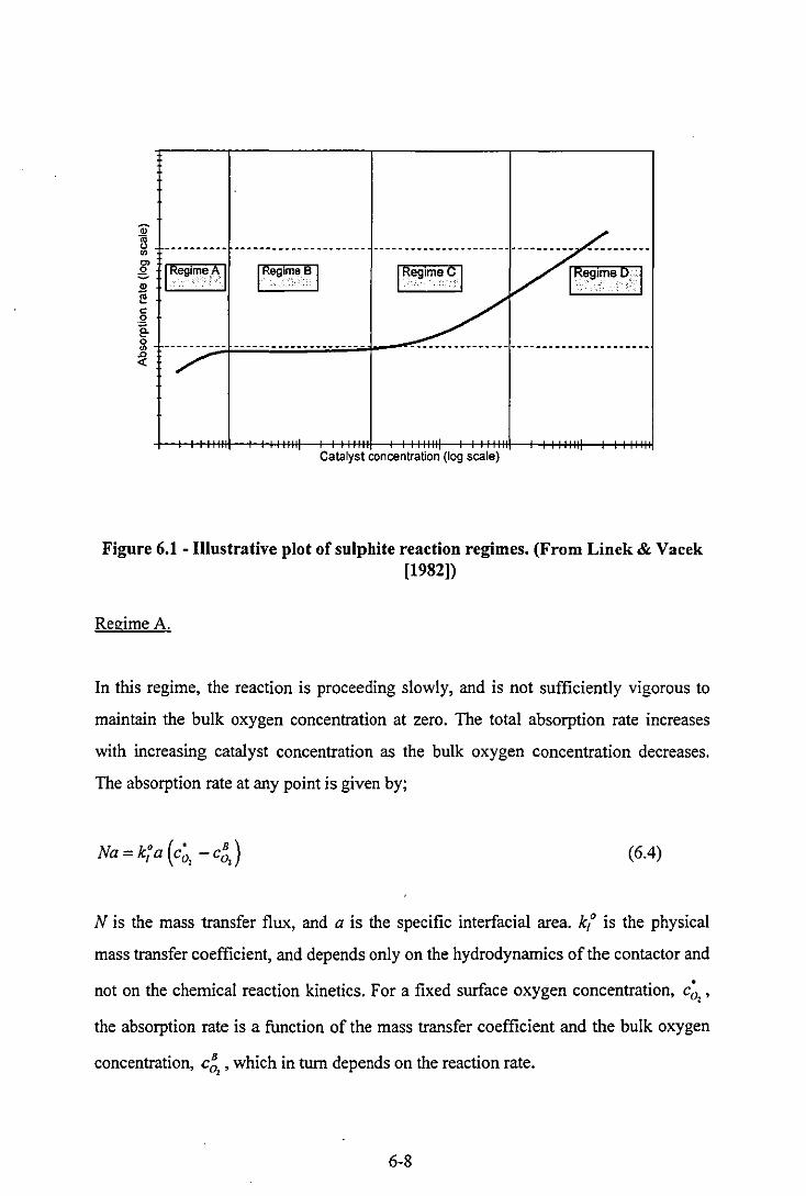
-----------------------------~-------I R~lm~? I V I ~eglrn~,DI
~----------------------
Catalyst concentration (log scale)
Figure 6.1 - Illustrative plot of sulphite reaction regimes. (From Linek & Vacek [1982))
Regime A.
In this regime, the reaction is proceeding slowly, and is not sufficiently vigorous to
maintain the bulk oxygen concentration at zero. The total absorption rate increases
with increasing catalyst concentration as the bulk oxygen concentration decreases.
The absorption rate at any point is given by;
Na=k:a(c~, -c~,) (6.4)
N is the mass transfer flux, and a is the specific interfacial area. kt is the physical
mass transfer coefficient, and depends only on the hydrodynamics of the contactor and
not on the chemical reaction kinetics. For a fixed surface oxygen concentration, c~"
the absorption rate is a function of the mass transfer coefficient and the bulk oxygen
concentration, c~" which in turn depends on the reaction rate.
6-8

Regime B.
At this point the reaction is sufficiently fast to maintain the bulk liquid oxygen
concentration at zero, yet is not fast enough to affect the transport of oxygen from the
surface to the bulk. In other words, all the reaction occurs in the bulk of the liquid
itself. The absorption rate is given by;
(6.5)
Here the reaction rate depends only on the physical mass transfer coefficient, kO p.
Regime c.
The reaction is now proceeding sufficiently fast that some of the oxygen is reacted
before it can transfer into the bulk of the liquid, and the mass transfer rate becomes
enhanced. The rate of absorption increases with increasing catalyst concentration as
the reaction becomes more vigorous. The total absorption rate for a 2nd order reaction
is given by;
(6.6)
Do, is the liquid diffusivity of oxygen. The absorption rate depends on both the
reaction constant and on the mass transfer coefficient.
6-9
Regime D.
Here the reaction proceeds at such a rate that all the oxygen is reacted very close to
the liquid surface. The absorption rate increases in proportion to the square root of the
reaction rate up to the point at which the catalyst begins to form a precipitate. The
absorption rate is given by;
[2 ]112
Na=ac~, 3Do,k,,(c~,) (6.7)
In this regime, the absorption rate depends only on the reaction rate and on the surface
area.
Conditions for the reaction regimes.
The analysis which leads to the above equations is based on the assumption of a
pseudo 2nd order reaction with respect to oxygen. For this assumption to hold, the
following condition should be satisfied.
8 ( ) 112 cso'- Dso'-Ha «-'- --'-
zc~, Do, (6.8)
Where Ha is the dimensionless Hatta number which is a measure of the relative rates
of the physical absorption and chemical reaction processes;
(6.9)
The four reaction regimes also have their own conditions. For regime B, the reaction
should be fast enough to maintain the bulk oxygen level at zero, whilst not being
6-10

sufficiently fast that oxygen can react before reaching the bulk of the liquid. These
two conditions can be expressed mathematically as;
(6.10)
Ha < 0.3 (6.11 )
The condition which needs to be satisfied for regime C is that the reaction should be
fast enough that some, but not all of the diffusing oxygen will react before it reaches
the bulk of the liquid. This is expressed mathematically as;
0.3 < Ha < 3 (6.12)
In addition, condition 6.10 must be satisfied so that the bulk concentration of oxygen
is zero.
The condition for regime D is that the reaction must proceed sufficiently fast for all of
the oxygen to react close to the liquid surface. This is expressed mathematically as:
Ha>3 (6.13)
Once again the condition relating to the bulk oxygen concentration (6.10) must be
satisfied.
These conditions require knowledge of kt, a and kz as separate parameters, and so
cannot be easily applied before the mass transfer experiments are carried out. The
kinetics of the sulphite reaction are known to be highly sensitive to the presence of
impurities, so the generally held view is that literature data on the reaction constant is
of little use. The value of the rate constant, kz, should be determined experimentally,
and will depend on the quality of sulphite used, and on the properties of the water
which is used in making the solutions. The kinetic constant for the sulphite reaction
6-11
can be detennined by measuring the absorption rate of oxygen in a stirred cell
contactor with a known surface area. The absorption is assumed to proceed in regime
D (see above), such that the absorption rate does not depend on the hydrodynamic
conditions, and hence kt. This can safely be assumed, providing the stirring is of a
sufficiently slow speed. One experimental test which can verify this regime is that the
absorption rate should increase in proportion to the square root of the catalyst
concentration.
6.3.3 Experimental.
The experiments were carried out in two parts. The aim of the first series was to
detennine the reaction rate constant at various catalyst concentrations by studying
oxygen absorption in a simple stirred cell absorber. The second series of experiments
involved measuring the oxygen absorption rate in the co-current flow contactor with
varying catalyst concentration in order to determine the values of kt and a.
Detennination of reaction constant.
The reaction constant, kb was detennined at various catalyst concentrations using the
apparatus shown in figure 6.2. The absorption cell 'is a simple stirred device in which
the total surface area for mass transfer can easily be detennined from the geometry.
The stirrer was set at 60 rpm, this being a typical stirrer speed recommended in the
literature. Provided the absorption is proceeding in the correct regime, the absorption
rate should not depend on the stirrer speed.
The experiments were carried out using I litre batches of sulphite solution prepared in
the same way as for the rig absorption experiments. The solutions were prepared to an
initial sulphite strength of 0.45 moles/lit using distilled water and S.L.R. grade
sodium sulphite. The catalyst concentration for each experiment was set by the
addition of a measured amount of analar grade cobalt (II) sulphate solution. The pH of
each sample was set by the addition of 0.1 M analar grade sulphuric acid solution. The
6-12

pH was measured using a standard pH electrode calibrated against pH 7.0 and pH 10.0
buffer solutions.
The oxygen absorption rate was determined indirectly by measuring the depletion of
sulphite ions in the liquid phase. 5ml samples were taken at set intervals and analysed
using iodometric back titration. In this technique the sample is mixed with a fixed
volume of a standardised iodine solution, with which the remaining sulphite ions
instantly react. The amount of unreacted iodine is then determined by titration against
a standard sodium thiosulphate solution with an appropriate indicator. The oxygen
absorption rate for each experiment was determined from the rate of change of
sulphite concentration with time. All the experiments were carried out at 25 QC, at a
pH of 9.00. The catalyst concentration was varied between 6xlO's and 5xlO-l
moles/litre. The upper limit was the solubility limit for the catalyst in sulphite solution
at this pH.
Water bath with temperature control
Air supply
Stirrer
Figure 6.2 - Stirred cell absorber used to determine reaction rate constants
6-13
Rig absomtion experiments
The experiments intended to characterise the liquid side mass transfer behaviour of
the novel contactor were carried out in the experimental rig shown in figure 6.3. The
two contacting stages beneath the experimental stage were used to humidify the feed
gas and bring it to the appropriate temperature. The intermediate carryover collection
section beneath the sulphite contacting stage was provided in order to prevent any
entrained water from the humidification section from reaching the sulphite section and
causing some dilution.
Humidification of the feed gas was essential in order to prevent evaporation in the
experimental stage which would lead to a temperature change between the inlet and
outlet of the experimental stage. If the feed sulphite solution contacted saturated gas
of an equal temperature, there should be no temperature change other than the slight
increase caused by the exotherm from the oxidation reaction.
The gas temperature at the inlet to the sulphite contacting stage was controlled by
altering the recirculation rate of the warm water in the lower two stages. The liquid
and gas inlet and outlet temperatures were measured using the thermocouples. The gas
flow rate was measured by the rotameter, and the liquid flow rate was known from the
pump calibration.
The feed solution was prepared as for the stirred cell absorber, although using a larger
volume of 2 litres. The sulphite solution was recirculated through the contacting rig at
the appropriate flow rate by the pump. The carryover liquid (that which passes
through the dis-entrainer with the gas phase) was not returned to the reservoir and was
collected separately. The absorption rate was determined by taking 5 ml samples from
the reservoir at two or three minute intervals and analysing them using the back
titration method as before. The rig was run for 3 minutes before sampling commenced
in order to allow a pseudo steady state to be reached. Each experimental run lasted
between 8 and 12 minutes depending on the catalyst concentration with 5 samples
being taken in each experimental run.
6-14
The reservoir was provided with a nitrogen blanket in order to ensure that the sulphite
was not being oxidised outside of the contacting unit. A simpler method, in which a
batch of sulphite solution is pumped through the contactor on a once through basis
was evaluated and rejected because the concentration change on one passage through
the contactor was so small that slight measurement errors would greatly affect the
calculated mass transfer rate.
The initial aim was to discover whether the sulphite oxidation method was a viable
technique in evaluation the liquid side mass transfer characteristics of the contactor.
For this reason, the contactor operating characteristics were kept constant and the
variables which were altered were those which affected the kinetics of the sulphite
reaction. The rig was run at the maximum gas flow rate of 1600 litlmin, corresponding
to a column velocity of 13.6 m1s. The liquid rate was kept constant at 0.6litlmin. The
liquid solutions were prepared at 25°C, and the gas temperature was also controlled at
this value. It was noted during the experimental runs that there was no significant
heating of the liquid due to the exotherrnic nature of the oxidation reaction.
The parameters which were varied were the pH and the catalyst concentration. Runs
were carried out with catalyst [C02+] concentrations of between lxl0·5 Molesllit and
lxl0'3 Molllit. The pH was set at either 9.00 or 8.50, with the lower pH being used at
the higher catalyst concentrations in order to aid catalyst solubility.
6-15
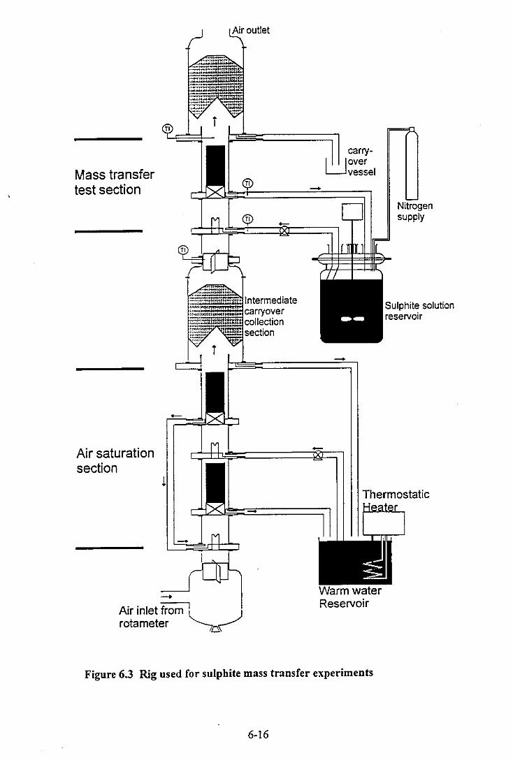
Mass transfer test section
Air saturation section
-+
Air inlet from I
rotameter
Air outlet
Intermediate Sulphite solution reservoir
Thermostatic
Warm water Reservoir
Figure 6.3 Rig used for sulphite mass transfer experiments
6-16
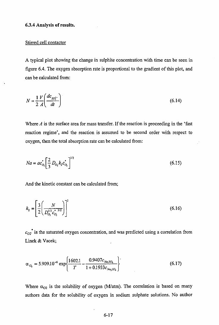
6.3.4 Analysis of results.
Stirred cell contactor
A typical plot showing the change in sulphite concentration with time can be seen in
figure 6.4. The oxygen absorption rate is proportional to the gradient of this plot, and
can be calculated from:
(6.14)
Where A is the surface area for mass transfer. If the reaction is proceeding in the 'fast
reaction regime', and the reaction is assumed to be second order with respect to
oxygen, then the total absorption rate can be calculated from:
(6.15)
And the kinetic constant can be calculated from;
(6.16)
C02' is the saturated oxygen concentration, and was predicted using a correlation from
Linek & Vacek;
- 5 90910";; {I 602.1 a o -. . exp , T O.9407cNa,s0, }.
1 + O.l933c No so , , (6.17)
Where a02 is the solubility of oxygen (Mlatm). The correlation is based on many
authors data for the solubility of oxygen in sodium sulphate solutions. No author
6-17
offers data for the solubility of oxygen in sodium sulphite solutions because the
reaction between the two species would prevent phase equilibrium from being
established. For determining the rate of the sulphite reaction, it was assumed that the
air feed to the absorption cell was sufficient to provide a constant gas phase oxygen
concentration at the liquid surface, this being equal to the normal atmospheric oxygen
concentration.
It can be seen from equation (6.15) that the absorption rate should be proportional to
the square root of the reaction constant. All the literature data suggests that this
reaction constant should be proportional to the concentration of CoS04 catalyst. A
plot of absorption rate against catalyst concentration on logarithmic co-ordinates
should, therefore be a straight line with a gradient of 112.
Rig absorption studies.
Unlike the gas side mass transfer experiments, there was no need to take account of
the contactor flow pattern in evaluating the mass transfer results for the sulphite
system because the bulk and interfacial oxygen concentrations would not have varied
between different points in the contactor. In the regimes of the sulphite reaction which
were being studied it should have been safe to assume that the reaction was
proceeding at a sufficient rate for the bulk oxygen concentration in the liquid phase to
be effectively zero. Examination of a mass balance showed that the oxygen
concentration in the gas phase, and hence the liquid interfacial oxygen concentration
would not alter significantly between the contactor inlet and outlet.
Allowance did, however, have to be made for the dynamics of the recirculatory
system which was used to measure the absorption rate, because the total mass transfer
rate could not be determined simply from the rate of change of sulphite concentration
in the reservoir. There was also a significant hold-up of liquid in the pipes and in the
rig itself, which was flowing in plug flow. This volume could not simply be added to
that of the stirred vessel for the purposes of calculating the total absorption rate
6-18
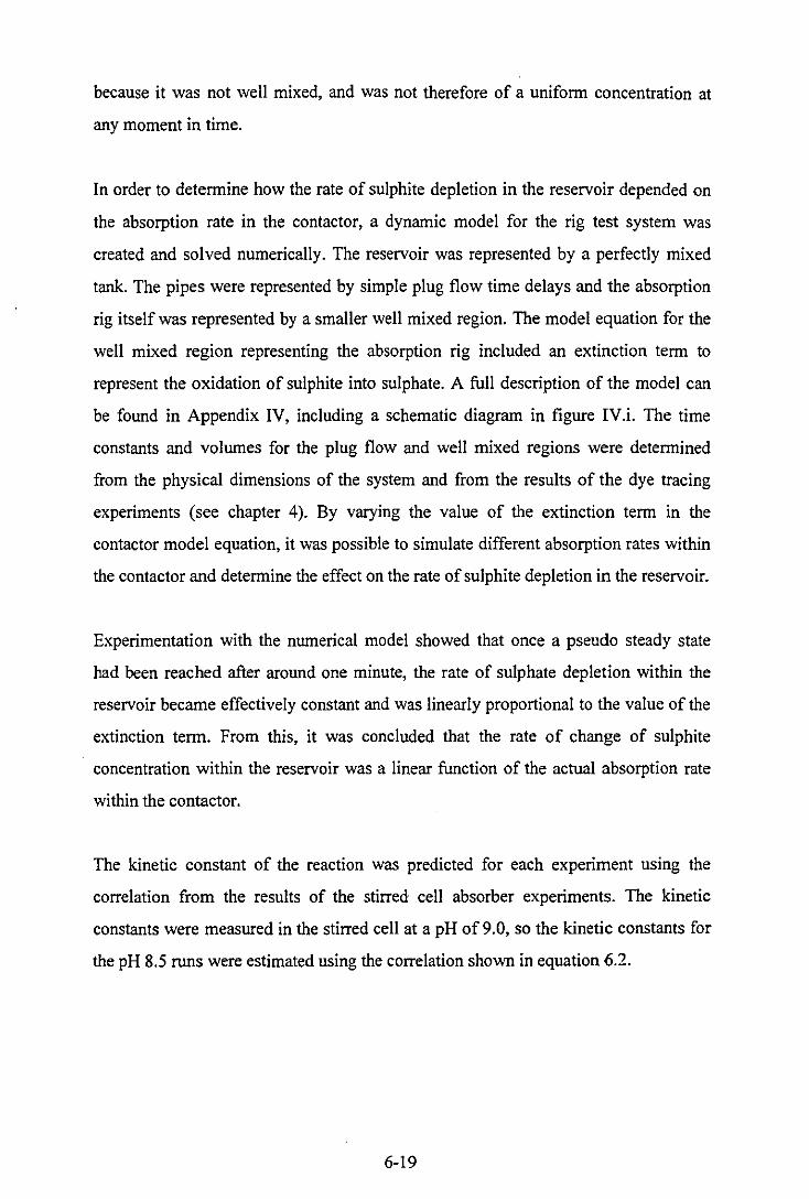
because it was not well mixed, and was not therefore of a uniform concentration at
any moment in time.
In order to determine how the rate of sulphite depletion in the reservoir depended on
the absorption rate in the contactor, a dynamic model for the rig test system was
created and solved numerically. The reservoir was represented by a perfectly mixed
tank. The pipes were represented by simple plug flow time delays and the absorption
rig itself was represented by a smaller well mixed region. The model equation for the
well mixed region representing the absorption rig included an extinction term to
represent the oxidation of sulphite into sulphate. A full description of the model can
be found in Appendix IV, including a schematic diagram in figure IV.i. The time
constants and volumes for the plug flow and well mixed regions were determined
from the physical dimensions of the system and from the results of the dye tracing
experiments (see chapter 4). By varying the value of the extinction term in the
contactor model equation, it was possible to simulate different absorption rates within
the contactor and determine the effect on the rate of sulphite depletion in the reservoir.
Experimentation with the numerical model showed that once a pseudo steady state
had been reached after around one minute, the rate of sulphate depletion within the
reservoir became effectively constant and was linearly proportional to the value of the
extinction term. From this, it was concluded that the rate of change of sulphite
concentration within the reservoir was a linear function of the actual absorption rate
within the contactor.
The kinetic constant of the reaction was predicted for each experiment using the
correlation from the results of the stirred cell absorber experiments. The kinetic
constants were measured in the stirred cell at a pH of 9.0, so the kinetic constants for
the pH 8.5 runs were estimated using the correlation shown in equation 6.2.
6-19
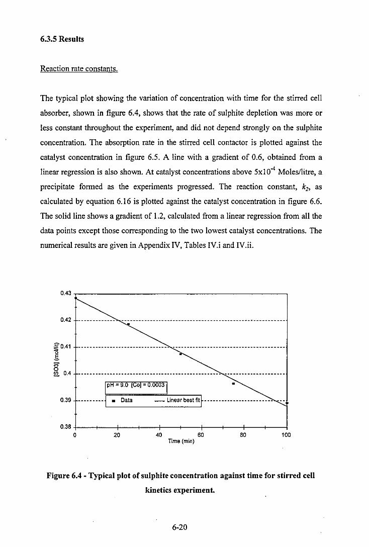
6.3.5 Results
Reaction rate constants.
The typical plot showing the variation of concentration with time for the stirred cell
absorber, shown in figure 6.4, shows that the rate of sulphite depletion was more or
less constant throughout the experiment, and did not depend strongly on the sulphite
concentration. The absorption rate in the stirred cell contactor is plotted against the
catalyst concentration in figure 6.5. A line with a gradient of 0.6, obtained from a
linear regression is also shown. At catalyst concentrations above 5x10⁻⁴ Moles/litre, a
precipitate formed as the experiments progressed. The reaction constant, kz, as
calculated by equation 6.16 is plotted against the catalyst concentration in figure 6.6.
The solid line shows a gradient of 1.2, calculated from a linear regression from all the
data points except those corresponding to the two lowest catalyst concentrations. The
numerical results are given in Appendix IV, Tables IV.i and IV.ii.
0.43,------------------------,
0.42 - - --- - ----- - - ------- - ---- --- ---------- - -- -- - - -- - ---- - - --- - - - - --- -- - ---
g0.41 '" g ;:; o !!l. 0.4
0.39
1 pH = 9.0 [Co] = 0.0003 1 •
"·"----1 • Data _linearbestfit~---------_--------------
0.38 -t---+----+--+--+--+--f--+---+-----<f-------1 o 20 40 60 80 100
TIme (min)
Figure 6.4 - Typical plot of sulphite concentration against time for stirred cell
kinetics experiment.
6-20
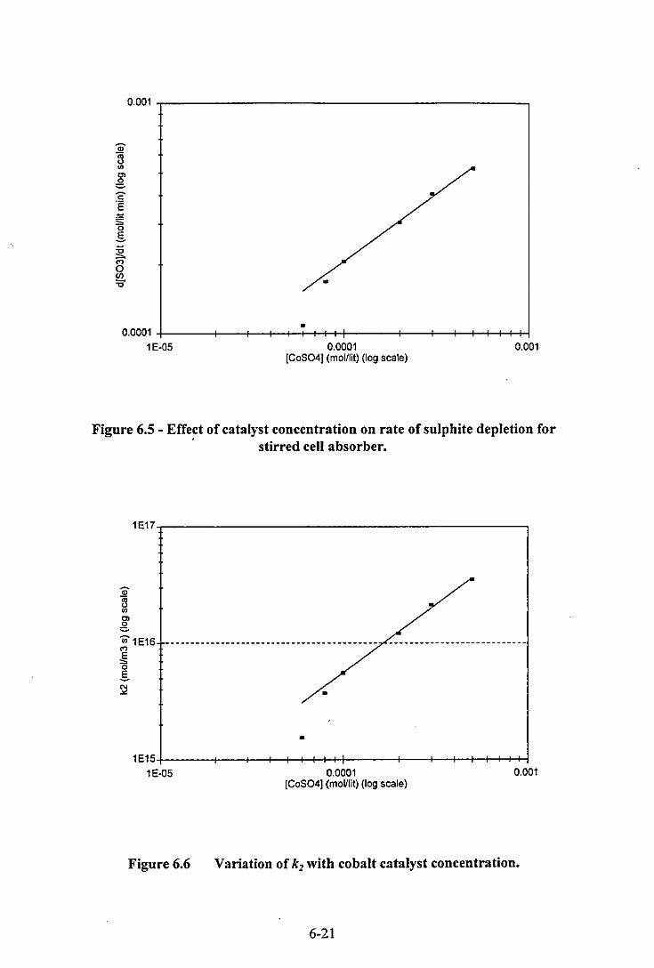
0.001 ,--------------------------,
:9l rl '" '" g c 'E '" ~ g i '" 0 f!1. • ."
• 0.0001 +------i--f---+--+--+--+-t-+-!------i--f---+--+-+--+-+-+-I
1E-OS 0.0001 0.001 [CoS041 (mollli!) (log scale)
Figure 6.5 - Effect of catalyst concentration on rate of sulphite depletion for . stirred cell absorber.
1E17~---------------------_.
:9l rl '" '" g '" 1 E16 '" t ~ •
• 1E1S+-----~--+_-r-r~++~------+---~~~+-~+1
1E-OS 0.0001 0.001 [CoS041 (moVli!) (log scale)
Figure 6.6 Variation of k] with cobalt catalyst concentration.
6-21

Rig absomtion experiments.
A typical plot showing the variation of sulphite concentration with time for the co
current flow contactor recirculation experiment is shown in figure 6.7. Once again the
graph is approximately linear, although with more scatter than was observed with the
stirred cell absorber. The rate of sulphite depletion. in the reservoir, which is
proportional to the absorption rate in the rig, is plotted against the predicted kinetic
constant in figure 6.8. The points relating to the runs carried out at a pH of 8.5 are
differentiated from those relating to the pH 9.0 runs although the difference in
reaction rates for a given catalyst concentration should have been accounted for. The
numerical results are given in Appendix IV, Table IV.iii
0.47.,-_______________________ -,
g0.45 "" o S M g 0.44
pH = 8.5. [Co) = 5E-3M
• Data
0.43 _______________________ ---- _______ -- - ____________ - ---- -- ___ ____ - _ - -- __ _
0.42 +---+----l---f----'f-----<f-----f---+---j o 2 4
TIme (min) 6 8
Figure 6_7 - Typical plot of concentration against time for co-current flow contacting rig experiment_
6-22

0.01 ,----_______________ ~---__,
• pH 8.9 c pH 8.5 - Y=kxA(1I2)1
• • • •
• • =
• • •
•
0.001 +---+-I--f-+-+-I-++t---+--+-+-+++++-ii--+---+--+-+++++1 lE15 lE16 lE17 lE18
K2 (m3 mol-l 5-1)(109 scale)
Figure 6.8 - Variation in absorption rate with k2 for co-current flow contacting rig experiments.
6.3.6 Discussion.
Reaction Kinetics.
It can be seen from figure 6.5 that the relationship between absorption rate and
catalyst concentration does not appear to show classic 112 order behaviour as
suggested by the literature. With the catalyst concentration above 1.10-4 moles/lit, the
line on the log-log plot is linear and seemed to suggest that the absorption rate varies
in proportion to the catalyst concentration raised to the power of around 0.6. When the
catalyst concentration is below 1.1 0-4 moles/lit, it would appear that the absorption
rate is below that which is predicted by extrapolation of the line downwards from
higher concentrations. This cannot be easily explained by a departure from the 'fast
reaction' regime, as this would cause the line to curve upwards with decreasing
reaction rate (see figure 6.1). The more likely explanation therefore was that, with this
6-23
batch of sulphite at least, the actual rate showed a more complex dependence on the
catalyst concentration than the simple first order relationship suggested in the
literature.
Linear regression showed that for catalyst concentration of 1.104 moles/lit and above
the kinetic constant can be correlated by;
(6.18)
This correlation was used for predicting the kinetic constants In the later ng
absorption studies.
Rig absomtion studies.
The first thing which is apparent from figures 6.8 is that there is a large amount of
experimental scatter, and a poor degree of reproducibility between experiments
conducted under supposedly similar conditions. Although a general trend of
increasing absorption rate with increasing reaction rate constant is apparent, it is not
easy to correlate the behaviour with any of the reaction regimes illustrated in figure
6.1. With the spread of reaction rates covering two orders of magnitude, it should have
been possible to see at least one of the reaction regimes clearly in some part of the
graph. It could be argued that the graph is levelling off at the lower catalyst
concentrations, with the absorption rate becoming less dependent on the reaction rate,
but there is so much scatter in this region that it would be hard to justity drawing this
conclusion.
The poor reproducibility of the results was the largest problem encountered with this
method. It is well known that many impurities can significantly affect the rate of the
sulphite reaction by interfering with the catalytic effect of the Cobalt (lI) ions. One
such impurity with a known detrimental effect is iron, and it was thought that some
corrosion of the stainless steel components may have been taking place in the strong
6-24
reducing environment of the sulphite solution, leading to dissolution of iron into the
solutions. A reddish brown deposit was found on some of the stainless steel
components, particularly on the knit mesh section above the carryover collection
plate. Analysis of washings from this deposit using atomic absorption showed that it
did not contain any significant iron, and was probably formed by deposition of some
cobalt complex similar to that which precipitated at high catalyst concentrations.
The reason for the poor reproducibility of the results is still therefore not clear.
Explaining the scatter in terms of variations in the chemical reaction rate may also not
be valid as in some of the reaction regimes, the absorption rate does not depend
strongly on the rate of the chemical reaction.
One possible explanation for the lack of an apparent reaction regime is that the mass
transfer is so intense that the absorption is proceeding in the regime in which the bulk
concentration of oxygen is not zero. Most previous work on the sulphite system
described in the literature has been carried out with less intense gas liquid contactors
such as bubble columns and gas sparged stirred vessels. A further possibility is that
several different mass transfer processes occur in the contactor due to the different
physical processes which occur in the various regions, e.g. drop formation, droplet
flight, dis-entrainment etc. It is possible that, with a given chemical reaction rate, the
absorption could be proceeding in different regimes in the different regions of contact.
If this was the case, then the graph showing the variation of absorption rate with
reaction rate (figure 6.8) would not show the classical shape shown in figure 6.1, but
would still show the general trend of increasing absorption rate with increasing
reaction rate.
Charpentier [1981] suggests that sometimes there may not be a regime in which the
absorption rate is independent of the reaction rate, because when the reaction rate
becomes high enough to maintain the bulk concentration at zero, it is already
sufficiently rapid to enhance the mass transfer process. This comment was made with
respect to chemical systems in general and no authors seem to suggest that this is a
particular problem with the sulphite oxidation system.
6-25

6.3.7 Conclusions.
It was ultimately concluded that the sulphite oxidation system was not a particularly
suitable system for measuring the liquid side mass transfer resistance of this contactor.
The main problems were poor reproducibility of results and a lack of agreement with
the type of behaviour suggested in the literature.
The first of these could possibly be explained by some variable contamination of the
reaction system although this would have to be very large in order to explain the large
variabilities in the results. The second problem could have had one of a number of
causes, the most likely being that the type of behaviour suggested in the literature was
that suggested by somewhat simplified models, and had only been observed
practically in simpler contactors than the one which was being studied here.
6.4 CO2 desorption system
This section will describe the experiments using the CO2 desorption system which
were used to determine the liquid side mass transfer resistance. Sub-section 6.4.1
gives an introduction and a brief description of the theory of the system. Sub-sections
6.4.2 and 6.4.3 describe the experiments themselves and the interpretation of the
results. The results are presented and discussed in sub-sections 6.4.4 and 6.4.5, whilst
sub-section 6.4.6 gives details on comparisons between the co-current flow contactor
and conventional equipment.
6.4.1 Introduction and theory
With the sulphite oxidation system having been found to be unsuitable, it was decided
that chemical systems in general were likely to be affected by similar problems, and it
was decided to use a purely physical system to characterise the liquid side mass
transfer performance. The system which was eventually chosen is one in which CO2 is
desorbed from a saturated water stream into the air. This system had the advantage
6-26

over other physical systems that the CO2 concentration in water could be determined
by acid base titration and did not require any specialist analysis equipment.
Desorption was chosen over an absorption type of system because only small
quantities of CO2 were required in order to saturate the liquid feed. An absorption
type of system would have required large amounts of CO2 gas to be added to the air
stream in the contactor.
Although CO2 does undergo a chemical reaction with water to from carbonic acid
(H2C03) which can then dissociate, this is not significant in terms of enhancing the
mass transfer rate. In a typical CO2 solution, only 0.5% of the total CO2 will be
present as carbonic acid, and an even smaller percentage as dissociated carbonate and
hydrogen carbonate ions (Margolis [1966]).
6.4.2. Experimental
The first stage of each experimental run was to saturate the feed water with CO2 at
atmospheric pressure. This was achieved using the plunging jet contactor illustrated in
figure 6.9. The main vessel had a volume of2.3 litres. The feed water was made from
a mixture of distilled water and ice from an ice maker, in order to give a feed
temperature after saturation of around 15°C. This lower temperature was chosen to
increase the solubility of the gas, and hence give a greater concentration change over
the apparatus. The saturation process was typically allowed to proceed for 45 minutes.
The mass transfer experiments were carried out in the apparatus shown in figure 6.10.
The saturated liquid was pumped into the contacting stage where it contacted the pre
humidified air. As with the sulphite oxidation experiments, the gas was saturated in
order to allow isothermal operation, and the gas temperature was controlled by
adjusting the flow of water in the saturating stages. The liquid was pumped through
the contactor in a single pass, rather than with a recirculatory system, and flowed into
a waste reservoir.
6-27
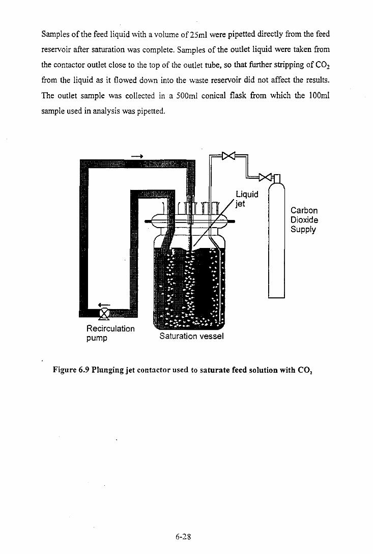
Samples of the feed liquid with a volume of 25ml were pipetted directly from the feed
reservoir after saturation was complete. Samples of the outlet liquid were taken from
the contactor outlet close to the top of the outlet tube, so that further stripping of CO2
from the liquid as it flowed down into the waste reservoir did not affect the results.
The outlet sample was collected in a 500ml conical flask from which the IOOml
sample used in analysis was pi petted.
Recirculalion pump Saturation vessel
Liquid jet
Carbon Dioxide Supply
Figure 6.9 Plunging jet contactor used to saturate feed solution with CO,
6-28
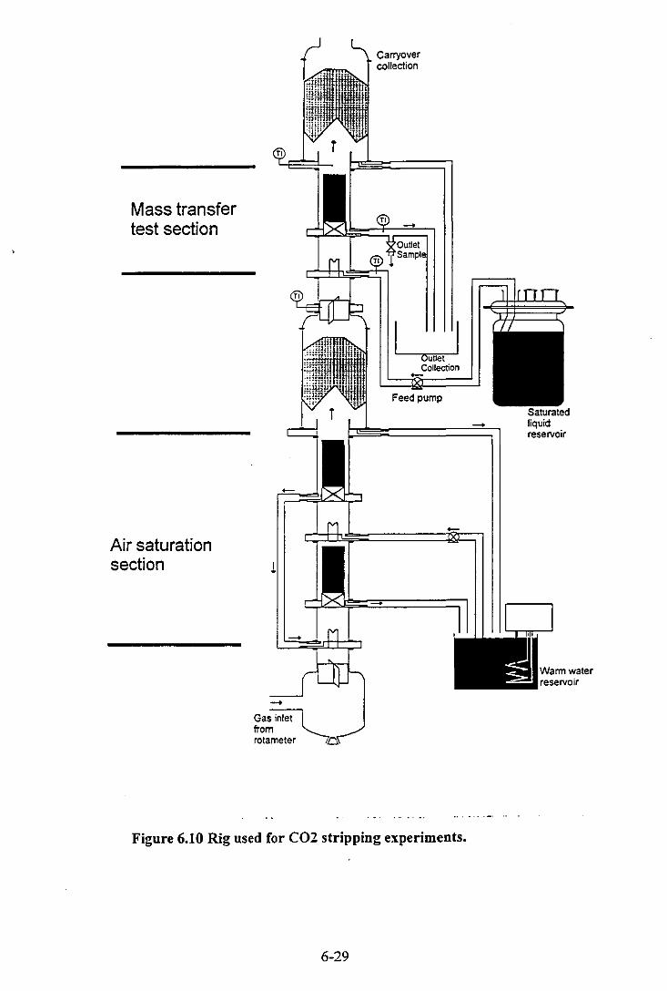
Mass transfer test section
Air saturation section
Gas inlet from rotameter
L;,J Collection
Feed pump
Figure 6.10 Rig used for C02 stripping experiments.
6-29
liquid reservoir
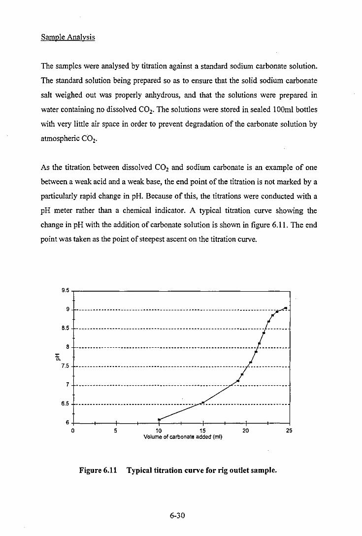
Sample Analysis
The samples were analysed by titration against a standard sodium carbonate solution.
The standard solution being prepared so as to ensure that the solid sodium carbonate
salt weighed out was properly anhydrous, and that the solutions were prepared in
water containing no dissolved CO2• The solutions were stored in sealed 100ml bottles
with very little air space in order to prevent degradation of the carbonate solution by
atmospheric CO2•
As the titration between dissolved CO2 and sodium carbonate is an example of one
between a weak acid and a weak base, the end point of the titration is not marked by a
particularly rapid change in pH. Because of this, the titrations were conducted with a
pH meter rather than a chemical indicator. A typical titration curve showing the
change in pH with the addition of carbonate solution is shown in figure 6.11. The end
point was taken as the point of steepest ascent on the titration curve.
9.5
9
8.5
8 :I: "-
7.5
7
6.5
6 0 5 10 15 20 25
Volume of carbonate added (ml)
Figure 6.11 Typical titration curve for rig outlet sample.
6-30
Experimental variables
The variables which were manipulated were the same as for the gas side mass transfer
experiments, namely, the gas flow rate, the liquid flow rate and the entrainment tube
size. The experimental temperature was not varied and was close to 15°C in all
experiments. The gas flow was varied between 330 Iit/min and 1600 lit/min whilst the
. liquid flow was varied between 0.7 and 2.2 lit/min. Entrainer tube sizes of 15mrn
20mm and 25mm were used in order to determine whether the liquid side mass
transfer performance depended on the local gas velocity at the entrainment point.
6.4.3. Interpretation of results.
Unlike the sulphite oxidation experiments, the flow pattern assumed for the liquid
phase does affect the kp value calculated from a given set of experimental results,
because the bulk concentration of CO2 changes significantly as the liquid passes
through the contactor. Examination of an overall mass balance showed that the gas
phase concentration of CO2, and hence the interfacial liquid phase concentration, does
not alter significantly as the gas flows through the contactor. The flow pattern which
is assumed for the gas phase, does not therefore affect the results.
The local mass transfer rate at any point in the contactor is given by;
(6.19)
The flow pattern model is used to calculate an average overall mass transfer
coefficient by attempting to calculate an effective average driving force. As with the
gas phase mass transfer experiments, assuming that the liquid phase is well mixed will
give higher kp values than those generated by assuming plug flow behaviour. This is
because the driving force for mass transfer predicted by the well mixed model is lower
as the whole volume of liquid is assumed to be at the outlet concentration. The results
6-31

of each experiment were analysed using both the plug flow and well mixed models,
and those generated with the 25mm entrainer were analysed using the recycle model,
in which the concentration of CO2 in the liquid in contact with the feed gas is
somewhere between the feed and outlet concentrations.
The recycle model was applied in a similar way to that which it had been for the
humidification experiments (see chapter 5), although in this case it is the effective
inlet CO2 concentration which is determined by the mixing model, rather then the
temperature.
The equations used to determine the kfI values for the various models were;
Well mixed model.
(6.20)
Plug flow model.
(6.21)
Where (c-c*)Lm is defined as:
_ * _ (C-C*}OUT -(c:",c*}/N
(c C )Lm - Ln((C-C*}OUT)
(c - C *) IN
(6.22)
The recycle model uses the same equation as the plug flow model but with a lower
inlet concentration calculated from a mass balance using the recycle ratios predicted
by the dye tracing experiments (see chapter 4). The effective liquid inlet
concentration, c'IN can be calculated from:
6-32
c = Rco", +CIN
IN R+1 (6.23)
Where R is the recycle flow ratio, as defined in chapter 4, equation (4.1). The Kp
value can be calculated from:
(6.24)
In this case (c-c*Jrm is defined as:
(6.25)
6.4.4. Results
The dependence of kp on the gas and liquid flows as calculated by the various flow
models is shown in figures 6.12 to 6.18. Figures 6.12 to 6.14 show the results for the
25mm entrainer, generated using the three different flow models. Figures 6.15 and
6.16 show the results for the 20mm entrainer generated using the plug flow and well
mixed models and figures 6.17 and 6.18 show the results for the 15mm entrainer
generated using the same two models. Figures 6.19 and 6.20 compare the results
generated by the different entrainer tube size using the well mixed model and the plug
flow model.. The experimental results are also given in Appendix IV, Table IV.iv.
6-33

1,-________________________________________ --.
liquid load (kg!s sqrn)
0.8 -001 ___ 5.9 _ .. 7.6 _._ 10.2 -4- 14.4 _::1_ 18.7 lnnnn-n--n 0.6
J!!. ~ 0.4
0.2
O+-~--~--~_r--+-_+--~~---r--~-+--+_~--~ o 2 4 6 8 10 12 14
Superficial gas velocity (rn!s)
Figure 6_12 Kp results, 25mm entrainer, well mixed flow model.
0.12.------------------------;x..----,
"" ./.-, .. • _____________________ • __ .. _________ • ______________ • ___ ______ .J! ____ ~~--------0.1
:c' ""
.!!!
0.08 / "" ...... .. ..
............................ -- .... -- .............. -- .................... -_--.-,.-':; ~r-:: .... -. -,:. ~::::: ,,,,~ : ..... -.............. .. ...... .. ...
-~, ...... """" ::. 0.06 J!!.
-- ..... ,.;:tI"-
------------------------.----:;.-:-.....: .. -... -.. -.. -::--:;":.1'-:'"-- --......... .. .... .JP'
Jt"" ___ .. --::,: - - --~ 0.04
.----..... :: --------------------- -.---~ -----------------------------------------------
liquid load (kg!s sqrn) 0.02 1--- 5.9 - .. 7.6 _._ 10.2 -4' 14.4 ~,18.7 10000_00_00 ____ 00 _____ 00 __
O+-__ ~--_+--~----~--+---~---+--_,~--+---~ o 3 6 9 12 15
Superficial gas velocity (rn!s)
Figure 6_13 Kp results, 25mm entrainer, plug flow model.
6-34

0.3
0.25 --------------------------------------------------------------------~-------Liquid load (kg/s sqm) ,,:'
0.2
.!!!
,'/ ,. f ? .' -.- 10.2 .... _ 14.4 _,,_ 18.7 ------.,.L-.-'--T-------
/ • ,!' ,.
.:(", ;,"
___ j ___ 5.9 _?- 7.6
~ 0.15 -- / _. ------- -- -- ----- -- ------- -_. ---- --- --- --.-.;;:' -= ~-::.:::.--~ ::.- --------- ------~ :;;:
.!!!
;....E;-: -~ - .' 0.1 ~"!":
-----._ ... _---_.-.---.... ~~~ .. ~--------------------------------------------- :;:.-
0.05
0
0 3 6 9 12 15 Superficial gas velocity (m/s)
Figure 6_14 KIl results, 25mm entrainer, recycle flow model.
0.4 T""--------------------_--,
Liquid load (kg/s sqm) I
T I
0.3 -1 ___ 7.6 I
-.,.. 14.4 r--------------------------------------- -;;----------I
I
~ 0.2 ~
I I
--------------------------------------------------.- ----;~-----------------:;;:
0.1
/
---_-.-r-~/ -----------------------------.~--~---------------------- --------------------
O+---+--+---r--~-~-~--~-~--~-~ o 2 4 6 8 10
Superficial gas velocity (rnIs)
Figure 6_15 KIl results, 20mm entrainer, well mixed flow model_
6-35

0.12
0.1 liquid load (kg/s sqm)
~
0.08 --1 ___ 7.6 - .. 14.4 1-----mm----------------------~-;----,L----------
.!!! = 0.06 .,...-
~ 'J:t
.!!!
.. --- ...... 0.04 ________________________________ ---" .... oc-~------------------- ________________ _
0.02
0
0 2 4 6 8 10 Superficial gas velocity (m/s)
Figure 6_16 Kfl results, 20mm entrainer, plug flow model.
0.4 ,-________________________ --,
Liquid load (kg/s sqm)
0.3 -1--- 7.6 _ .. 14.4 1_ --- ---- - - - -- ------- -.-- - - - ----- - ___ " ; .:r ___ - -- ---------
/
/ /
/
= 0.2 ~
/
~ ... -----------------------'J:t
0.1 __________________________ ~_:"_:__ -: ______________ - ------- _______________ --_ ----
o+-__ ~~--_+----~----+_----~--~----~----~ o 2 4 6 8
Superficial gas velocity (m/s)
Figure 6_17 Kfl results, 15mm entrainer, well mixed flow model.
6-36
0.12 ~ ______________________ --,
0.1 Liquid load (kg/s sqm)
" 0.08 --1 ___ 7.6 - ... 14.4 t--------------------------:::.-~-~::::-------------m ~
~~
:::. 0.06 ~ :;t
0.04 --------------------------....... -~--~--~--~-::---------------------------------------0.02 ______________________________________________________ -----------------------
0+---~--4_--~--~--~--_+--_+--~
o 2 4 6 8 Superficial gas velocity (m/s)
Figure 6.18 Ktfl results, 15mm entrainer, plug flow model.
0.6.,-______________________ --,
Tube size
0.4 _nJ --- 25mm - ... 20mm -.- 15mm L-n---r------n-I
. . . . •
0.2 _________________________ "."- _______ ~.::::_ .' ... . , .--
I
O+-_~-_+-~----~--+_--~---+----~--+---~
o 3 6 9 12 15 Superficial gas velocity (m/s)
Figure 6.19 Effect of tube size on Kp value, well mixed model. 7.6 kg/s m2
liquid load.
6-37
0.08 -,-_______________________ ---,
0.06
~.-----------..,.--::- --
Tube size
0.02 -------------[ ___ 25mm - .. 20mm -.- 15mm f-----------------------------
O+---~--_+--~----~--~--_r--~----~--+---~ o 3 6 9 12 15
Superficial gas velocity (m/s)
Figure 6.20 Effect of tube size on XII value, plug flow model. 7.6 kgls m2 liquid load.
6.4.5. Discussion
Effect of gas flow.
As with the gas side mass transfer studies, the kll value increases with increasing gas
flow rate in all cases. This can easily be explained in tenns of the increase in turbulent
mixing due to the higher gas velocities. The nature of the kll - gas flow relationship
depends on the model which is used in analysing the results. With the plug flow
model, the relationship appears to be approximately linear, but with the well mixed
model there is a strong upwards curve to the line. The recycle model gives a
reasonably straight line relationship until the highest gas flows.
6-38
Effect of flow model choice.
As with the gas side mass transfer results, the choice of flow pattern model has a
significant effect on the calculated kp value. This can be seen by comparing figure
6.12 with 6.13, figure 6.15 with 6.16 and figure 6.17 with 6.18. In the case of the
highest gas flows, the difference in results between the two models can be as high as a
whole order of magnitude. This is because almost all of the CO2 in these runs was
desorbed, and the driving force calculated assuming outlet conditions at all points was
much higher than that taken by calculating the log mean concentration difference.
Unlike the gas side mass transfer measurements the results generated by the recycle
model (figure 6.14) agree more strongly with the plug flow model (figure 6.13) than
with the well mixed model (figure 6.12).
The results from any of the three models could be said to represent the experimental
results by saying that the contactor was equivalent to a pure co-current flow contactor
with a certain average kp or was equivalent to a well mixed contactor with a different
average kp. If the results are to be used in predicting the performance with other
systems, then kp results generated using an assumed flow pattern close to the actual
flow pattern are required. These results, together with the assumed flow pattern could
then be used in modelling the behaviour of the contactor with other systems. It is the
opinion of this author, therefore, that the results generated by the recycle model,
together with the appropriate recycle rate, determined from dynamic experiments
would offer the best chance of accurately modelling the mass transfer performance.
The recycle flow ratio becomes a further adjustable parameter which would change
the predicted performance for a real mass transfer system.
In reality, however it would not be wise to attempt to use the mass transfer
coefficients generated here to predict the performance with other mass transfer
systems.
6-39
Effect ofliguid load.
The effect ofliquid load on the kfl value depends on which flow pattern model is used
in analysing the results. When the plug flow model is used, it can be seen from figures
6.13, 6.16 and 6.18 that the calculated kfl value increases with the increasing liquid
loading, this being the case with all three entrainment tubes. With the well mixed
model (figures 6.12, 6.15 and 6.17) the reverse is true and the calculated kp value
decreases strongly with increasing liquid load, especially at the highest gas flow rates.
The results generated using the recycle model lie somewhere between these two
extremes, with the calculated mass transfer coefficient appearing to vary little with the
liquid loading until the highest gas flow rates, at which point the kfl value begins to
increase with liquid flow rate. A further point to bear in mind with the recycle model
is that the recycle rate, which affects the result generated from an experiment is also a
function of both gas and liquid flows.
Because of the ambiguous nature of these results it is difficult to draw any firm
conclusions as to the effect of liquid load on the mass transfer coefficient. The results
generated using the recycle model with the estimated recycle flow rates suggest that
the mass transfer coefficient does not depend strongly on the liquid loading until the
highest gas flow rates, where the calculated kp value increases with increasing liquid
load.
Changes in the liquid loading are likely to lead to changes in several variables within
the contactor, namely the droplet size distribution, the droplet density, the effective
recycle ratio, and possibly the intensity and scale of turbulence within the entrainment
tube.
An increase in liquid load would most likely cause the average droplet size to increase
as the liquid level around the weirs would be higher, and more liquid will be forced
into each forming droplet before it is sheared off by the gas stream. The effect of
increasing droplet size on the surface area would depend on what would happen to the
droplet density as the liquid load was increased. If the droplet density (in terms of
6-40

number of droplets per contactor volume) remained constant or increased, then the
total surface area would increase. The rate of droplet production and the lifetime of
each droplet within the contactor would depend mainly on the gas velocity in the
entrainment tube. Increasing the liquid flow whilst keeping the same droplet
production rate, lifetime, and hence density would give the same number of droplets
as at lower liquid flows, but with each droplet being bigger. This would increase the
total surface area within the contacting unit and hence the kp value.
The limited results of the dynamic dye tracing experiments seemed to suggest that the
recycle ratio generally increases with increasing liquid load. Increasing the recycle
flow rate would cause the calculated kp value to increase unless the recycle flow
model which takes account of this is used in analysing the results. Increasing the
liquid load would most likely have a negative effect on the turbulence within the
contactor, and would thus give a reduction in the kp value.
The net effect of these different influences of liquid load would most probably be that
the kp value would increase to some extent with increasing liquid load. This
behaviour was noticed experimentally when the plug flow or recycle models was used
to analyse the results. This type of behaviour is also noticed with conventional spray
chambers (Sherwood & Pigford [1952]).
Effect of tube size.
It can be seen from figures 6.19 and 6.20 that, unlike the gas-side resistance, the liquid
side resistance to mass transfer does depend on the size of the entrainment tube with
the other variables being equal. This effect is apparent with either of the two flow
pattern models. At a given combination of gas and liquid flows, the kp value is
always higher with the smaller sized entrainment tubes. This suggests that the mass
transfer rate is a strong function of the gas velocity at the entrainment point.
6-41

6.4.6 Comparisons with conventional equipment.
One of the aims of conducting mass transfer experiments at this early stage of the
contactor development was to ascertain how the co-current flow contactor compared
with conventional equipment with respect to mass transfer performance. As was
mentioned in the previous chapter, comparing different equipment using mass transfer
coefficients is of little use when the flow patterns within the contactors are different,
especially when these patterns are not known in full detail. An alternative method of
comparing the co-current spray contactor with a conventional contactor, such as a
packed tower would be to compare the size of the co-current spray contactor with that
of a packed tower to carry out the same CO2 desorption duty as in the mass transfer
experiments.
This was achieved by calculating the number of transfer units which a counter current
contactor would require to perform the stripping duty for each experimental data
point. The number of transfer units for an equivalent counter current column is
calculated from equation 6.26.
Ln[( x/N - Y/N I m )(1-~) +~] XOUT-YIN Im
N =--~~------------~ 10L. l-~
(6.26)
Where m is the equilibrium constant and q, is the absorption factor (~ = UmG). The
performance of the contactor in terms of equivalent number of counter current transfer
units as a function of gas and liquid flows is shown in figures 6.21 to 6.23.
6-42

5~ ______________________________________ ,
Liquid load (kgls sqrn)
4 -j ....... 5.9 _ .. 7.6 -.- 10.2 -,0._ 14.4 -lE- 18.7
3 ..J
Q z
2
o+-__ ~ __ -+ __ ~ ____ ~ __ ~--~--_+--~~--+---~ o 3 6 9 12 15
Superficial gas velocity (rnls)
Figure 6.21 Equivalent number of counter current transfer units (NtOL). 25mm entrainer.
4~ __________________________________________ ,
Liquid load (kgls sqm)
3 __ 1--- 7.6 - .... 14.4 [_ .... _ .... ______ .. _ .. _ .... __ .......... __ ..........
..J Q 2 _______________________________________ _
z
... ---~-1
_ .. - _ ... --
o+-__ ~--~--~--_+---+--~----~--+_--+---~ o 2 4 6 8 10
Superficial gas velocity (rnls)
Figure 6.22 Equivalent number of counter current transfer units (NtOL). 20mm entrainer.
6-43

3,-______________________________________________ -,
Liquid load (kg/s sqrn)
2.5 ---1--- 7.6 - ... 14.4 1-----------------------------2 ______________________________________ _
-' Q 1.5 z
~ -----------------------------------------------------------------------------~
~-
0.5 ____________________________________________________________________________ _
O+-----~--~-----r----~----r---~-----+----~ o 2 4 6 8
Superficial gas velocity (rnls)
Figure 6.23 Equivalent number of counter current transfer units (NIDL). 15mm entrainer.
De-carbonation of water with air is occasionally carried out as an industrial process
using packed columns. Strigle [1994] gives typical HOL for this process as being
between 2.6ft (O.78m) and 3.2ft (O.96m). The figures given are for 2" plastic Super
Intalox random packing. These figures correspond to liquid loadings of between 20 kg
s-' m2 and 36 kg s-' m2• The height of a transfer unit increases with increasing liquid
load, in other words the mass transfer performance becomes worse. A typical
superficial gas velocity for this application would be just 0.3 m s-' in order to prevent
flooding at such a high liquid load. The liquid to gas ratio for. this process would
therefore be around 70 kglkg. The co-current flow contactor studied here has been
operated up to a liquid load of 19 kg s-' m2, providing the equivalent of between 1.2
and 2.2 transfer units, depending on gas flow, in a total height of 0.35m, giving
equivalent HOL value as low as 0.16m. The liquid to gas ratio with the combination of
the highest liquid load and the lowest gas velocity was 2.8 kglkg so the results are not
easily comparable with those for desorption in packed columns. The maximum liquid
6-44

load at these lower gas flows was set by a weeping point. It is not known what the
limiting upper liquid flow is at higher gas rates. During hydrodynamic trials, this was
set by the capacity of the liquid pump and by the limitations of the small scale test
column. These problems were discussed fully in chapter 3.
Sherwood & Pigford [1952] give HOL data for CO2 absorption using 2" steel Raschig
rings with superficial gas velocities of between 0.024 m S·l and 0.42 m S·l and with
liquid loads of between 18 kg S·I m2 and 76 kg S·l m2• The HOL value increased with
increasing liquid load and decreased with increasing gas velocity. The lowest HOL
value reported by the authors was 2.8 ft (0.85m), corresponding to the lowest liquid
load at the highest gas velocity. The upper limit on HOL is 8.5 ft (2.6m) corresponding
to the highest liquid load and a gas velocity of 0.05 m S·l.
A further useful parameter which can be calculated is the pressure drop per equivalent
transfer unit. This was calculated by dividing the total stage pressure drop, as
predicted by the correlations which will be presented in chapter 7, by the equivalent
number of transfer units for each stage, as calculated from equation 6.26. This
parameter could be used to determine the optimum tube size in cases where smaller
tube sizes give better mass transfer performance at the expense of greater pressure
drop. This will be discussed further in chapter 7. The pressure drop per equivalent
transfer unit is plotted against gas flow rate for the three entrainer tube sizes in figure
6.24. It can be seen that the lowest figures are for the 25mm diameter unit, so the
optimum tube size, for this system at least, is likely to be greater then 25mm.
6-45
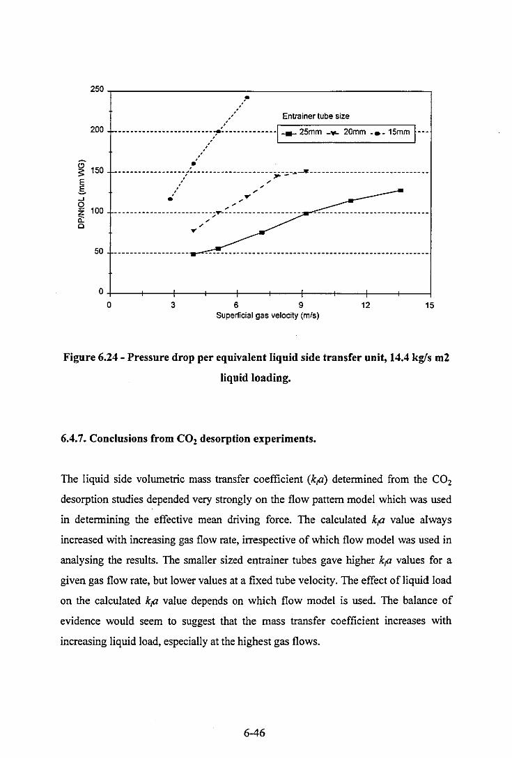
250,-____________________________________________ --.
200
~ 150 E E. -'
~ 100
c
//- Entrainer tube size
__________ m ___ m __ :,~:,:~:.':-m--m---I-- 25mm -Y- 20mm -.- 15mm fm
• .----------------::---------------------;;-;-~~-------- ------------.-.-------, ~ " ~ , ~
.: .,." ~
--------------------------~--------------------
".
~ ~
~
50 ____________________ <'<_,,-_. _:-= ____________________________________________________ _
O+-__ ~--_+----~--+_--~--~----+---~---+--~ o 3 6 9 12 15
Superficial gas velocity (m/s)
Figure 6.24 - Pressure drop per equivalent liquid side transfer unit, 14.4 kg/s m2
liquid loading.
6.4.7. Conclusions from CO2 desorption experiments.
The liquid side volumetric mass transfer coefficient (kp) determined from the CO2
desorption studies depended very strongly on the flow pattern model which was used
in determining the effective mean driving force. The calculated kp value always
increased with increasing gas flow rate, irrespective of which flow model was used in
analysing the results. The smaller sized entrainer tubes gave higher kp values for a
given gas flow rate, but lower values at a fixed tube velocity. The effect ofliquid load
on the calculated kp value depends on which flow model is used. The balance of
evidence would seem to suggest that the mass transfer coefficient increases with
increasing liquid load, especially at the highest gas flows.
6-46

The results of these experiments show that the mass transfer performance of the new
contactor with systems showing mainly liquid side resistance to mass transfer could
be somewhat superior to that of conventional packed columns, with the single stage of
0.35m height being able to carry out the same duty as a packed column of up to 1.6m
in height operating at the same liquid loading.
6-47

CHAPTER SEVEN

Chapter 7
Discussion and Implications.
7.1 Scope.
The purpose of this chapter is to summarise the overall results from this research
project and discuss what potential the co-current flow contactor has in terms of
offering improvements over existing gas-liquid contactors. A discussion of the
features which an industrial contactor based on this technology would include is also
given.
Section 7.2 summarises the current state of the contactor development and includes
the limiting gas and liquid flows together with correlations for the stage pressure drop
which may be useful in predicting the pressure drop with other systems or different
geometries. Section 7.3 discusses the relative merits of the co-current flow contactor
in comparison with conventional equipment. Section 7.4 describes the features which
an industrial version of the contactor would include.
7.2 Performance limits
The limits of performance for the contactor, and the pressure drop data are given here
for a contactor consisting of a 25mm diameter weir based entraining section, and a
dis-entraining section employing the 45° pitch angle guide vane and a Dutch weave
mesh cylinder. All the data concerns the air-water system. How the contactor would
operate with other systems will be discussed in due course.
7-1

7.2.1 Hydrodynamic limits
The hydrodynamic limits are given in terms of the maximum and minimum gas and
liquid flow rates at which the contactor operates satisfactorily by intimately mixing
the two phases and then separating them successfully in such a way that a column
with many such contactors could operate in an overall counter current manner.
Maximum gas flow: The contactor has been proven to operate satisfactorily up to a
maximum gas flow of 1700 lit/min, corresponding to a superficial gas velocity of
14.5 rnfs. This limit is set by the capacity of the test rig, and there is no reason to
suspect that the contactor could not be operated at still higher flows. At this point the
dis-entrainment efficiency is above 95%, although the efficiency appears to be
declining slightly with gas flow at this point.
Minimum gas flow: The minimum operating gas flow rate for the experimental scale
contactor was set by the weeping point, below which the liquid begins to weep down
through the entraining tube. This depended on the size of the entrainer tube and on the
liquid flow rate. The gas flow below which weeping occurred for the 25mm entrainer
was 200 lit/min, corresponding to a column gas velocity of 1.7 rnfs.
In a full size contactor with many entrainment tubes on each plate, the minimum
practical gas velocity would be set by the point corresponding to the minimum
pressure drop. This would be because a plate with many tubes would not operate at
flows below this in the region where pressure drop is decreasing with increasing gas
flow rate. Attempting to operate in this region would lead to a situation in which some
of the tubes were operating at a low gas 'velocity flow and hence weeping, whilst
others were operating at a higher gas velocity in the spray regime. This problem is
encountered in conventional sieve trays with a large open area. The minimum point in
the pressure drop curve for the single 25mm entrainer was dependent on the liquid
load, and was found to be around 500 lit/min at the highest liquid load, corresponding
to a column gas velocity of around 4.2 rnfs. The velocity corresponding to this
minimum point is lower for lower liquid loads and for smaller entrainer tubes.
7-2
Maximum liquid flow: The maximum liquid flow used thus far with both entrainer
and dis-entrainer in place is 2.2 Iit/min, corresponding to a column loading of 19.0
Kg/m2 s. Above this rate the liquid cannot drain from the dis-entrainment plate at a
sufficient rate, and a pool of liquid builds up which overflows into the dis-entrainment
tube. This limit is set by the scale of the test rig and is not fundamental to the
contactor design. Using a larger drain hole in the dis-entrainment plate would alIow a
higher liquid flow rate, but there was,. however, insufficient space for this within the
confines of the 50mm Ld. test column.
Minimum liquid flow: There does not appear to be a minimum liquid flow below
which satisfactory operation cannot be maintained, at least with a single entrainment
tube in each stage. It is possible that a combination of a low liquid flow and a high gas
flow may lead the 'pulsing' effect described in section 3.3 .2, even with the V notches
present, although this effect has not actualIy been observed at any measurable liquid
flow. For a larger scale column with several entrainment tubes on each entraining
plate, a low liquid flow may result in liquid distribution problems with only some of
the tubes on each plate functioning correctly, and others functioning as by-passes.
7.2.2 Pressure drop correlations.
The aims of this section of work were to establish the entrainer and dis-entrainer
pressure drops at varying gas and liquid loadings, and attempt to correlate them in
such a way as to predict the pressure drops when using at gas and liquid flow rates
outside the experimental range, and with different contactor geometries.
It is general practice with gas-liquid contactors to give pressure drop correlations as
the sum of the dry pressure drop and the additional pressure drop due to the presence
of liquid, and this approach has been used here:
(7.1)
7-3
Entrainer dry pressure drop
The dry pressure drop, that caused by the sudden contraction and expansion within the
entrainment tube and by friction was found to vary in proportion to the square of the
entrainment tube gas velocity as one would expect for fully turbulent flow. Regression
analysis of the log-log plot showed that the dry pressure drop varies in proportion to
the gas velocity raised to the power of between 1.85 and 2.05, depending on the tube
size. Forcing the fit to give the pressure drop proportional to the exact square of the
gas velocity still gives a good agreement. For a given entrainment tube therefore the
dry pressure drop can be predicted from:
(7.2)
A plot of dry pressure drop against (uTUBEl for the three entrainer tube sizes can be
seen in figure 7.1. The fact that the lines for the three entrainer tube sizes are linear
would suggest that equation (7.2) gives a good fit. The value of the constant k depends
on the size of the entrainment tube. Regression analysis shows that k varies in
proportion to the reciprocal of the tube diameter. Hence the dry pressure drop for any
tube size can be predicted from:
(7.3)
A plot of dry pressure drop against the group (UTUBEl/d, comparing the experimental
results from the three different entrainer tube sizes with equation (7.3) can be seen in
figure 7.2. The constants for the dry pressure drop model can be found in Appendix V. . .
7-4 .
400~----------------------______ ~ ____________ -7~'
Entrainer tube diameter
300 ________ 1--- 15mm -'F- 20mm -.- 25mm 1 ____________ _
100
o ." o 1000
/ /
.. ~.--------------------------------/""
2000 3000 4000 5000 V(TUBE),2 (m2152)
Figure 7.1 - Dry pressure drop as function of u2 TUBE for the three entrainer tube
sizes.
400~ ________________________________________ ~.-__ ,
300
i .s go 200 -t; i!! " .. .. £
Entrainer tube diameter
'" -'" •
'" -• 100 ---------------y-.. -----------------~------------------ --.-------._-------.-
o ..1'-o
'" ",-"'. %-
50000 100000 150000 200000 250000 300000 350000 V'21d (m/52)
Figure 7.2 - Dry pressure drop as function of the group (u2 TUBtJld for the three
entrainer tube sizes.
7-5

Entrainer wet pressure drop.
The additional pressure drop due to liquid entrainment is somewhat more complex,
and depends on both the gas and liquid flow rates as well as the tube diameter.
A typical plot showing how the additional pressure drop due to liquid entrainment
varied with both gas and liquid flow for the 25mrn entrainer can be seen in figure 7.3.
In the bubbling regime, the additional pressure drop due to liquid decreases as the gas
flow is increased, this will be because the hold-up of liquid on the plate, and hence the
hydrostatic head will decrease as the gas flow is increased. At higher gas flows the
additional pressure drop is approximately constant and may increase with increasing
gas flow. The net effect from these two regimes is that the additional pressure drop
due to liquid entrainment Is highest at the lowest gas flows, decreases to a minimum,
and then increases slightly with increasing gas flow. For a given entrainer size and
liquid load, the additional pressure drop can be correlated well by an expression such
as' ,
(7.4)
The constants A and B depend on both the liquid loading and on the entrainer tube
size. A good fit can be obtained by fitting the constants to powers of the liquid flow
rate i.e.
A = X(L)" B = Y(L)' (7.5)
The X Y. n and I constants still depend on the tube size however, and the correlation
becomes rather complex, and hence less reliable with respect to extrapolating the
results. The results generated using the above correlation are compared with the
experimental results in figures 7.4 to 7.6. The values of the constants are given in
Appendix V.
7-6
70~ __________________________________________ --,
Liquid load (kg!s sqm)
60 -uuuu--u~;-uu-u-1--- 5.9 _~ 10 _._ 14 ..... _ 18 10000-00-00--00 \
.t 40 Cl
30
"\ '. --------------,,----------------------------------------------------------,\
" ~ _A """__ . _k-. -..... .x-- •
--------------.- ----~---~:-------------~,,----------~.~------:;~------" - ........ --, ....... -lit' ..... - "
,.. ... - " ,/ ,,'" " ;,;' ... .:11' ~-- ...
20+-----r---~-----+----~----+-----~---4----~ o 4 8 12 16
Column gas velocity (m!s)
Figure 7.3 - Additional entrainer pressure drop due to the presence ofliquid for the 25mm entrainer.
• Dry data _ Dry fit .., 2.0 kg/s sqm data
__ 2.0 kg!s sqm correlation • 14 kg!s sqm data ____ 14 kg/s sqm correlation
500~==========================================~
400
6' N
:J: 300 E §.
~ '0
!! 200 " ~ a.
100
o
" /, /,
---------------- .. ------------------------------------- ----------,~~--~-----// .. / ,-' "
" / / / , /
---------------- .. -------------------------------------~~-- --------------.... " ~ -- / -- / ,. /
.//1 ---------------------------------------~;,.:?~--- ----.---------------------...... /
. ~ ........ " .. ,,___ .... 'fI",
----------------~::::~:----~~-~- ----------------------------------------~ .... '"
100 200 300 400 500 600 700 800 Gas Flow (lit/m in)
Figure 7.4 - Comparison between the full pressure drop correlation and experimental data for the 15mm entrain er.
7-7
• Dry data __ Dry fit y 2.0 kg!s sqm data
__ 2.0 kg!s sqm correlation • 14 kg!s sqm data •••• 14 kg!s sqm correlation
300
250
~ 200
§ g. 150 .;; ~ "' ~ 100 0..
• /~
~ .............................................................................................................................. -,' .. , .............. .. ,,' ... . ,. ,
, , /T , ,
---------------------------------------- .. -------.------~~-)---- ---_.------", .. ",.
A ,
-- , " .., ----------------------------------------------~--7---- -.--------------.---, ......... ...
, , " ,
.. '" .. . " -----------~:-----------------:~~ .. ---:;~---- -----------.------------------.... .. .. !'........., · ... ,,-v--.... ,. . ,'"
"J"
50 .. --- .... --- .... -- ............ y-- .. ~ ::.: -_ .. '!.._'!.---
0+----r~~----~--~---+----~--+---_r----~__4
o 2 4 6 8 10 Column gas velocity (m!s)
Figure 7.5 - Comparison between the full pressure drop correlation and experimental data for the 20mm entrainer.
• Dry data __ Dry fit y 6 kg!s sqm data
_ _ 6 kg!s sqm correlation _ 18 kg!s sqm data •••• 18 kg!s sqm correlation
200'-:;::===================9==;~
~ E .s
150
c. 100 e "0
~
" '" '" ~ 0.. 50
-- ., -- ' , ,
,~ ... -- ' , ,
--------------------- .. ---------------- .. ----------------;~--7·------- ' ..... " , , ........ ..... ,,"
" , -' .. ------_. ---- •• - ._--- -- -_ •• - - __ M - - ______ .. ~ ... ___ ,.. __ - __ - __ - - ___ - - - ________ _
.' , ...... " .............. .---. --............. ~ ... ... - - ·t----- ~ ........ .... - --
-------------~---------------------- -----------------------------------
O+-----+-----+-----r-----r-----~--~r_----~--~ o 4 8 12 16
Gas flow (Iit/min)
Figure 7.6 - Comparison between the full pressure drop correlation and experimental data for the 25mm entrainer.
7-8
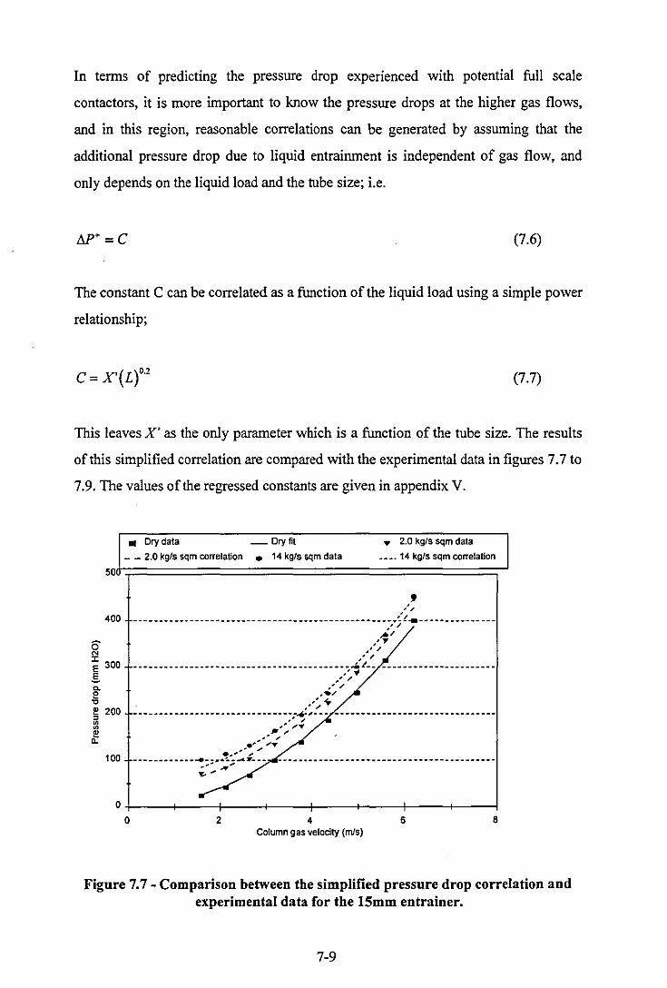
In terms of predicting the pressure drop experienced with potential fun scale
contactors, it is more important to know the pressure drops at the higher gas flows,
and in this region, reasonable correlations can be generated by assuming that the
additional pressure drop due to liquid entrainment is independent of gas flow, and
only depends on the liquid load and the tube size; i.e.
j)J>+=C (7.6)
The constant C can be correlated as a function of the liquid load using a simple power
relationship;
C= X'(L)02 (7.7)
This leaves X' as the only parameter which is a function of the tube size. The results
of this simplified correlation are compared with the experimental data in figures 7.7 to
7.9. The values of the regressed constants are given in appendix V.
6" N
• Dry data _ Dry fit ... 2.0 kg/s sqm data
_ _ 2.0 kg/s sqm correlation • 14 kg/s sqm data ~ ••. 14 kg/s sqm correlation
50a-:;:==================;-' 400 l
/' __________________________________________________ ~~t~ __________ • ___ _ . , .. '
/"
J: 300 ~
.' , .' , ______ • __________ • ___________________ w __ _ ,~~ f. ______________________ _
,..'~ /
.~" ~ " ./~~
--------------------------------4-'--- -------------------------------~ 200 ! .' , " ,.., -, ....... :~ .' ~ 100 ________________ ,.~: .. _c;___ _ __ • ____ • _________ • _____________ . _______ ._
........... ... ~
o+-_~--~--~-_+--~--~--+--~ o 2 4 6 8
Column gas velocity (m/s)
Figure 7.7 - Comparison between the simplified pressure drop correlation and experimental data for the 15mm entrainer.
7-9
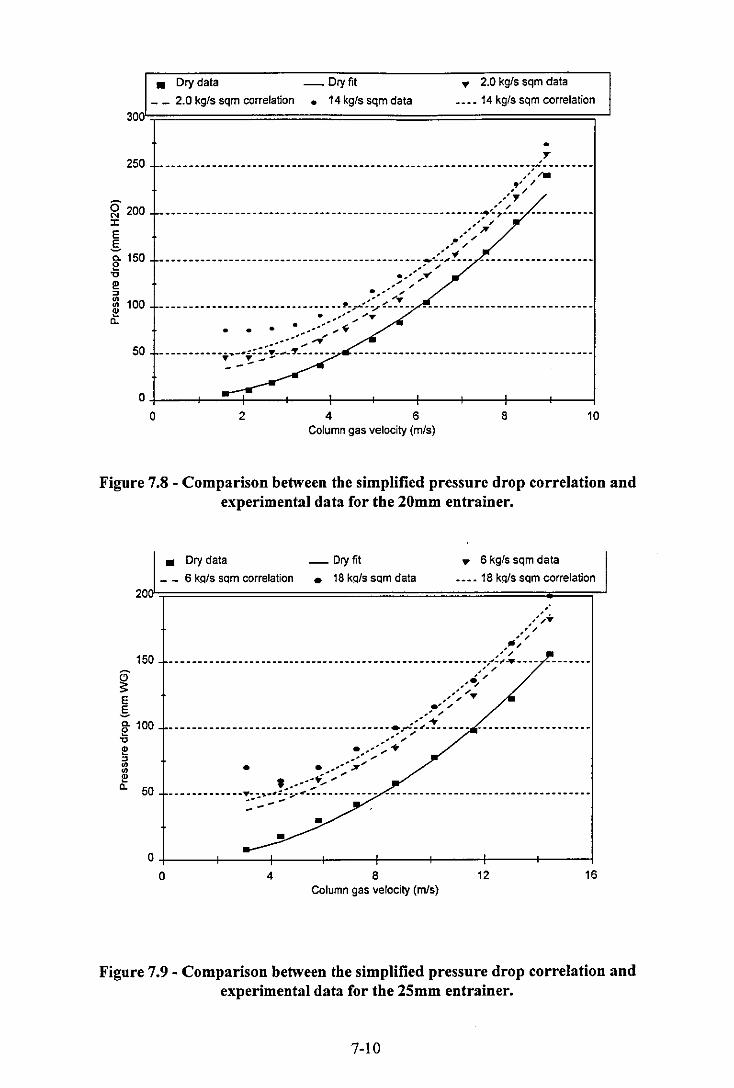
• Dry data _ Dry fit ., 2.0 kgls sqm data
__ 2.0 kgls sqm correlalion • 14 kgls sqm data ____ 14 kgls sqm correlalion
3001'-:;=======================;-'
• 250 -----------------------------------------------------------------;~:--------//11 .' / , /
6" 200 N
/y , /
--------------------------------------------------------~~7---- -----------:c E
,;,'/r"
E i 150
;,.',," / ~
----------------------------------------------~~-,---- ---_._------------_. / , -1',' "",""
......... -:, " "0
I!! " ~ 100
.... ". ..... - - - - -- -- - -- -- - _.- _ .. -- - - - .... - - - - ~;r"-'l- - - - - - - - - - - - --- -- --- -- - - - - -- - - -- ----
• .... "or a. . . . . ........ ~ ...
50 ----- --- ---T.-.~::.:!:::~~~-::. ~ ---- ----- -- -- --- ----- ---- -- -- ---- ---- -------O+-__ -+ __ =-+-__ ~--~----+_--_+----+_--~----~--~
o 2 4 6 8 10 Column gas velocity (mls)
Figure 7.8 - Comparison between the simplified pressure drop correlation and experimental data for the 20mm entrainer •
• Dry data _ Dry fit ., 6 kgls sqm data
__ 6 kQls sqm correlation ,. 18 kQls sqm data ____ 18 kws sqm correlation
20~====================================~==~
~ E .s
150
Q. 100 e "0
e " ., ., ~ a. 50
,'.
" /Y " , , , ," , /' . _____________________________________________________ __ ;J_~~----
/' .... ~/
,. .... ~/. e' , /, .........
---------------------------------------~---~-------- -------------------.' , ...... "'" ....... ""' .... ...... "'" • • ........ ;IT"'" , .... " .. "'" "'" -- --------------~:~~-.~:~.~-~----------- ------------------------------------
O+_--~----~----~---+----~----+_---+----~
o 4 8 12 16 Column gas velocity (mls)
Figure 7.9 - Comparison between the simplified pressure drop correlation and experimental data for the 25mm entrainer.
7-10
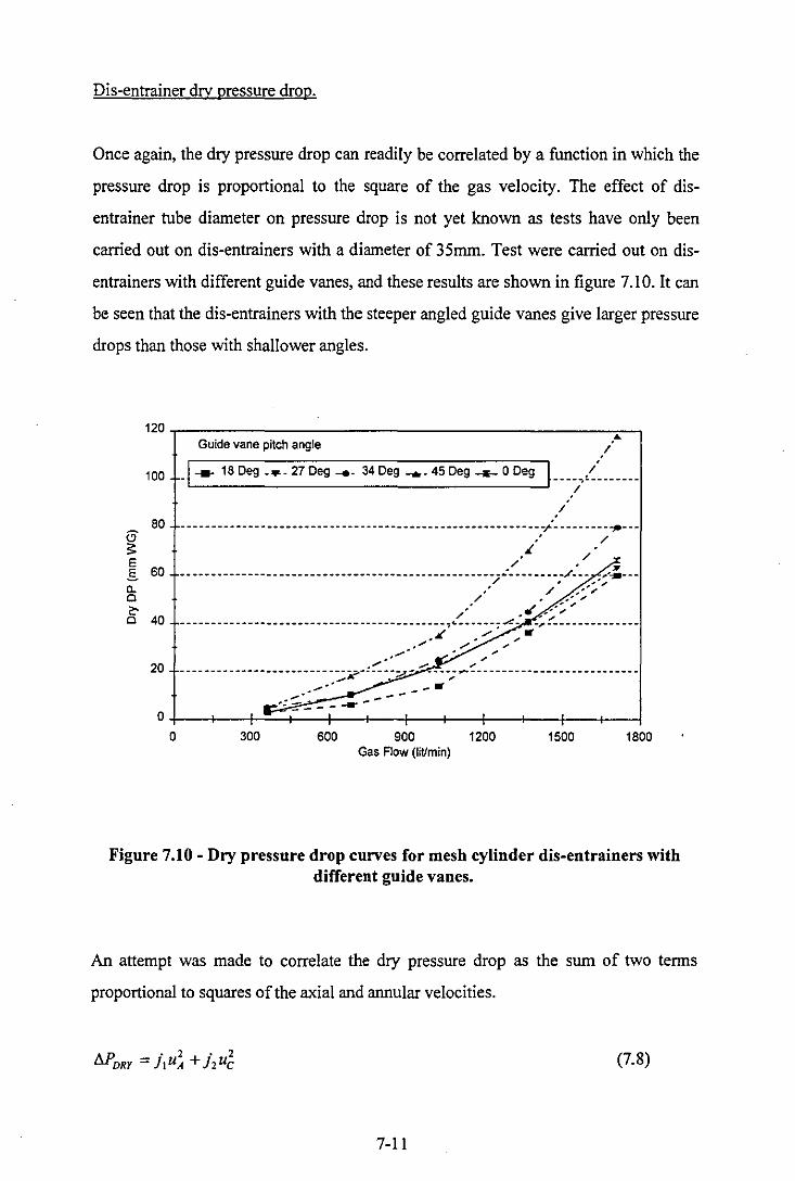
Dis-entrainer dry pressure drop.
Once again, the dry pressure drop can readily be correlated by a function in which the
pressure drop is proportional to the square of the gas velocity. The effect of dis
entrainer tube diameter on pressure drop is not yet known as tests have only been
carried out on dis-entrainers with a diameter of 35mm. Test were carried out on dis-
entrainers with different guide vanes, and these results are shown in figure 7.1 O. It can
be seen that the dis-entrainers with the steeper angled guide vanes give larger pressure
drops than those with shallower angles.
120
100
80 6' ;s: E g 60 0-0 ~ 0 40
20
0
0
," / Guide vane pitch angle
_1 --- 18 Deg _ ... 27 Deg ..... 34 Deg ... 45 Deg ...... 0 Deg ~ ____ ,/~ ____ __ /
/
----------------------.-.----------.------------------ -----r---------~---" /
J / ,/ ';'IT
----------------------------------------------------~---------~--- ,~---/ " .. '." " / ..... ,.
/ ",' '" " ., ";''''
/ ""'" ---- --- -- _._-- --_. __ .-. - ___ e. _____ e. _____ ~, .. ____ - _; /-- ., _, __ - - -- _____ - __ _
,.. ...... ~ .,. ---- --- -----_ •• _- ------ --:;?"" -- -.-;";!'''' ,,- - -; - - - - - - -- - -- -- -- - - - -- _.- - ----
w' _ .,
300 600 900 1200 1500 1800 Gas Flow (liUmin)
Figure 7.10 - Dry pressure drop curves for mesh cylinder dis-entrainers with different guide vanes.
An attempt was made to correlate the dry pressure drop as the sum of two tenus
proportional to squares of the axial and annular velocities,
(7.8)
7-11
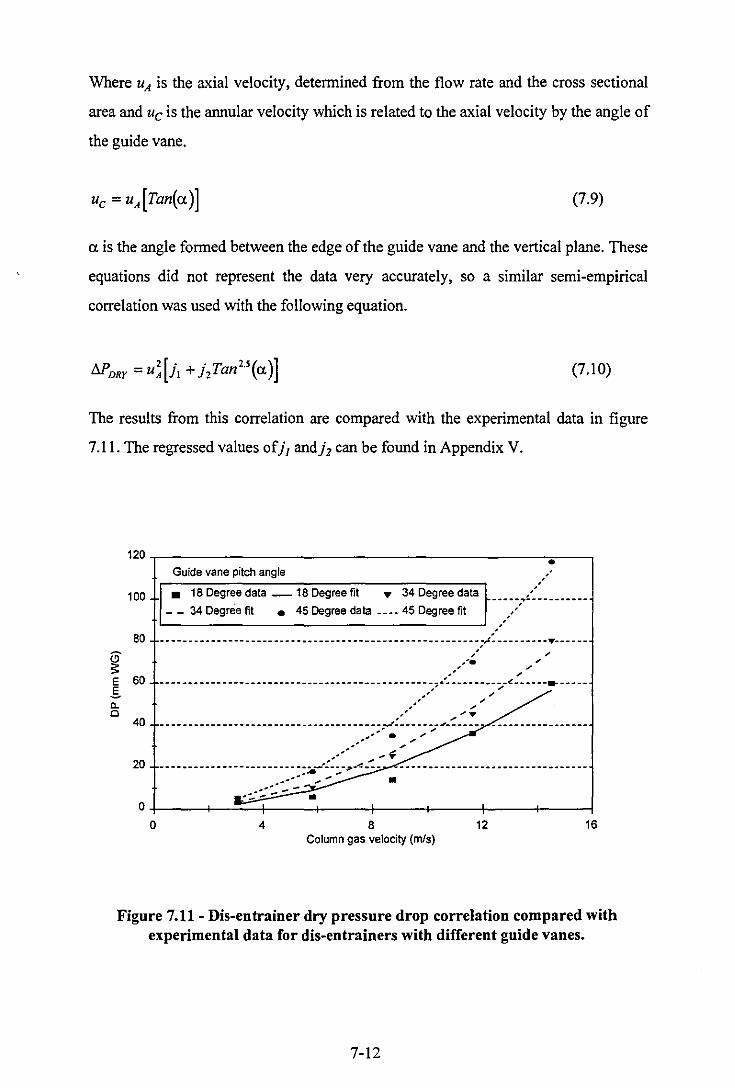
Where U A is the axial velocity, determined from the flow rate and the cross sectional
area and Uc is the annular velocity which is related to the axial velocity by the angle of
the guide vane.
(7.9)
a is the angle formed between the edge of the guide vane and the vertical plane. These
equations did not represent the data very accurately, so a similar semi-empirical
correlation was used with the following equation.
(7.10)
The results from this correlation are compared with the experimental data in figure
7.11. The regressed values ofjJ andjz can be found in Appendix V.
120 • Guide vane pitch angle . .
100 • 18 Degree data _18 Degree fit ... 34 Degree data ••••••• : •••••••••
__ 34 Degree fit • 45 Degree data •••• 45 Degree fit •
80
~ E 60 S a.
---------------._---------------------------_.-.------ -:;~----------~------/ ,
,...... .,,' ...... "
-----------------------------------------------:~&_--------/-~------~-----.' , . , .' ,
0 40
.... .... . , -- -- ... -------- - .. ---- -- - - - -- -- - .-- - -- -----"._-- -- --~------ - -- -- - - - ----- ----.' , ...... . .;'" ...... ".. ...
20 ----.- --- -- _.-- ---- -- --- --- -'::. -;>-"!!::-.......... .; .... ........ :.. --- - .
0
0 4 8 12 16 Column gas velocity (m/s)
Figure 7.11 - Dis-entrainer dry pressure drop correlation compared with experimental data for dis-entrainers with different guide vanes.
7-12
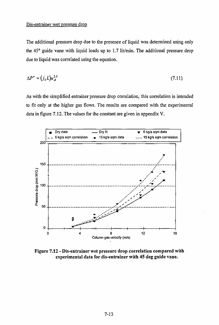
Dis-entrainer wet pressure drop
The additional pressure drop due to the presence of liquid was determined using only
the 45° guide vane with liquid loads up to 1.7 lit/min. The additional pressure drop
due to liquid was correlated using the equation.
(7.11 )
As with the simplified entrainer pressure drop correlation, this correlation is intended
to fit only at the higher gas flows. The results are compared with the experimental
data in figure 7.12. The values for the constant are given in appendix V.
• Dry data _ Dry fit " 6 kg!s sqm data _ _ 6 kg!s sqm correlation • 15 kg!s sqm data • ___ 15 kg!s sqm correlation
200':;::===================:::;--'
~
(j ~ E E
150
-;;: 100 E!
"C
I!? " ~ I!? a. 50
, , , , , • ,
._-----------._------------._---------------------------------.----------,
;',',.:. ,,'" Aip
.,' /" /' /y ___________________________________________________ ~~ ___ -c. ____________ _
" , ,--,' ","
, '.., ;,1' '" '" " , , ,
." /
------------------------------------~:/-~- ------------.---------_.-- .. -.' /
• .., " / .' / . . /
y:. .. :; ... .. .........
o+-_~-~~--+--_+--~--~--+--~ o 4 8 12 16
Column gas velocity (m!s)
Figure 7.12 - Dis-entrainer wet pressure drop correlation compared with experimental data for dis-entrainer with 45 deg guide vane.
7-13

7.3 Comparisons with conventional equipment.
7.3.1 Introduction
In order to be a viable alternative to existing contactor designs, the co-current flow
contactor would have to offer lower total lifetime costs, the total lifetime cost being
formed from a combination of the capital costs and the operating costs using a method
such as discounted cash flow. The capital cost is the cost of designing, constructing,
installing and commissioning the separation column and its ancillary equipment. The
operating costs are primarily the energy costs associated with transporting the fluid
phases through the device and carrying out the separation, but also include costs such
as labour and maintenance.
The physical construction costs for the separation column can be broken down into
the cost of the column shell, the cost of the internals and the cost of foundations and
support structures. The cost of the column shell depends on its physical size, the
operating pressure and the material of construction. Smaller columns are cheaper than
large ones, and ones operating at lower pressures are cheaper because thinner column
walls are required to withstand the internal pressure. The wall thickness, e, for
cylindrical pressure vessels can be calculated from;
1',D e= '
(2/ -1',) (7.12)
Where Pi is the internal pressure, Di is the diameter and/is the design stress. It can be
seen that the wall thickness for a given pressure depends on the diameter, so a smaller
diameter column will have thinner walls as well as less wall area. At lower pressures,
columns are designed using a minimum wall thickness in order to ensure that the
column walls are sufficiently rigid to support their own weight and resist wind and
other miscellaneous loadings. This minimum wall thickness is also higher for larger
diameter columns (Sinnott [1983]). Columns constructed from corrosion resistant
7-14
alloys or alloys selected to withstand extremes of temperature will be significantly
more expensive than those constructed from carbon steel.
The cost of the column internals will also depend on the size of the column, which
will determine the number and size of the plates in a tray column or the total volume
of packing in a packed column. In addition the cost of the internals will depend on the
complexity of the internals and on the materials of construction. For example, bubble
cap trays typically cost around three times the amount of simple sieve trays (Sinnott
[1983]), because of the fabrication costs, and are little used for this reason.
The costs of foundations and support structures will also depend on the size of the
column and on its normal operating weight, which includes the weight of the liquid
and vapour inventory.
The energy cost for a separation column performing a given separation depends
entirely on the pressure drop caused by the flow of gas or vapour through the column.
In the case of absorption or desorption columns, additional pressure drop leads to
increased pumping costs. In the case of fractionating columns, additional pressure
drop leads to an increased re-boiler costs caused by the increase in bottom pressure
and temperature.
Maintenance costs for a separation column will depend largely on the size and
complexity of the column internals. Complex internals, especially those with moving
parts such as valve trays are likely to require more maintenance intervention than
simpler designs. The internals are generally more accessible in larger columns,
although larger columns will contain either more trays, trays with more units, or a
greater volume of packing, making the internals more expensive to replace when worn
out.
7-15

7.3.2 Performance comparison
The co-current flow contactor should always give a lower column diameter than any
conventional contactor for a given duty because the allowable gas velocity will be
higher. Conventional columns are sized by calculating the capacity factor, F'v which
is calculated from;
(7.13)
Where Uvs is the superficial vapour velocity, Pv is the vapour or gas density and PL is
the liquid density. When the vapour density is insignificant in comparison with the
liquid velocity the simpler vapour capacity factor F v is used;
(7.14)
The maximum design Fv value for conventional contacting columns is around 3.0 to
3.2. The maximum Fv value so far achieved with the co-current flow contactor
operating with the air-water system is 15.9. Fv is also equal to the square root of the
number of velocity heads, a parameter on which variables such as the drag on liquid
films and drops and the pressure drops will directly depend. From this, it should be
safe to say that the F v factor can also be applied in scaling up the co-current flow
contactor, and that these contactors should be able to operate up to Fv values of 15.9
with systems other than air and water.
,
It can be concluded from this that a co-current flow contactor should be able to
operate with a superficial column velocity of around five times that of a conventional
contactor, giving less than half the diameter of a conventional column for a given
separation duty.
The above applies to cases where the total column capacity is limited by the
maximum allowable gas rate. It is not yet known whether the new contactor could
7-16
offer a reduction in column diameter compared to conventional equipment in cases
where the total column capacity is limited by the maximum allowable liquid loading.
It is not yet clear what sort of reduction in column height the new contactor could
offer in comparison to conventional equipment. The total height of a gas-liquid
contactor depends on the mass transfer performance, which determines the total
number of stages required in the case of tray type columns, or the total height of
packing required in the case of packed columns. The comparisons of mass transfer
performance with conventional columns detailed in chapters 5 and 6 showed that for
the humidification system, one showing mainly gas side resistance to mass transfer,
the single co-current flow contacting stage with a height of 350mm was equivalent to
a packed column with a total height of around 200mm, subject to doubts regarding the
mass transfer data for the packed column.
For systems showing mainly liquid side resistance to mass transfer, the mass transfer
performance was rather better (see chapter 6) and the single stage with a height of
350mm was shown to be equivalent to a packed height of up to l800mm for the CO2
desorption system. It is not possible to accurately predict the likely performance with
other systems from this limited data, although a similar pattern may emerge with other
gas and liquid controlled systems.
The general consensus in the standard texts (Treybal [1968] and McCabe et al.
[1993]) is that most industrial distillation separations are gas film controlled.
Industrial absorption or stripping processes are also gas film controlled in cases where
the gas being absorbed is very soluble in the liquid, or undergoes a rapid reaction with
the liquid. The only industrial separations, in which the liquid phase is controlling
appear to be absorption processes in which the absorbing gas is sparingly soluble in
the liquid or undergoes a slow reaction in the liquid. Industrial examples of these
processes given by Strigle [1994] include the absorption of gases such as oxygen,
carbon dioxide or Chlorine into water, and the absorption of carbon dioxide from gas
mixtures into alkaline solutions such as amine or caustic solutions. McCabe et al.
[1993] suggest that, for distillation systems, the liquid film resistance becomes more
7-17
important for a given system as the pressure is increased. Strigle [1994] however still
states that for industrial high pressure distillations, such as the separation of low
boiling hydrocarbons, the gas phase is still controlling.
The designers of previous co-current flow contactors, described in chapter 2, found
that their designs appeared to give reasonable Murphree efficiencies with distillation
systems such as ethanol-water or hydrocarbon separations. Zhavoronkov et al. [1969],
whose contactor employed local vapour velocities similar to those encountered with
this contactor, found Murphree efficiencies of between 40% and 90% for the ethanol
water system. Also of interest is the fact that the efficiency of this contactor increased
with the degree of liquid recirculation. The authors found that the efficiency was 90%
with recirculation rates above about 6 times the liquid feed rate. The dye tracing
investigations carried out with this column, detailed in chapter 7, showed recirculation
rates at the highest gas velocities of between 3 and 4 times the liquid feed rate. At
these recirculation rates, Zhavoronkov et al. found that the efficiency of their
contactor was between 60% and 70%.
de Villiers [1987] also found Murphree efficiencies as high as 90% with his contactor
operating with the ethanol-water system This figure was achieved with vapour
velocities above about 30 mls, and with no liquid recirculation. The contacting tube in
de Villiers' contactor was somewhat longer than the contacting zone found in the
contactor studied here, being of around I m length, and hence giving a longer contact
time. The author did find, however, that increasing the length of the contacting tube to
2m did not significantly improve the efficiency.
In practice, the mass transfer performance of a contactor operating in a counter-current
column also depends on the ability of the contactor to operate in a satisfactory counter
current manner as well as on the mass transfer rates themselves. A stage offering good
contact between the phases with high Kga or Kp values will still give poor overall
efficiencies if the gas flowing upwards contains excessive liquid entrainment or is
using the downcomers as by passes. The efficiency will also be poor if the liquid
flowing down the column contains a lot of entrained gas. Packed columns can also
7-18

suffer from similar difficulties. A packing offering good contacting with low
theoretical H. T. U. values will still give poor mass transfer performance if the liquid is
maldistributed or is mostly flowing down the walls. These types of problems will
often manifest themselves when contactors are required to work over a large range of
gas and liquid flows.
A contactor which can maintain proper counter-current performance over a wide range
of "flows may therefore give better practical mass transfer performance than a more
restricted design with better mass transfer performance at optimum flows. The co
current flow contactor has shown the ability to maintain good counter-current
behaviour over a wide range of gas flows, with the turndown ratio based on gas
velocity being around 3.5:1. The range of liquid flows is not yet known because the
true maximum liquid loading is not yet known.
The capital cost for the column shell for a co-current flow contactor is likely,
therefore, to be less than that for a conventional column to carry out the same
separation, particularly when operating at high pressures, when the advantages of the
smaller diameter become more significant, and with systems showing largely liquid
side mass transfer resistance, in which cases the better mass transfer performance
could lead to lower column heights.
The cost of the intemals for the co-current flow contactor is likely to be similar to
those for the more complex conventional columns such as bubble cap trays or valve
trays, and are not likely to be competitive with those for simpler devices such as sieve
trays and dumped packing. The co-current flow contactor should not require any parts
to be made to great degrees of accuracy. The most complex part for fabrication
purposes would be the guide vane in the dis-entrainer, although this part could be
manufactured using mass production techniques. The entrainer stages at their simplest
would be similar to sieve trays, but with a bigger hole diameter and with entrainment
tubes welded over the holes. The dis-entrainer plates would be similar, but would also
include the guide vanes, and the wire mesh cylinders joined to the top of the tubes. It
should also be remembered that the trays themselves will be smaller in diameter, and
7-19
therefore cheaper than those in a conventional column carrying out the same duty. The
co-current flow design does, of course necessitate the use of two trays per stage, one
for the dis-entrainer and one for the entrainer. How this affects the costs will depend
on how the stage efficiencies compare with those for conventional trays.
The costs of foundations and support are likely to be much lower than those for
conventional columns because the columns will be smaller and lighter. The costs of
ancillary equipment such as reboiIers and condensers for fractionation processes and
fans and pumps for absorption or desorption processes is related to the required duty
of these pieces of equipment which will be mostly dependent on the column pressure
drop. The co-current flow contactor is likely to give higher pressure drops than
conventional equipment, and this would be reflected in the higher cost of the ancillary
equipment.
The likely running costs of a co-current flow contactor are likely to be much higher
than those for conventional equipment due to the much larger pressure drop. At the
maximum gas flow rate the total stage pressure drop for the pilot scale column was
350 mmWG. By comparison, a typical structured packing would give a pressure drop
of 60 mmWG per meter of packed height operating at a typical design Fv of 3.2
(Billet [1995]). It is likely that further development particularly for the dis-entrainer
guide vane, and the use ofIarger contacting elements would allow the pressure drop to
be reduced, although it is unlikely that the pressure drop could be reduced down to the
levels of conventional equipment. Using entrainment tubes with a diameter of 30mm
would allow the dry entrainer pressure drop to be halved in comparison with the
25mm entrainer tubes for a given gas flow rate. What effect this would have on the
additional pressure drop due to liquid is not clear. Using larger entrainment tubes will
cause the minimum gas velocity to be reduced, and will hence give lower turn down
ratios.
7-20
7.3.3 Other performance factors.
It is thought that the co-current flow contactor may also be useful in handling systems
which show excessive foaming behaviour. Foaming systems tend to be unsuitable for
packed columns, and require the use of plate columns, generally at lower gas
velocities. The co-current flow contactor may be suitable because the high centrifugal
forces and fine holes in the wire mesh dis-entrainer may be effective in breaking the
foam. A trial was conducted with the two stage pilot scale contactor in which
detergent was added to the water in order to encourage foaming. The main contactor
parts appeared to be operating satisfactorily, with the only problem being that the
liquid in the downcomer between the two stages had a fine foam like consistency and
was not providing sufficient hydrostatic head to fill the lower entrainer stage at the
highest gas velocities. It should be noted that a detergent-water mixture gives an
exceptionally stable and persistent foam of the sort that is not usually encountered in
normal separations.
7.3.4 Discussion.
In order for the new contactor design to be viable, therefore, the savings in capital cost
in comparison with conventional equipment, due to the smaller diameter, and possibly
shorter columns, must be more than sufficient to make up for the increased running
costs due to the higher pressure drop.
In normal atmospheric pressure or vacuum gas absorption and fractionation processes,
the energy cost, determined by the pressure drop is usually far more significant than
the capital cost (Strigle [1994]), so that most recent developments in mass transfer
equipment have been towards contactors with lower pressure drops. The co-current
flow contactor is not likely therefore to be economically competitive for these types of
process.
In general the pressure drop becomes less economically significant as the operating
pressure is increased (Strigle [1994]). In practice, industrial separations are not carried
7-21
out at pressures significantly greater than atmospheric, unless this requirement is
dictated by other process conditions. Widely practised examples of high pressure
separations include the fractionation of low boiling point liquids such as the lighter
hydrocarbons. In these processes, high pressures (typically above 20 bar) are used to
raise the boiling points so that expensive refrigeration is not required for cooling in
the condenser.
These types of processes tend to have very high volumetric liquid to gas flow ratios
due to the high gas density, and in order to be suitable for operation with these
systems, the co-current flow contactor would have to prove itself suitable for
operation at these high specific liquid loads. Industrial tray columns operating with
these types of system tend to require large downcomer areas, up to 40% of the total
column cross-section, because of both the high specific volumetric liquid flow and
because of the low surface tension and density difference between the two phases
which makes phase separation difficult. In this situation the co-current flow contactor
may offer an advantage because the centrifugal field applied in the dis-entrainer will
aid in the separation of the two phases, and the pool of liquid on the dis-entrainment.
plate around the dis-entrainment units provides a quiescent region in which some
further phase dis-engagement can occur.
Other gas-liquid processes which are carried out at high pressure are those involving
the treatment of natural gas, such as acid gas removal with amine solutions and
dehydration using glycol solutions. These are carried out at pressures of around 90 to
100 bar and are sometimes carried out offshore. In this type of process there is
sometimes a substantial pressure driving force available at no cost. Space is invariably
at a premium on offshore facilities, and the capital costs associated with supporting
large vessels on offshore platforms are very large, so in this situation the capital cost
saving in comparison with conventional columns is likely to be large, and the increase
in running costs perhaps not so apparent.
A further possibility is that the column internals for the co-current flow contactor
could be used to improve the capacity of existing conventional equipment which is
7-22
already operating at its limit of capacity. This could be achieved at a much lower cost
than replacing the whole column, and could find application in de-bottlenecking
exercises. This would of course be achieved at the expense of a higher pressure drop
and would only be economic where this higher operating cost over the life of the
modification would be out-weighed by the capital cost saving in comparison with
constructing a new column.
7.3.5. Conclusions.
At this stage, it is not easy to say whether the co-current flow contactor offers
sufficient overall improvements over conventional technology to become widely used
in the chemical and process industries. The industrial effectiveness of this method will
depend on whether the pressure drop can be significantly reduced, and on whether the
mass transfer performance with systems showing gas side resistance compares
favourably with existing equipment. The evidence from other authors who have
studied co-current flow contactors is that these contactors can achieve good
efficiencies with distillation systems, particularly where this some liquid recirculation.
What has been demonstrated is the ability to operate contacting units which can be
connected in a counter current fashion at superficial column velocities up to 5 times
that possible with conventional equipment. It has also been shown that the mass
transfer performance with a system showing liquid side resistance appears to be
significantly better than that of conventional equipment.
It is most likely that the co-current flow contactor will only offer improvements over
conventional equipment for a relatively limited number of processes, namely those in
which the pressure drop is of lower than usual importance, and/or the capital costs of
the pressure vessel and its supports are unusually high, such as at very high pressures
or where expensive alloys are required. A further possibility is that these contacting
units could be retro-fitted to existing columns in order to boost their capacity in de
bottlenecking exercises.
7-23
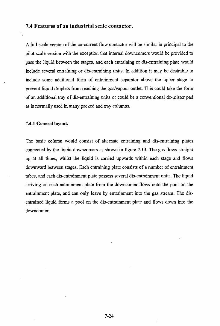
7.4 Features of an industrial scale contactor.
A full scale version of the co-current flow contactor will be similar in principal to the
pilot scale version with the exception that internal downcomers would be provided to
pass the liquid between the stages, and each entraining or dis-entraining plate would
include several entraining or dis-entraining units. In addition it may be desirable to
include some additional form of entrainment separator above the upper stage to
prevent liquid droplets from reaching the gas/vapour outlet. This could take the form
of an additional tray of dis-entraining units or could be a conventional de-mister pad
as is normally used in many packed and tray columns.
7.4.1 General layout.
The basic column would consist of alternate entraining and dis-entraining plates
connected by the liquid downcomers as shown in figure 7.13. The gas flows straight
up at all times, whilst the liquid is carried upwards within each stage and flows
downward between stages. Each entraining plate consists of a number of entrainment
tubes, and each dis-entrainment plate possess several dis-entrainment units. The liquid
arriving on each entrainment plate from the downcomer flows onto the pool on the
entrainment plate, and can only leave by entrainment into the gas stream. The dis
entrained liquid forms a pool on the dis-entrainment plate and flows down into the
downcomer.
7-24

Liquid from stage above
Liquid to stage below Gas/vapour Flow
Figure 7.13 General column features.
7-25
Dis-entrainer
Entrainer
Dis-entrainer
Entrainer
Dis-entrainer
Entrainer
Dis-entrainer
Entrainer

7.4.2 Downcomers
The function of the downcomers is as in a conventional tray column, i.e. to transport
the liquid down from one stage to the one beneath. Unlike a conventional column,
however, the downcomer would have to pass through two plates because the liquid
leaving the dis-entraining section of one stage would have to travel past the entraining
section of that stage and the dis-entraining section of the stage beneath before being
delivered to the entraining section of the stage beneath, as illustrated in figure 7.13. It
would not be necessary to seal the downcomer into the plates through which it passes
through with permanent join, provided some sort of wall is included on the plate
which the downcomer passes through in order to prevent liquid from flowing down
through the gap around the outside of the downcomer. as illustrated in figure 7.14.
Some gas will be able to pass through the gap, but provided the gap is small enough,
this should not be too significant.
Downcomer
Bulk gas flow
Leakage
Figure 7.14 Arrangement at plate edges.
7-26

Downcomer sizing and plate spacing.
The downcomers would need to be sized so as to allow the flow of liquid down to the
entraining section of the plate beneath without causing such pressure drop as to force
the liquid to back right up to the stage from which it originates. In conventional tray
columns, the downcomers must also be large enough to allow sufficient residence
time for the dis-engagement of the two phases. This problem occurs when trays are
operated in the foaming regime, and the foaming mass of liquid and gas flows over
the weir into the downcomer. This would probably not be so much of a problem with
the co-current flow contactor, because the centrifugal phase separators should assist in
breaking any foams.
The downcomer also functions as a liquid seal, preventing the gas from bypassing the
contacting units on each plate. The static head of liquid backed up in the downcomer
must balance the gas phase pressure drop across the plates through which the
downcomer passes, whilst also providing for any frictional losses from the liquid
flowing in the downcomer itself and through the outlet. The stage spacing in the co
current flow contactor must therefore be large enough to provide this static head of
liquid in the downcomers, and is therefore governed by the gas phase pressure drop.
In a conventional column, each downcomer must provide sufficient static head to
transport the liquid past one plate. In the new column, the downcomer head must
balance the pressure drop across two dis-entraining sections and one entraining
section.
For a conventional column, the tray spacing must be large enough to prevent too
many liquid droplets entrained in the gas stream from being carried upwards to the
plate above, ultimately leading to entrainment flooding. This is not a problem of
course for the new contactor design because the dis-entrainment units prevent
carryover
In conventional tray design, allowance has to be made for the fact that the liquid in
the upper part of the downcomers contains some entrained vapour, which adversely
7-27
affects its density. For this reason, the tray spacing is usually selected to be twice the
predicted clear liquid downcomer backup. This should not be necessary in the new
design of contactor because the liquid in the downcomer should be relatively free of
entrained vapour due to the centrifugal phase separation process in the dis-entrainment
units.
Downcomer positioning.
Normal practice with conventional tray columns is to include the downcomers as a
chord shaped section at the edge of the plate. This type of arrangement leads to the
cross flow type of arrangement in which the liquid flows across each tray from one
downcomer to the next. The flow pattern which is required for the co-current flow
contactor is slightly different because the liquid arriving on an entraining plate must
be spread out over the plate to reach each entraining tube from which it leaves the
plate.
If a conventional chord type downcomer was used in which the liquid arrives at the
side of the plate then there may be a sloping liquid surface formed in which the
entrainment tubes close to the downcomer exit are swamped with liquid whilst those
further away are dry and operating as by-passes for the gas phase. This problem may
not be too serious because of the large amount of recirculation of the entrained liquid
droplets which occurs due to the liquid drops impacting on the underside of the tray
above, causing the liquid to be distributed around the plate.
One solution to the problem ofliquid distribution would be to provide several smaller
downcomers between each pair of dis-entraining and entraining plates. This is more
feasible than in conventionally tray columns because single large downcomers would
not be required for phase dis-engagement purposes. Another solution would be to
arrange the downcomer outlet on each entrainment plate such that different portions of
the liquid are delivered to different areas on the plate. The distribution of liquid
around larger multi-unit plates of this type is one are in which much further
development work is required.
7-28
7.4.3 Detail design of entrainer units.
The final design for the entraining unit in the pilot scale columns was for a simple
tube protruding from the plate into which two V shaped notches were cut. In a full
scale contactor, the entrainment tubes could take on this simple form, or further
measures could be taken to reduce the pressure drop. This could be achieved by
including an angled convergent section at the base of the entrainment tube, as shown
in figure 7.15. This would reduce the pressure drop caused by the sudden contraction
of the gas flow into the tube.
•
• - . . • • • • • • • ••• • •
• . . ... .-• •
t
Entrained Liquid drops • • . • • · • •
• · -• •• · • • • : .. .... · • • # .
• • • • • • # • • •• • • •
t\, Gas Flow
. •
•
• . •• •
• .' . "
... . .. . . ........ . • • • .'
• •
t Converging section
Figure 7.15 Entrainer units with converging sections.
A further reduction in pressure drop could be achieved by placing a narrow angled
divergent section above the entrainment tube. as shown in figure 7.16, to assist with
the energy recovery as the gas-liquid mixture decelerates into the space above the
entrainment tube. With both these features added, the entrainer becomes similar to the
7-29

venturi type device mentioned in chapter 3 with the exception that the area available
for liquid flow into the entrainment tube will be much larger.
•• •
... •
t
Diverging section , \ · '
• • •• • • •• • • •• • •• . '.. .-. .. . . .. • • • •• • •• •
t Gas flow
• • • •
t Converging section
Figure 7.16 Entrainer units with converging and diverging sections.
Selection of entrainer tube size.
The size of the entrainer tube would be selected to give the best compromise between
mass transfer efficiency and pressure drop. The total column pressure drop is the
number of stages multiplied by the pressure drop per stage. The number of stages
required for a given duty depends on the mass transfer performance of each stage, so
there is likely to be an optimum tube size which gives the minimum total pressure
drop for a given separation duty. In part this optimum can be predicted by calculating
the pressure drop per transfer unit for the various tube sizes, as was done for the CO2
desorption results in chapter 6. In practice the capital cost of the column, which
depends on the number of stages may also be significant. This is likely to weight the
balance slightly more in favour of the smaller tube sizes which give better mass
transfer performance.
7-30
The above applies to systems in which the mass transfer efficiency depends on the
entrainer tube size, and would give the economic optimum tube size. In practice
however, other factors would be considered in designing the entraining section.
Because the entrainer tube size detennines the entrainer pressure drop, it will also
determine the flooding point. In this device the flooding point is the point at which the
stage pressure drop becomes so large that the liquid in the downcomers doe not have
sufficient hydrostatic head to flow down the column. Larger entrainment tubes will
therefore give higher maximum gas velocities than smaller ones due to their lower
pressure drop. A further factor which would affect the selection of the entrainer tube
size would be the desired minimum gas flow rate which would be governed by the
point at which the pressure drop is minimum (see section 7.2). This point was found
to be at higher gas flows for the larger entrainer tube sizes.
7.4.4 Detail dis-entrainer unit design
The design of dis-entrainer in the full scale contactor is likely to be very similar to that
used in the pilot scale rig, although more development work could be done to produce
an effective guide vane giving a lower pressure drop. It is also likely that the final dis
entrainer would have some form of slight constriction at the top, as shown in figure
7.17, in order to create a slight back pressure to maintain the liquid film on the wire
mesh walls. This would be particularly important for systems with low surface tension
in which capillarity is not as effective in holding the liquid film on the mesh wall. It
may also be desirable to include some construction to kill the vortex in the gas flow as
it leaves the dis-entrainer in order to prevent cyclonic flow in the entrainer above,
which may cause the liquid droplets to be thrown outwards rather than upwards. How
this would affect the entrainer operation is not yet known.
The diameter of the dis-entrainer will affect the pressure drop and may also affect the
mass transfer performance in a similar way to the entrainer tube size. It is most likely
that the dry pressure drop will be proportional to the reciprocal of the tube diameter
for a given gas velocity, although this can not be confirmed without further
experimentation. The dependence of the additional pressure drop due to liquid on the
7-31
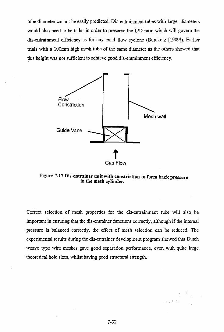
tube diameter cannot be easily predicted. Dis-entrainment tubes with larger diameters
would also need to be taller in order to preserve the LID ratio which will govern the
dis-entrainment efficiency as for any axial flow cyclone (Burckolz [1989]). Earlier
trials with a 100mm high mesh tube of the same diameter as the others showed that
~s height was not sufficient to achieve good dis-entrainment efficiency.
Flow Constriction
Guide Vane
Mesh wall
f Gas Flow
Figure 7.17 Dis-entrainer unit with constriction to form back pressure in the mesh cylinder.
Correct selection of mesh properties for the dis-entrainment tube will also be
important in ensuring that the dis-entrainer functions correctly, although if the internal
pressure is balanced correctly, the effect of mesh selection can be reduced. The
experimental results during the dis-entrainer development program showed that Dutch
weave type wire meshes gave good separation performance, even with quite large
theoretical hole sizes, whilst having good structural strength.
7-32

CHAPTER EIGHT
Chapter 8.
Conclusions and suggestions for further work.
8.1 Conclusions.
The main conclusion drawn from this work was that it is possible to operate co
current flow gas-liquid contacting units at a superficial column gas velocity up to 5
times that possible with a conventional tray or packed column without excessive
entrainment of liquid from each stage to the stage above. This was achieved using air
and water to represent the gas/vapour and liquid phases respectively. It is thought that
a similar improvement relative to other equipment could be achieved with other
systems.
This increase in maximum usable gas velocity would allow a separation column using
these contactors to have around half the diameter of a conventional column to perform
an identical duty. What is not yet known is whether a column employing this
technology would be lower in height than a conventional column performing the same
duty. This would depend on how the mass transfer efficiency of the co-current flow
contacting units compares with that of existing equipment designs.
The results from the limited mass transfer experiments suggest that for a system
showing mainly liquid side resistance to mass transfer, the co-current flow design may
offer an improvement over conventional equipment with each stage, of 350mm
height, being equivalent to around 600mm' of conventional packing. With a system
showing predominantly gas side resistance to mass transfer the performance appeared
to be somewhat inferior to conventional equipment, with each 350mm high contacting
stage being equivalent to approximately 200mm of conventional packing. This figure,
is however subject to some doubt.
8-1
Literature information would suggest that most industrial gas liquid contacting
operations are gas side controlled with respect to mass transfer, suggesting that a
column employing the co-current flow contacting technique would be somewhat taller
than a conventional column performing the same duty for most industrial separations.
Whether or not this is actually the case can not be determined until the co-current flow
design has been tested with a wider range of mass transfer systems which are similar
to those used industrially.
If a column based on the co-current flow technology was to be a viable alternative to a
more conventional column for any real gas liquid contacting process then it would
have to offer a lower combination of both capital and operating costs. The operating
cost for a gas liquid process will depend primarily on the column pressure drop. In the
current state of development, the co-current flow contactor suffers from a very high
pressure drop in comparison with conventional equipment. The total pressure drop is
350 mmWG per stage. Typical pressure drops for conventional tray and packed
columns would be 50 mmWG per tray and 60 mmWG per metre of packing
respecti vel y.
During the development process, no attempts were made in the direction of further
reducing the pressure drop. The development process was focused towards increasing
the maximum allowable gas velocity and developing a system which gave effective
contact and separation. When larger scale columns are constructed, it will be possible
to operate with larger diameter entrainment tubes, giving a lower pressure drop,
possibly at the expense of mass transfer efficiency. Use of converging and diverging
sections below and above the entrainment tubes themselves could also lead to a
reduction in pressure drop. Larger diameter dis-entrainment tubes should also give
lower pressure drops, whilst it has also been shown that employing a dis-entrainer
guide vane with a lower pitch angle can give a lower pressure drop, at little expense in
terms of additional carryover of liquid.
The potential of columns based on the techniques studied here in terms of improving
on the performance of conventional equipment would depend on whether further
8-2
development work can lead to a substantial reduction in stage pressure drop, whilst
maintaining the maximum gas velocity and the mass transfer performance, and on
whether this mass transfer performance is comparable to that of conventional
columns, particularly with systems showing mostly gas side resistance to mass
transfer.
If the pressure drop cannot be reduced significantly by further development work, or
the gas side mass transfer performance proves to be poorer than conventional
equipment, then there may still be a limited number of specialist processes for which
the co-current flow contactor may be competitive, namely processes where the
pressure drop is of little importance and where the mass transfer resistance lies mainly
on the liquid side.
8.2 Suggestions for further work.
It is suggested that future research into this method of gas liquid contacting be carried
out in four main areas, namely:
a) Developing both entraining and dis-entraining units to give a substantially lower
pressure drop, whilst maintaining hydrodynamic and mass transfer performance.
b) Building and testing a larger diameter column with mUltiple entraining or dis
entraining units on each tray. This would show any potential problems in terms of
liquid and gas distribution or other large scale operating problems This rig could
also be used to test operation at much higher specific liquid loads ..
c) Testing the co-current flow contactors with a wider range of mass transfer test
systems such as distillation systems.
d) Evaluation of the hydrodynamic performance with systems other than air/water ..
Further information and suggestions regarding these research areas are given below.
8-3
8.2.1 Pressure drop reduction.
The main ways in which the pressure drop could be reduced were mentioned earlier in
section 8.1 above. This part of the development could easily be carried out using air
and water with equipment similar to that used already. Testing of entrainers with
converging or diverging sections could be achieved using the existing hydrodynamic
test rig, as could evaluation of alternative dis-entrainer guide vanes.
Testing of larger diameter entraining and dis-entraining tubes could probably not be
carried out within the existing column size due to the space required for liquid
handling. These tests would require a larger diameter column for example 100mm,
together with appropriate equipment to provide a suitably high gas flow.
Alternatively, larger units could be developed using the multiple unit column
mentioned in b) above.
8.2.2 Testing of columns with multiple units on each tray.
Any industrial application of this type of contacting method would require columns
with more than one entraining or dis-entraining unit on each entraining or dis
entraining tray. It would obviously be desirable to test the hydrodynamics of such a
column before operation with a real gas liquid contacting processes was attempted.
This could be achieved using air and water to represent the two phases, but would
require a much larger diameter column, say 300mm, together with a suitable fan or
blower to provide the appropriate air flow, which would be around 65,000 lit/min.
A column of this size would also allow internal downcorners to be tested, instead of
the external downcomers which have been necessary so far due to the small scale of
the test columns. Testing with a large multi-unit column could also indicate whether
liquid distribution between the different contacting units is likely to be problematic.
8-4
The large scale column could also incorporate larger diameter entraining and dis
entraining units, although it would be desirable to test any new design of entraining or
dis-entraining unit individually before incorporating them into a multi-unit column.
8.2.3 Additional mass transfer tests.
Thus far, the mass transfer performance of the contactor has only been tested with two
systems, each representing mass transfer control by one phase or the other. This has
generated KIfl and Kp values which are largely only of academic interest, and would
be difficult to meaningfully apply to other separation systems.
In order to compare the performance of a column based on the co-current flow
contacting units with that of conventional columns, it would be necessary to test a
multi-stage column with a wider range of mass transfer systems including distillation
systems. It would also be desirable to carry out these tests with a larger diameter,
multi-unit column, as described above. Carrying out a distillation in such a column
would require a large reboiler and condenser, bearing in mind that a 300mm diameter
co-current flow column would operate at the same capacity as a conventional column
of at least 600mm in diameter.
The ability to carry out mass transfer experiments thus far has been reduced by the
inability to safely deal with toxic or flammable vapours. It is not easy to name two
liquids which are separable from each other by distillation, neither of which are
flammable or toxic. A mixture of chloro-fluoro-carbons may fill this criteria but
would be expensive and may be difficult to obtain due to environmental legislation.
Testing with some realistic industrial distillation systems would therefore require
facilities to safely process and contain flammable or toxic vapours. Significant
quantities of these materials would also be required, particularly for absorption or
stripping processes where it may not be possible to recycle the product streams.
8-5
8.2.4 Testing of hydrodynamics with other systems.
The development work so far was conducted with the air/water system. Other systems
will have different properties which will affect the hydrodynamic performance. The
most important properties will by the gas or vapour density, the liquid density, and the
surface tension.
The gas density will affect the drag on liquid films and drops, and the pressure drop. It
is thought that the effect of different gas densities can be accounted for by evaluating
an Fv factor, as mentioned in chapter 7. The liquid density will affect the additional
pressure drop due to liquid, and the performance of the dis-entrainer. Where the
density difference between vapour and gas is lower, the centrifugal separation will
become less effective.
The surface tension may be an important factor in the droplet formation process in the
entraining section, but is most likely to be significant in governing the performance of
the mesh cylinder based dis-entrainers. The air-water system has a much higher
surface tension than is encountered in virtually any gas-liquid or vapour-liquid
system.
It is thought that surface tension is necessary in the current design of entrainer to
maintain the liquid film in and around the mesh wall, preventing the gas outside the
cylinder from being sucked in, causing the liquid to be carried upwards by the bulk
gas flow inside and leading to liquid re-entrainment from the top of the mesh cylinder.
It may not be possible to maintain this liquid film with lower surface tension systems,
even with the finest holed meshes are used. '
One solution to this potential problem, which has already been suggested, would be to
include a small constriction at the top of the mesh cylinder in order to provide
sufficient back pressure to prevent the inflow of gas from outside the cylinder.
8-6

The effect of these different variable on the hydrodynamic performance of the column
would have to be evaluated by testing the contactors with different gas-liquid and
vapour liquid systems, preferably in a small single unit column in order to facilitate
visual observation. It would be desirable to carry out this research before mass
transfer experiments with these systems in a large scale column were attempted.
Once again these experiments would most likely require flammable or toxic materials.
Furthermore, testing of a full range of gas densities may require the construction of a
column to operate at higher pressures.
8-7

CHAPTER NINE
Chapter 9.
References.
Berry, J.L. Premiere etude theorique et experimentale d'une colonne de
fractionnement du type "Pulverisation-choc". Genie Chimique Vo! 79, No.5, pp129-
38, 1958.
Billet, R. Packed towers in processing and environmental technology. VCH
Publishers Inc., New York, 1995.
Burkholz, A. Droplet Separation. VCH Publishers, New York, 1989.
Cannon, M.R. Here's a new type of Distillation, Absorption, and Extraction Column.
Oil and Gas Journal Vo151, Pt.12, pp268-320, 1952.
Charpentier, J.C. Mass transfer rates in gas-liquid absorbers and reactors. Advances
in Chemical Engineering Volll, ppl-133, 1981.
Coulson, J.M.; and Richardson, J.F. Chemical Engineering Volume 1 - Fourth edition.
Pergamon Press, Oxford, 1990.
Danckwerts, P.V. Gas-liquid reactions. McGraw-Hill Book Company, London, 1970.
de Villiers, W.E. A concept for mass transfer based on co-current gas-liquid flow
followed by separation in a cyclone. Msc Thesis, University of Stellenbosch, S.A.
1987.
Eidner, D.; and Schingnitz, M. Stoffaustauschelemente fur Absorptions und
Destillationsapparate bei hoher Leistung. East German Patent No. 67,968, July 1969.
9-1

Elenkov, D.; and Minchev, A Mass transfer controlled by the gas boundary layer in a
new type of vortex apparatus. Int. Chem. Eng. Vol 11, No.!, pp35-9, 1971.
Fowler, R. Higee - a status report. The Chemical Engineer, pp35-7 Jan 1989.
Hanigan, N. Solvent recovery: try power jluidics. The Chemical Engineer, pp19-22
Dec. 1993.
Jharveri, A.S.; and Shanna, M.M. Absorption of oxygen in aquous alkaline solutions
of sodium dithionite. Chem. Eng. Sci. Vol 23, No 2, ppl-8, 1968.
Kruichenko, F.K.; Zhadaev, S.S.; Korotkevich, B.S.; Korbasova, V.V.; and
Kriuchenko, V.K. Rectification apparatus. U.S.S.R. Patent No. 117,518, April 1959.
Linek, V.; and Vacek, V. Chemical engineering use of catalyzed sulfite oxidation
kinetics for the determination of mass transfer characteristics of gas-liquid
contactors. Chem. Eng. Sci. Vol 36, No 11, ppl 747-1 768, 1981.
McCabe W.L.; Smith, C.S.; and Harriott, P. Unit operations of Chemical Engineering
- Fifth edition. McGraw-HiII, Inc., London, 1993.
Manning, E. High capacity disillation trays. Ind. Eng. Chem. Vol 56, No.4, pp 14-9,
1964.
Margolis, EJ. Chemical principles in calculations of ionic equilibria, solution theory
for general chemistry, qualitative analysis and quantitative analysis. McMiIIan
publishers, 1966.
Martin, J.J. Wetted-wall tube-plate column. Ind. Eng.Chem. Vol 44, No.4, pp920-4,
1952.
Nikolaev, N.A., and Zhavoronkov, N.M., Int. Chem. Eng. 5, No.2, pp347-50 (1965).
9-2
Patterson, J.A. Vapor-liquid contacting unit. V.S. Patent No. 2,497,136, Feb 1950.
Ramshaw, C.; and Arkley, K. Process intensification by miniature mass transfer.
Process Engineering Jan. 1983, pp 29-30.
Ramshaw, C.; "Higee" distillation - an example of process intensification. The
Chemical Engineer Feb. 1983, pp 13-4.
Ravier, P.M.H. Improvements in or relating to Fractional Distillation and similar
Liquid-vapor Contacting Apparatus. British Patent No. 705,913, March 1954.
Robinson, K. Trays or packings - which to choose. The Chemical Engineer No 499,
pp23-26, June 27 1991.
Sharma, M.M.; and Danckwerts, P.V. Chemical methods of measuring interfacial
area and mass transfor coefficients in two-jluid systems. Brit. Chem. Eng. Vol 15,
pp522-528, 1970.
Sherwood, T.K.; and HoIIoway, F.A.L. Performance of packed towers. -
Experimental studies of absorption and desorption. Trans. Am. Inst. Chem. Engrs.
Vol 36, pp21-37, 1940.
Sherwood, T.K.; and Pigford, R.L. Absorption and Extraction. McGraw-HiIl book
company, 1952.
Sinnot, R.K. Chemical Engineering Volume 6 (Design). Pergamon press, Oxford,
1991.
Strigle, R.F. Packed tower design and applications - Random and structured
packings. Gulf Publishing Company Book Division, Houston, 1994.
9-3
Tanigawa, S.; Yokoyama, T.; and Karakawa, K.; Gas-liquid contacting apparatus.
V.S. Patent No. 3,779,527, Dec 1973.
Tanigawa, S.; Yokoyama, T.; and Karakawa, K.; Gas-liquid contacting apparatus.
U.S. Patent No. 3,779,528, Dec 1973.
Tanigawa, S.; Yokoyama, T.; and Karakawa, K.; Gas-liquid contacting apparatus.
U.S. Patent No. 3,864,439, Feb 1975.
Treybal, R.E. Mass transfer operations - Second edition. McGraw-Hill book
coprnany,London,1968
Vnderwood, A.J.V. Improvements in or relating to a method of and means for
fractinoal distillation and like operations. British Patent No. 448,556, June 1936.
Vidwans, R.D.; and Sharrna, M.M. Gas-side mass-transfer coefficients in packed
columns. Chern. Eng. Sci. Vo122, pp673-684, 1967.
Was, D.A. Schotel voor het met elkaar in contact brengen van vloeistoffen en gassen.
Netherlands Patent No. 299,912, Aug. 1965.
Was, D.A. Kolom voor het met elkaar in contact brengen von vloistoffen en gassen.
Netherlands Patent No. 299,913, Aug. 1965.
Was, D.A. Schotel voor het met elkaar in contact brengen van vloistoffen en gassen.
Netherlands Patent No. 300,388, Sept. 1965,
Was, D.A. Werkwijze en inrichting voor het met elkaar in contact brengen van
vloistoffen en gassen. Netherlands Patent No. 6,407,227, Dec. 1965.
Vagi, S.; and Inoue, H. The absorptionof oxygen into sodium sulphite solution. Chern.
Eng. Sci. Vo117, pp411-421, 1962.
9-4

Yoshida, F.; and Akita, K. Performance of gas bubble columns: Volumetric liquid
phase mass-transfer coefficients and gas holdup. A.I.Ch.E. Journal Volll, No I, pp9-
13, 1965.
Zhavoronkov, N.M.; Malyusov, V.A.; and Malakeev, N.A Rectification in columns
with co-current flow contactors. I.Chem.E. Symposium series No.32, ppl:48-1:54
1969.
9-5
Appendix I.
Data from contactor development experiments.

Table I.i - Entrainment rates for the venturi type entrainer.
LlqUlO nelgm = ~umm LlqUlO nelgm = oumm Gas Superficial Venturi throat Dry pressure LlqUla t'resssure LlqUla t'resssure flow gas velocity velocity drop entrainment rate drop entrainment rate drop
(Iit/min) (m/s) (m/s) (mmWG) (kg/s) (mmWG) (kg/s) (mmWG)
125 1.06 26.5 33 0.00111 48 0.00155 62 156 1.32 33.1 49 0.00128 73 0.00166 82 187 1.59 39.7 71 0.00130 95 0.00167 104 219 1.86 46.5 91 0.00128 123 0.00162 133 250 2.12 53.1 118 0.00123 151 0.00153 166 281 2.39 59.6 148 0.00124 187 0.00150 199 312 2.65 66.2 188 0.00124 227 0.00147 240 344 2.92 73.0 227 0.00126 271 0.00146 284 376 3.19 79.8 274 0.00130 326 0.00151 340 410 3.48 87.0 331 0.00139 384 0.00157 402 444 3.77 94.2 389 0.00151 462 0.00170 462 478 4.06 101.4 464 0.00168 535 0.00191 545
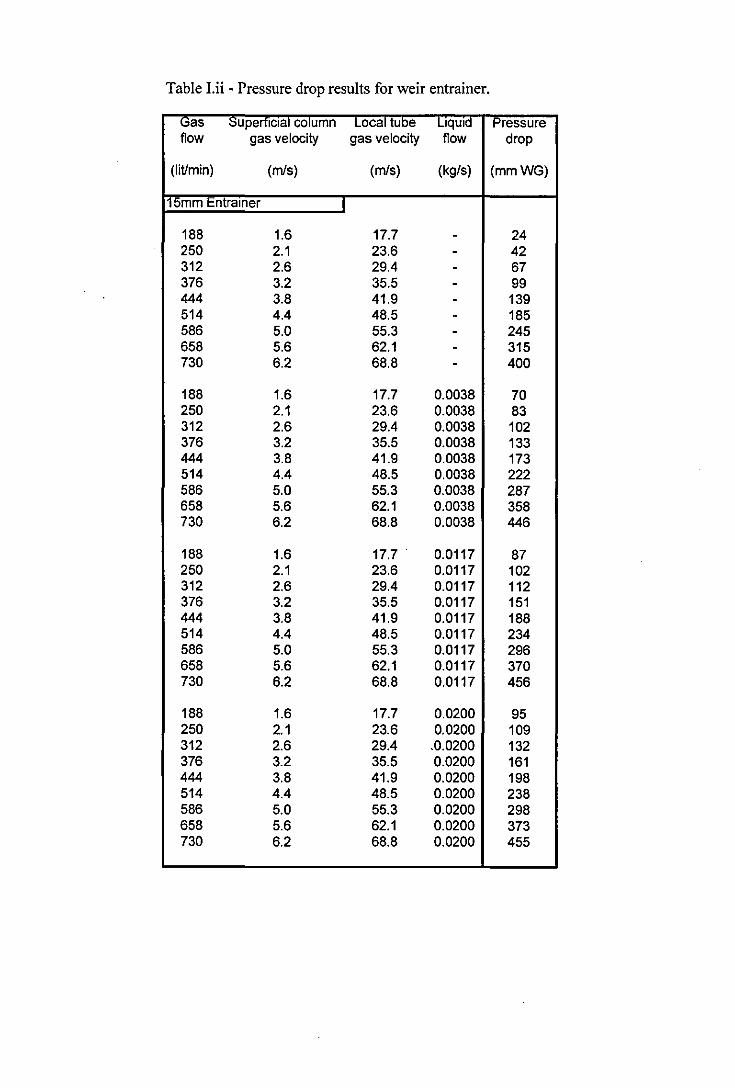
Table I.ii - Pressure drop results for weir entrainer.
Gas Superficial column Local tube Liquid Pressure flow gas velocity gas velocity flow drop
(litlmin) (m/s) (m/s) (kg/s) (mmWG)
115mm Entralner I
188 1.6 17.7 - 24 250 2.1 23.6 - 42 312 2.6 29.4 - 67 376 3.2 35.5 - 99 444 3.8 41.9 - 139 514 4.4 48.5 - 185 586 5.0 55.3 - 245 658 5.6 62.1 - 315 730 6.2 68.8 - 400
188 1.6 17.7 0.0038 70 250 2.1 23.6 0.0038 83 312 2.6 29.4 0.0038 102 376 3.2 35.5 0.0038 133 444 3.8 41.9 0.0038 173 514 4.4 48.5 0.0038 222 586 5.0 55.3 0.0038 287 658 5.6 62.1 0.0038 358 730 6.2 68.8 0.0038 446
188 1.6 17.7 . 0.0117 87 250 2.1 23.6 0.0117 102 312 2.6 29.4 0.0117 112 376 3.2 35.5 0.0117 151 444 3.8 41.9 0.0117 188 514 4.4 48.5 0.0117 234 586 5.0 55.3 0.0117 296 658 5.6 62.1 0.0117 370 730 6.2 68.8 0.0117 456
188 1.6 17.7 0.0200 95 250 2.1 23.6 0.0200 109 312 2.6 29.4 .0.0200 132 376 3.2 35.5 0.0200 161 444 3.8 41.9 0.0200 198 514 4.4 48.5 0.0200 238 586 5.0 55.3 0.0200 298 658 5.6 62.1 0.0200 373 730 6.2 68.8 0.0200 455
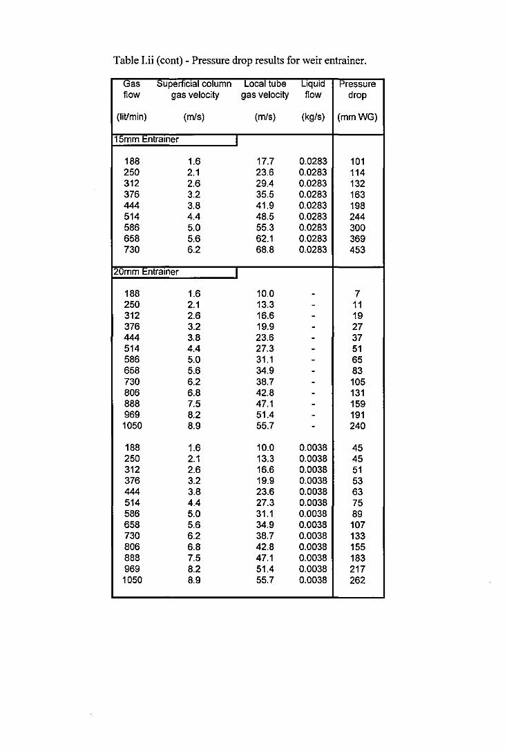
Table I.ii (cont) - Pressure drop results for weir entrainer.
Gas ::;uperflClal column Local tube Liquid Pressure flow gas velocity gas velocity flow drop
(liVmin) (m/s) (m/s) (kg/s) (mmWG)
15mm I::ntralner I
188 1.6 17.7 0.0283 101 250 2.1 23.6 0.0283 114 312 2.6 29.4 0.0283 132 376 3.2 35.5 0.0283 163 444 3.8 41.9 0.0283 198 514 4.4 48.5 0.0283 244 586 5.0 55.3 0.0283 300 658 5.6 62.1 0.0283 369 730 6.2 68.8 0.0283 453
20mm Entralner I
188 1.6 10.0 - 7 250 2.1 13.3 - 11 312 2.6 16.6 - 19 376 3.2 19.9 - 27 444 3.8 23.6 - 37 514 4.4 27.3 - 51 586 5.0 31.1 - 65 658 5.6 34.9 - 83 730 6.2 38.7 - 105 806 6.8 42.8 - 131 888 7.5 47.1 - 159 969 8.2 51.4 - 191 1050 8.9 55.7 - 240
188 1.6 10.0 0.0038 45 250 2.1 13.3 0.0038 45 312 2.6 16.6 0.0038 51 376 3.2 19.9 0.0038 53 444 3.8 23.6 0.0038 63 514 4.4 27.3 0.0038 75 586 5.0 31.1 0.0038 89 658 5.6 34.9 0.0038 107 730 6.2 38.7 0.0038 133 806 6.8 42.8 0.0038 155 888 7.5 47.1 0.0038 183 969 8.2 51.4 0.0038 217 1050 8.9 55.7 0.0038 262
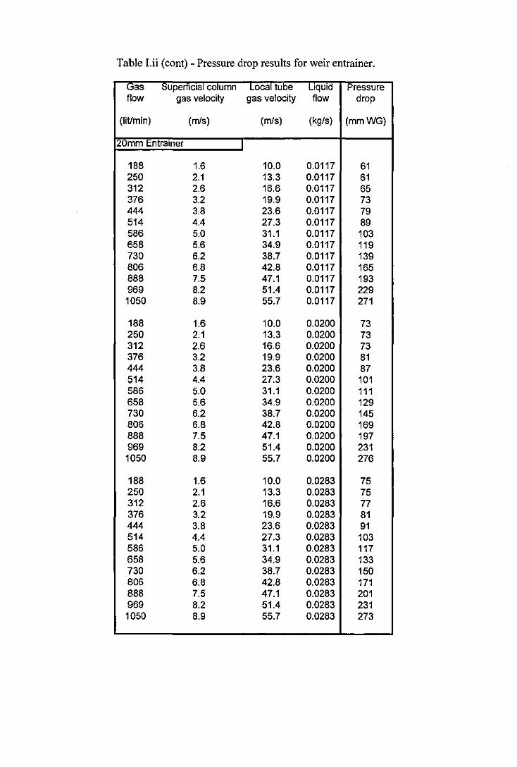
Table I.ii (cont) - Pressure drop results for weir entrainer.
l:Oas SupemclaJ cOfumn Tocaitube Liquid Pressure flow gas velocity gas velocity flow drop
(liVmin) (m/s) (m/s) (kg/s) (mmWG)
120mm Entralner I
188 1.6 10.0 0.0117 61 250 2.1 13.3 0.0117 61 312 2.6 16.6 0.0117 65 376 3.2 19.9 0.0117 73 444 3.8 23.6 0.0117 79 514 4.4 27.3 0.0117 89 586 5.0 31.1 0.0117 103 658 5.6 34.9 0.0117 119 730 6.2 38.7 0.0117 139 806 6.8 42.8 0.0117 165 888 7.5 47.1 0.0117 193 969 8.2 51.4 0.0117 229 1050 8.9 55.7 0.0117 271
188 1.6 10.0 0.0200 73 250 2.1 13.3 0.0200 73 312 2.6 16.6 0.0200 73 376 3.2 19.9 0.0200 81 444 3.8 23.6 0.0200 87 514 4.4 27.3 0.0200 101 586 5.0 31.1 0.0200 111 658 5.6 34.9 0.0200 129 730 6.2 38.7 0.0200 145 806 6.8 42.8 0.0200 169 888 7.5 47.1 0.0200 197 969 8.2 51.4 0.0200 231 1050 8.9 55.7 0.0200 276
188 1.6 10.0 0.0283 75 250 2.1 13.3 0.0283 75 312 2.6 16.6 0.0283 77 376 3.2 19.9 0.0283 81 444 3.8 23.6 0.0283 91 514 4.4 27.3 0.0283 103 586 5.0 31.1 0.0283 117 658 5.6 34.9 0.0283 133 730 6.2 38.7 0.0283 150 806 6.8 42.8 0.0283 171 888 7.5 47.1 0.0283 201 969 8.2 51.4 0.0283 231 1050 8.9 55.7 0.0283 273
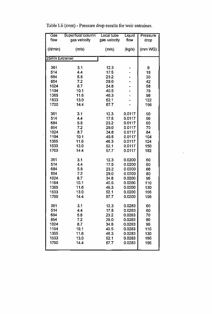
Table l.ii (cont) - Pressure drop results for weir entrainer.
Gas Superficial column Local tube liquid Pressure flow gas velocity gas velocity flow drop
(IiVmin) (m/s) (m/s) (kg/s) (mmWG)
I25mm Entralner I
361 3.1 12.3 - 8 514 4.4 17.5 - 18 684 5.8 23.2 - 30 854 7.2 29.0 - 42
1024 8.7 34.8 - 58 1194 10.1 40.5 - 78 1365 11.6 46.3 - 98 1533 13.0 52.1 - 122 1700 14.4 57.7 - 156
361 3.1 12.3 0.0117 50 514 4.4 17.5 0.0117 56 684 5.8 23.2 0.0117 60 854 7.2 29.0 0.0117 70 1024 8.7 34.8 0.0117 84 1194 10.1 40.5 0.0117 104 1365 11.6 46.3 0.0117 124 1533 13.0 52.1 0.0117 150 1700 14.4 57.7 0.0117 182
361 3.1 12.3 0.0200 60 514 4.4 17.5 0.0200 60 684 5.8 23.2 0.0200 66 854 7.2 29.0 0.0200 80
1024 8.7 34.8 0.0200 96 1194 10.1 40.5 0.0200 110 1365 11.6 46.3 0.0200 130 1533 13.0 52.1 0.0200 156 1700 14.4 57.7 0.0200 196
361 3.1 12.3 0.0283 60 514 4.4 17.5 0.0283 60 684 5.8 23.2 0.0283 70 854 7.2 29.0 0.0283 80 1024 8.7 34.8 0.0283 96 1194 10.1 40.5 0.0283 110 1365 11.6 46.3 0.0283 130 1533 13.0 52.1 0.0283 160 1700 14.4 57.7 0.0283 196

Table I.ii (cont) - Pressure drop results for weir entrainer.
(;;as ::;upertlclal COlumn Local tube Liquid Pressure flow gas velocity gas velocity flow drop
(litlmin) (m/s) (m/s) (kg!s) (mmWG)
25mm t:ntramer I
361 3.1 12.3 0.0350 70 514 4.4 17.5 0.0350 60 684 5.8 23.2 0.0350 70 854 7.2 29.0 0.0350 84 1024 8.7 34.8 0.0350 100 1194 10.1 40.5 0.0350 116 1365 11.6 46.3 0.0350 136 1533 13.0 52.1 0.0350 164 1700 14.4 57.7 0.0350 200
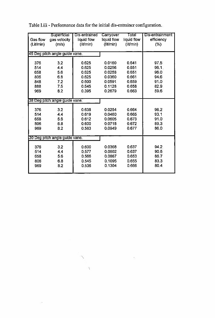
Table Liii - Performance data for the initial dis-entrainer configuration.
::;upemclal uls-emralnea varryover IOlal uls-emrammem Gas flow gas velocity liquid flow liquid flow liquid flow efficiency (Litlmin) (m/s) (Iitlmin) (Iitlmin) (Iitlmin) (%)
140 ueg pltcn angle gUlae vane. I
376 3.2 0.625 0.0160 0.641 97.5 514 4.4 0.625 0.0256 0.651 96.1. 658 5.6 0.625 0.0258 0.651 96.0 806 6.8 0.625 0.0360 0.661 94.6 848 7.2 0.600 0.0591 0.659 91.0 888 7.5 0.545 0.1128 0.658 82.9 969 8.2 0.395 0.2679 0.663 59.6
Ij/j ueg pllcn angle gUlae vane. I
376 3.2 0.638 0.0254 0.664 96.2 514 4.4 0.619 0.0460 0.665 93.1 658 5.6 0.612 0.0605 0.673 91.0 806 6.8 0.600 0.0718 0.672 89.3 969 8.2 0.583 0.0949 0.677 86.0
30 LJeg pltcn angle gUlae vane. I
376 3.2 0.600 0.0368 0.637 94.2 514 4.4 0.577 0.0602 0.637 90.5 658 5.6 0.566 0.0867 0.653 86.7 806 6.8 0.545 0.1095 0.655 83.3 969 8.2 0.536 0.1304 0.666 80.4
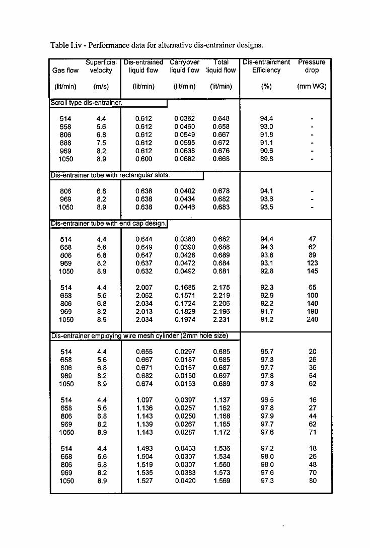
Table I.iv - Performance data for alternative dis-entrainer designs.
:::;uperTIclal Dls-entralnea l;arryover Total Dis-entralnment Pressure Gas flow velocity liquid flow liquid flow liquid flow Efficiency drop
(IiVmin) (m/s) (IiUmin) (liUmin) (IiVmin) (%) (mmWG)
IScroll type dls-entralner. I
514 4.4 0.612 0.0362 0.648 94.4 -658 5.6 0.612 0.0460 0.658 93.0 -806 6.8 0.612 0.0549 0.667 91.8 -888 7.5 0.612 0.0595 0.672 91.1 -969 8.2 0.612 0.0638 0.676 90.6 -1050 8.9 0.600 0.0682 0.668 89.8 -
Uls-entralner tube with rectangular SlotS. I
806 6.8 0.638 0.0402 0.678 94.1 -969 8.2 0.638 0.0434 0.682 93.6 -1050 8.9 0.638 0.0446 0.683 93.5 -
IUls-entralner tuoe wltn ena cap aeslgn.1
514 4.4 0.644 0.0380 0.682 94.4 47 658 5.6 0.649 0.0390 0.688 94.3 62 806 6.8 0.647 0.0428 0.689 93.8 89 969 8.2 0.637 0.0472 0.684 93.1 123 1050 8.9 0.632 0.0492 0.681 92.8 145
514 4.4 2.007 0.1685 2.175 92.3 65 658 5.6 2.062 0.1571 2.219 92.9 100 806 6.8 2.034 0.1724 2.206 92.2 140 969 8.2 2.013 0.1829 2.196 91.7 190 1050 8.9 2.034 0.1974 2.231 91.2 240
Dls-entralner emploYing wire mesh cylinder (2mm hole size)
514 4.4 0.655 0.0297 0.685 95.7 20 658 5.6 0.667 0.0187 0.685 97.3 26 806 6.8 0.671 0.0157 0.687 97.7 36 969 8.2 0.682 0.0150 0.697 97.8 54 1050 8.9 0.674 0.0153 0.689 97.8 62
514 4.4 1.097 0.0397 1.137 96.5 16 658 5.6 1.136 0.0257 1.162 97.8 27 806 6.8 1.143 0.0250 1.168 97.9 44 969 8.2 1.139 0.0267 1.165 97.7 62 1050 8.9 1.143 0.0287 1.172 97.6 71
514 4.4 1.493 0.0433 1.536 97.2 18 658 5.6 1.504 0.0307 1.534 98.0 26 806 6.8 1.519 0.0307 1.550 98.0 48 969 8.2 1.535 0.0383 1.573 97.6 70 1050 8.9 1.527 0.0420 1.569 97.3 80

Table I.v - Perfonnance data for the square hole meshes.
Superficial Uls-entralnea varryover Total uls-entralnment Pressure Gas flow velocity liquid flow liquid flow liquid flow Efficiency drop
(kg/s) (m/s) (litlmin) (Iitlmin) (Iitlmin) (%) (mmWG)
2000 micron square~o e mesh I
0.0073 3.1 0.685 0.0127 0.698 98.2 18 0.0139 5.9 0.677 0.0127 0.690 98.2 32 0.0209 8.9 0.682 0.0200 0.702 97.2 52 0.0279 11.8 0.605 0.0933 0.698 86.6 88 0.0312 13.3 0.584 0.1217 0.705 82.8 122 0.0348 14.8 0.331 0.3741 0.705 47.0 158
0.0073 3.1 1.154 0.0163 1.170 98.6 25 0.0139 5.9 1.161 0.0200 1.181 98.3 37 0.0209 8.9 1.165 0.0333 1.198 97.2 67 0.0279 11.8 1.031 0.1899 1.221 84.4 113 0.0312 13.3 0.843 0.3448 1.188 71.0 137 0.0348 14.8 0.606 0.5964 1.202 50.4 177
0.0073 3.1 1.639 0.0250 1.664 98.5 25 0.0139 5.9 1.613 0.0283 1.641 98.3 35 0.0209 8.9 1.596 0.0483 1.644 97.1 75 0.0279 11.8 1.336 0.2988 1.635 81.7 125 0.0312 13.3 1.115 0.5291 1.644 67.8 155 0.0348 14.8 0.771 0.8902 1.661 46.4 205
1200 micron square ho e mesh I
0.0073 3.1 0.632 0.0143 0.646 97.8 15 0.0139 5.9 0.645 0.0133 0.658 98.0 32 0.0209 8.9 0.658 0.0133 0.671 98.0 55 0.0279 11.8 0.598 0.0650 0.663 90.2 92 0.0312 13.3 0.476 0.1887 0.665 71.6 122 0.0348 14.8 0.453 0.2256 0.679 66.8 150
0.0073 3.1 1.130 0.0217 1.152 98.1 25 0.0139 5.9 1.147 0.0233 1.171 98.0 35 0.0209 8.9 1.158 0.0217 1.180 98.2 67 0.0279 11.8 1.136 0.0483 1.185 95.9 118 0.0312 13.3 1.010 0.1875 1.198 84.3 135 0.0348 14.8 0.845 0.3563 1.201 70.3 173
0.0073 3.1 1.523 0.0300 1.553 98.1 25 0.0139 5.9 1.575 0.0300 1.605 98.1 45 0.0209 8.9 1.600 0.0283 1.628 98.3 75 0.0279 11.8 1.563 0.0667 1.629 95.9 115 0.0312 13.3 1.379 0.2459 1.625 84.9 155 0.0348 14.8 1.176 0.4910 1.667 70.6 195

Table Lv (cont) - Performance data for the square hole meshes.
Superficial 'Dls-entrained Carryover Total Dls-entralnment Pressure Gas flow velocity liquid flow liquid flow liquid flow Efficiency drop
(kgts) (mts) (Iitlmin) (litlmin) (litlmin) (%) (mmWG)
70lf micron squarenDre mesh T
0.0073 3.1 0.638 0.0147 0.653 97.8 18 0.0139 5.9 0.654 0.0157 0.669 97.7 32 0.0209 8.9 0.658 0.0137 0.672 98.0 55 0.0279 11.8 0.661 0.0180 0.679 97.3 92 0.0312 13.3 0.592 0.0317 0.623 94.9 118 0.0348 14.8 0.589 0.0683 0.658 89.6 145
0.0073 3.1 1.124 0.0217 1.145 98.1 23 0.0139 5.9 1.143 0.0217 1.165 98.1 35 0.0209 8.9 1.165 0.0183 1.183 98.5 55 0.0279 11.8 1.128 0.0583 1.186 95.1 95 0.0312 13.3 1.087 0.0917 1.179 92.2 125 0.0348 14.8 1.036 0.1467 1.183 87.6 165
0.0073 3.1 1.523 0.0333 1.556 97.9 23 0.0139 5.9 1.613 0.0267 1.640 98.4 45 0.0209 8.9 1.571 0.0250 1.596 98.4 65 0.0279 11.8 1.542 0.0883 1.631 94.6 123 0.0312 13.3 1.500 0.1417 1.642 91.4 147 0.0348 14.8 1.446 0.2083 1.654 87.4 187
410 micron square hore mesn I
0.0073 3.1 0.638 0.0177 0.656 97.3 20 0.0139 5.9 0.654 0.0127 0.666 98.1 28 0.0209 8.9 0.652 0.0107 0.663 98.4 55 0.0279 11.8 0.638 0.0433 0.682 93.6 85 0.0312 13.3 0.630 0.0633 0.694 90.9 112 0.0348 14.8 0.605 0.0767 0.682 88.8 138
0.0073 3.1 0.619 0.0170 0.636 97.3 20 0.0139 5.9 0.626 0.0113 0.638 98.2 28 0.0209 8.9 0.619 0.0137 0.632 97.8 53 0.0279 11.8 0.601 0.0533 0.655 91.9 87 0.0312 13.3 0.613 0.0617 0.675 90.9 112 0.0348 14.8 0.598 0.0733 0.671 89.1 138
0.0073 3.1 1.132 0.0250 1.157 97.8 25 0.0139 5.9 1.179 0.0200 1.199 98.3 35 0.0209 8.9 1.176 0.0217 1.198 98.2 65 0.0279 11.8 1.119 0.0933 1.213 92.3 105 0.0312 13.3 1.095 0.1217 1.217 90.0 137 0.0348 14.8 1.085 0.1417 1.227 88.5 165
0.0073 3.1 1.538 0.0350 1.573 97.8 25 0.0139 5.9 1.622 0.0250 1.647 98.5 40 0.0209 8.9 1.613 0.0267 1.640 98.4 67 0.0279 11.8 1.519 0.1250 1.644 92.4 127 0.0312 13.3 1.500 0.1667 1.667 90.0 160 0.0348 14.8 1.449 0.2041 1.653 87.7 185

Table Lv (cont) - Performance data for the square hole meshes.
Supemclru I Dls-entralned Carryover Total Dis-entralnment Pressure Gas flow velocity liquid flow liquid flow liquid flow Efficiency drop
(kg/s) (m/s) (Iitlmin) (Iitlmin) (litlmin) (%) (mmWG)
260 micron square hole meSll T
0.0073 3.1 0.595 0.0233 0.619 96.2 20 0.0139 5.9 0.617 0.0167 0.634 97.4 27 0.0209 8.9 0.622 0.0147 0.637 97.7 50 0.0279 11.8 0.592 0.0383 0.630 93.9 80 0.0312 13.3 0.552 0.0883 0.641 86.2 107 0.0348 14.8 0.522 0.1233 0.645 80.9 140
0.0073 3.1 1.101 0.0317 1.133 97.2 22 0.0139 5.9 1.115 0.0267 1.142 97.7 33 0.0209 8.9 1.132 0.0233 1.155 98.0 60 0.0279 11.8 1.073 0.0633 1.137 94.4 100 0.0312 13.3 1.040 0.1150 1.155 90.0 124 0.0348 14.8 0.979 0.1685 1.147 85.3 156
0.0073 3.1 1.508 0.0400 1.548 97.4 27 0.0139 5.9 1.542 0.0350 1.577 97.8 37 0.0209 8.9 1.550 0.0317 1.582 98.0 67 0.0279 11.8 1.508 0.1033 1.611 93.6 115 0.0312 13.3 1.408 0.1818 1.590 88.6 145 0.0348 14.8 1.348 0.2479 1.596 84.5 180
14S-micron squarenDfe mesh I
0.0073 3.1 0.652 0.0203 0.673 97.0 -0.0139 5.9 0.670 0.0120 0.682 98.2 -0.0209 8.9 0.673 0.0067 0.679 99.0 55 0.0279 11.8 0.661 0.0207 0.681 97.0 85 0.0312 13.3 0.644 0.0333 0.677 95.1 100 0.0348 14.8 0.630 0.0517 0.682 92.4 125
0.0073 3.1 0.619 0.0250 0.644 96.1 23 0.0139 5.9 0.647 0.0130 0.660 98.0 33 0.0209 8.9 0.645 0.0090 0.654 98.6 53 0.0279 11.8 0.633 0.0300 0.663 95.5 85 0.0312 13.3 0.617 0.0500 0.667 92.5 105 0.0348 14.8 0.596 0.0700 0.666 89.5 125
0.0073 3.1 1.136 0.0283 1.165 97.6 17 0.0139 5.9 1.165 0.0200 1.185 98.3 33 0.0209 8.9 1.170 0.0127 1.182 98.9 53 0.0279 11.8 1.115 0.0667 1.182 94.4 97 0.0312 13.3 1.070 0.1100 1.180 90.7 127 0.0348 14.8 1.020 0.1467 1.167 87.4 153
0.0073 3.1 1.523 0.0350 1.558 97.8 25 0.0139 5.9 1.546 0.0233 1.570 98.5 35 0.0209 8.9 1.604 0.0183 1.623 98.9 65 0.0279 11.8 1.508 0.0967 1.604 94.0 115 0.0312 13.3 1.474 0.1467 1.621 91.0 135 0.0348 14.8 1.429 0.1923 1.621 88.1 180

Table Lv (cont) - Performance data for the square hole meshes.
~upertlclal Dls-entralned carry over Total IUls-entralnment Pressure Gas flow velocity liquid flow liquid flow liquid flow Efficiency drop
(kg/s) (m/s) (Iitlmin) (Iitlmin) (Iitlmin) (%) (mmWG)
77 micron square no le mesn I
0.0073 3.1 0.596 0.0367 0.633 94.2 25 0.0139 5.9 0.633 0.0123 0.645 98.1 33 0.0209 8.9 0.634 0.0053 0.640 99.2 47 0.0279 11.8 0.641 0.0033 0.644 99.5 87 0.0312 13.3 0.649 0.0030 0.652 99.5 113 0.0348 14.8 0.647 0.0037 0.650 99.4 133
0.0073 3.1 1.107 0.0417 1.149 96.4 25 0.0139 5.9 1.152 0.0193 1.171 98.3 33 0.0209 8.9 1.165 0.0077 1.173 99.3 57 0.0279 11.8 1.163 0.0067 1.169 99.4 105 0.0312 13.3 1.156 0.0067 1.163 99.4 133 0.0348 14.8 1.161 0.0077 1.168 99.3 167
0.0073 3.1 1.449 0.0433 1.493 97.1 22 0.0139 5.9 1.500 0.0217 1.522 98.6 33 0.0209 8.9 1.511 0.0100 1.521 99.3 63 0.0279 11.8 1.500 0.0100 1.510 99.3 110 0.0312 13.3 1.511 0.0103 1.522 99.3 147 0.0348 14.8 1.515 0.0117 1.527 99.2 177
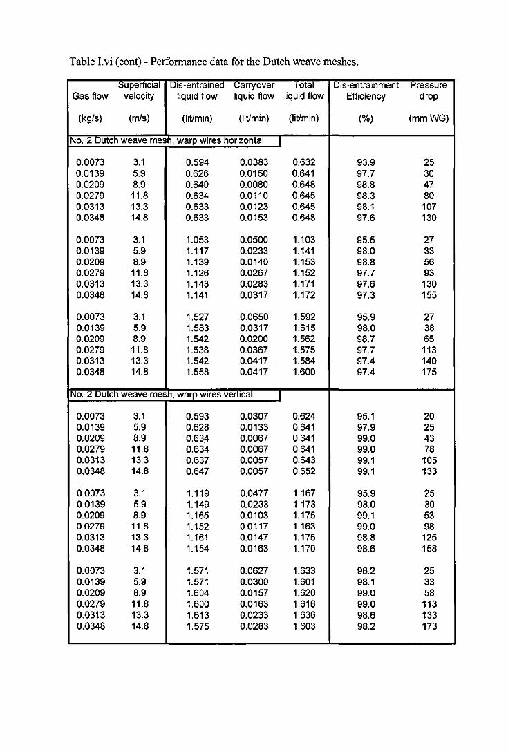
Table Lvi (cont) - Performance data for the Dutch weave meshes.
::;u pertlclal Dls-entralnea <.;arryover lotal Dls-entralnment Pressure Gas flow velocity liquid flow liquid flow liquid flow Efficiency drop
(kg/s) (m/s) (Iitlmin) (Iitlmin) (Iitlmin) (%) (mmWG)
INO. 2 uutcn weave mesn, warp wires nonzontal I
0.0073 3.1 0.594 0.0383 0.632 93.9 25 0.0139 5.9 0.626 0.0150 0.641 97.7 30 0.0209 8.9 0.640 0.0080 0.648 98.8 47 0.0279 11.8 0.634 0.0110 0.645 98.3 80 0.0313 13.3 0.633 0.0123 0.645 98.1 107 0.0348 14.8 0.633 0.0153 0.648 97.6 130
0.0073 3.1 1.053 0.0500 1.103 95.5 27 0.0139 5.9 1.117 0.0233 1.141 98.0 33 0.0209 8.9 1.139 0.0140 1.153 98.8 56 0.0279 11.8 1.126 0.0267 1.152 97.7 93 0.0313 13.3 1.143 0.0283 1.171 97.6 130 0.0348 14.8 1.141 0.0317 1.172 97.3 155
0.0073 3.1 1.527 0.0650 1.592 95.9 27 0.0139 5.9 1.583 0.0317 1.615 98.0 38 0.0209 8.9 1.542 0.0200 1.562 98.7 65 0.0279 11.8 1.538 0.0367 1.575 97.7 113 0.0313 13.3 1.542 0.0417 1.584 97.4 140 0.0348 14.8 1.558 0.0417 1.600 97.4 175
No. 2 uutcn weave mesn, warp wires vertical I
0.0073 3.1 0.593 0.0307 0.624 95.1 20 0.0139 5.9 0.628 0.0133 0.641 97.9 25 0.0209 8.9 0.634 0.0067 0.641 99.0 43 0.0279 11.8 0.634 0.0067 0.641 99.0 78 0.0313 13.3 0.637 0.0057 0.643 99.1 105 0.0348 14.8 0.647 0.0057 0.652 99.1 133
0.0073 3.1 1.119 0.0477 1.167 95.9 25 0.0139 5.9 1.149 0.0233 1.173 98.0 30 0.0209 8.9 1.165 0.0103 1.175 99.1 53 0.0279 11.8 1.152 0.0117 1.163 99.0 98 0.0313 13.3 1.161 0.0147 1.175 98.8 125 0.0348 14.8 1.154 0.0163 1.170 98.6 158
0.0073 3·1 1.571 0.0627 1.633 96.2 25 0.0139 5.9 1.571 0.0300 1.601 98.1 33 0.0209 8.9 1.604 0.0157 1.620 99.0 58 0.0279 11.8 1.600 0.0163 1.616 99.0 113 0.0313 13.3 1.613 0.0233 1.636 98.6 133 0.0348 14.8 1.575 0.0283 1.603 98.2 173
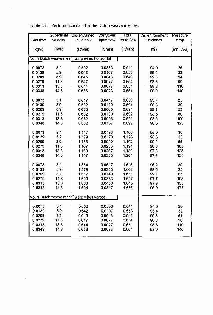
Table Lvi - Performance data for the Dutch weave meshes.
::;upernclal I Uls-entralned L;arryover lotal Uls-entralnment I-'ressure Gas flow velocity liquid flow liquid flow liquid flow Efficiency drop
(kg/s) (rn/s) (litlmin) (litlmin) (litlmin) (%) (mmWG)
INo. 1 Dutch weave mesh, warp wires hOrizontal I
0.0073 3.1 0.602 0.0383 0.641 94.0 26 0.0139 5.9 0.642 0.0107 0.653 98.4 32 0.0209 8.9 0.645 0.0043 0.649 99.3 54 0.0279 11.8 0.647 0.0077 0.654 98.8 90 0.0313 13.3 0.644 0.0077 0.651 98.8 110 0.0348 14.8 0.656 0.0073 0.664 98.9 140
0.0073 3,.1 0.617 0.0417 0.659 93.7 25 0.0139 5.9 0.682 0.0120 0.694 98.3 30 0.0209 8.9 0.685 0.0060 0.691 99.1 53 0.0279 11.8 0.682 0.0100 0.692 98.6 80 0.0313 13.3 0.682 0.0093 0.691 98.6 100 0.0348 14.8 0.682 0.0107 0.692 98.5 123
0.0073 3.1 1.117 0.0483 1.166 95.9 30 0.0139 5.9 1.179 0.0170 1.196 98.6 35 0.0209 8.9 1.183 0.0090 1.192 99.2 55 0.0279 11.8 1.167 0.0233 1.191 98.0 105 0.0313 13.3 1.163 0.0267 1.189 97.8 125 0.0348 14.8 1.167 0.0333 1.201 97.2 155
0.0073 3.1 1.554 0.0617 1.616 96.2 30 0.0139 5.9 1.579 0.0233 1.602 98.5 35 0.0209 8.9 1.617 0.0140 1.631 99.1 65 0.0279 11.8 1.609 0.0383 1.647 97.7 105 0.0313 13.3 1.600 0.0450 1.645 97.3 135 0.0348 14.8 1.604 0.0517 1.656 96.9 175
INo. 1 Dutch weave mesh, warp wires vertical I
0.0073 3.1 0.602 0.0383 0.641 94.0 26 0.0139 5.9 0.642 0.0107 0.653 98.4 32 0.0209 8.9 0.645 0.0043 0.649 99.3 54 0.0279 11.8 0.647 0.0077 0.654 98.8 90 0.0313 13.3 0.644 0.0077 0.651 98.8 110 0.0348 14.8 0.656 0.0073 0.664 98.9 140

Table I.vii - Effect of dis-entrainer position on separation perfonnance
::>upertlclal Total Dls-entralnment eftlciencles Gas flow velocity liquid flow Original position Upper position
(kg/s) (m/s) (liUmin) (%) (%)
11Z00 micron square hO ed meSh
0.0073 3.1 0.65 97.8 95.7 0.0139 5.9 0.65 98.0 96.3 0.0209 8.9 0.65 98.0 87.5 0.0279 11.8 0.65 90.2 21.0 0.0312 13.3 0.65 71.6 -0.0348 14.8 0.65 66.8 -
0.0073 3.1 1.17 98.1 96.0 0.0139 5.9 1.17 98.0 96.0 0.0209 8.9 1.17 98.2 81.8 0.0279 11.8 1.17 95.9 25.4 0.0312 13.3 1.17 84.3 -0.0348 14.8 1.17 70.3 -
260 micron square hole mesh
0.0073 3.1 0.65 96.2 95.0 0.0139 5.9 0.65 97.4 96.8 0.0209 8.9 0.65 97.7 87.1 0.0279 11.8 0.65 93.9 68.6 0.0312 13.3 0.65 86.2 62.8 0.0348 14.8 0.65 80.9 58.4
0.0073 3.1 1.17 97.2 95.7 0.0139 5.9 1.17 97.7 97.1 0.0209 8.9 1.17 98.0 88.7 0.0279 11.8 1.17 94.4 77.7 0.0312 13.3 1.17 90.0 73.5 0.0348 14.8 1.17 85.3 70.9
1145 micron square hole meSh
0.0073 3.1 0.65 97.0 95.4 . 0.0139 5.9 0.65 98.2 97.7
0.0209 8.9 0.65 99.0 98.6 0.0279 11.8 0.65 97.0 98.8 0.0312 13.3 0.65 95.1 98.9 0.0348 14.8 0.65 92.4 98.8
0.0073 3.1 1.17 96.1 95.8 0.0139 5.9 1.17 98.0 98.0 0.0209 8.9 1.17 98.6 98.7 0.0279 11.8 1.17 95.5 99.0 0.0312 13.3 1.17 92.5 98.9 0.0348 14.8 1.17 89.5 98.8

Table Lvii (cont) - Effect of dis-entrainer position on separation performance.
SuperfICIal Total Dls-entralnment efficlencles Gas flow velocity liquid flow Original position Upper position
(kg/s) (m/s) (liVmin) (%) (%)
77 mIcron square hOlea mesh
0.0073 3.1 0.65 94.2 95.4 0.0139 5.9 0.65 98.1 98.2 0.0209 8.9 0.65 99.2 98.6 0.0279 11.8 0.65 99.5 99.2 0.0312 13.3 0.65 99.5 99.3 0.0348 14.8 0.65 99.4 99.3
0.0073 3.1 1.17 96.4 95.7 0.0139 5.9 1.17 98.3 98.1 0.0209 8.9 1.17 99.3 98.7 0.0279 11.8 1.17 99.4 99.2 0.0312 13.3 1.17 99.4 99.2 0.0348 14.8 1.17 99.3 99.2
NO 1. uutcn weave meSh. -0.0073 3.1 0.65 94.0 92.9 0.0139 5.9 0.65 98.4 97.1 0.0209 8.9 0.65 99.3 97.9 0.0279 11.8 0.65 98.8 98.5 0.0312 13.3 0.65 98.8 98.6 0.0348 14.8 0.65 98.9 98.6
0.0073 3.1 1.17 95.9 94.0 0.0139 5.9 1.17 98.6 97.0 0.0209 8.9 1.17 99.2 97.9 0.0279 11.8 1.17 98.0 98.5 0.0312 13.3 1.17 97.8 98.5 0.0348 14.8 1.17 97.2 98.3

Table Lviii - Results from pressure manipulation rig.
INO. 2 uutch weave mesh. Gas flow 0.0313 kg/s - 13.3 mls superficial gas velocity Liquid flow 1.1 liVmin
Measurea Dls-entralnment P(lnside) P(Outside) Pressure difference efficiency
(mmWG) (mmWG) (mmWG) (%)
I t:xternal pressure mampUlatea, Internal pressure Tlxea.
-18.288 19.558 -37.8 81.2 -18.288 14.478 -32.8 90.1 -18.288 9.398 -27.7 94.6 -18.288 4.318 -22.6 96.2
External pressure atmospheric, Internal pressure mampulatea.
-18.3 0 -18.3 96.7 -11.9 0 -11.9 97.9 -6.9 0 -6.9 97.9 0.3 0 0.3 98.4 6.9 0 6.9 98.4
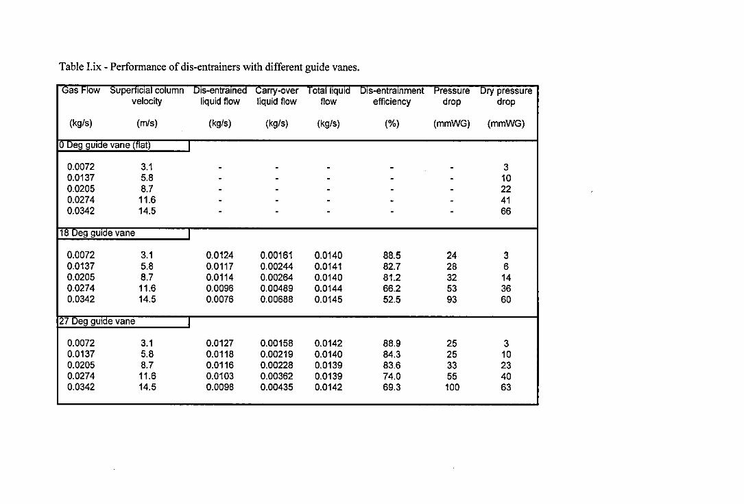
Table I.ix - Performance of dis-entrainers with different guide vanes.
(;;as I-IOW ::;upertlclal column uls-entralnea (jarry-over lotal IIqUla uls-entralnment I-'ressure ury pressure velocity liquid flow liquid flow flow efficiency drop drop
(kg/s) (m/s) (kg/s) (kg/s) (kg/s) (%) (mmWG) (mmWG)
o Deg guide vane (flat) I
0.0072 3.1 - - - - - 3 0.0137 5.8 - - - - - 10 0.0205 8.7 - - - - - 22 0.0274 11.6 - - - - - 41 0.0342 14.5 - - - - - 66
18 Deg guide vane I
0.0072 3.1 0.0124 0.00161 0.0140 88.5 24 3 0.0137 5.8 0.0117 0.00244 0.0141 82.7 28 6 0.0205 8.7 0.0114 0.00264 0.0140 81.2 32 14 0.0274 11.6 0.0096 0.00489 0.0144 66.2 53 36 0.0342 14.5 0.0076 0.00688 0.0145 52.5 93 60
;l.7 ueg gUlae vane I
0.0072 3.1 0.0127 0.00158 0.0142 88.9 25 3 0.0137 5.8 0.0118 0.00219 0.0140 84.3 25 10 0.0205 8.7 0.0116 0.00228 0.0139 83.6 33 23 0.0274 11.6 0.0103 0.00362 0.0139 74.0 55 40 0.0342 14.5 0.0098 0.00435 0.0142 69.3 100 63
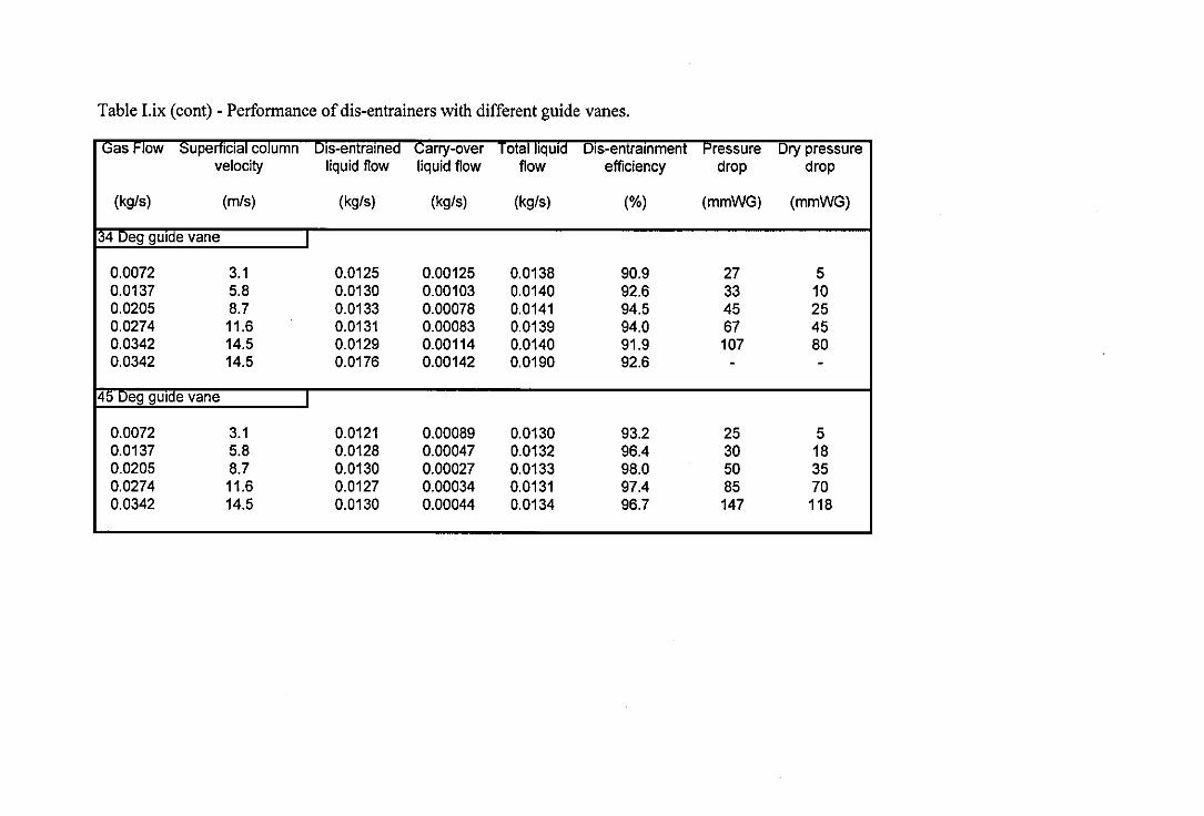
Table I.ix (cont) - Perfonnance of dis-entrainers with different guide vanes.
Ijas r IOW ::;upemclal cOlumn Uls-entralnea t;arry-over I otal IIqUla uls-entralnment I-'ressure Dry pressure velocity liquid flow liquid flow flow efficiency drop drop
(kg/s) (m/s) (kg/s) (kg/s) (kg/s) (%) (mmWG) (mmWG)
34 Deg gUide vane I
0.0072 3.1 0.0125 0.00125 0.0138 90.9 27 5 0.0137 5.8 0.0130 0.00103 0.0140 92.6 33 10 0.0205 8.7 0.0133 0.00078 0.0141 94.5 45 25 0.0274 11.6 0.0131 0.00083 0.0139 94.0 67 45 0.0342 14.5 0.0129 0.00114 0.0140 91.9 107 80 0.0342 14.5 0.0176 0.00142 0.0190 92.6 - -
40 ueg gUlae vane I
0.0072 3.1 0.0121 0.00089 0.0130 93.2 25 5 0.0137 5.8 0.0128 0.00047 0.0132 96.4 30 18 0.0205 8.7 0.0130 0.00027 0.0133 98.0 50 35 0.0274 11.6 0.0127 0.00034 0.0131 97.4 85 70 0.0342 14.5 0.0130 0.00044 0.0134 96.7 147 118
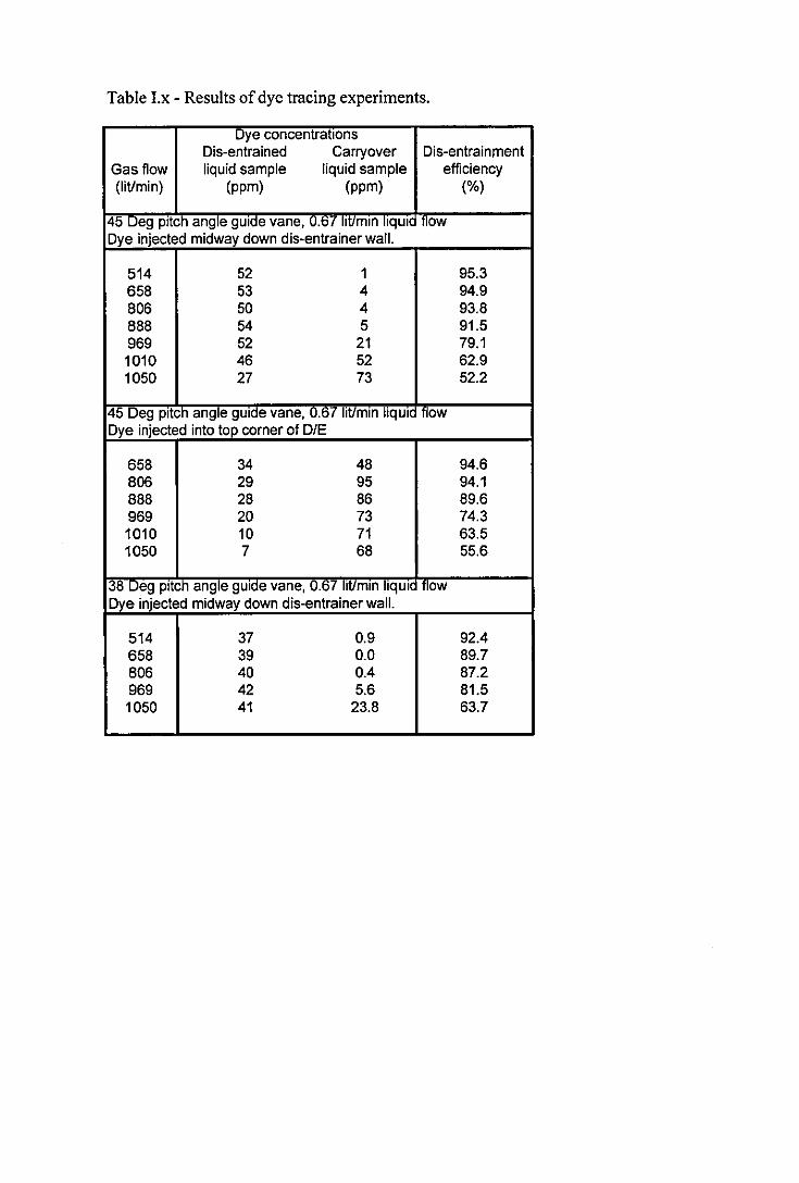
Table Lx - Results of dye tracing experiments.
Dye concentrations Dis-entrained Carryover Dis-entrainment
Gas flow liquid sample liquid sample efficiency (IiVmin) (ppm) (ppm) (%)
45 ueg pitch angle guide vane, 0.67 lit/mm liquicl flow Dye injected midway down dis-entrainer wall.
514 52 1 95.3 658 53 4 94.9 806 50 4 93.8 888 54 5 91.5 969 52 21 79.1 1010 46 52 62.9 1050 27 73 52.2
45 Deg pitch angle guide vane, 0.67 lit/mm liquic flow Dye injected into top corner of DIE
658 34 48 94.6 806 29 95 94.1 888 28 86 89.6 969 20 73 74.3 1010 10 71 63.5 1050 7 68 55.6
38 Deg pitch angle guide vane, 0.67 IiVmm liqUl I flow Dye injected midway down dis-entrainer wall.
514 37 0.9 92.4 658 39 0.0 89.7 806 40 0.4 87.2 969 42 5.6 81.5 1050 41 23.8 63.7
Appendix 11
Data and models for dynamic dye-tracing experiments.

Appendix n.
Dynamic model equations.
Please consult the figure overleaf for definitions.
1. Equations for the well mixed pool on the entrainment plate.
Mass balance around liquid pool on the entrainment plate, assumed to be weII mixed.
q,+q,=q2
q,c, (t) + q,c,(t) = q2c2 (t) + VL( d;;) dC2 q,c,(t)+q,c,(t)-q2C2(t) _ = -"-'--'-'-':"""""'::":"...:...0.':"""""":"::''''':''''>'-'-
dt VL
The liquid volume, VL was estimated as 14 m!.
2. Equations for the droplet flight section.
A mass balance around plug flow section corresponding to droplet flight gives:
q2=q,+q.
Assuming negligible time delay during droplet flight, and equal dye concentration in
the two outlet streams gives:
c.(t) = c,(t) = c2(t)

... .....
D is-ent- ... r ained "" liquid flow ...
""
q6,c6 ~ ,.
q 7,C7 LiqPool
t . L Iq 0 utlet
Return liquid flow down wall
q4'C4 ...
Entrained liquid flow
Mesh Wall
Mass ~ ....
transfer
Mass ~ ....
transfer
Mass ~ ....
transfer
Mass ~ ....
transfer
Gas Outlet
Cyclone
Dis-entrainer
Entrainer
Figure ILi Dynamic model for the contactor

3. Equations for return liquid flow down the entrainer wall.
An overall mass balance around the plug flow section corresponding to flow down the
wall gives:
q, = q.
Assuming a I second time delay for the liquid flowing down the wall gives:
c,(t)=c.(t-I)
4. Equations for the dis-entrainment section.
Neglecting the time delay between dye entering the dis-entrainrnent section and
arriving at the pool on the plate gives: (The results of the model did not depend on any
time delay in this section.)
q6 = q3
c6 (t) = c3 (t)
A mass balance around the liquid pool on the dis-entrainrnent plate gives:
q, = q6
q6C6(t) = q,c,(t)+VL( ~;) dc, = q6C6(t)-q,c,(t) dt VL
The liquid volume, VL was estimated as 7 m!.
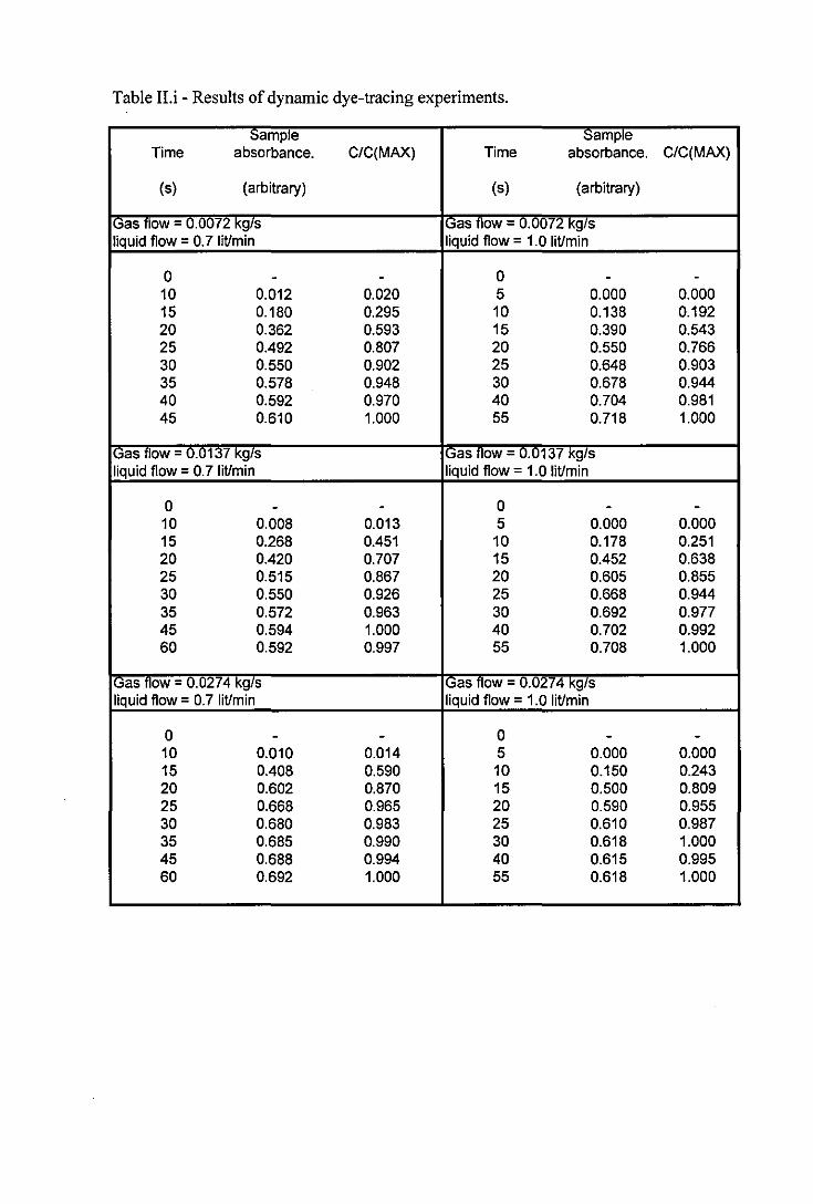
Table lLi - Results of dynamic dye-tracing experiments.
Sample ::;ample Time absorbance. C/C{MAX) Time absorbance. C/C{MAX)
(s) (arbitrary) (s) (arbitrary)
Gas flow = 0.0072 kg/s Gas flow - 0.0072 kg/s liquid flow = 0.7 litlmin liquid flow = 1.0 litlmin
0 - - 0 - -10 0.012 0.020 5 0.000 0.000 15 0.180 0.295 10 0.138 0.192 20 0.362 0.593 15 0.390 0.543 25 0.492 0.807 20 0.550 0.766 30 0.550 0.902 25 0.648 0.903 35 0.578 0.948 30 0.678 0.944 40 0.592 0.970 40 0.704 0.981 45 0.610 1.000 55 0.718 1.000
(;;as flOW - 0.0137 Kg's (;;as flow 0.0137 Kg'S liquid flow = 0.7 litlmin liquid flow = 1.0 litlmin
0 - - 0 - -10 0.008 0.013 5 0.000 0.000 15 0.268 0.451 10 0.178 0.251 20 0.420 0.707 15 0.452 0.638 25 0.515 0.867 20 0.605 0.855 30 0.550 0.926 25 0.668 0.944 35 0.572 0.963 30 0.692 0.977 45 0.594 1.000 40 0.702 0.992 60 0.592 0.997 55 0.708 1.000
I(;;as flOW 0.0274 Kg'S (;;as flOW - 0.0274 kg'S liquid flow = 0.7 litlmin liquid flow = 1.0 litlmin
0 - - 0 - -10 0.010 0.014 5 0.000 0.000 15 0.408 0.590 10 0.150 0.243 20 0.602 0.870 15 0.500 0.809 25 0.668 0.965 20 0.590 0.955 30 0.680 0.983 25 0.610 0.987 35 0.685 0.990 30 0.618 1.000 45 0.688 0.994 40 0.615 0.995 60 0.692 1.000 55 0.618 1.000
Table lLi (cont) - Results of dynamic dye-tracing experiments.
sample Sample Time absorbance. C/C(MAX) Time absorbance. C/C(MAX)
(s) (arbitrary) (s) (arbitrary)
Gas flow ~ 0.0307 kg/s IGas flow = u.u307 kg/s liquid flow = 0.7 litlmin liquid flow = 1.0 litlmin
0 - - 0 - -10 0.008 0.013 5 0.002 0.003 15 0.355 0.555 10 0.168 0.267 20 0.560 0.875 15 0.530 0.841 25 0.615 0.961 20 0.606 0.962 30 0.632 0.988 25 0.622 0.987 35 0.632 0.988 30 0.626 0.994 45 0.640 1.000 40 0.630 1.000 60 0.640 1.000 55 0.630 1.000
(jas flOW 0.0342 Kg/S l\,jas flow = u.Uj4:l Kg/s liquid flow = 0.7 litlmin liquid flow = 1.0 litlmin
0 - - 0 - -10 0.002 0.003 5 0.000 0.000 15 0.362 0.603 10 0.142 0.269 20 0.528 0.880 15 0.440 0.833 25 0.572 0.953 20 0.510 0.966 35 0.596 0.993 25 0.520 0.985 45 0.598 0.997 30 0.520 0.985 60 0.600 1.000 40 0.520 0.985
55 0.528 1.000
Tabel II.ii - Summary of dye tracing results.
\,jas ::;u pemclal t;alculatea recycle rates flow gas velocity 0.7litlmin liquid 1.0 litlmin liquid
(kg/s) (m/s) (R = q4/q1) (R = q4/q1)
0.0072 3.1 6.1 7.8 0.0137 5.8 5.9 6.4 0.0274 11.6 3.8 2.5 0.0307 13.0 2.7 3.7 0.0342 14.5 3.4 4.2

Appendix III
Results from humidification experiments.

Table III.i - Experimental results from humidifcation experiments.
£:>mm entralner ,JU l,.; approx water Inlet tef'!lperature I LiqUid K(Q)a results Gas Column Gas temperatures an umiditles Gas specific entha pies liquid Temperatures I Plug flow Well mixed Recycle t:qUlvalent flow velocity nlet temp Inlet humidity uutlet temp Uutlet humidity
I (~~~~) (~~;:~) H~~~\k~~rr Flow rate T((g \(~\~ model model model number of (kg/s) (m/s)' (C) (%) (C) (%) (Iit/min) (kg/s) (lis) (1/s) (lis) transfer units.
0.0122 5.2 20.9 21 17.4 94 28.8 45.9 49.4 0.439 0.00732 29.8 21.6 10.2 15.2 14.1 0.552 0.0166 7.0 21.1 20 16.9 90 28.7 43.4 46.1 0.427 0.00711 30 20.3 12.1 19.6 17.9 0.482 0.0216 9.2 21.1 20 16.0 91 28.7 41.3 43.9 0.431 0.00718 30.2 19.3 14.3 25.0 22.1 0.429 0.0265 11.2 21.1 20 15.4 91 28.7 39.7 41.7 0.438 0.00730 29.9 18.6 15.4 28.1 23.6 0.386 0.0320 13.6 20.9 21 14.9 90 28.8 38.2 40.6 0.429 0.00714 29.8 17.1 19.8 41.5 32.1 0.387 0.0122 5.2 21.1 20 18.1 89 28.7 46.3 49.0 0.429 0.00714 30.1 21.8 9.6 14.2 13.2 0.544
0.0122 5.2 21.2 24 19.2 88 30.5 49.1 54.4 0.655 0.01092 29.2 22.8 12.7 17.3 16.4 0.682 0.0166 7.0 21.2 24 18.0 90 30.5 49.4 51.4 0.656 0.01094 29.2 21.6 15.8 23.4 21.7 0.606 0.0216 9.2 21.2 24 17.0 92 30.5 44.2 48.9 0.664 0.01106 29.2 20.6 18.9 29.9 27.0 0.555 0.0265 11.2 21.2 24 16.3 91 30.5 42.1 46.8 0.665 0.01109 29.1 19.8 21.1 35.0 30.8 0.507 0.0320 13.6 21.2 24 15.8 90 30.5 40.5 45.4 0.658 0.01096 29.2 18.8 25.5 46.2 38.1 0.485 0.0320 13.6 20.8 20 15.8 90 28.2 40.5 43.0 0.667 0.01111 29.2 19.0 18.5 36.4 30.8 0.441
0.0122 5.2 19.0 21 19.3 86 26 48.6 53.1 0.897 0.01495 28.9 23.6 12.2 15.4 14.8 0.698 0.0166 7.0 19.0 21 18.2 86 26 45.6 51.2 0.924 0.01541 29.6 23.1 15.0 19.8 18.9 0.625 0.0216 9.2 19.0 21 17.4 88 26 44.1 48.9 0.923 0.01538 30 22.3 17.8 24.9 23.3 0.563 0.0265 11.2 19.0 21 16.8 88 26 42.5 47.1 0.924 0.01541 30.4 21.7 20.0 29.3 26.1 0.515 0.0320 13.6 19.0 21 16.2 88 26 40.9 46.4 0.939 0.01565 30.7 20.7 25.1 39.6 35.3 0.514 0.0122 5.2 19.4 20 19.4 86 26.3 49 56.3 0.938 0.01563 31 25.4 11.4 14.2 13.8 0.662

Table IIU (cant) - Experimental results from humidifcatian experiments.
number of transfer units.
0.0122 5.2 18.9 24 17.6 86 26.9 44.0 50.7 0.229 0.00382 40 21.8 8.4 17.2 14.8 0.417 0.0166 7.0 18.9 24 16.2 88 26.9 40.9 46.7 0.234 0.00390 40.1 19.9 10.5 24.2 19.9 0.374 0.0216 9.2 18.9 24 15.2 90 26.9 39.0 43.3 0.233 0.00388 40.2 18.3 12.2 31.4 24.6 0.333 0.0265 11.2 18.9 24 14.5 91 26.9 37.5 41.2 0.234 0.00390 40 16.8 15.2 44.7 31.6 0.318 0.0320 13.6 18.9 24 13.9 91 26.9 36.0 39.3 0.234 0.00391 40.1 15.7 17.6 57.8 37.0 0.295 0.0122 5.2 19.1 20 17.6 85 25.9 43.7 48.1 0.206 0.00344 40.3 21.4 7.5 15.4 13.3 0.382
0.0122 5.2 20.8 22 21.0 86 29.0 54.4 60.0 0.411 0.00685 39.8 26.6 8.7 14.0 12.8 0.471 0.0166 7.0 20.8 22 19.4 88 29.0 50.0 55.5 0.413 0.00688 39.8 24.5 11.1 19.8 17.6 0.432 0.0216 9.2 20.8 22 18.3 90 29.0 46.4 52.0 0.424 0.00707 39.9 23.1 13.1 25.2 21.8 0.391 0.0265 11.2 20.8 22 17.5 91 29.0 44.4 50.1 0.441 0.00735 40 21.8 16.1 33.4 27.3 0.379 0.0320 13.6 20.8 22 16.8 91 29.0 42.8 47.8 0.434 0.00724 40.1 20.2 19.4 45.4 33.6 0.363 0.0216 9.2 20.8 22 18.2 85 29.0 47.2 52.6 0.452 0.00754 40 23.8 12.8 23.6 20.6 0.388
0.0122 5.2 21.0 20 22.8 88 28.6 60.5 68.9 0.665 0.01109 40.2 29.6 10.1 14.6 13.7 0.561 0.0166 7.0 21.0 21 21.5 89 29.0 55.9 63.4 0.647 0.01078 39.7 27.0 13.6 21.5 19.7 0.531 0.0216 9.2 21.0 21 20.1 88 29.0 52.4 58.1 0.645 0.01075 39.7 25.7 15.0 25.2 22.6 0.457 0.0265 11.2 21.0 21 19.2 89 29.0 49.4 55.5 0.651 0.01085 40 24.5 17.6 31.6 27.1 0.429 0.0320 13.6 21.0 21 18.4 89 29.0 47.5 52.4 0.645 0.01075 39.8 23.1 19.9 37.9 30.7 0.398 0.0122 5.2 21.0 21 23.0 91 29.0 60.3 68.6 0.632 0.01053 39.6 28.6 11.0 16.4 15.2 0.589
0.0122 5.2 20.0 18 24.5 86 26.4 64.8 73.9 0.857 0.01429 40.6 30.9 11.4 15.7 14.9 0.628 0.0166 7.0 20.0 18 21.5 88 26.4 60.7 68.1 0.878 0.01464 40.9 29.6 13.6 19.9 18.7 0.553 0.0216 9.2 20.0 18 21.6 91 26.4 57.4 63.1 0.882 0.01471 41.6 28.7 15.2 23.3 21.4 0.478 0.0265 11.2 20.2 16 20.6 90 26.0 53.9 58.6 0.885 0.01475 41.6 27.6 16.7 26.6 23.1 0.431 0.0320 13.6 20.2 16 19.8 89 26.0 51.2 55.9 0.880 0.01466 41.8 26.2 19.6 33.2 29.1 0.411 0.0122 5.2 20.2 16 24.0 92 26.0 65.9 71.3 0.882 0.01471 40.9 31.9 9.7 12.9 12.4 0.56

Table Ill.i (cant) - Experimental results from humidifcation experiments.
120mm Entramer 3u I.,.; approx water In et temperature I LlqUla ~ a resuts Gas Column Gas temperatures and humidit,es (,jas specl le ent alples LlqUla Te~eratures .-,ug nOW "ell mlxe" "ecycle ~qulvalent flow velocity nlet temp Inlet humidity Outlet temp Outlet humidity H~~I). (~~t~) n~~~i..~~rr
Flow rate '~\' 't~t
model model model number of (kgls) (mls)' (C)(%) (C) (%) (KJlkg) (IiUmin) (kgls) (115) (115) (lis) transfer units.
0.0093 3.9 18.1 13 14.9 96 22.2 39.8 40.5 0.202 0.00336 30.1 18.0 7.2 12.5 - -0.0122 5.2 18.1 13 13.9 96 22.4 37.2 38.0 0.203 0.00339 29.9 16.5 8.9 17.2 - -0.0152 6.5 18.1 15 13.1 99 22.9 35.9 36.2 0.202 0.00337 30.0 15.6 9.9 20.6 - -0.0184 7.8 18.1 15 12.5 99 22.9 34.4 34.4 0.201 0.00335 29.9 14.7 10.8 24.3 - -0.0216 9.2 18.0 14 12.0 100 22.4 33.4 32.8 0.201 0.00334 30.0 13.9 11.9 28.5 - -0.0122 5.2 18.0 14 13.7 98 22.2 37.2 37.6 0.203 0.00338 30.1 16.8 8.2 15.4 - -0.0093 3.9 18.0 13 17.8 87 22.1 44.9 50.6 0.452 0.00754 30.2 21.8 10.1 14.4 - -0.0122 5.2 18.0 13 16.6 88 22.1 42.0 46.5 0.449 0.00749 30.1 20.6 11.5 17.2 - -0.0152 6.5 18.0 13 15.6 92 22.1 40.5 43.3 0.448 0.00747 29.7 19.4 12.9 20.5 - -0.0184 7.8 18.0 13 15.0 96 22.1 40.0 41.3 0.446 0.00743 30.0 18.6 14.5 23.9 - -0.0216 9.2 18.0 13 14.5 95 22.1 38.5 39.7 0.448 0.00746 30.0 17.8 16.0 28.0 - -0.0093 3.9 18.0 13 17.5 91 22.1 45.3 50.8 0.457 0.00761 30.1 21.7 10.4 14.9 - -
0.0093 3.9 18.0 14 19.0 86 22.4 47.8 54.9 0.668 0.01114 30.1 23.6 10.8 14.1 - -0.0122 5.2 18.0 14 17.7 90 22.4 45.5 51.0 0.668 0.01114 29.8 22.3 13.0 17.8 - -0.0152 6.5 18.0 13 16.8 90 22.1 43.1 47.8 0.667 0.01111 29.9 21.5 14.3 20.3 - -0.0184 7.8 18.0 13 16.1 90 22.1 41.2 45.6 0.668 0.01114 29.9 20.6 16.3 24.1 - -0.0216 9.2 18.0 13 15.5 94 22.1 40.8 43.9 0.670 0.01116 30.0 19.9 18.0 28.0 - -0.0216 9.2 18.0 13 15.5 94 22.1 40.8 43.7 0.662 0.01104 30.0 19.9 17.8 28.0 - -
0.0093 3.9 17.9 16 20.3 93 22.9 54.1 58.5 0.863 0.01439 29.9 24.4 12.3 15.2 - -0.0122 5.2 17.9 16 19.2 94 22.9 51.1 55.2 0.882 0.01471 29.9 23.5 14.6 18.9 - -0.0152 6.5 17.9 16 18.2 94 22.9 48.2 52.5 0.896 0.01493 30.1 22.9 16.3 21.9 - -0.0184 7.8 17.9 15 17.4 95 22.6 46.2 49.6 0.902 0.01504 29.9 22.0 18.3 25.4 - -0.0216 9.2 17.9 15 16.9 90 22.6 43.4 48.3 0.906 0.01511 30.2 21.4 20.7 30.1 - -0.0184 7.8 17.9 15 17.4 90 22.6 44.7 49.5 0.912 0.01520 30.0 22.2 17.7 24.5 - -
Table III.i (cant) - Experimental results from humidifcation experiments.
number of transfer units.
0.0093 3.9 18.2 13 17.7 92 22.4 46.2 49.8 0.197 0.00329 40.1 21.5 7.2 14.2 0.457 0.0122 5.2 18.2 13 16.5 94 22.4 43.4 44.8 0.197 0.00328 39.9 19.9 7.9 16.9 0.395 0.0152 6.5 18.1 13 15.5 94 22.2 40.8 42.1 0.201 0.00336 40.2 18.7 9.1 20.8 0.363 0.0184 7.8 18.1 13 14.8 96 22.2 39.5 39.6 0.201 0.00336 40.3 17.5 10.2 25.0 0.333 0.0216 9.2 18.1 13 14.0 98 22.2 37.9 37.7 0.202 0.00336 40.3 16.5 11.2 29.6 0.311 0.0152 6.5 18.1 13 15.0 94 22.2 40.8 42.3 0.205 0.00341 40.1 18.7 9.3 21.2 0.368
0.0093 3.9 18.4 16 21.6 95 23.6 59.0 65.4 0.417 0.00694 40.1 26.7 9.5 15.2 0.618 0.0122 5.2 18.4 16 20.4 93 23.6 54.4 58.7 0.419 0.00698 40.0 25.3 10.4 17.3 0.529 0.0152 6.5 18.4 15 19.2 94 23.3 51.1 54.5 0.418 0.00696 40.3 24.0 11.6 20.8 0.479 0.0184 7.8 18.4 15 18.1 93 23.3 47.6 50.9 0.420 0.00700 40.1 22.7 13.1 24.5 0.443 0.0216 9.2 18.4 16 17.4 94 23.6 45.9 48.7 0.419 0.00698 40.1 21.5 14.9 29.6 0.422 0.0152 6.5 18.4 16 19.1 94 23.6 50.8 55.1 0.427 0.00712 40.4 24.3 11.6 20.3 0.479
0.0093 3.9 17.5 20 24.6 90 23.6 67.1 76.5 0.642 0.01071 40.7 29.7 11.1 16.1 0.728 0.0122 5.2 17.5 20 23.0 90 23.6 61.6 68.7 0.637 0.01062 40.7 28.3 12.2 18.5 0.624 0.0152 6.5 17.8 16 21.6 94 22.7 58.6 62.5 0.634 0.01057 40.9 27.2 12.9 20.5 0.546 0.0184 7.8 17.8 16 20.5 94 22.7 55.1 58.9 0.649 0.01082 40.7 26.0 14.8 24.3 0.514 0.0216 9.2 17.9 16 19.5 95 22.9 52.4 55.1 0.636 0.01059 40.4 24.7 16.2 27.8 0.478 0.0122 5.2 17.9 16 22.8 92 22.9 61.8 68.3 0.656 0.01094 40.8 28.7 11.6 17.3 0.611
0.0093 3.9 18.8 22 26.1 86 26.0 70.4 84.5 0.867 0.01445 40.3 31.3 12.6 17.1 0.827 0.0122 5.2 18.8 22 24.5 94 26.0 68.6 76.6 0.886 0.01477 40.2 30.2 13.7 19.2 0.709 0.0152 6.5 18.8 22 23.4 94 26.0 64.7 72.0 0.888 0.01479 40.4 29.1 15.6 23.0 0.648 0.0184 7.8 18.8 16 22.2 94 26.0 60.6 67.5 0.890 0.01484 40.4 28.1 17.2 26.3 0.592 0.0216 9.2 18.8 16 21.4 94 26.0 58.0 64.7 0.896 0.01493 40.6 27.2 19.2 30.6 0.559 0.0093 3.9 18.8 16 26.0 94 24.0 74.2 82.5 0.908 0.01513 40.6 32.0 11.1 14.7 0.773

Table Ill.i (cont) - Experimental results from humidifcation experiments.
15mm Entralner 30 ?PP_rOX water Inlet temperature LiqUid K(Q)a resu ts Gas (;olumn Gas tern eratures and hum I ItleS Gas specifiC enthalples liquid Temperatures Plug flOW Well mixed Recycle t:qUlvalent flow velocity nlet temp Inlet humlalty uutlet temp Uutlethumlalty (~~~) (~~/~~) H~~~~~~rr Flow rate 'c(~\1 '!~\l model model model number of
(kg/s) (m/s) (C) (%) (C) (%) (lit/m in) (kg/s) (1/5) (1/5) (1/5) transfer units.
0.00800 3.4 16.9 13 16.0 88 20.7 40.4 44.2 0.223 0.00371 30.3 18.2 9.0 15.6 - -0.00930 3.9 16.9 13 15.5 93 20.7 40.5 42.8 0.228 0.00380 30.6 17.7 9.8 17.7 - -0.01080 4.6 17.0 13 14.9 93 20.9 39.0 41.0 0.233 0.00388 30.6 17.2 10.2 19.1 - -0.01220 5.2 17.0 13 14.2 95 20.9 37.7 39.5 0.237 0.00395 30.0 16.2 12.0 23.5 - -0.01360 5.8 17.0 12 13.5 96 20.6 36.2 37.0 0.234 0.00390 30.8 17.1 8.8 16.2 - -0.01220 5.2 17.0 12 14.8 95 20.6 39.2 37.6 0.237 0.00395 30.5 17.9 7.8 13.4 - -0.00800 3.4 17.0 12 17.8 89 20.6 45.5 48.2 0.424 0.00706 30.3 22.8 7.0 9.4 - -0.00930 3.9 17.0 12 17.0 90 20.6 43.6 47.4 0.426 0.00710 30.2 21.8 8.5 12.0 - -0.01080 4.6 17.1 13 16.5 91 21.0 42.6 46.0 0.430 0.00717 30.3 21.3 9.3 13.5 - -0.01220 5.2 17.1 13 15.2 92 21.0 41.5 44.6 0.427 0.00711 30.4 20.7 10.1 15.1 - -0.01360 5.8 17.1 13 15.4 94 21.0 40.5 43.1 0.431 0.00718 30.3 20.3 10.6 16.0 - -0.01360 5.8 17.1 13 15.5 94 21.0 40.8 42.6 0.426 0.00709 30.4 20.5 9.9 14.9 - -0.00800 3.4 17.1 13 19.6 90 21.0 50.9 55.0 0.651 0.01085 30.7 24.7 8.5 10.6 - -0.00930 3.9 17.1 13 19.0 89 21.0 48.9 54.0 0.649 0.01082 30.7 23.9 10.1 13.1 - -0.Q1080 4.6 17.1 12 18.0 90 20.7 46.4 49.8 0.645 0.01075 30.5 23.5 9.7 12.6 - -0.01220 5.2 17.1 12 17.4 90 20.7 44.7 48.4 0.648 0.01080 30.6 23.1 10.4 13.8 - -0.01360 5.8 17.2 13 17.1 90 21.1 43.9 48.6 0.647 0.01078 30.8 22.5 12.2 16.8 - -
0.00800 3.4 16.9 14 21.6 84 21.0 54.7 61.6 0.847 0.01412 29.6 24.1 14.3 17.3 - -0.00930 3.9 16.9 14 20.7 84 21.0 52.0 58.4 0.846 0.01410 29.4 23.5 14.5 18.3 - -0.01080 4.6 17.0 14 20.0 88 21.1 51.4 58.2 0.870 0.01449 29.9 23.3 16.8 21.7 - -0.01220 5.2 17.0 14 19.2 90 21.1 49.8 55.9 0.858 0.01431 29.6 22.5 18.3 24.6 - -0.01360 5.8 17.0 14 18.6 91 21.1 48.4 54.6 0.872 0.01453 29.5 22.0 20.4 27.7 - -0.01080 4.6 17.0 14 19.6 89 21.1 50.6 57.7 0.872 0.01453 29.7 23.2 16.6 21.5 - -

Table III.i (cont) - Experimental results from humidifcation experiments.
15mm Entralner 4 approx water mlet temperature LiqUla K(g)a resu ts (;as Golumn Gas temperatures and umldltlBS Gas specl le enthall:lIes _Llqula Temperatures I I"lug tlow Well mlxea Kecycle eqUivalent flow velocity nlet temp Inlet numlalty uutlet temp uutletnumlalty
I (~~/~~) (~~~~) H~~jlk~~rr Flow rate \(~\1 I «~\l model model model number of (kg/s) (m/s)' (C) (%) (C) (%) (liVmin) (kg/s) (lis) (lis) (lis) transfer units.
0.00800 3.4 17.5 13 19.3 88 21.5 49.4 53.9 0.229 0.00381 40.0 23.7 6.5 11.4 - 0.498 0.00930 3.9 17.5 13 18.4 88 21.5 46.8 51.3 0.231 0.00385 40.1 22.9 7.0 12.7 - 0.466 0.01080 4.6 17.5 13 17.6 89 21.5 45.0 49.0 0.230 0.00384 40.3 21.8 7.8 15.2 - 0.443 0.01220 5.2 17.5 13 16.9 90 21.5 43.4 47.0 0.233 0.00388 40.7 21.5 7.9 15.7 - 0.406 0.01360 5.8 17.5 11 16.2 90 20.9 41.5 45.2 0.237 0.00395 40.5 20.5 8.9 18.1 - 0.401 0.01220 5.2 17.5 11 16.6 93 20.9 43.4 46.1 0.238 0.00397 40.2 21.7 7.6 14.5 - 0.399
0.00800 3.4 17.5 13 22.9 84 21.5 58.7 66.4 0.449 0.00749 40.6 29.1 7.1 10.2 - 0.587 0.00930 3.9 17.5 13 22.0 87 21.5 57.1 63.6 0.453 0.00755 40.4 28.0 8.1 12.1 - 0.568 0.01080 4.6 17.5 12 20.6 90 21.2 53.9 59.1 0.452 0.00753 39.7 26.7 8.8 13.5 - 0.535 0.01220 5.2 17.5 12 20.4 88 21.2 52.6 58.1 0.452 0.00754 40.9 26.6 9.3 14.7 - 0.499 0.01360 5.8 17.5 14 19.7 88 21.8 50.5 56.9 0.450 0.00751 40.9 25.7 10.4 17.2 - 0.491 0.01080 4.6 17.5 14 21.1 86 21.8 53.9 61.5 0.452 0.00754 41.0 27.4 8.8 13.8 - 0.531
0.00800 3.4 17.5 13 25.0 82 21.5 84.6 73.4 0.641 0.01068 40.8 31.5 7.5 10.1 - 0.643 0.00930 3.9 17.5 13 24.0 84 21.5 62.2 71.0 0.648 0.01080 40.9 30.7 8.5 11.7 - 0.62 0.01080 4.6 17.5 14 22.8 85 21.8 58.8 67.3 0.648 0.01080 40.3 29.4 9.7 13.8 - 0.599 0.01220 5.2 17.5 14 22.0 88 21.8 57.5 65.1 0.648 0.01080 40.5 28.8 10.5 15.2 - 0.571 0.01360 5.8 17.5 13 21.7 87 21.5 56.2 84.3 0.648 0.Q1080 40.8 27.9 12.1 18.5 - 0.574 0.00930 3.9 17.5 13 23.5 84 21.5 60.6 70.2 0.656 0.01094 39.9 30.0 9.0 12.4 - 0.647
0.00800 3.4 17.5 13 27.4 82 21.5 73.0 85.3 0.873 0.01456 40.6 32.2 10.7 13.9 - 0.84 0.00930 3.9 17.5 13 26.1 84 21.5 69.4 80.6 0.867 0.01445 40.5 31.4 11.4 15.2 - 0.779 0.01080 4.6 17.5 11 25.1 84 20.9 65.9 76.8 0.885 0.01475 40.6 30.8 12.2 16.8 - 0.729 0.01220 5.2 17.5 11 24.5 84 20.9 63.9 74.2 0.898 0.01497 40.6 30.2 13.3 18.5 - 0.698 0.01360 5.8 17.4 12 23.6 86 21.0 61.8 70.1 0.888 0.01479 40.8 30.0 12.9 18.1 - 0.627 0.00800 3.4 17.4 12 26.6 83 21.0 70.7 83.2 0.893 0.01488 40.9 32.9 9.3 11.9 - 0.775
Appendix IV.
Results from liquid side mass transfer experiments.
Appendix IV.
Model equations used to take account of the dynamic nature of the
sulphite recirculation system.
1. Mass balances around the sulphite solution reservoir.
Overall:
d~ q, =q, + dt
d~ dt =q,-q,
q, = 0.017 lit I s, ~ (0) = 2.3 lit.
Sulphite:
2. Mass balances around the section corresponding to the liquid flow to the
contacting stage.
Overall:
Sulphite:
3. Mass balances around the gas-liquid contacting stage.
Overall:
Q2=q3+q.
Q3 = O.02Q2
Assuming 98% dis-entrainment efficiency and constant liquid volume around the
entrainment tube.
Sulphite:
Q2C2(t) = Q3C3(t) + q.c. (t) + v2( ~.) - R
c3(t) = c.(t) V2 = 0.015 lit.
R is the rate of conversion of sulphite to sulphate, expressed in Molls. This would be
independent of the sulphite concentration, provided the reaction is pseudo zero order
with respect to sulphite. The concentration of sulphite in the carryover liquid is
assumed to be the same as that in the dis-entrained liquid.

4. Mass balances around the section corresponding to the flow of dis-entrained
liquid to the reservoir.
Overall:
Sulphite:

, ,
q.,C.
Return flow of
Carryover liquid flow
A ~3,C3
...
....
Gas-liquid contacting stage
dis-entrained liquid to reservoir
Sulphite solution Reservoir
... .. qs,cs
q2,C2
Flow of liquid to contacting stage
quc,
Figure IV.i - Dynamic model for the sulphite oxidation rig with Recirculation.
J ~
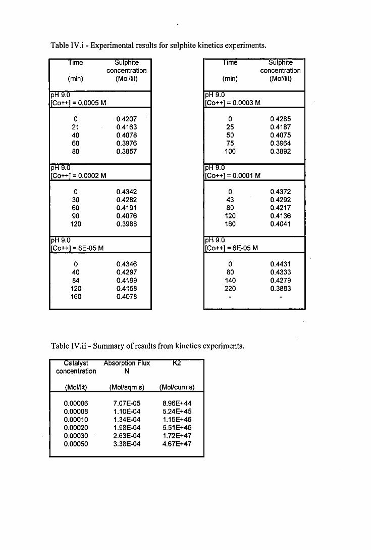
Table IV.i - Experimental results for sulphite kinetics experiments.
lime ::;ulpmte lime ::;ulphite concentration concentration
(min) (Mol/lit) (min) (Mol/lit)
pH 9.u. pH 9.0 [Co++] = 0.0005 M [Co++] = 0.0003 M
0 0.4207 0 0.4285 21 0.4163 25 0.4187 40 0.4078 50 0.4075 60 0.3976 75 0.3964 80 0.3857 100 0.3892
pH 9.0 pH 9.0 [Co++] = 0.0002 M [Co++] = 0.0001 M
0 0.4342 0 0.4372 30 0.4282 43 0.4292 60 0.4191 80 0.4217 90 0.4076 120 0.4136 120 0.3988 160 0.4041
pH 9.0 pH 9.U [Co++] = 8E-05 M [Co++] = 6E-05 M
0 0.4346 0 0.4431 40 0.4297 80 0.4333 84 0.4199 140 0.4279 120 0.4158 220 0.3883 160 0.4078 - -
Table IV.ii - Summary of results from kinetics experiments.
(.;atalyst Absorption I-Iux KZ concentration N
(Mol/lit) (Mol/sqm s) (Mol/cum s)
0.00006 7.07E-05 8.96E+44 0.00008 1.10E-04 5.24E+45 0.00010 1.34E-04 1.15E+46 0.00020 1.98E-04 5.51E+46 0.00030 2.63E-04 1.72E+47 0.00050 3.38E-04 4.67E+47
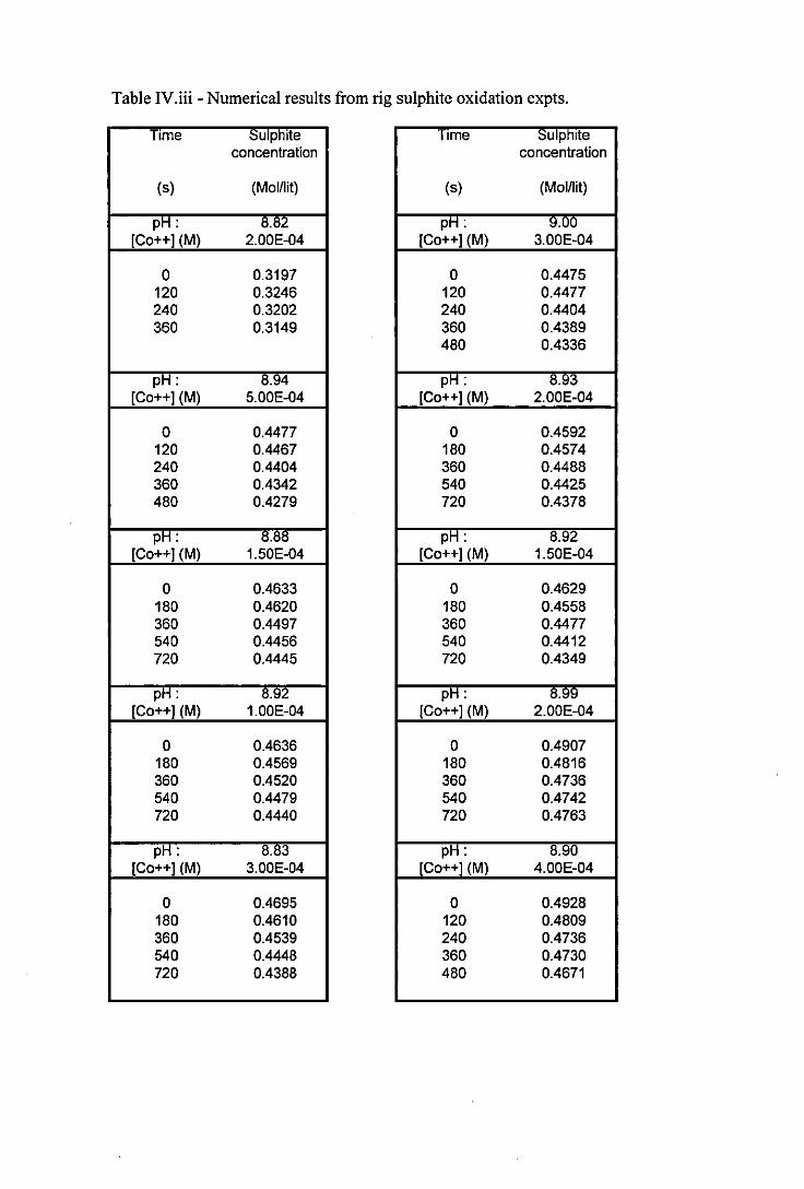
Table IV.iii - Numerical results from rig sulphite oxidation expts.
lime ::;ulpnlte lime ::;ulpnlte concentration concentration
(s) (Mol/lit) (s) (Mol/lit)
pH: 8.82 pH: 9.00 [Co++] (M) 2.00E-04 [Co++] (M) 3.00E-04
0 0.3197 0 0.4475 120 0.3246 120 0.4477 240 0.3202 240 0.4404 360 0.3149 360 0.4389
480 0.4336
PH: 8.94 PH: 8.1;13 [Co++] (M) 5.00E-04 [Co++] (M) 2.00E-04
0 0.4477 0 0.4592 120 0.4467 180 0.4574 240 0.4404 360 0.4488 360 0.4342 540 0.4425 480 0.4279 720 0.4378
PH: IUltl pH: 8.92 [Co++] (M) 1.50E-04 [Co++] (M) 1.50E-04
0 0.4633 0 0.4629 180 0.4620 180 0.4558 360 0.4497 360 0.4477 540 0.4456 540 0.4412 720 0.4445 720 0.4349
PH: 8.92 pH: 8.99 [Co++] (M) 1.00E-04 [Co++] (M) 2.00E-04
0 0.4636 0 0.4907 180 0.4569 180 0.4816 360 0.4520 360 0.4736 540 0.4479 540 0.4742 720 0.4440 720 0.4763
pH: 8.83 pH: 8.90 [Co++] (M) 3.00E-04 [Co++] (M) 4.00E-04
0 0.4695 0 0.4928 180 0.4610 120 0.4809 360 0.4539 240 0.4736 540 0.4448 360 0.4730 720 0.4388 480 0.4671
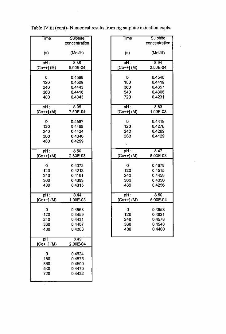
Table IV.iii (cont)- Numerical results from rig sulphite oxidation expts.
lime ::;ulphite Time Sulphite concentration concentration
(5) (Mol/lit) (5) (Mol/lit)
pH: B.B8 pH: 8.94 [Co++] (M) 5.00E-04 [Co++] (M) 2.00E-04
0 0.4588 0 0.4546 120 0.4509 180 0.4419 240 0.4443 360 0.4357 360 0.4416 540 0.4308 480 0.4343 720 0.4231
pH: B.95 pH: 8.83 [Co++] (M) 7.50E-04 [Co++](M) 1.00E-03
0 0.4587 0 0.4418 120 0.4469 120 0.4276 240 0.4424 240 0.4209 360 0.4340 360 0.4129 480 0.4259
pH: 8.50 pH: 8.47 [Co++] (M) 2.50E-03 [Co++] (M) 5.00E-03
0 0.4373 0 0.4678 120 0.4213 120 0.4515 240 0.4161 240 0.4458 360 0.4093 360 0.4350 480 0.4015 480 0.4256
pH: 8.44 pH: 8.50 [Co++](M) 1.00E-03 [Co++] (M) 5.00E-04
0 0.4568 0 0.4658 120 0.4459 120 0.4621 240 0.4431 240 0.4578 360 0.4407 360 0.4548 480 0.4283 480 0.4480
pH: B.49 [Co++] (M) 2.00E-04
0 0.4624 180 0.4575 360 0.4509 540 0.4470 720 0.4432

Table IV.iv - Numerical results from C02 desorption experiments.
25mm t:ntralner, U.U1<! Kg/S liqUid I-IOW I K(IJ~ results Column Temperatures C02 concentrations Plug Well Recycle Equivalent
Gas Flow Gas velocity Air inlet Air outlet Liquid inlet liquid outlet Liquid inlet Liquid outlet flow mixed transfer units (kg/s) (m/s) (C) (C) (C) (C) (MoI/L) (MoIIL) (1/s) (1/5) (1/s)
0.0092 3.9 15.5 16.3 15.6 15.5 0.0266 0.00280 0.0385 0.147 0.095 2.26 0.0120 5.1 15.7 17.9 15.9 16.1 0.0284 0.00302 0.0382 0.145 0.094 2.24 0.0168 7.1 15.4 16.3 15.9 15.7 0.0298 0.00197 0.0464 0.244 0.128 2.72 0.0216 9.2 14.8 16.9 16.8 16.0 0.0270 0.00130 0.0520 0.346 0.150 3.05 0.0265 11.2 15.5 17.3 15.8 16.1 0.0284 0.00098 0.0577 0.491 0.162 3.38 0.0320 13.6 16.3 17.5 17.2 16.5 0.0307 0.00057 0.0685 0.944 0.183 4.01
25mm Entralner, 0.015 kgls Liquid Flow I 1\(I)a resUlts (.;olumn I emperatures (';U<! concentrations Plug Well Recycle t:qUlvalent
Gas Flow Gas velocity Air inlet Air outlet Liquid inlet liquid outlet Liquid inlet Liquid outlet flow mixed transfer units (kg/s) (mls) (C) (C) (C) (C) (MoIIL) (MoIIL) (1/s) (1/s) (1/s)
0.0092 3.9 15.4 16.2 16.3 16.2 0.0290 0.0049 0.0388 0.1078 0.0856 1.7731 0.0120 5.1 16.0 16.8 16.2 16.1 0.0280 0.0044 0.0407 0.1195 0.0908 1.8607 0.0168 7.1 15.1 16.9 15.5 15.0 0.0316 0.0034 0.0487 0.1818 0.1195 2.2249 0.0216 9.2 15.5 17.0 16.4 15.9 0.0293 0.0023 0.0557 0.2583 0.1424 2.5428 0.0265 11.2 15.6 16.6 16.1 15.5 0.0311 0.0017 0.0638 0.3839 0.1470 2.9111 0.0320 13.6 15.3 16.7 16.3 15.5 0.0289 0.0011 0.0721 0.5710 0.1994 3.2874
Table IV.iv (cont)- Numerical results from C02 desorption experiments.
125mm Entralner, U.UL Kg/S LlqUlO t'IOW I "-(I)~ results l,;Olumn I emperatures C02 concentrations Plug Well Recycle ~qUlvalent
Gas Flow Gas velocity Air inlet Air outlet Liquid inlet liquid outlet Liquid inlet Liquid outlet flow mixed transfer units (kg/s) (m/s) (C) (C) (C) (C) (Mol/L) (Mol/L) (1/5) (1/5) (1/5)
0.0092 3.9 15.9 16.1 15.3 15.4 0.0305 0.0065 0.0453 0.1093 0.0910 1.55 0.0120 5.1 15.6 16.8 15.8 15.6 0.0316 0.0066 0.0455 0.1103 0.0900 1.56 0.0168 7.1 15.5 17.1 15.6 15.7 0.0293 0.0049 0.0520 0.1450 0.1092 1.78 0.0216 9.2 16.2 17.2 16.9 16.6 0.0300 0.0034 0.0641 0.2344 0.1483 2.20 0.0265 11.2 15.5 16.3 17.0 16.1 0.0307 0.0025 0.0737 0.3376 0.1582 2.52 0.0320 13.6 15.8 18.1 17.2 16.6 0.0264 0.0014 0.0854 0.5185 0.2205 2.92
IL5mm t:ntralner, U.O:ltl Kg/s LlqUlO t'IOW I "-(Ila results Column Temperatures C02 concentrations Plug Well Recycle EqUivalent
Gas Flow Gas velocity Air inlet Air outlet Liquid inlet liquid outlet Liquid inlet Liquid outlet flow mixed transfer units (kg/s) (m/s) (C) (C) (C) (C) (Mol/L) (MoIIL) (1/5) (1/s) (1/s)
0.0092 3.9 15.0 15.8 14.3 14.5 0.0325 0.0098 0.0495 0.0961 0.0851 1.20 0.0120 5.1 15.3 16.8 15.5 15.6 0.0307 0.0081 0.0550 0.1156 0.0988 1.33 0.0168 7.1 14.9 16.5 13.9 14.1 0.0325 0.0074 0.0610 0.1399 0.1138 1.47 0.0216 9.2 15.2 16.1 13.6 14.1 0.0309 0.0060 0.0681 0.1740 0.1315 1.65 0.0265 11.2 15.3 16.6 15.6 15.4 0.0307 0.0042 0.0826 0.2650 0.1577 2.00 0.0320 13.6 15.3 17.4 15.6 15.3 0.0309 0.0025 0.1048 0.4830 0.2483 2.53
Table IV.iv (cont)- Numerical results from C02 desorption experiments.
L5mm t:ntralner, u.O;J7 Kg/S LlqUlQ !-IOW I K(I)a results (;OIUmn I emperatures (;02 concentrations Plug Well . Recycle t:qulvalent
Gas Flow Gas velocity Air inlet Air outlet Liquid inlet liquid outlet Liquid inlet Liquid outlet flow mixed transfer units (kg/s) (m/s) (C) (C) (C) (C) (Mol/L) (Mol/L) (1/s) (1/s) (1/5)
0.0168 7.1 - - - - 0.0318 0.0085 0.0706 0.1472 0.1237 1.3185 0.0216 9.2 - - - - 0.0339 0.0076 0.0803 0.1871 0.1470 1.4998 0.0265 11.2 - - - - 0.0311 0.0054 0.0939 0.2572 0.1684 1.7545 0.0320 13.6 - - - - 0.0334 0.0037 0.1179 0.4335 0.2569 2.2010
20mm Entralner, 0.015 kg/s Liquid Flow I K(I)a results \,;olumn I emperatures (;UL concentrations Plug Well Recycle t:qUlvalent
Gas Flow Gas velocity Air inlet Air outlet Liquid inlet liq u id outlet Liquid inlet Liquid outlet flow mixed transfer units (kg/s) (m/s) (C) (C) (C) (C) (MoIIL) (MoIIL) (1/s) (1/s) (1/s)
·0.0092 3.9 16.1 16.1 16.2 16.3 0.0311 0.0049 0.0404 0.1172 - 1.84 0.0120 5.1 16.2 16.3 16.3 16.3 0.0293 0.0045 0.0411 0.1218 - 1.88 0.0152 6.5 15.3 14.4 13.5 14.1 0.0316 0.0035 0.0481 0.1763 - 2.20 0.0184 7.8 15.1 14.9 15.1 16.0 0.0320 0.0027 0.0546 0.2452 - 2.49 0.0216 9.2 14.7 14.3 14.3 14.3 0.0325 0.0017 0.0645 0.3979 - 2.94

Table IV.iv (cont)- Numerical results from C02 desorption experiments.
20mm Entralner, 0.028 Kg/S LlqUlO rlOW I "'(I J? resUlts Column I emperatures CV" concentrations Plug Well Recycle ~qUlvalent
Gas Flow Gas velocity Air inlet Air outlet Liquid inlet liquid outlet Liquid inlet Liquid outlet flow mixed transfer units (kg/s) (m/s) (C) (C) (C) (C) (MoI/L) (MoI/L) (1/s) (1/s) (1/s)
0.0092 3.9 15.5 13.8 13.1 13.4 0.0341 0.0103 0.0496 0.0964 - 1.20 0.0120 5.1 15.9 15.4 15.1 15.1 0.0320 0.0087 0.0540 0.1118 - 1.31 0.0152 6.5 15.7 15.1 15.0 15.3 0.0325 0.0069 0.0643 0.1553 - 1.55 0.0184 7.8 15.4 15.2 15.1 15.1 0.0298 0.0052 0.0725 0.1985 - 1.75 0.0216 9.2 16.0 16.4 17.2 16.7 0.0302 0.0032 0.0926 0.3490 - 2.24
115mrn Entralner, 0.015 Kg/S LlqUlO rlOW I "'(I)a resUlts Column I emperatures cv2 concentrations Plug Well Recycle ~qUlvalent
Gas Flow Gas velocity Air inlet Air outlet Liquid inlet liquid outlet Liquid inlet Liquid outlet flow mixed transfer units (kg/s) (rnls) (C) (C) (C) (C) (MoI/L) (MoI/L) (1/s) (1/s) (1/s)
0.0066 2.8 15.6 14.5 13.5 14.1 0.0352 0.0056 0.0403 0.1167 - 1.84 0.0092 3.9 15.9 14.0 13.2 13.7 0.0343 0.0051 0.0420 0.1281 - 1.92 0.0120 5.1 14.5 14.0 13.4 13.5 0.0357 0.0036 0.0503 0.1971 - 2.29 0.0152 6.5 15.5 14.9 14.7 14.8 0.0313 0.0020 0.0601 0.3219 - 2.74
Table IV.iv (cont)- Numerical results from C02 desorption experiments.
15mm Entralner, 0.028 kg/s Liquid Flow I K(I)a resUlts t;olumn I emperatures t;Ul concentrations Plug Well Recycle EqUivalent
Gas Flow Gas velocity Air inlet Air outlet Liquid inlet liquid outlet Liquid inlet Liquid outlet flow mixed transfer units (kg/s) (mls) (C) (C) (C) (C) (MoI/L) (MoI/L) (1/5) (1/5) (1/5)
0.0066 2.8 14.9 15.2 14.5 14.7 0.0311 0.0091 0.0511 0.1014 - 1.23 0.0092 3.9 15.5 16.3 14.6 14.8 0.0332 0.0082 0.0578 0.1265 - 1.39 0.0120 5.1 14.5 13.7 13.2 13.4 0.0357 0.0065 0.0704 0.1867 - 1.70 0.0152 6.5 14.7 13.7 13.0 13.3 0.0352 0.0043 0.0874 0.3028 - 2.11
Appendix V.
Details of pressure drop correlation results.

Appendix v.
Numerical constants for pressure drop correlations.
Entrainer dry pressure drop correlation.
Units:
Units:
urUBE
15mm Entrainer
20mm Entrainer
25 mm Entrainer
mmWG -I ms .
mmWG
urUBE m s-1
d m.
All entrainer sizes
Constantk
0.0819
0.0710
0.0465
Constant k'
0.00127
(V.i)
(V.ii)
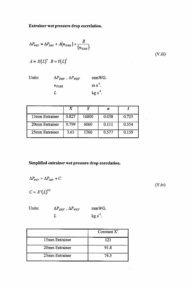
Entrainer wet pressure drop correlation.
B M'WET = M'DRY + A( UTUBE ) + ( )
U1VBE
(V.iii)
A = X(L)" B = Y(L)'
Units: mmWG.
L
x Y n I
15mm Entrainer 0.827 16800 0.058 0.725
20mm Entrainer 0.799 6060 0.111 0.554
25mm Entrainer 3.63 1260 0.577 0.159
Simplified entrain er wet pressure drop correlation.
(V.iv)
c= X'(Lt2
Units:
L
Constant X'
15mm Entrainer 121
20mm Entrainer 91.8
25mm Entrainer 74.5
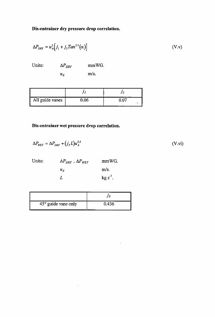
Dis-entrainer dry pressure drop correlation.
Units: mmWO.
All guide vanes 0.06 0.07
Dis-entrainer wet pressure drop correlation.
Units:
L
45° guide vane only
mmWO.
mls.
kg S-I.
0.436
(V.v)
(V.vi)