Embed Size (px)
Citation preview

DEVELOPMENT OF A 3 AXES PC NUMERICAL CONTROL SYSTEM FOR
INDUSTRIAL APPLICATIONS
A THESIS SUBMITTED TO
THE GRADUATE SCHOOL OF NATURAL AND APPLIED SCIENCES
OF
THE MIDDLE EAST TECHNICAL UNIVERSITY
BY
FEZA BAŞAR
IN PARTIAL FULFILMENT OF THE REQUIREMENTS FOR THE DEGREE OF
MASTER OF SCIENCE
IN
THE DEPARTMENT OF ELECTRICAL AND ELECTRONICS ENGINEERING
SEPTEMBER 2003

ii
Approval of the Graduate School of Natural and Applied Sciences
Prof. Dr. Canan Özgen
Director
I certify that this thesis satisfies all the requirements as a thesis for the degree of
Master of Science.
Prof. Dr. Mübeccel Demirekler
Head of Department
This is to certify that we have read this thesis and that in our opinion it is fully
adequate, in scope and quality, as a thesis for the degree of Master of Science.
Prof. Dr. Mirzahan Hızal
Supervisor
Examining Committee Members
Prof. Dr. Ahmet Rumeli
Prof. Dr. Muammer Ermiş
Prof. Dr. Mirzahan Hızal
Prof. Dr. Nevzat Özay
M.Sc. Abdullah Nadar

iii
ABSTRACT
DEVELOPMENT OF A 3 AXES PC NUMERICAL CONTROL SYSTEM FOR
INDUSTRIAL APPLICATIONS
BAŞAR, Feza
M.Sc. , Department of Electrical and Electronics Engineering
Supervisor: Prof. Dr. Mirzahan Hızal
September 2003, 96 Pages
In this study, a three-axes PC numerical control system for industrial
applications has been developed. With this system, fast and cheap prototyping of
designed objects can be realized. The system consists of software and a hardware
which includes an XYZ positioning table and three step motors controlling this table.
A proper drive circuit for the stepper motors is utilized. The software digitizes two
dimensional drawings of three dimensional objects and generates the control signals
for the XYZ positioning table.
The software is developed under Microsoft Studio Visual Basic 6.0
environment regardless of the OS of the PC. The parallel port of the PC has been
utilized for generating the necessary control signals for the stepper motors.
Keywords: Machine Tool, Step Motor, Motion Control, Parallel Port
Programming, Step Motor Drive

iv
ÖZ
ENDÜSTRİYEL AMAÇLI 3 EKSENLİ BİR BİLGİSAYAR SAYISAL KONTROL
SİSTEMİNİN GELİŞTİRİLMESİ
BAŞAR, Feza
Yüksek Lisans , Elektrik-Elektronik Mühendisliği Bölümü
Tez Yöneticisi: Prof. Dr. Mirzahan Hızal
Eylül 2003, 96 sayfa
Bu çalışmada endüstriyel amaçlı üç eksenli bir bilgisayar sayısal kontrol
sistemi geliştirilmiştir. Bu sistemle tasarlanan objelerin hızlı ve ucuz prototipleri
gerçekleştirilebilir. Sistem bir yazılım ve XYZ ekseninde hareket eden tezgahtan ve
bu tezgahı kontrol eden üç adet adımlı motordan oluşmaktadır. Adımlı motorlar için
uygun bir sürücü devresi kullanılmıştır. Yazılım ise iki boyutlu olarak modellenen üç
boyutlu nesneleri sayısallaştırıp tezgah için gerekli kontrol işaretlerini üretmektedir.
Yazılım bilgisayarın işletim sisteminden bağımsız olarak Microsoft Studio
Visual Basic 6.0 ortamında geliştirilmiştir. Adımlı motorların gerekli kontrol
işaretleri bilgisayarın paralel kanalının kullanılması ile oluşturulmaktadır.
Anahtar Kelimeler: Tezgah, Adımlı Motor, Hareket Kontrol, Paralel Kanal
Programlama, Adımlı Motor Sürücüsü

v
to my beloved husband Çağrı,

vi
ACKNOWLEDGEMENTS
I would like to express my sincere appreciation to Prof. Dr. Mirzahan Hızal
for his encouragements, guidance and supervision.
Special thanks to my pet Pisigül for her great interest in my papers.
Finally, I would like to thank my beloved husband Çağrı for his precious
help, great support and understanding. I believe without him this thesis would not
have been completed.

vii
TABLE OF CONTENTS
ABSTRACT............................................................................................................iii
ÖZ ........................................................................................................................... iv
ACKNOWLEDGEMENTS .................................................................................... vi
TABLE OF CONTENTS.......................................................................................vii
LIST OF TABLES ................................................................................................... x
LIST OF FIGURES ................................................................................................ xi
LIST OF ABBREVIATIONS............................................................................... xiv
CHAPTER
1. INTRODUCTION............................................................................................... 1
2. STEPPING MOTORS ........................................................................................ 4
2.1 Stepping Motor Types.............................................................................. 6
2.1.1 Permanent Magnet Motors............................................................... 6
2.1.2 Variable Reluctance Motors............................................................. 7
2.1.3 Hybrid Motors.................................................................................. 7
2.1.4 Comparison of Motor Types ............................................................ 8
2.2 Stepping Motor Winding Types............................................................... 9
2.2.1 Unifilar Winding .............................................................................. 9
2.2.2 Bifilar Winding ................................................................................ 9
2.3 Stepping Modes...................................................................................... 10
2.4 Drive Circuits ......................................................................................... 11
2.5 Static Torque Characteristics ................................................................. 13
2.6 Torque-Speed Characteristics ................................................................ 17
2.7 Step Motor Control ................................................................................ 19
2.7.1 Open-Loop Control ........................................................................ 20
2.7.2 Closed-Loop Control...................................................................... 21
3. HARDWARE AND SOFTWARE SOLUTIONS ............................................ 23

viii
3.1 Hardware ................................................................................................ 23
3.1.1 Digital I/O ...................................................................................... 24
3.1.1.1 Requirements for Digital I/O ..................................................... 24
3.1.1.2 Parallel Port of PC...................................................................... 24
3.1.2 Stepper Motor Driver Circuit ......................................................... 27
3.1.3 Stepper Motors ............................................................................... 30
3.1.4 Drilling Material and Cutting Tools............................................... 30
3.2 Software ................................................................................................. 31
3.2.1 GUI Based Programming Languages............................................. 32
3.2.2 Step Motor Control Software ......................................................... 33
3.2.3 Parallel Port Control Software ....................................................... 34
3.2.4 Image Processing Software ............................................................ 35
3.2.4.1 Definitions of Connectivity and Contour Tracing ..................... 35
3.2.4.2 Pseudo Code of Contour Tracing............................................... 37
4. SOFTWARE DESCRIPTION .......................................................................... 38
4.1 Software Requirements Specifications .................................................. 38
4.1.1 Image Requirements and Limitations ............................................ 40
4.2 Software Modules .................................................................................. 43
4.2.1 “Start Up” Module ......................................................................... 44
4.2.2 “User Information Interface” Module............................................ 45
4.2.3 “Drill Options” Module ................................................................. 46
4.1.1.1 Calculation of the Prototype Dimensions .................................. 47
4.1.2 “Go To Information” Module ........................................................ 48
4.1.3 “Profile Selection” Module ............................................................ 49
4.1.4 “Main” Module .............................................................................. 50
4.1.4.1 Loading the Object..................................................................... 51
4.1.4.2 Digitizing Two Dimensional Object .......................................... 52
4.1.4.3 Digitizing Three Dimensional Object ........................................ 54
4.1.4.4 Saving / Loading the Digitized Object....................................... 55
4.1.4.5 Drilling the Object ..................................................................... 56
4.1.5 “About” Module............................................................................. 59
5. RESULTS ......................................................................................................... 61

ix
5.1 Image Processing Performance .............................................................. 61
5.2 Drilling Performance.............................................................................. 62
5.3 Drilled Samples...................................................................................... 64
6. CONCLUSIONS............................................................................................... 68
REFERENCES....................................................................................................... 71
APPENDIX
A Modules and Critical Variables of the Software……………………………. 73
B Parameters/Selections in the Software……………………………………… 75
C Motor Drive Circuit Components…………………………………………... 77
C.1 L298 Dual Full-Bridge Driver…………………………………………... 77
C.2 L297 Stepper Motor Controller…………………………………………. 78
C.3 Two Phase Bipolar motor Control Circuit with L297 and L298………... 80
D Declarations and Relations of Functions and Subs of the Software ……...... 81
D.1 “Main” Form..……………………………………................................... 81
D.2 “GoTo” Form..…………………………………...................................... 89
D.3 “Information” Form..…………………………….................................... 91
D.4 “Options” Form..…………………………………................................... 91
D.5 “Profile” Form……………………………………................................... 92
D.6 “Start Options” Form..…………………………...................................... 93
D.7 “Main” Module..…………………………………................................... 94

x
LIST OF TABLES
3.1 Parallel Port Address Table................................................................................. 24
3.2 Cable connection of X-Y axis card ..................................................................... 29
3.3 Cable connection of Z axis card.......................................................................... 30
3.4 Cable connection of cards and supply................................................................. 30
3.5 A rough estimation of average number of LOC required for building one
complexity unit in various programming languages. .......................................... 33
5.1 Comparison of the drilling process time with respect to selected options.......... 63
B.1 Parameters/Selections in “Start Up Options”……………….............................. 75
B.2 Parameters/Selections in “Drilling Options”………………............................... 75
B.3 Parameters/Selections in “Go To Coordinates”…..…………........................... 76
B.4 Parameters/Selections in “Main”…….……………………….......................... 76
C.1 Absolute maximum ratings of L297 ..………………………........................... 78
C.2 Absolute maximum ratings of L298 ...………………………........................... 79

xi
LIST OF FIGURES
1.1 An object that cannot be represented by only one two-dimensional view.......... 2
2.1 Permanent Magnet Motor ................................................................................... 6
2.2 Variable Reluctance Motor ................................................................................. 7
2.3 Hybrid Motor ...................................................................................................... 8
2.4 4-Lead Unifilar Motor......................................................................................... 9
2.5 6 and 8-Lead Bifilar Motors.............................................................................. 10
2.6 Drive circuit scheme ......................................................................................... 11
2.7 One phase of a transistor bridge bipolar drive circuit ....................................... 12
2.8 Three phase unipolar drive circuit..................................................................... 13
2.9 Static torque/rotor position characteristics at various currents ......................... 14
2.10 Static torque/rotor position characteristics at rated phase currents................... 15
2.11 Static torque/rotor position characteristics for a variable reluctance stepping
motor (a) one-phase-on excitation (b) two-phases-on excitation ..................... 17
2.12 A typical torque-speed characteristics of a stepping motor .............................. 18
2.13 Simplified step motor control system ............................................................... 20
2.14 A typical microprocessor-based open-loop control .......................................... 21
2.15 Block diagram of a closed-loop control of a stepping motor............................ 22
3.1 Block diagram of the parallel interface............................................................. 26
3.2 Parallel Port I/O Scheme................................................................................... 27
3.3 (X-Y) Axis Drive Circuit .................................................................................. 28
3.4 Z Axis Drive Circuit ......................................................................................... 29
3.5 Software Modules Data Flow Diagram ............................................................ 32
3.6 Flow Chart of the Step Motor Control Software............................................... 34
3.7 I/O ActiveX Communications Software Message Box .................................... 35

xii
3.8 Neighbors of a pixel p in a square tessellation.................................................. 36
3.9 Examples of (a) 4-connectivity (b) 8-connectivity .......................................... 36
3.10 The tracking sequence of neighbors for 4-connectivity.................................... 37
4.1 A typical drawing for a two dimensional object ............................................... 40
4.2 The requirements and limitations concerned with the peripherals.................... 41
4.3 The requirements and limitations concerned with the number of neighbors of a
point .................................................................................................................. 41
4.4 A typical drawing for a three dimensional object ............................................. 42
4.5 A typical drawing for a profile.......................................................................... 43
4.6 Software Data Flow Diagram ........................................................................... 44
4.7 Start Up Module User Interface ........................................................................ 45
4.8 User Information Interface................................................................................ 46
4.9 Drill Options Interface ...................................................................................... 47
4.10 Go To Information Interface ............................................................................. 48
4.11 Profile Selection Interface................................................................................. 49
4.12 Main module of the drilling program................................................................ 51
4.13 The neighborhood scanning order for a point for digitizing a two dimensional
object. ............................................................................................................... 53
4.14 Digitizing and drilling path for a non closed curve with “Digitize Min
Distance” and “Digitize Top”........................................................................... 54
4.15 The neighborhood scanning order for a point for digitizing a three dimensional
object. ............................................................................................................... 55
4.16 Digitizing process of a three dimensional object .............................................. 55
4.17 Digitizing with two-dimensional method examples ......................................... 57
4.18 Digitizing with three-dimensional method example ......................................... 58
4.19 Consecutive and simultaneous movement paths for X and Y motors .............. 59
4.20 About module of the drilling program .............................................................. 60
5.1 Top drawing of an ellipse as a two-dimensional object.................................... 62
5.2 A sample of a drilled object by 2D modelling .................................................. 64
5.3 A gear realized by 2D modelling ...................................................................... 65
5.4 A pyramid realized by 3D modelling................................................................ 65
5.5 A dome realized by 3D modelling .................................................................... 66

xiii
5.6 A heart realized by 3D modelling ..................................................................... 66
5.7 A stamp realized by 2D modelling ................................................................... 67
5.8 An application of labelling by 2D modelling.................................................... 67
C.1 Block Diagram of L298 ……………………............................................... 77
C.2 Block Diagram of L297 ……………………............................................... 79
C.3 Two Phase Bipolar Stepper Motor Control Circuit with L297 and L298…. 80

xiv
LIST OF ABBREVIATIONS
BMP : Bit Map
CAD : Computer Aided Design
DC : Direct Current
I/O : Input/Output
JPG : Joint Photographers Experts Group
OS : Operating System
LOC : Lines of Code
PC : Personal Computer
IC : Integrated Circuit
GUI : Graphical User Interface
TIFF : Tagged Image File Format
1
CHAPTER 1
INTRODUCTION
The efficiency of the industrial applications has increased enormously with
the introduction of the computers to the processes. Computers have started to take
place in every single point in the industry enhancing the development and
manufacturing stages. One of the important areas of interest in the application of
computers is the “Computer Aided Design” (CAD) followed by implementation and
production stages.
CAD can be efficiently used for prototyping issues in industrial applications.
A proper prototyping machine tool with specially designed CAD program will
decrease the time for design and implementation of prototypes.
The three-dimensional objects can be represented in the CAD applications by
various methods. One method is to show a three dimensional object represented by
three views which are drawn from “Front”, “Left” and “Top” [1]. The advantage of
this method is that no information on the object is ambiguous so that the object is
totally represented by the drawing, but this method requires intensive care while
drawing the object and requires specially trained technicians.
Another method for representing the three dimensional objects is using two
dimensional models where only the top view is sufficient. In this method, the depth
information is kept in an algorithm or a color pattern. It is obvious that, an object as

2
shown in Figure 1.1 cannot be represented by this method. But the advantage of this
method is ease of generating the views and the digital image of the object.
Figure 1.1 An object that cannot be represented by only one two-dimensional
view
In the industry, various motion control tools are used widely but among these,
step motors are one of the easiest to be applied and cheapest to be purchased. The
simple drive circuits can easily be controlled via digital signals which enable full
control over a regular PC. By the application of these motors, an XYZ positioning
system can easily be constructed and furthermore this machine tool will be easily
controlled via a PC.
In this study, a CAD program has been developed to recognize objects from
standard image files (BMP, JPG, TIFF, etc.) that contain only top view. This method
accelerates the digitizing process of the objects with respect to the modeling with
three views.
The program generates the necessary control signals for a specially designed
three-axes positioning table that is controlled by three step motors. The step motors’
movements are based on the digitizing process i.e. the motors follow the path that is

3
specified by the digitizing process resulting in fast response of the system. The
motors never move on points that will never be drilled. Furthermore, all points
having the same depth level are drilled consequently which lead to smooth shape of
the drilled object as well as saving time.
The software has been developed under Microsoft Studio Visual Basic 6.0
environment. This tool has been chosen because of its superior properties and ease of
programming. The system requires no extra hardware except the three axes XYZ
positioning table and so the cost of the system is decreased. The parallel port of the
PC has been utilized for sending the necessary control signals for the stepper motors.
An ActiveX based special interface software for the parallel port is used to free the
software of the OS of the PC.
The organization of the thesis is as follows:
In Chapter 2, general properties, types, operation principles, modes, driver
circuits, characteristics and control types of step motors are given. The
advantages of using step motors are discussed.
In Chapter 3, the hardware and software solutions are introduced and GUI
based programming languages and definitions about image processing are
discussed.
In Chapter 4, the image requirements specifications are given. The software
modules and their tasks are explained and analyzed in detail.
In Chapter 5, the image processing and drilling performances are analyzed
and the drilled samples are given.
In Chapter 6, the final conclusions on this study are made and the further
work on this area is proposed.

4
CHAPTER 2
STEPPING MOTORS
A stepping motor is a permanent magnet or variable reluctance dc motor that
has the following performance characteristics:
• rotation in both directions,
• precision angular incremental changes,
• repetition of accurate motion or velocity profiles,
• a holding torque at zero speed, and
• capability for digital control.
It is an electromechanical device which converts electrical pulses into discrete
mechanical movements. Basically, it is a synchronous motor with the magnetic field
electronically switched to rotate the armature magnet around. The shaft or spindle of
a stepper motor rotates in discrete step increments when electrical command pulses
are applied to it in the proper sequence.
The number and rate of the pulses control the position and speed of the motor
shaft. The motor rotation has several direct relationships to these applied input
pulses. The sequence of the applied pulses is directly related to the direction of motor
shafts rotation. The speed of the motor shaft’s rotation is directly related to the
frequency of the input pulses and the length of rotation is directly related to the
number of input pulses applied. Generally, stepping motors are manufactured with

5
steps per revolution of 12, 24, 72, 144, 180, and 200, resulting in shaft increments of
30, 15, 5, 2.5, 2, and 1.8 degrees per step.
Theoretically, a stepping motor is a marvel in simplicity. They are very
reliable at low cost, since there are no brushes or contacts in the motor. Therefore the
life of the motor is simply dependent on the life of the bearing. The rotation angle of
the motor is proportional to the input pulse and the motor has full torque at standstill
if the windings are energized.
Stepping motors have precise positioning and repeatability of movement
since good stepper motors have an accuracy of 3 – 5% of a step and this error is non
cumulative from one step to the next. They give excellent responses to
starting/stopping/reversing actions and it is possible to achieve very low speed
synchronous rotation with a load that is directly coupled to the shaft. Also, there is a
wide range of rotational speeds that can be realized as the speed is proportional to the
frequency of the input pulses. Besides all these advantages, resonances that can occur
and the difficulty of operation at high speeds are the disadvantages of using a
stepping motor.
Stepping motors are either bipolar, requiring two power sources or a
switchable polarity power source, or unipolar, requiring only one power source. They
are powered by DC current sources and require digital circuitry to produce the coil
energizing sequences for rotation of the motor. Feedback is not always required for
control, but the use of an encoder or other position sensors can ensure accuracy when
it is essential. Generally, stepping motors produce less than one horsepower (746W)
and therefore they are frequently used in low-power position control applications. A
stepper motor can be a good choice whenever controlled movement is required. They
can be used to advantage in applications where you need to control rotation angle,
speed, position and synchronism.

6
2.1 Stepping Motor Types
There are basically two types of motors as permanent magnet and variable
reluctance stepping motors and the hybrid type of these two basic ones. They differ
in terms of construction based on the use of permanent magnets and/or iron rotors
with laminated steel stators. The type of the motor determines the type of the circuit
driver and the type of the translator to be used.
2.1.1 Permanent Magnet Motors
The permanent magnet motor has, as the name implies, a permanent magnet
rotor. It is a relatively low speed, low torque device with large step angles of either
45 or 90 degrees. Its simple construction and low cost make it an ideal choice for non
industrial applications.
Figure 2.1 Permanent Magnet Motor
Unlike the other stepping motors, the permanent magnet motor’s rotor has no
teeth and is designed to be magnetized at a right angle to its axis. The permanent
magnet motor shown in Figure 2.1 is a simple, 90 degree permanent magnet motor
with four phases (A-D). Applying current to each phase in sequence will cause the
rotor to rotate by adjusting to the changing magnetic fields. Although it operates at
fairly low speed the permanent magnet motor has a relatively high torque
characteristic.

7
2.1.2 Variable Reluctance Motors
The variable reluctance motor does not use a permanent magnet. As a result,
the motor rotor can move without constraint or “detent” torque. This type of
construction is good in non industrial applications that do not require a high degree
of motor torque, such as the positioning of a micro slide .
Figure 2.2 Variable Reluctance Motor
The variable reluctance motor in Figure 2.2 has four "stator pole sets" (A, B,
C,), set 15 degrees apart. Current applied to pole A through the motor winding causes
a magnetic attraction that aligns the rotor (tooth) to pole A. Energizing stator pole B
causes the rotor to rotate 15 degrees in alignment with pole B. This process will
continue with pole C and back to A in a clockwise direction. Reversing the procedure
(C to A) would result in a counterclockwise rotation.
2.1.3 Hybrid Motors
Hybrid motors combine the best characteristics of the variable reluctance and
permanent magnet motors. They are constructed with multi-toothed stator poles and
a permanent magnet rotor. Standard hybrid motors have two hundred rotor teeth and
rotate at 1.80 step angles. Other hybrid motors are available in 0.9 and 3.6 degrees
step angle configurations. As they exhibit high static and dynamic torque and run at

8
very high step rates, hybrid motors are used in a wide variety of industrial
applications.
Figure 2.3 Hybrid Motor
2.1.4 Comparison of Motor Types
Variable-reluctance motors have two important advantages when the load
must be moved a considerable distance. Firstly, typical step lengths are longer than in
the hybrid type so less steps are required to move a given distance. A further
advantage is that it has a lower rotor mechanical inertia than the hybrid and
permanent-magnet types, as there is no permanent-magnet on its rotor.
Hybrid motors have a small step length which can be a great advantage when
high resolution angular positioning is required. The torque producing capability for a
given motor volume is greater in the hybrid than in the variable-reluctance motor.
Therefore, a hybrid motor is obviously a better choice, compared with the variable
reluctance one, for applications requiring a small step length and high torque in a
restricted working space. When the winding of the hybrid motor are unexcited the
magnet flux produces a small detent torque which retains the motor at the step
position. Although the detent torque is less than the motor torque with one or more
windings fully excited, it can be a useful feature where the rotor position must be
preserved during a power failure.
The permanent-magnet stepping motor has a similar stator construction to the
single-stack variable reluctance type, but the rotor is not toothed and is composed of

9
permanent magnet material. It is difficult to manufacture a small permanent-magnet
rotor with a large number of poles and consequently stepping motors of this type are
restricted to step lengths in the range 30-90 degrees.
2.2 Stepping Motor Winding Types
Stepping motors are classified as unifilar and bifilar according to the winding
number per stator pole.
2.2.1 Unifilar Winding
Unifilar, as the name implies, has only one winding per stator pole. Stepper
motors with a unifilar winding will have 4 lead wires. The wiring diagram in Figure
2.4 illustrates a typical unifilar motor:
Figure 2.4 4-Lead Unifilar Motor
2.2.2 Bifilar Winding
Bifilar wound motor means that there are two identical sets of windings on
each stator pole. This type of winding configuration simplifies operation in that
transferring current from one coil to another one, wound in the opposite direction,
will reverse the rotation of the motor shaft. Whereas, in a unifilar application, to
change direction requires reversing the current in the same winding.

10
Figure 2.5 6 and 8-Lead Bifilar Motors
The most common wiring configuration for bifilar wound stepping motors is
8 leads because they offer the flexibility of either a series or parallel connection.
There are however, many 6 lead stepping motors available for series connection
applications.
2.3 Stepping Modes
The most common drive modes of the stepping motors are wave drive (1
phase on), full step drive (2 phases on), half step drive (1 & 2 phases on) and
microstepping (continuously varying motor currents).
In wave drive mode, only one winding is energized at any given time. The
disadvantage of this drive mode is that it is not possible to get the maximum output
torque from the motor.
In full step drive mode, two phases are energized at any given time. It offers
the simplest control electronics and it is recommended for high- and medium-
frequency operation. At these frequencies, the inertia of the motor and the load
smooth out the torque, resulting in less vibration and noise compared to low-speed
operation.
Half stepping with 140% 1-phase-on current gives smoother movement at
low step rates compared to full stepping and can be used to lower resonances at low
speeds. Half stepping also doubles the system resolution. Compared to the full
stepping, there is a slightly-higher torque at low speed and a small decrease at higher

11
step rates. The main advantage is the lowered noise and vibrations at low stepping
rates. If maximum performance at both low and high step rates is essential, a switch
to full-step mode can be done at a suitable frequency.
In microstepping drive the currents in the windings are continuously varying
to be able to break up one full step in many smaller discrete steps. The smoothest
movements at low frequencies are achieved with microstepping and higher resolution
is also offered. If resonance-free movement at low step rates is important, the
microstepping driver is the best choice. Microstepping can also be used to increase
stop position accuracy beyond the normal motor limits.
2.4 Drive Circuits
The stepper motor driver receives low-level signals from the indexer or
control system and converts them into electrical (step) pulses to run the motor. One
step pulse is required for every step of the motor shaft. This process is shown in
Figure 2.6.
Figure 2.6 Drive circuit scheme
Speed and torque performance of the step motor is based on the flow of
current from the driver to the motor winding. The factor that inhibits the flow, or
limits the time it takes for the current to energize the winding, is known as
inductance. The lower the inductance, the faster the current gets to the winding and
the better the performance of the motor. To reduce inductance, most types of driver
circuits are designed to supply a greater amount of voltage than the motors rated
voltage.

12
The stepper motor driver circuit has two major tasks:
• To change the current and flux direction in the phase windings
• To drive a controllable amount of current through the windings, and enabling
as short current rise and fall times as possible for good high speed
performance.
Stepping of the stepper motor requires a change of the flux direction
independently in each phase. The direction change is done by changing the current
direction. It may be done in two different ways, using a bipolar or a unipolar drive.
Bipolar drive refers to the principle where the current direction in one winding is
changed by shifting the voltage polarity across the winding terminals. The bipolar
drive method requires one winding per phase. A two-phase will have two windings
and accordingly four connecting leads. One phase of a transistor bridge bipolar drive
circuit is given in Figure 2.7 [2].
Figure 2.7 One phase of a transistor bridge bipolar drive circuit
Dc supply +Vs
A- Control Signal
base drive
A+ Control Signal
base drive
base drive
A- Control Signal
A+ Control Signal
base drive
Phase winding and forcing resistance

13
The unipolar drive principle requires a winding with a center-tap or two
separate windings per phase. Flux direction is reversed by moving the current from
one half of the winding to the other half. This method requires only two switches per
phase. On the other hand, the unipolar drive utilizes only half the available copper
volume of the winding. Power loss in the winding is therefore twice the loss of a
bipolar drive at the same output power. The three-phase unipolar drive circuit is
given in Figure 2.8 [2].
Figure 2.8 Three phase unipolar drive circuit
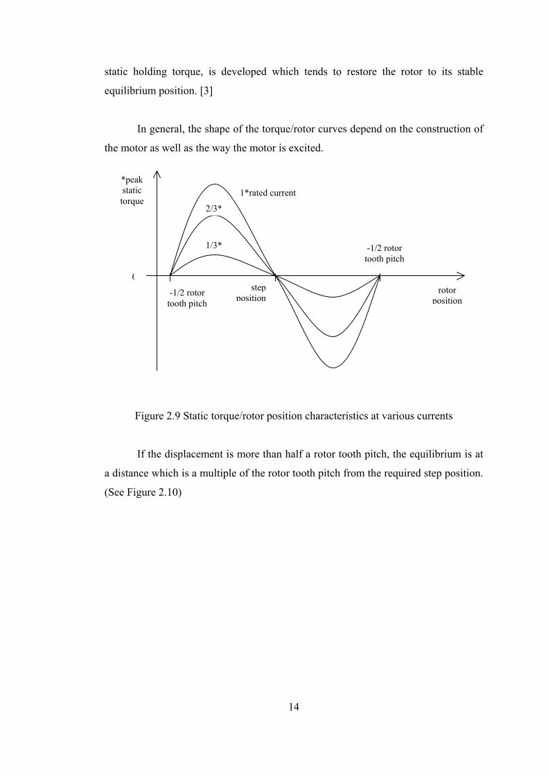
2.5 Static Torque Characteristics
The static torque/rotor characteristic, that shows the torque developed by the
motor as a function of rotor position for several values of winding current, supply the
information about the torque producing capability of a stepping motor. A typical
static torque/rotor position characteristic at various currents is shown in Figure
2.9.[2] When the step motor is energized and with its rotor at the equilibrium
position i.e. the step position, no torque is developed on the rotor shaft. When the
rotor is displaced from the equilibrium position, a restoring torque, that is called
base drive
Dc supply +Vs
Freewheeling resistance and Diode
Switching Trannsistor
Control Signal
Forcing Resistance and phase winding resistance
14
static holding torque, is developed which tends to restore the rotor to its stable
equilibrium position. [3]
In general, the shape of the torque/rotor curves depend on the construction of
the motor as well as the way the motor is excited.
Figure 2.9 Static torque/rotor position characteristics at various currents
If the displacement is more than half a rotor tooth pitch, the equilibrium is at
a distance which is a multiple of the rotor tooth pitch from the required step position.
(See Figure 2.10)
rotor position
-1/2 rotor tooth pitch
stepposition
-1/2 rotor tooth pitch
1*rated current
2/3*
*peak static torque
1/3*
0

15
Figure 2.10 Static torque/rotor position characteristics at rated phase currents
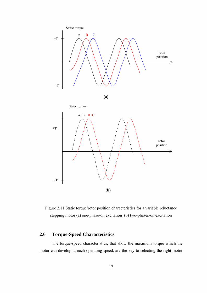
The phase windings of both hybrid and variable reluctance stepping motors
are electrically isolated and each phase is excited by a separate drive circuit, so it is
possible to excite several phases at any time. When the static torque/rotor
characteristics for one-phase and two-phases on excitation in Figure 2.11(a) and (b)
are compared, it is apparent that they are still sinusoidal. The excitation of a three
phase variable reluctance motor with two phases on rather than one phase on, has the
benefit of reducing the static position error, which results from the displacement of
the rotor by a small angle from the expected step position because of the torque
developed by the motor to balance the load torque. This can be confirmed
analytically with the following formulations. The torque equations for each phase for
the static torque/rotor position characteristics of Figure 2.11(a) are
)3/4sin()3/2sin(
)sin(
πθπθ
θ
−−=−−=
−=
pTTpTT
pTT
PK
PKB
PKA
C
(2.1)
rotor position
static torque
Alternative equilibrium position
Required step position
Alternative equilibrium position
Rotor tooth pitch
0

16
and the resultant torque equations for “phase A + phase B” and “phase B + phase C”
for the static torque/rotor position characteristics of Figure 2.11(b), that are simply
obtained by summing the corresponding phase torque expressions, are
)sin()3/sin(
πθπθ−−=+=
−−=+=pTTTT
pTTTT
PKCBBC
PKBAAB (2.2)
It is obvious that the both graphical and analytical results indicate that the
only difference between the excitation schemes is in the equilibrium positions.
An alternative method for minimizing the static position error is to connect
the motor to the load by a gear.
It is true that the excitation of several phases improves the torque produced,
but in applications where the available power is limited to drive the motor, it should
be considered that the more power is required to excite the extra phases.
17
Figure 2.11 Static torque/rotor position characteristics for a variable reluctance
stepping motor (a) one-phase-on excitation (b) two-phases-on excitation
2.6 Torque-Speed Characteristics
The torque-speed characteristics, that show the maximum torque which the
motor can develop at each operating speed, are the key to selecting the right motor
rotor position
Static torque
+T
-T
+T′
rotor position
-T′
A B C
A+B B+C
Static torque
(a)
(b)
18
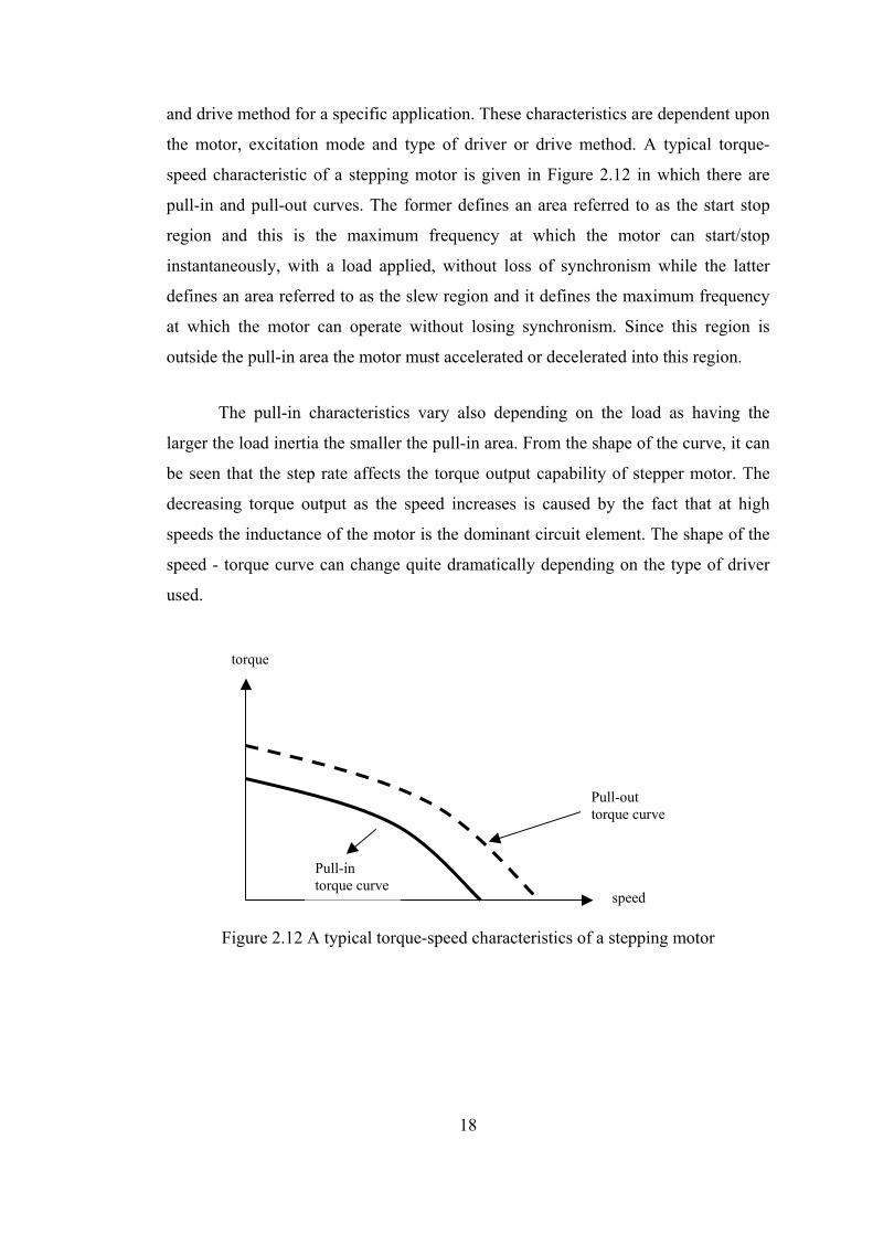
and drive method for a specific application. These characteristics are dependent upon
the motor, excitation mode and type of driver or drive method. A typical torque-
speed characteristic of a stepping motor is given in Figure 2.12 in which there are
pull-in and pull-out curves. The former defines an area referred to as the start stop
region and this is the maximum frequency at which the motor can start/stop
instantaneously, with a load applied, without loss of synchronism while the latter
defines an area referred to as the slew region and it defines the maximum frequency
at which the motor can operate without losing synchronism. Since this region is
outside the pull-in area the motor must accelerated or decelerated into this region.
The pull-in characteristics vary also depending on the load as having the
larger the load inertia the smaller the pull-in area. From the shape of the curve, it can
be seen that the step rate affects the torque output capability of stepper motor. The
decreasing torque output as the speed increases is caused by the fact that at high
speeds the inductance of the motor is the dominant circuit element. The shape of the
speed - torque curve can change quite dramatically depending on the type of driver
used.
Figure 2.12 A typical torque-speed characteristics of a stepping motor
speed
torque
Pull-out torque curve
Pull-in torque curve

19
2.7 Step Motor Control
Step motors have an increasing application area and this is due to the wide
selection of motor control systems that are currently available. The choice of a
particular control scheme depends largely on whatever performance criteria and
economic factors that has to be met in a specific application. Once an initial selection
has been made among the types of the step motors, the next step is to determine the
best combination of the motor and the control type.
Step motor control systems can be generally classified into two groups: the
open-loop and closed-loop systems. In these basic categories there are several control
variations, each of which has its own characteristics and applications. In general, any
step control system can be represented by a simplified system as shown in Figure
2.13. In this system, the command source, where start-stop and direction commands
are generated, may be a manual or local control or part of a controller in a larger
system. The function generator is the source of step motor advance pulses which are
manipulated in such a manner so as to achieve the desired motor dynamics. The
sequence logic provides for proper driver switching sequences. The motor drive
circuits consist of solid state devices capable of sufficient current carrying capacity
and voltage breakdown protection to handle worst case operating conditions. If
closed loop operation is desired then an optical, magnetic or capacitive feedback
device is used in conjunction with an amplifier to supply feedback signals to the
function generator.

20
Figure 2.13 Simplified step motor control system
Stepping motors are often used as output devices for microprocessor-based
control systems. The essential feature of these systems is that the microprocessor
program produces a “result” and the stepping motor must then move the load to the
position corresponding to this “result”. Figure 2.14 shows an open-loop
microprocessor controlled step motor where the phase control signals are calculated
within the microprocessor according to the timing and sequencing requirements.
The second method is hardware-based system in which the microprocessor
program feeds the target position information and a start controller which generates
the phase control signals for the motor drive circuits and a finish signal for the
microprocessor when the target is reached. In applications involving the real-time
control of several other devices this method may be the only realistic alternative
because of programming constraints.
2.7.1 Open-Loop Control
The open-loop control scheme has the advantages simplicity and low cost. A
typical microprocessor-based open-loop control system is shown in Figure 2.14. as
Command Source
Motor Drive
Sequence Logic
Function Generator
Amp
Stepping Motor
Feedback Transducer

21
seen in this figure, the digital phase control signals are generated by the
microprocessor and amplified by the drive circuit before being applied to motor.
Figure 2.14 A typical microprocessor-based open-loop control
In an open-loop system there is no feedback of load position to the controller
and therefore it is imperative that the motor responds correctly to each excitation
change. If the excitation changes are made too quickly the motor is unable to move
the load to the new demanded position and so there is a permanent error in the actual
load position compared to the expected one. Also it is important that in the
applications where the load is likely to fluctuate the timings must be set for the worst
conditions, i.e. the largest load, and the control scheme is then non-optimal for all
other loads. As there is no feedback in this type of control, the need for expensive
sensing and feedback devices such as optical encoders is eliminated. The position
data is simply get by keeping track of the input step pulses.
An open-loop control system of a step motor suffers from the disadvantage
that the motor may not be able to follow the input pulse train so that the top speed
which a motor can run is limited. Also, the speed of a step motor under open-loop
control may have wide fluctuations. But it is still true to say that an open-loop system
is entirely adequate for many applications.
2.7.2 Closed-Loop Control
A closed loop system can overcome the difficulties met in an open-loop
control system by using positional feedback to the step motor to determine the proper
Microprocessor Drive Circuit Motor Load
timed phase control signals
phase currents
torque

22
positions at which phase switchings should occur. With the closed loop control, one
not only achieves much higher speeds and more stability in speed, but more
versatility in many other aspects of the control of the step motor. Each step command
is issued only when the motor has responded satisfactorily to the previous command
and so there is no possibility of the motor losing synchronism.
A block diagram illustrating a closed-loop control scheme of a step motor is
shown in Figure 2.15. The feedback sensor in this case could either be a
photoelectric device or a magnetic pickup device which would give a pulse for every
step of motion. The motor is started initially with one pulse from the controller and
subsequent pulses are generated from the feedback sensor assembly. [3]
Figure 2.15 Block diagram of a closed-loop control of a stepping motor
Logic Circuit Controller Motor Feedback
sensor
Reference Input

23
CHAPTER 3
HARDWARE AND SOFTWARE SOLUTIONS
It is obvious that in order to obtain a drilling process from a digitally
generated object will require hardware and properly designed software. As it is
desired to have a precisely drilled object it is convenient to use step motors, as
covered in the previous chapter, for this specific application.
The critical point in the software is that to convert the given image of the
object in a way that the computer can send the data through the parallel port to the
hardware of the system as digital control signals. The digital control signals for the
step motor drive circuit are generated from the parallel port of the computer. As a
control method, an open-loop control system (see 2.7.1) is used with only full step
mode of operation (see 2.3). The mode of operation for all motors is always full step
regardless of the direction of rotation of the motors that is clockwise or counter-
clockwise.
3.1 Hardware
Hardware configuration consists of three stepping motors (X, Y and Z
motors) that are responsible from the control of movements in the corresponding
directions, driver cards for each motor, a XYZ positioning table and digital I/O for
the control motors.
24
3.1.1 Digital I/O
3.1.1.1 Requirements for Digital I/O
Base drive circuit is designed such that the control signals are at TTL logic
level which is 0 or 5 Volts. In order to have maximum efficiency in the system, these
control signals must be as fast as possible. This speed depends on the torque
requirement from the motor, simply the physical characteristics of the material
drilled, and the control scheme of the motors. As stated in the previous chapter,
closed-loop control scheme will require faster signals than the open-loop case.
Experimental results show that with the open-loop control scheme, motor types and
material given, 5 msec, as the step motor pulse duration is adequate.
These signals may be generated by specially designed, commercially
available professional devices that are sold by various vendors with respectively
higher prices. Another solution for digital I/O is utilizing the parallel port which is
available on every personal computer.
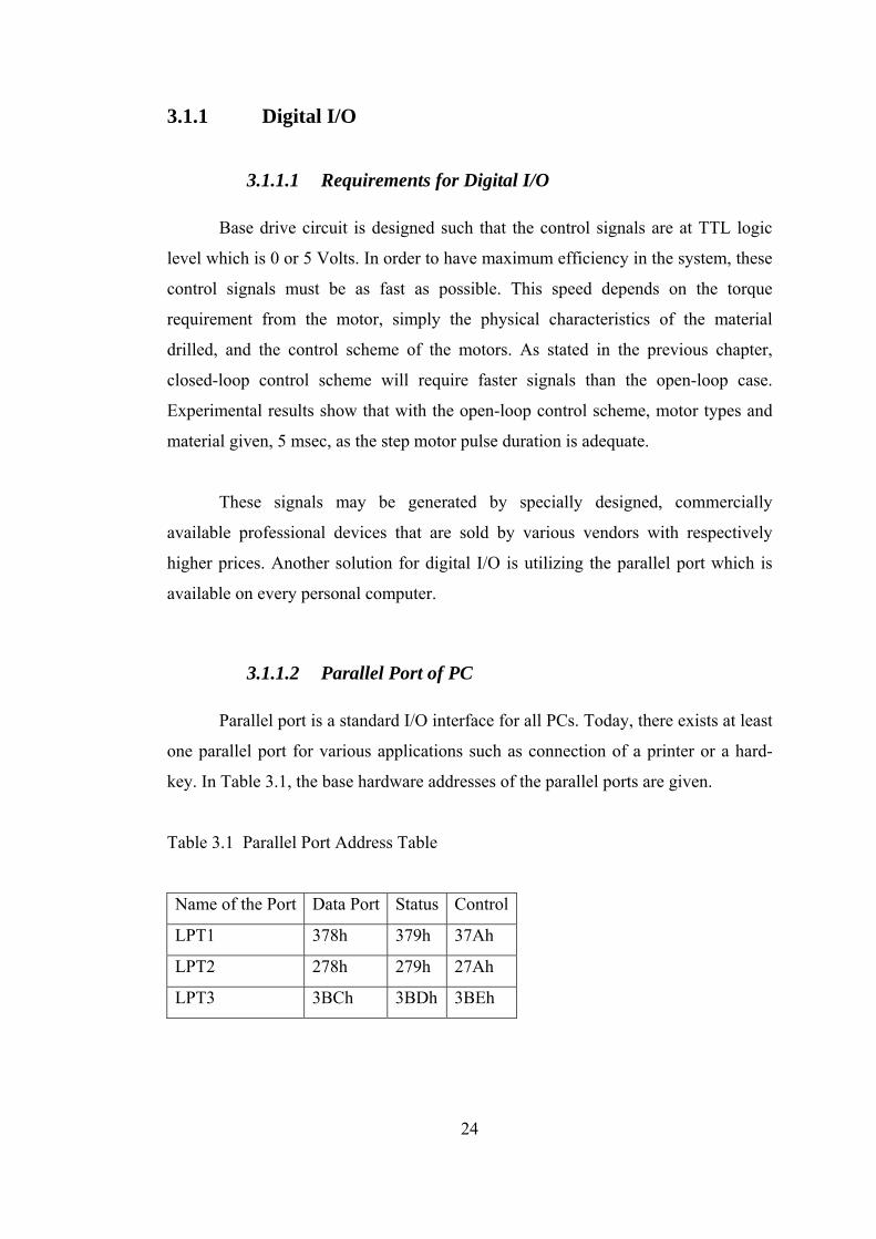
3.1.1.2 Parallel Port of PC
Parallel port is a standard I/O interface for all PCs. Today, there exists at least
one parallel port for various applications such as connection of a printer or a hard-
key. In Table 3.1, the base hardware addresses of the parallel ports are given.
Table 3.1 Parallel Port Address Table
Name of the Port Data Port Status Control
LPT1 378h 379h 37Ah
LPT2 278h 279h 27Ah
LPT3 3BCh 3BDh 3BEh

25
There exist three types of I/O interface in the parallel port namely data port,
status port and control port.
• Data Port : There exist eight digital output terminals that are accessed by
data ports.
• Status Port : There exist five digital input terminals, of which one of them
is inverted, that are accessed by status ports.
• Control Port : There exist four digital output terminals, of which three of
them are inverted, that are accessed by control ports.
All ports are defined at TTL logic levels (An electrical "high" on the pin is
TTL high, +2.4 to +5 volts. An electrical "low" is TTL low, 0 to +0.8 volts.). Data
port is driven by the high impedance octal D-type flip-flop (74LS374). This IC can
source 2.6 mA while it can sink 24 mA. As these values are relatively low, it may be
necessary to amplify the outputs for specific applications. Control port pins are
driven by the 7405 inverter IC which may supply 1 mA up to 7 mA. In parallel port
applications, for not to damage the mainboard the driver circuits should fulfill the
requirements given above.
In Figure 3.1, the block diagram of the parallel interface is given while in
Figure 3.2 the illustration of a parallel port is shown.

26
Figure 3.1 Block diagram of the parallel interface
PC Interface
IRQ Logic
Control Register
Data Register
Status Register
Address Decode Control
5
3
2
1
4
6
7
9
10
11
12
8
17
16
14
13
15
18
19
25
24
23
22
21
20
GND
IRQ5/7
D0..D7
A0..A9
IOR
IOW
FEH
DSL
INI
ALF
STB
D0..D7
ACK
BSY
PAP
ONOF

27
Figure 3.2 Parallel Port I/O Scheme
3.1.2 Stepper Motor Driver Circuit
The drive circuits are used to drive the two phase bipolar X, Y and Z step
motors. The drive circuit to drive the X and Y axes is given in Figure 3.3 while the
circuit for driving the Z axis is given in Figure 3.4. The principal function of the
driver circuits is to generate motor phase sequences.
In these circuits L298 dual full-bridge driver and L297 stepper motor
controller IC (see Appendix C) are used as motor drive circuit components. There are
three control signals, which are used to control the each of the motor axes, as “clock”
to give the stepping command, “direction” to determine the sense of rotation of the
motor and “half/full” to decide whether to operate in full or in half step mode.
Although it is possible to choose full or half step mode, only the full step mode is
used as it is indicated before. Normal drive mode is practiced to for the full step
mode and it is selected by a low logic level on Half/Full* input (Full step mode). In
this mode Inh1* and Inh2* outputs remain high throughout the operation [4].
The cable connection used between the stepper motor controller circuit inputs
to the proper outputs in order to drive the step motors are given in Table 3.2, Table
3.3 and Table 3.4.

28
Figure 3.3 (X-Y) Axis Drive Circuit
12345678910
SYNC GND
HOME
A
INH1
B
C
INH2
D
ENABLE
20 19 18 17 16 15
13 12 11
14
CONTROL
HALF/FULL
CLOCK
CW/CCW
OSC
VREF
SENS1
SENS2
VS
RESET 2 4 6 8
OUTPUT1 VS
ENABLE A
GND
INPUT3
INPUT4
OUTPUT4
1357911
1513
OUTPUT2
INPUT1
INPUT2
VSS
ENABLE B
OUTPUT3
C.SEN. B
C. SEN. A
10 12 14
12
345678910
SYNC GND
HOME
A
INH1
B
C
INH2
D
ENABLE
20 19 18 17 16 15
13 12 11
14
CONTROL
HALF/FULL
CLOCK
CW/CCW
OSC
VREF
SENS1
SENS2
VS
RESET 2 46 8
OUTPUT1 VS
ENABLE A
GND
INPUT3
INPUT4
OUTPUT4
1357911
1513
OUTPUT2
INPUT1
INPUT2
VSS
ENABLE B
OUTPUT3
C.SEN. B
C. SEN. A
10 12 14
KN1
KN1
KN1
KN1
KN1
KN3
KN3
KN3
KN3
KN3
L297
L297
L298
L298
3.3 nF
C
KN
2
KN
2
KN
2
KN
2
KN
2
KN
2
KN
2
KN
2
KN
2
KN
2
KN
2
KN
2
3.3 nF
1
2
3
4
5
1
2
3
4
5
1 2 3
5 6 7
D IN4001
D IN4001
R DR5
100 nF
100 nF
470 nF/50 V
470 nF /50 V
D IN4001
D IN4001
R DR5
D IN4001
D IN4001
R DR5
D IN4001
D IN4001
R DR5
D IN4001
D IN4001
D IN4001
D IN4001
D IN4001
D IN4001
D IN4001
D IN4001
R R
R
C
R
R

29
Figure 3.4 Z Axis Drive Circuit
Table 3.2 Cable connection of X-Y axis card
X-Y Axis Card Parallel Port Connector Stepper Motor
KN1-1 - GND pin of Y axis motor KN1-2 - Phase line 1 of Y axis motor KN1-3 - Phase line 2 of Y axis motor KN1-4 - Phase line 3 of Y axis motor KN1-5 - Phase line 4 of Y axis motor KN3-1 - GND pin of X axis motor KN3-2 - Phase line 1 of X axis motor KN3-3 - Phase line 2 of X axis motor KN3-4 - Phase line 3 of X axis motor KN3-5 - Phase line 4 of X axis motor KN2-1 Pin 1 (Half/Full*) - KN2-2 Pin 6 (Clock X) - KN2-3 Pin 7 (Cw/CCw X) - KN2-5 Pin 1 (Half/Full*) - KN2-6 Pin 4 (Clock Y) - KN2-7 Pin 5 (Cw/CCw Y) -
1 2 3 4 5678910
SYNC GND
HOME
A
INH1
B
C
INH2
D
ENABLE
20 19 18 17 16 15
13 12 11
14
CONTROL
HALF/FULL
CLOCK
CW/CCW
OSC
VREF
SENS1
SENS2
VS
RESET 2 4
6 8
OUTPUT1 VS
ENABLE A
GND
INPUT3
INPUT4
OUTPUT4
1357911
1513
OUTPUT2
INPUT1
INPUT2
VSS
ENABLE B
OUTPUT3
C.SEN. B
C. SEN. A
10 12 14
KN1
KN1
KN1
KN1
KN1
3
4
2
1
KN
2
KN
2
KN
2
KN
2
KN
2
KN
2
KN
2
KN
2
KN
2
5
1 2 3
100 nF 470 nF/50 V
D IN4001
D IN4001
R DR5
D IN4001
D IN4001
R DR5
3,3 nF
R
C R
R

30
Table 3.3 Cable connection of Z axis card
Z Axis Card Parallel Port Connector Stepper Motor KN1-1 - GND pin of Z axis motor KN1-2 - Phase line 1 of Z axis motor KN1-3 - Phase line 2 of Z axis motor KN1-4 - Phase line 3 of Z axis motor KN1-5 - Phase line 4 of Z axis motor KN2-1 Pin 1 (Half/Full*) - KN2-2 Pin 2 (Clock Z) - KN2-3 Pin 3 (Cw/CCw Z) -
Table 3.4 Cable connection of cards and supply
X-Y Axis Card Z Axis Card Power Supply Cable Connector
KN2-8 KN2-8 +5V - KN2-4 KN2-4 GND GND pin1 KN2-9 KN2-9 +24V -
3.1.3 Stepper Motors
The stepping motors are used to drive the positioning table in X and Y
directions and the cutter in Z direction. The motors used are two phase bipolar
stepping motors with 1.8 degrees per step. The rated voltage for one of them is 5 V
DC and 3.2 V DC for the other two. In case of using motors with different degrees
per step, the constant values in the equations (4.1) and (4.2) must be changed due to
the motor type selection.
3.1.4 Drilling Material and Cutting Tools
For different types of applications there exist various kinds of drilling
materials and consequently there are proper cutting tools for every drilling material.
The drilling materials can be classified basically as follows.

31
• Soft Materials (perspex, fiber, etc.)
• Soft Metals (brass, aluminum, etc.)
• Materials made of steel
As a cutting tool, the HSS (High Speed Steel) is used for the first two types
while tungsten-carbide type is preferred for the materials that are made of steel. The
tip type must also be considered according to the object to be drilled. For example, it
is proper to use a cornered tip for a rectangular shape, while a round tip is more
convenient for an elliptical one.
3.2 Software
The software should be developed under a GUI based programming language,
which is a more powerful language compared to the other ones, following the
reasons given in 3.2.1.
The software consists of three main modules (Figure 3.5) which are image
processing software module that handles the digitizing issues of the image, step
motor control software module that is associated with the drilling process and finally
the parallel port control software module that is, in fact can be thought as a
submodule of the step motor control software module, responsible for the
communication between the hardware part and the software.

32
Figure 3.5 Software Modules Data Flow Diagram
3.2.1 GUI Based Programming Languages
GUI based languages, such as Visual Basic and Visual C, are today’s state-of-
the-art programming languages that are respectively powerful than the former
programming tools. They ease the burden of programming with more user friendly
graphical interfaces. In Table 3.5, the lines of code per complexity unit are given for
different programming languages [7].
Among various GUI based languages, Visual Basic is the most user-friendly
and easy to use respectively. Because of these properties, Microsoft Visual Basic 6.0
is used in this thesis.
Main Module
Step Motor Control Module
Image Processing
Module
Paralel Port Control Module

33
Table 3.5 A rough estimation of average number of LOC required for building one
complexity unit in various programming languages.
Programming Language LOC/Complexity Unit
Assembly language 320
C 128
Cobol 105
Fortran 105
Pascal 90
Ada 70
Object-oriented languages 30
Grapchical languages 4
3.2.2 Step Motor Control Software
One of the critical points in the software is to send the data to the driver
circuit properly i.e. to the right axis with the right timing. The main module sends
how many pixels to move in which direction.
The first step is to determine the movement axes that are in fact to determine
to change which bits of the parallel port. Then the number of steps should be
extracted from the multiplication of the step/pixel and the pixel count. A counter
variable is utilized to keep the track of the steps achieved where the value of is
initialized to zero. According to the axes and movement determined the signals are
generated and sent to the driver circuit. Note that there should be a delay between the
two steps of the motors because of the reasons discussed in Section 2.6. The usage of
the open-loop control simplifies the process as there is no feedback. In Figure 3.6 the
flowchart of the step motor control software is illustrated.

34
Figure 3.6 Flow Chart of the Step Motor Control Software
3.2.3 Parallel Port Control Software
Microsoft Visual Basic could access the parallel port of the computer without
introducing an additional interface program (these programs are called drivers) in
Windows 9X OS. By using “c:\windows\system\win95io.dll” library file it is
possible to access the parallel port of the computer [5]. Because of the “Hardware
Abstraction Layer” of Windows NT and Windows 2000, none of the applications can
directly access to the hardware, ports and devices. The remedy for this problem is to
START
Determine the movement axes
Movement# =step/pixel * pixel count
Reset the counter
Send step command to excitation sequence control
Increment counter
Wait
Counter==movement#
NO
Exit to main
YES

35
introduce a third party program. One of these third party programs that can be easily
obtained and can be used is the “I/O ActiveX Communications Control Software”
(Figure 3.7) [6]. Application of this program will provide the developed software to
run independent from the type of the windows OS.
The I/O ActiveX Communications Control Software is an ActiveX control
software component that can easily be used in a variety of “Visual” programming
environments. To use an ActiveX control, it must first be installed on the system
being used for development. Then it can be inserted into the programming
environment where it will be used. ActiveX controls are typically inserted on a form.
After the control is placed on the form the member functions and properties are
available to be used by the programmer.
Figure 3.7 I/O ActiveX Communications Software Message Box
3.2.4 Image Processing Software
The modules and the critical methods used while developing the modules are
explained in Chapter 4 in detail. The critical algorithm of the software is built by the
connectivity and contour tracing issues.
3.2.4.1 Definitions of Connectivity and Contour Tracing
In a discrete binary image, objects are represented in terms of discrete pixels.
A square tessellation is a partitioning of a plane into regions of square parts and a
regular tessellation means a tessellation made up of regular polygons that are same
size and shape [8]. In Figure 3.8, a black pixel p and the neighborhood of p, that is

36
the set of pixels intersecting p, are shown. The eight neighbors of p can be classified
into two groups as having an edge in common with p or having a point in common
with p. The former, which is shown with shaded areas in Figure 3.8, is called the “4-
neighbors” of p while the latter, that is the whole neighbors of p, is called “8-
neighbors” of p.
Figure 3.8 Neighbors of a pixel p in a square tessellation
An object or pattern in a tessellation is said to be a connected component of
black pixels where the background is assumed to be consisted of white pixels or vice
versa. As having two types of neighbors, there are two types of connectivity as “4-
connected” and “8-connected”. In other words, if the neighbors of a pixel, in an
object or pattern, are only of type “4-neighbors” then it is said to be a “4-
connectivity”, otherwise “8-connectivity”. In Figure 3.9 examples of 4- and 8-
connectivity are shown. Following the connectivity definitions, Jordan Curve
Theorem says a simple closed curve separates the plane into two simply connected
components (namely, the inside and the outside) [9, 10]
Figure 3.9 Examples of (a) 4-connectivity (b) 8-connectivity
P
(a) (b)

37
3.2.4.2 Pseudo Code of Contour Tracing
For the contour tracing of a point with 4-connectivity, whose neighbor
tracking sequence is given in Figure 3.10, the following algorithm is used. Note that
the final value for counter I in this code would be converted to eight in case of the
application of an 8-connected point.
The pseudo code for the algorithm:
Repeat until no black_neighbor found
For I=1 to 4
If neighbor(I)=black then
Assign this point to next examination point
Save this point
Break
Else
Continue
End If
Next I
Loop Repeat
Figure 3.10 The tracking sequence of neighbors for 4-connectivity
4 2
3
1P

38
CHAPTER 4
SOFTWARE DESCRIPTION
4.1 Software Requirements Specifications
• Software should be able to load, digitize and drill the 2D and 3D images
which are properly designed and drawn as given in 4.1.1.
• The program should let the user to choose the following options to be chosen
from the start up screen.
o Show/Do not Show “Current Position” of the motors in “mm” units.
o Show/Do not Show “Current Position” of the motors in “pixel” units.
o Enable/Disable “Pause Program”.
o Draw/Do not Draw the track of the motor movement.
• The main screen of the program should show the following information.
o A user information message area.
o Elapsed and remaining time information during the drilling process.
o The name and the path of the selected image file.
o The required options that are selected from the start up screen.
o A “Stop” button to stop the drilling.
o A “Start At (X, Y, Z)” button to start the drilling at a specified (X, Y,
Z) point.
o A “Pause” button to pause the drilling process.

39
o A ”Pause Program” button to program the position of the pause
action.
o A “GoTo (X, Y, Z)” button to make the motors to go to a specified
point.
o A menu consisting of “File”, “Digitizing”, “Drilling”, “3D Menu”,
“About” and “Exit”.
o The menu items are going to be enabled in a logical way. For example
the “Digitizing” item is going to be enabled only after the file to be
loaded is selected.
o The “File” item should consist of “Load Image File”, “Load
Digitized Image” and “Save Digitized Image”.
o The “Digitizing” item should consist of “Digitize Min Distance” and
“Digitize Top”.
o The “Drilling” item should consist of “Drill Image”, “Drill Options”
and “repeat Drill”.
o The “3D Menu” item should consist of “3D Imaging”.
• After the selection of the image file from the “Load Image File” item under
the “File” item of the menu, the “Digitizing “ item should be enabled.
• After the digitizing process, that begins with the selection of either “Digitize
Min Distance” or “Digitizing Top”, an “Image Property Window” showing
the following information should appear.
o Maximum dimensions of the object that would be drilled in pixel and
mm. units.
o Number of images found.
o A warning for checking the image file if the number of images found
is not the expected one.
• After closing the “Image Property Window” the “Drilling Options” window
should open having the following properties.

40
o A textbox to enter the pulse delay value of X and Y motors and a
textbox to enter the pulse delay value of Z motor in milliseconds.
o A textbox to enter the step per pixel value of X and Y motors and a
textbox to enter the step per pixel value of Z.
o The possibility of choosing “Delta Z Profile” to use a z-axis profile
file, “Delta Z Uniform” to use a uniform depth or “Delta Z” to give
different depth levels (up to 20 levels at most depending on the
number of images) manually.
o A “Defaults” button to have the default values instead of entering
them manually.
• A “Job Finished” message box also showing the total time elapsed for
drilling.
• General requirement for the program:
o All errors will be handled by the error handling procedures.
4.1.1 Image Requirements and Limitations
For the drawing of a two dimensional object, that means in fact a three
dimensional object is got from the drawing of top view and proper depth value(s), the
following requirements and limitations should be covered.
• The background should be white where the drawing is black in color. A
typical drawing for a two dimensional object is shown in Figure 4.1
Figure 4.1 A typical drawing for a two dimensional object

41
• There should not be any points on the neighborhood of the peripherals.
Figure 4.2 The requirements and limitations concerned with the peripherals
• There should not be more than two neighbors of a point.
Figure 4.3 The requirements and limitations concerned with the number of neighbors
of a point
For the drawing of a three dimensional object, that means a three dimensional
object is got from the drawing of top view, whose inside region is red, and proper
profile, the following requirements and limitations should be held.
• The background should be white where the drawing is black and the inside
part of the drawing is red in color. A typical drawing for a two dimensional
object is shown in Figure 4.4.
False True

42
Figure 4.4 A typical drawing for a three dimensional object
• The contour of the drawing, i.e. the black part, must be closed.
• There should not be any contour, i.e. black points, on the neighborhood of the
peripherals and there should not be more than two neighbors of a black point
as it is in the requirements and limitations of the drawing of a two
dimensional object.
The drawing of a profile to be used as the depth function of 3D images the
following requirements should be covered.
• The horizontal axis should be the axis for the layers of the object and the
vertical one for the depth values of the layers in the z-direction.
• There should not be any points on the neighborhood of the peripherals and
there should not be more than two neighbors of a point.
• There should be only one z depth value for a given layer.
• The origin (0, 0) point should be in red color where the background in white,
the axes in black and the function in blue color. A typical drawing for a two
dimensional object is shown in Figure 4.5.

43
Figure 4.5 A typical drawing for a profile
4.2 Software Modules
Each of the modules of the program consists of the forms in Visual Basic.
The modules are illustrated in Figure 4.6. As it is seen from the figure, the software
consists of a main module which is responsible from all of the abilities of the system.
Note that this figure does not show the sequence but the data flow between the
modules.
“depth values”
axis
“layers” axis
origin
“depth” function

44
Figure 4.6 Software Data Flow Diagram
4.2.1 “Start Up” Module
As the name implies, the “Start Up” module is the first user interface seen
when the program starts. Identity of the program and the programmer with the
options are shown on this form. As seen in Figure 4.7, the following options, that
would be used as the program is running, are available.
• The current position information (in pixel or millimeter units) that
would appear in the main module to show the position of the cutter as
the object is being drilled,
• The pause program option to be able to pause the drilling action and
start again from the same position whenever wanted as the drilling of
the object is going on.
• The drill tracking option that would show the track of drilling with a
different color as the drilling of the object.
Start Up
Main
Profile Selection
Go To Information
Drill Options selection
Pause At Programming
User Information
Interface
File System

45
Although all these options useful in use, as they cause about a 10% increase
in drilling time it is convenient not to select them when drilling time is important.
Figure 4.7 Start Up Module User Interface
4.2.2 “User Information Interface” Module
The “User Information Interface” module is called after an image digitizing
process of the main module. On this form, the requirement of showing the physical
properties, i.e. the dimensions, of the object is satisfied. With this property the user
can know the exact size of the drilling material block that will be used for the desired
object. Also the number of the images detected and a warning message against some
mistakes that may be caused by the drawings out of standards are displayed. For
example, if there is an extra point that does not belong to the object in fact, the
program will take it as an object and the number of images counted by the program
will be one more than the actual one. In such a case the user can control the drawing
again to prevent a mistake.

46
Figure 4.8 User Information Interface
4.2.3 “Drill Options” Module
The “Drill Options” module that is used for specifying motor actions and
depth levels of the layers for the object to be drilled is called after “User Information
Interface” module. In this module there are three options to specify the depth levels
as “Delta Z Profile” accessing a z-axis profile file (see Section 4.1.1), “Delta Z
Uniform” using a uniform depth level for all layers and “Delta Z” giving different
depth levels. There are at most twenty different levels that can be specified manually.
The number of those boxes, used to specify different depth levels, change in respect
of the number of the objects detected. For example if there object are detected in the
digitizing process, there will be three delta depth value boxes. The pulse delay values
that are necessary for proper motor actions are also set on this form. As “diagonal
movement”, that is to move x and y motors simultaneously, is used the pulse delay
values for these should be same. The number of steps for each motor per pixel is also
set on this form. As it is seen in Figure 4.9 there is a “Default” button for using the
default values that are the optimal ones for the motors specified. “Drill Options”
module can also be used to change the options by the menu item “Drilling Options”
under “Drilling”.

47
Figure 4.9 Drill Options Interface
4.1.1.1 Calculation of the Prototype Dimensions
In the prototyping process of an object, it is important to use the appropriate
values in the “Drilling Options” to get the desired prototype with the desired size. As
it is given in the equations (4.1) and (4.2), the actual size of the prototype is directly
proportional with the number of pixels and step per pixel value for the relative
direction and a constant.
0289.0*)/(* )/()()(/ YXpixelmmYXPHYSICAL pixelstepnd = (4.1)
0157.0*)/(* )()()( ZpixelmmZPHYSICAL pixelstepnd = (4.2)

48
4.1.2 “Go To Information” Module
The “Go To Information” module that is used to specify the position
information of the actions “Go To”, “Start At” and “Pause At” is called with the
relevant buttons on the main form. For “Go To” that is called to move the motors to
the desired position there are also buttons to move them pixel by pixel. The
movements are in terms of entered pixel value times the step per pixel value that is
specified in the “Drilling Options” form. With “Pause At” it is possible to program
the pause position before starting drilling but he position information that should be
given in pixels has to match to a point on the drawing of the object otherwise it will
not have any effect. There are also buttons on this form to move the motors to the
desired position.
Figure 4.10 Go To Information Interface

49
4.1.3 “Profile Selection” Module
The “Profile Selection” module is called when the “Delta Z Profile” option in
the “Drilling Options” form is selected. With the use of this module the drawing of a
profile file, whose requirements given in Section 4.1.1, is called to be used as the
depth function of three dimensional images. The critical point in loading a profile file
is that the number of layers in the profile should be equal or greater than the number
of layers that are found in the digitizing process of the three dimensional object,
otherwise there will be an error message indicating this situation.
Figure 4.11 Profile Selection Interface

50
4.1.4 “Main” Module
The main module interface is shown in Figure 4.12 where the main drilling
machine program controls take place. In this interface there are menu items as file,
digitizing, drilling, 3D menu, about and exit with their sub-items and for the most
common used ones shortcuts on the toolbar. There exist also two textboxes, one to
show the file name and its path that is being digitized or drilled and one to give
messages to the user for the next step to run the program properly.
The loaded object comes into sight on the “picture box“ which changes its
size automatically up to the size of the picture loaded. During the drilling process,
the progress bar showing the percentage of the completed part, the time elapsed,
current positions both in pixels and millimeters depending upon the choice made at
the beginning of the program (see 4.2.1) are activated.
The “Start At (X, Y, Z)”, “Go To (X, Y, Z)” and “Pause Program” buttons are
used for the relevant actions (see 4.1.2). When the “Pause” button is clicked the
program pauses regardless of the position of the cutter until it is re-clicked. With the
“Stop” button it is possible to stop the process that is going on and start the process
for a new object without exiting the program.
As the “Debug Mode” is enabled by clicking its checkbox, the drilling
process is carried without sending any signals to the parallel port, i.e. it does not drill
in fact but the drilling process can be observed on the screen as if it is drilling. It is
obvious that a this kind of process takes much shorter time than drilling the object
with the cutting tool so it is sometimes better to use this property before drilling.

51
Figure 4.12 Main module of the drilling program
4.1.4.1 Loading the Object
An image file is selected by using the “Load Image File” under the “File”
item (“mnuLoadImageFile” is called) which will trigger a “Microsoft Common
Control Dialog Box” object to select the image file. The selected image is loaded into
a picture box object on the main form named as “DrillPicture”. All the calculations
and image processing jobs are realized by utilizing this picture box object methods
(for example “Point” method is used for accessing the color map of a specific point).
With this property of VB, it is possible to load all type of image files (gif, bmp, jpg,
tiff, etc.).
There are two critical points to set in the “Properties Window”. The
“Scalemode” property should be changed to “Pixel” value since the drawings are in
pixel unit format and “Autoredraw” property should be set to “False” value to be
able to digitize and obtain the whole points of the image even it is larger than the
screen.
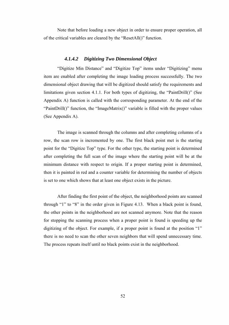
52
Note that before loading a new object in order to ensure proper operation, all
of the critical variables are cleared by the “ResetAll()” function.
4.1.4.2 Digitizing Two Dimensional Object
“Digitize Min Distance” and “Digitize Top” items under “Digitizing” menu
item are enabled after completing the image loading process successfully. The two
dimensional object drawing that will be digitized should satisfy the requirements and
limitations given section 4.1.1. For both types of digitizing, the “PaintDrill()” (See
Appendix A) function is called with the corresponding parameter. At the end of the
“PaintDrill()” function, the “ImageMatrix()” variable is filled with the proper values
(See Appendix A).
The image is scanned through the columns and after completing columns of a
row, the scan row is incremented by one. The first black point met is the starting
point for the “Digitize Top” type. For the other type, the starting point is determined
after completing the full scan of the image where the starting point will be at the
minimum distance with respect to origin. If a proper starting point is determined,
then it is painted in red and a counter variable for determining the number of objects
is set to one which shows that at least one object exists in the picture.
After finding the first point of the object, the neighborhood points are scanned
through “1” to “8” in the order given in Figure 4.13. When a black point is found,
the other points in the neighborhood are not scanned anymore. Note that the reason
for stopping the scanning process when a proper point is found is speeding up the
digitizing of the object. For example, if a proper point is found at the position “1”
there is no need to scan the other seven neighbors that will spend unnecessary time.
The process repeats itself until no black points exist in the neighborhood.

53
Figure 4.13 The neighborhood scanning order for a point for digitizing a two
dimensional object.
After completing one object, the picture is scanned to determine if any other
black point exists. If one is found, then the object number counter is incremented by
one and the whole process is started from the beginning for this new object until no
black points found.
Digitizing with either “Digitize Min Distance” or “Digitize Top” has a
significant importance when the image is not a closed curve. An example of this
situation is shown in
Figure 4.14 where the image consists of two non closed curves. When the image is
digitized with “Digitize Min Distance” the path for digitizing and also drilling will be
as shown in the figure and so there will be three images detected instead of two.
From the view of drilling, this is not only waste of time but as the number of images
in the objects is not correct the problem of giving different depths for different
images appears.
1 2 3
4 5
6 7 8

54
Figure 4.14 Digitizing and drilling path for a non closed curve with “Digitize Min Distance” and “Digitize Top”
4.1.4.3 Digitizing Three Dimensional Object
“3D Imaging” menu item under “3D Menu” is used for digitizing a three
dimensional object whose drawing should satisfy the requirements and limitations
given section 4.1.1. The image is scanned through the columns and after completing
columns of a row, the scan row is incremented by one. The first black point met is
the starting point. Then with a similar process in digitizing a two dimensional object,
the black part, i.e. the contour, is digitized. For each point on the contour, a
“PaintInner()” function is called in order to determine the following layer. The
function searches the 4-neighbors (see Section 3.2.4.1) of the point and when a red
An image consisting of two non closed curves.
Path for “Digitize Min Distance”
Path for “Digitize Top”

55
point is detected, it is painted to blue. As the contour is a closed one, searching for
the 4-neighbors will ensure the existence of a red point. At the end of the closed
contour, all of the blue points, which will allow all of the process to start from the
beginning, are painted to black.
The reason to use a different order for scanning the neighborhood (see Figure
4.13 and Figure 4.15) is that as the number of digitized layers is increased, the
contour starts to look like a rectangular shape. By application of this method, the
motors will only move within the object not the rectangle that covers the object [5].
Figure 4.15 The neighborhood scanning order for a point for digitizing a three
dimensional object.
Figure 4.16 Digitizing process of a three dimensional object
4.1.4.4 Saving / Loading the Digitized Object
Digitizing two- or three-dimensional objects creates an identical type of
digitizing matrix which keeps the values of X’s and, Y’s with the corresponding Z
7 1 6
4 2
8 3 5
(a) (b) (c)
Black to GreenBlue to Black
56
values. These matrix values may be saved to a text file whose path and filename are
user-selected.
Loading of a digitized image is in fact loading the digitizing matrix that is
identical to digitizing the object. In order to use this property, the image should be
loaded as described in Section 4.1.4.1 and after that “Load Digitized Image” menu
item under “File” should be chosen.
The aim of using the “saving” and “loading” properties is saving the time of
the digitizing process if the same object is desired to be drilled for more than one
time.
4.1.4.5 Drilling the Object
The (x, y, z) data in the digitizing matrix is transformed into a new matrix
which is sorted with respect to the “Z-Depth” values (each value of the matrix
corresponds to a layer of the object) with corresponding X and Y values. The drilling
process starts from the smallest Z-depth value for two-dimensional objects and the Z
value matching the first layer on the profile file (see Section 4.1.1) for the three-
dimensional objects.
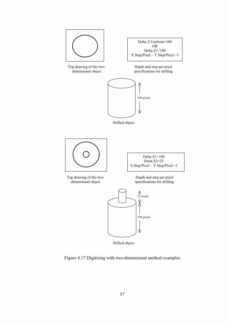
57
Figure 4.17 Digitizing with two-dimensional method examples
Delta Z Uniform=100 OR
Delta Z1=100 X Step/Pixel – Y Step/Pixel =1
100 pixels
Delta Z1=100 Delat Z2=25
X Step/Pixel – Y Step/Pixel =1
Top drawing of the two-dimensional object
Depth and step per pixel specifications for drilling
Top drawing of the two-dimensional object
Depth and step per pixel specifications for drilling
25 pixels
100 pixels
Drilled object
Drilled object

58
Figure 4.18 Digitizing with three-dimensional method example
The drilling process follows the exact path illustrated in digitizing process. It
is clear that when a mismatching occurs in the digitizing process, the user should not
attempt to drill the object. During the drilling process, the progress bar shows the
percentage of the completed part to give an idea about the remaining time to the user.
Also the time elapse and the current position information are given on the main
module interface (see 4.1.4).
In the case of having a hard drilling material (see 3.1.3) or having a large
depth, for not to damage the cutting tools it is better to use the “Repeat Drill” menu
item under “Drilling” and drill the object step by step. Also the same object can be
drilled again to some other position by shifting the coordinates with “Start At” (see
4.1.2).
In drilling process, the “diagonal movement”, i.e. the movement of the x and
y motors simultaneously as long as possible, is used where available as it is obvious
that a diagonal movement takes shorter time than the movement of one motor to the
Top drawing of the three-dimensional object
Depth function
Drilled object

59
desired position first then the other. As it is seen in Figure 4.19, when the path for the
consecutive movement is followed the total time needed is:
delaytimexxyytime utivecon *)]()[( 0101sec −+−= (4.3) where the total time for simultaneous movement of the motors is:
delaytimexxyytime eoussimul *)}(),max{( 0101tan −−= (4.4)
Figure 4.19 Consecutive and simultaneous movement paths for X and Y motors
From the equations (4.3) and (4.4) and Figure 4.19, it is clear that the time to
be followed is shortened with the diagonal movement.
At the end of every drilling process, the cutter returns to its starting position
i.e. the (0,0,0) point.
4.1.5 “About” Module
The name and version of the program, copyright and contact e-mail address
for support take place in the interface of “About” module.
P0( x0,y0 )
P1( x1,y1 ) P1( x1,y1 )
P0( x0,y0 )

60
Figure 4.20 About module of the drilling program

61
CHAPTER 5
RESULTS
5.1 Image Processing Performance
The drilling process follows the exact path illustrated in digitizing process. It
is clear that when a mismatching occurs in the digitizing process, the user should not
attempt to drill the object. Any kind of mismatch that can be occur in image
processing, i.e. in the number of the images or dimensions, can be detected by
observing the user information interface window that appears after digitizing the
object (see 4.2.2).
Two different methods for digitizing, i.e. minimum distance and top distance
options that are mentioned in 4.1.4.2, also improves image processing when the
appropriate one is chosen.
Another method for saving time in digitizing process is to use “saving” and
“loading” properties (see 4.1.4.4) if the same object is desired to be drilled for more
than one time. Thanks to this method there is no need to digitize an object again and
again but it is enough to save the matrix that holds the coordinate data of the
digitized object.

62
5.2 Drilling Performance
As the path of the drilling process follows the exact path illustrated in
digitizing process, there is no time loss with tracing the points that will never be
drilled and the resulting object is much smoother compared with the other algorithms
for the elliptical objects.
The “diagonal movement” of the motors, in other word movement of the X
and Y motors at the same time as long as possible shortens the drilling time up to
%50 (see 4.1.4.5). The “Repeat Drill” option mentioned in 4.1.4.5 also improves the
drilling time with holding the previous drilling option values.
The current position information in pixels and millimeters, pause program
and drill tracking options, that take place in the “Start Up” module (see 4.2.1), are
also the effective factors for time of drilling. As an example drilling time data for an
elliptical object, whose top drawing is given in Figure 5.1 with the following drilling
options, is given in Table 5.1.
Maximum X Dimension = 286 pixel Maximum Y Dimension = 144 pixel Delay X-Y = 5 msec. Delay Z = 5 msec. Step/Pixel X-Y = 8 Step/Pixel Z = 1
Figure 5.1 Top drawing of an ellipse as a two-dimensional object

63
As it can be observed from the data in Table 5.1, the minimum time required
for this specified drilling process is the one with all options, including “Debug”
which means that there will not be a real drilling process but only a simulation on the
screen, are selected. When a comparison is made between the debug-off ones, it is
seen that the most effective option is drill tracking which can be a trade of especially
for drilling processes that are being repeated.
Table 5.1 Comparison of the drilling process time with respect to selected options
Debug Current Position
(mm)
Current Position (pixel)
Pause At Track Time Elapsed
(sec)
418.0391
427.0512
447.1094
443.0012
439.6016
441.0005
439.8891
465.7695

64
5.3 Drilled Samples
The samples given in Figure 5.2 through Figure 5.8 illustrate the drilled
samples realized by 2D and 3D modeling methods. 2D modeling is more suitable for
the objects that have smooth surfaces and for labeling applications where 3D
modeling is preferred for the objects that have curved surfaces.
Figure 5.2 A sample of a drilled object by 2D modelling

65
Figure 5.3 A gear realized by 2D modelling
Figure 5.4 A pyramid realized by 3D modelling

66
Figure 5.5 A dome realized by 3D modelling
Figure 5.6 A heart realized by 3D modelling

67
Figure 5.7 A stamp realized by 2D modelling
Figure 5.8 An application of labelling by 2D modelling

68
CHAPTER 6
CONCLUSIONS
In this study, software for a specific CAD application has been developed
under Microsoft Studio Visual Basic 6.0 environment for industrial prototyping. The
software is packaged as an executable program so that it requires only the run-time
libraries of Visual Basic therefore the licensing problem for a third party software is
eliminated.
The software has ability to recognize and digitize two dimensional models of
three dimensional objects. By this method the user can easily draw and model an
object compared to the three view modeling which will result in saving of time and
money consequently. A drawing technician without the skills or education of
technical drawing can easily model the objects. But it is clear that objects similar to
Figure 1.1 cannot be modeled.
Besides the ease of modeling, the drilling process has been improved
significantly. The motors do not scan the entire surface but only move on the
contours. So that the motors never move on points that will never be drilled. This
method introduces an improvement. Another improvement on the drilling time is
achieved by deactivating visual properties such as showing the current position of the
table. This brings an improvement about 10% in drilling time. Note that this
improvement is tested under a relatively slower PC. The state-of-the-art computer

69
systems will decrease the benefit of this property because of their fast visual
response.
The elliptical objects are digitized and drilled like a spiral shape such as the
same depth levels are drilled consequently. By this method the drilled objects are
smoother with respect to the other scanning methods.
The drawbacks of the software are clear. The drawings should strictly satisfy
the requirements given in Section 4.1.1. After the digitizing process the user is
informed of the properties of the digitized object. The user may comment on the
information given and make proper corrections
The parallel port of the PC has been used for digital signal generation for the
drive circuit so that no extra hardware, that will cause an extra cost, has been
introduced. The utilization of special interface software for the parallel port has
enabled the program to run regardless of the OS. The previous applications could
only run on Windows 95/98 platforms because of the restrictions of the OS. This
software, which uses the ActiveX technology, eases the programming burden and
handles the application versus OS communication. The demonstration version of IO
ActiveX software can be found on the web.
Finally, the implemented software and the hardware have been tested and
various prototypes have been drilled. The results are quite satisfying. Especially,
labels (names or words drilled on the materials), conical or spherical shapes are
satisfactorily realized.
The future work on this topic may be the introduction of a closed-loop control
system for the stepping motors. By this method a further improvement of the drilling
time may be achieved but the cost and the complexity of the system will obviously
increase. Another improvement may be using additional motors on X- and Y-axis to
be able to drill an object having the properties similar to Figure 1.1. It is clear that

70
such kind of an object will require more than one drilling axis and also more than
one drawing views.
71
REFERENCES
[1] Mustafa Bağcı, Prof. Dr. Cemil Bağcı, “Teknik Resim”, 1988.
[2] P.P. Acarnley, “Stepping Motors: A guide to modern theory and practice”,
Revised Second Edition, IEE Control Engineering Series 19, 1984.
[3] Benjamin C. Kuo, “Theory and Applications of Step Motors”, West
Publishing Co., 1974
[4] SGS Thompson Microelectronics, “Stepper Motor Controllers”, August 1996
[5] Semih Mümin Ateş, “A PC Controlled Three Dimensional Machine Tool
Control System”, METU MS Thesis, Dec. 2001.
[6] www.jspayne.com
[7] Roger S. Pressman, ”Software Engineering ”, The McGraw-Hill Companies,
Inc., 4th Edition, 1997.
[8] http://mathforum.org
[9] Oliver Faugeras, “Three Dimensional Computer Vision: A Geometric
Viewpoint”, MIT Press, 1993.

72
[10] Berthold Klaus Paul Horn, “Robot Vision”, MIT Press, 1986.
[11] Kemal Şen, “ A PC Based Industrial Position Control System”, ”, METU MS
Thesis, May. 2000.
[12] A.E. Fitzgerald, Charles Kingsley, Jr, Stephen D. Umans, “Electric
Machinery”, Fifth Edition in SI Units, McGraw-Hill, 1992.
[13] http://www.dai.ed.ac.uk , web page of department of Artificial Intelligence of
the University of Edinburg.
[14] Microsoft MSDN Library,2000.
[15] Microsoft Visual Basic 6.0 Language Reference, Microsoft Press, 1998.

73
APPENDIX A
MODULES AND CRITICAL VARIABLES OF
SOFTWARE
PaintDrill():
Synopsis:
Boolean DigType
Description:
Digitizes an image according to DigType parameter. See Section 3.2.4.1.
Returns:
None.
PaintInner():
Synopsis:
Integer x, y
Description:
Searches for 4-neighbors of the point(x, y) and if a red is detected, it is
painted to blue.
Returns:
None.

74
ResetAll():
Synopsis:
None.
Description:
Clears digitizing matrix and variables used for visual purposes.
Returns:
None.
space Type:
Type:
x, y, z integer
ImageMatrix:
Type:
space
Dimension:
(1600, 1600)
First column implies the object number and the second one implies the points
of the corresponding object.

75
APPENDIX B
PARAMETERS/SELECTIONS IN THE SOFTWARE
B.1 Parameters/Selections in “Start Up Options"
Name Type Comment(s)
Current Position (Pixel) Boolean Show/hide the current position
information in pixels
Current Position (mm) Boolean Show/hide the current position
information in millimeters
Pause Program Boolean Enable/disable “Pause Program”
Drill Tracking Boolean Enable/disable drill tracking
B.2 Parameters/Selections in “Drilling Options”
Name Type Comment(s)
X Step/Pixel-Y Step/Pixel Integer Determines how many step will the
motor moves for each pixel
Z Step/Pixel Integer Determines how many step will the
motor moves for each pixel
Delta Z Profile Boolean Type of delta Z
Delta Z Uniform Boolean Type of delta Z
Delta Z Uniform Integer Determines uniform Z value
Delta Z Boolean Type of delta Z
DeltaZ1..DeltaZ20 Integer Determines non-uniform Z values

76
B.3 Parameters/Selections in “Go To Coordinates”
Name Type Comment(s)
X (Pixel) Integer The number of movements in X axis
Y (Pixel) Integer The number of movements in Y axis
Z (Pixel) Integer The number of movements in Z axis
Button Moves the X-axis by one (+) step
Button Moves the X-axis by one (-) step
Button Moves the Y-axis by one (+) step
Button Moves the Y-axis by one (-) step
Button Moves the Z-axis by one (+) step
Button Moves the Z-axis by one (-) step
Go To Button Enabled only at “GoTo” operation
Start At Button Enabled only at “StartAt” operation
Pause At Button Enabled only at “PauseAt”
programming
B.4 Parameters/Selections in “Main”
Name Type Comment(s)
Message Text Textbox Messages to the user are given
Debug Mode Boolean Enables/disables debug mode
X+
X-
Y+
Y-
Z+
Z-

77
APPENDIX C
MOTOR DRIVE CIRCUIT COMPONENTS
C.1 L298 Dual Full-Bridge Driver
The L298 is an integrated monolithic circuit which is a high voltage, high current
dual full-bridge driver designed to accept standard TTL logic levels and drive
inductive loads such as relays, solenoids, DC and stepping motors. Two enable
inputs are provided to enable or disable the device independently of the input signals.
The emitters of the lower transistors of each bridge are connected together and the
corresponding external terminal can be used for the connection of an external sensing
resistor. An additional supply input is provided so that the logic works at a lower
voltage.
Figure C.1 Block Diagram of L298

78
Table C.1 Absolute Maximum Ratings of L298
Symbol Parameter Value Unit
VS Power Supply 50 V
VSS Logic Supply Voltage 7 V
Vl, Ven Input and Enable Voltage -0,3 to 7 V
I0 Peak Output Current (each Channel)
-Non Repetetive (t=100µs)
-Repetetive (80% on -20% off; ton=10ms)
-DC Operation
3
2,5
2
A
A
A
Vsens Sensing Voltage -1 to 2,3 V
Ptot Total Power Dissipation (Tcase = 75°C) 25 W
Top Junction Operating Temperature -25 to 130 °C
Tstg, Tj Storage and Junction Temperature -40 to 150 °C
C.2 L297 Stepper Motor Controller
The L297 Stepper Motor Controller IC generates four phase drive signals for two
phase bipolar and four phase unipolar step motors in microcomputer controlled
applications. The motor can be driven in half step, normal and wave drive modes and
on chip PWM chopper circuits permit switch-mode control of the current in the
windings. A feature of this device is that it requires only clock, direction and mode
input signals. Since the phase are generated internally the burden on the
microprocessor, and the programmer, is greatly reduced. L297 can be used with
monolithic bridge drives such as the L298N or L293E, or with discrete transistors
and darlingtons.

79
Figure C.2 Block Diagram of L297
Table C.2 Absolute Maximum Ratings of L297
Symbol Parameter Value Unit
VS Supply Voltage 10 V
Vi Input signals 7 V
Ptot Total Power Dissipation (T amb = 70°C) 1 W
Tstg, Tj Storage and Junction Temperature -40 to 150 °C

80
C.3 Two Phase Bipolar Stepper Motor Control Circuit with L297 and L298
L297 and L298 can be used as shown in Figure C.3 for various motor drive
applications. In the figure, the diodes with 2A current rating are used.
Figure C.3 Two Phase Bipolar Stepper Motor Control Circuit with L297 and L298

81
APPENDIX D
DECLARATIONS AND RELATIONS OF FUNCTIONS
AND SUBS OF THE SOFTWARE
D.1 “Main” Form
Declarations
Dim XX, YY, ZZ As Integer
Dim XXX, YYY As Integer
Dim pausedrill As Boolean
Dim StopDrill As Boolean
Dim PauseDrillProgram As Boolean
Dim lngTotalPoints As Long 'For the Progress Bar
Function CreateMatrixFile()
Declaration
Dim fso, txtfile
Dim count As Integer
Called by
Private Sub mnuRepeatDrill_Click()
Function CalculateTotalPoints()
Declaration
Dim count As Integer

82
Called by
Function PaintDrill3D(ByVal DigType As Boolean)
Function LoadMatrixFile(ByVal strDataFile As String)
Declaration
Dim count As Integer
Called by
Private Sub mnuLoadDigitizedImage_Click()
Function PaintDrill(ByVal DigType As Boolean)
Declaration
Dim x, y, z As Long
Dim mapX(8), MapY(8) As Integer
Dim found, Search As Boolean
Dim xPrev, yPrev As Integer
Dim count, counter As Long
Dim distance As Double
Dim xTemp, yTemp As Integer
Dim EndOfPicture As Boolean
Dim result As Integer
Called by
Private Sub mnuDrillImage_Click()
Public Sub drill2D(x, y, z As Integer)
Declaration
Dim i As Integer
Dim result As Integer
Dim intDiff As Integer
Dim intSimStep As Integer

83
Dim int1DStep As Integer
Called by
Private Sub cmdStartAtXYZ_Click()
Private Sub cmdGotoOrigin_Click()
Called by
ButtonClick “GoToOrigin”
Private Sub cmdGoToXYZ_Click()
Called by
ButtonClick “GoToXYZ”
Private Sub mnuRepeatDrill_Click()
Private Sub cmdPauseProgram_Click()
Called by
ButtonClick “PauseProgram”
Private Sub cmdStartAtXYZ_Click()
Calls
ButtonClick “Drill Image”
Called by
ButtonClick “StartAtXYZ”
Private Sub cmdStop_Click()
Called by
ButtonClick “Stop”

84
Private Sub DrillPicture_Paint()
Calls
PaintDrill3D
Private Sub mnuDrillImage_Click()
Declaration
Dim count As Integer
Dim xPrev, yPrev, zPrev As Integer
Dim lngTemp As Long 'For Progress Bar
Calls
Function drillOrigin(x, y, z As Integer)
cmdPauseResume_Click()
ResetAll()
Public Sub drill2D(x, y, z As Integer)
Function drill(x, y, z As Integer)
Called by
Private Sub cmdStartAtXYZ_Click()
Private Sub mnuRepeatDrill_Click()
Private Sub tlbMain_ButtonClick(ByVal Button As ComctlLib.Button)
ButtonClick “Drilling/Drill Image”
Private Sub Form_Load()
Called by
“Main” form when the form is loaded.
Private Sub mnuDigitize_Click()
Calls
ResetAll()
PaintDrill(boolean)

85
Called by
ButtonClick “Digitize/Digitize Min”
Private Sub mnuDigitizeTop_Click()
Calls
ResetAll()
PaintDrill(boolean)
Called by
ButtonClick “Digitize/Digitize Top”
Private Sub mnuDrillOptions_Click()
Called by
ButtonClick “Drilling/Drill Options”
Private Sub mnuExit_Click()
Called by
ButtonClick “Exit”
Private Sub mnuLoad3DMatrix_Click()
Calls
ResetAll()
PaintDrill3D()
Private Sub mnuLoadDigitizedImage_Click()
Declaration
Dim strDataFile As String

86
Calls
LoadMatrixFile(strDataFile)
Called by
ButtonClick “File/Load Digitized Image”
Private Sub mnuLoadImageFile_Click()
Calls
ResetAll()
Called by
Private Sub mnuRepeatDrill_Click()
Private Sub tlbMain_ButtonClick(ByVal Button As ComctlLib.Button)
ButtonClick “File/Load Digitized Image”
Function drill(x, y, z As Integer)
Declaration
Dim i As Integer
Dim result As Integer
Called by
Private Sub mnuDrillImage_Click()
Function drillOrigin(x, y, z As Integer)
Declaration
Dim i As Integer
Dim result As Integer
Called by
Private Sub mnuDrillImage_Click()

87
Private Sub mnuRepeatDrill_Click()
Calls
cmdGoToXYZ_Click()
mnuDrillImage_Click()
CreateMatrixFile()
Called by
ButtonClick “Drilling/Repeat Drill”
Private Sub tlbMain_ButtonClick(ByVal Button As ComctlLib.Button)
Calls
mnuLoadImageFile_Click()
mnuDrillImage_Click()
Called by
ButtonClick “Toolbar”
Function ResetAll()
Called by
Private Sub cmdStartAtXYZ_Click()
Private Sub mnuDigitizeTop_Click()
Private Sub mnuLoad3DMatrix_Click()
Private Sub mnuLoadImageFile_Click()
Function Matrix6Converter()
Declaration
ReDim Matrix6Interface(188, width6, height6)
ReDim ZValueMatrix(1600)
Calls
PaintDrill3D(1)

88
Function PaintDrill3D(ByVal DigType As Boolean)
Declaration
Dim x, y, z As Long
Dim mapX(8), MapY(8) As Integer
Dim found, Search As Boolean
Dim xPrev, yPrev As Integer
Dim count, counter As Long
Dim distance As Double
Dim xTemp, yTemp As Integer
Dim EndOfPicture As Boolean
Dim result As Integer
Calls
PaintInner(xPrev, yPrev)
PaintInner(xPrev, yPrev)
PaintBlueToBlack
CalculateTotalPoints
Called by
Private Sub mnuLoad3DMatrix_Click()
Function Matrix6Converter()
Function PaintInner(ByVal x As Integer, ByVal y As Integer)
Declaration
Dim count As Integer
Dim mapX(3), MapY(3) As Integer
Called by
Function PaintDrill3D(ByVal DigType As Boolean)
Function PaintBlueToBlack()
Called by
Function PaintDrill3D(ByVal DigType As Boolean)

89
D.2 “GoTo” Form
Private Sub cmdCancelGoTo_Click()
Called by
ButtonClick “Cancel for Go To”
Private Sub cmdOKGoTo_Click()
Declaration
Dim x, y, z As Integer
Called by
ButtonClick “OK for Go To”
Private Sub cmdOKStartAt_Click()
Declaration
Dim x, y, z As Integer
Called by
ButtonClick “OK for Start At”
Private Sub cmdPauseAtXYZ_Click()
Called by
ButtonClick “Pause At XYZ”
Private Sub cmdXMinus_Click()
Called by
ButtonClick “X- (Decrease X)”

90
Private Sub cmdXPlus_Click()
Called by
ButtonClick “X+ (Increase X)”
Private Sub cmdYMinus_Click()
Called by
ButtonClick “Y- (Decrease Y)”
Private Sub cmdYPlus_Click()
Called by
ButtonClick “Y+ (Decrease Y)”
Private Sub cmdZMinus_Click()
Called by
ButtonClick “Z- (Decrease Z)”
Private Sub cmdZPlus_Click()
Called by
ButtonClick “Z+ (Decrease Z)”
Private Sub Form_Activate()
Called by
“Go To” form when the form is activated.

91
Private Sub Form_Load()
Called by
“Go To” form when the form is loaded.
D.3 “Information” Form
Private Sub cmdOK_Click()
Called by
ButtonClick “OK”
Private Sub Form_Activate()
Called by
“Go To” form when the form is activated.
Private Sub Form_Load()
Called by
“Go To” form when the form is loaded.
D.4 “Options” Form
Private Sub btnCancel_Click()
Called by
ButtonClick “Cancel”
Private Sub btnDefaults_Click()
Called by
ButtonClick “Defaults”

92
Private Sub btnOK_Click()
Declaration
Dim j, k As Integer
Called by
ButtonClick “OK”
Private Sub chkDeltaZNonUniform_Click()
Called by
CheckClick “DeltaZNonUniform”
Private Sub chkDeltaZProfile_Click()
Called by
CheckClick “DeltaZProfile”
Private Sub chkDeltaZUniform_Click()
Called by
CheckClick “DeltaZUniform”
Private Sub Form_Activate()
Called by
“Options” form when the form is activated.
D.5 “Profile” Form
Private Sub cmdOK_Click()
Called by
ButtonClick “OK”

93
Private Sub cmdSelectProfileFile_Click()
Declaration
Dim x, y, x0, y0 As Integer
Dim result, count As Integer
Dim found As Boolean
Called by
ButtonClick “Select Profile File”
D.6 “Start Options” Form
Private Sub chkCurrentPositionMm_Click()
Called by
CheckClick “Current Position (mm)”
Private Sub chkCurrentPositionPixel_Click()
Called by
CheckClick “Current Position (pixel)”
Private Sub chkDrillTrack_Click()
Called by
CheckClick “Drill Track”
Private Sub chkPauseProgram_Click()
Called by
CheckClick “Pause Program”

94
Private Sub cmdOK_Click()
Called by
ButtonClick “OK”
Private Sub Form_Load()
Called by
“Start Options” form when the form is loaded.
D.7 “Main” Module
Declare Sub sleep Lib "kernel32" Alias "Sleep" (ByVal dwMilliseconds As Long)
Public intXStep, intYStep, intZstep As Integer
Public intPulseDelayXY, intPulseDelayZ As Integer
Public intDeltaZUniform As Integer
Public intDeltaZNonUniform(500) As Integer
Public blnDeltaZType As Boolean 'True for Uniform-False for NonUniform
Public XMax, YMax, ZMax, XMin, YMin, ZMin As Integer
Public intNoOfImages As Integer
Public Const intmmAccr As Integer = 0
Public blnFrmClosed As Boolean 'used for frmGoToInfo form to be closed
Public intCountImage As Integer
'For "Start Options"
Public blnShowCurrentPositionPixel As Boolean
Public blnShowCurrentPositionMm As Boolean
Public blnShowPauseProgram As Boolean
Public blnShowDrillTrack As Boolean
Public blnGotoOrigin As Boolean
'For "Repeat Drill" action
Public blnRepeatDrill As Boolean

95
Type space
x As Integer
y As Integer
z As Integer
End Type
Public ImageMatrix() As space 'Digitized Image
Public ImagePoints() As Long 'Digitized Image shown on Picture
Public curpos2D As space
Public PausePosition As space
Public Matrix6Interface() As Long
Public ZValueMatrix() As Long
'3D Options
Declare Function ExtFloodFill Lib "Gdi32" (ByVal hdc%, ByVal i%, ByVal i%,
ByVal w&, ByVal i%) As Integer
Public Image1, Image2, Image3 As String
Public crimageno, width1, height1, width2, height2, width3, height3, regions,
pauseprog As Integer
Public width4, width5, width6, width7, height4, height5, height6, height7 As Integer
Public startcolred, startrowred, endcolred, endrowred, credx, credy, stepx As Integer
Public matrix1() As Integer
Public matrix2() As Integer
Public matrix3() As Integer
Public matrix4() As Integer
Public matrix5() As Integer
Public matrix6() As Integer
Public matrix7() As Integer
Public sum7() As Long
Public regheight(), borders4(), borders5() As Integer
Public stepsize As Double
Public sumsum6, fcolor As Long

96
Public pixelstepx, pixelstepy, steppixelx, steppixely, steppixelz, drilltime, lastcolscan
As Integer
Public pulsedelayy, nextpos, corrected, subfinished, xdiameter, ydiameter As Integer
Public paso, curpos, curdrill, drillno, steppixw6, steppixcol, pulsedelayx,
pulsedelayz, lastcoldone As Integer
Public xdist, ydist, zdist, cutter, maxpoint, todrill, state, startcol3, startrow3 As
Integer
Public pausex, pausey, pauselayer, curx, cury, curz As Integer
Public pausedrill, fromgoto As Boolean
Public starttime, endtime As Variant
![Index [pc-textbook.mcmaster.ca]pc-textbook.mcmaster.ca/Marlin-Index.pdf · Index Accumulation, 53 Accuracy: numerical integration, 83-84 sensor, 383, 772-773 Adaptive tuning:](https://img.pdfslide.net/doc/110x75/5b90b2bd09d3f252108c69e0/index-pc-pc-index-accumulation-53-accuracy-numerical-integration-83-84.jpg)