Development of a coal reserve GIS model and estimation of

Graduate Theses, Dissertations, and Problem Reports

2009

Development of a coal reserve GIS model and estimation of the Development of a coal reserve GIS model and estimation of the

recoverability and extraction costs recoverability and extraction costs

Chandrakanth Reddy Apala West Virginia University

Follow this and additional works at: https://researchrepository.wvu.edu/etd

Recommended Citation Recommended Citation Apala, Chandrakanth Reddy, "Development of a coal reserve GIS model and estimation of the recoverability and extraction costs" (2009). Graduate Theses, Dissertations, and Problem Reports. 2062. https://researchrepository.wvu.edu/etd/2062

This Thesis is protected by copyright and/or related rights. It has been brought to you by the The Research Repository @ WVU with permission from the rights-holder(s). You are free to use this Thesis in any way that is permitted by the copyright and related rights legislation that applies to your use. For other uses you must obtain permission from the rights-holder(s) directly, unless additional rights are indicated by a Creative Commons license in the record and/ or on the work itself. This Thesis has been accepted for inclusion in WVU Graduate Theses, Dissertations, and Problem Reports collection by an authorized administrator of The Research Repository @ WVU. For more information, please contact [email protected].

https://researchrepository.wvu.edu/

https://researchrepository.wvu.edu/

https://researchrepository.wvu.edu/etd

https://researchrepository.wvu.edu/etd?utm_source=researchrepository.wvu.edu%2Fetd%2F2062&utm_medium=PDF&utm_campaign=PDFCoverPages

https://researchrepository.wvu.edu/etd/2062?utm_source=researchrepository.wvu.edu%2Fetd%2F2062&utm_medium=PDF&utm_campaign=PDFCoverPages

mailto:[email protected]

Development of a Coal Reserve GIS Model and Estimation of the Recoverability and Extraction Costs

Apala Chandrakanth Reddy

Thesis submitted to the

College of Engineering and Mineral Resources

West Virginia University

in partial fulfillment of the requirements

for the degree of

Master of Science

in

Mining Engineering

Dr. Yi Luo, Ph.D., Chair,

Dr. Felicia F. Peng, Ph.D.,

Dr. Brijes Mishra, Ph.D.

Department of Mining Engineering

Morgantown, West Virginia

2009

Keywords: Resources; ARC GIS; Recoverability; Ventilation costs

ABSTRACT

The United States has the world largest coal resource and coal will serve as the major and

dependable energy source in the coming 200 years or more. However, the amount of

recoverable coal reserve depends on the geological formations and quality of the coal seams,

future development of mining technology and the extraction cost. A NETL sponsored

cooperative research was conducted by the researchers at Carnegie Mallon University (CMU)

and West Virginia University (WVU) to estimate the recoverable coal reserve. This thesis

presents some of the works that WVU performed to enhance the coal reserve model including

characterization of coal reserves, estimation of recovery ratio and extraction cost.

To characterize the coal reserve, a GIS model was developed. In this model, information

of coal reserve, rank, gas content, etc. have been collected from published sources and integrated

into a combined coal reserve database. A GIS interface has been developed to interact with the

database to display the needed information in map forms.

Room and pillar mining method could still remain to be the main method to mine small

and difficult reserves. To maximize the coal reserve recovery by designing proper sized coal

pillars is the most important task in room and pillar mining operation. Though pillar design

methodology has been proposed long time ago, it needs an iterative solution process. To

facilitate programming the coal reserve model and engineering application, a straight-forward

pillar design method was developed.

Mine ventilation often is a limiting factor for underground coal mine operations.

Ventilation requirement for an underground coal mine (i.e., fan head and quantity) depends on

the gas content and production rate. A method to estimate the ventilation requirement in mine

planning stage described in the SME handbook has been modified to take the variation of coal

seam gas content into consideration. It should be noted that the gas content of a coal seam

depends on the coal rank and the average burial depth. Again, the method was made easy to be

programmed into the coal reserve model and to be applied by engineers.

iii

Acknowledgements I want to express my sincere gratitude and appreciation to my academic advisor, Dr. Yi Luo, for

his persistent encouragement, support and guidance during the period of graduate study and

thesis work. He is one of the best teachers I ever saw since my childhood. He is a wonderful

person in the academic field and a great motivator. I learned a lot from his hard working and

great personality. I can say it is my luck and pleasure to have him as my teacher.

I would like to thank Dr. Felicia F. Peng, and Dr. Brijes Mishra for their valuable and

constructive suggestions, comments and advices.

iv

Table of Contents

1. Introduction ................................................................................................................................. 1

2. Objective .................................................................................................................................. 4

3. Literature Overview ................................................................................................................. 7

3.1 Coal ....................................................................................................................................... 7

3.2 Distribution of Coal Reserves in United States ..................................................................... 8

3.3 Mineable Coal seams in US and their Rank Information .................................................... 14

3.4 Coal Production in USA ...................................................................................................... 20

3.5 Mining methods................................................................................................................... 22

3.6 Mining costs ........................................................................................................................ 25

3.7 Previous Cost Models.......................................................................................................... 26

4. Characteristics of US Coal Reserves ..................................................................................... 28

4.1 ARC GIS ............................................................................................................................. 29

4.2 Sources for the Data ............................................................................................................ 32

4.3 Methodology ....................................................................................................................... 33

4.4 Results……………………………………………………………………………………...33

5. Recovery Ratio ...................................................................................................................... 41

v

5.1 Pillar Design ........................................................................................................................ 42

5.2 Determination of Pillar size ................................................................................................. 43

5.3 Determination of the Recovery Ratio: ................................................................................ 48

5.4 Example ............................................................................................................................... 49

6. Mining Economics ................................................................................................................. 50

6.1 Estimation of Ventilation Costs .......................................................................................... 51

6.2 Base method for Estimating Ventilation Requirement ....................................................... 51

6.3 Ventilation Capital Cost ...................................................................................................... 52

6.4 Ventilation Operating Cost.................................................................................................. 52

6.5 Adjustments to the Ventilation Requirement ...................................................................... 53

6.6 Gas Content ......................................................................................................................... 54

6.7 Indirect method to Estimate Gas Content ........................................................................... 54

6.8 Correction Factor to Ventilation Air Quantity: ................................................................... 56

6.9 Example:.............................................................................................................................. 59

7. Conclusion ............................................................................................................................. 60

References………………………………………………………………………………………..62

Appendix…………………………………………………………………………………………63

vi

TABLE OF FIGURES

Figure 1: Delineation of U.S. Coal Resources and Reserves5, EIA 1997 ..................................... 12

Figure 2: Coal-Bearing Areas of the United States5 ..................................................................... 13

Figure 3: US Coal Regions 1996.png8 .......................................................................................... 18

Figure 4: Coal production in USA ................................................................................................ 21

Figure 5: Different grades of Coal Production in USA ................................................................ 22

Figure 6: Screen shot of the United States map showing different states ..................................... 35

Figure 7: Screen shot of the United States map showing counties of different states .................. 36

Figure 8: Counties of Bituminous coal rank in United States. ..................................................... 38

Figure 9: Counties whose total production is more than 10,000 Million short tons (2008) ......... 39

Figure 10: States with Longwall Productivity is greater than 5 .................................................... 40

Figure 11: Sizes of the coal pillar at Different depths and Mining Heights ................................. 45

Figure 12: Relationship between Coefficient A and Mining Height (m) ..................................... 47

Figure 13: Relationship between Coefficient B and Mining Height (m) ...................................... 48

Figure 14: Recovery Ratios for Various Mining Height (m) and Depth (h) ................................ 49

Figure 15: Base Capital and Annual Operating Costs of a Mine Ventilation System .................. 53

Figure 16: Gas Content in Major US Coal Seams ........................................................................ 55

Figure 17: Correction Factors for Required Ventilation Air Quantity ......................................... 57

vii

Figure 18: Graph showing the percentage of Ventilation costs to Total costs for different coal

seams at varying depths. ............................................................................................................... 58

viii

List of Tables

Table 1: Carbon content and the heating values of different grades of coal2, 3 ............................... 8

Table 2: Rank and location of different coal seams throughout United States ............................. 19

Table 3: Derived Coefficients A and B for the Power Function in Pillar Size Design with ........ 44

Table 4: Results of the regression studied for the coefficients A and B in the power function ... 46

Table 5: Determined Regression Coefficients for the Selected Coal Seams ................................ 56

Table 6: Coefficients for Correction Factor for the Selected Coal Seams .................................... 57

Table 7: Average sale price of coal by state and coal rank, 2008 ................................................. 63

Table 8: Coal Production and Number of Mines by State, County and Mine Type ..................... 65

Table 9: Coal Production by State and Mine Type ....................................................................... 76

Table 10: Coal Production and Number of Mines by State and Coal Rank ................................. 78

Table 11: Recoverable Coal reserves and Average Percentage at producing mines by State ...... 80

1

1. Introduction

Coal has played a significant role in the industrialization of the many major countries in

the world. It is estimated that there are about 847 billion tons of proved coal reserves worldwide.

It still supplies about 25% of the world energy. Coal has many important uses worldwide. The

most significant uses are in electricity generation, steel production, cement manufacturing and as

a liquid fuel. Around 5.8 billion tons of hard coal were used worldwide last year (2008) and 953

million tons of brown coal. Since 2000, global coal consumption has grown faster than any other

fuel. The five largest coal users – USA, China, India, Japan and Russia account for 72% of total

global coal use (World Coal Institute, 2009).

Coal has been an energy source for hundreds of years in the United States. Many envision

a future in which coal continues to play a predominant role in the nation’s diverse energy supply.

It helped to provide basic needs of energy for domestic heating and cooking to transportation for

people, products and raw materials to energy for industrial applications and electricity

generation. America’s economic progress historically linked to the use of coal from its abundant

coal resources.

The estimation of the current coal reserves provides more accurate information of how

much of the total US coal resource database is actually available for extraction in the coming

years. The earlier studies have already confirmed that the economically recoverable resources are

considerably less than that of the total resource database and it is required that more

comprehensive assessment of the reserves should be done in order to extract coal economically.

2

More studies are encouraged on the study of characteristics of coal, especially the depth of

mining and the quality of coal to calculate the recoverability and feasibility of extraction.

The amount of recoverable coal reserves mainly depends on the geological formations

and quality of the coal seams, future development of mining technology and the extraction costs.

The objective of the research proposed by NETL is to design a financial model to estimate the

cost of mining coal based on the technology chosen by geological conditions. In these efforts,

CMU and WVU have evaluated the costs of extracting coal from myriad coal regions by

developing a model. A cooperative research has been carried out by Carnegie Mellon University

and West Virginia University to estimate different parameters for designing the model. In this

aspect the contribution of West Virginia University in this study is to provide some of the works

to enhance the coal reserve model. The recovery ratio estimation, the ventilation costs are

included in the model and these works are contributed by WVU. The flow sheet in the next page

explains the various inputs of the coal reserve model and the contributions of WVU in this

project to calculate the cost per extracting each ton of coal.

The Department of Energy (DOE) has enabled the continued and potentially expanded

use of nations secure domestic coal resources through the deployment of efficient generation

technologies by eliminating environmental issues which act as barriers for coal utilization.

Flow sheet showing various inputs for the Coal Reserve Model for calculating the cost of

extracting ton of coal mined. Output

Cost per ton of coal

3

1. Advanced technologies

and methods of coal

extraction to enhance

productivity

2. Recovery Ratio

(Contributed by WVU)

1. Equipment Fuel costs

2. Ventilation costs

(Contributed by WVU)

3. Electricity costs

4. Overburden removal costs

5. Shaft and hoist cost

6. Taxes (CMU and NETL)

Costs

Involved

Calculating the

Mine Performance

1. Available coal

Resources

2. Resource Based Mine

Lifetime

(CMU and NETL)

Resource

Assessment

Coal Reserve Model

Input for the model

4

2. Objective

The main purpose of the project undertaken by National Energy Technology Laboratory

(NETL) is to estimate the cost to extract coal from different US coal regions. The extraction

costs are calculated as a function of geological characteristics and technology performance. This

methodology mainly comprises performing a resource assessment on the available quantity of

coal and its geological characteristics and then calculating the mining costs as a function of coal

depth and thickness. Multiple calculations are employed to estimate the costs to underground or

surface mine resource. The costs are found on a process based model that represents the unit

operations of expected equipment to be used in these mining systems, and expected capital and

operating costs for these methods, including salaries and taxes.

The scope of this project includes developing and demonstrating long-term coal supply

associated with future scenarios of extraction technology and mine operations, developing

regional cost curves, assessing regional coal resource availability and quality, and evaluating

technologies and practices to minimize environmental impacts from mining and incorporating

them into the estimation of coal mining costs. This work assesses the implications of continued

coal use, as resources are consumed, and mining is undertaken under more challenging

conditions than those that exist today. The analysis will evaluate the cost of mining coal in

consideration of more advanced technologies and techniques to mitigate environmental impacts

that may arise from extraction in the future.

5

This thesis is related to the description of the characteristics of the United States coal

reserves and designing of a coal resource database to identify different grades and properties of

the coal available throughout the country using ARC GIS software. A set of databases are

designed for describing different statistics of coal throughout the country and are incorporated

into the software to identify the data directly on the United States map.

Analysis of these resources implied the continuous use of coal as the resources are

consumed and mining is undertaken under more challenging conditions than those of today. With

the extinction of the shallow deposits in this country, the increase in demand of coal led to deep

seam mining. In order to face some challenging issues with increase in depth, the recovery ratio

of extraction of coal is estimated to find the feasibility of extraction of a particular reserve. The

complete extraction of the coal from underground is possible only when we have a very good

idea on the nature of the reserve and the type of mining method. The recovery ratio of extraction

of these coal resources at various depths and mining heights is calculated by designing suitable

pillars for Room and Pillar mining method to prevent underground mine structural failures and

surface subsidence. The pillar size is determined to estimate the recovery ratio using regression

analysis.

This analysis also involves the study of cost of mining coal under challenging conditions.

The most economic method of extraction mainly depends on the depth, thickness, geology of the

coal seam and environmental factors. The ventilation costs which are substantially increased

these days due to increase in the electricity costs are calculated for different coal seams at

various depths. The methods used in SME hand book are used as base methods for calculation

6

and are further adjusted by coal rank and depth. Because of the differences in coal seams and

depths there is considerable change in the gas content in a ton of the mined coal and thus the

required ventilation air quantity changes. It has been demonstrated by studies that the gas content

in coal is a function of the coal rank and mining depth considering the gas emission is

proportional to the gas content. Thus, the required ventilation air quantity also depends on the

coal rank and the mining depth.

7

3. Literature Overview

3.1 Coal

Coal is a fossil fuel which is formed from the partial decomposition of decaying animal and

plant matter. It is created over millions of years under intense pressure from the layers of the

rock and other sediments. The rank of coal is classified according to its heating value, fixed

carbon and volatile matter content and also its caking properties during combustion. Based on

these factors the rank of coal is classified into four categories.

Anthracite is a jet black coal with high heating value and is considered as the highest

quality of coal.

Bituminous which is softer black and has somewhat low fuel value. This is the most

common commercially mined grade of coal in the country.

Sub-bituminous coal which is dull black or slightly brownish and it has a lower heating

value.

Lignite which is brownish black in color and is considered as the lowest of the all

commercial grades. This grade of coal is usually mined where no other low cost fuels are

available.

8

Table 1: Carbon content and the heating values of different grades of coal ( EIA and ABA,

2009)

Coal Rank Carbon Content % Heating Value (in BTUs per pound)

Anthracite 86-97 % Nearly 15,000

Bituminous 45-86 % 10,500 to 15,500

Sub-bituminous 35-45 % 8,300 to 13,000

Lignite 25-35 % 4000 to 8,300

3.2 Distribution of Coal Reserves in United States

Coal is the most abundant fossil fuel in United States. It has got the biggest supply of

coal reserves in the world. Of the total world’s coal reserve 27 % exist in United States (i.e. 249

billion tons). Its abundance led to its major use for electricity generation, rails, and fueling

factories. It is known that the coal production has been increased by 70% since 1970. Nine out of

every 10 tons of coal mined in United States today is used for electricity generation and about 56

% of the electricity used is generated from coal (American Coal Foundation, 2009).

Coal will continue to serve us in the forth coming years at the same rate as today as it is

more abundant and cost effective than oil and natural gas. As per the current use it is known that

the supplies are good enough for more 300 years.

9

In Mining terminology, the resources are defined as the deposits of coal which occur in the

Earth’s crust that are economic in extraction and that are currently or may become feasible. (Coal

Resource Classification System of the US Bureau of Mines and US Geological Survey)

Resources are classified into different types. Some of them are explained below (Coal Reserves

Data, EIA, 2009):

1. Measured Resources:

The measured resources are defined as those, where the rank and quality estimation is done from

a high degree of geologic assurance from sample analysis and measurements from a closely

spaced and geologically well know sample sites. Under the USGS criteria, the points of

observation are not greater than half mile apart and the measured coal is projected to extend as a

¼ mile wide belt from the outcrop of observation.

2. Indicated Resources:

Indicated resources are those where the estimates of rank, quality and quantity are computed to a

moderate degree of geologic assurance, partly from sample analyses and measurements and

partly from reasonable geologic projections. Under the USGS criteria, the points of observation

are from ½ to 1 ½ miles apart. Indicated coal is projected to extend as a ½ mile wide belt that lies

more than ¼ mile from the outcrop or points of observation.

3. Demonstrated resources:

Demonstrated resources are one which are the sum of the measured resources and indicated

resources.

10

4. Demonstrated reserve base (DRB):

The Demonstrated reserve base is defined as the parts of identified resources that meet specified

minimum physical and chemical criteria related to the current mining and production practices,

including quality, depth, thickness, rank and distance from points of measurement. The “reserve

base” is the in-place demonstrated resource from which reserves are estimated. This reserve base

may contain resources which are economically recoverable within planning horizons that extend

beyond those which assume proven technology and current economics.

5. Inferred resources:

Inferred resources are defined as the estimates of the lowest degree of geologic assurance in

unexplored extensions of demonstrated resources for which estimates of the quality and size are

based on geologic evidence and projection. The total quantity estimation is always based on

good knowledge and geologic character of the bed and also the regions where few measurements

are available and on assumed continuation from demonstrated coal for which there is geologic

evidence. The points of measurement are from 1 ½ to 6 miles apart. Inferred coal is projected to

extend as a 2 ¼ mile wide belt that lies more than ¾ mile from the outcrop or points of

observation or measurement. Inferred resources are not a part of the DRB. Minable refers to the

coal that can be mined using present day mining technology under current restrictions, rules and

regulations.

11

Reserve

The term reserve refers the quantity which can be recoverable at a reasonable profit with the

application of extraction technology available currently or in the nearby future.

The USGS conducts mappings and field studies to calculate the identified coal resources

and makes an estimation of the undiscovered resources based on the available geologic

information. The demonstrated reserve base is only part of the coal resource data and the EIA

estimates are of the United States government coal resource assessment data. The coal reserves

which are estimated by EIA are generally considered to be very limited for long term analysis as

there is only limited data available to gather from the coal industry. So in-order to have detailed

information on the coal reserves, it analyzes the DRB and also the measured, indicated, inferred

resources. The estimated recoverable coal reserves are developed from DRB and also from the

data on coal accessibility and recoverability. The identified and the inferred resources are

estimated by USGS and are not included in DRB and the undiscovered resources estimated by

USGS are included in the total resources classification.

The data shown in the figure 1 might be interrelated conceptually but in real time they

cannot be maintained uniformly. The recoverable reserves at the working mines are included in

the estimated recoverable reserves by EIA. As some of the data at mines may include reserves

other than the one from the DRB and the EIA, the mine data EIA receives are not good enough

to use for analysis. And the data from the active mines are more accurate and timely than

detailed resource studies from which the estimated recoverable reserves are derived. In the figure

the data of the active mines are more current than the DRB as the data was derived from more

updated sources when the USGS compiled the total resources. As there is very limited planning

as of now it is difficult to assume that the total resources of coal will be updated by USGS in the

near future (Coal Reserves Data, EIA, 2009).

Figure 1: Delineation of U.S. Coal Resources and Reserves5, EIA 1997

(Unit: Billion short tons) (Source: U.S. Geological Survey in Coal Resources of the United States,

January 1, 1974.)

The above figure clearly defines the relationships of magnitude of the data and also the reliability

among the coal resource data. The data of the reserves presented in figure 1 are in billion short

tons. The topmost part of the above figure represents greater reliability of the data. It clearly

12

indicates that the 19 billion short tons of recoverable reserves at active mines are part of the same

body of resource data.

The figure 2 shown below shows the major coal bearing areas by states in United States. It shows

the areas which contains the identified and undiscovered resources, occur primarily as tabular

deposits or coal beds within the rocks in certain coal bearing areas and also the demonstrated

reserve base (DRB).

Figure 2: Coal-Bearing Areas of the United States5

Sources: (http://www.eia.doe.gov/cneaf/coal/reserves/chapter1.html#fig1)

13

14

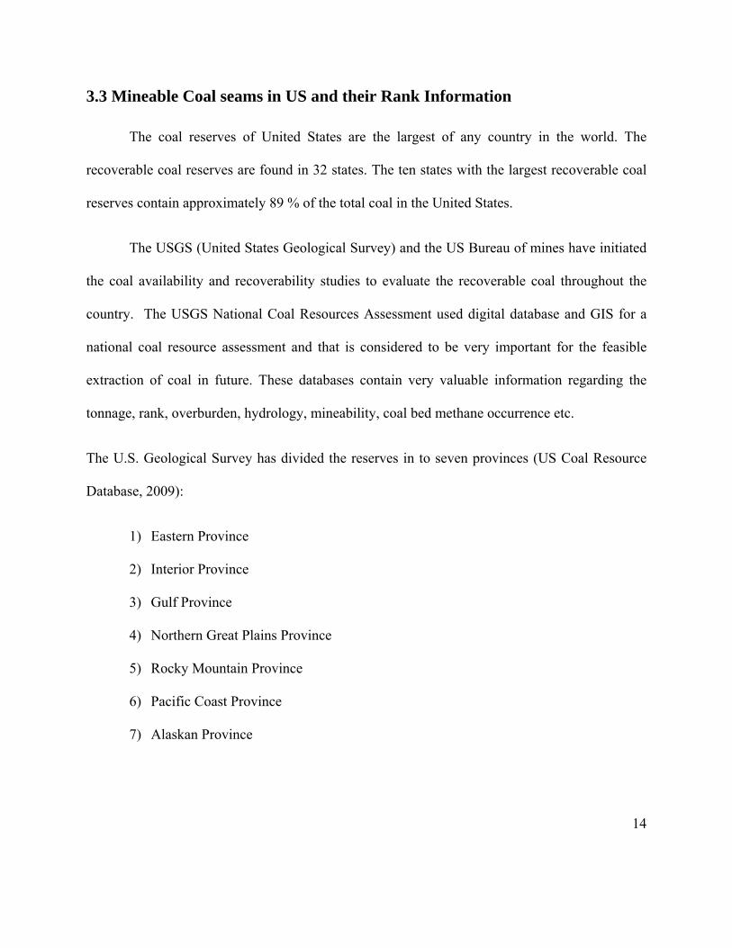
3.3 Mineable Coal seams in US and their Rank Information

The coal reserves of United States are the largest of any country in the world. The

recoverable coal reserves are found in 32 states. The ten states with the largest recoverable coal

reserves contain approximately 89 % of the total coal in the United States.

The USGS (United States Geological Survey) and the US Bureau of mines have initiated

the coal availability and recoverability studies to evaluate the recoverable coal throughout the

country. The USGS National Coal Resources Assessment used digital database and GIS for a

national coal resource assessment and that is considered to be very important for the feasible

extraction of coal in future. These databases contain very valuable information regarding the

tonnage, rank, overburden, hydrology, mineability, coal bed methane occurrence etc.

The U.S. Geological Survey has divided the reserves in to seven provinces (US Coal Resource

Database, 2009):

1) Eastern Province

2) Interior Province

3) Gulf Province

4) Northern Great Plains Province

5) Rocky Mountain Province

6) Pacific Coast Province

7) Alaskan Province

15

These provinces are further sub-divided into regions, fields and districts and they are clearly

represented in the figure 3.

1. Eastern Province:

The eastern province which is about 900 miles long and 200 miles wide majorly includes

the anthracite regions of Pennsylvania and Rhode Island, the Atlantic coast region of middle

Virginia and North Carolina and also the Appalachian basin which extends from

Pennsylvania, Tennessee and Alabama. There are about 760 million short tons of anthracite

in Eastern Pennsylvania in this province.

The Appalachian region is known to be the largest region of bituminous coal deposits in

the United States. The southern part of this basin’s coal is mainly of high volatile bituminous

rank also with some medium and low bituminous rank. The northern part of this region has

high volatile coal in the west to low volatile bituminous coal in the east. The central region

coal varies from low volatile to high volatile bituminous in rank.

2. Interior Province:

The interior province consists of 3 major regions that include the northern region

consisting of Michigan, the eastern region or the Illinois basin and the western region.

The Illinois basin consists of Illinois, southern Indiana and the western Kentucky. And the

western region consists of Iowa, Missouri, Nebraska, Kansas, Oklahoma, Arkansas and

western Texas.

16

This region has vast number of reserves in Illinois and western Kentucky. The coal in

this province is mainly bituminous in rank and tends to be lower in rank and higher in sulfur

than the Eastern Province bituminous coals.

3. Gulf Province

The Mississippi region in the east and the Texas region in the west are the main regions

of the gulf province. These coals are basically lignite in rank and are considered to be the

lowest rank coals in the United States which have moisture content up to 40%.

4. Northern Great Plains Province

The lignite deposits in North Dakota, South Dakota and Eastern Montana are part of the

Northern Great Plains. These are considered to be the largest lignite deposits in the world and

are present in the Fort Union Region. The sub-bituminous fields of the northern and eastern

Montana and northern Wyoming are also a part of the Northern Great Plains Province. The

states of Wyoming and Montana are considered to be the states with largest recoverable

reserves in United States. The reserves of the Wyoming state are shared by the Northern

Great Plains and the Rocky Mountain Province. The Northern Great Plains contains sub-

bituminous coal from the Powder River basin. The Powder River basin coals contain 1 %

sulphur with low ash content (3-10%) and are used as power station fuels.

17

5. Rocky Mountain Province

The mountainous districts of Montana, Wyoming, Utah, Colorado and New Mexico are

the major coal regions of the Rocky Mountain province. These coals rank varies from lignite

to anthracite. The coals from the areas of Wyoming, primarily from the Green River, Hanna

and Hanna Fork are the most prominent fields of this province and are sub-bituminous in

rank.

6. Pacific Coast Province

The deposits in Washington, Oregon and the California are of the Pacific Coast Province.

These coals are very limited and scattered and their rank range from lignite to anthracite.

7. Alaskan Province

The Alaskan province also contains coal in different regions and their rank ranges from

lignite to bituminous with little anthracite. The coal available in this area is considered to be

15% bituminous and 85% sub-bituminous and lignite. This province is not shown in the

figure.

T

minimum

for sub-b

(Source

The deep co

m thicknesse

bituminous c

e: http://en.w

lor represen

es included a

coal and lign

Figure 3: UUS Coal Reegions7

wikipedia.orgg/wiki/File:U

nts the areas

are 14 inche

nite. The ligh

Us_coal_reg

s of coal re

es for anthra

ht color repre

ions_1996.ppng)

eserves of g

acite and bit

esents the do

good comme

tuminous co

oubtful value

ercial value.

oal and 30 in

e for coal. T

. The

nches

his is

18

http://en.wikipedia.org/wiki/File:Us_coal_regions_1996.png

19

further divided into three regions: (1) areas containing thin or irregular beds, which have very

less or no value but thick enough to mine, (2) the areas with poor quality of coal (3) areas where

there is no enough information on the thickness and quality of the coal beds. The Alaskan

province is not shown in the above figure.

Table 2: Rank and location of different coal seams throughout United States

Region Location Coal Rank

Eastern

Pennsylvania and Rhode

Island, the Atlantic Coast

region of middle Virginia

and North Carolina

Some of the coal deposits are anthracite and this

region contains largest deposits of Bituminous coal

in United States. Northern region of the

Appalachian basin the coal rank ranges from high

volatile bituminous coal.

Interior Illinois and Western

Kentucky

The coal in this region is mainly bituminous in

rank and tends to be lower in rank and higher in

sulphur than the Eastern Province bituminous

coals.

Gulf Mississippi, Louisiana and

Texas

The coal in these regions is lowest rank coals in the

United states having moisture contents up to 40 %.

Northern

Great

Part of Wyoming, North

Dakota, South Dakota,

Sub-bituminous fields in Northern and Eastern

Montana and Northern Wyoming. And lignite

20

plains Eastern Montana deposits are contained in the Fort Union Region

and are the largest lignite deposits in the world.

Rocky

Mountain

Montana, Wyoming, Utah,

Colorado, and New Mexico.

The coals from Wyoming primarily from the Green

River, Hanna Fork coal Fields are sub Bituminous.

Pacific

Coast

Washington, Oregon and

California These coals range from lignite to Anthracite

3.4 Coal Production in USA

Coal production in USA grew steadily over years. In 1950 the coal was consumed by

various sectors like industrial, residential and commercial, metallurgical coke ovens, electric

power and transportation. These sectors distributed the consumption evenly with 5 to 25 % of the

total consumption. The use of coal for rail and water transportation has been declined since the

Second World War however with the growth after the war; the demand of coal grew rapidly with

increased electricity generation. From the graph we can see that the coal production in 1950 was

560 Million Short Tons and in 2003 was 1.07 Billion Short Tons. There has been an average

increase of 1.2 per every year since 1950. Presently the coal demand is majorly controlled by the

electric power sector which accounts for 90 % of the consumption compared to the 19 % it

represented in 1950. With the increase in the demand for electricity, the demand for coal

generation also increased and that resulted in increased coal production (Coal Production in US,

2006). The figure 4 explains the rate coal production in United States over years.

Figure 4: Coal production in USA 1890-20058

(Source: Coal Production in the United States, Energy Information Administration, Oct 2006)

As the coal production in United States is increasing steadily it is clear that the high

quality coal is nearing its end. From the graph we can see that the anthracite production has been

declining steadily since 1950 and the bituminous coal is also declining since 1990. Even though

the anthracite and bituminous coal productions are declining the total production is still

increasing about 20 MT per year since 1960. Since the past few years the production of the low

quality sub-bituminous and low quality lignite has been increasing substantially. This is majorly

responsible for the increase in the total production of the coal (Energy Watch Group, 2007). The

figure 5 below represents the production rates of different grades of coal in United States over

years.

21

Figure 5: Different grades of Coal Production in USA9

(Source: Coal: Resources and Future Production, Energy Watch Group, March 2007)

3.5 Mining methods

Mining is the economical extraction of the valuable minerals from the ore body from the

Earth’s crust. The most economic method of extraction basically depends on the depth and the

geology of the coal seam. The coal mining processes are differentiated by surface and

underground extraction. Most of the seams are considered as too deep for surface mining and

require underground mining. Based on the characteristics of the coal seams different methods are

employed for extraction.

22

23

The selection of mining method is mainly dependent on the geology of the deposit and the

extent of ground support needed to make the method productive and safe. The two major

methods of extraction involved in underground mining of coal are:

1. Room and Pillar Mining (Continuous Mining): This method is oldest method which is

applied to horizontal or nearly horizontal deposits and is used in both coal and non-coal

mining. This method is considered to be very cheap, easily mechanized, highly

productive and is also simple in design. Compared to longwall mining this method is

flexible and does not require high capital and development costs.

Room and Pillar method of mining is an open stoping method and is applied in a

competent rock where the roof is primarily supported by the pillars. The coal is extracted

from the rectangular or square shaped pillars driven into the coal seam leaving parts of

coal between the entries to support the roof. Continuous miners are used for extraction in

this method. The dimensions of the pillars formed depend on many design factors like the

strength of the ore, the thickness of the deposit, depth of the mining etc. our main goal is

extract maximum percentage of coal from the ore body under safe working conditions.

The left out coal after the ore extraction is considered non recoverable but in some cases

it can be recovered by backfilling which is one of the limiting factors for this method

especially when mining at greater depths. Generally the pillars are recovered by retreat

mining which allows the roof to cave and thus relieves the stress and reduce bumps.

Even though the advance rates are much higher in longwall method all except

very minor faults should be avoided and with this large areas of reserve are not mineable

24

and give much lower recovery rate than retreat Room and Pillar mining method which is

highly flexible. (Hartman, H.L., and Mutmansky, J.M., 2002)

2. Longwall mining: This method of mining is employed where the deposits are tabular,

horizontal and having a thickness from 3 to 8 ft, and dipping at less than 120, and lying at

depths up to 3000 ft or more. In this method a system of props are employed to support

the roof and the working areas. These supports advance with the face and are responsible

for the caving of the roof in the mined out area. The over lying deposits should be thin

bedded, and cave freely in order to implement this method. Also the floor should be

sufficient strong enough to support the prop loads.

In this method of mining the panel layout is very simple and provides good

ventilation and always safe to work under the supported roof. This is considered to be

much safer than the room and pillar method and complies easily with current US laws. As

the coal is extracted completely with leaving lesser residual pillars with full caving the

coal recovery is higher and the surface subsidence is uniform and complete.

In United States retreating longwall is generally followed. The entries on the both

sides of the panel are called head gate and tail gate where head gate is used for the intake

air and coal transportation and the tail gate is for the return air. The coal at the face is cut

by a shearer and is loaded on the armored flexible conveyor (AFC) and is then transferred

to the stage loader and then to belt conveyor. A series of powered supports are used to

support the roof and these supports along with the AFC advance with the face. This

25

method of roof control is called as roof caving method. The area behind the supports after

the face advances is called as gob. (Hartman, H.L., and Mutmansky, J.M., 2002)

3.6 Mining costs

The success of a mining company mainly depends on the cost of the product and the sales

realization. This means that the costs for every mining operation have to be pre-calculated in

order to have a good idea of the costs and prices. This is considered to be a very difficult task as

it involves lot of variables which vary with different conditions. The wide variety use of

equipment and variation in the working conditions makes very complex to get the results very

accurately. Mining costs are mainly dependent on the nature of the deposit and the type of

extraction. It is not like we use a lowest cost mining method to extract the ore but we should

employ a method which result the lowest cost per unit of product when mining costs and

treatment are considered together. Ventilation is the most useful and mostly used process

underground because of the extent of its demand and it might get complicated and costly when

the distance that air must travel from the surface to ventilation face is increased.

There are different kinds of costs involved in mining.

1. Capital costs: The capital costs mainly include the cost of new equipment, taxes, wages

etc.

2. Operating costs: Operating costs are calculated according once the method of extraction

and the output rate have been established. These costs mainly include things like

production, labor, materials, supplies, maintenance, drilling, blasting, loading etc. The

26

labor costs are estimated by establishing the crews needed to operate a mine production

section.

Many of the mining companies claim to have model that estimate the mine costs. The mine

cost analysis which is very expensive seems to be done on individual computer models. The

major research organizations disclose sufficient details of their models and operational variables

to validate their cost analysis, and usually provide their models in electronic for purchases. The

cost estimates are always dependent on the complete technical information of the mine.

3.7 Previous Cost Models

Many companies would like to know what would be the capital cost and the operating

cost before starting the actual production. As no one can estimate the exact figure as it is very

difficult, it is very important the how accurate the model can predict the cost of extraction. Some

of the cost estimation models are derived before and they are explained below.

US Bureau of Mines Cost Estimating System

One of the best mine cost modeling systems in US is US Bureau of Mines Cost

Estimating System or CES which was developed in the USBM’s Field Operations Centers and

by well known mining Engineering consultants. Cost Estimation System (CES) is developed for

estimating the capital and operating costs for development and operations at mineral properties.

The system can be customized according to the availability of engineering and other operating

data.

27

The cost equations in CES are based on individual cost estimates for a variety of

capacities, based on current technology applicable to each section. Regression analysis is then

applied to the individual costs at the various capacities or size ranges using actual mine operating

data to produce the resulting cost equations. Each section of CES has capital and operating costs

appropriate for the specific unit process, plus descriptive text planning what aspects of a typical

operation are included in the cost equations for that section. Capital and operating costs are

usually expressed in three equations: labor, supply, and equipment.

SME Handbook

According to the SME handbook estimation of costs is being done in a different way. The

accuracy of the estimation of capital costs and operating costs depends on the quality of the

technical assessment and knowledge of expected mining and mineral processing conditions.

Accurate operating costs are estimated from the quantities and unit costs of all components. The

capital costs and operating costs of a mining project will be influenced by many factors that must

be assessed before costs can be estimated for a preliminary feasibility study. (Mine Cost Models,

USBM, 2009)

28

4. Characteristics of US Coal Reserves

The United States coal reserves are considered to be larger than the present natural gas and

oil resources. These reserves are identified throughout the country by Energy Information

Administration (EIA) and the remaining tons of coal are updated every year in the Demonstrated

Reserve Base (DRB). As the data quality of the coal resources is poor, EIA has started updating

the records through coal reserve database program (CRDB). In this program the states are

encouraged to revise the coal reserves in their respective states and collect the data and are

further updated in the Demonstrated Reserve Base by EIA. The estimation of the current reserves

provides information regarding the actual amount of coal that is actually available for extraction

in future. (Luppens, J.A., et al., 2009)

This data collected gives a comprehensive view of the coal resources based on the past and

current coal production and makes an analysis to provide an outlook on the possible coal

production in the coming decades. The EIA has taken initiative and proposed a new project in

2008 to incorporate the existing reserves data into a geographic information system (GIS) based

program. This includes the current and the USGS data.

In this regard, my application of the ARC GIS software is to incorporate the available coal

resource data taken from the EIA and USGS into the software and create mappings to view

different characteristics and availability of the coal resources throughout the country. The

databases are designed to represent several things like the total amount of recoverable coal

29

reserves, production from surface and underground, number of mines in each state, sale price of

coal, measured and indicated coal reserves in different regions throughout the country.

4.1 ARC GIS 9.3

Introduction

GIS is one of the most powerful technologies that focuses on integrating the data from

multiple sources and creates cross cutting environment for collaboration. It is also attractive to

all people as it is intuitive and cognitive. It combines a strong analytic and modeling framework

that is rooted in the science of geography.

Basically there are three fundamental views in GIS. They are:

1. Geo-database View: The geographic information is basically managed by GIS and it is

considered as a spatial base containing different datasets that represent geographic

information. The datasets are like map layers which are geographically referenced to

overlay on to the earth’s surface.

2. Map View: GIS is a set of intelligent maps and views where different features and

feature relationships are shown. Various map vies of the underlying geographic

information can be constructed and used as “windows into the geographic database” to

support query, analysis, and editing of geographic information. A series of two

dimensional or three dimensional map applications are provided in GIS for working with

geologic information through these views.

30

3. Geo-processing View: GIS is a set of information transformation tools that derive new

information from existing datasets. These geo-processing functions take information from

existing datasets, apply analytic functions, and write results into new derived datasets.

In this study Arc Map is used for incorporating the database into the software and views the

results.

ARC MAP

ARC MAP is the central application used in Arc GIS. The data sets which we take into

consideration are being studied in this area. We can create and edit datasets and also create map

layouts for printing in this area. The map represents the geographic information as a collection of

layers and other elements in a map.

Arc Map documents

Once we create the map using this application it is saved with filename extension .mxd

on the disk. The map documents contain display properties of the geographic information we

work within the map like the map layers, data frames etc.

Views in Arc Map

The map contents in an Arc Map are displayed in one of the two views below. Each view

makes us to look and interact with the map in a specific way:

• Data view

• Layout view

31

Tables

Tables are generally made up of rows and columns and it is necessary that all rows

should have the same columns. In GIS, the rows are termed as records and the columns as fields.

Each field can store a specific type of data like a number or a text. In our databases the fields are

the rank, tonnage, depth, production, productivity etc and the records are the states and the

counties. The databases used in this work are made in the form of tables for simple usage. The

records of one table can be associated to another table in this software. This can be done by using

joins or creating relationship classes in our geo-database.

Joins

The application of Joins is generally used whenever we need to append the fields of one

table to those of another through an attribute or field which is common in both the tables. We can

define the join based on the attributes or a pre-defined geo-database relationship. Number of

tables can be joined to a single table. When a join table is removed, all the data from the tables

which were joined after it is also removed, but the data from previously joined tables remain. We

can add the tables from different sources to the Arc Map in the similar way as we add data to our

map. The attributes of a layer on a map can be explored by opening its attribute table and find

features with particular attributes. We can open multiple tables at a time in Arc Map.

Adding tables to a layout

We can display the attributes tables to edit and make a selected appearance on the layout.

We can select the rows which can be displayed on the layout by arranging the data in the table

window beforehand.

Identify function

This function is primarily used for the identification of the attributes of the selected area.

The data from the tables which is incorporated into the map can be viewed directly by using this

function. We can edit the fields that are needed to display in this function.

Select by attributes function

This function is used for query building. As the name suggest “select by” indicates that

we can select the desired set of results by developing a query and using it in the select by

attributes function. In the query builder the number values should be given in single quotes.

4.2 Sources for the Data

The production and productivity data, recoverable reserves data, average mine sale price

data are primarily obtained from the annual coal report tables 2008.

The measured and indicated reserves data is obtained from the US Coal Resources

Database. The location, quality and several characteristics of coal are available in the database.

The coal tonnage for a specific area like state or county is estimated and the rest of the 32

javascript://void()�

33

characteristics are given in terms of USGS classification system. The published US coal

resources estimates are organized by state, county, coal field, geologic age and formation, rank,

thickness of coal, thickness of overburden and reliability of data.

List of databases

1. Average sale price of coal by state and coal rank (2008).

2. Coal production and number mines in different states at county and state level (2008).

3. Complete database of the recoverable coal reserves, estimated recoverable reserves and

Demonstrated Reserve Base (DRB) by mining method (2008).

4. Recoverable coal reserves and the recovery percentage at producing mines 2008, 2007.

5. Underground coal production and productivity by state and mining method (2008).

6. USGS measured and indicated reserve database.

4.3 Methodology

The databases are primarily designed in Excel for simple usage. A different set of

databases are taken as sources and used in this software to obtain the results. The datasets are

obtained from the United States Geological Survey and the Energy Information Administration

and are the main sources for the data used in this study. The datasets taken from the sources are

defined in a used defined database form.

The USA maps at state level and county level are viewed by adding the .shp files into the

arc map. The .shp files that are required for loading the maps are obtained from ESRI. We can

change the color of the map to get the desired view. After adding those files, data the database

34

tables which are designed in Excel are then added to the same layer. The attributes of the

database defined can be viewed by right clicking on the database added and open.

It is required that the fips codes for the states and the counties in the designed databases

are added as they are used as the primary key for incorporating the data into the map. The fips

codes in the database tables are required to be entered in string format as they are in the text

format in the shape file.

In order to incorporate this data on to the map, the database table should be joined to the

shape file using fips code as the primary key. This can be done by right clicking on the shape file

and got to joins and relates and then join. We have to select the field in that layer in which the

join bases on and select the same field as they act as the primary keys and then click ok.

This adds the data present in the database table to the main table and they can be further

viewed by using Identify function. The identify function which is indicated by letter “i” is

located in the tool bar. All we need to do is click on the identify function and then click on the

desired location to view the characteristics of that location. Using select by attributes function we

can define different queries to view the selected data on the map. The data highlighted in the map

represents the areas which satisfy the written command.

4.4 Results

The following views are some of the results obtained after incorporating the database

elements into the software. The results are completely based on the input elements given in the

databases.

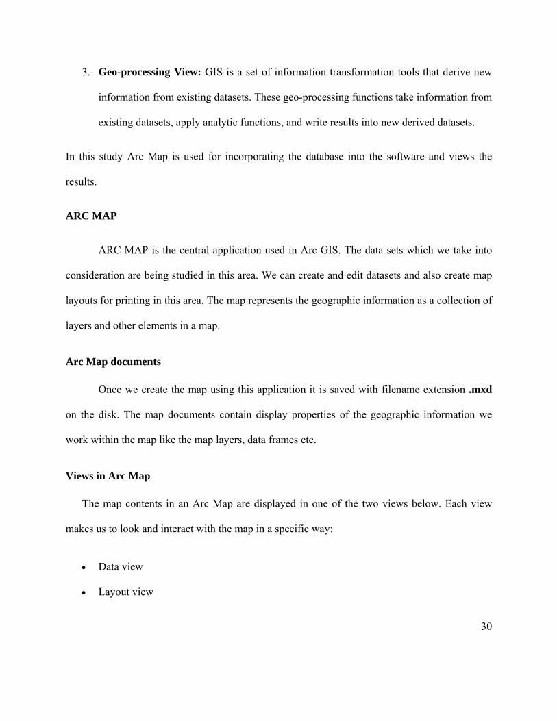
The figure 6 represents the screen shot of the map showing different states in United States in

ARC MAP after loading the states shape file.

Figure 6: Screen shot of the United States map showing different states

35

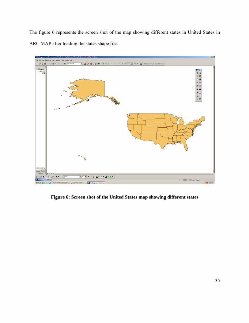
The figure 7 shows the screen shot of the map showing counties of different states throughout the

United States.

Figure 7: Screen shot of the United States map showing counties of different states

To view the areas where the bituminous coal throughout the United States at county

level, we need to add the USGS measured and indicated reserves database table to the map and

join with the shape file. In the select by attributes function we need to define the following

query:

SELECT * FROM COUNTIES Database$ WHERE “Database$.Rank”=’BIT’

36

37

After writing the query we need to verify whether there are any errors by clicking the

“verify” button. After the expression is successfully verified click OK to view the result on the

map. The characteristics data of a particular county can be further checked by using the identify

function.

A screen shot of the view after successfully executing above defined query. The

following figure represents the coal regions (counties) of United States where the measured and

identified bituminous coal reserves are available.

Query:

“Database$.Rank” =’BIT’

Figure 8: Counties of Bituminous coal rank in United States.

38

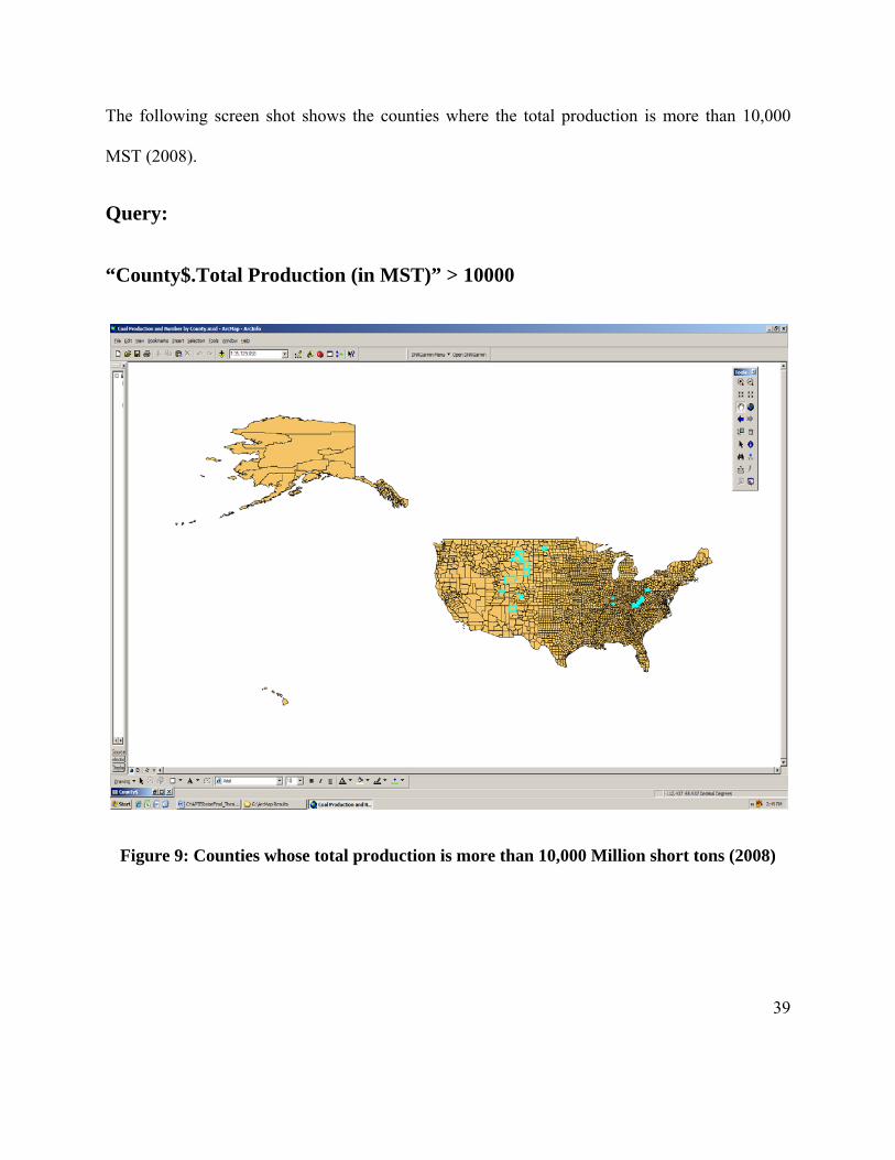
The following screen shot shows the counties where the total production is more than 10,000

MST (2008).

Query:

“County$.Total Production (in MST)” > 10000

Figure 9: Counties whose total production is more than 10,000 Million short tons (2008)

39

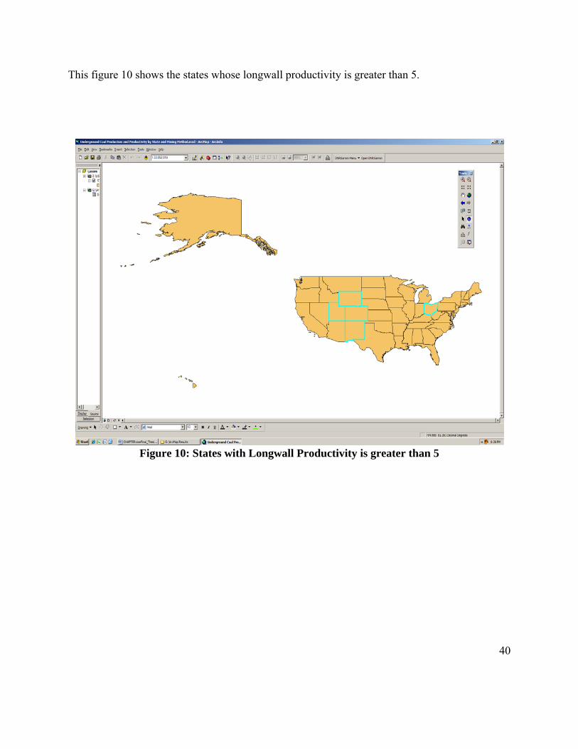
This figure 10 shows the states whose longwall productivity is greater than 5.

40

Figure 10: States with Longwall Productivity is greater than 5

41

5. Recovery Ratio

Over recent years it has been observed that the reserve to production ratio has been falling.

We are at a point at which the maximum coal production rate is reached and from here on now it

is found that the rate of production will enter irreversible decline. So considering the extinction

of these valuable fossil fuels it is necessary that we have to use them very efficiently. The

reserves which are available now can be extended further by various developments like

improving the exploration activities to find new reserves and implementation of advanced

mining techniques which will allow the inaccessible reserves to be reached which improves the

recovery ratio of extraction.

The recovery ratio of extraction of coal by underground mining varies a lot with the surface

mining of coal. In underground mining, some portion of the coal is left as pillars to support the

roof and this portion of coal is left out and cannot be recovered. In addition to this some amount

of coal is lost with the geological disturbances like folding, faulting etc and this limits the

recovery ratio. It’s been a challenge for the engineers today to extract the maximum percentage

of coal from the total recoverable reserves where the depth of mining is increasing gradually and

the recovery ratio is decreasing.

The estimation of the recovery ratio of the pillars in room and pillar method of mining is

made in this study. This is done by calculating the size of the pillar as a function of mining depth

and mining height. One of the important aspects involved in room and pillar method is the design

of the pillars. The ground control in this method is completely dependent on the pillar design.

42

Many theories have been proposed and there has been a substantial progress in the design over

years. (Mark, C., 2006)

5.1 Pillar Design

In order to have a good recovery ratio at a given mining condition using room and pillar

method, the design of pillars should be properly done in order to prevent the underground mine

structural failures and subsidence. This can be done by designing square pillars in a plan view.

The size of the pillars is calculated as a function of coal depth and mining height so that it is

easier to determine the size of the pillar at a desired depth.

The size (i.e., the side length, W, ft) of the pillar mainly depends on the in-situ strength of the

coal (σi), the overburden depth, room width, mining height and the pillar safety factor (SF). The

Strength of the pillar is estimated using Bieniawski formula. The size of the pillar can be

obtained by solving the non-linear equation 1.

1.1 · · · 0.64 0.36 (1)

Where W is the side length, ft

σi is the in-situ strength of the coal, psi

h is the overburden depth, ft

Wr is the room width, ft

H is the mining height, ft

43

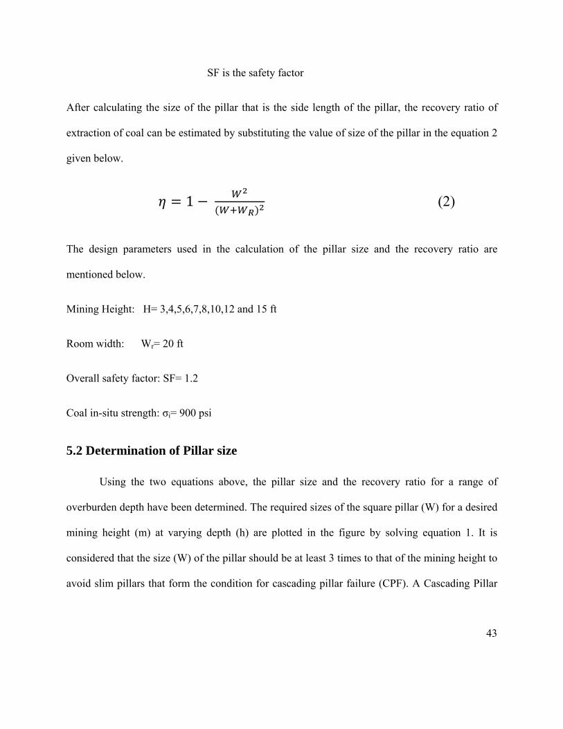
SF is the safety factor

After calculating the size of the pillar that is the side length of the pillar, the recovery ratio of

extraction of coal can be estimated by substituting the value of size of the pillar in the equation 2

given below.

1 (2)

The design parameters used in the calculation of the pillar size and the recovery ratio are

mentioned below.

Mining Height: H= 3,4,5,6,7,8,10,12 and 15 ft

Room width: Wr= 20 ft

Overall safety factor: SF= 1.2

Coal in-situ strength: σi= 900 psi

5.2 Determination of Pillar size

Using the two equations above, the pillar size and the recovery ratio for a range of

overburden depth have been determined. The required sizes of the square pillar (W) for a desired

mining height (m) at varying depth (h) are plotted in the figure by solving equation 1. It is

considered that the size (W) of the pillar should be at least 3 times to that of the mining height to

avoid slim pillars that form the condition for cascading pillar failure (CPF). A Cascading Pillar

44

Failure (CPF) event is a rapid failure of pillars in a large area that could cause serious safety

problem to a mining operation.

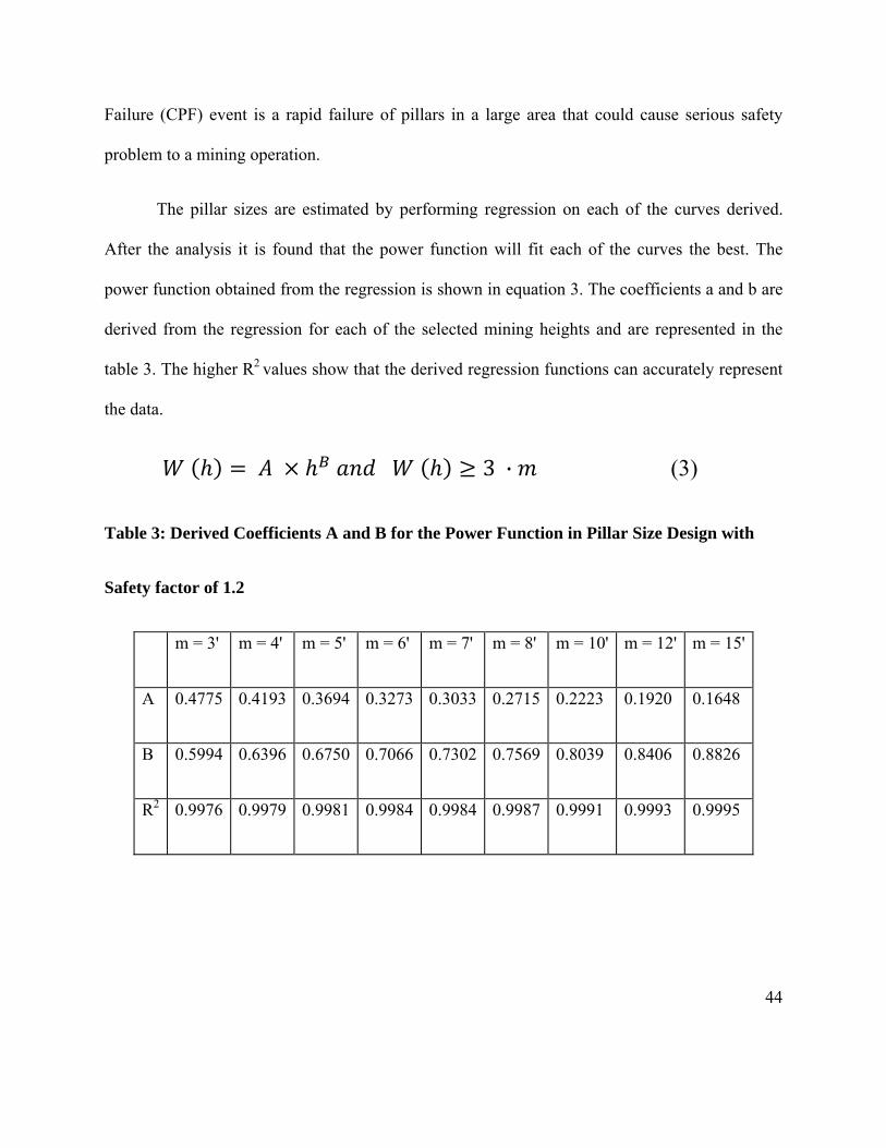
The pillar sizes are estimated by performing regression on each of the curves derived.

After the analysis it is found that the power function will fit each of the curves the best. The

power function obtained from the regression is shown in equation 3. The coefficients a and b are

derived from the regression for each of the selected mining heights and are represented in the

table 3. The higher R2 values show that the derived regression functions can accurately represent

the data.

3 · (3)

Table 3: Derived Coefficients A and B for the Power Function in Pillar Size Design with

Safety factor of 1.2

m = 3' m = 4' m = 5' m = 6' m = 7' m = 8' m = 10' m = 12' m = 15'

A 0.4775 0.4193 0.3694 0.3273 0.3033 0.2715 0.2223 0.1920 0.1648

B 0.5994 0.6396 0.6750 0.7066 0.7302 0.7569 0.8039 0.8406 0.8826

R2 0.9976 0.9979 0.9981 0.9984 0.9984 0.9987 0.9991 0.9993 0.9995

Figure 11:: Sizes of thee coal pillarr at Differennt depths annd Mining HHeights

A

15 it is u

the calcu

A and B

relationsh

vapor pre

As the pillar

unnatural tha

ulation much

in the pow

hip between

essure mode

sizes are est

at the mining

h easier, the

wer function

n coefficient

l.

timated for

g heights sho

relationship

of equation

(A) and min

different mi

ould be one

p between th

n 3 is studied

ning height

ining heights

of the above

he mining he

d. After the

(m) can be

s like 3, 4, 5

e values. So

eight (m) and

analysis it

represented

5, 6, 7, 8, 10

in-order to m

d the coeffic

is found tha

by the follo

0, 12,

make

cients

at the

owing

45

46

/ . (4)

In the similar way the relationship between the coefficient (B) and the mining height (m) is

represente n fun ion. d by an exponential associatio ct

(5)

The coefficients for each of the two empirical functions are listed in Table 4.

Table 4: Results of the regression studied for the coefficients A and B in the power function

Reg

ress

ion

Stud

ies f

or

the

Coe

ffic

ient

s

Coefficient a Coefficient b Vapor Pressure Model: Exponential Association: y=exp(a+b/x+cln(x)) y=a(b-exp(-cx))

a = 0.94906 a = 0.54774 b = -1.84890 b = 1.84267 c = -0.97667 c = 0.09773 R = 0.99940 R = 0.99980

m Original Fit Error % Error Original Fit Error % Error 3 0.4775 0.4770 0.0005 0.10% 0.5994 0.6008 -0.0014 -0.23% 4 0.4193 0.4202 -0.0009 -0.21% 0.6396 0.6388 0.0008 0.13% 5 0.3694 0.3706 -0.0012 -0.33% 0.6750 0.6733 0.0017 0.25% 6 0.3273 0.3299 -0.0026 -0.79% 0.7066 0.7046 0.0020 0.29% 7 0.3033 0.2965 0.0068 2.23% 0.7302 0.7329 -0.0027 -0.38% 8 0.2715 0.2690 0.0025 0.91% 0.7569 0.7587 -0.0018 -0.23% 10 0.2223 0.2266 -0.0043 -1.92% 0.8039 0.8032 0.0007 0.09% 12 0.1920 0.1956 -0.0036 -1.85% 0.8406 0.8398 0.0008 0.10% 15 0.1648 0.1622 0.0026 1.59% 0.8826 0.8828 -0.0002 -0.03%

The relat

figure 7 a

tionship betw

and figure 8

ween the m

.

ining heightt (m) and thhe coefficiennts A and B is plotted iin the

Figure 122: Relationsship between Coefficiennt A and Mining Heighht (m)

47

Figure 133: Relationsship betweeen Coefficiennt B and Miining Heighht (m)

5.3 Determinatioon of the RRecovery RRatio:

T

is determ

calculate

be practic

The recovery

mined. Using

ed and plotte

cal.

y ratio of the

g the equatio

d in the figu

e pillar can b

on 2 the reco

ure 9. The re

be easily cal

overy ratio fo

covery ratio

culated once

or various m

s greater tha

e the size of

mining heigh

an 75 % are

f the square

hts and depth

considered n

pillar

hs are

not to

48

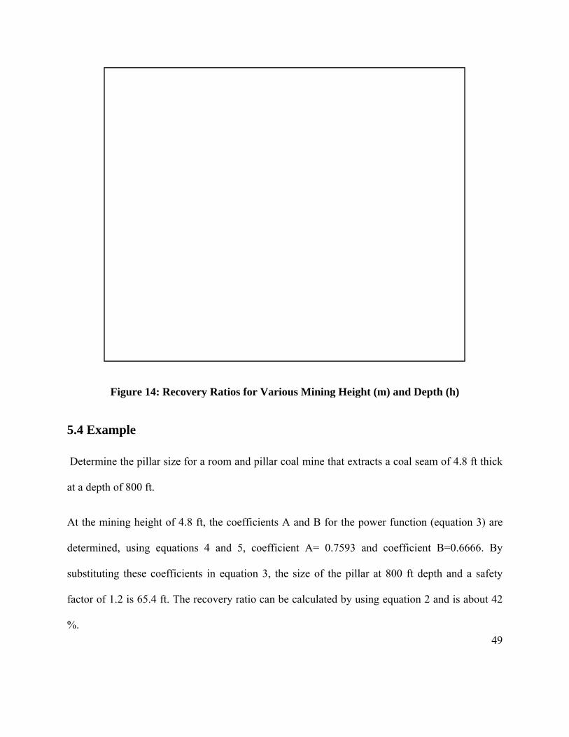
Figure 14: Recovery RRatios for VVarious Minning Height (m) and Deepth (h)

5.4 Exaample

Determi

at a depth

ne the pillar

h of 800 ft.

r size for a rooom and pilllar coal minne that extraccts a coal seaam of 4.8 ft thick

At the m

determin

substituti

factor of

%.

mining height

ned, using e

ing these co

f 1.2 is 65.4

t of 4.8 ft, th

equations 4

oefficients in

ft. The recov

he coefficien

and 5, coe

n equation 3

very ratio ca

nts A and B

efficient A=

3, the size o

an be calcula

B for the pow

0.7593 and

of the pillar

ated by usin

wer function

d coefficien

at 800 ft de

ng equation 2

n (equation 3

nt B=0.6666

epth and a s

2 and is abo

3) are

6. By

safety

out 42

49

50

6. Mining Economics

In an industrial system it is very important to assess the costs before developing it. Coal

mining can be done only where the coal is technically feasible and economically profitable. So, it

is important for us to assess the costs before extracting the ore. The most economic method of

extraction mainly depends on the depth, thickness, geology of the coal seam and the

environmental factors. Ventilation is often the second most essential auxiliary operations next to

ground control in underground mining operations. In underground mines, good production and

environment conditions can be satisfied by providing sufficient quantities of air to the work

places. Under adverse conditions 10-20 tons of air has to be provided for each ton of coal

produced. This involves a large cost, as there is huge energy consumption in order to the force

the air to the mine openings. In order to decrease the ventilation cost suitable ventilation system

must be designed which is functionally reliable and cost effective. As the coal mining will be

conducted in deeper ground in the future, the ventilation cost will substantially increase.

The success of a mining company mainly depends on the cost of the product and the sales

realization. This means that the costs for every mining operation have to be pre-calculated in

order to have a good idea of the costs and prices. This is considered to be a very difficult task as

it involves lot of variables which vary with different conditions. The wide variety use of

equipment and variation in the working conditions makes very complex to get the results very

accurately. Mining costs are mainly dependent on the nature of the deposit and the type of

extraction. It is not like we use a lowest cost mining method to extract the ore but we should

51

employ a method which result the lowest cost per unit of product when mining costs and

treatment are considered together. Ventilation is the most useful and mostly used process

underground because of the extent of its demand and it might get complicated and costly when

the distance that air must travel from the surface to ventilation face is increased.

6.1 Estimation of Ventilation Costs

Mine ventilation cost is one of the major cost items in a coal mine operation. The

methods in SME handbook for estimating the ventilation costs are used as the base methods for

calculation. The base costs calculated from those methods are then adjusted by the coal seam

(rank) and mine depth. The capital and operating costs for a ventilation system are entirely based

on the horsepower requirement for the mine which in turn is dependent on the gas emission and

fan head needed. (Hartman, H.L., 1992)

6.2 Base method for Estimating Ventilation Requirement

The ventilation requirement includes the quantity of the ventilation air (Q) and fan head

(H). In SME handbook, these two values for coal mines are estimated using the following two

equations based on i p t da ly roduc ion:

500 . (1)

2.4 . � (2)

Where T is daily production in Short Tons

52

The installed fan horsep P) is th ower (H en estimated as

(3)

6.3 Ventilation Capital Cost

In general, the most reliable method to estimate the capital cost for an installed

ventilation system is the total installed horsepower (HP) of all ventilation fans in the system. For

underground coal mi s i Cc) is estimated by the following equation: ne , the cap tal cost (

7500 . (4)

6.4 Ventilation Operating Cost

The ventilation operating costs is mainly the electricity cost. Since the ventilation system

will operate year ro st for a m n v ntilation system will be: a und, the annual operation co i e e

0.75 24 365 (5)

Where, c is the electricity cost per kilowatt-hour.

Based on this method the capital and the annual operating costs for a coal mine

ventilation system are calculated for normal range of underground coal mine production and

plotted in figure 15.

$0.00

$200,000.00

$400,000.00

$600,000.00

$800,000.00

$1,000,000.00

$1,200,000.00

$1,400,000.00

$1,600,000.00

0 10000 20000 30000 40000 50000 60000

Cos

t /ye

ar

Daily Production, Tons/day

Ventilation Costs, Pittsburgh Seam @ 600 ft Depth

Capital

Operating

Figure 15: Base Capital and Annual Operating Costs of a Mine Ventilation System

6.5 Adjustments to the Ventilation Requirement

Underground coal mines are operated in different coal seams and at different depths.

These differences make the gas content in a ton of the mined coal vary considerable. The

required ventilation air quantity is to dilute the emitted gas to the underground to safe levels. It is

assumed in this study that the gas emission is proportional to the gas content. It has been

demonstrated by studies that the gas content in coal is function of the coal rank and mining depth

(related to the reservoir pressure). Therefore, the required ventilation air quantity (Q) depends on

the coal rank and mining depth.

53

54

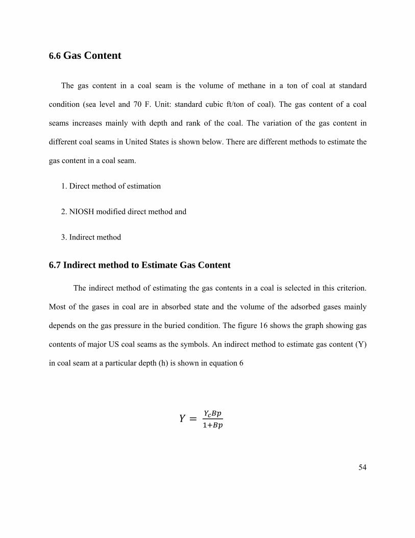
6.6 Gas Content

The gas content in a coal seam is the volume of methane in a ton of coal at standard

condition (sea level and 70 F. Unit: standard cubic ft/ton of coal). The gas content of a coal

seams increases mainly with depth and rank of the coal. The variation of the gas content in

different coal seams in United States is shown below. There are different methods to estimate the

gas content in a coal seam.

1. Direct method of estimation

2. NIOSH modified direct method and

3. Indirect method

6.7 Indirect method to Estimate Gas Content

The indirect method of estimating the gas contents in a coal is selected in this criterion.

Most of the gases in coal are in absorbed state and the volume of the adsorbed gases mainly

depends on the gas pressure in the buried condition. The figure 16 shows the graph showing gas

contents of major US coal seams as the symbols. An indirect method to estimate gas content (Y)

in coal seam at a particular depth (h) is shown in equation 6

B

p-

b-

h-

- Volume to

– Character

Reservoir p

Modified se

Depth of se

Figure 16

o cover and

istic constan

pressure, atm

eam characte

eam, ft

(6)

6: Gas Conte

saturate the surface commpletely, ft3

nt of the coall seam, atm-1

m, p = d/3 psii =0.022682 d atm (1 psi=0.068046 atm)

eristic

ent in Majoor US Coal SSeams

55

56

Non linear regressions have been performed on the measured data and the coefficients of

the coal seams are listed in table and the regression curves are plotted back into figure 16. The

high r values indicate good fitting to the data.

Table 5: Determined Regression Coefficients for the Selected Coal Seams

Seam Castlegate Seam Illinois No.6 Pittsburgh Seam Pocahontas No.3 Hartshorne Seam

Yc= 352.77 392.44 360.58 498.29 607.76

b = 0.00164 0.00075 0.00301 0.00419 0.00293

r = 0.9961 0.9990 0.9990 0.9907 0.9873

6.8 Correction Factor to Ventilation Air Quantity:

It is assumed that the empirical equation for estimating the air quantity in the SME

handbook is of the Pittsburgh coal seam at a depth of 600 ft. A correction factor should be

applied for mining conducted in the other coal seams and at different depth. Based on this

assumption, the empirical equation for the correction factors is shown in equation7 and the

coefficients in the empirical equation are listed in Table 2. The correction factors for different

coal seams (S) and depth (h) are plotted in the figure. And the adjusted air quantity is estimated

by using the equation 8.

, (7)

, (8)

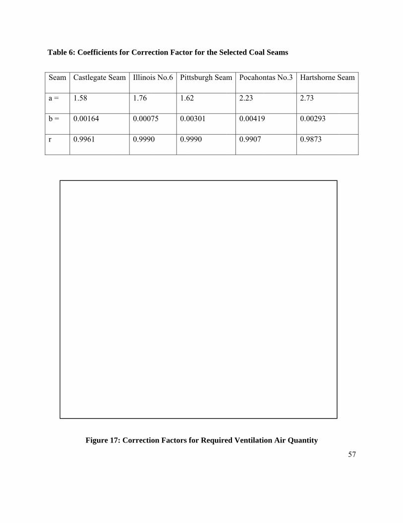
Table 6: Coefficientts for Correection Factoor for the Seelected Coall Seams

Seam C

a = 1

b = 0

r 0

Castlegate Se

1.58

0.00164

0.9961

eam Illinoi

1.76

0.000

0.999

Figure 1

is No.6 Pit

1.6

75 0.0

0 0.9

17: Correcti

ttsburgh Seam

62

00301

9990

ion Factors

m Pocahon

2.23

0.00419

0.9907

for Require

ntas No.3 H

2

9 0

0

ed Ventilati

Hartshorne S

2.73

0.00293

0.9873

Seam

on Air Quaantity

57

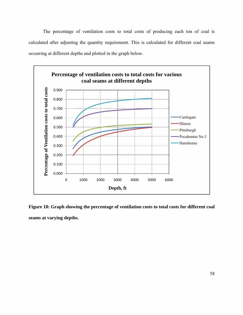
The percentage of ventilation costs to total costs of producing each ton of coal is

calculated after adjusting the quantity requirement. This is calculated for different coal seams

occurring at different depths and plotted in the graph below.

0.000

0.100

0.200

0.300

0.400

0.500

0.600

0.700

0.800

0.900

0 1000 2000 3000 4000 5000 6000

Perc

enta

ge o

f Ven

tilat

ion

cost

s to

tota

l cos

ts

Depth, ft

Percentage of ventilation costs to total costs for various coal seams at different depths

CastlegateIllinoisPittsburghPocahontas No.3Hartshorne

Figure 18: Graph showing the percentage of ventilation costs to total costs for different coal

seams at varying depths.

58

59

6.9 Example:

Determine the ventilation requirement and ventilation costs for a coal mine extracting in the

Hartshorne seam at a depth of 1800 ft. the daily production is 20,000 tons and electricity cost is

$0.04/Kilo watt-hour.

Based on SME handbook method and the above adjustments, the ventilation requirement is

determined. The air quantity required is first estimated by using the base methods of SME and

then later a correction factor for the given seam is applied and the adjusted air quantity is

calculated. The capital and operating costs are further calculated by using the adjusted air

quantity.

Quantity = 1,379,730 cubic feet per min

H = 6.46 inches of water

Correction factor, C(S, h) = 2.29

Adjusted Air Quantity, Q' = 3,166,200 cubic feet per min

Horse Power = 5,383 hp

Capital cost Cc = $1,299,200

Annual operating cost Co= $1,414,650

60

7. Conclusion

This thesis discusses the coal resource assessment and the use of ARC GIS software to project

the information regarding different characteristics of coal, production scenarios, reserve

availability, on a map. This makes the users much more convenient than to go through the tables

and analyze the data for reference. The query builder in this software is mainly used to acquire

the desired results. Analysis of these coal resources has implied the demand of coal in the present

era and that forced us to extract coal under more challenging conditions than those exist today.

With the increase in depth the implementation of more advanced technologies with various

techniques to improve the recoverability of coal has been made. The recoverability of extraction

is estimated for room and pillar mining in this study for various geological conditions. This is

considered to be a good approximation as the size of the pillar and the recovery ratio of

extraction can be readily determined for a given mining height and depth. The analysis of the

costs especially the ventilation costs involved in the extraction of deep coal deposits is done in

this study. The advantage of this analysis is that the user can obtain the percentage of the

ventilation costs in the total production costs readily in a given geological conditions. As the

study is mainly done on the major coal seams, the estimations are also limited to the same.

61

References

1. World Coal Institute, http://www.worldcoal.org/coal/uses-of-coal/, 12/02/2009.

2. Coal Basics, Energy Information

Administration, http://tonto.eia.doe.gov/kids/energy.cfm?page=coal_home-basics,

11/20/2009

3. Coal Types, Appalachian Blacksmiths

Association, http://www.appaltree.net/aba/coaltypes.htm, 11/24/2009

4. All About Coal, American Coal

Foundation http://www.teachcoal.org/aboutcoal/articles/coalppf.html, 10/25/2009.

5. Coal Reserves Data, Energy Information

Administration, http://www.eia.doe.gov/cneaf/coal/reserves/chapter1.html, 10/24/2009

6. US Coal Resource Database, National Coal Resources Data

System, http://energy.er.usgs.gov/coalres.htm, United States Geological Survey (USGS)

7. Luppens, J.A., Rohrbacher, T.J., Osmonson, L.M., and Carter, M.D., 2009, Coal resource

availability, recoverability, and economic evaluations in the United States—A Summary,

pp.1,3.

8. EIA., 2006, Coal Production in United States, pp.1,2.

9. Energy Watch Group., 2007, Coal: Resources and Future Production, Final-Version

28032007, EWG-Series No 1/2007, pp.31.

10. United States Coal Regions, Coal,

Wikipedia, http://en.wikipedia.org/wiki/File:Us_coal_regions_1996.png 11/15/2009

11. Hartman, H.L., Mutmansky, J.M., and Wang, Y.J., 1982, Mine Ventilation and Air

Conditioning, 2nd ed, New York: Wiley, pp. 421,449 & 561.

12. Shurick, A. T., 1922, Coal Mining Costs, 1st ed, INC New York [etc.] McGraw-Hill Book

Company, Inc., pp. 10-30 & 443.

http://www.worldcoal.org/coal/uses-of-coal/

http://tonto.eia.doe.gov/kids/energy.cfm?page=coal_home-basics

http://www.appaltree.net/aba/coaltypes.htm

http://www.teachcoal.org/aboutcoal/articles/coalppf.html

http://www.eia.doe.gov/cneaf/coal/reserves/chapter1.html

http://energy.er.usgs.gov/coalres.htm

http://en.wikipedia.org/wiki/File:Us_coal_regions_1996.png

62

13. Hartman, H.L., and Mutmansky, J.M., 2002, Introductory Mining Engineering, 2nd ed,

Hoboken, N.J.: J. Wiley, pp. 323 & 405.

14. Mine Cost Models, U.S Bureau of Mines, http://www.minecost.com/models.htm, Aug

2009.

15. Hartman, H.L., 1992, SME Mining Engineering Handbook, Volume 1, Littleton, Co:

SME, pp.2049.

16. Energy Information Administration, Annual Coal Report 2008, Report No.: DOE/EIA

0584 (2008) Report Released: September 18, 2009,

(http://www.eia.doe.gov/cneaf/coal/page/acr/acr_sum.html)

17. Mark, C., 2006, The Evolution of Intelligent Coal Pillar Design: 1981-2006,

Proceedings of 25th International Conference on Ground Control in Mining, pp.325-334. 18. Mark, C., Chase, F., and Pappas, D., 2003, Reducing the Risk of Ground Falls during

Pillar Recovery, SME preprint 03-137. Littleton, CO: SME, pp.1-7.

19. Support, Environmental Systems Research Institute, http://support.esri.com/.

http://www.minecost.com/models.htm

http://mountainlynx.lib.wvu.edu/vwebv/search?searchArg=Hartman,%20Howard%20L.&searchCode=NAME&searchType=4

http://mountainlynx.lib.wvu.edu/vwebv/search?searchArg=Seeley%20W.%20Mudd%20Memorial%20Fund%20of%20AIME.&searchCode=NAME&searchType=4

http://www.eia.doe.gov/cneaf/coal/page/acr/acr_sum.html

http://support.esri.com/

63

Appendix 1: DATABASES USED IN THE SOFTWARE

Conventions used:

MST: Million Short Tons

TST: Thousand Short Tons

BIT: Bituminous

SUBBIT: Sub-bituminous

Table 7: Average sale price of coal by state and coal rank, 2008

(Source: Annual Coal Report 2008, EIA)

State FIPS Bituminous($)Sub-

Bituminous($) Lignite($) Anthracite($) Total($)

Alabama 01 71.31 - - - 71.31

Alaska 02 - W - - W

Arizona 04 W - - - W

Arkansas 05 W - - - W

Colorado 08 W W - - 32.67

Illinois 17 40.3 - - - 40.3

Indiana 18 34.95 - - - 34.95

Kansas 20 W - - - W

Kentucky 21 51.32 - - - 51.32

Louisiana 22 - - W - W

Maryland 24 42.19 - - - 42.19

Mississippi 28 - - W - W

Missouri 29 W - - - W

Montana 30 - W W - 12.31

New Mexico 35 W W - - 33.16

North Dakota 38 - - 12.92 - 12.92

64

Ohio 39 41.4 - - - 41.4

Oklahoma 40 47.72 - - - 47.72

Pennsylvania 42 50.52 - - 60.76 50.77

Tennessee 47 48.94 - - - 48.94

Texas 48 - - 18.16 - 18.16

Utah 49 26.39 - - - 26.39

Virginia 51 84.57 - - - 84.57

West

Virginia 54 60.21 - - - 60.21

Wyoming 56 W W - - 11.39

United

States 51.4 12.31 16.5 60.76 31.26

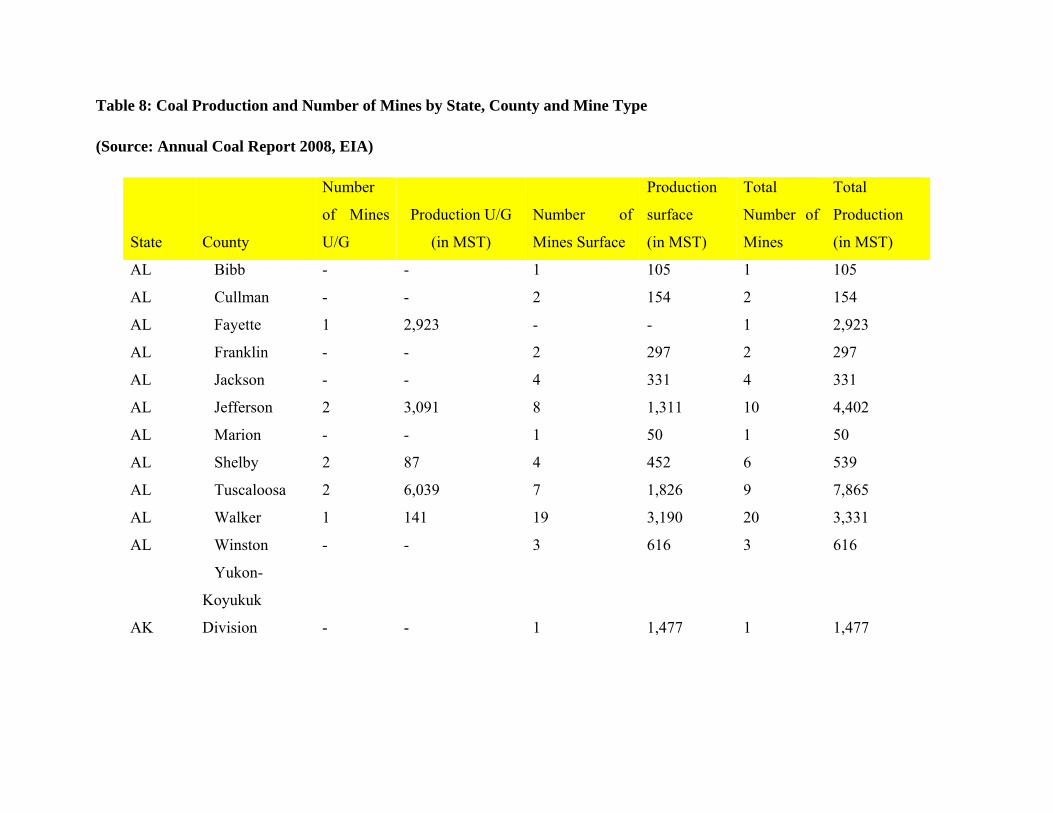
Table 8: Coal Production and Number of Mines by State, County and Mine Type


State County

Number

of Mines

U/G

Production U/G

(in MST)

Number of

Mines Surface

Production

surface

(in MST)

Total

Number of

Mines

Total

Production

(in MST)

AL Bibb - - 1 105 1 105

AL Cullman - - 2 154 2 154

AL Fayette 1 2,923 - - 1 2,923

AL Franklin - - 2 297 2 297

AL Jackson - - 4 331 4 331

AL Jefferson 2 3,091 8 1,311 10 4,402

AL Marion - - 1 50 1 50

AL Shelby 2 87 4 452 6 539

AL Tuscaloosa 2 6,039 7 1,826 9 7,865

AL Walker 1 141 19 3,190 20 3,331

AL Winston - - 3 616 3 616

AK

Yukon-

Koyukuk

Division - - 1 1,477 1 1,477

66

AZ Navajo - - 1 8,025 1 8,025

AR Sebastian 1 67 1 2 2 69

CO Adams - - 1 21 1 21

CO Delta 1 2,862 - - 1 2,862

CO Garfield 1 283 - - 1 283

CO Gunnison 2 10,761 - - 2 10,761

CO La Plata 2 392 - - 2 392

CO Moffat - - 2 7,235 2 7,235

CO Montrose - - 1 403 1 403

CO Rio Blanco 1 2,067 - - 1 2,067

CO Routt 1 8,004 - - 1 8,004

IL Gallatin - - 2 2,322 2 2,322

IL Jackson 1 196 2 1,387 3 1,582

IL Macoupin 1 1,408 - - 1 1,408

IL Perry 1 1,112 3 1,118 4 2,230

IL Randolph 1 3,198 - - 1 3,198

IL Saline 3 9,594 - - 3 9,594

IL Sangamon 1 2,261 - - 1 2,261

IL Vermilion 1 1,130 - - 1 1,130

IL Wabash - - 1 1,037 1 1,037

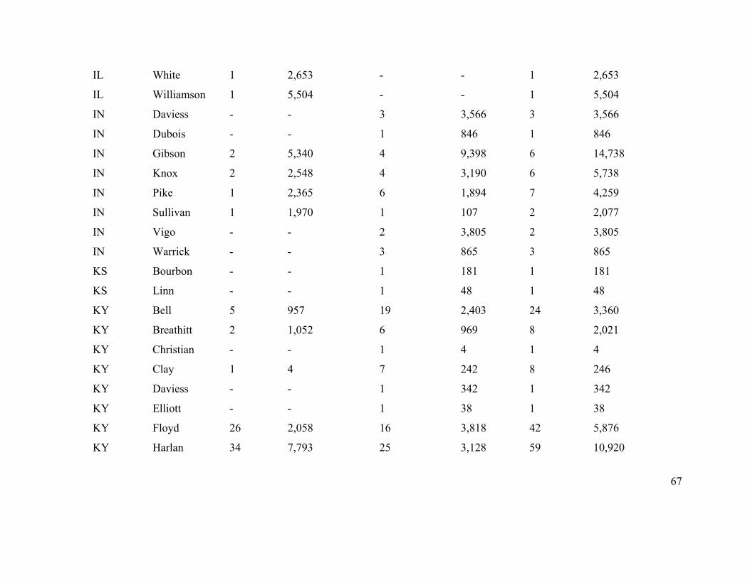
67

IL White 1 2,653 - - 1 2,653

IL Williamson 1 5,504 - - 1 5,504

IN Daviess - - 3 3,566 3 3,566

IN Dubois - - 1 846 1 846

IN Gibson 2 5,340 4 9,398 6 14,738

IN Knox 2 2,548 4 3,190 6 5,738

IN Pike 1 2,365 6 1,894 7 4,259

IN Sullivan 1 1,970 1 107 2 2,077

IN Vigo - - 2 3,805 2 3,805

IN Warrick - - 3 865 3 865

KS Bourbon - - 1 181 1 181

KS Linn - - 1 48 1 48

KY Bell 5 957 19 2,403 24 3,360

KY Breathitt 2 1,052 6 969 8 2,021

KY Christian - - 1 4 1 4

KY Clay 1 4 7 242 8 246

KY Daviess - - 1 342 1 342

KY Elliott - - 1 38 1 38

KY Floyd 26 2,058 16 3,818 42 5,876

KY Harlan 34 7,793 25 3,128 59 10,920

68

KY Henderson 1 1,462 2 1,358 3 2,820

KY Hopkins 4 14,175 1 80 5 14,255

KY Jackson - - 2 45 2 45

KY Johnson 2 281 8 748 10 1,028

KY Knott 26 4,938 14 2,598 40 7,536

KY Knox 3 80 6 363 9 443

KY Laurel - - 4 35 4 35

KY Lawrence - - 10 622 10 622

KY Leslie 7 2,215 9 2,405 16 4,620

KY Letcher 24 4,645 15 886 39 5,531

KY Magoffin 1 16 12 3,412 13 3,427

KY Martin 8 3,480 7 2,212 15 5,693

KY Morgan - - 2 205 2 205

KY Muhlenberg 1 2,235 6 2,142 7 4,377

KY Ohio 1 584 1 807 2 1,391

KY Owsley - - 3 57 3 57

KY Perry 8 4,132 32 13,040 40 17,172

KY Pike 56 12,355 41 8,659 97 21,014

KY Union 2 4,884 - - 2 4,884

KY Webster 2 1,990 - - 2 1,990

69

KY Whitley 2 137 2 234 4 371

LA De Soto - - 1 3,285 1 3,285

LA Red River - - 1 559 1 559

MD Allegany 1 431 13 1,490 14 1,920

MD Garrett 1 322 6 617 7 940

MS Choctaw - - 1 2,842 1 2,842

MO Bates - - 2 247 2 247

MT Big Horn - - 3 31,210 3 31,210

MT Musselshell 1 168 - - 1 168

MT Richland - - 1 355 1 355

MT Rosebud - - 1 13,053 1 13,053

NM McKinley - - 3 9,693 3 9,693

NM San Juan 1 7,046 1 8,906 2 15,952

ND McLean - - 1 7,533 1 7,533

ND Mercer - - 2 17,589 2 17,589

ND Oliver - - 1 4,505 1 4,505

OH Belmont 1 5,798 5 1,076 6 6,873

OH Carroll 1 110 2 39 3 149

OH Columbiana - - 4 351 4 351

OH Coshocton - - 2 249 2 249

70

OH Harrison 1 1,536 7 1,726 8 3,262

OH Jackson - - 1 374 1 374

OH Jefferson 4 923 2 1,512 6 2,435

OH Lawrence - - 1 3 1 3

OH Mahoning - - 2 8 2 8

OH Monroe 1 6,844 - - 1 6,844

OH Muskingum - - 1 165 1 165

OH Noble - - 2 791 2 791

OH Perry 2 1,418 2 648 4 2,066

OH Stark - - 2 368 2 368

OH Tuscarawas 1 425 3 1,211 4 1,636

OH Vinton - - 1 677 1 677

OK Craig - - 1 261 1 261

OK Haskell - - 1 169 1 169

OK Le Flore 1 441 2 423 3 864

OK Okmulgee - - 1 1 1 1

OK Rogers - - 1 168 1 168

PA Allegheny - - 4 121 4 121

PA Armstrong 8 2,873 10 831 18 3,704

PA Beaver 1 380 - - 1 380

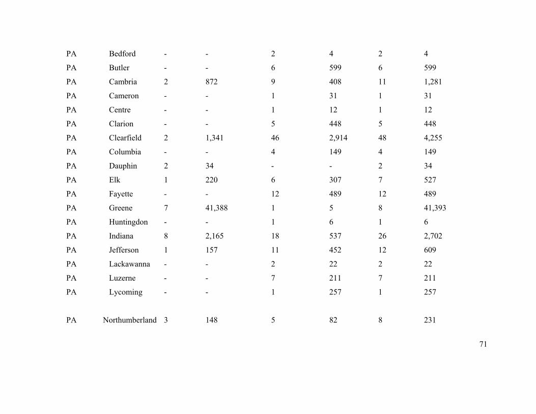
71

PA Bedford - - 2 4 2 4

PA Butler - - 6 599 6 599

PA Cambria 2 872 9 408 11 1,281

PA Cameron - - 1 31 1 31

PA Centre - - 1 12 1 12

PA Clarion - - 5 448 5 448

PA Clearfield 2 1,341 46 2,914 48 4,255

PA Columbia - - 4 149 4 149

PA Dauphin 2 34 - - 2 34

PA Elk 1 220 6 307 7 527

PA Fayette - - 12 489 12 489

PA Greene 7 41,388 1 5 8 41,393

PA Huntingdon - - 1 6 1 6

PA Indiana 8 2,165 18 537 26 2,702

PA Jefferson 1 157 11 452 12 609

PA Lackawanna - - 2 22 2 22

PA Luzerne - - 7 211 7 211

PA Lycoming - - 1 257 1 257

PA

Northumberland 3 148 5 82 8 231

72

PA Schuylkill 8 59 35 995 43 1,054

PA Somerset 7 1,843 18 2,694 25 4,537

PA Tioga - - 1 2 1 2

PA Venango - - 1 13 1 13

PA Washington 1 1,838 3 471 4 2,309

PA Westmoreland - - 5 34 5 34

TN Anderson 1 37 2 148 3 185

TN Campbell 3 387 7 409 10 796

TN Claiborne 1 364 8 966 9 1,330

TN Fentress - - 1 22 1 22

TX Atascosa - - 1 3,079 1 3,079

TX Freestone - - 1 3,339 1 3,339

TX Harrison - - 1 4,055 1 4,055

TX Hopkins - - 1 1,943 1 1,943

TX Lee - - 1 3,754 1 3,754

TX Leon - - 1 6,454 1 6,454

TX Panola - - 2 6,886 2 6,886

TX Robertson - - 1 2,122 1 2,122

TX Rusk - - 1 4,655 1 4,655

TX Titus - - 1 2,730 1 2,730

73

UT Carbon 5 11,545 - - 5 11,545

UT Emery 3 5,874 - - 3 5,874

UT Sevier 1 6,946 - - 1 6,946

VA Buchanan 23 5,596 18 2,843 41 8,439

VA Dickenson 10 1,804 5 266 15 2,070

VA Lee 1 326 3 830 4 1,156

VA Russell 6 952 3 181 9 1,134

VA Tazewell 4 650 1 95 5 745

VA Wise 21 6,477 19 4,691 40 11,169

WV Barbour 4 1,466 4 634 8 2,100

WV Boone 27 12,660 14 17,918 41 30,578

WV Brooke - - 2 524 2 524

WV Clay 1 291 1 3,310 2 3,600

WV Fayette 9 2,578 13 4,468 22 7,046

WV Greenbrier 6 626 2 434 8 1,059

WV Harrison 3 5,932 3 115 6 6,047

WV Kanawha 15 6,850 11 5,021 26 11,870

WV Lincoln 3 1,226 - - 3 1,226

WV Logan 12 7,205 14 11,336 26 18,541

WV Marion 1 5,193 1 26 2 5,218

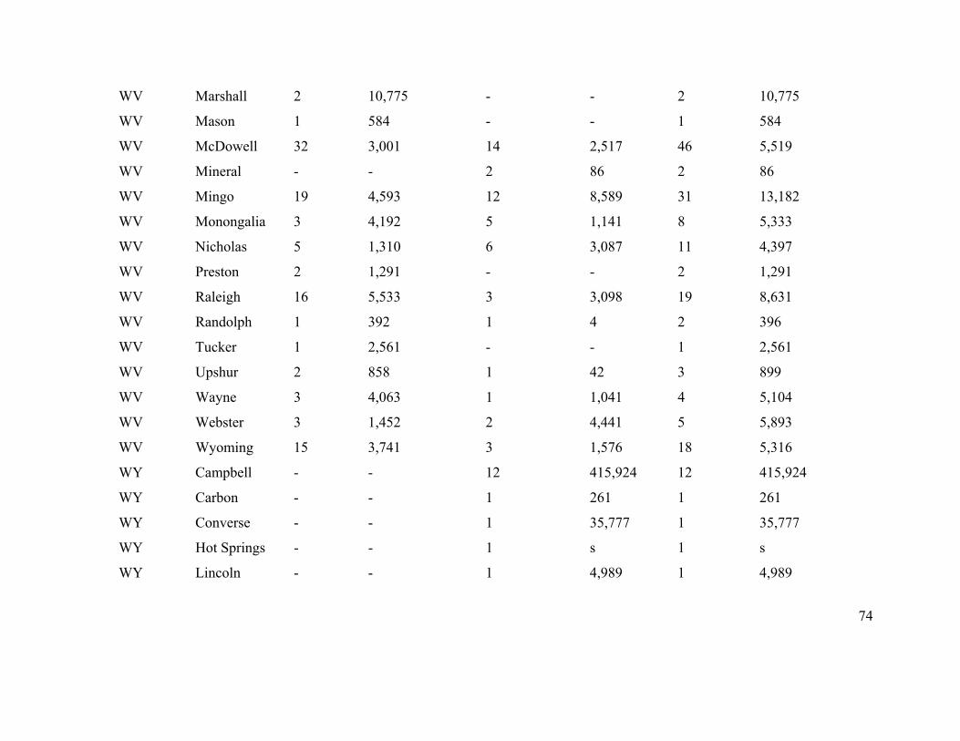
74

WV Marshall 2 10,775 - - 2 10,775

WV Mason 1 584 - - 1 584

WV McDowell 32 3,001 14 2,517 46 5,519

WV Mineral - - 2 86 2 86

WV Mingo 19 4,593 12 8,589 31 13,182

WV Monongalia 3 4,192 5 1,141 8 5,333

WV Nicholas 5 1,310 6 3,087 11 4,397

WV Preston 2 1,291 - - 2 1,291

WV Raleigh 16 5,533 3 3,098 19 8,631

WV Randolph 1 392 1 4 2 396

WV Tucker 1 2,561 - - 1 2,561

WV Upshur 2 858 1 42 3 899

WV Wayne 3 4,063 1 1,041 4 5,104

WV Webster 3 1,452 2 4,441 5 5,893

WV Wyoming 15 3,741 3 1,576 18 5,316

WY Campbell - - 12 415,924 12 415,924

WY Carbon - - 1 261 1 261

WY Converse - - 1 35,777 1 35,777

WY Hot Springs - - 1 s 1 s

WY Lincoln - - 1 4,989 1 4,989

75

WY Sweetwater 1 3,501 3 7,191 4 10,692

U.S.

Subtotal 583 357,079 852 813,322 1,435 1,170,401

Table 9: Coal Production by State and Mine Type


State

Total

Number

of Mines

Number

of Mines

U/G

Number

of Mines

Surface

Production

U/G (in

MST)

Production

surface (in

MST)

Total

Production

(in MST)

Alabama 59 8 51 12,281 8,330 20,611

Alaska 1 - 1 - 1,477 1,477

Arizona 1 - 1 - 8,025 8,025

Arkansas 2 1 1 67 2 69

Colorado 12 8 4 24,370 7,659 32,028

Illinois 19 11 8 27,055 5,863 32,918

Indiana 30 6 24 12,223 23,670 35,893

Kansas 2 - 2 - 229 229

Kentucky 469 216 253 69,474 50,849 120,323

Louisiana 2 - 2 - 3,843 3,843

Maryland 21 2 19 753 2,107 2,860

Mississippi 1 - 1 - 2,842 2,842

Missouri 2 - 2 - 247 247

Montana 6 1 5 168 44,617 44,786

New Mexico 5 1 4 7,046 18,599 25,645

North

Dakota 4 - 4 - 29,627 29,627

Ohio 48 11 37 17,053 9,198 26,251

Oklahoma 7 1 6 441 1,023 1,463

Pennsylvania 266 51 215 53,318 12,095 65,414

Tennessee 23 5 18 789 1,544 2,333

Texas 11 - 11 - 39,017 39,017

Utah 9 9 - 24,365 - 24,365

77

Virginia 114 65 49 15,806 8,907 24,712

West

Virginia 301 186 115 88,369 69,409 157,778

Wyoming 20 1 19 3,501 464,143 467,644

U.S.

Subtotal 1,435 583 852 357,079 813,322 1170401

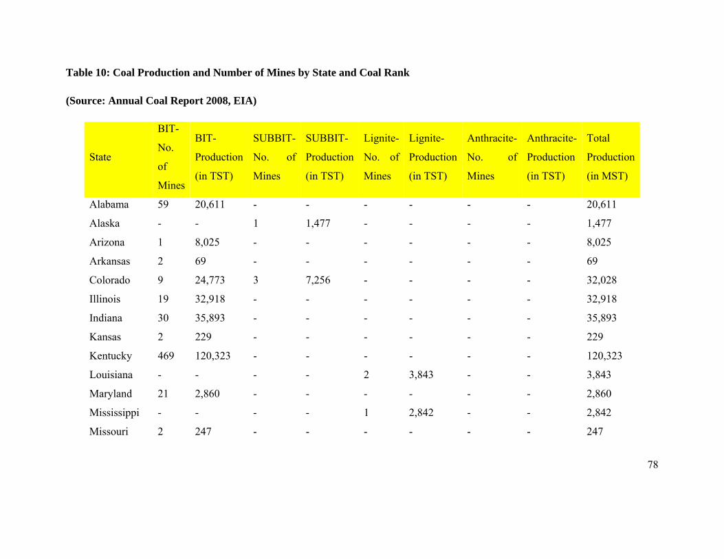
78

Table 10: Coal Production and Number of Mines by State and Coal Rank


State

BIT-

No.

of

Mines

BIT-

Production

(in TST)

SUBBIT-

No. of

Mines

SUBBIT-

Production

(in TST)

Lignite-

No. of

Mines

Lignite-

Production

(in TST)

Anthracite-

No. of

Mines

Anthracite-

Production

(in TST)

Total

Production

(in MST)

Alabama 59 20,611 - - - - - - 20,611

Alaska - - 1 1,477 - - - - 1,477

Arizona 1 8,025 - - - - - - 8,025

Arkansas 2 69 - - - - - - 69

Colorado 9 24,773 3 7,256 - - - - 32,028

Illinois 19 32,918 - - - - - - 32,918

Indiana 30 35,893 - - - - - - 35,893

Kansas 2 229 - - - - - - 229

Kentucky 469 120,323 - - - - - - 120,323

Louisiana - - - - 2 3,843 - - 3,843

Maryland 21 2,860 - - - - - - 2,860

Mississippi - - - - 1 2,842 - - 2,842

Missouri 2 247 - - - - - - 247

79

Montana - - 5 44,431 1 355 - - 44,786

New Mexico 1 7,046 4 18,599 - - - - 25,645

North

Dakota - - - - 4 29,627 - - 29,627

Ohio 48 26,251 - - - - - - 26,251

Oklahoma 7 1,463 - - - - - - 1,463

Pennsylvania 200 63,713 - - - - 66 1,701 65,414

Tennessee 23 2,333 - - - - - - 2,333

Texas - - - - 11 39,017 - - 39,017

Utah 9 24,365 - - - - - - 24,365

Virginia 114 24,712 - - - - - - 24,712

West

Virginia 301 157,778 - - - - - - 157,778

Wyoming 1 261 19 467,383 - - - - 467,644

U.S.

Subtotal 1,319 553,872 31 539,145 19 75,684 66 1,701 1,170,401

80

Table 11: Recoverable Coal reserves and Average Percentage at producing mines by State


State Name FIPS Recoverable Coal

Reserves 2008

Average

Recovery

%, 2008

Recoverable

Coal Reserves

2007

Average

Recovery %,

2007

% Change Recoverable

Coal Reserves (2008 and

2007)

Alabama 01 330 57.98 327 57.15 1

Alaska 02 W W W W -

Arizona 04 W W W W W

Arkansas 05 W W W W -

Colorado 08 325 70.92 328 72.85 -0.9

Illinois 17 1189 60.43 1286 61.99 -7.5

Indiana 18 421 69.52 401 67.58 5.1

Kansas 20 W W W W W

Kentucky 21 1167 58.37 1182 59.91 -1.3

Louisiana 22 W W W W W

Maryland 24 22 74.01 24 61.75 -9.1

Mississippi 28 W W W W W

Missouri 29 W W W W W

Montana 30 925 89.55 1251 88.01 -26.1

81

New Mexico 35 605 88.44 483 90.64 25.4

North Dakota 38 1225 90.6 1252 90.64 -2.2

Ohio 39 308 69.32 333 73 -7.6

Oklahoma 40 85 54.74 155 52.67 -45.6

Pennsylvania 42 526 71.96 532 71.69 -1.2

Tennessee 47 10 75.05 12 79.31 -16.9

Texas 48 752 90.82 737 90.04 2

Utah 49 212 56.97 211 57.92 0.4

Virginia 51 217 55.8 256 56.25 -15.4

Washington 53 - - - - -

West Virginia 54 1908 57.24 1828 57.49 4.4

Wyoming 56 7010 91.52 7330 91.36 -4.4

U.S. Total 17875 79.64 18584 79.92 -3.8

Documents

Development of a coal reserve GIS model and estimation of