Embed Size (px)
Citation preview

Development of a Computational Framework for the
Prediction of Free–Ion Activities, Ionic Equilibria and
Solubility in Dairy Liquids
A thesis submitted in fulfilment
of the requirements for the
degree of Doctor of Philosophy
in Chemical and Process Engineering
University of Canterbury
New Zealand
Pariya Noeparvar
November 2018

I
ABSTRACT
The electrolytes in milk are essential as nutrients and for osmotic balance and have been well
characterised at normal milk concentrations. When milk is concentrated by evaporation or
reverse osmosis, the concentration of ions can easily exceed solubility limits. Hence, it seems
necessary to deeply understand the ion partitioning in milk and milk–like solutions at various
concentrations either at equilibrium or in a dynamic state.
An ion speciation model was proposed to comprehensively consider principal milk components
such as calcium, magnesium, sodium, potassium, and hydrogen as the main cations, and citrate,
phosphate, carbonate, sulphate, chloride, phosphate esters, carboxylate, and hydroxide as the
main anions in serum milk. The dissociable side groups of amino acids in αs1–, αs2–, β–, and
κ–casein were incorporated into the model as well as the calcium phosphate nanoclusters
(CPN) and phosphoserine residues in the bovine casein. The saturation of potential solid salts
such as calcium phosphate in different phases and calcium citrate were obtained. The Mean
Spherical Approximation (MSA) method was used to calculate free–ion activity coefficients
as it contained terms that enhanced accuracy at higher concentrations. Further, it allows the
addition of non–electrolyte components such as lactose. This approach led to a system of over
180 non–linear equations for equilibria, electroneutrality and conservation, that were scaled
and then solved using Newton’s method.
The dynamic calculation of ion speciation was also implemented using Euler’s method to solve
differential equations for precipitation kinetics. This enabled the monitoring of pH, saturation,
and the concentration of calcium salts formed over time. The model was first applied to the
binary solutions of calcium chloride, sodium chloride, buffer solutions of citrate and phosphate
with and without lactose, calcium carbonate, calcium phosphate, and calcium citrate solid
phases, and milk serum both at equilibrium and dynamically. Moreover, the model was applied
to milk as the main system including serum and casein proteins with and without CPN, for
which net charge of the molecule was calculated as the means of validation. The model could
satisfactorily predict pH and saturation of calcium solid salts in concentrated milk up to four
times its normal concentration.
The calcium phosphate precipitation was studied experimentally at various concentrations
under varied and controlled pH values. The experiments were carried out at 23 ˚C with various
concentrations of calcium and phosphate solutions without and with 9.5%w/w lactose. pH was

II
a key factor to determine the amount of calcium phosphate precipitation. Zetasizer analysis
showed that lactose strongly influenced the calcium phosphate solution by forming
nanoparticles with a size of about 1 nm. The role of lactose in enabling the formation of
nanoparticles was previously unknown but is likely to be an important property of milk.

III
ACKNOWLEDGMENTS
I would like to express my gratitude to my supervisor, Associate Professor Ken Morison, for
his invaluable guidance, enthusiasm, generous support, and most importantly to develop and
encourage me as a researcher in the best possible way. I am very thankful for your warm
supervision throughout the journey. I am really grateful to a number of people who have helped
me during my research:
• Dr Aaron Marshall for his support as postgraduate coordinator.
• CAPE technical staff, especially Glen Wilson, Stephen Beuzenberg, Michael
Sandridge, Rayleen Fredericks, and Graham Furniss for their technical help and being
so approachable.
• Master student Elisabeth Scheungrab from Technical University of Munich, not only
for her assistance during the running of experiments, but also speaking in German
language in the lab after 3 years of having no practice. She has become one of my very
closest friend. Eli, thank you for your encouraging and heart–warming messages.
• CAPE undergraduate students, Hassan Ahmed and Hope Neeson, for their assistance
and ideas during the experimentation.
• CAPE administrative staff, Ranee Hearst and Joanne Pollard for their kindness and
help.
• To my CAPE friends, Balaji and Wasim for the funny discussions we had during the
study breaks.
• Mr and Mrs Stanbury, my landlords. I really appreciate you because of being so kind
and considerate. The words cannot describe my feelings to you. You are angels.
• My parents for their unconditional support and kindness. I could have never done my
PhD without your love to pursue this path. Dad, wish you could remember me, call me,
and sing my favourite song for your daughter. You both are always in my heart and
mind.
• My sisters, Vida and Diana, my beloved niece, Andia, my brother in law, Peyman, and
my families in law.
Lastly, Hani, my husband and my best friend. Thank you for your love, kindness, and patience.
I love you.

IV
Table of Contents ABSTRACT I ACKNOWLEDGMENTS III ABBREVIATIONS VII 1 Introduction 1
1.1 Overview 1 1.2 Objectives and outcomes 2 1.3 Outline of thesis 3
2 Literature Review 4 2.1 Principal constituents of milk 4
2.1.1 Lactose 5 2.1.2 Milk fat 8 2.1.3 Milk proteins 9 2.1.4 Milk salts 14 2.1.5 Other milk components 25
2.2 Ion Equilibria 26 2.2.1 Activity based on the free–ion approach 26 2.2.2 Activity based on the ion–pair approach 32 2.2.3 Water activity 33 2.2.4 Association and dissociation constants 34 2.2.5 Solubility 37 2.2.6 Activity coefficient models 41 2.2.7 Ion speciation models 58
3 The Mathematical Model and its Applications 62 3.1 Introduction 62 3.2 Gibbs–Duhem equation 62
3.2.1 Theory 62 3.2.2 Implementation of algorithm 65
3.3 Ion speciation model 66 3.3.1 Set of equations 67 3.3.2 Activity coefficient and dielectric constant 69 3.3.3 CaCl2 solution as an example 71 3.3.4 Solving using Newton’s method 72
3.4 Extra equations for precipitation 73 3.5 Application of the model to sodium chloride and calcium chloride solutions 74
3.5.1 Ion–pair approach 74 3.5.2 Free–ion approach 76
3.6 Application of the model to buffer systems 77 3.6.1 Citrate and phosphate buffer solutions 78
V
3.6.1.1 Method of preparation 78 3.6.1.2 Results and analysis of data 79
3.6.2 Citrate buffer with lactose solution 82 3.7 Application of the model to solid phase systems 85
3.7.1 Calcium carbonate solution 86 3.7.2 Calcium phosphate solution 91 3.7.3 Calcium citrate solution 100
3.8 Application of the model to milk serum 113 3.8.1 Equilibrium study of milk serum 113 3.8.2 Dynamic study of milk serum 115
3.9 Conclusions 119 4 Experimental Aspects of Calcium Phosphate Precipitation 121
4.1 Introduction 121 4.2 Materials and methods 121
4.2.1 Chemicals and reagents 121 4.2.2 Analytical instruments 122 4.2.3 Solution preparations 123
4.3 Results and discussion 125 4.3.1 CaCl2 solution 125 4.3.2 NaH2PO4 solution 130 4.3.3 Lactose solution 131 4.3.4 Mixed solutions 132
4.4 Conclusions 138 5 Development of the Model to Bovine Milk 139
5.1 Introduction 139 5.2 Description of the model 139
5.2.1 Net charge of a protein 141 5.2.2 Initial concentration of each amino acid 143
5.3 Results and discussion 145 5.3.1 Individual aqueous proteins 145 5.3.2 Individual micellar proteins 149 5.3.3 Milk solutions 151 5.3.4 Calcium phosphate nanoclusters in the milk simulation 155
5.4 Conclusions 162 6 Overall Discussion 164 7 Conclusions and Future work 168
7.1 Conclusions 168 7.2 Future work 171
References 173

VI
Appendix 1: MATLAB scripts for the NPMSA parameters 194 Appendix 2: Density of sodium chloride solution 199 Appendix 3: Milk components sizes 201 Appendix 4: MATLAB scripts for Newton’s and Jacobian functions 203 Appendix 5: MATLAB scripts for sodium chloride solution 205 Appendix 6: Precipitation and dissolution rate constants 208 Appendix 7: Chemical structure of amino acids 209 Appendix 8: MATLAB scripts for milk solution with CPN 213

VII
ABBREVIATIONS
ACP Amorphous calcium phosphate
Ala Alanine
Arg Arginine
Asn Asparagine
BMCSL Boublik–Mansoori–Carnahan–Starling–Leyland
Asp Aspartic acid
BSA Bovine serum albumin
CCP Colloidal calcium phosphate
CDA Calcium–deficient apatite
CPN Calcium phosphate nanoclusters
Cys Cysteine
DCPA Dicalcium phosphate anhydrous
DCPD Dicalcium phosphate dihydrate
DLS Dynamic light scattering
es Electrostatic
EXAFS Extended x–ray absorption fine structure FTIR Fourier–transform infrared spectroscopy
Gln Glutamine
Glu Glutamic acid
Gly Glycine
HAP Hydroxyapatite
His Histidine
hs Hard sphere
IAP Ion activity product
IEP Isoelectric point
Ile Isoleucine
IM Immunoglobulin
Ka Association constant
Kac Acidity constant
Kd Dissociation constant
Ksp Solubility product

VIII
Ksp,C Thermodynamic solubility product
Kw water constant
Lact lactate
Leu Leucine
Lys Lysine
MCP Micellar calcium phosphate
Met Methionine
MPC Milk protein concentrate
MSA Mean Spherical Approximation
NPMSA Non–Primitive Mean Spherical Approximation
OCP Octacalcium phosphate
Phe Phenylalanine
prec Precipitation
Pro Proline
SAXS Small angle x–ray scattering
SEM Scanning electron microscope
Ser Serine
SerP Phosphoserine
SI Saturation index
SMUF Simulated milk ultrafiltrate
TCCH Tricalcium citrate hexahydrate
TCCT Tricalcium citrate tetrahydrate
Thr Threonine
Trp Tryptophan
Tyr Tyrosine
UHT Ultra high temperature
Val Valine
WH Whitlockite
XRD X–ray powder refraction
α–la α–lactalbumin
β–lg β–lactoglobulin

1
1 Introduction
1.1 Overview
Evaporation and reverse osmosis have been widely used to concentrate raw milk by dairy
producers to decrease costs of transportation from farms to factories or by factories for further
processing (Grandison and Lewis, 1996). When bovine milk is concentrated by any means of
concentration, the activity of ions can easily exceed solubility limits leading to fouling and
changes in the solubility of the dried milk products. Hence, saturation is of great importance
to avoid any undesirable precipitation of the dissolution of dried milk products.
Some of the milk minerals are soluble at concentrations below their solubility limits, although
some of them such as calcium phosphate exceed their solubility limits at room temperature
milk (Holt, 1997). Different phases of calcium phosphate and citrate can be formed under
different conditions and it is suggested that casein micelles prevent their uncontrolled
precipitation (Mekmene and Gaucheron, 2011). Hence, the ion partitioning of milk in
presence of the casein micelles and other salts seem significant to determine the behaviour of
casein during milk processing (Holt, 1997).
Calcium, magnesium, sodium, and potassium ions are the primary cations, and phosphate,
citrate, carbonate, and chloride are the main anions in milk (Davies and White, 1960; Holt,
1997). The milk minerals distribute differently between both the serum and casein milk, i.e.
about 70% of calcium, 50% of inorganic phosphate, 40% of magnesium, and 10% of citrate
are partially associated to the casein micelles as undissolved ion complexes called micellar
calcium phosphate (Holt, 1997; Mekmene et al., 2010). In milk serum, the minerals are
present either as free ions or as ion–pairs, e.g. sodium and potassium ions have weak affinities
with chloride, citrate, and inorganic phosphate, thus are mainly present as free ions. The
calcium and magnesium ions form ion–pairs primarily with citrate and to a lower degree with
the hydrogen phosphate ion. However, CaHPO4 is calculated to be supersaturated in milk
serum but precipitation is prevented by its low activity in the serum (Walstra and Jenness,
1984; Mekmene, Le Graet, et al., 2009).
The ion–pairs and free ions are in a rapid and dynamic equilibrium in milk serum, while there
is a slow and dynamic salt equilibrium between both serum and casein milk (Walstra and

2
Jenness, 1984). The alteration of ion equilibria can alter the salts distribution and ions
concentrations in both phases of milk leading to changes in the physicochemical features of
the casein micelles (Walstra et al., 2006). This affects the product stability during both
processing and storage. Therefore, it is very useful to deeply understand the ion partitioning
in milk by considering casein and serum proteins under various conditions (Gao, 2010).
Several ion speciation models have been proposed for the ion equilibria calculation in milk
and milk–like systems based on the ions interaction through the association constants. Wood
et al. (1981) proposed an ion equilibria model for the calculation of milk ions concentrations.
Since then, multiple computational models, which are useful for the improvement of relevant
works, have been developed under various conditions by considering different components.
Almost all of the models have used either Debye–Hückel or Davies theories to predict the
activity coefficients of ions. The main drawback with these theories is that the activity
coefficient of zero–charged species is ignored due to the presence of a charge parameter in
their formulas leading to zero value for the species with zero charge.
Nevertheless, a generalised model seems essential to predict ions activity, activity coefficient,
and solubility for any dairy liquid even at high concentration. The Mean Spherical
Approximation (MSA) theory can determine the activity coefficient of zero–charged values
by incorporating a size variable as well as charge.
Several investigations have been done on the ions equilibria calculation at equilibrium, but no
model has been proposed for the dynamic prediction of ions partitioning in milk. The
concentration and saturation of potential solid phases of milk can be calculated over time.
1.2 Objectives and outcomes
The main objective of this study was to improve the understanding of the ions speciation and
solubility by considering almost all principal components of milk or dairy liquids, as to be
able to model the milk partitioning especially at high concentration. To achieve this, another
objective was to predict activity coefficients of all ions, ion–pairs, and non–electrolytes
regardless of their charges.
It was hoped that the outcomes of this study provide insight into the influence of the state of
the components on the properties of milk–based liquids over a range of concentration. The

3
results might also be helpful for the prediction of fouling in reverse osmosis, mineral
precipitation in whey processing, solubility of concentrates and dried milk products in dairy
industry.
1.3 Outline of thesis
A literature review is provided in Chapter 2, including the description of principal milk
components and ion equilibria, in which the fundamental definitions of activity, activity
coefficient, solubility, and association constants are given.
The proposed model is given in Chapter 3 for the calculation of ion equilibria both at
equilibrium and dynamically. It is then applied to different systems such as the binary
solutions of sodium chloride and calcium chloride, the buffer solutions of citrate and
phosphate with and without lactose, the potential solid salts in milk, and milk serum. The
experimental data from literature, water activity, and reproducing of other methods are used
for the validation. This chapter provides the confidence to apply the model to milk in Chapter
5.
Chapter 4 covers the effect of lactose on the precipitation of calcium phosphate solutions
experimentally under various and controlled pH values. Solutions of calcium chloride, sodium
phosphate, and sodium hydroxide were mixed with no and 9.5%w/w lactose with Ca/P of
unity, pH, and conductivity of which were measured over time to monitor the precipitation of
solution. The particles size of solution was analysed by the Zetasizer instrument to determine
if any nanoparticles were formed.
In Chapter 5, the proposed model is applied to different milk–like solutions by considering
dissociable side groups of amino acids in the serum and casein proteins. Net charge is
calculated for the solution as a mean of validation. Calcium phosphate nanoclusters (CPN)
and phosphoserine residues of casein were incorporated into the model.
An overall discussion is given in Chapter 6. The conclusions and recommendation for future
work are provided on Chapter 7.

4
2 Literature Review
2.1 Principal constituents of milk
Milk is one of the most significant foods in human history and is a complex liquid including
numerous components in several states of dispersion. It can be defined as the excretion of the
mammary glands of all female mammals including humans, cows, buffaloes, goats, etc.
(Walstra and Jenness, 1984; Fox and McSweeney, 1998; Walstra et al., 2006). The term ‘milk’
is sometimes used specifically for the healthy cow’s milk, which is white, opaque, and can be
a yellowish fluid especially in summer when the cows are grazed on pasture (Spreer, 1998).
The principal constituents of milk are water, lipids, sugar (lactose), proteins, and minerals,
which are categorised as shown in Table 2.1. Several factors have a significant effect on the
composition of milk such as lactation stage, nutritional, genetic and environmental conditions
of the cow, which cause a wide change in the concentration of various minerals; however, this
variation is partly due to contamination and analytical errors happening during collection,
multiple processing units, and operational procedures (Flynn and Cashman, 1997). The
concentrations of the main components, as well as minor constituents, differs widely for
various mammals e.g. lipids, 2–55%; proteins, 1–20%; lactose, 0–10%, primarily depending
on the energy needs and growth rates of the neonate. The fat and protein content of cow’s
milk varies among different breeds. In contrast, the osmotic pressure of milk is much more
constant so the total concentrations of molecules and ions are also relatively constant (Fox,
2009).
Table 2.1 Composition of cow’s milk (Walstra and Jenness, 1984).
Component Average value in milk (%w/w) Approximate range (%w/w) Water 87.3 85.5–88.7 Solids excluding fat 8.8 7.9–10.0 Lactose 4.6 3.8–5.3 Protein 3.25 2.4–5.5 Casein 2.6 2.3–4.4 Mineral elements 0.65 0.53–0.80 Organic ions 0.18 0.13–0.2 Others 0.14 – Fat 3.9 2.4–5.5

5
The knowledge of milk components and their influences on each other are required to
understand physical characteristics, nutritive quality, and the several changes that can happen
in milk (Walstra and Jenness, 1984). In addition to the major components, there are plentiful
minor components such as minerals, vitamins, hormones, enzymes, and several compounds
that are chemically alike in various species (Fox, 2009).
2.1.1 Lactose
2.1.1.1 General overview
The primary carbohydrate of most mammals’ milk is lactose (4–O–β–D–galactopyranosyl–
D–glucose) comprising galactose and glucose bound by a β1–4 glycosidic bond. Almost all
of mammals’ milk contains lactose, whose concentration can vary from zero to around 100 g
L–1 depending on the mammal species, e.g. no lactose has been found in the milk of California
sea lions and other Pacific seals (Kuhn and Low, 1949; Trucco et al., 1954; Reithel and
Venkataraman, 1956; Walstra and Jenness, 1984; Holsinger, 1997; Walstra et al., 2006; Fox,
2009). There are two isomers of lactose, α and β, that are equilibrated in an aqueous solution
depending on the temperature (Spreer, 1998).
Bovine milk contains lactose 4.6% (Renner, 1983; Holsinger, 1997), but several dairy
products such as evaporated, condensed, and dried milk have higher quantities of lactose.
Dried skim milk has 50–53% lactose, whereas the higher level of fat in dry whole milk reduces
its lactose content to 36–38% (Freeley et al., 1975; Nickerson, 1978; Morrissey, 1985).
The concentration of lactose in bovine milk is affected by various factors, among which the
cow’s breed and health condition have the most significant impacts. The content of lactose
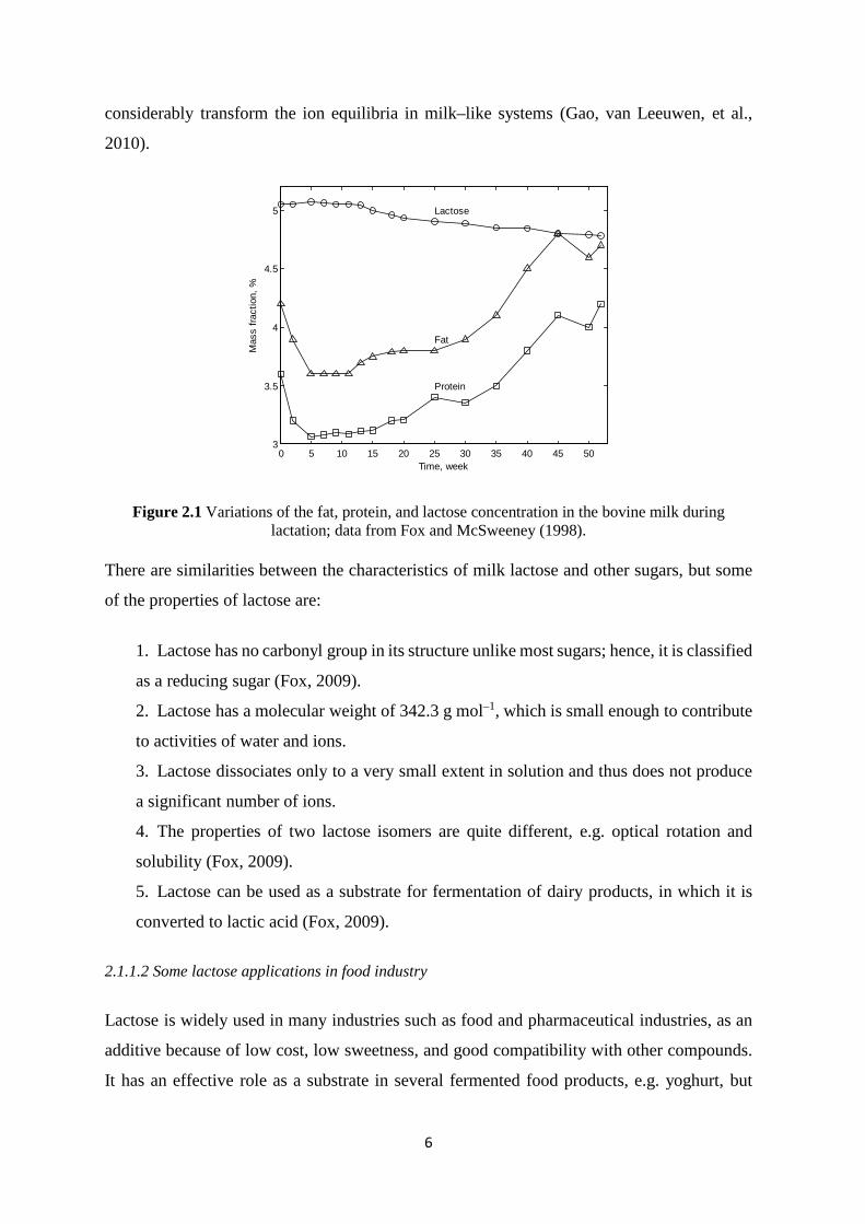
reduces during lactation (Figure 2.1), although this trend is in contrast to the increase in fat
and protein content of milk (Fox and McSweeney, 1998).
Sugars has been commonly added to foods to improve and modify physicochemical,
microbial, sensorial features of food like decreasing activity of water, viscosity, texture, and
softness improvement (Fennema, 1996; Lindsay, 1996). Several researchers claimed that
sugars could alter properties of protein such as casein hydration, thermal stability, its surface
activity (Mora-Gutierrez et al., 1997; Mora-Gutierrez and Farrell, 2000). At high
concentrations of lactose or other sugars, such as in sweetened condensed milk, the stability
of casein micelles can be affected by ‘salt partitioning’. Accordingly, sugars such as lactose
6
considerably transform the ion equilibria in milk–like systems (Gao, van Leeuwen, et al.,
2010).
Figure 2.1 Variations of the fat, protein, and lactose concentration in the bovine milk during lactation; data from Fox and McSweeney (1998).
There are similarities between the characteristics of milk lactose and other sugars, but some
of the properties of lactose are:
1. Lactose has no carbonyl group in its structure unlike most sugars; hence, it is classified
as a reducing sugar (Fox, 2009).
2. Lactose has a molecular weight of 342.3 g mol–1, which is small enough to contribute
to activities of water and ions.
3. Lactose dissociates only to a very small extent in solution and thus does not produce
a significant number of ions.
4. The properties of two lactose isomers are quite different, e.g. optical rotation and
solubility (Fox, 2009).
5. Lactose can be used as a substrate for fermentation of dairy products, in which it is
converted to lactic acid (Fox, 2009).
2.1.1.2 Some lactose applications in food industry
Lactose is widely used in many industries such as food and pharmaceutical industries, as an
additive because of low cost, low sweetness, and good compatibility with other compounds.
It has an effective role as a substrate in several fermented food products, e.g. yoghurt, but
0 5 10 15 20 25 30 35 40 45 503
3.5
4
4.5
5
Time, week
Mas
s fra
ctio
n, %
Protein
Fat
Lactose

7
yeast, as one of the essential ingredients of beer industry cannot ferment lactose. Hence,
lactose improves mouth feel taste, and smoothness of the final product (Holsinger, 1997;
Illanes et al., 2016).
Other similar applications of lactose are in the dairy industry where lactose is used as an
additive for milk, in particular, skimmed milk, buttermilk, chocolate milk etc. (Reimerdes,
1990; Zadow, 1991). Cheese and casein whey used to be a waste substance given to farm
animals or applied to land with water, but nowadays they are used more effectively. Lactose
is crystallised in large quantities from concentrated and/or ultrafiltrated whey, which is
additionally the primary source for producing different kinds of whey proteins and whey
powders. About 400,000 tonnes crystals of lactose are produced annually (Holsinger, 1997;
Walstra et al., 2006).
2.1.1.3 Lactose phosphate
Production of lactose containing products with high and consistent qualities has been a
challenge for dairy industries where a comprehensive understanding of the production
processing is sought in either long or short process such as double crystallisation of lactose or
production of lactose powders from whey permeate (Zadow, 2005). Lactose phosphate was
found as a contaminant in pharmaceutical grade lactose for the first time by Visser (1980),
who later claimed that lactose phosphate slows down lactose crystal formation in solution
(Visser, 1984, 1988). This impurity can strongly influence on the solubility of the component
being crystallised preventing crystal growth. This retarding behaviour of lactose phosphate
was originated by two factors, one of which is due to molecular resemblance of lactose
phosphate to lactose. Another factor is that lactose phosphate acts as an anion at most of pH
ranges except in very pH lower than 1 (Visser, 1988).
Some research was done on lactose phosphate mainly by Visser (1980, 1984, 1988), Pigman
and Horton (1972), and Lifran (2007). Lactose phosphate has an extra monophosphate, which
is the only difference between lactose and lactose phosphate in terms of structure. The
phosphate group of 90% of lactose phosphate is linked to the galactose part of the lactose
(Berg et al., 1988; Visser, 1988).
8
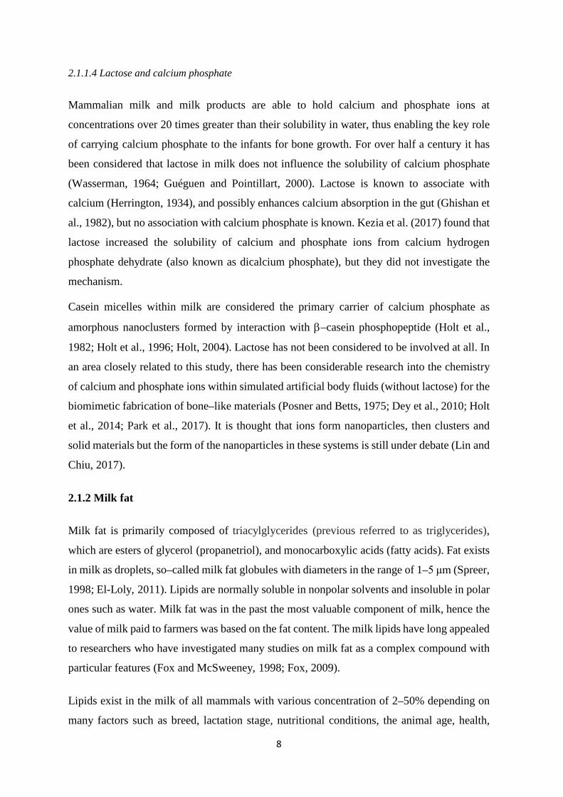
2.1.1.4 Lactose and calcium phosphate
Mammalian milk and milk products are able to hold calcium and phosphate ions at
concentrations over 20 times greater than their solubility in water, thus enabling the key role
of carrying calcium phosphate to the infants for bone growth. For over half a century it has
been considered that lactose in milk does not influence the solubility of calcium phosphate (Wasserman, 1964; Guéguen and Pointillart, 2000). Lactose is known to associate with
calcium (Herrington, 1934), and possibly enhances calcium absorption in the gut (Ghishan et
al., 1982), but no association with calcium phosphate is known. Kezia et al. (2017) found that
lactose increased the solubility of calcium and phosphate ions from calcium hydrogen
phosphate dehydrate (also known as dicalcium phosphate), but they did not investigate the
mechanism.
Casein micelles within milk are considered the primary carrier of calcium phosphate as
amorphous nanoclusters formed by interaction with β–casein phosphopeptide (Holt et al.,
1982; Holt et al., 1996; Holt, 2004). Lactose has not been considered to be involved at all. In
an area closely related to this study, there has been considerable research into the chemistry
of calcium and phosphate ions within simulated artificial body fluids (without lactose) for the
biomimetic fabrication of bone–like materials (Posner and Betts, 1975; Dey et al., 2010; Holt
et al., 2014; Park et al., 2017). It is thought that ions form nanoparticles, then clusters and
solid materials but the form of the nanoparticles in these systems is still under debate (Lin and
Chiu, 2017).
2.1.2 Milk fat
Milk fat is primarily composed of triacylglycerides (previous referred to as triglycerides),
which are esters of glycerol (propanetriol), and monocarboxylic acids (fatty acids). Fat exists
in milk as droplets, so–called milk fat globules with diameters in the range of 1–5 μm (Spreer,
1998; El-Loly, 2011). Lipids are normally soluble in nonpolar solvents and insoluble in polar
ones such as water. Milk fat was in the past the most valuable component of milk, hence the
value of milk paid to farmers was based on the fat content. The milk lipids have long appealed
to researchers who have investigated many studies on milk fat as a complex compound with
particular features (Fox and McSweeney, 1998; Fox, 2009).
Lipids exist in the milk of all mammals with various concentration of 2–50% depending on
many factors such as breed, lactation stage, nutritional conditions, the animal age, health,

9
feed, and season within cows (Auldist et al., 1998; Fox and McSweeney, 1998; Mansson,
2008; Heck et al., 2009). The highest concentration of milk fat in cows is from Jersey cows
with nearly 5% fat, whereas the lowest one is from Holstein/Friesians cows (Fox and
McSweeney, 1998).
Lipids are normally categorised into two groups: neutral lipids, which are a combination of
glycerol esters, mono–, di–, and triglycerides, comprise 98.5% of total milk lipids that are the
main type of lipids available in all foods. Another class of lipids is polar lipids, which are a
varied combination of esters of fatty acids, with either glycerol or other. Polar lipids mainly
contain phosphoric acid, a nitrogen compound, or a sugar comprising about 1% of total milk
lipids approximately; however, they have significant roles in milk by forming the membrane
around globules of milk lipids (Fox, 2009).
2.1.2.1 Membrane of milk fat globule
Almost all of lipids are insoluble in aqueous solutions, but in milk, lipids are contained within
fat globules, which are surrounded by a thin layer that is called the ‘milk fat globule
membrane’. The membrane comprises phospholipids, lipoproteins, cerebrosides, nucleic
acids, enzymes, trace components, and water (Fox and McSweeney, 1998; Fox, 2009).
Natural milk fat globule membrane does not contain milk proteins, which are casein and whey
protein; thus, the interaction between fat globules and milk protein is either weak or even
noninteractive. In addition, no hydrophobic interaction can occur between the milk fat globule
membrane and whey protein. Both milk fat globule membrane and casein micelles carry
negative charges with pH of 6 preventing any interactions between ions (Volkov, 2001). But,
Corredig and Dalgleish (1996) found that β–lactoglobulin interacts with milk fat globules at
temperature higher than 65 ˚C when whole milk is either heated by UHT or direct steam
injection.
2.1.3 Milk proteins
Proteins are made up of amino acids that are bound into different structures. Each amino acid
has an amino (–NH2) group and a carboxyl (–COOH) group. The α–amino acids are those
whose NH2 group is attached to the second carbon atom. Since nine amino acids cannot be
formed by the human digestion system, they must be consumed for human sustenance. There
is an internal transfer of a hydrogen ion from the –COOH group to the –NH2 group to leave
10
an ion with both a negative charge and a positive charge. This is called a zwitterion. The
electrical charge of proteins is strongly dependent on the pH of the solution and the
accessibility of the free amino or carboxyl groups (Spreer, 1998). The amino acids of bovine
milk can be classified by their side chains as uncharged and nonpolar such as alanine, glycine,
isoleucine, leucine, methionine, phenylalanine, proline, and tryptophan; polar side chains
such as asparagine, cysteine, glutamine, serine, threonine, and tyrosine; and charged side
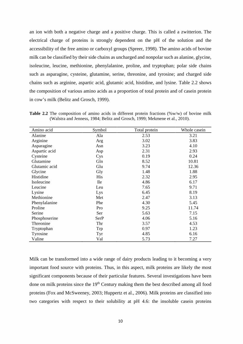
chains such as arginine, aspartic acid, glutamic acid, histidine, and lysine. Table 2.2 shows
the composition of various amino acids as a proportion of total protein and of casein protein
in cow’s milk (Belitz and Grosch, 1999).
Table 2.2 The composition of amino acids in different protein fractions (%w/w) of bovine milk (Walstra and Jenness, 1984; Belitz and Grosch, 1999; Mekmene et al., 2010).
Amino acid Symbol Total protein Whole casein Alanine Ala 2.53 3.21 Arginine Arg 3.02 3.83 Asparagine Asn 3.23 4.10 Aspartic acid Asp 2.31 2.93 Cysteine Cys 0.19 0.24 Glutamine Gln 8.52 10.81 Glutamic acid Glu 9.74 12.36 Glycine Gly 1.48 1.88 Histidine His 2.32 2.95 Isoleucine Ile 4.86 6.17 Leucine Leu 7.65 9.71 Lysine Lys 6.45 8.19 Methionine Met 2.47 3.13 Phenylalanine Phe 4.30 5.45 Proline Pro 9.25 11.74 Serine Ser 5.63 7.15 Phosphoserine SerP 4.06 5.16 Threonine Thr 3.57 4.53 Tryptophan Trp 0.97 1.23 Tyrosine Tyr 4.85 6.16 Valine Val 5.73 7.27
Milk can be transformed into a wide range of dairy products leading to it becoming a very
important food source with proteins. Thus, in this aspect, milk proteins are likely the most
significant components because of their particular features. Several investigations have been
done on milk proteins since the 19th Century making them the best described among all food
proteins (Fox and McSweeney, 2003; Huppertz et al., 2006). Milk proteins are classified into
two categories with respect to their solubility at pH 4.6: the insoluble casein proteins
11
comprising around 80% of total milk proteins; and soluble whey proteins, which constitute
20% of the total (Huppertz et al., 2006).
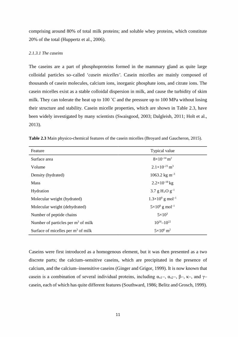
2.1.3.1 The caseins
The caseins are a part of phosphoproteins formed in the mammary gland as quite large
colloidal particles so–called ‘casein micelles’. Casein micelles are mainly composed of
thousands of casein molecules, calcium ions, inorganic phosphate ions, and citrate ions. The
casein micelles exist as a stable colloidal dispersion in milk, and cause the turbidity of skim
milk. They can tolerate the heat up to 100 ˚C and the pressure up to 100 MPa without losing
their structure and stability. Casein micelle properties, which are shown in Table 2.3, have
been widely investigated by many scientists (Swaisgood, 2003; Dalgleish, 2011; Holt et al.,
2013).
Table 2.3 Main physico-chemical features of the casein micelles (Broyard and Gaucheron, 2015).
Feature Typical value
Surface area 8×10–14 m2
Volume 2.1×10⁻²¹ m3
Density (hydrated) 1063.2 kg m–3
Mass 2.2×10⁻¹⁸ kg
Hydration 3.7 g H2O g–1
Molecular weight (hydrated) 1.3×10⁹ g mol–1
Molecular weight (dehydrated) 5×10⁸ g mol–1
Number of peptide chains 5×10³
Number of particles per m3 of milk 1020–1022
Surface of micelles per m3 of milk 5×10⁶ m2
Caseins were first introduced as a homogenous element, but it was then presented as a two
discrete parts; the calcium–sensitive caseins, which are precipitated in the presence of
calcium, and the calcium–insensitive caseins (Ginger and Grigor, 1999). It is now known that
casein is a combination of several individual proteins, including αs1–, αs2–, β–, κ–, and γ–
casein, each of which has quite different features (Southward, 1986; Belitz and Grosch, 1999).

12
αs1–casein is the main fraction of bovine milk protein that makes up around 38% of the whole
casein source (Eigel et al., 1984; Fox, 2009). The B variant of αs1–casein comprises a chain
of peptide containing 199 amino acid residues, among which 8 phosphoserine residues are
situated in positions 43–80 attached to highly polar regions of carboxyl groups. The polarity
of amino acid residues 100–199 is high leading to a strong linkage; however, phosphate
groups decrease the association by making repulsive forces (Belitz and Grosch, 1999).
αs2–casein has a dipolar structure, anionic and cationic groups of which are located at the N–
and C–terminal regions, respectively. Both αs1–and αs2–casein are phosphorylated peptides.
In the presence of Ca2+, αs2–casein solubility is less than that of αs1–casein (Belitz and Grosch,
1999; Broyard and Gaucheron, 2015).
β–casein is the second most plentiful protein among all the proteins in serum milk, leading to
the formation of colloidal aggregates in the aqueous solution with a concentration higher than
0.5 mg mL–1 (Leclerc and Calmettes, 1997; Dickinson, 1999). β–casein is a peptide chain
comprising 209 residues with a molar mass of 24.5 kDa. Bovine β–casein contains five
phosphoserine residues, where all ionising positions of the molecule are located. The amino
acid residues of β–casein are usually less hydrophobic than that of a normal globular protein
and more than that of an unfolded protein. The charged and phosphorylated sites of β–casein
is mostly localised at the N–terminal 21 residues, whilst the uncharged part of structure is
mainly made up of the hydrophobic residues (Follows et al., 2011). The precipitation of the
protein normally occur in the range of the bovine Ca2+ concentration (Belitz and Grosch,
1999; Ginger and Grigor, 1999).
Bovine κ–casein comprises 10% of the total casein content, and consists of 169 amino acid
residues helping to increase the colloidal stability of αs1–, αs2–, and β–caseins by the
formation of casein micelles. It can be mostly found on the outer surface of the micelle
creating a hairy structure, composed of macropeptides that stretch out from the micelle. It has
a key role in the stabilisation of the structure of casein micelles by making a hydrophilic
coating preventing the association and the aggregation of the micelles (de Kruif, 1999;
Swaisgood, 2003; Johansson et al., 2009; Palmer et al., 2013).

13
2.1.3.2 The serum
The precipitation of casein occurs when the pH of milk decreases to about 4.6 at 20˚C. The
supernatant residue is called milk whey or serum and contains 20% of the whole milk protein
(Walstra and Jenness, 1984). It is also called as ‘diffusate phase’ by Holt et al. (1981), whereas
micellar phase sometimes referred to ‘non–diffusible phase’.
Unlike caseins, the whey proteins are globular and contain more organised and consistent
structures (Ng-Kwai-Hang, 2003). They are bound to each other by disulfide crosslinks. Whey
proteins are more sensitive to heat than casein proteins, but are less sensitive to calcium
(Kinsella, 1984).
β–lactoglobulin (β–lg), α–lactalbumin (α–la), bovine serum albumin (BSA), immunoglobulin
(IM), and proteose–peptone are considered the main characterised components of the whey
proteins. They represent more than 95% of the non–casein proteins (Ng-Kwai-Hang, 2003;
Farrell et al., 2004). Table 2.4 shows the composition of milk serum proteins.
Table 2.4 Composition of milk serum proteins (Walstra and Jenness, 1984).
Protein Concentration in skimmed milk, mM
Mass fraction in total protein, %w/w
β–lactoglobulin 180 9.8 α–lactalbumin 90 3.7 Bovine serum albumin 6 1.2 Immunoglobulin 4 2.1 Miscellaneous 40 2.4
β–lactoglobulin represents about 50% of the total whey protein, and 10% of the total protein
of bovine milk (Creamer and Sawyer, 2003). The monomeric molecular weight of β–
lactoglobulin is 18,300 Da (Kinsella, 1984). It has 162 amino acids, among which 5 cysteine
residues are able to form disulphide bonds between various positions (Ng-Kwai-Hang, 2003).
It can also interacts with other proteins, in particular κ–casein and α–lactalbumin (Walstra
and Jenness, 1984).
Dimerisation of β–lactoglobulin normally occurs in the pH range 3.5–7.5 depending on the
protein concentration, pH, temperature, and ionic strength. There are strong electrostatic
repulsions at pH below 3.5 where the dimer dissociates; however, octamers are formed for
14
pH between 3.5–5.2. The dimer becomes stable at pH between 5.5–7.5, and unstable at pH
above 8.0 where the aggregations of denatured proteins usually occur (Lyster, 1972).
The second most plentiful of the whey proteins is α–lactalbumin representing 20% of the total
whey protein and 2–5% of the total skim milk protein (Wong et al., 1996). It has a compact
globular structure with a molecular weight of 14,175 Da and 123 amino acids. There are 4
disulphide bonds connecting 8 cysteine residues in different positions (Kinsella, 1984; Ng-
Kwai-Hang, 2003).
According to Zhang and Brew (2003), the stability and structure of α–lactalbumin is highly
affected by ionic calcium (Ca2+); however, the protein becomes unstable as the pH reduces
due to removal of ionic calcium. Besides, α–lactalbumin has other cationic binding with other
divalent ions such as Zn2+, Mn2+, Hg2+, and Pb2+.
Bovine serum albumin (BSA) is a polypeptide consisting of 582 amino acids with a molecular
weight of 66,433 Da approximately. It constitutes 5% of the total bovine whey proteins
(Walstra and Jenness, 1984; Haggarty, 2003). Bovine serum albumin contains 1 free thiol and
17 disulphide linkages which hold the structure as a multiloop. The function of serum albumin
is probably limited in cow’s milk but it can bind to metals and fatty acids (Fox and
McSweeney, 1998; Ng-Kwai-Hang, 2003).
The largest and the most heterogeneous protein of the whey proteins are immunoglobulins
with molecular weights over 1000 kDa. They are usually 10% of the bovine whey proteins
and are available as either monomer or light and heavy polymers of polypeptide chains, which
are attached by disulphide linkages leading to the immunoglobulin basic structure (Walstra
and Jenness, 1984).
Lactoferrin and transferrin, β2–microglobulin, and proteose–peptone form a small fraction of
the bovine whey proteins (Walstra and Jenness, 1984).
2.1.4 Milk salts
The term ‘minerals’ was previously used in the field of dairy science to describe milk salts;
however, it is nowadays considered to be an incorrect word, since the minerals are not
naturally occurring in the milk salts. The bovine milk salt fraction, which is 8–9 g L–1 of the
total skimmed milk, contains several cations (calcium, magnesium, sodium, and potassium)
15
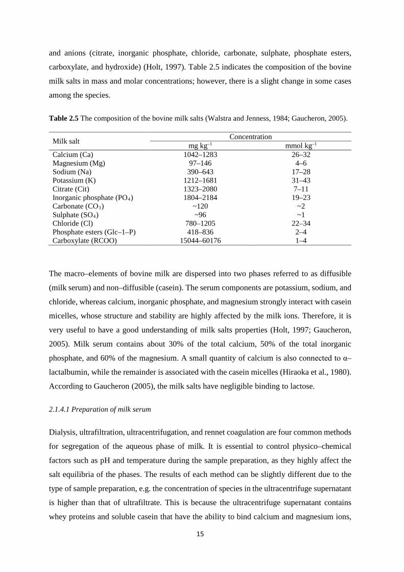
and anions (citrate, inorganic phosphate, chloride, carbonate, sulphate, phosphate esters,
carboxylate, and hydroxide) (Holt, 1997). Table 2.5 indicates the composition of the bovine
milk salts in mass and molar concentrations; however, there is a slight change in some cases
among the species.
Table 2.5 The composition of the bovine milk salts (Walstra and Jenness, 1984; Gaucheron, 2005).
Milk salt Concentration mg kg–1 mmol kg–1
Calcium (Ca) 1042–1283 26–32 Magnesium (Mg) 97–146 4–6 Sodium (Na) 390–643 17–28 Potassium (K) 1212–1681 31–43 Citrate (Cit) 1323–2080 7–11 Inorganic phosphate (PO4) 1804–2184 19–23 Carbonate (CO3) ~120 ~2 Sulphate (SO4) ~96 ~1 Chloride (Cl) 780–1205 22–34 Phosphate esters (Glc–1–P) 418–836 2–4 Carboxylate (RCOO) 15044–60176 1–4
The macro–elements of bovine milk are dispersed into two phases referred to as diffusible
(milk serum) and non–diffusible (casein). The serum components are potassium, sodium, and
chloride, whereas calcium, inorganic phosphate, and magnesium strongly interact with casein
micelles, whose structure and stability are highly affected by the milk ions. Therefore, it is
very useful to have a good understanding of milk salts properties (Holt, 1997; Gaucheron,
2005). Milk serum contains about 30% of the total calcium, 50% of the total inorganic
phosphate, and 60% of the magnesium. A small quantity of calcium is also connected to α–
lactalbumin, while the remainder is associated with the casein micelles (Hiraoka et al., 1980).
According to Gaucheron (2005), the milk salts have negligible binding to lactose.
2.1.4.1 Preparation of milk serum
Dialysis, ultrafiltration, ultracentrifugation, and rennet coagulation are four common methods
for segregation of the aqueous phase of milk. It is essential to control physico–chemical
factors such as pH and temperature during the sample preparation, as they highly affect the
salt equilibria of the phases. The results of each method can be slightly different due to the
type of sample preparation, e.g. the concentration of species in the ultracentrifuge supernatant
is higher than that of ultrafiltrate. This is because the ultracentrifuge supernatant contains
whey proteins and soluble casein that have the ability to bind calcium and magnesium ions,
16
whereas the ultrafiltrate does not have the soluble proteins (Gaucheron, 2005). The method
of milk serum preparation can affect experimental results.
2.1.4.2 Salt concentration and association in the milk serum
Free ions are not the only ions of the solution, but there are various associations among the
ions that interact with each other depending on the association constants and the solubilities
(Holt et al., 1981; Walstra and Jenness, 1984; Holt, 1985).
Generally, calcium is present in the serum as free calcium (Ca2+) and several complexes
mostly with trivalent citrate (Cit3–) e.g. CaCit–, to a lesser level with mono valent and divalent
inorganic phosphates (H2PO4–, HPO4
2–), and chloride (Cl–) i.e. CaCl+. The solubility of
calcium phosphate salts is rather low. Potassium and sodium are mostly available as free ions
in milk serum; however, there is a small affinity with citrate, inorganic phosphate, and
chloride (Gaucheron, 2005).
2.1.4.3 Micellar calcium phosphate and CPN
According to Gaucheron (2005), the casein molecules contains phosphoserine residues in
their structures. The cations can mainly bind to the casein through the phosphate groups of
the phosphoserine residues of the casein molecules. There is a decrease in the order of cation
binding capacity of the casein proteins as αs2– > αs1– > β– > κ–casein due to the number of
phosphoserine groups. However, the phosphoserine residues are not the only amino acid
group within the casein proteins, but other amino acids existing in the milk solution can be
associated to the cations, which will be discussed in the Chapter 5 in detail.
Multiple undissolved complexes named colloidal calcium phosphate (CCP) or micellar
calcium phosphate (MCP) or calcium phosphate nanoclusters (CPN) constitute the salts in the
casein micelles and include 70% of the total calcium, 30% of the total magnesium, 50% of
the total inorganic phosphate, and 10% of the total citrate (Holt, 1997). The micellar calcium
phosphate can have several compositions with various Ca/P ratios due to its complex physico–
chemical properties, various crystallised forms, and a very slow thermodynamic equilibrium.
The definition of micellar calcium phosphate is quite complicated because calcium is not only
associated with inorganic phosphate in the casein micelles, but also has a strong affinity with
phosphoserine residues. Hence, the calcium in the micellar phase can be described as a
combination of calcium caseinate and calcium phosphate containing organic and inorganic

17
phosphate, respectively, but the composition of each cannot be calculated individually
because they are inseparable. However, several approaches have been used to specify the
composition, the structure, and Ca/P ratio of the micellar calcium phosphate (Gaucheron,
2005).
When the calcium phosphate matrix incorporates the bound calcium and the casein ester
phosphate, it is assumed that the ratio of Ca/P is approximately 1.5 representing the tri–
calcium phosphate (Ca3(PO4)2). Brushite (DCPD, CaHPO4.2H2O) is another proposed form
of micellar calcium phosphate assumed as an essential part of the calcium phosphate structure.
The analyses of X–ray absorption and infrared spectroscopy were used to verify that the
micellar calcium phosphate structure is similar to brushite (Gaucheron, 2005).
However, Holt (1992) suggested the dicalcium phosphate anhydrous (DCPA, CaHPO4) for
the brushite structure by using the solubility product of the salt.
McGann et al. (1983) and Lyster et al. (1984) proposed an amorphous structure for the
micellar calcium phosphate by the methods of diffraction and high resolution transmission
electron microscopy.
A chemical formula was suggested by van Dijk (1990) representing the affinity between the
casein and the micellar calcium phosphate containing a couple of phosphoserine residues, 4
inorganic phosphate, and 8 divalent cations mainly calcium; however, the formula does not
adapt to the existence of clusters with nanometre diameter.
Micellar calcium phosphate strongly interacts with the milk serum through calcium citrate,
calcium phosphate, and negatively charged citrate and phosphate anions at the pH of milk as
shown in Figure 2.2. According to Gaucheron (2005), approximately one minute is needed to
exchange all calcium to the colloidal phase.

18
H2PO4–
H+HCit2–
+ Cit3–
HPO42–
+
+ +Ca2+
CaCit–
CaHPO4
Casein micelles
Figure 2.2 The interaction between the calcium phosphate and citrate of serum and casein micelles (Gaucheron, 2005).
Calcium phosphate nanoclusters are thought to be equilibrated particles with a certain
composition, in which a shell of casein phosphopeptides with 1.6 nm thickness surrounds a
core of acidic and hydrated amorphous calcium phosphate (Holt et al., 2009). The
spontaneous formation of calcium phosphate nanoclusters occurs by adding the
phosphopeptide to amorphous calcium phosphate, which was confirmed by several
characterisation analyses. The core of calcium phosphate nanoclusters is believed to have
resemblance with the micellar calcium phosphate in respect to structure, solubility, and
dynamics (Holt et al., 2009). Holt et al. (1998) prepared calcium phosphate nanoclusters using
10 mg mL–1 of the β–casein 25–amino–acid N–terminal tryptic phosphopeptide as a stabilised
component. The mathematical model estimated a spherical core of 355±20 units of dicalcium
phosphate dihydrate for nanoparticles with density of 2.31 g mL–1 and radius of 2.30±0.05
nm covered by a shell comprising 49±4 peptide chains. They also suggested that the
phosphopeptide inhibits the growth process of calcium phosphate precipitate.
Holt et al. (1996) tested the idea of calcium phosphate nanoclusters formation by a short
phosphopeptide at roughly 1 mM concentration that prevent the solution from precipitating
and lead to a stable phase of solution even for a supersaturated solution. The nanoparticles
have been found to be stable for months.
Holt (1997) claimed that the nanoparticles composition is very similar to that of dicalcium
phosphate containing tiny amounts of citrate and magnesium ions with identical solubility to
that of colloidal calcium phosphate. They also found that the nanoparticles were coated by the
phosphopeptides, structure of which seemed to be unclear.
Later on, the formation of nanoparticles in the preventing or reducing the precipitation of
calcium phosphate was discussed by Holt (2004), and hence will add to the stability of calcium

19
phosphate in milk. This effect will be in addition to the role of casein in stabilising calcium
phosphate in milk.
More recently, Lenton et al. (2016) applied neutron diffraction and contrast–matching
methods to identify long–range order of calcium phosphate nanoparticles within
phosphopeptide of milk casein and osteopontin. The results confirmed the presence of
amorphous calcium phosphate in the core of nanoparticles.
It is thought that ions form nanoparticles, then clusters and solid materials but the form of the
nanoparticles in these systems is still under debate (Lin and Chiu, 2017). In Chapter 4, a set
of experiments was done regarding the unexpected role of lactose in the possible formation
of calcium phosphate nanoparticle under varied and controlled pH and at different
concentrations.
2.1.4.4 Calcium phosphate solid solutions
Calcium phosphates are formed in various amorphous and crystalline phases under different
experimental conditions. The most frequent forms are categorised and shown in Table 2.6, in
which some inconsistencies in the chemical formula and solubility product values were seen
for different versions of calcium phosphate phases due to various conventions for ion activity
product. The full description of solubility product is given in Section 2.2.5.
The precipitation of calcium phosphate are mostly dependent on temperature, phosphate and
calcium concentrations, pH, and considering other ions during the precipitation (Madsen and
Thorvardarson, 1984; Madsen and Christensson, 1991). Several studies have been done on
the precipitation of calcium phosphate salts under different conditions using mathematical
and experimental solutions.
Ferguson and McCarty (1971) studied the effect of magnesium and carbonate on calcium
phosphate precipitation at the concentrations very similar to the anaerobic digestion process
for phosphate removal from wastewater. They explored that the precipitation was highly
influenced by magnesium and carbonate concentration, time, and pH. It was suggested that
the optimum pH for phosphate removal was between 7.5 to 9.5.

20
Table 2.6 Calcium phosphate solid phases.
Solid phase name Chemical formula Ion activity product (IAP) Solubility product, Ksp References
Dicalcium phosphate dihydrate (brushite, DCPD)
CaHPO4.2H2O 𝑎𝑎𝐶𝐶𝑎𝑎2+ × 𝑎𝑎𝐻𝐻𝐻𝐻𝑂𝑂42−
2.57 × 10⁻⁷ [mol2 L–2] (Driessens and Verbeeck, 1990) 1.87 × 10⁻⁷ [mol2 L–2] (Johnsson and Nancollas, 1992) 2.09 × 10⁻⁷ [mol2 L–2] (Mekmene, Quillard, et al., 2009) 1.12 × 10⁻⁷ [mol2 L–2] (Bleek and Taubert, 2013)
Dicalcium phosphate anhydrous (monetite, DCPA)
CaHPO4 𝑎𝑎𝐶𝐶𝑎𝑎2+ × 𝑎𝑎𝐻𝐻𝐻𝐻𝑂𝑂42− 1.26 × 10⁻⁷ [mol2 L–2] (Driessens and Verbeeck, 1990; Bleek and Taubert, 2013)
Octacalcium phosphate (OCP)
Ca8H2(PO4)6.5H2O 𝑎𝑎𝐶𝐶𝑎𝑎2+8 × 𝑎𝑎𝐻𝐻+
2 × 𝑎𝑎𝐻𝐻𝑂𝑂43−6 2.51 × 10−97 [mol16 L–16]* (Bleek and Taubert, 2013)
Ca8(HPO4)2(PO4)4.5H2O 𝑎𝑎𝐶𝐶𝑎𝑎2+8 × 𝑎𝑎𝐻𝐻𝐻𝐻𝑂𝑂42−
2 × 𝑎𝑎𝐻𝐻𝑂𝑂43−4 3.16 × 10−73 [mol14 L–14] (Driessens and Verbeeck, 1990)
2.51 × 10−97 [mol14 L–14]* (Dorozhkin, 2014) Ca4(HPO4)(PO4)2.5H2O 𝑎𝑎𝐶𝐶𝑎𝑎2+
4 × 𝑎𝑎𝐻𝐻𝐻𝐻𝑂𝑂42− × 𝑎𝑎𝐻𝐻𝑂𝑂43−2 1.26 × 10−47 [mol7 L–7] (Mekmene, Quillard, et al., 2009)
Ca4H(PO4)3.5H2O 𝑎𝑎𝐶𝐶𝑎𝑎2+4 × 𝑎𝑎𝐻𝐻𝐻𝐻𝑂𝑂42−
3 × 𝑎𝑎𝐻𝐻+ 1.26 × 10−49 [mol8 L–8] (Gao, van Halsema, et al., 2010)
Amorphous calcium phosphate (ACP)
CaxHy(PO4)z.nH2O; n=3–4.5 𝑎𝑎𝐶𝐶𝑎𝑎2+𝑥𝑥 × 𝑎𝑎𝐻𝐻+
𝑦𝑦 × 𝑎𝑎𝐻𝐻𝑂𝑂43−𝑧𝑧 Cannot be measured precisely (Dorozhkin, 2014)
Ca3(PO4)2.nH2O 𝑎𝑎𝐶𝐶𝑎𝑎2+3 × 𝑎𝑎𝐻𝐻𝑂𝑂43−
2 1.00 × 10⁻²⁶ [mol5 L–5] (Gao, van Halsema, et al., 2010)
1.99 × 10⁻³³ [mol5 L–5] (pH=5) 1.26 × 10⁻³⁰ [mol5 L–5] (pH=6)
1.99 × 10⁻³³ [mol5 L–5] (pH=7.4) (Bleek and Taubert, 2013)
Hydroxyapatite (HAP)
Ca10(PO4)6(OH)2 𝑎𝑎𝐶𝐶𝑎𝑎2+10 × 𝑎𝑎𝐻𝐻𝑂𝑂43−
6 × 𝑎𝑎𝑂𝑂𝐻𝐻−2 1.58 × 10−117 [mol18 L–18] (Dorozhkin, 2014)
Ca5(PO4)3(OH) 𝑎𝑎𝐶𝐶𝑎𝑎2+5 × 𝑎𝑎𝐻𝐻𝑂𝑂43−
3 × 𝑎𝑎𝑂𝑂𝐻𝐻− 1.82 × 10−58 [mol9 L–9] (McDowell et al., 1977)
Whitlockite (α–TCP) Ca3(PO4)2 𝑎𝑎𝐶𝐶𝑎𝑎2+
3 × 𝑎𝑎𝐻𝐻𝑂𝑂43−2 3.16 × 10⁻²⁶ [mol5 L–5] (Bleek and Taubert, 2013)
Ca10(HPO4)(PO4)6 𝑎𝑎𝐶𝐶𝑎𝑎2+10 × 𝑎𝑎𝐻𝐻𝐻𝐻𝑂𝑂42− × 𝑎𝑎𝐻𝐻𝑂𝑂43−
6 1.99 × 10−82 [mol17 L–17] (Driessens and Verbeeck, 1990) Tricalcium phosphate (β–TCP) Ca3(PO4)2 𝑎𝑎𝐶𝐶𝑎𝑎2+
3 × 𝑎𝑎𝐻𝐻𝑂𝑂43−2 1.26 × 10⁻²⁹ [mol5 L–5] (Dorozhkin, 2014)
Calcium–deficient apatite (CDA)
Ca10-x(HPO4)x(PO4)6-x(OH)2-x (0<x<1) 𝑎𝑎𝐶𝐶𝑎𝑎2+
10−𝑥𝑥 × 𝑎𝑎𝐻𝐻𝐻𝐻𝑂𝑂42−𝑥𝑥 × 𝑎𝑎𝐻𝐻𝑂𝑂43−
6−𝑥𝑥 1.00 × 10−85 (Dorozhkin, 2014)
Ca9(HPO4)(PO4)5(OH) 𝑎𝑎𝐶𝐶𝑎𝑎2+9 × 𝑎𝑎𝐻𝐻𝐻𝐻𝑂𝑂42− × 𝑎𝑎𝐻𝐻𝑂𝑂43−
5 × 𝑎𝑎𝑂𝑂𝐻𝐻− 7.94 × 10−86 [mol16 L–16] (Driessens and Verbeeck, 1990) *Not consistent.

21
Boskey and Posner (1976) showed that the hydroxyapatite precipitation could occur in a
relatively low supersaturation without the formation of the amorphous calcium phosphate.
pH, calcium and inorganic phosphate concentrations, ionic strength and temperature are the
key parameters to determine the initial precipitate in respect to the hydroxyapatite formation.
Chhettry et al. (1999) obtained the stability constants for the ion–pairs CaH2PO4+, CaHPO4˚,
NaHPO4–, and calcium acetate (CaAc+) by the Extended Debye–Hückel equation to solve the
relevant equilibria of apatite dissolution systems. Dicalcium phosphate dihydrate was used as
a probe to evaluate the equilibrium constants because of quick equilibration and availability
of its solubility product.
Lu and Leng (2005) analysed the driving force and nucleation rate of calcium and phosphate
formation in simulated body fluids by using theoretical crystallisation method. The results
indicated that octacalcium phosphate has a considerable higher nucleation rate than
hydroxyapatite (HAP) because of less stability of octacalcium phosphate in simulated body
fluid. They also claimed that precipitation of DCPD is unlikely to occur unless calcium and
phosphate concentrations increase to a higher value than the normal concentration in normal
simulated body fluid.
Pan and Darvell (2009a) investigated the titration of hydroxyapatite, octacalcium phosphate,
tricalcium phosphate in a 100 mmol L–1 KCl solution at 37 ˚C. They claimed that DCPD
formation occurred above pH of 4.2, under which it can be formed a metastable phase under
particular conditions. It was stated that DCPD is less stable than HAP in an acidic environment
where pH is below 4.2.
Combes and Rey (2010) presented a review on fundamental formation details, physico–
chemical and structure features, and characterisation of amorphous calcium phosphate.
Moreover, several methods were suggested to synthesise ACP for different industrial and
biomedical applications.
Lango et al. (2012) investigated dicalcium phosphate dihydrate and hydroxyapatite
homogenous precipitation and seed–assisted precipitation in chloride solutions at 22 ˚C. The
homogenous precipitation of DCPD was faster than that of the seed–assisted one due to low
supersaturation. Calcium–deficient hydroxyapatite was formed at pH 7.6 under particular
supersaturation by both methods, which were different in size of nanocrystalline and shape.

22
Gao, van Halsema, et al. (2010) proposed a thermodynamic model enabling ion equilibria
prediction of freshly prepared and equilibrated simulated milk ultrafiltrate (SMUF) by
incorporating solubility products of various calcium phosphate phases, calcium carbonate,
calcium citrate, and magnesium phosphate solids. However, the model is unable to ascertain
the kinetic changes for the calcium phosphate precipitation.
Holt et al. (2014) studied the precipitation of amorphous calcium phosphate in milk ultra–
filtrate, artificial blood serum, urine, and saliva in terms of pH and osteopontin or casein
phosphopeptide concentration. They believed that stable calcium phosphate solutions are
undersaturated with amorphous calcium phosphate; however, they could be supersaturated
with hydroxyapatite. A solution containing ACP nanoclusters will be stable if the saturation
of solution is lower than one, or the sequestered ACP is not able to grow into larger solid
particles, or there is no contact between the solution and crystalline calcium phosphate.
Kezia et al. (2017) assessed the solubility of calcium phosphate in concentrated solutions
containing sodium chloride, lactose, organic acids, and anions for three different temperature.
They explored that calcium activity increases by addition of more sodium chloride leading to
decrease in other ions concentrations due to changes in activity coefficient values. It was
stated that lactose has less but significant effect on calcium activity due to the formation of a
calcium salt with lactose.
Some investigations have been conducted on the kinetics of calcium phosphate precipitation
assuming conditions similar to milk solutions.
Dicalcium phosphate dihydrate, amorphous calcium phosphate, octacalcium phosphate,
hydroxyapatite were formed and grown in various conditions of pH, temperature, and
supersaturation (van Kemenade and de Bruyn, 1987). The kinetics of precipitation was
determined by the growth rate and relaxation curve and was validated by the Ostwald rule of
changes.
According to Schmidt and Both (1987), dicalcium phosphate dihydrate was obtained as the
first solid phase formed in the calcium and phosphate solution at 25 and 50 ˚C in the pH range
between 5.3 and 6.8.

23
Pouliot et al. (1991) studied the induction of amorphous calcium phosphate precipitation in
cheese whey permeate using two alkalinisation methods: a simple one and the seeding
combination, the second of which showed extensive crystallisation by dropping soluble
calcium phosphate in the solution.
Andritsos et al. (2002) improved the crystallisation with solution aging leading to the
formation of amorphous calcium phosphate followed by hydroxyapatite precipitation.
Arifuzzaman and Rohani (2004) designed a set of experiments to monitor the effect of initial
calcium and phosphate concentration on the formation of solid phase, pH of solution, and
distribution of particle size over time by characterisation analyses that revealed the presence
of dicalcium phosphate dihydrate precipitate.
Spanos et al. (2007) and Rosmaninho et al. (2008) continued the calcium phosphate
precipitation studies with mathematical modelling of simulated milk ultrafiltrate in which
milk proteins was ignored. The aim of their research was to comprehend the fouling of milk
in heat exchangers due to presence of calcium phosphate precipitation at 50–70 ˚C.
Mekmene, Quillard, et al. (2009) dynamically investigated the effects of calcium to phosphate
ratio and constant and drifting pH on the calcium phosphate precipitation. The
characterisation of precipitates ascertained the presence of brushite as the main crystalline
phase followed by the formation of calcium–deficient apatite. They concluded that pH is an
important parameter to determine and control the precipitation process as well as the
crystalline structure of calcium phosphate precipitation.
Despite of all of this research, essential studies need to be done on this matter due several
uncertainties and lack of information about the mechanism as well as the dynamic and steady
state changes of calcium phosphate precipitation.
2.1.4.5 Structure of casein micelles
The large amounts of calcium phosphate and calcium citrate which are mainly bound to casein
proteins help to form the structure of casein micelles. The micellar calcium phosphate was
considered as the integral part of the casein micelle in all proposed models for the structure
of the casein micelle (Gaucheron, 2005).

24
The oldest model proposed for the casein micelle molecules was presented by Waugh (1958),
and later Schmidt (1982) assumed that the micellar calcium phosphate binds to a subunit
structure. According to Walstra and Jenness (1984), casein micelles are composed of more
diminutive submicelles which are bound to each other constantly by calcium phosphate bonds.
Horne (2003) proposed the dual–binding model, in which the polymerisation of caseins occurs
via the several interactive locations in the molecules. The phosphoserine clusters in the
caseins are the sites where there is a possibility to interact with calcium phosphate. The
common basis of all these models was the ability of caseins to self–assemble to form micellar
structures even in the absence of calcium. The protein sub–micelles are bound by the micellar
calcium phosphate, which is placed at the periphery of a small sphere (sub–micelle) with the
radius of 9.3 nm in both sub–micelle and the dual–binding model (Horne, 2003).
The nanocluster model, which was first presented by de Kruif and Holt (2003), was described
as dispersion of the MCP in a homogeneous protein matrix as a nanogel. Phosphorylated
caseins bind to the developing nanoclusters to hinder the calcification process of the
mammary gland. The association of the protein tails with other proteins containing weak
interactions make an almost homogeneous protein matrix. The term weak interactions
expresses the hydrophobic interactions, hydrogen bonding, ion bonding, and weak
electrostatic interactions (de Kruif and Grinberg, 2002; de Kruif et al., 2002; Mikheeva et al.,
2003).
Figure 2.3 Presumptive model of casein micelles proposed after Dalgleish (2011).
The substructure of micellar calcium phosphate is very similar to that of the calcium
phosphate nanoclusters, which is produced when the pH of the calcium phosphate solution
and β–casein phosphopeptide 4P (f1–25) is increased up to ~ 6.7. The determinations of the

25
peptide nanoclusters can be done by neutron and X–ray scattering showing a nanometric
calcium phosphate core covered by approximately 49 peptides producing a shell with
thickness of 1.6 nm (Holt et al., 1998; de Kruif and Holt, 2003; Holt, 2004). Dalgleish (2011)
proposed a model for the structure of casein micelles that described the binding of calcium
phosphate nanoclusters (in black dots) to casein molecules (in orange curly shape). The outer
surface has a high concentration of κ–casein with a hairy appearance shown in Figure 2.3.
Water channels is shown in blue in the micelle.
2.1.5 Other milk components
The enzymes are another category of the milk components in bovine milk that are normally
secreted in the secretory cells, blood, leukocytes etc. The native enzymes are localised at
various regions in the cow’s milk. A large amount of enzymes are correlated with the milk fat
globule membrane; however, some of the enzymes are both associated with both the milk
serum and the casein micelles. The milk enzymes do not seem to have a significant biological
role in milk even at high concentration (Walstra et al., 2006).
A large number of milk constituents do not belong to any of the previous milk component
categories having a concentration of less than 100 mg kg–1 (Walstra and Jenness, 1984;
Walstra et al., 2006).
Carbon dioxide (CO2), nitrogen (N2), and oxygen (O2) are the gases present in the milk in a
very low concentrations. Carbon dioxide is associated with bicarbonate anion (HCO3–) in the
milk solution, but the carbon dioxide concentration decreases quickly when milk is
uncovered, although exposure of milk to air causes an increase in the oxygen and nitrogen
concentrations. Moreover, several processes can lead to removal of carbon dioxide from the
milk such as heating and vacuum stripping (Walstra and Jenness, 1984; Walstra et al., 2006).
Several trace components are present in the bovine milk in different proportions, among
which zinc (Zn) is the highest one in concentration (about 3 mg kg–1) having a relatively high
affinity with the casein micelles. Copper is another trace element causing the autoxidation of
milk fat globules. Almost 100 μg kg–1 of iron is found in the milk fat globule membrane
(Walstra and Jenness, 1984; Walstra et al., 2006).

26
Other trace elements of milk with less importance are manganese (Mn), molybdenum (Mo),
selenium (Se), cobalt (Co), bromine (Br), boron (B) etc. that can be variable depending on the
cow’s food source (Walstra and Jenness, 1984; Walstra et al., 2006).
2.2 Ion Equilibria
As mentioned in the previous section, milk serum contains both free ions as well as complexes
‘ion–pairs’ that dynamically and quickly associate with each other within the aqueous phase
of the milk. Although the associations among the salts of the milk serum and casein are
similarly dynamic, they are relatively slow (Walstra and Jenness, 1984). The ion equilibria
significantly affect the stability and the structure of casein micelles (Walstra, 1990; Horne,
1998). Any changes in the ion equilibria can lead to considerable changes in the concentration
of free ions and ion–pairs within the both phases of milk. Moreover, these alterations can
influence the physicochemical features of the colloidal phase as well as the products stability
in various processing operations (de La Fluente, 1998; Fox and McSweeney, 1998; Huppertz
and Fox, 2006). Hence, it seems necessary to determine the ion equilibria precisely in various
conditions.
Generally, when a salt dissolves in water, the ions are available in various forms in solution,
such as free ions, ion–pairs, or ion complexes, and undissolved species depending on the
magnitude of association constant. Thus, in milk, several association and dissociation
dynamic equilibria are developed with various rates depending on the activities.
There are two approaches used to determine activity coefficients and hence ion activities:
free–ion and ion–pair approaches.
2.2.1 Activity based on the free–ion approach
The free–ion approach is predicated on the partial dissociation of a salt in a solvent or in a
mixed solution. In other words, the salt is not totally dissociated into free ions, but also forms
compounds called ion–pairs, which must be considered in the ion equilibria calculations. For
example, when calcium chloride salt adds to water, it dissociates into the free ions like Ca2+,
Cl– as well as the ion–pair CaCl+. Although the free–ion approach does incorporate all ions
into a solution including free ions and ion–pairs, it might be confusing due to the title of
approach. This method was named free–ion approach, because all the ions from a dissolved
salt (e.g. Na+ from NaCl) are free to associate independently from their initial counter ion.

27
The properties in a salt solution are thermodynamically specified by activities and not by
concentrations (Walstra and Jenness, 1984). The activity of a free species in a solution (𝑎𝑎𝑖𝑖) is
defined by the mean of chemical potential depending on temperature, pressure, and salt
composition in solution (Stokes, 1991):
𝜇𝜇𝑖𝑖 = 𝜇𝜇𝑖𝑖° + 𝑅𝑅𝑅𝑅 ln(𝑎𝑎𝑖𝑖 /𝑎𝑎𝑖𝑖°) (2.1)
Here 𝜇𝜇𝑖𝑖 is chemical potential of species i in a solution; 𝜇𝜇𝑖𝑖° is standard chemical potential of
species 𝑖𝑖 in a solution; 𝑎𝑎𝑖𝑖° is standard activity of species i in a solution; 𝑅𝑅 is gas constant; and
T is the absolute temperature in K.
The standard activity is often chosen as unity. Hence, Equation (2.1) can be rearranged as
follows (Stokes, 1991):
𝜇𝜇𝑖𝑖 = 𝜇𝜇𝑖𝑖° + 𝑅𝑅𝑅𝑅 ln(𝑎𝑎𝑖𝑖) (2.2)
Molal activity (aim) and molal concentration (mi, moles of solute per kg of water) are generally
related by the molal activity coefficient (γi) of species i in a solution as follows:
𝛾𝛾𝑖𝑖 =
𝑎𝑎𝑖𝑖𝑚𝑚
𝑚𝑚𝑖𝑖, 𝛾𝛾𝑖𝑖 → 1 𝑎𝑎𝑎𝑎 𝑚𝑚𝑖𝑖 → 0 (2.3)
Molality is defined as moles of solute per kg of water (mol kg–1water).
𝑚𝑚𝑖𝑖 =𝑛𝑛𝑖𝑖
𝑀𝑀1𝑛𝑛1, 𝑖𝑖 = 2,𝐶𝐶 (2.4)
Here 𝑀𝑀1 is molar mass of water in kg mol–1. Equally we could use molarity, Ci, in mol L–1
(or mol m–3) or mole fraction, xi.
Similarly, there is a relationship between molar activity and molar concentration (Ci, moles
of solute per litre of solution) given as follows:
𝑦𝑦𝑖𝑖 =
𝑎𝑎𝑖𝑖𝐶𝐶
𝐶𝐶𝑖𝑖,𝑦𝑦𝑖𝑖 → 1 𝑎𝑎𝑎𝑎 𝐶𝐶𝑖𝑖 → 0 (2.5)
where yi is the molar activity coefficient of species i in a solution. The activity coefficients 𝛾𝛾𝑖𝑖
and 𝑦𝑦𝑖𝑖 should have the same value at equivalent concentrations, but they are often defined
separately so that the basis for their calculation is clear.

28
Activities can have the unit of mole fraction too, so can be written in the same way:
𝑓𝑓𝑖𝑖 =
𝑎𝑎𝑖𝑖𝑥𝑥
𝑥𝑥𝑖𝑖,𝑓𝑓𝑖𝑖 → 1 𝑎𝑎𝑎𝑎 𝑥𝑥𝑖𝑖 → 0 (2.6)
Here x is mole fraction; fi is the rational activity coefficient of species i based on mole fraction
scale; aix is activity of species i based on mole fraction scale. When applied to ions some
authors argue that it is not possible to measure the activity coefficient of a free ion, but the
measurement of these will not concern us here.
In food systems, it would be more applicable to employ molality scale than molarity, as it is
quite difficult to visualise one litre of milk products such as cheese, but molar basis can be
used for solutions (van Boekel, 2008). Moreover, the molal concentration remains constant,
in contrast with molar scale, when temperature varies over the time (Goel, 2006). Equilibria
between the phases occurs by definition when the chemical potentials (J mol–1) of the phases
are equal.
Activity can be defined from chemical potential using any concentration units. By substituting
Equations (2.3), (2.5), and (2.6) into the Equation (2.2), chemical potential can be written in
terms of both scales (Stokes, 1991):
𝜇𝜇𝑖𝑖 = 𝜇𝜇𝑖𝑖(𝑚𝑚)° + 𝑅𝑅𝑅𝑅 ln (𝑚𝑚𝑖𝑖𝛾𝛾𝑖𝑖) (2.7)
𝜇𝜇𝑖𝑖 = 𝜇𝜇𝑖𝑖(𝐶𝐶)° + 𝑅𝑅𝑅𝑅 ln (𝐶𝐶𝑖𝑖𝑦𝑦𝑖𝑖) (2.8)
𝜇𝜇𝑖𝑖 = 𝜇𝜇𝑖𝑖(𝑥𝑥)° + 𝑅𝑅𝑅𝑅 ln (𝑥𝑥𝑖𝑖𝑓𝑓𝑖𝑖) (2.9)
Here superscript o indicates a reference state, which can be arbitrarily chosen. The subscripts
m, x, and C indicate concentration scales of molality (mol kg–1solvent), molarity (mol L–1), and
mole fraction, respectively. These equations are mathematically incorrect, as they require a
logarithm of a variable with units, but there are methods of allowing this.
We can equate chemical potential and hence for a given solution:
𝜇𝜇𝑖𝑖(𝑚𝑚)° + 𝑅𝑅𝑅𝑅 ln𝑎𝑎𝑖𝑖𝑚𝑚 = 𝜇𝜇𝑖𝑖(𝑥𝑥)
° + 𝑅𝑅𝑅𝑅 ln𝑎𝑎𝑖𝑖𝑥𝑥 = 𝜇𝜇𝑖𝑖(𝐶𝐶)° + 𝑅𝑅𝑅𝑅 ln𝑎𝑎𝑖𝑖𝑐𝑐 (2.10)
Differentiating and dividing by RT we get

29
𝑑𝑑 ln 𝑎𝑎𝑖𝑖𝑚𝑚 = 𝑑𝑑 ln𝑎𝑎𝑖𝑖𝑥𝑥 = 𝑑𝑑 ln 𝑎𝑎𝑖𝑖𝐶𝐶 (2.11)
Now if we consider an actual change in concentration, which can be expressed
as, Δ𝑚𝑚𝑖𝑖,Δ𝐶𝐶𝑖𝑖,Δ𝑥𝑥𝑖𝑖. It is required Δ𝜇𝜇𝑖𝑖 to be equal regardless of the activity units used. Therefore,
∆ ln𝑎𝑎𝑖𝑖𝑚𝑚 = ∆ ln𝑎𝑎𝑖𝑖𝑥𝑥 = ∆ ln𝑎𝑎𝑖𝑖𝐶𝐶 (2.12)
Formally, we are considering a change from state 1 to state 2 represented by corresponding
concentrations 1 and 2. Then by integrating,
𝑑𝑑𝑑𝑑𝑛𝑛 𝑎𝑎𝑖𝑖,𝑚𝑚𝑚𝑚2
𝑚𝑚1
= 𝑑𝑑𝑑𝑑𝑛𝑛 𝑎𝑎𝑖𝑖,𝑥𝑥𝑥𝑥2
𝑥𝑥1= 𝑑𝑑𝑑𝑑𝑛𝑛 𝑎𝑎𝑖𝑖,𝐶𝐶
𝐶𝐶2
𝐶𝐶1 (2.13)
Or in other words considering concentrations 1 and 2:
ln𝑎𝑎𝑖𝑖,2𝑚𝑚 − ln 𝑎𝑎𝑖𝑖,1𝑚𝑚 = ln𝑎𝑎𝑖𝑖,2𝑥𝑥 − ln𝑎𝑎𝑖𝑖,1𝑥𝑥 = ln𝑎𝑎𝑖𝑖,2𝐶𝐶 − ln𝑎𝑎𝑖𝑖,1𝐶𝐶 (2.14)
Hence, the activities in different units can be easily relaxed.
2.2.1.1 Setting the reference state for activity
It seems essential to set a basis for activity and activity coefficient definitions, as they are
frequently used in this thesis and thus a good definition can clarify the concept. There is no
requirement that the reference states are the same and hence the effective definitions of
activity might be different. The reference state can essentially be defined by deciding a basis
for setting an activity coefficient to 1.0. Four options are suggested here for setting a reference
state:
Option 1.
It can be stated that activities represent a concentration of active component i:
𝑎𝑎𝑖𝑖𝑥𝑥 =
moles of active component itotal moles in a solution
(2.15)
For example for pure water
𝑎𝑎𝑖𝑖𝑥𝑥 =
moles of active watertotal moles in a solution
=moles of watermoles of water
= 1.0 (2.16)

30
If, e.g. we have a mixture of water and methanol, each component is defined as having an
activity coefficient of 1.0 when it is pure.
This effectively defines the quantity of each active component. Molal and molar activity can
also be expressed as
𝑎𝑎𝑖𝑖𝑚𝑚 =
moles of active component ikgwater
(2.17)
𝑎𝑎𝑖𝑖𝐶𝐶 =
moles of active component iL
(2.18)
It seems that this approach is normally taken for liquids and gases, for which the reference
state for the chemical potential is pure component i at a defined pressure and temperature.
Option 2.
For electrolyte solutions, Lewis and Randall (1921) defined molal activity coefficient of the
solute to be 1.0 at infinite dilution. That was because they wished it to be related to
dissociation. At infinite dilution, an ionic molecule should be fully dissociated and hence it
might be seen as fully active. However, the activity coefficients of many ionic molecules
exceed 1.0 indicating they are not fully active at infinite dilution.
This definition seems to be common on electrolyte thermodynamics. All ion–pair activity
coefficients seem to be defined on this basis.
Option 3.
For non–electrolyte solutes, Williamson (1967) used the melting point of the pure solute as
the reference condition at which the activity equals 1.0. The activities of pure solute or solute
in equilibrium with pure solute, at other temperatures can be found using:
𝑅𝑅 ln 𝑓𝑓𝑖𝑖𝑥𝑥𝑖𝑖 = −
Δ𝑓𝑓𝐻𝐻𝑅𝑅2
𝑇𝑇
𝑇𝑇𝑚𝑚𝑑𝑑𝑅𝑅 (2.19)
where 𝑓𝑓𝑖𝑖 is the mole fraction activity coefficient of the solute i in the saturated solution at
temperature T; ∆𝑓𝑓𝐻𝐻 is the enthalpy change of fusion of the pure solvent; Tm is the melting
point.

31
Option 4.
Bressan and Mathlouthi (1994) defined the activity coefficient (as mole fraction, molar or
molal) of the solute to be 1 at the saturation concentration at a standard temperature. In this
thesis, all of the calculations and definitions are based on Option 1.
2.2.1.2 Conversion of the scales
The aim of this section is to know the relationships between different scales of concentrations
and activities in a solution expecting to have equivalent activities in the range of possible units
by assuming Option 1 as reference state. Table 2.7 indicates the concentration conversion
among the molar, molal, and mole fraction scales, in which the sum over j represents the sum
of all solutes but not water.
Table 2.7 Concentration conversion of molar, molal, and mole fraction scales.
To 𝐶𝐶𝑖𝑖 To 𝑚𝑚𝑖𝑖 To 𝑥𝑥𝑖𝑖
From 𝐶𝐶𝑖𝑖 – 𝐶𝐶𝑖𝑖/𝜌𝜌𝑠𝑠𝑠𝑠𝑠𝑠𝑠𝑠
1 − Σ𝑗𝑗𝐶𝐶𝑗𝑗𝑀𝑀𝑗𝑗/𝜌𝜌𝑠𝑠𝑠𝑠𝑠𝑠𝑠𝑠
𝐶𝐶𝑖𝑖∑ 𝐶𝐶𝑗𝑗 𝑗𝑗
From 𝑚𝑚𝑖𝑖 𝜌𝜌𝑠𝑠𝑠𝑠𝑠𝑠𝑠𝑠𝑚𝑚𝑖𝑖
1 + Σ𝑗𝑗𝑀𝑀𝑗𝑗𝑚𝑚𝑗𝑗 –
𝑚𝑚𝑖𝑖
1/𝑀𝑀1 + ∑ 𝑚𝑚𝑗𝑗𝑗𝑗
From 𝑥𝑥𝑖𝑖 𝑥𝑥𝑖𝑖 𝜌𝜌𝑠𝑠𝑠𝑠𝑠𝑠𝑠𝑠
𝑥𝑥1𝑀𝑀1 + ∑ 𝑥𝑥𝑗𝑗 𝑀𝑀𝑗𝑗𝑗𝑗
𝑥𝑥𝑖𝑖𝑀𝑀1𝑥𝑥1
=𝑥𝑥𝑖𝑖
𝑀𝑀1(1− ∑ 𝑥𝑥𝑗𝑗)𝑗𝑗 –
If the density of solution (𝜌𝜌𝑠𝑠𝑠𝑠𝑠𝑠𝑠𝑠) is assumed in kg m–3, then it is needed to divide by 1000 to
get consistent molal activity, thus kg L–1 is chosen appropriate unit of density used in Table
2.7. Activities can also be converted to different scales as shown in Table 2.8.
Table 2.8 Activity conversion of molar, molal, and mole fraction scales.
To 𝑎𝑎𝑖𝑖𝑐𝑐 To 𝑎𝑎𝑖𝑖𝑚𝑚 To 𝑎𝑎𝑖𝑖𝑥𝑥
From 𝑎𝑎𝑖𝑖𝑐𝑐 – 𝑎𝑎𝑖𝑖𝐶𝐶(1 + ∑ 𝑚𝑚𝑗𝑗𝑀𝑀𝑗𝑗𝑗𝑗 )𝜌𝜌𝑠𝑠𝑠𝑠𝑠𝑠𝑠𝑠
𝑎𝑎𝑖𝑖𝑐𝑐(𝑥𝑥1𝑀𝑀1 + ∑ 𝑥𝑥𝑗𝑗𝑀𝑀𝑗𝑗𝑗𝑗 )
𝜌𝜌𝑠𝑠𝑠𝑠𝑠𝑠𝑠𝑠
From 𝑎𝑎𝑖𝑖𝑚𝑚 𝜌𝜌𝑠𝑠𝑠𝑠𝑠𝑠𝑠𝑠𝑎𝑎𝑖𝑖𝑚𝑚
1 + Σ𝑗𝑗𝑀𝑀𝑗𝑗𝑚𝑚𝑗𝑗 –
𝑎𝑎𝑖𝑖𝑚𝑚
1𝑀𝑀1
+ ∑ 𝑚𝑚𝑗𝑗𝑗𝑗
=𝑎𝑎𝑖𝑖𝑚𝑚𝑀𝑀1
1 + 𝑀𝑀1∑ 𝑚𝑚𝑗𝑗𝑗𝑗
From 𝑎𝑎𝑖𝑖𝑥𝑥 𝑎𝑎𝑖𝑖𝑥𝑥 𝜌𝜌𝑠𝑠𝑠𝑠𝑠𝑠𝑠𝑠
𝑥𝑥1𝑀𝑀1 + ∑ 𝑥𝑥𝑗𝑗𝑀𝑀𝑗𝑗𝑗𝑗
𝑎𝑎𝑖𝑖𝑥𝑥
𝑥𝑥1𝑀𝑀1 –

32
It is usually essential to convert free ion activity coefficients of one scale to another. For this
reason, free ion activity and subsequently the free ion activity coefficient of the other scale
can be obtained by multiplying the free ion activity coefficient and the concentration to get
the free ion activity of the certain scale by using Table 2.8.
2.2.2 Activity based on the ion–pair approach
The ion–pair approach assumes full dissociation of a salt in a solvent. The term ion–pair is
used here to refer to the pair of ions in the original solute, e.g. Ca2+ and Cl– from CaCl2. It is
assumed that the ions are fully dissociated and have the same concentrations as in the solute.
This approach assumes that ion–pairs, e.g. CaCl+, do not exist in solution. Therefore, the title
might be a misnomer, as the title may bring the idea that the ion–pair approach assumes ion–
pairs in calculations.
It is only possible to add an electrolyte with a chemical formula of 𝑀𝑀𝜈𝜈1𝑋𝑋𝜈𝜈2, but not an ion to
a solution due to the electroneutrality requirement (Stokes, 1991; van Boekel, 2008) as
follows:
𝜈𝜈1𝑧𝑧1 = −𝜈𝜈2𝑧𝑧2 (2.20)
Here M and X represent cation and anion with charge number of z1 and z2; ν1 and ν2 are the
stoichiometric number of moles of cation and anion in a one molar solution of mixed salts.
Thus the total number of cations and anions moles in a one molar solution of mixed salts:
𝜈𝜈 = 𝜈𝜈1 + 𝜈𝜈2 (2.21)
The chemical potential of the electrolyte 𝑀𝑀𝜈𝜈1𝑋𝑋𝜈𝜈2 R can be given by putting cation by 1 and
anion by 2:
𝜇𝜇𝑀𝑀𝜈𝜈1𝑋𝑋𝜈𝜈2= 𝜈𝜈1𝜇𝜇𝑀𝑀𝑧𝑧1 + 𝜈𝜈2𝜇𝜇𝑋𝑋𝑧𝑧2 = 𝜇𝜇°𝑀𝑀𝜈𝜈1𝑋𝑋𝜈𝜈2
+ 𝜈𝜈1𝑅𝑅𝑅𝑅 ln(𝑚𝑚1𝛾𝛾1) + 𝜈𝜈2𝑅𝑅𝑅𝑅 ln(𝑚𝑚2𝛾𝛾2) (2.22)
Here 𝜇𝜇𝑀𝑀𝜈𝜈1𝑋𝑋𝜈𝜈2° is a combined term for the free ions. Then, it is rearranged as:
𝜇𝜇𝑀𝑀𝜈𝜈1𝑋𝑋𝜈𝜈2= 𝜇𝜇°𝑀𝑀𝜈𝜈1𝑋𝑋𝜈𝜈2
+ 𝑅𝑅𝑅𝑅 ln(𝑚𝑚1𝜈𝜈1𝑚𝑚2
𝜈𝜈2) + 𝑅𝑅𝑅𝑅 ln(𝛾𝛾1𝜈𝜈1𝛾𝛾2
𝜈𝜈2) = 𝜇𝜇°𝑀𝑀𝜈𝜈1𝑋𝑋𝜈𝜈2+ 𝜈𝜈𝑅𝑅𝑅𝑅 ln(𝑚𝑚± 𝛾𝛾±)) (2.23)
Hence, mean molality of solution and mean ion–pair molal activity coefficient are given as:

33
𝑚𝑚± = 𝑚𝑚1
𝜈𝜈1𝑚𝑚2𝜈𝜈2
1𝜈𝜈, 𝛾𝛾± = (𝛾𝛾1𝜈𝜈1𝛾𝛾2𝜈𝜈2)
1𝜈𝜈 (2.24)
The molal activity of electrolyte 𝑀𝑀𝜈𝜈1𝑋𝑋𝜈𝜈2 is given by using Equations (2.22) and (2.24) as
follows (van Boekel, 2008):
𝑎𝑎𝑀𝑀𝜈𝜈1𝑋𝑋𝜈𝜈2𝑚𝑚 = (𝑎𝑎𝑀𝑀𝑧𝑧1
𝑚𝑚 )𝜈𝜈1(𝑎𝑎𝑋𝑋𝑧𝑧2𝑚𝑚 )𝜈𝜈2 = (𝛾𝛾𝑀𝑀𝑧𝑧1)𝜈𝜈1(𝛾𝛾𝑋𝑋𝑧𝑧2)𝜈𝜈2(𝑚𝑚𝑀𝑀𝑧𝑧1)𝜈𝜈1(𝑚𝑚𝑋𝑋𝑧𝑧2)𝜈𝜈2 (2.25)
When the electrolyte is completely dissociated into free ions:
𝑚𝑚𝑀𝑀𝑧𝑧1 = 𝜈𝜈1𝑚𝑚𝑀𝑀𝜈𝜈1𝑋𝑋𝜈𝜈2, 𝑚𝑚𝑋𝑋𝑧𝑧2 = 𝜈𝜈2𝑚𝑚𝑀𝑀𝜈𝜈1𝑋𝑋𝜈𝜈2
(2.26)
By substituting Equation (2.26) into Equation (2.25):
𝑎𝑎𝑀𝑀𝜈𝜈1𝑋𝑋𝜈𝜈2𝑚𝑚 = (𝛾𝛾1)𝜈𝜈1(𝛾𝛾2)𝜈𝜈2 𝜈𝜈1𝑚𝑚𝑀𝑀𝜈𝜈1𝑋𝑋𝜈𝜈2
𝜈𝜈1𝜈𝜈2𝑚𝑚𝑀𝑀𝜈𝜈1𝑋𝑋𝜈𝜈2
𝜈𝜈2= (𝛾𝛾1)𝜈𝜈1(𝛾𝛾2)𝜈𝜈2𝜈𝜈1
𝜈𝜈1𝜈𝜈2𝜈𝜈2 𝑚𝑚𝑀𝑀𝜈𝜈1𝑋𝑋𝜈𝜈2
𝜈𝜈1+𝜈𝜈2 (2.27)
Thus, molal activity of the electrolyte can be defined by using Equations (2.25) and (2.27) as
follows; however, similar equation is applicable for molar activity of the electrolyte:
𝑎𝑎𝑀𝑀𝜈𝜈1𝑋𝑋𝜈𝜈2𝑚𝑚 = 𝜈𝜈1
𝜈𝜈1𝜈𝜈2𝜈𝜈2 𝛾𝛾±𝑚𝑚𝑀𝑀𝜈𝜈1𝑋𝑋𝜈𝜈2
𝜈𝜈1+𝜈𝜈2
(2.28)
The ion–pair approach has been very popular and useful for studying simple solutes in water.
However, it is very difficult to extend it to multi–ion systems and hence is not used in this
thesis, except when interpreting data created using this approach.
2.2.3 Water activity
In the food industry, the main solvent is water, thus the water activity is of great importance
in respect to food stability (van Boekel, 2008).
The water activity of a solution can be numerically obtained by the Gibbs–Duhem
relationship, in which either mean ion–pair or free ion properties can be used, but both
calculations should yield similar results if they are consistent. This will be further discussed
in Chapter 3.
Water activity can be expressed in terms of chemical potential. Several measurement methods
such as osmotic measurements, electromotive force measurements, and ion selective
electrodes can be used for estimation of activities. It is desired to ascertain how solutes can

34
influence water activity. The osmotic coefficient is a term by which nonideality of a solvent
is specified. In other words, the osmotic coefficient can describe the deviation of the solvent
from nonideality in a mixed solution (Stokes, 1991; van Boekel, 2008).
𝜙𝜙 = −
ln𝑎𝑎1𝑀𝑀1 ∑ 𝜈𝜈𝑘𝑘𝑚𝑚𝑘𝑘𝑘𝑘
(2.29)
Here 𝑀𝑀1 is molar mass of the solvent (water) in standard SI units of kg mol–1, thus avoiding
the need for 1000 in equations; subscript k represents the electrolyte.
2.2.4 Association and dissociation constants
A substance in a thermodynamically closed system proceeds through a set of metastable and
unstable intermediates to reach to the lowest level of free energy. The relative partial molal
free energy is a term by which the composition effect of solution on the free energy of a
substance i (𝐺𝐺𝑖𝑖) is expressed in an ideal solution as (Clegg and Whitfield, 1991):
𝐺𝐺𝑖𝑖 = 𝜇𝜇𝑖𝑖 − 𝜇𝜇𝑖𝑖° = 𝑅𝑅𝑅𝑅 ln
𝑎𝑎𝑖𝑖𝑎𝑎𝑖𝑖° (2.30)
Chemical potentials are very useful for the determination of reactants and products
concentrations in an equilibrated system. The overall change of the free energy (ΔG) is
obtained from the subtraction of total reactants and products chemical potentials as:
Δ𝐺𝐺 = 𝑛𝑛𝑖𝑖𝜇𝜇𝑖𝑖𝑖𝑖
−𝑛𝑛𝑗𝑗𝜇𝜇𝑗𝑗𝑗𝑗
(2.31)
where n is the moles number of the components; subscripts i and j represent the reactants and
products, respectively.
The overall change of the free energy can be also shown by using the Equations (2.30) and
(2.31) as follows:
Δ𝐺𝐺 = 𝑛𝑛𝑖𝑖𝜇𝜇𝑖𝑖°
𝑖𝑖
−𝑛𝑛𝑗𝑗𝜇𝜇𝑗𝑗°
𝑗𝑗
+ 𝑅𝑅𝑅𝑅𝑛𝑛𝑖𝑖 ln𝑎𝑎𝑖𝑖𝑖𝑖
−𝑛𝑛𝑗𝑗 ln𝑎𝑎𝑗𝑗𝑗𝑗
(2.32)
It can be written Δ𝐺𝐺 = 0 for the system at equilibrium:
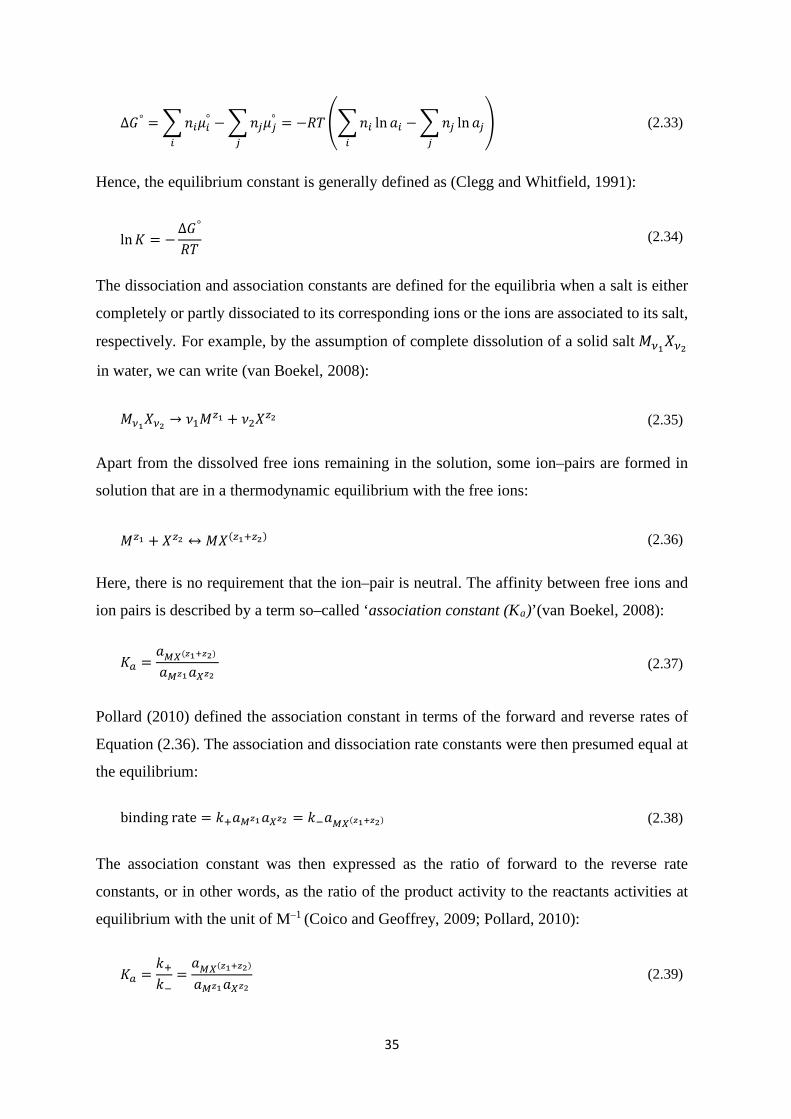
35
Δ𝐺𝐺° = 𝑛𝑛𝑖𝑖𝜇𝜇𝑖𝑖°
𝑖𝑖
−𝑛𝑛𝑗𝑗𝜇𝜇𝑗𝑗°
𝑗𝑗
= −𝑅𝑅𝑅𝑅𝑛𝑛𝑖𝑖 ln𝑎𝑎𝑖𝑖𝑖𝑖
−𝑛𝑛𝑗𝑗 ln𝑎𝑎𝑗𝑗𝑗𝑗
(2.33)
Hence, the equilibrium constant is generally defined as (Clegg and Whitfield, 1991):
ln𝐾𝐾 = −
Δ𝐺𝐺°
𝑅𝑅𝑅𝑅 (2.34)
The dissociation and association constants are defined for the equilibria when a salt is either
completely or partly dissociated to its corresponding ions or the ions are associated to its salt,
respectively. For example, by the assumption of complete dissolution of a solid salt 𝑀𝑀𝜈𝜈1𝑋𝑋𝜈𝜈2 R
in water, we can write (van Boekel, 2008):
𝑀𝑀𝜈𝜈1𝑋𝑋𝜈𝜈2 → 𝜈𝜈1𝑀𝑀𝑧𝑧1 + 𝜈𝜈2𝑋𝑋𝑧𝑧2 (2.35)
Apart from the dissolved free ions remaining in the solution, some ion–pairs are formed in
solution that are in a thermodynamic equilibrium with the free ions:
𝑀𝑀𝑧𝑧1 + 𝑋𝑋𝑧𝑧2 ↔ 𝑀𝑀𝑋𝑋(𝑧𝑧1+𝑧𝑧2) (2.36)
Here, there is no requirement that the ion–pair is neutral. The affinity between free ions and
ion pairs is described by a term so–called ‘association constant (Ka)’(van Boekel, 2008):
𝐾𝐾𝑎𝑎 =𝑎𝑎𝑀𝑀𝑋𝑋(𝑧𝑧1+𝑧𝑧2)
𝑎𝑎𝑀𝑀𝑧𝑧1𝑎𝑎𝑋𝑋𝑧𝑧2 (2.37)
Pollard (2010) defined the association constant in terms of the forward and reverse rates of
Equation (2.36). The association and dissociation rate constants were then presumed equal at
the equilibrium:
binding rate = 𝑘𝑘+𝑎𝑎𝑀𝑀𝑧𝑧1𝑎𝑎𝑋𝑋𝑧𝑧2 = 𝑘𝑘−𝑎𝑎𝑀𝑀𝑋𝑋(𝑧𝑧1+𝑧𝑧2) (2.38)
The association constant was then expressed as the ratio of forward to the reverse rate
constants, or in other words, as the ratio of the product activity to the reactants activities at
equilibrium with the unit of M–1 (Coico and Geoffrey, 2009; Pollard, 2010):
𝐾𝐾𝑎𝑎 =
𝑘𝑘+𝑘𝑘−
=𝑎𝑎𝑀𝑀𝑋𝑋(𝑧𝑧1+𝑧𝑧2)
𝑎𝑎𝑀𝑀𝑧𝑧1𝑎𝑎𝑋𝑋𝑧𝑧2 (2.39)

36
Similarly, the dissociation constant (Kd) is defined as the inverse of the association constant
(Pollard, 2010):
𝐾𝐾𝑑𝑑 =
𝑘𝑘−𝑘𝑘+
=𝑎𝑎𝑀𝑀𝑧𝑧1𝑎𝑎𝑋𝑋𝑧𝑧2𝑎𝑎𝑀𝑀𝑋𝑋(𝑧𝑧1+𝑧𝑧2)
(2.40)
Some authors use the terms association constant and dissociation constant without following
the definitions given here.
The equilibrium constant of an acid/base system is defined as a dissociation constant (Atkins,
1990). For a standard point of view, the equilibrium for a simple acid/base system is written
as follows:
Unionised acid(aq) + H2O(l) ↔ Anion + 𝐻𝐻+ (2.41)
The pH of a solution by definition is:
pH = − log10 𝑎𝑎𝐻𝐻+ (2.42)
The acidity constant, Ka c, is expressed as follows for acids:
𝐾𝐾𝑎𝑎𝑐𝑐 =𝑎𝑎𝐻𝐻+𝑎𝑎Anion
𝑎𝑎Unionised acid (2.43)
A large value of Kac indicates a strong acid, e.g. the value of HCl acidity constant is quite
large, hence, most of the salt dissociates to its corresponding free ions and a very tiny amount
of the electrolyte remains as an undissociated ion. Lactose is a good example of weak
electrolyte, which sometimes refers to a non–electrolyte with very low value of acidity
constant that mostly remains as the undissociated ion in the solution.
In most of the literature, the symbol for acidity constant and association constants are the
same. In this thesis, Kac and Ka are used for acidity constant and association constant,
respectively to avoid confusion. The acidity association constants values cover a wide range;
hence, it is appropriate to use the base 10 logarithm of Ka c:
𝑝𝑝𝐾𝐾𝑎𝑎𝑐𝑐 = − log10(𝐾𝐾𝑎𝑎𝑐𝑐) (2.44)
Equation (2.44) is combined with Equations (2.42) and (2.43) to give:

37
pH = 𝑝𝑝𝐾𝐾𝑎𝑎𝑐𝑐 + log10𝑎𝑎Anion
𝑎𝑎Unionised acid (2.45)
which is also called Henderson–Hasselbach Equation.
Similarly, pKb can be written for bases:
𝐾𝐾𝑏𝑏 =𝑎𝑎𝑂𝑂𝐻𝐻−𝑎𝑎𝐶𝐶𝑎𝑎𝐶𝐶𝑖𝑖𝑠𝑠𝑠𝑠𝑎𝑎unionised acid
(2.46)
And:
𝑝𝑝𝐾𝐾𝑏𝑏 = − log10(𝐾𝐾𝑏𝑏) (2.47)
Water dissociation in aqueous solutions is expressed as:
𝐾𝐾𝑤𝑤 = 𝑎𝑎𝐻𝐻+𝑎𝑎𝑂𝑂𝐻𝐻− (2.48)
Harned and Cook (1937) proposed a relationship between dissociation constant of water and
temperature based on experiments as:
𝑝𝑝𝐾𝐾𝑤𝑤 = − log10 𝐾𝐾𝑤𝑤 =4787.3𝑅𝑅
+ 7.1321 log10 𝑅𝑅 + 0.010365𝑅𝑅 − 22.801 (2.49)
At 298.15 K (25°C), pKw is 13.9966 mol2 L–2 but often 14 mol2 L–2 is used.
In some literature, the term “intrinsic association constant” was used to describe the affinity
between the reactants and products of equilibrium and has the same definition as association
constant. According to Cruse and Lewis (2010), intrinsic association constant represents the
case when a ligand is univalently bound to a special site of a protein if all sites are exactly the
same. Holt et al. (1981) used the intrinsic association constant parameter using activities and
not concentrations, and so the intrinsic association constant depends on the activity coefficient
models. In this thesis, it is used with the same meaning as Holt et al. (1981).
2.2.5 Solubility
According to Mullin (2001), the solubility of a solid substance is described as the maximum
dissolved amount of a solid substance in a solvent (water) under certain conditions. The
solubility product constant, Ksp , is a term by which the dissolution reaction is often described
(Stumm and Morgan, 1996). The dissolution reaction of a solid salt can be shown as:

38
𝑀𝑀𝜈𝜈1𝑋𝑋𝜈𝜈2(𝑠𝑠) ↔ 𝜈𝜈1𝑀𝑀𝑧𝑧1 + 𝜈𝜈2𝑋𝑋𝑧𝑧2 (2.50)
and the solubility product constant, 𝐾𝐾𝑠𝑠𝑠𝑠, equals the ion activity product (𝐼𝐼𝐼𝐼𝐼𝐼) when the solid
and ions are at equilibrium:
𝐼𝐼𝐼𝐼𝐼𝐼 = 𝑎𝑎𝑀𝑀𝑧𝑧1𝜈𝜈1𝑎𝑎𝑋𝑋
𝑧𝑧2𝜈𝜈2 (2.51)
Here IAP is the product chemical activities of free ions existing in the supersaturated solution.
The activity of the solid salt is not included in the solubility product equation, because the
solid phase is usually presumed to be pure component with an activity of 1.0, see Section
2.2.1.1, Option 4). This might contradict with the definitions of molar, molal, and mole
fraction activity shown in Equations (2.3), (2.5), and (2.6). They use different reference points
and neither of the definitions is wrong.
Precipitation can happen when the IAP is higher than the Ksp of a particular salt in the aqueous
phase. In contrast, dissolution occurs when the IAP is lower than the Ksp. These result in the
supersaturation and undersaturation concepts and a driving force for either precipitation or
dissolution. Having the knowledge of the supersaturation and undersaturation concepts is
essential to predict precipitation or dissolution phenomena. The supersaturation ratio, Ω, is
shown as (Mullin, 2001):
Ω =
𝐼𝐼𝐼𝐼𝐼𝐼𝐾𝐾𝑠𝑠𝑠𝑠
1𝜈𝜈
= (𝑆𝑆𝑎𝑎𝑆𝑆)1𝜈𝜈 (2.52)
Here ν is the total number of participating ions in the solid formula. The term ‘Sat’ refers to
saturation, which is defined as the ratio of IAP to Ksp. In some literature, the supersaturation
ratio is also called the oversaturation (Mullin, 2001). Relative supersaturation is another term
to describe the state of the supersaturated solution that is expressed as (Nielsen, 1984):
𝜎𝜎 = Ω − 1 =
𝐼𝐼𝐼𝐼𝐼𝐼𝐾𝐾𝑠𝑠𝑠𝑠
1𝜈𝜈− 1 (2.53)
The supersaturation value directs the equilibrium state to proceed to either precipitation or
dissolution. Another parameter that can be used to determine the equilibrium state is the
saturation index (SI):
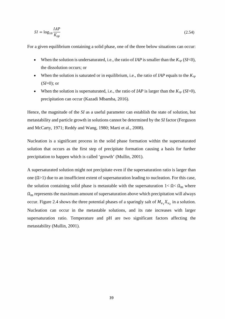
39
𝑆𝑆𝐼𝐼 = log10𝐼𝐼𝐼𝐼𝐼𝐼𝐾𝐾𝑠𝑠𝑠𝑠
(2.54)
For a given equilibrium containing a solid phase, one of the three below situations can occur:
• When the solution is undersaturated, i.e., the ratio of IAP is smaller than the Ksp (SI<0),
the dissolution occurs; or
• When the solution is saturated or in equilibrium, i.e., the ratio of IAP equals to the Ksp
(SI=0); or
• When the solution is supersaturated, i.e., the ratio of IAP is larger than the Ksp (SI>0),
precipitation can occur (Kazadi Mbamba, 2016).
Hence, the magnitude of the SI as a useful parameter can establish the state of solution, but
metastability and particle growth in solutions cannot be determined by the SI factor (Ferguson
and McCarty, 1971; Reddy and Wang, 1980; Marti et al., 2008).
Nucleation is a significant process in the solid phase formation within the supersaturated
solution that occurs as the first step of precipitate formation causing a basis for further
precipitation to happen which is called ‘growth’ (Mullin, 2001).
A supersaturated solution might not precipitate even if the supersaturation ratio is larger than
one (Ω>1) due to an insufficient extent of supersaturation leading to nucleation. For this case,
the solution containing solid phase is metastable with the supersaturation 1< Ω< Ωm where
Ωm represents the maximum amount of supersaturation above which precipitation will always
occur. Figure 2.4 shows the three potential phases of a sparingly salt of 𝑀𝑀𝜈𝜈1𝑋𝑋𝜈𝜈2 in a solution.
Nucleation can occur in the metastable solutions, and its rate increases with larger
supersaturation ratio. Temperature and pH are two significant factors affecting the
metastability (Mullin, 2001).

40
Figure 2.4 A phase scheme of a relatively insoluble salt (Kazadi Mbamba, 2016). The brackets represent the molar concentration of species.
2.2.5.1 Dynamic solubility
The precipitation or dissolution reactions of a sparingly insoluble salt can be predicted by
dynamic models leading to a mathematical solution, by which the solution phase transition
can be determined over time (Kazadi Mbamba, 2016).
Many researchers have worked on the solid formation mechanism of a solution by various
methods (Kralj et al., 1997; Babić-Ivančić et al., 2006; Cha et al., 2013; Othman et al., 2014;
Shen et al., 2014). Hanze et al. (2000) proposed a model to predict phosphate precipitation by
a pseudo–equilibrium reaction, considering both precipitation and dissolution kinetic rates, in
which the pH of solution is presumed neutral.
Nielsen and Toft (1984) and Wiechers et al. (1975) presented a semi–empirical kinetic rate
law for a simple reaction including precipitation with a first and nth orders influence on the
solid phase concentration and supersaturation in the solution, respectively. The kinetic
precipitation rate of the solid phase is shown as follows:
𝑟𝑟𝑠𝑠𝑝𝑝𝑝𝑝𝑐𝑐 = 𝑘𝑘𝑠𝑠𝑝𝑝𝑝𝑝𝑐𝑐𝐶𝐶𝑠𝑠𝑝𝑝𝑝𝑝𝑐𝑐 𝜎𝜎𝑠𝑠 (2.55)
where 𝑟𝑟𝑠𝑠𝑝𝑝𝑝𝑝𝑐𝑐 is the rate of precipitation in mol L–1 h–1; 𝑘𝑘𝑠𝑠𝑝𝑝𝑝𝑝𝑐𝑐 is the precipitation rate constant
in h–1; 𝐶𝐶𝑠𝑠𝑝𝑝𝑝𝑝𝑐𝑐 is the dynamic (time–dependent) molar concentration of precipitate; n is the
order of the solid phase reaction; and 𝜎𝜎 is the relative supersaturation determines how far the
solution is from precipitation or dissolution or neither. The kinetic rate law can be also
[M]z 1
[X]z2
Supersaturated solution Ω >1
Meastable phase
Undersaturated solution Ω <1
↑ Ωm
↑ Ω=1

41
dynamically applied to dissolution (Kazadi Mbamba, 2016). The rate of precipitation becomes
zero in Equation (2.55) for 𝜎𝜎<1.
2.2.6 Activity coefficient models
Generally, association and dissociation constants pertain to activities, and only to
concentrations when they are at infinite dilution. The activity coefficients of species in the
solution can be significantly less than 1.0 when the molal ionic strength of the solution is
larger than about 0.01 mol kg–1water. Several models and experimental methods have been
proposed for the calculation and measurement of mean ion–pair and free ion activity
coefficient. However, it is impossible to measure the activity coefficient of individual ions
due to the electroneutrality principle (Gao, 2010). Hence, free ion activity coefficients need
to be inferred from measurements of the same ion in multiple solutions with different counter
ions.
In the following sections, various proposed models and theories are categorised based on the
ion–pair and free ion approaches to be able to distinguish mean ion–pair and free ion activity
coefficients.
2.2.6.1 Mean ion–pair activity coefficients models
As already discussed in Section 2.2.2, the mean ion–pair activity coefficient assumes a fully
dissociated electrolyte in a solution.
Debye–Hückel theory
The Debye–Hückel theory is an empirical model, in which the electrostatic effects determine
the solution deviation from non–ideality in regards to a central ion whereas other ions are
considered as point charges. The general equation is a relationship between the mean molal
ion–pair activity coefficient (𝛾𝛾±), charge numbers of cations and anions (z+ and z–), and the
distance of closest approach (𝜎𝜎, [m]) as (Zemaitis et al., 1986; van Boekel, 2008):
ln 𝛾𝛾± = −
|𝑧𝑧+𝑧𝑧−|𝑒𝑒02
8𝜋𝜋𝜀𝜀0𝜀𝜀𝑝𝑝𝑘𝑘𝐵𝐵𝑅𝑅𝜅𝜅
1 + 𝜅𝜅𝜎𝜎 (2.56)
where the Debye screening parameter (𝜅𝜅) is defined as:

42
𝜅𝜅 = 4𝜋𝜋𝐿𝐿𝐵𝐵𝜌𝜌𝑖𝑖𝑧𝑧𝑖𝑖2
𝑖𝑖
(2.57)
Here 𝜌𝜌𝑖𝑖 is the number density of component 𝑖𝑖 . The Bjerrum parameter (𝐿𝐿𝐵𝐵 , [m]) is the
distance at which either the attractive or repulsive energies between ion charges equal to the
thermal energy:
𝐿𝐿𝐵𝐵 =
𝑒𝑒02
4𝜋𝜋𝜀𝜀0𝜀𝜀𝑝𝑝𝑘𝑘𝐵𝐵𝑅𝑅 (2.58)
The full details of parameters with their corresponding units are shown in Table 2.9.
Table 2.9 Full description of the Debye–Hückel parameters (van Boekel, 2008).
The Debye–Hückel parameter The symbol The unit in SI
Mean molal ion-pair activity coefficient 𝛾𝛾± Dimensionless
Charge numbers of cation and anion 𝑧𝑧+, 𝑧𝑧− Dimensionless
Boltzmann constant 𝑘𝑘𝐵𝐵 1.38 × 10⁻²³ m2kg s−2K−1
Debye screening length parameter 𝜅𝜅 m−1
The permittivity of vacuum 𝜀𝜀0 8.854 × 10⁻¹² Faradsm
or C2s2
m3 kg
The elementary charge 𝑒𝑒0 1.602 × 10⁻¹⁹ coulomb
The relative permittivity of the medium* 𝜀𝜀𝑝𝑝 Dimensionless
Absolute temperature 𝑅𝑅 K
Bjerrum parameter 𝐿𝐿𝐵𝐵 m
The distance of closest approach 𝜎𝜎 m
The number of density of species 𝜌𝜌𝑖𝑖 Number of particles m–3
*The old name of the relative permittivity of the medium is the dielectric constant. In this thesis, the dielectric constant is used.
Shilov and Lyashchenko (2015) extended a correlation between the dielectric constant and
molar concentration of the electrolyte. However, this influence was ignored by Debye–Hückel
theory, e.g. Tikanen and Fawcett (1996) and Buchner et al. (1999) showed the dependency of
the dielectric constant of electrolyte with the molar concentration of sodium chloride (NaCl)
and calcium chloride (CaCl2) solutions as:

43
𝜀𝜀𝑝𝑝𝑁𝑁𝑎𝑎𝐶𝐶𝑠𝑠 = 𝜀𝜀𝑤𝑤 − 15.45𝐶𝐶 + 3.76𝐶𝐶1.5 (2.59)
𝜀𝜀𝑝𝑝𝐶𝐶𝑎𝑎𝐶𝐶𝑠𝑠2 = 𝜀𝜀𝑤𝑤 − 34𝐶𝐶 + 10𝐶𝐶1.5 (2.60)
𝜀𝜀𝑤𝑤 is dielectric constant of water which is 78.65 at 298.15 K. The density number of species
and molar concentration of species i (𝐶𝐶𝑖𝑖) can be expressed as (van Boekel, 2008):
𝜌𝜌𝑖𝑖 = 103𝐶𝐶𝑖𝑖 𝑁𝑁𝐴𝐴𝐴𝐴 (2.61)
where 𝑁𝑁𝐴𝐴𝐴𝐴 is Avogadro’s number (6.022 × 10²³ mol−1).
The distance of closest approach (𝜎𝜎 or in some other literature shown as 𝑑𝑑𝑅𝑅) is another
parameter of Debye–Hückel theory representing the sum of the interacting ions effective radii.
Kielland (1937) defined it as ‘the effective radii of the hydrated ions’ that was estimated for
various mono–, di–, and tri–valent ions. Shannon and Prewitt (1969) have carried out research
on the crystal radii and the effective ionic radii. According to Debye–Hückel theory, all ions
in a particular system are presumed to have identical sizes equal to the means ion diameter
(van Boekel, 2008).
Debye–Hückel Limiting Law and Extended Debye–Hückel theories
The principal Debye–Hückel theory was modified relating mean molal ion–pair activity
coefficient to the total molal ionic strength (𝐼𝐼𝑚𝑚,𝑇𝑇) giving the Debye–Hückel Limiting Law and
the Extended Debye–Hückel equations as shown by Equations (2.62) and (2.63), respectively
(van Boekel, 2008):
log10 𝛾𝛾± = −𝐼𝐼𝐷𝐷𝐻𝐻|𝑧𝑧+𝑧𝑧−|𝐼𝐼𝑚𝑚,𝑇𝑇 (2.62)
and
log10 𝛾𝛾± = −
𝐼𝐼𝐷𝐷𝐻𝐻|𝑧𝑧+𝑧𝑧−|𝐼𝐼𝑚𝑚,𝑇𝑇
1 + 𝐵𝐵𝐷𝐷𝐻𝐻𝜎𝜎𝐼𝐼𝑚𝑚,𝑇𝑇 (2.63)
Lewis and Randall (1921) defined the ionic strength as a function of molal concentration and
charge number of ions:

44
𝐼𝐼𝑚𝑚,𝑇𝑇 =12𝑚𝑚𝑖𝑖𝑧𝑧𝑖𝑖2
𝑖𝑖
(2.64)
The subscripts m and T represent molal scale and total of ionic strength, respectively, due to
the full dissociation of electrolyte. Equations (2.62), (2.63), and (2.64) can be similarly used
for the molar scale, but they should be substituted with the total molar ionic strength (𝐼𝐼𝐶𝐶,𝑇𝑇)
and mean molar ion–pair activity coefficient (𝑦𝑦±).
𝐼𝐼𝐷𝐷𝐻𝐻 and 𝐵𝐵𝐷𝐷𝐻𝐻 are two temperature dependent parameters of the Limiting Law and Extended
Debye–Hückel equations that can be used for both scales:
𝐼𝐼𝐷𝐷𝐻𝐻 =2𝜋𝜋𝑁𝑁𝐴𝐴𝐴𝐴 × 1000 𝐿𝐿𝐵𝐵3
ln 10 mol−
12. L
12 or mol−
12kg
12
(2.65)
𝐵𝐵𝐷𝐷𝐻𝐻 =𝜅𝜅
𝐼𝐼𝑇𝑇, mol−
12. kg
12. m−1or [mol−
12. L
12. m−1] (2.66)
Schmidt and Both (1987) proposed an equation for the calculation of 𝐼𝐼𝐷𝐷𝐻𝐻 in terms of
temperature (˚C):
𝐼𝐼𝐷𝐷𝐻𝐻 = 0.486 + 6.07 × 10⁻⁴𝑅𝑅 + 6.43 × 10⁻⁶𝑅𝑅2 (2.67)
Table 2.10 indicates the values of the temperature–dependent parameters, relative
permittivity, and Bjerrum length in terms of different temperature at 1 bar pressure (van
Boekel, 2008).
Table 2.10 The numerical values of the Debye–Hückel equations (van Boekel, 2008).
Temperature (˚C) 𝜀𝜀𝑝𝑝[−] 𝐿𝐿𝐵𝐵 × 109[m] 𝐼𝐼𝐷𝐷𝐻𝐻 𝐵𝐵𝐷𝐷𝐻𝐻 × 10−10 0 87.74 0.696 0.491 0.325 15 81.94 0.707 0.502 0.327 20 80.10 0.711 0.506 0.328 25 78.30 0.715 0.510 0.329 30 76.54 0.719 0.515 0.330
The effect of long–range Coulomb forces is demonstrated by the numerator of the Extended
Debye–Hückel, whereas the dominator specifies the short–range interactions among the

45
species. Debye–Hückel theories should be used only when the solution is dilute with a
maximum total molar ionic strength of 100 mmol L–1. Another drawback of these theories is
that the finite size of species is neglected and this causes inaccuracies when the solution
becomes concentrated (Debye and Hückel, 1923; van Boekel, 2008).
Davies theory
Davies (1962) proposed an empirical extension that has been extensively applied to various
systems to predict mean molal ion–pair activity coefficient. This model is a modified version
of Guggenheim (1926) method, that gives a better fit to experimental values even for solutions
with higher ionic strength up to 0.5 mol kg–1water:
log10 𝛾𝛾± = −𝐼𝐼𝐷𝐷𝐻𝐻
|𝑧𝑧+𝑧𝑧−|𝐼𝐼𝑚𝑚,𝑇𝑇
1 + 𝐼𝐼𝑚𝑚,𝑇𝑇− 0.2 𝐼𝐼𝑚𝑚,𝑇𝑇 (2.68)
This model has been used extensively in literature for calculation of activity coefficient
because it is simple to use, requiring only concentrations and charge number of ions.
Bromley’s theory
The mean molal ion–pair activity coefficient can be accurately predicted for concentrated
solutions with the total molal ionic strength up to 6 mol kg–1water at 25 ˚C (Bromley, 1972).
log10 𝛾𝛾± =
− 𝐼𝐼𝐷𝐷𝐻𝐻 |𝑧𝑧+𝑧𝑧−|𝐼𝐼𝑚𝑚,𝑇𝑇
1 + 𝐼𝐼𝑚𝑚,𝑇𝑇+
(0.06 + 0.6 𝐵𝐵)|𝑧𝑧+𝑧𝑧−| 𝐼𝐼𝑚𝑚,𝑇𝑇
1 +1.5 𝐼𝐼𝑚𝑚,𝑇𝑇|𝑧𝑧+𝑧𝑧−|
2 + 𝐵𝐵𝐼𝐼𝑚𝑚,𝑇𝑇 (2.69)
where B is the interaction parameter, kg mol–1. Table 2.11 indicates the numerical values of
B determined by the least squares methods for some electrolytes at 25˚C. The application of
this model to multicomponent systems is not defined.
Table 2.11 Numerical values of B for Bromley’s method at 25 ˚C (Bromley, 1972).
HCl CaCl2 NaCl H2SO4 Na2HPO4 NaH2PO4 B, [kg mol–1] 0.1433 0.0948 0.0574 0.0606 –0.0265 –0.0460
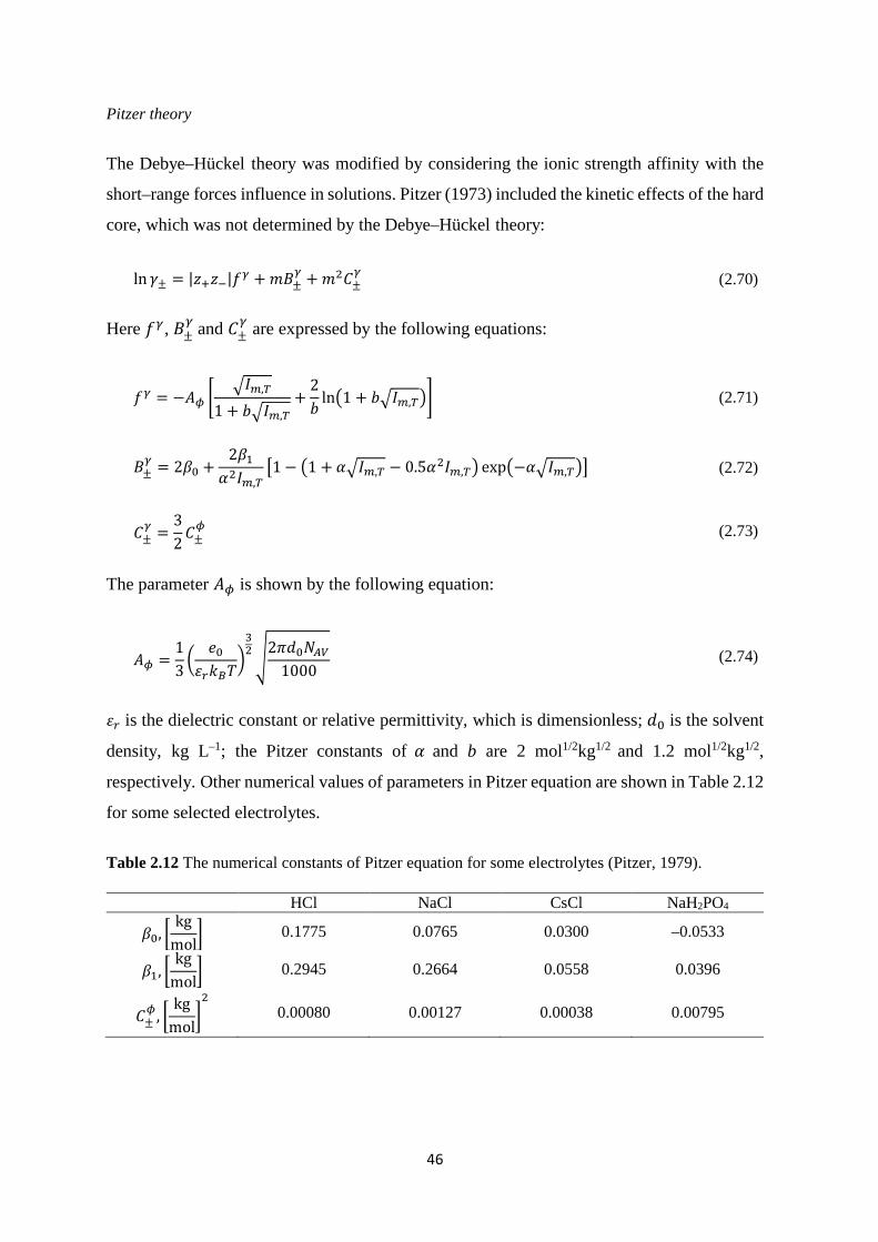
46
Pitzer theory
The Debye–Hückel theory was modified by considering the ionic strength affinity with the
short–range forces influence in solutions. Pitzer (1973) included the kinetic effects of the hard
core, which was not determined by the Debye–Hückel theory:
ln 𝛾𝛾± = |𝑧𝑧+𝑧𝑧−|𝑓𝑓𝛾𝛾 + 𝑚𝑚𝐵𝐵±𝛾𝛾 + 𝑚𝑚2𝐶𝐶±
𝛾𝛾 (2.70)
Here 𝑓𝑓𝛾𝛾, 𝐵𝐵±𝛾𝛾 and 𝐶𝐶±
𝛾𝛾 are expressed by the following equations:
𝑓𝑓𝛾𝛾 = −𝐼𝐼𝜙𝜙
𝐼𝐼𝑚𝑚,𝑇𝑇
1 + 𝑏𝑏𝐼𝐼𝑚𝑚,𝑇𝑇+
2𝑏𝑏
ln1 + 𝑏𝑏𝐼𝐼𝑚𝑚,𝑇𝑇 (2.71)
𝐵𝐵±𝛾𝛾 = 2𝛽𝛽0 +
2𝛽𝛽1𝛼𝛼2𝐼𝐼𝑚𝑚,𝑇𝑇
1− 1 + 𝛼𝛼𝐼𝐼𝑚𝑚,𝑇𝑇 − 0.5𝛼𝛼2𝐼𝐼𝑚𝑚,𝑇𝑇 exp−𝛼𝛼𝐼𝐼𝑚𝑚,𝑇𝑇 (2.72)
𝐶𝐶±𝛾𝛾 =
32𝐶𝐶±𝜙𝜙 (2.73)
The parameter 𝐼𝐼𝜙𝜙 is shown by the following equation:
𝐼𝐼𝜙𝜙 =
13
𝑒𝑒0𝜀𝜀𝑝𝑝𝑘𝑘𝐵𝐵𝑅𝑅
32 2𝜋𝜋𝑑𝑑0𝑁𝑁𝐴𝐴𝐴𝐴
1000 (2.74)
𝜀𝜀𝑝𝑝 is the dielectric constant or relative permittivity, which is dimensionless; 𝑑𝑑0 is the solvent
density, kg L–1; the Pitzer constants of 𝛼𝛼 and b are 2 mol1/2kg1/2 and 1.2 mol1/2kg1/2,
respectively. Other numerical values of parameters in Pitzer equation are shown in Table 2.12
for some selected electrolytes.
Table 2.12 The numerical constants of Pitzer equation for some electrolytes (Pitzer, 1979).
HCl NaCl CsCl NaH2PO4
𝛽𝛽0, kg
mol 0.1775 0.0765 0.0300 –0.0533
𝛽𝛽1, kg
mol 0.2945 0.2664 0.0558 0.0396
𝐶𝐶±𝜙𝜙 ,
kgmol
2
0.00080 0.00127 0.00038 0.00795

47
Meissner’s theory
Meissner and Kusik (1978) defined the reduced activity coefficient to be able to use a
computational method for calculating the mean molal ion–pair activity coefficient of a pure
electrolyte in a solution at 25 ˚C.
Γ° = 𝛾𝛾±
1𝑧𝑧+𝑧𝑧− (2.75)
Here Γ°is the reduced activity coefficient:
Γ° = 1 + 𝐵𝐵1 + 0.1𝐼𝐼𝑚𝑚,𝑇𝑇𝑞𝑞 − 𝐵𝐵Γ∗ (2.76)
Γ∗ and B can be obtained as follows:
log10 Γ∗ = −
0.5107 𝐼𝐼𝑚𝑚,𝑇𝑇
1 + 𝐶𝐶 𝐼𝐼𝑚𝑚,𝑇𝑇 (2.77)
𝐵𝐵 = 0.75− 0.065 𝑞𝑞 (2.78)
in which C has an exponential relation with the total molal ionic strength.
𝐶𝐶 = 1 + 0.055 𝑞𝑞 exp(−0.023 𝐼𝐼𝑚𝑚,𝑇𝑇3 ) (2.79)
Numerical values of the Meissner parameter (q) are indicated in Table 2.13 for some selected
electrolytes:
Table 2.13 The values of parameter q for some electrolytes at 25˚C (Meissner and Kusik, 1978).
CsCl HCl NaCl Na2SO4 CaCl2 NaH2PO4 q 0.16 6.69 2.23 –0.19 2.40 –1.59
None of these ion–pair methods can be easily extended to multi–ion systems in which
dissociation of the salts is not complete. Moreover, these models are approximations in the
activity coefficient determination. However, much of the existing data for simple solution e.g.
Zemaitis et al. (1986) is based on one or more of these mentioned equation, so they are useful
for validation.

48
2.2.6.2 Free–ion activity coefficients models
According to Gao (2010), ion–pairs and free ions activity coefficients are also essential to
account for the calculation of the ionic strength of the multicomponent solution. For example,
CaCl2 can exist in solution as Ca2+, Cl–, and ion–pair CaCl+. Therefore, a free ion activity
coefficient model will help to determine activity coefficient and hence activities of all ions in
any multicomponent solution. Below are various theories for calculation of free ion activity
coefficient that were proposed for different systems in different scales.
Debye–Hückel theory
The Limiting Law (Equation 2.80) and Extended Debye–Hückel (Equation 2.81) theories can
be applied to both cations, anions, and ion–pairs of the multicomponent solution to obtain the
molal activity coefficient of all species (Debye and Hückel, 1923):
log10 𝛾𝛾+ = −𝐼𝐼𝐷𝐷𝐻𝐻𝑧𝑧+2𝐼𝐼𝑚𝑚,𝐻𝐻; log10 𝛾𝛾− = −𝐼𝐼𝐷𝐷𝐻𝐻𝑧𝑧−2𝐼𝐼𝑚𝑚,𝐻𝐻 (2.80)
log10 𝛾𝛾+ =
−𝐼𝐼𝐷𝐷𝐻𝐻𝑧𝑧+2𝐼𝐼𝑚𝑚,𝐻𝐻
1 + 𝐵𝐵𝐷𝐷𝐻𝐻𝜎𝜎𝐼𝐼𝑚𝑚,𝐻𝐻; log10 𝛾𝛾− =
−𝐼𝐼𝐷𝐷𝐻𝐻𝑧𝑧−2𝐼𝐼𝑚𝑚,𝐻𝐻
1 + 𝐵𝐵𝐷𝐷𝐻𝐻𝜎𝜎𝐼𝐼𝑚𝑚,𝐻𝐻 (2.81)
Although the partial molal ionic strength formula (𝐼𝐼𝑚𝑚,𝐻𝐻) is apparently identical to the Equation
(2.64), it involves the molal concentration and charge of free ions as well as ion–pairs.
Therefore, the subscript P represents the partial dissociation of electrolyte.
Similarly, Debye–Hückel theories are applicable to the molarity scales.
The Limiting Law and Extended Debye–Hückel equations give good estimation of free ion
activity coefficient of diluted solutions, e.g. 𝐼𝐼𝐶𝐶,𝐻𝐻 < 10 mM and 𝐼𝐼𝐶𝐶,𝐻𝐻 < 100 mM for Limiting
Law and Extended Debye–Hückel theories, respectively (van Boekel, 2008).
Several authors used different numerical values for the constant parameters of Debye–Hückel,
e.g. Holt et al. (1981) modified the Debye–Hückel Extended equation as follows:
log10 𝑦𝑦𝑖𝑖 =
−0.358 𝑧𝑧𝑖𝑖2Γ12
1 + 2.32𝑎𝑎Γ12
(2.82)

49
where a is the closest distance approach or in other words, effective size parameter, nm; Γ is
the partial molar ionic strength and is defined as twice the previously defined molar ionic
strength:
Γ = 𝐶𝐶𝑖𝑖𝑧𝑧𝑖𝑖2
𝑖𝑖
= 2𝐼𝐼𝐶𝐶,𝐻𝐻 (2.83)
Davies theory
The Davies theory (Davies, 1962) for the mean ion–pair activity coefficient can be similarly
used for the determination of free ion activity coefficient with larger ionic strength (𝐼𝐼𝐶𝐶,𝐻𝐻 <
0.5 M) by adding a ‘salting out’ term to the Extended Debye–Hückel formula as:
log10 𝛾𝛾𝑖𝑖 = −𝐼𝐼𝐷𝐷𝐻𝐻
𝑧𝑧𝑖𝑖2𝐼𝐼𝑚𝑚,𝐻𝐻
1 + 𝐼𝐼𝑚𝑚,𝐻𝐻− 0.2 𝐼𝐼𝑚𝑚,𝐻𝐻 (2.84)
The Davies equation error was generally estimated to be less than 3% and 8% for the molar
ionic strength less than 0.1 M and 0.5 M, respectively (Butler, 1998).
Mean Spherical Approximation theory (MSA)
The finite size of free ions is neglected in the Debye–Hückel theory resulting in the
overestimation of the ion–ion interaction effects. The Mean Spherical Approximation theory
(MSA) was first proposed by Lebowitz and Percus (1966) who assumed the electrolyte as a
group of hard spheres constituting the corresponding anions and cations. The hard spheres are
presumed to be submerged in a dielectric continuum of solvent. This theory is considered as
‘primitive’, because the discrete nature of the solvent molecules are neglected (Fawcett and
Tikanen, 1996). The strength of MSA theory is to include the excluded volume of the ions,
short and long–range interactions leading to the prediction of activity coefficient at higher
concentrations (Taghikhani and Vera, 2000). Hence, MSA theory is of great interest for
researchers to thermodynamically determine the properties of multicomponent electrolyte
solutions that has been widely applied to ionic solutions and real solutions (Liu et al., 1998).
Waisman and Lebowitz (1972) applied the MSA theory to a symmetrical electrolyte with
identical sizes of ions. A general solution of the MSA with unequal ion size was proposed and
is called ‘unrestricted MSA’ (Blum, 1975; Blum and Høye, 1977; Sanchez-Castro and Blum,
1989). It was used to predict the mean activity coefficient of the electrolyte solutions (Triolo

50
et al., 1976; Triolo et al., 1977, 1978). The term ‘restricted’ is used when the ions size are
assumed to be equal (Fawcett and Tikanen, 1996).
The calculations of the equations are based on the molarity scale; hence, in some stage,
conversion of molarity to molality can be necessary. The free ion molar activity coefficient is
made up of two contributions; the electrostatic contribution, ‘es’, that correlates any
thermodynamic property of an aqueous multicomponent solution containing hard spheres of
charged ions in a dielectric continuum, and the excluded volume of free ions is incorporated
into the hard sphere contribution, ‘hs’ (Vilariño and Sastre de Vicente, 1999; van Boekel,
2008):
ln𝑦𝑦𝑖𝑖 = ln𝑦𝑦𝑖𝑖𝑝𝑝𝑠𝑠 + ln𝑦𝑦𝑖𝑖ℎ𝑠𝑠 (2.85)
The ion effective diameter of the species (𝜎𝜎𝑖𝑖) is assumed unequal according to the unrestricted
approach of the electrostatic contribution. The molar free ion activity coefficient of the
electrostatic contribution is obtained as (van Boekel, 2008):
ln𝑦𝑦𝑖𝑖𝑝𝑝𝑠𝑠 = −𝐿𝐿𝐵𝐵
Γ𝑧𝑧𝑖𝑖2
1 + Γ𝜎𝜎𝑖𝑖+ 𝜍𝜍𝜎𝜎𝑖𝑖
2𝑧𝑧𝑖𝑖 − 𝜍𝜍𝜎𝜎𝑖𝑖2
1 + Γ𝜎𝜎𝑖𝑖+𝜍𝜍𝜎𝜎𝑖𝑖2
3 2
(2.86)
The equation for the restricted approach for when the ions size is equal is:
ln𝑦𝑦𝑖𝑖𝑝𝑝𝑠𝑠 = −𝐿𝐿𝐵𝐵
Γ𝑧𝑧𝑖𝑖2
1 + Γ𝜎𝜎𝑖𝑖 (2.87)
The parameters of this equation are listed in the Table 2.14.
Several variations are given in the literature for the electrostatic contribution of MSA theory
as shown in Table 2.15. In early work, electrostatic system of units (ESU) was used. So, the
quantity of 4𝜋𝜋𝜀𝜀0 did not appear in the equations.

51
Table 2.14 The parameters of the electrostatic contribution of the MSA (van Boekel, 2008).
Parameter The equation Approach SI units
Γ
𝜅𝜅2
Unrestricted m−1
12𝜎𝜎 √
1 + 2𝜅𝜅𝜎𝜎 − 1 Restricted m−1
𝜎𝜎 𝜎𝜎𝑐𝑐𝑎𝑎𝐶𝐶𝑖𝑖𝑠𝑠𝑠𝑠 + 𝜎𝜎𝑎𝑎𝑠𝑠𝑖𝑖𝑠𝑠𝑠𝑠
2 both m
𝜅𝜅 4𝜋𝜋𝐿𝐿𝐵𝐵𝜌𝜌𝑖𝑖𝑧𝑧𝑖𝑖2𝑖𝑖
both m−1
𝜌𝜌𝑖𝑖 103𝑐𝑐𝑖𝑖𝑁𝑁𝐴𝐴𝐴𝐴 both Number of particlesm3
𝜍𝜍 𝜋𝜋2ΩΔ
𝜌𝜌𝑖𝑖𝜎𝜎𝑖𝑖𝑧𝑧𝑖𝑖
1 + Γ𝜎𝜎𝑖𝑖𝑖𝑖
Unrestricted m−2
Ω 1 +𝜋𝜋
2Δ
𝜌𝜌𝑖𝑖𝜎𝜎𝑖𝑖3
1 + Γ𝜎𝜎𝑖𝑖𝑖𝑖
Unrestricted [−]
Δ 1 −𝜋𝜋6𝜌𝜌𝑖𝑖𝜎𝜎𝑖𝑖3
𝑖𝑖
Unrestricted [−]
Table 2.15 Variations in the electrostatic contribution of MSA.
Free ion activity coefficient of the electrostatic contribution Reference
ln𝑦𝑦𝑖𝑖𝑝𝑝𝑠𝑠 = −𝐿𝐿𝐵𝐵 Γ𝑧𝑧𝑖𝑖2
1 + Γ𝜎𝜎𝑖𝑖+ 𝜍𝜍𝜎𝜎𝑖𝑖
2𝑧𝑧𝑖𝑖 − 𝜍𝜍𝜎𝜎𝑖𝑖2
1 + Γ𝜎𝜎𝑖𝑖+𝜍𝜍𝜎𝜎𝑖𝑖2
3 2
(van Boekel, 2008)
ln𝑦𝑦𝑖𝑖𝑝𝑝𝑠𝑠 = −𝐿𝐿𝐵𝐵 Γ𝑧𝑧𝑖𝑖
2
1+Γ𝜎𝜎𝑖𝑖+ 𝜍𝜍𝜎𝜎𝑖𝑖
2𝑧𝑧𝑖𝑖−𝜍𝜍𝜎𝜎𝑖𝑖2
1+Γ𝜎𝜎𝑖𝑖+ 𝜍𝜍𝜎𝜎𝑖𝑖
2
3 − 𝐿𝐿𝐵𝐵
4𝜋𝜋𝜀𝜀0𝜀𝜀𝑟𝑟∑ 𝜌𝜌𝑖𝑖𝑧𝑧𝑖𝑖𝑁𝑁𝑖𝑖
𝜕𝜕𝜀𝜀𝑟𝑟𝜕𝜕𝜌𝜌𝑖𝑖𝑖𝑖 ;
where
𝑁𝑁𝑖𝑖 = Γzi+𝜍𝜍𝜎𝜎𝑖𝑖1+Γ𝜎𝜎𝑖𝑖
(Fawcett et al., 1977)
Δ ln𝑦𝑦𝑖𝑖𝑝𝑝𝑠𝑠 = −𝛽𝛽𝑝𝑝02
𝜀𝜀𝑟𝑟 Γ𝑧𝑧𝑖𝑖
2
1+Γ𝜎𝜎𝑖𝑖+ 𝜍𝜍𝜎𝜎𝑖𝑖
2𝑧𝑧𝑖𝑖−𝜍𝜍𝜎𝜎𝑖𝑖2
1+Γ𝜎𝜎𝑖𝑖+ 𝜍𝜍𝜎𝜎𝑖𝑖
2
3 +∑ 𝜌𝜌𝑗𝑗𝑞𝑞𝑗𝑗𝑗𝑗 𝜕𝜕𝜎𝜎𝑗𝑗
𝜕𝜕𝜌𝜌𝑗𝑗+
𝑝𝑝02 ∑ 𝜌𝜌𝑖𝑖𝑧𝑧𝑖𝑖𝑁𝑁𝑖𝑖𝑖𝑖𝑘𝑘𝐵𝐵 𝑇𝑇 𝜀𝜀𝑟𝑟2
𝜕𝜕𝜀𝜀𝑟𝑟𝜕𝜕𝜌𝜌𝑖𝑖 P
*,
where
𝑞𝑞𝑗𝑗 = 𝛽𝛽𝑝𝑝02
𝜀𝜀𝑟𝑟
Γ2𝑧𝑧𝑗𝑗2
1+Γ𝜎𝜎𝑗𝑗2 + 𝜍𝜍
𝜍𝜍𝜎𝜎𝑗𝑗22−Γ2𝜎𝜎𝑗𝑗
2−2𝑧𝑧𝑗𝑗
1+Γ𝜎𝜎𝑗𝑗2 ;
(Simonin et al., 1996)
* This equation is in ESU units.

52
Mansoori et al. (1971) presented an equation of state for a multicomponent mixture of hard
spheres to determine molar free ion activity coefficient of hard sphere contribution so–called
‘Boublik–Mansoori–Carnahan–Starling–Leyland (BMCSL)’:
ln 𝑦𝑦𝑖𝑖ℎ𝑠𝑠 = − ln(1 − 𝑋𝑋3) + 𝜎𝜎𝑖𝑖𝐹𝐹1 + 𝜎𝜎𝑖𝑖2𝐹𝐹2 + 𝜎𝜎𝑖𝑖3𝐹𝐹3 (2.88)
where
𝑋𝑋𝑠𝑠 =𝜋𝜋6𝜌𝜌𝑖𝑖𝜎𝜎𝑖𝑖𝑠𝑠
𝑖𝑖
(2.89)
𝐹𝐹1 =3𝑋𝑋2
1 − 𝑋𝑋3 (2.90)
𝐹𝐹2 =
3𝑋𝑋11 − 𝑋𝑋3
+3𝑋𝑋22
𝑋𝑋3(1− 𝑋𝑋3)2 +3𝑋𝑋22
𝑋𝑋32ln(1 − 𝑋𝑋3) (2.91)
𝐹𝐹3 = 𝑋𝑋0 −𝑋𝑋23
𝑋𝑋32
11 − 𝑋𝑋3
+3𝑋𝑋1𝑋𝑋2 −
𝑋𝑋23𝑋𝑋32
(1 − 𝑋𝑋3)2 +2𝑋𝑋23
𝑋𝑋3(1 − 𝑋𝑋3)3 −2𝑋𝑋23
𝑋𝑋33ln(1 − 𝑋𝑋3) (2.92)
The Percus–Yevick equation was presented for the hard sphere contribution when the ions are
equal in size (𝜎𝜎) (Fawcett and Tikanen, 1996):
ln𝑦𝑦𝑖𝑖ℎ𝑠𝑠 = ln𝑦𝑦±
ℎ𝑠𝑠 =6𝑋𝑋3
1 − 𝑋𝑋3+
3𝑋𝑋32
(1 − 𝑋𝑋3)2 +2𝑋𝑋3
(1 − 𝑋𝑋3)3 (2.93)
When the ions size are not identical then:
ln𝑦𝑦𝑖𝑖ℎ𝑠𝑠 = − lnΔ +
𝜎𝜎𝑖𝑖3𝑋𝑋0 + 3𝜎𝜎𝑖𝑖2𝑋𝑋1 + 3𝜎𝜎𝑖𝑖𝑋𝑋2Δ
+3𝜎𝜎𝑖𝑖3𝑋𝑋1𝑋𝑋2 + 9
2𝜎𝜎𝑖𝑖2𝑋𝑋22
Δ2+
3𝜎𝜎𝑖𝑖3𝑋𝑋23
Δ3 (2.94)
The hard sphere term allows the equations to be used for species with zero charge numbers
such as lactose and sucrose (van Boekel, 2008).
Pitzer theory
Pitzer (1980) described the mole fraction free ion activity coefficient (𝑓𝑓𝑖𝑖) of a multicomponent
solution with charge number (𝑧𝑧𝑖𝑖) and mole fraction of ions:

53
ln𝑓𝑓𝑖𝑖 = −1000𝑀𝑀1
12𝐼𝐼𝜙𝜙
⎣⎢⎢⎢⎡
2𝑧𝑧𝑖𝑖2
𝑟𝑟 ln1 + 𝑟𝑟𝐼𝐼𝑥𝑥12+
𝑧𝑧𝑖𝑖2𝐼𝐼𝑥𝑥12 − 2𝐼𝐼𝑥𝑥
32
1 + 𝑟𝑟𝐼𝐼𝑥𝑥12
⎦⎥⎥⎥⎤ (2.95)
where 𝑟𝑟 is the Pitzer parameter set to 8.94 representing the closest approach term; 𝑀𝑀1 is the
solvent (water) molecular weight, [kg mol–1]; 𝐼𝐼𝑥𝑥 is the mole fraction ionic strength:
𝐼𝐼𝑥𝑥 =12𝑥𝑥𝑖𝑖𝑧𝑧𝑖𝑖2
𝑖𝑖
(2.96)
Non-Primitive Mean Spherical Approximation theory (NPMSA)
Blum and Wei (1987) developed the non–primitive mean spherical approximation theory
(NPMSA), based on which the features of an arbitrary size multicomponent mixture
containing charged ionic hard spheres can be described by three explicit parameters; a
screening or ion–ion interaction parameter (Γ, [nm−1]), an ion–dipole interaction parameter
(𝐵𝐵10, [nm−2]), and a dipole–dipole interaction parameter (𝑏𝑏2, [−]). A numerical method was
deduced to solve NPMSA equations by iteration method from a set of three algebraic and
non–linear equations in SI scaled version (nm, Coulombs, s, g, K) to validate the accuracy of
units (Blum and Wei, 1987; Blum et al., 1992):
∑ 𝜌𝜌𝑖𝑖𝑎𝑎𝑖𝑖02
𝑖𝑖 + 𝜌𝜌𝑠𝑠(𝑎𝑎𝑠𝑠1)2 = 𝛼𝛼02
Number of particle inm3 (nm2)2 + Number of solvent (water)
nm3 (nm2)2 = nm (2.97)
−∑ 𝜌𝜌𝑖𝑖𝑎𝑎𝑖𝑖0𝐾𝐾𝑠𝑠𝑖𝑖10 + 𝑎𝑎𝑠𝑠1(1− 𝜌𝜌𝑠𝑠𝑘𝑘𝑠𝑠𝑠𝑠11) = 𝛼𝛼0𝛼𝛼2𝑖𝑖
Number of particle i nm3 nm2nm3+ [nm2dimensionless] = nm2
(2.98)
(1 − 𝜌𝜌𝑠𝑠𝐾𝐾𝑠𝑠𝑠𝑠11)2 + 𝜌𝜌𝑠𝑠 ∑ 𝜌𝜌𝑖𝑖𝐾𝐾𝑠𝑠𝑖𝑖102
𝑖𝑖 = 𝑦𝑦12 + 𝜌𝜌𝑠𝑠𝛼𝛼22
[−] + Number of solvent (water) nm3
2(nm3)2 = [−] + Number of solvent (water)
nm3 nm3 (2.99)
All of the NPMSA parameters are listed in Table 2.16 accurately along with their dimensions
in SI units.

54
Table 2.16 Parameters of NPMSA theory (Wei and Blum, 1987; Liu et al., 1998).
Parameters available in NPMSA theory Dimension in SI
Electron charge: 𝑒𝑒 = 4.803 × 10⁻¹⁰StatC = 15.189 g0.5nm1.5s−1
𝛽𝛽 = 1𝑘𝑘𝐵𝐵𝑇𝑇
= 11.38×10−2×298.15
= 0.243 g−1nm−2s2
The permittivity of vacuum: 𝜀𝜀0 = 8.854 × 10−42 s2C2
nm3g[=]
Fnm
𝛼𝛼02 = 4𝜋𝜋𝛽𝛽𝑒𝑒2 nm
Electric dipole moment of solvent: 𝜇𝜇 = 10−18StatC = 0.699 g0.5nm2.5s−1
𝛼𝛼22 = 4𝜋𝜋𝛽𝛽𝜇𝜇2
3 nm3
𝛽𝛽6 = 1 − 𝑏𝑏26
[−]
𝜆𝜆 =1+𝑏𝑏23𝛽𝛽6
[−]
𝑦𝑦1 = 4[(1+𝜆𝜆)2𝛽𝛽6] [−]
𝑎𝑎𝑖𝑖0 = 𝛽𝛽6Γ𝑖𝑖𝑠𝑠𝐷𝐷𝑖𝑖
𝐹𝐹
𝐷𝐷𝑎𝑎𝑎𝑎 nm2
𝑎𝑎𝑠𝑠1 =𝐷𝐷𝛽𝛽6
𝜎𝜎𝑛𝑛𝐵𝐵10
2 +Ω10𝜆𝜆𝐷𝐷𝛽𝛽6
2𝐷𝐷𝑎𝑎𝑎𝑎 nm2
−𝐾𝐾𝑠𝑠𝑖𝑖10 =𝜎𝜎𝑛𝑛2𝐷𝐷𝑖𝑖
𝐹𝐹𝑉𝑉𝜂𝜂
𝜎𝜎𝑛𝑛+𝜎𝜎𝑖𝑖𝜆𝜆+Ω10Γ𝑖𝑖
𝑠𝑠
𝐷𝐷𝑎𝑎𝑎𝑎
2𝐷𝐷𝛽𝛽62+ 𝜎𝜎𝑛𝑛3𝐵𝐵10𝑎𝑎𝑖𝑖
0
12𝛽𝛽6 nm3
1 − 𝜌𝜌𝑠𝑠𝐾𝐾𝑠𝑠𝑠𝑠11 =𝜆𝜆+𝜌𝜌𝑛𝑛𝜎𝜎𝑛𝑛
2Ω10𝑎𝑎𝑛𝑛1
2𝛽𝛽62
𝐷𝐷𝛽𝛽6+ 𝜌𝜌𝑛𝑛𝜎𝜎𝑛𝑛3𝐵𝐵10𝑎𝑎𝑛𝑛1
12𝛽𝛽6 [−]
𝐷𝐷𝑖𝑖𝐹𝐹 = 𝑧𝑧𝑖𝑖𝛽𝛽6[2(1+𝜎𝜎𝑖𝑖Γ−ΔΓ𝑖𝑖)] [−]
Γ𝑖𝑖𝑠𝑠 = [1+𝜎𝜎𝑖𝑖Γ−ΔΓi]𝐷𝐷−1𝜎𝜎𝑖𝑖
nm–1
𝑚𝑚𝑖𝑖 = 𝐴𝐴𝜂𝜂𝐷𝐷𝑖𝑖𝐹𝐹
(𝜎𝜎𝑛𝑛+𝜎𝜎𝑖𝑖𝜆𝜆) nm
ΔΓ𝑖𝑖 = 𝐴𝐴𝜂𝜂𝜌𝜌𝑛𝑛𝜎𝜎𝑛𝑛2𝜎𝜎𝑖𝑖2𝐵𝐵10
[8𝛽𝛽6(𝜎𝜎𝑛𝑛+𝜎𝜎𝑖𝑖𝜆𝜆)] [−]
𝑉𝑉𝜂𝜂 =−𝑊𝑊1
2 +𝑊𝑊12
2+2𝐵𝐵
10𝑊𝑊2𝛽𝛽62
𝑊𝑊2
nm2
𝑤𝑤1 = ∑ 𝜌𝜌𝑖𝑖𝑧𝑧𝑖𝑖2
[𝛽𝛽6(𝜎𝜎𝑛𝑛+𝜎𝜎𝑖𝑖𝜆𝜆)(1+𝜎𝜎𝑖𝑖Γ)]𝑖𝑖 nm–4
𝑤𝑤2 = 12𝜌𝜌𝑠𝑠𝜎𝜎𝑠𝑠2𝐵𝐵10 ∑
𝜌𝜌𝑖𝑖𝑧𝑧𝑖𝑖2𝜎𝜎𝑛𝑛2
[2𝛽𝛽6(𝜎𝜎𝑛𝑛+𝜎𝜎𝑖𝑖𝜆𝜆)(1+𝜎𝜎𝑖𝑖Γ)]2𝑖𝑖 nm–6
𝐷𝐷𝑖𝑖𝐺𝐺 = 𝐷𝐷𝑖𝑖𝐹𝐹
𝐷𝐷 [−]
𝐷𝐷𝑎𝑎𝑐𝑐 = ∑ 𝜌𝜌𝑖𝑖𝐷𝐷𝑖𝑖𝐹𝐹2
𝑖𝑖 nm–3
Ω10 = 𝑉𝑉𝜂𝜂 ∑𝜌𝜌𝑖𝑖𝜎𝜎𝑖𝑖𝐷𝐷𝑖𝑖
𝐹𝐹2
(𝜎𝜎𝑛𝑛+𝜆𝜆𝜎𝜎𝑖𝑖)𝑖𝑖 nm–1
𝐷𝐷 = 1 + 𝑉𝑉𝜂𝜂2𝜌𝜌𝑠𝑠𝜎𝜎𝑠𝑠2 ∑𝜌𝜌𝑖𝑖𝜎𝜎𝑖𝑖
2𝐷𝐷𝑖𝑖𝐹𝐹
2
[2𝛽𝛽6(𝜎𝜎𝑛𝑛+𝜆𝜆𝜎𝜎𝑖𝑖)]2𝑖𝑖 [−]
𝑁𝑁𝑖𝑖 = 2𝐷𝐷𝑖𝑖𝐹𝐹
𝛽𝛽6𝜎𝜎𝑖𝑖1 + 𝜌𝜌𝑛𝑛𝜎𝜎𝑛𝑛3𝐵𝐵10𝜈𝜈𝜂𝜂𝜎𝜎𝑖𝑖
24(𝜎𝜎𝑛𝑛+𝜆𝜆𝜎𝜎𝑖𝑖) − 𝑧𝑧𝑖𝑖
𝜎𝜎𝑖𝑖 nm–1

55
NPMSA theory is able to predict free ion activity coefficient based on the mole fraction by
assuming the indefinite dilution as the reference state for ions (Liu et al., 1998):
ln𝑓𝑓𝑖𝑖 = 𝛽𝛽[𝜇𝜇𝑖𝑖(𝑥𝑥𝑖𝑖) − 𝜇𝜇𝑖𝑖(𝑥𝑥𝑖𝑖 → 0)] (2.100)
Here 𝑓𝑓𝑖𝑖 is free ion activity coefficient of species i in a solution in mole fraction scale; 𝜇𝜇𝑖𝑖 is the
chemical potential of species i; 𝑥𝑥𝑖𝑖 is the mole fraction of species i.
The chemical potential of species i consists of two contributions for calculation: MSA and
hard sphere contributions (Liu et al., 1998):
𝛽𝛽𝜇𝜇𝑖𝑖 = 𝛽𝛽𝜇𝜇𝑖𝑖𝑀𝑀𝑀𝑀𝐴𝐴 + 𝛽𝛽𝜇𝜇𝑖𝑖ℎ𝑠𝑠 (2.101)
An equation was proposed by Hoye and Stell (1977) to obtain chemical potential of species i
based on the MSA contribution:
𝛽𝛽𝜇𝜇𝑖𝑖𝑀𝑀𝑀𝑀𝐴𝐴 =
𝑧𝑧𝑖𝑖(𝛼𝛼02𝑁𝑁𝑖𝑖 − 𝛼𝛼0𝛼𝛼2𝜌𝜌𝑠𝑠𝑚𝑚𝑖𝑖)4𝜋𝜋
(2.102)
Mansoori et al. (1971) proposed a set of equations for the determination of hard sphere
contribution of chemical potential of species i in a mixed solution given by Equations (2.103)
to (2.106).
𝛽𝛽𝜇𝜇𝑖𝑖ℎ𝑠𝑠 = − lnΔ +
𝜋𝜋𝐼𝐼ℎ𝑠𝑠𝜎𝜎𝑖𝑖3𝛽𝛽6
+3𝜎𝜎𝑖𝑖(𝜉𝜉2 + 𝜉𝜉1𝜎𝜎𝑖𝑖)
Δ+
9𝜉𝜉22𝜎𝜎𝑖𝑖2
2Δ2
+ 3 𝜉𝜉2𝜎𝜎𝑖𝑖𝜉𝜉3
2
lnΔ +𝜉𝜉3Δ−
12𝜉𝜉3Δ2
− 𝜉𝜉2𝜎𝜎𝑖𝑖𝜉𝜉3
3
2 lnΔ +𝜉𝜉3(1 + Δ)
Δ (2.103)
where
𝜋𝜋𝐼𝐼ℎ𝑠𝑠𝛽𝛽6
=𝜉𝜉0Δ
+3𝜉𝜉1𝜉𝜉2Δ2
+(3 − 𝜉𝜉3)𝜉𝜉23
Δ3 (2.104)
𝜉𝜉𝐼𝐼 =
𝜋𝜋6𝜌𝜌𝑖𝑖𝜎𝜎𝑖𝑖𝐼𝐼𝑠𝑠
𝑖𝑖=1
(𝐼𝐼 = 0, 1, 2, 3) (2.105)
Δ = 1 − 𝜉𝜉3 (2.106)

56
Another method was suggested by Liu et al. (2002) to give an equation for calculation of free
ion activity coefficient based on the mole fraction scale on indefinite dilution as reference
state:
ln 𝑓𝑓𝑖𝑖 = 𝛽𝛽[𝜇𝜇𝑖𝑖(𝑥𝑥𝑖𝑖) − 𝜇𝜇𝑖𝑖(𝑥𝑥𝑖𝑖 → 0)] + ln
𝜌𝜌(𝑥𝑥𝑖𝑖)𝜌𝜌(𝑥𝑥𝑖𝑖 → 0) (2.107)
Several inconsistencies and typographical errors were found in the formulas and units of
NPMSA theory. The contradictions with the corresponding references are shown in Table
2.17. Hence, it was very difficult to obtain a consistent set of variable of NPMSA with any
certainty to solve free ion activity coefficients of species in the multicomponent solutions in
this thesis.
A best guess of the algebraic parameters was made to enable a comparison between the
NPMSA parameters shown in Table 2.16 and values given by Wei and Blum (1987). The
resulting variables for sodium chloride are shown in Figure 2.5. 𝑏𝑏2 had the best fit, while Γ
and B10 were significantly different.
Based on the incomplete dissociation of an electrolyte in a solvent, the NaCl solution in water
contains free ions and ion pairs (Na+, Cl–, NaCl˚), which have ionic diameters of 0.19 and
0.365 nm (Wei and Blum, 1987) for free sodium and chloride, and 0.365 nm for NaCl˚. The
electric dipole moment of water was assumed to be 2.21 Debye, which is equivalent to 0.699
g0.5nm2.5s−1. It is clear from Figure 2.5 that this simulation was not successful. More details
on the simulation are shown in Appendix 1.
Therefore, NPMSA was rejected and MSA theory was used to calculate the free ion activity
coefficients of species in the multicomponent solutions studied in this thesis.

57
Table 2.17 The inconsistencies of the Non–Primitive Mean Spherical Approximation theory (NPMSA).
Parameter Inconsistency SI unit Reference
𝛼𝛼02
4𝜋𝜋𝛽𝛽𝑒𝑒2 g−1nm−2s2Coulomb2 (Wei and Blum, 1987)
4𝜋𝜋𝑒𝑒2
𝑘𝑘𝐵𝐵𝑅𝑅𝜎𝜎𝑖𝑖2𝜌𝜌𝑖𝑖𝑧𝑧𝑖𝑖
𝑖𝑖
s2Coulomb2
nm3g[=]
Fnm
(Blum et al., 1992)
4𝜋𝜋𝛽𝛽𝑒𝑒2
4𝜋𝜋𝜀𝜀0 nm (Lotfikhan and
Modarress, 2003)
𝛼𝛼22
4𝜋𝜋𝛽𝛽𝜇𝜇2
3 nm3 (Wei and Blum,
1987) 4𝜋𝜋𝛽𝛽𝜌𝜌𝑠𝑠𝜇𝜇2
3 [−] (Blum et al.,
1992)
4𝜋𝜋𝛽𝛽𝜇𝜇2
12𝜋𝜋𝜀𝜀0
nm6gs2C2
(Lotfikhan and
Modarress, 2003)
𝑤𝑤2
12𝜌𝜌𝑠𝑠𝜎𝜎𝑠𝑠2𝐵𝐵10
𝜌𝜌𝑖𝑖𝑍𝑍𝑖𝑖2𝜎𝜎𝑠𝑠2
[2𝛽𝛽6(𝜎𝜎𝑠𝑠 + 𝜎𝜎𝑖𝑖𝜆𝜆)(1 + 𝜎𝜎𝑖𝑖Γ)]2𝑖𝑖
nm−6 (Wei and Blum, 1987)
12𝜌𝜌𝑠𝑠𝜎𝜎𝑠𝑠2𝐵𝐵10
𝜌𝜌𝑖𝑖𝑍𝑍𝑖𝑖2𝜎𝜎𝑖𝑖2
[2𝛽𝛽6(𝜎𝜎𝑠𝑠 + 𝜎𝜎𝑖𝑖𝜆𝜆)(1 + 𝜎𝜎𝑖𝑖Γ)]2𝑖𝑖
nm−6 (Li et al., 1996; Lotfikhan and
Modarress, 2003)
Γ𝑖𝑖𝑠𝑠
1𝜎𝜎𝑖𝑖
[1 + 𝜎𝜎𝑖𝑖Γ − ΔΓi]𝐷𝐷
− 1 nm−1 (Wei and Blum, 1987)
1 + 𝜎𝜎𝑖𝑖Γ − ΔΓ𝑖𝑖 [−] (Li et al., 1996)
1𝜎𝜎𝑖𝑖
[1 + 𝜎𝜎𝑖𝑖Γ − ΔΓi]𝐷𝐷 − 1 nm−1 (Liu et al., 1998)
𝑎𝑎𝑖𝑖0
𝛽𝛽6Γ𝑖𝑖𝑠𝑠𝐷𝐷𝑖𝑖𝐹𝐹
𝐷𝐷𝑎𝑎𝑐𝑐 nm2 (Wei and Blum,
1987)
𝛽𝛽6𝜎𝜎𝑖𝑖𝐷𝐷𝑎𝑎
𝑧𝑧𝑖𝑖𝛽𝛽6
2−𝐷𝐷𝑖𝑖𝐺𝐺 −
𝜋𝜋𝜎𝜎𝑖𝑖2
2Δ𝜌𝜌𝑖𝑖𝜎𝜎𝑖𝑖𝐷𝐷𝑖𝑖𝐺𝐺𝑠𝑠−1
𝑖𝑖=1
nm2 (Li et al., 1996)
𝐷𝐷𝑖𝑖𝐹𝐹
𝑧𝑧𝑖𝑖𝛽𝛽6𝐷𝐷[(2(1 + 𝜎𝜎𝑖𝑖Γi𝑠𝑠)] [−] (Wei and Blum,
1987) 𝑧𝑧𝑖𝑖𝛽𝛽6
[2(1 + 𝜎𝜎𝑖𝑖Γ − ΔΓ𝑖𝑖)] [−] (Liu et al., 1998)
𝑁𝑁𝑖𝑖
𝑧𝑧𝑖𝑖 1
𝜎𝜎𝑖𝑖Γ𝑖𝑖𝑠𝑠+
𝜌𝜌𝑠𝑠𝜎𝜎𝑠𝑠3𝐵𝐵10𝑉𝑉𝜂𝜂24(𝜎𝜎𝑠𝑠 + 𝜆𝜆𝜎𝜎𝑖𝑖)Γ𝑖𝑖𝑠𝑠
[−] (Li et al., 1996)
2𝐷𝐷𝑖𝑖𝐹𝐹
𝛽𝛽6𝜎𝜎𝑖𝑖1 +
𝜌𝜌𝑠𝑠𝜎𝜎𝑠𝑠3𝐵𝐵10𝜈𝜈𝜂𝜂𝜎𝜎𝑖𝑖24(𝜎𝜎𝑠𝑠 + 𝜆𝜆𝜎𝜎𝑖𝑖)
−𝑧𝑧𝑖𝑖𝜎𝜎𝑖𝑖
nm−1 (Liu et al., 1998)

58
Figure 2.5 NPMSA explicit parameters for different molar concentrations of NaCl. The ‘+’ symbol represents some spots of the simulated results by Wei and Blum (1987).
2.2.7 Ion speciation models
Ion speciation models that determine the ionic equilibria as well as the ions interaction of milk
and milk–like solutions, have been extensively studied since the 1980s (Holt et al., 1981).
Wood et al. (1981) proposed a computational model for the ion equilibria between the milk
components by neglecting the presence of milk proteins, magnesium, and phosphate esters.
The model was then extended by Lyster (1981) who assumed the supersaturation of calcium
and magnesium phosphate salts at different temperature and pH ranges. The presence of
magnesium ions was included in the model.
Holt et al. (1981) developed a comprehensive model, into which almost all of the milk serum
components were incorporated except milk proteins. Additionally, they calculated free
calcium and magnesium ions concentrations theoretically that were in good agreement with
0 0.5 1 1.5 2 2.5 30
1
2
3
4
5
6
7
8
NaCl concentration, mol/L
Γ, n
m-1
0 0.5 1 1.5 2 2.5 30
0.5
1
1.5
2
2.5
3
3.5
4
NaCl concentration, mol/L
B10, n
m2
0 0.5 1 1.5 2 2.5 30
0.5
1
1.5
2
2.5
NaCl concentration, mol/L
b 2, [-]
This study Wei and Blum, 1987

59
the corresponding experiments. They solved conservation, dissociation equilibria, and activity
coefficients by using the Debye–Hückel equation. They calculated the total molar
concentration of serum milk phase, and later Holt (2004) determined the composition of milk
components by including milk proteins. The intrinsic association constants were obtained
from Smith and Martell (1976a) and were extrapolated for dilute solutions.
These effective models have been applied to various dairy and biological systems by several
researchers for many years to ascertain the ion interactions between the salts and to understand
the physicochemical features of casein micelles.
van Kemenade and de Bruyn (1987) investigated the formation of various calcium phosphate
compounds in terms of different pH values and initial supersaturation. Then, they studied the
effect of temperature on solubility isotherms of octacalcium phosphate and DCPD. The
concentration of all ions and complexes were computed by the model of Holt et al. (1981).
Kent et al. (1998) examined the calcium partitioning in sows’ milk and studied the
relationships between the free and diffusible calcium and citrate ions by using the model
proposed by Holt and Muir (1979).
Chhettry et al. (1999) attempted to solve the relevant equilibria of apatite dissolution systems
by assuming a probe phase and find out a set of mathematical parameters for the evaluation
of the apatite metastable equilibrium solubility. A probe phase was used to assess the
equilibrium constants, which were essential to examine the solubility behaviour of the
apatites. Therefore, dicalcium phosphate dihydrate was selected as it is equilibrated quickly,
and the numerical value for its solubility product is well defined in phosphate solutions.
Le Graët and Gaucheron (1999) determined the molar concentration of calcium, magnesium,
inorganic phosphate, citrate, and chloride during casein micelle acidification in the pH range
of 1.5–6.7. They used the computation model of Holt et al. (1981) to calculate the mineral
contents of the milk ultrafiltrates.
Lu and Leng (2005) analysed the free energy, nucleation rate, and driving force of calcium
phosphate precipitation in simulated body fluid. They obtained the molar activities of species
mathematically by solving a set of mass balances, ion equilibria, and supersaturation
equilibria using the model of Holt et al. (1981).

60
Nonetheless, the main weakness of these models is that the micellar calcium phosphate as
well as the ion–pairs bound to casein were not included as a part of the casein micelles. Hence,
more developments were required to predict the ion equilibria in milk and milk–like systems.
Holt (2004) proposed an equilibrium thermodynamic model for determination of the ion
interactions in milk by assuming the micellar calcium phosphate in the form of CPN, for
which an empirical formula was generalised to obtain the molar ratios of calcium, magnesium,
inorganic phosphate, and citrate in association with a casein phosphorylated sequence, or
phosphate centre. This model was capable of predicting ion equilibria in both aqueous and
colloidal phases of milk and the simulated results were in reasonable agreement with the
experimental data of White and Davies (1963). However, more expansions are essential to
confirm the accuracy of the model under various conditions (Gao, 2010).
Mekmene, Le Graet, et al. (2009) developed the model of Holt et al. (1981) to improve the
understanding of salt equilibria in both milk serum and casein and mineral–enriched milk
(with CaCl2, NaCl, Na3Citrate, and Na2HPO4) by taking into account the cations (calcium,
magnesium, sodium, and potassium) and casein molecules in the colloidal phase as well as
the inorganic calcium phosphate solubility. However, the simulated results were based on the
constant pH value of 6.75, and other pH values were not considered in the model. Moreover,
the different types of casein were not considered, and only the total casein was included in
the model.
Mekmene et al. (2010) extended the model of Mekmene, Le Graet, et al. (2009) to predict the
salt partitioning in milk for a wide range of pH values upon acidification. However, other
components such as sulphate and carbonate were not integrated in the model. According to
Gao (2010), the existence of magnesium citrate in the colloidal phase of milk was an incorrect
assumption of the model.
Rice et al. (2010) presented a model to describe the calcium, phosphate, and citrate equilibria
as a function of pH and temperature which was solved using ‘an iterative approach’.
Saturation ratios of different calcium phosphate solids were assumed in the model such as
hydroxyapatite and octacalcium phosphate, however, the kinetics effects and supersaturated
solutions in a metastable state were neglected. The non–electrolyte species was assumed to
have an activity of unity.

61
Gao, van Halsema, et al. (2010) developed an ion speciation model, by which the ion
composition of SMUF was calculated at thermodynamic equilibrium. Supersaturation of
some solids were included in the model such as different calcium phosphate phases, calcium
citrate, calcium phosphate, and calcium carbonate, and magnesium phosphate. Experiments
were performed under different conditions with SMUF as well as SMUF with CaCl2 and
Na2HPO4 in the 4.8–7.4 pH range. They also proposed another model, by which the salt
equilibria of freshly prepared SMUF were described, i.e. in the presence of no solid. The
AESolve program was used to compute the salt equilibria by incorporating the main
components of milk, however, the limitation of this model is that the lactose and proteins were
excluded in the calculations.
Gao, van Leeuwen, et al. (2010) applied the MSA theory to milk–like solutions containing
calcium chloride, potassium chloride, and potassium citrate as well as to SMUF and skim
milk to understand pH and activity of free calcium (Ca2+) in presence of disaccharides. For
this purpose, the experiments were carried out in a multicomponent solution comprising the
corresponding species with various sucrose concentrations.
Mekmene and Gaucheron (2011) investigated the association of calcium to species such as
phosphoserine, caseinophosphopeptide, β–casein, caseinate, citrate, and pyrophosphate using
a non–linear least squares model that enables fitting with the experimental data.
More recently, Bijl et al. (2018) improved the models of Holt (2004) and Little and Holt
(2004) by assuming a reaction between all individual or grouped phosphorylated residues of
a casein molecule and a calcium phosphate nanocluster. In other words, either the
phosphorylated residues bind to a calcium phosphate nanocluster or there is no affinity
between them. There is no affinity between κ–casein and the calcium phosphate, because this
protein has no strong binding site either to bind or to sequester the calcium phosphate.
Little information is currently available regarding the salt equilibria in concentrated milk
solutions by assuming all proteins in both casein and serum, whether it is time–dependent or
not. Lactose has not been assumed in the salt partitioning calculations due to applying activity
coefficient models that only incorporate charged ions. Therefore, activity coefficient and
activity of zero–charged ions could not be involved in the previous simulations.

62
3 The Mathematical Model and its Applications
3.1 Introduction
Despite all the models given in Chapter 2, a mathematical model is still necessary to predict
ion partitioning in milk and dairy liquids under various conditions. The aim of this chapter is
to mathematically propose a comprehensive model to be able to accurately describe
association, activity, and solubility of ions in any dairy liquid up to high concentrations. The
previous works had generally identified the ion equilibria of various systems only for a low
to medium concentrations by using either the Debye–Hückel or Davies theories and by
incorporating phosphoserine and carboxylic residues of casein molecules (Mekmene, Le
Graet, et al., 2009; Mekmene et al., 2010). The Mean Spherical Approximation (MSA)
method was used to calculate free ion activity coefficients as it contained terms that enhanced
accuracy at higher concentrations for ionic strengths beyond 1 mol L–1 (Rice et al., 2010), e.g.
when milk is concentrated by evaporation or reverse osmosis. Further, it allows the addition
of non–electrolyte components such as lactose. Lactose is of great importance as a sidestream
product in dairy industry, thus, better understanding of association, kinetic precipitation, and
interaction with salts seems useful to avoid any precipitation with lactose and whey proteins
(Garcia et al., 2018).
3.2 Gibbs–Duhem equation
The Gibbs–Duhem relationship is an appropriate approach to obtain a numerical method for
the calculation of water activity from ion activities to validate the activity coefficient results
given by the MSA with literature. This is then to be applied using both ion–pair, and free–ion
approaches to determine water activity, which must be independent of the approach used to
calculate it. Hence, it should be possible to numerically compare different equations for free–
ion and ion–pair activity coefficients.
3.2.1 Theory
The Gibbs–Duhem relationship can be applied to a mixture of c-1 species, i, in solvent 1
(normally water) at constant temperature and pressure.

63
𝑛𝑛1𝑑𝑑𝜇𝜇1 + 𝑛𝑛𝑖𝑖𝑑𝑑𝜇𝜇𝑖𝑖𝑖𝑖=2,𝑐𝑐
= 0 (3.1)
Here n represents the number of moles of a substance and 𝜇𝜇 is the chemical potential which
is a function of temperature, pressure and composition. From this, an expression is required
for water activity, 𝑎𝑎1, in terms of the molal concentration of dissociated ions with their activity
coefficients. It is useful to use molality scale, which is defined earlier in Chapter 2. Therefore,
from the definition of molality and Equation (3.1):
𝑑𝑑𝜇𝜇1 + 𝑀𝑀1 𝑚𝑚𝑖𝑖𝑑𝑑𝜇𝜇𝑖𝑖𝑖𝑖=2,𝑐𝑐
= 0 (3.2)
From the corresponding equations of chemical potential in Chapter 2, Equation (2.2):
𝑅𝑅𝑅𝑅𝑑𝑑ln𝑎𝑎1 + 𝑀𝑀1𝑅𝑅𝑅𝑅 𝑚𝑚𝑖𝑖𝑑𝑑 ln 𝛾𝛾𝑖𝑖𝑚𝑚𝑖𝑖𝑖𝑖=2,𝑐𝑐
= 0 (3.3)
removing RT:
𝑑𝑑ln𝑎𝑎1 + 𝑀𝑀1 𝑚𝑚𝑖𝑖𝑑𝑑 ln 𝛾𝛾𝑖𝑖𝑚𝑚𝑖𝑖𝑖𝑖=2,𝑐𝑐
= 0 (3.4)
With an ion–pair approach in mind having 𝜈𝜈1 cations M and 𝜈𝜈2 anions X, 𝑚𝑚𝑖𝑖 was considered
as the molality of ion 𝑖𝑖 when 𝑀𝑀𝜈𝜈1𝑋𝑋𝜈𝜈2 is fully dissociated, so 𝑚𝑚𝑖𝑖 in this section has a different
meaning to that in the free–ion approach section.
𝑑𝑑ln𝑎𝑎1 + 𝑀𝑀1(𝑚𝑚𝑀𝑀𝑑𝑑 ln 𝛾𝛾𝑀𝑀𝑚𝑚𝑀𝑀 + 𝑚𝑚𝑋𝑋𝑑𝑑 ln 𝛾𝛾𝑋𝑋𝑚𝑚𝑋𝑋) = 0 (3.5)
by rearranging the Equation (3.5):
𝑑𝑑ln𝑎𝑎1 + 𝑀𝑀1(𝑚𝑚𝑀𝑀𝑑𝑑 ln 𝛾𝛾𝑀𝑀 + 𝑚𝑚𝑀𝑀𝑑𝑑 ln𝑚𝑚𝑀𝑀 +𝑚𝑚𝑋𝑋𝑑𝑑 ln 𝛾𝛾𝑋𝑋 + 𝑚𝑚𝑋𝑋𝑑𝑑 ln𝑚𝑚𝑋𝑋) = 0 (3.6)
by substituting the molal concentration of the undissociated electrolyte, m, into Equation
(3.6):
𝑑𝑑ln𝑎𝑎1 + 𝑀𝑀1(𝜈𝜈1𝑚𝑚𝑑𝑑 ln 𝛾𝛾𝑀𝑀 + 𝜈𝜈1𝑚𝑚𝑑𝑑 ln𝑚𝑚𝑀𝑀 + 𝜈𝜈2𝑚𝑚𝑑𝑑 ln 𝛾𝛾𝑋𝑋 + 𝜈𝜈2𝑚𝑚𝑑𝑑 ln𝑚𝑚𝑋𝑋) = 0 (3.7)
and using some of the rules below:
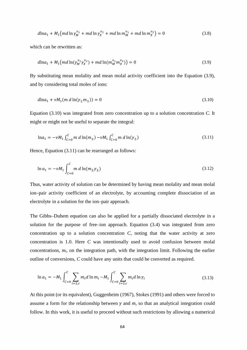
64
𝑑𝑑ln𝑎𝑎1 + 𝑀𝑀1𝑚𝑚𝑑𝑑 ln 𝛾𝛾𝑀𝑀𝜈𝜈1 + 𝑚𝑚𝑑𝑑 ln 𝛾𝛾𝑋𝑋
𝜈𝜈2 + 𝑚𝑚𝑑𝑑 ln𝑚𝑚𝑀𝑀𝜈𝜈1 + 𝑚𝑚𝑑𝑑 ln𝑚𝑚𝑋𝑋
𝜈𝜈2 = 0 (3.8)
which can be rewritten as:
𝑑𝑑ln𝑎𝑎1 + 𝑀𝑀1𝑚𝑚𝑑𝑑 ln(𝛾𝛾𝑀𝑀𝜈𝜈1𝛾𝛾𝑋𝑋
𝜈𝜈2) + 𝑚𝑚𝑑𝑑 ln(𝑚𝑚𝑀𝑀𝜈𝜈1𝑚𝑚𝑋𝑋
𝜈𝜈2) = 0 (3.9)
By substituting mean molality and mean molal activity coefficient into the Equation (3.9),
and by considering total moles of ions:
𝑑𝑑ln𝑎𝑎1 + 𝜈𝜈𝑀𝑀1(𝑚𝑚 𝑑𝑑 ln(𝛾𝛾±𝑚𝑚±)) = 0 (3.10)
Equation (3.10) was integrated from zero concentration up to a solution concentration C. It
might or might not be useful to separate the integral:
ln𝑎𝑎1 = −𝜈𝜈𝑀𝑀1 ∫ 𝑚𝑚 𝑑𝑑 ln(𝑚𝑚±)𝐶𝐶𝐶𝐶=0 −𝜈𝜈𝑀𝑀1 ∫ 𝑚𝑚 𝑑𝑑 ln(𝛾𝛾±)𝐶𝐶
𝐶𝐶=0 (3.11)
Hence, Equation (3.11) can be rearranged as follows:
ln𝑎𝑎1 = −𝜈𝜈𝑀𝑀1 𝑚𝑚 𝑑𝑑 ln(𝑚𝑚±𝛾𝛾±)
𝐶𝐶
𝐶𝐶=0 (3.12)
Thus, water activity of solution can be determined by having mean molality and mean molal
ion–pair activity coefficient of an electrolyte, by accounting complete dissociation of an
electrolyte in a solution for the ion–pair approach.
The Gibbs–Duhem equation can also be applied for a partially dissociated electrolyte in a
solution for the purpose of free–ion approach. Equation (3.4) was integrated from zero
concentration up to a solution concentration C, noting that the water activity at zero
concentration is 1.0. Here C was intentionally used to avoid confusion between molal
concentrations, mi, on the integration path, with the integration limit. Following the earlier
outline of conversions, C could have any units that could be converted as required.
ln𝑎𝑎1 = −𝑀𝑀1 𝑚𝑚𝑖𝑖𝑑𝑑 ln𝑚𝑚𝑖𝑖
𝑖𝑖=2,𝑐𝑐
𝐶𝐶
𝐶𝐶=0−𝑀𝑀1 𝑚𝑚𝑖𝑖𝑑𝑑 ln 𝛾𝛾𝑖𝑖
𝑖𝑖=2,𝑐𝑐
𝐶𝐶
𝐶𝐶=0 (3.13)
At this point (or its equivalent), Guggenheim (1967), Stokes (1991) and others were forced to
assume a form for the relationship between 𝛾𝛾 and m, so that an analytical integration could
follow. In this work, it is useful to proceed without such restrictions by allowing a numerical

65
solution to be used. Hence, Equation (3.13) is a sufficient description of the calculation of
water activity for the free–ion approach, either numerically or analytically.
Nevertheless, several other validations were used depending on the solutions and their
conditions that will be discussed in detail for each particular system. These calculations were
also done for dynamic conditions, i.e. for time dependent to see the changes of ion partitioning
over time.
3.2.2 Implementation of algorithm
Equation (3.13) can be applied to different systems for calculation of water activity as a
method of validation for activity coefficient quantities. Below are the required steps toward
the water activity calculation:
– An array of concentration from zero to the concentration of interest was defined.
– The molar activity coefficients were calculated at each concentration by the MSA
theory using molar concentration, size, and charge of each species. The MSA theory
was described in detail in Chapter 2.
– The molar activity of each species including cations, anions, and ion–pairs was
calculated by using their corresponding molar activity coefficient and concentration.
– Molar activity was converted to molal activity for all components using the formula
given in Chapter 2, Table 2.8, from that the molal activity coefficient was obtained.
– Molal activity coefficient and molal concentration were substituted into Equation
(3.13).
– The cumulative trapezoidal numerical integration (cumtrapz) in MATLAB was used
to compute the approximate integral for water activity calculation.
Hence, water activity could be solved theoretically for either ion–pair or free–ion approach in
a multicomponent solution. Figure 3.1 indicates the water activities of sodium chloride,
calcium chloride, and sulphuric acid solutions as a function of molal electrolyte concentration
that were solved for both the ion–pair (Equation (3.12) (Zemaitis et al., 1986)) and the free–
ion approach (Equation (3.13)). The simulated results for both approaches were in a good
agreement with experimental data used from Robinson and Stokes (1959). The Gibbs–Duhem
equation with the MSA theory was likely able to predict water activity for even high
concentrations, e.g. 6 M of the electrolyte solution. Less experimental data are available for

66
water activity of binary and multicomponent solutions in literature. Therefore, these systems
were used as the examples for water activity calculation.
Figure 3.1 Water activity of sodium chloride, calcium chloride, and sulphuric acid solutions at 25 ˚C by both the ion–pair and free–ion approaches.
Water activity of both approaches yielded similar results representing the consistency of them.
Stokes (1991) used Equation (3.14) to calculate water activity as a function of osmotic
coefficient, values of which were experimentally obtained by Robinson and Stokes (1959) to
validate the model that are shown in Figure 3.1.
ln𝑎𝑎1 = −
𝜙𝜙𝑀𝑀1 ∑ 𝜈𝜈𝑖𝑖𝑚𝑚𝑖𝑖𝑖𝑖
(3.14)
Here 𝑎𝑎1 is water activity, mol kg–1water; 𝜙𝜙 is osmotic coefficient, [–]; 𝑀𝑀1 is molar mass of
water, kg mol–1; 𝜈𝜈𝑖𝑖 is the number of ions in solution from each molecule of solute (assuming
complete dissociation), [–]; 𝑚𝑚𝑖𝑖 is the molal concentration of the electrolyte, mol kg–1water.
3.3 Ion speciation model
The model was based on the simultaneous calculations of equilibrium, conservation, and
electroneutrality equations. Generally, the components, which can include cations, anions,
lactose, and proteins available in milk, were clearly incorporated into each system mostly
based on their molar activity.
0 1 2 3 4 5 6
0.4
0.5
0.6
0.7
0.8
0.9
1
Concentration of electrolyte, mol/kgw ater
Act
ivity
of w
ater
, mol
/kg w
ater
CaCl2 ↑
NaCl ↓
H2SO4 ↑
Free-ion approach by MSARobinson and Stokes, 1959Ion-pair approach by MSA

67
3.3.1 Set of equations
The components are assumed to be in a thermodynamic equilibrium with each other through
intrinsic association constants that lead to the formation of species such as free ions and ion–
pairs. An example of thermodynamic equilibrium was given in Chapter 2, Equation (2.37). A
full list of available cations, anions, and ion–pairs is shown in Table 3.1 along with the
corresponding intrinsic association constants, which are only for the temperature range
between 20–25 ˚C. The set of equations were assembled first for the steady state condition.
Duplicate components were dropped from the set of components to ensure the number of
equations and variables are equal, e.g. H2Cit– acts both as anion and as ion–pair in a system
containing citrate, therefore, it is only considered as an anion in the set of calculations, and
was not included in the set of ion–pairs.
In Table 3.1 for milk serum, there are 5 cations, 15 anions, and 75 ion–pairs, and of these 7
ion–pairs are already in the list of anions, and the concentration of H2O is determined
independently. Thus, there are 5+15+75–7–1=87 concentration variables. Table 3.1 provides
74 equilibria in the form of Equation (2.37).
The hydrogen ion and hydroxide ion equilibrium was constructed as another essential
equation in the conservation calculation, for which water activity (𝑎𝑎𝑤𝑤𝑎𝑎𝐶𝐶𝑝𝑝𝑝𝑝 , mol L−1) is
essential:
𝐾𝐾𝑤𝑤 =𝑎𝑎𝑤𝑤𝑎𝑎𝐶𝐶𝑝𝑝𝑝𝑝𝑎𝑎𝐻𝐻+𝑎𝑎𝑂𝑂𝐻𝐻−
(3.15)
where 𝐾𝐾𝑤𝑤 is water association constant which can be used from Table 3.1. Molar water
activity was ascertained as follows;
𝑎𝑎𝑤𝑤𝑎𝑎𝐶𝐶𝑝𝑝𝑝𝑝 =
𝜌𝜌𝑠𝑠𝑠𝑠𝑠𝑠𝑠𝑠 − ∑ 𝐶𝐶𝑖𝑖𝑀𝑀𝑊𝑊𝑖𝑖𝑖𝑖
𝑀𝑀𝑊𝑊𝑤𝑤𝑎𝑎𝐶𝐶𝑝𝑝𝑝𝑝 (3.16)
Here 𝜌𝜌𝑠𝑠𝑠𝑠𝑠𝑠𝑠𝑠 is the density of solution, [kg L−1], which was set as the density of a NaCl solution
for the simulations in this thesis due to insufficient data for density of multicomponent
systems that was calculated according to the Appendix 2; 𝐶𝐶𝑖𝑖 is the total molar concentration
of the species, [mol L−1]; 𝑀𝑀𝑊𝑊𝑖𝑖 and 𝑀𝑀𝑊𝑊𝑤𝑤𝑎𝑎𝐶𝐶𝑝𝑝𝑝𝑝 are the molecular weight of species and water
[kg mol−1], respectively.

68
Table 3.1 Intrinsic association constant between the principal ions of milk serum at 25 ˚C (Holt et al., 1981; Mekmene, Le Graet, et al., 2009; Mekmene et al., 2010).
Ca2+ Mg2+ Na+ K+ H+
Ion–pair Ka, mol–1 L Ion–pair Ka, mol–1 L Ion–pair Ka, mol–1 L Ion–pair Ka, mol–1 L Ion–pair Ka, mol–1 L
H2Cit– CaH2Cit+ 28 MgH2Cit+ 15 NaH2Cit 1 KH2Cit 1 H3Cit 1380
HCit2– CaHCit 876 MgHCit 402 NaHCit– 10 KHCit– 10 H2Cit– 6×10⁴
Cit3– CaCit– 1.65×10⁵ MgCit– 1.11×10⁵ NaCit2– 20 KCit2– 16 HCit2– 2.57×10⁶
H2PO4– CaH2PO4
+ 11 MgH2PO4+ 12 NaH2PO4 1 KH2PO4 1 H3PO4 200
HPO42– CaHPO4 642 MgHPO4 838 NaHPO4
– 17 KHPO4– 13 H2PO4
– 2.87×10⁷
PO43– CaPO4
– 2.88×10⁶ MgPO4– 8.35×10⁴ NaPO4
2– 100 KPO42– 100 HPO4
2– 2.47×10¹²
HCO3– CaHCO3
+ 23 MgHCO3+ 19 NaHCO3 1 KHCO3 1 H2CO3 2.25×10⁶
CO32– CaCO3 1.4×10³ MgCO3 758 NaCO3
– 10 KCO3– 10 HCO3
– 2.13×10¹⁰
HSO4– CaHSO4
+ 10 MgHSO4+ 10 NaHSO4 1 KHSO4 1 H2SO4 1×10⁻⁸d
SO42– CaSO4 204 MgSO4 170 NaSO4
– 5 KSO4– 7 HSO4
– 98
Cl– CaCl+ 9.4 MgCl+ 5.6 NaCl 0.9 KCl 1 HCl 1×10-9.3
Glc–1–PH– CaGlc–1–PH+ 10 MgGlc–1–PH+ 10 NaGlc–1–PH 1 KGlc–1–PH 1 Glc–1–PH2 1×10⁻¹⁰
Glc–1–P2– CaGlc–1–P 316 MgGlc–1–P 295 NaGlc–1–P– 7 KGlc–1–P– 5 Glc–1–PH– 3.19×10⁶
RCOO– CaRCOO+ 15 MgRCOO+ 19 NaRCOO 0.7 KRCOO 0.7 RCOOH 5.71×10⁴
OH– CaOH+ 25.11a MgOH+ 162.18a NaOH 0.2b KOH 0.2b H2O Kwc
a (Clark, 2015), b (van Boekel, 2008), c The intrinsic association constant of water for one kilogram of molecule: 5.507 × 10¹⁵ mol−1L, d Assumed to be very low.

69
Electroneutrality provides another equation to describe the need for the identical numbers of
equations and species:
𝐶𝐶𝑖𝑖𝑧𝑧𝑖𝑖𝑖𝑖
= 0 (3.17)
The total concentration of each group of species was required to equal the specified total. It
was constructed as a sum of all corresponding free ions and ion–pairs for each species
providing the mass balance equations for Ca, Mg, Na, K, citrate, phosphate, carbonate,
sulphate, chloride, phosphate esters, and carboxylate giving 11 equations.
Hence, there were 74+1+1+11=87 equations, which matched the number of variables.
Steady state calculations of ion–equilibria were implemented by the total amount of each
species as an initial guess to enable covering a wide range of concentration and subsequently
pH values. A concentration ratio was defined to mathematically make up various initial
concentrations of cations, anions, and ion–pairs from dilute to concentrated ones.
Mathematical addition of NaOH/HCl to the multicomponent solution enabled the pH to be
indirectly adjusted.
3.3.2 Activity coefficient and dielectric constant
The molar activity of each species was calculated by the multiplication of molar concentration
and molar–based activity coefficient calculated by the MSA theory that was described in
detail in Chapter 2.
The relative permittivity of water was another variable for calculation of Bjerrum distance in
the set of MSA equations.
Equation (3.18), which was given by Tikanen and Fawcett (1996) and Buchner et al. (1999),
was used to determine the relative permittivity of water for sodium chloride solution and was
compared with the experimental data presented by Mollerup and Breil (2015) that was shown
in Figure 3.2.
𝜀𝜀𝑝𝑝𝑁𝑁𝑎𝑎𝐶𝐶𝑠𝑠 = 78.65− 15.45𝐶𝐶 + 3.76𝐶𝐶1.5
𝜀𝜀𝑝𝑝𝑁𝑁𝑎𝑎𝐶𝐶𝑠𝑠 = 78.65− 𝐼𝐼𝐶𝐶 + 𝐵𝐵𝐶𝐶𝐷𝐷 (3.18)

70
Here 𝜀𝜀𝑝𝑝𝑁𝑁𝑎𝑎𝐶𝐶𝑠𝑠 is the relative permittivity of water for the NaCl solution; [–]; A, B, and D
represent the coefficients for the equation; 𝐶𝐶 is molar concentration of electrolyte.
Figure 3.2a shows that the parameter values given by the literature were not provided a match
with the experimental data for the NaCl solution, but a much better fit was obtained with the
numerical values of 15.8, 2.0, and 1.7 for A, B, and D coefficients, respectively.
Figure 3.2 The dielectric constant as a function of a) sodium chloride and b) calcium chloride molar concentration for various coefficients of the Equations (3.18) and (3.19). The solid curves are from the Equations (3.18) and (3.19) given by Tikanen and Fawcett (1996) using A=15.45, B=3.76, and
D=1.5 for sodium chloride solution, and A=34, B=10, D=1.5 for calcium chloride solution. The symbol ‘∗’ represents the experimental data from and Mollerup and Breil (2015). The dash lines
represent the best fit with the experimental data.
Similarly, Tikanen and Fawcett (1996) and Buchner et al. (1999) proposed an equation for
the dielectric constant of water in a calcium chloride solution as a function of molar
concentration of electrolyte:
𝜀𝜀𝑝𝑝𝐶𝐶𝑎𝑎𝐶𝐶𝑠𝑠2 = 78.65 − 34𝐶𝐶 + 10𝐶𝐶1.5
𝜀𝜀𝑝𝑝𝐶𝐶𝑎𝑎𝐶𝐶𝑠𝑠2 = 78.65 − 𝐼𝐼𝐶𝐶 + 𝐵𝐵𝐶𝐶𝐷𝐷 (3.19)
The CaCl2 data were also fitted using the same equation giving the numerical values of
A=14.7, B=1.2, D=1.9.
For simple binary solutions such as calcium chloride, the free calcium and chloride ion
concentrations were substituted for the electrolyte concentration in the water dielectric
constant formula, but for multicomponent solutions, the two main cation and anion of that
0 1 2 3 4 5 620
30
40
50
60
70
80
NaCl concentration, mol/L
Die
lect
ric c
onst
ant,
[-]
a
0 1 2 3 4 5 620
30
40
50
60
70
80
CaCl2 concentration, mol/L
Die
lect
ric c
onst
ant,
[-]
b
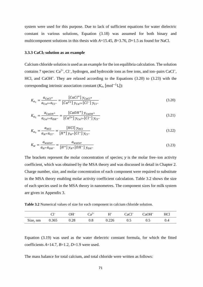
71
system were used for this purpose. Due to lack of sufficient equations for water dielectric
constant in various solutions, Equation (3.18) was assumed for both binary and
multicomponent solutions in this thesis with A=15.45, B=3.76, D=1.5 as found for NaCl.
3.3.3 CaCl2 solution as an example
Calcium chloride solution is used as an example for the ion equilibria calculation. The solution
contains 7 species: Ca2+, Cl–, hydrogen, and hydroxide ions as free ions, and ion–pairs CaCl+,
HCl, and CaOH+. They are relaxed according to the Equations (3.20) to (3.23) with the
corresponding intrinsic association constant (Ka, [mol−1L]):
𝐾𝐾𝑎𝑎1 =
𝑎𝑎𝐶𝐶𝑎𝑎𝐶𝐶𝑠𝑠+ 𝑎𝑎𝐶𝐶𝑎𝑎2+𝑎𝑎𝐶𝐶𝑠𝑠−
=[𝐶𝐶𝑎𝑎𝐶𝐶𝑑𝑑+] 𝑦𝑦𝐶𝐶𝑎𝑎𝐶𝐶𝑠𝑠+
[𝐶𝐶𝑎𝑎2+] 𝑦𝑦𝐶𝐶𝑎𝑎2+[𝐶𝐶𝑑𝑑−] 𝑦𝑦𝐶𝐶𝑠𝑠− (3.20)
𝐾𝐾𝑎𝑎2 =
𝑎𝑎𝐶𝐶𝑎𝑎𝑂𝑂𝐻𝐻+
𝑎𝑎𝐶𝐶𝑎𝑎2+𝑎𝑎𝑂𝑂𝐻𝐻−=
[𝐶𝐶𝑎𝑎𝐶𝐶𝐻𝐻+] 𝑦𝑦𝐶𝐶𝑎𝑎𝑂𝑂𝐻𝐻+
[𝐶𝐶𝑎𝑎2+] 𝑦𝑦𝐶𝐶𝑎𝑎2+[𝐶𝐶𝑑𝑑−] 𝑦𝑦𝐶𝐶𝑠𝑠− (3.21)
𝐾𝐾𝑎𝑎3 =
𝑎𝑎𝐻𝐻𝐶𝐶𝑠𝑠𝑎𝑎𝐻𝐻+𝑎𝑎𝐶𝐶𝑠𝑠−
=[𝐻𝐻𝐶𝐶𝑑𝑑] 𝑦𝑦𝐻𝐻𝐶𝐶𝑠𝑠
[𝐻𝐻+] 𝑦𝑦𝐻𝐻+[𝐶𝐶𝑑𝑑−] 𝑦𝑦𝐶𝐶𝑠𝑠− (3.22)
𝐾𝐾𝑤𝑤 =𝑎𝑎𝑤𝑤𝑎𝑎𝐶𝐶𝑝𝑝𝑝𝑝𝑎𝑎𝐻𝐻+𝑎𝑎𝑂𝑂𝐻𝐻−
=𝑎𝑎𝑤𝑤𝑎𝑎𝐶𝐶𝑝𝑝𝑝𝑝
[𝐻𝐻+] 𝑦𝑦𝐻𝐻+[𝐶𝐶𝐻𝐻−] 𝑦𝑦𝑂𝑂𝐻𝐻− (3.23)
The brackets represent the molar concentration of species; 𝑦𝑦 is the molar free–ion activity
coefficient, which was obtained by the MSA theory and was discussed in detail in Chapter 2.
Charge number, size, and molar concentration of each component were required to substitute
in the MSA theory enabling molar activity coefficient calculation. Table 3.2 shows the size
of each species used in the MSA theory in nanometres. The component sizes for milk system
are given in Appendix 3.
Table 3.2 Numerical values of size for each component in calcium chloride solution.
Cl– OH– Ca2+ H+ CaCl+ CaOH+ HCl Size, nm 0.365 0.28 0.8 0.226 0.5 0.5 0.4
Equation (3.19) was used as the water dielectric constant formula, for which the fitted
coefficients A=14.7, B=1.2, D=1.9 were used.
The mass balance for total calcium, and total chloride were written as follows:

72
[𝐶𝐶𝑎𝑎]𝐶𝐶𝑠𝑠𝐶𝐶𝑎𝑎𝑠𝑠 = [𝐶𝐶𝑎𝑎2+] + [𝐶𝐶𝑎𝑎𝐶𝐶𝑑𝑑+] + [𝐶𝐶𝑎𝑎𝐶𝐶𝐻𝐻+] (3.24)
[𝐶𝐶𝑑𝑑]𝐶𝐶𝑠𝑠𝐶𝐶𝑎𝑎𝑠𝑠 = [𝐶𝐶𝑑𝑑−] + [𝐶𝐶𝑎𝑎𝐶𝐶𝑑𝑑+] + [𝐻𝐻𝐶𝐶𝑑𝑑] (3.25)
The electroneutrality was constructed according to the following equation:
2 [𝐶𝐶𝑎𝑎2+] + [𝐶𝐶𝑎𝑎𝐶𝐶𝑑𝑑+] + [𝐶𝐶𝑎𝑎𝐶𝐶𝐻𝐻+] + [𝐻𝐻+] − [𝐶𝐶𝑑𝑑−] − [𝐶𝐶𝐻𝐻−] = 0 (3.26)
There are seven equations, (3.20) to (3.26), equally the number of species.
The proposed model is capable of predicting ion association in any aqueous solution
regardless of any charge or size of the components. This means lactose can be incorporated
into the ion partitioning calculation of solutions. In later sections, lactose was also treated as
an individual species that can affect the solution.
3.3.4 Solving using Newton’s method
The equations form a non–linear system, which can be solved using Newton’s method.
Newton’s method uses the iteration scheme as follows:
𝐱𝐱𝑘𝑘+1 = 𝐱𝐱𝑘𝑘 − 𝐉𝐉−1𝐟𝐟(𝐱𝐱𝑘𝑘), 𝑘𝑘 = 0, 1, … (3.27)
The vector x0 is the initial guess and J is the Jacobian matrix of the vector function f(x). The
functions must be in the form of f(x)=0.
In this work, the Jacobian matrix was obtained numerically as given in Appendix 4. The
variables in x and the functions varied greatly in scale. It was found that using units of
μmol L– 1 gave a satisfactory range for x. Each of the functions was scaled, by dividing the
entire function by a power of 10, so that extreme function values were avoided. The solution
obtained at any iteration was constrained by upper and lower bounds, which were set to
maintain the solution in a physically feasible space.
The simulations were implemented in MATLAB R2013b and R2017a which unexpectedly
returned slightly different results for the solution of J Δx=–f using the syntax Δx =–J\f.

73
The MATLAB language programming is a user–friendly software that enables using purpose–
written programs, which could be controlled and manipulated by the user. The MATLAB
programs for the Newton’s and Jacobian functions are shown in Appendix 4.
The initial guess for each component was equal to the total concentration of the corresponding
species in the solution. Then, the previous mathematical solution was used as the next initial
guess when Newton’s method was used again for a similar concentration, e.g. when producing
a graph. For some systems, it was found necessary to refine the initial guesses to smaller
values.
3.4 Extra equations for precipitation
Solid precipitates were incorporated into the calculation by considering the ion activity
product (IAP) and solubility product (Ksp) of the solid phase, which were mostly available in
literature. Concentration of potential solid phase was obtained using Euler’s method, by which
the level of precipitation was ascertained for each time step as follows:
𝐶𝐶precipitate(𝑠𝑠)(𝑖𝑖+1) = 𝐶𝐶precipitate(𝑠𝑠)(𝑖𝑖) +
𝑑𝑑𝐶𝐶(𝑠𝑠)(𝑖𝑖)
𝑑𝑑𝑆𝑆.Δ𝑆𝑆 (3.28)
Here 𝐶𝐶precipitate(𝑠𝑠)(𝑖𝑖+1) is molar concentration of potential solid phase at the time step 𝑖𝑖 + 1;
𝐶𝐶precipitate(𝑠𝑠)(𝑖𝑖) is molar concentration of potential solid phase at the time step 𝑖𝑖; Δ𝑆𝑆 is time
step, [min]; 𝑑𝑑𝐶𝐶(𝑠𝑠)(𝑖𝑖)
𝑑𝑑𝐶𝐶 is the rate of solid phase concentration over time, [mol L–1 min–1], which
is the sum of precipitation and dissolution differential equations (Kazadi Mbamba, 2016):
𝑑𝑑𝐶𝐶(𝑠𝑠)(𝑖𝑖)
𝑑𝑑𝑆𝑆 =
𝑑𝑑𝐶𝐶precipitation(𝑠𝑠)(𝑖𝑖)
𝑑𝑑𝑆𝑆+
𝑑𝑑𝐶𝐶dissolution(𝑠𝑠)(𝑖𝑖)
𝑑𝑑𝑆𝑆 (3.29)
𝑑𝑑𝐶𝐶precipitation(𝑠𝑠)(𝑖𝑖)
𝑑𝑑𝑆𝑆= 𝑘𝑘𝑠𝑠𝑝𝑝𝑝𝑝𝑐𝑐 𝐶𝐶precipitate(𝑠𝑠)(𝑖𝑖) 𝜎𝜎𝑠𝑠; 𝜎𝜎 = 𝑆𝑆at
1𝜈𝜈 − 1 (3.30)
𝑑𝑑𝐶𝐶dissolution(𝑠𝑠)(𝑖𝑖)
𝑑𝑑𝑆𝑆= 𝑘𝑘𝑑𝑑𝑖𝑖𝑠𝑠𝑠𝑠 𝐶𝐶precipitate(𝑠𝑠)(𝑖𝑖) 𝜎𝜎 (3.31)
Here n is the solid phase reaction order; 𝑘𝑘𝑠𝑠𝑝𝑝𝑝𝑝𝑐𝑐 and 𝑘𝑘𝑑𝑑𝑖𝑖𝑠𝑠𝑠𝑠 are precipitation and dissolution rate
constants of solid phase that are unlikely available in literature. ‘Sat’ represents saturation as
defined in Section 2.2.5.

74
Precipitation and dissolution equations were constructed for each potential solid component
and were recalculated for each time step. Small time steps gave accurate results. Initial
concentration of each precipitate was normally assumed to be 0.02 μmol L–1 as nucleation
kinetics were not included.
For instance, the precipitation of dicalcium phosphate dihydrate (DCPD, CaHPO4.2H2O) is a
common phenomenon in the milk liquids that results from supersaturation of calcium and
phosphate ions (Pouliot et al., 1991). The saturation equilibrium of dicalcium phosphate
dihydrate can be written as:
𝐶𝐶𝑎𝑎𝐻𝐻𝐼𝐼𝐶𝐶4. 2𝐻𝐻2𝐶𝐶(𝑠𝑠) ↔ 𝐶𝐶𝑎𝑎(𝑎𝑎𝑞𝑞)2+ +𝐻𝐻𝐼𝐼𝐶𝐶42−(𝑎𝑎𝑞𝑞)
𝑆𝑆𝑎𝑎𝑆𝑆 =𝑎𝑎𝐶𝐶𝑎𝑎2+𝑎𝑎𝐻𝐻𝐻𝐻𝑂𝑂42−
𝐾𝐾𝑠𝑠𝑠𝑠= 𝐼𝐼𝐴𝐴𝐻𝐻
𝐾𝐾𝑠𝑠𝑠𝑠
(3.32)
The dynamic simulation of calcium phosphate solution was implemented for time
incorporation by applying Euler’s method, by which the level of precipitation was ascertained
for each time step using the following equation:
𝐶𝐶DCPD(𝑠𝑠)(𝑖𝑖+1) = 𝐶𝐶DCPD(𝑠𝑠)(𝑖𝑖) +
𝑑𝑑𝐶𝐶DCPD(𝑠𝑠)(𝑖𝑖)
𝑑𝑑𝑆𝑆.Δ𝑆𝑆 (3.33)
The precipitation and dissolution rate constants were chosen 0.25 and 0.0001 min–1,
respectively with the precipitation reaction order of 2.
3.5 Application of the model to sodium chloride and calcium chloride solutions
Sodium chloride and calcium chloride solutions were used to validate the model by assuming
both ion–pair and free–ion approaches, because they are significant components of milk and
a large amount of accurate experimental data is available in literature.
3.5.1 Ion–pair approach
Although the ion–pair approach ignores free complexes and interactions between free ions,
several activity coefficient models were presented in literature to determine the mean activity
coefficient. The base ten logarithms of the mean molar ion–pair activity coefficients of
sodium chloride and calcium chloride solutions were plotted as a function of molar ionic
strength at 25 ˚C (Figure 3.3).

75
The MSA theory performs better than the other theories to fit with the experimental data for
the ion–pair approach for the both solutions. Many researchers have used Davies theory to
calculate ion partitioning for obtaining mean and free ion activity coefficients in various
systems, but the MSA theory shows better agreement with the experimental data particularly
for higher concentrations of the electrolyte. Figure 3.3 also shows that the Debye–Hückel
theory is only valid for lower sodium chloride concentrations when the total molar ionic
strength is lower than 0.3 mol L–1.
Figure 3.3 Mean molar ion–pair activity coefficient of NaCl and CaCl2 solutions at 25 ˚C. The experimental data were taken from van Boekel (2008).
Figure 3.4 indicates a direct correlation between the effective ion size parameter (𝜎𝜎) and the
mean ion–pair activity coefficient of sodium chloride solution (y±). 0.5 nm was selected as
the optimum size for the sodium and chloride ion for Figure 3.4 which is slightly larger than
Kielland (1937) suggested. However, the effective size parameter for free calcium was
assumed 0.6 nm according to Kielland (1937). The effect of size parameters of the free sodium
(Na+), free chloride (Cl–), and free calcium (Ca2+) ions were identical. The size of free
hydrogen (H+) and hydroxide (OH–) ions seemed to have no effect on the mean ion–pair
activity coefficient of both sodium chloride and calcium chloride solutions.
0 1 2 3 4 5-1.5
-1
-0.5
0
0.5
1
1.5
2
2.5
Molar ionic strength, mol/L
log 10
y± ,
[-]
NaCl solution
MSA theoryDavies theoryExperimentalDebye-Hückel theory
0 1 2 3 4 5-1.2
-1
-0.8
-0.6
-0.4
-0.2
0
0.2
0.4
Molar ionic strength, mol/L
log 10
y± ,
[-]
CaCl2 solution

76
Figure 3.4 Mean ion–pair activity coefficient of NaCl solution for different ion size of Na+ and Cl– by the MSA theory; the ‘×’ symbol refers to experimental data taken from van Boekel (2008).
3.5.2 Free–ion approach
The free–ion approach will be required when considering milk solutions with many different
ions and ion–pairs. Therefore, it was also used for the simulation of both calcium chloride and
sodium chloride solutions. Figure 3.5 shows the natural logarithm of free ion activity
coefficient of sodium chloride solution and calcium chloride showing that the MSA theory
fits best to predict free ion activity coefficients over the range of concentrations. To obtain
these results, the size of following ions were adjusted: Na+ to 0.51, Cl– to 0.44 nm, Ca2+ to
0.8 nm.
The Davies theory is unable to individually predict the molar activity coefficient for the free
ions due to lack of a parameter that can differentiate the cation from the anion activity
coefficients, whereas the MSA theory can distinguish the free ion activity coefficients by
adjusting the effective size parameter leading to the different numerical values for the free ion
activity coefficient in a particular system.
0 1 2 3 4 5 6-1
0
1
2
3
4
Molar ionic strength, mol/L
log 10
y± ,
[-]
0.5 nm
0.4 nm
0.3 nm
0.2 nm
0.6 nm
Na+ or Cl- size

77
Figure 3.5 The natural logarithm of molar free–ion activity coefficient as a function of molar concentration of NaCl and CaCl2.
Figure 3.5 was drawn up to the maximum solubility of the electrolytes where they remain
soluble in this range. The MATLAB scripts for sodium chloride solution is detailed in
Appendix 5.
From Sections 3.2–3.5, it can be concluded that:
1. The MSA theory could satisfactorily predict molar activity coefficient of any free ions
of an assumed solution up to high concentration, and enabled better fitting with the
experimental data in compared with the other theories.
2. Water activity of both approaches was in a good agreement with the corresponding
experimental data as a means of validation.
3. As there is no similar relationship for the correlation between the dielectric constant
and the molar concentration of various electrolytes and multicomponent solutions in
literature, Equation (3.18) was applied to the simulation of all models in this study.
3.6 Application of the model to buffer systems
Buffer solutions are derived from weak acids and bases along with their conjugate bases and
acids with the intrinsic association constants close to the neutral pH, i.e. the effective buffer
solution should normally have pH=pKa±1.5, and subsequently strong electrolytes with pKa
values either larger or smaller than the range that called ‘non–buffer ions’ (Constable, 1997).
Buffer solutions such as citrate and phosphate were modelled, not only because of the
containing significant ions in milk, but also they are appropriate examples with available
0 0.5 1 1.5 2-4
-3.5
-3
-2.5
-2
-1.5
-1
-0.5
0
0.5
√ NaCl concentration, (mol/L)1/2
ln y
, [-]
NaCl
MSA theory, Na+
MSA theory, Cl-
Wilczek-Vera et al., 2004; Na+
Wilczek-Vera et al., 2004; Cl-
Davies theory, Na+ or Cl-
Debye-Hückel theory, Na+ or Cl-
0 0.5 1 1.5 2-20
-15
-10
-5
0
√ CaCl2 concentration, (mol/L)1/2
ln y
, [-]
CaCl2
MSA theory, Ca2+
MSA theory, Cl-
Wilczek-Vera et al., 2004; Ca2+
Wilczek-Vera et al., 2004; Cl-
Davies theory, Ca2+ or Cl-
Debye-Hückel theory, Ca2+ or Cl-
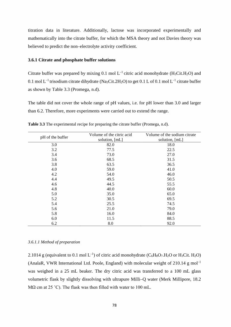
78
titration data in literature. Additionally, lactose was incorporated experimentally and
mathematically into the citrate buffer, for which the MSA theory and not Davies theory was
believed to predict the non–electrolyte activity coefficient.
3.6.1 Citrate and phosphate buffer solutions
Citrate buffer was prepared by mixing 0.1 mol L–1 citric acid monohydrate (H3Cit.H2O) and
0.1 mol L–1 trisodium citrate dihydrate (Na3Cit.2H2O) to get 0.1 L of 0.1 mol L–1 citrate buffer
as shown by Table 3.3 (Promega, n.d).
The table did not cover the whole range of pH values, i.e. for pH lower than 3.0 and larger
than 6.2. Therefore, more experiments were carried out to extend the range.
Table 3.3 The experimental recipe for preparing the citrate buffer (Promega, n.d).
pH of the buffer Volume of the citric acid solution, [mL]
Volume of the sodium citrate solution, [mL]
3.0 82.0 18.0 3.2 77.5 22.5 3.4 73.0 27.0 3.6 68.5 31.5 3.8 63.5 36.5 4.0 59.0 41.0 4.2 54.0 46.0 4.4 49.5 50.5 4.6 44.5 55.5 4.8 40.0 60.0 5.0 35.0 65.0 5.2 30.5 69.5 5.4 25.5 74.5 5.6 21.0 79.0 5.8 16.0 84.0 6.0 11.5 88.5 6.2 8.0 92.0
3.6.1.1 Method of preparation
2.1014 g (equivalent to 0.1 mol L–1) of citric acid monohydrate (C6H8O7.H2O or H3Cit. H2O)
(AnalaR, VWR International Ltd. Poole, England) with molecular weight of 210.14 g mol–1
was weighed in a 25 mL beaker. The dry citric acid was transferred to a 100 mL glass
volumetric flask by slightly dissolving with ultrapure Milli–Q water (Merk Millipore, 18.2
MΩ cm at 25 ˚C). The flask was then filled with water to 100 mL.

79
2.9410 g (equivalent to 0.1 mol L–1) of trisodium citrate dihydrate (C6H5Na3O7.2H2O or
Na3Cit.2H2O) (Merck, Germany) with molecular weight of 294.10 g mol–1 was weighed by
the balance and made up to 0.1 mol L–1 like the afore–mentioned procedure for the citric acid
solution.
One mL of the citric acid solution was drawn up by a clean and dry 1±0.007 mL glass pipette
and was thrown away to be able to have 99 mL of the citric acid solution. The same volume
was drawn up from the sodium citrate solution and was then added to the citric acid solution
to make up 0.1 mol L–1 citrate buffer. Other volumes of the solutions were made up similarly
to for low and high pH values, i.e. 97, 92, and 85 mL of citric acid solutions with
corresponding 3, 8, and 15 mL of sodium citrate solutions. The other experiments were based
on the Table 3.3.
pH of solutions was measured by a CyberScan pH 310 pH/mV meter (Eutech, Germany) that
was equipped with an automatic temperature control probe and an Eutech pH probe with a
capability of measuring to two decimal places. Calibration was carried out every day before
the measurements to avoid any experimental errors for the pH meter using three standard
buffer solutions with pH values of 4, 7, and 10. The uncertainty was estimated to be ±0.02.
3.6.1.2 Results and analysis of data
The experimental data from literature and those carried out in this study were compared with
the simulated ones in terms of ratio of total sodium to citric acid and pH value, as shown in
Figure 3.6a. The intrinsic association constants of ions given by Holt et al. (1981) were used.
However, small changes were made to the Ka of hydrogen citrate and citrate in equilibrium
with free hydrogen ions. The pH values seem to be sensitive to the intrinsic association
constants of hydrogen citrate and citrate with hydrogen ion leading to the formation of
dihydrogen and hydrogen citrates. The constants, 𝐾𝐾𝑎𝑎1 and 𝐾𝐾𝑎𝑎2 , (as defined below) were
changed from 6.00 × 10⁴ to 7.9 × 10⁴ and from 2.57 × 10⁶ to 6.9 × 10⁶ mol–1 L,
respectively, to be able to get better fitting with the experimental data. The Ka values of other
species remained unchanged in the simulation.
𝐻𝐻2𝐶𝐶𝑖𝑖𝑆𝑆−𝐾𝐾𝑎𝑎1 𝐻𝐻𝐶𝐶𝑖𝑖𝑆𝑆2− + 𝐻𝐻+ 𝐾𝐾𝑎𝑎1 =
𝑎𝑎𝐻𝐻2𝐶𝐶𝑖𝑖𝐶𝐶−𝑎𝑎𝐻𝐻𝐶𝐶𝑖𝑖𝐶𝐶2−𝑎𝑎𝐻𝐻+
(3.34)

80
𝐻𝐻𝐶𝐶𝑖𝑖𝑆𝑆2−𝐾𝐾𝑎𝑎2 𝐶𝐶𝑖𝑖𝑆𝑆3− + 𝐻𝐻+ 𝐾𝐾𝑎𝑎2 =
𝑎𝑎𝐻𝐻𝐶𝐶𝑖𝑖𝐶𝐶2−𝑎𝑎𝐶𝐶𝑖𝑖𝐶𝐶3−𝑎𝑎𝐻𝐻+
(3.35)
Figure 3.6 (a) The ratio of total sodium to total citrate for citrate buffer as a function of pH. The solid curve and ‘×’ symbol respectively represent this study and experimental data from
Promega (n.d). (b) The sensitivity of pH to 𝐾𝐾𝑎𝑎1and 𝐾𝐾𝑎𝑎2values with the experimental pH.
To test the sensitivity of the pH to 𝐾𝐾𝑎𝑎1and 𝐾𝐾𝑎𝑎2, the values of 𝐾𝐾𝑎𝑎1and 𝐾𝐾𝑎𝑎2were increased by
32% and 100%, respectively. Sensitivity was defined as change in pH over relative change in
𝐾𝐾𝑎𝑎, i.e. ΔpH/(𝐾𝐾𝑎𝑎adjusted−𝐾𝐾𝑎𝑎)
𝐾𝐾𝑎𝑎. pH was more sensitive to 𝐾𝐾𝑎𝑎1 in the pH range of 3–6, whereas
it was sensitive to 𝐾𝐾𝑎𝑎2 at pH values greater than 4.5 as shown by Figure 3.7. The larger
quantity of 𝐾𝐾𝑎𝑎2 caused less citrate (Cit3–) and hydrogen ions in the solution and hence caused
higher pH, whereas a lower value of 𝐾𝐾𝑎𝑎1led to release of hydrogen citrate (HCit2–) and more
hydrogen ion according to Equations (3.34) and (3.35). The citrate ion was the dominant
species in higher pH values, while dihydrogen citrate and hydrogen citrate ions were produced
in more acidic environments. The intrinsic association constant for other species did not
significantly influence the ion interactions due to their very small values compared with
𝐾𝐾𝑎𝑎1and 𝐾𝐾𝑎𝑎2values.
2 3 4 5 6 7 80
0.5
1
1.5
2
2.5
3
pH
Tota
l sod
ium
/ to
tal c
itrat
e
a
2 3 4 5 6 7 80
0.05
0.1
0.15
0.2
0.25
0.3
0.35
Sens
itivi
ty o
f pH
to K
aExperimental pH
b
Ka1
Ka2
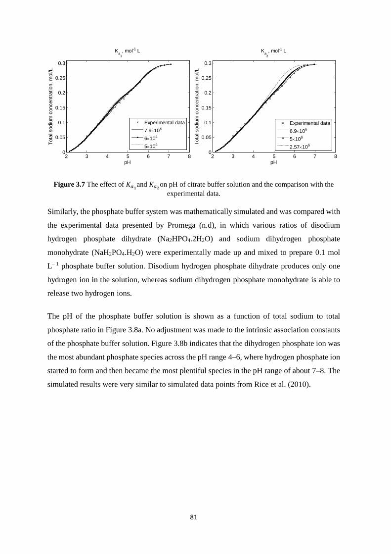
81
Figure 3.7 The effect of 𝐾𝐾𝑎𝑎1and 𝐾𝐾𝑎𝑎2on pH of citrate buffer solution and the comparison with the experimental data.
Similarly, the phosphate buffer system was mathematically simulated and was compared with
the experimental data presented by Promega (n.d), in which various ratios of disodium
hydrogen phosphate dihydrate (Na2HPO4.2H2O) and sodium dihydrogen phosphate
monohydrate (NaH2PO4.H2O) were experimentally made up and mixed to prepare 0.1 mol
L– 1 phosphate buffer solution. Disodium hydrogen phosphate dihydrate produces only one
hydrogen ion in the solution, whereas sodium dihydrogen phosphate monohydrate is able to
release two hydrogen ions.
The pH of the phosphate buffer solution is shown as a function of total sodium to total
phosphate ratio in Figure 3.8a. No adjustment was made to the intrinsic association constants
of the phosphate buffer solution. Figure 3.8b indicates that the dihydrogen phosphate ion was
the most abundant phosphate species across the pH range 4–6, where hydrogen phosphate ion
started to form and then became the most plentiful species in the pH range of about 7–8. The
simulated results were very similar to simulated data points from Rice et al. (2010).
2 3 4 5 6 7 80
0.05
0.1
0.15
0.2
0.25
0.3
pH
Tota
l sod
ium
con
cent
ratio
n, m
ol/L
Ka1, mol-1 L
Experimental data7.9×104
6×10⁴
5×10⁴
2 3 4 5 6 7 80
0.05
0.1
0.15
0.2
0.25
0.3
pH
Tota
l sod
ium
con
cent
ratio
n, m
ol/L
Ka2, mol-1 L
Experimental data6.9×106
5×10⁶
2.57×10⁶

82
Figure 3.8 (a) Total sodium to phosphate ratio vs pH of phosphate buffer solution; (b) Relative concentration of dihydrogen phosphate and hydrogen phosphate ions.
3.6.2 Citrate buffer with lactose solution
The ion equilibria of citrate buffer were simulated and experimentally studied with two
different concentrations of lactose to determine the effect of milk sugar on the ions interaction:
45 g L–1 and 250 g L–1, that are roughly equal to, and five times, the lactose concentration in
milk, respectively.
Citric acid and sodium citrate solutions were made up of 0.1 mol L–1 in a 100 mL glass
volumetric flask, each of which was prepared similarly to the recipe for the preparation of
citrate buffer without lactose solution that was described in the previous section. Solutions
were made up with citric acid, sodium citrate, and monohydrate lactose (C12H22O11.H2O)
(BDH Chemicals Ltd., Poole, England) with molecular weight of 360.312 g mol–1. The final
concentrations of lactose were 0, 45, and 250 g L–1. A range of pH values were obtained by
varying the volumes of 0.1 mol L–1 citric acid and sodium citrate added.
Lactose was assumed theoretically as a non–electrolyte in the simulation with zero charge
number and effective size parameter of 0.455 nm (Isaad and Perwuelz, 2010). pH was
mathematically calculated for 45 g L–1 and 250 g L–1 as shown in Figure 3.9a.
4 5 6 7 8 91
1.2
1.4
1.6
1.8
2
pH
Tota
l sod
ium
/ to
tal p
hosp
hate
a
LiteratureThis study
4 5 6 7 8 90
0.2
0.4
0.6
0.8
1
pH
Phos
phat
e re
lativ
e co
ncen
tratio
n
H2PO4- ↑
↓ HPO42-
b
Rice et al., 2010This study

83
Figure 3.9 (a) The total sodium concentration versus pH of citrate buffer solution with and without lactose; (b) The relative concentration of citrate ions using MSA theory.
The model was fitted with the experimental data for no lactose, 45 g L–1 lactose, and 250 g
L– 1 lactose solutions as shown in Figure 3.9a indicating no significant change between the
pH of the buffer solution with and without lactose. Figure 3.9b shows that there is a little
change in the concentrations of different ions. The activity coefficients of the species were
obtained by the Extended Debye–Hückel theory, in which the effective size parameter was
assumed 0.9 nm for H+, 0.5 nm for Cit3–, and 0.4 nm for the monovalent ions (Holt et al.,
1981), and then compared with the corresponding data calculated by the MSA theory for the
citrate buffer solution with 250 g L–1 lactose.
H2Cit– was the most abundant citrate species across the pH range 2–4. Following this, HCit2–
was the most plentiful species in the pH range of about 4–6, after which Cit3– became the
most prevalent species when citric acid had the lowest concentration in the buffer solution.
The arrows in Figure 3.9b represent the corresponding pKa values of citrate ions.
Since lactose did not show notable influence on the equilibria of the buffer solution, the molar
activity coefficients of citrate species were obtained for the solution containing no lactose and
250 g L–1 lactose and are shown in Figure 3.10a and b. This confirms that the molar activity
coefficients of citrate species in the 250 g L–1 lactose solution are higher than in solutions
without lactose, demonstrating the strength of MSA theory to predict activity coefficient of
solutions containing the non–electrolyte. In contrast, Davies theory shows similar results for
the buffer solution with and without lactose. The differences predicted by the MSA theory are
2 3 4 5 6 7 80
0.5
1
1.5
2
2.5
3
3.5
4
4.5
pH
Tota
l sod
ium
/ to
tal c
itrat
ea
No lactose45 g L-1 lactose250 g L-1 lactoseSimulated dataHolt et al., 1981
2 3 4 5 6 7 80
0.1
0.2
0.3
0.4
0.5
0.6
0.7
0.8
0.9
b
pH
Citr
ate
rela
tive
conc
entra
tion
H2Cit- ↓
↑ Cit3- ↓ HCit2-
No lactose45 g L-1 lactose250 g L-1 lactose
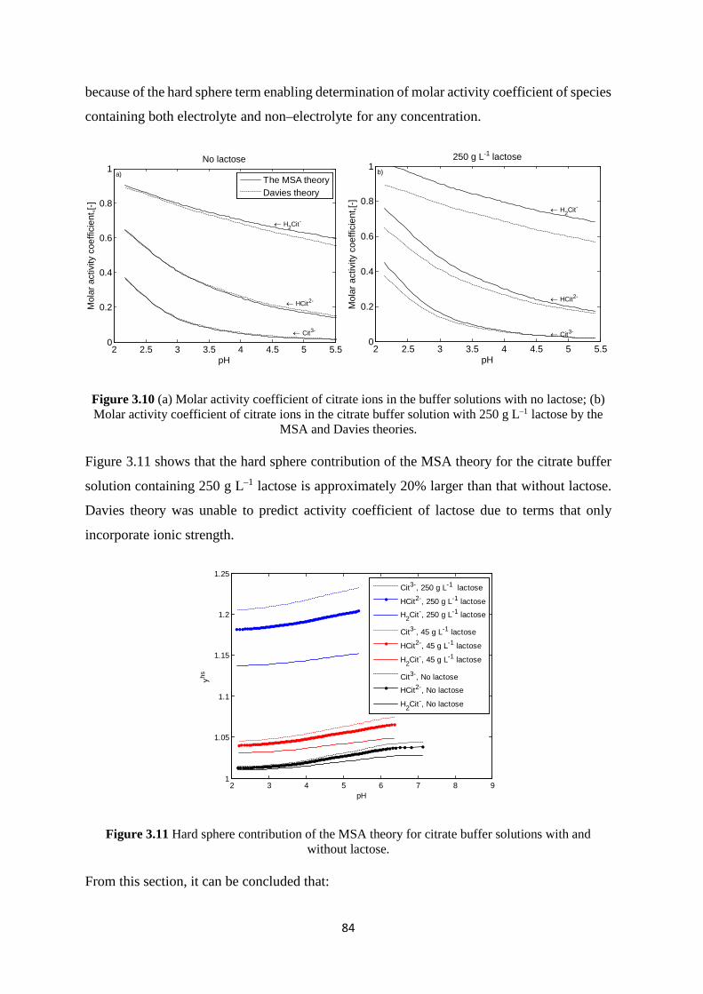
84
because of the hard sphere term enabling determination of molar activity coefficient of species
containing both electrolyte and non–electrolyte for any concentration.
Figure 3.10 (a) Molar activity coefficient of citrate ions in the buffer solutions with no lactose; (b) Molar activity coefficient of citrate ions in the citrate buffer solution with 250 g L–1 lactose by the
MSA and Davies theories.
Figure 3.11 shows that the hard sphere contribution of the MSA theory for the citrate buffer
solution containing 250 g L–1 lactose is approximately 20% larger than that without lactose.
Davies theory was unable to predict activity coefficient of lactose due to terms that only
incorporate ionic strength.
Figure 3.11 Hard sphere contribution of the MSA theory for citrate buffer solutions with and without lactose.
From this section, it can be concluded that:
2 2.5 3 3.5 4 4.5 5 5.50
0.2
0.4
0.6
0.8
1
pH
Mol
ar a
ctiv
ity c
oeffi
cien
t,[-]
No lactose
← H2Cit-
← HCit2-
← Cit3-
a)The MSA theoryDavies theory
2 2.5 3 3.5 4 4.5 5 5.50
0.2
0.4
0.6
0.8
1
← H2Cit-
← HCit2-
← Cit3-
pHM
olar
act
ivity
coe
ffici
ent,[
-]
b)
250 g L-1 lactose
2 3 4 5 6 7 8 91
1.05
1.1
1.15
1.2
1.25
pH
yhs
Cit3-, 250 g L-1 lactose
HCit2-, 250 g L-1 lactoseH2Cit-, 250 g L-1 lactose
Cit3-, 45 g L-1 lactose
HCit2-, 45 g L-1 lactose
H2Cit-, 45 g L-1 lactose
Cit3-, No lactoseHCit2-, No lactose
H2Cit-, No lactose

85
1. The proposed model using MSA theory could satisfactorily predict ion equilibria of
citrate buffer with and without lactose, as well as the phosphate buffer lactose.
2. The interactions between hydrogen citrate, citrate ions, and hydrogen were more likely
to affect the ion equilibria rather than other species in the citrate buffer solution, the
intrinsic association constants of which were adjusted to get better fitting with the
corresponding experimental data.
3. The results showed that lactose had a marginal effect on the ion equilibria of citrate
buffer solution, but significantly affected the activity coefficients through its effect on
the hard sphere contribution of all ions.
3.7 Application of the model to solid phase systems
Supersaturated solutions can exist as metastable and unstable phases. They occur in many
scientific fields such as biology, industrial processes, and material sciences (Brečević and
Füredi-Milhofer, 1972; Söhnel and Mullin, 1982; Brečević et al., 1986; Brečević and Nielsen,
1989).
During evaporation or reverse osmosis of milk, the concentration of ions can easily exceed
the solubility limits. This leads to heterogeneous precipitation of milk minerals on evaporator
surfaces or reverse osmosis membranes, which reduces the operating time of the equipment
before cleaning is required (Kezia et al., 2017).
Several investigations have been done on the ion equilibria in dairy liquids by incorporating
solid phases, which are mainly calcium phosphate (CaHPO4), calcium carbonate (CaCO3),
calcium citrate (Ca3Cit2) (Mekmene, Quillard, et al., 2009; Gao, van Halsema, et al., 2010;
Kazadi Mbamba, 2016; Kezia et al., 2017; Garcia et al., 2018). However, most of these studies
focused on the solubility of solid phase and did not provide investigation of high concentration
of electrolytes by either considering steady state condition or dynamically. In this thesis, the
proposed model was applied individually to calcium carbonate, calcium phosphate, and
calcium citrate solutions along with lactose. The MSA theory was used to determine activity
coefficients of species by both assuming time dependent and equilibrium conditions, because
it is believed that, the MSA theory is better able to predict activity coefficients at high
concentrations of species.

86
3.7.1 Calcium carbonate solution
Calcium carbonate is one of the most significant minerals, which can be found in nature
abundantly (Njegić-Džakula et al., 2010). Various metastable phases of calcium carbonate
can be formed during a spontaneous precipitation such as calcite, aragonite, and vaterite,
among which calcite is the most stable type at ordinary conditions with low solubility
(Brečević and Nielsen, 1989). Calcium carbonate can exist as hexahydrate, monohydrate, or
amorphous (Brooks et al., 1950). In milk, apart from calcium phosphate as the main
precipitating component with low solubility, calcium carbonate is another potential insoluble
salt in the serum phase of skimmed milk with an approximate concentration of 0.014 mM
(Walstra and Jenness, 1984).
3.7.1.1 Steady state study
The ion equilibria of calcium carbonate solution were determined mathematically and
experimentally when hydrochloric acid (HCl) was incorporated into the system to maintain
the pH values of the solutions without disturbing the equilibria. The available data in literature
was not sufficient, so several experiments were implemented to measure pH values of calcium
carbonate and hydrochloric acid mixtures.
0.01 g (equivalent to 1 mmol L–1) of anhydrous calcium carbonate (CaCO3) (AnalaR
Normapur, VWR PROLABO, Belgium) with molecular weight of 100.09 g mol–1 was
weighed and transferred to a clean and dry 100 mL glass volumetric flask.
One mL of 1.0 mol L–1 hydrochloric acid solution was drawn up by a clean and dry 1±0.007
mL glass pipette and was then added to the volumetric flask containing calcium carbonate.
The flask was filled up with fresh and ultrapure Milli–Q water to be able to prepare a solution
with 1.0 mmol L–1 calcium carbonate and 10 mmol L–1 hydrochloric acid. Similarly, several
calcium carbonate solutions were made up with 10 mmol L–1 hydrochloric acid, and pH was
measured.
The results were then compared with other experimental data available in literature that are
shown in Figure 3.12. The experimental data of this study were closest to the data presented
by Reardon and Langmuir (1974); however, more deviation was observed for higher
concentration of calcium carbonate solution when the system became complicated with more

87
ion interaction. The solutions were supersaturated in respect to calcium carbonate, and no sign
of precipitation was observed by either eye or shining a laser pointer through the solution.
Figure 3.12 Experimental pH values investigated in this study and compared with Nakayama (1968), Reardon and Langmuir (1974), and Smith and Martell (1976b).
Calcium carbonate solution was simulated by the proposed model. Figure 3.13 shows the pH
of different concentrations of calcium carbonate for various numerical values of the intrinsic
association constant, which was adjusted to 9 × 10⁹from 2.13 × 10¹⁰ mol–1 L given by Holt
et al. (1981). This adjustment was made according to the Equation (3.36) for the equilibrium
between hydrogen and carbonate ions (CO32–) to get better fitting with the corresponding
experimental data. Intrinsic association constants of other species remained unchanged in the
simulation and were used from Table 3.1.
Figure 3.13 Adjustment of the intrinsic association constant to the corresponding experimental data.
6 6.2 6.4 6.6 6.8 7 7.2 7.4 7.6 7.81
2
3
4
5
6
7
8
9
10
11
CaCO
3 con
cent
ratio
n, m
mol
/L
pH
This studyNakayama, 1968Reardon and Langmuir, 1974Smith and Martell, 1976
5.5 6 6.5 7 7.5 8 8.5 9 9.5 100
2
4
6
8
10
12
14
16
CaC
O3 c
once
ntra
tion,
mm
ol/L
pH
Experimental data
Ka1=2.13x10¹⁰
Ka1=1x10¹⁰
Ka1=9x10⁹
Ka1=7.50x10⁹

88
𝐻𝐻𝐶𝐶𝐶𝐶3− ↔ 𝐻𝐻+ + 𝐶𝐶𝐶𝐶32− 𝐾𝐾𝑎𝑎 =𝑎𝑎𝐻𝐻𝐶𝐶𝑂𝑂3−
𝑎𝑎𝐻𝐻+𝑎𝑎𝐶𝐶𝑂𝑂32− (3.36)
A lower intrinsic association constant than the original value represents high dissociation and
thus higher concentration of hydrogen and carbonate ions. Therefore, a lower pH was obtained
lower for a particular total concentration of calcium carbonate solution. Figure 3.14 shows the
relative concentration of each individual calcium or carbonate ion.
Figure 3.14 Simulated distribution of calcium and carbonate species in supersaturated aqueous calcium carbonate solution.
Free calcium remained at a relative concentration above 99% below pH 8.5, after which it
started to drop corresponding to the formation of free carbonate ions, and the calcium
carbonate ion–pair. This simulation did not calculate precipitation dynamics so the predicted
concentration of CaCO3(aq) is likely to exceed the solubility limit.
Molar activity coefficients of the free carbonate and calcium were calculated by both the MSA
and Davies methods as shown in Figure 3.15. The hydrogen carbonate activity coefficient
obtained from the MSA is much higher than that calculated by Davies theory. This difference
is more likely to be observed at concentrations above 100 mmol L–1 of calcium carbonate
solution where the MSA theory is more likely capable for prediction of activity coefficients
than Davies theory.
3 4 5 6 7 8 9 100
0.2
0.4
0.6
0.8
1
pH
Rel
ativ
e co
ncen
tratio
n
Ca2+
CO32-
HCO3-
H2CO3
CaCO3(aq)

89
Figure 3.15 Molar activity coefficient of free a) carbonate and b) calcium species in the calcium carbonate solution.
3.7.1.2 Dynamic study
The proposed model in this study was applied dynamically to the calcium carbonate system
to determine ion equilibria and parameters changing over time. Precipitation of calcium
carbonate was investigated mathematically and experimentally by Kazadi Mbamba (2016) to
develop an approach for wastewater applications, and data from this work were used as a
validation for the current study.
The dynamic simulation of calcium carbonate solution was implemented over time by
applying Euler’s method as outlined in Section 3.4.
The rate of calcium carbonate precipitation, [mol L–1 min–1] was given by the following
equation:
𝑑𝑑𝐶𝐶𝐶𝐶𝑎𝑎𝐶𝐶𝑂𝑂3(𝑠𝑠)(𝑖𝑖)
𝑑𝑑𝑆𝑆= 𝑘𝑘𝑝𝑝𝑟𝑟𝑒𝑒𝑐𝑐 𝐶𝐶𝐶𝐶𝑎𝑎𝐶𝐶𝑂𝑂3(𝑠𝑠)(𝑖𝑖)
𝜎𝜎𝑠𝑠; 𝜎𝜎 = 𝑆𝑆at 1𝜈𝜈 − 1 (3.37)
where the solid phase reaction order (n) and precipitation rate constant (𝑘𝑘𝑠𝑠𝑝𝑝𝑝𝑝𝑐𝑐) were chosen
to be 2 and 0.0025 min–1, respectively (Kazadi Mbamba, 2016). 𝜎𝜎 is the relative
supersaturation which was calculated according to the saturation parameter that was
considered as an individual species in the set of ions and obtained as follows:
𝑆𝑆𝑎𝑎𝑆𝑆 =𝐼𝐼𝐼𝐼𝐼𝐼𝐾𝐾𝑠𝑠𝑠𝑠
=𝑎𝑎𝐶𝐶𝑎𝑎2+ 𝑎𝑎𝐻𝐻𝐶𝐶𝑂𝑂32−
𝐾𝐾𝑠𝑠𝑠𝑠 (3.38)
0 0.2 0.4 0.6 0.8 10
0.2
0.4
0.6
0.8
1M
olar
act
ivity
coe
ffici
ent,[
-]
CaCO3 concentration, mol L-1
↓ HCO3-
↓ CO32-
a
0 0.2 0.4 0.6 0.8 10
0.2
0.4
0.6
0.8
1
Mol
ar a
ctiv
ity c
oeffi
cien
t,[-]
CaCO3 concentration, mol L-1
b
↓ Ca2+
The MSA theoryDavies theory
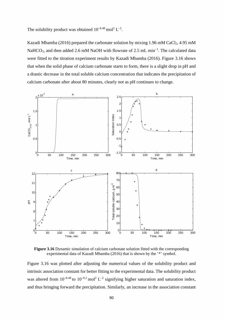
90
The solubility product was obtained 10–8.48 mol2 L–2.
Kazadi Mbamba (2016) prepared the carbonate solution by mixing 1.96 mM CaCl2, 4.95 mM
NaHCO3, and then added 2.6 mM NaOH with flowrate of 2.5 mL min–1. The calculated data
were fitted to the titration experiment results by Kazadi Mbamba (2016). Figure 3.16 shows
that when the solid phase of calcium carbonate starts to form, there is a slight drop in pH and
a drastic decrease in the total soluble calcium concentration that indicates the precipitation of
calcium carbonate after about 80 minutes, clearly not as pH continues to change.
Figure 3.16 Dynamic simulation of calcium carbonate solution fitted with the corresponding experimental data of Kazadi Mbamba (2016) that is shown by the ‘*’ symbol.
Figure 3.16 was plotted after adjusting the numerical values of the solubility product and
intrinsic association constant for better fitting to the experimental data. The solubility product
was altered from 10–8.48 to 10–9.2 mol2 L–2 signifying higher saturation and saturation index,
and thus bringing forward the precipitation. Similarly, an increase in the association constant
0 50 100 150 200 250 3000
0.5
1
1.5
2 x 10⁻³
Time, min
CaC
O3
(s),
mol
L-1
a
0 50 100 150 200 250 300-1.5
-1
-0.5
0
0.5
1
1.5
2
2.5
Time, min
Satu
ratio
n In
dex
b
0 50 100 150 200 250 3006
7
8
9
10
11
12
Time, min
pH
c
0 50 100 150 200 250 3000
10
20
30
40
50
60
70
80d
Time, min
Tota
l sol
uble
cal
cium
, g m
-3

91
between free calcium and hydrogen carbonate (𝐾𝐾𝑎𝑎1) from 1.4×10³ to 9.0×10³ mol–1 L leads to
lower level of free ions, thus higher quantities of saturation according to the Equation (3.39).
𝐶𝐶𝑎𝑎𝐻𝐻𝐶𝐶𝐶𝐶3(𝑎𝑎𝑞𝑞) ↔ 𝐶𝐶𝑎𝑎2+ + 𝐻𝐻𝐶𝐶𝐶𝐶3− 𝐾𝐾𝑎𝑎1 =
𝑎𝑎𝐶𝐶𝑎𝑎𝐻𝐻𝐶𝐶𝑂𝑂3(𝑎𝑎𝑎𝑎)
𝑎𝑎𝐶𝐶𝑎𝑎2+ 𝑎𝑎𝐻𝐻𝐶𝐶𝑂𝑂3− (3.39)
The intrinsic association constant between hydrogen and carbonate ions (𝐾𝐾𝑎𝑎2 ) (Equation
(3.40)) was roughly doubled from 2.13 × 10¹⁰ to 4.5 × 10¹⁰ mol–1 L, resulting in lower pH
values in the very early stage of reaction for the purpose of better fitting.
𝐻𝐻𝐶𝐶𝐶𝐶3− ↔ 𝐻𝐻+ + 𝐶𝐶𝐶𝐶32− 𝐾𝐾𝑎𝑎2 =𝑎𝑎𝐻𝐻𝐶𝐶𝑂𝑂3−
𝑎𝑎𝐻𝐻+ 𝑎𝑎𝐶𝐶𝑂𝑂32− (3.40)
The Runge–Kutta fourth–order method was also employed in the dynamic simulation of
calcium carbonate, as this method has higher accuracy than Euler’s method. 𝐾𝐾𝑎𝑎1 and 𝐾𝐾𝑎𝑎2 were
kept the same with the Runge–Kutta method. The solubility product of calcium carbonate was
the only parameter that was altered from 10–8.48 to 10–8.722 mol L–1 showing less saturation in
the very early stage of the dissolution as shown in Figure 3.17b compared to Figure 3.16b. In
addition, the decrease in pH was matched better with the experimental data when the
precipitation started to occur at about 80 minutes. However, this method did not influence on
the kinetics of formed precipitates and could only bring forward the total calcium
concentration.
3.7.2 Calcium phosphate solution
Calcium phosphate precipitation has been studied extensively in various research areas such
as medical, biological, and environmental sciences for analysing kidney stones, accumulation
of calcium salts in the body, mechanically stabilising bone and teeth, and extraction of
phosphate components from wastewater (Joko, 1984; Nicollas et al., 1989; Raynaud et al.,
2002; Bleek and Taubert, 2013). In milk, calcium is bound with inorganic phosphate forming
a sparingly soluble calcium phosphate that is stabilised by the micellar organic phosphate so–
called phosphoseryl residues of casein (Holt, 1992; Little and Holt, 2004).

92
Figure 3.17 Dynamic simulation of calcium carbonate using Runge–Kutta method fitted with the corresponding experimental data of Kazadi Mbamba (2016) that is shown by the ‘*’ symbol.
Investigations of calcium phosphate solubility are complicated and continuing due to
incongruent mechanisms throughout the equilibria (Miyazaki et al., 2009; Pan and Darvell,
2009a, 2009b). A large number of investigations has been done on the solubility of calcium
phosphate, but less data are available for the speciation of ions in a wide range of pH and for
high concentration of the solution either at equilibrium or dynamically. The aim of this section
is to evaluate how changes in pH and ions activity can affect the speciation and the
precipitation of the solution.
3.7.2.1 Controlling pH by NaOH in steady state study
The speciation of calcium phosphate system was determined by the model, to which the MSA
theory was applied for calculation of activity coefficient of ions. The saturation of dicalcium
phosphate dihydrate was calculated using the solubility product of 2.07×10⁻⁷ mol2 L–2, which
0 50 100 150 200 250 3000
0.5
1
1.5
2 x 10⁻³
Time, min
CaC
O3
(s),
mol
L-1
a
0 50 100 150 200 250 300-1.5
-1
-0.5
0
0.5
1
1.5
2
2.5
Time, min
Satu
ratio
n In
dex
b
0 50 100 150 200 250 3006
7
8
9
10
11
12
Time, min
pH
c
0 50 100 150 200 250 3000
10
20
30
40
50
60
70
80
Time, min
Tota
l cal
cium
, g m
-3
d

93
was taken from Mekmene, Quillard, et al. (2009). The simulation was implemented for
calcium and phosphate speciation in which pH was controlled mathematically by adding
sodium hydroxide to the solution. Typical results for phosphate and calcium relative
concentrations are shown in Figure 3.18 with 2 mM concentrations for calcium and phosphate
compounds. These calculations were done with the assumption that all products remain as
stable ion–pairs in solution and do not precipitate.
Figure 3.18 Simulated relative concentrations of 2 mM; a) phosphate ions and b) calcium ions and other components in water with pH adjustment by NaOH. The symbols ‘×’, ‘+’, and ‘*’ represent
some points of simulated data from Rice et al. (2010).
Figure 3.18 shows the simulated phosphate and calcium species in a calcium phosphate
system that was compared with the predicted data from Rice et al. (2010). They used the
Davies model to calculate activity coefficients and hence it was not expected that identical
results would be obtained. Dihydrogen phosphate ion (H2PO4–) was the most plentiful species
in the pH range of 4–7, while hydrogen phosphate ion started to increase from pH of 5. The
contribution of other species was low to be incorporated into Figure 3.18.
The graphs of dihydrogen phosphate and hydrogen phosphate ions intersected each other at
pH about 7 representing the pKa numerical value between those species approximately. The
intrinsic association constants were from Table 3.1 without altering any values.
From the calculation of ion speciation and activities, one can obtain the ion activity product
and hence the saturation as shown in Figure 3.19. The concentration of both Ca2+ and PO43–
in milk serum are about 10 mM (Walstra et al., 2006). If no other ions were present, which
would reduce the ion activities, then 10 mM Ca2+ and PO43– would be about 25 times the
saturation limit at a typical pH of 6.7.
2 4 6 8 10 12 140
0.2
0.4
0.6
0.8
1
↓ PO43-
H2PO4- ↑
HPO42- ↓
pH
Phos
phat
e re
lativ
e co
ncen
tratio
n
a
2 4 6 8 10 12 140
0.2
0.4
0.6
0.8
1
Ca2+ ↑CaPO4
- ↑
CaHPO4 ↓
pH
Cal
cium
rela
tive
conc
entra
tion
b

94
Figure 3.19 indicates the saturation for lower concentrations of Ca and PO4 started from the
pH about 4 where no NaOH had been added. Precipitation was predicted to start occurring
from pH about 5 for the 10 mM Ca and PO4 concentrations, but the 5 mM and 3 mM solutions
might start to precipitate at pH higher than 5. The highest saturations are predicted to occur
at pH about 7.5 for all three solutions, where hydrogen phosphate are likely at its maximum
in the solution.
Figure 3.19 Saturation of CaHPO4 at different molar concentration of Ca2+ and PO43–.
The MSA and Davies theories were employed to calculate free calcium activity coefficient
for 3 and 20 mM concentrations of Ca2+ and PO43– as shown in Figure 3.20. The ionic strength
values of marked points are provided in Table 3.4 to explicitly indicate the distinction between
the two different points. The ionic strength, which appears directly in the Davies equation,
but indirectly through 𝜍𝜍 in the MSA equation, was defined earlier in Chapter 2.
Table 3.4 Numerical values of ionic strength at four marked points shown in Figure 3.20 at 3 and 20 mM concentrations of Ca2+ and PO4
3–.
Ca2+ and PO43– concentrations, mM
3 20 NaOH, mM 3.2 6.2 20 40 Ionic strength term for MSA, 𝜍𝜍 6.05×10¹⁴ –3.57×10¹⁴ 2.85×10¹⁵ –2.22×10¹⁵ Ionic strength, I 0.014 0.010 0.08 0.06
Generally, addition of NaOH increases the total concentration of added ions, but it changes
the speciation and hence can reduce the ionic strength, and increase activity coefficients.
4 5 6 7 8 9 10 11 12 130
5
10
15
20
25
30
pH
Sat
urat
ion
10 mM5 mM3 mM

95
Figure 3.20 Activity coefficient of Ca2+ by the MSA and Davies theories in a Ca2+, PO43–, and Na+
solution.
Figure 3.20 shows that the activity coefficients hit a low point at 20 mM NaOH for 20 mM
Ca2+ and PO43– concentration corresponding to a high concentration of free calcium and
sodium ions. This causes a strong positive contributions to the ionic strength term ‘𝜍𝜍’ which
causes the electrostatic contribution to activity coefficient ‘yes’ in the MSA theory to have a
lower value. In contrast, chloride and aqueous ion–pair calcium phosphate (𝐶𝐶𝑎𝑎𝐼𝐼𝐶𝐶4(𝑎𝑎𝑎𝑎)− ) made
strong negative contributions at 40 mM NaOH concentration but with a lower ionic strength,
because the ions exist as an ion–pair with lower charge. The ionic strength term represents
the effect of either positive or negative contributions of ion–pairs for the Davies theory.
Similarly, the ionic strength values was higher for the 3 mM Ca2+ and PO43– concentration at
3.2 mM NaOH for both approaches leading to lower yes and hence lower activity coefficient.
The term ‘𝜍𝜍’ for the MSA theory and ionic strength for Davies theory was calculated for the
four minimum and maximum points indicated in Figure 3.20 and Table 3.4. There is a stronger
positive contribution to 𝜍𝜍 and ionic strength for 20 mM Ca2+ and PO43– concentration at 20
mM NaOH than that of 3 mM Ca2+ and PO43– concentration at 3.2 mM NaOH. Hence, the
low point of 20 mM of Ca2+ and PO43– concentration had lower value of Ca2+ activity
coefficient.
Similarly, stronger negative contributions of chloride ion for 3 mM Ca2+ and PO43–
concentration at 6.2 mM NaOH than that of 20 mM Ca2+ and PO43– concentration at 40 mM
NaOH represent higher Ca2+ activity coefficient value. Generally, lower concentrations of
0 10 20 30 40 50 60 70 80 90 1000.25
0.3
0.35
0.4
0.45
0.5
0.55
0.6
0.65
0.7
NaOH concentration, mmol/L
Act
ivity
coe
ffici
ent o
f Ca 2
+
→ lower ionic strength
↓higherionicstrength
↓ lowerionicstrength↓
higher ionic strength
The MSA theory, 3 mMDavies theory, 3 mMThe MSA thoery, 20 mMDavies theory, 20 mM
96
Ca2+ and PO43– need less NaOH to get to the low point where there has strong positive
contribution to 𝜍𝜍. This example shows some of the complexity in this system.
3.7.2.2 Dynamic study by continuously adding NaOH
Dynamic simulations of calcium phosphate solution were also performed to monitor the
change over time. To obtain more data for validation, an experiment was also carried out in
which the pH was monitored after a solution of 6 mM CaCl2 and NaH2PO4 was created.
Arifuzzaman and Rohani (2004) tested a set of experiments to obtain pH of calcium phosphate
over time. 6 mM CaCl2 and 6 mM NaH2PO4 were assumed as initial concentrations with
continuous addition of NaOH at a flowrate of 6.4 mL min–1. Due to their short time scale,
similar experiments were needed to a cover wider time scale.
0.882 g calcium chloride dihydrate (CaCl2.2H2O) (99.0 –105.0% UNIVAR, Thermo Fisher
Scientific, Australia) with molecular weight of 147.008 g mol–1 was transferred to a clean and
dry 500 mL volumetric flask and then filled up with Milli–Q water until to the limit line of
the flask. Similarly, 0.828 g sodium dihydrogen phosphate monohydrate (NaH2PO4.H2O)
(99.0 –102.0 % AnalaR Normapur, VWR Chemicals, Poole, England) with molecular weight
of 137.99 g mol–1 was made up in a 500 mL volumetric flask. The prepared solutions were
mixed up together to get 6 mM concentration of CaCl2 and NaH2PO4 in a 2L beaker that was
then covered by a cling wrap to avoid any carbon dioxide dissolution from air. In the
meantime, 2 L of 0.01 mol L–1 NaOH (97.0% Proanalys AR ACS LabServ, Thermo Fisher
Scientific, Australia) with molecular weight of 39.997 g mol–1 solution was prepared. The
sodium hydroxide solution was added gradually to the mixed solution to increase pH using a
peristaltic pump at a flowrate of 6.4 mL min–1.
The proposed model in this study was applied dynamically to the calcium phosphate system
to determine ion equilibria and parameters changing over time. Precipitation of calcium
phosphate was investigated experimentally to ascertain the effect of initial calcium and
phosphate concentration on the formation of precipitate phase. The dynamic modelling of
calcium phosphate solution was simulated similarly to that of calcium carbonate system that
was described in Section 3.7.1.2.

97
The progression of the simulated precipitation over time is shown for 6 mM concentrations
of Ca and PO4 in Figure 3.21a. The Ka value given by Holt et al. (1981) was used for the
equilibrium between H+ and HPO42– according to Equation (3.41):
𝐻𝐻2𝐼𝐼𝐶𝐶4− ↔ 𝐻𝐻+ + 𝐻𝐻𝐼𝐼𝐶𝐶42− 𝐾𝐾𝑎𝑎1 =𝑎𝑎𝐻𝐻2𝐻𝐻𝑂𝑂4−
𝑎𝑎𝐻𝐻+ 𝑎𝑎𝐻𝐻𝐻𝐻𝑂𝑂42− (3.41)
However, that was altered from 2.84×10⁷ suggested by Holt et al. (1981) to 2.29×10⁷ mol–1 L
to get better fitting particularly in the area where pH is increasing in the time range between
20 to 40 minutes, after which the solution pH started to drop signifying the formation of
precipitate as shown in Figure 3.21b. This was also observed experimentally by observation
of turbidity after 10 minutes. Interestingly, Mekmene et al. (2010) used a Ka value of 1.0×10⁷
mol–1 L which is even lower. The decrease in Ka leads to higher activity of H+ and hence
lower pH for a specific time that was desired to get better agreement with the corresponding
experimental data. Arifuzzaman and Rohani (2004) analysed the crystal in the precipitate
phase using XRD, FTIR, and SEM revealing the presence of brushite (DCPD, CaHPO4.2H2O)
as the most possible type of calcium phosphate in the solid phase solution.
Figure 3.21 Dynamic pH changes for a 6 mM CaCl2 and NaH2PO4 solution; a) No adjustment was made on Ka b) Ka between H+ and HPO4
2– was adjusted to 2.29×10⁷ mol–1 L.
At pH less than about 6.7, H2PO4– is the most abundant form of phosphate in solution. When
it reaches the saturation level with Ca2+ it forms CaHPO4 releasing a proton and lowering the
pH. One could also state this as when an HPO42– ion precipitates with Ca2+, an H2PO4
– ion
dissociates to HPO42– releasing a proton.
0 100 200 300 400 5004
5
6
7
8
9
10
11
12
13
Time, min
pH
a
SimulatedArifruzzaman and Rohani, 2004Experimental
0 100 200 300 400 5004
5
6
7
8
9
10
11
12
13
Time, min
pH
b

98
3.7.2.3 Effect of pH and Ca/P ratio in the dynamic study
Another investigation was done by Mekmene, Quillard, et al. (2009) on the time response of
calcium phosphate solutions to determine the effect of pH and calcium to phosphate ratio on
the calcium phosphate precipitates. A model of this study was compared with their results and
is shown in Figure 3.22. They used NaH2PO4 and CaCl2 to combine 20 mM PO43– with Ca2+
at Ca/P ratios of 1.0, 1.5, and 2.0. Mekmene, Quillard, et al. (2009) described the irregularity
of slow decrease due to the formation of an intermediate phase. DCPD was found to be the
most possible crystalline in the precipitates according to the characterisation analyses such as
XRD, FTIR, and SEM. Therefore, DCPD was assumed as the solid phase in the mathematical
solution, but another solid phase was needed to justify the first decrease of pH over time,
which might be dicalcium phosphate anhydrous (DCPA) in this thesis.
Figure 3.22 A comparison of simulations with experimental data from Mekmene, Quillard, et al. (2009) a) pH development of calcium phosphate; b) DCPD and DCPA concentrations over time for
1.0, 1.5, and 2.0 calcium to phosphate molar ratios with initial 20 mM phosphate.
Mekmene, Quillard, et al. (2009) proposed that both DCPD and DCPA were formed. The
model was modified to allow precipitation of both and the subsequent dissolution of either.
DCPA is more soluble than DCPD and both were assumed to have the same IAP
(𝑎𝑎𝐶𝐶𝑎𝑎2+𝑎𝑎𝐻𝐻𝐻𝐻𝑂𝑂42−). However, by setting the precipitation rate constant for DCPA higher than
DCPD, it was possible to simulate precipitate of DCPA.
The Ksp of DCPD was set to 2.09 × 10⁻⁷mol2 L–2 from Mekmene, Quillard, et al. (2009) and
the Ksp of DCPA was adjusted to 4.0 × 10⁻⁷mol2 L–2. The precipitation rate constants were
set at 0.255 and 0.9 min–1 for DCPA and DCPD respectively, with n=2 for both. The
0 50 100 150 200
4.6
4.8
5
5.2
5.4
5.6
5.8
Time, min
pH
a
This study, Ca/P=1Mekmene, Quillard, et al., 2009, Ca/P=1This study, Ca/P=1.5Mekmene, Quillard, et al., 2009, Ca/P=1.5This study, Ca/P=2Mekmene, Quillard, et al., 2009, Ca/P=2
0 50 100 150 2000
0.5
1
1.5
2
Con
cent
ratio
n, m
mol
/L
Time, min
b
DCPD, Ca/P=1DCPA, Ca/P=1DCPD, Ca/P=1.5DCPA, Ca/P=1.5DCPD, Ca/P=2DCPA, Ca/P=2

99
dissolution rate constant was set to 5 min–1 for DCPA. Figure 3.22a shows that these
parameters enabled the data of Mekmene, Quillard, et al. (2009) to be fitted well. Figure 3.22b
shows the simulated concentrations of the precipitates. These results were obtained by
assuming that DCPA can form less soluble DCPD, but the results neither disprove nor prove
a mechanism. Consequently, DCPA seemed to have a higher solubility but faster precipitation
than DCPD.
pH was considered as the main variable that indicated the precipitation of calcium phosphate
leading to the release of H+ and removal of HPO42–, and thus decrease in pH. The pH reduced
very quickly after an initial lag signifying the calcium phosphate precipitation in a
supersaturated solution. After that, an irregular slow decrease occurred for all three ratios
followed by another decrease in pH values at about 40 to 60 minutes, after which the solution
reached equilibrium.
3.7.2.4 Effect of lactose in the dynamic study
Lactose was incorporated into the mathematical simulation to dynamically identify its
influence on the pH and activity coefficient for the calcium phosphate system. In this section,
lactose was individually added to the mathematical solution with 0.147 and 0.817 mol L–1
(Walstra et al., 2006), which are respectively one–fold and 5.5 times bovine milk lactose
concentration (4.5%w/w, 25%w/w) in a solution with 20 mM PO4 concentration and Ca/P of
1 (Figure 3.23a). Other calcium to phosphate ratios indicated similar results and thus only one
ratio has been shown in this thesis.
Lactose caused a slight decrease in pH over time for all ratios of calcium phosphate solution.
This is because lactose altered the solution speciation by changes in activity coefficient of
species predicted by the MSA theory. For instance, when lactose is added to a solution
containing many species, it will increase the activity coefficient of species such as H+, and
subsequently this will increase activity and hence solubility leading to decrease in pH that is
also confirmed by Figure 3.23b. Consequently, the activities of Ca2+ and HPO42– ions increase
when lactose is added, causing a higher ion activity product and hence a lower solubility of
CaHPO4.

100
Figure 3.23 a) pH development and b) activity coefficient of Ca2+ of calcium phosphate solution over the time with no, 4.5% w/w, and 25% w/w lactose for Ca/P=1.
In Chapter 4, full details of the role of lactose in the calcium phosphate solubility will be
investigated experimentally with varied and controlled pH and at different concentration.
The MSA and Davies theories were both used to dynamically monitor activity coefficient
alterations shown in Figure 3.23b. Ca2+ was used as an example although other species had
similar results. The time range for Figure 3.23b was shorter to be able to see the slight increase
of Ca2+ activity coefficient at about 10 minutes.
Figure 3.23b indicates that the activity coefficients of higher concentration lactose solutions
obtained using the MSA theory were higher than those with less or no lactose. This is because
zero–charge species are incorporated into the hard sphere contribution leading to give
different results for different lactose concentrations. Conversely, Davies theory ignores the
contribution of zero–charge species automatically as it calculates the activity coefficient based
on the ionic strength of solution, and hence it is not capable of predicting the effect of sugars
on activity coefficients.
There is a similar logic for the decrease and increase in the activity coefficient value to those
of Figure 3.20 as shown in Figure 3.23b, i.e. strong positive contribution to the ionic strength
causes lower electrostatic contribution and vice versa.
3.7.3 Calcium citrate solution
Citrate has a significant content in milk and dairy products (Garnsworthy et al., 2006). The
affinity between citrate and calcium is relatively high in milk serum (Holt et al., 1981; Holt,
0 50 100 150 200 250
4.6
4.8
5
5.2
5.4
5.6
5.8
Time, min
pHa
No lactose4.5%w/w lactose25%w/w lactose
0 20 40 60 80 1000.34
0.36
0.38
0.4
0.42
0.44
0.46
Time, min
Activ
ity c
oeffi
cien
t of C
a 2+
b
The MSA theory, 25% lactoseThe MSA theory, 4.5% lactoseThe MSA theory, no lactoseDavies theory, 25% lactoseDavies theory, 4.5% lactoseDavies theory, no lactose
101
1992; Little and Holt, 2004), in which about 65% of calcium and 28% of magnesium are
bound to citrate as aqueous calcium citrate (CaCit–) and aqueous magnesium citrate (MgCit– ).
Free citrate ions including HCit2– and Cit3– constitute the rest of this fraction (Mekmene et
al., 2010). 10% of the citrate is associated with the casein micelles at natural pH as calcium
citrate (Ca3Cit2) and magnesium citrate (Mg3Cit2) (Davies and White, 1960; Gaucheron et al.,
1996), or as CPN (see Section 2.1.4.3).
Addition of phosphate to calcium citrate solutions may cause precipitation as sparingly
soluble calcium salts (Kubantseva et al., 2004; Vavrusova et al., 2013; Vavrusova and
Skibsted, 2016). Precipitation of calcium citrate and phosphate salts leads to fouling
increasing the need for cleaning (Jeurnink and Brinkman, 1994; Jeurnink et al., 1996). The
solubility of sparingly soluble calcium citrate salt has been extensively studied by several
researchers for various systems (Vavrusova and Skibsted, 2016; Vavrusova et al., 2017;
Garcia et al., 2018; Vavrusova et al., 2018). Less study has been done on the speciation of
ions in a wide range of pH and for high solution concentrations either at equilibrium or
dynamically, or on the solubility of calcium citrate in milk–like systems. The aim of this
section is to evaluate how changes in pH and ions activity can affect the speciation and the
precipitation of the solution.
3.7.3.1 Controlling pH by NaOH at equilibrium
The speciation of calcium and citrate in solution was calculated at equilibrium using the MSA
theory to determine activity coefficients. Moreover, the saturation of tricalcium citrate
tetrahydrate (Ca3Cit2.4H2O, TCCT) and tricalcium citrate hexahydrate (Ca3Cit2.6H2O,
TCCH) were calculated with the solubility products of 2.29×10⁻¹⁸ and 2.10×10⁻¹⁷ mol5 L–5
(Gao, van Halsema, et al., 2010; Vavrusova and Skibsted, 2016).
Vavrusova and Skibsted (2016) defined two types of solubility product, one of which was the
so–called ‘thermodynamic solubility product’ (Ksp) based on the activity of species and is
generally valid at room temperature, whereas the other definition was according to the molar
concentrations of species:
𝐾𝐾𝑠𝑠𝑠𝑠 = 𝑎𝑎𝐶𝐶𝑎𝑎2+3 𝑎𝑎𝐶𝐶𝑖𝑖𝐶𝐶3−
2 (3.42)
𝐾𝐾𝑠𝑠𝑠𝑠 = [𝐶𝐶𝑎𝑎2+]3[𝐶𝐶𝑖𝑖𝑆𝑆3−]2 (3.43)
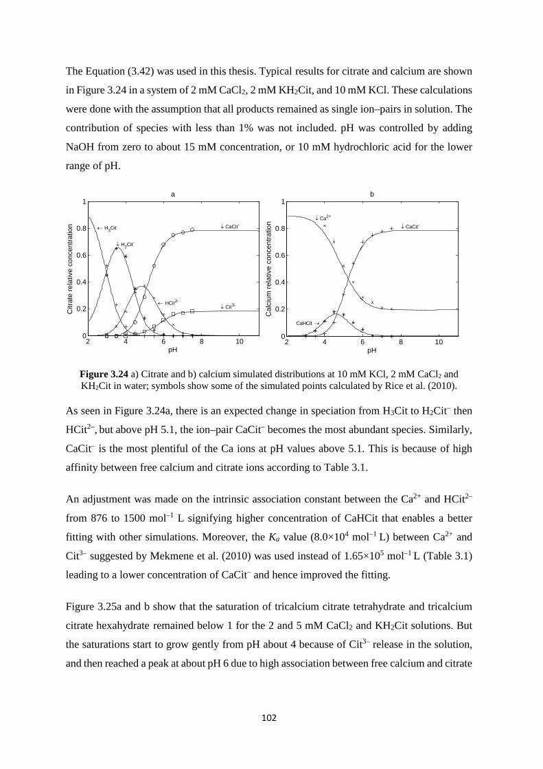
102
The Equation (3.42) was used in this thesis. Typical results for citrate and calcium are shown
in Figure 3.24 in a system of 2 mM CaCl2, 2 mM KH2Cit, and 10 mM KCl. These calculations
were done with the assumption that all products remained as single ion–pairs in solution. The
contribution of species with less than 1% was not included. pH was controlled by adding
NaOH from zero to about 15 mM concentration, or 10 mM hydrochloric acid for the lower
range of pH.
Figure 3.24 a) Citrate and b) calcium simulated distributions at 10 mM KCl, 2 mM CaCl2 and KH2Cit in water; symbols show some of the simulated points calculated by Rice et al. (2010).
As seen in Figure 3.24a, there is an expected change in speciation from H3Cit to H2Cit– then
HCit2–, but above pH 5.1, the ion–pair CaCit– becomes the most abundant species. Similarly,
CaCit– is the most plentiful of the Ca ions at pH values above 5.1. This is because of high
affinity between free calcium and citrate ions according to Table 3.1.
An adjustment was made on the intrinsic association constant between the Ca2+ and HCit2–
from 876 to 1500 mol–1 L signifying higher concentration of CaHCit that enables a better
fitting with other simulations. Moreover, the Ka value (8.0×10⁴ mol–1 L) between Ca2+ and
Cit3– suggested by Mekmene et al. (2010) was used instead of 1.65×10⁵ mol–1 L (Table 3.1)
leading to a lower concentration of CaCit– and hence improved the fitting.
Figure 3.25a and b show that the saturation of tricalcium citrate tetrahydrate and tricalcium
citrate hexahydrate remained below 1 for the 2 and 5 mM CaCl2 and KH2Cit solutions. But
the saturations start to grow gently from pH about 4 because of Cit3– release in the solution,
and then reached a peak at about pH 6 due to high association between free calcium and citrate
2 4 6 8 100
0.2
0.4
0.6
0.8
1
pH
Citr
ate
rela
tive
conc
entra
tion
↓ H2Cit-
← HCit2-↓ Cit3-
← H3Cit ↓ CaCit-
a
2 4 6 8 100
0.2
0.4
0.6
0.8
1
↓ Ca2+
CaHCit →
↓ CaCit-
pH
Cal
cium
rela
tive
conc
entra
tion
b

103
leading to high concentration of ion–pair calcium citrate, and then slightly drop due to
decrease in free calcium and citrate ions.
These simulated results were in good agreement with the simulated results presented by Rice
et al. (2010). The concentration of both Ca2+ and Cit3– in milk serum are about 10 mM (Holt,
1997). If no other ions were present, which would reduce the ions activities, then 10 mM Ca2+
and Cit3– would be about 1.6 and 0.17 times the saturation limit in presence of TCCT and
TCCH at a typical pH of 6.7, respectively. Consequently, the system was predicted to be
supersaturated in respect to calcium citrate tetrahydrate.
As shown by Figure 3.25, the saturation of TCCT is always higher than that of TCCH. This
is because of the larger solubility product of TCCH than that of TCCT signifying higher
solubility and hence less saturation of TCCH.
Figure 3.25 a) Saturation of tricalcium citrate tetrahydrate and b) tricalcium citrate hexahydrate at different molar concentrations of CaCl2 and KH2Cit, with 10 mM KCl. The y–axes scales of graphs
are different.
3.7.3.2 Addition of phosphate to steady state study of calcium citrate
In another study, 2 mM potassium hydrogen phosphate (KH2PO4) was incorporated into the
simulation of calcium citrate based on Rice et al. (2010). Figure 3.26a shows the predicted
distribution of free ions in the phosphate–citrate system in which the solubility product of
DCPD was assumed to be 2.07×10⁻⁷ mol2 L–2. Generally, the calcium citrate system with
phosphate was similar to the system without phosphate. Small quantities of calcium phosphate
species were formed at pH above 6 where the concentrations of hydrogen phosphate and
citrate started to increase.
2 4 6 8 10 120
0.2
0.4
0.6
0.8
1
1.2
1.4
1.6
1.8
pH
Satu
ratio
n of
TC
CT
a
10 mM5 mM2 mM
2 4 6 8 10 120
0.05
0.1
0.15
0.2
pH
Satu
ratio
n of
TC
CH
b
10 mM5 mM2 mM

104
Figure 3.26 a) Simulated distribution of calcium in 10 mM KCl, 2 mM CaCl2, 2 mM KH2Cit, and 2 mM KH2PO4; b) Saturation of DCPD and TCCT for both 10 mM KCl, 5 mM CaCl2, 5 mM KH2Cit, 5 mM KH2PO4 and 10 mM KCl, 2 mM CaCl2, 2 mM KH2Cit, 2 mM KH2PO4. The symbols express
some of simulated points calculated by Rice et al. (2010).
Saturations of DCPD and TCCT were compared for 2 and 5 mM concentrations as shown in
Figure 3.26b according to the Equations (3.44) and (3.45). Although the Ksp of DCPD is larger
than that of TCCT, it does not necessarily mean less saturation of DCPD as the ion activity
product equations are different. It can be seen that the hydrogen phosphate concentration is
higher than the citrate ion for almost the entire pH range in Figure 3.26a.
𝐾𝐾𝑠𝑠𝑠𝑠𝐷𝐷𝐶𝐶𝐻𝐻𝐷𝐷 =𝑎𝑎𝐶𝐶𝑎𝑎2+ 𝑎𝑎𝐻𝐻𝐻𝐻𝑂𝑂42−𝑆𝑆𝑎𝑎𝑆𝑆𝐷𝐷𝐶𝐶𝐻𝐻𝐷𝐷
= 2.07 × 10⁻⁷ mol2L–2 (3.44)
𝐾𝐾𝑠𝑠𝑠𝑠 𝑇𝑇𝐶𝐶𝐶𝐶𝑇𝑇 =
𝑎𝑎𝐶𝐶𝑎𝑎2+3 𝑎𝑎𝐶𝐶𝑖𝑖𝐶𝐶3−
2
𝑆𝑆𝑎𝑎𝑆𝑆𝑇𝑇𝐶𝐶𝐶𝐶𝑇𝑇= 2.29 × 10⁻¹⁸ mol5L–5 (3.45)
Generally, the presence of citrate decreases the saturation of DCPD in a solution containing
calcium phosphate (Hignett and Brabson, 1961). This can be seen clearly by comparing Figure
3.19 and 3.26b, in both of which the saturation of DCPD is plotted as a function of pH for 5
mM calcium and phosphate solutions. The one containing citrate (Figure 3.26b) had a
maximum of about 2, whereas the peak point of saturation reached 12 in Figure 3.19.
Mekmene et al. (2012) investigated the effect of some additives such as citrate in a milk–like
solutions containing calcium phosphate. They claimed that the saturation of solutions were
reduced by addition of citrate due to sequestration of free calcium. Similarly, Vavrusova et
al. (2017) claimed that excess sodium citrate drops the Ca2+ ion concentration because of
strong affinity between Ca2+ and Cit3– leading to higher calcium citrate solubility, and hence,
2 4 6 8 100
0.1
0.2
0.3
0.4
0.5
0.6
0.7
0.8
0.9
↑ Ca2+
↓ CaHCit
↓ CaCit-
CaHPO4 ↓ CaPO4
- ↓
pH
Rel
ativ
e co
ncen
tratio
n
← HPO42-
↓ Cit3-
a
2 4 6 8 10 12 140
0.5
1
1.5
2
2.5
pH
Satu
ratio
n
b
DCPD, 5 mMDCPD, 2 mMTCCT, 5 mMTCCT, 2 mM

105
Ca2+ concentration is controlled by Cit3– concentration. Both figures confirm that the level of
free calcium was lower when citrate was present.
3.7.3.3 Addition of lactate to equilibrium of calcium citrate and phosphate
Calcium lactate (CaLact2) is another salt available in dairy products such as Cheddar cheese
that may precipitate under certain conditions (Dybing et al., 1988). For instance, sodium
gluconate was used as an additive to Cheddar cheese to prevent calcium lactate precipitation
(Ramachandan et al., 2006; Phadungath and Metzger, 2011). Several works have been done
on the solubility of solutions composed of calcium lactate with other salts at different
temperatures (Vavrusova et al., 2013; Vavrusova et al., 2014; Vavrusova and Skibsted, 2014).
Despite these, no study has been done on the speciation of lactate in a solution constituting of
citrate and phosphate. Therefore, the MSA theory was employed to simulate a solution
containing 10 mM KCl, 2 mM CaCl2, 2 mM KH2Cit, 2 mM KH2PO4, and 2 mM lactic acid,
the pH of which was controlled continuously by NaOH addition. Apart from DCPD, TCCT,
and TCCH saturations, calcium lactate saturation was incorporated into the simulation as an
individual species with solubility product of 5.8×10⁻³ mol3 L–3 according to Vavrusova et al.
(2013) based on the Equation (3.46):
SaturationCaLact2 =
𝑎𝑎𝐶𝐶𝑎𝑎2+ 𝑎𝑎𝐿𝐿𝑎𝑎𝑐𝑐𝐶𝐶−2
𝐾𝐾𝑠𝑠𝑠𝑠 (3.46)
The intrinsic association constants of lactate (Lact–) and other cations in the system were used
according to Table 3.5, but other Ka values remained the same as in previous systems.
Table 3.5 Intrinsic association constants (mol–1 L) between lactate (Lact–) and principal cations in the simulation.
Ca2+ Na+ K+ H+ Ion–pair Ka Ion–pair Ka Ion–pair Ka Ion–pair Ka
Lact– CaLact+ 15a NaLact 2b KLact 2b HLact 7.14×10³c a (Jackson, 2004), b assumed values according to the other components ratios, c (Kubantseva and Hartel, 2002).
Typical results for calcium are shown in Figure 3.27a and for lactate in Figure 3.27b. Similar
to previous equilibrium systems, calculations were done with the assumption that all products
remained as single ion–pairs in solution without precipitation. The species with a contribution
of less than 1% are CaH2PO4+, CaHPO4, CaH2Cit+, CaLact+, and KLact. Among the ion–pairs
in the solution, Lact– is higher than the others for almost the entire pH range, following by the

106
ion–pairs CaCit– and CaPO4–. The high concentration of lactic acid (HLact) in the acidic part
of graph is due to high affinity between Lact– and H+.
Figure 3.27 Predicted distribution of a) calcium and b) lactate and compounds in a solution containing 10 mM KCl, 2 mM CaCl2, 2 mM KH2Cit, 2 mM KH2PO4, and 2 mM lactic acid.
The addition of lactate does not lower considerably the concentration of calcium species. This
is because of the low value of association constant between free calcium and lactate leading
to release of Ca2+ and Lact– ions. The association constants between free calcium and Cit3–
and PO43– are quite large, hence, calcium complexes are not affected greatly by the presence
of lactate.
Similar to previous citrate and citrate–phosphate systems, addition of lactate decreased the
DCPD saturation in a solution of calcium citrate–phosphate due to the sequestration of free
calcium. Hence, DCPD seems to precipitate first among the other salts, e.g., calcium citrate
and calcium lactate, according to the saturation graphs. However, this cannot be generalised
as the mechanism of precipitation determines the order of solid phase formation and the
subsequent rate of growth (Nancollas, 1992).
The simulation can be used to estimate the amount of lactic acid required to acidify milk from
its natural pH of 6.7 to the lowest possible pH of milk where the isoelectric point (IEP) of
casein is 4.6 according to Walstra et al. (2006) (Figure 3.28). The pH value at which the
average net charge of protein is equivalent to zero, is termed as isoelectric point at which the
protein has the least solubility (Southward, 1998; Salis et al., 2011). Casein proteins
precipitates around the pH of 4.6 at which casein proteins have no net charge leading to milk
coagulation. In bovine milk, the casein micelles are stable at pH of about 6.7 because of
negative net charge (Walstra et al., 2006).
2 4 6 8 10 120
0.2
0.4
0.6
0.8
1
Ca2+ ↑
CaHCit ↓
↓ CaCit-
pH
Cal
cium
rela
tive
conc
entra
tion
CaPO4- ↓
a
2 4 6 8 10 120
0.2
0.4
0.6
0.8
1Lact- ↑
← HLact
NaLact ↓
pHLa
ctat
e re
lativ
e co
ncen
tratio
n
b

107
Figure 3.28 The required amounts of lactic acid needed to change the pH of a solution of milk electrolytes from pH 6.7.
Hence, in this study, calcium and potassium as cations, and chloride, citrate, and phosphate
as anions were incorporated into the simulations with the same salt concentrations of milk:
Ca (29 mM) (Mekmene, Le Graet, et al., 2009), K (38.3 mM), Cl (30.4 mM), Cit (9.5 mM) ,
PO4 (20.6 mM) (Holt, 2004). Figure 3.28 shows that no lactic acid was required to reach to
natural pH, and 23 mM was the amount of lactic acid required to get a pH of 4.6. Therefore,
an addition of 23 mM of lactic acid would cause this pH change. However, only the main
electrolyte constituents of milk were included in the model and the role of other components
such as sodium, sulphate, carbonate, lactose, and proteins were neglected.
3.7.3.4 Effect of lactose on calcium, potassium, chloride, and citrate solution
Another simulation, in which the MSA theory was used to calculate activity coefficient and
subsequently Ca2+ molar activity and pH, was implemented with various lactose contents in
a multicomponent solution comprising CaCl2, KCl, and K3Cit. The reason for choosing this
mixture is that similar work has been done on this system theoretically and experimentally
with sucrose rather than lactose. Therefore, results of Gao, van Leeuwen, et al. (2010) were
reproduced as an appropriate validation for this study with 5 mM CaCl2, 55 mM KCl, and 4
mM K3Cit throughout the range of sucrose.
In this study, the association between calcium, potassium, and the sugars were considered
despite of their tiny values, although Gao, van Leeuwen, et al. (2010) presumed only the
affinity between sugars and hydrogen ion. Another adjustment was the ionic size which was
0 10 20 30 40 50 60 70 80 90 1003
3.5
4
4.5
5
5.5
6
6.5
7
Lactic acid concentration, mmol/L
pH
← pH=6.7
← pH=4.6 at 23 mM lactic acid

108
used from the data of Gao, van Leeuwen, et al. (2010) and Isaad and Perwuelz (2010), for
sucrose (0.7 nm) and lactose (0.454 nm), respectively, although no value was found for the
size of corresponding ion–pairs, therefore, they were estimated relatively close to those sugar
sizes, i.e. 0.6 nm for sucrose and 0.4 nm for lactose ion–pairs.
Figures 3.29a, b, and d show that pH, Ca2+ activity, and molar activity coefficients calculated
by the MSA theory were in good agreement with the literature results for sucrose solutions.
However, sucrose was allowed to dissociate in the solution as an anion (Sucrose–) that
interacted with the cations such as calcium, potassium (K+), and hydrogen by their
corresponding association constants. Stearn (1931) proposed intrinsic association constants
between H+ and sugars including sucrose and lactose which are 5.00×10¹² and 1.31×10¹²
mol– 1 L, respectively according to Equations (3.47) and (3.48). 𝐻𝐻𝑆𝑆𝐻𝐻𝑐𝑐𝑟𝑟𝐻𝐻𝑎𝑎𝑒𝑒 represents
undissociated sucrose. In addition, the saturation of TCCT was included in the calculation and
was shown in Figure 3.29c.
𝐻𝐻𝑆𝑆𝐻𝐻𝑐𝑐𝑟𝑟𝐻𝐻𝑎𝑎𝑒𝑒 ↔ 𝐻𝐻+ + 𝑆𝑆𝐻𝐻𝑐𝑐𝑟𝑟𝐻𝐻𝑎𝑎𝑒𝑒 − 𝐾𝐾𝑎𝑎 =𝑎𝑎𝐻𝐻𝑀𝑀𝐻𝐻𝑐𝑐𝑝𝑝𝑠𝑠𝑠𝑠𝑝𝑝
𝑎𝑎𝐻𝐻+𝑎𝑎𝑀𝑀𝐻𝐻𝑐𝑐𝑝𝑝𝑠𝑠𝑠𝑠𝑝𝑝− (3.47)
𝐻𝐻𝐿𝐿𝑎𝑎𝑐𝑐𝑆𝑆𝐻𝐻𝑎𝑎𝑒𝑒 ↔ 𝐻𝐻+ + 𝐿𝐿𝑎𝑎𝑐𝑐𝑆𝑆𝐻𝐻𝑎𝑎𝑒𝑒− 𝐾𝐾𝑎𝑎 =𝑎𝑎𝐻𝐻𝐿𝐿𝑎𝑎𝑐𝑐𝐶𝐶𝑠𝑠𝑠𝑠𝑝𝑝
𝑎𝑎𝐻𝐻+𝑎𝑎𝐿𝐿𝑎𝑎𝑐𝑐𝐶𝐶𝑠𝑠𝑠𝑠𝑝𝑝− (3.48)
Since the association constant of sucrose is larger than that of lactose, less HSucrose
dissociated to the H+ and sucrose– than HLactose to its corresponding free ions. Hence, the
pH of sucrose solutions was higher than that of lactose. On the other hand, the association
constant for sucrose– and lactose– were adjusted to 500 and 2000 for Ca2+, 100, and 2200
mol– 1 L for K+, respectively to be able to get better fitting in pH graph leading to higher Ca2+
activity in sucrose solution that than of lactose (Equations (3.49) and (3.50)). Hence, the
saturation of TCCT in sucrose solutions was higher than that of lactose solutions because
higher activity of Ca2+.
𝐶𝐶𝑎𝑎𝐿𝐿𝑎𝑎𝑐𝑐𝑆𝑆𝐻𝐻𝑎𝑎𝑒𝑒 ↔ 𝐶𝐶𝑎𝑎2+ + 𝐿𝐿𝑎𝑎𝑐𝑐𝑆𝑆𝐻𝐻𝑎𝑎𝑒𝑒− 𝐾𝐾𝑎𝑎 =𝑎𝑎𝐶𝐶𝑎𝑎𝐿𝐿𝑎𝑎𝑐𝑐𝐶𝐶𝑠𝑠𝑠𝑠𝑝𝑝
𝑎𝑎𝐶𝐶𝑎𝑎2+𝑎𝑎𝐿𝐿𝑎𝑎𝑐𝑐𝐶𝐶𝑠𝑠𝑠𝑠𝑝𝑝− = 2000 (3.49)
𝐾𝐾𝐿𝐿𝑎𝑎𝑐𝑐𝑆𝑆𝐻𝐻𝑎𝑎𝑒𝑒 ↔ 𝐾𝐾+ + 𝐿𝐿𝑎𝑎𝑐𝑐𝑆𝑆𝐻𝐻𝑎𝑎𝑒𝑒− 𝐾𝐾𝑎𝑎 =𝑎𝑎𝐾𝐾𝐿𝐿𝑎𝑎𝑐𝑐𝐶𝐶𝑠𝑠𝑠𝑠𝑝𝑝
𝑎𝑎𝐾𝐾+𝑎𝑎𝐿𝐿𝑎𝑎𝑐𝑐𝐶𝐶𝑠𝑠𝑠𝑠𝑝𝑝− = 2200 (3.50)

109
The variation in Ca2+ activity and pH became larger between simulated and experimental data
at higher concentrations of sugars. This is probably because of the non–ideality of highly
concentrated solutions for which the MSA theory still has some uncertainty. Nonetheless, the
MSA theory is likely capable of activity coefficient prediction for high concentrations of
sugars in a multicomponent solution.
Figure 3.29 Effect of sucrose on a) pH, b) Ca2+ molar activity, c) TCCT saturation and d) predicted molar activity coefficient of Ca2+ and H+ by the MSA theory in a multicomponent system containing 5 mM CaCl2, 55 mM KCl, and 4 mM K3Cit. The solid and dash curves represent this study based on the simulation. × and × symbols indicate experimental data from Gao, van Leeuwen, et al. (2010)
and data based on the calculation, respectively.
3.7.3.5 Dynamic study of calcium citrate system
In a study, Garcia et al. (2018) measured pH over time to dynamically investigate precipitation
of amorphous calcium citrate (ACP) for 0.1 mol L–1 equimolar binary solutions of aqueous
calcium chloride with sodium dihydrogen phosphate (NaH2PO4), trisodium citrate (Na3Cit),
0 0.5 1 1.5 2
6
6.2
6.4
6.6
6.8
7
7.2
7.4
Non-electrolyte concentration, mol/L
pH
↑ Sucrose
↓ Lactose
a
0 0.5 1 1.5 24
6
8
10
12
14 x 10-4
Non-electrolyte concentration, mol/L
Activ
ity o
f Ca 2
+ , mol
/LSucrose ↓
↑ Lactose
b
0 0.5 1 1.5 20
0.5
1
1.5
2
2.5
3
3.5
Non-electrolyte concentration, mol/L
Satu
ratio
n of
TC
CT
Sucrose ↓↓ Lactose
c
0 0.5 1 1.5 20
0.5
1
1.5
2
2.5
3
Non-electrolyte concentration, mol/L
Mol
ar a
ctiv
ity c
oeffi
cien
t,[-]
d
Sucrose ↓
↑ Lactose
H+
Ca2+

110
or disodium hydrogen citrate (Na2HCit). This system was simulated using the MSA theory
with the precipitation and dissolution rate constants set to 0.01 and 4×10⁻⁴ min–1 for TCCT
and to 0.2 and 0.5 min–1 for TCCH, respectively to reasonably match the experimental data.
Figure 3.30 shows the pH of binary solutions over time for three aforementioned species, in
all of which precipitation was recognisable from the change in pH trend, although it initiated
differently for each solution depending on the ions interaction.
Figure 3.30 pH of solutions of 0.1 mol L–1 CaCl2 with Na3Cit, Na2HCit, or NaH2PO4. The curves and × symbols represent simulation from this study and experimental data from Garcia et al. (2018).
Dynamic simulation of calcium citrate solutions were performed to determine the solubility
and precipitates over time in multicomponent solutions containing 30 mM CaCl2, 20 mM
NaH2PO4, and 9.5 mM KH2Cit with 0, 4.5, and 25%w/w lactose contents. The reason for
choosing this composition is that no similar work has been done dynamically on the calcium
citrate and phosphate system by assuming potential precipitate phases. Therefore,
concentrations close to milk were selected with various levels of lactose. The pH of solution
was controlled by continuous addition of sodium hydroxide for each time step. Similar to the
previous simulations, Euler’s method was employed together with the equilibrium
calculations for each presumed solid phase species (DCPD, DCPA, TCCT, and TCCH) along
with their solubility products. Lactose was also incorporated into the system and was allowed
to dissociate to form an anion with a single negative charge (lactose–) that is in association
with the other cations in the system.
0 2 4 6 8 10 12 14 16 18 203.5
4
4.5
5
5.5
6
6.5
7
7.5
8
Time, hour
pH
Na3Cit
Na2HCit
NaH2PO4

111
Figure 3.31 Dynamic simulation of precipitation in a multicomponent solution comprising CaCl2, NaH2PO4, and KH2Cit with 0, 4.5, and 25%w/w lactose. a) pH changes; b) DCPD; c) DCPA; d)
TCCT; and e) molar activity coefficient of Ca2+ over the time.
0 100 200 300 400 5004.4
4.6
4.8
5
5.2
5.4
5.6
5.8
6
Time, min
pHa
No lactose4.5%w/w lactose25%w/w lactose
0 100 200 300 400 5000
1
2
3
4
5 x 10⁻³
Time, min
DC
PD c
once
ntra
tion,
mol
/L
b
0 100 200 300 400 500-2
0
2
4
6
8 x 10⁻⁴
Time, min
DC
PA c
once
ntra
tion,
mol
/L
c
0 100 200 300 400 5000
0.5
1
1.5
2
2.5 x 10⁻³
Time, min
TCC
T co
ncen
tratio
n, m
ol/L
d
0 100 200 300 400 5000.3
0.31
0.32
0.33
0.34
0.35
0.36
0.37
Time, min
Mol
ar a
ctiv
ity c
oeffi
cien
t, [-]
↑ The MSA theory, 25%w/w lactose
↓ The MSA theory, 4.5%w/w lactose
↑ The MSA theory, No lactose
↑ Davies theory
e

112
Figure 3.31 shows the changes in pH, DCPD, DCPA, TCCT, and molar activity coefficient
over time for the solution containing no lactose, 4.5, and 25%w/w lactose. Figure 3.31a, b, c,
and d indicate that the parameters were unlikely affected by the addition of lactose. However,
a slight difference between highest content of lactose (25%w/w) with the two other fractions
(0 and 4.5%w/w) is observed from the graphs. The principal change is evident in Figure 3.31e,
for which molar activity coefficient of Ca2+ was calculated by the MSA and Davies theories.
The MSA theory could satisfactorily distinguish the distinct between various lactose contents
because of the hard sphere contribution in the formula.
The initial pH drop in Figure 3.31a indicates the formation of the first solid phase in the first
5 minutes of the reaction followed by a second pH drop representing TCCT formation at about
50 minutes. DCPD and TCCT were predicted to remain insoluble in the solution, while DCPA
dissolved as seen in Figure 3.31c. TCCH and all other solids were given a low initial
concentration to avoid modelling primary nucleation. The trends of precipitate concentrations,
pH, and activity coefficient are highly dependent on the precipitation and dissolution rates,
for which no reliable source could be found. Therefore, they were adjusted to a set of values,
for which results of Garcia et al. (2018) were reproduced (Figure 3.30).
From this section, it can be concluded that:
1. The proposed model is adequately able to predict salt partitioning and speciation of
ion–pairs in a solution containing solid phase by calculating the saturation of calcium
salts as an individual species in the set of ions.
2. Kinetics of precipitation calcium salts including calcium carbonate, phosphate, and
citrate were predicted satisfactorily by the proposed model. However, more
experimental data is required to determine the precipitation and dissolution
mechanisms and their rates as well as crystallisation of various forms of calcium salts
by taking account of lactose.
3. Calcium phosphate is thermodynamically the most stable solid phase (Elliot, 1994)
that is formed in the mixed solutions under certain concentrations, following by the
calcium citrate but with lower stability possibly due to the smaller value of solubility
product and subsequently lower solubility. During sudden precipitation, some
intermediate solid phases may be formed but dissolution may occur later.

113
3.8 Application of the model to milk serum
The electrolytes in milk are essential as nutrients and for osmotic balance and have been well
characterised at normal milk concentrations. When milk, whey, whey permeate or milk
protein concentrates are concentrated by evaporation or reverse osmosis, the concentration of
ions particularly calcium phosphate can easily exceed solubility limits. This leads to
heterogeneous fouling of salts on the evaporators’ surfaces or reverse osmosis membranes,
causing a serious reduction in performance and thus gradual depreciation of equipment in
dairy industry (Kezia et al., 2017).
Several investigations have been carried out on the ion equilibria and interactions of milk
serum under various conditions by assuming different solid phases in milk that were discussed
earlier in this chapter. However, less study has been done on ion association, activity, and
solubility in concentrated bovine milk. The aim in this section is to develop a robust method
for predicting the state of minerals in any dairy serum (without proteins) up to high
concentrations. The MSA method was used to calculate free–ion activity coefficients as it
contained terms that enhanced accuracy at higher concentrations. The role of proteins in milk
will be thoroughly investigated in Chapter 5.
3.8.1 Equilibrium study of milk serum
The proposed model was used in order to calculate the ion partitioning of milk serum, in
which lactose and saturations of potential solid phase species such as brushite, monetite
(DCPA), octacalcium phosphate (OCP), whitlockite (WH), hydroxyapatite (HAP), calcium–
deficient apatite (CDA), calcium carbonate (calcite), tricalcium citrate tetrahydrate, and
magnesium phosphate (Mg3(PO4)2) were calculated. The following species were included in
the model: calcium, magnesium, sodium, and potassium as cations; citrate, phosphate,
carbonate, sulphate, chloride, phosphate esters, and carboxylate as anions. Lactose was
included in the system as an individual species but the presence of milk proteins was ignored
here and is dealt with separately in Chapter 5. The components were presumed to be
equilibrated by their corresponding intrinsic association constants for ion–pairs and by
solubility products for solid phase species. Table 3.1 shows the intrinsic association constants
for the serum milk ions and Table 3.6 shows the solubility products of solid phases. These
were presented first by Holt et al. (1981) and then modified by Mekmene, Le Graet, et al.
(2009) and Mekmene et al. (2010).

114
Table 3.6 Solubility products of solid phase components (Driessens and Verbeeck, 1990; Mekmene, Quillard, et al., 2009; Gao, van Halsema, et al., 2010).
Chemicals Chemical formula Solubility product IAP
DCPD CaHPO4.2H2O 2.09×10⁻⁷ mol2 L–2 𝑎𝑎𝐶𝐶𝑎𝑎2+ × 𝑎𝑎𝐻𝐻𝐻𝐻𝑂𝑂42−
DCPA CaHPO4 4.00×10⁻⁷ mol2 L–2 𝑎𝑎𝐶𝐶𝑎𝑎2+ × 𝑎𝑎𝐻𝐻𝐻𝐻𝑂𝑂42−
OCP Ca8(HPO4)2(PO4)4.5H2O 3.16×10–73 mol14 L–14 𝑎𝑎𝐶𝐶𝑎𝑎2+8 × 𝑎𝑎𝐻𝐻𝐻𝐻𝑂𝑂42−
2 × 𝑎𝑎𝐻𝐻𝑂𝑂43−4
HAP Ca10(PO4)6(OH)2 1.58×10–117 mol18 L–18 𝑎𝑎𝐶𝐶𝑎𝑎2+10 × 𝑎𝑎𝐻𝐻𝑂𝑂43−
6 × 𝑎𝑎𝑂𝑂𝐻𝐻−2
CDA Ca9(HPO4)(PO4)5(OH) 7.94×10–86 mol16 L–16 𝑎𝑎𝐶𝐶𝑎𝑎2+9 × 𝑎𝑎𝐻𝐻𝐻𝐻𝑂𝑂42− × 𝑎𝑎𝐻𝐻𝑂𝑂43−
5 × 𝑎𝑎𝑂𝑂𝐻𝐻−
WH Ca10(HPO4)(PO4)6 1.99×10–82 mol17 L–17 𝑎𝑎𝐶𝐶𝑎𝑎2+10 × 𝑎𝑎𝐻𝐻𝐻𝐻𝑂𝑂42− × 𝑎𝑎𝐻𝐻𝑂𝑂43−
6
Calcite CaCO3 4.8×10⁻⁹ mol2 L–2 𝑎𝑎𝐶𝐶𝑎𝑎2+ × 𝑎𝑎𝐶𝐶𝑂𝑂32−
Magnesium phosphate Mg3(PO4)2 1.0×10⁻²⁴ mol5 L–5 𝑎𝑎𝑀𝑀𝑔𝑔2+
3 × 𝑎𝑎𝐻𝐻𝑂𝑂43−2
TCCT Ca3Cit2 2.29×10⁻¹⁸ mol5 L–5 𝑎𝑎𝐶𝐶𝑎𝑎2+3 × 𝑎𝑎𝐶𝐶𝑖𝑖𝐶𝐶2−
2
The total concentration of each component in milk serum (Table 3.7) was used to determine
initial guesses of ion equilibria in milk serum.
Table 3.7 The total concentration of each principal constituent in milk serum (Holt, 1997).
Anions Total concentration, mM
Citrate 9.368 Inorganic phosphate 12.394 Carbonate 0.448 Sulphate 1.205 Chloride 32.300 Carboxylate 3.110 Phosphate esters 2.592 Cations Calcium 10.184 Magnesium 3.407 Sodium 22.006 Potassium 38.006

115
Figure 3.32 shows the saturation of potential precipitates in a milk–like solution, for which a
wide range of concentration was assumed without precipitation. Figure 3.32a and b indicate
the role of lactose on the saturation of calcium salts. Magnesium salts were not significantly
affected by the addition of lactose, and thus they were not included in these graphs. Lactose
has a significant effect on saturation of calcium phosphate particularly DCPD and DCPA and
less effect on the other solid phases, when milk serum is concentrated up to 50% solids. This
was also confirmed by Herrington (1934) who stated that lactose associates with calcium and
increase supersaturation of solution with respect to calcium salt compounds.
Figure 3.32 Saturation of solid phase calcium salts with a) no lactose; b) 25% lactose. The ‘’ indicates points corresponding to the normal electrolyte concentrations of serum (121.4 mM). See
Table 3.6 for calcium phosphate abbreviations.
3.8.2 Dynamic study of milk serum
The kinetics of change in salt equilibria in milk and milk–like systems have been less
investigated. More recently, Gao, van Halsema, et al. (2010) proposed a theoretical model for
the ion partitioning prediction of freshly prepared SMUF, for which a kinetics study was
investigated to ascertain the change of solubility product over time using the AESolve
program.
Despite this study and those that were previously described in Chapter 2, further research is
required to clarify the change in ion equilibria as well as the formation of potential precipitates
over time. Milk ions and solid phase salts were incorporated into the dynamic system. The
intrinsic association constants and solubility products were used from Tables 3.1 and 3.6.
0 0.2 0.4 0.6 0.8 10
10
20
30
40
50
Electrolyte concentration, mol/L
Satu
ratio
n
a
DCPDDCPAOCPCDAWHHAP
0 0.2 0.4 0.6 0.8 10
10
20
30
40
50
Electrolyte concentration, mol/L
Satu
ratio
n
b

116
Figure 3.33 illustrates the simulated dynamic change on salt equilibria of milk serum when
the solution has 0, 4.5%w/w, and 25%w/w lactose, showing that higher contents of lactose
cause formation of higher concentrations of DCPD and DCPA (Figure 3.33c), and an earlier
drop in pH (Figure 3.33a). DCPD is known to be the dominant precipitate formed in the
solution, whose saturation and concentration was higher than other solid salts as confirmed
by van Kemenade and de Bruyn (1987). Gao, van Halsema, et al. (2010) claimed that DCPD
precipitate was the main reason for the pH drop in SMUF over time.
Figure 3.33 Influence of lactose addition on a) pH; b) saturation of potential solid phase species with no lactose in the solution; c) dominant solid phase concentrations; and d) molar activity
coefficient of Ca2+ over time in a simulation containing milk serum components. The legend from Figure 3.33a corresponds also to Figure 3.33c.
Gao, van Halsema, et al. (2010) predicted the precipitation of calcium salts such as DCPD,
OCP, and DCPA to a higher degree, and less quantities of CDA from milk serum. Mg3(PO4)2,
0 100 200 300 400 5006.1
6.2
6.3
6.4
6.5
6.6
Time, min
pH
a
No lactose4.5%w/w lactose25%w/w lactose
0 100 200 300 400 5000
0.5
1
1.5
2
2.5
3
3.5
4
Time, min
Satu
ratio
n
b
DCPDOCPDCPACDAWHTCCT
0 100 200 300 400 5000
0.5
1
1.5
2
2.5
3
Time, min
Con
cent
ratio
n of
pre
cipi
tate
, mm
ol/L
c
DCPDOCPDCPA
0 100 200 300 400 5000.35
0.4
0.45
0.5
0.55
Time, min
Mol
ar a
ctiv
ity c
oeffi
cien
t of C
a2+, [
-]
d
↑ The MSA thoery, 25%w/w lactose
↓ The MSA thoery, 4.5%w/w lactose
↑ The MSA thoery, No lactose

117
CaCO3, and WH remained soluble in the solution and the saturation of hydroxyapatite (HAP)
was close to zero (Gao, van Halsema, et al., 2010).
In milk serum, the ions are either free or in association as ion–pairs according to their
association constants. As shown in Figure 3.34, about 70% of total soluble calcium was
associated with the calcium citrate, and 20% was present as free calcium, which were in a
good agreement with the mineral distribution calculated by Mekmene, Le Graet, et al. (2009)
for a milk serum solution. The reason for low concentration of calcium phosphate was its low
solubility. Other calcium salts constituted the remaining 10% of total soluble calcium.
Nonetheless, these values dropped over time due to formation of calcium solid phase salts
that are mainly DCPD, OCP, and DCPA with a total concentration of about 3 mM. However,
the milk serum is supersaturated in respect to calcium phosphate salts, and hence no
precipitation should be predicted. The time scale here is quite fast, but in a study by Howell
(1998), fouling in the whey permeate occurred over days showing that fouling content did not
change much over few days.
The soluble calcium phosphates had lower concentration than soluble calcium citrates,
remaining mainly as ion–pairs with total concentration of 5.70 mM as indicated in Table 3.8,
while calcium phosphates appeared mostly as calcium solid phases.
Figure 3.34 The simulated dynamic change of total calcium species over time in the milk serum solution.
Table 3.8 shows the simulated soluble and insoluble calcium species in the milk serum
solution after 500 minutes.
0 50 100 150 200 250 300 350 400 450 5000
2
4
6
8
10
12
Time, min
Con
cent
ratio
n, m
mol
/L
Total soluble calciumSoluble calcium citratesCa2+
Soluble calcium phosphatesSoluble calcium chloride

118
The precipitation and dissolution rate constants of the solid phase salts were estimated to get
results as discussed in the earlier sections on precipitation in previously reported systems. The
rate constant values are provided in Appendix 6. The DCPD rate constants were used to guess
for other rate constants of potential salts. E.g. DCPA might have higher solubility and hence
precipitation than DCPD leading to have large precipitation rate constants. Further, DCPA
dissolves in the solution implying higher dissolution rate constant than DCPD.
Table 3.8 The calcium ion–pairs and precipitates at 500 minutes.
Soluble ions Concentration, mM Total, mM Precipitate Chemical formula mM
CaH2Cit+ 4.75×10⁻⁵
5.70 TCCT 5.64×10⁻⁵
CaHCit 0.03
CaCit– 5.67 DCPD 1.57
CaH2PO4+ 0.03
0.13 CaHPO4 0.01 OCP 1.50
CaPO4– 3.96×10⁻⁴
CaHCO3+ 0.002
0.002 DCPA 10–82
CaCO3 7.91×10⁻⁶
CaHSO4+ 1.01×10⁻⁷
0.03 HAP 1.24×10⁻⁶ CaSO4 0.03
CaCl+ 0.11 0.11 CDA 2.28×10⁻⁴
CaGlc–1–PH+ 0.004 0.06
CaGlc–1–P 0.06 WH 2.58×10⁻⁶
CaRCOO+ 0.02 0.02
CaOH+ 2.26×10⁻⁷ 2.3×10⁻⁷ CaCO3 10–33
Ca2+ 1.04 1.04
Total soluble calcium 7.10 Total insoluble calcium 3.08
In another similar dynamic simulation of milk serum, initial concentrations were doubled to
check the effect on the ion equilibria of milk serum. Other parameters remained unchanged
as it is desirable to see only the effect of concentrations. The higher concentration of species
caused a higher initial pH and subsequently higher pH after 500 minutes, leading to double
the saturation over time for all potential salts. The DCPD concentration was seen to be

119
relatively high among the other solid phase species with about 8 mM, followed by the DCPA
formation in the first 100 minutes. The OCP concentration was too small to include in Figure
3.35c.
Figure 3.35 Effect of double the normal concentration of milk serum on a) pH; b) saturation; and c) concentrations of potential solid phase salts.
3.9 Conclusions
The simulation method was able to predict speciation and precipitation in a range of solutions,
some of which were validated using experimental data. The model gave satisfactory results
for various aqueous solution, in the sense that there was a good match of the shape and values
of the graphs between the results of this study and other works either experimentally or by
simulation.
0 100 200 300 400 5005.9
6
6.1
6.2
6.3
6.4
Time, min
pH
a
0 100 200 300 400 5000
1
2
3
4
5
6
7
8
Time, min
Satu
ratio
n
b
DCPDOCPDCPACDAWHTCCT
0 100 200 300 400 5000
1
2
3
4
5
6
7
8
Con
cent
ratio
n of
pre
cipi
tate
, mm
ol/L
Time, min
c
DCPDDCPA
120
Adjustments of association constants were sometimes necessary to get better fitting with
corresponding experimental and simulated data in literature because there are many different
values for each association constant.
The Mean Spherical Approximation (MSA) method was used to calculate free–ion activity
coefficients as it contained terms that enhanced accuracy at higher concentrations. Further, it
allows the addition of zero–charge component such as lactose, whereas the other models like
Davies theory or Extended Debye–Hückel contain the charge term in their formula leading to
activity coefficient of unity for zero–charge species. The MSA theory is capable of making
distinction between activity coefficient of a solution comprising sugar by incorporating size
and concentrations related terms as the main strength of this method.
The results were in reasonable agreement with those presented by the literature from either
experiments or other simulations. This shows that the assumptions made are quite accurate
for calculations of salt partitioning in various systems, and can be applied to various milk–
like systems as long as the initial concentrations are well defined and determined. However,
more validation with complex milk solutions is desirable. The intrinsic association constants
and solubility products were assumed in the temperature range of 20–25 ˚C. More research is
required to identify the constants for other temperatures to be able to expand this model for
other milk–like solutions and possibly in cheese making process where heat treatment and
other temperature–related factors are inevitable (Mekmene, Le Graet, et al., 2009).
No sufficient data are available for the precipitation and dissolution rate constants of
precipitates in milk, and hence investigations seem necessary for the calculations of those
values under different conditions.

121
4 Experimental Aspects of Calcium Phosphate Precipitation
4.1 Introduction
The aim of this chapter was to investigate the effect of lactose on the solubility of calcium
phosphate with varied and controlled pH and at different concentrations. Different
concentrations of calcium chloride, sodium phosphate, sodium hydroxide with and without
lactose were mixed, and pH and conductivity were measured to follow the precipitation of
calcium phosphate over the time. This system was used because it is one the simplest to mimic
milk. Moreover, calcium phosphate can precipitate as the principal salt available in milk. The
outcomes of this study will show a possible role of lactose in stabilising calcium phosphate
solutions possibly by formation of calcium phosphate nanoparticles.
Doherty and Wright (2004) studied the effect of sugars on various calcium salts in a calcium
oxalate (CaC2O4) solution in presence of sucrose. In other research, Besic (1985) speculated
that sucrose influences calcium and phosphate solubility in teeth.
The experiment work was begun with research into the effect of milk minerals on “fouling”
of reverse osmosis membranes used for concentration of milk (Tew, 2015) and then the effect
of ion activities on solubility of calcium phosphate in milk in Chapter 3. Preliminary
experiments of the model solutions containing CaCl2, NaH2PO4, and NaOH showed an
unexpected absence of precipitation when lactose was added. Although similar results have
been obtained using simulated body fluids (Oyane et al., 2002), no work with lactose in the
calcium phosphate system has been found. Little data are available from literature for
validation in this thesis. Therefore, a few experiments were carried out to gain more data for
comparison.
4.2 Materials and methods
4.2.1 Chemicals and reagents
Fresh stock solution of 1 mol L–1 calcium chloride dihydrate (CaCl2.2H2O, Thermo Fischer
Scientific, Australia), 1 mol L–1 sodium dihydrogen phosphate monohydrate (NaH2PO4.H2O,
AnalaR, VWR International Ltd., Poole, England), and 1 mol L–1 sodium hydroxide (NaOH,
LabServ, Australia) were prepared.

122
14.7 g (equivalent to 1 mol L–1) CaCl2.2H2O was weighed into a 100 mL volumetric flask and
was made up to 100 mL with Milli–Q water.
Likewise, stock solutions of sodium phosphate and sodium hydroxide were prepared
individually in 100 mL volumetric flasks. Dilute stock solutions of sodium hydroxide with
0.5 and 0.02 mol L–1 were also prepared.
Stock solutions were made up a day before the experiments to ensure that their temperatures
were fully equilibrated to the laboratory temperature.
Generally, solutions of lactose monohydrate (C12H22O11.H2O, AnalaR, Poole, England) with
a concentration of 9.5%w/w lactose were made up in 100 mL volumetric flasks a day before
for experiments containing lactose. However, due to three different recipes for mixing
solutions containing lactose, full descriptions on the preparation will be given at each related
section.
All of the experiments were carried out at room temperature, which was about 23 ˚C, but the
temperature was recorded throughout the runs over time to ensure no heat was produced that
might affect the results.
4.2.2 Analytical instruments
4.2.2.1 pH meter
The pH of solutions was measured by a CyberScan pH 510 pH/mV meter (Eutech, Germany)
with an Eutech pH probe that was equipped with an automatic temperature compensation.
Another CyberScan pH 310 pH/mV meter (Eutech, Germany) was also used when the pH of
two solutions needed to be adjusted simultaneously before mixing. The pH meters were
calibrated to ±0.02 of standard buffer pH values.
4.2.2.2 Conductivity meter
The electrical conductivity meter of solutions were measured with a Lab 960 conductivity
meter that was equipped with a Lab LF413T standard conductivity cell (Schott, Germany)
with a resolution of ±1 μS cm–1. The conductivity meter was set to a linear temperature
compensation with an accuracy of ±0.5% and a temperature coefficient of 1.754% K–1. The
probe was rinsed with Milli–Q water before and after each measurement.

123
4.2.2.3 Dynamic Light Scattering
Dynamic light scattering (DLS, Zetasizer, Model Nano Series, Malvern Instruments,
Worcestershire, United Kingdom) was used to determine size distribution of particles in the
mixed solutions. Three runs were defined in the software, in which water was chosen as a
dispersant with the refractive index of 1.333 and absorption of zero. Temperature and
equilibration time were set to 23 ˚C and 90 minutes, respectively. Standard operating
procedures were followed.
4.2.3 Solution preparations
In this section, binary solutions of CaCl2, NaH2PO4, and lactose were individually tested,
because in initial experiments (without argon), it was found that the pH of ingredient
solutions, especially CaCl2, fluctuated rapidly within minutes when magnetically stirred and
exposed to air. Hence, ternary solutions of CaCl2, NaH2PO4, and lactose with NaOH were
also prepared to improve pH and conductivity stabilisation over time. This enabled the
estimation of the right concentration of each solution before mixing to obtain the desirable
initial and stable pH values after mixing.
4.2.3.1 Preparation of binary solutions of CaCl2 and NaH2PO4
Six mL (equivalent to 0.06 mol L–1) of the calcium chloride stock solution was drawn up by
a clean and dry 5±0.015 mL glass pipette and 1 mL by a 1±0.007 mL glass pipette. They were
transferred to a clean and dry 100 mL volumetric flask, which was filled up with milli–Q
water to 100 mL. The calcium chloride solution was shaken gently and was transferred to a
250 mL glass beaker, into which probes of analytical instruments were placed to measure pH,
conductivity, and temperature over time. 60 mM NaH2PO4 solution was made up similar to
the preparation of 60 mM CaCl2 solution.
4.2.3.2 Preparation of binary solution of lactose
A solution of 9.5%w/w lactose was prepared by adding 10%w/w lactose monohydrate to
water.

124
The lactose solution was incubated at 40 C with orbital shaking at 140 rpm for approximately
4 hours to ensure complete dissolution of lactose. It was then stored at laboratory temperature
(23 ˚C) to equilibrate.
4.2.3.3 Preparation of ternary solutions of CaCl2 or NaH2PO4 or lactose with NaOH
Ternary solutions of CaCl2 or NaH2PO4 or lactose with NaOH were made up very similar to
the preparation of corresponding binary solutions, but a certain amount of NaOH was added
to 100 mL of flask. For example, identically, 6 mL (equivalent to 0.06 mol L–1) of the CaCl2
stock solution was drawn up and transferred to a 100 mL volumetric flask, to which 2 mL
(equivalent to 1 mM) of the 0.05 M NaOH stock solution was added. The solution was then
filled up with Milli–Q water and was poured to a container for pH and conductivity
measurements.
Smaller quantities of NaOH were drawn up by micropipettes in the range of 20–100, or 200–
1000 μL, both of which were calibrated before each set of experiment to ensure the accuracy
of taken volume by weighting Milli–Q water on the balance.
Similarly, ternary solutions of lactose and NaOH solutions were made up in the same way but
a different amount of NaOH was added.
4.2.3.4 Preparation of mixed solutions
For each mixed solution, solutions of both CaCl2 and NaH2PO4 (unmixed) were prepared in
a 100 mL volumetric flask with various concentrations, and sodium hydroxide was added to
achieve a desired pH value in a similar way of ternary solution preparations. Once both
solutions reached to a stable and same pH values, they were mixed.
For mixed solutions containing lactose, two 9.5%w/w lactose solutions with NaOH were
prepared in an identical method to the preparation of ternary solutions. One lactose solution
was used for preparation of calcium chloride solution and the other one for sodium phosphate
solution.
4.2.3.5 Experimental operation conditions
Five modes of operation were tested to determine how the experimental conditions would
affect the pH and conductivity of the solutions:

125
1. The solution was poured to a beaker which is exposed to open air;
2. The container was sealed by a lid to avoid CO2 absorption from air;
3. The container was open to air placed on magnetic stirrer while bubbling air in;
4. The container was placed on a magnetic stirrer while flowing argon into the headspace;
5. The container was placed on a magnetic stirrer while bubbling argon into the solution
as shown in Figure 4.1.
Holes were drilled in the lid of container for gas and probes as shown in Figure 4.1.
Instruments grade argon gas was bubbled at 40 cm3 min–1 to the bottom of each solution to
strip and prevent absorption of any carbon dioxide which strongly influenced pH. pH,
conductivity, and temperature were measured and recorded over time while argon was
bubbling in. Samples were taken from time to time for the particle size analysis using the DLS
instrument to identify the possible formation of nanoparticles.
Figure 4.1 The experimental set–up for the majority of experiments.
4.3 Results and discussion
4.3.1 CaCl2 solution
A binary solution of CaCl2 was exposed to air to monitor how pH and conductivity are
affected dynamically. Figure 4.2a shows the values of pH and conductivity of 60 mM CaCl2
solution which was exposed to air. The drop in pH and conductivity clearly implies absorption
of carbon dioxide from air.

126
Figure 4.2 pH and conductivity changes of 60 mM CaCl2 solution over the time while open to air.
It was believed that gaseous CO2 enters the aqueous phase of a solution to achieve
thermodynamic equilibrium with atmosphere:
𝐶𝐶𝐶𝐶2(𝑔𝑔)𝐾𝐾𝐶𝐶𝑂𝑂2⎯ 𝐶𝐶𝐶𝐶2(𝑎𝑎𝑞𝑞) (4.1)
where 𝐾𝐾𝐶𝐶𝑂𝑂2 is the solubility coefficient of CO2 in the aqueous phase of solution, dissolution
of which is about 0.038 mol L–1 bar–1.
𝐶𝐶𝐶𝐶2(𝑎𝑎𝑞𝑞) = 𝐾𝐾𝐶𝐶𝑂𝑂2𝐼𝐼𝐶𝐶𝑂𝑂2 (4.2)
Here [𝐶𝐶𝐶𝐶2(𝑎𝑎𝑞𝑞)] is the molar concentration of CO2 in the aqueous phase; 𝐼𝐼𝐶𝐶𝑂𝑂2 is the partial
pressure of CO2 on the surface solution, [bar].
The dissolved carbon dioxide thermodynamically interacts with water forming carbonic acid,
which may lose up two protons according to the following equilibria with three different
intrinsic association constants (Zeebe and Wolf-Gladrow, 2001; Wikipedia, n.d):
𝐶𝐶𝐶𝐶2(𝑎𝑎𝑞𝑞) + 𝐻𝐻2𝐶𝐶(𝑠𝑠) ↔ 𝐻𝐻2𝐶𝐶𝐶𝐶3(𝑎𝑎𝑞𝑞) 𝐾𝐾𝑎𝑎1 =𝑎𝑎𝐻𝐻2𝐶𝐶𝑂𝑂3𝑎𝑎𝐶𝐶𝑂𝑂2
= 1.7 × 10⁻³[−] (4.3)
𝐻𝐻2𝐶𝐶𝐶𝐶3 ↔ 𝐻𝐻𝐶𝐶𝐶𝐶3– + 𝐻𝐻+ 𝐾𝐾𝑎𝑎2 =𝑎𝑎𝐻𝐻2𝐶𝐶𝑂𝑂3
𝑎𝑎𝐻𝐻𝐶𝐶𝑂𝑂3−𝑎𝑎𝐻𝐻+= 4 × 10³ [mol−1 L] (4.4)
0 10 20 30 405.9
6
6.1
6.2
6.3
6.4
Time, min
pHa
0 10 20 30 405.72
5.73
5.74
5.75
5.76
5.77
5.78
5.79
5.8
5.81
Time, min
Con
duct
ivity
, mS/
cm
b

127
𝐻𝐻𝐶𝐶𝐶𝐶3– ↔𝐶𝐶𝐶𝐶32− + 𝐻𝐻+ 𝐾𝐾𝑎𝑎3 =𝑎𝑎𝐻𝐻𝐶𝐶𝑂𝑂3−
𝑎𝑎𝐶𝐶𝑂𝑂32−𝑎𝑎𝐻𝐻+= 2.13 × 10¹⁰ [mol−1 L] (4.5)
The 𝐾𝐾𝑎𝑎2 value is inconsistent and far lower than that of the 2.25 × 10⁶ mol–1 L presented by
Holt et al. (1981). Zeebe and Wolf-Gladrow (2001) used the ratio 𝐾𝐾𝑎𝑎2𝐾𝐾𝑎𝑎1
representing:
𝐾𝐾𝑎𝑎2𝐾𝐾𝑎𝑎1
=𝑎𝑎𝐶𝐶𝑂𝑂2(𝑎𝑎𝑎𝑎)
𝑎𝑎𝐻𝐻𝐶𝐶𝑂𝑂3−𝑎𝑎𝐻𝐻+= 2.35 × 10⁶ (4.6)
The transmission of gaseous to aqueous CO2 then to carbonic acid leads the solution to release
up to two hydrogen ions and subsequently drop in pH.
These equilibria were used to simulate influence of CO2 absorption on pH values of CaCl2
solution. Calcium, bicarbonate (HCO3–), carbonate (CO3
2–), hydrogen, hydroxide ions were
incorporated into the model with identical corresponding intrinsic associations given in
Chapter 3 (Zeebe and Wolf-Gladrow, 2001).
Figure 4.3 illustrates the pH drop in 60 mM CaCl2 solution as a function of CO2 concentration
as the result of simulation. This clearly shows that pH reduces rapidly at very low CO2
concentrations and then drops slowly for higher concentration. According to Figure 4.2, the
initial pH value was 6.4 for the experimental measurement of CaCl2 solution that is equivalent
to absorption of about 4 ppm CO2 from air into the solution. This is possibly because there
was a little delay in pH measurement due to pouring the solution and adjusting analytical
probes in the beaker.
Figure 4.3 pH of 60 mM CaCl2 solution when it was assumed to be exposed to air.
0 50 100 150 200 250 300 350 4005.4
5.6
5.8
6
6.2
6.4
6.6
6.8
7
Concentration of CO2 in air, ppm
pH
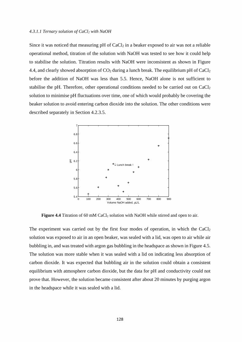
128
4.3.1.1 Ternary solution of CaCl2 with NaOH
Since it was noticed that measuring pH of CaCl2 in a beaker exposed to air was not a reliable
operational method, titration of the solution with NaOH was tested to see how it could help
to stabilise the solution. Titration results with NaOH were inconsistent as shown in Figure
4.4, and clearly showed absorption of CO2 during a lunch break. The equilibrium pH of CaCl2
before the addition of NaOH was less than 5.5. Hence, NaOH alone is not sufficient to
stabilise the pH. Therefore, other operational conditions needed to be carried out on CaCl2
solution to minimise pH fluctuations over time, one of which would probably be covering the
beaker solution to avoid entering carbon dioxide into the solution. The other conditions were
described separately in Section 4.2.3.5.
Figure 4.4 Titration of 60 mM CaCl2 solution with NaOH while stirred and open to air.
The experiment was carried out by the first four modes of operation, in which the CaCl2
solution was exposed to air in an open beaker, was sealed with a lid, was open to air while air
bubbling in, and was treated with argon gas bubbling in the headspace as shown in Figure 4.5.
The solution was more stable when it was sealed with a lid on indicating less absorption of
carbon dioxide. It was expected that bubbling air in the solution could obtain a consistent
equilibrium with atmosphere carbon dioxide, but the data for pH and conductivity could not
prove that. However, the solution became consistent after about 20 minutes by purging argon
in the headspace while it was sealed with a lid.
0 100 200 300 400 500 600 700 800 9005.4
5.6
5.8
6
6.2
6.4
6.6
6.8
7
Volume NaOH added, µL/L
pH
↓ Lunch break !

129
Figure 4.5 pH and conductivity of 60 mM CaCl2 solutions under four different experimental operations.
Subsequently, bubbling argon in the aqueous phase along with the addition of NaOH was
found the most effective operational condition in comparison with the others. Figure 4.6a
shows the pH of CaCl2 solutions with different concentrations of NaOH operating under
bubbling argon. When argon was bubbled through the solution, the pH values were about 1.5
units higher and more repeatable between experiments than those exposed to air. It clearly
shows that NaOH and bubbling argon could effectively improve pH stabilisation over time
especially for higher amounts of NaOH. Thus, it seems that CaCl2 solution with lower
quantities of NaOH could be harder to control due to potential absorption of carbon dioxide
into the solution as the pH gets closer to natural milk pH.
Figure 4.6b indicates the titration results of CaCl2 solution with NaOH, which is more
consistent than those exposed to air. Figure 4.6 helped to determine the required amount of
NaOH to get the desired initial pH value before mixing solutions.
0 20 40 60 80 100 120 1405.6
5.7
5.8
5.9
6
6.1
6.2
6.3
6.4
Time, min
pHa
0 20 40 60 80 100 120 14011.3
11.4
11.5
11.6
11.7
11.8
11.9
12
Time, min
Con
duct
ivity
, mS/
cm
b
Argon to the headspaceOpen to air,air bubbling inOpen in beakerSealed with a lid

130
Figure 4.6 pH of 60 mM CaCl2 solution with bubbled argon a) over time; and b) as a function of various NaOH added in mM.
4.3.2 NaH2PO4 solution
Solutions of sodium phosphate were much more stable even without NaOH addition or
bubbling argon. This is because the solution has naturally low pH hence addition of carbonic
acid is not able to reduce pH anymore.
Similarly, pH and conductivity of NaH2PO4 solutions were measured by addition of NaOH
and argon gas bubbling in to avoid any CO2 absorption. Figure 4.7a shows the pH and
conductivity of 60 mM NaH2PO4 solution when pH was adjusted to 7.5 by adding NaOH in
the middle of the experiment. First, 10 mM NaOH was added to the solution giving pH of
about 6.1, then about 47.1 mM was added to reach to adjusted pH but it was a bit higher than
expected. 45 mM NaOH gave closer stable pH values but a bit lower than the adjusted one.
Therefore, 9 mM more was added to the solution giving pH about 7.5. Figure 4.7b indicates
the measured conductivity, which corresponds to the pH change data for the three sodium
phosphate solutions. This shows that solutions containing more NaOH are likely more
conductive, this is because the solution contains more charged species.
0 20 40 60 80 100 120 1407
7.5
8
8.5
9
9.5
10
10.5
11
Time, min
pHa
1 mM NaOH0.05 mM NaOH0.02 mM NaOH0.015 mM NaOH0.014 mM NaOH0.0135 mM NaOH0.0125 mM NaOH0.01 mM NaOH
0 0.01 0.02 0.03 0.04 0.056
6.5
7
7.5
8
8.5
9
9.5
Concentration NaOH added, m M
pH
b

131
Figure 4.7 a) pH and b) conductivity of 60 mM NaH2PO4 solution titrated with NaOH while argon gas bubbled in the aqueous phase.
4.3.3 Lactose solution
Binary solutions of lactose in water with 2.5, 5, and 7.5%w/w lactose were tested in open
beakers exposed to air and a 9.5%w/w solution was tested with argon bubbling into the
solution. The resulting pH and conductivity are shown in Figure 4.8. During the experiments,
conductivity, and especially pH values were unstable for those solutions exposed to air, so the
mean value of each measurement was recorded each minute. However, more improvement
was observed once the solution was sealed with a lid with argon bubbling. This is probably
because of less carbon dioxide absorbed in the solution. The 9.5%w/w solution will have been
more stable because of its lower pH.
Figure 4.8 a) pH and b) conductivity of lactose solutions with 2.5, 5, 7.5, and 9.5%w/w contents when they are either exposed to air or sealed while argon gas purging in.
0 20 40 60 80 100 1204
4.5
5
5.5
6
6.5
7
7.5
8
Time, min
pHa
45 mM+ 9 mM NaOH10 mM+ 47.1 mM NaOHNo NaOH
0 20 40 60 80 100 1203.5
4
4.5
5
5.5
6
6.5
7
7.5
Time, min
Con
duct
ivity
, mS/
cm
b
0 10 20 30 40 50 60 70 80 90 1004.2
4.4
4.6
4.8
5
5.2
5.4
5.6
5.8
6
6.2
Time, min
pH
a
2.5%w/w lactose, exposed to air5%w/w lactose, exposed to air7.5%w/w lactose, exposed to air9.5%w/w lactose, sealed while argon bubbling in
0 20 40 60 80 10010
20
30
40
50
60
70
80
Time, min
Con
duct
ivity
, mS/
cm
b

132
Hence, the titration of lactose with NaOH seemed necessary with bubbling argon gas to
stabilise pH values. Figure 4.9a shows the titration of 9.5%w/w lactose with different
concentrations of NaOH to see how much base is needed to obtain the adjusted pH. Moreover,
consistent and stable results were observed for each solution of lactose with NaOH over time.
Figure 4.9 Titration of 9.5%w/w lactose solutions with argon bubbling a) with various NaOH concentrations, and b) by different lactose sources.
During pH adjustment, it was noticed that adjustment of lactose solutions required more
NaOH than expected. Lactose can dissociate a very small amount in solution with a 𝐾𝐾𝑎𝑎𝑐𝑐 given
by Stearn (1931) of 7.6×10⁻¹³ mol–1 L. Using this acidity constant one can calculate that a
9.5% solution has an expected pH of 6.33. Once 3 mmol/L of NaOH has been added the pH
is expected to tend to about 11.5 but the pH reached only 10.2 in the experiments as shown in
Figure 4.9b. The test was repeated using three different samples of lactose from Sigma–
Aldrich, AR, and AnalaR, though is possible that all samples had the same origin. The
possibility of the presence of lactose phosphate was considered as this would have the effect
of lowering the pH and would interact with NaOH more than lactose (Lifran, 2007).
4.3.4 Mixed solutions
Solutions of CaCl2 and NaH2PO4 with a 1:1 ratio of Ca/P were prepared individually for the
mixed solutions either with or without lactose but with NaOH based on the preparation
method given in Section 4.2.3.4.
Concentrations after mixing of 3.5, 5, and 10 mM Ca and PO4 with the adjusted initial pH of
about 6.5 were tested and shown in Figure 4.10 along with their corresponding DLS analysis
0 20 40 60 804.5
5
5.5
6
6.5
7
7.5
Time, min
pH
a
0.3 mM NaOH0.25 mM NaOH0.22 mM NaOH0.15 mM NaOH0.015 mM NaOH
0 1 2 3 44
5
6
7
8
9
10
11
12
NaOH added, mM
pH
b
No lactoseSigma-AldrichAnalaRAR

133
results as a function of particle size. Samples were taken for analysis as soon as the previous
run of Zetasizer was completed to ensure each part of the graph was analysed by the Zetasizer.
Differences were seen for 5 mM solutions with and without lactose at pH about 6.5 (Figure
4.10c). In this figure, it can be seen that precipitation, as indicated by the pH drop, is not
instantaneous. This is explained by the rate of precipitation being proportional to the area of
precipitated particles already in the system. The solution with lactose delayed precipitation
even though it was at a slightly higher pH and hence less stable. Similarly, for 3.5 mM (Figure
5a) with almost identical pH in both solutions, the presence of lactose increased the stability
of the solution. No precipitation was observed even after 200 minutes. Figure 4.10e illustrates
the pH change over time for 10 mM solution, in which both solutions with 9.5 and 19.95%w/w
lactose had a slightly lower initial pH, even though the ternary solution pH values were
stabilised at about 6.5, but it immediately dropped. This is probably because of higher
saturation of the solution so the stabilisation by lactose was insufficient.
By comparing Figures 4.10a, c, and e, it can be concluded that lower contents of CaCl2 and
NaH2PO4 are more stable and thus the precipitation occurs at a later time with a small drop in
pH.
The most striking difference between solutions with and without lactose was shown by the
Zetasizer response as seen in Figure 4.10b, d, and f. Mixtures with 9.5% w/w lactose at a pH
about 6.5 showed a peak at a particle diameter close to 1 nm. Mixtures without lactose did not
show this peak. The same peak was observed in a sample with lactose that had been kept for
3 days before particle size measurement, indicating that the particles were stable. Samples of
lactose only did not show any peaks so it was concluded that the peak is from a reaction
product and not an artefact.

134
Figure 4.10 pH changes and DLS analysis, indicating precipitation, for a, b) 3.5 mM; c, d) 5 mM; and e, f) 10 mM CaCl2 and NaH2PO4 with 9.5%w/w and without lactose with adjusted initial pH of
about 6.5.
In another experiment with 2.5 mM of CaCl2 and NaH2PO4 without lactose, no precipitation
was detected either by eye, by shining a laser pointer through the solution, even though a
0 50 100 150 200 2505.4
5.6
5.8
6
6.2
6.4
Time, min
pHa
3.5 mM, 9.5%w/w lactose3.5 mM, no lactose
10-2 100 102 1040
5
10
15
20
25
30
35
40
Particle size, nm
DLS
inte
nsity
, %
b
0 50 100 1505.4
5.6
5.8
6
6.2
6.4
Time, min
pH
c
5 mM, 9.5%w/w lactose5 mM, no lactose
10-2 100 102 1040
5
10
15
20
25
30
35
40
Particle size, nm
DLS
inte
nsity
, %
d
0 20 40 60 80 100 1205.4
5.6
5.8
6
6.2
6.4
Time, min
pH
e
10 mM, 9.5%w/w lactose10 mM, 19.95%w/w lactose10 mM, no lactose
10-2 100 102 1040
20
40
60
80
100
Particle size, nm
DLS
inte
nsity
, %
f

135
small peak is seen at about 103 nm in Figure 4.11b. pH remained relatively constant for about
1 hour indicating the absence of precipitation.
Figure 4.11 a) pH changes, and b) DLS analysis of 2.5 mM CaCl2 and NaH2PO4 without lactose.
The initial pH of solutions was adjusted to about 5.5 by adding less NaOH for the solution
with 10 mM concentration to see if any precipitation occurred in the solution. At lower pH
values, solutions with 10 mM no sign of precipitation was seen either with or without lactose
at pH 5.2 as shown in Figure 4.12a and b. These results are consistent with the lower saturation
at lower pH that was simulated previously in Figure 3.19 in Chapter 3. Hence, the amount of
NaOH or the pH is a factor affecting the formation of nanoparticles in the mixed solutions.
Figure 4.12c indicates that precipitation started immediately for the 20 mM solution without
lactose and within 3 minutes for the solution with lactose.
0 10 20 30 40 50 60 706
6.1
6.2
6.3
6.4
6.5
6.6
Time, min
pH
a
10 mM, no lactose
10-2 100 102 1040
5
10
15
20
25
30
35
40
Particle size, nmD
LS in
tens
ity, %
b

136
Figure 4.12 pH changes and DLS analysis, for a, b) 10 mM; c, d) 20 mM; CaCl2 and NaH2PO4 with 9.5%w/w and without lactose with adjusted initial pH of about 5.5.
Similar nm size particles have been found in simulated body fluids by Oyane et al. (2002)
using 2.5 mM Ca2+ and 1.0 mM HPO42– at pH 7.4 and by Onuma and Ito (1998). Kellermeier
et al. (2012) found stable clusters in a calcium carbonate silica system. A number of structures
have been proposed. A popular one has been the Posner cluster (Posner and Betts, 1975),
Ca9(PO4)6, which has a theoretical diameter of 0.95 nm. Lin and Chiu (2017) simulated
possible structures for calcium phosphate clusters with sizes of about 1 nm and obtained some
alternative structures with lower energies than the Posner cluster.
Without a known composition, it was not possible to include the nanoparticles into the model.
Hence, simulation of the pH change was not possible.
The results shown in Figure 4.10 are the key results of this chapter. When lactose is added to
the calcium phosphate system with concentrations similar to those found in bovine milk,
0 20 40 60 80 100 120 1405
5.2
5.4
5.6
5.8
6
Time, min
pHa
10 mM, 9.5%w/w lactose10 mM, no lactose
10-2 100 102 1040
5
10
15
20
25
30
35
40
Particle size, nm
DLS
inte
nsity
, %
b
0 20 40 60 80 100 120 1404.4
4.6
4.8
5
5.2
5.4
5.6
5.8
6
Time, min
pH
c
20 mM, 9.5%w/w lactose20 mM, no lactose
10-2 100 102 1040
5
10
15
20
25
30
35
40
Particle size, nm
DLS
inte
nsity
, %
d

137
nanoparticles are formed. The formation of these seems to prevent or reduce the precipitation
of calcium phosphate and hence will add to the stability of calcium phosphate in milk. This
effect will be in addition to the role of casein in stabilising calcium phosphate in milk as
discussed by Holt (2004). Lactose will act in the milk serum (outside of the casein micelles)
so might have a role in stabilising the fraction in the serum.
There are many uncertainties in these experiments and the mechanism for the increased
stabilisation is unclear. It is reasonably certain that when lactose is present, nanoparticles of
about 1 nm are formed, while solutions containing no lactose formed precipitates with larger
particles size.
There is no evidence at this stage of the composition or structure of these particles. Given the
unexpected titration curve of lactose, it is possible that there is a significant amount of lactose
phosphate or other substance in the lactose, and that this forms part of the nanoparticle. If
lactose does not make up part of the nanoparticle, there are other mechanisms for interactions.
The presence of lactose will increase the solution viscosity and possibly reduce the rate of
normal precipitation. Disaccharides like sucrose, maltose, and lactose typically are hydrated
by about five water molecules in solution, which reduces the water activity, hence affecting
calcium and phosphate ion interaction. Little and Holt (2004) showed that β–casein
phosphopeptide in milk will stabilise casein phosphate nanoparticles, but did not speculate on
a structure. Likewise Oyane et al. (2002) who measured 1 nm calcium phosphate particles did
not discuss their structure. Lin and Chiu (2017) showed that the structures have not yet been
confirmed.
In this preliminary work, the Ca/P ratio used as 1:1, but the Posner cluster has a ratio of 1.5:1.
Little and Holt (2004) suggested a lower limit of 1.15 for Ca/P in a CPN solution containing
5 mg β–casein in a buffer solution of 30 mM Ca(NO3)2, 5 mM Mg(NO3)2, 20 mM KH2PO4,
26 mM KNO3, and 1.5 mM NaN3. It is expected that a ratio closer to 1.5 will increase stability
so some future experiments are recommended with this ratio.
The nanoparticles have been found to be stable for at least 3 days, but this duration needs to
be extended and tested for a range of conditions. Oyane et al. (2002) showed stability for 7
days in simulated body fluids.
Lactose is the first sugar found to form nanoparticles with calcium phosphate, but the effect
of other sugars like disaccharides and monosaccharides are unknown monosaccharides are

138
unknown which are useful to be tested to see how they can influence the solubility of calcium
phosphate solution.
4.4 Conclusions
Binary solutions of calcium chloride and sodium phosphate as well as corresponding ternary
solutions with lactose were stabilised by designing an effective experimental set–up to reach
the desired initial pH value before mixing them together and to prevent any carbon dioxide
absorption from the air which strongly affected the pH of ingredient solutions especially
calcium chloride. Given the experimental results, it was found that purging argon in the
solution and sealing the container could satisfactorily minimise carbon dioxide absorption
from air into the solutions.
The experimental results clearly showed the formation of a 1 nm nanoparticle in solutions of
lactose and calcium and phosphate ions. Lactose was found to prevent or slow down the
precipitation of calcium phosphate, probably as calcium dihydrogen phosphate. The structure
of the nanoparticle is not known and, based on current research in this area, might be difficult
to determine. The effects of many of the conditions such as concentration, ion ratios, pH,
lactose concentration, and time need to be tested. The effects of lactose in this ideal system
indicate that it might have a role for the stabilisation of calcium phosphate in milk that might
add to the stabilisation produced by the casein micelles.

139
5 Development of the Model to Bovine Milk
5.1 Introduction
Fundamental research has been conducted on the calculations of salt equilibria in milk serum
and simulated milk ultrafiltrate (SMUF) without proteins (Holt et al., 1981; Lyster, 1981;
Wood et al., 1981; Gao, van Halsema, et al., 2010) and fewer studies have been done on salt
partitioning of milk by incorporating phosphoserine residues of casein molecule (Holt, 2004;
Little and Holt, 2004; Mekmene, Le Graet, et al., 2009; Mekmene et al., 2010). More recently,
Bijl et al. (2018) developed a comprehensive model, in which magnesium ions were assumed
to bind to caseins with identical association constants as calcium and by incorporating
dissociable side groups of amino acids in casein proteins. In this thesis, the proposed model
described in Chapter 3 was applied to milk to calculate ion equilibria between the aqueous
and micellar phases of milk by including dissociable amino acids of both phases. Further, the
model was used to predict dynamic changes due to supersaturation in milk.
5.2 Description of the model
The proposed model, which was fully described in Chapter 3, was used to determine ion
speciation in milk. The model was applied to various systems and gave reasonable results
under various conditions. The major constituents of aqueous and micellar phases of milk that
were included in the model are calcium, magnesium, sodium, potassium, hydrogen, citrate,
inorganic phosphate, carbonate, sulphate, phosphate esters, chloride, carboxylate, and
hydroxide. In this chapter, the model is extended to include the amino acids of αs1–, αs2–, β–,
κ–casein and β–lactoglobulin, α–lactalbumin, and bovine serum albumin.
Some of the amino acids in proteins have a dissociable side chain in their structures that is
either basic or acidic depending on their dissociation constants. Only dissociable side groups
of particular amino acid were used in the model. E.g., alanine is a non–polar and uncharged
side chain, which is unlikely to affect pH of the solution, whereas aspartic acid with one
dissociable side group acts as an acid (Belitz and Grosch, 1999). The chemical structure of all
amino acids with either charged or uncharged side groups are listed in Appendix 7. Table 5.1
gives the dissociable side groups of amino acids with their dissociation constants.

140
Table 5.1 The dissociation of the amino acids side groups of the milk proteins (Belitz and Grosch, 1999; Mercadé-Prieto et al., 2007).
Amino acid Side group The equilibrium Kd of the side group
Arginine –CH2CH2CH2NHCNHNH2 (–RNH2) Arg + H+ ↔ ArgH+ 𝐾𝐾𝑑𝑑𝐴𝐴𝑟𝑟𝐴𝐴 =[−RNH2][H+]
[−RNH3+] =
[Arg][H+][ArgH+] = 10−12.52
Aspartic acid –CH2COOH (–RCOOH) Asp− + H+ ↔ AspH 𝐾𝐾𝑑𝑑𝐴𝐴𝑠𝑠𝑠𝑠 =[−RCOO−][H+]
[−RCOOH] =[Asp−][H+]
[AspH] = 10−4.0
Cysteine –CH2SH (–RSH) Cys− + H+ ↔ CysH 𝐾𝐾𝑑𝑑𝐶𝐶𝐶𝐶𝑠𝑠 =[−RS−][H+]
[−RSH] =[Cys−][H+]
[CysH] = 10−8.5
Glutamic acid –CH2CH2COOH (–RCOOH) Glu− + H+ ↔ GluH 𝐾𝐾𝑑𝑑𝐺𝐺𝐺𝐺𝐺𝐺 =[−RCOO−][H+]
[−RCOOH] =[Glu−][H+]
[GluH] = 10−4.0
Histidine HN
NCH2
(–RNH, imidazole)
His + H+ ↔ −HisH+ 𝐾𝐾𝑑𝑑𝐻𝐻𝑖𝑖𝑠𝑠 =[−Imidazole][H+]
[−ImidazoleH+] =[His][H+][HisH+] = 10−6.0
Lysine –CH2CH2CH2CH2NH2 (–RNH2) Lys + H+ ↔ LysH+ 𝐾𝐾𝑑𝑑𝐿𝐿𝐶𝐶𝑠𝑠 =[−RNH2][H+]
[−RNH3+] =
[Lys][H+][LysH+] = 10−10.95
Serine –CH2OH (–RCOH) Ser− + H+ ↔ SerH 𝐾𝐾𝑑𝑑𝑆𝑆𝑆𝑆𝑟𝑟 =[−RCO−][H+]
[−RCOH] =[Ser−][H+]
[SerH] = 10−13.22
Threonine –CHOHCH3 (–RCOH) Thr− + H+ ↔ ThrH 𝐾𝐾𝑑𝑑𝑇𝑇ℎ𝑟𝑟 =[−RCO−][H+]
[−RCOH] =[Thr−][H+]
[ThrH] = 10−13.22
Tyrosine OHCH2(–RCOH)
Tyr− + H+ ↔ TyrH 𝐾𝐾𝑑𝑑𝑇𝑇𝐶𝐶𝑟𝑟 =[−RCO−][H+]
[−RCOH] =[Tyr−][H+]
[TyrH] = 10−9.60
Note: the formula written in the parentheses represent the abbreviated form of the side groups.

141
Each protein molecule has many different residues with potential hydrogen ion equilibria.
Dissociable acidic and basic side groups are bound covalently to a higher degree to hydrogen
ions and to a lesser degree to other cations (Kuehner et al., 1999). The affinity between other
cations and amino acids was not ignored despite being small. At any pH given, these residues
will be in various protonation states depending on their individual ion dissociation constant,
i.e. Kd often expressed as pKd. Thus, the protein will have a net charge, which varies with pH.
With knowledge of all the individual pKd values of all the possible hydrogen ion and other
cations ion–pairs found in a protein, it is possible to calculate the absolute net electric charge
of a protein as a function of pH.
Each amino acid was treated as an anion with either negative or neutral charge depending on
their acidic or basic side groups. Consider arginine in a protein. The H2N–CH–COOH head
has been condensed as a part of the protein group –CH2CH2CH2NHCNHNH2 abbreviated
here as −RNH2. In acid conditions leaving the side, this will carry an extra proton and be
−RNH3+, dissociation constant of which was shown in Table 5.1. The forms will be designated
as Arg and ArgH+ (–RNH3+). The other side groups in milk proteins with the same behaviour
are lysine and histidine, and the NH2 terminal group. –RCOOH is the side group for aspartic
acid, which dissociates to –RCOO–. The forms will be designated as Asp– and AspH.
Dissociation of other acidic amino acids will be the same as aspartic acid such as cysteine,
glutamic acid, serine, threonine, and tyrosine.
5.2.1 Net charge of a protein
Physico–chemical properties of a protein are highly affected by the parameter ‘net electric
charge’ of the medium that implies the solution but the charge is of the protein. The pH at
which the electric repulsion between proteins is minimised and near to zero, is called
‘isoelectric point (IEP)’ (Ninham and Lo Nostro, 2010). Hence, the net electric charge of the
molecule is zero at the IEP, i.e. positive and negative charge numbers of a zwitterion become
equal (Sørensen et al., 1927).
Net electric charge was calculated by three different methods, all of which should give
consistent results for any protein. In this thesis, all three methods were used as a means of
mathematical validation.

142
5.2.1.1 Approach 1 for net charge calculation
Cameselle et al. (1986) defined the net electric charge as the total number of charges (z)
divided by the total number of molecules (n, see Equation (5.6)). The degree of ionisation (𝛼𝛼)
determines instant charge of a particular group due to the continuous fluctuating values.
Therefore, the net electric charge is obtained as the total charge number of a molecule:
Net charge =
∑𝑧𝑧𝑛𝑛
(5.1)
The degree of ionisation is identical to the time fraction of an acid–base molecule for
dissociated groups, while the degree of non–dissociation (1 − 𝛼𝛼) is attributed to the time
fraction for undissociated ones. The net charge should be equal to the sum over all the side
groups in a protein:
Net charge = 𝑧𝑧𝑑𝑑𝛼𝛼 + 𝑧𝑧𝐻𝐻(1− 𝛼𝛼) (5.2)
where 𝑧𝑧𝑑𝑑 and 𝑧𝑧𝐻𝐻 are charge numbers of dissociated and undissociated groups, respectively.
The Henderson–Hasselbach (Equation (5.3)) can be rearranged as a function of degree of
ionisation (Fennema, 1996):
[dissociated form][undissociated form]
= 10pH−𝑠𝑠𝐾𝐾𝑎𝑎 =𝛼𝛼
1 − α (5.3)
Therefore:
𝛼𝛼 =1
10𝑠𝑠𝐾𝐾𝑎𝑎−pH + 1 (5.4)
Substituting in Equation (5.2) gives:
Net charge =𝑧𝑧𝑑𝑑
10𝑠𝑠𝐾𝐾𝑎𝑎−pH + 1+
𝑧𝑧𝐻𝐻10pH−𝑠𝑠𝐾𝐾𝑎𝑎 + 1
(5.5)
Hence, the overall net electric charge can be obtained for a molecule:
Net charge = 𝑧𝑧𝑖𝑖𝑑𝑑
10𝑠𝑠𝐾𝐾𝑖𝑖−pH + 1+
𝑧𝑧𝑖𝑖𝐻𝐻10pH−𝑠𝑠𝐾𝐾𝑖𝑖 + 1
𝑠𝑠
𝑖𝑖=1 (5.6)

143
Here 𝑛𝑛 is the number of amino acid side groups.
5.2.1.2 Approach 2 for net charge calculation
Salis et al. (2011) proposed a formula for calculation of bovine serum albumin surface charge
at various pH values based on the potentiometric titrations, but Equation (5.7) can be also
applicable to other proteins:
Net charge =𝐶𝐶HCl − 𝐶𝐶NaOH
𝑚𝑚protein/𝑀𝑀𝑊𝑊protein (5.7)
𝐶𝐶HCl and 𝐶𝐶NaOH are molar concentrations of HCl and NaOH, [mol L–1] that are required to
achieve a net zero surface charge; 𝑚𝑚protein is mass of protein, [g L–1]; 𝑀𝑀𝑊𝑊protein is the molar
mass of protein, [g mol–1].
5.2.1.3 Approach 3 for net charge calculation
Another method was used to calculate the net charge of a protein molecule as a function of
the molar concentration and charge number of each amino acid and their corresponding ion–
pairs per protein as follows:
Net charge =
∑ 𝐶𝐶𝑖𝑖𝑧𝑧𝑖𝑖𝑖𝑖
𝑚𝑚protein/𝑀𝑀𝑊𝑊protein (5.8)
The subscript 𝑖𝑖 represents the species. This approach is originated from the net charge
definition, which is used as the main method for this study.
However, all these methods assume no interaction between amino acid residues. Li et al.
(2005) outlined a more rigorous method that takes into account these interactions.
5.2.2 Initial concentration of each amino acid
The molar concentration of each protein in milk should be determined to be able to obtain the
concentration of each amino acid that was required for the simulation. The concentration of
each dissociable amino acid was calculated from concentration of each protein in milk and
the number of each dissociable amino acid per protein as shown in Table 5.2.

144
Table 5.2 Dissociable amino acid concentration in bovine milk and per protein of milk (Walstra and Jenness, 1984; Walstra et al., 2006).
β–lg α–la BSA αs1–casein αs2–casein β–casein κ–casein
molAA∗molβ–lg
μmolAA𝐿𝐿milk
molAA
molα–la μmolAA𝐿𝐿milk
molAA
molBSA μmolAA𝐿𝐿milk
molAA
molαs1 μmolAA𝐿𝐿milk
molAA
molαs2 μmolAA𝐿𝐿milk
molAAmolβ–
μmolAA𝐿𝐿milk
molAAmolκ–
μmolAA𝐿𝐿milk
Arg 3 540 1 88 23 144 6 2813 6 640 4 1605 5 898
Asp 10 1800 9 789 42 262 7 3282 4 427 4 1605 4 718
Cys 5 900 8 701 35 219 0 0 2 213 0 0 2 359
Glu 16 2880 8 701 62 387 25 11723 25 2666 18 7224 13 2334
His 2 360 3 263 17 106 5 2345 3 320 5 2007 3 539
Lys 15 2700 12 1051 60 375 14 6565 24 2560 11 4415 9 1616
Ser 7 1260 7 613 28 175 16 7502 17 1813 16 6422 13 2334
Thr 8 1440 7 613 34 212 5 2345 15 1600 9 3612 14 2513
Tyr 4 720 4 350 19 119 10 4689 12 1280 4 1605 9 1616
*AA abbreviated for amino acid.

145
Table 5.3 gives the molar concentrations of β–lactoglobulin, α–lactalbumin, bovine serum
albumin, αs1–, αs2–, β–, and κ–casein in bovine milk.
Table 5.3 Concentration of micellar and serum proteins of milk (Walstra and Jenness, 1984; Walstra et al., 2006).
Protein Concentration, kg kg–1milk MW, kg mol–1 Concentration, μmol L–1
milk β–lg 0.0032 18.40 180 α–la 0.0012 14.18 88 BSA 0.0004 66.27 6 αs1–casein 0.0107 23.62 469 αs2–casein 0.0026 25.23 107 β–casein 0.0093 23.99 401 κ–casein 0.0033 19.02 180
5.3 Results and discussion
5.3.1 Individual aqueous proteins
Individual simulations were implemented by the proposed model for casein and serum
proteins, among which more data are available for β–lactoglobulin net charge as a means of
validation. Figure 5.1a shows the net electric charge of β–lactoglobulin in solution, for which
neither NaOH nor HCl was added mathematically to see, what range of pH is covered with
only dissociable side groups of the amino acids. pH was changed by changing the
concentration of β–lactoglobulin in water. The pH values between about 5 to 7 were obtained
showing negative net charge values. The curves from this study and Cameselle et al. (1986)
were overlapped, so that they might be seen as one solid curve in Figure 5.1. The calculations
of Figures 5.1 and 5.2 were based on the adjusted pKd values of amino acids to get IEP of
about 5.2 for β–lactoglobulin solution.
Figure 5.1b shows the net charge of solution when both HCl and NaOH were added to cover
the acidic and basic parts with a predicted IEP of about 5.2 which is in good agreement with
5.2 given by Walstra et al. (2006). The titration curve of this study was fitted effectively with
those theoretically predicted by Cameselle et al. (1986) and Burrington (2017); however, the
net charge values estimated by Meissner et al. (2015). Approach 2 (Section 5.2.1.2) did not
match with the current study calculations. Cornell and Patterson (1989) claimed that the net
charge of β–lactoglobulin is between 8 to 10 electron volts per molecule at pH 4.4. The current
study predicted a net charge of 9.9, which is within the range.

146
Figure 5.1 The net electric charge of β–lactoglobulin as a function of pH when a) neither NaOH nor HCl was used; b) both NaOH and HCl were used for the of β–lactoglobulin solution. IEP=5.20. The
‘*’ symbol shows some of the simulated data from Meissner et al. (2015).
At low pH, the overall net charge of protein is positive, leading to increasing repulsive forces
in the solution (Ye, 2008) and hence the prevention of interaction between proteins even if
they are heated (Burrington, 2017). Figure 5.2 depicts the contribution of each residue over
the whole range of pH. At low values of pH the basic amino acids, such as arginine with 3
residues per molecule, histidine to a lower extent with 2 residues and lysine to a higher degree
with 15 side groups, contribute to the positive net charge.
Figure 5.2 Contribution of each residue as a function of pH for a solution of β–lactoglobulin. Threonine residue is overlapped with serine.
As the pH increases, the role of basic amino acids becomes insignificant and then the net
charge is affected by the acidic residues mainly through the 16 glutamic acid and 10 aspartic
2 4 6 8 10 12-40
-30
-20
-10
0
10
20
30
pH
Net
cha
rge/β-
lact
oglo
bulin
mol
ecul
ea
2 4 6 8 10 12-80
-60
-40
-20
0
20
40
60
pH
Net
cha
rge/β-
lact
oglo
bulin
mol
ecul
e
← IEP=5.20
b
This studyCameselle et al., 1986Salis et al., 2011Meissner et al., 2015Burrington, 2017
2 3 4 5 6 7 8 9 10 11 12
-15
-10
-5
0
5
10
15↑Lysine
↓ Arginine
↓ Histidine ↓ Serine
↓ Tyrosine
Cysteine ↑
Aspartic acid ↑
Glutamic acid ↓
pH
Net
cha
rge

147
acid residues. As the charges of glutamic acid and aspartic acid become negative from pH
above about 4, the net charge of protein starts to drop until about pH 6, from which glutamic
acid and lysine partly neutralise the charge of each other up to pH 8. Hence, less drop in net
charge as seen in Figure 5.1b in this range of pH that is mainly caused by aspartic acid. The
influence of cysteine residues starts to grow and lysine residues begin to drop from pH 8,
leading to a large decrease in the overall net charge.
Consequently, lysine, aspartic acid, and glutamic acid are the major amino acids that control
the β–lactoglobulin net charge. The net charge was also calculated using various dissociation
constants given by literature as shown in Table 5.4. Dissociation constants of other residues
remained unchanged from Table 5.1 for this comparison.
Table 5.4 IEPs of β–lactoglobulin solution examined with different pKd values.
Reference pKd
IEP Asp Glu Lys
(Belitz and Grosch, 1999) 3.65 4.25 10.28 4.538 (Fennema, 1996) 3.65 4.25 10.53 4.538 (Walstra and Jenness, 1984) 3.90 4.30 10.60 4.634 (Mercadé-Prieto et al., 2007) 4.0 4.0 10.95 4.467 Adjustments in this study 4.70 4.79 10.20 5.203
The IEP of solution is altered even by a slight change in dissociation constants between the
amino acids and hydrogen. The pKd values of aspartic acid and glutamic acid should be
slightly increased to increase the net charge to obtain a higher IEP, i.e. low dissociation
constants will produce less hydrogen and hence will give higher pH and IEP.
Aspartic acid and glutamic acid pKd values are effective for determination of IEP because
their values are near the range of IEP of β–lactoglobulin protein. However, glutamic acid
contains more residues than aspartic acid and hence influences the IEP greatly with a small
change of dissociation constant as shown in Figure 5.3. Lysine pKd is only able to alter net
charge over the basic ranges.

148
Figure 5.3 IEP change of β–lactoglobulin solution as a function of pKd when one was kept constant and the other one was changed.
Similarly, α–lactalbumin solution was simulated as a function of pH with the residues, and
side group numbers given in Table 5.2. Figure 5.4a shows the net charge per molecule of α–
lactalbumin, which was also calculated by Approaches 1 and 2. An effective matching was
seen between the data calculated by this study and the Approach 1 (Cameselle et al., 1986),
but the Approach 2 (Salis et al., 2011) did not fit well for low and high pH values. Similar to
β–lactoglobulin, glutamic acid, aspartic acid, and lysine are key amino acids to determine net
charge of the solution as shown in Figure 5.4b. The effect of aspartic and glutamic acids are
less in α–lactalbumin than in β–lactoglobulin, due to smaller numbers of aspartic acid and
glutamic residues (8 and 9) in α–lactalbumin than those in β–lactoglobulin (10 and 16).
The IEP calculated by this study was about 4.35 which is in a good agreement with the 4.3
value given by Walstra and Jenness (1984). The IEP of α–lactalbumin is lower than that of
β–lactoglobulin, reflecting that α–lactalbumin carries less positive and more negative charges
than β–lactoglobulin. This leads to weaker repulsive forces in β–lactoglobulin, and hence, α–
lactalbumin molecule is less likely to aggregate or precipitate at natural pH
(Anandharamakrishnan et al., 2008). The calculated net charge of the protein was about –3 at
pH of 6.7 which is in a reasonable agreement with the –3 IEP value presented by Al-Makhlafi
et al. (1994).
4 4.1 4.2 4.3 4.4 4.5 4.6 4.7 4.8 4.9 54.7
4.8
4.9
5
5.1
5.2
5.3
5.4
5.5
pKd
IEP
of β
-lact
oglo
bulin
mol
ecul
e
AspGlu

149
Figure 5.4 a) Net charge per molecule of α–lactalbumin calculated by the approaches 1 (Cameselle et al., 1986) and 2 (Salis et al., 2011) with IEP of about 4.35; b) Net charge contributions of amino
acids as a function of pH. The black and blue solid curves overlap in Figure 5.4a.
5.3.2 Individual micellar proteins
The casein proteins were simulated individually also in the same manner as the serum proteins
of milk. These are αs1–, αs2–, β–, and κ–casein shown in Figure 5.5 with added NaOH and
HCl to simulate the acidic and basic ranges. The predicted IEPs were in good agreements with
those claimed by Walstra et al. (2006) that are reported 4.5 for αs1–casein, 5.0 for αs2–casein,
4.8 for β–casein, and 5.6 for κ–casein. Similarly, the net charge calculation method proposed
by Cameselle et al. (1986) was a good match with this study but the calculation approach
claimed by Salis et al. (2011) did not fit well for pH below 4 and above 10 for αs1–casein as
shown in Figure 5.5a. The net charge was also calculated by the Approaches 1 and 2 for other
casein proteins giving similar results as for αs1–casein but these are not included in this
document.
αs1–casein variant B 8P (i.e., with 8 phosphorylated serine residues, SerP) is the more
predominant isoform with relatively high negative charges over the natural pH range
(Spuergin et al., 1996), than the less common isoform with 9 phosphate groups. The high
negative charge at high pH and low charge at low pH are due to large quantities of glutamic
acid and lysine residues as shown in Figure 5.5b. αs1–casein has a lower charge than αs2–
casein because αs1–casein contains 5 threonine residues and no cysteine while αs2–casein has
15 threonine residues, although the numbers of aspartic acid residues in αs1–casein is higher
than that of αs2–casein.
2 4 6 8 10 12-60
-40
-20
0
20
40
60
pH
Net
cha
rge/α
-lact
albu
min
mol
ecul
e
← IEP=4.35
a
This studyCameselle et al., 1986Salis et al., 2011
2 4 6 8 10 12
-15
-10
-5
0
5
10
15
↑Lysine
↓ Arginine↓ Histidine ↓ Serine
↓ TyrosineCysteine ↑
Aspartic acid ↓
Glutamic acid ↑
pH
Net
cha
rge
b

150
Figure 5.5 Net charge distribution of a) αs1–casein, b) αs1–, αs2–, β–, and κ–casein per molecule as a function of pH. IEPαs1−casein=4.51, IEPαs2−casein=5.09, IEPβ−casein=4.85, IEPκ−casein=5.62.
αs2–casein is known to have 10 to 14 phosphorylated amino acids but the form with 11
phosphorylated amino acids is the most common (Fang et al., 2017). Six of these are
considered as the strong binding sites with a large and positive net charge due to 24 moles of
lysine per molecule of protein. The overall net charge at the neutral pH of milk was estimated
to be about –21 by Farrell et al. (2004) caused mainly by the 2 strong anionic clusters of
phosphoserine residues that corresponds well to the same value at pH 6.7 in Figure 5.5b. αs2–
casein has the highest positive and negative charges over the pH because of large numbers of
glutamic acid and lysine residues.
β–casein has five phosphoserine residues (3 strong and 2 weak bonds) that occur more near
the N–terminus head. These mostly determine the net charge of molecule which was
calculated to be about –11 at milk pH by Farrell et al. (2004). That is more negative than that
calculated in this study. The remaining 80% carries no charge and is quite hydrophobic
(Cosman et al., 2005). κ–casein has no strong phosphorylated serine residues in its structure
with a net charge of about –3.0 which is close to –3.6 as given by Bijl et al. (2018) at the
natural pH of milk.
Marchessau et al. (1997) measured higher IEPs for casein proteins and reported then as 5.1
for αs1–casein, 5.3 for β–casein, and 5.4 for κ–casein. These are contradictory with those
calculated in this study, although the values can be achieved by slightly altering dissociation
constants between amino acids and hydrogen leading to a change in pH and hence net charge
per each protein molecule.
2 4 6 8 10 12
-40
-30
-20
-10
0
10
20
30
40
pH
Net
cha
rge/α
s1-c
asei
n m
olec
ule
a
← IEP=4.51
This studyCameselle et al., 1986Salis et al., 2011
2 4 6 8 10 12-40
-30
-20
-10
0
10
20
30
40b
pH
Net
cha
rge/
mol
ecul
e
αs2-casein
αs1-casein
β-caseinκ-casein

151
Apart from pH, the protein net charge is dependent on the ionic strength of the solution
(Kuehner et al., 1999), which is 0.08 M in this simulation; however, less data are available in
literature to examine the net charge of protein solution at different ionic strengths. According
to Kuehner et al. (1999), net charges increase for higher ionic strengths at low pH.
Kuehner et al. (1999) simulated the net charge of hen–egg–white lysozyme over a range of
pH values, for which the residues at the N– and C–terminuses were incorporated into their
model. Similarly, arginine and tryptophan residues were assumed to attach to hydrogen and
hydroxide ions at the head and tail of αs1–casein, the pKd values of which were 9.04 for
arginine and 2.38 for tryptophan (Fennema, 1996).
Figure 5.6 Net charge distribution of αs1–casein with arginine and tryptophan residues at the N– and C– terminuses of the molecule.
Figure 5.6 indicates the net charge of αs1–casein protein, for which 1 residue of each C– and
N– terminuses amino acids were used. This gives more negative net charge compared with
the simulation without C– or N– terminuses, and hence lowered the IEP of the protein. Despite
of potential accuracy of the calculations, the lower IEP would match with the IEP reported by
literature with a slight difference. It is likely that greater accuracy could be obtained using
more advanced methods such as the method by Li et al. (2005).
5.3.3 Milk solutions
In this section, milk proteins such as β–lactoglobulin, α–lactalbumin, blood serum albumin,
αs1–casein, αs2–casein, β–casein, and κ–casein were included in the mathematical model with
2 3 4 5 6 7 8 9 10 11 12-40
-30
-20
-10
0
10
20
30
pH
Net
cha
rge/α
s1-c
asei
n m
olec
ule
← IEP=4.44
With Arg and Trp residuesNo C- or N- terminus residues

152
their amino acid side groups. Concentration of each amino acid was assumed as the sum of
each amino acid concentration in each protein. Additionally, milk salts were included in the
mathematical model with total concentrations similar to milk i.e., citrate (9.5 mM), phosphate
(20.6 mM), carbonate (0.4 mM), sulphate (1.2 mM), chloride (30.4 mM), phosphate esters
(2.6 mM), and carboxylate (2.58 mM) as potential anions, and calcium (29 mM), magnesium
(4.9 mM), sodium (22 mM), and potassium (38.3) as potential cations. 0.147 mol L–1 lactose
(equivalent to 4.5%w/w) was included in the model. Intrinsic association constants between
amino acids, anions, and cations were used from the previous sections and were remained
unchanged. The calculation was implemented by the addition of HCl and NaOH enabling to
cover almost all ranges of pH. Results of net protein charge are shown in Figure 5.7 with only
proteins, and with proteins, salts, and 0.147 mol L–1 lactose.
Figure 5.7 Net charge distribution as a function of pH for the solution containing only milk proteins in terms of dissociable amino acid side groups with IEP=4.63, and the solution containing both milk
proteins, salts, and 0.147 mol L–1 lactose with IEP=4.49.
The predicted net charge distribution for both solutions shows similar trends, however, a slight
deviation was seen for low pH values indicating higher net charge for the solution containing
only milk proteins than that of the solution with both proteins, minerals, and lactose. This is
possibly because the small associations between calcium, magnesium, potassium, and amino
acids were not included in the solution containing only proteins. Hence, the simulations did
not result in the same IEP value for both solutions.
At lower pH approaching the IEP, the charge reduces to zero and hence casein micelles
aggregate and precipitate (Broyard and Gaucheron, 2015). The casein micelles are negatively
2 4 6 8 10 12 14-40
-30
-20
-10
0
10
20
30
40
pH
Net
cha
rge
/ milk
pro
tein
s
Milk proteinsMilk proteins, minerals, and 4.5%w/w lactose

153
charged at natural pH and quite stable (Southward, 1998). It is not common to perform milk
alkalinisation in dairy industry, but it has been studied to predict and understand salt
partitioning of casein micelles at high pH values. The net charge of casein micelles becomes
more negative leading to decrease opaqueness and whiteness of milk especially at pH higher
than 9 (Broyard and Gaucheron, 2015). It seemed necessary to theoretically predict ion
speciation over the pH range for the milk solution.
Figure 5.8 shows the simulated prediction of the main component speciation over the pH
range for the milk solution with dissociable amino acid side groups of casein and serum
proteins. Negative–charged glutamic acid has a higher contribution than other residues with
about 28 mM concentration at pH higher than 4, followed by aspartic acid with about 8 mM
that are shown in Figure 5.8a. Glutamic and aspartic acids followed by the cysteine and serine
residues mainly determine the net charge at high pH values as shown by Figure 5.8b. But,
hydrogen lysine (LysH+), hydrogen histidine (HisH+), and hydrogen arginine (ArgH+), which
are all positive charged species determine the net charge for pH lower than 4 as shown in
Figure 5.8c. The other amino acid side groups are neutral at low pH and do not contribute to
the net charge. The ion–pairs formed by the amino acids and other cations are likely to be at
low concentrations, so the net charge are unlikely be affected by them. This assumption was
ignored in the study by Bijl et al. (2018).
H2Cit– was the most abundant citrate species across the pH range 2–4, after which CaCit–
became the most plentiful because of large association between free calcium and citrate ions
that was shown in Figure 5.8d. The Cit3– concentration started to increase when hydrogen
citrate deprotonated and release one hydrogen and citrate ion above pH about 6. Figure 5.8e
depicts the calcium relative concentrations, among which free calcium remained at the level
of about 75% until pH 8.5, after which it started to drop, coinciding with CaPO4– formation
as the most plentiful species at pH about 9 because of high affinity between free calcium and
phosphate ions.

154
Figure 5.8 a) Simulated concentration and b) relative concentration of dissociable amino acids side groups as anion; c) as ion–pairs. Simulated distribution of d) citrate; e) calcium; and f) phosphate; species as a function of pH in a milk solution containing 29 mM calcium, 4.9 mM magnesium, 22 mM sodium, 38.3 mM potassium, 20.6 mM phosphate, 9.5 mM citrate, 4 mM carbonate, 1.2 mM
sulphate, 30.4 mM chloride, 2.6 mM phosphate esters, and 2.58 mM carboxylate.
2 4 6 8 10 12 140
5
10
15
20
25
30
pH
Con
cent
ratio
n, m
mol
/La
Glu-
Asp-
LysTyr-
HisSer-
Thr-
ArgCys-
2 4 6 8 10 12 140
0.2
0.4
0.6
0.8
1
Asp- →
← Glu-
His →
Cys- →
← Tyr-
← Lys
← Arg
← Ser- & Thr-
pH
Rel
ativ
e co
ncen
tratio
n
b
2 4 6 8 10 12 140
0.2
0.4
0.6
0.8
1
Asp →
← Glu
HisH+ →
Cys →
← Tyr
← LysH+
← ArgH+
← Ser & Thr
pH
Rel
ativ
e co
ncen
tratio
n
c
2 4 6 8 10 12 140
0.2
0.4
0.6
0.8
1
pH
Citr
ate
rela
tive
conc
entra
tion
d
H2Cit-
HCit2-
Cit3-
CaH2Cit+
CaHCitCaCit-
2 4 6 8 10 12 140
0.2
0.4
0.6
0.8
1
pH
Cal
cium
rela
tive
conc
entra
tion
e
Ca2+
CaHCitCaCit-
CaH2PO4+
CaHPO4
CaPO4-
2 4 6 8 10 12 140
0.2
0.4
0.6
0.8
1
pH
Phos
phat
e re
lativ
e co
ncen
tratio
n
f
H2PO4-
HPO42-
PO43-
CaH2PO4+
CaHPO4
CaPO4-

155
Similarly, dihydrogen phosphate is at the highest level at low pH value among the other
phosphates, following by the hydrogen phosphate at pH between 6 to 8 that was shown in
Figure 5.8f. CaH2PO4+ had the lowest content due to its low intrinsic association constant
between free calcium and dihydrogen phosphate.
5.3.4 Calcium phosphate nanoclusters in the milk simulation
The interaction between the caseins and amorphous calcium phosphate mainly occurs through
a few phosphorylated residues known as ‘phosphate centres’. The sequestration of amorphous
calcium phosphate forms CPN with the phosphate centres (Holt et al., 1986; Follows et al.,
2011). In other words, the phosphate centres are a group of at least two phosphorylated amino
acids, especially phosphoserine (SerP) that act together as the core of a calcium phosphate
nanocluster (Holt, 2004). A bovine casein micelle has about 800 calcium phosphate
nanoclusters, each of which has a 60 kDa molecular weight and a radius of 2.4 nm (Bijl et al.,
2018).
Holt (2011) determined that the structure of CPN is:
[Ca13.2(HPO4)6.5Mg1.0Cit1.3Casein1.0(SerP)4]49 (5.9)
but this seems to require 49 casein molecules to be involved, each with 4 SerP. Bijl et al.
(2018) seemed to have refined this to (SerP)4 and (SerP)3. They proposed that at least one
strong divalent cation should present in the sequestering caseins. Given that (SerP)3 was
considered in each casein protein for the milk simulation, Casein1.0 can be ignored. Therefore,
another representation could be:
Ca13.2(HPO4)6.5Mg1.0Cit1.3(SerP)group49 (5.10)
Here SerPgroup means a group of three phosphorylated serines. For the model, there is no need
to consider 49 repeats. Hence the IAP might be:
𝐼𝐼𝐼𝐼𝐼𝐼 = [Ca2+]13.2[HPO42−]6.5[Mg2+][Cit3−]1.3[SerP3] (5.11)
Without evidence, an arbitrary choice will be made to use the ions as shown and to obtain a
Ka value that gives a suitable equilibrium with milk. Table 5.5 shows the estimation of CPN
concentration in casein which was assumed to have a concentration of 0.026 kg kgmilk–1. 0.9

156
was chosen for the fraction of SerP groups occupied at natural pH. By choosing a value less
than 1.0 to determine the Ka, it is then possible for other conditions to increase the fraction.
Having these in mind, the Ka value for CPN could be guessed according to IAP and total of
Ca in CPN. A reasonable value was found and adjusted to be 9.2×10–62 μmol22 L–22. That gave
a total concentration of Ca as CPN in the casein micelles of 18 mM which corresponds to the
value of 18.8 mM given by Holt (2004).
Table 5.5 CPN estimation in each casein proteins (Walstra and Jenness, 1984; Bijl et al., 2018).
Casein proteins Mole fraction Concentration,
mM (SerP)3 per molecule
Maximum CPN, mM
Ca in CPN, mM
αs1–casein 0.37 0.43 2 0.86 10.23 αs2–casein 0.103 0.12 2 0.24 2.85 β–casein 0.372 0.41 1 0.41 4.93 κ–casein 0.156 0.22 0 0.00 0.00 Total 1.00 – 1.52 18.00
5.3.4.1 Simulation of milk at equilibrium
The proposed model in Chapter 3 was applied to this system by considering all of the principal
cations and anions in milk including calcium, magnesium, sodium, potassium, hydrogen,
citrate, phosphate, carbonate, sulphate, phosphate esters, carboxylate, chloride as well as
(SerP)3 and phosphoserine (SerP). Bijl et al. (2018) determined an affinity between different
types of (SerP)3 and phosphoserine (SerP) as anions and cations with their association
constants according to Table 5.6. The dissociable side groups of amino acids were
incorporated into the simulation for the calculation of ion equilibria in milk including Arg,
Asp, Cys, Glu, His, Lys, Ser, Thr, and Tyr in both casein and whey proteins. The saturations
of potential calcium salts were calculated from their solubility products. 0.147 mol L–1 lactose
(equivalent to 4.5%w/w) was included in the model as a non–electrolyte. The MATLAB
scripts for the milk simulation is given in Appendix 8.
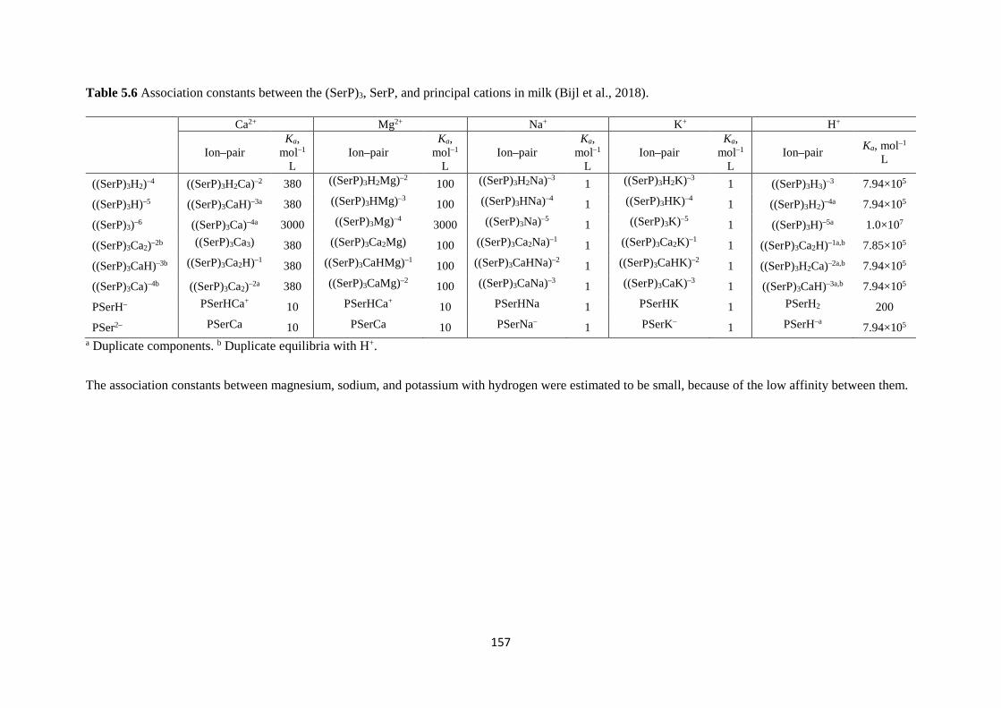
157
Table 5.6 Association constants between the (SerP)3, SerP, and principal cations in milk (Bijl et al., 2018).
Ca2+ Mg2+ Na+ K+ H+
Ion–pair Ka,
mol–1 L
Ion–pair Ka,
mol–1 L
Ion–pair Ka,
mol–1 L
Ion–pair Ka,
mol–1 L
Ion–pair Ka, mol–1 L
((SerP)3H2)–4 ((SerP)3H2Ca)–2 380 ((SerP)3H2Mg)–2 100 ((SerP)3H2Na)–3 1 ((SerP)3H2K)–3 1 ((SerP)3H3)–3 7.94×10⁵
((SerP)3H)–5 ((SerP)3CaH)–3a 380 ((SerP)3HMg)–3 100 ((SerP)3HNa)–4 1 ((SerP)3HK)–4 1 ((SerP)3H2)–4a 7.94×10⁵
((SerP)3)–6 ((SerP)3Ca)–4a 3000 ((SerP)3Mg)–4 3000 ((SerP)3Na)–5 1 ((SerP)3K)–5 1 ((SerP)3H)–5a 1.0×10⁷
((SerP)3Ca2)–2b ((SerP)3Ca3) 380 ((SerP)3Ca2Mg) 100 ((SerP)3Ca2Na)–1 1 ((SerP)3Ca2K)–1 1 ((SerP)3Ca2H)–1a,b 7.85×10⁵
((SerP)3CaH)–3b ((SerP)3Ca2H)–1 380 ((SerP)3CaHMg)–1 100 ((SerP)3CaHNa)–2 1 ((SerP)3CaHK)–2 1 ((SerP)3H2Ca)–2a,b 7.94×10⁵
((SerP)3Ca)–4b ((SerP)3Ca2)–2a 380 ((SerP)3CaMg)–2 100 ((SerP)3CaNa)–3 1 ((SerP)3CaK)–3 1 ((SerP)3CaH)–3a,b 7.94×10⁵
PSerH– PSerHCa+ 10 PSerHCa+ 10 PSerHNa 1 PSerHK 1 PSerH2 200
PSer2– PSerCa 10 PSerCa 10 PSerNa– 1 PSerK– 1 PSerH–a 7.94×10⁵ a Duplicate components. b Duplicate equilibria with H+.
The association constants between magnesium, sodium, and potassium with hydrogen were estimated to be small, because of the low affinity between them.

158
It was also assumed that the activity coefficient of CPN and (SerP)3 are independent of the
conditions, so unity was used arbitrarily for both components. 1.52 and 0.1 mM were the
initial values for (SerP)3 and SerP concentrations corresponding to the total Ser in milk. The
CPN charge was calculated from the Equation (5.11) to be –1 if there are no other amino acids
involved. When there is one positive charge from another amino acid, the CPN will be neutral,
but there is no need in the model for neutrality. The charge of CPN was set to –1 in the
simulation.
Similar to previous simulations, the calculations were performed both at equilibrium and
dynamically. No adjustments were made to the association constants of species. Duplicate
components were dropped from the set of ions as shown in Table 5.6. Three duplicate
equilibria were removed due to being equivalent to the product of two other equilibria. For
example, Equation (5.12) gives similar products as the Equation (5.13), so only Equation
(5.12) was incorporated into the model and Equation (5.13) was removed from the set of
equations.
(SerP)3Ca2H ↔ Ca2+ + (SerP)3CaH (5.12)
(SerP)3Ca2H ↔ H+ + (SerP)3Ca2 (5.13)
Figure 5.9a shows the concentration of CPN and the total of (SerP)3 over the pH range for the
milk solution at equilibrium. The CPN concentration starts to increase from pH about 4.3,
reaching to 1.5 mM at pH between 6 and 9, then it drops to zero at pH 11. For pH values
between 4 to 9, where the CPN has its highest value, (SerP)3 reaches to almost zero, implying
that CPN is produced by using up (SerP)3 components.
The saturations of potential milk salts are shown in Figure 5.9b, in which DCPD is the most
insoluble calcium phosphate salt formed in milk, following by the DCPA and OCP to a lower
extent at pH about 6.7. But this does not necessarily mean that DCPD is the dominant calcium
phosphate over the entire pH range. For example, the CDA and OCP seem to be the main
calcium phosphate salt at high pH values, while TCCT is the dominant calcium citrate at low
pH values. The HAP saturation remains closest to zero throughout the pH range.

159
Figure 5.9 The simulated distribution of a) CPN concentration, b) saturation of potential solid phases, c) net charge, d) (SerP)3 relative concentration over the pH in milk solution.
Figure 5.9c shows the trend of milk net charge over the pH estimating IEP of about 4.61 that
is in a good agreement with the 4.60 value reported in Walstra et al. (2006). The precipitation
of milk starts from below 5.0 because of instability of casein micelles. At pH of 6.7, about
10% of the (SerP)3 is included in CPN. The relative concentration of the remaining (SerP)3
species is shown in Figure 5.9d. (SerP)3H3 is the most abundant phosphoserine species up to
pH 5. (SerP)3Ca becomes the most plentiful between pH 6 to 9, where CPN is formed and
uses up (SerP)3Ca. Therefore, (SerP)3Ca relative concentration is not very high.
Consequently, this model is capable of predicting the ion speciation, saturation, and net charge
in the milk including all casein and whey proteins. The model is flexible enough to test a wide
range of milk components under different concentrations, and in all cases, it could obtain
feasible solution. This implies that there is no limitation for the number of components
2 4 6 8 10 12 140
0.2
0.4
0.6
0.8
1
1.2
1.4
1.6
pH
Con
cent
ratio
n, m
mol
/La
CPN(SerP)3
2 4 6 8 10 12 140
2
4
6
8
10
12
14
16
pH
Satu
ratio
n
b
DCPDDCPAHAPTCCTOCPCDAWH
2 4 6 8 10 12 14-40
-30
-20
-10
0
10
20
pH
Net
cha
rge/
mol
ecul
e
← IEP=4.61
c
2 4 6 8 10 12 140
0.2
0.4
0.6
0.8
1
pH
(Ser
P)3 r
elat
ive
conc
entra
tion
d
(SerP)3H3(SerP)3Ca
(SerP)3H2Ca
(SerP)3Ca2
(SerP)3(SerP)3Ca3

160
included in the model, and thus it can simulate milk as a good and complex example
constituting a large number of ions, sugar, and proteins. Hence, it seems very likely that other
dairy liquids can be simulated accordingly.
5.3.4.2 Simulation of concentrated milk
Milk was concentrated up to 4 times by using the proposed model applied to all initial
concentrations of milk components including proteins. Therefore, a concentration ratio was
defined for concentrating from the range 1 to 4, at which no precipitation is yet expected to
be seen in milk. Figure 5.10a and b show the pH changes and saturations of DCPD, DCPA,
and OCP as the potential dominant calcium salts.
Figure 5.10 a) Simulated pH, and b) DCPD, DCPA, and OCP saturations when milk concentrated up to 4 times of its normal concentration.
The natural pH of milk solutions starts to increase significantly from 6.67 to about 8.4 as milk
gets concentrated up to twice of its normal concentration. This is because, milk is getting more
supersaturated with respect to the calcium phosphate leading to producing less hydrogen ions
and increasing pH values. The trend becomes slow due to the releasing less hydrogen ions as
the concentration factors increases compared to the less concentrated milk. Figure 5.10b
confirms that DCPD is the main potential calcium salt with a relatively high saturation,
following by the DCPA, and OCP to a lesser extent. Other potential solid phases were not
included in the graphs as they remain at low saturation. The IEP point of each individual
concentrated solution was estimated to be between 4.6 to 4.7 as long as there can be a positive
net charge calculated. However, for concentrated solutions with concentration factor higher
1 1.5 2 2.5 3 3.5 46.5
7
7.5
8
8.5
9
Concentration factor
pH
a
1 1.5 2 2.5 3 3.5 40
50
100
150
Concentration factor
Satu
ratio
nb
DCPDDCPAOCP

161
than 2.5, no IEP could be calculated because the proteins have a negative charge throughout
the pH range which is unexpected.
5.3.4.2 Dynamic simulation of milk
The dynamic simulation of milk was also carried out with a solution at normal concentration
containing calcium (30 mM), magnesium (4.9 mM), sodium (22 mM), and potassium (38.7
mM) as cations, citrate (9 mM), phosphate (20.04 mM), carbonate (0.4 mM), sulphate (1.205
mM), chloride (30.4 mM), RCOO (3 mM), and phosphate esters (2.5 mM) as anions as well
as (SerP)3, phosphoserine, and amino acids of both serum and casein proteins. Similarly, CPN
and lactose with 0.147 mol L–1 were included in the model. The precipitation and dissolution
of potential solid phases were calculated using rate constants given in Appendix 6. The CPN
association constant was adjusted to 7.0×10–50 μmol22 L–22 to get reasonable decreasing trend
for pH.
Figure 5.11 indicates the dynamic simulated responses for the milk solution containing
almost all components. The initial pH was predicted to be 6.67, which is very close to the
natural pH. However, it is predicted to decrease to a pH value of about 6 after 1000 minutes.
The initial CPN concentrations is predicted 1.55 mM, which is in the reasonable range, but it
reaches to zero after about 750 minutes (Figure 5.11b). Here, t0 represents the time when all
the milk components was brought together in the simulation.
The saturations of potential solid phases of milk solution are shown in Figure 5.11c. As
expected, DCPD following by OCP and DCPA are the dominant calcium salts that are formed
in the solution as shown in Figure 5.11d. However, DCPA kinetics are predicted to be faster
than OCP remaining longer in the solution and dissolves after 800 minutes. The DCPD
concentration is predicted to remain about 3 mM roughly which is in a good agreement with
the corresponding DCPD in milk serum that was already described in Chapter 3.

162
Figure 5.11 The simulated a) pH, b) CPN concentration, c) saturations of potential solid phases, and d) DCPD, OCP, and DCPA concentrations over time for milk solution with an adjustment of CPN Ka value from 9.0×10–62 to 7.0×10–50 μmol22 L–22.
Nonetheless, no precipitation should be observed in skim milk despite the prediction of
calcium phosphate precipitation over time. It is known that both milk serum and milk itself
are supersaturated with respect to calcium phosphate salts (Lenton et al., 2015). If milk was
not supersaturated, the saturations of calcium solid phases should have been calculated less
than unity to represent lack of precipitation. Thus, the solution is in a metastable state or there
are other components not included in the model, which lower the IAPs of possible precipitates.
Hence, despite of robustness of model, it is not yet able to show all the mechanisms of
stabilisation in milk.
5.4 Conclusions
The proposed model gave satisfactory results for different milk solutions by assuming
dissociable side groups of amino acids either individually or in the mixed state. The net charge
0 200 400 600 800 1000
6
6.2
6.4
6.6
6.8
7
Time, min
pHa
0 200 400 600 800 10000
0.2
0.4
0.6
0.8
1
1.2
1.4
1.6
Time, min
CPN
con
cent
ratio
n, m
mol
/L
b
0 200 400 600 800 10000
1
2
3
4
5
6
Time, min
Satu
ratio
n
c
DCPDOCPDCPAWHTCCT
0 200 400 600 800 10000
0.5
1
1.5
2
2.5
3
Con
cent
ratio
n of
pre
cipi
tate
, mm
ol/L
Time, min
d
DCPDOCPDCPA

163
of each protein was calculated as a means of validation due to lack of complex experimental
data in literature. The IEP of each protein was used as another method of validation. Lysine,
glutamic acid, and aspartic acid had the greatest contributions to charge among the amino
acids in the simulated solutions.
For the milk solution containing all ions, proteins, and CPN, the model could predict the ions
speciation, saturations, and potential solid phase concentrations. CPN concentrations were
predicted within a reasonable range. However, more investigations seem required for
considering a metastable phase to be able to show supersaturation of milk–like solutions in
respect to calcium solid phases.

164
6 Overall Discussion
As mentioned in the previous chapters, several investigations have been extensively done on
the ion equilibria of milk and milk–like solutions at different conditions. However, a
comprehensive model seemed essential that could incorporate all the components of milk with
their ions activities, activity coefficients, and solubilities of potential solid salts for a broad
range of concentrations. The results of the proposed model in Chapter 3 show the
effectiveness of the different aspects of a robust method for the salt partitioning prediction in
various systems.
The first step of doing the research was to find an effective activity coefficient model enabling
the distinction of electrolytes and non–electrolytes activity coefficients with sufficient
complexity as well as the capability of activity coefficient calculation for high concentration
systems. There are a vast number of models available in literature that can be used for activity
coefficient prediction based on either the ion–pair or free–ion approach including ePC–SAFT
(Held et al., 2014), which was applied to biochemical systems, but testing multiple models
may have led to getting far from the scope of thesis. Although the ePC–SAFT model is quite
strong for this purpose, it has its own drawbacks. For example, the model requires numerical
determination of some parameters such as kij which is unlikely available for all ions in a
complex solution like milk with about 180 free ions and ion–pairs. Hence, Debye–Hückel and
Davies are the main models discussed in this thesis, which are most used models in literature
for prediction of activity coefficient. Meanwhile, a model was required to be complex enough
to be able to predict activity coefficient of ions in milk by incorporating the role of non–
electrolytes with zero charge number. On the other hand, a suitable model required the most
of its numerical parameters could be found in literature.
The non–primitive mean spherical approximation (NPMSA) theory, which was proposed by
Blum and Wei (1987), was seen to offer rigorousness that is able to calculate activity
coefficient species for solutions with the ionic strengths larger than 0.3 M (van Boekel,
1996). Unfortunately, it was very difficult to implement due to undefined units and several
typographical errors (Section 2.2.6.2). Even with the best guess of a consistent set of
equations, the resulting set of equations was ill–conditioned and they did not yield reliable
values of activity coefficients.

165
Having this in mind, the MSA theory was used for the activity coefficient calculation of free–
ions and ion–pairs in different systems. The hard sphere contribution allows the activity
coefficient of individual electrolytes and non–electrolytes, such as lactose, to be determined
by incorporating a size variable into the formula. Davies and other activity coefficient models
are unable to calculate activity coefficient of non–electrolytes, and the electrolytes for
concentrated solutions. The MSA formula for activity coefficient calculation requires the
dielectric constant of the solution and the prediction was improved by using a concentration
dependent value, and not the value for water (Valisko and Boda, 2015). It would be possible
to further improve the calculation of the dielectric constant used in the simulation by obtaining
more correlations for a range of electrolytes. Hence, the MSA theory stood up well by
applying it to various milk solutions, and it seems suitable for any liquid dairy system.
Another feature of this work was the use of Newton’s method as an appropriate mathematical
approach used for conducting the ion equilibria in milk solutions. All of the past studies found
seem to have used purpose-written iterative schemes. The mathematical calculation was not
specified in the model developed by Holt et al. (1981), while Mekmene, Le Graet, et al. (2009)
used a series of iterative loops as the computational method for calculation of ion equilibria
in milk. Gao, van Halsema, et al. (2010) specified the ‘AESolve’ software package as the
computational method used to calculate ion equilibria in SMUF.
Newton’s method was effective and enabled extensions of the model to be made with ease.
Solutions were obtained within about 30 seconds. It seemed to work well for a broad range of
initial concentrations. Two key factors led to the success of this method. Firstly, equations
and variables were scaled so that terms in the equations and the variables were closer to one
and hence the Jacobian matrix was less likely to be singular. Hence the unit of concentration
was set to µmol L–1. The scaling of the equations was manual, but opportunities exit to find
better systematic scaling procedures. Secondly, values at each iteration of Newton’s method
were bounded with upper and lower values. Attempted violation of the bounds were reported,
enabling convergence problems to be identified easily. Normally the initial guesses of the
system components were set to the maximum possible value based on the specified
composition, though, in some cases, attempted violation of the bounds indicated the variables
for which better initial guesses were required. To avoid divergence during the first few steps,
a fractional step (relaxation) was used for a few initial steps.

166
The dynamic calculation of ion equilibria in milk solutions has not been studied so far, thus
few experimental data were found for validation with the simulated results given by the
proposed method in Chapter 3. To validate the method, the simulated data given by Kazadi
Mbamba (2016) of calcium carbonate precipitation were used. Arifuzzaman and Rohani
(2004) and Mekmene, Quillard, et al. (2009) investigated experimentally the dynamics of
calcium phosphate solutions that were used as a means of validation for the simulation given
in this study.
The proposed model in Chapter 3 was applied to several systems including the binary
solutions of calcium chloride and sodium chloride, the buffer solutions of citrate and
phosphate, solid phase systems such as calcium phosphate and calcium citrate, milk serum,
milk with proteins, and CPN. They all gave reasonable and satisfactory results that were
matched to the available experimental and simulated data in literature implying the success
of the model. Hence, it is expected that this model can be applied to other liquid dairy
solutions with a variety of components for any concentration.
Due to lack of sufficient data for the dynamics of calcium phosphate solution, precipitation
of calcium phosphate was studied experimentally in Chapter 4. However, the simulation of
the results was not possible, as the structure of precipitate was not known. The prediction of
nanoparticles formed in the presence of lactose seems significant because it allows the
understanding of solubility and kinetics of calcium phosphate solution. This area of research
is quite fascinating and needs further investigations.
In Chapter 5, the model was extended to whey and casein proteins, for which the protein net
charge was calculated and compared with the corresponding data in literature. Mekmene et
al. (2010) specified the pH of milk for simulation and adjusted the concentration of a counter–
ion (typically Cl–) to achieve electroneutrality In the current study, the pH was one of the
variables determined from the composition of the mixture.
The proposed model was successfully extended to include components of the casein micelles
such as the addition of CPN, for which free calcium, free magnesium, hydrogen phosphate,
aqueous citrate, and a group of three phosphoserine residues were incorporated into the ion
association equation. The roles of casein carboxyl groups and citrate were ignored in the CPN
ion activity product by Gao (2010). The casein carboxyl groups were automatically included
in the current model by considering the dissociable side groups of amino acids in whey and

167
casein proteins. These side groups were free to associate with any counter-ion given the
appropriate association constants.
The results of the dynamic solution of milk with proteins and CPN was clearly incorrect. This
was either because the metastability of supersaturated components of milk was not included
in the model, or because the model over-estimates the activity of these components. When
milk was concentrated in the simulations the pH increased sharply for the double concentrated
milk, and then slightly for higher concentration ratios. Despite this research, more
investigations need to be carried out especially on the possible experiments that can determine
the behaviour of supersaturated milk salts at various concentrations.
There are a large number of parameters in each simulation that vary significantly in each
literature such as association constant for each equilibrium, solubility product for potential
solid phase equilibrium, and initial concentration of each ingredient. Therefore, the
uncertainty of variables were not involved in this thesis. However, the uncertainty of the
association constants in citrate buffer solution was stated as the sensitivity of pH to 𝐾𝐾𝑎𝑎 values
in Chapter 3, Section 3.6.1.2. With reliable data, this approach could be extended to find the
uncertainty of many other parameters used in the model, but without such data an analysis of
uncertainties would be of limited value.
168
7 Conclusions and Future work
7.1 Conclusions
The objective of this study was to deeply understand the ion partitioning in milk and milk–
like solutions at various concentration either time–dependently or at equilibrium. Therefore,
an ion speciation model was proposed to comprehensively include milk components such as
calcium, magnesium, sodium, potassium, and hydrogen as the principal cations, and citrate,
phosphate, carbonate, sulphate, chloride, phosphate esters, carboxylate, and hydroxide as the
main anions in aqueous phase of milk, as described in detail in Chapter 3. The model
successfully determined the ion compositions in milk–like solutions and milk serum either at
equilibrium over a wide range of pH values or dynamically over time.
Equilibrium calculation of the simulation required theoretical addition of HCl and NaOH to
cover a wide range of pH values. The ion equilibria, conservation, and electroneutrality
equations, which were applied to various systems, were scaled and then solved using
Newton’s method. The initial concentrations of species and scaling of equilibrium functions
were significant parameters to lead convergence of the simulations.
Solid precipitates were incorporated into the simulation using the ion activity product (IAP)
and solubility product (Ksp) of the solid phase, which were mostly available in literature.
Differential equations were formulated for the precipitation equations and these were solved
with Euler’s method. The Euler’s method was used in almost all dynamic simulations because
it gives good results, which were in a good agreement with either the experimental or the
simulated results available in literature. Dynamic calcium carbonate simulation was the only
exception that did not give good matching with the experimental results. Therefore, the
Euler’s method was replaced with Runge–Kutta to get better fitting.
Ion–pair and free–ion approaches for activity coefficient calculations were defined based on
the full and partial dissociation of electrolytes in solution, respectively. The ion–pair approach
is thought to be an inaccurate description of dissociation, but it was used to obtain the mean
activity coefficients and hence water activity of previous studied solutions. The Gibbs–
Duhem relationship was applied to both approaches for the calculation of water activity as a
means of validation. The results gave a satisfactory fitting between simulated and

169
experimental values given by Robinson and Stokes (1959) for water activity of CaCl2, NaCl,
and H2SO4 up to six molal electrolyte concentration.
The Mean Spherical Approximation (MSA) theory was used to accurately calculate free ion
molar activity coefficients of any species regardless of its charge quantity in multicomponent
solutions. This enabled incorporation of zero–charged species such as lactose in the
calculation, while previous models such as Davies and Extended Debye–Hückel were not able
to take into account the effects of zero–charged species. The size parameter is the factor that
enables the calculation of unique activity coefficients for each ion, ion–pair, or non–
electrolyte. This was shown by employing the MSA theory and afore–mentioned theories to
citrate buffer solutions containing zero, 4.5%w/w, and 25%w/w lactose. Addition of lactose
did not significantly influence the ion equilibria of citrate species, but notably affected the
free–ion activity coefficients of citrate ions calculated by the MSA theory at different lactose
contents.
Furthermore, the MSA allows the prediction of free–ion activity coefficient of species at high
concentration of electrolyte. This was shown by comparing free–ion activity coefficient
obtained by the Davies, Extended Debye–Hückel, and the MSA theories in calcium chloride
and sodium chloride solutions individually by both ion–pair and free–ion approaches in
Chapter 3. Hence, the effectiveness of MSA theory for free–ion activity coefficient
calculation is because of the hard sphere contribution in the formula.
The model was applied to the citrate and phosphate buffer solutions individually, the results
of which were in a good agreement with the literature data. However, the intrinsic association
constants of citrate ions were slightly changed to get better fitting with experimental data.
Phosphate association constants remained unchanged throughout the calculation.
The ion speciation of calcium carbonate system was also studied. The dynamic simulation of
this gave close agreement to previous experimental data.
Calcium phosphate as the main insoluble milk component was investigated both steady state
and dynamically. The simulated results showed reasonable pH at equilibrium and also over
the time. H2PO4– was found to be the most abundant species at low pH values, following by
the formations of HPO42– and PO4
3– at neutral and high pH. CaPO4– was the most plentiful
species among the calcium and phosphate component because of high association between

170
calcium and phosphate ion indicating potential formation of precipitate in the solution with
respect to DCPD. A dynamic study of calcium phosphate either with or without addition of
NaOH indicated that DCPA precipitated first but then dissolved while DCPD precipitated.
Addition of lactose did not significantly influence pH over the time but affected the activity
coefficient of species.
Calcium citrate as another potential solid phase system was studied using the proposed model.
TCCT was found to have a higher saturation than TCCH. Additions of citrate and lactate to
phosphate system altered the speciation of solution leading to a decrease in the saturation of
calcium phosphate due to the formation of CaCit– ion–pairs.
Milk serum was investigated at equilibrium when lactose was added to the solution. The
results showed that lactose significantly affected the saturation of solid phase salts particularly
DCPD and DCPA. Dynamic simulation of milk serum indicated high saturation values of
DCPD, OCP, and DCPA among the other assumed salts, although DCPA might dissolve in
the solution. The calcium composition was calculated after 500 minutes predicting that 3 mM
of the solid precipitates out of 10 mM total calcium in milk serum. This time scale is quite
fast, but Howell (1998) investigated the effect of time on the fouling of whey permeate
showing that the fouling changed with a time scale of days due to apparent precipitation within
the whey.
In Chapter 4, calcium phosphate precipitation was studied experimentally at various
concentrations under varied and controlled pH values. The experimental results clearly
showed the formation of a 1 nm nanoparticle in solutions of lactose, calcium and phosphate
ions. Lactose was found to prevent or slow down the precipitation of calcium phosphate,
probably as calcium dihydrogen phosphate. The structure of the nanoparticle is not known
and, based on current research in this area, might be difficult to determine. The effects of
many of the conditions such as concentration, ion ratios, pH, lactose concentration, and time
need to be tested.
The effects of lactose in this ideal system indicate that it might have a role for the stabilisation
of calcium phosphate in milk that might add to the stabilisation produced by the casein
micelles.
In Chapter 5, dissociable side groups of casein and serum proteins amino acids were
incorporated as individual components in the simulation. Glutamic and aspartic acids

171
following by cysteine determined the negative contribution of net charge, while lysine and
histidine were dominant amino acids contributing the positive net charge at low pH. The
simulation of individual milk proteins gave satisfactory net charges over a pH range. A
comparison was made between simulations with and without addition of minerals to milk
proteins, resulting in relatively similar trend of net charge over pH but a slight difference in
IEP possibly due to low affinity between principal cations and amino acids.
CPN was incorporated into the milk simulation and was estimated to be at about 1.5 mM
concentration between the pH values 4–9, at which the (SerP)3 concentration reached to 10%.
Out of this range, the CPN concentration was predicted to be zero. DCPD, DCPA, and OCP
were predicted to be the most dominant potential solid phases at natural pH, while TCCT was
estimated to be the main calcium salt at low pH values.
The proposed model has strengths and limitations that need to be addressed:
- The matching between the simulated results obtained and experimental data in
literature implies that the assumptions and adjustments were made accurately.
- The model can be applied to any dairy liquids up to high concentration even if one or
more of species are zero–charged components.
- The distinction of different milk proteins are another feature of the model allowing
addition of other proteins such as lactoferrin.
- Prediction of ion speciation was studied dynamically on different aqueous systems
successfully.
However, the model was unable to determine the ion speciation at other temperatures other
than 20–25 ˚C, e.g. during milk or cheese heat treatments. The model requires equations to
describe the change of association and solubility constants with temperature. These might be
difficult to obtain.
7.2 Future work
Some recommendations are suggested to enhance effectively the understanding of the milk
partitioning at various conditions:
1. The proposed model in Chapter 3 could be made as a user–friendly software package
for the prediction of ion speciation for any milk and milk–like solutions.

172
2. The model could be applied to different products such as milk protein concentrate
(MPC) for prediction of solubility, as to be able to get acceptable appearance of
product when it dissolves in water.
3. Further experimental studies could be performed on the different Ca/P ratios and pH
with and without lactose in respect to calcium phosphate precipitation to find out at
what condition nanoparticles form.
4. Other analytical tests could be implemented such as small angle x–ray scattering
(SAXS) and synchrotron based extended x–ray absorption fine structure (EXAFS) to
identify the structure in comparison with known crystalline compounds.
5. It would be interesting to test the calcium phosphate precipitation experimentation
with other sugars such as sucrose and maltose to see if the nanoparticles are formed in
presence of only lactose or not.
6. Experimental data is needed for validation of milk system simulation in the case of
precipitation. It would be interesting to propose a comprehensive recipe for a model
milk solution that could produce repeatable precipitation of minerals.
7. There are some relationships available for temperature effects of association constants
in literature, but not much data is present. Hence, it might be a good idea to follow
whey or whey permeate evaporation to be able to incorporate the effect of temperature
on the simulation, especially for the changes of association constants with
temperature.

173
References
Al-Makhlafi, H., McGuire, J., & Daeschel, M. (1994). Influence of preadsorbed milk proteins
on adhesion of Listeria monocytogenes to hydrophobic and hydrophilic silica surfaces
Applied and Environmental Microbiology, 60, 3560-3565.
Anandharamakrishnan, C., Rielly, C. D., & Stapley, A. G. F. (2008). Loss of solubility of α-
lactalbumin and β-lactoglobulin during the spray drying of whey proteins. LWT-Food
Science and Technology, 41, 270-277.
Andritsos, N., Yiantsios, S. G., & Karabelas, A. J. (2002). Calcium phosphate scale formation
from simulated milk ultrafiltrate solutions. Food and Bioproducts Processing, 80,
223-230.
Arifuzzaman, S. M., & Rohani, S. (2004). Experimental study of brushite precipitation.
Journal of Crystal Growth, 267, 624-634.
Atkins, P. W. (1990). Physical chemistry. Great Britain: Oxford University Press.
Auldist, M. J., Walsh, B. J., & Thomson, N. A. (1998). Seasonal and lactational influences on
bovine milk composition in New Zealand. Journal of Dairy Research, 65, 401-411.
Babić-Ivančić, V., Kntrec, J., Brečević, L., & Kralj, D. (2006). Kinetics of struvite to
newberyite transformation in the precipitation system MgCl2–NH4H2PO4–NaOH–
H2O. Water Research, 40, 3447-3455.
Belitz, H. D., & Grosch, W. (1999). Food Chemistry. Berlin: Springer.
Berg, J., Romijn, D., van Halbeek, H., Vlienenthart, J. F. G., & Visser, R. A. (1988).
Characterisation of four lactose monophosphates by application of 31P-,13C-, and 1H-
NMR spectroscopy. Carbohydrate Research, 174, 23-26.
Besic, F. C. (1985). Food materials for prevention of carious degradation of teeth, United
States Patent No. 4515770A.
Bijl, E., Huppertz, T., van Valenberg, H. J., & Holt, C. (2018). A quantitative model of the
bovine casein micelle: ion equilibria and calcium phosphate sequestration by
individual caseins in bovine milk. European Biophysics Journal, 1-15.
Bleek, K., & Taubert, A. (2013). New developments in ploymer-controlled, bioinspired
calcium phosphate mineralization from aqueous solution. Acta Biomaterialia, 9, 6283-
6321.
Blum, L. (1975). Mean spherical model for asymmetric electrolytes. Molecular Physics, 30,
1529-1535.

174
Blum, L., & Høye, J. S. (1977). Mean spherical model for asymmetric electrolytes. 2.
Thermodynamic properties and the pair correlation function. The Journal of Physical
Chemistry, 81, 1311-1316.
Blum, L., Vericat, F., & Fawcett, W. R. (1992). Mean spherical approximation for hard ions
and dipoles. The Journal of Chemical Physics, 96, 3039-3044.
Blum, L., & Wei, D. (1987). Analytical solution of the mean spherical approximation for an
arbitrary mixture of ions in a dipolar solvent. The Journal of Chemical Physics, 87,
555-565.
Boskey, A. L., & Posner, A. S. (1976). Formation of hydroxyapatite at low supersaturation.
The Journal of Physical Chemistry, 80, 40-45.
Brečević, L., & Füredi-Milhofer, H. (1972). Precipitation of calcium phosphates from
electrolyte solutions. Calcified Tissue Research, 10, 82-90.
Brečević, L., & Nielsen, A. E. (1989). Solubility of Amorphous Calcium Carbonate. Journal
of Crystal Growth, 98, 504-510.
Brečević, L., Škrtić, D., & Garside, J. (1986). Transformation of calcium oxalate hydrates.
Journal of Crystal Growth, 74, 399-408.
Bressan, C., & Mathlouthi, M. (1994). Thermodynamic activity of water and sucrose and the
stability of crystalline sugar. Zuckerindustrie, 119, 652-658.
Bromley, L. A. (1972). Approximate individual ion values of β (or B) in extended Debye-
Hückel theory for uni-univalent aqueous solutions at 298.15 K. The Journal of
Chemical Thermodynamics, 4, 669-673.
Brooks, R., Clark, L. M., & Thurston, E. F. (1950). Calcium carbonate and its hydrates.
Philosophical Transactions of the Royal Society of London, 243, 145-167.
Broyard, C., & Gaucheron, F. (2015). Modifications of structures and functions of caseins: a
scientific and technological challenge. Dairy Science and Technology, 95, 831-862.
Buchner, R., Hefter, G. T., & May, P. M. (1999). Dielectric relaxation of aqueous NaCl
solutions. The Journal of Physical Chemistry, 103, 1-9.
Burrington, K. J. (2017). Whey protein heat stability: US Dairy, Dairy Research Institute.
Butler, J. N. (1998). Activity coefficients and pH Ionic equilibrium-Solubility and pH
calculations. New York: John Wiley & Sons.
Cameselle, J. C., Ribeiro, J. M., & Sillero, A. (1986). Deviation and use of a formula to
calculate the net charge of acid-base compounds. Its application to amino acids,
proteins and nucleotides. Biochemical Education, 14, 131-136.

175
Cha, J., Lee, J. S., Yoon, S. J., Kim, Y. K., & Lee, J. K. (2013). Solid-state phase
transformation mechanism for formation of magnetic multi-granule nanoclusters. RSC
Advances, 3, 3631-3637.
Chhettry, A., Wang, Z., Fox, J. L., Baig, A. A., Zhuang, H., & Higuchi, W. I. (1999). Use of
dicalcium phosphate dihydrate as a probe in an approach for accurate calculations of
solution equilibria in buffered calcium phosphate systems. Journal of Colloid and
Interface Science, 218, 47-56.
Clark, I. (2015). Groundwater Geochemistry and Isotopes. Boca Raton: CRC Press, Taylor
& Francis Group.
Clegg, S. L., & Whitfield, M. (1991). Activity coefficients in natural waters. In K. S. Pitzer
(Ed.), Activity Coefficients in Electrolyte Solutions. The USA: CRC Press, Inc.
Coico, R., & Geoffrey, S. (2009). Immunology A short course. The USA: John Wiley & Sons,
Inc.
Combes, C., & Rey, C. (2010). Amorphous calcium phosphates: Synthesis, properties and
uses in biomaterials. Acta Biomaterialia, 6, 3362-3378.
Constable, P. D. (1997). A simplified strong ion model for acid-base equilibria: application
to horse plasma. Journal of Applied Physiology, 83, 297-311.
Cornell, D. G., & Patterson, D. L. (1989). Interaction of phospholipids in monolayers with β–
lactoglobulin adsorbed from solution. Journal of Agricultural and Food Chemistry,
37, 1455-1459.
Corredig, M., & Dalgleish, D. G. (1996). Effect of different heat treatments on the strong
binding interactions between whey proteins and milk fat globules in whole milk.
Journal of Dairy Research, 63, 441-449.
Cosman, N. P., Faith, K., & Roscoe, S. G. (2005). Electrochemical impedance spectroscopy
study of the adsorption behaviour of α-lactalbumin and β-casein at stainless steel.
Journal of Electroanalytical Chemistry, 574, 261-271.
Creamer, L. K., & Sawyer, L. (2003). Beta-lactoglobulin. In H. Roginski, J. W. Fuquay & P.
F. Fox (Eds.), Encyclopedia of Dairy Sciences. London: American Press.
Cruse, J. M., & Lewis, R. E. (2010). Atlas of Immunology. The USA: CRC Press.
Dalgleish, D. G. (2011). On the structural models of bovine casein micelles—review and
possible improvements. Soft Matter, 7, 2265–2272.
Davies, C. W. (1962). Ion Association London: Butterworths Scientific Publications.

176
Davies, D. T., & White, J. C. D. (1960). The use of ultrafiltration and dialysis in isolating the
aqueous phase of milk and in determining the partition of milk constituents between
the aqueous and disperse phases. Journal of Dairy Research, 27, 171-190.
de Kruif, C. G. (1999). Casein micelle interactions. International Dairy Journal, 9, 183-188.
de Kruif, C. G., & Grinberg, V. Y. (2002). Micellisation of β-casein. Colloids and Surfaces
A: Physicochemical and Engineering Aspects, 210, 183-190.
de Kruif, C. G., & Holt, C. (2003). Casein micelle structure, functions and interactions. In P.
F. Fox & P. McSweeney (Eds.), Advanced Dairy Chemistry. Proteins (3 ed.). New
York: Kluwer Academic/Plenum Publishers.
de Kruif, C. G., Tuinier, R., Holt, C., Timmins, P. A., & Rollema, H. S. (2002).
Physicochemical study of κ- and β-casein dispersions and the effect of cross-linking
by transglutaminase. Langmuir, 18, 4885-4891.
de La Fluente, M. A. (1998). Changes in the mineral balance of milk submitted to
technological treatments. Trends in Food Science and Technology, 9, 281-288.
Debye, P., & Hückel, E. (1923). The theory of electrolytes, lowering of freezing point and
related phenomena. Physikalische Zeitschrift, 24, 185-206.
Dey, A., Bomans, P. H., Muller, F. A., Will, J., Frederik, P. M., de With, G., & Sommerdijk,
N. A. (2010). The role of prenucleation clusters in surface-induced calcium phosphate
crystallization. Nature Materials, 9, 1010-1014.
Dickinson, E. (1999). Adsorbed protein layers at fluid interface: interactions, structure and
surface rheology. Colloids Surfaces B: Biointerfaces, 15, 161-176.
Doherty, W. O. S., & Wright, P. G. (2004). A solubility model for calcium oxalate formation
in a sugar mill. Proceedings-Australian Society Of Sugar Cane Technologists, 26,
519-526.
Dorozhkin, S. V. (2014). Calcium orthophosphates: Occurrence, properties and major
applications. Bioceramics Developments and Applications, 4, 1-20.
Driessens, F. C. M., & Verbeeck, R. M. H. (1990). Biominerals. The USA: CRC Press.
Dybing, S. T., Wiegand, J. A., Brudvig, S. A., Huang, E. A., & Chandan, R. C. (1988). Effect
of processing variables on the formation of calcium lactate crystals on Cheddar cheese.
Journal of Dairy Science, 71, 1701-1710.
Eigel, W. N., Butlet, J. E., Ernstrom, C. A., Farrell, H. M., Harwalker, V. R., Jenness, R., &
Whitney, R. M. (1984). Nomenclature of protein of cow's milk: fifth revision. Journal
of Dairy Science, 67, 1599-1631.

177
El-Loly, M. M. (2011). Compostion, properties and nutritional aspects of milk fat globule
membrane- A review. Polish Journal of Food and Nutrition Sciences, 61, 7-32.
Elliot, J. C. (1994). Structure and chemistry of the apatite and other calcium orthophosphates.
Amsterdam: Elsevier Science B.V.
Fang, Z. H., Bovenhuis, H., Delacroix-Buchet, A., Miranda, G., Boichard, D., & Visker, M.
H. P. W. (2017). Genetic and nongenetic factors contributing to differences in αs–
casein phosphorylation isoforms and other major milk proteins. Journal of Dairy
Science, 100, 5564-5577.
Farrell, J. H., Jimenez-Flores, R., Bleck, G. T., Butler, J. E., Brown, E. M., Creamer, L. K., .
. . Swaisgood, H. E. (2004). Nomenclature of the proteins of cows' milk. Journal of
Dairy Science, 87, 1641-1674.
Fawcett, W. R., & Tikanen, A. C. (1996). Role of solvent permittivity in estimation of
electrolyte activity coefficients on the basis of the mean spherical approximation. The
Journal of Physical Chemistry, 100, 4251-4255.
Fawcett, W. R., Tikanen, A. C., & Henderson, D. J. (1977). The mean spherical
approximation and medium effects in the kinetics of solution reactions involving ions.
Canadian Journal of Chemistry, 75, 1649-1655.
Fennema, O. R. (1996). Food Chemistry. New York: Marcel Dekker, Inc.
Ferguson, J. F., & McCarty, P. L. (1971). Effects of carbonate and magnesium on calcium
phosphate precipitation Environmental Science and Technology, 5, 534-540.
Flynn, A., & Cashman, K. (1997). Nutritional aspects of minerals in bovine and human milks.
In P. F. Fox (Ed.), Advanced Dairy Chemistry: Lactose, Water, Salts and Vitamins (2
ed., Vol. 3, pp. 257-302). London: Chapman & Hall.
Follows, D., Holt, C., Thomas, R. K., Tiberg, F., Fragneto, G., & Nylander, T. (2011). Co-
adsorption of β–casein and calcium phosphate nanoclusters (CPN) at hydrophilic and
hydrophobic solid-solution interfaces studied by neutron reflectometry. Food
Hydrocolloids, 25, 724-733.
Fox, P. F. (2009). Milk: an overview. In A. Thompson, M. Boland & H. Singh (Eds.), Milk
Proteins: From Expression to Food. Boston, US: Elsevier, Inc.
Fox, P. F., & McSweeney, P. (1998). Dairy Chemistry and Biochemistry. London, UK:
Blackie Academic & Professional, an imprint of Chapman & Hall.
Fox, P. F., & McSweeney, P. L. H. (2003). Proteins Advanced Dairy Chemistry (3 ed., Vol.
1). New York, USA: Kluwer Academic-Plenum Publishers.

178
Freeley, R. M., Criner, P. E., & Slover, H. T. (1975). Major fatty acids and proximate
composition of dairy products. Journal of The American Dietetic Association, 66, 140-
146.
Gao, R. (2010). Ion speciation in milk-like systems. (Doctor of Philosophy), Wageningen
University, Netherlands.
Gao, R., van Halsema, F. E. D., Temminghoff, E. J. M., van Leeuwen, H. P., van Valenberg,
H. J. F., Eisner, M. D., . . . van Boekel, M. A. J. S. (2010). Modelling ion composition
in simulated milk ultrafiltrate (SMUF). I: Influence of calcium phosphate
precipitation. Food Chemistry, 122, 700-709.
Gao, R., van Leeuwen, H. P., Temminghoff, E. J. M., van Valenberg, H. J., Eisner, M. D., &
van Boekel, M. A. J. S. (2010). Effect of disaccharides on ion properties in milk-based
systems. Journal of Agricultural and Food Chemistry, 58, 6449-6457.
Garcia, A. C., Vavrusova, M., & Skibsted, L. F. (2018). Supersaturation of calcium citrate as
a mechanism behind enhanced availability of calcium phosphates by presence of
citrate. Food Research International, 107, 195-205.
Garnsworthy, P. C., Masson, L. L., Lock, A. L., & Mottaram, T. T. (2006). Variation of milk
citrate with stage of lactation and de novo fatty acid synthesis in dairy cows. Journal
of Dairy Science, 89, 1604-1612.
Gaucheron, F. (2005). The minerals of milk. Reproduction Nutrition Development, 45, 473-
483.
Gaucheron, F., Le Graët, Y., Piot, M., & Boyaval, E. (1996). Determination of anions of milk
by ion chromatography. Lait, 76, 433-443.
Ghishan, F. K., Stroop, S., & Meneely, R. (1982). The effect of lactose on the intestinal
absorption of calcium and zinc in the rat during maturation. Pediatric Research, 16,
566-568.
Ginger, M. R., & Grigor, M. R. (1999). Comparative aspects of milk caseins. Comparative
Biochemistry and Physiology Part B, 124, 133-145.
Goel, A. (2006). Surface chemistry. New Delhi: Discovery Publishing House.
Grandison, A. S., & Lewis, M. J. (1996). Separation processes in the food and biotechnology
industries: Principles and applications. England: Woodhead Publishing Ltd.
Guéguen, L., & Pointillart, A. (2000). The bioavailability of dietary calcium. The Journal of
the American College of Nutrition, 19(sup2), 119S-136S.
Guggenheim, E. A. (1926). On the determination of the velocity constant of a unimoelcular
reaction. Philosophical Magazine, 2, 538-543.

179
Guggenheim, E. A. (1967). Thermodynamics, an advanced treatment for chemists and
physics. The Netherlands: North-Holland Publishing Company.
Haggarty, N. W. (2003). Minor proteins, bovine serum albumin and vitamin-binding proteins.
In H. Roginski, J. W. Fuquay & P. F. Fox (Eds.), Encyclopedia of Dairy Sciences.
London: Academic Press.
Hanze, M., Gujer, W., Mino, T., & Van Loosdrecht, M. (2000). Activated sludge models
ASM1, ASM2, ASM2d and ASM3. London: IWA Publishing.
Harned, H., & Cook, M. A. (1937). The ionic activity coefficient product and ionization of
water in uni-univalent halide solutions-A numerical summary. Journal of The
American Chemical Society, 59, 2304-2305.
Heck, J. M., van Valenberg, H. J., Dijkstra, J., & van Hooijdonk, A. C. (2009). Seasonal
variation in the Dutch bovine raw milk composition. Journal of Dairy Science, 90,
706-715.
Held, C., Reschke, T., Mohammad, S., Luza, A., & Sadowski, G. (2014). ePC-SAFT revised.
Chemical Engineering Research and Design, 92, 2884-2897.
Herrington, B. L. (1934). Some physico-chemical properties of lactose. VI The solubility of
lactose in salt solutions; the isolation of a compound of lactose and calcium chloride.
Journal of Dairy Science, 17, 805-814.
Hignett, T. P., & Brabson, J. A. (1961). Evaluation of water-insoluble phosphorus in fertilizers
by extraction with alkaline ammonium citrate solutions. Journal of Agricultural and
Food Chemistry, 9, 272-276.
Hiraoka, Y., Segawa, T., Kuwajima, K., Sugai, S., & Murai, N. (1980). α–lactalbumin: a
calcium metalloprotein. Biochemical and Biophysical Research Communications, 95,
1098-1104.
Holsinger, V. H. (1997). Physical and chemical properties of lactose. In P. F. Fox (Ed.),
Advanced Dairy Chemistry Volume 3: Lactose, water, salts and vitamins. London:
Chapman & Hall.
Holt, C. (1985). The milk salts: their secretion, concentration and physical chemistry. In P. F.
Fox (Ed.), Developments in Dairy Chemistry, Lactose and minor constituents (Vol. 3,
pp. 143-181). London: Elsevier Science
Holt, C. (1992). Structure and stability of bovine casein micelles. Advances in Protein
Chemistry, 43, 63-151.
180
Holt, C. (1997). The milk salts and their interaction with casein. In P. F. Fox (Ed.), Advanced
Dairy Chemistry Volume 3: Lactose, Water, Salts and Vitamins (2 ed., Vol. 3, pp. 233-
254). London: Chapman & Hall.
Holt, C. (2004). An equilibrium thermodynamic model of the sequestration of calcium
phosphate by casein micelles and its application to the calculation of the partition of
salts in milk. Eur Biophys J, 33, 421-434.
Holt, C. (2011). Milk salts: interaction with caseins. In J. W. Fuquay, P. F. Fox & P.
McSweeney (Eds.), Encyclopedia of Dairy Sciences (2 ed., Vol. 3, pp. 917-924). San
Diego, CA: Academic Press.
Holt, C., Carver, J. A., Ecroyd, H., & Thorn, D. C. (2013). Invited review: Caseins and the
casein micelle: Their biological functions, structures, and behavior in foods. Journal
of Dairy Science, 96(10), 6127-6146.
Holt, C., Dalgleish, D. G., & Jenness, R. (1981). Calculation fo the ion equilibria in milk
diffusate and comparison with experiment. Analytical Biochemistry, 113, 154-163.
Holt, C., Davies, D. T., & Law, A. J. R. (1986). Effects of colloidal calcium-phosphate content
and free calcium-ion concentration in the milk serum on the dissociation of bovine
casein micelles. Journal of Dairy Research, 53, 557-572.
Holt, C., Hasnain, S. S., & Hukins, D. W. L. (1982). Structure of bovine milk calcium
phosphate determined by x-ray absorption spectroscopy. Biochim Biophys Acta (BBA)
- General Subjects, 719, 299-303.
Holt, C., Lenton, S., Nylander, T., Sørensen, E. S., & Teixeira, S. C. M. (2014). Mineralisation
of soft and hard tissues and the stability of biofluids. Journal of Structural Biology,
185, 383-396.
Holt, C., & Muir, D. D. (1979). Inorganic constituents of milk. I. Correlation of soluble
calcium with citrate in bovine milk. Journal of Dairy Research, 46, 433-439.
Holt, C., Sørensen, E. S., & Clegg, S. L. (2009). Role of calcium phosphate nanoclusters in
the control of calcification. The FEBS Journal, 276, 2308-2323.
Holt, C., Timmins, P., Errington, N., & Leaver, J. (1998). A core-shell model of calcium
phosphate nanoclusters stabilized by β-casein phosphopeptides, derived from
sedimentation equilibrium and small-angle X-ray and neutron-scattering
measurements. European Journal of Biochemistry, 252, 73-78.
Holt, C., Wahlgren, N. M., & Drakenberg, T. (1996). Ability of a β-casein phosphopeptide to
modulate the precipitation of calcium phosphate by forming amorphous dicalcium
phosphate nanoclusters. Biochemical Journal, 314, 1035-1039.

181
Horne, D. S. (1998). Casein interactions: Casting light on the black boxes, the structure in
dairy products. International Dairy Journal, 8, 171-177.
Horne, D. S. (2003). Casein micelles as hard spheres: limitations of the model in acidified gel
formation. Colloids and Surfaces A: Physicochemical and Engineering Aspects, 213,
255-263.
Howell, J. M. (1998). Whey permeate fouling of evaporators. (Master of Engineering),
University of Canterbury, Christchurch, New Zealand.
Hoye, J. S., & Stell, G. (1977). Thermodynamics of the MSA for simple fluids. The Journal
of Chemical Physics, 67, 439-445.
Huppertz, T., & Fox, P. F. (2006). Effect of NaCl on some physico-chemical properties of
concentrated bovine milk. International Dairy Journal, 16, 1142-1148.
Huppertz, T., Fox, P. F., de Kruif, K. G., & Kelly, A. L. (2006). High pressure-induced
changes in bovine milk proteins: A review. Biochimica et Biophysica Acta, 1764, 593-
598.
Illanes, A., Guerrero, C., Vera, C., Wilson, L., Conejeros, R., & Scott, F. (2016). Lactose-
Derived Prebiotics. United Kingdom: Elsevier.
Isaad, J., & Perwuelz, A. (2010). New color chemosensors for cyanide based on water soluble
azo dyes. Tetrahedron Letters, 51, 5810-5814.
Jackson, D. C. (2004). Surviving extreme lactic acidosis: the role of calcium lactate formation
in the anoxic turtle. Respiratory Physiology & Neurobiology, 144, 173-178.
Jeurnink, T. J. M., & Brinkman, D. W. (1994). The cleaning of heat exchangers and
evaporators after processing milk or whey. International Dairy Journal, 4, 347-368.
Jeurnink, T. J. M., Walstra, P., & de Kruif, C. G. (1996). Mechanisms of fouling in dairy
processing. Netherlands Milk and Dairy Journal, 50, 407-426.
Johansson, A., Lugand, D., Rolet-Repecaud, O., Molle, D., Delage, M. M., Peltre, G., . . .
Dupont, D. (2009). Epitope characterization of a supramolecular protein assembly
with a collection of monoclonal antibodies: the case of casein micelle. Molecular
Immunology, 46, 1058-1066.
Johnsson, M. S. A., & Nancollas, G. H. (1992). The role of brushite and octacalcium
phosphate in apatite formation. Critical Reviews in Oral Bilogy and Medicine, 3, 61-
82.
Joko, I. (1984). Phosphorus removal from wastewater by the crystallization method. Water
Science and Technology, 17, 121-132.
182
Kazadi Mbamba, C. (2016). Dynamic modelling of minerals precipitation in wasterwater
treatment. (Doctor of Philosophy), The University of Queensland, Australia.
Kell, G. S. (1975). Density, thermal expansivity, and compressibility of liquid water from 0˚
to 150˚C: Correlations and tables for atmospheric pressure and saturation reviewed
and expressed on 1968 temperature scale. Journal of Chemical and Engineering Data,
20, 97-105.
Kellermeier, M., Gebauer, D., Melero‐García, E., Drechsler, M., Talmon, Y., Kienle, L., . . .
Kunz, W. (2012). Colloidal stabilization of calcium carbonate prenucleation clusters
with silica. Advanced Functional Materials, 22, 4301-4311.
Kent, J. C., Arthur, P. G., & Hartmann, P. E. (1998). Citrate, calcium, phosphate and
magnesium in sows' milk at initiation of lactation. Journal of Dairy Research, 65, 55-
68.
Kezia, K., Lee, J., Zisu, B., Chen, G. Q., Gras, S. L., & Kentish, S. E. (2017). Solubility of
calcium phosphate in concentrated dairy effluent brines. J Agric Food Chem, 65,
4027-4034.
Kielland, J. (1937). Individual activity coefficients of ions in aqueous solutions. Journal of
The Americal Chemical Society, 59, 1675-1683.
Kinsella, J. E. (1984). Milk proteins: Physical and functional properties. CRC Critical
Reviews in Food Science and Nutrition, 21, 197-262.
Kralj, D., Brečević, L., & Kontrec, J. (1997). Vaterite growth and dissolution in aqueous
solution III. Kinetics of transformation. Journal of Crystal Growth, 177, 247-257.
Kubantseva, N., & Hartel, R. W. (2002). Solubility of calcium lactate in aqueous solution.
Food Reviews International, 18, 135-149.
Kubantseva, N., Hartel, R. W., & Swearingen, P. A. (2004). Factors affecting solubility of
calcium lactate in aqueous solutions. Journal of Dairy Science, 87, 863-867.
Kuehner, D. E., Engmann, J., Fergg, F., Wernick, M., Blanch, H. W., & Prausnitz, J. M.
(1999). Lysozyme net charge and ion binding in concentrated aqueous electrolyte
solutions. Journal of Physical and Chemistry B, 103, 1368-1374.
Kuhn, R., & Low, I. L. (1949). The occurrence of lactose in the plant kingdom. Chemische
Berichte, 82, 479-481.
Lango, F., Rocha, S. D. F., Katsarou, L., & Demopoulos, G. P. (2012). Supersaturation-
controlled synthesis of dicalcium phosphate dihydrate and nanocrystalline calcium-
deficient hydroxyapatite. Industrial & Engineering Chemistry Research, 51, 6605-
6612.

183
Le Graët, Y., & Gaucheron, F. (1999). pH-induced solubilization of minerals from casein
micelles: influence of casein concentration and ionic strength. Journal of Dairy
Research, 66, 215-224.
Lebowitz, J. L., & Percus, J. K. (1966). Mean spherical model for lattice gases with extended
hard cores and continuum fluids. Physical Review, 144, 251-258.
Leclerc, E., & Calmettes, P. (1997). Interactions in micellar solution of β-casein Physical
Review Letters, 78, 150-153.
Lenton, S., Nylander, T., Holt, C., Sawyer, L., Härtlein, M., Müller, H., & Teixeira, S. C.
(2016). Structural studies of hydrated samples of amorphous calcium phosphate and
phosphoprotein nanoclusters. European Biophysics Journal, 45, 405-412.
Lenton, S., Nylander, T., Teixeira, S. C., & Holt, C. (2015). A review of the biology of
calcium phosphate sequestration with special reference to milk. Dairy Science and
Technology, 95, 3-14.
Lewis, G. N., & Randall, M. (1921). The activity coefficient of strong electrolytes. Journal
of The American Chemical Society, 43, 1112-1154.
Li, C., Li, Y., Lu, J., & Yang, L. (1996). Study of the ionic activity coefficients in aqueous
electrolytes by the non-primitive mean spherical approximation equation. Fluid Phase
Equilibria, 124, 99-110.
Li, H., Robertson, A. D., & Jensen, J. H. (2005). Very fast empirical prediction and
rationalization of protein pKa values. Proteins: Structure, Function, and
Bioinformatics, 61, 704-721.
Lifran, E. V. (2007). Role of lactose phosphate in lactose containing dairy products.
University of Western Sydney, Sydney, Australia.
Lin, T. J., & Chiu, C. C. (2017). Structures and infrared spectra of calcium phosphate clusters
by ab initio methods with implicit solvation models. Physical Chemistry Chemical
Physics, 20, 345-356.
Lindsay, R. C. (1996). Food additives. In O. Fennema (Ed.), Food Chemistry (pp. 767-823).
New York: Marcel Dekker.
Little, E. M., & Holt, C. (2004). An equilibrium thermodynamic model of the sequestration
of calcium phosphate by casein phosphopeptides. European Biophysics Journal, 33,
435-447.
Liu, W. B., Li, Y. G., & Lu, J. F. (1998). Nonprimitive model of mean spherical
approximation applied to aqueous electrolyte solutions. Industrial & Engineering
Chemistry Research, 37, 4183-4189.

184
Liu, Z. P., Li, Y. G., & Lu, J. F. (2002). Low-density xxpansion of the solution of mean
spherical approximation for ion-dipole mixtures. The Journal of Physical Chemistry,
106, 5266-5274.
Lotfikhan, M., & Modarress, H. (2003). Modification and Application of a Non-Primitive
Mean Spherical Approximation Model for Simple Aqueous Electrolyte Solutions.
Fluid Phase Equilibria, 209, 13-27.
Lu, X., & Leng, Y. (2005). Theoretical analysis of calcium phosphate precipitation in
simulated body fluid. Biomaterials, 26, 1097-1108.
Lyster, R. L. J. (1972). Review of the progress of dairy science, section C. Chemistry of milk
proteins. Journal of Dairy Science, 39, 279-318.
Lyster, R. L. J. (1981). Calculation by computer of individual concentrations in a simulated
milk salt solution. 2. an extension to the previous model. Journal of Dairy Research,
48, 85-89.
Lyster, R. L. J., Mann, S., Parker, S. B., & Williams, R. (1984). Nature of micellar calcium
phosphate in cow’s milk as studied by high resolution electron microscopy.
Biochimica et Biophysica Acta, 801, 315-317.
Madsen, H. E. L., & Christensson, F. (1991). Precipitation of calcium phosphate at 40 C from
neutral solution. Journal of Crystal Growth, 114, 613-618.
Madsen, H. E. L., & Thorvardarson, G. (1984). Precipitation of calcium phosphate from
moderately acid solution. Journal of Crystal Growth, 66, 369-376.
Mansoori, G. A., Carnahan, N. F., Starling, K. E., & Leland JR, T. W. (1971). Equilibrium
thermodynamic properties of the mixture of hard spheres. The Journal of Chemical
Physics, 54, 1523-1525.
Mansson, H. L. (2008). Fatty acids in bovine milk fat. Food and Nutrition Research, 52, 1-3.
Marchessau, S., Gastaldi, E., Lagaude, A., & Cuq, J. L. (1997). Influence of pH on protein
interactions and microstructure of process cheese. Journal of Dairy Science, 80, 1483-
1489.
Marti, N., Bouzas, A., Seco, A., & Ferrer, J. (2008). Struvite precipitation assessment in
anaerobic digestion processes. Chemical Engineering Journal, 141, 67-74.
McDowell, H., Gregory, T. M., & Brown, W. E. (1977). Solubility of Ca5(PO4)3OH in the
system Ca(OH)2-H3PO4-H2O at 5, 15, 25, and 37 °C. Journal of Research of the
Notional Bureau of Standards, 81A, 273-281.

185
McGann, T., Buchheim, W., Kearney, R. D., & Richardson, T. (1983). Composition and
ultrastructure of calcium phosphate-citrate complexes in bovine milk systems.
Biochimica et Biophysica Acta, 760, 415-420.
Meissner, H. P., & Kusik, C. L. (1978). Electrolyte activity coefficients in inorganic
processing. AIChE Symposium Series 173, 74, 14-20.
Meissner, J., Prause, A., Bharti, B., & Findenegg, G. H. (2015). Characterization of protein
adsorption onto silica nanoparticles: influence of pH and ionic strength. Colloid and
Polymer Science, 293, 3381-3391.
Mekmene, O., & Gaucheron, F. (2011). Determination of calcium-binding constants of
caseins, phosphoserine, citrate and pyrophosphate: A modelling approach using free
calcium measurement. Food Chemistry, 127, 676-682.
Mekmene, O., Le Graet, Y., & Gaucheron, F. (2009). A model for predicting salt equilibria
in milk and mineral-enriched milks. Food Chemistry, 116, 233-239.
Mekmene, O., Le Graët, Y., & Gaucheron, F. (2010). Theoretical model for calculating ionic
Equilibria in milk as a function of pH: comparison to experiment. Journal of
Agricultural and Food Chemistry, 58, 4440-4447.
Mekmene, O., Quillard, S., Rouillon, T., Bouler, J. M., Piot, M., & Gaucheron, F. (2009).
Effect of pH and Ca/P molar ratio on the quantity and crystalline structure of calcium
phosphates obtained from aqueous solutions. Dairy Science Technology, 89, 301-316.
Mekmene, O., Rouillon, T., Quillard, S., Pilet, P., Bouler, J. M., Pezennec, S., & Gaucheron,
F. (2012). Effects of citrate and NaCl on size, morphology, crystallinity and
microstructure of calcium phosphates obtained from aqueous solutions at acidic or
near-neutral pH. ournal of Dairy Research, 79, 238-248.
Mercadé-Prieto, R., Falconer, R. J., Peterson, W. R., & Wilson, D. I. (2007). Swelling and
dissolution of β-lactoglobulin gels in alkali. Biomacromolecules, 8, 469-476.
Mikheeva, L. M., Grinberg, N. V., Grinberg, V. Y., Khokhlov, A. R., & de Kruif, C. G.
(2003). Thermodynamics of micellization of bovine ß-casein studied by high-
sensitivity differential scanning calorimetry. Langmuir, 19, 2913–2921.
Miyazaki, T., Sivaprakasam, K., Tantry, J., & Suryanarayanan, R. (2009). Physical
characterization of dibasic calcium phosphate dihydrate and anhydrate. Journal of
Pharmaceutical Sciences, 98, 905-916.
Mollerup, J. M., & Breil, M. P. (2015). Modeling the permittivity of electrolyte solutions.
AlChe Journal, 61, 2854-2860.
186
Mora-Gutierrez, A., & Farrell, H. M. (2000). Sugar-casein interaction in deuterated solutions
of bovine and caprine casein as determined by oxygen-17 and carbon-13 nuclear
magnetic resonance: A case of preferential interactions. Journal of Agricultural and
Food Chemistry, 48, 3245-3255.
Mora-Gutierrez, A., Kumosinski, T. F., & Farrell, H. M. (1997). Oxygen-17 nuclear magnetic
resonance studies of bovine and caprine casein hydration and actvity in deuterated
sugar solutions. Journal of Agricultural and Food Chemistry, 45, 4545-4553.
Morrissey, P. A. (1985). Lactose: chemical and physiochemical properties. In P. F. Fox (Ed.),
Developments in dairy Chemistry 3: Lactose and Minor Constituents. London:
Elsevier Applied Science Publishers.
Mullin, J. W. (2001). Crystallization. Oxford: Elsevier Butterworth-Heinemann.
Nakayama, F. S. (1968). Calcium activity, complex and ion-pair in saturated CaCO3. Soil
Science, 106, 429-434.
Nancollas, G. H. (1992). The involvement of calcium phosphates in biological mineralization
and demineralization processes. Pure and Applied Chemistry, 64, 1673-1678.
Ng-Kwai-Hang, K. F. (2003). Heterogeneity, fractionation and isolation. In H. Roginski, J.
W. Fuquay & P. F. Fox (Eds.), Encyclopedia of Dairy Sciences (Vol. 3). London:
Academic Press.
Nickerson, T. A. (1978). Why use lactose and its derivatives in food? Food Technology, 32,
40-46.
Nicollas, G. H., Lore, M., Perez, L., Richardson, C., & Zawacki, S. J. (1989). Mineral phases
of calcium phosphate. The Anatomical Record, 224, 234-241.
Nielsen, A. E. (1984). Electrolyte crsytal growth mechanisms. Journal of Crystal Growth, 67,
289-310.
Nielsen, A. E., & Toft, J. M. (1984). Electrolyte crystal growth kinetics. Journal of Crystal
Growth, 67, 278-288.
Ninham, B. W., & Lo Nostro, P. (2010). Molecular forces and seld assembly in colloid, nano
sciences and bilogy. Cambridge: Cambridge University Press.
Njegić-Džakula, B., Falini, G., Brečević, L., Skoko, Ž., & Kralj, D. (2010). Effects of initial
supersaturation on spontaneous precipitation of calcium carbonate in the presence of
charged poly-L-amino acids. Journal of Colloid and Interface Science, 343, 553-563.
Onuma, K., & Ito, A. (1998). Cluster growth model for hydroxyapatite. Chemistry of
Materials (ACS Publications), 10, 3346-3351.

187
Othman, K. I., Hassan, A. A., Abdelal, O. A. A., Elshazly, E. S., El-Sayed Ali, M., El-Raghy,
S. M., & El-Houte, S. (2014). Formation mechanism of barium titanate by solid-state
reactions. International Journal of Scientific & Engineering Research, 5, 1460-1465.
Oyane, A., Onuma, K., Ito, A., Kim, H. M., Kokubo, T., & Nakamura, T. (2002). Formation
and growth of clusters in conventional and new kinds of simulated body fluids.
Journal of Biomedical Materials Research Part A, 64A, 339-348.
Palmer, D. S., Sorensen, J., Schiott, B., & Fedorov, M. V. (2013). Solvent binding analysis
and computational alanine scanning of the bovine chymosin−bovine κ‑casein
complex using molecular integral equation theory. Journal of Chemical Theory and
Computation, 9, 5706-5717.
Pan, H. B., & Darvell, B. W. (2009a). Calcium phosphate solubility: The need for re-
evaluation. Crystal Growth and Design, 9, 639-645.
Pan, H. B., & Darvell, B. W. (2009b). Solubility of dicalcium phosphate dihydrate by solid
titration. Caries Research, 43, 254-260.
Park, K. H., Kim, S. J., Hwang, M. J., Song, H. J., & Park, Y. J. (2017). Biomimetic
fabrication of calcium phosphate/chitosan nanohybrid composite in modified
simulated body fluids. Express Polym Lett, 11, 14-20.
Phadungath, C., & Metzger, L. E. (2011). Effect of sodium glocunate on the solubility of
calcium lactate. Journal of Dairy Science, 94, 4843-4849.
Pigman, W., & Horton, D. (1972). The carbohydrates chemistry and biochemistry. New York
and London: Academic Press.
Pitzer, K. S. (1973). Thermodynamics of electrolytes. I. Theoretical basis and general
equations. The Journal of Physical Chemistry, 77, 268-277.
Pitzer, K. S. (1979). Ion interaction approach: Theory and data correlation Activity
Coefficients in Electrolyte Solutions. Boca Raton: CRC Press, Inc.
Pitzer, K. S. (1980). Electrolytes. From dilute solutions to fused salts Journal of The American
Chemical Society, 102, 2902–2906.
Pollard, T. D. (2010). A guide to simple and informative binding assays. Molecular Biology
of the Cell, 21, 4061-4067.
Posner, A. S., & Betts, F. (1975). Synthetic amorphous calcium phosphate and its relation to
bone mineral structure. Accounts of Chemical Research, 8, 273-281.
Potter II, R. W., & Brown, D. L. (1977). The volumetric properties of aqueous sodium
chloride solutions from 0˚ to 500˚C at pressure up to 2000 bars based on a regression

188
of available data in the literature. Washington: United States Goverment Printing
Office.
Pouliot, Y., Landry, J., & Giasson, J. (1991). Induction of calcium phosphate precipitation in
sweet whey permeate. Lait, 71, 313-320.
Promega. (n.d). Buffers for Biochemical Reactions. from
https://worldwide.promega.com/resources/product-guides-and-selectors/protocols-
and-applications-guide/buffers-for-biochemical-reactions/. www.promega.com
Ramachandan, S., Fontanille, P., Pandey, A., & Larroche, C. (2006). Gluconic acid:
Properties, applications and microbial production. Food Technology and
Biotechnology, 44, 185-195.
Raynaud, S., Champion, E., Bernache-Assollant, D., & Thomas, P. (2002). Calcium
phosphate apatites with variable Ca/P atomic ratio. I. Synthesis, characterisation and
thermal stability of powders. Biomaterials, 23, 1065-1072.
Reardon, E. J., & Langmuir, D. (1974). Thermodynamic properties of the ion pairs MgCO3˚
and CaCO3˚ from 10 to 50˚ C. American Journal of Science, 274, 599-612.
Reddy, M. M., & Wang, K. K. (1980). Crystallization of calcium carbonate in the presence
of metal ions: I. Inhibitation by magnesium ion at pH 8.8 and 25°C. Journal of Crystal
Growth, 50, 470-480.
Reimerdes, E. H. (1990). Lactose as a food ingredient Association of Lactose Manufacturers.
Maarsse, The Netherlands: Expoconsult Publishers.
Reithel, F. J., & Venkataraman, R. (1956). Lactose in the sapotaceae. American Association
for the Advancement of Science, 123, 1083-1084.
Renner, E. (1983). Milk and dairy products in human nutrition. Munich:
Volkswirtschaftlicher Verlag.
Rice, G., Barber, A., O'Connor, A., Stevens, G., & Kentish, S. (2010). A theoretical and
experimental analysis of calcium speciation and precipitation in dairy ultrafiltration
permeate. International Dairy Journal, 20, 694-706.
Robinson, R. A., & Stokes, R. H. (1959). Electrolyte solutions. London: Butterworths
Scientific Publications.
Rosmaninho, R., Rizzo, G., Müller-Steinhagen, H., & Melo, L. F. (2008). Deposition from a
milk mineral solution on novel heat transfer surfaces under turbulent flow conditions.
Journal of Food Engineering, 85, 29-41.

189
Salis, A., Boström, M., Medda, L., Cugia, F., Barse, B., Parsons, D. F., . . . Monduzzi, M.
(2011). Measurements and theoetical interpretation of points of zero charge/potential
of BSA protein. Langmuir, 27, 11597-11604.
Sanchez-Castro, C., & Blum, L. (1989). Explicit approximation for the unrestricted mean
spherical approximation for ionic solutions. The Journal of Physical Chemistry, 93,
7478–7482.
Schmidt, D. G. (1982). Association of caseins and casein micelle structure. In P. F. Fox (Ed.),
Developments in Dairy Chemistry (pp. 61-86). Barking, UK: Applied Science
Publishers.
Schmidt, D. G., & Both, P. (1987). Studies on the precipitation of calcium phosphate. I.
Experiments in the pH range 5.3 to 6.8 at 25 ˚C and 50 ˚C in the absence on additives.
Netherlands Milk and Dairy Journal, 41, 105-120.
Shannon, R. D., & Prewitt, C. T. (1969). Effective ionic radii in oxides and flurides. Acta
Crystallographica Section, B25, 925-946.
Shen, Y., Søndergaard, M., Christensen, M., Birgisson, S., & Iversen, B. B. (2014). Solid state
formation mechanism of Li4Ti5O12 from an anatase TiO2 source. Chemistry of
Materials (ACS Publications), 26, 3679-3686.
Shilov, I. Y., & Lyashchenko, A. K. (2015). The role of concentration dependent static
permittivity of electrolyte solutions in the Debye-Hückel theory. The Journal of
Physical Chemistry, 119, 10087-10095.
Simonin, J. P., Blum, L., & Turq, P. (1996). Real ionic solutions in the mean spherical
approximation. 1. Simple salts in the primitive model. The Journal of Physical
Chemistry, 100, 7704-7709.
Smith, R. M., & Martell, A. E. (1976a). Critical Stability Constants (Vol. 1-4). New York:
Plenum.
Smith, R. M., & Martell, A. E. (1976b). Critical statbility constants (Vol. 4: Inorganic
Complexes). New York: Plenum Press.
Söhnel, O., & Mullin, J. W. (1982). Precipitation of calcium carbonate. Journal of Crystal
Growth, 60, 239-250.
Sørensen, S. P. L., Linderstrøm-Lang, K., & Lund, E. (1927). The influence of salts upon the
ionisation of egg albumin. Journal of General Physiology, 8, 543-599.
Southward, C. R. (1986). Utilisation of milk components: Casein Modern dairy Technology.
New York, USA: Elsevier Applied Science Publishers.

190
Southward, C. R. (1998). Casein products (Vol. III-Dairy-E-Casein-12, pp. Consumer and
Applications Science Section, New Zealand Dairy Research Institute). New Zealand:
The New Zealand Dairy Research Institute.
Spanos, N., Patis, A., Kanellopoulou, D., Andritsos, N., & Koutsoukos, P. G. (2007).
Precipitation of calcium phosphate from simulated milk ultrafiltrate solutions. Crystal
Growth and Design, 7, 25-29.
Spreer, E. (1998). Milk and Dairy Product Technology. New York: Marcel Dekker, Inc.
Spuergin, P., Mueller, H., Walter, M., Schiltz, E., & Forster, J. (1996). Allergenic epitopes of
bovine αs1–casein recognized by human IgE and IgG. Allergy, 51, 306-312.
Stearn, A. E. (1931). The polybasicity of several common sugars. The Journal of Physical
Chemistry, 35, 2226-2236.
Stokes, R. H. (1991). Thermodynamics of solutions. In K. S. Pitzer (Ed.), Activity coefficients
in electrolyte solutions (2 ed.). Boca Raton, USA: CRC Press.
Stumm, W., & Morgan, J. J. (1996). Aquatic chemistry: chemical equilibria and rates in
natural waters. New York: WIley.
Swaisgood, H. E. (2003). Chemistry of the caseins. In P. F. Fox & P. L. H. McSweeney (Eds.),
Advanced Dairy Chemistry-1 Proteins. Boston, USA: Springer.
Taghikhani, V., & Vera, J. H. (2000). Correlation of activity coefficients in electrolyte
solutions using a kelvin hard sphere-mean spherical approximation (K-MSA) model.
Industrial & Engineering Chemistry Research (ACS Publications), 39, 759-766.
Tew, X. W. (2015). Fouling and cleaning of reverse osmosis membranes in the dairy industry.
(PhD), University of Canterbury, Christchurch.
Tikanen, A. C., & Fawcett, W. R. (1996). Role of solvent permittivity in estimation of
electrolyte activity coefficients for systems with ion pairing on the basis of the Mean
Spherical Approximation. Berichte der Bunsengesellschaft für physikalische Chemie,
100, 634-640.
Triolo, R., Blum, L., & Floriano, M. A. (1977). Simple electrolytes in the mean spherical
approximation. III. A workable model for aqueous solutions. The Journal of Chemical
Physics, 67, 5956-5959.
Triolo, R., Blum, L., & Floriano, M. A. (1978). Simple electrolytes in the mean spherical
approximation. 2. Study of a refined model The Journal of Physical Chemistry, 82,
1368-1370.
Triolo, R., Grigera, J. R., & Blum, L. (1976). Simple electrolytes in the mean spherical
approximation. The Journal of Physical Chemistry, 80, 1858-1861.

191
Trucco, R. E., Verdier, P., & Rega, A. (1954). New carbohydrate compunds from cow milk.
Biochimica et Biophysica Acta, 15, 852-853.
Valisko, M., & Boda, D. (2015). Comment on 'The role of concentration dependent static
permittivity of electrolyte solutions in the Debye-Hückel theory'. The Journal of
Physical Chemistry B, 119, 10087-10095.
van Boekel, M. A. J. S. (1996). Kinetic modelling of sugar reactions in heated milk-like
systems. Netherlands Milk and Dairy Journal, 50, 245-266.
van Boekel, M. A. J. S. (2008). Kinetic Modeling of Reactions in Foods. Boca Raton: CRC
Press, Taylor & Francis Group.
van Dijk, H. (1990). The properties of casein micelles. 1. The nature of the micellar calcium
phosphate. Netherlands Milk and Dairy Journal, 44, 65-81.
van Kemenade, M. J. J. M., & de Bruyn, P. L. (1987). A kinetic study of precipitation from
supersaturated calcium phosphate solutions. Journal of Colloid and Interface Science,
118, 564-585.
Vavrusova, M., Danielsen, B. P., Garcia, A. C., & Skibsted, L. F. (2018). Codissolution of
calcium hydrogenphosphate and sodium hydrogencitrate in water. Spontaneous
supersaturation of calcium citrate increasing calcium bioavailability. Journal of Food
and Drug Analysis, 26, 330-336.
Vavrusova, M., Garcia, A. C., Danielsen, B. P., & Skibsted, L. F. (2017). Spontaneous
supersaturation of calcium citrate from simultaneous isothermal dissolution of sodium
citrate and sparingly soluble calcium hydroxycarboxylates in water. RSC Advances, 7,
3078-3088.
Vavrusova, M., Liang, R., & Skibsted, L. F. (2014). Thermodynamics of dissolution of
calcium hydroxycarboxylates in water. Journal of Agricultural and Food Chemistry,
62, 5675-5681.
Vavrusova, M., Munk, M. B., & Skibsted, L. F. (2013). Aqueous solubility of calcium L-
lactate, calcium D-gluconate, and calcium D-lactobionate: Importance of complex
formation for solubility increase by hydroxycarboxylate mixtures. Journal of
Agricultural and Food Chemistry, 61, 8207-8214.
Vavrusova, M., & Skibsted, L. F. (2014). Spontaneous supersaturation of calcium D-
gluconate during isothermal dissolution of calcium L-lactate in aqueous sodium D-
gluconate. Food and Function, 5, 85-91.
Vavrusova, M., & Skibsted, L. F. (2016). Aqueous solubility of calcium citrate and
interconversion between the tetrahydrate and the hexahydrate as a balance between

192
endothermic dissolution and exothermic complex formation. International Dairy
Journal, 57, 20-28.
Vilariño, T., & Sastre de Vicente, M. E. (1999). The mean spherical approximation
methodology applied to the acid–base equilibria of glycine in artifcial seawater.
Physical Chemistry Chemical Physics, 1, 2453-2456.
Visser, R. A. (1980). A natural crystal growth retarder in lactose. Netherlands Milk and Dairy
Journal, 34, 255-275.
Visser, R. A. (1984). Experiments for tracing growth retarders in lactose. Netherlands Milk
and Dairy Journal, 38, 107-133.
Visser, R. A. (1988). Crystal growth retarding of alpha-lactose hydrate by sugar phosphates,
a continued study. Netherlands Milk and Dairy Journal, 42, 449-468.
Volkov, A. G. (2001). Liquid interfaces in chemical, biological, and pharmaceutical
applications. New York, The USA: Marcel Dekker, Inc.
Waisman, E., & Lebowitz, J. L. (1972). Mean spherical model integral equation for charged
hard spheres I . Method of solution. The Journal of Chemical Physics, 56, 3086-3093.
Walstra, P. (1990). On the stability of casein micelles. Journal of Dairy Science, 73, 1965-
1979.
Walstra, P., & Jenness, R. (1984). Dairy chemistry and physics. New York: John Wiley and
Sons , Inc.
Walstra, P., Wouters, J., & Geurts, T. J. (2006). Dairy Science and Technology (2 ed.). The
United States of America: Taylor & Francis Group.
Wasserman, R. H. (1964). Lactose-stimulated intestinal absorption of calcium: a thoery.
Nature, 201, 997-999.
Waugh, D. F. (1958). The interaction of αs, β- and κ-caseins in micelle formation. Faraday
Society Discuss, 25, 186-192.
Webb, E. K., Pearman, G. I., & Leuning, R. (1980). Correction of flux measurements for
density effects due to heat and water vapour transfer. Quarterly Journal of the Royal
Meteorological Society, 106, 85-100.
Wei, D., & Blum, L. (1987). The mean spherical approximation for an arbitrary mixture of
ions in a dipolar solvent: Approximate solution, pair correlation functions, and
thermodynamics. The Journal of Chemical Physics, 87, 2999-3007.
White, J. C. D., & Davies, D. T. (1963). Determination of citric acid in milk and milk sera.
Journal of Dairy Research, 30, 171-189.

193
Wiechers, H. N. S., Sturrock, P., & Marais, G. V. R. (1975). Calcium carbonate crystallization
kinetics. Water Research, 9, 835-845.
Wikipedia. (n.d). Carbonic acid.
Williamson, A. G. (1967). An introduction to non-electrolyte solutions. Edinburgh, London:
Oliver & Boyd.
Wong, D. W. S., Camirand, W. M., & Pavlath, A. E. (1996). Structures and functionalities of
milk proteins. Critical Reviews in Food Science and Nutrition, 36, 807-844.
Wood, G. B., Reid, D. S., & Elvin, R. (1981). Calculation by computer of individual
concentrations in a simulated milk salt solution. I. Journal of Dairy Research, 48, 77-
83.
Ye, A. (2008). Complexation between milk proteins and polysaccharides via electrostatic
interaction: principles and applications – a review. International Journal of Food
Science and Technology, 43, 406-415.
Zadow, J. G. (1991). Lactose utilization CSIRO Food Research Quarterly, 51, 99-106.
Zadow, J. G. (2005). Review and report on whey utilization. Mardialloc, Victoria, Australia:
Report for the Dairy Reserach and Development Corporation.
Zeebe, R. E., & Wolf-Gladrow, D. (2001). CO2 in seawater: Equilibrium, kinetics, isotopes.
Amsterdam, The Netherlands: Elsevier Oceanography Series.
Zemaitis, J. F., Clark, D. M., Rafal, M., & Scrivner, N. C. (1986). Handbook of Aqueous
Electrolyte Thermodynamics. New York: American Institute of Chemical Engineers,
INC.
Zhang, Y., & Brew, K. (2003). Alpha-lactalbumin. In H. Roginski, J. W. Fuquay & P. F. Fox
(Eds.), Encyclopedia of Dairy Sciences (Vol. 3). London: Academic Press.
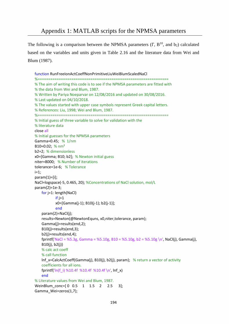
194
Appendix 1: MATLAB scripts for the NPMSA parameters
The following is a comparison between the NPMSA parameters (Γ, B10, and b2) calculated
based on the variables and units given in Table 2.16 and the literature data from Wei and
Blum (1987).
function RunFreeIonActCoeffNonPrimitiveLiuWeiBlumScaledNaCl %============================================================== % The aim of writing this code is to see if the NPMSA parameters are fitted with % the data from Wei and Blum, 1987. % Written by Pariya Noeparvar on 12/08/2016 and updated on 30/08/2016. % Last updated on 04/10/2018. % The values started with upper case symbols represent Greek capital letters. % References: Liu, 1998; Wei and Blum, 1987. %============================================================== % Initial guess of three variable to solve for validation with the % literature data close all % Initial guesses for the NPMSA parameters Gamma=0.45; % 1/nm B10=0.02; % nm² b2=2; % dimensionless x0=[Gamma; B10; b2]; % Newton initial guess niter=8000; % Number of iterations tolerance=1e-6; % Tolerance i=1; param(1)=[i]; NaCl=logspace(-5, 0.465, 20); %Concentrations of NaCl solution, mol/L param(2)=1e-3;
for j=1: length(NaCl) if j>1 x0=[Gamma(j-1); B10(j-1); b2(j-1)]; end
param(2)=NaCl(j); results=Newton(@NewtonEquns, x0,niter,tolerance, param); Gamma(j)=results(end,2); B10(j)=results(end,3); b2(j)=results(end,4); fprintf('NaCl = %5.3g, Gamma = %5.10g, B10 = %5.10g, b2 = %5.10g \n', NaCl(j), Gamma(j), B10(j), b2(j)) % calc act coeff % call function lnf_x=CalcActCoeff(Gamma(j), B10(j), b2(j), param); % return a vector of activity coefficients for all ions. fprintf('ln(f_i) %10.4f %10.4f %10.4f \n', lnf_x) end
% Literature values from Wei and Blum, 1987. WeinBlum_conc=[ 0 0.5 1 1.5 2 2.5 3]; Gamma_Wei=zeros(1,7);

195
B10_Wei=[ 0 0.3 0.4 0.5 0.6 0.7 0.75]; b2_Wei=[ 0 1.75 1.6 1.4 1.25 1.1 1.0]; figure plot(NaCl, Gamma,'k') ylim([-0.1 8]) hold on plot(WeinBlum_conc, Gamma_Wei,'k+') xlabel('NaCl concentration, mol/L', 'fontsize',13) ylabel('\Gamma, nm^-^1', 'fontsize',13) set(gca,'fontsize',13) figure plot(NaCl, B10,'k-') hold on plot(WeinBlum_conc, B10_Wei,'k+') xlabel('NaCl concentration, mol/L','fontsize',13) ylabel('B^1^0, nm^2','fontsize',13) set(gca,'fontsize',13) figure plot(NaCl, b2,'k-') hold on plot(WeinBlum_conc, b2_Wei,'k+') xlabel('NaCl concentration, mol/L','fontsize',13) ylabel('b_2, [-]','fontsize',13) legend('This study',' Wei and Blum, 1987') set(gca,'fontsize',13) end function f=NewtonEquns(x, param, flag) % Call Newton's method [f, lnf_x]=FreeIonActCoeffNonPrimitive(x, param, flag); End function lnf_x=CalcActCoeff(Gamma, B10, b2, param) % Activity coefficient calculation flag='Act'; x=[Gamma; B10;b2]; [f, lnf_x]=FreeIonActCoeffNonPrimitive(x, param, flag); End function [f, lnf_x]= FreeIonActCoeffNonPrimitive(x, param, flag) %================================================================ % This function will solve free–ion activity coefficient by the NPMSA method. %================================================================ Scale=1e7; % scale to convert cm to nm i=param(1); NaCl=param(2); sigma=Scale*[0.19e-7; 0.365e-7; 0.52e-7]; % Wei and Blum 1987 sigma_d=Scale*0.265e-7; % Ion size parameter of water,nm % Wei and Blum 1987 z=[1; -1; 0]; % charge numbers of Na+, Cl- and NaCl° N_AV=6.022e23; % Avogadro's number, mol^-1 Na=NaCl; % Concentrations of Na+ solution, mol/L

196
Cl=NaCl; % Concentrations of Cl- solution, mol/L NaCl_0=1e-16; %Concentrations of NaCl° solution, mol/L rho=(1/Scale^3)*(N_AV*1e-3).*[Na(i); Cl(i); NaCl_0(i)]; % Number of particle per cm³ or nm³ rho_water=(1/Scale^3)*WaterConc(NaCl(i),25).*N_AV.*1e-3; % Number of particle per cm³ or nm³ density=NaClDensityMolar(NaCl(i), 25)/1000; % Density of the solution, kg/L M=[0.0229898; 0.035453; 0.0229898+0.035453]; % Molar mass, kg/mol % Molality of each species m_NaCl=convertCtoM(NaCl(i),M(3,:),density); %molality, mol/kg_water m_Na=convertCtoM(Na(i),M(1,:),density); %molality, mol/kg_water m_Cl=convertCtoM(Cl(i),M(2,:),density); %molality, mol/kg_water m_NaCl_0=convertCtoM(NaCl_0(i),M(3,:),density); %molality, mol/kg_water %Mole fraction of each species x_NaCl=molalitytomolefraction(m_NaCl(i)); x_Na=molalitytomolefraction(m_Na(i)); x_Cl=molalitytomolefraction(m_Cl(i)); x_NaCl_0=molalitytomolefraction(m_NaCl_0(i)); x_solv=1-(x_Na(i)+x_Cl(i)+x_NaCl_0(i)); k_B=Scale^2*1.38064852e-23*1e7; % Boltzmann constant, nm².g.s^-2,K^-1 T=25+273.15; % Absolute temperature, K e=Scale^1.5*4.80320427e-10; % electron charge, statC=g^0.5 cm^1.5.s^-1 % All variables are first defined to be able to solve three non-linear equations by Newton's method. beta=1/(k_B*T); d_0=sqrt(4*pi*beta*e^2); % nm mu=Scale^2.5*2.21e-18; %Dipole moment of water,1Debye=1e-18 StatCoulomb.cm d_2=sqrt((4*pi*beta*mu.^2)/3); % nm³ % initial guess of three variables of NPMSA Gamma=x(1); B10=x(2); b2=x(3); % NPMSA variables beta_3=1+(b2/3); beta_6=1-(b2/6); lambda=beta_3/beta_6; xi_0=pi./6*(sum(rho.*sigma.^0)+(rho_water.*sigma_d^0)); xi_1=pi./6*(sum(rho.*sigma.^1)+(rho_water.*sigma_d^1)); xi_2=pi./6*(sum(rho.*sigma.^2)+(rho_water.*sigma_d^2)); xi_3=pi./6*(sum(rho.*sigma.^3)+(rho_water.*sigma_d^3)); Delta=1-xi_3; P_hs_term=(xi_0./Delta)+((3*xi_1.*xi_2)./Delta.^2)+(((3-xi_3).*xi_2.^3)./Delta.^3); w1=sum((rho.*z.^2) ./(beta_6.*(sigma_d+lambda*sigma).*(1+Gamma*sigma))); y1=4/(beta_6*(1+lambda)^2); w2=0.5*rho_water*sigma_d^2*B10* ... sum((rho.*z.^2.*sigma_d.^2)./(2*beta_6.*(sigma_d+(lambda.*sigma)).*(1+Gamma.*sigma)).^2); nu_eta=((-w1/2)+sqrt(((w1/2).^2)+((2*B10*w2)/beta_6^2)))./w2; Delta_Gamma=(nu_eta*rho_water*sigma_d^2*sigma.^2*B10)./(8*beta_6*(sigma_d+(lambda*sigma))); D_F=(z*beta_6)./(2*(1+(sigma*Gamma)-Delta_Gamma));

197
D=1+(nu_eta^2*rho_water*sigma_d^2)*sum(rho.*sigma.^2.*D_F.^2./(2*beta_6*(sigma_d+lambda*sigma)).^2); Gamma_s=((1+(sigma*Gamma)-Delta_Gamma).*D-1)./sigma; m=(nu_eta*D_F)./(sigma_d+(lambda*sigma)); D_ac=sum(rho.*(D_F.^2)); Omega_10=nu_eta*sum(rho.*sigma.*D_F.^2./(sigma_d+lambda*sigma)); N=(2.*D_F./beta_6.*sigma).*(1+((rho_water.*sigma_d.^3.*B10.*nu_eta.*sigma)./24.*(sigma_d+lambda.*sigma)))-(z./sigma); a_0=beta_6*Gamma_s.*D_F./D_ac; a_nI=(beta_6*D/(2*D_ac))*(sigma_d*B10*0.5+Omega_10*lambda/(D*beta_6)); k_n10=-(sigma_d^2*D_F/(2*D*beta_6^2).*(nu_eta./(sigma_d+lambda*sigma)+ ... Omega_10.*Gamma_s/D_ac)+sigma_d^3*B10*a_0/(12*beta_6)); % vector one_rho_k_nm11=1/(D*beta_6)*(lambda+rho_water*sigma_d^2*Omega_10*a_nI/(2*beta_6^2))+ ... rho_water*sigma_d^3*B10*a_nI/(12*beta_6); % 1 - rho_n k_nm11 % Three equations which should be solved by Newton's method, are presented here. f=zeros(3,1); f(1)= (sum(rho.*a_0.^2)+rho_water*a_nI^2-d_0^2); f(2) =(-sum(rho.*a_0.*k_n10)+a_nI*one_rho_k_nm11-d_0*d_2); f(3)=one_rho_k_nm11^2+rho_water*sum(rho.*k_n10.^2)-(y1^2+rho_water*d_2^2);
if strcmp(flag, 'converged') dummy=1; end if strcmp(flag, 'maxiterations')
dummy=1; end
if strcmp(flag, 'Act') Beta_Mu_hs=-log(Delta)+P_hs_term*sigma.^3+(3*sigma.*(xi_2+xi_1*sigma))./Delta+((9*xi_2^2*sigma.^2)./(2*Delta^2))+ ... ((3*(xi_2*sigma/xi_3).^2).*(log(Delta)+(xi_3/Delta)-(xi_3/Delta)^2/2))- ... (((xi_2*sigma./xi_3).^3)*(2*log(Delta)+xi_3*(1+Delta)/Delta)); % dimensionless Beta_Mu_MSA=(z.*(d_0^2.*N-d_0*d_2*rho_water*m))/(4*pi); %dimensionless Beta_Mu_ex=Beta_Mu_MSA+Beta_Mu_hs; % The actual equation is Ln f_x=exp(beta[µ(xi)-µ(xi to 0)], in which % f_x is free ion activity coeffcient based on mole fraction scale. lnf_x=Beta_Mu_ex; %-exp(Beta_Mu_ex_x_0); else lnf_x=zeros(3,1); end
end function water=WaterConc(MolarConc, T_C) % Concentration of water in the solution. MW_NaCl=58.44; % g/mol MW_water=18.01528; % g/mol water=(1000-((MolarConc.*MW_NaCl)./(NaClDensityMolar(MolarConc,T_C)/1000))) ... .*(NaClDensityMolar(MolarConc,T_C)./(1000.*MW_water)); %mol/L End

198
function density=NaClDensityMolar(MolarConc, T_C) % Calculation of density (kg/m3) of a NaCl solution given molar concentration % T_C is temperature in ˚C based on 25 ˚C % mole conc in mol/L of NaCl density = waterdensity(T_C) *((-6.44E-4.*MolarConc.^2 + 4.04E-02.*MolarConc) + 1.00E+00); % kg/m3 end function density=waterdensity(T_C) % From Kell JCED 1975 p97 density = (999.83952 + 16.945176 * T_C - 0.0079870401 * T_C ^ 2 - 0.000046170461 * T_C ^ 3 + 0.00000010556302 * T_C ^ 4 - 2.8054253E-10 * T_C ^ 5) / (1 + 0.01687985 * T_C); End function m=convertCtoM(C,M, density) % convert concentrations from molar to molal % C is a vector of all the species (could be ions) in the solution in mol/L % M is a vector of the corresponding molecular masses of the species kg/mol % density input is kg/L % output m is vector of molal concentrations mol/kgwater m=C./(density.*(1- (sum(C.*M))./density)); end function x=molalitytomolefraction(m) % convert concentrations from molal to mole fraction % m is a vector of all the species (could be ions) in the solution in mol/kgwater % MWwater is molecular masses of the water kg/mol % output x is vector of mole fraction concentration concentrations. x=m./(1/0.018528+sum(m)); end
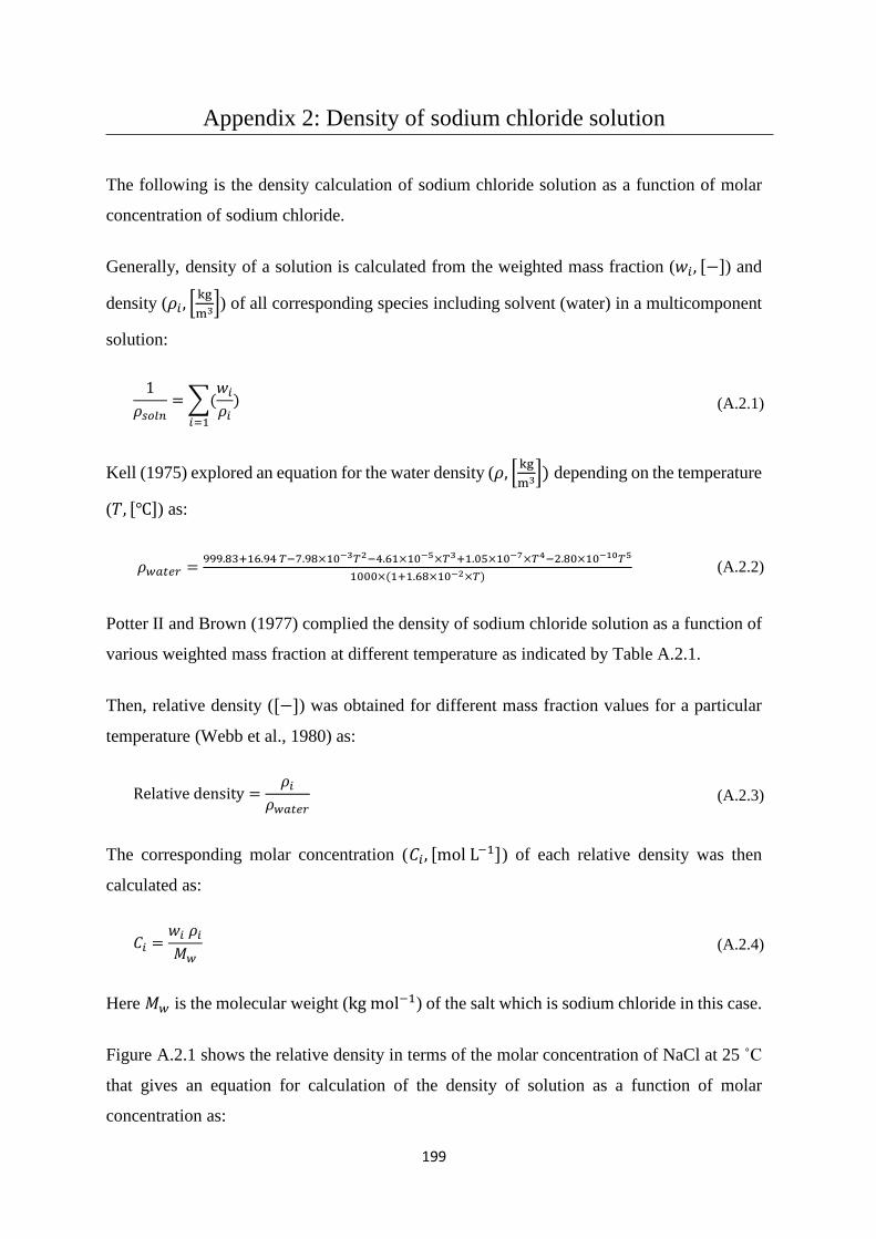
199
Appendix 2: Density of sodium chloride solution The following is the density calculation of sodium chloride solution as a function of molar
concentration of sodium chloride.
Generally, density of a solution is calculated from the weighted mass fraction (𝑤𝑤𝑖𝑖, [−]) and
density (𝜌𝜌𝑖𝑖 , kgm3) of all corresponding species including solvent (water) in a multicomponent
solution:
1𝜌𝜌𝑠𝑠𝑠𝑠𝑠𝑠𝑠𝑠
= (𝑤𝑤𝑖𝑖𝜌𝜌𝑖𝑖
)𝑖𝑖=1
(A.2.1)
Kell (1975) explored an equation for the water density (𝜌𝜌, kgm3) depending on the temperature
(𝑅𝑅, []) as:
𝜌𝜌𝑤𝑤𝑎𝑎𝐶𝐶𝑝𝑝𝑝𝑝 = 999.83+16.94 𝑇𝑇−7.98×10⁻³𝑇𝑇2−4.61×10⁻⁵×𝑇𝑇3+1.05×10⁻⁷×𝑇𝑇4−2.80×10⁻¹⁰𝑇𝑇5
1000×(1+1.68×10⁻²×𝑇𝑇) (A.2.2)
Potter II and Brown (1977) complied the density of sodium chloride solution as a function of
various weighted mass fraction at different temperature as indicated by Table A.2.1.
Then, relative density ([−]) was obtained for different mass fraction values for a particular
temperature (Webb et al., 1980) as:
Relative density =𝜌𝜌𝑖𝑖
𝜌𝜌𝑤𝑤𝑎𝑎𝐶𝐶𝑝𝑝𝑝𝑝 (A.2.3)
The corresponding molar concentration (𝐶𝐶𝑖𝑖, [mol L−1]) of each relative density was then
calculated as:
𝐶𝐶𝑖𝑖 =𝑤𝑤𝑖𝑖 𝜌𝜌𝑖𝑖𝑀𝑀𝑤𝑤
(A.2.4)
Here 𝑀𝑀𝑤𝑤 is the molecular weight (kg mol−1) of the salt which is sodium chloride in this case.
Figure A.2.1 shows the relative density in terms of the molar concentration of NaCl at 25 ˚C
that gives an equation for calculation of the density of solution as a function of molar
concentration as:

200
Density of NaCl solution = −6.44 × 10⁻⁴𝐶𝐶𝑁𝑁𝑎𝑎𝐶𝐶𝑠𝑠 + 4.04 × 10⁻²𝐶𝐶𝑁𝑁𝑎𝑎𝐶𝐶𝑠𝑠 + 1.00 (A.2.5)
Table A.2.1 Density of NaCl solution in terms of different mass fraction and temperature (Potter II and Brown, 1977).
Mass fraction, (w/w%)
𝜌𝜌𝑁𝑁𝑎𝑎𝐶𝐶𝑠𝑠𝑠𝑠𝑠𝑠𝐺𝐺𝑛𝑛 , kgL
0, [] 25, [] 50, [] 75, [] 100, [] 0 0.99984 0.99704 0.98803 0.97485 0.95836
0.01 1.00755 1.00411 0.99480 0.98160 0.96300 0.03 1.02283 1.01823 1.00850 0.99520 0.97900 0.05 1.03814 1.03247 1.02220 1.00900 0.99300 0.07 1.05354 1.04688 1.03620 1.02290 1.00700 0.09 1.06908 1.06146 1.05030 1.03720 1.02100 0.11 1.08476 1.07624 1.06470 1.05160 1.03500 0.13 1.10060 1.09122 1.07930 1.06630 1.04900 0.15 1.11660 1.10639 1.09420 1.08130 1.06300 0.17 1.13276 1.12176 1.10930 1.09650 1.07800 0.19 1.14906 1.13732 1.12470 1.11190 1.09300 0.21 1.16551 1.15307 1.14030 1.12770 1.10900 0.23 1.18210 1.16900 1.15610 1.14360 1.12500 0.25 1.19880 1.18509 1.17220 1.15980 1.14200
Figure A.2.1 Relative density of NaCl solution vs NaCl molar concentration.
0 0.5 1 1.5 2 2.5 3 3.5 4 4.5 51
1.02
1.04
1.06
1.08
1.1
1.12
1.14
1.16
1.18
1.2
Concentration of NaCl solution, mol/L
Rel
ativ
e de
nsity
,[-]

201
Appendix 3: Milk components sizes
The following section shows the estimated sizes of milk components used in the MSA theory. The anions and ion–pairs formed by the H+
interactions sizes were assumed larger than other ion–pairs.
Table A.3 Numerical values of size for each component in milk.
Ca2+, 0.8 nm Mg2+, 0.4 nm Na+, 0.365 nm K+, 0.45 nm H+, 0.226 nm
Anions Size, nm Ion–pair Size,
nm Ion–pair Size, nm Ion–pair
Size,
nm Ion–pair Size,
nm Ion–pair Size, nm
H2Cit– 0.65 CaH2Cit+ 0.4 MgH2Cit+ 0.5 NaH2Cit 0.25 KH2Cit 0.3 H3Cit 0.55
HCit2– 0.75 CaHCit 0.4 MgHCit 0.5 NaHCit– 0.25 KHCit– 0.3 H2Cit– 0.55
Cit3– 0.65 CaCit– 0.4 MgCit– 0.5 NaCit2– 0.25 KCit2– 0.3 HCit2– 0.55
H2PO4– 0.69 CaH2PO4
+ 0.4 MgH2PO4+ 0.5 NaH2PO4 0.25 KH2PO4 0.3 H3PO4 0.55
HPO42– 0.35 CaHPO4 0.4 MgHPO4 0.5 NaHPO4
– 0.25 KHPO4– 0.3 H2PO4
– 0.55
PO43– 0.65 CaPO4
– 0.4 MgPO4– 0.5 NaPO4
2– 0.25 KPO42– 0.3 HPO4
2– 0.55
HCO3– 0.6 CaHCO3
+ 0.4 MgHCO3+ 0.5 NaHCO3 0.25 KHCO3 0.3 H2CO3 0.55
CO32– 0.6 CaCO3 0.4 MgCO3 0.5 NaCO3
– 0.25 KCO3– 0.3 HCO3
– 0.55
HSO4– 0.6 CaHSO4
+ 0.4 MgHSO4+ 0.5 NaHSO4 0.25 KHSO4 0.3 H2SO4 0.55
SO42– 0.6 CaSO4 0.4 MgSO4 0.5 NaSO4
– 0.25 KSO4– 0.3 HSO4
– 0.55
Glc–1–PH– 0.6 CaGlc–1–PH+ 0.4 MgGlc–1–PH+ 0.5 NaGlc–1–PH 0.25 KGlc–1–PH 0.3 Glc–1–PH2 0.55
Glc–1–P2– 0.6 CaGlc–1–P 0.4 MgGlc–1–P 0.5 NaGlc–1–P– 0.25 KGlc–1–P– 0.3 Glc–1–PH– 0.55

202
Cl– 0.365 CaCl+ 0.5 MgCl+ 0.5 NaCl 0.36 KCl 0.3 HCl 0.4
RCOO– 0.6 CaRCOO+ 0.4 MgRCOO+ 0.5 NaRCOO 0.25 KRCOO 0.3 RCOOH 0.55
Arg 0.6 CaArg2+ 0.4 MgArg2+ 0.5 NaArg+ 0.25 KArg+ 0.3 ArgH+ 0.55
Asp– 0.6 CaAsp+ 0.4 MgAsp+ 0.5 NaAsp 0.25 KAsp 0.3 AspH 0.55
Cys 0.6 CaCys+ 0.4 MgCys+ 0.5 NaCys 0.25 KCys 0.3 CysH 0.55
Glu– 0.6 CaGlu+ 0.4 MgGlu+ 0.5 NaGlu 0.25 KGlu 0.3 GluH 0.55
His 0.6 CaHis2+ 0.4 MgHis2+ 0.5 NaHis+ 0.25 KHis+ 0.3 HisH+ 0.55
Lys 0.6 CaLys2+ 0.4 MgLys2+ 0.5 NaLys+ 0.25 KLys+ 0.3 LysH+ 0.55
Ser– 0.6 CaSer+ 0.4 MgSer+ 0.5 NaSer 0.25 KSer 0.3 SerH 0.55
Thr– 0.6 CaThr+ 0.4 MgThr+ 0.5 NaThr 0.25 KThr 0.3 ThrH 0.55
Tyr– 0.6 CaTyr+ 0.4 MgTyr+ 0.5 NaTyr 0.25 KTyr 0.3 TyrH 0.55
((SerP)3H2)–4 0.45 ((SerP)3H2Ca)–2 0.5 ((SerP)3H2Mg)–2 0.5 ((SerP)3H2Na)–3 0.25 ((SerP)3H2K)–3 0.3 ((SerP)3H3)–3 0.55
((SerP)3H)–5 0.45 ((SerP)3CaH)–3 0.5 ((SerP)3HMg)–3 0.5 ((SerP)3HNa)–4 0.25 ((SerP)3HK)–4 0.3 ((SerP)3H2)–4 0.55
((SerP)3)–6 0.45 ((SerP)3Ca)–4 0.5 ((SerP)3Mg)–4 0.5 ((SerP)3Na)–5 0.25 ((SerP)3K)–5 0.3 ((SerP)3H)–5 0.55
((SerP)3Ca2)–2 0.35 ((SerP)3Ca3) 0.5 ((SerP)3Ca2Mg) 0.5 ((SerP)3Ca2Na)–1 0.25 ((SerP)3Ca2K)–1 0.3 ((SerP)3Ca2H)–1 0.55
((SerP)3CaH)–3 0.35 ((SerP)3Ca2H)–1 0.5 ((SerP)3CaHMg)–1 0.5 ((SerP)3CaHNa)–2 0.25 ((SerP)3CaHK)–2 0.3 ((SerP)3H2Ca)–2 0.55
((SerP)3Ca)–4 0.45 ((SerP)3Ca2)–2 0.5 ((SerP)3CaMg)–2 0.5 ((SerP)3CaNa)–3 0.25 ((SerP)3CaK)–3 0.3 ((SerP)3CaH)–3 0.55
PSerH– 0.65 PSerHCa+ 0.5 PSerHCa+ 0.5 PSerHNa 0.25 PSerHK 0.3 PSerH2 0.55
PSer2– 0.65 PSerCa 0.5 PSerCa 0.5 PSerNa– 0.25 PSerK– 0.3 PSerH–a 0.55
OH– 0.28 CaOH+ 0.5 MgOH+ 0.5 NaOH 0.25 KOH 0.3 H2O 0.55

203
Appendix 4: MATLAB scripts for Newton’s and Jacobian functions
The following section is a MATLAB script for Newton’s and Jacobian methods to calculate
ion equilibria non–linearly for any dairy liquids.
function x=MyNewton(func,x,maxits,tol, lb, ub, flag) %================================================================ % solves a set of equations given by the function func using Newton's method % Inputs: func file handle for function that gives f(y) % x0: initial guess of vector x, same dimension as f % tol: convergence tolerance % Outputs: x: solution vector %================================================================
if strcmp(flag, 'start') relaxation=0.5; else relaxation=1; end for k=1:maxits f=func(x); J=jacobian(func,x); deltax=-J\f; x=x+relaxation*deltax; x(x<lb)=lb(x<lb); % limit to lower bound x(x>ub)=ub(x>ub); normx=norm(deltax); normf=norm(f);
if normx<tol && normf < tol convergence=true; fprintf('%3i iterations: normf %5.3g ',k, normf) break end if k>=10 dummy=1; end
end if k>=maxits fprintf('Not converged after %3i iterations ',k) end
end
function J=jacobian(func, x) %================================================================ % Jacobian function generates a numerical Jacobian matrix of partial derivatives % Call: J=jacobian(func, x) % Inputs: func - function handle for function to return column % Vector f=f(x), dimension m % x: vector of values at which to evaluate the Jacobian dimension n % Outputs: f: column vector for f(x)

204
% J: matrix of partial derivatives m rows by n columns % Written by Ken Morison, 7 July 2004, and modified slightly % by John Hannah, 11 August 2006 % Get unperturbed f(x) %================================================================ n=max(size(x)); % find the maximum dimension of x f0=func(x); % evaluate function with unperturbed x transposef=0;
if size(f0,2)>size(f0,1) % a row vector. Give warning and transpose disp('Warning from Jacobian.m. Your function should return f(x) as a column vector. Transpose your result') f0=f0'; transposef=1; end for i=1:n % x(i) deltax=x(i)*1e-7; x0=x(i);
if abs(x0)< 1e-9 % for values of x close to zero, ensure a non-zero perturbation deltax=1e-9; end
x(i)=x(i)+deltax; f=func(x); % perturbed function
if transposef==1 % f needs to be transposed f=f'; % transpose f end
J(:,i)=(f-f0)./deltax; x(i)=x0; % return to original value end
end % end of Jacobian function

205
Appendix 5: MATLAB scripts for sodium chloride solution
The following section is a MATLAB script for the calculation of sodium chloride solution by
using the free–ion approach.
function SolveNaClFreeionMSA %================================================================ % This function will solve the ion equilibria of sodium chloride (NaCl) solution for free–ion approach. % Written by Pariya Noeparvar. % Last updated on 24/04/2018. %================================================================ close all global y global z NaCl=1*[logspace(-1,0,100) logspace(0.01, 6.6,100)]; % total amount of NaCl added, µmol/L tol=1e-10; maxits=1000;
for i=1 : length(NaCl) if i==1 % Initial guess
%Cl OH Na H NaCl° NaOH HCl, µmol/L x=[NaCl(i); 0.40*NaCl(i); NaCl(i); 0.1*100; 0.5*NaCl(i); 0.5*NaCl(i);0.4*NaCl(i)]; end
x0=x ; % use previous solution lb=zeros(length(x),1); ub=NaCl(i)*ones(length(x),1); ub(1)=NaCl(i); ub(2)=1e6; % i.e. 1 mol/L pH 14 ub(4)=1e6; % pH 0 fanon=@(x) MyEquations(x, NaCl(i)); x=MyNewton(fanon,x0,maxits, tol, lb, ub); xsol(:,i)=x; % record last solution pH(i)=-log10(xsol(4,i)/1e6); Na(i)=xsol(3,i)/1e6; % free sodium concentration, mol/L Cl(i)=xsol(1,i)/1e6; % free chloride concentration, mol/L y_Na(i)=y(3); % Molar activity coefficient of free sodium y_Cl(i)=y(1); % Molar activity coefficient of free chloride fprintf(' NaCl pH %5.2g %5.2f \n', NaCl(i), pH) IM(i)=0.5*sum((xsol(:,i)/1e6).*z.^2); % Molar ionic strength, mol/L y_davies=Davies(z, IM); % Activity coefficient by Davies theory y_DH=DH(z,IM); % Activity coefficient by Debye-Hückel theory DH_Na=y_DH(3,:); % Activity coefficient of free sodium by Debye-Hückel theory end
Exp_Na=[0 -0.1 -0.13 -0.27 -0.33 -0.4 -0.5 -0.48 -0.3 -0.1 0.1]; % Activity coefficient of free sodium from Wilczek-Vera et al., 2004 sqrt_NaCl=[0 0.1 0.15 0.35 0.48 0.7 1 1.3 1.6 1.8 2]; % squared molar concentration of NaCl, (mol/L)^½

206
Exp_Cl=[ 0 -0.1 -0.13 -0.3 -0.42 -0.5 -0.58 -0.62 -0.57 -0.49 -0.40 ]; % Activity coefficient of free chloride from Wilczek-Vera et al., 2004 plot(sqrt(NaCl/1e6), log(y_Na),'k') hold on xlabel('\surd NaCl concentration, (mol/L)^1/2') ylabel('ln y, [-]') plot(sqrt(NaCl/1e6), log(y_Cl),'k--') plot(sqrt_NaCl, Exp_Na,'ko') plot(sqrt_NaCl, Exp_Cl,'k^') plot(sqrt(NaCl/1e6), log(y_Na_Davies),'k:') plot(sqrt(NaCl/1e6), log(DH_Na), 'k.-') legend('MSA theory, Na^+', 'MSA theory, Cl^-', 'Wilczek-Vera et al., 2004; Na^+','Wilczek-Vera et al., 2004; Cl^-', 'Davies thoery, Na^+ or Cl^-',' Debye-Hückel thoery, Na^+ or Cl^-','location','southwest') ylim([-2.6 0.5]) end function f=MyEquations(x, NaCl_initial) global z global y global sigma % Intrinsic association constant from Holt et al., 1981 Ka1=0.9/1e6; % Na+ Cl- NaCl° Ka2=0.2/1e6; % Na+ OH- NaOH° Ka3=10^-9.3/1e6; % H+ Cl- HCl° % Cl- OH- Na+ H+ NaCl°NaOH° HCl° z=[ -1; -1; 1; 1; 0; 0; 0]; % Charge number of ions sigma=1e-9*[ 0.44; 0.28; 0.51; 0.226; 0.40; 0.4; 0.4]; % The effective size parameter, m T=25+273.15; % Temperature, K logKw=-4787.3/T-7.1332*log10(T)-0.010365*T+22.801; % Natural logarithm of the intrinsic association constant of water, Harned and Cook 1937 Kw=10^logKw; % (mol/L)^2 Kw1=(55.5/Kw)/1e6; Cl=x(1); OH=x(2); Na=x(3); H=x(4); NaCl_0=x(5); NaOH=x(6); HCl=x(7); Na_t=NaCl_initial; % Total concentration of Na, µmol/L Cl_t=NaCl_initial; % Total concentration of Cl, µmol/L Density_soln=NaClDensityMolar((NaCl_initial)/1e6, 25); % kg/m3 MW_NaCl=58.4/1000; % Molar mass of NaCl, kg/mol MW_water=0.01802; %Molar mass of water, kg/mol C_H2O=(Density_soln-NaCl_initial*1e3/1e6*MW_NaCl)/MW_water*1e6/1000; % mol/m3 converted to µmol/L f=zeros(7,1); % the function values N_A=6.022e23; % Avogadro's number, 1/mol rho=x(1:7)/1e6*N_A*1000; % The number of density, mol/m³

207
y=FreeIonMolarActCoeff(z, sigma, rho, (Na+Cl)/1e6); a=y.*x(1:7); % Molar activity of the species, µmol/L f(1)=(Ka1*a(3)*a(1)-a(5))/1e3; % Na+, Cl-, NaCl° f(2)=(Ka2*a(3)*a(2)-a(6))/1e3; % Na+, OH-, NaOH° f(3)=(Ka3*a(1)*a(4)-a(7))/1e3; % H+, Cl-, HCl° f(4)=(Kw1*a(2)*a(4)-C_H2O)/1e9; % Water equilibrium f(5)=sum(z.*x(1:7))/sum(x(1:7))/1; % Electroneutrality f(6)=(Na_t-(Na+NaCl_0+NaOH))/1e0; % Total sodium f(7)=(Cl_t-(Cl+HCl+NaCl_0))/1e0; % Total chloride end
function y=FreeIonMolarActCoeff(z, sigma, rho, C_s) % with considering epsilon_r as function of Conc % Mean Spherical aprroximation method: Elecrostatic+hard sphere contributions % Ref: Van Boekel, 2008 % z in species charge % sigma is species diameter in m. % rho is number density,mol/m³ e_0=1.6e-19; %Electron charge, Coulomb epsilon_r=78.65-15.45*C_s +3.76*C_s^1.5; % Dielectric constant,[-] KB=1.38e-23; % Boltzmann constant, m².kg/s-²K^-1 epsilon_0=8.85e-12; %Vacuum permitivitty, Farads/m T=25+273.15; % Absolute temperature, K L_B=e_0^2/(4*pi()*epsilon_r*epsilon_0*KB*T); %Bjerrum distance, m kappa=sqrt(4*pi*L_B*sum(rho.*z.^2)); Gamma=sqrt(kappa^2/4); sigma2=sigma.^2; sigma3=sigma.^3; Delta=1-(pi/6*sum(sum(rho.*sigma3))); Omega=1+((pi/2*Delta)*sum((rho.*sigma3)./(1+Gamma*sigma))); xi=(pi/(2*Omega*Delta))*sum((rho.*sigma.*z)./(1+Gamma*sigma)); % Electrostatic contribution lny_es=-L_B*((Gamma*z.^2)./(1+Gamma*sigma)+xi*sigma.*((2*z-xi*sigma2)./(1+Gamma*sigma)+(xi*sigma2)/3).^2); y_es=exp(lny_es); X_0=(pi/6)*sum(rho); X_1=(pi/6)*sum(rho.*sigma); X_2=(pi/6)*sum(rho.*sigma2); X_3=(pi/6)*sum(rho.*sigma3); F1=(3*X_2)/(1-X_3); F2=(3*X_1/(1-X_3))+(3*X_2^2/(X_3*(1-X_3)^2))+(3*X_2^2*log(1-X_3)/X_3^2); F3=(X_0-X_2^3/X_3^2)*(1/(1-X_3))+((3*X_1*X_2-(X_2^3/X_3^2))/(1-X_3)^2)+(2*X_2^3/(X_3*(1-X_3)^3))-(2*X_2^3*log(1-X_3)/X_3^3); % Hard sphere contribution y_hs=exp(-log(1-X_3)+sigma.*F1+sigma.^2.*F2+sigma.^3.*F3); y=exp(log(y_es)+log(y_hs)); % electrostatic contribution+hard sphere contribution end

208
Appendix 6: Precipitation and dissolution rate constants
Following are the numerical values of precipitation and dissolution rate constants of potential
milk solid phases such as DCPD, DCPA, OCP, WH, HAP, CDA, Mg3(PO4)2, CaCO3, TCCT,
and TCCH, for which lack of sufficient data was found in literature except for CaCO3. These
values are required for the dynamic calculation of salt equilibria in milk or milk–like
solutions.
Table A.6.1 Precipitation and dissolution rate constant of milk solid phases.
Precipitation rate constant, min–1 Dissolution rate constant, min–1 DCPD 0.25 0.0001 DCPA 0.9 5 OCP 20 0.1a WH 3 0.1a HAP 4 0.01 CDA 5 0.001 Mg3(PO4)2 1 0.01a CaCO3 0.0025 (Kazadi Mbamba, 2016) 0.1 TCCT 0.01 0.0004a TCCH 0.2 0.5a
a these components had the saturation below 1 and had dissolution.
DCPA and DCPD values were based on the Section 3.7.2.3.

209
Appendix 7: Chemical structure of amino acids
The following is the amino acids exist in milk proteins regardless of dissociation state with
the corresponding dissociation constants on both C– and N–terminuses heads.
Table A.8.1 Chemical structure of milk protein amino acids with the dissociation constants (Fennema, 1996; Belitz and Grosch, 1999; Mercadé-Prieto et al., 2007).
Amino acids Chemical structure and dissociation constant Type of the chain
The side group
Alanine CH CH3
C
O OH
N
H
H
pKd2=9.69
pKd1=2.34
No dissociable
and uncharged side chain
–
Arginine CH CH2
C
O OH
N
H
H
pKd1=2.17
pKd2=9.04
CH2 NH C
N H
N
H
H
pKd3=12.52
CH2
One dissociable
positive charged
(basic) side group
–RNH2
Asparagine CH CH2
C
C
O OH
N
H
H
pKd1=2.02
pKd2=8.8
N
OH
H
No dissociable
and uncharged side chain
–
Aspartic acid
pKd2=4.0
CH CH2
C
O OH
N
H
H
pKd1=1.88
pKd3=9.6
C
O
OH
One dissociable
negative charged (acidic)
side group
–RCOOH
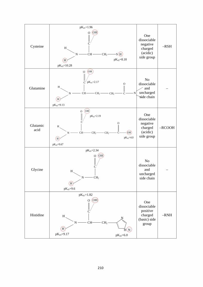
210
Cysteine
pKd2=8.18CH CH2
C
O OH
N
H
H
pKd1=1.96
pKd3=10.28
S H
One dissociable
negative charged (acidic)
side group
–RSH
Glutamine CH CH2
C
O OH
N
H
H
pKd2=9.13
CH2 N
O
C
pKd1=2.17
No dissociable
and uncharged side chain
–
Glutamic acid
CH
C
O
N
H
H
pKd3=9.67
OH
CH2 CH2
pKd2=4.0
C
O
OH
pKd1=2.19
One dissociable
negative charged (acidic)
side group
–RCOOH
Glycine C
O
N
H
H
pKd1=2.34
pKd2=9.6
OH
CH2
No dissociable
and uncharged side chain
–
Histidine C
O
N
H
H
pKd1=1.82
pKd3=9.17
OH
CH CH2
H N
N
pKd2=6.0
One dissociable
positive charged
(basic) side group
–RNH

211
Isoleucine
CH
C
O
N
H
H
pKd2=9.68
OH
CH2 CH CH3
CH3
pKd1=2.36
No dissociable
and uncharged side chain
–
Leucine
CH
C
O
N
H
H
pKd2=9.6
OH
CH CH3
pKd1=2.3
CH2
CH3
No dissociable
and uncharged side chain
–
Lysine CH
C
O
N
H
H
pKd2=8.95
OH
CH2 CH2 CH2 CH2 N
pKd1=2.18
pKd3=10.
One dissociable
positive charged
(basic) side group
–RNH2
Methionine CH
C
O
N
H
H
pKd2=9.21
OH
CH2 CH2 S CH3
pKd1=2.28
No dissociable
and uncharged side chain
–
Phenylalanine
CH
C
O
N
H
H
pKd2=9.13
OH
CH2
pKd1=1.83
No dissociable
and uncharged side group
–
Proline
H N
pKd2=10.6
C
O OH
pKd1=1.94
No dissociable
and uncharged side group
–

212
Serine CH
C
O
N
H
H
pKd2=9.15
OHpKd1=2.2
pKd3=13.22
CH2 OH
One dissociable
negative charged (acidic)s
side group
–RCOH
Threonine CH
C
O
N
H
H
pKd2=9.15
OH
CH
pKd1=2.21
CH3
OH pKd3=13.22
One dissociable
negative charged (acidic)
side group
–RCOH
Tryptophan CH
C
O
N
H
H
pKd2=9.39
CH2
pKd1=2.38OH
HN
No dissociable
and uncharged side group
Tyrosine CH
C
O
N
H
H
pKd2=9.11
OH
CH2
pKd1=2.2
pKd3=10.4
OH
One dissociable
negative charged (acidic)
side group
–RCOH
Valine CH
C
O
N
H
H
pKd2=9.62
OH
CH
pKd1=2.32
CH3
CH3
No dissociable
and uncharged side group
–
The round red circles represents N–, C– terminuses and/or dissociable side groups.

213
Appendix 8: MATLAB scripts for milk solution with CPN
The following is the MATLAB scripts for the milk solution including CPN and saturations of
the potential solid salts at equilibrium.
function SolveMILKCPNSaturation %========================================================== % This function will solve the ion equilibria of milk and CPN. % Written by Pariya Noeparvar, 16 October 2018 % Last updated on 5 November 2018 %========================================================== global z global y close all nlog=100; ConcRatio=1; HCl=[logspace(-6, -1.0, nlog) zeros(1, nlog)]*1e6; % µmol/L NaOH=[zeros(1, nlog) logspace(-6, -1.0, nlog)]*1e6; % There are 32 anions and 5 cations n_A=32; n_C=5; % Association constant [K_eq]=AssocConstants; tol=1e-10; % Tolerance maxits=100; % Max iteration
for j=1 : length(HCl) if j<= nlog i=nlog+1-j; else i=j; end % Arg Asp Cys Glu His Lys Ser Thr Tyr SerP3 AAperBLG=[3 10 5 16 2 15 7 8 4 0]; % Amino acid side groups per molecule of BLG AAperALA=[1 9 8 8 3 12 7 7 4 0 ]; % Amino acid side groups per molecule of ALA AAperBld=[ 23 42 35 62 17 60 28 34 19 0]; % Amino acid side groups per molecule of Bld AAperAs1=[6 7 0 25 5 14 16 5 10 2 ]; % Amino acid side groups per molecule of As1Cas AAperAs2=[6 4 2 25 3 24 17 15 12 2]; % Amino acid side groups per molecule of As2Cas AAperBCas=[4 4 0 18 5 11 16 9 4 1]; % Amino acid side groups per molecule of BCas AAperkCas=[5 4 2 13 3 9 13 14 9 0]; % Amino acid side groups per molecule of kCas % Conc_BLG in milk: 0.0032 kg/kg accroding to Wasltra Jenness 1984 % Can be 0.003 kg/kg according to Elofsson et al., 1997

214
% Density of BLG=1.035 kg/L % MW_BLG=18.4 kg/mol According to Meissner et al., 2015 and Walstra and Jenness 1984
Conc_BLG_milk=0.0032*1.035*1e6/18.4; % Concentration BLG in milk ,µmol/L Conc_ALA_milk=0.0012*1.035*1e6/14.176; % Concentration ALA in milk ,µmol/L Conc_Bld_milk=0.0004*1.035*1e6/66.267; % Concentration Bld in milk ,µmol/L Conc_as1cas_milk=0.0107*1.035*1e6/23.618; % Concentration as1_cas in milk ,µmol/L Conc_as2cas_milk=0.0026*1.035*1e6/25.23; % Concentration as2_cas in milk ,µmol/L Conc_Bcas_milk=0.0093*1.035*1e6/23.983; % Concentration Bcas in milk ,µmol/L Conc_kcas_milk=0.0033*1.035*1e6/19.025; % Concentration kcas in milk ,µmol/L BLG=ConcRatio*Conc_BLG_milk; % BLG conc, µmol/L ALA=ConcRatio*Conc_ALA_milk; % ALA conc, µmol/L Bld=ConcRatio*Conc_Bld_milk; % Bld conc, µmol/L As1_Cas=ConcRatio*Conc_as1cas_milk; % As1_Cas conc, µmol/L As2_Cas=ConcRatio*Conc_as2cas_milk; % As2_Cas conc, µmol/L B_Cas=ConcRatio*Conc_Bcas_milk; % B_Cas conc, µmol/L k_Cas=ConcRatio*Conc_kcas_milk; % k_Cas conc, µmol/L % Total concentration of AA from all proteins in milk, µmol/L Conc_AA_milk=sum(AAperBLG)*Conc_BLG_milk+sum(AAperALA)*Conc_ALA_milk+... sum(AAperBld)*Conc_Bld_milk+sum(AAperAs1)*Conc_as1cas_milk+... sum(AAperAs2)*Conc_as2cas_milk+sum(AAperBCas)*Conc_Bcas_milk+... sum(AAperkCas)*Conc_kcas_milk; % Concentration of each AA in milk, µmol/L Arg_initial=AAperBLG(1)*BLG+AAperALA(1)*ALA+AAperBld(1)*Bld+AAperAs1(1)*As1_Cas+ AAperAs2(1)*As2_Cas+AAperBCas(1)*B_Cas+AAperkCas(1)*k_Cas; Asp_initial=AAperBLG(2)*BLG+AAperALA(2)*ALA+AAperBld(2)*Bld+AAperAs1(2)*As1_Cas+ AAperAs2(2)*As2_Cas+AAperBCas(2)*B_Cas+AAperkCas(2)*k_Cas; Cys_initial=AAperBLG(3)*BLG+AAperALA(3)*ALA+AAperBld(3)*Bld+AAperAs1(3)*As1_Cas+ AAperAs2(3)*As2_Cas+AAperBCas(3)*B_Cas+AAperkCas(3)*k_Cas; Glu_initial=AAperBLG(4)*BLG+AAperALA(4)*ALA+AAperBld(4)*Bld+AAperAs1(4)*As1_Cas+ AAperAs2(4)*As2_Cas+AAperBCas(4)*B_Cas+AAperkCas(4)*k_Cas; His_initial=AAperBLG(5)*BLG+AAperALA(5)*ALA+AAperBld(5)*Bld+AAperAs1(5)*As1_Cas+ AAperAs2(5)*As2_Cas+AAperBCas(5)*B_Cas+AAperkCas(5)*k_Cas; Lys_initial=AAperBLG(6)*BLG+AAperALA(6)*ALA+AAperBld(6)*Bld+AAperAs1(6)*As1_Cas+ AAperAs2(6)*As2_Cas+AAperBCas(6)*B_Cas+AAperkCas(6)*k_Cas; Ser_initial=AAperBLG(7)*BLG+AAperALA(7)*ALA+AAperBld(7)*Bld+AAperAs1(7)*As1_Cas+ AAperAs2(7)*As2_Cas+AAperBCas(7)*B_Cas+AAperkCas(7)*k_Cas; Thr_initial=AAperBLG(8)*BLG+AAperALA(8)*ALA+AAperBld(8)*Bld+AAperAs1(8)*As1_Cas+ AAperAs2(8)*As2_Cas+AAperBCas(8)*B_Cas+AAperkCas(8)*k_Cas; Tyr_initial=AAperBLG(9)*BLG+AAperALA(9)*ALA+AAperBld(9)*Bld+AAperAs1(9)*As1_Cas+ AAperAs2(9)*As2_Cas+AAperBCas(9)*B_Cas+AAperkCas(9)*k_Cas; % Phosphoserines initial concentrations, µmol/L SerP3_initial=1559; SerP_initial=100; % Cit , PO4, CO3, SO4, Cl, Phosphate esters, Carboxylate, µmol/L Cit_initial=9500*ConcRatio; PO4_initial=20600*ConcRatio; CO3_initial=400*ConcRatio; SO4_initial=1200*ConcRatio; Cl_initial=30.4e3*ConcRatio; Esters_initial=2600*ConcRatio; RCOO_initial=3100*ConcRatio;

215
% Cations: Ca, Mg, Na, K Ca_initial=29000*ConcRatio; Mg_initial=4900*ConcRatio; Na_initial=22000*ConcRatio; K_initial=38300*ConcRatio; Lactose=147e3*ConcRatio; All_components(j)=Conc_AA_milk*ConcRatio+Cit_initial+PO4_initial+CO3_initial+... SO4_initial+ Cl_initial+HCl(j)+Esters_initial+RCOO_initial+Ca_initial+Mg_initial+... Na_initial+NaOH(j)+K_initial; % all components concentration, µmol/L % 32 anions for initial guesses C_A=ConcRatio*[Cit_initial*[0.0001; 0.01; 0.1]; PO4_initial*[0.2;0.1; 0.0001];... CO3_initial*[1; 0.01]; SO4_initial*[0.001; 1]; Esters_initial*ones(2,1); ... Cl_initial+HCl(j); RCOO_initial;... Arg_initial*ones(1,1)/3; Asp_initial*ones(1,1)/3;... Cys_initial*ones(1,1)/3; Glu_initial*ones(1,1)/3;... His_initial*ones(1,1)/3; Lys_initial*ones(1,1)/3;... Ser_initial*ones(1,1)/2; Thr_initial*ones(1,1)/2; Tyr_initial*ones(1,1)/3;... SerP3_initial*0.001*ones(6,1); SerP_initial*ones(2,1); ... 0.1/10]; % Initial guess for 5 cations C_C=ConcRatio*[Ca_initial; Mg_initial; NaOH(j)+Na_initial; K_initial; 0.1*100]; % Ca Mg Na K H % Ion pairs initial guess C_CA(1:n_A, 1:n_C)=min(max(1e-20*ones(n_A, n_C),C_A(1:n_A)*C_C'./(K_eq*1e-6)),C_A(1:n_A)*ones(1,n_C)+ones(n_A,1)*C_C'); xx=reshape(C_CA,n_A*n_C,1); C_CA_initial=[xx(1:24); xx(27:28); xx(30:129); xx(132); xx(135); xx(137); xx(139); xx(141:152); xx(158)];
if j==1 % Anions (32), Cation (5), ionpairs (180), CPN TCCT DCPD DCPA HAP, Lactose µmol/L, x0=[C_A; C_C; C_CA_initial;0.01; 0.1; 0.1; 0.1; 0.1; 0.1 ]; x=x0; flag='start'; % Newton's method will use more relaxation for the first solution. end if j==nlog+1 x=x00; end
x0=x ; % use previous solution lb=zeros(length(x),1); ub=All_components(j)*ones(length(x),1); ub(32)=1e6; % OH- ie 1 mol/L ub(37)=1e6; % H+ fanon=@(x) MyEquations(x, All_components(j), Cit_initial, ... PO4_initial, CO3_initial, SO4_initial, Esters_initial, HCl(j)+Cl_initial,... RCOO_initial, Arg_initial, Asp_initial, Cys_initial, Glu_initial, His_initial, Lys_initial, ... Ser_initial, Thr_initial, Tyr_initial, SerP3_initial, SerP_initial, ... Ca_initial, Mg_initial, Na_initial+NaOH(j), K_initial, Lactose); x=MyNewton(fanon,x0,maxits, tol, lb, ub, flag); flag='good';
if j==1

216
x00=x; % retain solution for neutral condition for 2nd half with NaOH end
xsol(:,i)=x; % record last solution µmol/L ysol(:,i)=y; % Activity coefficient pH(i)=-log10(xsol(37,i)/1e6); Sat_TCCT(i)=x(182); % saturation of tri calcium citrate tetrahydrate Sat_DCPD(i)=x(183); % saturation of DCPD Sat_DCPA(i)=x(184); Sat_HAP(i)=x(185); a=y(1:181).*x(1:181)/1e6; % activities in mol/L pKsp_OCP=72.5; pKsp_WH=81.7; % Whitlockite pKsp_CDA=85.1; % calcium def HAP Sat_OCP(i)=a(33)^(8/14)*a(5)^(2/14)*a(6)^(4/14)/(10^-(pKsp_OCP/14)); % Ca(8) HPO4(2) PO4(4) % 8+2+4=14 Sat_WH(i)=(a(33)^10*a(5)*a(6)^6/(10^-pKsp_WH))^(1/17); % Ca(10) HPO4 PO4(6) Sat_CDA(i)=(a(33)^9*a(5)*a(6)^5*a(32)/(10^-pKsp_CDA))^(1/16); % Ca(9) HPO4 PO4(5) OH fprintf(' HCl conc, µmol/L pH %5.6f %5.2f \n', HCl(, pH(i)) % for debugging C_Asol=xsol(15:31,i)'; % the first nine amino acids C_Casol=xsol(52:65,i)'; % the ions pairs corresponding to amino acids(Ca) C_Mgsol=xsol(81:97,i)'; % the ions pairs corresponding to amino acids(Mg) C_Nasol=xsol(113:129,i)'; % the ions pairs corresponding to amino acids(Na) C_Ksol=xsol(145:161,i)'; % the ions pairs corresponding to amino acids(K) C_Hsol=xsol(170:180,i)'; % the ions pairs corresponding to amino acids(H) % General method of net charge of the molecule % this method is based on the activities of species Electroneutrality(i)=sum(z(15:31).*xsol(15:31,i))+sum(z(52:65).*xsol(52:65,i))+... sum(z(81:97).*xsol(81:97,i))+sum(z(113:129).*xsol(113:129,i))+... sum(z(145:161).*xsol(145:161,i))+sum(z(170:180).*xsol(170:180,i)); NetChargePerMolecule(i)=Electroneutrality(i)/(As1_Cas+As2_Cas+B_Cas+k_Cas+BLG+ALA+Bld); CPN(i)=xsol(181,i)/1e3; SerP3free(i)=(xsol(24,i)+xsol(25,i)+xsol(26,i)+xsol(27,i)+xsol(28,i)+xsol(29,i)+... xsol(61,i)+xsol(62,i)+xsol(63,i)+xsol(90,i)+xsol(91,i)+xsol(92,i)+... xsol(93,i)+xsol(94,i)+xsol(95,i)+xsol(122,i)+xsol(123,i)+xsol(124,i)+... xsol(125,i)+xsol(126,i)+xsol(127,i)+xsol(154,i)+xsol(155,i)+xsol(156,i)+... xsol(157,i)+xsol(158,i)+xsol(159,i)+xsol(179,i))/1e3; % mM Rel_SerP3H2(i)=xsol(24,i)/(1000*SerP3free(i)); Rel_SerP3H(i)=xsol(25,i)/(1000*SerP3free(i)); Rel_SerP3(i)=xsol(26,i)/(1000*SerP3free(i)); Rel_SerP3Ca2(i)=xsol(27,i)/(1000*SerP3free(i)); Rel_SerP3CaH(i)=xsol(28,i)/(1000*SerP3free(i)); Rel_SerP3Ca(i)=xsol(29,i)/(1000*SerP3free(i)); Rel_SerP3H2Ca(i)=xsol(61,i)/(1000*SerP3free(i)); Rel_SerP3Ca3(i)=xsol(62,i)/(1000*SerP3free(i)); Rel_SerP3Ca2H(i)=xsol(63,i)/(1000*SerP3free(i)); Rel_SerP3H3(i)=xsol(179,i)/(1000*SerP3free(i)); end
[PI_charge, PI_index]=min(abs(NetChargePerMolecule)); figure

217
plot(pH, CPN,'k') xlabel('pH','fontsize',13) ylabel('Concentration, mmol/L','fontsize',13) hold on plot(pH, SerP3free,'k--') legend('CPN','(SerP)_3') set(gca,'fontsize',13) title('a') figure plot(pH, NetChargePerMolecule,'k') hold on plot(pH(PI_index),NetChargePerMolecule(PI_index),'ko','linewidth',3) xlabel('pH','fontsize',13) ylabel('Net charge/molecule','fontsize',13) txt= [' \leftarrow IEP=', num2str(pH(PI_index))]; text(pH(PI_index),NetChargePerMolecule(PI_index)+1.2,txt) grid on set(gca,'fontsize',13) title('c') figure plot(pH, Sat_DCPD,'k') hold on plot(pH, Sat_DCPA,'k-.') plot(pH, Sat_HAP,'k:') plot(pH, Sat_TCCT,'k-x') plot(pH, Sat_OCP,'k.-') plot(pH, Sat_CDA,'k--') plot(pH, Sat_WH,'k-^') legend('DCPD','DCPA','HAP','TCCT','OCP','CDA','WH','location','northwest') xlabel('pH','fontsize',13) ylabel('Saturation','fontsize',13) set(gca,'fontsize',13) title('b') figure plot(pH, Rel_SerP3H3,'k->') hold on plot(pH, Rel_SerP3Ca,'k--') plot(pH, Rel_SerP3H2Ca,'k') plot(pH, Rel_SerP3Ca2,'k.-') plot(pH, Rel_SerP3,'k:') plot(pH, Rel_SerP3Ca3,'k-.') xlabel('pH','fontsize',13) ylabel('(SerP)_3 relative concentration','fontsize',13) legend('(SerP)_3H_3','(SerP)_3Ca','(SerP)_3H_2Ca','(SerP)_3Ca_2','(SerP)_3','(SerP)_3Ca_3') set(gca,'fontsize',13) title('d') end function f=MyEquations(x, All_components, Cit_initial, PO4_initial, ... CO3_initial, SO4_initial, Esters_initial, Cl_initial, RCOO_initial, Arg_initial,... Asp_initial, Cys_initial, Glu_initial, His_initial,Lys_initial, Ser_initial, Thr_initial,... Tyr_initial, SerP3_initial, SerP_initial, Ca_initial, Mg_initial, Na_initial, K_initial, Lactose)

218
global z global y % Ref:Fennema and Mercado, 2015 [Ka]=1e-6*AssocConstants; %L/µmol Ka_CPN=9e-62; % (µmol/L)^-22 Ksp_TCCT=2.29e-18*(1e6)^5; % (µmol/L)^5 Gao et al., 2010 Ksp_DCPD= 2.09e-7*(1e6)^2; % (µmol/L)^2 Mekmene et al., 2012 Ksp_DCPA=4.0e-7*(1e6)^2; Ksp_HAP=1.58e-117*(1e6)^18; z_A=[ -1 -2 -3 -1 -2 -3 -1 -2 -1 -2 -1 -2 -1 -1 0 -1 -1 -1 0 0 -1 -1 -1 -4 -5 -6 -2 -3 -4 -1 -2 -1]; z_C=[2 2 1 1 1]; % Ca Mg Na K H z=[z_A z_C ... 1 0 -1 1 0 -1 1 0 1 0 1 0 1 1 2 1 1 1 2 2 1 1 1 -2 0 -1 1 0 1 ... 1 0 -1 1 0 -1 1 0 1 0 1 0 1 1 2 1 1 1 2 2 1 1 1 -2 -3 -4 0 -1 -2 1 0 1 ... 0 -1 -2 0 -1 -2 0 -1 0 -1 0 -1 0 0 1 0 0 0 1 1 0 0 0 -3 -4 -5 -1 -2 -3 0 -1 0 ... 0 -1 -2 0 -1 -2 0 -1 0 -1 0 -1 0 0 1 0 0 0 1 1 0 0 0 -3 -4 -5 -1 -2 -3 0 -1 0 ... 0 0 0 0 0 0 0 1 0 0 0 1 1 0 0 0 -3 0 -4 0]'; sigma=1e-9*[0.65 0.75 0.65 0.69 0.35 0.65 0.6*ones(1,17) 0.45 0.45 0.45 0.35 0.35 0.45 0.65 0.65 0.35 ... 0.65 0.4 0.45 0.45 0.33... 0.4*ones(1,20) 0.5*ones(1,9)... 0.5*ones(1,32)... 0.25*ones(1,32)... 0.3*ones(1,32)... 0.55*ones(1,18) 0.22 0.495]'; % m H2Cit=x(1); HCit=x(2); Cit=x(3); H2PO4=x(4); HPO4=x(5); PO4=x(6); HCO3=x(7); CO3=x(8); HSO4=x(9); SO4=x(10); Ester_1=x(11); Ester_2=x(12); Cl=x(13); RCOO=x(14); Arg=x(15); Asp_=x(16); Cys_=x(17); Glu_=x(18); His=x(19); Lys=x(20); Ser_=x(21); Thr_=x(22); Tyr_=x(23); SerP3H2=x(24); SerP3H=x(25); SerP3=x(26);

219
SerP3Ca2=x(27); SerP3CaH=x(28); SerP3Ca=x(29); PSerH=x(30); PSer=x(31); OH=x(32); Ca=x(33); Mg=x(34); Na=x(35); K=x(36); H=x(37); CaH2Cit=x(38); CaHCit=x(39); CaCit=x(40); CaH2PO4=x(41); CaHPO4=x(42); CaPO4=x(43); CaHCO3=x(44); CaCO3=x(45); CaHSO4=x(46); CaSO4=x(47); Ca_Ester_1=x(48); Ca_Ester_2=x(49); CaCl=x(50); CaRCOO=x(51); ArgCa=x(52); AspCa=x(53); CysCa=x(54); GluCa=x(55); HisCa=x(56); LysCa=x(57); SerCa=x(58); ThrCa=x(59); TyrCa=x(60); SerP3H2Ca=x(61); SerP3Ca3=x(62); SerP3Ca2H=x(63); PSerHCa=x(64); PSerCa=x(65); CaOH=x(66); MgH2Cit=x(67); MgHCit=x(68); MgCit=x(69); MgH2PO4=x(70); MgHPO4=x(71); MgPO4=x(72); MgHCO3=x(73); MgCO3=x(74); MgHSO4=x(75); MgSO4=x(76);

220
Mg_Ester_1=x(77); Mg_Ester_2=x(78); MgCl=x(79); MgRCOO=x(80); ArgMg=x(81); AspMg=x(82); CysMg=x(83); GluMg=x(84); HisMg=x(85); LysMg=x(86); SerMg=x(87); ThrMg=x(88); TyrMg=x(89); SerP3H2Mg=x(90); SerP3HMg=x(91); SerP3Mg=x(92); SerP3Ca2Mg=x(93); SerP3CaHMg=x(94); SerP3CaMg=x(95); PSerHMg=x(96); PSerMg=x(97); MgOH=x(98); NaH2Cit=x(99); NaHCit=x(100); NaCit=x(101); NaH2PO4=x(102); NaHPO4=x(103); NaPO4=x(104); NaHCO3=x(105); NaCO3=x(106); NaHSO4=x(107); NaSO4=x(108); Na_Ester_1=x(109); Na_Ester_2=x(110); NaCl=x(111); NaRCOO=x(112); ArgNa=x(113); AspNa=x(114); CysNa=x(115); GluNa=x(116); HisNa=x(117); LysNa=x(118); SerNa=x(119); ThrNa=x(120); TyrNa=x(121); SerP3H2Na=x(122); SerP3HNa=x(123); SerP3Na=x(124); SerP3Ca2Na=x(125); SerP3CaHNa=x(126); SerP3CaNa=x(127);

221
PSerHNa=x(128); PSerNa=x(129); NaOH=x(130); KH2Cit=x(131); KHCit=x(132); KCit=x(133); KH2PO4=x(134); KHPO4=x(135); KPO4=x(136); KHCO3=x(137); KCO3=x(138); KHSO4=x(139); KSO4=x(140); K_Ester_1=x(141); K_Ester_2=x(142); KCl=x(143); KRCOO=x(144); ArgK=x(145); AspK=x(146); CysK=x(147); GluK=x(148); HisK=x(149); LysK=x(150); SerK=x(151); ThrK=x(152); TyrK=x(153); SerP3H2K=x(154); SerP3HK=x(155); SerP3K=x(156); SerP3Ca2K=x(157); SerP3CaHK=x(158); SerP3CaK=x(159); PSerHK=x(160); PSerK=x(161); KOH=x(162); H3Cit=x(163); H3PO4=x(164); H2CO3=x(165); H2SO4=x(166); H_ester=x(167); HCl=x(168); RCOOH=x(169); ArgH=x(170); Asp=x(171); Cys=x(172); Glu=x(173); HisH=x(174); LysH=x(175); Ser=x(176); Thr=x(177); Tyr=x(178);

222
SerP3H3=x(179); PSerH2=x(180); CPN=x(181); a_H=x(182); sat_TCCT=x(182); sat_DCPD=x(183); Sat_DCPA=x(184); Sat_HAP=x(185); Arg_t=Arg_initial; Asp_t=Asp_initial; Cys_t=Cys_initial; Glu_t=Glu_initial; His_t=His_initial; Lys_t=Lys_initial; Ser_t=Ser_initial; Thr_t=Thr_initial; Tyr_t=Tyr_initial; Cit_t=Cit_initial; PO4_t=PO4_initial; CO3_t=CO3_initial; SO4_t=SO4_initial; Cl_t=Cl_initial; Esters_t=Esters_initial; RCOO_t=RCOO_initial; Ca_t=Ca_initial; Mg_t=Mg_initial; Na_t=Na_initial; K_t=K_initial; SerP_t=SerP_initial; SerP3_t=SerP3_initial; Density_soln=MilkDensityMolar((All_components)/1e6, 25); % kg/m3 MW_Milk=0.150; % MW of milk components 18 Oct 2018.xlsx MW_water=0.01802; MW_Cl=35.46; % g/mol MW_NaOH=40/1000; C_H2O=(Density_soln-All_components*(1e3/1e6)*MW_Milk)/MW_water*1e6/1000; % mol/m3 converted to µmol/L f=zeros(182,1); N_A=6.022e23; % Avogadro's number rho=[x(1:181)]/1e6*N_A*1000; % mol base y=FreeIonMolarActCoeff(z, sigma, rho, (SerP3)/1e6); a=y.*x(1:182); %µmol/L scale=1e4; % Ca f(1)=(Ka(1,1)*a(33)*a(1)-a(38))/scale; f(2)=(Ka(2,1)*a(33)*a(2)-a(39))/scale; f(3)=(Ka(3,1)*a(33)*a(3)-a(40))/scale; f(4)=(Ka(4,1)*a(33)*a(4)-a(41))/scale; f(5)=(Ka(5,1)*a(33)*a(5)-a(42))/scale; f(6)=(Ka(6,1)*a(33)*a(6)-a(43))/1e6; f(7)=(Ka(7,1)*a(33)*a(7)-a(44))/scale;

223
f(8)=(Ka(8,1)*a(33)*a(8)-a(45))/scale; f(9)=(Ka(9,1)*a(33)*a(9)-a(46))/1e3; f(10)=(Ka(10,1)*a(33)*a(10)-a(47))/scale; f(11)=(Ka(11,1)*a(33)*a(11)-a(48))/scale; f(12)=(Ka(12,1)*a(33)*a(12)-a(49))/scale; f(13)=(Ka(13,1)*a(33)*a(13)-a(50))/2e5; f(14)=(Ka(14,1)*a(33)*a(14)-a(51))/scale; f(15)=(Ka(15,1)*a(33)*a(15)-a(52))/scale; f(16)=(Ka(16,1)*a(33)*a(16)-a(53))/scale; f(17)=(Ka(17,1)*a(33)*a(17)-a(54))/scale; f(18)=(Ka(18,1)*a(33)*a(18)-a(55))/1e3; f(19)=(Ka(19,1)*a(33)*a(19)-a(56))/scale; f(20)=(Ka(20,1)*a(33)*a(20)-a(57))/scale; f(21)=(Ka(21,1)*a(33)*a(21)-a(58))/scale; f(22)=(Ka(22,1)*a(33)*a(22)-a(59))/scale; f(23)=(Ka(23,1)*a(33)*a(23)-a(60))/scale; f(24)=(Ka(24,1)*a(33)*a(24)-a(61))/scale; f(25)=(Ka(25,1)*a(33)*a(25)-a(28))/scale; f(26)=(Ka(26,1)*a(33)*a(26)-a(29))/scale; f(27)=(Ka(27,1)*a(33)*a(27)-a(62))/scale; f(28)=(Ka(28,1)*a(33)*a(28)-a(63))/scale; f(29)=(Ka(29,1)*a(33)*a(29)-a(27))/scale; f(30)=(Ka(30,1)*a(33)*a(30)-a(64))/scale; f(31)=(Ka(31,1)*a(33)*a(31)-a(65))/scale; f(32)=(Ka(32,1)*a(33)*a(32)-a(66))/scale; % Mg f(33)=(Ka(1,2)*a(34)*a(1)-a(67))/scale; f(34)=(Ka(2,2)*a(34)*a(2)-a(68))/scale; f(35)=(Ka(3,2)*a(34)*a(3)-a(69))/scale; f(36)=(Ka(4,2)*a(34)*a(4)-a(70))/scale; f(37)=(Ka(5,2)*a(34)*a(5)-a(71))/scale; f(38)=(Ka(6,2)*a(34)*a(6)-a(72))/1e6; f(39)=(Ka(7,2)*a(34)*a(7)-a(73))/scale; f(40)=(Ka(8,2)*a(34)*a(8)-a(74))/scale; f(41)=(Ka(9,2)*a(34)*a(9)-a(75))/1e3; f(42)=(Ka(10,2)*a(34)*a(10)-a(76))/scale; f(43)=(Ka(11,2)*a(34)*a(11)-a(77))/scale; f(44)=(Ka(12,2)*a(34)*a(12)-a(78))/scale; f(45)=(Ka(13,2)*a(34)*a(13)-a(79))/1e6; f(46)=(Ka(14,2)*a(34)*a(14)-a(80))/scale; f(47)=(Ka(15,2)*a(34)*a(15)-a(81))/scale; f(48)=(Ka(16,2)*a(34)*a(16)-a(82))/scale; f(49)=(Ka(17,2)*a(34)*a(17)-a(83))/scale; f(50)=(Ka(18,2)*a(34)*a(18)-a(84))/1e3; f(51)=(Ka(19,2)*a(34)*a(19)-a(85))/scale; f(52)=(Ka(20,2)*a(34)*a(20)-a(86))/scale; f(53)=(Ka(21,2)*a(34)*a(21)-a(87))/scale; f(54)=(Ka(22,2)*a(34)*a(22)-a(88))/scale; f(55)=(Ka(23,2)*a(34)*a(23)-a(89))/scale; f(56)=(Ka(24,2)*a(34)*a(24)-a(90))/scale; f(57)=(Ka(25,2)*a(34)*a(25)-a(91))/scale;

224
f(58)=(Ka(26,2)*a(34)*a(26)-a(92))/scale; f(59)=(Ka(27,2)*a(34)*a(27)-a(93))/scale; f(60)=(Ka(28,2)*a(34)*a(28)-a(94))/scale; f(61)=(Ka(29,2)*a(34)*a(29)-a(95))/scale; f(62)=(Ka(30,2)*a(34)*a(30)-a(96))/scale; f(63)=(Ka(31,2)*a(34)*a(31)-a(97))/scale; f(64)=(Ka(32,2)*a(34)*a(32)-a(98))/scale; % Na f(65)=(Ka(1,3)*a(35)*a(1)-a(99))/scale; f(66)=(Ka(2,3)*a(35)*a(2)-a(100))/scale; f(67)=(Ka(3,3)*a(35)*a(3)-a(101))/scale; f(68)=(Ka(4,3)*a(35)*a(4)-a(102))/scale; f(69)=(Ka(5,3)*a(35)*a(5)-a(103))/scale; f(70)=(Ka(6,3)*a(35)*a(6)-a(104))/1e6; f(71)=(Ka(7,3)*a(35)*a(7)-a(105))/scale; f(72)=(Ka(8,3)*a(35)*a(8)-a(106))/scale; f(73)=(Ka(9,3)*a(35)*a(9)-a(107))/1e3; f(74)=(Ka(10,3)*a(35)*a(10)-a(108))/scale; f(75)=(Ka(11,3)*a(35)*a(11)-a(109))/scale; f(76)=(Ka(12,3)*a(35)*a(12)-a(110))/scale; f(77)=(Ka(13,3)*a(35)*a(13)-a(111))/scale; f(78)=(Ka(14,3)*a(35)*a(14)-a(112))/scale; f(79)=(Ka(15,3)*a(35)*a(15)-a(113))/scale; f(80)=(Ka(16,3)*a(35)*a(16)-a(114))/scale; f(81)=(Ka(17,3)*a(35)*a(17)-a(115))/scale; f(82)=(Ka(18,3)*a(35)*a(18)-a(116))/1e3; f(83)=(Ka(19,3)*a(35)*a(19)-a(117))/scale; f(84)=(Ka(20,3)*a(35)*a(20)-a(118))/scale; f(85)=(Ka(21,3)*a(35)*a(21)-a(119))/scale; f(86)=(Ka(22,3)*a(35)*a(22)-a(120))/scale; f(87)=(Ka(23,3)*a(35)*a(23)-a(121))/scale; f(88)=(Ka(24,3)*a(35)*a(24)-a(122))/scale; f(89)=(Ka(25,3)*a(35)*a(25)-a(123))/scale; f(90)=(Ka(26,3)*a(35)*a(26)-a(124))/scale; f(91)=(Ka(27,3)*a(35)*a(27)-a(125))/scale; f(92)=(Ka(28,3)*a(35)*a(28)-a(126))/scale; f(93)=(Ka(29,3)*a(35)*a(29)-a(127))/scale; f(94)=(Ka(30,3)*a(35)*a(30)-a(128))/scale; f(95)=(Ka(31,3)*a(35)*a(31)-a(129))/scale; f(96)=(Ka(32,3)*a(35)*a(32)-a(130))/scale; % K f(97)=(Ka(1,4)*a(36)*a(1)-a(131))/scale; f(98)=(Ka(2,4)*a(36)*a(2)-a(132))/scale; f(99)=(Ka(3,4)*a(36)*a(3)-a(133))/scale; f(100)=(Ka(4,4)*a(36)*a(4)-a(134))/scale; f(101)=(Ka(5,4)*a(36)*a(5)-a(135))/scale; f(102)=(Ka(6,4)*a(36)*a(6)-a(136))/1e6; f(103)=(Ka(7,4)*a(36)*a(7)-a(137))/scale; f(104)=(Ka(8,4)*a(36)*a(8)-a(138))/scale; f(105)=(Ka(9,4)*a(36)*a(9)-a(139))/1e3; f(106)=(Ka(10,4)*a(36)*a(10)-a(140))/scale;

225
f(107)=(Ka(11,4)*a(36)*a(11)-a(141))/scale; f(108)=(Ka(12,4)*a(36)*a(12)-a(142))/scale; f(109)=(Ka(13,4)*a(36)*a(13)-a(143))/1e6; f(110)=(Ka(14,4)*a(36)*a(14)-a(144))/scale; f(111)=(Ka(15,4)*a(36)*a(15)-a(145))/scale; f(112)=(Ka(16,4)*a(36)*a(16)-a(146))/scale; f(113)=(Ka(17,4)*a(36)*a(17)-a(147))/scale; f(114)=(Ka(18,4)*a(36)*a(18)-a(148))/1e3; f(115)=(Ka(19,4)*a(36)*a(19)-a(149))/scale; f(116)=(Ka(20,4)*a(36)*a(20)-a(150))/scale; f(117)=(Ka(21,4)*a(36)*a(21)-a(151))/scale; f(118)=(Ka(22,4)*a(36)*a(22)-a(152))/scale; f(119)=(Ka(23,4)*a(36)*a(23)-a(153))/scale; f(120)=(Ka(24,4)*a(36)*a(24)-a(154))/scale; f(121)=(Ka(25,4)*a(36)*a(25)-a(155))/scale; f(122)=(Ka(26,4)*a(36)*a(26)-a(156))/scale; f(123)=(Ka(27,4)*a(36)*a(27)-a(157))/scale; f(124)=(Ka(28,4)*a(36)*a(28)-a(158))/scale; f(125)=(Ka(29,4)*a(36)*a(29)-a(159))/scale; f(126)=(Ka(30,4)*a(36)*a(30)-a(160))/scale; f(127)=(Ka(31,4)*a(36)*a(31)-a(161))/scale; f(128)=(Ka(32,4)*a(36)*a(32)-a(162))/scale; % H f(129)=(Ka(1,5)*a(37)*a(1)-a(163))/scale; f(130)=(Ka(2,5)*a(37)*a(2)-a(1))/scale; f(131)=(Ka(3,5)*a(37)*a(3)-a(2))/scale; f(132)=(Ka(4,5)*a(37)*a(4)-a(164))/scale; f(133)=(Ka(5,5)*a(37)*a(5)-a(4))/scale; f(134)=(Ka(6,5)*a(37)*a(6)-a(5))/1e8; f(135)=(Ka(7,5)*a(37)*a(7)-a(165))/scale; f(136)=(Ka(8,5)*a(37)*a(8)-a(7))/1e5; f(137)=(Ka(9,5)*a(37)*a(9)-a(166))/1e3; f(138)=(Ka(10,5)*a(37)*a(10)-a(9))/scale; f(139)=(Ka(11,5)*a(37)*a(11)-a(167))/scale; f(140)=(Ka(12,5)*a(37)*a(12)-a(11))/scale; f(141)=(Ka(13,5)*a(37)*a(13)-a(168))/1e6; f(142)=(Ka(14,5)*a(37)*a(14)-a(169))/scale; f(143)=(Ka(15,5)*a(37)*a(15)-a(170))/1e10; f(144)=(Ka(16,5)*a(37)*a(16)-a(171))/scale; f(145)=(Ka(17,5)*a(37)*a(17)-a(172))/1e5; f(146)=(Ka(18,5)*a(37)*a(18)-a(173))/1e3; f(147)=(Ka(19,5)*a(37)*a(19)-a(174))/scale; f(148)=(Ka(20,5)*a(37)*a(20)-a(175))/1e8; f(149)=(Ka(21,5)*a(37)*a(21)-a(176))/1e11; f(150)=(Ka(22,5)*a(37)*a(22)-a(177))/1e11; f(151)=(Ka(23,5)*a(37)*a(23)-a(178))/1e7; f(152)=(Ka(24,5)*a(37)*a(24)-a(179))/scale; f(153)=(Ka(25,5)*a(37)*a(25)-a(24))/scale; f(154)=(Ka(26,5)*a(37)*a(26)-a(25))/scale; % f(155)=(Ka(27,5)*a(36)*a(27)-a(63))/scale; % f(156)=(Ka(28,5)*a(36)*a(28)-a(61))/scale;
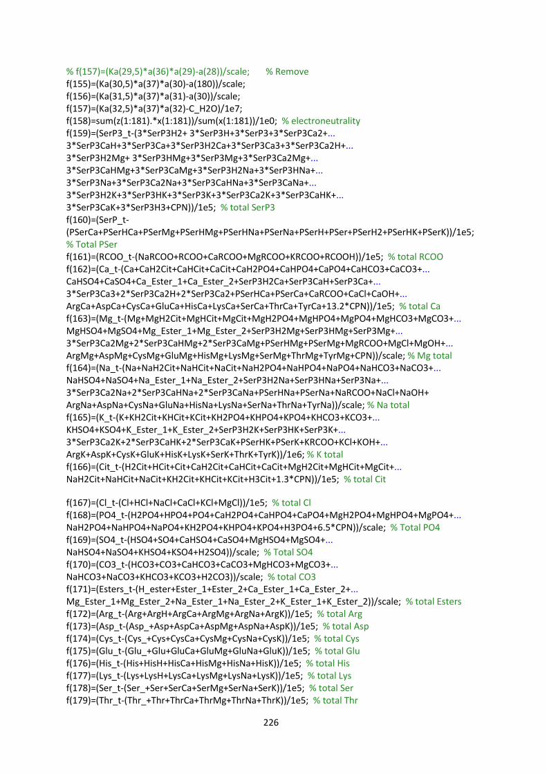
226
% f(157)=(Ka(29,5)*a(36)*a(29)-a(28))/scale; % Remove f(155)=(Ka(30,5)*a(37)*a(30)-a(180))/scale; f(156)=(Ka(31,5)*a(37)*a(31)-a(30))/scale; f(157)=(Ka(32,5)*a(37)*a(32)-C_H2O)/1e7; f(158)=sum(z(1:181).*x(1:181))/sum(x(1:181))/1e0; % electroneutrality f(159)=(SerP3_t-(3*SerP3H2+ 3*SerP3H+3*SerP3+3*SerP3Ca2+... 3*SerP3CaH+3*SerP3Ca+3*SerP3H2Ca+3*SerP3Ca3+3*SerP3Ca2H+... 3*SerP3H2Mg+ 3*SerP3HMg+3*SerP3Mg+3*SerP3Ca2Mg+... 3*SerP3CaHMg+3*SerP3CaMg+3*SerP3H2Na+3*SerP3HNa+... 3*SerP3Na+3*SerP3Ca2Na+3*SerP3CaHNa+3*SerP3CaNa+... 3*SerP3H2K+3*SerP3HK+3*SerP3K+3*SerP3Ca2K+3*SerP3CaHK+... 3*SerP3CaK+3*SerP3H3+CPN))/1e5; % total SerP3 f(160)=(SerP_t-(PSerCa+PSerHCa+PSerMg+PSerHMg+PSerHNa+PSerNa+PSerH+PSer+PSerH2+PSerHK+PSerK))/1e5; % Total PSer f(161)=(RCOO_t-(NaRCOO+RCOO+CaRCOO+MgRCOO+KRCOO+RCOOH))/1e5; % total RCOO f(162)=(Ca_t-(Ca+CaH2Cit+CaHCit+CaCit+CaH2PO4+CaHPO4+CaPO4+CaHCO3+CaCO3+... CaHSO4+CaSO4+Ca_Ester_1+Ca_Ester_2+SerP3H2Ca+SerP3CaH+SerP3Ca+... 3*SerP3Ca3+2*SerP3Ca2H+2*SerP3Ca2+PSerHCa+PSerCa+CaRCOO+CaCl+CaOH+... ArgCa+AspCa+CysCa+GluCa+HisCa+LysCa+SerCa+ThrCa+TyrCa+13.2*CPN))/1e5; % total Ca f(163)=(Mg_t-(Mg+MgH2Cit+MgHCit+MgCit+MgH2PO4+MgHPO4+MgPO4+MgHCO3+MgCO3+... MgHSO4+MgSO4+Mg_Ester_1+Mg_Ester_2+SerP3H2Mg+SerP3HMg+SerP3Mg+... 3*SerP3Ca2Mg+2*SerP3CaHMg+2*SerP3CaMg+PSerHMg+PSerMg+MgRCOO+MgCl+MgOH+... ArgMg+AspMg+CysMg+GluMg+HisMg+LysMg+SerMg+ThrMg+TyrMg+CPN))/scale; % Mg total f(164)=(Na_t-(Na+NaH2Cit+NaHCit+NaCit+NaH2PO4+NaHPO4+NaPO4+NaHCO3+NaCO3+... NaHSO4+NaSO4+Na_Ester_1+Na_Ester_2+SerP3H2Na+SerP3HNa+SerP3Na+... 3*SerP3Ca2Na+2*SerP3CaHNa+2*SerP3CaNa+PSerHNa+PSerNa+NaRCOO+NaCl+NaOH+ ArgNa+AspNa+CysNa+GluNa+HisNa+LysNa+SerNa+ThrNa+TyrNa))/scale; % Na total f(165)=(K_t-(K+KH2Cit+KHCit+KCit+KH2PO4+KHPO4+KPO4+KHCO3+KCO3+... KHSO4+KSO4+K_Ester_1+K_Ester_2+SerP3H2K+SerP3HK+SerP3K+... 3*SerP3Ca2K+2*SerP3CaHK+2*SerP3CaK+PSerHK+PSerK+KRCOO+KCl+KOH+... ArgK+AspK+CysK+GluK+HisK+LysK+SerK+ThrK+TyrK))/1e6; % K total f(166)=(Cit_t-(H2Cit+HCit+Cit+CaH2Cit+CaHCit+CaCit+MgH2Cit+MgHCit+MgCit+... NaH2Cit+NaHCit+NaCit+KH2Cit+KHCit+KCit+H3Cit+1.3*CPN))/1e5; % total Cit f(167)=(Cl_t-(Cl+HCl+NaCl+CaCl+KCl+MgCl))/1e5; % total Cl f(168)=(PO4_t-(H2PO4+HPO4+PO4+CaH2PO4+CaHPO4+CaPO4+MgH2PO4+MgHPO4+MgPO4+... NaH2PO4+NaHPO4+NaPO4+KH2PO4+KHPO4+KPO4+H3PO4+6.5*CPN))/scale; % Total PO4 f(169)=(SO4_t-(HSO4+SO4+CaHSO4+CaSO4+MgHSO4+MgSO4+... NaHSO4+NaSO4+KHSO4+KSO4+H2SO4))/scale; % Total SO4 f(170)=(CO3_t-(HCO3+CO3+CaHCO3+CaCO3+MgHCO3+MgCO3+... NaHCO3+NaCO3+KHCO3+KCO3+H2CO3))/scale; % total CO3 f(171)=(Esters_t-(H_ester+Ester_1+Ester_2+Ca_Ester_1+Ca_Ester_2+... Mg_Ester_1+Mg_Ester_2+Na_Ester_1+Na_Ester_2+K_Ester_1+K_Ester_2))/scale; % total Esters f(172)=(Arg_t-(Arg+ArgH+ArgCa+ArgMg+ArgNa+ArgK))/1e5; % total Arg f(173)=(Asp_t-(Asp_+Asp+AspCa+AspMg+AspNa+AspK))/1e5; % total Asp f(174)=(Cys_t-(Cys_+Cys+CysCa+CysMg+CysNa+CysK))/1e5; % total Cys f(175)=(Glu_t-(Glu_+Glu+GluCa+GluMg+GluNa+GluK))/1e5; % total Glu f(176)=(His_t-(His+HisH+HisCa+HisMg+HisNa+HisK))/1e5; % total His f(177)=(Lys_t-(Lys+LysH+LysCa+LysMg+LysNa+LysK))/1e5; % total Lys f(178)=(Ser_t-(Ser_+Ser+SerCa+SerMg+SerNa+SerK))/1e5; % total Ser f(179)=(Thr_t-(Thr_+Thr+ThrCa+ThrMg+ThrNa+ThrK))/1e5; % total Thr

227
f(180)=(Tyr_t-(Tyr_+Tyr+TyrCa+TyrMg+TyrNa+TyrK))/1e5; % total Tyr f(181)=(Ka_CPN*a(33)^13.2*a(3)^1.3*a(5)^6.5*a(34)*SerP3-CPN)/1e0; % here we are assuming full activity of SerP3 and CPN f(182)=(a(3)^2*a(33)^3/Ksp_TCCT-sat_TCCT)/1e0; f(183)=(a(5)*a(33)/Ksp_DCPD-sat_DCPD)/1e0; f(184)=(a(33)*a(5)/Ksp_DCPA-Sat_DCPA)/1e1; f(185)=(a(33)^10*a(6)^6*a(32)^2/Ksp_HAP-Sat_HAP)/1e2; f(186)=a_H-a(37); end function [K_eq]=AssocConstants % 25 °C % L/mol T=25+273.15; logKw=-4787.3/T-7.1332*log10(T)-0.010365*T+22.801; % Harned and Cook 1937 Kw=10^logKw; % mol/L Kw1=55.5/Kw; % 55.5 mol/L/1e-14 in normal association constant form % Ca Mg Na K H K_eq=[28 15 1 1 1380; % H2Cit 876 402 10 10 6e4; % HCit 1.65e5 1.11e5 20 16 2.57e6; % Cit 11 12 1 1 200; % H2PO4 642 838 17 13 2.87e7; %HPO4 2.88e6 8.35e4 100 100 2.47e12; % PO4 23 19 1 1 2.25e6; % H2CO3 1.4e3 758 10 10 2.13e10; % HCO3 10 10 1 1 10^-8; % H2SO4 204 170 5 7 98; % HSO4 10 10 1 1 10^-10; % GlcPH 316 295 7 5 3.19e6; % GlcP 9.4 5.6 0.9 1 10^-9.3; % HCl 15 19 0.7 0.7 5.71e4; % RCOO 0.1 0.1 0.1 0.1 1/10^(-12.52); % Arg 0.1 0.1 0.1 0.1 1/10^(-3.6); % Asp 0.1 0.1 0.1 0.1 1/10^(-8.50); % Cys 0.1 0.1 0.1 0.1 1/10^(-4.0); % Glu 0.1 0.1 0.1 0.1 1/10^(-6.00); % His 0.1 0.1 0.1 0.1 1/10^(-10.95); % Lys 0.1 0.1 0.1 0.1 1/10^(-13.22); % Ser 0.1 0.1 0.1 0.1 1/10^(-13.22); % Thr 0.1 0.1 0.1 0.1 1/10^(-9.60); % Tyr 380 100 1 1 7.94e5; %SerP3H2 380 100 1 1 7.94e5; %SerP3H 3000 3000 1 1 1e7; % SerP3 380 100 1 1 7.85e5; %SerP3Ca2 380 100 1 1 7.94e5; %SerP3CaH 380 100 1 1 7.94e5; %SerP3Ca 10 10 1 1 200; % HPSer 380 380 16.9 16.9 7.94e5; % PSer 25.11 162.18 0.2 0.2 Kw1]; % OH end