Embed Size (px)
Citation preview

Development of a Decision Support System for Defect Reports
Linus Olofsson, Petter Gulin
MASTER’S THESIS | LUND UNIVERSITY 2014
Department of Computer ScienceFaculty of Engineering LTH
ISSN 1650-2884 LU-CS-EX 2014-24


Development of a Decision SupportSystem for Defect Reports
Linus [email protected]
Petter [email protected]
June 25, 2014
Master’s thesis work carried out atthe Department of Computer Science, Lund University.
Supervisor: Markus Borg, [email protected]
Examiner Per Runeson, [email protected]


Abstract
Issue management is a time consuming activity in Software Engineer-ing. In industrial practice defect report prioritization is usually han-dled manually. In large organizations the amount of defect reports canbe overwhelming and prioritization is critical. We develop a decisionsupport system for defect prioritization based on Machine Learning atSony Mobile Communications, a large telecommunications company.By using classification our system predicts whether a defect reportswill be rejected or fixed. We perform a large scale evaluation of severalclassification algorithms. Furthermore we study how attribute selec-tion, training set size, and time locality of the training set affect the pre-diction accuracy. Our system achieves a prediction accuracy of above70% when evaluated on a sequestered test set of real industrial defectreports submitted between January 2014 and March 2014. We showthat several attributes are more useful for prediction than priority, e.g.geographic location and development milestones. Our system reachesa feasible prediction accuracy when trained on 4,000 defect reports.Also, our results suggest that frequent retraining is not necessary inthis context. Finally we discuss how our system could be deployed atSony and present practical lessons learned.
Keywords: Machine Learning, Software Engineering, Classification, DefectManagement

2

Acknowledgements
We would like to thank our supervisors Markus Borg and Peter Visuri for all oftheir valuable input. We would also like to thank the employees of Sony Mo-bile Communications for their help and patience, and the members of the SERGresearch group for all of their useful comments.
3

4

Contents
1 1: Introduction 111.1 Introduction and Problem Definition . . . . . . . . . . . . . . . . . . 111.2 Outline . . . . . . . . . . . . . . . . . . . . . . . . . . . . . . . . . . . 11
2 2: Glossary 13
3 3: Background and Related Work 153.1 Theoretical Background . . . . . . . . . . . . . . . . . . . . . . . . . 15
3.1.1 Natural Language Processing . . . . . . . . . . . . . . . . . . 153.1.2 Machine Learning . . . . . . . . . . . . . . . . . . . . . . . . 163.1.3 Metrics . . . . . . . . . . . . . . . . . . . . . . . . . . . . . . . 19
3.2 Case Description . . . . . . . . . . . . . . . . . . . . . . . . . . . . . 203.3 Solution Approach . . . . . . . . . . . . . . . . . . . . . . . . . . . . 213.4 Related Work . . . . . . . . . . . . . . . . . . . . . . . . . . . . . . . 22
4 4: Method 254.1 Research Goals . . . . . . . . . . . . . . . . . . . . . . . . . . . . . . 254.2 Research Method . . . . . . . . . . . . . . . . . . . . . . . . . . . . . 25
4.2.1 Gain Domain Knowledge . . . . . . . . . . . . . . . . . . . . 264.2.2 Develop a Prototype Tool . . . . . . . . . . . . . . . . . . . . 264.2.3 Prototype Tool Configuration Evaluation . . . . . . . . . . . 26
4.3 Evaluation Method . . . . . . . . . . . . . . . . . . . . . . . . . . . . 264.3.1 Step 1: Attributes . . . . . . . . . . . . . . . . . . . . . . . . . 284.3.2 Step 2: Algorithms . . . . . . . . . . . . . . . . . . . . . . . . 314.3.3 Step 3: Size . . . . . . . . . . . . . . . . . . . . . . . . . . . . 324.3.4 Step 4: Timeframe . . . . . . . . . . . . . . . . . . . . . . . . 334.3.5 Step 5: Proportion . . . . . . . . . . . . . . . . . . . . . . . . 334.3.6 Step 6: Usage of Ensemble learners . . . . . . . . . . . . . . . 344.3.7 Step 7: Nominal and or Textual Attribute Exclusion Evalu-
ation . . . . . . . . . . . . . . . . . . . . . . . . . . . . . . . . 34
5
CONTENTS
4.3.8 Analysis of results . . . . . . . . . . . . . . . . . . . . . . . . 35
5 5: Prototype Tool Description 375.1 Prototype Tool Description . . . . . . . . . . . . . . . . . . . . . . . . 37
5.1.1 Step 1: Fetching of Training and Test Data . . . . . . . . . . . 395.1.2 Step 2: Training of Classifier . . . . . . . . . . . . . . . . . . . 395.1.3 Step 3: Prediction of Classification on Data using a Classifier 395.1.4 Step 4: Evaluation of Classifier . . . . . . . . . . . . . . . . . 39
6 6: Results 416.1 Step 1. Attribute Evaluation . . . . . . . . . . . . . . . . . . . . . . . 41
6.1.1 Nominal and Numerical attributes . . . . . . . . . . . . . . . 416.1.2 Textual attributes . . . . . . . . . . . . . . . . . . . . . . . . . 43
6.2 Step 2: Algorithm Evaluation . . . . . . . . . . . . . . . . . . . . . . 436.3 Step 3: Size Evaluation . . . . . . . . . . . . . . . . . . . . . . . . . . 466.4 Step 4: Timeframe Evaluation . . . . . . . . . . . . . . . . . . . . . . 486.5 Step 5: Proportion Evaluation . . . . . . . . . . . . . . . . . . . . . . 50
6.5.1 Step 6: Ensemble Learning Evaluation . . . . . . . . . . . . . 566.6 Step 7: Nominal and or Textual Attribute Exclusion Evaluation . . 57
7 7: Discussion 617.1 Results Discussion . . . . . . . . . . . . . . . . . . . . . . . . . . . . 61
7.1.1 Attribute Evaluation . . . . . . . . . . . . . . . . . . . . . . . 617.1.2 Algorithm Evaluation . . . . . . . . . . . . . . . . . . . . . . 637.1.3 Size Evaluation . . . . . . . . . . . . . . . . . . . . . . . . . . 647.1.4 Timeframe Evaluation . . . . . . . . . . . . . . . . . . . . . . 657.1.5 Proportion Evaluation . . . . . . . . . . . . . . . . . . . . . . 657.1.6 Ensemble Learning Evaluation . . . . . . . . . . . . . . . . . 667.1.7 Nominal and/or Textual Attribute Exclusion Evaluation . . 66
7.2 Threats to Validity . . . . . . . . . . . . . . . . . . . . . . . . . . . . . 677.2.1 Theory to Practice . . . . . . . . . . . . . . . . . . . . . . . . 677.2.2 Unification of Training and Test Set Headers . . . . . . . . . 687.2.3 Usage of Submission Dates . . . . . . . . . . . . . . . . . . . 687.2.4 Overfitting . . . . . . . . . . . . . . . . . . . . . . . . . . . . . 68
7.3 Deploying the Prototype in Practice . . . . . . . . . . . . . . . . . . 69
8 8: Conclusions 738.1 Conclusions . . . . . . . . . . . . . . . . . . . . . . . . . . . . . . . . 738.2 Future Work . . . . . . . . . . . . . . . . . . . . . . . . . . . . . . . . 74
Bibliography 75
Appendix A Expanded Attribute Evaluation Results 79A.1 Additional Results . . . . . . . . . . . . . . . . . . . . . . . . . . . . 79
A.1.1 Attribute Evaluation . . . . . . . . . . . . . . . . . . . . . . . 79A.1.2 Algorithm Evaluation . . . . . . . . . . . . . . . . . . . . . . 83A.1.3 Size Evaluation . . . . . . . . . . . . . . . . . . . . . . . . . . 88
6

CONTENTS
A.1.4 Timeframe Evaluation . . . . . . . . . . . . . . . . . . . . . . 90A.1.5 Nominal and or Textual Attribute Exclusion Evaluation . . . 92
7

CONTENTS
8

Contributions
Prototype DevelopmentPetter Implemented most of the configuration functionality of the prototype aswell as implemented new features regarding the classification functionality.Linus Implemented most of the classification handling, the database connector,the format converter and saver and the preprocessing abilities.
Report WritingPetter Has written the glossary, machine learning section, metrics section, all ofthe tables in the result section, algorithm evaluation discussion, size evaluationdiscussion, timeframe evaluation discussion, proportion evaluation discussion,ensemble learning discussion, deploying the prototype in practice section, threatsto validity section and appendix A.Linus Has written the outline, natural language processing section, case descrip-tion, project method, prototype tool description, most of the figures in the resultsection, most of the attribute evaluation discussion.
The rest of the thesis was performed jointly with no one doing more workthan the other.
9

CONTENTS
10

Chapter 1
Introduction
1.1 Introduction and Problem DefinitionThis project has its background in the expressed need for the software devel-opers and testers at Sony Mobile Communications to find a method aiding theprioritization of defect reports. Typically, databases with large amounts of de-fect information related to this exist that is presently of limited use in this regard.There is also a need to more correctly prioritize defect reports with regard to theimportance of customer satisfaction.
The aim of this thesis work is to examine if the information in these databasescan be used to develop a tool that aids in the prioritization of defect reports, andto develop a prototype tool. The tool should be designed to help developers iden-tify critical defect reports early in the prioritization process, as well as to help inthe task of filtering out less critical ones.
1.2 OutlineThis thesis is divided into eight chapters.
1. The first chapter, Introduction, defines the problem that elicits this thesis.
2. The second chapter provides a glossary of terms used in this thesis.
3. The third chapter describes the approach used to find the best solution tothe problem described in the introduction. It contains the theoretical back-ground and the related work that we have identified.
11

1. 1: INTRODUCTION
4. Chapter four presents our research goals used to describe the goals of thethesis. It presents our evaluation methods and metrics.
5. Chapter five contains a description of the prototype tool developed.
6. Chapter six contains the results of our evaluation.
7. Chapter seven provides a discussion about the results and relates them backto the goal formulation, as well as contains our experiences.
8. Chapter eight, the final chapter, consists of our conclusions from our work.It suggests what future work can be done in the area and potential improve-ments to the prototype tool.
The thesis also includes an appendix that contains results that were not deemedrelevant enough to include in the results chapter.
12
Chapter 2
Glossary
• Arff format - Attribute-Relation File format. An ASCII text file that de-scribes a list of instances sharing a set of attributes. Used in the Weka ma-chine learning software[1].
• Attribute - A property of an object that can be used as a basis for classifyingthat object into a certain category[4].
• Classification - The process of categorizing a new observed object basedupon its properties, based on the properties of a set of objects with a knowncategory membership[4].
• Classification Model - An algorithm created to perform a certain type ofclassification[14].
• Classification Value - A possible value that a classification model can clas-sify an instance with.
• Ensemble Learner - A type of meta classifier that uses a set of classifiers toperform classifications, with the intention of yielding a better performancethan individual classifiers. Common types of ensemble learners include”Boosting”, ”Bagging” and ”Stacking” algorithms[19].
• K-fold Cross Validation - A method of evaluating a classification model.The training set used to build the model is divided into K equally sizedparts. For each of these parts, one part is used as a test set, the others usedas a training set and an evaluation is performed. The results of these eval-uations are averaged and the result is used to assess the accuracy of theoriginal model[16].
13
2. 2: GLOSSARY
• Meta Classifier - An algorithm that can be applied to one or several class-ification algorithms with the intent to alter their behavior or improve theirperformance.
• Nominal Attribute - An attribute that has a set amount of distinct possiblevalues. All values in nominal attributes are considered separate and are notcompared to each other[1].
• Numeric Attribute - An attribute that contains a numerical value. Values innumerical attributes can be compared by measuring the difference in theirnumerical value[1].
• Precision - The number of instances correctly given a certain classificationdivided by the number of instances that have been given this classification[2].
• Prioritization - The activity were defect reports are evaluated based uponhow critical it is to find a solution for the corresponding defect.
• Recall - The number of instances correctly given a certain classification di-vided by the number of instances that should have been given this classification[2].
• Test Set - A collection of classification items used to evaluate a classificationmodel. The items in a test set have a known classification. When a modelis evaluated these known classifications are compared to the classificationsthe model provides in order to assess the model’s accuracy.
• Textual Attribute - An attribute that contain a string of text as a value. Val-ues in textual attributes can be processed by using techniques such as tok-enization and word stemming to find useable information in string values.Such information can then be compared using for example logistic regres-sion in order to find similarities between strings[1].
• Training Set - A collection of classification items used to build a classifica-tion model. The information in these items is what forms the basis for theclassifications.
14

Chapter 3
Background and Related Work
3.1 Theoretical Background
3.1.1 Natural Language ProcessingNatural language processing is defined as ”From an applied and industrial view-point, language and speech processing, which is sometimes referred to as natural lan-guage processing (NLP) or natural language understanding (NLU), is the mechanizationof human language faculties”[13]. In our context we use natural language process-ing techniques to process textual data so that it can be used by our algorithms tobuild a classifier that classifies on textual data.
Processing of Textual DataTokenization is defined as ”Tokenization breaks a character stream, that is, a text fileor a keyboard input, into tokens - separated words - and sentences.” [13]. This is usedto be able to build our classifiers on textual data.
The different kinds of text processing that we have performed are Stemmingand Tokenization as well as Stop-Words removal. Stemming is ”Stemming consistsof removing the suffix from the rest of the word.”[13]. As an example, the stem of theword ”retrieve” or ”retrieving” is ”retriev”.
Stop Word removal is the act of removing words like ”the” and ”a” from textto reduce size and remove words that typically do not carry any information rel-evant to the information in the text other than grammatically.
15
3. 3: BACKGROUND AND RELATED WORK
Stemming and Stop Word removal is mainly used in this context to reducesize of the dimensional space and to reduce noise in the data.
3.1.2 Machine LearningMachine learning is a branch in the area of artificial intelligence and is the processin which a system can adapt to new circumstances and detect and extrapolate pat-terns by learning from data[17]. For example, a system can predict if the weatherwill be sunny or rainy by examining large amount of data with parameters re-garding the weather (humidity, time of year, etc.) and finding patterns in thisdata that correlate with the resulting weather. These patterns can then be used topredict what the weather will, (most likely), be given new input parameters. Thisprocess is called classification and is a form of supervised learning, i.e. when amachine learns from examples with explicit input-output pairs[17]. The learningis performed by using the patterns found in the input data to create an algorithmthat classifies new input data by examining the values of the input parameters.Such an algorithm is called a classification model.
Classifier TypesThere exists a large amount of algorithms that create classification models fromincoming data. It is therefore important when performing classification to selectwhich algorithm one wants to use, typically the one which is able to most ac-curately classify given input data. The No Free Lunch Theorem states that ”Ifalgorithm A outperforms algorithm B on some cost functions, then loosely speaking theremust exist exactly as many other functions where B outperforms A.”[18]. This meansthat one cannot categorically claim the superiority of one algorithm over another,but rather that the accuracy of one algorithm will depend on the given input dataand that one cannot be entirely sure whether one algorithm will outperform an-other without knowledge of the input data[18]. Therefore it is prudent to evaluateseveral of these classification algorithms before deciding on which one to use tobuild the classification model. Below follows descriptions of some commonlyused classification algorithm types.
Decision Trees
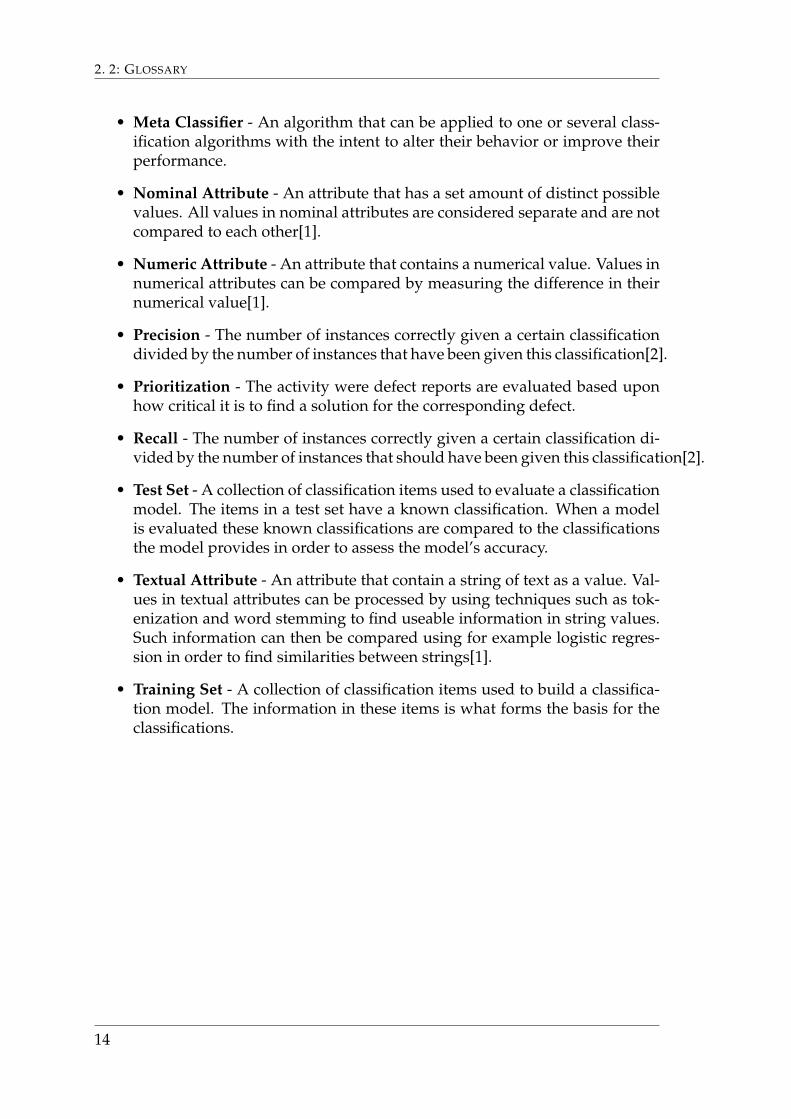
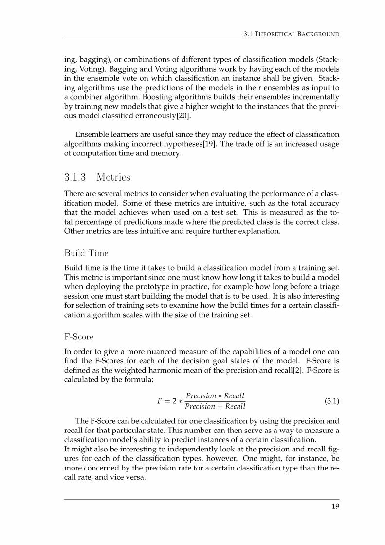
Decision trees are among the simplest, yet also among the most powerfultypes of classification models. Decision trees work by taking a vector of attributevalues as input and then performs a series of tests on these attributes and reachesa decision based upon their values. Each node in the decision tree represents atest upon an attribute. Each classification is performed by performing the test atthe top of the tree and then moving down to the child node that corresponds tothe result of the test. Each leaf node is labeled by a decision value and when aleaf node is reached that value will be the given classification[17]. One examplesof a decision tree is shown in Figure 3.1
16
3.1 THEORETICAL BACKGROUND
Decision trees are built by examining the patterns (such as the informationgain of the attributes, see Section 3.1.3) in a set of training data and then use somesome algorithm to create a tree that will be a good representation of these pat-terns. These algorithms will aim at creating the tree that most accurately repre-sents the training data while also being as small as possible. Since it is unfeasibleto test all possible trees that could be created from a set, a greedy strategy willtypically be used to create the tree. For example, in the ID3 algorithm the at-tribute that is most important (i.e. the one that has the highest correlation with aclassification value) is tested first, then for each of the children the most impor-tant attribute for the data with the child’s value is tested. This process continuesuntil the entire tree is built[17].Decision trees have the advantage of being very simple to understand and vi-sualize and are also capable of handling large amounts of data, without expo-nential growth in time or memory requirements[8]. They are however prone tooverfitting[17]. When a decision tree is built using large amounts of data there isa large risk that the algorithm that builds the decision tree will find patterns thatare not relevant and use them to build very large trees that often make erroneouspredictions. Decision tree pruning is sometimes used as a way to combat overfit-ting in decision trees[17].
Common decision tree algorithms include ID3, C4.5 a.k.a. J48, Reduced ErrorPruning (REP) trees, Alternating Decision (AD) Trees, Random Tree and RandomForest .
Figure 3.1: Image showing an example decision tree. Theleaves of the tree determine the classification.
17
3. 3: BACKGROUND AND RELATED WORK
Support Vector Machines
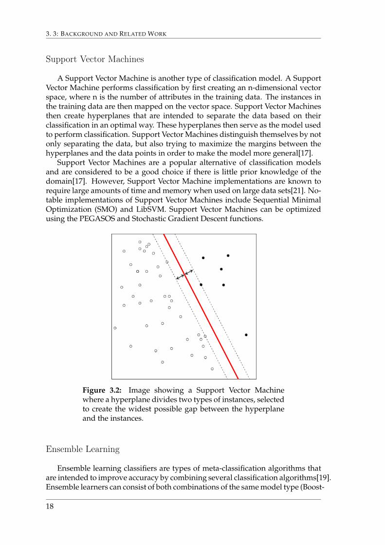
A Support Vector Machine is another type of classification model. A SupportVector Machine performs classification by first creating an n-dimensional vectorspace, where n is the number of attributes in the training data. The instances inthe training data are then mapped on the vector space. Support Vector Machinesthen create hyperplanes that are intended to separate the data based on theirclassification in an optimal way. These hyperplanes then serve as the model usedto perform classification. Support Vector Machines distinguish themselves by notonly separating the data, but also trying to maximize the margins between thehyperplanes and the data points in order to make the model more general[17].
Support Vector Machines are a popular alternative of classification modelsand are considered to be a good choice if there is little prior knowledge of thedomain[17]. However, Support Vector Machine implementations are known torequire large amounts of time and memory when used on large data sets[21]. No-table implementations of Support Vector Machines include Sequential MinimalOptimization (SMO) and LibSVM. Support Vector Machines can be optimizedusing the PEGASOS and Stochastic Gradient Descent functions.
Figure 3.2: Image showing a Support Vector Machinewhere a hyperplane divides two types of instances, selectedto create the widest possible gap between the hyperplaneand the instances.
Ensemble Learning
Ensemble learning classifiers are types of meta-classification algorithms thatare intended to improve accuracy by combining several classification algorithms[19].Ensemble learners can consist of both combinations of the same model type (Boost-
18
3.1 THEORETICAL BACKGROUND
ing, bagging), or combinations of different types of classification models (Stack-ing, Voting). Bagging and Voting algorithms work by having each of the modelsin the ensemble vote on which classification an instance shall be given. Stack-ing algorithms use the predictions of the models in their ensembles as input toa combiner algorithm. Boosting algorithms builds their ensembles incrementallyby training new models that give a higher weight to the instances that the previ-ous model classified erroneously[20].
Ensemble learners are useful since they may reduce the effect of classificationalgorithms making incorrect hypotheses[19]. The trade off is an increased usageof computation time and memory.
3.1.3 MetricsThere are several metrics to consider when evaluating the performance of a class-ification model. Some of these metrics are intuitive, such as the total accuracythat the model achieves when used on a test set. This is measured as the to-tal percentage of predictions made where the predicted class is the correct class.Other metrics are less intuitive and require further explanation.
Build TimeBuild time is the time it takes to build a classification model from a training set.This metric is important since one must know how long it takes to build a modelwhen deploying the prototype in practice, for example how long before a triagesession one must start building the model that is to be used. It is also interestingfor selection of training sets to examine how the build times for a certain classifi-cation algorithm scales with the size of the training set.
F-ScoreIn order to give a more nuanced measure of the capabilities of a model one canfind the F-Scores for each of the decision goal states of the model. F-Score isdefined as the weighted harmonic mean of the precision and recall[2]. F-Score iscalculated by the formula:
F = 2 ∗ Precision ∗ RecallPrecision + Recall
(3.1)
The F-Score can be calculated for one classification by using the precision andrecall for that particular state. This number can then serve as a way to measure aclassification model’s ability to predict instances of a certain classification.It might also be interesting to independently look at the precision and recall fig-ures for each of the classification types, however. One might, for instance, bemore concerned by the precision rate for a certain classification type than the re-call rate, and vice versa.
19

3. 3: BACKGROUND AND RELATED WORK
Information GainInformation gain is a measure of the correlation between two quantities[9]. Inmachine learning, this value can be used to measure how the value of an attributecorrelates with a classification. In other words the information gain is a measureof how much an attribute influences a classification. This value is used both indeciding how classification models should be built and when selecting whichattributes that should be used to build classification models.
3.2 Case DescriptionThe work was carried out at Sony Mobile Communications in Lund, Sweden be-tween October 2013 and April 2014. A Defect Management System, called DMS,to store defect reports regarding defects found in their products and use them todetermine which defects they should fix in their products is used.
The defect reports in this system contain attributes and textual data whichcontains information about the defect. Example attributes are at which activ-ity the defect was discovered and in which version of the software the defectis found. These attributes are meant to help developers analyze and prioritizewhich defects should be fixed first. The procedure for doing this depends onwhat phase a particular project is in.
During the first phase of development, depicted in Figure 3.3 when a defectreport enters the system it is analyzed by the first recipient1 and categorized. Thedefect report is then either sent to a third party developer or fixed internally bysending it to a pool of developers, depending on which part of the system is af-fected. The decision of which defects that are critical is made by the developersthemselves. The developers choose which defect reports to fix out of the onesthey have received based on their own priority and risk assessment.
Figure 3.3: How defect reports are handled in the first phaseof development
As time progresses, it becomes increasingly crucial to only fix the defects thatare blocking defects, meaning they block progress from being made. To achieve
1The first recipient is either the owner of the area the defect was found in or the contact personto the customer that found the defect, depending on whether the defect was found internally orexternally.
20
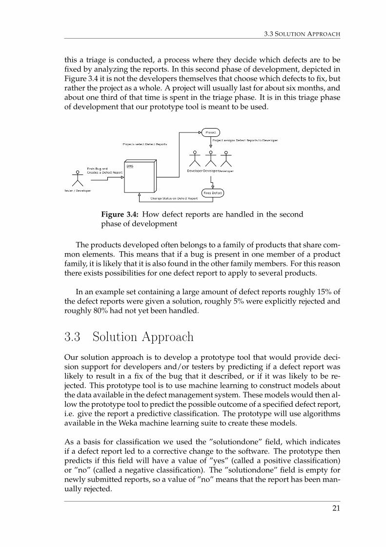
3.3 SOLUTION APPROACH
this a triage is conducted, a process where they decide which defects are to befixed by analyzing the reports. In this second phase of development, depicted inFigure 3.4 it is not the developers themselves that choose which defects to fix, butrather the project as a whole. A project will usually last for about six months, andabout one third of that time is spent in the triage phase. It is in this triage phaseof development that our prototype tool is meant to be used.
Figure 3.4: How defect reports are handled in the secondphase of development
The products developed often belongs to a family of products that share com-mon elements. This means that if a bug is present in one member of a productfamily, it is likely that it is also found in the other family members. For this reasonthere exists possibilities for one defect report to apply to several products.
In an example set containing a large amount of defect reports roughly 15% ofthe defect reports were given a solution, roughly 5% were explicitly rejected androughly 80% had not yet been handled.
3.3 Solution ApproachOur solution approach is to develop a prototype tool that would provide deci-sion support for developers and/or testers by predicting if a defect report waslikely to result in a fix of the bug that it described, or if it was likely to be re-jected. This prototype tool is to use machine learning to construct models aboutthe data available in the defect management system. These models would then al-low the prototype tool to predict the possible outcome of a specified defect report,i.e. give the report a predictive classification. The prototype will use algorithmsavailable in the Weka machine learning suite to create these models.
As a basis for classification we used the ”solutiondone” field, which indicatesif a defect report led to a corrective change to the software. The prototype thenpredicts if this field will have a value of ”yes” (called a positive classification)or ”no” (called a negative classification). The ”solutiondone” field is empty fornewly submitted reports, so a value of ”no” means that the report has been man-ually rejected.
21
3. 3: BACKGROUND AND RELATED WORK
3.4 Related WorkNaidu and Geethanjali[11] have built a system that groups defects into categoriescorresponding to how critical the defects are. They analyzed the results of soft-ware tests and based on the results and built a classifier using the ID3 classifica-tion algorithm that predicts the severity of a defect. The classifier is built basedon information about defects such as effort estimations and the size of the pro-gram. They then evaluate the performance of this classifier using metrics suchas accuracy and precision. This thesis expands on this study by using informa-tion in defect reports to classify defects, and examines several dimensions suchas training set size and time locality in order to find the optimal configuration foraccurately classifying defects.
Runesson, Alexandersson and Nyholm[15] have developed a system that de-tects duplicate defect reports by using textual classification to find defect reportsthat are similar to one and other. They describe the life cycle of the defect reportand give an in depth explanation of how to process textual data with natural lan-guage processing techniques. They also performed a case study at Sony EricssonMobile Communications and presented their findings, which measured how wella classifier could identify the defect reports that were known to be duplicates.This thesis similarly examines the use textual information in defect reports, inorder to evaluate if this information can be used to determine if a defect will begiven a solution or not.
Anvik [7] has developed a tool that provides automatic recommendations forhow defect reports should be handled in the triage process. One of these possiblerecommendations is prediction of the end state of defect reports using machinelearning. He has also described how attribute and algorithm selection was per-formed in order to develop this tool, and presents the precision and recall ratesthat the tool can achieve when used to classify defect reports in several open-source projects. This thesis expands on this work by examining the performanceof additional classification algorithms when used to classify defect reports, andalso examines the effect of changing the proportion of positively versus nega-tively classified defect reports in the training data, as well as examining if us-ing only textual attributes, only nominal attributes, or combinations of the typesyields the best performance.
Jonsson [10] has performed a study of classifying defect reports. It builds onthe work of Anvik[7], among others, and attempts to improve the classificationof defect reports using the Stacked Generalization ensemble learning algorithm.Find a set of useful classification algorithms available in the Weka frameworkand then evaluates how using Stacked Generalization affects the performance.He also performs an evaluation on how performing the classification across dif-ferent projects and different timeframes affects the performance. This thesis usesa selection of different ensemble learning methods in a similar way to evaluateif they can be used to improve the performance of a classifier trained to classify
22

3.4 RELATED WORK
defect reports.
Menzies and Marcus [12] have developed an automated method of assessingseverity levels of defect reports. The automated method, known as SEVERIS, useseveral natural language processing techniques to process textual informationpresent in five sets of defect reports produced at NASA. This method mainly usetextual attributes and only use one machine learning algorithm based on rulesto predict severity levels. This thesis also use textual attributes but evaluatesseveral classification algorithms. A prototype tool is also developed as a part ofthis thesis work, which contains capabilities similar to SEVERIS.
23

3. 3: BACKGROUND AND RELATED WORK
24

Chapter 4
Method
4.1 Research GoalsThis project aims to fulfill the following goals:
1. To investigate what useful information that can be extracted from the exist-ing databases at Sony and what uses this information can have.
2. To find a method of prioritizing defect reports with the help of MachineLearning to be used as decision support in the prioritization process.
3. To develop a prototype, building on previous work in Language Technol-ogy and Artificial Intelligence, which will provide decision support for de-velopers on what action to take when presented with an defect report, basedon historic data.
4. To conduct a large-scale evaluation of the developed prototype in a realisticsetting.
4.2 Research MethodThe work involved in the thesis was divided into three different stages. Thesestages were:
• Gain Domain Knowledge
• Develop a Prototype Tool
• Prototype Tool Configuration Evaluation
These stages are briefly described below. Prototype Tool Configuration Evalua-tion has its own, more in depth section in Section 4.3.
25
4. 4: METHOD
4.2.1 Gain Domain KnowledgeOne of our first goals was to gain some domain knowledge about the contextthat the prototype tool was to be used in. This involved examining the defectreport database for information that could potentially be used as attributes whentraining a classifier and to determine at which point in time in the developmentprocess the tool was intended to be used in. This was to done fulfill the goal 2outlined in the Goal Formulation.
4.2.2 Develop a Prototype ToolWe will develop a prototype tool with capabilities to retrieve defect reports andsave them in an appropriate format, train a classifier from defect reports andclassify defect reports using the trained classifier. This tool would mainly be usedto examine the data existent in the defect reports database, but also serve as anexample and a foundation for further development. This would partly fulfill goal1 and fulfill goals 3 and 4 outlined in the Goal Formulation.
4.2.3 Prototype Tool Configuration EvaluationWe will also perform an evaluation of different configurations that can be usedwith the prototype tool. This is to give an estimate of how well it performs andhelps determine the feasibility of using such a prototype tool in this context. Thiswas to partly fulfill goal 1 outlined in the Goal Formulation.
4.3 Evaluation MethodAn evaluation was carried out to assess and increase the accuracy (percentageof correctly classified defect reports) and training time (time it takes to train theclassifier) of the prototype tool. The most important quality aspects are accuracyand training time.
One purpose was to know which combination of attributes yields the best re-sults and was logically sound to use. Reducing the attributes used by eliminat-ing attributes that would not provide any useful information would also reducememory usage and training time by providing the algorithms with fewer vari-ables to process.
We also examined how the accuracy of the prototype tool was dependent onother variables. These evaluations were performed in a sequential order, wherethe best results from one step were used in the next. These variables were whichclassification algorithm we should use and the nature of the set of defect reportsused to build the classifier. The purpose was to find the algorithms that pro-vided both good training time and high accuracy. Similarly we intended to find
26

4.3 EVALUATION METHOD
at which amount of defect reports, used to build the classifier, the classifier pro-vided good accuracy without too large negative effect on the training time. Thetime frame from which the defect reports were fetched was also examined, in or-der to assess what impact moving the timeframe had on the accuracy. Finally wetested how the proportion of defect reports with a known positive classificationrelative a negative classification affected the accuracy. We also used this in or-der to find how the change in proportion affected the prototype tool’s ability toclassify both positive and negative instances. We also tried to apply these con-figurations to a set were no textual attributes were used to see how accurate aclassifier only built on nominal and numerical attributes were.Lastly we combined several classifiers to see if they would provide better accu-racy together.
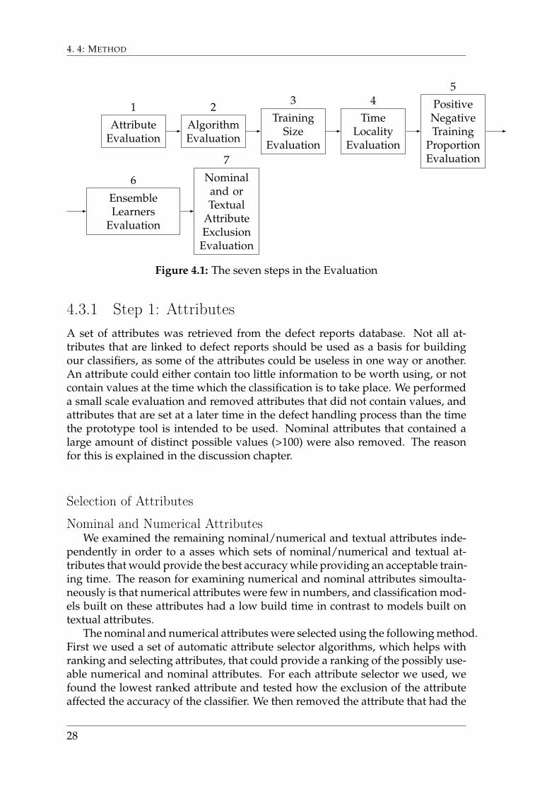
An overview of our evaluation method is presented in Figure 4.1. We con-ducted the evaluation in seven steps:
1. Determine to which degree text attributes and nominal attributes combinedcan be used to construct classifiers to be used in our prototype tool anddetermine the set of attributes that we use in the later tests.
2. Evaluate several algorithms that build classifiers and choose a set of themost promising ones.
3. Evaluate the effect of the size of the training set on the accuracy of the class-ification models.
4. Evaluate the effect of the time locality on the accuracy of the classificationmodels.
5. Evaluate the effect of the the proportion of negative defect reports versuspositive defect reports on the accuracy of the classification models.
6. Train ensemble learners to evaluate the combination of several classifiers.
7. Examine the difference in accuracy with classification models built on onlynominal/numerical attributes versus those built on textual attributes.
8. Determine how the accuracy and training time is affected when substan-tially larger training set are used with only nominal attributes.
27
4. 4: METHOD
AttributeEvaluation
1
AlgorithmEvaluation
2Training
SizeEvaluation
3
TimeLocality
Evaluation
4 PositiveNegativeTraining
ProportionEvaluation
5
EnsembleLearners
Evaluation
6 Nominaland orTextual
AttributeExclusion
Evaluation
7
Figure 4.1: The seven steps in the Evaluation
4.3.1 Step 1: AttributesA set of attributes was retrieved from the defect reports database. Not all at-tributes that are linked to defect reports should be used as a basis for buildingour classifiers, as some of the attributes could be useless in one way or another.An attribute could either contain too little information to be worth using, or notcontain values at the time which the classification is to take place. We performeda small scale evaluation and removed attributes that did not contain values, andattributes that are set at a later time in the defect handling process than the timethe prototype tool is intended to be used. Nominal attributes that contained alarge amount of distinct possible values (>100) were also removed. The reasonfor this is explained in the discussion chapter.
Selection of Attributes
Nominal and Numerical AttributesWe examined the remaining nominal/numerical and textual attributes inde-
pendently in order to a asses which sets of nominal/numerical and textual at-tributes that would provide the best accuracy while providing an acceptable train-ing time. The reason for examining numerical and nominal attributes simoulta-neously is that numerical attributes were few in numbers, and classification mod-els built on these attributes had a low build time in contrast to models built ontextual attributes.
The nominal and numerical attributes were selected using the following method.First we used a set of automatic attribute selector algorithms, which helps withranking and selecting attributes, that could provide a ranking of the possibly use-able numerical and nominal attributes. For each attribute selector we used, wefound the lowest ranked attribute and tested how the exclusion of the attributeaffected the accuracy of the classifier. We then removed the attribute that had the
28

4.3 EVALUATION METHOD
smallest negative effect on our accuracy from our set of attributes. This processcontinued incrementally until no attributes remained in the set. We then selectedthe configuration of attributes that yielded the highest accuracy. This process isillustrated in Figure 4.3
Other discarded attributes contained duplicated information, as well as at-tributes related to time such as submit dates. The reason for this is explainedin the discussion chapter. We also had to discard some attributes at the requestof Sony, as the use of these attributes was considered unethical, for example, at-tributes related to individual developers. All the remaining attributes were fur-ther evaluated for how they affected the accuracy of the prototype tool using theattribute selection algorithms.The intent was to find a set of attributes that provides the best accuracy of the pro-totype tool. The contribution of an attribute was measured by metrics providedby the use of attribute selector algorithms. These algorithms output the informa-tion gain, or other metrics used in a similar fashion, provided by the attribute.
The following attribute evaluators were used as a basis for the attribute selec-tion:
1. Chi Squared Attribute Evaluator
2. Gain Ratio Attribute Evaluator
3. Information Gain Attribute Evaluator
4. OneR Attribute Evaluator
5. Symmetrical Uncertainty Attribute Evaluator
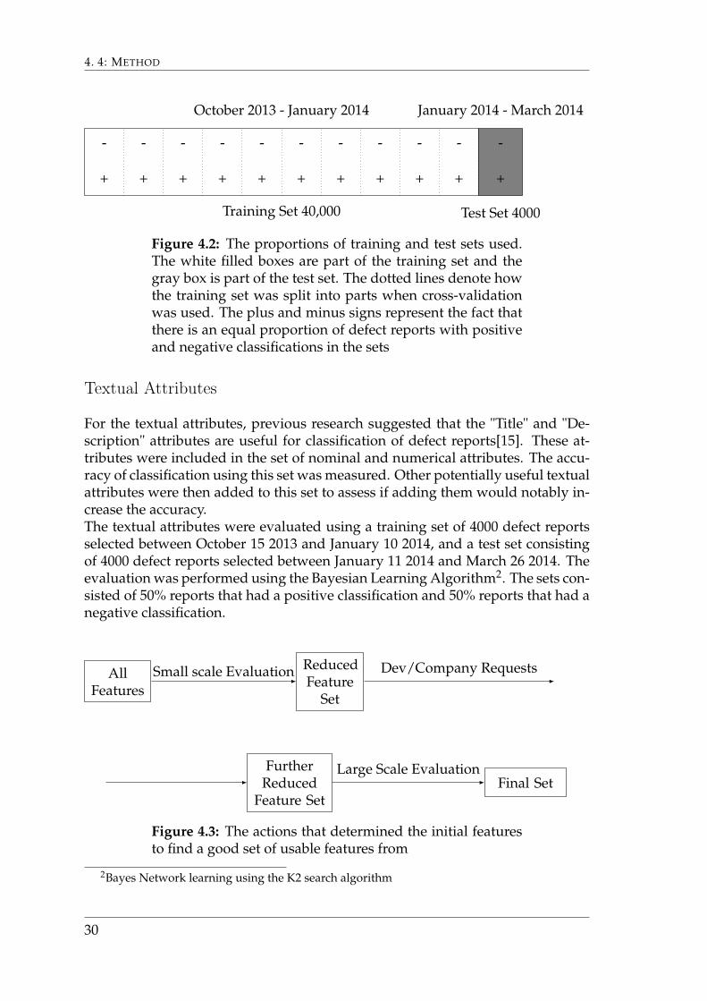
The attribute selections were evaluated using a Bayesian Learning classifica-tion algorithm1. The nominal and numerical attribute selection were performedusing a training set of 40,000 defect reports, and a test set of 40,000 defect reports.The training set was selected from defect reports submitted between October 152013 and January 10 2014, the test set was selected from defect reports submittedbetween January 11 2014 and March 26 2014, as shown in Figure 4.2. The setsconsisted of 50% reports that had a positive classification and 50% reports thathad a negative classification. The defect report database was free to return anydefect report as long as these conditions were met.In all training and test sets we used, the database were free to return any de-fect reports as long as our conditions were met, meaning we did not ourselvesmanually select or filter the reports further.
1Bayes Network learning using the K2 search algorithm
29
4. 4: METHOD
+
-
+
-
+
-
+
-
+
-
+
-
+
-
+
-
+
-
+
-
+
-
October 2013 - January 2014 January 2014 - March 2014
Training Set 40,000 Test Set 4000
Figure 4.2: The proportions of training and test sets used.The white filled boxes are part of the training set and thegray box is part of the test set. The dotted lines denote howthe training set was split into parts when cross-validationwas used. The plus and minus signs represent the fact thatthere is an equal proportion of defect reports with positiveand negative classifications in the sets
Textual Attributes
For the textual attributes, previous research suggested that the "Title" and "De-scription" attributes are useful for classification of defect reports[15]. These at-tributes were included in the set of nominal and numerical attributes. The accu-racy of classification using this set was measured. Other potentially useful textualattributes were then added to this set to assess if adding them would notably in-crease the accuracy.The textual attributes were evaluated using a training set of 4000 defect reportsselected between October 15 2013 and January 10 2014, and a test set consistingof 4000 defect reports selected between January 11 2014 and March 26 2014. Theevaluation was performed using the Bayesian Learning Algorithm2. The sets con-sisted of 50% reports that had a positive classification and 50% reports that had anegative classification.
AllFeatures
ReducedFeature
Set
FurtherReduced
Feature SetFinal Set
Small scale Evaluation Dev/Company Requests
Large Scale Evaluation
Figure 4.3: The actions that determined the initial featuresto find a good set of usable features from
2Bayes Network learning using the K2 search algorithm
30

4.3 EVALUATION METHOD
4.3.2 Step 2: AlgorithmsAll classification algorithms in the Weka3 framework were evaluated for their ap-plicability, training time and accuracy for the prototype tool. The intent was tofind the algorithm that provided the best accuracy for this prototype tool. Al-gorithms that provided a poor accuracy or those that were not applicable to thistype of classification were discarded. The following algorithms were used in theevaluation.
• DecisionStump
• J48
• RandomForest
• RandomTree
• JRip
• ZeroR
• Logistic
• SGD
• SGDText
• BayesNet
• NaiveBayes
• NaiveBayesMultinominalText
• NaiveBayesUpdateable
• IBk
• ADTree
• DecisionTable
• OneR
• HyperPipes
• VFI
• SMO
• VotedPerceptron
3The tested algorithms were found in the Weka 3.7 and Weka 3.6 versions
31
4. 4: METHOD
• SPegasos
• RBFNetwork
• LibSVM
• REPTree
• Ridor
The algorithm selection was performed using a training set consisting of 4000defect reports selected between October 15 2013 and January 10 2014. The test setconsisted of 4000 defect reports selected between January 11 2014 and March 262014
The tests were performed using the attributes selected in step 1. All sets con-sisted of 50% reports that had a positive classification and 50% reports that hada negative classification. Evaluations were made using both 10-fold cross valida-tion and the corresponding test set. If a test of an algorithm took longer than 30minutes to complete the evaluation was stopped.
The initial algorithm evaluation produced a set of algorithms that were deemeduseful for further evaluation. Upon these algorithms we applied all of the avail-able so-called meta classification algorithms. These are algorithms intended toimprove the accuracy of a classification algorithm. The purpose was to evaluatewhether it was feasible to use meta classification algorithms during subsequentevaluations. All meta algorithm evaluations were performed using a test set eval-uation with the same training and test sets as the previous step in the evaluation.
4.3.3 Step 3: SizeThe effect the size of the training set had on accuracy was tested by first increasingthe size from 200 to 1800 in 200 report increments, then increasing the size from2000 defect reports up to either 24000 reports or to the point at which we use allour available memory (2GB). The increases in size were done cumulatively. Thepurpose of this test was to analyze which set size is the best one, both from anaccuracy and a time and memory consumption standpoint. This evaluation wasperformed using the top attributes and best performing algorithms previouslychosen in steps 1 and 2. The test were carried out using a sequestered test set.The test set consisted of 4000 defect reports selected between January 11 2014and March 26 2014. The training sets were selected between October 15 2013 andJanuary 10 2014. All sets consisted of 50% reports that had a positive classificationand 50% reports that had a negative classification.
32
4.3 EVALUATION METHOD
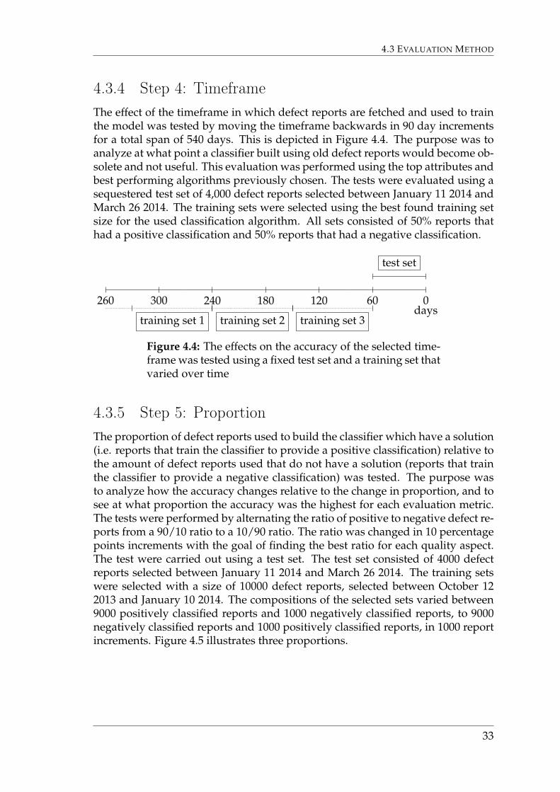
4.3.4 Step 4: TimeframeThe effect of the timeframe in which defect reports are fetched and used to trainthe model was tested by moving the timeframe backwards in 90 day incrementsfor a total span of 540 days. This is depicted in Figure 4.4. The purpose was toanalyze at what point a classifier built using old defect reports would become ob-solete and not useful. This evaluation was performed using the top attributes andbest performing algorithms previously chosen. The tests were evaluated using asequestered test set of 4,000 defect reports selected between January 11 2014 andMarch 26 2014. The training sets were selected using the best found training setsize for the used classification algorithm. All sets consisted of 50% reports thathad a positive classification and 50% reports that had a negative classification.
test set
training set 1 training set 2 training set 3
260 300 240 180 120 60days
0
Figure 4.4: The effects on the accuracy of the selected time-frame was tested using a fixed test set and a training set thatvaried over time
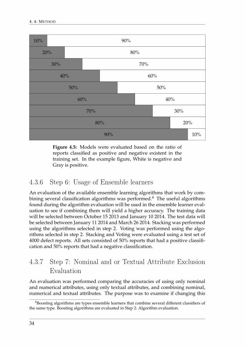
4.3.5 Step 5: ProportionThe proportion of defect reports used to build the classifier which have a solution(i.e. reports that train the classifier to provide a positive classification) relative tothe amount of defect reports used that do not have a solution (reports that trainthe classifier to provide a negative classification) was tested. The purpose wasto analyze how the accuracy changes relative to the change in proportion, and tosee at what proportion the accuracy was the highest for each evaluation metric.The tests were performed by alternating the ratio of positive to negative defect re-ports from a 90/10 ratio to a 10/90 ratio. The ratio was changed in 10 percentagepoints increments with the goal of finding the best ratio for each quality aspect.The test were carried out using a test set. The test set consisted of 4000 defectreports selected between January 11 2014 and March 26 2014. The training setswere selected with a size of 10000 defect reports, selected between October 122013 and January 10 2014. The compositions of the selected sets varied between9000 positively classified reports and 1000 negatively classified reports, to 9000negatively classified reports and 1000 positively classified reports, in 1000 reportincrements. Figure 4.5 illustrates three proportions.
33
4. 4: METHOD
10% 90%
20% 80%
30% 70%
40% 60%
50% 50%
60% 40%
70% 30%
80% 20%
90% 10%
Figure 4.5: Models were evaluated based on the ratio ofreports classified as positive and negative existent in thetraining set. In the example figure, White is negative andGray is positive.
4.3.6 Step 6: Usage of Ensemble learnersAn evaluation of the available ensemble learning algorithms that work by com-bining several classification algorithms was performed.4 The useful algorithmsfound during the algorithm evaluation will be used in the ensemble learner eval-uation to see if combining them will yield a higher accuracy. The training datawill be selected between October 15 2013 and January 10 2014. The test data willbe selected between January 11 2014 and March 26 2014. Stacking was performedusing the algorithms selected in step 2. Voting was performed using the algo-rithms selected in step 2. Stacking and Voting were evaluated using a test set of4000 defect reports. All sets consisted of 50% reports that had a positive classifi-cation and 50% reports that had a negative classification.
4.3.7 Step 7: Nominal and or Textual Attribute ExclusionEvaluation
An evaluation was performed comparing the accuracies of using only nominaland numerical attributes, using only textual attributes, and combining nominal,numerical and textual attributes. The purpose was to examine if changing this
4Boosting algorithms are types ensemble learners that combine several different classifiers ofthe same type. Boosting algorithms are evaluated in Step 2: Algorithm evaluation.
34
4.3 EVALUATION METHOD
composition could lead to an increase in accuracy.
Test 1 The first test compared the three compositions using a set consisted of4,000 defect reports selected between January 11 2014 and March 26 2014. Thetraining sets were selected with a size of 1000 defect reports up to 10000 defectreports in increments of 1000. The training sets were selected between October15 2013 and January 10 2014. All sets consisted of 50% reports that had a positiveclassification and 50% reports that had a negative classification. This test wasperformed using the one of the algorithms found in step 2.
Test 2 Afterwards another test was performed using only the nominal and nu-merical attributes, given that this composition has a smaller time and memoryrequirement and will therefore allow for the use of larger training sets. The testset consisted of 4,000 defect reports selected between January 11 2014 and March26 2014. The training sets were selected with a size of 10000 defect reports up to60000 defect reports in increments of 10000. The training sets were selected be-tween July 13 2013 and January 10 2014. All sets consisted of 50% reports that hada positive classification and 50% reports that had a negative classification. Thistest was performed using the algorithms selected in step 2.
4.3.8 Analysis of resultsTo evaluate the usefulness of an algorithm by simply checking the amount of cor-rectly classified defect reports in a test set, for example, is not sufficient since avery poor classifier could still receive a high accuracy score using this method.For example, if a test set consisted of 80% defect reports with a positive class-ification and 20% defect reports with a negative classification, a classifier whichonly gave a ”positive” classification, regardless of input, would still receive anaccuracy score of 80%.
35

4. 4: METHOD
36
Chapter 5
Prototype Tool Description
5.1 Prototype Tool DescriptionThe Prototype Tool that was developed has four distinct functions:
• Fetching of Training and Test Data
• Training of a Classifier
• Prediction of Data using a Classifier
• Evaluation of a Classifier
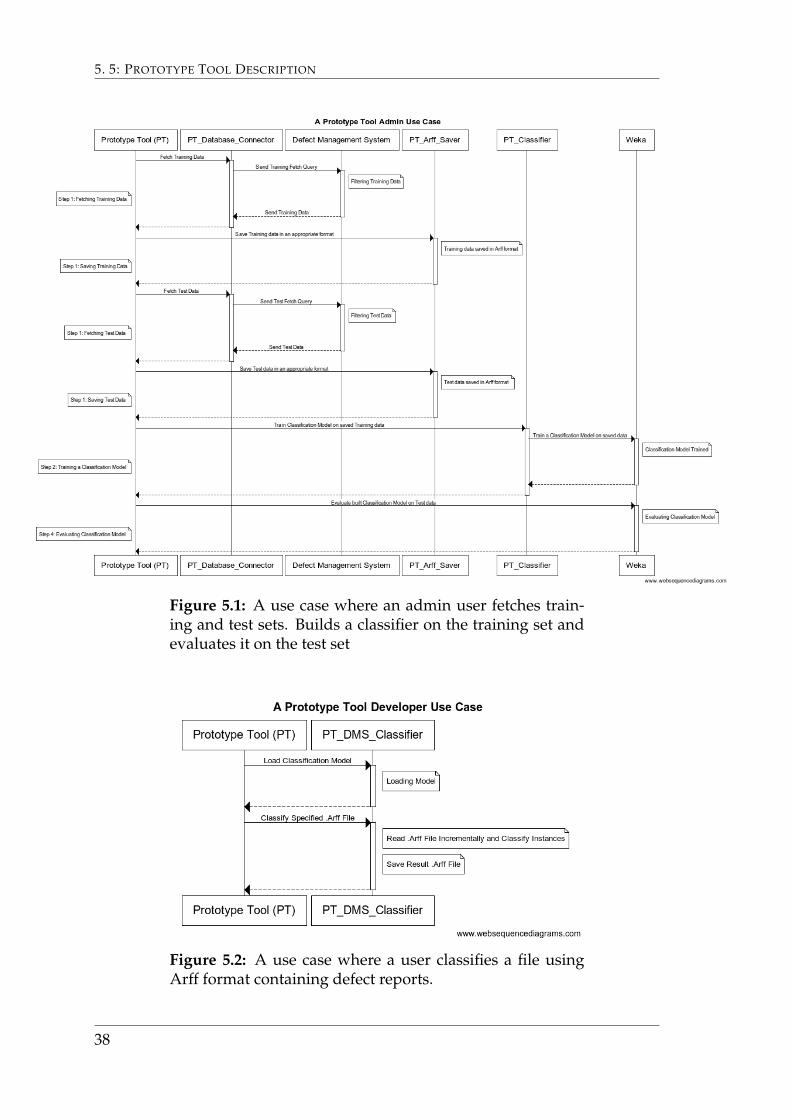
These functions will be further outlined in the subsections below, correspond-ing to each function. The prototype fetches data from an SQL database, savesthe data in the Arff formated file and uses the Weka machine learning softwareto build models and perform classifications using this data. A typical use casesequence diagram for an admin wanting to update the classification model isshown in Figure 5.1. Whilst a use case for a user in the possesion of defect re-ports stored in a file in using Arff format wanting to classify them is shown inFigure 5.2
37
5. 5: PROTOTYPE TOOL DESCRIPTION
Figure 5.1: A use case where an admin user fetches train-ing and test sets. Builds a classifier on the training set andevaluates it on the test set
Figure 5.2: A use case where a user classifies a file usingArff format containing defect reports.
38
5.1 PROTOTYPE TOOL DESCRIPTION
5.1.1 Step 1: Fetching of Training and Test DataThe Prototype Tool can fetch data using SQL-Queries specified in configurationfiles and store the results in an arff format. This format is readable by the machinelearning framework Weka. The data that is fetched is categorized into one of threedifferent categories. The categories are:
• Nominal
• Numerical
• String (Textual)
5.1.2 Step 2: Training of ClassifierThe Prototype Tool can train a classifier given training data. The classificationalgorithm can be specified to be one existent in the Weka framework or a customalgorithm. Options for these algorithms can also be specified in the configurationfile. The classifiers can also be stored and retrieved for later use.
5.1.3 Step 3: Prediction of Classification on Data using aClassifier
The Prototype Tool can also predict the classification of examples located in a file,formated as an Arff file, using a classifier. The predictions are stored as a separatefile.
5.1.4 Step 4: Evaluation of ClassifierThe Prototype Tool can apply a test set or use cross-validation to evaluate theperformance of a classifier.
39

5. 5: PROTOTYPE TOOL DESCRIPTION
40

Chapter 6
Results
6.1 Step 1. Attribute Evaluation
6.1.1 Nominal and Numerical attributesEach defect report contains 142 attributes that may have non-null values whenthe report is submitted. Out of these, 19 nominal and numerical attributes werefound that were suitable to use as a basis for classification. A classifier built usingthese attributes using the Bayesian Learning Model gave the accuracy 73.115%.
The final attribute rank was the following:
1. mastership - The site from which the report was submitted.
2. fix for - The milestone or release the defect should be solved for.
3. ratl mastership - The site from which the attached record for a certain branchwas submitted.
4. externalsupplier- The external supplier.
5. ratl keysite - Unknown
6. project - The project the report is associated with.
7. proj id - The id of project the report is associated with.
8. attachment share saved - Unknown
9. found during - The phase of the development cycle the report was foundduring.
41
6. 6: RESULTS
10. business priority - The business priority.
11. found in product - The product the defect was found in.
12. found by - The department or team that found the product.
13. abc rank - The ”abc” priority ranking given to the defect report.
14. detection - How often the defect is likely to be detected.
15. impact - The estimated impact of the defect remaining unsolved.
16. occurrence - How often the defect is likely to occur.
17. priority - The estimated priority of the defect report.
18. is platform - Unknown
19. qa state - The state of quality assurance.
Detailed results from this evaluation are found in Appendix A.1.1.
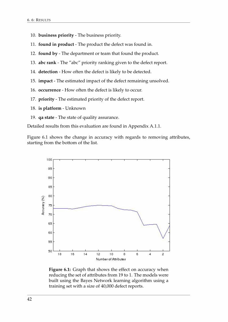
Figure 6.1 shows the change in accuracy with regards to removing attributes,starting from the bottom of the list.
Figure 6.1: Graph that shows the effect on accuracy whenreducing the set of attributes from 19 to 1. The models werebuilt using the Bayes Network learning algorithm using atraining set with a size of 40,000 defect reports.
42
6.2 STEP 2: ALGORITHM EVALUATION
The graph shows that removing the attributes has little effect until the seventhhighest ranked attribute is removed. The highest accuracy was found using thetwelve highest ranked nominal and numerical attributes. These attributes weretherefore used during further testing.
6.1.2 Textual attributesBelow follows a table that shows the effect of adding new textual attributes com-pared to only using ”title”, ”description” and the nominal attributes. The base-line contained the previously selected nominal and numerical attributes, as wellas the textual attributes ”title” and ”description”. The models were built usingthe Bayes Network learning algorithm with a training set of 4,000 defect reports.The other attributes were evaluated by adding them to the baseline.
Added Attribute F-Score Yes F-Score No AccuracyBaseline 0.704 0.300 58.375%Attachment History 0.705 0.309 58.7%Associated Branches 0.056 0.664 50.4%Consequence if not app 0.667 0.004 50.075%
Given that adding more textual attributes did not provide a significant increasein accuracy, and that textual attributes are known to greatly lower performance,it was decided that ”title” and ”description” should be the only textual attributesused.
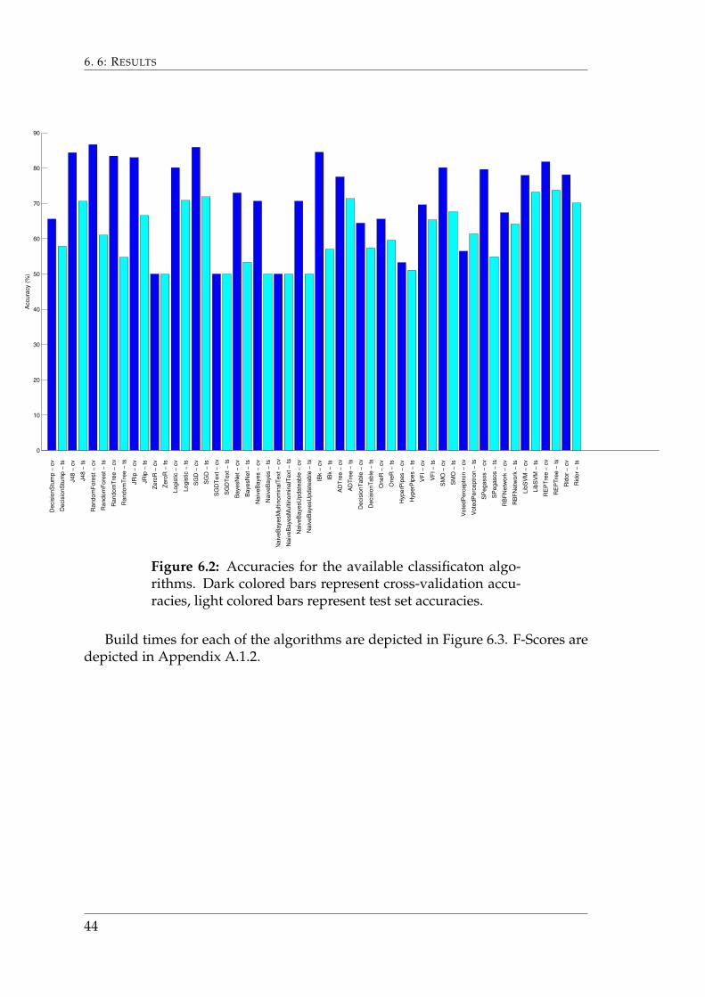
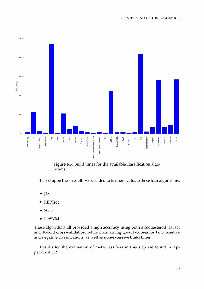
6.2 Step 2: Algorithm EvaluationFigure 6.2 describes the total accuracy of the 10-fold cross validation and test setvalidation for each classification algorithm. The algorithms that were discardeddue to their time and memory usage are listed in Appendix A.1.2.
One should note that the ZeroR algorithm will always simply return the mostcommon classification. The results of the ZeroR algorithm serve as a benchmarkthat is compared to the results of the other algorithms.
43
6. 6: RESULTS
0
10
20
30
40
50
60
70
80
90
De
cis
ionS
tum
p −
cv
Decis
ionS
tum
p −
ts
J48 −
cv
J48 −
ts
Random
Fore
st −
cv
Random
Fore
st −
ts
Random
Tre
e −
cv
Random
Tre
e −
ts
JR
ip −
cv
JR
ip −
ts
Zero
R −
cv
Zero
R −
ts
Logis
tic −
cv
Logis
tic −
ts
SG
D −
cv
SG
D −
ts
SG
DT
ext −
cv
SG
DT
ext −
ts
BayesN
et
− c
v
BayesN
et
− ts
Naiv
eB
ayes −
cv
Naiv
eB
ayes −
ts
Naiv
eB
ayesM
ultin
om
ina
lText −
cv
Naiv
eB
ayesM
ultin
om
inalT
ext −
ts
Naiv
eB
ayesU
pdate
able
− c
v
Naiv
eB
ayesU
pdate
able
− ts
IBk −
cv
IBk −
ts
AD
Tre
e −
cv
AD
Tre
e −
ts
Decis
ionT
able
− c
v
Decis
ionT
able
− ts
OneR
− c
v
OneR
− ts
HyperP
ipes −
cv
HyperP
ipe
s −
ts
VF
I −
cv
VF
I −
ts
SM
O −
cv
SM
O −
ts
Vote
dP
erc
eptr
on −
cv
Vote
dP
erc
eptr
on −
ts
SP
egasos −
cv
SP
egasos −
ts
RB
FN
etw
ork
− c
v
RB
FN
etw
ork
− ts
Lib
SV
M −
cv
Lib
SV
M −
ts
RE
PT
ree −
cv
RE
PT
ree −
ts
Rid
or
− c
v
Rid
or
− ts
Accura
cy (
%)
Figure 6.2: Accuracies for the available classificaton algo-rithms. Dark colored bars represent cross-validation accu-racies, light colored bars represent test set accuracies.
Build times for each of the algorithms are depicted in Figure 6.3. F-Scores aredepicted in Appendix A.1.2.
44
6.2 STEP 2: ALGORITHM EVALUATION
0
50
100
150
200
250
Decis
ionS
tum
p
J48
Random
Fore
st
Random
Tre
e
JR
ip
Zero
R
Logis
tic
SG
D
SG
DT
ext
BayesN
et
Naiv
eB
ayes
Na
iveB
ayesM
ultin
om
inalT
ext
Naiv
eB
ayesU
pdate
able
IBk
AD
Tre
e
Decis
ion
Table
OneR
Hype
rPip
es
VF
I
SM
O
Vote
dP
erc
eptr
on
SP
egasos
RB
FN
etw
ork
Lib
SV
M
RE
PT
ree
Rid
or
Build
Tim
e (
S)
Figure 6.3: Build times for the available classification algo-rithms
Based upon these results we decided to further evaluate these four algorithms;
• J48
• REPTree
• SGD
• LibSVM
These algorithms all provided a high accuracy using both a sequestered test setand 10-fold cross-validation, while maintaining good F-Scores for both positiveand negative classifications, as well as non-excessive build times.
Results for the evaluation of meta-classifiers in this step are found in Ap-pendix A.1.2.
45
6. 6: RESULTS
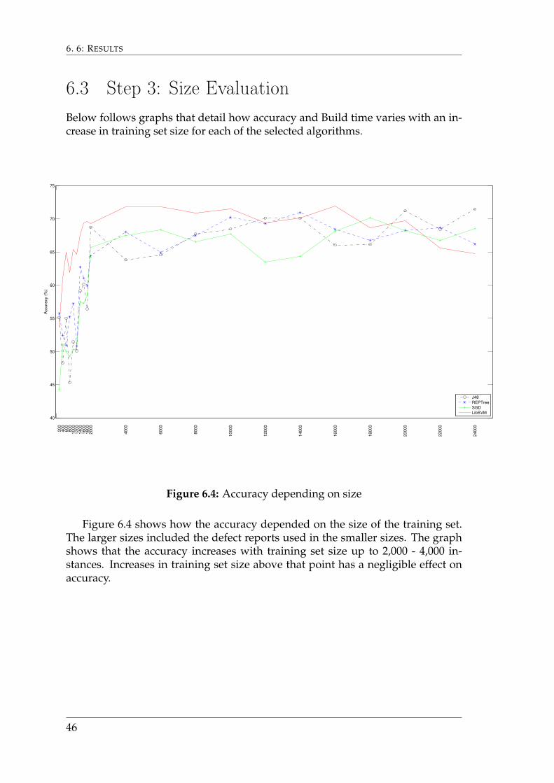
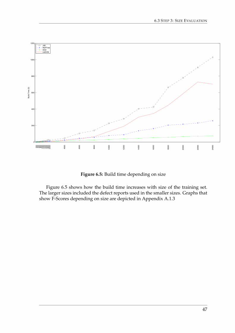
6.3 Step 3: Size EvaluationBelow follows graphs that detail how accuracy and Build time varies with an in-crease in training set size for each of the selected algorithms.
40
45
50
55
60
65
70
75
Accura
cy (
%)
200
400
600
800
10
00
12
00
14
00
16
00
18
00
20
00
40
00
60
00
80
00
10
000
12
000
14
000
16
000
18
000
20
000
22
000
24
000
J48
REPTree
SGD
LibSVM
Figure 6.4: Accuracy depending on size
Figure 6.4 shows how the accuracy depended on the size of the training set.The larger sizes included the defect reports used in the smaller sizes. The graphshows that the accuracy increases with training set size up to 2,000 - 4,000 in-stances. Increases in training set size above that point has a negligible effect onaccuracy.
46
6.3 STEP 3: SIZE EVALUATION
0
200
400
600
800
1000
1200
Bu
ild T
ime (
S)
200
400
600
800
10
00
12
00
14
00
16
00
18
00
20
00
40
00
60
00
80
00
10
000
12
000
14
000
16
000
18
000
20
000
22
000
24
000
J48
REPTree
SGD
LibSVM
Figure 6.5: Build time depending on size
Figure 6.5 shows how the build time increases with size of the training set.The larger sizes included the defect reports used in the smaller sizes. Graphs thatshow F-Scores depending on size are depicted in Appendix A.1.3
47
6. 6: RESULTS
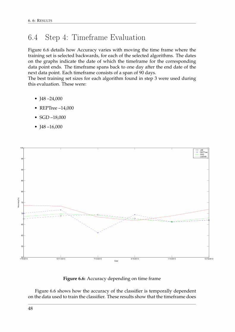
6.4 Step 4: Timeframe EvaluationFigure 6.6 details how Accuracy varies with moving the time frame where thetraining set is selected backwards, for each of the selected algorithms. The dateson the graphs indicate the date of which the timeframe for the correspondingdata point ends. The timeframe spans back to one day after the end date of thenext data point. Each timeframe consists of a span of 90 days.The best training set sizes for each algorithm found in step 3 were used duringthis evaluation. These were:
• J48 –24,000
• REPTree –14,000
• SGD –18,000
• J48 –16,000
1/10/2014 10/11/2013 7/13/2013 4/15/2013 1/14/2013 10/16/201250
55
60
65
70
75
80
85
90
95
100
Date
Accura
cy(%
)
J48
REPTree
SGD
LibSVM
Figure 6.6: Accuracy depending on time frame
Figure 6.6 shows how the accuracy of the classifier is temporally dependenton the data used to train the classifier. These results show that the timeframe does
48

6.4 STEP 4: TIMEFRAME EVALUATION
not significantly affect the accuracy. Graphs that show F-Scores and Build timesdepending on time locality are depicted in Appendix A.1.4
49
6. 6: RESULTS
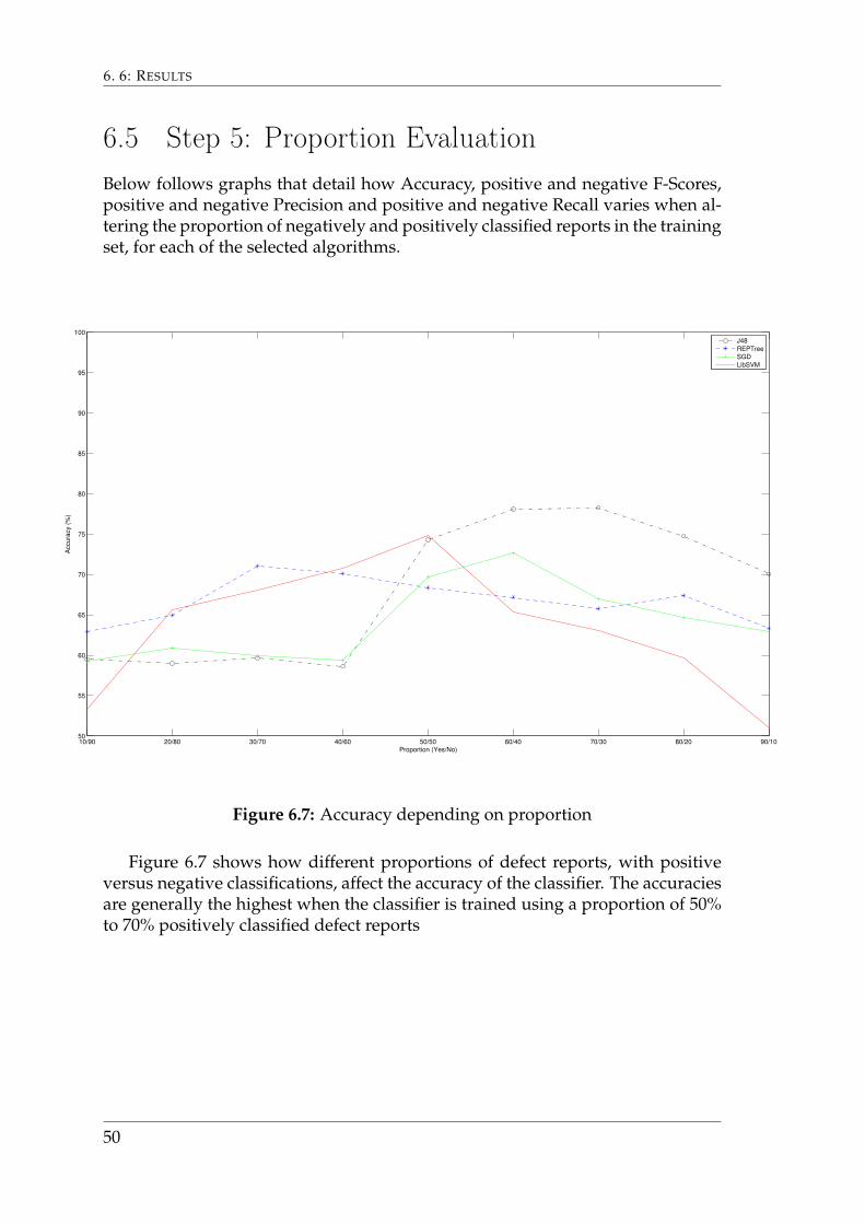
6.5 Step 5: Proportion EvaluationBelow follows graphs that detail how Accuracy, positive and negative F-Scores,positive and negative Precision and positive and negative Recall varies when al-tering the proportion of negatively and positively classified reports in the trainingset, for each of the selected algorithms.
10/90 20/80 30/70 40/60 50/50 60/40 70/30 80/20 90/1050
55
60
65
70
75
80
85
90
95
100
Proportion (Yes/No)
Accura
cy (
%)
J48
REPTree
SGD
LibSVM
Figure 6.7: Accuracy depending on proportion
Figure 6.7 shows how different proportions of defect reports, with positiveversus negative classifications, affect the accuracy of the classifier. The accuraciesare generally the highest when the classifier is trained using a proportion of 50%to 70% positively classified defect reports
50
6.5 STEP 5: PROPORTION EVALUATION
10/90 20/80 30/70 40/60 50/50 60/40 70/30 80/20 90/100
0.1
0.2
0.3
0.4
0.5
0.6
0.7
0.8
0.9
1
Proportion (Yes/No)
FS
co
re
J48
REPTree
SGD
LibSVM
Figure 6.8: F-Score for positive classification depending onproportion
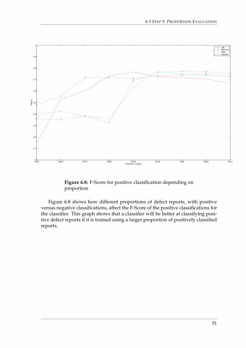
Figure 6.8 shows how different proportions of defect reports, with positiveversus negative classifications, affect the F-Score of the positive classifications forthe classifier. This graph shows that a classifier will be better at classifying posi-tive defect reports if it is trained using a larger proportion of positively classifiedreports.
51
6. 6: RESULTS
10/90 20/80 30/70 40/60 50/50 60/40 70/30 80/20 90/100
0.1
0.2
0.3
0.4
0.5
0.6
0.7
0.8
0.9
1
Proportion (Yes/No)
FS
co
re
J48
REPTree
SGD
LibSVM
Figure 6.9: F-Score for negative classification depending onproportion
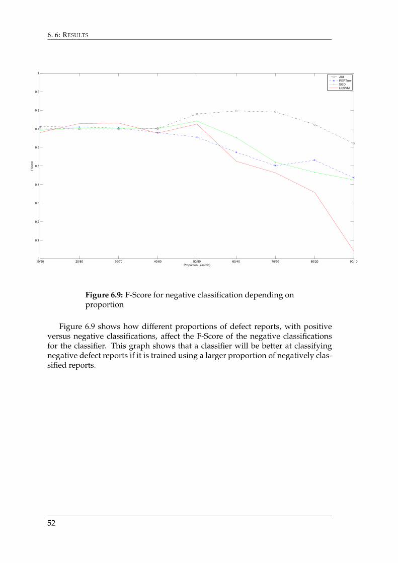
Figure 6.9 shows how different proportions of defect reports, with positiveversus negative classifications, affect the F-Score of the negative classificationsfor the classifier. This graph shows that a classifier will be better at classifyingnegative defect reports if it is trained using a larger proportion of negatively clas-sified reports.
52
6.5 STEP 5: PROPORTION EVALUATION
10/90 20/80 30/70 40/60 50/50 60/40 70/30 80/20 90/100
0.1
0.2
0.3
0.4
0.5
0.6
0.7
0.8
0.9
1
Proportion (Yes/No)
Pre
cis
ion
J48
REPTree
SGD
LibSVM
Figure 6.10: Precision for positive classification dependingon proportion
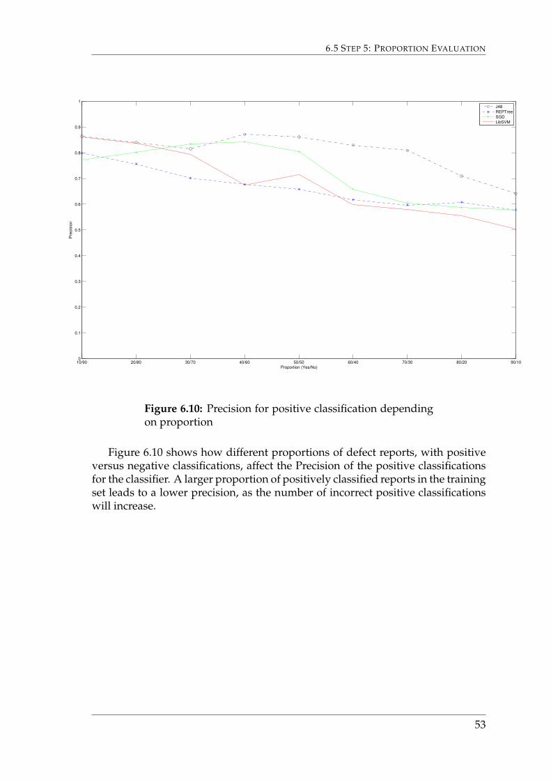
Figure 6.10 shows how different proportions of defect reports, with positiveversus negative classifications, affect the Precision of the positive classificationsfor the classifier. A larger proportion of positively classified reports in the trainingset leads to a lower precision, as the number of incorrect positive classificationswill increase.
53
6. 6: RESULTS
10/90 20/80 30/70 40/60 50/50 60/40 70/30 80/20 90/100
0.1
0.2
0.3
0.4
0.5
0.6
0.7
0.8
0.9
1
Proportion (Yes/No)
Pre
cis
ion
J48
REPTree
SGD
LibSVM
Figure 6.11: Precision for negative classification dependingon proportion
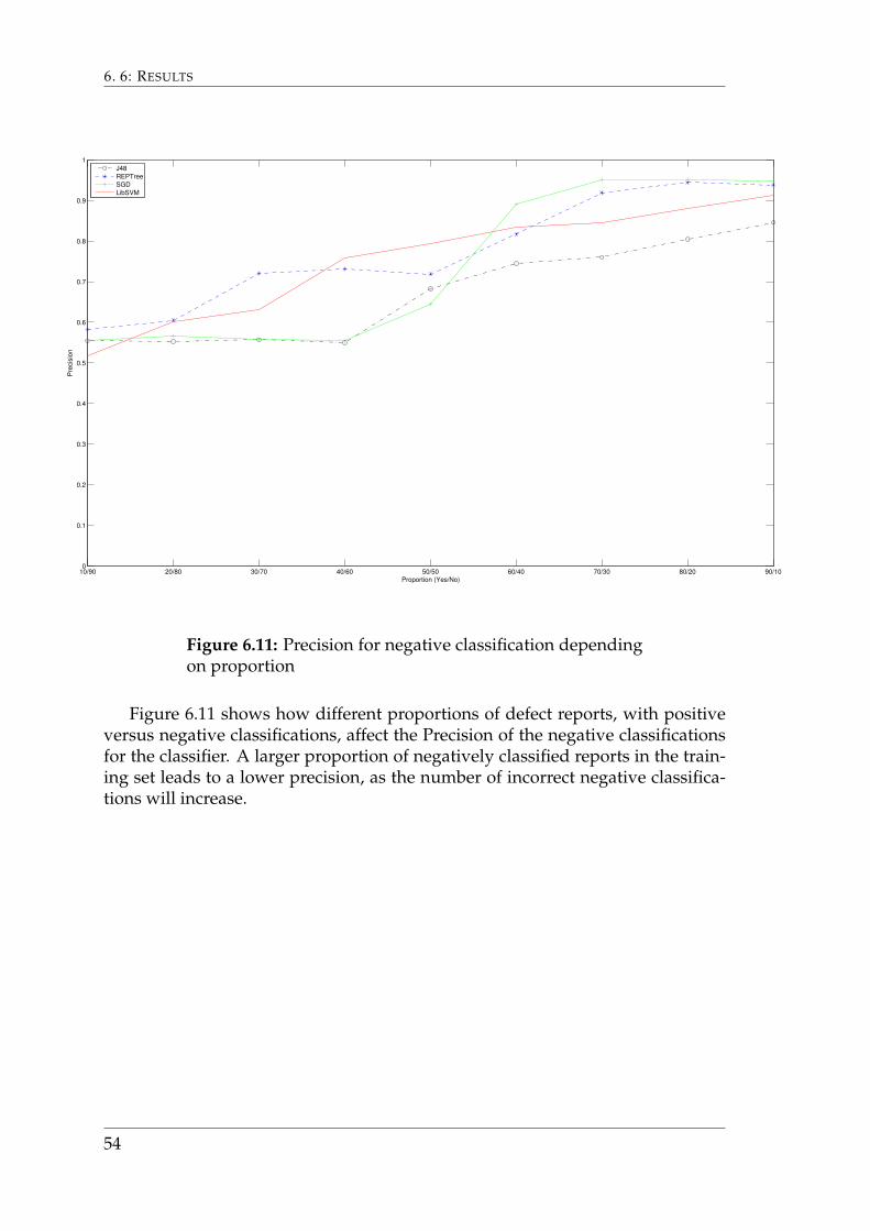
Figure 6.11 shows how different proportions of defect reports, with positiveversus negative classifications, affect the Precision of the negative classificationsfor the classifier. A larger proportion of negatively classified reports in the train-ing set leads to a lower precision, as the number of incorrect negative classifica-tions will increase.
54
6.5 STEP 5: PROPORTION EVALUATION
10/90 20/80 30/70 40/60 50/50 60/40 70/30 80/20 90/100
0.1
0.2
0.3
0.4
0.5
0.6
0.7
0.8
0.9
1
Proportion (Yes/No)
Re
ca
ll
J48
REPTree
SGD
LibSVM
Figure 6.12: Recall for positive classification depending onproportion
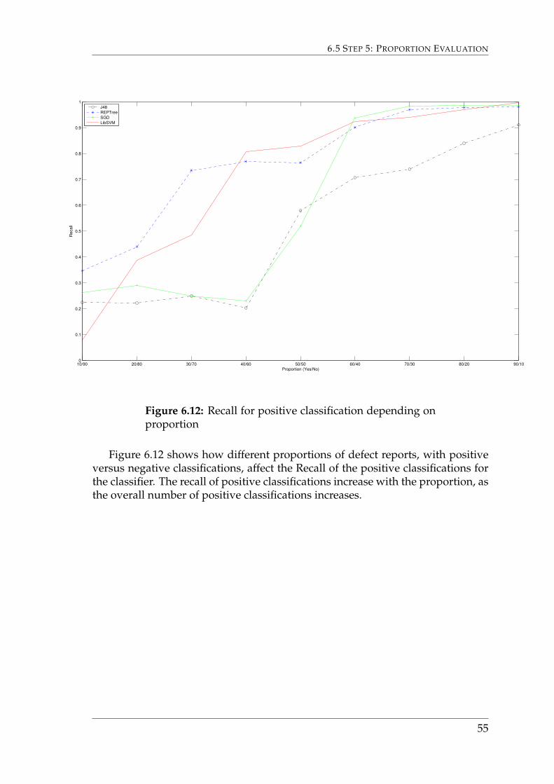
Figure 6.12 shows how different proportions of defect reports, with positiveversus negative classifications, affect the Recall of the positive classifications forthe classifier. The recall of positive classifications increase with the proportion, asthe overall number of positive classifications increases.
55
6. 6: RESULTS
10/90 20/80 30/70 40/60 50/50 60/40 70/30 80/20 90/100
0.1
0.2
0.3
0.4
0.5
0.6
0.7
0.8
0.9
1
Proportion (Yes/No)
Re
ca
ll
J48
REPTree
SGD
LibSVM
Figure 6.13: Recall for negative classification depending onproportion
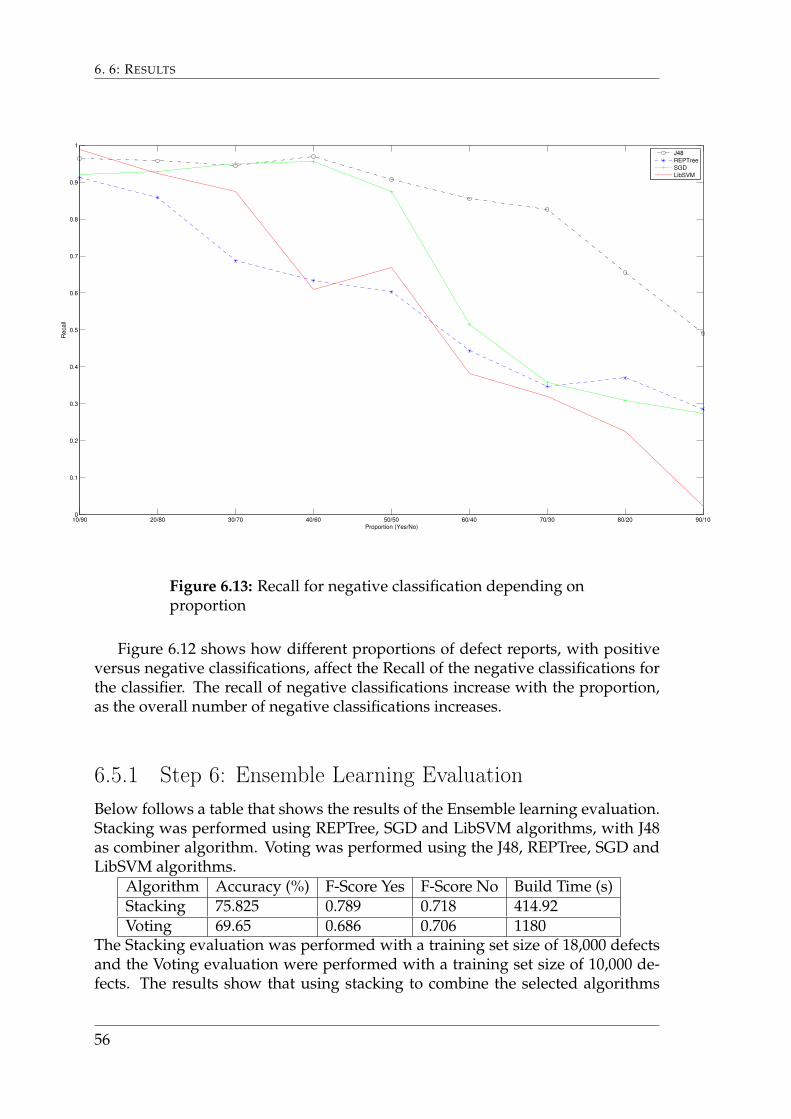
Figure 6.12 shows how different proportions of defect reports, with positiveversus negative classifications, affect the Recall of the negative classifications forthe classifier. The recall of negative classifications increase with the proportion,as the overall number of negative classifications increases.
6.5.1 Step 6: Ensemble Learning EvaluationBelow follows a table that shows the results of the Ensemble learning evaluation.Stacking was performed using REPTree, SGD and LibSVM algorithms, with J48as combiner algorithm. Voting was performed using the J48, REPTree, SGD andLibSVM algorithms.
Algorithm Accuracy (%) F-Score Yes F-Score No Build Time (s)Stacking 75.825 0.789 0.718 414.92Voting 69.65 0.686 0.706 1180
The Stacking evaluation was performed with a training set size of 18,000 defectsand the Voting evaluation were performed with a training set size of 10,000 de-fects. The results show that using stacking to combine the selected algorithms
56
6.6 STEP 7: NOMINAL AND OR TEXTUAL ATTRIBUTE EXCLUSION EVALUATION
can yield an improvement in accuracy.
6.6 Step 7: Nominal and or Textual Attribute Ex-clusion Evaluation
1000 2000 3000 4000 5000 6000 7000 8000 9000 1000050
55
60
65
70
75
80
85
90
95
100
Training Size
Accu
racy (
%)
SGD Text + Nom/Num
SGD Nom/Num Only
SGD Text Only
Figure 6.14: Accuracy depending on the usage of Nomi-nal/Numerical and Textual attributes
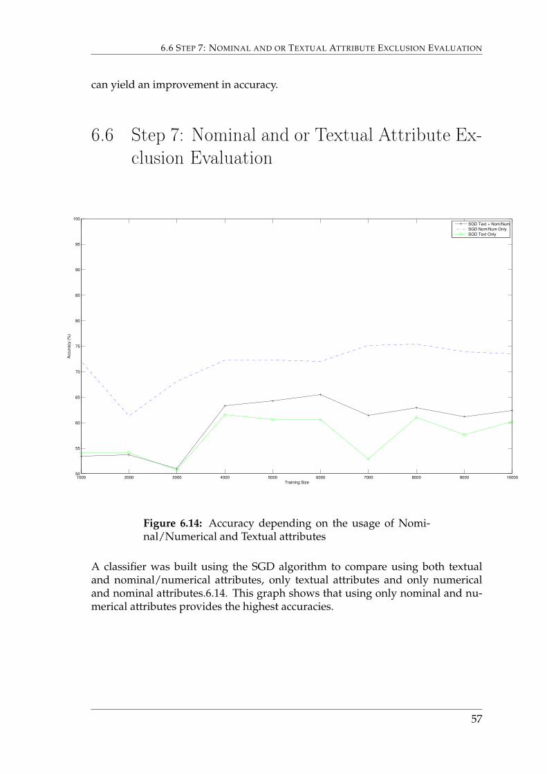
A classifier was built using the SGD algorithm to compare using both textualand nominal/numerical attributes, only textual attributes and only numericaland nominal attributes.6.14. This graph shows that using only nominal and nu-merical attributes provides the highest accuracies.
57
6. 6: RESULTS
10000 20000 30000 40000 50000 6000050
55
60
65
70
75
80
85
90
95
100
Training Size
Accu
racy (
%)
REPTree
SGD
J48
LibSVM
Figure 6.15: Accuracy depending on size using only nomi-nal and numerical attributes
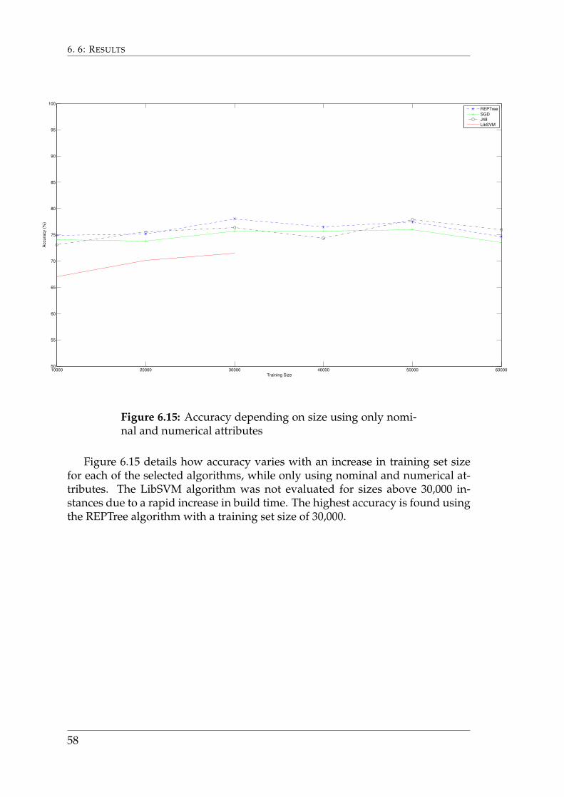
Figure 6.15 details how accuracy varies with an increase in training set sizefor each of the selected algorithms, while only using nominal and numerical at-tributes. The LibSVM algorithm was not evaluated for sizes above 30,000 in-stances due to a rapid increase in build time. The highest accuracy is found usingthe REPTree algorithm with a training set size of 30,000.
58
6.6 STEP 7: NOMINAL AND OR TEXTUAL ATTRIBUTE EXCLUSION EVALUATION
10000 20000 30000 40000 50000 600000
100
200
300
400
500
600
700
800
900
1000
1100
Training Size
Build
Tim
e (
Se
co
nd
s)
REPTree
SGD
J48
LibSVM
Figure 6.16: Build time depending on size using only nom-inal and numerical attributes
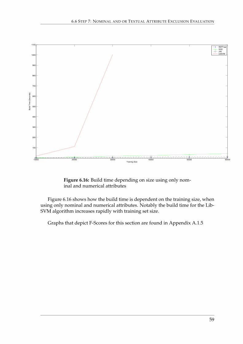
Figure 6.16 shows how the build time is dependent on the training size, whenusing only nominal and numerical attributes. Notably the build time for the Lib-SVM algorithm increases rapidly with training set size.
Graphs that depict F-Scores for this section are found in Appendix A.1.5
59

6. 6: RESULTS
60

Chapter 7
Discussion
7.1 Results DiscussionBelow follows discussions based on the results of our evaluation. It is structuredto first discuss each stage in the evaluation separately. Afterwards it will discussareas that were relevant for the entire report.
7.1.1 Attribute EvaluationOne of our goals was to find a method of aiding the prioritization of defect re-ports, described in Section 4.1. To accomplish this goal we not only needed todevelop a prototype that could be used to classify defect reports, but also providethe tool with useful data. We reduced the number of attributes because of ”Oneconcern about multivariate methods is that they are prone to overfitting. The problem isaggravated when the number of variables to select from is large compared to the numberof examples”[6]. Backwards elimination provided us with a set of attributes thatyielded higher accuracy than the initial set of all candidate attributes. In otherwords, reducing the amount of relevant information provided us with better re-sults. This can be explained with the concept of ”Curse of Dimensionality” whichin machine learning has the implication ”For machine learning problems, a small in-crease in dimensionality generally requires a large increase in the numerosity of the datain order to keep the same level of performance for regression, clustering, etc.”[5] Thoughthe removed data was relevant, the reduction of dimensionality that was causedby the removal led to a better accuracy regardless.
One noticeable matter about the selected attributes was that the attributes”mastership” and ”project” were nearly identical ( 95%) in the information theycontained to the attributes ”’ratl mastership” and ”proj id”. This meant that
61
7. 7: DISCUSSION
adding all of these attributes led to duplicate data being used for classification.This duplication did however increase the measured accuracy, which is why theywere all included among the selected attributes. This results may suggest that du-plicating the useful attributes may increase the accuracy of a classification model,or that the value of the information that differentiated the nearly identical at-tributes was higher than the risk of including redundant information.
Another notable result was that the fields that intuitively would be used toprioritize defect reports, such as ”priority” and ”abc rank” were not very usefulattributes. This did not come as a surprise since these attributes were no longerused by Sony to prioritize defect reports. This confirmed that there was a needfor better decision support, as the prioritization methods that were used did notcorrelate highly with the actual rejection or acceptance of defect reports.
Textual Attribute SelectionAs mentioned in Section 4.3.1, the attributes ”title” and ”description” were se-lected due to the fact that they are commonly used as a basis when performingsimilar evaluations. The other potentially useful textual attributes were discardeddue to their negligible or even negative effect on accuracy, as well as the potentialincrease in build times they may bring. It is important to note that the resultsfrom the textual attribute selection should not be compared directly to the resultsof the evaluation of nominal and numerical attributes, as they are based on mod-els built from a much smaller training set and are only used to internally comparethe effects of including certain attributes.
Removal of nominal attributes with many distinct valuesWe investigated the ranked attributes and tried to determine what was causingsome of them to be notably higher ranked than others. Some of these attributeshad a large amount of distinct possible values, almost in the same order of mag-nitude as the amount of examples used to train the classifier, which meant thatmany of these values were unique for one defect report.We had also noticed an issue where some models yielded very high accuracieswhen evaluated by some test sets and very low accuracies with evaluated by oth-ers.Another problem we observed was that the attributes with a very large amountsof distinct values were often placed high up in the tree near the root. From thiswe hypothesized that these models were over-fitted and severely over-estimatedthe importance of these attributes. For example, a decision tree might use an at-tribute that almost exclusively has unique values as the first attribute tested inthe tree. When the tree is used to classify new defect reports it may simply givethese reports the overall most probable classification, as the values these reportshave in the first examined attribute is not contained in the training set. This ex-ample is also related to the unification of training and test set headers discussedin Section 7.2.2We therefore concluded that attributes with over 100 distinct values would prob-
62
7.1 RESULTS DISCUSSION
ably not be very helpful to our specific context, where the defects being classifiedmay be very new and as such may have a new values for theses attributes.
EthicsAmong the attributes that were available for classification were attributes thatidentified individual persons that were connected to the defect reports. Thisopened for the possibility for the prototype to be used to prioritize defects basedon the people who identified them, and to identify which people who submit de-fect reports that will or will not be handled. In other words, the prototype couldbe used as an automatic way to evaluate the performance of individuals. Thoughthese attributes may have been useful as a way to determine if a defect should befixed or not, including them would have opened up for the prototype to be usedin this unintended manner. Therefore Sony requested us to not include theseattributes in this project.
Unknown AttributesOut of the 19 attributes found useful in step 1, three attributes have been given thedescription ”Unknown”. This meant that the purpose of the attribute could notbe ascertained by their names or by examining the values they contained. Theirpurpose was not even known by the technicians responsible for the database.This is quite remarkable, especially given that the information contained in someof these attributes was more strongly linked to the decision of fixing a defect ornot than the information in attributes such as ”Priority” or ”Impact”. Nonethe-less, given that these attributes were found to be useable in step 1, they werestill used in the later steps of the evaluation, though it may be possible that theinformation in these attributes is not suitable to use for classification.
7.1.2 Algorithm EvaluationAccording to the ”No Free Lunch” theorem ”If algorithm A outperforms algorithmB on some cost functions, then loosely speaking there must exist exactly as many otherfunctions where B outperforms A.”[18] Therefore we decided to try and find a class-ification algorithm that suited our context by evaluating a large and diverse setof algorithms on a test set that we had produced. After evaluating all the applica-ble algorithms in the Weka framework (That were able to build a classifier using4000 examples within 30 minutes), four algorithms were selected that provided agood accuracy when evaluated on a test set. The J48 and REPTree decision treealgorithms, the LibSVM support vector machine implementation and StochasticGradient Descent using a Support Vector Machine function. These algorithmswere then used in the further evaluations. The algorithms ADTree and Logisticalso provided accuracies similar to the four selected algorithms, but given thatthey belong to the same families as the selected algorithms they were not consid-ered likely to provide radically different results than the selected algorithms andwere therefore not included in further evaluation.
63
7. 7: DISCUSSION
Meta ClassifiersThis evaluation also contained an evaluation of the available meta-classifiers (thatare applied on single algorithms). Some of these, such as AttributeSelectedClas-sifier, were useful for reducing build times. Others could be used to slightly in-crease accuracies with a large trade-off in build times. Some of the meta clas-sifiers were unusable or had overly long build times in combination with somealgorithms. The results showed that the effects of a meta-algorithms varied de-pending on which algorithm it was applied to. None of the four selected basealgorithms shared a best meta algorithm with regards to accuracy, the accuracyof J48 could be improved by a percentage of 4.675% while no meta-algorithmwas able to improve the accuracy of SGD. It is important to note that none ofthese meta classification algorithms were used in the further evaluations due totime constraints.
Test Sets versus Cross ValidationWe used sequestered test sets as our main form of evaluation instead of Cross Val-idation because of two reasons. The first reason was time constraint. A Ten-FoldCross Validation takes a lot longer to perform since it has to train ten classifiersinstead of just one and time was a concern when these evaluations were carriedout. The most significant reason however was the validity and realism of the pro-posed accuracy. When Cross Validation was used, many algorithms scored highfigures and seemed to be highly adequate. We then evaluated the classifier on theTest Set and noticed a significant loss of accuracy on some algorithms. This pat-tern had also been observed before during the implementation of the prototypetool. The Cross Validation yielded an overly optimistic accuracy figure comparedto our evaluations done on different Test Sets.Defect reports are not independent and results from cross-validation should beinterpreted carefully. This is explained by ”For a fixed validation set, statistical testscan be used, but their validity is doubtful for cross-validation because independence as-sumptions are violated.”[6]. This was the major reason why we chose to use testsets instead of cross-validation in the evaluations.
7.1.3 Size EvaluationThe size evaluation showed that there was a steep climb in accuracy for the J48,REPTree, and SGD algorithms at a training set size of 1400 instances, while theLibSVM algorithm has a steep climb at a training set size of 600 instances. Train-ing set sizes lower than these were basically unusable. Increases in training setsizes seem to have little effect on the accuracy after the mark of 2000 instances.This is consistent with research which shows that the effects on accuracy of thetraining set size will diminish significantly after a certain threshold[22]. Buildtimes increased radically with training set size as expected.
Another noticeable feature of the size evaluation was that there seemed to
64
7.1 RESULTS DISCUSSION
be a notably big difference between the results found between the sizes 200 to1800 and the results found between the sizes 2000 and 24000. The reason forthis is unknown, though the evaluation of the size 200 to 1800 data points wasperformed at a much later date than the evaluation of the size 2000 to 24000 datapoints. It is possible that the nature of the data within the used span of submissiondates had been altered between the two evaluations. This is discussed further inSection 7.2.3.
7.1.4 Timeframe EvaluationThe results of the timeframe evaluation showed that moving the timeframe of thetraining set back did not lead to a significant decrease in accuracy. This showedthat within the evaluated timeframe there did not seem to be any significant dif-ferences in the nature of the data and that classification models are not likely tobecome obsolete quickly.
7.1.5 Proportion EvaluationThere were many interesting results that could be derived from the proportionevaluation:
• The accuracy depending on proportion varied largely on the algorithm thatwas used. J48 and SGD seemed to generally benefit from a slightly higherproportion of positively classified defect reports, with a significant increase40/60 to 50/50 range. LibSVM on the other hand seemed to benefit from aprecise 50/50 proportion, while REPTree seemed to provide a similar accu-racy regardless of proportion.
• The F-Scores for both positive and negative classifications were quite sta-ble when having a higher than 50% proportion of the tested classification,while the F-Scores were unstable and generally worse when having a lowerthan 50% proportion. This showed a general increase in performance fora certain classification if the model was build using a higher proportion ofreports with that classification, which was expected.
• The precision and recall graphs showed, as expected, that an increase in pro-portion of training examples for a certain classification led to an increase inrecall and a decrease in precision for that classification. In other words, themodel will make more classifications of the type that had the highest pro-portion, while at the same time being less sure about those classifications.Conversely, however, a decrease in proportion for a certain classification ledto it having a higher precision, though a (much) lower recall.
• When using a proportion of 50/50, the F-Scores were on average slightlyhigher (0.726 compared to 0.7) for negative classifications. This proportionalso had a higher average precision (0.76 compared to 0.711) for positiveclassifications and a higher average recall (0.764 compared to 0.673) for
65
7. 7: DISCUSSION
negative classifications. One should note, however, that the LibSVM andREPTree algorithms showed the opposite patterns, though not as distinc-tive patterns as the other two algorithms.
These tests did not show that a certain proportion was the best to use for clas-sifying our data. Which proportion to use is instead largely dependent on thepurpose for building the model. For example, one might be mostly interested inhaving a high precision for a certain classification, and only partially interestedin a high recall. If so one would do best to train a classifier using a high propor-tion of the other classification. If one does not hold any bias for any particularclassification it might be prudent to stick with a 50/50 proportion, or the nativeproportion of the training data, though some algorithms provided a slightly bet-ter accuracy with a slightly higher proportion of positive classifications.
7.1.6 Ensemble Learning EvaluationThe evaluation of the two available ensemble learners that combine different al-gorithms showed that stacking, performed using the four selected algorithms,produced an increase in total accuracy. The accuracy found during this evalu-ation (75.825%) was the highest measured accuracy in the prototype evaluationwhile using textual attributes.
7.1.7 Nominal and/or Textual Attribute Exclusion Evalua-tion
This final evaluation was meant to determine if the best course of action would beto use only nominal attributes, only textual attributes, or a combination of both.The previous evaluations, apart from the attribute evaluation, were all performedusing both nominal and textual attributes since this seemed to be the most intu-itive approach. Our evaluation, however, indicated that only using the nominalattributes seemed to yield slightly better results than using both nominal andtextual, with using only textual attributes yielding even lower accuracies. Theevaluation using only nominal and numerical attributes with larger training setsizes further indicated an advantage when using only nominal and numerical at-tributes. This test give us the highest recorded accuracy in all of the evaluations(78.05%) when using the REPTree algorithm on a training set of 30000 examples,while at the same time having a significantly lower build time than comparabletests that included textual attributes.The LibSVM algorithm, however, has a steeply increasing build time with regardsto training set size. This is consistent with previous evaluations of the LibSVMalgorithm[3]. So much so that it was not possible to evaluate this algorithm usingtraining sets larger than 30000 instances.
Other studies in the same area have all used textual information found in de-fect reports as a primary basis of classification[15][10] The fact that our resultsshowed textual information to be less useful may be explained by the curse of
66

7.2 THREATS TO VALIDITY
dimensionality. The increase of dimensionality may overfit the data and loweraccuracy[6]. Another explanation may be that the defect reports in this studyhave a larger amount and more useful nominal attributes. Another explanationfor our results could be the way textual attributes were preprocessed before usedto train a classifier. We did not utilize much of the available functionality to pre-process the text, which may have reduced the accuracy when using textual at-tributes compared to what might otherwise have been possible.
7.2 Threats to Validity
7.2.1 Theory to PracticeThere are a number of potential threats to the validity of this thesis that couldoccur when applying it in practical use.
• The evaluation of the prototype was performed by using the same test set toevaluate classifiers built using a number of training sets. It is possible thatthe data in this test set is not representative of the available data as a whole.The defect reports in this test set may be unusually easy (or unusually hard)to classify, meaning that the results of this thesis may not coincide with theprototype’s performance in practical use.
• The evaluation was performed using a series of steps aimed at evaluatingthe dimensions that could affect the performance of the prototype inde-pendently, in order to find the optimal configuration of these dimensions.Therefore the evaluation ignored possible dependencies between these di-mensions. For example, the best set of attributes may change if the attributeevaluation is performed using a different classification algorithm or a dif-ferent training set size. Due to the fact that there was an unfeasibly largeamount of dependency combinations, these were not tested. It is possiblethat a better configuration could be found if more of the possible configura-tions were evaluated.
• Though the evaluations were only performed using defect reports from asingle company, the defect reports were selected from all of the concurrentlydeveloped projects within that company. It is possible that the companydeploys different practices when handling defect reports between differ-ent projects. It is likely that the prototype will be used in practice to onlytrain classification models and perform classification using defect reportsselected from a single project. If so, the performance of the prototype maydiffer from the results in this thesis.
• The prototype has only been evaluated by using metrics such as accuracyand F-Score. The prototype was never evaluated by its intended users, i.e.the developers at Sony. Such evaluations may find that a tool based on theprototype is less useful in practice than what the results in this thesis sug-gest. In other words, the metrics used in this thesis to evaluate the prototype
67
7. 7: DISCUSSION
may not be sufficient to assess how useful a tool based on the prototype willbe. Section 7.3 lists recommendations of how these problems should be han-dled when the prototype is practically implemented.
7.2.2 Unification of Training and Test Set HeadersOne of the limitations of the Weka framework is that the training and test setsmust have all of the distinct nominal values declared in their headers. If the testsets include values that are not included in the training sets then the sets are in-compatible and cannot be used together. This becomes a problem if the trainingsets are relatively small and/or the sets use attributes that have many distinctvalues, as the training set may then not contain all the possible nominal values.A crude way to get around this problem is to, before building the classifiers, com-bine the headers of the training and tests sets so all of the distinct nominal valuesare declared in both sets. This approach was used to ensure that all the models inthe evaluation could be evaluated by the corresponding test sets. This approach ishowever known to cause a number of problems. First of all, the approach cannotbe used if you want to use an existing model to perform classification, as the uni-fication must be performed on the set that built the model. Secondly, models builton training sets with unified headers are known to cause overfitting problems, asdescribed in Section 7.1.1. Though the effects of this problem were decreased byremoving the attributes with large amounts of distinct values, the fact that unifi-cation of training and test sets was used may still have effected the results of theevaluation.
7.2.3 Usage of Submission DatesIn order to perform the date evaluation and to ensure that training and test setswould not contain the same data, we selected all of the sets used in the evalua-tions within submission date time spans. Given that we performed our evalua-tions using a database that was active and in use, the information within thesetime spans was subject to changes during the time the evaluations were per-formed. This produced a problem in the size evaluation, which suggested thatbig changes in the data had been made between the points in time where thesize evaluation was performed. This indicates that our results will not be repro-ducible, and that these kinds of changes are capable of significantly altering theresults.
7.2.4 OverfittingThe results were examined to see if the model is over fitting the data and henceprovide a model that is more adjusted to the specific training and test data then amore general situation. If a certain test configuration gives a suspiciously high ac-curacy it is likely due to this model being overfitted. Because of this we applieda variation of test sets on the models with the best accuracy, in order to ensure
68
7.3 DEPLOYING THE PROTOTYPE IN PRACTICE
that these models are useful in a wide variety of situations. We also made surethat the models had acceptable F-Scores for both positive and negative classifica-tions to ensure that the models were useful for classifying both types of instances.
7.3 Deploying the Prototype in PracticeThe most intuitive way to implement this prototype in practical use would beto use the configuration that produces the highest accuracy to build a classifica-tion model. This model would then be used to classify incoming defect reportsbased on whether they are likely to be given a solution or not, and then use theseclassifications as support in the process of prioritizing defect reports. The foundoptimal configuration is the following:
• The REPTree algorithm
• A training set size of 30,000 instances
• A proportion of 50% positively and 50% negatively classified defect reportsin the training set
• The attributes listed below
1. mastership
2. fix for
3. ratl mastership
4. externalsupplier
5. ratl keysite
6. project
7. proj id
8. attachment share saved
9. found during
10. business priority
11. found in product
12. found by
However, one should be aware of a number of factors when implementing a de-cision support tool similar to our prototype.
69
7. 7: DISCUSSION
• All results are subject to change along with changes in the nature of the in-put data. There is no guarantee that the optimal configuration found in thisevaluation will remain optimal in the future. It is therefore recommendedthat similar evaluations should be performed with regular intervals to en-sure that the decision support tool retains a good performance.
• This evaluation was performed using data from all projects that were devel-oped during the examined time periods. If the decision support tool is to betailored for a single project, it would be prudent to perform an evaluationusing data from only that project in order to find a good configuration forthat situation.
• The algorithms that provided the highest accuracies were decision tree al-gorithms. Though these algorithms have the advantages of fast build times,and that decision trees are easily examined and understood, they are alsoprone to overfitting problems. This increases the need to periodically eval-uate decision tree models using sequestered test sets in order to ensure thatthey perform classifications in a relevant way.
• The size evaluation found that using training sets with sizes of over 4,000 in-stances did not significantly affect accuracy. Though if no textual attributesare used the difference in build time between using 4,000 and 30,000 in-stances in the training set is negligible.
• The timeframe evaluation found that the time locality of the chosen trainingset did not significantly affect accuracy. However, this might be subject tochange if, for example, a classifier is built for a single project.
• Using meta-classifiers such as Stacking may improve or worsen the per-formance of a classifier. The effect of meta-classifiers should be evaluatedperiodically, to assess their usefulness.
• Which proportion of positively and negatively classified reports in the train-ing set to use depends on the intended function of the decision supporttool. For example, if one wishes to have a high confidence (precision) in thenegative classifications, the proportion of positively classified reports in thetraining set should be increased.
• When selecting attributes, one should always make sure that the selectedattributes have set values when the report is submitted. Otherwise evalua-tions may give erroneously high accuracies.
• It is important to remember that the classifiers are trained using histori-cal data, and will perform predictions based on what has previously hap-pened. For example, if the historical prioritization has not been satisfactory,then this will be reflected in the behavior of the classifier. This also meansthat analyzing how a classification model performs classifications can be agood way to examine how the current prioritization process functions. Thismeans that there is a risk that testers may learn and imitate which attribute
70

7.3 DEPLOYING THE PROTOTYPE IN PRACTICE
values affect the classifier, in order to ensure that the defect reports theysubmit receive positive classifications.
• If a decision support tool has been in use for some time, then the input dataused to train a classifier may be affected by the previous output of the de-cision support tool. Depending on how influential the tool has been in thedecision process, this may lead to a kind of feedback loop where new classi-fications are dependent on previous classifications. This could lead to flawsin the classification process being amplified over time. This shows that therewill be a need for humans to be the final decision makers in the prioriti-zation process, and that one should carefully evaluate the performance ofnewly created classifiers.
Machine learning can be used in many areas other than defect reports to per-form predictions. As long as there exist data available that correlates with a vari-able that warrants prediction, machine learning may be useful to predict thatvariable.
71

7. 7: DISCUSSION
72

Chapter 8
Conclusions
8.1 ConclusionsThe purpose of this thesis was, as stated in Section 4.1, to investigate what use-ful informaton existed in the existing databases at Sony Mobile Communicationsand to find a method of prioritizing defect reports using Machine Learning forthe purpose of decision support. The thesis’ purpose was also to develop andevaluate a prototype of a tool with the capabilites of performing a classificationof defect reports. The results showed that it was indeed possible to use this datato perform classification with a reasonably high accuracy.
An interesting result was that using the textual information in the defect reportsas a basis for classification produced lower than expected accuracies. This dif-fered from research within a similar area in which the textual attributes providethe main source of predictive information. However, the many nominal attributescontained enough relevant information to make up for this problem.
This thesis also concluded that the effects of the size of the training sets willgenerally be small using sizes over 4,000 instances, and that the effect of the times-pan is negligible within the examined scope of about two years for this context.The results also showed that altering the proportion of positively and negativelyclassified defect reports in the training data will effect the accuracy of the classi-fier, particularly the precision and recall rates of the possible classifications. Thiscan be used to tailor classification models to suit a specific purpose.
The thesis also concluded that it is important to analyze the data existent inthe attributes used when building a classifier, as there are many situations whereadding seemingly useful data may lower the accuracy of the classification model.
73
8. 8: CONCLUSIONS
8.2 Future WorkFuture work could include revising the preprocessing procedure for textual at-tributes to attempt to increase the information gained from the textual attributes.These improvements could include techniques such as limiting the number ofwords to save for each defect report or building a stop word list based on thecontext of the company.
Since there exists such a large amount of different combinations of parametersone could use to build classifiers, there will always exist possibilities for furtherevaluations. One interesting possibility might be to evaluate the selected algo-rithms combined with the useful meta classification algorithms with regards totheir effect on the performance and accuracy when parameters such as size ortimeframe are changed.Another interesting analysis would be to evaluate how well a classifier, trainedto classify defect reports with a fixed set of attribute values could perform. Oneexample could be reports originating from one specific project where the fields inthe defect reports are used in a homogenous way. This may be beneficial sincedifferent divisions within companies have different requirements when decidingon defect reports and thus may require different classifiers.
Other interesting possibilities include performing tests (such as Step 6: En-semble Learning Evaluation) using only nominal and numerical attributes, in-creasing or decreasing the number of used attributes, further evaluation of theeffects of training set size, combining meta-algorithms with each other and redothe attribute evaluation using other classification algorithms.
74

Bibliography
[1] Weka Documentation, Website, http://www.cs.waikato.ac.nz/ml/weka/arff.html, June 2014.
[2] C. Goutte, E. Gaussier. "A Probabilistic Interpretation of Precision, Recalland F-Score, with Implication for Evaluation." Advances in information re-trieval. Springer Berlin Heidelberg, 2005. 345-359.
[3] C.C. Chang, C.J. Lin. "LibSVM: A Library for Support Vector Machines."ACM Transactions on Intelligent Systems and Technology (tist) 2.3 (2011):27.
[4] D. Michie, D.J. Spiegelhalter, C.C. Taylor. "Machine learning, neural andstatistical classification." (1994).
[5] E. Keogh, A. Mueen. Curse of Dimensionality. In C. Sammut, G. I. Webb,editor, Encyclopedia Machine Learning. Springer (2010).
[6] I. Guyon, A. Elisseeff. "An Introduction to Variable and Feature Selection."The Journal of Machine Learning Research 3 (2003): 1157-1182.
[7] J.K. Anvik. "Assisting Bug Report Triage through Recommendation". Diss.University of British Columbia, 2007.
[8] J.R. Quinlan. "Induction of Decision Trees." Machine Learning 1.1 (1986):81-106.
[9] J.T. Kent. "Information Gain and a General Measure of Correlation."Biometrika 70.1 (1983): 163-173.
[10] L. Jonsson, M. Borg, D. Broman, K. Sandahl, S. Eldh, and P. Runeson. "Au-tomating Bug Assignment using Stacked Generalization: An Evaluation ofMachine Learning in Proprietary Contexts". To appear.
75

BIBLIOGRAPHY
[11] M. Surendra Naidu, N. Geethanjali. "Classification of Defects in Software us-ing Decision Tree Algorithm." International Journal of Engineering Scienceand Technology (IJEST) 5.06 (2013).
[12] T. Menzies and A. Marcus. Automated severity assessment of software de-fect reports. In Software Maintenance, 2008. ICSM 2008. IEEE InternationalConference on, pages 346–355, Sept 2008.
[13] P. M. Nugues. "An Introduction to Language Processing with Perl and Prolog".Springer-Verlag Berlin Heidelberg, 2006.
[14] P. N. Tan, M. Steinbach, V. Kumar. "Introduction to Data Mining". PearsonEducation Ltd., 2013.
[15] P. Runeson, M. Alexandersson and O. Nyholm. "Detection of DuplicateDefect Reports using Natural Language Processing." Software Engineering,2007. ICSE 2007. 29th International Conference on. IEEE, 2007.
[16] R. Kohavi. "A study of cross-validation and bootstrap for accuracy estima-tion and model selection." IJCAI. Vol. 14. no. 2. 1995.
[17] S. Russel, P. Norvig. "Artificial Intelligence: A Modern Approach". Prentice Hall,2010.
[18] S.Ali, K.A. Smith. "On Learning Algorithm Selection for Classification." Ap-plied Soft Computing 6.2 (2006): 119-138.
[19] T.G Dietterich. "Ensemble Learning." The handbook of brain theory andneural networks (2002): 405-408.
[20] T.G. Dietterich. "Ensemble methods in machine learning." Multiple classifiersystems. Springer Berlin Heidelberg, 2000. 1-15.
[21] T.Joachims. "Making Large Scale SVM Learning Practical." (1999).
[22] X. Zhuang, D.F. Lozano-Garcia, B.A. Engel, R.N. Fernandez, C.J. Johannsen."Optimization of Training Data required for Neuro-Classification." REMOTESENSING 15.16 (1994): 3271-3277.
76

Appendices
77

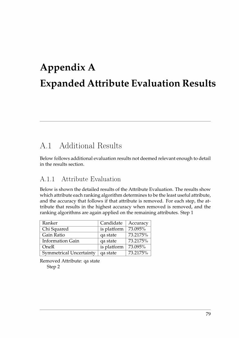
Appendix A
Expanded Attribute Evaluation Results
A.1 Additional ResultsBelow follows additional evaluation results not deemed relevant enough to detailin the results section.
A.1.1 Attribute EvaluationBelow is shown the detailed results of the Attribute Evaluation. The results showwhich attribute each ranking algorithm determines to be the least useful attribute,and the accuracy that follows if that attribute is removed. For each step, the at-tribute that results in the highest accuracy when removed is removed, and theranking algorithms are again applied on the remaining attributes. Step 1
Ranker Candidate AccuracyChi Squared is platform 73.095%Gain Ratio qa state 73.2175%Information Gain qa state 73.2175%OneR is platform 73.095%Symmetrical Uncertainty qa state 73.2175%
Removed Attribute: qa stateStep 2
79
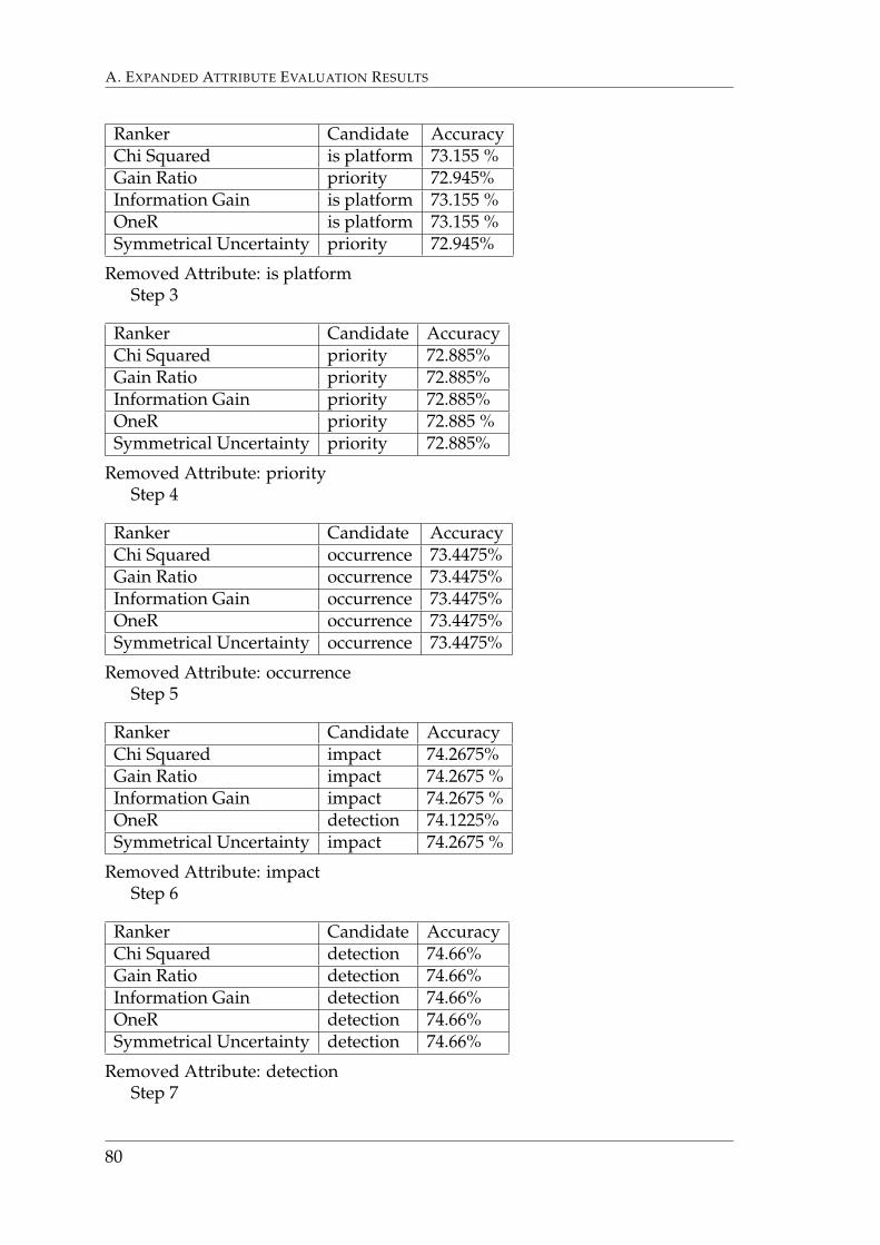
A. EXPANDED ATTRIBUTE EVALUATION RESULTS
Ranker Candidate AccuracyChi Squared is platform 73.155 %Gain Ratio priority 72.945%Information Gain is platform 73.155 %OneR is platform 73.155 %Symmetrical Uncertainty priority 72.945%
Removed Attribute: is platformStep 3
Ranker Candidate AccuracyChi Squared priority 72.885%Gain Ratio priority 72.885%Information Gain priority 72.885%OneR priority 72.885 %Symmetrical Uncertainty priority 72.885%
Removed Attribute: priorityStep 4
Ranker Candidate AccuracyChi Squared occurrence 73.4475%Gain Ratio occurrence 73.4475%Information Gain occurrence 73.4475%OneR occurrence 73.4475%Symmetrical Uncertainty occurrence 73.4475%
Removed Attribute: occurrenceStep 5
Ranker Candidate AccuracyChi Squared impact 74.2675%Gain Ratio impact 74.2675 %Information Gain impact 74.2675 %OneR detection 74.1225%Symmetrical Uncertainty impact 74.2675 %
Removed Attribute: impactStep 6
Ranker Candidate AccuracyChi Squared detection 74.66%Gain Ratio detection 74.66%Information Gain detection 74.66%OneR detection 74.66%Symmetrical Uncertainty detection 74.66%
Removed Attribute: detectionStep 7
80
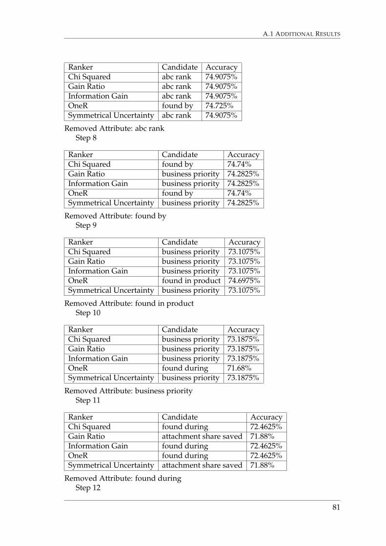
A.1 ADDITIONAL RESULTS
Ranker Candidate AccuracyChi Squared abc rank 74.9075%Gain Ratio abc rank 74.9075%Information Gain abc rank 74.9075%OneR found by 74.725%Symmetrical Uncertainty abc rank 74.9075%
Removed Attribute: abc rankStep 8
Ranker Candidate AccuracyChi Squared found by 74.74%Gain Ratio business priority 74.2825%Information Gain business priority 74.2825%OneR found by 74.74%Symmetrical Uncertainty business priority 74.2825%
Removed Attribute: found byStep 9
Ranker Candidate AccuracyChi Squared business priority 73.1075%Gain Ratio business priority 73.1075%Information Gain business priority 73.1075%OneR found in product 74.6975%Symmetrical Uncertainty business priority 73.1075%
Removed Attribute: found in productStep 10
Ranker Candidate AccuracyChi Squared business priority 73.1875%Gain Ratio business priority 73.1875%Information Gain business priority 73.1875%OneR found during 71.68%Symmetrical Uncertainty business priority 73.1875%
Removed Attribute: business priorityStep 11
Ranker Candidate AccuracyChi Squared found during 72.4625%Gain Ratio attachment share saved 71.88%Information Gain found during 72.4625%OneR found during 72.4625%Symmetrical Uncertainty attachment share saved 71.88%
Removed Attribute: found duringStep 12
81
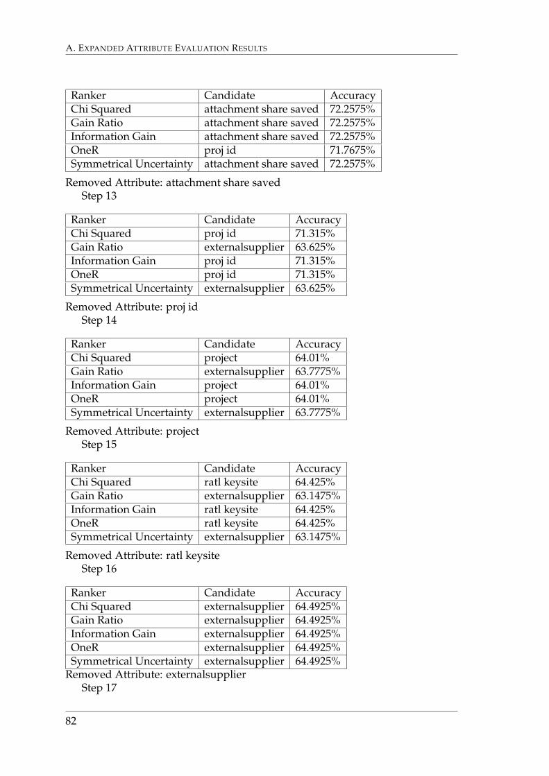
A. EXPANDED ATTRIBUTE EVALUATION RESULTS
Ranker Candidate AccuracyChi Squared attachment share saved 72.2575%Gain Ratio attachment share saved 72.2575%Information Gain attachment share saved 72.2575%OneR proj id 71.7675%Symmetrical Uncertainty attachment share saved 72.2575%
Removed Attribute: attachment share savedStep 13
Ranker Candidate AccuracyChi Squared proj id 71.315%Gain Ratio externalsupplier 63.625%Information Gain proj id 71.315%OneR proj id 71.315%Symmetrical Uncertainty externalsupplier 63.625%
Removed Attribute: proj idStep 14
Ranker Candidate AccuracyChi Squared project 64.01%Gain Ratio externalsupplier 63.7775%Information Gain project 64.01%OneR project 64.01%Symmetrical Uncertainty externalsupplier 63.7775%
Removed Attribute: projectStep 15
Ranker Candidate AccuracyChi Squared ratl keysite 64.425%Gain Ratio externalsupplier 63.1475%Information Gain ratl keysite 64.425%OneR ratl keysite 64.425%Symmetrical Uncertainty externalsupplier 63.1475%
Removed Attribute: ratl keysiteStep 16
Ranker Candidate AccuracyChi Squared externalsupplier 64.4925%Gain Ratio externalsupplier 64.4925%Information Gain externalsupplier 64.4925%OneR externalsupplier 64.4925%Symmetrical Uncertainty externalsupplier 64.4925%
Removed Attribute: externalsupplierStep 17
82
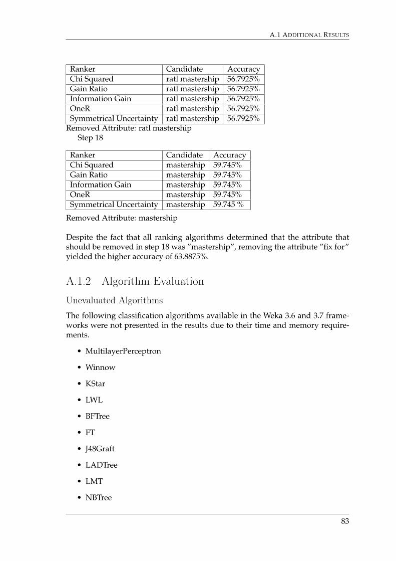
A.1 ADDITIONAL RESULTS
Ranker Candidate AccuracyChi Squared ratl mastership 56.7925%Gain Ratio ratl mastership 56.7925%Information Gain ratl mastership 56.7925%OneR ratl mastership 56.7925%Symmetrical Uncertainty ratl mastership 56.7925%
Removed Attribute: ratl mastershipStep 18
Ranker Candidate AccuracyChi Squared mastership 59.745%Gain Ratio mastership 59.745%Information Gain mastership 59.745%OneR mastership 59.745%Symmetrical Uncertainty mastership 59.745 %
Removed Attribute: mastership
Despite the fact that all ranking algorithms determined that the attribute thatshould be removed in step 18 was ”mastership”, removing the attribute ”fix for”yielded the higher accuracy of 63.8875%.
A.1.2 Algorithm Evaluation
Unevaluated AlgorithmsThe following classification algorithms available in the Weka 3.6 and 3.7 frame-works were not presented in the results due to their time and memory require-ments.
• MultilayerPerceptron
• Winnow
• KStar
• LWL
• BFTree
• FT
• J48Graft
• LADTree
• LMT
• NBTree
83
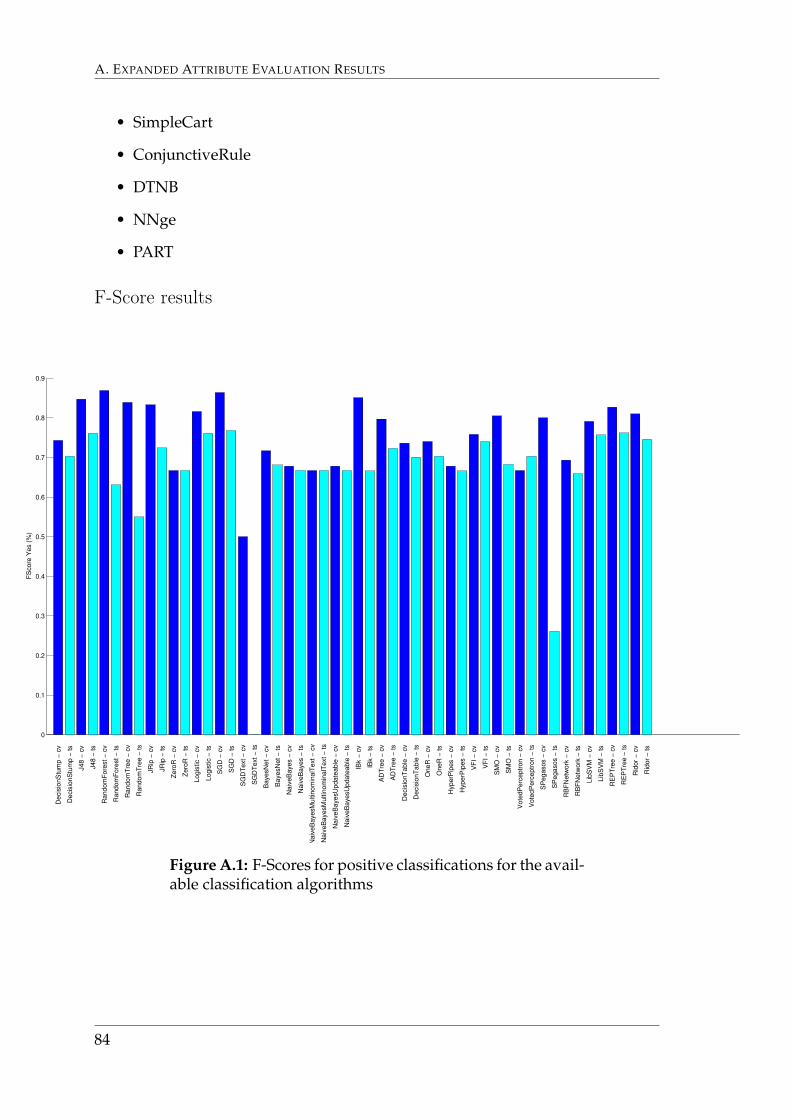
A. EXPANDED ATTRIBUTE EVALUATION RESULTS
• SimpleCart
• ConjunctiveRule
• DTNB
• NNge
• PART
F-Score results
0
0.1
0.2
0.3
0.4
0.5
0.6
0.7
0.8
0.9
Decis
ionS
tum
p −
cv
Decis
ionS
tum
p −
ts
J48 −
cv
J48 −
ts
Random
Fore
st −
cv
Random
Fore
st −
ts
Random
Tre
e −
cv
Random
Tre
e −
ts
JR
ip −
cv
JR
ip −
ts
Zero
R −
cv
Zero
R −
ts
Logis
tic −
cv
Logis
tic −
ts
SG
D −
cv
SG
D −
ts
SG
DT
ext −
cv
SG
DT
ext −
ts
BayesN
et −
cv
BayesN
et −
ts
Naiv
eB
ayes −
cv
Naiv
eB
ayes −
ts
Naiv
eB
ayesM
ultin
om
inalT
ext −
cv
Naiv
eB
ayesM
ultin
om
inalT
ext −
ts
Naiv
eB
ayesU
pdate
able
− c
v
Naiv
eB
ayesU
pdate
able
− ts
IBk −
cv
IBk −
ts
AD
Tre
e −
cv
AD
Tre
e −
ts
Decis
ionT
able
− c
v
Decis
ionT
able
− ts
OneR
− c
v
OneR
− ts
HyperP
ipes −
cv
HyperP
ipes −
ts
VF
I −
cv
VF
I −
ts
SM
O −
cv
SM
O −
ts
Vo
tedP
erc
eptr
on −
cv
Vote
dP
erc
eptr
on −
ts
SP
egasos −
cv
SP
egasos −
ts
RB
FN
etw
ork
− c
v
RB
FN
etw
ork
− ts
Lib
SV
M −
cv
Lib
SV
M −
ts
RE
PT
ree −
cv
RE
PT
ree −
ts
Rid
or
− c
v
Rid
or
− ts
FS
core
Ye
s (
%)
Figure A.1: F-Scores for positive classifications for the avail-able classification algorithms
84
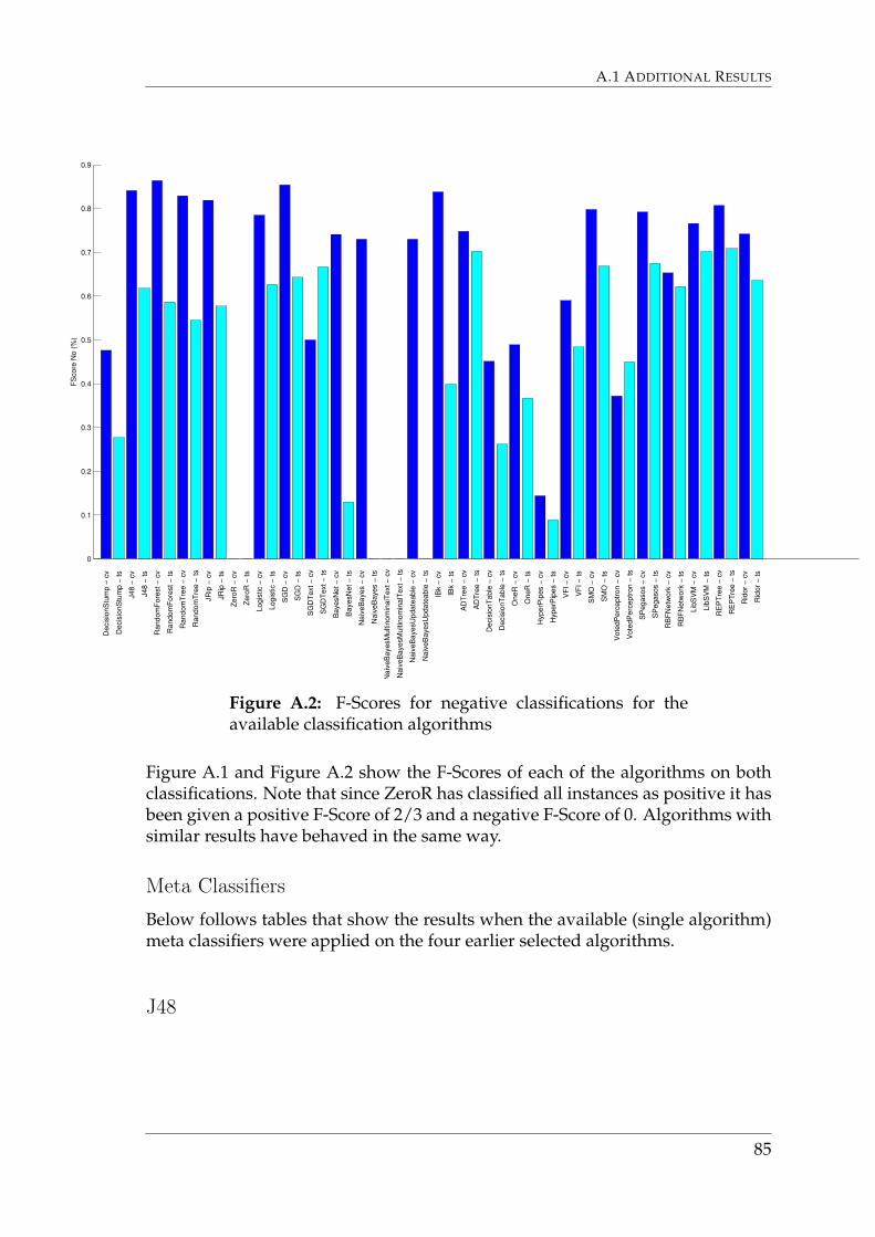
A.1 ADDITIONAL RESULTS
0
0.1
0.2
0.3
0.4
0.5
0.6
0.7
0.8
0.9
De
cis
ionS
tum
p −
cv
Decis
ionS
tum
p −
ts
J48 −
cv
J48 −
ts
Random
Fore
st −
cv
Random
Fore
st −
ts
Random
Tre
e −
cv
Random
Tre
e −
ts
JR
ip −
cv
JR
ip −
ts
Zero
R −
cv
Zero
R −
ts
Logis
tic −
cv
Logis
tic −
ts
SG
D −
cv
SG
D −
ts
SG
DT
ext −
cv
SG
DT
ext −
ts
BayesN
et
− c
v
BayesN
et
− ts
Naiv
eB
ayes −
cv
Naiv
eB
ayes −
ts
Naiv
eB
ayesM
ultin
om
ina
lText −
cv
Naiv
eB
ayesM
ultin
om
inalT
ext −
ts
Naiv
eB
ayesU
pdate
able
− c
v
Naiv
eB
ayesU
pdate
able
− ts
IBk −
cv
IBk −
ts
AD
Tre
e −
cv
AD
Tre
e −
ts
Decis
ionT
able
− c
v
Decis
ionT
able
− ts
OneR
− c
v
OneR
− ts
HyperP
ipes −
cv
HyperP
ipe
s −
ts
VF
I −
cv
VF
I −
ts
SM
O −
cv
SM
O −
ts
Vote
dP
erc
eptr
on −
cv
Vote
dP
erc
eptr
on −
ts
SP
egasos −
cv
SP
egasos −
ts
RB
FN
etw
ork
− c
v
RB
FN
etw
ork
− ts
Lib
SV
M −
cv
Lib
SV
M −
ts
RE
PT
ree −
cv
RE
PT
ree −
ts
Rid
or
− c
v
Rid
or
− ts
FS
core
No
(%
)
Figure A.2: F-Scores for negative classifications for theavailable classification algorithms
Figure A.1 and Figure A.2 show the F-Scores of each of the algorithms on bothclassifications. Note that since ZeroR has classified all instances as positive it hasbeen given a positive F-Score of 2/3 and a negative F-Score of 0. Algorithms withsimilar results have behaved in the same way.
Meta ClassifiersBelow follows tables that show the results when the available (single algorithm)meta classifiers were applied on the four earlier selected algorithms.
J48
85
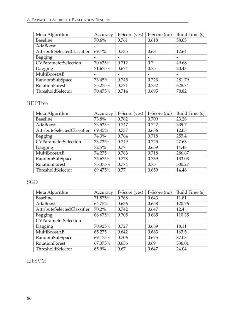
A. EXPANDED ATTRIBUTE EVALUATION RESULTS
Meta Algorithm Accuracy F-Score (yes) F-Score (no) Build Time (s)Baseline 70.6% 0.761 0.618 58.05AdaBoost - - - -AttributeSelectedClassifier 69.1% 0.735 0.63 12.64Bagging - - - -CVParameterSelection 70.625% 0.712 0.7 49.68Dagging 71.675% 0.674 0.75 20.43MultiBoostAB - - - -RandomSubSpace 73.45% 0.745 0.723 281.79RotationForest 75.275% 0.771 0.732 628.74ThresholdSelector 70.475% 0.714 0.695 78.82
REPTree
Meta Algorithm Accuracy F-Score (yes) F-Score (no) Build Time (s)Baseline 73.8% 0.762 0.709 23.28AdaBoost 73.525% 0.747 0.722 339.7AttributeSelectedClassifier 69.45% 0.737 0.636 12.03Bagging 74.3% 0.764 0.718 255.4CVParameterSelection 73.725% 0.749 0.725 27.63Dagging 72.5% 0.77 0.659 14.48MultiBoostAB 74.275 0.763 0.718 286.67RandomSubSpace 75.675% 0.773 0.739 133.03RotationForest 75.375% 0.774 0.73 500.27ThresholdSelector 69.475% 0.77 0.659 14.48
SGD
Meta Algorithm Accuracy F-Score (yes) F-Score (no) Build Time (s)Baseline 71.875% 0.768 0.643 11.81AdaBoost 64.75% 0.636 0.658 120.76AttributeSelectedClassifier 70.2% 0.742 0.647 12.4Bagging 68.675% 0.705 0.665 110.35CVParameterSelection - - - -Dagging 70.925% 0.727 0.689 18.11MultiBoostAB 65.275 0.642 0.663 163.5RandomSubSpace 69.175% 0.706 0.675 87.03RotationForest 67.375% 0.656 0.69 536.01ThresholdSelector 65.9% 0.67 0.647 24.04
LibSVM
86
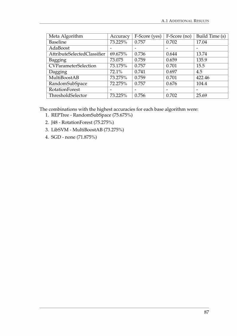
A.1 ADDITIONAL RESULTS
Meta Algorithm Accuracy F-Score (yes) F-Score (no) Build Time (s)Baseline 73.225% 0.757 0.702 17.04AdaBoost - - - -AttributeSelectedClassifier 69.675% 0.736 0.644 13.74Bagging 73.075 0.759 0.659 135.9CVParameterSelection 73.175% 0.757 0.701 15.5Dagging 72.1% 0.741 0.697 4.5MultiBoostAB 73.275% 0.759 0.701 422.46RandomSubSpace 72.275% 0.757 0.676 104.4RotationForest - - - -ThresholdSelector 73.225% 0.756 0.702 25.69
The combinations with the highest accuracies for each base algorithm were:1. REPTree - RandomSubSpace (75.675%)
2. J48 - RotationForest (75.275%)
3. LibSVM - MultiBoostAB (73.275%)
4. SGD - none (71.875%)
87
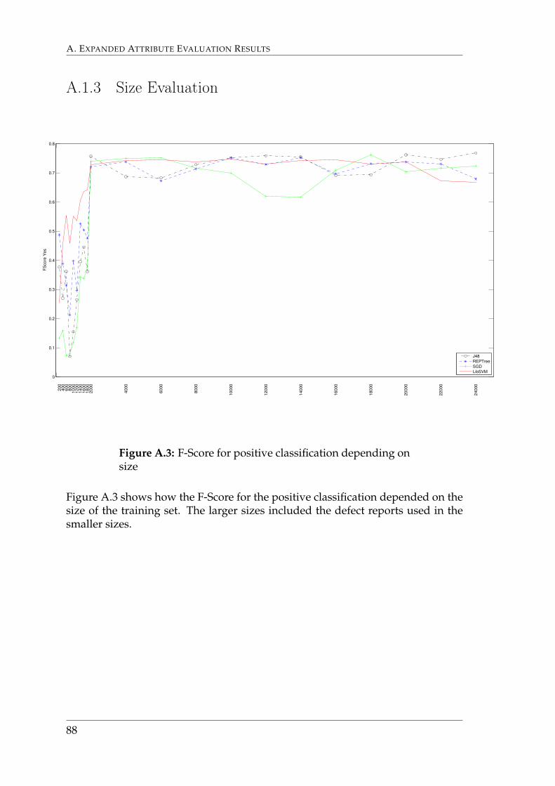
A. EXPANDED ATTRIBUTE EVALUATION RESULTS
A.1.3 Size Evaluation
0
0.1
0.2
0.3
0.4
0.5
0.6
0.7
0.8
FS
co
re Y
es
200
400
600
800
10
00
12
00
14
00
16
00
18
00
20
00
40
00
60
00
80
00
10
000
12
000
14
000
16
000
18
000
20
000
22
000
24
000
J48
REPTree
SGD
LibSVM
Figure A.3: F-Score for positive classification depending onsize
Figure A.3 shows how the F-Score for the positive classification depended on thesize of the training set. The larger sizes included the defect reports used in thesmaller sizes.
88
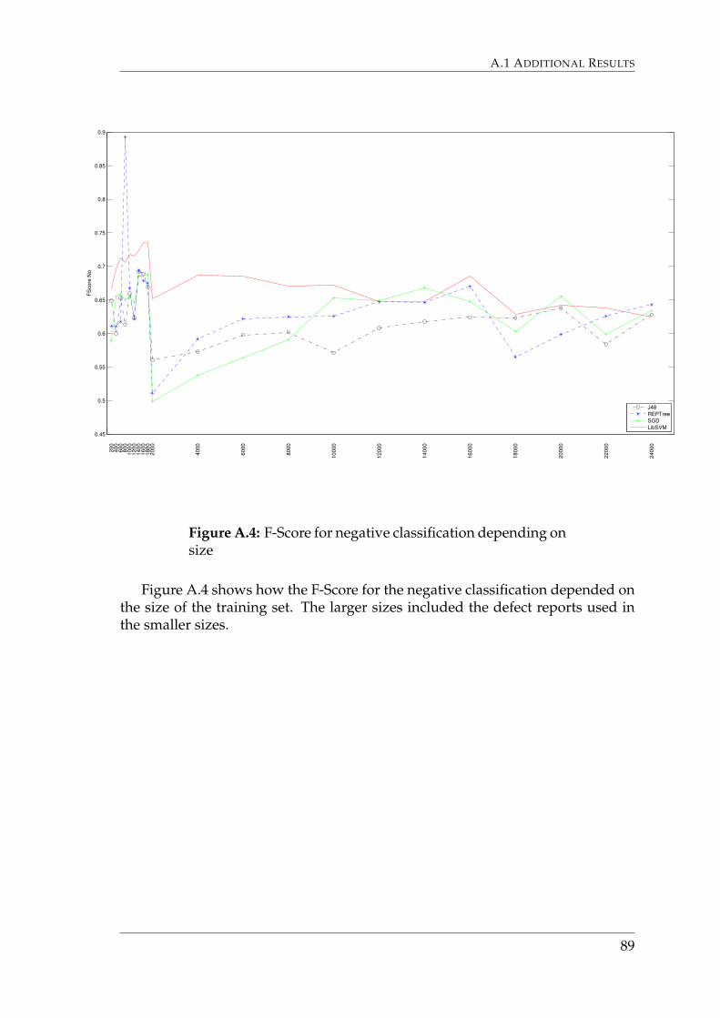
A.1 ADDITIONAL RESULTS
0.45
0.5
0.55
0.6
0.65
0.7
0.75
0.8
0.85
0.9
FS
core
No
200
400
600
800
10
00
12
00
14
00
16
00
18
00
20
00
40
00
60
00
80
00
10
000
12
000
14
000
16
000
18
000
20
000
22
000
24
000
J48
REPTree
SGD
LibSVM
Figure A.4: F-Score for negative classification depending onsize
Figure A.4 shows how the F-Score for the negative classification depended onthe size of the training set. The larger sizes included the defect reports used inthe smaller sizes.
89
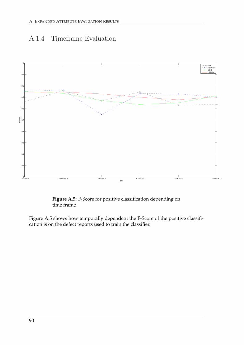
A. EXPANDED ATTRIBUTE EVALUATION RESULTS
A.1.4 Timeframe Evaluation
1/10/2014 10/11/2013 7/13/2013 4/15/2013 1/14/2013 10/16/20120
0.1
0.2
0.3
0.4
0.5
0.6
0.7
0.8
0.9
1
Date
FS
co
re
J48
REPTree
SGD
LibSVM
Figure A.5: F-Score for positive classification depending ontime frame
Figure A.5 shows how temporally dependent the F-Score of the positive classifi-cation is on the defect reports used to train the classifier.
90
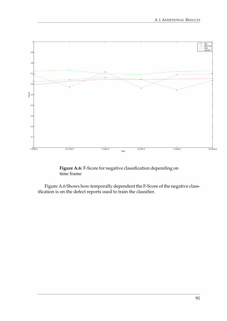
A.1 ADDITIONAL RESULTS
1/10/2014 10/11/2013 7/13/2013 4/15/2013 1/14/2013 10/16/20120
0.1
0.2
0.3
0.4
0.5
0.6
0.7
0.8
0.9
1
Date
FS
co
re
J48
REPTree
SGD
LibSVM
Figure A.6: F-Score for negative classification depending ontime frame
Figure A.6 Shows how temporally dependent the F-Score of the negative class-ification is on the defect reports used to train the classifier.
91
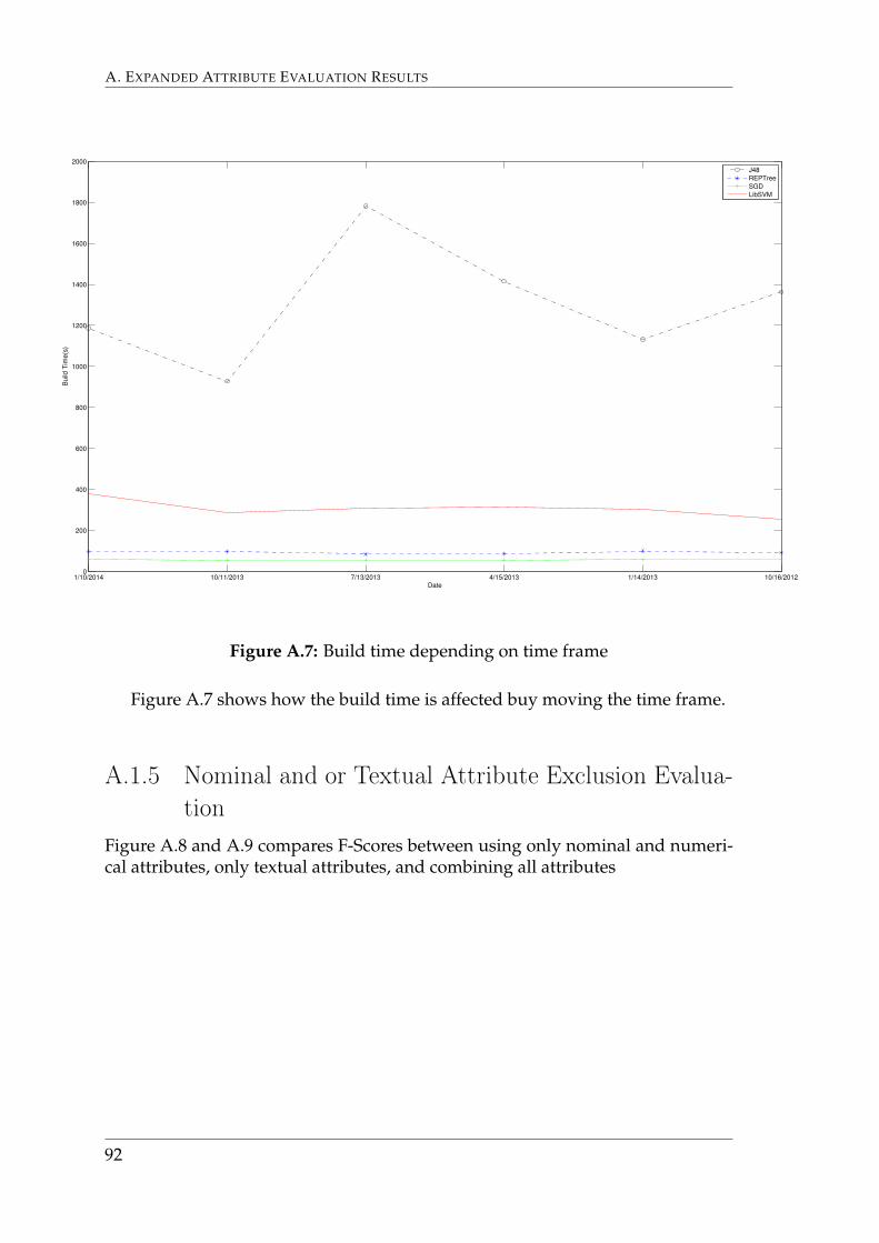
A. EXPANDED ATTRIBUTE EVALUATION RESULTS
1/10/2014 10/11/2013 7/13/2013 4/15/2013 1/14/2013 10/16/20120
200
400
600
800
1000
1200
1400
1600
1800
2000
Date
Bu
ild T
ime
(s)
J48
REPTree
SGD
LibSVM
Figure A.7: Build time depending on time frame
Figure A.7 shows how the build time is affected buy moving the time frame.
A.1.5 Nominal and or Textual Attribute Exclusion Evalua-tion
Figure A.8 and A.9 compares F-Scores between using only nominal and numeri-cal attributes, only textual attributes, and combining all attributes
92
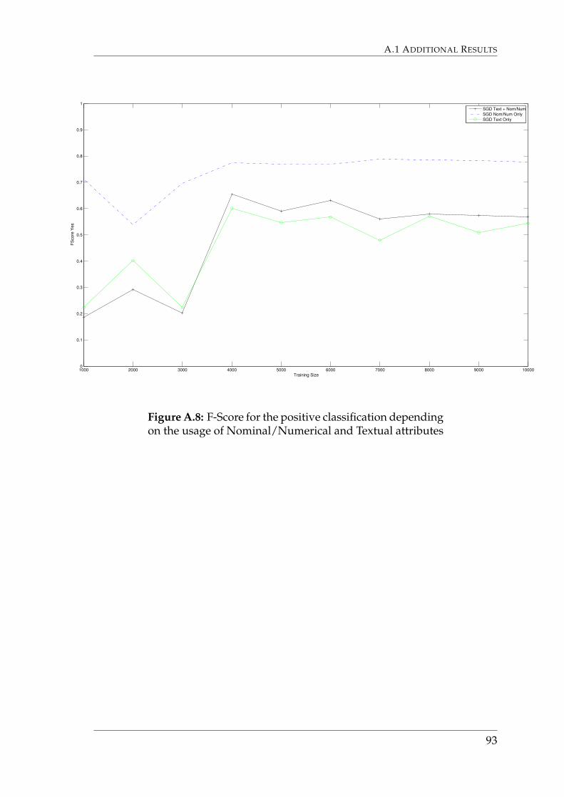
A.1 ADDITIONAL RESULTS
1000 2000 3000 4000 5000 6000 7000 8000 9000 100000
0.1
0.2
0.3
0.4
0.5
0.6
0.7
0.8
0.9
1
Training Size
FS
co
re Y
es
SGD Text + Nom/Num
SGD Nom/Num Only
SGD Text Only
Figure A.8: F-Score for the positive classification dependingon the usage of Nominal/Numerical and Textual attributes
93
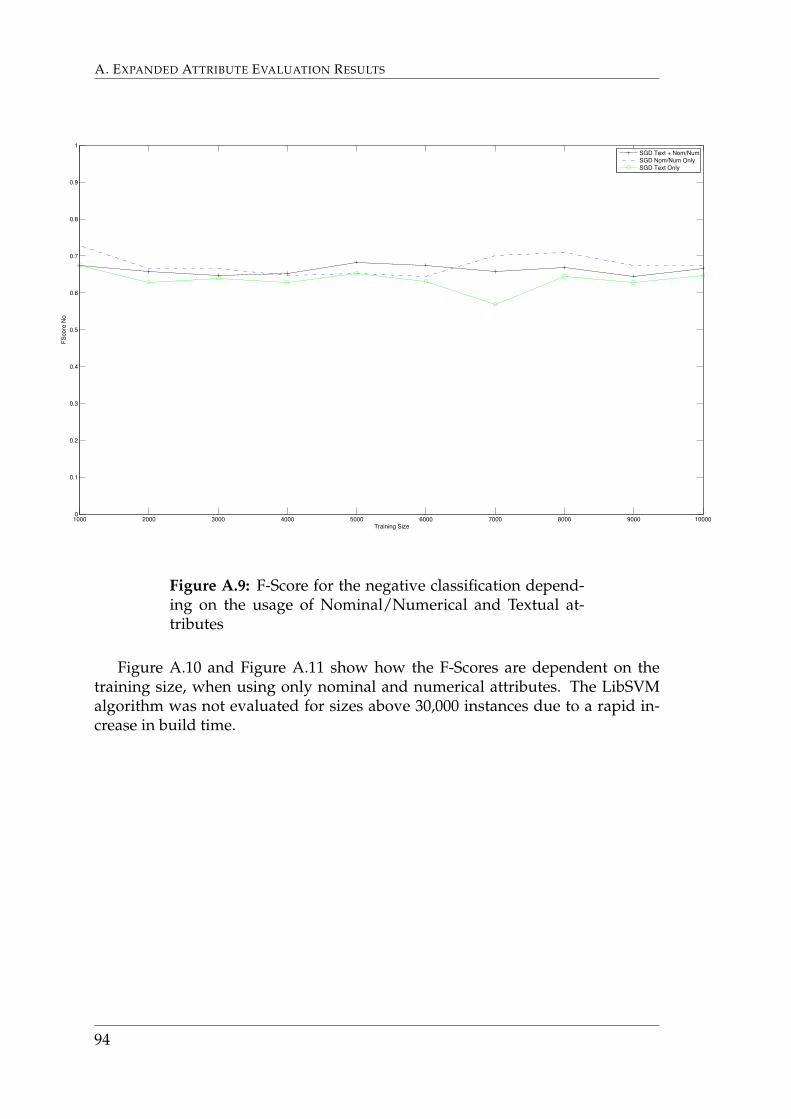
A. EXPANDED ATTRIBUTE EVALUATION RESULTS
1000 2000 3000 4000 5000 6000 7000 8000 9000 100000
0.1
0.2
0.3
0.4
0.5
0.6
0.7
0.8
0.9
1
Training Size
FS
co
re N
o
SGD Text + Nom/Num
SGD Nom/Num Only
SGD Text Only
Figure A.9: F-Score for the negative classification depend-ing on the usage of Nominal/Numerical and Textual at-tributes
Figure A.10 and Figure A.11 show how the F-Scores are dependent on thetraining size, when using only nominal and numerical attributes. The LibSVMalgorithm was not evaluated for sizes above 30,000 instances due to a rapid in-crease in build time.
94
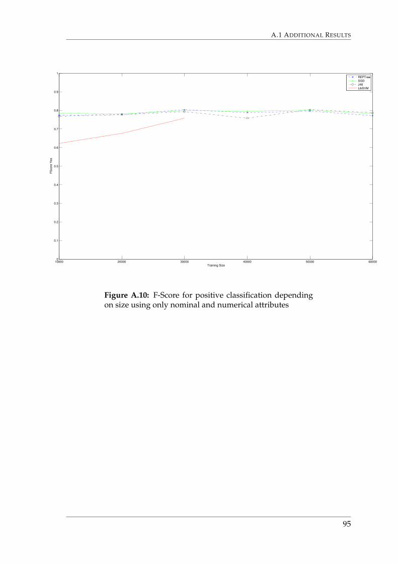
A.1 ADDITIONAL RESULTS
10000 20000 30000 40000 50000 600000
0.1
0.2
0.3
0.4
0.5
0.6
0.7
0.8
0.9
1
Training Size
FS
co
re Y
es
REPTree
SGD
J48
LibSVM
Figure A.10: F-Score for positive classification dependingon size using only nominal and numerical attributes
95
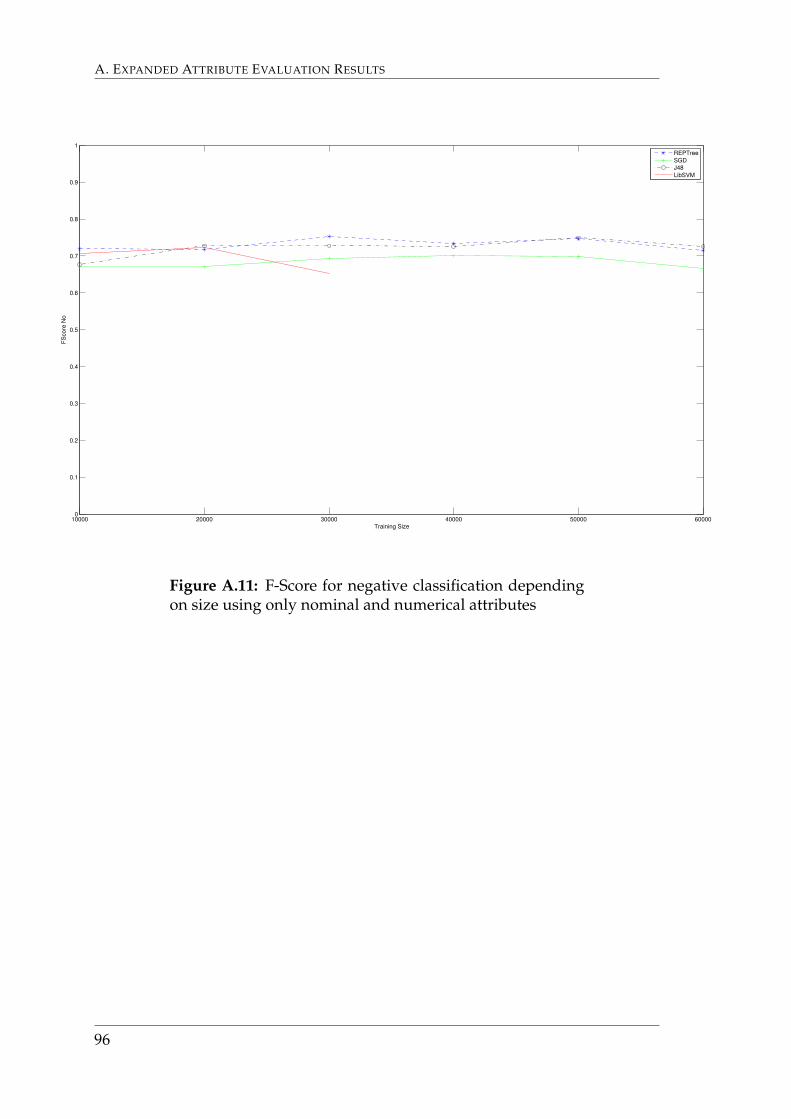
A. EXPANDED ATTRIBUTE EVALUATION RESULTS
10000 20000 30000 40000 50000 600000
0.1
0.2
0.3
0.4
0.5
0.6
0.7
0.8
0.9
1
Training Size
FS
co
re N
o
REPTree
SGD
J48
LibSVM
Figure A.11: F-Score for negative classification dependingon size using only nominal and numerical attributes
96